luis gustavo tomal ribas camera-based driver's health ...

FEDERAL UNIVERSITY OF PARANÁ

LUIS GUSTAVO TOMAL RIBAS

CAMERA-BASED DRIVER’S HEALTH MONITORING SYSTEM

CURITIBA

2019

LUIS GUSTAVO TOMAL RIBAS

CAMERA-BASED DRIVER’S HEALTH MONITORING SYSTEM

CURITIBA

2019

Dissertação submetida ao curso de Pós-Graduação em Engenharia Elétrica, Setor de Tecnologia, Universidade Federal do Paraná, como requisito parcial à obtenção do título de Mestre em Engenharia Elétrica. Orientador UFPR: Prof. Dr. Leandro dos Santos

Coelho

Coorientador THI: Prof. Dr. Alessandro Zimmer

Catalogação na Fonte: Sistema de Bibliotecas, UFPR Biblioteca de Ciência e Tecnologia

R482c Ribas, Luis Gustavo Tomal Camera -based driver’s health monitoring system [recurso

eletrônico] / Luis Gustavo Tomal Ribas – Curitiba, 2019.

Dissertação - Universidade Federal do Paraná, Setor de Tecnologia, Programa de Pós-graduação em Engrenharia Elétrica.

Orientador: Prof. Dr. Leandro dos Santos Coelho Coorientador: Prof. Dr. Alessandro Zimmer

1. Rede Neural Convolucional. 2. Frequência Cardíaca. I.

Universidade Federal do Paraná. II. Coelho, Leandro dos Santos III. Zimmer, Alessandro. IV. Título.

CDD: 004.65

Bibliotecária: Roseny Rivelini Morciani CRB-9/1585

ACKNOWLEDGMENTS

First and foremost, I would like to thank God Almighty for giving me strength,

knowledge, ability, and this opportunity. I am truly grateful for your exceptional love

and grace during this entire journey.

To my wife, Florence, which is present at all times by my side as a friend and

wise adviser, supporting me during the whole process.

To my parents, Luis Carlos and Inês, as well as my sisters, Camila, and

Priscila, for supporting, educating, and motivating me along my journey.

I extend my gratitude to Prof. Leandro Coelho and Prof. Alessandro Zimmer,

for the advice and support during the research and experiments development, as well

as the opportunity to work together.

“Everything should be as simple as it is, but not simpler.”

Albert Einstein

RESUMO

O desenvolvimento de veículos autônomos tornou-se possível devido ao salto

tecnológico obesrvado nos equipamentos embarcados disponíveis no mercado

atualmente, principalmente no que se refere à sua capacidade computacional. Este

desenvolvimento afeta toda a cadeia produtiva, visto que proporciona a possibilidade

de implementação de sistemas de assistência ao condutor (ADAS) mais complexos,

como sistemas robustos em tempo real para monitoramento do nível de atenção e o

estado de saúde do motorista. Muitos estudos afirmam que fatores psicológicos, como

doença e fadiga, são as principais causas de acidentes de trânsito graves, e neste

contexto o monitoramento do estado da saúde do motorista pode aumentar a

segurança ao dirigir. O indicador mais expressivo para inferir o estado de saúde é a

frequência cardíaca, a qual pode indicar com precisão, condições como cansaço e

sonolência. No presente trabalho, é proposta a avaliação da viabilidade de uma

abordagem em tempo real de um estimador de frequência cardíaca, sem contato,

baseado em aprendizado profundo, em uma tarefa de regressão, utilizando três

diferentes tipos rede neural convolucional (CNN) tendo como entrada um mapa

espaço-temporal. Três arquiteturas de CNN são utilizadas, a saber: VGG16,

RESNET18 e MobieNETV2. Muitos estudos têm sido realizados usando abordagens

de aprendizado de máquinas e técnicas de processamento de sinais para obter uma

estimativa robusta da frequência cardíaca a partir de sequências de imagens. Além

disso, abordagens de aprendizado profundo têm sido propostas, mas devido à falta

de um conjunto massivo de dados, essas soluções não são capazes de oferecer uma

boa generalização na solução do problema. Neste trabalho é proposta uma melhoria

na abordagem de aprendizado profundo baseada em CNN e representação de mapas

espaço-temporais, utilizando uma segmentação da pele usando uma malha poligonal

combinada com filtragem independente para cada segmento. O desempenho do

método é avaliado utilizando uma base de dados de alta resolução concebida e

construída para treinamento e teste. Além disso, também é avaliado o uso de três

modelos de representação de cores – RGB, HSV e YUV para representação da

imagem de entrada da CNN. Em contraste com o método proposto, três algoritmos

estado da arte são utilizados como referência para comparação do desempenho das

técnicas aplicadas à base de dados da THI. Os resultados dos experimentos mostram

que é possível usar o método proposto com representação de mapas espaço-

temporais para obter uma estimativa confiável da frequência cardíaca a partir de

sequências de imagens, obtendo resultados mais precisos do que os métodos do

estado da arte utilizados na técnica chamada remote photoplethysmography (rPPG).

Além disto, a malha poligonal cria uma representação rica, e a filtragem independente

elimina mudanças presentes na face que geram erros nas medições, oriundos de

movimentos ou devido à brusca variação de luz. Além disso, é possível verificar que

o modelo de representação de cores HSV (Hue Saturation Value) é o melhor a ser

usado neste problema. Quanto às arquiteturas de rede, utilizando o espaço de cores

HSV a CNN com arquitetura VGG16 oferece um desempenho 46% melhor que a

arquitetura ResNET18, e por sua vez, 490% melhor que a rede MobileNETv2.

Palavras-chave: Aprendizado profundo, Remote Photoplethysmography, Rede Neural

Convolucional, Frequência Cardíaca.

ABSTRACT

Currently, the development of autonomous vehicles has become common in

the automotive context, due to progress on embedded hardware in terms of

computational power. Therefore, this affects all the production chain, due to the

possibility of implementing more complex driver assistance systems, such as driver’s

health monitoring. Many studies state that psychological factors, such as illness and

fatigue, are the primary causes of major traffic accidents, thus monitoring driver health

status can increase driver safety. In this context, the most expressive indicator of the

health condition is the heart rate, which may indicate health conditions such as

sleepiness and drowsiness. In the present work is proposed an evaluation of the

feasibility of a real-time, non-contact approach of deep learning-based heart rate

estimator using a pre-trained CNN (Convolutional Neural Network) architecture using

a spatial-temporal map as input in a regression task. Many studies have been done in

the field using machine learning and deep learning approaches and signal processing

techniques to obtain a robust heart rate estimation from image sequences. In the

present work, an improvement of a deep learning approach based on CNN is proposed

using a polygonal segmentation combined with independent filtering for each segment.

The performance of the proposed method is evaluated using a high-resolution

database devised and built for training and testing. Besides, an optimal color space in

the context of three state of the art image classification CNNs is also evaluated, in

addition, three state of the art algorithms for remote photoplethysmography (rPPG) are

used as a reference for comparison. The experimental results show that it is possible

to use the proposed improved method with spatial-temporal map representation to

obtain a reliable heart rate estimation from video sequences, overperforming the state

of the art algorithms. The polygonal mesh creates rich maps representation, and the

filtering can cut exaggerated movement artifacts from the measurements, such as the

abrupt light changes effect along the map windowing process. Besides, It is possible

to verify that HSV (Hue Saturation Value) is the best color space to be used in this

problem, as the VGG16 performs 46% better than RESNET18 and 490% better than

MOBILENETV2 architectures.

Keywords: Heart Rate, Deep Learning, Convolutional Neural Network, Remote

Photoplethysmography.

LIST OF FIGURES

FIGURE 1.1 – AUTONOMOUS VEHICLE SALES PREDICTION ........................................................ 16

FIGURE 2.1 – ELECTROPHYSIOLOGY OF THE HEART .................................................................. 24

FIGURE 2.2 – CONTACT AND NON-CONTACT HR MEASUREMENT .............................................. 25

FIGURE 2.3 – HRV SIGNAL OBTAINED FROM ECG ......................................................................... 26

FIGURE 2.4 – ECG CONNECTION ...................................................................................................... 27

FIGURE 2.5 – ECG SIGNAL PROCESSING WITH BIOSPPY LIBRARY ............................................ 28

FIGURE 2.6 – ECG SIGNAL SELECTION ........................................................................................... 29

FIGURE 2.7 – SKIN LAYER AND PPG x ECG COMPARISON ........................................................... 30

FIGURE 2.8 – SPECTRUM OF BLOOD LIGHT ABSORPTION .......................................................... 31

FIGURE 2.9 – SITUATIONS WHICH INFLUENCE THE rPPG SIGNAL .............................................. 32

FIGURE 2.10 – RGB COLOR SPACE .................................................................................................. 36

FIGURE 2.11 – Y’UV COLOR SPACE ................................................................................................. 37

FIGURE 2.12 – HSV COLOR SPACE .................................................................................................. 38

FIGURE 2.13 – SPATIAL-TEMPORAL MAPS STRUCTURE .............................................................. 39

FIGURE 2.14 – SLIDING WINDOW...................................................................................................... 40

FIGURE 2.15 – FACE DETECTION USING RESNET10_SSD ............................................................ 41

FIGURE 2.16 – LANDMARK DETECTOR METHODS ......................................................................... 42

FIGURE 2.17 – 3DDFA CNN ................................................................................................................ 43

FIGURE 2.18 – SEVERAL RESULTS ON ALFW-2000 DATASET. ..................................................... 44

FIGURE 2.19 – 68 FACIAL LANDMARK .............................................................................................. 44

FIGURE 2.20 – ML AND DL APPROACHES ....................................................................................... 45

FIGURE 2.21 – CNN EXAMPLE ........................................................................................................... 47

FIGURE 2.22 – FEATURE DETECTION IN A CONVOLUTIONAL NETWORK ARCHITECTURE ..... 48

FIGURE 2.23 – PADDING ON CONVOLUTION. ................................................................................. 49

FIGURE 2.24 – STRIDE IN CONVOLUTION ....................................................................................... 49

FIGURE 2.25 – MAXPOOL ................................................................................................................... 50

FIGURE 2.27 – FULLY CONNECTED LAYER ..................................................................................... 51

FIGURE 2.28 – STATE OF THE ART CNN ARCHITECTURES .......................................................... 52

FIGURE 3.1 – PROPOSED PIPELINE WORKFLOW .......................................................................... 58

FIGURE 3.2 – STATE OF THE ART METHODS WORKFLOW ........................................................... 60

FIGURE 3.3 – SKIN SEGMENTATION USING SEMANTIC CNN ....................................................... 60

FIGURE 3.4 – THI DATABASE MANAGER ......................................................................................... 62

FIGURE 3.5 – FILTER APPROACH ..................................................................................................... 63

FIGURE 3.6 – POLYGONAL SEGMENTATION ................................................................................... 64

FIGURE 3.7 – POLYGONAL FACE SEGMENTATION ........................................................................ 64

FIGURE 3.8 – THI DATASET SETUP .................................................................................................. 65

FIGURE 3.9 – THI EXPERIMENT HR SAMPLE ................................................................................... 66

FIGURE 3.10 – THI DATABASE SAMPLE ........................................................................................... 67

FIGURE 4.1 – PROPOSED METHOD COMPARISON ........................................................................ 70

FIGURE 4.2 – POLYGONAL MESH PATTERN ................................................................................... 71

FIGURE 4.3 – RESNET18 RGB TRAINING CURVE ........................................................................... 72

FIGURE 4.4 – RESNET18 RGB EVALUATION ................................................................................... 74

FIGURE 4.5 – RESNET18 Y’UV TRAINING CURVE ........................................................................... 75

FIGURE 4.6 – RESNET18 YUV EVALUATION .................................................................................... 76

FIGURE 4.7 – RESNET18 HSVTRAINING CURVE ............................................................................. 77

FIGURE 4.8 – RESNET18 HSV EVALUATION .................................................................................... 79

FIGURE 4.9 – VGG16 YUV CURVE RESULTS .................................................................................. 81

FIGURE 4.10 – VGG16 YUV EVALUATION ........................................................................................ 82

FIGURE 4.11 – MOBILENETV2 YUV CURVE RESULTS ................................................................... 83

FIGURE 4.12 – MOBILENETV2 Y’UV EVALUATION .......................................................................... 85

FIGURE 4.13 – COMPARISON OF σ VALUE for CNN, ICA, LGI, POS .............................................. 87

FIGURE 4.14 – COMPARISON OF σ ICA, LGI, POS OVER EXP 12 .................................................. 88

FIGURE 4.15 – COMPARISON OF σ ICA, LGI, POS OVER EXP 19 ................................................. 89

FIGURE 4.16 – ECG-FITNESS DATASET EXAMPLE ......................................................................... 91

FIGURE 4.17 – SKIN SEGMENTATION SEQUENCE FROM ECG-FITNESS SELECTED SUBJECT91

FIGURE 4.18 – ECG-FITNESS SPATIAL-TEMPORAL MAPS ............................................................ 92

FIGURE 4.19 – RESULT OF CROSS-DATABASE TEST .................................................................... 92

LIST OF TABLES

TABLE 2.1: VGG ARCHITECTURE ...................................................................................................... 54

TABLE 2.2: RESNET18 ........................................................................................................................ 55

TABLE 2.3: MOBILENET V2 ................................................................................................................. 56

TABLE 3.1: THI DATASET OVERVIEW ............................................................................................... 68

TABLE 4.1: DATABASE RESULTS RESNET18 WITH RGB ............................................................... 73

TABLE 4.2: DATABASE RESULTS RESNET18 WITH Y’UV ............................................................... 75

TABLE 4.3: DATABASE RESULTS RESNET18 WITH HSV ................................................................ 78

TABLE 4.4: COMPARISON OF COLOR SPACES OVER RESNET18 ARCHITECTURE .................. 79

TABLE 4.5: DATABASE RESULTS VGG16 WITH Y’UV ..................................................................... 81

TABLE 4.6: DATABASE RESULTS MOBILENETV2 Y’UV .................................................................. 84

TABLE 4.7: CNN ARCHITECTURE COMPARISON ............................................................................ 86

TABLE 4.8: RESULTS OF THE BEST CNN AGAINST STATE OF THE ART ALGORITHMS ............ 87

TABLE 4.9: COMPARISON OF RPPG METHODS .............................................................................. 90

LIST OF ACRONYMS

3DDFA 3D Dense Face Alignment

3DMM 3D Morphable Model

ADAM Adaptive Moment estimation ANN Artificial Neural Network ANS Autonomic Nervous System BP Blood Pressure BPM Beats per minute BSS Blind Source Separation BVP Blood Volume Pressure CbCr Chrominance (CbCr) components CNN Convolutional Neural Network CV Cross-Validation DAS Driver assistance systems

DRM Shafer’s dichromatic reflection model

DSRL Digital Single Lens Reflex ECG Electrocardiography

EDA Electrodermal Activity

EEG Electroencephalography

EMG Electromyographic

FC Fully Connected Layers fps Frames per second HR Heart rate Hz Hertz

iBCG Imaging ballistocardiography

ICA Independent Component Analysis

IoU Intersection over Union IR Infrared

LBL Lambert-Beer law MAE Mean average error min Minutes MLP Multilayer Perceptron MP Maximum peak detector ms Millisecond

MSE Mean Squared Error mV Millivolt

NMS Non-maximum suppression

PCA Principal Component Analysis

PNCC Projected Normalized Coordinate Code PPG Photoplethysmography PSD Power Spectral Density RAM Random Acces Memory

rBCG Ballistocardiogram

ReLU Rectified Linear Unit RGB Red-Green-Blue

ROI Region of Interest rPPG Remote Photoplethysmography s Seconds

SSD Single Shot Detector

SVM Support vector machine

UV Chrominance (UV) component V Volt

Y Luminance component Y' Brightness component

LIST OF SYMBOLS

reflection strength

C(t) luminescence

time-varying function

varying parts of specular reflections

luminance intensity level

the stationary part of the luminance intensity

the k-th element of the solution vector x

non-physiological variations - rigid and non-rigid movements

blood volume pressure

the stationary part of specular reflections

σ standard deviation

unit color vector of the skin reflection

light reflection from the skin surface

scattering of light in skin tissue

image sensor noise

solution vector

CONTENTS

1 INTRODUCTION ................................................................................................................................ 16

1.1 PROBLEM DEFINITION ................................................................................................................. 17

1.2 STATE OF THE ART ...................................................................................................................... 18

1.3 OBJECTIVE..................................................................................................................................... 19

1.4 LIMITATIONS .................................................................................................................................. 20

1.5 MAIN CONTRIBUTION ................................................................................................................... 21

1.6 OVERALL STRUCTURE OF THE DISSERTATION....................................................................... 21

2 LITERATURE REVIEW ..................................................................................................................... 22

2.1 HEALTH CONDITION MONITORING ............................................................................................ 23

2.1.1 Cardiac physiology ....................................................................................................................... 23

2.1.2 Heart Rate Measurement ............................................................................................................. 24

2.1.2.1 Contact Measurements .......................................................................................................... 26

2.1.2.1.1 Electrocardiograph ................................................................................................................. 26

2.1.2.1.2 Photoplethysmography .......................................................................................................... 30

2.1.2.2 Non-contact Measurements ................................................................................................... 31

2.1.2.2.1 Remote Photoplethysmography (rPPG) ................................................................................ 31

2.1.3 Skin Reflection Model ................................................................................................................... 34

2.2 COLOR SPACE .............................................................................................................................. 36

2.2.1 RGB .............................................................................................................................................. 36

2.2.2 Y‘UV ............................................................................................................................................. 37

2.2.3 HSV .............................................................................................................................................. 38

2.3 SPATIAL-TEMPORAL MAPS ......................................................................................................... 39

2.4 FACE DETECTION ......................................................................................................................... 40

2.4.1 Face Alignment ............................................................................................................................ 42

2.5 DEEP LEARNING ........................................................................................................................... 45

2.5.1 CNN .............................................................................................................................................. 46

2.5.1.1 Convolution Layer .................................................................................................................. 47

2.5.1.1.1 Filter size ................................................................................................................................ 48

2.5.1.2 Padding .................................................................................................................................. 48

2.5.1.3 Stride ...................................................................................................................................... 49

2.5.1.4 Activation Layer ..................................................................................................................... 49

2.5.1.5 Pooling Layer ......................................................................................................................... 50

2.5.1.6 Classification Layer ................................................................................................................ 50

2.5.1.7 Training Terminology ............................................................................................................. 51

2.5.1.8 Architectures .......................................................................................................................... 52

2.5.1.8.1 VGG16 ................................................................................................................................... 53

2.5.1.8.2 RESNET 18............................................................................................................................ 54

2.5.1.8.3 MobileNetV2........................................................................................................................... 55

2.6 DATABASE ..................................................................................................................................... 56

3 METHODOLOGY ............................................................................................................................... 58

3.1 HR WORKFLOW ............................................................................................................................. 58

3.2 RESEARCH PLANNING ................................................................................................................. 58

3.3 STATE OF THE ART METHODS COMPARISON.......................................................................... 59

3.4 DEVELOPMENT OF THE PLATFORM .......................................................................................... 61

3.4.1 Software used .............................................................................................................................. 61

3.4.1.1 Python .................................................................................................................................... 61

3.4.1.2 OpenCV ................................................................................................................................. 61

3.4.1.3 Pytorch ................................................................................................................................... 61

3.4.2 Software development .................................................................................................................. 62

3.5 THE POLYGON FILTER APPROACH ............................................................................................ 62

3.6 PROPRIETARY THI DATABASE.................................................................................................... 65

3.7 TRAINING PROCESS ..................................................................................................................... 68

3.7.1 Optimizer ...................................................................................................................................... 68

3.7.2 Loss Function ............................................................................................................................... 68

4 EXPERIMENTAL RESULTS ............................................................................................................. 70

4.1 POLYGONAL MESH EVALUATION ............................................................................................... 70

4.2 OPTIMAL COLOR SPACE EVALUATION ...................................................................................... 71

4.2.1 RGB evaluation ............................................................................................................................ 72

4.2.2 Y‘UV evaluation ............................................................................................................................ 74

4.2.3 HSV evaluation ............................................................................................................................. 76

4.2.4 COLOR SPACE COMPARISON .................................................................................................. 79

4.3 NETWORK ARCHITECTURE EVALUATION ................................................................................ 80

4.3.1 VGG16 .......................................................................................................................................... 80

4.3.2 MOBILENETV2 ............................................................................................................................ 82

4.3.3 RESNET18 ................................................................................................................................... 85

4.3.4 Network architecture comparison ................................................................................................. 85

4.4 STATE OF THE ART ALGORITHMS ............................................................................................. 86

4.4.1 Algorithm comparison ................................................................................................................... 89

4.5 CROSS-DATABASE VALIDATION ................................................................................................. 90

5 CONCLUSION AND FUTURE WORK .............................................................................................. 94

REFERENCES ...................................................................................................................................... 96

16

1 INTRODUCTION

The surge in autonomous vehicle development has shaken the automotive market,

along with the promises of better traffic and safer roads, also reducing the human factor

on the driving task. The automotive industry is continuously working to develop better

cars in terms of safety for its consumers. (Litman, 2019) explores the autonomous

vehicle benefits and costs and examines how fast self-driving vehicles are probable to

be developed and implemented based on prior car technology experience. According

to their work, even though the development of autonomous vehicles increases, the

market specialists estimate that a fully automated fleet is distant from becoming a

reality in at least 30 years. The market penetration of this kind of vehicle will take time,

and during the market changing period, the traffic in the streets in the near feature will

be a mix between autonomous and high-level assistance human-driven cars.

This effect is mainly because modern vehicles are durable, resulting in a slow

fleet turnover, and new vehicle technologies typically require three to five decades to

be implemented in 90% of operating vehicles. Taking into account the patterns of other

vehicle technologies penetration in the market, it will take one to three decades to

dominate vehicle sales, plus one or two more decades to dominate vehicle travel, as

shown in FIGURE 1.1. Still, according to (Litman, 2019), it is probable that even at

market saturation, a substantial portion of vehicles and its journey will continue to be

self-driven. FIGURE 1.1 – AUTONOMOUS VEHICLE SALES PREDICTION

SOURCE: (Litman, 2019)

Therefore, the advances in the autonomous vehicle industry lead a turning point

in the embedded hardware industry, enabling possibilities to implement more

computational complex driver assistance systems based on high throughput sensors

or highly computational costs algorithms, such as driver’s status monitoring, including

17

health and attention which relies on cameras or a fusion between different sensors. All

these achievements in the embedded processing platforms have a reason: driving is a

cognitively complex task related to multiple functions, and even for a human, many of

these cerebral functions may be affected due to the driver’s health conditions.

(Racioppi et al., 2004) mentioned that psychological factors are the primary

cause of major traffic accidents, and they can be classified into three aspects: external

ambient environment, illness, and fatigue. The last two are strictly related to the driver’s

health status, which in turn can be measured and monitored through vital signs such

as respiration, heart rate (HR), blood oxygen saturation, arterial blood pressure.

According to (Q. Zhang et al., 2017), the most effective and expressive indicator of

health condition is the HR and its derivations, such as heart rate variability (HRV).

Many definitions have been used for fatigue in the literature, and the concepts of

“fatigue,” “drowsiness” or “sleepiness,” are frequently used interchangeably (Johns,

2000; NHTSA, 2001).

Measuring driver’s health indicators with an acceptable precision is one of the

challenges in the automotive safety industry nowadays. According to (Saini & Saini,

2014; Wright et al., 2007), there are many types of systems built in vehicles to detect

the driver’s sleepiness. The first systems used to monitor the vehicle’s movements,

correlating these with the driver’s attention and sleepiness.

The current solutions in the market technology have different approaches as

tracking lane deviation such as new sensors placed in a seat to monitor changes in

heart rate, as well the use of contactless measurement of heart rate using camera or

doppler effect radar, gaze detection, and tracking the driver’s eye position. There are

many types of research set on the direction of driver’s health status, being referred in

throughout the present work, due to their capability of inferring information from the

health of the subject just using the heart rate analysis.

1.1 PROBLEM DEFINITION

There are many procedures and methods for HR monitoring available on the

market, where the most precise and robust rely on the physical connection of

electrodes in standard positions on the body skin. Even if fixed-on-body wires are

reliable and give good signal quality, they are inconvenient and inadequate for long-

term measurements, limiting the movements because of the length of the cables

18

(Scalise, 2012). In this context, the problem to be addressed in this work consists of

identifying and evaluating if it is possible to obtain a robust and reliable measure from

non-contact heart rate estimation using camera image considering its limitations,

turning embedded applications under real conditions scenario possible.

1.2 STATE OF THE ART

Many methods can be used to noninvasive measurement of the HR, frequently

referred as time between beats or “RR interval,” using different physical phenomena

such as laser Doppler (Gouveia et al., 2019; Kazemi et al., 2014), microwave Doppler

radar (Obeid et al., 2011, 2013), ultrasound (Noguchi et al., 1995), video imaging at

visible spectrum (Hassan et al., 2017) and thermal imaging (Gault & Farag, 2013; Hu

et al., 2018). Image-based methods have been studied mainly due to the possibility of

acquiring more information about the measured element using the same image

captured, such as gender, color, head position, eyes blinking, and many others, which

are not possible to get with radar for instance. Many of the studies in this field use

image processing, blind source separation, or a machine learning approach to obtain

the HR using cameras (Hassan et al., 2017; Sun & Thakor, 2015).

Additionally, the use of the face for HR measurement is one of the most used in

the literature, since human facial skin contains abundant capillaries, and the blood

volume in the vessels of the body will change according to heart rate. Therefore,

increasing the blood volume in the capillaries under the skin, the blood will absorb more

light, and the skin in the image becomes darker and vice versa. At the naked eye, it is

not possible to realize this subtle variation; however, these weak signal changes can

be extracted using video image processing techniques. A variety of techniques have

been proposed in order to solve the HR estimation problem, but many of them rely on

controlled environment situations, such as the presence of significative movement

artifacts and light changing, which is not suitable for embedded automotive

applications, and new techniques are demanded.

In (Hassan et al., 2017) a review of HR estimation using facial video is presented,

making a comparison between several video processing techniques to measure the

heart rate with non-contact method using cameras, in which the main objective of the

conducted experiment was to determine the reliability of the HR measurement

methods under realistic situations. According to their work, the biggest challenges in

19

HR facial estimation are the illumination and head movements that disturb the

measurement. The light due to an asymmetric human face is disproportionally

scattered through the surface of the skin, and the positioning of the light source and

the orientation of the face causes illumination variance. The head motion can be

represented as a sum of two types of movements: rigid and nonrigid, in which the first

is related to change of head orientation or body posture and the second caused by

expressing facial emotions, yawning or talking (Kumar et al., 2015; Li et al., 2014).

Other prominent studies in the literature (X. He et al., 2017; C. Zhang et al., 2017)

are focused on detecting HR at night, or low light scenarios, in which they create

several experiments to test the reliability of the heart rate and the eye blink rate

measurements, using IR camera to measure the heart rate even in the absence of

light.

Many studies on deep learning approaches for HR estimation are performed, with

the most prominent one being (W. Chen & McDuff, 2018; Hsu et al., 2017; Niu et al.,

2018, 2019; Shyam et al., 2019). In (Hsu et al., 2017) a reliable model to perform real-

time pulse estimation by using conventional RGB cameras is presented by using a

frequency-domain map as input for the VGG-151 network architecture, resulting in a

superior estimation efficacy when compared with most of the state of the art pulse

estimation algorithms. In (Niu et al., 2018), instead of the frequency domain, a temporal

map is used as input for the ResNET182 architecture, also resulting in a superior

estimation efficacy.

1.3 OBJECTIVE

The literature review shows that it is possible to obtain a reliable measure from

the driver’s heart rate with non-contact through camera image, thus being possible to

estimate the HR in time and then determine dangerous driving situations. Identifying

these scenarios can improve vehicle safety and traffic safety as well, even in a mixed

fleet with autonomous and human drivers.

_______________ 1 VGG-15 – It is a Convolutional Neural Network architecture. The VGG stands for “Visual Geometry

Group from University of Oxford” , and the term VGG-15 indicates a network with 15 layers 2 ResNET is a Convolution Neural Network, introduced by Microsoft, wich uses Residual block

conections. Resnet18 stands for a RESNET with 18 layers.

20

In this study, it is proposed a feasibility analysis of a real-time, non-contact

approach of deep learning-based heart rate estimator using a pre-trained image

classification CNN architecture with a spatial-temporal map as input in a regression

problem. The core of this work relies on the comparison between three different states

of the art CNN architectures, namely: VGG16(Simonyan & Zisserman, 2014),

RESNET18 (K. He et al., 2016), and MobileNetv2 (Sandler et al., 2018, p. 2) measuring

how capable are each one to estimate the driver’s heart rate measurement using an

RGB camera image. Furthermore, three different color space models, namely RGB

(Red, Green, Blue), YUV (Luma, Cchrominance) and HSV (Hue, Saturation, Value),

have been tested to verify which is more suitable for the desired application.

A new database was devised and built to perform the CNN training, following the

standards for data splitting and metrics used in the literature – training, validation, and

testing datasets. The samples of this dataset consist of a reference signal captured

using a gold standard medical precision Electrocardiography (ECG) equipment

connected to the subjects and image sequence from a high-resolution camera focused

on the subject, recorded during short two minutes sessions with two sessions per

subject. In the first session, a baseline is captured, and for the second session, the

subject has the HR increase by a physical exercise, been recorder immediately after

it. The camera setup follows a specific configuration where it is placed in front of the

driver based on a real-world scenario. The solution must be capable of measuring HR

with reasonable precision - less than five beats per minute (bpm) of error at different

illumination scenarios and under the natural driver motion artifacts.

1.4 LIMITATIONS

This study aims to test a deep learning algorithm to extract HR from the RGB

camera in a specific setup environment replicating the cockpit from the interior of a car

and thus building a limited size dataset, but not claiming to devise a functional

application. The database proposed in this work claims to provide a certain level of

robustness, which means that a limited set of motions, independent translational, and

scaling movements are present in the data.

21

1.5 MAIN CONTRIBUTION

The workflow proposed in this work has inspiration on the work of (Niu et al.,

2018), with two essential improvements proposed to the method: use of robust

polygonal face segmentation and a unitary and parallel frequency filter clipping the

signal to the center of the pixel range [0, 255], in order to give more stability to the

spatial-temporal map representation. At least two main outputs from this work will serve

the scientific community. The first is a comparative study under a rich and high-

resolution database of which color space is more suitable for spatial-temporal map

representations. The second is a comparative study of the results from three different

convolutional neural networks (CNNs), verifying which type of architecture performs

better in the given problem.

1.6 OVERALL STRUCTURE OF THE DISSERTATION

The remainder of this dissertation is organized as follows. In Chapter 2, a

literature review is presented, focusing on the heart physiology and the mechanism of

HR measurement. Additionally, in this chapter, a brief description of deep learning and

the techniques used for developing the experiment are depicted. Chapter 3 is about

the methodology and the tools used to perform the study. In Chapter 4, the results

obtained in the experiments are shown, with a description of the metrics used and the

performance obtained. Finally, Chapter 5 presents the final considerations with a

conclusion of the study and suggestions for future research.

22

2 LITERATURE REVIEW

This chapter will focus on the essential phenomena and concepts related to

remote HR techniques, mainly those related to the present work. All the advances in

the embedded hardware industry driven by the autonomous cars market bring a new

step to the Driver Assistance Systems (DAS) development. Due to the development of

available computer power on embedded hardware platforms, it is possible to

implement functionalities that were previously unfeasible due to the high processing

effort. One of the DAS applications that have emerged is the driver’s health monitoring,

being possible to detect dangerous situations and act accordingly to avoid a crash

event.

As stated before, in (Racioppi et al., 2004) shows that psychological factors

are the primary cause of major traffic accidents, classified into three aspects: external

ambient environment, illness, and fatigue, in which the last two are strictly related to

the driver’s health status. The first aspect, external ambient environments such as

temperature, humidity, or road status, can result in unfit driver physical conditions or

stress. The second aspect, illness, is a common chronic or less severe disease that

can reduce the auditory, tactile, visible capabilities, and reduce the physical reaction

speed of the drivers. Finally, fatigue is related to stress and sleep, with sleepiness

being the most frequent cause of traffic accidents.

The sleepiness is a result of the restriction, interruption or fragmentation of

sleep, reducing the driver reaction time, vigilance, attention, and information

processing. Furthermore, depending on the driver’s sleep conditions, an event called

microsleep can occur a brief state of drowsy unconsciousness, which can happen even

if the eyes remain open (Bener et al., 2017). The sleepiness causes a heart rate

decrease and an excessively and abnormal eye blinking pattern. These and other

patterns are measured and monitored through many vital signs such as respiration

rate, HR, blood oxygen saturation, and arterial blood pressure. According to (Zhang et

al., 2017), the most effective and expressive indicator of health condition is the HR,

and its derivations such as HRV, with many studies correlating these with stress

detection (Chuang et al., 2009; Kim et al., 2018).

The following section will explore in a more comprehensive approach the heart

physiology and the working mechanism of HR measurement, as state of the art in the

literature about remote heart rate measure.

23

2.1 HEALTH CONDITION MONITORING

As stated before, human health can be measured and monitored through many

vital signs as respiration rate, heart rate, blood oxygen saturation, arterial blood

pressure, with the most effective and expressive indicator being the HR (Zhang et al.,

2017). It may indicate with precision a medical emergency like a heart attack or a health

condition such as sleepiness, tiredness, and drowsiness. Monitoring and analysis of

HR provide valuable information regarding health status and have been extensively

investigated in various activities. The next section will address the physiology of the

heart and different approaches to measure this phenomenon.

2.1.1 Cardiac physiology

The heart is a muscular organ that pumps blood through the circulatory system

composed of arteries and veins, located just behind the breastbone (Katz, 2010; Opie,

2004). An electrical system connected to the brain, in the Autonomic Nervous

System(ANS) (Malik et al., 1996) controls the heartbeats by an electrical stimulus,

causing a contraction in the heart walls. To ensure the blood flows in the right direction,

inside the chambers, the heart has inlet and outlet valves, acting as flow control. A

more detailed definition is found (Katz, 2010; Opie, 2004):

“The heart has 2 atria, 4 chambers, and 2 ventricles. De-oxygenated blood returns to

the right side of the heart via the venous circulation. It is pumped into the right ventricle

and then to the lungs where carbon dioxide is released, and oxygen is absorbed. The

oxygenated blood then travels back to the left side of the heart into the left atria, then

into the left ventricle from where it is pumped into the aorta and arterial circulation [...]”

The electrical signal from the ANS is widely used to detect the HR in methods

like ECG, but this wave is a result of a superposition of several signals. FIGURE 2.1

shows the different waveforms for each of the specialized regions found in the heart,

and the timing shown in the bottom figure approximates that typically found in a healthy

heart (Medeiros, 2010).

24

FIGURE 2.1 – ELECTROPHYSIOLOGY OF THE HEART

SOURCE: (Medeiros, 2010)

LEGEND: The electric wave captured in the ECG equipment is composed of the electrical stimulus in

different parts from the heart, and highlighted in red the QRS complex wave.

From the image above, in the red highlighted box, it is possible to verify a

sequence given by the points Q, R, S. The pattern formed by these points delimit a

pattern signal called “QRS” complex wave, which is mostly used to obtain the heart

rate from the raw signal.

2.1.2 Heart Rate Measurement

Measurement of the heart rate is possible in two distinct ways: direct, with

contact between the sensor and the human body and indirect, without physical contact.

Many studies have been published with a comparison of the robustness of different

types of non-contact HR algorithms, taking into account the influence of real-life

interference and noise (Kazemi et al., 2014; Obeid et al., 2013; Wang et al., 2017).

According to the literature, the most accurate measure of HR is reached using the

ECG, and due to this fact, this is the most used sensor in medical applications.

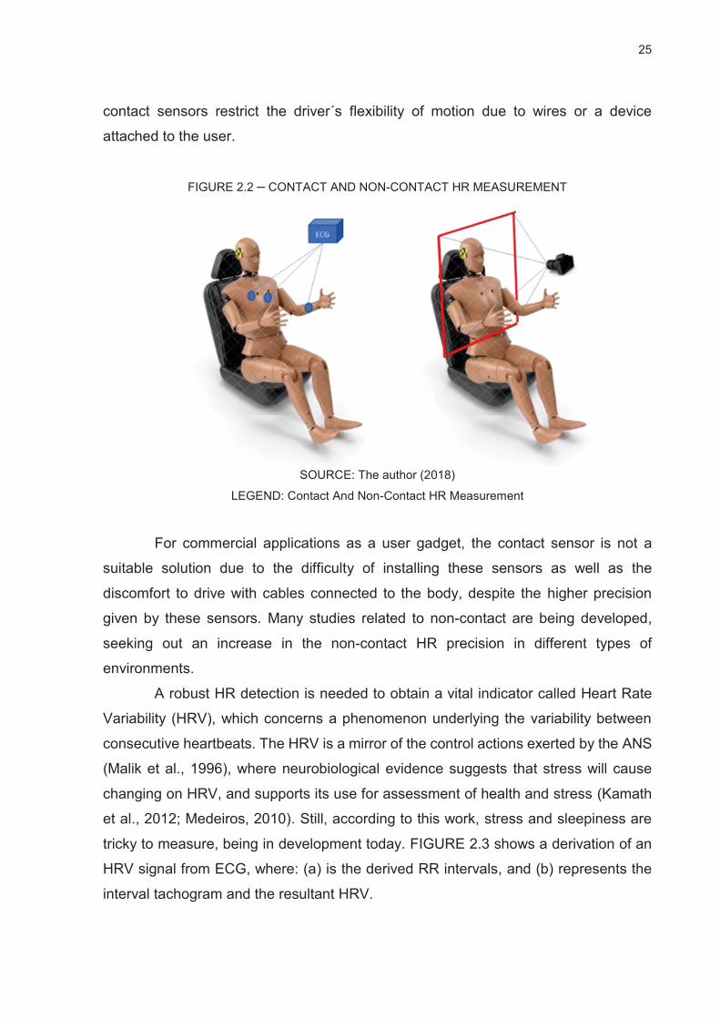
The difference between contact and non-contact approaches are shown in

FIGURE 2.2. The non-contact HR measurement shows benefits in the driving

scenarios due to a non-physical connection between the user and the device. The

25

contact sensors restrict the driver´s flexibility of motion due to wires or a device

attached to the user.

FIGURE 2.2 – CONTACT AND NON-CONTACT HR MEASUREMENT

SOURCE: The author (2018)

LEGEND: Contact And Non-Contact HR Measurement

For commercial applications as a user gadget, the contact sensor is not a

suitable solution due to the difficulty of installing these sensors as well as the

discomfort to drive with cables connected to the body, despite the higher precision

given by these sensors. Many studies related to non-contact are being developed,

seeking out an increase in the non-contact HR precision in different types of

environments.

A robust HR detection is needed to obtain a vital indicator called Heart Rate

Variability (HRV), which concerns a phenomenon underlying the variability between

consecutive heartbeats. The HRV is a mirror of the control actions exerted by the ANS

(Malik et al., 1996), where neurobiological evidence suggests that stress will cause

changing on HRV, and supports its use for assessment of health and stress (Kamath

et al., 2012; Medeiros, 2010). Still, according to this work, stress and sleepiness are

tricky to measure, being in development today. FIGURE 2.3 shows a derivation of an

HRV signal from ECG, where: (a) is the derived RR intervals, and (b) represents the

interval tachogram and the resultant HRV.

26

FIGURE 2.3 – HRV SIGNAL OBTAINED FROM ECG

SOURCE: Adapted from (Medeiros, 2010)

LEGEND: The HVR is calculated by the rate of change in the HR signal

2.1.2.1 Contact Measurements

Many techniques to obtain the measurement are available in the literature, but

the most usual are the Electrocardiograph and Photoplethysmography and its

variations. In the next sections, each method will be explained in a more detailed

fashion.

2.1.2.1.1 Electrocardiograph

The most commonly used and precise method is the ECG, which is the result

of the recorded potential differences generated at the surface of the thorax due to the

heart electrical activity. Willem Einthoven, responsible for the method, received the

Nobel Prize in Physiology or Medicine in 1924 for his work “the discovery of the

mechanism of the ECG” (Zetterström, 2009). It is mostly used for clinical diagnosis

because it provides critical information about the heart conditions, detected by different

patterns and disorders shown in the ECG waveform (Goldberger et al., 2017).

Traditionally, an ECG-based system requires at least three electrodes

arranged in different body locations to be able to operate effectively. In this context,

many references bring the concept of "lead,” referring to the difference of signal voltage

between two electrodes, and the wires used to connect the electrodes to the ECG

equipment are referred to as "wires.”

27

The arrangement of connections in an ECG Unit can be made by two main

configurations, unipolar or bipolar. On the left side of FIGURE 2.4, the points used in

both configurations are shown. In the bipolar configuration, the lead electrodes are

used as shown in “LA” - Left Arm, “RA” - Right Arm, “LL” - Left Leg, and “RL” - Right

Leg. Still, in the same image, the unipolar lead electrode positions are marked as

points: V1, V2, V3, V4, V5, or V6 on the chest. In the right, a simplified electrical

diagram of the connection of a portable ECG is shown.

FIGURE 2.4 – ECG CONNECTION

SOURCE: (ShimmerSensing, 2018)

LEGEND: Positioning of the electrodes for ECG measurement (left) Simplified Block Diagram (right)

The device chosen to perform all the ECG acquisition was the “ECG Shimmer

3”, from Shimmer Sensing company. The raw device signal measured along the

experiment session is recorded inside the device memory and recovered afterward

using a Shimmer Sensing proprietary tool – the Consensys3 software. The version

used in this study is the free version, capable only to read the raw data from the device

without any post-processing, which is only available as an additional plug-in in the PRO

version.

Due to this fact, another software toolbox was used to address this problem,

called Biosppy (Carreiras et al., 2015). It is a toolbox for biosignal processing written

in Python, offering support for various biosignals such as BVP (blood Volume

Pressure), ECG, EDA, EEG, EMG, and Respiration. It is open-source software, with

all code available on Github4. FIGURE 2.5 shows an example of the output from the

_______________ 3 Available in http://www.shimmersensing.com/products/consensys, accessed in 01.09.2019 4 Available in https://github.com/PIA-Group/BioSPPy, accessed in 02.04.2019

28

toolbox, which contains in the left in a sequence of top to bottom: the RAW signal, the

filtered signal added to the R waves markers, and the HR calculated using the R peaks.

On the right side of the image, the template matching graph is shown. It is crucial to

notice that the template graph indicates the quality of the ECG signal, as there are at

least three leads recorded by the equipment. The image below shows, intentionally, a

noisy signal which may create a mismatch in the algorithm, and thus must be verified

and removed manually after the experiment. For each signal, the library BioSPPY

calculates the superposition of the “R” wave found in the signal.

FIGURE 2.5 – ECG SIGNAL PROCESSING WITH BIOSPPY LIBRARY


LEGEND: The output of the BioSPPy toolbox: in the left in a sequence of top to bottom: the RAW signal,

the filtered signal added to the R waves markers, and the HR calculated using the R peaks, and at right,

the template matching graph.

In order to find the QRS wave template, the ECG signal at first must be filtered,

segmented using the Hamilton algorithm (Hamilton, 2003), so then the templates are

extracted, and the HR is computed. The Hamilton algorithm is a beat classifier,

reaching a positive predictivity of 96.48% on the MIT/BIH5 arrhythmia database and

positive predictivity of 97.83% on the AHA arrhythmia database6. The beat detection

_______________ 5 MIT/BIH arrhythmia database –First generally available set of standard test material for evaluation of

arrhythmia detectors (https://physionet.org/content/mitdb/1.0.0/ - accessed in 01.09.19 21:35) 6 AHA arrhythmia database - database of arrhythmias and normal electrocardiograms

(https://www.ecri.org/american-heart-association-ecg-database-usb - accessed in 01.09.19 21:40 )

29

algorithm can be broken down into two sections: the filters and the detection rules. The

filtering process is composed of the following function blocks: a low pass filter, a high

pass filter, a derivative function, the absolute value function, and an averaging of the

total value over an 80 ms window.

The detection rules are applied after the signal has been filtered. Each time a

peak is detected, it is classified as either a QRS complex or a noise. If the signal has

more than 200 ms, has positive and negative slopes, happens at least within 360 ms

after the previous one, and if it is larger than the detection threshold, then it is classified

as a valid QRS complex wave (Hamilton, 2003).

To extract heartbeat templates from an ECG signal, given a list of R-peak

locations, a signal slice is done using a defined number of samples before and after

each R-peak. Since there are at least three sources for HR calculation, the best signal

should be selected, that is, the QRS waves tend to be better superposed in this

template feature. The sum of the error between all the templates referred to as a

reference randomly selected among every other is used as a metric, where the source

with the lowest value is selected as the best signal. FIGURE 2.6 shows an example of

data collected from the ECG. The signal selection is made using the template figure

calculated by the superposition of R-waves.

FIGURE 2.6 – ECG SIGNAL SELECTION


LEGEND: ECG signal processed by python Biosppy library with high correlation (bottom) The same

signal with a low correlation (top).

30

The difference of signal quality observed in the figure above can be explained

by the quality of the mechanical connection between the pads and the skin. Poor

connection due to the presence of dirt in the contact region, misplacement, or

movement artifacts can generate noise in the signal, leading to false positives in the

algorithm.

2.1.2.1.2 Photoplethysmography

The PPG is a low-cost and straightforward method used to detect volumetric

changes in the peripheral blood circulation at the skin surface. It is a technique of

measuring the variation in the absorption of light by human skin, first introduced by

Hertzman in 1937 (Hertzman, 1937). Due to the fact that blood absorbs light more than

surrounding skin tissue, than, the variations in blood volume affect the overall skin

transmission or reflectance correspondingly. This method is used in many devices,

such as pulse oximetry and fitness smartwatch. Moreover, oxygen saturation or breath

rate can also be determined with this measurement.

A general PPG apparatus contains a light source and a photodetector, where

the light source emits a specific wavelength light to tissue, and a photodetector

measures the reflected or transmitted light from the tissue, as shown in FIGURE 2.7 in

the left. Considering the light absorption mechanism shown previously, the PPG signal

will be formed by pulsatile and superimposed components, where the first is related to

the variations in blood volume that arise from heartbeats, and the last component by

respiration, as shown in FIGURE 2.7 in the right.

FIGURE 2.7 – SKIN LAYER AND PPG x ECG COMPARISON

SOURCE: (Bousefsaf et al., 2018)

LEGEND: Photoplethysmography consists of measuring variations in light absorption on skin tissues.

Naturally, the effect of absorption is not linear in the visible light spectrum, nor

linear distributed between the primary colors. The blood absorbance coefficient

31

spectrum is shown in FIGURE 2.8, where it is possible to verify a peak of absorption

on ultraviolet t(UV) wavelength spectrum ( = 400 nm), a second peak at the green

wavelength ( =550 nm) and a small residual bastion in the IR wavelength ( > 800

nm).

FIGURE 2.8 – SPECTRUM OF BLOOD LIGHT ABSORPTION

SOURCE: (Lindelöw & Lindqvist, 2016)

LEGEND: Light absorption for oxyhemoglobin and deoxyhemoglobin in a LOG scale.

Those curves are the reason smartwatches with ECG capabilities use green led

to performing signal reflection measurement, where the same phenomenon can be

observed in any part of the body skin but is more evident in the thinner skin tissue and

most vascularized areas.

2.1.2.2 Non-contact Measurements

Among the different developed methods for noninvasive measurement of HR,

such as laser Doppler (Gouveia et al., 2019; Kazemi et al., 2014), microwave Doppler

radar (Obeid et al., 2011, 2013), ultrasound (Noguchi et al., 1995), and thermal imaging

(Gault & Farag, 2013; Hu et al., 2018), a technique widely used is the “remote

Photoplethysmography” (rPPG), which aims at measuring the same parameters as

PPG using a video camera facing the subject under evaluation, or remote rBCG as

well as the motions related to respiratory movement or the head movement

(Balakrishnan et al., 2013)

2.1.2.2.1 Remote Photoplethysmography (rPPG)

It consists of the verification of the absorption of the transmitted light, similar

to the PPG method, to a sequence of images captured in a certain distance of the

object, measuring the color changes in a specific area. Usually, for visible light

32

spectrum analysis, any active source of light is used, relying only upon the environment

light. In this method, any part of the body can be used, but the literature shows that the

most sensitive part is the face, since human facial skin contains abundant capillaries.

With the increase of the blood volume in the capillaries under the skin, the blood

absorbs more light, and the facial image becomes darker because less light is reflected

from the face and vice versa – the same mechanism of PPG. The naked eyes cannot

observe this subtle variation; however, the weak HR signals can be extracted using

video image processing (Sun & Thakor, 2015).

The rPPG technique relies on visual contact with the target to be measured,

and all methods require face tracking, where many rely on skin segmentation, color

space transformation, signal decomposition, and frequency-domain filtering (W. Chen

& McDuff, 2018). Furthermore, most of the HR extraction algorithms are based on an

RGB image input.

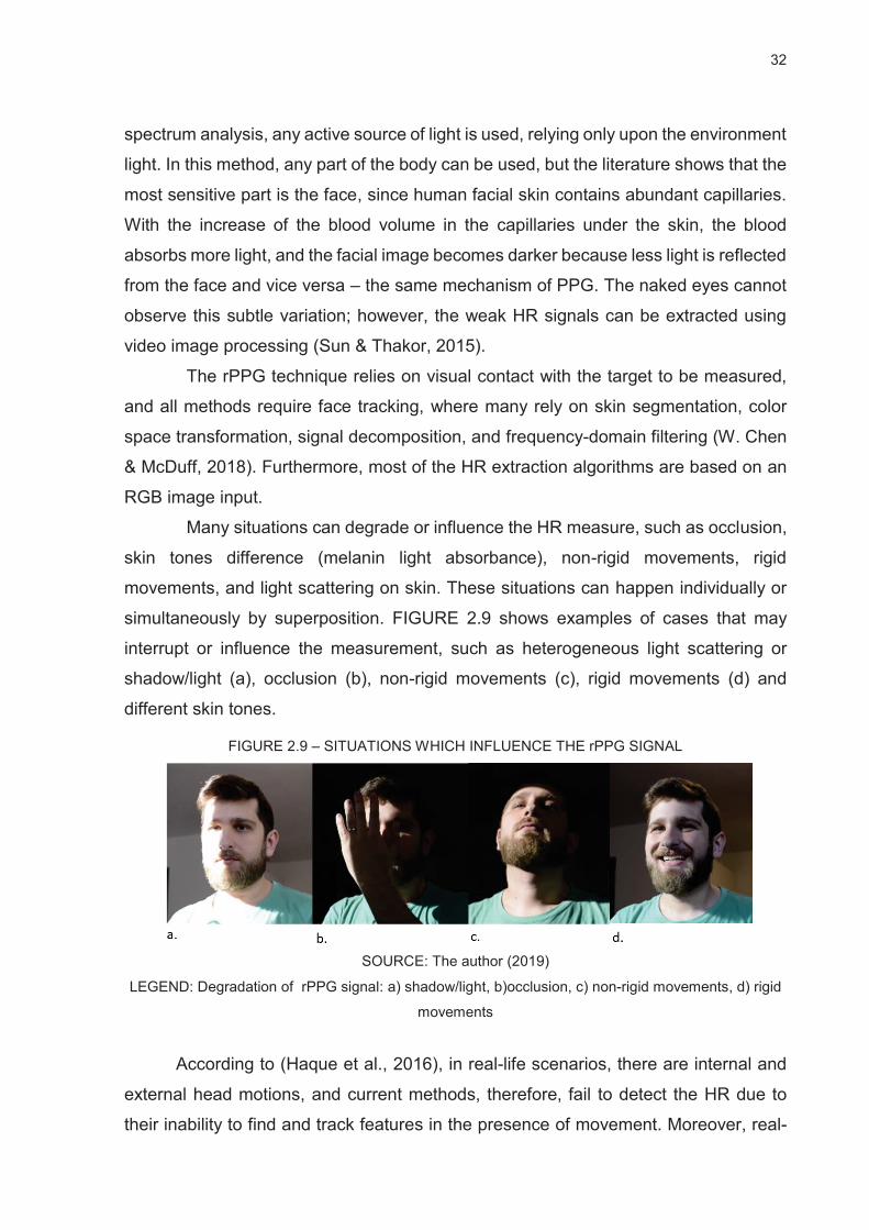
Many situations can degrade or influence the HR measure, such as occlusion,

skin tones difference (melanin light absorbance), non-rigid movements, rigid

movements, and light scattering on skin. These situations can happen individually or

simultaneously by superposition. FIGURE 2.9 shows examples of cases that may

interrupt or influence the measurement, such as heterogeneous light scattering or

shadow/light (a), occlusion (b), non-rigid movements (c), rigid movements (d) and

different skin tones.

FIGURE 2.9 – SITUATIONS WHICH INFLUENCE THE rPPG SIGNAL


LEGEND: Degradation of rPPG signal: a) shadow/light, b)occlusion, c) non-rigid movements, d) rigid

movements

According to (Haque et al., 2016), in real-life scenarios, there are internal and

external head motions, and current methods, therefore, fail to detect the HR due to

their inability to find and track features in the presence of movement. Moreover, real-

33

life scenarios challenge the algorithms due to motion blur, lousy posing, and poor

lighting conditions, inducing noise in the motion trajectories obtained for measuring

HR.

Many publications make some statement about the time window technique used

to increase the robustness of signal processing algorithms (Lindelöw & Lindqvist,

2016). According to this work, robustness is achieved with a period of 13 s, not be

suitable for real-time applications. Timed window processing has a long delay, typically

half of the window length before HR changes are present in the estimated HR, i.e., for

a time window of 30 seconds, it will take 30 seconds before the first HR estimation is

available.

One of the most relevant papers on rPPG signal processing is (Wang et al.,

2016). In this work several core rPPG methods have been evaluated for extracting the

pulse-signal from a video: Blind Source Separation (BSS) (Pal et al., 2013), such as

Principal Component Analysis (PCA) (Hongchuan Yu & Bennamoun, 2006) and

Independent Component Analysis (ICA) (Tharwat, 2018); CHROM (Xu et al., 2014),

2SR and its proposed method Plane-Orthogonal-to-Skin (POS). The BSS is based on

uncorrelated or independent signal sources to retrieve the pulse. The CHROM is a

linear combination of the chrominance-signals by assuming a standardized skin-color

to white-balance the images. The PBV uses the signature of blood volume changes in

different wavelengths to distinguish the HR from motion noise in RGB measurements.

The 2SR measure the temporal rotation of the spatial-subspace of skin-pixels for pulse

extraction. Still, in their work, the Plane-Orthogonal-to-Skin (POS) proposed by him

overperformed the techniques described before, which describe in the temporally

normalized RGB space a plane orthogonal to the skin-tone, using an adaptative

parameter method called “alpha tunning” for pulse extraction.

Another relevant work is found in (Pilz et al., 2018), where is proposed another

technique called Local Group Invariance (LGI), a method which introduces features

invariant with respect to the action of a differentiable local group of local

transformations, resulting in a energy of the blood volume signal re-arranged in vector

space with a more concentrated distribution (Pilz et al., 2018).

Another technique described in (Niu et al., 2018) uses a deep learning method

based on spatial-temporal map representation, which can effectively model the

periodic signal from face sequences. In the same paper, they address the problem of

a small number of images on the dataset for training and testing, proposing an

34

algorithm to generate synthetic heart rhythm, replicating the color-changing typical for

an rPPG signal.

Another technique used in the literature is the Imaging ballistocardiography -

iBCG, based on the taking of small motions of the body as a result of the mechanical

flow of blood. According to (W. Chen & McDuff, 2018), respiratory signals can also be

recovered using color and motion-based analyses. The iBCG method typically

leverages optical flow estimation to track the vertical motion of the head or body from

a video sequence. Both rPPG and iBCG methods can be used to recover vital human

signals (McDuff et al., 2017).

2.1.3 Skin Reflection Model

According to (W. Chen & McDuff, 2018; McDuff, 2018/2019; Wang, 2017), to

model the skin reflection problem, many previous works used the Lambert-Beer law -

LBL (Lam & Kuno, 2015; Xu et al., 2014) or Shafer’s dichromatic reflection model -

DRM (Wang et al., 2017). Considering a light source, either active or passive,

illuminating a piece of human skin tissue containing pulsating blood and a remote color

camera, the skin measured by the camera has a particular color that varies over time,

due to the motion-induced intensity or specular variations and subtle color changes

induced by the heart pulse. These temporal changes are directly proportional to the

luminance intensity level (Wang et al., 2017). In the DRM mode, the RGB values of the

skin pixel in an image sequence can be defined by a time-varying function :

(2.1)

where is the luminance intensity level, being modulated by two components: a

specular reflection , which is the sum of diffuse reflection and light reflection from

the skin surface, a component, which is the absorption and scattering of light in

skin tissue, and finally which represents the noise of the image sensor. On the

other hand, the , and values can be described using a stationary and a

time-dependent, as shown in (2.2), (2.3) and (2.4) (Wang et al., 2017):

(2.2)

35

where represents the tissue unit color vector; denotes the stationary reflection

strength, denotes the relative pulsating strengths caused by hemoglobin and

melanin absorption, and denotes the BVP.

(2.3)

where is the unit color vector of the light source spectrum; and

stands for the specular reflections - the stationary and varying parts, respectively. The

quantity depends on represents all the non-physiological variations related to

rigid and no-rigid movements as well as , the BVP.

(2.4)

where represents the static luminance intensity captured by the image sensor, and

the quantity intensity variation. The interaction between physiological

and non-physiological motions - φ and , are usually complex non-linear functions

(Wang et al., 2017). Still, according to (W. Chen & McDuff, 2018), the specular and

diffuse reflections components can be described as:

(2.5)

where stands for the unit color vector of the skin reflection and denotes the

reflection strength. Substituting 2.2, to 2.5 into 2.2, produces (Wang et al., 2017):

(2.6)

As the time-varying components are much smaller than the stationary

components, it is possible to neglect any product between varying terms and

approximate as (W. Chen & McDuff, 2018):

(2.7)

As stated in the model, video-based physiological measurement methods aim

to extract the from . According to (W. Chen & McDuff, 2018), all rPPG works

have ignored the non-linearity of , assuming a linear relationship between from

36

which holds when the skin ROI (Region of Interest) is stationary under constant

lighting conditions - m(t) is small, which not holds in a realistic scenario. Hence, a linear

assumption will harm measurement performance. Still, this motivates the use of deep

learning techniques to capture the more general and complex relationship between

and .

2.2 COLOR SPACE

Color space is a mathematical model visualization that depicts the color

spectrum as a multidimensional model, using three or four different color components

(Vezhnevets et al., 2003). Those representation models have various applications,

such as image processing, image compression in TV broadcasting, and computer

vision. In the last one, many color spaces are used to represent an image to highlight

some aspects of the information contained in the image. The three most used color

spaces in the literature review are used in this work, namely RGB, HSV, and Y’UV.

The details of each one will be briefly explained in the following sections.

2.2.1 RGB

The RGB color model is usually the default color space for storing and

representing digital images, and from it, it is possible to get any other color space after

either a linear or non-linear transformation. FIGURE 2.10 shows the reference image

at left in the RGB color space and the sequence of decompositions on each component

represented in a monochromatic image sequence.

FIGURE 2.10 – RGB COLOR SPACE

SOURCE: the Author (2019)

LEGEND: The RGB color space representation. From left to right: original image in RGB color space, the “B” component, the “G” component, and finally, the “R” component.

37

From section 2.1.2.1.2, it is possible to observe that the blood light absorption

reaches maximum value on the UV component of the visible light spectra, followed by

a minor peak at the green component. In addition to this, the presence of red

component on the skin tone, the skin invariably contains a significant level of green

and red, with specific values of the “R” or ”G” component ratio been used as skin

presence indicators (Kolkur et al., 2017).

2.2.2 Y‘UV

It is a luminance based color space defined in terms of one luma - the brightness

- component (Y′) and two chrominance (UV) components which carry the color

information, such as blue-luminance and red-luminance, respectively. It is essential to

mention that YCbCr - component (Y) and two chrominance (CbCr) components, and

Y’UV color space are often used interchangeably due to represent the same space,

but the Y’UV represent analog model, and YCbCr is the digital format. FIGURE 2.11

shows the decomposition of a reference image originally in RGB converted into a Y’UV

using the OpenCV library, resulting in the remapped color at left and the sequence of

three images in grayscale representing the Y’, U and V components respectively.

FIGURE 2.11 – Y’UV COLOR SPACE

SOURCE: The Author (2019)

LEGEND: The Y’UV color space representation. From left to right: original image converted from RGB

to Y’UV color space, the “Y’” component, the “U” component, and finally, the “V” component.

In the Y’UV color space, the black and white information is separated from the

color information, historically being a natural evolution in analog television standards,

when color information was added to the existing luminance channel, still in use

nowadays for analog and digital encoding as well. In 2.8 describes one of the many

38

methods to convert RGB to Y’UV color space, defined by ITU-R BT.6017 , which is a

simple linear relationship in terms of digital YCbCr representation, where R, G, B

represent 8-bit (0 to 255) values for each channel.

(2.8)

2.2.3 HSV

The HSV color space is composed by “H” – hue8, expressed as a value from

0 to 360 degrees, “S” – saturation, express the amount of gray in a particular color,

and the “V” – value or brightness, which in conjunction with saturation describes the

brightness or intensity of the color. It was designed in the 1970s to carefully align the

way human vision perceives color-making attributes in computer graphics applications.

FIGURE 2.12 shows the decomposition of a reference image originally in RGB

converted into an HSV using the OpenCV library, resulting in the remapped color at

left and the sequence of 3 images in grayscale representing the H, S and V

components respectively.

FIGURE 2.12 – HSV COLOR SPACE


LEGEND: The HSV color space representation. From left to right: original image in RGB converted to

HSV color space, the “H” component, the “S” component, and finally, the “V” component.

The equations (2.9),(2.10) and (2.11) describe the method to convert RGB to

the HSV color space, where R, G, B represent 8-bit values each.

_______________ 7 „International Telecomunication Union: Studio encoding parameters of digital television for standard

4:3 and wide-screen 16:9 aspect ratios“, available in: https://www.itu.int/dms_pubrec/itu-r/rec/bt/R-REC-BT.601-7-201103-I!!PDF-E.pdf, acessed in 03.09.2019 at 22:00

8 In (Fairchild, 2010), hue it is defined as: "attribute of a visual sensation according to which an area appears to be similar to one of the perceived colors: red, yellow, green, and blue, or to a combination of two of them"

39

(2.9)

(2.10)

(2.11)

2.3 SPATIAL-TEMPORAL MAPS

The state of the art algorithms on deep learning methods applied to health

monitoring relies on spatial-temporal maps representation to encode the information

that will feed a CNN architecture, such as (Niu et al., 2018). The concept of a spatial-

temporal map is based on a 3D block structure, with “c” dimensions, where each

dimension has a 2D structure. Each pixel in the column “N” represents a sample value

information, such as the color mean, and the map weight “T” which delimit a time

window, containing several samples, ending up in a data unit with size (N x T x c).

FIGURE 2.13 shows the spatial-temporal maps created from the sequence of values

that change over time.

FIGURE 2.13 – SPATIAL-TEMPORAL MAPS STRUCTURE

SOURCE: The author (2019).

LEGEND: Example of a spatial-temporal map created from a sequence of values retrieved from a

specific area of an image

40

The maps described above can show events and oscillations in a specific

number of samples. Using this data structure, it is possible to scroll it through time

using a sliding window technique, which acts as a buffer, where the data is updated

after each frame is captured by the camera, shown in FIGURE 2.14 on the left. In the

same figure, on the right, the color space maps are stacked together (RGB, HSV, and

Y’UV in a vertical fashion) in 3 distinct moments in time: frame_1 = 80, frame_2 = 100

and frame_3 = 120, where its possible to see the memory stored inside the buffer, as

the features moving from the right to the left along the time changes.

FIGURE 2.14 – SLIDING WINDOW

SOURCE: The author (2019).

LEGEND: Sliding window approach method (left), and color space maps are stacked together (RGB,

HSV, and Y’UV in a vertical fashion) in 3 distinct moments in time: frame_1 = 80, frame_2 = 100 and

frame_3 = 120, which is possible to see the memory stored inside the buffer (right).

2.4 FACE DETECTION

According to the literature review, face detection is one of the most studied

topics in computer vision, playing an essential role as a requirement for applications

such as face recognition, face tracking, pose estimation, and expression recognition

(Rizvi, 2011; Zafeiriou et al., 2015). It is a challenging task due to the high variance on

human faces, environmental impact such as light, shadow, occlusion, pose orientation,

and finally, the facial disguises. All the stated limitations decrease the overall

performance in object identification (Arya et al., 2015).

Many libraries and frameworks are available to perform face detection, but in

this work, one specific deep learning model is chosen for the processing pipeline. The

face detector used is based on the Caffe framework (Jia et al., 2014), using a pre-

trained CNN architecture, available in the DNN module from OpenCV. It is a face

41

detector based on modified SSD (Single Shot Detector) framework, using a reduced

ResNet-10, which presents 84.9% of accuracy on COCO9 dataset using a detection

threshold of 50% of IoU – Intersection over Union. The network results on COCO are

in average good due to the dataset difficulty regarding its images, with the result being

improved if the model is applied in scenarios with boundary conditions, such as small

distance between object and camera, and the high-quality image is the approach used

in the present work.

The SSD (Liu et al., 2016) is one of the first attempts of using a convolutional

neural network’s pyramidal feature hierarchy for efficient detection of objects of various

sizes. It enables extract features at multiple scales and progressively decreases the

size of the input to each subsequent layer. The network output is shown in FIGURE

2.15, where the SSD returns a list of bounding boxes ordered by the highest

confidence, which must pass through a technique called non-maximum suppression

(NMS), to remove duplicate predictions pointing to the same object, and then the

threshold.

FIGURE 2.15 – FACE DETECTION USING RESNET10_SSD

SOURCE: the author (2019)

LEGEND: An example of resnet10_SSD output, at the left: the raw network output without NMS and a

low threshold value, in the right, classification with NMS filter and high value of the threshold.

The output from a face detector is just an ROI that contains a face in an

unknown pose or any other reference point inside of it. To tracking a target, the center

of the ROI is used to identify the subject, where it is possible to track more than one

subject at the same time instant on the image. Another essential fact is that measuring

_______________ 9 COCO dataset is a free large-scale object detection, segmentation, and captioning dataset, available

in http://cocodataset.org.

42

a specific region of the facial skin in the ROI is not trivial due to head pose and light

conditions. To address this problem, it is necessary to apply a facial landmark detector,

briefly elucidated in the next section.

2.4.1 Face Alignment

Face alignment plays a crucial role in face recognition, expression analysis,

and 3D modeling (Z. He et al., 2017). It usually relies on an ROI already detected by a

face detector. The face alignment methods are based on fiducial facial landmark points

around facial components, capturing rigid and non-rigid facial deformations due to

head movements and facial expressions. They are hence, crucial for various facial

analysis tasks (Y. Wu & Ji, 2019). FIGURE 2.16 illustrates an overview of different

types of face alignment methods in use nowadays.

FIGURE 2.16 – LANDMARK DETECTOR METHODS

SOURCE: (Y. Wu & Ji, 2019)

Many applications perform only the 2D landmark, but other applications can

use a 3D model to find a better estimation of the head pose. The chosen method used

in the present work to obtain the head pose with the 68 face landmark points is called

“3D Dense Face Alignment (3DDFA)”. It is a hybrid deep learning method, combining

a CNN with 3D vision. Instead of directly predicting the 2D facial landmark locations, it

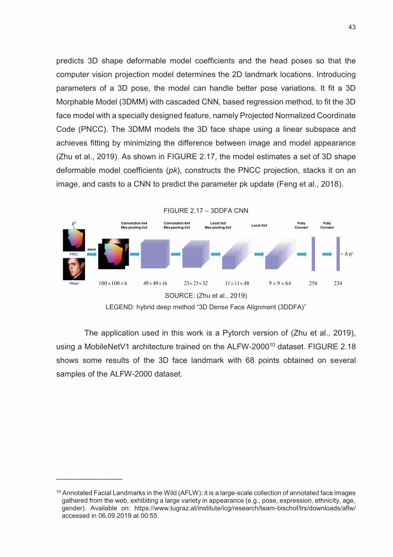
43

predicts 3D shape deformable model coefficients and the head poses so that the

computer vision projection model determines the 2D landmark locations. Introducing

parameters of a 3D pose, the model can handle better pose variations. It fit a 3D

Morphable Model (3DMM) with cascaded CNN, based regression method, to fit the 3D

face model with a specially designed feature, namely Projected Normalized Coordinate

Code (PNCC). The 3DMM models the 3D face shape using a linear subspace and

achieves fitting by minimizing the difference between image and model appearance

(Zhu et al., 2019). As shown in FIGURE 2.17, the model estimates a set of 3D shape

deformable model coefficients (pk), constructs the PNCC projection, stacks it on an

image, and casts to a CNN to predict the parameter pk update (Feng et al., 2018).

FIGURE 2.17 – 3DDFA CNN

SOURCE: (Zhu et al., 2019)

LEGEND: hybrid deep method “3D Dense Face Alignment (3DDFA)”

The application used in this work is a Pytorch version of (Zhu et al., 2019),

using a MobileNetV1 architecture trained on the ALFW-200010 dataset. FIGURE 2.18

shows some results of the 3D face landmark with 68 points obtained on several

samples of the ALFW-2000 dataset.

_______________ 10 Annotated Facial Landmarks in the Wild (AFLW): it is a large-scale collection of annotated face images

gathered from the web, exhibiting a large variety in appearance (e.g., pose, expression, ethnicity, age, gender). Available on: https://www.tugraz.at/institute/icg/research/team-bischof/lrs/downloads/aflw/ accessed in 06.09.2019 at 00:55.

44

FIGURE 2.18 – SEVERAL RESULTS ON ALFW-2000 DATASET.

SOURCE: (Zhu et al., 2019)

LEGEND: Several 3d results on the ALFW-2000 dataset.

The 3D landmark follows the same structure of feature nomenclature found in

2D detectors, as shown in FIGURE 2.19, with the relative position in the face.

FIGURE 2.19 – 68 FACIAL LANDMARK


45

2.5 DEEP LEARNING

According to the literature, Deep Learning (DL), is defined as a subfield of

Artificial Intelligence and Machine Learning, defining a multistage way to learn features

representations from data, which emphasizes learning successive layers of

increasingly meaningful representations (Gad, 2018). The term “deep” in DL stands

for an idea of successive layers of representations, which mimics the neocortex of the

brain, responsible by many cognitive abilities. It is developed in a layered and

hierarchical architecture of learning and representing data, where higher-level features

are described in terms of lower-level features (NAJAFABADI et al., 2015). FIGURE

2.20 represents the difference between DL and Machine learning approaches: ML

requires feature engineering, which is done internally on DL methods. FIGURE 2.20 – ML AND DL APPROACHES

SOURCE: (“What’s New in Deep Learning,” n.d.)

LEGEND: ML and DL differences: ML requires a feature engineering, which is done internally on DL

methods.

An essential definition in DL is the depth of the model, which is defined by how

many layers are placed inside the model architecture, often involving tens or even

hundreds of successive layers of representations in modern deep learning. All these

layers and their parameters are learned from exposure to training data (Schmidhuber,

2014). State of the art in image classification, image segmentation, and speech

recognition are based on DL models, far away from classical approaches used so far.

The primary reason for it is that makes problem-solving much more comfortable

because it completely automates a machine-learning important step, the feature

engineering.

These features are obtained through a process called learning, which can be

supervised or unsupervised, or else semi-supervised. In supervised learning, the input

data is called training data and has a known label or result to use on an optimization

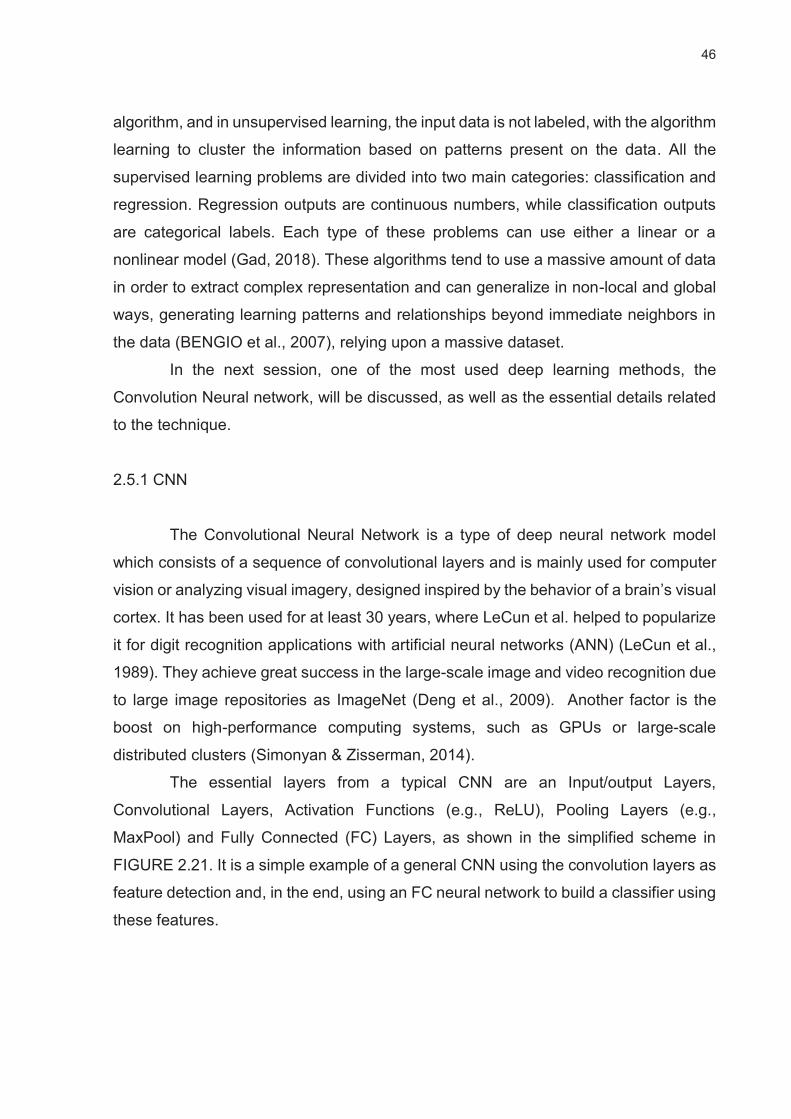
46

algorithm, and in unsupervised learning, the input data is not labeled, with the algorithm

learning to cluster the information based on patterns present on the data. All the

supervised learning problems are divided into two main categories: classification and

regression. Regression outputs are continuous numbers, while classification outputs

are categorical labels. Each type of these problems can use either a linear or a

nonlinear model (Gad, 2018). These algorithms tend to use a massive amount of data

in order to extract complex representation and can generalize in non-local and global

ways, generating learning patterns and relationships beyond immediate neighbors in

the data (BENGIO et al., 2007), relying upon a massive dataset.

In the next session, one of the most used deep learning methods, the

Convolution Neural network, will be discussed, as well as the essential details related

to the technique.

2.5.1 CNN

The Convolutional Neural Network is a type of deep neural network model

which consists of a sequence of convolutional layers and is mainly used for computer

vision or analyzing visual imagery, designed inspired by the behavior of a brain’s visual

cortex. It has been used for at least 30 years, where LeCun et al. helped to popularize

it for digit recognition applications with artificial neural networks (ANN) (LeCun et al.,

1989). They achieve great success in the large-scale image and video recognition due

to large image repositories as ImageNet (Deng et al., 2009). Another factor is the

boost on high-performance computing systems, such as GPUs or large-scale

distributed clusters (Simonyan & Zisserman, 2014).

The essential layers from a typical CNN are an Input/output Layers,

Convolutional Layers, Activation Functions (e.g., ReLU), Pooling Layers (e.g.,

MaxPool) and Fully Connected (FC) Layers, as shown in the simplified scheme in

FIGURE 2.21. It is a simple example of a general CNN using the convolution layers as

feature detection and, in the end, using an FC neural network to build a classifier using

these features.

47

FIGURE 2.21 – CNN EXAMPLE

SOURCE: (Research Group on Machine Learning for Smart Environments, 2019)

LEGEND: Basic CNN architecture example, with 1 channel input, 2 layers depth, and a fully

connected layer as a classifier, with 13 output classes.

Many CNN architectures have been proposed and used to solve many types

of problems, such as LeNet, AlexNet, GoogLeNet/Inception, ResNET, VGGNET,

Xception, Inception-ResNets and ResNeXt-50, each with specific pros and cons. What

differs one network from another is how the modules are interconnected, creating a

wide range of possible configurations, influencing in this way, its complexity, and the

data flow. According to (Szegedy et al., 2015):

“Most of this progress is not just the result of more powerful hardware, larger datasets,

and bigger models, but mainly a consequence of new ideas, algorithms, and improved

network architectures.”

2.5.1.1 Convolution Layer

The Convolutional layer, usually referred simply as the “Conv” layer, is the core

of CNN - it uses manly a kernel as a filter to slide on the original image, performing the

2D convolution. More types of convolution can be performed, such as 3D convolution,

1x1 convolution, depending on the proposed architecture. This kind of operation

enables the features detection of the image extracted with a designed kernel.

Common terminology used in the CNN context is filters and kernels. A filter is

a 3D structure, which contains several numbers of kernels, that creates an “Activation

Map” as the output and defining the input and output sizes in each layer. A kernel is a

2D matrix, usually a square shape, which contains the weights, what is used to perform

the convolution operation.

48

The kernel parameters include kernel size, depth, stride, and zero-padding. In

general terms, the convolution acts as feature detection, defined by the arrangement

of weights inside each filter. Those weights can be fixed or set as trainable parameters,

where the training procedure refers to the search on the best filter weights given a pre-

defined filter structure according to a loss function error, which propagates backward

in the network. FIGURE 2.22 shows an example from the MNIST (Modified National

Institute of Standards and Technology database) dataset with a handwritten digit,

where the Activation Map after the operation highlights the horizontal patterns defined

on the 3x3 filter found in the original image.

FIGURE 2.22 – FEATURE DETECTION IN A CONVOLUTIONAL NETWORK ARCHITECTURE


LEGEND: Feature Detection In A Convolutional Network Architecture

2.5.1.1.1 Filter size

Usually, the filters found in the literature are square, but CNN does not limit

this structure, allowing filters with different sizes for height and width. A vital

characteristic of this element is its size concerning the size of the input, and this could

be an image in the first convolution layer or an activation layer for the following layers.

2.5.1.2 Padding

Due to successive convolutional layers, the reduction in output dimension can

become a problem, since some area is lost at every convolution. The padding is a

margin with zero values placed around the image, whose depth is set so that the

convolutional layer output does not become smaller in size after convolution, as shown

in FIGURE 2.23 below.

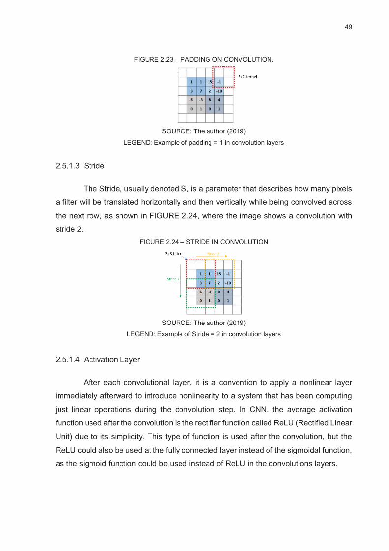
49

FIGURE 2.23 – PADDING ON CONVOLUTION.


LEGEND: Example of padding = 1 in convolution layers

2.5.1.3 Stride

The Stride, usually denoted S, is a parameter that describes how many pixels

a filter will be translated horizontally and then vertically while being convolved across

the next row, as shown in FIGURE 2.24, where the image shows a convolution with

stride 2. FIGURE 2.24 – STRIDE IN CONVOLUTION


LEGEND: Example of Stride = 2 in convolution layers

2.5.1.4 Activation Layer

After each convolutional layer, it is a convention to apply a nonlinear layer

immediately afterward to introduce nonlinearity to a system that has been computing

just linear operations during the convolution step. In CNN, the average activation

function used after the convolution is the rectifier function called ReLU (Rectified Linear

Unit) due to its simplicity. This type of function is used after the convolution, but the

ReLU could also be used at the fully connected layer instead of the sigmoidal function,

as the sigmoid function could be used instead of ReLU in the convolutions layers.

50

2.5.1.5 Pooling Layer

The pooling layer performs a downsampling operation along the spatial

dimensions (width, height), and was developed to reduce the number of parameters

needed to describe layers deeper in the network, which reduces the number of

computations required for running the forward loop of the network (used to determine

the outputs) or to train the network. A popular pooling function is the “max pooling”

operation, that reports the maximum output within a rectangular neighborhood, as

shown in FIGURE 2.25, but other pooling functions can be used, such as min pooling,

for example. As seen in the picture, the max pool operation depends on the stride

configuration, where it controls the magnitude of shift around the input data. Another

characteristic of pooling is that it provides fundamental invariance to translation and

rotation of the input image.

FIGURE 2.25 – MAXPOOL


LEGEND: Example of pooling functions in pooling layer

2.5.1.6 Classification Layer

One of the most used methods in the Classification layer is the Fully-Connected

(FC) layer, which computes the class scores in case of classification or the estimated

value in case of regression problems, according to the outputs of the “convolution-

activation-pooling” layers. In some cases, the FC layers can be changed by any other

classifier, such as a support vector machine (SVM) (Dong et al., 2018).

The FC is an ordinary Artificial Neural Network (Abiodun et al., 2018; Ghorbani

et al., 2016), where each neuron in this layer will be connected to all neurons of the

previous layer. FIGURE 2.26 shows an example of FC used in CNNs.

51

FIGURE 2.26 – FULLY CONNECTED NETWORK

SOURCE: (Nielsen, 2015)

LEGEND: Example of a Fully Connected layer with size = 9 and depth = 3

According to (Basha et al., 2019), in a typical deep neural network, the FC layers

comprise most of the parameters of the network. AlexNet has 60 million parameters,

out of which 58 million parameters correspond to the FC layers, for example.

2.5.1.7 Training Terminology

During the evolution of CNN over the years, many special functions have been

aggregated to the CNN portfolio, especially those related to the training process in

order to prevent overfitting - when a function is too fitted to a limited set of data, and

also enhances classification accuracy.

Firstly, to perform training on a DL or ML algorithm, a dataset is needed, which

is a collection of the data sample containing inputs and one or more outputs. The

algorithm is fed with the input, and the output is used to compare the error between

what is predicted and what is calculated through a loss function. Due to hardware

limitations and the massive amount of data used in these processes, it is necessary to

split the dataset into smaller parts, called batches.

Commonly in classical batch approaches, the training algorithm updates the

model only after iterating over the whole dataset, called epoch. The minibatch method

comes as an evolution of the classical method, where the model in this time is updated

in every batch data iteration, speeding up the training process (Masters & Luschi,

2018). In any case, the size of a batch is a hyperparameter that defines the number of

52

samples to work at the same time, limited by the quantity of available memory in the

hardware, such as GPU (Graphics Processing Unit).

The interaction is defined as the number of batches needed to complete one

epoch. The number of epochs is a hyperparameter that defines the number of times

the learning algorithm runs over the whole training dataset.

Another term that comes up in the training process is weight regularization,

where “L2 Regularization” is the most frequently used. It implements a penalizing

method related to the sum of squared magnitude of all parameters in a layer, adding

as regularization strength parameter - λ on the loss function (Karpathy, 2018). To

apply the weight regularization, batch normalization is used, which normalizes the data

in each training minibatch in order to avoid internal covariant shift, allowing the use of

much higher learning rates during the training process (S. Wu et al., 2019).

In the same way, another frequently used method to avoid overfitting is the

dropout operation, which is applied to FC layers: given a percentage of elements,

simply randomly discard neurons from the neural network during training, preventing

neurons from co-adapt too much, reducing overfitting and giving significant

improvements over other regularization methods (Srivastava et al., 2014).

2.5.1.8 Architectures

The way that every layer build-up using the modules defined above and its

internal connection defines the model architecture, which determines the data

workflow, the data type, and the filter size as well. FIGURE 2.27 shows a benchmark

of state of the art on Deep Neural Network Architectures in the image classification

task (Bianco et al., 2018), with the number of operations in [G-Flops], Top-1% Accuracy

in [%] and the number of parameters.

FIGURE 2.27 – STATE OF THE ART CNN ARCHITECTURES

53

SOURCE: (Bianco et al., 2018)

LEGEND: State Of The Art CNN Architectures

The networks chosen to be tested in the present work were, namely

RESNET18, VGG16, and MobileNetV2. VGG16 is classically used for image

classification, with well know drawbacks such as size. The Resnet18 has a deeper

structure and performs better than VGG in some situations and MobileNetV2, a new

architecture developed by Google team, it is lightweight and designed for mobile

applications. Those three different patters of construction and sizes were chosen to

seek what con influence in the HR estimation task. In the next section, each one of

these architectures will be briefly explained.

2.5.1.8.1 VGG16

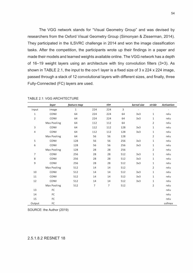
54

The VGG network stands for “Visual Geometry Group” and was devised by

researchers from the Oxford Visual Geometry Group (Simonyan & Zisserman, 2014).

They participated in the ILSVRC challenge in 2014 and won the image classification

tasks. After the competition, the participants wrote up their findings in a paper and

made their models and learned weights available online. The VGG network has a depth

of 16–19 weight layers using an architecture with tiny convolution filters (3×3). As

shown in TABLE 2.1, the input to the cov1 layer is a fixed size of 3 x 224 x 224 image,

passed through a stack of 12 convolutional layers with different sizes, and finally, three

Fully-Connected (FC) layers are used.

TABLE 2.1: VGG ARCHITECTURE


2.5.1.8.2 RESNET 18

layer feature map kernel size stride Activationinput image 1 224 224 3 - - -

1 CONV 64 224 224 64 3x3 1 relu2 CONV 64 224 224 64 3x3 1 relu

Max Pooling 64 112 112 64 2 relu3 CONV 64 112 112 128 3x3 1 relu4 CONV 64 112 112 128 3x3 1 relu

Max Pooling 64 56 56 128 2 relu5 CONV 128 56 56 256 3x3 1 relu6 CONV 128 56 56 256 3x3 1 relu

Max Pooling 128 28 28 256 2 relu7 CONV 256 28 28 512 3x3 1 relu8 CONV 256 28 28 512 3x3 1 relu9 CONV 256 28 28 512 3x3 1 relu

Max Pooling 512 14 14 512 2 relu10 CONV 512 14 14 512 3x3 1 relu11 CONV 512 14 14 512 3x3 1 relu12 CONV 512 14 14 512 3x3 1 relu

Max Pooling 512 7 7 512 2 relu13 FC relu14 FC relu15 FC relu

Output FC sofmax

size

55

ResNet, short for Residual Networks, was first introduced in 2015 and is a kind

of deep neural network which uses an “identity shortcut connection” that skips one or

more layers inside the deep architecture. ResNets was revolutionary due to the

possibility to solve the famous known vanishing gradient problem (K. He et al., 2016),

which is a tendency due to several applications of the chain rule during

backpropagation the loss function converges to zero in deep architectures, causing no

learning due to weights never being updated. Using ResNets, the gradients can flow

directly through the skip connections backward from later layers to initial filters. As

shown in TABLE 2.2, the first RESNET was 18 Conv11 layers using small filters as

VGG and uses an input image with a size of 3 x 224 x 224.

TABLE 2.2: RESNET18

SOURCE: (Pham et al., 2019)

2.5.1.8.3 MobileNetV2

The general trend on image classification is to create more complex and

deeper networks, commonly resulting in a bigger and complex architecture. However,

these advances to improve accuracy are not linear related to the efficiency concerning

_______________ 11 Conv Layer – Convolutional Layer

56

the size and speed of the model. In (Howard et al., 2017), they propose the MobileNet

model, which aims to increase the model performance, applying improvements such

as the replacement of standard convolutional filters by two layers: the depthwise

convolution and the pointwise convolution, in order to build a depthwise separable

filter. According to their work, using this module, the network uses 8 to 9 times less

computation than standard convolutions, at only a small reduction in output accuracy.

In (Sandler et al., 2018, p. 2), an improvement for the first architecture was

proposed introducing new features to the architecture: the linear bottlenecks between

the layers and shortcut connections between the bottlenecks. In (“MobileNetV2,” 2018,

p. 2): “The intuition is that the bottlenecks encode the model’s intermediate inputs and outputs

while the inner layer encapsulates the model’s ability to transform from lower-level

concepts such as pixels to higher-level descriptors such as image categories. Finally,

as with traditional residual connections, shortcuts enable faster training and better

accuracy.”

As shown in TABLE 2.3, where t is the expansion factor, c is the number of

output channels, n is the repeating number, and s the stride. The MobileNetV2 uses a

3×3 depthwise separable convolutions and an image input with size 3 x 224 x 224.

TABLE 2.3: MOBILENET V2

Input layer t c n s

3x 224 x 224 conv2d * 32 1 2 32 x 112 x 112 bottleneck 1 16 1 1 16 x 112 x 112 bottleneck 6 24 2 2

24 x 56 x 56 bottleneck 6 32 3 2 32 x 28 x 32 bottleneck 6 64 4 2 64 x 14 x 14 bottleneck 6 96 3 1 96 x 14 x 14 bottleneck 6 160 3 2 160 x 7 x 7 bottleneck 6 320 1 1 320 x 7 x 7 conv2d 1x1 - 1280 1 1 1280 x 7 x 7 avgpool 7x7 - - 1 - 1 x 1x 1280 conv2d 1x1 - k -

SOURCE: (Howard et al., 2017)

2.6 DATABASE

57

Due to an intrinsic necessity of deep learning methods on a massive amount

of data to perform training and obtain good results in classification or regression tasks,

a high-quality database is mandatory. Real scenarios data are the most crucial

component to develop any machine learning or deep learning application. Therefore,

there are some public available datasets for evaluation of HR estimation methods,

such as MAHNOB dataset (Soleymani et al., 2012), DEAP dataset (Koelstra et al.,

2012), VIPL-HR dataset (Niu et al., 2019), PURE dataset (Stricker et al., 2014),

COHFACE dataset (X. Chen et al., 2019) and the ECG-Fitness (Spetlík et al., 2018).

Unfortunately, many of the available datasets does not use a medical ECG as ground

truth, except MANHOB, and ECG-fitness. Between both, ECG-fitness has the most

realistic scenario with head movements and light changing, but the video recorder was

made at 30 fps.

Due to its restrictions and lack of data, it was necessary to build a new

database for training the CNN HR estimator: the THI database, using a medical

precision ECG as ground truth, a high resolution, and a high fps camera to build the

DL based HR estimator. More details about the experiment protocol will be addressed

in section 3.6 of this document.

The database contains 16 different persons with distinct etymology and skin

tones where 4 of them are Indians, two are then are Asiatics, and the rest are

Caucasian; among them, 6 are women. Those samples inside the database are

essential due to the relationship of light reflection in the presence of different quantities

of melanin.

58

3 METHODOLOGY

This chapter will focus on the methodology applied to solve the problem

described in the previous chapters, as well as introduce detailed information about

each process involved.

3.1 HR WORKFLOW

As stated before, in the present work, it is proposed to verify the feasibility of

a real-time, non-contact approach of deep learning-based HR estimator, using a pre-

trained image classification CNN architecture with a spatial-temporal map as input in

a regression problem. Taking into account the literature review and all work that has

been done, a workflow pipeline was devised to perform the HR estimation. The

proposed algorithm is shown in FIGURE 3.1 which has inspiration on the work of (Niu

et al., 2018), with 2 essential improvements proposed to the method: use of robust

polygonal face segmentation and a unitary and parallel frequency filter clipping the

signal to the center of the pixel range [0, 255], in order to give more stability to the

spatial-temporal map representation.

FIGURE 3.1 – PROPOSED PIPELINE WORKFLOW

SOURCE: the author (2019).

LEGEND: Workflow for HR estimation using spatial-temporal maps

3.2 RESEARCH PLANNING

The core of this work relies on the comparison between three different state of

the art CNN architectures, namely: VGG16, RESNET18, and MobileNet v2, measuring

how capable are each one to estimating the driver HR measurement using an RGB

camera image. Furthermore, three different color space models, namely RGB, YUV,

and HSV, have been tested to verify which is more suitable for the desired application.

All the experiments and testing are extremely time-consuming and rely on the

development of specific tools and applications along with the project development. In

59

order to make the work development feasible, it was organized in sequential steps as

follows:

1. Literature review;

2. Evaluate methods and network models used as face detector and alignment

in the proposed workflow;

3. Build and test the new method to create the spatial-temporal maps with

independent filtering;

4. Build the software tools to perform the pipeline proposed in the present work.

5. Build a high-quality database for test and training: record the experiment

sessions, filter, and organize the data.

6. Build the software tools to perform and manage the experiments;

7. Evaluation of the optimal color space for spatial-temporal maps

representation for deep learning HR application, using the same CNN

architecture and same configurations such as learning rate, maximum

epochs, and optimization method;

8. Evaluate three different state of the art image classification CNNs, using the

same color map and same configurations such as learning rate, maximum

epochs, and optimization method.

9. Evaluate three different rPPG state of the art algorithms against the best

configuration of our proposed DL CNN method;

3.3 STATE OF THE ART METHODS COMPARISON

Among the algorithms available and in use in the literature, three of them were

selected to perform a comparison between the proposed method in this work and those

used as reference, namely Plane Orthogonal to Skin - POS (Wang et al., 2016),

Independent Component Analysis - ICA (Verkruysse et al., 2008) and Local Group

Invariance - LGI (Pilz et al., 2018). The three methods share the same workflow, as

shown in FIGURE 3.2, which relies on a facial skin segmentation, normally given by a

previous face detector, as well as a peak detector in case of a time-domain extraction

or a spectrum analysis in case of frequency-domain HR extraction.

60

FIGURE 3.2 – STATE OF THE ART METHODS WORKFLOW


LEGEND: State of the art methods workflow based on the skin segmentation process.

The present work implements the workflow above using a temporal analysis

with peak detection to perform the testing for each algorithm in every subject and every

experiment among the THI Database. The process relies on a common core: a face

detector, a skin segmentation, and a peak detector.

The face segmentation used in this process is the same used in the present

proposed algorithm – an SSD Resnet10 CNN network. To implement the peak

detector, it is used the function “find peaks”12 from Mathworks, which offers a robust

and configurable tool. To perform the skin segmentation, a CNN method was used

based on the work of Nasir Hayat13 , which developed an application written in Python

using Pytorch framework and the CNN LinkNet34 architecture, available in its Github

page. The model has shown a good performance regarding motion, multiple poses,

and segmenting skin pixels from non-skin. The mask created by the network is then

applied to the original image, and the value of the mean of the R, G, B components

are computed for every frame. FIGURE 3.3 shows the result of the CNN skin

segmentation applied to the THI database.

FIGURE 3.3 – SKIN SEGMENTATION USING SEMANTIC CNN


LEGEND: The facial skin removed from the image sequence for experiment 3 of the THI database.

_______________ 12 Available in https://de.mathworks.com/help/signal/ref/findpeaks.html, accessed in 07.010.2019 13 Available in https://github.com/nasir6/face-segmentation, accessed in 08.05.2019

61

3.4 DEVELOPMENT OF THE PLATFORM

To build the proposed method, many tolls and software were used and

developed in each stage of the work. During the development of the solutions, many

tests have been made, but only strictly related to the results obtained are described in

this work. In this section, all the frameworks used or devised in the solution are listed.

3.4.1 Software used

All the development made in this work is based on three basic frameworks and

programming languages: Python, OpenCV, and Pytorch.

3.4.1.1 Python

It is a free and open-source language, cross-platform, and largely used to

software prototyping. It is a versatile language, easy to use and learn, readable, and

well-structured, focuses on code readability, and is based on the object-oriented

paradigm. Additionally, it has an extensive selection of in-built libraries, as well as a

massive development community.

3.4.1.2 OpenCV

OpenCV is a cross-platform library widely used to develop real-time computer

vision applications. It focuses on image processing, video capture, and analysis. It has

a DNN module with the capability to read models from another framework, such as

Caffe and Yolo, without the installation of those. All the image processing operation in

the present work was performed with the OpenCV library.

3.4.1.3 Pytorch

PyTorch is a Python-based scientific GPU capable computing package and a

deep learning research platform that provides flexibility and prototyping speed. It

enables GPU-accelerated tensor computations and provides rich options of APIs for

neural network applications. Based on Dynamic Computational graphs, it supports

different back-end working with CPU and GPU, and it is deeply integrated with the C++

62

code, sharing some C++ backend with the deep learning framework, Torch, offering in

this way a highly extensible platform (Paszke et al., 2017).

3.4.2 Software development

During the development process, two different software was devised to

perform the experiments. The first one runs as a script, and it is able to create, edit,

and resume a network training in PyTorch using the THI database as the data source

under GPU. The second one was developed using pyQT5, shown in FIGURE 3.4,

which was design as a platform to process ECG and video data, in order to create the

spatial-temporal maps and visualize the result of the face detectors and polygonal

segmentation. FIGURE 3.4 – THI DATABASE MANAGER


LEGEND: THI Database manager software

3.5 THE POLYGON FILTER APPROACH

In this work it was proposed a modification on spatial-temporal map originally

stated by (Niu et al., 2018), where a polygonal mesh grid is used with an independent

gain and bandpass filter applied in each polygon before creating the map itself, clipping

63

the signal to the center of the pixel range [0, 255]. FIGURE 3.5 shows the proposed

spatial-temporal map creation method.

FIGURE 3.5 – FILTER APPROACH


LEGEND: Proposed filter Approach

To implement the polygonal mesh grid, the projection of the 3D landmark

points is used. However, connecting the only the 68 points given points to build a mesh

is not sufficient to cover all the highly sensitive HR regions in the face, namely the

forehead and the cheeks. To address this problem, a sequence of “anchor” points is

proposed: 21 points in total, seven located in each cheek, and seven points at the

forehead region. The anchor positions are given by the relationship between the

original landmark points, for example, the position of anchor 75 is located in the middle

of the line which connects the original landmark “1” to “38”, and so on. The final mesh

is defined as polygons connecting the points listed in a configuration file. FIGURE 3.6

shows the segmentation using anchor points over 89 face landmark points. In total, the

polygonal mesh has 56 pieces, ensuring the accurate tracking of the region measured

on the face skin.

64

FIGURE 3.6 – POLYGONAL SEGMENTATION

(a) (b) SOURCE: the author (2019)

LEGEND: 56 polygonal segmentation using 21 anchor points over 68 original face landmark

As stated before, the position of the landmark points are given by the 3D model

in a 2D projection, and for some head poses, many points may be in a hidden position

– not visible in the image, but still, the points will appear in the network output following

its projection. Building a polygon with an invisible point will lead to wrong

measurements of inexistent areas, which is undesirable. To address the problem, a

landmark position check must be performed to verify whether or not the point is visible

and if a polygon has invisible vertices, the algorithm ignores it. FIGURE 3.7 shows the

result for visibility check, where the red dots indicate a non-visible face landmark and

the blue dots the visible ones. Nevertheless, another critical aspect being considered

is the size of the polygon: if the size is smaller than a threshold, the polygon is ignored

by the algorithm. FIGURE 3.7 – POLYGONAL FACE SEGMENTATION


LEGEND: Hidden 3D landmark points due to the head pose (red dots in the image)

65

Following the next step on the proposed algorithm on polygonal face

segmentation and filtering, to implement a continuous filter that processes the batch

data from the camera, a function is written in python, which controls the initialization of

the internal states. A 2nd order normalized Butterworth is used for the bandpass filter,

using a cascade topology, where it is possible to compose higher filter orders with a

more straightforward and smaller filter such as 1st and 2nd orders. Using the Laplace

domain equation and its coefficients, a discrete-time version of a differential operator

in the continuous-time was used, applying the bilinear mapping from Laplace to Z-

space, mapping a discrete-time digital filter with coefficients in terms of the original

continuous-time filter coefficients. The first time that the function runs, the program

initializes the internal states. On the following steps, the value initializes the internal

memories with the final states from the previous call to this instance of the filter,

working as continuous filtering.

3.6 PROPRIETARY THI DATABASE

In order to create a driver-like scenario, stated in Chapter 2, a proprietary dataset

was recorded. It contains 31 recorded sessions with an average of 2:30 minutes each,

with 16 different healthy subjects under 50 years, male and female. FIGURE 3.8 shows

the experimental setup used to acquire the data, where the camera position as chosen

to reproduce the same scenario as is in a car cockpit, in order to not disturb the driving

task. FIGURE 3.8 – THI DATASET SETUP


LEGEND: THI dataset setup

66

The database contains 16 different subjets, 6 women and 10 men – with distinct

etymology and skin tones where 4 of them are Indians, 2 are then are Asiatics, and the

rest are Caucasian. Each participant was asked to perform two recordings - the first

one was made with the participant in a resting position, which represents, for a healthy

young person, values between 50 to 120 bpm. The second recording was made after

an induced HR increase through a small physical exercise, as shown in As is possible

to verify from the image below, the HR signal is not a smooth curve due to the strict

dependence in the ANS balance, and the most precise estimation of HR can lead to a

better estimation of HRV and, subsequently, the human health status.

FIGURE 3.9, in order to induce a negative ramp in the HR value, creating samples

in a determined range, essential to enrich the database samples. As is possible to

verify from the image below, the HR signal is not a smooth curve due to the strict

dependence in the ANS balance, and the most precise estimation of HR can lead to a

better estimation of HRV and, subsequently, the human health status.

FIGURE 3.9 – THI EXPERIMENT HR SAMPLE


LEGEND: The THI dataset example: decreasing HR experiment with a high HRV

The most significant improvement related to other databases is the medical

precision ECG. As stated before, the chosen device to perform all the ECG acquisition

was the “ECG Shimmer 3”, from Shimmer Sensing company. The raw device signal

measured along the experiment session is recorded inside the device memory and

recovered afterward using the Consensys software. The camera used to capture the

data during the sessions is a Nikon D5300, which is a DSRL (Digital Single Lens Reflex)

camera with 24,4 megapixels, capable of recording videos with a resolution of 1080p at 60

67

frames per second. The camera uses an 18 mm lens, keeping a fixed focus during video

capture.

FIGURE 3.10 shows some samples recorded in the database.

FIGURE 3.10 – THI DATABASE SAMPLE


LEGEND: THI sample database image with resolution:1920x1080 at 60 fps.

The spatial-temporal maps database was created using the software to 3.4.2,

performing the ECG raw signal processing and the video frame synchronization, made

by timestamp, performing the workflow proposed in the present work. Due to the use

of window technique in order to represent the color average changing through time, a

new spatial-temporal map is created every newly calculated data, as in a first-in-first-

out (FIFO) structure.

For a video length of 02:30 minutes, it will contain 9000 sequential frames, and

after processing it, it will generate 8800 spatial maps. In total, the dataset has 99

68

minutes, which corresponds to 359.113 samples of space-temporal maps, each one

consisting of an RGB, Y’UV, and HSV color space with a bpm target value.

The maps were generated using the software described in 3.4.2. TABLE 3.1

shows an overview of the whole dataset. Due to the nature of spatial-temporal maps

formation – a circular buffer, if many frames are used consecutively, it may bias the

result in the training process, decreasing the generalization degree of the model. In

order to create the training subset, a random selection using uniform distribution of

25% from the whole database was used to avoid high similarity and sequences, where

statistically has also 25 % of each subject example, and over this subset, another slice

was made with 66% used as training and 33% as validation.

TABLE 3.1: THI DATASET OVERVIEW Dataset Samples Training Validation Testing

359113 59253 30525 269335 16.5% 8.5% 75.0%


3.7 TRAINING PROCESS

The problem of training a CNN can be classified as a problem of minimization

of a defined loss function, and there are many algorithms approaches to do this work,

gradient-based or not. The next section will explain the basis of the algorithms used in

this work to perform the CNN networks training.

3.7.1 Optimizer

The method chosen to train the CNN network in the present work is the ADAM

(Adaptive Moment estimation) (Kingma & Ba, 2014). ADAM is an adaptive learning

rate optimization algorithm designed specifically for training deep neural networks.

First published in 2014, Adam was presented at ICLR 2015, since then, has been one

of the best optimization algorithms for deep learning.

3.7.2 Loss Function

69

The metric selected to use as loss function in this work is the Mean Squared

Error (MSE), which averages the squared difference between the estimated values

and true value, as shown below:

(3.1)

where denotes the target value, the estimated value and N the number of

samples in the vector and .

70

4 EXPERIMENTAL RESULTS

All the software development and experiments evaluation were performed in a

Technische Hochschule Ingolstadt server, supplied by the Center of Automotive

Research on Integrated Safety Systems and Measurement Area (CARISSMA). It was

computed on a Ubuntu 18.04 OS with a CPU (Central Processing Unit) Intel(R)

Xeon(R) Silver 4110 2.1 GHz, two physical processors, 16 cores, 32 threads, RAM

(Random Access Memory) 32 GB and three units of NVIDIA RTX 2080ti, 11GB RAM,

with 4352 Cuda (Compute Unified Device Architecture) cores. The applications

developed during the study are based on Python 3.7, Pytorch 1.2, and OpenCV4.1.

The experiments performed during the study will be detailed in the next sections,

namely polygonal mesh evaluation, color space evaluation, and network architecture

evaluation.

4.1 POLYGONAL MESH EVALUATION

The effect of adding a filter for every sample of the spatial-temporal map

representation can be observed in FIGURE 4.1, where the theoretical signal pattern

expected is shown in (I), the real signal obtained by sensors without filtering and

normalization is shown in (II), with filter and max/min normalization in (III) and the

model proposed in this work, with a filter and independent normalization in (IV). The

image shows that the proposed method is most similar to the theoretically expected

signal pattern. FIGURE 4.1 – PROPOSED METHOD COMPARISON


71

All the videos recorded during the database acquisition were processed using

the algorithm pipeline proposed in this work. FIGURE 4.2 shows one example of this

data, where the sunlight partially covers the face. It indicates that the polygonal mesh

can: 1) find the face, 2) track all the points in the face even with obstructions, 3) identify

what is a valid region or not, and 4) update the spatial-temporal map buffer without

interfering in the other points. FIGURE 4.2 – POLYGONAL MESH PATTERN


LEGEND: Example of polygonal mesh and the map forming. The highlighted area in red represents

the facial area under the sunlight.

4.2 OPTIMAL COLOR SPACE EVALUATION

All the evaluation process for the comparison of the suitable color space for

spatial-temporal maps representation for deep learning HR application was made

using the same CNN architecture – the RESNET18, under the same training

configurations such as learning rate, maximum epochs, and optimizer. The parameters

for training are described as follows: architecture: ResNET18, learning rate: 1e-6,

number of epochs: 150, optimizer: ADAM, loss function: MSE, weight decay: 1e-5. To

run every training in the server, it took 23 hours for each experiment. The following

sessions will present the results obtained in each experiment.

72

4.2.1 RGB evaluation

The curve of training losses for the RESNET18 architecture with an RGB color

space image, calculated along the epochs, is shown in FIGURE 4.3.The overall process

took 114 epochs and 23 hours to reach the best value for the validation loss (0.115344

bpm). TABLE 4.1 shows an overview of all the MSE and σ obtained for the whole THI

database experiments evaluation using the complete dataset, as described in 3.6. The

first value, “idx,” refer to the number of the recording session ( 2 for each subject ), the

column under “CNN” refers to the results using the CNN output only, and “CNN +

output” filter refers to the result of applying a 2nd order Butterworth low pass filter on

the CNN output. The MSE value indicates how fitted is the estimated curve over the

target, where smaller values mean better approximation. The σ represents the

standard deviation of the error, in which values inferior to 5 bpm are acceptable. The

network has seen only 16.5% of the data during the training.

FIGURE 4.3 – RESNET18 RGB TRAINING CURVE


73

TABLE 4.1: DATABASE RESULTS RESNET18 WITH RGB

CNN CNN + filter idx MSE (bpm) σ (bpm) MSE (bpm) σ (bpm) 1 29.57 5.02 14.79 3.22 2 30.89 5.19 15.19 3.34 3 23.23 4.68 10.08 2.95 4 34.25 5.64 14.87 3.51 5 20.26 4.32 9.11 2.74 6 26.42 5.07 12.74 3.47 7 14.72 3.81 7.43 2.68 8 42.03 6.45 24.96 4.94 9 24.20 4.79 12.35 3.32 10 31.74 5.51 12.39 3.31 11 30.29 5.35 12.88 3.35 12 33.83 5.36 16.39 3.36 13 26.01 5.10 11.55 3.40 14 9.90 3.14 4.24 2.04 15 21.80 4.51 10.23 2.96 16 24.90 4.95 12.63 3.49 17 13.43 3.62 5.93 2.37 18 30.59 5.18 13.66 3.15 19 11.60 3.40 5.58 2.35 20 36.71 5.99 17.56 4.08 21 26.38 4.62 14.41 3.07 22 19.64 4.25 8.82 2.68 23 29.39 5.36 12.47 3.43 24 46.81 6.50 20.66 4.01 25 26.80 5.13 12.03 3.38 26 16.68 4.06 7.75 2.74 27 17.77 4.05 8.63 2.69 28 28.95 5.24 15.08 3.67 29 19.88 4.28 9.74 2.86 30 28.43 5.29 13.96 3.66 31 14.70 3.81 7.09 2.62 32 29.76 5.26 13.01 3.29 33 15.33 3.91 7.80 2.78 26.38 5.02 12.39 3.29


Among the 33 sessions of the THI database, the table above shown two

highlighted rows, which are chosen randomly to be demonstrated in FIGURE 4.4,

where the HR estimation output of the proposed method is represented in blue and the

target measured by the ECG during the session in red in two different experiments. On

the left, the result for the experiment “1”, in which the model results in a standard

deviation (σ) of 5.02 bpm without low-pass filtering (top curve), and with low-pass

filtering, σ=3.22 bpm (bottom curve). At the right, the experiment “4” is shown, where

the model results in σ = 5.64 bpm without low-pass filtering (top curve), and with

filtering, σ = 3.51 bpm (bottom). As it is possible to verify, the output error decreases

by 34% using the filter, as shown in the table results.

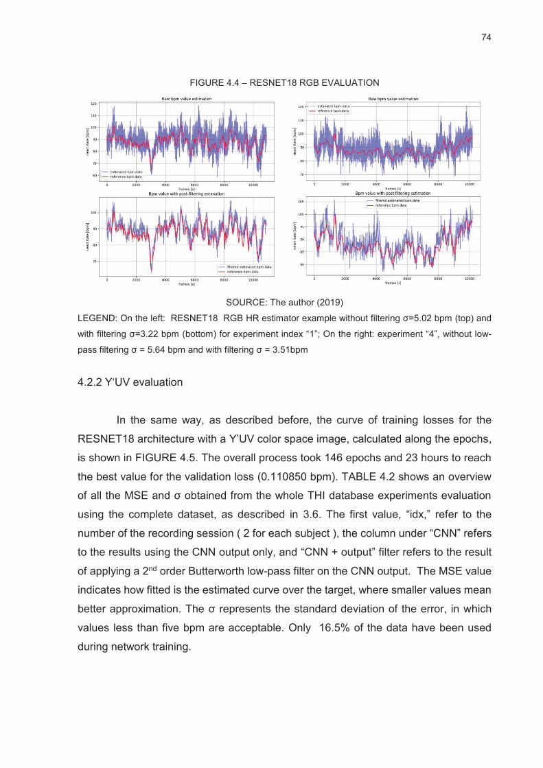
74

FIGURE 4.4 – RESNET18 RGB EVALUATION


LEGEND: On the left: RESNET18 RGB HR estimator example without filtering σ=5.02 bpm (top) and

with filtering σ=3.22 bpm (bottom) for experiment index “1”; On the right: experiment “4”, without low-

pass filtering σ = 5.64 bpm and with filtering σ = 3.51bpm

4.2.2 Y‘UV evaluation

In the same way, as described before, the curve of training losses for the

RESNET18 architecture with a Y’UV color space image, calculated along the epochs,

is shown in FIGURE 4.5. The overall process took 146 epochs and 23 hours to reach

the best value for the validation loss (0.110850 bpm). TABLE 4.2 shows an overview

of all the MSE and σ obtained from the whole THI database experiments evaluation

using the complete dataset, as described in 3.6. The first value, “idx,” refer to the

number of the recording session ( 2 for each subject ), the column under “CNN” refers

to the results using the CNN output only, and “CNN + output” filter refers to the result

of applying a 2nd order Butterworth low-pass filter on the CNN output. The MSE value

indicates how fitted is the estimated curve over the target, where smaller values mean

better approximation. The σ represents the standard deviation of the error, in which

values less than five bpm are acceptable. Only 16.5% of the data have been used

during network training.

75

FIGURE 4.5 – RESNET18 Y’UV TRAINING CURVE


TABLE 4.2: DATABASE RESULTS RESNET18 WITH Y’UV



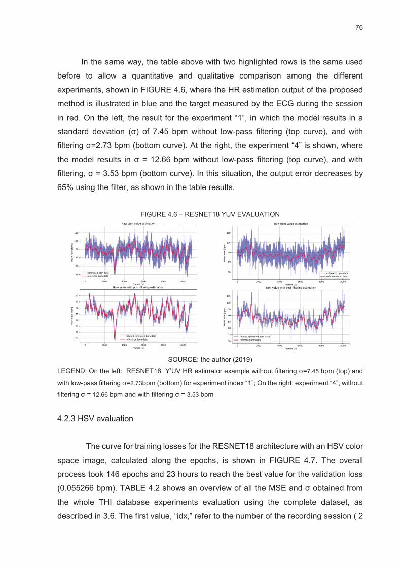
76

In the same way, the table above with two highlighted rows is the same used

before to allow a quantitative and qualitative comparison among the different

experiments, shown in FIGURE 4.6, where the HR estimation output of the proposed

method is illustrated in blue and the target measured by the ECG during the session

in red. On the left, the result for the experiment “1”, in which the model results in a

standard deviation (σ) of 7.45 bpm without low-pass filtering (top curve), and with

filtering σ=2.73 bpm (bottom curve). At the right, the experiment “4” is shown, where

the model results in σ = 12.66 bpm without low-pass filtering (top curve), and with

filtering, σ = 3.53 bpm (bottom curve). In this situation, the output error decreases by

65% using the filter, as shown in the table results.

FIGURE 4.6 – RESNET18 YUV EVALUATION


LEGEND: On the left: RESNET18 Y’UV HR estimator example without filtering σ=7.45 bpm (top) and

with low-pass filtering σ=2.73bpm (bottom) for experiment index “1”; On the right: experiment “4”, without

filtering σ = 12.66 bpm and with filtering σ = 3.53 bpm

4.2.3 HSV evaluation

The curve for training losses for the RESNET18 architecture with an HSV color

space image, calculated along the epochs, is shown in FIGURE 4.7. The overall

process took 146 epochs and 23 hours to reach the best value for the validation loss

(0.055266 bpm). TABLE 4.2 shows an overview of all the MSE and σ obtained from

the whole THI database experiments evaluation using the complete dataset, as

described in 3.6. The first value, “idx,” refer to the number of the recording session ( 2

77

for each subject ), the column under “CNN” refers to the results using the CNN output

only, and “CNN + output” filter refers to the result of applying a 2nd order Butterworth

low-pass on the CNN output. The MSE value indicates how fitted is the estimated

curve over the target, where smaller values mean better approximation. The σ

indicates the standard deviation of the error, in which values less than five bpm are

acceptable. Only 16.5% of the data have been used during network training.

FIGURE 4.7 – RESNET18 HSVTRAINING CURVE


78

TABLE 4.3: DATABASE RESULTS RESNET18 WITH HSV



Besides, the table above shown two highlighted rows, which are the same used


experiments, shown in FIGURE 4.8, where the CNN HR estimation is pictured in blue

and the target measured by the ECG during the session in red. Still on the left, the

result for the experiment “1”, in which the model results in a standard deviation (σ) of

3.60 bpm without low-pass filtering (top curve), and with filtering σ=1.90 bpm (bottom

curve). At the right, the experiment “4” is shown, where the model results in σ = 5.96

bpm without low-pass filtering (top curve), and with filtering, σ = 2.44 bpm (bottom

curve). The output error decreases by 51% using the filter, as shown in the table

results.

79

FIGURE 4.8 – RESNET18 HSV EVALUATION



with filtering σ=1.90 bpm (bottom) for experiment index “1”; On the right: experiment “4”, without filtering

σ = 5.96 bpm and with filtering σ = 2.44 bpm

4.2.4 COLOR SPACE COMPARISON

The comparison of the best color model is shown in TABLE 4.4, based on the

performance evaluated previously, and depends on the average of the MSE given in

each experiment, evaluated in all database (359113 samples) for the Resnet18

architecture, using Y’UV, HSV, and RGB color spaces. As a remark, the networks have

seen only 16.5% of the samples during the training procedure, with the rest being part

of the testing dataset. The first two columns are related to raw CNN output, and the

last two columns are the result of the filtered output.

TABLE 4.4: COMPARISON OF COLOR SPACES OVER RESNET18 ARCHITECTURE

CNN CNN + filter Color space MSE (bpm) σ (bpm) MSE (bpm) σ (bpm)

RGB 26.378 5.020 12.390 3.294 YUV 23.296 9.964 4.695 3.041 HSV 10.730 4.258 3.272 2.063


80

According to TABLE 4.4, among the color space models used, it is possible to

state that HSV color space represents by far the most suitable color model to be used

in the application of HR estimation using spatial-temporal maps.

4.3 NETWORK ARCHITECTURE EVALUATION

For comparison of the suitable CNN architecture for spatial-temporal maps

representation to be used as HR estimator, the input color map model was used – the

Y’UV color space (same used by (Niu et al., 2018)), under the same training

configurations, using the following networks: ResNET18, VGG, and MobileNETV2.

The parameters for training each model are described as follows: architecture:

depends on the experiment, learning rate: 1e-6, number of epochs: 150, optimizer:

ADAM, loss function: MSE, weight decay: 1e-5. To run every training in the server, it

took 23 hours for each experiment. The following sessions will present the results

obtained in each experiment in a more detailed way.

4.3.1 VGG16

The curve of training losses for the VGG16 architecture with a Y’UV color

space image, evaluated along the epochs is shown in FIGURE 4.9. The overall process

took 114 epochs and 28 hours to reach the best value for the validation loss (0.00992

bpm). TABLE 4.5 shows an overview of all the MSE and σ obtained for the whole THI

database experiments evaluation using the complete dataset, as described in 3.6. The

first value, “idx,” refer to the number of the recording session ( 2 for each subject ), the

column under “CNN” refers to the results using the CNN output only, and “CNN +

output” filter refers to the result of applying a 2nd order Butterworth low-pass on the

CNN output. The MSE value indicates how fitted is the estimated curve over the target,

where smaller values mean better approximation. The σ represents the standard

deviation of the error, in which values less than five bpm are acceptable. The network

has seen only 16.5% of the data during the training.

81

FIGURE 4.9 – VGG16 YUV CURVE RESULTS


TABLE 4.5: DATABASE RESULTS VGG16 WITH Y’UV



82

The TABLE 4.5 shown two highlighted rows, which are the same used before

to allow a quantitative and qualitative comparison among the different experiments,

shown in FIGURE 4.8, where the CNN HR estimation is drawn in blue and the target

measured by the ECG during the session in red. Still on the left, the result for the

experiment “1”, in which the model results in a standard deviation (σ) of 1.51 bpm

without low-pass filtering (top curve), and with filtering σ=1.27 bpm (bottom curve). At

the right, the experiment “4” is shown, where the model results in σ = 1.69 bpm without

low-pass filtering (top curve), and with filtering σ = 1.64 bpm (bottom curve). The output

error decreases by 6% using the filter, as shown in the table results.

FIGURE 4.10 – VGG16 YUV EVALUATION





4.3.2 MOBILENETV2

The curve of training losses for the MobileNETV2 architecture with a Y’UV

color space image, evaluated along the epochs is shown in FIGURE 4.11. The overall

process took 142 epochs and 20 hours to reach the best value for the validation loss

(0.28829 bpm). TABLE 4.6 shows an overview of all the MSE and σ obtained for the

whole THI database experiments evaluation using the complete dataset, as described

in 3.6. The first value, “idx,” refer to the number of the recording session ( 2 for each

83

subject ), the column under “CNN” refers to the results using the CNN output only, and

“CNN + output” filter refers to the result applying a 2nd order Butterworth low-pass on

the CNN output. The MSE value indicates how fitted is the estimated curve over the

target, where smaller values mean better approximation. The σ represents the

standard deviation of the error, in which values less than five bpm are acceptable. The

network has seen only 16.5% of the data during the training. The first two columns are

related to raw CNN output, and the last two columns are the result of the filtered CNN

output.

FIGURE 4.11 – MOBILENETV2 YUV CURVE RESULTS


84

TABLE 4.6: DATABASE RESULTS MOBILENETV2 Y’UV



Besides, the table above shown two highlighted rows, which are the same used


experiments, shown in FIGURE 4.8, where the CNN HR estimation is drawn in blue

and the target measured by the ECG during the session in red. Still on the left, the

result for the experiment “1”, in which the model results in a standard deviation (σ) of

6.92 bpm without low-pass filtering (top curve), and with filtering, σ=5.86 bpm (bottom

curve). At the right, the experiment “4” is shown, where the model results in σ = 9.18

bpm without low-pass filtering (top curve), and with filtering, σ = 8.29 bpm (bottom

curve). In this situation, the output error decreases by 9% using the filter, as shown in

the table results.

85

FIGURE 4.12 – MOBILENETV2 Y’UV EVALUATION





4.3.3 RESNET18

The network experiment in this section is the same as shown in 4.2.2;

consequently, the same results will be used in this session.

4.3.4 Network architecture comparison

The comparison of the best architecture shown in TABLE 4.7, was made using

the previous results obtained in 4.2.2 for the ResnNet18 and the result obtained in the

previous sections for VGG16 and MobileNET. The performance analysis depends on

the average of the MSE given in each experiment, evaluated in all the database

(359.113 samples) for the MobileNet V2, Resnet18 ad VGG16 architecture using Y’UV

color space map. As stated before, all the networks only visualize 16.5% of these

values during the training procedure, and the rest is part of the test dataset. TABLE

4.7 shows in the first two columns the result for raw CNN output and the last two

columns the result for low-filtered output.

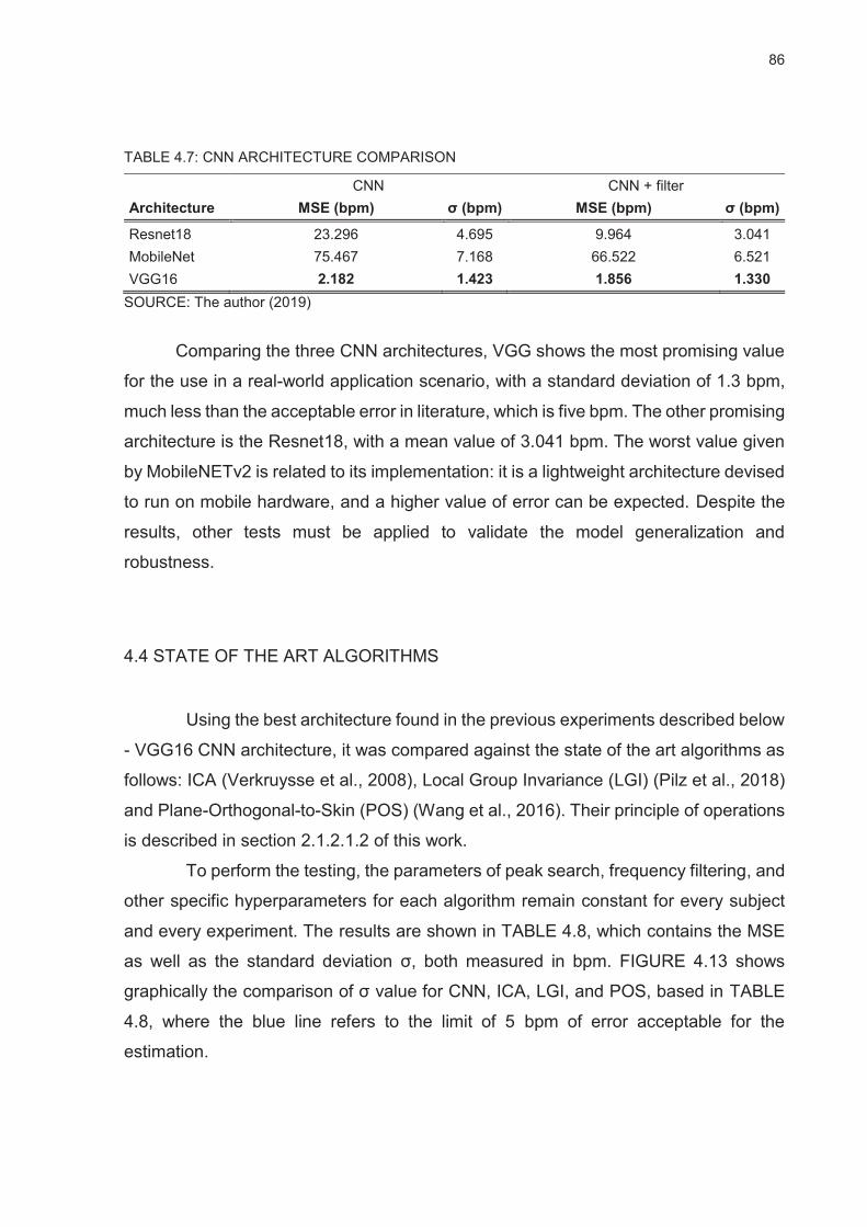
86

TABLE 4.7: CNN ARCHITECTURE COMPARISON

CNN CNN + filter Architecture MSE (bpm) σ (bpm) MSE (bpm) σ (bpm)

Resnet18 23.296 4.695 9.964 3.041 MobileNet 75.467 7.168 66.522 6.521 VGG16 2.182 1.423 1.856 1.330


Comparing the three CNN architectures, VGG shows the most promising value

for the use in a real-world application scenario, with a standard deviation of 1.3 bpm,

much less than the acceptable error in literature, which is five bpm. The other promising

architecture is the Resnet18, with a mean value of 3.041 bpm. The worst value given

by MobileNETv2 is related to its implementation: it is a lightweight architecture devised

to run on mobile hardware, and a higher value of error can be expected. Despite the

results, other tests must be applied to validate the model generalization and

robustness.

4.4 STATE OF THE ART ALGORITHMS

Using the best architecture found in the previous experiments described below

- VGG16 CNN architecture, it was compared against the state of the art algorithms as

follows: ICA (Verkruysse et al., 2008), Local Group Invariance (LGI) (Pilz et al., 2018)

and Plane-Orthogonal-to-Skin (POS) (Wang et al., 2016). Their principle of operations

is described in section 2.1.2.1.2 of this work.

To perform the testing, the parameters of peak search, frequency filtering, and

other specific hyperparameters for each algorithm remain constant for every subject

and every experiment. The results are shown in TABLE 4.8, which contains the MSE

as well as the standard deviation σ, both measured in bpm. FIGURE 4.13 shows

graphically the comparison of σ value for CNN, ICA, LGI, and POS, based in TABLE

4.8, where the blue line refers to the limit of 5 bpm of error acceptable for the

estimation.

87

TABLE 4.8: RESULTS OF THE BEST CNN AGAINST STATE OF THE ART ALGORITHMS

CNN + filter ICA IDG POS idx

MSE [bpm]

σ [bpm]

MSE [bpm]

σ [bpm]

MSE [bpm]

σ [bpm]

MSE [bpm]

σ [bpm]

1 1.41 1.16 257.85 10.84 218.04 10.41 187.03 11.35 2 0.70 0.83 126.28 11.20 174.95 13.12 145.16 11.98 3 1.80 1.27 970.52 18.03 938.79 17.53 1004.70 19.64 4 2.51 1.52 614.61 13.05 467.60 8.13 750.53 19.93 5 1.67 1.19 377.41 13.20 109.33 9.47 158.91 10.40 6 2.06 1.42 70.28 8.34 94.93 9.26 90.24 9.29 7 2.35 1.36 36.66 6.06 42.24 6.40 16.08 4.01 8 8.49 2.91 714.70 18.96 533.58 16.48 464.04 17.68 9 2.60 1.33 384.01 12.01 134.47 8.39 104.21 8.90 10 1.60 1.25 173.31 13.17 175.15 11.52 108.35 10.00 11 2.03 1.35 354.60 12.15 243.87 10.74 396.75 12.66 12 1.66 1.27 165.33 12.54 118.98 10.24 106.25 9.97 13 2.06 1.44 1312.20 16.39 1245.90 15.59 883.89 20.20 14 2.30 1.32 1532.30 10.90 1010.40 17.90 969.65 16.27 15 1.37 1.11 1610.60 24.09 573.93 22.18 1044.20 26.26 16 3.92 1.85 92.82 9.51 100.77 9.01 109.15 8.49 17 1.58 1.17 287.95 13.77 589.97 15.02 488.61 20.18 18 1.30 1.07 150.60 9.02 155.07 9.60 133.63 9.06 19 1.48 1.07 79.17 8.23 60.40 7.11 71.91 7.85 20 2.94 1.70 698.69 21.94 339.95 13.30 394.68 17.03 21 1.13 0.94 408.36 13.57 164.08 12.80 217.12 14.42 22 2.31 1.52 327.74 18.08 190.07 13.66 128.79 11.38 23 2.02 1.42 4179.70 17.97 2713.90 29.69 1590.80 30.00 24 1.16 1.07 155.49 10.21 160.30 10.53 142.38 9.89 25 1.68 1.29 91.95 9.57 82.66 9.09 121.47 11.04 26 2.54 1.47 838.79 18.80 230.03 13.63 176.74 11.30 27 1.86 1.24 1091.10 15.19 683.84 14.70 367.35 14.86 28 4.52 2.07 61.94 7.88 51.93 7.20 97.93 9.84 29 1.36 1.13 106.07 10.32 63.10 7.87 93.54 9.63 30 5.32 1.98 369.22 13.64 538.13 13.56 392.15 12.86 31 2.40 1.13 151.46 11.73 77.82 8.76 49.99 7.04 32 1.12 1.06 999.21 16.57 584.13 17.55 443.20 16.78 33 2.69 1.39 219.12 8.34 183.86 7.78 114.10 7.09 2.02 1.29 327.74 12.54 183.86 10.74 158.91 11.35


FIGURE 4.13 – COMPARISON OF σ VALUE for CNN, ICA, LGI, POS


88

It is possible to verify that the result of the tested algorithms has a high variation

across the dataset experiments, not performing as the DL CNN method proposed in

the present work. All three methods – ICA, POS, and LGI are based on signal

processing or filtering techniques resulting in a BVP signal which needs to be

converted to a bpm estimation, relying upon a robust peak detection algorithm to

assure better results under any situation. The problem is that some of the algorithm's

hyperparameters are difficult to set for a global generalization, and an optimum set for

one experiment could not be the best for another. To tackle the problem, a setting was

made using some examples of the dataset, and then, all the parameter for each

algorithm was kept constant to not disturb the robustness evaluation under the whole

database. FIGURE 4.14 and FIGURE 4.15, shown the result through time for the

state of the art methods over experiment 12 and 19, respectively. It is possible to verify

that the algorithms give some erroneous predictions in some situations, generally

related to moments of high facial movements or abrupt light changing.

FIGURE 4.14 – COMPARISON OF σ ICA, LGI, POS OVER EXP 12


LEGEND: The Result for evaluation of POS, ICA and LGI algorithms over the experiment number 12

of THI dataset

89

FIGURE 4.15 – COMPARISON OF σ ICA, LGI, POS OVER EXP 19


LEGEND: The Result for evaluation of POS, ICA and LGI algorithms over the experiment number 19

of THI dataset

The performance for every experiment in the THI database can vary due to the

hyperparameters setup. For those results with a high value of MSE or standard

deviation, the curves show a higher error between the reference bpm and the

estimated ones. In order to increase the robustness of these methods, a smart peak

detector must be devised to avoid mismatching of the peaks in the signal given by the

algorithms; meanwhile, this development is not one of the goals of the present work.

4.4.1 Algorithm comparison

The comparison of all methods used in this works to solve the problem of HR

estimation through camera images are shown in TABLE 4.9, using the previous results

obtained for the ResnNet18, VGG16, and MobileNET. Additionally, it is shown the

results of the state of the art algorithms – ICA, LGI ad POS, obtained in the previous

sections. As stated before, is important to notice that these algorithms are based on

signal processing and filtering techniques, and they are highly dependent on robust

90

peak detection algorithms to perform better under any situation. All the parameter for

each algorithm was kept constant to not disturb the robustness evaluation under the

whole database. Regarding the DL CNN architectures, the result shown was evaluated

in the whole database (359113 samples) for the MobileNet V2, Resnet18 ad VGG16

architectures using Y’UV color space map. All the networks only visualize 16.5% of

these values during the training procedure, and the rest is part of the test dataset.

TABLE 4.9: COMPARISON OF RPPG METHODS

MSE [bpm] σ [bpm]

CNN Resnet18 9.96 3.04 CNN MobileNet 66.52 6.52 CNN VGG16 1.86 1.33 ICA 327.74 12.54 IDG 183.86 10.74 POS 158.91 11.35


Comparing the three CNN architectures used in this work with the state of the

art algorithms, the proposed method using VGG16 CNN shows the most promising

value for the use in a real-world application scenario (highlighted in blue), with a

standard deviation of 1.33 bpm, much less than the acceptable error in literature, which

is five bpm and performs much better than any of the three algorithms commonly used

in the literature.

4.5 CROSS-DATABASE VALIDATION

In order to validate the CNN model generalization, a cross-database evaluation

was performed to test the generality of the model as referred in (Baltrusaitis et al.,

2015), since the color spatial-temporal maps depend on the image sensor quality, lens,

focus, and resolution. To perform the test, the ECG-Fitness (Radim, 2018) database

was used, and one example was selected among all the examples. The ECG-Fitness

contains a total of 204 videos from web cameras – model c920, 1 minute each, were

recorded with 30 fps, 1920 × 1080 pixels, and stored in an uncompressed YUV planar

pixel format. The age range of subjects is 20 to 53 years. During the video capture, an

electrocardiogram was recorded with a two-lead Viatom CheckMeTMPro device.

FIGURE 4.16 shows an example of the subjects in the database.

91

FIGURE 4.16 – ECG-FITNESS DATASET EXAMPLE

SOURCE: (Radim, 2018)

LEGEND: The ECG-Fitness dataset

One of the subjects was selected, and the spatial-temporal maps created using

the software developed in section 3.4.2 of this document. FIGURE 4.17 shows the result

for the skin segmentation of the randomly selected ECG-Fitness subject.

FIGURE 4.17 – SKIN SEGMENTATION SEQUENCE FROM ECG-FITNESS SELECTED SUBJECT


LEGEND: The Result for skin segmentation of ECG-Fitness selected subject

An important feature in this database must be pointed: the FPS is half of that

used in the THI database. As the workflow proposed in the present work uses a window

92

of 2 seconds, the maps generated from the ECG-Fitness has half of the size of the

original one, used to train the CNN model. In order to tackle this problem, all the maps

must be resized in order to fit it into the input of the network, and then, evaluate its

performance, as shown in FIGURE 4.18. There are also two examples of the same

spatial-temporal maps – on top, it uses a signal amplification gain of 100, and the

bottom one uses a signal amplification gain of 10. The result of the evaluation in a

different database is shown in FIGURE 4.19, where the red curve represents the

reference HR signal (target) and the curves in blue and green the 2 tests using different

gain to create the spatial-temporal maps.

FIGURE 4.18 – ECG-FITNESS SPATIAL-TEMPORAL MAPS


LEGEND: The Result for evaluation of POS, ICA, and LGI

FIGURE 4.19 – RESULT OF CROSS-DATABASE TEST


LEGEND: The Result for evaluation of the proposed method in a different database

93

As is it possible to verify, a cross-database evaluation shows that the generality

of the model is not enough to assimilate the results from a different database, since

the color spatial-temporal maps depend on the image sensor quality, lens, focus,

resolution, and position.

94

5 CONCLUSION AND FUTURE WORK

In the present work, a test of the feasibility of applying a spatial-temporal HR

estimation through deep learning under similar conditions found in real driving

scenarios is proposed. For that, a database with high resolution and high fps images

were recorded, in which the camera setup follows the required configuration.

The workflow based on (Niu et al., 2018a) with the improvements of polygonal

face segmentation and a frequency filter clipping improvements works as designed,

where the polygonal mesh creates a rich map representation, and the filtering can cut

excessed movements such as rigid or non-rigid from the measurements.

From the result tables of MSE and σ over the whole database, in all

experiment, it's notorious that highest values for standard deviation are related to

experiments which contain a higher number of interference events, such as movement

or light changing.

According to the comparison between the color space models, the HSV color

space model shows the best color model to the application, following by the Y’UV, and

the last, the RGB. As the testing dataset is closely related to the real-world situation, it

is possible to state that HSV color space represents by far the most suitable color

model to be used in the application of HR extraction using spatial-temporal maps. It is

important to notice that the results obtained on the HSV and YUV color maps confirm

the statement found on the literature review, where these transformations can highlight

aspects of light reflection and absorption on human skin, which is intimately correlated

to the PPG effect.

Regarding the architecture analysis, over the three options tested, the VGG

performs better than others, being the best architecture choice to implement the

spatial-temporal maps estimation for HR. The VGG model, therefore, is hefty, with a

size of 1.7 GB on Pytorch, which limits the capability of some GPUs to run it.

In addition, a comparison between the three CNN architectures used in this

work against three selected state of the art algorithms shows that our proposed DL

CNN based methods deliver an excellent performance against the state of the art

methods, being a promising solution for a real-world application scenario, with a

standard deviation of 1.33 bpm, much less than the acceptable error in literature, which

is 5 bpm and performs much better than any of the three algorithms commonly used

in the literature.

95

In conclusion, due to the results shown in the present work, it is possible to

use spatial-temporal maps to obtain a reliable and precise HR estimation from video

sequences, where the tests performed in the dataset shows that is possible to keep

reliable measurements even under movement and light changes, where the VGG16

performs 46% better than RESNET18, 490% better than MOBILENETV2 architectures

and 10x the state of the art algorithms – ICA, POS, and LGI.

However, due to the results obtained on the cross-database test, it possible to

verify that the methodology does not perform well for any situation. The methodology

has shortcomings and limitations, and as future works, it is possible to point out the

following.

A cross-database training must be performed to test the generality of the model

as referred in (Baltrusaitis et al., 2015) since the color spatial-temporal maps depend

on the image sensor quality, lens, focus, and resolution, and regarding the database,

including more samples of challenging situations can corroborate to increase the

capability of the model generalization.

96

REFERENCES

Abiodun, O. I., Jantan, A., Omolara, A. E., Dada, K. V., Mohamed, N. A., & Arshad, H. (2018). State-of-the-art in artificial neural network applications: A survey. Heliyon, 4(11), e00938. https://doi.org/10.1016/j.heliyon.2018.e00938

Arya, S., Pratap, N., & Bhatia, K. (2015). Future of Face Recognition: A Review. Procedia Computer Science, 58, 578–585. https://doi.org/10.1016/j.procs.2015.08.076

Balakrishnan, G., Durand, F., & Guttag, J. (2013). Detecting Pulse from Head Motions in Video. 2013 IEEE Conference on Computer Vision and Pattern Recognition, 3430–3437. https://doi.org/10.1109/CVPR.2013.440

Baltrusaitis, T., Mahmoud, M., & Robinson, P. (2015). Cross-dataset learning and person-specific normalisation for automatic Action Unit detection. 2015 11th IEEE International Conference and Workshops on Automatic Face and Gesture Recognition (FG), 1–6. https://doi.org/10.1109/FG.2015.7284869

Basha, S. H. S., Dubey, S. R., Pulabaigari, V., & Mukherjee, S. (2019). Impact of fully connected layers on performance of convolutional neural networks for image classification. Neurocomputing. https://doi.org/10.1016/j.neucom.2019.10.008

Bener, A., Yildirim, E., Özkan, T., & Lajunen, T. (2017). Driver sleepiness, fatigue, careless behavior and risk of motor vehicle crash and injury: Population based case and control study. Journal of Traffic and Transportation Engineering, 4(5), 496–502. https://doi.org/10.1016/j.jtte.2017.07.005

Bianco, S., Cadene, R., Celona, L., & Napoletano, P. (2018). Benchmark Analysis of Representative Deep Neural Network Architectures. IEEE Access, 6, 64270–64277. https://doi.org/10.1109/ACCESS.2018.2877890

Bousefsaf, F., Maaoui, C., & Pruski, A. (2018). Remote sensing of vital signs and biomedical parameters: A review. Modelling, Measurement and Control C, 79, 173–178. https://doi.org/10.18280/mmc_c.790404

Carreiras, C., Alves, A. P., Lourenço, A., Canento, F., Silva, H., Fred, A., & others. (2015). BioSPPy: Biosignal Processing in Python. https://github.com/PIA-Group/BioSPPy/

Chen, W., & McDuff, D. (2018). DeepPhys: Video-Based Physiological Measurement Using Convolutional Attention Networks. In V. Ferrari, M. Hebert, C. Sminchisescu, & Y. Weiss (Eds.), Computer Vision – ECCV 2018 (Vol. 11206, pp. 356–373). Springer International Publishing. https://doi.org/10.1007/978-3-030-01216-8_22

Chen, X., Cheng, J., Song, R., Liu, Y., Ward, R., & Wang, Z. J. (2019). Video-Based Heart Rate Measurement: Recent Advances and Future Prospects. IEEE Transactions on Instrumentation and Measurement, 68(10), 3600–3615. https://doi.org/10.1109/TIM.2018.2879706

Chuang, C.-Y., Han, W.-R., & Young, S.-T. (2009). Heart Rate Variability Response to Stressful Event in Healthy Subjects. In C. T. Lim & J. C. H. Goh (Eds.), 13th International Conference on Biomedical Engineering (pp. 378–380). Springer Berlin Heidelberg.

97

Deng, J., Dong, W., Socher, R., Li, L., Kai Li, & Li Fei-Fei. (2009). ImageNet: A large-scale hierarchical image database. 2009 IEEE Conference on Computer Vision and Pattern Recognition, 248–255. https://doi.org/10.1109/CVPR.2009.5206848

Dong, T., Qi, X., Li, W., & Qin, M. (2018). Target Feature Recognition Based on Wavelet Transform and CNN-SVM. 2018 11th International Symposium on Computational Intelligence and Design (ISCID), 347–350. https://doi.org/10.1109/ISCID.2018.00085

Fairchild, M. D. (2010). Color appearance models and complex visual stimuli. Journal of Dentistry. https://www.sciencedirect.com/science/article/pii/S0300571210001168

Feng, Y., Wu, F., Shao, X., Wang, Y., & Zhou, X. (2018). Joint 3D Face Reconstruction and Dense Alignment with Position Map Regression Network. In V. Ferrari, M. Hebert, C. Sminchisescu, & Y. Weiss (Eds.), Computer Vision – ECCV 2018 (Vol. 11218, pp. 557–574). Springer International Publishing. https://doi.org/10.1007/978-3-030-01264-9_33

Gad, A. F. (2018). Practical Computer Vision Applications Using Deep Learning with CNNs: With Detailed Examples in Python Using TensorFlow and Kivy (1st ed.). Apress;

Gault, T. R., & Farag, A. A. (2013). A Fully Automatic Method to Extract the Heart Rate from Thermal Video. 2013 IEEE Conference on Computer Vision and Pattern Recognition Workshops, 336–341. https://doi.org/10.1109/CVPRW.2013.57

Ghorbani, M. A., Zadeh, H. A., Isazadeh, M., & Terzi, O. (2016). A comparative study of artificial neural network (MLP, RBF) and support vector machine models for river flow prediction. Environmental Earth Sciences, 75(6), 476. https://doi.org/10.1007/s12665-015-5096-x

Goldberger, A., Goldberger, Z., & Shvilkin, A. (2017). Goldberger’s Clinical Electrocardiography: A Simplified Approach: Ninth Edition.

Gouveia, C., Vieira, J., & Pinho, P. (2019). A Review on Methods for Random Motion Detection and Compensation in Bio-Radar Systems. Sensors, 19, 604. https://doi.org/10.3390/s19030604

Hamilton, P. (2003). Open source ECG analysis. https://doi.org/10.1109/CIC.2002.1166717

Haque, M. A., Irani, R., Nasrollahi, K., & Moeslund, T. B. (2016). Heartbeat Rate Measurement from Facial Video. IEEE Intelligent Systems, 31(3), 40–48. https://doi.org/10.1109/MIS.2016.20

Hassan, M. A., Malik, A., Fofi, D., MOHAMAD SAAD, M. N., Karasfi, B., Ali, Y., & Meriaudeau, F. (2017). Heart rate estimation using facial video: A review. Biomedical Signal Processing and Control, 38, 346–360. https://doi.org/10.1016/j.bspc.2017.07.004

He, K., Zhang, X., Ren, S., & Sun, J. (2016). Deep Residual Learning for Image Recognition. 2016 IEEE Conference on Computer Vision and Pattern Recognition (CVPR), 770–778. https://doi.org/10.1109/CVPR.2016.90

98

He, X., Goubran, R., & Knoefel, F. (2017). IR night vision video-based estimation of heart and respiration rates. 2017 IEEE Sensors Applications Symposium (SAS), 1–5. https://doi.org/10.1109/SAS.2017.7894087

He, Z., Zhang, J., Kan, M., Shan, S., & Chen, X. (2017). Robust FEC-CNN: A High Accuracy Facial Landmark Detection System. 2017 IEEE Conference on Computer Vision and Pattern Recognition Workshops (CVPRW), 2044–2050. https://doi.org/10.1109/CVPRW.2017.255

Hertzman, A. B. (1937). Photoelectric Plethysmography of the Fingers and Toes in Man. Proceedings of the Society for Experimental Biology and Medicine, 37(3), 529–534. https://doi.org/10.3181/00379727-37-9630

Hongchuan Yu, & Bennamoun, M. (2006). 1D-PCA, 2D-PCA to nD-PCA. 18th International Conference on Pattern Recognition (ICPR’06), 4, 181–184. https://doi.org/10.1109/ICPR.2006.19

Howard, A. G., Zhu, M., Chen, B., Kalenichenko, D., Wang, W., Weyand, T., Andreetto, M., & Adam, H. (2017). MobileNets: Efficient Convolutional Neural Networks for Mobile Vision Applications. ArXiv:1704.04861 [Cs]. http://arxiv.org/abs/1704.04861

Hsu, G., Ambikapathi, A., & Chen, M. (2017). Deep learning with time-frequency representation for pulse estimation from facial videos. 2017 IEEE International Joint Conference on Biometrics (IJCB), 383–389. https://doi.org/10.1109/BTAS.2017.8272721

Hu, M., Zhai, G., Li, D., Fan, Y., Duan, H., Zhu, W., & Yang, X. (2018). Combination of near-infrared and thermal imaging techniques for the remote and simultaneous measurements of breathing and heart rates under sleep situation. PLOS ONE, 13(1), e0190466. https://doi.org/10.1371/journal.pone.0190466

Jia, Y., Shelhamer, E., Donahue, J., Karayev, S., Long, J., Girshick, R., Guadarrama, S., & Darrell, T. (2014). Caffe: Convolutional Architecture for Fast Feature Embedding. ArXiv Preprint ArXiv:1408.5093.

Johns, M. W. (2000). A sleep physiologist’s view of the drowsy driver. Transportation Research Part F: Traffic Psychology and Behaviour, 3(4), 241–249. https://doi.org/10.1016/S1369-8478(01)00008-0

Kamath, M. V., Watanabe, M., & Upton, A. (2012). Heart Rate Variability (HRV) Signal Analysis: Clinical Applications (1st Edition). CRC Press.

Karpathy, A. (2018). Stanford university cs231n: Convolutional neural networks for visual recognition. Url: Http://Cs231n. Stanford. Edu/Syllabus. Html.

Katz, A. M. (2010). Physiology of the Heart. Lippincott Williams & Wilkins. Kazemi, S., Ghorbani, A., Amindavar, H., & Li, C. (2014). Cyclostationary approach to

Doppler radar heart and respiration rates monitoring with body motion cancelation using Radar Doppler System. Biomedical Signal Processing and Control, 13, 79–88. https://doi.org/10.1016/j.bspc.2014.03.012

Kim, H.-G., Cheon, E.-J., Bai, D.-S., Lee, Y. H., & Koo, B.-H. (2018). Stress and Heart Rate Variability: A Meta-Analysis and Review of the Literature. Psychiatry Investigation, 15(3), 235–245. https://doi.org/10.30773/pi.2017.08.17

99

Kingma, D. P., & Ba, J. (2014). Adam: A Method for Stochastic Optimization. ArXiv:1412.6980 [Cs]. http://arxiv.org/abs/1412.6980

Koelstra, S., Muhl, C., Soleymani, M., Lee, J., Yazdani, A., Ebrahimi, T., Pun, T., Nijholt, A., & Patras, I. (2012). DEAP: A Database for Emotion Analysis ;Using Physiological Signals. IEEE Transactions on Affective Computing, 3(1), 18–31. https://doi.org/10.1109/T-AFFC.2011.15

Kolkur, S., Kalbande, D., Shimpi, P., Bapat, C., & Jatakia, J. (2017). Human Skin Detection Using RGB, HSV and YCbCr Color Models. Proceedings of the International Conference on Communication and Signal Processing 2016 (ICCASP 2016). International Conference on Communication and Signal Processing 2016 (ICCASP 2016), Lonere, India. https://doi.org/10.2991/iccasp-16.2017.51

Kumar, M., Veeraraghavan, A., & Sabharwal, A. (2015). DistancePPG: Robust non-contact vital signs monitoring using a camera. Biomedical Optics Express, 6(5), 1565–1588. https://doi.org/10.1364/BOE.6.001565

Lam, A., & Kuno, Y. (2015). Robust Heart Rate Measurement from Video Using Select Random Patches. 2015 IEEE International Conference on Computer Vision (ICCV), 3640–3648. https://doi.org/10.1109/ICCV.2015.415

LeCun, Y., Boser, B., Denker, J. S., Henderson, D., Howard, R. E., Hubbard, W., & Jackel, L. D. (1989). Backpropagation Applied to Handwritten Zip Code Recognition. Neural Computation, 1(4), 541–551. https://doi.org/10.1162/neco.1989.1.4.541

Li, X., Chen, J., Zhao, G., & Pietikainen, M. (2014). Remote Heart Rate Measurement from Face Videos under Realistic Situations. 2014 IEEE Conference on Computer Vision and Pattern Recognition, 4264–4271. https://doi.org/10.1109/CVPR.2014.543

Lindelöw, M., & Lindqvist, A. (2016). Remote heart rate extraction from near infrared videos—An approach to heart rate measurements for the smart eye head tracking system.

Litman, T. (2019). Implications for Transport Planning (p. 39). Victoria Transport Policy Institute.

Liu, W., Anguelov, D., Erhan, D., Szegedy, C., Reed, S., Fu, C.-Y., & Berg, A. C. (2016). SSD: Single Shot MultiBox Detector. In B. Leibe, J. Matas, N. Sebe, & M. Welling (Eds.), Computer Vision – ECCV 2016 (pp. 21–37). Springer International Publishing.

Malik, M., Bigger, J. T., Camm, A. J., Kleiger, R. E., Malliani, A., Moss, A. J., & Schwartz, P. J. (1996). Heart rate variabilityStandards of measurement, physiological interpretation, and clinical use. European Heart Journal, 17(3), 354–381. https://doi.org/10.1093/oxfordjournals.eurheartj.a014868

Masters, D., & Luschi, C. (2018). Revisiting Small Batch Training for Deep Neural Networks. ArXiv:1804.07612 [Cs, Stat]. http://arxiv.org/abs/1804.07612

McDuff, D. (2019). A MATLAB toolbox for iPPG analysis. The toolbox includes implementations of commonly used methods.: Danmcduff/iphys-toolbox

100

[MATLAB]. https://github.com/danmcduff/iphys-toolbox (Original work published 2018)

McDuff, D., Hurter, C., & Gonzalez-Franco, M. (2017). Pulse and vital sign measurement in mixed reality using a HoloLens. Proceedings of the 23rd ACM Symposium on Virtual Reality Software and Technology - VRST ’17, 1–9. https://doi.org/10.1145/3139131.3139134

Medeiros, J. M. (2010). Development of a Heart Rate Variability analysis tool. MobileNetV2: The Next Generation of On-Device Computer Vision Networks. (2018).

Google AI Blog. http://ai.googleblog.com/2018/04/mobilenetv2-next-generation-of-on.html

NHTSA. (2001). Drowsy driving and automobile crashes. Report of the NCSDR/NHTSA expert panel on driver fatigue and sleepiness. National Highway Traffic Safety Administration, Washington DC. https://one.nhtsa.gov/people/injury/drowsy_driving1/Drowsy.html

Nielsen, M. A. (2015). Neural Networks and Deep Learning. http://neuralnetworksanddeeplearning.com

Niu, X., Han, H., Shan, S., & Chen, X. (2018). SynRhythm: Learning a Deep Heart Rate Estimator from General to Specific. 10.1109/ICPR.2018.8546321, 3580–3585. http://vipl.ict.ac.cn/uploadfile/upload/2018071916431195.pdf

Niu, X., Han, H., Shan, S., & Chen, X. (2019). VIPL-HR: A Multi-modal Database for Pulse Estimation from Less-Constrained Face Video. In C. V. Jawahar, H. Li, G. Mori, & K. Schindler (Eds.), Computer Vision – ACCV 2018 (pp. 562–576). Springer International Publishing.

Noguchi, Y., Sugimoto, S., Yoshida, A., Kobayashi, H., & Kobayashi, M. (1995). Measurement accuracy of ultrasound heart rate monitor [versus ECG]. Proceedings of 17th International Conference of the Engineering in Medicine and Biology Society, 2, 941–942 vol.2. https://doi.org/10.1109/IEMBS.1995.579363

Obeid, D., Sadek, S., Zaharia, G., & Zein, G. (2011). Doppler radar for heartbeat rate and heart rate variability extraction.

Obeid, D., Sadek, S., Zaharia, G., & Zein, G. (2013, September 2). Microwave Doppler Radar for Heart Beat Detection Versus Electrocardiogram: A Validation Approach.

Opie, L. H. (2004). Heart Physiology: From Cell to Circulation. Lippincott Williams & Wilkins.

Pal, M., Roy, R., Basu, J., & Bepari, M. S. (2013). Blind source separation: A review and analysis. 2013 International Conference Oriental COCOSDA Held Jointly with 2013 Conference on Asian Spoken Language Research and Evaluation (O-COCOSDA/CASLRE), 1–5. https://doi.org/10.1109/ICSDA.2013.6709849

Paszke, A., Gross, S., Chintala, S., Chanan, G., Yang, E., DeVito, Z., Lin, Z., Desmaison, A., Antiga, L., & Lerer, A. (2017). Automatic differentiation in PyTorch. https://openreview.net/forum?id=BJJsrmfCZ

Pham, T., Nguyen, D., Park, C., & Ryoung Park, K. (2019). Deep Learning-Based Multinational Banknote Type and Fitness Classification with the Combined

101

Images by Visible-Light Reflection and Infrared-Light Transmission Image Sensors. Sensors, 19, 792. https://doi.org/10.3390/s19040792

Pilz, C. S., Zaunseder, S., Krajewski, J., & Blazek, V. (2018). Local Group Invariance for Heart Rate Estimation from Face Videos in the Wild. 2018 IEEE/CVF Conference on Computer Vision and Pattern Recognition Workshops (CVPRW), 1335–13358. https://doi.org/10.1109/CVPRW.2018.00172

Racioppi, F., World Health Organization, & Regional Office for Europe. (2004). Preventing road traffic injury: A public health perspective for Europe. World Health Organization Regional Office for Europe.

Radim, Š. (2018). Robust Visual Heart Rate Estimation. https://dspace.cvut.cz/handle/10467/77090

Research Group on Machine Learning for Smart Environments. (2019, August 9). Convnet. Convolutional Neural Networks. An Example with Pytorch. http://giant.uji.es/blog/convnet/convnet.html

Rizvi, D. Q. M. (2011). A Review on Face Detection Methods. Journal of Management Development and Information Technology, 11.

Saini, V., & Saini, R. (2014). Driver Drowsiness Detection System and Techniques: A Review. Vol. 5 (3).

Sandler, M., Howard, A., Zhu, M., Zhmoginov, A., & Chen, L.-C. (2018). MobileNetV2: Inverted Residuals and Linear Bottlenecks. 2018 IEEE/CVF Conference on Computer Vision and Pattern Recognition, 4510–4520. https://doi.org/10.1109/CVPR.2018.00474

Scalise, L. (2012). Non Contact Heart Monitoring. In R. Millis (Ed.), Advances in Electrocardiograms—Methods and Analysis. InTech. https://doi.org/10.5772/22937

Schmidhuber, J. (2014). Deep Learning in Neural Networks: An Overview. ArXiv:1404.7828 [Cs]. https://doi.org/10.1016/j.neunet.2014.09.003

ShimmerSensing. (2018). ECG User Guide. http://www.shimmersensing.com/images/uploads/docs/ECG_User_Guide_Rev1.12.pdf

Shyam, A., Ravichandran, V., S.P, P., Joseph, J., & Sivaprakasam, M. (2019). PPGnet: Deep Network for Device Independent Heart Rate Estimation from Photoplethysmogram. 2019 41st Annual International Conference of the IEEE Engineering in Medicine and Biology Society (EMBC), 1899–1902. https://doi.org/10.1109/EMBC.2019.8856989

Simonyan, K., & Zisserman, A. (2014). Very Deep Convolutional Networks for Large-Scale Image Recognition. ArXiv:1409.1556 [Cs]. http://arxiv.org/abs/1409.1556

Soleymani, M., Lichtenauer, J., Pun, T., & Pantic, M. (2012). A Multimodal Database for Affect Recognition and Implicit Tagging. IEEE Transactions on Affective Computing, 3(1), 42–55. https://doi.org/10.1109/T-AFFC.2011.25

Spetlík, R., Franc, V., Cech, J., & Matas, J. (2018). Visual Heart Rate Estimation with Convolutional Neural Network. BMVC.

102

Srivastava, N., Hinton, G., Krizhevsky, A., Sutskever, I., & Salakhutdinov, R. (2014). Dropout: A Simple Way to Prevent Neural Networks from Overfitting. Journal of Machine Learning Research, 15, 1929–1958.

Stricker, R., Müller, S., & Gross, H. (2014). Non-contact video-based pulse rate measurement on a mobile service robot. The 23rd IEEE International Symposium on Robot and Human Interactive Communication, 1056–1062. https://doi.org/10.1109/ROMAN.2014.6926392

Sun, Y., & Thakor, N. (2015). Photoplethysmography Revisited: From Contact to Noncontact, From Point to Imaging. IEEE Transactions on Bio-Medical Engineering, 63. https://doi.org/10.1109/TBME.2015.2476337

Szegedy, C., Wei Liu, Yangqing Jia, Sermanet, P., Reed, S., Anguelov, D., Erhan, D., Vanhoucke, V., & Rabinovich, A. (2015). Going deeper with convolutions. 2015 IEEE Conference on Computer Vision and Pattern Recognition (CVPR), 1–9. https://doi.org/10.1109/CVPR.2015.7298594

Tharwat, A. (2018). Independent component analysis: An introduction. Applied Computing and Informatics. https://doi.org/10.1016/j.aci.2018.08.006

Verkruysse, W., Svaasand, L. O., & Nelson, J. S. (2008). Remote plethysmographic imaging using ambient light. Optics Express, 16(26), 21434–21445. https://doi.org/10.1364/OE.16.021434

Vezhnevets, V., Sazonov, V., & Andreeva, A. (2003). A Survey on Pixel-Based Skin Color Detection Techniques. IN PROC. GRAPHICON-2003, 85–92.

Wang, W. (2017). Robust and automatic remote photoplethysmography [Phd Thesis 1 (Research TU/e / Graduation TU/e)]. Technische Universiteit Eindhoven.

Wang, W., Brinker, A. C. den, Stuijk, S., & Haan, G. de. (2017). Algorithmic Principles of Remote PPG. IEEE Transactions on Biomedical Engineering, 64(7), 1479–1491. https://doi.org/10.1109/TBME.2016.2609282

Wang, W., den Brinker, A., Stuijk, S., & de Haan, G. (2016). Algorithmic Principles of Remote-PPG. IEEE Transactions on Biomedical Engineering, PP. https://doi.org/10.1109/TBME.2016.2609282

What’s New in Deep Learning. (n.d.). Opti-Num Solutions. Retrieved September 6, 2019, from https://optinum.co.za/whats-new-deep-learning/

Wright, N. A., Stone, B. M., Reed, N., & Horberry, T. J. (2007). A Review of in-vehcle spleepiness detection devices (No. PPR157; p. 37). TRL, Limited QinetiQ.

Wu, S., Li, G., Deng, L., Liu, L., Wu, D., Xie, Y., & Shi, L. (2019). $L1$ -Norm Batch Normalization for Efficient Training of Deep Neural Networks. IEEE Transactions on Neural Networks and Learning Systems, 30(7), 2043–2051. https://doi.org/10.1109/TNNLS.2018.2876179

Wu, Y., & Ji, Q. (2019). Facial Landmark Detection: A Literature Survey. International Journal of Computer Vision, 127(2), 115–142. https://doi.org/10.1007/s11263-018-1097-z

Xu, S., Sun, L., & Rohde, G. K. (2014). Robust efficient estimation of heart rate pulse from video. Biomedical Optics Express, 5(4), 1124–1135. https://doi.org/10.1364/BOE.5.001124

103

Zafeiriou, S., Zhang, C., & Zhang, Z. (2015). A survey on face detection in the wild: Past, present and future. Computer Vision and Image Understanding, 138, 1–24. https://doi.org/10.1016/j.cviu.2015.03.015

Zetterström, R. (2009). Nobel Prize to Willem Einthoven in 1924 for the discovery of the mechanisms underlying the electrocardiogram (ECG). Acta Pædiatrica. https://onlinelibrary.wiley.com/doi/abs/10.1111/j.1651-2227.2009.01311.x

Zhang, C., Wu, X., Zhang, L., He, X., & Lv, Z. (2017). Simultaneous detection of blink and heart rate using multi-channel ICA from smart phone videos. Biomedical Signal Processing and Control, 33, 189–200. https://doi.org/10.1016/j.bspc.2016.11.022

Zhang, Q., Wu, Q., Zhou, Y., Wu, X., Ou, Y., & Zhou, H. (2017). Webcam-based, non-contact, real-time measurement for the physiological parameters of drivers. Measurement, 100, 311–321. https://doi.org/10.1016/j.measurement.2017.01.007

Zhu, X., Lei, Z., Liu, X., Shi, H., & Li, S. Z. (2019). Face Alignment Across Large Poses: A 3D Solution. IEEE Transactions on Pattern Analysis and Machine Intelligence, 41(1), 78–92. https://doi.org/10.1109/TPAMI.2017.2778152

luis gustavo tomal ribas camera-based driver's health ...

Documents

Transcript of luis gustavo tomal ribas camera-based driver's health ...