A mechanism for differential frost heave and its implicationsfor patterned-ground formation

Rorik A PETERSON1 William B KRANTZ2

1Department of Chemical Engineering University of Colorado Boulder Colorado 80309-0424 USAE-mail ffrap1aurorauafedu

2Institute of Arctic and Alpine Research University of Colorado CB-450 Boulder Colorado 80309-0450 USA

ABSTRACT The genesis of some types of patterned ground including hummocksfrost boils and sorted stone circles has been attributed to differential frost heave (DFH)However a theoretical model that adequately describes DFH has yet to be developed andvalidated In this paper we present a mathematical model for the initiation of DFH anddiscuss how variations in physical (ie soilvegetation properties) and environmental (iegroundair temperatures) properties affect its occurrence and length scale Using theFowler and Krantz multidimensional frost-heave equations a linear stability analysisanda quasi-steady-state real-time analysis are performed Results indicate that the follow-ing conditions positively affect the spontaneous initiation of DFH silty soil smallYoungrsquosmodulus small non-uniform surface heat transfer or cold uniform surface temperaturesand small freezing depths The initiating mechanism for DFH is multidimensional heattransfer within the freezing soil Numerical integration of the linear growth rates indi-cates that expression of surface patterns canbecome evidenton the10^100 year time-scale

1 NOTATION

Cp Heat capacityCTsup2 Constant in the perturbed temperature-gradient

solutionCTplusmn Constant in the perturbed temperature-gradient

solutiond0 Length scale corresponding to the maximum depth

of freezingE Youngrsquos moduluse12 Group of constants in the definition of N 0

flhellip1 iexcl Agravedaggerp

Agraveq

g Gravitational constantGf i Temperature gradient at zf

h Dimensional heat-transfer coefficientH Dimensionless heat-transfer coefficienth1 Thickness of the frozen region zs iexcl zfhellip daggerk Overall thermal conductivityk0 Unfrozen soil hydraulic conductivitykfu Thermal conductivity of frozenunfrozen soil

kh k0Wl

iquest

sup3 acutereg

L Heat of fusion for water

NP iexcl p1

frac14

p Exponent in the soil characteristic functionP Total pressurePb Pressure due to bendingp1 Pressure in the far field (eg basal plane)q Exponent in the soil characteristic functiont TimeT TemperatureT0 Dimensionless reference temperature in Newtonrsquos

law-of-cooling boundary conditionTair Dimensionless air temperatureTb Temperature at the basal reference plane zb

Tfu Temperature of the frozenunfrozen soilTs Temperature at the ground surfacecentT Temperature scale typical for the freezing processVf Freezing front velocityvi Ice velocityw Deflection of the plate mid-plane in thin-plate theoryWl Unfrozen water fraction of the total soil porosity at

the lowest ice lensW 0

l Derivative of the unfrozen water content in thedownward direction at zl

x y Horizontal space coordinatesz Vertical space coordinatezb Basal plane permafrost table in the fieldzf Location of the freezing frontzl Location of the lowest ice lenszs Location of the ground surfacenot Dimensionless wavenumber in the x directionnotfk

~shy 1 Dagger macrhellip dagger Dagger middot iquest iexcl Wlhellip dagger 1 Dagger ~shyiexcl cent

~shy shy lfl iexcl N

iexclWlf0l iexcl macrreg fl iexcl Nhellip dagger

micro para

shy lregraquoiL

2kh

gkT0

Journal of Glaciology Vol 49 No 164 2003

Present address Institute forArctic Biology University ofAlaska Fairbanks Fairbanks Alaska 99709-7000 USA

Present address Department of Chemical Engineering Uni-versity of Cincinnati Cincinnati Ohio 45221-0171 USA

69

macr 1 iexcl raquoi

raquow

sup3 acute

reg Exponent for hydraulic-conductivity functioniexcl Exponential growth rate according to linear theorysup2 Perturbation in the freezing front locationpara Wavelength of the perturbationsparaG Constant in the Gilpin thermal regelation theory

middotparaGLraquow

ku

cedil Poissonrsquos ratioraquof Frozen soil densityraquoiw Icewater mass densityfrac14 Pressure scale of 1bariquest Unfrozen soil porosityAgrave Unfrozen-water fraction of the void space ˆ Wl=iquestAacute Ratio of sup2=plusmnplusmn Perturbation in the ground-surface location

2 INTRODUCTION

Frost heave refers to the uplifting of the ground surface owingto freezing of water within the soil Its typical magnitudeexceeds that owing to the mere expansion of water uponfreezing (sup19)because of freezing additional water drawnupward from the unfrozen soil below the freezing frontTheprocess of drawing water through a soil matrix towards afreezing domain is known as cryostatic suction Primary frostheave is characterized by a sharp interface between a frozenregion and an unfrozen region In contrast secondary frostheave (SFH) is characterized by a thin partially frozenregion separating the completely frozen region from theunfrozen region Within this region termed the frozen fringediscrete ice lenses can form if there is sufficient ice present tosupport the overburden pressureThe theory of primary frostheave cannot account for the formation of multiple discreteice lenses Miller (1980) states that ice-lens formation prob-ably only occurs by the primary heave mechanism in highlycolloidal soils with negligible soil particle-to-particle contact

Frost heave that is laterally non-uniform is referred to asdifferential frost heave Differential frost heave (DFH) requiresthat the freezing be both significant and slow Adequateupward water flow by cryostatic suction requires eithersaturated soil conditions or a very high water table becauseunsaturated soil conditions can suppress the heaving pro-cess Suppression occurs due to insufficient interstitial icewhich is required to support the overburden pressure andallow for ice-lens formation (Miller1977)

The DFH process is not fully understood The complexinteractions that occur in freezing soil have not been fullydetermined or described and there are as yet no predictivemodels for this phenomenon However secondary frost heavewhich is often associated with DFH has received a certainamount of attention from the scientific community Severalmathematical models and empirical correlations have beendeveloped to describe one-dimensional SFH Most of themathematical models represent variations and refinementsof the original one-dimensional SFH model of OrsquoNeill andMiller (1985) A set of describing equations for three-dimen-sional SFH based on the OrsquoNeill and Miller model has beendeveloped by Fowler and Krantz (1994) Here these equa-tions are used as a basis for investigating the DFH process

DFH has been cited as a possible cause for some forms ofpatterned ground by Taber (1929) and Washburn (1980)

among others Patterned ground refers to surface features madeprominent by the segregation of stones ordered variationsin ground cover or color or regular topography Since pat-terned ground is a manifestation of self-organization in nat-ure its formation is a question of fundamental significanceIn this paper we present a mathematical model for a mech-anism by which DFH can occur and may cause the initia-tion of some types of patterned ground Using this model alimited parameter space of environmental (ie tempera-ture snow cover) and physical (ie soil porosity hydraulicconductivity) conditions is defined within which DFH caninitiate spontaneously

3 PRIOR STUDIES

Semi-empirical models correlate observable characteristicsof the SFH process with the relevant soil properties andclimatic variables The more prevalent models include thesegregation potential (SP) model of Konrad and Morgenstern(198019811982) and that of Chen andWang (1991) Typicallysemi-empirical models are calibrated at a limited number ofsites under unique conditions Since these unique conditionsare accounted for by using empirical constants it can be dif-ficult to generalize the models for use with varying environ-mental conditions and field sites Semi-empirical models areeasy to use computationally simple and provide fairlyaccurate predictions of SFH (Hayhoe and Balchin 1990Konrad and others 1998) However they provide limitedinsight into the underlying physics and cannot predict DFH

Fully predictive models are derived from the fundamen-tal transport and thermodynamic equations In theory theyrequire only soil properties and boundary conditions inorder to be solved Based on ideas due to Gilpin (1980) andHopke (1980) Miller (19771978) proposed a detailed modelfor SFH This model was later simplified by Fowler (1989)extended to include DFH by Fowler and Krantz (1994) andextended further to include the effects of solutes and com-pressible soils by Noon (1996) Nakano (1990 1999) intro-duced a model called M1 for frost heave using a similarapproach Fully predictive models do not require calibra-tion and can be applied to anywhere the relevant soil prop-erties and thermal conditions are knownThese models alsoprovide insight into the underlying physics involved Theseattributes facilitate model improvements and extensionsDue to the complexity of some models they can be compu-tationally difficult and inconvenient to use

Except under asymptotic conditions these models mustbe solved numerically One-dimensional numerical solu-tions to the model by Miller (19771978) have been presentedby OrsquoNeill and Miller (19821985) Black and Miller (1985)Fowler and Noon (1993) Black (1995) and Krantz andAdams (1996) In several instances numerical results agreefavorably with laboratory results such as those of Konrad(1989) The predictive capability of the M1 model has alsobeen demonstrated (Nakano andTakeda19911994)

Lewis (1993) and Lewis and others (1993) were the firstto use a linear stability analysis (LSA) in an attempt to pre-dict the occurrence of DFH Using the model equations de-veloped by Fowler and Krantz (1994) they found that DFHoccurs spontaneously under a wide range of environmentalconditions Lewis (1993) included the necessary rheology bymodeling the frozen region as an elastic material and usingthin-plate theory However this ` elastic conditionrsquorsquo was

Journal of Glaciology

70

macr 1 iexcl raquoi

raquow

sup3 acute

reg Exponent for hydraulic-conductivity functioniexcl Exponential growth rate according to linear theorysup2 Perturbation in the freezing front locationpara Wavelength of the perturbationsparaG Constant in the Gilpin thermal regelation theory

middotparaGLraquow

ku

cedil Poissonrsquos ratioraquof Frozen soil densityraquoiw Icewater mass densityfrac14 Pressure scale of 1bariquest Unfrozen soil porosityAgrave Unfrozen-water fraction of the void space ˆ Wl=iquestAacute Ratio of sup2=plusmnplusmn Perturbation in the ground-surface location

2 INTRODUCTION

Frost heave refers to the uplifting of the ground surface owingto freezing of water within the soil Its typical magnitudeexceeds that owing to the mere expansion of water uponfreezing (sup19)because of freezing additional water drawnupward from the unfrozen soil below the freezing frontTheprocess of drawing water through a soil matrix towards afreezing domain is known as cryostatic suction Primary frostheave is characterized by a sharp interface between a frozenregion and an unfrozen region In contrast secondary frostheave (SFH) is characterized by a thin partially frozenregion separating the completely frozen region from theunfrozen region Within this region termed the frozen fringediscrete ice lenses can form if there is sufficient ice present tosupport the overburden pressureThe theory of primary frostheave cannot account for the formation of multiple discreteice lenses Miller (1980) states that ice-lens formation prob-ably only occurs by the primary heave mechanism in highlycolloidal soils with negligible soil particle-to-particle contact

Frost heave that is laterally non-uniform is referred to asdifferential frost heave Differential frost heave (DFH) requiresthat the freezing be both significant and slow Adequateupward water flow by cryostatic suction requires eithersaturated soil conditions or a very high water table becauseunsaturated soil conditions can suppress the heaving pro-cess Suppression occurs due to insufficient interstitial icewhich is required to support the overburden pressure andallow for ice-lens formation (Miller1977)

The DFH process is not fully understood The complexinteractions that occur in freezing soil have not been fullydetermined or described and there are as yet no predictivemodels for this phenomenon However secondary frost heavewhich is often associated with DFH has received a certainamount of attention from the scientific community Severalmathematical models and empirical correlations have beendeveloped to describe one-dimensional SFH Most of themathematical models represent variations and refinementsof the original one-dimensional SFH model of OrsquoNeill andMiller (1985) A set of describing equations for three-dimen-sional SFH based on the OrsquoNeill and Miller model has beendeveloped by Fowler and Krantz (1994) Here these equa-tions are used as a basis for investigating the DFH process

DFH has been cited as a possible cause for some forms ofpatterned ground by Taber (1929) and Washburn (1980)

among others Patterned ground refers to surface features madeprominent by the segregation of stones ordered variationsin ground cover or color or regular topography Since pat-terned ground is a manifestation of self-organization in nat-ure its formation is a question of fundamental significanceIn this paper we present a mathematical model for a mech-anism by which DFH can occur and may cause the initia-tion of some types of patterned ground Using this model alimited parameter space of environmental (ie tempera-ture snow cover) and physical (ie soil porosity hydraulicconductivity) conditions is defined within which DFH caninitiate spontaneously

3 PRIOR STUDIES

Semi-empirical models correlate observable characteristicsof the SFH process with the relevant soil properties andclimatic variables The more prevalent models include thesegregation potential (SP) model of Konrad and Morgenstern(198019811982) and that of Chen andWang (1991) Typicallysemi-empirical models are calibrated at a limited number ofsites under unique conditions Since these unique conditionsare accounted for by using empirical constants it can be dif-ficult to generalize the models for use with varying environ-mental conditions and field sites Semi-empirical models areeasy to use computationally simple and provide fairlyaccurate predictions of SFH (Hayhoe and Balchin 1990Konrad and others 1998) However they provide limitedinsight into the underlying physics and cannot predict DFH

Fully predictive models are derived from the fundamen-tal transport and thermodynamic equations In theory theyrequire only soil properties and boundary conditions inorder to be solved Based on ideas due to Gilpin (1980) andHopke (1980) Miller (19771978) proposed a detailed modelfor SFH This model was later simplified by Fowler (1989)extended to include DFH by Fowler and Krantz (1994) andextended further to include the effects of solutes and com-pressible soils by Noon (1996) Nakano (1990 1999) intro-duced a model called M1 for frost heave using a similarapproach Fully predictive models do not require calibra-tion and can be applied to anywhere the relevant soil prop-erties and thermal conditions are knownThese models alsoprovide insight into the underlying physics involved Theseattributes facilitate model improvements and extensionsDue to the complexity of some models they can be compu-tationally difficult and inconvenient to use

Except under asymptotic conditions these models mustbe solved numerically One-dimensional numerical solu-tions to the model by Miller (19771978) have been presentedby OrsquoNeill and Miller (19821985) Black and Miller (1985)Fowler and Noon (1993) Black (1995) and Krantz andAdams (1996) In several instances numerical results agreefavorably with laboratory results such as those of Konrad(1989) The predictive capability of the M1 model has alsobeen demonstrated (Nakano andTakeda19911994)

Lewis (1993) and Lewis and others (1993) were the firstto use a linear stability analysis (LSA) in an attempt to pre-dict the occurrence of DFH Using the model equations de-veloped by Fowler and Krantz (1994) they found that DFHoccurs spontaneously under a wide range of environmentalconditions Lewis (1993) included the necessary rheology bymodeling the frozen region as an elastic material and usingthin-plate theory However this ` elastic conditionrsquorsquo was

Journal of Glaciology

70

incorrectly integrated into the analysis giving unconven-tional results that predicted a single unstable wavenumber

Independently Noon (1996) and Fowler and Noon (1997)reported results for a LSA using the Fowler and Krantzmodel with a purely viscous rheology Noonrsquos results indi-cated that one-dimensional heave is linearly unstable usingtwo different ground-surface temperature conditions con-stant temperature and snow cover However the constant-temperature results are not physical due to unrealisticparameter choices The remaining condition necessary forinstability the presence of snow cover appears too restric-tive Patterned ground is observed both in the presence andin the absence of snow cover (Williams and Smith 1989)Furthermore since only a single soil was investigated theinfluence of soil type on the predictions is difficult to evalu-ate In lightof these points further investigation of the linearstability of DFH (this study) was warranted

4THE DFH MODEL

The model for SFH that we use in this paper is that due toFowler and Krantz (1994) which is a modified version of theOrsquoNeill and Miller modelWe chose to use this model becauseit contains all the necessary physics to describe DFH whilemaintaininga numerically tractable form (Fowler and Noon1993) Most importantly this model properly takes into accountthermal regelation in the partially frozen region termed thefrozen fringe Thermal regelation within the fringe allows fordifferential heaving The original OrsquoNeill and Miller (19821985) model used a rigid-ice approximationthat assumes allthe ice within the frozen fringe and lowest ice lens moves asa uniform body with a constant velocity In order for differ-ential heave to occur this cannot be the case Fowler andKrantz (1994) demonstrate that thermal regelation withinthe fringe allows for DFH Readers should refer to Fowlerand Krantz (1994) and Krantz and Adams (1996) for details

41 Physical description

The physical system in which frost heaving occurs is shownin Figure 1 Top-down freezing occurs over a time-scale ofweeks to monthsThe upper frozen region is separated fromthe lower unfrozen region by the frozen fringe a partiallyfrozen transition region containing ice liquid water and

soil The thickness of the frozen fringe in seasonally frozenground is on the order of 1^10 mm The frozen region ischaracterized by regular bands of pure ice called ice lensesIt is the existence of ice lenses that gives rise to surface heavegreater than the 9 associated with the volume change ofwater upon freezing (Washburn1980) In typical field situ-ations where frost heave occurs permafrost underlies theunfrozen region (Williams and Smith1989)

Because the frozen fringe is relatively thin it can bereduced mathematically to aplane across which jump bound-ary conditions are applied (Fowler and Krantz 1994) Thisplane is located at zf in Figure 1 Freezing of saturated soils isfairly slow as can be inferred from the large Stefan number(St sup2 LCiexcl1

p centTiexcl1) associated with this process Because thetime-scale for freezing is much longer than that for heat con-duction the temperature distributions in the unfrozen andfrozen regions are quasi-steady state The thermal gradientsin the unfrozen and frozen region are obtained by solving forthe temperature distributions in each region

Because ice lenses occur in a discrete manner the frost-heave process is inherently a discontinuous process How-ever Fowler and Krantz (1994) demonstrate using scalingarguments that the time-scales for equilibration of the pres-sure and temperature profiles within the frozen fringe aremuch shorter than the time-scale for the freezing processThus the entire frost-heave process can be modeled assemi-continuous where some parameters are evaluated atthe base of the warmest (lowest) ice lens zl

For one-dimensional frost heave the surfaces zs and zf

are parallel planes The frozen region including ice lensesmoves upwards relative to zb but does not deform In thisinstance the rheology of the frozen material is irrelevantIn DFH however the frozen region deforms as it movesand the rheology of the material must be specified so themechanical problem can be solved in conjunction with thethermal and frost-heave problems

42Thermal problem

Due to the large Stefan number for freezing soil thethermal problems in both the frozen and unfrozen regionsabove and below the frozen fringe respectively are greatlysimplified The two-dimensional steady-state temperaturedistributions in both regions are obtained from the solutionto the Laplace equation

r2Tu ˆ 0 zb lt z lt zf hellip1daggerr2Tf ˆ 0 zf lt z lt zs hellip2dagger

The boundary condition at the ground surface is Newtonrsquoslaw of cooling For both problems the boundary conditionat zf specifies the temperature as the standard temperatureand pressure (STP) freezing point of water For this paperthe temperature at zb will also be specified

Tf

nˆ iexclHhellipTf iexcl Tairdagger at z ˆ zs hellip3dagger

Tf ˆ 0 at z ˆ zf hellip4daggerTu ˆ 0 at z ˆ zf hellip5daggerTu ˆ Tb at z ˆ zb hellip6dagger

where H is a heat-transfer coefficient Tair is the dimensionlessair temperature at the ground surface and Tb is the dimension-less temperature of the underlying permafrost In the absenceof significant solutes Tb ˆ0 corresponding to 0sup3C

Fig 1 Diagram of saturated soil undergoing top-down freezingThe region between zl and zf is the frozen fringe Ice lensesoccur in the frozen region giving rise to frost heave

71

Peterson and Krantz Differential frost heave and patterned-ground formation

43 Mechanical problem

The choice of an elastic rheology can introduce several con-ceptual and modeling difficulties To address these difficul-ties we adopt several assumptions about the geometry ofthe frozen region as well as its mechanical properties Thefrozen fringe is mathematically reduced to a plane acrosswhich jump boundary conditions are applied (Fowler andKrantz1994)This plane is the lower boundary of the frozenregion zf However because it will be perturbed and dis-torted albeit infinitesimally and will no longer be a planein a strict mathematical context we refer to it as an interface

Figure 2 shows a schematic of the frozen fringe beforeand after inception of DFH due to initiation of a new icelens In fact the location of the newly forming ice lens isvery close to the base of the lowest ice lens relative to thethickness of the frozen fringe There is a boundary layer inthe frozen fringe near the lowest ice lens wherein most of thepressure drop causing upward permeation occurs The newice lens will form within this boundary layer (Fowler andKrantz1994)

The dashed line labeled zf is the bottom of the frozenfringe defined as where the ice content is zero At the incep-tion of DFH the location of zf can move either up or downBecause of the quasi-steady-state assumption any movementof zf is relative to the stationary one-dimensional boundaryAlthough zf is always moving downwards on the time-scaleof freezing-front penetration quasi-steady state must beassumed in order to conduct the LSA While this is anabstraction from reality it is an expedient and useful prac-tice for LSA of systems with unsteady basic states (Fowler1997) Two possible locations for zf are shown in Figure 2(right side) one for upward movement and one for down-ward movementWhich of these two possible outcomes actu-ally occurs is not prescribed in the model but is a result of theLSA However linear theory does prescribe that zf is eitherin phase or anti-phase with the ground-surface perturbationzs Any relative displacement other than 0 or ordm is notallowedThe location of zl in Figure 2 will be in phase withthe ground surface at zs since the lowest ice lens precludeswater migration above it Thus Figure 2 demonstrates howzs and zf can be either in phase or anti-phase due to the for-mation of a new ice lens

Mechanically when non-uniform ice-lens formationbegins the frozen region will begin to deform and bendWe model this as the bending of a thin elastic plate thougha viscous viscoelastic or visco-plastic model might also beused Laboratory experiments by Tsytovich (1975) demon-strate that frozen soil does behave elastically on short time-scalesThe necessity for including the rheology of the frozenmaterial in the model is to provide a ` resistive forcersquorsquo todeformation of the frozen material As will be demonstratedlater when the rheology is neglected a LSA predicts thatthe most unstable mode has a wavelength approachingzerowhich is intuitively incorrect

A conceptual difficulty is encountered when assuming anelastic rheology in this problem since frozen material is beingaccretedThis problem can be avoided if we neglect the addi-tion of newly frozen material in the geometry of the elasticmaterial being bentWhat this means physically is that whena non-uniform ice lens begins to form only the material span-ning from the ground surface zs to the lowest ice lens zl isactuallybeing bent In the sense of the elastic model the new-ly accreted material has an elastic modulus of zero This

approach is convenient because it avoids some inherent com-plexity and there is considerable justification for its useExperimental data for Youngrsquos modulus of frozen soil as afunction of temperature show that the modulus approacheszero as the sub-freezing temperature approaches zero(Tsytovich1975 p185) Large amounts of unfrozen water at0sup3C are the cause of this ` weaknessrsquorsquo Thus we would expectthe newly accreted material to have a very low Youngrsquosmodulus so that neglecting it completely introduces only asmall error In fact as a first approximationthe entire frozenregion is assumed to have a constant Youngrsquos modulus Thisapproximation is crude since there is a non-zero temperaturegradient within the frozen region In reality the Youngrsquosmodulus monotonically increases with decreasing tempera-ture and has a maximum value at the ground surface whereit is coldest

Due to the simplifications discussed above the mechan-ical model reduces to the bending of a thin elastic plate witha constant Youngrsquos modulus If the deformation is smallrelative to the thickness of the plate the deflection of theplatersquos mid-plane from equilibrium w canbe approximatedas (Brush and Almroth1975)

Pb ˆ D r4xyw hellip7dagger

D sup2 E h31

12hellip1 iexcl cedil2dagger hellip8dagger

r4xyw sup2 wxxxx Dagger wxxyy Dagger wyyyy hellip9dagger

where Pb is the pressure E is Youngrsquos modulus h1 is thefrozen-region thickness and cedil is Poissonrsquos ratio In thisanalysis cedil ˆ 05

Boundary conditions for Equation (7) must be specifiedin the x and y directions Because the problem is unboundedin these directions periodic boundary conditions are usedFor the x direction

whellipx ˆ 0dagger ˆ 0 hellip10daggerwxxhellipx ˆ 0dagger ˆ 0 iexcl no torque hellip11dagger

whellipx ˆ 0dagger ˆ whellipx ˆ nordm=2dagger iexcl periodicity hellip12daggerwxxhellipx ˆ 0dagger ˆ wxxhellipx ˆ nordm=2dagger iexcl periodicity hellip13dagger

There is a corresponding set for the y direction (how-ever only the two-dimensional problem will be considered

Fig 2 Diagram of the frozen fringe showing the initiation ofDFH Relative dimensions are not to scaleThe dashed line inthe left figure shows the location of zf which is defined wherethe ice content is zero A new ice lens forms within the water-pressure boundary layer below the lowest ice lens After initi-ation of a new ice lens the location of zf will move eitherupwards or downwards relative to its previous position Thetwopossibilities are shown by z0

f and z00f The ice crystals labeled

`possible icersquorsquowill exist for z0f and not for z00

fThe new location ofzf is predicted by the LSAand is not prescribed in the model

Journal of Glaciology

72

here) The mechanical problem is coupled to the frost-heaveproblem through the load pressure at zl In the one-dimen-sional basic state the frozen region is planar and there is nobending (Pb ˆ 0) In the two-dimensional state the non-zero Pb is a function of x The load pressure is the sum ofthe weightof the overlying soil andthe pressure due to bend-ing

P ˆ raquofgh1 Dagger Pb hellip14dagger

44 Non-dimensionalized frost-heave equations

The Fowler and Krantz frost-heave equations are twocoupled vector equations that describe the velocity of boththe upward-moving ice at the top of the lowest ice lens viand the downward-moving freezing front Vf Specificallythe equations are

Vf ˆraquopound

1 Dagger macr iexcliexcliquest iexcl Wl

centmiddot

curren kf

ku

sup3 acuteGi iexcl

iexcl1 Dagger ~shy

centGf

macrWl Dagger iquest Dagger ~shyiexcliquest iexcl Wl

centiexcl middot

iexcliquest iexcl Wl

centWl

frac14hellip15dagger

vi ˆ iexcl notfkkf

ku

sup3 acuteGi iexcl WlVf

micro para hellip16dagger

where Gi and Gf are the thermal gradients in the unfrozenand frozen regions respectively iquest is the soil porosity Wl isthe unfrozen-water volume fraction at the top of the frozenfringe (base of the lowest ice lens) and kf and ku are thefrozen and unfrozen thermal conductivities respectivelyVectors are denoted in bold and the coordinate system isoriented with z pointing up as shown in Figure 1 The valueof Wl is determined using the lens-initiation criterion (Fowlerand Krantz1994) that involves the characteristic function

N

iquestˆ 1 iexcl Wl

iquest

sup3 acutefl ˆ

1 iexcl Wl

iquest

plusmn sup2pDagger1

Wl

iquest

plusmn sup2q hellip17dagger

The solution to the one-dimensional problem is fairlystraightforwardThe steady-state one-dimensional Laplaceequation for temperature is solved to determine the relevanttemperature gradients Gi and Gf Work by Fowler andNoon (1993) and Krantz and Adams (1996) has shown thatthis model predicts the one-dimensional frost-heave beha-vior observed in the laboratory quite well

5 LINEAR STABILITYANALYSIS

LSA is performed here to determine under what circum-stances the one-dimensional solution to the SFH equations(15) and (16) is unstable to infinitesimal perturbations Theconditions under which the one-dimensional solution is un-stable will provide insight into the mechanisms responsiblefor DFH This in turn will help explain the evolution ofsome types of patterned ground that are due to DFH

The LSA performed here follows standard linear sta-bility theory (Drazin and Reid 1981) A complete detailedanalysis is available in Peterson (1999) Equations (15) and(16) are perturbed around the one-dimensional basic statesolution and linearized Because the equations are linear inthe perturbed variables the solution to these perturbedvariables will take the general form

X0 ˆ bXhellipz tdagger einotx Dagger ishy y hellip18daggerwhere not and shy are the wavenumbers of the disturbance in

the x and y directions respectively Because one-dimen-sional frost heave occurs in the z direction perturbationsin both the x and y directions cause a three-dimensionalshape to evolve Initially however only the propensity fora two-dimensional instability will be investigated by settingshy ˆ 0 The functional form of bX in Equation (18) dependson whether the problem is steady-state or transientAlthough the frost-heave process is inherently transient itwill be treated as quasi-steady-state If the instabilities growvery rapidly relative to the basic state this assumption is jus-tified A successful example using this technique for alloysolidification is presented in Fowler (1997) In this instanceassuming quasi-steady state yields results somewhat close toexperimental observations Thus the solution to the per-turbed variables takes the general form

X0 ˆ X0hellipzdagger einotx eiexclt hellip19dagger

where iexcl is an exponential growth coefficientThe perturbed temperature distribution is determined

in terms of the basic-state temperature distribution Firstthe solution to Equation (2) subject to boundary conditions(3) and (4) yields the unperturbed temperature in the frozenregion

Tf ˆ H Tairz iexcl zf

1 Dagger H zs iexcl zfhellip dagger hellip20dagger

Solution of Equation (1) subject to boundary conditions (5)and (6) is trivial when Tb ˆ 0

Tu ˆ 0 hellip21dagger

The frost-heave equations (15) and (16) require thethermal gradient at zf Steady state is also assumed in theperturbed region in anticipation that the time-scale for per-turbation growth is greater than the time-scale for heat con-duction Starting with the two-dimensional form ofEquation (2) the temperature is perturbed and the differen-tiation carried out Boundary conditions are applied at per-turbed locations where the Taylor series is truncated afterthe linear term The perturbed temperature field is solvedand then differentiated again to yield

T 0f

z

shyshyshyshyzˆzf

sup2 G0i ˆ CTsup2sup2 Dagger CTplusmnplusmn hellip22dagger

where

CTsup2 ˆ iexclnotGie2notzf Dagger e2notzshellip daggere2notzf iexcl e2notzs

hellip23dagger

CTplusmn ˆ 2notGiH

not Dagger H

enothellipzf Daggerzsdagger

e2notzf iexcl e2notzs hellip24dagger

The thermal gradient below the freezing front isassumed to be zero in this analysis This condition is repre-sentative of active-layer freezing above permafrost ThusGf ˆ G0

f ˆ 0The perturbed mechanical problem begins by perturb-

ing the pressure condition Equation (14) The pressure isnon-dimensionalized with the pressure scale frac14

N Dagger N 0 ˆ P hellipzdagger Dagger P 0hellipz xdaggerfrac14

ˆ raquofgh1 Dagger Pb

frac14hellip25dagger

The linearized form of N 0 is

N 0 ˆ e1sup2 iexcl e2plusmn hellip26dagger

73

Peterson and Krantz Differential frost heave and patterned-ground formation

where

e1 ˆ iexclraquofgh1

frac14hellip27dagger

e2 ˆiexclraquofgh1 Dagger E

9 h13not4

plusmn sup2

frac14 hellip28dagger

h1 is the thickness of the frozen region and E is Youngrsquosmodulus

The frost-heave equations (16) and (15) are complicatedfunctions of the temperature gradients and the pressure atthe top of the frozen fringe Each potentially varying param-eter must be perturbed (eg replacing ~shy with ~shy Dagger ~shy 0) Thusthe following parameters are perturbed shy fl Gi Gf N Vfvi Wl zf and zs

The perturbed variables are substituted into Equations(15) and (16) and the equations linearized Two equationsresult that describe the perturbed ice and freezing-frontvelocities in terms of perturbed quantities

G0i

kf

ku

sup3 acute1 Dagger macr iexcl iquest iexcl W l

iexcl centmiddot

pound curreniexcl 1 Dagger ~shy

plusmn sup2G0

f iexcl ~shy 0Gf

ˆ V 0f macrW l Dagger iquest Dagger ~shy iquest iexcl W l

iexcl centiexcl middot iquest iexcl W l

iexcl centW l

h i

Dagger V f macrW 0l iexcl ~shy W 0

l Dagger ~shy 0 iquestiexclW l

iexcl centiexcl middot iquestiexcl W l

iexcl centW 0

l Dagger middotW lW0l

h i

hellip29dagger

and

1 Dagger ~shyplusmn sup2

v0i Dagger ~shy 0vi ˆ iexclmiddotiquest

kf

ku

sup3 acuteG0

i iexcl W lV0f iexcl W 0

l V f

micro para

Dagger middotkf

ku

sup3 acuteW 0

l Gi Dagger kf

ku

sup3 acuteWlG

0i iexcl W l

2V 0

f iexcl 2W lW0l V f

micro para

iexcl 1 Dagger macrhellip daggermicro

kf

ku

sup3 acuteG0

i~shy Dagger kf

ku

sup3 acuteGi

~shy 0 iexcl ~shy W lV0f

iexcl ~shy W 0l V f iexcl ~shy 0W lV f

para hellip30dagger

The perturbed temperature gradients and pressure weredetermined in the previous sections The remaining per-turbed variables can be cast in terms of N 0 by use of theirdefinitions Then using Equation (26) the two equationsare only functions of sup2 and plusmnThis process is straightforwardbut algebraically complicated (Peterson1999)

The perturbed velocities are determined using the kine-matic condition The kinematic condition at the freezingfront is slightly complicated because the flux of materialthrough the boundary zf must be accounted for Howeverbecause the accreted material is neglected in the elasticmodel both conditions are straightforward

v0i ˆ plusmn

tˆ iexclplusmn hellip31dagger

V 0f ˆ sup2

tˆ iexclplusmn hellip32dagger

Solution of the perturbed frost-heave equation is nowpossible Equations (29) and (30) can be expressed in termsof iexcl not sup2 plusmn and parameters that are constant for the specificcase being analyzed An eigenvalue problem for the growthcoefficient iexcl as a function of not results

Ahellipnotdaggeriexcl2 Dagger Bhellipnotdaggeriexcl Dagger Chellipnotdagger ˆ 0 hellip33dagger

The algebraically cumbersome expressions for A B andC can be seen in Peterson (1999) An explicit expression forthe two roots of iexcl is easily obtained

6 LINEARIZED MODEL PREDICTIONS

This section presents the predictions obtained from the LSAIt was shown in section 4 that there are many parametersthat arise from the frost-heave modelThese are divided intothree groups soil parameters environmental conditions andphysical constantsWe define a reference set that comprises aset of environmental conditions about which we will varysome parameters and analyze their effect on the stability ofone-dimensional frost heave These conditions were chosento be representative of areas where DFH is observed Thereare an additional six parameters that describe the particularsoil being analyzed p q iquest k0 reg and raquos The first two comefrom the characteristic function that relates the difference in iceand water pressures to the amount of unfrozen water Thevalues of p and q are determined empirically by fitting thecharacteristic function to experimental data In this paperthree different types of frost-susceptible soils are analyzedChena Silt Illite Clay and Calgary Silt These soils werechosen because values for all six parameters could be obtainedfrom previously published data (Horiguchi and Miller 1983)with curve fitting when necessary Table 1 lists the values forall six soil parameters for the three soils investigated

The environmental conditions include the temperatureboundary conditions at the ground surface zs and at thepermafrost table zb The general Newtonrsquos law-of-coolingboundary condition is applied at the ground surface Theeffects of varying degrees of snow cover (including none)and differing vegetative cover can be explored using thisboundary condition For simplicity the gradient in thelower unfrozen region is zero for this analysis

The final environmental condition is the freezing depthh1 This parameter has a range in dimensional form of 0 d0 where d0 is the depth of the active layer It should beapparent that the freezing depth is a function of time Asfreezing progresses h1 increasesThus by specifying a valuefor h1 in the reference set of parameters the stability of one-dimensional frost heave at a certain frozen instant of time isbeing analyzed The value of h1 for the reference set waschosen to correspond to a time early in the freezing processwhen it is believed DFH is most likely to be initiated It willbe shown in section 67 that the mechanism for instability isrelated to differential heat transfer The temperature gradi-ent in the frozen region is greatest early in the ground-freez-ing process so DFH is more likely to initiate at early timesin the freezing process The quasi-steady-state assumptionallows for specification of h1

The physical constants that arise in this problem are pri-marily concerned with the properties of ice and liquid waterThese values are summarized inTable 2 Aconstant-tempera-ture boundarycondition of ^10sup3C was chosen for the top sur-face (Smith 1985) This is accomplished in the thermalproblem by allowing H 1 Chena Silt was chosen as the

Table 1 Parameter values for frost-susceptible soils

p q iquest k0 reg raquos

m s^2 kg m^3

Chena Silt 148 066 048 122610^8 64 1378Illite Clay 244 727 067 169610^9 100 875Calgary Silt 200 658 045 250610^9 89 1529

Journal of Glaciology

74

soil type because as will be demonstrated it has the greatestrange of unstable behavior A depth of freezing of 10 cm orabout 10 of the maximum depth of freezing was alsochosen There is no surface load because in field situationsthe only overburden is the weight of the frozen soil AYoungrsquos modulus of 5 MPa is used for the elastic modulus(Andersland and Ladanyi1994)

61 Effects of parameter variations

In the following subsections the effects of varying differentparameters from their reference-set values are investigatedThe results are presented by plotting the dimensionless growthrate iexcl as a function of the dimensionless wavenumber not (seeEquation (19))The scaling factors for these parameters are

iexcls ˆ 1

permiltŠˆ d2

0raquowL

kucentTordm 350iexcl1 daysiexcl1 hellip34dagger

nots ˆ 2ordm

parad0ordm 6

parameteriexcl1 hellip35dagger

For comparison purposes the results will be presented indimensionless form The stability criterion Equation (33) isquadratic and therefore there are two roots iexclDagger iexcliexcl withiexclDagger gt iexcliexcl In this analysis the lower root iexcliexcl was alwaysnegative The positive value iexclDagger is plotted for the referenceset using Chena Silt in Figure 3 In all cases both roots are realnumbers for the range of not values presented and the principleof exchange of stabilities is valid (Drazin and Reid1991)

There are three values that are of most importance ineach plot iexclmax notmax and notntl indicated in Figure 3 Themaximum value of the growth rate iexclmax and the corres-ponding value of the wavenumber notmax indicate whichmode grows fastest in the linearized model Also notmax indi-cates the lateral spacing of the most highly amplified two-dimensional mode through Equation (35)The neutrally stablewavenumber notntl indicates the maximum wavenumber forwhich modes can be linearly unstable These values are notexplicitly marked in subsequent figures to reduce clutter

62 Effect of soil type

The type of soil is the most influential parameter in the modelwhen determining the stability of one-dimensional frostheave It is important to note that only a small fractionof soilsexhibit frost heave (Williams and Smith 1989) A delicatebalance between the hydraulic conductivity of the partiallyfrozen soil particle size and its porosity is necessary for frostheave to occur Silts and silty clays meet these requirementsin general Furthermore DFH is not necessarily observed inall frost-susceptible soils Determining whether this obser-vation is due to the specific soil or its environmental condi-tions is a major objective of this analysis Figure 4 plots the

growth rate as a function of wavenumber for the three soiltypes specified inTable1

All three soils are considered frost-susceptible Howeverfor the reference set of parameter values only Chena Silt hasa propensity for DFH (ie positive value of iexclDagger) It should benoted that these results do not indicate that Calgary Silt andIllite Clay will never heave differentially Other parameters canhave a significant effect on the stability predictions and underthe correct conditions the soils may heave differentially

The utility of a model such as this onehinges onwhether itcan predict observations made in the field Unfortunatelythere is a limited number of soil types to analyze due to adearth of adequate characterization data including hydraulicconductivity and sub-freezing temperature as functions ofunfrozen water content In fact the work by Horiguchi andMiller (1983) is one of the few comprehensive datasets forfrost-susceptible soils available in the open literature Fortu-nately the predictions shown in Figure 4 do agree withobservations made in the field In almost all instances hum-mocks are observed in silty-clayey materials The value ofnotmax for Chena Silt is of the order unity This wavenumbercorresponds to a dimensional wavelength on the order ofmeters which is also observed in the field (Williams andSmith 1989) The value of iexclmax is several orders of magni-tude less than unity indicating that DFH will take (dimen-sionally) several years to develop It is commonly believedthat most types of patterned ground form onthe10 100 yeartime-scale (Mackay1980 Hallet1987)

Table 2 Physical constants for the LSA model

Parameter Symbol Value

Ice density raquoi 096103 kg m^3

Water density raquow 106103 kg m^3

Heat of fusion L 306105 J kg^1

Ice thermal conductivity ki 22 W m^1 K^1

Water thermal conductivity kw 056W m^1K^1

Heat capacity Cp 20 kJ kg^1 K^1

Gravitational acceleration g 98 m s^2

Fig 3 Plot of the positive root of the linear stability relation asa function of the wavenumber for the reference set of parametervaluesThe soil is Chena SiltWavenumbers greater than notntl

are stable and notmax is the wavenumber with the maximumgrowth rate under these conditions

Fig 4The linear growth coefficient for three soil types usingthe reference set of parameter values

75

Peterson and Krantz Differential frost heave and patterned-ground formation

63 Effect of the elastic constant

In this and subsequent subsections we investigate the effects ofparameter variations away from the reference set for ChenaSilt which has the greatest propensity for DFH Althoughcalculating the effect of the elastic constant on linear stabilityis not difficult interpreting the results canbe confusing due tosome of the assumptions made in the mechanical modelThecomplication arises due to the difficulty in determining anappropriate value for the Youngrsquos modulus E While thereare several references that address the Youngrsquos modulus forfrozen soils (Tsytovich 1975 Puswewala and Rajapankse1993 Andersland and Landanyi 1994 Yuanlin and others1998) there is a large range of reported values Anderslandand Ladanyi (1994) report that for frozen silts sands andclays aYoungrsquos modulus of about 5 MPa is typical for the tem-perature range of interest ^10 0sup3C The effect of Youngrsquosmodulus on the growth-rate predictions is shown in Figure 5

As might be expected the range of unstable modesdecreases with increasingYoungrsquos modulus The value of notmax

decreases indicating that a ` stifferrsquorsquo soil results in less closelyspaced patterning Because iexclmax decreases with increasing Eit would also take longer for patterns to become expressed instiffer soils It appears that increasing elasticity is a stabilizingmechanism As it becomes more difficult to ` bendrsquorsquo the frozenregion the propensity for differential heave is reduced

It is worth noting that only in the limit of E 1 doesthe propensity for DFH at some value of not disappear Bothnotntl and notmax approach zero only when E 1 One majorcause for larger values of E for a particular soil would becolder temperatures However colder temperatures alsoaffect the thermal regime in the frozen regionThis effect isexplored separately in section 64 and 65

64 Effect of the ground surface heat-transfercoefficient

In all the previous results we have assumed a constant tem-perature of ^10sup3C at the ground surface However a con-stant-temperature condition is unrealistic for prolongedperiods of time (ie 41^2 days) A lumped parameterboundary condition with an overall heat-transfer coefficientis more reasonable for long-term analysisThe constant-tem-perature condition is obtained from the heat-transfer-coeffi-cient condition by allowing H 1 Figure 6 plots iexclDagger as afunction of not for three values of the dimensionless heat-transfer coefficient A dimensional value of the heat-transfer

coefficient h can be obtained by reversing the scalingH sup2 h d0 kiexcl1

f It is readily apparent that the ` insulatingrsquorsquo effect repre-

sented by smaller values of H causes a greater range ofunstable modes Furthermore as H decreases from 1 to 10iexclmax increases two orders of magnitude Insulation obviouslyhas a destabilizing effect

Both notmax and the corresponding value of iexclmax increaseas H decreases There are several scenarios in the field inwhich small values of H might be applicable The mostobvious instance is that of increased ground cover in the formof grasses mosses and shrubs It is noteworthy that the exten-sive survey of earth hummocks byTarnocai and Zoltai (1978)supports this prediction In essentially all places where earthhummocks are found there is a moderate amount of organicground cover The fact that the tops of hummocks are some-times more barren than the trough regions is most likely theresult of changes in soil moisture after the hummock shapehas matured It is reasonable to assume that the differentialheight between the crest and the trough would cause waterdrainage from the top that collects in the inter-hummockspaces thus propagating further organic growth in thedepressions

65 Effect of ground-surface temperature

Snow cover which is almost always present to some degree inarctic and subarctic regions also has an insulating effectHowever snow is more likely to maintain a constant tem-perature at the ground surface due to its ability to functionas a ` heat sinkrsquorsquo because of the relatively large latent heatassociated with freezing To analyze the effect of snow coverit is more useful to return to the constant-temperature bound-ary condition and vary the value of Tair Since H 1 forthe constant-temperature condition the ground-surface tem-perature is equivalent to Tair A smaller (in magnitude) valueof Tair corresponds to a thicker andor less thermally conduc-tive snow layer In fact the only limitation in this case isTair lt 0 The effect of the ground-surface temperature isshown in Figure 7

In Figure 7 it can be observed that as the ground-surfacetemperature warms iexclmax decreases Furthermore in thelimit of Tair 0 the growthcoefficient for all unstablemodestends to zero These results indicate that the occurrence ofDFH should be more prevalent in less snow-covered areas

Fig 5 The lineargrowth coefficient iexclDagger as a function of wave-number not for three values of theYoungrsquos modulus EThe soiltype is Chena Silt

Fig 6 The linear growth coefficient iexclDagger as a function ofwavenumber not for three values of the dimensionless heat-transfer coefficient H sup2 h d0 kiexcl1

f The value of iexclmax forH ˆ 10 is two orders of magnitude greater than for a con-stant-temperature boundary condition (H 1)

Journal of Glaciology

76

than those where snow accumulates and in fact this isobserved A good example is the Toolik Lakes (AlaskaUSA) field site where D A Walker (personal communica-tion 2000) has observed that frost boils tend to be moreprevalent in the wind-blown areas Frost boils are smallmounds of soil material sup11m in diameter presumed to havebeen formed by frost action (NSIDC 1998) Ground-surfacetemperature measurements in both regions confirm that sur-face temperatures are indeed colder in the barren regions

66 Effect of freezing depth

It is appropriate to investigate the effect of freezing depthh1 sup2 zs iexcl zf on the stability theory predictions The non-di-mensionalizationestablishes that h1 is of the order oneWhenground freezing commences h1 begins at zero and increases(approximately with the square root of time (Fowler andNoon 1993)) By examining the behavior of notmax and iexclmax

for increasing values of h1 we are able to observe how thestability of the system changes as ground freezing progressesFigure 8 shows the effect of freezing depth on the stabilityanalysis predictions As one might expect the largest rangeof unstable modes occurs at the smallest values of the freezingdepth and slowly decreases as h1 increases However con-trary to previous results where unstable modes existed for allvalues of a parameter stabilization occurs at a finite value ofh1 For the reference set of parameter values shown here thatvalue is h1 ordm 023 which corresponds to a dimensional valueof 23 cm

The fact that there is a critical value of the freezingdepth is important when attempting to gauge what wave-

number might commonly be most expressed in the field Inthe limit h1 0 all wavenumbers have a positive growthrate As freezing progresses and h1 increases from zero thelargest wavenumbers are `cut off rsquorsquo (ie iexclDagger lt 0) while thesmaller wavenumbers continue to grow albeit at a slowerrate As h1 continues to increase more and more wave-numbers are cut off Eventually when h1 ordm 023 all wave-numbers are cut off and no differential modes are unstableIt can be seen in Figure 8 that very small wavenumbersalways have small positive growth rates until cut off Largewavenumbers have large growth rates but are cut off earlyMid-range wavenumbers have moderate growth rates forintermediate periods of time Thus mid-range wavenum-bers might become most expressed in the field since theyhave a moderate length of time to grow and moderategrowth rates for most of the time

Although linear theory is not strictly valid once differen-tial modes grow to a finite amplitude it is insightful to seewhat wavenumber the model predicts would become mostexpressed during the entire period of freeze-upThis assump-tion is not excessively crude since the dimensionless growthrates are much less than unity in this case and the perturba-tions are going to grow relatively slowly As a simple approxi-mation we define the normalized growth rate as follows

_plusmn sup2 1

plusmn

plusmn

tˆ ln plusmn

t hellip36dagger

where plusmn is the perturbation in the ground-surface locationThe magnitude of plusmn at time t0 is determined by integration

ln plusmn ˆZ t0

0

_plusmn dt hellip37dagger

plusmn

plusmn0ˆ exp

Z t0

0

_plusmn dt

Aacute

hellip38dagger

where plusmn0 is the magnitude of the originalperturbation at t ˆ 0Figure 9 shows the numeric results of integrating Equa-

tion (38) for several values of the wavenumber not indicatedby the dots The integration is performed until a time t0 atwhich point all modes become stable (ie h1 ordm 023) Themost expressed wavenumber under these conditions is not ˆ23 which corresponds to a dimensional wavelength of 27 mThis result is quite encouraging since the spacing of hum-mocks is typically 1^3 m (Tarnocai and Zoltai 1978)Because all modes are stable for times greater than t0 (or

Fig 7 The effect of warmer constant-temperature conditions onthe growth of differential modes for the reference set of param-eter valuesThe growth rate iexcl is plotted in dimensional form

Fig 8 The lineargrowth coefficient iexclDagger as a function ofwave-number not for three depths of freezing h1There are no positiveroots (iexclDagger iexcliexcl lt0) at freezing depths greater than h1 ordm 023

Fig 9 Relative amplitude of the ground-surface perturbationplusmn=plusmn0 for several values of the wavenumber not at the time t0

when all modes become stable Soil type is Chena Silt andH ˆ 10 At t ˆ t0 h1 ordm 023

77

Peterson and Krantz Differential frost heave and patterned-ground formation

h1 gt 023) a further increase in frost depth will result in allmodes decreasing in amplitude

To determine the evolution of plusmn=plusmn0 in time as h1 increasesEquation (38) is integrated in time up to t0 for a given wave-number The results for not ˆ 26 are shown in Figure 10Thisfigure shows the evolution of plusmn=plusmn0 as freezing progresses (ieh1 increases) The normalized perturbation amplitudereaches a maximum at h1 ordm 008 and then begins to decreaseAt h1 ˆ 02 plusmn=plusmn0 ordm 265 as expected from Figure 9 Theamplitude returns to its initial value at h1 ordm 036 and con-tinues to decrease as h1 increases further These results indi-cate that an initial perturbation of magnitude plusmn0 will haveincreased in magnitude at the end of the freezing season foractive-layer depths 5036 m

There is no assumption in this derivation that the per-turbation grows as exppermiliexcl tŠ as linear theory requires In thissense this is a real-time analysis However other assump-tions have implications that must be examined Perhapsmost importantly all product terms in perturbed variablesare assumed small and neglected Hence this real-timeanalysis is still only applicable when all perturbations arerelatively small in magnitude

67 Mechanism for instability

It has been demonstrated above that there is a range ofmodes that are unstable for most cases of interest In fact iftheYoungrsquos modulus is allowed to approach zero (E 0) allmodes are unstable for some soils while no modes areunstable for other soils In this limit the bending resistanceof the frozen soil is essentially removed (see Equation (7))Figure 11 shows the LSA prediction for the reference set ofparameter values and Chena Silt except that E ˆ 0 It is evi-dent that the elasticity of the frozen layer is providing thestabilizing mechanism for DFH

In order to help explain the mechanism that causes theinstability Figure 12 shows a schematic of the in-phase per-turbed surfaces Also sketched are approximate isothermsfor the constant-temperature boundary condition at thetop surface The large arrow pointing to the right shows thenet direction of differential heat flow that is occurring froma crest region to a trough region Before the perturbationsoccur heat transfer occurs only in the vertical directionHowever once the system is perturbed heat transfer canoccur in both the horizontal and vertical directions

Solving Equation (33) for sup2=plusmn indicates that the magni-tude of the bottom surface perturbation sup2 is less than the

top surface perturbation plusmn albeit by a small differenceHowever linear stability theory predicts perturbations growexponentiallyThus althoughthe difference between sup2 and plusmnis small initially that difference will grow exponentially fast(at least until non-linear terms become significant) In fact itis difficult to speculate about what form the perturbationswill take once non-linear terms become significant Figure12 shows that the thickness has increased from the basic statevalue underneath a crest and decreased underneath a troughBecause the temperatures at the boundaries zf and zs are fixedat the basic-state values and the conduction path length haschanged the temperature gradient at the bottom surfaceGi has also changed Underneath a crest the gradient hasdecreased in magnitude and according to Equation (15) thevelocity of the freezing front will also decrease Continuingthis line of reasoning since the conduction path underneatha trough has decreased the gradient at zf has increased andthe velocity of the freezing front has correspondinglyincreased Since there is a positive feedback mechanismoccurringat this point the perturbations will continue to grow

In order to understand the increase in iexcl with increasingwavenumber observed in Figure11 it is necessary to consid-er the magnitude of differential heat flow shown in Figure12 As the wavenumber increases the magnitude of heat fluxfrom a crest region to a trough region increases In order forfrost heave to occur the latent heat of the incoming water at

Fig10 Evolution of the normalized ground-surface perturbationas a function of the freezing depth h1 Fig 11 Stability predictions for the fundamental case when

theYoungrsquos modulus is set to zero (E ˆ 0)

Fig12 Schematic of the perturbed surfaces showing isothermsand the direction of differential heat flowThe basic state sur-faces zs and zf are shown by the dashed lines and the per-turbed surfaces are the thick solid lines

Journal of Glaciology

78

zl must be removed Since there is differential flow from acrest to a trough additional heaving can occur underneaththe crest region This also corresponds to less heave occur-ring in the trough region

68 Implications of the steady-state assumption

This analysis is based on the quasi-steady-state assumptionthat perturbations grow much faster than changes in thebasic state However predictions indicate that the growthrate iexcl is actually less than unity in most cases and thus per-turbations grow slowly relative to changes in the basic stateFor some time-periodic problems with slow growth ratesFloquet theory has been successfully applied when solvingthe linear stability problem (Drazin and Reid 1991 p354)However the entire freeze^thaw cycle (or period) must bemodeled This analysis has only addressed the frost-heaveprocess that occurs during freezing which is only part of alarger cycle The thawing process involves solifluction soilconsolidation water percolation and evaporation and pos-sibly other processes

The present analysis indicates that the frost-heave processalone is capable of causing spontaneous pattern generationalbeit on a 10^100 year time-scale Combination of the frost-heave model with a thaw model could possibly yield moreconclusive theoretical evidence that patterns are generatedby the processes discussed here It may be that the matureperiglacialpatterns observed are actually the result of a com-plex combination of all the processes mentioned above

7 CONCLUSIONS

In this paper we have demonstrated that the frost-heavemodel due to Fowler and Krantz (1994) is linearly unstableunder a range of environmental conditions and for several(but not all) soil types Differential heat flow coupled withthe delicate balance between hydraulic conductivity andcryostatic suction potential act as a destabilizing mechan-ism for one-dimensional frost heaveWhen the upper frozenregion is modeled as a purely elastic material the forcerequired to deform the frozen region acts as a stabilizingmechanism to DFH Previous stability analyses in the litera-ture (Lewis and others 1993 Fowler and Noon 1997) havefailed to describe accurately the mechanisms at work thatcan give rise to DFH The analysis presented here has cor-rected errors in how Lewis (1993) coupled the mechanicalproblem to the frost-heave problem and identified a sourceof instability that was overlookedby Noon (1996) in the caseof a constant-temperature boundary condition

The mechanisms responsible for DFH are dependent onthe instantaneous depth of freezing and can effectively beshut off when depths of freezing exceed a critical valueNumerical integration of the predicted growth rates as freez-ing progresses beyondthis critical value indicates that there isan intermediate-valued wavenumber that is most expressed

The dimensionless growth rates predicted by the theorypresented here are small frac121 indicating that pattern expres-sion would take tens to hundreds of years to matureThis pre-dicted length of time is similar to the scale reported by manyfield observers (Washburn 1980 Williams and Smith 1989)However the mechanisms discussed here apply only to thefreezing process Active-layer thaw is itself a unique processand may possess additional mechanisms that could give riseto patterning One possibility is thebuoyancy-inducedsoil cir-

culation theory presented by Hallet and Waddington (1992)Coupling the DFH model with Hallet and Waddingtonrsquosmodel might provide a more complete explanation of patternformation and soil circulation by accounting for both thefreezing and thawing processes

The use of thin-plate theory to describe the upper frozenregion as a purely elastic material is restricted to the linearregion Vertical displacements are assumed very smallFurthermore thin-plate theory assumes h1 frac12 2ordmpara or thatthe thickness of the region being deformed is much less thanthe characteristic lateral dimension This assumption isobviously not valid for larger freezing depths To describethe evolution of DFH after initiation when these assumptionsbreak down a more comprehensive elastic constitutiverelation needs to be implemented Alternatively a differentrheology can be used such as viscous viscoelastic or visco-plastic These rheologies may in fact describe the long-termevolution of DFH more accurately than a purely elastic one

The steady-state assumption can only be used as a firstapproximation and is obviously invalid near marginal sta-bility This drawback points to the necessity of solving thenon-linear equations as a time-evolution problem While anon-linear stability analysis can provide further informa-tion about the observed planform and sub- or supercriticalstability it must also use a frozen-time assumption Currentstability theory cannot adequately account for the effects ofa changing basic state Thus a numerical solution of thetime-evolution problem is probably the most valuable con-tinuation of this investigation

ACKNOWLEDGEMENTS

We greatly appreciate the helpful comments from S J JonesM Sturm and an anonymous reviewer This work was sup-ported by US National Science Foundation grant OPP-9321405 RAP acknowledges the American GeophysicalUnion for financial support

REFERENCES

Andersland O B and B Ladanyi1994 Introduction to frozen ground engineeringNewYork Chapman and Hall

Black P B1995 RIGIDICEmodel of secondary frost heaveCRREL Rep95-12Black P B and R D Miller1985 A continuum approach to modeling frost

heaving In Anderson D M and P JWilliams eds Freezing and thawingofsoilwater systems a state of the practice report NewYork American SocietyofCivil Engineers 36^45

Brush D O and BO Almroth 1975 Buckling of bars plates and shells NewYork McGraw-Hill Inc

Chen Xiaobai and YaqingWang1991 New model of frost heave predictionfor clayey soils Science in China Ser B 34(10)1225^1236

Drazin P G andW H Reid1991 Hydrodynamic stability NewYork CambridgeUniversity Press

Fowler A C 1989 Secondary frost heave in freezing soils SIAM J ApplMath 49(4) 991^1008

Fowler A C 1997 Mathematical models in the applied sciences CambridgeCambridge University Press

Fowler A C and W B Krantz 1994 A generalized secondary frost heavemodel SIAMJ Appl Math 54(6)1650^1675

Fowler A C and C G Noon1993 A simplified numerical solutionof the Millermodel of secondary frost heaveCold Reg SciTechnol 21(4)327^336

Fowler A C and C G Noon 1997 Differential frost heave in seasonallyfrozen soils In Knutsson S ed Ground freezing 97 frost action in soilsRotterdam A A Balkema 81^85

Gilpin R R1980 A model for the prediction of ice lensing and frost heavein soilsWater Res Res 16(5) 918^930

Hallet B 1987 On geomorphic patterns with a focus on store circles viewedas a free-convection phenomenon In Nicolis C and G Nicolis edsIrreversible phenomena and dynamical systems analysis in geosciences Dordrecht

79

Peterson and Krantz Differential frost heave and patterned-ground formation

zl must be removed Since there is differential flow from acrest to a trough additional heaving can occur underneaththe crest region This also corresponds to less heave occur-ring in the trough region

68 Implications of the steady-state assumption

This analysis is based on the quasi-steady-state assumptionthat perturbations grow much faster than changes in thebasic state However predictions indicate that the growthrate iexcl is actually less than unity in most cases and thus per-turbations grow slowly relative to changes in the basic stateFor some time-periodic problems with slow growth ratesFloquet theory has been successfully applied when solvingthe linear stability problem (Drazin and Reid 1991 p354)However the entire freeze^thaw cycle (or period) must bemodeled This analysis has only addressed the frost-heaveprocess that occurs during freezing which is only part of alarger cycle The thawing process involves solifluction soilconsolidation water percolation and evaporation and pos-sibly other processes

The present analysis indicates that the frost-heave processalone is capable of causing spontaneous pattern generationalbeit on a 10^100 year time-scale Combination of the frost-heave model with a thaw model could possibly yield moreconclusive theoretical evidence that patterns are generatedby the processes discussed here It may be that the matureperiglacialpatterns observed are actually the result of a com-plex combination of all the processes mentioned above

7 CONCLUSIONS

In this paper we have demonstrated that the frost-heavemodel due to Fowler and Krantz (1994) is linearly unstableunder a range of environmental conditions and for several(but not all) soil types Differential heat flow coupled withthe delicate balance between hydraulic conductivity andcryostatic suction potential act as a destabilizing mechan-ism for one-dimensional frost heaveWhen the upper frozenregion is modeled as a purely elastic material the forcerequired to deform the frozen region acts as a stabilizingmechanism to DFH Previous stability analyses in the litera-ture (Lewis and others 1993 Fowler and Noon 1997) havefailed to describe accurately the mechanisms at work thatcan give rise to DFH The analysis presented here has cor-rected errors in how Lewis (1993) coupled the mechanicalproblem to the frost-heave problem and identified a sourceof instability that was overlookedby Noon (1996) in the caseof a constant-temperature boundary condition

The mechanisms responsible for DFH are dependent onthe instantaneous depth of freezing and can effectively beshut off when depths of freezing exceed a critical valueNumerical integration of the predicted growth rates as freez-ing progresses beyondthis critical value indicates that there isan intermediate-valued wavenumber that is most expressed

The dimensionless growth rates predicted by the theorypresented here are small frac121 indicating that pattern expres-sion would take tens to hundreds of years to matureThis pre-dicted length of time is similar to the scale reported by manyfield observers (Washburn 1980 Williams and Smith 1989)However the mechanisms discussed here apply only to thefreezing process Active-layer thaw is itself a unique processand may possess additional mechanisms that could give riseto patterning One possibility is thebuoyancy-inducedsoil cir-

culation theory presented by Hallet and Waddington (1992)Coupling the DFH model with Hallet and Waddingtonrsquosmodel might provide a more complete explanation of patternformation and soil circulation by accounting for both thefreezing and thawing processes

The use of thin-plate theory to describe the upper frozenregion as a purely elastic material is restricted to the linearregion Vertical displacements are assumed very smallFurthermore thin-plate theory assumes h1 frac12 2ordmpara or thatthe thickness of the region being deformed is much less thanthe characteristic lateral dimension This assumption isobviously not valid for larger freezing depths To describethe evolution of DFH after initiation when these assumptionsbreak down a more comprehensive elastic constitutiverelation needs to be implemented Alternatively a differentrheology can be used such as viscous viscoelastic or visco-plastic These rheologies may in fact describe the long-termevolution of DFH more accurately than a purely elastic one

The steady-state assumption can only be used as a firstapproximation and is obviously invalid near marginal sta-bility This drawback points to the necessity of solving thenon-linear equations as a time-evolution problem While anon-linear stability analysis can provide further informa-tion about the observed planform and sub- or supercriticalstability it must also use a frozen-time assumption Currentstability theory cannot adequately account for the effects ofa changing basic state Thus a numerical solution of thetime-evolution problem is probably the most valuable con-tinuation of this investigation

ACKNOWLEDGEMENTS

We greatly appreciate the helpful comments from S J JonesM Sturm and an anonymous reviewer This work was sup-ported by US National Science Foundation grant OPP-9321405 RAP acknowledges the American GeophysicalUnion for financial support

REFERENCES

Andersland O B and B Ladanyi1994 Introduction to frozen ground engineeringNewYork Chapman and Hall

Black P B1995 RIGIDICEmodel of secondary frost heaveCRREL Rep95-12Black P B and R D Miller1985 A continuum approach to modeling frost

heaving In Anderson D M and P JWilliams eds Freezing and thawingofsoilwater systems a state of the practice report NewYork American SocietyofCivil Engineers 36^45

Brush D O and BO Almroth 1975 Buckling of bars plates and shells NewYork McGraw-Hill Inc

Chen Xiaobai and YaqingWang1991 New model of frost heave predictionfor clayey soils Science in China Ser B 34(10)1225^1236

Drazin P G andW H Reid1991 Hydrodynamic stability NewYork CambridgeUniversity Press

Fowler A C 1989 Secondary frost heave in freezing soils SIAM J ApplMath 49(4) 991^1008

Fowler A C 1997 Mathematical models in the applied sciences CambridgeCambridge University Press

Fowler A C and W B Krantz 1994 A generalized secondary frost heavemodel SIAMJ Appl Math 54(6)1650^1675

Fowler A C and C G Noon1993 A simplified numerical solutionof the Millermodel of secondary frost heaveCold Reg SciTechnol 21(4)327^336

Fowler A C and C G Noon 1997 Differential frost heave in seasonallyfrozen soils In Knutsson S ed Ground freezing 97 frost action in soilsRotterdam A A Balkema 81^85

Gilpin R R1980 A model for the prediction of ice lensing and frost heavein soilsWater Res Res 16(5) 918^930

Hallet B 1987 On geomorphic patterns with a focus on store circles viewedas a free-convection phenomenon In Nicolis C and G Nicolis edsIrreversible phenomena and dynamical systems analysis in geosciences Dordrecht

79

Peterson and Krantz Differential frost heave and patterned-ground formation

etc D Reidel Publishing Co 533^553 (NATO ASI Series C Math-ematical and Physical Sciences192)

Hallet B and E D Waddington 1992 Buoyancy forces induced by freeze^thaw in the active layer implications for diapirism and soil circulation InDixon J C and A D Abrahams eds Periglacial geomorphology Chichesteretc JohnWiley and Sons 251^279

Hayhoe H N and D Balchin1990 Field frost heave measurement and pre-diction during periods of seasonal frost Can Geotech J 27(3) 393^397

Hopke SW 1980 A model for frost heave including overburden Cold RegSciTechnol 3(2^3)111^127

Horiguchi K and R D Miller 1983 Hydraulic conductivity functions offrozen materials In Permafrost Fourth International Conference ProceedingsWashington DC National Academy Press 498^503

Konrad J-M 1989 Influence of overconsolidation on the freezing charac-teristics of a clayey silt Can Geotech J 26(1) 9^21

Konrad J-M and N R Morgenstern 1980 A mechanistic theory of icelens formation in fine-grained soils Can Geotech J 17(4) 473^486

Konrad J-M and N R Morgenstern 1981 The segregation potential of afreezing soil Can Geotech J 18(4) 482^491

Konrad J-M and N R Morgenstern1982Prediction of frost heave in thelaboratory during transient freezing Can Geotech J 19(3) 250^259

Konrad J M M Shen and R Ladet 1998 Prediction of frost heaveinduced deformation of Dyke KA-7 in northern Quebec CollectionNordicana 57 Universite Laval Centre drsquoEtudes Nordiques 595^599

KrantzW B and K E Adams1996Validation of a fully predictive modelfor secondary frost heave Arct Alp Res 28(3) 284^293

Lewis G C 1993 A predictive model for differential frost heave and itsapplication to patterned ground formation (MSc thesis University ofColorado Boulder)

Lewis G C W B Krantz and N Caine 1993 A model for the initiation ofpatternedground owing to differential frost heave In Cheng G edPerma-frost Sixth International Conference July 5^91993 Beijing China ProceedingsVol2 Guangzhou South China University ofTechnologyPress1044^1049

Mackay J R1980The origin of hummocks western Arctic coast CanadaCan J Earth Sci 17(8) 996^1006

Miller R D 1977 Lens initiation in secondary heaving In Proceedings of theInternational Symposium on Frost Action in Soils held at the University of LuleOcirc16^8 February 1977 Vol 1 LuleOcirc University of LuleOcirc Division of SoilMechanics 68^74

Miller R D 1978 Frost heaving in non-colloidal soils In Proceedings of theThird International Conference on Permafrost 10^13July1978EdmontonAlberta

Vol 1 Ottawa Ont National Research Council of Canada708^713Miller R D 1980 Freezing phenomena in soil In Hillel D ed Applications

of soil physics NewYork Academic Press 254^299NakanoY1990 Quasi-steady problems in freezing soils 1 Analysis on the

steady growth of an ice layer Cold Reg SciTechnol 17(3) 207^226NakanoY1999Existence of travelling wave solutions to the problem of soil

freezing described by a model called M1 CRREL Rep 99-5NakanoY and K Takeda1991 Quasi-steady problems in freezing soils 3

Analysis of experimental data Cold Reg SciTechnol 19(3) 225^243NakanoY and K Takeda1994 Growth condition of an ice layer in frozen

soils under applied loads 2 Analysis CRREL Rep 94-1National Snow and Ice Data Center (NSIDC) 1998 Circumpolar active-layer

permafrost system (CAPS)Version 1 Boulder CO University of ColoradoCooperative Institute for Research in Environmental Sciences NationalSnow and Ice Data Center

Noon C G 1996 Secondary frost heave in soils (D Phil thesis CorpusChristi College Oxford)

OrsquoNeill K and R D Miller1982 Numerical solutions for a rigid-ice modelof secondary frost heave CRREL Rep 82-13

OrsquoNeill K and R D Miller 1985 Exploration of a rigid ice model of frostheaveWater Res Res 21(3) 281^296

Peterson R A 1999 Differential frost heave manifest as patterned groundmodeling laboratoryand field studies (PhD thesis UniversityofColoradoBoulder)

Puswewala U G A and R K N D Rajapakse1993 Computational analysisof creep in ice and frozen soil basedon Fishrsquos unifed model Can J Civ Eng20(1)120^132

Smith MW 1985 Observations of soil freezing and frost heave at InuvikNorthwestTerritories Canada Can J Earth Sci 22(2) 283^290

Taber S1929 Frost heaving J Geol 37 428^461Tarnocai C and S C Zoltai1978 Earth hummocks of the Canadian Arctic

and Subarctic Arct Alp Res 10(3) 581^594Tystovich N A 1975 The mechanics of frozen ground Washington DC

McGraw-HillWashburn A L1980Geocryology a survey of periglacialprocesses and environments

NewYork etc JohnWiley and SonsWilliams P J and MW Smith 1989The frozen Earth fundamentals of geo-

cryology Cambridge Cambridge University PressYuanlin Z H Ping Z Jiayi and Z Jianming1998 Effects of temperature

and strain rate on the constitutive relation of frozen saturated silt Collec-tion Nordicana 57 Universite Laval Centre drsquoEtudes Nordiques1235^1239

MS received 23 March 2000 and accepted in revised form 9 December 2002

Journal of Glaciology

80
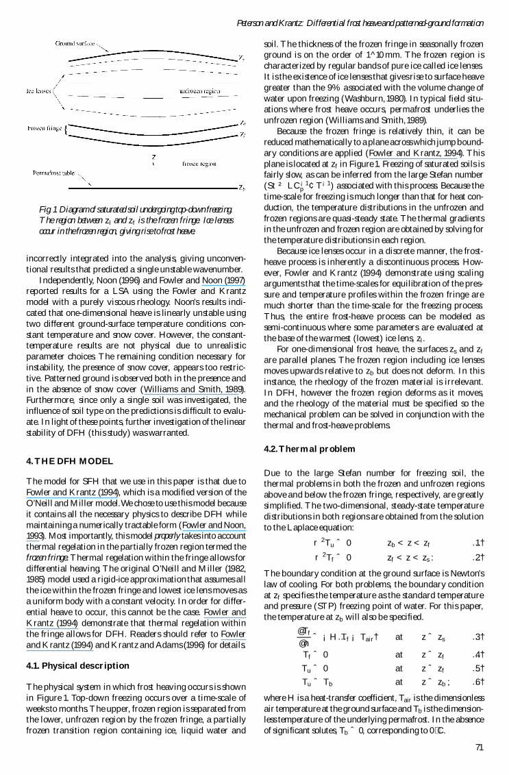