WATER RESOURCES RESEARCH, VOL. 27, NO. 12, PAGES 3119-3135, DECEMBER 1991

A Large-Scale Flow and Tracer Experiment in Granite 2. Results and Interpretation

HARALD ABELIN, 1 LARS BIRGERSSON, 1 LUIS MORENO, 2 HANS WIDi•N, 1 THOMAS •tGREN, 1 AND IVARS NERETNIEKS 2

Water and tracer flow has been monitored in a specially excavated drift in the Stripa mine. Several new experimental techniques and equipment were developed and used. The whole ceiling and the upper part of the walls were covered with 375 individual plastic sheets where the water flow into the drift could be collected. Eleven different tracers were injected at distances between 11 and 50 m from the ceiling of the drift. The flow rate and tracer monitoring was kept up for more than 2 years. The tracer breakthrough curves and flow rate distributions were used to study the flow paths, velocities, hydraulic conductivities, dispersivities and channeling effects in the rock. In a companion paper the experimental design and performed experiments are described. The present paper describes the interpretation of flow and tracer movement in the rock outside the drift. The tracer movement was measured by the more than 160 individual tracer curves. The tracer experiments have permitted the flow porosity and dispersion to be studied. The possible effects of channeling and the diffusion of tracers into stagnant waters in the rock matrix and in stagnant waters in the fractures have also been addressed.

SOME CONCEPTS OF WATER FLOW AND TRACER

TRANSPORT IN FRACTURED ROCK

It is often implicitly assumed that the fractured rock, even at depth, is sufficiently fractured to allow for an averaging to be performed of the properties in a volume of rock such that it is meaningful to assign an average value of the properties to a "point" in the rock. The properties of interest for flow are the hydraulic conductivity and the porosity. The size of the volume over which the averaging is performed is called a representative elementary volume (REV). It is implicitly assumed that the REV is considerably smaller than the rock volume studied. To calculate the flow rate in the rock

volume, Darcy's law is used together with the appropriate boundary conditions to calculate the flow rate and flow directions in "all" points in the rock mass of interest. These implicit assumptions may not be valid for fractured rocks.

Solutes which are dissolved in water will be carried by the moving water but will als ø move independently by various mechanisms such as diffusion and will be retarded by inter- actions with the solids. Molecules or ions diffuse in a

concentration gradient and can move from one "stream tube" to another. Different water volumes move with dif-

ferent velocities and may mix at more or less regular intervals. A very frequent mixing may be described as a process of the same type as molecular diffusion and is often described as such by what is called Fickian dispersion.

With only advection and dispersion active, the classical advection-dispersion description results. It has been used extensively to describe tracer movement in porous media. It has also been used to model transport in individual fractures and channels. It is possible to modify the equations to account for an instantaneous chemical reaction with linear or

nonlinear equilibria and reaction rates can also be accom-

I Chemflow AB, Stockholm. 2Department of Chemical Engineering, Royal Institute of Tech-

nology, Stockholm.

Copyright 1991 by the American Geophysical Union.

Paper number 9 IWR01404. 0043-1397/91/91WR-01404505.00

modated if the reactions cannot be approximated as instan- taneous.

The dissolved species may also be affected by physical processes which modify their residence time distribution. One such process which has a very large impact for flow in fractured rock is the diffusion in and out of zones with water

moving so very slowly that it can for practical purposes be assumed to be stagnant. Such stagnant zones can be ex- pected in fractures with uneven surfaces.

In rocks with a connected matrix porosity, the accessible pore volume of the matrix can be very much larger than the mobile water volume in the fracture. The species which have access to the pore water will then have a residence volume and residence time determined by the sum of the water volume in the fractures with flow and the water volume

accessed in the stagnant areas. As the stagnant zones are reached by diffusion, the volume of stagnant water accessed is dependent on the time that the rock is in contact with the water containing the diffusing species. Stagnant zones of water may also exist in fractures with channeling where the water volumes between the channels do not participate in the flow.

Fractures may have preferential channels where the water flows. Channels in the same fracture may not meet and mix their water over considerable distances. The mixing required for the process to become one of hydrodynamic dispersion, in the sense that it may be modeled as a Fickian process, may not be attained over the distances of interest. The situation may then be better described as stratified flow or channeling. It may be expected that the mixing will eventu- ally be sufficient to obtain Fickian dispersion. This may not happen in media where even larger features are encountered when the distance increases. The larger pathways may always dominate the flow.

The properties of the medium can vary considerably in crystalline fractured rock. Fracture openings and thus the transport capacity of the individual fractures are known to span many orders of magnitude. Fractures are only open in places where the blocks are not in contact. The open areas may be much smaller than the closed areas. The porosity of and diffusivity in the rock matrix have similar variability.

3119

3120 ABELIN ET AL.: FLOW AND TRACER EXPERIMENT IN GRANITE, 2

Fracture coating and filling materials may also vary consider- ably as to the type and amount. In fracture zones the block sizes vary from very small particles up to blocks of consider- able size. The size of the blocks will strongly influence the amount of stagnant volume accessible at a given contact time.

Channeling

Fractured rock, especially at larger depths, may have considerable distances between water-bearing fractures. Data from deep holes, down to 800 m, in the Swedish rock indicate that at depths below a few hundred meters the spacing of conducting fractures is of the order of 1 fracture per 5-10 m [Carlsson et al., 1983]. Other observations in individual fractures by Abelin et al. [ 1985] and Neretnieks et al. [1982] indicate that even in well-defined fractures in crystalline rock there is considerable channeling. Abelin et al. [1985] found that in three highly visible fractures in the Stripa deep (360 m) rock laboratory, 5-20% of the fracture widths carried more than 90% of the flow. The actual width

of the channels is less than 1 m and could be considerably smaller. Similar observations have been made in a fracture in

a granitic body in Wales [Bourke et al., 1985]. Observations in several tunnels in Sweden show that

water flows are very unevenly distributed in the fractured crystalline rocks. The water flows into the drifts in distinct channels or spots and the flow rates of the different spots vary considerably [Neretnieks, 1987; Moreno and Neret- nieks, 1987]. A model has been tested where all "disper- sion" is assumed to be caused by channeling [Neretnieks, 1983]. It was tested in some laboratory experiments using a natural fracture [Neretnieks et al., 1982; Moreno et al., 1985] and in field experiments [Moreno et al., 1983].

Dispersion

Dispersion is defined, in a general sense, by broadening the residence time distribution (RTD) of a species trans- ported by a fluid as the fluid moves in a medium. There are many causes for this including velocity variations in the fluid in a channel, velocity variations between channels in a porous medium, physical interactions with the solid mate- rial, and molecular diffusion in the liquid. In addition, chemical interaction also will cause the RTD to broaden. It

is often difficult to separate these effects from each other. Velocity variation between channels is a very important

dispersion mechanism. Bear [1969] gives a comprehensive treatment on hydrodynamic dispersion theories in porous media. An early description is found in the paper by de Josselin de Jong [ 1958]. The common basis for practically all these treatments is that the spreading is described by one parameter, the variance of a pulse as it spreads with dis- tance. The variance increases with traveled distance but the

dispersion coefficient is independent of distance after an initial buildup. Gelhar and Axness [1983] show that for certain media there is a theoretical basis for this observation.

In some investigations [Neretnieks, 1985], the dispersion coefficient increases considerably with distance. The expla- nation for this is usually summarized in the words "chan- neling" or "uneven distribution." Schwartz [1977], by com- puter simulation, has shown that the uneven distribution of resistances may not lead to a variance which increases proportionally to the distance traveled. Mercado [1967] and Neretnieks [1983] by a different method showed that in a

medium where stratification occurs, where there are parallel unconnected strata with transmissivity differences between strata, the dispersion coefficient should increase with dis- tance. Matheron and de Marsily [1980] arrived at the same conclusion and also concluded that the common "convec-

tion diffusion equation" cannot in general be applied even for large distances.

Neretnieks [1983] discussed several dispersion mecha- nisms including stratification and derived a model which includes these effects as well as the effects of physical interaction by diffusion into stagnant zones of water in the matrix of the rock. It was shown that matrix diffusion effects

can have a dominating influence on the pulse spreading when the accessed stagnant water volume is large in comparison to the mobile water.

Diffusion Into the Porous Matrix

Crystalline rocks, such as granites and gneisses, have microscopically small fractures between the crystals. These microfissures compose an interconnected pore system con- taining water. The dissolved species are much smaller than the microfissures and can diffuse into this pore system. Solutes will move slower than the flowing water, since they diffuse into the stagnant water in the pores.

Gneisses and granites in Swedish Precambrian rock have been found to have a continuous pore system consisting of the microfissures between the crystals in the rock matrix. The porosity in this pore system varies between 0.06% and 1% for the rock matrix [Skagius and Neretnieks, 1986a]. Similar results have been obtained by other investigators [Brace et al., 1968; Bradbury et al., 1982]. Fracture minerals and rock in crushed zones have higher porosities. Values between 1 and 9% have been measured [Skagius, 1986]. Substances dissolved in the water can diffuse into this pore system and sorb on the inner surfaces. The penetration depth increases with time. Nonsorbing species penetrate far into the matrix, while sorbing species are retarded since they also have to fill up the sorption sites before migrating further. The penetration depth can be calculated using Fick's law for diffusion, if the diffusivity is known and by taking the retardation due to sorption into account.

MATHEMATICAL MODELING

The simplest models are based on the concept of advective flow in a porous medium where a tracer would be subject to dispersion due to velocity variations and molecular diffu- sion. These models have been much studied and are well

summarized by Maloszewski and Zuber [1984]. They are readily extended to include instantaneous sorption on the surfaces of the solid and also instantaneous sorption in the bulk of the solid. Another group of models include the phenomenon of nonstationary uptake by diffusion of tracers into the rock matrix or other stagnant zones of water. These models are readily extended to include instantaneous sorp- tion on the inner surfaces [Neretnieks, 1980; Rasmuson and Neretnieks, 1980; Tang et al., 1981]. A further group of models assume that the flow takes place in flow paths which for any given situation are isolated from each other, the so-called channeling models. These also can easily include the matrix diffusion effects [Neretnieks, 1983].

Advection-Dispersion Model The advection-dispersion (AD) model can be written for

short as

ABELIN ET AL.' FLOW AND TRACER EXPERIMENT IN GRANITE, 2 3121

TABLE 1. Models Used and Parameter Values Determined

Model Parameters Reference

Advection-dispersion Advection-channeling Advection-dispersion-matrix diffusion Advection-channeling-matrix diffusion

tw, Pe, DF t w , O'l, DF t•, Pe, DF tw, O'l, D D, DF

Lapidus and Amundsen [ 1952] Neretnieks [1983] Tang et al. [1981] Neretnieks [1983]

C/Co = f(t, (tw, Pe)) (1)

thus indicating that the concentration is a function of time t. The two parameters, tw, water residence time, and a mea- sure of dispersivity, the Peclet number, Pe, suffice to fully define the solution.

Channeling Model

The advection-channeling (AC) model is based on the assumption that all channels conduct the flow from the inlet to outlet without mixing between channels on the way. At the outlet, however, the fluid from all channels is instanta- neously mixed. This would simulate a very common way of sampling for tracers. It is assumed that the channels can be uniquely described by their apertures in regard to the flow rate and concentration response. Similarly to the AD model, the AC model can be written

C/Co =f(t, (t w, O'l) ) , (2)

where O•l-•S a 'measure of the variability of the channel properties. in the model applied here we assume a lognormal distribution of fracture (channel) apertures and then •r t is the standard de. viation in the lognormal distribution.

The tracer solution makes up only a small fraction of the water flowing in the rock. It is thus diluted and is accounted for by dividing the function f by a dilution factor DF in the models.

Matrix Diffusion

There is considerable experimental evidence on crystalline rock porosities and diffusivities from the laboratory [Skagius, 1986; Skagius and Neretnieks, 1985, 1986a, b; Bradbury, 1982], and from the field [Birgersson and Neretnieks, 1982, 1984, 1988] in undisturbed rock. Porosities in unaltered rock range from 0.06 to over 1% and the effective diffusivities, De, for small ions and molecules range from 1 x 10 -14 to 70 x 10 -14 m 2/s. The effects of matrix diffusion will be larger in flow paths which have a larger exposed rock surface from which the dissolved species may diffuse into the matrix.

The models can be written for short as

C/Co =f(t, (tw, Pe, A)) (3)

where A accounts for the diffusion mechanism and includes data on the diffusivity and Wetted surface area. A similar relation is obtained for channeling with matrix diffusion.

• • EVALUATION AND INTERPRETATION OF . EXPERIMENTAL RESULTS

The tracer tests are interpreted with various models. The basis for the models and the mechanisms pertaining to each model have been described above.

Some items that are of special interest in evaluating the different models include water travel time (flow porosity),

dispersivity, matrix diffusion effects, wetted area, and chan- neling characteristics. Models which have more parameters may describe more mechanisms and thus may give better agreement with the experimental results. Of the models used, the simplest models contain only two parameters, e.g., travel time and dispersivity, and the more complex models include three or four independent parameters. By including more parameters it is easier to obtain better fits without actually increasing the physical meaning of the obtained parameter values. However, a good fit does not imply that the mechanisms which the model is based on actually are active at all. Therefore several models have been analyzed with different mechanisms which may give similar results; e.g., the spreading of a tracer pulse may be Caused by hydrodynamic dispersion, channeling, matrix diffusio n, or some other causes which are not included in the model. The

three mentioned mechanisms will in many circumstances lead to a similar spreading of a pulse and cannot be distin- guished from one another by just fitting one or a few experimental curves in a model. In order to separate out the various mechanisms, independent information, e.g., labora- tory data on matrix diffusion, is needed.

Increasingly more complex models are used to fit the tracer breakthrough curves to obtain the various parameter values which quantify the mechanisms.

Models Used for Fitting Tracer Concentration Curves

Table 1 summarizes the models used and the parameters which are obtained with each model.

The Fitting Process

The theoretical models were fitted to the experimental results by a nonlinear least squares fitting process. The preprocessed concentration time curves (breakthrough curves) contained thousands of conc9ntration time data points, but were finally reduced to.•about 50 data by a smoothing procedure .•

First, all the selected individual data curye s were fitted with the AD model (advection-dispersion model). 0f.•the nearly 170 different curves fitted many had hig• dilution factors DF and contained v9-ry small amounts of the tracer in comparison to the other curves.• This difference Was cauõed by either small flow rates 6r i øw tracer conceritration or by a combination of both factors. These curves contribute very little to the total transport of the tracer: The breakthrough curves were first fitted using the advection-dispersion model. The curves which were near the detection limit were often

erratic and were not used. In-total, 167 individual break- through curves were fitted. In these nonlinear least squares fits three parameters were fitted: the Peclet number, the residence time, and a dilution factor.

3122 ABELIN ET AL..' FLOW AND TRACER EXPERIMENT IN GRANITE, 2

60

a)O 4 8 12 16 ,,• t i i i i i i i i l

b

• +++++ / ..,.

("3 +4. ++• + , +++ '• •0 I ......... 4 8 12 16

T I ME ( HOURS )

xlO 3 zorn

20 ø xlO 3

66 108 xlO 3 xlO 3

0 4 8 12 16 20 ,,. 0 4 8 12 16 20,.

.. • + ++ . *l •• N• ++

0 4 8 1• 16 • 0 4 B IZ 16 •0 ø TIME ( HOURS ) xlO 3 TIME (HOURS) xlO 3

120 xlO 3

•0 , 4 8 12 16 20 I I I I I I I I k"qd

O :,,, , , , , , ' [ ] [ O 0 4 8 12 16 20

T I ME ( HOURS ) x 10 3

Fig. 1. Eosin B breakthrough curves from selected sheets. The solid lines give a fitted curves by the AD model and the crosses show selected experimental points.

Results of the Model Fitting of Breakthrough Curves

After fitting all the tracer breakthrough curves, a set of five selected curves were chosen for each tracer. The selected

curves accounted for a significant amount of the tracer. These curves were studied in more detail with the advection-

dispersion-matrix diffusion (ADD) model and advection- channeling (AC) model.

The results from the model fits indicate that the dispersion for many of the breakthrough curves was very high. There are many conceivable reasons for high dispersion values. One is the spreading of the tracer pulse by diffusion of the tracer into and out of stagnant or nearly stagnant volumes of water. Such volumes of water are known to exist in the

ß

porous matrix of the rock as well as in the fracture itself. They can be accessed by molecular diffusion from the flowing water in the channels. The ADD model was used to investigate this possible cause of dispersion and also to investigate the matrix diffusion. The matrix diffusion mech- anism may be an important cause of withdrawing the tracer

from the flowing water and into the rock, thus causing a less than full recovery to be obtained even after very long collecting time periods.

The injection flow varied with time. The breakthrough curve of variable injection was calculated usirig the convo- lution theorem which requires an integration over time. To simplify the calculations the injection flow was represented as a function of time as a series of square pulses.

It was found that bromide had been severely disturbed in the analysis by the presence of iodide and therefore was only partly used in the subsequent analysis.

Preliminary results showed that most of the curves have a very low Peclet number (high dispersion). The model used was not valid for Peclet numbers less than 3 [Sauty, 1980]. For this reason and because the fit became worse for the

rising part of the breakthrough curve the Peclet number was limited to values greater than 4.0. It was observed that the dispersion was low for the runs with the tracer iodide. The runs with the tracers Eosin B and Uranin showed high

ABELIN ET AL..' FLOW AND TRACER EXPERIMENT IN GRANITE, 2 3123

•Om

..

4 8 1•2 16

,4-4-+ +4.+ ++•

TIME ( HOURS ) '=;o 2o •

x10 3

Fig. 2. Uranin breakthrough curve in sheet 108. The solid line gives a fitted curve by the AD model and crosses show selected experimental points.

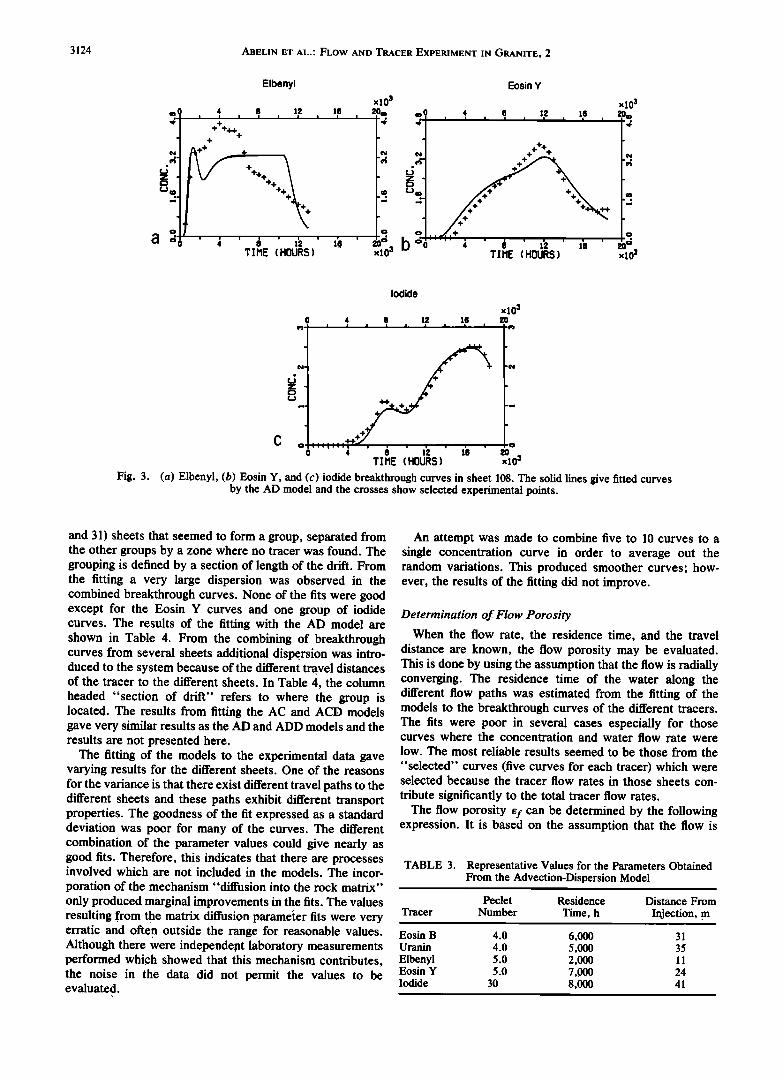
dispersion. The agreement between the fitted curves and the experimental data was good for the runs with the tracers Eosin Y and iodide. The agreement was very bad for the runs with the tracer Uranin. Figure 1 shows some typical results of the fitting.

In Figure 1 a it is shown that the theoretical curve does not reproduce the form of the experimental points very well. There are two distinct dips in the experimental points at 5000 hours and at 15,000 hours which are not seen in the tilted curve. The fit gives a residence time of 7045 hours and a Peclet number of 5.1. A visual observation of the experimen- tal points shows that the fitted curve cuts over the two early peaks. Inspection of the other curves for Eosin B shows that the forms of the response curves are quite different in some cases. This indicates that there is something other than just advection and hydrodynamic dispersion occurring which influences the responses along these pathways. Figure 2 shows a response curve for Uranin.

It is clear that there is little similarity between the ex- pected (fitted) cU,rve and the obtained curve. The other Uranin curves show an equally poor fit; see Table 2. which summarizes the results of the fitting with the AD model. The fight column in the table contains the standard deviation of the fit. Figure s 3a •, 3b, and 3c show some selected response curves and the fitted curves for Elbenyl, Eosin Y, and

.

iodide.

From Figure 3, the Elbenyl responses deviate more from the model than do the Eosin Y and iodide results. This is also

clearly shown in Table 2 where the standard deviation of the fit for these tracers is much less than for the other tracers.

Because a large number of the curves contributed to a very small amount of the total recovered tracer, five curves for each tracer were chosen for continued analysis. These curves were chosen because they represented an important part of the tracer recovered during the observation time or because they represented the different zones where the tracer was found.

The results for the advection-dispersion model for these 25 chosen curves are shown in Table 2. In these calculations the condition that the Peclet number is greater than 4.0 is imposed.

From these results representative values for the transport parameters are determined and are shown in Table 3. The tracers Eosin B and Uranin show a very high dispersion. The pCClet numbers for the tracer iodide were about 30.

The advection-dispersion-matrix diffusion model requires

TABLE 2. Results Obtained Using the Advection-Dispersion Model

Sheet Peclet Residence Dilution Standard Number Number Time, h Factor Deviation

Tracer Eosin B

57 5.1 7,045 151 0.14 60 4.0 20,470 182 0.11 66 4.0 5,004 313 0.22

108 4.0 5,331 797 0.32 120 4.0 7,077 136 0.09

Tracer Uranin

64 4.7 2,273 1,152 0.38 71 4.0 4,223 695 0.25 90 4.0 7,445 1,670 0.19

108 4.0 3,634 2,194 0.29 134 12.0 11,810 190 0.03

Tracer Elbenyl 60 4.0 2,112 286 0.15 64 6.1 2,014 248 0.22 66 4.0 1,969 202 0.20 68 5.6 1,978 382 0.1 !

108 6.3 1,636 584 0.29

Tracer Eosin Y

64 6.6 5,090 131 0.10 68 5.5 7,320 95 0.07 71 5.3 7,320 94 0.07 90 4.7 8,933 72.4 0.03

108 6.0 6,224 278 0.08

Tracer Iodide

61 18.6 7,209 128 0.08 62 4.0 11,160 40.3 0.05

103 34.0 7,558 98.6 0.06 108 54.5 7,113 82.3 0.06 110 34.5 7,031 76.2 0.06

The condition that the Peclet number be greater than 4.0 is imposed.

the determination of four parameters: the Peclet number, the water residence time, a parameter which takes into account the diffusion into the rock matrix (A parameter), and the dilution. The A parameter is defined by

A = 8/2(Del?p) 1/2 (4) where 8 is the fracture aperture, D e is the effective diffu- sivity in the rock matrix and l?p is the matrix porosity.

The A parameter depends on the fracture geometry and the properties of the rock matrix (porosity and pore diffu- sivity) (see (4)). Results show that the A parameter varies by several orders of magnitude, 20-10 6 . The results are very insensitive to the value of the A parameter. These large variations cannot be explained by the variations in the rock and channel properties. In the fitting procedure, the effects of matrix diffusion and hydrodynamic dispersion are not well distinguished because they influence the breakthrough in a similar way. The noise observed in the experimental results was large, so that in order to distinguish between the different mechanisms additional information was required. The A parameter could thus not be determined with suffi- cient accuracy by fitting the individual breakthrough curves. A different approach was used and is described later.

For the tracers Eosin B, Uranin, Elbenyl, Eosin Y, and iodide, fittings were done for some breakthrough curves that were constructed by adding together several (between three

3124 ABELIN ET AL.' FLOW AND TRACER EXPERIMENT IN GRANITE, 2

Elbenyl Eosin Y

16 m ! i

xlO 3

,

4 8 12 16 i • m I I I I I I

+++_• + -,'

"' • ' i ' :• ' :• ' TI HE ( HOURS )

xlo 3

xlO:

Iodide

xlO 3

øo ' ',i ' •i • :'• zo T I ME ( HOURS ) x 10 2

Fig. 3. (a) Elbenyl, (b) Eosin Y, and (c) iodide breakthrough curves in sheet 108. The solid lines give fitted curves by the AD model and the crosses show selected experimental points.

and 31) sheets that seemed to form a group, separated from the other groups by a zone where no tracer was found. The grouping is defined by a section of length of the drift. From the fitting a very large dispersion was observed in the combined breakthrough curves. None of the fits were good except for the Eosin Y curves and one group of iodide curves. The results of the fitting with the AD model are shown in Table 4. From the combining of breakthrough curves from several sheets additional dispersion was intro- duced to the system because of the different travel distances

..

of the tracer to the different sheets. In Table 4, the column headed "section of drift" refers to where the group is located. The results from fitting the AC and ACD models gave very similar results as the AD and ADD models and the results are not presented here.

The fitting of the models to the experimental data gave varying results for the different sheets. One of the reasons for the variance is that there exist different travel paths to the different sheets and these paths exhibit different transport properties. The goodness of the fit expressed as a standard deviation was poor for many of the curves. The different combination of the parameter values could give nearly as good fits. Therefore, this indicates that there are processes involved which are not included in the models. The incor- poration of the mechanism "diffusion into the rock matrix" only produced marginal improvements in the fits. The values resulting from the matrix diffusion parameier fits were very erratic and often outside the range for reasonable values. Although there were independem laboratory measurements performed which showed that this mechanism contributes, the noise in the data did not permit the values to be evaluated.

An attempt was made to combine five to 10 curves to a single concentration curve in order to average out the random variations. This produced smoother curves; how- ever, the results of the fitting did not improve.

Determination of Flow Porosity

When the flow rate, the residence time, and the travel distance are known, the flow porosity may be evaluated. This is done by using the assumption that the flow is radially converging. The residence time of the water along the different flow paths was estimated from the fitting of the models to the breakthrough curves of the different tracers. The fits were poor in several cases especially for those curves where the concentration and water flow rate were low. The most reliable results seemed to be those from the

"selected" curves (five curves for each tracer) which were selected because the tracer flow rates in those sheets con- tribute significantly to the total tracer flow rates.

The flow porosity ef can be determined by the following expression. It is based on the assumption that the flow is

TABLE 3. Representative Values for the Parameters Obtained From the Advection-Dispersion Model

Peclet Residence Distance From Tracer Number Time, h Injection, m

Eosin B 4.0 6,000 31 Uranin 4.0 5,000 35 Elbenyl 5.0 2,000 11 Eosin Y 5.0 7,000 24 Iodide 30 8,000 41

ABELIN ET AL.: FLOW AND TRACER EXPERIMENT IN GRANITE, 2 3125

TABLE 4. Results of Combined Flows From Fitting With the AD Model With a Penalty Function for Peclet Numbers Lower Than 4.0

Tracer Peclet Residence Dilution Standard Section of

Number Time, h Factor Deviation Drift, m

Eosin B Eosin B Uranin Uranin

Elbenyl Eosin Y Eosin Y Iodide Iodide

4.0 6,338 185 0.10 39-45 4.0 4,481 1,068 0.46 25-35 4.0 3,583 1,200 0.26 25-35 4.0 4,932 2,895 0.20 12-22 4.8 1,658 607 0.23 25-35 5.9 6,938 153 0.07 25-35 4.0 10,320 234 0.06 12-22

32.8 7,262 118 0.05 25-35 4.0 4,544 760 0.48 39-45

radially convergent in a homogeneous porous medium where Darcy's law applies.

ef= 2twQ/Ao(r22/rl - rl) (5)

A0 is the collecting area of the drift, tw is the residence time, and r 2 and r• are the distances to the injection and tunnel radius respectively.

The flow rate to the drift was very unevenly distributed. Tracers were found mainly in the central part of the drift. Other large parts of the drift were dry with the exception of the far end and the right arm where most of the water flow to the drift was located. The question then arises, At which water flow rate has a tracer been monitored? Is it for all the

water to the drift including that to the uncovered bottom part, is it for all the water to the covered part of the drift including the water where no tracers were found, or is it for only that water in which tracers were found? In this case the latter assumption is used. The next question then is, What area of the tunnel is correct to use in the above equation? Is it only the area of those sheets in which the water with tracers were found or should a dry portion of the tunnel near to the tracer carrying sheets also be included? There are no established correct ways of choosing the area. It has been elected to use a length of drift where the tracers were found, including the area of the dry sheets in that section of the drift.

A further question is, Which travel distance is correct? It might be argued that for every sheet there is a correct travel distance, which is the shortest distance between the injec- tion point and the collection sheet. It may also be argued that the shortest distance between the injection point and the drift is more representative because that is where the flow

would be in an ideal porous medium, which is the basis for the equation used. It has been elected to use the latter approach. Considering the uncertainties in the basic assump- tions the resulting flow porosities are not to be taken as exactly determined experimental values. The porosities will differ by more than a factor of 2 if the other extreme combinations of the assumptions are used.

The radius r of the drift is taken to be 2.2 m. This would be

the radius of a cylinder with the same surface area as the drift. The drift has a covered area of 7 m/meter of length.

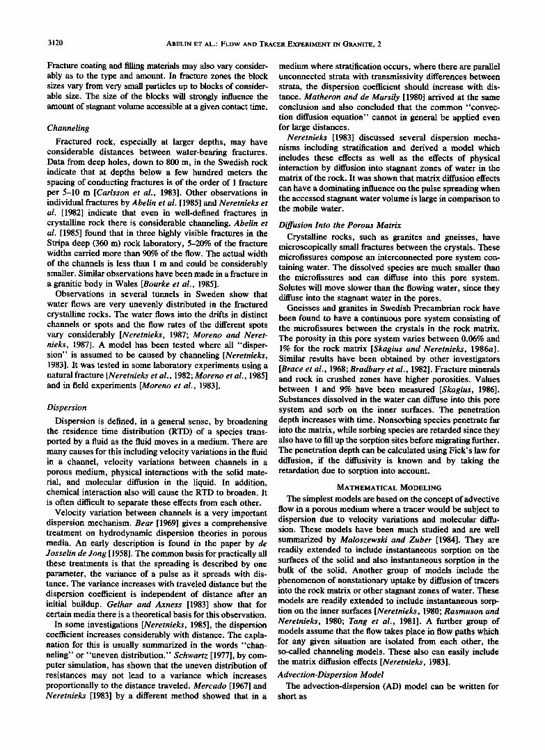
Table 5 shows the data used for evaluating the porosities and the obtained porosity values. Figure 4 shows a plot of the porosity as a function of the distance to the injection point. There is a tendency for the porosity to decrease with increasing distance.

In the determination of the porosity there is an underlying assumption that the residence time measured with the trac- ers represents that of the main flow in which the tracers were subsequently found as they emerged in the drift. The average individual injection flow rates are in the range 0.45-8.94 mL/h for the six tracers in Table 5. The sum of the flow rates

for these six recovered tracers is 24.4 mL/h. This may be compared to the total flow rate to the drift ranging from 600-700 mL/h. The injection flow rates of these tracers made up 3--4% of the flow rate to the drift. The tracers were recovered in the flow to the central part of the drift where the flow was only about 150-200 mL/h. The dilution of the individual tracers is then between 22 and 396.

The paths for the tracers may not be representative of those waters where the tracers were found if the mixing of the tracer solution with the main water flow has occurred

near the drift. In the extreme the porosity of the rock where

TABLE 5. Porosities Obtained and Basic Data Used in the Calculations

Flow Rate Distance

Residence in Section, Length of to Injection Porosity Tracer Time, h mL/h Section, m Point, m x 105

Eosin B 3,000 175 22 9 3.4 Uranin 5,500 153 23 32 2.0 Elbenyl 2,000 178 10 10 15.5 Eosin Y 6,000 198 27 8 6.9 Iodide 7,000 200 31 29 3.0 Bromide 2,500* 200 31 13 4.5

*The bromide residence times obtained from the fits using the collection time are in error because of interference from iodide. The early residence time of 2500 hours was estimated by visually observing the breakthrough curves for the early times when the iodide has not yet reached the collection sheets in any appreciable concentration. The value is only an approximate.

3126 ABELIN ET AL.: FLOW AND TRACER EXPERIMENT IN GRANITE, 2

2e-4

le-4

Oe+O 0

Flow-porosity in Strips

Distance from drift, m 40

Fig. 4. Porosity versus distance from drift.

the tracers have migrated might be smaller by a factor equal to th e dilution factor.

Interpretation of Recovery of Tracers

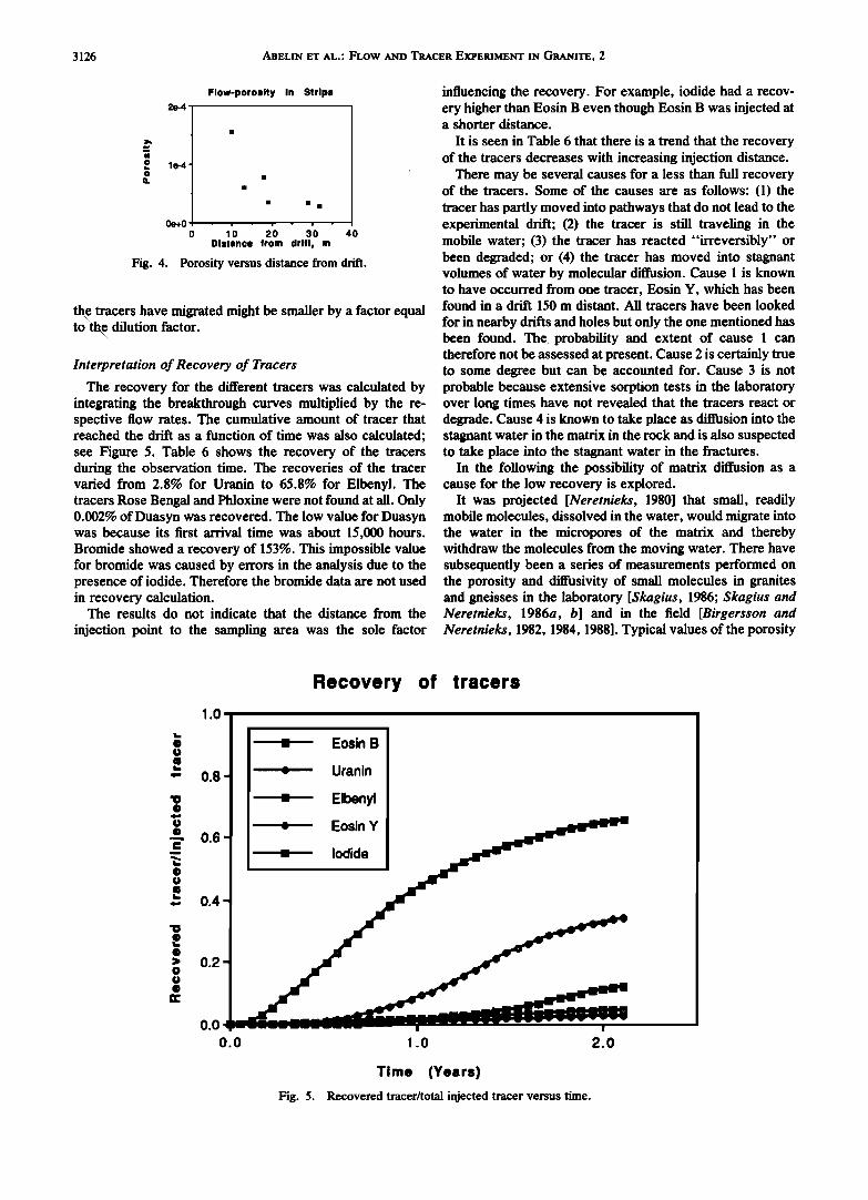
The recovery for the different tracers was calculated by integrating the breakthrough curves multiplied by the re- spective flow rates. The cumulative amount of tracer that reached the drift as a function of time was also calculated; see Figure 5. Table 6 shows the recovery of the tracers during the observation time. The recoveries of the tracer varied from 2.8% for Uranin to 65.8% for Elbenyl. The tracers Rose Bengal and Phloxine were not found at all. Only 0.002% of Duasyn was recovered. The low value for Duasyn was because its first arrival time was about 15,000 hours. Bromide showed a recovery of 153%. This impossible value for bromide was caused by errors in the analysis due to the presence of iodide. Therefore the bromide data are not used in recovery calculation.

The results do not indicate that the distance from the

injection point to the sampling area was the sole factor

influencing the recovery. For example, iodide had a recov- ery higher than Eosin B even though Eosin B was injected at a shorter distance.

It is seen in Table 6 that there is a trend that the recovery of the tracers decreases with increasing injection distance.

There may be several causes for a less than full recovery of the tracers. Some of the causes are as follows: (1) the tracer has partly moved into pathways that do not lead to the experimental drift; (2) the tracer is still traveling in the mobile water; (3) the tracer has reacted "irreversibly" or been degraded; or (4) the tracer has moved into stagnant volumes of water by molecular diffusion. Cause 1 is known to have occurred from one tracer, Eosin Y, which has been found in a drift 150 m distant. All tracers have been looked

for in nearby drifts and holes but only the one mentioned has been found. The probability and extent of cause 1 can therefore not be assessed at present. Cause 2 is certainly true to some degree but can be accounted for. Cause 3 is not probable because extensive sorption tests in the laboratory over long times have not revealed that the tracers react or degrade. Cause 4 is known to take place as diffusion into the stagnant water in the matrix in the rock and is also suspected to take place into the stagnant water in the fractures.

In the following the possibility of matrix diffusion as a cause for the low recovery is explored.

It was projected [Neretnieks, 1980] that small, readily mobile molecules, dissolved in the water, would migrate into the water in the micropores of the matrix and thereby withdraw the molecules from the moving water. There have subsequently been a series of measurements performed on the porosity and diffusivity of small molecules in granites and gneisses in the laboratory [Skagius, 1986; Skagius and Neretnieks, 1986a, b] and in the field [Birgersson and Neretnieks, 1982, 1984, 1988]. Typical values of the porosity

Recovery of tracers

1.0

0.8-

0.6

0.4

0.2

0.04

0.0

Eosin B

Uranin

Elbenyl

Eosin Y

1 .o 2.0

Time (Years)

Fig. 5. Recovered tracer/total injected tracer versus time.

ABELIN ET AL.: FLOW AND TRACER EXPERIMENT IN GRANITE, 2 3127

TABLE 6. Some Data on Tracer Residence Times and Recoveries

Injection Residence Porosity Section Recovery, Tracer Distance, m Time*, h x 105• ' Length, m %

Elbenyl (II) 9-11 2,000 15.5 10 Bromide (III) 12-14 2,500 4.5 31 Eosin Y (I) 17-19 6,000 6.9 27 Eosin B (III) 18-20 3,000 3.4 22 Iodide (III) 28-30 7,000 3.0 31 Rose Bengal (II) 33-35 ......... Uranin (I) 31-33 5,500 2.0 23 Duasyn (III) 36-38 > 15,000 ...... Phloxine (II) 55-57 ......... STR-7 (I) 31-33 ......... Flouride (I) 31-33 .........

*Approximate average values estimated from the fits with AD, AC and ADD models. tDetermined from flow rate and residence time.

65.8 oo.

34.2 4.8

12.4

2.8 0.002 0

0

0

are 0.05-0.5% for intact rock. Higher values are often found near fracture surfaces. Effective diffusivities, De, are typi- cally in the range 10-14 to 10-12 m 2/s. Pore diffusivities are higher by 2 to 3 orders of magnitude in comparison to the effective diffusivities (De = De ep, where ep is the matrix porosity). To illustrate the potential capacity and accessibil- ity of the matrix water to the molecules, it may be noted that the water volume contained in a fracture of thickness 0.05

mm is as large as the water volume in a 100-mm-thick slab of rock adjacent to the fracture if the rock has a porosity of 0.05%. Consider the possible dilution effect as follows' if the fracture was filled with a tracer solution with concentration

C and the solution was given time to equilibrate with the noncontaminated water in the pores of a 50-mm-thick rock slab on either side of the fracture (total rock slab on both sides of the fracture is 100 mm), then the concentration in the fracture and in the pores would be 0.5C. If the fracture was emptied of the water, the recovery would be 50% and the rest of the tracers would reside in the porous rock matrix. The time for this process can also be estimated. From the diffusion equation [Bird et al., 1960] it is found that the penetration thickness • for this case can be determined by

• = (Dpt) 1/: (6) For a pore diffusivity D e of 10 -1ø m:/s the time to com- pletely penetrate 50 mm is 0.8 years. The duration of the experiment was more than 2 years and the water residence times for the tracers were in the time interval 0.2-0.8 years or more. It thus seems reasonable that this effect may be of importance if the fracture apertures are small enough.

The fracture apertures can be estimated if the flow poros- ity and the fracture frequency are known. The flow porosity was estimated from data on residence times and total flow

rates. The porosities ranged between 2 x 10 -5 and 15 x 10 -5. For a given fracture spacing (parallel fully open fractures), the flow porosity ef is 15/S (the aperture divided by the fracture spacing). For a flow porosity of 5 x 10 -5 and a fracture aperture of 0.05 mm, the spacing is 1 m.

The above data are in the range of possible values. It thus seems worthwhile to explore this possibility further.

The specific surface a', which is the average fracture surface wetted by the flowing water per volume of rock, was determined by comparing the experimental recovery and the recovery obtained from model calculations. Several calcula- tions were made using the advection-dispersion-matrix dif-

fusion model to fit the recovery. Fitting all three unknown parameters t w, P e, and the specific surface a' at the same time sometimes gave quite erratic values for Pe and tw, but a' values were rather constant. Attempts were made to hold Pe or tw at previously obtained values and only determine a' and the other unknown parameter. Whatever was done gave very similar results for the specific surface a'. The obtained range of values is given in Table 7 (third column from the left) using the matrix porosity and diffusivity data obtained in the diffusion laboratory measurements [Abelin et al., 1987]. The porosity obtained from the diffusivity measurements is about 10 times lower than that obtained by weighing a wet and dry sample. The higher values may be more appropriate for the long contact times in the tracer experiment. If the higher values are used about a factor of 3 smaller surface, a' is obtained. It should be noted that the matrix porosity and diffusivity measurements were made on samples of rock not directly adjacent to a fracture with flowing water. Skagius and Neretnieks [1986a, b] found that the rock directly adjacent to fractures practically always has considerably higher porosity and diffusivity than rock further from the fracture. Porosities of 1 to more than 7% were found in the

rock adjacent to the fracture. Diffusivities were mostly larger and sometimes several orders of magnitude larger in the rock adjacent to the fracture than in rock at some distance from the fracture surface. If the fractures in contact with the

tracers in the field experiment have 2% porosity and a diffusivity of 5 x 10 -14 m2/s, the specific surface needed to account for the nonrecovery of tracers is much smaller. The right column gives these values of a'.

The large specific surfaces for diffusion into the rock matrix, a' in the third column from the left, which were obtained for the dyes are not reasonable because they imply

TABLE 7. Compilation of Obtained Specific Surfaces

Tracer

Specific Surface, m 2/m 3

Injection Low Porosity High Porosity Distance, m and Diffusivity and Diffusivity

Eosin B Uranin

Elbenyl Eosin Y Iodide

19 14-27 1.4-2.7 32 5.1-12 0.5-1.2 10 15-20 1.5-2.0 18 4.7-7.7 0.5-0.8 29 0.49-1.1 0.22-0.5

3128 ABELIN ET AL..' FLOW AND TRACER EXPERIMENT IN GRANITE, 2

Flow direction

Stagnant water • water

2--;--'

Fig. 6. A fracture cross section with a channel containing flowing water is shown. In contact with the flowing water are stagnant volumes of water into which the tracer is carried by diffusion.

that there should be spacing of conducting fractures of 2/a' meters. For iodide this would mean spacing of 1-2 m and for the dyes 0.07-0.4 m. This contradicts the observations in the drift, where considerably less than 100 water conducting fractures were observed over a length of 100 m. Since only a fraction of the fractures conduct water this means that the

fracture spacing must be larger than 1 m in the rock near the drift. Unless the diffusivity and porosity of the rock adjacent to the water conducting channels are considerably larger, matrix diffusion effects alone cannot explain the low recov- eries. The values in the right column of Table 7 are more reasonable.

It is possible that the effects of matrix diffusion can account for most or even all of the nonrecovery of the tracers if the rock adjacent to the fracture surfaces with flowing water is more porous than rock further in.

It cannot be resolved at present which are the more correct values for the diffusivity and the porosity. A much more extensive sampling of rock near fracture surfaces is needed to do this.

Another possible cause for the low recovery of tracers is also explored. It is based on the concept that the water flows in channels that are in contact with practically stagnant pools of water. The tracer in the flowing water in the channel may diffuse into the nearby stagnant water and thus be withdrawn from the mobile water. Figure 6 illustrates this process.

The aperture of the channel is /5 and the width of the channel is 2d. The species diffuse into the stagnant water. For a channel with a small width in comparison to the diffusion distance, it may be assumed that the concentration of the species across the width of the channel is constant. Therefore, the previously used equation for diffusion into stagnant water in the rock matrix can also be used to describe this case. The effective diffusivity will then be equal to the diffusivity in unconfined water (D e = Dw) and the equivalent of the matrix porosity is equal to unity.

The diffusivity of the dyes in water is of the order of 10 -9 m2/s and for iodide it is 4 x 10 -9 m2/s [Skagius, 1986]. The obtained channel widths, 2d, are summarized in Table 8. They are based on an average value of a' from the previous calculations.

The channel widths obtained are smaller or, at most, of the same magnitude as the penetration depths into the stagnant water for 1 year contact time (equation (6)). Therefore, the assumption that the concentration over the channel width is evened out is not grossly violated.

The above analysis gives no indications of how large the apertures of the channels are. An estimate of the sum of the apertures of the channels, assuming that they all have the same widths, can be made in the following way. The sum of all the cross-section areas of the channels is denoted as

2d(•/5); see Figure 6. The total area of rock, A0, that these channels intersect at the face of the drift was utilized to

evaluate the flow porosity, ef; see Table 5. The porosity is the ratio of the cross section of the channels to the cross

section of the area containing the channels,

e f = (•t5)2d/Ao (7)

From the above expression the sum of the channel apertures (•/5) can be obtained. The values range from 19 mm to 567 mm and are given in Table 8.

The tracers arrived in many of the sheets. If every sheet on the average had a few channels, several tens of channels would determine the sum of apertures (•/5). So for 50 channels this would mean a 3-mm individual channel aper- ture for Eosin B, slightly more than 1 mm for Uranin and Elbenyl, more than 10 mm for Eosin Y, and a 0.4-mm aperture for iodide. However, most of these values are considerably larger than what the visual observations indi- cated.

The diffusion into stagnant pools of water cannot alone explain the loss of tracer. The diffusion into the rock matrix may also not be the sole cause for the loss of tracer. The tracers may have taken paths which are directed to some other drifts in the mine although they are much further away. There is one such observation.

Eosin Y was found to have migrated in substantial quan- tities to a gallery about 150 m away from the injection point although the sheeted drift was located only 18 m away. This indicates that the assumption that all the injected tracer mass moves toward the experimental drift is not true for one tracer and may not be true for the other tracers either. In that case the analysis based on this assumption may determine too large specific surfaces and channel widths.

If most of the tracer moved in the direction of the drift the results of the calculations indicate that both matrix diffusion

and diffusion into stagnant pools of water may play a role. There are probably other mechanisms which could cause the

Tracer Flow

Porosity

Eosin B Uranin

Elbenyl Eosin Y Iodide

TABLE 8. Estimated Equivalent Channel Widths 2d

eœ x 10 5* Dee•, x 1016, Channel Width Sum of Apertures

a', m -1 m/s (2d), m (•/5), m

3.4 2.0

15.5

6.9 3.0

20 0.1 0.034 8 0.1 0.050

17 0.1 0.182 6 0.1 0.023 0.8 2 0.335

0.154 0.064

0.060

0.567 0.019

ABELIN ET AL.' FLOW AND TRACER EXPERIMENT IN GRANITE, 2 3129

300

Heads all 3 holes

,

2OO

'• lOO

o

0 1 2 3 4 5

In(r2)

Fig. 7. Compilation of hydraulic heads in the different injection holes.

recovery to be small. One such possible cause is that the injection, although small, compared to the total flow rate may be large when viewed on a local scale. A dipole type of flow may then develop where some of the flow moves away from the drift for some distance before returning to the drift. This would produce a lengthening of the concentration curve tail s and a lowering of the tracer recovery during a certain observation time.

Determination of Hydraulic Conductivity

The hydraulic conductivity of the rock adjacent to the drift is evaluated based on the assumption that the rock mass may be described as a homogeneous porous medium and that DarcY's law is valid-. Some simplifying assumptions needed to be introduced because the head boundary conditions are not known exactly due to the presence of drifts and tunnels in the old mine. For a homogeneous porous medium the simplifying assumptions would introduce only minor errors and are generally accepted in most other cases which study the properties of fractured rocks.

The hydraulic conductivity can then be obtained from the following expression which is derived by applying Darcy's law to flow to an infinitely long cylinder located in an infinite medium with a constant head far from the cylinder:

Q In (r2/r•) (8) Kt• = 2•rLAhf where Q is the flow rate to an L meter long part of the drift where the water flow rate is measured over a fractionf of the area (the sheets cover 50% of the area of the drift). The term Ah is the hydraulic head difference between the drift and points at a distance r2 from the center of the drift. The radius of the drift is r•. The hydraulic head was measured in the three vertical injection holes. Flow rates were measured in about 375 sheets in the upper half of the drift. In addition, ventilation experiments were conducted to measure the inflow to the lower half of the drift and to the access drift.

Figure 7 shows all the heads in all the injection holes. The lines in the figure show the upper and lower bounds of the hydraulic head gradients in.the three holes.

Table 9 gives the flow rates in the different parts of the drifts.' Using these flow rate• and the head data in (8) the hydraulic conductivities of the different parts of drifts are obtained. These values are summarized in Table 10.

TABLE 9. Flow Rates in the Different Parts of the Drifts

Flow Rate, Length of Part of Drift L/h Drift, m

Plastic sheets 0.7 100 Bottom part 2.4' 100 Access drift 2 115

*Covered parts of floor and ventilation.

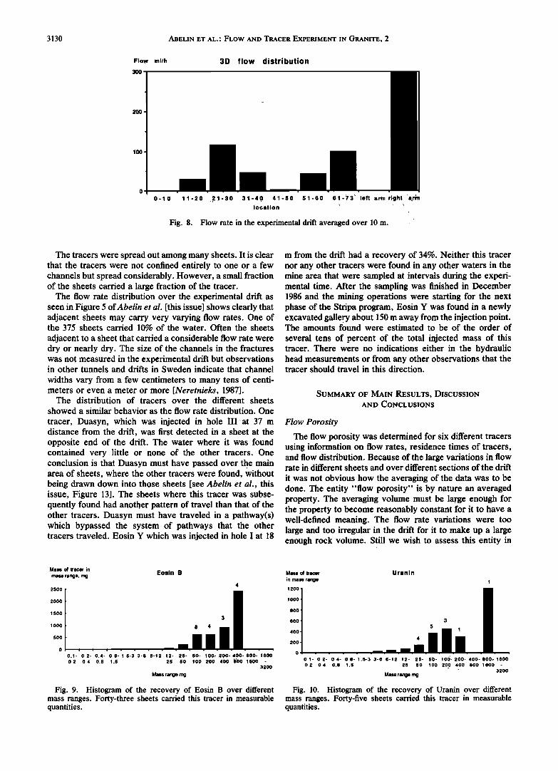
The flow rates varied considerably over the length of the drift and so did the hydraulic conductivities. The data in Table 10 were averaged over more than 100 m of drift. The variations within the experimental drift are shown in Figure 8 where 10-m averages are shown. It is observed that on a 10-m scale the hydraulic properties of the rock are far from constant. The difference of the hydraulic conductivity be- tween the access drift and the experimental drift is a factor of 2. This may indicate that the 100-m scale is not large enough to obtain reasonably constant average values.

Flow Rate and Tracer Distribution

The tracers arrived in very varying rates in concentration and in water flow to the different sheets. The mass flow rate to a sheet is determined b y the product of the flow rate and concentratio n' . The differences in mass flow rates to the different sheets show if any preferential paths may exist. Figures 9-13 show how the tracer recovery is divided among different sheets for the five tracers Eosin B, Uranin, Elbenyl, EoSin Y, and iodide. The bars in the histograms show how much of a tracer was recovered in a given range of mass

ß

recovery. The right-hand bar in Figure 9 shows that there were four sheets (the numeral above the bar) which had a tracer recovery in the range 400-800 mg. The sum of the tracer that arrived to these four sheets is given by the height of the bar.

It is Seen that for all the tracers three to five sheets out of 27 to 52 sheets carded more than half the tracer. It i s shown

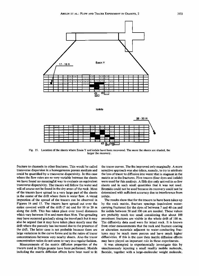
in Figure s !4 and 15 how the sheets, which carried different mass flows (recoveries) of the tracers, are located in the drift.

.,

The distribution of flow rates in the different sheets shows that a few spots carded most of the water. This is an indication of channeling. The dimensions of the channels are not known from these observations, but Figures 16 and i7 of Abelin et al. [this issue] indicate that the la•ge r flow rates are observed in those parts of the drift where many fracture intersections exist. This may be an indication that the water flows along fracture intersections where the channels 'are very narrow.

TABLE 10. Hydraulic Conductivities in the Stripa Three- Dimensional Drifts

Conductivity x 1011 m/s

Location Steep Gradient Low Gradient

Experimental Drift Ceiling + upper sides 0.56 1.07 Floor + lower sides 1.9 3.6 Average 1.3 2.3

Access drift 0.7 1.3

3130 ABELIN ET AL.' FLOW AND TRACER EXPERIMENT IN GRANITE, 2

Flow ml/h

:300 -

3D flow distribution

2OO

100

0-10 11-20 ,21-30 31-40 41-50 51-60 61-•'3' left arm right a,r•n location :'"•: "' •

Fig. 8. Flow rate in the experimental drift averaged over 10 m.

The tracers were spread out among many sheets. It is clear that the tracers were not confined entirely to one or a few channels but spread considerably. However, a small fraction of the sheets carried a large fraction of the tracer.

The flow rate distribution over the experimental drift as seen in Figure 5 of Abelin et al. [this issue] shows clearly that adjacent sheets may carry very varying flow rates. One of the 375 sheets carried 10% of the water. Often the sheets

adjacent to a sheet that carried a considerable flow rate were dry or nearly dry. The size of the channels in the fractures was not measured in the experimental drift but observations in other tunnels and drifts in Sweden indicate that channel

widths vary from a few centimeters to many tens of centi- meters or even a meter or more [Neretnieks, 1987].

The distribution of tracers over the different sheets

showed a similar behavior as the flow rate distribution. One

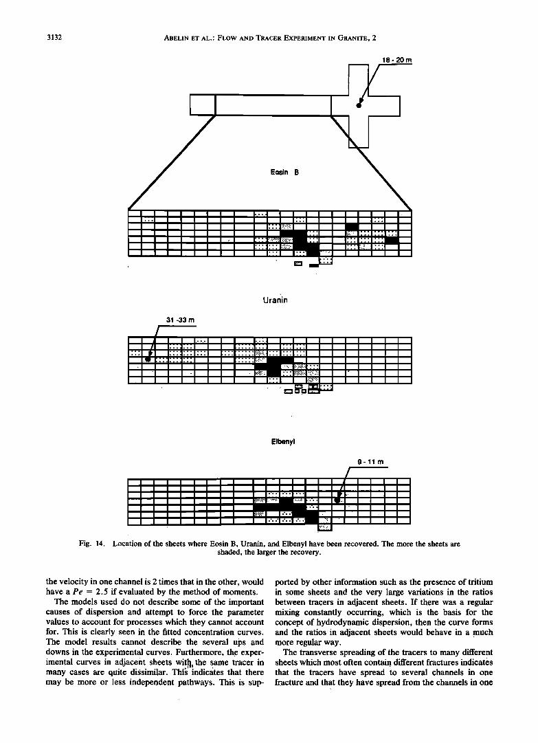
tracer, Duasyn, which was injected in hole III at 37 m distance from the drift, was first detected in a sheet at the opposite end of the drift. The water where it was found contained very little or none of the other tracers. One conclusion is that Duasyn must have passed over the main area of sheets, where the other tracers were found, without being drawn down into those sheets [see Abelin et al., this issue, Figure 13]. The sheets where this tracer was subse- quently found had another pattern of travel than that of the other tracers. Duasyn must have traveled in a pathway(s) which bypassed the system of pathways that the other tracers traveled. Eosin Y which was injected in hole ! at 18

m from the drift had a recovery of 34%. Neither this tracer nor any other tracers were found in any other waters in the mine area that were sampled at intervals during the experi- mental time. After the sampling was finished in December 1986 and the mining operations were starting for the next phase of the Stripa program, Eosin Y was found in a newly excavated gallery about 1 $0 m away from the injection point. The amounts found were estimated to be of the order of

several tens of percent of the total injected mass of this tracer. There were no indications either in the hydraulic head measurements or from any other observations that the tracer should travel in this direction.

SUMMARY OF MAIN RESULTS, DISCUSSION AND CONCLUSIONS

Flow Porosity

The flow porosity was determined for six different tracers using information on flow rates, residence times of tracers, and flow distribution. Because of the large variations in flow rate in different sheets and over different sections of the drift

it was not obvious how the averaging of the data was to be done. The entity "flow porosity" is by nature an averaged property. The averaging volume must be large enough for the property to become reasonably constant for it to have a well-defined meaning. The flow rate variations were too large and too irregular in the drift for it to make up a large enough rock volume. Still we wish to assess this entity in

Mass of tracer in Eosin B Mass of tracer Uranin mass range, rng in mass range 1

4 2500 1200

2000 1000

1500 800

3 600 5 3 lOOO

400 1 500

200

o o o.1- 0.2- 0.4- 0.8- 1.5-3 3-6 6-12 12- 25- 50- lOO- 200- 400- 800- 16oo 0.2 0.4 0.8 1.5 25 50 loo 200 400 •oo 16oo - o.1- 0.2- 0.4- 0.8- 1.5-3 3-6 6-12 12- 25- 50- lo•- 200- 400- 800- 16oo

3200 0.2 0.4 0.8 1.5 25 50 lOO 200 400 800 16oo - 3200

Mass range mg Mass range rng

Fig. 9. Histogram of the recovery of Eosin B over different mass ranges. Forty-three sheets carried this tracer in measurable quantities.

Fig. 10. Histogram of the recovery of Uranin over different mass ranges. Forty-five sheets carried this tracer in measurable quantities.

ABELIN ET AL.: FLOW AND TRACER EXPERIMENT IN GRANITE, 2 3131

Mass o! tracer Mass of tracer I 0 d i d ß 8 1

4000 i ...... ge Elbenyl 3 60 i in mass rang e I 1 3500 50 3 3000

40 2500

3O

2000 5 2O

1500

IOO0 4 1 10 500 0

5 5

0 0.02 0.05 0.1 0.2 0.4 0.8 1.5 0.1- 0.2- 0.4- 0.8- 1.5-3 3-6 6-12 12- 25- 50- 100- 200- 400- 600- 1600 0.2 0.4 0.8 1.5 25 50 100 200 400 800 1600 -

3200 Mass rangemg

Fig. 11. Histogram of the recovery of Elbenyl over different mass ranges. Twenty-seven sheets carried this tracer in measurable quantities.

some well-defined way. Two approaches were explored. In the first it was assumed that the flow rate of all the water to all of the drift was the representative flux. The residence time for this water would be represented by the residence times of the different tracers from the different injection distances. This approach would assume that the drift as a whole makes up a representative volume. It is known, however, that most of the water to the drift (end and right arm) carried no tracer. The residence time of this water is thus not known. In the Second approach we chose not to include this water flow rate in the evaluations. Only that section (length) of the drift where the traced water was collected was used as a representative rock area. The water flow rate in that section and the residence time of that water were used in the calculations.

Even so, there still remained some uncertainties in the porosity values. The length section of drift used in the calculations contained some dry areas which were included. Other dry areas of rock are located immediately adjacent to sections used. The unresolved question is how large a portion of the adjacent dry rock belongs to the section of wet rock. The porosity values may be representative for the wet part of the rock but then ther6 is an unknown mass of "dry" rock which has a porosity equal to zero.

The porosity was found to decrease with distance from the drift. The values for the rock far from the drift were found to be of the order of 2 x 10 •5 to 7 x 10 -5 and the porosity in the 10 m nearest the drift was found to be 15.5 x 10-5 which indicates that the presence of the drift has increased the porosity.

The water residence times which were used t O estimate

Mass of tracer Eosin Y 2

25øø I in mass range 6 1 2000

1500 2

1000

500

0

0.1- 0.2- 0.4- 0.6-1.5-3 3-6 6-12 12- 25- 50- 100-2•)0-400-600-1600 0.2 0.4 0.6 1.5 25 50 100 200 400 6 '00 t600 -

3200

Mass range mg

Fig. 12. Histogram of the recovery of Eosin Y over different mass ranges. Forty-six sheets carried this tracer in measurable quantities.

Mass range mmol

Fig. 13. Histogram of the recovery of iodide over different mass ranges. Fifty-two sheets carried this tracer in measurable quantities.

the porosity varied considerably between sheets. Also the residence times for major flow paths and averaged flow paths were quite variable. These and other observations indicate the presence of channeling. This adds further to the need to use the average properties with considerable caution. The presence of tritium in some sheets, for example, indicates that there is some part of the porosity which is not well connected to other parts of the rock porosity.

Dispersion

Three mechanisms for "dispersion" have been modeled: hydrodynamic dispersion, channeling, and matrix diffusion effects. Hydrodynamic dispersion is modeled as Fickian diffusion. It can be quantified as a Peclet number, Pe, a dispersion length, a, or dispersivity, DE. Channeling has been modeled as if flow were to take place in a multitude of independent channels with a known flow rate distribution. The distribution of channel apertures is modeled as being lognormal and the cubic law is assumed to be valid. The channeling can be quantified by a single entity, the standard deviation in the lognormal distribution of apertures. Other ways of describing channeling are known, e.g., by assuming a given number of channels (two, three, four or more), each having known characteristics. In the latter approach at least one parameter value must be assigned to each channel and it is our experience that such values seldom can be uniquely chosen. If no independent information is known for the channels this approach gives dubious results.

When the channels are few the first approach is not good either because it implicitly assumes that the statistics apply to a large number of channels. The evaluated Peclet numbers range from very low values, less than 4 to about 35. Values less than 4 indicate that the transport to a large extent is dominated by dispersion. For values of Pe < 1, as was found in many of the :fitted curves, the hydrodynamic dispersion description is very dubious. In molecular diffu- sion situations it would imply that the molecular diffusion in the mobile water dominates the transport of the tracer over that induced by advection. In the present case the dispersion is induced by the advection and it is not easily conceived how advection can be neglected in comparison to the disper- sion if the latter is induced by the former. Seemingly very low Peclet numbers (high dispersion) are easily attained when there are channels which have different velocities and which do not mix their waters much over the travel distance. It may be illustrated as follows: A system of two channels which have the same flow rate and no dispersion, but where

3132 ABELIN ET AL.: FLOW AND TRACER EXPERIMENT IN GRANITE, 2

18- •rn

Eosin B

uranin

31 -33 rn

Elbenyl

9-11m

, r

......... i •i ! i• i• .... me mm me m "+":'" mmmmlm me' . m m mmm me m mmmm mmmm• meNme mmmm

......... :ll•i• . S1•1•1•$ •l ';• ..-- .....

....... ?!:i:i:i:::i

Fig. 14. Location of the sheets where Eosin B, Uranin, and Elbenyl have been recovered. The more the sheets are shaded, the larger the recove'ry.

the velocity in one channel is 2 times that in the other, would have a Pe - 2.5 if evaluated by the method of moments.

The models used do not describe some of the important causes of dispersion and attempt to force the parameter values to account for processes which they cannot account for. This is clearly seen in the fitted concentration curves. The model results cannot describe the several ups and downs in the experimental curves. Furthermore, the exper- imental curves in adjacent sheets with. the same tracer in many cases are quite dissimilar. This indicates that there may be more or less independent pathways. This' is sup-

ported by other information such as the presence of tritium in some sheets and the very large variations in the ratios between tracers in adjacent sheets. If there was a regular mixing constantly occurring, which is the basis for the concept of hydrodynamic dispersion, then the curve forms and the ratios in adjacent sheets would behave in a much more regular way.

The transverse spreading of the tracers to many different sheets which most often contain different fractures indicates that the tracers have spread to several channels in one fr. acture and that they have spread from the channels in one

ABELIN ET AL.' FLOW AND TRACER EXPERIMENT IN GRANITE, 2 3133

17 - 19 rn Eosin Y

Iodide

28- 3O m

Fig. 15. Location of the sheets where Eosin Y and iodide have been recovered. The more the sheets are shaded, the larger the recovery.

fracture to channels in other fractures. This would be called

transverse dispersion in a homogeneous porous medium and could be quantified by a transverse dispersivity. In this case where the flow rates are so very variable between the sheets we have found no meaningful way to evaluate an equivalent transverse dispersivity. The tracers will follow the water and will of course not be found in the dry areas of the rock. Most of the tracers have spread to a very large part of the sheets in the center of the drift where there is water flow. A visual

inspection of the spread of the tracers can be observed in Figures 14 and 15. The tracers have spread out over the entire covered width of the drift (7 m) and for 10 to'20 m along the drift. This has taken place over travel distances which vary between 10 m and more than 30 m. The spreading may have occurred gradually along the travel path but it may also be argued that it may have taken place mostly near the drift where the porosity has increased due to the presence of the drift. The latter case is not probable because there are large variations in the curve forms and in the ratios of tracer concentrations between very nearby sheets. Also the tracer concentration ratios do not seem to vary in a regular fashion.

Measurements of the matrix diffusion properties of the tracers used in Stripa granite have been performed. Models including the matrix diffusion effects have been used to fit

the tracer curves. The fits improved only marginally. A more sensitive approach was also taken, namely, to try to attribute the loss of tracer to diffusion into water that is stagnant in the matrix or in the fractures. Five tracers (four dyes and iodide) were used for this analysis. A fifth dye only arrived in so few sheets and in such small quantities that it was not used. Bromide could not be used because its recovery could not be determined with sufficient accuracy due to interference from iodide.

The results show that for the tracers to have been taken up by the rock matrix, fracture spacings (equivalent water- carrying fractures) for the dyes of between 7 and 40 cm and for iodide between 50 and 100 cm are needed. These values

are probably much too small considering that about 100 prominent fractures are visible in the whole drift of 100 m. The diffusivity data used were for intact rock. It is known from other measurements that the rock and fracture coating or alteration materials adjacent to water-conducting frac- tures may be much more porous and have much higher diffusivities. If this is the case then matrix diffusion effects

may have played an important role in these experiments. It was attempted to experimentally investigate this by

simultaneously injecting a small readily mobile molecule, fluoride, together with a large-molecular weight molecule,

3134 ABELIN ET AL..' FLOW AND TRACER EXPERIMENT IN GRANITE, 2

STR-7, which was specifically synthesized for the purpose. STR-7 is based on a polyethylene-glycol of molecular weight 15,000. Both molecules were injected simultaneously at the injection zone where Uranin was previously injected. The injection of Uranin was also continued during the same time. Neither fluoride nor STR-7 could be found in the sheets

where Uranin was found. The reason for this is not known.

The Uranin curves behave as if the Uranin injection also was discontinued because better fits were obtained with this

assumption. The diffusion into stagnant water in the fracture was also

explored. For Uranin, Elbenyl, and iodide this effect may contribute noticeably, but it probably has a small effect for Eosin B and Eosin Y. This latter effect is more speculative than the matrix diffusion because many assumptions must be made regarding the geometry and quantity of the stagnant water zones. Similar effects may be caused by the slow flow into semistagnant pools of water. There is even less infor- mation available for speculations on this process.

Channeling

The water flow is very unevenly distributed over the investigated portion of the rock. There are large dry areas extending over many tens of meters. If the Stripa rock is representative for low-permeability granites, then the use of porous medium models with essentially constant properties may give results with unknown and probably large errors for water flow and especially for tracer transport.

The results of the tracer experiments and the tritium measurements give strong support to the notion that a nonnegligible portion of the flow takes place in channels which have little contact with other main channels. This

cannot be treated by the models which have been applied in the analysis of the experiment. A probably fruitful avenue would be to try to incorporate the variability in the models. So-called stochastic models are available for porous media and some attempts to apply them to this type of rock have been made recently [Gelhar, 1987; Moreno et al., 1987, 1988; Tsang et al., 1988]. These models need considerable amounts of data to obtain the statistical properties. They also must be made to incorporate the correct processes.

The mechanisms of diffusion into stagnant pools of water, matrix diffusion, frequency of mixing, and especially the nonmixing of channels will have to be studied more.

Acknowledgments. This work was performed within the OECD/ NEA international Stripa project managed by the Swedish Nuclear Fuel and Waste Management Company SKB. We gratefully ac- knowledge the financial support and the never failing encourage- ment and help from the initiator of the project Lars B. Nilsson and the project manager Hans Carlsson.

REFERENCES

Abelin, H., I. Neretnieks, S. Tunbrant, and L. Moreno, Final report of the migration in a single fracture--Experimental results and evaluation, Tech. Rep. 85-03, Stripa Proj., Stockholm, 1985.

Abelin, H., L. Birgersson, J. Gidlund, L. Moreno, I. Neretnieks, H. Wid6n, and T./•gren, 3-D migration experiment Report 3, part I, Performed experiments, results and evaluation, Tech. Rep. 87-21, Stripa Proj., Stockholm, Nov. 1987.

Abelin, H., L. Birgersson, J. Gidlund, and I. Neretnieks, A large- scale flow and tracer experiment in granite, 1, Experimental design and flow distribution, Water Resour. Res., this issue.

Bear, J., Hydrodynamic dispersion, in Flow Through Porous Me-

dia, edited by R. J. M. de Wiest, p. 109, Academic, San Diego, Calif., 1969.

Bird, R. B., W. E. Stewart, and E. N. Lightfoot, Transport Phenomena, John Wiley, New York, 1960.

Birgersson, L., and I. Neretnieks, Diffusion in the matrix of granitic rock: Field test in the Stripa mine, Scientific Basis for Nuclear Waste Managements, Mater. Res. Soc. Symp. Proc., 11, 519, 1982.

Birgersson, L., and I. Neretnieks, Diffusion in the matrix of granitic rock: Field test in the Stripa mine, Scientific Basis for Nuclear Waste Management 7, Mater. Res. Soc. Symp. Proc., 26, 247, 1984.

Birgersson, L., and I. Neretnieks, Diffusion in the matrix of granitic rock: Field test in the Stripa mine, Scientific Basis for Nuclear Waste Management 11, Mater. Res. Soc. Symp. Proc., 112, 189, 1988.

Bourke, P. J., E. M. Durrance, M. J. Heath, and D. P. Hodgkinson, Fracture hydrology relevant to radionuclide transport, Rep. AERE-R 11414, At. Energy Res. Estab., Harwell, England, Jan. 1985.

Brace, W. F., J. B. Walsh, and W. I. Frangos, Permeability of granite under high pressure, J. Geophys. Res., 73, 2225, 1968.

Bradbury, M. H., D. Lever, and D. Kinsey, Aqueous phase diffusion in crystalline rock, Scientific Basis for Nuclear Waste Management 5, Mat. Res. Soc. Symp. Proc., 11,569, 1982.

Cadsson, L., A. Winberg, and B. Grundfelt, Model calculations of the groundwater flow at FinnsjOn, Fj/illveden, Gideft and Karo- lunge, KBS Tech. Rep. 83-45, 1983.

de Josselin de Jong, G., Longitudinal and transverse diffusion in granular deposits, Eos Trans. AGU, 39, 68, 1958.

Gelhar, L. W., Applications of stochastic models to solute transport in fractured rocks, report, Mass. Inst. of Technol., Cambridge, Jan. 1987.

Gelhar, L. W., and C. L. Axness, Three-dimensional stochastic analysis of macrodispersion in aquifers, Water Resour. Res., 19, 161, 1983.

Lapidus, L., and N. R. Amundsen, Mathematics of adsorption in beds, J. Phys. Chem., 56, 984, 1952.

Maloszewski, P., and A. Zuber, On the theory of tracer experiments in fissured rock with a porous matrix, Rapp. 1244/17P, Inst. of Nucl. Phys., Cracow, Poland, 1984.

Matheron, G., and G. de Marsily, Is transport in porous media always diffusive? A counterexample, Water Resour. Res., 6, 901, 1980.

Mercado, A., The spreading pattern of injected water in a perme- ability stratified aquifer, Symposium of Haifa: Artificial Recharge and Management of Aquifers, IAHS-AISH Publ., 72, 23, 1967.

Moreno, L., and I. Neretnieks, Channeling and its potential conse- quences for radionuclides transport, paper presented at Materials Research Society Symposium, Boston, Mass., Nov. 30 to Dec. 3, 1987.

Moreno, L., I. Neretnieks, and C.-E. Klockars, Evaluation of some tracer tests in the granitic rock at FinnsjOn, KBS Tech. Rep., 83-38, 1983.

Moreno, L., I. Neretnieks, and T. Eriksen, Analysis of some laboratory tracer runs in natural fissures, Water Resour. Res., 21, 951, 1985.

Moreno, L., Y. W. Tsang, C. F. Tsang, and I. Neretnieks, Flow and solute transport in a single fracture: A two-dimensional statistical model, technical report, Nucl. Fuel Safety Proj., Stockholm, 1987.

Moreno, L., Y. W. Tsang, C. F. Tsang, F. V. Hale, and I. Neretnieks, Flow and tracer transport in a single fracture: A stochastic model and its relation to some field observations, Water Resour. Res., 24, 2033, 1988.

Neretnieks, I., Diffusion in the rock matrix: An important factor in radionuclide retardation?, J. Geophys. Res., 85, 4379, 1980.

Neretnieks, I., A note on fracture flow mechanisms in the ground, Water Resour. Res., 19, 364, 1983.

Neretnieks, I., Transport in fractured rock, paper presented at the 17th International Congress on the Hydrology of Rocks of Low Permeability, Int. Assoc. ofHydrogeol., Tucson, Ariz., Jan. 1985.

Neretnieks, I., Channeling effects in flow and transport in fractured rocks--Some recent observations and models, paper presented at GEOVAL symposium, $wed. Nucl. Power Insp., Stockholm, April 1987.

ABELIN ET AL.: FLOW AND TRACER EXPERIMENT IN GRANITE, 2 3135

Neretnieks, I., T. Eriksen, and P. T•ihtinen, Tracer movement in a single fissure in granitic rock: Some experimental results and their interpretation, Water Resour. Res., 18, 849, 1982.

Rasmuson, A., and I. Neretnieks, Exact solution of a model for diffusion in particles and longitudinal dispersion in packed beds, AlehE J., 26, 686, 1980.

Sauty, J.P., An analysis of hydrodispersive transfer in aquifers, Water Resour. Res., 16, 145, 1980.

Schwartz, F. W., Macroscopic dispersion in porous media: The controlling factors, Water Resour. Res., 13, 743, 1977.

Skagius, K., Diffusion of dissolved species in the matrix of some Swedish crystalline rocks, Ph.D. thesis, Dep. of Chem. Eng. R. Inst. of Technol., Stockholm, May 1986.

Skagius, K., and I. Neretnieks, Measurements of cesium and strontium diffusion in biotite gneiss, SKB Tech. Rep., 85-15, 1985.

Skagius, K., and I. Neretnieks, Porosities and diffusivities of some nonsorbing species in crystalline rocks, Water Resour. Res., 22, 389, 1986a.

Skagius, K., and I. Neretnieks, Diffusivity measurements and

electrical resistivity measurements in rock samples under me- chanical stress, Water Resour. Res., 22,570, 1986b.

Tang, G. H., E. O. Frind, and E. A. Sudicky, Contaminant transport in fractured porous media: An analytical solution for a single fracture, Water Resour. Res., 17, 555, 1981.

Tsang, Y. W., C. F. Tsang, I. Neretnieks, and L. Moreno, Flow and tracer transport in fractured media: A variable aperture channel model and its properties, Water Resour. Res., 24, 2049, 1988.

H. Abelin, I. ]tgren, L. Birgersson, and H. Wid6n, Chemfiow AB, Pipersgatan 21, S- 11228 Stockholm, Sweden.

L. Moreno and I. Neretnieks, Department of Chemical Engineer- ing, Royal Institute of Technology, S-100 44 Stockholm, Sweden.

(Received July 16, 1989; revised March 14, 1991; accepted May 22, 1991.)