ARTICLE IN PRESS

0301-4797/$ - se

doi:10.1016/j.je

�CorrespondE-mail addr

Journal of Environmental Management 82 (2007) 519–528

www.elsevier.com/locate/jenvman

A graphical screening method for assessing stream water qualityusing specific conductivity and alkalinity data

Arthur D. Kney�, David Brandes

Department of Civil and Environmental Engineering, Acopian Engineering Center, Lafayette College, Easton, PA 18042, USA

Received 25 June 2005; received in revised form 24 December 2005; accepted 20 January 2006

Available online 18 April 2006

Abstract

In areas of varying geology, it is difficult to infer water quality from specific conductance or electrical conductivity (EC) data without

an understanding of the expected range of EC values based on local bedrock composition. This paper describes a user-friendly graphical

screening method that addresses this issue by plotting the EC against concurrent alkalinity data, which correlates well with the presence

of carbonate bedrock under natural conditions, and thus serves as an index of bedrock type. The upper limit of EC vs. alkalinity expected

in a stream is determined using regional groundwater quality data, based on the assumption that stream chemistry reflects groundwater

under baseflow conditions. Stream samples with EC/alkalinity values that consistently plot above this limit are considered impacted by

anthropogenic sources. The effect of dilution and runoff on the EC vs. alkalinity plot of stream samples is considered using a simple

baseflow/storm runoff-mixing model. The graphical method’s utility as a screening tool is demonstrated by application to stream

chemistry data from watersheds of southeastern Pennsylvania and northwestern New Jersey in several distinct geologic settings; however

the method is general and widely applicable to watersheds in humid temperate regions. Its use is intended for watershed stewards of both

professional and nonprofessional qualification.

r 2006 Elsevier Ltd. All rights reserved.

Keywords: Alkalinity; Specific conductance; Graphical method; Base flow and water quality

1. Introduction

Water quality remains a basic concern of water resourceprofessionals, regulatory agencies, and citizens throughoutthe United States. Citizens are encouraged to participate inwater quality monitoring programs with support from theUnited States Environmental Protection Agency (USEPA)Volunteer Monitoring Program (USEPA, 2005a) andsimilar programs at state agencies and other organizations.Support is available in the form of guidance manuals,training programs, conferences, and websites offering avariety of information to volunteers. These programs helpto ensure that the sampling and analysis done by volunteersresults in useful data for water resource managers anddecision makers. Volunteer monitoring groups typicallyuse low-cost test kits to measure general water qualityparameters such as dissolved oxygen, temperature, pH,

e front matter r 2006 Elsevier Ltd. All rights reserved.

nvman.2006.01.014

ing author. Tel.: +1610 330 5439; fax: +1 610 330 5059.

ess: kneya@lafayette.edu (A.D. Kney).

turbidity, nutrients, specific conductivity, alkalinity, hard-ness, and bacteria. For most of these parameters,interpretation of sample results is straight forward;however methods for using specific conductance orelectrical conductivity (EC) data to assess potentialanthropogenic impact from a water chemistry perspectiveare not well established.An example is in the Bushkill Creek watershed (North-

ampton County, Pennsylvania) where volunteer monitorsoften find EC values over 500 mS/cm. EC measurements inthe upper watershed, which is underlain by shale bedrock,are consistently much lower than in the lower watershed,which is underlain by carbonate bedrock; thus differinggeology plays an important role in the distribution ofdissolved salts as measured through EC values (Peters,1984). However, frequent EC measurements above1000 mS/cm in the lower Bushkill Creek indicate thepossible influence of anthropogenic activity. One optionfor investigating this issue further is additional testing forindividual ionic species; however, this takes time, is

ARTICLE IN PRESS

y = 2.161x + 10.601R2 = 0.940

0

100

200

300

400

500

600

0 50 100 150 200 250

Alk (mg/L as CaCO3)

EC

(uS

/cm

)Fig. 1. Relationship between stream EC and alkalinity based on long-

term median concentrations of 25 USGS Hydrologic Benchmark Network

watersheds of eastern and central US (Mast and Turk, 1999a, b).

y = 5.418x + 13.625R2 = 0.990

0

100

200

300

400

500

600

0 20 40 60 80 100

Hardness (mg/L)

EC

(uS

/cm

)

Fig. 2. Relationship between stream EC and hardness based on long-term

median concentrations of 25 USGS Hydrologic Benchmark Network

watersheds of eastern and central US (Mast and Turk, 1999a, b).

A.D. Kney, D. Brandes / Journal of Environmental Management 82 (2007) 519–528520

expensive, and is not feasible for most volunteer monitor-ing groups. Therefore, there is a need for rapid, inexpensiveinterpretation methods in areas of spatially variablegeology for assessing EC data collected during watershedmonitoring programs. This paper introduces a graphicalscreening tool using EC measurements normalized withalkalinity measurements that addresses this need.

2. Background

Dissolved solids concentrations in natural waters are theresult of weathering and dissolution of minerals from localsoil and bedrock (Hem, 1959; Freeze and Cherry, 1979;Peters, 1984). Consequently, the EC of a stream sample willlargely reflect the geologic composition of the watershed upgradient of the sample location. However, ionic pollutantsfrom anthropogenic sources also contribute to EC, and it isthis portion of an EC measurement that is of primaryinterest in watershed monitoring and assessment programs.Peters (1984) showed that there is a correlation betweenpopulation and dissolved solids concentrations for much ofthe eastern US, due to both point source and non pointsource impacts, such as the use of deicing salt on roadways(Smith et al., 1987). Therefore, it is necessary to have amethod to account for the geologic or natural portion ofthe EC measurement so that the extent of anthropogenicinfluence can be assessed.

Relative to other bedrock types, the more solublecarbonates contribute a disproportionately large amountof dissolved solids. In a study of stream chemistry of 424watersheds of the Chesapeake Bay drainage basin, Liu et al(2000) concluded that values of alkalinity, calcium,magnesium, and EC were related primarily to the presenceor absence of carbonate bedrock. In a national study,Peters (1984) found that the flux of calcium, magnesium,bicarbonate and dissolved solids from watersheds under-lain with carbonate was 4–10 times larger than that frombasins underlain with sandstone or crystalline bedrock.Thus, it is hypothesized that either alkalinity or hardness(the sum of the calcium and magnesium) concentrationscan be used as an index of bedrock geology, in that undernatural conditions, a particular range of expected ECvalues corresponds to a particular range of alkalinity orhardness. Therefore, it should be possible to use concurrentalkalinity or hardness measurements with EC measure-ments (i.e., normalizing EC measurements) to distinguishthose EC values that are unnaturally high, and thus mayindicate anthropogenic impact.

Water quality data from the United States GeologicalService (USGS) Hydrologic Benchmark Network (HBN)watersheds (established to provide long-term data in areaswith minimal human influence) show the strong relation-ships between EC, alkalinity, and hardness that can beexpected under natural conditions (Mast and Turk,1999a, b). Figs. 1 and 2 show long-term median EC vs.alkalinity and EC vs. hardness, respectively, for 25 HBNwatersheds in humid temperate regions of the eastern and

central US. For the watersheds with median alkalinitygreater than 30mg/L (as CaCO3), there are strongcorrelations between EC and alkalinity and between ECand hardness. For the watersheds with alkalinity less than30mg/L, the correlations are weaker as expected becausethese particular watersheds are underlain by siliciclasticand crystalline bedrock, not carbonates. Although Figs. 1and 2 indicate that either alkalinity or hardness data couldbe used as an index of bedrock geology for scaling EC data,

ARTICLE IN PRESS

0

200

400

600

800

1000

0 50 100 150 200 250 300

Alk (mg/L as CaCO3)

EC

(uS

/cm

)

Carbonates - Reese & Lee (1998)Saliciclastic - Reese & Lee (1998)Crystalline - Reese & Lee (1998)Barker (1984)Serfes (2004)Conservative upper boundBest-fit lineLower bound

Fig. 3. Relationship between EC and alkalinity for southeastern

Pennsylvania and northwestern New Jersey groundwater samples.

Formations with alkalinity less than 30mg/L as CaCO3 are not included.

The best-fit line is given by EC ¼ 2.044Alk+126.1. The dotted line is an

upper bound on EC that exceeds 95% of the data points. The dashed line

is a lower bound based on laboratory measurements of sodium

bicarbonate solutions of known concentration.

A.D. Kney, D. Brandes / Journal of Environmental Management 82 (2007) 519–528 521

this paper focuses on alkalinity, because alkalinity is moreoften measured in watershed assessment programs.

The implication of Figs. 1 and 2 is that high stream ECvalues are not unusual in areas with carbonate bedrock;however, high EC values combined with low alkalinityvalues are suspect, and are indicative of an anthropogenicimpact. Using this central idea, this paper describes thedevelopment and use of a graphical screening methodallowing improved interpretation of EC data withoutextensive knowledge of local geology. Limits on expectedor natural EC and alkalinity values of stream samples aredetermined using regional groundwater quality data. Theeffect of dilution and runoff on the EC/alkalinity relation-ship is examined using a simple baseflow/storm runoff-mixing model. The utility of the method is shown byapplication to stream chemistry data from watersheds ofsoutheastern Pennsylvania and northwestern New Jersey ina variety of geologic settings. The results are shown to beconsistent with available data on impaired reaches, landuse, and National Pollution Discharge Elimination System(NPDES) permitted discharges for the subject watersheds.

3. Methods

3.1. Development of the graphical screening method

The graphical screening method is based on defininglower and upper bounds on a specific conductivity vs.alkalinity plot that distinguish expected EC values basedon local geology from those which indicate anthropogenicinfluence.

The lower bound is constructed from solutions in whichcarbonates are the only anions in solution. This wasdetermined experimentally by measuring the EC andalkalinity of solutions consisting of known masses ofsodium bicarbonate dissolved in deionized water (resis-tance 415MO). EC was measured using an ORIONr—Model 122 specific conductivity meter. Alkalinity wasmeasured by a titration with 0.02N sulfuric acid (Clesceriet al., 1998) and expressed in the traditional units of mg/Las CaCO3. The plotted points generate a line thatrepresents the minimum possible value of EC for a givenvalue of alkalinity. This line is likely to be approached onlyduring high flow conditions due to dilution of baseflowconcentrations with surface runoff. It is well establishedthat EC of a stream declines with increasing flow (Hem,1959). Typical ion concentrations in rainfall are muchlower than in groundwater (Aulenbach and Hooper, 1996;Serfes, 2004), thus higher flow conditions result in lowerEC values.

The upper bound of natural EC is more critical to thegraphical screening method, and is defined by groundwaterquality data representative of the geologic formations inthe watershed being assessed. Three assumptions areinherent in the use of groundwater data as the upperbound for EC of unpolluted streams: (1) that maximumstream EC and alkalinity occur under baseflow conditions

when streamflow consists of local groundwater discharge;(2) that the groundwater is in chemical steady-state withlocal bedrock geology; and (3) that the groundwaterquality data used are essentially free of anthropogenicinfluence.Fig. 3 shows a plot of combined EC vs. alkalinity data

from three sources (Barker, 1984; Serfes, 2004; Reese andLee, 1998) for southeastern Pennsylvania and northwesternNew Jersey groundwater. Barker (1984) provides mean ECand alkalinity values for five principal bedrock aquifertypes (crystalline, carbonate, shale, sandstone, and Triassicsedimentary) of Pennsylvania. Similarly, Serfes (2004)provides median values for three bedrock aquifer types(Middle Proterozoic crystalline and metamorphic rock,carbonate, and Martinsburg shale) of northwestern NewJersey. Reese and Lee (1998) summarized groundwaterquality data from 1089 monitoring points representing 104geologic formations across the southern half of Pennsylva-nia, consisting of primarily carbonate (25%), siliciclastic(53%), and crystalline (21%) bedrock. The medians ofmajor ion concentrations and alkalinity are provided foreach geologic formation, but EC was not directlymeasured. Therefore, EC values were estimated from thisdata set based on multiplying ion concentrations byequivalent ion conductances and correcting for ionicstrength effects (Clesceri et al., 1998). Formations withmedian alkalinity less than 30mg/L as CaCO3 wereomitted from Fig. 3, based on the results shown abovefor the HBN watersheds.Despite the expected scatter in the data due to the

combination of many rock types in one plot, Fig. 3 shows a

ARTICLE IN PRESSA.D. Kney, D. Brandes / Journal of Environmental Management 82 (2007) 519–528522

strong relationship between measured EC and alkalinity.A dotted line has been added to the plot parallel to thelinear best-fit line, and includes 95% of the data points,representing a conservative upper bound for baseflow ECvalues. Any stream in the region with (alkalinity, EC) datapairs in excess of the best-fit line is likely to be impacted bypollution from wastewater discharges or other sources.A stream with data that fall consistently above the upperbound is highly likely to be impacted. Data points thatoccasionally fall above these bounds may indicate inter-mittent discharge events. Watershed-specific groundwaterquality data can be used to refine the upper bounds shownin Fig. 3 for applications in other regions.

Note that in comparison to the HBN stream waterquality data shown in Figs. 1 and 2, the groundwater dataof Fig. 3 have higher EC values. The HBN stream data arenot baseflow concentrations but median values that includethe effect of dilution by runoff, so these data fall betweenthe groundwater data and the lower bound (dashed line).Consideration of the effect of dilution on the EC vs.alkalinity data is important and is discussed in thefollowing section.

3.2. Effect of streamflow conditions

Having defined the upper boundary of the expected EC/alkalinity relationship based on groundwater quality data,the screening method can be used to interpret sample

Table 1

Summary of scenarios for simple mixing model of baseflow and runoff

Case Scenario description Qpeak

1 Low EC baseflow, large storm, low EC runoff 6

2 Low EC baseflow, large storm, moderate EC runoff 6

3 Low EC baseflow, large storm, high EC runoff 6

4 Low EC baseflow, small storm, low EC runoff 2

5 Low EC baseflow, small storm, moderate EC runoff 2

6 Low EC baseflow, small storm, high EC runoff 2

7 High EC baseflow, large storm, low EC runoff 6

8 High EC baseflow, large storm, moderate EC runoff 6

9 High EC baseflow, large storm, high EC runoff 6

10 High EC baseflow, small storm, low EC runoff 2

11 High EC baseflow, small storm, moderate EC runoff 2

12 High EC baseflow, small storm, high EC runoff 2

13 Low EC baseflow, large storm, low EC runoff 6

14 Low EC baseflow, large storm, moderate EC runoff 6

15 Low EC baseflow, large storm, high EC runoff 6

16 Low EC baseflow, small storm, low EC runoff 2

17 Low EC baseflow, small storm, moderate EC runoff 2

18 Low EC baseflow, small storm, high EC runoff 2

19 High EC baseflow, large storm, low EC runoff 6

20 High EC baseflow, large storm, moderate EC runoff 6

21 High EC baseflow, large storm, high EC runoff 6

22 High EC baseflow, small storm, low EC runoff 2

23 High EC baseflow, small storm, moderate EC runoff 2

24 High EC baseflow, small storm, high EC runoff 2

Notes: for the shale bedrock cases (1–12), the baseflow Alk was set to 50mg

150mg/L.

results collected when stream chemistry is at or nearsteady-state with local bedrock. This typically occursduring low flow conditions in late summer and early fall.However, because water quality monitoring programscontinue throughout the year and streamflow conditionsare highly variable, it is important to understand the effectsof streamflow and dilution on the EC/alkalinity relation-ship. A simple mixing model of baseflow and runoff wasused to explore these effects. The model is given by thefollowing equations:

ECSTR ¼ECROQRO þ ECBFQBF

QSTR

, (1)

AlkSTR ¼AlkROQRO þAlkBFQBF

QSTR

. (2)

The symbol Q represents a flow rate and subscripts STR,RO, and BF correspond to streamflow, runoff, andbaseflow, respectively.Twelve scenarios were run to examine a range of possible

conditions for streams in shale and carbonate bedrock (seeTable 1). The baseflow EC and alkalinity concentrationsused in the model scenarios were based on the data shownin Fig. 3, and it was assumed that the flow rate, EC, andalkalinity of the baseflow component remain constantduring the storm.For the runoff component, the hydrograph shape was

assumed to be given by the Soil Conservation Service (SCS)unit hydrograph. Data show that dissolved solids (TDS)

/Qbf Baseflow EC (mS/cm)

Runoff initial EC

(mS/cm)

Runoff initial Alk

(mg/L as CaCO3)

220 100 20

220 300 60

220 600 120

220 100 20

220 300 60

220 600 120

350 100 20

350 300 60

350 600 120

350 100 20

350 300 60

350 600 120

425 100 20

425 300 60

425 600 120

425 100 20

425 300 60

425 600 120

550 100 20

550 300 60

550 600 120

550 100 20

550 300 60

550 600 120

/L; for the carbonate bedrock cases (13–24), the baseflow Alk was set to

ARTICLE IN PRESS

0

200

400

600

800

0 50 100 150 200 250

Alk (mg/L as CaCO3)

EC

(uS

/cm

)

0

200

400

600

800

0 50 100 150 200 250

Alk (mg/L as CaCO3)

EC

(uS

/cm

)

0

200

400

600

800

00

200

400

600

800

0 50 100 150 200 250

Alk (mg/L as CaCO3)

0 50 100 150 200 250

Alk (mg/L as CaCO3)

50 100 150 200 250

Alk (mg/L as CaCO3)

EC

(uS

/cm

)

0

200

400

600

800

EC

(uS

/cm

)E

C (

uS/c

m)

0

200

400

600

800

0 50 100 150 200 250

Alk (mg/L as CaCO3)

EC

(uS

/cm

)

(a)

(c)

(e) (f)

(b)

(d)

shalecarbonate

shalecarbonate

shalecarbonate

shalecarbonate

shalecarbonate

shalecarbonate

Fig. 4. Plots showing the effect of stream dilution during runoff events on the EC vs. alkalinity relationship. The filled data point is the initial and final

condition in all cases. Case (a) is for a small storm (Qpeak/Qi ¼ 2) with maximum runoff EC of 100mS/cm. Case (b) is the same as (a) except that the stream

is polluted and has a higher initial EC. Case (c) is for a large storm (Qpeak/Qi ¼ 6) with maximum runoff EC of 300mS/cm. Case (d) is the same as (c)

except that the stream is polluted and has a higher initial EC. Case (e) is for a large storm (Qpeak/Qi ¼ 6) with maximum runoff EC of 600mS/cm. Case (f)

is the same as (e) except that the stream is polluted and has a higher initial EC.

A.D. Kney, D. Brandes / Journal of Environmental Management 82 (2007) 519–528 523

and alkalinity concentrations can vary widely in urbanrunoff (Makepeace et al., 1995); however mean valuesreported are 178mg/L for TDS (corresponding to �280 mS/cm EC) and 50mg/L as CaCO3 for alkalinity. Based onthese values, it was assumed that the ratio of EC toalkalinity in the runoff component would stay a constant 5.It was further assumed that the EC and alkalinityconcentrations of the runoff component decline linearlyduring the storm to 10% of their initial values as pollutantsare washed off the land surface. Because of theseassumptions necessary for applying the mixing model, themodel results are viewed simply as patterns that could beexpected in field data collected over varying flow condi-tions. Selected results are shown in Fig. 4 together with thesteady-state relationships discussed above.

Based on Fig. 4, it is apparent that streamflowconditions can have a strong effect on the EC vs. alkalinitydata plot, so caution must be used when interpreting datathat were not collected under low flow conditions. Inparticular, under high flow conditions, a stream with poor-quality baseflow may appear clean, as shown in cases (b)and (d). High flow data that fall above low flow data on theplot, or wide loops in the plot are indicative of impactedrunoff (cases (d–f)). It is also apparent from the modelresults that streams with low alkalinity (i.e., streams withclastic bedrock such as shale or sandstone) show lessvariation with streamflow conditions than streams withhigh alkalinity (e.g., carbonate bedrock). For low alkalinitystreams with good runoff quality as shown in cases (a) and(b), data collected over the course of a year should plot as a

ARTICLE IN PRESSA.D. Kney, D. Brandes / Journal of Environmental Management 82 (2007) 519–528524

relatively tight cloud of points. Based on these observa-tions, it is clear that EC vs. alkalinity data should beplotted for a range of flow conditions, including low flow,before conclusions about water quality are made.

4. Applications

In this section, the graphical screening method isdemonstrated with two applications. The first uses publiclyavailable water quality data from watersheds of south-eastern Pennsylvania and western New Jersey. The seconduses field data collected in summer 2003 from six samplingsites in two adjacent watersheds of Northampton County,PA underlain by shale and carbonate bedrock (Allaire,2003).

4.1. Application using existing water quality data

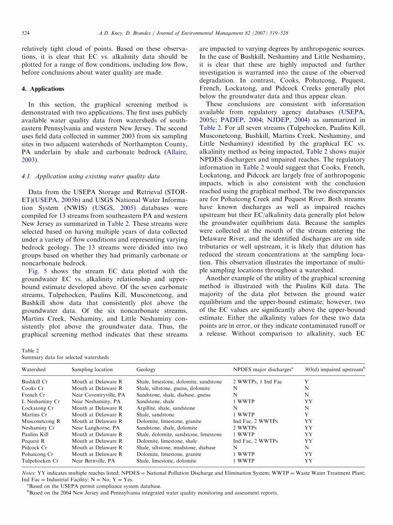
Data from the USEPA Storage and Retrieval (STOR-ET)(USEPA, 2005b) and USGS National Water Informa-tion System (NWIS) (USGS, 2005) databases werecompiled for 13 streams from southeastern PA and westernNew Jersey as summarized in Table 2. These streams wereselected based on having multiple years of data collectedunder a variety of flow conditions and representing varyingbedrock geology. The 13 streams were divided into twogroups based on whether they had primarily carbonate ornoncarbonate bedrock.

Fig. 5 shows the stream EC data plotted with thegroundwater EC vs. alkalinity relationship and upper-bound estimate developed above. Of the seven carbonatestreams, Tulpehocken, Paulins Kill, Musconetcong, andBushkill show data that consistently plot above thegroundwater data. Of the six noncarbonate streams,Martins Creek, Neshaminy, and Little Neshaminy con-sistently plot above the groundwater data. Thus, thegraphical screening method indicates that these streams

Table 2

Summary data for selected watersheds

Watershed Sampling location Geology

Bushkill Cr Mouth at Delaware R Shale, limestone, dolomite,

Cooks Cr Mouth at Delaware R Shale, siltstone, gneiss, dolo

French Cr Near Coventryville, PA Sandstone, shale, diabase, g

L Neshaminy Cr Near Neshaminy, PA Sandstone, shale

Lockatong Cr Mouth at Delaware R Argillite, shale, sandstone

Martins Cr Mouth at Delaware R Shale, sandstone

Musconetcong R Mouth at Delaware R Dolomite, limestone, granit

Neshaminy Cr Near Langhorne, PA Sandstone, shale, dolomite

Paulins Kill Mouth at Delaware R Shale, dolomite, sandstone,

Pequest R Mouth at Delaware R Dolomite, limestone, shale

Pidcock Cr Mouth at Delaware R Shale, siltstone, mudstone,

Pohatcong Cr Mouth at Delaware R Dolomite, limestone, granit

Tulpehocken Cr Near Bernville, PA Shale, limestone, dolomite

Notes: YY indicates multiple reaches listed; NPDES ¼ National Pollution Dis

Ind Fac ¼ Industrial Facility; N ¼ No; Y ¼ Yes.aBased on the USEPA permit compliance system database.bBased on the 2004 New Jersey and Pennsylvania integrated water quality

are impacted to varying degrees by anthropogenic sources.In the case of Bushkill, Neshaminy and Little Neshaminy,it is clear that these are highly impacted and furtherinvestigation is warranted into the cause of the observeddegradation. In contrast, Cooks, Pohatcong, Pequest,French, Lockatong, and Pidcock Creeks generally plotbelow the groundwater data and thus appear clean.These conclusions are consistent with information

available from regulatory agency databases (USEPA,2005c; PADEP, 2004; NJDEP, 2004) as summarized inTable 2. For all seven streams (Tulpehocken, Paulins Kill,Musconetcong, Bushkill, Martins Creek, Neshaminy, andLittle Neshaminy) identified by the graphical EC vs.alkalinity method as being impacted, Table 2 shows majorNPDES dischargers and impaired reaches. The regulatoryinformation in Table 2 would suggest that Cooks, French,Lockatong, and Pidcock are largely free of anthropogenicimpacts, which is also consistent with the conclusionreached using the graphical method. The two discrepanciesare for Pohatcong Creek and Pequest River. Both streamshave known discharges as well as impaired reachesupstream but their EC/alkalinity data generally plot belowthe groundwater equilibrium data. Because the sampleswere collected at the mouth of the stream entering theDelaware River, and the identified discharges are on sidetributaries or well upstream, it is likely that dilution hasreduced the stream concentrations at the sampling loca-tion. This observation illustrates the importance of multi-ple sampling locations throughout a watershed.Another example of the utility of the graphical screening

method is illustrated with the Paulins Kill data. Themajority of the data plot between the ground waterequilibrium and the upper-bound estimate; however, twoof the EC values are significantly above the upper-boundestimate. Either the alkalinity values for these two datapoints are in error, or they indicate contaminated runoff ora release. Without comparison to alkalinity, such EC

NPDES major dischargesa 303(d) impaired upstreamb

sandstone 2 WWTPs, 1 Ind Fac Y

mite N N

neiss N N

1 WWTP YY

N N

1 WWTP Y

e Ind Fac, 2 WWTPs YY

2 WWTPs YY

limestone 1 WWTP YY

Ind Fac, 2 WWTPs YY

diabase N N

e 1 WWTP YY

1 WWTP YY

charge and Elimination System; WWTP ¼Waste Water Treatment Plant;

monitoring and assessment reports.

ARTICLE IN PRESS

0

200

400

600

800

0 50 100 150 200 250

Alk (mg/L as CaCO3)

EC

(uS

/cm

)

CooksPohatcongPequestTulpehockenPaulinsMusconetcongBushkill

0

200

400

600

800

0 25 50 75 100 125 150

Alk (mg/L as CaCO3)

EC

(uS

/cm

)

FrenchLockatongPidcockMartinsNeshaminyL Neshaminy

(a)

(b)

Fig. 5. Stream EC data plotted with the groundwater EC vs. alkalinity

relationship and upper and lower bounds from Fig. 3: (a) streams

underlain by carbonate bedrock, (b) streams underlain by siliciclastic and

crystalline bedrock (note difference in x-axis scale). Filled symbols

indicate impacted streams, open symbols indicate unimpacted streams.

Data from the USEPA STORET and USGS NWIS databases.

A.D. Kney, D. Brandes / Journal of Environmental Management 82 (2007) 519–528 525

measurements would go unnoticed because they areconsistent with typical conductivity values from PaulinsKill Creek (i.e., 300–500 mS/cm).

4.2. Application using field data from Northampton County,

Pennsylvania

To further evaluate the graphical screening method, fieldsampling was conducted in the Bushkill and Monocacy

Creeks of Northampton County, Pennsylvania duringsummer 2003 over a range of flow conditions. EC andalkalinity were measured in a manner consistent with themethod described in Section 3.1. The sampling locationsare shown with bedrock geology in Fig. 6 and aresummarized in Table 3. Due to the contrasting geologyof the lower (carbonate) and upper (shale) portions of thesewatersheds, three sampling sites were used in each. Landuse, geology, and census data for these sites were providedby Northampton County, Pennsylvania as geographicinformation system (GIS) coverages (NorthamptonCounty, Pennsylvania, 2002). Based on land use andknown discharges, sites Bushkill 1 and Monocacy 1 wereconsidered likely to be impacted and Bushkill 3 andMonocacy 3 were considered likely to be unimpacted.In Fig. 7, the graphical screening method is used to

assess the sampling sites. The plot indicates that Bushkill 1and Monocacy 1 are indeed impacted, while Bushkill 3 andMonocacy 3 are not. The data also indicate that Bushkill 2and Monocacy 2 are impacted, particularly Monocacy 2,which is located immediately downstream of a limestonequarry and cement plant. Bushkill 1 and Monocacy 2appear to be subject to intermittent events of high ECwhich do not correlate well with estimated flow rates at thetime of sampling, suggesting the presence of point sourcedischarges.Differences between upstream and downstream results

correlate with changes in geology, dilution from additionalinflow, and pollutant discharges. There is a consistentincrease in stream EC from Bushkill 2 to Bushkill 1(separated by approximately 2 km), due to the presence ofseveral industrial discharges between these sites, includingone major discharge from a metals processing facility. Thedifferences between Monocacy 2 and Monocacy 1 can beexplained by a combination of a shift in geology anddilution. There is a considerable increase in flow fromMonocacy 2 to Monocacy 1 due to the addition of twomajor tributaries, as well as a change from shale-dominated to carbonate-dominated bedrock. These resultin an increase in alkalinity and a reduction of the high ECvalues observed at Monocacy 2.

5. Conclusions and limitations

The graphical screening method presented is evaluatedby comparing concurrent EC and alkalinity measurements.It provides a simple way to distinguish EC/alkalinity valuesof concern from expected values that would be attributedto chemistry based on local geology. Watershed monitoringgroups consisting of citizens with limited scientific back-ground can use the approach to improve their under-standing of EC/alkalinity data to identify stream reacheswith water quality problems, and to evaluate whether pointsource discharges may be impacting water quality. Thereason is that the EC/alkalinty relation of water derivedfrom anthropogenic origin differs from that of streamwater originated from groundwater. Once the screening

ARTICLE IN PRESS

Fig. 6. Map of summer 2003 sampling sites in Bushkill Creek and Monocacy Creek watersheds, Northampton County, Pennsylvania.

Table 3

Descriptive data for stream sampling sites—Bushkill Creek and Monocacy Creek watersheds

Site Drainage area

(km2)

Woodlands (%) 2000 Pop dens

(km�2)

Geology NPDES

discharges

upstream

303(d) impaired

upstream

Bushkill 1 (B1) 204.7 22 255 Shale, limestone,

dolomite,

sandstone

15, incl. 3 major

dischargers

Y

Bushkill 2 (B2) 188.3 24 176 Shale, limestone,

dolomite,

sandstone

12, incl 2 major

dischargers

Y

Bushkill 3 (B3) 22.9 55 74 Shale, sandstone None N

Monocacy 1 (M1) 90.4 6 342 Shale, limestone,

dolomite

5 Y

Monocacy 2 (M2) 23.0 15 205 Shale, limestone 2 Y

Monocacy 3 (M3) 0.8 8 106 Shale None N

Notes: NPDES ¼ National Pollution Discharge and Elimination System; N ¼ No; Y ¼ Yes.

A.D. Kney, D. Brandes / Journal of Environmental Management 82 (2007) 519–528526

ARTICLE IN PRESS

0

200

400

600

800

0 50 100 150 200 250

Alk (mg/L as CaCO3)

EC

(uS

/cm

)

Bushkill 1Bushkill 2Bushkill 3Monocacy 1Monocacy 2Monocacy 3

Fig. 7. EC data from the Bushkill Creek and Monocacy Creek sampling

sites, plotted with the groundwater EC vs. alkalinity relationship and

upper and lower bounds from Fig. 3.

A.D. Kney, D. Brandes / Journal of Environmental Management 82 (2007) 519–528 527

tool is set up it is shown to give rapid results that areconsistent with publicly available data from regulatoryagencies on impacted stream reaches, permitted discharges,and industrial land uses.

The principal requirement of the screening method isidentifying representative groundwater quality data todefine the expected relationship between EC and alkalinityunder natural conditions. The bounds used in the applica-tions presented here are specific to the Pennsylvania-NewJersey region; however, similar ground water data areavailable for most regions of the country through theUSGS and its state affiliates, as well as from stateenvironmental resource agencies. Thus, the method shouldbe widely applicable in humid, temperate regions except ingeological environments where alkalinity is naturally low(o 30mg/L). In that case, hardness data may be usedsimilarly; however, further work is required to investigatethe EC/hardness relationship. The method is not applicableto arid and semi-arid regions where dissolved solidsconcentrations are concentrated by evaporation andirrigation, and thus are not well correlated with thepresence of carbonate bedrock.

Additional limitations to the graphical method includeidentifying poor water quality due to organic contaminantsas well as identification of the presence of trace toxicmetals. When testing for contamination of these typesadditional testing protocol is necessary.

Acknowledgments

Former Lafayette College students Maura Allaire,Joseph Goodwill, and Jason Boyd conducted the field

sampling and analysis for the data shown in Fig. 7. BobLimbeck and Geoff Smith of the Delaware River BasinCommission provided water quality data on streams withinthe Delaware River basin. This material is based uponwork partially supported by the National Science Founda-tion under Grant No. 0088770. Any opinions, findings, andconclusions or recommendations expressed in this materialare those of the authors and do not necessarily reflect theviews of the National Science Foundation.

References

Allaire, M., 2003. Development of a method for rapid assessment of

anthropogenic influence on stream chemistry. Excel Scholar Report,

Lafayette College.

Aulenbach, B.T., Hooper, R.P., 1996. Trends in the chemistry of

precipitation and surface water in a national network of small

watersheds. Hydrological Processes 10, 151–181.

Barker, J.L., 1984. Compilation of ground-water quality data in

Pennsylvania. US Geological Survey Open-File Report 84-076.

Clesceri, C., Greenberg, G., Eaton, E. (Eds.), 1998. Standard Methods for

the Examination of Water and Wastewater, 20th ed. United Book

Press, Baltimore, MD.

Freeze, R.A., Cherry, J.A., 1979. Groundwater. Prentice-Hall, Englewood

Cliffs, NJ.

Hem, J.D., 1959. Study and interpretation of the chemical characteristics

of natural water. US Geological Survey Water-Supply Paper 1473.

Liu, Z., Weller, D.E., Correll, D.L., Jordan, T.E., 2000. Effects of land

cover and geology on stream chemistry in watersheds of Chesapeake

Bay. Journal of the American Water Resources Association 36 (6),

1349–1365.

Makepeace, D.K., Smith, D.W., Stanley, S.J., 1995. Urban stormwater

quality: summary of contaminant data. Critical Reviews in Environ-

mental Science and Technology 25 (2), 93–139.

Mast, M.A., Turk, J.T., 1999a. Environmental characteristics and water

quality of Hydrologic Benchmark Network stations in the Eastern

United States, 1963–95: U.S. Geological Survey Circular 1173-A,

158pp.

Mast, M.A., Turk, J.T., 1999b. Environmental characteristics and water

quality of Hydrologic Benchmark Network stations in the Midwestern

United States, 1963–95: US Geological Survey Circular 1173-B, 130pp.

New Jersey Department of Environmental Protection (NJDEP), 2004.

New Jersey 2004 Integrated Water Quality Monitoring And Assess-

ment Report. http://www.state.nj.us/dep/wmm/sgwqt/wat/integrated-

list/integratedlist2004.html, Retrieved June 17, 2005.

Northampton County, Pennsylvania, 2002. Northampton County Geo-

graphic Information System (GIS).

Peters, N.E., 1984. Evaluation of environmental factors affecting yields of

major dissolved ions of streams in the United States. USGS Water-

Supply Paper 2228.

Pennsylvania Department of Environmental Protection (PADEP), 2004.

2004 Pennsylvania Integrated Water Quality Monitoring and Assess-

ment Report. http://www.dep.state.pa.us/dep/deputate/watermgt/

wqp/wqstandards/303d-Report.htm#List, Retrieved June 17, 2005.

Reese, S.O., Lee, J.J., 1998. Summary of groundwater quality monitoring

data (1985–1997) from Pennsylvania’s Ambient and Fixed Station

Network (FSN) Monitoring Program’’ www.dep.state.pa.us/dep/

deputate/watermgt/wc/subjects/srceprot/ground/sympos/ground_mont_

rpt.htm Retrieved June 17, 2005.

Serfes, M.E., 2004. Ground-water quality in the bedrock aquifers of the

highlands and valley and ridge physiographic provinces of New Jersey.

New Jersey Geological Survey Geological Survey Report 39.

Smith, R.A., Alexander, R.B., Wolman, M.G., 1987. Water-quality trends

in the nation’s rivers. Science 235 (4796), 1607–1615.

ARTICLE IN PRESSA.D. Kney, D. Brandes / Journal of Environmental Management 82 (2007) 519–528528

United States Environmental Protection Agency (USEPA), 2005a.

Volunteer Monitoring. http://yosemite.epa.gov/water/volmon.nsf/

Home?openform, Retrieved June 17, 2005.

United States Environmental Protection Agency (USEPA), 2005b.

STORET http://www.epa.gov/storet/, Retrieved June 17, 2005.

United States Environmental Protection Agency (USEPA), 2005c. Permit

Compliance System (PCS) Database. http://www.epa.gov/enviro/html/

pcs/, Retrieved June 17, 2005.

United States Geological Survey (USGS), 2005. NWISWeb Data for the

Nation. http://waterdata.usgs.gov/nwis/, Retrieved June 17, 2005.