A Generic Approach to Environmental Assessment of ...
405
A Generic Approach to Environmental Assessment of Microbial Bioprocesses through Life Cycle Assessment (LCA) A thesis submitted to the University of Cape Town in fulfilment of the requirements for the degree of Doctor of Philosophy by Kevin Harding Department of Chemical Engineering University of Cape Town December 2008
-
Upload
khangminh22 -
Category
Documents
-
view
0 -
download
0
Transcript of A Generic Approach to Environmental Assessment of ...

A Generic Approach to Environmental Assessment of Microbial Bioprocesses through Life Cycle Assessment
(LCA)
A thesis submitted to the University of Cape Town in fulfilment of the requirements for the degree of
Doctor of Philosophy
by
Kevin Harding
Department of Chemical Engineering University of Cape Town
December 2008

A Generic Approach to Environmental Assessment of Microbial Bioprocesses through Life Cycle Assessment
(LCA)
Volume 1
Thesis
A thesis submitted to the University of Cape Town in fulfilment of the requirements for the degree of
Doctor of Philosophy
by
Kevin Harding
Department of Chemical Engineering University of Cape Town
December 2008


i
Acknowledgements
I would like to thank the following groups for their assistance throughout this thesis:
My supervisor, Prof. Sue Harrison (Centre for Bioprocess Engineering Research, Department of Chemical Engineering, University of Cape Town), for all her input and time in this project;
The Centre for Bioprocess Engineering Research (CeBER), Department of Chemical Engineering (University of Cape Town), for being my base during my postgraduate research;
Dr John Dennis and the Department of Chemical Engineering (Cambridge University), for time in the department and guidance on the project;
A/Prof Harro von Blottnitz (Environmental and Process Systems Engineering, Department of Chemical Engineering, University of Cape Town) for his input on Life Cycle Assessment (LCA);
The National Research Foundation (NRF), the KW Johnstone foundation and the Centre for Bioprocess Engineering Research (CeBER) (Department of Chemical Engineering, UCT), for financial support;
The UNEP/SETAC LCInitiative for LCA software used; and
My parents and brothers for all the encouragement and support throughout my studies.

ii
iii
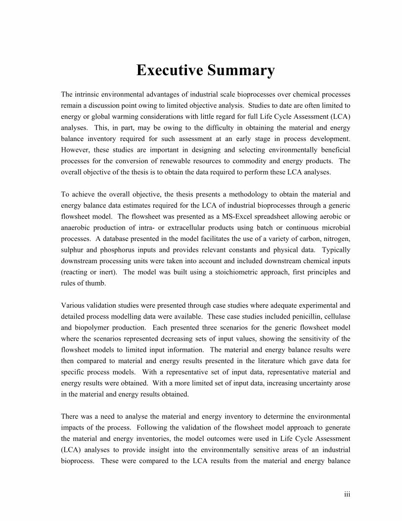
Executive Summary
The intrinsic environmental advantages of industrial scale bioprocesses over chemical processes
remain a discussion point owing to limited objective analysis. Studies to date are often limited to
energy or global warming considerations with little regard for full Life Cycle Assessment (LCA)
analyses. This, in part, may be owing to the difficulty in obtaining the material and energy
balance inventory required for such assessment at an early stage in process development.
However, these studies are important in designing and selecting environmentally beneficial
processes for the conversion of renewable resources to commodity and energy products. The
overall objective of the thesis is to obtain the data required to perform these LCA analyses.
To achieve the overall objective, the thesis presents a methodology to obtain the material and
energy balance data estimates required for the LCA of industrial bioprocesses through a generic
flowsheet model. The flowsheet was presented as a MS-Excel spreadsheet allowing aerobic or
anaerobic production of intra- or extracellular products using batch or continuous microbial
processes. A database presented in the model facilitates the use of a variety of carbon, nitrogen,
sulphur and phosphorus inputs and provides relevant constants and physical data. Typically
downstream processing units were taken into account and included downstream chemical inputs
(reacting or inert). The model was built using a stoichiometric approach, first principles and
rules of thumb.
Various validation studies were presented through case studies where adequate experimental and
detailed process modelling data were available. These case studies included penicillin, cellulase
and biopolymer production. Each presented three scenarios for the generic flowsheet model
where the scenarios represented decreasing sets of input values, showing the sensitivity of the
flowsheet models to limited input information. The material and energy balance results were
then compared to material and energy results presented in the literature which gave data for
specific process models. With a representative set of input data, representative material and
energy results were obtained. With a more limited set of input data, increasing uncertainty arose
in the material and energy results obtained.
There was a need to analyse the material and energy inventory to determine the environmental
impacts of the process. Following the validation of the flowsheet model approach to generate
the material and energy inventories, the model outcomes were used in Life Cycle Assessment
(LCA) analyses to provide insight into the environmentally sensitive areas of an industrial
bioprocess. These were compared to the LCA results from the material and energy balance

iv
inventories obtained from the literature data to further validate the modelling approach.
Thereafter, assessment of the Life Cycle Inventory data across four case studies completed was
undertaken.
The first case study investigated the production of penicillin by Penicillium chrysogenum using a
medium of glucose, Pharmamedia and phenoxyacetic acid. The key findings in the study
showed that electrical and agricultural inputs were key contributors to LCA impacts. Further, it
was found that poor separation efficiencies in downstream processing are the reason for high
operating volumes and large recycle flows within a process. This, in turn, increased electrical
and steam requirements, thereby LCA scores.
The production of cellulase was investigated using three separate flowsheets. These give a
comparison of aerobic and anaerobic microbial processes, different bioreactor designs and
different downstream processing units. The study showed that large water volumes associated
with low biomass concentrations of a submerged fermentation system increased the energy
requirements and thereby LCA scores compared to solid state cultivation. Where there was
limited downstream processing, a large volume of low purity product was formed. For the
cradle-to-gate approach used in the study, the LCA comparison of these systems was complex.
The third case study considered industrial production of the biopolymer, polyhydroxyalkanoate.
The data predicted by the generic flowsheet was compared with the experimental data reported
in literature. The comparison showed that 50 % of the material balance values predicted by the
model were within 12 % of the literature results for the most comprehensive scenario modelled.
Further, it was shown that electrical requirements for aeration dominated the contributions to
electricity supply and thereby the LCA scores.
The generic flowsheet model was further used to inform a secondary study into biodiesel
production. The material and energy balance requirements for production of the lipase, used in
an enzymatic transesterification route, were modelled and the total material and energy balance
obtained used in an LCA analysis. This analysis, together with the biopolymer LCA, was used
to compare biological and chemical production routes for equivalent products. The LCAs for
biodiesel production using a biological catalyst are compared to biodiesel using a chemical
catalyst, while the biopolymer polyhydroxyalkanoate is compared to the polyolefins
polypropylene, low density and high density polyethylene.
It was shown that there was no clear environmental advantage to either the chemical or
biological route of production for an equivalent product. Enzyme catalysed biodiesel production
had environmental advantages owing to avoided use of a chemical catalyst and neutralizing acid.

v
The lower pressures and temperatures required reduced LCA impacts across seven of the ten
environmental impacts considered. In the production of polymers, poly--butyrate (PHB)
production resulted in higher or similar LCA scores compared to polypropylene (PP) and
polyethylene (PE) for all impact categories when using the most recent LCA database. This
showed that despite the use of fossil fuels during polyolefin production, and the use of renewable
resources in PHB production, PP and PE are more beneficial environmentally. The results of the
LCA of polyolefins were shown to be sensitive to the database used, with substantial
development occurring in these databases over the last few years. The polymer comparison was
for the established industrial technology of polyolefin production versus the developing process
of PHB production, which is not fully optimised. This optimisation may be expected to
ultimately reduce the LCA impacts.
The thesis approaches the validation and comparison studies by interrogating the sensitivity to
specified variables in the generic flowsheet model in terms of both the material and energy
balance inventory generated and the life cycle impacts. These outputs are used to identify the
relative contributions of particular process components and process steps to creation of
environment burden, thereby allowing these to be targeted in process improvement.
A sensitivity analysis which varied all individual inputs to the generic flowsheet model for the
penicillin production case study was also performed. A detailed set of inputs, based on the
sensitivity of LCA results versus changes to the inputs, was used to determine the effects on the
energy requirements, LCA scores, reactor volumes and product purities. The detailed set of
inputs included yield coefficients, separation efficiencies and aeration rates amongst others. This
sensitivity informed the process selection and decision making regarding bioprocess design.
Further, the advantages of an improved bioreactor configuration were compared to optimisation
options for downstream processing.
The findings from the sensitivity analysis showed that the resulting changes to LCA impacts
could be larger than the relative changes to single inputs in the generic flowsheet model. For the
flowsheet used, this was shown to be the case for the product to biomass ratio as well as the
separation efficiencies of downstream processing units. It was also shown that LCA scores were
highly sensitive to changes in aeration rates, biomass concentrations, yield coefficients and
additives in downstream processing. Changes to a process that resulted in a greater volume, and
in turn greater energy requirements, led to higher LCA scores.
The thesis contributes to knowledge in several ways. It provides a tool for the mass and energy
balance calculation for industrial bioprocesses at an early stage of process design, facilitating the

vi
interrogation of feedstocks and technology selection. These early stage calculations can then be
used in Life Cycle Assessment (LCA) studies to allow for design considerations before detailed
engineering. The interrogation of the technology by several case studies has shown the
importance of volume and concentration of the biomass and product in processes. Efficient
downstream processing is required to purify the product and reduce process volumes throughout.
Effective aeration technologies were important to reduce overall electrical requirements.
In the case studies investigated, it was shown that energy requirements dominated the LCA
impacts; hence their reduction is a key area for reducing overall the life cycle impacts. The
impacts of carbon source raw materials in bioprocesses, and the agricultural feedstocks needed
for these, were also shown to add significantly to LCA scores in certain case studies investigated.
The thesis demonstrated that when comparing chemical and biological processes, the
environmental advantages should be investigated on a case by case basis.

vii
Table of Contents
VOLUME 1 – THESIS
Executive Summary ................................................................................................................... iii Table of Contents ...................................................................................................................... vii List of Figures ........................................................................................................................ xiii List of Tables ........................................................................................................................ xix List of Acronyms ..................................................................................................................... xxv
CHAPTER 1 : Introduction ............................................................................................................ 1 1.1. Context ........................................................................................................................ 3 1.2. Quantification of environmental damage .................................................................... 4 1.3. Life Cycle Assessment (LCA) .................................................................................... 5 1.4. Data gathering ............................................................................................................. 6 1.5. Thesis objectives ......................................................................................................... 7 1.6. Thesis structure ........................................................................................................... 8 References ......................................................................................................................... 10
CHAPTER 2 : Generic Flowsheet Model Development ............................................................. 17 2.1. Introduction ............................................................................................................... 19
2.1.1. Desirable functions of the model .......................................................................... 19 2.1.2. Model Description ................................................................................................. 20 2.1.3. Structure of the model ........................................................................................... 24
2.2. Sterilisation ................................................................................................................ 24 2.2.1. Introduction ........................................................................................................... 24 2.2.2. Filtration ................................................................................................................ 25 2.2.3. Steam sterilisation ................................................................................................. 25 2.2.4. Additional steam requirements .............................................................................. 26
2.3. Microbial growth and product formation .................................................................. 26 2.3.1. Introduction ........................................................................................................... 26 2.3.2. Mass balance – biomass growth and formation .................................................... 26 2.3.3. Anaerobic growth .................................................................................................. 29 2.3.4. Yield coefficients .................................................................................................. 30 2.3.5. Carbon source ........................................................................................................ 33 2.3.6. Nitrogen source ..................................................................................................... 33 2.3.7. Oxygen source ....................................................................................................... 34 2.3.8. Sulphur and phosphorus sources ........................................................................... 35 2.3.9. Maintenance coefficient calculations .................................................................... 35 2.3.10. Growth rate ............................................................................................................ 36 2.3.11. Reactor cooling ..................................................................................................... 36 2.3.12. Post microbial growth cooling .............................................................................. 37
viii
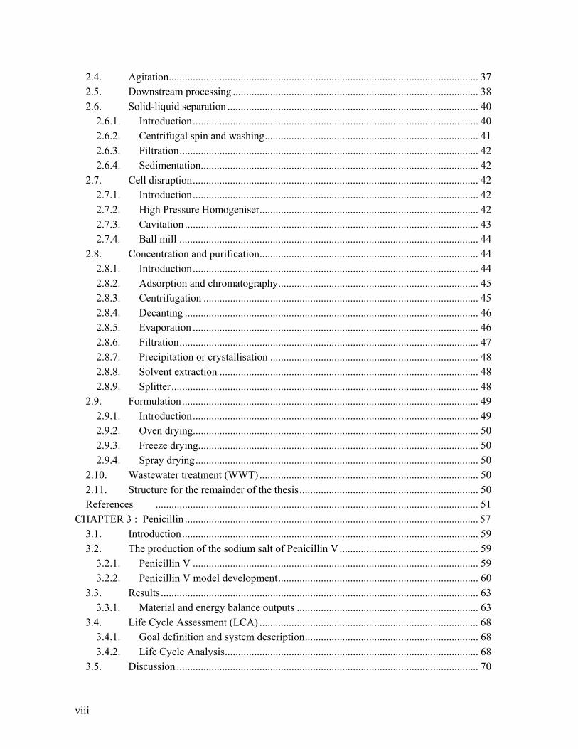
2.4. Agitation.................................................................................................................... 37 2.5. Downstream processing ............................................................................................ 38 2.6. Solid-liquid separation .............................................................................................. 40
2.6.1. Introduction ........................................................................................................... 40 2.6.2. Centrifugal spin and washing ................................................................................ 41 2.6.3. Filtration ................................................................................................................ 42 2.6.4. Sedimentation........................................................................................................ 42
2.7. Cell disruption ........................................................................................................... 42 2.7.1. Introduction ........................................................................................................... 42 2.7.2. High Pressure Homogeniser.................................................................................. 42 2.7.3. Cavitation .............................................................................................................. 43 2.7.4. Ball mill ................................................................................................................ 44
2.8. Concentration and purification.................................................................................. 44 2.8.1. Introduction ........................................................................................................... 44 2.8.2. Adsorption and chromatography ........................................................................... 45 2.8.3. Centrifugation ....................................................................................................... 45 2.8.4. Decanting .............................................................................................................. 46 2.8.5. Evaporation ........................................................................................................... 46 2.8.6. Filtration ................................................................................................................ 47 2.8.7. Precipitation or crystallisation .............................................................................. 48 2.8.8. Solvent extraction ................................................................................................. 48 2.8.9. Splitter ................................................................................................................... 48
2.9. Formulation ............................................................................................................... 49 2.9.1. Introduction ........................................................................................................... 49 2.9.2. Oven drying........................................................................................................... 50 2.9.3. Freeze drying......................................................................................................... 50 2.9.4. Spray drying .......................................................................................................... 50
2.10. Wastewater treatment (WWT) .................................................................................. 50 2.11. Structure for the remainder of the thesis ................................................................... 50 References ......................................................................................................................... 51
CHAPTER 3 : Penicillin .............................................................................................................. 57 3.1. Introduction ............................................................................................................... 59 3.2. The production of the sodium salt of Penicillin V .................................................... 59
3.2.1. Penicillin V ........................................................................................................... 59 3.2.2. Penicillin V model development ........................................................................... 60
3.3. Results ....................................................................................................................... 63 3.3.1. Material and energy balance outputs .................................................................... 63
3.4. Life Cycle Assessment (LCA) .................................................................................. 68 3.4.1. Goal definition and system description ................................................................. 68 3.4.2. Life Cycle Analysis ............................................................................................... 68
3.5. Discussion ................................................................................................................. 70
ix
3.5.1. Comparison with a full penicillin design .............................................................. 70 3.5.2. Life Cycle Impact Assessment (LCIA) ................................................................. 73 3.5.3. Process contributions ............................................................................................. 74
3.6. Conclusions ............................................................................................................... 77 References ......................................................................................................................... 78
CHAPTER 4 : Cellulase ............................................................................................................... 79 4.1. Introduction ............................................................................................................... 81 4.2. Cellulase – Its role and production process ............................................................... 81 4.3. Case study methodology ........................................................................................... 83
4.3.1. Material and Energy balance ................................................................................. 83 4.3.2. LCA goal definition and system description ......................................................... 83
4.4. Cellulase Flowsheet One: Aerobic production by SmF using Trichoderma reesei ............................................................................................................... 84
4.4.1. Cellulase model development ............................................................................... 84 4.4.2. Material and energy balance outputs ..................................................................... 87 4.4.3. Life Cycle Assessment (LCA) .............................................................................. 90 4.4.4. Process contributions ............................................................................................. 92 4.4.5. Discussion ............................................................................................................. 94
4.5. Cellulase Flowsheet Two: Anaerobic production by SmF using Clostridium thermocellum ................................................................................................... 95
4.5.1. Cellulase model development ............................................................................... 95 4.5.2. Material and energy balance outputs ..................................................................... 97 4.5.3. Life Cycle Assessment (LCA) .............................................................................. 99 4.5.4. Process contributions ........................................................................................... 101 4.5.5. Discussion ........................................................................................................... 103
4.6. Cellulase Flowsheet Three: Anaerobic production by SSC using Clostridium thermocellum ................................................................................................. 104
4.6.1. Cellulase model development ............................................................................. 104 4.6.2. Material and energy balance outputs ................................................................... 105 4.6.3. Life Cycle Assessment (LCA) ............................................................................ 108 4.6.4. Process contributions ........................................................................................... 109 4.6.5. Discussion ........................................................................................................... 111
4.7. Comparison of flowsheet models ............................................................................ 112 4.8. Conclusions ............................................................................................................. 114 References ....................................................................................................................... 115
CHAPTER 5 : Polymers ............................................................................................................ 117 5.1. Introduction ............................................................................................................. 119 5.2. The production of polyhydroxyalkanoates (PHAs) ................................................ 119
5.2.1. Polyhydroxyalkanoates ....................................................................................... 119 5.2.2. Poly-β-hydroxybutyric acid (PHB) model development .................................... 123
5.3. Results ..................................................................................................................... 126
x
5.3.1. Material and energy balance outputs .................................................................. 126 5.4. Life Cycle Assessment (LCA) ................................................................................ 129
5.4.1. Goal definition and system description ............................................................... 129 5.4.2. Life Cycle Impact Assessment (LCIA) ............................................................... 129
5.5. Comparison with a design of a biopolymer plant ................................................... 131 5.5.1. Material and energy balance ............................................................................... 131 5.5.2. Life Cycle Impact Assessment (LCIA) ............................................................... 137 5.5.3. Process contributions .......................................................................................... 138
5.6. Comparison of PHB LCA results to literature ........................................................ 141 5.7. Comparison of PHB to polyolefin production ........................................................ 142
5.7.1. Life Cycle Analysis ............................................................................................. 142 5.7.2. PHB vs. polypropylene ....................................................................................... 142 5.7.3. PHB vs. high density polyethylene ..................................................................... 144 5.7.4. PHB vs. low density polyethylene ...................................................................... 146
5.8. Conclusions ............................................................................................................. 147 References ....................................................................................................................... 148
CHAPTER 6 : Biodiesel ............................................................................................................ 153 6.1. Introduction ............................................................................................................. 155 6.2. Biodiesel production ............................................................................................... 155 6.3. Process flowsheet and mass and energy balance inventories ................................. 157
6.3.1. Introduction ......................................................................................................... 157 6.3.2. Alkali catalysed process ...................................................................................... 158 6.3.3. Biologically catalysed process ............................................................................ 160 6.3.4. Additional process flowsheets ............................................................................ 161 6.3.5. Production alternatives for biodiesel production ................................................ 162
6.4. Life Cycle Assessment (LCA) ................................................................................ 163 6.5. Lipase production .................................................................................................... 164
6.5.1. Process flowsheet and model development ........................................................ 164 6.5.2. Material and energy balance outputs .................................................................. 164 6.5.3. Life Cycle Assessment (LCA) of lipase production ........................................... 166
6.6. Life Cycle Assessment (LCA) of biodiesel production .......................................... 168 6.6.1. Alkali catalyst and methanol (Case 1) ................................................................ 170 6.6.2. Chemical vs. biological catalysts ........................................................................ 170 6.6.3. Reduced methanol recovery ................................................................................ 171 6.6.4. Alternative alcohol (methanol vs. ethanol) ......................................................... 172 6.6.5. Process contributions .......................................................................................... 174
6.7. Conclusions ............................................................................................................. 176 References ....................................................................................................................... 177
CHAPTER 7 : Heuristics ........................................................................................................... 183 7.1. Introduction ............................................................................................................. 185 7.2. Identifying key variables ......................................................................................... 186
xi
7.2.1. Sensitivity analysis .............................................................................................. 186 7.2.2. LCA single score ................................................................................................. 186 7.2.3. Summary of sensitivity results ............................................................................ 186 7.2.4. Product to biomass ratio and final biomass concentration .................................. 188
7.2.4.1. Product to biomass ratio ................................................................................ 188 7.2.4.2. Final biomass concentration .......................................................................... 190
7.2.5. Oxygen flowrate (vvm) and compression pressure ............................................. 192 7.2.5.1. Oxygen flowrate ............................................................................................ 192 7.2.5.2. Compression pressure ................................................................................... 195
7.2.6. Yield coefficients ................................................................................................ 197 7.2.6.1. Biomass on substrate (Yx/s) ........................................................................... 197 7.2.6.2. Product on substrate (Yp/s) ............................................................................. 198
7.2.7. Product fraction retained in downstream processing .......................................... 200 7.2.8. Waste fraction removed in downstream processing ............................................ 201
7.2.8.1. Effect of changing the waste fraction removed ............................................. 201 7.2.8.2. Filtration ........................................................................................................ 202 7.2.8.3. Centrifugation 1 ............................................................................................. 202 7.2.8.4. Centrifugation 2 ............................................................................................. 205 7.2.8.5. Fluid bed drying ............................................................................................ 206
7.2.9. The formation of the sodium salt of Penicillin V ................................................ 207 7.2.9.1. Percentage additive – Sodium acetate ........................................................... 207 7.2.9.2. Percentage of limiting reactant converted ..................................................... 208
7.2.10. Summary ............................................................................................................. 210 7.3. Increased production vs. optimised downstream processing .................................. 210
7.3.1. Introduction ......................................................................................................... 210 7.3.2. Penicillin V .......................................................................................................... 210
7.3.2.1. Process descriptions ...................................................................................... 210 7.3.2.2. Material and energy balance results .............................................................. 212 7.3.2.3. Life Cycle Assessment (LCA) Results .......................................................... 213
7.3.3. Cellulase .............................................................................................................. 215 7.3.3.1. Process descriptions ...................................................................................... 215 7.3.3.2. Material and energy balance results .............................................................. 216 7.3.3.3. Life Cycle Assessment (LCA) results ........................................................... 218
7.3.4. Poly--hydroxybutyric acid ................................................................................ 219
7.3.4.1. Process descriptions ...................................................................................... 219 7.3.4.2. Material and energy balance results .............................................................. 220 7.3.4.3. Life Cycle Assessment (LCA) results ........................................................... 222
7.3.5. Summary ............................................................................................................. 223 7.4. Conclusions ............................................................................................................. 223 References ....................................................................................................................... 224
CHAPTER 8 : Conclusions ......................................................................................................... 227

xii
8.1 Introduction ............................................................................................................. 229 8.2 Model development, validation and Life Cycle Assessment (LCA) ...................... 229 8.3 Findings from case studies ...................................................................................... 230 8.4 Chemical versus biological processes ..................................................................... 231 8.5 Technology selection .............................................................................................. 232 8.6 Conclusions ............................................................................................................. 233 8.7 Recommendations ................................................................................................... 235
VOLUME 2 – APPENDICES
Appendix A: Life Cycle Assessment (LCA) ……………...……………………….……….…. A.3 Appendix B: Generic Flow Sheet Calculations ……………..…………………..........……….A.11 Appendix C: Nomenclature used in Appendix B …………………………..…………….…... A.79 Appendix D: UML Diagrams for the Generic Flowsheet Model ……….……….……........…A.89 Appendix E: Using the Generic Flowsheet Model …………………...……………………… A.93 Appendix F: Electricity LCA from South African data …………..……….……..………..…A.111 Appendix G: Sugar LCA from South African Sugar Cane …...…………………..………… A.119 Appendix H: Sensitivity Analysis Data …………………..…………….……...…...………..A.123 Appendix I: Life Cycle Inventory Tables..……….…………………………………………. A.129

xiii
List of Figures
Figure 1.1: Phases of an LCA (modified from ISO 14040: 2006) ................................................. 6
Figure 2.1: Generic bioprocess model (Level 1) .......................................................................... 20 Figure 2.2: Generic bioprocess model (Level 2) .......................................................................... 21
Figure 2.3: Generic bioprocess model (Level 3) .......................................................................... 21
Figure 2.4: Generic bioprocess model (Level 4) .......................................................................... 22 Figure 2.5: Generic bioprocess model (Level 5) .......................................................................... 22 Figure 2.6: Outline of the process flowsheet used in the generic bioprocess model (Level 6) .... 23 Figure 2.7: Decision method to determine yield coefficients used in generic flowsheet
model ..................................................................................................................... 30
Figure 2.8: Decision method to determine max, Ks and rx values ............................................... 36
Figure 3.1: Basic penicillin structure, where R represents a side chain (R = C7H6 for Penicillin V) ........................................................................................................... 60
Figure 3.2: Simplified process flowsheet for penicillin V sodium salt production as modelled in the MS-Excel model (simplified from Biwer et al. 2005 and Heinzle et al. 2006) ............................................................................................... 61
Figure 3.3: Comparison of material, energy and utility inputs from the generic model for Penicillin V sodium salt production, relative to Scenario 1 .................................. 65
Figure 3.4: Comparison of material, energy and utility outputs from the generic model for Penicillin V sodium salt production, relative to Scenario 1 .................................. 66
Figure 3.5: Comparison of LCA results for Penicillin V sodium salt production for Scenarios 2 and 3 relative to Scenario 1 ................................................................ 69
Figure 3.6: Comparison of material, energy and utility inputs calculated for Penicillin V sodium salt production, relative to literature values of Heinzle et al. (2006) ....... 72
Figure 3.7: Comparison of material, energy and utility outputs calculated for Penicillin V sodium salt production, relative to literature values of Heinzle et al. (2006) ....... 72
Figure 3.8: Comparison of LCA results for Penicillin V sodium salt production for the the three scenarios presented in this study relative to Heinzle et al. (2006) results .... 74
Figure 3.9: Life Cycle Assessment process contributions of penicillin production (Scenario 1) using the CML Baseline 2.03 methodology (Abiotic depletion and Global warming) ................................................................................................................ 75
Figure 3.10: Life Cycle Assessment process contributions of penicillin production (Scenario 1) using the CML Baseline 2.03 methodology (Ozone layer depletion and Photochemical oxidation warming) ....................................................................... 76
Figure 3.11: Life Cycle Assessment process contributions of penicillin production (Scenario 1) using the CML Baseline 2.03 methodology (Acidification and Eutrophication) ...................................................................................................... 76
Figure 4.1: Simplified process flowsheet for cellulase production as modelled in the MS-Excel model ........................................................................................................... 85
xiv
Figure 4.2: Comparison of material, energy and utility inputs calculated for cellulase production, relative to literature values of Heinzle et al. (2006) .......................... 89
Figure 4.3: Comparison of material, energy and utility outputs calculated for cellulase production, relative to literature values of Heinzle et al. (2006) .......................... 89
Figure 4.4: Comparison of LCA results for cellulase production for the three scenarios presented in the study relative to Heinzle et al. (2006) data ................................. 92
Figure 4.5: Life Cycle Assessment process contributions of cellulase production (Heinzle et al. 2006) using the CML baseline 2.03 methodology (Abiotic depletion and Global warming) .................................................................................................... 93
Figure 4.6: Life Cycle Assessment process contributions of cellulase production (Heinzle et al. 2006) using the CML baseline 2.03 methodology (Ozone layer depletion and Photochemical oxidation) ............................................................................... 93
Figure 4.7: Life Cycle Assessment process contributions of cellulase production (Heinzle et al. 2006) using the CML baseline 2.03 methodology (Acidification and Eutrophication) ...................................................................................................... 94
Figure 4.8: Simplified process flowsheet for cellulase production as modelled in the MS-Excel model for the SmF method .......................................................................... 95
Figure 4.9: Comparison of LCA results for cellulase production by submerged fermentation for Scenarios SmF2 and SmF3 relative to Scenario SmF1 ................................. 100
Figure 4.10: Life Cycle Assessment process contributions of cellulase production by SmF using the CML baseline 2.03 methodology (Abiotic depletion and Global warming) ............................................................................................................. 101
Figure 4.11: Life Cycle Assessment process contributions of cellulase production by SmF using the CML baseline 2.03 methodology (Ozone layer depletion and Photochemical oxidation) .................................................................................... 102
Figure 4.12: Life Cycle Assessment process contributions of cellulase production by SmF using the CML baseline 2.03 methodology (Acidification and Eutrophication) 103
Figure 4.13: Simplified process flowsheet for cellulase production as modelled in the MS-Excel model for the SSC method ........................................................................ 104
Figure 4.14: Comparison of LCA results for cellulase production by solid state cultivation for Scenarios SSC2 and SSC3 relative to Scenario SSC1 ................................... 109
Figure 4.15: Life Cycle Assessment process contributions of cellulase production by SSC using the CML baseline 2.03 methodology (Abiotic depletion and Global warming) ............................................................................................................. 110
Figure 4.16: Life Cycle Assessment process contributions of cellulase production by SSC using the CML baseline 2.03 methodology (Ozone layer depletion and Photochemical oxidation) .................................................................................... 110
Figure 4.17: Life Cycle Assessment process contributions of cellulase production by SSC using the CML baseline 2.03 methodology (Acidification and Eutrophication) 111

xv
Figure 4.18: Comparison of LCA results for cellulase production by solid state cultivation (Scenario SSC1) relative to submerged fermentation (Scenario SmF1) as presented in the study .......................................................................................... 113
Figure 5.1: Process flowsheet for PHB production (based on Harrison 1990) .......................... 123 Figure 5.2: Comparison of material, energy and utility inputs from the generic model,
calculated for PHB production, relative to Scenario PHB1 ................................ 128
Figure 5.3: Comparison of material, energy and utility outputs from the generic model, calculated for PHB production, relative to Scenario PHB1 ................................ 128
Figure 5.4: Comparison of LCA results for 1 kg poly--butyrate for the three scenarios
developed ............................................................................................................. 131 Figure 5.5: Comparison of material, energy and utility inputs (excluding ammonium
sulphate) calculated for PHB production, relative to literature values of Harrison et al. (1990) ........................................................................................... 135
Figure 5.6: Comparison of material, energy and utility outputs calculated for PHB production, relative to literature values of Harrison et al. (1990) ....................... 135
Figure 5.7: Electrical energy contributions for the production of poly--butyrate as
determined by Harrison (1990), relative to Scenario PHB1 ................................ 136
Figure 5.8: Comparison of LCA results for PHB production for Scenarios PHB1 and PHB2 relative to Harrison (1990) data ........................................................................... 138
Figure 5.9: Life Cycle Assessment process contributions of PHB production (Scenario PHB1) using the CML baseline 2.03 methodology (Abiotic depletion and Global warming) .................................................................................................. 139
Figure 5.10: Life Cycle Assessment process contributions of PHB production (Scenario PHB1) using the CML baseline 2.03 methodology (Ozone layer depletion and Photochemical oxidation) .................................................................................... 140
Figure 5.11: Life Cycle Assessment process contributions of PHB production (Scenario PHB1) using the CML baseline 2.03 methodology (Acidification and Eutrophication) .................................................................................................... 140
Figure 5.12: Comparison of LCA results for PHB production for polypropylene (PP) production from three different Life Cycle Inventory (LCI) sets relative to Scenario PHB1 data ............................................................................................. 144
Figure 5.13: Comparison of LCA results for PHB production for high density polyethylene (HDPE) production from three different Life Cycle Inventory (LCI) sets relative to Scenario PHB1 data ............................................................................ 145
Figure 5.14: Comparison of LCA results for PHB production for low density polyethylene (LDPE) production from three different Life Cycle Inventory (LCI) sets relative to Scenario PHB1 data ............................................................................ 147
Figure 6.1: Biodiesel process flowsheet to be used in LCA – alkali catalyst; modified from Zhang et al. (2003a) to include recycle ............................................................... 159
Figure 6.2: Biodiesel process flowsheet to be used in LCA – biological catalyst ..................... 161

xvi
Figure 6.3: Flowsheet used for material and energy balance development for lipase production from Candida antarctica ................................................................... 164
Figure 6.4: Comparison of LCA results for lipase production for Scenario L2 relative to Scenario L1 .......................................................................................................... 167
Figure 6.5: Comparison of LCA results for equal masses of anionic and cationic resins relative to lipase produced by Scenario L2 ......................................................... 168
Figure 6.6: Comparison of LCA results for biodiesel for Cases 2 – 5 relative to Case 1 .......... 169 Figure 6.7: LCA results – chemical vs. biological catalysts (biodiesel production by alkali
catalysis assuming 94 % methanol recovery (Case 1) is compared to production using lipase as a biocatalyst (Case 2)) .............................................. 171
Figure 6.8: LCA results – reduced methanol recovery (biodiesel production by alkali catalysis assuming 94 % methanol recovery (Case 1) is compared to production assuming 50 % methanol recovery (Case 3)) .................................... 172
Figure 6.9: LCA results – alternative alcohol (methanol vs. ethanol) using alkali catalysis (biodiesel production by alkali catalysis assuming 94 % methanol recovery (Case 1) is compared to production using ethanol at 94 % recovery (Case 4)) .. 173
Figure 6.10: LCA results – alternative alcohol (methanol vs. ethanol) using lipase biocatalysis (biodiesel production by lipase biocatalysis using methanol (Case 2) is compared to production by lipase biocatalysis and ethanol (Case 5)) ........ 173
Figure 6.11: Life Cycle Assessment process contributions of biodiesel production (Case 2) using the CML baseline 2.03 methodology (Abiotic depletion and Global warming) ............................................................................................................. 175
Figure 6.12: Life Cycle Assessment process contributions of biodiesel production (Case 2) using the CML baseline 2.03 methodology (Ozone layer depletion and Photochemical oxidation) .................................................................................... 175
Figure 6.13: Life Cycle Assessment process contributions of biodiesel production (Case 2) using the CML baseline 2.03 methodology (Acidification and Eutrophication) 176
Figure 7.1: Electrical requirements, reactor volumes and LCA single scores for different product to biomass ratios (all other inputs at original defined values) in the production of 1000 kg Penicillin V ..................................................................... 189
Figure 7.2: Electrical requirements, reactor volumes and LCA single scores for different final biomass concentrations (all other inputs at original defined values) in the production of 1000 kg Penicillin V ..................................................................... 191
Figure 7.3: Electricity breakdown for different final biomass concentrations (all other inputs at original defined values) in the production of 1000 kg Penicillin V ................ 192
Figure 7.4: Electrical requirements, reactor volumes and LCA single scores for different oxygen flowrates (all other inputs at original defined values; compression pressure of 600 kPa) in the production of 1000 kg Penicillin V ......................... 194
Figure 7.5: Breakdown of requirements for electricity for different oxygen flowrates (all other inputs at original defined values; compression pressure of 600 kPa) in the production of 1000 kg Penicillin V ............................................................... 195

xvii
Figure 7.6: Total electrical requirements and LCA single scores for different compression pressures (all other inputs at original defined values; aeration rate of 0.021 vvm) in the production of 1000 kg Penicillin V (NOTE: Y-axis not zero) ..................................................................................................................... 196
Figure 7.7: Breakdown of requirements for electricity for different compression pressures (all other inputs at original defined values; aeration rate of 0.021 vvm) in the production of Penicillin V ................................................................................... 197
Figure 7.8: Electrical requirements, reactor volumes and LCA single scores for different yield coefficients (Yx/s) (all other inputs at original defined values) in the production of 1000 kg Penicillin V ..................................................................... 198
Figure 7.9: Electrical requirements, reactor volumes and LCA single scores for different yield coefficients (Yp/s) (all other inputs at original defined values) in the production of 1000 kg Penicillin V ..................................................................... 199
Figure 7.10: Electrical requirements, reactor volumes and LCA single scores for differing product retention in individual downstream process units (all other inputs at original defined values) in the production of 1000 kg Penicillin V .................... 201
Figure 7.11: Electrical requirements, reactor volumes and LCA single scores for different waste fractions removed (all other inputs at original defined values) in centrifugation 1 in the production of 1000 kg Penicillin V ................................. 204
Figure 7.12: LCA single scores and purities for different waste fractions removed in centrifugation 1 (all other inputs at original defined values) in the production of 1000 kg Penicillin V ........................................................................................ 205
Figure 7.13: Electrical requirements, reactor volumes and LCA single scores for different waste fractions removed in centrifugation 2 (all other inputs at original defined values) in the production of 1000 kg Penicillin V .................................. 206
Figure 7.14: Electrical requirements, reactor volumes and LCA single scores for different percentages of sodium acetate added (all other inputs at original defined values) in the production of 1000 kg Penicillin V ............................................... 208
Figure 7.15: Electrical requirements, reactor volumes and LCA single scores for different conversions rates of limiting reactants (all other inputs at original defined values) in the production of 1000 kg Penicillin V ............................................... 209
Figure 7.16: Comparison of LCA results for Penicillin V sodium salt production for Scenarios A, B and D relative to Scenario C ....................................................... 214
Figure 7.17: Comparison of LCA results for cellulase production by SmF using Trichoderma reesei for Scenarios E, F and H relative to Scenario G ................. 219
Figure 7.18: Comparison of LCA results for poly--hydroxybutyric acid production for
Scenarios I, J and K relative to Scenario L ......................................................... 223 Figure A.1: Phases of an LCA as given in ISO 14040: 2006 ......................................................... 3 Figure A.2: EPS structure as used in the Life Cycle Assessment (LCA) calculations for
single scores (Steen 1999a and 1999b) .................................................................... 7

xviii
Figure D.1: Simplified UML diagram showing basic flowsheet structure to calculate product mass .......................................................................................................... 89
Figure E.1: Generic flowsheet model (Input) – Screenshot 1 ...................................................... 95 Figure E.2: Generic flowsheet model (Input) – Screenshot 2 ...................................................... 96 Figure E.3: Generic flowsheet model (Input) – Screenshot 3 ...................................................... 97 Figure E.4: Generic flowsheet model (Input) – Screenshot 4 ...................................................... 98 Figure E.5: Generic flowsheet model (Input) – Screenshot 5 ...................................................... 99 Figure E.6: Generic flowsheet model (Input) – Screenshot 6 .................................................... 100 Figure E.7: Generic flowsheet model (Input) – Screenshot 7 .................................................... 101 Figure E.8: Generic flowsheet model (Input) – Screenshot 8 .................................................... 102 Figure E.9: Generic flowsheet model (Input) – Screenshot 9 .................................................... 103 Figure E.10: Generic flowsheet model (Input) – Screenshot 10 ................................................ 104 Figure E.11: Generic flowsheet model (Input) – Screenshot 11 ................................................ 105 Figure E.12: Generic flowsheet model (Input) – Screenshot 12 ................................................ 106 Figure E.13: Generic flowsheet model (Mat. & Energ bal.) – Screenshot 1 ............................. 107 Figure E.14: Generic flowsheet model (Vol. & Energ) – Screenshot 1 ..................................... 108 Figure F.1: Overall life cycle input/output structure for South African electricity mix ............ 111 Figure H.1: LCA sensitivity results using the CML Baseline 2.03 methodology. Variable
changed: Cooling water temperature ................................................................... 125

xix
List of Tables
Table 1.1: Examples of tools and approaches for the quantification and management of environmental impacts ............................................................................................. 4
Table 2.1: Requirements of the generic flowsheet model ............................................................ 19
Table 2.2: Sterilisation conditions reported for different microbial growth processes ................ 25
Table 2.3: Typical literature values for steam sterilisation .......................................................... 25 Table 2.4: Variables in the generic bioprocess model – mass balance around the reactor .......... 28
Table 2.5: Typical process conditions for microbial systems with reactors greater than 0.3 m3 ........................................................................................................................... 28
Table 2.6: Specific growth rate, concentration and yield for microbial growth .......................... 30
Table 2.7: Typical product concentration, yield and productivity for intra- and extracellular microbial products ................................................................................................. 33
Table 2.8: Typical literature values aeration rates ....................................................................... 35
Table 2.9: Typical literature values for agitation power requirements for turbulent flow ........... 38 Table 2.10: Literature review of commonly used downstream process units .............................. 39
Table 2.11: Approximate product recoveries and concentrations in downstream processing units ....................................................................................................................... 40
Table 2.12: Product fractions recovered and waste fractions removed in separation units ......... 41 Table 2.13: Typical centrifuge power requirements .................................................................... 41 Table 2.14: Literature values for extent of disruption and energy efficiency of a high
pressure homogeniser ............................................................................................ 43
Table 2.15: Default values for cavitation calculations ................................................................. 43 Table 2.16: Default values for ball mill calculations ................................................................... 44
Table 2.17: Product fractions recovered and waste fractions removed in concentration or purification units .................................................................................................... 45
Table 2.18: Typical literature values for steam and electricity requirements for different evaporation units .................................................................................................... 46
Table 2.19: Default energy per unit volumes for the different filtration options in the generic flowsheet model ........................................................................................ 47
Table 2.20: Possible filtration types and filter medium ............................................................... 47 Table 2.21: Power requirements in baffled tanks ......................................................................... 48
Table 2.22: Typical literature values for different drying methods ............................................. 49
Table 3.1: Literature yield coefficients for the production of penicillin V ................................... 62 Table 3.2: Sets of input values collated from Biwer et al. (2005) and Heinzle et al. (2006)
for the extracellular, aerobic production of penicillin in a batch reactor............... 62
Table 3.3: Material balance for the production of Penicillin V for the flowsheet developed ...... 64 Table 3.4: Energy and utility flows for the production of Penicillin V for the flowsheet
developed ............................................................................................................... 65
xx
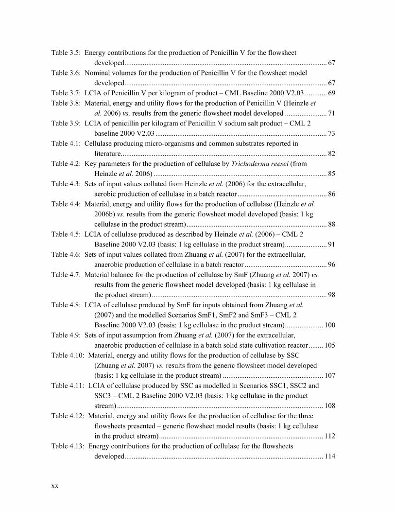
Table 3.5: Energy contributions for the production of Penicillin V for the flowsheet developed ............................................................................................................... 67
Table 3.6: Nominal volumes for the production of Penicillin V for the flowsheet model developed ............................................................................................................... 67
Table 3.7: LCIA of Penicillin V per kilogram of product – CML Baseline 2000 V2.03 ............ 69
Table 3.8: Material, energy and utility flows for the production of Penicillin V (Heinzle et al. 2006) vs. results from the generic flowsheet model developed ....................... 71
Table 3.9: LCIA of penicillin per kilogram of Penicillin V sodium salt product – CML 2 baseline 2000 V2.03 .............................................................................................. 73
Table 4.1: Cellulase producing micro-organisms and common substrates reported in literature ................................................................................................................. 82
Table 4.2: Key parameters for the production of cellulase by Trichoderma reesei (from Heinzle et al. 2006) ............................................................................................... 85
Table 4.3: Sets of input values collated from Heinzle et al. (2006) for the extracellular, aerobic production of cellulase in a batch reactor ................................................. 86
Table 4.4: Material, energy and utility flows for the production of cellulase (Heinzle et al. 2006b) vs. results from the generic flowsheet model developed (basis: 1 kg cellulase in the product stream) ............................................................................. 88
Table 4.5: LCIA of cellulase produced as described by Heinzle et al. (2006) – CML 2 Baseline 2000 V2.03 (basis: 1 kg cellulase in the product stream) ....................... 91
Table 4.6: Sets of input values collated from Zhuang et al. (2007) for the extracellular, anaerobic production of cellulase in a batch reactor ............................................. 96
Table 4.7: Material balance for the production of cellulase by SmF (Zhuang et al. 2007) vs. results from the generic flowsheet model developed (basis: 1 kg cellulase in the product stream) ................................................................................................ 98
Table 4.8: LCIA of cellulase produced by SmF for inputs obtained from Zhuang et al. (2007) and the modelled Scenarios SmF1, SmF2 and SmF3 – CML 2 Baseline 2000 V2.03 (basis: 1 kg cellulase in the product stream) ..................... 100
Table 4.9: Sets of input assumption from Zhuang et al. (2007) for the extracellular, anaerobic production of cellulase in a batch solid state cultivation reactor ........ 105
Table 4.10: Material, energy and utility flows for the production of cellulase by SSC (Zhuang et al. 2007) vs. results from the generic flowsheet model developed (basis: 1 kg cellulase in the product stream) ....................................................... 107
Table 4.11: LCIA of cellulase produced by SSC as modelled in Scenarios SSC1, SSC2 and SSC3 – CML 2 Baseline 2000 V2.03 (basis: 1 kg cellulase in the product stream) ................................................................................................................. 108
Table 4.12: Material, energy and utility flows for the production of cellulase for the three flowsheets presented – generic flowsheet model results (basis: 1 kg cellulase in the product stream) .......................................................................................... 112
Table 4.13: Energy contributions for the production of cellulase for the flowsheets developed ............................................................................................................. 114
xxi
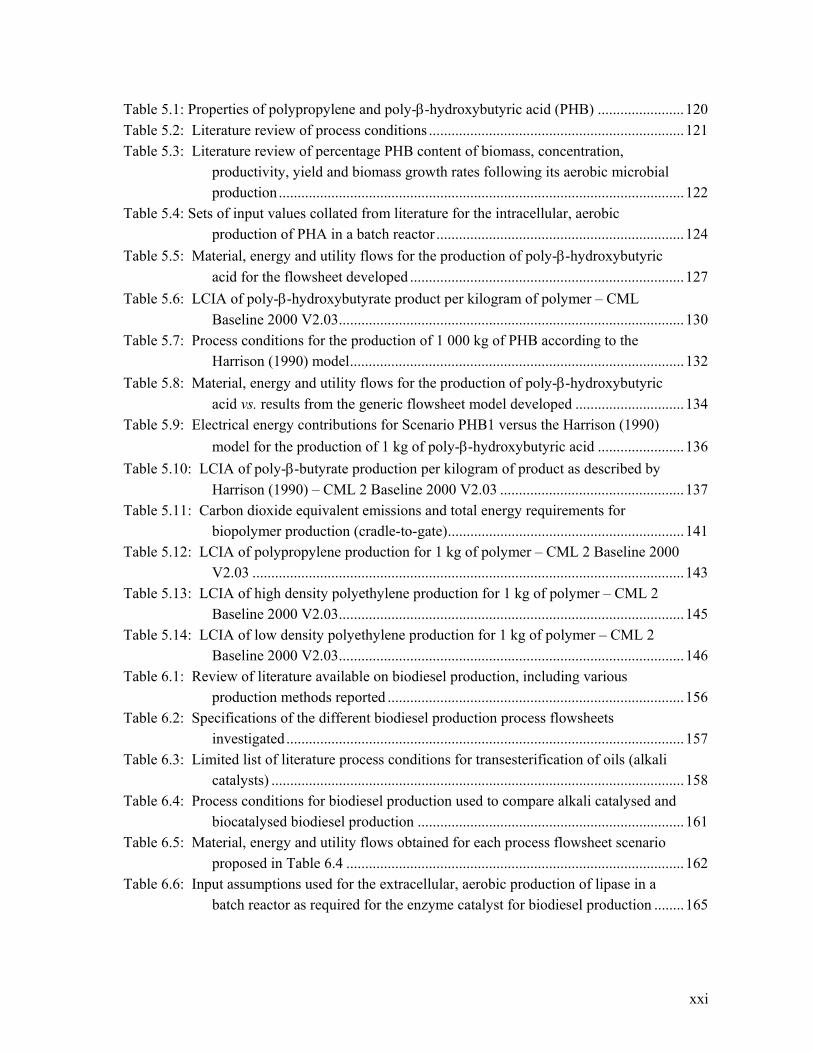
Table 5.1: Properties of polypropylene and poly--hydroxybutyric acid (PHB) ....................... 120
Table 5.2: Literature review of process conditions .................................................................... 121
Table 5.3: Literature review of percentage PHB content of biomass, concentration, productivity, yield and biomass growth rates following its aerobic microbial production ............................................................................................................ 122
Table 5.4: Sets of input values collated from literature for the intracellular, aerobic production of PHA in a batch reactor .................................................................. 124
Table 5.5: Material, energy and utility flows for the production of poly--hydroxybutyric
acid for the flowsheet developed ......................................................................... 127
Table 5.6: LCIA of poly--hydroxybutyrate product per kilogram of polymer – CML
Baseline 2000 V2.03 ............................................................................................ 130
Table 5.7: Process conditions for the production of 1 000 kg of PHB according to the Harrison (1990) model ......................................................................................... 132
Table 5.8: Material, energy and utility flows for the production of poly--hydroxybutyric
acid vs. results from the generic flowsheet model developed ............................. 134 Table 5.9: Electrical energy contributions for Scenario PHB1 versus the Harrison (1990)
model for the production of 1 kg of poly--hydroxybutyric acid ....................... 136
Table 5.10: LCIA of poly--butyrate production per kilogram of product as described by
Harrison (1990) – CML 2 Baseline 2000 V2.03 ................................................. 137
Table 5.11: Carbon dioxide equivalent emissions and total energy requirements for biopolymer production (cradle-to-gate) ............................................................... 141
Table 5.12: LCIA of polypropylene production for 1 kg of polymer – CML 2 Baseline 2000 V2.03 ................................................................................................................... 143
Table 5.13: LCIA of high density polyethylene production for 1 kg of polymer – CML 2 Baseline 2000 V2.03 ............................................................................................ 145
Table 5.14: LCIA of low density polyethylene production for 1 kg of polymer – CML 2 Baseline 2000 V2.03 ............................................................................................ 146
Table 6.1: Review of literature available on biodiesel production, including various production methods reported ............................................................................... 156
Table 6.2: Specifications of the different biodiesel production process flowsheets investigated .......................................................................................................... 157
Table 6.3: Limited list of literature process conditions for transesterification of oils (alkali catalysts) .............................................................................................................. 158
Table 6.4: Process conditions for biodiesel production used to compare alkali catalysed and biocatalysed biodiesel production ....................................................................... 161
Table 6.5: Material, energy and utility flows obtained for each process flowsheet scenario
proposed in Table 6.4 .......................................................................................... 162 Table 6.6: Input assumptions used for the extracellular, aerobic production of lipase in a
batch reactor as required for the enzyme catalyst for biodiesel production ........ 165

xxii
Table 6.7: Material, energy and utility flows for the production of lipase from Candida antarctica using the generic flowsheet model ..................................................... 166
Table 6.8: LCIA of lipase per kilogram of product from Candida antarctica – CML Baseline 2000 V2.03 ........................................................................................... 167
Table 6.9: LCIA of biodiesel per kilogram of product – CML 2 Baseline 2000 V2.03 ............ 169
Table 7.1: Summary of areas influencing environmental impact substantially, as identified in case studies ...................................................................................................... 185
Table 7.2: Sensitivity of single score LCA results for Penicillin V production (EPS 2000 v2.02) ................................................................................................................... 187
Table 7.3: Selected results when varying product to biomass ratio (all other inputs at original defined values) in the production of 1000 kg Penicillin V .................... 189
Table 7.4: Selected results when varying final biomass concentration (all other inputs at original defined values) in the production of 1000 kg Penicillin V .................... 190
Table 7.5: Selected results when varying oxygen flowrate (all other inputs at original defined values; compression pressure of 600 kPa) in the production of 1000 kg Penicillin V ............................................................................................ 193
Table 7.6: Selected results when varying compression pressure (all other inputs at original defined values; aeration rate of 0.021 vvm) in the production of 1000 kg Penicillin V .......................................................................................................... 196
Table 7.7: Selected results when varying the yield coefficient (Yx/s) (all other inputs at original defined values) in the production of 1000 kg Penicillin V .................... 198
Table 7.8: Selected results when varying the yield coefficient (Yp/s) (all other inputs at original defined values) in the production of 1000 kg Penicillin V .................... 199
Table 7.9: Selected results when varying waste fraction removed in filtration (all other inputs at original defined values) in the production of 1000 kg Penicillin V ..... 202
Table 7.10: Selected results when varying waste fraction removed in centrifugation 1 (all other inputs at original defined values) in the production of 1000 kg Penicillin V .......................................................................................................................... 203
Table 7.11: Selected results when varying waste fraction removed in centrifugation 2 (all other inputs at original defined values) in the production of 1000 kg Penicillin V .......................................................................................................................... 205
Table 7.12: Selected results when varying waste fraction removed in fluid bed drying (all other inputs at original defined values) in the production of 1000 kg Penicillin V .......................................................................................................................... 207
Table 7.13: Selected results when varying conversions rates of limiting reactants (all other inputs at original defined values) in the production of 1000 kg Penicillin V ..... 209
Table 7.14: Modified input values for the production of Penicillin V used in determining the impacts of improved production vs. optimised downstream processing ............. 211
Table 7.15: Selected results for the five scenarios comparing increased production vs. optimised downstream processing in the production of 1000 kg Penicillin V .... 212

xxiii
Table 7.16: Energy and glucose balances for the production and downstream processing of 1000 kg Penicillin V ............................................................................................ 212
Table 7.17: LCIA of Penicillin V per kilogram of product for Scenarios A – D (CML Baseline 2000 V2.03) .......................................................................................... 214
Table 7.18: Modified input values for the production of cellulase by SmF using Trichoderma reesei used in determining the impacts of improved production vs. optimised downstream processing ................................................................. 215
Table 7.19: Selected results for the five scenarios comparing increased production vs. optimised downstream processing in the production of product containing 1000 kg cellulase by SmF using Trichoderma reesei .......................................... 216
Table 7.20: Energy and cellulose balances for the production and downstream processing of product containing 1000 kg cellulase by SmF using Trichoderma reesei .......... 217
Table 7.21: LCIA of product containing 1 kg of cellulase produced by SmF using Trichoderma reesei for Scenarios E – F (CML Baseline 2000 V2.03) ............... 218
Table 7.22: Modified input values for the production of poly--hydroxybutyric acid used in
determining the impacts of improved production vs. optimised downstream processing ............................................................................................................ 220
Table 7.23: Selected results for the five scenarios comparing increased production vs.
optimised downstream processing in the production of 1000 kg poly--
hydroxybutyric acid ............................................................................................. 220
Table 7.24: Energy and glucose balances for the production and downstream processing of
1000 kg poly--hydroxybutyric acid ................................................................... 221
Table 7.25: LCIA of poly--hydroxybutyric acid per kilogram of product for Scenarios I –
L (CML Baseline 2000 V2.03) ............................................................................ 222 Table B.1: Micro-organisms that include additional experimental values and are available as
part of the generic flowsheet model database ........................................................ 18 Table B.2: Elemental formula for micro-organisms used in the model ....................................... 18 Table B.3: Chemical formulas and associated pure component densities for products
obtained in the model ............................................................................................ 22 Table B.4: Chemical formula for anaerobic products in the model ............................................. 27 Table B.5: Chemical formula for carbon sources used in the generic model .............................. 28 Table B.6: Chemical formula for nitrogen sources used in the generic model ............................ 30 Table B.7: Chemical formula for oxygen sources used in the generic model ............................. 31 Table B.8: Chemical formula for sulphur sources used in the generic model ............................. 32 Table B.9: Chemical formula for phosphorus sources used in the generic model ....................... 33 Table B.10: Values for maintenance coefficients as used in the model ........................................ 36 Table B.11: Maximum specific growth rate, limiting nutrient concentration and final
microbial concentrations used in the model .......................................................... 38 Table B.12: Dimensionless power numbers for agitation for various impeller types .................. 44

xxiv
Table B.13: Alternative correlations for gassed power requirements (as shown in Mann 1983 and presented by Atkinson and Mavituna 1983) ................................................... 51
Table B.14: Energy per unit volume values as used in model for different centrifuge types ...... 53 Table B.15: Flocculent chemical compositions and densities as used in the model .................... 55 Table B.16: Filter medium and initial voidages of the model ..................................................... 57 Table B.17: Possible additional reacting and non-reacting flow materials and solvents for
the concentration and purification section of the model ....................................... 60 Table F.1: Material and energy inputs and outputs for South African electricity production
mix ....................................................................................................................... 111 Table F.2: Life cycle inputs/outputs for electricity from coal (South Africa) ........................... 112 Table F.3: Life cycle inputs/outputs for coal from South African coal mine ............................ 112 Table F.4: Life cycle inputs/outputs for underground coal mine (South Africa) ...................... 113 Table F.5: Life cycle inputs/outputs for coal from open coal mine (South Africa) ................... 113 Table F.6: Life cycle inputs/outputs for infrastructure of underground coal mine (South
Africa) ................................................................................................................. 114 Table F.7: Life cycle inputs/outputs for infrastructure of open coal mine (South Africa) ........ 114 Table F.8: Life LCIA of South African electricity mix (functional unit: 1 GJ) – CML 2
Baseline 2000 V2.03 ........................................................................................... 114 Table G.1: Material and energy inputs and outputs for sugar (from cane) and bagasse ............ 119 Table G.2: Material and energy inputs and outputs for sugarcane ............................................ 120 Table G.3: LCIA of South African sugar from cane (functional unit: 1 t) – CML 2 Baseline
2000 V2.03 .......................................................................................................... 120 Table H.1: Original and modified input values for the extracellular, aerobic production of
penicillin in a batch reactor ................................................................................. 123 Table H.2: Sensitivity data for M&E balance for the production of Penicillin. Variable
changed: Cooling water temperature ................................................................... 125 Table I.1: Life Cycle Inventory for the production of 1 kg of Penicillin V, as used in
Chapter 3 ............................................................................................................. 129

xxv
List of Acronyms BPEO Best Practicable Environmental Option CIP Cleainging-in-Place CML Centre for Environmental Studies (University of Leiden) COD Chemical Oxygen Demand DSP Downsteam Processing EIA Environmental Impact Assessment ELUs Environmental Load Units EPS Environmental Priority Strategies ESAP Environmental Self-Assessment Program EULA End User License Agreement GMAT Green Management Assessment Tool GWP Global Warming Potential HDPE High Density Polyethylene HPH High Pressure Homoginisation IChemE Institution of Chemical Engineers ISO Organisation for Standardisation LCA Life Cycle Assessment LCI Life Cycle Inventory LCIA Life Cycle Impact Assessment LDPE Low Density Polyethylene MS Microsoft® ODP Ozone Depleting Potential (Ozone Layer Depletion) PE Polyethylene PHA Polyhydroxyalkanoate
PHB Poly--butryic acid
PLA Polyactides PP Polypropyelene SETAC Society of Environmental Toxicology and Chemistry SmF Submerged Fermentation SSC Solid State Cultivation StOD Stoichiometric Oxygen Demand TNS The Natural Step TPS Thermoplastic Starch UNEP United Nations Environmental Program UML Unified Modelling Language US-EPA United States Environmental Protection Agency WWF World Wildlife Fund, Worldwide fund for Nature WWT Wastewater Treatment


1
CHAPTER 1: INTRODUCTION

2

CHAPTER 1: Introduction – Context
3
1.1. Context Bioprocesses are becoming increasingly important for the production of chemical and energy products over conventional chemical synthesis, owing to emphasis on the use of renewable raw materials, the specificity and complexity of biologically catalysed reactions, or both (Lynd 1999, McLauglin et al. 2002, Dorsch and Miller 2003, Finlay 2003, Herman and Patel 2007, Herman et al. 2008, Lynd 2008). The use of environmental biotechnology, biocatalysis, bioremediation or similar is desired to promote biotechnology. These biological processes are frequently claimed to provide benefit over conventional chemical processes from an environmental or sustainable perspective (OECD 2001, Heller et al. 2003 and 2004, Sheehan et al. 2004, Gavrilescu and Chisti 2005, Botha and von Blottnitz 2006, von Blottnitz and Curran 2007), owing largely to their mild operating conditions, aqueous systems and the nature of the bio-system used. The use of agricultural feedstocks could become as large an industry as the petroleum industry is now (CLS NRC 2000, Duncan 2003, Realff and Abbas 2003), motivated by the possibility of positive contributions to a sustainable resource supply (Lynd and Wang 2003). However, review of the literature shows that biological processes cannot generally be assumed to be environmentally favourable (Anex 2003, Geigrich 2003). Gerngross (1999), Gerngross and Slater (2000) and Kurdikar et al. (2001) reported that polyhydroxyalkanoate production did not meet expectations with respect to environmental benefits. Roes and Patel (2007) showed that the uncertainties of inputs from a range of products, including various plastics as well as ethanol, were too large to conclude that the environmental risks of biotechnologically produced chemicals were lower than those of fossil-fuel-derived chemicals. McManus et al. (2003) found that replacing mineral oil with rapeseed oil in hydraulic systems impacted negatively on all environmental categories, except greenhouse gas emissions. Cunningham et al. (2003) showed that more energy is required to make a biolubricant than for a mineral based lubricant, but that less carbon dioxide was emitted during production. Further, many studies promoting biotechnology from a sustainability perspective, including those of Gerngross (1999), Gerngross and Slater (2000), Kurdikar et al. (2001), Dornburg et al. (2003), Pietrini et al. (2007) and Roes et al. (2007), are limited to just two considerations, namely, greenhouse gas emissions and energy consumption. Hall and Scarce (1998), Patel (2003) and Akiyama et al. (2003) all showed favourable environmental results in their studies encouraging biological processes, but these too were limited to one or two environmental categories only. Kim and Dale (2003) investigated the cumulative energy requirements of various energy crops to assess differences in the energy requirements compared to petroleum feedstocks. Such studies have encouraged open debate about the unquestioned environmental support for bio-based products (Miller et al. 2007).
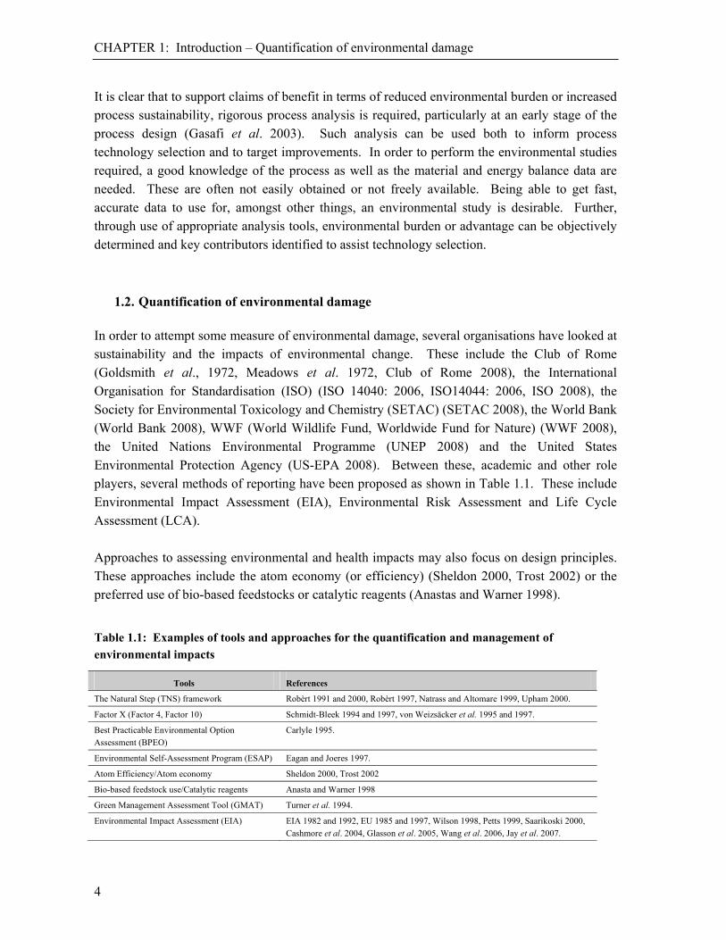
CHAPTER 1: Introduction – Quantification of environmental damage
4
It is clear that to support claims of benefit in terms of reduced environmental burden or increased process sustainability, rigorous process analysis is required, particularly at an early stage of the process design (Gasafi et al. 2003). Such analysis can be used both to inform process technology selection and to target improvements. In order to perform the environmental studies required, a good knowledge of the process as well as the material and energy balance data are needed. These are often not easily obtained or not freely available. Being able to get fast, accurate data to use for, amongst other things, an environmental study is desirable. Further, through use of appropriate analysis tools, environmental burden or advantage can be objectively determined and key contributors identified to assist technology selection.
1.2. Quantification of environmental damage In order to attempt some measure of environmental damage, several organisations have looked at sustainability and the impacts of environmental change. These include the Club of Rome (Goldsmith et al., 1972, Meadows et al. 1972, Club of Rome 2008), the International Organisation for Standardisation (ISO) (ISO 14040: 2006, ISO14044: 2006, ISO 2008), the Society for Environmental Toxicology and Chemistry (SETAC) (SETAC 2008), the World Bank (World Bank 2008), WWF (World Wildlife Fund, Worldwide Fund for Nature) (WWF 2008), the United Nations Environmental Programme (UNEP 2008) and the United States Environmental Protection Agency (US-EPA 2008). Between these, academic and other role players, several methods of reporting have been proposed as shown in Table 1.1. These include Environmental Impact Assessment (EIA), Environmental Risk Assessment and Life Cycle Assessment (LCA). Approaches to assessing environmental and health impacts may also focus on design principles. These approaches include the atom economy (or efficiency) (Sheldon 2000, Trost 2002) or the preferred use of bio-based feedstocks or catalytic reagents (Anastas and Warner 1998).
Table 1.1: Examples of tools and approaches for the quantification and management of environmental impacts
Tools References
The Natural Step (TNS) framework Robèrt 1991 and 2000, Robèrt 1997, Natrass and Altomare 1999, Upham 2000.
Factor X (Factor 4, Factor 10) Schmidt-Bleek 1994 and 1997, von Weizsäcker et al. 1995 and 1997.
Best Practicable Environmental Option Assessment (BPEO)
Carlyle 1995.
Environmental Self-Assessment Program (ESAP) Eagan and Joeres 1997.
Atom Efficiency/Atom economy Sheldon 2000, Trost 2002
Bio-based feedstock use/Catalytic reagents Anasta and Warner 1998
Green Management Assessment Tool (GMAT) Turner et al. 1994.
Environmental Impact Assessment (EIA) EIA 1982 and 1992, EU 1985 and 1997, Wilson 1998, Petts 1999, Saarikoski 2000, Cashmore et al. 2004, Glasson et al. 2005, Wang et al. 2006, Jay et al. 2007.

CHAPTER 1: Introduction – Life Cycle Assessment (LCA)
5
Tools References
Environmental Impact Indices Dee et al. 1973, Baasel 1985, Spreng 1988, Ellington and Meo 1990, Vesiland 1990, Jones 1992, Hollick 1993, Sheldon 1994, Stephan 1994, Elliott et al. 1996.
Environmental Risk Assessment Kletz 1999, Slater and Jones 1999, Lees 1996, Karman 2000, Darbra et al. 2008.
Environmental Management Systems (ISO 14000 series)
International Institute for Sustainable Development 1996, ISO 14001: 1996, ISO 14004: 1996, Pouliot 1996, Jackson 1997, Lee 1997, Steger 2000, Hui et al. 2001, Morrow and Rondinelli 2002, Melnyk et al. 2003, Ammenberg and Sundin 2005a and 2005b.
Ecoefficiency WBCSD 1996 and 2006, Saling et al. 2002, Shonnard et al. 2003, Saling 2005, Saling et al. 2005, García-Serna et al. 2007, Burnett and Hansen 2008.
Carbon Footprinting
(ISO 14064)
IPIECA 2003, WBCSD 2004, 2007, IPCC 2006, ISO 14064: 2006, Eckel, A. 2007, Carbon Trust 2007, Defra 2007, Hammond 2007, Haven 2007, Weidemann and Minx 2007.
Life Cycle Assessment (LCA) (ISO 14040 series)
Fava et al. 1991, 1993 and 1994, Heijungs et al.1992 and 1996, Guinée et al. 1993a, 1993b and 2001, Consoli et al. 1993, Keoleian 1993, Pesso 1993, Udo de Haes 1993 and 1996, Udo de Haes et al. 1994 and 2002, Vigon and Harrison 1994, Aelion et al. 1995, Lindfors et al. 1995, Kniel et al. 1996, Allen et al. 1997, Barnthouse et al. 1997, Bretz and Fankhauser 1997, Christiansen 1997, Steen 1997, Jödicke et al.
1999, Tukker 2000, Burgess and Brennan 2001, de Beaufort-Langeveld 2003, Dubreuil 2003, Kotaji et al. 2003, Rebitzer and Ekvall 2004, Poulson et al. 2005, Russell et al. 2005, ISO 14040: 2006, ISO14044: 2006, Li 2006, Udo de Haes and Heijungs 2007, Niederl-Schmidinger and Narodoslawsky 2008.
1.3. Life Cycle Assessment (LCA) In this thesis, cradle-to-factory gate LCA will be used to quantify the environmental burden associated with industrial bioprocesses. LCA is chosen as it is not location specific, gives results which can be compared readily to other processes and has a strong literature base which gives it a clear definition. In terms of the ISO 14040 standards (ISO 14040: 2006, ISO14044: 2006), the process of Life Cycle Assessment (LCA) is divided into four phases: goal and scope definition, inventory analysis (LCI), impact assessment (LCIA) and interpretation. The goal and scope definition gives details on the LCA including reasons, audience or geographic information if applicable. A system boundary and functional unit are also defined. The inventory analysis is modelled in a flowchart, defining material and energy inputs and releases of each process in relation to the functional unit. From these inputs and releases, potential environmental impacts are determined. These results are then grouped and weighted according to different criteria. Interpretation involves discussion and conclusions of the assessment at each stage (Figure 1.1). A more detailed explanation of life cycle assessment, and the way it is used in the thesis, is given in Appendix A.

CHAPTER 1: Introduction – Data gathering
6
Figure 1.1: Phases of an LCA (modified from ISO 14040: 2006)
1.4. Data gathering In order to perform a Life Cycle Assessment (LCA) study accurately, the quality of the data gathered is critical. The most important of this data is the inventory data. This is either obtained by collecting actual material and energy flows from a process or, where this is unavailable, by modelling the process using engineering software tools such as Aspen Plus® (AspenTech 2008), SuperPro Designer (Intelligen 2008) or other similar packages. Use of this software can require detailed engineering design which needs to be performed by experts with associated cost. These software tools frequently do not adequately address the needs of bioprocess modelling. Further, this modelling, to gather information for LCA inputs or other reasons (e.g. costing), may require more detail than is available at early process development stages. As such, in order to determine early stage process impacts of bioprocesses, a tool for modelling these flowsheets would be useful.

CHAPTER 1: Introduction – Thesis objectives
7
1.5. Thesis objectives The thesis covers several topics of concern. These range from comparisons of industrial scale biological and chemical process routes, the use of Life Cycle Assessment (LCA), to the investigation into questions around the sustainability of industrial biological processes. The objectives of the thesis are: 1. To develop a generic flowsheet model to provide material and energy balance data for
industrial bioprocesses at an early stage in process development The work seeks to establish a quantitative methodology for the rigorous assessment of bioprocesses from an environmental perspective. To do this, complete material and energy balance data are required. For many systems, including bioprocess systems, the desired data are not available. To overcome this, a model describing microbial growth and product formation, sterilisation, downstream processing, purification and simple waste water treatment is developed.
2. To validate the generic flowsheet model Using several case studies, material and energy balance data generated from the generic flowsheet model is validated against literature data. Each case study investigates scenarios where less input data is used to generate results. This identifies the sensitivity of variables in the generic flowsheet model.
3. To use these data with Life Cycle Assessment (LCA) methodology as a means of assessing and comparing industrial bioprocess systems
The data from the validation case studies are used to generate cradle-to-factory gate Life Cycle Assessment (LCA) profiles to determine full environmental impacts of production. These LCA results also give further validation against the LCA results calculated from material and energy balance data from literature values.
4. To use Life Cycle Assessment (LCA) methodology to compare industrial biological processes with chemical processes
The LCA results are also used to compare LCA results for similar products obtained through chemical processes. The comparisons between biological and chemical processes allow for identification of possible areas of high environmental sensitivity in the biological processes and are investigated in the heuristics section.
CHAPTER 1: Introduction – Thesis structure
8
5. To obtain heuristics which guide the sustainability decisions of industrial bioprocess systems From the comparative analysis of bioprocess systems in the case studies, variables which are most sensitive to change are identified. These variables are investigated by a more thorough sensitivity analysis to determine the effect on reactor volume, energy requirements, and cradle-to-factory gate Life Cycle Assessment results.
6. To investigate the environmental implications of bio-technology selection There are several process options available for industrial bioprocess systems. The environmental advantages of such things as submerged fermentation versus solid state cultivation and aerobic versus anaerobic systems are investigated. Other technology selection choices by different process routes to produce a similar product include varied recycle options and using different chemicals as raw materials. The environmental advantages of improved bioreactor production versus optimised downstream processing were also investigated.
1.6. Thesis structure The thesis is divided into six broad sections:
- Introduction (Chapter 1); - Generic model development (2);
- Validation of the model by case studies (3 – 5); - Use of the model to compare biological vs. chemical processes (5 – 6); - Heuristics; and
- Conclusions (7 – 8). Chapter 1 gives the context, scope and approach to the thesis. It identifies the need for the generic flowsheet model through explaining the need for a rapid, first estimate approach to material and energy balancing in bioprocesses. The chapter also introduces the concept of Life Cycle Assessment (LCA) and its structure in the ISO standards. The generic flowsheet model development is given in Chapter 2. The model is broken down into microbial growth and product formation, sterilisation, downstream processing and waste treatment. These are further broken down into the individual units (e.g. steam sterilisation, filtration, centrifugation, evaporation etc.). Assumptions, inputs and further details are given for each, with calculations given in Appendix B. Simplified Unified Modelling Language (UML) diagrams, flow diagrams showing the mathematical logic to the generic flowsheet model, are presented in Appendix D.

CHAPTER 1: Introduction – Thesis structure
9
Case studies, to inform the validation of the generic flowsheet approach, were selected based on availability of comprehensive data sets to facilitate rigorous comparison. These datasets are limited in the bioprocess literature. Case studies on penicillin, cellulase and bio-polymers are presented in Chapters 3, 4 and 5 as validation studies. Material and energy balance data from detailed flowsheet models (Harrison 1990, Biwer et al. 2005, Heinzle et al. 2006a and 2006b, Zhuang et al. 2007) are compared to the material and energy output generated from the generic flowsheet model. The energy data reported in the studies were for the total renewable and non-renewable energy in the process. Life Cycle Assessment results are also generated and compared using the software package SimaPro v7.1®. This is used as further validation of the modelled vs. literature flowsheet data, giving a sensitivity analysis on the material and energy balance results. The LCA burdens also help identify areas of high environmental sensitivity within the bioprocess flowsheets. These areas of possible environmental concern are investigated further in Chapter 7. Besides acting as validation, Chapter 5 introduces the concept of comparing a biological product to a similar chemically produced one. Polyhydroxyalkanoate (biopolymer) production is compared to polyolefin production on an LCA basis. The hotspot areas identified earlier are compared and quantified against the chemical process route. Chapter 6 provides a further case study in which biodiesel production using a chemical or biological catalyst (enzyme) is compared. The enzyme is a raw material in a process which otherwise has chemical inputs. The material and energy balance data for the enzyme are obtained from the generic flowsheet model. The relative LCA impacts of the enzyme in the total LCA score is determined, as are the overall impacts. These are compared to the LCA results from the chemical production route. Areas of high environmental sensitivity in the bioprocess route are assessed against the chemical alternative. Chapter 7 of the thesis provides a detailed analysis of the sensitivity of the generic flowsheet model. Using Penicillin V as a model flowsheet, each variable entered is varied and LCA scores are obtained. From these results, a group of the most sensitive input variables are selected. These variables are analysed more thoroughly, with reactor volume, electrical requirements, purity and LCA scores compared. Chapter 7 also includes an assessment on the benefits of increasing the bioreactor production versus improving downstream processing. The findings of the thesis are drawn together in Chapter 8 with conclusions.

CHAPTER 1: Introduction – References
10
References Aelion, V., Castells, F., Veroutis, A., 1995. Life cycle inventory analysis of chemical processes, Environ. Prog.,
14(3), 193-200. Akiyama, M., Tsuge, T., Doi, Y., 2003. Environmental life cycle comparison of polyhydroxyalkanoates produced
from renewable carbon resources by bacterial fermentation, Polym. Degrad. Stabil., 80, 183-194. Allen, D., Consoli, F., Davis, G., Fava, J., Warren, J. (eds), 1997. Public Policy Applications of Life-Cycle
Assessment, SETAC Publications. Ammenberg, J., Sundin, E., 2005a. Products in environmental management systems: drivers, barriers and
experiences, J. Clean. Prod., 13, 405-415. Ammenberg, J., Sundin, E., 2005b. Products in environmental management systems: the role of auditors, J. Clean.
Prod., 13, 417-431. Anastas, P.; Warner, J.C., 1998. Green chemistry: theory and practice; Oxford University Press: Oxford, U.K. Anex, R., 2003. Something new under the sun: the industrial ecology of biobased products, J. Ind. Ecol., 7(3-4), 1-
4. AspenTech, 2008. Aspen Technology, Inc., 200 Wheeler Road, Burling, Massachusetts 01803, USA,
http://www.aspentech.com/ Baasel, W.D., 1985. Economic methods for multipollutant analysis and evaluation, New York, USA: Marcel
Dekker. Barnthouse, L., Fava, J., Humphreys, K., Hunt, R., Laibson, L., Noesen, S., Norris, G., Owens, J, Todd, J., Vigon,
B., Weitz, K., Young, J. (eds), 1997. Life-Cycle Impact Assessment: The State-of-the-Art, 2nd ed., SETAC Publications.
Biwer, A., Griffith, S., Cooney, C., 2005. Uncertainty Analysis of Penicillin V Production Using Monte Carlo Simulation, Biotechnol. Bioeng., 90(2), 167-179.
Botha, T., von Blottnitz, H., 2006. A comparison of the environmental benefits of bagasse-derived electricity and fuel ethanol on a life-cycle basis, Energ. Policy, 34, 2654-2661.
Bretz, R., Fankhauser, P., 1997. Life cycle assessment of chemical production processes: a tool for ecological optimisation, Chimia, 14(5), 213-217.
Burgess, A.A., Brennan, 2001. Application of life cycle assessment to chemical processes, Chem. Eng. Sci., 56, 2589-2604.
Burnett and Hansen, 2008. Ecoefficiency: Defining a role for environmental cost management, Accounting, Organisations and Society, 33, 551-581.
Carbon Trust, 2007. Carbon Footprint Measurement Methodology, Version 1.1, The Carbon Trust, London, united Kingdom, http://www.carbontrust.co.uk.
Carlyle, S., 1995. In: Environmental management systems, ed. P. Sharratt, The Institution of Chemical Engineers (UK), 185-197.
Cashmore, M., Gwilliam, R., Morgan, R., Cobb, D., Bond, A., 2005. The interminable issue of effectiveness: substantive purposes, outcomes, and research challenges in the advancement of environmental impact assessment theory, Impact Assess Proj. Apprais., 22, 295-310.
CLS NRC, 2000. Biobased industrial products: Priorities for research and commercialization, Commission on the Life Sciences, National Research Council, Washington, DC: National Academy Press.
Club of Rome, 2006. The Club of Rome – Welcome, Available from: http://www.clubofrome.org/, [Accessed: 10 January 2008].
Consoli, F., Allen, D., Boustead, I., Fava, J., Franklin, W., Jense, A.A., de Oude, N., Parrish, R., Perriman, R., Postlewaite, D., Quay, B., Sequin, J., Vigon, B. (eds), 1993. Guidelines for Life-Cycle Assessment: A Code of Practice, SETAC Publications.
Christiansen, K., 1997. Simplifying LCA: Just a Cut?, SETAC Publications. Cunningham, B., Battersby, N., Wehrmeyer, W., Fothergill, C., 2003. A Sustainability Assessment of a
Biolubricant, J. Ind. Ecol., 7(3-4), 179-192. Darbra R.M., Eljarrat, E., Barceló, D., 2008. how to measure uncertainties in environmental risk assessment, Trends
in Analytical Chemistry, 27(4), 377-385. de Beaufort-Langeveld, A., Bretz, R., Hischier, R., Huijbregts, M., Jean, P., Tanner, T., van Hoof, G. (eds), 2003.
Code of Life-Cycle Inventory Practice, SETAC publications.

CHAPTER 1: Introduction – References
11
Dee, N., Baker, J., Drobny, N., Duke, K., 1973. An environmental evaluation system for water resource planning, Water Resour. Res., 9(3), 523-535.
DEFRA, 2007. Step forward on reducing climate change impacts from products, Department of Environment, Rural Affairs and Forestry (UK), Press Release, Available from: http://www.defra.gov.uk/news/2007/070530a.htm, [Accessed 30 May 2007].
Dornburg, V., Lewandowski, I., Patel, M., 2003. Comparing the Land Requirements, Energy Savings, and Greenhouse Gas Emissions Reduction of Biobased Polymers and Bioenergy: An Analysis and System Extension of Life-Cycle Assessment Studies. J. Ind. Ecol., 7(3-4), 93-116.
Dorsch, R.R., Miller R.W., 2003. Carbon, Carbon, Everywhere, nor Any Drop to… Market, J. Ind. Ecol., 7(3-4), 13-15.
Dubreuil, A. (ed.), 2005. Life-Cycle Assessment of Metals: Issues and Research Directions, SETAC Publications. Duncan, M., 2003. U.S Federal Initiatives to Support Biomass Research and Development, J. Ind. Ecol., 7(3-4),
193-201. Eagan, P.D., Joeres E., 1997. Development of a facility-bases environmental performance indicator relater to
sustainable development, J. Clean. Prod., 5(4), 269-278. Ekel, A., 2007. Gravure, 21(2), 35-36. EIA, 1982. Assessment Methods, Theory and Practice, EIA-series No. 13. The Hague, the Netherlands: Ministry of
housing, Physical Planning and Environment and Ministry of Agriculture and Fishing. EIA, 1992. Inventory Methods for Weighting of Effects, EIA-series No. 42. The Hague, the Netherlands: Ministry of
housing, Physical Planning and Environment and Ministry of Agriculture and Fishing. Elliott, A.D., Sowerby, B., Crittenden, B.D., 1996. Quantitative environmental impact analysis for clean design,
Comput. Chem. Eng., 20, S1377-S1382. EU, 1985. Council Directive 85/337/EEC of 27 June 1985 on the assessment of certain public and private projects
on the environment. EU, 1997, Council Directive 97/11 EC of 2 March 1997 amending Directive 85/337/EEC on the assessment of
certain public and private projects on the environment. Fava, J., Denison, R., Jones, B., Curran, M.A., Vigon, B., Selke, S., Barnum, J. (eds), 1991. A Technical
Framework for Life-Cycle Assessment, SETAC Publications. Fava, J., Consoli, F., Denison, R., Dickson, K., Mohin, T., Vigon, B. (eds), 1993. A Conceptual Framework for
Life-Cycle Impact Assessment, SETAC Publications. Fava, J., Jensen, A., Lindfors, L., Pomper, S., de Smet, B., Warren, J., Vigon, B. (eds), 1994. Life-Cycle Assessment
Data Quality: A Conceptual Framework, SETAC Publications. Finlay, M.R., 2003. Old efforts at new uses: a brief history of chemurgy and the American search for biobased
materials, J. Ind. Ecol., 7(3-4), 33-46. García-Serna, J., Pérez-Barrigón, L., Cocero, M.J., 2007. New trends for design towards sustainability in chemical
engineering: Green engineering, Chem. Eng. J., 133, 7-30. Gasafi, E., Meyer, L., Schebek, L., 2003. Using Life-Cycle Assessment in Process Design: Supercritical Water
Gasification of Organic Feedstocks, J. Ind. Ecol., 7(3-4), 75-91. Gavrilescu, M, Chisti, Y., 2005. Biotechnology – a sustainable alternative for chemical industry, Biotechnol. Adv.,
23, 471-499. Gasafi, E., Meyer, L., Schebek, L., 2003. Using Life-Cycle Assessment in Process Design: Supercritical Water
Gasification of Organic Feedstocks, J. Ind. Ecol., 7(3-4), 75-91. Geigrich, J., 2003. Modern Times and Imperfect Cycles – Managing Waste from Biobased Products, J. Ind. Ecol.,
7(3-4), 10-12. Gerngross, T.U., 1999. Can biotechnology move us toward a sustainable society?, Nat. Biotechnol., 17, 541-544. Gerngross, T.U., Slater, S.C., 2000. How green are green plastics?, Sci. Am., August 2000, 36-41. Glasson, J., Therivel, R., Chadwick, A., 2005. An introduction to environmental impact assessment, 3rd ed.,
London: Routledge. Goldsmith, E., Allen, R., Allaby, M., Davoll, J., Lawrence, S., 1972. Blueprint for Survival, Club of Rome, Boston:
Houghton Mifflin Company. Guinée, J.B., Udo de Haes, H.A., Huppes, G., 1993a. Quantitative life cycle assessment of products – 1. Goal
definition and inventory, J. Clean. Prod., 1(1), 3-13.
CHAPTER 1: Introduction – References
12
Guinée, J.B., Udo de Haes, H.A., Huppes, G., 1993b, Quantitative life cycle assessment of products – 2. Classification, valuation and improvement analysis, J. Clean. Prod., 1(2), 81-91.
Guinée, J.B., Gorrée, M., Heijungs, R., Huppes, G., Kleijn, R., de Koning, A., van Oers, L., Sleeswijk, A.W., Suh, S., Udo de Haes, H.A., de Bruijn, H., van Duin, R., Huijbregts, M.A.J., 2001. Life cycle assessment. An operational guide to the ISO standards. Part 1: LCA in perspective, Ministry of Housing, Spatial Planning and the Environment (VROM) and Centre of Environmental Science - Leiden University (CML).
Hall, D.O., Scarse, J.I., 1998. Will biomass be the environmentally friendly fuel of the future?, Biomass Bioenerg., 15(14/15), 357-367.
Hammond, G., 2007. Time to give due weight to the ‘carbon footprint’ issue, Nature, 445(7125), 256. Harrison, S.T.L., 1990. The Extraction and Purification of Alicaligens eutrophus, PhD dissertation, Cambridge
University. Haven, J., 2007. Environmental Business, 129, 27. Heijungs, R., Guinée, J.B., Huppes, G., Langkreijer, R.M., Udo de Haes, H.A., Wegner Sleeswijk, A., Ansems, A.,
Eggels, P.G., van Duin, R., de Goede H.P., 1992. Environmental life cycle analysis of products: backgrounds and guide, Leiden: Centre of Environmental Science, Leiden University.
Heijungs, R., 1996. Identification of key issues for further investigation in improving the reliability of life-cycle assessments, J. Clean. Prod., 4(3-4), 159-166.
Heinzle, E., Biwer, A., Cooney, C., 2006a. Modelling and Simulation of Bioprocesses, In: Development of Sustainable Bioprocesses: Modelling and Assessment, John Wiley & Sons, p61-80.
Heinzle, E., Biwer, A., Cooney, C., 2006b. Penicillin V, In: Development of Sustainable Bioprocesses: Modelling and Assessment, John Wiley & Sons, p193-210.
Heller, M.C., Keoleian, G.A., Volk, T.A., 2003. Life cycle assessment of a willow bioenergy cropping system, Biomass Bioenerg., 25, 147-165.
Heller, M.C., Keoleian, G.A., Mann, M.K, Volk, T.A., 2004. Life cycle energy and environmental benefits of generating electricity from willow biomass, Renew. Energ., 29, 1023-1042.
Herman, B.G., Patel, M., 2007. Today’s and Tomorrow’s Bio-Based Bulk Chemical from White Biotechnology : A Techno-Economic Analysis, Appl. Biochem. Biotech., 136, 361-388.
Herman, B.G., Blok, K., Patel, M.K., 2007. Producing Bio-Based Bulk Chemicals Using Industrial Biotechnology Saves Energy and Combats Climate Change, Environ. Sci. Technol., 41, 7915-7921.
Hollick, M., 1993. An introduction to project evaluation, Australia: Longman Cheshire. Hui, I.K., Chan, A.H.S., Pun, K.F., 2001. A study of the Environmental management System implementation
practices, J. Clean. Prod., 9, 269-276. Intelligen, 2008. Intelligen , Inc., Scotch Plain, NJ, USA, http://www.intelligen.com/ International Institute of Sustainable Development, 1996. Global Green Standards: ISO 14000 and Sustainable
Development, IISD, Winnipeg, Canada. IPCC, 2006. IPCC guidelines for National Greenhouse Gas Inventories, 5 volumes, Intergovernmental Panel on
Climate Change, Available from: http://www.ipcc-nggip.iges.or.jp/public/2006gl/index.html, [Accessed 7 July 2008].
IPIECA, 2003. Petroleum Industry Guidelines for Reporting Greenhouse Gas Emissions, International Petroleum Industry Environmental Conservation Association, American Petroleum Institute, International Association of Oil & Gas Producers
ISO, 2008. International Organization for Standardization – Overview of the ISO System, International Organization for Standardization, http://www.iso.org/iso/en/aboutiso/introduction/index.html, [Accessed 10 January 2008].
ISO 14001: 1996. Environmental management systems – specification with guidance for use, International Organization for Standardization.
ISO 14004: 1996. Environmental management systems – general guidelines on principles, systems and supporting techniques, International Organization for Standardization.
ISO 14040: 2006. Environmental management – Life cycle assessment – Principles and framework, International Organization for Standardization.
ISO 14044: 2006. Environmental management – Life cycle assessment – Requirements and guidelines, International Organization for Standardization.
CHAPTER 1: Introduction – References
13
ISO 14064: 2006. Greenhouse gases. Part 1: Specification with guidance at the organization level for quantification and reporting of greenhouse gas emissions and removals. Part 2: Specification with guidance at the project level for quantification, monitoring and reporting of greenhouse gas emission reductions or removal enhancements. Part 3: Specification with guidance for the validation and verification of greenhouse gas assertions, International Organization for Standardization.
Jackson, S.L., 1997. The ISO 14001 Implementation Guide: Creating an Integrated Management System, New York, NY: Wiley.
Jay, S., Jones, C., Slinn, P., Wood, C., 2007. Environmental impact assessment: Retrospect and prospect, Environ. Impact Assess. Rev., 27, 287-300.
Jödicke, G., Zenklusen, O., Weidenhaupt, A., Hungerbühler, K.., 1999. Developing environmentally-sound processes in the chemical industry: a case study on pharmaceutical intermediates, J. Clean. Prod., 7, 159-166.
Jones, J.D., 1992. Integrated pollution control through clean technology, Symposium Papers, Vol. 3, Institute of Chemical Engineers, North Western Branch, 2.1-2.10.
Karman, C.C., 2000. The Role of Time in Environmental Risk Assessment, Spill Sci. Technol. B., 6(2), 159-164. Keoleian, G.A., 1993. The application of life cycle assessment to design, J. Clean. Prod., 1(3-4), 143-149. Kim, S., Dale, B.E., 2003. Cumulative Energy and Global Warming Impact from the Production of Biomass for
Biobased Products, J. Ind. Ecol., 7(3-4), 147-162. Kletz, T.A., 1999. Identifying and assessing process industry hazards, 4th ed., UK: Institution of Chemical
Engineers. Kniel, G.E., Delmarco, K., Petrie, J.G., 1996. Life cycle assessment applied to process design: environmental and
economic analysis and optimisation of a nitric acid plant, Environ. Prog, 15(4), 221-228. Kotaji, S., Schuurmans, A., Edwards, S., 2003. Life-Cycle Assessment in Building and Construction: A State-of-the-
Art Report, SETAC Publications. Kurdikar, D., Paster, M., Gruys, K.J., Fournet, L., L., Gerngross, T.U., Slater, S.C., Coulon, R., 2001. Greenhouse
gas profile of a plastic material derived from a genetically modified plant, J. Ind. Ecol., 4(3), 107-122. Lee, W., 1997. ISO 14001 certifications: environmental management system, Engelwood Cliffs, NJ: Prentice Hall. Lees, F.P., 1996. Loss prevention in the process industries: Hazard identification, assessment and control, Vols. 1-
3, 2nd ed., Stoneham, MA: Butterworth-Heinemann. Li, 2006. A new life cycle impact assessment approach for buildings, Build Environ., 41, 1414-1422. Lindfors, L.-G., Christiansen, K., Hoffman, L., Virtanen, Y., Juntilla V., Hanssen, O.-J., Ronning, A., Ekvall, T.,
Finnveden, G., 1995. The Nordic guidelines on life-cycle assessment, Nord. Copenhagen: Nordic Council of Ministers.
Lynd, L.R., 1999. Biocommodity Engineering, Biotechnol. Prog., 15, 777-793. Lynd, L.R.., Wang, M.Q., 2003. A Product-Nonspecific Framework for Evaluating the Potential of Biomass-Based
Products to Displace Fossil Fuels, J. Ind. Ecol., 7(3-4), 17-32. Lynd, L.R., 2008. Energy Biotechnology, Curr. Opin. Biotech., 19, 199-201. McLaughlin, S.B., de la Torre Ugarte, D.G., Garten, C.T. (Jr), Lynd, L.R., Sanderson, M.A., Tolbert, V.R., Wolf,
D.D., 2002. High-Value Renewable Energy from Prairie Grasses, Environ. Sci. Technol., 36, 2122-2129. McManus, M.C., Hammond, G.P., Burrows, C.R., 2003. Life-cycle assessment of mineral and rapeseed oil in
mobile hydraulic systems, J. Ind. Ecol., 7(3-4), 163-177. Meadows, D.H., Meadows, D.L., Randers, J., Behrens (III), W.W., 1972. The Limits of Growth, Club of Rome,
New York: Universe Books. Melnyk, S.A., Sroufe, R.P., Calantone, R., 2003. Assessing the impact of environmental management systems on
corporate and environmental performance, J. Oper. Manag., 21, 329-351. Miller, S.A., Landis, A.E., Theis, T.L., 2007. Environmental Trade-offs of Biobased Production, Environ. Sci.
Technol., 41(15), 5176-5182. Morrow, D., Rondinelli, D., 2002. Adopting Corporate Environmental Management Systems: Motivations and
Results of ISO 14001 and EMAS Certification, European Management Journal, 20(2), 159-171. Natrass, B., Altromare, M., 1999. The Natural Step for Business: wealth, economy and the evolutionary
corporation, Gabriola Island, Canada: New York Society Publishers. Niederl-Schmidinger, A., Narodoslawsky, M., 2008. Life Cycle Assessment as an engineers’ tool?, J. Clean. Prod.,
16, 245-252.

CHAPTER 1: Introduction – References
14
OECD, 2001. The Application of Biotechnology to Industrial Sustainability – Sustainable Development, Organisation for Economic Co-operation and Development (OECD), Paris, France.
Patel, M., 2003. Surfactants based on renewable raw materials: carbon dioxide reduction potential and policies and measures for the European Union, J. Ind. Ecol., 7(3-4), 47-62.
Pesso, C., 1993. Life cycle methods and applications: issues and perspectives, J. Clean. Prod., 1(3-4), 139-142. Petts, J. (ed), 1999. Handbook of environmental impact assessment, Oxford: Blackwell. Pietrini, M., Roes, L., Patel, M, Chiellini, E., 2007. Comparative Life Cycle Studies on Poly(3-hydroxybutyrate)-
Based Composites as Potential Replacement for Conventional Petrochemical Plastics, Biomacromolecules, 8, 2210-2218.
Pouliot, C. 1996. ISO 14000: Beyond compliance to competitiveness, Manuf. Eng., May, 51-56. Poulsen, P.B., Jensen, A.A., Antson, A.-B., Bengtsson, G., Karling, M., Schmidt, A., Brekke, O., Becker, J.,
Verschoor, A., 2005. Working Environment in Life-Cycle Assessment (LCAE), SETAC Publications. Realf, M.J., Abbas, C., 2003. Industrial Symbiosis – Refining the Biorefinery, J. Ind. Ecol., 7(3-4), 5-9. Rebitzer, G., Ekvall, T., 2004. Scenarios in Life-Cycle Assessment (LCAS), SETAC Publications. Robèrt, K.-H., 1991. Education a nation: The Natural Step. In Context, 28:10, Available from:
http://www.emis.com/tns/documents/articles/robert.htm, Cited: Upham, 2000. Robèrt, K.-H., Daly, H., Hawken, P., Holmberg, J., 1997, Int. J. Sust. Dev. World Ecol., 4, 79-92. Robèrt, K.-H., 2000. Tools and concepts for sustainable development, how do they relate to a general framework
for sustainable development, and to each other?, J. Clean. Prod., 8, 243-254. Roes, A.L., Patel, M.K., 2007. Life Cycle Risks for Human Health: A Comparison of Petroleum Versus Bio-Based
Production of Five Bulk Organic Chemicals, Risk Anal., 27(5), 1311-1321. Roes, L., Pietrini, M., Chiellini, E., Patel, M., 2007. Environmental Life Cycle Studies of Poly(hydroxybutyrate)-
and Polypropylene-Based Composites, JNPN, 3(1), 22-32. Russell, A., Ekvall, T., Baumann, H., 2005. Life cycle assessment – introduction and overview, J. Clean. Prod., 13,
1207-1210. Saarikoski, H., 2000. EIA Procedure: Environmental impact assessment (EIA) as collaborative learning process,
Environ. Impact Assess. Rev., 20, 681-700. Saling, P., 2005. Ecoefficiency analysis of biotechnological processes, Appl. Microbiol. Biotechnol., 68, 1-8. Saling, P., Kicherer, A., Dittrich-Krämer, B., Wittlinger, R., Zombik, W., Schmidt, I., Schrott, S., 2002.
Ecoefficiency analysis by BASF: the method, Int. J. LCA, 7(4), 203-218. Saling, P., Maisch, R., Silvani, M., König, N., 2005. Assessing the environmental hazard potential for life cycle
assessment, ecoefficiency and SEEbalance, Int. J. LCA, 10(5), 364-371. Sheldon, R.A., 2000. Atom efficiency and catalysis in organic synthesis, Pure Appl. Chem, 72(7), 1233-1246. Schmidt-Bleek, F., 1994. Revolution in a resource productivity for a sustainable economy – a new research agenda,
Fresen. Environmen. Bull., 2, 245-490. Schmidt-Bleek, F., 1997. MIPS and Factor 10 for a sustainable and profitable economy, Wuppertal, Germany:
Wuppertal Institute. SETAC, 2008. SETAC – Welcome to SETAC.org, Society for Environmental Toxicology and Chemistry,
Available from: http://www.setac.org/, [Accessed 10 January 2008]. Sheehan, J., Aden, A., Paustian, K., Killian, K., Brenner, J., Walsh, M., Nelson, R., 2004. Energy and
environmental aspects of using corn stover for fuel ethanol, J. Ind. Ecol., 7(3-4), 117-146. Sheldon, R.A., 1994. Consider the Environmental Quotient, Chemtech, 38-47. Shonnard, D.R., Kicherer, A., Saling, P., 2003. Industrial applications using BASF ecoefficiency analysis:
perspectives on green engineering principles, Environ. Sci. Technol., 37(23), 5340-5348. Slater, D., Jones, H., 1999. Environmental risk assessment and the environmental agency, J. Hazard. Mater., 65,
77-91. Spreng, D.T., 1988. Net energy analysis and the energy requirements of energy systems, USA: Oak Ridge
Associated Universities. Steger, U., 2000. Environmental Management Systems: Empirical Evidence and Further Perspectives, European
Management Journal, 18(1), 23-37. Stephan, D.G., 1994. A “Mark I” measurement methodology for pollution prevention progress occurring as a result
of product decisions, Environ. Prog., 13(4), 232-246. Trost, B.M., 2002. On Inventing Reactions for Atom Economy, Acc. Chem. Res., 35, 695-705.

CHAPTER 1: Introduction – References
15
Tukker, A., 2000. Life cycle assessment as a tool in environmental impact assessment, Environ. Impact Assess. Rev., 20, 435-456.
Turner, R.K, Pearce, D., Bateman, I., 1994. Environmental Economics, Harvester Wheatsheaf. Udo de Haes, H.A., 1993. Applications of life cycle assessment: expectations, drawbacks and perspectives, J.
Clean. Prod., 1(3-4), 131-137. Udo de Haes, H.A., Jensen, A.A, Klöppfer, W., Lindfors, L.-G. (eds), 1994. Integrating Impact Assessment into
LCA, SETAC Publications. Udo de Haes, H.A., 1996. Towards a Methodology for Life Cycle Impact Assessment, SETAC Publications. Udo de Haes, H.A., Ginnveden, G., Goedkoop, M., Hauschild, M., Hertwich, E., Hofstetter, P., Jolliet, O., Klöppfer,
W., Krewitt, W., Lindeijer, E., Müller-Wenk, R., Olsen, S., Pennington, D., Potting, J., Steen, B. (eds), 2002. Life-Cycle Impact Assessment: Striving towards Best Practice, SETAC Publications.
Udo de Haes, H.A., Heijungs, R., 2007. Life-cycle assessment for energy analysis and management, Appl. Ererg., 84, 817-827.
UNEP, 2008. United Nations Environmental Programme (UNEP), Available from: http://www.unep.org/, [Accessed 10 January 2008].
Upham, P., 2000. An assessment of The Natural Step theory of sustainability, J. Clean. Prod., 8, 445-454. US-EPA, 2008. United States Environmental Protection Agency, Available from: http://www.usepa.org/, [Accessed
10 January 2008]. Verstraete, W., 2002. Environmental biotechnology for sustainability, J. Biotechnol., 94, 93-100. Vesiland, P.A., 1990. Environmental pollution and control, 3rd ed., Stoneham, USA: Butterworth-Heinemann. Vigon, D.A., Harrison, T.L., 1994. Life-Cycle Assessment – Inventory Guidelines and Principles, US-EPA, Lewis
Publishers, CRC Press. von Blottnitz, H., Curran, M.A., 2007. A review of assessments conducted on bio-ethanol as a transportation fuel
from a net energy, greenhouse gas and environmental life cycle perspective, J. Clean Prod., 15, 607-619. von Weizsäcker, E.U., Lovins, A.B., Lovins, L.H., 1995. Factor Vier: Doppelter Wohlstand – halbierter
Naturverbrauch, Munchen, Germany: Droemer Knaur, (In German). von Weizsäcker, E.U., Lovins, A.B., Lovins, L.H., 1997. Factor four doubling wealth – halving resource use,
London: Earthscan. Wang, Y.-M., Yang, J.-B., Xu, D.-L., 2006. Environmental impact assessment using the evidential reasoning
approach, Eur. J. Oper. Res., 174, 1885-1913. WBCSD, 1996. Congresses in Antwerp, November (1993), March (1995a) and Washington (1995b), WBCSD:
Ecoefficient Leadership for Improved Economic and Environmental Performance, World Business Council for Sustainable Development.
WBCSD, 2004. The Greenhouse Gas Protocol: A Corporate Accounting and Reporting Standard, World Business Council for Sustainable Development, World Resources Institute.
WBCSD, 2006. World Business Council for Sustainable Development, Available from: http://www.wbcsd.org. WBCSD, 2007. The Greenhouse Gas Protocol: Guidelines for Quantifying GHG Reductions from Grid-Connected
Electricity Projects, World Business Council for Sustainable Development, World Resources Institute. Wiedemann, T., Minx, J., 2007. A definition of ‘Carbon Footprint’, ISAUK Research Report 07-01, ISAUK Research
and Consulting, Durham, united Kingdom. Wilson, L., 1998, A practical method for environmental impact assessment audits, Environ. Impact Asses. Rev., 18,
59-71. World Bank, 2008. The World Bank, Available from: http://wwwworldbank.org/, [Accessed 6 February 2008]. WWF, 2008. WWF – for a living planet, Available from: http://www.panda.org/, [Accessed 10 January 2008]. Zhuang J., Marchant, M.A., Nokes, S.E., Strobel, 2007. Economic analysis of cellulase production methods for bio-
ethanol, App. Eng. Agric., 23(5), 679-687.

16

17
CHAPTER 2: GENERIC FLOWSHEET
MODEL DEVELOPMENT

18
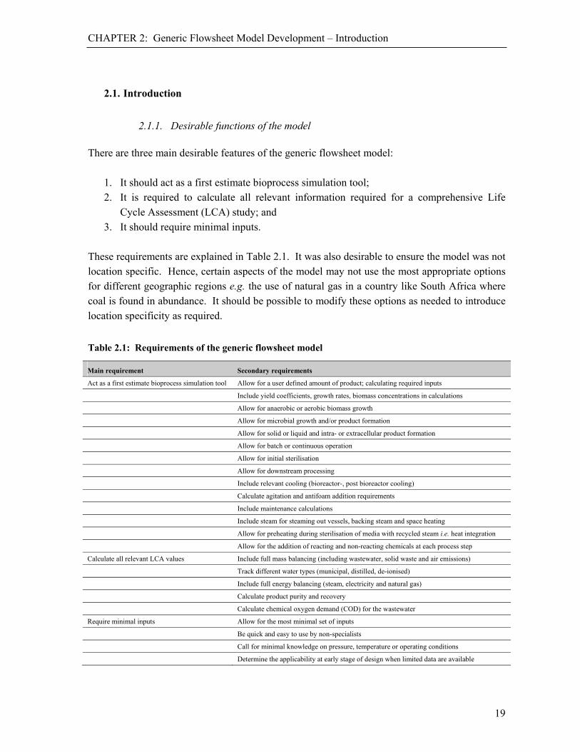
CHAPTER 2: Generic Flowsheet Model Development – Introduction
19
2.1. Introduction
2.1.1. Desirable functions of the model There are three main desirable features of the generic flowsheet model:
1. It should act as a first estimate bioprocess simulation tool; 2. It is required to calculate all relevant information required for a comprehensive Life
Cycle Assessment (LCA) study; and 3. It should require minimal inputs.
These requirements are explained in Table 2.1. It was also desirable to ensure the model was not location specific. Hence, certain aspects of the model may not use the most appropriate options for different geographic regions e.g. the use of natural gas in a country like South Africa where coal is found in abundance. It should be possible to modify these options as needed to introduce location specificity as required.
Table 2.1: Requirements of the generic flowsheet model
Main requirement Secondary requirements
Act as a first estimate bioprocess simulation tool Allow for a user defined amount of product; calculating required inputs
Include yield coefficients, growth rates, biomass concentrations in calculations
Allow for anaerobic or aerobic biomass growth
Allow for microbial growth and/or product formation
Allow for solid or liquid and intra- or extracellular product formation
Allow for batch or continuous operation
Allow for initial sterilisation
Allow for downstream processing
Include relevant cooling (bioreactor-, post bioreactor cooling)
Calculate agitation and antifoam addition requirements
Include maintenance calculations
Include steam for steaming out vessels, backing steam and space heating
Allow for preheating during sterilisation of media with recycled steam i.e. heat integration
Allow for the addition of reacting and non-reacting chemicals at each process step
Calculate all relevant LCA values Include full mass balancing (including wastewater, solid waste and air emissions)
Track different water types (municipal, distilled, de-ionised)
Include full energy balancing (steam, electricity and natural gas)
Calculate product purity and recovery
Calculate chemical oxygen demand (COD) for the wastewater
Require minimal inputs Allow for the most minimal set of inputs
Be quick and easy to use by non-specialists
Call for minimal knowledge on pressure, temperature or operating conditions
Determine the applicability at early stage of design when limited data are available

CHAPTER 2: Generic Flowsheet Model Development – Introduction
20
Further, the model should provide a framework to allow for future more complex modelling. These future modifications could include more complex biomass growth models, more detailed modelling of individual unit operations as well as the inclusion of complex recycle streams. It is also important that the model provides the required information for economic considerations of both capital and operating expenses.
2.1.2. Model Description In order to determine the environmental effects of a biological process using an LCA approach, material and energy inputs and emissions are required. These data are often not easily obtained or are not available at all (e.g. at the early stage of process design and development). In order to obtain this data, a Microsoft® Excel (MS-Excel) (MS-Office 2008) model has been developed which allows for the use of a limited set of inputs to calculate the data needed. The outputs are the material and energy balance data needed for further LCA analysis. The approach to the generic flowsheet model is based on first principles in many instances, supplemented by data from literature and practice in certain areas. To explain a typical industrial bioprocess, six levels have been defined. Level 1 is characterised by a bioconversion in a reactor. A microorganism is fed with nutrients (with or without oxygen) to form further biomass, a metabolic product and wastewater as shown in Figure 2.1.
Figure 2.1: Generic bioprocess model (Level 1)
Level 2 includes sterilisation of the raw materials by heat treatment with steam or filtration, as shown in Figure 2.2. Level 3 allows for solid liquid separation after the bioreactor, followed by an optional cell disruption stage. If needed, a second solid liquid separation unit separates biomass debris from the bulk solution as seen in Figure 2.3.

CHAPTER 2: Generic Flowsheet Model Development – Introduction
21
Figure 2.2: Generic bioprocess model (Level 2)
Figure 2.3: Generic bioprocess model (Level 3)
Level 4 includes the addition of a downstream purification train allowing for concentration and purification units as seen in Figure 2.4. These include such unit operations as adsorbers, chromatography units, decantors, evaporators etc. Level 5 includes the opportunity for formulation by spray drying, oven drying, freeze drying etc. as shown in Figure 2.5.

CHAPTER 2: Generic Flowsheet Model Development – Introduction
22
Figure 2.4: Generic bioprocess model (Level 4)
Figure 2.5: Generic bioprocess model (Level 5)

CHAPTER 2: Generic Flowsheet Model Development – Introduction
23
The generic flowsheet developed includes these levels as well as waste water treatment shown in Figure 2.6 (Level 6). The complete model developed allows for microbial growth with intra- or extracellular (liquid or solid) product formation in a batch or continuous set-up. Calculations are based on a pre-determined product amount. Sterilisation, inoculation, microbial growth and product formation are followed by solid liquid separation, cell disruption and further separation. Downstream processing is limited to six concentration or purification steps followed by a final formulation step. No recycle of products is taken into account and downstream reaction is only partially taken into account. The typical flowsheet is given in Figure 2.6. The model requires a flowsheet to be specified, as well as various parameters and constants associated with the flowsheet design. A database of constants is built into the model for common values and includes yield coefficients, densities and chemical compositions based on chosen parameters. Default values, or values close to typical operating norms, are also provided for many variables (e.g. standard operating pressures and temperatures etc.). All database and default values can be altered for a specific process if desired. Each unit with its assumptions is explained below with full sample calculations given in Appendix B.
Figure 2.6: Outline of the process flowsheet used in the generic bioprocess model (Level 6)
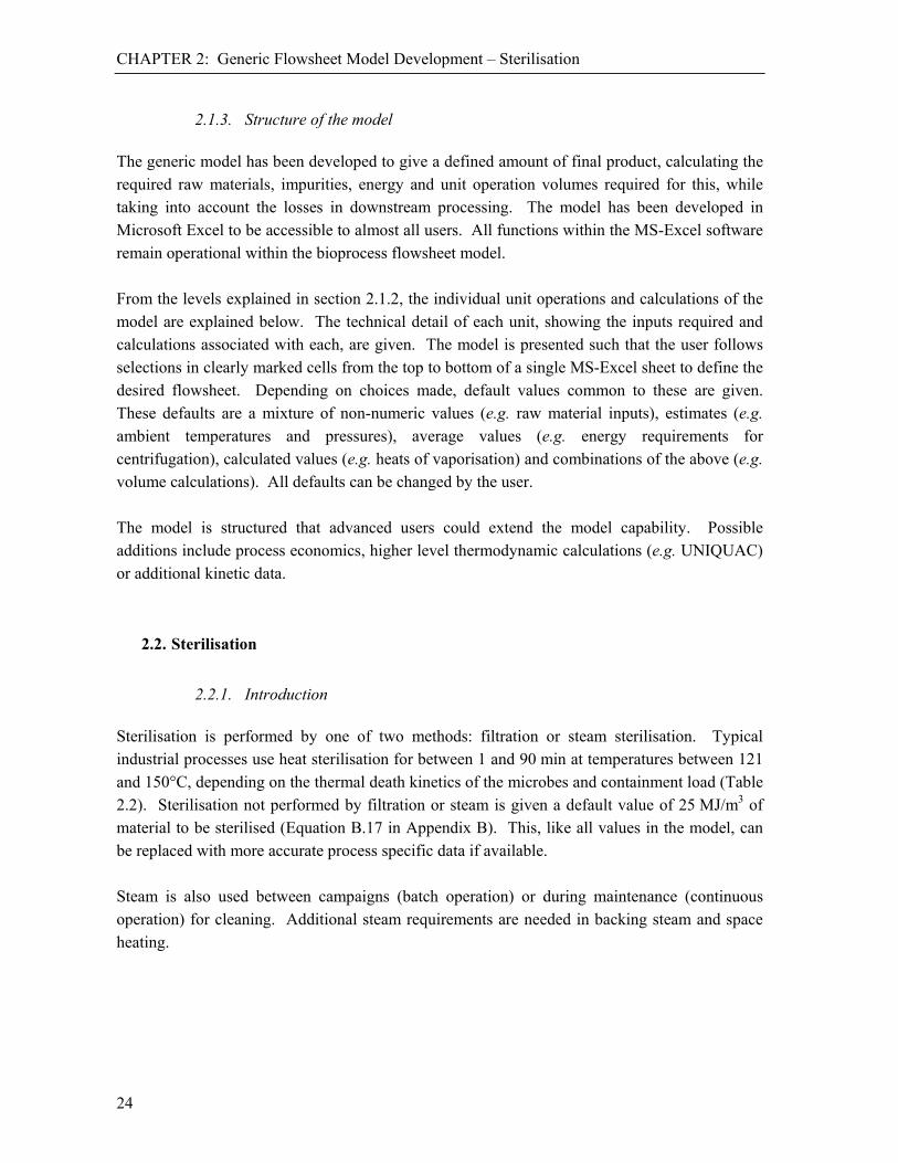
CHAPTER 2: Generic Flowsheet Model Development – Sterilisation
24
2.1.3. Structure of the model The generic model has been developed to give a defined amount of final product, calculating the required raw materials, impurities, energy and unit operation volumes required for this, while taking into account the losses in downstream processing. The model has been developed in Microsoft Excel to be accessible to almost all users. All functions within the MS-Excel software remain operational within the bioprocess flowsheet model. From the levels explained in section 2.1.2, the individual unit operations and calculations of the model are explained below. The technical detail of each unit, showing the inputs required and calculations associated with each, are given. The model is presented such that the user follows selections in clearly marked cells from the top to bottom of a single MS-Excel sheet to define the desired flowsheet. Depending on choices made, default values common to these are given. These defaults are a mixture of non-numeric values (e.g. raw material inputs), estimates (e.g. ambient temperatures and pressures), average values (e.g. energy requirements for centrifugation), calculated values (e.g. heats of vaporisation) and combinations of the above (e.g. volume calculations). All defaults can be changed by the user. The model is structured that advanced users could extend the model capability. Possible additions include process economics, higher level thermodynamic calculations (e.g. UNIQUAC) or additional kinetic data.
2.2. Sterilisation
2.2.1. Introduction Sterilisation is performed by one of two methods: filtration or steam sterilisation. Typical industrial processes use heat sterilisation for between 1 and 90 min at temperatures between 121 and 150°C, depending on the thermal death kinetics of the microbes and containment load (Table 2.2). Sterilisation not performed by filtration or steam is given a default value of 25 MJ/m3 of material to be sterilised (Equation B.17 in Appendix B). This, like all values in the model, can be replaced with more accurate process specific data if available. Steam is also used between campaigns (batch operation) or during maintenance (continuous operation) for cleaning. Additional steam requirements are needed in backing steam and space heating.

CHAPTER 2: Generic Flowsheet Model Development – Sterilisation
25
2.2.2. Filtration Constant pressure membrane filtration, with no cake build-up is assumed for sterilisation. Energy requirements, assumed to be provided by electricity, are calculated from first principles of the fluid flow through the filter as shown in Equations B.1 – B.3 of Appendix B.
2.2.3. Steam sterilisation Typical steam requirements for sterilisation are shown in Table 2.2 and Table 2.3. Steam used to sterilise the raw materials in the model is provided continuously at 140°C. The amount of steam needed to heat the media is calculated from an energy balance assuming ambient conditions of 20°C (no heat integration). Preheated feed (from recycled steam) can also be used, increasing the inlet temperature to 60°C (partial heat integration). During the holding cycle of sterilisation, a constant rate of heat loss of 0.003 kW/m2°C is assumed, an accepted value for insulated vessels (Woods 1995). The steam required to maintain the temperature, against this heat loss, is calculated assuming a surface area to volume ratio of 60 m2/m3; the median value for common piping sizes given in Welty, Wicks and Wilson (1969). After being sterilised, the raw materials are cooled by heat exchange with cooling water entering at 18°C to 37°C.
Table 2.2: Sterilisation conditions reported for different microbial growth processes
Product Type Temperature Time Amount of steam Reference
°C min
Cephalosporins Steam 121 Smith 1985
Ethanol Steam 135-140 1-2 0.035 kg/kg mash Maiorella 1985
Streptomycin 121 90 Florent 1985
It is assumed that steam is pressurised isentropically, with the energy required supplied by electricity. The mass of steam, electricity and cooling water needed for steam sterilisation are determined by Equations B.4 – B.16 of Appendix B.
Table 2.3: Typical literature values for steam sterilisation
Sterilisation type Value (kg steam/kg bioreactor medium)
Reference
Continuous sterilisation 0.2 Bartholomew and Reisman 1979, Petridies et al. 1989
Continuous sterilisation (143°C, 30s, with energy integration) <0.1 Gerngross 1999
Batch sterilisation (small scale) 0.8 Bartholomew and Reisman 1979
Batch sterilisation 0.2-0.4 Kalk and Langlykke 1979
*Adapted from Patel et al. 2006

CHAPTER 2: Generic Flowsheet Model Development – Microbial growth and product
formation
26
2.2.4. Additional steam requirements Additional steam requirements are needed for steaming out of the vessel, backing steam and space heating (Equations B.18 – B.28). These requirements are based on data from Dennis (2000) producing protease in a 147 m3 vessel. For this size vessel, 40 t steam is needed to clean the reactor and 0.082 and 0.02 t steam per day per m3 (reactor volume) are used in backing steam and space heating respectively. Space heating values from Dennis (2000) are calculated for the United Kingdom, and should be assumed as zero in a warmer South African climate.
2.3. Microbial growth and product formation
2.3.1. Introduction Microbial biomass, product and by-products formed are related to raw material requirements and emissions produced using stoichiometric equations, yield coefficients and a mass balance approach (section 2.3.2). The default conditions used are 37°C and 1 atm, similar to common literature values for mesophilic processes ( Table 2.5). These values can be altered for a specific process. Reactor volumes and residence times are calculated from variables defined in the system e.g. the calculated volumes of inputs, initial and final biomass concentrations, maximum specific growth rates, etc. The product can be defined as a primary product (e.g. ethanol), a secondary metabolite (e.g. Penicillin) or the microbial biomass itself (e.g. baker’s yeast). The product can be solid or liquid, intracellular or extracellular. Raw materials needed for the system are broken into those needed for biomass growth and product formation. Stoichiometrically, the carbon, oxygen, nitrogen, sulphur and phosphorus feed, as well as the carbon dioxide and water by-products, are calculated. The addition of antifoam is included if required. The water used in the process may be municipal, distilled or de-ionised, the distinction of which is important in the Life Cycle Assessment (LCA) which follows.
2.3.2. Mass balance – biomass growth and formation To determine the required raw materials for the specified amount of product, the calculation is split into microbial growth and product formation. From the amount of raw materials and waste calculated in each, and a specific product yield, total flow rates can be obtained.

CHAPTER 2: Generic Flowsheet Model Development – Microbial growth and product
formation
27
It is possible to include one of several micro-organisms as shown in Table B.1 of Appendix B. Various experimental data are associated with these to perform the mass balance. The elemental formulae for each micro-organism, as shown in Table B.2 of Appendix B, forms part of the dataset included in the model. Where values are not available, an average value is used. Products formed are divided into 9 categories: antibiotics, amino acids, enzymes, alcohols, vitamins, carbohydrates, organic acids, alkanes and others (Table B.3 of Appendix B). Chemical formulae for specific products are given. Those that are unknown within a specific grouping are assumed as the average of that group. These are used in the mass balance to calculate raw materials required for a specific amount of product formed. The exact chemical compositions of inputs were given as far as possible as a way to test the sensitivities of different input materials. Product densities are included as these are required for converting mass values to volumes throughout the model. Biomass growth and product formation are calculated using chemical balances for carbon, oxygen, nitrogen, sulphur and phosphorus, as well as yield coefficients (Yx/s for biomass growth and Yp/s for product formation) (Table 2.4). The general aerobic equation for microbial growth is used for each of biomass growth and product formation (Equation 2.1). Resulting raw materials from each can be added to give the final raw material requirements. The full equations used for biomass growth (B.29 – B.50), product formation (B.51 – B.65) and material balancing (B.77 – B.90) are given in Appendix B. Typical process conditions for microbial systems with reactors greater than 0.3 m3 are given in Table 2.5.
wastesPhosphorus Sulphur Nitrogen CO OH Product Biomass
sources Phosphorus Sulphur Nitrogen Oxygen Carbon
pppp2p2
ppppp
or
Equation 2.1

CHAPTER 2: Generic Flowsheet Model Development – Microbial growth and product
formation
28
Table 2.4: Variables in the generic bioprocess model – mass balance around the reactor
Biomass formation
Unknowns (12)
Carbon source 1, carbon source 2, oxygen source, nitrogen source 1, nitrogen source 2, sulphur source, phosphorus source, water waste, carbon dioxide waste, nitrogen waste, sulphur waste, phosphorus waste
Element Balances (6)
Carbon, hydrogen, oxygen, nitrogen, sulphur, phosphorus
Yield coefficient (1)
Yx/s
Ratios (2)
Carbon source 1: Carbon source 2, Nitrogen source 1: Nitrogen source 2
Constraints (3)
Nitrogen-, sulphur- and phosphorus sources are only sources of N, S, P respectively in biomass
Product formation
Unknowns (12)
Carbon source 1, carbon source 2, oxygen source, nitrogen source 1, nitrogen source 2, , sulphur source, phosphorus source, water waste, carbon dioxide waste, nitrogen waste, sulphur waste, phosphorus waste
Element Balances (6)
Carbon, hydrogen, oxygen, nitrogen, sulphur, phosphorus
Yield coefficient (1)
Yp/s
Ratios (2)
Carbon source 1: Carbon source 2, Nitrogen source 1: Nitrogen source 2
Constraints (3)
Nitrogen-, sulphur- and phosphorus sources are only sources of N, S, P respectively in product
Table 2.5: Typical process conditions for microbial systems with reactors greater than 0.3 m3
Product Microorganism
Initial inoculum added to reactor
Reactor volume
Reactor temperature
Residence time
Aeration rate
Agitation rate
(power/ volume)
Reference
v/v% m3 °C h vvm rpm (kw/m3)
Amino acids Coryneform bacteria
50-500 30-34 30-36 [5]
Anthracycline antibiotics
Streptomyces sp., E. coli
5-10 0.5-12 27-30 67-288 0.5-1.3 125 rpm [3]
Bakers’ Yeasts Saccharomyces sp.
20-32.5 [2]
Cephalosporins 5-7.5 0.5-100 24-28 120-160 (4 kW/m3) [9]
Cephamycin 2-10 50-200 28-37 66-90 0.25-0.35 [7]

CHAPTER 2: Generic Flowsheet Model Development – Microbial growth and product
formation
29
Product Microorganism
Initial inoculum added to reactor
Reactor volume
Reactor temperature
Residence time
Aeration rate
Agitation rate
(power/ volume)
Reference
v/v% m3 °C h vvm rpm (kw/m3)
Clavulanic acid Streptomyces sp. 5 0.3 26 1 (air) 210 rpm [1]
Glycerol Candida sp.,
Pichia sp., Saccharomyces sp.
0.5-50 20-35 72-120
Lactic acid Lactobacillus
sp.
5-10 2 30-60 24-144 [11]
Lincomycin Streptomyces sp. 2-5 50-150 28 144-192 250 rpm (1.7 kW/
m3)
[4]
Achromobacter delvacvate
Achromobacter delvacvate
3 35-36 48 [6]
Methylomonas clara
Methylomonas clara
0.01-4 34-40 [6]
Pseudomonas sp.
Pseudomonas sp.
6 36-38 [6]
Penicillin G or V
Penicillium sp. 10 40-200 0.5-1.0 (air)
(1-4 kW/m3)
[10]
Propionic Acid Propionibacterium sp.
30-38 54-336 [8]
Thienamycin Streptomyces sp. 8 50-57 27-28 [1]
*Further examples of bioprocesses smaller than 300 litres are given in Litchfield 1985
References:
[1] Buckland et al. 1985 [2] Chen and Chiger 1985 [3] Flickinger 1985 [4] Gonzalez and Miller 1985
[5] Hermann 2003 [6] Litchfield 1985 [7] Omstead et al. 1985 [8] Playne 1985
[9] Smith 1985 [10] Swartz 1985 [11] Vickroy 1985 [12] Wang et al. 2001
2.3.3. Anaerobic growth Both aerobic and anaerobic growth can be modelled in the flowsheeting model (Equations B.66 – B.73 in Appendix B). For anaerobic growth, oxygen is excluded from the mass balance. A secondary (anaerobic) product (Table B.4 in Appendix B) and hydrogen are formed instead of water. In addition to biomass growth and product formation equations, a stoichiometric equation is included to calculate the amount of anaerobic product (Equation 2.2).
wastesPhosphorus Sulphur Nitrogen CO H product Anaerobic
sources Phosphorus Sulphur Nitrogen Carbon
22
Equation 2.2

CHAPTER 2: Generic Flowsheet Model Development – Microbial growth and product
formation
30
2.3.4. Yield coefficients Yield coefficients, Yx/s (biomass yield on limiting carbon substrate), Yx/o (biomass yield on oxygen), sourced from the literature and summarised in Table 2.6, and Yp/s (yield of product per unit substrate), summarised in Table 2.7, provide information for the stoichiometric calculations used in the model and form part of a database accompanying the model. Yx/s and Yp/s provide the two additional equations required in the elemental balances used. Yx/o is available for validation. These data presented are also used to estimate default data. The closest approximation is chosen should the exact value not be available, according to the decision making framework of Figure 2.7. If available and desired, an alternative value can be entered.
Figure 2.7: Decision method to determine yield coefficients used in generic flowsheet model
Table 2.6: Specific growth rate, concentration and yield for microbial growth
Microorganism Carbon substrate
Max. specific
growth rate, max,
(half saturation
concentration, Ks)
Biomass conc., Cx
Growth yield, Yx/s
Growth yield (O2
consumed), Yx/o
Reference
h-1 (mg/l) g/l g/g substrate
g/g oxygen
Achromobacter delvacvate Diesel oil 10-15 [4]
Acinetobacter sp. Acetate 0.22 6.85 0.40 [4]
Ethanol 0.96 1.80 0.75 [4]
Other 0.4-2.0 8-10 0.10-1.20 [4]
Aerobacter aerogenes Acetate 0.18 0.31 [1]
Fructose 0.42 1.46 [1]
Glucose 1.22 (5) 0.40 1.11 [1], [2]
Glycerol 0.45 0.97 [1]
Lactate 0.18 0.37 [1]
Maltose 0.46 1.50 [1]

CHAPTER 2: Generic Flowsheet Model Development – Microbial growth and product
formation
31
Microorganism Carbon substrate
Max. specific
growth rate, max,
(half saturation concentration, Ks)
Biomass conc., Cx
Growth yield, Yx/s
Growth yield (O2
consumed), Yx/o
Reference
h-1 (mg/l) g/l g/g substrate
g/g oxygen
Mannitol 0.52 1.18 [1]
Pyruvate 0.20 0.48 [1]
Ribose 0.35 0.98 [1]
Succinate 0.25 0.62 [1]
Aeromona hydrophila Lactose-whey 1.1 0.598 [4]
Aspergillus sp. Cassava 0.11 [5]
Carob extract 0.16 [5]
Brevibacterium sp. Wood 0.44 [4]
Candida sp. Acetate 0.36 0.70 [1]
Ethanol 0.68 0.61 [1]
Glucose 0.51 1.32 [1]
n-alkane 15.2 1.1 [5]
Molasses 0.5 [5]
Sulfite liquor 10.7 0.6 [5]
Whey 22.5 0.54 [5]
Candida sp. Other 0.5 (0.2) [2]
Cellulomonas sp. Bagasse, barley straw
0.2-0.29 10-16 0.32-0.5 [4]
Chaetomium cellulolyticum Corn stover 0.24 [5]
Cornebacterium hydrocarboclastus
Propane 0.046 0.9 0.30 [4]
Escherichia coli Glucose 1.1 (3) [2]
Glycerol 0.87 (2) [2]
Lactose 0.8 (20) [2]
Fusarium sp. Glucose 0.28 [5]
Carob extract 0.22 [5]
Other 0.30 [5]
Fusarium moniliforme Carob extract 3.3 0.71 [5]
Geotrichum candidum Whiskey distillery wash
0.385 18.0 0.57 [5]
Klebsiella sp. Glycerol 0.85 (9) [2]
Glucose 0.85 (10) [2]
Methanol 0.38 0.56 [1]
Methalococcus capsulatus Methane 0.14 0.4 1.00-1.03 [4]

CHAPTER 2: Generic Flowsheet Model Development – Microbial growth and product
formation
32
Microorganism Carbon substrate
Max. specific
growth rate, max,
(half saturation concentration, Ks)
Biomass conc., Cx
Growth yield, Yx/s
Growth yield (O2
consumed), Yx/o
Reference
h-1 (mg/l) g/l g/g substrate
g/g oxygen
Methophilus methylotrophus Methanol 0.38-0.5 30 0.5 [4]
Methylomonas sp. Methane 1.01 0.29 [1]
Methanol 0.14-0.25 9.6-30 0.4-0.6 0.53 [1], [4], [5]
Norcadia sp. n-alkanes 1.25 14.7 0.98 [4]
Norcadia sp. n-propane 0.091 30 1.36 [4]
n-butane 22 [4]
Paecilomyces variotii Sulfite liquor 0.31 13 0.55 [5]
Penicillium chrysogenum Glucose 0.43 1.35 [1]
Penicillium cyclopium Whey 12.8 0.68 [5]
Penicillium sp. Milk whey, sucrose,
dextrins, starches, starch hydrolysate
0.20 30 [5], [6]
Protaminobacter ruber Methanol 85 [4]
Pseudomonas fluorescens Acetate 0.28 0.46 [1]
Ethanol 0.49 0.42 [1]
Glucose 0.38 0.85 [1]
Pseudomonas methanica Methane 0.56 0.17 [1]
Pseudomonas sp. Fuel oil 0.16 8-16 1.00 [4]
Methane 0.8 0.70 0.20 [4]
Methanol 0.41 0.44 [1]
Rhodopseudomonas gelatinosa Bicarbonate, wheat brain
0.31 3.15-4.33 [4]
Rhizopus oligosporus Mung bean whey
0.16 [5]
Saccharomyces cerevisiae Glucose 0.55 (25) 0.50 0.97 [1], [2]
Saccharomyces sp. Molasses 30-80 [3]
Thermomonospora sp. Cellulose, pulping fines
0.48 2.3 0.35-0.44 [4]
Trichoderma sp. Coffee wastes 0.10 [5]
References:
[1] Bailey and Ollis 1986 [2] Blanch and Clarke 1996
[3] Chen and Chiger 1985 [4] Litchfield 1985
[5] Solomons 1985 [6] Swartz 1985

CHAPTER 2: Generic Flowsheet Model Development – Microbial growth and product
formation
33
2.3.5. Carbon source All microbial growth, and associated product formation, requires a source of carbon. The database divides the carbon source into five categories: carbohydrates, hydrocarbons, volatile fatty acids or organic acids, proteins and other. Each has various examples of possible carbon sources with the associated chemical formulas for stoichiometric balancing (Table B.5 in Appendix B). The model allows two carbon sources to be chosen as raw material feed. Should the desired carbon source not be present, the chemical formula can be entered in the form CaHbOcNdSePf. The model assumes that the carbon source limits the microbial growth and product formation. From the mass balance calculations, 1 mol% excess is added as default. If two carbon sources are added, a mass ratio for the two carbon sources is required. This is a simplification as in biological systems, one source is often used in preference to the other through diauxic growth and catabolic repression.
2.3.6. Nitrogen source As with the carbon source, two nitrogen sources, either organic or inorganic, can be specific in the generic flowsheet model as raw materials. Examples include ammonia gas, ammonium nitrate, ammonium sulphate and urea as shown in Table B.6 in Appendix B. Nitrogen sources required but not found in this dataset can be entered in the form CaHbOcNdSePf. For the nitrogen source, a default of 5 mol% excess is assumed, unless specified. If two nitrogen sources are added, a mass ratio is required.
Table 2.7: Typical product concentration, yield and productivity for intra- and extracellular microbial products
Product Microorganism Carbon substrate Volumetric
product concentration
Product yield, Yp/s
Product productivity
Reference
g/l g/g
substrate
g/l/h
2,3-butanediol Klebsiella oxytoca Molasses, pentoses,
hexoses
3.4-99 0.25-0.46 0.9-2.7 [10]
Alginate Pseudomonas aerugenosa Glucose 15-30 [4]
Anthracycline antibiotics
Streptomyces sp. Glucose 1.39-8 [2]
Cephalosporins Cephalosporium sp. 15 [8]
Cephamycin Nocardia lactamdurans, Streptomyces clavuligerus
Corn-steep liquor, distillers’ solubles, yeast extract
0.5-2 [7]
Citric Acid Aspergillus niger, yeasts Glucose, n-alkanes,
pyruvate
0.7-0.9 [5]

CHAPTER 2: Generic Flowsheet Model Development – Microbial growth and product
formation
34
Product Microorganism Carbon substrate Volumetric
product concentration
Product yield, Yp/s
Product productivity
Reference
g/l g/g substrate
g/l/h
Clavulanic acid Streptomyces sp Dextrin 1.1 [1]
Ethanol Yeasts Molasses 79-86 2.2-10.8 [3]
Glycerol Saccharomyces cerevisiae Glucose 30-40 0.23-0.28 0.48-1.38 [11]
Molasses 55-80 0.25 0.48-1.38 [11]
Candida magnoliae Glucose 79-170 0.43 0.71-0.83 [11]
Candida glycerinogenes Glucose 110-130 0.52-0.63 1.2-1.3 [11]
Osmotolerent yeasts Glucose, sucrose 110-130 0.60 2.75 [11]
Pichia farinosa Glucose 300 3.12 [11]
Bacillus subtilis Glucose 14.7 0.29 0.08 [11]
Dunaliella tertiolecta CO2 0.12 0.0028 [11]
Gluconic acid Aspergillus niger Glucose 0.90 [5]
Itaconic acid Aspergillus terreus Glucose, anhydrous sucrose
100-180 0.55-0.65 [5]
Lactic acid Lactobacillus sp. Pentose sugars 0.90-0.95 1-3 [9]
Propionic Acid Propionibacterium Fructose, molasses 17.3-23.7 0.48-0.75 [6]
Thienamycin Streptomyces sp. Corn-steep liquor 1.1 [1]
Xanthan Xanthamonas campestris Glucose 15-30 0.31-0.60 [4]
References:
[1] Buckland et al. 1985 [2] Flickinger 1985 [3] Maiorella 1985 [4] Margaritis and Pace 1985
[5] Milsom and Meers 1985b [6] Playne 1985 [7] Omstead et al. 1985 [8] Smith 1985
[9] Vickroy 1985 [10] Voloch et al. 1985 [11] Wang et al. 2001
2.3.7. Oxygen source Under aerobic conditions, an oxygen source is required, either modelled as pure oxygen gas or air (Table B.7 in Appendix B). The default aeration rate is set at ten times the minimum aeration rate calculated stoichiometrically (Equations B.74 – B.76 of Appendix B), unless specified. The volume of air or oxygen enriched air passing through the reactor is often much higher than the stoichiometric amount to ensure sufficient mass transfer and to aid in mixing. Typical volumetric aeration rates are given in Table 2.5 and Table 2.8. The energy to compress the gas used is included as an electricity value as shown in Appendix B.4. The gas compression can be performed by a one-or two-stage reciprocating, centrifugal or axial compressor with intercooling as shown in Sinnot (1983). Once
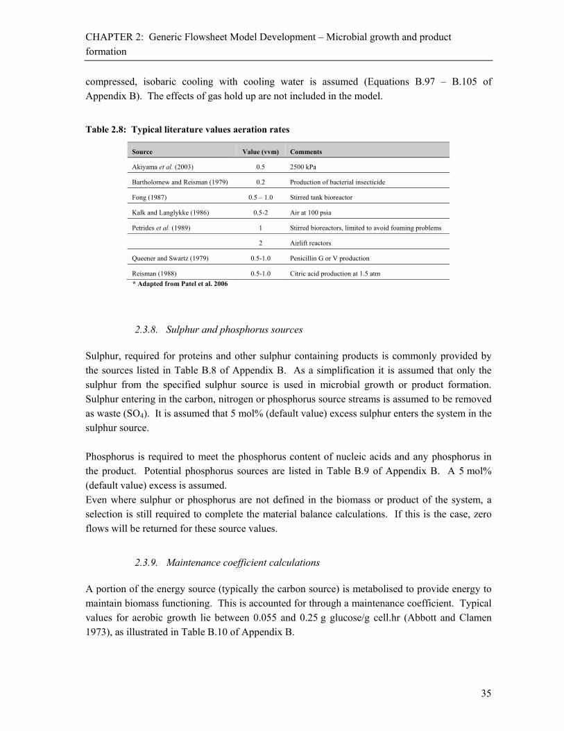
CHAPTER 2: Generic Flowsheet Model Development – Microbial growth and product
formation
35
compressed, isobaric cooling with cooling water is assumed (Equations B.97 – B.105 of Appendix B). The effects of gas hold up are not included in the model.
Table 2.8: Typical literature values aeration rates
Source Value (vvm) Comments
Akiyama et al. (2003) 0.5 2500 kPa
Bartholomew and Reisman (1979) 0.2 Production of bacterial insecticide
Fong (1987) 0.5 – 1.0 Stirred tank bioreactor
Kalk and Langlykke (1986) 0.5-2 Air at 100 psia
Petrides et al. (1989) 1 Stirred bioreactors, limited to avoid foaming problems
2 Airlift reactors
Queener and Swartz (1979) 0.5-1.0 Penicillin G or V production
Reisman (1988) 0.5-1.0 Citric acid production at 1.5 atm
* Adapted from Patel et al. 2006
2.3.8. Sulphur and phosphorus sources Sulphur, required for proteins and other sulphur containing products is commonly provided by the sources listed in Table B.8 of Appendix B. As a simplification it is assumed that only the sulphur from the specified sulphur source is used in microbial growth or product formation. Sulphur entering in the carbon, nitrogen or phosphorus source streams is assumed to be removed as waste (SO4). It is assumed that 5 mol% (default value) excess sulphur enters the system in the sulphur source. Phosphorus is required to meet the phosphorus content of nucleic acids and any phosphorus in the product. Potential phosphorus sources are listed in Table B.9 of Appendix B. A 5 mol% (default value) excess is assumed. Even where sulphur or phosphorus are not defined in the biomass or product of the system, a selection is still required to complete the material balance calculations. If this is the case, zero flows will be returned for these source values.
2.3.9. Maintenance coefficient calculations A portion of the energy source (typically the carbon source) is metabolised to provide energy to maintain biomass functioning. This is accounted for through a maintenance coefficient. Typical values for aerobic growth lie between 0.055 and 0.25 g glucose/g cell.hr (Abbott and Clamen 1973), as illustrated in Table B.10 of Appendix B.

CHAPTER 2: Generic Flowsheet Model Development – Microbial growth and product
formation
36
The maintenance coefficient is selected based on the organism. If no data exists, an average is used, based either aerobic or anaerobic values. The amount of carbon needed, defined by carbon source 1, is calculated from this maintenance coefficient and residence time. Under aerobic conditions, the carbon source required for maintenance undergoes complete oxidation to carbon dioxide, water vapour and energy. In the anaerobic process, the carbon source forms an additional anaerobic product. Calculations to determine the amount of carbon source required from maintenance are given in Equations B.91 – B.93 of Appendix B.
2.3.10. Growth rate Growth rate data allows calculation of the reactor residence time, which is used to calculate agitation energy, maintenance energy etc. The required data (maximum specific growth rate,
max; half saturation constant, Ks and final biomass concentration, Cx, final) is obtained from
literature and experimental values (Table B.11 in Appendix B or an average value is assumed (Figure 2.8). Monod kinetics have been assumed in the model developed (Equations B.94 – B.96 in Appendix B) owing to its widespread use. Opportunity exists to expand the model to incorporate other kinetic expressions.
Figure 2.8: Decision method to determine max, Ks and rx values
2.3.11. Reactor cooling Under aerobic conditions, microbial growth results in energy release at approximately 400 kJ/C-mol produced or 500 kJ/mol O2 consumed. When using glucose as the main substrate 315 kJ/C-mol produced is released. Under anaerobic conditions, with a glucose substrate, approximately 225 kJ/C-mol are produced i.e. approximately 70 % of the aerobic value (Roels 1983).
CHAPTER 2: Generic Flowsheet Model Development – Agitation
37
In the model, the energy generation during aerobic growth is calculated using a degree of reduction basis using Equations B.106 – B.111 in Appendix B. (von Stochar et al. 2006). For anaerobic growth 70 % of the aerobic value is used, in accordance with the ratios shown above for glucose metabolism by Roels 1983 (Equation B.112 in Appendix B). Cooling or chilled water is used to maintain the reactor at the specified temperature by heat exchange.
2.3.12. Post microbial growth cooling Once the required microbial growth and product formation is achieved, cooling of the materials can take place. A default cooled temperature of 15°C is assumed, requiring refrigeration. The refrigeration energy is calculated from compression of the refrigerant. An energy balance of the heat removal required from the microbial stream, with a 30 % compression cycle efficiency, is taken as the electrical energy requirement (Equations B.113 –B.114 in Appendix B.).
2.4. Agitation During biomass growth and product formation, agitation may be required. the model framework provides a selection grid for agitation requirements and choice of impeller type. Impeller types include: pitch-blade turbine, paddle turbine, Rushton turbine, marine propeller, axial flow impeller, radial turbine, bar turbine, saw tooth dispenser, anchor and helical ribbon impellors. Additional requirements to be considered include the number of tanks used, tank dimensions, agitation efficiency, impeller characteristics and rotational speed. Agitation power is calculated using a power number (Np) for a turbulent flow regime as shown in Table B.12 of Appendix B. The power per unit volume is calculated by the method of Sinnot (1983), using power number, impeller speed and diameter. Corrections for different ratios of blade width to impeller diameter (W/D) and gassed systems are included as shown in Dickey (1984) and Atkinson and Mavituna (1983) respectively. These agitation power calculations are detailed in Equations B.115 – B.140 of Appendix B, resulting in power per unit volume. Typical literature values are shown in Table 2.9 for comparison.

CHAPTER 2: Generic Flowsheet Model Development – Downstream processing
38
Table 2.9: Typical literature values for agitation power requirements for turbulent flow
Source Agitation power required (kW/m3)
Comments
Akiyama et al. 2003, Gerngross 1999 1 -
Bartholomew and Reisman 1979 1 – 2 -
Fong 1987 0.2 – 0.7 Mild mechanical agitation
0.2 – 2.2 Antibiotics (stirred tank bioreactor)
3.7 Yeast (stirred tank bioreactor)
2.2 – 6 Biomass production (stirred tank bioreactor)
Kalk and Langlykke 1979 1 – 3 -
Petrides et al. 1989 0.2 – 1 Mild agitation
1.5 – 3.5 Antibiotic production
3.5 – 5.0 Yeast production
>7 Xanthum gum production
Seider et al. 1998 2 Slurry
Reisman 1988 2 – 4
Patel et al. 2006 0.5 – 1
8 – 12 Viscous mixtures
*Adapted from Patel et al. 2006
2.5. Downstream processing Typical downstream processing operations require the recovery of the product and its purification from contaminating material. Unit operations typically used include filtration, centrifugation, solvent extraction, precipitation and freeze drying as shown in Table 2.10 with recoveries and yields as shown in Table 2.11. The downstream processing capability of the model is divided into solid-liquid separation for biomass concentration, cell disruption, a second solid-liquid separation for debris removal, six concentration and purification steps and a formulation step. The model includes the downstream units to provide for: adsorption, ball milling, cavitation, centrifugation, chromatography, decanting, evaporation, filtration, high pressure homogenisation, precipitation, crystallization, sedimentation, solvent extraction, splitter, oven drying, freeze drying and spray drying. Temperatures are tracked through the downstream process for energy calculations. Unless as a result of heat exchange, it is assumed that there is no heat loss in downstream processing.

CHAPTER 2: Generic Flowsheet Model Development – Downstream processing
39
Table 2.10: Literature review of commonly used downstream process units
Product (Microorganism)
Separationa Concentration and Purificationb Formulationc Reference
Anthracycline antibiotics (Streptomyces sp., E. coli)
Broth filtration, solvent extraction (CHCl3, butanol) centrifugation
Precipitation (dissolved with n-butanol. Acetone added)
Freeze drying Flickinger 1985
Cephalosporins Filtration (rotary drum), solvent extraction (methyl isobutyl ketone)
Precipitation (acetone added), adsorption (Activated carbon, non-polar resins), enzyme treatment
Smith 1985
Cephamycin Solvent extraction (acetone (aq.), 50 % v/v.)
Evaporation Omstead et al. 1985
Citric Acid (Aspergillus niger, yeasts)
Filtration, solvent extraction (butan-2-ol, tributyl phosphate), centrifugation
Precipitation (calcium citrate) Milsom and Meers 1985a
Glycerol (Aspergillus niger)
Broth filtration, centrifugation Precipitation, evaporation, ion exchange
Spray drying Milsom and Meers 1985b
Itaconic acid (Aspergillus terreus)
Broth filtration, centrifugation Precipitation, evaporation Milsom and Meers 1985b
Lactic acid (Lactobacillus sp.)
Filtration, solvent extraction, distillation
Precipitation, evaporation Vickroy 1985
Lincomycin (Streptomyces sp.)
Filtration (4.0 % filter aid before filtration. Water washed), solvent extraction (activated carbon, n-butanol)
Ion exchange (cationic resins), partition chromatography (cyclohexane, methyl ethyl ketone)
Freeze drying Gonzalez and Miller 1985
Penicillin G or V (Penicillium sp.)
Filtration (rotary vacuum drum), solvent extraction (amyl acetate, butyl acetate, cyclic ketones)
Precipitation (potassium or sodium added), centrifugation or filtration
Drying (pre-dried with anhydrous isopropyl alcohol, butyl alcohol. Dried with warm air, vacuum or radiant heat)
Swartz 1985
Polysaccharides (Xanthamonas campestris, Pseudomonas aerugenosa)
Centrifugation, milling Precipitation (alcohol, salt and acid)
Forced air or vacuum drying
Margaritis and Pace 1985
Streptomycin Broth filtration Precipitation, adsorption (activated carbon, non-ionic resins, alcohol, acid)
Florent 1985
Thienamycin (Streptomyces sp.)
Pressure rotary filtration Adsorption (Dowex 1x2 (HCO3-)
resin) Buckland et
al. 1985
Yeasts (Bakers’) (Saccharomyces cerevisiae, S. uvarum, S. carlsbergensis)
Freeze-, Roto-Louvre-, through circulation-, air-lift- and spray drying
Chen and Chiger 1985
Yeast (Saccharomyces cerevisiae)
Filtration (plate and frame), centrifugation
Smith 2005
a: Separation is defined as solid liquid separation. b: Concentration and purification are meant as the same thing here. This is the increase in product purity by any means of downstream processing. Strictly speaking, this may also include the unit operations defined in separation and formulation.
c: Formulation is defined as the final stage in downstream processing. It includes processes aimed at reducing the moisture content of the product. Typical examples include oven drying, freeze drying and spray drying.
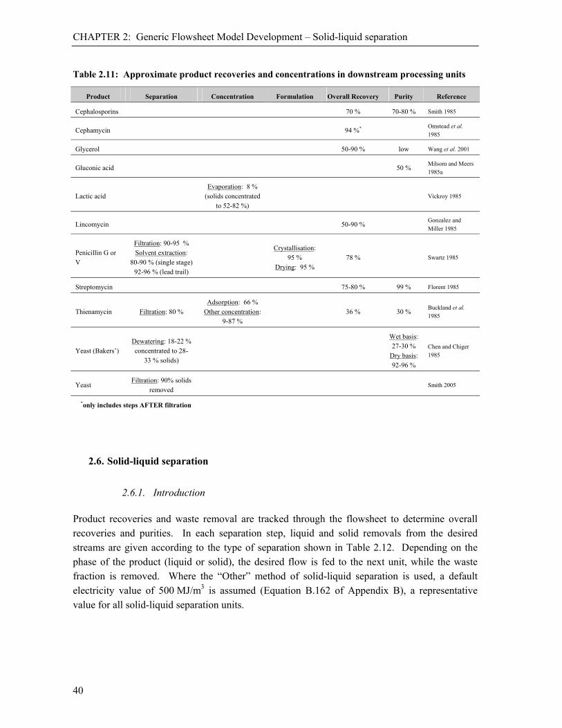
CHAPTER 2: Generic Flowsheet Model Development – Solid-liquid separation
40
Table 2.11: Approximate product recoveries and concentrations in downstream processing units
Product Separation Concentration Formulation Overall Recovery Purity Reference
Cephalosporins 70 % 70-80 % Smith 1985
Cephamycin 94 %* Omstead et al. 1985
Glycerol 50-90 % low Wang et al. 2001
Gluconic acid 50 % Milsom and Meers 1985a
Lactic acid Evaporation: 8 %
(solids concentrated to 52-82 %)
Vickroy 1985
Lincomycin 50-90 % Gonzalez and Miller 1985
Penicillin G or V
Filtration: 90-95 % Solvent extraction:
80-90 % (single stage) 92-96 % (lead trail)
Crystallisation:
95 % Drying: 95 %
78 % Swartz 1985
Streptomycin 75-80 % 99 % Florent 1985
Thienamycin Filtration: 80 % Adsorption: 66 %
Other concentration: 9-87 %
36 % 30 % Buckland et al. 1985
Yeast (Bakers’) Dewatering: 18-22 % concentrated to 28-
33 % solids)
Wet basis: 27-30 %
Dry basis: 92-96 %
Chen and Chiger 1985
Yeast Filtration: 90% solids
removed Smith 2005
*only includes steps AFTER filtration
2.6. Solid-liquid separation
2.6.1. Introduction Product recoveries and waste removal are tracked through the flowsheet to determine overall recoveries and purities. In each separation step, liquid and solid removals from the desired streams are given according to the type of separation shown in Table 2.12. Depending on the phase of the product (liquid or solid), the desired flow is fed to the next unit, while the waste fraction is removed. Where the “Other” method of solid-liquid separation is used, a default electricity value of 500 MJ/m3 is assumed (Equation B.162 of Appendix B), a representative value for all solid-liquid separation units.

CHAPTER 2: Generic Flowsheet Model Development – Solid-liquid separation
41
Table 2.12: Product fractions recovered and waste fractions removed in separation units
Solid or product fraction removed
Liquid or waste fraction removed
Centrifugal spin/washing 0.98 0.80
Filtration 0.95 0.70
Sedimentation 0.90 0.60
OTHER 0.94 0.70
2.6.2. Centrifugal spin and washing Five forms of centrifugation are provided in the model: tubular, disk, nozzle-discharge disk, helical conveyor decanter or “other”, each with a specific energy requirement per volume taken from Perry et al. (1984) (Table B.14 of Appendix B). Typical power requirements for centrifugation from the literature are given in Table 2.13. There is good agreement with the Perry et al. (1984) data for yeasts. However, bacterial cultures require greater energy owing to lower settling velocities, resulting from smaller cell size.
Table 2.13: Typical centrifuge power requirements
Source Centrifuge power
requirements (kJ/m3)
Comment
Bacterial harvesting
Bohlmann 2002 26 640 – 90 000 Axial solid ejecting centrifuge 37 kW, 1.5-5 m3/h
Tutunjian 1985 22 320 Continuous disc-type centrifuge, 37 HP motor, water removal rate 5 m3/h
Yeast Harvesting
Bohlmann 2002 2 520 – 9 000 Nozzle centrifuge 149 kW 50-200 m3/h concentrate 10-50 m3/hr
Kalk and Langlykke 1986 8 280 Continuous desludging disk centrifuge, 4 m3/h
Steffens et al. 1999, 2000 5 400 -
Tutunjian 1985 5 040 Continuous disc-type centrifuge, 37 HP motor, water removal rate 5 m3/h
*Adapted from Patel et al. 2006
The generic flowsheet model is used to calculate energy requirements from the data in Table B.14 and mass balance data assuming the solid and liquid recoveries and removals in Table 2.12 (Equations B.143 – B.148 of Appendix B). Repeat water (municipal, distilled or de-ionised) washing is allowed using mass balances to calculate further losses and accounting for the energy requirements of repeated centrifuges.

CHAPTER 2: Generic Flowsheet Model Development – Cell disruption
42
2.6.3. Filtration The material and energy balance calculations for filtration assume constant pressure membrane filtration, with no cake build-up. Energy requirements, assumed to be provided by electricity, are calculated from first principles of the fluid flow through the filter. The mass and flux of the material entering the filter, as well as the cross sectional area of the filtration unit, are used to calculate the linear velocity. From this, the power and energy requirements are calculated (Equations B.149 – B.153). A filter media and flocculent (Table B.15 of Appendix B) can also be added (Equations B.187 – B.161).
2.6.4. Sedimentation A flocculent (Table B.15) can also be added for a sedimentation unit operation. It is assumed that there is no energy requirement for sedimentation.
2.7. Cell disruption
2.7.1. Introduction Cell disruption to release intracellular products can be performed chemically (using e.g. chloroform, toluene, EDTA or lysozyme), by freeze-thaw cycling or by mechanical stress (e.g. cavitation, bead milling or high pressure homogenisation) (Engler 1985, Harrison 1991, Willson 1999). The model allows for mechanical disruption by high pressure homogenisation (HPH), cavitation (hydrodynamic or acoustic) or a bead mill only, being the preferred approaches for large scale processes. Typical disruption efficiencies (%) and energy productivities (mg/J) are summarised in Tables 2.14 to 2.16. These are used to estimate appropriate default values for the model, where necessary. It is assumed that product not released on cell disruption is lost on biomass separation in further processing. Energy requirements for high pressure homogeniser, cavitation and ball mills are calculated by Equations B.163 – B.164 of Appendix B. Where the “Other” method of cell disruption is used, a default electricity value of 25 MJ/m3 is assumed (Equation B.165 of Appendix B), a representative value for all cell disruptions.
2.7.2. High Pressure Homogeniser Extent of cell disruption and energy productivity (mg/J) on high pressure homogenisation are shown in Table 2.14. Data are given for Saccharomyces cerevisiae and Candida utilis. Cell disruption of bacteria requires less energy than yeasts (Harrison 1991a, 1991b). It is also

CHAPTER 2: Generic Flowsheet Model Development – Cell disruption
43
possible to reduce the energy requirement of disruption by chemical pre-treatment of the suspension (Bailey et al. 1995, Anand et al. 2007). Although other literature, including Hetherington et al. (1971), Follows et al. (1971), Doulah et al. (1975) and Sauer et al. (1989) give some data on protein release versus homogeniser pressure and number of passes, the required data for the model are not presented in these texts. A basic estimation of average values is used for other micro-organisms.
Table 2.14: Literature values for extent of disruption and energy efficiency of a high pressure homogeniser
Organism Disruption Biomass concentration Energy productivity
% %w/v mg/J
Saccharomyces cerevisiae 90 17 1.65
94 20 1.25
Candida utilis 90 20 1.26
87 20 0.83
Average 90.3 19.3 1.25
Reference: Engler 1985
2.7.3. Cavitation Cavitation data are split into hydrodynamic and acoustic cavitation. Energy productivity (mg/J) and energy efficiency (J/ml) values obtained from Save et al. (1994) and Kumar et. al. (2000) have been used in the model (Table 2.15). Additional literature on cavitation for the total or partial release of intracellular material have been reported by Save et al. (1997), Balasudaram and Pandit (2001), Gogate and Pandit (2001), Sundaram et al. (2003), Balasudaram and Harrison (2006), but these do not include the required data for the model.
Table 2.15: Default values for cavitation calculations
Organism Disruption Biomass concentration Energy productivity Reference
% %w/v mg/J
Hydrodynamic cavitation
Saccharomyces cerevisiae
90 - 0.02 [1]
Acoustic cavitation
Yeast cells 90 2.5 %w/w 1500 J/ml [2]
90 2.5 %w/v 0.00689 mg/J [2]
References: [1] Kumar et. al. 2000
[2] Save et. al 1994

CHAPTER 2: Generic Flowsheet Model Development – Concentration and purification
44
2.7.4. Ball mill Cell disruption (%) and energy productivities (mg/J) used in the model are given for a ball mill in Table 2.16. Data are given for Saccharomyces cerevisiae, Saccharomyces carlsbergensis and Candida utilis (Engler 1985). Additional literature on mills have been reported by Woodrow and Quirk (1982), Agerkvist and Enfors (1990) and Melendres et al. (1993), but these do not include the required data for the model.
Table 2.16: Default values for ball mill calculations
Organism Disruption Biomass concentration Energy productivities
% %w/v mg/J
Saccharomyces cerevisiae 80 6 0.51
80 11 1.11
80 16 1.11
85 10-20 0.93
95 17 1.26-1.39
65 13.5 2.32
42 13.5 1.25
40 13.5 5.4
Saccharomyces carlsbergensis 95 17 1.26-1.39
Candida utilis 85-90 17 0.84-1.07
Average 75 14 1.62
Reference: Engler 1985
2.8. Concentration and purification
2.8.1. Introduction A maximum of six concentration and purification units can be modelled to achieve a desired product purity from solution. These include adsorption, centrifugation, chromatography, decanting, evaporation, filtration, precipitation or crystallisation, solvent extraction and splitters. Where the “Other” method of concentration and purification is used, a default electricity value of 10 MJ/m3 is assumed (Equation B.192 of Appendix B), which is an estimated average energy based on the requirements for all other concentration and purification units. Material balancing for centrifugation and filtration is based on solid and liquid fractional removals. For precipitation or crystallisation, it is assumed that no product is lost or waste
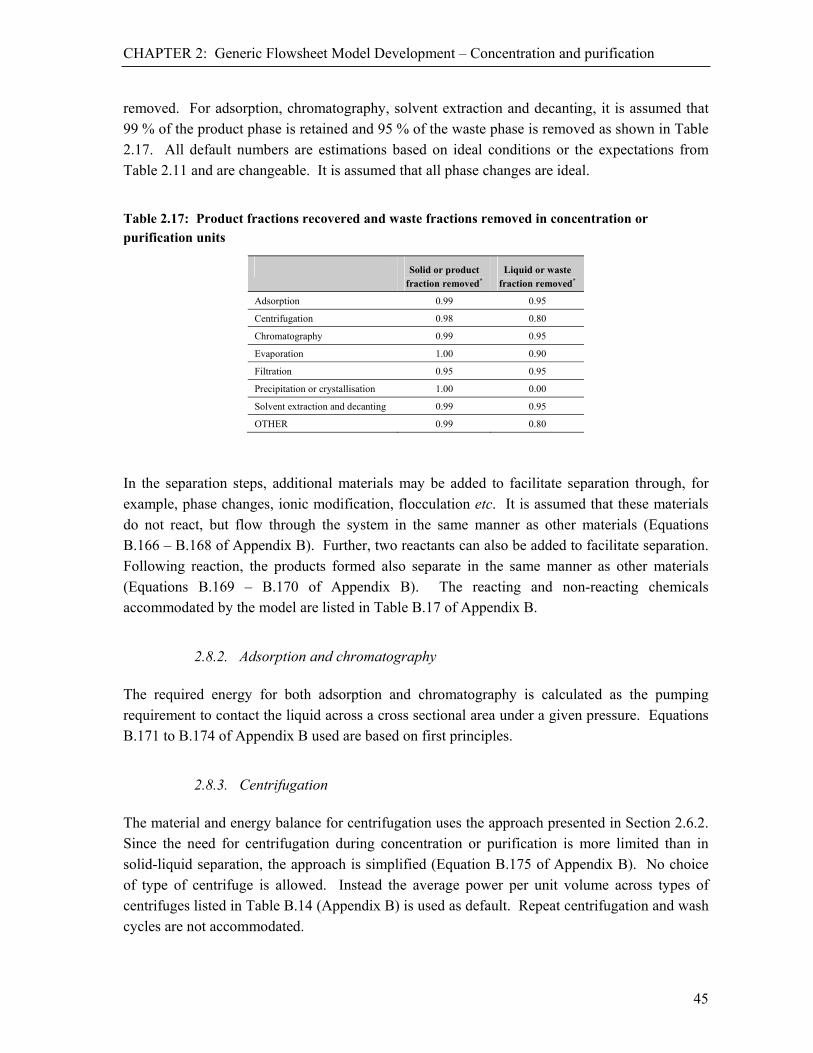
CHAPTER 2: Generic Flowsheet Model Development – Concentration and purification
45
removed. For adsorption, chromatography, solvent extraction and decanting, it is assumed that 99 % of the product phase is retained and 95 % of the waste phase is removed as shown in Table 2.17. All default numbers are estimations based on ideal conditions or the expectations from Table 2.11 and are changeable. It is assumed that all phase changes are ideal.
Table 2.17: Product fractions recovered and waste fractions removed in concentration or purification units
Solid or product fraction removed*
Liquid or waste fraction removed*
Adsorption 0.99 0.95
Centrifugation 0.98 0.80
Chromatography 0.99 0.95
Evaporation 1.00 0.90
Filtration 0.95 0.95
Precipitation or crystallisation 1.00 0.00
Solvent extraction and decanting 0.99 0.95
OTHER 0.99 0.80
In the separation steps, additional materials may be added to facilitate separation through, for example, phase changes, ionic modification, flocculation etc. It is assumed that these materials do not react, but flow through the system in the same manner as other materials (Equations B.166 – B.168 of Appendix B). Further, two reactants can also be added to facilitate separation. Following reaction, the products formed also separate in the same manner as other materials (Equations B.169 – B.170 of Appendix B). The reacting and non-reacting chemicals accommodated by the model are listed in Table B.17 of Appendix B.
2.8.2. Adsorption and chromatography The required energy for both adsorption and chromatography is calculated as the pumping requirement to contact the liquid across a cross sectional area under a given pressure. Equations B.171 to B.174 of Appendix B used are based on first principles.
2.8.3. Centrifugation The material and energy balance for centrifugation uses the approach presented in Section 2.6.2. Since the need for centrifugation during concentration or purification is more limited than in solid-liquid separation, the approach is simplified (Equation B.175 of Appendix B). No choice of type of centrifuge is allowed. Instead the average power per unit volume across types of centrifuges listed in Table B.14 (Appendix B) is used as default. Repeat centrifugation and wash cycles are not accommodated.
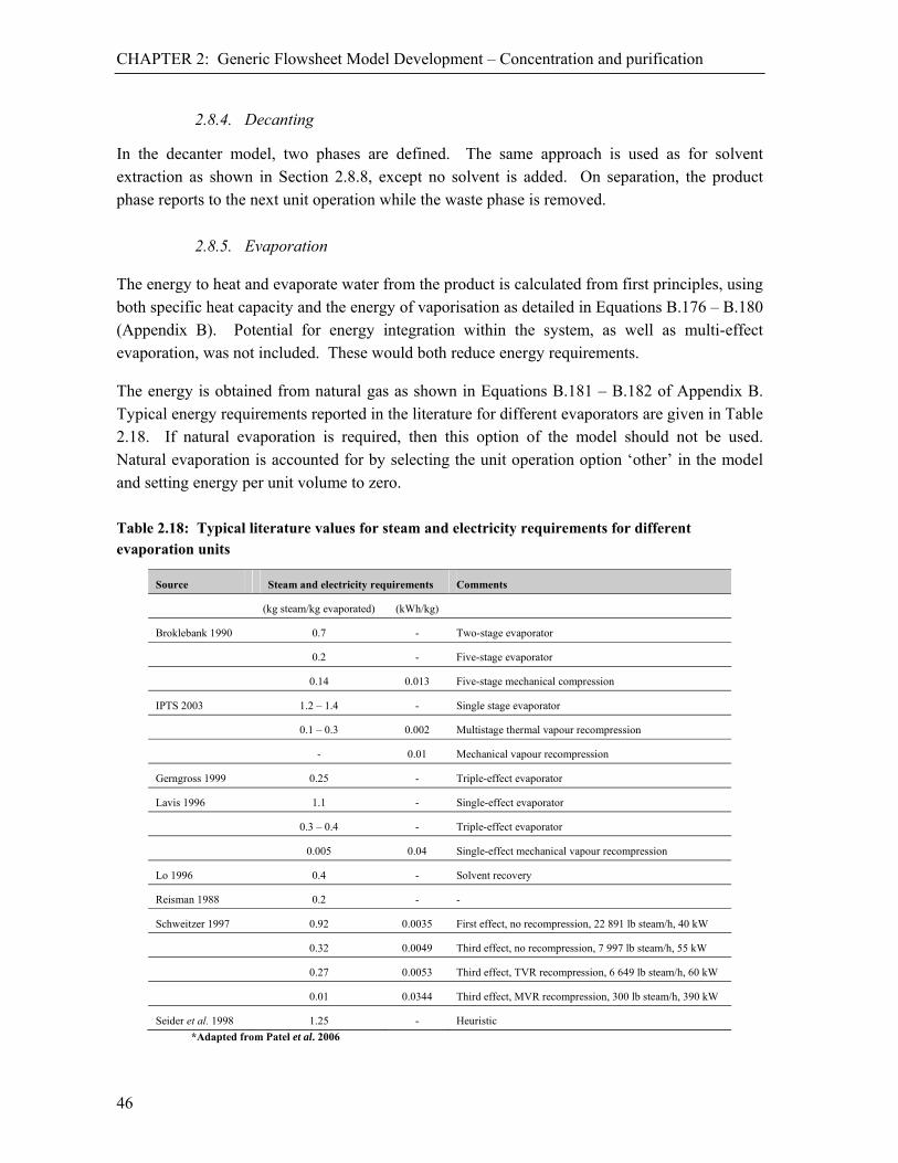
CHAPTER 2: Generic Flowsheet Model Development – Concentration and purification
46
2.8.4. Decanting
In the decanter model, two phases are defined. The same approach is used as for solvent extraction as shown in Section 2.8.8, except no solvent is added. On separation, the product phase reports to the next unit operation while the waste phase is removed.
2.8.5. Evaporation
The energy to heat and evaporate water from the product is calculated from first principles, using both specific heat capacity and the energy of vaporisation as detailed in Equations B.176 – B.180 (Appendix B). Potential for energy integration within the system, as well as multi-effect evaporation, was not included. These would both reduce energy requirements.
The energy is obtained from natural gas as shown in Equations B.181 – B.182 of Appendix B. Typical energy requirements reported in the literature for different evaporators are given in Table 2.18. If natural evaporation is required, then this option of the model should not be used. Natural evaporation is accounted for by selecting the unit operation option ‘other’ in the model and setting energy per unit volume to zero.
Table 2.18: Typical literature values for steam and electricity requirements for different
evaporation units
Source Steam and electricity requirements Comments
(kg steam/kg evaporated) (kWh/kg)
Broklebank 1990 0.7 - Two-stage evaporator
0.2 - Five-stage evaporator
0.14 0.013 Five-stage mechanical compression
IPTS 2003 1.2 – 1.4 - Single stage evaporator
0.1 – 0.3 0.002 Multistage thermal vapour recompression
- 0.01 Mechanical vapour recompression
Gerngross 1999 0.25 - Triple-effect evaporator
Lavis 1996 1.1 - Single-effect evaporator
0.3 – 0.4 - Triple-effect evaporator
0.005 0.04 Single-effect mechanical vapour recompression
Lo 1996 0.4 - Solvent recovery
Reisman 1988 0.2 - -
Schweitzer 1997 0.92 0.0035 First effect, no recompression, 22 891 lb steam/h, 40 kW
0.32 0.0049 Third effect, no recompression, 7 997 lb steam/h, 55 kW
0.27 0.0053 Third effect, TVR recompression, 6 649 lb steam/h, 60 kW
0.01 0.0344 Third effect, MVR recompression, 300 lb steam/h, 390 kW
Seider et al. 1998 1.25 - Heuristic
*Adapted from Patel et al. 2006
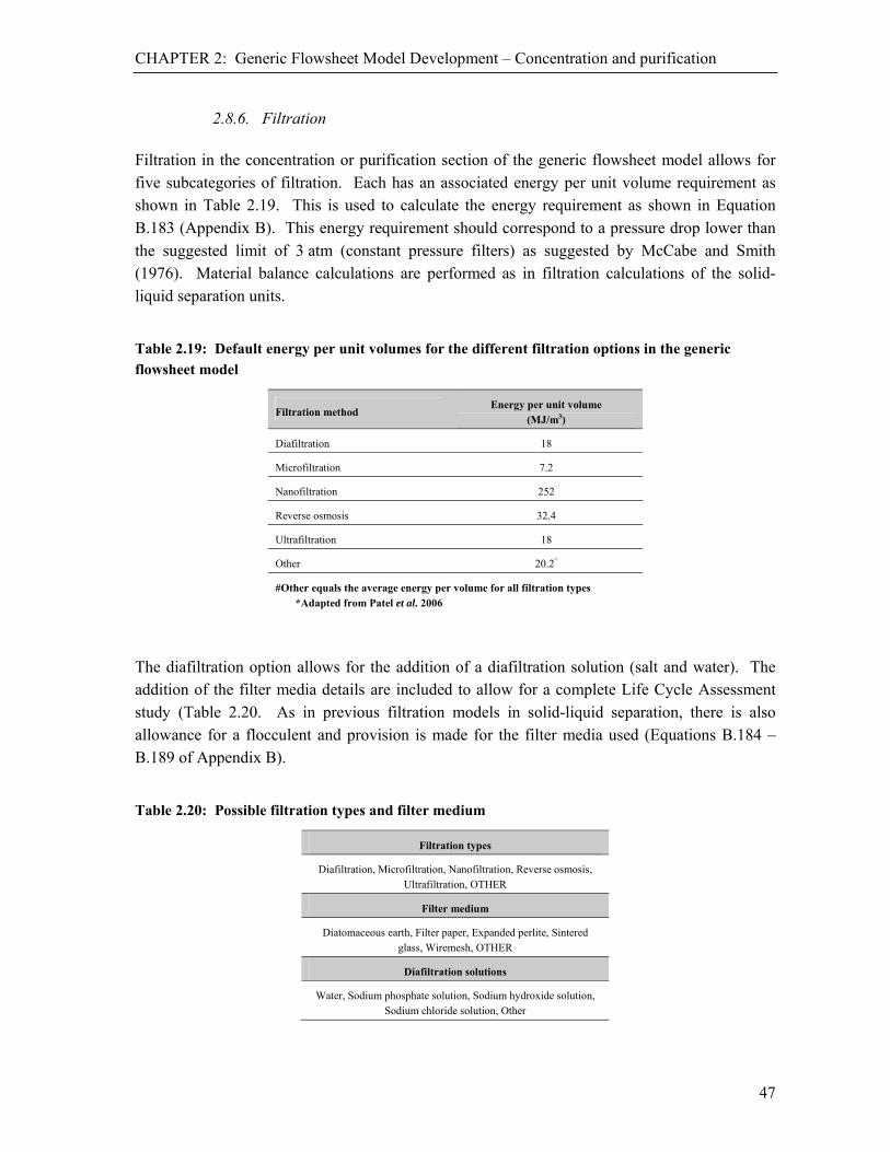
CHAPTER 2: Generic Flowsheet Model Development – Concentration and purification
47
2.8.6. Filtration Filtration in the concentration or purification section of the generic flowsheet model allows for five subcategories of filtration. Each has an associated energy per unit volume requirement as shown in Table 2.19. This is used to calculate the energy requirement as shown in Equation B.183 (Appendix B). This energy requirement should correspond to a pressure drop lower than the suggested limit of 3 atm (constant pressure filters) as suggested by McCabe and Smith (1976). Material balance calculations are performed as in filtration calculations of the solid-liquid separation units.
Table 2.19: Default energy per unit volumes for the different filtration options in the generic flowsheet model
Filtration method Energy per unit volume
(MJ/m3)
Diafiltration 18
Microfiltration 7.2
Nanofiltration 252
Reverse osmosis 32.4
Ultrafiltration 18
Other 20.2^
#Other equals the average energy per volume for all filtration types *Adapted from Patel et al. 2006
The diafiltration option allows for the addition of a diafiltration solution (salt and water). The addition of the filter media details are included to allow for a complete Life Cycle Assessment study (Table 2.20. As in previous filtration models in solid-liquid separation, there is also allowance for a flocculent and provision is made for the filter media used (Equations B.184 – B.189 of Appendix B).
Table 2.20: Possible filtration types and filter medium
Filtration types
Diafiltration, Microfiltration, Nanofiltration, Reverse osmosis, Ultrafiltration, OTHER
Filter medium
Diatomaceous earth, Filter paper, Expanded perlite, Sintered glass, Wiremesh, OTHER
Diafiltration solutions
Water, Sodium phosphate solution, Sodium hydroxide solution, Sodium chloride solution, Other

CHAPTER 2: Generic Flowsheet Model Development – Concentration and purification
48
2.8.7. Precipitation or crystallisation Electrical energy requirements for precipitation or crystallisation are based on the energy requirement for agitation, with a default power per unit volume value of 0.8 kW/m3 assumed (a mild to medium mixing value for precipitation as shown in Table 2.21) and an efficiency of 80 %. The unit can be heated with steam and cooled again before further processing. Both the steam and cooling water needed for this are included in material balance calculations. In modelling the precipitation or crystallisation unit, precipitating chemicals are assumed to undergo a perfect phase change from liquid to solid. The solids formed can then be removed in further processing (e.g. filtration or centrifugation) as desired to further purify the product.
Table 2.21: Power requirements in baffled tanks
Agitation Applications Power
kW/m3
Mild Blending, mixing 0.04 – 0.10
Homogenous reactions 0.01 – 0.03
Medium Heat transfer 0.03 – 1.0
Liquid-liquid mixing 1.0 – 1.5
Severe Slurry suspension 1.5 – 2.0
Gas absorption 1.5 – 2.0
Emulsions 1.5 – 2.0
Violent Fine slurry suspension > 2.0
Reference:
Sinnot 1983
2.8.8. Solvent extraction Modelling of solvent extraction requires the addition of a solvent, selected from Table B.17 of Appendix B, and the defining of 2 phases: product and waste. The product phase reports to the next unit operation, while the chemicals in the waste phase and the remaining liquid phase are removed according to the separation efficiency specified.
2.8.9. Splitter Defined by a split ratio of product to waste, a splitter can also be modelled in downstream processing (Equation B.191 of Appendix B).

CHAPTER 2: Generic Flowsheet Model Development – Formulation
49
2.9. Formulation
2.9.1. Introduction The final step in the generic flow sheet model is formulation. This can take the form of oven-, spray- or freeze drying. Energy is supplied as natural gas for spray drying and oven drying or electricity for freeze drying. It is assumed that 99 % of the product is retained in the formulation step and that 99 % of the moisture is removed in this unit. Typical final moisture contents can be as low as 2 % in baker’s yeasts, with dryer temperatures as high as 150°C (Chen and Chiger 1985). The heat lability of many bioproducts implies that careful control of the effective temperature of the product, and time of exposure, is required. Typical literature values for different drying methods and conditions are shown in Table 2.22. Where the “Other” method of formulation is used, a default electricity value of 15 MJ/m3 is assumed (Equation B.201 of Appendix B), a representative value for all formulation units.
Table 2.22: Typical literature values for different drying methods
Drying method Steam and electricity requirements
Temperature Time Drying rate (Final moisture
content)
Comments Reference
kg steam/kg evaporated
kWh/kg °C min kg water/h
(%)
Belt dryer 1.38 - Approx. 60°C [1]
Co-current drum dryer 1.76 - Evap. of 46 t/h water [1]
Fluidised bed dryer 0.24 - 25 bar steam produces 3 bar heating steam
[1]
Spray dryer 3 0.1 - [2]
Spray dryer 1.62 – 2.33 - 1, 2 & multistage dryers
[3]
Spray dryer 2 - [4]
Tower dryer 2.0 – 2.4 0.1 No heat recovery [5]
(Unknown) 1.2 – 1.67 0.25 – 1 Drying of food [1]
Air-lift dryer 100-150 10-240
160-350 (7)
[6]
Freeze drying -35 [6]
Heated air 38 (7-8) [6]
Roto-Louvre drying 50-60 600-1200 5400 Size: 4.85 x 2.2 [6]
Spray dryer In: 100-120 Out: 65-67
(5-6) [6]
Through circulation dryer 28-50 [6]
References: [1] IPTS 2003 [2] Bartholomew and Reisman 1979
[3] Energy Centre Denmark 1992 [4] Gerngross 1999
[5] Reisman 1989 [6] Chen and Chiger 1985

CHAPTER 2: Generic Flowsheet Model Development – Wastewater treatment (WWT)
50
2.9.2. Oven drying The energy required to heat material and evaporate moisture by oven drying is calculated from first principles as shown in Appendix B. The energy required is obtained from natural gas. Energy calculations are similar to those for steam used elsewhere in the model.
2.9.3. Freeze drying The energy to freeze dry the product is determined by the energy needed to cool the liquid to freezing, to freeze and subcool it, and the energy to create a vacuum in the container (Equations B.193 – B.197 of Appendix B). It is assumed that no external energy inputs are required to sublimate the liquid from the product. The energy required for vacuuming pumping is calculated as for other pumping requirements as shown in Equations B.171 – B.174 of Appendix B.
2.9.4. Spray drying Energy data for spray drying is calculated according to the energy balance given by Baker and McKenzie (2005) for spray drier energy requirements. In the model, a simplification is made that the thermal loss factor is zero (i.e. adiabatic system) and the calculation reduces to a simplified form as expressed by Keey (1992) as shown in Equation B.199 (Appendix B).
2.10. Wastewater treatment (WWT) A simplified wastewater treatment scenario is included whereby wastewater collected in the discarded streams may be neutralised by up to three chemicals (Equations B.202 – B.204 of Appendix B). A stoichiometric oxygen demand (StOD) value, as shown in IChemE (2003) (Equations B.205 – B.207 of Appendix B), has been included and can to be used as a water pollution value. Opportunity exists to expand the model to include more appropriate wastewater treatment scenarios.
2.11. Structure for the remainder of the thesis To support Chapter 2, several appendices are presented at the end of the thesis. These include:
Appendix B: Contains the generic flowsheet calculations, and all mathematical equations used in the model;
Appendix C: Nomenclature used in Appendix B;

CHAPTER 2: Generic Flowsheet Model Development – References
51
Appendix D: UML Diagrams for the generic flowsheet model. A simplified Unified Modelling Language (UML) diagram to describe the full logic to the material balance of the generic flowsheet model; and
Appendix E: Using the generic flowsheet model. A guide to using the MS-EXCEL model.
Subsequent chapters validate the material and energy balance results of the generic flowsheet
model using several case studies. These case studies, Penicillin V, cellulase and poly--butryic
acid (PHB) production (Chapters 3, 4, and 5 respectively), determine the accuracy of the model against rigorous material and energy balance calculations found in literature. Different process configurations are used to include, for example, aerobic versus anaerobic bioreactors and submerged fermentation versus solid state cultivation. These case studies are also used to generate a collection Life Cycle Assessment (LCA) studies for microbial bioprocesses. These LCA studies add further validation to the material and energy balance results and highlight the key biological issues in the flowsheets. Certain LCA results are also compared to the equivalent chemical processes. This is done to determine if any common issues are raised and to calculate the relative environmental impacts of each. Polymers and biodiesel (Chapters 5 and 6 respectively) are used as case studies for this. In Chapter 7, a sensitivity analysis is performed on the generic flowsheet model. This highlights the variables which lead to the greatest change in reactor volume, electrical requirements, purity and LCA scores. The advantages of improved production versus optimised downstream processing are also investigated. Heuristics can be drawn from these to determine reduced LCA scores during the initial design of a bioprocess as well as during operation.
References Abbott, B.J., Clamen, A., 1973. The relationship of substrate, growth rate, and maintenance coefficient to single
cell protein production, Biotechnol. Bioeng., 15, 117-127. Agerkvist, Enfors, S.-O., 1990. Characterisation of E. coli cell disintegrates from a bead mill and high pressure
homogenizers, Biotech. Bioeng., 36, 1083-1089. Akiyama, M., Tsuge, T., Doi, Y., 2003. Environmental life cycle comparison of polyhydroxyalkanoates produced
from renewable carbon resources by bacterial fermentation, Polym. Degrad. Stabil., 80, 183-194. Anand, H., Balasundaram, B., Pandit, A.B., Harrison, S.T.L., 2007. The effect of chemical pre-treatment combined
with mechanical disruption on the extent of disruption and release of intracellular protein from E. coli, Biochem. Eng. J., 35, 166-173.
Anex, R., 2003. Something new under the sun: the industrial ecology of biobased products, J. Ind. Ecol., 7(3-4), 1-4.
Atkinson B., Mavituna F. 1983. Biochemical Engineering and Biotechnology Handbook, Macmillan Inc., New York.
Bailey, J.E., Ollis, D.F., 1986. Biochemical Engineering Fundamentals, McGraw-Hill.

CHAPTER 2: Generic Flowsheet Model Development – References
52
Bailey, S.M., Blum, P.H., Meagher, M.M., 1995. Improved homogenisation of recombinant Escherichia coli following pre-treatment with guanidine hydrochloride, Biotechnol. Prog., 11, 533-539.
Baker, C.G.J., McKenzie, K.A., 2005. Energy consumption of industrial dryers, Dry. Technol., 23(1-2), 365-386. Balasundaram, B., Harrison, S.T.L., 2006. Study of physical and biological factors involved in the disruption of
E.coli by hydrodynamic cavitation, Biotechnol. Prog., 22, 907-913. Balasundaram, B., Pandit, A.B., 2001. Selective release of invertase by hydrodynamic cavitation Biochem. Eng. J.,
8, 251-256. Bartholomew, W.H., Reisman, H.B., 1979. Economics of fermentation processes, In: Microbial Technology, 2nd ed.
Vol. II, ed. Peppler, H.J., Perlman, D., Academic Press, London. Biwer, A., Griffith, S., Cooney, C., 2005. Uncertainty Analysis of Penicillin V Production Using Monte Carlo
Simulation, Biotechnol. Bioeng., 90(2), 167-179. Bohlmann, G., 2002. Several reports on White Biotechnology processes, Stanford Research International (SRI),
Menlo Park, CA, USA. Blanch, H.W., Clark, D.S., 1996. Biochemical Engineering, Marcel Dekker, New York. Brocklebank, M.P., 1990. Downstream processing plant and equipment, In: Separation Processes in Biotechnology,
ed.: J.A. Asenjo, Marcel Dekker, NY. Buckland, B.C., Omstead, D.R., Santamarina, V., 1985. Novel -Lactam Antibiotics, In: Comprehensive
Biotechnology; The Principles, Applications & Regulations of Biotechnology in Industry, Agriculture and Medicine, Vol. 3, The Practice of Biotechnology: Current Commodity Products, ed. M. Moo-Young, Chapter 3, Pergamon Press, New York.
Chen, S.L., Chiger, M., 1985. Production of Baker’s Yeast, In: Comprehensive Biotechnology; The Principles, Applications & Regulations of Biotechnology in Industry, Agriculture and Medicine, Vol. 3, The Practice of Biotechnology: Current Commodity Products, ed. M. Moo-Young, Chapter 20, Pergamon Press, New York.
CLS NRC, 2000. Biobased industrial products: Research and Commercialization Priorities, Commission on the Life Sciences, National Research Council, National Academy Press, Washington DC.
Dennis, J.S., 2000. Protease production, unpublished MS-EXCEL data. Dickey, D.S., 1984. Liquid Agitation, In: Handbook of Chemical Engineering Calculations ed. N. P. Chopey,
Chapter 12, McGraw-Hill, New York. Doulah, M.S., Hammond, T.H., Brookman, J.S.G., 1975. A hydrodynamic mechanism for the disintegration of
Saccharomyces cerevisiae in an industrial homogenizer, Biotechnol. Bioeng. 17, 845-858. Energy Centre Denmark (1992). Unknown source. Cited: Patel et al. 2006. Engler, C.R., 1985. Disruption of Microbial Cells, In: Comprehensive Biotechnology; The Principles, Applications
& Regulations of Biotechnology in Industry, Agriculture and Medicine, Vol. 2, The Principles of Biotechnology: Engineering Fundamentals, ed. M. Moo-Young, Chapter 20, Pergamon Press, New York.
Finlay, M.R., 2003. Old efforts at new uses: a brief history of chemurgy and the American search for biobased materials, J. Ind. Ecol., 7(3-4), 33-46.
Flickinger, M.C., 1985. Anticancer Agents, In: Comprehensive Biotechnology; The Principles, Applications & Regulations of Biotechnology in Industry, Agriculture and Medicine, Vol. 3, The Practice of Biotechnology: Current Commodity Products, ed. M. Moo-Young, Chapter 12, Pergamon Press, New York.
Florent, J., 1985. Streptomycin and Commercially Important Aminoglycodide Antibiotics, In: Comprehensive Biotechnology; The Principles, Applications & Regulations of Biotechnology in Industry, Agriculture and Medicine, Vol. 3, The Practice of Biotechnology: Current Commodity Products, ed. M. Moo-Young, Chapter 7, Pergamon Press, New York.
Follows, M., Hetherington P.J., Dunnill , P., Lilly, M.D., 1971. Release of enzymes from bakers yeast by disruption in an industrial homogenizer, Biotech. Bioeng., 13, 549-560.
Fong, 1987. Unknown source. Cited: Patel et al. 2006. Gerngross, T.U., 1999. Can biotechnology move us toward a sustainable society?, Nat. Biotechnol., 17, 541-544. Gerngross, T.U., Slater, S.C., 2000. How green are green plastics?, Sci. Am., August 2000, 36-41. Gogate, P.R., Pandit, A.B., 2001. Hydrodynamic cavitation reactors, a state of the art review, Rev. Chem. Eng., 17,
1-85. Gonzalez, J.E., Miller, T.L., 1985. Lincomycin, In: Comprehensive Biotechnology; The Principles, Applications &
Regulations of Biotechnology in Industry, Agriculture and Medicine, Vol. 3, The Practice of Biotechnology: Current Commodity Products, ed. M. Moo-Young, Chapter 10, Pergamon Press, New York.

CHAPTER 2: Generic Flowsheet Model Development – References
53
Hall, D.O., Scarse, J.I., 1998. Will biomass be the environmentally friendly fuel of the future?, Biomass Bioenerg., 15(14/15), 357-367.
Harrison, S.T.L., Dennis, J.S., Chase, H.A., 1991a. Combined chemical and mechanical processes for the disruption of bacteria, Bioseparation, 2, 95-105.
Harrison, S.T.L., Dennis, J.S., Chase, H.A., 1991b. The disruption of Alcaligenes eutrophus by high-pressure homogenisation: key factors involved in the process, Bioseparations, 2, 155-166.
Hermann, T., 2003. Industrial production of amino acids by coryneform bacteria, J. Biotechnol., 104, 155-172. Hetherington, P.J., Follows, M., Dunnill, P., Lilly, M.D. 1971. Release of protein from baker's yeast by disruption
in an industrial homogeniser. Trans. Inst. Chem. Engnrs, 49, 142-148. IChemE, 2003. IChemE Sustainability Metrics – Sustainable development progress metrics, Institute of Chemical
Engineers (UK), Available from: http://www.icheme.org/sustainability/metrics.pdf, [Accessed 31 January 2006]. IPTS, 2003. Draft Reference Document on Best Available Techniques in the Food, Drink and Milk Industry. Cited: Patel et al. 2006. . Kalk, J., Langlykke, A., 1979. ASM Manual of Industrial Microbiology and Biotechnology, In: Microbial
Technology, 2nd ed. Vol. II, ed. Peppler, H.J., Perlman, D., Academic Press, London. Keey, R.B., 1992. Drying of loose particulate materials, Hemisphere: New York, pp. 261-266. Krijgsman J., 1992. Product Recovery in Bioprocess Technology, BIOTOL Series, Butterworth-Heinemann. Kumar, P.S., Kumar, M.S., Pandit, A.B., 2000. Experimental quantification of chemical effects of hydrodynamic
cavitation, Chem. Eng. Sci., 55, 1633-1639. Kurdikar, D., Paster, M., Gruys, K.J., Fournet, L., L., Gerngross, T.U., Slater, S.C., Coulon, R., 2001. Greenhouse
gas profile of a plastic material derived from a genetically modified plant, J. Ind. Ecol., 4(3), 107-122. Lavis, G., 1996. Evaporation, In: Handbook of Separation Techniques for Chemical Engineers, 3rd ed., ed. P.A.
Schweitzer, McGraw-Hill, New York. Litchfield, J.H., 1985. Bacterial Biomass, In: Comprehensive Biotechnology; The Principles, Applications &
Regulations of Biotechnology in Industry, Agriculture and Medicine, Vol. 3, The Practice of Biotechnology: Current Commodity Products, ed. M. Moo-Young, Chapter 21, Pergamon Press, New York.
Lo, T.C., 1996. Commercial liquid-liquid extraction equipment, In: Handbook of Separation Techniques for Chemical Engineers, 3rd ed., ed. P.A. Schweitzer, McGraw-Hill, New York.
Maiorella, B.L., 1985. Ethanol, In: Comprehensive Biotechnology; The Principles, Applications & Regulations of Biotechnology in Industry, Agriculture and Medicine, Vol. 3, The Practice of Biotechnology: Current Commodity Products, ed. M. Moo-Young, Chapter 43, Pergamon Press, New York.
Margaritis, A., Pace, G.W., 1985. Microbial Polysaccharides, In: Comprehensive Biotechnology; The Principles, Applications & Regulations of Biotechnology in Industry, Agriculture and Medicine, Vol. 3, The Practice of Biotechnology: Current Commodity Products, ed. M. Moo-Young, Chapter 49, Pergamon Press, New York.
McManus, M.C., Hammond, G.P., Burrows, C.R., 2003. Life-cycle assessment of mineral and rapeseed oil in mobile hydraulic systems, J. Ind. Ecol., 7(3-4), 163-177.
Melendres, a.V., Honda, H., Shiragami, N., Unno, H., 1993. Enzyme release kinetics in a cell disruption chamber of a bead mill, J. Chem. Eng. Jpn., 26, 148-152.
Milsom, P.E., Meers, J.L., 1985a. Citric Acid, In: Comprehensive Biotechnology; The Principles, Applications & Regulations of Biotechnology in Industry, Agriculture and Medicine, Vol. 3, The Practice of Biotechnology: Current Commodity Products, ed. M. Moo-Young, Chapter 34, Pergamon Press, New York.
Milsom, P.E., Meers, J.L., 1985b. Gluconic and Itaconic Acids, In: Comprehensive Biotechnology; The Principles, Applications & Regulations of Biotechnology in Industry, Agriculture and Medicine, Vol. 3, The Practice of Biotechnology: Current Commodity Products, ed. M. Moo-Young, Chapter 35, Pergamon Press, New York.
MS-Office 2008. Microsoft Office Software Suite, Microsoft Corporation, http://office.microsoft.com/. Omstead, D.R., Hunt, G.R., Buckland, B.C., A., 1985. Commercial Production of Cephamycin Antibiotics, In:
Comprehensive Biotechnology; The Principles, Applications & Regulations of Biotechnology in Industry, Agriculture and Medicine, Vol. 3, The Practice of Biotechnology: Current Commodity Products, ed. M. Moo-Young, Chapter 9, Pergamon Press, New York.
Patel, M., 2003. Surfactants based on renewable raw materials: carbon dioxide reduction potential and policies and measures for the European Union, J. Ind. Ecol., 7(3-4), 47-62.

CHAPTER 2: Generic Flowsheet Model Development – References
54
Patel, M. et al. 2006. The BREW Project – Medium and long term opportunities and risks of the biotechnological production of bulk chemicals from renewable resources, European Commission, Available from http://www.chem.uu.nl/brew/, [Accessed 12 March 2007].
Perry, R.H., Green, D.W., Maloney, J.O. (eds.), 1984. Perry's Chemical Engineers' Handbook, 6th edition, McGraw-Hill, International edition.
Petrides, D.P., Cooney, C.L., Evans, L.B., 1989. An introduction to biochemical process design; Chemical engineering problems in biotechnology, ed. Schuler, M.L., American Institute of Chemical Engineers, New York.
Playne, M.J., 1985. Propionic and Butyric Acids, In: Comprehensive Biotechnology; The Principles, Applications & Regulations of Biotechnology in Industry, Agriculture and Medicine, Vol. 3, The Practice of Biotechnology: Current Commodity Products, ed. M. Moo-Young, Chapter 37, Pergamon Press, New York.
Queener, S.; Swartz, R., 1979. Penicillins: biosynthetic and semisynthetic. Economic Microbiology, Vol. 3: Secondary Products of Metabolism, (ed.) A.H. Rose, Academic Press, London.
Reisman, H.B., 1988. Economic Analysis of Fermentation, CRC Press, Boca Raton FL. Roels, J.A., 1983. Energetics and kinetics in biotechnology, Elsevier Biomedical Press, Amsterdam. Schweitzer, P.A., 1997. Handbook of Separation Techniques for Chemical Engineers, 3rd ed., McGraw-Hill,
London. Sauer, T., Robinson, C.W., Grick, B.R., 1989. Disruption of native and recombinant E. coli in a high pressure
homogeniser, Biotech. Bioeng., 33, 1330-1342. Save, S.S., Pandit, A.B., Joshi, J.B., 1994. Microbial cell disruption: Role of cavitation, Chem Eng J Biochem Eng
J, 55, B67-B72. Save, S.S., Pandit, A.B., Joshi, J.B., 1997. Use of hydrodynamic cavitation for large scale microbial cell disruption,
Inst. Chem. J., 71C, 41-48. Sinnott, R.K., 1983. Coulson & Richardson’s Chemical Engineering – Chemical Engineering Design, Volume 6,
3rd edition, Butterworth Heinemann, Oxford, UK. Seider, W.D.; Seader, J.D.; Lewin, D.R., 1998. Process Design Principles, John Wiley & Sons, New York. Smith, A., 1985. Cephalosporins, In: Comprehensive Biotechnology; The Principles, Applications & Regulations of
Biotechnology in Industry, Agriculture and Medicine, Vol. 3, The Practice of Biotechnology: Current Commodity Products, ed. M. Moo-Young, Chapter 8, Pergamon Press, New York.
Smith, M., 2005. SABMiller Brewery, Newlands, South Africa, Personal communication. Solomons, G.L., 1985. Production of Biomass by Filamentous Fungi, In: Comprehensive Biotechnology; The
Principles, Applications & Regulations of Biotechnology in Industry, Agriculture and Medicine, Vol. 3, The Practice of Biotechnology: Current Commodity Products, ed. M. Moo-Young, Chapter 22, Pergamon Press, New York.
Steffens, M.A.; Fraga, E.S.; Bogle, I.D.L., 2000. Synthesis of bioprocesses using physical properties data, Biotechnol. Bioeng., 68 (2), 219-230.
Sundaram, J., Mallein, B.R., Mitragotri, S., 2003. An experimental and theoretical analysis of ultrasound-induced permeabilization of cell membrane, Biophys. J, 84, 3087-3101.
Swartz, R.W., 1985. Penicillins, In: Comprehensive Biotechnology; The Principles, Applications & Regulations of Biotechnology in Industry, Agriculture and Medicine, Vol. 3, The Practice of Biotechnology: Current Commodity Products, ed. M. Moo-Young, Chapter 2, Pergamon Press, New York.
Tutunjian, R.S., 1985. Cell Separations with Hollow Fibre Membranes, In: Comprehensive Biotechnology; The Principles, Applications & Regulations of Biotechnology in Industry, Agriculture and Medicine, Vol. 2, The Principles of Biotechnology: Engineering Considerations, ed. M. Moo-Young, Chapter 24, Pergamon Press, New York.
Vickroy, T.B., 1985. Lactic Acid, In: Comprehensive Biotechnology; The Principles, Applications & Regulations of Biotechnology in Industry, Agriculture and Medicine, Vol. 3, The Practice of Biotechnology: Current Commodity Products, ed. M. Moo-Young, Chapter 38, Pergamon Press, New York.
Voloch, M., Jansen, N.B., Ladisch, M.R., Tsao, G.T., Narayan, R., Rodwell, V.W., 1985. 2,3,-Butanediol, In: Comprehensive Biotechnology; The Principles, Applications & Regulations of Biotechnology in Industry, Agriculture and Medicine, Vol. 3, The Practice of Biotechnology: Current Commodity Products, ed. M. Moo-Young, Chapter 45, Pergamon Press, New York.
von Stockar, U., Maskow, T., Liu, J., Marison, I.W., Patino, R., 2006. Thermodynamics of microbial growth and metabolism: An analysis of the current situation, J. Biotechnol., 121, 517-533.
CHAPTER 2: Generic Flowsheet Model Development – References
55
Wang, Z.-X., Zhuge, J., Fang, H., Prior, B.A., 2003. Glycerol production by microbial fermentation: a review, Biotechnol. Adv., 19, 201-223.
Welty, J.R., Wicks, C.E., Wilson, R.E., 1969. Fundamentals of momentum, heat and mass transfer, 3rd ed., John Wiley & Sons, New York.
Willson, R.C., 1999. Purification and Characterization of Proteins, In: Manual of Industrial Microbiology and Biotechnology, ed. A.L. Demain, J.E. Davies, Chapter 22, ASM Press, Washington, D.C.
Woodrow, J.R., Quirk, A.V., 1982. evaluation of the potential of a bead mill for the release of intracellular bacterial enzymes, Enzyme Microb. Technol., 4, 385-389.
Woods, D.R., 1995. Process design and engineering practice, PTR Prentice Hall, London.

56

57
CHAPTER 3: PENICILLIN

58

CHAPTER 3: Penicillin – Introduction
59
3.1. Introduction This chapter describes a case study for the application and validation of the generic flowsheet model, using the production of Penicillin V by the batch microbial growth of Penicillium chrysogenum as an example. The results obtained were used with the Life Cycle Assessment (LCA) software SimaPro v7.1® (PRé Consultants B.V. 2008) to determine the resulting environmental impacts. These were used as further validation through comparison with the LCA analysis using material and energy inventories from the literature. The advantage of testing the model on a well-established commodity is that there are numerous published studies, not only on the experimental determination of parameters such as yield coefficients to inform the flowsheet model, but also of detailed flowsheet designs, the material and energy inventories they generate and their experimental applicability, e.g. Biwer et al. (2005) and Heinzle et al. (2006). In addition to the validation of the flowsheet model, the environmental burdens of the process were calculated, and the key contributing components and feedstocks required for the production of Penicillin V were obtained. These would be used to inform the approach to bioprocess design later in the thesis.
3.2. The production of the sodium salt of Penicillin V
3.2.1. Penicillin V
Penicillin is a -lactam antibiotic produced by various Penicillium fungi. It is made up of a
C9H11N2O4S framework with a variable side chain, R-, as shown in Figure 3.1. Common penicillins include Penicillin G, Oxacillin and Ampicillin (Bailey and Ollis 1986). Penicillin V, also known as Phenoxymethylpenicillin and represented as C16H17N2O4S, is an orally administered form of penicillin and will be considered in this case.
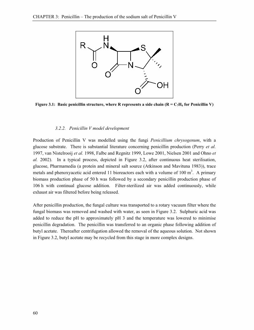
CHAPTER 3: Penicillin – The production of the sodium salt of Penicillin V
60
Figure 3.1: Basic penicillin structure, where R represents a side chain (R = C7H6 for Penicillin V)
3.2.2. Penicillin V model development Production of Penicillin V was modelled using the fungi Penicillium chrysogenum, with a glucose substrate. There is substantial literature concerning penicillin production (Perry et al. 1997, van Nistelrooij et al. 1998, Falbe and Regnitz 1999, Lowe 2001, Nielsen 2001 and Ohno et al. 2002). In a typical process, depicted in Figure 3.2, after continuous heat sterilisation, glucose, Pharmamedia (a protein and mineral salt source (Atkinson and Mavituna 1983)), trace metals and phenoxyacetic acid entered 11 bioreactors each with a volume of 100 m3. A primary biomass production phase of 50 h was followed by a secondary penicillin production phase of 106 h with continual glucose addition. Filter-sterilized air was added continuously, while exhaust air was filtered before being released. After penicillin production, the fungal culture was transported to a rotary vacuum filter where the fungal biomass was removed and washed with water, as seen in Figure 3.2. Sulphuric acid was added to reduce the pH to approximately pH 3 and the temperature was lowered to minimise penicillin degradation. The penicillin was transferred to an organic phase following addition of butyl acetate. Thereafter centrifugation allowed the removal of the aqueous solution. Not shown in Figure 3.2, butyl acetate may be recycled from this stage in more complex designs.

CHAPTER 3: Penicillin – The production of the sodium salt of Penicillin V
61
Figure 3.2: Simplified process flowsheet for penicillin V sodium salt production as modelled in the MS-Excel model (simplified from Biwer et al. 2005 and Heinzle et al. 2006)
Sodium acetate, acetone and water were added to the penicillin V solution for its re-extraction into the acetone/water phase and subsequent precipitation as crystals of the sodium salt. These were washed, separated in a basket centrifuge and air-dried in a fluidised bed dryer. The wash solution from the basket centrifuge as well as the previous centrifugal extraction wastewater was neutralised with sodium hydroxide before being discharged to effluent treatment. In a more optimum system, it may be possible to recycle sodium acetate or acetone and allow for water re-use. Parameters used in the generic flowsheet were estimated from the literature (Table 3.1). From these, three scenarios have been presented. Each contained progressively less input from the initial full list (Scenario 1). For many processes, not all inputs are available, hence successive scenarios (Scenario 2 and Scenario 3) assumed that the less accessible and more sensitive inputs were missing and the defaults as explained in Chapter 2 were used. Scenarios 2 and 3 used approximately 45 % and 30 % of the original information respectively. The lists of inputs used for the three scenarios are shown in Table 3.2.

CHAPTER 3: Penicillin – The production of the sodium salt of Penicillin V
62
Table 3.1: Literature yield coefficients for the production of penicillin V
Yield coefficients Value Units
Biomass yield on Pharmamedia YX/Pharmamedia 2.14 g/g
Biomass yield on glucose YX/glucose 0.45 g/g
Penicillin yield on glucose Ypenicillin/glucose 0.81 g/g
Penicillin yield on phenoxyacetic acid Ypenicillin/phenoxyacetic acid 2.00 g/g
Biomass yield on oxygen YX/O2 1.56 g/g
Maintenance coefficient mglucose 0.022 g glucose/g dcw h
Maintenance coefficient mO2 0.023 g O2/g dcw h
References:
Perry et al. (1997), van Nistelrooij et al. (1998), Falbe and Regnitz (1999), Lowe (2001), Nielsen (2001) and Ohno et al. (2002)
Table 3.2: Sets of input values collated from Biwer et al. (2005) and Heinzle et al. (2006) for the extracellular, aerobic production of penicillin in a batch reactor
Assumptions Scenario 1 Scenario 2 Scenario 3 Units
Cooling water temperature 5 [18] [18] °C
Steam Sterilisation (140°C, 3 bar)
Reactor temperature 32 [37] [37] °C
Microbial growth conditions (batch production of Penicillin from Penicillium chrysogenum)
Product: Biomass ratio 1.2 1.2 1.2 -
Carbon 1 source (excess): Glucose 2 [1] [1] %
Carbon 2 source (excess): Phenoxyacetic acid 1.7 [1] [1] %
Mass percentage of carbon source 2 as total carbon 10.6 10.6 10.6 %
Nitrogen source (excess): Pharmamedia (C55.7H6.7O18.9N16S2.7 (Phyllis 2006)) 15 [5] [5] %
Sulphur source excess 0 [5] [5]
Oxygen source (vvm): Air 0.021 (excluding
excess)
[10x the min. stoich.
requirement]
[10x the min. stoich.
requirement]
Compression: Single stage reciprocating compressor, 607.95 kPa compression pressure
Maintenance coefficient 0.022* 0.022 0.022 h
Time for over which maintenance is considered 106 106 [10] h
Final biomass concentration 45 45 [16.7] g/l
Yield coefficients: Yx/s 0.45* [0.43] [0.43] g/g
Yp/s 0.81* [0.64] [0.64] g/g
Yx/o 1.56* [1.35] [1.35] g/g
Agitation (11 tanks) (Energy: Electricity)
Power per unit volume 2.5 2.5 [0.083] kW/m3
Efficiency 1 [0.9] [0.9]

CHAPTER 3: Penicillin – Results
63
Assumptions Scenario 1 Scenario 2 Scenario 3 Units
Post bioreactor cooling
Outlet temperature 28 [15] [15] °C
Filtration (Energy: Electricity)
Solid fraction removed 100 [95] [95] %
Liquid fraction retained 91 91 [70] %
Additive: Sulphuric acid 0.028 0.028 0.028 %v/v
Centrifugation (Energy: Electricity)
Product fraction retained 98 [99] [99] %
Waste fraction removed 91.8 91.8 [95] %
Energy per unit volume 3060 [6420] [6420] kJ/m3
Additive: Butyl acetate (assume no recycle) 9.1 9.1 9.1 %v/v
Precipitation and Crystallisation (Energy: Electricity and steam)
Outlet temperature 6 [40] [40] °C
Residence time 12 [2] [2] h
Power per unit volume 0.6 [0.8] [0.8] kW/m3
Additive: Acetone 12.3 12.3 12.3 %v/v
Additive: Sodium acetate 7.8 7.8 7.8 %v/v
Reaction: Sodium acetate + Penicillin Acetic acid + Penicillin V sodium crystals (conversion: 97 % limiting reagent)
Centrifugation (Energy: Electricity)
Solid fraction retained 99 [98] [98] %
Liquid fraction removed 97.9 [80] [80] %
Fluid bed drying (Electricity: 72.2 MJ/m3)
Product fraction retained 99 [99] [99] %
Liquid fraction removed 90 [98] [98] %
Waste water treatment
Additive: Sodium hydroxide 0.25 0.25 0.25 %v/v
* Values available from literature and not specific to this flowsheet design [ ] Default values calculated or assumed in the MS-Excel model when no explicit inputs are given
3.3. Results
3.3.1. Material and energy balance outputs From the generic flowsheet model, the material and total energy (renewable and non-reneawble) requirements calculated are shown in Table 3.3 and Table 3.4. For Scenario 1, for each kilogram of the sodium salt of Penicillin V produced, 5.18 kg of glucose, 1.30 kg of Pharmamedia and
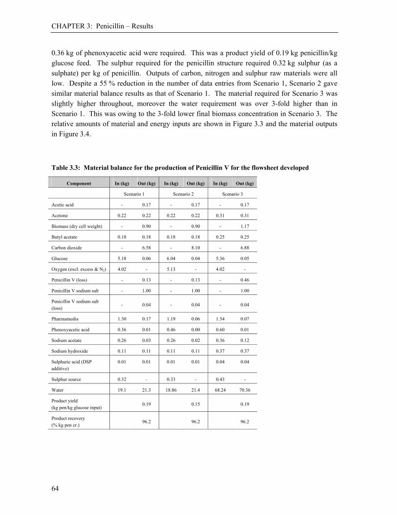
CHAPTER 3: Penicillin – Results
64
0.36 kg of phenoxyacetic acid were required. This was a product yield of 0.19 kg penicillin/kg glucose feed. The sulphur required for the penicillin structure required 0.32 kg sulphur (as a sulphate) per kg of penicillin. Outputs of carbon, nitrogen and sulphur raw materials were all low. Despite a 55 % reduction in the number of data entries from Scenario 1, Scenario 2 gave similar material balance results as that of Scenario 1. The material required for Scenario 3 was slightly higher throughout, moreover the water requirement was over 3-fold higher than in Scenario 1. This was owing to the 3-fold lower final biomass concentration in Scenario 3. The relative amounts of material and energy inputs are shown in Figure 3.3 and the material outputs in Figure 3.4.
Table 3.3: Material balance for the production of Penicillin V for the flowsheet developed
Component In (kg) Out (kg) In (kg) Out (kg) In (kg) Out (kg)
Scenario 1 Scenario 2 Scenario 3
Acetic acid - 0.17 - 0.17 - 0.17
Acetone 0.22 0.22 0.22 0.22 0.31 0.31
Biomass (dry cell weight) - 0.90 - 0.90 - 1.17
Butyl acetate 0.18 0.18 0.18 0.18 0.25 0.25
Carbon dioxide - 6.58 - 8.10 - 6.88
Glucose 5.18 0.06 6.04 0.04 5.36 0.05
Oxygen (excl. excess & N2) 4.02 - 5.13 - 4.02 -
Penicillin V (loss) - 0.13 - 0.13 - 0.46
Penicillin V sodium salt - 1.00 - 1.00 - 1.00
Penicillin V sodium salt (loss)
- 0.04 - 0.04 - 0.04
Pharmamedia 1.30 0.17 1.19 0.06 1.54 0.07
Phenoxyacetic acid 0.36 0.01 0.46 0.00 0.60 0.01
Sodium acetate 0.26 0.03 0.26 0.02 0.36 0.12
Sodium hydroxide 0.11 0.11 0.11 0.11 0.37 0.37
Sulphuric acid (DSP additive)
0.01 0.01 0.01 0.01 0.04 0.04
Sulphur source 0.32 - 0.33 - 0.43 -
Water 19.1 21.3 18.86 21.4 68.24 70.36
Product yield
(kg pen/kg glucose input)
0.19 0.15 0.19
Product recovery (% kg pen cr.)
96.2 96.2 96.2

CHAPTER 3: Penicillin – Results
65
Table 3.4: Energy and utility flows for the production of Penicillin V for the flowsheet developed
Energy requirements Scenario 1 Scenario 2 Scenario 3 Units
Electricity 22.0 (79.12)
22.9 (82.37)
29.9 (107.8)
kWh/kg pen. (MJ/kg pen)
Steam (140°C, 3 bar) 3.3 (8.91)
3.4 (9.18)
10.1 (27.3)
kg/kg pen. (MJ/kg pen)
Total energy equivalent 88.03 91.55 135.1 MJ/kg penicillin
Chilled water 0.86 1.41 1.55 m3/kg penicillin
Figure 3.3: Comparison of material, energy and utility inputs from the generic model for Penicillin V sodium salt production, relative to Scenario 1
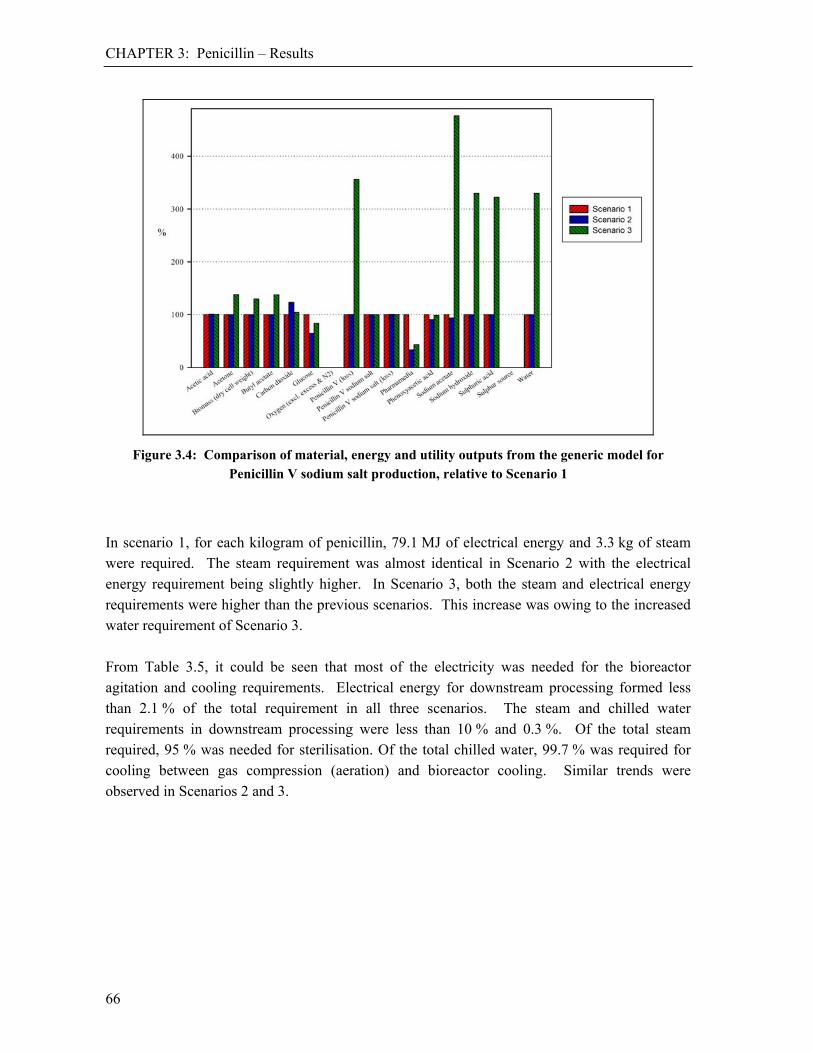
CHAPTER 3: Penicillin – Results
66
Figure 3.4: Comparison of material, energy and utility outputs from the generic model for Penicillin V sodium salt production, relative to Scenario 1
In scenario 1, for each kilogram of penicillin, 79.1 MJ of electrical energy and 3.3 kg of steam were required. The steam requirement was almost identical in Scenario 2 with the electrical energy requirement being slightly higher. In Scenario 3, both the steam and electrical energy requirements were higher than the previous scenarios. This increase was owing to the increased water requirement of Scenario 3. From Table 3.5, it could be seen that most of the electricity was needed for the bioreactor agitation and cooling requirements. Electrical energy for downstream processing formed less than 2.1 % of the total requirement in all three scenarios. The steam and chilled water requirements in downstream processing were less than 10 % and 0.3 %. Of the total steam required, 95 % was needed for sterilisation. Of the total chilled water, 99.7 % was required for cooling between gas compression (aeration) and bioreactor cooling. Similar trends were observed in Scenarios 2 and 3.
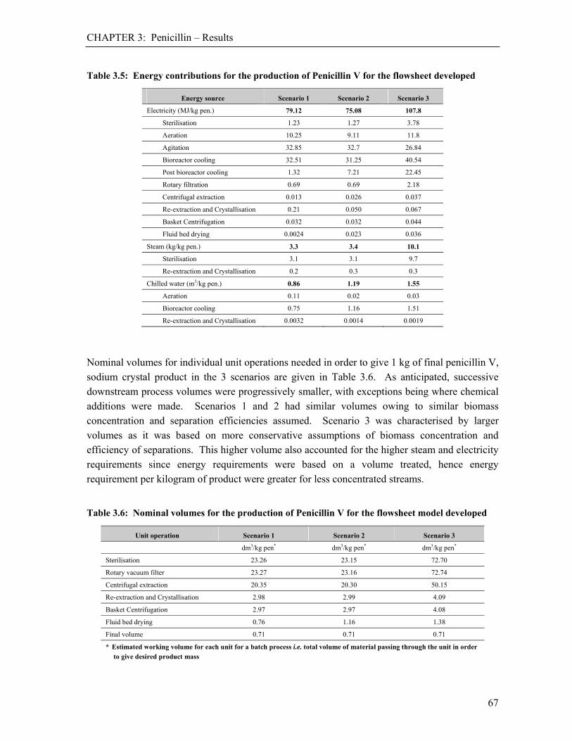
CHAPTER 3: Penicillin – Results
67
Table 3.5: Energy contributions for the production of Penicillin V for the flowsheet developed
Energy source Scenario 1 Scenario 2 Scenario 3
Electricity (MJ/kg pen.) 79.12 75.08 107.8
Sterilisation 1.23 1.27 3.78
Aeration 10.25 9.11 11.8
Agitation 32.85 32.7 26.84
Bioreactor cooling 32.51 31.25 40.54
Post bioreactor cooling 1.32 7.21 22.45
Rotary filtration 0.69 0.69 2.18
Centrifugal extraction 0.013 0.026 0.037
Re-extraction and Crystallisation 0.21 0.050 0.067
Basket Centrifugation 0.032 0.032 0.044
Fluid bed drying 0.0024 0.023 0.036
Steam (kg/kg pen.) 3.3 3.4 10.1
Sterilisation 3.1 3.1 9.7
Re-extraction and Crystallisation 0.2 0.3 0.3
Chilled water (m3/kg pen.) 0.86 1.19 1.55
Aeration 0.11 0.02 0.03
Bioreactor cooling 0.75 1.16 1.51
Re-extraction and Crystallisation 0.0032 0.0014 0.0019
Nominal volumes for individual unit operations needed in order to give 1 kg of final penicillin V, sodium crystal product in the 3 scenarios are given in Table 3.6. As anticipated, successive downstream process volumes were progressively smaller, with exceptions being where chemical additions were made. Scenarios 1 and 2 had similar volumes owing to similar biomass concentration and separation efficiencies assumed. Scenario 3 was characterised by larger volumes as it was based on more conservative assumptions of biomass concentration and efficiency of separations. This higher volume also accounted for the higher steam and electricity requirements since energy requirements were based on a volume treated, hence energy requirement per kilogram of product were greater for less concentrated streams.
Table 3.6: Nominal volumes for the production of Penicillin V for the flowsheet model developed
Unit operation Scenario 1 Scenario 2 Scenario 3
dm3/kg pen* dm3/kg pen* dm3/kg pen*
Sterilisation 23.26 23.15 72.70
Rotary vacuum filter 23.27 23.16 72.74
Centrifugal extraction 20.35 20.30 50.15
Re-extraction and Crystallisation 2.98 2.99 4.09
Basket Centrifugation 2.97 2.97 4.08
Fluid bed drying 0.76 1.16 1.38
Final volume 0.71 0.71 0.71
* Estimated working volume for each unit for a batch process i.e. total volume of material passing through the unit in order to give desired product mass

CHAPTER 3: Penicillin – Life Cycle Assessment (LCA)
68
3.4. Life Cycle Assessment (LCA)
3.4.1. Goal definition and system description The Life Cycle Assessment of the different penicillin production models was performed using the methodology explained in Section A.6. of Appendix A. The systems were defined as cradle-to-factory gate production of penicillin, including all raw material and agricultural inputs. A functional unit of 1 kg of crude sodium salt of Penicillin V, at a purity of 99 %, was used. Wherever possible, the Ecoinvent v1.3 inventory dataset was used in the LCA. Where this was not possible, the ETH-ESU (Oxygen) or BUWAL 250 (Pharmamedia) inventories were used. A South African electricity mix, with a high coal dependence, was used in the LCA. It was assumed that the glucose requirements of penicillin production were met by sugar, modelled using the South African sugar cane data as defined in Appendix G. All air, water and solid waste emissions from penicillin production have been included in the Life Cycle Assessment. Waste water treatment (WWT) was not included in any of the LCA studies. Complete sets of life cycle inventory data are presented in Appendix I. The Life Cycle Impact Assessment results are presented in Section 3.4.2. In the discussion that follows, the material and energy balance results are compared to the results from a full penicillin design as obtained from literature in Section 3.5.1. These material and energy flows are used in the LCA software and impacts compared to the generic flowsheet model LCA impacts in Section 3.5.2. The major process contributions to the LCA scores are presented and discussed in Section 3.5.3.
3.4.2. Life Cycle Analysis Using the material and energy balance results from Scenario 1, and the SimaPro LCA software, for 1 kg of Penicillin V produced, life cycle impacts of 25.5 kg CO2 eq., 0.227 kg Sb eq., 1.62 mg CFC-11 eq. and 0.254 kg SO2 eq., were obtained in the categories of global warming, abiotic depletion, ozone layer depletion and acidification respectively as shown in Table 3.7. The LCA results for the same categories for Scenario 2 were: 27.9 kg CO2 eq., 0.241 kg Sb eq., 1.78 mg CFC-11 eq. and 0.259 kg SO2 eq.. These values were all within 10 % of those calculated from Scenario 1, as were photochemical oxidation and all toxicities except terrestrial ecotoxicity, as can be seen in Figure 3.5. Impacts from Scenario 3 were all higher than those obtained in both Scenarios 1 and 2. More raw materials were required and emissions produced were higher throughout owing to less effective downstream processing and a lower final biomass concentration. With higher volumes

CHAPTER 3: Penicillin – Life Cycle Assessment (LCA)
69
in Scenario 3, the amount of water needed was much higher. To date water requirements are not reflected in life cycle impact analysis approaches explicitly. The larger volume of water increased the steam required in the sterilisation and the energy required in agitation, resulting in the highest energy need of all scenarios.
Table 3.7: LCIA of Penicillin V per kilogram of product – CML Baseline 2000 V2.03
Impact Category Unit Scenario 1 Scenario 2 Scenario 3
Abiotic Depletion kg Sbeq. 0.227 0.241 0.324
Global Warming (GWP100) kg CO2 eq. 25.5 27.9 35.1
Ozone Layer Depletion (ODP) mg CFC-11eq. 1.62 1.78 2.31
Human Toxicity kg 1,4-DBeq. 10.9 11.6 15.2
Fresh Water Aquatic Ecotoxicity kg 1,4-DBeq. 2.56 2.72 3.55
Marine Aquatic Ecotoxicity kg 1,4-DBeq. 16000 17100 22000
Terrestrial Ecotoxicity kg 1,4-DBeq. 0.0533 0.0610 0.0861
Photochemical Oxidation kg C2H4 0.00891 0.00952 0.0124
Acidification kg SO2 eq. 0.254 0.272 0.348
Eutrophication kg PO43-
eq. 0.0243 0.0259 0.0306
Figure 3.5: Comparison of LCA results for Penicillin V sodium salt production for Scenarios 2 and 3 relative to Scenario 1
CHAPTER 3: Penicillin – Discussion
70
3.5. Discussion
3.5.1. Comparison with a full penicillin design To compare the validity of the scenarios developed, the material and energy balance results were compared to a Penicillin V model presented by Biwer et al. (2005) and Heinzle et al. (2006). This was the most complete and technologically relevant analysis available in the open literature. The model was constructed using the process flowsheeting package SuperPro Designer v5.1 (Intelligen 2008) to provide material and energy balances as well as economic costing for a base case scenario. The model included design considerations reported by Perry et al. (1997), van Nistelrooij et al. (1998), Falbe and Regnitz (1999), Lowe (2001) and Ohno et al. (2002). The comparison on the basis of 1 kg penicillin V sodium salt is summarised in Table 3.8. The amount of Pharmamedia used in the generic flowsheet scenarios was higher (2.5 – 3 fold) than that for Biwer et al. (2005) and Heinzle et al. (2006); the latter was based on industrial norms and not calculation (Biwer 2006). The amount of glucose and phenoxyacetic acid was at most 18 % higher and 40 % lower respectively than the Biwer et al. (2005) and Heinzle et al. (2006) values. The amount of oxygen reported was the amount used and excludes the excess, since this was the value reported by Heinzle et al. (2006). The generic flowsheet model values were approximately 60 % higher than the literature. For each kilogram of penicillin produced, approximately 19 kg of process water was required for Scenarios 1 and 2. This showed good agreement with the amount of water shown to be required in the work of Heinzle et al. (2006). This was less than a third of the water required for Scenario 3. This was owing to poor assumptions resulting in a large reactor volume and the additional water requirement. The amount of steam predicted by the MS-Excel model was higher (3 – 8 fold) in all 3 scenarios, but electricity was lower (approximately 0.9 fold) as shown in Figure 3.6. This was a result of steam sterilisation in the generic flowsheet models versus heat sterilisation, by electricity, in the Heinzle et al. (2006) model. The total energy equivalent of Scenarios 1 and 2 were comparable (88.03- and 91.55 vs. 86.38 kWh/kg penicillin respectively) to the Heinzle et al. (2006) value, while Scenario 3 gave values approximately 60 % higher. Butyl acetate requirements were reduced to 43 % and acetone requirements increased by 3 fold because of simplifications on a recycle stream. Other inputs and outputs in Scenarios 1 and 2 were within 10 % of the Heinzle et al. (2006) values. Certain of the large differences seen in the material outputs of Scenario 3, compared to the literature values as shown in Figure 3.7, were for materials of low mass (e.g. sodium hydroxide and Penicillin V). The small changes in these absolute values resulted in large relative differences shown on the bar graph.
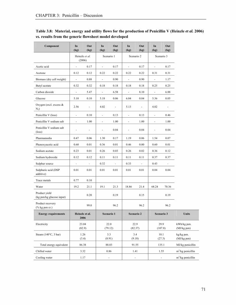
CHAPTER 3: Penicillin – Discussion
71
Table 3.8: Material, energy and utility flows for the production of Penicillin V (Heinzle et al. 2006) vs. results from the generic flowsheet model developed
Component In (kg)
Out (kg)
In (kg)
Out (kg)
In (kg)
Out (kg)
In (kg)
Out (kg)
Heinzle et al. (2006)
Scenario 1 Scenario 2 Scenario 3
Acetic acid - 0.17 - 0.17 - 0.17 - 0.17
Acetone 0.12 0.12 0.22 0.22 0.22 0.22 0.31 0.31
Biomass (dry cell weight) - 0.88 - 0.90 - 0.90 - 1.17
Butyl acetate 0.32 0.32 0.18 0.18 0.18 0.18 0.25 0.25
Carbon dioxide - 5.47 - 6.58 - 8.10 - 6.88
Glucose 5.10 0.10 5.18 0.06 6.04 0.04 5.36 0.05
Oxygen (excl. excess & N2)
2.56 - 4.02 - 5.13 - 4.02 -
Penicillin V (loss) - 0.10 - 0.13 - 0.13 - 0.46
Penicillin V sodium salt - 1.00 - 1.00 - 1.00 - 1.00
Penicillin V sodium salt
(loss) - - - 0.04 - 0.04 - 0.04
Pharmamedia 0.47 0.06 1.30 0.17 1.19 0.06 1.54 0.07
Phenoxyacetic acid 0.60 0.01 0.36 0.01 0.46 0.00 0.60 0.01
Sodium acetate 0.23 0.01 0.26 0.03 0.26 0.02 0.36 0.12
Sodium hydroxide 0.12 0.12 0.11 0.11 0.11 0.11 0.37 0.37
Sulphur source - - 0.32 - 0.33 - 0.43 -
Sulphuric acid (DSP additive)
0.01 0.01 0.01 0.01 0.01 0.01 0.04 0.04
Trace metals 0.77 0.10
Water 19.2 21.1 19.1 21.3 18.86 21.4 68.24 70.36
Product yield (kg pen/kg glucose input)
0.20 0.19 0.15 0.19
Product recovery (% kg pen cr.)
99.0 96.2 96.2 96.2
Energy requirements Heinzle et al. 2006
Scenario 1 Scenario 2 Scenario 3 Units
Electricity 23.04
(82.9)
22.0
(79.12)
22.9
(82.37)
29.9
(107.8)
kWh/kg pen.
(MJ/kg pen)
Steam (140°C, 3 bar) 1.26 (3.4)
3.3 (8.91)
3.4 (9.18)
10.1 (27.3)
kg/kg pen. (MJ/kg pen)
Total energy equivalent 86.38 88.03 91.55 135.1 MJ/kg penicillin
Chilled water 3.32 0.86 1.41 1.55 m3/kg penicillin
Cooling water 1.17 - - - m3/kg penicillin
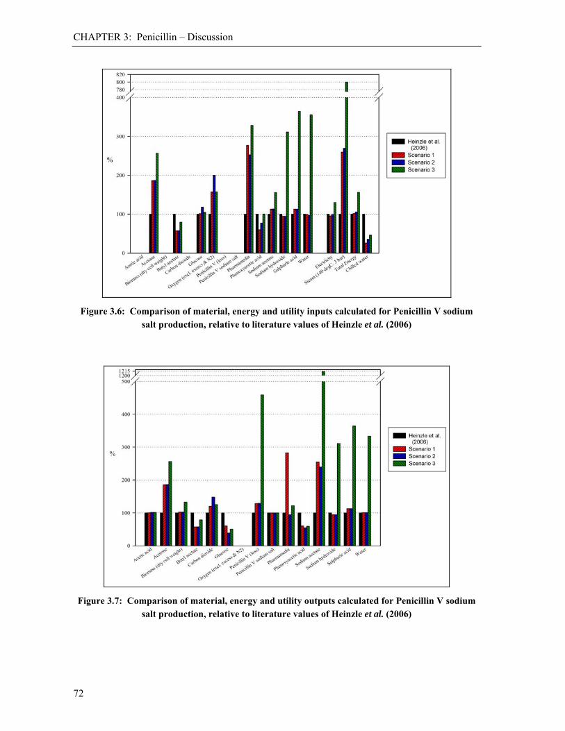
CHAPTER 3: Penicillin – Discussion
72
Figure 3.6: Comparison of material, energy and utility inputs calculated for Penicillin V sodium salt production, relative to literature values of Heinzle et al. (2006)
Figure 3.7: Comparison of material, energy and utility outputs calculated for Penicillin V sodium salt production, relative to literature values of Heinzle et al. (2006)

CHAPTER 3: Penicillin – Discussion
73
3.5.2. Life Cycle Impact Assessment (LCIA) The Life Cycle Impact Assessment (LCIA) across the detailed model of Biwer et al. (2005) and Heinzle et al. (2006) and Scenarios 1 to 3 are presented in Table 3.9 and Figure 3.8. Scenarios 1 and 2 were within 10 % of the LCA values using the data of Biwer et al. (2005) and Heinzle et al. (2006) across all categories except for terrestrial ecotoxicity (16 % lower) and eutrophication (17 % higher). LCA impacts for Scenario 1 were lower than those in the Biwer et al. (2005) and Heinzle et al. (2006) model for all categories except global warming, ozone layer depletion and eutrophication as seen in Figure 3.8. Prediction of eutrophication was higher in the MS-Excel scenarios owing to the higher usages of Pharmamedia and glucose, both produced from agricultural crops. The higher toxicity scores, particularly terrestrial ecotoxicity, in the results of Biwer et al. (2005) and Heinzle et al. (2006) were owing to greater emissions resulting from the higher phenoxyacetic acid and electricity requirements.
Table 3.9: LCIA of penicillin per kilogram of Penicillin V sodium salt product – CML 2 baseline 2000 V2.03
Impact Category Unit Heinzle et al. (2006) Scenario 1 Scenario 2 Scenario 3
Abiotic Depletion kg Sbeq. 0.232 0.227 0.241 0.324
Global Warming (GWP100) kg CO2 eq. 24.3 25.5 27.9 35.1
Ozone Layer Depletion (ODP) mg CFC-11eq. 1.64 1.62 1.78 2.31
Human Toxicity kg 1, 4-DBeq. 11.4 10.9 11.6 15.2
Fresh Water Aquatic Ecotoxicity kg 1, 4-DBeq. 2.67 2.56 2.72 3.55
Marine Aquatic Ecotoxicity kg 1, 4-DBeq. 16700 16000 17100 22000
Terrestrial Ecotoxicity kg 1, 4-DBeq. 0.0646 0.0533 0.0610 0.0861
Photochemical Oxidation kg C2H4 0.00921 0.00891 0.00952 0.0124
Acidification kg SO2 eq. 0.253 0.254 0.272 0.348
Eutrophication kg PO43-
eq. 0.0212 0.0243 0.0259 0.0306
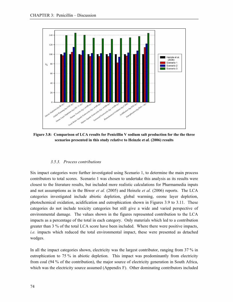
CHAPTER 3: Penicillin – Discussion
74
Figure 3.8: Comparison of LCA results for Penicillin V sodium salt production for the the three scenarios presented in this study relative to Heinzle et al. (2006) results
3.5.3. Process contributions Six impact categories were further investigated using Scenario 1, to determine the main process contributors to total scores. Scenario 1 was chosen to undertake this analysis as its results were closest to the literature results, but included more realistic calculations for Pharmamedia inputs and not assumptions as in the Biwer et al. (2005) and Heinzle et al. (2006) reports. The LCA categories investigated include abiotic depletion, global warming, ozone layer depletion, photochemical oxidation, acidification and eutrophication shown in Figures 3.9 to 3.11. These categories do not include toxicity categories but still give a wide and varied perspective of environmental damage. The values shown in the figures represented contribution to the LCA impacts as a percentage of the total in each category. Only materials which led to a contribution greater than 3 % of the total LCA score have been included. Where there were positive impacts, i.e. impacts which reduced the total environmental impact, these were presented as detached wedges. In all the impact categories shown, electricity was the largest contributor, ranging from 37 % in eutrophication to 75 % in abiotic depletion. This impact was predominantly from electricity from coal (94 % of the contribution), the major source of electricity generation in South Africa, which was the electricity source assumed (Appendix F). Other dominating contributors included

CHAPTER 3: Penicillin – Discussion
75
glucose, phenoxyacetic acid, Pharmamedia, acetone and sodium acetate. Steam, assumed to be raised by natural gas burning, did not play a large part in the LCA categories.
Figure 3.9: Life Cycle Assessment process contributions of penicillin production (Scenario 1) using the CML Baseline 2.03 methodology (Abiotic depletion and Global warming)
Abiotic depletion was dominated by the contribution of electricity (75 %, most from coal) and smaller portions by phenoxyacetic acid (7.5 %), Pharmamedia, acetone and sodium acetate (all 3 %). Global warming impacts were made up of similar contributors, although electricity to a lesser extent of 61 % as seen in Figure 3.9. LCA results for glucose were based on its production from sugar made from sugarcane. Data were taken from South African values as this was the most accurate LCA data available. The assumptions and calculations are presented in Appendix G. Carbon dioxide uptake was taken into account in the growth of sugarcane, resulting in a positive impact (negative value) on the global warming score. Since bio-based carbon in the final product has been deducted, it is unlikely that the ranking would change if incineration were chosen, since comparable amounts of CO2 would be released as a consequence.

CHAPTER 3: Penicillin – Discussion
76
* Note: Ozone layer depletion is of reduced importance in current processes (see Appendix A.6)
Figure 3.10: Life Cycle Assessment process contributions of penicillin production (Scenario 1) using the CML Baseline 2.03 methodology (Ozone layer depletion and Photochemical oxidation
warming)
The process contributors to ozone layer depletion score were spread more representatively owing to the contribution from intensive agriculture. Together with electricity (37 %), oxygen, Pharmamedia and phenoxyacetic acid each contributed over 10 %. In the photochemical oxidation score, electricity (73 %) dominated. Glucose (7 %), phenoxyacetic acid (5 %) and sodium acetate (4 %) had little impact as shown in Figure 3.10.
Figure 3.11: Life Cycle Assessment process contributions of penicillin production (Scenario 1) using the CML Baseline 2.03 methodology (Acidification and Eutrophication)

CHAPTER 3: Penicillin – Conclusions
77
For acidification, the relative contributions of electricity, glucose and phenoxyacetic acid were similar to photochemical oxidation as seen in Figure 3.11. Glucose, and in turn, sugar, sugarcane and fertilisers for the agriculture, contributed 32 % of the eutrophication score. Pharmamedia, modelled as protein from corn, was also a large fraction of the score (20 %) due to fertiliser requirements.
3.6. Conclusions The generic MS-Excel model was used to obtain material and energy balance data of a flowsheet for the production of Penicillin V sodium salt using a limited set of input data typically available at an early stage in process design. Where a maximum set of input data was used to inform the MS-Excel model, 50 % of the material and energy balance results were within 20 % of those of Biwer et al. (2005) and Heinzle et al. (2006), which was based on a detailed flowsheet design and industry values. When using a minimal set of inputs, 50 % of the material and energy balance results were within 55 % of the literature values. This illustrated that even when limited sets of inputs were available, order of magnitude results could be obtained. Pharmamedia and phenoxyacetic acid inputs differed as the analysis of Biwer et al. (2005) and Heinzle et al. (2006) assumed industrial norms, while in the MS-Excel model presented, the required amount was calculated from stoichiometric ratios. Glucose, sodium acetate, sodium hydroxide, sulphuric acid, water and electricity requirements were all within 20 % of literature results. Pharmamedia and steam requirements were at least 2.5 times higher for the two flowsheets with the most detailed sets of inputs (i.e. Scenarios 1 and 2). The material and energy balance data generated were used to complete a Life Cycle Assessment (LCA) study. The results of the LCA study showed good agreement between the material and energy balances in Scenarios 1 and 2 compared to the literature flowsheet provided by Biwer et al. (2005) and Heinzle et al. (2006), illustrating the appropriateness of the flowsheet model in providing early design stage data. Using the model, with only 45 % of the input dataset (Scenario 2), provided a material and energy dataset and LCA results that represented more rigorous models (e.g. Scenario 1). Deviations in Scenario 3 showed a sensitivity to critical inputs, especially those which affected the system volume. An increase in the bioreactor volume impacted the system with respect to energy and losses throughout. An analysis of the process contributions to environmental burden, targeted electricity provision and the provision for agricultural inputs as key items. Electricity requirements were over 60 % in each of abiotic depletion, global warming potential and photochemical oxidation, with the next largest process contribution in these categories represented less than 10 % of the LCA

CHAPTER 3: Penicillin – References
78
scores. While the electrical requirements still formed the largest single contribution to LCA scores in ozone layer depletion and eutrophication (37 % in each), the combined impacts from agriculture (sugar, Pharmamedia and phenoxyacetic acid) were 35.5 and 53 % respectively. Thus, decreases in electrical energy and agricultural inputs would have the greatest impact in reducing overall LCA scores. In summary:
- the model was appropriate if critical data was provided;
- it provided key data for a life cycle assessment analysis; and - it provided significant insight into critical items contributing to environmental
burden.
References Atkinson, B. and Mavituna, F, 1983. Biochemical Engineering and Biotechnology Handbook, Macmillan Inc., New
York. Bailey, J.E., Ollis, D.F., 1986. Biochemical Engineering Fundamentals, McGraw-Hill. Biwer, A., Griffith, S., Cooney, C., 2005. Uncertainty Analysis of Penicillin V Production Using Monte Carlo
Simulation, Biotechnol. Bioeng., 90(2), 167-179. Biwer, A., 2006. [email protected], Personal Communication. Falbe, J., Regnitz, M., 1999. Roempp Lexikon der Chemie, Vol. 10, CD-Rom, Stuttgart, Thieme. Heinzle, E., Biwer, A., Cooney, C., 2006. Penicillin V, In: Development of Sustainable Bioprocesses: Modelling
and Assessment, John Wiley & Sons, p193-210. Intelligen, 2008. Intelligen , Inc., Scotch Plain, NJ, USA, http://www.intelligen.com/ Lowe, D., 2001. Antibiotics, In: Basic Biotechnology, ed. C. Ratledge, B. Kristiansen, Cambridge, UK, Cambridge
University Press, p 349-375. Nielsen, J., 2001. Microbial process kinetics, In: Basic Biotechnology, ed. C. Ratledge, B. Kristiansen, Cambridge,
UK, Cambridge University Press, p 127-151. Ohno, M., Otsuka, M., Yagisawa, M. et al., 2002. Antibiotics, In: Ulmann’s encyclopaedia of industrial chemistry,
Weinheim, Wiley-VCH. Perry, R.H., Green, D.W, Maloney, J.O. (eds.), 1997. Perry’s Chemical Engineers’ Handbook, 7th edition,
McGraw-Hill, International edition. Phyllis 2006. Phyllis (database) - the composition of biomass and waste, ECN-Biomass, Energy Research Centre of
the Netherlands, http://www.ecn.nl/phyllis/ PRé Consultants B.V., 2008. Plotterweg 12, 3821 BB Amersfoort, The Netherlands http://www.pre.nl/ van Nistelrooij, H., Krikgsman, J., de Vroom, E., Oldenhof, C., 1998. Penicillin update: Industrial. In: Penicillin: a
paradigm for biotechnology, ed. R. Maltes, Chicago, Candida, p 95-102.

79
CHAPTER 4: CELLULASE

80

CHAPTER 4: Cellulase – Introduction
81
4.1. Introduction The aims of this chapter are multi-fold. The case study is used for additional validation of the generic model by presenting material and energy balance results and comparing these to literature flowsheets. Once the relevance of the material and energy balance inventories were determined, the values were further analysed by a Life Cycle Assessment (LCA) study. The LCA analysis was used to determine the environmental impacts of the process as well as compare LCA results obtained from the literature material and energy balance inventories with those obtained from the generic flowsheet model. As the example in this chapter, cellulase production by three different methods is used. These flowsheets, as defined by Heinzle et al. (2006) and two by Zhuang et al. (2007), show different methods of producing the same product using:
- aerobic and anaerobic microorganisms;
- different bioreactor setups; and - different downstream processing units.
Using three different flowsheet models allows for a greater number of validation studies to be performed. Further, it allows for a comparison of the same product using different processing technologies. The individual process contributions to the total LCA scores were calculated and compared across the different flowsheets. These key contributing components helped to inform further studies in Chapter 7 on heuristics for bioprocess technology selection.
4.2. Cellulase – Its role and production process Bioconversion of biomass to biofuels such as bioethanol and biogas is receiving increasing attention owing to depletion of fossil fuels (Lynd 1996, Lynd et al. 2005, Zhang et al. 2007) as well as global warming issues associated with air emissions. To meet the biomass capacity for this, processing of woody biomass is desirable. This requires conversion of their cellulosic component into fermentable sugar using either hot acid hydrolysis or enzyme catalysis by cellulase (Rabinovich et al. 2002).

CHAPTER 4: Cellulase – Cellulase – Its role and production process
82
Cellulases, together with hemicellulases, accounted for approximately 20 % of the world enzyme market in 2000 (Bhat 2000). They are typically used in the food, animal feed, textile and pulp and paper industries. The aerobic fungus Trichoderma reesei (Himmel, et al. 1999, Sáez et al. 2002) is commonly used to produce cellulase. Anaerobic organisms such as Clostridium papyrosolvens and Clostridium thermocellum are also used. Common substrates for microbial cellulase production include cellulose and wood waste, such as bagasse, corn cobs and straw as shown in Table 4.1.
Table 4.1: Cellulase producing micro-organisms and common substrates reported in literature
Micro-organisms used Aerobic/ Anaerobic
Substrates for micro-organism growth* References
Aspergillus terreus Aerobic Bagasse, filter paper and carboxymethyl cellulose (CMC) El-Nawwi and El-Kader 1996
Cellulomonas biazotae (unknown) Bagasse, cotton stalks, Kallar grass-, Dhancha-, and wheat straw, cellobiose, carboxymethyl cellulose (CMC), cotton wool,
filter paper, xylan, -cellulose, Sigmacell-100, Atriplex
lentiformis and Panicum maximum
Rajoka and Malik 1997
Chaetomium erraticum (unknown) Carboxymethyl cellulose (CMC) Soni et al. 1999
Clostridium papyrosolvens Anaerobic Glucose, trehalose, cellobiose and lactose Thirumale et al. 2001
Clostridium thermocellum Anaerobic Cellulose, cellobiose, fructose, glucose, hemicellulose, laminaribiose, mannitol, sorbitol and xylose
Demain et al. 2005
Clostridium thermocellum Anaerobic Paper pulp Zhuang et al. 2007
Neurospora crassa Aerobic Wheat straw Romero et al. 1999
Phanerochaete chrysosporium
(formerly Sporotrichum
pulverulentum)
(unknown) Glucose, wood sticks Szabó et al. 1996
Phlebia gigantean (unknown) Glucose, microcrystalline cellulose, carboxymethyl cellulose (CMC) and cellobiose
Niranjane et al. 2007
Saccharomyces cerevisiae (recombinant)
Aerobic Phosphoric acid swollen cellulose (PASC) Den Haan et al. 2007
Trichoderma reesei Aerobic Willow Reczey et al. 1996
Trichoderma reesei Aerobic Wood chips Himmel, et al. 1999
Trichoderma reesei Aerobic Corn cob residue and lignocellulosic waste from xylose industry Xia and Cen 1999
Trichoderma reesei Aerobic Agricultural residues (bagasse, corn stover, rice, straw, wood chips), municipal solid waste
Wooley et al. 1999a
Trichoderma reesei Aerobic Glucose, commercial cellulose (Solka-floc) Sáez et al. 2002
Trichoderma reesei Aerobic Corn cob residues, purified cellulose, corn stover Liming and Xueliang 2004
Trichoderma reesei Aerobic Dairy manure Wen et al. 2005
* Carbon sources listed are used either individually, in combination or all at once

CHAPTER 4: Cellulase – Case study methodology
83
4.3. Case study methodology
4.3.1. Material and Energy balance Three different cellulase production models have been defined to validate the generic flowsheet model:
Flowsheet 1 used data from Heinzle et al. (2006) for aerobic submerged cultivation of Trichoderma reesei;
Flowsheet 2 used data from Zhuang et al. 2007 for anaerobic submerged fermentation of Clostridium thermocellumi; and
Flowsheet 3 used data from Zhuang et al. 2007 for anaerobic solid state cultivation of Clostridium thermocellumi.
Within each flowsheet model, three scenarios were presented, with progressively decreasing initial data. The results were validated against material and energy balance results presented in literature from detailed flowsheeting models which included experimental data. The Life Cycle Assessment (LCA) impacts were calculated and compared across all scenarios.
4.3.2. LCA goal definition and system description The LCA was carried out using the methodology presented in Appendix A.6. The systems were defined as the cradle-to-factory gate production of cellulase, including all raw material and agricultural inputs. The functional unit was defined as the amount of product which contains 1 kg cellulase. It was assumed that equal masses of enzymes have the same activity irrespective of the method of production. Where energy is reported, this is for the total renewable and non-renewable energy in the process. Where bio-based carbon is found in the final product this was deducted in the calculations. It is unlikely that the LCA impact would change if incineration were chosen, since comparable amounts of CO2 would be released as a consequence. The Ecoinvent v1.3 inventory dataset was used in the LCA with a South African electricity mix characterised by a high coal dependence. It was assumed that cellulose inputs were obtained from wood chips for Flowsheet One and from wood pulp in Flowsheets Two and Three. All air, water and solid waste emissions from cellulase production have been included in the Life Cycle Assessment. Waste water treatment (WWT) was not included in any of the LCA studies for cellulase. The life cycle inventory data are presented in Appendix I.

CHAPTER 4: Cellulase – Cellulase Flowsheet One: Aerobic production by SmF using
Trichoderma reesei
84
For all three cellulase flowsheets, the material and energy balance results are presented following the description of the generic flowsheet models and literature. Thereafter Life Cycle Impact Assessment results are given, followed by a discussion. The major process contributions to the LCA scores are presented and discussed.
4.4. Cellulase Flowsheet One: Aerobic production by SmF using Trichoderma reesei
4.4.1. Cellulase model development The first cellulase production model considered was an aerobic production by submerged cultivation, traditionally referred to as submerged fermentation (SmF) of the extracellular enzyme using Trichoderma reesei, based on the studies of Himmel et al. (1999), Wooley et al. (1999a and 1999b), Sáez et al. (2002) and Heinzle et al. (2006). Cellulose, corn liquor, ammonia and nutrients were used as raw materials. A three stage inoculum development required three seed bioreactors. All feed streams to these reactors were individually steam sterilised. Downstream processing was limited to a rotary vacuum filtration unit to remove biomass and an ultrafiltration unit which separated waste water with unreacted raw materials from the cellulase product stream (Figure 4.1). Key parameters are shown in Table 4.2, with typical values sourced from the literature. The submerged fermentation process is known to have a high water content. The first two flow sheets modelled in this study used a SmF approach while the third (presented in Section 4.6) used a solid state cultivation (SSC) process, in which a continuous water phase is absent.
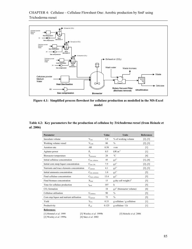
CHAPTER 4: Cellulase – Cellulase Flowsheet One: Aerobic production by SmF using
Trichoderma reesei
85
Figure 4.1: Simplified process flowsheet for cellulase production as modelled in the MS-Excel model
Table 4.2: Key parameters for the production of cellulase by Trichoderma reesei (from Heinzle et al. 2006)
Parameter Value Units References
Inoculum volume Vinoc 5.0 % of working volume [2], [3]
Working volume vessel Vwork 80 % [2], [3]
Aeration rate AR 0.58 vvm [1]
Agitator power Pa 0.5 kW.m-3 [1]
Bioreactor temperature Tbioreactor 28 °C [4]
Initial cellulose concentration Cinit, cellulose 45 g.l-1 [1], [4]
Initial corn steep liquor concentration Cinit, CSL 7.5 g.l-1 [2], [3]
Nutrients and trace elements concentration Cnutrient 4.1 g.l-1 [2], [3]
Initial ammonia concentration Cinit, ammonia 1.0 g.l-1 [5]
Final cellulase concentration Cfinal, cellulase 13.4 g.l-1 [5]
Final biomass concentration Xfinal 15 g dry cell weight.l-1 [5]
Time for cellulase production tprod 107 h [5]
CO2 formation 18 g.l-1 (bioreactor volume) [4]
Cellulose utilisation Ucellulose 90 % [5]
Corn step liquor and nutrient utilisation Unutrient 75 % [5]
Yield YP/S 0.33 g cellulase / g cellulose [1]
Productivity Pcell 0.125 g cellulase / l.h [1]
References:
[1] Himmel et al. 1999 [2] Wooley et al. 1999a
[3] Wooley et al. 1999b [4] Sáez et al. 2002
[5] Heinzle et al. 2006

CHAPTER 4: Cellulase – Cellulase Flowsheet One: Aerobic production by SmF using
Trichoderma reesei
86
Additional values required for the model were obtained from the cellulase production model of Heinzle et al. (2006). Three scenarios have been presented (Scenarios H1, H2 and H3). The first scenario (Scenario H1) assumed a full set of parameters shown in Table 4.2. Scenarios H2 and H3 used a subset of these inputs, omitting less accessible inputs. Defaults within the generic flowsheet model were used in these cases. Scenarios H2 and H3 used approximately 45 % and 30 % of the original information respectively. Corn liquor was assumed as a carbon source, although it is typically a nitrogen source, since ammonia and nutrients (trace elements needed by the system) were listed as nitrogen sources. The default power per unit volume for agitation and the cross sectional area for the rotary vacuum filtration were lower in Scenarios H2 and H3 owing to the first principle calculations and estimates used compared to actual values for the specific process as used in Scenario H1. The lists of inputs used for the three scenarios are shown in Table 4.3.
Table 4.3: Sets of input values collated from Heinzle et al. (2006) for the extracellular, aerobic production of cellulase in a batch reactor
Assumptions Scenario H1 Scenario H2 Scenario H3 Units
Cooling water temperature 25 [18] [18] °C
Chilled water temperature 5 [10] [10] °C
Max temp difference between exiting cooling water and hot inlet streams 10 [10] [10] °C
Steam Sterilisation (Cooling agent: Cooling water)
Preheated temperature 110 110 [60] °C
Sterilisation temperature 140 140 [121] °C
Steam temperature 152 152 [140] °C
Outlet temperature/Reactor temperature 35 [37] [37] °C
Microbial growth conditions (batch production of cellulase from Trichoderma reesei)
Product: Biomass ratio 0.89 0.89 [1] kg/kg
Carbon 1 source (excess): Cellulose 10 10 [1] %
Carbon 2 source (excess): Corn liquor 33.3 33.3 [1] %
Mass percentage Carbon 2 as total carbon 14.4 14.4 [50] -
Nitrogen 1 source (excess): Ammonia 0 [5] [5] %
Nitrogen 2 source (excess): Nutrients* 33.3 33.3 [5] %
Mass percentage Nitrogen 2 as total carbon 80.2 80.2 [50] -
Oxygen source (vvm): Air 0.58 0.58 [10x the min. stoich.
requirement]
Maintain reactor temperature (Cooling agent: Chilled water)
Yield coefficients: Yx/s [0.52] [0.52] [0.52] g/g
Yp/s 0.33* [0.56] [0.56] g/g
Yx/o [0.77] [0.77] [0.77] g/g

CHAPTER 4: Cellulase – Cellulase Flowsheet One: Aerobic production by SmF using
Trichoderma reesei
87
Assumptions Scenario H1 Scenario H2 Scenario H3 Units
Final biomass concentration 15.1 [16.7] [16.7] g/l
Agitation (Energy: Electricity)
No of tanks 1 [5] [5]
Height /Diameter (bioreactor) 3 [2] [2] -
Power per unit volume 0.5 0.5 [0.007] kW/m3
Aeration (Energy: Electricity)
Compressed pressure 608 [300] [300] kPa
Compressor efficiency 0.7 [0.65] [0.65] -
Rotary vacuum filter (Energy: Electricity)
Solids removed 100 100 [95] %
Liquid retained 100 100 [70] %
Cross sectional area 39.95 [0.037] [0.037] m2
Ultrafiltration (Energy: Electricity)
Solids (product) retained 98 98 [95] %
Liquid (waste) removed 81 81 [70] %
* Micro nutrients needed were modelled as an additional nitrogen source as they cannot be accounted for in any other manner # Values available from literature and not specific to this flowsheet design
[ ] Default data calculated or assumed in the MS-Excel model when no explicit inputs are given
4.4.2. Material and energy balance outputs From the model, the material and energy inventories obtained to produce 1 kg cellulase – containing product (i.e. product plus impurities) are shown in Table 4.4. From the scenarios developed, cellulase purities of 6.1, 6.7 and 4.7 % were obtained for Scenarios H1, H2 and H3 respectively, with the remainder largely being water. For Scenario H1, for 1 kg of cellulase (16.4 kg of product), 3.78 kg of cellulose, 0.77 kg of corn liquor, 0.52 kg of nutrients and 0.10 kg of ammonia were required. Energy requirements for Scenario H1 included 180 MJ electricity, 2.6 kg steam and 1.6 kg chilled water per kilogram of cellulase. Scenario H2 (14.9 kg of product) had similar material requirements as shown in Figure 4.2, but electrical energy needs were approximately halved. The electricity value of Scenario H3 was 70 % lower when compared to Scenario H1. As with Scenario H3 (21.2 kg of product), the reduction in electrical needs of Scenario H2 resulted from reduction in aeration pressure, the dominant contributor to the total electrical requirements at 74 % in Scenario H1. For Scenario H3, the material and energy inventory from the generic model showed large differences when compared to Scenarios H1 and H2. Ammonia, corn liquor and steam requirements were some 350, 450 and 250 % higher respectively. The high ammonia and corn liquor requirements resulted from the specifications for nitrogen source 2 and carbon source 2

CHAPTER 4: Cellulase – Cellulase Flowsheet One: Aerobic production by SmF using
Trichoderma reesei
88
respectively. The increase in the steam requirement (by mass) was a result of reduced heat integration with no preheating in steam sterilisation and lower steam quality. Cellulose and nutrient requirements were lower in Scenario H3 following definition of lower excesses and increased use of carbon source 2 and nitrogen source 2. As both the material inputs and the downstream separation efficiencies were similar, the outputs of Scenarios H1 and H2 were similar. In Scenario H3, poor downstream separation efficiencies led to the cellulase lost in wastewater being 25 times greater than previous scenarios. These poor separation efficiencies also led to larger volumes, aggravating the higher steam requirements. However, cellulose, corn liquor and nutrient outputs were lower in Scenario H3. As a lower excess was used, all other outputs were higher in Scenario H3 than Scenarios H1 and H2 as can be seen in Figure 4.3.
Table 4.4: Material, energy and utility flows for the production of cellulase (Heinzle et al. 2006b) vs. results from the generic flowsheet model developed (basis: 1 kg cellulase in the product stream)
Component In (kg)
Out (kg)
In (kg)
Out (kg)
In (kg)
Out (kg)
In (kg)
Out (kg)
Heinzle et al. (2006)
Scenario H1 Scenario H2 Scenario H3
Ammonia 0.082 0.00 0.10 0.00 0.10 0.00 0.27 0.01
Trichoderma reesei 0 1.17 0.07 1.22 0.07 1.22 0.09 1.52
Carbon dioxide - 1.48 - 4.00 - 4.00 - 5.91
Cellulase waste* - 0.04 - 0.02 - 0.02 - 0.50
Cellulose 3.62 0.32 3.78 0.28 3.47 0.28 2.81 0.02
Corn liquor 0.61 0.12 0.77 0.16 0.77 0.16 2.81 0.02
Product (enzyme) - 14.9 - 16.4 - 14.9 - 21.2
Nutrients 0.33 0.065 0.52 0.10 0.52 0.10 0.27 0.01
Oxygen (reacting O2 only) 0.81 - 3.21 - 3.21 - 5.10 -
Water 73.3 59.9 78.9 65.2 71.3 59.1 93.4 75.6
TOTAL 77.9 77.9 87.3 87.3 79.5 79.5 104.7 104.7
Product recovery (% kg cel.)
96.1 98.0 98.0 66.5
Chemical Oxygen Demand (COD)
N/A^ 2.91 2.59 3.01
Energy requirements Heinzle et al. 2006 Scenario H1 Scenario H2 Scenario H3 Units
Electricity 38.6 (139.0)
50.86 (183.1)
22.89 (82.4)
26.63 (95.88)
kWh/kg cel. (MJ/kg cel.)
Steam (152°C, 3 bar) 4.74 (12.8)
2.65 (7.14)
2.40 (6.47)
12.8** (34.6)
kg/kg cel. (MJ/kg cel)
Total energy equivalent 151.8 190.2 88.88 130.5 MJ/kg cellulase
Chilled water 0.84 1.60 1.60 1.38 m3/kg cellulase
Cooling water 2.62 - - - m3/kg cellulase
* Cellulase waste is non-recovered product lost in waste water **Steam at 140°C, 3 bar ^ Not available

CHAPTER 4: Cellulase – Cellulase Flowsheet One: Aerobic production by SmF using
Trichoderma reesei
89
Figure 4.2: Comparison of material, energy and utility inputs calculated for cellulase production,
relative to literature values of Heinzle et al. (2006)
Figure 4.3: Comparison of material, energy and utility outputs calculated for cellulase production, relative to literature values of Heinzle et al. (2006)

CHAPTER 4: Cellulase – Cellulase Flowsheet One: Aerobic production by SmF using
Trichoderma reesei
90
Comparing the results for Scenario H1 to the published data of Heinzle et al. (2006), the ammonia, cellulose and water requirements were in agreement (using the equivalent input data) within 18 %. Corn liquor inputs and electricity requirements were within 30 %, while nutrient requirements were 50 % higher in Scenario H1. The oxygen requirements were 4 fold higher in the modelled scenarios. However, the Heinzle et al. (2006) oxygen data is questioned as the study made the assumption that all oxygen entering the system was consumed by the microorganisms. Typically in aerobic systems, 10 to 20 % of oxygen supplied on aeration is taken up into the liquid phase and consumed. For each kilogram of cellulase produced as pure product excluding impurities, 79-, 71- and 93 kg of water was required for Scenarios H1, H2 and H3 respectively. The data of Heinzle et al. (2006) showed a water requirement of 73.3 kg. The amount of water removed from the systems, was shown to be under 60 kg for Scenario H2 and Heinzle et al. (2006) and 65- and 75 kg for Scenario H1 and H3 respectively. The large difference in the water in- and outputs of the process reported here is due to water inclusion in the product streams which are of low purities. The amount of carbon dioxide exiting the modelled scenarios was at least double that reported by Heinzle et al. (2006). Since it was shown where the carbon dioxide originates in the Heinzle et al. (2006) study, it is uncertain as to why there is this doubling. Trichoderma reesei, corn liquor and nutrient outputs varied between 4 and 50 % higher in the modelled scenarios of H1 and H2. Half the amount of cellulase product was lost to waste water in Scenarios H1 and H2, while the amount of wastewater varied between 3 % lower in Scenario H2 to 15 % higher in Scenario H3 as seen in Figure 4.3.
4.4.3. Life Cycle Assessment (LCA) For 1 kg of cellulase (16.4 kg of product) in Scenario H1, life cycle impacts of 0.50 kg Sb eq., 2.28 mg CFC-11 eq., 0.51 kg SO2 eq. and 0.034 kgPO4
3- eq. were obtained in the categories of
abiotic depletion, ozone layer depletion, acidification and eutrophication as shown in Table 4.5. The LCA results for the same categories for Scenario H2 (14.9 kg of product) were 0.27 kg Sb eq., 1.52 mg CFC-11 eq., 0.27 kg SO2 eq. and 0.022 kgPO4
3- eq.. In all categories, the impact of
Scenario H2 was lower than Scenario H1. This reduction could be attributed chiefly to electricity needs. This reduction in electrical requirements was a result of a lower compression pressure during aeration. Significant differences in the material and energy balance data were found in Scenario H3 (21.2 kg of product), relative to Scenario H1, owing to reduced downstream separation efficiencies and raw material input assumptions. The increased material and energy requirements in Scenario H3 resulted in higher LCA impacts compared with Scenario H2. The
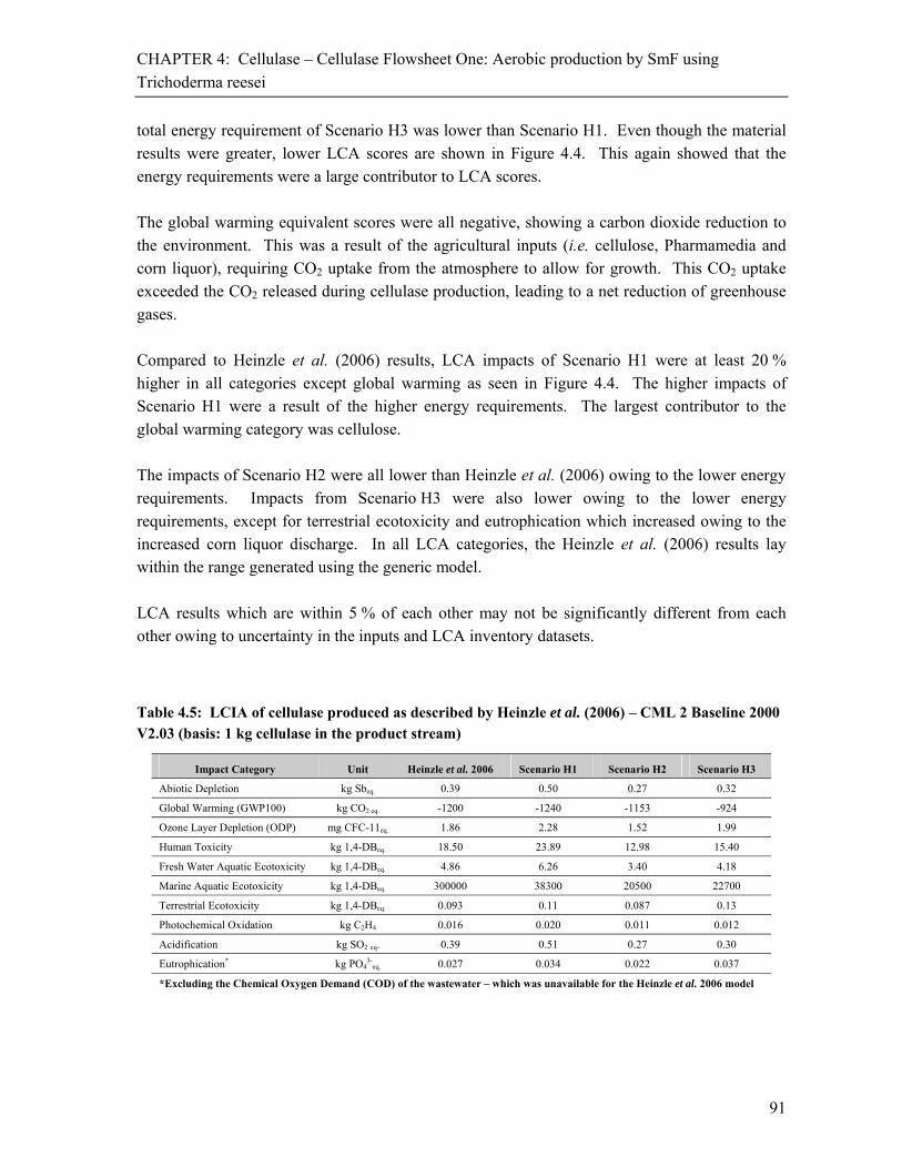
CHAPTER 4: Cellulase – Cellulase Flowsheet One: Aerobic production by SmF using
Trichoderma reesei
91
total energy requirement of Scenario H3 was lower than Scenario H1. Even though the material results were greater, lower LCA scores are shown in Figure 4.4. This again showed that the energy requirements were a large contributor to LCA scores. The global warming equivalent scores were all negative, showing a carbon dioxide reduction to the environment. This was a result of the agricultural inputs (i.e. cellulose, Pharmamedia and corn liquor), requiring CO2 uptake from the atmosphere to allow for growth. This CO2 uptake exceeded the CO2 released during cellulase production, leading to a net reduction of greenhouse gases. Compared to Heinzle et al. (2006) results, LCA impacts of Scenario H1 were at least 20 % higher in all categories except global warming as seen in Figure 4.4. The higher impacts of Scenario H1 were a result of the higher energy requirements. The largest contributor to the global warming category was cellulose. The impacts of Scenario H2 were all lower than Heinzle et al. (2006) owing to the lower energy requirements. Impacts from Scenario H3 were also lower owing to the lower energy requirements, except for terrestrial ecotoxicity and eutrophication which increased owing to the increased corn liquor discharge. In all LCA categories, the Heinzle et al. (2006) results lay within the range generated using the generic model. LCA results which are within 5 % of each other may not be significantly different from each other owing to uncertainty in the inputs and LCA inventory datasets.
Table 4.5: LCIA of cellulase produced as described by Heinzle et al. (2006) – CML 2 Baseline 2000 V2.03 (basis: 1 kg cellulase in the product stream)
Impact Category Unit Heinzle et al. 2006 Scenario H1 Scenario H2 Scenario H3
Abiotic Depletion kg Sbeq. 0.39 0.50 0.27 0.32
Global Warming (GWP100) kg CO2 eq. -1200 -1240 -1153 -924
Ozone Layer Depletion (ODP) mg CFC-11eq. 1.86 2.28 1.52 1.99
Human Toxicity kg 1,4-DBeq. 18.50 23.89 12.98 15.40
Fresh Water Aquatic Ecotoxicity kg 1,4-DBeq. 4.86 6.26 3.40 4.18
Marine Aquatic Ecotoxicity kg 1,4-DBeq. 300000 38300 20500 22700
Terrestrial Ecotoxicity kg 1,4-DBeq. 0.093 0.11 0.087 0.13
Photochemical Oxidation kg C2H4 0.016 0.020 0.011 0.012
Acidification kg SO2 eq. 0.39 0.51 0.27 0.30
Eutrophication* kg PO43-
eq. 0.027 0.034 0.022 0.037
*Excluding the Chemical Oxygen Demand (COD) of the wastewater – which was unavailable for the Heinzle et al. 2006 model

CHAPTER 4: Cellulase – Cellulase Flowsheet One: Aerobic production by SmF using
Trichoderma reesei
92
* Since global warming values were negative, the results for Scenario H1 are most desirable and Scenario H3 the least desirable
Figure 4.4: Comparison of LCA results for cellulase production for the three scenarios presented in the study relative to Heinzle et al. (2006) data
4.4.4. Process contributions Process contributions of six LCA impact categories were investigated from the Heinzle et al. (2006) material and energy balance results. The Heinzle et al. (2006) flowsheet was chosen as it was the most detailed process flowsheeting model. The LCA categories investigated include abiotic depletion, global warming, ozone layer depletion, photochemical oxidation, acidification and eutrophication. These are categories which do not include toxicity categories but give a broad perspective of environmental damage. The values shown in the figures represented contribution to the LCA impacts as a percentage of the total in each category. Only materials which led to a contribution greater than 3 % of the total LCA score have been included. In all six categories, electricity, cellulose and corn liquor formed the greatest portion of the LCA scores. In the abiotic depletion impact category, electricity formed 76 % of the total impact and wood chips, the assumed source of cellulose, contributed 20 % of the impact as seen in Figure 4.5. The impact of wood in the abiotic depletion category was a result of a large electrical energy requirement during processing. No other input added more than 3 % of the total abiotic score. In the global warming impact category, electricity was the main greenhouse gas emitter. The large agricultural component of cellulase production, and the associated biomass growth

CHAPTER 4: Cellulase – Cellulase Flowsheet One: Aerobic production by SmF using
Trichoderma reesei
93
(wood chips), resulted in a large carbon dioxide uptake from the atmosphere. Although corn liquor was also associated with biomass growth and carbon uptake, the ancillary energy requirements within corn liquor production resulted in an overall carbon uptake value less than 1 % of the total global warming score.
Figure 4.5: Life Cycle Assessment process contributions of cellulase production (Heinzle et al. 2006) using the CML baseline 2.03 methodology (Abiotic depletion and Global warming)
Electricity (73 %) and cellulose (25 %) again formed the greatest impacts in photochemical oxidation scores as shown in Figure 4.6. For ozone layer depletion impacts, steam (6.7 %) and corn liquor (3 %) were small contributors compared to the electricity (55 %) and cellulose (34 %) values.
* Note: Ozone layer depletion is of reduced importance in current processes (see Appendix A.6)
Figure 4.6: Life Cycle Assessment process contributions of cellulase production (Heinzle et al. 2006) using the CML baseline 2.03 methodology (Ozone layer depletion and Photochemical
oxidation)

CHAPTER 4: Cellulase – Cellulase Flowsheet One: Aerobic production by SmF using
Trichoderma reesei
94
Electricity impacts (82.5 %) were responsible for the major impact in the acidification score, with cellulose contributing 15.6 % of the overall score as shown in Figure 4.7. Eutrophication scores were also dominated by electricity (59 %) and cellulose (23 %), with corn liquor impacts adding 17 % of the total. Agricultural products tended to increase the eutrophication scores due to fertiliser usage. The impact of dilute wastewater was not taken into account in these calculations as the chemical oxygen demand (COD) value was not given for the Heinzle et al. (2006) model. In Scenarios H1, H2 and H3, the impact of the COD in the wastewater contributed over 65 % of the total eutrophication score. It is expected that similar results would be achieved if the COD value had been reported in the Heinzle et al. (2006) model.
Figure 4.7: Life Cycle Assessment process contributions of cellulase production (Heinzle et al. 2006) using the CML baseline 2.03 methodology (Acidification and Eutrophication)
4.4.5. Discussion It was seen in the process contributions that electricity formed more than half the LCA score for all categories investigated. The Heinzle et al. (2006) study made an assumption of 100 % oxygen utilisation during microbial growth and product formation. This is unrealistic and Scenarios H1, H2 and H3 assumed a typical experimental aeration rate of 0.58 vvm (Himmel et al. 1999). This difference in aeration rate, as well as compression pressure, was the main reason for the difference in electrical energy requirements and should be an area for further investigation. Wood chips are a by-product in the forestry industry, and may be expected to give a relatively small contribution to overall LCA impacts. However, the large volume used, when compared to other inputs in cellulase production, resulted in a large relative impact. The Ecoinvent v1.3 inventory used for wood chips assigned burden to electricity and transportation which added to this footprint.
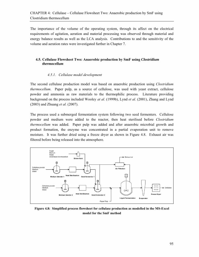
CHAPTER 4: Cellulase – Cellulase Flowsheet Two: Anaerobic production by SmF using
Clostridium thermocellum
95
The importance of the volume of the operating system, through its affect on the electrical requirements of agitation, aeration and material processing was observed through material and energy balance results as well as the LCA analysis. Contributions to and the sensitivity of the volume and aeration rates were investigated further in Chapter 7.
4.5. Cellulase Flowsheet Two: Anaerobic production by SmF using Clostridium thermocellum
4.5.1. Cellulase model development The second cellulase production model was based on anaerobic production using Clostridium thermocellum. Paper pulp, as a source of cellulose, was used with yeast extract, cellulose powder and ammonia as raw materials to the thermophilic process. Literature providing background on the process included Wooley at al. (1999b), Lynd et al. (2001), Zhang and Lynd (2003) and Zhuang et al. (2007). The process used a submerged fermentation system following two seed fermenters. Cellulose powder and medium were added to the reactor, then heat sterilised before Clostridium thermocellum was added. Paper pulp was added and after anaerobic microbial growth and product formation, the enzyme was concentrated in a partial evaporation unit to remove moisture. It was further dried using a freeze dryer as shown in Figure 4.8. Exhaust air was filtered before being released into the atmosphere.
Figure 4.8: Simplified process flowsheet for cellulase production as modelled in the MS-Excel model for the SmF method
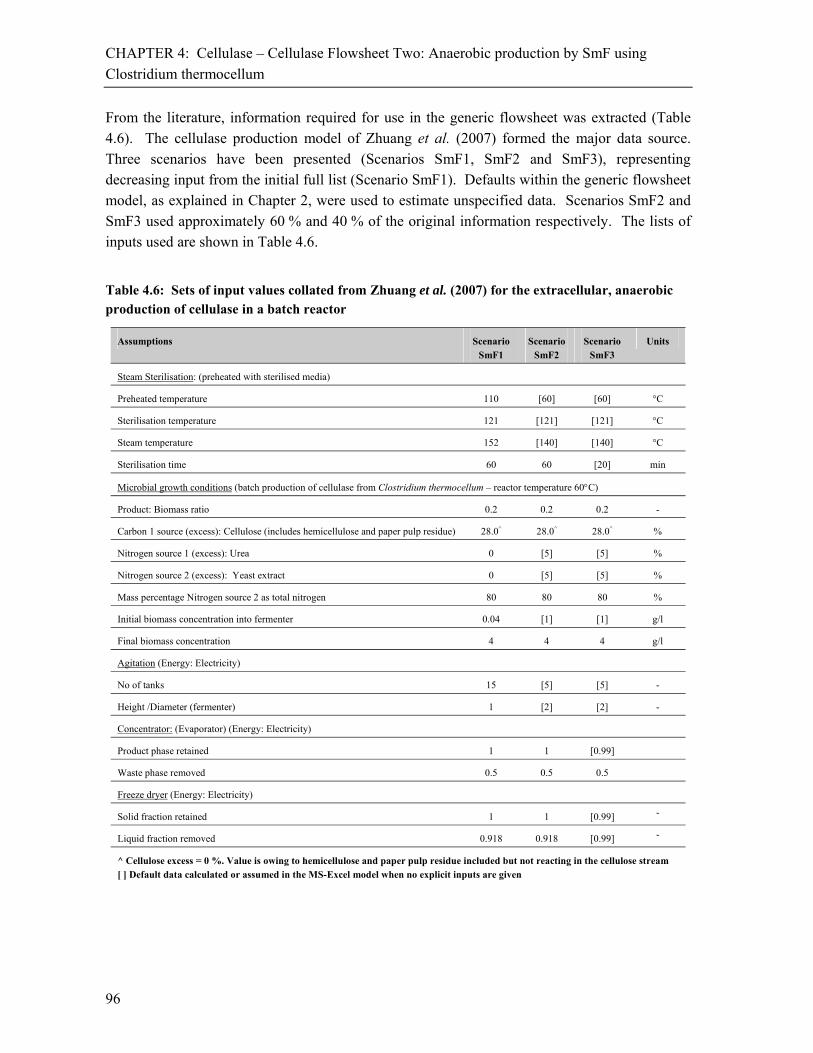
CHAPTER 4: Cellulase – Cellulase Flowsheet Two: Anaerobic production by SmF using
Clostridium thermocellum
96
From the literature, information required for use in the generic flowsheet was extracted (Table 4.6). The cellulase production model of Zhuang et al. (2007) formed the major data source. Three scenarios have been presented (Scenarios SmF1, SmF2 and SmF3), representing decreasing input from the initial full list (Scenario SmF1). Defaults within the generic flowsheet model, as explained in Chapter 2, were used to estimate unspecified data. Scenarios SmF2 and SmF3 used approximately 60 % and 40 % of the original information respectively. The lists of inputs used are shown in Table 4.6.
Table 4.6: Sets of input values collated from Zhuang et al. (2007) for the extracellular, anaerobic production of cellulase in a batch reactor
Assumptions Scenario SmF1
Scenario SmF2
Scenario SmF3
Units
Steam Sterilisation: (preheated with sterilised media)
Preheated temperature 110 [60] [60] °C
Sterilisation temperature 121 [121] [121] °C
Steam temperature 152 [140] [140] °C
Sterilisation time 60 60 [20] min
Microbial growth conditions (batch production of cellulase from Clostridium thermocellum – reactor temperature 60C)
Product: Biomass ratio 0.2 0.2 0.2 -
Carbon 1 source (excess): Cellulose (includes hemicellulose and paper pulp residue) 28.0^ 28.0^ 28.0^ %
Nitrogen source 1 (excess): Urea 0 [5] [5] %
Nitrogen source 2 (excess): Yeast extract 0 [5] [5] %
Mass percentage Nitrogen source 2 as total nitrogen 80 80 80 %
Initial biomass concentration into fermenter 0.04 [1] [1] g/l
Final biomass concentration 4 4 4 g/l
Agitation (Energy: Electricity)
No of tanks 15 [5] [5] -
Height /Diameter (fermenter) 1 [2] [2] -
Concentrator: (Evaporator) (Energy: Electricity)
Product phase retained 1 1 [0.99]
Waste phase removed 0.5 0.5 0.5
Freeze dryer (Energy: Electricity)
Solid fraction retained 1 1 [0.99] -
Liquid fraction removed 0.918 0.918 [0.99] -
^ Cellulose excess = 0 %. Value is owing to hemicellulose and paper pulp residue included but not reacting in the cellulose stream [ ] Default data calculated or assumed in the MS-Excel model when no explicit inputs are given

CHAPTER 4: Cellulase – Cellulase Flowsheet Two: Anaerobic production by SmF using
Clostridium thermocellum
97
4.5.2. Material and energy balance outputs Outputs obtained from the model for production of 1 kg cellulase – containing product (i.e. cellulase plus impurities) are shown in Table 4.7. From the scenarios developed, this gave cellulase mass purities of 0.83, 0.72 and 1.38 % for Scenarios SmF1, SmF2 and SmF3 respectively. For Scenario SmF1, to produce 1 kg of cellulase (120 kg of product), 90 kg of cellulose, 3.2 kg of yeast extract and 0.79 kg of urea was required. The cellulose requirement was a combination of cellulose, hemicellulose and paper pulp residue. Scenario SmF2 (140 kg of product) required 90 kg of cellulose, 3.3 kg of yeast extract and 0.83 kg of urea, owing to the increase in excess of nitrogen source specified. Scenario SmF3 (72 kg of product) required 91 kg cellulose, 3.4 kg of yeast extract and 0.85 kg of urea, higher than requirements for both of the previous scenarios as a result of inefficient downstream separations. Water requirements, and resultant wastewater, for Scenarios SmF2 and SmF3 were 33 and 40 % higher than Scenario SmF1 owing to the changes in initial biomass concentration and downstream separation efficiencies respectively. Owing to the low purity of the enzyme stream, waste values from all scenarios were low and similar outputs were calculated. Energy requirements for Scenario SmF1 included 1680 MJ electricity, 170 MJ steam and 6.2 kg of cooling water. The electricity requirement was only 15 % higher and 16 % lower in Scenarios SmF2 and SmF3 respectively. However, the steam requirement increased more than 3-fold in both cases owing to the assumption of no preheating of the media during sterilisation. Even though the holding time was three times lower in Scenario SmF3, steam requirements were similar to Scenario SmF2 since steam was chiefly needed to heat the media to the sterilisation temperature with the contribution to maintaining temperature being small. Cooling water requirements for Scenarios SmF1, SmF2 and SmF3 were 6.2, 6.4 and 6.0 kg per kg of cellulase respectively. The values of the material and energy balance given by Zhuang et al. (2007) showed that 80 kg, 4.8 kg and 1.2 kg for cellulose, yeast extract and urea were required respectively to produce 1 kg cellulase. Additionally, the flowsheet required 30 kg potassium chloride. Inorganic salts other than those containing nitrogen, sulphur or phosphorus were not accounted for in the generic flowsheet models. The Zhuang et al. (2007) flowsheet also showed emissions of 1.8 kg and 0.4 kg of nitrogen and oxygen respectively which were not seen in the generic flowsheet models. The generic flowsheet model included hydrogen air emissions and phosphate and sulphate in the wastewater, none of which were shown in the Zhuang et al. (2007) model. In the Zhuang et al. (2007) model, a simplification was made that only cellulose reacted to form biomass and cellulase. They assumed, unrealistically, that the yeast extract and urea did not form part of the reacting media for biomass growth or enzyme formation. In the generic
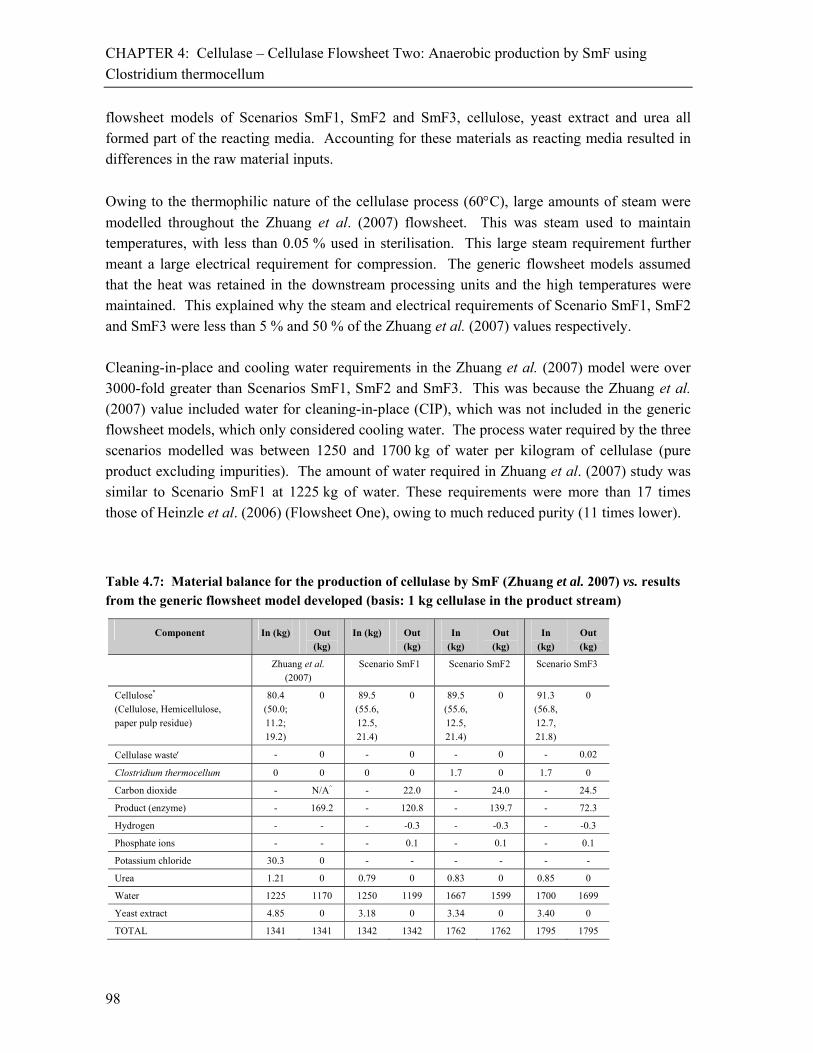
CHAPTER 4: Cellulase – Cellulase Flowsheet Two: Anaerobic production by SmF using
Clostridium thermocellum
98
flowsheet models of Scenarios SmF1, SmF2 and SmF3, cellulose, yeast extract and urea all formed part of the reacting media. Accounting for these materials as reacting media resulted in differences in the raw material inputs.
Owing to the thermophilic nature of the cellulase process (60C), large amounts of steam were
modelled throughout the Zhuang et al. (2007) flowsheet. This was steam used to maintain temperatures, with less than 0.05 % used in sterilisation. This large steam requirement further meant a large electrical requirement for compression. The generic flowsheet models assumed that the heat was retained in the downstream processing units and the high temperatures were maintained. This explained why the steam and electrical requirements of Scenario SmF1, SmF2 and SmF3 were less than 5 % and 50 % of the Zhuang et al. (2007) values respectively. Cleaning-in-place and cooling water requirements in the Zhuang et al. (2007) model were over 3000-fold greater than Scenarios SmF1, SmF2 and SmF3. This was because the Zhuang et al. (2007) value included water for cleaning-in-place (CIP), which was not included in the generic flowsheet models, which only considered cooling water. The process water required by the three scenarios modelled was between 1250 and 1700 kg of water per kilogram of cellulase (pure product excluding impurities). The amount of water required in Zhuang et al. (2007) study was similar to Scenario SmF1 at 1225 kg of water. These requirements were more than 17 times those of Heinzle et al. (2006) (Flowsheet One), owing to much reduced purity (11 times lower).
Table 4.7: Material balance for the production of cellulase by SmF (Zhuang et al. 2007) vs. results from the generic flowsheet model developed (basis: 1 kg cellulase in the product stream)
Component In (kg) Out (kg)
In (kg) Out (kg)
In (kg)
Out (kg)
In (kg)
Out (kg)
Zhuang et al. (2007)
Scenario SmF1 Scenario SmF2 Scenario SmF3
Cellulose* (Cellulose, Hemicellulose,
paper pulp residue)
80.4 (50.0;
11.2; 19.2)
0 89.5 (55.6,
12.5, 21.4)
0 89.5 (55.6,
12.5, 21.4)
0 91.3 (56.8,
12.7, 21.8)
0
Cellulase waste - 0 - 0 - 0 - 0.02
Clostridium thermocellum 0 0 0 0 1.7 0 1.7 0
Carbon dioxide - N/A^ - 22.0 - 24.0 - 24.5
Product (enzyme) - 169.2 - 120.8 - 139.7 - 72.3
Hydrogen - - - -0.3 - -0.3 - -0.3
Phosphate ions - - - 0.1 - 0.1 - 0.1
Potassium chloride 30.3 0 - - - - - -
Urea 1.21 0 0.79 0 0.83 0 0.85 0
Water 1225 1170 1250 1199 1667 1599 1700 1699
Yeast extract 4.85 0 3.18 0 3.34 0 3.40 0
TOTAL 1341 1341 1342 1342 1762 1762 1795 1795
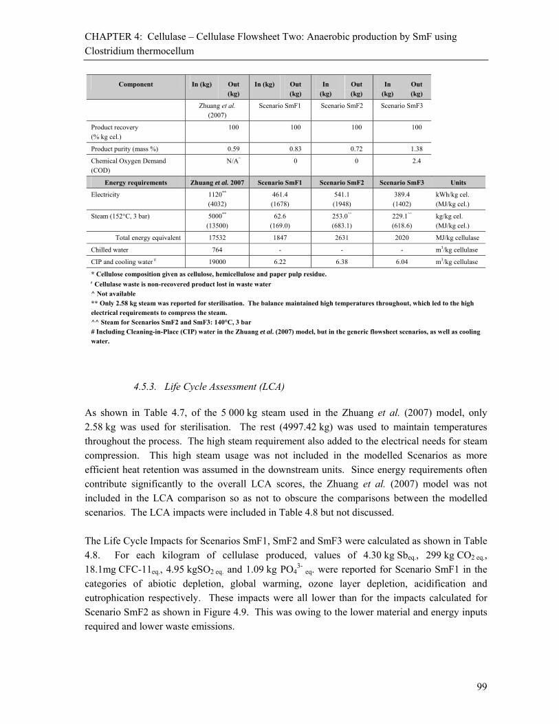
CHAPTER 4: Cellulase – Cellulase Flowsheet Two: Anaerobic production by SmF using
Clostridium thermocellum
99
Component In (kg) Out (kg)
In (kg) Out (kg)
In (kg)
Out (kg)
In (kg)
Out (kg)
Zhuang et al. (2007)
Scenario SmF1 Scenario SmF2 Scenario SmF3
Product recovery (% kg cel.)
100 100 100 100
Product purity (mass %) 0.59 0.83 0.72 1.38
Chemical Oxygen Demand (COD)
N/A^ 0 0 2.4
Energy requirements Zhuang et al. 2007 Scenario SmF1 Scenario SmF2 Scenario SmF3 Units
Electricity 1120** (4032)
461.4 (1678)
541.1 (1948)
389.4 (1402)
kWh/kg cel. (MJ/kg cel.)
Steam (152°C, 3 bar) 5000** (13500)
62.6 (169.0)
253.0^^ (683.1)
229.1^^ (618.6)
kg/kg cel. (MJ/kg cel.)
Total energy equivalent 17532 1847 2631 2020 MJ/kg cellulase
Chilled water 764 - - - m3/kg cellulase
CIP and cooling water # 19000 6.22 6.38 6.04 m3/kg cellulase
* Cellulose composition given as cellulose, hemicellulose and paper pulp residue.
Cellulase waste is non-recovered product lost in waste water
^ Not available ** Only 2.58 kg steam was reported for sterilisation. The balance maintained high temperatures throughout, which led to the high electrical requirements to compress the steam. ^^ Steam for Scenarios SmF2 and SmF3: 140°C, 3 bar # Including Cleaning-in-Place (CIP) water in the Zhuang et al. (2007) model, but in the generic flowsheet scenarios, as well as cooling water.
4.5.3. Life Cycle Assessment (LCA) As shown in Table 4.7, of the 5 000 kg steam used in the Zhuang et al. (2007) model, only 2.58 kg was used for sterilisation. The rest (4997.42 kg) was used to maintain temperatures throughout the process. The high steam requirement also added to the electrical needs for steam compression. This high steam usage was not included in the modelled Scenarios as more efficient heat retention was assumed in the downstream units. Since energy requirements often contribute significantly to the overall LCA scores, the Zhuang et al. (2007) model was not included in the LCA comparison so as not to obscure the comparisons between the modelled scenarios. The LCA impacts were included in Table 4.8 but not discussed. The Life Cycle Impacts for Scenarios SmF1, SmF2 and SmF3 were calculated as shown in Table 4.8. For each kilogram of cellulase produced, values of 4.30 kg Sbeq., 299 kg CO2 eq., 18.1mg CFC-11eq., 4.95 kgSO2 eq. and 1.09 kg PO4
3- eq. were reported for Scenario SmF1 in the
categories of abiotic depletion, global warming, ozone layer depletion, acidification and eutrophication respectively. These impacts were all lower than for the impacts calculated for Scenario SmF2 as shown in Figure 4.9. This was owing to the lower material and energy inputs required and lower waste emissions.

CHAPTER 4: Cellulase – Cellulase Flowsheet Two: Anaerobic production by SmF using
Clostridium thermocellum
100
Although the steam requirements of Scenario SmF3 were over 3-fold higher than Scenario SmF1 (by energy equivalent), the LCA impacts were lower in all categories except ozone layer depletion, terrestrial ecotoxicity and eutrophication as seen in Figure 4.9. The lower LCA scores were owing to the reduced electricity scores which dominated the LCA impacts. Ozone layer depletion, terrestrial ecotoxicity and eutrophication scores of Scenario SmF3 were higher than Scenario SmF1 owing to increased cellulose, urea and yeast extract inputs which contributed to give higher LCA scores.
Table 4.8: LCIA of cellulase produced by SmF for inputs obtained from Zhuang et al. (2007) and the modelled Scenarios SmF1, SmF2 and SmF3 – CML 2 Baseline 2000 V2.03 (basis: 1 kg cellulase in the product stream)
Impact Category Unit Zhuang et al. (2007) Scenario SmF1 Scenario SmF2 Scenario SmF3
Abiotic Depletion kg Sbeq. 18.9 4.30 5.29 4.07
Global Warming (GWP100) kg CO2 eq. 1940 299 403 290
Ozone Layer Depletion (ODP) mg CFC-11eq. 178 18.1 25.7 21.3
Human Toxicity kg 1,4-DBeq. 775 209 252 193
Fresh Water Aquatic Ecotoxicity kg 1,4-DBeq. 140 51.1 59.9 44.8
Marine Aquatic Ecotoxicity kg 1,4-DBeq. 940000 328000 385000 291000
Terrestrial Ecotoxicity kg 1,4-DBeq. 7.66 0.92 1.23 1.09
Photochemical Oxidation kg C2H4 0.54 0.18 0.21 0.16
Acidification kg SO2 eq. 13.6 4.95 5.76 4.48
Eutrophication kg PO43-
eq. 1.82 1.09 1.17 1.17
Figure 4.9: Comparison of LCA results for cellulase production by submerged fermentation for Scenarios SmF2 and SmF3 relative to Scenario SmF1

CHAPTER 4: Cellulase – Cellulase Flowsheet Two: Anaerobic production by SmF using
Clostridium thermocellum
101
4.5.4. Process contributions Using Scenario SmF1 as an example, process contributions for six LCA impact categories were investigated. Scenario SmF1 was chosen as it was the most detailed model of the three scenarios modelled and included yeast extract and urea as reacting media; a consideration not taken into account by Zhuang et al. (2007). In all categories, electricity was the main contributor to Life cycle Assessment impacts. Cellulose (paper pulp), steam and yeast extract also formed large portions of contributions in all LCA categories. In the abiotic depletion category, electricity formed 84 % of the impact, with cellulose and steam contributing 10 % and 4.3 % respectively. The main source of the LCA impact for cellulose was electricity, resulting in a total contribution by electricity of over 80 % as shown in Figure 4.10. In the global warming impact category, the cellulose from paper pulp reduced carbon dioxide in the atmosphere. The overall emissions of global warming gases were still positive, mainly due to a large electricity impact (which was not drawn to scale in the pie chart of Figure 4.10). This large electricity impacts were a result of large energy requirements of the downstream processing units. Steam and yeast extract also added 7.8 % and 9.4 % respectively. In the previous cellulase flowsheet study (Scenario H1), the impact to global warming showed a smaller relative impact from electricity and a greater negative portion contributed by the production of cellulose. This was owing to the fact that electricity increased 33-fold in Scenario SmF1, but the cellulose requirements only increased 24-fold.
Figure 4.10: Life Cycle Assessment process contributions of cellulase production by SmF using the CML baseline 2.03 methodology (Abiotic depletion and Global warming)

CHAPTER 4: Cellulase – Cellulase Flowsheet Two: Anaerobic production by SmF using
Clostridium thermocellum
102
Electrical impacts were calculated to be 61 % for ozone layer depletion and 78 % for photochemical oxidation as shown in Figure 4.11. The assumption of South African electricity implied the dominance of generation from coal. The remaining contributions for ozone layer depletion were made up of cellulose (19 %), steam (15 %) and yeast extract (4.8 %). Photochemical oxidation contributions were completed by yeast extract (13.1 %) and cellulose (6.5 %).
* Note: Ozone layer depletion is of reduced importance in current processes (see Appendix A.6)
Figure 4.11: Life Cycle Assessment process contributions of cellulase production by SmF using the CML baseline 2.03 methodology (Ozone layer depletion and Photochemical oxidation)
Electricity (79.2%) also formed the greatest contribution to acidification. Further contributors were yeast extract (11.9 %) and cellulose (7.1 %) as shown in Figure 4.12. Eutrophication scores were dominated by yeast extract (68.1 %), owing to the assumption of yeast production from glucose with an associated agricultural origin and a high eutrophication score. Electricity and cellulose contributed 17.5 % and 7.1 % respectively. Unlike the previous cellulase flowsheet, which assumed wood chips as the cellulose source, this process used paper pulp, which had a lower contribution to eutrophication. Yeast extract is typically a waste product and could have been modelled in the LCA study as a waste utilisation process. This would have meant a reduction of impacts as a result of the use of yeast extract.

CHAPTER 4: Cellulase – Cellulase Flowsheet Two: Anaerobic production by SmF using
Clostridium thermocellum
103
Figure 4.12: Life Cycle Assessment process contributions of cellulase production by SmF using the CML baseline 2.03 methodology (Acidification and Eutrophication)
4.5.5. Discussion The modelled Scenarios SmF1, SmF2 and SmF3 showed good agreement for material inputs and outputs. The Zhuang et al. (2007) energy requirements were at least 9 fold higher than the scenario (SmF1) with the lowest energy needs. This high energy requirement was owing to high steam requirements in the Zhuang et al. (2007) model to maintain temperatures throughout the process. This large steam requirement was not made in the generic flowsheet models as it was assumed that heat was not lost in the downstream processing units. Energy requirements (electricity and steam) were the main contributors in all LCA impact categories except eutrophication, which was dominated by the production of yeast extract. As such, differences in LCA results between the modelled scenarios were owing to the energy changes and had little to do with changes to the material inputs and emissions of the flowsheets. The large energy requirement was from downstream processing of the forced evaporator and freeze drying. LCA sensitivities to energy changes were investigated further in Chapter 7. Yeast extract used in the model was assumed to add to the LCA impacts during its production. However, yeast extract is typically a waste product and it could have been modelled as a waste utilisation process by burden allocation in the LCA analysis. This would have meant a reduction of impacts and a loss of carbon credits.
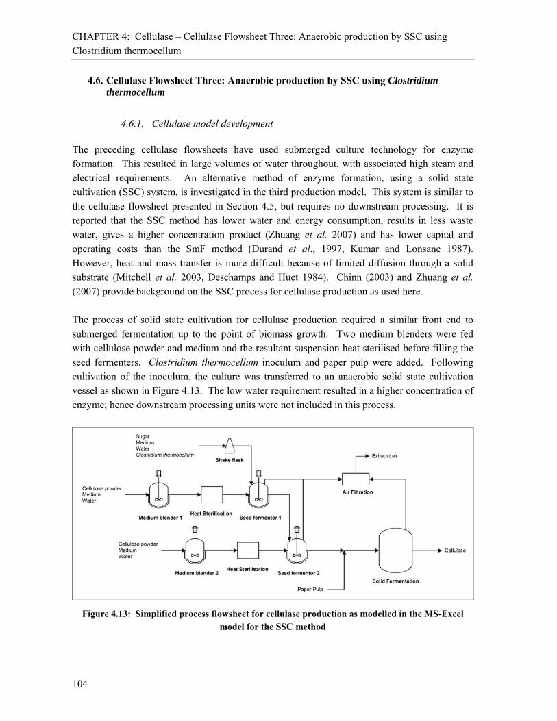
CHAPTER 4: Cellulase – Cellulase Flowsheet Three: Anaerobic production by SSC using
Clostridium thermocellum
104
4.6. Cellulase Flowsheet Three: Anaerobic production by SSC using Clostridium thermocellum
4.6.1. Cellulase model development The preceding cellulase flowsheets have used submerged culture technology for enzyme formation. This resulted in large volumes of water throughout, with associated high steam and electrical requirements. An alternative method of enzyme formation, using a solid state cultivation (SSC) system, is investigated in the third production model. This system is similar to the cellulase flowsheet presented in Section 4.5, but requires no downstream processing. It is reported that the SSC method has lower water and energy consumption, results in less waste water, gives a higher concentration product (Zhuang et al. 2007) and has lower capital and operating costs than the SmF method (Durand et al., 1997, Kumar and Lonsane 1987). However, heat and mass transfer is more difficult because of limited diffusion through a solid substrate (Mitchell et al. 2003, Deschamps and Huet 1984). Chinn (2003) and Zhuang et al. (2007) provide background on the SSC process for cellulase production as used here. The process of solid state cultivation for cellulase production required a similar front end to submerged fermentation up to the point of biomass growth. Two medium blenders were fed with cellulose powder and medium and the resultant suspension heat sterilised before filling the seed fermenters. Clostridium thermocellum inoculum and paper pulp were added. Following cultivation of the inoculum, the culture was transferred to an anaerobic solid state cultivation vessel as shown in Figure 4.13. The low water requirement resulted in a higher concentration of enzyme; hence downstream processing units were not included in this process.
Figure 4.13: Simplified process flowsheet for cellulase production as modelled in the MS-Excel model for the SSC method

CHAPTER 4: Cellulase – Cellulase Flowsheet Three: Anaerobic production by SSC using
Clostridium thermocellum
105
Values of the necessary parameters, summarised in Table 4.9, were extracted from the literature, predominantly from the cellulase production model of Zhuang et al. (2007). Three scenarios have been presented (Scenarios SSC1, SSC2 and SSC3), each less input data specified. Defaults within the generic flowsheet model, as explained in Chapter 2, were used to complete the necessary dataset. Scenarios SSC2 and SSC3 used approximately 60 % and 40 % of the original information respectively. The lists of inputs used for the three scenarios are shown in Table 4.9.
Table 4.9: Sets of input assumption from Zhuang et al. (2007) for the extracellular, anaerobic production of cellulase in a batch solid state cultivation reactor
Assumptions Scenario SSC1
Scenario SSC2
Scenario SSC3
Units
Steam Sterilisation: (preheated with sterilised media)
Preheated temperature 110 [60] [60] °C
Sterilisation temperature 121 [121] [121] °C
Steam temperature 152 [140] [140] °C
Sterilisation time 60 60 [20] min
Microbial growth conditions (batch production of cellulase from Clostridium thermocellum – reactor temperature 60C)
Product: Biomass ratio 0.2 0.2 0.2 -
Carbon 1 source (excess): Cellulose (includes hemicellulose and paper pulp residue) 28.0^ 28.0^ [1] %
Nitrogen source 1 (excess): Urea 0 [5] [5] %
Nitrogen source 2 (excess): Yeast extract 0 [5] [5] %
Mass percentage Nitrogen source 2 as total nitrogen 80 80 [50] %
Maintain rector temperature (Cooling agent: Cooling water) 60 60 60 °C
Initial biomass concentration into fermenter 0.04 [1] [1] g/l
Final biomass concentration 20.5 20.5 20.5 g/l
^ Cellulose excess = 0 %. Value is owing to hemicellulose and paper pulp residue included but not reacting in the cellulose stream [ ] Default data calculated or assumed in the MS-Excel model when no explicit inputs are given
4.6.2. Material and energy balance outputs The model outputs for the production of cellulase are shown in Table 4.10. Mass purities of 0.32, 0.31 and 0.32 % were calculated for Scenarios SSC1, SSC2 and SSC3 respectively. For Scenario SSC1, to produce 1 kg of cellulase (310 kg of product), 90 kg of cellulose, 3.2 kg of yeast extract and 0.79 kg of urea was required. The cellulose was a combination of all cellulose, hemicellulose and paper pulp residue requirements. Scenario SSC2 (330 kg of product) required 90 kg of cellulose, 3.3 kg of yeast extract and 0.83 kg of urea. Scenario SSC3 (310 kg of product) required 77 kg cellulose, 1.3 kg of yeast extract and 1.3 kg of urea. Since the microbial growth conditions of Scenarios SSC1 and SSC2 were the same as Scenarios SmF1 and SmF2

CHAPTER 4: Cellulase – Cellulase Flowsheet Three: Anaerobic production by SSC using
Clostridium thermocellum
106
respectively, the raw material inputs of the submerged fermentation were the same as the solid state cultivation method. Water requirements for Scenarios SSC1, SSC2 and SSC3 were 244, 257 and 257 kg respectively. The SSC models required one fifth that of the SmF models. Since there was no downstream processing in the SSC model, there was only one liquid stream. Owing to the way the scenarios were set up, gaseous emissions of carbon dioxide and hydrogen, were almost identical. Energy requirements for Scenario SSC1 included 6.5 MJ electricity, 47 MJ steam and 5.8 kg of cooling water. In agreement with volume reduction and the absence of agitation and downstream processing in the SSC models, energy requirements were 2.9 % of the Scenario SmF1 energy requirement. The electrical energy and steam requirements of Scenario SSC2 and SSC3 were 300 % and 245 % higher than Scenario SSC1 respectively, owing to the absence of heat integration with no preheating of media before steam sterilisation. The decrease in sterilisation holding time decreased the energy requirement for Scenario SSC3. The cooling water requirements for all scenarios were within 98 % of each other. The material input requirements for the Zhuang et al. (2007) model (315 kg of product) were shown to be: 80 kg, 0.87 kg and 0.22 kg for cellulose, yeast extract and urea respectively as shown in Table 4.10. Additionally, the flowsheet required 5.4 kg potassium chloride which was not accounted from in the generic flowsheet models. The Zhuang et al. (2007) flowsheet showed emissions of 0.26 kg and 0.097 kg of nitrogen and oxygen respectively, but did not elaborate on how these were formed since this was an anaerobic process. The generic flowsheet models included hydrogen emissions which were not shown in the Zhuang et al. (2007) model. Process water was higher in the SSC model of Zhuang et al. (2007) as cleaning-in-place (CIP) was taken into account, but not in the generic flowsheet models of Scenarios SSC1, SSC2 and SSC3. As in the submerged fermentation model of Zhuang et al. (2007) there was a large difference in energy between the SSC models. Large amounts of steam were required to maintain temperatures, which were not accounted for in the generic flowsheet models. Compression of this steam meant that additional electricity was also needed. Steam and electrical requirements of Scenario SSC1 were less than 18 % and 15 % of the Zhuang et al. (2007) values respectively. In the Zhuang et al. (2007) model for solid state cultivation, as in submerged fermentation, a simplification was made that only cellulose reacted to form biomass and cellulase. In the generic flowsheet models, cellulose, yeast extract and urea all formed part of the reacting media, resulting in the differences in the raw material inputs.
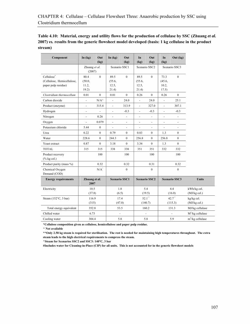
CHAPTER 4: Cellulase – Cellulase Flowsheet Three: Anaerobic production by SSC using
Clostridium thermocellum
107
Table 4.10: Material, energy and utility flows for the production of cellulase by SSC (Zhuang et al. 2007) vs. results from the generic flowsheet model developed (basis: 1 kg cellulase in the product stream)
Component In (kg) Out (kg)
In (kg) Out (kg)
In (kg)
Out (kg)
In (kg)
Out (kg)
Zhuang et al. (2007)
Scenario SSC1 Scenario SSC2 Scenario SSC3
Cellulose* (Cellulose, Hemicellulose, paper pulp residue)
80.4 (50.0, 11.2, 19.2)
0 89.5 (55.6, 12.5, 21.4)
0 89.5 (55.6, 12.5, 21.4)
0 73.3 (45.6, 10.2, 17.5)
0
Clostridium thermocellum 0.01 0 0.01 0 0.26 0 0.26 0
Carbon dioxide - N/A^ - 24.0 - 24.0 - 25.1
Product (enzyme) - 315.4 - 313.9 - 327.0 - 307.1
Hydrogen - - - -0.3 - -0.3 - -0.3
Nitrogen - 0.26 - - - - - -
Oxygen - 0.079 - - - - - -
Potassium chloride 5.44 0 - - - - - -
Urea 0.22 0 0.79 0 0.83 0 1.3 0
Water 228.6 0 244.3 0 256.8 0 256.8 0
Yeast extract 0.87 0 3.18 0 3.34 0 1.3 0
TOTAL 315 315 338 338 351 351 332 332
Product recovery (% kg cel.)
100 100 100 100
Product purity (mass %) 0.32 0.32 0.31 0.32
Chemical Oxygen Demand (COD)
N/A^ 0 0 0
Energy requirements Zhuang et al. 2007
Scenario SSC1 Scenario SSC2 Scenario SSC3 Units
Electricity 10.5 (37.8)
1.8 (6.5)
5.4 (19.5)
4.4 (16.0)
kWh/kg cel. (MJ/kg cel.)
Steam (152°C, 3 bar) 116.9 (315)
17.4 (47.0)
52.1^^ (140.7)
42.7^^ (115.3)
kg/kg cel. (MJ/kg cel.)
Total energy equivalent 352.8 53.5 160.2 131.3 MJ/kg cellulase
Chilled water 6.73 - - - M3/kg cellulase
Cooling water 304.4 5.8 5.8 5.9 m3/kg cellulase
*Cellulose composition given as cellulose, hemicellulose and paper pulp residue. ^ Not available **Only 2.58 kg steam is required for sterilisation. The rest is needed for maintaining high temperatures throughout. The extra steam leads to the high electrical requirements to compress the steam. ^Steam for Scenarios SSC2 and SSC3: 140°C, 3 bar #Includes water for Cleaning-in-Place (CIP) for all units. This is not accounted for in the generic flowsheet models

CHAPTER 4: Cellulase – Cellulase Flowsheet Three: Anaerobic production by SSC using
Clostridium thermocellum
108
4.6.3. Life Cycle Assessment (LCA) Since the total steam used in the Zhuang et al. (2007) model included excessive requirements to maintain temperatures, which were not shown in Scenario SSC1, SSC2 and SSC3, the Zhuang et al. (2007) model was not included in the LCA comparison. For 1 kg of cellulase (314 kg of product), life cycle impacts of 0.62 kg Sb eq., 5.41 mg CFC-11 eq., 0.97 kg SO2 eq. and 0.80 kgPO4
3- eq. were obtained for Scenario SSC1 in the categories of abiotic
depletion, ozone layer depletion, acidification and eutrophication as shown in Table 4.10. The LCA results for the same categories for Scenario SSC2 were: 0.72 kg Sb eq., 6.55 mg CFC-11 eq., 1.05 kg SO2 eq. and 0.94 kgPO4
3- eq.. In all categories, Scenario SSC2 impacts were larger than
Scenario SSC1 impacts. This was owing to the larger energy requirements for both electricity and steam. The global warming impacts showed that there was an overall carbon dioxide equivalent reduction as a result of cellulase production. The larger negative values indicated greater carbon dioxide equivalent reductions. The higher energy requirements of Scenarios SSC2 and SSC3 resulted in higher global warming impacts than Scenario SSC1. The burdens from Scenario SSC3 were lower than Scenario SSC1 and SSC2 in all categories except global warming (Figure 4.14). Even though the energy requirements of Scenario SSC3 were higher than for Scenario SSC1, LCA impacts were still lower by between 10 and 55 % owing to the lower cellulose and yeast extract inputs which dominated the LCA scores.
Table 4.11: LCIA of cellulase produced by SSC as modelled in Scenarios SSC1, SSC2 and SSC3 – CML 2 Baseline 2000 V2.03 (basis: 1 kg cellulase in the product stream)
Impact Category Unit Scenario SSC1 Scenario SSC2 Scenario SSC3
Abiotic Depletion kg Sbeq. 0.62 0.72 0.55
Global Warming (GWP100) kg CO2 eq. -35.0 -22.8 -23.8
Ozone Layer Depletion (ODP) mg CFC-11eq. 5.41 6.55 5.23
Human Toxicity kg 1,4-DBeq. 32.3 36.0 29.4
Fresh Water Aquatic Ecotoxicity kg 1,4-DBeq. 5.11 5.64 4.62
Marine Aquatic Ecotoxicity kg 1,4-DBeq. 40600 44400 35900
Terrestrial Ecotoxicity kg 1,4-DBeq. 0.51 0.56 0.45
Photochemical Oxidation kg C2H4 0.036 0.039 0.022
Acidification kg SO2 eq. 0.97 1.05 0.60
Eutrophication kg PO43-
eq. 0.80 0.94 0.35

CHAPTER 4: Cellulase – Cellulase Flowsheet Three: Anaerobic production by SSC using
Clostridium thermocellum
109
* Since global warming values are negative, the results for Scenario SSC1 were most desirable and Scenario SSC2 the least desirable
Figure 4.14: Comparison of LCA results for cellulase production by solid state cultivation for Scenarios SSC2 and SSC3 relative to Scenario SSC1
4.6.4. Process contributions For the production of cellulase by SSC, the individual contributions towards the overall LCA score were investigated. Using Scenario SSC1 the primary energy requirements from electricity used in cellulase production did not form a large portion of the LCA impact in any of the categories. This was expected when compared to the submerged fermentation results, since the energy requirements were up to 100 times lower in the SSC models, to produce equal product masses. In the abiotic depletion category, cellulose from paper pulp (63 %) formed the largest contribution to Life Cycle Assessment impacts as shown in Figure 4.15. The main impacts within the cellulose impact were electricity and hydrogen peroxide. Yeast extract, steam and urea contributed 18, 15 and 3.5 % respectively. In the global warming impact category, greenhouse gases were removed from the atmosphere during biomass growth of the cellulose production cycle. Carbon dioxide was emitted during yeast extract (47 %), steam (6.8 %) and urea (4.4 %) production. The overall carbon dioxide uptake from biomass growth was larger than the emissions, resulting in a global warming reduction (Figure 4.15).

CHAPTER 4: Cellulase – Cellulase Flowsheet Three: Anaerobic production by SSC using
Clostridium thermocellum
110
Figure 4.15: Life Cycle Assessment process contributions of cellulase production by SSC using the CML baseline 2.03 methodology (Abiotic depletion and Global warming)
In the ozone layer depletion category, cellulose production (67 %) formed two thirds of the overall impact. This impact was made up of electricity (45 %), transport (7.6 %), hydrogen peroxide (4.9%) and sodium silicate (3.9 %) as shown in Figure 4.16. Yeast extract (17 %), steam (9.2 %) and urea (6.5 %) were the remaining major contributors. In the photochemical oxidation impact category, yeast extract and cellulose contributed 64 % and 32 % respectively. The main contributor of the cellulose impact was electricity (27 %) which formed 85 % of the total cellulose score.
* Note: Ozone layer depletion is of reduced importance in current processes (see Appendix A.6)
Figure 4.16: Life Cycle Assessment process contributions of cellulase production by SSC using the CML baseline 2.03 methodology (Ozone layer depletion and Photochemical oxidation)

CHAPTER 4: Cellulase – Cellulase Flowsheet Three: Anaerobic production by SSC using
Clostridium thermocellum
111
As with photochemical oxidation, the yeast extract (60.5 %) and cellulose (35.9 %) were the main process contributors in the acidification impact category (Figure 4.17). The eutrophication category was dominated by impacts from yeast extract (92.9 %), with cellulose contributing 6.7 %. The yeast extract formed a large part in eutrophication owing to the agricultural impacts of sugar assumed to have been used in the growth of yeast.
Figure 4.17: Life Cycle Assessment process contributions of cellulase production by SSC using the CML baseline 2.03 methodology (Acidification and Eutrophication)
4.6.5. Discussion The modelled Scenarios SSC1, SSC2 and SSC3 showed good agreement with Zhuang et al. (2007) for material inputs, but did not show as great a steam requirement needed to maintain high temperatures. The high steam in the Zhuang et al. (2007) model also required a high electricity requirement and was the main reason for a greater total energy requirement compared to the modelled scenarios. The differences in the steam values were a result of limited information from the Zhuang et al. (2007) model, which meant a larger number of assumptions needed in the modelled flowsheets. Since there were fewer downstream processing (DSP) units for the SSC flowsheet and a smaller fraction of the total energy was attributed to DSP, the simplification to assume no DSP heating requirements, owing to perfect heat retention, was not the reason for large energy difference with respect to the SmF models. The lower electricity resulted in the LCA impacts from cellulose, yeast extract and urea showing greater relative contributions as a result. On a Life Cycle Assessment basis, this lower energy impact meant that changes in electricity requirements had less of an effect to process contributions than in other case studies.
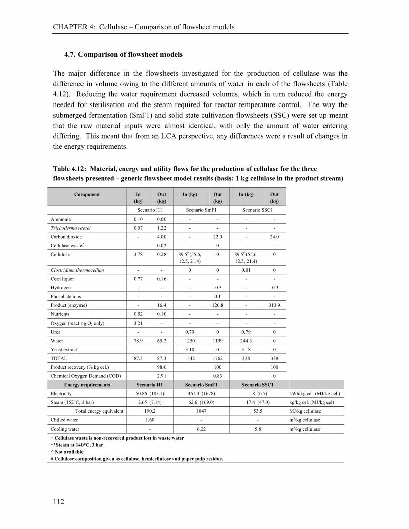
CHAPTER 4: Cellulase – Comparison of flowsheet models
112
4.7. Comparison of flowsheet models The major difference in the flowsheets investigated for the production of cellulase was the difference in volume owing to the different amounts of water in each of the flowsheets (Table 4.12). Reducing the water requirement decreased volumes, which in turn reduced the energy needed for sterilisation and the steam required for reactor temperature control. The way the submerged fermentation (SmF1) and solid state cultivation flowsheets (SSC) were set up meant that the raw material inputs were almost identical, with only the amount of water entering differing. This meant that from an LCA perspective, any differences were a result of changes in the energy requirements.
Table 4.12: Material, energy and utility flows for the production of cellulase for the three flowsheets presented – generic flowsheet model results (basis: 1 kg cellulase in the product stream)
Component In (kg)
Out (kg)
In (kg) Out (kg)
In (kg) Out (kg)
Scenario H1 Scenario SmF1 Scenario SSC1
Ammonia 0.10 0.00 - - - -
Trichoderma reesei 0.07 1.22 - - - -
Carbon dioxide - 4.00 - 22.0 - 24.0
Cellulase waste* - 0.02 - 0 - -
Cellulose 3.78 0.28 89.5# (55.6, 12.5, 21.4)
0 89.5# (55.6, 12.5, 21.4)
0
Clostridium thermocellum - - 0 0 0.01 0
Corn liquor 0.77 0.16 - - - -
Hydrogen - - - -0.3 - -0.3
Phosphate ions - - - 0.1 - -
Product (enzyme) - 16.4 - 120.8 - 313.9
Nutrients 0.52 0.10 - - - -
Oxygen (reacting O2 only) 3.21 - - - - -
Urea - - 0.79 0 0.79 0
Water 78.9 65.2 1250 1199 244.3 0
Yeast extract - - 3.18 0 3.18 0
TOTAL 87.3 87.3 1342 1762 338 338
Product recovery (% kg cel.) 98.0 100 100
Chemical Oxygen Demand (COD) 2.91 0.83 0
Energy requirements Scenario H1 Scenario SmF1 Scenario SSC1
Electricity 50.86 (183.1) 461.4 (1678) 1.8 (6.5) kWh/kg cel. (MJ/kg cel.)
Steam (152°C, 3 bar) 2.65 (7.14) 62.6 (169.0) 17.4 (47.0) kg/kg cel. (MJ/kg cel)
Total energy equivalent 190.2 1847 53.5 MJ/kg cellulase
Chilled water 1.60 - - m3/kg cellulase
Cooling water - 6.22 5.8 m3/kg cellulase
* Cellulase waste is non-recovered product lost in waste water **Steam at 140°C, 3 bar
^ Not available # Cellulose composition given as cellulose, hemicellulose and paper pulp residue.
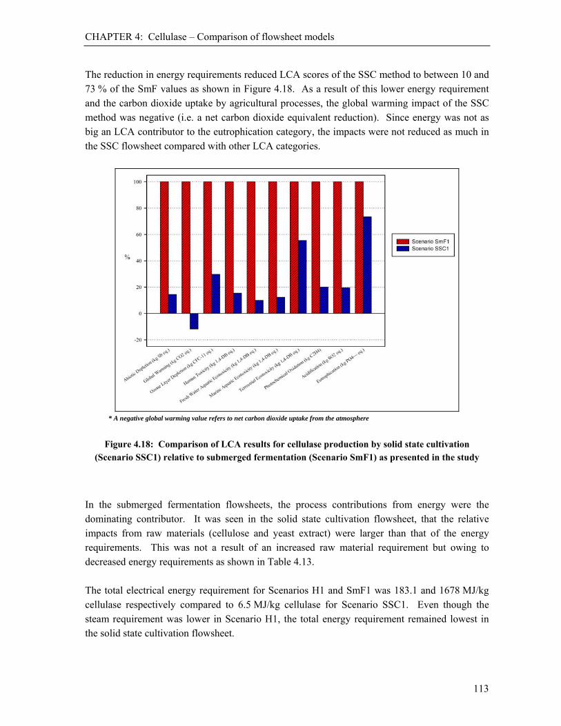
CHAPTER 4: Cellulase – Comparison of flowsheet models
113
The reduction in energy requirements reduced LCA scores of the SSC method to between 10 and 73 % of the SmF values as shown in Figure 4.18. As a result of this lower energy requirement and the carbon dioxide uptake by agricultural processes, the global warming impact of the SSC method was negative (i.e. a net carbon dioxide equivalent reduction). Since energy was not as big an LCA contributor to the eutrophication category, the impacts were not reduced as much in the SSC flowsheet compared with other LCA categories.
* A negative global warming value refers to net carbon dioxide uptake from the atmosphere
Figure 4.18: Comparison of LCA results for cellulase production by solid state cultivation (Scenario SSC1) relative to submerged fermentation (Scenario SmF1) as presented in the study
In the submerged fermentation flowsheets, the process contributions from energy were the dominating contributor. It was seen in the solid state cultivation flowsheet, that the relative impacts from raw materials (cellulose and yeast extract) were larger than that of the energy requirements. This was not a result of an increased raw material requirement but owing to decreased energy requirements as shown in Table 4.13. The total electrical energy requirement for Scenarios H1 and SmF1 was 183.1 and 1678 MJ/kg cellulase respectively compared to 6.5 MJ/kg cellulase for Scenario SSC1. Even though the steam requirement was lower in Scenario H1, the total energy requirement remained lowest in the solid state cultivation flowsheet.

CHAPTER 4: Cellulase – Conclusions
114
Table 4.13: Energy contributions for the production of cellulase for the flowsheets developed
Energy source Scenario H1 Scenario SmF1 Scenario SSC1
Electricity (MJ/kg cel.) 183.1 1678 6.5
Sterilisation 0.99 23.5 6.5
Aeration 135.2 - -
Agitation 2.57 68.1 -
Bioreactor cooling 39.38 156.4 -
Rotary vacuum filtration 2.49 - -
Evaporator - 921 -
Ultrafiltration 2.46 - -
Freeze drying - 509 -
Steam (kg/kg cel.) 2.65 62.6 17.4
Sterilisation 2.65 62.6 17.4
Total Energy (MJ/kg cel.) 190.2 1847 53.5
Chilled water (m3/kg cel.) 1.60 - -
Aeration 1.01 - -
Fermentation cooling 0.59 - -
Cooling water (m3/kg cel.) - 6.22 5.80
Fermentation cooling - 6.22 5.80
4.8. Conclusions The generic MS-Excel model was used to obtain three sets of material and energy balances for the production of cellulase, by three separate flowsheets. For each flowsheet, three scenarios were proposed with a less detailed input set in each successive scenario. For the most detailed scenarios of each flowsheet, it was found that half of the calculated material and energy balance results of flowsheet one, two and three were within 33, 35 and 50 % of literature results respectively. It was seen that values not within 10 % of the literature results were often a result of simplifying assumptions made in the literature models, while the generic flowsheets used more robust calculations. For example, Zhuang et al. (2007) assumed that the yeast extract and urea raw materials do not react in the biomass formation step. The thermophilic nature of the Zhuang et al. (2007) models required a large amount of steam and associated compression energy from electricity. This steam was poorly defined in the generic flowsheet model for the submerged fermentation (SmF) flowsheet. Cleaning-in-place (CIP) water was used in Zhuang et al. (2007) which had not been included as an option in the setup of the generic flowsheet model in Chapter 2. While water is tracked as an inventory item in the Life Cycle Impact Assessment method chosen, no water usage impact category was provided for the methodology used. This is viewed as an opening for future development owing to the important of optimising water use in bioprocesses.

CHAPTER 4: Cellulase – References
115
Using the results generated for the material and energy balances, life cycle assessment studies were completed. The most detailed material and energy balance results for Flowsheet 1 (Scenario H1) gave LCA results which were all within 30 % of the LCA results calculated from the literature material and energy balance inventory of Heinzle et al. (2006). The LCA results showed high contributions to overall impacts by electricity and steam in the submerged fermentation (SmF) models. These high electrical requirements were a result of greater volumes which required greater energy for agitation and downstream separations as well as steam during sterilisation. Cellulase production by solid state cultivation (SSC) gave an expected reduction in volumes and thus energy required. This resulted in a reduction in LCA scores to between 10 and 73 % of the SmF impacts across the various categories. With lower energy requirements in the SSC model, impacts from the raw materials (cellulose, yeast extract and urea) were more dominant.
References Bhat, M.K., 2000. Cellulases and related enzymes in biotechnology, Biotechnol. Adv., 18, 355-383. Chinn, M.S., 2003. Solid substrate cultivation of anaerobic thermophilic bacteria for the production of Cellulolytic
Enzymes, Unpublished PhD dissertation, University of Kentucky, Department of Biosystems and Agricultural Engineering.
Demain, A.L., Newcomb, M., Wu, J.H.D., 2005. Cellulase, Clostridia and ethanol, Microbiol. Mol. Biol. Rev., 69(1), 124-154.
Den Haan, R., Rose, S.H., Lynd, L.R., van Zyl, W.H., 2007. Hydrolysis and fermentation of amorphous cellulose by recombinant Saccharomyces cerevisiae, Metab. Eng., 9, 87-94.
Deschamps, F., Huet, M. C., 1984. Beta-Glucosidase Production in Agitated Solid Fermentation, Study of its Properties, Biotechnol. Lett., 6, 451-456.
Durand, A., Almanza, S., Renaud, R., Maratray, J., 1997. Solid State Fermentations: an attractive alternative to submerged-liquid fermentations, Agro Food Ind. Hi Tech., 8(3), 39-42.
El-Nawwi, S.A., El-Kader, A.A., 1996. Production of single-cell protein and cellulase from sugarcane bagasse: effect of culture factors, Biomass Bioenerg., 11(4), 361-364.
Heinzle, E., Biwer, A., Cooney, C., 2006. Modelling and Simulation of Bioprocesses, In: Development of Sustainable Bioprocesses: Modelling and Assessment, John Wiley & Sons, p61-80.
Himmel, M.E., Ruth, M.F., Wyman, C.E., 1999. Cellulase for commodity products from cellulosic biomass, Curr. Opin. Biotech., 10, 358-364.
Intelligen, 2008. Intelligen , Inc., Scotch Plain, NJ, USA, http://www.intelligen.com/ Kumar, P.K.R., Lonsane, B.K., 1987. Potential of Fed-Batch Culture in Solid State Cultivation for Production of
Gibberellic Acid, Biotechnol. Lett., 9, 179-182. Liming, X., Xueliang, S., 2004. High-yield cellulase production by Trichoderma reesei ZU-02 on corn cob residue,
Bioresource Technol., 91, 259-262. Lynd, L.R., 1996. Overview and evaluation of fuel ethanol from cellulosic biomass: technology, economics, the
environment, and policy, Annu. Rev. Energy Environ., 21, 403-465. Lynd, L.R., Lyford, K., South, C.R., van Walsum, P., Levenson, K., 2001. Evaluation of paper sludge for
amenability to enzymatic hydrolysis and conversion to ethanol, TAPPI J., 84, 50-55. Lynd, L.R., van Zyl, W.H., McBride, J.E., Laser, M., 2005. Consolidated bioprocessing of cellulosic biomass: an
update, Curr. Opin. Biotech., 16, 577-583. Mitchell, D.A., Meien, O.F., Krieger, N., Dalsenter, F.D.H., 2003. Recent Developments in Modelling of Solid
State Fermentation: Heat and Mass Transfer in Bioreactors, Biochem. Eng. J., 13, 137-147.
CHAPTER 4: Cellulase – References
116
Niranjane, A.P., Madhou, P., Stevenson, T.W., 2007. The effect of carbohydrate carbon sources on the production of cellulase by Phlebia gigantea, Enzyme Microb. Tech., 40, 1464-1468.
Rabinovich, M.L., Melnik, M.S., Bolobova, A.V., 2002. Microbial Cellulases (Review), Appl. Biochem. Micro., 38(4), 305-321.
Rajoka, M.I., Malik, K.A., 1997. Cellulase production by Cellulomonas biazotae cultured in media containing different substrates, Bioresource Technol., 59, 21-27.
Reczey K., Szengyel, Zs., Eklund, R., Zacchi, G., 1996. Cellulase production by T. reesei, Bioresource Technol., 57, 25-30.
Romera, M.D., Aguado, J., González, L., Ladero, M., 1999. Cellulase production by Neurospora crassa on wheat straw, Enzyme Microb. Tech., 25, 244-250.
Sáez, J.C., Schell, D.J., Tholudur, A., Farmer, J., Hamilton, J., Colucci, J.A., McMillan, J.D., 2002. Carbon mass balance evaluation of cellulase production on soluble and insoluble substrates, Biotechnol. Prog., 18, 1400-1407.
Soni, R., Sandhu, D.K., Soni, S.K., 1999. Localisation and optimisation of cellulase production in Chaetomium erraticum, J. Biotechnol., 73, 43-51.
Szabó, I.J., Johansson, G., Pettersson, G., 1996. Optimized cellulase production by Phanerochaete chrysosporium: control of catabolite repression by fed-batch cultivation, J. Biotechnol., 48, 221-230.
Thirmale, S., Rani, D.S., Nand, K., 2001. Control of cellulase formation by trehalose in Clostridium papyrosolvens CFR-703, Process Biochem., 37, 241-245.
Wen, Z., Liao, W., Chen, S., 2005. Production of cellulase by Trichoderma reesei from dairy manure, Bioresource Technol., 96, 491-499.
Wooley, R., Ruth, M., Glassner, D., Sheehan, J., 1999a. Process design and costing of bioethanol technology: a tool for determining the status and direction of research and development, Biotechnol. Prog., 15, 794-803.
Wooley, R., Ruth M., Sheehan, J., Ibsen, K., Majdeski, H., Galvez, A., 1999b. Lignocellulosic biomass to ethanol process design and economics utilizing co-current dilute acid prehydrolysis and enzymatic hydrolysis: current and futuristic scenarios, Report NREL/TP-580-26157, National Renewable Energy Laboratory, Golden, Colorado.
Xia, L, Cen, P., 1999. Cellulase production by solid state fermentation on lignocellulosic waste from the xylose industry, Process Biochem., 34, 909-912.
Zhang, Y., Lynd, L.R., 2003. Quantification of cell and cellulase concentrations during anaerobic cellulose fermentation: Development of an enzyme-linked immunosorbent assay-based method with application to Clostridium thermocellum batch cultures, Anal. Chem., 75(2), 219-227.
Zhuang J., Marchant, M.A., Nokes, S.E., Strobel, 2007. Economic analysis of cellulase production methods for bio-ethanol, App. Eng. Agric., 23(5), 679-687.

117
CHAPTER 5: POLYMERS

118

CHAPTER 5: Polymers – Introduction
119
5.1. Introduction Use of plastics is wide spread; however their disposal is difficult. Incinerating plastics is expensive and can release harmful chemicals. While re-use and recycling is the preferred route, implementation is difficult and results in limited applications for the recycled material (Reddy et al. 2003, Khanna and Srivastava 2005). Polypropylene is produced from fossil fuels hence affected by resource depletion. Polymer production from a renewable source is desirable. Such polymers include the polyhydroxyalkanoates (PHAs) group of polymers and the polylactides. This chapter describes a case study for the application and validation of the generic flowsheet model using the microbial production of polyhydroxyalkanoate (PHA) by Cupriavidus necator as an example. Three scenarios were defined for the generic flowsheet, each with a more limited set of inputs. These material and energy results are compared to a full biopolymer design of Harrison (1990). The material and energy balance results obtained from both the generic flowsheet models and the Harrison (1990) model were then used with the Life Cycle Assessment (LCA) software SimaPro v7.1® (PRé Consultants B.V. 2008) to determine the resulting environmental impacts. The LCA results were also compared to the LCA impacts for the production of polyolefins (polypropylene and polyethylene) to determine the relative impacts of an equivalent chemically produced material. While there are several commodity biopolymers, the advantage of testing the model on polyhydroxyalkanoates is that there are numerous laboratory scale data providing parameters required for the generic flowsheet model. These are reported by Harrison (1990), Wang and Lee (1997), He et al. (1998), Grothe et al. (1999), Kim (2000), Chen et al. (2001), Yu (2001) and Yu et al. (2005).
5.2. The production of polyhydroxyalkanoates (PHAs)
5.2.1. Polyhydroxyalkanoates A biodegradable polymer is advantageous where recycling and re-use is not possible or practicable. Biopolymers are renewable, largely biodegradable and can have very similar properties to conventional polymers. The potential environmental benefits of biopolymers currently carry an economic cost (Zinn et al. 2001, Godbole et al. 2003).

CHAPTER 5: Polymers – The production of polyhydroxyalkanoates (PHAs)
120
Biopolymers currently of interest include thermoplastic starch (TPS), polylactides (PLA), poly-
-hydroxybutyric acid (PHB) and its copolymers (PHAs), and polymer fills. PHBs are
considered strong candidates as they have very similar properties to synthetic polymers, as seen in Table 5.1, but degrade completely to water and carbon dioxide under aerobic conditions (Lee 1996). This is advantageous in, amongst other things, medical applications (Pouton and Akhtar 1996, Shum-Tim et al. 1999, Williams et al. 1999, Sudesh et al. 2000, Zinn et al. 2001, Reddy et al. 2003, Volova et al. 2003, Wang et al. 2003, Chen and Wu 2005, Khanna and Srivastava 2005). Polyhydroxyalkanoate synthesis can occur using aerobic conversion of agricultural feedstocks by wild type or recombinant micro-organisms (e.g. Akiyama et al. 2003), in vitro production via PHA-polymerase catalysed polymerisation, using genetically engineered plants (Poirer et al. 1995, Riesmeier et al. 1998, Gerngross 1999, Poirer 1999, Valentin et al. 1999, Gerngross and Slater 2000, Kurdikar et al. 2001, Moire et al. 2003, Snell and Peoples 2002, Capell and Christou 2004, Daae et al. 2004 and Mascia and Flavell 2004) or by the anaerobic digestion of biological wastes (Zinn et al. 2001 and Reddy et al. 2003). This study is confined to microbial production of poly-β-hydroxybutyric acid (PHB) under aerobic ambient growth temperatures (Lee 1996, Reddy et al. 2003). For many systems, the preferred carbon source for production is cane sugar or glucose (Nonato et al. 2001), although starch and whey can also be used to produce PHB (Kim 2000). In addition waste effluents, including beet- or cane molasses or starchy water (Yu 2001, Sudesh et al. 2000), plant oils, plant-derived fatty acids and alkanes (Sudesh et al. 2000) are used.
Table 5.1: Properties of polypropylene and poly--hydroxybutyric acid (PHB)
Units Polypropylene PHB
Density kg/m3 900-910 [4] 1250 [1]
Melting Point °C 176 [2] 45-180 [2] P(3HB) = 180 [2]
Tensile Strength MPa 38 [3] 13 – 40 [1]
Shrinkage % 1 – 3 [1]
Elongation % 400 [3] 5 – 680 [3]
Young’s Modulus MPa 17000 [3] 350 – 1000 [1]
Glass-transition Temperature °C -10 [2] 15 [1] P(3HB) = 4 [2]
Service Temperature °C -30 – 120 [1]
Specific Heat (20-80°C) kJ/kg.K 1.9 [4]
Thermal Conductivity (20-150°C) kW/m.K 0.42-0.61 [4]
References: [1] Delft 2004 [2] Doi 1990
[3] Sudesh et al. 2000 [4] Ogorkiewicz 1970
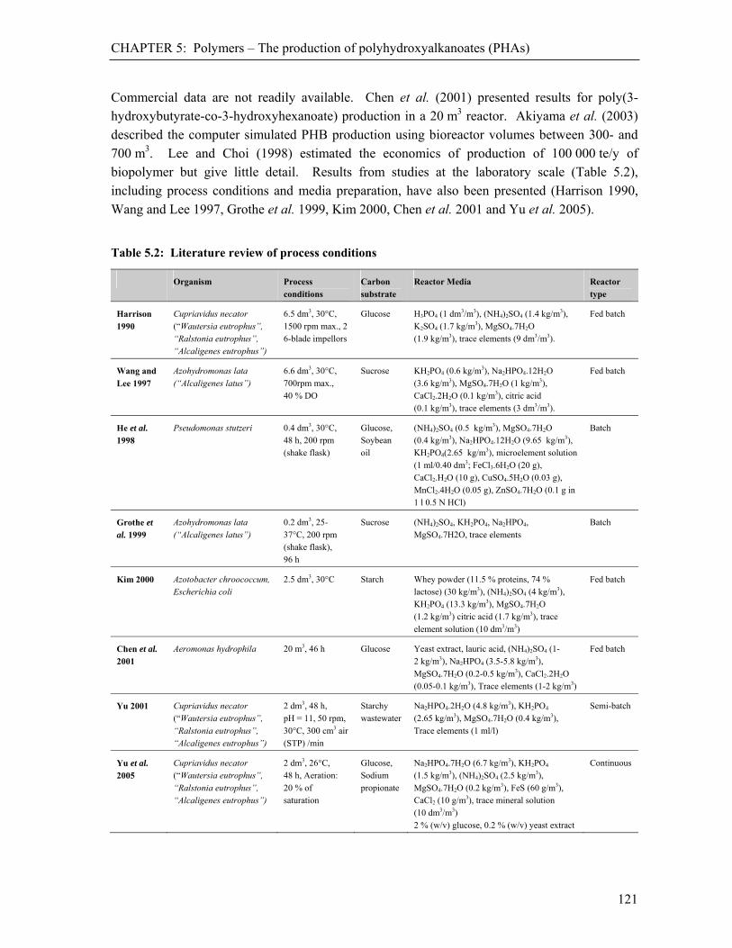
CHAPTER 5: Polymers – The production of polyhydroxyalkanoates (PHAs)
121
Commercial data are not readily available. Chen et al. (2001) presented results for poly(3-hydroxybutyrate-co-3-hydroxyhexanoate) production in a 20 m3 reactor. Akiyama et al. (2003) described the computer simulated PHB production using bioreactor volumes between 300- and 700 m3. Lee and Choi (1998) estimated the economics of production of 100 000 te/y of biopolymer but give little detail. Results from studies at the laboratory scale (Table 5.2), including process conditions and media preparation, have also been presented (Harrison 1990, Wang and Lee 1997, Grothe et al. 1999, Kim 2000, Chen et al. 2001 and Yu et al. 2005).
Table 5.2: Literature review of process conditions
Organism Process conditions
Carbon substrate
Reactor Media Reactor type
Harrison
1990
Cupriavidus necator (“Wautersia eutrophus”, “Ralstonia eutrophus”, “Alcaligenes eutrophus”)
6.5 dm3, 30°C, 1500 rpm max., 2 6-blade impellors
Glucose H3PO4 (1 dm3/m3), (NH4)2SO4 (1.4 kg/m3), K2SO4 (1.7 kg/m3), MgSO4.7H2O (1.9 kg/m3), trace elements (9 dm3/m3).
Fed batch
Wang and
Lee 1997
Azohydromonas lata (“Alcaligenes latus”)
6.6 dm3, 30°C, 700rpm max., 40 % DO
Sucrose KH2PO4 (0.6 kg/m3), Na2HPO4.12H2O (3.6 kg/m3), MgSO4.7H2O (1 kg/m3), CaCl2.2H2O (0.1 kg/m3), citric acid (0.1 kg/m3), trace elements (3 dm3/m3).
Fed batch
He et al. 1998
Pseudomonas stutzeri 0.4 dm3, 30°C, 48 h, 200 rpm (shake flask)
Glucose, Soybean oil
(NH4)2SO4 (0.5 kg/m3), MgSO4.7H2O (0.4 kg/m3), Na2HPO4.12H2O (9.65 kg/m3), KH2PO4(2.65 kg/m3), microelement solution (1 ml/0.40 dm3; FeCl3.6H2O (20 g), CaCl2.H2O (10 g), CuSO4.5H2O (0.03 g), MnCl2.4H2O (0.05 g), ZnSO4.7H2O (0.1 g in 1 l 0.5 N HCl)
Batch
Grothe et al. 1999
Azohydromonas lata (“Alcaligenes latus”)
0.2 dm3, 25-37°C, 200 rpm (shake flask), 96 h
Sucrose (NH4)2SO4, KH2PO4, Na2HPO4, MgSO4.7H2O, trace elements
Batch
Kim 2000 Azotobacter chroococcum, Escherichia coli
2.5 dm3, 30°C Starch Whey powder (11.5 % proteins, 74 % lactose) (30 kg/m3), (NH4)2SO4 (4 kg/m3), KH2PO4 (13.3 kg/m3), MgSO4.7H2O (1.2 kg/m3) citric acid (1.7 kg/m3), trace
element solution (10 dm3/m3)
Fed batch
Chen et al. 2001
Aeromonas hydrophila 20 m3, 46 h Glucose Yeast extract, lauric acid, (NH4)2SO4 (1-2 kg/m3), Na2HPO4 (3.5-5.8 kg/m3),
MgSO4.7H2O (0.2-0.5 kg/m3), CaCl2.2H2O (0.05-0.1 kg/m3), Trace elements (1-2 kg/m3)
Fed batch
Yu 2001 Cupriavidus necator (“Wautersia eutrophus”,
“Ralstonia eutrophus”, “Alcaligenes eutrophus”)
2 dm3, 48 h, pH = 11, 50 rpm,
30°C, 300 cm3 air (STP) /min
Starchy wastewater
Na2HPO4.2H2O (4.8 kg/m3), KH2PO4 (2.65 kg/m3), MgSO4.7H2O (0.4 kg/m3),
Trace elements (1 ml/l)
Semi-batch
Yu et al. 2005
Cupriavidus necator (“Wautersia eutrophus”,
“Ralstonia eutrophus”, “Alcaligenes eutrophus”)
2 dm3, 26°C, 48 h, Aeration:
20 % of saturation
Glucose, Sodium
propionate
Na2HPO4.7H2O (6.7 kg/m3), KH2PO4 (1.5 kg/m3), (NH4)2SO4 (2.5 kg/m3),
MgSO4.7H2O (0.2 kg/m3), FeS (60 g/m3), CaCl2 (10 g/m3), trace mineral solution (10 dm3/m3) 2 % (w/v) glucose, 0.2 % (w/v) yeast extract
Continuous

CHAPTER 5: Polymers – The production of polyhydroxyalkanoates (PHAs)
122
The data presented includes PHB production using Azotobacter chroococcum, Aeromonas hydrophila, Azohydromonas lata, Cupriavidus nectar, Escherichia coli and Pseudomonas stutzeri on carbon sources such as glucose, soybean oil, sucrose and starch in batch, fed batch and continuous processes. Partial details of microbial growth, PHB accumulation, process conditions and reviews are also described by Lee (1996), Steinbüchel and Füchtenbusch (1998), Nonato et al. (2001), Zinn et al. (2001) and Khanna and Srivastava (2005). PHB yields and growth rates are quoted by several authors, including Ackermann and Babel (1998), Grothe et al. (1999), Nonato et al. (2001) and Khanna and Srivastava (2005). The amount of polymer, as a percentage of total biomass, ranges from 20 to above 85 %. Maximum PHB concentrations, productivities and yields are shown to be 106 kg PHB/m3, 4.94 kg PHB/m3/h and 0.8 kg PHB/kg substrate respectively, as seen in Table 5.3.
Table 5.3: Literature review of percentage PHB content of biomass, concentration, productivity, yield and biomass growth rates following its aerobic microbial production
Percentage Polymer
Biomass Concentration
Polymer Concentration
Polymer Productivity
Polymer Yield Biomass Growth Rate
wt % PHB kg biomass/m3 kg PHB/m3 kg PHB/m3/h kg PHB/kg substrate
/h
Harrison 1990 70 150 106 1.18* 0.36 0.11-0.33
Wang and Lee 1997, Lee and Choi 1998
87-88.3 111 98.7 4.94-5.13 0.42 0.044*
Grothe et al. 1999 63 1.1-3.9* 0.73-2.48 0.15 (0.38 kg sucrose/m3/h)
0.4 0.075
Kim 2000 20-80 54-87 0.864-61 0.0149-0.9 0.04-0.33 0.017*
Chen et al. 2001 50 50 25 0.54 0.25* 0.029*
Nonato et al. 2001 65-70 120-150 78-105* 1.44 0.32 0.014-0.018*
Akiyama et al. 2003 75-85 100-200 75-170* 4.63 0.3-0.8 0.023-0.046*
Khanna and Srivastava 2005 76 9.3-159* 7.1-121 1.15-2.42 0.36-0.4 0.265
Yu et al. 2005 22-90* 3.10-7.96 1.73-2.8 0.045-0.252 0.019-0.136
*Calculated estimate values
Harrison (1990), Lee and Choi (1998), Chen et al. (2001), Zinn et al. (2001) and Akiyama et al. (2003) describe downstream processing for polymer recovery and purification units, including a selection of cell disruption, surfactant pre-treatment, solvent extraction, precipitation, flocculation, filter pressing, rotary vacuum drying, centrifugation and spray drying. Downstream processing can yield up to 95 % recovery of polymer (Lee and Choi 1998, Nonato et al. 2001) at purities greater than 98 % (Nonato et al. 2001, Zinn et al. 2001).
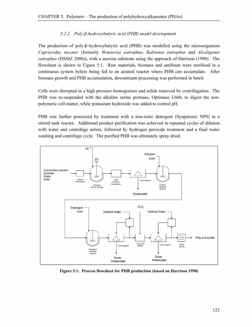
CHAPTER 5: Polymers – The production of polyhydroxyalkanoates (PHAs)
123
5.2.2. Poly-β-hydroxybutyric acid (PHB) model development
The production of poly--hydroxybutyric acid (PHB) was modelled using the microorganism
Cupriavidus necator (formerly Wautersia eutrophus, Ralstonia eutrophus and Alcaligenes eutrophus (DSMZ 2006)), with a sucrose substrate using the approach of Harrison (1990). The flowsheet is shown in Figure 5.1. Raw materials, biomass and antifoam were sterilised in a continuous system before being fed to an aerated reactor where PHB can accumulate. After biomass growth and PHB accumulation, downstream processing was performed in batch. Cells were disrupted in a high pressure homogeniser and solids removed by centrifugation. The PHB was re-suspended with the alkaline serine protease, Optimase L660, to digest the non-polymeric cell matter, while potassium hydroxide was added to control pH. PHB was further processed by treatment with a non-ionic detergent (Synperonic NP8) in a stirred tank reactor. Additional product purification was achieved in repeated cycles of dilution with water and centrifuge action, followed by hydrogen peroxide treatment and a final water washing and centrifuge cycle. The purified PHB was ultimately spray dried.
Figure 5.1: Process flowsheet for PHB production (based on Harrison 1990)
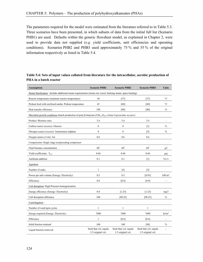
CHAPTER 5: Polymers – The production of polyhydroxyalkanoates (PHAs)
124
The parameters required for the model were estimated from the literature referred to in Table 5.3. Three scenarios have been presented, in which subsets of data from the initial full list (Scenario PHB1) are used. Defaults within the generic flowsheet model, as explained in Chapter 2, were used to provide data not supplied (e.g. yield coefficients, unit efficiencies and operating conditions). Scenarios PHB2 and PHB3 used approximately 75 % and 55 % of the original information respectively as listed in Table 5.4.
Table 5.4: Sets of input values collated from literature for the intracellular, aerobic production of PHA in a batch reactor
Assumptions Scenario PHB1 Scenario PHB2 Scenario PHB3 Units
Steam Sterilisation: Include additional steam requirements (steam out vessel, backing steam, space heating)
Reactor temperature (maintain reactor temperature) 30 [37] [37] °C
Preheat feed with sterilised media: Preheat temperature 65 [60] [60] °C
Heat transfer efficiency 100 [80] [80] %
Microbial growth conditions (batch production of poly--butyrate (CH0.13O0.67) from Cupriavidus necator)
Product: Biomass ratio 2.4 2.4 2.4 -
Carbon source (excess): Glucose 0 0 [1] %
Nitrogen source (excess): Ammonium sulphate 0 0 [5] %
Oxygen source (vvm): Air 0.6 0.6 0.6
Compression: Single stage reciprocating compressor
Final biomass concentration 44# 44# 44# g/l
Yield coefficients: Yp/s 0.44 0.44 0.44 g/g
Antifoam addition 0.1 0.1 [1] %v/v
Agitation
Number of tanks 1 [5] [5]
Power per unit volume (Energy: Electricity) 0.5 0.5 [0.95] kW/m3
Efficiency 0.8 [0.9] [0.9] -
Cell disruption: High Pressure homogenisation
Energy efficiency (Energy: Electricity) 0.8 [1.25] [1.25] mg/J
Cell disruption efficiency 100 [90.25] [90.25] %
Centrifugation
Number of wash/spin cycles 1 1 1
Energy required (Energy: Electricity) 7600 7600 7600 kJ/m3
Efficiency 1 [0.6] [0.6] -
Solid fraction retained 100 100 [98] %
Liquid fraction removed Such that vol. equals 1/3 original vol.
Such that vol. equals 1/3 original vol.
Such that vol. equals 1/3 original vol.
-

CHAPTER 5: Polymers – The production of polyhydroxyalkanoates (PHAs)
125
Assumptions Scenario PHB1 Scenario PHB2 Scenario PHB3 Units
Enzyme addition: Optimase L660 (MKC) – protease
Protease volume added 0.08 0.08 0.08 %v/v
Potassium hydroxide added** 10 10 10 %v/v
Agitation energy (Energy: Electricity) 5.76 5.76 5.76 MJ/m3
Detergent addition: Synperonic NP8 (ICI Ltd)
Detergent volume added 1 1 1 %v/v
Agitation energy(Energy: Electricity) 5.76 5.76 5.76 MJ/m3
Centrifugation
Number of wash/spin cycles (re-suspension with H2O) 5^ 5^ 5^
Energy required (Energy: Electricity) 7600 7600 7600 kJ/m3
Efficiency 1 [0.6] [0.6] -
Time 20 20 20 min
Solid fraction retained 100 100 [98] %
Liquid fraction removed Such that after 5 wash cycles vol. remaining equals
vol. entered
Such that after 5 wash cycles vol. remaining equals
vol. entered
Such that after 5 wash cycles vol. remaining equals
vol. entered
-
Hydrogen peroxide addition
H2O2 volume added 1.2 1.2 1.2 %v/v
Centrifugation
Number of wash/spin cycles (re-suspension with H2O) 2 2 2
Energy required (Energy: Electricity) 7600 7600 7600 kJ/m3
Efficiency 1 [0.6] [0.6] -
Time 20 20 20 min
Solid fraction retained 100 100 [98] %
Liquid fraction removed Such that after 2 wash cycles vol. remaining equals
vol. entered
Such that after 2 wash cycles vol. remaining equals
vol. entered
Such that after 2 wash cycles vol. remaining equals
vol. entered
-
Spray drying (Energy: Natural gas)
Solid fraction retained 100 [99] [99] %
Liquid fraction removed 100 100 [99] %
* Values available from literature and not specific to this flowsheet design ** The amount of potassium hydroxide added would normally be given as a mass per volume value. However, the generic flowsheet is set up to require a volume per volume value liquids are typically added. # Non-PHB biomass only ^ Not a direct input to the Excel model, but used to calculate other information required for the data input here [ ] Default values calculated or assumed in the MS-Excel model when no explicit inputs are given
CHAPTER 5: Polymers – Results
126
5.3. Results
5.3.1. Material and energy balance outputs Implementing the generic model as described in Chapter 2, material and energy balance data
were generated and the results are shown in Table 5.5, using a basis of one kilogram poly--
butyrate-containing product. These gave mass purities of 100, 100 and 90.5 % and recoveries of 100, 99 and 93.2 % for Scenarios PHB1, PHB2 and PHB3 respectively. Between 3.2 and 3.6 kg of glucose and between 0.23 and 0.28 kg ammonium sulphate were required as feed. These sets of values were both within 88 % of each other. At the aeration rate of 0.6 vvm, 107.6, 120.2 and 278.6 kg of air was required for Scenarios PHB1, PHB2 and PHB3 respectively. The more than doubling of air in Scenario PHB3 was owing to the increase in the reactor volume because of the assumptions made with regard to excess raw materials and the less efficient downstream processing. This increase in volume led to an increase in water, total energy (renewable and non-renewable) and downstream processing input requirements as shown in Figure 5.2. In the three scenarios, 31.8-, 34.8- and 92.2 kg of water per kilogram of plastic was required for Scenarios PHB1, PHB2 and PHB3 respectively. It was assumed that there was no excess carbon or nitrogen source in Scenarios PHB1 and PHB2. This resulted in there being no glucose or ammonium sulphate waste in the wastewater. Mass outputs for these scenarios were within 12 % of each other (except biomass waste) as shown in Figure 5.3. The increased volumes of Scenario PHB3, which were almost three times greater than previous scenarios, also increased the additives required in downstream processing by almost three times as these were added as volume fractions. Carbon dioxide formed from the three scenarios was within 10 % for all scenarios. For each kilogram of PHB formed in Scenario PHB1, 11.7 MJ of electrical energy, 4.96 kg steam and 503.7 kg natural gas were required. Similar, but slightly higher, requirements were found for Scenario PHB2. Compared with Scenario PHB1, the increased volumes of Scenario PHB3 required 164, 144 and 50 % more electricity, natural gas and steam respectively. Owing to the higher reactor temperatures of Scenarios PHB2 and PHB3 (37°C) versus Scenario PHB1 (30°C), less cooling water was required, since cooling water was only required for controlling reactor temperatures. A cooling water temperature of 18°C was used in all scenarios. The 7°C difference in reactor temperature resulted in a 4 fold lower cooling requirement in both Scenarios PHB2 and PHB3 compared to Scenario PHB1.
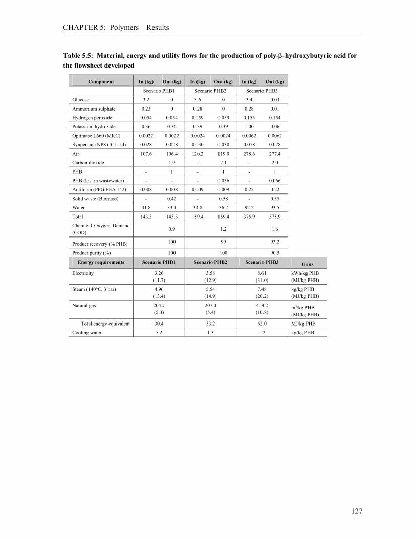
CHAPTER 5: Polymers – Results
127
Table 5.5: Material, energy and utility flows for the production of poly--hydroxybutyric acid for
the flowsheet developed
Component In (kg) Out (kg) In (kg) Out (kg) In (kg) Out (kg)
Scenario PHB1 Scenario PHB2 Scenario PHB3
Glucose 3.2 0 3.6 0 3.4 0.03
Ammonium sulphate 0.23 0 0.28 0 0.28 0.01
Hydrogen peroxide 0.054 0.054 0.059 0.059 0.155 0.154
Potassium hydroxide 0.36 0.36 0.39 0.39 1.00 0.06
Optimase L660 (MKC) 0.0022 0.0022 0.0024 0.0024 0.0062 0.0062
Synperonic NP8 (ICI Ltd) 0.028 0.028 0.030 0.030 0.078 0.078
Air 107.6 106.4 120.2 119.0 278.6 277.4
Carbon dioxide - 1.9 - 2.1 - 2.0
PHB - 1 - 1 - 1
PHB (lost in wastewater) - - - 0.036 - 0.066
Antifoam (PPG.EEA 142) 0.008 0.008 0.009 0.009 0.22 0.22
Solid waste (Biomass) - 0.42 - 0.58 - 0.55
Water 31.8 33.1 34.8 36.2 92.2 93.5
Total 143.3 143.3 159.4 159.4 375.9 375.9
Chemical Oxygen Demand (COD)
0.9 1.2 1.6
Product recovery (% PHB) 100 99 93.2
Product purity (%) 100 100 90.5
Energy requirements Scenario PHB1 Scenario PHB2 Scenario PHB3 Units
Electricity 3.26 (11.7)
3.58 (12.9)
8.61 (31.0)
kWh/kg PHB (MJ/kg PHB)
Steam (140°C, 3 bar) 4.96 (13.4)
5.54 (14.9)
7.48 (20.2)
kg/kg PHB (MJ/kg PHB)
Natural gas 204.7 (5.3)
207.0 (5.4)
413.2 (10.8)
m3/kg PHB (MJ/kg PHB)
Total energy equivalent 30.4 33.2 62.0 MJ/kg PHB
Cooling water 5.2 1.3 1.2 kg/kg PHB

CHAPTER 5: Polymers – Results
128
Figure 5.2: Comparison of material, energy and utility inputs from the generic model, calculated for PHB production, relative to Scenario PHB1
Figure 5.3: Comparison of material, energy and utility outputs from the generic model, calculated for PHB production, relative to Scenario PHB1

CHAPTER 5: Polymers – Life Cycle Assessment (LCA)
129
5.4. Life Cycle Assessment (LCA)
5.4.1. Goal definition and system description
A cradle-to-gate Life Cycle Assessment (LCA) of the poly--hydroxybutyrate (PHB) production
was performed using the methodology presented in Section A.6 of Appendix A. A functional unit was taken as 1 kg of polymer product immediately after the spray drier in the process shown in Figure 5.1. In the case of Scenario PHB3 where the purity was not 100 %, the mass of 1 kg includes impurities. However, there was only a 9% difference in the purities. Depending on the use of the polymer, this difference may be acceptable and lead to equal functions of the polymers of different purity. As such, an equal mass functional unit was considered more appropriate than an equal purity functional unit. The Ecoinvent v1.3 inventory dataset was used in the LCA for all inventories except sugar. It was assumed that the glucose requirements of PHB production were met by sugar, modelled using the South African sugar cane data defined in Appendix G. The LCA included a coal-based South African electricity mix,. All air, water and solid waste emissions from the polymer production have been included in the Life Cycle Assessment. Waste water from the process was assumed to be processed in a waste water treatment (WWT) facility. The life cycle inventory data sets are presented in Appendix I. The Life Cycle Impact Assessment results are presented in Section 5.4.2, followed by a discussion. The material and energy balance results are then compared to the results from a full biopolymer process design as obtained from literature in Section 5.5.1. These material and energy flows are used in the LCA software and impacts compared to the generic flowsheet model LCA impacts in Section 5.5.2. In Section 5.5.3, the major process contributions to the
LCA scores are presented and discussed. The LCA results from the poly--hydroxybutyrate
(PHB) are then compared to the results for polyolefins (polypropylene and polyethylene).
5.4.2. Life Cycle Impact Assessment (LCIA) Using the material and energy balance inventories shown in Table 5.5, Life Cycle Impacts for
the production of 1 kg of poly--hydroxybutyrate (PHB) are presented in Table 5.6 using
midpoint indicators. For Scenario PHB1, for each kilogram of polymer formed, global warming emissions of 5.74 kg CO2 eq., abiotic depletion equal to 0.045 kg Sb eq., ozone layer depletion equal to 0.33 mg CFC-11 eq. and acidification potential of 0.047 kg SO2 eq. were obtained.

CHAPTER 5: Polymers – Life Cycle Assessment (LCA)
130
The LCA results for the same categories for Scenario PHB2 were: 6.39 kg CO2 eq., 0.045 kg Sb eq., 0.37 mg CFC-11 eq. and 0.053 kg SO2 eq.. These increases were a result of the increases in electricity and steam requirements in Scenario PHB2. The increase in the eutrophication score was greater than the other LCA categories as a result of the additional impacts from increases in glucose requirements (Figure 5.4). Although raw materials to the bioreactor were similar in all three scenarios, LCA impacts from Scenario PHB3 were between 150 % and 250 % greater than of Scenarios PHB1 and PHB2, in all categories. This was a result of a doubling of the energy requirements as well as the increased downstream chemical inputs required. These increases are owing to the larger volumes needed to achieve the desired product mass with the less efficient separations of Scenario PHB3. For each kilogram of polymer formed, life cycle impacts of 10.2 kg CO2 eq., 0.093 kg Sb eq., 0.56 mg CFC-11 eq. and 0.098 kg SO2 eq., were obtained in the categories of global warming, abiotic depletion, ozone layer depletion and acidification respectively.
Table 5.6: LCIA of poly--hydroxybutyrate product per kilogram of polymer – CML Baseline
2000 V2.03
Impact Category Unit Scenario PHB1 Scenario PHB 2 Scenario PHB 3
Abiotic Depletion kg Sbeq. 0.045 0.045 0.093
Global Warming (GWP100) kg CO2 eq. 5.74 6.39 10.2
Ozone Layer Depletion (ODP) mg CFC-11eq. 0.33 0.37 0.56
Human Toxicity kg 1,4-DBeq. 2.20 2.46 4.87
Fresh Water Aquatic Ecotoxicity kg 1,4-DBeq. 0.43 0.48 1.00
Marine Aquatic Ecotoxicity kg 1,4-DBeq. 2400 2700 5800
Terrestrial Ecotoxicity kg 1,4-DBeq. 0.012 0.014 0.020
Photochemical Oxidation kg C2H4 0.0016 0.0018 0.0034
Acidification kg SO2 eq. 0.047 0.053 0.098
Eutrophication kg PO43-
eq. 0.026 0.033 0.045

CHAPTER 5: Polymers – Comparison with a design of a biopolymer plant
131
Figure 5.4: Comparison of LCA results for 1 kg poly--butyrate for the three scenarios developed
5.5. Comparison with a design of a biopolymer plant
5.5.1. Material and energy balance The validity of the material and energy balance results was compared to a full flowsheet design set up specifically for the PHB process. Using MS-Excel, specific design considerations for each unit operation were included. This full design was based on the laboratory study of Harrison (1990) using a variation of the BIOPOL flowsheet developed by ICI for production of bacterial PHB from glucose (Asrar and Gruys 2002). Here it was scaled up from laboratory data to give 1 000 kg of PHB and was referred to as the Harrison (1990) model. Process conditions are given in Table 5.7. Data from Perry et al. (1984), Engler (1985), Woods (1995), Dennis (2000) and Baker and McKenzie (2005) were also used.
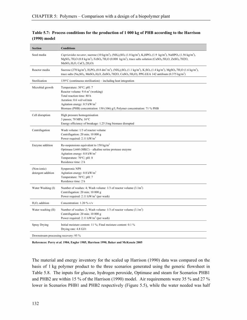
CHAPTER 5: Polymers – Comparison with a design of a biopolymer plant
132
Table 5.7: Process conditions for the production of 1 000 kg of PHB according to the Harrison (1990) model
Section Conditions
Seed media Cupriavidus necator, sucrose (10 kg/m3), (NH4)2SO4 (1.8 kg/m3), K2HPO4 (1.9 kg/m3), NaHPO4 (1.56 kg/m3), MgSO4.7H2O (0.8 kg/m3), FeSO4.7H2O (0.008 kg/m3), trace salts solution (CuSO4.5H2O, ZnSO4.7H2O, MnSO4.H2O, CaCl2.2H2O)
Reactor media Sucrose (270 kg/m3), H3PO4 (0.8 dm3/m3), (NH4)2SO4 (1.1 kg/m3), K2SO4 (1.4 kg/m3), MgSO4.7H2O (1.6 kg/m3), trace salts (Na2SO4, MnSO4.H2O, ZnSO4.7H2O, CuSO4.5H2O), PPG.EEA 142 antifoam (0.375 kg/m3)
Sterilisation 139°C (continuous sterilisation) – including heat integration
Microbial growth Temperature: 30°C; pH: 7 Reactor volume: 9.4 m3 (working) Total reaction time: 80 h Aeration: 0.6 vol/vol/min Agitation energy: 0.5 kW/m3
Biomass (PHB) concentration: 150 (106) g/l; Polymer concentration: 71 % PHB
Cell disruption High pressure homogenisation 3 passes; 70 MPa; 16°C Energy efficiency of breakage: 1.25 J/mg biomass disrupted
Centrifugation Wash volume: 1/3 of reactor volume Centrifugation: 20 min; 10 000 g Power required: 2.11 kW/m3
Enzyme addition Re-suspensions equivalent to 150 kg/m3
Optimase L660 (MKC) – alkaline serine protease enzyme Agitation energy: 0.8 kW/m3
Temperature: 70°C; pH: 8 Residence time: 2 h
(Non-ionic) detergent addition
Synperonic NP8 Agitation energy: 0.8 kW/m3
Temperature: 70°C; pH: 7 Residence time: 2 h
Water Washing (I) Number of washes: 4; Wash volume: 1/3 of reactor volume (3.1m3) Centrifugation: 20 min; 10 000 g Power required: 2.11 kW/m3 (per wash)
H2O2 addition Concentration: 1.20 % v/v
Water washing (II) Number of washes: 2; Wash volume: 1/3 of reactor volume (3.1m3) Centrifugation: 20 min; 10 000 g Power required: 2.11 kW/m3 (per wash)
Spray Drying Initial moisture content: 11 %; Final moisture content: 0.1 %
Drying rate: 4.8 GJ/t
Downstream processing recovery: 95 %
References: Perry et al. 1984, Engler 1985, Harrison 1990, Baker and McKenzie 2005
The material and energy inventory for the scaled up Harrison (1990) data was compared on the basis of 1 kg polymer product to the three scenarios generated using the generic flowsheet in Table 5.8. The inputs for glucose, hydrogen peroxide, Optimase and steam for Scenarios PHB1 and PHB2 are within 15 % of the Harrison (1990) model. Air requirements were 35 % and 27 % lower in Scenarios PHB1 and PHB2 respectively (Figure 5.5), while the water needed was half

CHAPTER 5: Polymers – Comparison with a design of a biopolymer plant
133
that of the scaled up Harrison (1990) model, which required 65.2 kg of water per kilogram of polymer.
In the Harrison (1990) model, formation of poly--hydroxybutyrate was achieved by nitrogen
limitation. Nitrogen was supplied in Scenarios PHB1, PHB2 and PHB3 as ammonium sulphate, but since physical limitation can not be modelled, the required amount was overestimated. The Harrison (1990) model included a large number of trace elements which were not modelled in the generic flowsheets scenarios. Since the cooling water requirement was directly affected by the amount of oxygen required for microbial growth and product formation, the lower oxygen requirements of the generic models
gave a lower cooling water value. The difference in the cooling water temperature (18C for the
generic flowsheets and 20C of the Harrison (1990) model) also contributed to the differences in
the cooling water requirements. The differences in electrical requirements, from 2.55 kWh/kg polymer in the Harrison (1990) model to 3.26 kWh/kg polymer in Scenario PHB1, were a result of the difference in compression energy. Output in the generic flowsheet model included carbon dioxide emissions which are not given for the Harrison (1990) model. Scenarios PHB1 and PHB2 both assumed no excess raw materials and thus no glucose or ammonium sulphate resulted in the waste stream. For all wastewater calculations, a chemical oxygen demand (COD) value was calculated. The Harrison (1990) value of 0.8 kg O2 per kg polymer compared to 0.9, 1.2 and 1.6 kg O2 per kg polymer for Scenarios PHB1, PHB2 and PHB3 respectively. Based on actual outputs, the volume of wastewater in Scenarios PHB1 and PHB2 was half of the Harrison (1990) model as shown in Figure 5.6.

CHAPTER 5: Polymers – Comparison with a design of a biopolymer plant
134
Table 5.8: Material, energy and utility flows for the production of poly--hydroxybutyric acid vs.
results from the generic flowsheet model developed
Component In (kg)
Out (kg)
In (kg)
Out (kg)
In (kg)
Out (kg)
In (kg)
Out (kg)
Harrison (1990) Scenario PHB1 Scenario PHB2 Scenario PHB3
Glucose 3.6 0 3.2 0 3.6 0 3.4 0.03
Ammonium sulphate 0.015 0 0.23 0 0.28 0 0.28 0.01
Sulphuric acid 0.0030 0 - - - - - -
Phosphoric acid 0.0081 0 - - - - - -
Hydrogen peroxide 0.052 0 0.054 0.054 0.059 0.059 0.155 0.154
Potassium hydroxide - - 0.36 0.36 0.39 0.39 1.00 0.06
Optimase L660 (MKC) 0.0024 0 0.0022 0.0022 0.0024 0.0024 0.0062 0.0062
Synperonic NP8 (ICI Ltd) 0.033* 0 0.028 0.028 0.030 0.030 0.078 0.078
Air 163.3 [N/D] 107.6 106.4 120.2 119.0 278.6 277.4
Carbon dioxide - [N/D] - 1.9 - 2.1 - 2.0
PHB - 1 - 1 - 1 - 1
PHB (lost in wastewater) - - - - - 0.036 - 0.066
Antifoam (PPG.EEA 142) 0.005* 0 0.008 0.008 0.009 0.009 0.22 0.22
Trace elements:
MgSO4.7H2O 0.021 0 - - - - - -
K2SO4 0.019 0 - - - - - -
Na2SO4 0.003 0 - - - - - -
ZnSO4.7H2O 0.001 0 - - - - - -
MnSO4.H2O 0.0009 0 - - - - - -
FeSO4.7H2O 0.0008 0 - - - - - -
CuSO4.5H2O 0.0001 0 - - - - - -
CaCl2.2H2O 0.0023 0 - - - - - -
K2HPO4 0.00009 0 - - - - - -
NaHPO4 0.00008 0 - - - - - -
Solid waste (Biomass) - 0.42 - 0.42 - 0.58 - 0.55
Water 65.2 65.2 31.8 33.1 34.8 36.2 92.2 93.5
Total** 66.6 66.6 36.9 36.9 40.4 40.4 98.5 98.5
Chemical Oxygen Demand (COD) (kg O2)
0.8 0.9 1.2 1.6
Product recovery (% PHB)
100 100 99 93.2
Product purity (%) 100 100 100 90.5
Energy requirements Harrison 1990 Scenario PHB1 Scenario PHB2 Scenario PHB3 Units
Electricity 2.55 (9.2)
3.26 (11.7)
3.58 (12.9)
8.61 (31.0)
kWh/kg PHB (MJ/kg PHB)
Steam (140°C, 3 bar) 4.89 (13.2)
4.96 (13.4)
5.54 (14.9)
7.48 (20.2)
kg/kg PHB (MJ/kg PHB)
Natural gas 77.4 (2.1)
204.7 (5.3)
207.0 (5.4)
413.2 (10.8)
m3/kg PHB (MJ/kg PHB)
Total energy equivalent 24.5 30.4 33.2 62.0 MJ/kg PHB
Cooling water 13.1 5.2 1.3 1.2 kg/kg PHB
* Volume: units = litres ** Excluding excess air
[N/D] = Not Determined
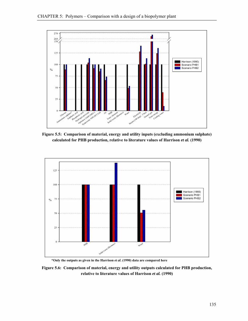
CHAPTER 5: Polymers – Comparison with a design of a biopolymer plant
135
Figure 5.5: Comparison of material, energy and utility inputs (excluding ammonium sulphate) calculated for PHB production, relative to literature values of Harrison et al. (1990)
*Only the outputs as given in the Harrison et al. (1990) data are compared here
Figure 5.6: Comparison of material, energy and utility outputs calculated for PHB production, relative to literature values of Harrison et al. (1990)

CHAPTER 5: Polymers – Comparison with a design of a biopolymer plant
136
The individual electrical requirements for the Harrison (1990) model (aeration, agitation, cell disruption and downstream processing units) were within 80 % of the Scenario PHB1 values for all electrical requirements except steam compression, which was not taken into account in the Harrison (1990) model (Table 5.9). The total electrical energy required by the Harrison (1990) model was 78 % of the electrical energy required for Scenario PHB1 (Figure 5.7).
The amounts of natural gas needed in the spray drying process were higher in Scenarios PHB1, PHB2 and PHB3 than the Harrison (1990) model. This was owing to an assumption that the initial moisture content of material entering the spray dryers in the Harrison (1990) model was 25 % while in the generic flowsheet models, the moisture content was calculated to be 39 %.
Table 5.9: Electrical energy contributions for Scenario PHB1 versus the Harrison (1990) model for
the production of 1 kg of poly--hydroxybutyric acid
Scenario PHB1 Harrison (1990) model
MJ MJ
Sterilisation - Steam compression 1.86 -
Aeration 6.5 5.8
Agitation 1.31 1.36
Cell Disruption - High Pressure homogeniser 1.77 1.77
Centrifugation 0.078 0.072
Enzyme addition - agitation 0.021 0.018
Detergent addition - agitation 0.022 0.018
Water washing (I) 0.134 0.120
Water washing (II) 0.076 0.072
TOTAL 11.7 9.2
Figure 5.7: Electrical energy contributions for the production of poly--butyrate as determined by
Harrison (1990), relative to Scenario PHB1

CHAPTER 5: Polymers – Comparison with a design of a biopolymer plant
137
5.5.2. Life Cycle Impact Assessment (LCIA) The life cycle impacts of Scenario PHB1 were less than 30 % higher than the results of the Harrison (1990) model in all categories except global warming (Figure 5.8). This was a result of the larger electricity value in the modelled scenarios as well as the over estimation in ammonium sulphate. As seen in Table 5.10, the global warming scores were 2.72, 5.74 and 6.39 kg CO2 eq. for the models of Harrison (1990) and Scenarios PHB1 and PHB2 respectively. The generic flowsheet values were over twice that of the Harrison (1990) values as a result of the carbon dioxide emitted from the reactor which was included in the generic model scenarios but not the Harrison (1990) model. For the scaled up Harrison (1990) model, for each kilogram of polymer formed, life cycle impacts of 0.034 kg Sb eq., 0.25 mg CFC-11 eq., 0.042 kg SO2 eq. and 0.023 kg PO4
3-eq. were obtained in the categories of abiotic depletion, ozone layer depletion,
acidification and eutrophication respectively. By allowing for waste water treatment, as well as possible biogas capture and use, the LCA values, particularly those for eutrophication, would decrease. LCA results which are within 5 % of each other may not be significantly different from each other owing to uncertainty in the inputs and LCA inventory datasets.
Table 5.10: LCIA of poly--butyrate production per kilogram of product as described by Harrison
(1990) – CML 2 Baseline 2000 V2.03
Impact Category Unit Harrison (1990) Scenario PHB1 Scenario PHB 2 Scenario PHB 3
Abiotic Depletion kg Sbeq. 0.034 0.045 0.045 0.093
Global Warming (GWP100) kg CO2 eq. 2.72 5.74 6.39 10.2
Ozone Layer Depletion (ODP) mg CFC-11eq. 0.25 0.33 0.37 0.56
Human Toxicity kg 1,4-DBeq. 1.69 2.20 2.46 4.87
Fresh Water Aquatic Ecotoxicity kg 1,4-DBeq. 0.34 0.43 0.48 1.00
Marine Aquatic Ecotoxicity kg 1,4-DBeq. 1900 2400 2700 5800
Terrestrial Ecotoxicity kg 1,4-DBeq. 0.0098 0.012 0.014 0.020
Photochemical Oxidation kg C2H4 0.0014 0.0016 0.0018 0.0034
Acidification kg SO2 eq. 0.042 0.047 0.053 0.098
Eutrophication kg PO43-
eq. 0.023 0.026 0.033 0.045

CHAPTER 5: Polymers – Comparison with a design of a biopolymer plant
138
Figure 5.8: Comparison of LCA results for PHB production for Scenarios PHB1 and PHB2 relative to Harrison (1990) data
5.5.3. Process contributions Six of the impact categories were investigated in Scenario PHB1 to determine the main contributors to total scores. The LCA categories investigated included abiotic depletion, global warming, ozone layer depletion, photochemical oxidation, acidification and eutrophication. The values shown in the figures represented contribution to the LCA impacts as a percentage of the total in each category. Only materials which led to a contribution greater than 3 % of the total LCA score have been included. Where there were positive impacts, i.e. impacts which reduced the total environmental impact, these were presented as detached wedges. In the categories shown, electricity was the largest contributor in 5 of the 6 categories, while the direct impacts during PHB production process (e.g. CO2 release and Chemical Oxygen Demand of wastewater) were the largest contributors in the sixth, eutrophication. Steam, natural gas, ammonium sulphate and sugar were also large contributors. Abiotic depletion scores are dominated by electricity (56.7 %), steam (20.5 %), ammonium sulphate (10.7 %) and natural gas (7.2 %) as shown in Figure 5.9. No other source contributed more than 3 % to the overall impact. The global warming impact showed a negative value from sugar production owing to the uptake of carbon dioxide during sugar cane growth. This uptake
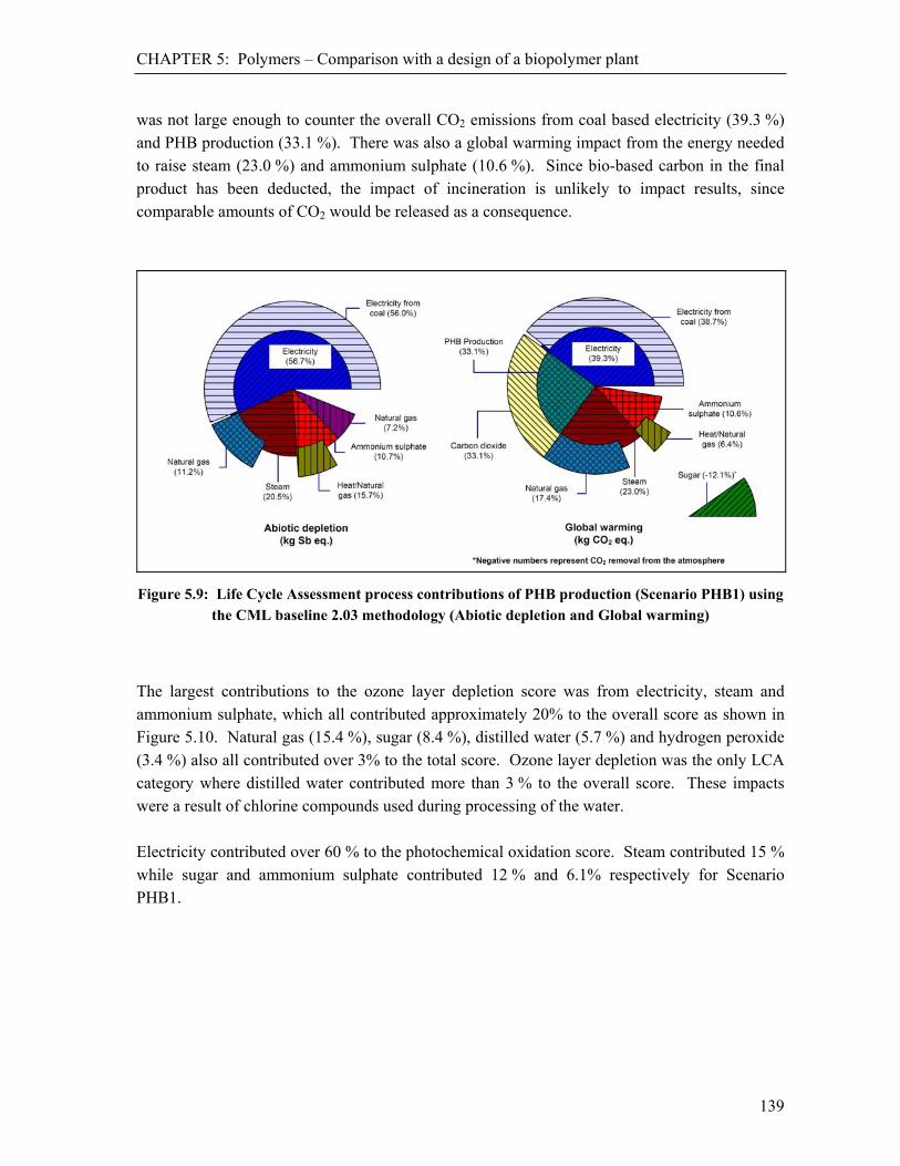
CHAPTER 5: Polymers – Comparison with a design of a biopolymer plant
139
was not large enough to counter the overall CO2 emissions from coal based electricity (39.3 %) and PHB production (33.1 %). There was also a global warming impact from the energy needed to raise steam (23.0 %) and ammonium sulphate (10.6 %). Since bio-based carbon in the final product has been deducted, the impact of incineration is unlikely to impact results, since comparable amounts of CO2 would be released as a consequence.
Figure 5.9: Life Cycle Assessment process contributions of PHB production (Scenario PHB1) using the CML baseline 2.03 methodology (Abiotic depletion and Global warming)
The largest contributions to the ozone layer depletion score was from electricity, steam and ammonium sulphate, which all contributed approximately 20% to the overall score as shown in Figure 5.10. Natural gas (15.4 %), sugar (8.4 %), distilled water (5.7 %) and hydrogen peroxide (3.4 %) also all contributed over 3% to the total score. Ozone layer depletion was the only LCA category where distilled water contributed more than 3 % to the overall score. These impacts were a result of chlorine compounds used during processing of the water. Electricity contributed over 60 % to the photochemical oxidation score. Steam contributed 15 % while sugar and ammonium sulphate contributed 12 % and 6.1% respectively for Scenario PHB1.
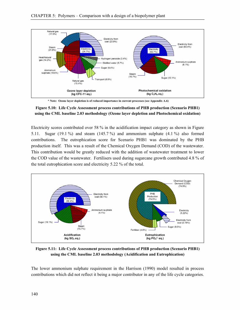
CHAPTER 5: Polymers – Comparison with a design of a biopolymer plant
140
* Note: Ozone layer depletion is of reduced importance in current processes (see Appendix A.6)
Figure 5.10: Life Cycle Assessment process contributions of PHB production (Scenario PHB1) using the CML baseline 2.03 methodology (Ozone layer depletion and Photochemical oxidation)
Electricity scores contributed over 58 % in the acidification impact category as shown in Figure 5.11. Sugar (19.1 %) and steam (145.7 %) and ammonium sulphate (4.1 %) also formed contributions. The eutrophication score for Scenario PHB1 was dominated by the PHB production itself. This was a result of the Chemical Oxygen Demand (COD) of the wastewater. This contribution would be greatly reduced with the addition of wastewater treatment to lower the COD value of the wastewater. Fertilisers used during sugarcane growth contributed 4.8 % of the total eutrophication score and electricity 5.22 % of the total.
Figure 5.11: Life Cycle Assessment process contributions of PHB production (Scenario PHB1) using the CML baseline 2.03 methodology (Acidification and Eutrophication)
The lower ammonium sulphate requirement in the Harrison (1990) model resulted in process contributions which did not reflect it being a major contributor in any of the life cycle categories.
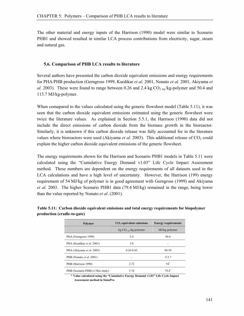
CHAPTER 5: Polymers – Comparison of PHB LCA results to literature
141
The other material and energy inputs of the Harrison (1990) model were similar to Scenario PHB1 and showed resulted in similar LCA process contributions from electricity, sugar, steam and natural gas.
5.6. Comparison of PHB LCA results to literature Several authors have presented the carbon dioxide equivalent emissions and energy requirements for PHA/PHB production (Gerngross 1999, Kurdikar et al. 2001, Nonato et al. 2001, Akiyama et al. 2003). These were found to range between 0.26 and 2.4 kg CO2 eq./kg-polymer and 50.4 and 113.7 MJ/kg-polymer. When comapared to the values calculated using the generic flowsheet model (Table 5.11), it was seen that the carbon dioxide equivalent emissions estimated using the generic flowsheet were twice the literature values. As explained in Section 5.5.1, the Harrison (1990) data did not include the direct emissions of carbon dioxide from the biomass growth in the bioreactor. Similarly, it is unknown if this carbon dioxide release was fully accounted for in the literature values where bioreactors were used (Akiyama et al. 2003). This additional release of CO2 could explain the higher carbon dioxide equivalent emissions of the generic flowsheet. The energy requirements shown for the Harrison and Scenario PHB1 models in Table 5.11 were calculated using the “Cumulative Energy Demand v1.03” Life Cycle Impact Assessment method. These numbers are dependent on the energy requirements of all datasets used in the LCA calculations and have a high level of uncertainty. However, the Harrison (199) energy requirement of 54 MJ/kg of polymer is in good agreement with Gerngross (1999) and Akiyama et al. 2003. The higher Scenario PHB1 data (79.4 MJ/kg) remained in the range, being lower than the value reported by Nonato et al. (2001).
Table 5.11: Carbon dioxide equivalent emissions and total energy requirements for biopolymer production (cradle-to-gate)
Polymer CO2 equivalent emissions Energy requirements
kg CO2 eq./kg-polymer MJ/kg-polymer
PHA (Gerngross 1999) 2.4 50.4
PHA (Kurdikar et al. 2001) 2.0 -
PHA (Akiyama et al. 2003) 0.26-0.45 50-59
PHB (Nonato et al. 2001) - 113.7
PHB (Harrison 1990) 2.72 54*
PHB (Scenario PHB1) (This study) 5.74 79.4*
* Value calculated using the “Cumulative Energy Demand v1.03” Life Cycle Impact Assessment method in SimaPro
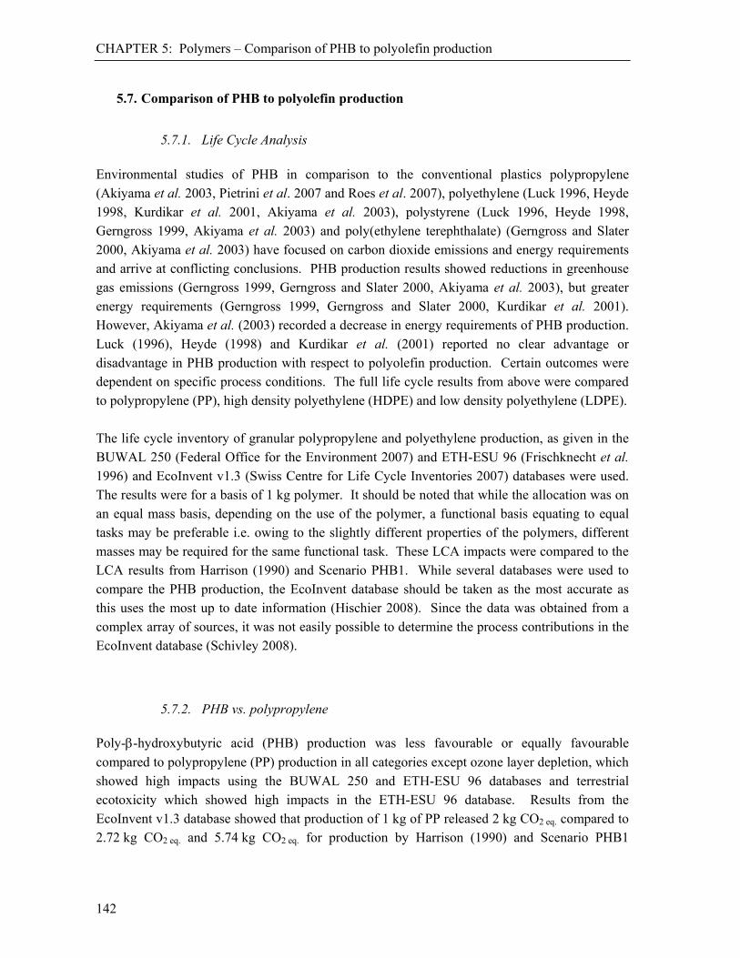
CHAPTER 5: Polymers – Comparison of PHB to polyolefin production
142
5.7. Comparison of PHB to polyolefin production
5.7.1. Life Cycle Analysis Environmental studies of PHB in comparison to the conventional plastics polypropylene (Akiyama et al. 2003, Pietrini et al. 2007 and Roes et al. 2007), polyethylene (Luck 1996, Heyde 1998, Kurdikar et al. 2001, Akiyama et al. 2003), polystyrene (Luck 1996, Heyde 1998, Gerngross 1999, Akiyama et al. 2003) and poly(ethylene terephthalate) (Gerngross and Slater 2000, Akiyama et al. 2003) have focused on carbon dioxide emissions and energy requirements and arrive at conflicting conclusions. PHB production results showed reductions in greenhouse gas emissions (Gerngross 1999, Gerngross and Slater 2000, Akiyama et al. 2003), but greater energy requirements (Gerngross 1999, Gerngross and Slater 2000, Kurdikar et al. 2001). However, Akiyama et al. (2003) recorded a decrease in energy requirements of PHB production. Luck (1996), Heyde (1998) and Kurdikar et al. (2001) reported no clear advantage or disadvantage in PHB production with respect to polyolefin production. Certain outcomes were dependent on specific process conditions. The full life cycle results from above were compared to polypropylene (PP), high density polyethylene (HDPE) and low density polyethylene (LDPE). The life cycle inventory of granular polypropylene and polyethylene production, as given in the BUWAL 250 (Federal Office for the Environment 2007) and ETH-ESU 96 (Frischknecht et al. 1996) and EcoInvent v1.3 (Swiss Centre for Life Cycle Inventories 2007) databases were used. The results were for a basis of 1 kg polymer. It should be noted that while the allocation was on an equal mass basis, depending on the use of the polymer, a functional basis equating to equal tasks may be preferable i.e. owing to the slightly different properties of the polymers, different masses may be required for the same functional task. These LCA impacts were compared to the LCA results from Harrison (1990) and Scenario PHB1. While several databases were used to compare the PHB production, the EcoInvent database should be taken as the most accurate as this uses the most up to date information (Hischier 2008). Since the data was obtained from a complex array of sources, it was not easily possible to determine the process contributions in the EcoInvent database (Schivley 2008).
5.7.2. PHB vs. polypropylene
Poly--hydroxybutyric acid (PHB) production was less favourable or equally favourable
compared to polypropylene (PP) production in all categories except ozone layer depletion, which showed high impacts using the BUWAL 250 and ETH-ESU 96 databases and terrestrial ecotoxicity which showed high impacts in the ETH-ESU 96 database. Results from the EcoInvent v1.3 database showed that production of 1 kg of PP released 2 kg CO2 eq. compared to 2.72 kg CO2 eq. and 5.74 kg CO2 eq. for production by Harrison (1990) and Scenario PHB1

CHAPTER 5: Polymers – Comparison of PHB to polyolefin production
143
respectively as seen in Table 5.12. PP scores for photochemical oxidation and acidification were less than 50 % of the PHB values by both biopolymer production methods. The PP score for ozone layer depletion was over 99.9 % lower by the EcoInvent v1.3 database. Human-, fresh water aquatic- and marine aquatic toxicities were all less than 5 % of the PHB impacts (Figure 5.12).
For PHB results, the increased eutrophication scores were owing to fertiliser inputs in the agricultural processes, while the impacts for the other categories were a result of the energy needs and for toxicity categories, hydrogen peroxide inputs. This identified the hydrogen peroxide as a prime target for substitution and reduced LCA scores. The PP scores for abiotic depletion, global warming and terrestrial ecotoxicity were a result of disposal of hazardous and other wastes. High ozone layer depletion scores in the ETH-ESU 96 database method were a result of CFCs released to the atmosphere during the refining of crude oil which is a precursor for PP production.
Table 5.12: LCIA of polypropylene production for 1 kg of polymer – CML 2 Baseline 2000 V2.03
Harrison
(1990) Scenario
PHB1 BUWAL 250a ETH-ESU 96b
EcoInvent v1.3c
Impact category Unit
Abiotic Depletion kg Sbeq 0.034 0.045 0.036 0.044 0.034
Global Warming (GWP100) kg CO2 eq. 2.72 5.74 1.88 3.38 2.00
Ozone Layer Depletion (ODP) mg CFC-11eq 0.25 0.33 1.10 8.62 0.00013
Human Toxicity kg 1,4-DBeq 1.69 2.20 0.187 2.47 0.051
Fresh Water Aquatic Ecotoxicity kg 1,4-DBeq 0.34 0.43 0.025 0.45 0.014
Marine Aquatic Ecotoxicity kg 1,4-DBeq 1900 2400 96.5 2600 70.8
Terrestrial Ecotoxicity kg 1,4-DBeq 0.0098 0.012 0.0010 0.041 0.011
Photochemical Oxidation kg C2H2 0.0014 0.0016 0.00057 0.0017 0.00068
Acidification kg SO2 eq. 0.042 0.047 0.018 0.049 0.020
Eutrophication kg PO43- eq. 0.023 0.026 0.001 0.006 0.001
a PP granulate average B250 (Average production of polypropylene in Europe according to APME. Data accounts for production from 14 companies which is half of the total Western European production.)
b PP ETH S (Polymerisation takes place with an efficiency of approximately 95 %. For this process 4 MJ electricity and 6 MJ thermal energy use is estimated. Emissions to air of VOC, NOx and dust are accounted for, water emissions (of aromatic substances, solvents, metals) can be expected during solvent and catalyst recycling.)
c Polypropylene, granulate, at plant /RER U (Data are from the Eco-profiles of the European plastics industry (APME). Not included are values reported for: recyclable wastes, amount of air/ N2/ O2 consumed, unspecified metal emission to air and to water, mercaptan emission to air, unspecified CFC/HCFC emission to air.)
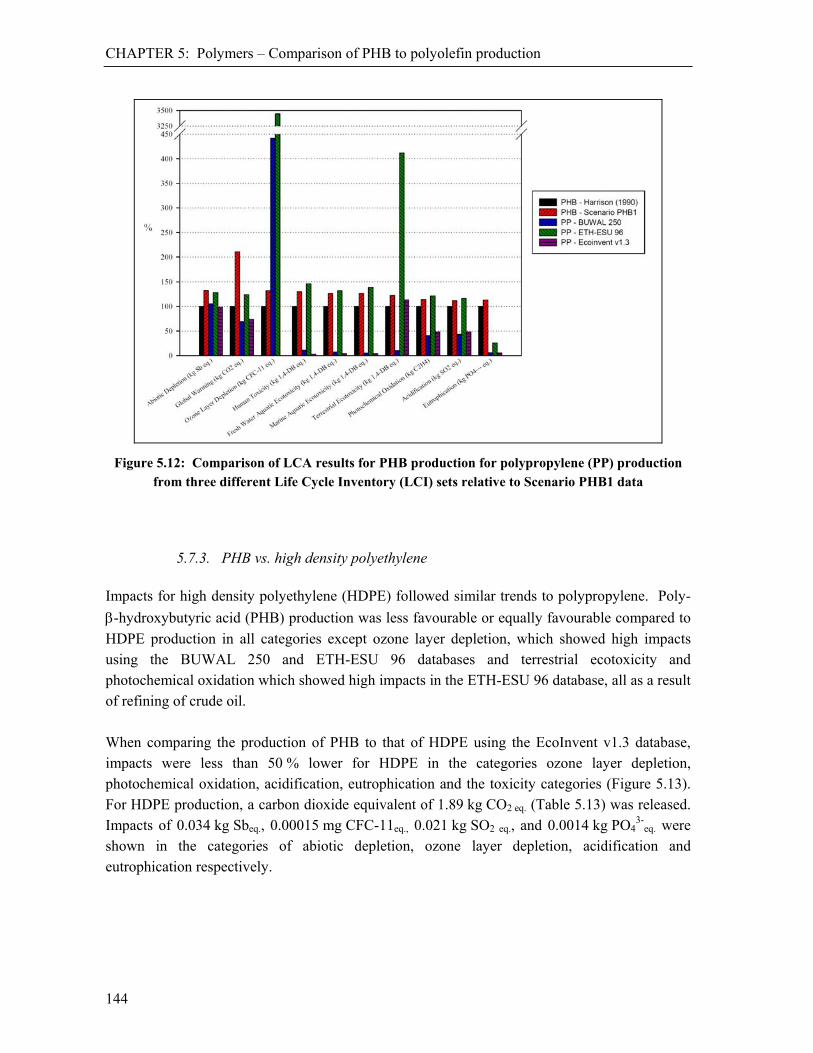
CHAPTER 5: Polymers – Comparison of PHB to polyolefin production
144
Figure 5.12: Comparison of LCA results for PHB production for polypropylene (PP) production from three different Life Cycle Inventory (LCI) sets relative to Scenario PHB1 data
5.7.3. PHB vs. high density polyethylene Impacts for high density polyethylene (HDPE) followed similar trends to polypropylene. Poly-
-hydroxybutyric acid (PHB) production was less favourable or equally favourable compared to
HDPE production in all categories except ozone layer depletion, which showed high impacts using the BUWAL 250 and ETH-ESU 96 databases and terrestrial ecotoxicity and photochemical oxidation which showed high impacts in the ETH-ESU 96 database, all as a result of refining of crude oil. When comparing the production of PHB to that of HDPE using the EcoInvent v1.3 database, impacts were less than 50 % lower for HDPE in the categories ozone layer depletion, photochemical oxidation, acidification, eutrophication and the toxicity categories (Figure 5.13). For HDPE production, a carbon dioxide equivalent of 1.89 kg CO2 eq. (Table 5.13) was released. Impacts of 0.034 kg Sbeq., 0.00015 mg CFC-11eq., 0.021 kg SO2 eq., and 0.0014 kg PO4
3-eq. were
shown in the categories of abiotic depletion, ozone layer depletion, acidification and eutrophication respectively.
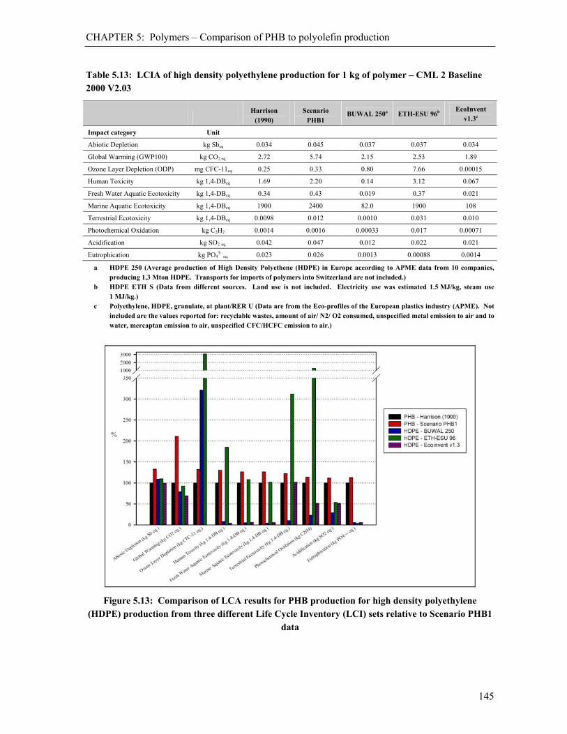
CHAPTER 5: Polymers – Comparison of PHB to polyolefin production
145
Table 5.13: LCIA of high density polyethylene production for 1 kg of polymer – CML 2 Baseline 2000 V2.03
Harrison
(1990) Scenario
PHB1 BUWAL 250a ETH-ESU 96b
EcoInvent v1.3c
Impact category Unit
Abiotic Depletion kg Sbeq 0.034 0.045 0.037 0.037 0.034
Global Warming (GWP100) kg CO2 eq. 2.72 5.74 2.15 2.53 1.89
Ozone Layer Depletion (ODP) mg CFC-11eq 0.25 0.33 0.80 7.66 0.00015
Human Toxicity kg 1,4-DBeq 1.69 2.20 0.14 3.12 0.067
Fresh Water Aquatic Ecotoxicity kg 1,4-DBeq 0.34 0.43 0.019 0.37 0.021
Marine Aquatic Ecotoxicity kg 1,4-DBeq 1900 2400 82.0 1900 108
Terrestrial Ecotoxicity kg 1,4-DBeq 0.0098 0.012 0.0010 0.031 0.010
Photochemical Oxidation kg C2H2 0.0014 0.0016 0.00033 0.017 0.00071
Acidification kg SO2 eq. 0.042 0.047 0.012 0.022 0.021
Eutrophication kg PO43- eq. 0.023 0.026 0.0013 0.00088 0.0014
a HDPE 250 (Average production of High Density Polyethene (HDPE) in Europe according to APME data from 10 companies, producing 1,3 Mton HDPE. Transports for imports of polymers into Switzerland are not included.)
b HDPE ETH S (Data from different sources. Land use is not included. Electricity use was estimated 1.5 MJ/kg, steam use 1 MJ/kg.)
c Polyethylene, HDPE, granulate, at plant/RER U (Data are from the Eco-profiles of the European plastics industry (APME). Not included are the values reported for: recyclable wastes, amount of air/ N2/ O2 consumed, unspecified metal emission to air and to water, mercaptan emission to air, unspecified CFC/HCFC emission to air.)
Figure 5.13: Comparison of LCA results for PHB production for high density polyethylene (HDPE) production from three different Life Cycle Inventory (LCI) sets relative to Scenario PHB1
data

CHAPTER 5: Polymers – Comparison of PHB to polyolefin production
146
5.7.4. PHB vs. low density polyethylene The Life Cycle impacts of low density polyethylene (LDPE) production were higher than those for high density polyethylene (HDPE). From the ETH-ESU 96 database, impacts in the categories ozone layer depletion, human-, fresh water aquatic-, terrestrial ecotoxicity and photochemical oxidation were higher than for PHB production. As with HDPE, these high impacts were a result of the refining of crude oil in the LDPE process. However, using the BUWAL 250 and EcoInvent v1.3 databases, with the exception of terrestrial toxicity in the EcoInvent database, toxicity impacts were all below 5% (Figure 5.14). When comparing PHB production to the EcoInvent v1.3 data for LDPE, as with HDPE, PHB had higher or similar impacts in all categories. The carbon dioxide equivalent released of 2.08 kgCO2 eq. (Table 5.14) was 10 % higher than HDPE. Impacts of 0.034 kg Sbeq., 0.00014 mg CFC-11eq., and 0.0015 kg PO4
3-eq. were shown in the categories of abiotic depletion,
ozone layer depletion and eutrophication respectively. These were all within 10% of the HDPE values.
Table 5.14: LCIA of low density polyethylene production for 1 kg of polymer – CML 2 Baseline 2000 V2.03
Harrison
(1990)
Scenario
PHB1 BUWAL 250a ETH-ESU 96b
EcoInvent v1.3c
Impact category Unit
Abiotic Depletion kg Sbeq 0.034 0.045 0.041 0.042 0.034
Global Warming (GWP100) kg CO2 eq. 2.72 5.74 2.43 3.06 2.08
Ozone Layer Depletion (ODP) mg CFC-11eq 0.25 0.33 0.98 8.32 0.00014
Human Toxicity kg 1,4-DBeq 1.69 2.20 0.192 2200 0.073
Fresh Water Aquatic Ecotoxicity kg 1,4-DBeq 0.34 0.43 0.025 220 0.019
Marine Aquatic Ecotoxicity kg 1,4-DBeq 1900 2400 258 2400 118
Terrestrial Ecotoxicity kg 1,4-DBeq 0.0098 0.012 0.0014 0.037 0.010
Photochemical Oxidation kg C2H2 0.0014 0.0016 0.00048 0.0039 0.00046
Acidification kg SO2 eq. 0.042 0.047 0.017 0.027 0.015
Eutrophication kg PO43- eq. 0.023 0.026 0.0016 0.0010 0.0013
a LDPE B250 (Average production of Low Density Polyethene in Europe according to APME data from 22 companies, producing 2.8 Mton total. LDPE. Transports for imports of polymers into Switzerland are not included.)
b LDPE ETH S (Data from different sources. Land use is not included. Electricity use was estimated 3 MJ/kg, steam use 4 MJ/kg.)
c Polyethylene, LDPE, granulate, at plant/RER U (Data are from the Eco-profiles of the European plastics industry (APME). Not included are the values reported for: recyclable wastes, amount of air/ N2/ O2 consumed, unspecified metal emission to air and to
water, mercaptan emission to air, unspecified CFC/HCFC emission to air.)
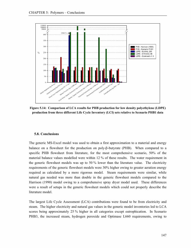
CHAPTER 5: Polymers – Conclusions
147
Figure 5.14: Comparison of LCA results for PHB production for low density polyethylene (LDPE) production from three different Life Cycle Inventory (LCI) sets relative to Scenario PHB1 data
5.8. Conclusions The generic MS-Excel model was used to obtain a first approximation to a material and energy
balance on a flowsheet for the production on poly--butyrate (PHB). When compared to a
specific PHB flowsheet from literature, for the most comprehensive scenario, 50% of the material balance values modelled were within 12 % of these results. The water requirement in the generic flowsheet models was up to 50 % lower than the literature value. The electricity requirements of the generic flowsheet models were 30% higher owing to greater aeration energy required as calculated by a more rigorous model. Steam requirements were similar, while natural gas needed was more than double in the generic flowsheet models compared to the Harrison (1990) model owing to a comprehensive spray dryer model used. These differences were a result of setups in the generic flowsheet models which could not properly describe the literature model. The largest Life Cycle Assessment (LCA) contributions were found to be from electricity and steam. The higher electricity and natural gas values in the generic model inventories led to LCA scores being approximately 25 % higher in all categories except eutrophication. In Scenario PHB3, the increased steam, hydrogen peroxide and Optimase L660 requirements, owing to
CHAPTER 5: Polymers – References
148
inefficient separation efficiencies, resulted in an even greater LCA impacts. It was found that the carbon dioxide uptake from the biological processes in PHB production was less than the carbon dioxide released during electricity production, giving a net carbon dioxide release. Hydrogen peroxide used in the production process of PHB was targeted as an area for possible substitution to give reduced LCA impacts.
Poly--butyrate (PHB) production resulted in higher or similar LCA scores compared to
polypropylene (PP) and polyethylene (PE) for all impact categories when using the EcoInvent v1.3 database. This showed that despite the use of fossil fuels during polyolefin production, and the use of renewable resources in PHB production, PP and PE are more environmentally beneficial. While carbon dioxide capture during the biomass growth for sugar production of PHB helped to reduce global warming scores, this was only by 10 %. The PHB LCA assumed largely coal-based electricity production compared with the cleaner European electricity for polyolefin production. As a more direct comparison to the PHB, the production of polymers in South Africa may show less beneficial trends for biopolymers. The LCA results were sensitive to the LCA database used. Since the EcoInvent v1.3 database was the most recent database used, it was assumed to be the most representative. Further, the polyolefin industry can be considered to be an established industry while the biopolymer industry is yet to mature. Data used in the PHB analysis can be considered dated. With research and development having moved forward, and with it likely to continue to do so, once the process is matured and optimised, the LCA scores for PHB production can be expected to be reduced significantly.
References Ackerman, J.-U., Babel, W., 1998. Approaches to increase the economy of the PHB production, Polym. Degrad.
Stabil., 59, 183-186. Akiyama, M., Tsuge, T., Doi, Y., 2003. Environmental life cycle comparison of polyhydroxyalkanoates produced
from renewable carbon resources by bacterial fermentation, Polym. Degrad. Stabil., 80, 183-194. Asrar, J., Grys, K.J., 2002. Biodegradable Polymer (BIOPOL®), In: Biopolymers, Polyesters III: Applications and
commercial products, Vol. 4, ed. Y. Doi, A. Steinbüchel, Wiley-VCH, Münster, 53-90. Baker, C.G.J., McKenzie, K.A., 2005. Energy consumption of industrial spray dryers, Dry. Technol., 23(1-2), 365-
386. Botha, T., 2003. Opportunity to apply recent advances in process design to bioenergy systems: the case of
sugarcane processing in South Africa, M.Sc. Dissertation, Department of Chemical Engineering, University of Cape Town.
Boustead, I., 2000. Eco-profiles of plastics and related intermediates, Association of Plastics Manufacturers in Europe (APME), Brussels, Belgium.
Capell, T., Christou, P., 2004. Progress in plant metabolic engineering, Curr. Opin. Biotech., 15, 148-154. Chen, G.Q., Zhang, G., Park, S.J., Lee, S.Y., 2001. Industrial scale production of poly(3-hydroxybutyrate-co-3-
hydroxyhexanoate), Appl. Microbiol. Biot., 57, 50-55.

CHAPTER 5: Polymers – References
149
Chen, G.-Q. and Wu, Q., 2005. Review: The application of polyhydroxyalkanoates as tissue engineering materials, Biomaterials, 26, 6565-6578.
Daae, E.B., Dunnill, P., Mitsky, T.A., Padgette, S.R., Taylor, N.B., Valentin, H.E., Gruys, K.J., 1999. Metabolic modelling as a tool for evaluating polyhydroxyalkanoate copolymer production in plants, Metab. Eng., 1, 243-254.
Delft, 2004. Industrieel Ontwerpen – Delft [online], Delft University of Technology, Available from: http://www.io.tudelft.nl/research/dfs/idemat/Onl_db/Typ113.htm, [Accessed 14 October 2005].
Dennis, J.S., 2000. Protease production, MS-Excel spreadsheet, selected data. Doi Y., 1990. Microbial polyesters. New York: VCH Publishers. DSMZ, 2006. Bacterial Nomenclature up-to-date (approved lists, validation lists), Deutsche Sammlung von
Mikroorganismen und Zellkulturen GmbH, April 2006, Available from: http://www.dsmz.de/download/bactnom/bactname.pdf [Accessed 5 May 2006]
Engler, C.R. 1985. Disruption of Microbial Cells, In: Comprehensive Biotechnology; The Principles, Applications & Regulations of Biotechnology in Industry, Agriculture and Medicine, Vol. 2, The Principles of Biotechnology: Engineering Considerations, ed. M. Moo-Young, Chapter 20, Pergamon Press, New York.
Federal Office for the Environment, 2007. Buwal 250, Department of the Environment, Transport, Energy and Communications, Federal Office for the Environment (FOEN), 3003 Bern, http://www.bafu.admin.ch/index.html?lang=en.
Frischknecht, R., Suter, P., 1996. Öko-inventare von Energiesystemen, ETH-ESU, 3rd edition. Frischknecht, R., Bollens, U., Bosshart, S., Ciot, M., Ciseri, L., Doka, G., Dones, R., Ganther, U., Hischier, R.,
Martin, A. 1996. Ökoinventare von Energiesystemen, Grundlagen für den ökologischen Vergleich von Energiesystemen und den Einbezug von Energiesystemen in Ökobilanzen für die Schweiz, Auflage No. 3, Gruppe Energie - Stoffe - Umwelt (ESU), Eidgenössische Technische Hochschule Zürich und Sektion Ganzheitliche Systemanalysen, Paul Scherrer Institut, Villigen, www.energieforschung.ch, Bundesamt für Energie (Hrsg.), Bern.
Gerngross, T.U., 1999. Can biotechnology move us toward a sustainable society?, Nat. Biotechnol., 17, 541-544. Gerngross, T.U., Slater, S.C., 2000. How Green are Green Plastics?, Sci. Am., August 2000, 36-41. Godbole, S., Gote, S., Latkar, M., Chakrabarti, T., 2003. Preparation and characterization of biodegradable poly-3-
hydroxybutyrate-starch blend films, Bioresource Technol., 86, 33-37. Grothe, E., Moo-Young, M., Chisti, Y., 1999. Fermentation optimization for the production of poly(3-
hydroxybutyric acid) microbial thermoplastic, Enzyme Microb. Tech., 25, 132-141. Harrison, S.T.L., 1990. The Extraction and Purification of Alcaligenes eutrophus, PhD dissertation, Cambridge
University. He, W., Tian, W., Zhang, G., Chen, G.-Q., Zhang, Z., 1998. Production of novel polyhydroxyalkanoates by
Pseudomonas stutzeri 1317 from glucose and soybean oil, FEMS Microbiol. Lett., 169, 45-49. Heyde, M., 1998. Ecological considerations on the use and production of biosynthetic and synthetic biodegradable
polymers, Polym. Degrad. Stabil., 59, 3-6. Hischier, R., 2008. Life Cycle Assessment & Modelling Group, Technology & Society Laboratory, Empa, Swiss
Federal Laboratories for Materials Testing & Research, Personal communication, [email protected], 24 August 2008.
Khanna, S., Srivastava, A.K., 2005. Recent advances in microbial polyhydroxyalkanoates, Process Biochem., 40, 607-619.
Kim, B.S., 2000. Production of poly(3-hydroxybutyrate) from inexpensive substrates, Enzyme Microb. Tech., 27, 774-777.
Kurdikar, D., Paster, M., Gruys, K.J., Fournet, L., L., Gerngross, T.U., Slater, S.C., Coulon, R., 2001. Greenhouse gas profile of a plastic derived from a genetically modified plant, J. Ind. Ecol., 4(3), 107-122.
Lee, S.Y., 1996. Plastic bacteria? Progress and prospects for polyhydroxyalkanoate production in bacteria, Trends Biotechnol., 14, 431-438.
Lee, S.Y., Choi, J., 1998. Effect of fermentation performance on the economics of poly(3-hydroxybutyrate) production by Alcaligenes latus, Polym. Degrad. Stabil., 59, 387-393.
Luck, T., 1996. Feasability-Studie Polyhydroxyfettsäuren – Kurzdarstellung der Ergebnisse der Studien 'Feasibility-Studie zur Abschätzung des Marktpotentials neuer Polyhydroxyfet-tsäuren (PHF)' und 'Abschätzende Ökobilanzen zu Polymerwerkstoffen auf der Basis biologisch erzeugter Polyhydroxyfettsäuren', Fraunhofer Institut für Lebensmitteltechnologie und Verpackung (ILV), Freising, Germany. Cited Patel et al. 2002.

CHAPTER 5: Polymers – References
150
Mascia, P.N., Flavell, R.B., 2004. Safe and acceptable strategies for producing foreign molecules in plants, Curr. Opin. Plant Biol., 7, 189-195.
Moire, L., Rezzonico, E., Poirer, Y., 2003. Synthesis of novel biomaterials in plants, J. Plant Physiol., 160, 831-839.
Nonato, R.V., Mantelatto, P.E., Rossell, C.E.V., 2001. Integrated production of biodegradable plastic, sugar and ethanol, Appl. Microbiol. Biot., 57, 1-5.
Ogorkiewicz, R.M. (ed.), 1970. Engineering Properties of Thermoplastics, Imperial Chemical Industries (ICI) Ltd., Plastics Division, London: Wiley-Interscience.
Patel, M., Bastioli, C., Marini, L., Würdinger, E., 2002. Life-cycle assessment of bio-based polymers and natural fibre composites. In: Biopolymers, General Aspects and Special Applications, Vol. 10, ed. A. Steinbüchel, Wiley-VCH, Münster.
Perry, R.H., Green, D.W., Maloney, J.O. (eds.), 1984. Perry's Chemical Engineers' Handbook, 6th edition, McGraw-Hill, International edition.
Pietrini, M., Roes, L., Patel, M, Chiellini, E., 2007. Comparative Life Cycle Studies on Poly(3-hydroxybutyrate)-Based Composites as Potential Replacement for Conventional Petrochemical Plastics, Biomacromolecules, 8, 2210-2218.
Poirer, Y., 1999. Production of new polymeric compounds in plants, Curr. Opin. Biotech., 10, 181-185. Poirer, Y., Somerville, C., Schechtman, L.A., Satkowski, M.M., Noda, I., 1995. Synthesis of high-molecular-weight
poly([R]-(–)-3-hydroxybutyrate) in transgenic Arabidopsis thaliana plant cells, Int. J. Biol. Macromol., 17(1), 7-12.
Pouton, C.W., Akhtar, S., 1996. Biosynthetic polyhydroxyalkanoates and their potential in drug delivery, Adv. Drug Deliver. Rev., 18, 133-162.
PRé Consultants B.V., 2008. Plotterweg 12, 3821 BB Amersfoort, The Netherlands, http://www.pre.nl/ Reddy, C.S.K., Ghaii, R., Rashmi, Kaliav, C., 2003. Polyhydroxyalkanoates: an overview, Bioresource Technol, 87,
137-146. Riesmeier, J., Koßmann, J., Trethewey, R., Heyer, A., Landschütze, V., Willmitzer, L., 1998. Production of novel
polymers in transgenic plants, Polym. Degred. Stabil., 59, 383-386. Roes, L., Pietrini, M., Chiellini, E., Patel, M., 2007. Environmental Life Cycle Studies of Poly(hydroxybutyrate)-
and Polypropylene-Based Composites, JNPN, 3(1), 22-32. Schivley, G., 2008. Environmental Engineer, Franklin Associates, A Division of ERG, Personal communication,
[email protected], 26 August 2008. Shum-Tim, D., Stock, U., Hrkach, J., Shinoka, T., Lien, J., Moses, M.A., Stamp, A., Taylor, G., Moran, A.M.,
Landis, W., Langer, R., Vacanti, J.P., Mayer Jr, J.E., 1999. Tissue engineering of autologous aorta using a new biodegradable polymer, Ann. Thorac. Surg., 68, 2298-2305.
Snell, K.D., Peoples, O.P., 2002. Polyhydroxyalkanoate polymers and their production in transgenic plants, Metab. Eng., 4, 29-40.
Steinbüchel, A., Füchtenbusch, B., 1998. Bacterial and other biological systems for polyester production, Tibtech, 16, 419-427.
Sudesh, K., Abe, H., Doi, Y., 2000. Synthesis, structure and properties of polyhydroxyalkanoates: biological polyesters, Prog. Polym. Sci., 25, 1503-1555.
Swiss Centre for Life Cycle Inventories, 2007. EcoInvent Centre, http://www.ecoinvent.org/. Theka, E., 2002. A life-cycle assessment of ethanol produced from sugarcane molasses, M.Sc. dissertation,
Department of Chemical Engineering, University of Cape Town. Valentin, H.E., Broyles, D.L., Casagrande, L.A., Colburn, S.M., Creely, W.L., DeLaquil, P.A., Felton, H.M.,
Gonzalez, K.A., Houmiel, K.L., Lutke, K., Mahadeo, D.A., Mitsky, T.A., Padgette, S.R., Reiser, S.E., Slater, S., Stark, D.M., Stock, R.T., Stone, D.A., Taylor, N.B., Thorne, G.M., Tran, M., Gruys, K.J., 1999. PHA production, from bacteria to plants, Int. J. Biol. Macromol., 25, 303-306.
Volova, T., Shishatskaya, E., Sevastianov, V., Efremov, S., Mogilnaya, O., 2003. Results of biomedical investigations of PHB and PHB/PHV fibers, Biochem. Eng. J., 16, 125-133.
Wang, F., Lee, S.Y., 1997. Poly(3-hydroxybutyrate) production with high productivity and high polymer content by a fed-batch culture of Alcaligenes latus under nitrogen limitation, Applied and Environmental Microbiology, 63(9), 3703-3706.

CHAPTER 5: Polymers – References
151
Wang, Z., Itoh, Y., Hosaka, Y., Kobayashi, I., Nakano, Y., Maeda, I., Umeda, F., Yamakawa, J., Kawase, M., Yagi, K., 2003. Novel transdermal drug delivery system with polyhydroxyalkanoate and starburst polyamidoamine dendrimer, J. Biosci. Bioeng., 95(5), 541-543.
Williams, S.F., Martin, D.P., Horowitz, D.M., Peoples, O.P., 1999. PHA applications: addressing the price performance issue I. Tissue engineering, Int. J. Biol. Macromol., 25, 111-121.
Woods, D.R, 1995. Process Design and Engineering Practice, New Jersey: Pretence Hall. Yu, J. 2001. Production of PHA from starchy wastewater via organic acids, J. Biotechnol., 86, 105-112. Yu, S.T., Lin, C.C., Too, J.R., 2005. PHBV production by Ralstonia eutropha in a continuous stirred tank reactor,
Process Biochem., 40-2734. Zinn, M., Witholy, B., Egli, T., 2001. Occurrence, synthesis and medical application of bacterial
polyhydroxyalkanoate, Adv. Drug Deliver. Rev., 53, 5-21.

152

153
CHAPTER 6: BIODIESEL

154

CHAPTER 6: Biodiesel – Introduction
155
6.1. Introduction As a fossil fuel, use of petroleum diesel is not sustainable indefinitely owing to limited supplies. Many nations are committed to production of a defined proportion of their transport fuels as biofuel. One such option is to produce biodiesel from oils. The purpose of this chapter was to compare different processing routes for the production of biodiesel. This was to allow for insight into flowsheet options at an early stage of design. Various routes for biodiesel production exist, which include designs with different alcohols for esterification, different recovery options and production by an alkali or enzymatic catalyst. The environmental advantages of these different processing options were investigated by using Life Cycle Assessment (LCA) methodology. Further, the environmental impact of the enzyme needed as a catalyst was not known as there are currently no industrial-scale processes for biodiesel production based on enzymatic esterification. The generic flowsheet model was used to provide the material and energy balance inventory for the enzyme. This inventory was used together with the material and energy balance results from five different biodiesel flowsheets to inform an LCA analysis of biodiesel production.
6.2. Biodiesel production Biodiesel is the generic term for alkyl esters of fatty acids, produced by esterification of vegetable oils with an alcohol, methanol. Ethanol, butanol or propanol can also be used as shown in Table 6.1. It is blended with diesel fuel derived from crude oil, reducing the CO2 attributed to the fossil-fuel on combustion. Biodiesel can also decrease other emissions characteristic of normal diesel fuel, such as particulates and SOx. The advantages of biodiesel combustion over petroleum diesel are well documented for both private and public transport (Table 6.1). Virgin and waste vegetable oils, as well as microalgal oils, can be converted into renewable fuel biodiesel. The most common oils include Jatropha carcus L., rapeseed-, sunflower- and soybean oils. Tallow or waste animal fat can also be used as a triglyceride source. Location-specific studies on biodiesel production, usage or environmental effects have been performed in many countries on both community (Van Dyne et al. 1996) and industrial scales (Zhang et al. 2003a). Typically, sodium hydroxide is used as a homogenous alkali catalyst although acids can also be used as a chemical catalyst to facilitate reaction. These include homogenous Lewis acids (acetates and synthesised stearates of various metals) as described by Di Serio et al. (2005). Recent studies, largely still at the laboratory stage, have explored the use of the enzyme lipase as a biological catalyst. These enzymes may be provided by immobilised enzymes (EC3.1.1.3), as

CHAPTER 6: Biodiesel – Biodiesel production
156
whole cell systems or crude extractions of, amongst others, Candida antarctica and Geotrichum candidum (Table 6.1). Other methods of preparation not included in this study have also been proposed. These include using supercritical fluids (Kusdiana and Saka 2001 and 2004, Saka and Kusdiana 2001, Demibraş 2002, 2003, 2005 and 2006, Madras et al. 2004), supercritical fluids with co-solvents (Cao et al. 2005, Han et al. 2005), or zeolites and metal catalysts. An alkali metal salt on alumina or sulphated zirconia, tungsten zirconium or sulphated tin oxides as super acids can be used as solid-base catalysts. The use of ultrasonic energy to increase transesterification kinetics has also been studied (Stavarache et al. 2005) as has the use of a peroxidation step in downstream processing to improve biodiesel properties (Lin et al. 2006) (Table 6.1).
Table 6.1: Review of literature available on biodiesel production, including various production methods reported
Key points Minor points and references
Previous studies on biodiesel (showing advantages over petroleum diesel)
Krahl et al. 1996, Kaltschmitt et al. 1997, Graboski and McCormick 1998, Hall and Scarse 1998, Sheehan et al. 1998a, Ma and Hanna 1999, Srivastava and Prasad 2000, Fuduka et al. 2001, ATTRA 2002, Beer et al. 2002a, 2002b, Dorado et al. 2003, Kerschbaum and Rinke 2003, Knothe et al. 2003, MacLean and Lave 2003, Makareviciene and Janulis 2003, Mortimer et al. 2003, Turrio-Baldassarri et al. 2004, Nabi et al. 2006
Country specific biodiesel studies
Australia, Brazil, India, Italy Nicaragua, the Philippines,
the United States of America
Beer et al. 2002b, Abreu et al. 2005, Azam et al. 2005, Barnwell and Shamra 2005, Subramanian et al. 2005, Bona et al. 1999, Cardone et al. 2003 Foidl et al. 1996, Tan et al. 2004,
Van Dyne et al. 1996,
Vegetable and plant oils used in
production
Jatropha carcus L., rapeseed, sunflower, soybean, Brassica carinata, castor bean, coconut, Camelina
sativa, copra, cotton seed, Cynara cardunculus L., groundnut (peanut), hazelnut soap stock/waste sunflower, Jojoba (Simmondsia chinesis Link Schneider), Karanja (Pongamia pinnata), linseed, niger, palm kernel, palm tree, rice bran, sesame, turnip, various Brazilian vegetable oils (e.g. Andiroba, Babassu, Cumara and Piqui oils), yellow nut-sedge (Cyperus esculentus L.), milkweed (Asclepias) seed, mahau (Madhuca indica), rubber seed, coconut and 75
different trees, shrubs and herbs in India
Foidl et al. 1996, Peterson et al. 1996, Zhang et al. 1996, Bona et al. 1999, Crabbe et al. 2001, Al-Widyan
and Al-Shyoukh 2002, Encinar et al. 2002, Kalam and Masjuki 2002, Köse et al. 2002, Abreu et al. 2004, Tan et al. 2004, Azam et al. 2005, Barnwell and Sharma 2005, Bouaid et al. 2005, Castro et al. 2005, Fröhlich and Rice 2005, Ghadge and Raheman 2005, 2006, Karmee and Chadha 2005, Han et al. 2005, Puhan et al. 2005, Ramadhas et al. 2005, Usta et al. 2005, Wood 2005, Zulliakah et al. 2005, Canoira et al. 2006, Hosler and Harry-O’Kuru 2006, Jitputti et al.
2006, Meher et al. 2006
Waste animal fat as oil for biodiesel production Ma et al. 1999, Alcantara et al. 2000, Tashtoush et al. 2004
Microalgal oil for biodiesel production Aresta et al. 1995, Sheehan et al. 1998b, Miao and Wu 2006, Sears 2006, Xu et al. 2006, Chisti 2007, 2008, Schmidt 2007
Micro-organisms used in production of lipase enzyme for catalysis
Lipases from: Candida antarctica, Candida lypolytica, Geotrichum candidum, Mucor miehei, Penicillium camembertii, Penicillium roqueforti, Pseudomonas cepacia, Pseudomonas florescens, Rhizomucor miehei, Rhizopus delemar and Rhizopus oryzae
Nelson et al. 1996, Kaieda et al. 1999, 2001, Shimada et al. 1999, 2002, Samukawa et al. 2000, Watanabe et al. 2000, 2001, 2002, Ban et al. 2001, 2002, Iso et al. 2001, Köse et al. 2002, Soumanou and Bornsheuer 2003, Shieh et al. 2003, Pizarro and Park 2003, Hama et al. 2006

CHAPTER 6: Biodiesel – Process flowsheet and mass and energy balance inventories
157
Key points Minor points and references
Alcohols used in transesterification process for biodiesel production
Methanol: Ethanol: Butanol: Propanol:
Karaosmanoğlu et al. 1996, Vicente et al. 1998, 2004, Antolin et al. 2001, Zhang et al. 2003a Peterson et al. 1996 Boocock et al. 1996 Lang et al. 2001
Catalyst types: Acid catalysts
Junek et al. 1998, Enchelmaier and Rasehorn 1994, Germani 1994, Vicente et al. 1998, Boocock et al. 1996, Karaosmanoğlu et al. 1996, Lang et al. 2001, Antolin et al. 2002, Zhang et al. 2003a, Vicente et al. 2004, Zulliakah et al. 2005, Zheng et al. 2006
Catalyst types: Biological catalysts
Mittelbach 1990, Shaw et al. 1991, Nelson et al. 1996, Kaieda et al. 1999, 2001, Shimada et al. 1999, 2002, Uosukainen et al. 1999, Abigor et al. 2000, Samukawa et al. 2000, Watanabe et al. 2000, 2001, 2002, Iso et al. 2001, Belafi-Bako et al. 2002, Köse et al. 2002, Chen and Wu, 2003, Shieh et al. 2003, Du et al. 2004, Madras et al. 2004, Al-Zuhair 2005, Oda et al. 2005, Noureddini et al. 2005, Salis et al. 2005, Al-Zuhair et al. 2006
Catalyst types: Zeolites and metal catalysts
Peterson and Scarrah 1984, Bayense et al. 1996, Corma et al. 1998, Leclercq et al. 2001, Suppes et al. 2001, 2004, Abreu et al. 2004
Catalyst types: Solid base catalysts
Alkali metal salt on alumina – Ebiura et al. 2005, Xie and Li 2006, Xie et al. 2006 Sulphated zirconium, Tungsten zirconium or Sulphated tin oxides as super acids – Furuta et al. 2004
6.3. Process flowsheet and mass and energy balance inventories
6.3.1. Introduction In order to determine the environmental impacts of biodiesel production through life cycle assessment, process flowsheets giving material and energy inputs and outputs were required. Simulation models for five process options were developed using Aspen Plus® (AspenTech 2008). The flowsheets developed used NaOH for chemical catalysis and the enzyme lipase from Candida antarctica for biological catalysis (Table 6.2). The energy data reported is for the total renewable and non-renewable energy in the process.
Table 6.2: Specifications of the different biodiesel production process flowsheets investigated
Flowsheet Case 1 Case 2 Case 3 Case 4 Case 5
Catalyst Alkali Lipase Alkali Alkali Lipase
Alcohol Used Methanol Methanol Methanol Ethanol Ethanol
Alcohol Recovery 94 % - 50 % 94 % -
The flowsheets were developed for continuous processes converting rapeseed oil (assumed to be pure triacylglycerol – C57H104O6), via a transesterification reaction, to biodiesel as shown in Equation 6.1. The process was based on the alkali catalysed transesterification approach of Zhang et al. (2003a), including supportive and alternative conditions described by others as given in Table 6.3. Economic and sensitivity data were given in Zhang et al. (2003b).

CHAPTER 6: Biodiesel – Process flowsheet and mass and energy balance inventories
158
OOC R3CH2
OOC R2CH
CH2 OOC R1
R'OH
OCH2
OHCH
CH2 OH
H
R1 COO R'
R2 COO R'
R3 COO R'
3+ +Catalyst
Oil 3 (Biodiesel) Glycerol3 (Alcohol)+ + Equation 6.1
Table 6.3: Limited list of literature process conditions for transesterification of oils (alkali catalysts)
Karaosmanoğlu et al. 1996
Boocock et al. 1996
Vicente et al. 1998 & 2004
Lang et al. 2001
Antolin et al. 2002
Zhang et al. 2003a
This study
Oil Used Rapeseed Soybean Sunflower Rapeseed, linseed, sunflower
Sunflower Waste cooking oil, Triacylglycerol
Triacyalglycerol (rapeseed oil)
Alcohol Used Methanol Methanol, Butanol
Methanol Methanol, Ethanol, 2-propanol, 1-butanol
Methanol Methanol Methanol, Ethanol
Alcohol to oil ratio 6:1 6:1-30:1 6:1 6:1 9:1 6:1 6:1
Catalyst Used NaOH NaOH or NaOCH3 in
THF*
NaOH KOH, sodium methoxide
KOH NaOH NaOH
Catalyst wt. fraction 0.016 0.002-0.01 0.013 0.01-0.02 0.0028-0.0055
0.01 0.01
Reactor temperature 65 C 20-60 C 20-65 C 25-110 C 60-70 C 60 C 60 C
Reactor pressure 1 atm 1 atm 1 atm 1 atm 1 atm 4 bar 4 bar
Residence Time 38-50 min 10-15 min 8 hr 40 min-3 hr 2 hr
Oil conversion 97.4-99.7 %
(50 min)
70-95 % 100 % 98 % (1 hr) 96 % 95 % (2 hr) 95 % (2 hr)
Methanol recovery ~100 % 94 % 94 %
50 %
Wash water (kg/kg oil)
Includes tannic acid or brine
Includes H3PO4
0.01 0.26
Neutralising acid H3PO4 HCl
*THF – tetrahydrofloran
6.3.2. Alkali catalysed process As shown in Figure 6.1, in the base case (Case 1), methanol (stream 101) entered at a 6:1 molar ratio with respect to the oil (stream 105) (twice the stoichiometric requirement) allowing the equilibrium to be shifted towards biodiesel production. The catalyst (NaOH) was present at a
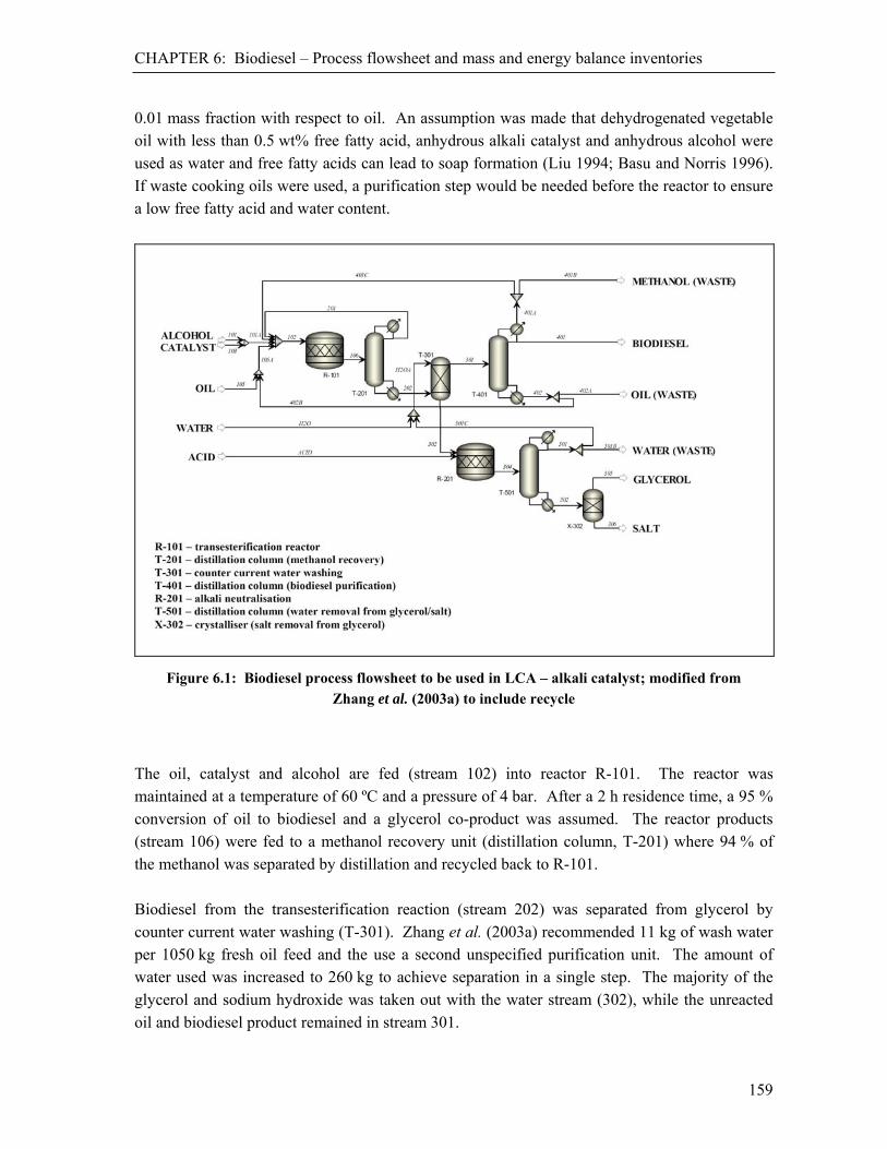
CHAPTER 6: Biodiesel – Process flowsheet and mass and energy balance inventories
159
0.01 mass fraction with respect to oil. An assumption was made that dehydrogenated vegetable oil with less than 0.5 wt% free fatty acid, anhydrous alkali catalyst and anhydrous alcohol were used as water and free fatty acids can lead to soap formation (Liu 1994; Basu and Norris 1996). If waste cooking oils were used, a purification step would be needed before the reactor to ensure a low free fatty acid and water content.
Figure 6.1: Biodiesel process flowsheet to be used in LCA – alkali catalyst; modified from Zhang et al. (2003a) to include recycle
The oil, catalyst and alcohol are fed (stream 102) into reactor R-101. The reactor was maintained at a temperature of 60 ºC and a pressure of 4 bar. After a 2 h residence time, a 95 % conversion of oil to biodiesel and a glycerol co-product was assumed. The reactor products (stream 106) were fed to a methanol recovery unit (distillation column, T-201) where 94 % of the methanol was separated by distillation and recycled back to R-101. Biodiesel from the transesterification reaction (stream 202) was separated from glycerol by counter current water washing (T-301). Zhang et al. (2003a) recommended 11 kg of wash water per 1050 kg fresh oil feed and the use a second unspecified purification unit. The amount of water used was increased to 260 kg to achieve separation in a single step. The majority of the glycerol and sodium hydroxide was taken out with the water stream (302), while the unreacted oil and biodiesel product remained in stream 301.

CHAPTER 6: Biodiesel – Process flowsheet and mass and energy balance inventories
160
Sodium hydroxide in stream 302 was neutralised in a second reactor (R-201). Zhang et al. (2003a) suggested phosphoric acid. As the thermodynamics of the resulting salt were unknown, hydrochloric acid (HCl) was chosen to replace it. Acid entered (acid stream) stoichiometrically so that all the alkali was treated. The products from the reactor (stream 304) were further purified in distillation column T-501 to remove water (stream 501) which was split and recycled or discarded. The salt was removed by a crystalliser (X-302), leaving 105 kg of 85 % purity glycerol (stream 305). The biodiesel and unconverted oil from the water washing unit (T-301) proceeded to distillation column T-401 (stream 301) for separation. Oil was removed in the bottoms and recycled to reactor R-101 via stream 402B. A liquid/vapour mixture was obtained from the distillate of column containing 99.6 wt.% liquid biodiesel product (stream 401) and a vapour methanol (68 %) stream (401A) which was split and recycled to reactor R-101 or discarded.
6.3.3. Biologically catalysed process Using the flowsheet model for biodiesel production with an alkali catalyst outlined above, relevant changes were made to accommodate an enzyme catalyst (Case 2). Where possible, features were kept unchanged to facilitate comparison through life cycle analysis. Lipase from Candida antarctica (immobilized on polyacrylate polymer beads as supplied by Novo Nordisk Bioindustrials – Novozym 435®) was used as the enzyme catalyst. It had been reported that Lypozyme IM-77 (also from Novo Nordisk), a commercial lipase from Rhizomucor meihei, could also be used (Shieh et al. 2003) as could any of the enzymes listed in Table 6.1. The enzyme can be used for over 25 cycles without loosing activity (Watanabe et al. 2002). As with the alkali catalysed scenario, the enzyme catalysed process included the continuous feeding of methanol (stream 101) and oil (stream 105) to reactor R-101 as shown in Figure 6.2. The enzyme loading was kept at 4 wt% (biomass and support) as recommended by Shimada et al. (2002). Methanol was fed such that the concentration is kept low. A concentration higher than half the stoichiometric amount would denature the catalyst (Shimada et al. 1999, 2002). Reaction was maintained at 25°C and 1 bar with a residence time of 20 hr. By design, and to avoid enzyme denaturation, no excess methanol was added and 90 % reacted. For this reason there was little need for methanol recovery by distillation; hence unit T-201 was omitted. Also, since no alkali was present in the system, there was no need for neutralization by acid and reactor R-201 and crystalliser X-302 were omitted.
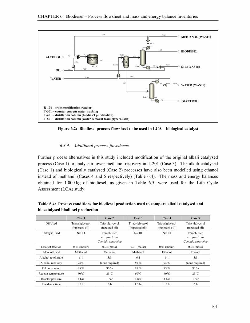
CHAPTER 6: Biodiesel – Process flowsheet and mass and energy balance inventories
161
Figure 6.2: Biodiesel process flowsheet to be used in LCA – biological catalyst
6.3.4. Additional process flowsheets Further process alternatives in this study included modification of the original alkali catalysed process (Case 1) to analyse a lower methanol recovery in T-201 (Case 3). The alkali catalysed (Case 1) and biologically catalysed (Case 2) processes have also been modelled using ethanol instead of methanol (Cases 4 and 5 respectively) (Table 6.4). The mass and energy balances obtained for 1 000 kg of biodiesel, as given in Table 6.5, were used for the Life Cycle Assessment (LCA) study.
Table 6.4: Process conditions for biodiesel production used to compare alkali catalysed and biocatalysed biodiesel production
Case 1 Case 2 Case 3 Case 4 Case 5
Oil Used Triacylglycerol (rapeseed oil)
Triacylglycerol (rapeseed oil)
Triacylglycerol (rapeseed oil)
Triacylglycerol (rapeseed oil)
Triacylglycerol (rapeseed oil)
Catalyst Used NaOH Immobilised enzyme from
Candida antarctica
NaOH NaOH Immobilised enzyme from
Candida antarctica
Catalyst fraction 0.01 (molar) 0.04 (mass) 0.01 (molar) 0.01 (molar) 0.04 (mass)
Alcohol Used Methanol Methanol Methanol Ethanol Ethanol
Alcohol to oil ratio 6:1 3:1 6:1 6:1 3:1
Alcohol recovery 94 % (none required) 50 % 94 % (none required)
Oil conversion 95 % 90 % 95 % 95 % 90 %
Reactor temperature 60°C 25°C 60°C 60°C 25°C
Reactor pressure 4 bar 1 bar 4 bar 4 bar 1 bar
Residence time 1.5 hr 16 hr 1.5 hr 1.5 hr 16 hr
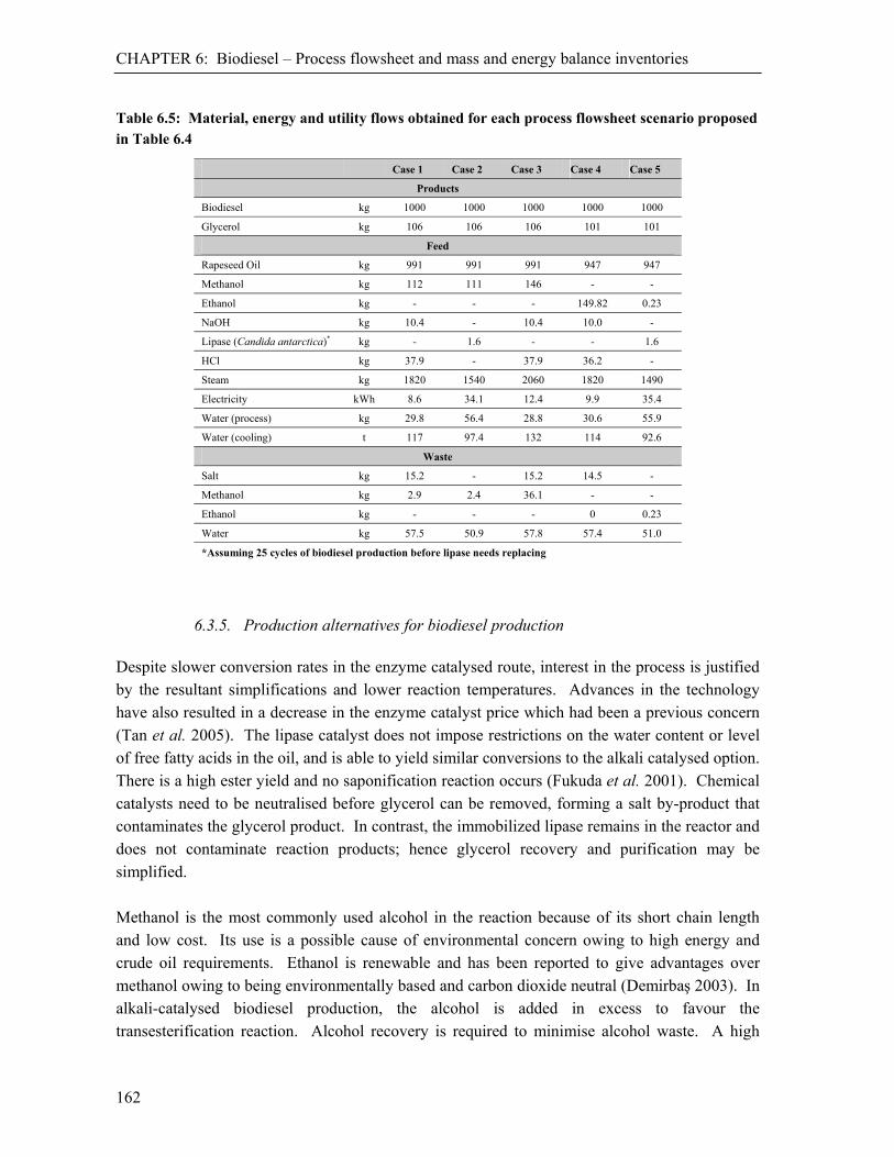
CHAPTER 6: Biodiesel – Process flowsheet and mass and energy balance inventories
162
Table 6.5: Material, energy and utility flows obtained for each process flowsheet scenario proposed in Table 6.4
Case 1 Case 2 Case 3 Case 4 Case 5
Products
Biodiesel kg 1000 1000 1000 1000 1000
Glycerol kg 106 106 106 101 101
Feed
Rapeseed Oil kg 991 991 991 947 947
Methanol kg 112 111 146 - -
Ethanol kg - - - 149.82 0.23
NaOH kg 10.4 - 10.4 10.0 -
Lipase (Candida antarctica)* kg - 1.6 - - 1.6
HCl kg 37.9 - 37.9 36.2 -
Steam kg 1820 1540 2060 1820 1490
Electricity kWh 8.6 34.1 12.4 9.9 35.4
Water (process) kg 29.8 56.4 28.8 30.6 55.9
Water (cooling) t 117 97.4 132 114 92.6
Waste
Salt kg 15.2 - 15.2 14.5 -
Methanol kg 2.9 2.4 36.1 - -
Ethanol kg - - - 0 0.23
Water kg 57.5 50.9 57.8 57.4 51.0
*Assuming 25 cycles of biodiesel production before lipase needs replacing
6.3.5. Production alternatives for biodiesel production Despite slower conversion rates in the enzyme catalysed route, interest in the process is justified by the resultant simplifications and lower reaction temperatures. Advances in the technology have also resulted in a decrease in the enzyme catalyst price which had been a previous concern (Tan et al. 2005). The lipase catalyst does not impose restrictions on the water content or level of free fatty acids in the oil, and is able to yield similar conversions to the alkali catalysed option. There is a high ester yield and no saponification reaction occurs (Fukuda et al. 2001). Chemical catalysts need to be neutralised before glycerol can be removed, forming a salt by-product that contaminates the glycerol product. In contrast, the immobilized lipase remains in the reactor and does not contaminate reaction products; hence glycerol recovery and purification may be simplified. Methanol is the most commonly used alcohol in the reaction because of its short chain length and low cost. Its use is a possible cause of environmental concern owing to high energy and crude oil requirements. Ethanol is renewable and has been reported to give advantages over methanol owing to being environmentally based and carbon dioxide neutral (Demirbaş 2003). In alkali-catalysed biodiesel production, the alcohol is added in excess to favour the transesterification reaction. Alcohol recovery is required to minimise alcohol waste. A high

CHAPTER 6: Biodiesel – Life Cycle Assessment (LCA)
163
recovery requires a higher energy input for distillation. The relative advantage of minimizing the distillation energy requirement requires assessment (comparison of Case 1 and Case 3). In the enzyme catalysed route, alcohol recovery is eliminated completely since a high alcohol concentration can inactivate the enzyme. Stepwise, stoichiometric addition is required (Shimada et al. 1999, 2002, Watanabe et al. 2000, 2001, 2002, Soumanou and Bornscheuer 2003). Immobilised lipases are deactivated by a high concentration of lower alcohols. When this occurs the lipase can be regenerated with 2- or tert-butanol (Chen and Wu 2003).
6.4. Life Cycle Assessment (LCA) Comparison of the different routes of biodiesel production was performed using the methodology explained in Section A.6. of Appendix A. The system was defined as cradle-to-gate production of 1000 kg of biodiesel, equivalent to a fuel with a calorific value of 27.1 GJ, or 33.3MJ/l (Beer et al. 2002b). The LCA included all raw materials, agricultural inputs and biodiesel processing required for the final biodiesel product. The life cycle inventory data are presented in Appendix I. The production included the useful by-product glycerol which, owing to process design and stoichiometry, is of equal purity and in equal proportion to biodiesel in each process. The assumption of equal purity may be conservative towards the enzyme process as the industrial process may give a purity slightly higher than the alkali catalysed process. The preferred method of burden allocation is by system expansion (Azapagic and Clift 1999, Ekval and Finnveden 2001, ISO 14040:2006). However, in order for readers to compare the biodiesel results against other literature values or against petroleum diesel values, this approach was avoided. Because of varying costs of glycerol as a function of purity, burden allocation on an economic basis was also not used. Therefore, the most appropriate allocation method was by mass ratios of useful end product. Since the mass ratios of glycerol to biodiesel were similar in all studies, allocation by economics or any other method would have given similar comparative results across the scenarios. Thus these suffice for comparison of technology selection as presented here. Before the LCA comparison of biodiesel production could be performed, the LCA impact of enzyme production needed to be calculated. Since the SimaPro v7.1® (PRé Consultants B.V. 2008) software and the EcoInvent v1.3 database (Swiss Centre for Life Cycle Inventories 2007), did not include an LCA module for immobilised enzyme production, the generic flowsheet model was used to determine material and energy balance inputs. These can then be used to determine the LCA impacts of biodiesel production.

CHAPTER 6: Biodiesel – Lipase production
164
6.5. Lipase production
6.5.1. Process flowsheet and model development Two processes for the extracellular production of lipase using an aerobic batch reactor, with glucose and yeast extract as raw materials were considered. The first scenario (Scenario L1) assumed submerged culture (SmF) which yielded a final default biomass concentration of 16.7 g/l as shown in Table 6.6, while the second (Scenario L2) assumed solid state cultivation (SSC) giving a biomass concentration of 40 g/l. In Scenario L1, biomass is removed by a filtration unit. This was followed by a downstream train identical to Scenario L2 which did not require biomass removal. This involved a unit to precipitate the lipase product and a filtration unit to recover the lipase as shown in Figure 6.3. It was assumed that the formulation unit removed enough liquid to give a purity of 85 % in both scenarios. The assumptions around the lipase production were based first approximations. Scenario L2 (SSC) could expect to export enzyme for longer than Scenario L1 (SmF), but also had greater mass transfer problems. In these calculations it was assumed that the rates were maintained in both production scenarios.
Figure 6.3: Flowsheet used for material and energy balance development for lipase production
from Candida antarctica
6.5.2. Material and energy balance outputs From the information used in Table 6.6, material and energy flows were calculated and are shown in Table 6.7. Although identical stoichiometry, nutrient excess and yield coefficients were used, owing to the additional filtration unit in Scenario L1 where nutrients were lost, for each kilogram of lipase product, 5.2 kg of glucose, 3.5 kg of yeast extract and 247 kg of air were required. In Scenario L2, 3.6 kg of glucose, 2.4 kg of yeast extract and 139 kg of air were required. Owing to the reduced biomass concentration with the same yield of lipase assumed per unit biomass, Scenario L1 required more water (76.5 kg) than Scenario L2 which required

CHAPTER 6: Biodiesel – Lipase production
165
28.7 kg water per kilogram of enzyme. This resulted in an increased requirement for precipitating chemical (3.7 kg in L1 vs. 1.5 kg in L2) since it was added on a basis of volumetric concentration. The increased volume in Scenario L1 also increased the electricity (70.7 MJ/kg) and steam (15.6 kg/kg) requirements beyond Scenario L2 which required 35.4 MJ/kg and 5.3 kg/kg respectively. The assumption of 0.5 kW/m3 agitation energy may be slightly high for the solid state cultivation (which represents pumping energy), but it was taken as a conservative estimate.
Table 6.6: Input assumptions used for the extracellular, aerobic production of lipase in a batch reactor as required for the enzyme catalyst for biodiesel production
Assumptions* Scenario L1 – SmF# Scenario L2 – SSC# Units
Steam Sterilisation: (preheated with sterilised media)
Steam temperature [140] [140] C
Steam pressure [300] [300] kPa
Microbial growth conditions: (batch production of lipase from Candida sp.)
Carbon 1 source (excess): Glucose [1] [1] %
Nitrogen source 1: Yeast extract [5] [5] %
Maintain reactor temperature (Cooling agent: Cooling water)
Final biomass concentration [16.7] 40 g/l
Aeration:
Oxygen source (vvm): Air [10x the min. stoich. requirement] [10x the min. stoich. requirement]
Agitation
Power per unit volume (Energy: Electricity) 0.5 0.5 kW/m3
Cool before downstream processing
Filtration
Solid fraction removed [0.95] -** %
Liquid fraction retained [0.70] -** %
Precipitation
Non-reacting additive: [Precipitating chemical] [5] [5] %v/v
Filtration
Solid fraction removed [0.95] [0.95] %
Liquid fraction retained [0.70] [0.70] %
Formulation (other)
Liquid fraction removed To give product purity of 85 % To give product purity of 85 % %
Product fraction retained [0.99] [0.99] %
[ ] Default data calculated or assumed in the MS-Excel model when no explicit inputs are given * Energy assumed to be supplied by electricity throughout, with steam used for heating during precipitation # Smf – submerged fermentation; SSC – solid state cultivation ** No filtration unit required for solid state cultivation method

CHAPTER 6: Biodiesel – Lipase production
166
Table 6.7: Material, energy and utility flows for the production of lipase from Candida antarctica using the generic flowsheet model
Component In (kg)
Out (kg)
In (kg)
Out (kg)
Scenario L1 Scenario L2
Glucose 5.2 0.052 3.6 0.036
Yeast extract 3.5 0.16 2.4 0.12
Candida sp. - 1.2 - 0.9
Air (reacting oxygen only) 5.2 - 3.6 -
Precipitating chemical 3.7 3.7 1.5 1.5
Lipase (lost in wastewater) - 0.40 - 0.05
Lipase (product) - 1 - 1
Carbon dioxide - 7.4 - 5.2
Phosphates - 0.13 - 0.09
Water 76.5 80.0 20.1 22.4
TOTAL 138.3 138.3 31.2 31.2
Chemical Oxygen Demand (COD) 8.1 3.7
Product recovery (% kg lip.) 65.8 94.1
Product purity (mass %) 85 85
Energy requirements Scenario SSC1 Scenario SSC2 Units
Electricity 19.64 (70.7)
9.83 (35.4)
kWh/kg lip. (MJ/kg lip)
Steam (152°C, 3 bar) 15.6 (42.12)
5.3 (14.3)
kg/kg lip. (MJ/kg lip.)
Total energy equivalent 115.8 49.7 MJ/kg lipase
Cooling water 33.8 14.0 kg/kg lipase
6.5.3. Life Cycle Assessment (LCA) of lipase production Using the material and energy inventory from Scenario L1, and the SimaPro software, for 1 kg of lipase produced, life cycle impacts of 53.7 kg CO2 eq., 0.320 kg Sb eq., 1.810 mg CFC-11 eq. and 0.87 kg SO2 eq. were obtained in the categories of global warming, abiotic depletion, ozone layer depletion and acidification respectively as shown in Table 6.8. The LCA results for the same categories for Scenario L2 were 33.0 kg CO2 eq., 0.181 kg Sb eq., 1.07 mg CFC-11 eq. and 0.55 kg SO2 eq.. Using a solid state cultivation method and increasing the final biomass concentration as in Scenario L2, reduced the LCA burden by between 36 % and 48 % as shown in Figure 6.4. Global warming, eutrophication and abiotic depletion were reduced by 39 %, 36 % and 43 % respectively.
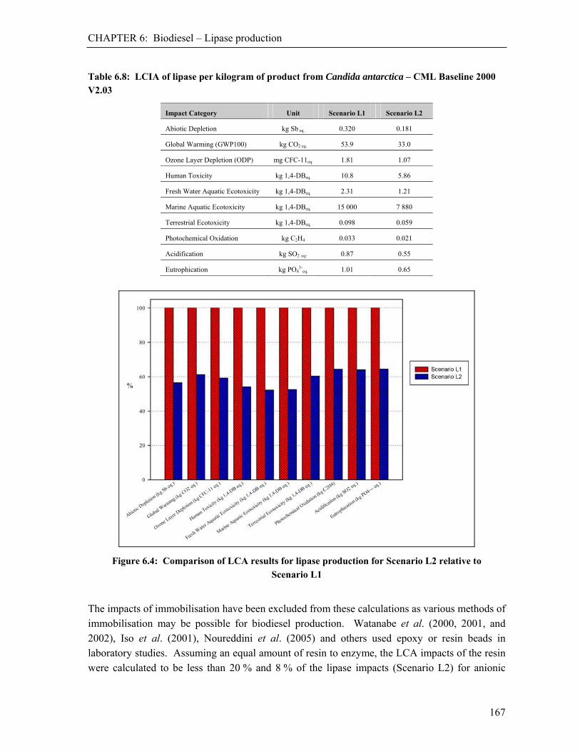
CHAPTER 6: Biodiesel – Lipase production
167
Table 6.8: LCIA of lipase per kilogram of product from Candida antarctica – CML Baseline 2000 V2.03
Impact Category Unit Scenario L1 Scenario L2
Abiotic Depletion kg Sb eq. 0.320 0.181
Global Warming (GWP100) kg CO2 eq. 53.9 33.0
Ozone Layer Depletion (ODP) mg CFC-11eq. 1.81 1.07
Human Toxicity kg 1,4-DBeq. 10.8 5.86
Fresh Water Aquatic Ecotoxicity kg 1,4-DBeq. 2.31 1.21
Marine Aquatic Ecotoxicity kg 1,4-DBeq. 15 000 7 880
Terrestrial Ecotoxicity kg 1,4-DBeq. 0.098 0.059
Photochemical Oxidation kg C2H4 0.033 0.021
Acidification kg SO2 eq. 0.87 0.55
Eutrophication kg PO43-
eq. 1.01 0.65
Figure 6.4: Comparison of LCA results for lipase production for Scenario L2 relative to
Scenario L1
The impacts of immobilisation have been excluded from these calculations as various methods of immobilisation may be possible for biodiesel production. Watanabe et al. (2000, 2001, and 2002), Iso et al. (2001), Noureddini et al. (2005) and others used epoxy or resin beads in laboratory studies. Assuming an equal amount of resin to enzyme, the LCA impacts of the resin were calculated to be less than 20 % and 8 % of the lipase impacts (Scenario L2) for anionic

CHAPTER 6: Biodiesel – Life Cycle Assessment (LCA) of biodiesel production
168
(anionic resin, at plant/kg/CH – Ecoinvent 1.3) and cationic resins (cationic resin, at plant/kg/CH – Ecoinvent 1.3) respectively (Figure 6.5). The exception was in the ozone layer depletion category where, owing to a large quantity of bromine compounds, the anionic score was 260 fold higher than that for the lipase. More environmentally friendly immobilisation materials such as gels, spun fibres, microcapsules can be expected to reduce this contribution still further.
Figure 6.5: Comparison of LCA results for equal masses of anionic and cationic resins relative to lipase produced by Scenario L2
6.6. Life Cycle Assessment (LCA) of biodiesel production The material and energy inventory for biodiesel production (Table 6.5), as calculated using the Aspen Plus® software (AspenTech 2008), was used to determine Life Cycle Assessment (LCA) indicators with the aid of SimaPro v7.1® (PRé Consultants B.V. 2008) LCA software. The impact of the lipase reported in Section 6.5, was used for Cases 2 and 5 where biological catalysts were used. Scenario L2 was used as this represented the best case. The impacts of the lipase are expected to decrease further with optimisation of the technology. Data from LCA results which are within 5 % of each other may not be significantly different from each other owing to uncertainty in the inputs and LCA inventory datasets.

CHAPTER 6: Biodiesel – Life Cycle Assessment (LCA) of biodiesel production
169
For the production of 1 kg of biodiesel, average life cycle impacts of 3.6 kg CO2 eq., 0.0141 kg Sb eq., 0.733 mg CFC-11 eq. and 0.0264 kg SO2 eq. were obtained in the categories of global warming, abiotic depletion, ozone layer depletion and acidification respectively as shown in Table 6.9. Differences in abiotic depletion, global warming, ozone layer depletion, photochemical oxidation, acidification and eutrophication were less than 20 % across all cases as shown in Figure 6.6. Impacts in terrestrial ecotoxicity showed as much as a 90 % variation across the different cases, with the enzyme catalysed route (Cases 2 and 5) showing the lowest impact because of the absence of hydrochloric acid.
Table 6.9: LCIA of biodiesel per kilogram of product – CML 2 Baseline 2000 V2.03
Impact category Unit Case 1 Case 2 Case 3 Case 4 Case 5 Average
Abiotic Depletion kg Sbeq. 0.0137 0.0130 0.0147 0.0149 0.0141 0.0141
Global Warming (GWP100) kg CO2 eq. 3.64 3.55 3.71 3.61 3.52 3.61
Ozone Layer Depletion (ODP) mg CFC-11eq. 0.776 0.698 0.785 0.749 0.658 0.733
Human Toxicity kg 1,4-DBeq. 0.231 0.174 0.249 0.359 0.301 0.263
Fresh Water Aquatic Ecotoxicity kg 1,4-DBeq. 0.0412 0.0315 0.0437 0.0755 0.0660 0.052
Marine Aquatic Ecotoxicity kg 1,4-DBeq. 189.8 140.2 2036 293.3 242.4 580.3
Terrestrial Ecotoxicity kg 1,4-DBeq. 0.00216 0.000160 0.00245 0.00222 0.00023 0.00144
Photochemical Oxidation kg C2H4 0.00127 0.00129 0.00128 0.00136 0.00138 0.00132
Acidification kg SO2 eq. 0.0245 0.0251 0.0246 0.0288 0.0292 0.0264
Eutrophication kg PO43-
eq. 0.0374 0.0387 0.0373 0.0421 0.0433 0.0398
Figure 6.6: Comparison of LCA results for biodiesel for Cases 2 – 5 relative to Case 1

CHAPTER 6: Biodiesel – Life Cycle Assessment (LCA) of biodiesel production
170
6.6.1. Alkali catalyst and methanol (Case 1) Using the CML 2 Baseline 2000 v2.03 method, for 1 kg of biodiesel produced by alkali catalysis in the presence of methanol (Case 1), 3.64 kg carbon dioxide equivalent was released into the atmosphere, while 24.5 g SO2 eq. and 37.4 g PO4
3-eq. were emitted. The major contributing
process in all LCA categories for the production of biodiesel was the farming process, including fertilizer production. Further major contributors included the energy requirements from natural gas, diesel and heat oil, as well as the impacts associated with steam production. The process contributions are further discussed in Section 6.6.5, later in this chapter. Because of the high energy contribution, milder process conditions were expected to improve LCA results as investigated in Case 2. Reducing methanol recovery should also reduce the energy needs (Case 3). To further improve LCA results, changing the alcohol used to ethanol allowed comparison with methanol from both the original alkali and enzyme processes (Case 1 and 2 for methanol and Case 4 and 5 for ethanol).
6.6.2. Chemical vs. biological catalysts When comparing biodiesel production (CML 2 Baseline 2000 v2.03 method) using inorganic- and biological catalysts with methanol as the transesterification alcohol (Case 1 and 2), all LCA impacts were lower for the enzyme catalysed process, except photochemical oxidation, acidification and eutrophication. Fresh water aquatic-, marine aquatic- and human toxicity were reduced by approximately 15 %. Terrestrial ecotoxicity was reduced by over 95% (mainly owing to the removal of hydrochloric acid from the biologically-catalysed process). Ozone layer depletion was reduced by 11 % and abiotic depletion by 5 %. Reductions in other categories were below 5 % as shown in Figure 6.7. Increases in photochemical oxidation, acidification and eutrophication were all less than 3 %. These reductions resulted from reduction in steam, as well as the absence of hydrochloric acid and sodium hydroxide. The increase in electricity in Case 2 balanced out the reductions from steam, hydrochloric acid and sodium hydroxide in the categories of photochemical oxidation, acidification and eutrophication.

CHAPTER 6: Biodiesel – Life Cycle Assessment (LCA) of biodiesel production
171
Figure 6.7: LCA results – chemical vs. biological catalysts (biodiesel production by alkali catalysis assuming 94 % methanol recovery (Case 1) is compared to production using lipase as a biocatalyst
(Case 2))
6.6.3. Reduced methanol recovery When methanol recovery in the alkali-catalysed process was lowered from 94 to 50 % (Case 1 vs. 3), impacts increased in all categories. In order to maintain an equal amount of biodiesel product, flow rates in the product recovery section increased when methanol recovery decreased. This resulted in greater pumping requirements and higher loads in distillation columns. Reducing recovery also increased waste methanol released and the methanol feed. Reducing methanol recovery to 50 % increased all recorded toxicity levels by at least 6 %. Abiotic depletion increased by 6 %, while increases in ozone layer depletion, global warming, photochemical oxidation, acidification and eutrophication were not significant (Figure 6.8). Since flows increased, capital and operating costs were also expected to increase, which would result in further favouring of Case 1.
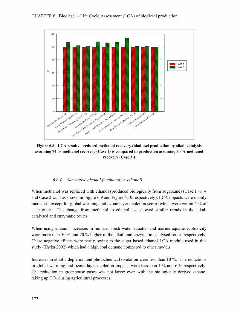
CHAPTER 6: Biodiesel – Life Cycle Assessment (LCA) of biodiesel production
172
Figure 6.8: LCA results – reduced methanol recovery (biodiesel production by alkali catalysis assuming 94 % methanol recovery (Case 1) is compared to production assuming 50 % methanol
recovery (Case 3))
6.6.4. Alternative alcohol (methanol vs. ethanol) When methanol was replaced with ethanol (produced biologically from sugarcane) (Case 1 vs. 4 and Case 2 vs. 5 as shown in Figure 6.9 and Figure 6.10 respectively), LCA impacts were mainly increased, except for global warming and ozone layer depletion scores which were within 5 % of each other. The change from methanol to ethanol use showed similar trends in the alkali catalysed and enzymatic routes. When using ethanol, increases in human-, fresh water aquatic- and marine aquatic ecotoxicity were more than 50 % and 70 % higher in the alkali and enzymatic catalysed routes respectively. These negative effects were partly owing to the sugar based-ethanol LCA module used in this study (Theka 2002) which had a high coal demand compared to other models. Increases in abiotic depletion and photochemical oxidation were less than 10 %. The reductions in global warming and ozone layer depletion impacts were less than 1 % and 6 % respectively. The reduction in greenhouse gases was not large; even with the biologically derived ethanol taking up CO2 during agricultural processes.

CHAPTER 6: Biodiesel – Life Cycle Assessment (LCA) of biodiesel production
173
Figure 6.9: LCA results – alternative alcohol (methanol vs. ethanol) using alkali catalysis (biodiesel production by alkali catalysis assuming 94 % methanol recovery (Case 1) is compared to
production using ethanol at 94 % recovery (Case 4))
Figure 6.10: LCA results – alternative alcohol (methanol vs. ethanol) using lipase biocatalysis (biodiesel production by lipase biocatalysis using methanol (Case 2) is compared to production by
lipase biocatalysis and ethanol (Case 5))
CHAPTER 6: Biodiesel – Life Cycle Assessment (LCA) of biodiesel production
174
6.6.5. Process contributions Using the example of biodiesel production with methanol and a lipase enzyme catalyst (Case 2), Life Cycle Assessment (LCA) process contributions were calculated to determine the impact of the lipase catalyst to the overall LCA score. The enzyme production Scenario L2 was used as the more favourable production route. The amount of lipase used was calculated assuming replacement after 1000 kg of biodiesel production. With improvements in enzyme activity and enzyme production technology, lipase impacts and their contributions to the LCA scores may be reduced. The results showed that production of rape seed oil, steam and lipase were the major contributing factors throughout. The LCA categories investigated included abiotic depletion, global warming, ozone layer depletion, photochemical oxidation, acidification and eutrophication. The values shown in the figures represented contribution to the LCA impacts as a percentage of the total in each category. Only materials which led to a contribution greater than 3 % of the total LCA score have been included. In the abiotic depletion category, rape seed oil made up 61.2 % of the total LCA score (Figure 6.11). This score, as in all the impact categories, was predominantly made up of the rape seed from farming, which in turn was made up of fertiliser and diesel. Steam (21 %), methanol (14.5 %) and lipase (2.0 %) made up the remaining dominant categories for abiotic depletion. Natural gas needed for steam and methanol production added a combined 30.7 % to the total score. In the category for global warming, rape seed oil (85.9 %) and steam (9.5 %) were the only 2 impacts with a contribution of over 3 % to the total score. The global warming impacts of rape seed oil production may have been expected to have been negative owing to carbon dioxide uptake during biomass growth, as well as the credit given for the production of animal feed as a by-product during the agricultural process, but electricity, fertiliser and chemical use resulted in a net carbon dioxide release of 3.4 kg CO2 eq. per kilogram of rapeseed oil produced. Where bio-based carbon is found in the final product this was deducted in the calculations. It is unlikely that the LCA impact would change if incineration were chosen, since comparable amounts of CO2 would be released as a consequence.
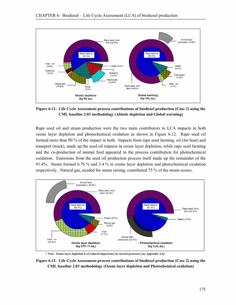
CHAPTER 6: Biodiesel – Life Cycle Assessment (LCA) of biodiesel production
175
Figure 6.11: Life Cycle Assessment process contributions of biodiesel production (Case 2) using the CML baseline 2.03 methodology (Abiotic depletion and Global warming)
Rape seed oil and steam production were the two main contributors to LCA impacts in both ozone layer depletion and photochemical oxidation as shown in Figure 6.12. Rape seed oil formed more than 90 % of the impact in both. Impacts from rape seed farming, oil (for heat) and transport (truck), made up the seed oil impacts in ozone layer depletion, while rape seed farming and the co-production of animal feed appeared in the process contribution for photochemical oxidation. Emissions from the seed oil production process itself made up the remainder of the 91.4%. Steam formed 6.76 % and 3.4 % in ozone layer depletion and photochemical oxidation respectively. Natural gas, needed for steam raising, contributed 75 % of the steam scores.
* Note: Ozone layer depletion is of reduced importance in current processes (see Appendix A.6)
Figure 6.12: Life Cycle Assessment process contributions of biodiesel production (Case 2) using the CML baseline 2.03 methodology (Ozone layer depletion and Photochemical oxidation)

CHAPTER 6: Biodiesel – Conclusions
176
Rape seed oil, lipase and steam contributed 91.7 %, 3.3 % and 3.2 % respectively in the acidification category as shown in Figure 6.13. The rape seed oil contributed 97.3 % to the eutrophication score, a result of fertiliser used during the farming process for rape seed and the co-production of animal feed. Lipase production only formed 2.3 % of the total impact in eutrophication.
Figure 6.13: Life Cycle Assessment process contributions of biodiesel production (Case 2) using the CML baseline 2.03 methodology (Acidification and Eutrophication)
6.7. Conclusions Biodiesel can be produced by the transesterification of oils using a chemical or biological catalyst. The environmental burdens of these production routes were investigated by a Life Cycle Assessment (LCA) methodology, where these impacts guide design considerations at an early stage of process development. In order to perform the LCA analyses, the material and energy inventories of each flowsheet design were required. These inventories were obtained by detailed Aspen Plus® (AspenTech 2008) designs. Since this data did not include the material and energy inventories for the lipase used as biological catalyst, the generic flowsheet model developed in Chapter 2 was used to generate this data. This full material and energy inventory then informed the LCA analysis for biodiesel production. When the overall biodiesel production was studied, enzyme catalysed biodiesel production had environmental advantages owing to avoided use of chemical catalyst and neutralising acid. The lower pressures and temperatures obtained helped give more favourable LCA results across seven of the ten environmental impacts considered. The major contributing processes to LCA

CHAPTER 6: Biodiesel – References
177
scores were similar in all processes. Rapeseed oil (including diesel and fertiliser use), steam (natural gas) and methanol/ethanol were all major contributors to overall LCA scores. Methanol production impacts were lower than the ethanol production impacts in all but two of the LCA categories. In the alkali catalysed process, lower alcohol recovery required greater flows to give similar product yield and purity. This increased the energy need, as well as pollutants, and caused a less favourable production route when analysed using life cycle assessment. It was found that the LCA impact of lipase production was less than 4 % of the total biodiesel impact across all categories. Improvements to technology to allow for greater optimisation of lipase production would see further reduction in this contribution to total LCA scores. As a result of recycle and distillation columns, the production of biodiesel was too complex to model using the generic flowsheet as given in Chapter 2. Therefore, Aspen Plus® was used. While Aspen Plus® gave the required material and energy data, the modelling effort was greater because of the additional engineering detail required and the complexity of the software package.
References Abigor, R.D., Uaudia, P.O., Foglia, T.A., Hass, M.J., Jones, K.C., Okoefa, E., Obibuzor, J.U., Bafor, M.E., 2000.
Lipase-catalysed production of biodiesel fuel from some Nigerian lauric oils, Biochem. Soc. T., 28, 979–981. Abreu, F. R., Lima, D.G., Hamú, E.H., Wolf, C., Suarez, P.A.Z., 2004. Utilization of metal complexes as catalysts
in the transesterification of Brazilian vegetable oils with different alcohols, J. Mol. Catal. A-Chem., 209, 29-33. Al-Widyun, M., Al-Shyoukh, A.O., 2002. Experimental evaluation of the transesterification of waste palm oil into
biodiesel, Bioresource Technol., 85, 253-256. Al-Zuhair, S., 2005. Production of biodiesel by lipase-catalyzed transesterification of vegetable oils: A kinetics
study, Biotechnol. Progr., 21, 1442-1448. Alcantara, R., Amores, J., Canoira, L., Fidalgo, E., Franco, M.J., Navarro, A., 2000. Catalytic production of
biodiesel from soy-bean oil, used frying oil and tallow, Biomass Bioenerg., 18, 515-527. Al-Zuhair, S., Jayaraman, K.V., Krishnan, S., Chan, W.-H., 2006. The effect of fatty acid concentration and water
content on the production of biodiesel by lipase, Biochem. Eng. J., 30, 212-217. Antolín, G., Tinaut, F.V., Briceño, Y., Castaño, V., Pérez, C., Ramírez, A.I., 2002. Optimisation of biodiesel
production by sunflower oil transesterification, Bioresource Technol., 83, 111-114. Aresta, M., Dibenedetto, A., Carone, M., Colonna, T., Fragale, C., 1995. Production of biodiesel from microalgae
by supercritical CO2 extraction and thermochemical liquefaction, Environ. Chem. Lett., 3, 136-139. AspenTech, 2008. Aspen Technology, Inc., 200 Wheeler Road, Burling, Massachusetts 01803, USA,
http://www.aspentech.com/ ATTRA, 2002. Biodiesel: A Brief Overview, Appropriate Technology Transfer for Rural Areas, Arkansas, USA
(Faupel, K. and Kurki, A.). Available from: http://www.attra.ncat.org/attra-pub/PDF/biodiesel.pdf [Accessed 14 April 2004].
Azam, M.M., Waris, A., Nahar, N.M., 2005. Prospects and potential of fatty acid methyl esters of some non-traditional seed oils for sue as biodiesel in India, Biomass Bioenerg., 29, 293-302.
Azapagic A., Clift R., 1999. Allocation of environmental burdens in multiple-function systems, J. Clean. Prod., 7(2), 101–19.

CHAPTER 6: Biodiesel – References
178
Ban, K., Kaieda, M., Matsumoto, T., Kondo, A., Fukuda, H., 2001. Whole cell biocatalyst for biodiesel fuel production utilizing Rhizopus oryzae cells immobilized within biomass support particles, Biochem. Eng. J., 8, 39-43.
Ban, K., Hama, S., Nishizuku, K., Kaieda, M., Matsumoto, T., Kondo, A., Noda, H., Fukuda, H., 2002. Repeated use of whole-cell biocatalysts immobilized within biomass support particles for biodiesel fuel production, J. Mol. Cat. B-Enzym., 17, 157-165.
Barnwell, B.K., Sharma, M.P., 2005. Prospects of biodiesel production from vegetable oils in India, Renew. Sust. Energ. Rev., 9, 363-378.
Basu, H.N., Norris, M.E., 1996. Process for production of esters for use as a diesel fuel substitute using a non-alkaline catalyst, US Patent 5525126.
Bayenes, C.R., Hinnekens, H., Martens, J., 1996. Esterification Process, United States Patent 5,508,457. Beer, T., Grant, T., Morgan, G., Lapszewicz, J., Anyon, P., Edwards, J., Nelson, P., Watson, H., Williams, D.,
2002a. Comparison of Transport Fuels: life cycle emissions analysis of alternative fuels for heavy vehicles, Australian Greenhouse Office, Victoria, Australia Available from: http://www.greenhouse.gov.au/transport/comparison/pubs/comparison.pdf, [Accessed 8 May 2004].
Beer, T., Grant, T., Williams, D., Watson, H., 2002b. Fuel-cell greenhouse gas emissions from alternative fuels in Australian heavy vehicles, Atmos. Environ., 36, 753-763.
Belafi-Bako, K., Kovacs, F., Gubicza, L., Hancsok, J., 2002. Enzymatic biodiesel production from sunflower oil by Candida antarctica lipase in a solvent-free system, Biocatal. Biotransfor., 20, 437–439.
Bona, S., Mosca, G., Vamerali, T., 1999. Oil crops for Biodiesel production in Italy, Renew. Energ., 16, 1053-1056. Boocock, D.G.B., Konar, S.K., Mao, V., Sidi, H., 1996. Fast one-phase oil-rich process for the preparation of
vegetable oil methyl esters, Biomass Bioenerg., 11(1), 43-50. Bouaid, A., Diaz, Y., Martinez, M., Aracil, J., 2005. Pilot plant studies of biodiesel production using Brassica
crinata as a raw material, Catal. Today, 106, 193-193. Canoira, L., Alcántara, R., García-Martínez, J., Carrasco, J., 2006. Biodiesel from Jojoba oil-wax:
Transesterification with methanol and properties as a fuel, Biomass Bioenerg., 30, 76-81. Cao, W., Han, H., Zhang, J., 2005. Preparation of biodiesel from soybean oil using supercritical methanol and co-
solvent, Fuel, 84, 347-351. Cardone, M., Mazzoncini, M., Menini, S., Rocco, V., Senatore, A., Seggiani, M., Vitolo, S., 2003. Brassica
carinata as an alternative oil crop for the production of biodiesel in Italy: agronomic evaluation, fuel production by transesterification and characterization, Biomass Bioenerg., 25, 623-636.
Castro, M.P.P., Andrade, A.A., Franco, R.W.A., Miranda, P.C.M.L., Sthel, M., Vargas, H., Constantino, R., Baesso, M.L., 2005. Thermal properties measurement in biodiesel oils using photothermal techniques, Chem. Phys. Lett., 411, 18-22.
Chen, J.-W., Wu, W.-T., 2003. Regeneration of Immobilized Candida antarctica lipase for transesterification, J. Biosci. Bioeng., 95(5), 466-469.
Chisti, Y., 2007. Biodiesel from microalgae, Biotechnol. Adv., 25, 294-306. Chisti, Y., 2008. Biodiesel from microalgae beats bioethanol, Trends Biotechnol., 26(3), 126-131. Corma, A., Iborra, S., Miquel, S., Primo, J., 1998. Catalysts for the production of fine chemicals: production of food
emulsifiers, monoglycerides, by glycerolysis of fats with solid base catalysts, J. Catal., 173, 315-321. Crabbe, E., Nolasco-Hipolito, C., Kobayashi, G., Sonomoto, K., Ishizaki, A., 2001. Biodiesel production from
crude palm oil and evaluation of butanol extraction and fuel properties, Process Biochem., 37, 65-71. Demibraş, A., 2002. Biodiesel from vegetable oils via transesterification in supercritical methanol, Energ. Convers.
Manage., 43, 2349-2356. Demibraş, A., 2003. Biodiesel fuels from vegetable oils via catalytic and non-catalytic supercritical alcohol
transesterifications and other methods: a survey, Energ. Convers. Manage., 44(13), 2093-2109. Demibraş, A., 2005. Biodiesel production from vegetable oils via catalytic and non-catalytic supercritical methanol
transesterification methods, Prog. Energ. Combust., 31, 466-487. Demibraş, A., 2006. Biodiesel production via non-catalytic SCF method and biodiesel fuel characteristics, Energ.
Convers. Manage., 47, 2271-2282. Di Serio, M., Tesser, R., Dimiccoli, M., Cammarota, F., Nastasi, M., Santacesaria, E., 2005. Synthesis of biodiesel
via homogeneous Lewis acid catalyst, J. Mol. Catal. A-Chem., 239, 111-115.

CHAPTER 6: Biodiesel – References
179
Dorado, M.P., Ballesteros, E., Arnal, J.M., Gómez, J., López, F.J., 2003. Exhaust emissions from a diesel engine fuelled with transesterified waste olive oil, Fuel, 82, 1311-1315.
Du, W., Xu, Y., Liu, D., Zeng, J., 2004. Comparative study on lipase-catalyzed transformation of soybean oil for biodiesel production with different acyl acceptors, J. Mol. Cat. B-Enzym., 30, 125-129.
Ebiura, T., Echizen, T., Ishikawa, A., Murai, K., Baba, T., 2005. Selective transesterification of triolein with methanol to methyl oleate and glycerol using alumina loaded with alkali metal salt as a solid-base catalyst, Appl. Catal. A – Gen., 283, 111-116.
Ekvall, T., Finnveden, G., 2001. Allocation in ISO 14041 – a critical review, J. Clean. Prod., 9, 197-208. Enchelmaier, H. Rasenhorn, H.J., 1994. German patent, 4,328,195. Encinar, J.M., González, J.F., Rodríguez, J.J., Tejedor, A., 2002. Biodiesel fuels from vegetable oils:
Transesterification of Cynara cardunculus L. oils with ethanol, Energ. Fuel., 16, 443-450. Foidl, N., Foidl, G., Sanchez, M., Mittelbach, M., Hackel, S., 1996. Jatropha carcus L. as a source for the
production of biofuel in Nicaragua, Bioresource Technol., 58, 77-82. Fröhlich, A., Rice, B., 2005. Evaluation of Camelina sativa oil as a feedstock for biodiesel production, Ind. Crop.
Prod., 21, 25-31. Fukuda, H., Kondo, A., Noda, H., 2001. Review: biodiesel fuel production by transesterification of oils, J. Biosci.
Bioeng., 92 (5), 405-416. Furuta, S., Matsuhashi, H., Arata, K., 2004. Biodiesel fuel production with solid super acid catalysts in fixed bed
reactor under atmospheric pressure, Catal. Comm., 5, 721-723. Germani, M.M., 1994. German patent, 4,324,875. Ghadge, S.V., Raheman, H., 2005. Biodiesel production from mahua (Madhuca indica) oil having high free fatty
acids, Biomass Bioenerg., 28, 601-605. Ghadge, S.V., Raheman, H., 2006. Process optimization for biodiesel production from mahua (Madhuca indica) oil
using response surface methodology, Bioresource Technol., 97, 379-384. Graboski, M.S., McCormick, R.L., 1998. Combustion of Fat and Vegetable Oil Derived Fuels in Diesel Engines,
Prog. Energ. Combust., 24, 125-164. Hall, D.O., Scrase, J.I., 1998. Will biomass be the environmentally friendly fuel of the future?, Biomass Bioenerg.,
15(14/15), 357-367. Hama, S., Tamalampudi, S., Fukumizu, T., Miura, K., Yamaji, H., Kondo, A., Fukuda, H., 2006. Lipase
localization in Rhizopus oryzae immobilized within biomass support particles for use as whole-cell biocatalysts in biodiesel-fuel production, J. Biosci. Bioeng., 101(4), 328-333.
Han, H., Cao, W., Zhang, J., 2005. Preparation of biodiesel from soybean oil using supercritical methanol and CO2 as co-solvent, Process Biochem., 40, 3148-3151.
Hossler, R.A., Harry-O’Kuru, R., 2006. Transesterified milkweed (Asclepias) seed oil as a biodiesel fuel, Fuel, 85, 2106-2110.
Ikwuagwu, O.E., Ononogbu, I.C., Njoku, O.U., 2000. Production of biodiesel using rubber [Hevea brasiliensis (Kunth. Muell.)] seed oil, Ind. Crop. Prod., 12, 57-62.
Iso, M., Chen, B., Eguchi, M., Kudo, T., Shrestha, S., 2001. Production of biodiesel fuel from triglycerides and alcohol using immobilized lipase, J. Mol. Catal. B – Enzym., 16, 53–58.
Jitputti, J., Kitiyanan, B., Rangsunvigit, P., Bunyakiat, K., Attanatho, L., Jenvantipanjukal, P., 2006. Transesterification of crude palm kernel by different solid catalysts, Chem. Eng. J., 116, 61-66.
Junek, H., Mittelbach, M., Andreae, F., 1998. German patent 3,727,981. Kaieda, M., Samukawa, T., Matsumoto, T., Ban, K., Kondo, A., Shimade, Y., Noda, H., Nomoto, F., Ohtsuka, K.,
Izumoto, E., Fukuda, H., 1999. Biodiesel fuel production from plant oil catalyzed by Rhizopus oryzae lipase in a water-containing system without an organic solvent, J. Biosci. Bioeng., 88(6), 627–631.
Kaieda, M., Samukawa, T., Kondo, A., Fukuda, H., 2001. Effect of methanol and water contents on production of biodiesel fuel from plant oil catalyzed by various lipases in a solvent free system, J. Biosci. Bioeng., 91(1), 12-15.
Kalam, M.A., Masjuki, H.H., 2002. Biodiesel from palm oil – an analysis of its properties and potential, Biomass Bioenerg., 23, 471-479.
Kaltschmitt, M., Reinhardt, G.A., Stelzer, T., 1997. Life Cycle Analysis of biofuels under different environmental aspects, Biomass Bioenerg., 12(2), 121-134.
Karmee, S.K., Chadha, A., 2005. Preparation of biodiesel from crude oil of Pongamia pinnata, Bioresource Technol., 96, 1425-1429.
CHAPTER 6: Biodiesel – References
180
Karaosmanoğlu, F., Ciğizoğlu, K.B., Tüter, M., Ertekin, S., 1996. Investigation of the refining step of biodiesel production, Energ. Fuel, 10, 890-895.
Kerschbaum, S., Rinke, G., 2004. Measurement of the temperature dependant viscosity of biodiesel fuels, Fuel, 83, 287-291.
Knothe, G., Matheaus, A.C., Ryan, T.W.(III), 2003. Cetane numbers of branched and straight-chain fatty esters determined in an ignition quality tester, Fuel, 82, 971-975.
Köse, O., Tuter, M., Aksoy, H.A., 2002. Immobilized Candida antarctica lipase-catalyzed alcoholysis of cotton seed oil in a solvent free medium, Bioresource Technol., 83, 125–129.
Krahl, J., Munack, A., Bahadir, M., Schumacher, L., Elser, N., 1996. Survey about biodiesel exhaust emissions and their environmental effects, Proceedings of the Third Liquid Fuel Conference, Nashville, Tennessee, Available from: http://bengal.missouri.edu/~pavt0689/Survey_About_Biodiesel_Exhuast_Emissions.pdf, [Accessed 30 May 2004].
Kusdiana, D., Saka, S., 2001. Kinetics of transesterification in rapeseed oil to biodiesel fuel as treated in supercritical methanol, Fuel, 80, 693-698.
Kusdiana, D., Saka, S., 2004. Effect of water on biodiesel fuel production by supercritical methanol treatment, Bioresource Technol., 91, 289-295.
Lang, X., Dalai, A.K., Bakhshi, N.N., Reaney, M.J., Hertz, P.B., 2001. Preparation and characterization of bio-diesels from various bio-oils, Bioresource Technol., 80, 53-62.
Leclercq, E., Finiels, A., Moreau, C., 2001. Transesterification of rapeseed oil in the presence of basic zeolites and related solid catalysts, JAOCS, 78(11), 1161-1165.
Lin, C.-Y., Lin, H.A., Hung, L.B., 2006. Fuel structure and properties of biodiesel produced by the peroxidation process, Fuel, 85, 1743-1749.
Liu, K.S., 1994. Preparation of fatty acid methyl esters for gas chromatographic analysis of lipids in biological materials, JAOCS, 71(11), 1179–1187.
Ma, F., Clements, L.D., Hanna, M.A., 1999. the effect of mixing on transesterification of beef tallow, Bioresource Technol., 69, 289-293.
Ma, F., Hanna, M.A., 1999. Biodiesel production: a review, Bioresource Technol., 70, 1-15. MaClean, H.L., Lave, L.B., 2003. Evaluating automobile fuel/propulsion system technologies, Prog. Energ.
Combust., 29, 1-69. Madras, G., Kolluru, C., Kumar, R., 2004. Synthesis of biodiesel in supercritical fluids, Fuel, 83, 2029-2033. Makareviciene, V., Janulis, P., 2003. Technical Note: Environmental effect of rapeseed oil ethyl ester, Renew.
Energ., 28, 2395-2403. Meher, L.C., Dharmagadda, V.S.S., Naik, S.N., 2006. Optimization of alkali –catalyzed transesterification of
Pongamia pinnata oil for production of biodiesel, Bioresource Technol., 97, 1392-1397. Miao, X, Wu, Q., 2006. Biodiesel production from heterotrophic microalgal oil, Bioresource Technol., 97, 841-846. Mittelbach, M., 1990. Lipase catalyzed alcoholysis of sunflower oil, JAOCS, 67, 168–170. Mortimer, N.D., Cormack, P., Elsayed, M.A., Horne, R.E., 2003. Evaluation of the comparative energy, global
warming and socio-economic costs and benefits of biodiesel, Sheffield Hallam University, Department for Environment, Food and Rural Affairs (DEFRA), UK.
Nabi, N., Akhter, S., Shahadat, Z., 2006. Improvement of engine emissions with conventional diesel fuel and diesel-biodiesel blends, Bioresource Technol., 97, 372-378.
Nelson, L.A., Foglia, T.A., Marmer, W.N., 1996. Lipase-catalyzed production of biodiesel, JAOCS, 73, 1191–1195. Nouredini, H., Gao, X., Philkana, R.S., 2005. Immobilized Pseudomonas cepacia lipase for biodiesel fuel
production from soybean oil, Bioresource Technol., 96, 769-777. Oda, M., Kaieda, M., Hama, S., Yamaji, H., Kondo, A., Izumoto, E., Fukuda, H., 2005. Facilitatory effect of
immobilized lipase-producing Rhizopus oryzae cells on acyl migration in biodiesel fuel production, Biochem. Eng. J., 23, 45-51.
Peterson, G.R., Scarrah, W.P., 1984. Rapeseed oil transesterification by heterogeneous catalysis, JAOCS, 61(10), 1593-1597.
Peterson, C.L., Reece, D.L., Thompson, J.C., Beck, S.M., Chase, C., 1996. Ethyl ester of rapeseed used as a biodiesel fuel – a case study, Biomass Bioenerg., 10(5/6), 331-336.
Pizarro, A.V.L., Park, E.Y., 2003. Lipase-catalyzed production of biodiesel fuel from vegetable oils contained in waste activated bleaching earth, Process Biochem., 38, 1077-1082.

CHAPTER 6: Biodiesel – References
181
PRé Consultants B.V., 2008. Plotterweg 12, 3821 BB Amersfoort, The Netherlands http://www.pre.nl/ Puhan, S., Vedaraman, N., Ram, B.V.B., Sankarnarayanan, G., Jeychandran, K. 2005. Mahau oil (Madhuca indica
seed oil) methyl ester as biodiesel-preparation and emissions characteristics, Biomass Bioenerg., 28, 87-93. Ramadhas, A.S., Jayaraj, S., Muraleedharan, C., 2005. Biodiesel production from high FFA rubber seed oil, Fuel,
84, 335-340. Saka, S., Kusdiana, D., 2001. Biodiesel fuel from rapeseed oil as prepared in supercritical methanol, Fuel, 80, 225-
231. Salis, A., Pinna, M., Monduzzi, M., Solinasv, 2005. Biodiesel production from triolein and short chain alcohols
through biocatalysis, J. Biotechnol., 119, 291-299. Samukawa, T., Kaieda, M., Matsumoto, T., Ban, K., Kondo, A., Shimada, Y., Noda, H., Fukuda, H., 2000. Pre-
treatment of immobilized Candida antarctica lipase for biodiesel production from plant oil, J. Biosci. Bioeng., 90(2), 180-183.
Schmidt, C.W., 2007. Biodiesel – Cultivating Alternative Fuels, Environ. Health Persp., 115(2) A86-A91. Sears, J.T., 2006. Method, apparatus and system for biodiesel production from algae, Patent numbers:
WO/2007/025145, PCT/US2006/033252. Shaw, J.-F., Wang, D.-L., Wang, Y.J., 1991. Lipase-catalysed ethanolysis and isopropanolysis of triglycerides with
long-chain fatty acids, Enzyme Microb. Tech., 13, 544–546. Sheehan, J., Camobreco, V., Duffield, J., Graboski, M., Shapouri, H., 1998a. Life cycle inventory of biodiesel and
petroleum diesel for use in an urban bus, United States Department of Agriculture and United States Department of Energy (USDA AND U.S. DOE), Colorado.
Sheehan, J., Dunahay, T., Benemann, J., Roesellar, P. 1998b. A Look Back at the U.S. Department of Energy’s Aquatic Species Program – Biodiesel from Algae, Report NREL/TP-580-24190, National Renewable Energy Laboratory, Golden, Colorado.
Shieh, C.-J., Liao, H.-F., Lee, C.-C., 2003. Optimization of lipase-catalyzed biodiesel by response surface methodology, Bioresource Technol., 88, 103-106.
Shimada, Y., Watanabe, Y., Sugiuhara, A., Tominaga, Y., 2002. Review: Enzymatic alcoholysis for biodiesel fuel production and application of the reaction to oil processing, J. Mol. Catal. B-Enzym., 17, 133-142.
Shimada, Y., Watanabe, Y., Samukawa, T., Sugihara, A., Noda, H., Fukuda, H., Tominaga, Y., 1999. Conversion of vegetable oil to biodiesel using immobilized Candida antarctica lipase, JAOCS, 76, 789–793.
Shimada, Y., Watanabe, Y., Sugihara, A., Tominaga, Y., 2002. Review: enzymatic alcoholysis for biodiesel fuel production and application of the reaction to oil processing, J. Mol. Catal. B – Enzym., 17, 133-142.
Soumanou, M.M., Bornscheuer, U.T., 2003. Improvement in lipase catalyzed synthesis of fatty acid methyl esters from sunflower oil, Enzyme Microb. Tech., 33, 97–103.
Srivastava, A., Prasad, R., 2000. Triglyceride based diesel fuels, Renew. Sust. Energ. Rev., 4, 111-133. Stavarache, C., Vinatoru, M., Nishimura, R., Maeda, Y., 2005. Fatty acids methyl esters from vegetable oil by
means of ultrasonic energy, Ultrason. Sonochem., 12, 367-372. Subramanian, K.A., Singal, S.K., Saxena, M., Singhal, S., 2005. Utilization of liquid biofuels in automotive diesel
engines: an Indian perspective, Biomass Bioenerg., 29, 65-72. Suppes, G.J., Bockwinkel, K., Lucas, S., Botts, J.B., Mason, M.H., Heppert, J.A., 2001. Calcium carbonate
catalyzed alcoholysis of fats and oils, JAOCS, 78(2), 139-145. Suppes, G.J., Dasari, M.A., Doskocil, E.J., Mankidy, P.J., Goff, M.J., 2004. Transesterification of soybean oil with
zeolite and metal catalysts, Appl. Catal. A – Gen., 257, 213-223. Swiss Centre for Life Cycle Inventories, 2007. EcoInvent Centre, http://www.ecoinvent.org/. Tan, R.R., Culaba, A.B., Purvis, M.R.I., 2004. Carbon balance implications of coconut biodiesel utilization in the
Philippine automotive transport sector, Biomass Bioenrg., 26, 579-585. Tan, T., Nie, K., Wang, F., 2005. Production of biodiesel by enzymatic conversion, Proceedings: Renewable
Resources and Biorefineries, Ghent, Belgium, 19-21 September 2005. Tashtoush, G.M., Al-Widyan, M.I., Al-Jarrah, M.M., 2004. Experimental study on evaluation and optimization of
conversion of waste animal fat into biodiesel, Energ. Convers. Manage., 45, 2697-2711. Theka, E., 2002. A life-cycle assessment of ethanol produced from sugarcane molasses, M.Sc. dissertation,
Department of Chemical Engineering, University of Cape Town.

CHAPTER 6: Biodiesel – References
182
Turrio-Baldassarri, L., Battistelli, C.L., Conti, L., Crebelli, R., De Berardis, B., Iamiceli, A.L., Gambino, M., Iannaccone, S., 2004. Emission comparison of urban bus engine fuelled with diesel oil and ‘biodiesel’ blend, Sci. Total Environ., 327, 147-162.
Usta, N., Öztürk, E., Can, Ö., Conkur, E.S., Nas, S., Çon, A.H., Can, A.Ç., Topcu, M., 2005. Combustion of biodiesel fuel produced from hazelnut soap stock/waste sunflower oil mixture in a diesel engine, Energ. Convers. Manage., 46, 741-755.
Uosukainen, E., Lamsa, M., Linko, Y.-Y., Linko, P., Leisola, M., 1999. Optimization of enzymatic transesterification of rapeseed oil ester using response surface and principal component methodology, Enzyme Microb. Tech., 25, 236–243.
Van Dyne, D.L., Weber, J.A., Braschler, C.H., 1996. Macroeconomic effects of a community-based biodiesel production system, Bioresource Technol., 56, 1-6.
Vicente, G., Coteron, A., Martinez, M., Aracil, J., 1998. Application of the factorial design of experiments and response surface methodology to optimize biodiesel production, Ind. Crop Prod., 8, 29-35.
Vicente, G., Martínez, M., Aracil, J., 2004. Integrated biodiesel production: a comparison of different homogenous catalyst systems, Bioresource Technol., 92, 297-305.
Watanabe, Y., Shimada, Y., Sugihara, A., Noda, H., Fukuda, H., Tominaga, Y., 2000. Continuous production of biodiesel fuel from vegetable oil using immobilized Candida antarctica lipase, JAOCS, 77(4), 355-360.
Watanabe, Y., Shimada, Y., Sugihara, A., Tominaga, Y., 2001. Enzymatic conversion of waste edible oil to biodiesel fuel in a fixed-bed bioreactor, JAOCS, 78(7), 703-707.
Watanabe, Y., Shimada, Y., Sugihara, A., Tominaga, Y., 2002. Conversion of degummed soybean oil to biodiesel fuel with immobilized Candida antarctica lipase, J. Mol. Catal. B – Enzym., 17, 151-155.
Wood, P., 2005. Out of Africa. Could Jatropha vegetable oil be Europe’s biodiesel feedstock?, Refocus, July/August 2005, 40-44.
Xie, W., Li, H., 2006. Alumina-supported potassium iodide as a heterogeneous catalyst for biodiesel production from soybean oil, Journal of Molecular Catalysis A: Chemical, 255, 1-9.
Xie, W., Peng, H., Chen, L., 2006. Transesterification of soybean oil catalyzed by potassium loaded on alumina as a solid-base catalyst, Appl. Catal. A – Gen., 300, 67-74.
Xu, H., Miao, X, Wu, Q., 2006. High quality biodiesel production from a microalga Chlorella protothecoides by heterotrophic growth in fermenters, J. Biotechnol., 126, 499-507.
Zhang, H.Y., Hanna, M.A., Ali, Y., Nan, L., 1996. Yellow nut-sedge (Cyperus esculentus L.) tuber oil as a fuel, Ind. Crop. Prod., 5, 177-181.
Zhang, Y., Dubé, M.A., McLean, D.D., Kates, M., 2003a. Review Paper: Biodiesel production from waste cooking oil: 1. Process design and technological assessment, Bioresource Technol., 89, 1-16.
Zhang, Y., Dubé, M.A., McLean, D.D., Kates, M., 2003b. Biodiesel production from waste cooking oil: 2. Economic assessment and sensitivity analysis, Bioresource Technol., 90, 299-240.
Zheng, S., Kates, M., Dubé, M.A., McLean, D.D., 2006. Acid-catalyzed production of biodiesel from waste frying oil, Biomass Bioenerg., 30, 267-272.
Zulliakah, S., Lai, C.-C., Vali, S.R., Ju, Y.-H., 2005. A two-step acid catalyzed process for the production of biodiesel from rice bran oil, Bioresource Technol., 96, 1889-1896.

183
CHAPTER 7: HEURISTICS

184
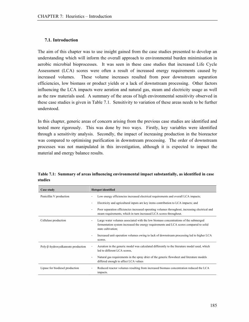
CHAPTER 7: Heuristics – Introduction
185
7.1. Introduction The aim of this chapter was to use insight gained from the case studies presented to develop an understanding which will inform the overall approach to environmental burden minimisation in aerobic microbial bioprocesses. It was seen in these case studies that increased Life Cycle Assessment (LCA) scores were often a result of increased energy requirements caused by increased volumes. These volume increases resulted from poor downstream separation efficiencies, low biomass or product yields or a lack of downstream processing. Other factors influencing the LCA impacts were aeration and natural gas, steam and electricity usage as well as the raw materials used. A summary of the areas of high environmental sensitivity observed in these case studies is given in Table 7.1. Sensitivity to variation of these areas needs to be further understood. In this chapter, generic areas of concern arising from the previous case studies are identified and tested more rigorously. This was done by two ways. Firstly, key variables were identified through a sensitivity analysis. Secondly, the impact of increasing production in the bioreactor was compared to optimising purification in downstream processing. The order of downstream processes was not manipulated in this investigation, although it is expected to impact the material and energy balance results.
Table 7.1: Summary of areas influencing environmental impact substantially, as identified in case studies
Case study Hotspot identified
Penicillin V production - Low energy efficiencies increased electrical requirements and overall LCA impacts;
- Electricity and agricultural inputs are key items contribution to LCA impacts; and
- Poor separation efficiencies increased operating volumes throughout, increasing electrical and steam requirements, which in turn increased LCA scores throughout.
Cellulase production - Large water volumes associated with the low biomass concentrations of the submerged fermentation system increased the energy requirements and LCA scores compared to solid
state cultivation;
- Increased unit operation volumes owing to lack of downstream processing led to higher LCA scores.
Poly--hydroxyalkanoate production - Aeration in the generic model was calculated differently to the literature model used, which led to different LCA scores,
- Natural gas requirements in the spray drier of the generic flowsheet and literature models differed enough to affect LCA values
Lipase for biodiesel production - Reduced reactor volumes resulting from increased biomass concentration reduced the LCA impacts.

CHAPTER 7: Heuristics – Identifying key variables
186
7.2. Identifying key variables
7.2.1. Sensitivity analysis In order to analyse the areas to which environmental burden is most sensitive, the effect of variation of each variable in the flowsheet needed to be quantified independently and systematically. From the material and energy balances obtained, LCA impacts could then be calculated and overall environmental effects determined. The changes to variables in this section have been considered theoretically one at a time. It is recognised that in practice it may not be possible to modify one variable without modifying several others. Further, these changes may not be physically possible for the microorganism used, but will still give an indication of the possible outcomes should different organisms be used (or products formed) in similar scenarios.
7.2.2. LCA single score When there are multiple processes to compare, a single score LCA result is useful as it will give a single definitive value over several categories. In this study, the EPS 2000 v2.02 single score method (Steen 1999a and 1999b) as presented in the SimaPro v7.1® software package (PRé Consultants B.V. 2008) was used. While the limitations of the single score method are well documented (ISO 14040: 2006, ISO14044: 2006), it provided a useful comparison for a large number of LCAs. An explanation of the single score method is described in Appendix A.
7.2.3. Summary of sensitivity results The Penicillin V model validation provided data showing the greatest consistency with literature and was used as a representative case to study sensitivity to input variables. Using Scenario 1 of the generic model and dataset developed in Chapter 3, each input was varied by 10 and 25 % above and below the setpoint as a screening assessment in order to determine which variables should be investigated further. The resultant material and energy balance outputs, and the LCA results ensuing from these, were used to assess sensitivities (Appendix H). The sensitivity is defined in Equation 7.1:
V
L S
Equation 7.1
Where: S = Sensitivity L = Percentage change in LCA single score [OR (Lo – Lm)/Lo) x 100] V = Percentage change in input variable [OR (Vo – Vm)/Vo) x 100]
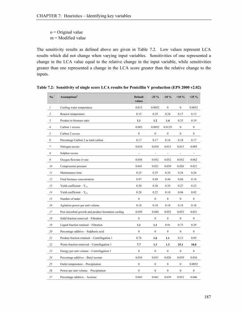
CHAPTER 7: Heuristics – Identifying key variables
187
o = Original value m = Modified value The sensitivity results as defined above are given in Table 7.2. Low values represent LCA results which did not change when varying input variables. Sensitivities of one represented a change in the LCA value equal to the relative change in the input variable, while sensitivities greater than one represented a change in the LCA score greater than the relative change to the inputs.
Table 7.2: Sensitivity of single score LCA results for Penicillin V production (EPS 2000 v2.02)
No.^ Assumptions# Default values
-25 % -10 % +10 % +25 %
1 Cooling water temperature 0.013 0.0052 0 0 0.0052
2 Reactor temperature 0.15 0.35 0.24 0.17 0.13
3 Product to biomass ratio 1.1 1.2 1.4 0.35 0.19
4 Carbon 1 excess 0.003 0.0052 0.0129 0 0
5 Carbon 2 excess 0 0 0 0 0
6 Percentage Carbon 2 as total carbon 0.17 0.17 0.14 0.18 0.17
7 Nitrogen excess 0.010 0.010 0.013 0.013 0.005
8 Sulphur excess - - - - -
9 Oxygen flowrate (vvm) 0.058 0.052 0.052 0.052 0.062
10 Compression pressure 0.041 0.021 0.039 0.026 0.021
11 Maintenance time 0.25 0.25 0.24 0.24 0.26
12 Final biomass concentration 0.97 0.49 0.44 0.04 0.18
13 Yield coefficient – Yx/s 0.29 0.38 0.35 0.27 0.23
14 Yield coefficient – Yp/s 0.28 0.22 0.18 0.04 0.02
15 Number of tanks 0 0 0 0 0
16 Agitation power per unit volume 0.18 0.18 0.18 0.18 0.18
17 Post microbial growth and product formation cooling 0.050 0.046 0.052 0.052 0.031
18 Solid fraction removed – Filtration 0 0 0 0 0
19 Liquid fraction retained – Filtration 1.1 1.1 0.91 0.73 0.29
20 Percentage additive – Sulphuric acid 0 0 0 0 0
21 Product fraction retained – Centrifugation 1 0.76 1.6 1.1 0.13 0.05
22 Waste fraction removed – Centrifugation 1 7.7 1.3 1.3 25.1 10.0
23 Energy per unit volume – Centrifugation 1 0 0 0 0 0
24 Percentage additive – Butyl acetate 0.034 0.031 0.026 0.039 0.036
25 Outlet temperature – Precipitation 0 0 0 0 0.0052
26 Power per unit volume – Precipitation 0 0 0 0 0
27 Percentage additive – Acetone 0.043 0.041 0.039 0.052 0.046

CHAPTER 7: Heuristics – Identifying key variables
188
No.^ Assumptions# Default values
-25 % -10 % +10 % +25 %
28 Percentage additive – Sodium acetate 0.089 1.1 0.68 0.10 0.08
29 Conversion of limiting reagent 1.2 1.4 1.1 0.27 0.11
30 Solid fraction removed – Centrifugation 2 1.5 1.36 1.12 0.064 0.026
31 Liquid fraction removed – Centrifugation 2 0.19 0.21 0.18 0.026 0.010
32 Product fraction retained – Fluid bed drying - 1.36 1.12 0.064 0.026
33 Liquid fraction removed – Fluid bed drying 0.026 0.031 0.026 0.026 0.010
34 Electricity required – Fluid bed drying 0 0 0 0 0
35 Percentage additive – Sodium hydroxide 0.007 0.010 0.013 0.013 0.005
^ Reference number for the variable changed # Values in bold indicate percentage changes in LCA values than the percentage changes to the variable modified
From the single score results, four areas were identified where controlled variation of the variables gave larger variations in the original LCA single scores (i.e. sensitivities greater than one). These included:
- Product to biomass ratio, - Product fraction retained in downstream processing, - Waste fraction removed in downstream processing, and - Penicillin V formation: (a) Percentage additive (Sodium acetate), and (b) Percentage
limiting reactant converted. In the following sections, these areas were analysed further by extending the range through which the variables may change to determine trends in reactor volumes, electrical requirements, purities and LCA single scores. For completeness, final biomass concentration, oxygen flowrate (vvm), compression pressure and yield coefficients (Yx/s and Yp/s) were also analysed as these were targeted from case studies (Table 7.1).
7.2.4. Product to biomass ratio and final biomass concentration
7.2.4.1. Product to biomass ratio
The product to biomass ratio describes the mass ratio between biomass growth and product formed. Lower ratios of product to biomass require more raw materials for biomass growth, increasing volumes and loads throughout the system, since biomass is a by-product of the product formed in the penicillin case. The product to biomass ratio was increased incrementally from zero, representing no product formation, to a minimal biomass formation representing biomass as a retained catalyst. Resultant reactor volumes, electrical requirements, recoveries, purities and single score LCA values for the production of the sodium salt of Penicillin V are shown in Table 7.3 and Figure 7.1.
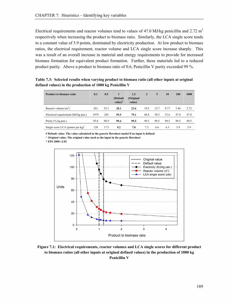
CHAPTER 7: Heuristics – Identifying key variables
189
Electrical requirements and reactor volumes tend to values of 47.0 MJ/kg penicillin and 2.72 m3 respectively when increasing the product to biomass ratio. Similarly, the LCA single score tends to a constant value of 5.9 points, dominated by electricity production. At low product to biomass ratios, the electrical requirement, reactor volume and LCA single score increase sharply. This was a result of an overall increase in material and energy requirements to provide for increased biomass formation for equivalent product formation. Further, these materials led to a reduced product purity. Above a product to biomass ratio of 0.6, Penicillin V purity exceeded 99 %.
Table 7.3: Selected results when varying product to biomass ratio (all other inputs at original defined values) in the production of 1000 kg Penicillin V
Product to biomass ratio 0.1 0.5 1
(Default value)#
1.2
(Original value)^
2 5 10 100 1000
Reactor volume (m3) 261 55.1 28.1 23.6 19.2 12.7 8.77 3.46 2.72
Electrical requirement (MJ/kg pen.) 1979 203 95.5 79.1 68.8 58.5 53.6 47.8 47.0
Purity (% kg pen.) 95.0 98.9 99.4 99.5 99.5 99.5 99.5 99.5 99.5
Single score LCA (points per kg)* 120 17.5 9.2 7.8 7.3 6.6 6.3 5.9 5.9
# Default value: The value calculated in the generic flowsheet model if no input is defined ^ Original value: The original value used as the input in the generic flowsheet * EPS 2000 v2.02
Figure 7.1: Electrical requirements, reactor volumes and LCA single scores for different product to biomass ratios (all other inputs at original defined values) in the production of 1000 kg
Penicillin V

CHAPTER 7: Heuristics – Identifying key variables
190
The original and default values for product to biomass ratios give LCA single scores within 16 % of each other. Over estimation of the original value showed less impact than underestimation. Doubling of the default value gives an LCA score 20 % lower, while halving it gives an LCA score 90 % higher. While increasing the product to biomass ratio benefits the process, values higher than 5 lead to diminishing returns, suggesting targeting of a product to biomass ratio of between 2 and 5 in this setup.
7.2.4.2. Final biomass concentration
Reducing the final biomass concentration in the range 5 to 45 g/l, with concomitant decrease in the product concentration owing to a constant ratio of product to biomass, sharply increased the reactor volume, electrical requirements and LCA single scores (Table 7.4). The increased volumes resulted in increased downstream processing inputs, which also resulted in increases in outputs. Unexpectedly, for Penicillin V production a biomass concentrations of 47 g/l represented a turning point for the electrical requirement and LCA single score with requirements increasing with increasing biomass concentration above 47 g/l as shown in Figure 7.2. At biomass concentrations higher than 10 g/l, the product purity was greater than 98 %. At biomass concentration lower than 10 g/l, the purity decreased sharply.
Table 7.4: Selected results when varying final biomass concentration (all other inputs at original defined values) in the production of 1000 kg Penicillin V
Final biomass concentration (g/l) 5 10 16.7 (Default value)#
25 45 (Original value)^
65 75
Reactor volume (m3) 178 92.2 56.9 39.2 23.3 21.0 20.3
Electrical requirement (MJ/kg pen.) 377 213 144.6 110 79.1 82.2 84.5
Purity (% kg pen.) 96.4 98.1 98.9 99.2 99.5 99.6 99.6
Single score LCA (points per kg)* 29.5 17.5 12.5 10.0 7.8 8.5 8.9
# Default value: The value calculated in the generic flowsheet model if no input is defined ^ Original value: The original value used as the input in the generic flowsheet * EPS 2000 v2.02
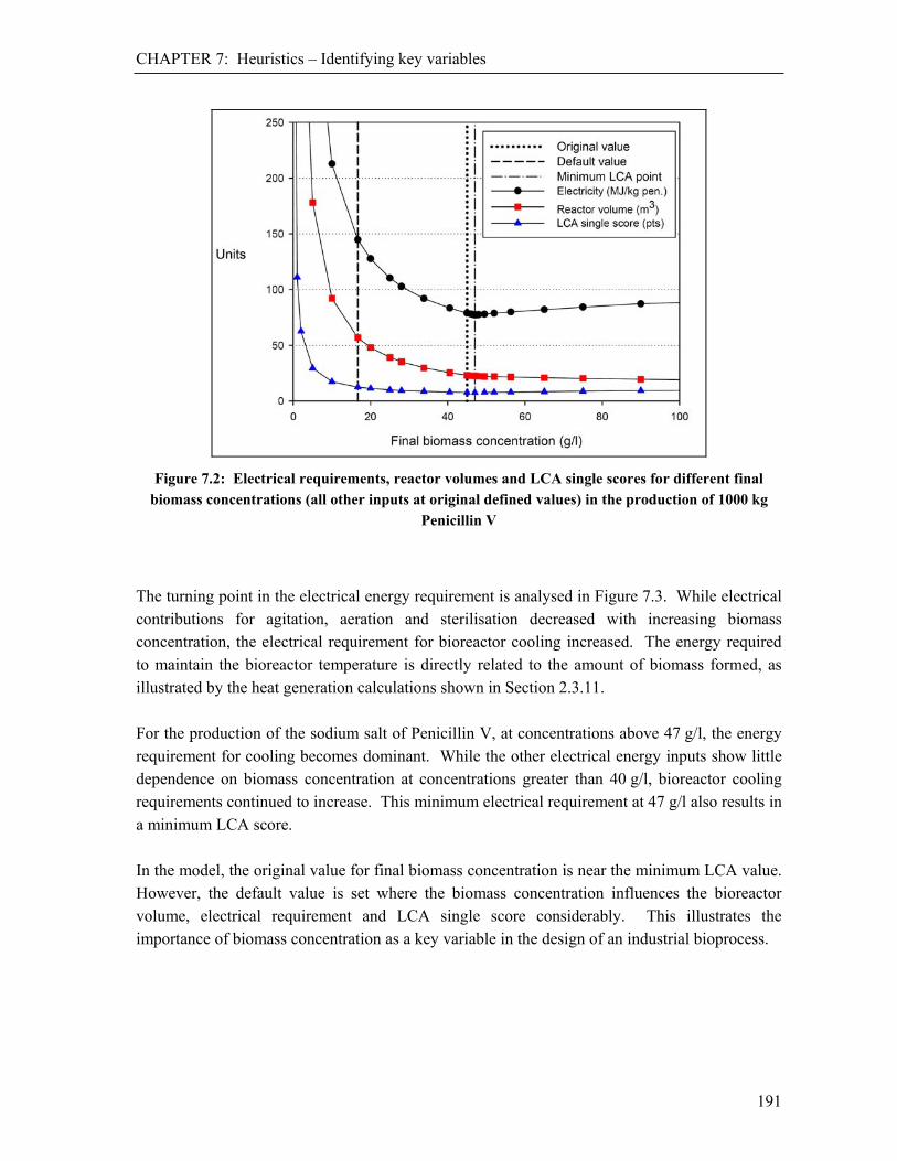
CHAPTER 7: Heuristics – Identifying key variables
191
Figure 7.2: Electrical requirements, reactor volumes and LCA single scores for different final biomass concentrations (all other inputs at original defined values) in the production of 1000 kg
Penicillin V
The turning point in the electrical energy requirement is analysed in Figure 7.3. While electrical contributions for agitation, aeration and sterilisation decreased with increasing biomass concentration, the electrical requirement for bioreactor cooling increased. The energy required to maintain the bioreactor temperature is directly related to the amount of biomass formed, as illustrated by the heat generation calculations shown in Section 2.3.11. For the production of the sodium salt of Penicillin V, at concentrations above 47 g/l, the energy requirement for cooling becomes dominant. While the other electrical energy inputs show little dependence on biomass concentration at concentrations greater than 40 g/l, bioreactor cooling requirements continued to increase. This minimum electrical requirement at 47 g/l also results in a minimum LCA score. In the model, the original value for final biomass concentration is near the minimum LCA value. However, the default value is set where the biomass concentration influences the bioreactor volume, electrical requirement and LCA single score considerably. This illustrates the importance of biomass concentration as a key variable in the design of an industrial bioprocess.

CHAPTER 7: Heuristics – Identifying key variables
192
Figure 7.3: Electricity breakdown for different final biomass concentrations (all other inputs at original defined values) in the production of 1000 kg Penicillin V
The decrease in electricity, reactor volume and LCA values from a high initial value with increasing biomass concentration appeared to follow a similar trend to that with increased product to biomass ratios as shown before. However, the optimal biomass concentration was indicated by a minimum point whereas the optimum product to biomass ratio was as high as physically possible. This trend resulted from an indirect relationship between the product to biomass ratios and biomass concentrations. Increasing the product to biomass ratio directly increased the product formed, but not the biomass concentration. Increases to the biomass concentration increased the biomass and, since the product to biomass ratio was constant, the product formed as well.
7.2.5. Oxygen flowrate (vvm) and compression pressure
7.2.5.1. Oxygen flowrate
In aerobic processes, the aeration rate is typically much higher than the stoichiometric requirement to overcome mass transfer limitations, ensure adequate oxygen provision to the micro-organisms and assist mixing. Typically air is supplied at a rate of 0.6 vvm, equating to approximately 0.12 vvm of pure oxygen. The original aeration rate of 0.021 vvm was defined for the stoichiometric oxygen requirement only for comparison to the original Biwer et al. (2005) and Heinzle et al. (2006) model.

CHAPTER 7: Heuristics – Identifying key variables
193
Air itself has little impact in a Life Cycle Assessment study, but the electricity required for its compression accounts for some 10 to 15 % of the overall electricity requirements estimated, thereby contributing significantly to the LCA impacts. Selected results for varying the flowrate of oxygen (Variable 9) in the production of the sodium salt of Penicillin V are presented in Table 7.5 and discussed below.
Table 7.5: Selected results when varying oxygen flowrate (all other inputs at original defined values; compression pressure of 600 kPa) in the production of 1000 kg Penicillin V
Oxygen flowrate (vvm) 0.021 (Original
value)^
0.05 0.1 0.2 0.4 0.6 0.7 0.8
Air equivalent 0.1 0.25 0.5 1 2 3 3.5 4
Reactor volume (m3) 23.3 23.3 23.3 23.3 23.3 23.3 23.3 23.3
Electrical requirement (MJ/kg pen.) 79.1 92.7 117 164 259 355 402 450
Purity (% kg pen.) 99.5 99.5 99.5 99.5 99.5 99.5 99.5 99.5
Single score LCA (points per kg)* 7.8 8.3 9.3 11.3 15.3 19.2 21.2 23.3
^ Original value: The original value used as the input in the generic flowsheet * EPS 2000 v2.02
Where the oxygen provision exceeds the stoichiometric limit, increasing the oxygen flowrate has no effect on the reactor liquid volume or product purity in the model developed. The modelling of gas holdup was not included in the model, but in reality this could play a part by increasing the volume of the reactor. Assuming a constant pressure differential on gas compression of 600 kPa, the electrical requirement was estimated to increase linearly with increasing oxygen flowrate as seen in Figure 7.4. This linear increase resulted in a linear increase in the LCA single score values.

CHAPTER 7: Heuristics – Identifying key variables
194
Figure 7.4: Electrical requirements, reactor volumes and LCA single scores for different oxygen flowrates (all other inputs at original defined values; compression pressure of 600 kPa) in the
production of 1000 kg Penicillin V
The breakdown of electrical requirements as a function of oxygen flowrate is given in Figure 7.5. At oxygen rates less than 0.06 vvm (equivalent air rate of 0.3 vvm), electricity requirements for agitation and bioreactor cooling dominate the overall electrical requirements. Above 0.06 vvm, electrical requirements for compression became the main requirement. Electrical requirements for sterilisation, post fermentation cooling and all downstream processing form less than 2 % of the total electrical requirements. At a typical aeration of 0.6 vvm using air (oxygen rate of 0.12 vvm), 45 % of the total electrical requirement is from compression for aeration, while at approximately 1.8 vvm using air (oxygen rate of 0.36 vvm), 72 % of the electrical energy is from compression.

CHAPTER 7: Heuristics – Identifying key variables
195
Figure 7.5: Breakdown of requirements for electricity for different oxygen flowrates (all other inputs at original defined values; compression pressure of 600 kPa) in the production of 1000 kg
Penicillin V
7.2.5.2. Compression pressure
Increased aeration rate affects the compression pressure. Changes in compression affect the electrical energy requirements and cooling water needed. Increases in electrical requirements are based on the number and type of compressors (centrifugal, axial or reciprocating compressor), inlet and outlet pressures and the efficiency of compression. While the changes in cooling water requirements do not affect the LCA scores (water usage does not impact LCA), the electrical requirements to chill the water add to the overall electrical energy changes. The compression pressure was varied from the minimum allowed pressure (atmospheric pressure) to 2000 kPa while keeping the original aeration rate of 0.021 vvm constant. Varying the compression pressure (Variable 10) does not affect reactor volume or purity obtained. Increases in the electrical requirements of compression and the Life Cycle Assessment scores with increasing compression pressure were shown in Table 7.6 and Figure 7.6. For reciprocating compressors used, the model uses three compression factors as described in Appendix B.4, depending on the compression pressure required. This led to the three distinct sections of the graph, separated by the inflection points.
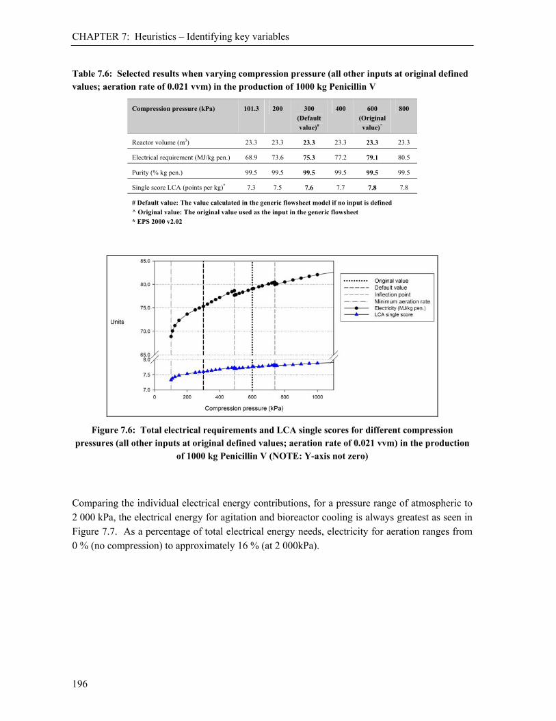
CHAPTER 7: Heuristics – Identifying key variables
196
Table 7.6: Selected results when varying compression pressure (all other inputs at original defined values; aeration rate of 0.021 vvm) in the production of 1000 kg Penicillin V
Compression pressure (kPa) 101.3 200 300 (Default value)#
400 600 (Original value)^
800
Reactor volume (m3) 23.3 23.3 23.3 23.3 23.3 23.3
Electrical requirement (MJ/kg pen.) 68.9 73.6 75.3 77.2 79.1 80.5
Purity (% kg pen.) 99.5 99.5 99.5 99.5 99.5 99.5
Single score LCA (points per kg)* 7.3 7.5 7.6 7.7 7.8 7.8
# Default value: The value calculated in the generic flowsheet model if no input is defined ^ Original value: The original value used as the input in the generic flowsheet * EPS 2000 v2.02
Figure 7.6: Total electrical requirements and LCA single scores for different compression pressures (all other inputs at original defined values; aeration rate of 0.021 vvm) in the production
of 1000 kg Penicillin V (NOTE: Y-axis not zero)
Comparing the individual electrical energy contributions, for a pressure range of atmospheric to 2 000 kPa, the electrical energy for agitation and bioreactor cooling is always greatest as seen in Figure 7.7. As a percentage of total electrical energy needs, electricity for aeration ranges from 0 % (no compression) to approximately 16 % (at 2 000kPa).

CHAPTER 7: Heuristics – Identifying key variables
197
Figure 7.7: Breakdown of requirements for electricity for different compression pressures (all
other inputs at original defined values; aeration rate of 0.021 vvm) in the production of Penicillin V
7.2.6. Yield coefficients
7.2.6.1. Biomass on substrate (Yx/s)
Increases in the yield of biomass on substrate (Yx/s), with a constant substrate feed, increased biomass production and, with a constant product to biomass ratio, resulted in more product formed. An increase in Yx/s, with constant biomass formation, results in decreased raw material requirements to obtain the same amount of product. This can lead to a greater product purity and make for easier downstream processing separation. It should be emphasised that changing single variables may only be possible mathematically, as a way to model the effects of theoretical scenarios, but may not be possible in physical systems. Decreasing the yield coefficient for biomass on substrate (Yx/s) (Variable 13) results in an increasing electrical requirement, reactor volume and LCA single score. At higher Yx/s values, variation is less pronounced and gave minimums at a maximum yield coefficient of 0.9 g/g as shown in Figure 7.8 and presented numerically in Table 7.7. This is a maximum yield coefficient allowed by the model for Penicillin V production. Yield coefficients below 0.05 g/g loose meaning as very little biomass would be formed and the process would no longer make physical or economic sense.

CHAPTER 7: Heuristics – Identifying key variables
198
Table 7.7: Selected results when varying the yield coefficient (Yx/s) (all other inputs at original defined values) in the production of 1000 kg Penicillin V
Yield coefficient – Yx/s (g/g) 0.1 0.2 0.3 0.43 (Default value)#
0.45 (Original value)^
0.6 0.7
Reactor volume (m3) 23.4 23.3 23.3 23.3 23.3 23.2 23.2
Electrical requirement (MJ/kg pen.) 163 109 91.0 80.2 79.1 73.2 70.7
Purity (% kg pen.) 99.5 99.5 99.5 99.5 99.5 99.5 99.5
Single score LCA (points per kg)* 15.8 10.6 8.9 7.9 7.8 7.2 7.0
# Default value: The value calculated in the generic flowsheet model if no input is defined ^ Original value: The original value used as the input in the generic flowsheet * EPS 2000 v2.02
Figure 7.8: Electrical requirements, reactor volumes and LCA single scores for different yield coefficients (Yx/s) (all other inputs at original defined values) in the production of 1000 kg
Penicillin V
7.2.6.2. Product on substrate (Yp/s)
Increases in the yield of product on substrate (Yp/s), with a constant substrate feed, increased the amount and concentration of product formed. An increase in Yp/s, with constant product formation, decreased raw material requirements per unit product. This led to an increased product concentration, easier downstream processing, requiring a smaller reactor volume and lower energy requirements per unit product.
CHAPTER 7: Heuristics – Identifying key variables
199
Selected results when varying the yield of product on substrate (Yp/s) (Variable 14) are presented in Table 7.8. At the highest allowed yield coefficient in the Penicillin V model (0.85 g/g), an electrical requirement, reactor volume and LCA single score of 78.9 MJ/kg, 23.2 m3 and 7.7 Pts (per kg) were recorded respectively. These results are shown graphically in Figure 7.9. Yield coefficients below 0.05 g/g loose meaning as very little biomass would be formed and the process would no longer make physical or economic sense.
Table 7.8: Selected results when varying the yield coefficient (Yp/s) (all other inputs at original defined values) in the production of 1000 kg Penicillin V
Yield coefficient – Yp/s (g/g) 0.1 0.2 0.3 0.4 0.49 (Default value)#
0.6 0.7 0.81 (Original value)^
Reactor volume (m3) 23.4 23.3 23.3 23.3 23.3 23.3 23.3 23.3
Electrical requirement (MJ/kg pen.) 172 117 99.4 90.6 85.9 82.4 80.4 79.2
Purity (% kg pen.) 99.5 99.5 99.5 99.5 99.5 99.5 99.5 99.5
Single score LCA (points per kg)* 17.6 11.8 9.5 9.1 8.6 8.2 8.0 7.8
# Default value: The value calculated in the generic flowsheet model if no input is defined ^ Original value: The original value used as the input in the generic flowsheet * EPS 2000 v2.02
Figure 7.9: Electrical requirements, reactor volumes and LCA single scores for different yield coefficients (Yp/s) (all other inputs at original defined values) in the production of 1000 kg
Penicillin V

CHAPTER 7: Heuristics – Identifying key variables
200
Over the range shown in Table 7.8, reactor volume was unchanged. The electrical requirements increased with a decreasing yield coefficient. This was a result of the stoichiometry of the calculations, predicting a greater amount of oxygen requirement, hence an increased aeration energy requirement and bioreactor cooling requirement. The trends in reactor volume, electricity use and LCA scores seen with increased product yield coefficients (Yp/s) were similar to those obtained for increased biomass yield coefficients (Yx/s). This resulted from the interconnected nature of the variables through defining a fixed biomass to product ratio. Thus changing either yield coefficient affected the product and biomass values similarly.
7.2.7. Product fraction retained in downstream processing In the downstream processing units (filtration, centrifugation and fluid bed drying), product may be lost in the waste streams. The model has been designed to give a fixed amount of final product. Losses in the downstream processing are compensated by increasing the amount of product formed through increasing biomass formation, raw material inputs, volume, electrical requirements and waste flows. For each downstream processing unit where product may be lost, the effect of varying the fraction of product retained on reactor volume, electrical requirement, purity and single score LCA value are shown in Figure 7.10. Increases in the product fractions retained for each of the filtration, centrifugation and fluid bed drying units, resulted in reduced reactor volume, decreased electricity and lower LCA scores.
CHAPTER 7: Heuristics – Identifying key variables
201
Figure 7.10: Electrical requirements, reactor volumes and LCA single scores for differing product retention in individual downstream process units (all other inputs at original defined values) in the
production of 1000 kg Penicillin V
Total energy required with changing product retention was correlated to reactor volume. A decrease in product retention increased electrical requirements owing to larger reactor volumes, increasing sterilisation, aeration, agitation heat and cooling energy requirements. A decrease in product fraction retained in any of the downstream processing units, resulted in higher LCA single score values as calculated using the EPS 2000 v2.02 method. The single score LCA values calculated from the material and energy balance data, were dominated by the patterns seen for reactor volume and electrical requirement in Figure 7.10.
7.2.8. Waste fraction removed in downstream processing
7.2.8.1. Effect of changing the waste fraction removed
Removing the waste from the product stream increases its purity and decreases the total volume entering the next downstream processing unit. This decrease in volume reduces downstream processing energy and chemical additions of subsequent operations. However, the model is designed to give a final mass of crude product (waste plus product). An increase in the purity, owing to increased waste removal, while keeping the total mass constant,
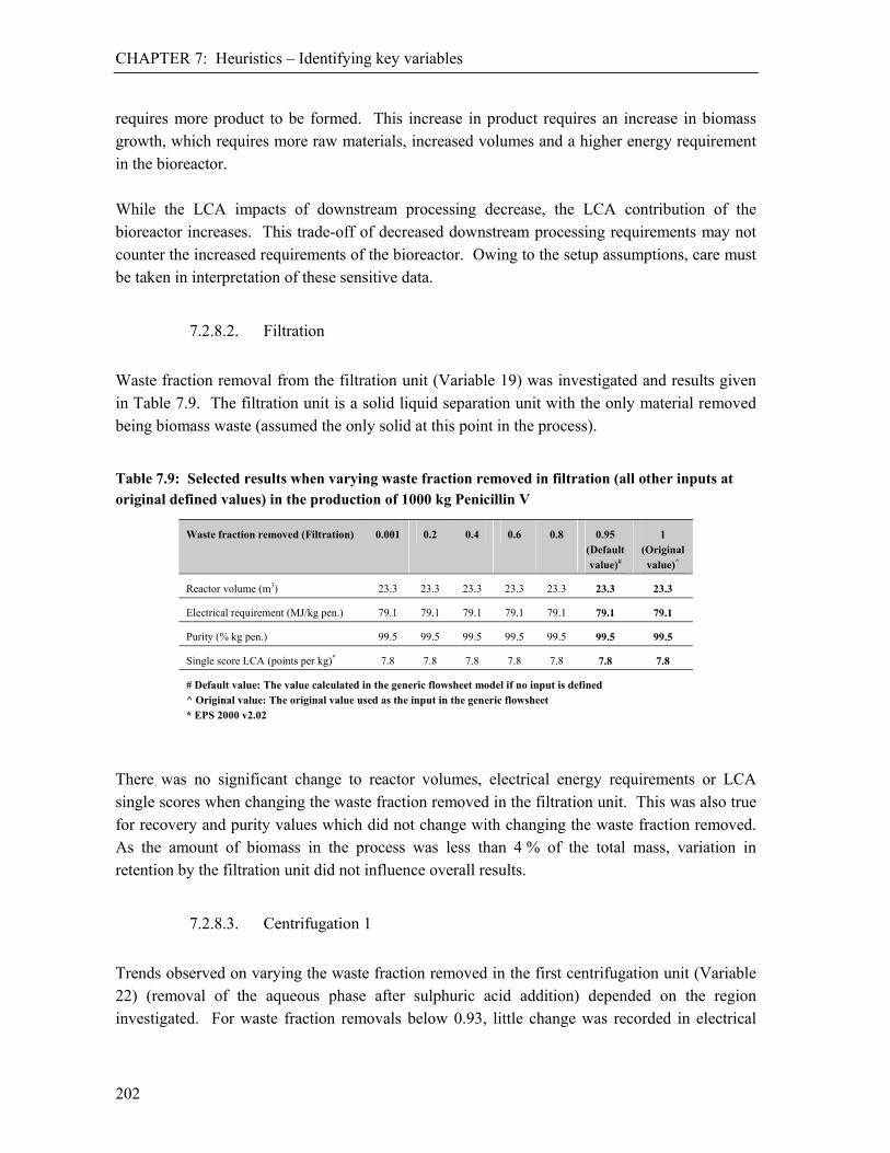
CHAPTER 7: Heuristics – Identifying key variables
202
requires more product to be formed. This increase in product requires an increase in biomass growth, which requires more raw materials, increased volumes and a higher energy requirement in the bioreactor. While the LCA impacts of downstream processing decrease, the LCA contribution of the bioreactor increases. This trade-off of decreased downstream processing requirements may not counter the increased requirements of the bioreactor. Owing to the setup assumptions, care must be taken in interpretation of these sensitive data.
7.2.8.2. Filtration
Waste fraction removal from the filtration unit (Variable 19) was investigated and results given in Table 7.9. The filtration unit is a solid liquid separation unit with the only material removed being biomass waste (assumed the only solid at this point in the process).
Table 7.9: Selected results when varying waste fraction removed in filtration (all other inputs at original defined values) in the production of 1000 kg Penicillin V
Waste fraction removed (Filtration) 0.001 0.2 0.4 0.6 0.8 0.95
(Default value)#
1
(Original value)^
Reactor volume (m3) 23.3 23.3 23.3 23.3 23.3 23.3 23.3
Electrical requirement (MJ/kg pen.) 79.1 79.1 79.1 79.1 79.1 79.1 79.1
Purity (% kg pen.) 99.5 99.5 99.5 99.5 99.5 99.5 99.5
Single score LCA (points per kg)* 7.8 7.8 7.8 7.8 7.8 7.8 7.8
# Default value: The value calculated in the generic flowsheet model if no input is defined ^ Original value: The original value used as the input in the generic flowsheet * EPS 2000 v2.02
There was no significant change to reactor volumes, electrical energy requirements or LCA single scores when changing the waste fraction removed in the filtration unit. This was also true for recovery and purity values which did not change with changing the waste fraction removed. As the amount of biomass in the process was less than 4 % of the total mass, variation in retention by the filtration unit did not influence overall results.
7.2.8.3. Centrifugation 1
Trends observed on varying the waste fraction removed in the first centrifugation unit (Variable 22) (removal of the aqueous phase after sulphuric acid addition) depended on the region investigated. For waste fraction removals below 0.93, little change was recorded in electrical

CHAPTER 7: Heuristics – Identifying key variables
203
and volume requirements. Purity increased from 95 % to 99.5 %. For waste fraction removals above 0.93, a pronounced change resulted in the values investigated as seen in Figure 7.11. Results for reactor volume, electrical requirements, purity and LCA single scores are given in Table 7.10.
Table 7.10: Selected results when varying waste fraction removed in centrifugation 1 (all other inputs at original defined values) in the production of 1000 kg Penicillin V
Waste fraction removed (Centrifugation 1) 0 0.2 0.4 0.6 0.8 0.918 (Original value)^
0.95 (Default value)#
1
Reactor volume (m3) 22.2 22.4 22.6 22.9 23.1 23.3 30.9 71.3
Electrical requirement (MJ/kg pen.) 77.8 78.0 78.3 78.6 78.9 79.1 104 241
Purity (% kg pen.) 95.0 95.9 96.9 97.9 98.9 99.5 99.5 99.4
Single score LCA (points per kg)* 17.5 15.4 13.3 11.2 9.0 7.8 9.8 27.2
# Default value: The value calculated in the generic flowsheet model if no input is defined
^ Original value: The original value used as the input in the generic flowsheet * EPS 2000 v2.02
For waste fraction removals below 0.93, in forming the sodium salt of Penicillin V, the limiting reagent is Penicillin V. On the improved waste removal with a fixed sodium acetate addition, sodium acetate becomes the limiting reagent. The unreacted Penicillin V in the system is not recovered. Should sodium acetate addition be increased proportionally with the change in waste fraction removal, such that Penicillin V remained the limiting reagent, trends would remain constant with those below 0.93. Hence the later are most relevant. The observation highlights the need to view each component of the sensitivity analysis holistically.

CHAPTER 7: Heuristics – Identifying key variables
204
Figure 7.11: Electrical requirements, reactor volumes and LCA single scores for different waste fractions removed (all other inputs at original defined values) in centrifugation 1 in the production
of 1000 kg Penicillin V
When changing the waste fraction removed in the first centrifuge, at fractions below 0.93, the reactor volume and electricity requirement decreased slightly with decreasing waste fractions removed. This was because the product purity decreased linearly and fewer raw materials were needed. However, the LCA single score increased (Figure 7.12) owing to greater downstream volumes with lower waste fraction removals. Hence, that more downstream additives were required. These additives, particularly acetone, sodium acetate and butyl acetate, influenced the total LCA score. Waste fraction values above 0.93 can be considered irrelevant since the likelihood of the process being run with sodium acetate as the limiting reactant are low.
CHAPTER 7: Heuristics – Identifying key variables
205
Figure 7.12: LCA single scores and purities for different waste fractions removed in centrifugation 1 (all other inputs at original defined values) in the production of 1000 kg
Penicillin V
7.2.8.4. Centrifugation 2
Waste fraction removal in the second centrifugation unit used to recover the crystalline product (Variable 31) is analysed in Table 7.11. Reactor volume, electrical requirement and LCA score varied between 19.1 to 23.4 m3, 64.9 and 79.5 MJ/kg penicillin product and 6.4 and 7.8 points respectively. The recovery remained constant at 98 % as product retained did not vary, while purity varied between 81.5 and 100 %.
Table 7.11: Selected results when varying waste fraction removed in centrifugation 2 (all other inputs at original defined values) in the production of 1000 kg Penicillin V
Waste fraction removed (Centrifugation 2) 0 0.2 0.4 0.6 0.8 (Default value)#
0.979 (Original value)^
1
Reactor volume (m3) 19.1 19.8 20.6 21.4 22.4 23.3 23.4
Electrical requirement (MJ/kg pen.) 64.9 67.4 70.0 73.0 76.1 79.1 79.5
Purity (% kg pen.) 81.5 84.7 88.0 91.7 95.7 99.5 100
Single score LCA (points per kg)* 6.4 6.6 6.9 7.2 7.5 7.8 7.8
# Default value: The value calculated in the generic flowsheet model if no input is defined
^ Original value: The original value used as the input in the generic flowsheet * EPS 2000 v2.02
CHAPTER 7: Heuristics – Identifying key variables
206
Increased waste fraction removal in centrifugation unit 2 increased electrical requirements, reactor volumes and single score LCA values as shown in Figure 7.13. While for centrifugation 1 removal of waste decreased volumes and consequently electrical requirements and LCA scores, increasing the waste fraction removal at a late stage in the downstream processing resulted in a greater increase in the product purity. In order to produce 1 000 kg of product at this increased purity, with all other variables held constant, more sodium salt of Penicillin V is required. This increased requirement for active product resulted in more raw materials required, a greater reactor volume and associated increases in energy considerations. The extra raw materials needed for this increased purity were greater than the reduction in volume achieved by a more efficient waste removal stage. Modifications to the model to give a fixed final mass of Penicillin V (i.e. a fixed mass of active product), show the same trends as described above.
Figure 7.13: Electrical requirements, reactor volumes and LCA single scores for different waste fractions removed in centrifugation 2 (all other inputs at original defined values) in the production
of 1000 kg Penicillin V
7.2.8.5. Fluid bed drying
Varying waste fraction removed from the fluid bed dryer (Variable 33) is analysed in Table 7.12. Limited impact was found. Reactor volume, electrical requirement, purity and LCA single score varied by 4.9, 4.7, 4.7 and 4% across the range of 0 to 1 respectively.
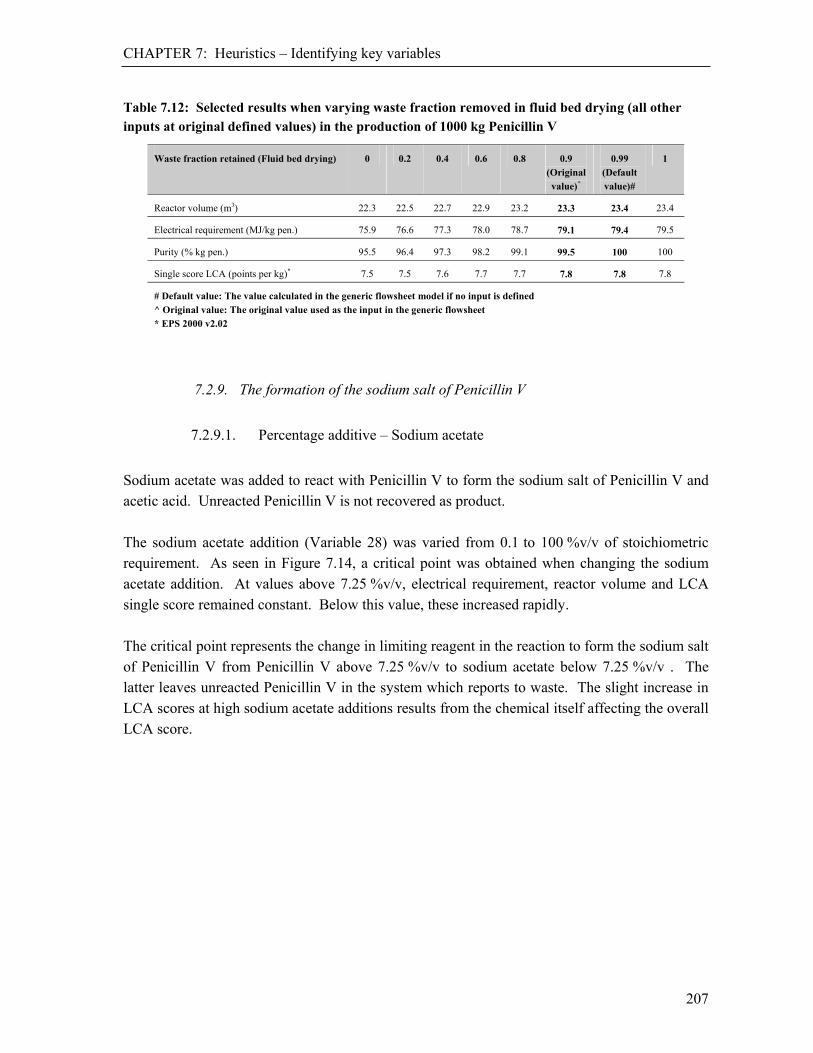
CHAPTER 7: Heuristics – Identifying key variables
207
Table 7.12: Selected results when varying waste fraction removed in fluid bed drying (all other inputs at original defined values) in the production of 1000 kg Penicillin V
Waste fraction retained (Fluid bed drying) 0 0.2 0.4 0.6 0.8 0.9 (Original value)^
0.99 (Default value)#
1
Reactor volume (m3) 22.3 22.5 22.7 22.9 23.2 23.3 23.4 23.4
Electrical requirement (MJ/kg pen.) 75.9 76.6 77.3 78.0 78.7 79.1 79.4 79.5
Purity (% kg pen.) 95.5 96.4 97.3 98.2 99.1 99.5 100 100
Single score LCA (points per kg)* 7.5 7.5 7.6 7.7 7.7 7.8 7.8 7.8
# Default value: The value calculated in the generic flowsheet model if no input is defined ^ Original value: The original value used as the input in the generic flowsheet * EPS 2000 v2.02
7.2.9. The formation of the sodium salt of Penicillin V
7.2.9.1. Percentage additive – Sodium acetate
Sodium acetate was added to react with Penicillin V to form the sodium salt of Penicillin V and acetic acid. Unreacted Penicillin V is not recovered as product. The sodium acetate addition (Variable 28) was varied from 0.1 to 100 %v/v of stoichiometric requirement. As seen in Figure 7.14, a critical point was obtained when changing the sodium acetate addition. At values above 7.25 %v/v, electrical requirement, reactor volume and LCA single score remained constant. Below this value, these increased rapidly. The critical point represents the change in limiting reagent in the reaction to form the sodium salt of Penicillin V from Penicillin V above 7.25 %v/v to sodium acetate below 7.25 %v/v . The latter leaves unreacted Penicillin V in the system which reports to waste. The slight increase in LCA scores at high sodium acetate additions results from the chemical itself affecting the overall LCA score.
CHAPTER 7: Heuristics – Identifying key variables
208
Figure 7.14: Electrical requirements, reactor volumes and LCA single scores for different percentages of sodium acetate added (all other inputs at original defined values) in the production
of 1000 kg Penicillin V
7.2.9.2. Percentage of limiting reactant converted
The amount of limiting reactant converted in the reaction of sodium acetate and Penicillin V to form the sodium salt of Penicillin V and acetic acid determines the recovery of penicillin to final product. A low conversion rate results in a low product purity and higher waste flows. In turn this results in higher bioreactor volumes and raw material requirements to meet the desired product mass. Selected results with varying the percentage limiting reactant converted are shown in Table 7.13. Halving the conversion rate resulted in a doubling of the reactor volume, electricity requirement and LCA single scores. At higher conversion rates (Figure 7.15), there are smaller changes in results, owing to smaller proportional changes.

CHAPTER 7: Heuristics – Identifying key variables
209
Table 7.13: Selected results when varying conversions rates of limiting reactants (all other inputs at original defined values) in the production of 1000 kg Penicillin V
Conversion rate (%) 10 25 40 60 80 (Default value)#
97 (Original value)^
100
Reactor volume (m3) 213 88.5 55.9 37.4 28.2 23.3 22.5
Electrical requirement (MJ/kg pen.) 725 301 190 127 95.8 79.1 76.8
Purity (% kg pen.) 94.0 97.6 98.6 99.1 99.4 99.5 99.6
Single score LCA (points per kg)* 71.3 29.6 18.7 12.5 9.4 7.8 7.6
# Default value: The value calculated in the generic flowsheet model if no input is defined ^ Original value: The original value used as the input in the generic flowsheet * EPS 2000 v2.02
Figure 7.15: Electrical requirements, reactor volumes and LCA single scores for different conversions rates of limiting reactants (all other inputs at original defined values) in the production
of 1000 kg Penicillin V
As with other scenarios where the electrical requirement, reactor volume and LCA single scores increase exponentially at lowered values, the purity also drops sharply when decreasing conversion rates. Below a conversion rate of 10 %, the purity falls below 95 % and LCA single score comparisons become less meaningful due to such large changes in concentration of Penicillin V.
CHAPTER 7: Heuristics – Increased production vs. optimised downstream processing
210
7.2.10. Summary Changing single variables in an industrial setup may have significant impacts on the performance of the process. In the example shown for the production of penicillin V, increases in the product to biomass ratio, yield coefficients, product fractions retained in downstream processing units and percentage limiting reagent converted resulted in decreasing electrical requirement, bioreactor volume and LCA single score. Increases in oxygen flowrate and compression pressure resulted in increasing electrical requirement, bioreactor volume and LCA single score values. Changes in the final biomass concentration, waste fraction removed in downstream processing units and percentage additive to a unit showed critical points for reasons such as a change in the limiting reactant. Variables showing critical points should be investigated more thoroughly to understand these critical points.
7.3. Increased production vs. optimised downstream processing
7.3.1. Introduction The effect of increasing production, by increasing the final biomass concentration, increasing the product to biomass ratio or increasing yield coefficients (Yp/s and Yx/s), resulted in a decreased single score LCA value. Similarly, a more effective product fraction recovery resulted in a decreased single score LCA value. To determine whether increasing the product production or optimising downstream processing has a greater effect on environmental burden, several
theoretical scenarios for each of Penicillin V, cellulase and poly--hydroxyalkanoate production
have been investigated. The reactor volume, electrical requirement, purity and single score LCA values are compared. Four scenarios were investigated for each product. The first represents the original design. In two scenarios production was increased while keeping downstream processing unchanged. The final scenario considered perfect product retention in downstream processing while keeping production unchanged.
7.3.2. Penicillin V
7.3.2.1. Process descriptions
In the production of Penicillin V, four downstream processing units were included: filtration, centrifugation 1, centrifugation 2 and fluid bed drying. These retain 100, 98, 99 and 99 % of the product respectively (Table 7.14). To compare the original setup (Scenario C) to that with

CHAPTER 7: Heuristics – Increased production vs. optimised downstream processing
211
optimised downstream processing (Scenario D), it was assumed that all units retained 100 % of the product. Two scenarios of increased production (Scenarios B and A) assumed a theoretical increase in product to biomass ratios of 2 and 5 respectively, as well as increases in the yield coefficients and final biomass concentrations. Scenario A further assumed that no excess raw materials were fed to the bioreactor. An increase in production increased product reporting to downstream processing. It was ensured that penicillin remained the limiting reagent in the reaction to form the sodium salt of Penicillin V.
Table 7.14: Modified input values for the production of Penicillin V used in determining the impacts of improved production vs. optimised downstream processing
Assumptions* Scenario A Scenario B Scenario C (Original scenario)
Scenario D Units
Microbial growth conditions
Product: Biomass ratio 5 2 1.2 1.2 -
Carbon 1 source (excess): Glucose 0 2 2 2 %
Carbon 2 source (excess): Phenoxyacetic acid 0 1.7 1.7 1.7 %
Nitrogen source (excess): Pharmamedia 0 15 15 15 %
Final biomass concentration 60 60 45 45 g/l
Yield coefficients: Yx/s 0.60 0.50 0.45 0.45 g/g
Yp/s 0.85# 0.85 0.81 0.81 g/g
Filtration
Solid fraction removed 100 100 100 100 %
Liquid (product) fraction retained 91 91 91 100 %
Centrifugation 1
Product fraction retained 98 98 98 100 %
Waste fraction removed 91.8 91.8 91.8 91.8 %
Centrifugation 2
Solid (product) fraction retained 99 99 99 100 %
Liquid fraction removed 97.9 97.9 97.9 97.9 %
Fluid bed drying
Product fraction retained 99 99 99 100 %
Liquid fraction removed 90 90 90 90 %
* For the full set of original inputs see Table 3.2. # Maximum allowed by the stoichiometry in the generic flowsheet model.

CHAPTER 7: Heuristics – Increased production vs. optimised downstream processing
212
7.3.2.2. Material and energy balance results
Both increasing production and optimising the downstream processing resulted in decreased reactor volume and electrical energy requirement values to produce 1 000 kg of the sodium salt of Penicillin V as seen in Table 7.15. Scenario A showed the greatest improvements in reactor volume and electrical requirements. The increase in separation efficiency (Scenario D) resulted in higher electrical energy requirements and a higher reactor volume than Scenario B. The scenarios developed indicate the benefit of optimising improvement on the production side over the downstream processing side.
Table 7.15: Selected results for the five scenarios comparing increased production vs. optimised downstream processing in the production of 1000 kg Penicillin V
Scenario A Scenario B Scenario C (Original scenario)
Scenario D Units
Reactor volume 5.0 11.5 23.3 20.5 m3
Electrical requirement 25.7 44.91 79.1 69.9 MJ/kg pen.
Purity 99.8 99.7 99.5 99.5 % kg pen.
The effect on energy when increasing production or optimising downstream processing is shown in Table 7.16. Scenario A and B resulted in decrease in both production and downstream processing energy to less than 35 % and 56 % respectively of that required in Scenario C. Improving the downstream processing efficiency (Scenario D) resulted in a 10 % decrease in production and downstream processing energy.
Table 7.16: Energy and glucose balances for the production and downstream processing of 1000 kg Penicillin V
Scenario A Scenario B Scenario C (Original scenario)
Scenario D Units
Energy
Production 27.5 48.7 86.5 76.4 GJ
Downstream processing 0.5 0.8 1.4 1.3 GJ
Total 28.0 49.5 87.9 77.7 GJ
Glucose
Into bioreactor 2.0 3.5 5.2 4.5 t
Out of bioreactor 0 0.04 0.06 0.05 t
Lost in wastewater 0 0.04 0.06 0.05 t
As impurities in product 0 0 0 0 t

CHAPTER 7: Heuristics – Increased production vs. optimised downstream processing
213
In Table 7.16 the amount of glucose added into the bioreactor, unreacted glucose leaving the bioreactor, as well as the glucose lost in wastewater and carried through as impurities in the product is shown. This represented the raw material flow through the system and showed the relationship of unreacted raw materials in the system versus inputs. None of the scenarios have a significant amount of glucose in the product stream with all unreacted material leaving in the wastewater streams of the various purification stages of the Penicillin V production process. For Scenario A, no excess for glucose, phenoxyacetic acid and Pharmamedia were assumed; hence no raw materials proceeded to downstream processing. In Scenario B, excess raw resulted in waste materials. This excess, and a lower yield coefficient (Yx/s), increased raw materials required for the process. The amount of glucose required increased from 2.0 t to 3.5 t, while the amount of Pharmamedia increased from 0.6 t to 1.0 t for the production of 1 000 kg of Penicillin V. The raw materials leaving the bioreactor reported dominantly into the waste streams with less than 0.02 % of each of glucose, phenoxyacetic acid and Pharmamedia remaining in the product after formulation. The original setup of Scenario C had the largest raw material requirements. There was a large increase in the phenoxyacetic acid required, from 0.2 t in Scenario B to 0.4 t in Scenario C. Glucose and Pharmamedia increased to 5.2 and 1.3 t respectively. Increased unreacted raw materials produced through the downstream units increased the energy requirements from 0.8 to 1.4 GJ. The energy required for the production also increased, from 48.7 to 86.5 GJ, owing to the larger volumes resulting from the greater raw material requirements. Improved recovery in Scenario D decreased glucose, phenoxyacetic acid and Pharmamedia required compared with Scenario C. This remained more than both of Scenarios A and B which had increased production. Even with optimised downstream processing, the energy needed for product purification was higher than for Scenarios A and B. The smaller volumes that resulted from these increased production scenarios resulted in greater energy savings than the optimised downstream processing of Scenario D. Improved product retention in downstream processing saves energy in the bioreactor since a smaller mass of raw materials was needed. This energy saving was not as large as the energy savings from the increased production scenarios.
7.3.2.3. Life Cycle Assessment (LCA) Results
The LCA results using the CML Baseline 2000 V2.03 method of assessment showed that, while similar, not all impact categories were reduced equally when improving production as seen in Figure 7.16. Scenario B impacts were approximately 40 % lower throughout, while Scenario A impacts were reduced by approximately 60 %.
CHAPTER 7: Heuristics – Increased production vs. optimised downstream processing
214
When improving the downstream processing of penicillin production, all categories were reduced equally. However, these decreases of some 10 % in LCA scores were lower than the production scenarios (Table 7.17).
Table 7.17: LCIA of Penicillin V per kilogram of product for Scenarios A – D (CML Baseline 2000 V2.03)
Impact Category Unit Scenario A Scenario B Scenario C (Original scenario)
Scenario D
Abiotic Depletion kg Sbeq. 0.0837 0.138 0.227 0.203
Global Warming (GWP100) kg CO2 eq. 8.76 15.4 25.5 22.7
Ozone Layer Depletion (ODP) mg CFC-11eq. 0.645 1.06 1.62 1.44
Human Toxicity kg 1,4-DBeq. 4.33 6.91 10.9 9.78
Fresh Water Aquatic Ecotoxicity kg 1,4-DBeq. 0.928 1.55 2.56 2.29
Marine Aquatic Ecotoxicity kg 1,4-DBeq. 5490 9450 16000 14300
Terrestrial Ecotoxicity kg 1,4-DBeq. 0.0228 0.0354 0.0533 0.0477
Photochemical Oxidation kg C2H4 0.00328 0.00545 0.00891 0.00799
Acidification kg SO2 eq. 0.0902 0.154 0.254 0.227
Eutrophication kg PO43-
eq. 0.00997 0.0162 0.0243 0.0217
Figure 7.16: Comparison of LCA results for Penicillin V sodium salt production for Scenarios A, B and D relative to Scenario C
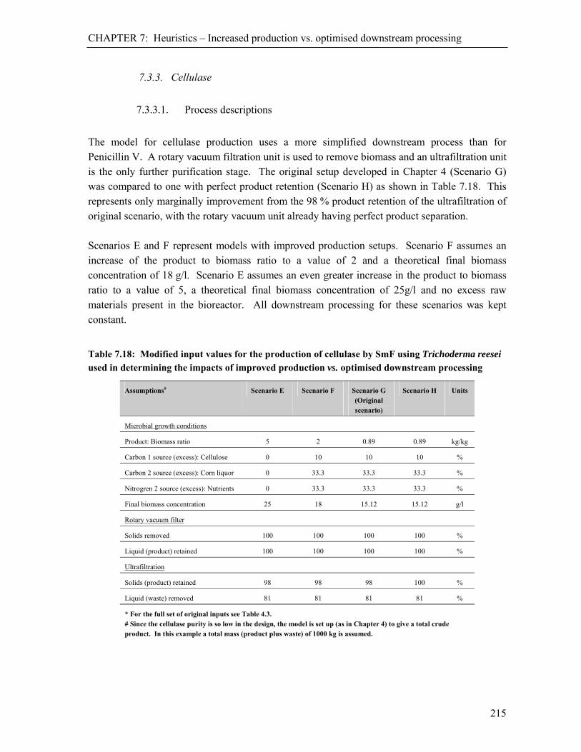
CHAPTER 7: Heuristics – Increased production vs. optimised downstream processing
215
7.3.3. Cellulase
7.3.3.1. Process descriptions
The model for cellulase production uses a more simplified downstream process than for Penicillin V. A rotary vacuum filtration unit is used to remove biomass and an ultrafiltration unit is the only further purification stage. The original setup developed in Chapter 4 (Scenario G) was compared to one with perfect product retention (Scenario H) as shown in Table 7.18. This represents only marginally improvement from the 98 % product retention of the ultrafiltration of original scenario, with the rotary vacuum unit already having perfect product separation. Scenarios E and F represent models with improved production setups. Scenario F assumes an increase of the product to biomass ratio to a value of 2 and a theoretical final biomass concentration of 18 g/l. Scenario E assumes an even greater increase in the product to biomass ratio to a value of 5, a theoretical final biomass concentration of 25g/l and no excess raw materials present in the bioreactor. All downstream processing for these scenarios was kept constant.
Table 7.18: Modified input values for the production of cellulase by SmF using Trichoderma reesei used in determining the impacts of improved production vs. optimised downstream processing
Assumptions# Scenario E Scenario F Scenario G (Original scenario)
Scenario H Units
Microbial growth conditions
Product: Biomass ratio 5 2 0.89 0.89 kg/kg
Carbon 1 source (excess): Cellulose 0 10 10 10 %
Carbon 2 source (excess): Corn liquor 0 33.3 33.3 33.3 %
Nitrogren 2 source (excess): Nutrients 0 33.3 33.3 33.3 %
Final biomass concentration 25 18 15.12 15.12 g/l
Rotary vacuum filter
Solids removed 100 100 100 100 %
Liquid (product) retained 100 100 100 100 %
Ultrafiltration
Solids (product) retained 98 98 98 100 %
Liquid (waste) removed 81 81 81 81 %
* For the full set of original inputs see Table 4.3. # Since the cellulase purity is so low in the design, the model is set up (as in Chapter 4) to give a total crude product. In this example a total mass (product plus waste) of 1000 kg is assumed.

CHAPTER 7: Heuristics – Increased production vs. optimised downstream processing
216
7.3.3.2. Material and energy balance results
The reactor volumes, electrical requirements and purities for the production of cellulase (Scenarios E to H), as calculated using the generic flowsheet, are shown in Table 7.19. For the production of 1000 kg cellulase (active ingredient), the optimisation of downstream processing lowered the reactor volume from 83.1 to 81.4 m3 and the electrical requirement from 183.1 to 179.4 MJ/kg cellulase, representing a 2 % decrease. Increasing the production of cellulase (Scenarios F and E) resulted in a much larger decrease in the reactor volume and electrical energy requirements. Improved product recovery in downstream processing presented little scope for improvement. The reactor volume and electrical requirement of Scenario E decreased to 11 % and 38 % of the original values respectively. Increasing the production also increased the purity of cellulase from 6.1 % to 38.3 %.
Table 7.19: Selected results for the five scenarios comparing increased production vs. optimised
downstream processing in the production of product containing 1000 kg cellulase by SmF using Trichoderma reesei
Scenario E Scenario F Scenario G (Original scenario)
Scenario H Units
Reactor volume 9.4 31.7 83.1 81.4 m3
Electrical requirement 33.8 74.6 183.1 179.4 MJ/kg cel.
Purity 38.34 14.75 6.09 6.21 % kg cel.
The main carbon entering the bioreactor for the production of cellulase was cellulose. Comparisons of cellulose required for each of Scenarios E – H is shown in Table 7.20. When no excess was added to the system and complete reaction occurred (Scenario E), no cellulose left the bioreactor. The addition of excess raw materials resulted in cellulose in the wastewater and as impurities in the product. Optimisation of the downstream processing, shown in Scenario H, resulted in the same amount of cellulose in the product as the original setup (Scenario G), but less cellulose in the wastewater stream. Although the same excess cellulose was added for Scenarios F, G and H, the improved production of Scenario F resulted in less cellulose in the product and wastewater streams. Since the downstream processing of cellulase required less than 3 % of the total energy requirements, improvements to the downstream processing did not result in a significant energy saving in either production or downstream processing energy. However, improving the

CHAPTER 7: Heuristics – Increased production vs. optimised downstream processing
217
production of cellulase reduced the volume of the bioreactor and the associated energy requirement with Scenarios F and G, showing a 60 and 80 % reduction in both the production and downstream processing energy.
Table 7.20: Energy and cellulose balances for the production and downstream processing of product containing 1000 kg cellulase by SmF using Trichoderma reesei
Scenario E Scenario F Scenario G (Original scenario)
Scenario H Units
Energy
Production 34.1 75.4 185.2 181.6 GJ
Downstream processing 0.6 1.8 4.9 4.8 GJ
Total 34.6 77.2 190.2 186.4 GJ
Cellulose
Into bioreactor 1.9 2.6 3.8 3.7 t
Out of bioreactor 0 0.24 0.34 0.33 t
Lost in wastewater 0 0.19 0.28 0.27 t
As impurities in product 0 0.05 0.06 0.06 t
Besides cellulose, corn steep liquor and ammonia were added to the bioreactor. Where no excess was added and complete reaction occurred (Scenario E), no unreacted raw materials left the bioreactor. Therefore no raw materials were present in the wastewater or as impurities in the product stream. In Scenario F, G and H, excess raw materials were added and unreacted raw materials were present in the downstream processing. Of the 0.24 t of cellulose entering the downstream process of Scenario F, 0.19 t (80 %) was removed in the wastewater stream and 0.05 t was left as impurities in the final product. Similarly, 0.11 of the 0.13 tonnes of corn steep liquor (80 %) and 0.002 of the 0.003 t of ammonia (80 %) entering downstream processing were removed in the waste stream. The original setup (Scenario G), assumed the same excess entered the bioreactor, but owing to lower production, more cellulose, corn steep liquor and ammonia were required. With more raw materials required, a greater mass of raw materials left the bioreactor. Masses of 0.34, 0.19 and 0.005 t of cellulose, corn steep liquor and ammonia respectively entered downstream processing. Scenario H, for optimised downstream processing, assumed a perfect product retention in the process. Since no product was lost, the mass of raw materials required was lower than in
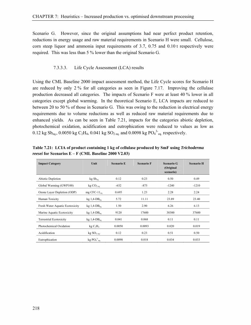
CHAPTER 7: Heuristics – Increased production vs. optimised downstream processing
218
Scenario G. However, since the original assumptions had near perfect product retention, reductions in energy usage and raw material requirements in Scenario H were small. Cellulose, corn steep liquor and ammonia input requirements of 3.7, 0.75 and 0.10 t respectively were required. This was less than 5 % lower than the original Scenario G.
7.3.3.3. Life Cycle Assessment (LCA) results
Using the CML Baseline 2000 impact assessment method, the Life Cycle scores for Scenario H are reduced by only 2 % for all categories as seen in Figure 7.17. Improving the cellulase production decreased all categories. The impacts of Scenario F were at least 40 % lower in all categories except global warming. In the theoretical Scenario E, LCA impacts are reduced to between 20 to 50 % of those in Scenario G. This was owing to the reduction in electrical energy requirements due to volume reductions as well as reduced raw material requirements due to enhanced yields. As can be seen in Table 7.21, impacts for the categories abiotic depletion, photochemical oxidation, acidification and eutrophication were reduced to values as low as 0.12 kg Sbeq., 0.0050 kg C2H4, 0.041 kg SO2 eq. and 0.0098 kg PO4
3-eq. respectively.
Table 7.21: LCIA of product containing 1 kg of cellulase produced by SmF using Trichoderma reesei for Scenarios E – F (CML Baseline 2000 V2.03)
Impact Category Unit Scenario E Scenario F Scenario G (Original scenario)
Scenario H
Abiotic Depletion kg Sbeq. 0.12 0.23 0.50 0.49
Global Warming (GWP100) kg CO2 eq. -632 -875 -1240 -1210
Ozone Layer Depletion (ODP) mg CFC-11eq. 0.695 1.23 2.28 2.24
Human Toxicity kg 1,4-DBeq. 5.72 11.11 23.89 23.40
Fresh Water Aquatic Ecotoxicity kg 1,4-DBeq. 1.50 2.90 6.26 6.13
Marine Aquatic Ecotoxicity kg 1,4-DBeq. 9120 17600 38300 37600
Terrestrial Ecotoxicity kg 1,4-DBeq. 0.041 0.068 0.11 0.11
Photochemical Oxidation kg C2H4 0.0050 0.0093 0.020 0.019
Acidification kg SO2 eq. 0.12 0.23 0.51 0.50
Eutrophication kg PO43-
eq. 0.0098 0.018 0.034 0.033

CHAPTER 7: Heuristics – Increased production vs. optimised downstream processing
219
Figure 7.17: Comparison of LCA results for cellulase production by SmF using Trichoderma reesei for Scenarios E, F and H relative to Scenario G
7.3.4. Poly--hydroxybutyric acid
7.3.4.1. Process descriptions
The production of the biopolymer, poly--hydroxybutyric acid (PHB) as modelled in Chapter 5,
assumed perfect product retention throughout. This meant that no improvement could be made to the setup. The original scenario (Scenario L) was modified to allow for product losses (Scenario K). It was assumed that only 95 % of the polymer product was retained at each downstream processing step as shown in Table 7.22. The two scenarios for improved production (Scenarios J and I) assumed a theoretical increase in the product to biomass ratio of 4 and 6 respectively. The final biomass concentration was assumed to increase to 50 and 60 g/l respectively, while the yield coefficient of product on substrate increased to 0.50 and 0.60 g/g respectively. These are optimistic assumptions and may only be attainable with different strains of microorganism.

CHAPTER 7: Heuristics – Increased production vs. optimised downstream processing
220
Table 7.22: Modified input values for the production of poly--hydroxybutyric acid used in
determining the impacts of improved production vs. optimised downstream processing
Assumptions Scenario I
Scenario J
Scenario K
Scenario L
(Original
scenario)
Units
Microbial growth conditions
Product: Biomass ratio 6 4 2.4 2.4 -
Final biomass concentration 60 50 44 44 g/l
Yield coefficients: Yp/s 0.60 0.50 0.44 0.44 g/g
Centrifugation
Solid fraction (product) retained 100 100 95 100 %
Centrifugation
Solid fraction (product) retained 100 100 95 100 %
Centrifugation
Solid fraction (product) retained 100 100 95 100 %
Spray drying
Solid fraction (product) retained 100 100 95 100 %
Liquid fraction removed 100 100 100 100 %
* For the full set of original inputs see Table 5.4
7.3.4.2. Material and energy balance results
As expected, an inferior downstream processing system resulted in an increase in reactor volume and electrical energy requirements as shown in Table 7.23. The loss of the product required a greater amount to be formed in the bioreactor to achieve the same mass of final polymer. The improvements of Scenario J reduced the reactor volume to 6.07 m3 for 1000 kg of product and reduced the associated electrical requirements to less than half.
Table 7.23: Selected results for the five scenarios comparing increased production vs. optimised
downstream processing in the production of 1000 kg poly--hydroxybutyric acid
Scenario I Scenario J Scenario K Scenario L (Original scenario)
Units
Reactor volume 3.77 6.07 13.12 10.69 m3
Electrical requirement 5.07 9.91 24.6 20.31 MJ/kg PHB
Purity 100 100 100 100 % kg PHB

CHAPTER 7: Heuristics – Increased production vs. optimised downstream processing
221
All four scenarios developed assumed that there was no excess glucose or ammonium sulphate entering the bioreactor according to the original model developed in Chapter 5. Hence, no glucose or ammonium sulphate entered downstream processing as shown in Table 7.24.
The energy required in downstream processing during production of poly--hydroxybutyric acid
was proportionally higher than for both Penicillin V and cellulase as a result of the homogenisation and centrifugation units. In Scenarios I, J, K and L, of the total energy, 28, 24, 19 and 19 % was required for downstream processing respectively. As with other examples, both increasing production and optimising downstream production led to a reduction in both production and downstream processing energy requirements.
Table 7.24: Energy and glucose balances for the production and downstream processing of 1000 kg
poly--hydroxybutyric acid
Scenario I Scenario J Scenario K Scenario L (Original
scenario)
Units
Energy
Production 15.1 20.4 36.2 31.6 GJ
Downstream processing 5.9 6.4 8.4 7.4 GJ
Total 21.0 26.8 44.6 39.1 GJ
Glucose
Into bioreactor 2.0 2.6 3.9 3.2 t
Out of bioreactor 0 0 0 0 t
Lost in wastewater 0 0 0 0 t
As impurities in product 0 0 0 0 t
Scenario I, where the greatest theoretical production was modelled, gave an energy requirement for production of 15.1 GJ per 1000 kg of polymer product, 48 % of the original Scenario L. This was the lowest of all four scenarios. A production slightly lower than Scenario I, as modelled in Scenario J, resulted in a higher glucose, but similar ammonium sulphate, requirement. The production and downstream processing energy increased to 20.4 and 6.4 GJ per 1000 kg of polymer respectively. This was a 35 and 8 % increase in production energy and downstream processing energy respectively compared to Scenario I. The original scenario (Scenario L) assumed perfect product retention. Scenario K was developed with a less than perfect efficiency but an identical production. This resulted in a material balance requiring more glucose and ammonium sulphate than any other scenario and an
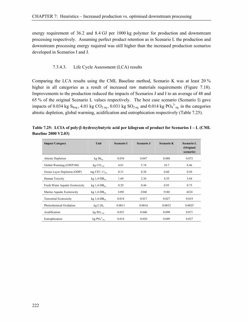
CHAPTER 7: Heuristics – Increased production vs. optimised downstream processing
222
energy requirement of 36.2 and 8.4 GJ per 1000 kg polymer for production and downstream processing respectively. Assuming perfect product retention as in Scenario L the production and downstream processing energy required was still higher than the increased production scenarios developed in Scenarios I and J.
7.3.4.3. Life Cycle Assessment (LCA) results
Comparing the LCA results using the CML Baseline method, Scenario K was at least 20 % higher in all categories as a result of increased raw materials requirements (Figure 7.18). Improvements to the production reduced the impacts of Scenarios J and I to an average of 48 and 65 % of the original Scenario L values respectively. The best case scenario (Scenario I) gave impacts of 0.034 kg Sbeq., 4.01 kg CO2 eq., 0.031 kg SO2 eq. and 0.014 kg PO4
3-eq. in the categories
abiotic depletion, global warming, acidification and eutrophication respectively (Table 7.25).
Table 7.25: LCIA of poly--hydroxybutyric acid per kilogram of product for Scenarios I – L (CML
Baseline 2000 V2.03)
Impact Category Unit Scenario I Scenario J Scenario K Scenario L (Original scenario)
Abiotic Depletion kg Sbeq. 0.034 0.047 0.088 0.072
Global Warming (GWP100) kg CO2 eq. 4.01 5.74 10.7 8.46
Ozone Layer Depletion (ODP) mg CFC-11eq. 0.31 0.38 0.60 0.50
Human Toxicity kg 1,4-DBeq. 1.69 2.36 4.55 3.64
Fresh Water Aquatic Ecotoxicity kg 1,4-DBeq. 0.29 0.44 0.93 0.75
Marine Aquatic Ecotoxicity kg 1,4-DBeq. 1450 2360 5180 4224
Terrestrial Ecotoxicity kg 1,4-DBeq. 0.014 0.017 0.027 0.019
Photochemical Oxidation kg C2H4 0.0011 0.0016 0.0032 0.0025
Acidification kg SO2 eq. 0.031 0.046 0.090 0.071
Eutrophication kg PO43-
eq. 0.014 0.020 0.049 0.027
CHAPTER 7: Heuristics – Conclusions
223
Figure 7.18: Comparison of LCA results for poly--hydroxybutyric acid production for Scenarios
I, J and K relative to Scenario L
7.3.5. Summary Improved production and downstream processing were analysed in the penicillin, cellulase and
poly--hydroxybutyrate models, to determine changes to energy and raw material requirements
and life cycle assessment scores. It was shown that improvements to either production or downstream processing decreased the LCA impacts, but that these were more pronounced for an improved production setup.
7.4. Conclusions Certain variables were identified as key variables in the generic flowsheet model developed on Chapter 2. These included the product to biomass ratio, final biomass concentration, oxygen flowrate and compression pressure, yield coefficients and downstream processing separation efficiencies. Small changes to these variables may escalate the material and energy requirements of the process. These escalations, particularly in energy requirements, ultimately affect the Life Cycle Assessment (LCA) scores for the production of the product. It was seen that some variables were interconnected to others such that changing either resulted in similar trends e.g.
CHAPTER 7: Heuristics – References
224
product to biomass ratio versus final biomass concentration and the yield coefficients for product on substrate and biomass on substrate. The smart breeding of strains or genetic modification may allow increased concentrations at higher yields, parallel to lower biomass production, which may result in more attractive processing conditions.. Default values in the generic flowsheet are chosen for specific reasons throughout e.g. literature values, common operating parameters etc. However, certain defaults, including product to biomass ratio and final biomass concentration, are defined in critical areas of influence. When using these defaults careful consideration needs to be taken as they are more sensitive than other defaults. Small changes near these default values influence all results including the material and energy balances as well as LCA scores. In all case studies analysed, the improvement of a process, by increasing production, gives more favourable results than optimising downstream processing. This may be a result of various factors. These include:-
- Most downstream processing units should already be optimised and have little scope for improvement;
- There may not be a large downstream processing (DSP) setup. Improvements to a single unit DSP system will not influence an entire process as much as multiple improvements over a more complex DSP setup;
- There may be a greater scope for improvement within the bioreactor (e.g. improving product to biomass ratio, yield coefficients, biomass concentrations, the amount of excess raw materials fed to a system etc.) versus improvements to product retention in a few units; and
- Improvements in production impacts the material and energy values of downstream processing.
However, there is a limit to the physical production increases that can be obtained using the microorganism of choice. While it is recommended to improve the production of product by modifying the bioreactor setup there will be a point where the increase in production no longer becomes physically or economically viable. At this point it would be more beneficial to optimise the downstream processing.
References Biwer, A., Griffith, S., Cooney, C., 2005. Uncertainty Analysis of Penicillin V Production Using Monte Carlo
Simulation, Biotechnol. Bioeng., 90(2), 167-179. Heinzle, E., Biwer, A., Cooney, C., 2006. Penicillin V, In: Development of Sustainable Bioprocesses: Modelling
and Assessment, John Wiley & Sons, p193-210.

CHAPTER 7: Heuristics – References
225
ISO 14040: 2006. Environmental management – Life cycle assessment – Principles and framework, International Organization for Standardization.
ISO 14044: 2006. Environmental management – Life cycle assessment – Requirements and guidelines, International Organization for Standardization.
PRé Consultants B.V., 2008. Plotterweg 12, 3821 BB Amersfoort, The Netherlands, http://www.pre.nl Steen, B., 1999a. A systematic approach to environmental strategies in product development (EPS). Version 2000
– General system characteristics, Centre for Environmental Assessment of Products and Material Systems, Chalmers University of Technology, Technical Environmental Planning, CPM report 1999:4.
Steen, B., 1999b. A systematic approach to environmental strategies in product development (EPS). Version 2000 – Models and data of the default methods, Centre for Environmental Assessment of Products and Material Systems, Chalmers University of Technology, Technical Environmental Planning, CPM report 1999:5.

226

227
CHAPTER 8: CONCLUSIONS

228
CHAPTER 8: Conclusions – Introduction
229
8.1 Introduction When comparing the environmental advantages of industrial scale chemical processes over biological processes, a full Life Cycle Assessment (LCA) analysis should be performed. Owing to the difficulty in obtaining the material and energy balance inventory required for an LCA analysis prior to completion of a full engineering design, a tool to obtain estimates of these was developed. Validation studies were then carried out to show the accuracy of the tool in obtaining the required material and energy values and also used compare literature and modelled LCA scores of each process. Using a combination of the modelling tool and literature values, four case studies were carried out to identify critical environmental burdens of commodity bioprocesses using LCA. The thesis also investigated the environmental advantages of industrial scale bioprocesses over chemical processes. The findings then guided a study to determine the areas of a bioprocess system which were most sensitive to change in individual input parameters. This showed which inputs resulted in high LCA scores were they not defined appropriately. The thesis addresses several main objectives: 1. To develop a generic flowsheet model to provide material and energy balance data for
industrial bioprocesses at an early stage in process development; 2. To validate the generic flowsheet model; 3. To use these data with Life Cycle Assessment (LCA) methodology as a means of assessing
and comparing industrial bioprocess systems; 4. To use Life Cycle Assessment (LCA) methodology to compare industrial biological
processes with chemical processes; 5. To obtain heuristics which guide the sustainability decisions of industrial bioprocess systems;
and 6. To investigate the environmental implications of bio-technology selection.
8.2 Model development, validation and Life Cycle Assessment (LCA) For many systems, including bioprocess systems, the desired material and energy balance input data are not available for Life Cycle Assessment (LCA) studies, especially at an early stage in technology selection and process design. A model was developed to provide these material and energy balance data for biological processes. The model allows for aerobic or anaerobic, intra- or extracellular biomass growth in a continuous or batch process. The model allows for various bioproducts produced from a selection of microorganisms using a range of raw materials. A database of yield coefficients, material properties and other constants required in the model,

CHAPTER 8: Conclusions – Findings from case studies
230
collected from literature sources, is included. These values can be modified to reflect more representative data during specific flowsheet development. The model, shown in an MS-Excel framework in the thesis, allows for sterilisation (steam or filtration) before the bioreactor and is followed by a downstream processing train as specified by the user. The bioreactor takes into account aeration, agitation, reactor cooling, biomass maintenance, yield coefficients, post microbial growth cooling and growth rate calculations. The downstream processing includes solid-liquid separation, cell disruption, concentration and formulation units as required. These downstream processing units include, amongst others, centrifugation, filtration, sedimentation, cavitation, milling, evaporation, precipitation, oven drying and freeze drying units as appropriate. At each downstream processing stage, non-reacting and reacting chemicals can be added. Waste water removed at each stage can also be modelled waste water treatment step. Several case studies were used to validate the generic flowsheet model developed in the thesis. For each validation study, three scenarios were presented. Each scenario assumed a smaller set of input data to represent the possibility of unavailable data and to determine the sensitivity of the model. Using the data from the generic flowsheets, the material and energy balance results obtained were compared to material and energy balance values of the equivalent process presented in literature. The case studies used for validation purposes included penicillin,
cellulase and poly--hydroxybutyrate production.
Using the maximum input data sets to inform the MS-Excel model, 50 % of the material and energy balance results were within 20 % and 12% of literature values for the penicillin and poly-
-hydroxybutyrate flowsheets. For the cellulase case study, three different flowsheets were used
as validation studies. For these, the maximum input data set gave results that showed 50 % of the material and energy balance results were within 33, 35 and 50 % of literature values respectively. The cellulase flowsheets had greater uncertainty, resulting in greater error. This uncertainty arose from poor flowsheet definition in the literature, resulting in an increased number of assumptions in the modelled flowsheet. This meant that a different process setup may have been modelled.
8.3 Findings from case studies From the case study for the production of the sodium salt of Penicillin V, it was shown that the model was appropriate when critical data were provided. The material inputs for glucose, sodium acetate, sodium hydroxide, sulphuric acid, water and electricity requirements were all within 20 % of the literature results for the most representative scenario modelled. When these material and energy inventories were used to inform a Life Cycle Assessment (LCA) study, and

CHAPTER 8: Conclusions – Chemical versus biological processes
231
compared against LCA results from literature material and energy balance inputs, agreement within 5 % in eight of the ten impact categories was achievable (penicillin case study). The LCA analysis showed that the provision of electrical and agricultural inputs were the largest contributors to overall scores. With a reduced data set, the Penicillin V flowsheet was still able to reproduce the material and energy balance data to a similar level as for the most representative flowsheet. The LCA results from literature material and energy balance inputs again agreed within 5 % in eight of the ten impact categories. This showed that with reduced datasets, even though the error may be larger, a good approximation of material and energy values and LCA results may be possible. The second case study investigated cellulase production by three different flowsheets. These flowsheets compared aerobic and anaerobic processes, different bioreactor design and different downstream processing units by submerged fermentation (SmF) and solid state cultivation (SSC). Production by solid state cultivation (SSC) gave a reduction in volume, and thereby energy. This reduction in electricity resulted in a reduction in LCA scores. The lower energy requirements in the SSC model resulted in increased dominance of the impacts from the raw materials (cellulose, yeast extract and urea). The generic flowsheet was used in a third case study to determine the material and energy
balance results for the production of the biopolymer poly--hydroxybutyrate. As a result of
different compression energies for aeration, the electrical energies for the generic flowsheet models were at least 25 % higher than the literature value, which resulted in the LCA values being higher. The uptake of carbon dioxide during agricultural processes was less than the carbon dioxide equivalent released and resulted in a net carbon dioxide equivalent release of at least 5.74 kg CO2 eq. from the polymer production process.
8.4 Chemical versus biological processes Using two case studies, Life Cycle Assessment (LCA) methodology was used to compare similar products produced by chemical and biological means. These were for the production of a
biopolymer (poly--hydroxybutyrate) and the production of biodiesel.
The LCA results of poly--hydroxyalkanoate production were compared to the production of
polyolefins with similar product characteristics (polypropylene, high density polyethylene and
low density polyethylene. When using the EcoInvent v1.3 LCA database, poly--
hydroxybutyrate (PHB) production resulted in higher LCA scores than polypropylene (PP) and polyethylene (PE) for all impact categories. Despite the use of renewable resources in the PHB

CHAPTER 8: Conclusions – Technology selection
232
production, and the carbon dioxide captured during biomass growth, the chemical route to polymer production was shown to be more environmentally beneficial on a cradle-to-gate LCA basis. The results for the polymer case study were shown to be sensitive to the LCA database used. As updates occur, these databases will give more representative results. Further, the polymer comparison here was for an established industrial technology against the developing biopolymer technology. Since the biotechnology is not optimised, improvements to the process will ultimately reduce the LCA impacts. Biodiesel is typically produced using an oil, a chemical catalyst and an alcohol. Process alternatives allow for production using a biological catalyst (enzyme) and different alcohols. Methanol is typically used, but ethanol, produced from renewable resources, has been proposed to be more environmentally beneficial. Lower alcohol recycle required greater flows throughout to give similar product yields and purities. Enzymic transesterification uses a simpler process conducted without acid and at lower pressures and temperatures. This resulted in the enzyme catalysed biodiesel production being more environmentally beneficial on an LCA basis. Using ethanol instead of methanol did not reduce environmental impacts owing to the high coal based electricity requirement for sugar in the ethanol production. The impact of the enzyme production on the LCA score was less than 4 % across all categories. In the alkali catalysed process, lower alcohol recovery required greater flows to give similar product yield and purity. This increased the energy needed, as well as pollutants produced, resulting in higher environmental burden when analysed using life cycle assessment. Where bio-based carbon is found in the final product this was deducted in the calculations. It is unlikely that the LCA impact would change if incineration were chosen, since comparable amounts of CO2 would be released as a consequence.
8.5 Technology selection It was found that decreasing the water requirement (e.g. by solid state cultivation (SSC)) decreases the overall volume requirements, which in turn decreased the energy required throughout the process. Since the energy requirement was a large contributor to the overall LCA scores, a reduction in energy also decreases the LCA scores. Certain input variables, including product to biomass ratio, final biomass concentration, oxygen flowrate and compression pressure, yield coefficients and downstream processing separation efficiencies, were identified as key variables in the generic flowsheet model developed. Small changes to these variables may escalate the material and energy requirements of the process.

CHAPTER 8: Conclusions – Conclusions
233
These escalations, particularly those that influence the energy requirements, affect the Life Cycle Assessment (LCA) scores for the production of the product. It was found that in the Penicillin V production flowsheet, the downstream processing units were typically optimised. This left little scope to improve the process by improvements to separation efficiencies. However, improvements in bioproduct formation in the bioreactor dominated improvements of the overall LCA scores, as this was effective in reducing impacts from both the bioreactor and the downstream processing units as a result of higher product concentrations. This may also be the case for processes with similar bioreactor and downstream processing setups, but may not be so for processes where the product leaves the bioreactor at low concentrations as was seen in the cellulase flowsheets.
8.6 Conclusions The thesis provided a generic flowsheet model for fast, first estimate material and energy balance inventories of industrial bioprocesses. Presented in an MS-Excel format, the model used a stoichiometric approach, together with first principles and rules of thumb. The model allowed for batch or continuous production by aerobic or anaerobic and intra- or extracellular means. Downstream processing units were included to allow for accurate representation of typical process setups. Typical information from bioprocess systems was stored in a database which included a relevant constants and physical data. Case studies were presented to act as validations of the generic flowsheet model against literature data. These case studies, including Penicillin V, cellulase and biopolymer production, showed good agreement with the literature inventories. The material and energy balance inventories obtained were then used to inform Life Cycle Assessment (LCA) studies. These LCA studies acted as further comparisons to the generic flowsheet model. Large differences in the modelled material and energy inventories compared with the literature values, for example between steam and electricity, could be converted to LCA scores and compared on this basis. The LCA results helped to develop an understanding of the environmental burdens and process contributions in the bioprocess flowsheets. It was possible to obtain LCA results for the case studies which were within 5 % of literature results; even when limited inputs sets were used in the generic flowsheet model. It was shown that electricity and agricultural inputs were large contributors to overall LCA scores. It was found that the carbon dioxide (CO2) uptake from agricultural processes was not always large enough to overcome the CO2 equivalent release from other processes, which may have otherwise resulted in a net cradle-to-gate reduction.

CHAPTER 8: Conclusions – Conclusions
234
With energy use dominating the LCA results in case studies, and trends in the global warming category often repeated in the other LCA categories, the ratio of effort to benefit in performing a Life Cycle Assessment across a full range of impact categories may appear unnecessary. However, important contributions were noted such as the eutrophication scores of bio-based products. Further, using only energy and greenhouse gases as the measure of environmental performance allowed important burdens to be overlooked in certain categories e.g. hydrogen peroxide used in the biopolymer production process reported more strongly in the ozone layer depletion category. The dominance of energy throughout the LCA results may have resulted from lack of process emission data. Where more accurate flowsheet information is available, a clearer understanding of the impacts of these emissions is achieved. The life cycle impact assessment method used did not track the water use or the biodiversity impacts, important categories in the overall understanding of the impacts of production. Water use can be followed through the inventory data, although this allows limited emphasis on the cradle-to-gate approach. A sensitivity study was performed by changing single input variables in the generic flowsheet model. This showed that aeration rates, biomass concentrations, yield coefficients and additive concentrations in downstream processing were important variables. It was also seen that any changes to the volume of the process impacted on the energy needs, which in turn influenced the LCA scores. Further, it is shown that it was more beneficial to increase production over optimisation of downstream processing in order to reduce LCA scores. The findings from the thesis showed that biological processes are not necessarily more environmentally friendly than chemical processes when producing similar products. While biodiesel production showed a lower LCA impact when using a biological catalyst in comparison to a chemical one, there was no advantage of a biopolymer over a conventional polyolefin. Hence, products need to be investigated on a case by case basis. The method produced to obtain material and energy balance results, through the use of the MS-Excel generic flowsheet, showed that sufficient material and energy balance information could be abstracted for a Life Cycle Assessment to be performed. Even with a limited input set, the key features required for the LCA were not lost. The method reduced the effort required to perform an LCA compared to the detailed engineering flowsheeting often needed for a Life Cycle Assessment, which is typically not feasible owing to cost and time implications. Specifically, this methodology allows LCA to be included from the earliest decision making stages of bioprocess development.

CHAPTER 8: Conclusions – Recommendations
235
8.7 Recommendations It is important that a tool is available for the early estimation of material and energy balance inventories for industrial processes. The generic flowsheet presented has allowed for this, but requires a knowledgeable user. The model should be developed into a more user-friendly format which can then be widely distributed. The analysis conducted has used a number of case studies to understand bioprocess systems and identify major contributions to Life Cycle Assessment (LCA) scores. In order to have a robust knowledge of bioprocess systems across different bioprocesses, a larger set of case studies should be investigated. The capital costs, social costs and environmental burdens associated with the production of bioprocesses can be included in the generic flowsheet model. This will give greater input to the decision making processes of industrial bioprocesses design. The flowsheet model was purposefully developed to only allow for a single bioproduct. The functionality of the model may be enhanced to allow for the analysis and formation of intermediate or multiple products in the bioreactor. The model also avoided recycle loops in downstream processing. The inclusion of these in future versions will allow for a greater set of bioprocesses to be investigated and help identify further ways to minimise the environmental burden of bioproducts. It is recommended that a material and energy balance inventory and Life Cycle Assessment (LCA) analysis be routinely performed at the early stages of all bioprocess designs. This will help in the understanding of the process and aid in the reduction of environmental burden. The full environmental advantages of bioproducts should be compared to any existing chemical equivalents to ensure that there is a real benefit in the biological route. It is further recommended to include the water inventory in LCA scores of future studies. Inclusion of an impact category primarily for water use would add to a more complete understanding of environmental impacts in LCA.

A Generic Approach to Environmental Assessment of Microbial Bioprocesses through Life Cycle Assessment
(LCA)
Volume 2
Appendices
A thesis submitted to the University of Cape Town in fulfilment of the requirements for the degree of
Doctor of Philosophy
by
Kevin Harding
Department of Chemical Engineering University of Cape Town
December 2008


A.i
Table of Contents VOLUME 1 – THESIS
CHAPTER 1: Introduction ………………………………………………………..…………….. 1 CHAPTER 2: Generic Flowsheet Model Development ..………………………….…………... 17 CHAPTER 3: Penicillin ..…………………………………………………………....………… 57 CHAPTER 4: Cellulase ..….……………………………………………………….…………... 79 CHAPTER 5: Polymers ………………………………………………………………………. 117 CHAPTER 6: Biodiesel ………………………….….….……………………………….......... 153 CHAPTER 7: Heuristics ……………………………………………………………..……….. 183 CHAPTER 8: Conclusions ……………………………………………………..………........... 227 VOLUME 2 – APPENDICES
Table of Contents……………………………………………………………………………... A.i List of Figures……………………………………………………………………………….. A.iii List of Tables…………………………………………………………………………………A.iv
Appendix A: Life Cycle Assessment (LCA) ……………...……………………….…….......... A.3 A. 1. Life Cycle Assessment (LCA) …………………………………….…………….. A.3 A.2. Goal and Scope Definition ……………………………………….……………… A.4 A.3. Life Cycle Inventory Analysis (LCI) ………………………….………………… A.4 A.4. Life Cycle Impact Assessment (LCIA) ……………………….…………………. A.4 A.5. Life Cycle Interpretation ………………………………………………….……... A.5 A.6. LCA Use in the Thesis ………………………………………………….……….. A.5 A.7 LCA single score………………………………………………………………………... A.6 References ……………………………………………….…………………….……….......... A.8
Appendix B: Generic Flow Sheet Calculations ……………..…………………...…………….A.11 B.1. Global assumptions …………………………………………….………………...A.11 B.2. Sterilisation …………………………………………………….………………...A.11 B.3. Microbial Growth and Product Formation …………………….……………….. A.17 B.4. Air compression ……………………………………………….……………….. A.40 B.5. Reactor cooling ……………………………………………….……………....... A.42 B.6. Post microbial growth cooling …………………………….…………………… A.43 B.7. Agitation ………………………………………………….……………………. A.44 B.8. Solid-Liquid Separation …………………………………….………………….. A.52 B.9. Cell disruption …………………………………………………………………. A.58 B.10. Concentration and Purification ……………………………………………........ A.59 B.11. Formulation …………………………………………………………………….. A.68 B.12. Waste Water Treatment …………………………………………….………….. A.72

A.ii
References ……………………………………………………………………..………........ A.73 Appendix C: Nomenclature used in Appendix B …………………………..……………....... A.79 Appendix D: UML Diagrams for the Generic Flowsheet Model ……….……….……...…… A.89 Appendix E: Using the Generic Flowsheet Model …………………...……………………… A.93
E.1. Overview ……………………………………………………….………………. A.93 E.2. System requirements …………………………………………….…………....... A.93 E.3. Getting started ………………………………………………….………………. A.93 E.4. User’s manual ………………………………………………….………………. A.93
Appendix F: Electricity LCA from South African data…………..……….……..…….……..A.111 References ………………………………………………………………………..……...... A.115
Appendix G: Sugar LCA from South African Sugar Cane …...………………...…………... A.119 References ……………………………………………………………………..………...... A.120
Appendix H: Sensitivity Analysis Data.…………………..…………….……...…………….A.123 Appendix I: Life Cycle Inventory Tables .……….………………………………………….A.129
A.iii
List of Figures Figure A.1: Phases of an LCA as given in ISO 14040: 2006 ………………………….……...…... A.3 Figure A.2: EPS structure as used in the Life Cycle Assessment (LCA) calculations for single
scores…………………………………………………………………………… A.7 Figure D.1: Simplified UML diagram showing basic flowsheet structure to calculate product
mass ……………………………………………………………….………….. A.89 Figure E.1: Generic flowsheet model (Input) – Screenshot 1 ……………………………….. A.95 Figure E.2: Generic flowsheet model (Input) – Screenshot 2 ……………………………….. A.96 Figure E.3: Generic flowsheet model (Input) – Screenshot 3 ……………………………….. A.97 Figure E.4: Generic flowsheet model (Input) – Screenshot 4 ……………………………….. A.98 Figure E.5: Generic flowsheet model (Input) – Screenshot 5 ……………………………….. A.99 Figure E.6: Generic flowsheet model (Input) – Screenshot 6 ………………………………..A.100 Figure E.7: Generic flowsheet model (Input) – Screenshot 7 ………………………………..A.101 Figure E.8: Generic flowsheet model (Input) – Screenshot 8 ………………………………..A.102 Figure E.9: Generic flowsheet model (Input) – Screenshot 9 ………………………………..A.103 Figure E.10: Generic flowsheet model (Input) – Screenshot 10 ……………………………..A.104 Figure E.11: Generic flowsheet model (Input) – Screenshot 11…….………………………..A.105 Figure E.12: Generic flowsheet model (Input) – Screenshot 12 ..……………….…………...A.106 Figure E.13: Generic flowsheet model (Mat. & Energ bal.) – Screenshot 1 …………………A.107 Figure E.14: Generic flowsheet model (Vol. & Energ) – Screenshot 1 ……………………..A.108 Figure F.1: Overall life cycle input/output structure for South African electricity mix ……..A.111 Figure H.1: LCA sensitivity results using the CML Baseline 2.03 methodology. Variable
changed: Cooling water temperature …...…………………….……………...A.125

A.iv

A.v
List of Tables Table B.1: Micro-organisms that include additional experimental values and are available as
part of the generic flowsheet model database …………………………….….. A.18 Table B.2: Elemental formula for micro-organisms used in the model ……………………... A.18 Table B.3: Chemical formulas and associated pure component densities for products obtained in
the model …………………………………………………….……………….. A.22 Table B.4: Chemical formula for anaerobic products in the model………………………….. A.27 Table B.5: Chemical formula for carbon sources used in the generic model ……………….. A.28 Table B.6: Chemical formula for nitrogen sources used in the generic model ……….……... A.30 Table B.7: Chemical formula for oxygen sources used in the generic model ……….……… A.31 Table B.8: Chemical formula for sulphur sources used in the generic model ……….……… A.32 Table B.9: Chemical formula for phosphorus sources used in the generic model …….……..A.33 Table B.10: Values for maintenance coefficients as used in the model ……………….…….. A.36 Table B.11: Maximum specific growth rate, limiting nutrient concentration and final microbial
concentrations used in the model …………………………………………….. A.38 Table B.12: Dimensionless power numbers for agitation for various impeller types ….…….A.44 Table B.13: Alternative correlations for gassed power requirements (as shown in Mann 1983 and
presented by Atkinson and Mavituna 1983) …………………………………. A.51 Table B.14: Energy per unit volume values as used in model for different centrifuge types
……………………………………………………………………………........ A.53 Table B.15: Flocculent chemical compositions and densities as used in the model ….……... A.55 Table B.16: Filter medium and initial voidages of the model ………………………………..A.57 Table B.17: Possible additional reacting and non-reacting flow materials and solvents for the
concentration and purification section of the model………………….………. A.60 Table F.1: Material and energy inputs and outputs for South African electricity production mix
……..………………………………………………………………….……….A.111 Table F.2: Life cycle inputs/outputs for electricity from coal (South Africa)……….……….A.112 Table F.3: Life cycle inputs/outputs for coal from South African coal mine ………………..A.112 Table F.4: Life cycle inputs/outputs for underground coal mine (South Africa) ……..…… A.113 Table F.5: Life cycle inputs/outputs for coal from open coal mine (South Africa) ………... A.113 Table F.6: Life cycle inputs/outputs for infrastructure of underground coal mine (South Africa)
……...………………………………………………………………………... A.114 Table F.7: Life cycle inputs/outputs for infrastructure of open coal mine (South Africa)…. A.114 Table F.8: Life LCIA of South African electricity mix (functional unit: 1 GJ) – CML 2 Baseline
2000 V2.03 …………………………………………………………….……. A.114 Table G.1: Material and energy inputs and outputs for sugar (from cane) and bagasse …… A.119 Table G.2: Material and energy inputs and outputs for sugarcane …………………….……A.120 Table G.3: LCIA of South African sugar from cane (functional unit: 1 t) – CML 2 Baseline 2000
V2.03 ……………………………………………………………………….. A.120

A.vi
Table H.1: Original and modified input values for the extracellular, aerobic production of penicillin in a batch reactor ……………………………………………..…... A.123
Table H.2: Sensitivity data for M&E balance for the production of Penicillin. Variable changed: Cooling water temperature ………………………….….. A.125

A.1
Appendix A
Life Cycle Assessment (LCA)

A.2

Appendix A: Life Cycle Assessment (LCA)
A.3
Appendix A: Life Cycle Assessment (LCA)
A. 1. Life Cycle Assessment (LCA) Life Cycle Assessment (LCA) is an analytical tool designed to assess environmental impacts relating to the production of goods. It is defined by the Society of Environmental Toxicology and Chemistry (SETAC) as “a process to evaluate the environmental burdens associated with a product, process or activity by identifying and quantifying energy and materials uses and wastes released to the environment; to assess the impact of those energy and material uses and releases to the environment; and to identify and evaluate opportunities to effect environmental improvements. The assessment includes the entire life cycle of a product, process or activity, encompassing extracting and processing raw materials; manufacturing transportation and distribution; use, re-use, maintenance; recycling, and disposal” (Consoli et al. 1993). LCA methodology comprises four phases: Goal and scope definition, Inventory analysis, Impact assessment and Interpretation (Figure A.1) (ISO 14040: 2006, ISO14044: 2006).
Figure A.1: Phases of an LCA as given in ISO 14040: 2006
LCA involves a certain amount of uncertainty. This arises from averaged input data, the choice of system boundary, limitations in the models used or in the variety of LCA methods used. Data errors (sometimes termed parametric uncertainty) can be described as normal or log-normal probability distributions (Steen 1997) and dealt with using Monte Carlo simulations within LCA software packages. Life Cycle assessment software packages include SimaPro (PRé Consultants B.V. 2008), GaBi (PE International 2007), Umberto (Ifu Hamburg GmbH 2007) and TEAM (Ecobilan 2007).
Direct applications: - Product development
and improvement - Strategic planning - Public policy making - Marketing
- Other
Life Cycle Assessment Framework
Goal and Scope
Definition
Inventory
Analysis
Impact
Assessment
Interpretation

Appendix A: Life Cycle Assessment (LCA)
A.4
A.2. Goal and Scope Definition The goal and scope of an LCA outlines the purpose and objective of the study. It sets the boundaries of the study, thereby defining the scope of a particular system. This boundary is defined as cradle-to-grave (including recycling or disposal) or as cradle-to-gate (ending as a final product). The boundary of the LCA defines where the inputs (primary resources) and outputs (final waste materials and products) are situated, drawing a system boundary around the material life cycle of interest. In theory, all processes should be included in the boundary. However, it is common practice to stop adding processes to the flowsheet where adding these does not change the outcome of the analysis. It is at the goal and scope stage that data quality limits and categories are defined. It is also here that a target audience is typically defined. A functional unit, a mathematical quantification of products or functions being analysed, is defined, and is the reference unit from which assessment values are measured (Wentzel et al. 1997). This should be chosen as a unit of service or quantity of product which gives an equal function, so that different systems can be compared on an equivalent basis. Should there be more than one product of interest; the system should be expanded to include all products or functions. Where this is not possible, burden allocation is required to share environmental burdens across products by mass, volume, economic value or other criterion.
A.3. Life Cycle Inventory Analysis (LCI) The Life Cycle Inventory Analysis (LCI) requires the collection of data to quantify resource and energy use. Data collected include all inputs to the system and products and wastes (solid, water and air) generated. Data that are collected should be validated (e.g. by mass or energy balance) and reported in terms of the functional unit. Where data are not available, models need to be created for such (Vigon and Harrison 1994). The need for accurate inventory data motivates the need for an approach to obtain material and energy balance data quickly and easily. Owing to the limited availability of such bioprocess data, this need justifies the development of a generic flowsheet model in Chapter 2 of this thesis.
A.4. Life Cycle Impact Assessment (LCIA) From the LCI results, a Life Cycle Impact Assessment (LCIA) is used to condense the large inventory data set into a manageable number of environmental impacts. Using different impact categories such as global warming, abiotic depletion and eutrophication, an LCIA converts the LCI data, using equivalency factors into, these groupings.

Appendix A: Life Cycle Assessment (LCA)
A.5
Where categories are left in these broad groupings, they are called midpoint categories. Midpoints are categories which stop midway in the environmental cause-effect chain. The midpoint categories can be added together to give endpoint categories. The endpoint categories attempt to model the actual damages (e.g. human health, ecosystem quality and climate change). It is also possible to group endpoints together to give a single score for all categories, but the practise of using single score values is discouraged in the ISO 14040: 2006 standard (ISO 14040: 2006).
A.5. Life Cycle Interpretation At every stage of the LCA, an interpretation of the process is undertaken. At the end of an LCA, the interpretation phase determines the environmental significance of the findings in the LCI and LCIA phases. Since Life Cycle Assessment is seen as an iterative process, successive steps can be compared through the interpretation phase. Interpretation can also include sensitivity or uncertainty analyses. Uncertainty data is often included in the more recent life cycle inventory datasets e.g. the Ecoinvent datasets. LCA software packages typically have Monte Carlo analysis options which allows for an error to be reported on each of the Life Cycle Impact Assessment results.
A.6. LCA Use in the Thesis The LCA work in the thesis uses the software package SimaPro 7.1® (PRé Consultants B.V. 2008) with the EcoInvent v1.3 database (Swiss Centre for Life Cycle Inventories 2007). Where data is not available in the EcoInvent v1.3 database, the LCA Food (Nielsen et al. 2003), IDEMAT 2001 (Design for Sustainability Program 2007), BUWAL 250 (Federal Office for the Environment 2007) and ETH-ESU 96 System and Unit (Frischknecht et al. 1996) databases were used. The CML 2 Baseline 2000 v2.03 assessment method has been used wherever possible. This is a midpoint method presenting the life cycle impact assessment results in the categories of:
Abiotic depletion (kg Sbeq.);
Global Warming (GWP100) (kg CO2 eq.);
Ozone Layer Depletion (ODP) (mg CFC-11eq.);
Human Toxicity (kg 1,4-DBeq.);
Fresh Water Aquatic Ecotoxicity (kg 1,4-DBeq.);
Marine Aquatic Ecotoxicity (kg 1,4-DBeq.);
Terrestrial Ecotoxicity (kg 1,4-DBeq.);
Photochemical Oxidation (kg C2H4);
Acidification (kg SO2 eq.); and
Eutrophication (kg PO43-
eq.).
Appendix A: Life Cycle Assessment (LCA)
A.6
The environmental categories given here are commonly included in the various Life Cycle Impact Assessment methods. However, different assessment methods define differing categories. In the CML 2 Baseline 2000 v2.03 method used, and hence this thesis, water usage and biodiversity were not included as impact categories. However, water is tracked as an inventory item. The systems used in LCA studies were defined as cradle-to-factory gate production, including all raw material and agricultural inputs. Where possible, waste water treatment was included. The process plant and equipment impacts are excluded according to Heijungs et al. (1992). A typical functional unit of 1 kg of crude product was used. Energy values reported in the material and energy inventories of the case studies are given as process inputs and represent a combination of final energy carriers and the primary energy inputs. Electricity requirements are reported as final energy, and not converted to the equivalent primary values, to enable comparison to literature. Typically, primary energy values (such as the steam and natural gas values used in this study) are used in Life Cycle Assessment studies. As ozone depleting compounds are being phased out, ozone depletion is of reduced importance in current processes. Due to the use of data collected over an extended time period, ozone depletion has been included in this analysis. With the ongoing reduction in ozone depleting compounds, it can be assumed that ozone layer depletion as a category will have decreased significance in current and future processes.
A.7 LCA single score The single score method used in thesis was that of the EPS 2000 v2.02 method (Steen 1999a and 1999b). The EPS 2000 v2.02 method is a robust calculation based on earlier work of Steen (1996) and Ryding et al. (1993). The single score is calculated by equally weighting the impacts on human health, ecosystem production capacity, abiotic stock resources and biodiversity. Each of these damage categories are quantified using characterisation indicators which include, for example, life expectancy, depletion of reserves, morbidity and severe nuisance (Figure A.2). These are typically reported in units of Environmental Load Units (ELUs) and calculated from a comprehensive substances list.

Appendix A: Life Cycle Assessment (LCA)
A.7
Figure A.2: EPS structure as used in the Life Cycle Assessment (LCA) calculations for single scores (Steen 1999a and 1999b)

Appendix A: Life Cycle Assessment (LCA)
A.8
References Consoli, F., Allen, D., Boustead, I., Fava, J., Franklin, W., Jense, A.A., de Oude, N., Parrish, R., Perriman, R.,
Postlewaite, D., Quay, B., Sequin, J., Vigon, B. (eds), 1993. Guidelines for Life-Cycle Assessment: A Code of Practice, SETAC Publications.
Ecobilan, 2007. PricewaterhouseCoopers / Ecobilan, Crystal Park, 63, rue de Villiers, 92200 Neuilly-sur-Seine – France, http://www.ecobilan.com/uk_team.php
Design for Sustainability Program, 2007. Faculty of Design, Engineering and Production, Delft University of Technology, http://www.io.tudelft.nl/research/dfs/idemat/index.htm.
Federal Office for the Environment, 2007. Buwal 250, Department of the Environment, Transport, Energy and Communications, Federal Office for the Environment (FOEN), 3003 Bern, http://www.bafu.admin.ch/index.html?lang=en.
Frischknecht, R., Bollens, U., Bosshart, S., Ciot, M., Ciseri, L., Doka, G., Dones, R., Ganther, U., Hischier, R., Martin, A. 1996. Ökoinventare von Energiesystemen, Grundlagen für den ökologischen Vergleich von Energiesystemen und den Einbezug von Energiesystemen in Ökobilanzen für die Schweiz, Auflage No. 3, Gruppe Energie - Stoffe - Umwelt (ESU), Eidgenössische Technische Hochschule Zürich und Sektion Ganzheitliche Systemanalysen, Paul Scherrer Institut, Villigen, www.energieforschung.ch, Bundesamt für Energie (Hrsg.), Bern.
Heijungs, R., Guinée, J.B., Huppes, G., Langkreijer, R.M., Udo de Haes, H.A., Wegner Sleeswijk, A., Ansems, A., Eggels, P.G., van Duin, R., de Goede H.P., 1992. Environmental life cycle analysis of products: backgrounds and guide, Leiden: Centre of Environmental Science, Leiden University.
Ifu Hamburg GmbH, 2007. Grosse Bergstrasse 219, 22767, Hamburg, Germany, http://www.umberto.de ISO 14040: 2006. Environmental management – Life cycle assessment – Principles and framework, International
Organization for Standardization. ISO 14044: 2006. Environmental management – Life cycle assessment – Requirements and guidelines, International
Organization for Standardization. Nielsen, P.H., Nielsen, A.M., Weidema, B.P., Dalgaard, R. Halberg. N., 2003. LCA food data base,
http://www.lcafood.dk/. PE International, 2007. Hauptstraße 111-113, 70771 Leinfelden-Echterdingen, Germany, http://www.gabi-
software.com PRé Consultants B.V., 2008. Plotterweg 12, 3821 BB Amersfoort, The Netherlands, http://www.pre.nl Ryding, S.-O., Steen, B., Wenblad, A., Karlsson, R., 1993. The EPS system – A Life Cycle Assessment Concept for
Cleaner Technology and Product Development. Strategies and Design for the Environment, EPA Workshop on Identifying a Framework for Human Health and Environmental Risk Ranking, Washington DC, June 30 – July 1, 1993.
Steen, B. 1996. EPS –Default Valuation of Environmental Impacts from Emission and Use of Resources, Version 1996, Swedish Environmental Protection Agency, AFR Report 111, April 1996.
Steen, B., 1997. On uncertainty and sensitivity of LCA-based priority setting, J. Clean. Prod., 5(4), 255-262. Steen, B., 1999a. A systematic approach to environmental strategies in product development (EPS). Version 2000
– General system characteristics, Centre for Environmental Assessment of Products and Material Systems, Chalmers University of Technology, Technical Environmental Planning, CPM report 1999:4.
Steen, B., 1999b. A systematic approach to environmental strategies in product development (EPS). Version 2000 – Models and data of the default methods, Centre for Environmental Assessment of Products and Material Systems, Chalmers University of Technology, Technical Environmental Planning, CPM report 1999:5.
Swiss Centre for Life Cycle Inventories, 2007. EcoInvent Centre, http://www.ecoinvent.org/. Vigon, D.A., Harrison, T.L., 1994. Life-Cycle Assessment – Inventory Guidelines and Principles, US-EPA, Lewis
Publishers, CRC Press. Wentzel, H., Hauschild, M., Alting, L., 1997. Environmental Assessment of Products, Volume 1: Methodology,
tools and case studies in product development, Boston: Kluwer Academic Publishers.

A.9
Appendix B
Generic Flow Sheet Calculations

A.10
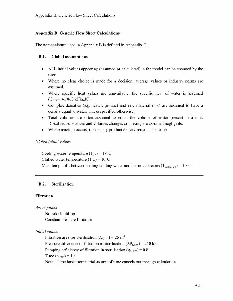
Appendix B: Generic Flow Sheet Calculations
A.11
Appendix B: Generic Flow Sheet Calculations The nomenclature used in Appendix B is defined in Appendix C.
B.1. Global assumptions
ALL initial values appearing (assumed or calculated) in the model can be changed by the user.
Where no clear choice is made for a decision, average values or industry norms are assumed.
Where specific heat values are unavailable, the specific heat of water is assumed (Cp, w = 4.1868 kJ/kg.K).
Complex densities (e.g. water, product and raw material mix) are assumed to have a density equal to water, unless specified otherwise.
Total volumes are often assumed to equal the volume of water present in a unit. Dissolved substances and volumes changes on mixing are assumed negligible.
Where reaction occurs, the density product density remains the same.
Global initial values Cooling water temperature (Tcw) = 18°C Chilled water temperature (Tcw) = 10°C
Max. temp. diff. between exiting cooling water and hot inlet streams (Tmax, cw) = 10°C
B.2. Sterilisation
Filtration Assumptions
No cake build-up Constant pressure filtration
Initial values
Filtration area for sterilisation (Af, ster) = 25 m2
Pressure difference of filtration in sterilisation (Pf, ster) = 250 kPa
Pumping efficiency of filtration in sterilisation (f, ster) = 0.8
Time (tf, ster) = 1 s Note: Time basis immaterial as unit of time cancels out through calculation

Appendix B: Generic Flow Sheet Calculations
A.12
Equations
ster f,ster f,
ster in, w,ster f, .tA
V v B.1
where: Vf, ster = Linear velocity through sterilisation filtration (m.s-1)
Vw, in, ster = Volume of water in sterilisation (m3) Since the volumes of the raw materials are small relative to the volume of water in the dilute systems typical of bioprocesses, only the volume of water is used as a simplification in these calculations. Volumes of raw materials are further avoided since calculating these requires the densities of each material. Although not used to calculate volumes, because the masses of raw materials are already calculated elsewhere, they are included in total mass calculations.
ster f,
ster f,ster f,ster f, η
.vP
P B.2
where: Pf, ster = Power for filtration in sterilisation (kPa)
ster f,ster f,ster f, .t E P B.3
where: Ef, ster = Energy for filtration in sterilisation (kJ)
Steam Sterilisation Initial values and Constants
Ambient or preheated temperature (Ta) = 20°C (60°C) Sterilisation temperature (Th) = 121°C Steam temperature (Tst)= 140°C Reactor temperature (Trct) = 37°C Cooling or chilled water temperature (Tcw) = [As for global initial values]
Max. temp. diff. between exiting cooling water and hot inlet streams (Tmax, cw) = 10°C
Sterilisation efficiency (ster) = 0.8 (used for all efficiencies in sterilisation)
Specific heat of water (Cp, w) = 4.1868 kJ/kg.K Specific heat of steam (Cp, st) = a + bT + cT2 + dT3 (J/mol.K)
(a = 29.163; b = 14.49 x 10⁻²; c = 2.02 x 10⁻⁶; d = 0)
Density (water) (w) = 1000 kg/m3
Pressure steam (before compression) (Pst, in) = 101.325 kPa Pressure (steam) (Pst, out) = 300 kPa

Appendix B: Generic Flow Sheet Calculations
A.13
Gas constant (R) = 8.314 kJ/kg.K
Latent heat of steam at 100°C and 101.3 kPa (st) = 2.7 MJ.kg-1
Equations
T = Trct – Tmax B.4
where: T = Temperature difference (oC)
Typically a log-mean temperature is used, but for the large T values often obtained, this
simplification is used. Mass of Steam needed:
rmwin w,h st, M .ρVM B.5
where: Mst, h = Mass of steam to heat to sterilisation temperature (Tster) (kg)
Mrm = Mass of raw material for (kg)
ah wp,h st,h TTCMq B.6
where: qh = Heat to raise temperature (kJ)
stersterster surf, .SVVA B.7
where: Asurf = Surface area of sterilisation unit(m2)
Vster = Volume of sterilisation unit (m3) SVster = Surface area to volume ratio for sterilisation unit (m2/m3)
T. U.AE surf B.8
where: = Rate of energy loss (kJ/s)
U = Overall heat transfer coefficient (kW/m2.oC)
T = Temperature difference (oC)
sterE.t q B.9
where: q = Heat loss during constant temperature period (kJ)
tster = Time for sterilisation (hr)

Appendix B: Generic Flow Sheet Calculations
A.14
q qq hT B.10
where: qT = Total heat lost (kJ)
hold St,st
Thold st, .ηλ
qM B.11
where: Mst, hold = Mass of steam required for holding period (kg)
st, hold = Efficiency for sterilisation during holding time
hold st,h st,Tst, M M M B.12
where: Mst, T = Total mass of steam required (kg) Steam compression required Assumption: Isentropic compression
st p,C
R
in st, ster,
out st, ster,stout st, ster, P
PTT
B.13
where: Tster, st, out = Temperature of steam leaving steriliser (oC)
Pster, st, out = Outlet pressure of steam from steriliser (kPa) Pster, st, in = Inlet pressure of steam to steriliser (kPa)
comp ster,
ststout st, ster,st p,comp ster, η
.mTTCE
B.14
where: Ester, comp = Energy consumption for sterilisation compression (kJ)
mst, ster = Number of moles steam – sterilization (moles)
ster, comp = Efficiency for sterilisation compression
Cooling water
in cw,out cw, ster,
rcthstercw ster, TT
TT.MM
B.15
where: Mster, cw = Mass of cooling water following sterilisation (kg) Mster = Mass of media to be sterilised (kg)
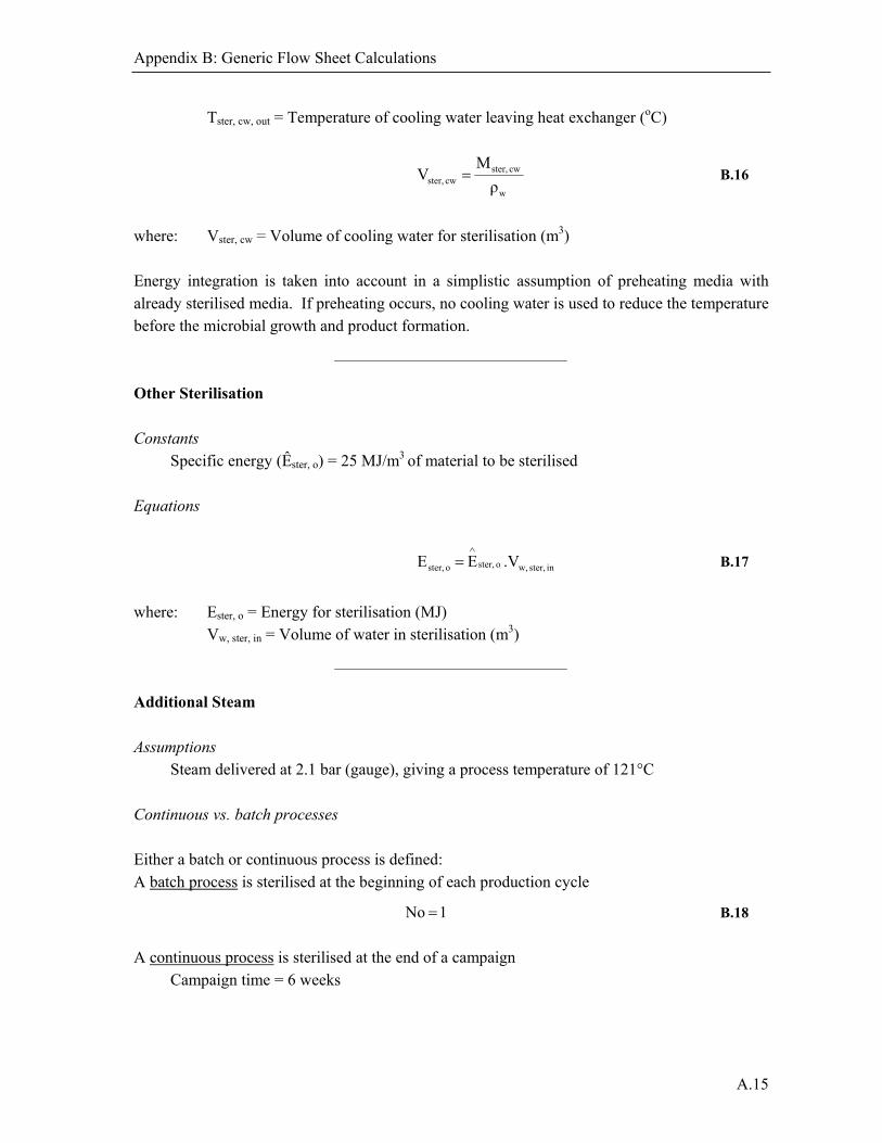
Appendix B: Generic Flow Sheet Calculations
A.15
Tster, cw, out = Temperature of cooling water leaving heat exchanger (oC)
w
cw ster,cw ster, ρ
MV B.16
where: Vster, cw = Volume of cooling water for sterilisation (m3) Energy integration is taken into account in a simplistic assumption of preheating media with already sterilised media. If preheating occurs, no cooling water is used to reduce the temperature before the microbial growth and product formation. Other Sterilisation
Constants Specific energy (Êster, o) = 25 MJ/m3 of material to be sterilised
Equations
in ster, w,o ster,o ster, .VE E
B.17
where: Ester, o = Energy for sterilisation (MJ)
Vw, ster, in = Volume of water in sterilisation (m3) Additional Steam Assumptions
Steam delivered at 2.1 bar (gauge), giving a process temperature of 121°C
Continuous vs. batch processes Either a batch or continuous process is defined: A batch process is sterilised at the beginning of each production cycle
1 No B.18
A continuous process is sterilised at the end of a campaign Campaign time = 6 weeks
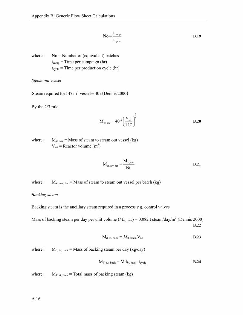
Appendix B: Generic Flow Sheet Calculations
A.16
cycle
camp
t
t No B.19
where: No = Number of (equivalent) batches
tcamp = Time per campaign (hr) tcycle = Time per production cycle (hr)
Steam out vessel
2000 Dennis t 40 vesselm 147for required Steam 3
By the 2/3 rule:
3
2
rctsov st, 147
V * 40 M
B.20
where: Mst, sov = Mass of steam to steam out vessel (kg)
Vrct = Reactor volume (m3)
No
M M st,sov
bat sov, st, B.21
where: Mst, sov, bat = Mass of steam to steam out vessel per batch (kg) Backing steam Backing steam is the ancillary steam required in a process e.g. control valves Mass of backing steam per day per unit volume (Mst, back) = 0.082 t steam/day/m3 (Dennis 2000) B.22
Md, st, back = Mst, back.Vrct B.23
where: Md, St, back = Mass of backing steam per day (kg/day)
MT, St, back = MdSt, back. tcycle B.24
where: MT, st, back = Total mass of backing steam (kg)
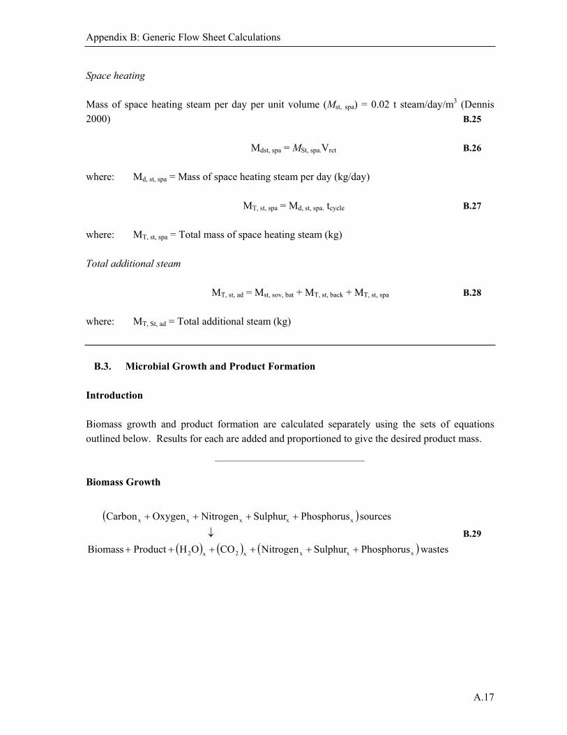
Appendix B: Generic Flow Sheet Calculations
A.17
Space heating Mass of space heating steam per day per unit volume (Mst, spa) = 0.02 t steam/day/m3 (Dennis 2000) B.25
Mdst, spa = MSt, spa.Vrct B.26
where: Md, st, spa = Mass of space heating steam per day (kg/day)
MT, st, spa = Md, st, spa. tcycle B.27 where: MT, st, spa = Total mass of space heating steam (kg) Total additional steam
MT, st, ad = Mst, sov, bat + MT, st, back + MT, st, spa B.28 where: MT, St, ad = Total additional steam (kg)
B.3. Microbial Growth and Product Formation
Introduction Biomass growth and product formation are calculated separately using the sets of equations outlined below. Results for each are added and proportioned to give the desired product mass. Biomass Growth
wastesPhosphorus Sulphur Nitrogen CO OH Product Biomass
sources Phosphorus Sulphur Nitrogen Oxygen Carbon
xxxx2x2
xxxxx
B.29

Appendix B: Generic Flow Sheet Calculations
A.18
x4x4x2x2x2ajaiahagafaeadacabaazy
xxwvutsxrqponm
xl'k'j'i'h'g'lkjihgx2xf'e'd'c'b'a'fedcba
POλSOκNιCOηOHγSPNOHCSPNOHφC
SPNOHCεSPNOHCδ
SPNOHCχ'SPNOHχCOβSPNOHCα'SPNOHαC
B.30
where: x: Components related to biomass growth only
Table B.1: Micro-organisms that include additional experimental values and are available as part of the generic flowsheet model database
Micro-organisms
Achromobacter delvacvate, Acinetobacter sp., Aerobacter aerogenes, Aeromona hydrophila, Aspergillus niger, Aspergillus sp., Aspergillus terreus, Azohydromonas lata, Bacillus licheniformis, Bacillus subtilis, Brevibacterium sp., Candida glycerinogenes, Candida magnoliae, Candida sp., Cellulomonas sp., Chaetomium cellulolyticum, Corynebacterium glutamicum, Cornebacterium hydrocarboclastus, Cupriavidus necator, Escherichia coli, Fusarium moniliforme, Fusarium sp., Geotrichum candidum, Klebsiella oxytoca, Klebsiella sp., Lactobacillus sp., Methalococcus capsulatus, Methophilus methylotrophus, Methylomonas sp., Norcadia sp., Paecilomyces variotii, Paracoccus denitrificans, Penicillium chrysogenum, Penicillium cyclopium, Penicillium sp., Propionibacterium sp., Protaminobacter rubber, Pseudomonas aerugenosa, Pseudomonas C12B, Pseudomonas fluorescens, Pseudomonas methanica, Pseudomonas sp., Rhizopus oligosporus, Rhodopseudomonas gelatinosa, Rhodopseudomonas spheroids,
Saccharomyces cerevisiae, Saccharomyces sp., Thermomonospora sp., Trichoderma sp., Xanthamonas campestris, OTHER.
Table B.2: Elemental formula for micro-organisms used in the model
Organism Carbon Hydrogen Oxygen Nitrogen Sulphur Phosphorus Reference
C H O N S P
Aerobacter aerogenes 1 1.83 0.55 0.25 [2]
Aspergillus niger 1 1.74 0.711 0.117 [1]
Azohydromonas lata 1 1.76 0.48 0.19 [2]
Candida sp. 1 1.84 0.52 0.16 [2]
Escherichia coli 1 1.77 0.49 0.24 [2]
Klebsiella sp. 1 1.75 0.43 0.23 [2]
Paracoccus denitrificans 1 1.66 0.49 0.2 [2]
Pseudomonas C12B 1 2 0.52 0.23 [2]
Saccharomyces cerevisiae 1 1.76 0.53 0.17 0.005 0.01 [2]
OTHER 1 1.82 0.53 0.21 0 0
References:
[1] El-Enshasy 1998 [2] Roels 1980

Appendix B: Generic Flow Sheet Calculations
A.19
To solve the stoichiometric equations for biomass growth:
Initial values
Biomass: = 1
Product: = 0 (assumption that no product is formed)
Unknowns (12)
Carbon source (x2): , '
Oxygen source:
Nitrogen source (x2): , '
Sulphur source:
Phosphorus source: Water waste:
Carbon dioxide waste: Nitrogen waste:
Sulphur waste:
Phosphorus waste:
Material balances (6)
Carbon: .a + '.a' + .g + '.g' + .m + .s – = .y B.31
Hydrogen: .b + '.b' + .h + '.h' + .n + .t – 2. = .z B.32
Oxygen: .c + '.c' + 2. + .i +'.i' + .o + .u – – 2. – 2. – 4. = .aa B.33
Nitrogen: .d + '.d' + .j + '.j' + .p + .v – – 2. = .ab B.34
Phosphorus: .e + '.e' + .k + '.k' + .q + .w – l = .ac B.35
Sulphur: .f + '.f' + .l + '.l' + .r + .x – = .ad B.36
Yield Coefficient (1)
Yx/s As defined by literature or experimental values in database (g/g)
φ Mm
.MmYα'.
Mm
.MmYα.
x
C2x/s
x
C1x/s
B.37
where: MmC1 = Molar mass carbon source 1 (kg/kmol)
MmC2 = Molar mass carbon source 2 (kg/kmol) Mmx = Molar mass biomass (kg/kmol)

Appendix B: Generic Flow Sheet Calculations
A.20
'.Mm.Mm.Mm
YC2C1
x
x/s B.38
'.Mm.Mm.32.07.ad 30.97.ac 14.01.ab 16.00.aa .z01.1 12.01.y
YC2C1
x/s
B.39
32.07.f' 30.97.e' 14.01.d' 16.00.c' .b'01.1 12.01.a''.
32.07.f 30.97.e 14.01.d 16.00.c .b01.1 12.01.a.
.32.07.ad 30.97.ac 14.01.ab 16.00.aa .z01.1 12.01.y
Yx/s
B.40
Ratios (2)
' C1/CT
r B.41
where: rC1/CT = Carbon 1 source to total carbon ratio
' N1/NT
r B.42
where: rN1/NT = Nitrogen 1 source to total nitrogen ratio To convert rC1/CT and rN1/NT from mass to mole values: Using rC1/CT as an example, with a basis of 100 kg of total carbon source:
C2C1 M - 100 M B.43
100 x w M C2C2 B.44
where: MC1 = Mass of carbon source 1 (kg)
MC2 = Mass of carbon source 2 (kg) wC2 = Mass fraction of carbon source 2

Appendix B: Generic Flow Sheet Calculations
A.21
For carbon source 1 and 2:
Mm
M m B.45
where: m = Number of moles (kmol)
M = Mass (kg) Mm = Molar mass (kg/kmol)
mCT = mC1 + mC2 B.46 where: mCT = Total number of moles carbon
mC1 = Number of moles carbon source 1 mC2 = Number of moles carbon source 2
100 x m
m
CT
C1C1/CT r B.47
A similar set of equations is required to determine rN1/NT Default values for rC1/CT and rN1/NT (which can be changed by the user) = 0.5
If there is no 2nd carbon or nitrogen source, ' = 0 and ' = 0, respectively
Constraints (3) Only nitrogen from either nitrogen source ends up in biomass. All other nitrogen is waste. Only sulphur from sulphur source ends up in biomass. All other sulphur is waste. Only phosphorus from nitrogen source ends in biomass. All other phosphorus is waste.
Nitrogen: .j + '.j’ = .ab B.48
Sulphur: .j = .ad B.49
Phosphorus: .w = .ac B.50

Appendix B: Generic Flow Sheet Calculations
A.22
Product Formation
wastesPhosphorus Sulphur Nitrogen CO OH Product Biomass
sources Phosphorus Sulphur Nitrogen Oxygen Carbon
pppp2p2
ppppp
B.51
p4p4p2p2p2ajaiahagafaeadacabaazy
pxwvutsprqponm
pl'k'j'i'h'g'lkjihgp2pf'e'd'c'b'a'fedcba
POλSOκNιCOηOHγSPNOHCSPNOHφC
SPNOHCεSPNOHCδ
SPNOHCχ'SPNOHχCOβSPNOHCα'SPNOHαC
B.52
where: p: Components related to product formation growth only The possible chemicals and their associated formulae are given in Table B.3. Chemical products not listed in these tables can be modelled as “OTHER” with the chemical formula modified as required.
Table B.3: Chemical formulas and associated pure component densities for products obtained in the model
Product Carbon Hydrogen Oxygen Nitrogen Sulphur Phosphorus Density*
Antibiotics
Penicillin 16 17 4 2 1 0 1410
Cephalosporin 14 13 4 8 3 0 (1410)
Erythromycin 37 67 13 1 0 0 (1410)
Nocardicin 23 24 9 4 0 0 (1410)
Clavulanic acid 8 9 5 1 0 0 (1410)
Thienamycin 11 16 4 2 1 0 (1410)
OTHER 18.17 24.33 6.5 3 0.83 0 1410
Amino Acids
Arginine 6 14 2 4 0 0 1100
Glutamine 5 10 3 2 0 0 (1393)
Phenylalanine 9 11 2 1 0 0 1290
Tyrosine 9 11 3 1 0 0 1456
Tryptophan 11 12 2 2 0 0 (1393)
Lysine 6 14 2 2 0 0 (1393)
Glysine 2 5 2 1 0 0 1607
Alanine 3 7 2 1 0 0 1401
Histidine 6 9 2 3 0 0 (1393)
Serine 3 7 3 1 0 0 1537
Proline 5 9 2 1 0 0 (1393)

Appendix B: Generic Flow Sheet Calculations
A.23
Product Carbon Hydrogen Oxygen Nitrogen Sulphur Phosphorus Density*
Amino Acids (cont.)
Glutamic acid 5 9 4 1 0 0 1538
Aspartic acid 4 7 4 1 0 0 1660
Threonine 4 9 3 1 0 0 (1393)
Cysteine 3 7 2 1 1 0 (1393)
Methionine 5 11 2 1 1 0 1340
Leucine 6 13 2 1 0 0 1165
Asparagine 4 8 3 2 0 0 (1393)
Isoleucine 6 13 2 1 0 0 (1393)
Valine 5 11 2 1 0 0 1230
Enzymes
Lipase 6 6 0 1 0 0 (1393) **
Pectinase 6 9 2 0 0 0 (1393) **
Cellulase 4 10 13 2 0 0 (1393) **
OTHER 5.33 8.33 5 1 0 0 (1393) **
Alcohols
2,3 Butanediol 4 10 2 0 0 0 980
Butanol 4 10 1 0 0 0 810
Ethanol 2 6 1 0 0 0 789
Ethylene glycol 2 6 2 0 0 0 1113.2
Glycerol 3 8 3 0 0 0 1261
Methanol 1 4 1 0 0 0 791.8
OTHER 2.67 7.33 1.67 0 0 0 957.5
Vitamins
Retinol 20 30 1 0 0 0 (1000)
B1, Thiamine 12 17 1 1 1 0 (1000)
B2, Riboflavin, G 17 20 6 4 0 0 (1000)
B3, Niacin 6 4 2 1 0 0 (1000)
B5, Pantothenic acid 9 17 5 1 0 0 (1000)
B6, Pyridoxine 8 11 3 1 0 0 (1000)
B7, Biotin 10 16 3 2 1 0 (1000)
B9, Folic acid 19 19 6 7 0 0 (1000)
B12, Cyanocobalamin 63 89 14 14 0 1 (1000)
Ascorbic acid 6 8 6 0 0 0 (1000)
D2, Ergocalciferol 28 44 1 0 0 0 (1000)
Vitamins (cont.)
D3, Cholecalciferol 27 44 1 0 0 0 (1000)
Tocopherol 29 50 2 0 0 0 (1000)
Naphthoquinone 31 46 2 0 0 0 (1000)
K1 31 46 2 0 0 0 (1000)
K2 51 76 2 0 0 0 (1000)
K3, Menadione 11 8 2 0 0 0 (1000)
Carbohydrates
Formaldehyde 1 2 1 0 0 0 1
Glucose 6 12 6 0 0 0 1540
Sucrose 12 22 11 0 0 0 1587

Appendix B: Generic Flow Sheet Calculations
A.24
Product Carbon Hydrogen Oxygen Nitrogen Sulphur Phosphorus Density*
Starch 6 10 5 0 0 0 1500
OTHER 6.25 11.5 5.75 0 0 0 1157
Organic acids
Acetic acid 2 4 2 0 0 0 1049
Citric acid 6 8 7 0 0 0 1665
Formic acid 1 2 2 0 0 0 1220
Fumaric acid 4 4 2 0 0 0 1635
Gluconic acid 6 12 7 0 0 0 1230
Itaconic acid 5 6 4 0 0 0 1573
Lactic acid 3 6 3 0 0 0 1200
Malic acid 4 6 5 0 0 0 1609
Oxalic acid 2 2 4 0 0 0 1770
Propionic acid 3 6 2 0 0 0 990
OTHER 3.60 5.60 3.80 0 0 0 1394.1
Alkanes
Butane 4 10 0 0 0 0 810
Hexadecane 16 34 0 0 0 0 773
Hexane 6 14 0 0 0 0 654.8
Methane 1 4 0 0 0 0 700
Octane 8 18 0 0 0 0 703
OTHER 7 16 0 0 0 0 728.2
Others
OTHER 10.2 16.0 3.2 1.2 0.1 0.0 1201 *Values in brackets are average values of the group or estimates based on the density of water (1 000 kg/m3) **Average protein density
To solve the stoichiometric equations for product formation: Initial values
Biomass: = 0 (assumption that no biomass is formed)
Product: = 1
Unknowns (12)
Carbon source (x2): , '
Oxygen source:
Nitrogen source (x2): , '
Sulphur source:
Phosphorus source: Water waste:
Carbon dioxide waste: Nitrogen waste:
Sulphur waste:
Phosphorus waste:
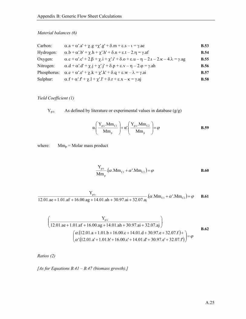
Appendix B: Generic Flow Sheet Calculations
A.25
Material balances (6)
Carbon: .a + '.a' + .g +'.g' + .m + .s – = .ae B.53
Hydrogen: .b + '.b' + .h + '.h' + .n + .t – 2. = .af B.54
Oxygen: .c + '.c' + 2. + .i + '.i' + .o + .u – – 2. – 2. – 4. = .ag B.55
Nitrogen: .d + '.d' + .j + '.j' + .p + .v – – 2. = .ah B.56
Phosphorus: .e + '.e' + .k + '.k' + .q + .w – = .ai B.57
Sulphur: .f + '.f' + .l + '.l' + .r + .x – = .aj B.58
Yield Coefficient (1)
Yp/s As defined by literature or experimental values in database (g/g)
Mm
.MmYα'.
Mm
.MmYα.
p
C2p/s
p
C1p/s
B.59
where: Mmp = Molar mass product
'.Mm.Mm.Mm
YC2C1
p
p/s B.60
'.Mm.Mm.32.07.a 30.97.ai 14.01.ah 16.00.ag .af01.1 12.01.ae
YC2C1
p/s
j
B.61
32.07.f' 30.97.e' 14.01.d' 16.00.c' .b'01.1 12.01.a''.
32.07.f 30.97.e 14.01.d 16.00.c .b01.1 12.01.a.
.32.07.aj 30.97.ai 14.01.ah 16.00.ag .af01.1 12.01.ae
Yp/s
B.62
Ratios (2)
[As for Equations B.41 – B.47 (biomass growth).]

Appendix B: Generic Flow Sheet Calculations
A.26
Constraints (3) Only nitrogen from either nitrogen source ends up in product. All other nitrogen is waste. Only sulphur from sulphur source ends up in product. All other sulphur is waste. Only phosphorus from nitrogen source ends in product. All other phosphorus is waste.
Nitrogen: .j + .j = .ab B.63
Sulphur: .j = .ad B.64
Phosphorus: .w = .ac B.65
Under certain conditions, due to over-specification of the system e.g. incorrect yield coefficients, results give negative mass balance values. For example, if insufficient carbon is added (a yield coefficient restriction), negative carbon dioxide emission and oxygen consumption may result. To overcome this, the yield coefficient is assumed inaccurate. To avoid the need for iterative solution by varying Y, the unknowns present are reduced by assuming that no oxygen enters as an oxygen source. This increases the amount of oxygen-bearing carbon input required to balance the oxygen needs, with excess carbon reporting to the waste streams. It is recognized that this approach is limiting in highly aerobic processes where a high carbon waste would signal the need for improved data or further correction on an individual case basis. An alternative approach of assuming zero carbon dioxide emissions to correct for negative values is not considered. This approach results in an increase in the amount of oxygen-bearing carbon source needed, but removes the outlet for both carbon and oxygen waste and results in negative oxygen input values.
Anaerobic Product Formation (anaerobic processes only)
wastesPhosphorus Sulphur Nitrogen CO H Product Anaerobic Biomass
sources Phosphorus Sulphur Nitrogen Carbon
apapapap2ap2
apapapap
B.66
ap4ap4ap2ap2ap2ajaiahagafaeadacabaazy
apxwvutsaprqponm
apl'k'j'i'h'g'lkjihgapf'e'd'c'b'a'fedcba
POλSOκNιCOηHγSPNOHCSPNOHφC
SPNOHCεSPNOHCδ
SPNOHCχ'SPNOHχCSPNOHCα'SPNOHαC
B.67

Appendix B: Generic Flow Sheet Calculations
A.27
Table B.4: Chemical formula for anaerobic products in the model
Anaerobic Product Carbon Hydrogen Oxygen Nitrogen Sulphur Phosphorus
2, 3-butanediol 4 10 2 0 0 0
Butanol 4 10 0 0 0 0
Butyric acid 4 8 2 0 0 0
Ethanol 2 6 0 0 0 0
Lactate 3 6 3 0 0 0
Methane 1 4 0 0 0 0
Propanol 3 8 1 0 0 0
Propionic acid 3 6 2 0 0 0
Succinic acid 4 6 4 0 0 0
OTHER 3.11 7.11 1.56 0 0 0
To solve the stoichiometric equations for anaerobic product formation: Initial values
Biomass: = 0
Anaerobic Product: = 1
Unknowns (11)
Carbon source (x2): , '
Nitrogen source (x2): , '
Sulphur source:
Phosphorus source: Water waste:
Carbon dioxide waste: Nitrogen waste:
Sulphur waste:
Phosphorus waste:
Material balances (6)
Carbon: .a + '.a' + .g +'.g' + .m + .s – = .ae B.68
Hydrogen: .b + '.b' + .h + '.h' + .n + .t – 2. = .af B.69
Oxygen: .c + '.c' + .i + '.i' + .o + .u – – 2. – 2. – 4. = .ag B.70
Nitrogen: .d + '.d' + .j + '.j' + .p + .v – – 2. = .ah B.71
Phosphorus: .e + '.e' + .k + '.k' + .q + .w – = .ai B.72
Sulphur: .f + '.f' + .l + '.l' + .r + .x – = .aj B.73
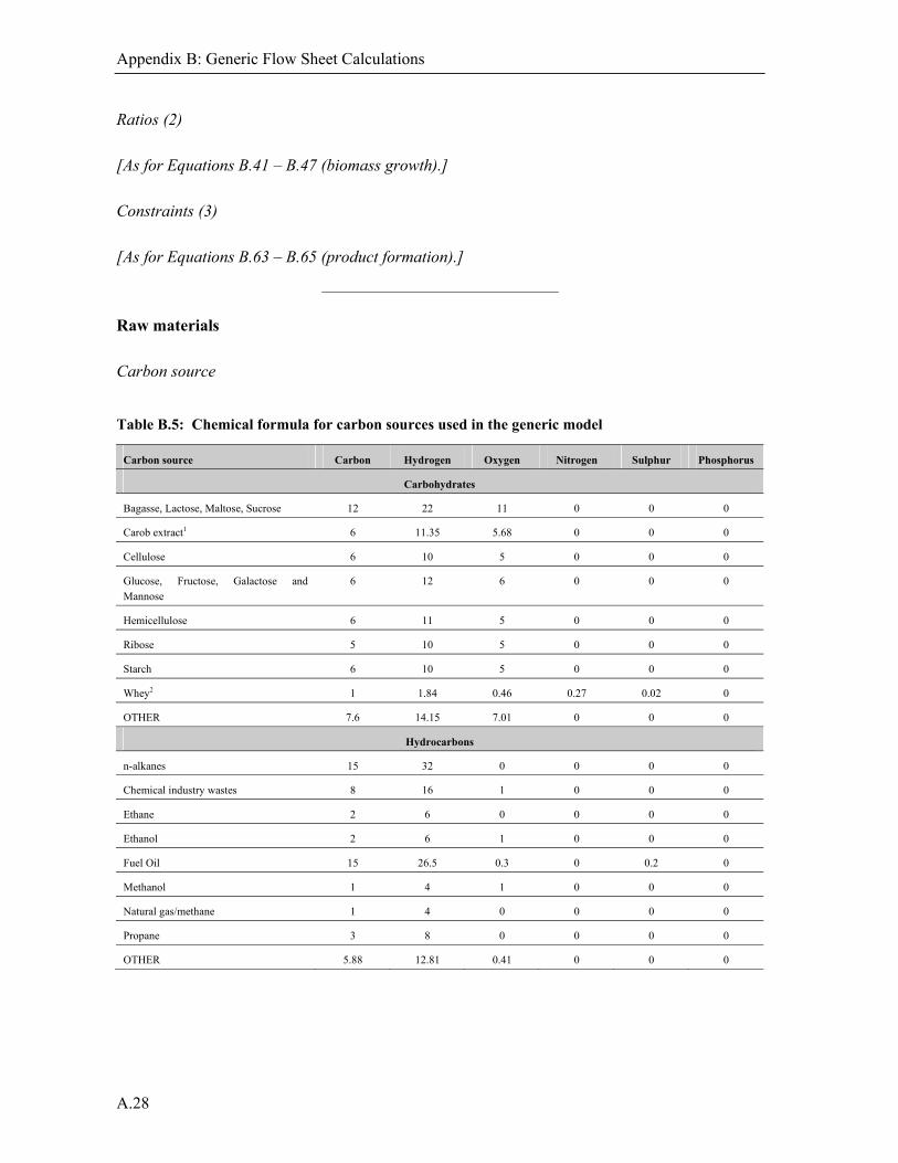
Appendix B: Generic Flow Sheet Calculations
A.28
Ratios (2)
[As for Equations B.41 – B.47 (biomass growth).] Constraints (3)
[As for Equations B.63 – B.65 (product formation).]
Raw materials Carbon source
Table B.5: Chemical formula for carbon sources used in the generic model
Carbon source Carbon Hydrogen Oxygen Nitrogen Sulphur Phosphorus
Carbohydrates
Bagasse, Lactose, Maltose, Sucrose 12 22 11 0 0 0
Carob extract1 6 11.35 5.68 0 0 0
Cellulose 6 10 5 0 0 0
Glucose, Fructose, Galactose and Mannose
6 12 6 0 0 0
Hemicellulose 6 11 5 0 0 0
Ribose 5 10 5 0 0 0
Starch 6 10 5 0 0 0
Whey2 1 1.84 0.46 0.27 0.02 0
OTHER 7.6 14.15 7.01 0 0 0
Hydrocarbons
n-alkanes 15 32 0 0 0 0
Chemical industry wastes 8 16 1 0 0 0
Ethane 2 6 0 0 0 0
Ethanol 2 6 1 0 0 0
Fuel Oil 15 26.5 0.3 0 0.2 0
Methanol 1 4 1 0 0 0
Natural gas/methane 1 4 0 0 0 0
Propane 3 8 0 0 0 0
OTHER 5.88 12.81 0.41 0 0 0

Appendix B: Generic Flow Sheet Calculations
A.29
Carbon source Carbon Hydrogen Oxygen Nitrogen Sulphur Phosphorus
Volatile fatty acids/Organic acids
Acetic acid 2 4 2 0 0 0
Butyric acid 4 8 2 0 0 0
Citric acid 6 8 7 0 0 0
Formic acid 1 2 2 0 0 0
Fumaric acid 4 4 4 0 0 0
Volatile fatty acids/Organic acids (cont.)
Gluconic acid 6 12 7 0 0 0
Itaconic acid 5 6 4 0 0 0
Lactic acid 3 6 3 0 0 0
Malic acid 4 6 5 0 0 0
Oxalic acid 2 2 4 0 0 0
Propionic acid 3 6 2 0 0 0
OTHER 3.64 5.82 3.82 0 0 0
Proteins
Actin, Collagen, Corn steep liquor, Peptione, Tubulin3
5.13 9.16 2.33 1.34 0 0
Alanine 3 7 2 1 0 0
Arginine 6 14 2 4 0 0
Asparginine 4 8 3 2 0 0
Aspartic acid 4 7 4 1 0 0
Cysteine 3 7 2 1 1 0
Glutamic acid 5 9 4 1 0 0
Glutamine 5 10 3 2 0 0
Glysine 2 5 2 1 0 0
Histidine 6 9 2 3 0 0
Isoluecine, Isoluecine 6 13 2 1 0 0
Lysine 6 14 2 2 0 0
Methionine 5 11 2 1 1 0
Phenylalanine 9 11 2 1 0 0
Proline 5 9 2 1 0 0
Serine 3 7 3 1 0 0
Threonine 4 9 3 1 0 0
Tryptophan 11 12 2 2 0 0

Appendix B: Generic Flow Sheet Calculations
A.30
Carbon source Carbon Hydrogen Oxygen Nitrogen Sulphur Phosphorus
Tyrosine 9 11 3 1 0 0
Valine 5 11 2 1 0 0
Yeast extract4 1 1.76 0.53 0.17 0.005 0.01
OTHER 5.13 9.16 2.33 1.34 0 0
OTHER
Corn stover5 21 30.7 14 0.25 0.02 0
Glycerol 3 8 3 0 0 0
Mannitol 6 14 6 0 0 0
Pyruvate 3 4 3 0 0 0
Succinate 4 6 4 0 0 0
Sulphite liquor 7 8 2 0 0 0
Whiskey distillery wash6 2 6 1 0 0 0
Wood7 20 29 13.8 0.01 0.003 0
OTHER 8.25 13.21 5.85 0.03 0 0
Notes:
1 – From average sugar composition (sucrose, 65 % fructose and glucose, 35 %) 2 – Average of amino acid values – protein 3 - Average composition of group used 4 – Assumed same composition as yeast 5- Reference: Phyllis (2006) 6 – Pure ethanol assumed 7 – Reference: Phyllis (2006)
Nitrogen source
Table B.6: Chemical formula for nitrogen sources used in the generic model
Nitrogen source Carbon Hydrogen Oxygen Nitrogen Sulphur Phosphorus
Organic
Actin, Collagen, Peptone, Tubulin1 5.13 9.16 2.33 1.34 0 0
Alanine 3 7 2 1 0 0
Arginine 6 14 2 4 0 0
Asparginine 4 8 3 2 0 0
Aspartic acid 4 7 4 1 0 0
Corn stover2 21 30.7 14 0.25 0.02 0
Cysteine 3 7 2 1 0 0
Glutamic acid 5 9 4 1 0 0
Glutamine 5 10 2 3 0 0
Glysine 2 5 2 1 0 0
Histidine 6 9 2 3 0 0
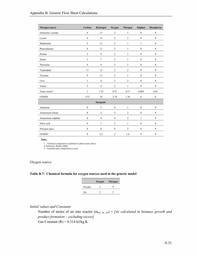
Appendix B: Generic Flow Sheet Calculations
A.31
Nitrogen source Carbon Hydrogen Oxygen Nitrogen Sulphur Phosphorus
Isoleusine, Leusine 6 13 2 1 0 0
Lysine 6 14 2 2 0 0
Methionine 5 11 2 1 1 0
Phenylalanine 9 11 2 1 0 0
Proline 5 9 2 1 0 0
Serine 3 7 3 1 0 0
Threonine 4 9 3 1 0 0
Tryptophan 11 12 2 2 0 0
Tyrosine 9 11 3 1 0 0
Urea 1 4 1 2 0 0
Valine 5 11 2 1 0 0
Yeast extract3 1 1.76 0.53 0.17 0.005 0.01
OTHER 5.57 10 2.74 1.36 0 0
Inorganic
Ammonia 0 3 0 1 0 0
Ammonium nitrate 0 4 3 2 0 0
Ammonium sulphate 0 8 4 2 1 0
Nitric acid 0 1 3 1 0 0
Nitrogen (gas) 0 0 0 2 0 0
OTHER 0 3.2 2 1.6 0 0
Notes:
1 – Chemical composition as defined in carbon source above 2- Reference: Phyllis (2006) 3 – Assumed same composition as yeast
Oxygen source
Table B.7: Chemical formula for oxygen sources used in the generic model
Oxygen Nitrogen
Oxygen 2 0
Air 2 2
Initial values and Constants
Number of moles of air into reactor (mair, in, rct) = [As calculated in biomass growth and
product formation – excluding excess] Gas Constant (R) = 8.314 kJ/kg.K
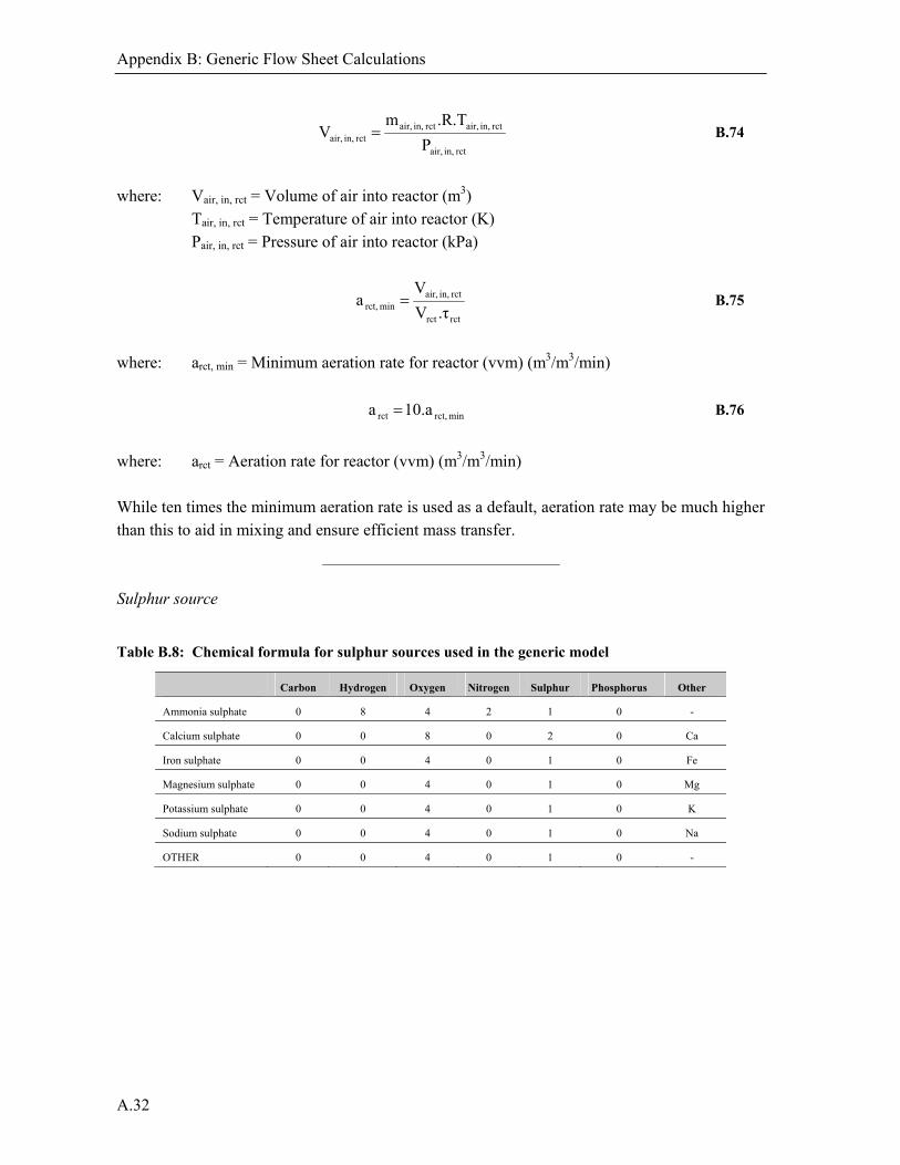
Appendix B: Generic Flow Sheet Calculations
A.32
rct in, air,
rct in, air,rct in, air,rct in, air, P
.R.Tm V B.74
where: Vair, in, rct = Volume of air into reactor (m3)
Tair, in, rct = Temperature of air into reactor (K) Pair, in, rct = Pressure of air into reactor (kPa)
rctrct
rct in, air,min rct, τ.V
V a B.75
where: arct, min = Minimum aeration rate for reactor (vvm) (m3/m3/min)
min rct,rct 10.a a B.76
where: arct = Aeration rate for reactor (vvm) (m3/m3/min) While ten times the minimum aeration rate is used as a default, aeration rate may be much higher than this to aid in mixing and ensure efficient mass transfer.
Sulphur source
Table B.8: Chemical formula for sulphur sources used in the generic model
Carbon Hydrogen Oxygen Nitrogen Sulphur Phosphorus Other
Ammonia sulphate 0 8 4 2 1 0 -
Calcium sulphate 0 0 8 0 2 0 Ca
Iron sulphate 0 0 4 0 1 0 Fe
Magnesium sulphate 0 0 4 0 1 0 Mg
Potassium sulphate 0 0 4 0 1 0 K
Sodium sulphate 0 0 4 0 1 0 Na
OTHER 0 0 4 0 1 0 -

Appendix B: Generic Flow Sheet Calculations
A.33
Phosphorus source
Table B.9: Chemical formula for phosphorus sources used in the generic model
Carbon Hydrogen Oxygen Nitrogen Sulphur Phosphorus Other
C H O N S P -
Phosphoric acid 0 3 4 0 0 1 -
K2HPO4 0 1 4 0 0 1 2 x K
KH2PO4 0 2 4 0 0 1 K
Na2HPO4 0 1 4 0 0 1 Na
NaH2PO4 0 2 4 0 0 1 2 x Na
OTHER 0 1.8 4 0 0 1 -
Mass Balance
Yield Coefficient (1)
Yp/x As defined by user (default value = 1)
Equations Mass balance
Final values of the stoichiometric coefficients to for biomass growth and product formation
are calculated using the equations above and then scaled according to the product to biomass ratio (Yp/x) defined. For i = all materials required and formed during microbial growth and product formation
p i,p/x
xi,T i, M
Y
M M
B.77
where: Mi, T = Total mass of substance i required for formation of 1 kg product (kg)
Mi, x = Mass of substance i required for formation of 1 kg biomass (kg) Mi, p = Mass of substance i required for formation of 1 kg product (kg)
Values are further scaled to give the desired amount of final product output.
ci T,*
i T, .S M M B.78

Appendix B: Generic Flow Sheet Calculations
A.34
where: MT, i* = Total mass of substance i after scaling (kg)
Sc = Scaling factor, where Sc is defined below. If the desired product is biomass from microbial growth:
φ
M S sep1 p,
c B.79
If the desired product is a metabolic product:
γ
M S sep1 p,
c B.80
where: Mp, sep1 = Mass of product to solid-liquid separation unit 1 (kg) The product mass (Mp, sep1) needed to give the final desired product output after downstream processing (including water and impurities not removed and taking losses into account), is determined by iterative solving of the mass balance problem.
Mp, final, ass = M p, final, req B.81 where: Mp, final, ass = Mass of final product assumed (kg)
Mp, final, req = Mass of final product required (kg)
Mp, final, calc = Mp, final, ass + Mw, ps + Mim B.82 where: Mp, final, calc = Mass of final product calculated (kg)
Mw, ps = Mass of water in the final product stream (kg) Mim, ps = Mass of impurities in the final product stream (kg)
1M
M M
M MM M
ass final, p,
ass final, p,calc final, p,
req final, p,calc final, p,ass final, p,
*ass final, p, B.83
where: Mp, final, ass
* = Mass of final product assumed (new value) (kg) Mp, final, calc = Mass of final product calculated (kg) Mw, ps = Mass of water in the final product stream (kg) Mim, ps = Mass of impurities in the final product stream (kg)

Appendix B: Generic Flow Sheet Calculations
A.35
Three iterations of Equations B.81 –B.83 are performed to calculate a final product value. If the product is biomass growth, the initial concentration of biomass entering the process needs to be taken into account as part of the final product. Less biomass is needed since there is already a small portion in the system. The corrected (new) final product is given by the iteration process of Equations B.84 – B.89.
For j = 1 350:
Mx, ass, j = Mx, req, j B.84
where: Mx, ass, j = Mass of biomass assumed (iteration j) (kg)
Mx, req, j = Mass of biomass required (iteration j) (kg)
Mx, calc, j = Mx, ass, j + Mx, 0, j B.85
where: Mx, calc, j = Mass of biomass calculated (iteration j) (kg)
Mx, 0, j = Initial mass of biomass (iteration j) (kg)
jej req, x,j calc, x,
j ass, x,*
j ass, x,
M MM M B.86
where: Mx, ass, j
* = Mass of biomass assumed (new value) (kg) ej = Error value for iteration j, where e is defined as below. e1 = 1 B.87 If (Mx, calc – Mx, req)j > (Mx, calc – Mx, required)j – 1,
ej = -2.ej – 1 B.88 This is used to help convergence by ensuring that the difference between
the desired and calculated values in successive steps does not get larger. else,
ej = ej – 1 B.89 Next j

Appendix B: Generic Flow Sheet Calculations
A.36
Yield coefficients Under certain conditions, negative mass balance values are obtained. This is attributed to carbon limitation (a yield coefficient restriction), which results in negative carbon dioxide emissions and negative oxygen consumption. To remedy, it is assumed that yield coefficient values are inaccurate and ignored. It is further assumed that there is no oxygen source (see Chapter 2, Section 0 of the main text). Equation B.59 is replaced with Equation B.90.
b = 0 B.90 Maintenance Coefficient Calculations
Initial values and constants Maintenance coefficient (m) = [As in Table B.10] Time (tmaint) = 10 hrs (or as entered by the user) – a warning is given if maintenance time is
less than residence time.
Table B.10: Values for maintenance coefficients as used in the model
Biomass Carbon Source Maintenance coefficient (g carbon source/g dry cell
weight biomass.h)
Reference
Aerobic microbial growth
Aerobacter aerogenes Citrate 0.058 [13]
Glucose 0.094 [10], [13]
Glycerol 0.076 [10], [13]
Aerobacter cloacae Glucose 0.094 [10], [11]
Azotobacter vinelandii - 0.15-1.5 [8], [9]
Escherichia coli Glucose 0.054-0.12 [2], [13]
Escherichia coli (uninduced recombinant strain) Glucose 0.17 [2]
Escherichia coli (IPTG induced recombinant strain) Glucose 0.32 [2]
Lactobacillus casei - 0.135 [5], [11]
Methane bacteria Methane 0.02 [13]
Penicillium chrysogenum Glucose 0.022 [3], [12], [13]
Pseudomonas putida Acetic acid 0.00552-0.07372 [6]
Saccharomyces cereviciae Glucose 0.018 [13]
Anaerobic microbial growth
Bacteroides ruminicola Glucose 0.135 [14]
Butyrivibrio fibrisolvens Glucose 0.049 [14]
Klebsiella aerogenes - 2.88-3.69 [11], [15]

Appendix B: Generic Flow Sheet Calculations
A.37
Biomass Carbon Source Maintenance coefficient (g carbon source/g dry cell
weight biomass.h)
Reference
Megasphaera elsdenii Glucose 0.187 [14]
Saccharomyces cerevisiae - 0.036-0.36 [11], [16]
Selenomonas ruminantium Glucose 0.022 [14]
Streptococcus bovis Glucose 0.150 [14]
Zymomonas mobilis Glucose 0.0-5.9 [1], [4], [7], [9]
References:
[1] Beyeler et al. 1984 [2] Bhattacharya and Dubey 1995 [3] Biwer et al. 2005 [4] Cromie and Doelle 1980 [5] De Vries et al. 1970 [6] Fieschko and Humphrey 1984
[7] Lee et al. 1979 [8] Nagai and Aiba 1972[9] Oliviera et al. 1992 [10] Pirt 1965 [11] Pirt 1975
[12] Righelato et al. 1968 [13] Roels and Kossen 1978 [14] Russell and Baldwin 1979 [15] Stouthamer and Bettenhausen 1973 [16] Watson 1970
Equations
MC1, maint = m.tmaint.Mx B.91 where: MC1, maint = Mass of carbon 1 for maintenance (kg)
m = Maintenance coefficient (g C source/g dry cell weight.h) tmaint = Time for maintenance (hr) Mx = Mass of biomass (kg)
Oxygen requirements (aerobic) are calculated Stoichiometrically according to Equation B.92
Energy OCO O M 222maint C1, B.92
For anaerobic processes, an anaerobic product needs to be specified and Equation B.93 balanced.
Energy product Anaerobic OCO M 22maint C1, B.93
Growth Rate Initial values and constants
Initial biomass concentration (Cx, 0) = 1 g/l Maximum specific growth rate (max) = [As in Table 2.6] (assumed constant) Half saturation constant (Ks) = [As in Table 2.6] Biomass concentration (Cx) = [As in Table 2.6] Ambient temperature (Ta) = 20°C Reactor temperature (Trct) = 37°C

Appendix B: Generic Flow Sheet Calculations
A.38
Table B.11: Maximum specific growth rate, limiting nutrient concentration and final microbial concentrations used in the model
Organism Limiting nutrient
Max. specific growth rate,
max (hr-1)
Half saturation constant, Ks (mg/l)
Concentration, rx (g/l)
Reference
Achromobacter delvacvate Diesel Oil 10-15 [3]
Acinetobacter sp. Acetate 0.22 6.85 [3]
Ethanol 0.96 1.8 [3]
Other 0.4-2.0 8-10 [3]
Aerobacter aerogenes Glucose 1.22 5-8 [1], [6]
Aeromona hydrophila Lactose 1.1 [3]
Aspergillus sp. Carob extract 0.11-0.16 [4]
Candida sp. n-alkanes 15.2 [4]
Sulfite liquor 10.7 [4]
Lactose 22.5 [4]
Other 0.5 0.2 [1]
Cellulomonas sp. Bagasse 0.14-0.16 13.2 [3]
Chaetomium cellulolyticum Corn stover 0.24 [4]
Cornebacterium hydrocarboclastus Propane 0.046 0.9 [3]
Enterobacter cloacae Glycerol 0.77 [6]
Escherichia coli Glucose 1.1 3 [1]
Glycerol 0.87 2 [1]. [6]
Lactose 0.8 20 [1]
Fusarium moniliforme Carob extract 0.22 3.3 [4]
Fusarium sp. Glucose 0.28 [4]
Other 0.3 [4]
Geotrichum candidum Whiskey distillery
wash
0.385 18 [4]
Klebsiella aerogenes Glycerol 0.85-0.95 9 [1], [6]
Glucose 0.85 10 [1], [6]
Klebsiella pneumoniae Glucose 0.503-1.07 31 [6]
Methalococcus capsulatus Methane 0.14 0.4 [3]
Methophilus methylotrophus Methanol 0.38-0.50 30 [3]
Methylomonas sp. Methanol 0.14-0.25 9.6-30.0 [3]
Norcadia sp. n-alkanes 1.25 14.7 [3]
Propane 0.091 30 [3]
Butane 22 [3]
Paecilomyces variotii Sulfite liquor 0.31 13 [4]

Appendix B: Generic Flow Sheet Calculations
A.39
Organism Limiting nutrient
Max. specific growth rate,
max (hr-1)
Half saturation constant, Ks (mg/l)
Concentration, rx (g/l)
Reference
Penicillium cyclopium Lactose 12.8 [4]
Penicillium sp. 0.2 30 [4], [5]
Protaminobacter ruber Methanol 85 [3]
Pseudomonas sp. Fuel oil 0.16 8-16 [3]
Methane 0.8 [3]
Rhodopseudomonas gelatinosa 0.31 3.15-4.33 [3]
Rhizopus oligosporus 0.16 [4]
Saccharomyces cerevisiae Glucose 0.55 25 [1]
Saccharomyces sp. Molasses 30-80 [2]
Thermomonospora sp. Cellulose 0.48 2.3 [3]
Trichoderma sp. 0.28 [4]
OTHER 0.50 11.86 16.70
References:
[1] Blanch and Clark 1996
[2] Chen and Chiger 1985
[3] Litchfield 1985
[4] Solomons 1985
[5] Swartz 1985
[6] Roels 1983
Equations
1000.V
M M S
rct
in C2,in C1, B.94
For batch processes:
model Monod - S.μ
SK
C
Clnτ
max
s
0 x,
xrct
B.95
For continuous processes:
1rct τ D B.96
where: S = Substrate concentration (mg/l)
MC1, in = Mass of carbon source 1 in (kg) MC2, in = Mass of carbon source 2 in (kg) Vrct = Reactor volume (m3)
rct = Residence time in reactor (hr)
D = max = Dilution rate (hr-1)

Appendix B: Generic Flow Sheet Calculations
A.40
B.4. Air compression
Initial values and Constants Inlet pressure (oxygen source) (Pcomp, in) = 101.325 kPa Compressed pressure (oxygen source) (Pcomp, out) = 300 kPa
Polyentropic efficiency (p) (Sinnot 1983):
Centrifugal compressor: 0.75 Axial compressor: 0.82 Reciprocating compressors: 0.75 (compression factor < 0.22) 0.82 (compression factor > 0.22 and <2.7) 0.85 (compression factor >2.7) Specific heat of air (Cp, air) = a + bT + cT2 + dT3 (J/mol.K)
(a = 28.088; b = 1.97 x 10⁻³; c = 4.8 x 10⁻⁶; d = -1.965 x 10⁻⁹) Specific heat of oxygen (Cp, O2) = a + bT + cT2 + dT3 (J/mol.K)
(a = 25.46; b = 1.519 x 10⁻²; c = -7.15 x 10⁻⁶; d = 1.311 x 10⁻⁹) For isentropic compression, efficiencies are given in a range of 65 % to 85 % (compression ratios of 1.5 to 6), since compression ratios are low here. Energy calculations are based on first principles, examples of which can be seen in Branan (1976), Walas (1990), Sandler (1999) and Branan (2002).
Assumptions The method of calculating energies is the same as shown for polyentropic efficiencies by Sinnot (1983). The intercooled gas is the same temperature as the final gas temperature
RC
C
C
C
p
p
v
p
B.97
where: = Ratio of specific heats
Cp = Cp, air or Cp, O2 (depending on oxygen source) ((J/mol.K)-1) R = Gas constant (kJ.(kg.K)-1)
1P
P
1-n
nVPW
**
n1n
in comp,
out comp,
*
*
compin comp,comp
^
B.98
where: Ŵcomp = Specific compression work (J/kg)
Vcomp= Compression volume (m3) and

Appendix B: Generic Flow Sheet Calculations
A.41
**
m1
1 n
B.99
with:
p
.
1 m* B.100
where: m* and n* are polyentropic compression variables
in g,comp,p
comp
^
comp M.W
W
B.101
where: Wcomp = Compression energy (kJ)
Mcomp, g, in = Mass of gas for compression If 2 compressors are used:
compfinal comp, W.2W B.102
where: Wcomp,final = Final compression energy (kJ) Cooling water
m
in comp,
out comp,hout g, comp, P
PTT
B.103
where: Tcomp, g, out = Temperature of gas out after compression (oC)
in cw,out cw, comp,
rctout g, comp,in g, comp,cw comp, TT
TT.MM
B.104
where: Mcomp, cw = Mass of cooling water for compression (kg)
Tcomp, cw, out = Temperature of cooling water out – compression (oC)

Appendix B: Generic Flow Sheet Calculations
A.42
w
cw comp,cw comp, ρ
MV B.105
where: Vcomp, cw = Volume of cooling water – compression (m3)
B.5. Reactor cooling Initial values and constants
Specific heat of water (Cp, w) = 4.1868 kJ/kg.K Degree of reduction values C: 4 H: 1 O: -2 N: -3 P: 5 S: 6
Equations
Energy generated during microbial growth
The degree of reduction is defined as:
sourcecarbon in components all i
i s,is .m B.106
where: s = Degree of reduction
mi = Moles of component i (mol)
s, i = Degree of reduction, component i
From von Stochar et al. 2006, the heat generated for aerobic growth can then be calculated as follows:
243.1 666.2
qs
gen
for s < 4.67 B.107
339 157q sgen for s > 4.67 B.108
where: qgen = Heat generation (kJ/mol C)
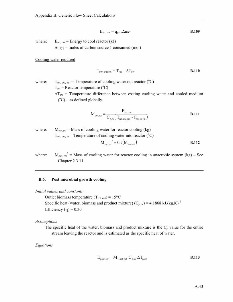
Appendix B: Generic Flow Sheet Calculations
A.43
Erct, cw = qgen.mC1 B.109
where: Erct, cw = Energy to cool reactor (kJ)
mC1 = moles of carbon source 1 consumed (mol)
Cooling water required
Tcw, out rct = Trct – Tcw B.110 where: Trct, cw, out = Temperature of cooling water out reactor (oC)
Trct = Reactor temperature (oC)
Tcw = Temperature difference between exiting cooling water and cooled medium
(oC) – as defined globally
in cw, rct,out cw, rct, wp,
cw rct,rct cw, T-T C
E M B.111
where: Mcw, rct = Mass of cooling water for reactor cooling (kg)
Trct, cw, in = Temperature of cooling water into reactor (oC)
rct cw,*
rct cw, M0.7 M B.112
where: Mcw, rct
* = Mass of cooling water for reactor cooling in anaerobic system (kg) – See Chapter 2.3.11.
B.6. Post microbial growth cooling
Initial values and constants Outlet biomass temperature (Trct, out) = 15°C Specific heat (water, biomass and product mixture) (Cp, w) = 4.1868 kJ.(kg.K)-1
Efficiency () = 0.30
Assumptions The specific heat of the water, biomass and product mixture is the Cp value for the entire
stream leaving the reactor and is estimated as the specific heat of water.
Equations
post wp,out rct, T,cw post, T..CM E B.113

Appendix B: Generic Flow Sheet Calculations
A.44
where: Epost, cw = Energy removal required to cool mass out reactor (kJ) MT, rct, out = Total mass leaving the reactor (kg)
Tpost = Temperature difference of cooled media (oC)
post
cw post,comp post, η
E E B.114
where: Epost, comp = Energy to compress coolant for post microbial growth cooling (kJ)
post = Compression efficiency for compression of coolant in post microbial cooling
B.7. Agitation
Assumptions Fully baffled, Newtonian fluid behaviour. Typically greater than 95 % of the liquid volume in the reactor is water, with unreacted raw
material volume being negligible. Initial values and constants
Number of tanks (Nt): 5 Ratio of tank height to tank diameter (Ht/Dt): 2 Impeller speed (N): 500 rpm Number of impeller blades (b): Pitch-blade turbine, paddle turbine: 4 Rushton turbine, bar turbine, radial turbine, ‘other’ turbine: 6 Ratio of impeller diameter to tank diameter (Dimp/Dt): 3 Ratio of impeller blade width to tank height (Wimp/Ht): 0.025
Efficiency (ag): 0.7
Residence time (rct): [As calculated in Equations B.95 or B.96]
Table B.12: Dimensionless power numbers for agitation for various impeller types
Impeller type (Pitch)
Commercial impeller name Number of impeller blades
Impeller diameter/ Tank diameter
Width of baffle/ Tank diameter
Power number
Reference
b Dimp/Dt B/Dt Np
Pitch-blade turbine
Chemineer-P4, Lightnin A200
4 1.27 [7]
Paddle turbine
Lightnin R200 4 3.4 [5]
Rushton
turbine
3 0.33 0.083 3.3 [6]

Appendix B: Generic Flow Sheet Calculations
A.45
Impeller type (Pitch)
Commercial impeller name Number of impeller blades
Impeller diameter/ Tank diameter
Width of baffle/ Tank diameter
Power number
Reference
b Dimp/Dt B/Dt Np
3 0.33 0.1 3.4 [6]
4 0.33 0.083 4.3 [6]
4 0.33 0.1 4.4 [6]
5 0.33 0.083 5.4 [6]
5 0.33 0.1 5.4 [6]
6 5.2 [6]
Chemineer D-6, Lightnin R100, Hayward Gordon RT
6 0.33 0.083 6 [6]
6 0.33 0.1 6 [6]
8 0.33 0.083 7.8 [6]
8 0.33 0.1 7.8 [6]
12 0.33 0.083 9.9 [6]
12 0.33 0.1 10 [6]
Marine propeller
(1.00)
Chemineer AP-3,
Lightnin A100 & A110
3 0.35 0.1 0.32 [6]
(1.00) 3 0.35 0.083 0.31 [6]
(1.00) 3 0.22 0.1 0.36 [6]
(1.00) 3 0.22 0.083 0.35 [6]
(1.50) 3 0.22 0.1 0.62 [6]
(1.50) 3 0.22 0.083 0.61 [6]
(2.00) 3 0.31 0.1 1 [6]
(2.00) 3 0.31 0.083 0.99 [6]
(2.50) 3 0.22 0.1 1.35 [6]
(2.50) 3 0.22 0.083 1.34 [6]
Axial flow impeller
Lightnin A310 & A510 3 0.3 [7]
Chemineer HE-3 3 0.4 0.22 [3]
Lightnin A320 & A340 3 0.64 [8]
Lightnin A315 & A345 3 0.75 [9]
Radial turbine
Chemineer CD-6, Lightnin R130, Philadelphia Mixers Smith Turbine, Hayward
Gordon RDC
6 3.2 [4]
Chemineer BT-6 6 2.3 [1]
Bar turbine Lightnin R510 6 0.65 [7]
Saw tooth dispenser
Lightnin R500 0.45 [7]
Anchor 0.35 [2]
Helical ribbon
0.35 [2]
OTHER 4.7 0.3 0.1 2.9
References:
[1] Bakker 2000 [2] Doran 1997 [3] Fasano et al. 1999
[4] Philadelphia Mixers 2006 [5] Post Mixing 2006 [6] Rushton et al. 1950
[7] Weetman and Oldshue 1988 [8] Weetman and Coyle 1989 [9] Weetman 1993
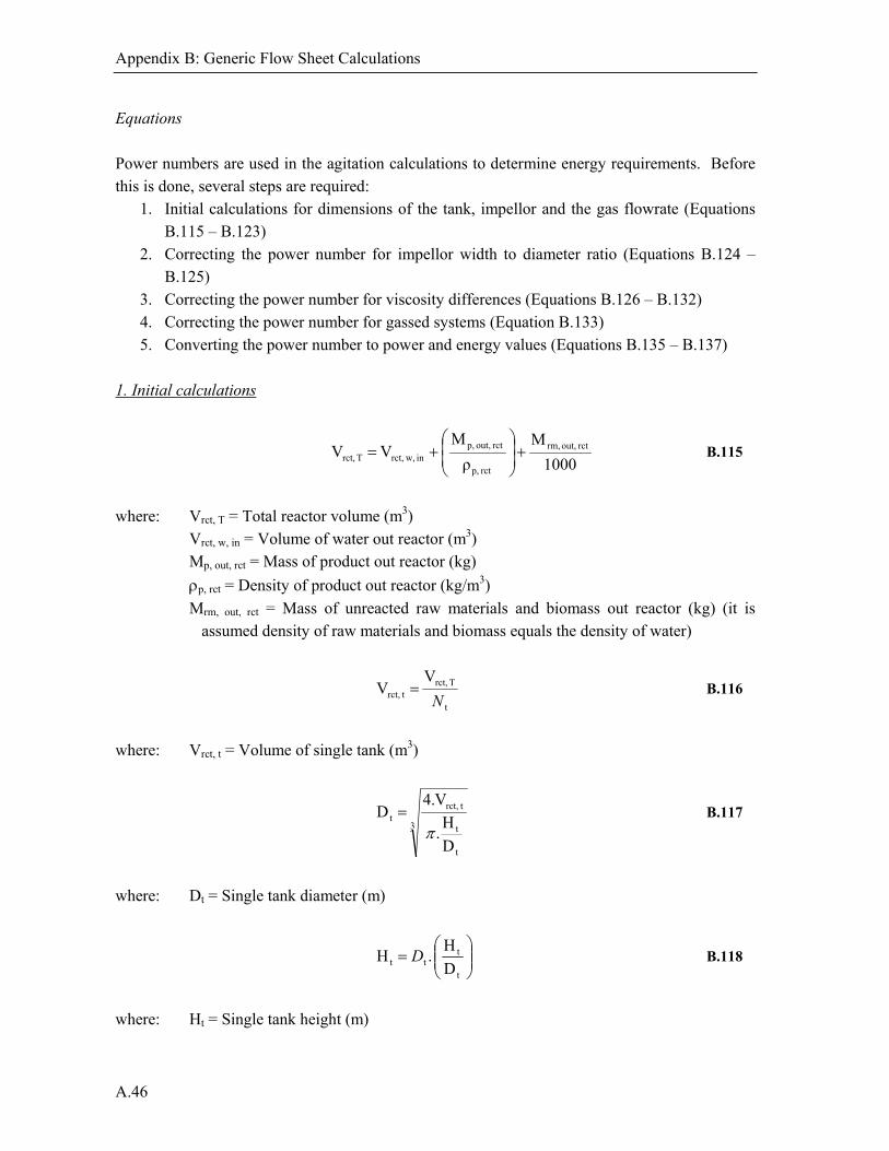
Appendix B: Generic Flow Sheet Calculations
A.46
Equations Power numbers are used in the agitation calculations to determine energy requirements. Before this is done, several steps are required:
1. Initial calculations for dimensions of the tank, impellor and the gas flowrate (Equations B.115 – B.123)
2. Correcting the power number for impellor width to diameter ratio (Equations B.124 – B.125)
3. Correcting the power number for viscosity differences (Equations B.126 – B.132) 4. Correcting the power number for gassed systems (Equation B.133) 5. Converting the power number to power and energy values (Equations B.135 – B.137)
1. Initial calculations
1000
M
ρ
M V V rct out, rm,
rct p,
rct out, p,in w,rct,T rct,
B.115
where: Vrct, T = Total reactor volume (m3)
Vrct, w, in = Volume of water out reactor (m3) Mp, out, rct = Mass of product out reactor (kg)
p, rct = Density of product out reactor (kg/m3)
Mrm, out, rct = Mass of unreacted raw materials and biomass out reactor (kg) (it is assumed density of raw materials and biomass equals the density of water)
t
T rct, trct,
V V
N B.116
where: Vrct, t = Volume of single tank (m3)
3
t
t
trct,t
D
H.
V.4 D
B.117
where: Dt = Single tank diameter (m)
t
ttt D
H . H D B.118
where: Ht = Single tank height (m)

Appendix B: Generic Flow Sheet Calculations
A.47
t
imptimp D
D .DD B.119
where: Dimp = Impeller diameter (m)
t
imptimp H
W.H W B.120
where: Wimp = Impeller blade width (m)
rct out, w,rct out, p,
rct out, p,
rct out, w,wrct out, p,T rct,
V ρ
M
Vρ Mρ
B.121
where: rct, T = Overall density of material in reactor (kg/m3)
Mp, out, rct = Mass of product out reactor (kg) Vw, out, rct = Volume of water out reactor (kg)
= Density of water (1000 kg/m3)
p, out, rct = Density of product out reactor (kg/m3)
Assumption: Density calculation based on water and product masses and volumes only. Change on volume owing to mixing is assumed negligible.
P
.R.TmV arct g,
rct g, B.122
where: Vg, rct = Volume of gas for aeration in reactor (m3)
mg, rct = Number of moles gas in reactor for aeration (mol) R = Gas constant (kJ.(kg.K)-1) Ta = Ambient temperature (oC) Pcomp, g, rct = Compressed gas pressure in reactor (kPa)
trct
rct g,t .τ
V Q
N B.123
where: Qt = Volumetric gas flow rate per tank (kg/s)

Appendix B: Generic Flow Sheet Calculations
A.48
2. Correcting for Wimp/Dimp ratio To correct for different width to diameter ratios of impellor blades, the following equations are used:
4 blade impellers:
D
W
D
W
N N
25.1
refimp
imp
actimp
imp
pp *
B.124
6 blade impellers:
refimp
imp
actimp
imp
pp
D
W
D
W
N N * B.125
where: Np = Power number
Np* = Old power number
(Wimp/Dimp)act = Original Wimp/Dimp ratio (Wimp/Dimp)ref = [Reference Wimp/Dimp ratio] given by:
- Pitch-blade turbine, paddle turbine: 1/6 (Dickey 1984) - Rushton turbine: 1/5 (Dickey 1984) - All other turbines not corrected for Wimp/Dimp differences.
3. Correcting for viscosity differences It is seen that viscosity does not play a part in the power number in the model. This is because the Reynolds number (NRe) is greater than 3500. Dickey (1984) showed that viscosity only affects power numbers for Reynolds number values less than 1000. Therefore, since the Reynolds number of 3500 is for conservative conditions, and expected to increase under other operating parameters, viscosity effects are assumed not to play a part in agitation energy requirements. Below is the calculation to show this why NRe is above 1000. The density of microbial biomass is typically in the order of 1100 kg.m-3 (Krijgsman 1992). This can vary from 1003 kg.m-3 in fungi, to 1030 kg.m-3 in bacteria, up to 1090 kg.m-3 in yeast cells (Aiba et al. 1965).
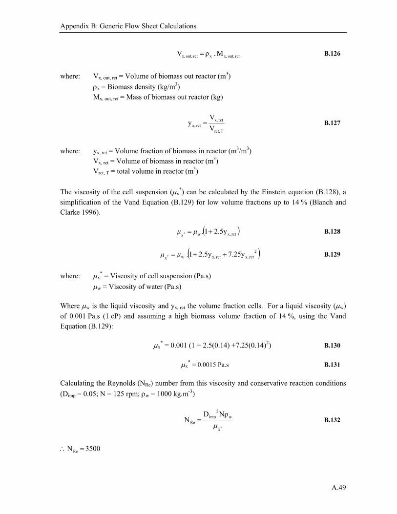
Appendix B: Generic Flow Sheet Calculations
A.49
rct out, x,xrct out, x, M . ρ V B.126
where: Vx, out, rct = Volume of biomass out reactor (m3)
x = Biomass density (kg/m3)
Mx, out, rct = Mass of biomass out reactor (kg)
T rct,
rct x,rct x, V
V y B.127
where: yx, rct = Volume fraction of biomass in reactor (m3/m3)
Vx, rct = Volume of biomass in reactor (m3) Vrct, T = total volume in reactor (m3)
The viscosity of the cell suspension (x*) can be calculated by the Einstein equation (B.128), a
simplification of the Vand Equation (B.129) for low volume fractions up to 14 % (Blanch and Clarke 1996).
rct x,wx2.5y 1. * μμ B.128
2rct x,rct x,wx
7.25y2.5y 1. * μμ B.129
where: x* = Viscosity of cell suspension (Pa.s)
w = Viscosity of water (Pa.s)
Where w is the liquid viscosity and yx, rct the volume fraction cells. For a liquid viscosity (w)
of 0.001 Pa.s (1 cP) and assuming a high biomass volume fraction of 14 %, using the Vand Equation (B.129):
x* = 0.001 (1 + 2.5(0.14) +7.25(0.14)2) B.130
x* = 0.0015 Pa.s B.131
Calculating the Reynolds (NRe) number from this viscosity and conservative reaction conditions
(Dimp = 0.05; N = 125 rpm; w = 1000 kg.m-3)
*x
w2
impRe
NρD N
B.132
3500 N Re
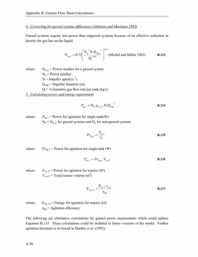
Appendix B: Generic Flow Sheet Calculations
A.50
4. Correcting for gassed systems differences (Atkinson and Mavituna 1983)
Gassed systems require less power than ungassed systems because of an effective reduction in density the gas has on the liquid.
0.45
0.56t
3imp
2p
g p,Q
N.DN0.72 N
(Michel and Miller 1962) B.133
where: Np, g' = Power number for a gassed system Np = Power number N = Impeller speed (s-1) Dimp = Impeller diameter (m) Qt = Volumetric gas flow rate per tank (kg/s)
5. Calculating power and energy requirement
3impT rct,p tag, .N.D.ρN P B.134
where: Pag, t = Power for agitation for single tank(W)
Np = Np, g' for gassed systems and Np for non-gassed systems
t
tag, tag, V
P
Pv B.135
where: Pvag, t = Power for agitation for single tank (W)
Trct, tag,T rct, .V PvP B.136
where: Prct, T = Power for agitation for reactor (W)
Vrct, T = Total reactor volume (m3)
ag
rctT rct,rct ag, η
.τP E B.137
where: Eag, rct = Energy for agitation for reactor (kJ)
ag = Agitation efficiency
The following are alternative correlations for gassed power requirements which could replace Equation B.133. These correlations could be included in future versions of the model. Further agitation literature is reviewed in Harnby et al. (1992).
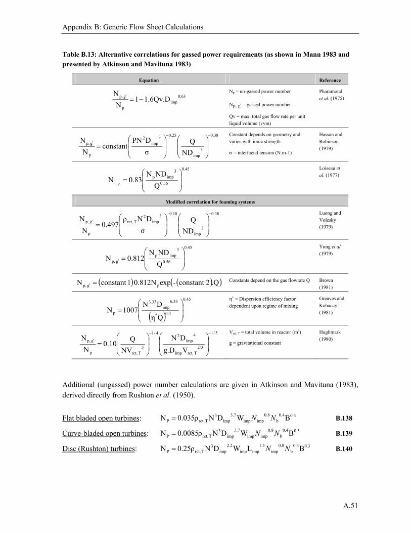
Appendix B: Generic Flow Sheet Calculations
A.51
Table B.13: Alternative correlations for gassed power requirements (as shown in Mann 1983 and presented by Atkinson and Mavituna 1983)
Equation Reference
0.63imp
p
g p, 1.6Qv.D 1 N
N
Np = un-gassed power number
Np, g' = gassed power number
Qv = max. total gas flow rate per unit liquid volume (vvm)
Pharamond et al. (1975)
0.38
3imp
0.253imp
2
p
g p,
ND
Q
σ
DPNconstant
N
N
Constant depends on geometry and varies with ionic strength
= interfacial tension (N.m-1)
Hassan and Robinson (1979)
0.45
0.56
3impp
Q
NDN0.83 N
g p,
Loiseau et
al. (1977)
Modified correlation for foaming systems
0.38
3imp
0.183imp
2T rct,
p
g p,
ND
Q
σ
DNρ497.0
N
N
Luong and Volesky (1979)
0.45
0.56
3impp
g p, Q
NDN0.812 N
Yung et al. (1979)
.Q2constant -exp0.812N 1constant N pg p, Constants depend on the gas flowrate Q Brown
(1981)
0.45
0.4*
6.33imp
3.33
pQη
DN1007 N
= Dispersion efficiency factor
dependent upon regime of mixing
Greaves and Kobaccy (1981)
5/1
2/3T rct,imp
4imp
24/1
3T rct,p
g p,
Vg.D
DN
NV
Q10.0
N
N
Vrct, T = total volume in reactor (m3)
g = gravitational constant
Hughmark (1980)
Additional (ungassed) power number calculations are given in Atkinson and Mavituna (1983), derived directly from Rushton et al. (1950).
Flat bladed open turbines: 0.30.4b
0.8impimp
3.7imp
3T rct,P BWDNρ035.0N NN B.138
Curve-bladed open turbines: 0.30.4b
0.8impimp
3.7imp
3T rct,P BWDNρ0085.0N NN B.139
Disc (Rushton) turbines: 0.30.4b
0.8imp
1.5impimp
2.2imp
3T rct,P BLWDNρ25.0N NN B.140

Appendix B: Generic Flow Sheet Calculations
A.52
where: Np = Power number
rct, T = Overall density of material in reactor (kg/m3)
N = Impeller speed (s-1) Dimp = Impeller diameter (m) Wimp = Impeller width (m) Limp = Impeller length (m) Nimp = Number of impeller blades Nb = Number of baffles B = Baffle width (m) Limp = Impeller length (m)
B.8. Solid-Liquid Separation
Initial values
Solid or product (mass) fraction removed from solid-liquid separation unit x (wsol, sepx): Centrifugal spin/washing = 0.98 Filtration = 0.95 Sedimentation = 0.90 OTHER = 0.94
Liquid or waste (mass) fraction removed from solid-liquid separation unit x (wl, sepx): Centrifugal spin/washing = 0.80 Filtration = 0.70 Sedimentation = 0.60 OTHER = 0.70
Equations The fraction of a component removed depends on the component and product phase. Water (Solid-liquid separation unit 1) is given as an example in Equations B.141 and B.142 for wastewater (liquid) removal with a solid product.
Mw, out, sepx = Mw, in, sepx.(1 – wl, sepx) B.141 where: Mw, out, sepx = Mass of water out of solid-liquid separation unit x (kg)
Mw, in, sepx = Mass of water into solid-liquid separation unit x (kg) wl, sepx = Liquid (mass) fraction removed from solid-liquid separation unit x (kg/kg)

Appendix B: Generic Flow Sheet Calculations
A.53
Mw, in, sepx = Mw, out, rct B.142 where: Mw, out, rct = Mass of water out of reactor (kg)
Centrifugal spin/washing Initial values and constants
Number of spin/wash cycles in solid-liquid separation unit x (Nsp, sepx) = 2
Efficiency of centrifugation in solid-liquid separation unit x (cen, sepx) = 0.6
Energy per unit volume for centrifugation in solid-liquid separation unit x (Êcen, sepx) = [As
selected from Table B.14]
Table B.14: Energy per unit volume values as used in model for different centrifuge types
Centrifuge type Energy needed (Êcen, sepx)
kWh/1000gal kJ/m3
min. max. min. max. Average Value used
Tubular 1 10 951.0 9510.2 5230.6 5230
Disk 1 10 951.0 9510.2 5230.6 5230
Nozzle-discharge disk 2 12 1902.0 11412.2 6657.1 6660
Helical-conveyor decanter 3 15 2853.1 14265.3 8559.2 8560
Other 1664.3 11174.5 6419.4 6420
Reference: Perry et al. 1984
Equations
1000
M
ρ
M V V sepx out, rm,
sepx p,
sepx out, p,in w,sepx,T sepx,
B.143
where: Vsepx, T = Total volume of solid-liquid separation unit x (m3)
Vsepx, w, in = Volume of water in solid-liquid separation unit x (m3) Mp, out, sepx = Mass of product out solid-liquid separation unit x (kg)
p, sepx = Density of product out solid-liquid separation unit x (kg/m3)
Mrm, out, sepx = Mass of unreacted raw materials and biomass out solid-liquid separation unit x (kg) (it is assumed density of raw materials and biomass equals the density of water 1000 kg/m3)

Appendix B: Generic Flow Sheet Calculations
A.54
sepx cen,
sepx cen,
^
T sepx,sepx cen, η
E.VE B.144
where: Ecen, sepx = Energy requirement for centrifugation in solid-liquid separation unit x (kJ)
sepx sol,
sepx sol,sepx sol,
sepx out, p,sepx in, p,
w1
w1.w-11
MM
sepx sp,N B.145
where: Mp, in, sepx = Mass of product into solid-liquid separation unit x (kg)
Mp, out, sepx = Mass of product out of solid-liquid separation unit x (kg) wsol, sepx = Solid (mass) fraction removed from solid-liquid separation unit x (kg/kg) Nsp, sepx = Number of spin/wash cycles in solid-liquid separation unit x
p, sepx = Mp, in, sepx – Mp, out, sepx B.146
where: p, sepx = Mass of product lost in solid-liquid separation unit x (kg)
Mw, sepx = Mw, out, sepx.Nsp, sepx B.147
where: p, sepx = Mass of water lost in solid-liquid separation unit x (kg)
Mw, out, sepx = Mass of product lost in solid-liquid separation unit x (kg)
Mw, ad, sepx = Mw, out, sepx.(Nsp, sepx – 1) B.148 where: Mw, ad, sepx = Mass of water added in solid-liquid separation unit x to make up for
spin/wash cycles of centrifugation (kg)
Filtration Initial values and constants
Pressure difference of filtration in solid-liquid separation unit x (Pf, sepx) = 250 kPa
Flux of filtration in solid-liquid separation unit x (Jf, sepx) = 10 kg.s-1
Pumping efficiency of filtration in solid-liquid separation unit x (f, sepx) = 0.6
Volume fraction flocculent in solid-liquid separation unit x (yfa, sepx) = 0.01
Density of flocculent in solid-liquid separation unit x (fa, sepx) = [As selected from Table
B.15]
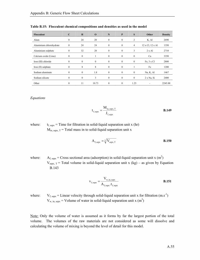
Appendix B: Generic Flow Sheet Calculations
A.55
Table B.15: Flocculent chemical compositions and densities as used in the model
Flocculent C H O N P S Other Density
Alum 0 24 20 0 0 2 K, Al 2690
Aluminium chlorohydrate 0 24 24 0 0 4 12 x Cl, 12 x Al 1350
Aluminium sulphate 0 32 28 0 0 3 2 x Al 2710
Calcium oxide (Lime) 0 0 1 0 0 0 Ca 3350
Iron (III) chloride 0 0 0 0 0 0 Fe, 3 x Cl 2800
Iron (II) sulphate 0 8 8 0 0 1 Fe 1200
Sodium aluminate 0 0 1.8 0 0 0 Na, K, Al 1467
Sodium silicate 0 0 3 0 0 0 2 x Na, Si 2400
Other 0 11 10.73 0 0 1.25 - 2245.88
Equations
sepx f,
T sepx, in,sepx f, J
Mt B.149
where: tf, sepx = Time for filtration in solid-liquid separation unit x (hr)
Min, sepx, T = Total mass in to solid-liquid separation unit x
3T sepx,sepx f, V A B.150
where: Af, sepx = Cross sectional area (adsorption) in solid-liquid separation unit x (m2)
Vsepx, T = Total volume in solid-liquid separation unit x (kg) – as given by Equation B.143
sepx f,sepx f,
sepx in, w,sepx f, .tA
V v B.151
where: Vf, sepx = Linear velocity through solid-liquid separation unit x for filtration (m.s-1)
Vw, in, sepx = Volume of water in solid-liquid separation unit x (m3) Note: Only the volume of water is assumed as it forms by far the largest portion of the total volume. The volumes of the raw materials are not considered as some will dissolve and calculating the volume of mixing is beyond the level of detail for this model.
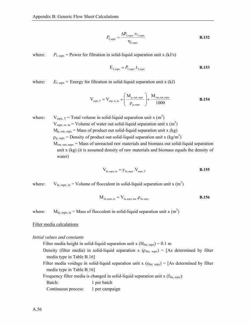
Appendix B: Generic Flow Sheet Calculations
A.56
sepx f,
sepx f,sepx f,sepx f, η
.vP
P B.152
where: Pf, sepx = Power for filtration in solid-liquid separation unit x (kJ/s)
sepx f,sepx f,sepx f, .t E P B.153
where: Ef, sepx = Energy for filtration in solid-liquid separation unit x (kJ)
1000
M
ρ
M V V sepx out, rm,
sepx p,
sepx out, p,in w,sep,T sepx,
B.154
where: Vsepx, T = Total volume in solid-liquid separation unit x (m3)
Vsepx, w, in = Volume of water out solid-liquid separation unit x (m3) Mp, out, sepx = Mass of product out solid-liquid separation unit x (kg)
p, sepx = Density of product out solid-liquid separation unit x (kg/m3)
Mrm, out, sepx = Mass of unreacted raw materials and biomass out solid-liquid separation unit x (kg) (it is assumed density of raw materials and biomass equals the density of water)
T sepx,sepx fa,in sepx, fa, .Vy V B.155
where: Vfa, sepx, in = Volume of flocculent in solid-liquid separation unit x (m3)
sepx fa,ina sepx, fa,in sepx, fa, .ρVM B.156
where: Mfa, sepx, in = Mass of flocculent in solid-liquid separation unit x (m3) Filter media calculations Initial values and constants
Filter media height in solid-liquid separation unit x (Hfm, sepx) = 0.1 m
Density (filter media) in solid-liquid separation x (fm, sepx) = [As determined by filter
media type in Table B.16] Filter media voidage in solid-liquid separation unit x (efm, sepx) = [As determined by filter
media type in Table B.16] Frequency filter media is changed in solid-liquid separation unit x (ffm, sepx): Batch: 1 per batch Continuous process: 1 per campaign
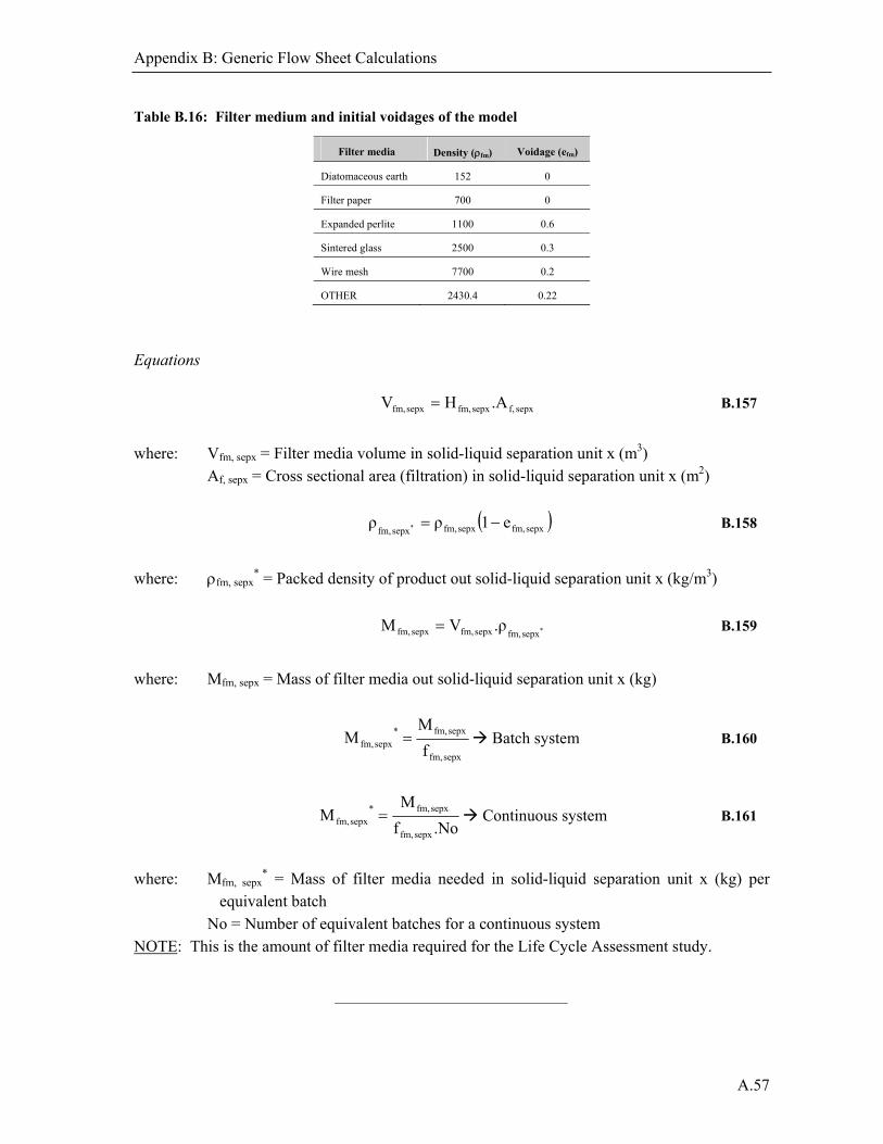
Appendix B: Generic Flow Sheet Calculations
A.57
Table B.16: Filter medium and initial voidages of the model
Filter media Density (fm) Voidage (efm)
Diatomaceous earth 152 0
Filter paper 700 0
Expanded perlite 1100 0.6
Sintered glass 2500 0.3
Wire mesh 7700 0.2
OTHER 2430.4 0.22
Equations
sepx f,sepx fm,sepx fm, .AHV B.157
where: Vfm, sepx = Filter media volume in solid-liquid separation unit x (m3)
Af, sepx = Cross sectional area (filtration) in solid-liquid separation unit x (m2)
sepx fm,sepx fm,sepx fm,e1ρρ * B.158
where: fm, sepx
* = Packed density of product out solid-liquid separation unit x (kg/m3)
*sepx fm,sepx fm,sepx fm, .ρVM B.159
where: Mfm, sepx = Mass of filter media out solid-liquid separation unit x (kg)
sepx fm,
sepx fm,*sepx fm, f
M M Batch system B.160
.Nof
M M
sepx fm,
sepx fm,*sepx fm, Continuous system B.161
where: Mfm, sepx
* = Mass of filter media needed in solid-liquid separation unit x (kg) per equivalent batch
No = Number of equivalent batches for a continuous system NOTE: This is the amount of filter media required for the Life Cycle Assessment study.

Appendix B: Generic Flow Sheet Calculations
A.58
Sedimentation
Assumptions No energy needed.
A flocculent can be added as in filtration for solid-liquid separation (Table B.15).
Other Separation Initial values
Specific energy (other) for solid-liquid separation unit x (Êsepx, o) = 500 MJ/m3 (a representative value for all solid-liquid separation units)
Equations
in sepx, w,o sepx,o sepx, .VE E
B.162
where: Esepx, o = Other energy for solid-liquid separation unit x (MJ)
Vw, sepx, in = Volume of water in solid-liquid separation unit x (m3)
B.9. Cell disruption
High pressure homogeniser, Cavitation, Ball Mill
Initial values Fraction product released on rupture (R/Rmax) = [As selected from Table 2.14 in Chapter 2] Biomass conc. in cell disruption (Cx, cd) = [As selected from Table 2.14 in Chapter 2]
Energy efficiency of breakage (cd) = [As selected from Table 2.14 in Chapter 2]
Equations
Intracellular product is released according to Equation B.163. Product from non-disrupted cells is treated as biomass waste.
max
cd in, p,cd out, p, /
M M
RR B.163
where: Mp, out, cd = Mass of product into cell disruption unit (kg) Mp, in, cd = Mass of product out of cell disruption unit (kg)

Appendix B: Generic Flow Sheet Calculations
A.59
cd
cd out, p,cd η
M E B.164
where: Ecd = Energy required to disrupt biomass in cell disruption unit (J)
cd = Disruption efficiency (kg/J)
Other Cell disruption
Specific energy (other) for cell disruption (Êcd, o) = 25 MJ/m3 (a representative value for all cell disruptions)
Equations
in cd, w,o cd,o cd, .VE E
B.165
where: Ecd, o = Other energy for cell disruption unit (MJ)
Vw, cd, in = Volume of water in cell disruption unit (m3)
B.10. Concentration and Purification
Initial values Solid or product (mass) fract. removed from concentration and purification unit x (wsol, cpx):
Adsorption = 1.00 Centrifugation = 0.98 Chromatography = 1.00 Evaporation = 1.00 Filtration = 0.95 Precipitation and Crystallisation= 1.00 Solvent extraction = 0.99 OTHER = 0.99
Liq. or waste (mass) fraction removed from concentration and purification unit x (wl, cpx): Adsorption = 0.00 Centrifugation = 0.80 Chromatography = 0.00 Evaporation = 0.90 Filtration = 0.95 Precipitation and Crystallisation= 0.00 Solvent extraction = 0.95 OTHER = 0.80

Appendix B: Generic Flow Sheet Calculations
A.60
Equations
[As for Equations B.141 – B.142 (solid-liquid separation). Subscripts as for concentration and purification unit x]
Additives (non-reacting and reacting) Non-reacting additives can be added in each concentration and purification step.
Initial values Volume fraction non-reacting additive in concentration and purification unit x (yadd, cpx) = 0.05
Density of non-reacting additive in concentration and purification unit x (add, cpx) = [As per
selected chemical as shown in Table B.17]
Table B.17: Possible additional reacting and non-reacting flow materials and solvents for the concentration and purification section of the model
Materials
Acetone, Acetonitrile, Alum, Amyl acetate, Anionic flocculent, Benzene, Butanol, Butyl acetate, Calcium citrate, Carbon tetrachloride, Chloroform, Cyclohexane, Cyclopentane, Dichloromethane, Diethyl ether, Ethanol, Ethyl acetate, Ferric chloride, Heptane, Hexane, Hydrochloric acid, Lime, Magnesium, Methanol, Methyl acetate, Methyl ethyl ketone
(butanone), Nitromethane, Pentane, Potassium, Propanol, Sodium, Sodium acetate, Sodium carbonate, Sodium hydroxide, Sulphuric acid, Tetrachloroethylene, Tetrahydrofuran, Toluene, Tributyl phosphate, Water, Other
Equations
1000
M
ρ
M V V cpx out, rm,
cpx p,
cpx out, p,in w,cpx,T cpx,
B.166
where: Vcpx, T = Total volume of concentration and purification unit x (m3)
Vcpx, w, in = Volume of water out concentration and purification unit x (m3) Mp, out, cpx = Mass of product out concentration and purification unit x (kg)
p, cpx = Density of product out concentration and purification unit x (kg/m3)
Mrm, out, cpx = Mass of unreacted raw materials and biomass out concentration and purification unit x (kg) (it is assumed density of raw materials and biomass equals the density of water)

Appendix B: Generic Flow Sheet Calculations
A.61
T cpx,cpx add,in cpx, add, .Vy V B.167
where: Vadd, cpx, in = Volume of additive in concentration and purification unit x (m3)
cpx add,in cpx, add,in cpx, add, .ρVM B.168
where: Madd, cpx, in = Mass of flocculent in concentration and purification unit x (m3) Additionally, two reacting chemicals can be added per concentration and purification step. These include any of those in Table B.17 or as specified by the user. Based on the stoichiometry of reaction, the amount of product and excess chemicals is calculated.
Initial values Volume fraction reacting additive x in concentration and purification unit x (yrax, cpx) = 0.25 Conversion rate of limiting additive in concentration and purification unit x (Xrax, cpx) = 80 %
K Cu Al Si Ca Mg Fe Na Cl PO SO N OH O CO
chemical Modified bproduct Reaction aproduct Reaction
chemical Existing bReactant aReactant
2422222
cpxcpxcpx
cpxcpxcpx
B.169
Solving the material balances for all chemicals in Equation B.169 yields the number of moles required for reaction. Taking the conversion (Xrax, cpx) rate into account, this value scaled for the number of moles of existing chemical available and converted to mass.
i cpx, rax,
i cpx, rax,i cpx, rax, Mm
M m B.170
where: mrax, cpx, i = Number of moles component i from reaction in concentration and
purification unit x (kmol) Mrax, cpx, i = Mass of component i from reaction in concentration and purification unit
x (kg) Mmrax, cpx, i = Molar mass of component i from reaction in concentration and
purification unit x (kg/kmol)

Appendix B: Generic Flow Sheet Calculations
A.62
Adsorption
Initial values
Pressure difference for adsorption in concentration and purification unit x (Pads, cpx) =
250 kPa
Pumping efficiency for adsorption in concentration and purification unit x (ads, cpx) = 0.6
Time basis for adsorption in concentration and purification unit x (tads, cpx) = 1 s Note: Time basis immaterial as unit of time cancels out through calculation
Equations
3
2
T cpx,cpx ads, L/D
V A
B.171
where: Aads, cpx = Cross sectional area (adsorption) in concentration and purification unit x
L/D (Length: Diameter ratio) = 3; except freeze drying; L/D = 6 Vcpx, T = Total volume in concentration and purification unit x (kg) – as given by
Equation B.166
cpx ads,cpx ads,
cpx in, w,cpx ads, .tA
V v B.172
where: Vads, cpx = Linear velocity through adsorption in conc. and purification unit x (m.s-1)
Vw, in, cpx = Volume of water in concentration and purification unit x (m3) Note: Only the volume of water is assumed as it forms by far the largest portion of the total volume. The volumes of the raw materials are not considered as some will dissolve and calculating the volume of mixing is beyond the level of detail for this model.
cpx ads,
cpx ads,cpx ads,cpx ads, η
.vP
P B.173
where: Pads, cpx = Power for adsorption in concentration and purification unit x (kPa)
cpx ads,cpx ads,cpx ads, .t E P B.174
where: Eads, cpx = Energy for adsorption in concentration and purification unit x (kJ)
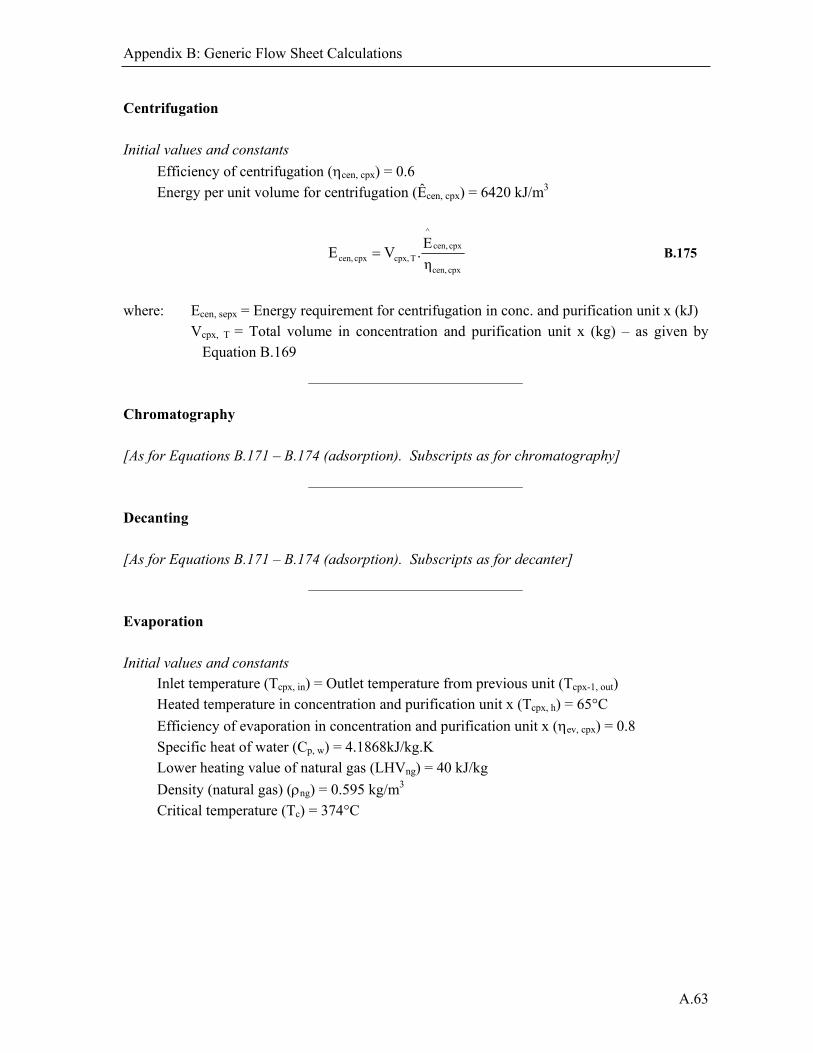
Appendix B: Generic Flow Sheet Calculations
A.63
Centrifugation
Initial values and constants
Efficiency of centrifugation (cen, cpx) = 0.6
Energy per unit volume for centrifugation (Êcen, cpx) = 6420 kJ/m3
cpx cen,
cpx cen,
^
T cpx,cpx cen, η
E.VE B.175
where: Ecen, sepx = Energy requirement for centrifugation in conc. and purification unit x (kJ)
Vcpx, T = Total volume in concentration and purification unit x (kg) – as given by Equation B.169
Chromatography
[As for Equations B.171 – B.174 (adsorption). Subscripts as for chromatography]
Decanting [As for Equations B.171 – B.174 (adsorption). Subscripts as for decanter] Evaporation Initial values and constants
Inlet temperature (Tcpx, in) = Outlet temperature from previous unit (Tcpx-1, out) Heated temperature in concentration and purification unit x (Tcpx, h) = 65°C
Efficiency of evaporation in concentration and purification unit x (ev, cpx) = 0.8
Specific heat of water (Cp, w) = 4.1868kJ/kg.K Lower heating value of natural gas (LHVng) = 40 kJ/kg
Density (natural gas) (ng) = 0.595 kg/m3
Critical temperature (Tc) = 374°C
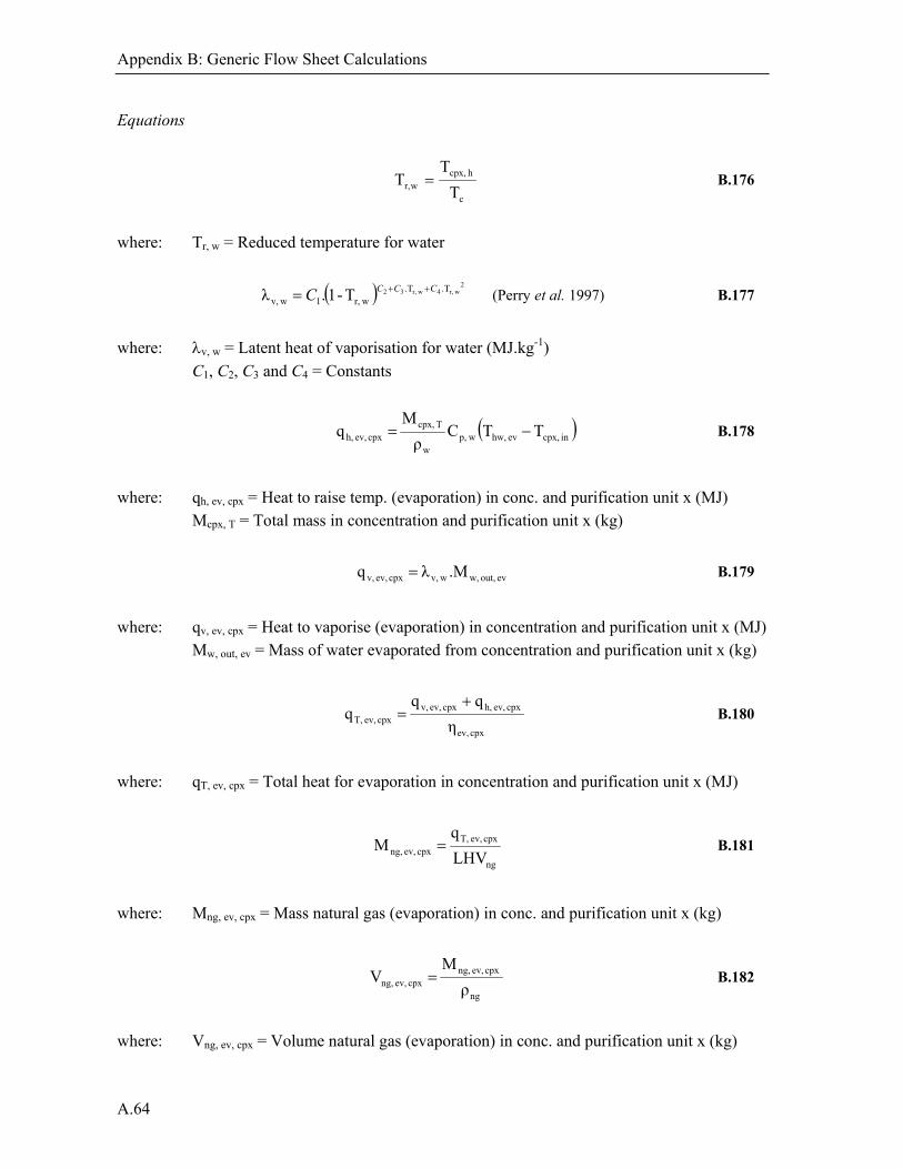
Appendix B: Generic Flow Sheet Calculations
A.64
Equations
c
h cpx,wr, T
TT B.176
where: Tr, w = Reduced temperature for water
2 wr,4 wr,32 .T.T
wr,1 wv, T-1. λ CCCC (Perry et al. 1997) B.177
where: v, w = Latent heat of vaporisation for water (MJ.kg-1)
C1, C2, C3 and C4 = Constants
in cpx,ev hw, wp,w
T cpx,cpx ev, h, TTC
ρ
M q B.178
where: qh, ev, cpx = Heat to raise temp. (evaporation) in conc. and purification unit x (MJ)
Mcpx, T = Total mass in concentration and purification unit x (kg)
ev out, w, wv,cpx ev, v, .Mλ q B.179
where: qv, ev, cpx = Heat to vaporise (evaporation) in concentration and purification unit x (MJ)
Mw, out, ev = Mass of water evaporated from concentration and purification unit x (kg)
cpx ev,
cpx ev, h,cpx ev, v,cpx ev, T, η
q q q
B.180
where: qT, ev, cpx = Total heat for evaporation in concentration and purification unit x (MJ)
ng
cpx ev, T,cpx ev, ng, LHV
q M B.181
where: Mng, ev, cpx = Mass natural gas (evaporation) in conc. and purification unit x (kg)
ng
cpx ev, ng,cpx ev, ng, ρ
M V B.182
where: Vng, ev, cpx = Volume natural gas (evaporation) in conc. and purification unit x (kg)
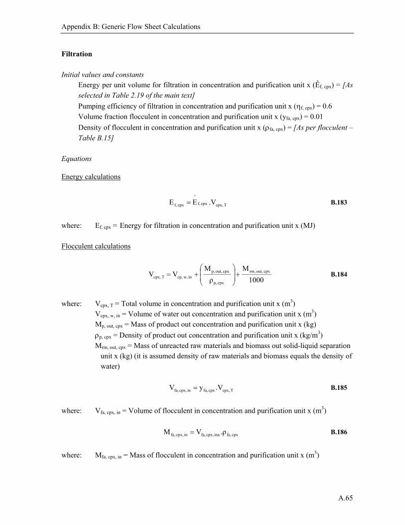
Appendix B: Generic Flow Sheet Calculations
A.65
Filtration
Initial values and constants Energy per unit volume for filtration in concentration and purification unit x (Êf, cpx) = [As selected in Table 2.19 of the main text]
Pumping efficiency of filtration in concentration and purification unit x (f, cpx) = 0.6
Volume fraction flocculent in concentration and purification unit x (yfa, cpx) = 0.01
Density of flocculent in concentration and purification unit x (fa, cpx) = [As per flocculent –
Table B.15] Equations
Energy calculations
T cpx,cpx f,
^
cpx f, .VE E B.183
where: Ef, cpx = Energy for filtration in concentration and purification unit x (MJ) Flocculent calculations
1000
M
ρ
M V V cpx out, rm,
cpx p,
cpx out, p,in w,cp,T cpx,
B.184
where: Vcpx, T = Total volume in concentration and purification unit x (m3)
Vcpx, w, in = Volume of water out concentration and purification unit x (m3) Mp, out, cpx = Mass of product out concentration and purification unit x (kg)
p, cpx = Density of product out concentration and purification unit x (kg/m3)
Mrm, out, cpx = Mass of unreacted raw materials and biomass out solid-liquid separation unit x (kg) (it is assumed density of raw materials and biomass equals the density of water)
T cpx,cpx fa,in cpx, fa, .Vy V B.185
where: Vfa, cpx, in = Volume of flocculent in concentration and purification unit x (m3)
cpx fa,ina cpx, fa,in cpx, fa, .ρVM B.186
where: Mfa, cpx, in = Mass of flocculent in concentration and purification unit x (m3)

Appendix B: Generic Flow Sheet Calculations
A.66
Filter media calculations
[As for Equations B.157 – B.161 (filtration in solid-liquid separation unit x). Subscripts as for concentration and purification unit x] Diafiltration calculations Initial values
Vol. frac. diafiltration soln added (conc. and purification unit x) (ydfs, cpx) = 0.25 %v/v Mole frac. diafiltration salt in soln (conc. and purification unit x) (xdf, cpx) = 25 mmol/l
Equations
T cpx,cpx dfs,cpx dfw, .Vy V B.187
where: Vdfw, cpx = Volume of diafiltration water in concentration and purification unit x (m3)
Vcpx, T = Total volume in concentration and purification unit x (kg) – as given by Equation B.166
cpx df,cpx dfw,cpx df, .xVm B.188
where: mdf, cpx = Number of moles diafiltration salt in concentration and purification unit x (m3)
1000
massmolar .mMsalt ion diafiltrat Mass dfdf B.189
Precipitation and Crystallisation
Initial values and constants
Inlet temperature (Tcpx, in) = Outlet temperature from previous unit (Tcpx-1, in) Heated temperature in concentration and purification unit x (Tcpx, h) = 55°C Outlet temperature in concentration and purification unit x (Tcpx, o) = 40°C
Efficiency of precipitation in concentration and purification unit x (prec, cpx) = 0.8
Residence time for precipitation in concentration and purification unit x (prec, cpx) = 2 h
Power per unit vol. (precipitation) in conc. and purification unit x (Pvcpx) = 0.8 kW/m3 Cooling or chilled water temperature (Tcw, prec) = [As for global initial values]

Appendix B: Generic Flow Sheet Calculations
A.67
Max. temp. diff. between exiting cooling water and hot inlet streams (Tmax, cw) = [As for
global initial values]
Latent heat (steam) (St) = 2.7 MJ/kg
Specific heat of water (Cp, w) = 4.1868kJ/kg.K
Density of product (p, prec) = [As determined by product choice in Table B.3]
Equations
Cooling water outlet temperature (To) = Th – Tm B.190
Agitation energy
[As for Equations B.136 – B.137 (agitation). Subscripts as for precipitation and concentration
and purification unit x.]
Steam requirements
[As for Equations B.5 – B.13 (steam sterilisation). Subscripts as for precipitation and
concentration and purification unit x.]
Cooling water requirements
[As for Equations B.15 – B.16 (steam sterilisation). Subscripts as for precipitation and
concentration and purification unit x.]
Solvent extraction
[As for Equations B.171 – B.174 (adsorption). Subscripts as for solvent extraction]
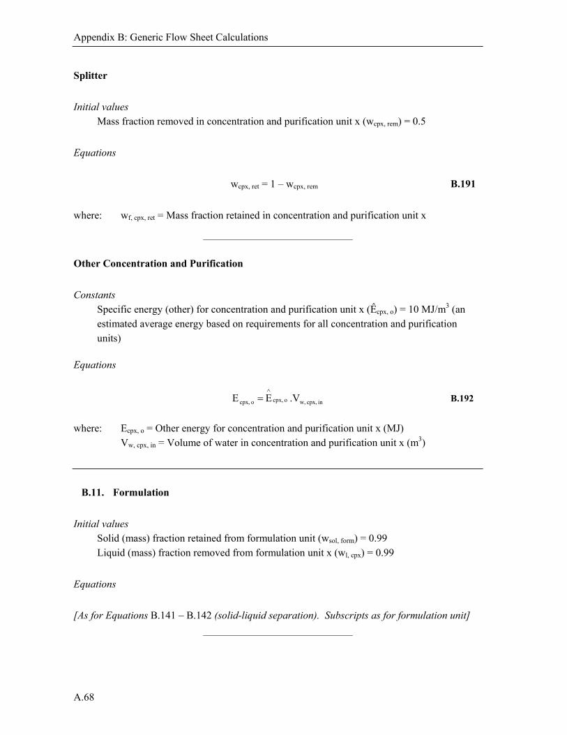
Appendix B: Generic Flow Sheet Calculations
A.68
Splitter
Initial values
Mass fraction removed in concentration and purification unit x (wcpx, rem) = 0.5
Equations
wcpx, ret = 1 – wcpx, rem B.191
where: wf, cpx, ret = Mass fraction retained in concentration and purification unit x
Other Concentration and Purification
Constants
Specific energy (other) for concentration and purification unit x (Êcpx, o) = 10 MJ/m3 (an estimated average energy based on requirements for all concentration and purification units)
Equations
in cpx, w,o cpx,o cpx, .VE E
B.192
where: Ecpx, o = Other energy for concentration and purification unit x (MJ) Vw, cpx, in = Volume of water in concentration and purification unit x (m3)
B.11. Formulation
Initial values
Solid (mass) fraction retained from formulation unit (wsol, form) = 0.99 Liquid (mass) fraction removed from formulation unit x (wl, cpx) = 0.99
Equations
[As for Equations B.141 – B.142 (solid-liquid separation). Subscripts as for formulation unit]

Appendix B: Generic Flow Sheet Calculations
A.69
Oven Drying
Initial values and constants
Inlet temp. (Tform, in) = Outlet temp. from final concentration and purification unit (Tcpx, out) Heated temperature in formulation unit (Tform, h) = 65°C
Efficiency of oven drying in formulation unit (ov, form) = 0.8
Equations
[As for Equations B.176 – B.182 (evaporation). Subscripts as for oven drying and formulation]
Freeze Drying
Assumptions
The sublimation energy (Esub, fd) requires no external energy and is assumed zero The volume of the vacuum apparatus is twice that of the total volume
Initial values and constants
Inlet temp. (Tform, in) = Outlet temp. from final concentration and purification unit (Tcpx, out) Subcooled temperature for freeze drying (Tsc, fd) = -40°C Freeze dryer vacuum inlet area (Afd, in) = 0.1 m2
Efficiency (fd) = 0.8
Specific heat of water (Cp, w) = 4.1868 kJ/kg.K Specific heat of ice (Cp, ice) = 2.1 kJ/kg.K
Latent heat of freezing (fr) = 333.68 kJ/kg
Sublimation energy (Esub, fd) = 2590 kJ/kg – but assumed no external energy inputs required
Equations
Heat to cool and freeze liquid
in form,in form, T, wp,fd c, .TM .Cq B.193
where: qcw, fd = Heat to cool (freeze dryer) in formulation (kJ)
MT, form = Total mass in formulation unit (kg)
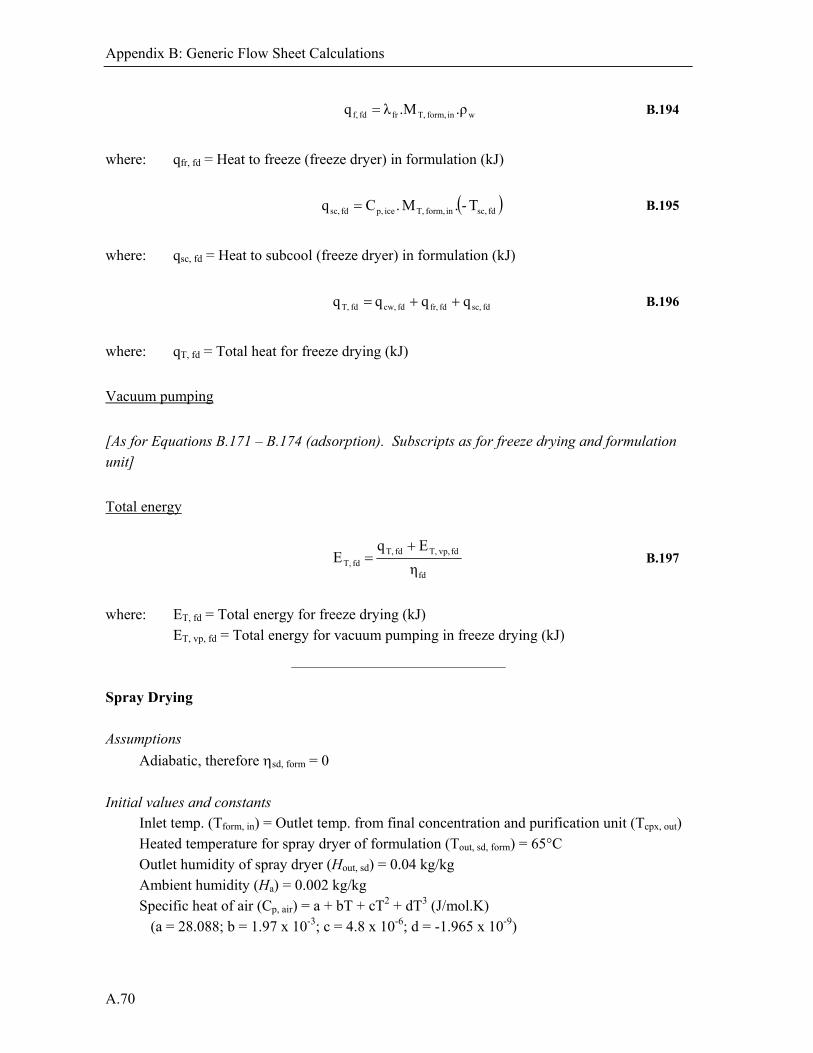
Appendix B: Generic Flow Sheet Calculations
A.70
win form, T,frfd f, .ρ.Mλ q B.194
where: qfr, fd = Heat to freeze (freeze dryer) in formulation (kJ)
fd sc,in form, T,ice p,fd sc, T-.M .Cq B.195
where: qsc, fd = Heat to subcool (freeze dryer) in formulation (kJ)
fd sc,fd fr,fd cw,fd T, q q q q B.196
where: qT, fd = Total heat for freeze drying (kJ)
Vacuum pumping
[As for Equations B.171 – B.174 (adsorption). Subscripts as for freeze drying and formulation unit]
Total energy
fd
fd vp,T,fd T,fd T, η
E q E
B.197
where: ET, fd = Total energy for freeze drying (kJ)
ET, vp, fd = Total energy for vacuum pumping in freeze drying (kJ) Spray Drying
Assumptions
Adiabatic, therefore sd, form = 0
Initial values and constants Inlet temp. (Tform, in) = Outlet temp. from final concentration and purification unit (Tcpx, out) Heated temperature for spray dryer of formulation (Tout, sd, form) = 65°C Outlet humidity of spray dryer (Hout, sd) = 0.04 kg/kg Ambient humidity (Ha) = 0.002 kg/kg Specific heat of air (Cp, air) = a + bT + cT2 + dT3 (J/mol.K)
(a = 28.088; b = 1.97 x 10⁻³; c = 4.8 x 10⁻⁶; d = -1.965 x 10⁻⁹)

Appendix B: Generic Flow Sheet Calculations
A.71
Latent heat of vaporization (v, w) = [As calculated in Equation B.177 using Tin, sd, form in
Equation B.176] Lower heating value of natural gas (LHVng) = 40 kJ/kg.
Density (natural gas) (ng) = 0.595 kg/m3
Equations
asd out,
aform sd,sd out, wv,
asd out,
in form,form sd,form sd, out,air p,form sd,
η1/0.001λ
Tη1/T0.001CE
HH
HH
HH
(Baker and McKenzie 2005) B.198
where: Êsd, form = Specific energy of spray drying in formulation (MJ/kg)
sd, form = Thermal loss factor
Since is it assumed the system is adiabatic, sd, form = 0, Equation B.198 reduces to:
wv,asd out,
in form,form sd, out,air p,form sd, 0.001λ
TT0.001CE
HH
(Keey 1992) B.199
in form, T,form sd,form sd, .ME E
B.200
where: Esd, form = Energy of spray drying in formulation (MJ)
MT, form = Total mass in spray dryer in formulation unit (kg) Volume of natural gas needed: [As given in Equations B.181 – B.182 with Esd, form as the total
energy requirement for natural gas energy.]
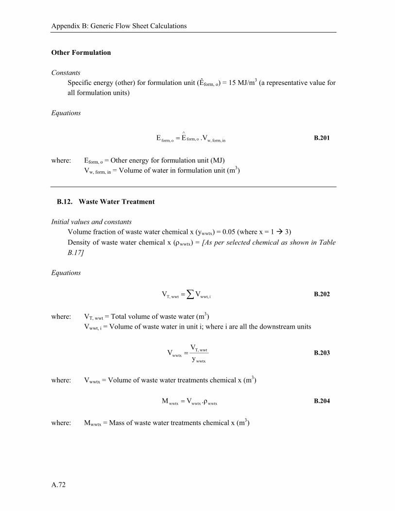
Appendix B: Generic Flow Sheet Calculations
A.72
Other Formulation
Constants Specific energy (other) for formulation unit (Êform, o) = 15 MJ/m3 (a representative value for all formulation units)
Equations
in form, w,o form,o form, .VE E
B.201
where: Eform, o = Other energy for formulation unit (MJ)
Vw, form, in = Volume of water in formulation unit (m3)
B.12. Waste Water Treatment
Initial values and constants Volume fraction of waste water chemical x (ywwtx) = 0.05 (where x = 1 3)
Density of waste water chemical x (wwtx) = [As per selected chemical as shown in Table
B.17] Equations
i wwt, wwtT, V V B.202
where: VT, wwt = Total volume of waste water (m3)
Vwwt, i = Volume of waste water in unit i; where i are all the downstream units
wwtx
wwtT,wwtx y
V V B.203
where: Vwwtx = Volume of waste water treatments chemical x (m3)
wwtxwwtxwwtx .ρV M B.204
where: Mwwtx = Mass of waste water treatments chemical x (m3)

Appendix B: Generic Flow Sheet Calculations
A.73
i
i Mm
o0.5na2.5p3s2.5nclh0.52c16StOD
(IChemE 2003)
B.205
where: StODi
* = Specific stoichiometric oxygen demand (chemical i) (kg/kg) Mmi = Molar mass substance i (kg/kmol) c, h, o, n, p, s, cl, na = Coefficients for chemical i given by: CcHhOoNnPpSsClclNana
i*
ii .MStOD StOD B.206
where: StODi = Stoichiometric oxygen demand (chemical i) (kg)
Mi = Mass of chemical i (kg)
n
1iiT StOD StOD B.207
where: StODT = Total stoichiometric oxygen demand (kg)
n = All chemicals i
References Aiba, S., Humphrey, A.E., Millis, N.F., 1965. Biochemical Engineering, Academic Press, New York. Atkinson B., Mavituna F. 1983. Biochemical Engineering and Biotechnology Handbook, Macmillan Inc., New
York. Baker, C.G.J., McKenzie, K.A., 2005. Energy consumption of industrial dryers, Dry. Technol., 23(1-2), 365-386. Bakker, A., 2000. A new gas dispersion impeller with vertical asymmetric blades, Available online:
http://www.bakker.org/cfmbook/bt6-book.pdf, [Accessed 23 August 2006]. Beyeler, W., Roger, P.L., Fiechter, A., 1984. Appl. Microbiol. Biot., 19, 277-280. Bhattacharya, S., Dubey A.K., 1995. Metabolic burden as reflected by maintenance coefficient of recombinant
Escherichia coli over expressing target gene, Biotechnol. Lett., 17(11), 1155-1160. Biwer, A., Griffith, S., Cooney, C., 2005. Uncertainty Analysis of Penicillin V Production Using Monte Carlo
Simulation, Biotechnol. Bioeng., 90(2), 167-179. Blanch, H.W., Clark, D.S., 1996. Biochemical Engineering, Marcel Dekker, New York. Branan, C.R., 1976. The process Engineers’ Pocket Handbook, Vol. 1, Gulf Publishing Co. Branan, C.R., 2002. Rules of Thumb for Chemical Engineers, 3rd edition, Gulf Publishing Co., New York. Brown, D.E., 1981. Fluid Mixing, Instn Chem. Engrs Symp. Ser, 64, N1 Chen, S.L., Chiger, M., 1985. Production of Baker’s Yeast, In: Comprehensive Biotechnology; The Principles,
Applications & Regulations of Biotechnology in Industry, Agriculture and Medicine, Vol. 3, The Practice of Biotechnology: Current Commodity Products, ed. M. Moo-Young, Chapter 20, Pergamon Press, New York.
Cromie, S., Doelle, H.W., 1980. Relationship between maintenance energy requirement, mineral salts and efficiency of glucose to ethanol conversion by Zymomonas mobilis, Biotechnol. Lett., 2(8), 357-362.
Dennis, J.S., 2000. Protease production, unpublished MS-EXCEL data.

Appendix B: Generic Flow Sheet Calculations
A.74
De Vries, W., Kapteijn, W.M.C., Van de Beek, E.G., Stouthamer, A.H., 1970. Molar growth yields and fermentation balances of Lactobacillus casei L3 in batch cultures and in continuous cultures, J. Gen. Microbiol., 63(3), 333-345.
Dickey, D.S., 1984. Liquid Agitation, In: Handbook of Chemical Engineering Calculations ed. N. P. Chopey, Chapter 12, McGraw-Hill, New York.
Doran, P.M., 1997. Bioprocess Engineering Principles, Academic Press. El-Enshasy, H., 1998. Optimisation of glucose oxidase production and extraction by recombinant Aspergillus niger,
MSc Thesis, Gesellschaft für Biotechnologische Forschung mbH (GBF). Fasano, J.B., Bakker, A., Penney, W.R., 1999. Advanced impeller geometry boosts liquid agitation, Advanced
Liquid Agitation, Chemineer, May 1999. Fieschko, J., Humphrey, A.E., 1984. Statistical analysis in the estimation of maintenance and true growth yield
coefficients, Biotechnol. Bioeng., 26, 394-396. Greaves, M., Kobaccy, K.A., 1981. Fluid Mixing, Instn Chem. Engrs Symp. Ser, 64, L1. Harnby, N., Edwards, M.F., Nienow, A.W., 1992. Mixing in the Process Industries, 2nd ed., Butterworth
Heinemann, Oxford. Hassan, I.T.M., Robinson, C.W., 1999. Stirred-tank mechanical power requirement and gas holdup in aerated
aqueous phases, Am. Inst. Chem. Engrs J., 23, 48. Hughmark, G., A., 1980. Power requirements and interfacial area in gas-liquid turbine agitated systems, Ind. Eng.
Chem. Process Des. Dev., 19, 638-641. IChemE, 2003. IChemE Sustainability Metrics – Sustainable development progress metrics, Institute of Chemical
Engineers (UK), Available from: http://www.icheme.org/sustainability/metrics.pdf, [Accessed 31 January 2006]. Keey, R.B., 1992. Drying of loose particulate materials, Hemisphere: New York, pp. 261-266. Lee, K.J., Tribe, D.E., Rogers, P.L., 1979. Biotechnol. Lett., 1, 421-426. Litchfield, J.H., 1985. Bacterial Biomass, In: Comprehensive Biotechnology; The Principles, Applications &
Regulations of Biotechnology in Industry, Agriculture and Medicine, Vol. 3, The Practice of Biotechnology: Current Commodity Products, ed. M. Moo-Young, Chapter 21, Pergamon Press, New York.
Loiseau, B. Midoux, N., Charpentier, J.C., 1977. Some hydrodynamics. and power input data in mechanically agitated gas-liquid contactors, Am. Inst. Chem. Engrs J., 27(6), 931.
Luong, H.T., Volesky, B., 1979. Mechanical power requirements of gas-liquid agitated systems, Am. Inst. Chem. Engrs J., 25, 893.
Mann, R., 1983. Gas-Liquid contacting in mixing vessels, Institution of Chemical Engineers (IChemE), Rugby. Michel, B.J., Miller, S.A., 1962. Power requirements of gas-liquid agitated systems, Am. Inst. Chem Engrs J., 8,
262-266. Nagai, S. Aiba, S., 1972. Reassessment of maintenance of energy uncoupling in the growth of Azotobacter
vinelandii, J. Gen. Microbiol., 73, 531-538. Oliveira, E.G., Morais, J.O., Pereira Jr., N., 1992. Determination of the energy maintenance coefficient of
Zymomonas mobilis, Biotechnol. Lett., 14(11), 1081-1084. Perry, R.H., Green, D.W., Maloney, J.O. (eds.), 1984. Perry's Chemical Engineers' Handbook, 6th edition,
McGraw-Hill, International edition. Perry, R.H., Green, D.W, Maloney, J.O. (eds.), 1997. Perry’s Chemical Engineers’ Handbook, 7th edition,
McGraw-Hill, International edition. Pharamond, J.C., Roustan, M., Roques, H., 1975. Determination de la Puissance Consommee dam une Cuve Aeree
et. agitee, Chem. Engng Sci., 30, 907. Philadelphia Mixers, 2006. Philadelphia Mixers, Available online: http://www.philadelphiamixers.com/, [Accessed
23 August 2006]. Phyllis, 2006. Phyllis (database) – the composition of biomass and waste, ECN-Biomass, Energy Research Centre
of the Netherlands, http://www.ecn.nl/phyllis/. Pirt, S.J., 1965. The maintenance energy of bacteria in growing cultures, Proc. R. Soc. Lond. B Biol. Sci., 163(991),
224-231. Pirt, S.J., 1975. Principles of Microbe and Cell Cultivation, Blackwell Scientific Publications, London. Post Mixing, 2006, Post mixing, Optimization and Solutions, Available online:
http://www.postmixing.com/mixing%20forum/impellers/impellers.htm, [Accessed 23 August 2006].
Appendix B: Generic Flow Sheet Calculations
A.75
Righaleto, R.C., Trinci, A.P.J., Pirt, S.J., Peat, A., 1968. The influence of maintenance energy and growth rate on the metabolic activity, morphology and condition of Penicillium chrysogenum, J. Gen. Microbiol., 50, 399
Roels, J.A., Kossen, N.W.F., 1978. On the modelling of microbial metabolism, Prog. Ind. Microbiol., 14, 95-203. Roels, J.A., 1980. Application of macroscopic principles to microbial metabolism, Biotechnol. Bioeng., 22, 2457-
2514. Roels, J.A., 1983. Energetics and kinetics in biotechnology, Elsevier Biomedical Press, Amsterdam. Rushton, J.H., Costich, E.W., Everett, H.J., 1950. Power Characteristics of Mixing Impellers, Part II, Chem. Eng.
Prog., 46(9), 467-476. Russell, J.B., Baldwin, R.L., 1979. Comparison of maintenance energy expenditures and growth yields among
several rumen bacteria grown on continuous culture, Appl. Environ. Microb., 37(3), 537-543. Sandler, S.I., 1999. Chemical and Engineering Thermodynamics, 3rd ed., John Wiley & Sons. Sinnott, R.K., 1983. Coulson & Richardson’s Chemical Engineering – Chemical Engineering Design, Volume 6,
3rd edition, Butterworth Heinemann, Oxford, UK. Solomons, G.L., 1985. Production of Biomass by Filamentous Fungi, In: Comprehensive Biotechnology; The
Principles, Applications & Regulations of Biotechnology in Industry, Agriculture and Medicine, Vol. 3, The Practice of Biotechnology: Current Commodity Products, ed. M. Moo-Young, Chapter 22, Pergamon Press, New York.
Stouthamer, A.H., Bettenhausen, C., 1973. Utilization of energy for growth and maintenance in continuous and batch cultures of micro-organisms, Biochim. Biophys. Acta., 301, 53-70.
Swartz, R.W., 1985. Penicillins, In: Comprehensive Biotechnology; The Principles, Applications & Regulations of Biotechnology in Industry, Agriculture and Medicine, Vol. 3, The Practice of Biotechnology: Current Commodity Products, ed. M. Moo-Young, Chapter 2, Pergamon Press, New York.
von Stockar, U., Maskow, T., Liu, J., Marison, I.W., Patino, R., 2006. Thermodynamics of microbial growth and metabolism: An analysis of the current situation, J. Biotechnol., 121, 517-533.
Walas, S.M., 1990. Chemical Process Equipment – Selection and Design, Elsevier, Online version Available at: http://www.knovel.com/knovel2/Toc.jsp?BookID=401&VerticalID=0
Watson, T.G., 1970. Effects of sodium chloride on steady-state growth. and metabolism of Saccharomyces cerevisiae, J.Gen. Microbiol, 64, 91-99.
Weetman, R.J., Oldshue, J.Y., 1988. Comparison of Mass Transfer Characteristics of Radial and Axial Flow Impellers, 6th European Conference on Mixing, Pavia, Italy, ISBN 0 947711 33 3, May 24-26 1988.
Weetman, R.J., Coyle, C.K., 1989. The Use of Fluidfoil Impellers in Viscous Mixing Applications, AIChE 1989 Annual Meeting, San Francisco, USA, Nov. 5-10, 1989.
Weetman, R.J., 1993. Process/Mechanical Design Aspects for Lightnin A315 Agitators in Minerals Oxidation, Beaver Creek, USA, pp. 247-253.
Yung, C.N., Wong, C.W., Chang, C.L., 1979. Gas hold-up and aerated power consumption in mechanically stirred tanks, Can. J. Chem. Engng, 57, 672.

A.76

A.77
Appendix C
Nomenclature used in Appendix B

A.78

Apendix C: Nomenclature used in Appendix B
A.79
Appendix C: Nomenclature used in Appendix B A m3 Area a vvm Aeration rate B Baffle width b Number of impeller blades C g.l-1, kg.m-3 Concentration C Constants Cp J.(mol.K)-1, cal.(mol.K)-1 Specific heat D m Diameter D hr-1 Dilution rate E J, kJ, MJ, GJ Energy E kJ/s Rate of thermal energy loss Ê kJ/mol, kJ/kg, MJ/m3, GJ/t Specific energy e Voidage e Error f Frequency (filter media changes) g m3.kg-1.s-2 Gravitational constant H m Height H kg/kg Humidity J kg.s-1 Flux Ks mg.l-1 Half saturation constant L m Length LHV kJ/kg.K Lower heating value M kg Mass Mm g/mol Molar mass M kg/m3/day Mass per volume per day Md kg/day Mass per day m mol Moles m g C source/g dry cell weight.h Maintenance coefficient m* Polyentropic compression variable N Number N rpm, s-1 Impeller speed n* Polyentropic compression variable No Number of equivalent batches Np Power number NRe Reynold’s number P W Power Pv kW.m-3 Power per unit volume P kPa Pressure

Apendix C: Nomenclature used in Appendix B
A.80
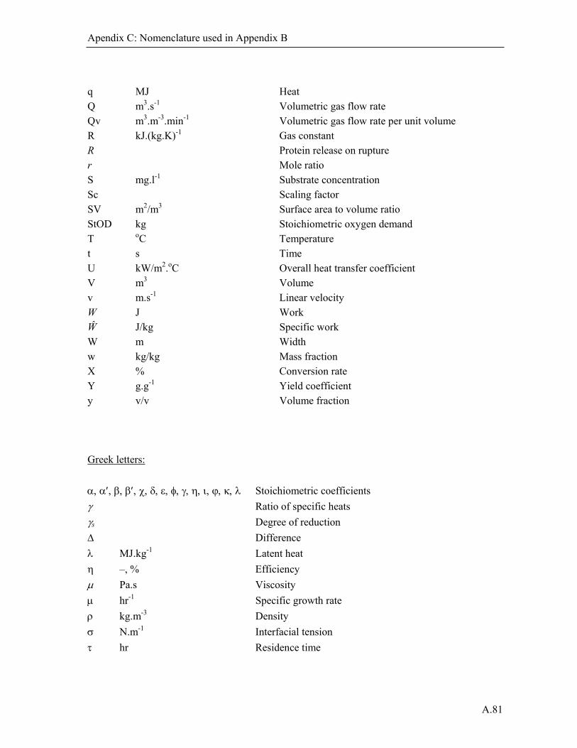
Apendix C: Nomenclature used in Appendix B
A.81
q MJ Heat Q m3.s-1 Volumetric gas flow rate Qv m3.m-3.min-1
Volumetric gas flow rate per unit volume R kJ.(kg.K)-1 Gas constant R Protein release on rupture r Mole ratio S mg.l-1 Substrate concentration Sc Scaling factor SV m2/m3 Surface area to volume ratio StOD kg Stoichiometric oxygen demand T oC Temperature t s Time U kW/m2.oC Overall heat transfer coefficient V m3 Volume v m.s-1 Linear velocity W J Work Ŵ J/kg Specific work W m Width w kg/kg Mass fraction X % Conversion rate Y g.g-1 Yield coefficient y v/v Volume fraction Greek letters:
Stoichiometric coefficients
Ratio of specific heatss Degree of reduction Difference
MJ.kg-1 Latent heat
–, % Efficiency
Pa.s Viscosity
hr-1 Specific growth rate
kg.m-3 Density
N.m-1 Interfacial tension
hr Residence time

Apendix C: Nomenclature used in Appendix B
A.82
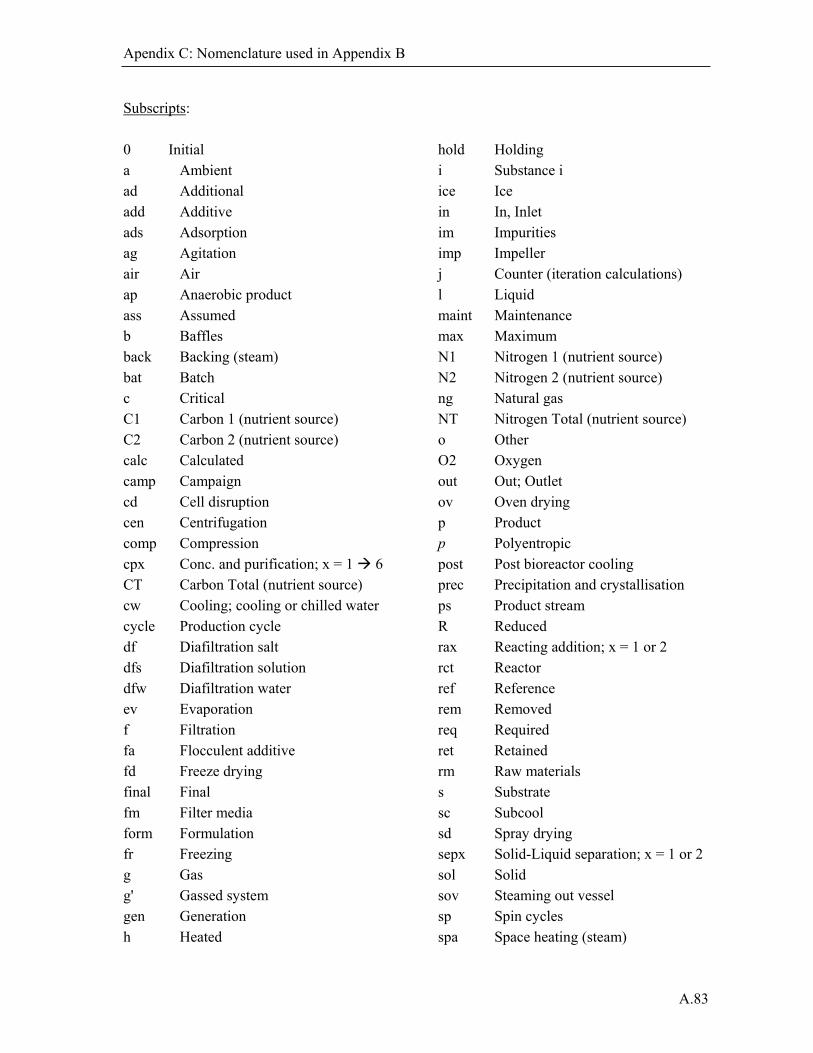
Apendix C: Nomenclature used in Appendix B
A.83
Subscripts: 0 Initial a Ambient ad Additional add Additive ads Adsorption ag Agitation air Air ap Anaerobic product ass Assumed b Baffles back Backing (steam) bat Batch c Critical C1 Carbon 1 (nutrient source) C2 Carbon 2 (nutrient source) calc Calculated camp Campaign cd Cell disruption cen Centrifugation comp Compression cpx Conc. and purification; x = 1 6 CT Carbon Total (nutrient source) cw Cooling; cooling or chilled water cycle Production cycle df Diafiltration salt dfs Diafiltration solution dfw Diafiltration water ev Evaporation f Filtration fa Flocculent additive fd Freeze drying final Final fm Filter media form Formulation fr Freezing g Gas g' Gassed system gen Generation h Heated
hold Holding i Substance i ice Ice in In, Inlet im Impurities imp Impeller j Counter (iteration calculations) l Liquid maint Maintenance max Maximum N1 Nitrogen 1 (nutrient source) N2 Nitrogen 2 (nutrient source) ng Natural gas NT Nitrogen Total (nutrient source) o Other O2 Oxygen
out Out; Outlet ov Oven drying p Product p Polyentropic post Post bioreactor cooling prec Precipitation and crystallisation ps Product stream R Reduced rax Reacting addition; x = 1 or 2 rct Reactor ref Reference rem Removed req Required ret Retained rm Raw materials s Substrate sc Subcool sd Spray drying sepx Solid-Liquid separation; x = 1 or 2 sol Solid sov Steaming out vessel sp Spin cycles spa Space heating (steam)

Apendix C: Nomenclature used in Appendix B
A.84

Apendix C: Nomenclature used in Appendix B
A.85
st Steam ster Sterilisation sub Sublimation surf Surface t Tank T Total
v Vaporisation vp Vacuum pumping w Water wwt Waste water treatment x Biomass

A.86

A.87
Appendix D
UML Diagrams for the generic flowsheet model developed

A.88
Appendix D: UML Diagrams for the Generic Flowsheet Model
A.89
Appendix D: UML Diagrams for the Generic Flowsheet Model A simplified Unified Modelling Language (UML) diagram for solving the entire material balance of the flowsheet model is shown in Figure D.1. This is the first part of several diagrams which can be found on the accompanying CD-Rom. Where reference is made to ‘values as calculated in the main calculations’, calculations as shown in Appendix B are used.
Figure D.1: Simplified UML diagram showing basic flowsheet structure to calculate product mass

A.90

A.91
Appendix E
Using the Generic Flowsheet Model

A.92
Appendix E: Using the Generic Flowsheet Model
A.93
Appendix E: Using the Generic Flowsheet Model
E.1. Overview This appendix gives details of the application of the generic flowsheet; including system requirements, installation instructions and how to use the software model.
E.2. System requirements The software was developed on Microsoft® Office Excel 2003 and has been further tested on MS-Excel XP. Complete testing has not been done on MS-Excel 2007. The software does not work with AppleWorks, OpenOffice or other spread sheeting packages.
E.3. Getting started The generic flowsheet model is presented in a single MS-Excel workbook: ‘Generic model vx.xx.xx.xls’ – where “x.xx.xx” refers to the version of the software. The workbook can be run from its current location or copied and used from the desktop. Before opening the software ensure that Macros are enabled in MS-Excel (Tools-Macro-Security; ‘Medium’ security level) and ensure that macros are always enabled during use. The file will display a copyright prompt (click “OK” to continue) followed by an End user License Agreement (EULA). After agreeing to the EULA, click “I Agree” to continue. You will then be taken to the Input screen of the spreadsheet. Note: The official name of the software, “Leap BioSoft”, is used in the MS-Excel spreadsheet.
E.4. User’s manual The MS-Excel spreadsheet is designed as a top down application and should be used as such to avoid entering invalid information. Select the worksheet labelled ‘Input’ and from the top, select the option button and drop down menus (green) as desired. Only use the orange cells to make changes to the default values which appear to the right of these cells.

Appendix E: Using the Generic Flowsheet Model
A.94
Example: Scenario 1 (sodium salt of Penicillin V) as given in Chapter 3 Below is a step-by-step guide for entering the data into the MS-Excel flowsheet model. The example applies to the generic flowsheet as provided in version v7.12.22 of the software. Modifications and enhancements which do not impact the results of this example have since been implemented in the model. The instructions are listed as:
- ‘click’, where a mouse action is required;
- ‘type’ where inputs need to be entered into the orange input cells using the keyboard; and
- ‘select’ where a dropdown menu appears and a selection needs to be made.

Appendix E: Using the Generic Flowsheet Model
A.95
Figure E.1: Generic flowsheet model (Input) – Screenshot 1
MS-EXCEL worksheet name: Input Worksheet (click): Input
Initial considerations Product location (click): Extracellular Aerobic/Anaerobic (click): Aerobic Process type (click): Batch Cooling options Chilled water temp. (type): 5 Min allowed temp. differences across streams in heat exchangers (type): 0
Product description Product category (select): Antibiotics Specific product (select): Penicillin Product to biomass ratio (type): 1.219 Biomass description Biomass (select): Penicillium chrysogenum

Appendix E: Using the Generic Flowsheet Model
A.96
Figure E.2: Generic flowsheet model (Input) – Screenshot 2
Carbon sources Main category (select): Carbohydrates Specific source (select): Glucose Carbon excess (type): 2 Add another carbon source: (Click) Main category 2 (select) – OTHER Carbon excess (type): 1.7 Carbon name (2) (type): Phenoxyacetic acid Chemical formula (type): C: 8, H: 8, 0: 8, N: 0 Mass percentage carbon source 2 as total carbon (type): 10.55
Nitrogen sources Main category (select): Organic Specific source (select): OTHER Nitrogen excess (type): 15 Nitrogen name (Type): Pharmamedia Chemical formula (type): C: 55.7, H: 6.7, O: 18.9, N: 16, S: 2.7

Appendix E: Using the Generic Flowsheet Model
A.97
Figure E.3: Generic flowsheet model (Input) – Screenshot 3
Oxygen source Oxygen source (select): O2 Aeration rate (type): 0.02 Compression Compressor type (select): Reciprocating compressor Multistage compression (select): Two stage compression with intercooling Cooling medium used (select): Chilled water Compressed pressure (type): 608 Sulphur source Sulphur source (select): OTHER Sulphur excess (type): 0
Maintenance coefficient Include maintenance coefficient: (Click) Maintenance time (type): 106

Appendix E: Using the Generic Flowsheet Model
A.98
Figure E.4: Generic flowsheet model (Input) – Screenshot 4
Reactor Temperature Reactor temperature (type): 32
Growth rate Initial biomass concentration (type): 1e-06 Final biomass concentration (type): 45 Yield coefficients Biomass on substrate (type): 0.45 Substrate on product (type): 0.81 Biomass on oxygen (type): 1.56
Water Water used in microbial growth (select): Distilled water Water used in downstream processing (select): Distilled water Reactor Cooling Maintain reactor temperature: (Click) Cooling medium used (select): Chilled water

Appendix E: Using the Generic Flowsheet Model
A.99
Figure E.5: Generic flowsheet model (Input) – Screenshot 5
Sterilisation Method Sterilisation method (select): Steam Preheat media with cooled (recycled) steam (select): Yes Agitation Agitation: (Click) Impeller type (select): OTHER Number of tanks (type): 11 Power per unit volume (type): 2.5 Post bioreactor cooling Cool before downstream processing: (Click) Coolant (select): OTHER Outlet biomass temperature (type): 28

Appendix E: Using the Generic Flowsheet Model
A.100
Figure E.6: Generic flowsheet model (Input) – Screenshot 6
Concentration and Purification 1 Concentration/Purification method (select): Filtration Solid fraction removed (type): 1 Liquid fraction removed (type): 0.91 Possible additive (Non-reacting) (select): Sulphuric acid Percentage added (type): 0.028 Add another concentration/purification unit: (Click)
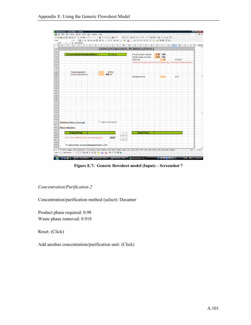
Appendix E: Using the Generic Flowsheet Model
A.101
Figure E.7: Generic flowsheet model (Input) – Screenshot 7
Concentration/Purification 2 Concentration/purification method (select): Decanter Product phase required: 0.98 Waste phase removed: 0.918 Reset: (Click) Add another concentration/purification unit: (Click)
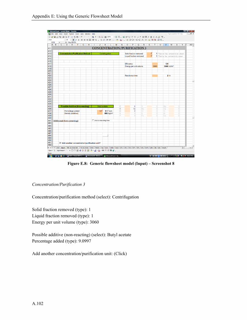
Appendix E: Using the Generic Flowsheet Model
A.102
Figure E.8: Generic flowsheet model (Input) – Screenshot 8
Concentration/Purification 3 Concentration/purification method (select): Centrifugation Solid fraction removed (type): 1 Liquid fraction removed (type): 1 Energy per unit volume (type): 3060 Possible additive (non-reacting) (select): Butyl acetate Percentage added (type): 9.0997 Add another concentration/purification unit: (Click)

Appendix E: Using the Generic Flowsheet Model
A.103
Figure E.9: Generic flowsheet model (Input) – Screenshot 9
Concentration/Purification 4 Concentration/purification method (select): Precipitation/Crystallisation Outlet temperature (type): 6 Cooling media used (select): Chilled water Residence time (type): 12 Power per unit volume (type): 0.6 Possible additive (non-reacting) (select): Acetone Percentage added (type): 12.33 Add a reacting flow: (Click)

Appendix E: Using the Generic Flowsheet Model
A.104
Figure E.10: Generic flowsheet model (Input) – Screenshot 10
Reactant A (select): Sodium acetate Percentage added (type): 7.8 Existing chemical (select): Penicillin Reaction product A (select): Other Reaction product A name (type): Acetic acid Chemical formula (type): C: 2, H: 4, O: 2, N: 0 Modified chemical name (type): Penicillin V sodium crystals Chemical formula (type): H: 16, Na: 1 Mass fraction limiting reactant converted (type): 97 Choose precipitating chemical (select): Penicillin V sodium crystals Add: (Click) [NOTE: This is an exception to the top down rule of the model] Add another concentration/purification unit: (Click)

Appendix E: Using the Generic Flowsheet Model
A.105
Figure E.11: Generic flowsheet model (Input) – Screenshot 11
Concentration/Purification 5 Concentration/purification method (select): Centrifugation Solid fraction removed (type): 0.99 Liquid fraction removed (type): 0.979 Residence time (type): 12 hr Formulation Formulation method (select): Other Product fraction retained (type): 0.99 Liquid fraction removed (type): 0.9 Electricity (type): 72.19
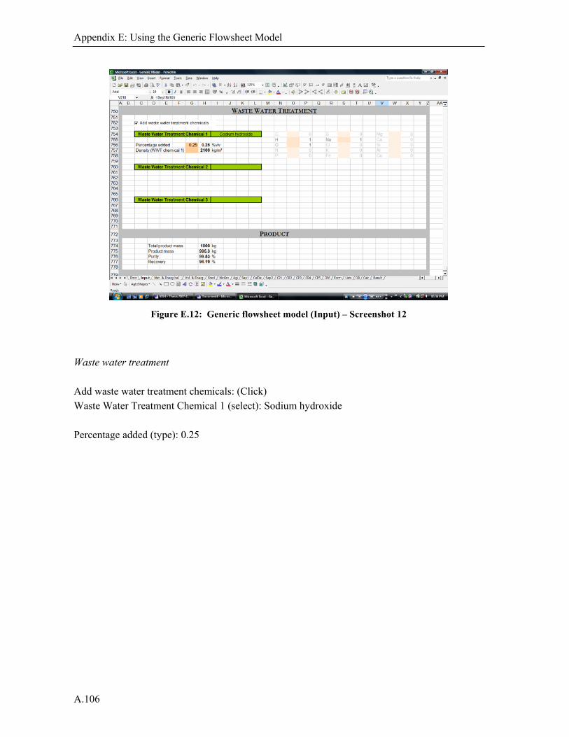
Appendix E: Using the Generic Flowsheet Model
A.106
Figure E.12: Generic flowsheet model (Input) – Screenshot 12
Waste water treatment Add waste water treatment chemicals: (Click) Waste Water Treatment Chemical 1 (select): Sodium hydroxide Percentage added (type): 0.25

Appendix E: Using the Generic Flowsheet Model
A.107
Figure E.13: Generic flowsheet model (Mat. & Energ bal.) – Screenshot 1
MS-EXCEL worksheet name: Results – Material and energy balances Worksheet (click): Mat. & Energ bal. This worksheet shows the results for the product produced. The product purity and recovery, product composition, material and energy requirements and waste streams are also given. Waste is given as water, air and solid emissions.

Appendix E: Using the Generic Flowsheet Model
A.108
Figure E.14: Generic flowsheet model (Vol. & Energ) – Screenshot 1
MS-EXCEL worksheet name: Results – Volumes and Energy contributions Worksheet (click): Vol. & Energ This worksheet shows volumes calculated for each of the units used in the flowsheet. The energy requirements are broken down by unit into electricity, natural gas, steam, cooling water and chilled water. These are also presented graphically in pie charts as percentages of the total energy requirement for each unit.

A.109
Appendix F
Electricity LCA from South African Data

A.110
Appendix F: Electricity LCA from South African data
A.111
Appendix F: Electricity LCA from South African data
The electricity mix used in the LCA studies is for South Africa. The electricity mix is given by Eskom (2006) and shown in Table F.1. Most of South African electricity is produced by coal (93 %). The LCA impacts of electricity from coal are shown in Tables F.2 – F.7 as provided by Gediga (2006) as part of GaBi data (PE International 2007). Life Cycle inventories from the EcoInvent v1.3 (Swiss Centre for Life Cycle Inventories 2007) and ETH-ESU (Frischknecht et al. 1996) databases were used to complete the “underground coal mine”, “coal from open coal mine”, “infrastructure of underground coal mine” and “infrastructure of open coal mine” models. LCA impacts for non-coal electricity are arbitrarily assumed equal to the impacts given for Great Britain as presented by the EcoInvent v1.3 database (Swiss Centre for Life Cycle Inventories 2007). The ways the electricity data are interlinked are shown in Figure F.1. Life Cycle Impact Assessment values are given in Table F.8.
Table F.1: Material and energy inputs and outputs for South African electricity production mix
Products and co-products Value Units Allocation
Electricity production mix 221 216 GWh 100%
Inputs from technosphere (materials/fuel) Value Units Comments
Electricity, coal 205 837 GWh
Electricity, hydropower, at power plant 1 141 GWh
Electricity, hydropower, at pumped storage power 2 867 GWh
Electricity, natural gas 78 GWh
Electricity, nuclear, water reactor power plant 11 293 GWh
Electricity, wind power 0 GWh No wind power taken into account
Figure F.1: Overall life cycle input/output structure for South African electricity mix

Appendix F: Electricity LCA from South African data
A.112
Table F.2: Life cycle inputs/outputs for electricity from coal (South Africa)
Products and co-products Value Units
Electricity, coal (South Africa) 1 MWh
Inputs from nature Value Units
Water, process and cooling, unspecified origin 0.000966 m3
Inputs from technosphere (materials/fuel) Value Units
Coal, from mine (South Africa) 0.381 t
Emissions to air Value Units Emissions to air Value Units
Carbon dioxide 688 kg Arsenic 0.0000267 kg
Particulates, < 10 um 0.206 kg Beryllium 0.00000324 kg
Sulphur dioxide 6.19 kg Cadmium 0.000000953 kg
Nitrogen oxides 2.77 kg Chromium 0.0000347 kg
Dinitrogen monoxide 0.0102 kg Dioxins, 7.24E-11 kg
Ammonia 0.00000914 kg Ethene, tetrachloro- 0.000013 kg
Benzene 0.0000103 kg Hydrogen chloride 0.0686 kg
Methane 0.00724 kg Hydrogen fluoride 0.00953 kg
Acrolein 0.0000137 kg Lead 0.0000354 kg
Cobalt 0.0000103 kg Manganese 0.0000876 kg
Formaldehyde 0.0000171 kg Mercury 0.0000251 kg
Phenol 0.0000255 kg Methane, dichloro-, HCC-30 0.0000533 kg
N-Nitrodimethylamine 0.0000029 kg Methane, tetrachloro-, CFC-10 0.0000137 kg
Carbon monoxide 0.114 kg Nickel 0.0000236 kg
Radioactive species, unspecified 0.000109 kBq Non-methane volatile organic compounds, unspecified origin
0.0133 kg
Aldehydes, unspecified 0.0000724 kg Selenium 0.0000953 kg
Antimony 0.00000533 kg Ethene, trichloro- 0.000013 kg
Emissions to water Value Units Emissions to water Value Units
Phosphate 0.00419 kg Boron 0.0335 kg
Organic substances, unspecified 0.00648 kg Chloride 0.00267 kg
Sulphuric acid 0.0838 kg Suspended solids, unspecified 0.0495 kg
Final waste flows Value Units
Waste, final, inert 110 kg
Table F.3: Life cycle inputs/outputs for coal from South African coal mine
Value Units
Products and co-products Coal, from mine (South Africa) 1 t
Inputs from technosphere (materials/fuel) Coal from underground mine (South Africa) 0.6 t
Coal from open mine (South Africa) 0.4 t

Appendix F: Electricity LCA from South African data
A.113
Table F.4: Life cycle inputs/outputs for underground coal mine (South Africa)
Products and co-products Value Units
Coal from underground mine (South Africa) 1 t
Inputs from nature Value Units
Water, unspecified natural origin 1700 kg
Gas, mine, off-gas, process, coal mining 6.7 kg
Coal, 18 MJ per kg 1670 kg
Land use II-III 4.87 m2a
Land use II-IV 0.2 m2a
Inputs from technosphere (materials/fuel) Value Units
Electricity production mix (South Africa) 0.000306 TJ
Concrete (un-reinforced) 10.6 kg
Wood 11.7 kg
Explosives 0.17 kg
Steel 2.5 kg
Diesel 1.10E-05 TJ
Industrial coal furnace (1-10MW) 0.00011 TJ
Underground coal mine infrastructure (SA) 1 t
Emissions to air Value Units
Methane 6.7 kg
Particulates, > 10 um 0.1 kg
Radon-222 12 kBq
Heat, waste 0.000306 TJ
Emissions to water Value Units
Ammonia, as N 0.001 kg
Chloride 17.05 kg
Fluoride 0.003 kg
Solved substances 1 kg
Aluminium 0.001 kg
Iron 0.002 kg
Manganese 0.001 kg
Nickel, ion 0.0001 kg
Strontium 0.005 kg
Zinc, ion 0.0001 kg
Sulphate 0.5 kg
Undissolved substances 0.015 kg
Emissions to soil Value Units
Coal tailings in landfill U 540 kg
Table F.5: Life cycle inputs/outputs for coal from open coal mine (South Africa)
Products and co-products Value Units
Coal from open mine (South Africa) 1 t
Inputs from nature Value Units
Water, unspecified natural origin 500 kg
Gas, mine, off-gas, process, coal mining 0.16 kg
Coal, 18 MJ per kg 1430 kg
Land use II-III 11.87 m2a
Land use II-IV 2.7 m2a
Land use III-IV 1.16 m2a
Inputs from technosphere (materials/fuel) Value Units
Electricity production mix (SA) 0.0000540 TJ
EPDM rubber 0.14 kg
Explosives 1.7 kg
Diesel in building equipment 0.00034 TJ
Open coal mine infrastructure (SA) 1 t
Emissions to air Value Units
Methane 0.16 kg
Particulates, > 10 um 0.4 kg
Radon-222 12 kBq
Heat, waste 5.40E-05 TJ
Emissions to water Value Units
Ammonia, as N 0.001 kg
Chloride 0.35 kg
Fluoride 0.003 kg
Solved substances 1 kg
Aluminium 0.001 kg
Iron 0.002 kg
Manganese 0.001 kg
Nickel, ion 0.0001 kg
Strontium 0.005 kg
Zinc, ion 0.0001 kg
Salts, unspecified 0.1 kg
Sulphate 0.5 kg
Undissolved substances 0.015 kg
Emissions to soil Value Units
Coal tailings in landfill U 430 kg
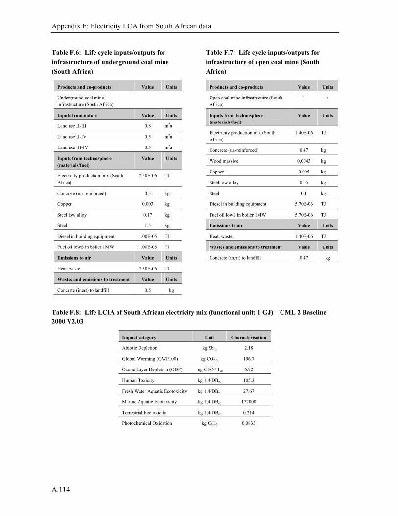
Appendix F: Electricity LCA from South African data
A.114
Table F.6: Life cycle inputs/outputs for infrastructure of underground coal mine (South Africa)
Products and co-products Value Units
Underground coal mine infrastructure (South Africa)
Inputs from nature Value Units
Land use II-III 0.8 m2a
Land use II-IV 0.5 m2a
Land use III-IV 0.5 m2a
Inputs from technosphere (materials/fuel)
Value Units
Electricity production mix (South Africa)
2.50E-06 TJ
Concrete (un-reinforced) 0.5 kg
Copper 0.003 kg
Steel low alloy 0.17 kg
Steel 1.5 kg
Diesel in building equipment 1.00E-05 TJ
Fuel oil lowS in boiler 1MW 1.00E-05 TJ
Emissions to air Value Units
Heat, waste 2.50E-06 TJ
Wastes and emissions to treatment Value Units
Concrete (inert) to landfill 0.5 kg
Table F.7: Life cycle inputs/outputs for infrastructure of open coal mine (South Africa)
Products and co-products Value Units
Open coal mine infrastructure (South Africa)
1 t
Inputs from technosphere (materials/fuel)
Value Units
Electricity production mix (South Africa)
1.40E-06 TJ
Concrete (un-reinforced) 0.47 kg
Wood massive 0.0043 kg
Copper 0.005 kg
Steel low alloy 0.05 kg
Steel 0.1 kg
Diesel in building equipment 5.70E-06 TJ
Fuel oil lowS in boiler 1MW 5.70E-06 TJ
Emissions to air Value Units
Heat, waste 1.40E-06 TJ
Wastes and emissions to treatment Value Units
Concrete (inert) to landfill 0.47 kg
Table F.8: Life LCIA of South African electricity mix (functional unit: 1 GJ) – CML 2 Baseline 2000 V2.03
Impact category Unit Characterisation
Abiotic Depletion kg Sbeq 2.18
Global Warming (GWP100) kg CO2 eq 196.7
Ozone Layer Depletion (ODP) mg CFC-11eq 6.92
Human Toxicity kg 1,4-DBeq 105.3
Fresh Water Aquatic Ecotoxicity kg 1,4-DBeq 27.67
Marine Aquatic Ecotoxicity kg 1,4-DBeq 172000
Terrestrial Ecotoxicity kg 1,4-DBeq 0.214
Photochemical Oxidation kg C2H2 0.0833
Appendix F: Electricity LCA from South African data
A.115
References ESKOM, 2006. Eskom Holdings Limited Annual Report, Available online: www.eskom.co.za/annreport06/,
[Accessed 9 November 2007]. Frischknecht, R., Bollens, U., Bosshart, S., Ciot, M., Ciseri, L., Doka, G., Dones, R., Ganther, U., Hischier, R.,
Martin, B. 1996. Ökoinventare von Energiesystemen, Grundlagen für den ökologischen Vergleich von Energiesystemen und den Einbezug von Energiesystemen in Ökobilanzen für die Schweiz, Auflage No. 3, Gruppe Energie - Stoffe - Umwelt (ESU), Eidgenössische Technische Hochschule Zürich und Sektion Ganzheitliche Systemanalysen, Paul Scherrer Institut, Villigen, www.energieforschung.ch, Bundesamt für Energie (Hrsg.), Bern.
Gediga, J., 2006. PE International GmbH, Personal communication. PE International, 2007. Hauptstraße 111-113, 70771 Leinfelden-Echterdingen, Germany, http://www.gabi-
software.com Swiss Centre for Life Cycle Inventories, 2007. EcoInvent Centre, http://www.ecoinvent.org/.

A.116
A.117
Appendix G
Sugar LCA from South African Sugar Cane

A.118

Appendix G: Sugar LCA from South African Sugar Cane
A.119
Appendix G: Sugar LCA from South African Sugar Cane Sugar and bagasse are used in several parts of the thesis for raw material inputs, including the LCA equivalent for glucose. A South African model is used for this and adapted from the work by Theka (2002), Botha (2003), Botha and von Blottnitz (2006) and von Blottnitz (2006). Inputs and outputs for the production of sugar (from cane) and bagasse are given in Table G.1 and the growth of the sugar cane in Table G.2. Life Cycle Impact Assessment values are given in Table G.3.
Table G.1: Material and energy inputs and outputs for sugar (from cane) and bagasse
Products and co-products Value Units Allocation
Sugar (from caner) 3 t 75 %
Molasses 1 t 25 %
Bagasse 20.14 t 0 % Used internally for energy
Inputs from nature Value Units Comments
Process water, unspecified origin 2540.64 l
Inputs from technosphere (materials/fuel) Value Units Comments
Lime 25 kg
Sugarcane 25 t
Truck (40t) 1249 tkm 30km distance travelled
Diesel 0.137 kg
Inputs from technosphere (electricity/heat) Value Units Comments
Heat, hard coal industrial furnace 0 GJ Assumption: Bagasse burning produces required heat (6.1 GJ)
Electricity, production mix South Africa 0 kWh Assumption: Bagasse burning produces required energy (23 kWh)
Emissions to air Value Units Comments
Carbon dioxide 9.7863 t Carbon uptake during cane growth shown in sugar cane data
Nitrogen oxides 24.107 kg
Particulates 2.3134 kg
Sulphur oxides 7.5 kg
Emissions to water Value Units Comments
Wastewater 85.479 l
Dissolved substances 0.1258 kg
Suspended solids 0.0014. kg
Chemical oxygen demand (COD) 0.0014 kg
Final waste flows Value Units Comments
Solid waste 0.3 t

Appendix G: Sugar LCA from South African Sugar Cane
A.120
Table G.2: Material and energy inputs and outputs for sugarcane
Products and co-products Value Units Allocation
Sugarcane 1 t 100 %
Inputs from nature Value Units Comments
Process water, unspecified origin 154.99 m3 Reference: Hlatshwayo (2005)
Arable land 154.99 m2a Reference: SASA (2005)
Inputs from technosphere (materials/fuel) Value Units Comments
Fertiliser 6.59 kg
Diesel 0.95 kg
Emissions to air Value Units Comments
Carbon dioxide -0.4692 t Carbon uptake
Table G.3: LCIA of South African sugar from cane (functional unit: 1 t) – CML 2 Baseline 2000 V2.03
Impact category Unit Characterisation
Abiotic Depletion kg Sbeq. 0.579
Global Warming (GWP100) kg CO2 eq. -433.9
Ozone Layer Depletion (ODP) mg CFC-11eq. 17.1
Human Toxicity kg 1,4-DBeq. 21.97
Fresh Water Aquatic Ecotoxicity kg 1,4-DBeq. 2.30
Marine Aquatic Ecotoxicity kg 1,4-DBeq. 12000
Terrestrial Ecotoxicity kg 1,4-DBeq. 0.0938
Photochemical Oxidation kg C2H2 0.121
References Botha, T., 2003. Opportunity to apply recent advances in process design to bioenergy systems: the case of
sugarcane processing in South Africa, M.Sc. Dissertation, Department of Chemical Engineering, University of Cape Town.
Botha, T., von Blottnitz, H., 2006. A comparison of the environmental benefits of bagasse-derived electricity and fuel ethanol on a life cycle basis, Energ. Policy, 34, 2654-2661.
Hlatshwayo, B., 2005. Tongaat-Huletts Sugar, Personal communication. SASA, 2005. The South African Sugar Association: Sugar Estimates; Online:
http://www.sasB.org.za/industryadmin/estimates.htm. Theka, E., 2002. A life-cycle assessment of ethanol produced from sugarcane molasses, M.Sc. dissertation,
Department of Chemical Engineering, University of Cape Town. von Blottnitz, H., 2006. Department of Chemical Engineering, University of Cape Town, Personal communication.

A.121
Appendix H
Sensitivity Analysis Data

A.122
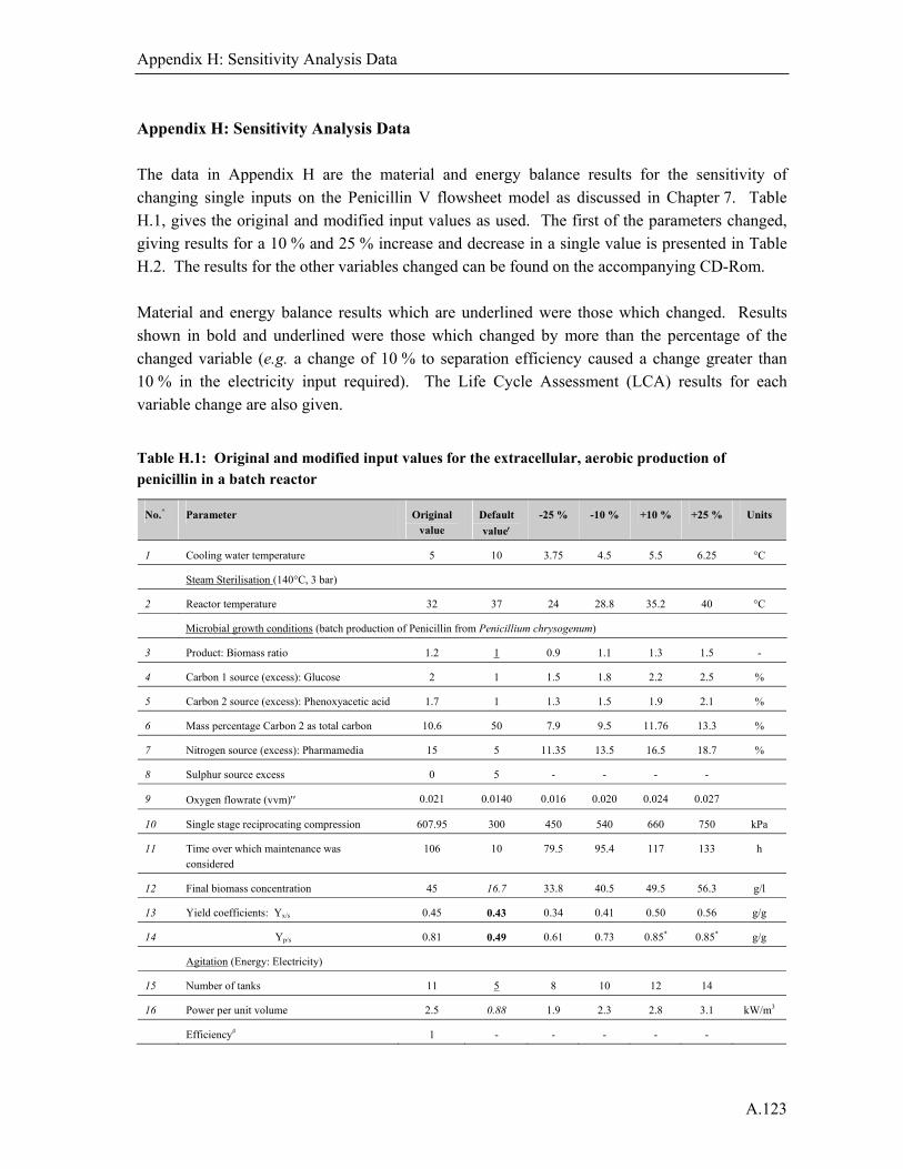
Appendix H: Sensitivity Analysis Data
A.123
Appendix H: Sensitivity Analysis Data The data in Appendix H are the material and energy balance results for the sensitivity of changing single inputs on the Penicillin V flowsheet model as discussed in Chapter 7. Table H.1, gives the original and modified input values as used. The first of the parameters changed, giving results for a 10 % and 25 % increase and decrease in a single value is presented in Table H.2. The results for the other variables changed can be found on the accompanying CD-Rom. Material and energy balance results which are underlined were those which changed. Results shown in bold and underlined were those which changed by more than the percentage of the changed variable (e.g. a change of 10 % to separation efficiency caused a change greater than 10 % in the electricity input required). The Life Cycle Assessment (LCA) results for each variable change are also given.
Table H.1: Original and modified input values for the extracellular, aerobic production of penicillin in a batch reactor
No.^ Parameter Original value
Default
value -25 % -10 % +10 % +25 % Units
1 Cooling water temperature 5 10 3.75 4.5 5.5 6.25 °C
Steam Sterilisation (140°C, 3 bar)
2 Reactor temperature 32 37 24 28.8 35.2 40 °C
Microbial growth conditions (batch production of Penicillin from Penicillium chrysogenum)
3 Product: Biomass ratio 1.2 1 0.9 1.1 1.3 1.5 -
4 Carbon 1 source (excess): Glucose 2 1 1.5 1.8 2.2 2.5 %
5 Carbon 2 source (excess): Phenoxyacetic acid 1.7 1 1.3 1.5 1.9 2.1 %
6 Mass percentage Carbon 2 as total carbon 10.6 50 7.9 9.5 11.76 13.3 %
7 Nitrogen source (excess): Pharmamedia 15 5 11.35 13.5 16.5 18.7 %
8 Sulphur source excess 0 5 - - - -
9 Oxygen flowrate (vvm) 0.021 0.0140 0.016 0.020 0.024 0.027
10 Single stage reciprocating compression 607.95 300 450 540 660 750 kPa
11 Time over which maintenance was considered
106 10 79.5 95.4 117 133 h
12 Final biomass concentration 45 16.7 33.8 40.5 49.5 56.3 g/l
13 Yield coefficients: Yx/s 0.45 0.43 0.34 0.41 0.50 0.56 g/g
14 Yp/s 0.81 0.49 0.61 0.73 0.85* 0.85* g/g
Agitation (Energy: Electricity)
15 Number of tanks 11 5 8 10 12 14
16 Power per unit volume 2.5 0.88 1.9 2.3 2.8 3.1 kW/m3
Efficiency# 1 - - - - -

Appendix H: Sensitivity Analysis Data
A.124
No.^ Parameter Original value
Default
value -25 % -10 % +10 % +25 % Units
Post bioreactor cooling
17 Outlet temperature 28 15 21 25 31 32* °C
Filtration (Energy: Electricity)
18 Solid fraction removed 100 95 75 90 100* 100* %
19 Liquid fraction retained 91 70 68 82 100* 100* %
20 Additive: Sulphuric acid 0.028 5 0.021 0.025 0.031 0.035 %v/v
Centrifugation (Energy: Electricity)
21 Product fraction retained 98 99 74 88 100* 100* %
22 Waste fraction removed 91.8 95 68.9 82.6 100* 100* %
23 Energy per unit volume 3060 6420 2300 2750 3370 3820 kJ/m3
24 Additive: Butyl acetate 9.1 5 6.8 8.2 10.0 11.4 %v/v
Precipitation and Crystallisation (Energy: Electricity and steam)
25 Outlet temperature 6 40 7.5 6.6 5.4 5* °C
Residence time** 12 - - - - - h
26 Power per unit volume 0.6 0.8 0.45 0.54 0.66 0.75 kW/m3
27 Additive: Acetone 12.3 5 9.2 11.1 13.5 15.4 %v/v
28 Additive: Sodium acetate 7.8 25 5.8 7.0 8.6 9.8 %v/v
Reaction: Sodium acetate + Penicillin Acetic acid + Penicillin V sodium crystals
29 Conversion of limiting reagent 97 80 73 87.3 100* 100* %
Centrifugation (Energy: Electricity)
30 Solid fraction removed 99 98 74 89 100* 100* %
31 Liquid fraction removed 97.9 80 73 88 100* 100* %
Fluid bed drying (Energy: Electricity)
32 Product fraction retained 99 99 74 89 100* 100* %
33 Liquid fraction removed 90 99 68 81 99 100* %
34 Electricity required 72.7 10 55 65 80 91 MJ/m3
Waste Water Treatment
35 Additive: Sodium hydroxide 0.25 5 0.18 0.22 0.28 0.32 %v/v
^ Reference number for the variable changed
Bold values indicate average values from various sources, values in italics are calculations, unaltered numbers indicate estimations
based on industry norms and underlined values are those which are the authors approximation based on possibly values required * Maximum or minimum value allowed; compromising the 10 or 25 % increase or decrease as shown
This accounts for oxygen content of the air only (excluding nitrogen)
# Changing efficiency has the same effect as changing the power per unit volume ** In batch units, residence time only affects power required – changing residence time has the same effect as changing power per unit volume.
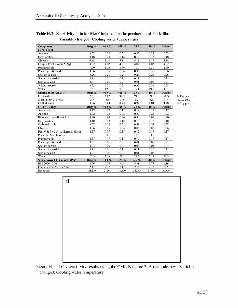
Appendix H: Sensitivity Analysis Data
A.125
Table H.2: Sensitivity data for M&E balance for the production of Penicillin. Variable changed: Cooling water temperature
Component Original +10 % +25 % -25 % -10 % Default INPUT (kg) Acetone 0.22 0.22 0.22 0.22 0.22 0.22 Butyl acetate 0.18 0.18 0.18 0.18 0.18 0.18 Glucose 5.18 5.18 5.18 5.18 5.18 5.18 Oxygen (excl. excess & N2) 4.02 4.02 4.02 4.02 4.02 4.02 Pharmamedia 1.30 1.30 1.30 1.30 1.30 1.30 Phenoxyacetic acid 0.36 0.36 0.36 0.36 0.36 0.36 Sodium acetate 0.26 0.26 0.26 0.26 0.26 0.26 Sodium hydroxide 0.11 0.11 0.11 0.11 0.11 0.11 Sulphuric acid 0.01 0.01 0.01 0.01 0.01 0.01 Sulphur source 0.32 0.32 0.32 0.32 0.32 0.32 Water 19.1 19.1 19.1 19.1 19.1 19.1 Energy requirements Original +10 % +25 % -25 % -10 % Default Electricity 79.1 79.2 79.3 79.0 79.1 81.5 MJ/kg pen. Steam (140°C, 3 bar) 3.3 3.3 3.3 3.3 3.3 3.3 kg/kg pen. Chilled water 0.86 0.90 0.95 0.78 0.83 1.49 m3/kg pen. OUTPUT (kg) Original +10 % +25 % -25 % -10 % Default Acetic acid 0.17 0.17 0.17 0.17 0.17 0.17 Acetone 0.22 0.22 0.22 0.22 0.22 0.22 Biomass (dry cell weight) 0.90 0.90 0.90 0.90 0.90 0.90 Butyl acetate 0.18 0.18 0.18 0.18 0.18 0.18 Carbon dioxide 6.58 6.58 6.58 6.58 6.58 6.58 Glucose 0.06 0.06 0.06 0.06 0.06 0.06 Pen. V & Pen. V., sodium salt (loss) 0.17 0.17 0.17 0.17 0.17 0.17 Penicillin V sodium salt 1 1 1 1 1 1 Pharmamedia 0.17 0.17 0.17 0.17 0.17 0.17 Phenoxyacetic acid 0.01 0.01 0.01 0.01 0.01 0.01 Sodium acetate 0.03 0.03 0.03 0.03 0.03 0.03 Sodium hydroxide 0.11 0.11 0.11 0.11 0.11 0.11 Sulphuric acid 0.01 0.01 0.01 0.01 0.01 0.01 Water 21.3 21.3 21.3 21.3 21.3 21.3 Single Score LCA results (Pts) Original +10 % +25 % -25 % -10 % Default EPS 2000 v2.02 7.76 7.76 7.77 7.75 7.76 7.86 Ecoindicator 99 (E) v2.04 2.17 2.17 2.17 2.16 2.17 2.2 Ecopoints 31200 31200 31200 31200 31200 31700
Figure H.1: LCA sensitivity results using the CML Baseline 2.03 methodology. Variable
changed: Cooling water temperature

A.126

A.127
Appendix I
Life Cycle Inventory Tables

A.128

Appendix I: Life Cycle Inventory Tables
A.129
Appendix I: Life Cycle Inventory Tables The Life Cycle Inventory data for the production of 1 kg of Penicillin V, as shown in Chapter 3, are given in Table I.1. This is a shortened version of the first of several tables which can be found on the accompanying CD-Rom for the Life Cycle Inventory data of the various LCA studies in this thesis.
Table I.1: Life Cycle Inventory for the production of 1 kg of Penicillin V, as used in Chapter 3
No Substance Compartment Unit Penicillin: Scenario 1
Penicillin: Scenario 2
Penicillin: Scenario 3
Penicillin: Biwer et al.
(2006)
1 Air Raw oz 49.54 62.60 50.62 31.33
2 Aluminium, 24% in bauxite, 11% in crude ore, in ground
Raw g 1.95 2.03 2.82 2.02
3 Anhydrite, in ground Raw mg 1.51 1.51 2.12 0.92
4 Atrazine Raw mg 264.68 242.28 313.54 95.69
5 Barite, 15% in crude ore, in ground Raw g 4.50 5.29 7.60 6.42
6 Baryte, in ground Raw mg 558.92 660.02 651.98 459.38
7 Basalt, in ground Raw g 1.87 2.07 2.90 2.43
8 Bauxite, in ground Raw g 1.36 1.61 1.47 1.18
9 Borax, in ground Raw µg 285.97 315.52 442.23 371.06
10 Calcite, in ground Raw g 121.29 127.83 179.46 128.56
11 Calcium sulfate, in ground Raw mg 1.30 1.30 1.93 0.70
12 Carbon dioxide, in air Raw g 51.14 56.20 77.79 64.48
The missing lines left out here can be found on the accompanying CD-ROM
798 Strontium Soil µg 246.55 291.64 407.51 356.79
799 Sulfur Soil mg 18.70 21.84 29.74 25.08
800 Tebutam Soil ng 37.18 41.23 57.50 47.74
801 Teflubenzuron Soil ng 8.23 8.91 12.36 9.74
802 Tin Soil µg 0.93 0.95 1.64 0.92
803 Titanium Soil µg 38.91 42.75 58.49 48.68
804 Vanadium Soil µg 1.11 1.22 1.67 1.39
805 Zinc Soil mg 0.99 1.13 1.55 1.29