A fingerprint of surface-tension anisotropy

in the free-energy cost of nucleation

Santi Prestipino1∗, Alessandro Laio2†, and Erio Tosatti2,3‡

1 Universita degli Studi di Messina,

Dipartimento di Fisica e di Scienze della Terra,

Contrada Papardo, I-98166 Messina, Italy

2 International School for Advanced Studies (SISSA) and UOS Democritos,

CNR-IOM, Via Bonomea 265, I-34136 Trieste, Italy

3 The Abdus Salam International Centre for Theoretical Physics (ICTP),

P.O. Box 586, I-34151 Trieste, Italy

(Dated: February 18, 2013)

Abstract

We focus on the Gibbs free energy ∆G for nucleating a droplet of the stable phase (e.g. solid)

inside the metastable parent phase (e.g. liquid), close to the first-order transition temperature. This

quantity is central to the theory of homogeneous nucleation, since it superintends the nucleation

rate. We recently introduced a field theory describing the dependence of ∆G on the droplet

volume V , taking into account besides the microscopic fuzziness of the droplet-parent interface,

also small fluctuations around the spherical shape whose effect, assuming isotropy, was found to be

a characteristic logarithmic term. Here we extend this theory, introducing the effect of anisotropy

in the surface tension, and show that in the limit of strong anisotropy ∆G (V ) once more develops

a term logarithmic on V , now with a prefactor of opposite sign with respect to the isotropic case.

Based on this result, we argue that the geometrical shape that large solid nuclei mostly prefer could

be inferred from the prefactor of the logarithmic term in the droplet free energy, as determined

from the optimization of its near-coexistence profile.

PACS numbers: 64.60.qe, 68.03.Cd, 68.35.Md

∗ Corresponding author. E-mail: sprestipino@unime.it† E-mail: laio@sissa.it‡ E-mail: tosatti@sissa.it

1

arX

iv:1

302.

3712

v1 [

cond

-mat

.sta

t-m

ech]

15

Feb

2013

I. INTRODUCTION

When a homogeneous, defect-free bulk system is brought across a first-order phase bound-

ary, it may survive in its metastable state even for a long time, until the stable phase sponta-

neously nucleates [1, 2]. The nucleation process has attracted much attention over the years,

both from a fundamental point of view as well as for its great practical interest. To mention

but one example, a better control of crystal nucleation in protein solutions could help hin-

der protein condensation which is at the heart of several human pathologies [3]. Thermal

fluctuations continuously sprout droplets of the stable phase inside the metastable mother

phase. Small droplets dissolve, for the gain in volume free energy fails to compensate the

loss in surface free energy. Occasionally, a droplet is sufficiently large that it is favorable for

it to grow. Once this happens, the solid nucleus expands until the whole liquid crystallizes.

Quenching the system deeper and deeper lowers the nucleation barrier until the point where

the barrier vanishes (kinetic spinodal limit). Beyond this threshold, nucleation ceases and

the phase transition occurs through spinodal decomposition and coarsening (i.e., uniformly

throughout the material). Classical nucleation theory (CNT) [4–6] provides the simplest the-

oretical framework in which the initial stage of the phase transformation can be described.

In this theory, an isolated droplet is schematized, regardless of its size, as a sphere of bulk

solid, separated from the liquid by a sharp interface with a constant free-energy cost per

unit area σ (“capillarity approximation”). This gives rise to a (Gibbs) free-energy difference

between the supercooled liquid system with and without a solid cluster, that is

∆G(V ) = −ρs|∆µ|V + (36π)1/3σV 2/3 , (1.1)

where V is the cluster volume, ∆µ < 0 is the difference in chemical potential between solid

and liquid, and ρs is the bulk-solid number density. The droplet grows if it exceeds a critical

size V ∗ corresponding to the maximum ∆G (≡ ∆G∗), which thus provides the activation

barrier to nucleation [7].

The cluster free energy ∆G(V ) can be accessed numerically via the statistics of cluster

size, through which the validity of Eq. (1.1) for specific model interactions can be directly

tested. We recently showed [8] that the accuracy of CNT is less than satisfactory in estimat-

ing the size probability distribution of clusters, especially the smaller ones, implying that

interface-tension estimates based on the use of CNT are systematically in error. We then

proposed a more detailed field theory of the nucleation barrier, based on the assumption

2

that clusters are soft and not sharp, and can deviate mildly from the spherical shape (“qua-

sispherical” approximation). If the solid-liquid interface tension is taken to be isotropic, the

volume dependence of the Gibbs free energy of a cluster is of the Dillmann-Meier form [9],

∆G(V ) = −ρs|∆µ|V + AV 2/3 +BV 1/3 + C − 7

9kBT ln

V

a3, (1.2)

where A,B, and C can all be expressed as explicit functions of the “microscopic” parameters

entering a Landau free energy, and a is a microscopic length. It turned out that the numerical

profiles of ∆G in a few test cases and at various supersaturations are better reproduced by

this theory.

Here we critically reconsider the most severe assumption made in that derivation, namely

the isotropy of the solid-liquid interface tension. We show that the theory introduced in

Ref. [8] can be extended relaxing this important approximation, and that the results change.

Starting once again from a Landau-like theory, we derive an interface Hamiltonian, that

allows estimating the probability of observing a cluster of any shape and size. The angular

dependence of the interface tension is taken into account by terms that depend on the local

orientation of the cluster surface. Within this framework, we calculate ∆G(V ) in the limit

of strong surface anisotropy and compare it with the isotropic case. For large anisotropy,

the cluster free energy still retains at large size a logarithmic term, however with a prefactor

of opposite sign to the isotropic one. On account of this, we suggest that the nominal

shape of large solid nuclei could be guessed from the optimization of the actual ∆G(V )

close to coexistence. Looking for a numerical exemplification, we conducted 3D Monte

Carlo simulations of the Ising model extracting ∆G(V ) for clusters of variable size V , at

various distances from coexistence. Although we could not really attain sizes where the

anisotropic shape effects are heavy, we do detect evidence that the sign is as expected for

large anisotropy.

The paper is organized as follows. We start in Section II by relaxing the approximation

of an infinitely sharp cluster interface, with the introduction of a Landau free energy. From

that, an effective sharp-interface Hamiltonian is derived in Section III, as an intermediate

step to building up a field theory for isotropic surfaces where small shape fluctuations are

allowed (Section IV.A). Eventually, this leads to a modified-CNT expression of ∆G(V ). In

Section IV.B, the issue of interface anisotropies is addressed, and we show by examples how

the dependence of the interface free energy on the local surface normal affects the formation

3

energy of a large cluster. Next, in Section V, we check our theory against old and fresh

Monte Carlo simulation data for the nucleation barrier to magnetization reversal in the 3D

Ising model above the roughening temperature. While confirming that CNT is not generally

adequate to fit the numerical ∆G(V ) data, this analysis also gives a quantitative measure of

the errors made with CNT and demonstrates their cancellation in the more general theory.

Finally, our conclusions are presented in Section VI.

II. DIFFUSE INTERFACE: LANDAU THEORY

The main assumption behind CNT is that of a sharp and spherical cluster surface. A

way to relax this approximation is through the introduction of a scalar, non-conserved

order-parameter (OP) field φ(x) (“crystallinity”) which varies smoothly from one phase to

the other. Hence, the solid-liquid interface becomes diffuse in space, even though only on a

microscopic scale. In practice, φ may be thought of as the local value of the main Fourier

coefficients of the crystal-periodic one-body density n(x), i.e., those relative to the reciprocal-

lattice vectors which are closest in modulus to the point where the liquid structure factor

reaches its maximum [10]. Otherwise, φ may be identified with the parameter discriminating

between solid and liquid in an ansatz like

n(x) =

(φ

π

)3/2∑R

e−φ(x−R)2 = ρs∑G

e−G2/(4φ)eiG·x , (2.1)

assuming a specific crystal symmetry and an overall number density ρs.

Across the solid-liquid interface, φ is no longer constant and, for a system with short-range

forces, the thermodynamic cost of the interface may be described through the free-energy

functional [11–15]

G[φ; n] =

∫d3x

c(n)

2(∇φ)2 +

κ(n)

2(∇2φ)2 + g(φ(x))

, (2.2)

where c, κ > 0 are stiffness parameters dependent on the interface orientation as defined by

the unit normal n and g(φ) is the specific Landau free energy of the homogeneous system,

taken the bulk liquid as a reference. In Eq. (2.2), besides the customary square-gradient

term, also a square-laplacian term appears. This is the next-to-leading isotropic term in the

gradient expansion of the Landau free-energy density [16]. Even though being a fourth-order

gradient term, it is however only second-order in the order parameter, and this places it on

4

the same footing as the square-gradient term (hence, potentially relevant). We shall see

below that, without such a term, the bending rigidity (i.e., the coefficient of H2 in Eq. (3.15)

below) would simply be zero. Below the melting temperature Tm, g shows, besides the liquid

minimum, also a second and deeper solid minimum. Exactly at coexistence, the two minima

are equal, falling at φ− = φs0 in the bulk solid and at φ+ = 0 in the bulk liquid, which

means that g(φs0) = g(0) = 0 while g(φ) > 0 otherwise.

When boundary conditions are applied such that φ→ φ± for z → ±∞, a planar interface

orthogonal to z is forced to appear in the system. The corresponding OP profile is the

stationary solution φ0(z; n) of (2.2) that satisfies the boundary conditions:

c(n)φ′′0 − κ(n)φ′′′′0 =dg

dφ(φ0;T = Tm) , with φ0(−∞) = φs0 and φ0(+∞) = 0 . (2.3)

From now on, we simplify the notation by dropping any reference to n in c, κ, and φ0.

Equation (2.3) can be simplified by multiplying both sides by φ′0(z) and integrating by

parts. We thus arrive at a new boundary value problem:

κφ′0φ′′′0 =

c

2φ′20 +

κ

2φ′′20 − g(φ0) , with φ0(−∞) = φs0 and φ0(+∞) = 0 . (2.4)

Obviously, G[φ0] represents the free-energy cost of the interface at T = Tm.

At temperature below coexistence, the absolute minimum of g(φ) falls at φ = φs > 0 for

∆T ≡ T − Tm < 0. This can be described by

g(φ) = c2φ2 + c3φ

3 + c4φ4 + . . . (2.5)

with c2 = c20 + c′20∆T (c20, c′20 > 0), all other cn coefficients being constant.

For the remaining part of this Section, we will assume that c and κ do not depend on n.

Under this condition, a large solid cluster can be assumed to be spherical, with a OP profile

described by φ0(r − R) [13], provided the center of φ0(z) is at z = 0. From this ansatz, in

[8] we derived an expression for the cluster free energy,

∆G(R) = 4πR2σL

(1− 2δL

R+εL

R2

)− 4

3πR3ρs|∆µ| , (2.6)

in terms of quantities (σL, δL, εL) which depend linearly on the supersaturation |∆µ| ∝ |∆T |.

Equation (2.6) resembles the CNT expression, Eq. (1.1), with the crucial difference that the

interface free energy is now a function of both R and T :

σ(R;T ) = σL

(1− 2δL

R+εL

R2

). (2.7)

5

Exactly of this form is the tension of the equilibrium interface between a liquid droplet and

the vapour background in the Lennard-Jones model, as being extracted from the particle-

number histogram in grand-canonical simulations of samples of increasing size [17]. At

coexistence, the solid-liquid interface tension and the Tolman length [18] are given by:

σm ≡ σL(Tm) =

∫ +∞

−∞dz[cφ′ 20 (z) + 2κφ′′ 20 (z)

];

δm ≡ δL(Tm) = −∫ +∞−∞ dz z [cφ′ 20 (z) + 2κφ′′ 20 (z)]∫ +∞−∞ dz [cφ′ 20 (z) + 2κφ′′ 20 (z)]

(2.8)

A nonzero δm occurs if and when φ0(z) is asymmetric around zero, as is generally the case for

the interface between phases of a different nature (see Appendix A). Summing up, Eq. (2.6)

describes the corrections to CNT which arise by replacing the assumption of a sharp solid-

liquid interface with a more realistic finite width, in the case of isotropic surface tension and

Tolman length.

III. SHAPE FLUCTUATIONS: THE INTERFACE HAMILTONIAN

A real cluster may be spherical only on average. Far from being static, clusters fluctuate

widely away from their mean shape [19, 20]. To describe fluctuations, we switch from a

description in terms of the crystallinity OP to another in which the cluster shape itself

rises to the role of fundamental variable. We begin by deriving a coarse-grained, purely

geometrical Hamiltonian for the cluster surface directly from the microscopic free-energy

functional (2.2), under the assumption of small deviations of the interface from planarity.

The outcome is a Canham-Helfrich (CH) Hamiltonian [21, 22], containing spontaneous-

curvature and bending penalty terms in addition to interface tension.

For the present derivation, we build on Refs. [23, 24]. Other attempts to derive an ef-

fective interface Hamiltonian from a mean-field density functional are described in [25, 26].

Let the cluster “surface” be depicted as a closed mathematical surface Σ embedded in

three-dimensional space and let R(u, v) be the parametrization (coordinate patch) of an

infinitesimal piece of Σ. We switch from 3D cartesian coordinates, r = (x, y, z), to new

coordinates qα = (u, v, ζ) (tangential and normal to Σ) by the transformation

r = R(u, v) + ζn(u, v) , (3.1)

6

where

n(u, v) =Ru ∧Rv

|Ru ∧Rv|(3.2)

is the unit normal to Σ. For a patch that deviates only slightly from planarity, we may

adopt a free energy G[φ0(ζ(x, y, z))], thus arriving at the surface Hamiltonian

Hs[Σ] =

∫du dv dζ J

c2

(∇φ0(ζ))2 +κ

2

(∇2φ0(ζ)

)2+ g(φ0(ζ))

(3.3)

with J = |ru · (rv ∧ rζ)| = |n · (ru ∧ rv)|. In order to make Eq. (3.3) simpler, it is convenient

to view the patch as parametrized in terms of orthonormal, arc-length coordinates, i.e.,

Ru ·Rv = 0 and |Ru| = |Rv| = 1 all over the patch. Although this construction is rigorously

possible only for surfaces having zero Gaussian curvature (K = 0) [27], we can reasonably

expect that only small errors of order K are made for quasiplanar interfaces. With this

caution in mind, we go on to get (see Appendix B):

∂r

∂u= (1− ζκ(1)

n )Ru − ζτgRv ;

∂r

∂v= −ζτgRu + (1− ζκ(2)

n )Rv ;

∂r

∂ζ= n , (3.4)

where κ(1)n and κ

(2)n are the normal curvatures of the u- and v-lines respectively, and τg ≡

τ(1)g = −τ (2)

g is the geodetic torsion. From Eqs. (3.4), we readily derive the metric tensor gαβ,

gαβ ≡∂r

∂qα· ∂r

∂qβ=

(

1− ζκ(1)n

)2

+ ζ2τ 2g −2ζτg + ζ2τg

(κ

(1)n + κ

(2)n

)0

−2ζτg + ζ2τg

(κ

(1)n + κ

(2)n

) (1− ζκ(2)

n

)2

+ ζ2τ 2g 0

0 0 1

, (3.5)

and the Jacobian,

J =(1− ζκ(1)

n

) (1− ζκ(2)

n

)− ζ2τ 2

g =√g , (3.6)

g being the determinant of (3.5). Considering that covariant and contravariant components

of a vector are built by projecting it on the bases ∇qα and ∂r/∂qα, respectively, we can

calculate the gradient of a scalar field φ and the divergence of a vector field A in local

coordinates as follows:

∇φ =∂φ

∂qαgαβ

∂r

∂qβand ∇ ·A =

1√g

∂

∂qα(√gAα) , (3.7)

7

gαβ being the inverse of (3.5). In particular,

∇φ(ζ) = φ′(ζ)n and ∇2φ(ζ) = φ′′(ζ) + φ′(ζ)∇ · n , (3.8)

where

∇ · n =1√g

(−κ(1)

n − κ(2)n − 2ζτ 2

g

). (3.9)

Finally, the mean and Gaussian curvatures of the patch are given by

H =1

2∇ · n

∣∣∣∣ζ=0

= −1

2

(κ(1)n + κ(2)

n

)(3.10)

and

K = n ·(∂n

∂u∧ ∂n

∂v

)= κ(1)

n κ(2)n − τ 2

g . (3.11)

Hence, 1) the mean curvature, which is defined only up to a sign depending on our conven-

tion on the orientation of n, is half the sum of the two normal curvatures relative to any

orthogonal parametrization, i.e., not necessarily the two principal curvatures; 2) since K

is the product of the two principal curvatures, the geodetic torsion must vanish when the

coordinate lines are also lines of curvature.

We are now in a position to simplify Eq. (3.3). Upon using Eq. (2.4) to eliminate g(φ0) in

favor of (c/2)φ′ 20 + (3κ/2)φ′′ 20 − κ (φ′0φ′′0)′, and inserting Eqs. (3.6), (3.8), (3.10), and (3.11),

we eventually get

Hs =

∫du dv dζ

(1 + 2ζH + ζ2K

)cφ′20 (ζ) +

3

2κφ′′20 (ζ)

+κ

2

(φ′′0(ζ) + φ′0(ζ)

2H − 2ζτ 2g

1 + 2ζH + ζ2K

)2

− κ (φ′0(ζ)φ′′0(ζ))′

. (3.12)

We now argue that, to a first approximation, any term of order higher than H2 and K can

be discarded. Moreover,∫

dudv =∫

dS since |Ru ∧Rv| = 1. Lastly, the geodetic torsion

vanishes if we perform a change of integration variables (that is, a change of parametrization)

such that the coordinate lines are also lines of curvature [28]. In the end, we are left with

the classic Canham-Helfrich Hamiltonian for fluid membranes:

Hs =

∫Σ

dS(a+ bH + cH2 + dK

), (3.13)

8

with the following explicit expressions for the coefficients:

a =

∫ +∞

−∞dζ[cφ′ 20 (ζ) + 2κφ′′ 20 (ζ)

];

b = 2

∫ +∞

−∞dζ ζ

[cφ′ 20 (ζ) + 2κφ′′ 20 (ζ)

];

c = 2κ

∫ +∞

−∞dζ φ′ 20 (ζ) ;

d =

∫ +∞

−∞dζζ2[cφ′ 20 (ζ) + 2κφ′′ 20 (ζ)

]− κφ′ 20 (ζ)

. (3.14)

A few remarks are now in order: 1) H and K are reparametrization invariants, hence no

ambiguity arises from the arbitrariness of the parametrization used. 2) The above derivation

actually applies for just one Σ patch. However, upon viewing Σ as the union of many

disjoint patches, the Hamiltonian (3.13) holds for the whole Σ as well. 3) As anticipated,

the coefficient d of the K term in (3.13) could be different from the quoted one since a

parametrization in terms of orthonormal coordinates does not generally exist. However, as

far as we only allow for clusters with the topology of a sphere,∫

ΣdS K takes the constant

value of 4π by the Gauss-Bonnet theorem and the K term in Hs can be dropped. Upon

comparing the definition of a and b in Eqs. (3.14) with Eqs. (2.8), we can rewrite Eq. (3.13)

in the form (restoring everywhere the dependence upon interface orientation):

Hs =

∫Σ

dS(σm(n)− 2σm(n)δm(n)H + 2λ(n)H2

), (3.15)

where λ = c/2 (we note that λ = κφ2s0/(3`) under the same hypotheses for which Eq. (A.15)

holds). 4) The term linear in H is related to the spontaneous curvature of Σ, H0 = −b/(2c),

which is proportional to the Tolman length δm. A nonzero value of H0 yields a difference

in energy between inward and outward interface protrusions, thus entailing a non-zero δm.

The additional fact that in systems, such as the Ising model, where the symmetry is perfect

between the two phases then δm = 0, has long been known [13].

We point out that Eq. (3.15) retains the same form as in the isotropic case [8]. In the

general anisotropic case, the dependence of the Hamiltonian parameters on the interface

normal is through the constants c and κ, and the function φ0(z).

9

IV. THE CLUSTER FREE ENERGY IN TWO EXTREME CASES:

ISOTROPIC AND STRONGLY ANISOTROPIC INTERFACE TENSION

Considering that every single realization of the profile of the cluster surface should be

sampled in equilibrium with a weight proportional to exp−βHs, it is natural to define a

volume-dependent cost of cluster formation through

∆G(V ) = −ρs|∆µ|V + Fs(V ) (4.1)

with

Fs(V ) = −kBT lnZs(V ) = −kBT ln

a3

∫DΣ e−βHs δ(V [Σ]− V )

. (4.2)

In the above expression of the constrained partition function Zs, a = ρ−1/3s is a microscopic

length of the system, V [Σ] is the volume enclosed by the closed surface Σ, and DΣ a yet-to-

be-specified integral measure.

While the calculation of Fs for a realistic form of n-dependent parameters in (3.15) is

certainly possible numerically once the admissible surfaces have been parametrized in terms

of a basis of eigenfunctions, some restrictions are to be made in practice if we want to make

analytical progress. In the following, we examine two limiting cases for σm(n), according

to whether it is constant or strongly anisotropic. In general, a strongly anisotropic σm is

typical of e.g. systems where melting is very strongly first order, implying very sharp and

thus direction dependent solid-liquid interfaces, such as for example in the case of alkali

halides [29]. That brings about a non-spherical cluster shape through the prescription that

the surface free energy be the minimum possible for the given cluster volume V . The same

condition is responsible for a spherical shape when the interface free energy is isotropic.

A. Isotropic interfaces

If σm, δm, and λ in Eq. (3.15) do not depend on n, the shape of a cluster is on average

spherical. We here compute the free energy (4.2) assuming small deviations from this shape.

Neglecting overhangs and liquid inclusions, let r = R(θ, φ) be the equation of Σ in

spherical coordinates. We assume only small deviations from a sphere, i.e., R(θ, φ) = R0[1+

10

ε(θ, φ)], with ε(θ, φ) 1 [30]. Then, we expand ε(θ, φ) in real spherical harmonics,

ε(θ, φ) =∞∑l=1

l∑m=−l

xl,mYl,m(θ, φ) , (4.3)

and we agree to ignore, from now on, all terms beyond second-order in the coefficients

xl,m. With these specifications, we obtain approximate expressions for the area of Σ and its

enclosed volume, as well as for the mean curvature H. Upon inserting this form of Hs in

terms of the xl,m into Eq. (4.2), we are left with the evaluation of a Gaussian integral. While

we refer the reader to Appendix C for all the technicalities, we here quote the result of the

calculation. The free energy cost of cluster formation for large V is

∆G(V ) = −ρs|∆µ|V + (36π)1/3σQSV 2/3 − (384π2)1/3σQSδQSV 1/3

+ 4πσQSεQS − 7

6kBT ln

((36π)1/3

(V

a3

)2/3), (4.4)

where σQS, δQS, and εQS can be read in Eq. (C.21). The above formula is strictly valid

only near coexistence, where the various assumptions beneath its derivation are expected to

hold true. We have thus found that the surface free energy has a form consistent with the

Dillmann-Meier ansatz, with T -dependent parameters σQS, δQS, and εQS that are different

(even at Tm!) from the corresponding ones in Landau-theory σL, δL, and εL, and with a

universal logarithmic correction to the mean-field form of ∆G. This term is responsible for

the well known R∗7/3 exponential prefactor to the nucleation rate [31].

B. Anisotropic interfaces

We now consider an interface tension of the form:

σ(n) = σ100

[1 +M

(n4x + n4

y + n4z − 1

)2]

(4.5)

with M → ∞, written in terms of the cartesian components of the outer normal to the

cluster surface. In the infinite-M limit, the equilibrium crystal shape is a cube, though

rectangular cuboids are also admissible, though not optimal, shapes (they arise at non-zero

temperatures). The terms in Eq. (3.15) beyond the first are singular in the M → ∞ limit;

however, they would contribute to the surface free energy if M were large but not infinite,

see more in Appendix D. In the same Appendix we show that the asymptotic, large-V

11

free-energy cost of cluster formation is given by:

∆G(V ) = −ρs|∆µ|V + 6σPPV 2/3 + 12νPPV 1/3 + kBT ln

(6

(V

a3

)2/3)

+ const. (4.6)

with σPP ≡ σ100. Similarly to the isotropic case, in the cluster free energy (4.6) both a

logarithmic term and an offset are added to the classical CNT expression of ∆G for a cubic

cluster of side V 1/3. The Tolman term in Eq. (4.6) only appears if we envisage an energy

penalty, that is νPP per unit length, also for the edges.

More generally, in all the anisotropic-nucleation models examined in Appendix D, the

consideration of clusters of same type but unequal edges/semiaxes provides for “breathing”

fluctuations of the surface that determine the appearance of a logarithmic term in ∆G. In

fact, for all such models, the analytically computed ∆G(V ) is asymptotically given, as in

Eq. (4.6), by the CNT expression – as written for the respective symmetric shape – plus

subleading terms in the form of a Tolman term, a universal logarithm (ckBT lnV (d−1)/d in

d dimensions), and a negative offset. The value of c is 1/2 for rectangles and 1 for both

cuboids and ellipsoids. This is to be contrasted with the quasispherical-cluster case, where

c = −7/6 by Eq. (4.4). Apparently, the value of c is sensitive to both the space dimensionality

and the number of independent parameters that are needed to describe the cluster shape,

in turn crucial to determine the entropy contents of the surface degrees of freedom (for a

quasispherical cluster, this number of parameters goes to infinity with V ). In short, a large

anisotropy in the interface tension has the overall effect of drastically reducing the spectrum

of thermal fluctuations of cluster shape. The reduction cancels the entropy gain which these

fluctuations produced in the isotropic case.

This attractive prediction is a difficult one to fully validate numerically at present. A

logarithmic correction to CNT can only be detected if we push the numerical investigation

of ∆G(V ) so close to coexistence as to make the Dillmann-Meier form exact for all but the

smallest clusters, and that is still a difficult task (see more in the next Section). In the near

future, with faster computers becoming available, we can imagine that it will be possible to

directly probe the cluster geometry through the optimization of the logarithmic prefactor

in an ansatz of the kind (4.4) or (4.6), and thus choose among the many cluster models on

the market the one which is most appropriate to the problem at hand.

12

V. NUMERICAL ASSESSMENT OF THE THEORY

We now critically consider if there are signatures of the degree of anisotropy of the

interface free energy in the free-energy cost of cluster formation for a specific instance of

microscopic interaction.

We first recall how the work of formation of a n-particle cluster is calculated from sim-

ulationsi [32–34]. Given a criterion to identify solid-like clusters within a predominantly

liquid system of N particles, the average number of n-clusters is given, for 1 n ' n∗, by

Nn = N e−β(Gn−nµl), where µl is the chemical potential of the liquid and Gn is theO(n) Gibbs

free energy of the n-cluster, including also the contribution associated with the wiggling of

the cluster center of mass within a cavity of volume V/N (observe that CNT estimates Gn as

nµs+cσ(n/ρs)2/3, where µs is the chemical potential of the solid and c a geometrical factor).

For rare clusters, it thus follows that ∆G(n) ≡ Gn − nµl = −kBT ln(Nn/N). This equation

is then taken to represent the work of cluster formation for all n > 1. Maibaum [35] has

shown that the same formula applies for the Ising model.

However, for quenches that are not too deep, the spontaneous occurrence of a large solid

cluster in the metastable liquid is a rare event. This poses a problem of poor statistics

in the Monte Carlo (MC) estimation of Nn, which is overcome through e.g. the use of a

biasing potential that couples with the size nmax of the largest cluster. In practice, this keeps

the system in the metastable state for all the n’s of interest. By properly reweighting the

sampled microstates one eventually recovers the ordinary ensemble averages. This umbrella-

sampling (US) method was used in Refs. [32, 36] to compute ∆G(n) for the Lennard-Jones

fluid and the 3D Ising model, respectively. The main obstacle to the calculation of ∆G(n)

by US is the necessity of performing the identification of the largest cluster in the system

after every MC move. This problem can be somewhat mitigated by the use of a hybrid MC

algorithm [37], which in our case reduced the simulation time by a factor of about 20.

A low-temperature Ising magnet where the majority of spins point against the applied

field probably yields the simplest possible setup for the study of nucleation. Along the

first-order transition line of the model, where two (“up” and “down”) ferromagnetic phases

coexist, the interface (say, (100)) between the two phases undergoes a roughening transition

at a certain T = TR. The up-down interface tension at coexistence is strongly anisotropic

close to zero temperature; moreover, it is either singular or smooth according to whether T

13

is below or above TR. Strictly speaking, the interface tension is anisotropic also above TR,

though less and less so when approaching the critical temperature Tc from below [38, 39].

Exactly at Tc the interface tension critically vanishes [40]. When a sample originally prepared

in the “down” phase is slightly pushed away from coexistence by a small positive field and

thus made metastable, the critical droplet of the “up” phase is expected to be less and less

spherical as T decreases.

With the 3D Ising model as a test system, we carried out a series of extensive US sim-

ulations, computing the cluster free energy ∆G(n) relative to the nucleation process of

magnetization reversal for a fixed T = 0.6Tc, slightly above the roughening temperature TR

of the (100) facet (TR = 0.5438 . . . Tc [41]), and for a number of values of the external field h

(0.30, 0.35, . . . , 0.65, in J units). Two up spins are said to belong to the same cluster if there

is a sequence of neighboring up spins between them; the counting of clusters was done with

the Hoshen-Kopelman algorithm [42]. The absolute value of ∆G(1) was determined through

a standard MC simulation of the system with all spins down, with no bias imposed on the

sampling of the equilibrium distribution. We point out that, at the chosen temperature,

the Ising surface tension is barely anisotropic [38], which would exclude a net preference for

either the spherical or the cubic shape. Furthermore, we are sufficiently far away from Tc

not to worry about the percolation transition of geometric clusters which was first described

in [43]. This event, which would invalidate the assumption (at the heart of the conventional

picture of nucleation) of a dilute gas of clusters, is still far away here.

Coherently with the physical picture at the basis of our theory, we verified for all the h

considered that clusters close to critical indeed contain the vast majority of up spins in the

system. A sample of the critical cluster for h = 0.30 is shown in Fig. 1. Looking at this

picture, it is hard to say whether this particular realization of the critical cluster resembles

more a sphere or a cube. When moving to h = 0, a spherical shape is eventually preferred

over the cube far above TR, whereas the opposite occurs much below TR.

In Fig. 2, the ratio σI(n) of the surface free energy Fs(n) = ∆G(n) + |∆µ|n to the area

S(n) of the cluster surface is reported as a function of n−1/3, and the data are fit using

the functions (4.4) and (4.6) (we stress that different expressions apply for S(n) on the left

and right panels of Fig. 2, i.e., (36π)1/3n2/3 and 6n2/3 respectively; accordingly, the spherical

σ’s would typically turn out a factor 6/(36π)1/3 larger than the cubic σ’s). Both fits are

based on three parameters, namely σ, δ, and ε, which enter in a different way in Eqs. (4.4)

14

FIG. 1: (Color online). A snapshot taken from our Monte Carlo simulation of the 3D Ising model

at T = 0.6Tc and h = 0.30, showing a cluster of n = 685 up spins, i.e., close to the critical size for

that h. Up spins are differently colored according to the number of nearest-neighboring up spins

(blue, 6; cyan, 5; green, 2-4; magenta, 1; red, 0). Down spins are not shown.

and (4.6). However, the dependence on n is similar for the two fitting functions, except for

the numerical factor in front of the (parameter-free) n−2/3 lnn term. Looking at Fig. 2, it

appears that the quality of the “cubic” fit is slightly better than that of the “spherical” fit,

in line with the fact that, for T & TR, the Ising surface tension is moderately anisotropic.

Clearly, at T = 0.6Tc the nucleus is neither spherical nor cubic, and one may object that

neither of the fits would actually be meaningful. We nonetheless argue that, within the

uncertainty associated with the finite h value in the simulations, the better one of the fits

will correspond to the regular shape which is closest to that of the real nucleus, thus giving

15

0 0.1 0.2

-0.002

0

0.002

0 0.1 0.2

-0.002

0

0.002

FIG. 2: (Color online). The cluster free energy σI of the 3D Ising model on a cubic lattice in

units of J/a2 is plotted as a function of n−1/3 (and up to 80−1/3) for three values of h and for

T = 0.6Tc (a is the lattice spacing and J > 0 is the spin-coupling constant). The lattice includes

203 sites (253 for h = 0.30). Umbrella-sampling simulations consisted of 4M equilibrium sweeps

for each n window (one window covering eleven values of n). Thick colored lines, MC data; black

lines, least-square fits of the n > 80 data points for h = 0.30, 0.40, 0.50, based on Eq. (4.4) (left)

and (4.6) (right). Data plotted in the two panels look different simply because the expressions of

cluster area S(n) are different between left and right (see text). Inset, the difference between the

raw data and the fit.

16

a qualitative indication of the prevailing isotropic or anisotropic character of the solid-liquid

interface tension. When going to smaller and smaller h, and provided T is sufficiently above

TR, we expect that the “spherical” fit would eventually become better than the “cubic” fit.

VI. CONCLUSIONS

In order to estimate from nucleation the solid-liquid interface free energy σm of a sub-

stance, two indirect routes are available: one is through the measurement of the solid nu-

cleation rate as a function of temperature (see e.g. [46–48]), the other is via the free energy

∆G of solid-cluster formation in a supercooled-liquid host, as determined for example in a

numerical simulation experiment for a system model. In both cases, the theoretical frame-

work of classical nucleation theory (CNT) has routinely been employed to extract σm. This

is far from satisfactory, as discussed at length in Ref. [8] and in many other papers, due to

the neglected cluster interface-tension dependence on both the droplet volume V and the

supersaturation |∆µ|.

Concentrating on the expression of the cluster formation energy ∆G as a function of

V and ∆µ, we gave here an extension of the modified CNT theory first introduced in [8],

now including anisotropy, which is important when only a few interface orientations survive

in the equilibrium average cluster shape. We showed that, also in this case, a universal

non-CNT lnV term is found in the asymptotic expression of the surface free energy versus

volume, so long as an infinity of regular shapes is allowed to occur. However that term

has now a different prefactor with respect to the quasispherical case. In particular, the

sign is positive for large anisotropy and negative for vanishing anisotropy. The sign of

that prefactor, which we surmise is related to the amount of surface entropy developed by

cluster shape fluctuations, is proposed as the imprinted signature of the geometrical shapes

most preferred by the nucleation cluster – negative for spherical or very isotropic shapes,

positive for nearly polyhedric or anyway very anisotropic shapes. For the 3D Ising model

slightly above the (100) roughening transition temperature, the detected sign suggests cubic

rather than spherical cluster symmetry for moderate supersaturation/external field. Much

more work and larger simulation sizes should be needed in the future in order to verify the

expected change of sign of the lnV term as spherical shapes will be approached closer and

closer to the coexistence line when the temperature is quite larger than TR (though still far

17

from the critical region).

Acknowledgements

This project was co-sponsored by CNR through ESF Eurocore Project FANAS AFRI,

by the Italian Ministry of Education and Research through PRIN COFIN Contract

2010LLKJBX004, by SNF Sinergia Project CRSII2 136287/1, and by EU ERC Advanced

Grant 320796.

Appendix A: Calculation of σm and δm

In this Appendix, we provide approximate expressions for the quantities σm and δm in

Eqs. (2.8) for a specific model of homogeneous-system free energy g(φ) in the functional

(2.2).

Once the exact OP profile φ0(z) of the planar interface has been determined for the given

g, the explicit values of σm and δm, and of εm ≡ εL(Tm) can be computed. While σm and

εm are strictly positive quantities, the sign of δm is not a priori definite. A special but

sufficiently general case of g function is the following:

g(φ;T = Tm) = c20φ2

(1− φ

φs0

)2 [1 + (γ5 + 2γ6)

φ

φs0+ γ6

φ2

φ2s0

](A.1)

with γ5 > −1 − 3γ6 for 0 < γ6 ≤ 1 and γ5 > −2γ6 − 2√γ6 for γ6 > 1. Equation (A.1) is

the most general sixth-degree polynomial which admits two non-equivalent minimum valleys

at 0 and φs0, and no further negative minimum between them. For this g, the differential

equation (2.4) is still too difficult to solve in closed form for generic κ, even when γ5 = γ6 = 0.

Hence, we decided to work perturbatively in κ, γ5, and γ6.

At zeroth order, i.e., κ = γ5 = γ6 = 0, corresponding to φ4 theory, the solution to (2.4) is

φ0(z) =φs02

1− tanh

(z − C`

)(A.2)

with ` =√

2c/c20 and arbitrary C. We fix C by requiring that the interface is centered at

z = 0 (hence C = 0). Then, by still keeping γ5 = γ6 = 0, we switch on κ and search for a

second-order solution to Eq. (2.4) in the form

φ0(z) = φ0(z) +κ

c`2χ1(z) +

( κ

c`2

)2

χ2(z) . (A.3)

18

We thus arrive at the two equations:

cφ′0χ′1 − g′0(φ0)χ1 = c`2

(φ′0φ′′′0 −

1

2φ′′20

)(A.4)

and

cφ′0χ′2 − g′0(φ0)χ2 = c`2

(φ′0χ′′′1 + χ′1φ

′′′0 − φ

′′0χ′′1

)− c

2χ′21 +

g′′0(φ0)

2χ2

1 , (A.5)

where

g0(φ) = c20φ2

(1− φ

φs0

)2

. (A.6)

By requiring that φ0(z) is centered at z = 0 we obtain

χ1(z) =φs0

cosh2(z/`)

(2 tanh

z

`− z

`

)(A.7)

and

χ2(z) =φs0

cosh2(z/`)

(32 tanh3 z

`− 12

z

`tanh2 z

`− 8 tanh

z

`+ 2

(z`

)2

tanhz

`− 3

z

`

). (A.8)

Hence, we find δm = 0 since the function cφ′20 (z) + 2κφ′′20 (z) is even. Actually, the result

δm = 0 is valid at any order in κ when γ5 = γ6 = 0 (see below). Up to second order in κ,

the values of σm and εm are given by:

σm =

[1 +

2

5

κ

c`2− 38

35

( κ

c`2

)2]cφ2

s0

3`;

εm =

[π2 − 6

12+

(26

5− π2

3

)κ

c`2+

(1566

175− 4π2

3

)( κ

c`2

)2]`2 . (A.9)

Next, we take κ, γ5, and γ6 all non-zero and of the same order of magnitude, and search

for a first-order solution to (2.4) in the form

φ0(z) = φ0(z) + γ5ψ1(z) + γ6ξ1(z) +κ

c`2χ1(z) . (A.10)

Upon inserting (A.10) into Eq. (2.4), we obtain two independent equations for ψ1(z) and

ξ1(z), namely

cφ′0ψ′1 − g′0(φ0)ψ1 =

φ0g0(φ0)

φs0(A.11)

and

cφ′0ξ′1 − g′0(φ0)ξ1 =

(2φ0

φs0+φ

2

0

φ2s0

)g0(φ0) , (A.12)

19

while χ1(z) is still given by Eq. (A.7). The solutions to Eqs. (A.11) and (A.12) such that each

term of (A.10) separately meets the requirement of being centered at zero are the following:

ψ1(z) = − φs0

8 cosh2(z/`)

(1− ln 2 +

z

`− ln cosh

z

`

)(A.13)

and

ξ1(z) = − φs0

8 cosh2(z/`)

[3(1− ln 2) + 3

z

`− 3 ln cosh

z

`− 1

2tanh

z

`

]. (A.14)

Upon plugging the by now specified φ0(z) in the integrals defining σm, δm, and εm, we

eventually obtain the formulae:

σm =

(1 +

1

4γ5 +

13

20γ6 +

2

5

κ

c`2

)cφ2

s0

3`, δm =

5

48(γ5 + 3γ6) ` , and

εm =

[π2 − 6

12− π2 − 6

48γ5 −

(17π2

240− 1

2

)γ6 +

(26

5− π2

3

)κ

c`2

]`2 . (A.15)

We thus see that δm is generically non-zero and may be of both signs.

In conclusion, we give a proof that δm vanishes identically for

g(φ) = c20φ2

(1− φ

φs0

)2

, (A.16)

whatever κ is (a different argument can be found in [13]). Let φ(z) be a solution to Eq. (2.4)

obeying the boundary conditions

φ(−∞) = φs0 , φ(+∞) = 0 , φ′(±∞) = φ′′(±∞) = . . . = 0 . (A.17)

There is an infinite number of such solutions, differing from each other by a simple transla-

tion. Let us first prove that φ(z) ≡ φs0 − φ(−z) is also a solution to (2.4). We have:

g(φ(z)) = g(φ(−z)) ; φ′(z) = φ′(−z) ; φ′′(z) = −φ′′(−z) ; φ′′′(z) = φ′′′(−z) . (A.18)

We thus see that

κφ′(z)φ′′′(z)− c

2φ′2(z)− κ

2φ′′2(z) + g(φ(z)) =

κφ′(−z)φ′′′(−z)− c

2φ′2(−z)− κ

2φ′′2(−z) + g(φ(−z)) = 0 , (A.19)

since Eq. (2.4) is satisfied by φ for any z. Hence, φ(z) obeys the differential equation (2.4).

Moreover, like φ(z), φ(z) also satisfies the conditions (A.17). This is not yet sufficient to

conclude that φ(z) and φ(z) are the same function since they could differ by a translation

20

along z. However, if among the infinite possibilities the one is selected such that φ(0) =

φs0/2, then φ(0) = φs0/2 and the two functions coincide: φ(z) = φ(z), implying

φ(z) + φ(−z) = φs0 for any z . (A.20)

Upon differentiating (A.20) with respect to z we find that φ′(−z) = φ′(z) and the function

φ′(z) is even. This is enough to conclude that∫

dz zφ′(z) = 0 (the interface is centered in 0).

Differentiating (A.20) once more, we obtain φ′′(−z) = −φ′′(z) and φ′′(z) is an odd function

of z (while φ′′2(z) is even). As a result, σmδm = −∫

dz z[cφ′2(z) + 2κφ′′2(z)] = 0 and the

proof is complete.

Appendix B: Derivation of Eq. (3.4)

Let ` be a curve in Σ parametrized by the arc length s and denote (t,n,b) the Frenet

trihedron in R(u0, v0) ∈ `. Note that we are using nearly the same symbol for the normal to

Σ (n) and for the normal vector to ` in R(u0, v0) (n), though the two vectors are generally

distinct. Now consider the Darboux frame (T,N,B) with T = t,N = n (the unit normal

to Σ in R(u0, v0)), and B = T ∧N. Clearly, by a convenient rotation around T = t, n and

b are carried to N and B, respectively. Calling α(s) the rotation angle,T

N

B

=

1 0 0

0 cosα sinα

0 − sinα cosα

t

n

b

. (B.1)

Using the Frenet-Serret formulae, namely

dt

ds= κn ;

dn

ds= −κt + τb ;

db

ds= −τn , (B.2)

where κ is the curvature and τ is the torsion of `, we easily getdT/ds

dN/ds

dB/ds

=

0 κn κg

−κn 0 τg

−κg −τg 0

T

N

B

, (B.3)

21

where κn = κ cosα is the normal curvature, κg = −κ sinα the geodetic curvature, and

τg = τ + dα/ds the geodetic torsion.

For the u-lines, if we identify T with Ru then B = T ∧ N = −Rv. Similarly, for the

v-lines, if we identify T with Rv then B = T ∧N = Ru. We thus obtain:

∂n

∂u= −κ(1)

n Ru − τ (1)g Rv and

∂n

∂v= τ (2)

g Ru − κ(2)n Rv . (B.4)

Moreover,

∂Ru

∂u= −κ(1)

g Rv + κ(1)n n and

∂Ru

∂v= −κ(2)

g Rv − τ (2)g n ;

∂Rv

∂u= κ(1)

g Ru + τ (1)g n and

∂Rv

∂v= κ(2)

g Ru + κ(2)n n . (B.5)

From Ruv = Rvu, we derive

κ(1)g Ru + κ(2)

g Rv +(τ (1)g + τ (2)

g

)n = 0 . (B.6)

Since Ru,Rv, and n are linearly independent, it necessarily follows that

κ(1)g = κ(2)

g = 0 and τ (2)g = −τ (1)

g ≡ −τg . (B.7)

Since the geodetic curvature vanishes, our assumption that Ru and Rv are orthonormal

vectors implies that the coordinate lines are surface geodesics.

Finally, putting Eqs. (B.4) and (B.7) together we promptly get Eq. (3.4).

Appendix C: Small fluctuations about a spherical interface

We here provide the detailed derivation of Eq. (4.4) for the free energy of a quasispherical

interface Σ. The starting point is the expansion of the relative amount of asphericity, ε(θ, φ),

in real spherical harmonics, Eq. (4.3). In view of the smallness of the expansion coefficients

xl,m, the enclosed volume and area of Σ can be approximated as

V [Σ] =1

3

∫Σ

dS r · n =4

3πR3

0 +R30

∑l>0,m

x2l,m ≡

4

3πR3

0 f(x) (C.1)

and

A[Σ] =

∫Σ

dS = 4πR20 +

R20

2

∑l>0,m

(l2 + l + 2

)x2l,m ≡ 4πR2

0 g(x) , (C.2)

22

f(x) and g(x) being close-to-1 factors. In writing the two formulae above we supposed

x0,0 = 0, which can always be assumed by suitably redefining in R(θ, φ) the radius R0 and

the other coefficients xl,m. In order to evaluate the mean curvature H, we start from

∇ · n =1

r2

∂(r2nr)

∂r+

1

r sin θ

∂

∂θ(sin θ nθ) +

1

r sin θ

∂nφ∂φ

, (C.3)

where

nr = 1− 1

2ε2θ −

1

2

ε2φsin2 θ

;

nθ = −εθ(1− ε) ;

nφ = −εφ(1− ε)sin θ

. (C.4)

From that we get

∇ · n =2

R(θ, φ)

(1 +

1

2L2ε(θ, φ)− 1

2ε(θ, φ)L2ε(θ, φ)

), (C.5)

where

L2 = − 1

sin θ

∂

∂θ

(sin θ

∂

∂θ

)− 1

sin2 θ

∂2

∂φ2. (C.6)

Eventually, we obtain:∫Σ

dS(σm − 2σmδmH + 2λH2

)= 4πσmR

20 +

σmR20

2

∑l>0,m

(l2 + l + 2)x2l,m

−8πσmδmR0 − σmδmR0

∑l>0,m

l(l + 1)x2l,m + 8πλ+

λ

2

∑l>1,m

l(l + 1)(l − 1)(l + 2)x2l,m .

(C.7)

Finally, we specify the integral measure in (4.2):∫DΣ =

∫ +∞

−∞

∏l>0,m

(S

sdxl,m

)∫ +∞

0

dR0

a, (C.8)

where S = (36π)1/3V 2/3 is the area of the spherical surface of volume V and s = 4πa2.

Equation (C.8) follows from requiring that the present theory (in fact the theory with an

upper cutoff on l, see below) should coincide with the continuum limit of the field theory

for a solid-on-solid (SOS) model with real heights defined on nodes uniformly placed over a

sphere of radius√S/(4π).

23

To prove this, first observe that the equation for the generic Σ entering in the functional

integral is R−R0 =∑

l>0,mR0Yl,m(θ, φ)xl,m. Since R0 =√S/(4π) up to terms O(x2

l,m), the

height profile which the equation for Σ corresponds to is

hi =∑l>0,m

√S

4πYl,m(Ωi)xl,m , (C.9)

for i = 1, 2, . . . , n and n = (lmax + 1)2 − 1 ' S/a2 (the necessity of an upper cutoff lmax on

l given by the following Eq. (C.17) will be motivated later). The relation between the two

theories passes through the identification∫ n∏i=1

dhia←→

∫J

an

∏l>0,m

dxl,m , (C.10)

where J is the Jacobian of the transformation (C.9):

J ≡ det

(∂hi∂xl,m

)=

(S

4π

)n/2 ∣∣∣∣∣∣∣∣∣Y1,−1(Ω1) . . . Ylmax,lmax(Ω1)

.... . .

...

Y1,−1(Ωn) . . . Ylmax,lmax(Ωn)

∣∣∣∣∣∣∣∣∣ . (C.11)

Called ∆Ω = 4π/n the element of solid angle assigned to each node Ωi, we have∑i

Yl,m(Ωi)Yl′,m′(Ωi) ≈1

∆Ω

∫d2ΩYl,m(Ω)Yl′,m′(Ω) =

1

∆Ωδl,l′δm,m′ . (C.12)

Hence, for sufficiently large n the columns of the matrix (C.11) are mutually orthogonal

n-vectors. In order that every column vector be normalized, it suffices to multiply the

whole matrix in (C.11) by√

∆Ω, thus getting an orthogonal matrix (of unit determinant).

Therefore, we findJ

an=

(S

4πa2

)n, (C.13)

which amounts to take s = 4πa2 in Eq. (C.8). This completes our proof.

We can now go on to compute the partition function (4.2). We first calculate the integral

on R0 by rearranging the delta function in Zs as

δ

(4

3πR3

0 f(x)− V)

=δ(R0 − [4πf(x)/(3V )]−1/3

)(36π)1/3V 2/3f(x)1/3

. (C.14)

After doing the trivial integral on R0, we remain with a factor f(x)−1/3 which, within a

quadratic theory, can be treated as follows:

f(x)−1/3 =

(1 +

3

4π

∑l>0,m

x2l,m

)−1/3

' 1− 1

4π

∑l>0,m

x2l,m ' exp

− 1

4π

∑l>0,m

x2l,m

. (C.15)

24

In the end, we arrive at a Gaussian integral which is readily computed:

Zs = (36π)−1/3

(V

a3

)−2/3

exp

βρs|∆µ|V − βσmS − 8πβλ+ 8πβσmδm

(3V

4π

)1/3

×(

2πS

s

)3∏l>1

( s

2πS

)2[1 +

βσmS

2(l2 + l − 2) + 2πβλ l(l + 1)(l − 1)(l + 2)

− 4πβσmδm

√S

4π(l2 + l − 2)

]−(l+1/2)

. (C.16)

Without a proper ultraviolet cutoff lmax the l sum in lnZs does not converge. This is a

typical occurrence for field theories on the continuum, which do not consider the granularity

of matter at the most fundamental level. We fix lmax by requiring that the total number of

(l,m) modes be equal to the average number of SOS heights/atoms on the cluster surface.

It thus follows:

lmax =

√S

a− 1 . (C.17)

With this cutoff, the surface free energy becomes Fs = σ(S)S, with an interface tension

σ(S) dressed by thermal fluctuations:

σ(S) = σm +kBT

2S

√S/a−1∑l=2

(2l + 1) ln[A+B(l2 + l − 2) + C(l2 + l − 2)2

]− 2σmδm

(4π

S

)1/2

− 2kBT

Sln

(S

a2

)− 3

kBT

Sln

(2πa2

s

)+

8πλ

S. (C.18)

The quantities A,B, and C in Eq. (C.18) are given by

A =A0

S2, B =

2C0

S2+

D0

S√S

+B0

S, C =

C0

S2, (C.19)

where

A0 =s2

4π2, B0 =

βσms2

8π2, C0 =

βλs2

2π, D0 = −βσmδms

2

2π√π

. (C.20)

By the Euler-Mac Laurin formula, the residual sum in Eq. (C.18) can be evaluated explicitly.

25

After a tedious and rather lengthy derivation, we obtain (for λ 6= 0):

σ(S) = σm +kBT

2a2

[ln

B0

a2e2+

(1 +

B0a2

C0

)ln

(1 +

C0

B0a2

)]+

[−2σmδm +

kBTD0

4C0

√π

ln

(1 +

C0

B0a2

)](4π

S

)1/2

− 7

6kBT

ln(S/a2)

S

+

[8πβλ− 3 ln

2πa2

s− 11

6lnB0

a2+ 3− 5

3ln 2− 25

96+

121

46080

+D0a

4C0

− D20

4B0C0

− 1

6ln

(B0

a2+C0

a4

)+

1

8C0(B0a2 + C0)2

×(−4B0C0D0a

3 − 18B0C20a

2 − 2C20D0a−

28

3C3

0 −26

3B2

0C0a4

−2B20D0a

5 + 2B0D20a

4 + 2C0D20a

2)] kBT

S, (C.21)

up to terms o(S−1). We wrote a computer code to evaluate the sum in (C.18) numerically

for large S, and so checked that every single term in Eq. (C.21) is indeed correct.

Appendix D: Anisotropic-interface models of nucleation

We here show that nonperturbative corrections to CNT do also arise when the interface

tension is infinitely anisotropic. In this case, the admissible cluster shapes are all regular

and the functional integral (4.2) is greatly simplified, reducing to a standard integral over

the few independent variables which concur to define the allowed clusters. The terms in

(3.15) beyond the surface-tension term do also contribute to the total surface free energy if

anisotropy is strong but not infinitely so.

Our argument goes as follows. Let us, for instance, consider the interface tension (4.5).

For M 1, we expect that the leading contribution to the functional integral (4.2) be

given by rectangular cuboids with slightly rounded edges and vertices. Since we are only

interested in making a rough estimation of the relative magnitude of each contribution to

Hs, we assume that the surface of a rounded edge is one fourth of a cylindrical surface

(H = 1/a) whereas that of a rounded vertex is an octant of a sphere (H = 2/a), a being

a microscopic diameter. Also observe that: σ100 ∼ kBTm/a2; the average value of σ(n) on

an edge or vertex is ∼ Mσ100; the Tolman length is δm ∼ a; λ is roughly κ/c times σm,

hence λ ∼ σma2. We now decompose (3.15) into the sum of three integrals, respectively over

faces, edges, and vertices. Denoting l1, l2, l3 (all much larger than a) the side lengths of the

26

cuboid if its edges and vertices were taken to be sharp, the integral over faces is practically

equal to 2σ100(l1l2 + l1l3 + l2l3) ∼ kBTm(l1l2 + l1l3 + l2l3)/a2; up to a factor of order one, the

integral over edges is given by MkBTm(l1 + l2 + l3)/a; finally, the integral over vertices is of

the order of MkBTm. We then see that, when M →∞ for fixed a, only faces contribute to

the integral (4.2), while edges and vertices would only matter if M were finite.

In general terms, from the knowledge of the “Wulff plot” σ(n), the equilibrium cluster

shape follows from the so-called Wulff construction [44]: (i) draw the planes perpendicular

to the unit vectors n and at a distance σ(n) away from the origin; (ii) for each plane, discard

the half-space of R3 that lies on the far side of the plane from the origin. The convex region

consisting of the intersection of the retained half-spaces is the cluster of lowest surface energy.

When σ(n) is smooth, this Wulff cluster is bounded by part of the envelope of the planes;

the parts of the envelope not bounding the convex body – the “ears” or “swallowtails” which

are e.g. visible in Figs. 3 and 6 below – are unphysical.

1. Rectangles

In two dimensions, a rudimentary model of nucleation is that which only allows for

rectangular clusters. This is relevant for two-dimensional crystals of square symmetry, and

could be obtained from a smooth interface tension of the form

σ(φ) = σ10

[1 +M sin2(2φ)

](D.1)

upon taking the infinite-M limit. In Eq. (D.1), φ is the polar angle of the normal vector

while σ10 is the free energy of the cheapest, (10) facet. As M → ∞, all normal directions

different from [10], [01], [10], and [01] are excluded from the equilibrium cluster shape and a

perfectly square surface is obtained. This is illustrated in Fig. 3 for three values of M ; here

and elsewhere, the envelope of perpendicular planes is given, in parametric terms, by the

equations [45]:

x = cosφσ(φ)− sinφσ′(φ) ;

y = sinφσ(φ) + cosφσ′(φ) . (D.2)

Note that the edge fluctuations deforming the square in a rectangle are still allowed by

(D.1) in the infinite-M limit, since rectangles and cubes share the same type of facets. Hence,

27

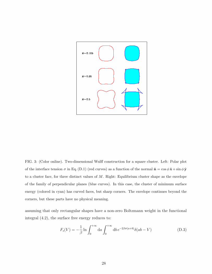
FIG. 3: (Color online). Two-dimensional Wulff construction for a square cluster. Left: Polar plot

of the interface tension σ in Eq. (D.1) (red curves) as a function of the normal n = cosφ x + sinφ y

to a cluster face, for three distinct values of M . Right: Equilibrium cluster shape as the envelope

of the family of perpendicular planes (blue curves). In this case, the cluster of minimum surface

energy (colored in cyan) has curved faces, but sharp corners. The envelope continues beyond the

corners, but these parts have no physical meaning.

assuming that only rectangular shapes have a non-zero Boltzmann weight in the functional

integral (4.2), the surface free energy reduces to:

Fs(V ) = − 1

βln

∫ +∞

0

da

∫ +∞

0

db e−2βσ(a+b)δ(ab− V ) (D.3)

28

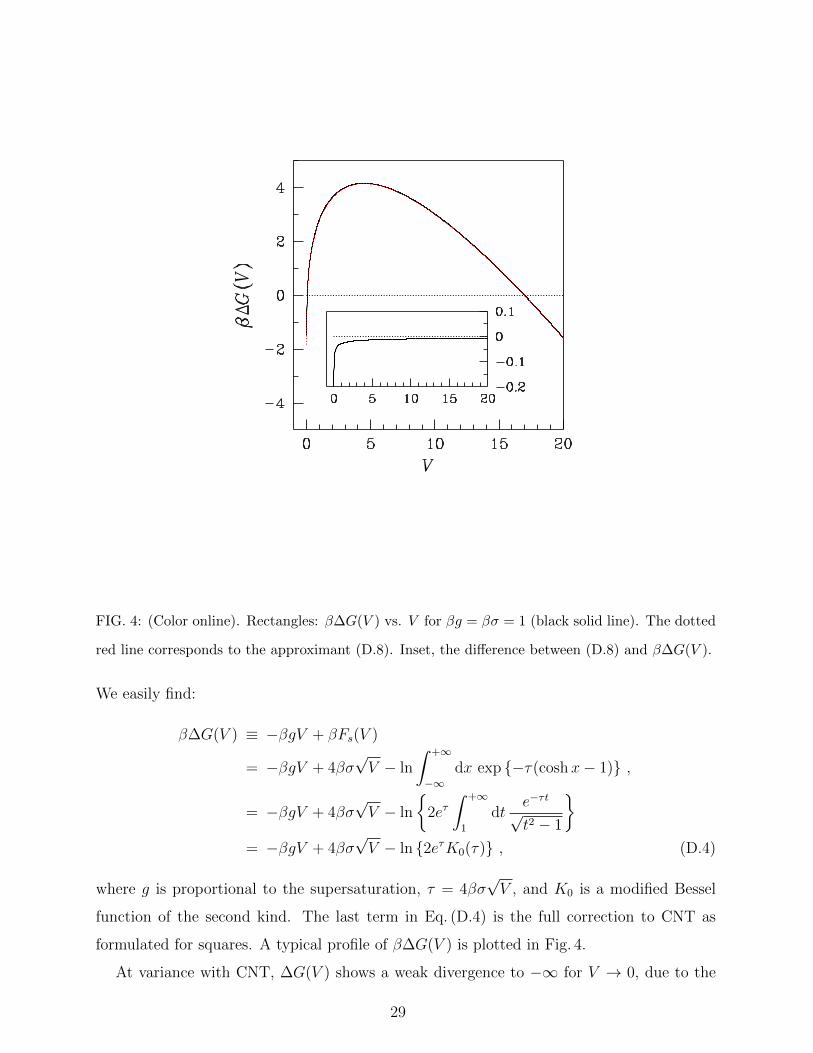
FIG. 4: (Color online). Rectangles: β∆G(V ) vs. V for βg = βσ = 1 (black solid line). The dotted

red line corresponds to the approximant (D.8). Inset, the difference between (D.8) and β∆G(V ).

We easily find:

β∆G(V ) ≡ −βgV + βFs(V )

= −βgV + 4βσ√V − ln

∫ +∞

−∞dx exp −τ(coshx− 1) ,

= −βgV + 4βσ√V − ln

2eτ∫ +∞

1

dte−τt√t2 − 1

= −βgV + 4βσ

√V − ln 2eτK0(τ) , (D.4)

where g is proportional to the supersaturation, τ = 4βσ√V , and K0 is a modified Bessel

function of the second kind. The last term in Eq. (D.4) is the full correction to CNT as

formulated for squares. A typical profile of β∆G(V ) is plotted in Fig. 4.

At variance with CNT, ∆G(V ) shows a weak divergence to −∞ for V → 0, due to the

29

absence of a lower cutoff volume. For τ 1,

K0(τ) = − ln(τ/2)− γ +O(τ 2 ln τ) , (D.5)

with γ = 0.5772 . . . (Eulero-Mascheroni constant). Hence, the singular behavior of β∆G(V )

for small V is of the kind

β∆G(V ) ' − ln− ln

(2βσ√V)

. (D.6)

Conversely, for large τ values,

K0(τ) ∼√

π

2τe−τ , (D.7)

and we obtain

β∆G(V ) ' −βgV + 4βσ√V +

1

2ln(

4βσ√V)− 1

2ln(2π) . (D.8)

The goodness of the approximation (D.8) can be judged from the inset of Fig. 4, which shows

that the approximation is accurate for all values of V but for the smallest ones.

2. Truncated rectangles

In order to study the effects on nucleation of a more complicate type of interface-tension

anisotropy, we further enrich our book of patterns, passing from rectangles to truncated

rectangles. By the name of truncated rectangle we mean the octagon represented in Fig. 5.

This occurs when the cost of (11) and equivalent facets is of the same order of σ10, while all

other facets are much higher in energy and can be ruled out.

A Wulff plot giving origin to truncated squares is:

σ(φ) = σ10

[1 +

(σ11

σ10

− 1

)sin2(2φ) +M sin2(4φ)

](D.9)

with infinite M (see Fig. 6). The polar plot of (D.9) for finite M is a smoothed eight-pointed

star with hollows at the normal directions satisfying sin(4φ) = 0. Depending on the ratio

of σ11 to σ10, the equilibrium cluster shape shows (i) just (11) facets (σ11/σ10 ≤√

2/2); (ii)

both (11) and (10) facets (√

2/2 < σ11/σ10 <√

2); (iii) just (10) facets (σ11/σ10 ≥√

2).

In order to prove this, we observe that, for fixed a, b, and ` (with ` ≤ `max ≡

(1/√

2) mina, b), the “volume” and “area” of the truncated rectangle are given respec-

tively by V = ab− `2 and A = A11 +A10, with A11 = 4` and A10 = 2(a+ b− 2√

2`), leading

30

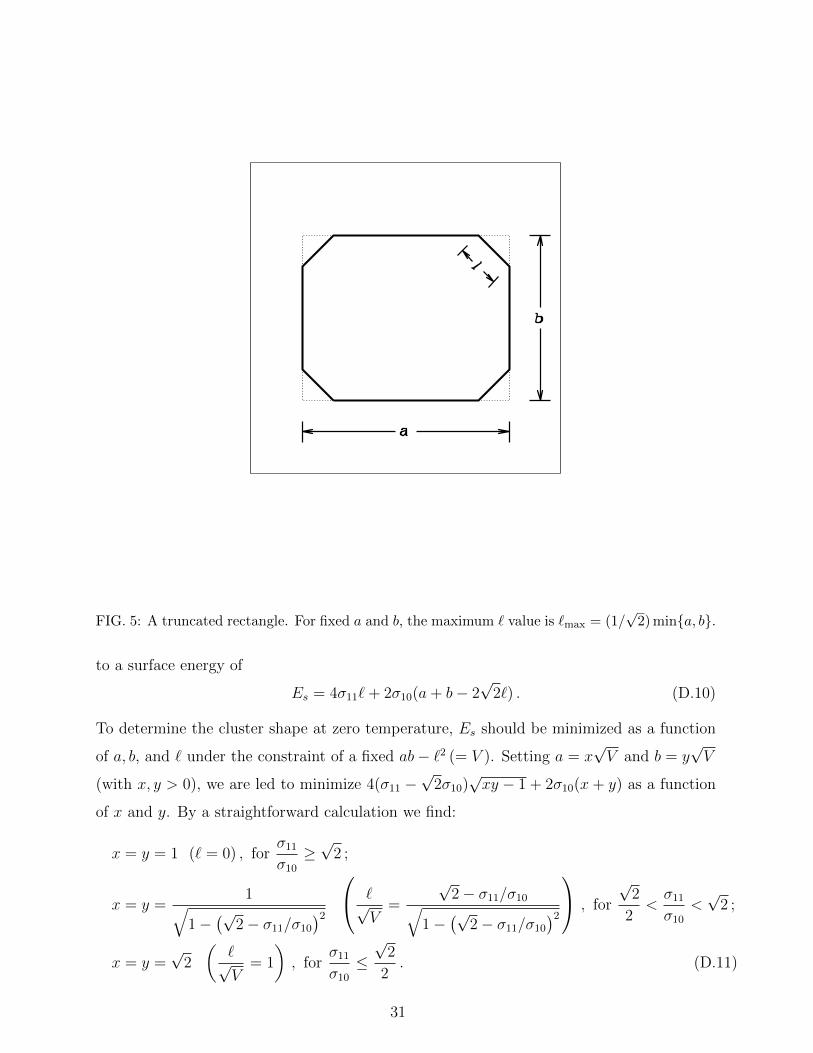
FIG. 5: A truncated rectangle. For fixed a and b, the maximum ` value is `max = (1/√

2) mina, b.

to a surface energy of

Es = 4σ11`+ 2σ10(a+ b− 2√

2`) . (D.10)

To determine the cluster shape at zero temperature, Es should be minimized as a function

of a, b, and ` under the constraint of a fixed ab− `2 (= V ). Setting a = x√V and b = y

√V

(with x, y > 0), we are led to minimize 4(σ11 −√

2σ10)√xy − 1 + 2σ10(x + y) as a function

of x and y. By a straightforward calculation we find:

x = y = 1 (` = 0) , forσ11

σ10

≥√

2 ;

x = y =1√

1−(√

2− σ11/σ10

)2

`√V

=

√2− σ11/σ10√

1−(√

2− σ11/σ10

)2

, for

√2

2<σ11

σ10

<√

2 ;

x = y =√

2

(`√V

= 1

), for

σ11

σ10

≤√

2

2. (D.11)

31

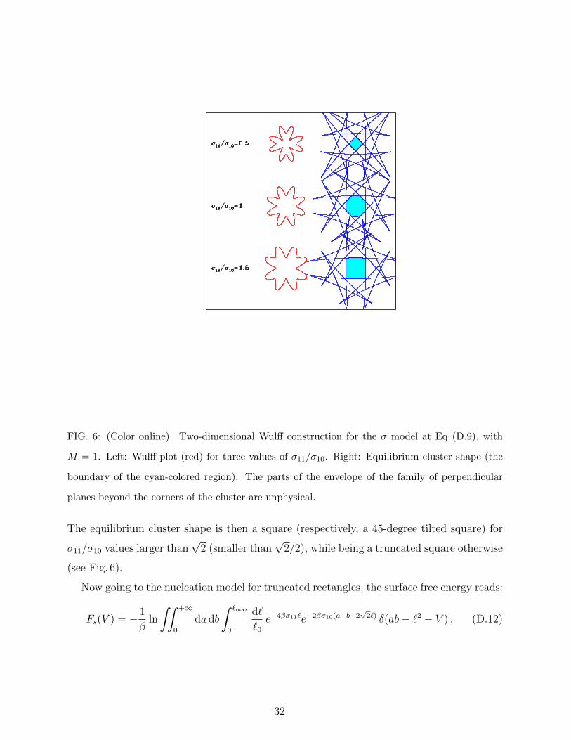
FIG. 6: (Color online). Two-dimensional Wulff construction for the σ model at Eq. (D.9), with

M = 1. Left: Wulff plot (red) for three values of σ11/σ10. Right: Equilibrium cluster shape (the

boundary of the cyan-colored region). The parts of the envelope of the family of perpendicular

planes beyond the corners of the cluster are unphysical.

The equilibrium cluster shape is then a square (respectively, a 45-degree tilted square) for

σ11/σ10 values larger than√

2 (smaller than√

2/2), while being a truncated square otherwise

(see Fig. 6).

Now going to the nucleation model for truncated rectangles, the surface free energy reads:

Fs(V ) = − 1

βln

∫∫ +∞

0

da db

∫ `max

0

d`

`0

e−4βσ11`e−2βσ10(a+b−2√

2`) δ(ab− `2 − V ) , (D.12)

32

where `0 is an arbitrary length. By integrating the delta out, we obtain:

β∆G(V ) = −βgV + 4βσ10

√V − 1

2ln

(V

`20

)− ln

∫ +∞

−∞dx

∫ +∞

0

dyΘ(

minex, (1 + y2)e−x −√

2y)

× exp−(τ11 −

√2τ10

)y

exp−τ10

2

(ex + (1 + y2)e−x − 2

), (D.13)

where Θ is Heaviside’s function, τ10 = 4βσ10

√V , and τ11 = 4βσ11

√V . For βσ10 = 1, `0 = 1,

and σ11/σ10 = 0.5, 1, 2, 20, 200, the plot of (D.13) is reported in Fig. 7. Note that a precritical

minimum shows up for any finite value of σ11/σ10, which moves toward zero upon increasing

the interface-tension anisotropy. An even more complex behavior is seen for σ11/σ10 = 0.5,

where a bump emerges beyond the critical maximum.

When σ11 σ10, it is natural to expect that the model of truncated rectangles reduces

to the rectangular-cluster model. This can be proved analytically starting from Eq. (D.12).

First, a, b, and ` are rescaled by dividing by√V ; then one observes that

√V e−4βσ11

√V ` ≈ 1

2βσ11

δ(`) . (D.14)

Hence, aside from a constant equal to ln(4βσ11), the β∆G(V ) function for truncated rect-

angles merges, for very large σ11/σ10, into the analogous function for rectangles. This fact

is shown numerically in the inset of Fig. 7.

3. Rectangular cuboids

When the Wulff plot is as in Eq. (4.5) with infinite M , the only admissible shapes are

rectangular cuboids. Denoting a, b, and c the edges of a cuboid, the V -dependent surface

free energy is defined as

βFs(V ) = − ln

∫∫∫ +∞

0

da db dc e−2βσ(ab+ac+bc)δ(abc− V )

= − ln

∫∫ +∞

0

da db1

abexp

−τ

3

(ab+

a+ b

ab

), (D.15)

where τ = 6βσV 2/3. With another change of variables, we arrive at

β∆G(V ) = −βgV + 6βσV 2/3− ln

∫∫ +∞

−∞dx dy exp

−τ

3

(ex+y + e−x + e−y − 3

). (D.16)

33

FIG. 7: (Color online). Truncated rectangles: β∆G(V ) vs. V for βg = βσ10 = 1 e `0 = 1. A

constant of ln(4βσ11) was subtracted from β∆G(V ) in order to garantee the confluence of its plot

to that for rectangles, in the limit σ11/σ10 → +∞. A number of σ11/σ10 values are considered:

0.5 (black), 1 (blue), 2 (cyan), 20 (magenta), and 200 (red, practically indistinguishable from the

rectangular case). In the inset, we zoom on the small-V region, evidencing the singular behavior

of ∆G(V ) for V → 0. Apparently, for all finite σ11 values, the curve blows up to +∞ rather than

to −∞, as instead occurs for rectangles.

The above formula is well suited for the numerical evaluation of ∆G(V ). For βg = βσ = 1,

the profile of β∆G(V ) is plotted in Fig. 8.

In order to discover the analytic behavior of ∆G(V ) at small and at large V ’s, we should

further elaborate on Eq. (D.16). Setting a + b = x and ab = y in (D.15), a and b are the

solutions to the equation t2 − xt + y = 0, whose discriminant is non-negative for x ≥ 2√y.

34

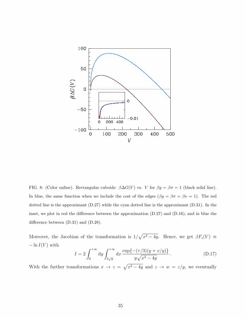
FIG. 8: (Color online). Rectangular cuboids: β∆G(V ) vs. V for βg = βσ = 1 (black solid line).

In blue, the same function when we include the cost of the edges (βg = βσ = βν = 1). The red

dotted line is the approximant (D.27) while the cyan dotted line is the approximant (D.31). In the

inset, we plot in red the difference between the approximation (D.27) and (D.16), and in blue the

difference between (D.31) and (D.28).

Moreover, the Jacobian of the transformation is 1/√x2 − 4y. Hence, we get βFs(V ) ≡

− ln I(V ) with

I = 2

∫ +∞

0

dy

∫ +∞

2√y

dxexp−(τ/3)(y + x/y)

y√x2 − 4y

. (D.17)

With the further transformations x → z =√x2 − 4y and z → w = z/y, we eventually

35

obtain:

I = 2

∫ +∞

0

dye−(τ/3)y

y

∫ +∞

0

dzexp−(τ/3)

√z2 + 4y/y√

z2 + 4y

= 2

∫ +∞

0

dye−(τ/3)y

y

∫ +∞

0

dwexp

−√w2 + 4τ2

9y

√w2 + 4τ2

9y

. (D.18)

Since ∫ +∞

0

dxexp−

√x2 + c2√

x2 + c2=

∫ +∞

c

dte−t√t2 − c2

= K0(c) , (D.19)

we finally find:

I = 2

∫ +∞

0

dye−(τ/3)y

yK0

(2τ

3√y

)= 4

∫ +∞

0

dx exp

− 4τ 3

27x2

K0(x)

x. (D.20)

In Eq. (D.20) we recognize a particular Meijer function, G3003((τ/3)3|0, 0, 0), whose behavior

at small τ is:9

2(ln τ)2 + 9(γ − ln 3) ln τ +O(1) . (D.21)

From the above, we can draw the main singular term in β∆G(V ) at small V , that is

β∆G(V ) ' −2 ln(− ln(6βσV 2/3)

), (D.22)

which is similar to (D.6).

The large-V behavior of ∆G(V ) can also be obtained from Eq. (D.20). For τ 1, we

are allowed to replace K0(x) with Eq. (D.7) and thus estimate I through the integral

I∞ = 2√

2π

∫ +∞

0

dxexp

−x− 4τ3

27x2

x3/2

. (D.23)

Suspecting a dominant term of τ in − ln I∞, we consider

eτI∞ = 2

√2π

τ

∫ +∞

0

dz z−3/2 exp

τ

(1− z − 4

27z2

). (D.24)

In order to compute the asymptotic behavior of (D.24), we use the Laplace method. The

maximum of the concave function φ(z) = 1− z − (4/27)z−2 falls at c = 2/3, with φ(c) = 0

and φ′′(c) = −9/2. Since, for any a < c < b,∫ b

a

dz f(z)eτφ(z) ∼√

2πf(c)eτφ(c)√−τφ′′(c)

, (D.25)

36

the asymptotic behavior of I reads:

I ∼ 2π√

3e−τ

τ(D.26)

and

β∆G(V ) ∼ −βgV + 6βσV 2/3 + ln(6βσV 2/3)− ln(2π√

3) . (D.27)

The last two terms in Eq. (D.27) give the subleading corrections to CNT as formulated for

cubic clusters. The quality of the approximation (D.27) can be judged from the inset of

Fig. 8, which shows a very good matching for all V ’s except for the smallest values, similarly

to what occurs for rectangles (cf. Fig. 4).

The calculation of ∆G can also be performed when a further energy cost, ν per unit

length, is assumed for the edges. Equation (D.16) is then modified to

β∆G(V ) = −βgV + 6βσV 2/3 + 12βνV 1/3

− ln

∫∫ +∞

−∞dx dy exp

−τ1

3

(ex+y + e−x + e−y − 3

)− τ2

3

(e−x−y + ex + ey − 3

),

(D.28)

where τ1 = 6βσV 2/3 and τ2 = 12βνV 1/3. By the same line of reasoning as followed above

we arrive at βFs ≡ − ln I(V ) with

I = 2

∫ +∞

0

dye−(τ1/3)y−τ2/(3y)

yK0

(2τ1

3√y

+2τ2

3y

). (D.29)

Laplace method can still be invoked to extract the asymptotic behavior of I, which turns

out to be

− ln I ∼ τ1 + τ2 + ln(τ1 + τ2)− ln(2π√

3) . (D.30)

From the above formula, we get

β∆G(V ) ∼ −βgV + 6βσV 2/3 + 12βνV 1/3 + ln(6βσV 2/3 + 12βνV 1/3)− ln(2π√

3) . (D.31)

In Fig. 8, we compare the approximation (D.31) with the exact value. We see that the

agreement is good for not too small V .

37

4. Ellipsoids

Let us finally study the case of an ellipsoidal cluster. Volume and area of an ellipsoid

with semiaxes a, b, and c are respectively given by

V =4

3πabc and A = 2π

(c2 +

bc2

√a2 − c2

F (φ|m) + b√a2 − c2E(φ|m)

),

(a ≥ b > c and a > b ≥ c ; A = 4πc2 for a = b = c) (D.32)

where

m =a2(b2 − c2)

b2(a2 − c2)=

1− c2/b2

1− c2/a2< 1 and φ = arcsin

√a2 − c2

a. (D.33)

F and E are elliptic integrals of the first and second kind, respectively. For −π/2 < φ < π/2,

they are defined as

F (φ|m) ≡∫ φ

0

dx1√

1−m sin2 xand E(φ|m) ≡

∫ φ

0

dx√

1−m sin2 x . (D.34)

Let now A(a, b, c) be the surface area of an ellipsoid of semiaxes a, b, and c (not necessarily

in descending order). By the usual transformations, the surface free energy becomes

βFs(V ) = − ln

∫∫ +∞

0

da db1

abexp

−βσ

(3V

4π

)2/3

A

(a, b,

1

ab

)+ ln

4π

3

= τ − ln

∫∫ +∞

−∞dq dp exp

− τ

4π

(A(eq, ep, e−q−p

)− 4π

)+ ln

4π

3, (D.35)

where τ = βσ(36π)1/3V 2/3. To obtain β∆G(V ), it is sufficient to add −βgV to (D.35). For

βg = βσ = 1, the plot of this function is reported in Fig. 9. In the same figure, β∆G(V ) is

compared with the asymptotic estimate

β∆G(V ) ∼ −βgV + βσ(36π)1/3V 2/3 + ln(βσ(36π)1/3V 2/3)− 0.4849 , (D.36)

where the last two terms give the correction to CNT as formulated now for spherical clusters.

Judging from the inset of Fig. 9, which shows the difference between the approximate and

exact values of β∆G(V ), the estimate (D.36) is very good for all V ’s except for the very

small ones.

The strong similarity between (D.36) and (D.27), together with the high accuracy with

which they reproduce the profile of β∆G(V ) for ellipsoids and cuboids respectively, indicates

that the difference between envisaging the nucleus as ellipsoidal rather than cuboidal entirely

38

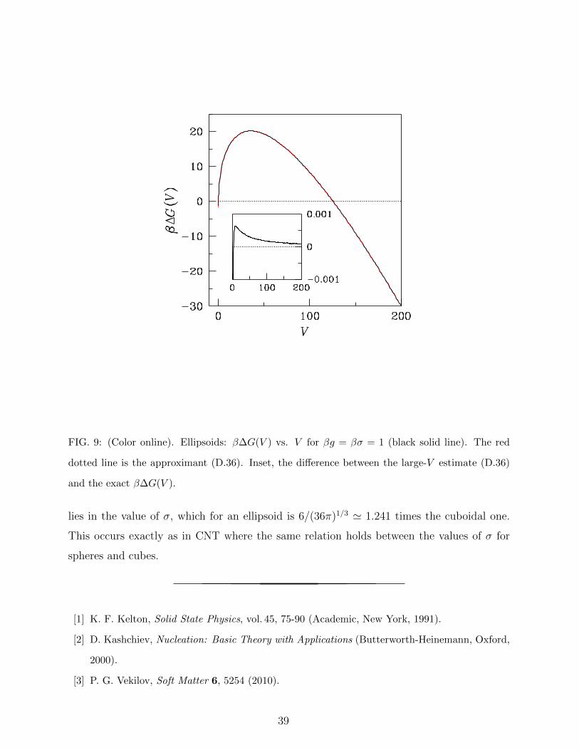
FIG. 9: (Color online). Ellipsoids: β∆G(V ) vs. V for βg = βσ = 1 (black solid line). The red

dotted line is the approximant (D.36). Inset, the difference between the large-V estimate (D.36)

and the exact β∆G(V ).

lies in the value of σ, which for an ellipsoid is 6/(36π)1/3 ' 1.241 times the cuboidal one.

This occurs exactly as in CNT where the same relation holds between the values of σ for

spheres and cubes.

[1] K. F. Kelton, Solid State Physics, vol. 45, 75-90 (Academic, New York, 1991).

[2] D. Kashchiev, Nucleation: Basic Theory with Applications (Butterworth-Heinemann, Oxford,

2000).

[3] P. G. Vekilov, Soft Matter 6, 5254 (2010).

39

[4] M. Volmer and A. Weber, Z. Phys. Chem. 119, 277 (1926).

[5] L. Farkas, Z. Phys. Chem. 125, 239 (1927).

[6] R. Becker and W. Doring, Ann. Phys. (Leipzig) 24, 719 (1935).

[7] See e.g. C. K. Bagdassarian and D. W. Oxtoby, J. Chem. Phys. 100, 2139 (1994).

[8] S. Prestipino, A. Laio, and E. Tosatti, Phys. Rev. Lett. , (2012).

[9] A. Dillmann and G. E. A. Meier, J. Chem. Phys. 94, 3872 (1991).

[10] See e.g. W. H. Shih, Z. Q. Wang, X. C. Zeng, and D. Stroud, Phys. Rev. A 35 2611 (1987).

[11] J. W. Cahn and J. E. Hilliard, J. Chem. Phys. 28, 258 (1957).

[12] J. W. Cahn and J. E. Hilliard, J. Chem. Phys. 31, 688 (1959).

[13] M. P. A. Fisher and M. Wortis, Phys. Rev. B 29, 6252 (1984).

[14] P. Harrowell and D. W. Oxtoby, J. Chem. Phys. 80, 1639 (1984).

[15] Y. C. Shen and D. W. Oxtoby, J. Chem. Phys. 105, 6517 (1996).

[16] See, for example, M. Kardar, Statistical Physics of Fields (Cambridge University Press, 2007).

[17] B. J. Block, S. K. Das, M. Oettel, P. Virnau, and K. Binder, J. Chem. Phys. 133, 154702

(2010).

[18] R. C. Tolman, J. Chem. Phys. 17, 333 (1949).

[19] See e.g. L. Filion, M. Hermes, R. Ni, and M. Dijkstra, J. Chem. Phys. 133, 244115 (2010).

[20] T. Zykova-Timan, C. Valeriani, E. Sanz, D. Frenkel, and E. Tosatti, Phys. Rev. Lett. 100,

036103 (2008).

[21] P. Canham, J. Theor. Biol. 26, 61 (1970).

[22] W. Helfrich, Z. Naturforsch. C 28, 693 (1973).

[23] H. S. Kogon and D. J. Wallace, J. Phys. A 14, L527 (1981).

[24] K. Kassner, e-print arXiv:cond-mat/0607823.

[25] M. Napiorkowski and S. Dietrich, Phys. Rev. E 47, 1836 (1993).

[26] J. G. Segovia-Lopez, A. Zamora, and J. A. Santiago, J. Chem. Phys. 135, 064102 (2011).

[27] M. Abate e F. Tovena, Curve e superfici (Springer Italia, Milano, 2006), Observations 5.3.21

and 5.3.22.

[28] M. Abate e F. Tovena, Curve e superfici (Springer Italia, Milano, 2006), Corollary 5.3.24.

[29] T. Zykova-Timan, D. Ceresoli, U. Tartaglino, and E. Tosatti, J. Chem. Phys. 123, 164701

(2005).

[30] S. T. Milner and S. A. Safran, Phys. Rev. A 36, 4371 (1987).

40

[31] N. J. Gunther, D. A. Nicole, and D. J. Wallace, J. Phys. A 13, 1755 (1980).

[32] P. R. ten Wolde and D. Frenkel, J. Chem. Phys. 109, 9901 (1998).

[33] H. Reiss and R. K. Bowles, J. Chem. Phys. 111, 7501 (1999).

[34] R. K. Bowles, R. McGraw, P. Schaaf, B. Senger, J.-C. Voegel, and H. Reiss, J. Chem. Phys.

113, 4524 (2000).

[35] L. Maibaum, Phys. Rev. Lett. 101, 019601 (2008).

[36] A. C. Pan and D. Chandler, J. Phys. Chem. B 108, 19681 (2004).

[37] L. D. Gelb, J. Chem. Phys. 118, 7747 (2003).

[38] K. K. Mon, S. Wansleben, D. P. Landau, and K. Binder, Phys. Rev. B 39, 7089 (1989).

[39] M. Hasenbusch and K. Pinn, Physica A 192, 342 (1993).

[40] C. Rottman and M. Wortis, Phys. Rev. B 29, 328 (1984).

[41] M. Hasenbusch and K. Pinn, J. Phys. A 30, 63 (1997).

[42] J. Hoshen and R. Kopelman, Phys. Rev. B 14, 3438 (1976).

[43] H. Muller-Krumbhaar, Phys. Lett. A 50, 27 (1974).

[44] G. Wulff, Z. Kristallogr. 34, 449 (1901).

[45] W. K. Burton, N. Cabrera, and F. C. Frank, Philos. Trans. R. Soc. London, Ser. A 243, 299

(1951).

[46] T. Li, D. Donadio, and G. Galli, J. Chem. Phys. 131, 224519 (2009).

[47] T. Li, D. Donadio, G. Russo, and G. Galli, Phys. Chem. Chem. Phys. 13, 19807 (2011).

[48] M. Franke, A. Lederer, and H. J. Schope, Soft Matter 7, 11267 (2011).

41