A Discrete Choice Based Facility Location Model forInland Container Depots

Yuanquan Xu

Dissertation submitted to theCollege of Engineering and Mineral Resources

at West Virginia Universityin partial fulfillment of the requirements

for the degree of

Doctor of Philosophyin

Engineering

David R. Martinelli, Ph.D., ChairDarrel R. Dean, Jr., Ph.D.

Ronald W. Eck, Ph.D.Wafik H. Iskander, Ph.D.John P. Zaniewski, Ph.D.

Department of Civil and Environmental Engineering

Morgantown, West Virginia1999

Keywords: Facility Location, Container Depot, Discrete Choice

ABSTRACT

A Discrete Choice Based Facility Location Model for Inland ContainerDepots

Yuanquan Xu

Container transport operations have been extending inland, providing more

comprehensive service across the shipping network. Accordingly, container transport

operators are making extensive capital investments in deploying inland container depot

(ICD) networks. Optimizing the location of such facilities financially is vital for both

capital and operating efficiencies. Currently, there are no models at the regional network

level to guide container operators in locating ICDs on their networks. This research

studies the ICD location problem and develops a comprehensive ICD location model.

Based on comprehensive analysis of the container transport industry, focusing on ICD

operations, this thesis developed a useful formulation of the ICD location problem. It

recognizes and emphasizes the need to embody the endogenous demand and market

competitiveness in the container transport business. The formulation combines the

multinomial logit model of discrete choice analysis to quantitatively describe the

shipper’s behaviors and preferences, addressing both the endogenous demand and market

competitiveness.

Fixed charge facility location problems are considered or proven to be NP complete.

The use of multinomial logit model inevitably further complicates the formulation in both

the objective function and constraints, which justifies the use of heuristics to solve the

formulation. Based on the mathematical properties of the formulation, a problem specific

tabu search heuristic algorithm was designed for its solution. Tabu search parameters,

tabu tenure, slack parameters, and cutoff parameters, are tested to decide their

contributions and sensitivity to the computational time and optimality. Statistical

inference was used to evaluate the performance of tabu search algorithm. The result of

the evaluation shows that the solutions of tabu search algorithm are within the confidence

interval of optimal solution of this formulation. This proves that the designed tabu

algorithm is efficient and effective in solving the problem.

Acknowledgement

I would like to express my heartfelt gratitude to my advisor, Dr. David Martinelli. He

provided me this precious opportunity to study at West Virginia University. His

involvement, guidance, support, and encouragement throughout my study and research at

WVU were invaluable and critical. His advice and help in making me, an international

student, familiar with the culture of the land, is unforgettable.

I deeply thank Dr. Ronald Eck, Darrel Dean, Jr., Wafik Iskander, and John Zaniewski

for teaching me at WVU and serving as my committee members. Their suggestions and

comments to my thesis were essential and insightful. I also deeply thank Dr. Hualiang

Teng who offered me advice in establishing the framework of my thesis and detailed

thoughts in many chapters of this thesis.

Many friends helped me in various ways during my study at WVU and made my life

in Morgantown an enjoyable experience. They are Pengguo Jiang, David Boyajian,

Chuck and Ginny Lewis, Sandy Wotring, Denise Brooks, Eleanor Palko, Ruijie Liu,

Xiaoming Jin, Faxian Yang, Dan Montag, Jennifer Reigle, and etc. I thank all of you for

your company and help.

In closing, I want to thank my parents for their unconditional love and support to me.

iv

Table of ContentsList of Tables.....................................................................................................................vii

List of Figures ..................................................................................................................viii

List of Acronyms................................................................................................................. x

1. Introduction ...................................................................................................................1

1.1 Background and Motivations ........................................................................... 1

1.2 Problem Statement ........................................................................................... 5

1.3 Research Objectives ......................................................................................... 6

1.4 Organization of the Dissertation ...................................................................... 6

2. Background ................................................................................................................... 8

2.1 Intermodal Container Transport ....................................................................... 8

2.2 Inland Facility of Intermodal Transport ......................................................... 13

2.3 Cargo Handling and Container Movements in Inland Transport of Different

Scenarios ............................................................................................................... 16

2.4 ICD Basics..................................................................................................... 22

2.4.1 ICD Layout............................................................................................ 22

2.4.2 Container handling operations and handling equipment....................... 25

2.4.3 Maintenance costs and operating costs ................................................. 29

3 Literature Review........................................................................................................ 30

3.1 Prototype Facility Location Problems............................................................ 30

3.2 Formulations and Algorithms of p-Median and Fixed Charge Facility

Location Problems................................................................................................. 32

3.2.1 Formulations.................................................................................... 32

3.2.2 Algorithms....................................................................................... 36

3.2.3 Performance Evaluation of Heuristic Algorithms Using Statistical

Inference.................................................................................................... 39

v

3.3 Summarization ............................................................................................... 40

4 Problem Formulation................................................................................................... 42

4.1 Introduction ..................................................................................................... 42

4.2 Shipper’s Transport Logistics Cost ................................................................. 42

4.3 Discrete Choice Analysis ................................................................................ 46

4.3.1 Random Utility................................................................................ 46

4.3.2 Parameterized Multinomial Choice Models.................................... 48

4.3.3 Estimation of Multinomial Logit..................................................... 50

4.3.4 Aggregation..................................................................................... 51

4.4 Representation of Selective Relationship between ICD and Freight Demand 52

4.5 Problem Formulation...................................................................................... 55

4.5.1 Objective Function .......................................................................... 56

4.5.2 Constraints....................................................................................... 63

4.6 Illustration of Formulation ............................................................................. 64

5 Algorithm Development............................................................................................... 73

5.1 Introduction .................................................................................................... 73

5.2 Exact Algorithm for Small Sized Problem..................................................... 74

5.3 Tabu Search Heuristic Algorithm .................................................................. 74

5.3.1 Introduction to Tabu Search ........................................................... 74

5.3.2 Simple Illustrative Example of Tabu Search................................... 75

5.3.3 Tabu Search Algorithm Design....................................................... 76

5.4 Experiments for Parameters of Tabu Search Algorithm ................................ 80

5.4.1 Settings for Algorithm Testing........................................................ 80

5.4.2 Experiments for Parameters of Tabu Search Algorithm ................. 80

6 Performance Evaluation for Heuristic Algorithm ......................................................... 87

6.1 Introduction .................................................................................................... 87

6.2 Comparison of Exact Algorithm and Tabu Search Algorithm for Small

Problems................................................................................................................ 88

vi

6.3 Evaluation of Tabu Search Algorithm ........................................................... 91

6.3.1 Point Estimation and Interval Estimation ..................................... 91

6.3.2 Maximum Likelihood Estimation (MLE) ..................................... 92

6.3.3 Evaluation of Tabu Search Algorithm .......................................... 93

7 Conclusions and Recommendations............................................................................ 95

7.1 Summarization ............................................................................................... 95

7.2 Contributions of the Research ........................................................................ 95

7.3 Recommendations for Future Study............................................................... 96

References ......................................................................................................................... 98

Appendix A. C++ Codes of Tabu Search Algorithm...................................................... 103

Appendix B. Fortran Codes of Monte Carlo Algorithm to Resolve Nonlinear Equations

System ............................................................................................................................. 122

vii

List of Tables

2.1 U.S. Waterborne Foreign Trade for 1990 to 1997 ..................................................... 12

2.2 U.S. Waterborne Foreign Trade Forecast................................................................... 12

2.3 Comparison between LT and RTG/RMG.................................................................. 26

2.4 RTG versus LT........................................................................................................... 29

4.1 ICD Manpower Requirements ................................................................................... 62

5.1 Comparison of Two Settings...................................................................................... 86

6. 1 Optimal Solutions by Exact Algorithm..................................................................... 89

6.2 Tabu Search Solutions................................................................................................ 90

6.3 Objective Values of Sample Solutions of Tabu Search Algorithm............................ 93

viii

List of Figures

1.1 APL Intermodal Terminal Network (Rail)................................................................... 3

1.2 Sea-Land (CSX) Intermodal Terminal Network.......................................................... 4

2.1 U.S Intermodal Rail Loadings (1961-1997)............................................................... 11

2.2 Sea-Land Intermodal Terminal at Chicago ................................................................ 15

2.3 Typical Transportation Options-Exports (Reverse Order for Imports)...................... 17

2.4 Import: Movement Destined to ICD with Clearance at the Port................................ 18

2.5 Import: Movement with Clearance at the ICD........................................................... 19

2.6 Export: Movement with Clearance at the Port ........................................................... 20

2.7 Export: Movement with Clearance at the ICD........................................................... 21

2.8 Corwith Rail Intermodal Terminal of BNSF.............................................................. 23

2.9 Highway ICD of Sinotrans......................................................................................... 24

2.10 SISU Rubber Tired Gantry Crane of Heavy Machines Inc...................................... 27

2.11 Kalma/SISU Reach Stacker of Heavy Machine Inc................................................. 27

2.12 Ferrari SLT of CVS S.p.A........................................................................................ 28

2.13 Ferrari T LT of CVS S.p.A ...................................................................................... 28

3.1 Classification of Facility Location Problems............................................................. 30

4.1 Transportation Cost vs. Logistics Cost ...................................................................... 45

4.2 Selective Relations between ICD and Demand.......................................................... 54

4.3 Illustrative Network for Formulation ......................................................................... 65

5.1 Flowchart of Designed Tabu Search Algorithm ........................................................ 79

5.2 Data Structure to Describe Shipper’s Selection of Facility........................................ 80

5.3 Problem Size vs. Execution Time .............................................................................. 81

5.4 Number of Outer Iterations vs. Objective Function Value ........................................ 82

5.5 Number of Outer Iterations vs. Execution Time........................................................ 82

ix

5.6 Number of Inner Iterations vs. Objective Function Value......................................... 83

5.7 Number of Inner Iterations vs. Execution Time......................................................... 84

5.8 Tabu Tenure vs. Objective Function Value ............................................................... 85

5.9 Tabu Tenure vs. Execution Time ............................................................................... 85

x

List of Acronyms

CFSContainer Freight Station

COFCContainer on Flat Car

CYContainer Yard

FAK Freight in All Kinds

FCLFull Container Load

FEUForty-foot Equivalent Unit

FLT Fork Lift Truck

ICDInland Container Depot

LCLLess than Container Load

LTLift Truck

MLEMaximum Likelihood Estimation

MNL Multinomial Logit

RMG Rail Mounted Gantry

RTG Rubber Tired Gantry

SK Straddle Carrier

SLT Side Lift Truck

TEUTwenty-foot Equivalent Unit

TLT Top Lift Truck

TOFCTrailer on Flat Car

1

Chapter 1

Introduction

1.1 Background and Motivations

Since the advent of marine containers in late 1950s, container transport has been growing

rapidly. Over 60 percent of the world’s deep sea general cargo now moves in containers,

and the percentage of containerizable cargo is higher between economically strong and

stable countries, approaching 100 percent in some cases (Muller 1995). The

Transportation Research Board (1992) estimates that in 1988 containerized imports and

exports represented 80 percent of liner trade valuing nearly $195 billion. Assuming

$30,000 per Twenty-foot Equivalent Unit (TEU)1, the total value of containerized

imports and exports of US in 1997 is about $440 billion2.

In the last decade, marine containers have been moving inland, extending from port-

to-port service to door-to-door intermodal container transport. The growth of container

inland transport has been very impressive. In North America, rail has played a

tremendous role in inland container transport and intermodal rail transport is used as an

example to show the growth of container inland transport in North America. The

Association of American Railroads (AAR)3 reports:

• Intermodal traffic has grown from 3 million trailers and containers in 1980 to 8.7

million in 1997;

• Intermodal accounts for more than 17 percent of rail revenues, second only to coal

at 22 percent;

1 This is based on World Bank survey. Due to the unavailability of reference, the author is responsible forthis statement as he used this parameter value in World Bank related assignment.2 The loaded import and export container volume of US was 14,794,751 TEU for 1997, MaritimeAdministration (1998).3 The following is quotation from AAR’s web site at <http://www.aar.org> as of March 21, 1999.

2

• Containers account for more than 60 percent of intermodal volume, up from 40

percent ten years ago.

Accordingly, inland container facilities are required to accommodate containers and

enclosed cargoes that move inland. At the end of 1980s and the beginning of 1990s,

major container operators began to build sophisticated inland container facility networks

in North America, whereas this task is just starting in developing countries. Beginning in

the late 1980s, American President Lines (APL) and Sea-Land Services, (two large

American flag container shipping lines,) commenced establishing inland facility systems

of intermodal container transport in United States. Today, they enjoy their sophisticated

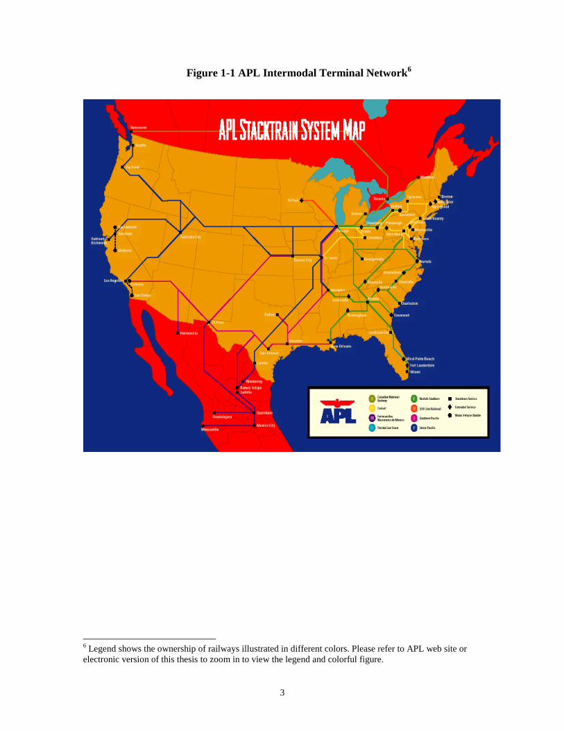
North American intermodal container terminal networks that are shown in Figure 1-14

and 1-25 respectively. Following APL and Sea-Land, major intermodal container

operators/carriers including Chinese COSCO, OOCL, and Evergreen, Danish Maersk,

Japanese NYK and K Line, etc. all have built similar intermodal terminal networks in

North America. In the emerging container markets, these intermodal transport operators

are just trying to form new inland container facility networks. For example, in China,

APL is working on the Dalian corridor starting from the Port of Dalian, Sea-Land on

Tianjin corridor from the Port of Tianjin, OOCL on Qingdao corridor from the Port of

Qingdao, etc.

Inland Container Depots (ICD’s) are capital intensive and perform functions

including loading/unloading containers, moving containers, and stuffing/stripping

containers. These functions are similar to those conducted at container facilities (such as

container terminals) at ports. It is not uncommon to cost tens of million dollars to build

one ICD. The location of ICD’s involves the financial feasibility for a single container

depot, and, more importantly, is concerned with the capture of container market share in

the whole region. This is because ICD’s are the means by which container operators

compete for their market presence.

4 Source: APL web site at <http://www.apl.com>5Source: Sea-Land web site at <http://www.sealand.com>

3

Figure 1-1 APL Intermodal Terminal Network 6

6 Legend shows the ownership of railways illustrated in different colors. Please refer to APL web site orelectronic version of this thesis to zoom in to view the legend and colorful figure.

4

Figure 1-2 Sea-Land (CSX) Intermodal Terminal Network

When starting a new ICD network, intermodal transport operators are faced with the

question of how to locate ICD’s. This question is even more profoundly asked when

modifying the existing sophisticated networks. One can imagine how competitive the US

container market would be, with each major carrier having its own intermodal terminal

network. When situations change, answers must be prepared to this question. For

example, when APL recently invested $270 million at its Seattle corridor, other operators

must be vigilant of this move. In 1998, the US congress stopped COSCO from renting the

container terminal at Long Beach, and COSCO had to change its gateway from Long

Beach to another port, meaning it had to adjust its inland service system in North

America. A method is needed to help the container transport industry to deploy ICD

networks, such that it expresses the market competitiveness and responsiveness.

5

1.2 Problem Statement

This research addresses the location problem for container inland facilities, particularly

from the standpoint of a regional network. Obviously, answers to how to locate ICD’s

cannot be attained from analyzing a single ICD. Instead, answers must be sought at the

network level. However, there does not exist a model at the network level that is

specifically developed for the intermodal transport industry to optimize such decision-

making. Such a model must also be able to represent the competitive environment.

Representing market competition is challenging, as most location models, if not all,

assume fixed demands and are unable to integrate market competition (see Chapter 3

Literature Review).

This research first formulates a model of the ICD location problem at the network

level, with an attempt to integrate market competition. The formulation of the model is

designed to answer the following questions:

• How many ICD’s are needed;

• Where to locate ICD’s; and

• How large the ICD’s should be in terms of capacity.

The research is based on the following assumptions:

• 1 year time horizon; Most facility location models use 1 year as the time horizon. In

order to simplify the problem at the beginning, this research also assumes the same

period as the time horizon.

• each demand within the network is known and does not change in total quantity

within this 1 year horizon but is shared by all ICD’s. Also, shippers are identical and

homogeneous in terms of behaviors in selecting ICD as a service provider;

6

• knowledge of current ICD layouts within the network that consists of all ICD’s, no

matter who they belong to, and knowledge of new ICD deployment plan within this 1

year horizon; and

• knowledge of ICD attributes that will influence shipper’s selection of service

providers from an ICD, such as service quality, charges, etc.

1.3 Research Objectives

Locating ICD’s is an important issue in today’s intermodal transport industry.

Unfortunately, decision-makers do not have a quantitative tool to help them deploy and

optimize the ICD network. This research is aimed at developing an optimization model

for ICD location problems of a regional network. The model will formulate the industrial

characteristics of intermodal transport. Moreover, this model will also characterize the

competitive environment by formulating shipper’s behaviors when selecting ICD’s.

In order to achieve the above goals, the following objectives are set:

• Formulate the ICD location problem. Formulation will incorporate the

competitive environment.

• Develop algorithms to resolve the formulation. Based on the analysis of the

complexity and characteristics of the formulation, we will explore algorithms

to resolve the formulation.

• Evaluate the performance of the designed algorithm. The performance of the

algorithm needs to be validated in terms of computational time and optimality.

• Draw conclusions to establish the degree of success of the modeling approach

and to set the course for future work.

1.4 Organization of the Dissertation

The organization of this dissertation is as follows. Chapter 1 is the introduction of this

thesis where the problem statement is given. Chapter 2 provides background in which a

7

brief history of container transport, definition of ICD’s, physical movement and

information flow of containers and enclosed cargoes, and detailed ICD basics are

covered. This chapter is intended to provide readers a broad picture of container transport

in general and ICD’s, in particular. A literature review follows as the subject of Chapter

3 to provide the state of the art formulation of location problems and corresponding

algorithms. Chapter 4 formulates the ICD location problem into a mathematical model.

Chapter 5 presents the design of the algorithms for the resolution of the mathematical

formulation. Evaluation of the performance of a designed algorithm is the contents of

Chapter 6. Finally, Chapter 7 concludes the research by pointing out the contributions of

this research and its remaining issues for future study. The references and appendixes for

computer programs of algorithms are attached at the end of the dissertation.

8

Chapter 2

Background

This chapter describes the background to the topic of the dissertation. It will first introduce

intermodal container transport in general, including its origin, growth, and future. It will

then cover the inland facility of intermodal transport, illustrate the cargo handling and

container movements in inland transport, and describe ICD equipment and operations.

2.1 Intermodal Container Transport

Origin 1

The most ideal and efficient form of freight transport is one in which the goods move in a

continuous flow from shipper to consignee without interruption. Such a form can be easily

materialized when cargo is shipped by a single transportation mode. When more than two

transportation modes are needed, transshipments between modes are inevitable. In the case

of international marine transport, intermodal transfers from land to sea and from sea to

land have to take place. If more than one mode in landside transport are engaged in a line

haul, delivery and pickup, then further interchanges between inland waterway, rail and

truck are necessary.

In April of 1956, Malcolm McLean, as a trucking company owner who had recently

purchased Pan Atlantic, a shipping company of dry cargo and tanker ships, re-constructed

a Pan Atlantic steamship tanker, the SS Maxton. On April 20, the SS Maxton began a

voyage from New York to Houston carrying 58 loaded truck-trailer vans. The vans were

lifted onto the SS Maxton by dockside gantry crane and were travelling without a chassis.

The experimental voyage involved a detachable container, which could be loaded at the

1 Please refer to Van Den Berg (1969) and Muller (1995) for containerization history

9

shipper’s door, sealed, trucked to the port, lifted off its chassis and stowed on board ship,

and unloaded at the port of destination. The process was proven to be highly effective for

intermodal transport.

In 1960s, Pan Atlantic changed its name to Sea-Land Service, and in late 1960s, began

the first transatlantic containership service with weekly sailing between Baltimore and

Rotterdam. Since then, container transport has vigorously developed worldwide and

international maritime shipping has totally changed. International organizations have been

modifying and redefining rules, regulations and conventions governing liability, insurance,

documentation, and cross border formalities of intermodal container transport (United

Nations 1992b). Boxes in length of 20, 40, and 45 feet are defined as ISO containers, with

40 and 45 footers being increasingly dominant. Container ships have evolved from first

generation to sixth generation, with capacity increasing from less than 1,000 to 9,000 TEU.

Worldwide, containership operators will be taking delivery of 35 vessels in the 4,500 to

9,000 TEU range from 1997 through 1999 (Maritime Administration 1998). Specialized

container terminals of draft as deep as 14 meters have been and are still being built or

converted from general cargo terminals almost at each important seaport and are getting

more sophisticated. Accordingly, container handling equipment is also modernized and

specialized, with heavy gantry cranes and lift-trucks appearing at more and more piers and

terminals.

Growth

Container transport has been continuously growing for both mature container markets and

emerging ones. Transportation Research Board (1992) quoted from the Port Import-Export

Reporting Service (PIER), a proprietary service of the Journal of Commerce, that a total of

8,050,000 loaded TEUs were exported and imported during 1988, and 9,015,000 during

1990-a 12 percent increase during this two year period. In the Report to Congress on the

Status of the Public Ports of the United States of 1996-1997, Maritime Administration

(1998) also quoted from PIER that the loaded import and export container volume was 13,

328,532 TEUs for 1996 and 14,794,751 for 1997-an annual increase of 11 percent.

Generally speaking, container traffic increases with international trade, but usually at a

10

higher growth rate than that of international trade. For example, loaded import and export

container traffic increased by 11 percent from 1996 to 1997. However, in the same period,

the waterborne foreign trade (the exact cargo source of import and export container

transport) of US decreased slightly, from $627.3 billion in 1996 to $625.6 billion in 1997

(Maritime Administration 1998). Container traffic even grows much faster in developing

countries than in developed countries. For example, loaded container traffic in China has

grown annually by 31.3 percent from 1985 to 1995, reaching 11,080,00 TEUs by 1995

(KPMG and Transmode 1998) 2.

The remarkable surge in intermodal container transport is attributed to the fact that

containerization has been attracting more and more shippers of containerizable cargoes.

The development in refrigerated and tanker container transport, plus sophistication of dry

container transport helps to tap the containerizable cargo market and maximize

containerization. There is no doubt that 100% of containerizable import and export cargoes

will be transported in containers.

Trend

Norris (1994) pointed out that 60 percent of an ocean carrier’s trip cost is landside

activities while United Nations (1992a) cited 70 percent. Therefore, not surprisingly, after

revolutions in conceptualized containers, large and advanced containerships, specialized

deep water container terminals, and container handling equipment, intermodal container

transport extends inland, extending port-to-port service to door-to-door service. The

sophistication of intermodal container transport begins with, and lies in, the landside or

inland leg. In North America, beside the legacy that Sea-Land materialized the concept of

container and APL pioneered the design and operation of the most advanced

containerships, these two largest US flag carriers took the lead once again in developing a

comprehensive and sophisticated inland container transport network3. This occurred in the

late 1980s and is in effect. But in economically emerging countries, this just gets started.

As mentioned before, intermodal container transport has grown faster than foreign

trade due to the maximization of containerization. In order to maximize the benefits of

2 Container traffic data does not include data for Hong Kong and Taiwan.3 Refer to Transportation Research Board (1992) for details.

11

containerization, port-to-port container transport became door-to-door transport.

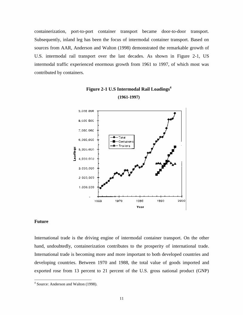
Subsequently, inland leg has been the focus of intermodal container transport. Based on

sources from AAR, Anderson and Walton (1998) demonstrated the remarkable growth of

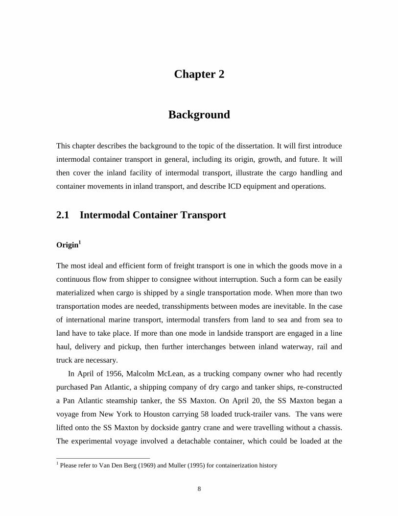
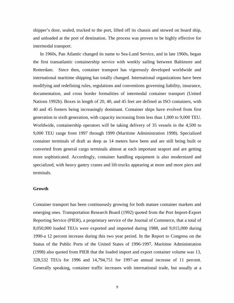
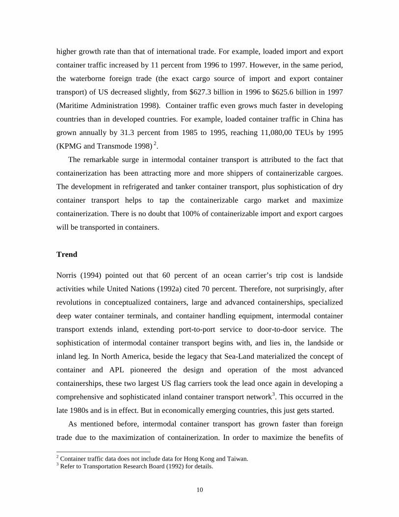
U.S. intermodal rail transport over the last decades. As shown in Figure 2-1, US

intermodal traffic experienced enormous growth from 1961 to 1997, of which most was

contributed by containers.

Figure 2-1 U.S Intermodal Rail Loadings4

(1961-1997)

Future

International trade is the driving engine of intermodal container transport. On the other

hand, undoubtedly, containerization contributes to the prosperity of international trade.

International trade is becoming more and more important to both developed countries and

developing countries. Between 1970 and 1988, the total value of goods imported and

exported rose from 13 percent to 21 percent of the U.S. gross national product (GNP)

4 Source: Anderson and Walton (1998).

12

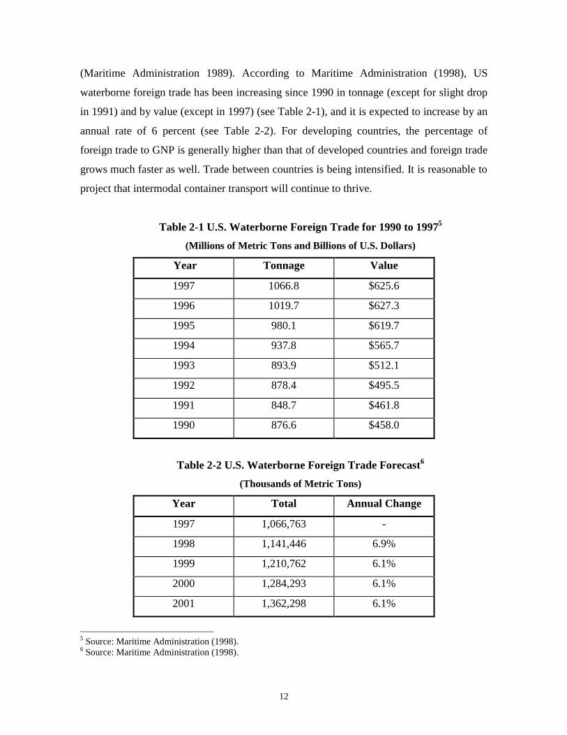
(Maritime Administration 1989). According to Maritime Administration (1998), US

waterborne foreign trade has been increasing since 1990 in tonnage (except for slight drop

in 1991) and by value (except in 1997) (see Table 2-1), and it is expected to increase by an

annual rate of 6 percent (see Table 2-2). For developing countries, the percentage of

foreign trade to GNP is generally higher than that of developed countries and foreign trade

grows much faster as well. Trade between countries is being intensified. It is reasonable to

project that intermodal container transport will continue to thrive.

Table 2-1 U.S. Waterborne Foreign Trade for 1990 to 19975

(Millions of Metric Tons and Billions of U.S. Dollars)

Year Tonnage Value

1997 1066.8 $625.6

1996 1019.7 $627.3

1995 980.1 $619.7

1994 937.8 $565.7

1993 893.9 $512.1

1992 878.4 $495.5

1991 848.7 $461.8

1990 876.6 $458.0

Table 2-2 U.S. Waterborne Foreign Trade Forecast6

(Thousands of Metric Tons)

Year Total Annual Change

1997 1,066,763 -

1998 1,141,446 6.9%

1999 1,210,762 6.1%

2000 1,284,293 6.1%

2001 1,362,298 6.1%

5 Source: Maritime Administration (1998).6 Source: Maritime Administration (1998).

13

2.2 Inland Facility of Intermodal Transport

The reason that 60 percent or 70 percent of transport cost from shipper to receiver occurs

in landside operations is because container handling operations are highly complex.

Compared to inland segments, ocean shipping is simplistic as containers are stowed on

vessels until the vessel docks at the port of destination. On the other hand, this is also the

reason that intermodal transport was concentrated in port areas and could not move inland

at the beginning of the establishment of container transport systems in a country.

Operations on land include loading/unloading containers on and off vessels/vehicles,

stuffing/stripping containers, storage of container boxes and cargoes, cargo inspections,

etc. Facilities are required to perform these operations.

By tariff and operations, container cargo is classified into Full Container Load (FCL)

and Less than Container Load (LCL) on the basis that the container box contains one or

more than one shipments. CFS and CY are the facilities to handle cargoes and containers.

CFS is short for Container Freight Station and CY for Container Yard. In the U.S.7, CFS is

defined as

“A shipping dock where cargo is loaded ("stuffed") into or unloaded ("stripped")

from containers. Generally, this involves less than container load shipments,

although small shipments destined to same consignee are often consolidated.

Container reloading from/to rail or motor carrier equipment is a typical activity”.

CY is defined as “The designation for full container receipt/delivery”.

The United Nations does not strictly define CFS and CY. Instead, it explains CFS and CY.

As part of UN, ILO (1995) representatively explains CFS as follows:

CFS is designed to serve the needs of consignors and consignees who need to

transport cargo in break-bulk form and wish to gain as many of the benefits of

containerized, intermodal transport as possible. CFS must perform the following

broad functions:

7 All definitions in the United States are from Glossary of Shipping Terms by Maritime Administration at itsweb site < http://marad.dot.gov/glossary.html>.

14

• to receive, sort, and consolidate export break-bulk cargoes from road

vehicles, rail wagons and inland waterway craft;

• to pack export cargoes into containers ready for loading aboard a vessel;

• to unpack import containers, and sort and separate the unpacked cargoes

into break-bulk consignments ready for distribution to consignees;

• to deliver import cargoes to inland transport –road vehicles, rail wagons

and inland waterway craft;

• to store import and export cargoes temporarily, between the times of

unloading and loading, while various documentary and administrative

formalities are completed (e.g. customs inspection, settling of charges for

packing, unpacking and storage, arranging transport).

It is agreed that CY is used for the storage of container boxes, both loaded and empty.

CFS and CY refer to facilities within port or close to port. When containers are carried

inland, similar facilities like CFS and CY are needed in the hinterland. In the U.S., these

inland facilities are widely called Intermodal Terminals while the UN names them ICD

(Inland Container Depot). Sometimes, ICD is nicknamed as dry port (UNTCD 1991) as

ICD performs the same function as a port.

“Intermodal Terminal” is not found in the Glossary of Shipping by Maritime

Administration that only defines Terminal in general. A Terminal is “An assigned area in

which containers are prepared for loading into a vessel, train, truck, or airplane or are

stacked immediately after discharge from the vessel, train, truck, or airplane”.

The United Nations (1992a) defines ICD as follows.

Inland Container Depots (ICD’s) may be generally defined as facilities located inland

or remote from port(s) which offer services for the handling, temporary storage and

customs clearance of containers and general cargo that enters or leaves the ICD in

containers. The primary purpose of Inland Container Depots is to allow the benefits of

containerization to be realized on the inland transport leg of international cargo

movements. ICD’s may contribute to the cost-effective containerization of domestic

cargoes as well, but this is less common. Container transport between the port(s) and

15

an ICD is under customs bond, and shipping companies will normally issue their own

bills of lading assuming full responsibility for costs and conditions between the in-

country ICD and a foreign port, or an ICD and the ultimate point of origin/destination.

Unless for descriptions of some specific U.S. intermodal terminals, the UN’s naming

and definition will be used, because:

• Intermodal transport is international in nature. As the most important

international organization, UN has been vigorously facilitating international

trade and intermodal transport and UN’s definitions are more accepted; and

• Institutional contents, such as cross border formalities and documentation, are

as important to intermodal transport as physical operations. UN’s definitions of

inland container facilities are able to represent institutional contents.

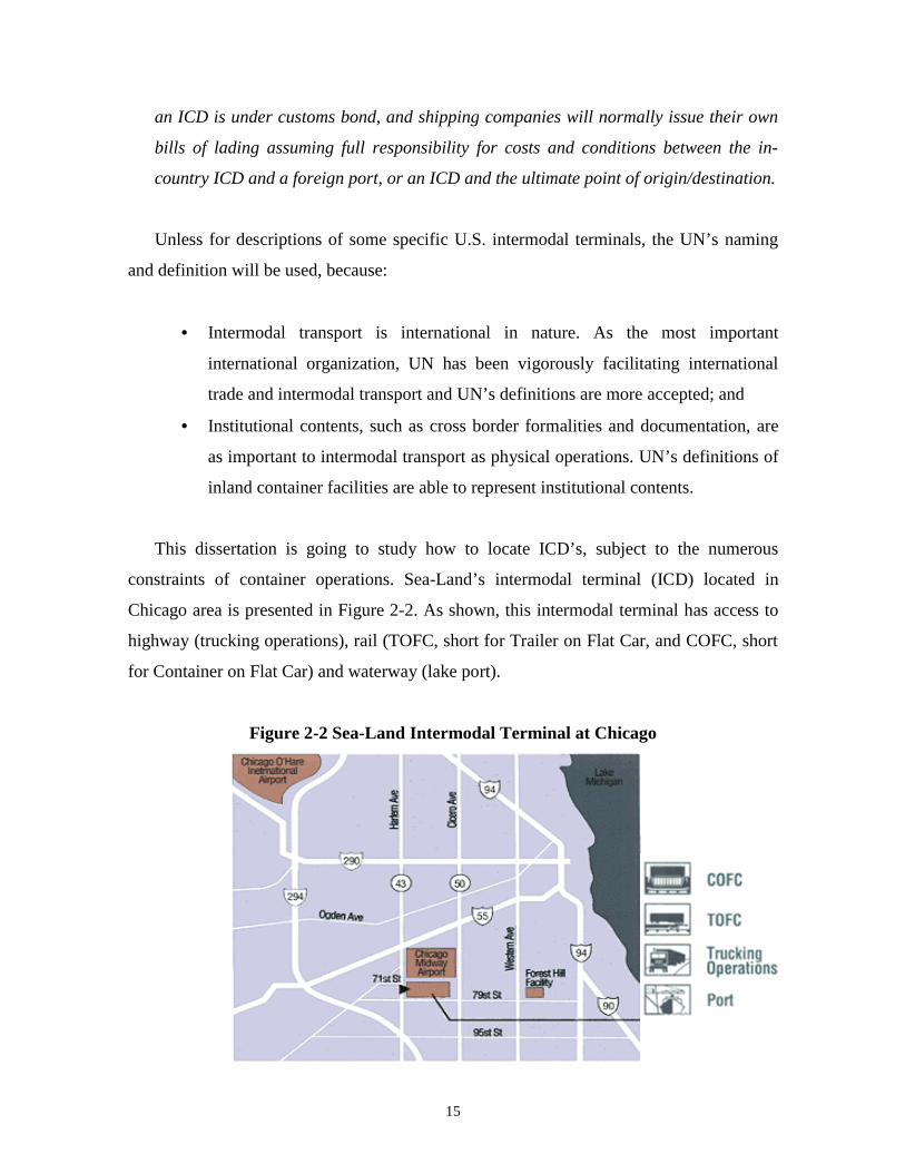
This dissertation is going to study how to locate ICD’s, subject to the numerous

constraints of container operations. Sea-Land’s intermodal terminal (ICD) located in

Chicago area is presented in Figure 2-2. As shown, this intermodal terminal has access to

highway (trucking operations), rail (TOFC, short for Trailer on Flat Car, and COFC, short

for Container on Flat Car) and waterway (lake port).

Figure 2-2 Sea-Land Intermodal Terminal at Chicago

16

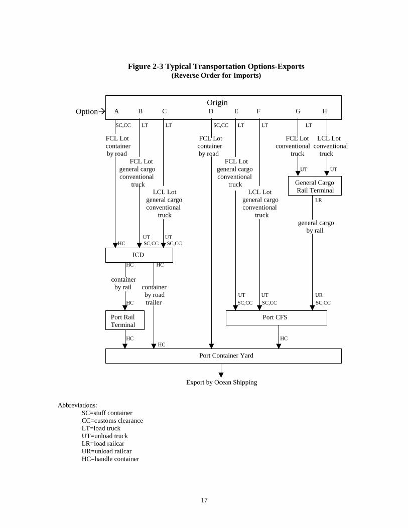
2.3 Cargo Handling and Container Movements in Inland

Transport of Different Scenarios

Shippers of inland cargo have a variety of options to have their cargoes carried to and from

ports: (1) by container and with customs clearance at ICD, or (2) in break-bulk form and

with customs clearance at a port, and (3) by rail, truck, or barge for line haul and pick-

up/delivery. Each combination of these choices is considered as a scenario to organize the

whole transport process of each shipment. The essential difference between scenarios is to

use port or ICD to clear cargo because this implies containerization stops/starts at port or

extends to ICD and then possibly to shipper/consignee’s door.

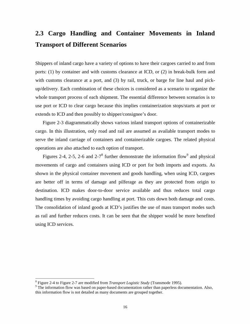
Figure 2-3 diagrammatically shows various inland transport options of containerizable

cargo. In this illustration, only road and rail are assumed as available transport modes to

serve the inland carriage of containers and containerizable cargoes. The related physical

operations are also attached to each option of transport.

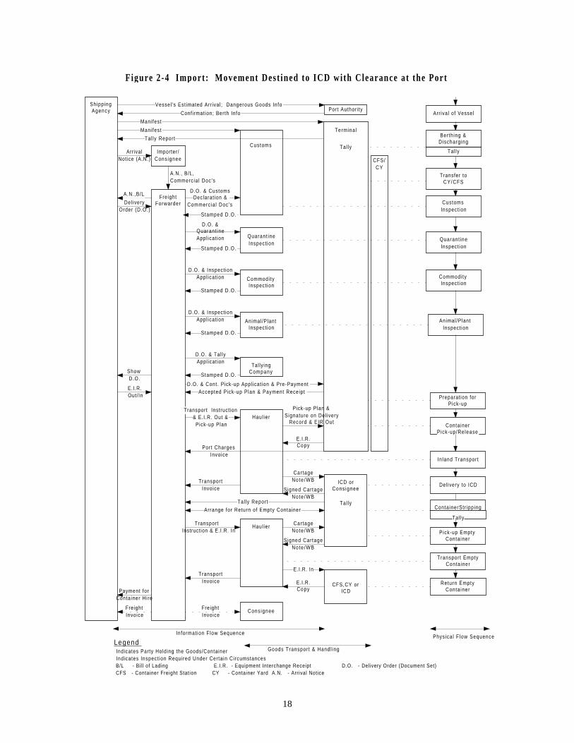
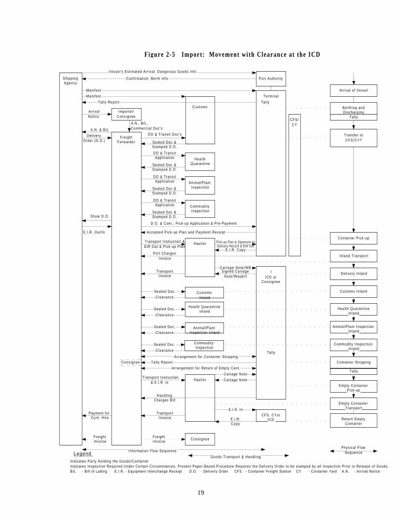
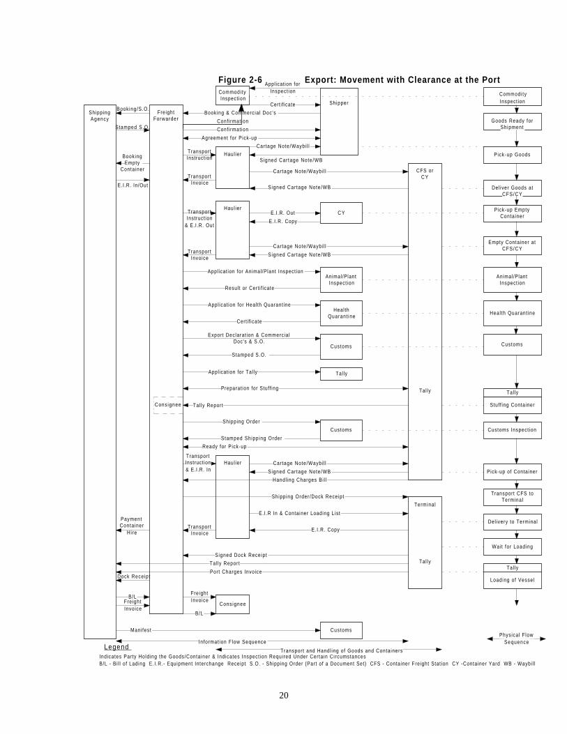
Figures 2-4, 2-5, 2-6 and 2-78 further demonstrate the information flow9 and physical

movements of cargo and containers using ICD or port for both imports and exports. As

shown in the physical container movement and goods handling, when using ICD, cargoes

are better off in terms of damage and pilferage as they are protected from origin to

destination. ICD makes door-to-door service available and thus reduces total cargo

handling times by avoiding cargo handling at port. This cuts down both damage and costs.

The consolidation of inland goods at ICD’s justifies the use of mass transport modes such

as rail and further reduces costs. It can be seen that the shipper would be more benefited

using ICD services.

8 Figure 2-4 to Figure 2-7 are modified from Transport Logistic Study (Transmode 1995).9 The information flow was based on paper-based documentation rather than paperless documentation. Also,this information flow is not detailed as many documents are grouped together.

17

Figure 2-3 Typical Transportation Options-Exports(Reverse Order for Imports)

Option�

SC,CC LT LT SC,CC LT LT LT

FCL Lot FCL Lot FCL Lot LCL Lotcontainer container conventional conventional

by road by road truck truck FCL Lot FCL Lot general cargo general cargo UT UT

conventional conventional truck truck LCL Lot LCL Lot general cargo general cargo LR

conventional conventional truck truck general cargo by rail UT UT HC SC,CC SC,CC

HC HC

container by rail container by road UT UT UR

HC trailer SC,CC SC,CC SC,CC

HC HC HC

Export by Ocean Shipping

Abbreviations:SC=stuff containerCC=customs clearanceLT=load truckUT=unload truckLR=load railcarUR=unload railcarHC=handle container

Origin A B C D E F G H

ICD

Port RailTerminal

Port Container Yard

General Cargo Rail Terminal

Port CFS

18

Shipping Agency

Freight Forwarder

Importer/Cons ignee

Haul ier

Arr ival of Vessel

Berth ing & Discharg ing

Tal ly

Animal/Plant Inspect ion

Quarant ineInspect ion

Transfer to CY /CFS

Customs Inspect ion

Tal ly ing Company

Customs

Haul ier

Cons ignee

CFS,CY or ICD

ICD or Cons ignee

Tal ly

Quarant ineInspect ion

Commodi ty Inspect ion

Preparat ion for P ick-up

Conta iner P ick-up/Release

In land Transport

Legend Indicates Party Holding the Goods/Container Indicates Inspect ion Required Under Certa in Circumstances B/L - Bi l l of Lading E.I.R. - Equipment Interchange Receipt D.O. - Delivery Order (Document Set) CFS - Container Freight Stat ion CY - Container Yard A.N. - Arr ival Notice

Commodi ty Inspect ion

Port Author i ty

Del ivery to ICD

Conta inerStr ipp ing

Animal /PlantInspect ion

Pick-up Empty Conta iner

Transport Empty Conta iner

Return Empty Conta iner

Termina l

CFS/C Y

Tal ly

Informat ion F low Sequence

Goods Transpor t & Handl ing

Phys ica l F low Sequence

Freight Invoice

Freight Invoice

Payment forConta iner Hi re

Transpor tInvoice E.I.R.

Copy

E.I.R. In

Transport Instruct ion & E.I.R. In

Signed Car tageNo te /WB

Car tageNo te /WB

Tal ly ReportArrange for Return of Empty Container

Transpor tInvoice Signed Car tage

No te /WB

Car tageNo te /WB

Port Charges Invoice

E.I.R. Copy

Transport Instruct ion & E.I .R. Out & Pick-up Plan

Pick-up Plan & Signature on Del ivery

Record & EIR Out

Accepted Pick-up Plan & Payment ReceiptD.O. & Cont . Pick-up Appl icat ion & Pre-Payment

E.I.R. Out/ In

Show D.O.

Stamped D.O.

D.O. & Tal lyAppl icat ion

Stamped D.O.

D.O. & Inspect ionAppl icat ion

Stamped D.O.

D.O. & Inspect ionAppl icat ion

D.O. & Quarant ineAppl icat ion

Stamped D.O.

Stamped D.O.

Del iveryOrder (D.O.)

A.N.,B/L D.O. & Customs Declarat ion &

Commerc ia l Doc 's

A.N., B/L,Commerc ia l Doc 's

Arr ival Not ice (A.N.)

Tal ly

Tal ly Report

Mani fest

Mani fest

Conf i rmat ion; Berth Info

Vessel 's Est imated Arr ival ; Dangerous Goods Info

Fi gure 2-4 Impor t : Movement Dest ined to ICD wi th C learance a t the Por t

19

Shipping Agency

Freight Forwarder

Cus toms

Port Author i ty

Arr ival of Vessel

Berth ing and Discharg ing

Animal/Plant Inspect ion

Heal th Quarant ine

Transfer to CFS/CY?

Commodi ty Inspect ion

Animal/Plant Inspect ion In land

Heal th Quarant ine In land

Haul ier

I

Tal ly

Haul ier

Cons ignee

CFS, CYor ICD

Heal th Quarant ine In land

Animal/Plant Inspect ion In land

Commodi ty Inspect ion In land

Container Str ipping

Empty Conta iner Pick-up

Empty Conta iner Transpor t

Return Empty Conta iner

Legend Indicates Party Hold ing the Goods/ContainerIndicates Inspect ion Required Under Certa in Circumstances, Present Paper-Based Procedure Requires the Del ivery Order to be stamped by a l l Inspect ion Pr ior to Release of Goods.B/L - Bi l l of Lading E.I .R. - Equipment Interchange Receipt D.O. - Del ivery Order CFS - Container Freight Stat ion CY - Container Yard A.N. - Arr ival Notice

Importer/Cons ignee

Commodi ty Inspect ion

Customs In land

CFS/C Y

Conta iner Pick-up

In land Transport

Customs In land

Del ivery In land

Tal ly

Tal ly

In format ion F low Sequence

Goods Transpor t & Handl ing

Physica l F lowSequence

Terminal

Tal ly

Cons ignee

Vessel 's Est imated Arr ival ; Dangerous Goods Info

Conf i rmat ion; Berth Info

Mani fest

Mani fest

Tal ly Report

Arr ivalNot ice

A.N. & B/L

Del ivery Order (D.O.) Sealed Doc &

Stamped D.O.

DO & Transi t Appl icat ion

Sealed Doc & Stamped D.O.

DO & Transi t Appl icat ion

DO & Transi t Appl icat ion

Sealed Doc & Stamped D.O.

Sealed Doc & Stamped D.O.Show D.O.

E.I .R. Out/ In

D.O. & Cont. ; Pick-up Appl icat ion & Pre-Payment

Accepted Pick-up Plan and Payment Receipt

Freight Invoice

Freight Invoice

Transport Invoice E.I.R.

Copy

E.I.R. InPayment for

Cont . Hire

Handl ing Charges Bi l l

Car tage Note

Car tage Note Transport Instruct ion

& E.I.R. In

Arrangement for Return of Empty Cont.

Tal ly ReportArrangement for Container Str ipping

Clearance

Sealed Doc.

Sealed Doc.

Sealed Doc.

Clearance

Clearance

Transport Invoice

Port Charges Invoice

Car tage Note /WBSigned Car tage

Note /Waybi l l

E. I .R. Copy

Pick-up Plan & Signature on Delivery Record & EIR Out

Transport Instruct ion & EIR Out & Pick-up Plan

Sealed Doc.

Clearance

ICD or Cons ignee

A.N., B/L,Commerc ia l Doc 's

DO & Transi t Doc 's

Fi gure 2-5 Impor t : Movement w i th C learance a t the ICD

20

Shipping Agency

Freight Forwarder

Commodi ty Inspect ion

CFS or C Y

Tal ly

Commodi ty Inspect ion

Haul ier

Shipper

Goods Ready for Sh ipment

Pick-up Goods

Del iver Goods at CFS/CY

Animal/Plant Inspect ion

Heal th Quarant ine

Pick-up Empty Conta iner

Empty Container at CFS/CY

Tal ly

Customs

Haul ier

Haul ier

Cons ignee

Customs

Terminal

Tal ly

Animal/Plant Inspect ion

Heal th Quarant ine

Customs

Tal ly

Stuf f ing Container

Customs Inspect ion

Legend Indicates Party Hold ing the Goods/Container & Indicates Inspect ion Required Under Certa in CircumstancesB/L - Bi l l of Lading E. I .R.- Equipment Interchange Receipt S.O. - Shipping Order (Part of a Document Set) CFS - Container F reight Stat ion CY -Container Yard WB - Waybi l l

Cus toms

C Y

Pick-up of Container

Transport CFS to Terminal

Del ivery to Terminal

Wai t for Loading

Tal ly

Loading of Vessel

Cons ignee

Appl icat ion for Inspect ion

Cert i f icate

Booking & Commerc ia l Doc 's

Conf i rmat ion

Conf i rmat ion

Agreement for Pick-up

Transport Instruct ion

Car tage Note/Waybi l l

S igned Car tage Note /WB

Cartage Note/Waybi l l

S igned Car tage Note /WB

Transport Invoice

Booking/S.O.

Stamped S.O.

Booking Empty

Conta iner

E.I .R. In/Out

Transport Instruct ion

& E.I .R. Out

Transport Invoice

E.I .R. Out

E.I .R. Copy

Car tage Note/Waybi l l

S igned Car tage Note /WB

Appl icat ion for Animal/Plant Inspect ion

Result or Cert i f icate

Appl icat ion for Heal th Quarant ine

Cert i f icate

Export Declarat ion & Commercia l Doc's & S.O.

Stamped S.O.

Appl icat ion for Tal ly

Preparat ion for Stuf f ing

Tal ly Report

Shipping Order

Stamped Shipp ing Order

Ready for Pick-up

Car tage Note/Waybi l l

S igned Car tage Note /WB

Transport Instruct ion& E.I.R. In

Transport Invoice

Handl ing Charges Bi l l

Sh ipp ing Order /Dock Receipt

E.I .R In & Container Loading List

E. I .R. Copy

Signed Dock Receipt

Payment Conta iner

Hire

Tal ly Report

Port Charges InvoiceDock Receipt

B/LFreightInvoice

B/L

FreightInvoice

Mani fest

In format ion F low Sequence

Transpor t and Handl ing of Goods and Conta iners

Physica l F lowSequence

Figure 2-6 Export: Movement with Clearance at the Port

21

Shipping Agency

Freight Forwarder

Commodi ty Inspect ion

Sh ipper

Tal ly

Commodi ty Inspect ion

Haul ier

ICD or CY

Goods Ready for Sh ipment

Pick-up Empty Conta iner

Del iver Empty Conta iner

Animal/Plant Inspect ion

Heal th Quarant ine

Animal /PlantInspect ion

Heal th Quarant ine

Customs

Tal ly

Customs

Haul ier

CFS or CY Near

Terminal Haul ier

Customs

Shipper

Customs

Terminal

Tally

Customs

Stuff ing the Conta iner

Customs Check

Pick-up Conta iner

Transport to Gateway

Temporary Storage of Loaded Conta iner

Del ivery to Terminal

Customs Clearance

Wai t for Loading

Tal ly

Loading of Vessel

Legend Indicates Party Hold ing the Goods/Container & Indicates Inspect ion Required Under Certa in CircumstancesB/L - Bi l l of Lading E. I .R.- Equipment Interchange Receipt S.O. - Shipping Order (Part of a Document Set) CFS - Container Freight Stat ion CY - Container Yard

Inspect ion Cert i f icate

Appl icat ion for Inspect ion

Booking Note & Commerc ia l Documents

Conf i rmat ionArrangements for Clearance, Stuf f ing and Pick-up

Booking/S.O.

Stamped S.O.

Booking EmptyConta iner

E.I .R. Out/ In

Transpor tInstruct ion& E.I .R. Out

E.I .R. Out

E.I .R. Copy

Transpor tInvoice

Car tage Note/Waybi l l

S igned Car tage Note/Waybi l l

Phys ica l SequenceTranspor t & Handl ing of Goods and Conta iners

Informat ion F low Sequence

Mani fest

DockReceipt

Shipping Order / Dock Receipt

S igned Dock Receipt

Export Declarat ion - Sealed Transi t Document & Dock Receip t

Stamped Dock Receip t

E. I .R. Copy

E.I .R. In & Container Loading ListTranspor tInvoice

ChargesBil l

S igned Car tage Note /Waybi l l

Car tage Note/Waybi l l Transport Instruct ion & E.I.R. In

Car tage Note/Waybi l l

S igned Car tage Note /Waybi l l

Car tage Note/Waybi l l

S igned Car tage Note/Waybi l l

Transpor tInvoice

Transpor tInstruct ion

Ready for Pick-up

Stamped S.O. & Sealed Trans i t Document

Appl icat ion for Tal ly

Export Declarat ion & Transi t &S.O. & Commerc ia l Documents

Cert i f icate

Appl icat ion for Heal th Quarant ine

Result or Cert i f icate

Appl icat ion for Animial /Plant Inspect ion

Payment Conta iner

Hi re

B/L Freight Invoice

B/LFreightInvoice

Figure 2-7 Export: Movement with Clearance at the ICD

22

2.4 ICD Basics

In order to model the siting of ICDs, it is advisable to get a big picture of ICD basics

concerning operations, equipment, investment, operating costs, and etc. In the following,

layouts of rail ICDs (using rail as the main line haul mode) and highway ICDs (using

highway as the main line haul mode) are first presented to provide the intuitive

understanding of ICDs. After that, container handling operations and handling equipment

is discussed. This touches on the core of ICDs because container handling equipment

determines land area and civil works requirements, accounts for about or more than 50

percent of total investment, and decides the efficiency and throughput of a certain size of

ICD. Finally, maintenance and operating costs such as manpower are addressed.

2.4.1 ICD Layout

Although each ICD has its specific characteristics and ICD layout may vary from one

another, generally speaking, ICDs have the following main components to perform

correspondent tasks:

• warehouse or shed for temporary storage of cargoes and stuffing/stripping of

containers;

• yard for stacking of loaded and empty container boxes;

• gatehouse for checking in and out container boxes and cargoes;

• offices for ICD personnel and inspection agencies; and

• internal roadways for vehicle circulation and equipment movement.

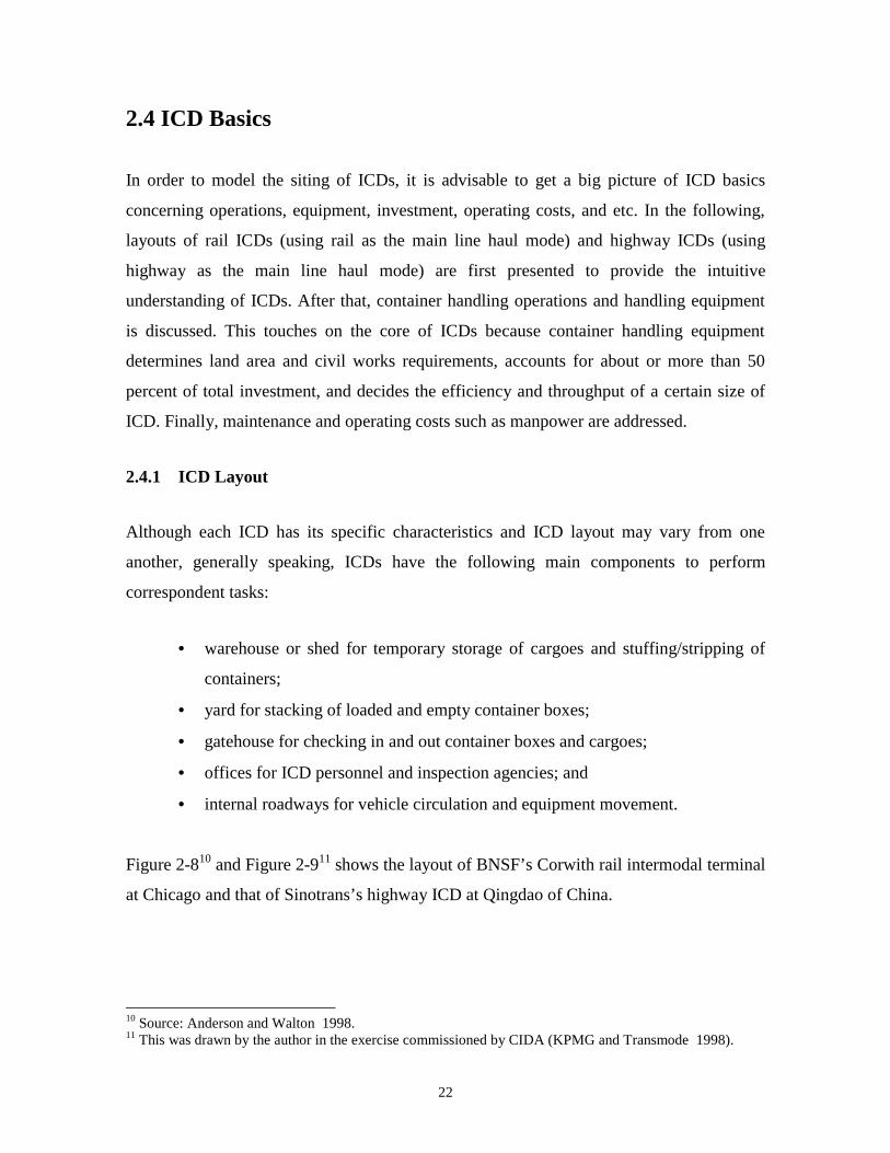
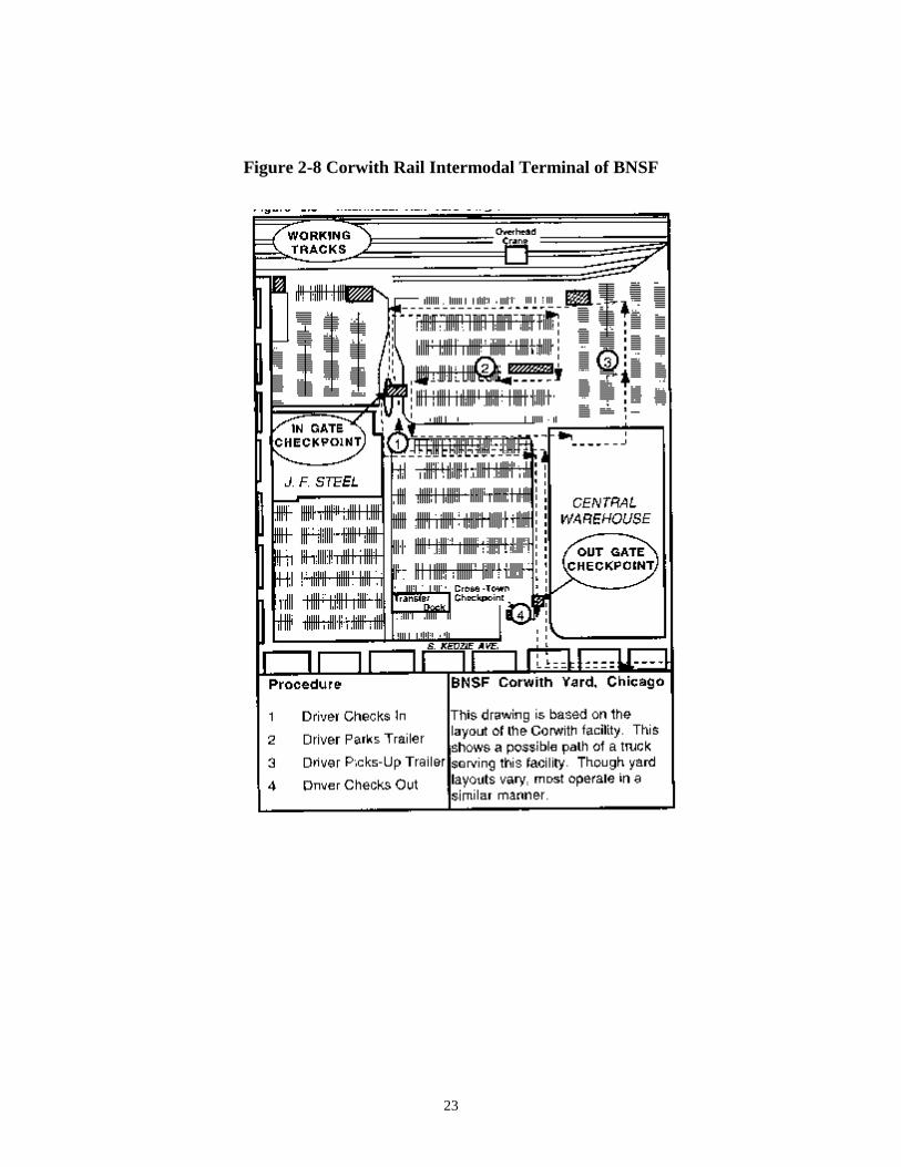
Figure 2-810 and Figure 2-911 shows the layout of BNSF’s Corwith rail intermodal terminal

at Chicago and that of Sinotrans’s highway ICD at Qingdao of China.

10 Source: Anderson and Walton 1998.11 This was drawn by the author in the exercise commissioned by CIDA (KPMG and Transmode 1998).

23

Figure 2-8 Corwith Rail Intermodal Terminal of BNSF

24

Figure 2-9 Highway ICD of Sinotrans

197 m

165 m

163 m

N

20m Crossdock

10m 10m

Empty Stack

142.8m

19 TEU=122.55m

20 TEU=129m

5m

163m

5m

GateGate

Office

LoadedStack

LoadedStack

LoadedStack

LoadedStack

New Warehouse

DemolishedWarehouse

Roadway

Roadway Roadway

Roadway

Roadway

Roadway

Note: Given the limitations of land availability and shape, the above figure shows two alternatives in thelength of loaded container stacks: either 19 TEU or 20 TEU.

25

2.4.2 Container Handling Operations and Handling Equipment

Container handling operations

There are various container handling operations in an ICD. They include lifting loaded

and empty containers on/off trailers/chassis/railcars from/to container stacks, shifting

loaded containers in stacks, moving containers between stacks and stuffing/stripping points

(this is referred to as horizontal movement), and stuffing/stripping of containers. These

handling activities are carried out using one of many different equipment configurations.

Container handling equipment

Typically, loaded and empty containers are stacked separately in yards which allows

the use of dedicated equipment which is best suited to the handling requirements. For

empty containers, light lift trucks of around 10 ton capacity are generally used. As to

loaded containers, heavy (30-42 ton) lift truck (LT), rubber tired gantry (RTG), and rail

mounted gantry (RMG) are most commonly used systems for the purpose of lifting or

hoisting and shifting containers although Straddle Carrier (SK) can also be seen in some

container depots.

Horizontal movement of containers within container depots depends on the selection of

lifting equipment. In RTG or RMG systems, which have no capability of horizontal

movement, containers travel between stuffing/stripping points and container stacks by

trailers/chassis, and stay on trailers/chassis while being stuffed/stripped. In heavy LT

systems, which have the ability of slow horizontal movement, containers to be

stuffed/stripped can be moved either by lift trucks or by trailers/chassises, dependent upon

traffic volume, distance and surface pavement. SK is able to move relatively fast and

distribute the container load to several axles, and thus it can achieve the horizontal

movement by itself and without requirement of high bearing capacity of pavement.

Stuffing/stripping of containers needs to be assisted by fork lift trucks (FLT) of 2, 3 or

6 tons. The number of FLT furnished to working gangs determines the needed

stuffing/stripping operators and laborers which account for a large amount overall staff

quantity of the whole container depot.

26

Comparison between LT and RTG/RMG

From the above analysis of container handling equipment, it can be seen that lifting

equipment is the decisive component as every container in container depot must be lifted at

least twice and lifting equipment directly impacts the selection of horizontal transport

equipment. It is also the most expensive part of ICD. Because of high container damage

rates, poor personnel safety, and former breakdown problems, SK is much less commonly

used as the main lifting equipment than LT or RTG/RMG although SK is sometimes used

as supplementary means in some container yards. LT and RTG/RMG are thus considered

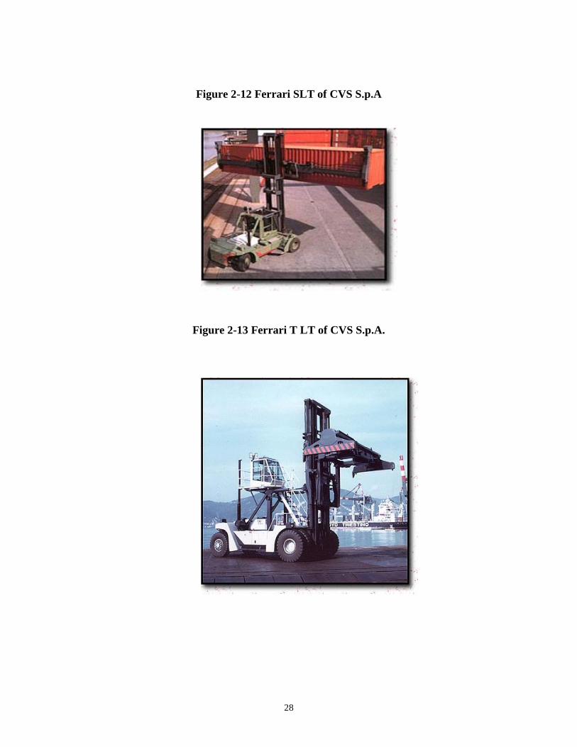
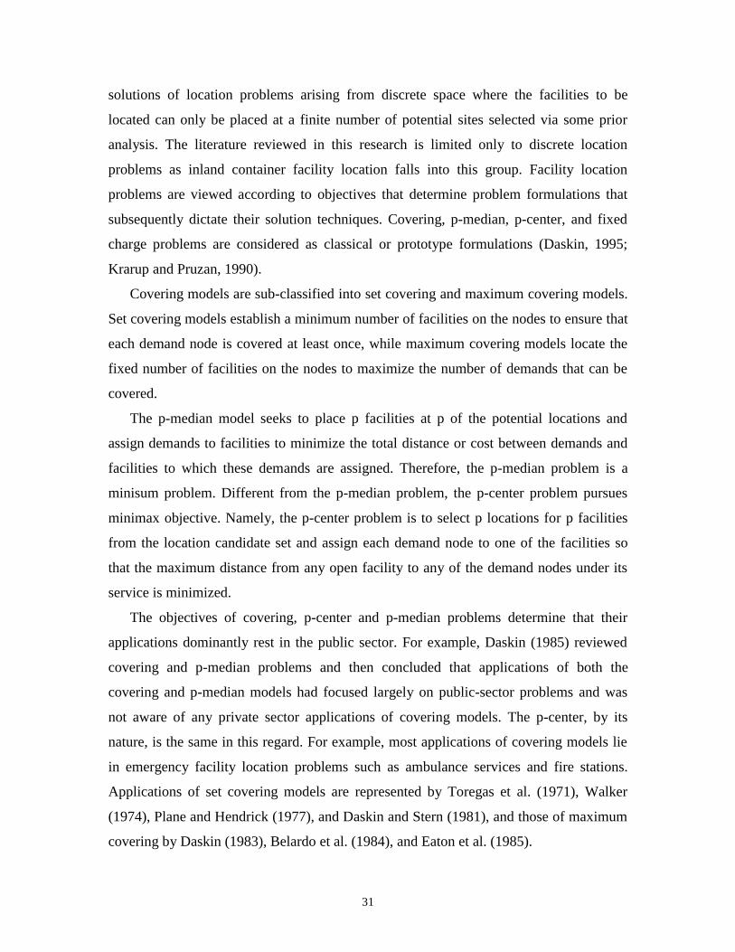
as the main container handling systems. Lift trucks (LT’s) include top lift trucks (TLT),

side lift trucks (SLT) and reach stackers. RTG is generally used in highway ICD and RMG

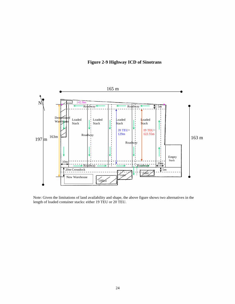
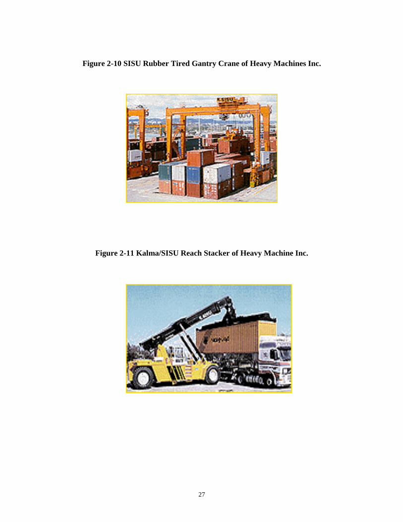
in rail ICD. Pictures of RTG and all kinds of LT are illustrated in Figure 2-10, 2-11, 2-12,

and 2-1312. The comparison between LT (TLT and SLT) and RTG/RMG is illustrated in

Table 2-313.

Table 2-3 Comparison between LT and RTG/RMG

LT RTG/RMG

Horizontal movement capability Slow and for short distance No

Average cycle time (lifts/hour) 17 17/22

Maximum stacking height 3 high 6 high

Maximum stacking depth 1 deep 7 deep/11deep

Storage density (m2/TEU) 20-60 6-12

Axle load High (80-90 tons) Low and Well distributed

Pavement requirement Heavy for large maneuver aisle Heavy only for narrow

laneways

Purchase cost ($ million) 0.35-0.5 1.6 (7 wide)/2.3-3 (middle size)

Economic life (years) 10 15-20/25-30

12 The author has no intention to recommend any handling equipment of any manufacturer mentioned here.13 Figures such as average cycle time and purchase costs are based on surveys and interviews that were madein CIDA study (KPMG and Transmode 1998).

27

Figure 2-10 SISU Rubber Tired Gantry Crane of Heavy Machines Inc.

Figure 2-11 Kalma/SISU Reach Stacker of Heavy Machine Inc.

28

Figure 2-12 Ferrari SLT of CVS S.p.A

Figure 2-13 Ferrari T LT of CVS S.p.A.

29

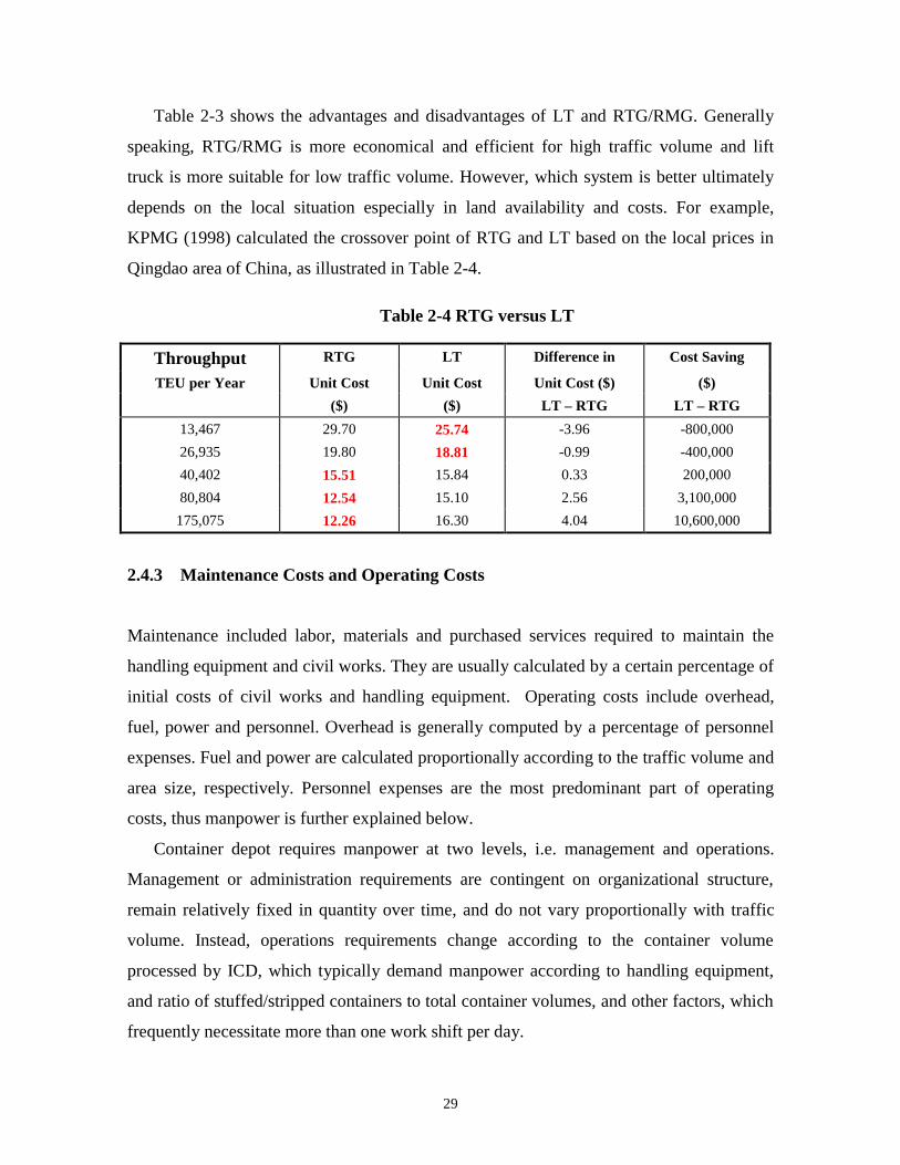
Table 2-3 shows the advantages and disadvantages of LT and RTG/RMG. Generally

speaking, RTG/RMG is more economical and efficient for high traffic volume and lift

truck is more suitable for low traffic volume. However, which system is better ultimately

depends on the local situation especially in land availability and costs. For example,

KPMG (1998) calculated the crossover point of RTG and LT based on the local prices in

Qingdao area of China, as illustrated in Table 2-4.

Table 2-4 RTG versus LT

Throughput RTG LT Difference in Cost Saving

TEU per Year Unit Cost Unit Cost Unit Cost ($) ($)

($) ($) LT – RTG LT – RTG

13,467 29.70 25.74 -3.96 -800,000

26,935 19.80 18.81 -0.99 -400,000

40,402 15.51 15.84 0.33 200,000

80,804 12.54 15.10 2.56 3,100,000

175,075 12.26 16.30 4.04 10,600,000

2.4.3 Maintenance Costs and Operating Costs

Maintenance included labor, materials and purchased services required to maintain the

handling equipment and civil works. They are usually calculated by a certain percentage of

initial costs of civil works and handling equipment. Operating costs include overhead,

fuel, power and personnel. Overhead is generally computed by a percentage of personnel

expenses. Fuel and power are calculated proportionally according to the traffic volume and

area size, respectively. Personnel expenses are the most predominant part of operating

costs, thus manpower is further explained below.

Container depot requires manpower at two levels, i.e. management and operations.

Management or administration requirements are contingent on organizational structure,

remain relatively fixed in quantity over time, and do not vary proportionally with traffic

volume. Instead, operations requirements change according to the container volume

processed by ICD, which typically demand manpower according to handling equipment,

and ratio of stuffed/stripped containers to total container volumes, and other factors, which

frequently necessitate more than one work shift per day.

30

Chapter 3

Literature Review

3.1 Prototype Facility Location Problems

Nearly every public and private sector enterprise encounters decisions on locating its

facilities. Facility location thus has attracted so much attention from academia and

industry that it has been addressed extensively and intensively in the last decades.

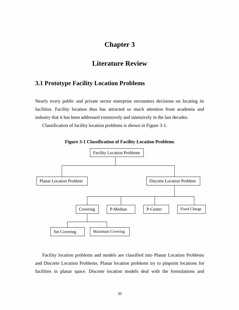
Classification of facility location problems is shown in Figure 3-1.

Figure 3-1 Classification of Facility Location Problems

Facility location problems and models are classified into Planar Location Problems

and Discrete Location Problems. Planar location problems try to pinpoint locations for

facilities in planar space. Discrete location models deal with the formulations and

Facility Location Problems

Planar Location Problem Discrete Location Problem

Covering P-Median P-Center Fixed Charge

Set Covering Maximum Covering

31

solutions of location problems arising from discrete space where the facilities to be

located can only be placed at a finite number of potential sites selected via some prior

analysis. The literature reviewed in this research is limited only to discrete location

problems as inland container facility location falls into this group. Facility location

problems are viewed according to objectives that determine problem formulations that

subsequently dictate their solution techniques. Covering, p-median, p-center, and fixed

charge problems are considered as classical or prototype formulations (Daskin, 1995;

Krarup and Pruzan, 1990).

Covering models are sub-classified into set covering and maximum covering models.

Set covering models establish a minimum number of facilities on the nodes to ensure that

each demand node is covered at least once, while maximum covering models locate the

fixed number of facilities on the nodes to maximize the number of demands that can be

covered.

The p-median model seeks to place p facilities at p of the potential locations and

assign demands to facilities to minimize the total distance or cost between demands and

facilities to which these demands are assigned. Therefore, the p-median problem is a

minisum problem. Different from the p-median problem, the p-center problem pursues

minimax objective. Namely, the p-center problem is to select p locations for p facilities

from the location candidate set and assign each demand node to one of the facilities so

that the maximum distance from any open facility to any of the demand nodes under its

service is minimized.

The objectives of covering, p-center and p-median problems determine that their

applications dominantly rest in the public sector. For example, Daskin (1985) reviewed

covering and p-median problems and then concluded that applications of both the

covering and p-median models had focused largely on public-sector problems and was

not aware of any private sector applications of covering models. The p-center, by its

nature, is the same in this regard. For example, most applications of covering models lie

in emergency facility location problems such as ambulance services and fire stations.

Applications of set covering models are represented by Toregas et al. (1971), Walker

(1974), Plane and Hendrick (1977), and Daskin and Stern (1981), and those of maximum

covering by Daskin (1983), Belardo et al. (1984), and Eaton et al. (1985).

32

The above three problems do not consider the fixed cost of a facility or assume that

every facility bears a uniform fixed cost and the number of facilities is taken as a proxy

for fixed costs. This, on the other hand, implies that these models are intended for the

public sector where costs and benefits are shared and/or incommensurable. On the

contrary, private sector or business logistics regard the minimization of the total cost or

maximization of profit as their primary objective. The business motivation initiates the

fixed charge facility model that seeks the minimum sum of fixed facility construction

costs and operating/transportation costs. The fixed charge facility mode differs from the

p-median model in two aspects: no predetermined number of facilities, and inclusion of

fixed capital costs. The fixed charge facility mode is also referred to as the warehouse

location problem.

From the problem statement of this dissertation, it can be easily seen that the inland

container facility (i.e. ICD in this study) location problem of question falls into the fourth

prototype location problem described above. Accordingly, more attention is thus turned

to the fixed charge location model. Due to the intrinsic relation between the p-median

location model and the fixed charge location model, some attention is also paid to the p-

median problem since there exists a similarity in algorithmic solution between the p-

median and fixed charge location models.

3.2 Formulations and Algorithms of p-Median and Fixed

Charge Facility Location Problems

3.2.1 Formulations

Most location problems are formulated as integer or mixed integer linear programming

problems. For the convenience of later discussion, the formulation of a fixed charge

facility location prototype problem based on Daskin (1995, p250) is presented.

As described previously, the fixed charge facility problem is to minimize the sum of

fixed construction costs and operating/transportation costs. The descriptive expression is

transformed into normative or prescriptive notation as follows.

33

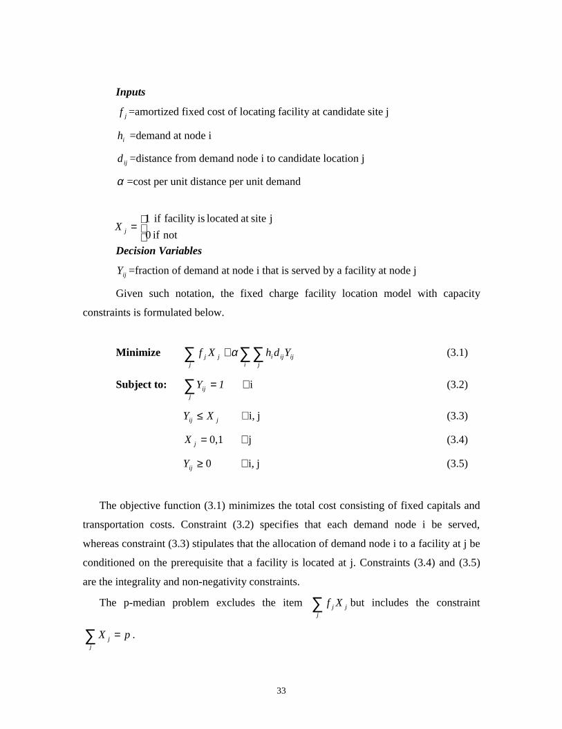
Inputs

jf =amortized fixed cost of locating facility at candidate site j

ih =demand at node i

ijd =distance from demand node i to candidate location j

α =cost per unit distance per unit demand

Decision Variables

ijY =fraction of demand at node i that is served by a facility at node j

Given such notation, the fixed charge facility location model with capacity

constraints is formulated below.

Minimize ∑ ∑∑+j i j

ijijijj YdhXf α (3.1)

Subject to: i ∑ ∀=j

ij 1Y (3.2)

ji, ∀≤ jij XY (3.3)

j 0,1 ∀=jX (3.4)

ji, 0 ∀≥ijY (3.5)

The objective function (3.1) minimizes the total cost consisting of fixed capitals and

transportation costs. Constraint (3.2) specifies that each demand node i be served,

whereas constraint (3.3) stipulates that the allocation of demand node i to a facility at j be

conditioned on the prerequisite that a facility is located at j. Constraints (3.4) and (3.5)

are the integrality and non-negativity constraints.

The p-median problem excludes the item ∑j

jj Xf but includes the constraint

∑ =j

j pX .

=not if 0

j siteat located isfacility if 1jX

34

As shown above, the p-median and fixed charge facility problems formulate the main

logistic components such as demand, cost, and allocation of demand to facilities.

Extensions are derived from changes in these facets.

The most significant extension in the p-median model is to locate the p facilities on a

stochastic network where transportation costs and/or demands are probabilistic rather

than deterministic (Larson, 1975; Mirchandani and Odoni, 1979; Berman et al., 1990).

Other important generations come from multiple objectives, hierarchy of functionally

interacting facilities such as different levels of post offices, and fractional assignment of a

demand node to a facility. Again, these are mainly for public sector facilities.

Fixed charge location problems are divided into uncapacitated facility location

problems and capacitated facility location problems, based on whether there are

constraints for facility capacity. As to capacitated facility location problems, a very

important variant is the dynamic location problem to locate facilities in a multi-period

horizon (Erlenkotter, 1981; Sweeney and Tatham, 1976; Van Roy and Erlenkotter, 1982).

Other variations result from multiple commodities (Geoffrion and Graves, 1974),

integration with routing (Perl and Daskin, 1985), and etc.

Business or private sector logistics consider minimal costs or maximal profits as their

commercial motive. In particular, maximal profits are the final business goal. This is an

undisputed cognizance. When modeling business logistic problems, modelers should

naturally take such motives as the objective. However, as shown in the formulation (3.1),

nearly all problem objective functions minimize total costs rather than maximize profits.

Such a formulation is based on the implicit assumption that cost minimization is

equivalent to profit maximization.

Such equivalence is valid only when the market share or demand served by facilities

remains insensitive or unchanged to decisions to locate facilities. Actually, constraint

(3.2) guarantees in acquiescence that all demands are served by facilities to be placed.

These formulations are correct for many cases, such as warehouses of a large

supermarket chain or those of a giant auto maker, in which facilities to be sited serve as

an internal part of production and do not interact with customers or markets. But for

many other cases such as the ICD location problem 1, these formulations cannot reflect

35

reality since such facilities, acting as independent business entities, directly face market

and interact with their customers.

The ICD location problem is further taken as an example to exemplify similar facility

problems. Although container inland transport is compartmentalized as one segment of

the whole sea borne container transport process, container transport on land is an

independent transport service. How to locate expensive ICD’s is strongly related to

canvassing for more containers and cargoes. Figures 2-4, 2-5, 2-6 and 2-7 of Chapter 2

has shown the difference in terms of container movement and cargo handling between

cargo clearance at ports and ICD’s. Suppose there are two operators in the market, one

has an ICD and another does not. It is obvious who will have more market share. If the

operator pursues minimal cost and does not invest in building an ICD, it will lose market

share to the one who has an ICD. Therefore, less investment or cost does not necessarily

mean more profit. On the contrary, more investment is likely to bring more profit because

better facilities and service might win over more market share. It is now easy to see that

cost minimization is not equivalent to profit maximization.

In addition, when looking at problems such as the ICD location problem, a modeler

should not assume that demands are exogenous or that the market is fixed and occupied

by one player who is the operator of facilities to be established. Conversely, he should

study the innate relationship between locations and demands. As such, demands are

endogenous or elastic to facility locations and participation by multiple players makes the

market competitive. In the paragraph to follow, the state of art of location problems with

endogenous demand and in a competitive environment is examined.

Literature of this area appears to be rather limited. Perl and Ho (1990) formulate a

public non-emergency facility location problem by maximizing Consumer’s Surplus

under different simple demand functions. Consumer’s Willingness to Pay and

Consumer’s Surplus, defined by welfare economists to measure benefits of public welfare

facilities and projects, are not suitable for the private sector. Hakimi (1990) proposes to

divide the demand among the facilities according to the distances between the demand

and the various facilities. He also recommends locating facilities using game theory to

simulate two service suppliers to compete for market share.

36

3.2.2 Algorithms

Hakimi (1964) first formulated the p-median problem and coined the terminology of the

p-median problem, then (1965) demonstrated that for the p-median problem, at least one

optimal solution could be found at p of the network nodes. Since then, the p-median

problem has been treated as a discrete location problem.

Even so, professionals have suffered from the complexity of the p-median problem.

Given a network composed of N nodes, the algorithm needs to examine the

alternative solutions. Although given P, the number of solutions is O( )PN (for P<<N)

and thus is seemingly polynomial in N, in practice with P or N increasing, this number

can be large enough to prevent modelers from solving the p-median problem in a

reasonable time. Kariv and Hakimi (1979) illustrated that the p-median problem can be

solved in polynomial time on a tree network but is NP-complete on a general graph.

Garey and Johnson (1979) has also shown that the p-median model is NP-hard.

In the case of the fixed charge or warehouse location problem that does not

predetermine the number of facilities to be located, the number of solutions goes up to

which is exponential in N.

Therefore, Handler and Mirchandani(1979) pointed out that p-median problems,

warehouse problems and their many extensions are almost all NP-complete.

The proposed ICD location problem, as a fixed charge facility location problem, can

thus be thought of as NP-complete.

Primarily because of the general convexity properties of tree networks, efficient

polynomial-time graphic theoretic algorithms have been developed for p-median

problems with linear costs on tree networks (Dearing et al., 1976). As general networks

underlie most of the real world problems, tremendous efforts have been made to explore

)!(!

!

PNP

N

P

N

−=

( )∑=

=−=

N

i

NN Oi

N

1

212

37

the algorithms for p-median and fixed charge facility location problems for which graphic

theoretic approaches are powerless.

Due to the similarity and indivisibility between p-median problems and fixed charge

facility location problems in terms of algorithms, in the following paragraphs, algorithms

are discussed without differentiating these two types of problems that are therefore

generally called facility location problems.

Algorithms used for facility location problems rooted on general networks can be

classified into three categories, namely, enumeration, mathematical programming based

algorithms and heuristics.

Of course, enumeration can only be employed for small-scale problems.

The Mathematical programming approaches are based on the integer or mixed integer

linear programming formulations of facility location problems. The popular methods of

addressing the NP-completeness comprise linear programming relaxation (ReVelle and

Swain, 1970), branch-and-bound (Khumawala, 1972; Akinc and Khumawala, 1977),

Lagrangian relaxation (Geoffrion, 1974; Geoffrion and McBride, 1978), dual-based

algorithm (Erlenkotter, 1978), and Bender’s decomposition (Geoffrion and Graves 1974).

Daskin (1995), Mirchandani (1990), Jacobsen (1990), and Mirchandani and Wong (1990)

extensively and intensively summarize the state of the art algorithms for p-median

problems and fixed charge facility location problems.

Among these mathematical programming based algorithms, linear programming

relaxation cannot guarantee integrality. This is the case in particular for most problems

that are involved with binary decision variables. Branch-and-bound algorithms are not

efficient in the sense that enumeration cannot be curtailed sufficiently due to the fact that

the bound at each node of the enumeration tree cannot be computed quickly. Lagrangian

relaxation, weighting the constraints by multipliers and putting them in the objective

function, is widely used for both p-median and fixed facility location problems. Bender’s

decomposition, solving the mixed integer programming formulation, has been improved

to accelerate the convergence. Dual-based procedure is considered promising.

These algorithms have significantly helped industry to optimize location decisions.

Due to the fact that most facility location problems are formulated into linear integer or

mixed integer programming problems, these algorithms are mainly based on linearity.

38

Given Lagrangian Relaxation as an example; it requires not only linearity but also

identical signs in the objective function, namely all positive or all negative signs.

Otherwise, the bounds cannot be generated. On the other hand, most of these algorithms

employ an approximation method, and some are heuristic in nature. For instance, many

professionals regard Lagragian relaxation as a heuristic. Moreover, some of these

algorithms are integrated with heuristics when applied to solve specific formulations.

Besides requirements for linearity, mathematical programming based algorithms cannot

completely guarantee optimality in theory. Also, mathematical programming based

algorithms are not easily manipulated or applied.

Even though scores of algorithms based on mathematical programming have been

devised, the NP-hardness or NP-completeness of facility location problems has made

researchers and practitioners resort to heuristics. As a matter of fact, heuristics were first

used in location problems and have been obtaining more and more attention. Greedy

(ADD) and interchange (exchange or DROP) heuristics (Kuehn and Hamburger, 1963)

are considered as the basis for various heuristics applied in facility location problems. But

theoretically speaking, greedy and interchange heuristics are likely to be confined to local

optimality. They can find a local optimal solution for complicated optimization problems

but are prone to be confined to local optimality. It is likely for these heuristics to yield a

bad solution, albeit a local optimal solution, for problems whose local optimums are

dramatically different. Many mathematical programming based algorithms, which are

heuristic in nature, try to theoretically look for better local optimums but cannot

guarantee the overall optimality, either.

Tabu search (Glover, 1989a; Glover 1989b; Glover and Laguna 1993; Glover and

Laguna 1997), genetic algorithms and simulated annealing were consider in the 1980s the

most promising heuristic algorithms to solve combinatorial NP-complete problems and

are named modern heuristics due to their late advent. All these heuristics try to transcend

local optimality to find a very good local optimum close to global optimum if not the

global one. Tabu search among them, in the author’s opinion, is most widely applied to

almost all combinatorial optimizations, as summarized in Glover and Laguna (1997).

Tabu search was also applied to location problems or other combinatorial optimizations

(e.g., Rolland et al, 1996; Wen and Huang, 1996; Lukkentangen and Glover, 1997).

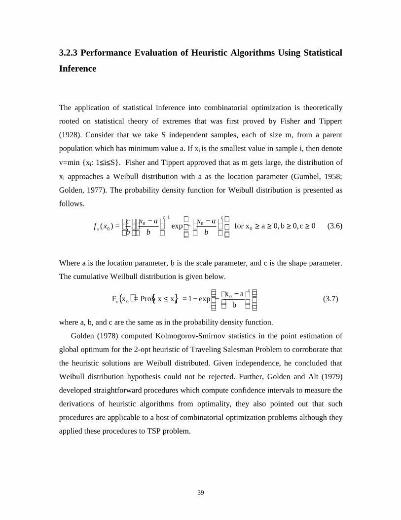
39

3.2.3 Performance Evaluation of Heuristic Algorithms Using Statistical

Inference

The application of statistical inference into combinatorial optimization is theoretically

rooted on statistical theory of extremes that was first proved by Fisher and Tippert

(1928). Consider that we take S independent samples, each of size m, from a parent

population which has minimum value a. If xi is the smallest value in sample i, then denote

v=min {xi: 1≤i≤S}. Fisher and Tippert approved that as m gets large, the distribution of

xi approaches a Weibull distribution with a as the location parameter (Gumbel, 1958;

Golden, 1977). The probability density function for Weibull distribution is presented as

follows.

0c0,b0,axfor exp)( 00

1

00 ≥≥≥≥

−−

−

=

− cc

x b

ax

b

ax

b

cxf (3.6)

Where a is the location parameter, b is the scale parameter, and c is the shape parameter.

The cumulative Weilbull distribution is given below.

( ) { }

−−−=≤=

c

000x b

axexp1xxProbxF (3.7)

where a, b, and c are the same as in the probability density function.

Golden (1978) computed Kolmogorov-Smirnov statistics in the point estimation of

global optimum for the 2-opt heuristic of Traveling Salesman Problem to corroborate that

the heuristic solutions are Weibull distributed. Given independence, he concluded that

Weibull distribution hypothesis could not be rejected. Further, Golden and Alt (1979)

developed straightforward procedures which compute confidence intervals to measure the

derivations of heuristic algorithms from optimality, they also pointed out that such

procedures are applicable to a host of combinatorial optimization problems although they

applied these procedures to TSP problem.

40

3.3 Summarization

Consensus has been made in several points pertaining to facility location problems, or

even the whole logistics (e.g., Daskin, 1985;Golden and Baker 1985; Hall 1985).

First, any logistic model must be grounded on the realistic characteristics and essence

of real world problems. That is, a model must abstract the most basic and crucial

elements of reality, further explain the intrinsic intricacy, and finally control and predict

the change of problems. Hence, for a specific problem, the realism of the proposed

logistic model is even of more important than the sophistication of the designed solution

algorithm in the sense that the realism of a model is the premise of a good solution to the

problem.

Second, no formulation exists that embodies all facets of a realistic problem although

many modelers have tried to rationally incorporate realism. Given such circumstances,

the optimal solution produced by theoretical optimal algorithms does not mean that this

solution is optimal to realistic problems.

Finally, due to extreme difficulty in computation caused by NP-completeness, more

solid and efficient algorithms remain to be developed and polished. More importantly, an

agreed recognition of algorithms is that heuristics may find better solutions than some

mathematical programming-based algorithms such as Lagrangian relaxation.

Model realism and solution algorithms have been the two main active subjects in the

area of logistics in recent decades and will likely continue so in the future.

The model realism can only be achieved by good mathematical formulations. By

extending from the prototype problems to diverse scenarios, previous sections have

described realistic facility location problems that were successfully addressed. However,

as pointed out, these formulations assume that cost minimization is equal to profit

maximization and that that demands are exogenous or that the market is fixed and

occupied by one player who is the operator of facilities to be established.

Literature in the ICD location problem appears to be very rare. The ICD location

problem has not been brought up sufficiently in academia. The United Nations (1990,

1992a) proposes an economic model to evaluate the financial and economic

consequences of a single ICD. Such a model is very helpful in analyzing investment and

41

operating costs for a single ICD under a specified throughput, but it is unable to represent

the problem at the network level. Chapter 4 presents the formulation of the ICD location

problem. This formulation takes profit maximization as the objective function. Also,

discrete choice analysis has been successfully developed and applied in demand

forecasting (Ben-Akiva and Lerman 1985). Discrete choice analysis generates the

aggregate traffic and freight demand by modeling individual passenger or shipper’s

behaviors and preferences in selecting transport alternatives. The thesis tries to integrate

discrete choice analysis into ICD location problem and thus treats demands endogenously

by formulating shipper’s preferences in selecting ICD services.

Current mathematical programming-based algorithms require linearity in formulation

and some of them require identical signs in the objective function. Mathematical

programming based algorithms cannot completely guarantee optimality in theory. By

reason of model realism, the ICD problem under a competitive environment is formulated

into exponentially nonlinear integer programming with maximization of profit as the

objective function (inevitably mixed with negative and positive signs). Such a

formulation precludes the existing mathematical programming based algorithms. Because

of the formerly articulated common perception of algorithms and especially heuristics;

modern heuristics are applied to solve the formulation. This is the content of Chapter 5.

Chapter 6 evaluates the performance of the designed heuristic algorithm using statistical

inference.

42

Chapter 4

Problem Formulation

4.1 Introduction

As summarized in Chapter 3, facility location models overwhelmingly treat facility location

problems with the assumption that demands are deterministic and exogenous to facilities, and

thus do not formulate the competitiveness among facilities. Also, the ICD location problem has

not been brought up sufficiently in academia and there is no ICD location model to help

container operators establish an ICD network.

The ICD business is under fierce competition. Demands are endogenous to ICD’s and where

to locate an ICD determines the container volume it can attract. In order to correctly formulate

the ICD location problem, the interaction between demands and ICD locations must be

quantitatively addressed. This chapter will study the shipper, quantify the shipper’s behavior in

selecting ICD services, and develop the formulation of ICD location problem.

4.2 Shipper’s Transport Logistics Cost

In intermodal container transport, demand is derived from international trade freight that is

owned and controlled by shippers, namely, importers and exporters. The shipper is the final

customer of intermodal container transport. The best way to study the relationship or interaction

is to study shipper’ behaviors or preferences in selecting transport services. Shipper’s behaviors

are associated with commodity attributes, and transport attributes of the modes. Commodity

attributes are described by the following variables:

43

• density

• value per pound

• shelf life

• typical packaging

And transport attributes of the modes include:

• availability of equipment

• transit time

• reliability

• load and unload cost

• loss and damage experience

Unlike bulky goods such as coal, fertilizer, etc., containerizable international trade goods are

high value-added commodities. Containerizable international trade commodities also share

common characteristics in their transport attributes. As commodity attributes and transport

attributes determine shipper’s behaviors in selecting transport service, we can thus assume that

shippers are homogeneous in selecting services provided by ICD’s.

The attributes determine the shipper’s behaviors in selecting transport service. All of these

attributes and behaviors can be integrated into the “shipper’s utility function” which,

quantitatively speaking, in this case, is mainly represented by the total transport logistics cost.

Transport logistics cost influences the final price of the export or the import, where the former

will affect the competitiveness of shipper’s goods in world markets while the latter raises the cost

of imported goods for shippers. Clearly, from the shipper’s perspective, the aim is to derive

maximum advantage from transport logistics cost by minimizing it to the extent possible.

The total transport logistics cost is associated with the ordering, transport, inventory and the

use of the product being shipped. Components that detail the total transport logistics costs of

acquiring, shipping and storing the product include:

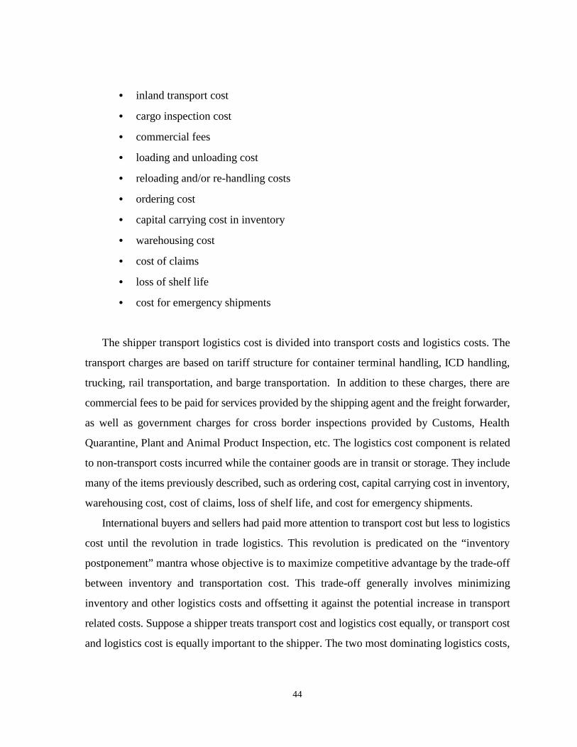
44

• inland transport cost

• cargo inspection cost

• commercial fees

• loading and unloading cost

• reloading and/or re-handling costs

• ordering cost

• capital carrying cost in inventory

• warehousing cost

• cost of claims

• loss of shelf life

• cost for emergency shipments

The shipper transport logistics cost is divided into transport costs and logistics costs. The

transport charges are based on tariff structure for container terminal handling, ICD handling,

trucking, rail transportation, and barge transportation. In addition to these charges, there are

commercial fees to be paid for services provided by the shipping agent and the freight forwarder,

as well as government charges for cross border inspections provided by Customs, Health

Quarantine, Plant and Animal Product Inspection, etc. The logistics cost component is related

to non-transport costs incurred while the container goods are in transit or storage. They include

many of the items previously described, such as ordering cost, capital carrying cost in inventory,

warehousing cost, cost of claims, loss of shelf life, and cost for emergency shipments.

International buyers and sellers had paid more attention to transport cost but less to logistics

cost until the revolution in trade logistics. This revolution is predicated on the “inventory

postponement” mantra whose objective is to maximize competitive advantage by the trade-off

between inventory and transportation cost. This trade-off generally involves minimizing

inventory and other logistics costs and offsetting it against the potential increase in transport

related costs. Suppose a shipper treats transport cost and logistics cost equally, or transport cost

and logistics cost is equally important to the shipper. The two most dominating logistics costs,

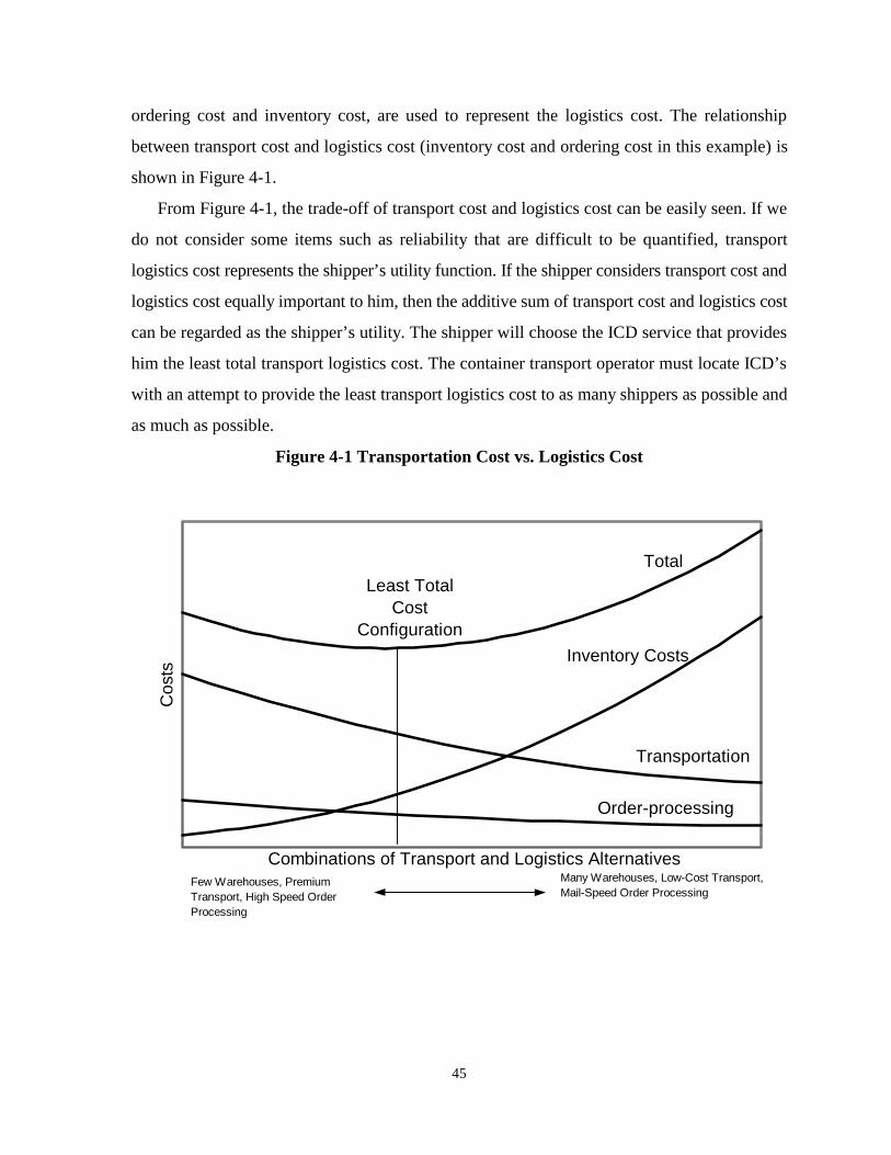
45

ordering cost and inventory cost, are used to represent the logistics cost. The relationship

between transport cost and logistics cost (inventory cost and ordering cost in this example) is

shown in Figure 4-1.

From Figure 4-1, the trade-off of transport cost and logistics cost can be easily seen. If we

do not consider some items such as reliability that are difficult to be quantified, transport

logistics cost represents the shipper’s utility function. If the shipper considers transport cost and

logistics cost equally important to him, then the additive sum of transport cost and logistics cost

can be regarded as the shipper’s utility. The shipper will choose the ICD service that provides

him the least total transport logistics cost. The container transport operator must locate ICD’s

with an attempt to provide the least transport logistics cost to as many shippers as possible and

as much as possible.

Figure 4-1 Transportation Cost vs. Logistics Cost

0

3

6

9

12

15

0 1 2 3 4 5 6 7 8 9 10Combinations of Transport and Logistics Alternatives

Cos

ts

Total

Inventory Costs

Transportation

Order-processing

Least Total Cost

Configuration

Few Warehouses, Premium Transport, High Speed Order Processing

Many Warehouses, Low-Cost Transport, Mail-Speed Order Processing

46

4.3 Discrete Choice Analysis1

Discrete choice analysis provides the theory and methods to model individual choice from a set

of mutually exclusive and collectively exhaustive alternatives and to investigate aggregate

demand from disaggregate data. This thesis applies theories and methods of discrete choice

analysis to quantitatively describe shipper’s selection of ICD service. Discrete choice analysis

employs the principle of utility maximization, i.e., a decision maker is modeled as selecting the

alternative with the highest utility among those available at the time a choice is made. This

section will first present the parameterized utility function, operational choice models, estimation

of choice models, and aggregation of individual choices.

4.3.1 Random Utility

The basic approach to the mathematical theories of individual choice behavior is that of

microeconomic consumer theory, which assumes “rational behavior” to describe a decision

maker with consistent and transitive preferences. Consumer theory was also adopted in discrete

choice analysis. Consider a universal set of alternatives, denoted C. Based on constraints, an

individual decision maker n defines his/her choice set CCn ⊆ . Every alternative is associated

with the following utility index

, ),,( nninin CiSzUU ∈= (4.1)

where inz is a vector of the attribute values for alternative i as viewed by decision maker n such

as transport time, cost and reliability, and nS is a vector of socioeconomic characteristics of the

decision maker n such as age, income, and education. The individual decision-maker is always

assumed to select the alternative with the highest utility. Therefore, the decision maker n chooses

alternative nCi ∈ if and only if

., all , njnin CjijUU ∈≠> (4.2)

However, in choice experiments, individuals have been observed to violate both consistence

1 Please refer to Ben-Akiva and Lerman (1985) for details of discrete choice analysis.

47

and transitiveness in selecting alternatives. In order to explain experimental observations of

inconsistent and non-transitive preferences, discrete choice analysis introduced a probabilistic

choice mechanism to capture unobserved variations among decision makers and unobserved

attributes of the alternatives. It can also account for pure random behavior as well as errors due

to incorrect perception of attributes and choices of sub-optimal alternatives. The observed

inconsistencies in choice behavior are deemed a result of observational deficiencies on the part

of the analyst. From the perspective of the analyst, utilities are not known with certainty. The

analyst thus regards utilities as random variables. This is the basis of the random utility approach.

Instead of selecting the alternative with the highest utility, the decision-maker is interpreted to

behave with choice probability defined by a probability distribution over the alternatives that

includes the utilities as parameters.

We denote the probability of decision maker n selecting alternative i as Pn(i),

or as

)|( nn CiP

The following conditions are required:

; all ,1)|(0 nnn CiCiP ∈≤≤ (4.3)

∑∈

=nCi

nn CiP .1)|( (4.4)

The choice probability of alternative i is equal to the probability that the utility of alternative i,

Uin, is greater than or equal to the utilities of all other alternatives in the choice set. This can be

written as follows:

]. all ,Pr[)|( njninnn CjUUCiP ∈≥= (4.5)

It can be seen that choice probability is derived from the joint probability distribution for the set

of the random utilities }.{ nin CiU ∈ . Unobserved attributes, unobserved taste variations,

measurement errors, and imperfect information, and instrumental variables are identified as

sources for randomness of utilities. The effect of each of these to the utility function is presented

below.

48

• Unobserved attributes Uinz

),,( Uinninin zSzUU = (4.6)

• Unobserved taste variations UnS

),,( Unninin SSzUU = (4.7)

• Measurement errors inε~

),~( nininin SzUU ε+= (4.8)

• Instrumental variables inz~~

),~~( ninin SzUU = (4.9)

inz~~ is not observable and can be written as

),~~)(

~~ininin zgz ε+= (4.10)

where g denotes the imperfect relationship between instruments and attributes and inε~~ is

a random error.

To summarize the above, the random utility of an alternative can be expressed as the sum

of observable and unobservable components as follows:

ininninninin VSzSzVU εε +=+= ),(),( (4.11)

inU is random variable composed of deterministic component inV , called systematic component,

and random component inε , termed disturbance. We substitute (4.11) for inU in (4.5) and obtain:

).ij,Cj,VVPr()C|i(P njnjnininnn ≠∈∀+≥+= εε (4.12)

4.3.2 Parameterized Multinomial Choice Models

As shown above, inV comes from ),( nin SzV and thus is a function of variables from inz and nS .

We use new vectors inx to represent inz and nS , ),( ininin Szhx = where h is a vector-valued

function. For the purpose of convenient computation, the function of inV is constructed linearly

49

in parameter, '21 ],,[ kβββ , ... â = , as follows.

inkininin xxV βββ +++= �2211 (4.13)

It is implicitly assumed here that all decision makers share the same '21 ],,[ kβββ , ... â = .

According to Section 4.2, we define transport cost and logistics cost as the variables of the

utility vector2. This is also due to the fact that both container operators and shippers recognize

the importance of these two factors and surveys for these two factors have been performed in the

container transport industry. Thus, the shipper’s deterministic part of choice utility can be written

as .2211 ininin xxV ββ +=

Each individual n defines his choice set nC . We denote nJ as the number of choices of nC .

If 2=nJ , there are two alternatives in the choice set, choice models are called binary choice

models. If 2>nJ , there are more than two alternatives, choice models are termed multinomial

choice models. Since the binary choice model is the special case of multinomial choice models

and the shipper in container transport industry is usually confronted with more than two

alternatives, we will discuss multinomial choice models, of which Multinomial Logit (MNL) will

be focused.

Equation (4.12) can be further transformed into

).,,Pr()|( ijCjVVCiP ninjninjnnn ≠∈∀+−≤= εε (4.14)

We use ),,,( 21 nJnn nf εεε � to denote the joint distribution of disturbances. Without loss of

generality suppose alternative i to be the first alternative in nC . Then

∫ ∫ ∫∞

−∞=

+−

−∞=

+−

−∞= −=n

nnn

n

nnnJn

nnJnnn

VV VV

nnJnJnJnnn dddfP1

121

2

1

1,121 ),,,()1(ε

ε

ε

ε

εεεεεεε ��� (4.15)

Probabilities of alternatives other than i=1 can be calculated accordingly by reordering

choices in nC .

Such an integral is not computationally convenient. We must find a closed form expression

of the choice probability. The multinomial logit concept is useful and has become the most

widely used method for discrete choice analysis.

2 How to determine shipper’s utility vector is listed as future study in Chapter 7.

50

If we assume that ininin VU ε+= , for all nCi ∈ , and that all the disturbances inε are (1)

independently distributed, (2) identically distributed, and (3) Gumbel-distributed, then the

multinomial logit is expressed as

∑ ∈

=n

jn

in

Cj

V

V

ne

eiP )( (4.16)

or

∑ ∈

=n

jn

in

Cj

x

x

ne

eiP '

'

)(β

β

(4.17)

Once again,

, allfor ,1)(0 nn CiiP ∈≤≤

and

.1)( =∑∈ nCi

n iP

In this research, multinomial logit is adopted in deciding the shipper’s choice probability in

selecting ICD service.

4.3.3 Estimation of Multinomial Logit

The estimation of multinomial logit is to find estimates kβββ ˆ , ,ˆ ,ˆ21 � for kβββ , , ,21 � . The

most widely used estimation procedure, maximum likelihood, is taken to estimate multinomial

logit. Consider a sample of N observations randomly drawn from the population. For each

observation, we define

=.0

, 1

otherwise

iealternativchosennobservatioifyin

We further define ∗λ as the likelihood function and obtain

∏∏= ∈

∗ =N

n Ci

yn

n

iniP1

)(λ (4.18)

51

where∑ ∈

=n

jn

in

Cj

x

x

ne

eiP '

'

)(β

β

.

We denote λ as the logarithm of ∗λ , and take the logarithm of equation (4.18)

∑ ∑ ∑= ∈ ∈

′

−′=

N

n Ci Cj

xinin

n n

jnexy1

ln ββλ . (4.19)

In order to get the maximum ofλ , we need to differentiate equation (4.19) with respect to each

of theβ ’s and achieve the first order conditions:

∑ ∑ ∑∑

= ∈∈

′∈

′

==

−=∂∂ N

n Ci

Cj

x

Cjjnk

x

inkin

k n

n

jn

n

jn

Kke

xe

xy1

.,,1for ,0ˆ

�β

β

βλ

(4.20)

By solving (4.20), we can seek the estimates kβββ ˆ , ,ˆ ,ˆ21 � .

4.3.4 Aggregation

Multinomial logit is a disaggregate model that predicts individual behavior. However, we are

more concerned with aggregate demand such as total passenger trips or freight traffic in real

world planning and investment. Therefore, we need to generate aggregate demand on the basis

of a disaggregate model. This is aggregation.

Let N denote the number of decision makers, travelers, or shippers, in the population and,

N(i), the total expected number of decision makers in N choosing alternative i. Apparently,

∑=

=N

nn iPiN

1

)()( . (4.21)

N(i) is the expected value of the aggregate number of individuals in the population choosing i

and is the estimate of the actual number of decision makers choosing i. We change the form of

equation (4.21) to express the share or percentage of the population of decision makers choosing

i, denoted as W(i), then

)]([ )(1

)(1

iPEiPN

iWN

nn == ∑

=

. (4.22)

52

To calculate )(iPn , we need to know every individual n’s attributes inx for each alternative

i, which is totally impossible when the population is large. Several techniques have been

developed to aggregate demand over individual behavior. One of these is average individual,

which constructs an “average individual” or “representative individual” for the population and

uses the choice probability for the average individual as an approximation for W(i).

Based on Section 4.2 of this chapter, we assume homogeneity of shippers of international

trade, for the purpose of simplification at the stage of trying to employ discrete choice analysis

addressing facility location problems3. Given this assumption, each shipper is considered an

“average individual” representing all shippers in the population, namely, )(iPn = )(iP . We thus

can use )(iP as the substitute of individual choice probability )(iPn and use this disaggregate

probability as the proxy for the share or percentage of total aggregate freight volume selecting

alternative i.

4.4 Representation of Selective Relationship between ICD and

Freight Demand

As described in Chapter 1, each major container carrier/operator has its own inland facility

system in North America and is deploying an ICD network in emerging market. Undoubtedly,

each shipper may have multiple ICD’s to select from. As shown in Figures 1-1 and 1-2, both

APL and Sea-Land have inland container terminals in Chicago. Shippers in Chicago would have

at least these two alternatives, plus other terminals of other intermodal container operators in the

Chicago area. The fact that shippers have multiple choices means that ICD business is conducted

in a competitive environment. When either locating new ICD’s or adjusting the existing ICD

network, a container operator must decide the siting of expensive ICD’s based on the analysis

of the shipper’s reaction to its ICD in a competitive marketplace. This research proposes to

employ multinomial logit of discrete choice analysis to quantitatively formulate the interaction

3 Aggregation is listed as future study in Chapter 7.

53

between the ICD siting and freight demand. But before doing this, let’s first denote the system

composed of ICD and demand.

From the standpoint of a container operator who is planning to configure an ICD network in

a regional market, an inland container transport network can be represented by four sets of nodes

defined as VD, X, VY, and P, respectively.

• VD = {vd1, vd2, ..., vdi, ..., vdI}, demand nodes, which are geographic centeroids of

jurisdictions such as city, town or county;

• VY = {vy1, vy2, ..., vyk, ..., vyK }, proposed possible ICD sites;

• X = {x1, x2, ..., xj, ..., xJ}, existing ICD sites; and

• P={p1, p2, ..., pg, ..., pG}, ports through which containers enter and/or exit a country.

The ICD location problem is to help the container operator to determine a subset of VY that

can maximize the operator's total financial benefit. We also define

• D = {d1, d2, ..., di, ..., dI}, demand volume at each demand node4 ; and

• Y = {y1, y2, ..., yk, ..., yK }, the decision variables.

Therefore, di is the sum of all fractional demands dig via each port pg, namely, ∑=

=G

gigi dd

1

. As

we assumed homogeneity in shippers, one shipper among shippers of fractional demand dig can

aggregately represent all shippers. In other words, we can think that fractional demand dig

belongs to one representative shipper, ig. Also, if a facility is located at site yk, then yk = 1,

otherwise yk = 0.

The interactive, selective relations of such a network are diagrammatically exemplified in

Figure 4-2. Ports p1 and p2 are loading (import cargo) and discharge (export cargo) ports for

demand node vd1, vd2, vd3, and vd4 that are currently served by existing ICD’s at x1 and x2. The

container operator is planning a new ICD at vy1 to offer services to demand node vd1, vd2, vd3

and vd4 as do ICD’s at x1 and x2. In this small network, demands at demand node vd1, vd2, vd3,

and vd4 can go through either port p1 or p2, represented by solid lines between port and demand

4 Demand is broken down in more detail in the formulation section of this chapter.

54

node. From the shipper’s standpoint, ICD’s at x1, x2, x3, x4 and vy1 are treated as competing

service suppliers to share the market composed of demands at vd1, vd2, vd3 and vd4 no matter

whether operators of ICD’s at x1, x2 and y1 are the same or different. If a shipper considers an

existing ICD an alternative, demand nodes and existing ICD’s are linked by dotted lines. If a

shipper considers a proposed ICD a potential alternative, demand nodes and proposed ICD’s are

linked by dot-dash line.

Figure 4-2 Selective Relations between ICD and Demand

vd1

x1 p1

vd2 x2

vy1

vd3 x3

x4 p2

vd4

As shown in Figure 4-2, if an ICD is decided to be located at vy1, it will be viewed as an

option by all demands. It can be seen that demands at vd1 and vd2 regard ICD at x1, x2, and vy1

as feasible choices while demands at vd3, vd4, ICD at x3, x4, and vy1. We now use one shipper ig

to represent shippers of fractional demand dig. Thus choice sets for Shipper ig of fractional

demands between demand node vd1, vd2, vd3, and vd4 and port p1 and p2 are

C11={x1, x2, vy1};

C12={x1, x2, vy1};

C21={x1, x2, vy1};

C22={x1, x2, vy1};

C31={x3, x4, vy1};

C32={x3, x4, vy1};

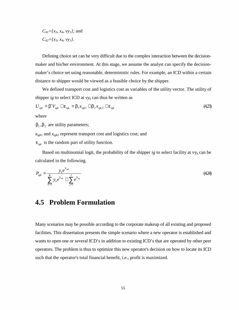
55

C41={x3, x4, vy1}; and

C42={x3, x4, vy1}.

Defining choice set can be very difficult due to the complex interaction between the decision-

maker and his/her environment. At this stage, we assume the analyst can specify the decision-

maker’s choice set using reasonable, deterministic rules. For example, an ICD within a certain

distance to shipper would be viewed as a feasible choice by the shipper.

We defined transport cost and logistics cost as variables of the utility vector. The utility of

shipper ig to select ICD at vyk can thus be written as

igkigkigkigkigkigk xxVU ε+β+β=ε+β′= 2211 (4.23)

where

21 ββ , are utility parameters;

xigk1 and xigk2 represent transport cost and logistics cost; and

igkε is the random part of utility function.

Based on multinomial logit, the probability of the shipper ig to select facility at vyk can be

calculated in the following.

∑ ∑= =

+= K

k

J

j

VV

k

V

kigk

igjigk

igk

eey

eyP

1 1

(4.24)

4.5 Problem Formulation

Many scenarios may be possible according to the corporate makeup of all existing and proposed

facilities. This dissertation presents the simple scenario where a new operator is established and

wants to open one or several ICD’s in addition to existing ICD’s that are operated by other peer

operators. The problem is thus to optimize this new operator's decision on how to locate its ICD

such that the operator's total financial benefit, i.e., profit is maximized.

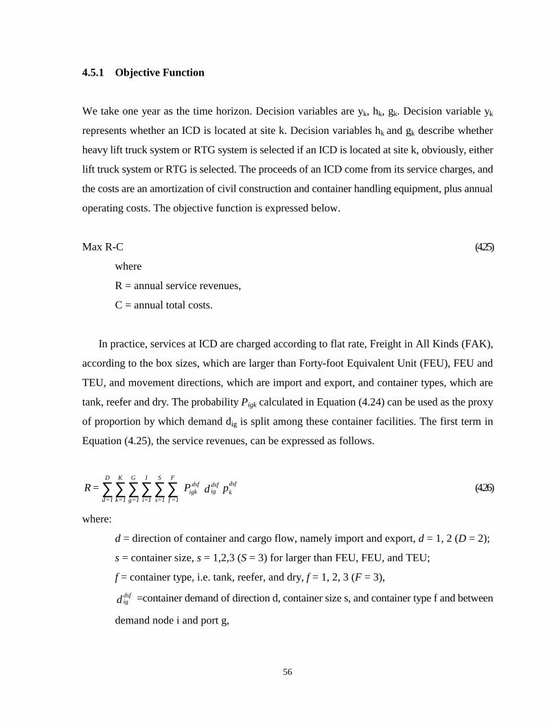
56

4.5.1 Objective Function

We take one year as the time horizon. Decision variables are yk, hk, gk. Decision variable yk

represents whether an ICD is located at site k. Decision variables hk and gk describe whether

heavy lift truck system or RTG system is selected if an ICD is located at site k, obviously, either

lift truck system or RTG is selected. The proceeds of an ICD come from its service charges, and

the costs are an amortization of civil construction and container handling equipment, plus annual

operating costs. The objective function is expressed below.

Max R-C (4.25)

where

R = annual service revenues,

C = annual total costs.

In practice, services at ICD are charged according to flat rate, Freight in All Kinds (FAK),

according to the box sizes, which are larger than Forty-foot Equivalent Unit (FEU), FEU and

TEU, and movement directions, which are import and export, and container types, which are

tank, reefer and dry. The probability Pigk calculated in Equation (4.24) can be used as the proxy

of proportion by which demand dig is split among these container facilities. The first term in

Equation (4.25), the service revenues, can be expressed as follows.

pd P = R dsfk

dsfig

dsfigk

F

=1f

S

=1s

I

=1i

G

=1g

K

=1k

D

=1d∑∑∑∑∑∑ (4.26)

where:

d = direction of container and cargo flow, namely import and export, d = 1, 2 (D = 2);

s = container size, s = 1,2,3 (S = 3) for larger than FEU, FEU, and TEU;

f = container type, i.e. tank, reefer, and dry, f = 1, 2, 3 (F = 3),

ddsfig =container demand of direction d, container size s, and container type f and between

demand node i and port g,

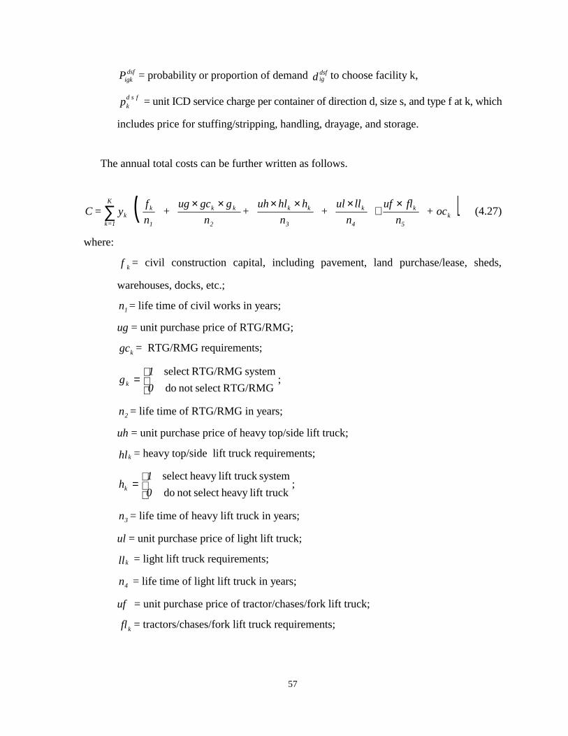
57

dsfigkP = probability or proportion of demand ddsf

ig to choose facility k,

p fsdk = unit ICD service charge per container of direction d, size s, and type f at k, which

includes price for stuffing/stripping, handling, drayage, and storage.

The annual total costs can be further written as follows.

( ) + ocn

fluf

n

llul +

n

hhluh+

n

ggcug +

n

f y = C k

5

k

4

k

3

kk

2

kk

1

kk

K

=1k

×+

×××××∑ (4.27)

where:

f k = civil construction capital, including pavement, land purchase/lease, sheds,

warehouses, docks, etc.;

1n = life time of civil works in years;

ug = unit purchase price of RTG/RMG;

gck = RTG/RMG requirements;

=RTG/RMGselect not do

systemRTG/RMG select

0

1gk ;

2n = life time of RTG/RMG in years;

uh = unit purchase price of heavy top/side lift truck;

hlk = heavy top/side lift truck requirements;

=lift truckheavy select not do

system lift truckheavy select

0

1hk ;

3n = life time of heavy lift truck in years;

ul = unit purchase price of light lift truck;

ll k = light lift truck requirements;

4n = life time of light lift truck in years;

uf = unit purchase price of tractor/chases/fork lift truck;

fl k = tractors/chases/fork lift truck requirements;

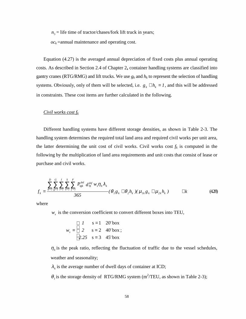
58

5n = life time of tractor/chases/fork lift truck in years;

ock =annual maintenance and operating cost.

Equation (4.27) is the averaged annual depreciation of fixed costs plus annual operating

costs. As described in Section 2.4 of Chapter 2, container handling systems are classified into

gantry cranes (RTG/RMG) and lift trucks. We use gk and hk to represent the selection of handling

systems. Obviously, only of them will be selected, i.e. 1hg kk =+ , and this will be addressed

in constraints. These cost items are further calculated in the following.

Civil works cost fk

Different handling systems have different storage densities, as shown in Table 2-3. The

handling system determines the required total land area and required civil works per unit area,

the latter determining the unit cost of civil works. Civil works cost fk is computed in the

following by the multiplication of land area requirements and unit costs that consist of lease or

purchase and civil works.

)hg)(hg(365

wdP

f kk2kk1k2k1

kksdsfig

F

=1f

S

=1s

I

=1i

G

=1g

D

=1dk

µµθθ

λη++=

∑∑∑∑∑ dsfigk

k∀ (4.28)

where

sw is the conversion coefficient to convert different boxes into TEU,

===

=box 45'3s

box 40'2s

box 20'1s

25.2

2

1

ws ;

kη is the peak ratio, reflecting the fluctuation of traffic due to the vessel schedules,

weather and seasonality;

kλ is the average number of dwell days of container at ICD;

1θ is the storage density of RTG/RMG system (m2/TEU, as shown in Table 2-3);

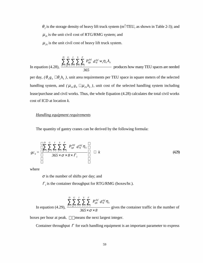
59

2θ is the storage density of heavy lift truck system (m2/TEU, as shown in Table 2-3); and

k1µ is the unit civil cost of RTG/RMG system; and

k2µ is the unit civil cost of heavy lift truck system.

In equation (4.28), 365

wdP kksdsfig

F

=1f

S

=1s

I

=1i

G

=1g

D

=1d

ληdsfigk∑∑∑∑∑

produces how many TEU spaces are needed

per day, )hg( k2k1 θθ + , unit area requirements per TEU space in square meters of the selected

handling system, and )hg( kk2kk1 µµ + , unit cost of the selected handling system including

lease/purchase and civil works. Thus, the whole Equation (4.28) calculates the total civil works

cost of ICD at location k.

Handling equipment requirements

The quantity of gantry cranes can be derived by the following formula:

×××

∑∑∑∑∑1

kdsfig

dsfigk

F

1=f

S

1=s

I

1=i

G

1=g

D

1=d

k 8365

dP

= gc

Γσ

η k∀ (4.29)

where

σ is the number of shifts per day; and

1Γ is the container throughput for RTG/RMG (boxes/hr.).

In equation (4.29), 8365

dP kdsfig

dsfigk

F

=1f

S

=1s

I

=1i

G

=1g

D

=1d

××

∑∑∑∑∑σ

ηgives the container traffic in the number of

boxes per hour at peak. means the next largest integer.

Container throughput Γ for each handling equipment is an important parameter to express

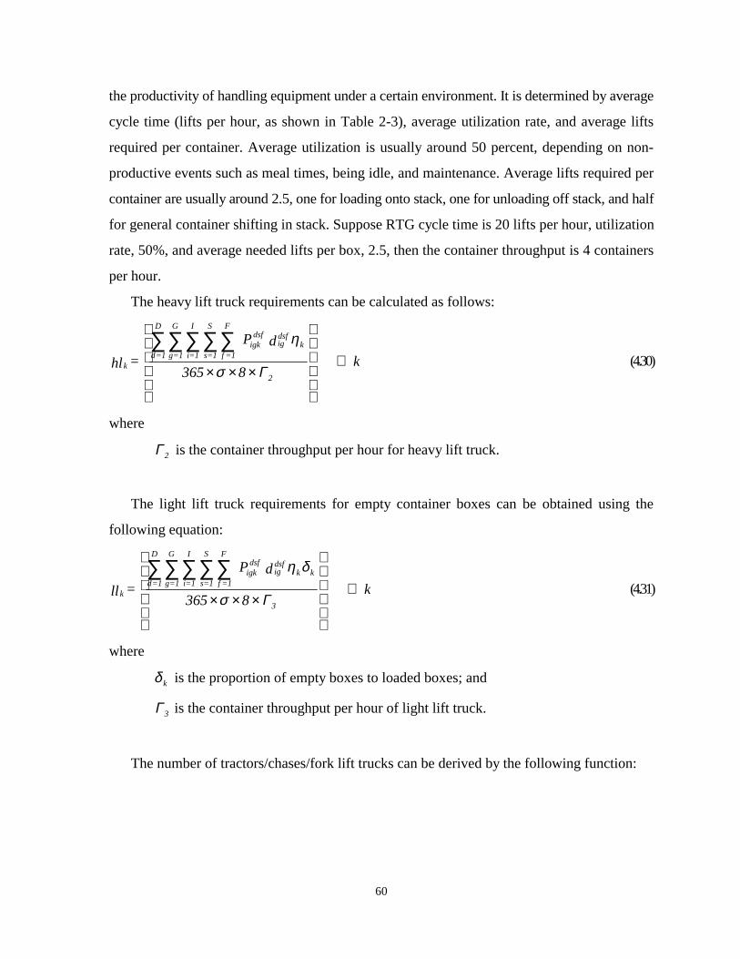
60

the productivity of handling equipment under a certain environment. It is determined by average

cycle time (lifts per hour, as shown in Table 2-3), average utilization rate, and average lifts

required per container. Average utilization is usually around 50 percent, depending on non-

productive events such as meal times, being idle, and maintenance. Average lifts required per

container are usually around 2.5, one for loading onto stack, one for unloading off stack, and half

for general container shifting in stack. Suppose RTG cycle time is 20 lifts per hour, utilization

rate, 50%, and average needed lifts per box, 2.5, then the container throughput is 4 containers

per hour.

The heavy lift truck requirements can be calculated as follows:

8365

dP

= hl2

kdsfig

dsfigk

F

=1f

S

=1s

I

=1i

G

=1g

D

=1dk

×××

∑∑∑∑∑Γσ

η k∀ (4.30)

where

2Γ is the container throughput per hour for heavy lift truck.

The light lift truck requirements for empty container boxes can be obtained using the

following equation:

8365

dP

= ll3

kkdsfig

dsfigk

F

=1f

S

=1s

I

=1i

G

=1g

D

=1dk

×××

∑∑∑∑∑Γσ

δη k∀ (4.31)

where

kδ is the proportion of empty boxes to loaded boxes; and

3Γ is the container throughput per hour of light lift truck.

The number of tractors/chases/fork lift trucks can be derived by the following function:

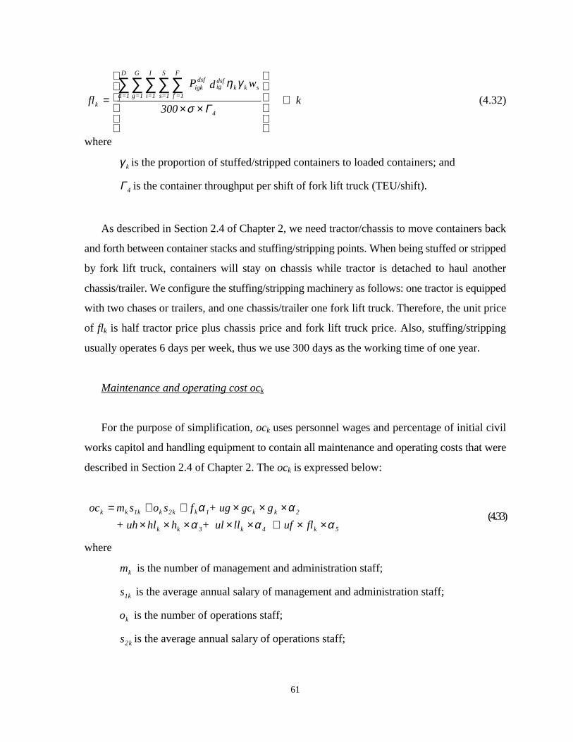
61

k300

wdP

fl4

skkdsfig

dsfigk

F

=1f

S

=1s

I

=1i

G

=1g

D

=1dk

∀

××=

∑∑∑∑∑

Γσ

γη (4.32)

where

kγ is the proportion of stuffed/stripped containers to loaded containers; and

4Γ is the container throughput per shift of fork lift truck (TEU/shift).

As described in Section 2.4 of Chapter 2, we need tractor/chassis to move containers back

and forth between container stacks and stuffing/stripping points. When being stuffed or stripped

by fork lift truck, containers will stay on chassis while tractor is detached to haul another

chassis/trailer. We configure the stuffing/stripping machinery as follows: one tractor is equipped

with two chases or trailers, and one chassis/trailer one fork lift truck. Therefore, the unit price

of flk is half tractor price plus chassis price and fork lift truck price. Also, stuffing/stripping

usually operates 6 days per week, thus we use 300 days as the working time of one year.

Maintenance and operating cost ock

For the purpose of simplification, ock uses personnel wages and percentage of initial civil

works capitol and handling equipment to contain all maintenance and operating costs that were

described in Section 2.4 of Chapter 2. The ock is expressed below:

fl uf ll+ ulhhl+ uh

ggc+ ugfsosm oc

5k4k3kk

2kk1kk2kk1kk

ααααα

××+××××××××++=

(4.33)

where

km is the number of management and administration staff;

k1s is the average annual salary of management and administration staff;

ko is the number of operations staff;

k2s is the average annual salary of operations staff;

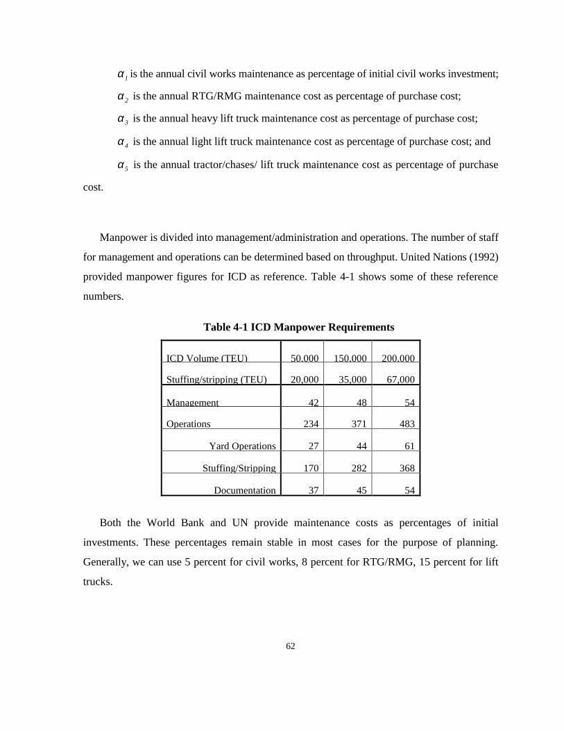
62

1α is the annual civil works maintenance as percentage of initial civil works investment;

2α is the annual RTG/RMG maintenance cost as percentage of purchase cost;

3α is the annual heavy lift truck maintenance cost as percentage of purchase cost;

4α is the annual light lift truck maintenance cost as percentage of purchase cost; and

5α is the annual tractor/chases/ lift truck maintenance cost as percentage of purchase

cost.

Manpower is divided into management/administration and operations. The number of staff

for management and operations can be determined based on throughput. United Nations (1992)

provided manpower figures for ICD as reference. Table 4-1 shows some of these reference

numbers.

Table 4-1 ICD Manpower Requirements

ICD Volume (TEU) 50,000 150,000 200,000

Stuffing/stripping (TEU) 20,000 35,000 67,000

Management 42 48 54

Operations 234 371 483

Yard Operations 27 44 61

Stuffing/Stripping 170 282 368

Documentation 37 45 54

Both the World Bank and UN provide maintenance costs as percentages of initial

investments. These percentages remain stable in most cases for the purpose of planning.

Generally, we can use 5 percent for civil works, 8 percent for RTG/RMG, 15 percent for lift

trucks.

63

4.5.2 Constraints

There are seven groups of constraints. First, decision variables are either 1 or 0.

k0,1

k0,1h

k1,0=y

k

k

∀=∀=∀

g

k

(4.34)

Second, only one handling system, either RTG/RMG or lift trucks, will be selected.

k1hg kk ∀=+ (4.35)

The selection of handling system conditioned on an ICD be located.

kyh

kyg

kk

kk

∀≤∀≤

(4.36)

According to scale economies, the container throughput of an ICD is required to reach up to

a certain level to justify the costly equipment and more importantly, the establishment of

concerned branches of customs and inspections. Such a constraint is declared below.

kQywd sdsfig

F

=1f

S

=1s

I

=1i

G

=1g

D

=1d

∀≥∑∑∑∑∑ P kdsfigk (4.37)

where Q is the required container volume in TEU.

Due to land availability, operations methods and skills, personnel quality, etc., the container

throughput of ICD is constrained, as expressed as follows:

kSCwd sdsfig

F

=1f

S

=1s

I

=1i

G

=1g

D

=1d

∀≤∑∑∑∑∑ kdsfigkP (4.38)

where SCk denotes the capacity for demand of direction d and at location k.

Similarly, because of land size, requirements of different cargo storage, etc., the total yearly

storage of different cargo is restricted by the capacity of the corresponding storage facility such

as refrigeration racks. This can be represented as:

k,f RC w df

ksdcfig

S

=1s

I

=1i

G

=1g

T

=1t

D

=1d

∀≤∑∑∑∑∑ Pdsfigk (4.39)

64

where fkRC denotes the capacity of storage of different cargo types.

Line haul capacity constraint is:

k, dLC wd d ks

dsfig

F

1=f

S

1=s

I

1=i

G

1=g

∀≤∑∑∑∑ Pdsfigk , (4.40)

where LCdk is the line haul capacity at location k for demand with direction d. This constraint

is especially applicable to rail and waterways.

4.6 Illustration of Formulation

For the purpose of illustration, a simple network is taken as an example. As shown in Figure 4-3,

this small network is composed of one port at p1, three demand nodes at vd1, vd2, and vd3, an

existing ICD at x1, and three possible ICD sites at vy1, vy2, and vy3. An ICD operator is deciding

how to locate his ICD’s among these three possible sites to compete for the market with the ICD

at x1 that does not belong to him. Demand volumes of these three demand nodes are d1, d2, and

d3. Because we have only one port at p1, therefore, d1=d11, d2=d21, and d3=d31. The choice sets

for d11, d21, and d31 are the same, i.e., {x1, vy1, vy2, vy3}. y1, y2 and y3 are decision variables to

describe whether an ICD is located. By the reason of simplification, traffic directions, container

types and sizes are not distinguished. In addition, y4 is used to as an additional decision variable

to represent the fact that an ICD is already at x1. Obviously, y4=1 is forced. The choice sets for

d11, d21, and d31 can be rewritten as {vy1, vy2, vy3, vy4} to map {y1, y2, y3, y4}. Such

transformation can be conducive to computer programming at the time of solving the

formulation.

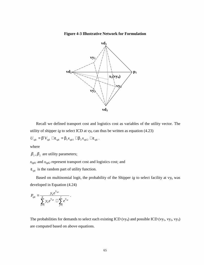
65

Figure 4-3 Illustrative Network for Formulation

vd1

vy1

vd2 p1 x1(vy4)

vy3 vy2

vd3

Recall we defined transport cost and logistics cost as variables of the utility vector. The

utility of shipper ig to select ICD at vyk can thus be written as equation (4.23)

igkigkigkigkigkigk xxVU ε+β+β=ε+β′= 2211 .

where

2 ββ ,1 are utility parameters;

xigk1 and xigk2 represent transport cost and logistics cost; and

igkε is the random part of utility function.

Based on multinomial logit, the probability of the Shipper ig to select facility at vyk was

developed in Equation (4.24)

∑ ∑= =

+= K

k

J

j

VV

k

V

kigk

igjigk

igk

eey

eyP

1 1

.

The probabilities for demands to select each existing ICD (vy4) and possible ICD (vy1, vy2, vy3)

are computed based on above equations.

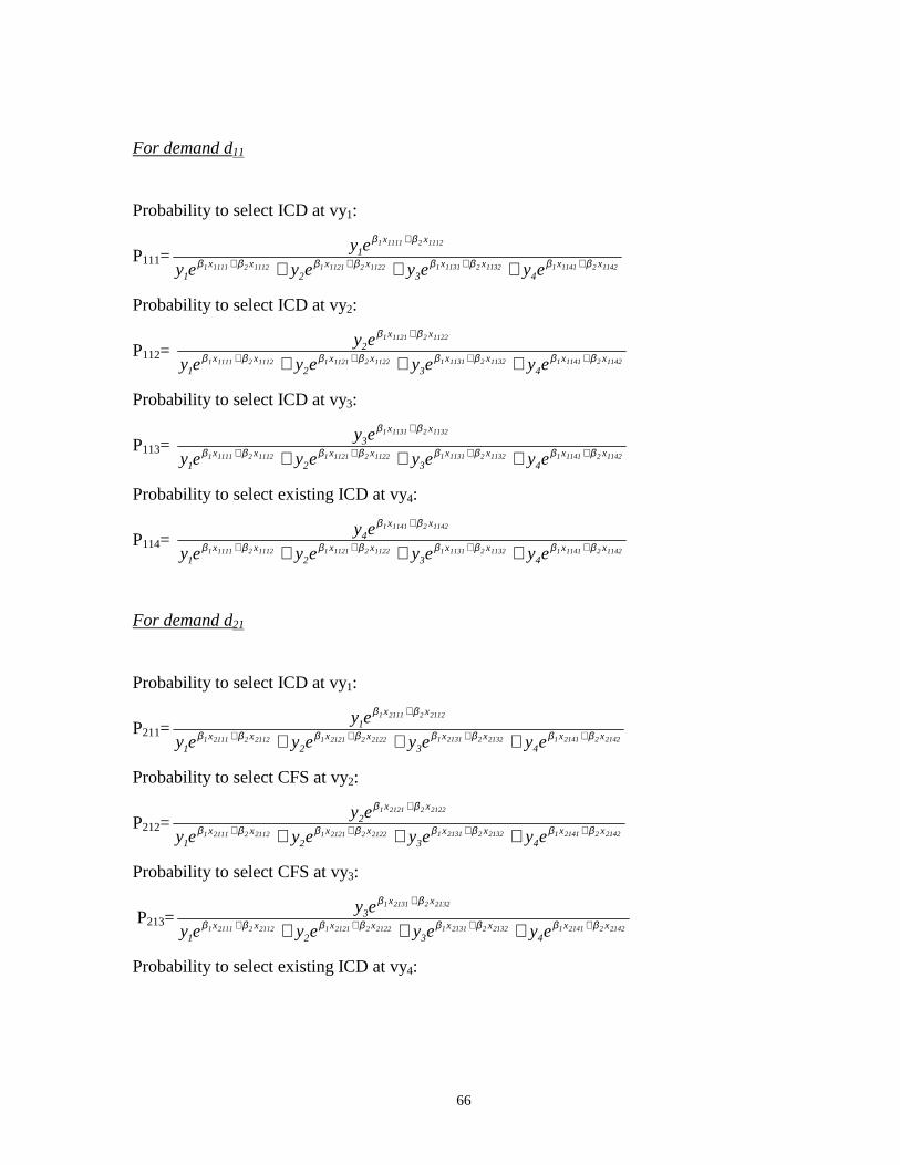
66

For demand d11

Probability to select ICD at vy1:

P111=1142211411113221131111222112111112211111

1112211111

xx4

xx3

xx2

xx1

xx1

eyeyeyey

eyββββββββ

ββ

++++

+

+++

Probability to select ICD at vy2:

P112= 1142211411113221131111222112111112211111

1122211211

xx4

xx3

xx2

xx1

xx2

eyeyeyey

eyββββββββ

ββ

++++

+

+++

Probability to select ICD at vy3:

P113= 1142211411113221131111222112111112211111

1132211311

xx4

xx3

xx2

xx1

xx3

eyeyeyey

eyββββββββ

ββ

++++

+

+++

Probability to select existing ICD at vy4:

P114= 1142211411113221131111222112111112211111

1142211411

xx4

xx3

xx2

xx1

xx4

eyeyeyey

eyββββββββ

ββ

++++

+

+++

For demand d21

Probability to select ICD at vy1:

P211=2142221411213222131121222212112112221111

2112221111

xx4

xx3

xx2

xx1

xx1

eyeyeyey

eyββββββββ

ββ

++++

+

+++

Probability to select CFS at vy2:

P212=2142221411213222131121222212112112221111

2122221211

xx4

xx3

xx2

xx1

xx2

eyeyeyey

eyββββββββ

ββ

++++

+

+++

Probability to select CFS at vy3:

P213=2142221411213222131121222212112112221111

2132221311

xx4

xx3

xx2

xx1

xx3

eyeyeyey

eyββββββββ

ββ

++++

+

+++

Probability to select existing ICD at vy4:

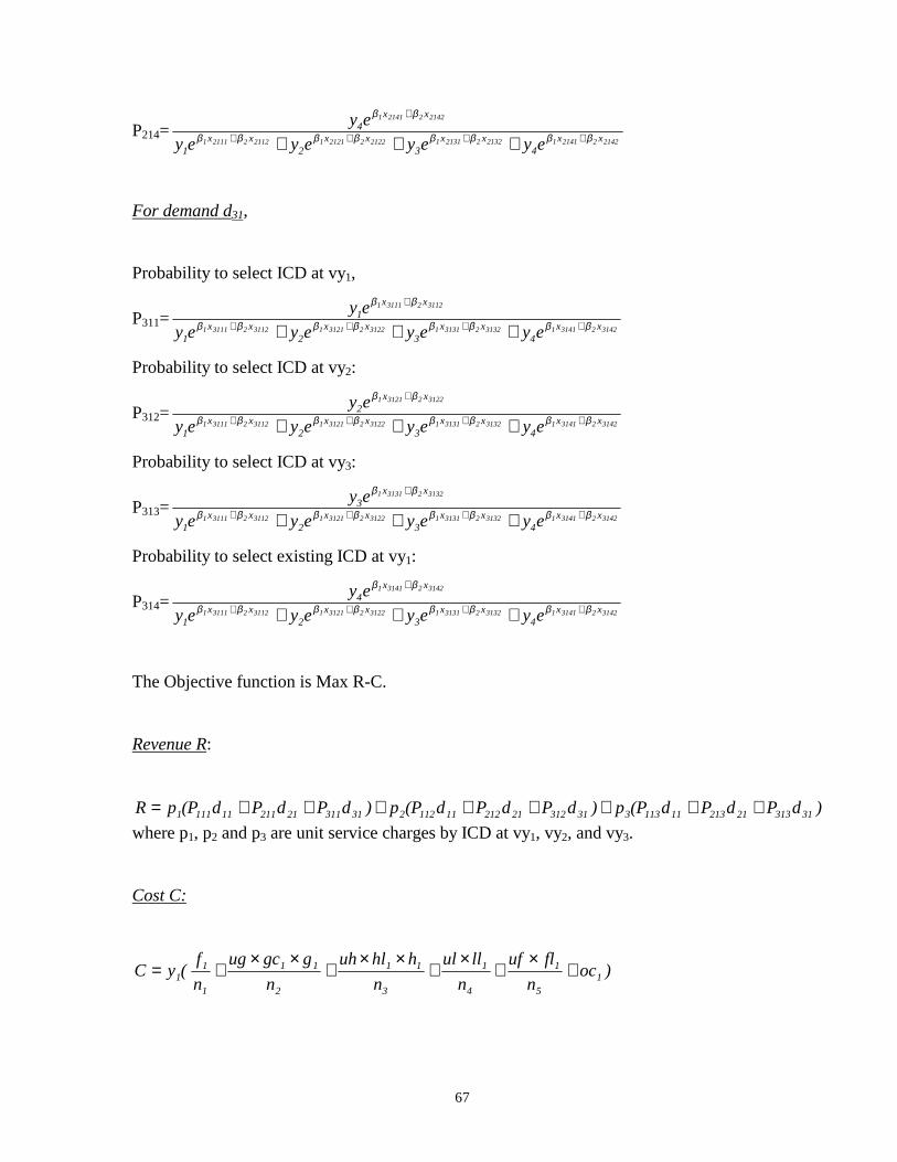
67

P214=2142221411213222131121222212112112221111

2142221411

xx4

xx3

xx2

xx1

xx4

eyeyeyey

eyββββββββ

ββ

++++

+

+++

For demand d31,

Probability to select ICD at vy1,

P311=3142231411313223131131222312113112231111

3112231111

xx4

xx3

xx2

xx1

xx1

eyeyeyey

eyββββββββ

ββ

++++

+

+++

Probability to select ICD at vy2:

P312=3142231411313223131131222312113112231111

3122231211

xx4

xx3

xx2

xx1

xx2

eyeyeyey

eyββββββββ

ββ

++++

+

+++

Probability to select ICD at vy3:

P313=3142231411313223131131222312113112231111

3132231311

xx4

xx3

xx2

xx1

xx3

eyeyeyey

eyββββββββ

ββ

++++

+

+++

Probability to select existing ICD at vy1:

P314=3142231411313223131131222312113112231111

3142231411

xx4

xx3

xx2

xx1

xx4

eyeyeyey

eyββββββββ

ββ

++++

+

+++

The Objective function is Max R-C.

Revenue R:

)dPdPd(Pp)dPdPd(Pp)dPdPd(PpR 313132121311113331312212121111223131121211111111 ++++++++=where p1, p2 and p3 are unit service charges by ICD at vy1, vy2, and vy3.

Cost C:

)ocn

fluf

n

llul

n

hhluh

n

ggcug

n

f(yC 1

5

1

4

1

3

11

2

11

1

11 +

×+

×+

××+

××+=

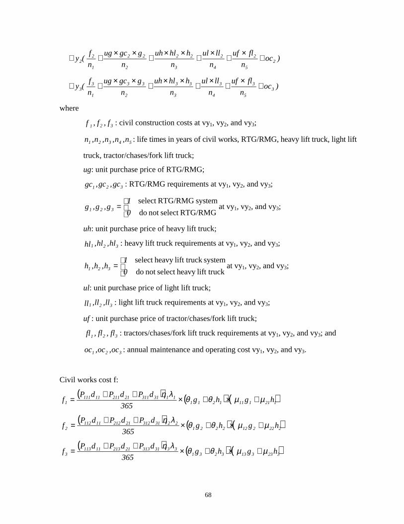
68

)ocn

fluf

n

llul

n

hhluh

n

ggcug

n

f(y 2

5

2

4

2

3

22

2

22

1

22 +

×+

×+

××+

××++

)ocn

fluf

n

llul

n

hhluh

n

ggcug

n

f(y 3

5

3

4

3

3

33

2

33

1

33 +

×+

×+

××+

××++

where

321 f,f,f : civil construction costs at vy1, vy2, and vy3;

54321 n,n,n,n,n : life times in years of civil works, RTG/RMG, heavy lift truck, light lift

truck, tractor/chases/fork lift truck;

ug: unit purchase price of RTG/RMG;

321 gc,gc,gc : RTG/RMG requirements at vy1, vy2, and vy3;

=RTG/RMGselect not do

systemRTG/RMG select

0

1g,g,g 321 at vy1, vy2, and vy3;

uh: unit purchase price of heavy lift truck;

321 hl,hl,hl : heavy lift truck requirements at vy1, vy2, and vy3;

=lift truckheavy select not do

system lift truckheavy select

0

1h,h,h 321 at vy1, vy2, and vy3;

ul: unit purchase price of light lift truck;

321 ll,ll,ll : light lift truck requirements at vy1, vy2, and vy3;

uf : unit purchase price of tractor/chases/fork lift truck;

321 fl,fl,fl : tractors/chases/fork lift truck requirements at vy1, vy2, and vy3; and

321 oc,oc,oc : annual maintenance and operating cost vy1, vy2, and vy3.

Civil works cost f:

( ) ( ) ( )121111121111313112121111111

1 hghg365

dPdPdPf µµθθλη

+×+×++

=

( ) ( ) ( )222212222122313122121211112

2 hghg365

dPdPdPf µµθθλη

+×+×++

=

( ) ( ) ( )323313323133313132121311113

3 hghg365

dPdPdPf µµθθλη

+×+×++

=

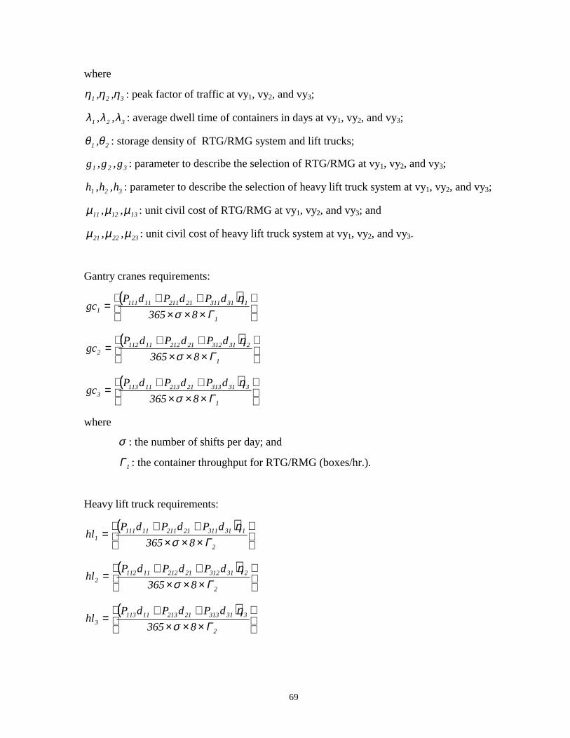
69

where

321 ,, ηηη : peak factor of traffic at vy1, vy2, and vy3;

321 ,, λλλ : average dwell time of containers in days at vy1, vy2, and vy3;

21 ,θθ : storage density of RTG/RMG system and lift trucks;

321 g,g,g : parameter to describe the selection of RTG/RMG at vy1, vy2, and vy3;

321 h,h,h : parameter to describe the selection of heavy lift truck system at vy1, vy2, and vy3;

131211 ,, µµµ : unit civil cost of RTG/RMG at vy1, vy2, and vy3; and

232221 ,, µµµ : unit civil cost of heavy lift truck system at vy1, vy2, and vy3.

Gantry cranes requirements:

( )

×××

++=

1

13131121211111111 8365

dPdPdPgc

Γση

( )

×××

++=

1

23131221212111122 8365

dPdPdPgc

Γση

( )

×××

++=

1

33131321213111133 8365

dPdPdPgc

Γση

where

σ : the number of shifts per day; and

1Γ : the container throughput for RTG/RMG (boxes/hr.).

Heavy lift truck requirements:

( )

×××

++=

2

13131121211111111 8365

dPdPdPhl

Γση

( )

×××

++=

2

23131221212111122 8365

dPdPdPhl

Γση

( )

×××

++=

2

33131321213111133 8365

dPdPdPhl

Γση

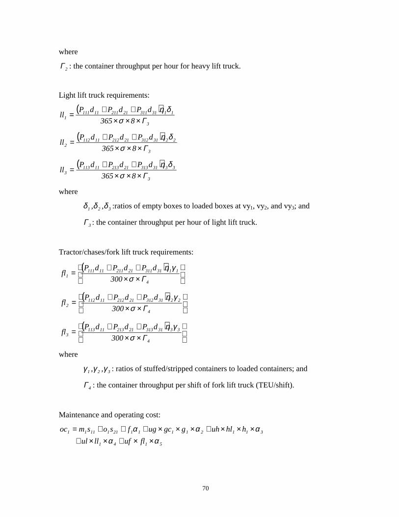
70

where

2Γ : the container throughput per hour for heavy lift truck.

Light lift truck requirements:

( )3

113131121211111111 8365

dPdPdPll

Γσδη

×××++

=

( )3

223131221212111122 8365

dPdPdPll

Γσδη

×××++

=

( )3

333131321213111133 8365

dPdPdPll

Γσδη

×××++

=

where

321 ,, δδδ :ratios of empty boxes to loaded boxes at vy1, vy2, and vy3; and

3Γ : the container throughput per hour of light lift truck.

Tractor/chases/fork lift truck requirements:

( )

××++

=4

113131121211111111 300

dPdPdPfl

Γσγη

( )

××++

=4

223131221212111122 300

dPdPdPfl

Γσγη

( )

××++

=4

333131321213111133 300

dPdPdPfl

Γσγη

where

321 ,, γγγ : ratios of stuffed/stripped containers to loaded containers; and

4Γ : the container throughput per shift of fork lift truck (TEU/shift).

Maintenance and operating cost:

5141

311211112111111

flufllul

hhluhggcugfsosmoc

ααααα

××+××+×××+×××+++=

71

5242

322222122221222

flufllul

hhluhggcugfsosmoc

ααααα

××+××+×××+×××+++=

5343

333233132331333

flufllul

hhluhggcugfsosmoc

ααααα

××+××+×××+×××+++=

where

321 m,m,m : the number of management/administration staff at vy1, vy2, and vy3;

131211 s,s,s : average annual salary of management/administration staff at vy1, vy2, and vy3;

321 o,o,o : the number of operations staff at vy1, vy2, and vy3;;

232221 s,s,s : average annual salary of operations staff at vy1, vy2, and vy3; and

54321 ,,,, ααααα : annual maintenance costs as percentages of initial civil works

investment, RTG/RMG purchase cost, heavy lift truck purchase cost, light lift truck

purchase cost, tractor/chases/fork lift truck purchase cost.

Constraints

Three most important and common constraints are considered.

Decision variables:

=1

0yi ; i = 1, 2, 3

=1

0hi ; i = 1, 2, 3

=1

0gi ; i = 1, 2, 3

Handling equipment system: only one handling system, either RTG/RMG or lift trucks, will be

selected.

1hg 11 =+ ;

72

1hg 22 =+ ;

1hg 33 =+ .

The selection of handling system is conditioned on an ICD be located.

.33

22

11

33

22

11

yh

;yh

;yh

;yg

;yg

yg

≤≤≤≤≤≤ ;

Scale of economy: the container throughput of an ICD is required to reach up to a certain level

to justify the costly equipment and more importantly, the establishment of concerned branches

of customs and inspections.

QydPdPdP 1313112121111111 ≥++

QydPdPdP 2313122121211112 ≥++

QydPdPdP 3313132121311113 ≥++

where

Q is the required container volume.

The solution of this formulation will decide where to locate ICD’s at these three candidate

sites. At the same time, the number of ICD’s is also determined by the sum of decision variables

equal to 1. Thereafter, the size of each ICD can be computed by adding demands that select each

ICD. Chapter 5 addresses algorithm to solve formulations.

73

Chapter 5

Algorithm Development

5.1 Introduction

As stated in Chapter 3, the ICD location problem is classified as a fixed charge location

problem or warehousing problem which has been considered or proven to be NP-

complete. In addition, the ICD location problem is formulated as non-linear binary

integer programming problem, as shown in Chapter 4. Such non-linearity leads to the

complexity of ICD location problem. Theoretically, no exact algorithm can be developed

to solve the formulation in Chapter 4 within polynomial time when the problem size goes

up. Inevitably, heuristics are sought to resolve the formulation. However, NP-

completeness does not eliminate the possibility of using exact algorithms to solve

sufficiently small sized problems within tolerable times. In this chapter, exact algorithms

are first tried for small networks. Later, a tabu search heuristic is designed especially for

problems of such a size that exact algorithms are unworkable. Also, several parameters of

importance to tabu search heuristic are tested to find out their sensitivity in computational

time and optimality.

As a heuristic must be evaluated in performance to demonstrate the validity in its

applications, solutions of exact algorithms will also serve as perfect benchmarks for

performance of tabu search heuristic in small sized problems. When size increases to

where exact algorithms are unavailable, statistical inference is employed to evaluate the

performance of the designed tabu search algorithm. The evaluation of the performance of

tabu heuristic is addressed in Chapter 6.

74

5.2 Exact Algorithm for Small Sized Problem

Traditionally, there are two exact techniques for solving zero-one programming

problems: explicit enumeration and implicit enumeration. Apparently, explicit

enumeration is not recommended because it is very time consuming. Implicit

enumeration for zero-one programming problems is branch and bound algorithm, which

is computationally much more efficient and less time consuming than explicit

enumeration. When solving integer programming problems, branch and bound algorithm

is usually coupled with linear programming relaxation or cutting planes, with linear

programming relaxation more efficient and more widely used.

The ICD location planning in question is formulated as a non-linear binary integer

programming problem. Given the non-linearity in the formulation, it is very difficult to

implement branch and bound or implicit algorithm. Therefore, enumeration is employed

as the exact algorithm to find the optimal solution for the proposed discrete choice based

formulation. The selection of enumeration is also based on following considerations:

• Exact algorithms, no matter which one is used, cannot solve nonlinear integer

programming problems efficiently, when the problem size increases; and

• The use of exact algorithm is mainly intended to provide benchmark in optimal

solution to evaluate heuristic algorithm for small problem.

5.3 Tabu Search Heuristic Algorithm

5.3.1 Introduction to Tabu Search

Tabu search is effective and efficient in transcending local optimality to find a very good

local optimum close to global optimum if not the global one. By defining a move in

searching for better solutions as tabu tenure, tabu search is able to cross boundaries of

feasibility or local optimality and thus to impose and release constraints to permit

exploration of otherwise forbidden domains. By employing flexible short term and long

term memories on the basis of recency, frequency, and quality of each solutions or

75

moves, tabu search can historically update better solutions in terms of optimality and

diversify and intensify new moves for search better solutions. Because of such

preponderance, the tabu search is considered by the author the most powerful mechanism

for combinatorial optimization problems in overcoming confinement to local optimality

and is selected to develop a heuristic algorithm for ICD location problem.

Several observations serve to justify the above conclusions. Among them are tabu

tenure, aspiration, and move value. Tabu tenure is intended to prevent search from

reversing or cycling by prescribing the number of iterations for one move to take place

again after its current operation. For instance, if a move from X1 to X2 is executed and 7

is set as tabu tenure for this move, such a move can not be considered as the admissible

move within the future 7 iterations even though it serves as a contributing option to the

objective function. Such a tabu tenure has exception, that is, aspiration. Aspiration is the

rule to override the predefined tabu tenure. If one move can sufficiently improve the

objective function, the tabu tenure will be overridden and the move can thus be

considered a new admissible move. From now on, the tabu tenure of this move is

renewed to control the reversing and duplication. Generally the contribution of one move

is evaluated by an evaluation function, called move value, which could be related to the

objective function. Moves with tabu tenure, together with evaluation functions or move

values are kept in short term memory by linked lists while the history of moves and

objective functions is kept in long term memory by linked lists. Such recency-based

memory greatly enhances search efficiency and effectiveness.

5.3.2 A Simple Illustrative Example of Tabu Search

Suppose the problem is to maximize f (x1, x2, x3, x4, x5) where x1, x2, x3, x4 and x5 are

binary decision variables and the initial solution is x1=1, x2=1, x3=0, x4=0, x5=1, and

f=20. Each time only one variable is selected to change its value while other variables

remain intact.

Randomly select x3=1 and generate f=24. Define x3=1 as a tabu for 5 future

iterations. Then, randomly select x2=0 and generate f=28. x2=0 is listed as another tabu

with 5 future iterations as its tabu tenure. After x2=0, the x3=1 is a tabu only for 4 future

iterations. Suppose x3=0 is elected and f=26. Now x3=1, x2=0, x3=0 have tabu tenures of

76

3, 4, and 5, respectively. Note although x3=0 does not improve the objective function

(f=26 is smaller than f=28 before x3=0 was executed), x3 is still selected because new

moves based on x3=0 may find a better solution later. This is one way of breaking the

domain of local optimality.

Suppose x3=1 is randomly selected again with f=36. As x3=1 is a tabu for another 3

iterations, we should not select x3=1 as a move according to tabu tenure. This can

prevent from cycling and reversing. However, as f=36 when x3=1, and if “better than

existing best solution”, which is f=28 in this case, is defined as aspiration level, then tabu

for x3=1 is overridden legally and thus x3=1 is selected again and defined again as a tabu

with 5 iterations. At this time, the tabu tenures for x2=0, x3=0 are updated to 3, 4

iterations.

The above can be repeated until a certain number of iterations are executed if a

certain number is defined as the stopping or cut-off rule. Also, historical performance of

each search and its combination with others is kept in memory to evaluate new search

and improve search speed and quality for a very good solution, if not the best.

5.3.3 Tabu Search Algorithm Design

The generation of a move is the most problem specific issue in the design of tabu search

algorithm. How to define a move is the first step in the design of tabu search algorithm

and dictates the efficiency and effectiveness of tabu search. The discrete choice based

formulation of the ICD location problem is a generic 0-1 non-linear programming

problem whose decision variables are yk, gk, and hk.

However, there exists close relationship between these decision variables. First, gk

and hk are conditional on the premise that an ICD be located at k, namely, as shown in the

constraint, y and k≤≤ kkk hyg . Second, the selection of either RTG or lift truck system

is location specific, and generally speaking, depends on land cost or rental and traffic. If

an ICD is located at location k, i.e., yk = 1, handling system can be selected through the

comparison of RTG and lift truck systems, based on service charge and cost of the

proposed ICD, as shown in Table 2-4.

77

Therefore, although the ICD location problem has decision variables, yk, gk, and hk,

the dependency between each other makes it practicable to solve the formulation by two

levels: first determine yk, and then decide gk and hk for each yk = 1. This will greatly cut

down the search for better solutions, compared to treating all yk, gk, and hk

simultaneously.

According to the above description, a move s is defined as follows:

s(y′ )= y′′

where y′ and y′′ are 0-1 vectors of decision variables yk , and the only difference between

y′ and y′′ is that there is only one decision variable, say yi, in the vector with different

value, therefore, if yi=1 in y′, then yi=0 in y′′, or vice versa. For each yk = 1, whether gk =

1 or hk = 1 is decided by comparing each other under the given cost and service charge of

ICD at k.

The initial solution is generated at random, i.e., each yk is set to 1 or 0 at random.

Based on an initial solution, every move such as s changes one variable of variable vector

of the current solution each time to improve solutions until cut-off rule. And tabu tenure

is added to moves such as s to prevent moves from cycling and/or reversing so that the

local optimality is overridden. Better move value than those of all executed moves so fat

is defined as the aspiration, which overrides the tabu tenure and zero this tabu tenure for

further search. The objective function, denoted as f, is used as the move value evaluation

function.

Short term memory is employed to keep records of tabu tenure and long term memory

to tag the history records for intermediate and final best solutions. History records will

guide the search to intensify or diversify moves. Two separate linked lists can serve the

purpose for short term and long term memories.

Three parameters are defined in a tabu search algorithm to control the tabu search for

good solutions. They are the number of maximum outer iterations, denoted as N, the tabu

tenure for a move, denoted as N1, and the slack parameter or number of maximum inner

iterations (after which the search for a better move within one outer iteration is stopped

and, K, the counter of N is increased by 1), denoted as N2. The tabu search algorithm is

developed as follows.

78

Step 1. Initialization

Step 1 (A). Set N, N1 and N2. Set K=0. Randomly generate the initial feasible

solution y′ and compute its objective function, denoted as ∗f .

Step 1(B). Set I=1 and J=0 as the counters, if K>N, go to step 4. Otherwise go to

step 2 (A).

Step 2. Choice

Step 2(A). Randomly select a decision variable in the solution y′ to generate a

move. Go to step 2 (B).

Step 2(B). If I<N1, find a candidate move s for next search and go to step 2 (C);

otherwise go to step 2 (D).

Step 2 (C). If move s is tabu and fails to satisfy the aspiration level, set I=I+1, go

to step 2 (A). Otherwise, record the objective function of move s, set I=I+1, go to step 2

(A).

Step 2 (D). Select the candidate move with the best objective function f′ being

next solution.

Step 3 Update

Step 3 (A). Update the tabu tenure and aspiration level. If f′<f∗, set J=J+1, go to

step 3 (B). Otherwise, set f∗=f′, I=1 and J=0, go to step 2 (B).

Step 3 (B). If J>N2, set K=K+1, go to step 1 (B). Otherwise, set I=1, go to step 2

(B).

Step 4. Termination. The f∗ is the objective function value of the near-optimal

solution and the corresponding vector of decision variables is the near-optimal solution.

The designed algorithm is demonstrated by flow chart below.

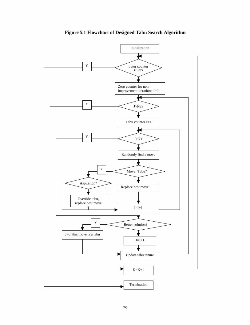
79

Figure 5.1 Flowchart of Designed Tabu Search Algorithm

Initialization

outer counterK>N?

Zero counter for nonimprovement iterations J=0

J>N2?

Tabu counter I=1

I>N1

Randomly find a move

Move: Tabu?

Replace best moveAspiration?

Override tabu,replace best move

I=I+1

Better solution?

J=J+1

J=0, this move is a tabu

Update tabu tenure

K=K+1

Termination

Y

Y

Y

Y

Y

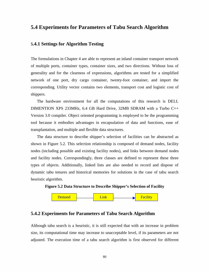
80

5.4 Experiments for Parameters of Tabu Search Algorithm

5.4.1 Settings for Algorithm Testing

The formulations in Chapter 4 are able to represent an inland container transport network

of multiple ports, container types, container sizes, and two directions. Without loss of

generality and for the clearness of expressions, algorithms are tested for a simplified

network of one port, dry cargo container, twenty-foot container, and import the

corresponding. Utility vector contains two elements, transport cost and logistic cost of

shippers.

The hardware environment for all the computations of this research is DELL

DIMENTION XPS 233MHz, 6.4 GB Hard Drive, 32MB SDRAM with a Turbo C++

Version 3.0 compiler. Object oriented programming is employed to be the programming

tool because it embodies advantages in encapsulation of data and functions, ease of

transplantation, and multiple and flexible data structures.

The data structure to describe shipper’s selection of facilities can be abstracted as

shown in Figure 5.2. This selection relationship is composed of demand nodes, facility

nodes (including possible and existing facility nodes), and links between demand nodes

and facility nodes. Correspondingly, three classes are defined to represent these three

types of objects. Additionally, linked lists are also needed to record and dispose of

dynamic tabu tenures and historical memories for solutions in the case of tabu search

heuristic algorithm.

Figure 5.2 Data Structure to Describe Shipper’s Selection of Facility

5.4.2 Experiments for Parameters of Tabu Search Algorithm

Although tabu search is a heuristic, it is still expected that with an increase in problem

size, its computational time may increase to unacceptable level, if its parameters are not

adjusted. The execution time of a tabu search algorithm is first observed for different

LinkDemand Facility

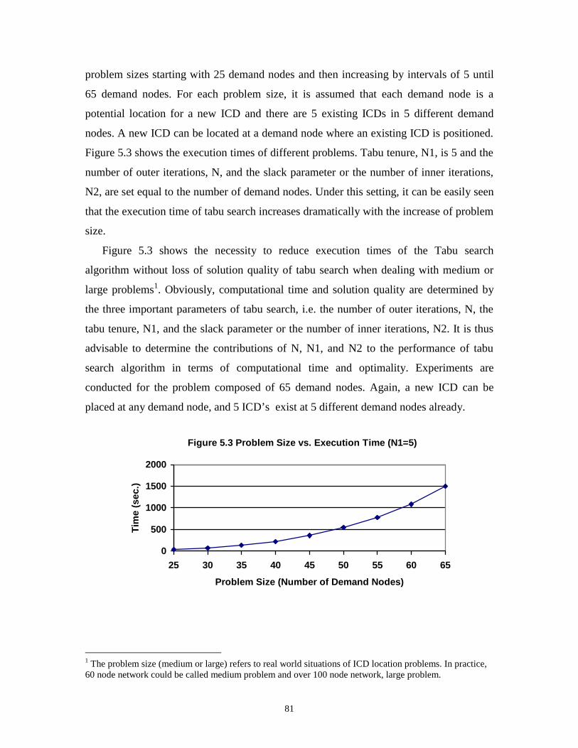
81

problem sizes starting with 25 demand nodes and then increasing by intervals of 5 until

65 demand nodes. For each problem size, it is assumed that each demand node is a

potential location for a new ICD and there are 5 existing ICDs in 5 different demand

nodes. A new ICD can be located at a demand node where an existing ICD is positioned.

Figure 5.3 shows the execution times of different problems. Tabu tenure, N1, is 5 and the

number of outer iterations, N, and the slack parameter or the number of inner iterations,

N2, are set equal to the number of demand nodes. Under this setting, it can be easily seen

that the execution time of tabu search increases dramatically with the increase of problem

size.

Figure 5.3 shows the necessity to reduce execution times of the Tabu search

algorithm without loss of solution quality of tabu search when dealing with medium or

large problems1. Obviously, computational time and solution quality are determined by

the three important parameters of tabu search, i.e. the number of outer iterations, N, the

tabu tenure, N1, and the slack parameter or the number of inner iterations, N2. It is thus

advisable to determine the contributions of N, N1, and N2 to the performance of tabu

search algorithm in terms of computational time and optimality. Experiments are

conducted for the problem composed of 65 demand nodes. Again, a new ICD can be

placed at any demand node, and 5 ICD’s exist at 5 different demand nodes already.

1 The problem size (medium or large) refers to real world situations of ICD location problems. In practice,60 node network could be called medium problem and over 100 node network, large problem.

Figure 5.3 Problem Size vs. E xecut ion Time (N1=5)

0

500

1000

1500

2000

25 30 35 40 45 50 55 60 65

Problem Size (Number of Demand Nodes)

Tim

e (s

ec.)

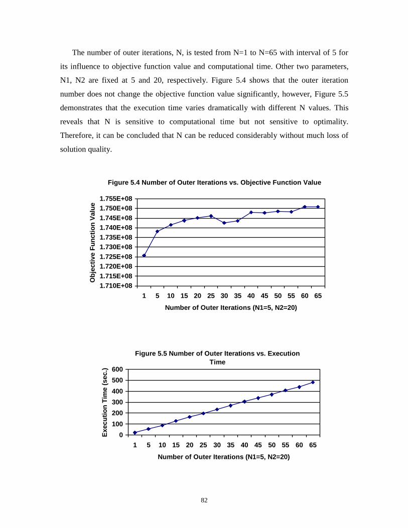
82

The number of outer iterations, N, is tested from N=1 to N=65 with interval of 5 for

its influence to objective function value and computational time. Other two parameters,

N1, N2 are fixed at 5 and 20, respectively. Figure 5.4 shows that the outer iteration

number does not change the objective function value significantly, however, Figure 5.5

demonstrates that the execution time varies dramatically with different N values. This

reveals that N is sensitive to computational time but not sensitive to optimality.

Therefore, it can be concluded that N can be reduced considerably without much loss of

solution quality.

Figure 5.4 Number of Outer It erat ions vs. Objective Function Value

1.710E+081.715E+081.720E+081.725E+081.730E+081.735E+081.740E+081.745E+081.750E+081.755E+08

1 5 10 15 20 25 30 35 40 45 50 55 60 65

Number of Outer Iterat ions (N1=5, N2=20)

Obj

ectiv

e F

unct

ion

Val

ue

Figure 5.5 Number of Outer It erat ions vs. E xecut ion Time

0

100

200

300

400

500

600

1 5 10 15 20 25 30 35 40 45 50 55 60 65

Number of Outer Iterat ions (N1=5, N2=20)

Exe

cutio

n T

ime

(sec

.)

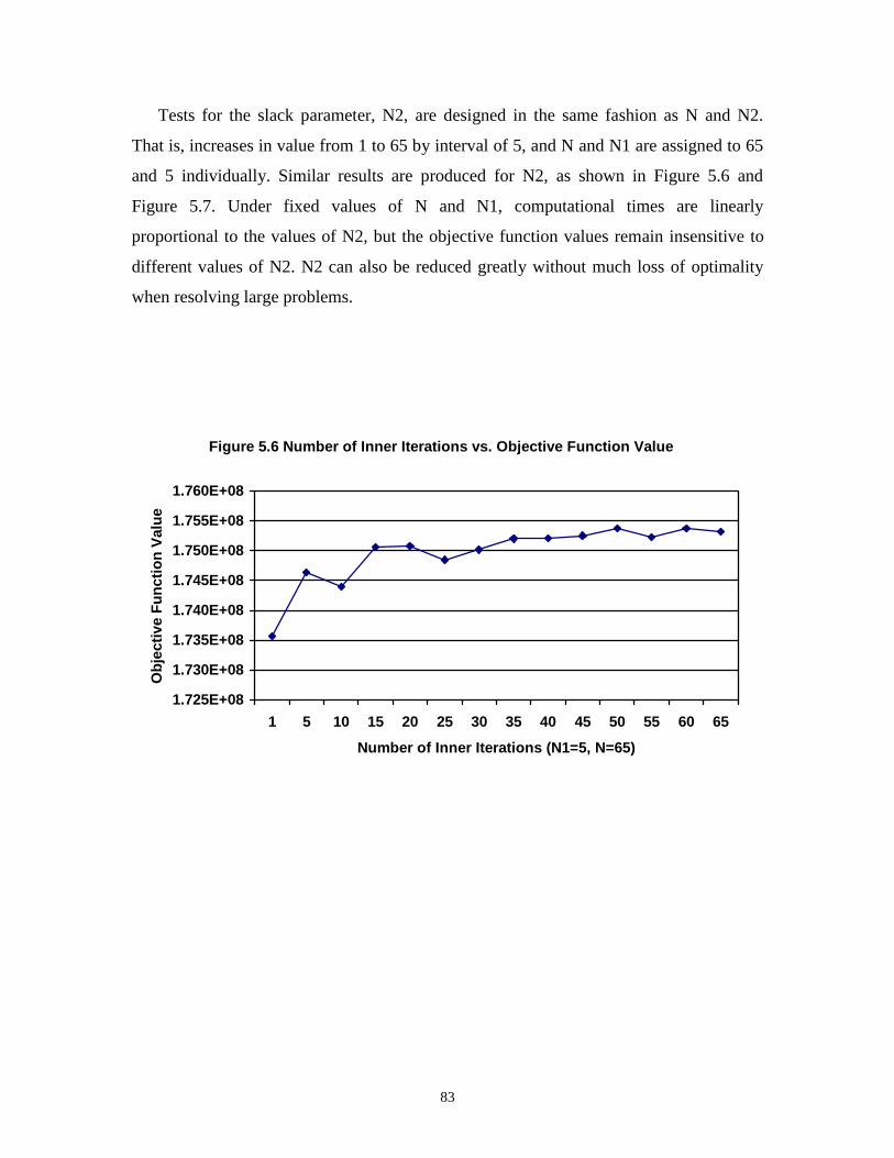
83

Tests for the slack parameter, N2, are designed in the same fashion as N and N2.

That is, increases in value from 1 to 65 by interval of 5, and N and N1 are assigned to 65

and 5 individually. Similar results are produced for N2, as shown in Figure 5.6 and

Figure 5.7. Under fixed values of N and N1, computational times are linearly

proportional to the values of N2, but the objective function values remain insensitive to

different values of N2. N2 can also be reduced greatly without much loss of optimality

when resolving large problems.

Figure 5.6 Number of Inner It erat ions vs. Objective Function Value

1.725E+08

1.730E+08

1.735E+08

1.740E+08

1.745E+08

1.750E+08

1.755E+08

1.760E+08

1 5 10 15 20 25 30 35 40 45 50 55 60 65

Number of Inner Iterat ions (N1=5, N=65)

Obj

ectiv

e F

unct

ion

Val

ue

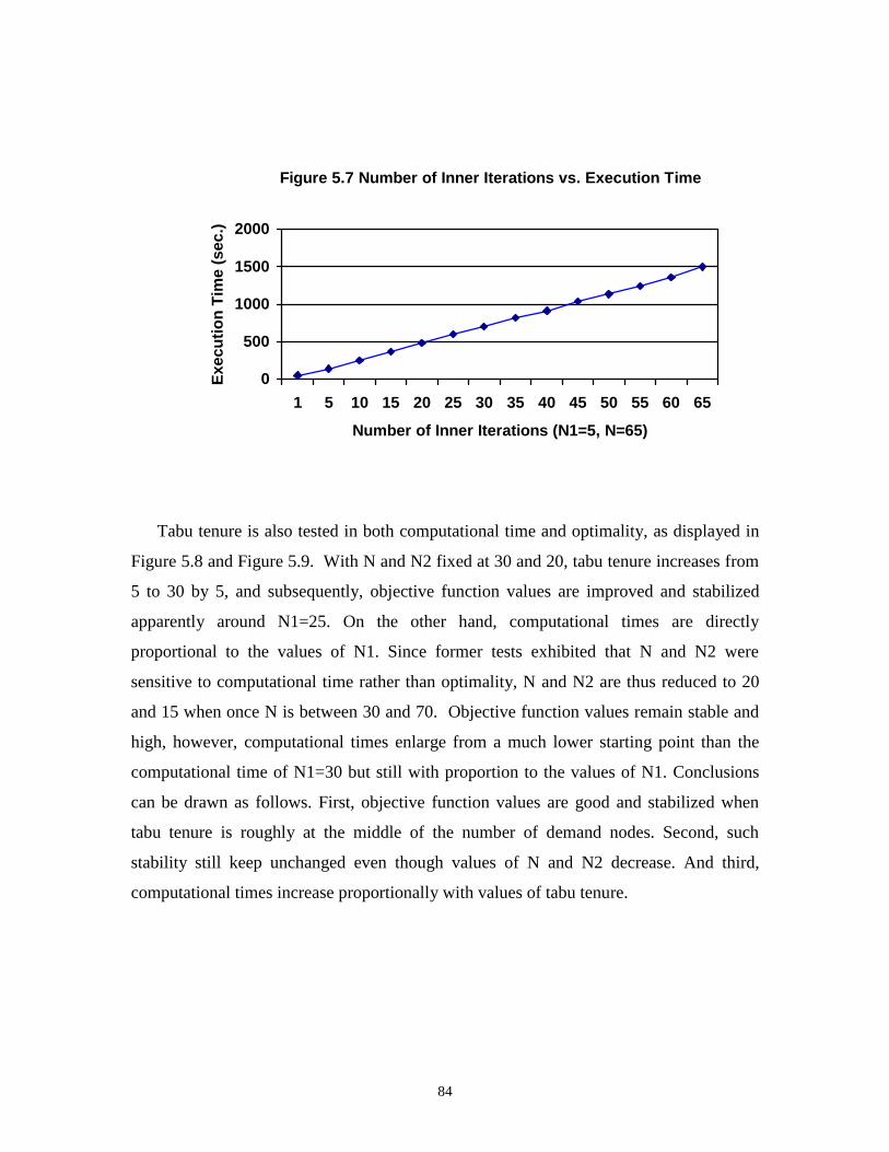
84

Tabu tenure is also tested in both computational time and optimality, as displayed in

Figure 5.8 and Figure 5.9. With N and N2 fixed at 30 and 20, tabu tenure increases from

5 to 30 by 5, and subsequently, objective function values are improved and stabilized

apparently around N1=25. On the other hand, computational times are directly

proportional to the values of N1. Since former tests exhibited that N and N2 were

sensitive to computational time rather than optimality, N and N2 are thus reduced to 20

and 15 when once N is between 30 and 70. Objective function values remain stable and

high, however, computational times enlarge from a much lower starting point than the

computational time of N1=30 but still with proportion to the values of N1. Conclusions

can be drawn as follows. First, objective function values are good and stabilized when

tabu tenure is roughly at the middle of the number of demand nodes. Second, such

stability still keep unchanged even though values of N and N2 decrease. And third,

computational times increase proportionally with values of tabu tenure.

Figure 5.7 Number of Inner Iterat ions vs. Execut ion Time

0

500

1000

1500

2000

1 5 10 15 20 25 30 35 40 45 50 55 60 65

Number of Inner Iterations (N1=5, N=65)

Exe

cutio

n T

ime

(sec

.)

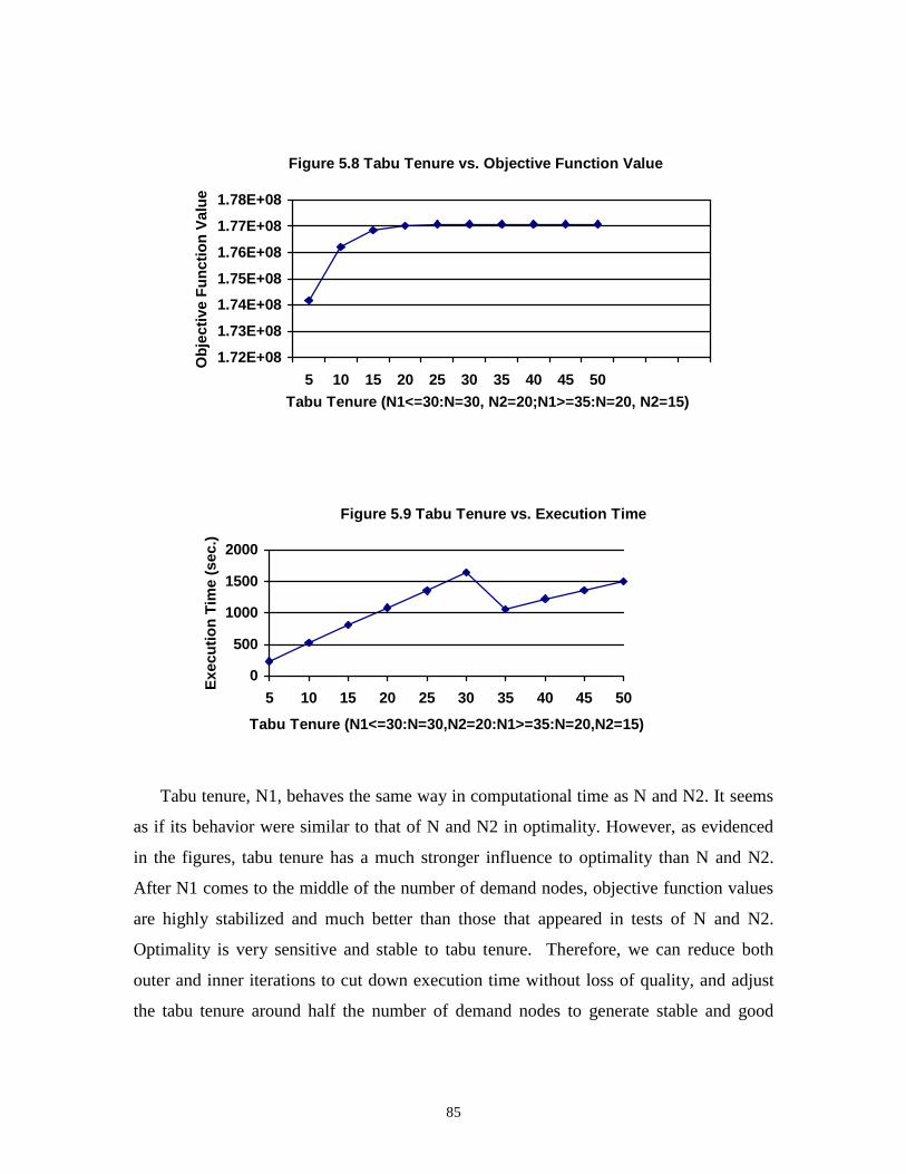
85

Tabu tenure, N1, behaves the same way in computational time as N and N2. It seems

as if its behavior were similar to that of N and N2 in optimality. However, as evidenced

in the figures, tabu tenure has a much stronger influence to optimality than N and N2.

After N1 comes to the middle of the number of demand nodes, objective function values

are highly stabilized and much better than those that appeared in tests of N and N2.

Optimality is very sensitive and stable to tabu tenure. Therefore, we can reduce both

outer and inner iterations to cut down execution time without loss of quality, and adjust

the tabu tenure around half the number of demand nodes to generate stable and good

Figure 5.8 Tabu Tenure vs. Objective Function Value

1.72E+08

1.73E+08

1.74E+08

1.75E+08

1.76E+08

1.77E+08

1.78E+08

5 10 15 20 25 30 35 40 45 50Tabu Tenure (N1<=30:N=30, N2=20;N1>=35:N=20, N2=15)

Obj

ectiv

e F

unct

ion

Val

ue

Figure 5.9 Tabu Tenure vs. E xecut ion Time

0

500

1000

1500

2000

5 10 15 20 25 30 35 40 45 50

Tabu Tenure (N1<=30:N=30,N2=20:N1>=35:N=20,N2=15)

Exe

cutio

n T

ime

(sec

.)

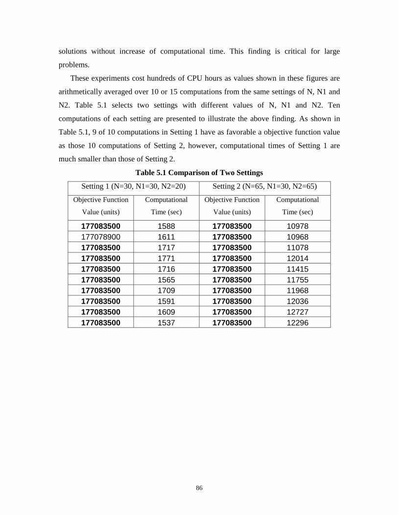
86

solutions without increase of computational time. This finding is critical for large

problems.

These experiments cost hundreds of CPU hours as values shown in these figures are

arithmetically averaged over 10 or 15 computations from the same settings of N, N1 and

N2. Table 5.1 selects two settings with different values of N, N1 and N2. Ten

computations of each setting are presented to illustrate the above finding. As shown in

Table 5.1, 9 of 10 computations in Setting 1 have as favorable a objective function value

as those 10 computations of Setting 2, however, computational times of Setting 1 are

much smaller than those of Setting 2.

Table 5.1 Comparison of Two Settings

Setting 1 (N=30, N1=30, N2=20) Setting 2 (N=65, N1=30, N2=65)

Objective Function

Value (units)

Computational

Time (sec)

Objective Function

Value (units)

Computational

Time (sec)

177083500 1588 177083500 10978177078900 1611 177083500 10968177083500 1717 177083500 11078177083500 1771 177083500 12014177083500 1716 177083500 11415177083500 1565 177083500 11755177083500 1709 177083500 11968177083500 1591 177083500 12036177083500 1609 177083500 12727177083500 1537 177083500 12296

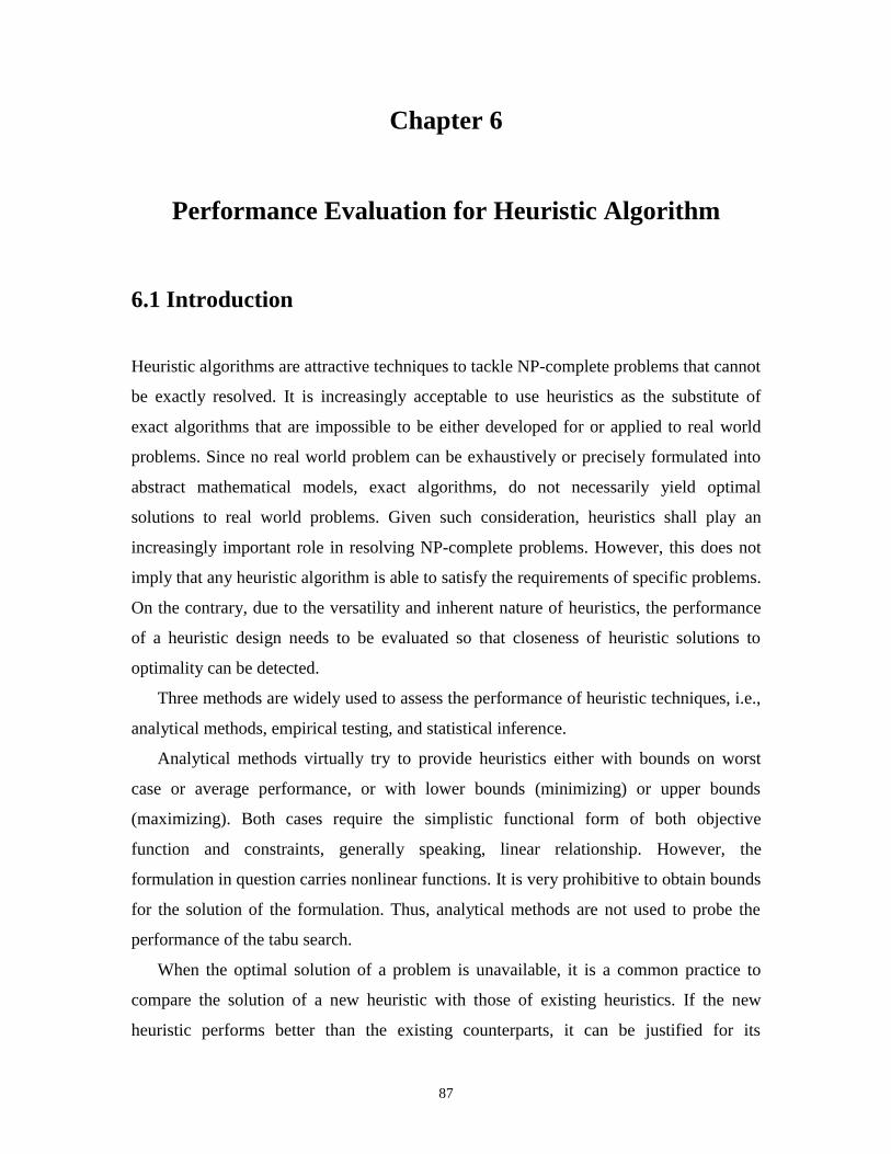
87

Chapter 6

Performance Evaluation for Heuristic Algorithm

6.1 Introduction

Heuristic algorithms are attractive techniques to tackle NP-complete problems that cannot

be exactly resolved. It is increasingly acceptable to use heuristics as the substitute of

exact algorithms that are impossible to be either developed for or applied to real world

problems. Since no real world problem can be exhaustively or precisely formulated into

abstract mathematical models, exact algorithms, do not necessarily yield optimal

solutions to real world problems. Given such consideration, heuristics shall play an

increasingly important role in resolving NP-complete problems. However, this does not

imply that any heuristic algorithm is able to satisfy the requirements of specific problems.

On the contrary, due to the versatility and inherent nature of heuristics, the performance

of a heuristic design needs to be evaluated so that closeness of heuristic solutions to

optimality can be detected.

Three methods are widely used to assess the performance of heuristic techniques, i.e.,

analytical methods, empirical testing, and statistical inference.

Analytical methods virtually try to provide heuristics either with bounds on worst

case or average performance, or with lower bounds (minimizing) or upper bounds

(maximizing). Both cases require the simplistic functional form of both objective

function and constraints, generally speaking, linear relationship. However, the

formulation in question carries nonlinear functions. It is very prohibitive to obtain bounds

for the solution of the formulation. Thus, analytical methods are not used to probe the

performance of the tabu search.

When the optimal solution of a problem is unavailable, it is a common practice to

compare the solution of a new heuristic with those of existing heuristics. If the new

heuristic performs better than the existing counterparts, it can be justified for its

88

development and application because of its superiority to existing techniques. Yet this

study pioneered to combine discrete choice analysis with location problem, no heuristic is

available to benchmark tabu search algorithm that was designed in this research. Thus,

the empirical testing is also ruled out.

The third means is to apply statistical theory to estimate the optimal solution and its

interval to appraise the performance of a heuristic. This method is employed in the

evaluation of the Tabu search algorithm.

Chapter 5 describes an exact algorithm that is workable for NP-complete problems of

small enough size. As shown in next section, when using enumeration, the ICD location

problem of less than 20 demand nodes can be solved by an exact algorithm within

acceptable time (3 hours). In order to provide a precise benchmark for a tabu search

algorithm, comparison of solutions of exact algorithm and those of tabu search algorithm

for small sized ICD location problems is presented. Such comparison is followed by

statistical inference method to evaluate tabu search algorithm.

6.2 Comparison of Exact Algorithm and Tabu Search

Algorithm for Small Problems

The testing of exact algorithm and tabu search algorithm is conducted on two networks.

In the first network, there are 14 demand nodes and 2 existing ICD’s are located at 2 of

these 14 demand nodes. The second network contains 20 demand nodes and 4 ICD’s

exist at 4 demand nodes already. For both networks, demand nodes are potential locations

for a new ICD. Throughput level to justify an ICD is 2,000 TEU (Q = 2,000 TEU in

constraint 4.36) and thus light truck system is selected (i.e., hk = 1 and gk = 0). Therefore,

only yk’s are decision variables. All other input data of utility vector and demands were

generated at random but within a reasonable range.

Computation times (CPU execution time), optimal solutions (decision variables

which are ordered from y1 up to y14 for the first network and to y20 for the second

network), and optimal objective function values of exact algorithm are shown in Table

6.1.

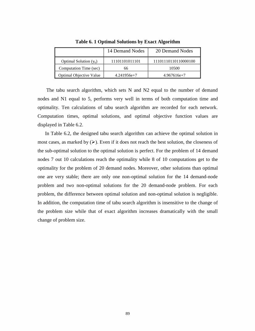
89

Table 6. 1 Optimal Solutions by Exact Algorithm

14 Demand Nodes 20 Demand Nodes

Optimal Solution (yk) 11101101011101 11101110110110000100

Computation Time (sec) 66 10500

Optimal Objective Value 4.241956e+7 4.967616e+7

The tabu search algorithm, which sets N and N2 equal to the number of demand

nodes and N1 equal to 5, performs very well in terms of both computation time and

optimality. Ten calculations of tabu search algorithm are recorded for each network.

Computation times, optimal solutions, and optimal objective function values are

displayed in Table 6.2.

In Table 6.2, the designed tabu search algorithm can achieve the optimal solution in

most cases, as marked by (�). Even if it does not reach the best solution, the closeness of

the sub-optimal solution to the optimal solution is perfect. For the problem of 14 demand

nodes 7 out 10 calculations reach the optimality while 8 of 10 computations get to the

optimality for the problem of 20 demand nodes. Moreover, other solutions than optimal

one are very stable; there are only one non-optimal solution for the 14 demand-node

problem and two non-optimal solutions for the 20 demand-node problem. For each

problem, the difference between optimal solution and non-optimal solution is negligible.

In addition, the computation time of tabu search algorithm is insensitive to the change of

the problem size while that of exact algorithm increases dramatically with the small

change of problem size.

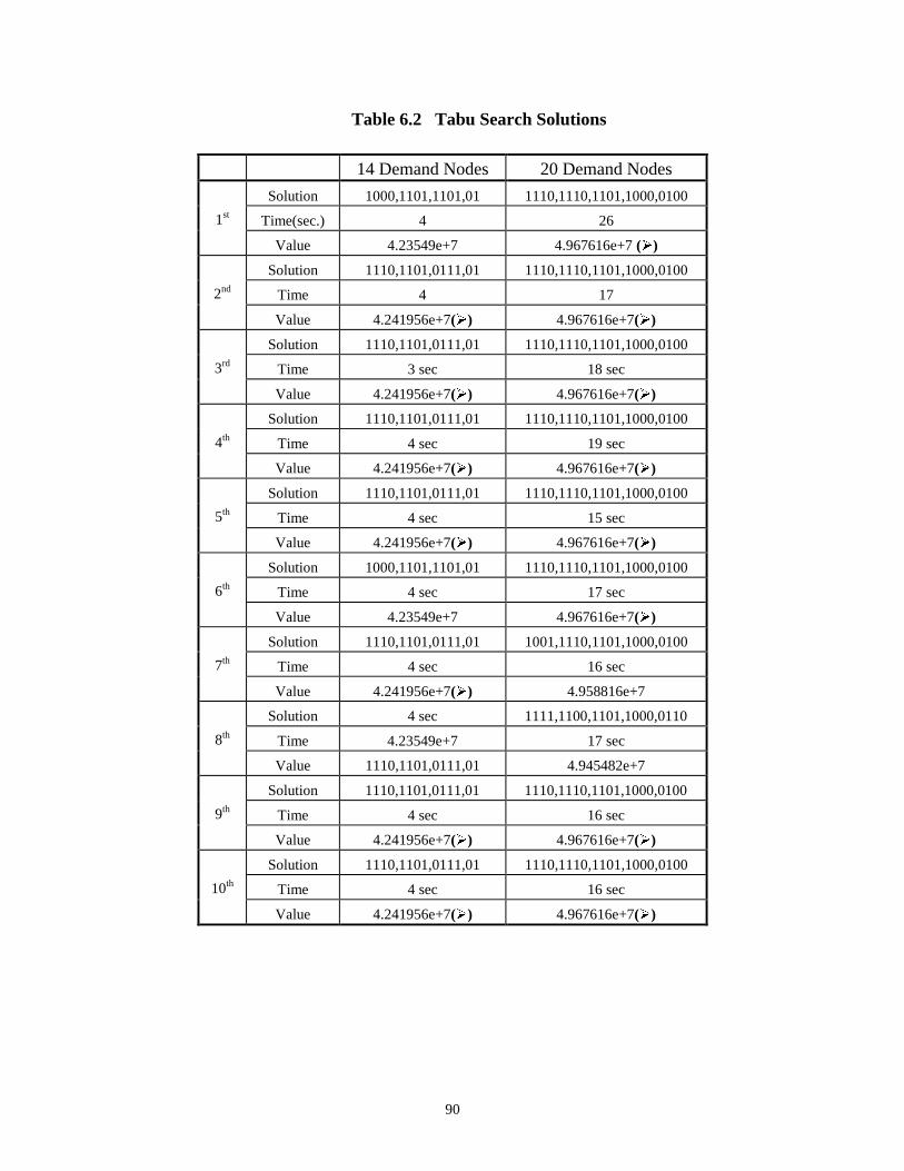
90

Table 6.2 Tabu Search Solutions

14 Demand Nodes 20 Demand Nodes

Solution 1000,1101,1101,01 1110,1110,1101,1000,0100

Time(sec.) 4 261st

Value 4.23549e+7 4.967616e+7 (��)

Solution 1110,1101,0111,01 1110,1110,1101,1000,0100

Time 4 172nd

Value 4.241956e+7(��) 4.967616e+7(��)

Solution 1110,1101,0111,01 1110,1110,1101,1000,0100

Time 3 sec 18 sec3rd

Value 4.241956e+7(��) 4.967616e+7(��)

Solution 1110,1101,0111,01 1110,1110,1101,1000,0100

Time 4 sec 19 sec4th

Value 4.241956e+7(��) 4.967616e+7(��)

Solution 1110,1101,0111,01 1110,1110,1101,1000,0100

Time 4 sec 15 sec5th

Value 4.241956e+7(��) 4.967616e+7(��)

Solution 1000,1101,1101,01 1110,1110,1101,1000,0100

Time 4 sec 17 sec6th

Value 4.23549e+7 4.967616e+7(��)

Solution 1110,1101,0111,01 1001,1110,1101,1000,0100

Time 4 sec 16 sec7th

Value 4.241956e+7(��) 4.958816e+7

Solution 4 sec 1111,1100,1101,1000,0110

Time 4.23549e+7 17 sec8th

Value 1110,1101,0111,01 4.945482e+7

Solution 1110,1101,0111,01 1110,1110,1101,1000,0100

Time 4 sec 16 sec9th

Value 4.241956e+7(��) 4.967616e+7(��)

Solution 1110,1101,0111,01 1110,1110,1101,1000,0100

Time 4 sec 16 sec10th

Value 4.241956e+7(��) 4.967616e+7(��)

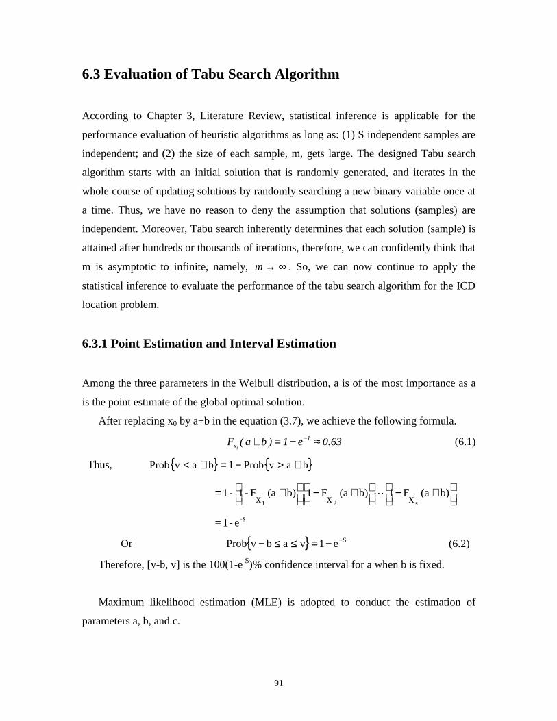
91

6.3 Evaluation of Tabu Search Algorithm

According to Chapter 3, Literature Review, statistical inference is applicable for the

performance evaluation of heuristic algorithms as long as: (1) S independent samples are

independent; and (2) the size of each sample, m, gets large. The designed Tabu search

algorithm starts with an initial solution that is randomly generated, and iterates in the

whole course of updating solutions by randomly searching a new binary variable once at

a time. Thus, we have no reason to deny the assumption that solutions (samples) are

independent. Moreover, Tabu search inherently determines that each solution (sample) is

attained after hundreds or thousands of iterations, therefore, we can confidently think that

m is asymptotic to infinite, namely, m→ ∞ . So, we can now continue to apply the

statistical inference to evaluate the performance of the tabu search algorithm for the ICD

location problem.

6.3.1 Point Estimation and Interval Estimation

Among the three parameters in the Weibull distribution, a is of the most importance as a

is the point estimate of the global optimal solution.

After replacing x0 by a+b in the equation (3.7), we achieve the following formula.

63.0e1)ba(F 1xi

≈−=+ − (6.1)

Thus, { } { }bavProb1bavProb +>−=+<

+−

+−

+= b)(a

xF1b)(a

xF1 b)(a

xF-1-1

s21�

-Se-1=

Or { } Se1vabvProb −−=≤≤− (6.2)

Therefore, [v-b, v] is the 100(1-e-S)% confidence interval for a when b is fixed.

Maximum likelihood estimation (MLE) is adopted to conduct the estimation of

parameters a, b, and c.

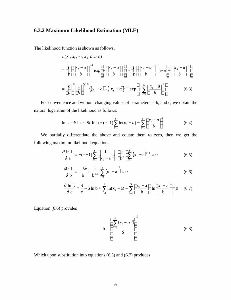
92

6.3.2 Maximum Likelihood Estimation (MLE)

The likelihood function is shown as follows.

),,;,,,( 21 cbaxxxL S�

−

−

−

−

−

−

=

−− c

S

1c

S

c

1

1c

1

b

axexp

b

ax

b

c

b

axexp

b

ax

b

c�

( ) ( ){ } exp1

1

11

−−−−

= ∑

=

−− S

i

c

icS

SScS

b

axaxax

bb

c� (6.3)

For convenience and without changing values of parameters a, b, and c, we obtain the

natural logarithm of the likelihood as follows.

∑∑=

−−−

S

i

c

i

b

axa

1

S

1=ii )ln(x1)-(c+b ln Sc-c ln S= Lln (6.4)

We partially differentiate the above and equate them to zero, then we get the

following maximum likelihood equations.

( ) 0axb

c

ax

11)(c

a

Lln S

1i

1cic

S

1i i

=−

+

−

−−= ∑∑=

−

=∂∂

(6.5)

( ) 0axb

c

b

Sc

b

LlncS

1ii1c =−+−= ∑

=+∂

∂(6.6)

∑ ∑ =

−

−−−−=

=

S

1=i

S

1i

i

c

ii 0

b

axln

b

axa)ln(x+b ln S

c

S

c

Lln

∂∂

(6.7)

Equation (6.6) provides

( ) cc

i

S

ax

1S

1=i=b

−∑(6.8)

Which upon substitution into equations (6.5) and (6.7) produces

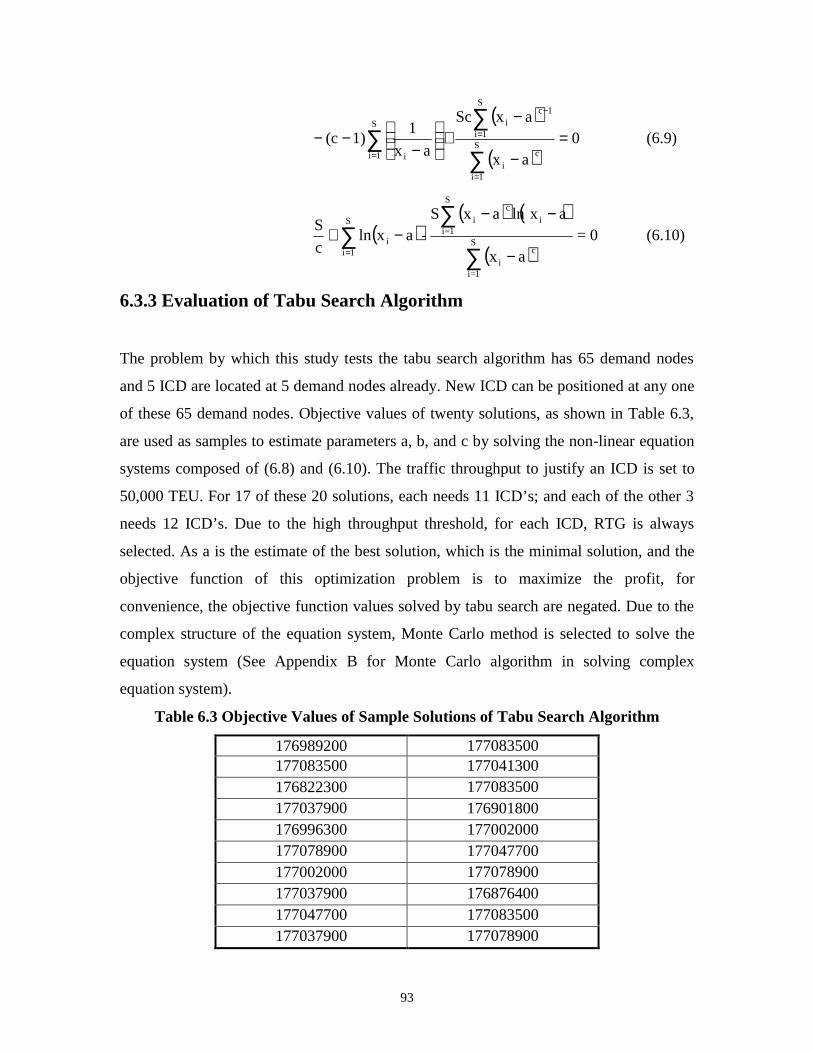
93

( )

( ) 0

ax

axSc

ax

11)(c S

1i

ci

S

1i

1ciS

1i i

=−

−+

−

−−∑

∑∑

=

=

−

=

(6.9)

( )( ) ( )

( )∑

∑

∑= −

−−−+

S

1iS

1=i

ci

S

1=ii

ci

i 0=ax

axlnaxS-axln

c

S(6.10)

6.3.3 Evaluation of Tabu Search Algorithm

The problem by which this study tests the tabu search algorithm has 65 demand nodes

and 5 ICD are located at 5 demand nodes already. New ICD can be positioned at any one

of these 65 demand nodes. Objective values of twenty solutions, as shown in Table 6.3,

are used as samples to estimate parameters a, b, and c by solving the non-linear equation

systems composed of (6.8) and (6.10). The traffic throughput to justify an ICD is set to

50,000 TEU. For 17 of these 20 solutions, each needs 11 ICD’s; and each of the other 3

needs 12 ICD’s. Due to the high throughput threshold, for each ICD, RTG is always

selected. As a is the estimate of the best solution, which is the minimal solution, and the

objective function of this optimization problem is to maximize the profit, for

convenience, the objective function values solved by tabu search are negated. Due to the

complex structure of the equation system, Monte Carlo method is selected to solve the

equation system (See Appendix B for Monte Carlo algorithm in solving complex

equation system).

Table 6.3 Objective Values of Sample Solutions of Tabu Search Algorithm

176989200 177083500177083500 177041300176822300 177083500177037900 176901800176996300 177002000177078900 177047700177002000 177078900177037900 176876400177047700 177083500177037900 177078900

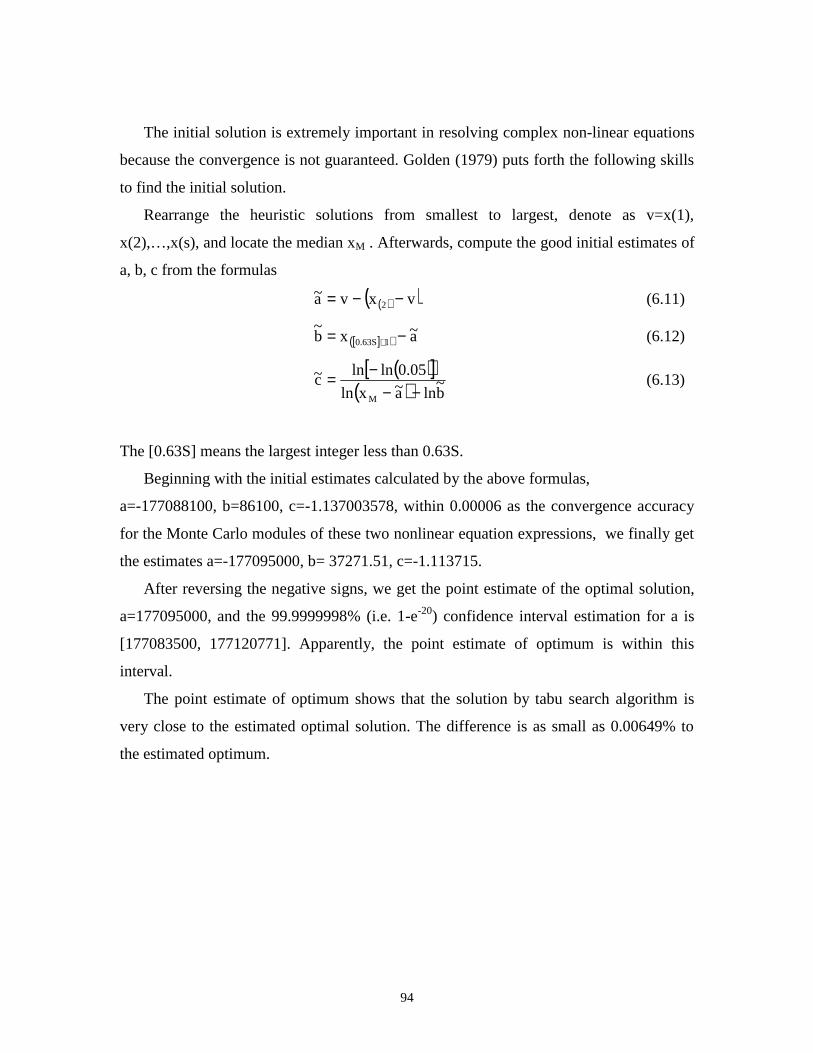
94

The initial solution is extremely important in resolving complex non-linear equations

because the convergence is not guaranteed. Golden (1979) puts forth the following skills

to find the initial solution.

Rearrange the heuristic solutions from smallest to largest, denote as v=x(1),

x(2),…,x(s), and locate the median xM . Afterwards, compute the good initial estimates of

a, b, c from the formulas

( )( )vxva~ 2 −−= (6.11)

[ ]( ) a~xb~

10.63S −= + (6.12)

( )[ ]( ) b

~lna~xln

0.05lnlnc~

M −−−= (6.13)

The [0.63S] means the largest integer less than 0.63S.

Beginning with the initial estimates calculated by the above formulas,

a=-177088100, b=86100, c=-1.137003578, within 0.00006 as the convergence accuracy

for the Monte Carlo modules of these two nonlinear equation expressions, we finally get

the estimates a=-177095000, b= 37271.51, c=-1.113715.

After reversing the negative signs, we get the point estimate of the optimal solution,

a=177095000, and the 99.9999998% (i.e. 1-e-20) confidence interval estimation for a is

[177083500, 177120771]. Apparently, the point estimate of optimum is within this

interval.

The point estimate of optimum shows that the solution by tabu search algorithm is

very close to the estimated optimal solution. The difference is as small as 0.00649% to

the estimated optimum.

95

Chapter 7

Conclusions and Recommendations

7.1 Summarization

In response to the size, complexity, and projected growth of the container market,

container transport operators are deploying ICD networks. Although these container

operators have done many surveys in order to decide the configuration of ICD networks,

there are no models at the regional level to help them on decision making. This

dissertation was intended to study the ICD location problem, formulate an effective

model, solve the formulation, and perform validation.

7.2 Contributions of the Research

This thesis has made two contributions: problem formulation and algorithm design.

This thesis is the first research to formulate the ICD location problem at the network

level. Based on comprehensive analysis of the container transport industry, focusing on

ICD operations, a formulation of the ICD location problem was developed. It greatly

recognized and emphasized the need to embody the endogenous demand and market

competitiveness in the container transport business. The formulation combined the

discrete choice model to quantitatively describe the shipper’s behaviors and preferences,

addressing both the endogenous demand and market competitiveness. As evidenced in

the literature review, addressing endogenous demand and market competitiveness are two

critical characteristics of facility location problems for the private sector. These have not

been adequately addressed in the scholarly literature and are worthy of exploration. The

formulation of ICD location problem using discrete choice models provides reference for

other similar facility location problems on how to formulate endogenous demand and

market competitiveness.

The fixed charge facility location problems are considered or proven to be NP

complete. The use of multinomial Logit model inevitably further complicates the

96

formulation in both objective function and constrains, which justifies the use of heuristics

to solve the formulation. Based on the structure of formulation, a problem specific tabu

search heuristic algorithm was designed to solve the formulation. Tabu search

parameters, tabu tenure, slack parameter, and cutoff parameter, are tested to decide their

contributions and sensitivity to the computational time and optimality. The findings of

these tests are very important when the problem size grows. Statistical inference was

used to evaluate the performance of the tabu search algorithm. The result of the

evaluation shows that the solutions of the tabu search algorithm are within the confidence

interval of the optimal solution of this formulation. This proves that the designed tabu

algorithm is efficient and effective.

7.3 Recommendations for Future Study

Based on the current availability of data and for the purpose of similarity, this thesis

has made several assumptions. In order to further improve the current accomplishments

of this thesis, the following are recommended for future research.

1. Utility Vector

Currently, the utility vector only has transport cost and logistics cost. In the future

when more detailed surveys are available, these two attributes should be re-examined to

further break down and include some elements, such as reliability, which are difficult to

be quantified.

2. Market Segmentation

The thesis assumes that all shippers are homogeneous in terms of tastes in selecting

ICD services. Therefore, the parameters, '21 ],,[ kβββ , ... â = are the same for all

shippers. In fact, although all shippers of international trade share much similarity,

shippers of different commodities behave differently. Shippers should be classified into

sub-groups, depending on commodities such as electronic products, garments, and

grocery. For each of these sub-groups, specific '21 ],,[ kβββ , ... â = should be calculated

to represent the taste of each sub-group. Also, if data are available for each shipper within

97

the sub-group, aggregation methods must be developed to aggregate demand from the

individual shipper’s selection.

3. Time Horizon

The time horizon in the research is one year. All costs are annualized. As the ICD

should stay in business for years, the model should represent the horizon of more than one

year. Multi-staging planning should be incorporated into the model.

98

References

Akinc, U. and B. M. Khumawala (1977) An efficient branch and bound algorithm for the

capacitated warehouse location problem. Manage. Sci. 23, 585-594.

Anderson, K.M. and C. M. Walton (1998) Evaluating Intermodal Freight Terminals: A Framework

for Government Participation. Center for Transportation Research, University of Texas at Austin,

Austin, Texas.

Belardo, S., J. Harrald, W. A. Wallace, and J. Ward (1984) A partial covering approach to siting

response resources for major maritime oil spills. Manage. Sci. 30, 1184-1196.

Ben-Akiva, M. and S. R. Lerman (1985) Discrete Choice Analysis: Theory and Application to

Travel Demand, The MIT Press.

Berman, O., S. S. Chiu, R. C. Larson, A. R. Odoni, and R. Batta (1990) Locations of mobile units

in a stochastic environment. Chapter 12, Mirchandani, P. R. and R. L. Francis, Discrete Location

Theory, John Wiley & Sons, Inc.

Cornuejols G., G. L. Nemhauser, and L. A. Wolsey (1990) The uncapacitated facility location

problem. Chapter 3, Mirchandani, P. R. and R. L. Francis, Discrete Location Theory, John Wiley &

Sons, Inc.

Daskin, M. S. (1983) A maximum expected covering location model: formulation, properties and

heuristic solution. Transp. Sci. 17, 48-70.

Daskin, M. S. (1985) Logistics: an overview of the state of the art and perspectives on future

research, Transp. Res. -A, Vol. 19A, No. 5/6, pp. 383-398.

Daskin, M. S. (1995) Network and Discrete Location: Models, Algorithms and Applications, John

Wiley & Sons, Inc.

Daskin M. S. and E. H. Stern (1981) A hierarchical objective set covering model for emergency

medical service vehicle deployment. Tranp. Sci. 15, 137-152.

99

Dearing, P. M., R. L.Francis, and T. J. Lowe (1976) Convex location problems on tree networks.

Oper. Res. 24, 628-641.

Eaton, D. J., M. S. Daskin, D. Simmons, B. Bulloch and G. Jansma (1985) Determining emergency

medical service vehicle deployment in Austin, TX. Interfaces 15, 96-108.

Erlenkotter, D.(1978) A dual-based procedure for uncapacitated facility location. Oper. Res. 26,

992-1009.

Erlenkotter, D.(1981) A comparative study of approaches and dynamic location problems.

European Journal of Operational Research 6, 133-143, 1981.

Fisher, R. and L. Tippert (1928) Limiting forms of the frequency distribution of the largest or

smallest member of a sample. Proc. Camb. Phil. Soc., 24, 180-190.

Garey, M.R., and D. S. Johnson (1979) Computers and Intractability: A Guide to the Theory and of

NP-Completeness. Freeman, San Francisco, California.

Geoffrion, A. M. (1974) Lagrangian relaxation for integer programming. Mathematical

Programming Study 2, 82-114.

Geoffrion, A. M. and G. W. Graves (1974) Multicommodity distribution system design by

Bender’s decomposition. Manage. Sci. 20, 822-844, 1974.

Geoffrion, A. and R. McBride (1978). Lagrangian relaxation applied to capacitated facility location

problems. AIIE Trans. 10, 40-47.

Golden, B. L. (1977) A ststistical approoach to the TSP. Networks, 7, 209-225.

Golden, B. L. and F. B. Alt (1979) Interval estimation of a global optimum for large combinatorial

problems. Naval Research Logistics Quarterly, 26, 69-77.

Golden, B. L. (1978) Point estimation of a global optimum for large combinatorial problems.

Comms. In Stats., B7, 361-367.

100

Golden, Bruce L. and E. K. Baker (1985) Future directions in logistics research. Transpn. Res.-A

Vol. 19A, No. 5/6, pp.405-409, 1985.

Glover, F. (1989a) Tabu search, part 1. ORSA Journal of Computing, Vol. 1 No. 3, summer 1989.

Glover, F. (1989b) Tabu search, part 2. ORSA Journal of Computing, Vo2. 1 No. 1, winter 1989.

Glover, F. and M. Laguna (1993) Tabu search . Chapter 3, Reeves, C. R., Modern Heuristic

Techniques for Combinatorial Problems. Hasted Press: an Imprint of John Wiley & Sons, Inc.

Glover, F. and M. Laguna (1997) Tabu Search . Kluwer Academic Publishers. Norwell, MA.

Gumbel E. (1958) Sattistics of Extremes. Columbia University Press, New York.

Hakimi, S. L. (1964) Optimum locations of switching centers and the absolute centers and medians

of a graph. Oper. Res. 12, 450-459.

Hakimi, S. L. (1965) Optimum distribution of switching centers in a communication network and

some related graph theoretic problems. Oper. Res. 13, 462-475.

Kakimi, S. L. (1990) Locations with spatial interactions: competitive locations and games. Chapter

10, Mirchandani, P. R. and R. L. Francis, Discrete Location Theory, John Wiley & Sons, Inc.

KPMG, and Transmode Consultants Inc. (1998) Container Transport Logistics Study of Sinotrans

Shandong , Canadian International Development Agency, Canada.

Hall, R. W. (1985) Research opportunities in logistics. Transpn. Res.-A Vol. 19A, No.5/6, pp399-

402.

Handler, G. Y. and P. B. Mirchandani (1979) Location on Networks: Theory and Algorithms.

M.I.T. Press, Cambridge, MA.

International Labor Organization (ILO) (1995) Container Freight Station Operations (Unit C.1.6),

Geneva, Switzerland.

101

Jacobson, S. K. (1990) Multiperiod capacitated location models. Chapter 4, Mirchandani, P. R. and

R. L. Francis, Discrete Location Theory, John Wiley & Sons, Inc.

Kariv, O. and S. L. Hakimi (1979) An algorithmic approach to network location problems. part 2.

the p-median . SIAM Journal on Applied Mathematics 37, 539-569, 1979.

Khumawala, B. M. (1972) An efficient branch and bound algorithm for the warehouse location

problem, Manage. Sci. 18, B718-B731.

Krarup, J. and P. M. Pruzan (1990) Ingredients of locational analysis. Chapter one, Mirchandani, P.

R. and R. L. Francis, Discrete Location Theory, John Wiley & Sons, Inc.

Kuehn, A. A. and M. J. Hamburger. (1963). A heuristic program for locating warehouses. Manage.

Sci. 9, 643-666.

Larson, R.C. (1975) Approximating the performance of urban emergency service systems. Oper.

Res. 23, 845-865.

Lukketangen, A and F. Glover (1997) Solving zero/one mixed integer programming problems

using tabu search. European Journal of Operational Research .

Magnanti, T. L. and R. T. Wong (1990) Decomposition methods for facility location problems.

Chapter 5, Mirchandani, P. R. and R. L. Francis, Discrete Location Theory, John Wiley & Sons,

Inc.

Maritime Administration (1989) United States Oceanborne Foreign Trade Routes. US Departmentof Transportation, Washington D.C.

Maritime Administration, US Department of Transportation (1998) A Report to Congress on theStatus of the Public Ports of the United States 1996 – 1997, Washington, D.C.

Mirchandani, P. R. (1990) The p-median problem and generalization. Chapter 2, Mirchandani, P.

R. and R. L. Francis, Discrete Location Theory, John Wiley & Sons, Inc.

Mirchandani, P. R. and R. L. Francis (1990) Discrete Location Theory, John Wiley & Sons, Inc.

102

Mirchandani, P. B. and A. R. Odoni (1979) Locations of medians on stochastic networks. Transp.

Sci. 13, 85-97.

Muller, G. (1995) Intermodal Freight Transportation, 3rd ed. Eno Transportation Foundation;

Intermodal Association of North America. Lansdowne, Va.; Greenbelt, Md.

Norris, B (1994) Intermodal Freight: an Industry Overview. FHWA, Washington, D.C.

Perl, J.and M. S. Daskin (1985) A warehouse location-rousing problem. Transpn. Res. –B Vol.

19B, No. 5 381-396.

Perl, J. and P. K. Ho (1990) Public facility location under elastic demand, Transp. Sci. Vol 24, No.

2, pp. 117-136.

Plane, D. R. and T. E. Hendrick (1977) Mathematical programming and the location of fire

companies for the Denver fire department. Oper. Res. 25, 563-578.

ReVelle, C. and R. W. Swain (1970) Central facilities location, Geographic Analysis 2, 30-42.

Rolland, E., D. A. Schilling and J. R. Current (1996) An efficient tabu search procedure for the p-

median problem. European Journal of Operational Research 96, 329-342.

Sweeney, D. J., and R. L. Tatham (1976) An improved long run model for multiple warehouse

location, Manage. Sci. 22(7), 748-7588.

Toregas C., R. Swain, C. ReVelle and L. Bergman (1971) The location of emergency service

facilities, Oper. Res. 19, 1363-1373.

Transmode Consultants Inc. and Soren Lennartsson (1995) Transport Logistics Study, Executed by

World Bank and Chinese Government.

Transportation Research Board (1992) Intermodal Marine Container Transportation (special

report 236), Washington, D.C.

United Nations (1990) Transportation Financial/Economic Planning Model, Volume 3, Inland

Container Deports with Model Split Module, ST/ESAP/000.

103

United Nations (1992a) Transportation Financial/Economic Planning Model, Volume 3, Inland

Container Deports with Model Split Module, ST/ESAP/1240.

United Nations (1992b) Multimodal Transport Handbook, UNCTAD/UNDP, UNCTAD /SHIP

/MISC.68 /REV.1, GE.92-55273.

United Nations Conference on Trade and Development (UNTCD) (1991) Handbook on the

Management and Operation of Dry Ports, Geneva, Switzerland.

Van Den Berg, G (1969) Containerization: A Modern Transport System. Hutchinson @ Co.,

London.

Van Roy, T. J., and D. Erlenkotter (1982) A dual-based procedure for dynamic facility location,

Manage. Sci. 28 (10) 1091-1105.

Walker W. E. (1974) Using the set-covering problem to assign fire companies to fire houses. Oper.

Res. 22, 275-277.

Wen, U.P. and A. D. Huang (1996) A simple tabu search method to solve the mixed-integer linear

bilevel programming problem. European Journal of Operational Research 88, 563-571.

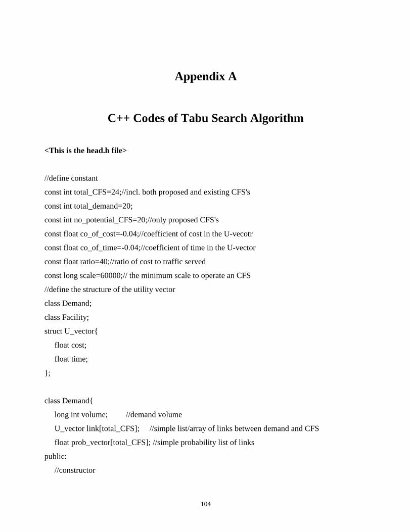
104

Appendix A

C++ Codes of Tabu Search Algorithm

<This is the head.h file>

//define constant

const int total_CFS=24;//incl. both proposed and existing CFS's

const int total_demand=20;

const int no_potential_CFS=20;//only proposed CFS's

const float co_of_cost=-0.04;//coefficient of cost in the U-vecotr

const float co_of_time=-0.04;//coefficient of time in the U-vector

const float ratio=40;//ratio of cost to traffic served

const long scale=60000;// the minimum scale to operate an CFS

//define the structure of the utility vector

class Demand;

class Facility;

struct U_vector{

float cost;

float time;

};

class Demand{

long int volume; //demand volume

U_vector link[total_CFS]; //simple list/array of links between demand and CFS

float prob_vector[total_CFS]; //simple probability list of links

public:

//constructor

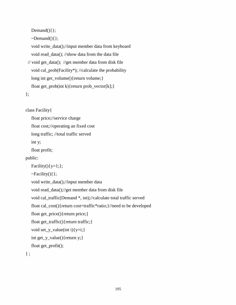
105

Demand(){};

~Demand(){};

void write_data();//input member data from keyboard

void read_data(); //show data from the data file

// void get_data(); //get member data from disk file

void cal_prob(Facility*); //calculate the probability

long int get_volume(){return volume;}

float get_prob(int k){return prob_vector[k];}

};

class Facility{

float price;//service charge

float cost;//operating an fixed cost

long traffic; //total traffic served

int y;

float profit;

public:

Facility(){y=1;};

~Facility(){};

void write_data();//input member data

void read_data();//get member data from disk file

void cal_traffic(Demand *, int);//calculate total traffic served

float cal_cost(){return cost=traffic*ratio;}//need to be developed

float get_price(){return price;}

float get_traffic(){return traffic;}

void set_y_value(int i){y=i;}

int get_y_value(){return y;}

float get_profit();

} ;

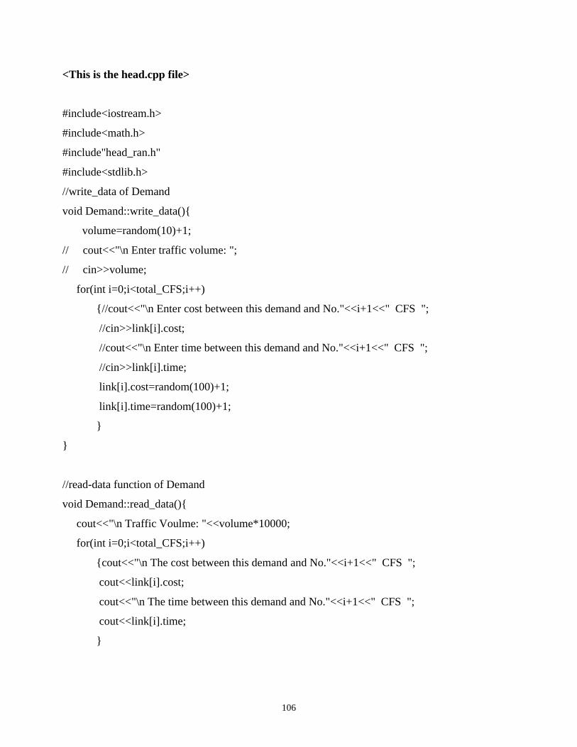
106

<This is the head.cpp file>

#include<iostream.h>

#include<math.h>

#include"head_ran.h"

#include<stdlib.h>

//write_data of Demand

void Demand::write_data(){

volume=random(10)+1;

// cout<<"\n Enter traffic volume: ";

// cin>>volume;

for(int i=0;i<total_CFS;i++)

{//cout<<"\n Enter cost between this demand and No."<<i+1<<" CFS ";

//cin>>link[i].cost;

//cout<<"\n Enter time between this demand and No."<<i+1<<" CFS ";

//cin>>link[i].time;

link[i].cost=random(100)+1;

link[i].time=random(100)+1;

}

}

//read-data function of Demand

void Demand::read_data(){

cout<<"\n Traffic Voulme: "<<volume*10000;

for(int i=0;i<total_CFS;i++)

{cout<<"\n The cost between this demand and No."<<i+1<<" CFS ";

cout<<link[i].cost;

cout<<"\n The time between this demand and No."<<i+1<<" CFS ";

cout<<link[i].time;

}

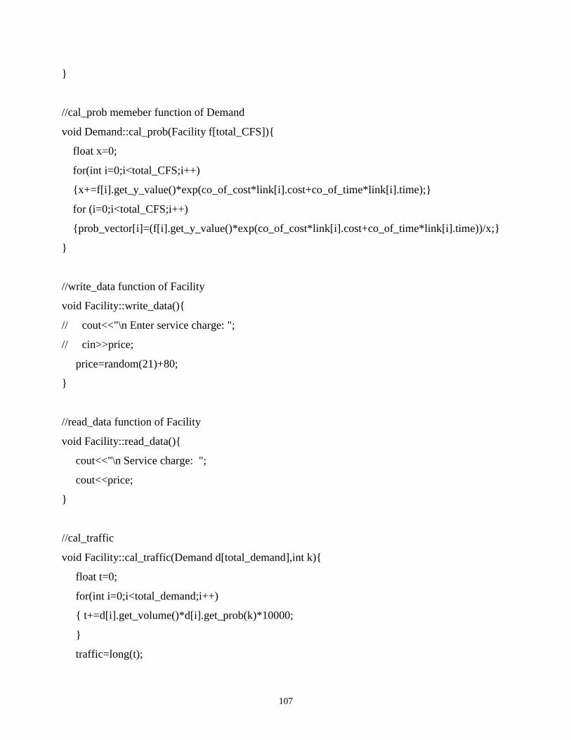
107

}

//cal_prob memeber function of Demand

void Demand::cal_prob(Facility f[total_CFS]){

float x=0;

for(int i=0;i<total_CFS;i++)

{x+=f[i].get_y_value()*exp(co_of_cost*link[i].cost+co_of_time*link[i].time);}

for (i=0;i<total_CFS;i++)

{prob_vector[i]=(f[i].get_y_value()*exp(co_of_cost*link[i].cost+co_of_time*link[i].time))/x;}

}

//write_data function of Facility

void Facility::write_data(){

// cout<<"\n Enter service charge: ";

// cin>>price;

price=random(21)+80;

}

//read_data function of Facility

void Facility::read_data(){

cout<<"\n Service charge: ";

cout<<price;

}

//cal_traffic

void Facility::cal_traffic(Demand d[total_demand],int k){

float t=0;

for(int i=0;i<total_demand;i++)

{ t+=d[i].get_volume()*d[i].get_prob(k)*10000;

}

traffic=long(t);

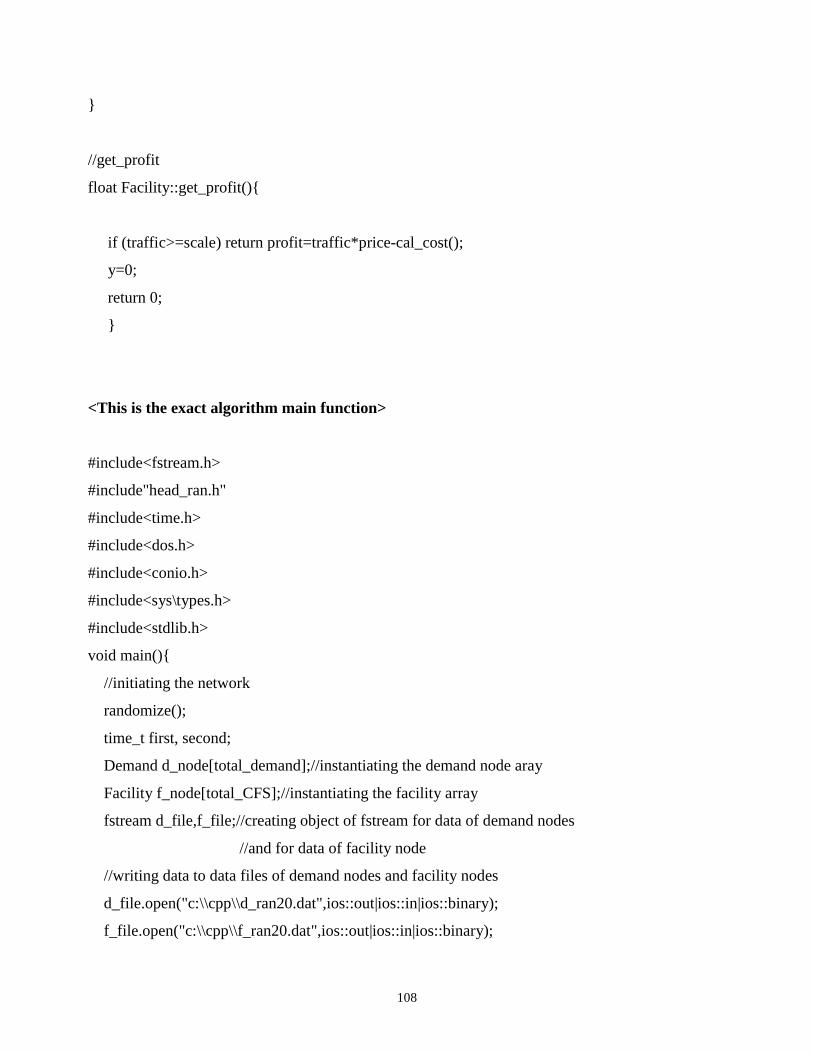
108

}

//get_profit

float Facility::get_profit(){

if (traffic>=scale) return profit=traffic*price-cal_cost();

y=0;

return 0;

}

<This is the exact algorithm main function>

#include<fstream.h>

#include"head_ran.h"

#include<time.h>

#include<dos.h>

#include<conio.h>

#include<sys\types.h>

#include<stdlib.h>

void main(){

//initiating the network

randomize();

time_t first, second;

Demand d_node[total_demand];//instantiating the demand node aray

Facility f_node[total_CFS];//instantiating the facility array

fstream d_file,f_file;//creating object of fstream for data of demand nodes

//and for data of facility node

//writing data to data files of demand nodes and facility nodes

d_file.open("c:\\cpp\\d_ran20.dat",ios::out|ios::in|ios::binary);

f_file.open("c:\\cpp\\f_ran20.dat",ios::out|ios::in|ios::binary);

109

int i;

/* //demand nodes

for(i=0;i<total_demand;i++)

{//cout<<"\n This is No."<<i+1<<" demand node";

d_node[i].write_data();

d_file.write((char*)&d_node[i],4+8*total_CFS);

}

for(i=0;i<total_CFS;i++)

{//cout<<"\n This is No."<<i+1<<" CFS";

f_node[i].write_data();

f_file.write((char*)&f_node[i],4);

}

*/ //reading data file of demand nodes

d_file.seekg(0);

f_file.seekg(0);

//demand nodes

for(i=0;i<total_demand;i++)

{d_file.read((char*)&d_node[i],4+8*total_CFS);

// cout<<"\n This is No."<<i+1<<" demand node";

// d_node[i].read_data();

}

//facility nodes

for(i=0;i<total_CFS;i++)

{f_file.read((char*)&f_node[i],4);

// cout<<"\n This is No."<<i+1<<" CFS";

// f_node[i].read_data();

}

//enumerate alternatives

first=time(NULL);

110

int y1[total_CFS],y2[total_CFS];//to record the best,and wrost solution

for(i=0;i<total_CFS;i++)

{y1[i]=0;y2[i]=0;}

float profit1=0; //best profit(objective function)

float profit2=0;//worst profit

float profit3=0;//average profit

int counter=0;

for(int i0=0;i0<=1;i0++)

for(int i1=0;i1<=1;i1++)

for(int i2=0;i2<=1;i2++)

for(int i3=0;i3<=1;i3++)

for(int i4=0;i4<=1;i4++)

for(int i5=0;i5<=1;i5++)

for(int i6=0;i6<=1;i6++)

for(int i7=0;i7<=1;i7++)

for(int i8=0;i8<=1;i8++)

for(int i9=0;i9<=1;i9++)

for(int i10=0;i10<=1;i10++)

for(int i11=0;i11<=1;i11++)

for(int i12=0;i12<=1;i12++)

for(int i13=0;i13<=1;i13++)

for(int i14=0;i14<=1;i14++)

for(int i15=0;i15<=1;i15++)

for(int i16=0;i16<=1;i16++)

for(int i17=0;i17<=1;i17++)

for(int i18=0;i18<=1;i18++)

for(int i19=0;i19<=1;i19++)

{ f_node[0].set_y_value(i0);

f_node[1].set_y_value(i1);

f_node[2].set_y_value(i2);

f_node[3].set_y_value(i3);

111

f_node[4].set_y_value(i4);

f_node[5].set_y_value(i5);

f_node[6].set_y_value(i6);

f_node[7].set_y_value(i7);

f_node[8].set_y_value(i8);

f_node[9].set_y_value(i9);

f_node[10].set_y_value(i10);

f_node[11].set_y_value(i11);

f_node[12].set_y_value(i12);

f_node[13].set_y_value(i13);

f_node[14].set_y_value(i14);

f_node[15].set_y_value(i15);

f_node[16].set_y_value(i16);

f_node[17].set_y_value(i17);

f_node[18].set_y_value(i18);

f_node[19].set_y_value(i19);

f_node[20].set_y_value(1);

f_node[21].set_y_value(1);

f_node[22].set_y_value(1);

f_node[23].set_y_value(1);

counter++;

//cal_prob

for (i=0;i<total_demand;i++)

d_node[i].cal_prob(f_node);

//cal_traffic

for(int j=0;j<no_potential_CFS;j++)

f_node[j].cal_traffic(d_node,j);

//feedback for the soluation to make it feasible

for(j=0;j<no_potential_CFS;j++)

if(f_node[j].get_traffic()>0&&f_node[j].get_traffic()<scale)

f_node[j].set_y_value(0);

112

//cal_prob

for (i=0;i<total_demand;i++)

d_node[i].cal_prob(f_node);

//cal_traffic

for(j=0;j<no_potential_CFS;j++)

f_node[j].cal_traffic(d_node,j);

//compare the objective function

float p=0;

for(j=0;j<no_potential_CFS;j++)

p+=f_node[j].get_profit();

if (p>=profit1)

{for(j=0;j<total_CFS;j++)

y1[j]=f_node[j].get_y_value();

profit1=p;

}

if(p<=profit2)

{for(j=0;j<total_CFS;j++)

y2[j]=f_node[j].get_y_value();

profit2=p;

}

profit3+=p;

}

second=time(NULL);

cout<<"\n The execution time is "<<difftime(second,first);

profit3=profit3/counter;

//print outcome;

cout<<"\nThe best solution is::"

<<"\n Objective function value: "<<profit1;

cout<<"\n The decision varialbles are: "<<"\n";

for(i=0;i<total_CFS;i++)

cout<<y1[i];

113

cout<<"\nThe worst solution is::"

<<"\n Objective function value: "<<profit2;

cout<<"\n The decision varialbles are: "<<"\n";

for(i=0;i<total_CFS;i++)

cout<<y2[i];

cout<<"\n The average objective function value is::"<<profit3;

}

<This is the TABU search algorithm>

#include<time.h>

#include<fstream.h>

#include"head_ran.h"

#include<stdlib.h>

#include<dos.h>

#include<conio.h>

#include<sys\types.h>

struct tabu_node

{ int n;// facility number

int s;//status:0 or 1

int t;//tabu_tenure

tabu_node *next;

};

class tabu_list{

tabu_node *head;

114

public:

tabu_list(){head=NULL;} //constructor

~tabu_list();//destructor

int check_node(int,int);// check node in list and in/decrease tenure or add/del node

//1st int: decision variable no., 2nd int: 1 or 0;

void override(int, int);

int decrement(); //all tenures decrease by 1 after one iteration

void add_node(int,int,int); //put new tabu in list,3rd int: tenure

int del_node(); //delete a tabu from the list if tenure is 0.

};

//destructor of tabu_list

tabu_list::~tabu_list(){

while(head!=NULL)

{tabu_node *temp=head;

head=temp->next;

delete temp;

}

}

//check_node function to see whether the move is in tabu list

int tabu_list::check_node(int i, int j){

if (head==NULL) return -1; //false

tabu_node *temp=head;

while(temp!=NULL)

{if (temp->n==i&&temp->s==j) return 1; //true

temp=temp->next;

}

return -1;//false

}

115

//override function to override the tanu restriction

void tabu_list::override(int i, int j){

if (head->n==i&&head->s==j)

{tabu_node * n=head->next;

delete head;

head=n;

return;

}

tabu_node * P=head;

tabu_node * N=P->next;

while(N!=NULL)

{if(N->n==i&&N->s==j)

{P->next=N->next;

delete N;

return;

}

N=N->next;

P=P->next;

}

}

//decrement

int tabu_list::decrement(){

if(head==NULL) return -1;

tabu_node *temp=head;

while(temp!=NULL)

{temp->t--;

temp=temp->next;

}

return 1;

}

116

//add_node

void tabu_list::add_node(int i, int j, int tenure){

tabu_node *new_node=new tabu_node;

new_node->n=i;

new_node->s=j;

new_node->t=tenure;

new_node->next=head;

head=new_node;

}

//del_node

int tabu_list::del_node(){

if(head==NULL) return -1;//no tabu node

if (head->t==0)

{tabu_node * n=head->next;

delete head;

head=n;

return 1;

}

tabu_node * P=head;

tabu_node * N=P->next;

while(N!=NULL)

{if(N->t==0)

{P->next=N->next;

delete N;

return 1;

}

N=N->next;

P=P->next;

}

117

return -1;

}

//the tabu serach function

void tabu(Demand d[total_demand], Facility f[total_CFS], int N=no_potential_CFS,

int N1=5,int N2=no_potential_CFS){

// N is the maximum outer iterations, N1 is tabu tenure and no. of candidates

tabu_list list; //instantiation of a tabu_list

int y_best[total_CFS];

int y_temp[total_CFS];

int y_temp_temp[total_CFS];

for (int i=0;i<total_CFS;i++) //total_CFS cover all decision variables

{y_best[i]=f[i].get_y_value();

y_temp[i]=f[i].get_y_value();

y_temp_temp[i]=f[i].get_y_value();

}

float p_best=0;

float p_temp=0;

float p_temp_temp=0;

int R;// randomly select the decision variable no.

int B;//to describe the move to 1 or to 0.

//randomly generate initial solution

for(i=0;i<no_potential_CFS;i++)

f[i].set_y_value(y_best[i]);

//cal_prob

for (i=0;i<total_demand;i++)

d[i].cal_prob(f);

//cal_traffic for the initial solution

for(i=0;i<no_potential_CFS;i++)

f[i].cal_traffic(d,i);

118

//cal the objective function

for(i=0;i<no_potential_CFS;i++)

p_best+=f[i].get_profit();

//initialize the solution after profit calcualtion(some y is set 0)

for(i=0;i<no_potential_CFS;i++)

{y_best[i]=f[i].get_y_value();

y_temp[i]=f[i].get_y_value();

}

//cal_prob

for (i=0;i<total_demand;i++)

d[i].cal_prob(f);

//cal_traffic for the initial solution

for(i=0;i<no_potential_CFS;i++)

f[i].cal_traffic(d,i);

//cal the objective function

p_best=0;

for(i=0;i<no_potential_CFS;i++)

p_best+=f[i].get_profit();

//Tabu serach

int K=1;

while(K<=N)

{int J=0;

while(J<=N2)

{int I=1;

p_temp=0;

//within tabu tenure

while(I<N1)

{for(int k=1;k<total_CFS;k++) //set y_temp_temp

y_temp_temp[k]=y_temp[k];

int r=random(no_potential_CFS+1); //randomly select the move

119

if(y_temp_temp[r]==1) {y_temp_temp[r]=0;} //change value of this decision

else{y_temp_temp[r]=1;}

int b=y_temp_temp[r];//for the use to check tabu list and add tabu

for(k=0;k<no_potential_CFS;k++)

f[k].set_y_value(y_temp_temp[k]);//generate a candidate move/solution

for (k=0;k<total_demand;k++) //cal_prob

d[k].cal_prob(f);

for(k=0;k<no_potential_CFS;k++)//cal traffic for this move

f[k].cal_traffic(d,k);

p_temp_temp=0;

for(k=0;k<no_potential_CFS;k++)//cal objective function

p_temp_temp+=f[k].get_profit();

for(k=0;k<no_potential_CFS;k++) //some y might be set 0.

y_temp_temp[k]=f[k].get_y_value();

for (k=0;k<total_demand;k++) //cal_prob

d[k].cal_prob(f);

for(k=0;k<no_potential_CFS;k++)//cal traffic for this move

f[k].cal_traffic(d,k);

p_temp_temp=0;

for(k=0;k<no_potential_CFS;k++)//cal objective function

p_temp_temp+=f[k].get_profit();

if(list.check_node(r,b)==1) // move is in tabu list

{if(p_temp_temp>p_best) //aspiration level

{list.override(r,b); //override the tabu restriction

p_temp=p_temp_temp;//record this objective function

//do not use y_best, it will come up later

for (k=0;k<no_potential_CFS;k++)

y_temp[k]=y_temp_temp[k];//refresh y_temp

R=r;

B=b;

}

120

}

else{if(p_temp_temp>p_temp) //select best candidate move

{p_temp=p_temp_temp;//record this objective function

for(k=0;k<no_potential_CFS;k++)

y_temp[k]=y_temp_temp[k];//refresh y_temp

R=r;

B=b;

}

}

I++;

}

//compare the best candidate from neighbour with the best solution

if (p_temp<p_best) {J++;}

else {J=0;

p_best=p_temp;

for(int d=0;d<no_potential_CFS;d++)

y_best[d]=y_temp[d];

list.add_node(R,B,N1+1);//N1=1 because decrement below

}

//update tabu list and aspiration level

list.decrement(); //tabu tenure minus 1

list.del_node(); //delete 0 tenure tabu

}

K++;

}

//output the outcome

cout<<"\n";

for(i=0;i<total_CFS;i++) cout<<y_best[i]<<" ";

cout<<"\n";

cout<<"the objective function is "<<p_best<<"\n";

121

}

void main(){

//initiating the network

time_t first, second;

Demand d_node[total_demand];//instantiating the demand node aray

Facility f_node[total_CFS];//instantiating the facility array

fstream d_file,f_file;//creating object of fstream for data of demand nodes

//and for data of facility node

//writing data to data files of demand nodes and facility nodes

d_file.open("c:\\cpp\\d_ran20.dat",ios::out|ios::in|ios::binary);

f_file.open("c:\\cpp\\f_ran20.dat",ios::out|ios::in|ios::binary);

/* //demand nodes

for(i=0;i<total_demand;i++)

{cout<<"\n This is No."<<i+1<<" demand node";

d_node[i].write_data();

d_file.write((char*)&d_node[i],4+8*total_CFS);

}

for(i=0;i<total_CFS;i++)

{cout<<"\n This is No."<<i+1<<" CFS";

f_node[i].write_data();

f_file.write((char*)&f_node[i],4);

}

//reading data file of demand nodes

*/

d_file.seekg(0);

f_file.seekg(0);

//demand nodes

for(int i=0;i<total_demand;i++)

{d_file.read((char*)&d_node[i],4+8*total_CFS);

// cout<<"\n This is No."<<i+1<<" demand node";

122

// d_node[i].read_data();

}

//facility nodes

for(i=0;i<total_CFS;i++)

{f_file.read((char*)&f_node[i],4);

// cout<<"\n This is No."<<i+1<<" CFS";

// f_node[i].read_data();

}

randomize();

first=time(NULL);

tabu(d_node,f_node);

second=time(NULL);

cout<<"\n The execution time is: "<<difftime(second,first);

}

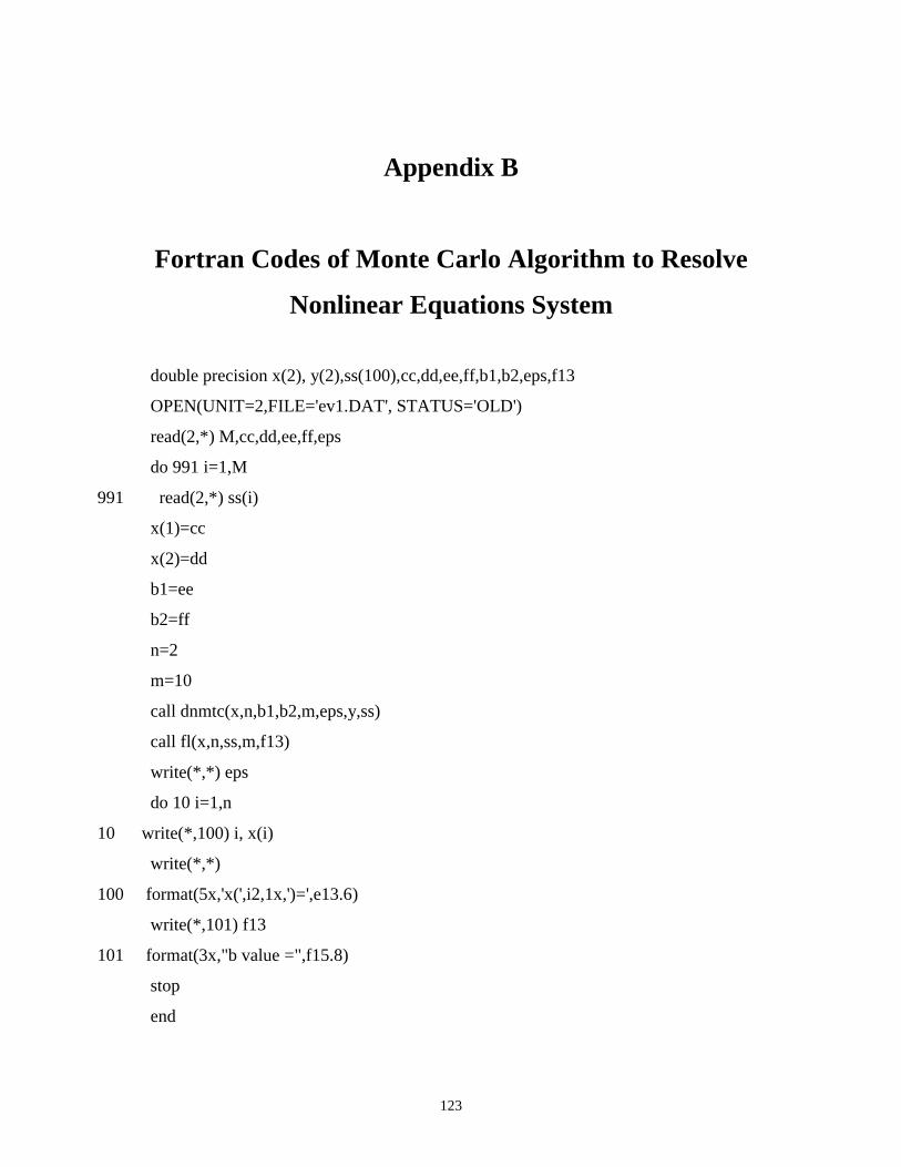
123

Appendix B

Fortran Codes of Monte Carlo Algorithm to Resolve

Nonlinear Equations System

double precision x(2), y(2),ss(100),cc,dd,ee,ff,b1,b2,eps,f13

OPEN(UNIT=2,FILE='ev1.DAT', STATUS='OLD')

read(2,*) M,cc,dd,ee,ff,eps

do 991 i=1,M

991 read(2,*) ss(i)

x(1)=cc

x(2)=dd

b1=ee

b2=ff

n=2

m=10

call dnmtc(x,n,b1,b2,m,eps,y,ss)

call fl(x,n,ss,m,f13)

write(*,*) eps

do 10 i=1,n

10 write(*,100) i, x(i)

write(*,*)

100 format(5x,'x(',i2,1x,')=',e13.6)

write(*,101) f13

101 format(3x,"b value =",f15.8)

stop

end

124

subroutine dnmtc(x,n,b1,b2,m,eps,y,ss)

double precision x(n), y(n),b1,b2,ss(100),eps

double precision r

double precision a1,a2,z,fa,z1

a1=b1

a2=b2

k=1

r=1.0

call f(x,n,ss,M,fa)

z=fa

l=0

write(*,*) eps

10 if(a1.ge.eps) then

l=l+1

write(*,*) l

119 call nrnd1(r,random)

y(1)=-a1+2.0*a1*random+x(1)

if(y(1).gt.-1.770835e8) goto 119

y(2)=-a2+2.0*a2*random+x(2)

write(*,101) y(1),y(2)

101 format(3x,"a=",f15.1,3x,"c=",f15.6)

call f(y,n,ss,M,fa)

z1=fa

write(*,*) z1

k=k+1

if (z1.ge.z) then

if (k.gt.m) then

k=1

a1=a1/2.0

a2=a2/2.0

endif

125

goto 10

else

k=1

do 30 i=1,n

30 x(i)=y(i)

z=z1

if (z.ge.eps) goto 10

end if

end if

return

end

subroutine nrnd1(r,random)

double precision s,u,v,r

s=65536.0

u=2053.0

v=13849.0

m=r/s

r=r-m*s

r=u*r+v

m=r/s

r=r-m*s

random=r/s

write(*,100) random

100 format(3x,"Random=",f15.8)

return

end

subroutine f(x,n,y,m,fa)

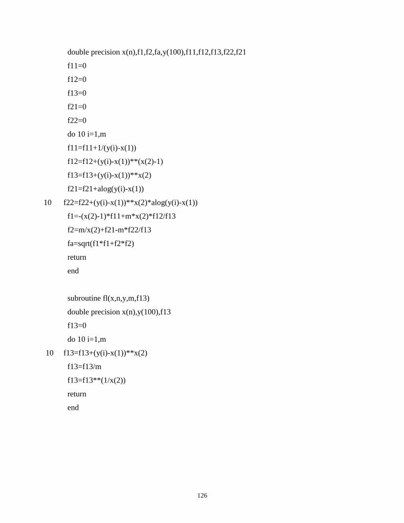
126

double precision x(n),f1,f2,fa,y(100),f11,f12,f13,f22,f21

f11=0

f12=0

f13=0

f21=0

f22=0

do 10 i=1,m

f11=f11+1/(y(i)-x(1))

f12=f12+(y(i)-x(1))**(x(2)-1)

f13=f13+(y(i)-x(1))**x(2)

f21=f21+alog(y(i)-x(1))

10 f22=f22+(y(i)-x(1))**x(2)*alog(y(i)-x(1))

f1=-(x(2)-1)*f11+m*x(2)*f12/f13

f2=m/x(2)+f21-m*f22/f13

fa=sqrt(f1*f1+f2*f2)

return

end

subroutine fl(x,n,y,m,f13)

double precision x(n),y(100),f13

f13=0

do 10 i=1,m

10 f13=f13+(y(i)-x(1))**x(2)

f13=f13/m

f13=f13**(1/x(2))

return

end