DEPARTMEM-7) ILTHE ARMY CORPS 00:10 ! EERS

/kao,

c,q

;

,

PROPERTY OF THF H S. GOVERNMENI

Volume 2 of 3

Cost - Benefit Analysis for Inland Navigation Improvements

OCTOBER 1970 IWR REPORT 70-4 U.S.-C.E.-C

iD- - VOLUME 2 OF 3 COST-BENEFIT ANALYSIS FOR INLAND NAVIGA' U.

1 .-3 CD C•1 CD i•-• •

- • CI

INSTITUTE FOR WATER RESOURCES

In 1969, the Subcommittees on Public Works, House and Senate Appropriations Committees, authorized formation of the Institute for Water Resources to assist in formu-lating Corps of Engineers water resources development planning and programming. Improved planning and eval-uation concepts and methods are needed if development and •utilization of these resources are to meet the public objectives of economic efficiency, protection and enhance-ment of the environment, regional development, income distribution, and general well - being of people. The Institute and its two Centers--the Center for Advanced Planning and the Cente r for E cononii c Studie s - -carry out both in-house and by contract, research studies to resolve conceptual and methodological problems involved in the development of our Nation's water and related land re-sources.

The Institute welcomes views and comments on its program and publications.

R. H. GROVES Brigadier General, USA Director

111191#11 COST-BENEFIT ANALYSIS FOR INLAND

NAVIGATION IMPROVEMENTS

A Report Submitted to the

U.S. Army Engineer Institute for Water Resources 206 North Washington Street Alexandria, Virginia 22314

by

Econometrics Center Northwestern University

Chicago, Illinois

Under Contract Number DA49-129-CIVENG-65-11

Edited by

Leon N. Mosses & Lester B. Lave Econometrics Center

Northwestern University

This document has been approved for public • release and sale; its distribution is unlimited.

Copies may be purchased from:

CLEARINGHOUSE for Federal Scientific and Technical Information

Springfield, Virginia 22141

OCTOBER 1970

IWR Report 70-4

(Vol. 2 of 3)

NORTHWESTERN UNIVERSITY

AN ECONOMETRIC MODEL

OF THE DEMAND FOR TRANSPORTATION

A DISSERTATION

SUBMITTED TO THE GRADUATE SCHOOL .

IN PARTIAL FULFILLMENT OF THE REQUIREMENTS

for the degree

DOCTOR OF PHILOSOPHY

Field of Economics

By

JAMES P. STUCKER

Evanston, Illinois August 1969

ACKNOWLEDGMENTS

The research reported in this dissertation would not have been

possible without the help of many individuals. Special appreciation

is due the officials of A. L. Mechling Barge Lines, Inc., and the

Central States Motor Freight Bureau, Inc. who so graciously supplied

data when other sources were lacking.

The staff of the Waterways Research Project at Northwestern

University, Professors R. B. Heflebower, L. B. Lave and R. H. Strotz,

provided advice and criticism at every stage of the research. Pro-

fessors A. P. Hurter and D. Mortensen were available for many helpful

comments and criticisms as the work progressed. The chairman of my

dissertation committee, Professor Leon N. Moses, is solely responsible

for my interest in transportation economics. His stimulating and con-

tinuing counsel was by far the most important factor in the completion

of this research. Finally, mention must be made of my colleague Joe

DeSalvo who has provided an almost daily sounding board for my ideas.

Of course none of the individuals cited above shares responsibility

for any remaining deficiencies.

Most of the calculations and data processing was performed by

George Sherling. Stina Hirsch typed many drafts of this dissertation

before Dottie Avakian made the final copy. To all of them, my thanks.

Finally, I am indebted to Northwestern University and to the

U.S. Army Corps of Engineers which sponsored the project from which

this dissertation developed.

CONTENTS

page ACKNOWLEDGMENTS

LIST OF FIGURES

• LIST OF TABLES

Chapter I. INTRODUCTION 1

II. REVIEW OF THE LITERATURE ON FREIGHT TRANSPORTATION 6 Theoretical Studies of Transportation 6 Empirical Studies of Freight Transportation 12

III. THE TWO-MARKET MULTI-MODE TRANSPORTATION MODEL 36 Geometrical Development of the Concepts 36 Transportation Associated Costs 46 Time Costs 47

Situation I: Consumer Ownership 47 Situation II: Producer Ownership 50 Other Situations 51

Other Associated Costs and the Transportation Supply Curve 51

Feeder Line and Interface Costs 52 Qualitative Analysis of the Two-Mode Two-Market Model 54

APPENDIX A TO CHAPTER III 60 The Elasticity of the Derived Demand for Transpor-

tation 60

APPENDIX B TO CHAPTER III 65 The Elasticity of Mode Two's Average Revenue Curve 65

APPENDIX C TO CHAPTER III 70 The Two-Market Multi-Mode Transportation Model:

The Monopolistic Case • 70 The Two-Mode Model 70 Parametric Associated Costs 72

*Endogenous Associated Costs for the Monopolistic Mode 75

IV. ESTIMATION OF THE DEMAND FOR TRANSPORTATION 79 The Estimating Model 79 Empirical Results - The Rate Equations 82

iii

Rail Transport 83 The Data 83 Group 960: All Commodities 85 Commodity. Group Totals 87 Commodity Groups Utilizing Data on Commodity

Classes 95 Barge Transport 103

The Data 103 All Commodity Classes 105 Commodity Classes by Commodity Groups 108

• Motor Transport 115 The Data 115 All Commodity Classes 116 Commodity Classes by Commodity Groups 117

Empirical Results - The Demand Equations 124 The Two-Mode Model 126 The Three-Mode Model 141

Summary of the Empirical Results 154

APPENDIX A TO CHAPTER IV 174 The Effects of Annual Tonnages Upon Rail Rates 174

V. SUMMARY AND CONCLUSIONS 182

BIBLIOGRAPHY 190

VITA 193

iv

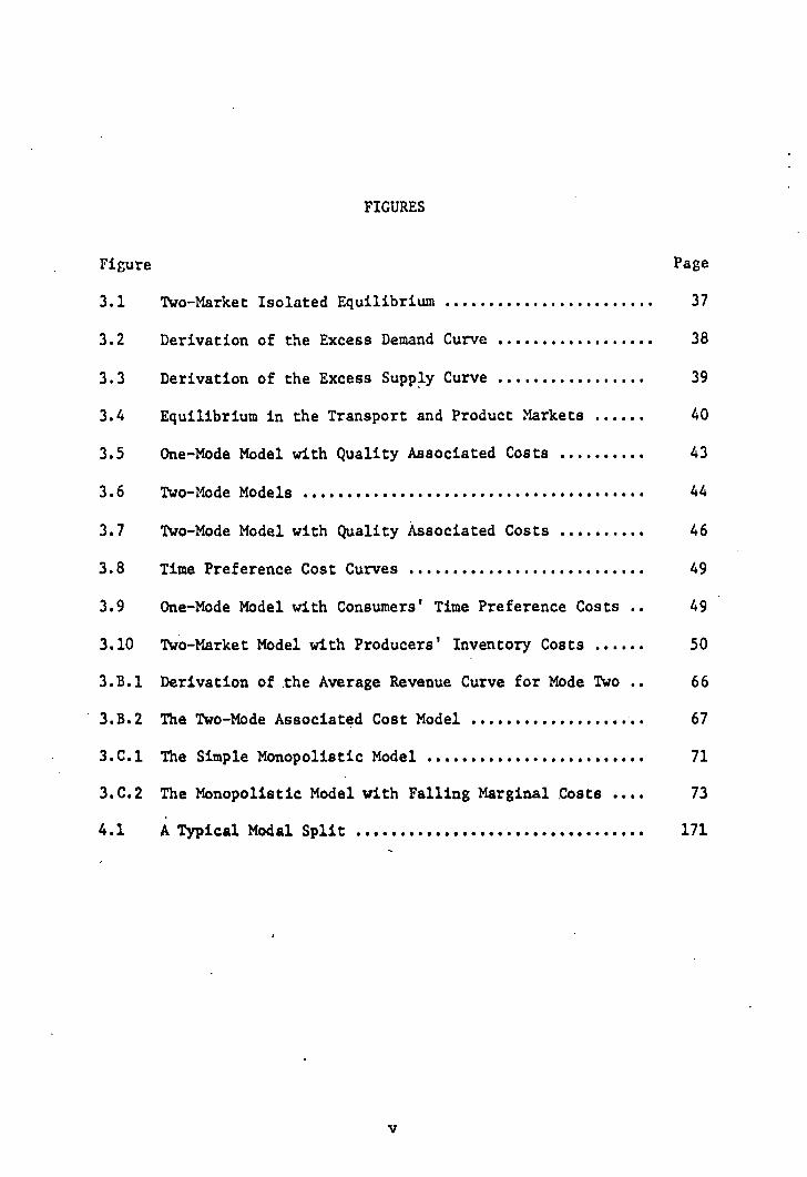
FIGURES

Figure Page

3.1 Two-Market Isolated Equilibrium 37

3.2 Derivation of the Excess Demand Curve 38

3.3 Derivation of the Excess Supply Curve 39

3.4 Equilibrium in the Transport and Product Markets 40

3.5 One-Mode Model with Quality Associated Costs 43

3.6 Two-Mode Models 44

3.7 Two-Mode Model with Quality Associated Costs 46

3.8 Time Preference Cost Curves 49

3.9 One-Mode Model with Consumers' Time Preference Costs 49

3.10 Two-Market Model with Producers' Inventory Costs 50

3.B.1 Derivation of the Average Revenue Curve for Mode Two 66

3.B.2 The Two-Mode Associated Cost Model 67

3.C.I The Simple Monopolistic Model 71

3.C.2 The Monopolistic Model with Falling Marginal Costs 73

4.1 A Typical Modal Split 171

TABLES

Page

Commodities Carried on the Mississippi River System (1962) 22

2.2 Hurter's Regression Price Coefficients 23

2.3 Regression Price Coefficients 27

3.1 Qualitative Analysis of the Two-Mode Model . 57

3.2 Further Qualitative Analysis of the Two-Mode Model 58

4.1 Rail Rate Regressions, All Commodities 88

4.2 Rail Rate Regressions, Group I: Products of Agriculture 90

4.3 Rail Rate Regressions, Group II: Animals and Products 91

4.4 Rail Rate Regressions, Group III: Products of Mines .. 92

4.5 Rail Rate Regressions, Group IV: Products of Forests . 93

4.6 Rail Rate Regressions, Group V: Manufactures and Miscellaneous 94

4.7 Rail Rate Regressions, Commodity Clauses, Group I: Products of Agriculture 97

•.8 Rail Rate Regressions, Commodity Clauses, Group II: Animals and Products 98

4.9 Rail Rate Regressions, Commodity Clauses, Group III: Products of Mines 99

4.10 Rail Rate Regressions, Commodity Clauses, Group IV: Products of Forests 100

4.11 Rail Rate Regressions, Commodity Clauses, Group V: Manufactures and Miscellaneous 101

Table

2.1

vii

134

135.

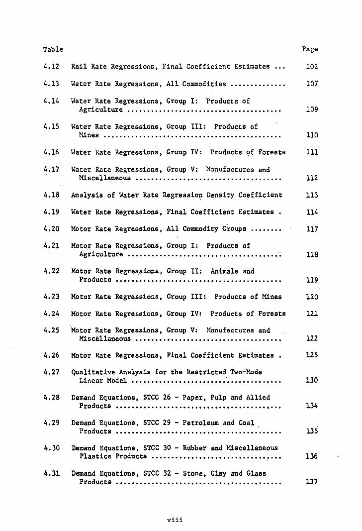
Table Page

4.12 Rail Rate Regressions, Final Coefficient Estimates 102

4.13 Water Rate Regressions, All Commodities 107

4.14 Water Rate Regressions, Group I: Products of Agriculture 109

4.15 Water Rate Regressions, Group III: Products of Mines 110

4.16 Water Rate Regressions, Group IV: Products of Forests 111

4.17 Water Rate Regressions, Croup V: Manufactures and Miscellaneous 112

4.18 Analysis of Water Rate Regression Density Coefficient 113

4.19 Water Rate Regressions, Final Coefficient Estimates . 114

4.20 Motor Rate Regressions, All Commodity Groups 117

4.21 Motor Rate Regressions, Group I: Products of Agriculture 118

4.22 Motor Rate Regressions, Group II: Animals and Products 119

4.23 Motor Rate Regressions, Group III: Products of Mines 120

4.24 Motor Rate Regressions, Group IV: Products of Forests 121

4.25 Motor Rate Regressions, Group V: Manufactures and Miscellaneous 122

4.26 Motor Rate Regressions, Final Coefficient Estimates 125

4.27 Qualitative Analysis for the Restricted Two-Mode Linear Model 130

4.28 Demand Equations, STCC 26 - Paper, Pulp and Allied Products

4.29 Demand Equations, STCC 29 - Petroleum and Coal . Products

4.30 Demand Equations, STCC 30 - Rubber and Miscellaneous Plastics Products 136

4.31 Demand Equations, STCC 32 - Stone, Clay and Glass Products 137

viii

Table Page

4.32 Selected Reduced Form Parameters .. 139

4.33 Ratio Estimates 141

4.34 Demand Equations, Three-Mode Model, STCC 29 142

4.35 Rate Equations, STCC 26 - Pulp, Paper and Allied Products 143

4.36 Rate Equations, STCC 29 - Petroleum and Coal Products 144

4.37 Rate Equations, STCC 30 - Rubber and Miscellaneous Plastics Products 145

4.38 Rate Equations, STCC 32 - Stone, Clay and Glass Products . 146

4.39 Demand Equations, STCC 23 - Apparel 147

4.40 Demand Equations, STCC 35 - Machinery, Except Electrical 148

4.41 Demand Equations, STCC 36 - Electrical Machinery and Equipment 149

4.42 Demand Equations, STCC 37 - Transportation Equipment 150

443 Ratio Estimates for the Three-Mode Model 153

4.44 Rate Data, Distribution of Observations by Commodity Group and Mode of Transport 155

4.45 Freight Rate Data Analysis 156

4.46 Rate Data, Distribution of Tonnage by Commodity Group 158

4.47 Rate Data, Distribution of Revenue by Commodity Group 158

4.48 Rate Regressions, Final Coefficient Estimates 160

4.49 Demand Regressions, Final Coefficient Estimates 168

4.50 Demand Analysis, Derived Estimates 172

4.A.1 Rate Regression Rail Quantity Analysis, Group I 175

4.A.2 Rate Regression Rail Quantity Analysis, Group II 176

4.A.3 Rate Regression Rail Quantity Analysis, Group III 177

4.A.4 Rate Regression Rail Quantity Analysis, Group IV 178

ix

Page

179

Table

4.A.5 Rate Regression Rail Quantity Analysis, Group V

4.A.6 Rate Regression Rail Quantity Analysis, All Commodity • Groups 181

x

CHAPTER I

INTRODUCTION

Transportation planners and analysts are often faced with the

problem of estimating the demand for a particular mode of transpor-

tation. Prospective transportation investments may take many forms.

Small or large alterations in the characteristics of an operating mode

may be under consideration. The introduction of an alternative, but

proven mode into the present system may be contemplated. Or, a com-

pletely new and novel mode may have been proposed. In all of these

cases the planners must be concerned with the effects of the structural

change upon (1) the operation of the mode in question, (2) the opera-

tions of all other modes in the system, and (3) the producers and con-

sumers of the products which are transported.

Implicit in the above questions are the assumptions that there is

some overall demand for tranaportation and that the various modes com-

pets for shares of the total traffic, i.e., that the modes are to some

extent substitutes for one another. At the same time it is recognized

that the modes may differ significantly in the service which they offer

to the shipper. Somehow we believe these differences can be compared

and we can speak of better services and, indeed, of better modes. In

fact, we may even seek to determine which mode, or conceivable future

mode, might constitute the optimum supply for certain transport needs.

1

This paper presents an economic model of a simple transportation

market and attempts to deal with the above questions. We consider the

complete interdependence of all elements of the system and attempt to

answer the two fundamental questions: How much will be transported, and

how this amount will be allocated among the competing modes.

Since the time of Alfred Marshall's analysis of the demand for knife

handles economists have been aware that the demand for freight trans-

portation is a derived demand. It is not desired for its own sake but

rather because it contributes to the consumption of something which is

desirable.1

Freight transport is desirable only because it moves goods

from one market to another and, in general, the people in both markets

are made better off by the transfer. All evaluations of the "benefits"

of transportation improvements must focus upon this flow of goods and

the effects of changes in the flow on producers and consumers in the

product markets. Beginning with an article by P. A. Samuelson2

an im-

pressive body of literature has developed dealing with these market flows.

This literature focuses upon the demand side of the transportation market

to almost the complete neglect of the supply side. Intermarket transport

1. In a recent article, Kelvin J. Lancaster has moved the point of ultimate demand back another step. He postulates that goods are con-mimed only because they possess "properties or characteristics" which yield utility. Thus, the demand for consumption goods itself is a derived demand. As we shall show this has far reaching applications in the theory of substitute goods. See K. J. Lancaster, "A New Approach to Consumer Theory," Journal of Political Economy, Vol. 14 (1966), 132-157.

2. Paul A. Samuelson, "Spatial Price Equilibrium and Linear Pro-gramming," American Economic Review, Vol. XLII, No. 2 (May 1962), 283-303.

2

demand is seen as being dependent upon the product supply and demand in

markets and the supply of transportation between each pair of markets.

However, to allocate the flows of goods among the markets it has been

necessary to deal with transport supply in a very restricted manner.

Our approach will be the converse of the above. By considering

only a simplified demand structure it will be possible to probe deeper

into the supply characteristics of a single transport market. The former

approach maybe said to result in a multi-market single mode transpor-

tation model whereas ours will lead to a "two-market multi-mode trans-

port model."

In the multi-market models the demand for transportation between

any two product markets is dependent upon the product supply and demands

in all markets and the supply of transportation between each pair of

markets. These transport supplies are viewed as independent of the

rest of the model. In the multi-mode model we will restrict ourselves

to two product markets so that the demand for transportation between

them is uniquely determined and we are able to investigate the inter-

actions of transport supply when several modes are present.

Given the derived demand for transportation all we need is a

"supply of transportation" to determine equilibrium in the transport

market. However, this supply of transport is rather difficult to define.

Supply will usually be composed of several operating modes each offering

a slightly different service to the shipper. Only by considering all

modes which are present, or contemplated, and all aspects of their

service is it possible to determine how the demand will be met, i.e.,

the modal split and the resulting rates, quantities and costs.

3

All transport modes are designed to move products from one market

to another. However, each moves the products in a slightly different

manner resulting in different service characteristics. We usually say

they offer differing "qualities of service." These service attributes

are of concern to the shipper. He must consider all the implications

of shipping by the various available modes before it is possible for

him to make an intelligent choice of mode decision.

Some of the more commonly listed quality attributes are: the

time required for transport; schedules and the convenience of. shipping

times; the reliability of schedules; breakage, spoilage and deterior-

ation of the product enroute; packaging requirements; and interface

costs on joint hauls. The main assumption of this paper is that con-

ceptually each of these quality attributes can, and should, be expressed

as costs associated with shipment by an individual mode. Each shipper

must then take all costs into account in making his choice of mode

decision, that is he must place quality costs on an equal basis with

transport rates. With this assumption we shall be able to develop an

analytical model of the transportation market and, subject to the form.

of the individual equations and the specification of parameters, derive

(1)the total quantity shipped and unit costs borne , by•the shippers,

(2)the modal split, should one occur, and the conditions under which

it will occur, (3) the conditions under which a resulting modalsplit -

is an efficient, cost minimizing, allocation of traffic, and (4) the .

resulting transport rates and associated costs for each participating

mode of transport. 3

3. A similar approach has recently been advocated for passenger transport as well. See R. E. Quandt, and W. J. Baumol, "The Demand

4

With the two-market multi-mode transportation model we shall also

be able to investigate how changes in the structure of the transport

market will affect market solutions and modal splits whether these

structural changes arise from changes in product demands or supplies,

changes in transport supply by any mode, changes in the quality aspects

of any mode, or the introduction of another mode into the system.

The next chapter contains a short review of the literature on the

demand for freight transportation. It traces the development of the

concepts contained in the multi-market single mode model and then re-

views some recent attempts to estimate freight transport parameters.

In Chapter III we develop the two-market multi-mode transportation model

and investigate the implications of our assumptions. The model is then

expanded to include one large, monopolistic-acting mode sharing a market

with several competitive modes, and touches upon the role of federal

regulatory agencies. In Chapter IV we convert the analytical model into

an empirical model and present the results of parameter estimations.

Chapter V contains a summary of our work and concluding remarks.

for Abstract Transport Modes: Theory and Measurement," Journal of Regional Science, Vol. 6, No. 2, 13-26. Their approach recognizes the multidimensional nature of passenger travel and treats it as such, rather than attempting to collapse the various attributes into a single, 'cost, dimension. We feel that, for freight transport at least, the transformation is feasible. See also W. J. Baumol, "Calculation of Optimal Product and Retailer Characteristics: The Abstract Product Approach," Journal of Political Economy, Vol. 75, No. 5 (Oct. 1967), 674-685.

5

CHAPTER II

REVIEW OF THE LITERATURE ON FREIGHT TRANSPORTATION

In this chapter we shall discuss some of the principal articles

published on the demand for freight transportation. Empirical studies

will be covered as well as papers of a purely theoretical nature.

While we have attempted a wide survey and believe we have covered most

of the important contributions to transport demand, this review is not

meant to be exhaustive. The selected theoretical works represent steps

in the advancement of understanding of basic concepts and their impli-

cations; the empirical studies represent the state of the art and il-

lustrate quite well present data limitations. We shall begin with the

theoretical studies.

Theoretical Studies of Transportation

One of the earliest statements of trade equilibrium between two

regions was by A. A. Cournot in 1838.1

He asserted that when two mar-

kets or regions both produce and consume a commodity the market clearing

conditions when the regions were isolated would be

(2.1) Da(P

a) - S

a(Pa) 0, and

Db (Pb ) Sb (Pb ) 0. •

1. A. A. Cournot, The Mathematical hainciples of the Theory of Wealth, (1838), Ch. X; citations are from the Irwin edition, Homewood, Ill., 1963.

6

Whereas if "communication" were present between the regions, and we

assume that in isolation the price in Market A was lower than that of

Market B by more than the transport costs, the equilibrium conditions

became

(2.2) Da(Pa

I ) + Db(Pa

+ Tc ) Sa(P

aI ) + S

b(Pa' + Tc ).

In the notation we are using:

A and B designate the two product markets;

Pa

and Pb

are product prices in the two markets;

Da

and Db

are the regional demand functions;

Sa

and Sb

are the regional supply functions;

Pa' is the after trade price in the exporting market; and

Tc is the unit transport cost.

Although he was not concerned with explicitly deriving the demand

for transportation, Cournot's trade conditions formed, and still repre-

sent, the basic equilibrium conditions for all transportation models.

These conditions are formed from the assumptions of a homogeneous

commodity which is demanded and supplied under conditions of perfect

competition in two separate geographic regions. When he speaks of trans-

portation costs he is referring to the costs to the shipper, which he

defines as costs to the transport merchant or industry plus some normal

profit. It thus appears that the transportation industry itself is

purely competitive and somehow instantaneously moves goods from market

to market. This implicit treatment, or neglect, of the transport in-

dustry is a condition which we shall find present in almost all of the

"transportation" models.

7

The first significant generalization of the Cournot two-market

model seems to have been the initial development of the linear program-

ming transportation model by Koopmans and Hitchcock.2

In this specifi-

cation there are many markets among which the commodity can flow. How-

ever, conditions of production and consumption within the product markets

are now ignored. Each market is considered as either a supply point or

a consumption point and the exact amount which it exports or imports is

specified. 3 Unit transport costs between each pair of regions are spe-

cified and the problem is to find the transport cost minimizing flows.

Thus the model generalizes the number of markets but specializes all

other relationships. While Cournot said very little about transpor-

tation costs, he did not express them as being completely independent

of quantity as the Koopmans-Hitchcock specification does. This speci-

fication ignores the effects of trade on the producers and consumers

of the commodity being traded and concerns itself simply with determin-

ing the least cost pattern of flows which will satisfy the market

requirements.4

2. The standard presentation of this model is found in T. Koopmans, - Activity Analysis of Production and Allocation, Cowles Commission Monograph No. 13, John Wiley, New York, 1951.

3. This requires a balance condition relating total exports to total imports. This condition takes the place of any equilibrating actions which might be present within the product markets.

4. Another broad class of transportation-type problems has arisen in the programming field. These are mainly network problems but may appear under many different names and may focus upon commodities, mar-kets and/or transport modes. However, in all cases the quantity to be exported or imported is specified for each region, and the trans-port charge for each possible link is given and fixed. Transport times may be included in the analysis and capacity constraints may or may not be imposed on each link. The problem is to minimize the total

8

At about this same time S. Enke was also grappling with the trans-

portation problem. His model as it evolved was also for a world com-

posed of many markets and one commodity. However, he hypothesized that

if each region was conceived to have linear product supply and demand

functions, and unit transport charges between regions were independent

of volume, the (transport cost minimizing and market clearing) flows

could be determined by analogy with the electrical network studies of

Clerk Maxwell and Kirchhoff.5

While his multi-market model was a maze

of resistors, power sources and current flows, he was able to present

a verbal discussion of the economic solution for the three-market case

based upon excess supply and demand functions. 6 Thus, while Koopmans

and Hitchcock were able to develop the fixed quantities case to a point

where a solution was possible, Enke's contribution was to suggest an

transport costs. These are actually allocation problems which ignore production and consumption conditions both in the product market and, essentially, in the transportation market.

In the multi-mode models it is possible for a modal split to occur. However, it must be of the "all or nothing" variety, that is either all of the traffic between two markets will be carried by one mode, or one mode will carry all it can handle before another will be brought into operation.

See, for example: K. B. Haley, "The Multi-Index Problem," Operations Research, Vol. 11 No. 3 (May, June), 1963, 368-379, and

. R. W. Lewis, E. F. Rosholdt, and W. L. Wilkinson, "A Multi-Mode Trans-portation Network Model," Naval Research Logistics Quarterly, Vol. 12, Nos. 3 & 4 (Sept., Dec.), 1965, 261-274.

5. S. Enke, "Equilibrium Among Spatially Separated Markets: Solu-tion by Electric Analogue," Econometrica, Vol. 19 (Jan. 1951), 40-47.

6. For an excellent discussion of this three-market case in geo-metric form.see: Eugene Silberberg, The Demand for Inland Waterway Transportation, unpublished Ph.D. dissertation, Purdue University, 1964.

9

artificially contrived solution method for the variable export and im-

port case. This path was also followed by Samuelson several years later. .

In 1962 Samuelson was able to take Enke's electric analogue trans-

portation model and express it in terms of an economic maximization

model.7

He created the concept of "social pay-off" which was defined as

the algebraic area under a region's excess-demand curve and showed that

the act of maximizing "net social pay-off" over all regions in the model

would result in trade equilibrium. By formulating his artificial maxi-

mization problem in a programming framework and heuristically sketching

its solution, he was able to show that the Koopmans-Hitchcock problem

was logically wholly contained within the larger problem.

Although the title of Samuelson's article is "Spatial Price Equilib-

rium and Linear Programming," the model which he presents is decidedly

non-linear, even assuming linear product supply and demand curves. This

problem specification issue is formulated very clearly in Vernon Smith's

paper of 1963.8

Smith reformulates Samuelson's problem and shows it as

the dual of a general programming problem of rent minimization.

We have now seen the transportation problem presented as an electric

analogue problem, a social pay-off maximization problem and a rent mini-

mization problem. Smith seems to feel that it is intuitively clearer

or purer to think of a competitive market system as one which minimizes

the sum of producer and consumer rents, and this is probably true. While

Samuelson's "net social pay-off" was novel, the concept of rent has been

7. Samuelson, p. 283.

8. V. L. Smith, "Minimization of Economic Rent in Spatial Price Equilibrium," Review of Economio Studies, Vol. XXX, No. 1 (1963), 24-31.

A.

with us for a long time and has become a satisfying analytic abstraction.

Smith's contribution was to formulate once again the transportation prob-

lem and to explicitly derive Cournot's equilibrium relations and the con-

ditions under which they would hold.

The latest step in the development of the many-market, variable

export and import, fixed transport charge model was the development of

a solution algorithm in 1964 by Takayama and Judge.9

They were able to

formulate the Samuelson problem in a quadratic programming context and

develop a specialization of the simplex linear programming algorithm for

• its solution.

We have traced the development of what we shall refer to as the

many-market single-mode transportation model. It is an analysis of the

production, flow and consumption of a single commodity in and between

many regions or markets. Each region may both produce and consume the

commodity and transportation between all pairs of regions is feasible.

All transport charges are given and are independent of volume. Capacity

constraints are never binding for the transporters. This model must be

considered as a system served by a single mode of transport although the

actual means of transportation are usually not specified, as all regions

are cOnnected by some means of transport whose only distinguishing at- .

tribute is its per unit charge.

While it is somewhat paradoxical that the analytical models of

transportation flows have almost completely disregarded the supply of

9. T. Takayama, and G. Judge, "Equilibrium Among Spatially Separated Markets: A Reformulation," Econometrica, Vol. 32, No. 6 (Oct. 1964), . 510-524.

11

trannportnLion, thin neglect ham cPrtalnly not been p.renent In thP in-

plitutionnl ntudien of trannwwt nyntemn. Thr ntructurPn or thP rnI1-

toad, trucking and nhIpping induatrira hnvP brnu ntudlen In rPit depth

and detail. Volumrn have herr; writtrn on the conditionn or nupply In

theNr induntrirn and concerning the naturn and quality of their product.

However, only recently have nerioun attemptn brPn made to quantify thene

production rvIationnhipn.10

Them, qunntifientionn are uneful in their

own right since they allow comparinonn of trnrinport ru ti'c uiiI contn both

I ndependently and acronn modes; however, their mont important applica•

tion would be in the determination of trannport flows if they could he

integrated into the many-market transportation model to provide a CCM-

plete statement of the transportation process. This paper presents an

initial effort at this integration. In Chapter III we develop a two-

market model which admits several modes of transport and -allows each

mode to exhibit unique service attributes.

Empirical Studies of Freight Transportation

We now turn from theoretical studies of the demand for freight

transportation to some recent attempts to estimate this demand. The

models were developed in terms of point-to-point flows of particular

10. J. S. DeSalvo, Linehaul Process &notions for Rail and Inland Waterway Transportation, unpublished Ph.D. dissertation, Northwestern University, 1968.

C. W. Howe, "Methods for Equipment Selection and Benefit Evaluation in Inland Waterway Transportation," Water Resources Research, Vol. 1 (1965), 25-39.

J. R. Meyer, M. J. Peck, J. Stenanson, and C. Zwick, The Economics of Competition in the Transportation Induatries, Cambridge, Harvard Univer-sity Press, 1960.

commodities and, conceptually, transport demands could be estimated

either directly or indirectly through estimates of regional product

demands and supplies. Three of the four empirical studies we reviewed

were forced to abandon the point-to-point flow concept completely. Due

basically to data limitations they were able to operate only with ag-

gregate shipments, composed of many point-to-point flows of many com-

modities. The degree of necessary aggregation varied in the different

applications; and we shall discuss them in the order of the grossness of

their input data, from more aggregate to less. These studies all con-

sidered several transport modes, and two of them examined cross modal

effects. The fourth study to be reviewed, by E. Silberberg, differs

fundamentally from the others. He first attempts to estimate regional

supplies and demands for several commodities. These regional estimates

are then entered as inputs into a linear programming model to predict

the flows of trade between the regions under the assumption that the •

competitive environment actually minimizes transport costs. Discussion

of this study which, in effect, is an application of the Koopmans-Hitchcock

model will conclude the chapter.

The first paper to be considered is by Benishay and Whitaker, who

were concerned with estimation of national demand functions for rail,

motor and water transport.11 In particular they desired to estimate the

direct or "own" price elasticity of demand for transport of each mode.

By estimating a separate demand function for each of the modes and en-

tering only one price or rate variable in each equation, that pertaining

11. H. Benishay, and G. R. Whitaker, Jr., Demand and Supply in Freight Transportation, The Transportation Center, Northwestern Univ., 1965.

13

to the mode under consideration, cross demand effects were not explicitly

taken into account.

Benishay and Whitaker begin with the basic, two-market spatial com-

petition model and suggest that the logic of this model can be extended

to cover the case of many commodities and regions. This is a correct

view as Takayama and Judge have shown that a multi-commodity, multi-

region spatial competition model can be solved through the use of quad-

ratic programming techniques. The possibility of this extension, how-

ever, does not justify, as Benishay and Whitaker apparently believe,

the derivation of transportation demand functions by mode that aggregate

all commodities and regions.

Another assumption underlying their empirical investigations ap-

pears questionable. They assert that the price elasticity of total

transportation demand is probably zero in the short run, where the short

run is defined as that period of time within which locational adjust-

,ments to across-the-board transportation price changes do not occur.

This statement does not appear to be justified. If product demand and

supply curves display their usual forms, the derived demand for trans-

portation will slope downward more sharply than the demand curve for

the product, but will seldom be a vertical line.

Equations of the following sort were estimated for each of the

three modei.

(2.3)

where

Tt

■ b0

+ bl

Pt + b

2 It + b

3 Ut + b

4 Yt

Tt

is ton-miles per capita carried by mode i in year t,

Pt

is total freight revenue divided by total ton-miles carried for mode i in year t, deflated by the C.P.I.,

It is the Index of Industrial Production for year t,

Ut is the percent of urban concentration in year t, and

Yt represents the year of the observation, 1946 1.

Some of the variables and underlying data, as well as the method-

ology, require comment. The index of industrial production is included

for obvious reasons: the larger the output of the economy the greater

are likely to be the shipments of commodities by all modes as well as

for each individually. The time trend variable is included as a kind

of catch-all and designed to pick up the influence of omitted variables

that are systematically related to time. The reason for the inclusion

of a variable on urban concentration requires somewhat more explanation.

There is a broad tendency toward the regional equalization of

population in the United States. That is, many of the less densely

populated areas of the nation have been growing more rapidly than the

already densely settled areas. At the same time there appears to be a

continuing tendency towards market orientation of manufacturing industry.

On the basis of these two tendencies some location specialists have con-

cluded that there has also been a reduction in the relative importance

of interregional trade in manufactured commodities and therefore their

transport. Benishay and Whitaker's inclusion of the percent urbani-

zation variable appears to be an outgrowth of this reasoning. The

actual effect of this variable in the estimating equations will be com-

mented upon shortly. At this point it should, however, be mentioned

15

that even if the reasoning is 'correct so far as manufactured goods are

concerned a tendency towards urbanization should have the opposite

effect on shipments of primary products. These products are locational-

ly bound and tend to occur in relatively few places. Hence, if urbani-

zation and broad dispersal of manufacturing activity do indeed go to-

gether one might expect that the relative importance of interregional

trade in primary products, and therefore the transport of these products,

would increase. The authors did not carry out separate regressions for

manufactured and primary products, and therefore did not determine

whether the urbanization variable has such opposite effects.

The variables considered so far bear more directly on total trans-

port demand than demand for the individual modes. We turn now to the

variable used to represent the price of transport, P. In the authors'

scheme this is the sole variable that is used to differentiate the

demand for one mode of transport from the demand for another. They have

, data on total freight revenue and revenue ton-miles for each mode on

an annual basis. By dividing the former by the latter value for each

year they derive an average price or rate per ton-mile. This figure

was then deflated by the Consumer Price Index to remove the purely

monetary affects of overall price changes and trends. These average •

rates per ton-mile reflect, of course, real changes in actual freight

rates in each year. Such changes are not, however, the only things

that may cause the average to change. A greater increase, for example,

in the shipment of goods with high freight rates in any year than in

other goods will cause the average to change. Similarly, a change in

the distance profile of shipments will also cause the average revenue

16

•1.

per ton-mile to change unless total transport changes increase pro-

portionately with distance. In short, it is not at all clear what the

price figure they use in their regressions really measures. Let us

comment on some variables that they did not include.

Since they had average freight rates for each of their three modes,

for each of sixteen years, Benishay and Whitaker might have included

all three rate variables in each demand equation. This would have pro-

vided estimates not only of the own or direct elasticity but also of

the cross elasticities of transport demand. They considered this idea

but rejected it as they felt the rates would be highly correlated.

However, failure to include the rates for competing modes does not

solve this problem. They claim that they have estimated the direct

elasticity of demand for each mode since they have included in each

estimating equation only the price of the mode involved. The point is,

hpwever, that the rates of the other modes •ware changing over the

entire period of their investigation so that the changes in tons carried

which they observe reflect these changes as well as changes in the rate

of that particular mode. The elasticities they estimate are joint

elasticities, some unknown combination of direct and cross elasticities.

By experimenting with various ways of including the rate of the other

modes they might have been able to separate these into direct and cross

components.

Benishay and Whitaker experimented with the inclusion of terms to

represent quality differences between the modes. They argued that if

changes in quality are always reflected in changes in rates the quality

variable need not be considered explicitly. Clearly the more important

condition, as they recognize, is one where the modes engage in quality

:7

competition, that is where the quality is improved but rates remain

constant and thus do not reflect the higher quality service.

Speed was the only quality variable that the authors felt they

could quantify in a meaningful way. To ascertain if the modes vary the

speed of their service in response to demand conditions they constructed

average speed variables for both rail and motor transport. The figure

for rail was derived from ICC data by dividing train-miles by train-

hours to give a mile-per-hour figure. The motor averages were derived

from highway checks of actual truck operating speeds. These averages

were each regressed on the Index of Industrial Production and a time

trend. These fits were poor so the averages were not included in the

demand equations •12

Benishay and Whitaker present the results of nine separate re-

gressions. For each of three modes they use (1) the actual values of

'the variables, (2) logarithms of the values, and (3) the first differ-

ence of the logarithmic values. Overall the results were quite good

and yielded parameter estimates which were in accord with their ex-'

pectations. The price coefficients in the rail and motor equations

were with one exception all of negative sign and highly significant.

The price coefficients for water transport were negative in two of the

three cases but never significant.

The income coefficients all displayed positive signs and were all

significant except for the motor first difference equation. This

12. This -was a rather strange test. These regressions showed the correlations between speed and both the Index of Industrial Production and time to be low. Thus, to include the speed variables in the demand ' regressions would have caused no problems. The "tests" revealed little concerning the effects of speed on tons shipped whereas the later in-clusion of the speed variables could have.

18

equation has by far the worst fit of the nine regressions-with an R2

value of .460, down from .986 in the logarithmic equation, with all

three parameter estimates insignificant.

The urban concentration coefficients came out negative as expected

in all but one case. However, only three of the nine estimates were

statistically significant.

All in all Benishay and Whitaker's parameter estimates appear quite

reasonable, most of them - confirming our a priori expectations as to sign

and size. Total ton-miles for each transport mode tend to increase with

national production and to decrease with average rates as we would ex-

pect. Since their interest was in national demands individual flows

were not considered; however, their reluctance to include the quality

variable, speed, and rates of the competing modes is regrettable. This

latter point, the investigation of the cross modal rate effects, is

- Considered in the remaining studies.

The next article to be discussed is by A. Hurter. 13 He begins by

observing that the demand for the services of inland waterway carriers

depends primarily on two things: (1) the demand for the kinds of goods

which are shipped on the waterways; and (2) the share of this demand

carried by waterway carriers. Hurter sees his efforts as explaining

the aggregate imports and exports for all regions of the United States

and for the region covered by Mississippi River carriers that take place

by barge.

13. A. P. Hurter, Jr., "Some Aspects of the Demand for Inland Water-way Transportation," The Economics of Inland Waterway Transportation, The Transportation Center, Northwestern University, 1965.

19

His estimating process is divided into two parts. In the first

section he attempts to relate ton-miles carried by barge to rate per -

ton-mile and other explanatory variables. The second section deals with

tons carried by barge and rail carriers. The first estimating equation

relates ton-miles carried by all waterway carriers to average freight

revenues per ton-mile, G.N.P. and a time trend for the period 1946

through 1962. The G.N.P. variable, measured in constant dollars, plays

the role of an indicator of the real level of economic activity for

the country as a whole. This relation is estimated first in log-linear

form and then using the first differences of the logarithms. For both

regressions the coefficients of the average revenue term, the price

elasticities, are negative as expected. However, only in the log-linear

equation is it significantly different from zero at -0.672. Both es-

timates of the income elasticity term are positive and significant at

2.360 and 3.095. In the log-linear regression the time coefficient is

significant and converts into a yearly growth rate of 3.7 percent. The

coefficient of determination of this equation is 0.924.

In the equations relating tons to average revenue per ton Hurter

distinguishes between three types of carriers: (1) all waterway carriers;

(2) rail carriers; and (3) Mississippi River carriers. For each of these

he runs a series of regressions. First, tons carried are regressed on

average revenue per ton and a time trend; then an income variable, G.N.P.

in constant dollars, is entered. This second set of equations also con-

tains a price variable for the competing mode. This is the rail aver-

age revenue variable in both water equations and the "all waterways price"

in the rail equations. Each equation is run for each mode first in log-

linear form and then in terms of first differences of the logs. Separate

20

regressions are also run for each of the five principal AAR commodity

classes.14

Some of the results Hurter obtains, as will be indicated below,

are quite good; some, however, are peculiar. The estimates of price

elasticities for the "all waterway carriers" group come out with wrong,

i.e., positive, signs. Such a result suggests that as the price of

barge service increases more tonnage is carried by barge. In the rail

equations a large number of the crots price elasticities have the wrong,

in this case negative, sign. These estimates, however, are never sta-

tistically significant. By far the best results obtained were for

water carriers operating on the Mississippi River system. These will

be discussed in somewhat greater detail.

For this river system he begins by determining the main commodities

carried by barge. This information is summarized in Table 2.1. We

see that Groups I, III and V comprise more than 98 percent of the total

tons transported and total revenue earned by the system carriers. Table

2.2 summarizes Hurter's price elasticity estimates for Mississippi River

carriers, and for the rail carriers for the three main commodity groups.

None of the price elasticity estimates for Products of Agriculture

carried by water are significantly different from zero. They do, how- .

ever, all have the right sign. The parameter estimates for Products of

Mines and Manufactures all have the proper sign and all but one are

statistically significant.

14, The Association of American Railroads' commodity classification approved by the Interstate Commerce Commission for reporting purposes during these years recognized five principal commodity classes:

I. Products of Agriculture • • • Animals and Products

III. Products of Mines IV. Products of Forests V. Manufactures and Miscellaneous Products

21

13.5 (0.0) 64.5 (0.0) 21.5

17.6 (0.0) 42.0 (0.0) 41.0

I. Products of Agriculture II. Animals and Products III. Products of Mines IV. Products of Forests V. Manufacturers

Table 2.1

COMMODITIES CARRIED ON THE MISSISSIPPI RIVER SYSTEM (1962)

• Percent Contribution to Commodity Class Total Tons Total Revenue

Source: A. P. Hurter, Some Aspects of the Demand for Inland Waterway Transportation, p. 15.

The estimates obtained from the rail carrier equations are in a

somewhat different category. Significant estimates are obtained for

commodity classes I and V, but not for Products of Mines. While sig-

nificant, the direct elasticity for Group V has the wrong, or a positive,

sign when the regression is run in terms of logs. It does, however,

come out negative when first differences of the logs are used. Half of

the cross elasticities have improper signs and there appears to be no .

correspondence between these cross elasticities and those appearing in

the water equations.

These results indicate that Hurter was able to include the price

of substitute goods, the rates of the competing mode, in his demand equa-

tions without incurring the dire complications predicted by Benishay

and Whitaker. In fact, his estimates were quite good. All estimated

own price elasticities were negative and most cross elasticities came

out positive as we would expect. Considering the grossness of his data

these results are about as consistent as he could have expected. The

next article we review carries these cross price investigations slightly

further.

22.

Set One1

Set Two2

-

0.054

0. 700

-1.008*

-0.273

0.119

0.752

Products of Agriculture

Products of Mines

Manufactures

-0.341 1 -0.800 1-0.891 I -0.745

-3.957*f -3.442* I -3.402*1 -3.538*

-2.093*I -3.138* 1 -0.865*I -3.023*

Table 2.2

• HURTER'S REGRESSION PRICE COEFFICIENTS (Estimated Elasticities).

Mississippi River Carriers Rail Carriers

Set Two2

Commodity Class log

Own Price

d log log'

Own Price 1 Rail Price

d log

Own Price Water Price

log I d log log

0.811 0.501 -0.528* -0.536*

3.149* 3.702* -0.602 -1.431

2.434* 0.171 •1.577* -2.162*

d.log log d 1og

• *Denotes an estimate statistically different from zero at the .05 confidence level.

1. Equation set one regresses tons carried by each mode on.average revenue per ton, G.N.P. and time trend.

2. Equation set two adds the rate of the competing mode to the list of independent variables.

Source: A. P. Hurter, Some Aspects of the Demand for Inland Wateroou Trannporiati.on, op. cit., Table 8, p. 25; Table 12, p. 32; Table 13, p. 34; Table 10, p. 29, and Table 11, p. 30.

- 15 In a recent volume on the de=and for transportation, E. ?erle•

concerned himself with the relation between =otor carrier and rail

service and whether these are substitutable goods. He estimated the

own and cross price elasticities of demand for the two modes as well as

the "elasticity of substitution" between them. The =ain theoretical

model that Perle employs to justify his empirical work is the two-market'

spatial competition =odel where two modes of transport are employed. .

The assu=ption is made that these two modes produce transport with dif-

ferent production functions but offer an identical quality of service.

As we shall see in the next chapter this allows the solution for the

transport =arket and, therefore, the solution for the product =arket, to

be readily determined. A total demand for transportation is derived •

fro= the product market de=and and supply functions. Then, under the

assumption that each of the two-transport sectors behaves as a perfectly

competitive industry, the separate supply functions are su=ed and an .

aggregate supply of transportation is obtained. The intersection of •

the transport demand function and the aggregate transport supply func-

tions determinei the equilibrium price of transportation and the equilib-

• riu= quantity transported fro= the market with the lower price to the .

higher priced market. ?erle then contends that many of these two-

market models can be aggregated to obtain a regional or national damand

for transportation. We have considered this aggregation process in

discussing a similar statement by Benishay and Whitaker and do not be-

lieve it to be meaningful.

13. E. D. ?erle, ::e :67.:and for Transrdorzon: .76,Tiona: and L'orrozii; in :he red Sus, Department of Geography, University of Chicago, (Planographed), 1964.

.24

Perle's empirical work is concerned with the relation between the —

quantities carried by rail and motor carriers and their rates. He

employs time series data on tons carried and freight revenues by regions

of the United States and by commodity class.16

The estimating equations

take the following form.

m m mr (2.4) log T ■ am + b log Pm + b log P

r

where

Tm

is tons carried by motor carriers,

m . P is the motor rate, and

Pr

is the rail rate.

Since the estimation is in terms of logs, bin is the own price elasticity

for motor transport and b mr is the cross price elasticity. A similar

estimation is carried out for rail.

(2.5) log Tr ■ ar + br log Pr + br log Pm

Perle also converts his data into ratios and estimates what he calls his

modified model.

(2.6) log (Tm/Tr ) ■ a + b log

In equation (2.6) b is considered to be the elasticity of substitution

between motor and rail transport.

Perle estimates these equations for each commodity and region.

This gives him 45 estimates for each parameter. He then performs an

16. Perle uses published ICC data grouped according to the AAR classifications discussed previously. See footnote 14.

1

25

aggregation over regions for each commodity, and over commodities for

each region. Finally, he pools all commodities and all regions into

one "macro" estimate. Wherever possible in the aggregation dummy var-

iables are employed for commodity, region and year to see if they im-

prove the equations. Since 585 separate elasticities were estimated, it

is not possible to comment on individual results. Instead some general

observations will be made, and the results of the three macro equations

will be presented. Some of the other results are presented later and

related to similar equations estimated by Hurter.

In general the motor carrier equations gave better fits than the

rail equations. In addition, the modified model, equation (2.6) con-

sistently appears to give better results than either of the other two. 17

The estimates obtained when the data for commodity groups and regions

were aggregated are presented below.

R2 log Tm ■ 6.450 - 2.023 log Pm + 1.554 log Pr .359

log Tr

6.543 - 0.979 log Pm

- 0.723 log Pr

.344

log (Tm/Tr) ■ 1.098 - 1.872 log (Pm/Pr)

17. Note the relationship between Perle's two models. Dividing equation (4) by equation (5) we have

M - brm)

r (bm - br) Mr m r m T /T ■ a /a P .

which is equivalent to equation (6) only if

m rm r mr.

b ■ (b - b) (b - b ).

Thus, it seems that adding an additional restriction to the model in-creases the goodness of fit. This is only possible due to the trans-formation of the dependent variable. The coefficients of determination are not comparable over different dependent variables.

26

.428

Rail • • Motor Commodity Class' Own Pricel Motor Price Own Price Rail Price

Products of Agriculture Products of Mines Manufactures

-2.187* -0.955 -1.578*

0.989 0.191

-0.583

0.378 -2.254* -1.214*

1.417 0.727 0.136

The estimates in the motor equation are reasonable with tonnage

sensitive to changes in both the motor rate and the rail rate. Both

elasticity estimates have the right sign. The rail equation, however,

did not turn out quite as expected. The cross price elasticity came out

negative which implies that if the rate for shipping goods by truck is

raised the amount shipped by rail will decline. Such a result suggests

a complementary rather than a substitution relationship between the

modes.

The set of elasticity estimates presented in Table 2.3 were ob-

tained when .Perle utilized data aggregated in a manner similar to the

data used by Hurter. Thus, Tables 2.2 and 2.3 can be used to crudely

compare the works of Hurter and Perle.

Table 2.3

REGRESSION PRICE COEFFICIENTS (Estimated Elasticities) .

*Denotes an estimate statistically significant at the .05 level. Source: Perle, Table 8, p. 59, and Table 9, p. 59.

Silberberg states that his objective is to. construct a model of

the demand for barge transportation on the Mississippi River system.18

He begins with a formulation of the two-region spatial competition

model, introduces alternative modes of transport and derives a demand .

27

18. Silberberg, op. cit.

for each of the modes under the assumption that they offer an identi-

cal quality of service. He also presents a geometric solution for the

three-market case that is interesting and original. It, however, con-

siders only one mode of transport.

Silberberg's empirical investigations are more closely related to

the theoretical model he espouses than any of the others we have re-

viewed. The theoretical model treats transport of particular goods

between specific supply and demand regions and his empirical work is

set in the same framework. That is, he attempts to predict the cost-

minimizing flows for the barge transportation of three commodities,

coal, grain, and iron and steel products, between twelve districts of .

the Mississippi River System. This empirical procedure consists of

two parts, a regression model and a linear programming transportation

model. The object of the former is to estimate the annual quantity of

each of the three commodities shipped by barge into or out of each of

the twelve districts into which the Mississippi River System is divided.

These shipments and the barge rates for the commodities between the

twelve districts are then entered as inputs into three separate program-

ming problems. These yield the region-to-region flows which satisfy

the fixed demands from the available supplies at minimum total trans-

portation cost. Then, since his model is constructed from historical

data, he is able to compare (1) his predicted district barge exports

and imports with the actual, (2) the predicted district to district

flows based on actual exports and imports with the actual flows, and

(3) the results of his completemodel, predicted flows based on pre- .

dicted exports and imports, with the actual flows. Each of these two

parts will now be considered in somewhat greater detail.

28

In the regression portion of his analysis Silberberg employs equa-

tions of the following sort to estimate barge shipments from each of

the twelve regions.

Sw •.b+b I+b ( Rr - Rw). (2.7) qi 0 lqi 2 qi qi

Here

qSi is total tons of commodity i shipped by barge from

region q,

qIi is a measure of some economic activity to which barge

shipments of commodity i are related,

R. is the weighted average rail rate for commodity i q 1

from region q, and

Rw

is the weighted average barge rate for commodity i q from region q.

Similar equations were used to estimate quantities shipped by barge

into each region. The major difference between the two sets of equa-

tions lies in I,' the measure of related economic activity. The measures

selected for the export equations were such things as production of the

commodity in the region. The import equations, on the other hand, em-

ployed indices that were thought to be more revealing of consumption

levels;

Both sets of equations required data on total shipments of each

commodity into and out of each region. This information was obtained

from statistics published by the U. S. Corps of Army Engineers for •the

period 1955 to 1961.19

The equations also required data on barge and

19. Corps of Engineers, United States Department of the Army, Waterborne Commerce of the United'Statee, Supplement to Part 5, 1956-1961, Domestic Inland Traffic Areas of Origin and Destination of Principal Commodities.

29

rail rates, and here he encountered difficulty since a large part of

water traffic is exempt and need not move at published rates. Silberberg

indicates, however, that talks he conducted with representatives of

barge companies revealed that certain commodities which need not move

at published rates did, in fact, travel at rates close to them. Coal

and grains were in this category. Since iron and steel products came

under ICC regulation and were required to travel at the published rates,

he claims that rate data were available for all his commodities. The

available rates were, however, for point-to-point shipments whereas

his regions were often composed of several states and all exports from

each region are aggregated.

Silberberg's solution to this problem was to select one large cen-

tral city in each region as the supply or demand point for the entire

region. For example, in region Twelve, the region in which the Illinois

River is found, Chicago was chosen as the demand point for each of the

three commodities and the supply point for iron and steel products.

Peoria was chosen as the supply point for coal and grain. Published

rates on shipments between main cities were used to represent region to

region rates. These rates were combined with actual tonnagea of each

commodity shipped between the regions to obtain an average commodity

rate for all shipments into or out of each region.20 A comparable

20. For example, in constructing an export "rate" for one commodity and one year for region One he had observations on shipments from region

One to each of the regions (S i 1 , Si 2 , ..., Si 12) and on the rates

for these shipments, (R 1 R1 12

). His "average rate" was then

12 12 w RT.4 ■ ( E Sij

Rwij

)/( E j ■1 j ■1

30

calculation was carried out for rail, and these weighted average barge

and rail rates were then entered into the estimating equations in an

attempt to isolate the partial demand for barge transportation. Some

co-ments follow on the regression results for the individual commodity

groups. .

In the coal export equations, emphasizing once more that in the

present context exports and imports refer only to shipments by barge,

coal production was used as the index of economic activity. Coal con-

sumption was used In the import equations. The results obtained from

the export equations were rather mixed. The R2,s ranged from .56 to

.99 with six of the eight being .90 or better. If, however, we focus

on the structure. and meaningfulness of the estimates the results are

somewhat less encouraging. Five of the eight b1 estimates are signifi-

cant at the five percent level, but one of them is of the wrong or

negative sign, meaning that the higher the index of related economic

activity the lower the barge shipments. Somewhat more disturbing is

the fact that only one of the eight b 2 estimates is significant. In

other words, the variable expressing the difference between the rail

and barge rates has no significant explanatory power, a result that goes

contrary to theoretical expectations and industry belief. The use of

average regional rates based on rates between cities is undoubtedly

one source of the difficulty. Some additional comments on this latter

point will be made shortly.

The coal import results were similar. The R2,s were in general

somewhat lower except for region Three where it was much lower, having •

a value of .27. Again the estimates were quite disappointing so far as

the b 2 values are concerned. It is true that five of the b 2

estimates

31

32

had statistical significance; however, they were all much lower in

value than in the supply equations and three of the significant es-

timates had the wrong, or a negative, sign.

The results for grain and iron and steel products were much the

same. In the grain supply equations only two of the b1 estimates were

significant, and one of these was of negative sign. Only one of the

b2 estimates turned out significant in the grain import equations.

Much the same results were found in the iron and steel equations. The

only overall pattern that emerged from the equations was that the b1

estimates fell between plus one and minus one and were not significant.

The four significant b 2 estimates ranged in value from -0.069 to -0.837.

Three significant b 2 estimates were obtained in the iron and steel im-

port equations. Again, however, the problem of signs was encountered'

with two of the estimates being positive and the other negative.

The main impression obtained from an overall view of Silberberg i s

regression results is that they represent somewhat encouraging first

approximations. The poorness of some of the results is surprising:

One would think, for example, that the larger the output of coal in a

region the greater would be the barge shipments of coal from that region.

No clearcut findings of this type came out of the analysis. Still more

disturbing are the mixed results obtained for the rate variable. On

a priori grounds one would have expected that the greater the positive

difference between the rail rate and the barge rate, the more tonnage

would move by barge. As indicated, however, the coefficient pertaining

to this variable often appeared with the wrong sign and, even when of :

the correct sign, was most often not statistically different from zero.

We suspect that many of these difficulties arose from the use of

Page 33 No Copy

flows with actual shipments. 21 The absolute difference between actual

and predicted region-to-region shipments was taken, summed, and then

expressed as a percent of actual total tonnage. In terms of this mea-

sure of error, the results for coal shipments were quite good, approxi-

mately 25 percent. The errors for the two remaining commodity groups

were high, however, many of them approaching 100 percent.

Earlier we indicated that one of the strong arguments in favor of

the Silberberg study is that the empirical formulation grew directly

out of a well-defined theoretical model: Even here, however, one im-

portant shortcoming must be noted which pertains to the use of three

independent programming formulations, one for each commodity group.

This criticism is given despite the fact that it seems clear he could

not have resolved the difficulty.

The typical transportation programming model treats transport cost

between regions as constant and unresponsive to changes in the volume

of shipments. Such an approach is valid under certain circumstances.

If, for example, the sector of the transport industry being studied is

largely regulated and rates are therefore sticky, there is no difficulty.

If the industry is largely unregulated but the commodity being studied

constitutes a small part of the total tonnage being moved by the mode,

the use of a fixed set of rates is again not likely to introduce ser-

ious error. However, inland water transport is basically a competitive

industry and, at least in the short run, 'Probably has a rising rather

than a perfectly elastic supply function. Moreover, the three commodi-

ties that Silberberg studied constitute a very large part of the total

34

21. This is comparison (3) as described on page 28 above.

35

tonnage moving by barge. Thus, it would seem that the use of constant

rates is open to serious question and might account for the large errors

found in the predicted interregional shipments.

This completes our review of the literature on the estimation of

the demand for freight transportation. Generalizing from the specific

comments we have made concerning each of the studies there appear to be

three major problem areas, not counting the data limitations. These

are: (1) usually an improper method of aggregating markets must be

resorted to before estimation is possible; (2) modal demand curves are

estimated with no direct reference to the total demand for transpor-

tation; and (3) quality differences between modes are usually completely

ignored. In the following chapters we present an alternative estima-

tion procedure which attempts to deal with these problems.

CHAPTER III

THE TWO-MARKET MULTI-MODE TRANSPORTATION MODEL

In this chapter we develop our two-market multi-mode transportation

model. The concepts'utiiized in the model are introduced first. The

next section contains i discussion of the quality-associated costs of

transportation and our method of integrating these costs into the model.

Finally, we present the full model in algebraic form and investigate

the effectsof structural changes. The appendices following the chapter

are concerned with - the elasticities of transport demand and the examina-

tion of a monopolistic model. In Appendix A we derive the elasticity

of the total demand •for transportation whereas Appendix B presents the

elasticity of a modal demand. Appendix C then examines the behavior of

a monopolistic transport mode facing this modal demand curve.

Geometrical Development of the Concepts

We shall begin by introducing the concepts utilized in our trans-

portation model. The starting point is the derivation of the demand for

the transportation of some commodity between two markets. A supply of

transportation function is introduced to close the system and determine

the equilibrium quantities and prices. The model is then expanded to

include shipper incurred transportation costs other than the direct

intermarket transport rate and several modes of transport. Finally,

36

0 Qa Qb

these concepts are combined in a discussion of the two-mode transpor-.

tation market with quality differentials and the conditions necessary'

• for the occurrence -of a modal split.' - ' •

Figures 3.1 through 3.4 illustrate the Claseical derivation of

the demand curve for transportation-for the special case in which all -

• curves are linear.

1 In Fig. 3.1 we have the demand and supply condi-

tions in two markets, Market A on the left and Market B on the right

side, for some commodity. These markets are assumed to be isolated

from each other. Under this restriction the equilibrium prices and '

quantities are observed as P a and . Qa in Market A and Pb and Qb in Market

B. Since the market price in B is higher', in isolated equilibrium, than

37

Fig. 3.1 -- Two-Market Isolated Equilibrium

1. This first set of diagrams may for example: Samuelson, op. cit., or Demand for Transport Service," Waseda 48-59.

be found in,many sources. See, S. Kobe, "Elasticity of Derived Economic Papera, Vol. III (1959),

the market price in A it is obvious that.ifrrade between the markets

were allowed any movement of the commodity which occurred would be from

Market A to Market B. Consequently we shall designate Market A as the

•exporting region and Market B as the importinvregion. • ..

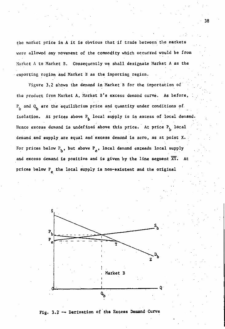
Figure 3.2 shows the demand in Market'B for the importation of - •

the product from Market A, Market B's excess demand curve. As before, 1

Pb

and Qb

are the equilibrium price and quantity under conditions of.

isolation. At prices above Pb local supply is in excess of local demand.

Hence excess demand is. undefined above this price. At price Pb local -

deMand.and. supply are equal and excess demand is zero, as at point X. :

For prices below Pb' but above Pe , local demand exceeds local supply • •

and excess demand is positive and is given by the line segment W. At

prices below Pe the local supply is non-existent and the original

Qb •

38

Fig..3.2'•-, Derivation of the Excess Demand•Curve

Market A

Pa

0 Qa

demand curve is also the excess demand curve. Thus, the demand in B for

A's product is given by XYZ.

Figure 3.3 then illustrates the derivation of the excess supply

curve for Market A. This is accomplished in a similar fashion. Sub-

tracting the demand curve, Da , horizontally from the supply curve, S a ,

we are left with the curve LMN, the excess supply curve.

39

Fig. 3.3 -- Derivation of the Excess Supply Curve

Since the excess supply and demand curves we have derived repre-

sent prices and quantities of the same product we can plot them on the

same diagram, as in Fig. 3.4. .Here ES represents the excess supply .

curve for Market A and EDb represents the excess demand curve for Market

B. If we would now allow the commodity to flow between the markets and,

• by an Act of God, transportation was completely costless, we would find

40

Pb

Po

Pa

Tr

0

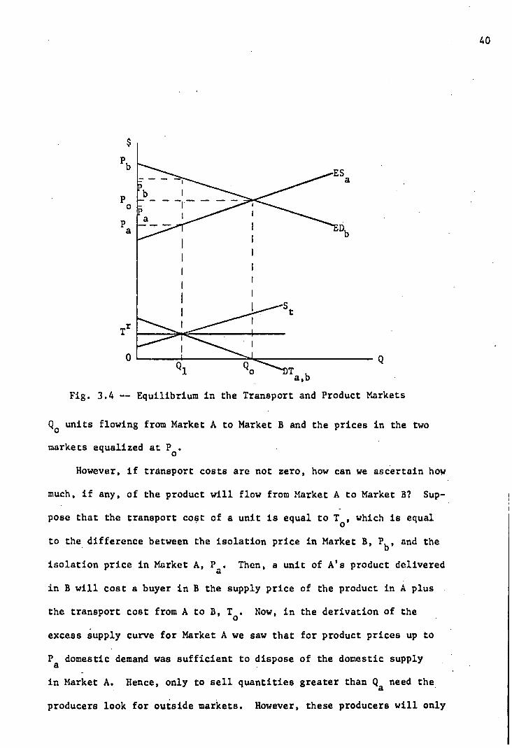
Fig. 3.4 -- Equilibrium in the Transport and Product Markets

Qo units flowing from Market A to Market B and the prices in the two

markets equalized at P o .

However, if transport costs are not zero, how can we ascertain how

much, if any, of the product will flow from Market A to Market B? Sup-

pose that the transport cost of a unit is equal to T o , which is equal

to the difference between the isolation price in Market B, Pb'

and the

isolation price in Market A, P. Then, a unit of A's product delivered

in B will cost a buyer in B the supply price of the product in A plus

the transport cost from A to B, T o . Now, in the derivation of the

excess supply curve for Market A we saw that for product prices up to

Pa domestic demand was sufficient to dispose of the domestic supply

in Market A. Hence, only to sell quantities greater than Q a need the

producers look for outside markets. However, these producers will only

desire to sell more than Qa if they receive a price higher than P a .

With e transport cost of T o they will desire to sell in Market B only

if the price they receive there is greater than P a + To ■ Pb .. But

for prices greater than P b' excess demand in Market B is zero. There-

.

fore, for transport costs greater than T o there can be no flow of pro-

duct from A to B, that is, the demand for transportation from A to B

must be zero. Analogous reasoning will show that for transportation

costs between zero and To there would be a desire to ship quantities

ranging from Qo to zero. This relationship is shown in Fig. 3.4 by

the curve DTa,b. It results from the vertical subtraction of the

excess supply curve from the excess demand curve and is the derived

demand curve for the transportation of the product from Market .A to

Market B. .

After having derived the demand for transportation, it is only

necessary to designate a transport rate or to specify a transport supply

function to close the system and determine the post-trade prices and

quantities. The solutions for the transportation market, the exporting

market and the importing market are achieved simultaneously. This is

also shown in Fig. 3.4. Our first assumption concerning the supply

side of-. the transportation market is that there is a single transport

industry which stands ready to carry any and all quantities of the

product from A to B at some Constant price. This rate is represented

- on the diagram as Tr. The intersection of the rate, line and the trans-

port demand curve determines the quantity which will be shipped between

the markets, Ql . Returning to the upper portion of the diagram we can

observe the new, post-trade, product prices in the two markets, Fa

in Market A and P in Market B. If, instead of charging a fixed rate

41

for all quantities, we conceive of the transport industry as having an

industry supply curve, S t , the intersection of this supply curve and

the transport demand curve will determine the solution prices and

quantities.

Before introducing costs associated with service attributes into

the analysis it will help to take a closer look at Fig. 3.4. The ex-

cess demand curve gives the "price," the total money outlay, which con-

sumers in B would be willing to give in order to obtain additional

• units of the product. The excess supply curve represents the addition-

al quantities of the product which producers in A would be willing to

supply at various "prices," dollar amounts realized by these producers.

If transport were completely costless these two curves could be set

equal. However, if there are any costs of transportation whatever,

excess demand price cannot be equated with excess supply price, since

the amount paid by the consumer is no longer the amount realized by

the producer. Thus far we have been assuming that the only cost of

transportation is the rate charged by the transport industry. As long

as this is the case, the price to the consumer is equal to the price

received by the producer plus the transport rate. This is the situation

illustrated in Fig. 3.4. However, if there are costs associated with

the transportation of goods from market to market other than those

covered by the transport rate, this treatment also becomes inadequate.

Excess demand price must then cover excess supply price plus the trans-

port rate plus the other costs.

This new situation is illustrated in Fig. 3.5. Here the curve

Ta represents the quality associated costs which the shipper must

42

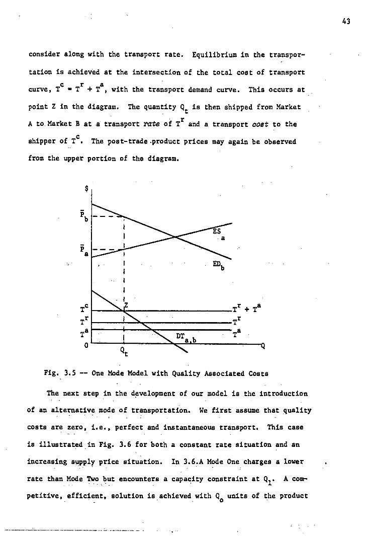
DTa_Lb

" ES . a

. .

I . • • . EDb

-• 1

'11Z

Qt

-4-

Tc

Tr

Ta

0

Tr + Ta

Tr

— a

consider along with the transport rate. Equilibrium in the transpor-

tation is achieved at the intersection of the total cost of transport

curve, Tc

■ Tr + T

a, with the transport demand curve. This occurs at

point Z• in the diagram. The quantity Q t is then shipped from Market .

A to. Market B at a transport rate of Tr and a transport coot to the

shipper of Tc. The post-trade product prices may again be observed

from the upper portion of the diagram.

43

Pb

Fig.. 3.5 -- One Mode Model with Quality Associated Costs

The next step in the development of our model is the introduction

of an alternative mode of transportation. We first assume that quality

costs are zero, i.e., perfect and instantaneous transport. This case

is illustrated in Fig. 3.6 for both a constant rate situation and an

increasing supply price situation. In 3.6.A Mode One charges a lower

rate than Mode Two but encounters a capacity constraint at Q1. A com-

petitive, efficient, solution is . achieved . with Q0 units of the product

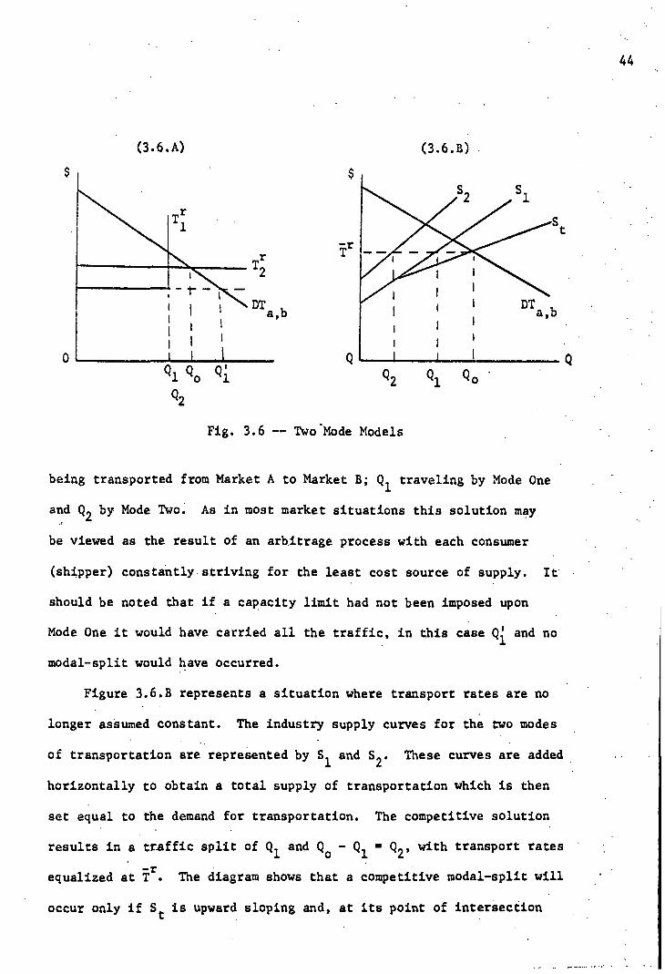
44

(3.6.A) (3.6.B)

0

Q2 Q0

Fig. 3.6 -- Two .Mode Models

being transported from Market A to Market B; Ql traveling by Mode One

and Q2 by Mode Two. As in most market situations this solution may

be viewed as the result of an arbitrage process with each consumer

(shipper) constantly striving for the least cost source of supply. It

should be noted that if a capacity limit had not been imposed upon

Mode One it would have carried all the traffic, in this case Qi and no

modal-split would have occurred.

Figure 3.6.B represents a situation where transport rates are no

longer assumed constant. The industry supply curves for the two modes

of transportation are represented by S 1 and S 2 . These curves are added .

horizontally to obtain a total supply of transportation which is then

set equal to the demand for transportation. The competitive solution

results in a traffic split of Q l and Qo - Ql ■ Q2 , with transport rates •

-r equalized at Tr. The diagram shows that a competitive modal-split will

occur only if S t is upward sloping and, at its point of intersection

curves.

with the transport demand curve, is not identical with one of the

supply curves.

The culmination of our geometrical model is presented in Fig. 3.7

where we have two modes supplying transport services with differing

levels of quality costs. The diagram has become rather cluttered but

the method of solution should now be obvious. As the shipper is in-

terested in all transport costs, we first sum the supply curve and the

quality cost curve vertically for each mode to obtain the unit trans-

c c port cost curves, T

1 and T. Then, to find the competitive market so-

lution, we sum these transport cost curves horizontally to obtain a

"transport - supply curve" and find the point where this curve intersects

the transport demand curve. As Fig. 3.7 is constructed, this is at a

quantity of Q and transport costs of T. This yields a modal-split .

of Q1 and Q2 . Then, working back to the modal supply curves, we see

that the rate Charged by - Mode One 'will be Tr and that of Mode Two T. 1 2

In general these rates will not be equal. The conditions for a modal-

split are, again, that S t be rising and that its intersection with the

demand for transportation occur at a point where both modes are rep-

resented.

These simple diagrams have served nicely in illustrating the

development of our'analysis. However, when the full Model is . presented,

as in 'Fig. 3.7, the diagram becomes rather confused, even when dealing

only With linear curves. After a discussion of the measure and form

of our associated costs, we shall utilize mathematical methods in

discussing the model And tracing the effects of shifting the various

45

• Q2 Qi Q0

46

Fig. 3.7 -- Two-Mode Model with Quality Associated Costs

Transportation Associated Costs

We now take a closer look at the associated costs of transportation

and the way we have entered them in our model. Markets A and B are

separate points and the physical movement of goods from one market to

the other requires time and effort. The effort is supplied, over time,

by the transportation industry. The transport rate is reimbursement re-

ceived by this industry for the effort it expends. During the time the

goods are in transit from A to B they are unavailable for use. This

unavailability may incur several alternative forms of economic costs,

all of which we shall call simply "time costs." Another category of •

costs may be termed "inconvenience costs." This category is tied in

very closely with the definition of the product of the transportation

industry. Since both these types of associated costs must be borne by

someone, we shall investigate their effects on our model. Then we

shall discuss the nature of the product of the transportation industry

and the interdependence between the definition of this product and the

nature of the quality-associated costs. Finally, we shall discuss a

third group of associated costs which might be termed "feeder and

interface costs." These costs arise when transport of the product in-

volves more than one "haul" and, perhaps, more than one mode of

transportation.

- - Time Costs •

We have defined the costs arising from the unavailability of the

product during transit as time costs. These time costs may take any

of several forms. We shall look at several situations which may occur

in the transportation market and investigate the time costs associated

with each. The framework of the single mode model is used: Market A

is the exporting market; Market B is the importing area; and one

transport industry serves the pair of markets. .

Situation I: Consumer Ownership. We assume that consumers from

Market B, in order to obtain additional units of the product, purchase

these units in Market A and contract with the transportation industry

to carry them to Market B where they are consumed. The sales take . . . .

place in A and the purchasers are forced to await the delivery of the

product to B. Time costs are thus a function of the consumer's time

47

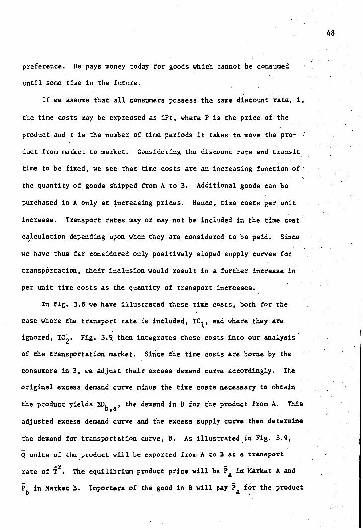
preference. He pays money today for goods which cannot be consumed

until some time in the future.

If we assume that all consumers possess the same discount rate, i,

the time costs may be expressed as iPt, where P is the price of the

product and t is the number of time periods it takes to move the pro-

duct from market to market. Considering the discount rate and transit

time to be fixed, we see that time costs are an increasing function •of

the quantity of goods shipped from A to B. Additional goods can be

purchased in A only at increasing prices. Hence, time costs per unit

increase. Transport rates may or may not be included in the time cost

calculation depending upon when they are considered to be paid. Since

we have thus far considered only positively sloped supply curves for

transportation, their inclusion would result in a further increase in

per unit time costs as the quantity of transport increases.

In Fig. 3.8 we have illustrated these time costs, both for the

case where the transport rate is included, TC 1 , and where they are

ignored, TC 2 . Fig. 3.9 then integrates these costs into our analysis

of the transportation market. Since the time costs are borne by the

consumers in B, we adjust their excess demand curve accordingly. The

original excess demand curve minus the time costs necessary to obtain

the product yields EDb,a , the demand in B for the product from A. This

adjusted excess demand curve and the excess supply curve then determine

the demand for transportation curve, D. As illustrated in Fig. 3.9,

Q units of the product will be exported from A to B at a transport

- rate of Tr. The equilibrium product price will be i" in Market A and

.13b in Market B. Importers of the good in B will pay P for the product a

48

Pb

b - TC

a

-r

TC

0

Tr in Market A, T for the transportation of the product from A to Bi and

incur waiting costs of TC..

TC1 ■ i(P + Tr)t

TC2 iPt

Fig. 3.8 -- Time Preference Cost Curves

49

Fig. 3.9 -- One-Mode Model with Consumers' Time Prefetence Costs

Situation II: Producer Ownership. This situation assumes the

producers retain ownership of the product until it is sold in Market B.

Again time costs are incurred, but here they are borne initially by

the producers and may be considered as a form of inventory costs. The

suppliers invest in their product and do not receive a return until

some later date. As production costs increase with quantity produced,

these inventory costs will be viewed as increasing with quantity shipped.

Figure 3.8 may again be used to illustrate these costs per unit if we

now consider i to be the producer's interest rate or capital cost. Given

a perfect capital market these costs will be identical with the time

preference costs of Situation I.

Figure 3.10 integrates these inventory costs into the analysis of

the transportation market. In this case the time costs are added to

50

Fig. 3.10 -- Two -Market Model with Producers' Inventory Costs

supply costs to obtain the supply of A's product in B, ES 8b . If we

assume this time.cost function is identical with the one utilized in

Fig. 3.9, the solutions for the two cases will be the same. All that

differs is the initial bearing of the time costs, and this does not

affect the solution values of Q, Pa'

Pb'

Tr

or TC.

Other Situations. At this point we could go on to discuss some

other situations. Two which readily come to mind are (III) Carrier

Ownership and (IV) Fourth Party Ownership. However, by now it should

be obvious that no matter who the shipping agent is, he must incur a

time cost during the transportation of the product. The only differ-

ences in the analysis are concerned with how we initially handle the

time cost functions. In cases III and IV we would probably begin by

adjusting the transportation supply curve. However, no matter how

we proceed, the market solutions would be identical with Situations

I and II.

Other Associated Costs and the Transportation Supply Curve

The costs which we wish to group under the term of transportation

associated costs mostly stem from aspects of transportation which are

usually termed the "quality of the service." In addition to transit

time, two other main categories are usually considered in discussions

of freight transportation. These are (1) losses due to breakage, spoil-

age or other deterioration of the product, and (2) uncertainty costs

which may arise with respect to either category (1) or transit time.

The question we wish to address here is whether or not these as-

sociated costs will increase with the quantity shipped. Offhand we

might think that some of them will and some will not. However, a

51

little consideration will reveal that their behavior is tied in quite

closely with what we consider the output of the transportation industry

to be and with the shape of the transportation supply curve.

If we believe that a transportation industry must render a quite

specific service for its output to be meaningfully measured, i.e., it

must adhere rigidly to schedules and maintain losses and uncertainties

at specified (minimum) levels no matter what level of traffic is being

carried, then our associated costs will probably remain constant or

perhaps even decrease as risks are spread. However, any industry which

must maintain this level of quality control will almost certainly ex-

perpience increasing costs and display a rising supply curve. On the

other hand, if we specify the output of our industry to be only the

physical movement of goods from market to market within a reasonable

period of time, it is reasonable to expect the supply curve to be

relatively flat but for the quality of service to decrease as greater

demands are placed upon the industry.

We should also mention another phenomenon quite often encountered

in transportation activities. This is the congestion which may be

encountered in almost any phase of transport activities. When conges-

tion occurs it causes both costs and transit times to increase and

often can be alleviated only by quite sizeable investment projects.

Feeder Line and Interface Costs

In our analyses we have been considering the individual markets to

be points in apace. We now relax this assumption and attempt to move

closer to a real world situation. While there may be a single railhead

or truck terminal where interregional shipments originate and terminate,

52

there are usually many other points in the region where production and

consumption occur. It is common practice to have a system of intra-

regional transport which links these points and performs the pick-up

and delivery functions. At the exporting terminals, then, it is neces-

sary to transfer the commodities from the intra-regional system to the

interregional system; this process is then reversed at the receiving

terminal.

It is to. the advantage of producers and consumers of goods which

are traded interregionally to be located near the transport terminals

and minimize intra-regional transport costs. However, all of the

economic activities cannot be located alongside the terminals; nor is

it likely that all producers and consumers could be located equidistant

from the terminals. Hence, in most situations where interregional

trade occurs we would imagine the first units would originate from

producers close to the exporting terminals and be consumed by house-

holds near the importing terminals. Then, as more product units are

drawn into trade, they would be drawn from, and consumed at, points

farther away.

When we attempt to measure the freight rates between regions, we

are usually forced to consider only the rates for the interregional

hauls. However, to fully reflect the total costs of transport, the

feeder and interface costs must also be considered. In this paper we

include these as another category of associated costs.

In this section we have introduced our concept of the associated

costs of transportation and argued that they, like transport supply

curves, would increase with quantities shipped. Analytically we have

53

considered these costs in several fashions and demonstrated that they

all result in the same solutions. However, in the next section, where

we again consider two modes of transport with differing associated

costs, it will be found necessary to handle these costs in a manner

analogous to the transport rates. Hence, we now adopt that approach

and define the total costs of transportation as the sum of the trans-

port rate and the associated costs. This will allow us to retain a

single and well-defined total demand for transportation function.

Qualitative Analysis of the Two-Mode Two-Market Model

In this section we shall present our transportation model in a

more formal manner and investigate the effects of controlled shifts in

the functions. We will find that we are able to place an unambiguous

sign upon all displacements of equilibrium and that in many instances

it is possible to make statements regarding the relative sizes of

these displacements.

Assuming that a Modal-split does occur our two-mode model may

be formulated as

(3.1) Qa

■ D(Tc, AB) the derived total demand for trans-

portation,

54

(3.2) Ql ■ S i (TI)

(3.3) Q2 ° s2 (Tr2)

a (3.4) Ti Z1 (Q1)

(3.5) Ta z2(Q )

2 2

(3.6) Tc Tr Ta

1 1 1

(3.7) T1 + T;

the supply of Mode One,

the supply of Mode Two,

associated costs for shipment by Mode One,

associated costs for shipment by Mode Two,

definitions of total transport costs,

(3.11.1)

(3.12.1)

(3.13.1)

(3.14.1)

(3.15.1)

Q1 Q2 1

-& (Ql' a2 )

-D(Tc )

+ Tr . 1

■ 0

0

55

(3.8) Q

(3.9) Tc ■ •q.

(3.10) Tc ■ T;

equilibrium conditions.

Since we are, primarily interested in investigating the effects of

rate and associated cost changes upon quantities and shipper costs, we

first invert (3.2) and (3.3) to express rates as functions of quanti-

ties. Then the definitions and equilibrium conditions can be utilized

to reduce the model to a set of five equilibrium relations in five

endogenous variables.

(3.11)

(3.12)

(3.13)

(3.14)

(3.15)

Q1 Q2 18 D(Tc' AB)

Tr

E1

1) 1 r 2

T2 E (Q2 )

c r 1 T - Ti ° (Q1)

c r T - T2 ° Z

2 (Q2 )

Equations (3.11) through (3.15) can be solved for Q 1 , Q2 , Tc ,

Tr and Tr' Knowing the values assumed by these variables, we can then 1 2

utilize equations (3.6) through (3.10) to find Q, 4, T;, T: and 11.

Now, to perform our qualitative analysis we rewrite (3.11) through

(3.13 adding a shift parameter to each function.

(3.16) a

Then, to calculate the rate of change of any system variable, call it

associated with a change in any parameter, call it ai , we differen-

tiate the system totally with respect to a j and solve the resulting

system of linear equations for 3X /3c.. Performing this calculation

for all Xi over all a and utilizing the assumptions contained in in-

equalities (3.16) through (3.25) it is found that we can unambiguously

evaluate the signs of the resulting expressions. Table 3.1 contains

the results of this analysis.

56

ap(Tc ,c( 1 ) <

aTc 0 the demand curve is downward sloping

1 a (Cll' a2 )

(3.17) > 0 a(1 1

g2(Q 2 ,a3 )

(3.18) >0 a(12

az 1 (Q1,a

4)

(3.19) >0

az 2 (Q2'

a5)

(3.20) > 0 aotl

2

the supply curves are upward sloping

the assoc. cost curves are upward sloping

(3 21) 3D(T1 ,a1 ) . > 0 the demand curve shifts to the right

1 a (Ql' a2 )

(3.22) >0 aa2

3a1

tr 2 m uS .42 ,a3 )

(3.23) > 0 aa

3

the supply curve shifts upward

aZ 2 (Q2 ,ab ) (3.25) >0

aa

the assoc. cost curve shifts upward

5

3Z1 (Q

1 ,a )

(3.24) 4 0

aa4

57

Table 3.1

QUALITATIVE. ANALYSIS OF THE TWO-MODE MODEL

Resulting From a Shift of Direction of the Change in

Q Ql Q2 Te T1 Tr2 T1 T;

The demand curve, rightward , Mode One's supply, Upward Mode Two's supply, upward Quality costs, Mode One, upward Quality costs, Mode Two, upward

++ + + + + + - - + + + + - + - + - + + + + - - + + - + + + - + - + + - + +

Table 3.1 shows: (1) an increase in demand will cause an increase

in the solution values of all endogenous variables; (2) a shift up-

wards in a modal supply curve will result in a decrease in the quantity

carried by that mode, total quantity shipped and quality costs for that

mode, all other variables increasing in value; (3) an increase in qUalitY

costs for a mode will cause a. decrease in the quantity carried by that

mode, its rate and the total quantity shipped, With all other variables

again increasing in value.

Furthermore, if we examine shifts of the same nature for the supply

curve and quality cost curve of each mode, e.g., we Compare uniform up-

ward shifts.of five cents per ton of the supply curve and the quality

cost curve, we.can derive the relationships expreSeed in Table 3.2.

These are, for uniform shifts:

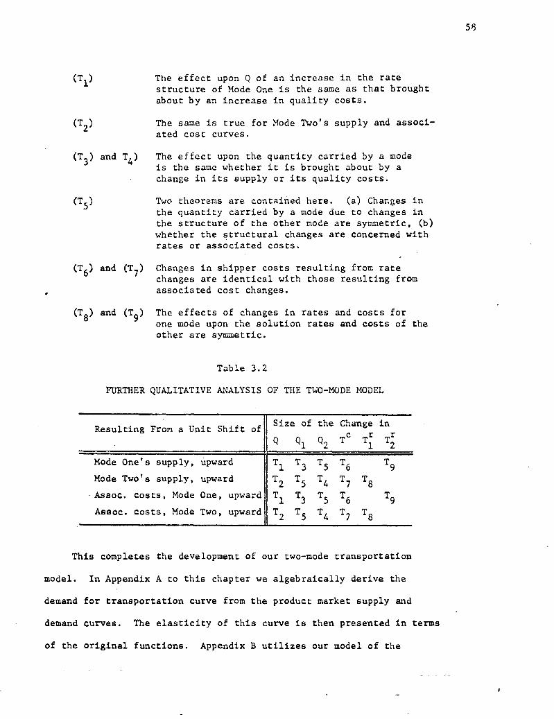
(T1)

(T2)

Resulting From a Unit Shift of Size of the Change in

Q Q, Q,, Tc T.Tr Tnr

Mode One's supply, upward

Mode Two's supply, upward

Assoc. costs, Mode One, upward

Assoc. costs, Mode Two, upward

T2

T5

T4

Tl

T3

T5

T6

T8

T2 T 5 T4

T7

T8

T9

The effect upon Q of an increase in the rate structure of Mode One is the same as that brought about by an increase in quality costs.

The same is true for Mode Two's supply and associ-ated cost curves.

(T3 ) and T4 ) The effect upon the quantity carried by a mode is the same whether it is brought about by a change in its supply or its quality costs.

Two theorems are contained here. (a) Changes in the quantity carried by a mode due to changes in the structure of the other mode are symmetric, (b) whether the structural changes are concerned with rates or associated costs.

(T6 ) and (T7) Changes in shipper costs resulting from rate

changes are identical with those resulting from associated cost changes.

58

(T5

)

(T8) and The effects of changes in rates and costs for

one mode upon the solution rates and costs of the other are symmetric.

Table 3.2

FURTHER QUALITATIVE ANALYSIS OF THE TWO-MODE MODEL

This completes the development of our two-mode transportation

model. In Appendix A to this chapter we algebraically derive the

demand for transportation curve from the product market supply and

demand curves. The elasticity of this curve is then presented in terms

of the original functions. Appendix B utilizes our model of the

transportation market to derive the demand for the services of one

of the transport modes. The elasticity of this "modal average revenue

function" is then derived and expressed in terms of the other market .

functions. In Appendix C the model is altered slightly to allow one

of the transport modes to be composed of a single firm, a monopolist.

The behavior of this monopolist is then examined as he confronts the

• modal demand curve derived in Appendix B.

59

(3.A.7)

(3.A.8)

P(Qs ) 4 a a

Pb " 91) ( 4) )

APPENDIX A TO CHAPTER THREE

The Elasticity of the Derived Demand for Transportation

We now present a more formal derivation of the demand curve for

transportation. This will allow us to explicitly derive the elasticity

of this transport demand and provide a firm foundation for what follows.1

Our basic conditions are given as:

(3.A.1)

(3.A.2)

.(3.A.3)

(3.A.4)

d d

qa

■ fa

(Pa

) demand in A,

q s ■ f (P ) supply in A, a a a d d

qb

■ fb

(Pb

) demand in B, and

s s

qb

■ fb

(Pb ) supply in B.

Then, under the assumption that the isolation price in A is less

than the isolation price in B, we derive

(3.A.5) Q8 f8 (P ) - fd

(P ) Fs (P ) excess supply in A, and

a a a a a a a

(3.A.6) Qd

■ fd

(P ) - fs

(P ) ■ F ) excess demand in B.

b b b b b b b

In (3.A.5) and (3.A.6) quantities are expressed as functions of price.

We invert them to obtain (3.A.7) and (3.A.8)

Now, we integrate the importing and exporting markets by dropping the

superscript from the Qs and subtract excess demand price from excess

1. This appendix is basically the same as Kobe's article. However, as he adds an extraneous minus sign to the final expression (our equation (3.A.25)) our conclusions will differ somewhat.

60

(3.A.9)

(3.A.10)

Tc

■ clob(Q) - ma (Q) • T(Q)

T-1 (Tc) ■ D

(Tc)

supply price to obtain the demand for transportation from A to B.

61

where Tc

is the transportation cost per unit of the product and Q is

the quantity transported. We desire to find the price (transport cost)

elasticity of equation (3.A.10).

We define

(3.A.11)

(3.A.12)

P fd,

(P) Ed

■ a Elasticity of demand in A. a

fd(P

) a

P fs '(P) Ea s a Elasticity of supply in A.

f:(P)

P fd '(P) ,d (3.A.13)

"b Elasticity of demand in B. f(P)

P fs '(P) (3.A.14) E.D ■ Elasticity of supply in B.

f:(P)

(3.A.15) P Fsl (P)

a na • Elasticity of excess supply in A.

Fa (P)

(3.A.16) P F'( P) • Elasticity of excess demand in B.

• Fb (P)

These lait two elasticities may also be expressed as:

62

■FQ -7,5-(43-- and (3.A.17)

(3.A.19) 19-i701 •

(3.A.18) QC 13 T.

bb (Q)

From (3.A.9) we can express the transport rate elasticity of transport

demand as

Expanding (3.A.19) by (3.A.9) it becomes

-1

(3.A.20) E m Q 91, 1 0) Q 911 '(Q)]

Y(Q) .

[

Q1 91) 1 (Q) 9b (Q) Q Ta '(Q) 9a (Q)] -1 - 9b0) -71-ra %co 7TOT •

Now, from (3.A.15) through (3.A.18) we see that

(3.A.21)

d, -1 • Q (Pb ' (Q) F Fb (F)

F(P) 1

and

(3.A.22) Q cp / (Q) s [12 e t (P)1 a

(Ti a ) mi F0(P)

Further expansion of the right-hand sides of (3.A.21) and (3.A.22) by

(3.A.6) and (3.A.5) respectively and substitution into (3.A.20) yields

IL fb (P) Fd (P) fs(P) Fd (P) b • b b

1 P 4 1 (P) f(P) P f: 1 (P) fl:(P) ..1 911 0,1)

I

63

od d s _ fro. s 8 ) P fb (P)-P fb t (P) b (Q) P fat(P)- •P fd (P)

a (3.A.23) Ed • F(P) Fa(P)

epao)ri. .

,(0 1

P f:t (p) f:(p) p _ea (p) f(P)

f:(P) F: (12) fa (P) Fa (P)

-1 9a(01 -1

T(Q )1

Finally, using (3.A.11) through (3.A.14), (3.A.23) may be expressed

as

elf.% (3.Al24).. Ed ) rd 1)"1 08

d

P(P) F(P)

-1 Vb (Q)

T(Q)

1

_ Es . f:(11 _ 'Ed fda (P) -1

• a F: (p) a F: (p)

or as

s -1 a d p •

(3.A.25) Ed 11 d qb

-

s qb1 1'bb -

s qa d qa al — — E — E —

-b DQ c aQaQ T1 •

When expressed as in equation (3.A.25) the elasticity of transport

demand is not as complex as it may at first appear. The first set of

brackets, [ I, enclose the demand and supply elasticities for the im-

porting region. Since demand elasticity is negative the two elasticities

are additive. An increase in either elasticity will make the bracketed

term more negative and, since it is twice inverted, increase the elas-

ticity of transport demand. The demand elasticity is weighted by the

ratio of domestic consumption in B to imports and the supply elasticity

is weighted by the ratio of domestic supply to imports. Since Market B

is the importing region, domestic consumption is greater than domestic

supply and the demand elasticity is given the greater weight.

Within the second pair of brackets the situation is reversed.

Market A is the exporting region so the supply elasticity is more

heavily weighted. Again the elasticities are additive; however, here

their sum is positive. The negative sign in front of the brackets

causes the elasticities to affect the transport elasticity positively,

i.e., an increase in the demand or supply elasticity of the exporting

region will result in a higher (more negative) elasticity of transport

demand.

The remaining two terms in equation (3.A.25) are the weights for

the bracketed expressions. Since B will be the importing region, we

know by definition that Pb > Pa and the importing region's elasticities

are weighted heavier than the exporting region's.

64

APPENDIX B TO CHAPTER THREE

The Elasticity of Mode Two's Average Revenue Curve

One way to derive the average revenue curve for Mode Two is to begin

with equations (3.11) through (3.15). From this set we remove equation

(3.13), the transport rate relation for Mode Two. This leaves four equa-

tions containing five variables. The solution of this reduced set for

Q2 in terms of T2 is the average revenue curve for Mode Two.

We now proceed to derive this average revenue curve in a cruder

manner. This is necessary to provide a basis for the derivation of the

elasticity of this function.

Given equations (3.1) through (3.10) we invert equations (3.2) and

(3.3) and then reduce the set to the following five equations.

(3.B.1) Q1 + Q2 ■ D(Tc) demand for transportation.

(3.B.2) Tc ■ e(Q1) + Z1 (Q1) r(41) total costs of shipping by Mode 1.

(3.B.3) Tr2 ■ C2 (Q2 ) supply curve for Mode 2.

(3.B.4) T; ■ Z2 (Q2 ) associated costs for Mode 2.

(3.B.5) TC ■ T; + T of total costs of shipping by Mode 2.

First, we define the inverse of (3.B.2) to be (3.B.6)

(3.B.6) Q1 ■ L(Tc).

Equation (3.B.6) is then subtracted from equation (3.B.1) to yield

(3.8.7) Q2

■ D(Tc) - L(Tc) ■ T(T

c)

65

(3.B.8) Tc • C(Q2 ).

(5.B.9) 4 • C(Q) - Z2(Q2 ) • F(Q2

)

and its inverse

66

Now from (3.B.5) we see that 4 • TC - T so that

is the average revenue curve for Mode Two.

0

Fig. 3.B.1 -- Derivation of the Average Revenue Curve for Mode Two

This procedure is illustrated graphically in Fig. 3.B.1. Here

we have the demand for transportation curve, DTa,b , the total cost .

curve for Mode One, Ti , and the associated cost curve for Mode Two,

a T . The total cost function for Mode One is first subtracted horizon-

tally from the demand curve to yield WY. This derived curve repre-

sents the shipper's demand for transport by Mode Two. However, einoe

a,b

not all shipper costs are received as revenue by the transport industry,

it is not the average revenue curve for Mode Two. That latter curve

is derived by subtracting the associated cost function vertically from

the derived curve XYZ to yield UVW.

In Fig. 3.B.2 we have included a supply curve for Mode Two and il-

lustrated the market solution in the same manner as in Fig. 3.7. The

average revenue curve for Mode Two is also included to illustrate that

it does, indeed, show the revenue received by that mode.

67

Fig. 3.B.2 -- The Two Mode Associated Cost Model

We now continue with the derivation of the elasticity of Mode Two's

average revenue curve. Given the average revenue curve as defined by

equation (3.B.9), its elasticity will be

-1 Q2 F'(Q2 ) 1 Q2 Ct(Q2 ) C(Q2 ) Q2 Z2,(Q2 ) Z2(Q2) -1

(3.13.10) E2 ■ Fin

"2' C(Q2) F(Q2) Z2(Q2 ) F(Q2 )

(3.3.13) TC T I (TC)

ET T(TC)

Now, going back to equation (3.3.7), if we define the transport cost

elasticity of this curve to be E we see that

- Tc TI(Tc) . 1 1

C(Q2)

Q2 C'(Q2)I (3.8.11) from (3.8.8). E ir(Tc)

68

Hence

(3.8.12)

2 -1

c(Q2) z -1 2 (Q2 ) d E2 %E "2' T'

- (E2)

1

where E2 is the elasticity of the Z2 curve.

Now,

Tc W(Te) D(Tc), TC L'(Tc) L(Tc )

D(Tc ) T(Tc) L(Tc) V(e)

. Ed D(Tc),_ Te W(Tc) L(Tc),

•. T(Tc) . L(Te) T(Tc)

Further, using (3.B.2)

• 1

(3.8.14) I Q 1" (Q1) 1- 14e,1 r(Q1)

_

1 - .

I .

Es -1 C ($41) Z -1 Z1 (Q1) i1

t 1) -fro1 + (EI) r(Q1)

1

.(11e'(Q1) C 1 (Q 1 ) Qi z1 '(11) zi (Q1) -1 1 7-(0717 4. z1 01) r(41 1 C (Q )

1-7t-If7T E1 (Q ) r(Q )

(3.B.16) D(21

Substituting this expression back into (3.B.13) we obtain

69

1

(3.B.15) E Ed D(Tc ) 8 -1 01) Z1(Q )

Z -1

T(Tc (El) + (EI)

`41'

-1 L(Tc)

T(Tc)

And, the substitution of (3.B.15) into (3.B.12) yields our result

d c (Q E ) (E8,-1 1

Y(Tc) r(Q )

1(Q1) -1 z -1 Z I

L Tc I C(Q2) (e)

-1 Z2(Q2 ) 1-1

+ (E ) I r(Q1 ) 7(Tc ) 1 F(Q2 ) 2 F(Q2 )

(3.B.17) 4 -2 _

1- Q2

a 8 -1 T1 Z -1 T1 (E) — + (E ) — 1 Tc 1 Tc

,a -1 1 Q0 Tc Z -1 A 2 -A WAI r (E2) 42) T2 T2

Equation (3.8.17) relates the elasticity of Mode Two's average

revenue curve to the elasticity of the demand for transportation, the

elasticity of the supply and associated cost functions for Mode One, the

elasticity of Mode Two's associated cost curve, the proportion of total

traffic carried by Mode Two, and the proportion of total shipper costs

attributable to transport rates for each mode. It is easily generalized

to include more transport modes. If we assume n modes are sharing the

traffic, the elasticity of Mode i's average revenue curve is

d (3.B.18) El J E 9,-- -1 + (E - I / 1.2- I Q

r 2 i 109 )-1

i jamlliT

c

iTc Qil Tr JOi

i

APPENDIX C TO CHAPTER THREE

The Two-Market Multi-Mode Transportation Model:

The Monopolistic Case

Thus far our analysis of the transportation market has been limited

to the study of competitive transport modes. The models were developed

under the assumption of perfect intra-mode competition as well as inter-

modal competition. In this section the former assumption is partially

relaxed. One of the modes is allowed to consist of a single firm, a

monopolist. All other modes continue to be thought of as separate cm-

• petitive industries.

We begin with the simple two-mode case with no associated costs.

The stability of the market is examined under various cost conditions

for the monopolist, the non-optimality of the modal-split is seen, and

the monopolist's reaction to Changes in market conditions is studied.

Transportation associated costs are then allowed in the model and,

finally, we examine the behavior of a monopolist who exercises some de-

gree of control over the associated costs of his mode.

The Two-Made Model

We begin with the case of two supplying modes of transport. Mode

One is a competitive transportation industry while Mode Two is a "monop-

olist." He is a monopolist in that he is the only producer of his pkr-

ticular type of transportation. Nevertheless, he is in direct compe-

tition with the other transportation industry. This monopolist is fully

aware of all market conditions and we assume that he is large enough

to greatly affect the market by his actions. Probably his scale of

70

operations is at least as large as that of the entire industry com-

prising Mode One.

In Fig. 3.C.1 we have a demand for transportation curve, DD, and

a derived demand for the services of Mode Two, D 2D2 .1 Since there are

no associated costs, shippers base their mode choice decision on supply

price alone. Mode One is composed of price takers whereas the monop-

olistic Mode Two is a price setter. He attempts to maximize his profits

and is assumed to act in a straightforward manner, employing no devious

strategies.

71

Fig. 3.C.1 -- The Simple Monopolistic Model

Monopolistic profits will be at a maximum when marginal revenue •

is equated with marginal cost. Hence the monopolist will set his

- - transport rate at T

r . . Charging this price he will attract Q 2 units of

1. See Appendix B for the derivation of this curve, especially, Fig. 3.B.1, p. 65.

product to be transported, Q1 units will travel by Mode One and demand

will be satisfied.

Figure 3.C.1 also brings out the social non-optimality of this

system. This is evident in two respects. First, the existing modal

split does not minimize total transport costs; second, total output in

the transportation industry(s) is restricted. Both of these conditions

arise from the profit maximizing behavior of the monopolist. If he

were forced to be a marginal cost pricer they would be eliminated. •

Under marginal cost pricing the monopolist Mode Two would carry C1 2 ,

charging a rate of Tr. This would allow Mode One to capture only &I

although total traffic would increase to units. Thus, if he priced

according to marginal cost the monopolist would capture a larger share

of the market, even though his total profit would be reduced.

In Fig. 3.C.2 we have illustrated an even more interesting case.

Here the monopolist is assumed to display falling long run marginal

costs. Profit maximization requires that he set a rate of Tr and bring - -

about the modal split Q 1 , Q2 . However, it is in the best interests of

society to disband Mode One and revert to a true monopolistic situation.

Enforcement of marginal cost pricing would then result in the monop-

^ olist carrying all of Q at a rate of Tr. The monopolistic solutions

are stable if marginal cost cuts marginal revenue from below and profits

are positive. The social solutions require regulation, enforcement and,

if profits are negative, subsidies:

Parametric Associated Costs

Here we examine the two-mode model where one mode is composed of

a single firm and there are costs other than the transport rate

72

73

(3.C.X) T2 ■ C(Q2) - Z2 (Q2 ) F(Q2).

(3.C.2) e(Q2 )

• Fig. 3.C.2 -- The Monopolistic Model with Falling Marginal Costs

associated with shipment by each mode. The carriers are assumed to

exercise no control over these other costs.

The average revenue curve facing Mode Two was derived in Appendix

B as

Instead of an industry supply curve for Mode Two we now have the monop-

olist's cost curve which we specify as

where Y is Mode Two's total cost of carrying Q2 units of the product

from Market A to Market B.

,(3.C.6) -r - T2 ■ F(Q2 ).

[2 FQ2

(Q2'a) + Q2 FQ2,Q2 (Q2' a) - e"(Q2 )] -- da

dQ2

The monopolist's profit function is then

4 .

74

(3.C. 3) '2 T; - Y." Q2 F(Q2 ) , - e(Q2 ),

and his profit maximizing quantity, is given by the solution of

(3.C.4) dQ2 F(Q2 ) + Q2 F'(Q2 ) -

(marginal revenue equals marginal cost), so long as

d2H (3.C.5) — 2 ■ 2 F'(Q2 ) + Q2 F"(Q2 ) - 2 ) < 0. dg2 .

The rate which he must charge to carry this quantity is then given by

To investigate how we would expect the monopolist to react to a

change in any of the underlying functions we again add our shift para-

meter, a, to equation (3.C.1). The equilibrium relationship (3.C.4)

then becomes

P(Q2 ,a) + Q2 FQ2 (Q2 ,0 - 0'(Q2 ) ■ O.

Differentiating (3.C.7) totally with respect to a yields

(3. C. 8) •

• -[Fa (Q2 °) Q2 FQ2,a (Q2 ,a)].

Or, defining the first bracketed expression in (3.C.8) as W

• dQ2 1 (3.C.9) -

rw in -% n w In %1 da 171 "a"2"" '2 'CI2'a`"2"/".

.f .,

Now, W was assumed to be negative in (3.C.5) so that

75

(3.C.10) dQ2

0 as F (Q2 ,a) + Q2 F (Q2 ,a) O. Q2 ,a <

Looking at (3.C.10), we would require F a (Q2 ,a) to be positive by

definition. Q 2 is also required to be non-negative. Thus the sign of dQ2

will depend upon the sign of F Q ,a(Q2'a) and the weight attached da 2 to it. Only if this term is negative and Q2 FQ2'a

(Q2'a) > -F(Q

2'a)

dQ2 will — be negative. That is, if the shift of the average revenue da

curve does not affect the slope of the curve or if the slope is in-

creased by the shift, the equilibrium quantity transported will increase.

If the slope is decreased, and if the reduction in revenue due to the •

slope shift outweights the increase in revenue due to the upward shift

of the curve, quantity transported will fall. As the average revenue

dTr

curve must be downward sloping, — will always differ in sign from da dQ2

do •

Endogenous Associated *Costs for the Monopolistic Mode

Finally, we assume that the monopolistic mode has some control

over its associated cost function. There is a-quality of service var-

iable, A, which costs the firm money. However, as the value of this

variable is increased, the quality of service of the monopolistic mode

increases, and the associated costs decrease. We have

(3.C.11) T2 ■ C(Q2' a) - Z2(Q2' A) Mode Two's average revenue function

(3.C.12) Y • 0(Q2 ,A) Mode Two's total cost function

The firm's profit function is thus

(3.C.13) n Q2 [C(Q2 9a) - 2 (/2 9A)] - n(Q2 9A).

f z

76

(3.C.16) B11" B22 > 0 and IBI < 0.

To obtain the greatest profits, the monopolist will maximize this

function with respect to both Q 2 and A. His profit maximizing conditions

are

(3.C.14) , + Q2 C(12 (Q2 ,02) -

202 ,0 acl .

2

-Q2 Z2 02' A) - Q (Q2' A) ■ 0

. Q2 2

and

(3.C.15)

Defining .r

• -Q2 Z

2 (Q2' A) - 0 A (Q2'X) ■ 0.

3A A

_ 2

3.1I a 2 H

an2 acl2 ax 1 811 B12'I '2 B ■ • ,

B21 B22 32H a2H

"a(12 ax2

the sufficiency conditions for profit maximization are that

To investigate the effects of a shift in the average revenue curve

upon the profit maximizing values of Q 2 and X, we differentiate (3.C.14)

and (3.C.15) totally with respect to a to obtain

13(12 2 2 t2C .- 2 + (3.C.17) - Z

142 Q2

CQ2'Q2 Q2 ZQ2'Q2

- eQ2'

Q2

a. • Q2

77

(3.C.18) 2 3(12 - IZ A + q2 Z2 + 0 A

1.--- "2 42 3a

- 1 ,2 e a)'o 42 -Ad, A,A act

Equations (3.C.17) and (3.C.18) are linear in the two unknowns

3(12 ax and may be solved for and -5-c; • It can be shown that the first

bracketed expression in (3.C.17) is equivalent to B ll ; the second

bracketed expression in (3.C.17) and the first bracketed expression in

(3.C.18) are equivalent to B 12 E B21 ; and the second bracketed ex-

pression in (3.C.18) is equivalent to B22 . Hence, we may rewrite these

two equations As

(3.C.19)

(3.C.20)

3(12 SA B + B C 11 3a 12 aa a 2 q2 ,a

Bq2 ax B + B — 0. 21 aa 22 3a

Solution by Cramer's Rule yields

(3.C.21)

(3.C.22)

B22 ICa +Q 2 Cq2'a 3q2 Sa IBI

B21 ICa +Q 2 Cq2'a ax aa 1BI

The expression 1Ca + q2 c is analogous to the expression

I Fa + q2 Fn '0 1 found in (3.C.9). Here we are shifting only the "C" '2

curve, whereas before the "C - Z2 ■ F" curve was shifted. This ex-

3(12 pression will again directly determine the sign of iv-, as B22 0 and

IBI c 0.

.1.,

OA The sign of — is only slightly more difficult to determine. aa

2 2 The sign of B

21 E B

12 -IZ + Q

2 ZQ2,A +

Q ,AI may be either posi-

tive or negative. The first two terms of this expression represent

the marginal increment to profits which could be brought about by in-

creasing the quality of service. The final term represents the mar-

ginal cost of this prospective increase. (Assuming for the moment

that ICa + Q2 CQ2,aI is positive) if MR > MC, A will be increased; whereas if MR < MC, A will be decreased.

78

CHAPTER IV

ESTIMATION OF THE DEMAND FOR TRANSPORTATION

This chapter contains the results of our empirical investigations.

As we are primarily interested in transport by rail, barge and motor,

we first expand the work of Chapter III into a three-mode model. This

model is then converted into suitable form for estimation and and es-

timating equations are derived. The data are then described and the

empirical results discussed.

The Estimating Model

The three-mode model may be expressed as

(4.1)

(4.2)

(4.3)

(4.4)

(4.5)

(4.6)

(4.7)

(4.8)

(4.9)

• (4.10)

gd • D(Tc)

T1

•

■1 (Q1)

T2

•

E2 (Q2 )

T3

•

■3 (Q3 )

a T1 Z1 (Q1)

a T2 ■ Z

2(Q

2)

a T3

■ Z3(Q

3)

T1

■ Tr + T

a

c r a T2 ■ T

2 + T

2 c r a

T3

T3 + T

3 •

• Demand .for transportation;

Transport rate by Mode One;

Transport rate by Mode Two;

Transport rate by Mode Three;

Associated costs for Mode One;

Associated costs for Mode Two;

Associated costs for Mode Three;

Total costs of shipping by Mode One;

Total costs of shipping by Mode Two;

Total costs of shipping by Mode Three;

79

(4.11)

(4.12)

(4.13)

(4.14)

111 Tc 1

c c T ■ T

2

Tc

■ T3

q ql q2 q3

80

Equilibrium conditions

The following definitions continue to apply:

d E quantity of transport demanded;

c _ T = total costs, to the shipper, of transportation;

Tc

= total costs of shipping by Mode i, (i ■ 1, 2, 3); i

E quantity transported by Mode 1, (i ■ 1, 2, 3);

r _ Ti = transport rate, per ton, charged by Mode i, (1 ■ 1, 2, 3);

Ta

= other shipping costs, borne by the shipper, associated i with shipping by Mode 1, (i ■ 1, 2, 3).

Now, the theoretical model has been developed for the case where

one specific market ships to only one other market. However, data to

fit such a model are unavailable at the present time. Any estimation

attempts must utilize data of a cross-sectional nature, i.e., shipments

between many pairs of markets during the same time period. To use data

of this type it is necessary to add several new variables to the struc-

tural equations which explicitly allow for the differences in market

size and the distances between the markets. We define

A E an indicator of the economic size of a city (0-D) pair, and

M E the distance, in miles, between a city pair.

The size indicator, A, is inserted in equation (4.1) as an ex-

ogenous variable and the distance variable, M, is included in equations

(4.2) through (4.7) in a like manner.

(4.15)

(4.16)

(4.17)

(4.18)

Q1 + Q2 + Q3 w D(Tc ,A)

T1

•

w E1(QM)

T2

•

■202'10

T3 • w3(Q3'M) .

We now substitute equations (4.8) through (4.14) into equations

(4.1) through (4.7) to eliminate Qd , T Ta

(i • 1, 2, 3). The

reduced equilibrium system then appears as

81

(4.19) Tc - Tr Z1 (Q

1 ,M)

1 r

(4.20) Tc - T2 • Z 2 (Q2 ,M)

(4.21) Tc - Tr3 Z3 (Q3'

M)

Two specifications are now imposed upon the system.

1. The equations are linear in all included variables.

2. The Qi do not appear in equations (4.16), (4.17) and

(4.18)

Specification 1 is necessary due to the nature of the model and the

estimation problems involved. The second specification recognizes

that rates for the commodities we are concerned with are fixed by law

and that the regulatory process may cause the process of rate adjust-

ment to be both long and complex. As will be seen below, it also

allows the empirical work to be separated into two distinct parts.

With these specifications the model may be written as

(4.22)

(4.23)

(4.24)

(4.25)

Ql + Q2 + Q3 wa+0Tc+yA

c r T - Tl w al + b l Ql + cl M

Tc - Tr wa2 +b2 Q2 +c2 M 2 C r T - T

3 w a

3 + b

3 Q3 + c3 M

82

(4.26)

(4.27)

(4.28)

Tl • gl + hl M

4 ■ g2 + h 2 M

T3

g3 + h

3 M

(4.29)

(4.30)

-b 2Q2 (4.31)

(4.32)

In this formulation we see that equations (4.26), (4.27) and (4.28)

are each a self-contained sub-set of order zero and may be estimated

separately and independently.1

Equations (4.22) through (4.25) then constitute a derived struc-

ture of the first order. Using (4.26), (4.27) and (4.28) to eliminate

the rate variables, they become

. Q1 Q2 + . (13 "c m a+ YA

-b1Q1 + Tc • (al + gl )

+ Tc ■ (82

+ g2)

-b3Q3 + T

c ■ (a

3 + g

3)

+ (c1 + h1) M

• + (c2 + h2 ) M

+ (c3 + h3) M

The following sections deal with our empirical investigations of

these two sets of estimating equations.

Empirical Results -- The Rate Equations

Having derived the estimating equations, we now turn to our em-

pirical work. In this section we shall deal with equations (4.26),

(4.27) and (4.28), the transport rate equations. The following section

contains our discussion of the demand equations. As stated previously,

1. The terminology and procedure is taken from H. A. Simon, "Causal Ordering and Identifiability," Chapter III of W. C. Hood and T. C. Koopmans, Studies in Econometric Method, Cowles Commission Monograph No. 14, Wiley, New York, 1952.

we are interested in three modes of transport, rail, water and motor.

The modes are discussed in that order.

Rail Transport

We begin with our investigation of point-to-point rail rates.

Utilizing cross-sectional data obtained from the 1963 Carload Waybill

Statistics published by the Interstate Commerce Commission, we estimate

regression equations linking the rail rate, for commodity classes and

commodity groups, to a small number of variables representing the

characteristics of the commodities and shipments.

The Data. The Carload Waybill Statistics are published annually

and contain data derived from a one-percent sample of audited revenue

waybills terminated by Class I railroads. This information is pro-

cessed and presented in a number of formats. The data utilized in this

study come primarily from the State-to-State Distribution Series.2

In

this series data are presented on total annual shipments by commodity

and by state of origin and state of destination. For each shipment

information is given on carloads, tons, revenue, short-line ton-miles,

short-line car-miles, average tons per car, average short-line haul

per ton . and haul per car, and average revenue per 100 pounds, car,

short-line car-mile and short-line ton-miles.

From the above list we selected the average revenue per 100 pounds,

which was later converted to a per ton figure, as our rail rate variable.

For explanatory variables we chose tons, average short-line haul per

ton and average tons per car.

2. "State-to-State Distribution(s)," Carload Waybill Statiatice, 1963, Statements SS-1 through SS-6, Bureau of Economics, Interstate Commerce Commission, Washington, D.C., Jan. 1966.

83

The tons figure is the total tonnage of the commodity carried from

the state of origin to the state of destination during 1963. This

should not be confused with the tons included in an individual ship-

ment. It is an annual total. Information on the size of individual

shipments would be valuable in that quantity rates and discounts are

usually figured in these terms. Such information is not available how-

ever. The annual tonnage data were selected because we believed it

would prove even more important in determining the level of rail rates.

This annual tonnage reveals how important the product is to both the

shipper and the railroads. We believed that as more of a product is

shipped annually the rate charged per ton would tend to decrease.

The average short-line haul per ton became our distance variable.

Clearly, in constructing the freight rate for a ton of any commodity,

the distance it is to be carried is the primary determinant. This

belief was verified time and time again.

Average tons per car was used as a surrogate for the density of the

product. The rate charged for transporting commodities of different

densities should vary, since undoubtedly the cost of transporting them

varies. This variable was only utilized when more than one commodity

was being. examined at the same time. That is, we selected the average

tons per car figure for all shipments of a commodity. Our explanatory

variable density then changed in value only when a new commodity was

considered. This was also true of the price variable.

So much is heard of value of service pricing in transportation that

we felt it necessary to include a variable to attempt to capture this

influence, if it was in fact present. For the vast majority of the

commodities we were going to investigate, no demand studies have ever

84

been undertaken and no measures of elasticity, however crude, were

available. However, we were able to find data on wholesale prices

for the ICC commodities and commodity groups.3 These prices were for

the year 1959 and, although most of the commodity prices had un-

doubtedly changed between 1959 and 1963, it was felt that relative

prices probably had not changed too much.

Before presenting the results of our analysis, it is necessary

to discuss the levels of aggregation of the ICC data. At the lowest

level we have state-to-state information for 262 "commodity classes."

These "commodity classes" are small groups of commodities. These com-

modity classes are then distributed into five "commodity groups," the

data are aggregated and state-to-state shipments of the commodity

groups are presented. Finally, for the highest level of aggregation,

all of the data are grouped together and tables giving the state-to-

state shipments of Group 960, "All Commodities," are presented. Our

empirical work included all three levels of data. We present our

analysis of Group 960 first, then the commodity group totals, and,

lastly, the commodity classes.

Group 960: All Commodities. In the analysis of shipments of

Group 960 between pairs of states, we were able to use information

only on rate, distance, annual tonnage and the geographical location

of the states. The other variables, price and density, are, at this

level of analysis, the average price and the average density of "all

commodities and thus are constant.

3. Freight Revenue and Wholesale Value at Destination of Commodi-ties Transported by Class I Line-Haul Railroads, 1959, Bureau of Transport Economics and Statistics, Interstate Commerce Commission, Statement No. 6112, File No. 18-C-23, Washington, D.C., Oct. 1961.

05

Since the aim of this study is to examine how the selected variables,

individually and jointly, help to determine or to explain the level of

rail rates, we have entered these variables into our regression equa-

tions in a stepwise fashion. This allows us to observe, and test, the

increase in explanatory power of the equation as each additional variable

is entered, and also to observe the stability or robustness of the co-

efficients of previously entered variables. The sequence in which the

variables enter the equation was determined beforehand and no variable,

once having entered the equation, was allowed to drop out. The enter-

ing sequence was, in almost all cases, the same as would have occurred

had we chosen the variable with the largest "F to enter" statistic at

each step.

In earlier studies, we had found linear equations usually provided

a better fit than semi-log or log-linear equations. For this case our

regression equations were

(4.33) R ■ S+SMe and ij 10 11 ij lij'

(4.34) Rij B20 •+ 021

Mij + 022

Qij + e2ij

where

Rij • average rate in cents-per-ton, for shipments • from state i to state j;

Mij ■ average distance, in miles, traveled by shipments from state i to state j; .

Qij • annual tonnage in thousands of tons, shipped

from state i to state j;

0 the nth

coefficient to be estimated in the mth

mn equation; and

■ the disturbance terms, (k ■ 1, 2).

86

Table 4.1 contains the results of this estimation process. This

table contains three sub-tables. The upper table contains the simple

correlation coefficients for this set of data. The center table con-

tains the estimated coefficients, the standard errors for the coefficients

of the third equation and the coefficients of determination. At the

bottom we have an analysis of variance table. The various F statistics

show whether the explanatory power of the basic regression equation is

increased significantly as each new variable is forced to enter.

From the center table we observe that distance alone is able to

account for 68 percent of the variance of rail rates. The distance co-

efficient estimate of 1.42 tells us that for each mile of haul, the

rate increases 1.42 cents above the base rate of $3.1937. This $3.19,

the intercept estimate, could possibly be interpreted as the average

terminal charges over all commodities. The distance coefficient shifts

very little as the other variables are added to the equation.

When the quantity variable is first entered its coefficient is es-

timated as -2.01 -- for every one thousand extra tons carried per year,

the rate per ton decreases by 2.01 cents. Although the coefficient of

determination increases by only .01, from .68 to .69, we see from the

analysis of variance table that the coefficient is significant, i.e.,

that annual tonnage does contribute significantly to the explanation of

rail rates.

87

Commodity Group Totals. We now turn to the analysis of rail rates

when the data are broken down into commodity groups. This is one step

less in the aggregation procedure than the data utilized in the last

section. There we were working with state-to-state totals for all

Distance Quantity Rate

Distance ' Quantity

Rate

1.000 -0.223 1.000

0.826 -0.231 1.000

Intercept Distance Quantity R2

Eq.

.68

.69 (4.33) (4.34)

1.42 1.40 -2.01

319.37 354.15

S .S. M.S. F Pr.

(1,000) (1,000) F. cm.025 Source of Variance D.F.

Table 4.1

RAIL RATE REGRESSIONS

ALL COMMODITIES

SIMPLE CORRELATION COEFFICIENTS

ESTIMATED COEFFICIENTS

ANALYSIS OF VARIANCE

Total

Reduction for mean *Remainder

1609 7,830,784 .

1 5,329,003 1608 2,501,780 1,553 3425 S.

Reduction for distance 1 Remainder 1607

Reduction for quantity 1 Remainder 1606

1,708,606 793,174 493 3461 S.

5,823 787,350 490 12 S.

88

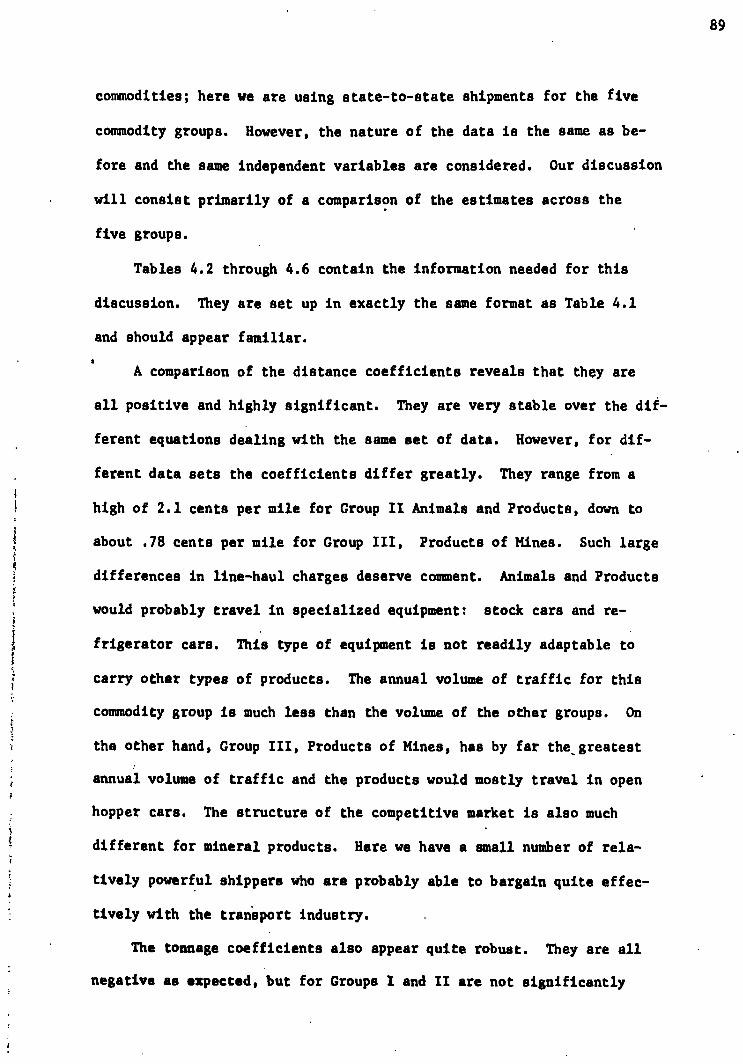
1

commodities; here we are using state-to-state shipments for the five

commodity groups. However, the nature of the data is the same as be-

fore and the sane independent variables are considered. Our discussion

will consist primarily of a comparison of the estimates across the

five groups.

Tables 4.2 through 4.6 contain the information needed for this

discussion. They are set up in exactly the same format as Table 4.1

and should appear familiar.

A comparison of the distance coefficients reveals that they are

all positive and highly significant. They are very stable over the dif-

ferent equations dealing with the same set of data. However, for dif-

ferent data sets the coefficients differ greatly. They range from a

high of 2.1 cents per mile for Group II Animals and Products, down to

about .78 cents per mile for Group III, Products of Mines. Such large

differences in line-haul charges deserve comment. Animals and Products

would probably travel in specialized equipment: stock cars and re-

frigerator cars. This type of equipment is not readily adaptable to

carry other types of products. The annual volume of traffic for this

commodity group is much less than the volume of the other groups. On

the other hand, Group III, Products of Mines, has by far the greatest

annual volume of traffic and the products would mostly travel in open

hopper cars. The structure of the competitive market is also much

different for mineral products. Here we have a small number of rela-

tively powerful shippers who are probably able to bargain quite effec-

tively with the transport industry.

The tonnage coefficients also appear quite robust. They are all

negative as expected, but for Groups I and II are not significantly

89

Distance Quantity Rate

Distance Quantity Rate

1.000 -0.232 1.000

0.939 -0.229 1.000

R Quantity Distance Intercept Eq.

97.65 106.78

.88

.88 -2.23 1.41 1.41

(4.33) (4.34)

Table 4.2

RAIL RATE REGRESSIONS

GROUP I: PRODUCTS OF AGRICULTURE

SIMPLE CORRELATION COEFFICIENTS

ESTIMATED COEFFICIENTS

ANALYSIS OF VARIANCE

S.S. M.S. Pr. D. F. F.

(1,000) (1,000) col.025 Source of Variance

Total

Reduction for meanRemainder

Reduction for distance Remainder

Reduction for quantity Remainder

628 2,055,201

1 1,268,282

627 786,918 1,255 1011 S.

1 693,407

626 93,511 149 4642 S.

1 118

625 93,393 149 1 N.S.

90

Rate • Distance Quantity

Distance Quantity Rite

1.000 0.007 1.000

0.905 -0.016 1.000

Eq. Intercept Distance Quantity R2 •

2.08 2.08

.82 -51.88 .82

425.18 441.69

(4.33) , (4.34)

Reduction for quantity 1 Remainder . 224 43,906 196 1 N.S.

123

Table 4.3

RAIL RATE REGRESSIONS

GROUP II: ANIMALS AND PRODUCTS

SIMPLE CORRELATION COEFFICIENTS

ESTIMATED COEFFICIENTS

ANALYSIS OF VARIANCE .

Source of Variance S.S. M.S. Pr.

D .F. F. (1,000) (1,000) a•.025

Total

Reduction for mean Remainder

.Reduction for distance Remainder

227 1,288,423

1 1,044,351

226 244,072 1,079 967 • S.

1 200,042

225 44,029 195 1022 S.

91

Distance Quantity Rate

ESTIMATED COEFFICIENTS

Intercept Distance Quantity R2 Eq.

ANALYSIS OF VARIANCE

Total 543 360,742

Reduction for mean 1 247,462 Remainder- 542 113,280 209 1184 S.

Reduction for distance 1 . 87,180 Remainder 541 26,099 48 1807 S.

Reduction for quantity 1 541 Remainder 540 25,557 47 11 S.

' •

D.F. a■ .025

1.000 -0.222 1.000

0.877 -0.262 1.000

Distance Quantity Rate

S.S. M.S. F. Pr. (1,000) (1,000) , Source of Variance

.77 185.36 0.79 (4.33) (4.34) 203.80 0.78 -0.85 .77

Table 4.4

RAIL RATE REGRESSIONS

GROUP III: PRODUCTS OF MINES

SIMPLE CORRELATION COEFFICIENTS

92

Distance Quantity Rate

Distance Quantity Rate.

1.000 -0.228 1.000

0.955 -0.290 1.000

Intercept Distance Quantity Eq. R2

.91

.92 (4.33) (4.34)

355.51 406.14 -15.86

0.96 0.94

S .S. M.S. F Pr. (1,000) (1,000) • col.025 Source of Variance D.F.

Total 353 1,127,350

Reduction for mean Remainder

1 766,353 352 360,896 1,025 747

Reduction for distance Remainder

Reduction for quantity Remainder

1 325,893 351 32,002

1 2,014

350 . 29,988 .

91 3607 r S.

85 24 S..

Table 4.5

RAIL RATE REGRESSIONS

GROUP IV: PRODUCTS OF FORESTS

SIMPLE CORRELATION COEFFICIENTS

ESTIMATED COEFFICIENTS

ANALYSIS OF VARIANCE

3

93

Reduction for distance 1 Remainder 1359

Reduction fOr quantity 1 Remainder 1358

Quantity

-0.239 1.000

Distance

1.000

Rate

0.833 -0.227 1.000

Distance Quantity Rate .

Intercept. Distance Quantity R2 Eq.

(4.33) 359.77 1.58 .69 (4.34) 387.21 1.57 -5.86 .70

Source of Variance S .S. M.S. Pr. F. (1,000) (1,000) col.025

Total 1361 7,219,579

Table 4.6

RAIL RATE REGRESSIONS

GROUP V: MANUFACTURES AND MISCELLANEOUS

SIMPLE CORRELATION COEFFICIENTS

Reduction for mean Remainder

ESTIMATED COEFFICIENTS

ANALYSIS OF VARIANCE

1 4,894,562

1360 2,325,017 1,709 2863 S.

1,614,009

711,007 523 3084 S.

1,914

709,092 522 4 N.S.

94

different from zero. Between groups they vary widely in size. The

greatest effect is again for Group II and the smallest for Group III.

Thus the comments made in the last paragraph are also pertinent here.

The commodity group with a small annual volume and requiring special-

ized equipment receives large quantity discounts; whereas the large

volume group probably charging rates close to costs, receives almost no

discount. This quantity effect should not be taken too seriously, how-

ever, as we shall later see that it is probably mostly due to equation

, error.4

Commodity Groups Utilizing Data on Commodity Classes. Again, we

are attempting to explain the level of rail rates for commodity groups.

However, we are now considering data on the individual commodity classes

comprising the groups. We have state-to-state shipment information for

each of the commodity classes. In estimating the equations for each

commodity group, we now utilize the data for all of the commodity classes

included within that group. Thus we are able to include the price and

density variables in the estimating equations. These equations now

become, for each commodity group,

(4.35) Rijk ■ 010 + 011 Mijk + e lijk

•

(4.36)R • ijk 820 + 82]. M ijk+O D 22 k + e2ijk

(4.37)R 210 +OP ijk 30 +0

31 M ijk +8 32 D k 33 k + e3ijk

(4.38) Rijk ■

95

84Q M +0 D+0 P+0 Q + e

40 41 ijk 42 k 43 k 44 ijk 411k

4. See especially Appendix A to this Chapter.

where

R

E average, revenue received, in cents per ton, for transporting the kth commodity class from state i to state j;

k E average distance, in miles, traveled by shipments of commodity k from state i to state j;

, of the kth

to state j;

Dk s the density, in average tons per car, of the kth

. • • • I. • - - •

Pk E the average wholesale price, in dollars per ton, of the ktn commodity class;

0 _ the nth coefficient to be estimated in the mt h mn = equation; and

elijk E the disturbance terms, (1 gm 1, 2, 3, 4).

Tables 4.7 through 4.11 present the results of this estimation

process. These tables differ slightly from the previous tables in that

they do not contain the correlation coefficients.

To begin with, we note that the distance coefficients are again

all positive and highly significant. They also retain their intra-

group stability. Comparison of these with the distance coefficient es-

timates contained in Tables 4.2 through 4.6 reveals that the coefficients

retain their intergroup standings in magnitude, and that coefficients

of the sane commodity group are roughly of the same magnitude. How-

ever, they are usually slightly higher for the less aggregate data.

The density variables, which we are using for the first time, all

enter with negative, and significant coefficients -- the greater the

average weight per carload the less the rate per ton. This effect is

kreatest for manufactured products where it is approximately 30 cents

96

Qijk = annual tonnage, in thousands of tons commodity class shipped from state i

commodity class shipped from state i to state j;

48.62 665.51 565.99 575.92

-13.57 -12.01 0.23 -12.71 0.23

.87

.89

.89 14.89 .90

1.47 1.34 1.35 1.35

D .F. (1,000) (1,000) " S.S. M.S. Pr.

F ' a•.025 Source of Variance

Total ' 1159 3,214,932

Table 4.7

RAIL RATE REGRESSIONS COMMODITY CLASSES

GROUP I: PRODUCTS OF AGRICULTURE

ESTIMATED COEFFICIENTS

Intercept Distance Density Price .Quantity R2

ANALYSIS OF VARIANCE

Reduction for mean Remainder .

1 1,566,880 1158 1,648,051 1,423 1101 S.

Reduction for distance 1 Remainder 1157

Reduction for density 1 Remainder 1156

1,433,202 214,848 185 7718 S.

38,901 175,946 152 256 S.

Reduction for price Remainder

1 1,926 1155 174,020 150 13 S.

Reduction for quantity 1. Remainder . - 1154

1,706 172,313 149 11 S.

97

7.70

.82

.83

.85

.85

2.23 2.11 2.02 2.02

332.42 808.54 478.58 477.43

-20.68 -17.23 -17.25

0.54 0.54

• Table 4.8

RAIL RATE REGRESSIONS COMMODITY CLASSES

GROUP II: ANIMALS AND PRODUCTS

ESTIMATED COEFFICIENTS

Intercept . Distance Density Price Quantity R2

ANALYSIS OF VARIANCE

S.S. M. S. D.F. F. (1,000) (1,000)

Pr. a.025 Source of Variance

Total

Reduction for mean Remainder

Reduction for distance Remainder

Reduction for density Remainder

Reduction for price Remainder

Reduction for quantity Remainder

197 1,182,713

1 948,006 196 233,707 1,192 796 S.

1 190,764 195 42,942 220 866 S.

1 3,760 194 39,182 201 19 S.

1 4,420 193 34,761 180 25 S.

1 • 192 34,761 181 '0 N.S.

98

3.05 2.99 -0.39

0.87 0.83 0.82 0.82

.78 .

.82 83 .83

-7.57 -6.46 -6.37

145.00 609.67 496.61 494.81

F.

Table 4.9

RAIL RATE REGRESSIONS COMMODITY CLASSES

GROUP III: PRODUCTS OF MINES

ESTIMATED COEFFICIENTS

2 Intercept Distance Density Price Quantity R -

ANALYSIS OF VARIANCE.

Source of Variance D.F; S.S. M.S. F Pr.

(1,000) (1,000) am.025

Total

Reduction for mean Remainder

935 377,326

1. 231,628

934 145,697 155 . 1485 S.

Reduction for distance 1 114,038 Remainder 933 31,658 33 3360 S.

N s

Reduction for density 1 5,164 Remainder 932 26,494 28 182 S.

1 1,893

. 931 24,600 26 72. S.

Reduction - for quantity 1 71 Remainder 930 • 24,529 26 3 N.S.

Reduction for price Remainder

99

.94

.94

.94

.94

0.98 0.98 0.97 0.96

269.02 931.44 900.75 870.73 -3.85

0.21 0.20

-16.98 -16.46 -15.47

S.S. (1,000)

N . S. (1,000)

Pr. a■ .025 Source of Variance D.F. F .

Table 4.10

RAIL RATE REGRESSIONS COMMODITY CLASSES

GROUP IV: PRODUCTS OF FORESTS

ESTIMATED COEFFICIENTS

Intercept Distance Density Price .Quantity • R2

ANALYSIS OF VARIANCE

Total - 444 1,360,657

Reduction for mean 1 Remainder 443

Reduction for distance 1 Remainder 442

• Reduction.for density 1 Remainder 441

Reduction for price Remainder

Reduction for quantity 1 Remainder 439

830,917 529,739

495,356 34,383

4,047 30,336

143 30,192

71 30,121

1 440

1,195 695 S.

77 6368 S.

68 59 S.

68 2 N.S.

68 1 N.S.

100

0.25

1.91 1.75 1.70 1.71 0.25

.60 '.71 .73 .73

286.69 1654.07 1392.87 1294.47 15.11

-36.13 -30.95 -31.29

S.S. M.S. D.F. F. (1,000) (1,000) - Source of Variance Pr.

ago.025

Table 4.11

RAIL RATE REGRESSIONS COMMODITY CLASSES

GROUP V: MANUFACTURES AND MISCELLANEOUS

ESTIMATED COEFFICIENTS' .

Intercept -2 Distance Density . Price Quantity R • •

.ANALYSIS OF VARIANCE

Total

Reduction for mean , Remainder, :

Reduction for distance Remainder

Reduction for density Remainder

Reduction for price -Remainder

• . . Reduction for quantity

Remainder

4200 18,216,183

1 9,097,443 4199. 9,118,740

• 5,428,736 4198 3,690,003

1 1,035,729 4197 2,654,274

. 1 179,886

4196 2,474,387

1 1,087 4195 2,473,300

2,171 4189 S.

878 6167 S.

632 1638 S.

589 305 S.

589 2 N.S.

101

Table 4.12

RAIL RATE REGRESSIONS

FINAL COEFFICIENTS ESTIMATES

Group Intercept Miles Quantity Density Price 1(2 it

"All Commodities"

354.15 1.40* -2.01* .69 1609

Commodity Groups

I 106.78 1.41* -2.23 .88 628 II 441.69 2.08* -51.88 .82 227 III 203.80 0.78* -0.85* .77 543

, IV 406.14 0.94* -15.86* .92 353 V 387.21 1.57* -5.86 .70 1361

Individual Commodities by Commodity Group?

575.92 1.35* 14.89* -12.71* 0.23* .90 1159 II 477.43 2.02* 7.70 -17.25* 0.54* .85 197 III 494.81 0.82* -0.39 -6.37* 2.99* .83 935 IV 870.73 0.96* -3.85 -15.47* 0.20 .94 444 V 1294.47 1.71* 15.11 -31.29* 0.25* .73 4200

All Commodity Groups

1226.41 1.36* 2.77* -23.92* 0.35* .73 6935

*Denotes an estimate significantly different from zero, in the direction indicated by its sign, at the a in .025 level.

per extra ton per car. It falls off to about 16 cents for Products of

Forests and Animals and Products, to 12 cents for Products of Agri-

culture and finally to 6 cents for Products of Mines.

The wholesale price of the commodity was the third variable en-

tered. We reasoned that if the railroads engaged in value of service

pricing, this variable should contribute significantly to the equation.

The estimated coefficients are quite stable and significant with the

exception of Group IV, Products of Forests. The estimated effect is

10;

greatest for Products of Mines where a one-dollar increase in the whole-

sale price of the product is associated with a 3.1-cent increase in the

rate. However, the most significant effect is achieved for Group V,

Manufactures. These results are in accord.with our a priori beliefs.

Due to the strange behavior of the tonnage coefficient estimates,

we shall discuss those effects further in Appendix.A to this Chapter.

.Table (4.12) summarizes our final coefficient estimates for the rail

rate equations.

Barge Transport

The data utilized in our investigations of water and motor freight

rates were of a different nature than the rail data. The rail data

were taken from public documents -- annual statistics collected and pub-

lished by the Interstate Commerce Commission. No such statistics ex-

isted for. water or truck transport. For these modes it was necessary

to collect and process revenue and tonnage information from private

sources. This was accomplished quite satisfactorily for motor carriage,

less so for barge.

The truck data will be seen to include some forty-six large carriers

and to cover at least the central United States quite well. The water

data are for only one carrier, A. L. Mechling Barge Lines, Inc, (MBL).

However, ME, is a large, and hopefully representative, water carrier.

During 1963, MBL operated on it least seventeen different river systems

and was one of the six largest water common carriers in the United States.

The Data. From A. L. Mechling Barge Lines, Inc., we have the follow-

ing usable information derived from freight bills for the year 1963.

103

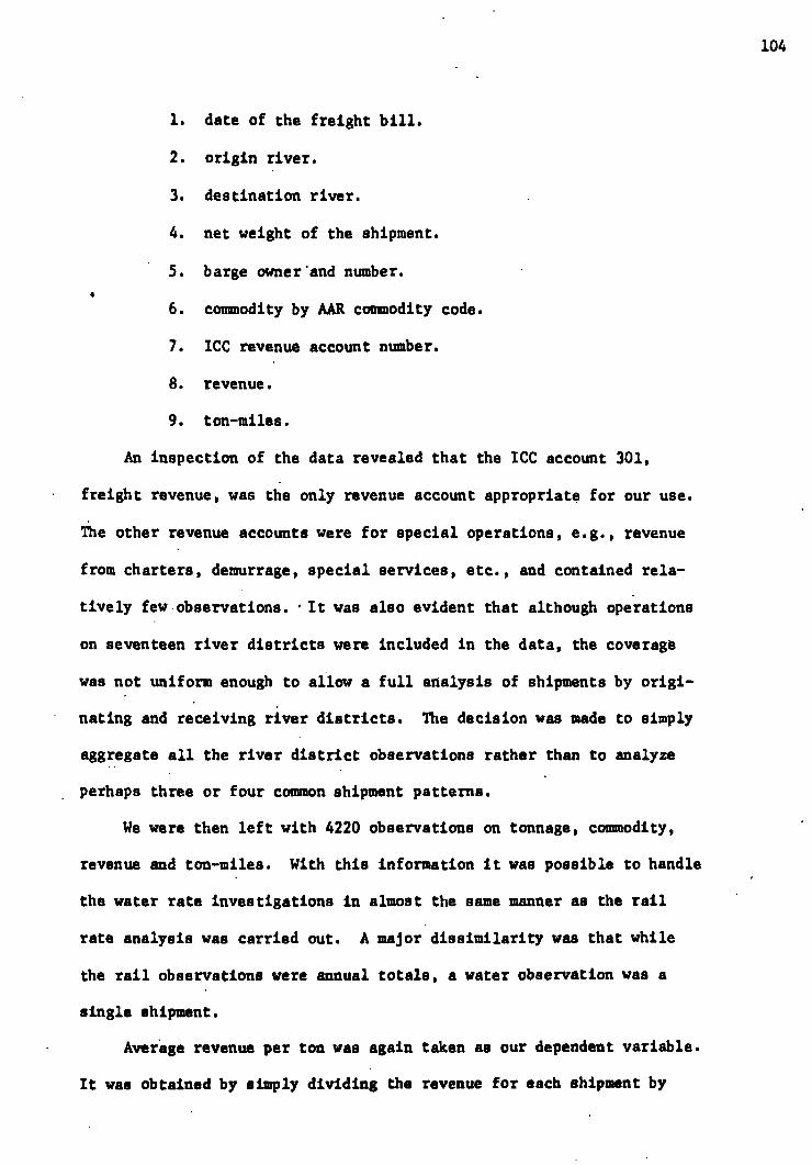
1. date of the freight bill.

2. origin river.

3. destination river.

4. net weight of the shipment.

5. barge owner and number.

6. commodity by AAR commodity code.

7. ICC revenue account number.

8. revenue.

9. ton-miles.

An inspection of the data revealed that the ICC account 301,

freight revenue, was the only revenue account appropriate for our use.

The other revenue accounts were for special operations, e.g., revenue

from charters, demurrage, special services, etc., and contained rela-

tively few observations. It was also evident that although operations

on seventeen river districts were included in the data, the coverage

was not uniform enough to allow a full analysis of shipments by origi-

nating and receiving river districts. The decision was made to simply

aggregate all the river district observations rather than to analyze

perhaps three or four common shipment patterns.

We were then left with 4220 observations on tonnage, commodity,

revenue and ton-miles. With this information it was possible to handle

the water rate investigations in almost the same manner as the rail

rate analysis was carried out. A major dissimilarity was that while

the rail observations were annual totals, a water observation was a

single shipment.

Average revenue per ton was again taken as our dependent variable.

It was obtained by simply dividing the revenue for each shipment by

104

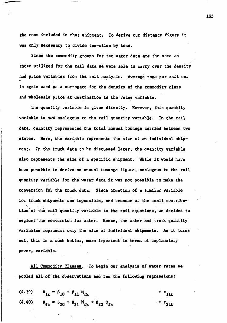
the tons included in that shipment. To derive our distance figure it

was only necessary to divide ton-miles by tons.

Since the commodity groups for the water data are the sane as

those utilized for the rail data we were able to carry over the density

and price variables from the rail analysis. Average tons per rail car

is again used as a surrogate for the density of the commodity class

and wholesale price at destination is the value variable.

The quantity variable is given directly. However, this quantity

variable is not analogous to the rail quantity variable. In the rail

data, quantity represented the total annual tonnage carried between two

states. Here, the variable represents the size of an individual ship-

ment. In the truck data to be discussed later, the quantity variable

also represents the size of a specific shipment. While it would have

been possible to derive an annual tonnage figure, analogous to the rail

quantity variable for the water data it was not possible to make the

conversion for the truck data. Since creation of a similar variable

for truck shipments was impossible, and because of the small contribu-

tion'of the rail quantity variable to the rail equations, we decided to

neglect the conversion for water. Hence, the water and truck quantity

variables represent only the size of individual shipments. As it turns

out, this is a much better, more important in terms of explanatory

power, variable.

All Commodity Classes. To begin our analysis of water rates we

pooled all of the observations and ran the following regressions:

(4.39) R.. ■ B10 10 4. 8 11 Mik

+ elk

(4.40) Rik 0

20 + 0

21 Mik

+ 022

Qik

+ e2ik

105

+ e3ik

(4.41) Rik ■ 030 + 031 Mik + 032 Qik + 033 Dk

(4.42) R.. ■ 840 40 4. 841 Mik 842 Qik 4. 8 43 Dk 4. 844 Pk e4ik

where

Rik

3 average revenue received, in cents per ton, for transporting the ith shipment of commodity class k;

Mik = distance, in miles, of the i

th shipment of commodity k;

Qik tons carried in the ith shipment of commodity k;

Dk 3 the density, in average tons per car, of the k th commodity class;

Pk the average wholesale price, in dollars per ton,

of the ktn-commodity class;

th Omn 3 the n- coefficient to be estimated in the mth equation; and

elik = the disturbance terms, (1 ■ 1, 2, 3).

Table 4.13 contains the estimated coefficients and an analysis of

variance table. We note first of all that all of the coefficients are

significantly different from zero. The distance coefficients are posi-

tive and quite robust. Each 100-mile increase in distance will increase

the water rate by about thirty cents. Later, we will compare these

coefficients with the rail coefficients.

The quantity coefficients are negative as expected and quite sig-

nificant. The greater the amount shipped at any one time, the less is

the rate per ton. The density coefficient also appears negative and

highly significant. Its effect is by far the largest of any examined

here. A one hundred ton increase in the density variable would lower

the water rate by perhaps $3.00.

The price coefficient is very interesting. Its value is relatively

small but it is positive and highly significant. Value of service rate

106

0.296 0.278 0.298 0.288

(0.004)

-0.171 -0.158 -3.794 -0.148 -2.785 0.164

(0.004) (0.203) (0.012)

.519

.640

.670

.685

58.769 230.607 394,535 322.947

Reduction due Remainder

Reduction due , Remainder

Reduction due Remainder

Table 4.13

WATER RATE REGRESSIONS

ALL COMMODITIES

ESTIMATED COEFFICIENTS (and final, standard errors)

r.

Intercept Distance •Quantity Density • Price R2

ANALYSIS OF VARIANCE

Source of Variance

D.F S.S. M.S. Pr.

. F. (1,000) (1,000) a•.025

.1•11.1111.11

4220 90,268

Reduction due to mean Remainder

to distance 1 18,116 4218 16,817' 4.22 4293 • S.

to quantity 1 4,240 •

4217 12,576 2.98 1423 S.

to density . 1 1,046

4216 11,530 2.74 382 S.

Reduction due to price 1 518 Unaccounted for 4215 11,012 2.61 198 S.

Total

1 55,336 4219 34,933 8.28 6683 S.

107

making is usually taken to refer to rail pricing. Here we have some

evidence of it in association with water rates. We usually refer to

water transport as a competitive industry and assume that rates should

be based solely on costs. However, only if we are willing to ignore

all demand considerations can we expect the price variable to have no

effect. If we allow for any demand conditions, we have a situation

where price affects quantity and quantity affects costs and thus rates.

While this may or may not be (or be considered to be) value of service

rate making it certainly allows product price a place in rate deter-

mination.

Commodity Classes by Commodity Groups. We next divided the data

up into the five major AAR commodity groups and ran separate regressions

for each group. The results of this work are presented in Tables 4.14

through 4.17. Commodity Group II, Animals and Products, was not repre-

sented in thewater data and Commodity Group IV, Products of Forests,

was represented by only two commodity classes. Hence we have no re-

gression results for the former group and, due to degrees of freedom

considerations, have only two meaningful regressions for the latter.

Comparing these tables, we see that all of the distance coefficients

are positive and significant. They range in value from about 0.20 for

Group III, Products of Mines, through 0.24 for Group I, Products of

Agriculture, and 0.34 for Group V, Manufactures and Miscellaneous,

up to about 0.40 for Group IV, Products of Forests. These coefficients

appear robust and reasonable. The great explanatory power of the dis-

tance variable for Groups I and IV should be noted.

For Groups I and V the quantity coefficients came out with the

expected, negative sign and were all significant. For Group IV the

108

0.242 0.243 0.243 0.244

-0.027 -0.015 -0.017

Total 1110 89,944

109

Table 4.14

WATER RATE REGRESSIONS

GROUP I: PRODUCTS OF AGRICULTURE

ESTIMATED COEFFICIENTS (and final standard errors)

Intercept Distance Quantity . Density Price R2

63.680 89.078

174.529 140.831

• .919 .922

-1.781 .924 -1.361 0.206 .925

(0.002) (0.005) (0.333) (0.046)

ANALYSIS OF VARIANCE

Source of Variance S.S. M.S. Pr.

D.F. F. F (1,000) (1,000) cm.025

Reduction due to mean • 1 61,399 Remainder 1109 28,544 25.74 2,385 S.

Reduction due Remainder

Reduction due Remainder

Reduction due Remainder

to distance 1 26,240

1108 • 2,303 2.08 12,621 S

to quantity 1 75 1107 2,228 2.01 37 S.

to density 1 59 1106 2,168 1.96 30 S.

Reduction due to price Unaccounted for

1 38 1105 2,130 1.93 19 S.

Total 728 79,603

Reduction due to mean Remainder.

1 70,242 727 9,360

Reduction due . Remainder

Reduction due Remainder

to distance 1 5,075 726 - 4,285

to quantity 1 46 725 4,239

Reduction due Remainder

to density 1 575 724 3,664

Reduction due to price Unaccounted for

1 33 723 3,630

Table 4.15

WATER RATE REGRESSIONS

GROUP III: PRODUCTS OF MINES

ESTIMATED COEFFICIENTS (and final standard errors)

Intercept Distance ,Quantity Density Price I2

•

-9.949 -34.383 -183,774 -147.429

0.210 .542

0.202 0.028 .547

0.196 0.005 2.629 .609

0.197 0.005 1.905 0.410 .612

(0.007) (0.010) (0.373) (0.159)

ANALYSIS OF VARIANCE •

Source of Variance S.S. M.S. Pr.

D.F. (1,000) (1,000) F or.025

12.88 5455 S. -

5.90 860 S.

5.85 7 S.

5.06 113 S.

5.02 . 6 S.

110

. 7

Source of Variance

1

• Table 4.16

WATER RATE REGRESSIONS '

GROUP IV: PRODUCTS OF FORESTS

ESTIMATED COEFFICIENTS (and final standard errors).

Intercept Distance Quantity :Density price R2-

'

67.936 139.490 238.571 -8:186

0.443 .973 0.428 -0.081 .973 0.389 -0.035 -2.390 •974 0.389 -0.035 2.250 0.922 .968

(0.039) (0.087) (0.000) (0.000)

ANALYSIS OF VARIANCE

S:S: M.S. Pr. •D.F. - F.

(1,000) (1,000) am.025

, • . _ . _

Total

Reduction due Remainder

Reduction due Remainder

Reduction due Remainder

Reduction due Remainder

59 8;917

to mean

to distance

to quantity 1

to density

1

1 7,183

58 1,734 29.90 240

1* . 1,686 •

57 . 48 0.84 201

56 . 56 . 47 0.83 1 N.S.

Reduction due to price Unaccounted 'for

111

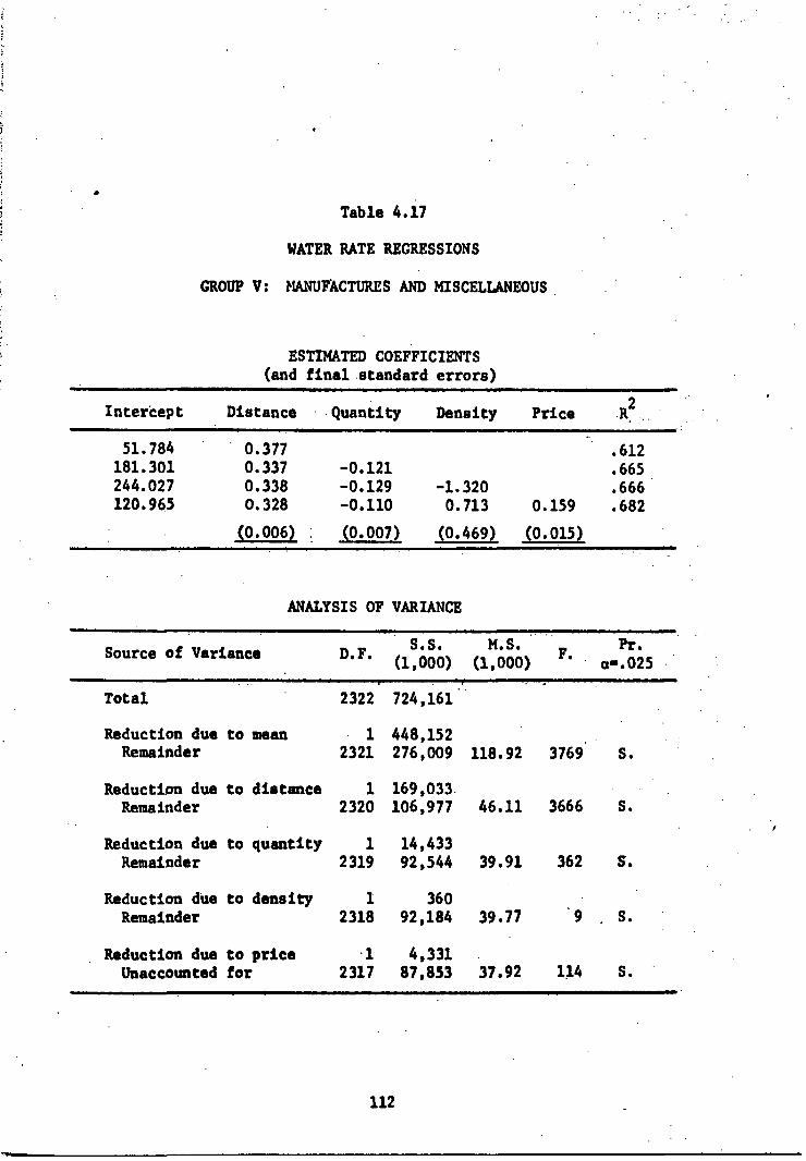
D.F S.S• M.S. Pr. . (1,000) (1,000) F. coi.025 Source of Variance

Total

Reduction due Remainder

Reduction due Remainder

Reduction due Remainder

Reduction due Remainder

2322 724,161'

to mean • 1 448,152 2321 276,009 118.92 3769 S.

to distance 1 169,033.

2320 106,977 46.11 3666 S.

to quantity 1 14,433 2319 92,544 39.91 362 S.

to density 1 360

2318 92,184 39.77 9 S.

Table 4.17

WATER RATE REGRESSIONS

GROUP V: MANUFACTURES AND MISCELLANEOUS

ESTIMATED COEFFICIENTS (and final standard errors)

Intercept Distance • -Quantity Density Price F

51.784 181.301 244.027 120.965

• 0.377 .612

0.337 -0.121 .665

0.338 -0.129 -1.320 .666

0.328 -0.110 0.713 0.159 .682

(0.006) (0.007) (0.469) (0.015)

ANALYSIS OF VARIANCE

Reduction due to price 1 4,331 Unaccounted for 2317 87,853 37.92 114 S.

112

113

quantity effect was estimated to be negative but never significant. It

appears that for this group distance may well be the determining factor.

In the regressions dealing with Products of Mines, the quantity

coefficient appears positive, but significant only if both density and

price are excluded from the equation. As in the rail section, we are

led to infer that this is due to the market structure of the Mining

Industry. Its market power vis-a-vis the transportation industry's .

must be very great. Rates for comparable distances for Mining products

are much lower than for any of the other commodity classes and quantity

discounts Jo not exist.

The density coefficients are even less consistent. For Group I,'

they are negative and significant'. The coefficients of Groups IV and V .

change their sign from negative to positive as the price variable is

entered and lose their significance, while the density coefficients

, for Products of Mines are positive and significant. Perhaps we may

attribute this behavior to rational action on the part of the carriers.

Table 4.18 indicates that the average density of the commodities con-

tained in Group I is about the same as the overall average density but

Table 4.18

ANALYSIS OF WATER RATE REGRESSION DENSITY COEFFICIENTS

Commodity Average Density Standard Deviation Estimated Coefficients Group (Tons per car) (Tons per car) Eq. (4.41) (Eq. 4.42)

I 54.1 29.9 (-)* (-)* III 71.9 11.2 (+)* (+)*

• IV . 45.1 • 8.1 ' (-) (+) V 44.4 10.3 (-)* (+) All 51.7 13.7 (-)* (-)

*Indicates a coefficient statistically different from zero, in the indicated direction, at the 0.05 level of significance.

there is a wide difference between commodities. The negative density

coefficients for Group I may then be an attempt to allocate costs among

the commodities in a proper manner.. Groups IV and V have a.lower aver-

age density but variance is much lower than for Group I so that as

strict a .cost allocation is perhaps not viewed as a necessity. Group

III meanwhile illustrates a very high average density and a below aver-.-

age standard deviation. Hence for the.commodities included in this .

group, any further increase in density may be thought to cause carriage_

costs to rise rather than to fall.

The price coefficients are, happily, all positive and significant :.

except for the Group IV coefficient which is meaningless.

, We summarize our results in Table 4.19. This table is analogous..

to Table 4.12 which summarized the rail results.

Table 4.19

WATER RATE REGRESSIONS

FINAL COEFFICIENT ESTIMATES

Group .Intercept Miles Quantity Density . .Price R- . n _

Individual Commodities by Commodity Groups

I . 140.831 0.244* -0.017* . -1.361* 0.206* .925 1110

III -147.429 0.197* 0.005 1.905* 0.410 .612 728 IV . 139.490 0.428* -0.081 .973 59

. V . 120.965 • 0.328* '40.110* 0.713 0.159* .682 2326

All Commodities . .

322.947 0.288* -0.148* -2.785* 0.164* .685 4220

114

•4

*Denotes an estimate significantly different from zero, in the direction indicated by its sign, at the o ■ .025 level.

Motor Transport

The Data. We Were extremely fortunate in accumulating data for use

in our analysis of freight rates for motor carriers. Officials of the

Central States Motor Freight Bureau, Inc. kindly made available for

our use data derived from a 1964 revenue study they had conducted. They

had sampled the freight bills of 46 of the larger motor carriers oper-

ating out of the Central States region. Gross revenue of these 46

carriers was 60 percent of the total region's gross revenue. The sample

was not limited to intra-regional shipments, but covered all shipments

regardless of origin or destination.5

For analysis here we selected data on volume and truck-load inter-

state shipments. It was felt that of all the available truck shipments. .

this was the category Which was most likely to be in competition with

rail and water, carriage. For this category, we again had individual

shipment observations on revenue, size of shipment, distance, AAR •

commodity class,6

and, from our rail study, measures of density and

price of each commodity class. -.

Our analysis of truck rates was carried out in the same fashion as

the analysis of water rates so there is no need to rewrite the equa-

tions on the definitions of the variables.

5. Commodities in the truck data were coded according to the Na-tional Freight Classification numbers. With the aid of the Table of National Motor Freight Classification Numbers with Applicable Standard Transportation Commodity Code Numbers, (6/22/65), published by the National Motor Freight Traffic Association, Washington, D.C., we were able to convert these into the AAR classifications. A computer tape matching these classifications is now on file at the Econometric Research Center, Northwestern University.

6. Their procedure, developed by a consultant statistician, was, in essence, to record each 50th waybill for truck-load shipments and each 200th waybill for less-than-truck-load shipments.

115

All Commodity Classes. Table 4.20 contains the estimated co-

efficients for the first regression run. Here all of the interstate

volume and truck-load data were utilized. The most noticeable of the

coefficients are those associated with the quantity variable. We must

remember that this variable is now a measure of the size of an indi-

vidual shipment. The coefficients are large in value, highly signifi-

cant and very robust. For every one-ton increase in shipment size,

the rate Charged per ton will decrease by about $1.30. This variable

assumes an importance in the truck regressions it did not display in

the water results. We now wish that a comparable variable had been

available for the rail analysis.

The distance coefficients are also highly stable and significant.

On the average each extra mile of haul will result in about 2.8 cents

added to the rate per ton. The density coefficients are negative and

significantly different from zero, but the price coefficient, while

significant, is so small as to be almost meaningless. We should note

here that these data are dominated by observations on Group V, Manufac-

tures and Miscellaneous, almost completely. The table gives useful

summery statistics but it must be remembered that very little weight,

justifiably, from the data, is given to Groups I through IV.

Commodity Classes by Commodity Groups. Tables 4.21 through 4.25

contain the results of the regression analysis applied to the individual

commodity groups. We note first that the overall explanatory power of

these regressions is relatively small as compared to the rail or water

regressions. Our four independent variables leave a substantial pro-

portion of the variance of truck rates unexplained.

116

Intercept. _Distance ' Quantity . .Density . Price R2

Source of Variance .

Total 9267 70,310

Reduction due Remainder

Reduction due' Remainder

Table 4. .20

MOTOR RATE REGRESSIONS

ALL COMNODITY GROUPS

ESTIMATED COEFFICIENTS (and final standard errors).

921.748 2912.837 3046.173 3144.157

2.860 .233

2.833 -134.329 .454

2.772 -130.370 -5.488 .456

2.814 -129.696 -7.642 -0.070 .456

(0.049) (2.363) (1.337) (0.019)

ANALYSIS OF VARIANCE .

DF S.S. M.S. Pr.

. p (1,000,000) (1,000,000) • ass.025

• 1 36;967

9266 - 33,343

to distance .1 7,776

9265 - 25,568

'to quantity 1 7,373

9264 18,195'

to density 1 • 40 9263 '18,154

Reduction due to price . 1 . 28 Unaccounted for 9262 18,126

Reduction due to mean Remainder

Reduction due. Remainder

4 9241 , ° ' S.

3 • 2818 S.

3686 S.

20 S.

2 14 S.

117

Total 100 599,255

Reduction due to mean Remainder

1 462,279 99 136,976 1384 334 S.

Source of Variance S .S. M.S.

D.F. (1,000) (1,000) F• Pr.

a-.025

Table 4.21

MOTOR RATE REGRESSIONS

GROUP I: PRODUCTS OF AGRICULTURE

ESTIMATED COEFFICIENTS (and final standard errors)

Intercept Distance Quantity Density Price R2.

1329.031 1.626 .234

2764.884 2.296 -131.772 .588

4220.643 2.324 -121.928 -60.433 .634

3949.472 2.350 -118.209 -48.046 -0.283 .637

10421.1 (14.476) (21.458) (0.287)

ANALYSIS OF VARIANCE

Reduction due to distance 1 32,000 Remainder 98 104,976 1071 30 S.

Reduction due to quantity 1 48,477 Remainder 97 56,499 582 83 S.

Reduction due to density 1 6,309 • Remainder 96 50,190 523 12 S.

Reduction due to price 1 509 . • Unaccounted for 95 49,681 523 1 N.S.

118

350 149

305 12

306 1

309 0.5

S .

S .

N.S.

N.S.

Table 4.22

MOTOR RATE REGRESSIONS

GROUP II: ANIMALS AND PRODUCTS

ESTIMATED COEFFICIENTS (and final standard errors)

Intercept • Distance Quantity Density . Price R2

•

1190.845 1.282

1894.572 1.390 -51.744

2140.549 1.418 -51.401 -10.623

1916.308 1.410 -51.603 -4.668

(0.109) (15.009) (15.383)

.665

.712

.715 0.128 .716

(0.209)

ANALYSIS OF VARIANCE

S .S. M.S. F. D.F. (1,000) (1,000) Pr. .

ce..025 Source of Variance •

Total

Reduction due to mean Remainder

77 367,478

•1 289,115 76 78,363 1031 280 S.

Reduction due to distance Remainder

Reduction due to quantity Remainder

Reduction due to density Remainder

Reduction due to price Unaccounted for

1 52,108 75 26,255

1 3,673

74 22,582

1 245

73 22,338

1 116 72 22,222

119

Intercept Distance Quantity Density Price R 2

Reduction due Remainder •

Reduction due Remainder

Reduction due Remainder

to distance

to' quantity •

to density

Table 4.23

•MOTOR RATE REGRESSIONS

GROUP /II: PRODUCTS OF MINES

ESTIMATED COEFFICIENTS (and final standard errors)

819.050 1401.683 901.188

1063.097

2.648

2.373 -30.111

2.347 -35.006

2.252 -41.148

.596

.644

9.981 .669

2.393 12.305 .692

S0.A5_61 (10.170) (5.536) (5.582)

ANALYSIS OF VARIANCE

Source of Variance S .S. M.S. D .F.

(1,000) (1,000) Pr.

0..025

Total

Reduction due to mean Remainder

Reduction due to price Unaccounted for

70. 223,475

1 175,806

69 47,669 691 254

1 28,431

68 19,238 283 100 S.

1 2,248

67 16,990 254 8 S.

1 1,198

66 15,792 239 • 5 S.

1 1,098

65 14,693 226 4 S.

120

S.S. M.S. D.F. F.

(1,000) (1,000) Pr.

am:025 Source of Variance

Table 4.24

MOTOR RATE REGRESSIONS

GROUP IV: PRODUCTS OF FORESTS

ESTIMATED COEFFICIENTS (and final standard errors)

Intercept Distance Quantity Density Price R2

1129.459 2.137 .335

2137.502 2.504 -91.098 .647

2264.707 2.486 -91.515 -3.137 .647

1570.596 2.583 -93.904 21.420 -1.050 .661

(0.375) (15.382) (28.523) (0.839)

ANALYSIS OF VARIANCE

Total 45 200,771

Reduction due to mean 1 179,118 Remainder 44 21,653 492 364 S.

Reduction due to distance 1 7,243 Remainder 43 14,409 335 22 S.

• Reduction due to quantity 1 . 6,766 Remainder 42 7,641. 182 37 - S.

Reduction due to density 1 4 Remainder 41 7,639 186 .0 N.S.

Reduction due to price 1 288 Unaccounted for 40 7,351 184 1.6 N.S.

121

Intercept Distance Quantity Density Price R2

Total

Reduction due Remainder

Reduction due Remainder

Reduction due, Remainder

Reduction due Remainder

TABLE 4.25

MOTOR RATE REGRESSIONS

GROUP V: MANUFACTURES AND MISCELLANEOUS

ESTIMATED COEFFICIENTS (and final standard errors)

898.326 2910.595 3040.786 3162.747 -

•

2.948 .236

2.910 -135.387 .457

2.848 -131.518 -5.368 .459

2.904 -130.683 -8.068 -0.087 .460

(0.051) (2.415) (1.387) (0.019)

ANALYSIS OF VARIANCE

Source of Variance S.S. M.S. Pr. D.F.

(1,000,000) (1,000,000) F aa.025•

8975 • 68,919

to moan 1 35,875

8974 33,044 4 8968 S.

to distance 1 7,787

8973 25,257 3 2766 S.

to quantity 1 7,326

8972 17,931 2 3663 S.

to density 1 36

8971 17,895 2 18 S.

1 42

8970 17,853 2 21 S. Reduction due to price

Unaccounted for

122

The distance coefficients are all of the corect sign, significant

and generally robust. However, the mileage variable alone does not

display nearly the power it had in the rail and water data. For Groups

II and III the first equations are quite respectable but certainly not

overwhelming.

The quantity variables, however, display more importance than pre-

viously. Their coefficients are large and powerful. It appears that

motor carriers give very large discounts for increases in shipment

size. . Groups II and III whose results, in general, were the most sat-

isfactory and which gave relatively more emphasis to the distance var-

iable in turn showed less reliance on the quantity variable :

quantity coefficients were smaller in value and slightly less signif-

icant for these two groups.7

The density coefficients came out negative except for Group III,

Products of Mines, and the final coefficient for Group IV, which was

not significant. In general, these coefficients displayed very little

7. It should be noted that since our data were limited to volume and interstate shipments the usual high correlation between distance and shipment size was not present. See: W. Y. Oi and A. P. Hurter, Jr., Economics of Private Tuck Transportation, Wm. C. Brown, Dubuque, Iowa, 1965. The simple correlations between distance and shipment size for our data were

Group Correlation

0.317 II 0.302 III -0.346 IV 0.175 V -0.014

In only one instance was this correlation greater than the correlations between these variables and the dependent variable, rate. That was for Group II where the simple correlation between shipment size and rate was only 0.04.

123

stability and density showed very little explanatory power as compared

to the distance and quantity variables.

The price variable also showed very little explanatory power. The

coefficients were significant only for Groups III and V and these dif-

fered in sign and relative size. In three of the five cases the co-

efficient was estimated to be negative indicating higher value commodi-

ties travel at lower rates. This is hardly in accord with our expecta-

tions or with the results of the rail and water analysis.

In general, the results of the truck analysis were not on a par •

with the rail and water results. The overall explanatory power of the

equations was less and the coefficients of the density and price vari-

ables came out rather poorly. On the other hand,, the distance co-

efficients, while weaker in overall explanatory power, were all of the

right sign, robust and highly significant. The really impressive per-

formers were the size of shipment variables. These displayed an

importance never approached in the rail or water data.

The final coefficient estimates for the motor rate equations are

summarized in Table 4.26. Following our discussion of the demand

equations,'all of our empirical results will be compared and summarized.

Empirical Results -- The Demand Equations

Comparable shipment data for several modes of freight transport,

even of a cross-sectional nature, are very scarce at the present time. -

We were forced, therefore, to utilize shipment information from the

1963 Census of Transportation.8 The Commodity Transportation Survey

8. For a critical appraisal of this census see: J. P. Crecine, L. N. Moses, and J. Stucker, "The Census of Transportation: An

124

Table 4.26

MOTOR RATE REGRESSIONS

FINAL COEFFICIENT ESTIMATES

Group Intercept Miles Quantity Density Price Rz

Individual Commodities by Commodity Groups

3949.47 2.35* -118.21* -48.05* -0.28 .64 100 II 1916.31 1.41* -51.60* -4.67 0.13 .72 77 III 1063.10 2.25* -41.15* 2.39 12.30* .69 70 IV 1570.60 2.58* -93.90* 21.42 -1.05 .66 45 V 3162.72 2.90* -130.68* -8.07* -0.09* .46 8975

All Commodities

3144.16 2.81* -129.70* -7.64* -0.07* .46 9267

*Denotes an estimate significantly different from zero, in the direction indicated by its sign, at the col.025 level.

of this census contains data on the shipments of commodities, by Trans-

portation Commodity Classification (TCC) groups and by major mode of

transportation between twenty-five standard metropolitan statistical

areas (SMSAs).

We considered it necessary to utilize the same commodity groupings

for both the rate equations and the demand equations. Since this re-

quired the difficult transformation of the rate data from AAR commodity .

Evaluation," published in Papers--Seventh Annual Meeting, Transportation Research Forum, Richard B. Cross, Oxford, Ind., 1966.

9. "Commodity Transportation Survey," 1963 Census of Transportation Parts 1 61 2, GPO, Washington, D.C. 1966.

10. The Transportation Commodity Classification is composed of the first five digits of the Standard Transportation Commodity Code de-veloped by the Association of American Railroads.

125

Qr + 9m ' a + BTc*

+ yA

Tc - Tr oa +bQ +cM r r rr r c r T - TM o am + bmgm + cmM

'Tr of +gM r r r

Tm o fm +g MM.

(4.43)

(4.44) '

(4.45)

(4.46)

(4.47)

groups into STCC commodity groups, we restricted our analysis to four

STCC groups. These were

• STCC 26 -- Pulp, paper and allied products,

STCC 29 -- Petroleum and coal products,

STCC 30 -- Rubber and miscellaneous plastics products, and

STCC 32 —. Stone, clay and glass products.

Group 29 was selected as it was the only commodity group which con-

tained a usable number of barge shipments. The other groups were se-

lected on the basis of number of usable rail and motor observations and

their compatibility with the rate commodity groupings. Our findings

are reported in the following sections. Section 1 deals with the es-

timation of the two-mode model for STCC Groups 26, 29, 30 and 32.

Section 2 discusses the application of the three-mode model to Group

29, Petroleum and coal products.

The Two-Mode Model

Using the subscripts r and m to denote rail and motor transport,

our two-mode model is

126

A two-step procedure is again utilized in estimating this system. First

the rate equations are estimated; then the reduced form of equations

(4.43), (4.44) and (4.46) is derived and estimated.

Since the census data did not include freight rates, it was neces-

sary to use our other data sources for the rate equations. This

. necessitated conversion of those data from their.original AAR groupings

into the STCC groups. 13 Freight rates were then regressed on distance,

quantity, density and price, as before. These estimates are presented

in Tables 4.35 through 4.38 following this section. Table 4.36 also

contains the estimated coefficients for water transport of STCC group

29. As these rate results are quite comparable with those presented

previously by AAR group, we shall concentrate on the demand equations.

Substituting equations (4.46) and (4.47) into (4.43), (4.44) and

(4.45), 'we obtain

(4.48) Qr + Qa - OTc

a + yA %

(4.49) -b 0 + Tc (a + f ) + (Cr + g ) M r -r r r r

(4.50) -b Q + Tc -(am f) + (c + g ) M. m m m m m

11. See footnote 8.

12. An investigation was made of the possibility of aggregating pub-lished freight tariffs to obtain rates for the selected commodity groups. It was found that due to the large number of commodities contained in each STCC group and the many , possible rates for each commodity, from a single city to another city, because of quantity discounts, packaging specifications, etc., a very expensive effort would be required to pro-duce any reasonable results.

13. This was a very subjective procedure.as the codes were largely incompatible. An attempt was made to match each classification to the other, individually. The following groupings appeared to contain a. minimum of misclassification.

STCC 26 -- MR 653, 657, 659, 661, 663, 665, 669 and 671 STCC 29 -- MR 501, 503, 505 and 507

. STCC 30 -- MR 525 and 549 STCC 32 -- MR 663, 637, 639, 641, 693, 695, 701 and 721.

127

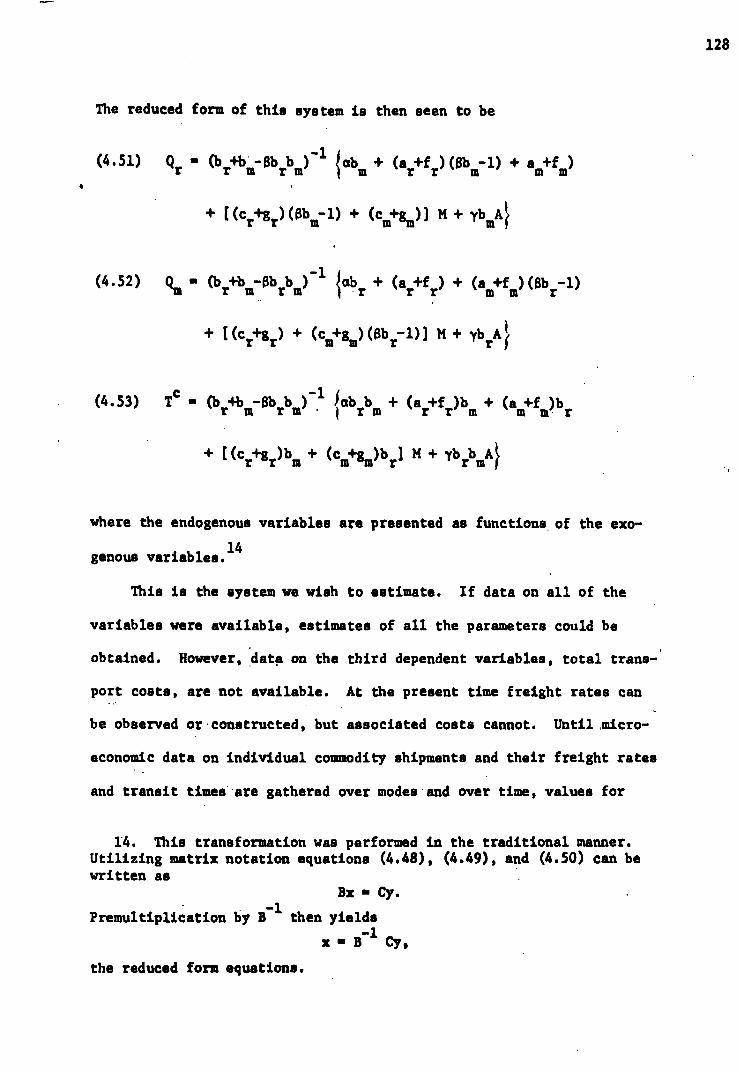
The reduced form of this system is then seen to be

(4.51) Qr (b +1) . -01) b ) -1 iab + (a +f )(8b -1) + a +f ) V in rm m r r m mm

+ [(cr+gr)(0bm-1) + (cli;lim)] M + mf

- (4.52) Qm ■ (b_+b_ L-0b_b_)1 iabr + (ar+fr) + (am+fm)(Obr-1) L

+ i(cr+gr) + (cm+gm)(0br-1)] M + ybrA lf

. (4.53) 'IC ■ (b 4b -Bb b ) -1 lab b + (a +f )b + (a +f )b rmrm.irm rrm mm- r

+ r(cr+gr)bm + (cm+gm)br] M + ybrbm4q

where the endogenous variables are presented as functions of the exo-

genous variables.14

This is the system we wish to estimate. If data on all of the

variables were available, estimates of all the parameters could be

obtained. However, data on the third dependent variables, total trans-

port costs, are not available. At the present time freight rates can

be observed or constructed, but associated costs cannot. Until micro-

economic data on individual commodity shipments and their freight rates

and transit times are gathered over modes and over time, values for

14. This transformation was performed in the traditional manner. Utilizing matrix notation equations (4.48), (4.49), and (4.50) can be written as

Bx ■ Cy. -

Premultiplication by B1 then yields

■ B-1 Cy ,

the reduced form equations.

128

this variable will remain unknown. We are restricted, then, to es-

timating the first two equations of the reduced form.

To illustrate the useful information to be gained from a quanti- • tative analysis of these "demand equations," we digress for a moment.

In Chapter III we were able to derive qualitative statements concern-

ing changes in the equilibrium values of the endogenous variables

brought about by changes in system parameters.15 Applying that analysis

to the two-mode linear model specified above, we can construct Table

4.27. This table relates unit changes in parameters and exogenous var-

iables to the induced changes in transport (endogenous) variables.

Given empirical estimates of these parameters, the table and the re-

lation AY ■ 3Y/3X AX can be utilized to make predictions of system

effects arising from parametric changes.

For example, suppose the ICC should grant a five cent per mile

increase in all rail rates. Between two markets M miles apart the rail

rate would increase by (50.M.Z/Z) or by 5M0. The truck rate, assumed

independent of the rail rate, would remain constant. The 5Mc increase

in the rail rate would shift the T c function upward by a like amount.

1

truck. The reduction in quantity shipped also lowers the value of Tc

Wilbb7br) 1 and the T

as by

r m • Shifts in all other system parameters can

be traced through the table in a similar manner.

15. See Chapter III, pp. 54-58.

129

This would result in a decrease in the total quantity shipped between MOb m

the two markets of — (since $ is negative). This decrease in the M(0b-1) m

total quantity is composed of a reduction of z in the quantity

carried by rail and an increase of — in the quantity transported by

Induced Changes in Endogenous Variables (Y)

Qm Tc IT: T: 1T Exogenous , Changes(X) Qr Qm Tc

Tr

Tm

a Tm

Transport demand (a)

Transport demand ($)

Transport demand (y)

Transport demand (A)

Rail Rate (fr)

Rail Rate (gr)

Motor Rate (fm)

Motor Rate (gm)

Assoc. costs, rail Car)

Assoc. costs, rail Cy

Assoc. costs, rail (Cr)

Assoc. costs, motor(am)

Assoc. costs, motor(b)

Assoc. costs, motor(cm)

b +b r m

Tc (br+bm)

A (br+bm)

y (br+bm)

Obm

M Bbm

Bbr

M Obr

Bbm

QrBbm

M 0 bm

$br

0 Bb r

M Bb r

br

Tcbr

A br

y br

1

$ br-1

M(Obr-1)

1

Qr

Obr-1

Q(b-1)

M(8br-1)

bb ✓ m

Tcb b ✓ m

A b b t in

y brbm

bm

Mb .m

br

Mbr

bm

Qrbm

Mbm

br

O b 'm r

Mb r

bb I ID

Tcb b t in

A b b ✓ m

y b b I DI

Bb b -b r m r

M(Ob b -b ) r m r

013 b -b I ID III

M(Bb rbm-bm)

UI

Qrbm

Mb in

br

0 b 'm r

Mb r

bb ✓ m

Tcb b t in

A b b t in

y b b I DI

Bb b -b ✓ m r

M(8b b -b ) ✓ m r

Bb b -b • 131 M

M(Bb rbutbm)

bm

Qrbm •

Mbm

br

0 b r

Mb r

bm

• in LbA b

m

y bm

0 bm-1

M( 8b -1)

1

8b in-1

Qr (Bbm-1)

M(8b-1)

1

Qm

in

0

0

0

0

M Z

0

0

0

0

0

0

0

0

0

0

0

0

0

0

M Z

0

0

0

0

0

0

Table 4.27

QUALITATIVE ANALYSIS FOR THE RESTRICTED TWO-MODE LINEAR MODEL

NOTE: All expressions have a common denominator of Z = b +b -013 b r in rm

Having investigated the information which would result if complete

estimation of the reduced form were possible, we are now able to ad-

dFess the implications of partial estimation. It turns out that

(1)as seen previously, complete estimation of the rate equations

is possible;

(2)estimation of only the first two equations of the reduced form

while, in general, ruling out quantitative (cardinal) estimates

of the system effects will allow qualitative comparisons to

be made.

For example, we may be able to derive an estimate of the ratio b m/br

as, say, three. This would allow us to estimate the decrease in total

quantity shipped and the increase in shipper's cost resulting from an

"x" cent increase in the rail rate to be three times that which would

result from a similar increase in the motor rate. The same relation

holds for changes in the associated costs. The relative total elastici-

ties of transport demand with respect to the transport rates can also

be derived.

After extensive preliminary investigations we selected the follow-

ing information from the available Census of Transportation data for

our reduced form eitimation.16

16. These preliminary investigations were presented in two documents. The relation between quantities shipped, by mode, and distance was re-ported upon in "Demand and Interface," 1967 Report to the Corps of Engineers.

The relationship between total exports and imports, by commodity, and various market indicators was presented in C. Letta, M.S. thesis, Trans-portation Center, Northwestern University.

Briefly we may summarize the conclusions as: (1) abstractly there is a very close relationship between distance and quantities shipped; but (2) none of the common indicators of economic activity (value added, employment in manufacturing, personal income, etc.) were found to be more than slightly correlated with a region's imports or exports.

131

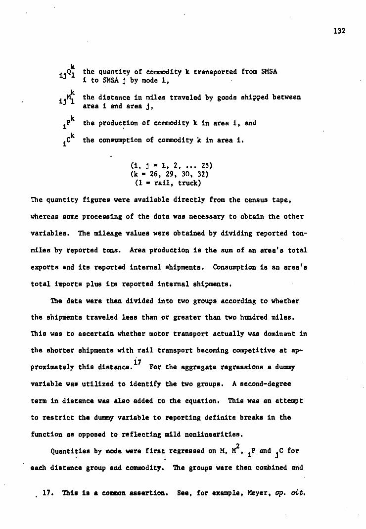
the quantity of commodity k transported from SMSA i to SMSA j by mode 1,

Mk the distance in miles traveled by goods shipped between ij 1 area i and area j,

Pk

the production of commodity k in area i, and

iCk

the consumption of commodity k in area i.

(i, j • 1, 2, ... 25) (k • 26, 29, 30, 32) (1 ■ rail, truck)

The quantity figures were available directly from the census tape,

whereas some processing of the data was necessary to obtain the other

variables. The mileage values were obtained by dividing reported ton-

miles by reported tons. Area production is the sum of an area's total

exports and its reported internal shipments. Consumption is an area's

total imports plus its reported internal shipments.

The data were then divided into two groups according to whether

the shipments traveled less than or greater than two hundred miles.

This was to ascertain whether motor transport actually was dominant in

the shorter shipments with rail transport becoming competitive at ap-

proximately this distance.17

For the aggregate regressions a dummy

variable was utilized to identify the two groups. A second-degree

term in distance was also added to the equation. This was an attempt

to restrict the dummy variable to reporting definite breaks in the

function as opposed to reflecting mild nonlinearities.

Quantities by mode were first regressed on M, M2 , iP and j C for

each distance group and commodity. The groups were than combined and

132

. 17. This is a common assertion. See, for example, Meyer, op. cit.

.133

an aggregate equation estimated, for each commodity group, with only

the dummy variable differentiating between the distance groups. Finally,

another set of aggregate regressions were estimated containing two ad-

ditional independent variables. These were P and iC and represented

an attempt to move behind the transport demand function to the area

product supply and demand functions.18

Tables 4.28 through 4.31 con-

tain the parameter estimates and related statistics.

In general, the overall fit of the equations may perhaps be said

to range from poor to fair. However, only one of the twenty-four equa-

tions is not statistically significant. Since the dummy variable was

set up to assume a value of one for distances less than two hundred

miles and zero for greater distances, we would expect the coefficient

to display a negative sign for rail and a positive sign for motor

transport. This expectation is realized in four of the eight equations.

Group 26 yielded the expected results for both specifications of the

• model. Groups 29 and 32, however, yielded the "correct" signs for the

third set of regressions. When the additional C and P variables were

entered into the equation the coefficient of the dummy variable for

rail transport became positive'.

STCC.30's dummy variable coefficient came out positive for both

equations. However, the peculiarity here appears to be not the absence

of a shift between the distance groups but the behavior of the greater

distance group itself. This is reflected in the mileage coefficient.

For rail transport they are all positive, indicating that shipments

18. In terms of the reduced form all of these Ps and Ca are elements of the vector A.

-4,489.0 31,266.0*

Pi ci

23,148.0 13,945.0

2,311.0 8,391.0

2,667.0 -13,048.0

245 Rail Motor 245

6.2 -13.4

Table 4.28

STCC 26 - PAPER, PULP AND ALLIED PRODUCTS

DEMAND EQUATIONS

Sample Size Intercept

Distance < 200 mi. Rail 42 Motor 42

Distance > 200 mi. Rail 203 Motor 203

All Distances Rail 245 Motor 245

H2 Pi

-389.910* 1.398* 0.001 0.006* -932.090 1.666 0.085* 0.077*

-3.800 0.001 0.003 0.007* -20.010* 0.005* 0.006* 0.013*

-4.550 0.001 0.003* 0.007*

-17.321 0.005 0.021* 0.032*

R2

4.98* .35 19.77* .68

2.88* .05 22.91* .32

3.27* .06 32.03* .40

Regression ci

-2.3 -59.3*

-0.007 0.002 0.006* 0.010* -0.006* -0.004 3.08* .28 -0.037 0.011 0.038* 0.058* 0.003 -0.006 21.19* .61

*Statistically significant at the a 0.05 level.

R2 Pi m2

Rail Motor

29.4 -192.8

29.6* 474.8*

0.014 0.018* -0.154 • -0.011 0.062

** 0.110*

-0.016* 0.005 8.53* .48 0.179* •** 13.84* .57

-0.052* 165 165

Table 4.29

STCC 29 - PETROLEUM AND COAL PRODUCTS

DEMAND EQUATIONS

Sample Regression Size Intercept

Distance < 200 mi. Rail • 21 Motor.

Distance > 200 mi. Rail . 144 Motor . 144

4,696.0 507,544.0

39,075.0 65,932.0

327.240 -2.316 0.002* -0.001 -7284.280 23.584 0.007* 0.004

-49.857* 0.015* •0.001* -0.001 . -110.299* 0.036* 0.001* -0.001

294* .42 4.52* .53

2.78* .07 12.66* .27

All Distances Rail . Motor

165 39,942.0 -2,722.0 165 68,722.0 110,096.0*

-57.220* 0.018* 0.001* 0.001 -158.570* 0.054* 0.001* 0.001*

3.11* .09 14.69* .32

*Statistically significant at the a = 0:05 level. **This coefficient was not strong enough to enter the final regression.

Regression Sample Size Intercept 242 P

i ci R2 Cl

Pi

Table 4.30

STCC 30 - RUBBER AND MISCELLANEOUS PLASTICS PRODUCTS

DEMAND EQUATIONS

Distance Rail Motor

Distance Rail Motor

< 200 mi. 39 39

> 200 mi. 238 238

-14,017.0 8,758.0

-1,391.0 -1,183.0

83.558 -0.268 0.008* 0.046* 2.064 -0.176 0.030* 0.092*

1.545 -0.001 0.002* 0.010* -7.542* 0.002 0.019 0.037*

7.02* .45 14.78* .63

3.28* .05 47.79* .45

-0.004* 0.003

277 -4.3 1.0 0.002 -0.001 0.004* 0.022* 0.010 277 -1.4 5.9 -0.009* 0.003 0.040* 0.044* -0.013

All Distances Rail

. Motor

Rail Motor

277 -2,257.0 395.4 1.997 277 -2,394.0 2,448.0 -7.673*

-0.001 0.002* 0.013* 0.002 0.020* 0.043*

4.63* .08 49.50* ' .48

5.98* .36 38.12* .70

*Statistically significant at the a 0.05 level.

Regression Sample Size Intercept M2 R2

Distance Rail Motor

< 200mi. 21 21

-52,260.0 106,362.0

Distance > Rail Motor

200 mi. 156 156

13,816.0 38,665.0

13,364.0 35,174.0

-1,104.0 60,372.0

All Distances Rail 177 Motor 177

.177 177

Rail Motor

137.4* 403.1*

2.7 -.16.1

- Table 4.31

.-STCC 32-- STONE, CLAY AND GLASS PRODUCTS

DEMAND EQUATIONS ..„

776.570 -2.626 0.008* 0.164 1.15 .22

-2857.534 11.425* 0.015 0.284* 6.82* .63

-12.374* 0.003 0.001 0.001 2.71* .07 -59.608* 0.015* 0.002 0.003 20.55* .36

-12.235 0.002 0.001 0.001 2.25* .06 -56.751* 0.013* 0.002* 0.004* 17.93* .34

-0.108* 0.008 -0.006 0.054* 0.031 -0.014 9.61* .52

-0.289* 0.023 0.024 0.141* 0.042 -0.037 11.83* .56

*Statistically significant at the a 0.05 level.

increase with distances. This is rather strange. Due to the nature

of the reported data, we might expect shipments to increase with dis-

tance for the first two hundred miles or so. Such behavior is in fact

displayed by Group 30. More to be expected, due to the comparative ad- . vantage argument, is the behavior exhibited by Groups 29 and 32. For

these groups the rail coefficient is positive for the shorter distances

while the truck coefficient is negative. For the greater distances,

and in the aggregate regressions, both coefficients are negative.

With one exception the signs of the estimated coefficients of the

square of distance were the opposite of the sign of the distance co-

efficients. However, this coefficient was never large enough in value

to completely override the influence of the first degree distance term.

That is, if the distance coefficient was negative and the distance

squared coefficient positive (for the relevant range) the net effect

of distance on quantity was negative.

Our model assumes that iP and C will exert a positive influence

on quantities transported whereas iC and J P will display a negative in-

fluence. Sixty-six of the seventy-eight estimated coefficients had

the "proper" sign. Fifty of these estimates were significantly dif-

ferent . from zero. Of these fifty, only one displayed an "improper"

sign. STCC Group 29 was the biggest offender in this regard. This is

probably due to the large quantity of barge shipments for these products.

These water shipments are ignored in this section but will be investi-

gated later with the three-mode model.

The Ps and Cs entered in our estimating equations are to be con-

sidered as elements of the vector A. That is

138

139

A' ■ (P C C- P) and

Y2 13 14 ) *

(4.54)

(4.55)

Motor •fl

Y4br y3br

Then referring to equations (4.51) and (4.52) the reduced form parameters

of the Ps and Cs are seen to be the elements of Table 4.32. .

Table 4.32

SELECTED REDUCED FORM PARAMETERS

Variable

Mode 1 iP JC

ylbm

y2bm

y3bm

y4bm

ZZZZ Rail

ylbr y2br

Z Z

From this table we can see that the reduced form estimates can be•

utilized to derive estimates of the ratio of b m and b , and the ratios

of the yis.: It also illustrates the hazards of overidentification.

For each commodity group it is possible to derive four estimates of

b /b from the final set of regression equations. For our purposes we M

shall use the simple average of the iP and ,C coefficients obtained -

from the third set of estimating equations as our "best" estimate of

this ratio. As indicated previously, these ratios can also be used to

estimate the ratios of the elasticities of transport demand with re-

spect to the transport rates.19

19. From Table 4.27 we see that

Ob mIL . r —•and afr Z afm Z •

Table 4.33 contains the derived ratio estimates. Reduced form

estimation was also carried out for STCC groups 23, 35, 36 and 37.

Table 4.33 also contains the ratio estimates for these groups. Their

reduced form parameter estimates are contained in Tables 4.39 through

4.42.

The Ratios b m /br may be used to compare elasticities in the follow-

ing manner. Suppose that the two markets of interest are five hundred

miles apart. From Tables 4.35 through 4.38 we derive estimates of rate

ratios, T:/T:, for the commodity groups. These turn out to be 0.475,

0.525, 0.643 and 0.872 for groups 26, 29, 30 and 32 respectively. Mul-

tiplying these by the ratios of b m/br then yields the ratio of the

elasticities. These are 0.086, 0.525, 0.129 and 0.150. Thus, for

markets five hundred miles apart, we estimate the elasticity of trans-

port demand with respect to the truck rate to range from twice the

elasticity with respect to the rail rate for Petroleum and Coal Products

to twenty times the elasticity with respect to the rail rate for Stone,

Clay and Class Products.

The elasticity of Q with respect to the rail rate is

Tr r Tr Obm ■ — ■ — E .

Q,TrrQrQZ aTr

Similarly, the elasticity of Q with respect to the motor rate is

Tr Tr Ob m mr E r •--

Q,TmQrQZ aTm

Hence EQ,Tr Tr b r r m EQ,Tr T

r br m m

140

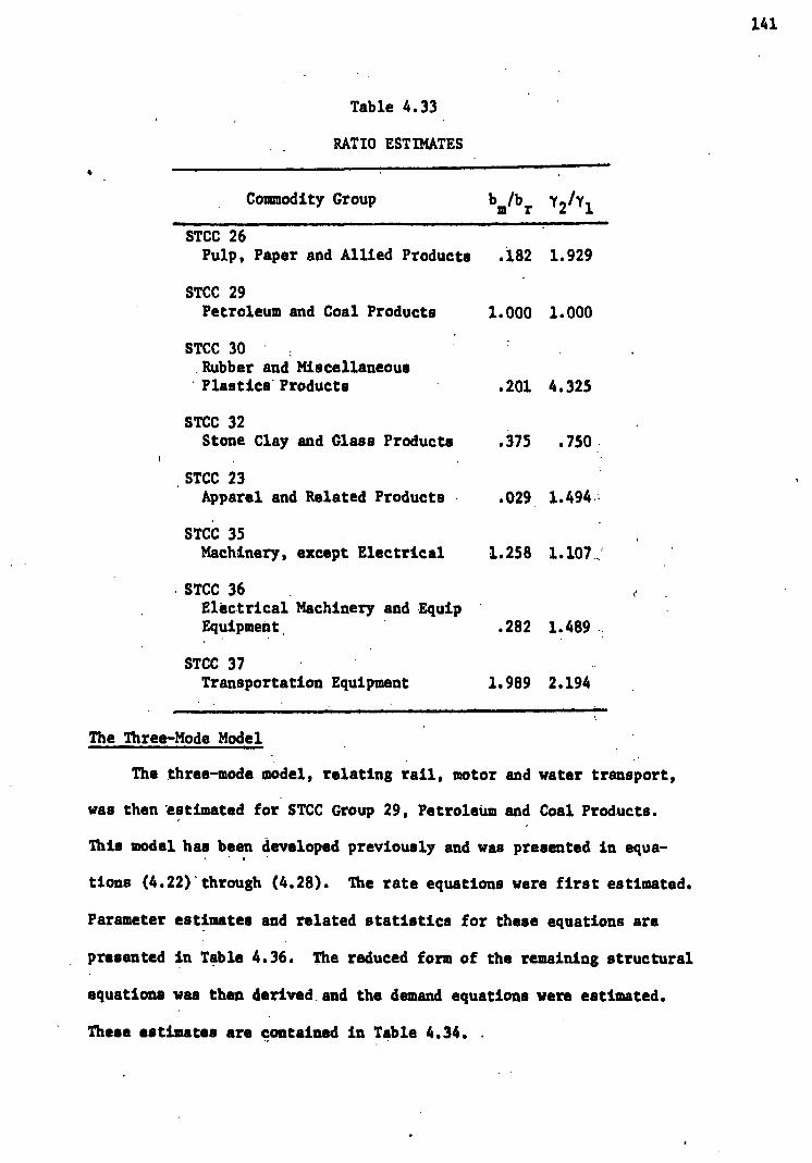
.STCC 36 . Electrical Machinery and Equip Equipment. .282 1.489

Table 4.33

RATIO ESTIMATES

Commodity Group bm/br y2/y1

STCC 26 Pulp, Paper and Allied Products .182 1.929

STCC 29 Petroleum and Coal Products 1.000 1.000

STCC 30 , Rubber and Miscellaneous Plastics Products .201 4.325

STCC 32 Stone Clay and Glass Products .375 .750

. STCC 23 Apparel and Related Products • .029 . 1.494.1

STCC 35 Machinery, except Electrical 1.258 1.107:

141

• STCC 37 Transportation Equipment 1.989 2.194

• The Three-Mode Model

The three-mode model, relating rail, motor and water transport,

was then estimated for STCC Group 29, PetroleUm and Coal Products.

This model has been developed previously and was presented in equa-

tions (4.22) through (4.28). The rate equations were first estimated.

Parameter estimates and related statistics for these equations are

presented in Table 4.36. The reduced form of the remaining structural

equations was then derived.and the demand equations were estimated.

These estimates are contained in Table 4.34. .

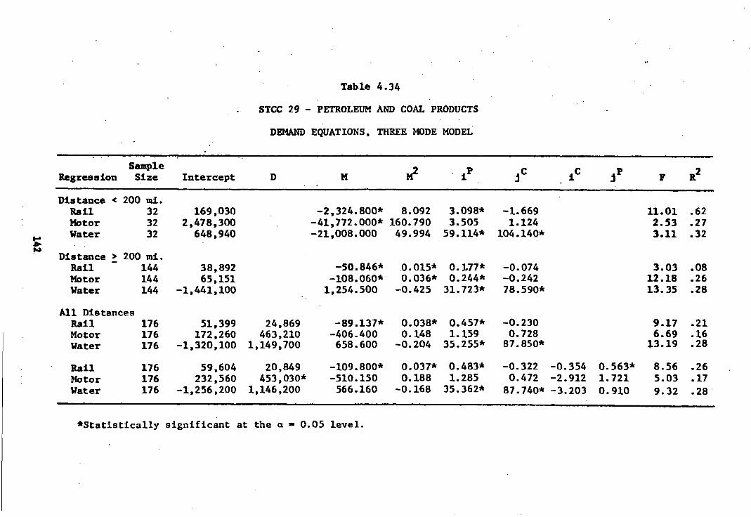
Sample Regression Size M2

. P 1C 1CF R2 Intercept

Table 4.34

STCC 29 - PETROLEUM AND COAL PRODUCTS

DEMAND EQUATIONS, THREE MODE MODEL

Distance < 200 mi. Rail 32 Motor 32 Water 32

Distance > 200 mi.

169,030 2,478,300

648,940

-2,324.800* 8.092 3.098* -1.669

-41,772.000* 160.790 3.505 1.124

-21,008.000 49.994 59.114* 104.140*

11.01 .62 2.53 .27 3.11 .32

Rail 144 Motor 144 Water 144

38,892 65,151

-1,441,100

-50.846* -108.060* 1,254.500

0.015* 0.177* -0.074

0.036* 0.244* -0.242

-0.425 31.723* 78.590*

3.03 .08 12.18 .26 13.35 .28

All Distances Rail 176 Motor 176 Water 176

Rail Motor Water

51,399 172,260

-1,320,100

59,604 232,560

-1,256,200

24,869 463,210

1,149,700

20,849 453,030*

1,146,200

-89.137* -406.400 658.600

-109.800* 510.150 566.160

0.038* 0.457* 0.148 1.159 -0.204 35.255*

0.037* 0.483* 0.188 1.285 -0.168 35.362*

-0.230 9.17 .21

0.728 6.69 .16

87.850* 13.19 .28

-0.322 -0.354 0.563* 8.56 .26

0.472 -2.912 1.721 5.03 .17

87.740* -3.203 0.910 9.32 .28

176 176 176

*Statistically significant at the a = 0.05 level.

SanifiLi Size Rate Distance. .Quantity. Density Price Mode

Table 4.35

STCC 26 - PULP, PAPER AND ALLIED PRODUCTS

RATE EQUATIONS

- - Distance Quantity Density Price

Mode Int. Coef. "t" Coef. "t" Coef. "t" Coef. "t" R2

Rail 405.61 1.281 39.25 .75 Motor 734.71 2.918 16.99 .45

Rail 484.18 1.267 39.75 -0.156 5.40 . .76 Motor 1950.36 2.966 20.84 -92.300 12.73 .62

Rail 1205.79 1.275 48.67 -0.067 2.73 -23.113 15.68 .84 Motor 2196.31 2.980 21.01 -92.826 12.86 -8.731 2.04 .63

Rail 1260.07 1.276 48.31 -0.068 2.76 -24.221 7.71 -0.073 0.40 .84 Motor 4096.52 3.101 20.61 -94.123 13.07 -49.542 2.72 -2.260 2.30 .68

s

•

Average Values of the Variables

Rail 512 . 128398 685.76 441.82 33.15 251.43 Motor 355 1984.80 428.45 13.39 28.05 349.54

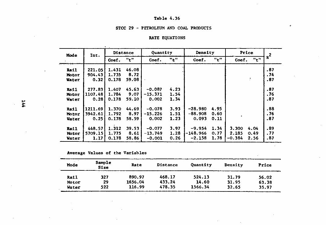
Distance Quantity Density Price Rate Sample Size Mode

Table 4.36

STCC 29 - PETROLEUM AND COAL PRODUCTS

RATE EQUATIONS

Mode Int. Distance Quantity Density Price

R2

Coef. "t" Coef. "t" Coef. "t" Coef. "t"

Rail 221.05 1.431 46.08 .87 Motor 904.43 1.735 8.72 .74 Water 0.32 0.178 59.08 ' .87

Rail 277.83 1.407 45.63 -0.087 4.23 .87 Motor 1107.48 1.784 9.07 -15.371 1.54 .76 Water 0.28 0.178 59.10 0.002 1.34 .87

Rail 1211.69 1.370 44.69 -0.078 3.93 -28.980 4.95 .88 Motor 3942.61 1.792 8.97 -15.226 1.51 -88.908 0.60 .76 • Water 0.25 0.178 58.59 0.002 1.23 0.093 0.11 .87

Rail 448.57 1.312 39.53 -0.077 3.97 -9.954 1.34 3.300 4.04 .89 Motor 5709.15 1.775 8.61 -13.749 1.28 -148.966 0.77 2.185 0.49 .77 Water 1.17 0.178 58.86 -0.001 0.26 -2.158 1.78 -0.384 2.56 .87

Average Values of the Variables

Rail 327 890.97 468.17 524.13 31.79 56.02 Motor 29 1656.04 433.24 14.60 31.95 63.38 Water 522 116.99 478.35 1566.34 32.65 35.97

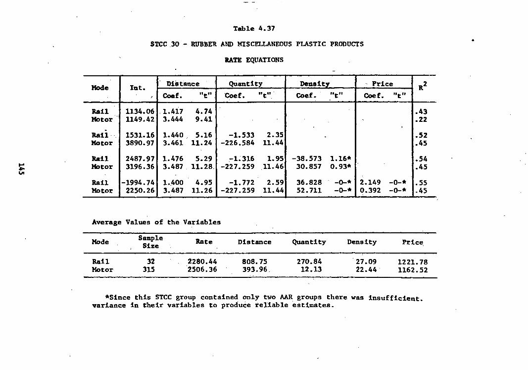
Sample , Size Mode Rate Distance Quantity Density Price

Table 4.37

STCC.30 - RUBBER AND MISCELLANEOUS PLASTIC PRODUCTS

RATE EQUATIONS

Distance Quantity Density Price Mode Int. R2

. Coef. "t" Coef. "t" Coef. "t" Coef. "t"

Rail 1134.06 1.417 4.74 .43 Motor 1149.42 3.444 9.41 .22

Rail 1531.16 1.440 5.16 -1.533 2.35 . .52 Motor 3890.97 3.461 11.24 -226.584 11.44 .45

Rail 2487.97 1.476 5.29 -1.316 1.95 -38.573 1.16* .54 Motor 3196.36 3.487 11.28 -227.259 11.46 30.857 0.93* .45

Rail -1994.74 1.400 4.95 -1.772 2.59 36.828 -0-* 2.149 -0-* •55 Motor 2250.26 3.487 11.26 -227.259 11.44 52.711 -0-* 0.392 -0-* •45

Average Values of the Variables

Rail 32 2280.44 808.75 270.84 27.09 1221.78 Motor 315 2506.36 393.96 12.13 22.44 1162.52

*Since this STCC group contained only two AAR groups there was insufficient. variance in their variables to produce reliable estimates.

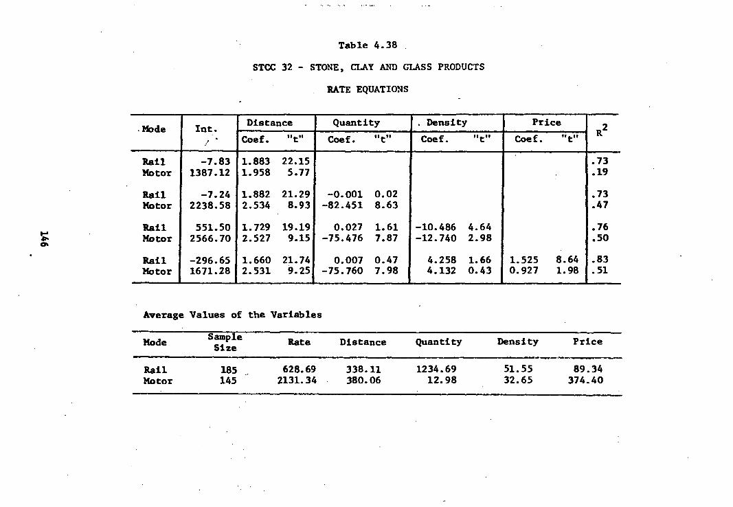
Rate Distance Quantity Density Price Sample Size Mode

Table 4.38

STCC 32 - STONE, CLAY AND GLASS PRODUCTS

RATE EQUATIONS

Distance Quantity . Density Price Mode Int. R

2

, - Coef. "t" Coef. "t" Coef. "t" Coef. "t"

Rail -7.83 1.883 22.15 .73 Motor 1387.12 1.958 5.77 .19

Rail -7.24 1.882 21.29 -0.001 0.02 .73 Motor 2238.58 2.534 8.93 -82.451 8.63 .47

Rail 551.50 1.729 19.19 0.027 1.61 -10.486 4.64 .76 Motor 2566.70 2.527 9.15 -75.476 7.87 -12.740 2.98 .50

Rail -296.65 1.660 21.74 0.007 0.47 4.258 1.66 1.525 8.64 .83 Motor 1671.28 2.531 9.25 -75.760 7.98 4.132 0.43 0.927 1.98 .51

Average Values of the Variables

Rail 185 628.69 338.11 1234.69 51.55 89.34 Motor 145 2131.34 380.06 12.98 32.65 374.40

ip I C ri2

All Distances Rail 176 Motor • 176

-44.880 -87.130 -0.012 0.001 0.002* 0.001 2350.400 2486.300* 0.409 -0.001 0.041* 0.102*

Table 4.39

STCC 23 - APPAREL

DEMAND EQUATIONS

Sample Regression Size Intercept

/.

I.

Distance Rail Motor

Distance Rail Motor

Rail Motor

< 200 mi. 33 33

> 200 mi. 143 143

• 4.922 -7843.700

-91.530 -262.740

0.017 0.001 0.002* -0.001 74.651 -0.291 0.067* 0.188*

-0.001 0.001 0.002* 0.002 -0.441 -0.001 0.029* 0.033*

2.19 .23 8.40 .54

6.25 .15 18.92 .35

5.42 .14 25.59 .43

176 -100.290 92.190 -0.050 0.001 0.001 0.003 0.004* 70.001 5.39 .18 176 -2346.300 2552.200 0.425 -0.001 0.042* 0.107* -0.004 -0.003 18.10 .43

*Statistically significant at the a 0.05 level.

R2

M2 jP jc

Distance < 200 mi. Rail 67 Truck 67

Distance > 200 mi. Rail 391 Truck 391

All Distances Rail 458 -11005.000 12650* Truck 458 -14.227 11031*

306.800 -2.092 0.090* 0.034 -337.930* 0.804 0.032* 0.072*

• 26.26 .63 24.50 .61

-4.783 0.001 0.009* 0.008* -10.333* 0.003* 0.012* 0.011*

18.26 .16 40.35 .29

2.413 -0.000 0.025* 0.023* -8.626* 0.002 0.017* 0.022*

30.32 .25 54.20 .37

-23018.000 14565.000

1084.700 5396.100

Table 4,40

'STCC 35 - MACHINERY, EXCEPT ELECTRICAL

DEMAND EQUATIONS

Sample Regression Size Intercept

Rail Truck

458 -9424.900 12497* 1.526 -0.000 0.027* 0.020* -0.007 0.002 21.92 .25 458 -1236.400 11219* -7.877* 0.002 0.016* 0.024* 0.005 -0.000 38.95 .38

*Statistically significant at the a ■ 0.05 level.

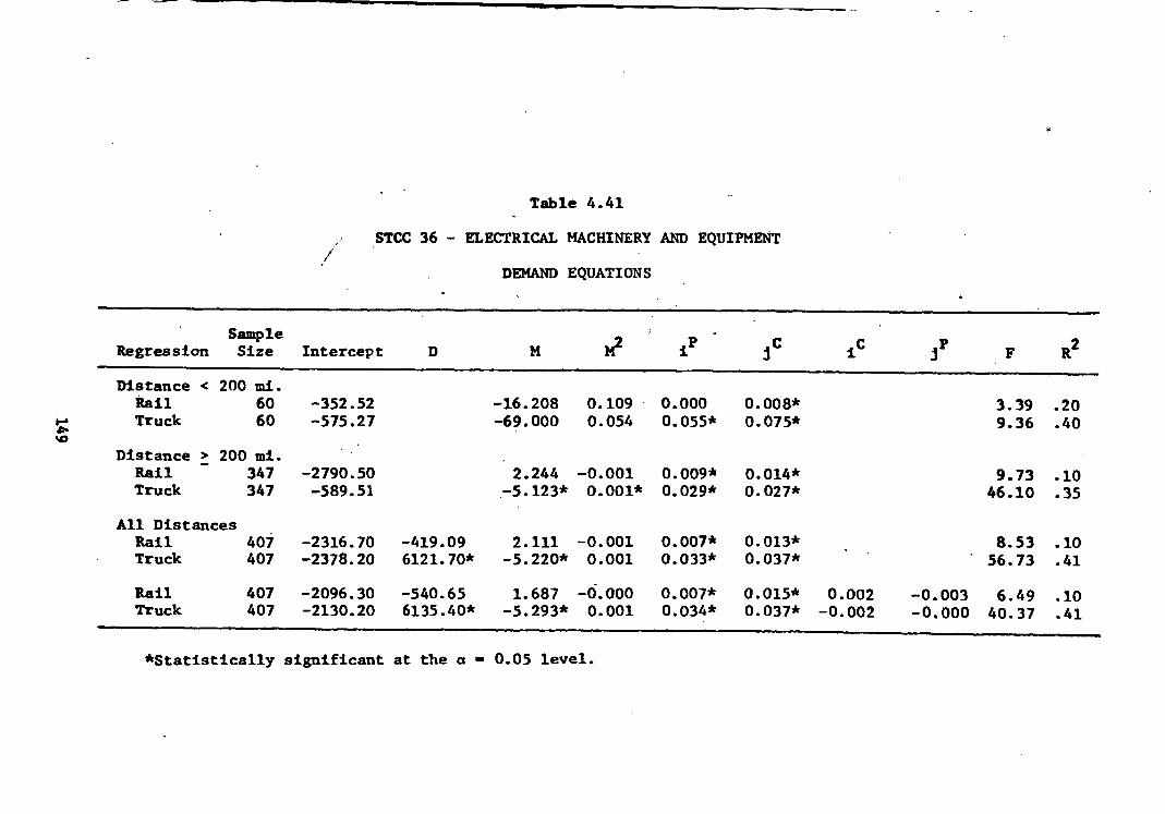
R2 ic Sample

Regression Size Intercept M2 iP

407 407

Rail Truck

-2096.30 -2130.20

Table 4.41

STCC 36 - ELECTRICAL MACHINERY AND EQUIPMENT

DEMAND EQUATIONS

Distance < 200 mi. Rail 60 Truck 60

Distance > 200 mi. Rail 347 Truck 347

All Distances . Rail 407 Truck 407

-352.52 -575.27

-2790.50 -589.51

-2316.70 -2378.20

-16.208 0.109 0.000 0.008* -69.000 0.054 0.055* 0.075*

2.244 -0.001 0.009* 0.014* -5.123* 0.001* 0.029* 0.027*

-419.09 2.111 -0.001 0.007* 0.013* 6121.70* -5.220* 0.001 0.033* 0.037*

3.39 .20 9.36 .40

9.73 .10 46.10 .35

8.53 .10 56.73 .41

-540.65 1.687 -0.000 0.007* 0.015* 0.002 -0.003 6.49 .10 6135.40* -5.293* 0.001 0.034* 0.037* -0.002 -0.000 40.37 .41

*Statistically significant at the a ■ 0.05 level.

C M2 ip Sample Regression Size Intercept F R2

Table 4.42

STCC 37 - TRANSPORTATION EQUIPMENT

DEMAND EQUATIONS

-70108 48082

-48061 17744

-46581 -18261

Distance < 200 mi. Rail 36 Truck 36

Distance > 200 Rail - 200 Truck 200

All Distances Rail 236 Truck 236

Rail Truck

771.160 -3.819 0.021* 0.079* -205.550* 7.871* 0.062* 0.080*

25.523 -0.010 0.030* 0.059* -35.157* 0.011* 0.006* 0.005*

2945.3 22.988 -0.010 0.029* 0.061*

65116.0* -15.879 0.004 0.014* 0.032*

-0.011 0.031* 0.081* -0.006 -0.010* 0.005 0.011* 0.015 0.016* 0.008*

15.83 .67 55.07 .88

36.09 .43 33.57 .41

37.25 .45 30.88 .40

27.43 .46 24.11 .43

236 -47979 2803.5 23.510 236 -21297 65316.0* -18.744

*Statistically significant at the a ■ 0.05 level.

The overall fit of the demand equations is, again, not very good,

'although all but one are statistically significant. All of the dummy

variable coefficients were positive, indicating that all modes shared

in the shorter hauls. The very large barge coefficient reflects what

we felt to be a rather unexpected aspect of the data. The census re-

ported many large water shipments of less than fifty miles, indicating

that, for this commodity group at least, barge was competitive with

rail and truck for short hauls as well as long hauls. Its long haul

advantage can be seen from the estimated mileage coefficients. Except

for the short distance data group, water shipments actually increased

with distance. The rail and motor coefficients, on the other hand, dis-

play the expected negative sign. The miles squared coefficients are,

as before, all of opposite sign to the miles coefficients, and of smaller

influence.

The production and consumption parameters are again a mixed group.

The rail and water production coefficients are all of the correct sign

and statistically significant. The motor coefficients are all positive

but only one is significant. The consumption coefficients do not be-

have as well. For water shipments they all are of the proper sign and

significant. However, for rail and motor they are mostly negative and

are all insignificant.

The two additional market variables seem to add very little to the

explanatory power of the equations. In each case the equation "F" value

decreased, and the estimated coefficient was never both of the proper .

sign and statistically significant.

The reduced form parameters of the two-mode model allowed us to

estimate comparative market responses. This was also possible with

151

the three-mode model. Table 4.43 displays both the reduced form par-

ameters and the response parameters. The average of the two-market co-

efficients for the third regression set was again utilized as our best

estimate of the ratios. Normalizing on motor transport, this procedure

yielded estimates of

bb r m

■ 0.039 andb b — mo 75.55. r w

It appears that the transportation market for STCC group 29 is much

more responsive (seventy-five times) to changes in barge costs than to

changes in truck costs. At the same time, it is much more responsive

(twenty-five times) to changes in truck costs than to changes in rail

costs.

As rate elasticities depend upon the levels of the rates, and as

barge rates were much lower than rail or truck rates, we estimated

relative rate elasticities for two sets of markets, one pair 500 miles

apart and the other 1,000 miles. For both sets of markets the estimated

ratio of the rail rate elasticity was 0.18 for the near markets and 2.64

for the more distant market pair. This difference was due entirely to

the relative rate structures.

The rather large difference between the value of the market re-

sponse ratio and the value of the elasticity ratio for motor and water

transport is due to the much higher rates charged by trucking firms.

For equal changes in rates, the market is much more responsive to the

water rate than to the motor rate. However, for proportional changes,

much greater in absolute value for motor than for barge, market re-

sponses are about equal.

152

bb mw bb r w

3Tc aQ Exogenous Change

Induced Change

(Rail Rate or Assoc. Cost)

(Motor Rate or Assoc. Cost)

(Water Rate or Assoc. Cost)

(3b b bb my mw B B

Sb b bb r w r w B B

13b b r m

bb r

Equation ip

• 'Rail Equation

Motor Equation

Water Equation

ylmw 2m bb ybbw B B

ylbrbw

y2brbw

B B

ylrm 2

r bb ybbm B B

Coefficient of

Table 4.43

RATIO ESTIMATES FOR THE THREE-MODE MODEL

A

Selected Market Response Parameters

Reduced Form Parameters

(Babb +bb +bb -Obbb] rm rw my rmw

153

Summary of the Empirical Results

In the preceding pages we have discussed our empirical results in-

dividually and in some detail. Here we wish to summarize those results

and to compare the separate findings. We begin again with the rate

equations.

The distribution of observations by commodity class for each mode

should be noted first of all. Although there is a substantially larger

number of truck shipments contained in our data, these truck shipments

are mostly Group V products, Manufactures and Miscellaneous. Rail and

water shipments, while also predominately of Group V products, also

contain a large number of Group I and Group III observations. Rela-

tively few shipments of Group II and Group IV products were observed.

Again we must discuss the difference between the rail data and the truck

and water data. A rail observation is for a total annual tonnage, where-

as a truck or water observation is for a single shipment. Thus the num-

ber of observations for the rail data denotes the number of origin-

destination pairs observed for the year and may bear little relation

to the number of separate shipments of the various commodity groups.

There were no water shipments of Group II, Animals and Products, present

in our data, and only two separate commodity classes were present in

the water data for Group IV, Products of Forests. To summarize, over

95 percent of the truck shipments in our sample were of Group V pro-

ducts. The water data is spread mostly over Groups I, III and V, whereas

the rail data seems to cover most products except those contained in

Group II, Animals and Products. Table 4.44 presents the percentage of

shipments observed, by commodity group and by mode of transport.

154

Commodity Group Mode of Transport Truck Rail Water All Modii

- 0.49 5.68 5.44 11.60 (1.08) (16.71) (26.30)

0.38 0.96 1.34 (0.83) (2.84) -

0.34 4.58 3.56 8.49 (0.76) (13.48) (17.25)

0.22 2.17 0.29 2.68

(0.49 (6.40) (1.40)

43.95 20.57 11.37 75.89 (96.85) (60.56) (55.05)

45.38 33.96 20.66 100.00 (100.00) (100.00) (100.00)

Group I

Group II

Group III

Group IV

Group V

Total

Table 4.44

RATE DATA DISTRIBUTION OF OBSERVATIONS BY COMMODITY GROUP

AND MODE OF TRANSPORT (percent)*

*The figures in parenthesis are the intra-mode percentages.

Table 4.45 contains the averages and standard deviations for the

variables by commodity group and mode of transport. The first two in-

dependent variables, distance and quantity, deal with the nature of the

shipment while the latter two, density and price, are concerned with the

type of individual products which are included in the commodity groups.

Average freight rates are much higher for truck shipments than

for rail or water shipments except for Group II. Here, the rail rate

is surprisingly high. In all other cases the average truck rate is

substantially above average rail rates and about five times the average

water rate.

155

Table 4.45

FREIGHT RATE DATA ANALYSIS

Avg. Revenue Distance Quantity Density Price

. Per Ton(C) (Miles) (Tons) (Tons/Car) (S/Ton) /

,• Std. Std. Std. Std. ' Std. Group Avg. Dev. Avg. Dev. Avg. Dev. Avg. Dev. Avg. Dev.

All Truck 1997 1896 376 320 14.75 6.64 30.78 13.42 817 921 Commodities Rail 1302 1347 653 661 (1472.00) (8794.00) 38.71 15.89 316 731

Water 362 287 1024 700 896.02 590.70 51.71 13.72 120 235

Group I: Truck 2150 1176 504 349 13.46 5.60 26.52 4.29 426 339 Products of Rail 1162 1192 760 759 (1029.00) (2690.00) 38.49 15.20 144 200 Agriculture Water 235 160 707 634 990.89 310.16 54.11 4.60 57 29

Group II: Truck 1937 1015 582 645 14.81 4.46 25.19 5.63 640 394 Animals and Rail 2194 1091 837 443 (248.00) (294.00) 18.51 7.11 627 293 Products Water - - • - - - - - - - -

Group III: Truck 1584 831 289 242 16.71 6.39 59.09 13.53 33 13 Products of Rail 497 394 406 402 (6286.00) (22,930.00) 59.59 9.99 17 15 Mines Water 310 113 1528 398 1294.58 303.75 71.93 11.16 30 25

Group IV: Truck 1995 701 405 189 12.70 4.37 36.48 3.40 200 109 Products of Rail 1368 1093 1117 1075 (1412.00) (3682.00) 38.57 5.65 107 112 Forests Water 348 172 633 384 755.22 92.87 45.65 8.05 37 39

Group V: Truck 1999 1918 373 315 • 14.76 6.67 30.63 13.31 832 930 Manufac- Rail 1471 1473 620 595 (586.00) (1118.00) 35.09 14.00 437 903 tures and Water 439 344 1029 716 729.32 690.47 44.38 10.28 181 302 Misc.

....

The distance variables display the reverse ranking in most cases.

Barge shipments are usually the longest, followed by rail with truck .

hauls always the shortest. Exceptions to this are for Groups I and IV

where the average distance for rail is greater than for barge. This

appears to be due more to the relative shortness of the water shipments

than to the length of rail shipments for these groups.

Comparison of the quantity variables is possible only for truck

and water, and here the two extremes are evident. The average inter-

state volume truck shipment is about fifteen tons whereas the size of

the average water shipment is approximately nine hundred tons. This

helps to explain the size of the quantity discounts offered by the

trucking industry:

Looking at the last two variables, we see that as a rule the less

dense, higher-priced commodities travel by truck. Rail ranks second

and water shipments are composed mainly of denser, lower-valued products.

This is in accord with our a priori expectations. However, the inter-

mode densities do not display as great a spread as we had imagined;

and while the general statement is certainly true for Groups I and V

it is much weaker as regards the other groups. Indeed, for Group II it

appears that denser products travel by truck more than by rail. The

very law value of the commodities classified as Group III, Products of

Mines, should also be observed. The average value of these products

is only about thirty dollars per ton. This is about one-twenty-fifth

of the average value of all the products carried by motor transport and

about one-fourth of the average value of those carried by barge.

Utilizing the data contained in Table 4.45, Tables 4.46 and 4.47

have been constructed. These tables illustrate the importance of

157

Commodity Group Mode of Transport Truck Rail Water

0.98 11.68 29.09

0.83 0.48 0

0.86 57.57 24.92

0.42 6.14 1.18

96.91 24.11 44.81

100.00 100.00 100.00

II III IV V

Total

Commodity Group Mode of Transport Truck Rail Water

1.06 15.58 19.73

0.81 1.20 0

0.70 32.87 22.33

0.42 9.64 1.19

97.01 40.70 56.76

100.00 100.00 100.00

II III IV V

Total

Table 4.46

RATE DATA DISTRIBUTION OF TONNAGE BY COMODITY GROUP

(percent)

Table 4.47

RATE DATA DISTRIBUTION OF REVENUE BY COMMODITY GROUP

(percent)

various commodity groups. to each mode of transport. Table 4.46 shows

the percentage distribution of tonnage carried by each transport mode,

whereas Table 4.47 shows the percentage of total revenue attributable

to the commodity groups for each mode of transport. It is seen that

for motor carriers over 95 percent of their tonnage is of Group V pro-

ducts and these products also account for over 95 percent of total

revenue. For rail transport the biggest tonnage is for Group III,

158

Products of Mines; but, because of the low rates charged for these pro-

ducts, the major source of revenue is Group V, where less tonnage is

carried but higher rates are charged. Water transport carries mostly

products included in Groups I, III and V. and mostly in proportion to

their contribution to total revenue. There is a slight bias in favor of

lower than average rates for Group I, Products of Agriculture, and higher

rates for Group V, Manufactures and Miscellaneous.

Table 4.48 contains our final coefficient estimates for the rate

equations arranged by commodity group and by mode of transport. This

table allows comparisons directly across modes.

While most of the equations fit quite well, we see that the fit of

the rail and water equations is always significantly better than the fit

of the truck equations. This is specially true for Group V which con-

tained the greatest number of observations as Well as the greatest num-

ber of individual products. Here the truck equation was able to explain

less than one-half of the total variance of the truck rates, whereas

the rail and water equations could account for almost three-quarters of

the variance of their respective rates. -

The intercept terns are, all except one, positive as we would ex-

pect, and without exception greatest for truck and smallest for water

transport. Group III shipments by water display a negative intercept.

Shipments of this group of products by barge were on the average much

longer and much larger than any other water shipments, and much more

so than any of the rail or truck shipments. This longer average length

of haul was accompanied by a small variance so that very few short

shipments of this group of products were observed. These products were

also heavier than the average and of much less value per ton. As we

159

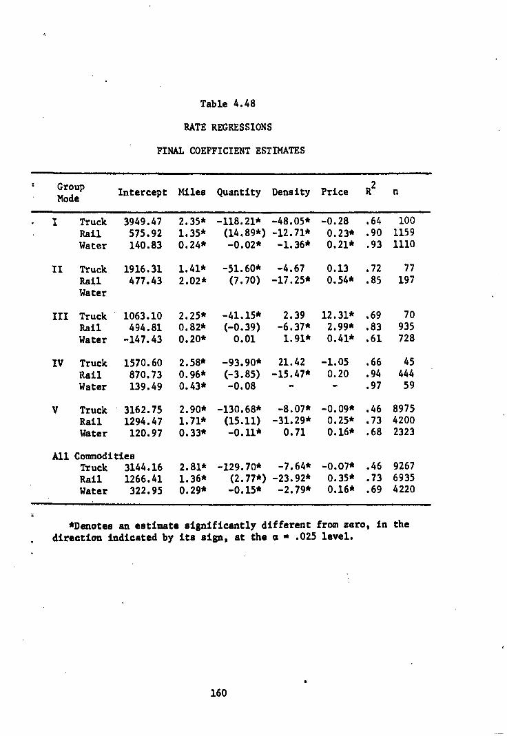
Table 4.48

RATE REGRESSIONS

FINAL COEFFICIENT ESTIMATES

Group Mode

Intercept Miles Quantity Density Price R2

n

. I Truck Rail Water

/I Truck Rail Water

III Truck Rail Water

IV Truck Rail Water

3949.47 2.35* -118.21* -48.05* -0.28 .64 100

575.92 1.35* (14.89*) -12.71* 0.23* .90 1159

140.83 0.24* -0.02* -1.36* 0.21* .93 1110

1916.31 1.41* -51.60* -4.67 0.13 .72 77

477.43 2.02* (7.70) -17.25* 0.54* .85 197

1063.10 2.25* -41.15* 2.39 12.31* .69 70

494.81 0.82* (-0.39) -6.37* 2.99* .83 935

-147.43 0.20* 0.01 1.91* 0.41* .61 728

1570.60 2.58* -93.90* 21.42 -1.05 .66 45

870.73 0.96* (-3.85) -15.47* 0.20 .94 444

139.49 0.43* -0.08 - .97 59

V Truck 3162.75 2.90* -130.68* -8.07* -0.09* .46 8975 Rail 1294.47 1.71* (15.11) -31.29* 0.25* .73 4200 Water 120.97 0•33* -0.11* 0.71 0.16* .68 2323

All Commodities Truck 3144.16 2.81* -129.70* -7.64* -0.07* .46 9267 Rail 1266.41 1.36* (2.77*) -23.92* 0.35* .73 6935 Water 322.95 0.29* -0.15* -2.79* 0.16* .69 4220

*Denotes an estimate significantly different from zero, in the . direction indicated by its sign, at the a ■ .025 level.

160

shall see later, it appears that all modes allowed these low-valued

commodities to move at lower rates than other products. Also, as noted

previously, it appears that the mining industry displays much power in

bargaining with the transport industry and is able to negotiate rates

which are probably quite close to (marginal) costs. These factors cause

the barge rate, when extrapolated back to zero quantity and zero dis-

tance in a linear manner, to yield the negative intercept.

Every distance coefficient was estimated to be positive and sig-

nificantly different from zero at the a ■ 0.025 level. Again the larger

estimates were for motor shipments and the smaller for barge with only

one exception. There were no observations on water transport of Group

II products. The rail distance coefficient for this commodity group

was estimated to be greater than the motor distance coefficient. This

can probably be explained by examining the nature of the products con-

tained in this commodity group and the characteristics of the typical

shipments. These products are, on the average, quite low in weight and

high in value. For the railroads they represent longer than average

shipments and quite small total annual tonnages. These characteristics

point to a product group which is probably rather inefficiently carried

by rail and whose value can apparently stand a rather large freight

rate. This is the one group of products which stand out in our data

as being discriminated against by one of the transport modes.

As we have remarked previously the quantity data, and hence the

estimated coefficients, are not comparable between rail and the other

modes. The rail observations were for annual total tonnage of the com-

modity class, whereas the truck and water data are on individual ship-

ments and their tonnage figures represent the size of the individual

161

shipments. After a lengthy analysis of the rail quantity coefficients,

reported on both within this chapter and in Appendix A following this

chapter, we have to conclude that the overall affect of the size of

annual tonnage upon rates appears to be positive. That is, as more of

a product class is shipped between two points during a year the average

shipping rate increases. Neither the characteristics of the shipments

or the attributes of the products appear to have any connection with

the intergroup behavior of these coefficients. Groups I, II and V have

a positive coefficient whereas Groups III and IV yield a negative es-

timate. However, we do observe that the average value of the products

included in Groups III and IV is substantially lower than the average.

Perhaps the railroads favor these groups with annual tonnage discounts

simply for this reason.

The truck and water tonnage coefficient estimates are much more

consistent. In all cases the statistically significant estimates are

negative in sign, indicating lower rates for larger shipments. In only

one case, water shipments of Group III products, does an estimate come

out positive, and here it is very small as well as being statistically

insignificant. The discounts are always much greater for truck than

for 'water, reflecting the fact that most of the truck shipments are

rather small whereas the average water shipment is very large and dis-

plays a large variance. For both modes the greatest discounts are given

on Group V products, their major source of revenue.

Most of the density Coefficients came out negative, indicating

"heavier" commodities received reduced rates per ton, and implying that,

over the range of densities carried by the modes, weight is less a con-4

straint than space to the transport industries. All of the rail

162

estimates turned out negative and statistically significant. The co-

efficient for Group V products appears to be appreciably larger than

the others, probably because of the large number of individual products

contained in this group. Table 4.45 indicates that there is quite a

large variance in the densities of these products, allowing a weight

discount to be utilized effectively. The coefficients for truck and

barge are a mixed group and the summary statistics are not of much help

in interpreting them. There appear to be factors at work here which

are not revealed by our data.

The price coefficients are mostly positive indicating some element

of value of service pricing. All of the rail estimates are positive

and only one is not significant. The coefficient for Group III, Products

of Mines, displays by far the greatest value, indicating a pronounced

effort to limit the rate to only what "the traffic will bear" for these

very low-value products. The water coefficients are also all positive

and significant with the Group III coefficient significantly larger

than the others. The truck coefficient estimates are much more complex.

It appears that for most products the trucking industry charges lower

fares for higher valued products. This within group tendency is, how-

ever, slightly modified by the between group rate behavior. It appears

that the higher valued products within the highest valued group, Group

V, are favored less by the rate making behavior of the trucking in-

dustry than are the higher valued products within the lower valued

groups. This observation is valid for Groups I, IV and V where the

price effect decreases in size as the average value of the products in

the groups decreases. The price coefficient for Group II is positive

but small and not statistically significant. However, the coefficient

163

for Group III is positive, large and significant, illustrating once

again the special treatment offered this group of products by all the

modes.

In summary, our rate results appear highly significant and mostly

in accord with our a priori expectations. On the whole rates are

higher (and increase faster with distance) for truck transport than

for rail, ere greater for rail than for water. Significant size of

shipment discounts are present for, at least, truck and barge transport.

Railroads appear to increase their rates between points with more than

an average amount of traffic, or, at least, when rate increases occur

they are concentrated primarily on these hauls. Heavier products travel

at lower rates per ton than less dense products, although there are

some oddities in the truck and water estimates here. And, finally, it

appears that some element of value of service pricing is present in

the rail and barge industries for all products, and also for some pro-

ducts carried by the trucking industry. This price effect is especially

evident among the very low valued products comprising Commodity Group

III, Products of Mines, where all modes offer large discounts to the

lower valued products These results appear sufficiently valid for many

uses. However, any potential user should note the large differences

in rate behavior between the different commodity groups as well as be-

tween modes of transport. The aggregate estimates, while useful as

summary statistics, should be viewed with caution.

. Before presenting the summary of results of our quantity equation

estimation we shall review the manner in which these equations differ

from the "transport demand equations" which have been estimated by

164

e 165

others. The usual estimating equation is a simple linear or log-linear

equation which expresses the quantity carried by a certain mode of

transportation as a function of the rate charged by that mode, perhaps

the rates charged by competing modes of transport and, usually, several

exogenous variables. This simple procedure is beset with several tech-

nical difficulties. First of all, the estimation of a single demand

equation is a touchy matter. Unless the estimating equation is derived

from a sound, and valid, theory we cannot be certain that the demand

relation will actually be captured. A supply curve may be estimated

or we may estimate some combination of the two curves. This indeter-

minacy is compounded when we desire to estimate two or more separate

but interrelated demand functions. We must first weed out the supply

influences and then separate the demand influences by mode. These are

very difficult problems. In short, simple estimation procedures which

deal with single demand functions for several modes of transport may

(1) not capture the demand influences at all, and/or (2) not discrimi-

nate between the modal demands in a meaningful manner.

We have attempted to overcome these difficulties by constructing

an economic model of the transportation market which takes account of

the influences of several separate modal supply curves and then de-

riving our estimating equations directly from this model. This pro-

cedure has been only partially successful. In order to construct a

model which at least partially reflects the real world we have had to

introduce the associated costs of transportation. These costs differ

for each mode of transport and have not been captured in any of the data

collected thus far. Therefore, it has been impossible to estimate our

entire model and, in general, we have not been able to derive estimates

of the underlying structural parameters. That is, we also are unable

to estimate meaningful "modal demand curves." We have been able, how-

ever, to estimate the reduced form equations relating the quantity

carried, by mode, to the exogenous variables contained in the model.

These estimates allow us to predict the quantities which will be carried

by the various modes of transport given specified levels of the exogenous

variables and also to predict the changes in quantities as these var-

iables change in value. That is, if more of a product is produced in

some shipping area we shall be able to predict the increase in the

transport of that commodity. If desired, we can construct elasticities

of demand, by mode, with respect to these exogenous variables. However,

from knowledge of the reduced form parameters alone, we are not able

to derive relationships between the endogenous variables. That is, if

some structural change should take place, say a change in the cost

structure of one mode, we shall not be able to predict how this will

affect the quantities carried by that mode or by the other modes.

Our estimates do allow us to make qualitative comparisons of sev-

eral structural parameters and their effects upon selected endogenous

variables. We are able to compare the sensitivity of the transport

market in terms of total quantity shipped and total shipping costs borne

by the shipper for 'changes in the rate structure of the various modes.

These estimates can also be converted into estimates of elasticity

ratios. These results, while falling far short of the full range of

estimates we had wished to obtain, were all that could be derived from

the available data. In fact, it may be contended that the data base

is insufficiently structured and not statistically sound enough to

produce reliable estimates of even this limited number of parameters.

166

Our estimates should be viewed, therefore, as first approximations, as

the best that can be achieved at the present time, but as only frag-

mentary evidence of what may be found when a thorough, detailed analysis

of the transport market becomes possible. We hope that our theoretical

development, the specification of the variables which must be considered,

will assist and encourage the gathering of more complete and compre-

hensive data. We shall first discuss the reduced form parameter es-

timates and then comment upon the derived sensitivity ratios.

Table 4.49 contains our final parameter estimates for the quantity

equations. Although the overall fit of the equations is not overly im-

pressive it should be noted that all'of the equation F values are sig-

nificant and approximately half of the R 2 values are of respectable

size. Since the dummy variable was set up to assume a value of one for

distances less than two hundred miles and zero for greater distances,

the assumption of motor transport being dominant .for the shorter ship-

ments with rail becoming competitive only after several hundred miles

yields the expectation that this coefficient would display a negative

sign for rail and a positive sign for motor transport. This expecta-

tion is realized for only one of the commodity groups. Group 26, Pulp,

Paper and Allied Products, yielded the expected results. For the other

commodity groups all coefficients were positive. This implies that,

for the shipments covered by our data at least, all modes of transport

share in the short hauls.

Five of the nine estimated intercept terms turned out negative.

For the usual demand equation this would be a disastrous result. How

ever, it is rather to be expected in our reduced form equations. A

glance at these equations, (4.51)' and (4.52), reveals that each intercept

167 .7

C, C P FR2

Pi Group and Mode Intercept M }e

Table 4.49

DEMAND REGRESSIONS

FINAL COEFFICIENT ESTIMATES - (All Distances)

STCC Group 26 Rail 6 -2 -0.007 0.002 0.006* 0.010* -0.006* -0.004 3.08* .28 245 Motor -13 59* -0.037 0.011 0.038* 0.050* 0.003 -0.006 21.19* .61 245

STCC Group 29 t-. Rail 59,604 20,849 -109.800* 0.037* 0.483* -0.322 -0.354 0.563* 8.56* .26 176 a. Motor 232,560 453,030* -510.150 0.188 1.285 0.472 -2.912 1.721 5.03* .17 176 co

Water -1,256,200 1,146,200 566.160 -0.168 35.362 87.740 -3.203 0.910 9.32* .28 176

STCC Group 30 Rail -4 1 0.002 -0.001 0.004* 0.022* 0.010 -0.004* 5.98* .36 277 Motor -1 6 -0.009* 0.003 0.040* 0.044* -0.013 0.003 38.12* .70 277

STCC Group 32 Rail 3 137* -0.108* 0.008 -0.006 -0.054* 0.031* -0.014 -9.61* .52 177 Motor -16 403* -0.289* 0.023 0.024 0.141* 0.042 -0.037 11.83* .56 177

*Denotes an estimate statistically different from zero at the a •. 0.05 level.

term contains one bracketed expression, (8b 1-1), which is negative

by assumption. If this expression dominates, the overall intercept

term will be negative. It should also be noted that whenever the in-

tercept is estimated as negative the dummy variable coefficient is es-

timated to be positive.

In general we expected the mileage coefficients to be negative.

Our theory assumes that for each commodity group the total amount

transported would decrease with distance. This assumption was valid.

However, if one mode enjoys a great advantage in the shorter hauls and

another in the longer ones, the latter mode may display a positive dis-

tance coefficient and remain consistent with our theory so long as

this positive effect is more than compensated for by the reduction in

tonnage for the former mode. Two of the nine estimated coefficients

came out positive and both of these were offset by negative intercept

terms. Water shipments of Group 29, Petroleum and Coal Products, in-

creased rather largely with distance and rail shipments of Group 30,

Rubber and Miscellaneous Plastics Products, increased a very small

amount. However, all of the statistically significant estimates showed

a negative mileage effect.

Without exception the signs of the estimated coefficients of the .

square of distance were the opposite of the sign of the distance co-

efficients. This coefficient, however, was never large enough in value

to completely override the influence of the first degree term. That

is, if the distance coefficient was negative and the distance squared

coefficient positive, for the relevant range, the net effect of dis-

tance on quantity was negative.

169

The model assumes that the Pi and C will exert a positive in-

fluence on quantities transported whereas Ci and Pj will display a

negative influence. This expectation was realized in most cases. All

of the Pi coefficients displayed the proper sign, and only one C co-

efficient came out negative. All statistically significant estimates

were of the proper sign. The Ci and P coefficients are less satis-

factory. Two Ci coefficients displayed positive signs and four of the

coefficients, one statistically different from zero, are also posi-

tive. This necessitated the basing of the sensitivity ratios solely

on the Pi and C coefficients.

The derived sensitivity ratio and elasticity ratio estimates are

summarized in Table 4.50. In all cases the transportation market ap-

pears much more sensitive to changes in motor rates than to changes in

rail rates. This was an implicit assumption of our theoretical model

and is here verified empirically. The condition is most easily de-

scribed by referring to Fig. 4.1. If a modal split is to occur between

two markets, and if we expect the railroad to carry most of the ship-

ments with truck becoming competitive only as more of the product is

transported so that the railroad can no longer easily carry all of the

tonnage, the modal total cost curves must cross in the manner illus-

trated. Under these conditions it is easy to demonstrate that the

supply of transportation curve is affected more by changes in truck

• supply than by changes in rail supply. This implies that the total

quantity market will be influenced in a similar manner.20

20. If we define the modal cost curves as

Cr •a +b + b Q r r

C ■ a + b m in in

Qui

170

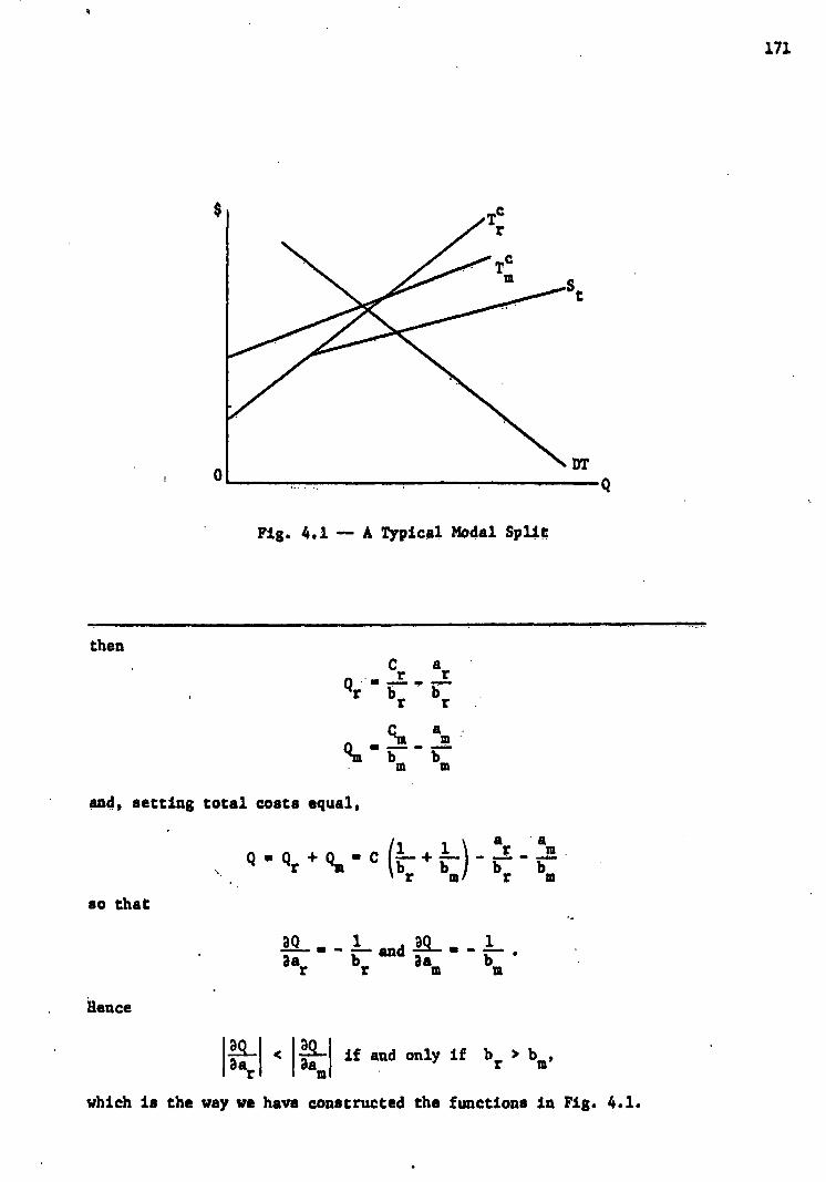
171

0

Fig. 4.1 -- A Typical Modal Split

then C a

A . r r 4r br br

m am Qui

b bm •

and, setting total costa equal,

a . a

+ g A ( 1 .1) _ r_ 111.

gr m im b b bm r m '•

so that

3Q 1 19._ 1 - - and ■ - — • par br Dam in

Hence

r1-1 < 1 22-1 if and only if b > b II) , Oa Oa r r m

which is the way we have constructed the functions in Fig. 4.1.

Table 4.50

DEMAND ANALYSIS

DERIVED ESTIMATES

Market Sensitivity Ratigs Elasticity Ratios

500 miles 1,000 miles

Sens. to A rail rate Sens. to A water rate EQ,T

r EQ,Tw EQ,Tr EQ,Tw Commodity Group Sens. to A truck rate Sens. to A truck rate EQ,Tm EQ,Tm EQ,Tm E, ,,m

Group 26 Pulp, paper and allied products 0.18 0.09 0.08

Group 29 Petroleum and coal products 0.04 75.55 0.21 3.78 0.03 5.14

Group 30 Rubber and mis- cellaneous plastics products 0.20 0.13 0.12

Group 32 Stone, clay and glass products 0.38 0.15 0.21

This situation is also in accord With the rite analysis where

we found that rail rates were, as a rule, Much lower than motor retie.

Thus, unless there is a quality of service differential favoring truck

equal to the rate differential, fail Will have the initial Atege;

The quality of Service differential for these prOddct groups is prOhihiY

very alail is they are nee-perishable, bulky, And except iot ditio

heavy and lot; or tedium priced products. Group 12, StOne, Ciey and

Glase Products, displays the largeet ratio ifidicating the iiait Chihge

in comparative advantage over the Observed tonnage range: GrOup 10 ihz

didated the ieit ehtegi;

Applying the Sable reasoning tO the three-mode thottel, We see that

water tranapOri clearly Aftindisi the market tAiefi large quantities ae

to be moved. This le again in obiioüS result.

The elasticity fait) eetilatee are indinded in the tahie fo664=

pleteneds and to allow Us to Agiin coiMient that ab kreight ihieg

treade with detente; rate or associated Cost elietititide Of dekind

will, in general, increase di the markets / Under tOnsideritiOn ire

farther iOitt.

17

APPENDIX A TO CHAPTER FOUR

The Effects of Annual Tonnages Upon Rail Rates

The behavior of the annual tonnage coefficient estimates in the

rail regressions requires special consideration. In the first two

sections of that analysis (those dealing with all commodities and with

commodity group totals) the tonnage coefficients were always estimated

with a negative sign and all but four were statistically different from

zero. The estimates, did not behave so well in the final set of re- '

gressions. With the less aggregate data, and including variables rep-

resenting price and density, six of the ten tonnage coefficients were

estimated as positive. Only two of these were significantly positive

but none of the four negative coefficients was significant.

Upon observing these estimates it was decided to investigate the

effect of the quantity variable further. A new set of regressions was

run for each commodity group using the sane data but forcing the tonnage

variable to enter the estimating equation at the second step, distance

• -.being retained as the first independent variable. Tables 4.A.1 through

4.A.5 contain the results of these runs.

The tonnage coefficient estimates definitely are not stable. They

shift greatly in size and frequently change sign. For Groups I and V,

the estimates are at first negative and then, as other variables enter

the equation, become positive. For Groups III and IV, the estimates

are first significantly negative and then move in the direction of

positiveness, losing their significance in the process. The tonnage

coefficient for Group II first appears positive, then goes negative,

and finally returns positive, never achieving significance.

174

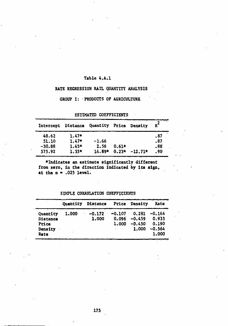
Table 4.A.1

RATE REGRESSION RAIL QUANTITY ANALYSIS

GROUP I: .PRODUCTS OF AGRICULTURE

ESTIMATED COEFFICIENTS

Intercept Distance Quantity Price Density

48.62 1.47* .87

51.10 1.47* -1.66 .87

-30.88 1.45* 2.56 0.61* .88

575.92 1.35* 14.89* 0.23* -12.71* .90

*Indicates an estimate significantly different from zero, in the direction indicated by its sign, at the a • .025 level.

SIMPLE CORRELATION COEFFICIENTS

Quantity Distance PriCe' . Density Rate

Quantity 1.000 -0.172 -0.107 0.281 -0.164 Distance 1.000 0.096 -0.459 0.933 Price 1.000 -0.450 0.190 Density 1.000 -0.564 Rate 1.000

175 ,

Table 4.A.2

RATE REGRESSION RAIL QUANTITY ANALYSIS

GROUP II: ANIMALS AND PRODUCTS

ESTIMATED COEFFICIENTS

• • Intercept Distance Quantity Price Density. R.

332.42 2.23* .82

326.10 2.23* 28.66 .82

54.36 2.10* -7.37 0.61* .84

477.43 2.02* 7.70 0.54* -17.25* .85

*Indicates an estimate significantly different from zero, in the direction indicated by its sign, at the a ■ .025 level.

SIMPLE CORRELATION COEFFICIENTS,

Quantity Distance Price Density . Rate

Quantity 1.000 0.050 0.074 0.010 0.053 Distance 1.000 0.301 -0.336 0.903 Price 1.000 -0.238 0.420

'Density 1.000 -0.423 Rate 1.000

176

Table 4.A.3

RATE REGRESSION RAIL QUANTITY ANALYSIS

GROUP III: PRODUCTS OF MINES

ESTIMATED COEFFICIENTS

Intercept Distance Quantity Price Density

145.00 0.87* .78

153.93 0.86* -0.99* •79

93.69 0.84* -0.68* 3.91* .81

494.81 0.82* -0.39 2.99* -6.36* .83

*Indicates an estimate significantly different from zero, in the direction indicated by its eige, at the et w .025 level.

SIMPLE CORRELATION COEFFICIENTS

. Quantity Distance Price Dehti4r Rate

Quantity 1.000 -0.117 -0.140 0.150 -6.1'60 Distance 1.000 0.190 -0.179 0.885 Price 1.000 -0.262 0.321 Density 1.000 -0.344 Rate 1.006

177

Table 4.A.4

RATE REGRESSION RAIL QUANTITY ANALYSIS

GROUP IV: PRODUCTS OF FORESTS

ESTIMATED COEFFICIENTS

Intercept Distance Quantity Price Density R2

269.02 0.98* .94

299.90 0.97* -14.26* .94

281.94 0.96* -13.42* 0.32* .94

870.73 0.96* -3.85 0.20 -15.47* .94

*Indicates an estimate significantly different from zero, in the direction indicated by its sign, at the a ■ .025 level.

SIMPLE CORRELATION COEFFICIENTS

Quantity Distance Price Density Rate

Quantity 1.00000 -0.19660 -0.19615 0.41537 -0.23630 Distance 1.00000 0.53079 -0.07798 0.96700 Price 1.00000 -0.17551 0.53879 Density 1.00000 -0.16256 Rate 1.00000

178

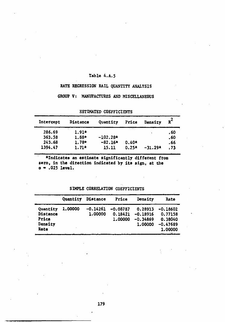
Table 4.A.5

RATE REGRESSION RAIL QUANTITY ANALYSIS

GROUP V: MANUFACTURES AND MISCELLANEOUS

ESTIMATED COEFFICIENTS

Intercept Distance Quantity Price Density R2

286.69 1.91* .60

363.58 1.88* -102.28* .60

243.68 1.78* -82.16* 0.40* .66

1394.47 1.71* 15.11 0.25* -31.29* .73

*Indicates an estimate significantly different from zero, in the direction indicated by its sign, at the a • .025 level.

SIMPLE CORRELATION COEFFICIENTS

Quantity Distance Price Density Rate

Quantity 1.00000 -0.14261 -0.08787 0.28913 -0.18602 Distance 1.00000 0.18421 -0.18916 0.77158 Price 1.00000 -0.34869 0.38040 Density 1.00000 -0.47689 Rate 1.00000

179

The overall tendency appears to be that the tonnage variable

exerts a negative influence on rate when tonnage and distance are the

only explanatory variables. Then, the negative influence becomes less,

sometimes changing into a positive influence, as other variables are

entered into the equation. This finding is confirmed in Table 4.A.6

where we have again utilized the pooled data for all five commodity

groups. Here the coefficient is first significantly negative and then

proceeds to become positive, never losing its significance.

This table also shows the simple correlation between the tonnage

and rate data as -0.098. Further processing of these data show that

the partial correlation of tonnage and rate, given the distance data,

and the partial correlation of tonnage and rate, given distance and

density, is positive. Hence, if we believe that mileage and density

belong in our regression equations along with annual tonnage we must

conclude that the true effect of tonnage on rate is positive. When we

have excluded one of the above variables from our analysis, we have

misspecified the equation and the effect of the excluded variable upon

both rate and tonnage forces the tonnage coefficient to be biased

negatively.

1. In some earlier work with Group V, Manufactures, we tried dif-ferent tonnage data in less complex equations. In these equations we entered only distance and tonnage and found that the present defini-tion of Q, as annual tonnage of the k-th commodity, gave more signifi-cant results than defining it as either the state-to-state annual tonnage of (1) all manufactured products or (2) all commodities. We believe this conclusion would hold for the other groups as well.

180

Table 4.A.6

RATE REGRESSION RAIL QUANTITY ANALYSIS

ALL COMMODITY GROUPS

ESTIMATED COEFFICIENTS

Intercept Distance Quantity Price Density R2

284.41 1.56* .59

296.59 1.55* -5.61* .59

180.85 1.48* -3.86* 0.52* .67

1226.41 1.36* 2.77* 0.35* -23.92* .73

*Indicates an estimate significantly different from zero, in the direction indicated by its sign, at the a 011 .025 level.

SIMPLE CORRELATION COEFFICIENTS

Quantity Distance Price Density Rate

Quantity 1.00000 -0.08072 -0.05146 0.18655 -0.09819 Distance 1.00000 0.13907 -0.26000 0.76585 Price 1.00000 -0.36151 0.38354 Density 1.00000 -0.52092 Rate 1.00000

181

'

CHAPTER V

SUMMARY AND CONCLUSIONS

Researchers engaged in the estimation of demand relationships recog-

nize that goods and services usually exist which are close substitutes

for those they are directly investigating. However, this recognition

is seldom transformed into action. Ideally, these substitute goods

should be dealt with in the estimation process. One common and easy

method is to enter the prices of these goods in the demand equations.

Usually this is done in a very ad hoc manner with little consideration

given to what the estimated coefficients may actually represent.

This approach is perhaps most common in the field of transporta-

tion. Observing many transportation links and networks which are served

by two or more modes of transport, most people believe these modes are

substitutes for one another, more or less perfect, depending upon the

level of their "quality of service differentials." However, most

attempts to estimate the demand for these transport modes are hampered

by an inability, or a lack of desire, to explicitly deal with this

substitutability.

This paper has attempted to construct an economic model of a

transportation market. We employed traditional economic methods and

used as our starting point the derived demand for transportation. By

quantifying the variables usually considered as determinants of quality

of service, and expressing these as costs associated with shipment by

182

the respective modes of transport, we were able to treat these dif-

ferent modes as perfect substitutes. This allowed us to view the

shipper's choice of mode decision as a simple problem of cost minimiza-

tion. Emphasizing at all times the interdependencies within the market,

we were able to investigate the conditions under which a modal split

may occur and to derive the "demand curves" confronting the individual

modes.

In Chapter I we reviewed the structure and functioning of a traria-

portation market. Possible reasons for investigating the workings of

such a market were also discussed. The best of the current economic

models of the transportation process were classified as basically "multi-

market single-mode transport models." These models have probed deeply

into the relationships between product demands and supplies and trans-

port demands. .However, these investigations have been possible only

by almost completely ignoring the supply side of the transportation

market. Our "two-market multi-mode transportation model" was then pro-

posed as the next step in the development of a full multi-market multi-

mode model of transportation.

Chapter II contained a review of the transportation literature.

In a rather thorough review of the theoretical literature we traced the

major steps in the development of transportation models from 1838 through

1964. It was found that these studies have become increasingly con-

cerned with the case where many markets are served by a single mode of

transportation, or several modes displaying quite simple supply attri-

butes. Selected recent empirical works were .then reviewed. These works,

in contrast with the theoretical studies, were concerned with determining

quantities carried by different modes of transport. In constructing a

183

theoretical basis for their empirical studies the authors were forced

to utilize the traditional two-market model, adapting it to consider

several different modes of transport. An exception to this approach

was E. Silberberg. He followed the path of the theoreticians and es-

timated a multi-market single-mode model adapted to recognize the exis-

tence of a competing mode of transport.

In Chapter III we developed our two-market multi-mode transporta-

tion model. The construction of the transportation market began with

the classical derivation of the demand for transportation for a single

commodity between two markets. Introduction of a single supply of

transport then brought this model up to date. Our first generalization

was the introduction of several competing sources of supply, each of

which was considered as a perfectly competitive industry. The concept

of shipper cost was then introduced. All former models of transporta-

tion seem to operate on the assumption that the direct transport rate

is the only cost of direct concern to the shipper. We put forth the

assumption that all of the components of quality service can and should

be considered also as costs which the shipper must take into account.

Time preference costs, inventory costs, schedule and convenience costs,

feeder-line costs and interface and congestion costs were then con-

sidered, and the connection of these costs with the definition of the

supply of transportation was discussed.

The transportation model was then extended to include all these

components of shipper costs. This was accomplished in two steps.

First, transportation associated costs were considered in a market

with only a single supply of transportation. Then, several supplying

184

modes, each with individual associated cost characteristics, were in-

cluded in the model.

The complete model was then cast in terms of a simultaneous equa-

tion system and a qualitative analysis was undertaken. This analysis

allowed us to investigate the effects of changes in system parameters

upon the equilibrium values of all the endogenous variables. It was

found that by making quite plausible assumptions concerning the signs of

simple partial derivatives we were able to unambiguously derive.the signs

of the resulting changes in solution values of the variables. It was

also shown that in many cases statements could be made concerning the

relative sizes of the effects. That is, we were able to show that a

five-cent increase in the transport rate for a certain mode would have

the same effect upon the quantities carried by the various modes and

shipper's costs as a five-cent increase in associated costs for that

mode. A complete listing of these theorems is contained in Table 3.2

In the three appendices to Chapter III we derived measures of re-

sponse for the transportation market. Appendix A contained a derivation

of the elasticity of transport demand in terms of the elasticities of

the product supply and demand curves. Appendix B showed the derivation

of the elasticity of the "demand" for a particular mode of transport.

This elasticity was presented in terms of the elasticity of the demand

for transportation and the elasticities of the transport supply and as-

sociated cost functions.

In Appendix C to Chapter III we investigated the implications of

allowing one of the transport modes to be composed of a single large

firm. This model, with its obvious reference to rail transport, views

this one, monopolistic, industry as competing directly with one or more

185

competitive industries. Applying this model first to a transportation

market with no associated costs, the conditions under which a stable

solution will arise were determined, and the welfare implications of

this solution investigated. The model was then expanded to include as-

sociated costs for both the monopolist and the other modes. Finally,

we investigated the behavior of the monopolist when he is able to ex-

ercise some control over the quality of his service. Now, varying the

quality of a transport product is actually only a special case of pro-

duct differentiation, so that this analysis is quite analogous to that

of a firm considering the effects of, say, advertising expenditures.

Both categories of expenditures allow the firm some control over its

"demand curve," and in each case the firm must consider both the cost

of the control and its effects upon the market.

Chapter IV reports on our empirical investigations. To allow the

theoretical model to be estimated certain specializations were re-

quired. First, the equations were assumed linear in all variables.

This allowed the application of standard estimating techniques. Second,

since all available data was of a cross-sectional variety, adjustment

variables were added to each equation to compensate for the differ-

ences in market size and shipment distance. Finally, in recognition

of the fact that transport rates are closely regulated by the Interstate

Commerce Commission and, therefore, at least slow in responding to mar-

ket forces, the rates were specified as being exogenous to the re-

mainder of the system. -

These specifications resulted in a simultaneous linear equation

system. Since the transport rates were assumed to be exogenously

determined, they were estimated independently of each other and of the

186

rest of the system. The rate equations were then substituted into the

system to derive a linear structure of the first order. The reduced

form of this structure was then obtained and utilized in estimating

demand equations for the individual transport models.

Prior to our study a few simple estimating equations for rail and

motor rates existed. These usually expressed the rates as linear func-

tions of distance and, perhaps, distance squared for individual com-

modities. By utilizing published sources of rail data, and obtaining

comprehensive shipment data from private sources for motor and water

transport, we were able to conduct a thorough analysis of transport

rates for these three modes. Our approach was to relate the average

revenue per ton of the commodity shipped to the distance it was shipped ;

a quantity variable and several product attributes. For rail shipments

the quantity variable was the total annual tonnage shipped between the

two markets. For motor and water transport the size of the individual

shipments was available. The carload waybill statistics yielded ob-

servations on the average density and estimated prices of the com-

modities. These were used as product attributes.

Rate regressions were estimated for all five of the major MR com-

modity groupings. Then, after conversion of the commodity groups, rate

parameters were estimated for the four STCC groups selected for reduced

form estimation.

Distance proved to be the best single explanatory variable for

rail and water transport, whereas shipment size was the most important

for motor transport. The quantity variable also proved significant in

explaining water rates, whereas its effects were quite mixed for rail.

These quantity relationships for rail transport were explored further

187

in the appendix to that chapter. The product attributes, while contri-

buting to the explanatory power of the equations, did not exhibit as

strong an influence as distance or quantity.

The reduced form equations expressed the endogenous variables as

functions of the exogenous variables. Ideally, we would have estimated

these equations and derived estimates of all structural parameters. How-

ever, no data existed on transport associated costs, nor was it possible

to estimate this variable from the available data. Consequently, we

could estimate only the quantity equations and were unable to derive

estimates of individual structural parameters. However, in the quali-

tative analysis performed in Chapter III it was shown that most changes

in the system are represented by groups of parameters. This indicated

that useful knowledge may perhaps be gained without complete identifi-

cation. We then performed a complete qualitative analysis for the es-

timating model. This analysis, the results of which were presented in

Table 4.27 indicated that, with only partial estimation of the reduced

form, comparative statements could be made concerning changes in

shipper's cost and quantities shipped brought about by changes in

freight rates or quality associated costs.

For the two-digit Standard Transportation Commodity Classification

groups 26, 29, 30 and 32 we regressed quantity shipped, by mode, on

distance, a dummy variable indicating short or long haul, distance

squared, and a vector of market attributes. In one set of regressions

the market attributes were production of the commodity in the exporting

region and consumption of the commodity in the importing region. For

the other set of regressions, we added consumption in the exporting

market and production in the importing market.

188

These parameter estimates indicated that transportation market

responses, in terms of shipper's cost and quantities shipped, were

about five times greater for a unit change in motor rates or associated

costs than for unit changes in rail cost parameters for Groups 26 and

30. For Commodity Group 32 the response to changes in motor costs was

almost three times greater thin for rail cost changes, whereas for

Group 29 the responses were approximately equal. Estimates of the com-

parative rate elasticities of transport demand were also derived.

In general the overall fits of these reduced form regressions were

not too good. It is felt that this was due primarily to the nature of

the model and the available shipment data. Attempting to estimate a

derived demand from cross-sectional data is difficult, even with the

best possible data. A comprehensive analysis of the individual mar-

kets over time is required if reliable parameter estimates are to be

obtained.

We have attempted to demonstrate that several modes of transport

can be handled in a simultaneous equation model, analogous to the manner

in which several markets have been handled previously. We believe that

this has been demonstrated satisfactorily, and hope that it will con-

tribute ta the eventual development of a complete multi-market multi-

mode model of production, transportation and consumption.

189

BIBLIOGRAPHY

Baumol, W. J., "Calculation of Optimal Product and Retailer Character-istics: The Abstract Product Approach," Journal of Political Economy, Vol. 75, No. 5 (Oct. 1967) 674-685.

Benishay, H., and G. R. Whitaker, Jr., Demand and Supply in Freight Transportation, The Transportation Center, Northwestern University, 1965.

Cournot, A. A., The Mathematical Principles of the Theory of Wealth (1838), Irwin, Homewood, Ill., 1963.

Crecine, J. P., L. N. Moses, and J. Stucker, "The Census of Transpor-tation: An Evaluation," Papers -- Seventh Annual Meeting, Transpor-tation Research Forum, Richard B. Cross, Oxford, Ind., 1966.

DeSalvo, J. S., Linehaul Process Functiohs for Rail andinland Waterway Transportation, unpublished Ph.D. dissertation, Northwestern Univer-sity, 1968.

Enke, S., "Equilibrium Among Spatially Separated Markets: Solution by Electric Analogue," Econometrica, Vol. 19 (1951), 40-47.

Haley, K. B., "The Multi-Index Problem," Operations Research, Vol. 11, No. 3 (1963), 368-379.

Howe, C. W., "Methods for Equipment Selection and Benefit Evaluation in Inland Waterway Transportation," Water Resources Research, Vol. 1 (1965), 25-39.

Hurter, A. P., Jr., "Some Aspects of the Demand for Inland Waterway Transportation," The Economics of Inland Waterway Transportation, The Transportation Center, Northwestern University, 1965.

Kobe, S., "Elasticity of Derived Demand for Transport Service," Waseda Economic Papers, Vol. III (1959), 48-59.

Koopmans, T., Activity Analysis of Production and Allocation, Cowles Commission Monograph No. 13, John Wiley, New York, 1951.

Lancaster, K. J., "A New Approach to Consumer Theory," Journal of Political Economy, Vol. 14 (1966), 132-157.

Lewis, R. W., E. F. Rosholdt, and W. L. Wilkinson, "A Multi-Mode Trans- portation Network Model," Naval Research Logistics Quarterly, Vol. 12 (1965), 261-274.

190

Meyer, J. R., M. J. Peck, J. Stenanson, and C. Zwich, The Economics of Competition in the Transportation Industries, Harvard University Press, Cambridge, 1960.

National Motor Freight Traffic Association, Table of National Motor Freight Classification Numbers with Applicable Standard Transporta-tion Commodity Code Numbers, Washington, D. C., June 1965.

0i, W. Y., and A. P. Hurter, Jr., Economics of Private Truck Trans-portation, Wm. C. Brown, Dubuque, Iowa, 1965.

Perle, E. D., The Demand for Transportation; Regional and Commodity Studies in the United States, Department of Geography, University of Chicago, (Planographed), 1964.

Quandt, R. E., and W. J. Baumol, "The Demand for Abstract Transport Modes: Theory and Measurement," Journal of Regional Science, Vol. 6, No. 2, 13-26.

Samuelson, Paul A., "Spatial Price Equilibrium and Linear Programming," American Economic Review, Vol. XLII, No. 2 (May 1962), 283-303.

Silberberg, E., The Demand for Inland Waterway Transportation, un-published Ph.D. dissertation, Purdue University, 1964.

Simon, H. A., "Causal Ordering and Identifiability," Chapter III of W. C. Hood and T. C. Koopmans, Studies in Econometric Method, Cowles Commission Monograph No. 14, Wiley, New York, 1952.

Smith, V. L., "Minimization of Economic Rent in Spatial Price Equilib-rium," Review of Economic Studies, Vol. XXX (1963), 24-31.

Takayama, T., and G. Judge, "Equilibrium Among Spatially Separated Markets: A Reformulation," Econometrica, Vol. 32, No. 6 (Oct. 1964).. 510-524.

United States Department of the Army, Corps of Engineers, "Domestic Inland Traffic Areas of Origin and Destination of Principal Com-modities," Supplement to Part 5, Waterborne Commerce of the United States, Washington, D. C., 1956-1961.

United States Department of Commerce, Bureau of the Census, "Commodity Transportation Survey," 1963 Census of Transportation, Parts 1 & 2, GPO, Washington, D. C., 1966.

- United States Department of Commerce, Interstate Commerce Commission, • Bureau of Economics, "State-to-State Distribution(s)," Carload

Waybill Statistics, 1963, Statements SS-1 through SS-6, Washington, D. C., Jan. 1966.

191

United States Department of Commerce, Interstate Commerce Commission, Bureau of Transport Economics and Statistics, Freight Revenue and Wholesale Value at Destination of Commodities Transported by Class I Line-Haul Railroads, 1959, Statement No. 6112, File No. 18-C-23, Washington, D. C., Oct. 1961.

192

VITA

James P. Stucker was born on August 27, 1936, in Cullom, Illinois.

He attended primary and secondary schools there. After graduation

from secondary school in 1954, he attended Bradley University for one

year. He then spent four years as an enlisted man in the United States

Navy. Following his release from active service in 1959, he resumed

his studies at Illinois State University and was awarded a bachelor's

degree in Business Education. After a short period of service with

Henning, Strouse and Jordan, a public accounting firm, he entered the

• Northwestern graduate program in 1963, from which he received a Ph.D.

in Economics in August, 1969. Mr. Stucker is at present a member of

the professional staff of The RAND Corporation.

193

NORTHWESTERN UNIVERSITY

A MODEL OF THE DEMAND FOR TRANSPORTATION:

THE CASE OF AIR FREIGHT

A DISSERTATION

SUBMITTED TO THE GRADUATE SCHOOL IN PARTIAL FULFILLMENT OF THE REQUIREMENTS

, for the degree

DOCTOR OF PHILOSOPHY

Field of ECONOMICS

By

WILLIAM BRUCE ALLEN

Evanston, Illinois

June 1969

•

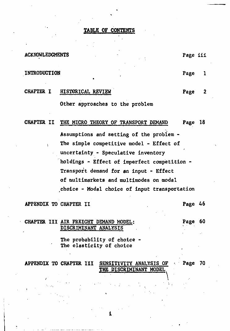
TABLE OF CONTENTS

ACKNOWLEDGMENTS

INTRODUCTION

CHAPTER I HISTORICAL REVIEW

Other approaches to the problem

Page iii

Page 1

Page 2

CHAPTER II THE MICRO THEORY OF TRANSPORT DEMAND Page 18

Assumptions and setting of the problem -

,

The simple competitive model - Effect of

uncertainty - Speculative inventory

holdings - Effect of imperfect competition -

Transport demand for an input - Effect

of multimarkets and multimodes on modal

,choice - Modal choice of input transportation

• APPENDIX TO CHAPTER II

• CHAPTER III AIR FREIGHT DEMAND MODEL: DISCRIMINANT ANALYSIS

Page 46

Page 60

The probability of choice - • The elasticity of choice

APPENDIX TO CHAPTER III SENSITIVITY ANALYSIS OF - • Page 70 THE DISCRIMINANT MODEL ■

CHAPTER IV EMPIRICAL RESULTS . Page 73

Data sources - Specific model used -

• Adaption of the theoretical and

statistical model to the data

available - Empirical results -

Derivation of demand and cross demand

relationships for air freight -

Conclusion

BIBLIOGRAPHY Page 98

VITA Page 111

•

ii

ACKNOWLEDGMENTS

The author is greatly indebted to his thesis advisor,

Dr. Leon N. Moses, for his advice, interest, and encourage-

ment - without which this thesis could never have been written;

nor would a career orientation taken place.

The aid of my two committeemen, Dr. Arthur Treadway and

Dr. Dale Mortensen, also added much to my understanding of the

problem I undertook. All faults in the analysis are, of

course, to be considered those of the author.

Many data sources should be mentioned and thanked for

their total co-operation. Without the help of the Federal

Maritime Commission (FMC), the Bureau of the Census (Census),

and the International Air Transport Association (IATA), the

empirical work could not have been undertaken.

Specifically, Mr. Maurice Vail of the FMC deserves the

utmost in thanks for his provision of the ship rates. He

most kindly received me in Washington on two occasions,

answered all correspondence and phone calls with the greatest

of efficiency and productivity.

Two visits to Washington also yielded the Census trade

flow information. Appreciation is extended to Mr. Milton

Kauffman and the staff in the microfilm section of Inter-

national Trade Statistics.

A visit to IATA in New York yielded the air rates from

Mr. C. R. Murphy.

I also wish to thank my contemporaries at Northwestern,

Mr. Fred Giertz and Mr. Phillip Teets, for their aid in

programming and helpful diseussions of the issues.

Finally, I wish to thank the staff of the Transportation

Center Library at Northwestern.

1

. INTRODUCTION

Our goal is to study the demand for air freight. What

type of firms ship by air? What kinds of goods travel by

air? What are the relevant factors determining the demand

for air freight?

s In the process of answering these questions a theory of

the profit maximizing firm, with transportation costs included,

will be considered. A probability model of modal choice,

based on the relevant factors of transport demand, will be

developed. The model uses a statistical technique known as

discriminant analysis, and we are looking for variables which

enable us to discriminate air users from users of other trans-

port modes.

The concept of elasticity of choice will be developed

from the probability of choice analysis. That is, how

sensitive is a shipper's choice of mode to changes in the

explanatory variables? In particular, from the airline's

point of view, how sensitive is a shipper's choice of mode to

changes in the explanatory variables - such as rate, frequency

of service, etc. - which are under the control of the air

carrier?

Finally, we include the results of the tests of the

model.

2

CHAPTER I

HISTORICAL REVIEW

Although goods were carried in flight almost coinciden-

tally-with the invention of the airplane, the air cargo 1 industry really developed after World War II. Military

experience showed shippers that goods could physically be .

moved by air - both in terms of volume and in terms of

reliability. After the War, some shippers, studying their

transportation needs, found that certain goods or situations

could economically command air use. That is, studies indicated

that air cargo had become the cheapest way of sending these

goods.

Recently air cargo has been growing at the rate of twenty

percent per year. Such a growth rate is somewhat deceiving

because of the small base involved. Air freight only amounts

to one tenth of one percent of all cargo ton-miles shipped in

this country. 2

Many studies have been done by the industry to study the

potential for air freight. 3 The goal was to determine

investment procedures and allocation of resources between

passenger services and freight services.

1For an exhaustive survey of air freight happenings from 1918 to 1945 see John Frederick, CotlercialAimi 'ransortation, fourth edition, •(Homewood, Illinois, Richard D. Irwin Inc.,1955).

21963 Census of Transportation, Commodity Transportation

Survey - Production Area Series - Area 2, Advance Report TC63 (A)C2-2, (Washington D.C., U.S. Department of Commerce, Bureau of the Census, 1963), p. 4, table C.

3See [4], [5], [6], [7], [8], [11], [12], [13], [15], [1 6], [19], [23], [27], [29], [34], [36], [40], [44], [45], [ 46], [47], [48], [52], [53], [54], [64], [66], [67], [72], [77], [78], [84], [85], [87], [88], [93], [94], [98], [103], [110], [112], [117], [119], [122], [128].

3

Other studies have been done by the academic community.4

A

few dissertations have been written in the field. 5 We will

review the above mentioned material, but our conclusion will

be that no study has provided a satisfactory explanation for

why shippers will ship by air or of how much shippers will ship by air. This is shown by the, facts that all past fore-

casts have been overly optimistic and that the airlines

enthusiastically responded to our offer to explore this area.

Some goods like industrial diamonds, hormones, pearls,

platinum and certain furs move virtually 100% by air. Other

goods such as oil, coal and basic foodstuffs never move by

air. Still other goods like fresh onions, cigarettes, perfumes,

resins, projectors and typewriters move by air and also by

other modes. More specifically, in the latter case, the same

good is shipped by different modes between locations i and j.

This reflects demand conditions, or the firm's cost structure

or both. What types of goods are "air types" will be

mentioned in the empirical section.

Observation of the types of goods carried by air indicate

that two characteristics of shipments tend to predominate -

those of high value and those of low density. These two

characteristics are modified by the geographic concentration

of the source of supply or demand (e.g. if an area is only

accessible by air); the average length of haul (which attempts

to measure the market are of the good); perishability (both

physically-related and obsolescence-related); and seasonality

(which attempts to measure a demand for speed).

4See [14], [20], [21], [22], [24], [25], [26], [28], [30], [31], [32], [33], [37], [38], [41], [43], [56], [61], [63], [68], [69], [80], [83], [102], [103], [104], [107], [113], [114], [116], [127].

5See [96], [100], [123].

4

Why high value goods should be carried by air or are

considered "air candidates" can be better appreciated when

the theoretical section on transport costs and transport-

associated costs and the theory of the firm are viewed. Here

we cite empirical evidence by Brewer [26] that more than

sixty percent of the 'commodities now being transported by air

have values in excess of three dollars per pound. It is

argued by the proponents of the high value thesis that high

rates can be "absorbed" better by high value goods.6

That low density (pounds per cubic foot) prevails can

be witnessed in air managerial statements that planes "bulk"

out before they "weight" out. That is, the weight capability

of the planes is seldom met because all the volume is filled.

Shipments also tend to be small. More than seventy

percent are less than one hundred pounds. 7

Initial analysis shows that pick-up and delivery

service is basically limited to areas within a twenty-five

mile radius of the airports. Of course, within this area

(and out of it also), the shipper can take the good to the

terminal himself, hire a common carrier to do so, or give

his business to a freight forwarder.

••

6It should be pointed out that if rates are stated in ton-•

mile terms, air may not be at as great a disadvantage as first appears. For if the shipper is traditionally a surface shipper, he will neglect the fact that great circle distances are shorter than surface point-to-point distances. Since he thinks of distance between i and j in terms of surface miles, air cost will always be overstated. See Stanley Brewer, Vision of Air Cargo, (Seattle, Bureau of Business Research, University of Washington, 1957), p. 27.

7Stanley Brewer, John Thompson, and William Boore, The Air-craft Industry - A Study of the Possibilities for Use of Air. Freight, (Seattle, University of Washington, 1960)..

5

. Recently air freight has grown away from its previous

joint-product status. While all-cargo carriers exist (e.g.

Flying Tiger, Slick), the bulk of the business is carried

by airlines best known for their passenger business. A

change has occurred in the operation of these carriers.

Approximately sixty percent of their cargo business is

carried on all-cargo flight. Some of this is done by all-

cargo planes (in some cases old propeller driven passenger

planes converted for freight use, but in more and more cases

new jet aircraft specifically designed for freight). The

rest is done by quick-change (Q-C) aircraft; aircraft which

serve passengers during the day and cargo during the night.

Forty percent (and an always decreasing percentage) is

carried in the belly of planes on passenger runs. At one

time 100% was in this category. In this last case, freight

is the low priority item ranking behind the passenger, his

baggage, and mail.

Air's natural advantage is in the speed it has to

offer. It also "sells" other time related services such

as reduced warehousing, reduced inventory, ability to take

advantage of a time-limited situation, less spoilage, etc.

In addition, other services are sold in the form of less

packaging, less pilferage, less damage, etc. These services,

the more of the desirable items like speed and the less of

the undesirable items like damage, are compensated for at a

rate which is higher than other modes charge. Thus, for the

same amount shipped, the transportation bill will be higher

forairthanforatieralodessioe.rji7r stiwilerer.is

the rate by a (air) or s (sea) and is the amount shipped.

6

However, the transportation bill is not the only cost

of a firm which is affected by the mode of transport used.

Mode of. transport also influences the firm's costs of

inventories, warehousing, packaging, insurance, etc.

If the firm's goal is to maximize profits, then it must

analyze the effect of a mode choice on its profit picture.

Again we stress that this entails analysis beyond the trans-

port sector. The firm must consider a profit analysis which

surveys the entire company. 8

Many of the difficulties that the air industry has had,

and is having, in selling the use of air services stem from

a lack of understanding of the above type of analysis. Many

firms have autonomous transportation divisions which render

the firm's transportation decisions so as to minimize trans-

port costs for shipping outputs, the levels of which have

been determined by another division.

Such suboptimization will seldom lead to an overall

profit maximization by the firm. In this case, the whole is

not equal to the sum of its parts, because some sector's are

interdependent upon other sectors. Thus optimizing each

individual sector will not necessarily optimize for the total

firm (unless one finds the overall optimum position and then

defines its constituent parts the suboptima). Therefore,

absolutely minimizing transportation costs, for which, under

much of current industry thinking, the transportation manager

is rewarded, may really result in a profit position which is

unfavorable relative to the profit position which is avail-

able if a broader, all-firm scope is taken.

8See American Management Association, A New Approach to

Physical Distribution, (New York, 1967).

7

For instance, suppose a firm has two sectors x and y.

Sector x has a cost function a2 - a+5. Sector y has a cost

function 2a2 - 4a+10. Together, as a firm, the cost equation

is Z=3a2 - 5a+15. Sector x and sector y are inter-related

through the additive function Z. Suppose that the goal is

to minimize Z. Suppose that sector y must accept the

decision of section x. Sector x is obviously minimized at a

value of a-4 However, when both are combined into an

operating unit (the firm), the firm achieves an overall

minimum at a=(5/6).

To capture this notion of interdependence of sectors,

the concept of full distribution costs has arisen9 . Full

distribution costs refer to all costs which are directly or

indirectly related to the transportation decision being

considered. This concept, in relation to air freight, has

evolved quite recently from H.T. Lewis' and J.W. Cullaton's

book The Role of Air Freight in Physical Distribution [83].

Prior to this work, air freight was not considered a

candidate for the job except for emergencies and perishables.

All thinking seemed to gravitate around this limited

number of shipping situations. The point to be made from

the full distribution cost argument is that higher costs in

the transport sector may be offset by lower costs in other

sectors to such a degree that it becomes more profitable to

ship by the higher price mode.

• 9See [20] p. 5; [25] pp. 46, 61, 62; [26] p. 39; [29] p. xiv; [42]; [56] pp. 16, 26; [64] pp. 11, 13, 54, 67, 71; [65] p. 98; [73] p. 20; [81] pp. 32-33; [82] p. 39; [100] Chapter 4; [102] p. 6; [110] pp. 1, 35, 42, 121; [113] pp. 163, 164, 217, 231; [116]; [123] pp. 44-45; [103] p. A-13.

8

Most distribution arguments stress the interdependence

of the transportation sector with the warehousing, inventory,

insurance, etc., sectors. One contribution of this disserta-

tion will be to show an important interdependence effect

with the production sector. That is, it will be shown that

use of different modes of transport implies different levels

of output for profit maximization.

Most of the distribution studies were verbalizations of

the problem. Their important function was to suggest

variables, which our theoretical analysis attempts to

incorporate. If shippers were interested in these costs, it

was felt that the analysis undertaken should attempt to

answer their questions.

Two basic approaches have been used in past air freight

investigations: a macro approach and a micro approach. The

macro approach ties air freight with growth in population,

Gross National Product, industrial production, and other

aggregate indicators.10

It is hypothesized that a certain

relationship, e.g. log linear, exists between the dependent

variable (generally air tonnage) and the independent

variables. •Such procedures do not deal explicitly with the

determinants of demand. They cannot, therefore, be used to

reveal the influence of changes that are expected to take

place in the cost and quality of air freight on tonnage. In

a similar vein are some recent air cargo forecasts which are

obtained by simple extrapolation or by fitting a growth curve

to past data on air cargo . tonnages. 11 These forecasts

. 10see [23], [27], [ 35], [ 44], [ 52], [53], [93], [94], [100].

11See Northrop Corporation, Air Freight Statistics, (Hawthorne, California, Norair Division, NB 60-265, 1960).

9

receive the same criticisms as above.

Most micro approaches to the problem were attempts to im-

plement full distribution analysis. Very few studies involved

empiricalwork, and most empirical work found was relatively

poor in quality and in method. A pioneering work is found in

Umpleby's [123] masters dissertation. Although his work is

basically verbal, he stresses the importance of the costs of

production, market prices, the nature of the demand, substitute

modes available, and en-route delays as they affect selling

prices. 12 These items play a large role in the analysis

contained in the present paper.

Case studies of distribution costs for individual firms

are also found in the literature.13

Wein [127] attempts to construct a point demand for air

freight. Air freight demand is made up of a normal component

(what is traveling at today's rates) plus air cargo potential

(which is the penetration rate times the tonnages in categories

of goods which are air candidates). Prime categories for air are

general and household freight traveling by class I, II, and III

common and contract carriers, LCL rail freight, LTL truck freight,

rail freight forwarder traffic, REA traffic, and surface mail.

The penetration rate is calculated by comparing the current air

rate versus the competing mode's rate. Multiplying the penetra-

tion rate times the tonnage in each category, then adding this

to the normal component, yields the demand point for

today's rate. Vein generally neglects all other costs

12Arthur Umpleby, A Study of the Economics of Air Freight in

Production and DiiTAbution, (Columbus, Ohio State University, Masters Thesis, 1957), pp. 23-24. •

13See [3], [6], [64], [86], [102].

10

or services in his analysis and concentrates only on rates.

Sealy and Herdon [102] break down the productive

processes of machinery and textile firms into four components:

(1) transport, (2) inventory, (3) warehousing, and (4) packing.

The authors then calculated total distribution costs by

air and sea. They found that only two percent of the

consignments studied were cheaper by air when assessed on

freight charges alone; but that eighteen percent were

cheaper when assessed on. total distribution costs.14

Total

cost by surface transport was, on the average, the surface

freight charge plus 254% (of the surface freight charge).

On the same basis, the total cost by air is the air

rate charge plus 457. (of the air freight charge).15

From the above a demand curve for air freight was

derived. Given the current levels of traffic for good A

and rates of a (for air) and s (for sea), the percentage

drop in the air rate could be calculated which would make

1.45a 4: 3.54s. At that, and all lower rates, all of

commodity A would go by air. This was done for all commodi-

ties and yielded the graph AA. (Currently 18.67. of the

consignments are going by air).

14Kenneth Sealy and Peter Herdon, Air Freight and Anglo-European Trade, (London, ATS Ltd., 1961), p. 8..

15Ibid, p. 39.

eme.soaa so ft

a • 4

• I e

.1

•••••.

Per Cent WA Decrease From Current Level Of Air Rate

-00% • Percent Of

Total Air __ Consignments

11

meN

Diagram I-1

Similar types of studies are described in Stratford [113],

and [114]. More commodities are surveyed (forty) and more

sectors of the firm are considered (six). The type of

analysis is referred to as substitution analysis. Unfortun-

ately, none of the empirical results are presented nor

were production costs taken into account.

Brewer [27] derives the demand curve for air freight

between the United States and Europe for 1957. Using

Bureau of the Census data, he chooses to view all commodity

groups having an average value per pound greater than $.40.

The rationale for this choice is that an average of $.40

per pound means an appreciable proportion of the goods in

that category have value of greater than $1.00 per pound,

which is his true criterion for air candidacy. Brewer

subscribes to a "well developed thesis that high value

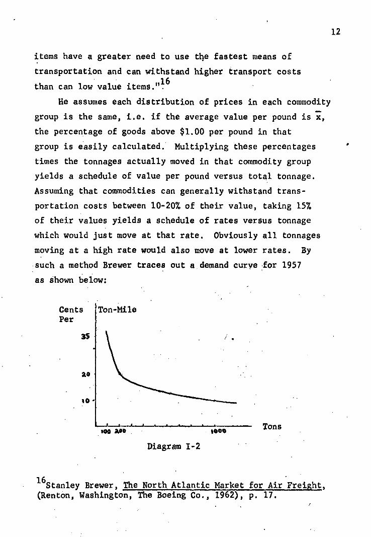
ao

% O•

items have a greater need to use the fastest means of

transportation and can withstand higher transport costs ,

than can low value items.'16

.

He assumes each distribution of prices in each commodity

group is the same, i.e. if the average value per pound is 74,

the percentage of goods above $1.00 per pound in that

group is easily calculated. Multiplying these percentages

times the tonnages actually moved in that commodity group

yields a schedule of value per pound versus total tonnage.

Assuming that commodities can generally withstand trans-

portation costs between 10-20% of their value, taking 157

of their values yields a schedule of rates versus tonnage

which would just move at that rate. Obviously all tonnages

moving at a high rate would also move at lower rates. By

such a method Brewer traces out a demand curve for 1957

as shown below:

12

Cents Per

Ton-Mile

35

Tons . moo loo woo . • • •

Diagram 1-2

• 16Stanley Brewer, The North Atlantic Market for Air Freight,

(Renton, Washington, The Boeing Co., 1962), p. 17.

13

Brewer's analysis depends solely on the value per

pound of the good. Such strpng allegiance to that single

variable has had many followers. 17 However, dissidents

have recently attacked the sole use of value per pound as

the criterion and purpose that it must be considered along

with other , transport variables. 18

Two important theoretical contributions remain to be

mentioned. The first is The Demand for Air Cargo Trans-

portation: A Pilot Study by Ferguson and Schnabel [56].

There is a lower limit to the demand for air freight which

is set by the volume of traffic currently moving at existing

rates of the competing modes. "The extent to which the

actual demand curve differs from such a lower limit estimate

depends on the difference to the shippers of the value of

air as opposed to surface transportation. This difference

in the value of air and other forms of transportation is

intimately tied to the value of speed in making possible

savings in inventory costs." 19

Output is assumed exogenous. The authors then attempt

to design an optimal inventory policy co-ordinated with an

optimal transportation policy. The end result states the air .

rate as an additive function of the surface rate and the

change in the expected shortage cost when air is used. No

empirical tests are reported.

. 17See [36], [58], [65], [106], [116], [123].

18See [48], [59], [113].

19Allen Ferguson and Constance Schnabel, The Demand for Air •

Cargo Transportation: A Pilot Study, (Evanston, Northwestern, University Transportation Center, 1960). p. v and p. 17.

'.,:li'Z'T'Atkl'M,A441i0;414.0044 -0'0144:4;i1ORIONaMCMOSIMMOONMINgekcinar:itstircapppri.mcgi.04104:NR4Mikikg retsowtparnogawawsinswammawmagangmamasominem

The second theoretical work is Baumol and Vinod's

Studies in the Demand for Freight Transportation [14].

Both a micro and a macro model are presented. Only the

micro model is of interest here. Output is assumed exogenous

(although Baumol later states that profit maximization and

not transport and inventory cost minimization should be the

.goal). An inventory type of approach is taken. Quantity

transported is a non-linear function of price difference

between regions, shipping. cost per unit (freight, insurance,

etc.), carrying costs per unit, and the level of safety

stock. The above relationship is derived from a marginal•

revenue equals marginal cost framework. This is a form of

profit maximization. However, production costs are not

included in the cost calculations. Such a suboptimization

may not lead to the overall goal of profit maximization.

Both the Ferguson and Schnabel and the Baumol and

Vinod studies come under criticism due to the assumption of

exogenous output. In addition, the failure to put their

maximization or minimization schemes into a proper time-order

is criticized. Revenues and costs are being received and

incurred throughout their analyses without regard to their

sequencing and, hence, without regard to capital costs on

tied up funds. Although the model presented in Chapter II

does not totally rectify this problem, an attempt is made

to incorporate capital costs.

A few studies suggest a model of overall profit

maximization, but no formalizations of the problem are

presented. 20 •

14

2 °See [48], [52], [77], [113].

15

A different type of approach, is taken by the Stanford,

Research Institute (SRI) [110] which .attempted not to •

provide an estimate,of the.demand . curve for air freight, but

rather to provide a check list for shippers and airlines to

attempt to identify characteristics of the firm as a potential

user of air freight. SRI advocated a firm approach rather , . than a commodity approach. ,

SRI concluded that businesses could have three major:

- reasons for using air freight: , • , ,

(1). Use of speed. to decrease .. time. in -transit .

(2). Use of speed to decrease;.the costs of : holding

, ; goods in inventory,

(3). Use of superior conditions of .carriage by air - , . to decrease risks and,costs associated' with . .

alternative transportation

Specifically, speed.may enable the firm to increase

sales in a time limited situation, increase utilization of

productive facilities and equipment, decrease investment in

goods in transit, and meet unpredictable demand and

emergencies.

Inventory investment can be decreased with increased

speed. Also increased speed.-can decrease the risk of

inventory , obsolescence, decrease the investment and operating

expenses associated with inventory facilities and services,

and decrease inventories held by jobbers or wholesalers.

The service characteristics of air freight are such as

to decrease the risk associated with having goods lost,

stolen, damaged, or spoiled in transit; to decrease costs

and time over which provisions for protecting or preserving

goods are required; to enhance control or management over

goods in transit; to decrease duties in international move- ,

ments, and to expedite handling of small lots.

16

A large check list is used, asking the shipper about .

his shipment policies and desires. If a certain number of

questions are answered in the affirmative, a more thorough

investigation of air freight possibilities should be

undertaken.

Essentially the SRI report was a surrender to the non-

quantifiers. All attempts to have an empirical analysis

had been fruitless and will continue to be so, concluded SRI.

Researchers in the area criticized the report for this

conclusion and suggested that its value was in pointing out

the parameters to be considered in future empirical analyses.21

While transport economics has been citing the inelasticity

of transport demand, 22 all writers in air freight have

emphasized the elasticity of the demand for air freight.23

Brewer is typical when he states, "The presence of

substantial elasticity in the demand curve for air trans-

portation is well recognized."24 Sealy and Herdon estimate

the elasticity to be 1.7. 25 Echard estimates an elasticity

of 3.0.26

21See [103], [113].

22See [95] pp. 82-97, and [99] pp. 174-176.

23See [127] p. 6; [29] p. 82; [94] p. 31;[73] pp. 106-107.

24Stanley Brewer, Vision in Air Cargo, (Seattle, Bureau of Business Research, University of Washington, 1960), p. 13.

25Quoted from Alan Stratford Air Transport Economics in the Supersonic Era, (New York, St. Martin's Press, 1967), p. 221.

26E.W. Echard, Free World Air Cargo: 1965-1980 Rate Elasticity Forecast, (Commercial Marketing Research Department, CMRS 77, Lockheed Georgia Co., June, 1967), p. 3.

17

These substantial estimates of elasticity suggest that

reducing air rates will overwhelm the carriers with business.

Elasticity is an important planning tool for the carriers

and also rate-making bodies. It shall, therefore, be

investigated in the context of the model of the dissertation.

As can be witnessed, quite a bit of work has been done

in the field of air cargo. Unfortunately, much of it has

involved considerable resources but little appreciable output.

The goal of this disseratation is to rectify this state

and give a study solidly based on economic theory. The

outline will be as follows: Chapter II is the micro

development of the theory of transport demand. Here demand

functions for transportation with respect to rate, time in

shipment, damage rate, etc., will be derived for both

inputs and for output under , all market conditions. Chapter

III is the air freight demand model in its 'statistical form.

Herein the discriminant model is developed which will test

the theory of the previous chapter. Chapter IV is the

adaption of_the model to statistical testing and the empirical

results of the model. Herein that part of the theoretical

model tested is described, as is the way in which the model

was adapted to conform to available data. Finally, the

empirical findings are presented and discussed.

18

CHAPTER II .

THE MICRO THEORY OF TRANSPORT DEMAND

Dupuit, in 1844, said, "The ultimate purpose of a means

of transportation ought not to be to reduce the expenses of

transportation, but to reduce the expenses of production. " 1

Transportation rates are but one member of a transportation

package, which includes the costs of production. Since 1844

researchers and theorists have attacked problems calling for

the minimization of transport costs or the minimization of

transport and transport associated costs (e.g. packaging,

inventory costs, etc.), but few have paid attention to

Dupuit's emphasis on the relationship of production and

transportation. The costs of transportation and the costs

associated with transportation (of both inputs and outputs)

will be viewed to see how they fit into the conventional

spaceless and timeless theoretical analysis of the theory of

the firm.

In order to develop a theory of freight transport demand

a situation is postulated which closely resembles the scenario

in which the theory of the firm is studied. The model below

adds nothing but a limited concept of space and a limited

concept of time to the conventional analysis.

Implicit in the classroom teachings of price theory is

the coincidence of resource sources, the production point,

1Howard T. Lewis, "The Economics of Air Freight", in Nicholas A. Glaskowsky ed., Management for Tomorrow, (Stanford, California, Graduate School of Business, Stanford University, 1957), quoting Dupuit, p. 71.

19

and the consumption points. These assumptions will now be

altered by supposing that consumption takes place away from

the production point. It will still be assumed, as does

conventional analysis, that consumption takes place at a point

(as opposed to having consumers located over a plane). Raw•

materials will also be located away from the production

point. Thus the theory of the demand for transport will be

developed in the context of having the profit maximizing

firm producing its product at point B; using resources on

hand at B, but also resources from other points W; and

selling the final product at C points. Hence distance enters

the analysis.

Time also enters into the analysis. Goods must move

from the production point to the consumption points in order

to produce revenue. Resources must move from W points to the

production points in order for goods to be produced. Both

these movements entail a cost - that of capital tied up on

goods or materials in shipment. The profit maximizing pro-

ducer must account for these time costs when making his

production decision. Demand, however, will be considered as

instantaneous once the goods reach, market, i.e. all goods

are sold on the day that they arrive in the market. Hence

time enters the analysis.

Since the theory of the demand for transport is analogous

to the theory of the firm, a thorough analysis would parallel

a price theory textbook with all the various market cases,

.e.g. monopoly in the product market with competition in the

factor market, etc. Rather than burden the analysis with

many similar arguments, a few cases will be presented. The

procedure will become obvious and the interested reader may

trace out particular market schemes which interest him.

Initially a case will be considered where W and B

coincide. Only one C exists and pure competition prevails

in all markets. Only one mode exists to carry the finished

product from B to C. This mode is characterized by a certain

transport rate per unit carried, a certain time for trans-

porting goods from B to C, and a certain damage, loss,

theft, or perishability rate. The producer has a variable

cost of production function which is assumed to yield the

typical U shaped average and marginal cost curves. Costs of

production are incurred instantaneously. The inventory prob-

lem will be disregarded for the time being, i.e. it is

assumed that the demand horizon is for one time period.

Demand will be considered as instantaneous once the goods

reach the market, i.e. all the goods are sold on the day they

arrive at the market. To insure the relevence of transport

time it is assumed that payment for the final product is on

a C.O.D. basis. There is a separation in time between the

incidence of production of the goods and the realization of

the revenues from their sale. This is measured by the cost

of the tied up capital referred to above. Later multimodes,

multimarkets, imperfect competition, transport of inputs,

and inventory holdings will be considered.

II

Under the assumptions of perfect competition, the firm

can sell all the output it chooses to produce at C for the

market price. How does the transport rate, the time in

transit, the interest rate, and the damage rate influence

the firm's decision of what output to produce and ship?

20

21

Initially, the determinants of a firm's demand for a

single type of transportation will be examined. The following

notation is employed:

IT the producing firm's profit

Q the quantity the firm produces and ships

the market price of the firm's product

ek the time required to ship the goods from • point of production to the point of sale

the transport charge per unit of product

i the interest rate

the damage, pilferage, loss, or perishability rate

The firm's profit is:

(1) . -rr „ -t (k)•

In this equation, the second termHon the right side is

the total cost of production. The numerator of the first

term is net revenue. This is defined as total revenue, PQ,

times (1-) ) minus total transportation cost, TQ. times (1-J1 )

The total revenue is multiplied by (1-) ) because only

(1-) ) of the goods produced ever reach the market, i.e.

only = (l-p )Q sellable goods actually arrive at C,

although Q left from B. 2 Transport rates are payable for

services rendered and for only non-damaged goods. Since

this net revenue is received only after at days, it is

divided by (1+i) determine its present value.

• • 2It is assumed here that the firm bears the cost of damage,

etc. If the transportation firm "made good" on all losses, • the producing firm would behave as if p =0 and end up

selling )3 % of Q to the transport company.

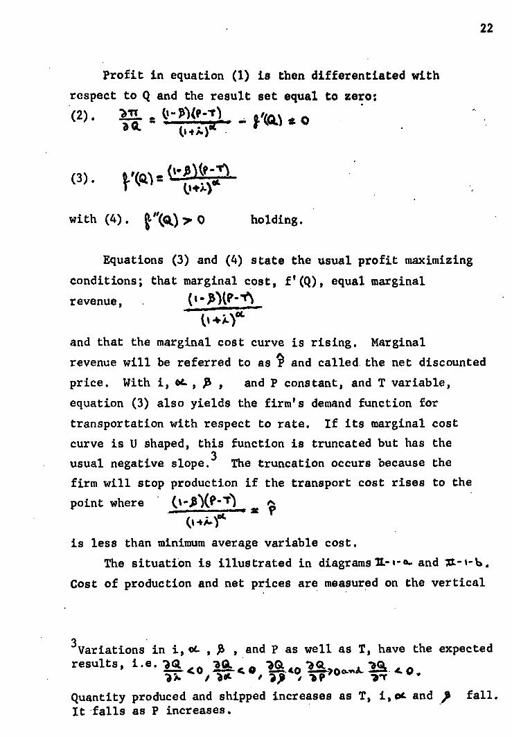
Profit in equation (1) is then differentiated with

respect to Q and the result set equal to zero:

(2) . 3)0•11 . s 0 4")

(3). 0.44

with (4). t ii(k)7. 0 holding.

Equations (3) and (4) state the usual profit maximizing

conditions; that marginal cost, f'(Q), equal marginal

revenue, ( 1- AMP-1)

0+44'

and that the marginal cost curve is rising. Marginal

revenue will be referred to as and called the net discounted

price. With i, , and P constant, and T variable,

equation (3) also yields the firm's demand function for

transportation with respect to rate. If its marginal cost

curve is U shaped, this function is truncated but has the

usual negative slope. 3 The truncation occurs because the

firm will stop production if the transport cost rises to the

22

point where • 0-1)0)- 1) - 044(

is less than minimum average variable cost.

The situation is illustrated in diagrams 1.-1 -0- and 11.-1-6.

Cost of production and net prices are measured on the vertical

3Variations in i,c4. , , and P as well as T, have the expected results, i.e. 1GL 4o /Ce- o

C) a" /CA4 .a sa )0 A, 21 4. 0

VA I 21,- i .

Quantity produced and shipped increases as T, 1.014 and )0 fall. It falls as P increases.

(1:531044%) 2 go

(I 4 i.Yg

0

p 1 0.tra-n• -

Q 1 Q1. Qt4Q.

axis. Q is the quantity the firm would produce and ship if

the market price were P and the. transport rate were zero.

Tm T2' T1, represent successively higher transport rates. .

At rate T1

the firm will produce and ship Q. Any further

increase in the transport rate will cause the firm to cease

operation.

rC AV C

23

• • go QL Qq■Si

to.tir 0.-tft -

The demand function., is shown in diagram II-1-b,-where

rates are 'measured on,the vertical and quantity produced and

shipped on the horizontal axis. 4, 5, 6

4 See Appendix to Chapter II, note 1.

5See Appendix to Chapter II, note 2.

6See Appendix to Chapter II, note 3.

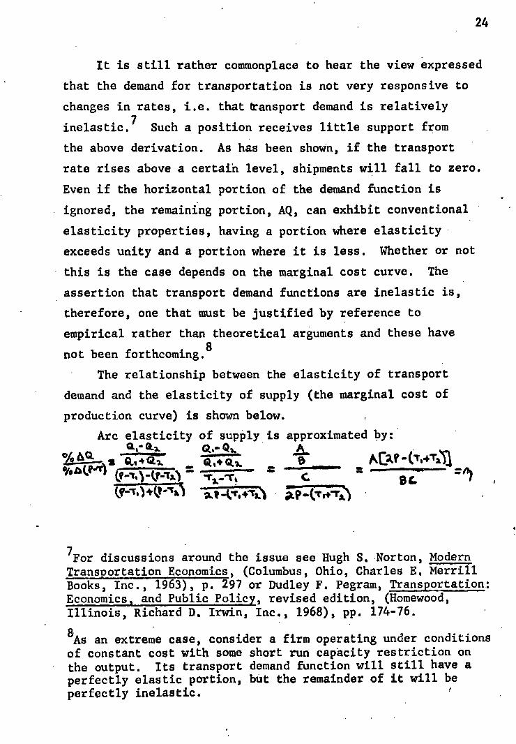
24

It is still rather commonplace to hear the view expressed

that the demand for transportation is not very responsive to

changes in rates, i.e. that transport demand is relatively

inelastic. 7 Such a position receives little support from

the above derivation. As has been shown, if the transport

rate rises above a certain level, shipments will fall to zero.

Even if the horizontal portion of the demand function is

ignored, the remaining portion, AQ, can exhibit conventional

elasticity properties, having a portion where elasticity

exceeds unity and a portion where it is less. Whether or not

this is the case depends on the marginal cost curve. The

assertion that transport demand functions are inelastic is,

therefore, one that must be justified by reference to

empirical rather than theoretical arguments and these have

not been forthcoming.8

The relationship between the elasticity of transport

demand and the elasticity of supply (the marginal cost of

production curve) is shown below.

Arc elasticity of supply is approximated by: Cle"a4.. at'• A GIA 4G4 (k,4 /kCAr - 0,414

"°414

(t%) -(?_T,') W044"1) l'a=k771711)

7For discussions around the issue see Hugh S. Norton, Modern Transportation Economics, (Columbus, Ohio, Charles E. Merrill Books, Inc., 1963), p. 297 or Dudley F. Pegram, Transportation: Economics, and Public Policy, revised edition, (Homewood, Illinois, Richard D. Irwin, Inc., 1968), pp. 174-76.

8As an extreme case, consider a firm operating under conditions of constant cost with some short run capacity restriction on the output. Its transport demand function will still have a perfectly elastic portion, but the remainder of it will be perfectly inelastic.

25

Arc elasticity of the associated transport demand

(adjusted to be positive) is approximated by:

cts-4). A

c. 3c. - Ts +Tx

-r, If the elasticity of supply is multiplied by ---1-----) AS *-rx

it will yield the elasticity of demand for transport. With

certain values of T T2' and P, 6 will exceed 1.

Or alternatively, consider point elasticity. If the

cost function, T, and P are such that the kink in the demand

curve occurs at a quantity less than half way to the quantity

where T=0, the curve will have elastic sections. It is

seen, however, that the kink increases the chances of the

transport demand curve being inelastic.

It should be obvious from the above diagram that a

marginal cost curve, with a gentler slope than the one

presented, will yield a demand curve for transportation with

a gentler slope than the one derived above.

The above analysis treated the transport and the transport

associated costs from the demand side, i.e. as net prices.

The same analysis could have been treated just as easily from

the cost side, yielding of course, the same results. 9

T. E. •

9See Appendix to Chapter II, note 4.

III

Suppose now that uncertainty is allowed to enter the

analysis. In the real world the precise market price in the

future is unknown. Likewise the exact delivery time is not

known with perfect certainty; nor is the damage rate. Busi-

nessmen expect certain market prices, delivery times, and

damage rates to prevail, i.e. the variables have probability

distributions associated with them; and, in the absence of

any a priori knowledge, the businessman expects the average

of the variable to occur. We will assume all distributions

are symmetrical (which is essential for generality of the

conclusions). T and i are fixed.

The handling of the P and )3 distributions is straight-

forward (if they are the only variable distributions, i.e. if

a is fixed). To maximize profits the firm should assume

that the average market price P, P = L P,xk where (xkl tun A.

is the probability distribution of prices, and the average

damage rate yycl where {4'1) is the st

probability distribution of damage rates, will prevail.

Placing these values in equation (3) above will yield the

firm's expected demand for transportation.

Variable delivery times change the analysis. It is not

known whether the goods will reach the market in oc,o 2.4 —

or ay.. days. To maximize profits the firm will not do

best to assume that the expected delivery time prevails.

The true criterion is the produce and ship the output dictated

by the expected net discounted price P, i.e.

26

A*es (-p)/-11 Skto

4441. • ik

where {741 is the probability distribution of days. When A

only P and were considered, P, P, and )3 were one in the

• same criteria. However, when variable time costs enter, the

discounting changes the analysis.

(1-3 )( -1) - P is not equal to -------r--- In fact (1 +X ) •

10

P —77.7

With all three variables random, the net discounted price

is:

1 1.. leny'XY, "P"Arv'T) (6) . ? =

Iv% v• •, 0 +44'

The demand curve for transport is solved for as above.

The second moment of {0441 also yields an interesting

conclusion in this model. The variance of olL may be viewed

as a measure of reliability or dependability of service.

Given the symmetry of the a distribution, increasing or

decreasing the variance of ot will not change a . Will the

shipper prefer dependability, ceteris paribus?

2 7

10See Appendix to Chapter II, note 5.

Waar)

p.

v. v.

•

•

2.-SW a-11/4a a+sk 41/441

9.11,Arop. "lis, 2.

Under the assumptions of the model (a one period demand

model with no inventory holding), the firm will prefer

undependability in delivery time. That is, given a choice

between two types of delivery, both having the same mean, the

shipper will prefer the one with the greatest variance of

delivery time - for it will yield the highest expected net

discounted price (which implies the greatest profit in the

competitive model). - •

The demonstration of this risk preference is shown

be ^ Taking the first two partials of P •

01.441

-a li -D-AX11 -13 ints14 0 ( 7). --- = .. Zoe.

(8) 0 4D4V-11306NektfAt • ---r re. '7, 0 .ioce. (.10.44.

Thus as a increases, 1P decreases but does so at a

decreasing rate, i.e. the curve is concave upward as is

shown below. .

28

with respect to oc yields:

2 9

Suppose that the range of one choice is from a -k to

c. +k days. The second choice takes one day longer or shorter

than the other choice, i.e. a -k-1 and a +k+1. The chords BA and DC, drawn show that the expected price is always higher

when the variance of delivery time is greater. Consider. a.

If a were not variable, the net discounted price is P o . If,

however, cc. has probability distribution one, expected net

discounted price is P1'

Probability distribution two (with

a greater variance) yields a still higher price P 2 . This

also ties into the analysis of why St. does not yield the

expected net discounted price.

• IV

The analysis can be extended by allowing for speculative

inventory holding. The desire to hold inventory comes about

as the result of variable market prices WS . Production (and thence shipping decisions) must take into account the

possibility of inventory holdings. Under what conditions

will a firm wish to hold inventory - obviously under

conditions which increase their expected profits. Inventory

cost knowledge is thus necessary to determine the firm's

profit maximizing output, Q. Once the goods are produced,

the firm may act differently than was postulated in deter-

mining the Q because Q is now fixed and the production costs

become fixed costs. At that time the firm will only compare

inventory costs versus expected revenues.

A very simple case of the above model will be dealt

with. The transport rate is T; the interest rate is i; the

time in transit is a ; the firm's cost function C=f(Q);

30

and the probability distribution d[x m) of market prices (Pm) .

Inventory cost per unit per day is q. Perfect competition

exists in all markets.

When goods had to be sold on arrival in the market, as

was assumed previously, the profit maximizing output was A

determined by assuming that P would be the net discounted ..-T price that would prevail (where P = ).

0:0°4

With inventory holding allowed, the shipper now has

the option of shipping his goods, having them arrive oL

days from the date of shipment, viewing the market price

at that time and deciding whether he wishes to sell or to

hold the goods in inventory, waiting for a more attractive

market price. Although tomorrow's price may be higher, this

must be weighed against the inventory cost and the extra

time cost.

The analysis becomes more complicated as the number of

days a good can be held in inventory increases. It also is

more complicated the greater the variance of tP3 . To

avoid such problems yet showing the point of the analysis,

we constrain the inventory holding period to one day. That

is, the shipper either sells his good in the market on the

ot th or the o.+1 St day. After the ot41 St day, the good

spoils so that it is unsellable. The price probability

distribution is symmetrical, tx -t) where k=1,2,3. The

mean price will be Y 1)2 .

It is clear that if the market price is P 3 on the 04 th

day, the shipper will sell all goods on that day - for he

never can do better. If the price is P 2 on the oc. th day,

the shipper will also choose to sell all his goods on that

day. Without any a priori knowledge, the price he expects

to prevail on the oc.4.1 St day is Te = P 2 . Getting P 2 today

31

is better than getting P 2 tomorrow. However, if the market

price is P i a days from now, the shipper's decision

depends on the level of inventory costs and the interest rate.

The profit maximizing condition when no inventories

were allowed is shown as:

(9). IP +11 e(0) 1x 1 2x2 - 3x3=-

The firm should account for inventories in its output ft

decision if V A

P ,

'‘ • • ' (The P-q is divided by (i+1) because this is the expected

price received one day after P i would be received. q̂ are

discounted inventory costs). This says that the expected

net price after inventory costs for the sales of the goods

on the oc. +1 St day exceed what the goods could have sold

for on the a th day. e.

If '?j, profit maximizing output is

determined as follows:

(10). Fr r-1-731 1K + l'&1‘;_t PIX;] L.

14:‘ I

^ *rn• ■ 41,

(11) . 1.• .̂ CI + its:X% P.3%3 • tqc4.):-.0

"

P - (12) . 7‘. + 11'3 %) (G2.) It"-

Solving (12) for Q yields the optimum output produced

and transported to maximize expected profits. Obviously

shippers must account for inventory costs in determining

output to be produced and transported. Also obvious is

that the level of inventory costs influence transport demand.

When inventory holding becomes profitable more will be

shipped. This is so because the right hand side of (12) t ^ exceeds the right hand side of (9). If ^

7 ?,

output produced and shipped will be greater when inventory

holding becomes more profitable. The higher the inventory "

costs, the lower the differential of p

and P1 and thus the less shipped.

A graph of q versus Q would appear as below:

Ct.

thasive..... IV%

32

144.

33

A,

At the kink P1 = . Any_further raising of

4 will make inventory holding unprofitable and thus the 11 .

To show how the analysis becomes more complicated as .

the number of possible prices below the mean price increases.

Consider the following complication: vector of prices (P3 and probabilitiesi(x , k=1,5 and symmetrical. Thus P=P3

t and P=P3' However, three possibilities must be allowed for.

It should be mentioned that if P3' P4' or P

5 prevails,

the goods will all be sold on the 0. th day (when they arrive

at the market).

Case 1. (P-T) - ( 1 + i)(P l-T) c q

(P-T) - (1 + i)(P 2-T) 4 q

Inventory holding is too expensive, so that output

implied by P = f' (Q) will be produced and shipped and sold

when it arrived in the market piaci.

Case 2. (P-T) - ( 1 + 0(121-T) > q (P-T) - (1 + i)(P2-T) < q

Inventory holding is too expensive is the market price

on the ot th day is P 2 but not if the market price is P l .

To maximize profits the firm should produce and ship the

quantity dictated by the following: 0 ^

(13) . [-f-ft Its av f1.7-s. 443%s tst, %Is ts Ss] Q— itkR) P".

VIT 2 _ " 0.4) tr. + 10.7ca. 1'37c3 tot% + ps — IVO es 0

ZCI.

(15) .4)

%.14. 43 X3 'it I,%9 f Is S OZ) ,-

11See Appendix to Chapter II, note 6

output produced and shipped will be that dictated by 15 (say .11)

34

Case 3. (f-T) - (1 + i)(13 1-T) > q

(f-T) - (1 + i)(P 2-T) 7, q

Inventory holding is profitable for the discounted

market prices?). and 1112 . To maximize expected profits the

firm should produce and ship the quantity dictated by the

following:

P ^ (16) . =[..----01-14/C0 443%3 feKd 141.)

1-rr - (17) . (% 1 4244+ fe3 7C3 0

t+).

f. •

La( ‘41 f0 0 • (18) X.,41ct 3)(3 ii %4 Islts = CO)

P It;••

As an example of how the analysis complicates as the

number of inventory days allowed increases, suppose the goods

can be sold on the o. th, o4+1 st, and 4X+2 nd days after

production. (The latter two sales the result of inventory

holding for one or two days). Suppose the price (1)13

probability distribution is , k=1,3.

Firstly, if. the market price is P 3 or P2 on the a th

.day, the goods will •be sold on delivery.

Three things may happen. Inventory costs may be so

high that the most profitable decision for the firm to make

. is to sell all goods on the a th day, regardless of the

market price; or inventory costs may be such as to make one

day inventory profitable - in such case, if the market price

is P1 on the &4 th day, the firm will hold the goods until

the next day (when the expected market price is f) and then

sell the goods no matter what market price prevails; or

inventory costs may be such as to make two day inventory

holding profitable - in such a case, if the market price is

P1 on the oc th day, the firm will hold the goods until the

oe. +1 st day. If the market price is P2 or P3 on the

oc. +1 St day, the goods will be sold then. If the price is

P1, the goods will be held until the oC. +2 rid day (when the

expected market price is I) and then sold at whatever the market price may be.

Optimal outputs are found as follows:

For case one above, it is where .i.f t (Q).

/ A For case two'

• For case three (assuming that the storage costs are

due when the goods leave the warehouse), ^

1.1 * Vx (Ka+14)(1)i- P3 (X3 4)0E3) 14(t)

As the variance of the probability distribution of

prices and the number of days of possible inventory holding•

increases, the analysis becomes complicated at an increasing

rate.

Inventory holding in a multi-time period analysis has

been developed elsewilere. 12 •

35

12William Baumol et al, Studies on the Demand for Freight Transportation, (Princeton, New Jersey, Mathematics, August, 1967).

36

V

Imperfect competition can also be added to the analysis.

Transport rates and time costs can be viewed as tax analogues -

the rate T affects the demand curve for the product as would

a per unit tax and the time costs affecting the demand curve

as would an ad valorem tax. Damage costs must be viewed

slightly differently. Net discounted demand curves now exist

and yield net discounted marginal revenue curves. Changing

the transport variables changes the position of the marginal

revenue curve and these changes, with the marginal cost of

production curve, trace out demand curves for the various

variables as was done in the case of perfect competition.

Assume a linear demand curve for the final good,

P=a-bQ. What demand curve will the shipper "see" after

accounting for the costs of transport and those associated

with transport? The price that the firm will receive in the

market place depends on the number of goods which actually

reach the market place in a salable condition. If Q are

produced and shipped, 0.-p A will reach the market. Market price will be P=a-a-j11 )bQ. Total revenue will be

TR=a(1-)3 )Q - (1-ft) 2 bQ2 . Since this revenue will not be

received until sit. days, it must be discounted to be made

comparable to the production costs which are incurred

instantaneously. The present value of total revenue is thus:

( 19) • n a-(1-)))4.•( 1-elaC4.1. TR = (4.1.)4

The shipper must pay a transport bill of (1-,15 )Tig in

ot days. This is also discounted to make comparable all

elements of the analysis:

(!*1-)4

Discounted net revenue will be:

(20). ClInet

Q.4 ;CP

Profits are:

(21). -rr 127(11,.".(1-ebCt.1..—(1-"Yrti.

(1-014 19(41)

■■•

The net discounted marginal revenue function is thus:

37

' t (22). PR

net

CI-AT

Equating (22) to f t (Q) and solving for Q and varying one

of JP , o. , i, T, and a (changes in a will measure

parallel shifts in the market demand curve), while holding the

other constant, will yield the various demand curves for 13 transport.

Probability distributions for the variables T, i, a,

boC. , and A could also be considered. These would not

alter the analysis seriously and would affect the model as

they did under pure competition.

13See Appendix to Chapter II, note 7.

38

. VI

Another line of expansion involves allowing for the

transport of an input. The demand for transport of a factor

of production can be viewed as a derived demand curve twice

removed. That is, the demand for a resource itself is said

to be derived from the demand for the product. Then the

demand for transport is derived from the demand for the

resource. Only the transport rate on the input will be

viewed. The procedure for changes in the other variables

should now be obvious.

Assume that perfect competition exists in all markets.

The firm's production function is Q=f(L,Z); where L is

located at B selling for PL'

but Z is found at W (away from

B) selling for P. Z is subject to a per unit transport charge

of t1 for the trip from W to B. Therefore ' PZ + t1

is the

price of a unit of Z at B.

The firm will produce any given output where the marginal

conditions MRS = (P + t1) / PL = MPP / MPPL

hold. The

profit maximizing output is easily determined. This yields

an output Q l which will subsequently be transported to C and

a Z 1 which needs to be transported from W to B. Thus one

point (t i ,Z 1) on the demand curve for transport of an input

is determined.

The theory of adjustments by the firm to changes in

input prices has been well developed. 14 Changes in t will

change the price of resource Z at B. Increases of t will

increase Z's price and hence decrease its use; therefore,

14See for example, Charles Ferguson, MicroEconomic Theory, (Homewood, Illinois, Richard D. Irwin, Inc., 1967), pp

39

quantity transported of Z decreases. Decreases in t will

decrease Z's price and hence increase its use; therefore,

the quantity transported of Z increases.

To show that this must be true consider the initial

optimum position (Q 1 ,Z io t i). Call it point one. Suppose

transport rates decrease to t 2 , i.e. (t1-t2) 7 0. A new

profit maximizing position results, i.e. (Q2 ,Z 2 ,t2). Call it

point two.

At point two Z is now cheaper because t 1 , t2 . If

point one's profits are evaluated at point two's resource

prices, they will be less than those profits evaluated at

point one's resource prices (since this latter position is

the revealed "best", the profit maximizing situation).

Thus,

Q-P14- (23). •----QT et..t. t"(..14..+74)-t

1) i Q ?Lt. Qa4,72)'t si.. /

or

( 23 ) . 01.%""

The same analysis is made of point two. Point two's

• profits evaluated at point two's resource costs will exceed

point two's profits evaluated at point one's resource costs

(since point two is a point of maximum profit).

Thus,

(24) . faa:: Pici• .alax. , taq.- -kite-Jr-4k

40

. Adding (23') and (24),

/ 41 Qs ). - ?O.., -114.L3, -Qa1. 1

Substracting common terms,

(26).

Multiplying by -1,

(27)•

Subtracting common terms from both sides,

(28).

-xxLv,,- -ex) o

or

(29).

It was assumed that (t 1-t2) > 0. This implies that

(Z 1-Z 2) 0 or Z 1 4: Z2 . Thus if the transport rate on

inputs is reduced, making Z cheaper to the firm, the firm will

use more Z and thus demand more transport. Likewise, if the

rate was increased from t1 to t 3'

then (t1-t

3) 0 implying

(Z 1-Z3) 7 0 or Z1 Z3 -- a decrease in the quantity

demanded of Z and thus of the quantity demanded of transport

of Z.

(25).

••• •• • • •• • •• • •

a a

The analysis yields a downward sloping demand curve

for transport of an "input. 15

1.0••••• as

41

72.

e 3 ;a 1 vLa

Diagram 11-4

The above analysis also holds if the market for the

final product is imperfect.

There is a lesson here for transport companies. It

stems from the interdependence of transport rates with profit

maximizing output. Certain rate changes on inputs influence

the firm's cost of product curves and hence the demand for

transport of final goods. Likewise, certain rate changes on

outputs influence profit maximizing output, and hence the

demand for transportation of inputs. Changes in travel time

and damage rate can have the same effect.

15Time costs ( oc. and i) and damage rates (p ) will have negative effects on quantity demanded and shipped, i.e.

11E -II—. ° 4' 0 •Anok. 4. 0 1A, I 04 1 11,0 as expected.

42

Presumably the transportation firm wishes to maximize

profits. Thus, when contemplating rate or service changes,

it should be aware of the important intertwining of transporta-

tion and production in the theory of the firm. For instance,

decreasing *L in the transport of the final good will

increase P, increase Q, which will (unless the resource is

inferior) increase the use of Z. Thus on two fronts,

more final product transported and more input transported,

the transportation company has increased its business both

quantity wise and revenue wise. When the rates are changed,

the shipping firm will change Q and Z, but whether the

transport company's revenues change favorably depends on

the elasticity of transport demand - both input and output.16

If imperfect competition in the product market is added, the

analysis is complicated further by the elasticity of demand

for the product.

VII

Two additional complications remain to be added to

the analysis - that of multimarkets and multimodes. For

simplicity view only the demand for transport of the final

product.

Above the theory was developed in terms of a single

mode and a single market. Its extension to the case of choice

• between m modes or n markets, with perfect competition in

the product market, is now a simple matter. The firm takes the pc , T, and )01 values of each mode and the P's

16See Appendix to Chapter II, note 8.

of each market and calculates each combination of market

and mode's P's (or net discounted prices). It chooses

the combination of mode and market with the highest P

and then equates marginal cost of production to this

value to determine what quantity it will produce and ship.

' If marginal costs are constant or rising, this two stage

decision process will automatically assure profit maximiza-

tion. If, in other words, Pm

exceeds P. for j=1,2,...,m-1,

thenQwillexceed.and 'WIN will exceed ITi• Under m

Qj

these conditions, it will ship all of its product to one

market via one mode. . ,

It should be pointed out that different transport

modes generally imply different final outputs produced '

and shipped. Thus, if the shipper is talking solely of

using air freight, he is talking of output produced and

shipped QA; if he is talking solely of using sea freight,

•he is talking of output produced and shipped Q s ; where QA

in general does not equal Qs . A similar statement holds

for different markets. Of course, the shipper should only

be interested in the highest output.

Supposing one market and two modes, A and S, we have

graphically:

43

•

The only time that modal splitting would occur would

be when there is a tie for the highest net discounted price.

Under those circumstances the shipper could ship all by air,

all by sea, or split the shipment. The theory developed

here can not explain the magnitude of splitting when the

shipper is indifferent as to modes.

The transport firm must now make its rate and service

decisions with the recognition that certain changes in his

policy may make another mode more attractive to the shipper.

Certain policy changes may make the transport firm's revenue

function take great jumps, i.e. it may be discontinuous

because of shipper's switching modes.

When imperfect competition in the product market enters

the multimarket, multimode analysis, the possibility of the

•firm splitting modes, becomes a reality. However, this is

really an aggregation problem. On any given route the firm

will only ship by one mode. Over separate routes different

modes may be used.

If there is one product market and two modes, the firm

has two net discounted marginal revenue functions to view.

The firm must now choose the maximum maximorem. Each marginal

revenue curve implies a particular output. The firm chooses •

that output and hence that mode which is the greatest of

the great (in yielding the largest profit). No clear cut

net price rule can be stated here. Profits will change

depending on the elasticity of the product , demand curve.

Depending on the demand assumption made, modal splitting 17

will only occur if the net discounted prices are equal

or net discounted marginal revenues are equal.18

•

17See Appendix to Chapter II, note 9.

18See Appendix to Chapter II, note 10.

44

If more consumption points ,are added, the model becomes

one of profit maximization when separate markets exist,

i.e. the standard model of third degree price discrimination.

The rule in the standard model is to produce where

MR=MC to maximize profits. In the context of the

above analysis, the shipper must compare all possible

MR=MC relationships and pick the maximum maximorem.19

Results here depend on the elasticity of demand for the

product.

VIII

Modal choice of inputs is much simpler. Under

assumptions of perfect competition in the factor markets,

the firm merely chooses the mode which yields the lowest

net price of the resource.

45

19See Appendix to Chapter II, note U.

(1' • Ig (Q.)

APPENDIX TO 'CHAPTER. II

Note 1. Most rate structures have some amount of taper

built into them. Instead of being constant, as was assumed

in the text, transport charges per unit decline as quantity

shipped increases. The adjustment the model requires to

take such economies into account is a bit complicated.

There is now a marginal revenue function unequal to P which

must be equated to marginal cost of production to yield a

profit maximization.

Suppose that the transport function is T=T(Q).

Equation (1) in the text now becomes:

46

Profit in equation (1') is then differentiated with

respect to Q and the result set equal to zero:

ti-p)? 04)ETW+QVUZ)3

(2') . - • (p0.147 1' s Tit 0

or

(31). a.i.1"41•"...(rACT(CLISCLTICLE

)gt' soLVA

.which states that marginal cost equals marginal revenue.

To insure profit maximization we need:

• (4') Ice`

1.

Q-14.)4 e a. or a. 08 • 40 .0 ea /re r e.

. Net MRI (as the result of taper 1)

Net MR 2 (as the result • of taper 2)

osAird.". rt.

or

`("P)EXarg (Q) +GUrn(03 (5 1) .

Qix) 14 which states that the slope of the marginal cost curve is

greater in Value than the slope of the marginal cost of

transport curve....

If we require that the firm's transport bill always

be increasing, i. e. 1)(1.450.40 071 I Q0 + 4T(.40) 7 0

ea IX

then the net marginal revenue curve must always intersect

marginal cost at less than

(1 40" •

If, in addition, we require T u (Q)"? 0, i.e. the curve is

concave upward, then the following possibilities exist

for changes in the level of the taper:

47

where taper 2 involves higher transport costs than taper 1.

48

2. . 010 Q4;•)*.

■•• M. Oa .10 IP OP ON O. Mr OW MO MO IS• 5

Net la' 1

Net MR

(OP toq4

•■• MP Am aft mis Min

MC

Net MR 1

Net MR2

gleatrev" -

7V-3 Thus, with the conditions given, no changes occur in

the analysis. A higher rate structure will inhibit ship-

ments. A change in the analysis does occur in the sense

that industries of increasing returns can now be viewed.

Without the second order condition, it is possible to

have reversals. Consider case 4.

49

4.

0 -A? 040-

Net MR1

Net MR2

• e

CO I

1).0211-.60.• 31 4-

GLI

the.r.v. 21.4.

0 so. Ira." 1t 44..

Note 2. Other demand for transport functions can be con-

structed, e.g. the demand for transport as a function of

travel time, etc. All will have kinks in them at the

critical values of ot. j) i, and P ( oC 1, ), 1 and P

1) where P

1 equals minimum average variable cost.

These are shown below. 1

r,

•Q. 4R 1 GI

M I- B

Note 3. The reader may be interested in an experiment

carried out by the author based partly on reality and partly

on assumption. It is designed to view the process in the

text of deriving a transport demand curve for a firm from

information on market price, time of transport, the interest

rate, the transport rate, and the firm's cost function.

From the Bureau of the Census information on Schedule B

commodity 6933120 - wire cloth and other woven wire products

of iron and steel - was obtained. This commodity group had

an average value per pound of $4.757. The commodity moved

solely by air during January, 1967 at a transport rate of

$.72 per pound. (Such a commodity was chosen because the

transport rate lies between 10-20% of the value per pound -

a criterion Brewer used for his demand study in The North

Atlantic Market for Air Freight mentioned in Chapter I).

The interest rate is 6.57. per annum. Transport time is

nine days (based on a single firm's experience of time

required when air shipping from the production point to the

final destination point (North Atlantic Route - New York to

Europe). Thus P=4.757, T...72,-i=.065/365, and 04 =9

representa the reality.•

50

To determine the demand curve for transportation the

cost function of the firm must be known. Not having any

a alai knowledge as to its form, it is assumed to be TC=

(1/3)Q3-(1/2)Q

211+5. Such a form yields the conventional U

shaped average and marginal cost curves.

The firm's demand for transport function is derived by

setting marginal revenue (net discounted price) equal to

marginal cost. Doing so and solving for Q by the quadratic

method yields the desired function.

-- (1). c = 7- A. T-4

(0 -T This function is subject to the constraint that

MIN AVC ='(13/16). The firm will produce and ship at least

(3/4) of a unit or none at all.

Taking partials of (1) with respect to the transport

variables (T, i , at. ) yields:

51

▪ z • o . (2). •i (1.04—VIL.--1.1 since Q > (3/4)

..K.V-T) 0 (3) •

• 2

7a :-.-iye41(a-lE)

ao. -Cult(' '4 (t -T)

(4) 774: (144bc <

All relationships have the expected sign, i.e. if the

transport rate increase, ceteris paribus, quantity produced

and shipped falls; likewise for increases in time and the

interest rate. •

Second derivatives of (1) will tell about the shapes of

the demand for transport functions with respect to changes in

T, i, and a . Taking these derivatives:

-1

( 2 ) • 'a "r (t+i-ri (41.1:13

4 et ca.+ %)(e- 7.) (31) > A. 10,10 04.1.rx (Goxy ,z

52

(4 a...-erlfe4- 1- 3` lt • 14 r '

tkr 9±2.2. _ 0'1)0°10 +itS3 L

Thus the transport demand function with respect to rate

is bowed out as shown in diagram 1-b in the text. The functions

with respect to i and it depend on the absolute values of

transport demand assumed. Thus while it is known that the

curves are downward sloping, there is no a priori or theoretical

expectation of them being concave, convex, or some mixture of

both.

It is also interesting to see the effect of market

price changes on quantities produced and shipped. Taking

the first and second partials of (1) with respect to P yields:

-- Q. (5). 7-aT a(s 4 .) (Q.--k) °

(5 ) — a" — 0 ( 1'4Y (ø..4f)'

The above equations (1-4) were solved for in the

example for the values of the variables given. Experiments

were then conducted by changing the numerical values of the

variables. The i and 0. functions were found to be very

inelastic. Rates were allowed to. range between $.50 and

$1.00 per pound to correspond to Brewer's method cited

above. The function was highly inelastic. (Recall, however,

that these results are a function of the cost curve assumed).

Note 4. Consider, for example, a model where )5 =0 and

a =0. Define total cost as the sum of the total cost of

production and the total cost of transport, i.e. TC=f(Q) +

TQ. Total revenue (TR) equals PQ, where P is the market

price. Profits ( IT ) are 17 = TR-TC=PQ-f(Q)-TIQ. The

profit maximizing conditions read:

(1) =

or

(2). ? ti Ce0

This says equate market price to the marginal cost of

production plus the marginal cost of transport. Subtracting

T from both sides gives the same results as the net discounted

price argument would give with et =0 and ft =0. Similar,

but slightly more complex, proofs show the same for vac ,

i, and 53

53

I •

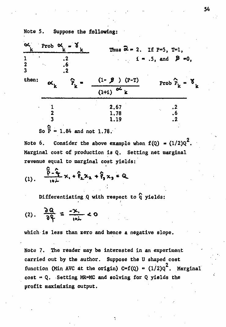
1 ' .2 2 ••.6 3 .2

then: ak k

• = .5, and

(1- ) (P-T)

(1+i) k

Prob /Pk ' k

Note 5. Suppose the following:

k .Prob 014 ,1c mi

k Thus am 2. If P=5, T=1,

54

1 2.67 . .2

2 1.78 .6

3 1.19 .2

A . • So P = 1.84 and not 1.78...

Note 6. Consider the above example when f(Q) = (1/2)Q 2.

Marginal cost of production is Q. Setting net marginal

• revenue equal to marginal cost yields:

P - (1)

Differentiating Q with respect to 'CI yields:

n

(,) . • ge. 0 1+:6

which is less than zero and hence a negative slope.

Note 7. The reader may be interested in an experiment

carried out by the author. Suppose the U shaped cost

function (Min AVC at the origin) C=f(Q) = (1/2)Q2 . Marginal

cost = Q. -Setting MR=MC and solving for Q yields the

profit maximizing output.

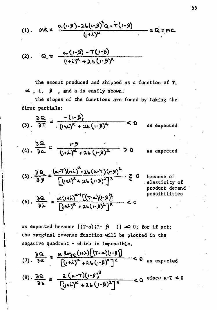
55

0.0.13)-/6(1-A.-4(‘-A) A..)4 CL. = (I). 1■1

Mi■ oi. teere(w4[trep-) -n

< 0 +Ar xL ("Pr] (7). Id. as expected

(8). •a [*11f4 +2.6

alb 11111 4. 0 since a-T <0

f4'• (".P) 0- 53) (+4` + (imil)

The amount produced and shipped as a function of T,

,i , , and a is easily shown.

The slopes of the functions are found by taking the

first partials:

= o (3). Z-r 0+;%.)4 * • -•51)2` as expected

'41 GL (4). (143-Y4 + Q-300- >0 as expected

2.6 ) 51)2b

Ect44 )1

IQ. 0.044.4 a-A • (6).

(5). 21-4-- ap 0 because of

elasticity of product demand possibilities

<0

as expected because [(T-a)(1- 11% )] • 0; for if not;

the marginal revenue function will be plotted in the

negative quadrant - which is impossible.

56

Note 8. As one of the many possible examples, consider an

increase in t. Such an increase will increase the marginal

cost of producing any given output. (MC = Pz+t/MPPz = / P.MPP 1. L.

If t increases to t Z becomes more expensive and less is

used; whereas L becomes relatively less expensive, so more

is used. Given diminishing marginal productivity, MPP L

decreases. Since PL

is constant, Me must increase). The

increase in MC will decrease profit maximizing Q. The

result will be less Q transported. Less Z will also be

transported. However, the transportation company may

have gained, lost, or had constant revenues. If the demand

for transport of the resources is elastic or of unitary

elasticity, total revenue of the transport firm will decrease.

However, if the demand for transport of the resource is

inelastic enough, the increase in revenue for the input

transportation may be more than enough to offset the loss

of revenues in the transport of the final product. The

interested reader can investigate cases. The important

point here is that the transport company should recognize

the domain of impact of their decisions.

Note 9. The question of modal splitting in this context

is a difficult one because it entails changing an assumption

made previously about the demand for the product. If modal

• splitting is allowed for, certain goods will get to the

market very rapidly whereas other goods will arrive after

a longer period of time. Assume, for simplicity, the

existence of an expensive, instantaneous mode (called air)

and a free, slow mode (called sea). How is the equilibrium

output of goods decided? What will be their prices? Speed

loses its advantage if the A goods must wait until the S

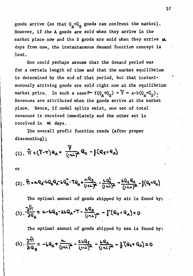
6% • 0-443 - al•QA CT • • trAs 4 QA) = . •

").

goods arrive (so that QA+QS goods can confront the market).

However, if the A goods are sold when they arrive in the

market place now and the S goods are sold when they arrive 01,

days from now, the instantaneous demand function concept is

lost.

One could perhaps assume that the demand period was

for a certain length of time and that the market equilibrium

is determined by the end of that period, but that instant-

aneously arriving goods are sold right now at the equilibrium

market price. In such a caseP=4 f(QA

-1-QS) = rg = a-b(Q 4Q )

A S Revenues are attributed when the goods arrive at the market

place. Hence, if modal splits exist, one set of total

revenues is received immediately and the other set is

received in 0C. days.

The overall profit function reads (after proper

discounting);

(1) . 1.6 (.‘ ) 12(A f t ‘I‘S 1* 1/46Z S 4 ‘:4"

or

0.9,s na• (2) . tc °AA" %CAP:- CZA j la`s w‘A

The optimal amount of goods shipped by air is found by:

57

The optimal amount of goods shipped by sea is found by:

7?‘ 2.1)GtS 1.10S+ GIA) 2 (4) . "IAA+ (■4;..YL 01;‘r(417-) Gtis

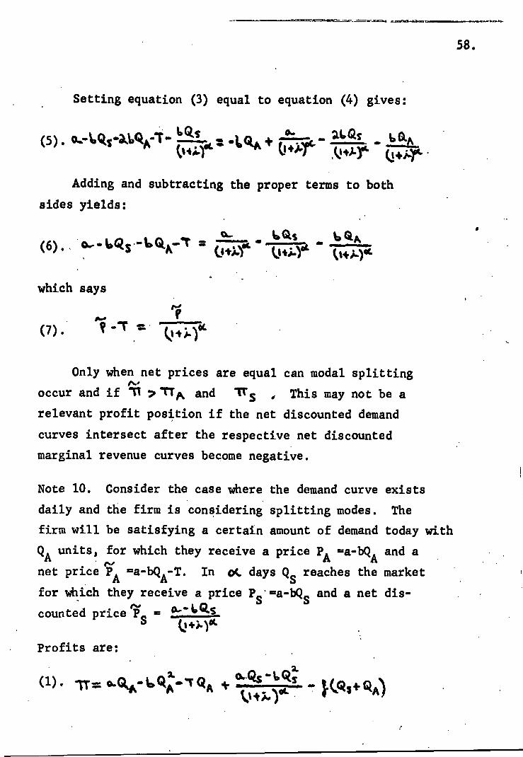
( 7). i7°

58.

Setting equation (3) equal to equation (4) gives:

ir. 6(4 2112s 60. (5 ) .

‘11 ajaqA • tst +a ^ (14:46t ,Q,xr Q+44

Adding and subtracting the proper terms to both

sides yields:

a- laGls QA (6) . koqs -1) qr-r 6;7)4 c%4Xrit

which says

Only when net prices are equal can modal splitting

occur and if 13 71Tik and 11s , This may not be a

relevant profit position if the net discounted demand

curves intersect after the respective net discounted

marginal revenue curves become negative.

Note 10. Consider the case where the demand curve exists

daily and the firm is considering splitting modes. The

firm will be satisfying a certain amount of demand today with

QA

units, for which they receive a price PA =a-bQA

and a

net price PA

=a-bQA-T. In a. days Q reaches the market

for which they receive a price P and a net dis-

counted price Ps = Q#1")°‘

Profits are:

(1). IT=

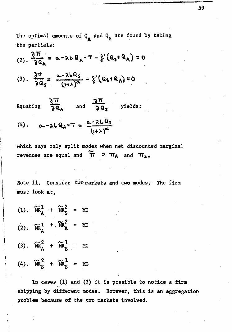
...sewooMem.

59

The optimal amounts of QA and Qs are found by taking

•the partials:

(2) . 1" 611C 'IT (45* QA) =

rtT Q." (3). 51,, (Iasi 614 =0

Equating ')Q.A and 1,ct s yields:

(4) .

which says only split modes when net discounted marginal

revenues are equal and IT 1Th and ITs.

Note 11. Consider two markets and two modes. The firm

must look at,

(1). + = mc

(2): . MC MRA A

(3). „1 ,c A i'vmS

(4). '‘Mit 2 + Mki = MC

In cases (1) and (3) it is possible to notice a firm

shipping by different modes. However, this is an aggregation

problem because of the two markets involved.

k

••■•04...•••••01.1.

60

CHAPTER III

AIR FREIGHT DEMAND MODEL: DISCRIMINANT ANALYSIS

The firm's demand curve for transport with respect to

several variables has been developed above. Also shown was

a model for modal choice. It is time to put the theoretical

model of transport choice and transport demand into a testable

statistical model. The variables suggested to us by the

theoretical analysis will be used to see if they explain

empirical shipments and yield the expected direction of

influence.

A statistical model will now be developed which will

form the framework for the empirical tests of the theoretical

model. A model, expressing the probability that a certain

shipment identified by values of the explanatory variables

goes by a particular mode, is presented below.

At this stage in the analysis, it is not important

to explicitly denote the explanatory variables in the

analysis. Identify the explanatory variables by a vector X

[where X = P, TA'

TS'

ott,'S' A'

)] Each )5 S • shipment has a vector of explanatory variables associated

with it, i.e. each shipment will be sold at a certain

price, incur a certain transport cost, take a certain

number of days to get from origin to destination, etc.

The model is based on a statistical technique known

as discriminant analysis. Discriminant analysis has been

used quite often in the biological sciences. Recently

onaoramr.

61

1 it has been used in economics.

Basically it is a method which separates entities

(as measured by the vector of explanatory variables) into

members of certain populations. It accomplishes this by

a linear function (if there are two populations; or by

n-1 linear equations if there are n•populations), the

coefficients of which are determined by maximizing the

distance between the means of the two: poPulations divided

by the variance within the populations.2

For the two population case, any vector of explanatory

variables,. X, which yields a value of the discriminant

function higher than a certain value (a critical value)

will be said.to be a member of one population; any X

yielding a value of the discriminant less than'the critical

value will be said to be a member of. other. population.

1See for example:

D. Durand, "Risk Elements in Consumer Installment Financ-ing", Financial Research Program, Studies in Consumer Installment Financing 8, (New York, National Bureau of Economic Research, 1941), p. 125.

G. Tintner, "Some Applications of Multivariate Analysis to Economic Data", Journal of the American Statistical Association, Volume 46, 1946, p. 476.

Stanley Warner, Stochastic Choice of Mode in Urban Travel: A Study in Binary Choice, (Evanston, Northwestern Press, 1962).

D. Blood and C. Baker, "Problems of Linear Discrimin- ation", Journal of Farm Economics, Volume XL, 1958, pp. 674-683.

2T.W.

Anderson, Introduction to Multivariate Statistical Analysis, (New York, John Wiley and Sons, .1958), Chapter'6.

The basis for this analysis is T.W. Anderson's

Introduction to Multivariate Statistical Analysis.3

Let A

and S be two populations (air and sea) with density functions

zA (X) and z (X) respectively. The goal is to divide the

universe of observations into two mutually exclusive and

exhaustive regions RA and Rs . If an observation falls ,

into region RA , it is said that it comes from A.

The, design is to detetmine the probability that a given

observation comes from A based on discriminant analysis. If

the probability is of a certain level, that observation will

be assigned to population A. The goal is to chOose the R A

and R so that the costs of misclassification (i.e. the cost

associated with classifying an actual air shipment as a sea

shipment - placing an actual resident of R A into Rs - and

vice versa) are minimized.

If the a priori, probabilities are known (q h is the a

priori probability for the hth

population) for the popula-

tions A and S, the conditional probability of an observation

coming from a population given the values of the components

of the vector of explanatory variables can be defined. The

a priori probabilities may be based on previous studies done

or may be based on the assumption of equal ignorance, i.e.

qA=q

S=.5.

The conditional probability of the observation (with

explanatory vector X) coming from A is:

62

qA ( 1.) • zA

(X)

h q z

h (X)

h=A,S

Call this ' r

, (K). A

(Anderson, p. 143) .

3Ibid

An analogous relationship exists forP rs (X), i.e.

(2). q zS (X)

S qh Z(X)

h=A,S

Now form P (X)/PrA

(X) which is: rS

(3). • P (K) qS z,(X) rS P(X)

qA

zA(X)

rA

From Anderson it is known that if the below are

multivariate normal populations with equal covariance

matrices i.e. N(M1, V) and N(M

2, V) where M

h = h

...,Mh) w

is the vector of means of the h th population (h=A,S) and V

is the matrix of variances and covariances of each population

(the assumption that the V's are equal for all populations

is not crucial - unequal V's merely add computational

burden but leave the analysis intact), then the hth

density is:

E;3

(4). zh(X) = 1 -(X-M15' V e ̀

(211. ) 1/2z Iv (Anderson, p. 133)

- Thus, 1 e-k(X-MA)1 V

-1 (XM) (5).zA(X) = (2c .

(6). zs(X) - 1

e4(X-M5)'V-1 (X-M)

(21r)IV

- Then forms(X)/ z

A(X)

which is

, (7) Zs(x) eX'V -1 (Ms-MA)-V ,Ms+MA) V -1 %Ms-MA)

zA(X)

By substitution

(8). P (X) q z (X) q -1

rS .SS .S e CKs-MAYV /X-3/4(Ms4MA)'V (Ms-Mi)

Pr (X) qA zA(X) qA

A . . •.

where:Prh

(X) is the predicted probability that mode h is chosen

qh

is the a priori probability that mode h is chosen •

Mh is the vector of means of the explanatory variables

(MS-MA)'V

-1X is the discriminant function 4

-1 V is the inverse of the variance

covariance matrix

It can be shown that:

' 1 (9). P

rA(X) = Prc (X) ,

• P (K) rA FP

The derivation is as follows:

(10). PrS

(X) PrA

(X) r• v = h=A S

Pr

A4. (X) P

rA*W P (X) -rA

4Ibid, p. 143.

64

Now a probability distribution must sum to one, so that:

(11). Prh(X) PrA(X) + P (X) 1

rS

Thus,

(12). P (lc) P (X)

Prh

(X)

rS rA h=A,S 1

r-737 -C 17-17E "r (X) la Pr (X)

rA rA A A

Therefore,

1 1 (13).PrA(X) = ... - -Pr (X) P (X) PrA

(X) 1+ S rS

PrA

(X) rA

1-5-77C) + P(X) rA

From the above is determined the value of P r (X)/Pr (X)

Calling

-1

(14).

-1 DSA (X)=[ (M -•MA ) ' V X-3/4(MS +MA ) 1 V (ms-MA)] + log S. f " " %

. - • '

By substitution,

1 (15). P

rA(X) =

1 + eDSA(X)

DSA(X) is the discriminant function [(M s-NYV-1X]

•

•

and its associated constants [-k(Ms4MA)'V (Ms-MA) + log

and is obtained by a straight forward method

from the data as shown by Anderson pp. 150-151.

65

(17).' AP(X) i// LS TA

PrA

(X) if • TA

which is termed

• which. is termed

••

• The analysis can easily be generalized to more than

• two modes. If n modes are available, there are n regions,

and n-1 relevantPrh

(X)/ Pr (X) relations. A

In general, .

(16). P (X) = 1

rA 1 + e DhA (39

It is of interest to determine the sensitivity of

dhoice to a change in the decision variables e.g.

P (X)/ TA .

Multiplying the above by TA/Pr CO yields: A

66•

as the own price elasticity of choice. Taking .) P (XVI T rA •

and multiplying by Ts/ Prs (X) yields:

.( 18). AV

/I

*. ti T

/

S

, T7-717 Ts rA • rA

as the cross price elasticity of choice.

Viewing PrA

(X) = 1

•(19).

1 + e DSA(X)

--_.—..---...........AawmarA eilkr.ZdYoeidsm.ankv •

•■• 04. Xf• 2 _)e _ 2

21x1 rpr 06

L. A 1

§7

• .

DSA(X) will be of the form

DSA(X) = 0t1 - xl- 2x2- ". - w w

where xh is one of the explanatory variables.

e DSA

(X)

(20).21P, (X) xl 'A ..., [1+ e

DSA(X)] .2

l' xl

• D (X) 2

p I e SA [Pr (XI A

So,

' (21), Pr

A(X) xl

D (X) e SA Pr (X)

Pr (X) x1 A

A

If x1A' it is expected that

(22). Pr (X)

A GO or )TA

D (X) 2

SA [

Pr 01 0 A

2 • D Since e SA (X) ;PO and [p... (X1 11. 0, " 1 40 is

s needed to insure)1)rA

(XV ) 1T 0. This is as expected A

from the theoretical section, i.e. the sign of the own

transport Tate to be negative.

Cross rate elasticities and elasticities with respect

to changes in the other explanatory variables may also be

calculated.

•

68

' ' •

. DIAGRAM 11/-1 .

Duo

The probability function can be graphed as shown, below: .;

( Dg) p •

.• • . sA D 00 SA rA

fx‘

1/2 • 1 0 • • ' .

0 oe

1 .0 , 00

3/4 1/3. -. -1.10

4/5 ;1/4 -1:39 • •

1/3 2. . .69 s . . 1/4 3

• /5 . 4 ••••• /.39 .

..••••■•601..11111111.s.••■••■•..... ..■111.

70

.;

APPENDIX TO CHAPTER III

SENSITIVITY ANALYSIS OF A DISCRIMINANT MODEL

It has been shown that:

1 , (1).

PrA(X)

q5 CMS-MYV 1X-3/4(MS+1.1`A) 1 V /(MS -MA:) •

A •

Now perform a sensitivity analysis on PrA

(X) for

various values of qA . The purpose of this sensitivity analysis ,

is to see how various choices of qA (e.g. equal ignorance,

past study results, educated guesses, etc.) influence the

end results and how great the range of possible end results

is.

Assume possible values for

(2). W (MS-M) 1V 1X - k(MS+MYV 1 (MS-MA).

Suppose W takes on values of -1, 0, 1, and 2 which says

ew takes on values .37, 1, 2.7, and 7.4.

The effects of different a priori probability choices'

. under the assumptions given above are shown below:

1+

(W=-1) (W= 0) (W= 1) (W= 2)

ciS• Pr (X) PrA

(X) PrA

(X) PrA

(X) A

.5 .5 .73 .50 .27 .119

.1 .9 .23 , .10 .04 .013

.2 .8 . .40 .20 ' .08 . .033

.3 .7 .54 .30 .14 .054

.4 .6 .65 .40 .20 .083 -

.6 .4 .80 .60 .36 .170

.7 .3 . .86 .70 .45 .240

.8 .2 .92 .80 .60 .350

.9 • .1 .96 .90 .77 .550

At first glance it appears that the a priori

probabilities are very important for the model to function.

For instance, a vector of independent variables yielding a

W of 1 will yield aPr (X) of .04 if the a priori probability A

for air is .1; whereas the same observation will yield a

Pr (X) of .77 if q •= .9. However, these are not the A A'

necessary probabilities for proper classification.

It can be recognized that the correct value of

the a priori probabilities are only needed for "true"

predicted probabilities of air movement -- but is not

necessary for classification purposes. This can be

seen by looking across the above table. For any given

a priori probability the value of the discriminant (the Pr (X) ) •

A

will always give higher numerical probabilities as W •

71.

.72..

decreases. Proper choice of PrA

(X) given a qA will insure

the same classification of air and sea under any qA chosen.

Thus, although only one a priori probability is truely

correct and will give the precise numerical probability

that a shipment will go by air, any a priori probability

will classify a given observation in the same manner

relative to any other observation.

As an example, suppose the true a priori probability

is q =.5 (implying q = .5). If W equals -1, the true A

probability that that particular shipment would go by

air is .73. However, suppose that qA = .1 was chosen.

The W of -1 would yieldP r (X) = .23. This would not A

be the numerical probability that this good goes by air,

but the choice of PrA

(X) insures that this shipment is

classified as air. If Pr (X) = .5 when qA = .5, then

• A • Pr (X) =..1 when qA

= .1. Analogous.statements hold for A •

other values of qA .

CHAPTER IV

. EMPIRICAL RESULTS

It is time to turn to the actual empirical testing

of the theoretical model. The theory presented previously

can incorporate the influence of competition among many

modes.

Rate structures can either be known, as they are under

regulation, or subject to variation, as they would be in a

competitive situation. A variety of quality differences

can be introduced, i.e. differences in such things as

average travel time and average damage and loss rates pose

no problem as was shown above. The same is true of the

probability distributions of these quality variables.

In order to simplify exposition, however, the analysis

will be conducted under the atmosphere of perfect competition

and perfect knowledge. There will only be five determinants

of transport demand considered: the shipper's cost of - production, the interest rate, transport rates, average

travel times, and the demand for the shipper's product.

Inventory costs, aside from those that are directly due to

transport time, are ignored. Production and the costs it

entails are treated as instantaneous, but revenue is

received only after goods reach market.

The analysis developed in the theoretical body of the

thesis suggests that what is popularly called modal split-

ting, i.e. the division of shipments between several modes,

is due to various kinds of aggregation, i.e. to the grouping

of data over time, groupings of firms who produce different

73

74

products, have different cost functions, and/or ship to

different markets.

• Previous work by Beuthe and Moses ' clearly demonstrates

that individual shippers of relatively homogeneous products

tend to choose one mode or another. For that study the

authors were able to obtain excellent data on shipments

of grain from hundreds of individual elevators in Illinois

to the Chicago market and to Southern markets, primarily to

New Orleans. Data on transport costs from each elevator

to these markets by rail, truck, and water were obtained

directly. Excellent price data was available on a daily

basis. It was found that more than eighty-five per cent

of all shipments involved a single mode.

Phenomena that involve exclusive choice lend them-

elves to a statistical technique known as discriminant

• analysis in which the dependent variable takes on values

of zero or one. In the grain study there was a vector

of independent variables for each shipping point, these

variables representing time, cost, etc., of shipping.

The model was able to separate the various mode populations

successfully, which is to say that it tended to correctly

• allocate shipments to the mode actually used. For the

study of air cargo demand detailed data of the above sort

was not available. It was, therefore, necessary to adjust

• the basic statistical procedure from that described in

Chapter III above. The data available and the required

adjustment are explained below. •

. 1M.V. BeuthDand L.N. Moses, "The Demand for Transportation: The Influence of Time", in Transportation: A Service, (New York Academy of Sciences, New York, 1968), pp. 61-65.

.e.valeirsobe

75

The most comprehensive data on overseas shipments

of commodities is published by the Bureau of the Census.2

This source contains information on tonnages shipped by air

and sea from various customs districts to different countries.

Information on total value and value per pound are also

found in this source. The quantity and value data are in

terms of a seven digit classification of commodities.

Information on rates by air and sea was obtained from the

International Air Transport Association 3 and the Federal

Maritime Commission. 4 The model was applied to the North

Atlantic Trade Route, and in particular to shipments from

the United States to Great Britain, because it involves

the largest number of commodity groups. A sample of 459

Schedule B commodities was available for January, 1967.

Obviously many more than 459 commodities are traded. The

data availability is constrained because of the Maritime

commodity-rate code, which is not the same as Schedule B. .•

Only the Schedule B codes that have a one to one correspond-

ence with the Maritime code were used. This gave unique

rates to each Schedule B movement.

21J.S., Department of Commerce, Bureau of the Census, U.S.

Exports of Domestic and Foreign Merchandise, District of Exportation by Country of Destination by Schedule B Commodity and Method of Transportation, January, 1967, microfilm I.D. number EM 565, Suitland, Maryland.

3A.C.T. (Air Cargo Tariff) Worldwide, a publication of Scandinavian Airlines System and Swissair, provided by IATA.

4Rates are based on North Atlantic-United Kingdom Freight Conference Tariff 46, (FMC-1), Washington, D.C., 1967.

76 '

The above data falls short of the quality of the

%information that was available for the grain study. As

government publications go, a seven digit classification

is relatively detailed. It, nevertheless, represents an

aggregation of shippers with different costs of production,

who are located differently and who face different transport

costs. The empirical work had, for example, to proceed as

if all producers were located in the New York customs

district and paid transport from there to Great Britain.

Almost all of the seven digit groups involve more

than one commodity, and some more than a hundred. There

is every reason to believe that the individual commodities

within any group have different values per pound, but

the average of the entire group had to be used. It is

known that several different rates are charged for many

of the individual commodities within a seven digit group.

This cut the potential sample size down as was explained

above. Rate structures are, in addition, tapered. Since

quantities for individual commodities within a group, and

the frequency distribution of sizes of shipments were

unknown, simple average rates were used.

Finally, data on total transport time, as against

schedule time which is considered misleading because of

days in loading, unloading, queuing, etc., were only

available for a single firm which estimated that sea and

air delivery required thirty-eight and nine days respectively.

These times were used in a test run of a subsample of our

459 sample with results that are mentioned below. In

summary, the statistical analysis of competition between

air and sea had to be cross sectional, each seven digit

group being treated as the homogeneous output of a single

shipper or a group of identical shippers.

*A t NI%

77

Discriminant analysis can be applied to data of the

above kind. The rationale for such application is summarized

in the diagram below where commodity groups 1,2,...,n are

arranged on the horizontal axis from the lowest value

per pound, measured at the origin, to the highest value

per pound.

C A, 5 C.Ai CS

DIAGRAM IV -1

The costs, including the direct transport charge and the

value of time, of shipping these by air and sea are measured

on the vertical axis and are shown in the two functions CA

and C. The latter starts out lower because ship rates are S

■■•

78 .

lower than air rates. It rises more rapidly because the

value of time or cost of capital tied up in shipment is

based on a fixed percentage of the value of the commodities.

(Also other costs such as warehousing and damage which are

higher by sea than air have a positive relationship to

value). According to this appraoch, shippers of the k th

commodity would be indifferent between the two modes. The

k + 1,...,n commodities would go exclusively by air, and

the remaining ones exclusively by sea.

A discriminant model based on the above logic was

applied to the sample of 459 commodities with results that

were neither very good nor very bad. That such an applica-

tion could even be contemplated was due to the fact that

343 of the commodity groups actually involved exclusive

mode choice, 66 going entirely by air and 277 going entirely

by sea. This is a surprising result, given the degree of

heterogeneity within most seven digit groups. It is a

result that supports the basic approach to transport demand

which the theoretical section of the dissertation developed.

A second experiment, involving an application of

ordinary regression techniques to the entire sample was

also performed. Here the dependent variable was percent

of total tonnage of a given commodity group that went by

air. The results were poor. The diagram below explains

why this is the case.

• •

07. % Air 1007.

79 •

all air ji shipments

modal split e shipments

• •

•

all sea ' shipments

•

DIAGRAM IV-2

Here per cent air is measured on the horizontal axis,

and W, a vector of explanatory variables is measured on

the vertical axis. The two end points represent the

commodity groups which exhibit exclusive mode choice. For

each of these groups, wide variations in the independent

variables, W, are associated with no variation in the

dependent variable. A least square "line" involves sub-

stantial deviations and therefore a low R 2.

One of the objectives of the study was to estimate

a meaningful demand function for air freight. The results

of the above two experiments suggested that, given the data

available, it would be best to adopt a compromise approach

that would involve three stages: (1). application of

discriminant analysis to the commodity groups that exhibited

exclusive modal choice; (2). use of ordinary regression

techniques to analyze the remainder; (3). the drawing

together of the results from the first two stages and the

derivation of an overall demand function. The entire

procedure implies that modal split groups are more hetero-

genous than those that move exclusively by one mode. The

data necessary to carry out a satisfactory test of this

hypothesis are not available; had they been it would not

have been necessary to adopt the compromise approach. The

number of separate commodities listed in each of the com-

modity groups were, however, compared. There were, on

the average, fewer separate commodities in the exclusive

mode groups.

As explained in Chapter III, discriminant analysis

•enables observations to be separated into two or more

classifications (in this case, two, sea and air) on the

basis of a vector of independent variables. The coefficients

of the discriminant function are determined by maximizing

•the variance between populations over the variance within

• populations. Once the function is determined, a certain

amount of leeway is allowed the researcher in determining a

cutoff score for values of the discriminant (the P (X) in rA Chapter III).

80

81

This score is the criterion for classification. If a

value yielded by the discriminant function for the independent

variables associated with a given commodity is above the

critical value of the discriminant, the commodity is

classified in one population; if below, it is classified

in the other population. The decision rule is to

minimize the cost of misclassifications. In the present

study the Pr (X) was chosen which minimized the squared A

error of tonnage misclassified.

When there are only two regions of classification,

discriminant analysis is equivalent to a linear probability

model.5

Our model in Chapter III will thus be simplified

by using this equivalence. The linear regression was carried

out with the result shown in Table

5Dwight Blood and C.F. Baker, "Some Problems in Linear Discrimination", Journal of Farm Economics, XL, (November, 1958), pp.. 674-683.

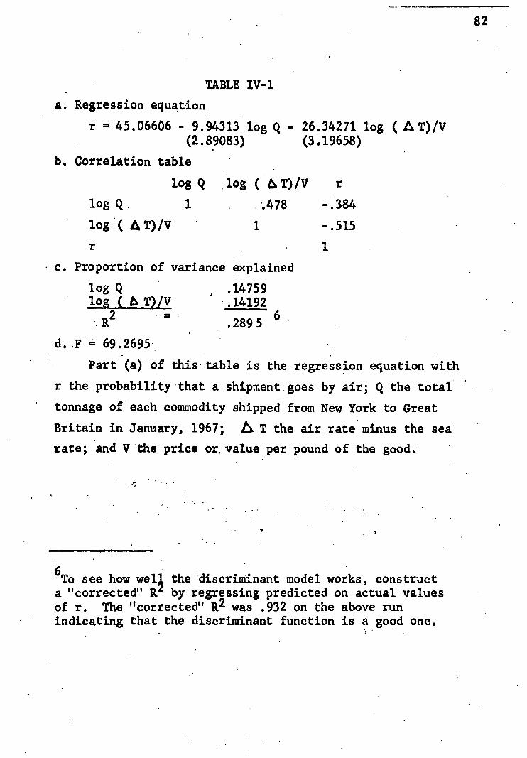
82

TABLE IV-1

a. Regression equation

r = 45.06606 - 9.94313 log Q - 26.34271 log ( AT)/V (2.89083) (3.19658)

b. Correlation table

log Q 'log ( t6T)/V r

log Q 1 -.384

log ( thT)/V 1 -.515

1

c. Proportion of variance explained

log Q .14759 log ( b■ T)/V .14192

6 R2

.2895

d..F = 69.2695

Part (a) of this table is the regression equation with

r the probability that a shipment goes by air; Q the total

tonnage of each commodity shipped from New York to Great

Britain in January, 1967; T the air rate minus the sea

rate; and V the price or , value per pound of the good.

• 6To see how well the discriminant model works, construct a "corrected" R2 by regressing predicted on actual values of r. The "corrected" R2 was .932 on the above run indicating that the discriminant function is a good one.

The variables have the correct signs. Let us first

examine the logic behind the negative sign of (11 T)/V

holding V constant. If TA, the rate by air, rises and T s ,

the ship rate, is constant, falls, or rises less, A T increases in absolute amount. In this case, the probability

that a commodity will move by air should fall. The implied

sign for (A1 T)/V is therefore negative. Holding b. T

constant, a change in V has the same impact. For example, as

V increases, greater savings in capital can be achieved by

faster transport, and the possibility is greater that the

commodity will go by air. Since an increase in V reduces

( ti 7)/V and increases r, the effect is negative. Thus

the negative coefficient seems reasonable though the impact

of simultaneous changes.in A T and V is less clear. 7

The price variable has, the reader will note, not been

discounted as in the theoretical analysis because adequate

data, on transport time was not available. As mentioned

earlier, information from a large firm estimated that its

sea and air shipments required thirty eight and nine days.

These values were used in a regression on a sample of 69

commodities, a difference in capital costs between the modes

being derived for each of the commodities. The inclusion of

this variable slightly increased the R 2 . '(The increase

being based on other runs of the 69 sample size). The

coefficient had the proper sign but was not statistically

7As further' substantiation a result shown later shows that when run separately, V has a positive sign and AT a negative sign, thus accounting for the negative sign of log ( T)/V.

83

84

significant. 8 It was, therefore, decided to leave the

time variable out of the analysis until better data could

be obtained.

8For regression on modal split goods:

r = 1.43781'- .25788 log Q - 181.2 bi,C (.09106) (238.5)

Proportion of variance explained

log Q .25825 where &C = CA-C

S

C .01555 CA al TA+iA

R2

= .2738 iA = (1+001 VA-VA

and AC is in cents per pound

Here the Cs. C coefficient is not statistically significant.

For the discriminant function:

r = 1.36882 - .08522 log Q - 1340.2 b, C (.10344) ( 283.4)

Proportion of variance explained

log Q .13352

,A c .33254

R = .4661

Here the c coefficient is vastly significant but the coefficient of log Q is insignificant. Because of the insignificance of the coefficients, it was felt that the time cost runs should be dropped until better data is available.

••• • .........41.roctssauscleurbsoc...1.. • ,drArZattulg.. is* S.

The logic behind the statement that the quantity

variable's coefficient has the correct sign is a bit complex.

As will be explained below, it involves a relationship between

value per pound and total quantity exported and a further

relationship between average size of shipment and total

quantity exported.

Air freight capacity is quite limited and cannot be

expanded much in the short run. It is therefore not possible -

to ship by air all, or even a significant percentage, of

those commodities for which export tonnages are very large.

It would not, for example, be possible to ship all U.S.•

-exports of coal by air, even if all air freight capacity

were allocated to this commodity. This reasoning suggests

that a variable for total tonnage of each commodity group

exported should be included. The (hoped for and realized)

negative relationship between total quantity and prob-

ability of air shipment is due to several factors.

A high rate structure has been established which

tends to maximize the return to fixed capacity and to

allocate that capacity to those commodities most able to

bear high rates, i.e. the high value commodities.

There tends to be a negative, though not strong,

relationship between total tonnage exported and average

value per pound.9 In other words, goods that are exported

9For a sample of 69 commodities, the following was run: r 134.58040 - 15.40050 log Q + 2.184 V -156.126 LIT

. ( 2.55626) ( .232) ( 61.839) log Q V AT

•log Q 1 -.230 .169 -.384 -

V 1 -.173 .504

a T 1 -.166 ' r • 1

85

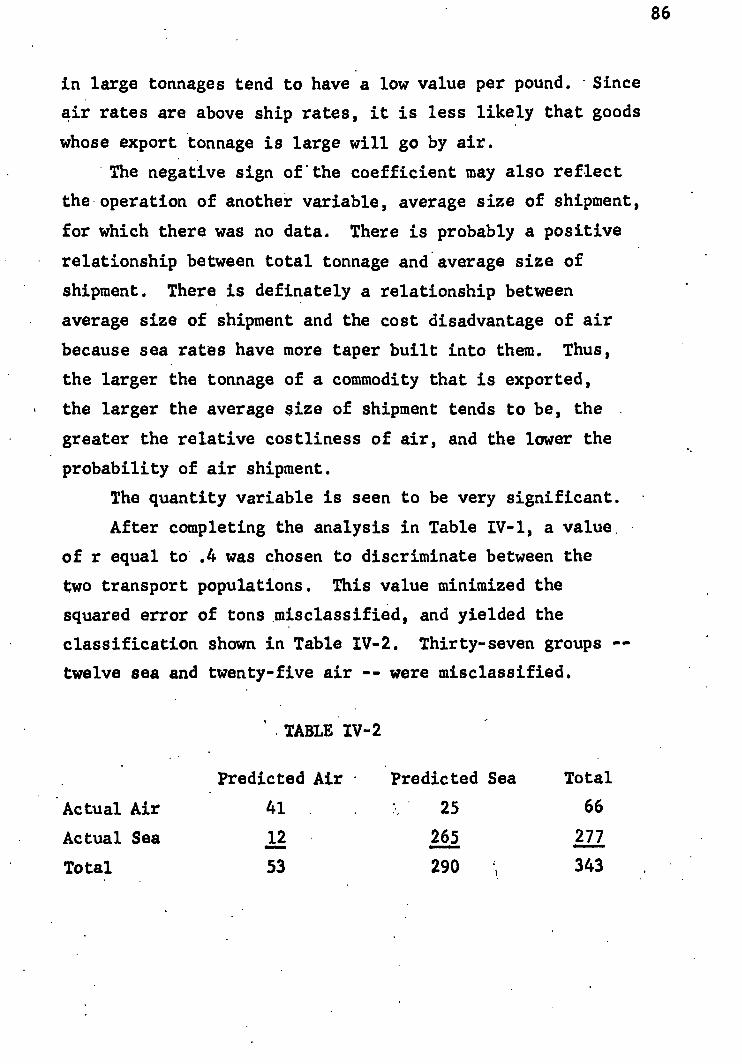
in large tonnages tend to have a low value per pound. Since

air rates are above ship rates, it is less likely that goods

whose export tonnage is large will go by air.

The negative sign of the coefficient may also reflect

the operation of another variable, average size of shipment,

for which there was no data. There is probably a positive

relationship between total tonnage and average size of

shipment. There is definately a relationship between

average size of shipment and the cost disadvantage of air

because sea rates have more taper built into them. Thus,

the larger the tonnage of a commodity that is exported,

the larger the average size of shipment tends to be, the

greater the relative costliness of air, and the lower the

probability of air shipment.

The quantity variable is seen to be very significant.

After completing the analysis in Table IV-1, a value

of r equal to .4 was chosen to discriminate between the

two transport populations. This value minimized the

squared error of tons misclassified, and yielded the

classification shown in Table 1V-2. Thirty-seven groups --

twelve sea and twenty-five air -- were misclassified.

'.TABLE 1V-2

Predicted Air • Predicted Sea Total

Actual Air 41 25 66

Actual Sea 12 265 277

Total 53 290 , 343

86

vs • 01..401.SICt....a.

87

There is some intuitive appeal to using .5 as the

cutoff value. It implies each population is equally likely •

to occur. It is also a "popular" value to choose.10 The

analysis was carried out with this value and a much poorer

result was obtained. Fewer sea commodities were misclassi-

fied but many more air were misclassified. The explanation

for the poorer result is that the empirical modal is biased

against air shipments. Since data on transport time was

not'availabe, the simple difference in transport rates, ca T,

had to be used. This variable overstates the cost advantage

of sea freight and overstates the cost disadvantage of air

freight. Use of a value of r less than .5 compensates for

the bias, increasing the probability of air shipment. Thus

even if excellent data on tonnage had not been available, a

cutoff value less than .5 would have been used.

The model above predicted the number of sea shipments

very wall. However, it was disturbing that a model of air

freight demand did not predict the number of air shipments

very well -- with twenty-five of sixty-six shipments mis-

classified. It was felt that the cost disadvantage of Air

(TA -TS ) may have been too high. This is felt for two reasons.

Reason one was stated above -- that time costs are not

included in the model. Reason two relates to average ship-

ment size and value per pound. There is a tendency for high

value goods to travel in relatively small average shipment

size. There is also a tendency for low value goods to travel

in relatively large average shipment size. In the analysis

above the same average shipment size was assumed for all

commodities. This has resulted in an overstating of tL T. View the diagram below.

10Blood and Baker, op. cit, p. 682.

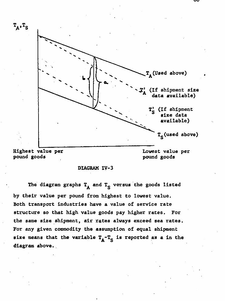
Tii (Used above)

(If shipment size A data available)

T (If shipment size data available)

(used above)

Highest value per pound goods

Lowest value per pound goods

T .A T° S

DIAGRAM IV-3

The diagram graphs TA and Ts versus the goods listed

by their value per pound from highest to lowest value.

Both transport industries have a value of service rate

structure so that high value goods pay higher rates. For

the same size ,shipment, air rates always exceed sea rates.

For any given commodity the assumption of equal shipment

size means that the variable TATS is reported as a in the

diagram above.

More realistically, the known difference in shipment

size should be allowed for (and shipment sizes' effect on

rates). (But the answer to how much should be allowed for

without data on average shipment size explains why this

study did not account for the same in the empirical work).

Allowing for the above would change the TA

line as follows.

For high value goods it would be the same as assumed.

However, for lower value goods, as more weight is shipped,

a taper comes into play; and the rate decreases below that

which is reported. These rates trace out T I above. A

A similar type of occurence happens to sea rates.

These rates are based on fairly large shipment size. For

shipments less than this large size higher rates must be

paid. The effect on the ship rates is shown as T above.

If shipment size were available, one would be able to

state the "true" AT which each shipment faced. This would appear as b in the diagram above.

To correct for this, the AT for the twenty-five misclassified groups was lowered to one. (It was realized

that this is unrealistically low; however, it was only

meant to demonstrate that A T was too high previously). The program was then rerun. The cutoff value of P - (X) was

A

increased as expected. The classification scheme appeared

as below: TABLE IV-3

Predicted Air Predicted Sea Total

Actual Air 53 13 66 Actual Sea 4 273 277

Total 57 286 343

89

90

. In addition, only the smallest quantities remain

misclassified. A much better classification results by

lowering the cost disadvantage of air.

It should be pointed out that the commodities mis-

classified are members of the lowest value per pound sector

which travels by air. Likewise, the sea misclassified

are members of the highest value per pound sector which

travels by sea. Why do these relatively low value goods

travel by air? (Especially when many higher value goods

travel by sea and are appropriately classified as such).

It is suggested here that these goods may represent emergency

shipments. In future runs with different monthly data

these commodities will be run with a dummy variable denoting

emergency shipment.

The results obtained for the commodity groups that

involved modal splits are shown in Table IV-4. The

variables are the same as earlier:

TABLE IV-4

a. Regression equation

r = 129.28368 - 25.80999 log Q - 5.82761 log ( 4 T)/V (2.48905) (2.62722)

b. Correlation table

log Q log (11T)/V r

log Q 1 .261 -.722

log (1% T)/V 1 -.325

1

c. Proportion of variance explained

log Q .52162

log ( thT)/V .01996

R2

= .5416

d. F = 66.7504

The signs of the coefficients are all correct and

significant. Note the difference in the significance

of the variables in this equation compared with that of

the discriminant equation. Rates and prices are relatively

more significant in the discriminant model, as we would

have hoped.

Some air freight demand functions will shortly be

presented. Their reliability depends on the statistical

goodness of the three-stage compromise approach that has •

been adopted. Some Insight into this is obtained by compuLing

an overall R2 . Obviously, if we have discriminated well in •

stage one, many predicted values will equal actual values.

91

Here the deviations are zero. The residuals for the mis-

classified groups, where the errors are 1007, are squared

and summed. The second stage yields a percentage of each

commodity group that will go by air. These percentages

were multiplied by total export tonnages and predicted

absolute tonnages were obtained. Again the errors were

squared and summed. An overall R 2 was obtained by weighting

the R2's from stages one and two by their relative contribu-

tions to total air tonnage. This yielded an overall R 2 of

.6616.11

In general it is hazardous to separate observations

into separate groups, calculating separate relationships,

and then determine overall goodness by regressing predicted

on actual values. Such a procedure can readily turn a very

poor result into what appears to be a good result. In the

present case, however, there was sound theoretical and

empirical justification for the procedure.

The empirical relations estimated in the preceding two

stages can be used to trace out portions of direct and cross

demand curves.. This can be done in several ways, one of

which involves across the board percentage changes in air

rates. According to this method, a one percent change, for

example, in all air rates is assumed, and a new set of air

rates' TA' computed. Ship rates, TS' are assumed constant

•and a new set of Li T's derived. These are entered into

the two equations of stages one and two, everything else is

held constant, new r's and thus new Qs are estimated. This

procedure was followed for changes up to plus and minus ten

11As

.

comp -

• w• • • • • •• • • _ 2

of .2315.

92

4I

0 - "I

••

eS

percent.

The results of the above changes are shown in the

graphs below. First the direct demand curve for air freight:

93

10-

°A/CrA

-10

430 450 410 1190 540 530 550 S.-10 $i 0 Cith(10001 0 541

DIAGRAM IV-4

The solid line is the estimated demand curve. The two

dotted lines form the 95 percent confidence level demand

"band". Since the rate and price coefficient can vary in a

certain range, the demand estimates will also have a range

of variation. All elasticity statements must be made with

this band concept in mind.

The diagram above was found to be relatively inelastic

over the range investigated, with .3 being about an average

value for decreases in air rates. This is a good deal

more inelastic than current industry thinking suggests (in

fact, the industry feels it is dealing with an elastic

demand curve as is mentioned in Chapter I). In order to

get large increases in air freight, percentage changes in

excess of 15 percent must be assumed. Such changes would

have caused some commodities that are exported in large

tonnages by sea to shift to air. The method employed above

is, however, not valid for large percentage changes because

it cannot be assumed that the coefficients of the regression

equations remain unchanged.

The diagram below shows the cross demand relationship.

It is also relatively inelastic over the range investigated.

94

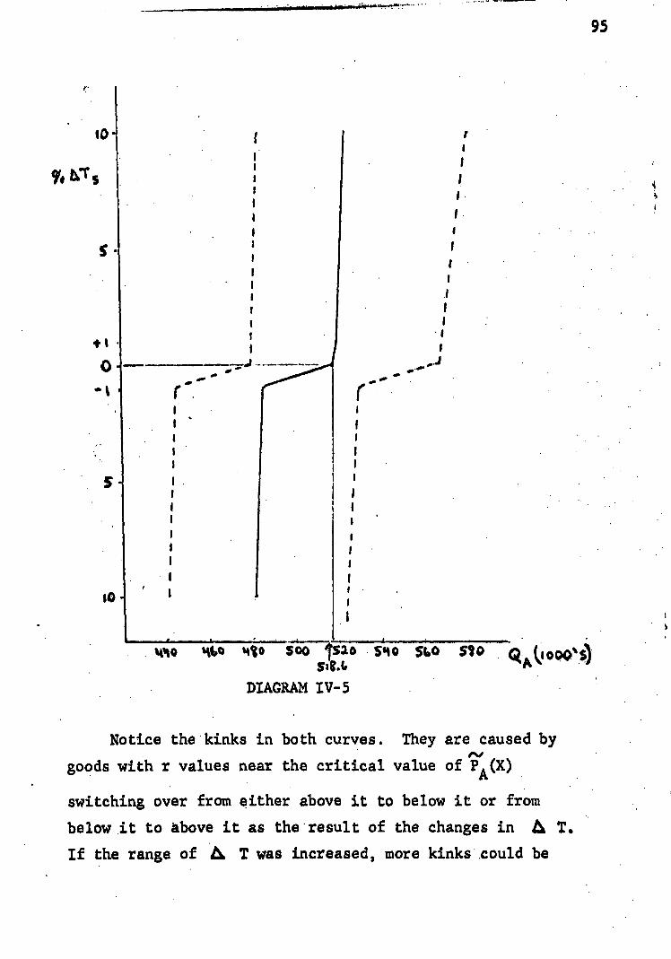
10 H

ts

0

-t

sO

s

'-a

•

1

95

f.

•

• 4to ti4Do tejo 500 1Sao 540 560 510 n I iond0s)

•

518.4 'AcA

DIAGRAM IV-5

Notice the kinks in both curves. They are caused by

goods with r values near the critical value of P A(X)

switching over from either above it to below it or from

below it to above it as the result of the changes in ti T.

If the range of A. T was increased, more kinks could be

96

expected as goods in the discriminant part of the analysis

switch classifications. Obviously as TA

increases, previous

air goods are going to switch over to sea. In addition,

previous sea goods, misclassified as air goods, will fall

back into the sea classification. The opposite occurs as T A

decreases. As T increases, previous all sea goods will switch

over to air. In addition, some all air goods which had

previously been misclassified into sea will now be properly,

classified back into air. As T decreases, vice versa.

It should be recognized that the above method of

estimating demand functions is biased downward because

total export tonnage of each commodity group is held

constant. There are two reasons why these tonnages could

change in response to changes in air rates. First, a

reduction in these rates should increase the profitability

of selling in foreign markets and cause a diversion of sales

to them from the domestic market. Second, the assumption

that tonnage is constant implies that firms operate subject

to constant cost and a short run constraint on capacity. If

they have rising marginal cost curves, as was assumed in

the theoretical analysis, a reduction in air rates will not

only cause some existing tonnage to shift to air, but will

also bring about some increase in output, and therefore

exports.

This chapter was the empirical culmination of the

development of a micro theory of transport. A method of

estimating transport demand functions was presented. The

method was applied to sea-air competition for shipment

between the New York customs district and Great Britain.

It is hoped that a domestic application of such a model

will be forthcoming. Such functions would be immensely

useful to the industries involved and to regulatory bodies.

At the present time, these bodies make rate decisions on

the basis of evidence on demand elasticity that is obtained

by the application of questionable techniques to inadequate

data.

97

BIBLIOGRAPHY •

[1] Air Cargo Magazine, Air Freight Survey, 1963.

[2], Air Freight Survey, 1964.

[3], April, 1961.

[4] Air France, Do It Yourself Distribution Cost Comparison

Analysis: Surface Freight versus Air Freight,

New York, 1962.

[5] Air Research Bureau, Air Freight Marketing Survey,

Brussels, ARB 208, no date.

[6], Air Freight Market Study, Brussels, no date.

[7], Intra-European Air Cargo Traffic, Brussels,

ARB, 102, 1955.

[8] Alden, V.W., and Echard, E.W., Air Cargo Study for U.S.-

Latin America Area, Market Research Department,

Lockheed Georgia Co., August, 1965.

[9] American Management Association, A New Approach to

Physical Distribution, New York, 1967.

[10] Anderson, T.W., Introduction to Multivariate Statistical

Analysis, New York, John Wiley and Sons, 1958.

• [11] Aviation Studies Limited, Air Cargo Commodity Survey,

London, 1961.

[12], Dimensions of World Traffic: III Freight,

No. 87, London, 1960.

[13], Scheduled Airlines Frei:ht Traffic Growth,

No. 52, London, 1958.

. [14] Baumol, William, and Vinod, H.D., Studies on the Demand

for Freight Transportation, Volume 1, Princeton,

Mathematica, 1967.

98

,to•Lanaohnaliaseimildft.ha. • •••• • •

.99

[15] Bellaschi, J.J., An Analysis of International Cargo

Flow Between Nine Geographical Areas of the World,

Renton, Washington, The Boeing Co., No. TRS 645,

1960.

[16], Summary of the University of Washington

International Cargo Study., Renton, Washington,

The Boeing Co., No. 5256, 1960.

[17] Beuthe, M.V., and Moses, L.N., "The Demand for Trans-

portation: The Influence of Time", in Transportation:

A Service, New York, New York Academy of Sciences,

1968, pp. 61-65.

[18] Blood, Dwight M., and Baker, C.B., "Some Problems of

Linear Discrimination", Journal of Farm Economics,

XL, 1958, pp. 674-683.

[19] The Boeing Co., Forecast of Free World Passenger and

Cargo Air Traffic (1965-70-75), Renton, Washington,

Market Research and Operations Analysis Section,

. 1959 and 1962.

[20] Brewer, Stanley, Air Cargo - The Big Breakthrough,

Seattle, Bureau of Business Research,

University of Washington, 1959.

•[21]

, Air Cargo Comes of Age, Seattle, Graduate

School of Business Administration, University of .

• Washington, 1566.

[22], Air Cargo - The Gold is in the Terminals,

Seattle, Management Series No. 5, College of

Business Administration, University of Washington,

no date.

[23], Air Cargo - The Next Ten Years: 1956-1965,

Renton, Washington, The Boeing Co., 1957.

100

[24]2 Study of the

Possibilities for Use of Air Freight, Seattle,

University of Washington, November, 1960.

[25], The Environment of International Air Carriers

in the Development of Freight Markets, Seattle,

Graduate School of Business Administration, University

of Washington, 1967.

[26], The Europe-Asia Market for Air Freight,

Seattle, College of Business Administration,

University of Washington, 1963.

[27], The North Atlantic Market for Air Freight,

Renton, Washington, The Boeing Co., 1962.

[28], Rhocrematics: A Scientific Approach for the

Management of Material Flows, Seattle, Bureau of

Business Research, University of Washington, 1960.

[29], U.S. International Air Cargo Future, Renton,

Washington, The Boeing Co., 1958 and 1960.

[30], Vision in Air Cargo, Seattle, Bureau of

,Business Research, University of Washington, 1957.

[31], and Rosenzweig, James, The Domestic Environ-

ment of the Air Cargo Industry, Seattle, Graduate

School of Business Administration, University of

Washington, 1967.

[32], and , Military Airlift and its

Relationship to the Commercial Air Cargo Industry,

Seattle, Graduate School of Business Administration,

University of Washington, 1967. ,

101

[33], Thompson, John, and Boore, William, The

Aircraft Industry - A Study of the Possibilities

for Use of Air Freight, Seattle, University of

Washington, 1960.

[34], and Ulvested, Roger, The Cargo Jet in Military

Air Transportation - An Economic Evaluation, Renton,

Washington, The Boeing Co, 1960.

[35] Busch, G.A., and Mayer, K.M., An Examination of the

Economic and Technical Factors Underlying the

Future U.S. Domestic Market for Air Cargo Trans-

portation Services, National IAS/ARS Joint

Meeting, 1961.

[36] Carter, LA., and Jackovich, J.C., Trends in Air Cargo,

Paper No. 61-88-1782, The Boeing Co, 1961.

[37] Carteri, John, "Air Cargo Economics", AirCargo, Law

and Contemporary Problems, Durham, Duke University,

1950.

[38] Caves, Richard, Air Transport and Its Regulators: An

Industry Study, Cambridge, Harvard University

Press, 1962.

[39] 1963 Census of Transportation, Commodity Transportation

Survey Production Area Series - Area 2, Advance

Report TC63(A)C2-2, Washington, U.S. Department of

Commerce, Bureau of the Census.

[40] Craig, Thomas Rs, Forecast of Free World Air Freight

Traffic: 1962-1975, Renton, Washington, The

Boeing Co., 1964.

[41] Crane, John B., "The Economics of Air Transportation",

Harvard Business Review, XXII, Summer, 1944.

102

[42] Dawson, Michael, "A Technique of Air Cargo Market Research",

American Transportation Research Forum 1964,

Oxford, Indiana, Richard B. Cross Co., 1965.

[43] DeLoach, D.B., and Miklius, W., "The Effect of Air

Freight Rates on Cut Flowers Sales", Journal of

Farm Economics, August, 1961.

[44] Douglas Aircraft Co., Air Cargo Analysis and Forecast,

Santa Monica, California, 1956.

[45], The Air Cargo Handbook, Santa Monica,

California, 1958.

[46], Commercial Air Cargo Transportation: A

Survey, Santa Monica, California, 1959.

[47], Preliminary Analysis of Future Air Cargo

and Air Parcel Post, Santa Monica, California, 1955.

[48], Survey of Domestic Freight Movement:

1960-61, Long Beach California, 1963.

[49] Douglas, Lord ofKirtleside„, "The Economics of Speed, An

Examination of the Future Roles of Jet and Turbo

Prop Transport Aircraft", Journal of the Institute

• of Transport, XXVII, May, 1957.

[50] Durand, D., "Risk Elements in Consumer Installment

Financing", New York, Financial Research Program,

• Studies in Consumer Installment Financing 8,

National Bureau of Economic Research, 1941.

[51] Durham, Jai, and Feldstein, M.J., "Regulation as a

Tool in the Development of the Air Freight

Industry", Virginia Law Review, October, 1948.

103

[52] Echard, E.W., Air Carp Growth Study, Marketing Research

Department, MRS 49, Lockheed Georgia Co., 1965.

[53] Free World Air Cargo: 1965-1980 Rate

Elasticity Forecast, Commercial Marketing Research

Department, CMRS 77, Lockheed Georgia Co., June, 1967.

[54], Marketing Planning Report - The 1963 Census

of Transportation: Air Cargo, Marketing Research

Department, MRS 53, Lockheed Georgia Co., no date.

[55] Federal Maritime Commission, North Atlantic-United

Kingdom Freight Conference, Tariff 46 (FMC-1),

Washington, D.C., 1968.

[56] Ferguson, Allen R., and Schnabel, Constance, The Demand

for Air Cargo: A Pilot Study, Evanston, Northwestern

University Transportation Center, 1960.

[57] Ferguson, Charles, Microeconomic Theory, Homewood,

Illinois, Richard D. Irwin, Inc., 1967.

[58] Frederick, John, Commercial Air Transportation, 4th

edition,H-omewood, Richard D. Irwin.

[59] Gilbert, Jerome, "The Potential for International

Commercial Air Shipments", International Forum for

Air Cargo 1964, New York, Society of Automotive .

Engineers Inc., 1964.

[60] Geisser, Seymour, Predictive Discrimination in Multi-

variate Analysis, edited by Paruchuri Krishnaish,

New York, Academic Press, 1966.

[61] Gentry, Dwight, "Air Cargo Transportation and Marketing",

Journal of Marketing, July, 1952.

104.

[62] Gorham, G., Sealy, K.R. 1 and Stratford, A.H., "Why

Companies Use Air Freight", International Forum

for Air Cargo, New York, Society of Automotive

Engineers, Inc., 1964.

[63] Gorrill, Edgar S., "Rationalization of Air Transport",

Journal of Air Law and Commerce, IX, June, 1938.

[64].Groenewege, Adrianus, and Hertmayer, Roderick, Air

Freight: A Key to Greater Profit, Southall,

Middlesex, England, Aerad Printers and Publishers,

1964.

[65] Grumbridge, Jack, Marketing Management in Air Transport,

London, George Allen Unwin Ltd., 1966.

[66] Guth, Herbert, and Waldo, Richard, Domestic Air Cargo

Forecast: 1955-1960, Washington, D.C., Program

Planning Staff, Office of the Administrator of

Civil Aeronautics, October, 1952.

[67] Guy, John L., "Air Cargo Marketing in Europe - Problems

' and Possibilities", Third International Forum for

' Air Cargo, New York, American Institute of Aero-

nautics and Astranautics, 1966. •

[68] Henry, Robert S., "The Impact of Air Freight on Surface

Transportation", Air Cargo, Law and Contemporary

Problems, Durham, Duke University, 1950.

[69] Heskett, J.L., "Macroeconomic Cost of Physical Distribu-

tion", Third International Forum for Air •Cargo,

New York, American Institute of Aeronautics and

Astranautics, 1966.

[70] Hill, D.M., and Irwin, N.A., Modal Split Models for

Interurban Travel, Washington, D.C., Northeast

Corridor Transportation Project Technical Paper .

No. 7, U.S. Department of Transportation,. Feb. 1967.

105

[711 Hoel, Paul, Introduction to Mathematical. Statietics,

3rd edition, New York, John Wiley and Sons Inc.,

1962.

[72] International Civil Aeronautics Organization, Air

Freight in the Latin American Region, Montreal,

June, 1965.

173] , Air Freight Trends and Developments in the

• World Air Freight Industry. - A Pteliminaey. Study

and Forecast, Montreal, Document 8235-c/937 ;

circa 1963.

[74] Josephs, A Discriminant Analysis Appioach to

Modal.Split, Washington, D.C., NOrtheast tortidor

• Transportation Project Technicel ll'aper kw. 7,

U.S. Department of Transportatidh, 1967:

[75] Kendall; LG., A Course in Multivariate Analysie, London,

Griffen's Statistical Monographs and Cduises, 1965.

• [76]

, And Stuart, A. ; The Advanced Theory of

Statistics, Vol. 3, 1966

[77] King, R.W., "The Outlook for the Future in Air Catg6

Transportation" ; Third International Forum for

Air Cargo, NeW York; Atheriban Institute Of Aeto=

nautics and Astranautics, 1966.

• [78] Konschegg, Lambert, "Air Freight - Its DevelOpMent and

Economic Advantages"; Third International E'oruM

for Air Cargo, New York; American Institute of

Aeronautics and Astraniutice; 1966:

[79] Lansing, John B., and Blood, Dwight M., "A Cross Section

Analysis of Nonbusiness Air Travel", Joutnal of the

American Statistical Association, LIII, 1958,

pp. 928-947.

106

■•■•■■•••••••••

[80] Larsen, Spencer Allen, and Reitz, William, Air Cargo

Potential in Drugs and Pharmaceuticals, Detroit,

Wayne University Press, 1946.

[81] Lemieux, P.M., Wickstrom, L.A., and Pressler, L.L.,

All Air Freight Distribution - U.S. to Europe,

Honeywell, Inc., no date.

[82] Lewis, H.T., "The Economics of Air Freight", in Manage-

ment for Tomorrow, edited by Nicholas Glaskowsky,

Stanford, Graduate School of Business, Stanford

University, 1958.

[83] , and Cullaton, J.W., The Role of Air Freight

in Physical Distribution, Boston, Harvard University

Press, 1956.

[84] Lockheed Aircraft Corp., Air Cargo Trends in the U.S.,

Burbank, California, No. SLR/1005, 1952.

[85] Loeing, Grover, "Air Freight in Competition with Motor

Transport", Aeronautical Engineering Review, XVI,

June, 1957.

[86] Magnusson, Glen, and Nye, Thomas, International Cargo -

Air or Sea, Payne Bruce and Associates, Inc.

[87] McDonald, B.A., and Drew, J.L., Air Transportation in

the Immediate Postwar Period, Buffalo, Curtiss

Wright, Airplanes Division, 1944.

[88] McIntyre, Douglas P., The Economics of Air Freighting,

Melbourne, TAA, 1958.

[89] Miller, Ronald E., Domestic Airline Efficiency - An ,

Application of Linear Programming, Cambridge,

The MIT Press, 1963.

107.

[90] Mongini, Arrigo, Some Aspects of Discriminant and

Other Interurban Modal Split Models, Washington,

D.C., Northeast Corridor Transportation Project

Technical Paper No. 7, U.S. Department of Trans-

portation, Feb., 1967.

[91] Mossman, Frank, "Logistics Systems and Total Cost

Analysis", Papers of the Transportation Research

Forum, Oxford, Indiana, Richard B. Cross Co., 1963.

[92] National Economic Development Office, Exports by Air,

London, Her Majesty's Stationary Office, 1967

[93] Northrop Corporation, Air Freight Statistics, Hawthorne,

California, Norair. Division, NB 60-265, 1960.

[94], Air Freight Trends: 1946-1970, Hawthorne,

California, Norair Division, NB 60-263, 1960.

[95] Norton, Hugh S., Modern Transportation Economics,

Columbus, Ohio, Charles E. Merrill Books, Inc.,

1963.

[96] Orion, Henry, Domestic Air Cargo 1945-1965: A Study

of Competition in a Regulated Industry, New York,

Columbia University Ph.D. Thesis, 1967.

• [97] Orr, Earle W., "A Synthesis of Theories of Location,

of Transport Rates, and of Spatial Price Equilib-

rium", Journal of Regional Science, 1958.

[98] Parrish, Wayne W., "Let the Customer be Heard", Third

International Forum for Air Cargo, New York,

American Institute of Aeronautics and Astranautics,

1966.

[99] Pegrum,.Dudley F., Transportation: Economics and Public

Policy, revised edition, Homewood, Illinois,

Richard D. Irwin Inc., 1968.

108.

[100] Richards, Anthony, The Role of Aviation in the Domestic

Frei:ht Trans.ortation S stem of the United

States, McGill University, Ph.D. Thesis, 1963.

[101] Scandinavian Airlines System and Swissair, A.C.T.

(Air Cargo Tariff) Worldwide, New York, 1967.

[102] Sealy, Kenneth, and Herdon, Peter, Air Freight and

Anglo-European Trade, London, ATS Ltd., The

London School of Economics and Political Science,

1961.

[103], and Stratford, Alan, "Why Companies Use Air

Freight", International Forum for Air Cargo,

New York, Society of Automotive Engineers Inc.,

1964.

[104], and Wheatcroft, S.F., World Air Freight,

London, Blackburn and General, 1959.

[105] Short Bros. and Harland Ltd., The Potential of Air

Freight, Belfast, 1959.

[106], Survey of World Trade and Air Freighting,

• Queens Island, Belfast, Design Department Report

No. DD44, June, 1960.

[107] Shutz, George, "Air Freight from a Marketing Point of

View", Journal of Marketing, October, 1960.

[108] Smykay, Bowersox, and Mossman, Physical Distribution

Management, New York, MacMillan, 1961.

[109] Stanford Research Institute, Economic Principles for

Pricing Aircraft Services, South California Labs,

. November, 1961.

[110] •

, How to Identify Potential Users of Air Freight,

South Pasadena, California, 1963.

109.

[111] Stephenson, Paul R., "Manufacturer's Physical Distrib-

ution Service Knowledge and Penalties: An Experi-

mental Analysis", Papers of the Transportation

Research Forum, Oxford, Indiana, Richard B. Cross

Inc., 1963.

[112] Stoessel, Robert F., Air Freight - From Acorn to Oak,

London, World Air Cargo Marketing Forum, November,

1967.

[113] Stratford, Alan, Air Transport Economics in the Super-

sonic Era, New York, St. Martin's Press, 1967.

[114], Prospects for the Growth of Intra European

Air Cargo, Rome, Centro Per Lo Sviluppo Del

Trasporti Aerie, June, 1962.

[115] Suits, D., "Linear Probability Functions and Dis-

criminations", Ann Arbor, Michigan, discussion

paper of the Research Seminar in Quantitative

Economics, University of Michigan, October, 1957.

[116] Tapner, H., Air Cargo, London, Cassell and Co. Ltd.,

1967.

[117] Thayer, Russell, "Changing Concepts of Air Cargo",

Third International Forum for Air Cargo, New York,

American Institute of Aeronautics and Astranautics,

1966.

[118] Tintner, G., "Some Applications of Multivariate

Analysis to Economic Data", Journal of the

American Statistical Association, Vol. 41, 1946.

[119] Tipton, Stuart G., "Beyond the Breakthrough in Air

Freight", Third International Forum for Air Cargo,

New York, American Institute of Aeronautics and

• Astranautics, 1966.

110.

[120] Traffic World Marketing Study, An Assessment of the

Potential Market for Air Freight, Washington,

D.C., Traffic World Publishing Co., 1964.

[121] The Transportation Workshop 1967, Air Transportation

1975 and Beyond: A Systems Approach, Boston, .

The MIT Press. 1968.

[122] Ulvested, Roger, New Markets for Air Freight, Renton,

Washington, The Boeing Co., 1960.

[123] Umpleby, Arthur, A Study of the Economics of Air Freight

Production and Distribution, Columbus, Ohio,

Ohio State University, Masters Thesis, 1957.

[124] United States Department of Commerce, Bureau of the

Census, U.S. Exports of Domestic and Foreign

Merchandise, District of Exportation by Country

of Destination by Schedule B Commodity and

Method of Transportation, Suitland, Maryland,

Microfilm identification number EM563, 1967.

[125] Warner, Stanley, "Multivariate Regression of Dummy

Variates Under Normality Assumptions", Journal

of the American Statistical Association,

December, 1963, pp. 1054-1063.

[126], Stochastic Choice of Modem n Urban Travel:

• A Study in Binary Choice, Evanston, Northwestern

University Press, 1958.

[127] Wein, Harold, Domestic Air Cargo: Its Prospects,

East Lansing, Michigan, Bureau of Business and

Economic Research, Graduate School of Business

Administration, Michigan State University, 1962.

[128] Young, Douglas, Current Air Cargo Traffic Statistics,

Montreal, Canadair Ltd., November, 1961.

VITA

William Bruce Allen

Born: January 25, 1942 .

Place: New Brunswick, New Jersey

Education: Brown University AB Economics 1964

Northwestern.University Ph.D. Economics 1969

Publications: "Overseas Trade - Competition of Air and

Sea" with Leon N. Moses in Papers and

• Proceedings of the Transportation Research

Forum, Oxford, Indiana, Richard B. Cross

and Co., 1968.

111

\

NORTHWESTERN UNIVERSITY

!

,o/ i

FREIGHT TRANSPORTATION MODE CHOICE:

An Application to Corn Transportation

A DISSERTATION

• SUBMITTED TO THE GRADUATE SCHOOL

IN PARTIAL FULFILLMENT OF THE REQUIRMENTS

for the degree

DOCTOR OF PHILOSOPHY

Field of Economics

By

. MICHEL VINCENT BEUTHE / i

Evanston, Illinois

August 1968

/ ,`1 1/ NORTHWESTERN UNIVERSITY LIBRARY

Manuscript Theses

Unpublished theses submitted for the , Master's and Doctor's degrees and deposited in the Northwestern University Library are open for inspection, but are to be used only with due regard to the rights of the authors. Bibliographical references may be noted, but passages may be copied only with the permission of the authors, and proper credit must be given in subsequent written or published work. Extensive copying or publication of the thesis in whole or in part requires also the consent of the Dean of the Graduate School of Northwestern University.

This thesis by has been used by the following persons, whose signatures attest their acceptanie of the above restrictions. •

A library which borrows this thesis for use by its patrons is expected to secure the signature of each user.

NAME AND ADDRESS DATE

44 Ica WC • (4)

1196051

While working on this dissertation I received numerous

comments and criticisms from many friends and professors. Among

them I want to thank particularly Professor L.N. Moses, my

director of research, who gave much impetus to my research, and

C.J. Leasing, Vice-President, Board of Trade of the City of Chicago,

who freely dispensed his expertise in transportation problems and

provided most of the data.

CONTENT

INTRODUCTION

CHAPTER I - The Firm's Transport Demand in Perfect Competition

CHAPTER II - Discrimination with one Variable

CHAPTER III - An Application - Corn Transportation in Illinois

1. Grain Marketing in Illinois

2.Critique of the Data

3. The Statistical Results

CHAPTER IV - A Predictive Model of Regional Demands for Freight Transportation

1. Spatial Competition Model

2.Rail-Water Competition: One Port Problem

3. The Multiple Ports Problem

4. Summary and Conclusion

CHAPTER V - This Chapter attempts to use the basic tools developed in the fourth chapter, to reach more realistic spatial models of modal choice

1. Three Routes Choice

2, Two Markets Model

3. The Circuitous River Case 4. Application to Cord Shipments in Illinois

CONCLUSION AND SUMMARY

(i)

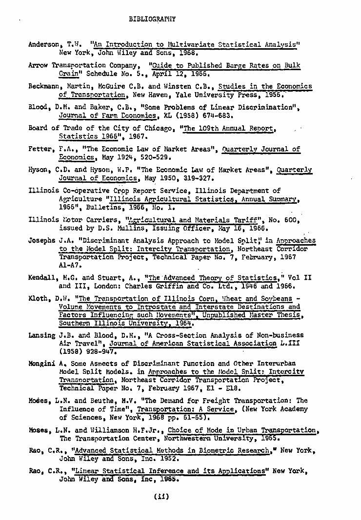
BIBLIOGRAPHY

Anderson, T.W. "An Introduction to Multivariate Statistical Analysis" New York, John Wiley and Sons, 1968,

Arrow Transportation Company, "Guide to Published Barge Rates on Bulk Crain" Schedule No. 5., April 12, 1966.

Beckmann, Martin, McGuire C.B. and Winsten C.B., Studies in the Economics of Transnortation, New Haven, Yale University Press, 1956..

Blood, D.M. and Baker, Ca., "Some Problems of Linear Discrimination", Journal of Farm Economics, XL (1958) 674-683.

Board of Trade of the City of Chicago, "The 109th Annual Report, Statistics 1966", 1967.

Fetter, F.A., "The Economic Law of Market Areas", Quarterly Journal of Economics, May 1924, 520-529.

Hyson, C.D. and Hyson, W.P. "The Economic Law of Market Areas", Quarterly Journal of Economics, May 1950, 319-327.

Illinois Co-operative Crop Report Service, Illinois Department of Agriculture "Illinois Apricultural Statistics, Annual Summary, 1966", Bulletins, 1966, No. 1.

Illinois Notor Carriers, "Agricultural and Materials Tariff", No. 600, issued by D.S. Mullins, Issuing Officer, May 16, 1966.

Josephs J.A. "Discriminant Analysis Approach to Model Split': in Anproaches to the Model Split: Intercity Transportation, Northeast Corridor Transportation Project, Technical Paper No. 7, February, 1967 Al-A7.

Kendall, M.G. and Stuart, A., "The Advanced Theory of Statistics," Vol II and III, London: Charles Griffin and Co. Ltd., 1946 and 1966.

Kloth, D.W. "The Transportation of Illinois Corn, Wheat and Soybeans - Volume Movements to Introstate and Interstate Destinations and Factors Influencing such Movements", Unpublished Master Thesis, Southern Illinois University, 1964.

Lansing J.B. and Blood, D.M., "A Cross-Section Analysis of Non-business Air Travel", Journal of American Statistical Association L.III (1958) 928-947.

Mongini A, Some Asnects of Discriminant Function and Other Interurban Model Split Models, in pnproaches to the Model Split: Intercity Transnortation, Northeast Corridor Transportation Project, Technical Paper No. 7, February 1967, El - E18.

Modes, L.N. and Beuthe, MV. "The Demand for Freight Transportation: The Influence of Time", Transportation: A Service, (New York Academy of Sciences, New York, 1968 pp. 61-65).

Moses, L.N. and Williamson H.F.Jr., Choice of Mode in Urban Transportation, The Transportation Center, Northwestern University, 1965.

Rao, CA., "Advanced Statistical Methods in Biometric Research," New York, John Wiley and Sons, Inc. 1952.

Rao, C.R., "Linear Statistical Inference and its Applications" New York, John Wiley and Sons, Inc, 1965.

(ii)

Sakashita, N. "A Microscopic Theory of Traffic Assignment'; Papers and Proceedings of the First Far East Conference of the Regional Science Association, Tokyo, 1963, 49-59.

Thomas, G.B. "Calculus and Analytical Geometry," Third Edition, Addison and Wesley, 1960.

.Tobin J. "Estimations of Relationships for Limited Dependent Variables", Econometrica, Vol. 26, No. 1. Jan 1968, 24-36.

Thorburn T.H., "Supply and Demand of Water Transport," F.F.I. Report, The Business Research Institute at the Stockholm School of Economics, Stockholm, 1960.

Tintner, G. "Econometrics", New York, John Wiley and Sons, Inc. 1963.

United States Department of Agriculture, Consumer and Marketing Service, Grain Division, Chicago. "Grain Market News Weekly."

Wardrop J.G., "The Distribution of Traffic on a Road System", in Theory of Traffic Flow, edited by R. Herman, 1961.

Warner S.L., "Stochastic Choice of Mode in Urban Travel: A Study in Binary Choice", Northwestern University Press, 1962.

Warner, S.L. "Multivariate Regressions of Dummy Variates under Normality Assumptions". Journal Of the American Statistical Association, December, 1963, 1054-1063.

Wills, W.J. Problems in Grain Transportation, School of Agricultural Publications, No. 22, Southern Illinois University, Carbondale, Illinois, 1966.

(iii)

VITA

MICHEL VINCENT BEUTHE

Born in Forest (Brussels), Belgium on the 4th December, 1935

DOCTEUR EN DROIT and LICENCIE EN SCIENCES ECONOMIQUES (UNIVERSITE

CATHOLIQUE DE LOUVAIN)

PUBLICATIONS: "Economie en Croissance Lente: Le Cas de la

Belgique", 0.B.A.P., Brussels, 1964.

"The Demand for Freight Transportation: The /

Influence of Time", with L.N. Moses,

in Transportation: A Service, (New York

Academy of Sciences, New York, 1968

pp. 61-65)

(iv )

FREIGHT TRANSPORTATION MODE CHOICE:

An Application to Corn Transportation

The aim of the present study is first to propose a model of

the mode of transportation choice for a particular commodity; second,

using this theoretical model, to develop statistical method(s) for

forecasting choices by shippers. In a sense it is a model of demand

for transportation, although it is not designed to estimate the tonnage to

be transported. Instead it answers the question: which mode(s) will be

used? (The actual tonnage transported may be found in surveys of production).

The choice of a mode for a specific transportation task is made

by comparing the various advantages and disadvantages of the physically

possible modes. These characteristics are the rates and other costs, which

together comprise the direct outlay costs; the expected time taken to

accomplish the transportation; the risk of loss or damage; the dependability

of the service from other points of view; and many other conveniences and 8

inconveniences presented by each transportation mode.

It seems safe to assume that shippers as entrepreneurs are

essentially profit maximising, and that all the mode characteristics haye

for them only one relevant and common dimension: the money value. Depending

upon whether a characteristic involves a saving or a cost for the shipper

relative to other modes, this money value can be positive or negative. Most

of the direct outlay costs are readily available whenever public trans-

portation is involved. The time costs can be easily estimated if accurate

information exists about journey time. But the other characteristics that

one is . to call "quality" differences between modes, are far more difficult

to convert into money values • They are, however, taken into account in

actual mode choice. As such they cannot be ignored in a theoretical model,

and any method which aims at forecasting the demand for a mode of transportation

should propose some means of estimating their -money equivalents. This is one

important aspect of the present research.

Chapter I presents the theoretical choice model. The time element

2

of cost iv iazroduced at once along with the direct outlay costsa The

"quality" characteristias are then introduced by means of a stochastic

element which makes the model suitable to statistical analysis° Chapter /I

generalizes the stochastic model and discusses the statistical method

appropriate for its testing° Chapter III applies and tests the model to

a concrete problem of mode choice: the corn shipments in Illinois.

As it stands, this statistical method is able to forecast in

probabilistic terms the mode which will be used from a particular origin. Applied systematically to all relevant origins it can predict the regional

pattern of demand for each mode. Whenever it is possible to link some

important costs of transportation to the space co-ordinates a definite region-

al pattern should be expected. Chapter IV and V, therefore, attempt to

build a spatial model of mode choice along the lines of traditional location

theory. It is closely related to the first model and uses its estimates

of the "quality" differences money equivalents.

Throughout this study it is assumed that the commodity trans- .

ported is produced under conditions of perfect competition. No attempt

has been made to generalize to other conditions, although such a task .

appears quite feasible.

CHAPTER I

The Firm's Transport Demand in Perfect Competition.

Consider a firm that operates under conditions of perfect

competition. It is located at A and sells all of its output of a single

homogeneous product in a market located at B. The firm purchases all of

its inputs locally so that the only transport it requires is for shipping

its product to market. In order to introduce the two problems of mode

choice and quantity the firm will ship in the simplest possible manner,

two modes with radically different characterisitcs will be assumed. One

of them is very expensive but very fast: it will be treated as instanta7

neous in the theoretical model. The other mode is very slow but very

cheap: the firm's cost function is given. The price of its product in

the market (P), the number of days required to ship the product to the

market by the slow mode (a), the interest rate per day (i) and the per

unit transport cost by the fast mode (g) are also given.

Suppose the firm's total cost (of production) function is of

the form:

(1) C = Zn , where Z is output per day and n > 1.

The firm's total cost of producing and shipping by the fast mode will then be:

(2) C1 = Zn

+ gZ.

Total cost of producing and shipping by the slow mode is:

(3) C2

= Cl + i) aZn , where the term (1 1. i) aZn represents the interest

charge on the money the firm must tie up in production cost when it ships

by the slow mode.

-3-

In the present theoretical formulation the price of the

product does not depend on the mode by which it is shipped. There

is therefore only one revenue function:

(4) R = PZ.

The profit by each of the modes is:

(5) 1T1 = PZ C1 = PZ - Zn - gZ.

(6) w2 = PZ - Cx = PZ - (1 + i)Zn

w1 and w2 are not comparable since the former is realized without

delay whereas the latter is realized only after some days. They can

be made comparable by discounting back to the present. Let us call

this discounted value

PZ - (1 + i) aZn PZ 2 -

(1 + i) (1 + i) a

We now take the difference between equations (5) and (7): ,

(8) 21= x PZ _n

PZ + Zn + gZ (1 + i) a

= Z[ P (1 + i) a

For any given output, in other words, aside from times when transport

capacity is strained, choice of mode depends solely on the two net

prices in brackets. If X is positive the firm will ship by the slow

mode; if X is negative it will ship by the fast mode; if X is equal

to zero it will be indifferent. In the latter case the firm may

ship all by one mode, all by the other, or engage in modal splitting.

The argument is illustrated in Diagram 1 where OC is the

firm's marginal cost (of production) function, the first derivative

of equation (1). The firm maximizes profit by equating marginal cost

to whichever of the net prices is higher. Under the conditions shown

the firm would produce Zo , ship all of this output by the fast mode,

expend OZ0E on production, JEFP on transport, and realize a profit

of OEJ.

(7)

p ga LT

P a K (1 + i) a

0 Zo

4

5

Diagram ).

t l •

The diagram emphasizes several results: (a) the choice of mode

depends on the price of the product, time of transport, the

interest rate, and money cost of transport, but not on the production

cost; (b) the fines cost function determines only the output it

will ship.

The extreme assumption that one mode is instantaneous and

the other one free may now be dropped and a more realistic definition

of X adopted.

[(13 - g2 ) (P - g1 )1 ( 9) x m z ,

(1 + + i)B

Here gl and g2 are respectively the money charges for the slow and fast modes; a and 8 are the trip times.

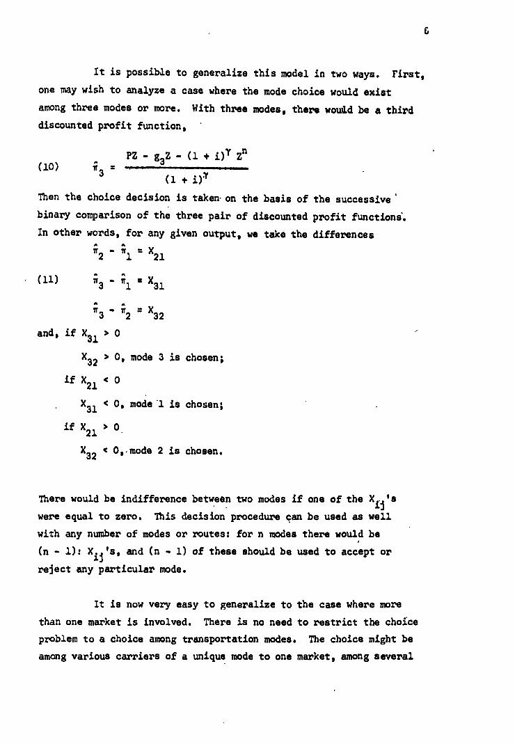
It is possible to generalize this model in two ways. First,

one may wish to analyze a case where the mode choice would exist

among three modes or more. With three modes, there woad be a third

discounted profit function, '

PZ - g3Z - (1 + O T Zn

3 - (1 + 01

Then the choice decision is taken on the basis of the successive'

binary comparison of the three pair of discounted profit functions'.

In other words, for any given output, we take the differences

1 = X

21

(10)

• (11) A A

If3

- w1 = X31

A A

w3 - it2 = X32

and, if X31 > 0

X32 > 0, mode 3 is chosen;

if X21 < 0

X31 < 0, model is chosen; •

if X21 > 0 -

X32 < 0, mode 2 is chosen.

There would be indifference between two modes if one of the X's

were were equal to zero. This decision procedure can be used as well

with any number of modes or routes: for n modes there would be

(n - 1):X1j 's, and (n - 1) of these should be used to accept or

reject any particular mode.

It is now very easy to generalize to the case where more

than one market is involved. There is no need to restrict the choice

problem to a choice among transportation modes. The choice might be

among various carriers of a unique mode to one market, among several

7

routes and several modes to one market, as well as among all of these

to various markets. For each combination of route, carrier, mode,

market there would be a particular price of the product on the relevant

market. Then one proceeds as above, from the n net prices to the

(n -X's, and through successive (n - subsets of these to the ij

- final choice.

Thus, we have achieved a model to explain (under conditions

of perfect competition) not only the transportation mode choice, but

more generally the mode and market choice. The choice is reached through

successive binary comparisons of all the possible mode-market

combinations. There is no limitation as to the number of these

combinations.

A Stochastic Model.

Throughout the first section of this chapter it was implicitly

assumed that the only costs of transportation were the direct money

costs and the interest cost arising from the transportation time.

However, there are still some other costs incurred by the shipping firm,

which may vary with the moce of transportation: the costs resulting

from the particular loading equipment of the shipper, the cost of

uncertainty, and, in general, the cost of the difference in service

quality of the various modes. All these costs are grouped under the

heading "additional costs".

We might then consider that the choice between any two

modes is not based on their X1, the difference between their net

prices as defined in the first section, but rather on a Y ij = Xij t E i3 where E. is the difference between their additional costs. This 13

will be called the net income difference. The E,. 's are 13 presumably known or estimated by the shippers and incorporated into •

the calculation of which mode is most profitable. In reality, the

shippers use Yij instead of Xij and choose the higher net income mode.

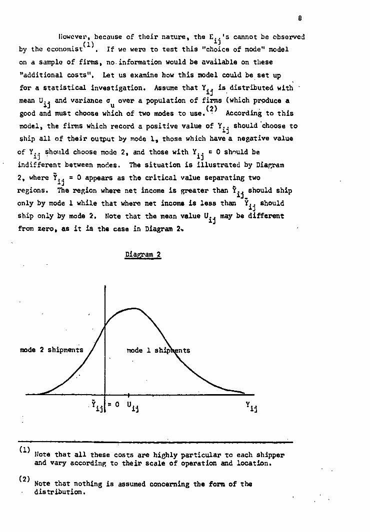
8

however, because of their nature, the's cannot be observed E.

by the economist(1)

. If we were to test this "choice of mode" model

on a sample of firms, no-information would be available on these

"additional costs". Let us examine how this model could be set up

for a statistical investigation. Assume that Y ij is distributed with -

mean U. and variance au over a population of firms (which produce a

(2) good and must choose which of two modes to use. • According to this

model, the firms which record a positive value ofshould choose to

ship all of their output by mode 1, those which have a negative value

ofshould choose mode 2 and those with = 0 shnuld be Yij , Yij

indifferent between modes. The situation is illustrated by Diagram

2, where 0 appears as the critical value separating two

regions. The region where net income is greater than / ij.should ship

only by mode 1 while that where net income is less thanshould

ship only by mode 2. Note that the mean value U il may be different

from zero, as it is the case in Diagram

Diagram 2

mode 2 shipments ir 1 mode 1 shiPhonts

(1) Note that all these costs are highly particular to each shipper and vary according to their scale of operation and location.

(2) Note that nothing is assumed concerning the form of the

• distribution.

9

The choice of mode decision is not so easily solved since

the E..'s are not available, and the parameters of the distribution

of Y.. are not known. Let us assume, however, that E.. is ;3 13

distributed independently of the

13

If the additional costs were so small that they did not

affect mode choice, the distribution of X.. could be cut into two 13

pieces at X.. = 0, as it was done for Y in Diagram 2. Thus, 13 ij

R.. would define two decision regions for mode i and mode j 13

respectively. The distributions of these two modes origins would

correspond to the portions of thedistribution of the Xto each

side of the critical value. If the E.. were this small, we would 13

be back to the deterministic model of section I.

However, ifEij magnitude, is of significant maitude, the two

distributions should overlap each other. As Eij

is a random variable

independent of Xij

, for any particular value of X. , say X?1r

there 0 1J

exists a complete conditional distribution of Xi j + E. • It follows 1j ,

that among the shippers characterized by X7 j , those with Xij + Eij > 0

will choose mode i, while those with X° + c 0 will choose mode j.

The overlapping distributions presented by Diagram 3 illustrate this

influence of E ij°

Had the deterministic model been the correct one, its test

would have been an easy one. The theory provides its own decision value,

i.e.,= 0. A simple check of the transportation mode used by firms

with, on one hand, a positive value of X ij , and, on the other hand, a

negative value ofcould have solved the question. Since it doesn't

take account of other costs, this model is not realistic; the influence

(1) Note that nothing is assumed concerning the fbrill of the distribution.

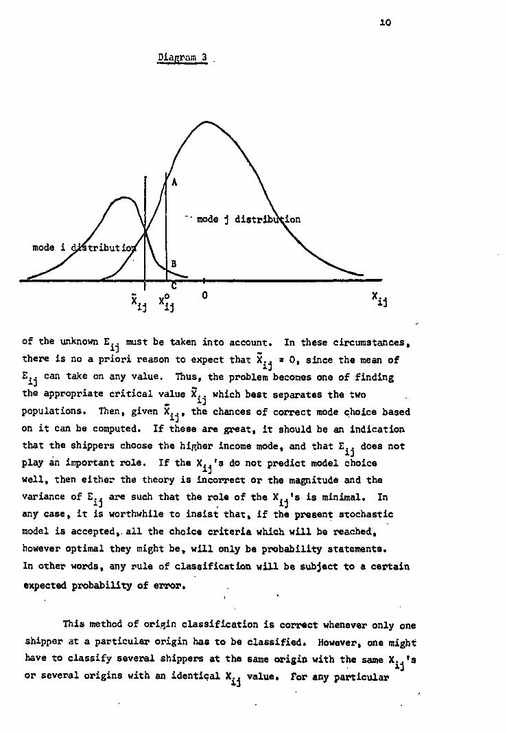
ij xo ij

0 Xij

10

,Diagram 3, .

of the unknownEij must be taken into account. In these circumstances,

there is no a priori reason to expect that= 0, since the mean of

Eij can take on any value. Thus, the problem becomes one of finding

the appropriate critical valuewhich best separates the two

populations. Then, given the chances of correct mode choice based

on it can be computed. If these are great, it should be an indication

that the shippers choose the higher income mode, and thatE ij does not

play in important role. If the X ij 's do not predict model choice

well, then either the theory is incorrect or the magnitude and the

variance ofEi are such that the role of the Xij's is minimal. In j

any case, it is worthwhile to insist that, if the present stochastic

model is accepted,. all the choice criteria which will be reached,

however optimal they might be, will only be probability statements.

In other words, any rule of classification will be subject to a certain

expected probability of error.

This method of origin classification is correct whenever only one

shipper at a particular origin has to be classified. However, one might

have to classify several shippers at the same origin with the same X's 13 or several origins with an identical X ij value. For any particular

shipper characterized by X probability that he will use the jth

mode is greater if X X ° is greater than , (see diagram 3). This is so ij ij

because it is more likoly that its= = E. ° will be greater than ij + i

zero. Iiut, given thatis a random variable, some of the X ; ° shippers

nay have a Yij value smaller than zero. These origins would use the ith

moue. It follows that a certain proportion of these shippers should be

allocated to mode i. The percentage split between the two modes can be

read from diagram 3: forX o , it corresponds to the.ratio of AB to BC (1). ij

This second approach to mode classification is undoubtedly the correct

one whenever several shippers are located at the same origin.

It should also be used whenever one wants to estimate the

proportions in which the modes will be used to ship a commodity from

a region of production. However, to forecast the choice of a particular

shipper - or, as in the case of Chapter III, the choice of each of a

series of shippers - one should retain the former "discrimination"

approach which generates only exclusive choices of mode. In that

respect, the present stochastic model should be clearly distinguished

from all the "model-split" models.

Before closing this chapter, an important point must be made

Rij concerning the meaning of the critical value For the sake of this

argument, let us provisionally agree that gij is the value indicated in

Diagram 3: theat which the two distributions intersect. is Eij

a random variable independent ofX particular Therefore, to any pa ii

value ofX , say X, . o corresponds a conditional distribution of ij ij

(1) Chapter II gives a method to estimate these percentages.

- X. o + E similar to the distribution of E1.1° but with median value lj

12

equal to+ where E is the median of If the E. ij Eij Eij .

distribution was known, the percentage split between the two modes

for any given value ofX i could be determined on the former j

distribution. In particular, for X i°j , all the observations with sum o + greater than zero should correspond to mode i shipments, Eij

and all the observations with such a sum smaller than zero should

correspond to mode j shipments. Atit is observed that the

percentage split between the two modes is: half of the shipments

by mode 1, and half of the shipments by mode 2. This may occur only

because the median value+ = O. It follows that E. -gil . Xij

Thus we have a way of estimating what might be called the average

quality difference between modes.

Further, one could also estimate the other parameters of

the distribution ofE i It is possible to compute from Diagram 3, j

or from the two mode distributions, the percentage split between

the two modes: forXij o it is equal to the ratio of the ordinates of

the two distributions at X. But, this percentage corresponds to 3.3

the relative number of o 's which, in the distribution of o + Xij X. E.

are greater and smaller thanX i + o = O. It follows that it gives j Eij

the value of the cumulative distribution ofat Eij E. =j

Proceeding in that fashion for successive values of Xij , it is possible

to derive the cumulative distribution ofE ij then its density function. ,

To estimate in this way the parameters of E ij 's distribution,

it is necessary to assume thatX i and E are distributed independently j ij

of each other. If this were not the case, the conditional distribution

ofX Eij given X would vary with X ij Then the percentage split ij + .

between the two modes at various values ofX would give only some ij

information about the successive different conditional distributions.

In principle, this information is not sufficient to estimate with

precision the parameters of the distribution of E... though it might 13 provide a useful approximation.

13

Section II dealt with the choice between two modes. Chapter

II will generalize the stochastic model to the case of more than two

modes. We will also discuss the statistical method of determining the

best critical value ofalong with other statistical problems. X iJ

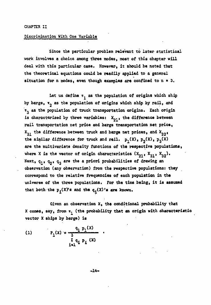
(1) 1 3

ql p1(X) ■ P.m%

CHAPTER II

Discrimination With One Variable

Since the particular problem relevant tO later statistical

work involves a choice among three modes, most of this chapter will

deal with this particular case. However, it should be noted that

the theoretical equations could be readily applied to a general

situation for n modes, even though examples are confined to n a 3•

Let us define w 1 as the population of origins which ship

by barge, 112 as the population of origins which ship by rail, and

113 as the population of truck transportation origins. Each origin

is characterized by three variables: X 21 , the difference between

rail transportation net price and barge transportation net price,

X31 the difference between truck and barge net prices, and X32 ,

the similar difference for truck and rail. p i(X), p2(X), p3 (X)

are the multivariate density functions of the respective populations,

where X is the vector of origin characteristics (X21 , X31 , X32 ).

Next, qi , q2 , q3 are the a priori probabilities of drawing an

observation (any observation) from the respective populations: they .

correspond to the relative frequencies of each population in the

universe of the three populations. For the time being, it is assumed

that both the pi(X)'s and the qi(X)'s are known.

Given an observation X, the conditional probability that

X comes, say, from wi (the probability that an origin with characteristic

vector X ships by barge) is

qi pi (X) i=1

-14-

15

p1 (X) is the probability that X will be observed among all the X's

belonging to sub-population wi . To find pi(X), the probability

that a random observation X of w1 be drawn from the total population

of all origins, pi (X) must be weighed by qi , the probability that

an observation (any observation) will come from it. In general,

the product qi pi (X) is the probability that X of w i will be drawn

and the sum of these products over the three sub-populations gives

the probability of X. It follows that the ratio.(1) is the

conditional probability that, given observation X, X comes from

wi . The expected loss of classifying that observation as from w 2 is:

qi pi(X) (2) E 3 C(2/1),

is1,3 E q p (X) i=1

where C(2/i) is the cost of classifying an observation from w l as

from w2 . Then, one chooses the population ir k , or the mode of

transportation k, which minimizes the expected loss for X. Assuming

here that all the C(i/j) 's are equal, this is equivalent to minimizing

3 (3) E qi pi(X),

i=1 i0k

Proceeding in this fashion for successive observations, it is possible

to define decision or classification regions R 1 , R2 , R3. The rule is:

assign X to Rk if

• (4) E qi pi(x) c E (14 pi(X), for all j 0 k. i0k

This procedure minimizes the expected loss and is unique, if the

probability of equality between right-hand and left-hand sides of the

equation is zero . Subtracting from each side of (4) E qi pi(X),

(1) T.W. Anderson, 'Introduction to Multivariate Statistical Analysis' 1958, pp. 143-144. .

16

which is,.in this case, the only q i pi(X), i g j and k, remaining

common to both sides, the rule becomes: assign X to R k if

(5) qk Pip) > qj pi (X), for all j g k.

In other words, as the.probabilitY that the observation comes from

nk is greater, the observation must be assigned to R. Finally the

criterion may be writtern as: assign X to R k if

Pk(X) > a

(6) , for all j k. 1-75-6 elk

In our case there are two such equations for each of the three regions

of classification. For instance, the X's such that

p1(X) q2

175C > 717

p1(X) q3 , should be assigned to R 1 1757( ql

As is shown in this example, this statistical approach to

the mode choice problem leads to binary comparisons of every pair of

modes. In that respect it corresponds to the deterministic model

with three modes (which was discussed in Chapter I). Aside from the

probabilistic approach, there is however one difference. One of the

results of Chapter I was that the only relevant variable for deciding

between any two modes was the difference between the net prices

provided by these' two modes. When comparing truck and barge

transportations, one should refer only to X31 ; when comparing rail

and barge one should use only X 21 ; only X32 should be used for the

truck-rail comparison. But note that until now in this chapter, the

vector X containing the three net price differences have been always

used. We shall now try to include only the X to each of

the binary comparisons.

(7)

(8 )

(9)

17

Let us define n(X 1 ) as the probability distribution of i Xiji over the ith population. Then, say, n 1(X21 ) is the probability

distribution of X21 over the barge origin population. The n.(X ) ij

are assumed to be normally distributed with means p ij and

variances jai. It follows that

1 1 . (20-2 . e

n (X ) a „Lid_ .

iJ 1 . (20 . e

ni(Xi .) 40. 4. (X - U. ) 2 (X. - • )2 ln 7,7 7 71:7 = in till in

ij 2"a2 1 li

11 1 ii 2

3 13 i J 11 2 iaij

'

( 10) = ln + ( iali )A + 2 X. ( U 02 U 2 ) 11 i eii . iaij 2 2

2

U2 a2 U2 2 j i 2 2 2 iaij jaij

or

n (X..) (11) in - n X a. + b. X + c X

2 . ) lj ij ij ij

.U2 .a. U? 02 where a = in 2.4-1 + 111L11 .

ki

i 2 2 ii 2 iij iaij

2 2 2 bij = jaij - j Uij laijViaij f. (12)

cij = 102ii 72 1.02ij

Pii) 2/2 gij

'4)(14 2412 jail

Notc that the first subscript of a.., b. and refers to the

lj 1j cij

distribution subscript of the numerator, and the second subscript

to the subscript of the distribution in the denominator. If it 2

is possible to assume that i a. = .0ij

2 = 0ij'

2 equation (10) becomes,

ij

n.(X ) (13) in 1

h.(XJ a . b!. X. . with

1] ij

2 2 2 a:. = - 0'229 1] / J.]

2 b' = (.0. - .U..)/0.. ij llj 3 13 / 1)

Now the criteria for R1 given by (7) can be rewritten as

in n1(X

21) ' q2/

- A' ' ln q1 n2 (X21 ) 1 + b2 12 X 21 >

(15) n1 (X31 ) 43,

in r-r71---7( = ai3 bi3 X31 > in 'qv if the variances are 3‘ 31!

equal. Similar sets of criteria can be derived for R 2 and R3 . The

critical values X21

and X31 which define R

1 are those which make the

left-hand side of the inequalities (14) equal to their right-hand side.

Each of these critical values can also be used to define regions of

classification when the choice is restricted to two modes. It is then

easy to compute the chances of misclassifying an origin or firm with

characteristic Xij when the choice is restricted to modes i and J.

With iU. > U the probability of misclassifying an observation lj j ij

from w as from w, is 7

Rij 2 .1 •1(Xii i./4 )2/1.44 : dXij (16) P(j/i) = (2 joie) A

_ft

(14)

=AO

i( TC - U )/a A R i ij i ij 1 i ik ( 19) P(J,k/i)

•

f(Z ik)dZij dZik

10

ilkii -

. (17) 2. 2 -1 -1(Zij)2

(2 iij w) .0 0111

while the probability of misclassifying an observation from w j as from

wi is

(18) NUJ) ' • 2

.dWij (2 iaij )4

-1(w )2 '

Jr (51ij -

Furthermore, it is possible to compute the overall chances

of misclassifying an observation from w i as from wj or wk. With

U >U and iU kUik' iJ ii s

where f(Zij' Zik ) is the standard form of the bivariate normal

distribution. The respective probabilities of correct classification

are equal to 1 - PQM, 1 - P(i/j), and 1 - P(j,k/i).

An alternative and equivalent, though more complicated,

, method of classification would be to compute the Pi(X) 1 21, the

conditional probabilities that given X, the ith mode will be chosen,

and assign X to the mode with the greatest P1(X). (1) Following (1) above,

• qi N1 (X) ' (20) Pi (X) Is 3

s

E 414 Nj (X) . j=1 J

where multivariate normal distributions are assuTed& gut, as

(1) See S.L. Warner 'Multivariate Regression of Dummy Variates under Normality Assumption' Journal o Amer can Statistic Association, December, 1963, pp. 1054-1063.

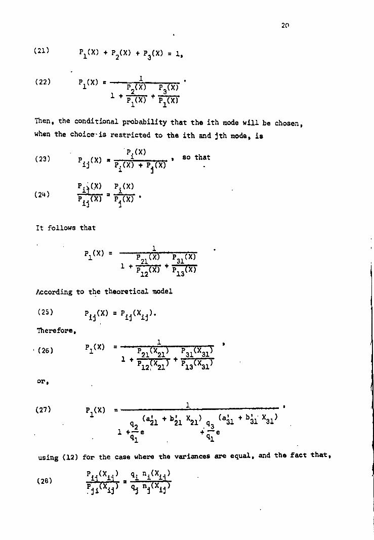
Pij (X) = P (X. ). ij .a.j

P (x) = 1 P21(x21 ) 1331(x31 ) 1 + FIT---(2 3) +

(25)

Therefore,

, (26)

9 1

20

P1 (X) + P2 (X) + P3 (X) = 1,

.i. (22) P1(X) = P

2 (X) P3 (X) 1 4.

P1

4. (X) P1 (X)

Then, the conditional probability that the ith mode will be chosen,

when the choice-is restricted to the ith and jth mode, is

. P .(X) (23) P

ij (X) = that

P.(X) + P (X) • 1 i

pii((X)Pi . (X)

Pij X) Pi(X) •

It follows that

P (X) = 1 P21

(X) P31(X) 1 +17-0 +175-0

According to the theoretical model

I .' 1)

1

(24)

1 .

or,

(27) PI (X) =

q2 (a21 21 ' + b' X21

) q3 (a31 ' + b' • X31 ) • 31

1 +—e

ql

using (12) for the case where the variances are equal, and the fact that,

(29) P (X..) ij 11

P (X )

qi n i(Xi .)

cai 1-77-131j

21

Moreover,

+ b' X ) q2 21 21 21

P2'(X) = P (X).--e 1 qi

(a' + b' X ) q3 31 31 31

P3 '(X) = 1 qi

However, these last two equations should not be relied upon to compute P 2 (X)

and P3(X), because they do not use all the information available to do so.

For instance, P2(X) as computed by (27), uses only the ratios P 21(X21

)/P12(X

21)

and P31(X31)/P13(X31), but not P32(X32)/P23(X32) which evaluates the relation

between mode 2 and mode 3. This feature would have been without consequence,

had not equation (24) been used. This can be seen in the following way. Let

us assume that

P2(X) a P3(X) c

P2(X)

a

FlTn. zriT1752-17;1*-3736ac Then,

3 (31) E P (X) =

1 • + 1 __ _ _ 4 A. ......■■■ U 1

i a c b+c 1

' 1=1 1 + — + — 1 + — -.. + k + A b b a a c c ,

- and, say, •

P2(X) (32) p2(x) is 1 P (X). 1 a — P i (X1 b c 1 - • TM' - a c • b 2" 1 +1 + a 1 1 + + — b b

Equations (27) give..the conditions for having the sum of the Pi(X)'s'equal

to 1 and P (X) 3: P'(X). These conditions are guaranteed when the successive'

, ratios of probability ore based on the same variable(s). This is what equations (24) preclude. Then if

• • P31(X31)/P13(X31 ) k/b c/b, while .

P21(X21 ) a P23(X32 ) • a P3---17—T21 • 117 9 7717

(29)

(30)

( 33 )

be • K - (a + b + c) (A b + c + e)

, if k = c + e. (36)

;2

1 1 a (34) P2(X)

' = and Pl(X) - b c 2 a k • b

• a a b b

The two formulas give different results for the same probability. P 2 (X)

should be taken as the correct result, since it is based on the full

available information concerning mode 2. It remains that one cannot be

sure that the sum of these P (X)'s equals 1. In general, they will not add

to one, but the divergence should be small. Still using (30) 4

. 3 . • 1 1 (35) E p (x) 2 •■■■,...... .1. .........■ f

i ak bb b a. + 3 + 3 1 + -a- + -; l + r + 3

Assuming k/b > c/b, the second term of (32) is smaller than the second term

of (28). It is exactly smaller by

Similarly, if k/b c/b the third term of (32) is greater by

(37) L

ce (a + b + c) (a + b + c e) 9

if k c a

K and L should be small, and as they tend to compensate each other, the

sumoftheP. ( X) should be close to one. We conclude that the use of

1 P (X) would be reasonably safe. . •

Obviously, no such problem arises in the computation of

1 1 (38) P..(X. ) = 13 ij - (A' ' X )

li li 1 + e ji + b ji

1 + Pij (Xil )

23

Finally, let us note that P i(X) corresponds to the conditional

probability that a given observation within the classficiation region

of the ith mode is correctly classified into the ith population.

Similarly, Pii (Xii ) corresponds to the probability of correct - classi-

fication in the case of restricted mode choice. These probabilities

correspond to the percentage split between modes of all the shippers

with an identical Xij value.

CHAPTER III

An Application - Corn Trans2ortation in Illinois.

The purpose of this chapter is to apply and test the model

proposed in Chapters I and II to a concrete - problem of mode choice:

the corn shipments in Illinois.

I. Grain Marketing in Illinois.

A. It seems necessary to summarize how grain is marketed from

the farms to the final market before discussing the available body of data

and its value.. (1)

Most of the grain (wheat, corn, soybeans, oats) is delivered

by the farmers at the harvest or shortly after, but less so for the corn

which is progressively sold during the whole year.. (2) The farmer has the

choice of several outlets for his grain. He may sell to other farmers,

usually feeders who do not raise enough grain to feed their livestock,

or to millers established in grain producing areas. In these cases, he

uses his own truck or the services of a commercial trucking concern to

deliver the grain. The farmers located near a terminal market may truck

and sell the grain directly to terminal elevators equipped to unload trucks.

They may also sell the grain to an intinerant trucker, who buys the grain

on the farm and resells it wherever a suitable market is available. However,

the great bulk of the grain is trucked to the country elevator.

(1) Most of this information on grain marketing was found in 'Grain Transportation in the North Central ReRion', U.S. Department of Agriculture, Transportation and Facilities Research Division, Report No. 490, July 1961; and in stenciled notes prepared by the Grain Exchange Institute, Inc., Board of Trade of the City of Chicago, 1966.

42) See 'Field Crops Production. Sales. Prices' Illinois Coop. Crop Report Service, Illinois Department of Agriculture Bulletin, 65-3, 1965.

-24-

25

Elevators obtain grain from farmers by purchasing it outright

at the time of delivery, by contracting in advance of delivery, by accepting

grain for storage with the sale to be consummated at a later date, and by

handling grain for the farmer's account, without ever taking possession of

it. Most of the grain passing through the country elevator is grown no more

than 15 miles away from the elevator. The most usual method employed in

buying the farmer's grain is outright purchase. The country elevator

operator receives continuous market information from commission merchants

operating in the terminal market, from interior dealers who purchase grain

for resale to interior mills, processing plants, and terminal elevators,

and by radio broadcasts. He bases his price on these bids, taking into

consideration the freight charges to the terminal market, the terminal

market handling costs, and his own costs and profit margin.

The country elevator grain can be sold locally, or it can

be shipped to an interior mill, or processing plant. The country elevator

also ships to some principal terminal market or to an export point. There,

his interests are usually represented by a commission merchant or cash grain

receiver. The grain is either consigned to them, or sold for deferred

delivery on 'to arrive' or 'on track' bids. When consigning grain, the

country elevator ships the grain to its representative to be sold after

arrival in the market. In this case, he retains ownership of the grain, pays

all costs of shipping the grain, is subject to any loss incurred while the

grain is in transit, and takes the risk of adverse price changes. When the

grain is sold on a deferred shipment basis, the price is agreed on at the

time of the contract, usually before the grain is shipped. Then the buyer

assumes the risk of price fluctuation.

Once the grain is loaded, the country elevator operator fills

out the 'order' bill of lading, which is signed by the carrier. This kind

of bill of lading is negotiable in bank, if endorsed by the shipper. In

this way the elevator is able to finance its operations. The bill of lading

is sent by the bank to another bank in the consignee's city, and after payment

is released to the consignee, who can then dispose of the shipment. The

elevator operator pays interest to his bank for the money borrowed up to the

26

time the draft is honored by the consignee, who will eventually borrow

against the shipment.

Besides the country elevators, there are some river elevators,

which originally were operated as sub-terminals, i.e., to feed the terminal

elevators. In recent years, due to the growth of the poultry industry in

the South, and, above all, to the demand for barge grain at the Gulf for

export, most of the grain originating on the river did not go to the

terminal houses. For instance, in 1964, only 15 per cent of all the barge

grain shipments from Illinois were sent to Chicago and other terminal -

places. Even a smaller percentage of the barge corn shipments reached

these places. Many of the river elevators do not have rail facilities. They

generally rely on grain bought from country elevators which deliver by truck.

The terminal elevators are located in Chicago, Peoria, and

St. Louis. They buy from cash grain merchants, river elevators, and country

elevators. Most of the terminal elevators can receive grain by barge, rail,

and truck. The terminal elevator, in turn, sells to processors, millers,

distillers, feed manufacturers, exporters, and sometimes to elevators in

other parts of the country. Most of their shipments are by rail or water.

They benefit from the rail transit privilege for the grain received by rail

or by barge, when the inbound barge shipment is regulated.

B. Some detailed information is available concerning part of

the grain movements just described. In some cases these data deserve quite

a number of comments. However, the most important data will first be quickly

described, in order to indicate the kind of concrete problem that will be

dealt with later.

The Board of Trade of the City of Chicago made available to us

monthly data covering all the grain shipments from Illinois to Chicago by

truck and by rail during the year 1966. These include the shipment origins,

the name of the railway carrying from these origins, the rail mileages, the

rail rates, and the quantity of each shipment. For the rail shipments, the

number of days it took for each shipment to reach Chicago was also given.

27

Truck rates for grain shipments within Illinois are published.

Truck and rail shipment origins of corn, as provided by this

body of data, have been mapped for three months. As can be seen from these

maps, most of the shipments originate in the upper third of the Stare.

However, within that region, few shipments arise along the Illinois River. (1)

Although abundant quantities of corn are grown in that area, this pattern

should be expected. If some of that area's production is shipped to a

market, it should go by the river.

Additional information could be gathered to complete this

body of data. One df the most iMportant Illinois grain dealers gave a

list of the country elevators with which its river stations (down to

Peoria) were dealing during the crop-year 1966, the estimated quantities "

of grain these country elevators shipped to various destinations, and the

transportation modes they used. Rail and truck rates could be compiled

for these barge grain origins. Finally, some barge rates are published,

while it was .possible to estimate the barge transportation time on data

provided by the Corps of Army Engineers.

These last data about complete the information required to

apply our statistical model to the corn shipments from the upper part of

Illinois.

(1) 'Illinois Agricultural Statistics, Annual Summary, 1966', Illinois Coop'.

- Crop Report Service, Illinois, Department of Agriculture Bulletin, 66-1, pp. 60-61.

2. Critique of the Data.

We must now examine how well the data fit the theoretical

model. Some of their particularities must also be reviewed in more detail.

The theoretical model requires perfect competition in the

production of a homogeneous product. The study of the shipments of an

agricultural product as widely grown in Illinois and as well defined as

corn should reasonnably meet that requirement. Doubtless, there are

several qualities of corn according to its moisture and the .percentage

of damaged kernels. These differences in quality can be of some importance

as to the corn destination, and the price it commands on the market.

However, we cannot narrow down further than corn in general. Another reason

for choosing corn was that the harvest is sold progressively during the '

entire year, so that it would be possible to compare the results of several

months.

Given the nature of our information and according to the

dominant pattern of corn shipments, the actual choice among shipments will

be restricted in the statistical study to truck shipments to Chicago, rail

shipments to Chicago, and the combination truck to the rimer then barge to

New Orleans.

Table I gives the sample sizes per mode for each of the

months which have been retained for the statistical analysis. It gives also

the number and the percentage of origins commcq to two samples. As can be

readily seen, the large majority of origins use exclusively one mode of

transportation.(1) This fact seems to indicate that country elevators make

their decisions much in the way that was suggested in Chapter I, and that the

discrimination model of inclusive choice is the relevant one(2)

. INION•wea•

(1) From now on, as a convenience, we shall not refer any more to mode-market combinations but only to modes whenever this convention will be permissible without confusion.

(2) Note that in practically all cases, there is only one shipper per origin.

28

29

Barge and Truck

Barge and Rail

Table I. Number of Origins per Mode (i.e., sample sizes),

Number and Percentage of Origins common to two Modes.

January February July

Truck Origins 48 53 3E,

Rail Origins 225 260 193

Barge Origins 159 159 159

Origins common to

Rail and Truck 26 24 10% 8%

18 a%

10 9 6 5% 4% 3%

28 45 32 8%. 2% 10%

We do not have any information about shipments which could have

been made by these same origins to some other destinations, or to the same

destinations by other modes. However, the fact, just mentioned, that the

country elevators seem to make an exclusive choice, tends to make this lack

of information irrelevant. The data as we have them should give reliable

information about choices which actually maximized the shippers' profit.

Moreover, on principle ground, it would not matter if some relevant, and,

for some origins, some best mode-market combination co4d not be entered

in the statistical analysis. In that event, the latter would be restricted

to the modes for which some information is available, the decision rules

obtained would only be pertinent to the choice among these modes, and the

probabilities conditipnal upon the restriction over the available modes.

However, it does not seem that the present statistical analysis

should rest on such a conditional basis. Another fragmentary piece of

evidence exists to support that point of view. In 1963, according to a survey

30

made through questionnaires to country elevators, (1) the three modes

shipments represented about 60 per cent of all the corn shipped from

the five crop districts which enclose the area under study; 21 per cent

were shipped to Peoria, Decatur, and other destinations in Illinois;

about 5 per cent was shipped by barge to Chicago, and the rest was shipped

to more distant markets, mainly-to the South and the West by rail or

by truck. Accordingly, if one sets aside the corn shipments to

destinations within Illinois other than Chicago, approximately 80 per cent

of the remaining corn shipments were made by one of the three modes the

present study is taking into account. These statistics should confirm the

relevance of these three modes.

As mentioned above, three months have been selected for separate

statistical analysis. The month period appeared to be a reasonable

compromise among several requirements: the need for sufficient sample size:,

the wish to take into account seasonal pecularities, and the necessity of

using a period short enough to keep the influence of the variations in

market prices- within reasonable limits. This may be the time to point out

that this analysis will deal with three different' marketprices: the price

on the market of New-Orleans, the price for truck grain in Chicago, and the

price for rail grain in Chicago. Monthly averages of these prices have to

be introduced since we do not know the precise price that each shipment of

corn obtained.(2)

Variations in the relations among these three prices

during a month probably explain a .certain amount of the shipments which

are made by two modes from a common origin.

D.W. Kloth, 'The Transurtation of Illinois Corn, Wheat, and Soybeans - Volume Movements to Intrastate and Interstate Destinations and Factors Influencing such Movements', Unpublished Master Thesis, Southern Illinois University, 1964, pp. 43 - 58. As the categories used by the author do not correspond completely to ours, these percentages are only good approximations. The five districts used to reach these percentages are the Northwest, Northeast, West, East, and Central Districts.

(2) Averages computed from the spot prices of No. 2 Yellow Corn published in 'Grain Market News, Weekly', United States Department of Agriculture, Consumer and Marketing Service, Grain Division, Chicago.

(1)

31

The months of January and February were chosen because they are

not harvest months, while considerable quantities of corn are still shipped.

Presumably they should be months during which there is no capacity constraint

on the choice of the shippers. The month of July has been chosen for the

opposite reason: according to the statistics of the Chicago Board of Trade, (1) it is the second most active month for the receipt of all grains. Note

that the Illinois River is rarely blocked by ice; in January 1966 the river

was completely free of ice, while in February the traffic was only slowed

at the locks during a few days. (2)

It has been noted above that the truck and rail data were

available on a monthly basis for each of the grains. Unhappily, this is not

the case for the barge data. On the one hand, they do not make any

distinction among different kinds of grain, and it cannot be ascertained

whether corn, wheat, or soybeans were shipped to the river station; on the

other hand, they are yearly data, which do not tell which origins actually

shipped to the river during a particular month. These two weaknesses of the

barge data are not as serious as they may appear at first. First, in the

area under study, the corn production is so dense and abundant relative to

the production of other grain that it is very likely that if some grain has

been shipped from a particular origin to the river, some corn has been shipped. (a)

Second, yearly data can only be over-extensive. In other words, by including.

in a month sample all the origins which'shipped some grain to the river during

the year, one includes all the marginal origins which do not usually ship by

barge during that month. They certainly cannot introduce a bias favorable

to a strong decision rule. As, at the same time, the information concerning

the truck and rail shipment origins is complete and presumably very accurate,

(1) Board of Trade of the City of Chicago, 'The. 109th Annual Report, Statistics 1966', 1967, pp. 4.

(2)'train Market News, Weekly', ibid., issues of January and February.

(3) 'Illinois Agricultural Statistics, Annual Summary, 1966', ibid. pp. 60-61.

32

we can still hope to obtain satisfactory statistical results. If they are

so, they should be really meaningful, since the defects of the barge sample

could only worsen the results.

Another weakness of the barge sample is that, if the data

indicate to which river point each country elevator is shipping, they do

not say to which destination the corn is sent from the river station.

A solution to this problem has already been suggested above. As not much

grain is sent to Chicago or other points on the river by barge, but most

of the grain is sent to the Gulf, (1) we shall assume

'that all the corn

shipped to a river point is thereafter shipped to New Orleans (by far

the most important destination). Given the situation of perfect

competition, the prices of grain on the various markets should be tightly

connected, and the differences between them closely related to the costs

of transportation. Therefore, the proposed solution should not be a

source of much distortion.

We have now to compute for each of the origins in the three

samples the net prices which could be obtained by using each of the three

modes during the relevant months. Before doing so, we must still review

the quality of some basic components of these net prices. First, the rates.

The rail rates, as is well known, are regulated, so that e can trust that

for each origin the 'published rate is the rate which has been used or would

have been used. For some origins, several rates were proposed. The usual

case was of an origin which had a special rate for shipments to the East

through Chicago (I.?. rate), besides the regular rate. Whenever such a special

rate was lower, it was retained under the presumption that the grain was

then going beyond Chicago.

The Transportation Act of 1940 exempted certain classes of

traffic carried by water carriers, and in certain cases grain transportation

(1) This fact has been checked on the records of barge shipments of the same corporation which gave us the list of country elevators it was dealing with: only 15 per cent of its all grain barge shipments went to Chicago.

33

falls within this exempted class. This exemption is found in Section 303,

paragraph B, Part III, of the Interstate Commerce Act: "Nothing in Part

III shall apply to the transportation by water carriers of commodities

in bulk the cargo space of the vessel in which such commodities are

transported is used for carrying of not more than three such commodities .

For the purpose of this sub -section two or more vessels while navigated as a

unit shall be considered to be a single vessel." As a consequence,

according to reliable information from grain dealers, the actual rates for

grain transportation by barge were 15 per cent below the common carrier

published rates during the period of time which is dealt with.(1)

Section 14 and Section 15 of the Illinois Motor Carrier of

Property Act set forth the Duties and Practices of common and contract

carriers by motor vehicle. Along with other provisions, these sections

require every common or contract carrier by motor vehicle to (1) establish

and observe just and reasonable rates, charges, and classifications, and

(2) to file with the Commission and print and keep open to the public

inspection tariffs showing all the rates and charges for transportation

and services in connection therewith. Section 18 provides that any motor

carrier operating upon the highways of this state who transports commodities

for a rate other than the lawful rate on file ... is guilty of a misdemeanor

and shall be puhished by a fine of not less than 25.00 dollars nor more than

300.00 dollars or by imprisonment or both. Discussions with officials of

the state regulatory body revealed that efforts are made to enforce the

law. Since firms can change rates legally by publishing a new tariff, and

since the motor carrier industry is very competitive, it is believed that

these rates could be used to approximate truck charges from each community (2)

to Chicago. They should correspond to the actual rates as far as the

(1) The preCise_Source of the published rates was 'Guide to Published Barge Rates on Bulk Grain', Schedule No. 5, issued by Arrow Transportation Company, April 12, 1966.

(2) These rates are published through the intermediary of truckers' associations The general tariff per mileage block appear to be the same for all the associations. It can be found, for instance, in the 'Agricultural and Materials Tariff', No. 600, of the Illinois Motor Carriers' Bureau, issued by Donald S. Mullins, Issuing Officer, May 16, 1966.

34

common and contract carriers are concerned. When the transportation is perfornee

by the farmer, by the country elevator, or by an itenerant dealer, they can be .

taken as approximations to the cost or the charge for the transportation.

It is important to point out that for the three modes, the rates do

not depend on the quantity shipped. The only 'restriction in that respect is a

requirement of minimum loading which is approximately equal to the average

capacity of the mode unit of transportation (a barge, a boxcar, a truck).

The rail shipments data give the number of days each boxcar of grain

took to reach Chicago. It is equal to the number of days between the data at

which the waybill was completed and the data at which the grain was inspected in

Chicago. (1) -After a careful examination of these data, it appears that this

lapse of time includes some time during which the boxcar was loaded and waitin:

for a train at the country elevator, and also some time during which the car was

waiting to be inspected (for instance, when the train reached Chicago during the

weekend). Therefore, this time input is a fairly comprehensive measure of the

transportation time. Some simple linear regressions of the number of days as a

dependent variable on the rail miliage as an independent variable were computed

for each of the railways involved in grain transportation. They were run for

the months of January and February together, in order to have sufficient sample

sizes, and for the month of July. While the fit of a linear regression line

appeared to be the correct one on the diagrams of the plotted data, the regressions'

R2 's are ver low. In fact they are so low that the regressions only interest is

that they give good estimates of the average time of transportation for all the

relevant mileages. Since we do not have any information about the rail

transportation time for many origins from which grain was shipped by truck or berg::

these regressions will be used to produce the rail time input required to

compute the discounted net prices. (2). The regression results are given in

(1) All grains are inspected at their arrival by the Division of Inspection of the State of Illinois Department of Agriculture. They must also be weighed under the control of the Weighing Department of Chicago Board of Trade. These requirements explain how such detailed data were available.

(2) Note that these estimated times were used even in the case of rail origins, for which one could have used as well their particular time averages. Some experimental computations made with these averages, when available, showed that their introduction did not affect the results in any meaningful way whatsoever.

35

Table II.

No time information was available for grain truck transportation.

It was decided to take that time uniformly equal to one day both for the

transportation by truck to the river point and for the truck shipments to

Chicago. This assumption seems to correspond fairly well to the nature of

the rail time information which includes more than the time of moving the

grain. It allows some time for the loading, unloading and inspection of

the grain.

The time to transport the grain from river points to New Orleans

by barge has been estimated from data recording all the barge movements on (1)

the Illinois River with the points and the dates of shipment and arrival.

Again some simple linear regressions have been computed on the basis of the

data concerning the movements from points on the Illinois River to New Orleans

and its vicinity. The results of these regressions were not much better than

the rail time regressions, but give also good estimates of the average time

of barge transportation from the various points on the Illinois River to the

Gulf. Table III gives the coefficients of these regressions. Note the

negative regression coefficient for the month of July. It is obviously wrong

but should not matter much here. The coefficient is relatively so small that

it produces practically the same time estimates for all the river points

which are relevant for this study (from Havana to Lockport).

It is worthwhile to mention that some fees are requested for the

inspection and weighing of the grain. As they are proportional to the quantities

processed, they have not been introduced in the computation of the differences

between net prices. (2) For the transportation by barge to New Orleans, five cents

per bushel as handling cost at the river station and at New Orleans have been

added to the cost of transportation.

(1) Provided by the U.S. corps of army engineers.

(2) See Board of Trade of the City of Chicago, 'The 109th Annual Report Statistics 1966', 1967, pp. 183-184.

Table II. Rail Time Regressions: Time in days on rail mileage: T = 1) 0 + biD -

One regression per railway, per month or group of months.

Railway Months Sample size bo R2

A Jan + Feb 528 .995 .020 .095 (.003)

July 558 1.954 .006 .091 (.001)

B Jan + Feb 1,119 2.276 .012 .036 (.002)

July 498 2.799 .007 .032 (.002)

C Jan + Feb 1,556 2.578 .006 .019 (.001)

July 527 2.641 .006 .036 (.001)

D Jan + Feb 361 1.254 :030 .082 (.005) '

July 142 -.775 .045 .190 • (.008)

E Jan + Feb 828 2.473 .008 .040 • (.001)

July 666 2.437 .008 .067 (.001)

F Jan + Feb 1,149 2.816 .004 .005 (.002)

. July • 518 4.535 -.009 .016 . • (.003)

GJan + Feb 141 1.612 .018 .086 , • (.005)

July - .110 1.157 .024 .171 (.005)

H Jan + Feb + 111 3.170 .005 .020 ' July (.003)

I Jan + Feb + 267 2.034 .016 .130 July (.003)

J Jan + Feb + 292 .401 .049 .112 July (.008)

K Jan + Feb + 134 3.123 .016 .116 July (.004)

Note : Only railway H's coefficient of regression is not

significant at .05 level. .

-36-

Barge Time Regressions : Time in days, as dependent variable,

on distance, as an independent variable. T = ao + alEt.

Table III.

Month Sample Size ao , a1 R2

January 242 -2.164 .013 •345 (.2)

February 301 -6.883 .015 .386

. (.002) •

July 258 14.260 -.002 .049 (.3)

where P1 is the price in New Orleans, and P 3

is the price for truck grain in

Chicago; gl is the transportation cost (including handlinrr cost) by truck and

barge to New Orleans, and g3 is the transportation cost by truck to Chicago;

a is the number of days to transport the corn to Chicago from a particular

origin, and 0 the number of days by barge. Finally i is the rate of interest

per day calculated on the basis of an annual rate of interest of 6 1/2 per cent.(1)

38

3. The Statistical Results.

After this review of all the components of the net prices, it is

possible to compute them. As we are concerned with a choice among three

modes, there are three such net prices for each origin in the samples. There

are also three differences of net prices. They will be denoted byX ij , the

difference between the net prices of the ith and jth modes. Then the formula

for X31 is: ,

P P - p 3 '3 1 '1 (33) X

31 -

(1 + •)a

(1 + i)

The formulas for X21

and X32

are:

P -g P - g x = 2 '2 1 1 , and 21

(1 + i)y

(1 +

P -g P - or (35) X32 -

3 3 2 c"2

(1 i) e (1 + i) Y

where P2

is the price for rail corn in Chicago, g2

is the transportation cost

by rail to Chicago, and y is the number of days by rail to Chicago for a

particular origin. Similar formulas exist for X 13 , X12 and X23 .

On the basis of the sample observations, it is possible to estimate

the distributions' parameters which are required to compute the discriminant

functions and the critical values. First, we need to compute the :W. is, the 1 1J-2

averages of the differences between net prices; then their variances .0. ; and, lj

(1) This was the current interest rate according to the Grain Dealers.

(34)

39

finally the covariance of each pair of X Xkj , which will be denoted by

.o. The additional'subscript in front of the estimated parameters indicates •

the sample - of origins on whd.ch it is computed.

' The various parameters were estimated'in two different ways.

No account wad taken at first of the quantities shipped by each origin. In

other words the same weight was given to each origin. Then, in order to

give less weight to some origins which shipped very little corn, and which,

therefore, are less indicative of a commitment to a particular mode, each

origin was given a weight proportional to the quantity shipped.

In all cases it Was assumed that the a priori probabilities -

were'eqUal. The reason for this assumption is that we want tá find out '

fiow'the mode choice decisions were taken regardless of the geographical' ,

circumstances in wliich they were made. To put the point more concretely,

the extension of Ctiicago and its suburbs are such that • not much grain •

is groin within a short distance of Chicago: As truck transportaiion — is particularly favorable for short haul, there could not be many corn

shipments by truck. Our sample sizes for the truck shipments demonstrate '

this point: they are relatively small.(1) If no correction were made and

the a priori probabilities were taken as equal to the relative frequencies -

Of the respective kinds of shipments, the statistical analysis, Minimizing

- correctly the chances of misclassification, would produce rules of

classification such that practically no origin would be attributed to

truck transportation. 'This is hardly what is looked for in this analysis.

' The important problem of the normality assumption still remains

to be discussed: It'will be convenient to defer its discussion until

after the review of 'the statistical results.

(1) _See Table I.

40

Table IV gives the discriminant functions. They are computed

according to the formula (11) of Chapter II. The solution of each of

these functions, i.e. the value of Xij which makes them equal to zero,

gives the required critical values for each of the binary problems.

These critical values denoted by L, are given in Table V, along with 13

the :W. . Note that all theX j 's are in cents per one hundred pounds. 1.1j i

Let us remember that T the quality difference, equals the critical value. It follows that in January truck transportation is

preferred to barge transportation, rail transportation is preferred to

barge transportation, and truck transportation is preferred to rail

transportation. These preferences mean that, at equal cost of transportation,

the,shippers in average prefer a particular mode. The same results appear

for the month of February. In both months the quality differences are

very consistent since 1:31 is greater than T21 as the preference of truck

over rail requires. In other words, the preference of truck over barge

transportation is greater than the preference of rail over barge transportation,

which is consistent with the preference of truck over rail transportation.

The situation is different in July. During this month, truck

transportation is still preferred to the two other modes, but the preference

over rail is stronger. Very consistently, barge transportation is preferred

to rail transportation, since ; 1 is negative. This result is undoubtedly•

expressing the rail capacity constraint during the harvesting season.

It is also worthwhile mentioning that the preferences are stronger

in February. This could be the result of the relative uncertainty that

existed in FebruAry 1966 about the weather and the reliability of barge

transportation. In these circumstances, rail should be more strongly preferred

to barge, and so should truck transportation be. It is not clear, however, why

the preference of truck over rail transportation should also be stronger.

Table VI gives the probabilities that an observation will be

successfully attributed to the true mode. These probabilities were defined in

equations (15), (16), and (17) of Chapter II. They are the probabilities for

Table IV Discriminant Functions,(Xii 's are in

Cents Per Hundred Pounds)

January weighed

n3(X31 ) 2 in = 2.458 - .273 X 31 - .066 X31

n2 (X21 ) in., 2.215 + .394 X

21 - .018 X 1 21

n 3 (X32 ) in = 1.938 + .648 X + .033 X2 n

2(X

32) 32 32

January non-weighed

n 3(X31 ) 2' in IT:77 = 2.037 - '.128 X 31

- .042 X31

n2 (X21 ) in = 1.891 + .375 X21 - .011 X2

n1(X21 ) 21

n 3 (X32 ) 2 . in - 2.071 - .767 X

32 + .048 X32 n2 (X32 )

41

February weighed

n3(X31 ) in = 2.567 - .261 X 31 -

1% 31' .041 X2 ' 31

n2 (X21 ) in = 2.498 + .342 X

21 - .005 X2 -

n1 ( X21 ) 21

2 in 771742 (4:3225. = 2.283 + .562 X32

+ .024 X32

n2 (X21 ) ln = -1.363

nl% 21' + .591 X - .020 Xz

21 21 2

in n*--;73---c31) 0 .955 + .265 X31 - .057 X 2

31

n2(X21) 2 ln =

1 % 21!

-.712 + .240 X21 + .011 X21

n3(X

31)

2

Table IV Discriminant Functions (continued)

February non-weighed

n3(X

31)

in----= 2.269 - .024 - .017 X2 n 41 31 1 31

42

Inn2(X21 ) 7:17-e-tr, " "21 1 2

n3(X,n ) in -

July weighed

2.174 - .370 X + .005 X2 21 21

1.820 - .364 X32 + .009 X2

32

n (X ) 3 31 _ 2 .. .1 X . X' ni(X31) 1774 + 36 31 - 03831

n (X ) in = 2.505 - .671 X32 + .037 X32

July non-weighed

in n3 (X32 )

2 = 2.670 + .743 X32 + .042 X32

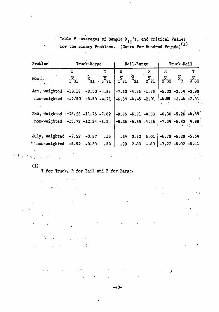
Rail-Barge

1 21 X21 2

x21

-7.33 -4.65 -1.79

-6.69 -4.45 -2.01

Truck-Rail

X 2.32 C 37

-5.02 -3.54-2.99

-4,99 -3.44 -2.91

Problem'

Month 1X31 7C'31 - 3731

Truck-Barge

T I B

Jan; weighted -13.18 -8.50 -4.85

non-weighted -12:60 -8.59 -4.71

R R

Feb, Weighted :-16.28 -11.75 -7.82

non-weighted -15.72 -12.24 -8.24

July, weighted -7.52 -3.57 .16

' non-weighted -6.92 -3.39 .53

- '

-9.95 -671 -4:33 I-6.96 -5.26 -4:69'

8.36 -6.39 -4:66 -7.34 -5.62 4.86

.34 2.50 5.01

.99 2.89 4.80

-6.79 -5.29 -5.54

-7.22 -5.02 -5.41

.t

• Table V Averages of SampleXi /s, and Critical Values j (1)

(1) T for Truck, R for Rail and B for Barge.

for the Binary Problems. (Cents Per Hundred Pounds)

-43-

144

the binary problems, when the choice is restricted to two modes. It

appears that the classification can be done rather successfully in many

cases. However, when rail and truck shipments are compared, a fair

percentage of origins which actually use truck would be mis-allocated.

Table VII gives the probabilities that an origin will be

correctly assigned to the mode it uses as against the two other modes.

They have been computed according to equation (18) of Chapter II. The

probabilities of correct overall classification are not quite as good

as the probabilities of correct binary classification. It could not be

otherwise. The application of a second classification rule to the same

set of observations can only reduce the number of origins correctly ,

classified.

Let us note that the discounting of the net prices contributed •

to a reduction of the distance between the 5. and rc involved in each . ij

binary problem, thereby decreasing the probabilities of correct classification.(11

It is now appropriate to examine the assumptions, made in

Chapter II, that the X's normally distributed can be safely used. To 13

test if the parent distributions of the X1 .'s sample distributions were 3

normally distributed, Chi-square tests were made for each of the X.. over

the month of January sample. The results were as follows: two of the tests

sustained the hypothesis of normality at the .10 and .50 level of significance

respectively. The four other tests rejected the hypothesis at the .05 level

of significance. When plotted, these four sample distributions were shown

to have tails but otherwise were either irregular or closer to some Chi-

square distributions. As no general pattern of distribution appeared through

that examination, it does not seem that one could find a distribution which

could fit the six samples.

(1) Because only a few days time is involved, the reduction due to discounting is small.

Table VI Probability of , a correct classification for

the binary problems.(1)

Problem , , Truck-Barge Rail-Barge 'Truck-Rail

Month B T B R R T

January, weighed .84 .94 .78 .84 .74 .61

non-weighed .77 .91 .75 .79 .77 .58

„

February, weighed •.83 .92 .74 .76 .74 .57

non-weighed .74 .85 .72 .69 .70 .62

July, weighed .80 .90 .74 .81 .75 .46

non-weighed .75 .80 .72 .72 .81 .45 -'

••• • - ap • ••

T for Truck, R for Rail, and B for Barge. (1)

-45-

•

Table VII Probabilities that an observation will be

correctly classified when the choice is not

restricted. (1)

January February July

weighed non-weighed weighed non-weighed weighed ' non-weighed

- Barge • .73 .69 • .64 .65 .67 .65

Rail .67 .66 .58 .48 .61 .61 ., i

Truck .57 .57 .56 .59 .45 .35

Computed from the 'Tables of the Bivariate Normal Distribution Function and Related Functions' published by the National Bureau of Standards, Applied Mathematical Series No. 50, 1959.

(1)

-146r

These results are disappointing, but should have been expected.

On the one hand, one might think that each X ij is normally distributed

over the totai-sample:of the orie.ns óf the three modes. There are no

a priori reasons to expect another distribution. Therefore, one might,

speculate that they are normally distributed as "pure" random variables

are. But, if the total sample is normally .distributed, each separate , sub-Sample :cannot be so distributed'. This can be seen if one considers

that—the X-'s which make up the ith mode sub-sampl correspond largely j

to the X. 's in one of the tails of the total sample. distribution. Ii

the extreme case where the's would be insignificant, the distribution

of theX 's would correspond to a chunk of the former distribution and ij

could not be normal. On the other hand, these observations are also

conditionalby the actual geographic circumstances of the experiment,

and some of the possible value ofX 's within their observed range are ij

not at all represented in the sample. These distributions are essentially

reflecting the geographic pattern of corn production.

This situation raises a double question. First, if it is not

possible to justify the hypothesis of normality - on empirical or theoretical -

grounds - is it still possible to use it as a purely ad hoc device? This

is the question of the robustness of the proposed statistical procedure.

Second, is there not another method, a distribution-free method, which -

could be used in place of the procedure with normality assuMption? ,

As an answer to the first question, M.G. Kendall'nd A. Stuart

propose to apply the discriminators, or classification rules, to each member

of the samples on which they are based and to observe the errors in the

samp1es. (1) This procedure has been applied to the non-weighed January sample,

and the results reported in Table VIII.

(1) M.G. Kendall and A. Stuart 'The Advanced Theorx_of Statistics(, Vol. 3, 1966, pp. 324-.325.

Table VIII,

Probability of Correct Classification

Problem Estimated Actual B T R B T R

Truck-Barge }131 = -8.59 .77 .91 . .79 .85 - ,

Rail-Barge 3121 = -4.45 •75 . .79 .75 - .77

Truck-Rail ;2 = -3.44 . .58 ,77 - .58 .79

Table IX

Actual Probability of Correct Problem Classification

Truck-Barge 1 31 = -6.96 to -7.34 .82 .85

A Rail-Barge X21 = .or -4.41 .76 .77

°thick -Barge X 32 = -3.31 to -3.38 .56 .81

s -48-

L9

By adding the two percentages for each problem, it can be seen that the

global percentage of actual correct classification is hardly different

from the estimated one. Moreover, the percentages directly computed

on the samples do not differ significantly from the estimated percentages.

It is possible to go further to test the robustness of the ;

. "normal" procedure. In answer to the second question, there is a

distribution-free method to find classification rules. Thus, the new

discriminators can be compared with the former discriminators, and their

actual probabilities of correct classification can be computed. This

distribution-free discriminator is simply thevalue which maximizes Xij

over the sample the probabilities of correct classification.(1)

It depends

only on the rank order of the observed X ij 's and can be found by simple

counting of ;aft ob.tervaLidns. Table IX gives the new discriminators

denoted as

Since no distribution is assumed and the computation directly

made on the samples, the discriminators cannot be estimated more accurately

than they are given in . Table IX. For instance, there are no observations.

of X31 between -6.95 and -7.35, neither in the truck origins sample nor in the '

barge origins sample. In this situation one might arbitrarily decide to

choose theAdd-value -7.15 as discriminator. Obviously, this is a weakness of •

the distribution-free method. Furthermore, there were no observations of X 31

between -6.95 and -8.95 in the truck sample. But there were a few observatiOns

between -7.35 and -8.95 in the barge sample. In this particular situation,

the discriminator R31 was unduly pulled toward a greater value than would

have been the case if the truck s'ample had been larger and/or the observations

more evenly spread over the range of x values. Given the relatively small ij re

size of the truck sample, this constitutes an important deficiency of the '

method. To a lesser extent, the same problem arises in the truck-rail case,

while the larger sizes of the rail and barge samples minimized the difficulty

in the rail-barge case. Given the nature of our information, these 'distribution-

free' estimators cannot be considered as very reliable. Yet, they are not -

1 M.G. Kendall and A. Stuart, ibid. pp. 332-335.

50

significantly different from the 'normal' discriminators when the differences

between the two discriminators are compared to the standard deviations of

the sub-samples. This comparison is made in Table X.

Table X(1)

Variates R.. - 13 13

Actual Probabilities of Correct Classification

_ X31 1.440 .82 .85 -

X21 .045 .76 - .77

X32

.095 . .56 .81

Standard Deviation

X31 5.39 2.89 -

X21 3.36 - 3.02

X32

. 2.68 2.06

Moreover, the actual probabilities of correct classification are of a

similar order.

Considering the deficienaes of the distribution-free method,

the nature of our information, and the apparent robustness of the 'normal'

method, we think that the latter should be adopted.

Let us note that to improve the accuracy of the results, it was

decided not to use the assumption that the variances were equal, even in the

cases where an F-test sustained such a hypothesis. AlthOugh very convenient

in computing the's this hypothesis would decrease the robustness of the

procedure. It is also unwarranted by the nature of the samples.

(1) - Xij

is taken as the mid-value of the intervals given in Table IX.

51

As mentioned above, the critical values are consistent, since

the preferences are transitive. But will these critical values as decision

rules classify an observation in a transitive way? In other words it is

desirable that, if an observation is classified as a truck origin by the

barge-truck classification rule, and as a rail origin by the rail-truck

classification rule, it should not be classified as a barge origin by

the rail-barge rule. Transitivity in classification will not be generally

respected, and this can be seen in the following way. From the definition

ofwe have Xij ,

(36) X31

- X21

= X32

for any particular observation. In the case of the January non-weighted

critical values: X 31 2 -8.59 if truck is to be chosen in place of-barge,

X21

S -4.45 if barge is -to be chosen in place of rail,

X32

S -3.44 if rail is to be chosen in place of truck.

Such an intransitive classification is entirely possible within restriction

(36). If X 32 cannot be greater than -3.44, it.follows. that on the left-hand .

side of (36) X31 should be small compared to X 21. In the present situation

X can be as small as -8.59, and X21 as large as -4.45. Subtracting -4.45 .31

from , -8.59 gives -.4.14,.the corresponding value of X32 , which is smaller

than 73.44. Therefore, there could be observations classified in an

intransitive fashion by this set of decision rules. Diagram 1 maps-the area

of intransitivity for this case. The shaded area corresponds to the set of

X31 and X21 values such that the classification would be intransitive. It

suggests also that to preclude intransitivity, it-is necessary that

1 - 221 32

in in which case the shaded araa would be reduced to a point.

None of the sets of decision rules fulfills this condition.

However, this problem should not be given much importance. In-the case of

the January non-weighted data, no observation was within the area of

intransitivity. Moreover, the observations falling in that area could only

correspond to origins where the shippers are close to indifference. One might

wish not to classify them at all. Another solution would be to correct the -

's in such a way that the transitivity condition X31

- X21 = X32 would be Xij

respected. In the case of January non-weighted data, we would then have

3; = 8.36, 7("21-= -4.68, and X32 = -3.66. 31

BARGE AREA

TRUCK

RAIL

lalm■•••

AREA

5.15

L4.45

7.89 8.59 -X31

DIAGRAM 1

52

-X _21

Given equation (36) it is also possible to draw the boundaries

of the three decision regions on the X31 X21 plane, as was done in Diagram 1.

We can now compute theprobabilities that each mode will be chosen

at a.particular shipment point by using equation (25) for P 1(X), and the

corresponding equations for P2 (X), and P3(X). Let us compute an example,

assuming that X31 = -lo --' -21 6, and X32 = -4. Then, for the January

weighed set of rules,

• n3(X31 ) n (X ) n3(X32 ) 2 21 _ " -1.412, in r. • . n (X ). 797

in

2 32 in =

1 21 = -.126.

The inverse of these ratios are identical except for the sign. It follows that

1 1 P1(X) -

.591 P2(X) =

- .244 1 + e-1.412+ e

-.797 1 + e

-.126+ e

.797

1 P3

(X) - .161. 1 + e

1.412+ e

.126

P1 (X) + P

2(X) + P

3(X) = .591 + .244 + .161 = .996, which is very close to 1.

As the probability that barge will be chosen is .591, one should classify this

origin as a barge origin. Note that if the probabilities were used to classify

origins, and if the classification was always transitive, one could be

satisfied by a probability greater than .333 to attribute a shipment

point to a mode of transportation. Since the possibility of

intransitivity is not excluded, one might set a level slightly higher

before classifying an origin in a mode category.

Both methods reach exactly the same classificatin of origins.

If it is then wished to estimate the volume of shipments by each mode,

one could for instance compute the sum of the tonnages shipped by all

the origins in each class. Alternatively, one might regroup the origins

per county and allocate each county production to the three modes in

proportion to the number of shippers in each class.

Finally, one could investigate the influence of variation in the

market prices, the rates, the interest rate, and the time on the choices

of mode.

53

CHAPTER IV.

A Predictive Model of Regional Demands for Freight Transportation

The model developed in Chapters I and II, and applied in

Chapter III can predict the mode choice of a particular origin or firm.

Obviously this operation can be repeated systematically for all the

origins in a given space. In that way, some pattern of regional demands

could eventually be determined. However, this does not constitute a

spatial model, since the origins spatial loCation does not enter explicitly

as a variable in the model.

In this chapter, an attempt is made to develop a spatial model

to predict which mode of transportation will be used to carry a commodity

from a given point defined by its location in the space, and thereon from

an entire production region. This model should incorporate some of the

results obtained in the preceding chapters. First a well-known spatial

competition model is recalled and set up in terms which make it applicable

to the present context. Second, its elements are used to build up a

model for explaining choice of mode. Then various cases of the model are

presented.

I. Spatial Competition Model.(

It is assumed that a homogeneous product is produced under

conditions of constant cost and perfect competition at several locations.

Consumers are distributed over a uniform transport space, meaning that

every point is in straight-line connection with every other point.

Transportation cost is the sum of loading and unloading the commodity plus

the carrying cost, which is proportional to distance. Once transportation

cost is known, it is possible to compute the delivered price, the sum of

production and transport cost, from each production site to each consumption

place. The problem is to determine the market area of each production site.

(1) The first expression of this model was given by F.A. Fetter in "The Economic Law of Market Areas", quarterly Journal of Economics, May 1924, p. 525.

-54-

55

The solution rests, on the derivation of market boundaries along which

consumers are indifferent as between alternative suppliers because their

delivered prices are equal.

'Take a simple case involving two production sites only, the

boundary will be the locus of the points in space where the following

'equation holds:

Pa 1. CaZa 4. La 2 Pb CbZb 4. Lb .

where Pa

and Pb are the prices or costs of productions at the points A and B

respectively,

Ca

and Cb are the carrying costs per ton-mile from A and B,

Za and Zb are 'the 'distances over which the product is carried from

A and B respectively,

La

and Lb are the costs of loading and unloading a ton of commodity •

produced at A and B.

If one assumes that Ca = Cb , and La

= Lb , equation (1) becomes:

(2) , Ca(Za - Zb ) = Pb = Pa .

Let us define Pb

- Pa

i CabZab'

where Z is the distance between A and B, and ab

C is a coefficient such that the identity holds. Equation (2) becomes: ab

(Za - Zb ) = Cab/Ca . Zab .

As Pb

- Pa is a constant value, so are Z ab and Cab

. The cost of transportation

Ca is also a constant, while Z a and Zb

are variables. Equation (3) is therefor*

the equation of a hyperbola, defined as the locus of the points for which the

difference between the distances which separate them from two fixed points is

equal to a constant. Here the two fixed points are A and B. The position and

the shape of this hyperbola will depend on the right-hand-side of the equation,

i.e., on the value of the ratio C ab/Ca and on the distance Zab. Diagram 1

illustrates the various possibilities: If P b - Pa = 0, i.e., if CabZab = 0,

then Za

= Zb' and the boundary is a perpendicular straight line midway between

the two production points. If CabZab is greater than zero, and if the ratio

(1)

(3)

56

Cab

/Ca

is smaller than one, the boundary will be a real hyperbola. Its vertex

is to the right of the mid-point and it curves around the higher cost site B.

The greater the ratio, the closer to B is the vertex and the more sharply

curved the hyperbola. The distance between the mid-point and the vertex is

readily seen equal to Cab/2Ca .Zab . If CabZab is greater than zero, but the

ratio Cab

/Ca

= 1, then Za

- Zb = Z the hyperbola degenerates in a

simple horizontal line going from B to the right. The points'on this line

'constitute the only market of B; but A is able to offer at those points the

same prices as B. Were the ratio C ab/Ca greater than one, there would not

remain any market for B. These conditions suggest an interpretation for the

coefficient Cab'

For a given Zal,'

its value indicates the minimum carrying

cost per ton-mile which will lead the two producers to share the total market.

Below that level, i.e., if Ca is lower than Cab , the lowest cost producer

would take over the whole market. If Cab

Zabis less than zero, similar cases

will arise for the successive negative values of the ratio C ab/Ca. The only

difference will be that the hyperbolas will curve around A, which is now the

higher cost producer.

The assumption that La and Lb are unequal, would not change the

analysis very much. Equation (2) would become:

(2a) Ca(Za . - Zb ) = Pb - Pa + Lb - La .

The right-hand-side of this equation would be defined as equal to CabZab , and

one would be back to equation (3).

More complex situations would result if the rates Ca and Cb were

different and if they were non-linear, either with respect to distance or to

quantity.

The transport analog of this spatial competition problem for the

case of freight transportation will now be considered.(1)

This extension of the model follows the line of the analog developed by L.N. Moses and H.F. Williamson, Jr., for the case of Urban Transportation, in 'Choice of Mode in Urban Transportation,' Ch. IV, Transportation Center, Northwestern University, 1965. This analog has been mentioned by C.D. and W.P. Hyson in "The Economic Law of _Market Areas:, Q.J.E. May 1950, p. 320. J.G. Wardrop uses one of its cases for studying a highway problem in "The-Distribution of Traffic on a Road System.," in Theory of Traffic Flow, ed. b. R. Herman, 1961, pp. 57.78.

1

DIAGRAM 1

-5.7-

58

II. Rail-Water Competition: One Port Problem

Suppose that A, instead of being a production point, is a major

market or consumption point, an outlet for the production of grain of the

whole area considered. Suppose again that every point of space where

the grain is grown is in straight-line connection with every other by road.

Make a waterway of the line between A and B, and assume that B is the only

port on the waterway shipping grain to A. With this set of assumptions, the

grain producer has the choice of sending his grain directly to A by truck

or shipping it to B by truck, then having it transferred on barges and

carried on water down to A. To simplify the matter at the beginning, it

is supposed that there is no difference in the quality of transportation

services produced by the truckers and the bargelines, and that the time .

factor is of no importance in the shipper decision. The problem is to

determine which producers will send their grain via B and the waterway,

and which producers will only rely on trucks. The solution lies in the

derivation of a market boundary or curve along which the producers are .

indifferent as between the two routes.

At first, the elements of the former problem appear somewhat

reversed as the producers are distributed throughout the space and the

consumption function centralized at A. However, our present problem is not

the one of grain marketing but the one of transport marketing. More precisely,

the farmers want to ship their grain to A, and have to choose between two ,

possible routes. One might say that the "gpod", "to have a ton of grain

at A," is produced at two points, A and B. The prices of the "good" at

and B are constant. It is zero at A, so the delivered price equals the

cost of transporting one ton of grain from the farm. At B, the price equals

the cost of transporting one ton of grain by barge from B to A, while the

delivered price is equal to this price at B plus the cost of transporting it

from the farm up to B.

Let us define Ct

as the constant rate per ton-mile of grain by truck,

Cw as the constant rate per ton-mile of grain by water,

Za as the distance in miles between any producing

point and A,

59

Zb as the distance in miles between any producing point and B,

as the fixed distance in miles between A and B.

For the time being, let us make an abstraction from all handling costs,

including the cost of transferring from trucks to barges. The boundary, or

indifference locus for this problem will be given by the following equation:

CZ :CZ b + CZ ta t w

ab

which becomes

Za -z

b = C/C • Z w t ab.

This equation is similar to equation (3) of the spatial competition model. -

The shape and the position of the boundary will depend on the same conditions

as in the former problem:

If C = C, Z a = Zb' and the frontier will be a perpendicular straight line .

. midway between A and B.

If C > 0 and C> 0, then w , t

if Cw/Ct = 1, Za - Zb = Zab , the boundary degenerates into .

a simple line from B to the right in the axis of A-b; if

C /C > 1, all farmers will ship directly by truck to A; if w t 0 < C

w/Ct

< 1, the boundary is a hyperbola with vertex to

the right of the mid-point and curving around B.

These cases are the most interesting, although one could conceive

of cases where either Cw or Ct would be smaller than zero. These would be cases •

where one of the two modes is subsidized. The conditions for position and shape

of the boundary would be similar: if C w/Ct < 1, all grain producers will ship

to B and use the waterway;

if -I< Cw/C

t< 0, the boundary will be a hyperbola with

vertex to the left of the mid-point between A and B, and

curving around A.

These cases are in Diagram 2, which is similar to Diagram 1. Note that, as

above, the distance between the mid-point and the vertex is equal to C w/2Ct • Z.

(Li)

( 5 )

60

Until now, no attention has been paid to the loading and unloading

costs. Introducing them in the analysis gives the next equation:

(6) CZ + L = CZb + L + CZab +L ta t t t w w

where.I.t

and Lw are the costs of loading and unloading a ton of grain,

transported by truck and by water respectively. Equation (6) becomes:

(7) Za - Zb = Cw/Ct • Zab + Lw/Ct

Thus, if Cw = 0, equation (7) becomes:

Za - Zb = Lw/Ct ,

and in place of a straight line through the mid-point, the boundary will be

a hyperbola with vertex at the right of the mid-point, since Lw is a constant.

In this case, the distance between the mid-point and the vertex is equal to .

Lw/2Ct' When C

w is not equal to zero, this distance Lw/2C

t must be added to

Cw/2C

t • Z

ab' to obtain the total distance from the vertex to the mid-point.

This is illustrated in Diagram 3. The major result of introducing the

handling cost in the model, is to reduce the number of farmers who use the

waterway.

It was assumed that every point in the space was in straight-line

connection with every other by means of road and at the same time, that road

and water were the only transportation means available. In order to make

model more realistic, we assume now that, while every point in space is still

in straight-line connection with B by truck, the farmers can reach A by rail

only. This modification hardly brings more realism into the model, but is

useful as an expository device.

For the time being this provides us with a new equattion:

(6) CZ +L =CtZb +Lt tap + L ra r w

where Cr,

and Lr respectively are the constant rate per ton-mile of grain by

rail and the loading-unloading cost by rail. We may define C t kCr, and

rewrite (8) as

■

\ cw .. cw -- c \

\ I ./

/ • . . .••• . . . . .

. ■ I / , t / I / ■• ---

cw . . \ 1

, I / /

/ .

t I I / / , c

I A --€-" 4"--i-- W i

\ \ . ■...........

/ I \ \

-....

/ 1 \ ■ .....

/ \ ...

/ I \ - .......

•-.

/ I ■

N -.

/ 1 .■ •■

/ t. ■ / •■

1 . .

A

DIAGRAM 2

C /2C • Z / w t ab

4 -\ \

Lw/2Ct \

DIAGRAM 3

-61-

62

(Za - kZb ) = Cw

/Cr Zab + (Lt +L w - Lr)/Cr

The variable Zb is now.weighted by the coefficient k. Equation (9) might still

be taken as a hyperbola equation with variable Z a and kZb . However, it is not

anymore a hyperbola in the variables Z a and Zb . Equation (9) which can be

rewritten,

(10) Za - kZb = h

is a different case of the general family of curves, called hypercircles, or

Descartes ovals, which are characterized by equation (11):

(11) Z a

+ kZb = +h -- --

The hyperbola corresponds to the case where

(12) Za - Zb = + h

Were h = 0, and k 1, the curve, or indifference locus would be a circle. It

would circle around A if k < 1, and around B if k > 1. Neither A nor B, however,

would be the center of such a circle.

The case of interest here is when h 0 and k > 1. Then, according

to the value of k, the curve is as one of the curves in Diagram 4.

Similar curves around A would correspond to the case where k < 1.

Equation (10) is a complex quartic equation which has the form:

(13) A x4 +Bx3 +Cx2 +1Dx+Ey4 +Fy2 +Gx

2y2 +Hxy+ K.

It would be easy, even though tedious, to find out the coefficients of (13).

However, there is no point here to go into more details. (1)

(1) See C.D. and H.P. Hyson, 'The Economic Law of Market Areas', Llag.,E., May 1950, pp. 319-327.

9 )

A

k m 1

k > 1

63

DIAGRAM 4

Similar curves around A would correspond to the case where k 4 1.

Equation (10) is a complex quartic equation which has the form:

(13) Ax4 + Bx3 + Cx2 + Dx + Ey4 + Fy2 + GX2y2 + Hxy + K.

It would be easy, even though tedious, to find out the coefficients of

(13). However, there is no point here to go into more detail (1)

It was also assumed that the time factor was of no importance for the

(1)' See C.D. and H.P. Hyson, "The Economic Law of Market Areas," 121E; May, 1950, pp. 319-327.

64

shipper. In the reality of competition between modes of transportation, the

difference between the time taken to reach the destination may be of

importance. In the case of commuting passengers, the utilities or dis-

utilities of money cost and time are weighed against each other in a complex

and unique fashion by each individual. In the case of freight transportation

one may suppose that each and every producer is rationally income-maximizing,

converting time into money and taking this cost into account in his decision.

Let us. define:

V as the value of one ton of grain at the producing place,

I as the interest for one dollar per day,

S r , SW and St

as the speed per day of trains, barges and trucks

respectively,

Mr) M and Mt as the loading and unloading time in days for a w

whole train, a complete tow and a truck respectively.

Then,

T = r S

r

is the money cost of time necessary to carry a ton of grain by rail over one

mile, and

N = V.I r

is the money cost of time necessary to load and unload a train. (1) Similarly,

one gets Tw and Nw for water transportation, and Tt and Nt for truck transport-ation. The boundary equation becomes:

(14) (Cr + Tt) Z

a + L

r + N

r =

(Ct + Tt ) Zb + Lt + Nt + (Cw + Tw) Zab + Lw + Kw.

This equation may be rewritten as:

(15) (Cr + Tr) Za - (Ct + Tt ) Zb =

(Cw + Tw) Zab + L

t + N

t + L

w Nw - Lr

- Nr

.

The right hand side of equation (15) is constant while the left hand side is

made of the difference between two variables, each of which is weighted by a

(1) See Thomas Thorburn, 'Supply and Demand of Water Transport', F.F.I. Report, The Business Research Institute at the StoCkholm School of Economics, 1960.

V.I

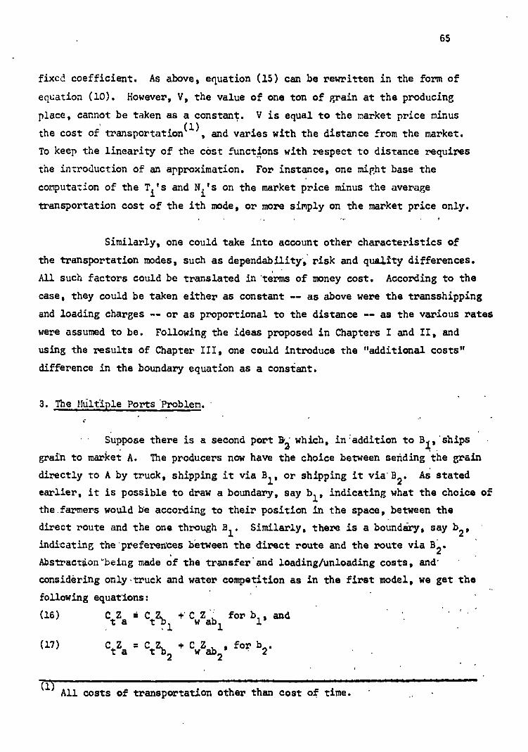
65

fixcd coefficient. As above, equation (15) can be rewritten in the form of

equation (10). However, V, the value of one ton of grain at the producing

place, cannot be taken as a constant. V is equal to the market price minus

the cost of transportation (1) , and varies with the distance from the market.

To keep the linearity of the cost functions with respect to distance requires

the introduction of an approximation. For instance, one might base the

computationoftheT.'s and N.'s on the market price minus the average

transportation cost of the ith mode, or more simply on the market price only.

Similarly, one could take into account other characteristics of

the transportation modes, such as dependability, risk and quality differences.

All such factors could be translated in terms of money cost. According to the

case, they could be taken either as constant -- as above were the transshipping

and loading charges -- or as proportional to the distance -- as the various rates

were assumed to be. Following the ideas proposed in Chapters I and II, and

using the results of Chapter III, one could introduce the "additional costs"

difference in the boundary equation as a constant.

3. The lIti1t421e Ports 'Problem. -

• • Suppose there is a second port Bri

which, in :addition to B1 , 'ships •

grain to market A. The producers now have the choice between sending the grain

directly to A by truck, shipping it via B 1 , or shipping it vial:3 2 . As stated

earlier, it is possible to draw a boundary, say 1)1 , indicating what the choice of

the farmers would be according to their position in the space, between the

direct route and the one through Bl . Similarly, there is a boundary, say b2 ,

indicating the 'preferences between the direct route and the route via B .2 .

Abstraculon'being made of the transfer and loading/unloading costs, and '

considering only 'truck and water competition as in the first model, we get the

following equations:

(16) CtZa = CtZb +' CZab for bl , and ,1

w 1 •

(17) CtZa = CtZb + CwZab , for b2 . 2 2

(1-) All costs of transportation other than cost of time.

66

DIAGRAM 5

For the most interesting case where 0 < C w < et , Diagram 5 shows that these

two curves cross. 'this must be so because, given a particular ratio of rates

Cw/Ct , the position and the shape of the hyperbola change with the distance

Z ab. • the larger will be Z the more open will be the hyperbola. In this case ab Zab1

is smaller than Z ab2°

It is easily seen that the producers located in the area completely

enclosed by b1 and b2 prefer to use the waterway via B1. Also, the producers

located above b1 but below b2 in the top part of the diagram, and those located

below b1 but above b

2 in the lower part of the diagram, prefer to use the

waterway via B2 . However, it is not yet clear what will be the choice of the

farmers to the right' of b2 and inside bl ; some of them could very well prefer

to ship via B1 , if there was such a possibility. The solution consists in

drawing a new boundary, the locus of the points where the producers would be

indifferent to shipping via Bl or via B2 where the possibility of direct

shipment to A is excluded. The equation of this third boundary is: ••■•■■•

(18) CtZb + CwZab = CtZb + CwZab 1 1 2 2

A

67

which becomes,

(19) Zb - Zb = Cw/Ct • (Zab Z" )

Again this is a hyperbola, say b, which is shown in the next diagram. The

new hyperbola must cross bl and b2 at the points were these cross each other.

At these points, K and H on diagram 5, equations (16) and (17) hold for the

same specific value of CtZa ; therefore, the right-hand-side of these two

equations must be equal. It follows that (18) is verified at points K and H.

I• , •

DIAGRAM 6 . Now, the preference areas are well defined: producers in the shaded area on

the diagram will choose the waterway via B l ; those at the right, of b but inside

will prefer B2 , the others will ship directly to A. 2

It is possible to extend this analysis for cases with more than

two ports and find the preference areas for the multiple possible routes.

This is illustrated by Diagram '7 for five ports, B 1 , B2 , up to B5 . To keep

the diagram clear, the additional curves necessary to epirate the preference

areas for B1, B2 have not been drawn. This extension of the model encompasses

more of the reality of water transportation; the shipping points on the

68

DIAGRAM 7

waterway may be numerous. In fact, in the case of grain transportation, the

elevators storing the grain to be loaded on barges may be sometimes located

in a quasi-continuous way along the water. Diagram 7 suggests that, when the

distance between A and the nearest port decreases, and the number of ports

increase, the preference area for the waterway, which is the combination of

the successive preference areas for waterway via 8 1 , 82 , takes the form of

a triangle with a corner toward A.

This continuous case may be presented in analytical fashion. For

that purpose, we are changing the notation and return to a regular diagram with

coordinate axes X and Y. Suppose there are shipping points continuously located

along the X axis (the waterway). For some producer located in the space at a

point yo, the problem is to minimize the cost of transportation to the origin

0. In terms of Diagram 8 he may choose between the direct truck route and any

(19) , (X0 - X

1 - 2

(Ct

- C2W

) •

C T 2 Y2 0

69

indirect route via the shipping points on the waterway leg X0 - 0. More

explicitly, his problem is to

2/ 1 (16) Min C = Ct

1,(X0-X

1 ) 2 + Y0 + CXl' ' for X X

0 - 0

l X 1

For the producer the only variable is X 1 , which indicates the position of

the shipping points on the waterway. The above cost formula includes all

the possible routes and will give the cost of the direct one when X1 = 0.

DIAGRAM 8

Taking the first derivative with respect to X 1 , gives: 1

6? 2 2 -2

(17) -6---x— = - Ct ((X0 - X1) t Y0 ) • (X0 - X) + Cw = 0 1

') 2

Multiplying throuzh by ((X0 - X1 ) 2 + Y) , and squaring both sides gives:

2

(18) C ((X0 ' - X1 )

2 + Y

2) = C

2 (X0 - X1 )

2 , and w 0 t

Taking the square root of both sides one gea

Cw IY0 e2

t w

(20) 0 .1

70

Note the restriction of Y to its absolute values. This is necessary to ensure

the symmetry of the boundary around the river. Negative values of Y would

introduce negative costs in the problem, and produce a meaningless boundary.

At the points where the direct road is preferred X1.= 0, and

< Cw 1 Y0 1

(21) - X - 0

On the frontier the equality sign holds. Then the indifference locus is a

straight line on both sides of the river: the upper boundary has a positive

slope, the lower one a negative slope; thy meet each other at the origin.

The angle they are making with the X axis, can be found through

C2 - C2 t (22) Itan 81 - w Cw

It is interesting to note that the angle made by the truck route from the

point X0 Y0 to the waterway is given by

2 2 C - C Lt w

Cw

which is equal to Itan el. This means that in this simple case, diagram 8

is incorrect and should be drawn as in diagram 9. On this diagram the points

C, D, and E represent typical points on the frontier, while F is any point

using the combination truck-water as less expensive. Note that all the

farmers located on one of the parallel lines joining the X axis use the same

shipment point on the river.

One could now introduce rail transportation as the only way to

ship grain directly to the market. Assume that Cr < C. Then, rail

transportation will be cheaper for some points in the space. The frontier

will still be linear.

Suppose that at point C. the shipper is indifferent between the

two routes, because the two routes' costs are identical (see Diagram 10). On

the same line originating at 0, let us take another point D, such that the

length of OD is twice the length of OC. The cost of transportation by rail

directly to 0 is twice the similar cost from C. The triangles OCE and ODF are

c2 - c2 t w

(23) 'tan r 1

X

DIAGRAM 9

71.

similar and therefore

OC _ OE _ CE OD - OF DF

Then, when OD = 20C, OF = 20E, and DF = 2CE, so that the costs of the two

routes must be equal at D. The frontier is linear as it was constructed, the

magnitude of 0 depending on the values of Cr

C. and Cw. Nothing would be

. changed to the triangular shape of the bohndary if additional costs proportional

to the .distance were added to the model.

It remains then, to'introduce costs which are not proportional to

the distance and which do not cancel each other as being equal for the two

routes. Let us introduce the cost of transshipment and the costs of loading-

unloading. As far as the choice of the less expensive truck-barge route is

concerned, nothing is changed: the charges or costs Lw-and Lt are constant and

are applied for all possible indirect routes. Therefore, the angle y t is the

same as before. However, the frontier does not necessarily reach the origin.

In the likely case where Cw < Cr , a minimum distance of. transportation on the

waterway is required in order to make up for the additional cost involved by

72

X

DIAGRAM 10

the road-water route. In

(24) Ct((X

0 - X1)2

terms of 1

+Y20 ) +

diagram 7, the boundary equation is 1

L +CX+L=C(X2 + Y

2)2

+ Lr t wl w r0 0

Cw I Y01 subject to the condition that X0 - X1

(Ct2 - C

and X0, Xi ! 0 2 2 w )

(24)may be rewritten more simply:

(25) CZ +CX +L: CZ ti wl

where.Z0 represents the square root term on the right-hand-side of the equation,

and is equal to the distance between the point xoyo and the origin; Z1 represents the square root term on the left-hand-side and is equal to

the distance between the point yo and the point X1 on the X axis;

L =L+L- L t w r

For points on the boundary closer and closer to the horizontal axis, Z 1

approaches zero, and Zo approaches X1 so that the boundary tends to the

point where

- L +L -L L t w r (26) X = ----- =

1 C - C C -c r w r w

DIAGRAM 11

- I

73

This point is represented by E in diagram 10. However, it must be noted that

for the 'points on the river itself (X axis), Lt = 0, so that the boundary has

an outgrowth along the . X axis to the left. Were Lw < Lr , the frontier would

reach in that way to the origin. In diagram 11, the frontier actually reaches

point F.

.Furthermore, the boundary is not linear anymore because of the

constant term introduced in its equation. The'equation of the boundary is

.equation (24). The minimum cost condition (20), for the truck-water route, must be introduced in (24). It allows us to get rid of

1 C2 Iv I - A

(27) c C2

Ct - Cw 2 ' 2 w •

1

-w 2 2 2 IY I +L+CX - Cr(X0 + Yo ) 0 w 0 2 2 (C - C )

t w

where_L is defined'as above. Note, once again, the restriction of Y to its

Absolute values, in order to guarantee the symmetry of the solution on both

sides of the X axis. This can be rewritten:

2> (28)(C2 - C2 )1 IYI+L+CwXO IBC (X

2 Y • t w 0 r00

74

Squaring both sides, one obtains an equation corresponding to the general

quadratic equation, except for the restriction on the values of Y:

(29) AX2

+ BX IYI + CY2

+ DX + E II + F = O.

Where A = C2

- C2

r w 2

B = 2Cw(C2

t - C2w )

C = C2

+ C2 -C

2 r w t

D = -2 L Cw 2 2 2

E = -2L (Ct - C

w)

F = - L2

To find the form of equation (28), it is enough to find the value of its

discriminant B2

- 4AC.(1) For doing so, one has to know something about the

rates. The interesting case for us is 0 < Cw

< Cr

< Ct.

Then, the .

discriminant, which is equal to 4C2C

2t --4C4 , must be positive, and (29) is a

r hyperbola but for the restriction on Y.

The negative values of Y cannot be used to derive at once the

boundary on both sides of the river. They would introduce negative costs in

the problem and produce a meaningless boundary in the lower half-space. This

is important to point out as the coefficients of (29) are such that the

hyperbola could not be symmetric around the X-axis. On the other hand, the

cross-product term BXIYI does not vanish, so that the hyperbola is tilted

on the X-axis:(2) on the other hand, the terms D X and E Y do not vanish

either, and the hyperbola does not .have its center at the origin.

This problem is illustrated by Diagram 12. The lower boundary,

symmetric to the upper boundary, can be obtained by rotating the latter 180 0

around the X-axis. Bouth boundaries are segments of hyperbolas. But the

(1). As given by G.B. Thomas, 'Calculus, And Analytic Geometry', Third edition, Addison-Wesley, 1960, p. 496.

(2) The angle a made by the transverse axis with tab coordinate axes can be

- found through Cot 2a = - C .2j2 Cw(C2t - C!)1.

.1

(x) dx A =

75

overall locus of indifference cannot be one since the curve is kinked at

the point where the two segments meet.

DIAGRAM 12

Using the quadratic formula, it is possible to rewrite (29)

as an explicit function ,

(30) f (X) -(BX + E) + i(BX + E) 2 - 4C(AX2 + DX +' F) -

2C

Then, for the case where C t > Cr > Cw > 0, the area of the water

transportation market, from its westerhmost point up to the vertical line

x = a, is

Unfortunately, gquation (30) is very awkward to handle. Its

integration, and for that matter, its differentiation, do not provide

76

interesting expressions. However, there would not be much difficulty in

'using it in a concrete case.

4. Summary and Conclusion.

In the spatial competition model presented at the beginning

of this chapter there were two places where a homogeneous commodity was

produced under conditions of perfect competition and constant costs of

-production. Therefore, the prices of this commodity at the places of

production equal the average cost of production and are constant regardless

of the quantity produced. It followed that the delivered price of one

unit of commodity from either center of production was equal to the

relevant cost of production plus the cost of transportation. There was only

one mode of transportation in this very simple model. The commodity being

homogeneous, the buyers were choosing to buy from the center of production

with the lowest delivered price. The boundary of the two production centers'

respective markets was given by the locus of the points where the deliveries

were equal and the buyers indifferent as to the origin. The amount sold at

each point could be determined by the demand curve particular to each buying

point confronted with the lowest delivered price as shown in diagram 13.

But this determination goes beyond the problem of market boundaries.

In the transportation analog, the homogeneous "good" offered to

the farmers was a very special one: 'to have a ton of grain at the market

place'. The price of this "good" was zero and constant at the market place

itself so that its delivered price anywhere in the space was equal to its

transportation cost. Two means of transportation Were available: the road

(or the rail) using a direct route to the marketplace, and a combination of

; modes, road-water, through an indirect route. Again, the buyers or farmers

I were choosing the cheapest way, and boundaries could be derived as the locus

of the points where, costs being equal, the farmers were indifferent. At

first it was assumed that the transportation services offered by the two

routes were identical, and that only their rates, or direct money outlays,

were unequal. Then time and service differences were introduced and

translated into additional costs for the shippers, under the assumption that

they were moneywise maximizing. In some cases, the solution for the boundary

DEMAND CURVE AT POINT M

••■ •■••■••■■■■■

DELIVERED PRICE

FROM A

FROM B DIAGRAM 13

77

gave rise to complex analytical forms, although throughout the analysis it

was always assumed that the costs were linearly related to distance.

In the third section, the analysis was extended first to the case

of several transshipment points, then to the case of continuous transshipment

possibility along the river. In the latter, a simple analytical solution

was presented for a rather special case of spatial market competition.

In Chapter V, this should be further examined and more complex cases

introduced. Chapter V will further generalize the model to the case whei'e

more than two modes of transportation are involved.

'The model presented in this chapter is essentially a mode choice'.'

model. Like the model proposed in the first three chapters, the quantities

actually transported do not play any role in the mode choice, and are not

estimated by the model. These have to be determined separately given the . -

mode chosen and 'the cost of production function. This is only one ofe

similarities between the spatial model and the 'discrimination' model. In

fact, they are basically similar. This can be best seen if one considers

that the, boundaries classify the regions according to the mode they use.

In a sense, the boundaries are spatial discriminators. Furthermore, in •

both approaches, the basic criterion of classification is the same: the

relative costs, or, as it will be seen in the next chapter, the relative

net incomes. Some differences though are worth pointing out. First, the

treatment of time cost is less accurate in the spatial 'model. Second, it

is unable to provide any estimate of 'quality' difference. From 4-l'At point of

miew, it has to rely on the estimate generated by the first model, or some

additional. information. Otherwise, it requires less information: no sample of

the origin's choices of mode is needed, but only the rates and other

charges of transportation plus, eventually, the market prices.

QUANTITY BOUGET AT POINT M FROM B

CHAPTER V.

This chapter attempts to use the basic tools developed in the

fourth chapter, to reach more realistic spatial models of modal choice.

1. Three Routes Choice.

Throughout the whole of the fourth chapter, the choice was

arbitrarily restricted to two routes: on the one hand the direct route

either by road or by rail -- but not both; on the other hand the indirect

water route. But what happens when two direct routes, rail and road, are

competing against each other as well as against the water route? It is

easily possible to decompose the problem in a triple binary choice by

analyzing separately the choices between each pair of two routes.

In the fourth chapter, the locus of indifference between the

water route and the rail route was defined by equation (24):

1 -

(1) C 2 2-t 2 tE(X0-X1) +Y.I+L +CX +L =C(X

2 + Y2 ) + Lr 0 t wl wr 0 0

subject to

CwY0 X0 - X1 = (C -C ) .t w

X X > 0 0' 1 '

When it is assumed that 0 < C < Cr < Ct' this gives rise to a boundary the w branches of which, on each side of the river, are segments of hyperbolas.

At Y = 0,

L +L -L t X say X - W r

0' rw C -C r w

The locus of indifference between the water route and the direct

road route can be determined in a similar way:

1

2 2 (21

c. [(x0 - X1 ) 2 + + Lt + Lw + CwX1 = Ct (X0 + Y0) • Lt 0

-78-

79

SU'DJCCt to:

X0'

X1

3. 0.

When manipulated as was equation (24), equation (35) produces a quadratic

equation similar to (29). Its coefficients are:

2 A = C

t

Bt= -2C (C2

- C2

)2

W V W

C = C2'

" w

D = -2L C w w

E = -2Lw(Ct - Cw )

2 F = -Lw

It follows that the discriminant equals zero and that the upper and lower'

boundaries are segments of parabolas. They meet at the point Y o = 0,

X = tw Ct

- Cw

The third binary choice is between truck and rail. Here, the

indifference locus is determined by

,

(3) C (X2.

Y2

)2 L = C (X

2 .1. Y

2)2

Lr z 0 0 t r 0+Y0)

or,

(u). - C ) EX2 Y201 2 = L - L t r 0 t

Again, this produces a quadratic equation. Its coefficients are:

A = (Ct

- Cr

) 2

B =D=E= 0

C = (Ct - C

r)2

Lw

TOTAL TRUCK,/ COST

IL

TOTAL . COST

ARGE

X. X X MILES rw tw tr X X X

tr tw rw MILES

A

CO

D = -(Lr - Lt )2

The cross-product term vanishes, and A = C g O. The boundary is a circle

with center at the origin. At Y o = 0,X, say Xtr , is equal to Lr - L

t . Ct

- Cr

With the restriction that 0 < Cw

< Cr

< Ce, two cases are possible.

They are illustrated in Diagram 14, where the total cost by each mode for one

unit of weight is given as a function of distance.

DIAGRAM 14

In case A, the cost curve of truck transportation intersects first the water

transportation curve. Then, at a farther point, it intersects the rail

transportation cost curve. This case can be summarized as the one where,

on the river (or at Y = 0), Xrw < Xtw

< Xtr. Its boundaries and market 0

areas are drawn in Diagram 15. The three boundaries are intersecting at two

points, A and B. The respective market areas can be easily deduced, and are

indicated in the diagram. Note that the water market boundary is made up of

four segments.

81

I Truck-

Boundary Rail

RAIL

Rail-Water Boundary

WATER

Truck-Water Boundary

RAI

TRUCY RAtL

RAL

00"

••••••••

Rail-Water boundary

Truck-Rail boundary

Truck-Water boundary

WATER

DIACRAM 16

DIAGRAM 15

In case :3, the cost curve of truck transportation intersects

first the rail curve, then farther, the water curve. Here, X tr < X < X . (1)tw rw The boundaries, drawn in Diagram 15, cannot intersect each other, and

the water boundary corresponds to the boundary between the rail and the truck-

water market.

(1) The case where the three cost curves would intersect at the same point would De similar to this second case: the three boundaries would meet, but not intersect at one oint on the river.

and

subject --co CwN

(C2 -C2 )i

t wa

ewbfrOl X - X = 2 o (c - c )

.t wb

'Co - X1 -

82 2. Two Markets Model.

Suppose that two markets are available at each end of the river,

but that the second market can be reached only by water, while the first

one can be reached by the three modes. The choice problem is considerably

complicated since the number of binary choices, and partial boundaries is

augmented by three. However, each of these new boundaries can be

derived as easily as were the others.

If the two-market prices are different, they must be taken into

account in the shipping decision. For. doing so, it is necessary to consider

the net income indifference locus rather than the transportation cost

indifference locus.

For the competition between market A and market B through truck-

water transportation, the boundary is defined by: ,

(5) - Ct 1(X0 - Xi )2 + Y) - - CwaXi Lwa =

1

Pb

- Ct t • • wb 3 2 wb • ■

X0' X1 - 0.

Where Pa and Pb are the commodity market prices at A and B respectively, X3

is the distance between A and B, X2 is the trans-shipment point on the river

Awl the grain is shipped to B, and Cwa ,and Cwb are the barge rates toA and

B respectively, and •lisla and Lwb are the fixed costs to A and B respectively, The two restrictions guarantee that optimal trans-shipment points are selected.

The second one can be derived as the first one was in Chapter IV.

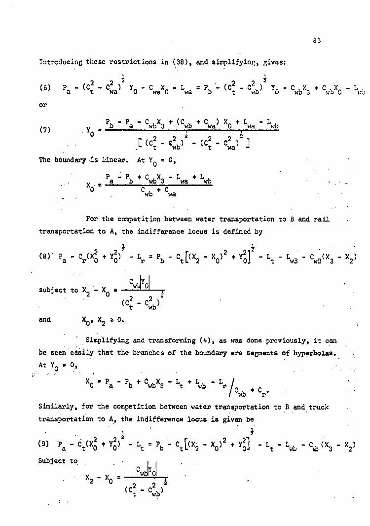
subject to X2

Subject to

siblY01

83

Introducing these restrictions in (38), and simplifying, gives:

1

(6) P- (C2

- C2 )Y-CX-L =P •- (62 - C

2 )2Y-CX+CX- L a t wa 0 wa 0 wa b t wb 0 wb 3 wb 0

or

+C)X+L - L b a wb 3 wb wa 0 wa wb

(7) . Y - i 0 i 15. E , c2 _ c2 .1 _ (02 _ 02 1 1 . 1" ‘ t wb' ‘ t wa' J

The boundary is linear. At Y o = 0,

• Pa -P b +C wbX3 -L wa +L

'0_ Cwb + Cwa

For the competition between water transportation to a and rail transportation to A, the indifference locus is defined by

1 1 2 (8) . Pa - Cr(X

2 0 + Y

20 )

2 - Lr = Pb - Ct [(X2 - X0 )

2 + Y1 o - Lt - LwB - CwB (X3 - X2 )

and X X > 0. 0' 2 '

,Simplifying and transforming (4) 1 as was done previously, it can

be seen easily that the branches of the boundary are segments of hyperbolas.

- At Y = 0 0 '

X =P-P+CX+L+L -L it 0 a b wb 3 t wb r Cwb + C

r. •

Similarly, for the competition between water transportation to .8 and truck

transportation to A, the indifference locus is given . be 1 2

(9) P - d (x20 + Y20 )

2 - L = P

b - C

t [(X

2 . - X

0 ) + Y

oj - L

t - L

wL - t t

2 21 a

84

X0,

X2

- 0.

It can readily be seen that it defines a boundary, the branches of which, on

each side of the river, are segments of parabolas. At Y o = 0,

XO

= Pa

- Pb + LB

+ Cwb

X3 //C + C

t wb

At this point, it seems difficult to combine these results in

any simple model. One might be interested to assume C wb < C

wa, and P

b > P

a.

In these conditions, a remote downstream market would be able to compete for

the production of an area close to another market. But these restrictions

are not enough to lead to some simple solutions as were obtained above. Too

many parameters are involved and the number of particular cases quite large.

However, there should not be any particular difficulty in applying these

results to a concrete problem.

3. The Circuitous River Case

Until now, it was assumed implicitly or explicitly that the

river was as a straight line. One might object that this assumption is

farfetched in many cases. However, this assumption is not necessary at all

in the simple one port model.

Let us suppose that the river is wiggling as in Diagram 17, and

that the grain shipped to A can only be transshipped at the point B. Making

abstraction from all handling costs and using the other assumptions made in.

the one port case above; we get exactly the same boundary equation as .(5) in Chapter Iv:

(10) Z - Z = C/C • z a b w r ab

This is a hyperbola equation giving a boundary centered around the axis going

from A to B. Introducing fixed costs would only change the shape of the

hyperbola. Note that here Zab is the river distance in miles from A to B.

Diagram 18 corresponds to the two ports case discussed above.

The difference is that the two hyperbolas are not necessarily centered around

the same axis. This would have been the case only if the second port had been

located at D. From these particular boundaries it is easy to deduce the eAvelope

85

DIAGRAM 17

,DIAGRAM 18

boundary dividing the .space into the respective markets for barge and rail

transportation. It is made of the portions of the particular .bqundaries

• which are the furthest North and South from the river.

Proceeding in the same way, one could increase the number of ports

without any difficulty. however, as the successive hyperbolas are not

centered around the same axis, it is not possible to generalize to the con-

tinuous case. The envelope boundary would possibly be without kinks -- if

Outside boundary

River

LB

/Inside boundary

86

the river does not have any --, but its equation would be extremely

complex.

DIAGRAM 19

We can only suggest the following. In Diagram 19, two axes,

AC and AD, were drawn through the points on the river the furthest

north and south. Given some fixed or proportional costs, it is

possible to draw the two envelope boundaries centered around those

two axes. This gives us an outside boundary defining the largest

possible market area for water transportation. It also gives an

inside boundary for the smallest possible market .for water transporta-

tion. In other words, we obtained an upper bound and a lower bound

estimate of the market aria. An alternative would be to use a centered

axis like AB as a linear proxy for the river and a basis for the

systems of co-ordinates. The boundary centered around this axis would

give some kind of average estimation of the market area for water

• transportation.

87

4, Applicon to C.nan Shinments in Illinois •

As seen in Chapter III, this particular problem opposes the market

of New-Orleans, which can be reached economically only by the combination

of road and water transportation, to the market of Chicago where corn is

shipped only by road or by rail. The problem is, therefore, to derive the

boundaries between three mode-destination market areas. Under some

assumptions similar boundaries have already been derived in Section s2 and 3

of this chapter. These assumptions require a few comments and modifications

before these results can be used.

• First of all, Figure 1, which reproduces the relevant part of the

State bf Illinois, shows that here is a case where the river is not:d'straight

line. One of the alternatives proposed in Section 3 was used to solve the

.

problem: an axis fairly in the middle of all the possible. axes was drawn from

Chicago to Lacon and used as a linear proxy to the river. It is also used as

-abscissafor a system of co-ordinates with the origin at Chicago.

Furthermore, throughout the presentation of the spatial model , the

assumption was made that every point in the space was in straight line

connection by rail and by road with' every other point. It is still possible

to proceed as if every point were connected by road and by rail, since

practically all actual origins of corn shipments are so connected, As to the

other points they do not matter in the least: they eventually grow some horn

but do not ship it directly to Chicago or New-Orleans; boundaries can be .

derived as if they were also connected because it is highly convenient to

assign the other points of actual shipments to mode-destination market areas.

However, it is no longer possible'to assume straight-line conneation

between points. This complication has been solved in different ways for the

three modes. For.road transportation to Chicago, the assumption meant only

that every point was in straight-line connection with Chicago. Since it was

far from being the case, it was necessary to find a relation between the .

actual road mileages to Chicago and the corresponding Euclidean distances used

:sLY: x rail 0 truck 0 rail and truch

FREEPoRT

1 ROCKFoom

*

s gimlet

4

X x 0

0 C l..4104

10 K X 3,

&MON X

K X 4 N

ClitNESie Pa ea %Crawl

a

100110401elt x

UW01;E IC A o

AC

st.eisimoaci,-Tow

X X. X k

kRiANA 0A X1V AAA

FIGURE I

T:iRLL MARI:LTS 2OUI:DARIES ORYIIM or nIE :',A0PLE CORN SEM:LI:TO JANUARY, 1066

-RA -

K 0 0

00

- 6

1?) 1.1000%TooK

0

0 CIA III

Ogling-rpm

)11(

A

A

X

1'

K X (MON

0 et.oeM104 -rotJ

X X

,14 x

Ogx

"4'

A

OrT014%,

g

OWITIOC

Kcouns

X

0 k

lows&KA

0

,

x ; * 0

0

X Ei 0

4

4, II 2

IC A A

URCANA 0

Og g4,A, 0

ORIGINS OF Tid: SA1:PLE CORN SNIP:INTS

FEBROAPY, 1966_

x rail 0 truck 0 'rail and tuck

• wsk=101100•01"mummilll

j( Cal.Netie

, x

X

R41P0RT

0 x 0

Rocla OR a

• x X X

r

x

a

A

X

Gia

0 "4....5,

!I

Socala I ,,,,, 4 , i:

A ' P i i Kx 4 ; 1

! 0 P

W 9! KANKdiat W 11

0

kop.

X A

A X

11:7:

•

0

FIGURE II

'NLY: K rail 0 truck 0 rail and truck

.FREE Po RT

C)

X X

X

rs Diatom

X x X

■ g i C10411.0 PRosiToW

X X

0

17-T. 0 gi.00M sai te -TOW

x ,

0 x

ta actilete

x x x

XA t

X° x

0 m 9

X

POST I at

ac

X

PEKsti

X ° mOCKFORCI 0

X X X

X

X 0

X

'CO

x

GE mat U 0 I X

X X

X 0 X

COTAWil Vi

)(X

x

KALI X

X X at

X X

fi 4. ° t 101080170c.K

OICi SAnPLE COM SEIPUNr. JULY, 1066

FIGURE III

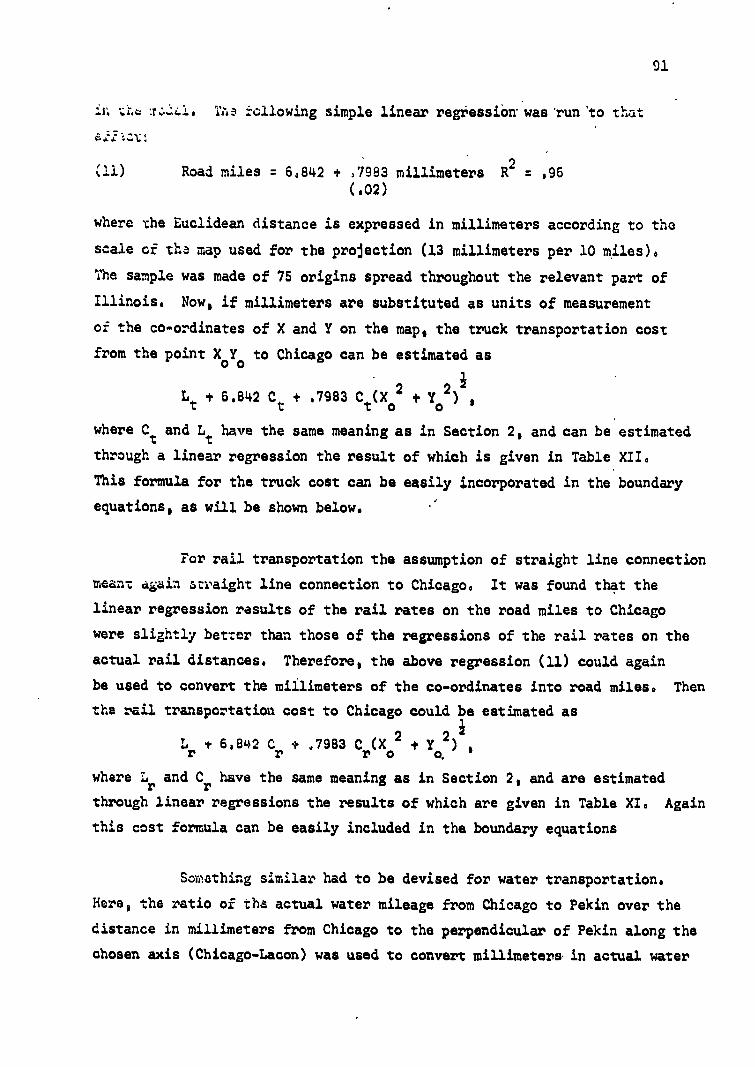
91

tha TA a ±ollowing simple linear regressiOnwasrunto that

(11) Road miles = 64842 + 37983 millimeters R 2 = .96 (.02)

where the Euclidean distance is expressed in millimeters according to the

scale of tha map used for the projection (13 millimeters per 10 miles),

The sample was made of 75 origins spread throughout the relevant part of

Illinois. Now, if millimeters are substituted as units of measurement

of the co-ordinates of X and Y on the map, the truck transportation cost

from the point X0Y0 to Chicago can be estimated as

Lt + 6.842 C t .7983 Ct (Xo

2 + o2 )

where Ct and L

t have the same meaning as in Section 2, and can be estimated

through a linear regression the result of which is given in Table XII.

This formula for the truck cost can be easily incorporated in the boundary

equations, as will be shown below.

For rail transportation the assumption of straight line connection

meant again straight line connection to Chicago. It was found that the

linear regression results of the rail rates on the road miles to Chicago

were slightly better than those of the regressions of the rail rates on the

actual rail distances. Therefore, the above regression (11) could again

be used to convert the millimeters of the co-ordinates into road miles. Then

the rail transportation cost to Chicago could be estimated as 1

Lr t 6.842 C + .7983 C (X 2 +c) ) r

2' r o

where Lr and Cr have the same meaning as in Section 2, and are estimated

through linear regressions the results of which are given in Table XI. Again

this cost formula can be easily included in the boundary equations

Something similar had to be devised for water transportation.

Here, the ratio of the actual water mileage from Chicago to Pekin over the

distance in millimeters from Chicago to the perpendicular of Pekin along the

chosen axis (Chicago-Lacon) was used to convert millimeters in actual water

Table XI. Rail Rates Regressions: Cents (per one hundred pounds) on road

miles: Rr

= Lr

+ Cr

Dt. One regression per railway, on the

three months sample with one observation per origin.

Railway Sample Size Lr

Cr

R2

A 30 12.145 .015 .02 (.018)

B 50 11.325 .025 .85 (.001)

C 62 10,835 .036 .62 (.004)

D 13 7.465 .068 .87 (.008)

E 50 9.813 .045 .64 (.005)

F 38 10.231 .039 .58 (.006)

G 10 3.715 .112 .36 (.053)

H 14 7.442 .058 .81 (.008)

I 13 9,425 .030 .57 (.008)

J 24 12.500 . (1)

K 12 11.450 .032 .79 . (.005)

(1) Railway J has constant rates for all observations.

- 92 -

Table'XII. Water and Truck Regressions: Cents (per one hundred pounds)

on water and road miles respectively.

WATER (to Pekin): Sample Size: 23

R = L + CD R2

w w

w w

1.27 .0085 .91 (.0006)

TRUCK: Sample Size: 28

Rt = Lt + Ct Dt R2

44174 .1185 .98 (.004) ' . .

Sources: 'Guide to Published Barge Rates on Bulk Grain', Schedule No.5, issued by Arrow Transportation Company, April', 12, 1966. The rates used in the regression are discounted by 15 percent (see p. 32-33).

'Aim.a.....111..t.m1.22,114=1............alsTariff', No. 600, of the Illinois Motor Carriers' Bureau, Issued by D.S. Mullins, Issuing Officer, May 16, 1966.

- 93 -

94

mileages. The reason why this ratio was related only to the leg Chicago-

Pekin of the Illinois River is simple. Since no country elevators used

a transshipment point on the river lower than Pekin, the cost of water

transportation from Pekin to New-Orleans could be considered as a fixed

cost. Then the water transportation cost to New-Orleans from a point

X2 on the river could be computed as

Lwb + Np + Cwb$w(Xp - X2 )

where N is the cost of transportation from Pekin to P New-Orleans which is constant,

w is the ratio discusied in the above paragraph,

X is the distance along the Chicago -Lacon axis between P Pekin and Chicago,

X2 is the point of origin on the same axis,

Cwb is the coefficient of the regression of the water rates to Pekin from points between Chicago and Pekin as given in Table XII,

• Lwb is the usual fixed cost, which is the sum of the intercept of the regression just mentioned and other fixed fees (see Chapter III).

Finally, for the road leg of the combined road-water transportation,

only the regression coefficient of (11) was used to convert millimeters into

actual road miles. The intercept term was not introduced because of the

shortness of the road leg and also because it essentially corresponds to

the characteristics of the road network leading to Chicago.

- -

(12) Pa - C0t o o (X 2 + Y 2 )1 -L -a r

a r r

Ni ' Pb - Ct0.t[(X2 ... Xo )2 + Yo-1 -Lt

- Lwb .. Np - Cwb

$w(Xp - \ X2 ) + E21

\ . s.t. X2 - X

Cwb w rYo l

. .(Ct fit - - cwb2Bw

2)1 2 2

With all these modifications, the basic water-rail boundary equation,

as an example, became

- - and Xo, X2 % 0

05

where moL.t cf the symbols have the same meaning as before and,

at = .7983, the coefficient of regression (11) 3w = 1

ar

= 6,842 Cr •

0 E21

= X21 the money estimate of the quality difference between

rail and barge transportation.

This new equation form is identical to the form of equation (8), so

that the boundary is made up of segments of hyperbolas. The other

boundary equations of Section 2 can be easily modified in the same way.

Again, the water-truck boundary is made up of segments of parabolas, and

the, rail-truck boundary is a circle.

The results of the linear regressions of the rates on distance

. were very good ih the'case of river and road transports. As to rail

transport results, they were good enough for our purpose, most of the R2

being above .60, and the coefficients significant. However, railway A's

'regression was very bad, for the reason that its rates hardly vary with

distance, and a few of them are completely out of line (1) . A graphic

inspection of the rate structures of the railways revealed that they were

best summarized by a linear relationship between rate and distance, despite

some tariff peculiarities. In these conditions, the linearity assumptions

of the model could be used without reservations.

The actual boundary equatibns can then be computed on the basis of

this information plus what has been gathered in Chapter III. These equations

are given in Table XIII (2) . Note that the time cost was not included in

their computation. The little role that time plays in this particular

problem did not warrant the additional complication. The next task is to

draw all the curves corresponding to these equations on the Illinois map,

using the Chicago-Lacon axis as an abscissa. Note that there are one

OSCIONIIM

• (1) These rates relate to points of origin which are not located on railway A network but on another railway feeder line.

(2) In the case of the rail-truck boundaries, only the radius of the circles have been given.

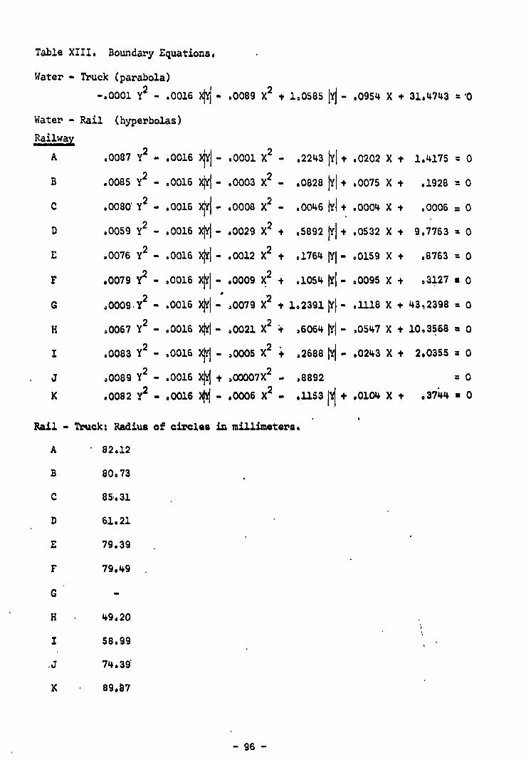
Table XIII. Boundary Equations.

Water - Truck (parabola)

-.0001 Y2 - .0016 XIYI - . 0089 X2 + 1.0585 .0954 X + 31,4743 = .0

Water - Rail (hyperbolas)

Railway

A .0087 Y2

- .0016 #1- .0001 X2 - .2243 I'll+ .0202 X + 1.4175 = 0 .0085 Y2 - .0016 X11 - .0003 X2 - .0828 IY1+ .0075 X + .1928 = 0 .0080 y2 .0016 XH- .0008 X2 - .0046 VI+ .0004 X + .0006 = 0 .0059 Y2 - .0016 XVI- .0029 X2 + .5892 M+ .0532 X + 90763 = 0

.0076 Y2 - .0016 *1- .0012 X 2 + .1764 11- .0159 X + .8763 = 0 40079 Y

2 • .0016 411• 60009 X2 + .1054 • .0095 X + 63127 • 0

,0009.Y2 • .0016 4/I• .0079 X

2 + 1.2391 tfl • .1118 X + 43,2398 = 0

.0067 Y2

- .0016 *I- ,0021 X2 4. ,6064 ,0547 X + 10.3568 = 0 -

I .0083 Y2

- .0016 )11 - , 0005 X2 + .2688 Pi- .0243 X + 2.0355 = 0 . J .0089 Y

2 - .0016 XYI + ,00007X

2 . . 8892 0

.0082 Y2 - .0016 1YI - .0006 X 2 .0 .1153 + .0104 X + .3744 • 0

Rail - Truck: Radius of circles in millimeters.

A 82.12

80,73

86.31

61.21

79.39

79.49

•

H 49.20

58.99

74,39

K 89.87

• 96 -•

/MU IBM es= 4EM. OW.

■■■•

•■•• """' "•••• ■■

/0

-- Railway A

Railway B

As Boundary

B's Boundary

LACON CHICAGO

07

a4d one truck-rail radius for each of the railways.

sincc, covers only parts of Illinois, only the

tc of its culwes which correspond to these regions need to be drawn.

As for the a'es where two railways have a line, only the curve corresponding

:.h:r1Dt.r railway should be kept. In that way it is possible to

generate complex rail-water and rail-truck boundaries combining segments

of several curves. This is illustrated in Diagram 20 where a typical complex

boundary is assembled from segments of two rail-water boundaries. Some

links between portions of curves have eventually to be added to obtain a

continuous complex boundary. This is the case of the line OP in Diagram 20.

Once the three boundaries corresponding to the three binary choice

problems are so derived and drawn, it remains to combinethemto obtain the

DIAGRAM 20

three mode-destination market areas and their limits. Each mode destination

area corresponds to the region where that mode destination is preferred to

both others. An example is given in Diagram 21 where the resulting boundaries

correspond to the continuous thick lines. Note that it should not be

expected that the three boundaries meet at a common point. The money

equivalents of the quality differences which were estimated in Chapter III,

have been used for their computation and we know that these estimates are

somewhat inconsistent. For the same reason as we had an intransitivity area

in the classification space, we should have here a region where the preferences

conflict.

98

DIAGRAM 21

Figure T shows the actual boundaries and market areas obtained for

the month of January: around Chicago is the "truck to Chicago" market area;

further away from Chicago along the axis is the "truck-water to New-Orleans"

market area; and on both .sides of the latter are the "rail to Chicago" market

areas.

It is possible to evaluate the boundaries corresponding to each of the

binary choice problems as well as the limits of the three market areas (shown

in Figure I), by computing the percentages of sample origins which are

correctly classified. These percentages are given in Table XIV. They can be

compared to the probability of correct classification by the discrimination

approach which was given in TablesVI and VII of Chapter III (1) . The

Cl) Another useful comparison may be made with the probabilities given in Tables VIII and IX.

09

The percentc.g.,:6 are of the same order of magnitude as the probabilities.

However, of the rail and truck origins the classification in the binary

choice problems is improved, while the classification of the water origin

is not as good as before. As to the limits of the three market areas,

TABLE XIVI Percentages of sample origins correctly classified; month of January.

Binary choice boundaries

Problem Truck-Barge Rail-Barge Truck-Rail-

MODE'

BARGE - ' 75% 75%

RAIL- - ' 92%. 79%

TRUCK' ' 96% . 58%.

Three market boundaries

BARGE 70%

RAIL 73%

TRUCK 55%

they provide a better classification of the rail origins without changing

much the two other modes' results. Altogether the results of the spatial

model are fairly satisfactory.

Figure I gives enough information (1) to suggest the main defect in the

predictions of both the spatial model and the discrimination approach. It

appears at once that the boundary which separates the rail and truck areas

is at too great a distance from Chicago. A boundary drawn closer to Chicago

would certainly improve the classification of rail origins without much

affecting that of the truck origins, The reason for this fault should be

found in the peculiarities of the sample of truck origins. On one hand, the

(1) The points of origin of truck-water shipments are not given on the maps as this information was of confidential nature.

100

truck sample is small ( 148 origins in January). This is due to the fact

that truck transportation is particularly favorable for short haul, and

little corn is grown within a short distance of Chicago. On the other

hand, the few truck origins spread far away from Chicago have a lot of

weight (35%) in the sample, although they hardly can be considered as

typical origins of truck shipments. In that respect, it is worthwhile

to point out that most of these origins are also shipping by rail. They

probably use truck shipments occasionally, or have unusual characteristics.

Now, the parameters of the population of truck origins have been computed

on the basis of the whole sample and have been biased by the peculiar

characteristics of these origins. Therefore, the estimates of the money

equivalents of quality differences between road transportation and the

two other modes have also been biased. It is likely that more realistic

estimates would have been obtained on the basis of a truck sample reduced

to the "typical" origins. For the boundaries an example shows well how

sensitive they are to variations of the money equivalents of quality

differences. In the case of Railway C a change of the money equivalent

from -3.54 to -2.54 would have reduced the radius of the circumference

limit between road and rail areas from 85.31 to about 70 millimeters.

Variations of the same order of magnitude have been found for the other

railways.

In view of these remarks our confidence in the spatial model is

increased. On the basis of correct information it can produce fairly accurate

predictions of the choice of modes. As the results take the form of market

areas for transportation modes they are particularly convenient to generate

estimates of demand for transportation and evaluate investment projects

in ways of transportation.

101

CCN.:LUS10N. AND SUMARY

Tha theoretical model presented in Chapter I implied that the

shipper of a commodity to a particular destination should choose one

• mode c2 t17,ansportation to the exclusion of all others.

The data concerning corn shipments in Illinois suggested that this was

the case for most shippers.

Two forecasting models embodying the idea of exclusive choice

were developed and tested on the data. The first uses the statistical

approach of discriminant analysis. It predicts the choice of mode made by

any shipper on the basis of the relative costs of transportation. Applied

systematically to shippers spread over a region of production, it can also

predict the regional pattern of use of several modes. Such predictions can

be used to generate estimates of demand for a mode of transportation.

The second model is an extension of traditional location theory.

Here transportation costs are related to distance and location, and the

predictions take the form of boundaries between market areas for the

respective modes. In a strict sense, it is a spatial model.

Both models take into account all costs of transportation including

time cost and the (relative) costs of 'quality' differences between modes.

The latter are rarely available, and it is the advantage of the discrimination

model that it estimates the quality differential. The spatial model cannot provide such

estimates, and, therefore, requires additional information. Another weakness

of the spatial model is that its treatment of time cost rests upon an

approximation. In addition, it requires that the costs be linear functions

of distance. However, the spatial model has the important advantage that it

does not require a sample of actual shipments made by the various modes

involved, but only information concerning all costs of transportation. It

might be the case that such information can be obtained from trade sources

or derived from the technical characteristics of the modes.

102

In this application of the spatial Model use was made of the estimates of

'quality' differences obtained from the discrimination model.

Both models provide very similar and fairly satisfactory results,

despite some deficiencies in the sample.

NORTHWESTERN UNIVERSITY

LINEHAUL PROCESS FUNCTIONS FOR RAIL AND

INLAND WATERWAY TRANSPORTATION

A DISSERTATION

SUBMITTED TO THE GRADUATE SCHOOL

IN PARTIAL FULFILLMENT OF THE REQUIREMENTS

for the degree

DOCTOR OF PHILOSOPHY

Field of Economics

By

JOSEPH S. SALVO

Evanston,. Illinois June: 1968

NORTHWESTERN UNIVERSITY LIBRARY

Manuscript Theses

Unpublished theses submitted for the Master's and Doctor's degrees and deposited in the Northwestern University Library are open for inspection, but are to be used only with due regard to the rights of the authors. Bibliographical references may be noted, but passages may be copied only with the permission of the authors, and proper credit must be given in subsequent written or published work. Extensive copying or publication of the thesis in whole or in part requires also the consent of the Dean of the Graduate School of Northwestern University.

This thesis by has been used by the following persons, whose signatures attest their acceptance of the above restrictions.

A library which borrows this thesis for use by its patrons is expected to secure the signature of each user.

NAME AND ADDRESS DATE

ACKNOWLEDGMENTS

The research reported in this dissertation required the coopera-

tion of industry as well as the counsel of scholars. I was particularly

fortunate on both counts. Personnel of bargeline firms and railway

companies gave freely of their time and honored most of the data requests

which were made of them. Helpful information was also received from the

two major trade associations: The Association of American Railroads and

the American Waterway Operators Association. Finally, the U.S. Army

Corps of Engineers, and particularly their North Central Division, pro-

vided technical information and acted as liaison between the researcher

and industry.

During the early stages of the research, I was fortunate in having

the almost daily counsel of Professor L. B. Lave of Carnegie-Mellon

University. Professor Lave was on leave to Northwestern at the time.

After his return to Carnegie, Professor Lave continued to provide help-

ful comments and criticisms on the work as it progressed. At North-

western my dissertation committee--Professors R. B. Heflebower, A. P.

Hurter, L. N. Moses (chairman), and R. H. Strotz--provided advice and

criticism at every stage of the research. Each exhibited an exasperat-

ing talent for finding flaws, and their countless major and minor crit-

icisms have done much to improve the dissertation. Finally, mention

must be made of C. W. Howe of Resources for the Future, Incorporated,

to whom I owe a great intellectual debt. His development of a process

function for barge tows provided the starting point for the method used

1188270

in the dissertation. In addition, he set me straight on one occasion

concerning an interpretation of his results. Unfortunately, tradition

dictates that these people must be absolved of all blame for any re-

maining errdrs.

Most of the calculations and computer programs were performed by

George Sherling and Jim Schuyler. The various memorandums generated

in the course of the research were typed in rough draft by my wife

Sandie and in final form by Stina L. Hirsch. Sandie also typed the

rough draft of this dissertation, the final version being the work of

Kay Hogue. Mrs. Hirsch graciously handled All of the "interface"

between me and my committee after I had left Northwestern. I am

grateful to all of them.

Finally, I am indebted to Northwestern University for the financial

aid provided by a Research Assistantship with the Econometrics Research

Center and to the U.S. Army Corps of Engineers which sponsored the pro-

ject from which this dissertation developed.

IL

ACKNOWLEDGMENTS

LIST OF FIGURES

LIST OF TABLES

Page

vi

CONTENTS

Chapter I. INTRODUCTION 1

Production and Cost Functions in Theory 1 Purpose Production and Process Functions 2 Cost Functions 3

Estimation of Production and Cost Functions 5 Introduction 5 Statistical Approach 6 Engineering Approach 7 Summary 8

Process Functions for Transportation 9 Transportation Processes - 9 Linchaul Process 10 Linehaul Process Functions 11

II. REVIEW OF RESEARCH IN COST AND PRODUCTION OF TRANSPORTATION: INLAND WATERWAY AND RAIL 15

Introduction 15 Research in Costs and Production of Inland

Waterway Transportation 16 Research in Cost and Production of Rail Transportation 33

III. METHOD OF ANALYSIS 47 Introduction 47 Form of Linehaul Process Function 48 Analysis of Transportation Vehicle in Motion 51

Introduction 51 Constant Velocity State 52 Acceleration State 54 Deceleration State 57

Delays and Cargo Capacity ' 58

IV. LINEHAUL PROCESS FUNCTION FOR BARGE TOWS 60 Introduction 60 Form of Process Function 62 Cargo Capacity of Tow 65

iv

Analysis of Tow in Motion 66 Introduction 66 Tow Resistance Formu!ations 67 Tractive-Effort Function 70 Constant Velocity State 72 TCSLS of Tow Speed Function 73 Acceleration and Deceleration 79 Note on Calculation of Mass 84

Delay Analysis of Tows 85 Introduction 85 Locking 87 Note on Capacity of a Waterway and Optimal Tolls 95 Making and Breaking Tow 103 Miscellaneous Delays 105 Note on Frequency of Miscellaneous Delays 112

Recapitulation of Tow Linehaul Process Function 113 Obtaining Costs from Process Function for Barge Tows 118

V. RAIL LINEHAUL PROCESS FUNCTION 121 Introduction 101 Form of Rail Linehaul Process Function 122 Cargo Capacity and Light Weight of Rail Tin 124 Analysis of Train in Motion 130

Introduction 130 Tractive-Effort Function 130 Drag-Force Function 131 Adjustment for Grade and Curvature 134 Constant Velocity State 136 Acceleration 138 Deceleration 140

Rail Linehaul Delays 141 Introduction 141 Delays en Route 142

Rail Productivity Relationships 147 Rail Costs 159

Introduction 159 Costs of Linehaul Process • 161 Cost Curves for Linehaul Process 171 Cost Curves for Railway Firm 174 Summary 183

VI. SUMMARY AND CONCLUSIONS 184

FOOTNOTES 193

BIBLIOGRAPHY 204

VITA 209

FIGURES

Figure Page

3.1 Acceleration Speed-Time Curve 56

4.1 Acceleration-Speed-Time Curve for Barge Tow (3000-Horsepower Towboat, 4 Jumbo Open-Hopper Barges) 80

4.2 Acceleration-Speed-Time Curve for Barge Tow (3000-Horsepower Towboat, 9 Jumbo Open-Hopper Barges) ... 81

4.3 Acceleration-Speed-Time Curve for Barge Tow (3000-Horsepower Towboat, 18 Jumbo Open-Hopper Barges) .. 82

4.4 Locking Time 96

5.1 Determination of Cruising Speed of Train 138

5.2 Productivity Curves for Rail Linehaul Process Function 152

5.3 Isoquants of Rail Linehaul Process Function 154

5.4 Rail Linehaul Cost Curves 173

5.5 Railway Firm Cost Curves 182

•

TABLES

Table

Statistical Results of Tow Resistance Estimation

4.2 Statistical Results of Tow Effective-Push Estimation

4.3 Acceleration Times and Distances for Barge Tows 83

4.4 Perceritage of Active Time Accounted for by Various Delays for Nineteen Towboats, 1960-64 86

4.5 Average Locking Time per Tow for Five Locks on the Illinois Waterway, 1949 93

4.6 Average Locking Time per Tow for Five Locks on the Illinois Waterway, 1950 94

4.7 Individual and System Effects on Tows Due to Increased Arrival Rates at Lock 98

4.8 Waterway-Dependent and Waterway-Independent Miscellaneous Delays 108

5.1 Statistical Analysis of Trip Times and'Delay Times for 100 Unit Train Movements 146

5.2 Effect of Horsepower on Train Performance for Single and Multiple Locomotive Units for 50-Car Train 156

5.3 Effect of Gradient on Train Performance for Fifty 70-Ton Box Cars Pulled by 2000-Horsepower Locomotive 157

5.4 Effect of Curvature on Train Performance for Fifty 70-Ton Box Cars Pulled by 2000-Horsepower Locomotive 158

5.5 Effect of Carloading on Train Performance for Fifty 70-Ton Box Cars Pulled, by 2000-Horsepower Locomotive 159

5.6 Freight Train Crew Wage Rates, 1967 163

5.7 Freight Car Purchase Prices by Type, 1964 167

5.8 Long-Run Marginal Cost of Rail Freight Transportation 176

vi

Page

6E

71

CHAPTER I

INTRODUCTION

Production and Cost Functions in Theory

Purpose. In general, the reasons for developing process functions-

for transportation modes are much the same as those usually given for

developing any production or cost function. With the help of produc-

tion and cost functions, economists can measure returns to scale. Such-

information is desirable in determining observed or potential size dis-

tribution of firms in the industry. It is possible also, with the aid

of production and cost functions, to estimate possible effects of regu-

lation in the industry on costs. One might also wish to know how well

observed factor proportions approximate the minimum cost input combina-

tions, given factor prices. Such analyses might also provide informa-

tion of more direct use to the firm. For example, they could be used

to determine the effect of changes in certain parameters on the output

of the firm or process.

In particular, the current study was undertaken as part of a

larger effort whose goal was to provide an improved methodology for

benefit-cost evaluation of proposed public investment projects in in-

land waterways. Without going into any detail concerning current or

proposed benefit-cost analysis, it is clear that benefits will be based

to some extent on inland waterway transportation costs before and after

the proposed improvements. Improvements may take several forms, e.g.,

1

deepening or widening the channel, providing new or larger locks. In

order to know how such changes in the operating environment affect the

cost of shipping by barge, it is necessary to have a detailed cost-

estimating procedure. However, changes in transportation costs on the

waterway do not take place in a vacuum; there are repercussions on

competing modes, most notably rail. Thus it is desirable to be able

to estimate the cost of rail transportation as well as that of inland

waterway transportation. It was with these goals in mind that the

research in this dissertation was undertaken.

Production and Process Functions. 1 In economic theory a produc-

tion function is defined as a relationship between inputs and outputs.

The production function states the maximum output obtainable from

every possible input combination. Inputs are usually defined as any

good or service which contributes to the production of an output. The

terms lazd. and service may be defined broadly to include other than

economic goods and may be either stocks or flows. Inputs are usually

thought of as either fixed or variable for a given period of production;

however, they may be fixed for one period of time or variable for a

longer period. Production functions are defined only for non-negative

values of the inputs and outputs.

The most general production function would be a long-run relation-

ship between inputs and output in which all inputs are variable. Short-

ran production functions could be obtained from the long-run functions

by assigning fixed levels to some of the inputs and permitting the others

to vary. One might even define various "intermediate" runs depending on

which sets of inputs are held constant.

2

The production function is a very general concept. It may be

represented by a single point, a single continuous or discontinuous

function, or a system of equations. Moreover, although the production

function is usually regarded as describing a firm's activities, this

need not be the case. Much less aggregative productive activities

may be described by production functions. For example, the firm may

be thouht of as performing a number of productive activities. Each

such activity or process will possess its own production function.

In order to avoid confusion with the firm production function, these

less aggregative production relations will be called proceds functions.2

A process function may be used in much the same manner as a pro-

duction function. Productivity relationships for the process may be

investigated. Isoquants between inputs to the process may be derived.

Returns to scale for the process may be examined. It does not follow,

however, that the firm will exhibit the same magnitude or direction

in returns to scale as that enjoyed by a process. For example, increas-

ing returns to a process may be offset in the firm by administrative

difficulties. 3

Cost functions. Since inputs are not costless, their use is an

economic decision. With this in mind, one may wish to maximize out-

put subject to a cost constraint or to minimize the cost of producing

a prescribed level of output. It turns out these two criteria yield

the same decision rule, which is to equate the ratio of the marginal

productivities of the inputs with the ratio pf their prices. Graph-

ically, the optimal input combinations for various cost or output

levels consist of the locus of points of tangency between isocost

3

lines and isoquants. This locus is known as the expansion path. If

inputs were freely variable, production would take place along the ex-

pansion path.

Cost functions may be derived from knowledge of the production

function, the expansion path, and input prices. In the short run, how-

ever, an input combination on the expansion path cannot always be chosen

because of the fixity of one or more inputs. In this case, a "short-

run" expansion path may be obtained from the first-order conditions of

the usual constrained cost minimization, except that the production

function and isocost equation will reflect the condition of input fix-

ity. The system of these equations, consisting of short-run production

function, short-run isocost equation, and short-run expansion path, can

be reduced to a single equation in which cost is stated as an explicit

function of the level of output plus the cost of the fixed inputs, i.e.,

a short-run total cost curve. However, this is only true where the

three functions have the appropriate properties. 4

In cases where the production function is not amenable to mathe-

matical manipulation, an alternative method may be used to deter-

mine cost curves. Of course, both methods should be equivalent. 5 The

following steps are involved: (1) choose a level for all inputs;

(2) compute cost: (3) compute output; (4) change level of one input;

(5) compute cost; (6) compute output; (7) repeat (4), (5), and (6) a

number of times to generate a.series of cost-output combinations;

(8) plot cost against output; (9) repeat process with a new level of

the "fixed" input(s) to get another short-run cost curve. By doing

this successively for various levels of the fixed inputs, one would

4

generate a family of short-run cost curves. From this family of short-

run curves, the envelope or long-run cost curve would be obtained. Al-

though this procedure is less elegant than having a functional form for

the long-run cost relationship, it is adequate for purposes of reveal-

ing shapes and levels of short-run and long-run cost curves. It is

this procedure that will be used below in developing cost curves for:

the rail linehaul process.

Estimation of Production and Cost Functions ,

Introduction. There are basically two ways in which production '

and cost functions may be estimated. These two approaches are referred .

to as statistical and engineerins. The statistical approach to cost

and production estimation is clearly the older of the two methods.

Cost studies appeared in the late 1930's and early 1940's in the studies

of Ehrke,6 Yntema,

7 and Dean.

8 These early works were based on time-

series data and dealt with the firm's short-run cost function. Time-

series analysis of production functions appeared with the work of Cobb -

and Douglas. 9 The use of cross-section data in the estimation of

production functions appeared first in the work of Bronfenbrenner'and

Douglas.10

Early cross-section cost functions are found in the work

of the Temporary National Economic Committee 11 and Dean and James.

12

The statistical approach to cost and production function estimation

has received much criticism over the years. This has resulted in im-

proved techniques and probably motivated the development of the engi-

neering approach. The early engineering-type studies were pioneered

by Chenery 13 and Ferguson. 14

In what follows, the discussion is

5

limited to the cost and production relations of the firm and the pro-

cess; more aggregative relationships (such as economy-wide or industry

analysis) are ignored. Moreover, the discussion is general in that

methods are considered, not specific applications of those methods.

Statistical Approach. 15 Estimation of cost and production func-

tions by statistical methods depends on data generated during the opera-

tions of the firm or process. It is unlikely that firms will be in

long-run equilibrium at the time they are observed. If they are not,

then it is not likely that a long-run cost or production function will

be estimated. :Therefore, statistically-estimated cost and production

functions are.merely a means of summarizing actual operating. conditions. ,

at particular times. These functions do not possess the characteristics

of production efficiency and cost minimization displayed by their theo-

retical counterparts.

Apart from this basic criticism of the statistical approach, there

are a host of other problems. In statistical estimation of cost and.

production functions, choice of an algebraic form of the function is

important. This may be based on some knowledge of the physical nature

of the productive process or merely on the basis of "goodness of fit"

criteria. In simultaneous equation models the problem of identifica-

tion remains after the form of the model has been chosen, and the prob-

lems of estimation vary considerably according to the specification of •

the model. Since the source of much cost information is accounting

data, deficiencies which characterize these data carry over to the es-

timated functions.

6

EnAincering Approach. The data on which engineering production

functions are based consist either of technological information from

physical or chemical theory or from empirical analyses of carefully

controlled experiments. For example, in the estimation of a produc-

tion function for electrical transmission, the following relationships

were used: the law of energy consumption, the law of heat dissipation

in electrical circuits, Ohm's law governing electricity flow in a cir-

cuit, and an empirical law concerning the conductive and resistive

properties of materials.16

There are several advantages in estimating production functions

from engineering data and principles. The range of applicability of

the function is known in advance; it does not depend, in general, on

data limitations. Unlike the information used in cross-section and

time-series studies, engineering variables are not typically restricted

to the range of actual observation. Moreover, the results of produc-

tion investigations are not biased by the type of equipment actually

installed in a plant. Therefore, production functions based on engi-

neering data and relationships more closely conform to the production

function of economic theory. It follows that cost curves derived from '

such production functions also possess the same advantages and also ,

approximate more closely those of economic theory.

Problems remain, however. If one wishes to estimate a firm's

production function, it may be necessary Co first estimate process,

functions for the several processes comprising a firm's total activi-

ties. In order to do this, processes must be independent and additive.

It has, however, been suggested that this is not an insurmountable

problem because engineers also attempt to avoid interaction effects in

specifying their processes) ' Nevertheless, were it possible to esti-

mate independent and additive process fpnctions and to aggregate them

in an appropriate manner, a firm production function still might not

emerge. , This is . so because the entrepreneurial inputs are not intro-

duced explicitly into engineering processes (although such inputs may

be reflected in the data if these are of the "average experience" type).

In addition, it may be difficult or impossible to include nontechnical .

processes, such as selling activities, in an engineering-type produc-

tion function. Perhaps, however, a combined engineering-statistical

production function could be derived, the statistical approach being

used to handle such processes as selling. (This is attempted in .

Chapter V.)

Summary.. Production and cost functions can be estimated in

either of two ways. Statistical techniques may be used to synthesize

the behavior of a firm or firms in a given industry. Such relation-

ships, whether they be based on time-series or cross-section data, are

subject to many reservations and at best summarize what firms have

actually been doing. Alternatively, production functions may be de- . ,

rived from technological data and relationships. Production functions

so obtained may be used to determine coat functions by associating

prices with the inputs of the function. Production and cost functions

so derived have several advantages over those statistically obtained.

In addition, they more closely conform to their corresponding theo-

retical counterparts.

8

Process Functions for Transportation

Transportation Processes. Like most productive activities, trans-

portation may be divided into processes. The discussion will be re-

stricted to freight transportation, but analogous processes could be

developed for passenger transportation. Freight transportation con-

sists, in general, of three distinct processes which are connected

by a flow of empty and loaded vehicles (e.s.., rail freight cars, cargo

barges, cargo aircraft, highway vans). The three processes are loading,

assembly, and linehaul.18

The relative importance of these varies as

between modes. In rail and barge transportation, the distinction be-

tween the three processes is quite clear. There is even a noticeable

division of labor. In many cases a large part of the loading process

is performed by other than a transportation firm. This is true of

barge, rail, and highway, but less true of aircraft. The assembly

process is a major activity in the case of rail, where large freight

yards are in operation, and consumes a large share of the total ship-

ping time. It is less important in the case of inland waterway trans-

portation, where the typical procedure is for the towboat to pick up

loaded barges at a point or points along the river. Assembly is still

less important for air and highway transportation. The linehaul pro-

cess consists of the transfer of assembled vehicles between terminals.

In all cases, it consumes a large portion of the time and expense of

transportation. It is the linehaul process to which the analysis in •

this dissertation is directed.

It should be pointed out here that only the point-to-point aspect

of the linehaul process is considered. That is, scheduling activities

9

are ignored. Making sure that the right vehicle is at the right place

at the right time is an important requisite of any transportation firm.

It is a difficult and interesting problem and one on which several

studies have dwelt.19

Moreover, scheduling models can be employed

to combine the long -run process functions into a long-run production

function for the firm. This will be touched on again in Chapter IV;

however, the more fundamental linehaul activity is all that is dealt

with in this dissertation.

Linehdul Process. A more detailed discussion of the linehaul pro-

cess is now undertaken. The linehaul process may be thought of as con-

sisting of several phases: acceleration, cruising, deceleration, delay. -

The vehicle begins its linehaul activity by accelerating from a stopped

position to its cruising speed. The term cruising speed is used to de-

note the maximum attainable speed of the vehicle given the currently

experienced conditions. Cruising speed is not a constant but will vary

with many factors. It considerably simplifies the analysis if it is

assumed that the vehicle operates at cruising speed when it is not ac-

celerating, decelerating, or stopped. The relevance of this assumption

to real-world transportation vehicles is commented upon and tested

where appropriate below. Cruising speed, once attained, is maintained

until the vehicle is required to or desires to stop. It then deceler-

ates to a stop. The vehicle remains at rest for a period determined

by the cause of the stop, e.g., loading or unloading, assembly of cargo

vehicles, and delays en route of various sorts. The term delay is used

to signify a period during which the vehicle is stopped. The term may

also be applied to the extra time required to complete a trip because

1 0

the vehicle operated at less than cruising speed. The context should

denote which of these is meant. The importance of delays, of course,

varies with different modes. The primary emphasis in this research is

on linehaul delays, i.e., delays en route.

Linehaul Process Functions. The method of obtaining a linehaul

process funct:on I!, presented in Chapter III and applied to inland

water and rail transportation in Chapters IV and V. A verbal state-

ment of the approach will be presented in this section.

The output of the linehaul process function is ton-miles per hour.

This may be thought of as the product of the cargo tonnage and the

average speed of the vehicle. The analysis involves methods for esti-

mating the two multiplicative terms. Cargo tonnage will del5end on

various characteristics of the transportation vehicle, e.g., size, type,

and number of cargo carrying units. It may also vary with commodity

type and with institutional restraints. A cargo-tonnage function must

be developed for each mode for which a linehaul process function is

desired. Average vehicle speed between origin and destination, the

second multiplicative term in the process function, is a complicated

relationship involving acceleration, deceleration, cruising, and delays. _

This relationship clearly will depend on the motive power characteris-

tics of the vehicle, the vehicle drag-force characteristics, terrain

characteristics, and a variety of delay-causing factors. It is the

derivation of the average speed function that consumes most of the

pages in what follows. The linehaul process function, therefore, re-

lates the cargo ton-miles per hour produced by a transportation vehicle

in the carriage of commodities from origin to destination to a host of

11

variables, the form of the basic relationship being the same for all

modes but differing in the actual variables affecting output.

The output of the linehaul process function, ton-miles per unit

time, reflects the quantity of cargo carried, the distance it is car-

ried, and the speed of the carrying vehicle. It is not an unambiguous

measure of output, but it has been adopted in many studies of trans-

portation. Usually, however, the time unit is longer than the hour.

This is usually dictated by the nature of the data which is annually,

quarterly, or monthly. Since the linehaul process function is devel-

oped from engineering data and relationships, the time unit is not re-

stricted by the data. Moreover, in transportation many factors affect

the speed of the vehicle, thereby influencing productivity. A process'

function that reflects this situation would seem desirable. In addi-

tion, implicit in the formulation of the process function is the trip

time, route characteristics, and the equipment to be used. Therefore,

the function is very detailed and can be made as precise as desirable.

It should be remarked, however, that the prediction of the ton-

miles generated by a transportation vehicle over a period of time com-

posed .of many point-to-point movements should involve consideration of •

scheduling problems. It would not be correct to assume that each move-

ment was made optimally since in practice equipment is often not avail-

able when and where it should be. If, however, the scheduling condi-

tions were known, then the process function could be used to estimate

the output for each of the point-to-point movements involved.

The linehaul process is similar to the job-lot or batch process of

production firms. The vehicle may be regarded as producing a lot or

12

batch as it travels from origin to destination or, alternatively, as

engaging in a production run.. Job lots are usually discussed in the

operations research literature;20

however, batch production functions

are reported in Smith.21

Also, the linchaul process seems to provide

an example of the type of production for which volume of output (i.e.,

the aggregate output produced during one production run) should be dis-

tinguished from the rate of output.22

A given volume linehaul movement

(e.g., 100,000 ton-miles) can occur at a variety of rates (e.g., dif-

ferent sized locomotives will pull the same cargo tonnage at different

speeds). It would be interesting to investigate the behavior of mar-

ginal costs when volume is varied at a given rate and vice versa. That

is, what effect does increasing length of haul have on costs given the

rate of output? And, in transporting a given amount of cargo a given

distance, what effect on costs results from varying the rate of output?23

Once the linehaul process function has been obtained, one may in-

vestigate the various productivity relationships, isoquants, and re-

turns to scale. It is also possible to obtain cost curves for tHe

linehaul process. However, due to the complexity of the linehaul pro-

cess function, it may not be possible to obtain the functional form of

the expansion path and to derive therefrom functional forms for the

cost curves. Cost curves may be obtained from the process function

by holding input(s) constant at various levels and varying the other

input(s), calculating the total cost of each iteration. (In the cases

worked out below, there are ultimately only two inputs: one represent-;

ing the cargo vehicles and the other representing the motive vehicle.

Labor, fuel, etc. vary in known ways with these two inputs.) The

13

family of cost curves obtained in the above manner may be designated

short-run costs of the process. A long-run cost curve for the linehaul

process may be traced in as the envelope to the family of short-run

curves. Economies of scale inherent in the linehaul process will be

evident from the shape of the long-run curve.

It should be emphasized again that the terms "short-run," "long-

run," "returns to scale," and "economies of scale" all relate to the

linehaul process, not to the transportation firm. Specification of

functions for the other processes comprising the firm's activities as

well as consideration of the scheduling problem are required before

firm production functions and cost curves can be derived.

14

CHAPTER II

REVIEW OF RESEARCH IN COST AND PRODUCTION OF TRANSPORTATION: INLAND WATERWAY AND RAIL

Introduction

There exist a number of studies dealing in part or in whole with

cost or production relations for rail and inland water transportation

modes. In general, the goals of these studies are similar to the

goals of any industry cost or production analysis: examination of

extent of returns to scale in order to gain insight into the observed

or potential size distribution of firms in the industry; evaluation of

efficiency of firms in terms of how well they approximate minimum cost,

given factor prices; and, with detailed enough production relations,

examination of factor productivities, substitution possibilities, ex-

pansion paths, etc. In considering transportation industries, however,

additional considerations emerge. For example, transportation regula-

tory agencies need cost information for their decision-making processes.

Also, decisions regarding public investment in waterways improvements

or construction require estimation of benefits to the public. These

benefit estimates are quite closely connected with the expected cost

saving due to the proposed investment and its effect on competing

modes.

Approaches toward achieving these goals differ in part because

goals have differed: one wishing to answer the question whether

15

economies of scale exist in ihe transportation firm may use a differ-

ent method of analysis from someone wishing to determine the cost of

a particular trip. Noreover, approaches differ over time because both

techniques and theory have changed.

In the review to follow, an attempt is made to bring out both the

goal and the method of analysis as well as the results of each piece

of research considered. Some attempt is also made to relate the work

being discussed to the analysis contained in later chapters of this

dissertation. Criticisms are given where they are felt warranted.

The review is divided into two parts, each part dealing with the re-

search performed on one mode. In each part, both cost and production

studies relating to that mode are examined.

Research in Costs and Production of Inland Waterway Transportation

While the economics literature on cost and production is volumi-

nous, including both theoretical and empirical analyses, there are .

only .a few studies that have dealt with inland waterway transporta-

tion. Most important of these are the studies of Charles W. Howe and

of Arthur P. Hurter. Although both Howe and Hurter have estimated

cost and production functions for waterway operations, their approaches

have been quite different, as will be shown below. This review will

be restricted to their work and will begin with Howe's analyses.

Howe has developed production and cost functions for both the

barge tow, which is the smallest unit of a waterway firm's productive

capacity, and the entire bargeline firm. The methods employed by

Howe in developing the two sets of functions are different and require

16

' a1/(U-H) 'a2

a3+a

4/(W-B) , a

5 a6 R a

0e S H L B , = , (2:1)

separate explanation. The study of a barge tow is taken up first,

then the analysis of the waterway firm is discussed.

In his attempt to develop empirical representations of tow per-

formance,1 Howe began with certain basic engineering relationships.

A barge flotilla must be pushed through the water by a towboat. The

resistance of the flotilla is a function of the speed at which the

flotilla is moving through the water; certain characteristics of the

flotilla (length, breadth, and draft); and certain characteristics of

the waterway (width and depth). On the other hand, the push generated

by the towboat is a function of certain characteristics of the boat

(horsepower and speed) and the depth of the waterway. (The width of

the waterWay wah not regarded by Howe to be an important factor in

determining a towboat's effective push.) In order for a tow to be

operating at a Constant speed through still water, flotilla resistance

must equal the effective push of the towboat. 2

Howe then estimated these functional relationships. In order to

estimate the resistance function, data were taken from tank tests of

barge flotillas, i.e., tests using small scale-model tows in large

water-filled teat tanks. According to Howe, naval design theory indi-

cates that the resistance function should take a log-linear form.

After trying many equations, he decided that the following gave the

best fit to his data:

17

18

in which R = resistance, in taw-rope horsepower .

D = depth of waterway, in feet ..

H = draft of flotilla, in feet

S = speed, in miles per hour . , .

W = width of waterway, in feet . .

B = breadth of barge flotilla, in feet . .

L = length of barge flotilla, in feet.

Equation (2.1) was fitted to five different groups of data, each group

corresponding to a particular flotilla configuration (i.e., a given

arrangement of barges). A sixth regression was performed using all

the data. Although the parameter estimates showed considerable vari-

ation between flotilla configurations, Howe chose to confine his anal-

ysis to the sixth set of parameter estimates. This was done "on the

pragmatic grounds that the resulting function will be used to evaluate

a wide variety of tow performances." 3 Moreover, this function "ex-

plained" over 92 percent of the observed variance in resistance.

The effective-push function was fitted in a similar manner, but

data were for actual towboat operations rather than tank tests and .

were obtained by Howe from barge operators. The form adopted for fit-

ting was

EP = b 1HP + b2HP2 + b

3HP.D + b

4S2 + b

55•11P, (2.2)

in which EP is effective push, HP is horsepower, and the other variables •

have the same interpretation as in (2.1).

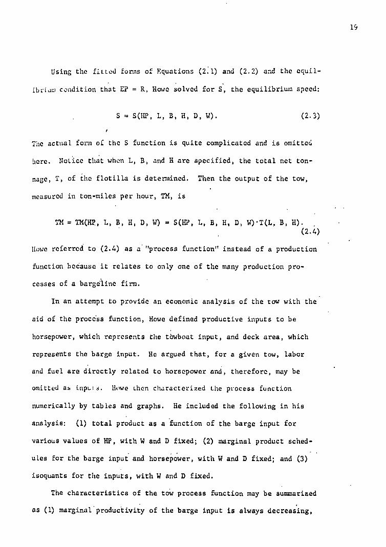
Using the fitted forms of Equations (2.1) and (2.2) and the cquil-

ibriam condition that EP = R, Howe solved for S, the equilibrium speed:

S = S(HP, L, B, H, D, W). (2.3)

The actual form of the S function is quite complicated and is omitted

here. Notice that when L, B, and H are specified, the total net ton-

nage, T, of the flotilla is determined. Then the output of the tow,

measured in ton-miles per hour, TM, is

TM = TM(HP, L, B, H, D, W) = S(HP, L, B, H, D, W).T(L, B, H). (2.4)

Howe referred to (2.4) as a'"process function" instead of a production

function because it relates to only one of the many production pro-

cesses of a bargdiine firm.

In an attempt to provide an economic analysis of the tow with the

aid of the process function, Howe defined productive inputs to be

horsepower, which represents the towboat input, and deck area, which

represents the barge input. He argued that, for a given tow, labor

and fuel are directly related to horsepower and, therefore, may be

omitted as inpLis. Howe Olen characterized the process function

numerically by tables and graphs. He included the following in his

analysis: (1) total product as a function of the barge input for

various values of HP, with W and D fixed; (2) marginal product sched-

ules for the barge input and horsepower, with W and D fixed; and (3)

isoquants for the inputs, with W and D fixed.

The characteristics of the tow process function may be summarized

as (1) marginal productivity of the barge input is always decreasing,

19

20

(2)marginal productivity of the boat input is always decreasing,

(3)marginal productivities of both inputs eventually become negative. , .

The first two results are not surprising. It is a standard assump-

tion of production theory that beyond some point the marginal produc-

tivities of inputs decrease. This behavior of marginal productivity -

is usually referred to as the law of diminishing marginal productivity. 4

In the case of barge tows, there appears to be no stage of increasing .

returns for either input. The negativity of the boat-input marginal

productivity is probably due to the fact that too large a boat in a

given waterway can draw water from under the barge flotilla causing'

the latter to sink lower in the water thereby increasing resistance

substantiatly. The negativity of the barge-input marginal productiv-

ity probably results from the increase in flotilla size relative to,

the fixed width of the waterway. .

In addition to the above results, Howe examined the substitution

possibilities of both inputs by means of isoquants. The isoquants

exhibited the usual convexity to the origin. Moreover, the spacing

of the isoquants indicated decreasing returns to scale for the process.

Howe next derived unit cost curves (average linehaul cost per ton

mile) for the tow. These were obtained by attaching factor prices to

the boat and barge inputs. With horsepower fixed, varying the barge

input permitted the derivation of a "short-run" cost curve. A family . . .,

of such curves was presented. The short-run curves possessed the

typically assumed U-shape. The implied envelope curve was quite flat

over a wide range of output rates, "implying a fairly broad range of

tow makeups capable of producing output at essentially the same aver-

age cost."5

Howe investigated the effects of width and depth on output, find-

ing that the former always led to increased output but that the latter's

beneficial effect on output was exhausted at widths approximating twice

the tow breadth.

It might be commented here that the procedure adopted for measur-

ing the barge input leaves much to be desired. Recall that square feet

of deck area was used as a measure of barge input. This was adopted be-

cause Howe's process function accommodates only rectangular tow config-

urations. It is, of course, quite possible to add barges to a tow such

that the resulting configuration is not rectangular. This presents a

problem in measuring barge input, for adding one barge in different .

ways will not result in the same affect on output. Therefore, Howe

adopted, as a measure of the barge input, the square feet of deck area.

Increases in the barge input were achieved by adding square feet in such

a manner that a rectangular configuration remained. .

Although Howe' S process function for a barge tow is a path-breaking

analysis of a complicated problem and is likely to be of much importance

to anyone interested in linehaul production and costs, some limitations

should be pointed out. As was mentioned above, there was considerable

variation between coefficients of the resistance functions for differ-

ent flotilla configurations, yet Howe finally adopted the resistance ,

function which combined all configurations. When the function is used

with configurations different from those of the data, it is difficult

to know the magnitude of error. Moreover, Howe's function applies only

to open-hopper barges (195 feet long and 35 feet wide) organized into

rectangular flotillas, and loaded to a uniform draft. Obviously, these

21

22

conditions are not always met in practice, and again it is difficult

to determine the magnitude of error. It was pointed out by Howe that

his effectivepush function Probably should not be extrapolated beyond

5000 horsepower, for that was the highest horsepower in his data.

While these limitations appear formidable, they may not seriously im-

pair the ,:,efulness of the process function. This conjecture will

receive attdntion in Chapter IV.

While not a criticism of Howe's analyais, it should be remarked

that his process function comprises oily a part of the linehaul opera- .

tions of a barge tow. A complete process fundtion of linehaUf tow . -

operations wOuld provide for inclusion of acceleration, deceleration,

and delays. 'These additions are Provided in Chapter IV.

As has been indicated Howe's process function will receive some

attention at a later point as it forms the basis for the tow linehaul

process function to be developed below. It may be pointed out here,

however, that some minor alterations and tests of the original functions

' have been made by Howe in a more recent unpublished paper. 6 These will also

be discussed fully in Chapter IV.

Rather than extending the linehaul process function as indicated

above, Howe proceeded directly to an analysis of the bargeline firm.7

In his production analysis of the firm, Howe distinguished between a

planning function and a production function. The term planning func-

tion was reserved for the relationship between outputs and inputs in

which capital stocks are considered inputs. The relationship between

output and inputs in which capital services are inputs was called a

production function.

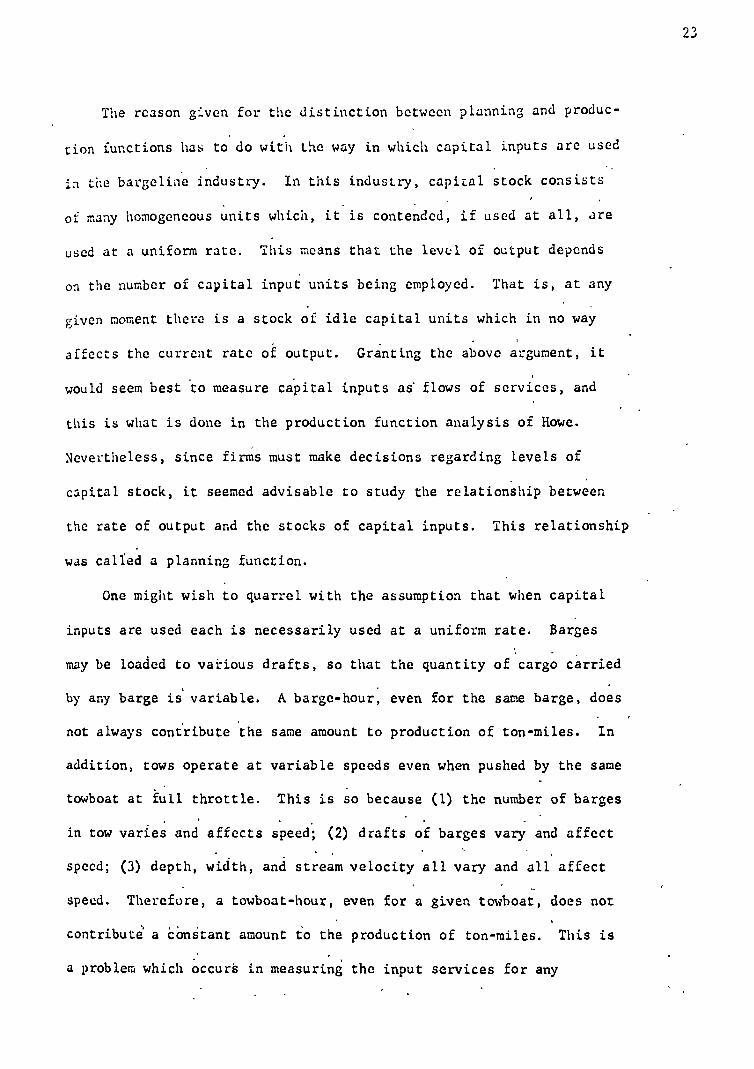
The reason given for the distinction between planning and produc-

tion functions has to do with the way in which capital inputs are used

in the bargeline industry. In this industry, capital stock consists

of many homogeneous units which, it is contended, if used at all, are

used at a uniform rate. This means that the level of output depends

on the number of capital input units being employed. That is, at any

given moment there is a stock of idle capital units which in no way

affects the current rate of output. Granting the above argument, it

would seem best to measure capital inputs as flows of services, and

this is what is done in the production function analysis of Howe.

Nevertheless, since firms must make decisions regarding levels of

capital stock, it seemed advisable to study the relationship between

the rate of output and the stocks of capital inputs. This relationship

was called a planning function.

One might wish to quarrel with the assumption that when capital

inputs are used each is necessarily used at a uniform rate. Barges

may be loaded to various drafts, so that the quantity of cargo carried

by any barge is variable. A barge-hour, even for the same barge, does

not always contribute the same amount to production of ton-miles. In

addition, tows operate at variable speeds even when pushed by the same

towboat at full throttle. This is so because (1) the number of barges

in tow varies and affects speed; (2) drafts of barges vary and affect

speed; (3) depth, width, and stream velocity all vary and all affect

speed. Therefore, a towboat-hour, even for a given towboat, does not

contribute a constant amount to the production of ton-miles. This is

a problem which occur k in measuring the input services for any

22,

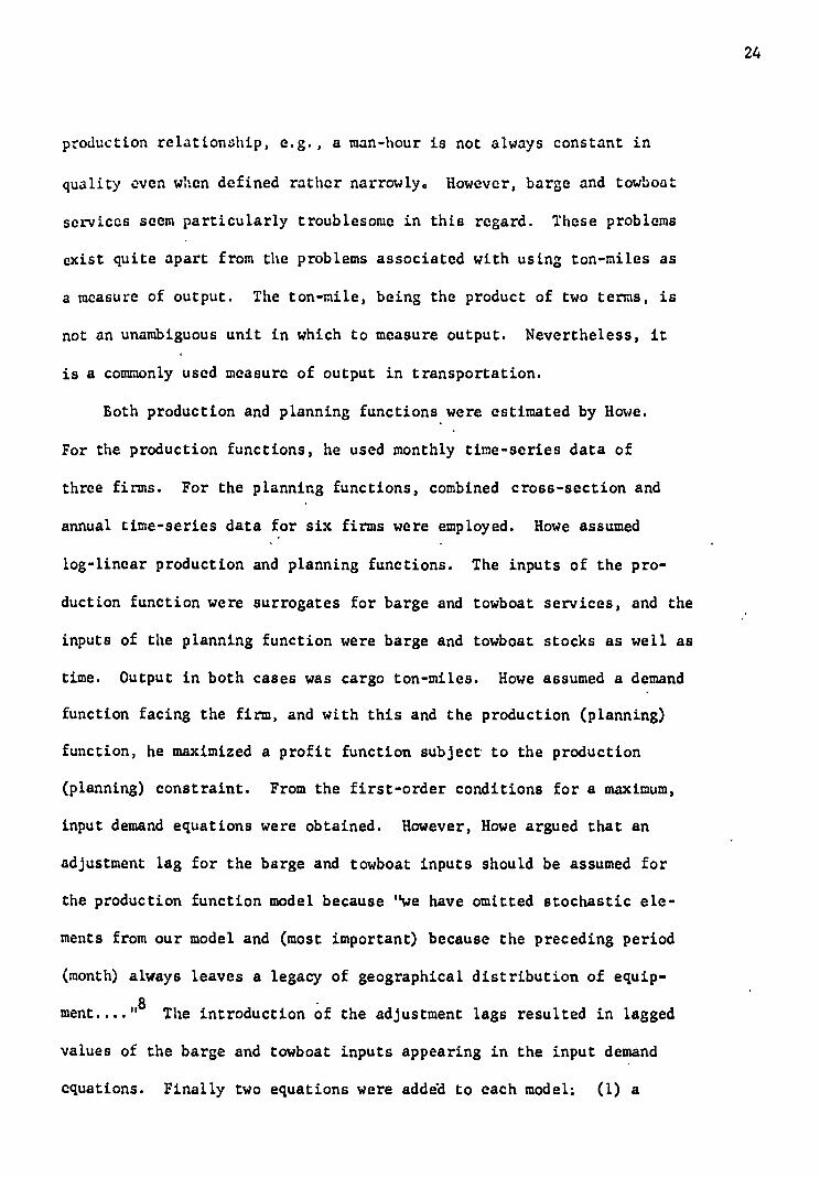
production relationship, e.g., a man-hour is not always constant in

quality even when defined rather narrowly. However, barge and towboat

services seem particularly troublesome in this regard. These problems

exist quite apart from the problems associated with using ton-miles as

a measure of output. The ton-mile, being the product of two terms, is

not an unambiguous unit in which to measure output. Nevertheless, it

is a commonly used measure of output in transportation.

Both production and planning functions were estimated by Howe.

For the production functions, he used monthly time-series data of

three firms. For the planning functions, combined cross-section and

annual time-series data for six firms were employed. Howe assumed

log-linear production and planning functions. The inputs of the pro-

duction function were surrogates for barge and towboat services, and the

inputs of the planning function were barge and towboat stocks as well as

time. Output in both cases was cargo ton-miles. Howe assumed a demand

function facing the firm, and with this and the production (planning)

function, he maximized a profit function subject to the production

(planning) constraint. From the first-order conditions for a maximum,

input demand equations were obtained. However, Howe argued that an

adjustment lag for the barge and towboat inputs should be assumed for

the production function model because "we have omitted stochastic ele-

ments from our model and (most important) because the preceding period

(month) always leaves a legacy of geographical distribution of equip-

ment...."8 The introduction of the adjustment lags resulted in lagged

values of the barge and towboat inputs appearing in the input demand

equations. Finally two equations were added to each model: (1) a

24

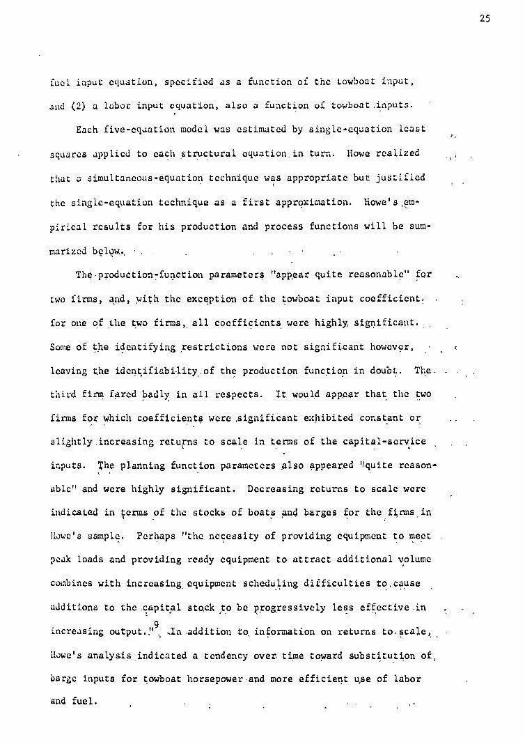
fuel input equation, specified as a function of the towboat input,

and (2) a labor input equation, also a function of towboat inputs.

Each five-equation model was estimated by single-equation least

squares applied to each structural equation, in turn. Howe realized

that a simultaneous-equation technique was appropriate but justified

the single-equation technique as a first approximation. Howe's,em-

pirical results for his production and process functions will be sum-

marized below, „ .

The-production-function parameters "appear quite reasonable" for

two firms, and, with the exception of the towboat input coefficient 7

for one of the two firms, all coefficients, were highly, significant._ .

Some of the identifying restrictions were not significant however,

leaving th.e identifiability,.of the production function in doubt. The. _

third firm fared badly in all respects. It would appear that the two

firms for which coefficients were significant exhibited constant or

slightly,increasing returns to scale in terms of the capital-service ,

inputs. The planning function parameters Also appeared "quite reason- , .

able" and were highly significant. Decreasing returns to scale were

indicated in terms of the stocks of boats and barges for the ( firms . in

Howe's sample. Perhaps "the necessity of providing equipment to meet .

peak loads and providing ready equipment to attract additional volume

combines with increasing equipment scheduling difficulties to,cause

additions to the .capital stock to be progressively less effective-in

increasing output." 9, ,In addition to, information on returns to.scale,,

Howe's analysis indicated a tendency over time toward substitution of

barge inputs for towboat horsepower-and more efficient use of labor

and fuel.

25

Howe's production and planning models discussed above have been

subjected to a more extensive analysis in another paper.10

He'has

applied the two-stage least squares estimation procedure to the equa-

tions of these models. Nevertheless, the conclusions of the earlier

study were not materially affected.

Hurter, following Howe, attempted to summarize the activities of -

firms in the industry by estimating planning and production functions.11

Recall that whenever capital stocks are used as inputs, the' function .

is referred to as a planning function; whenever flows of services are '

used as inputs in a relation, it is called a production function. In

Hurter's analysis the sample of bargeline firms was substantially in-

creased over that of Howe. It included all Class A certificated car-

riers operating on the Mississippi River for three years: 1950; 1951, '

and 1962. Data were obtained from the Interstate Commerce Commission;.

they represent annual firm operations and do not relate solely to reg-

ulated traffic.

Six least-squares regression equations were fitted for each year;

all the equations were in log-linear form. These relationships were

(1) annual firm tonnage' regressed' on the number of boats, the number

of barges, annual gallons of fuel, and annuallabor hours; (2) the

product of annual mileage by towboats and annual tonnage regressed

on the same variables as in (1); (3) annual tonnage regressed on aver-

age horsepower per towboat, average horsepower age, fuel consumption,

and labor hours; (4) annual tonnage regressed on -annual mileage,

average horsepower per towboat, average horsepower age, fuel-oil

26

consumption, and labor hours; (5) average horsepower per towboat re-

grcbsed on fuel-oil consumption, towboat miles, and labor hours; and

((i) annual tonnage regressed on the product of (a) average horsepower

per towboat, (b) number of towboats, and (c) towboat miles and (enter-,.

ing separately) average age per horsepower, fuel . consumption, and

labor hours. .

The results of the regression analysis will be summarized briefly.

The regression results for (1) for all three years revealed a relatively : • 1

stable towboat coefficient ranging from 0.680 to 1.036. For each of -

these estimates the value of "t" was comparatively large, with the

exception of one year (1950). However, the other parameter estimates

varied considerably between years. Nevertheless, the labor-hours co-

efficient showed a downward movement from 1950 to 1962, but the stan-

dard errors were quite large. The coefficient of the barge variable,

on the other hand, showed upward movement. Little may be said about

the parameter estimate of the fuel variable. One percent increases

in all inputs in 1950 led to a 1.79 percent increase in tonnage con-

trasted with a 1 percent increase in 1957 and a 2 percent increase in

1962. Hurter viewed the behavior of tonnage when all inputs are

changed proportionately as reflecting the relatively high level of

waterways activities in 1957. Finally, the proportion of the observed .

variance in annual tonnage explained by relation (1) ranged from 64

to 75 percent.

In the next relationship investigated, (2), the towboat coefficients

were about the same in 1950 and 1957, but the estimate for 1962 was

larger. Although the standard errors were very large, the estimates

27

of the barge coefficient seemed to follow the same pattern. The ex-

ponents of the labor-hours term appeared to fall over time. Hurter

recognized the possibility of strong collinearity between the fuel and

labor variables; he therefore examined the sum of the coefficients df

these variables as an indication of the effect of current inputs.

This sum was about 0.6 in 1962, 0.93 in 1957, and 1.3 in 1950, clearly,

according to Hurter, indicating a diminishing role for the current

inputs relative to the capital inputs. Relation (2) explained 75 to

90 percent of the observed variance in ton-miles.

In relationship (3), an upward trend in the exponent of the aver-

age horsepower variable seemed to indicate increasing importance of - f

that variable; however, standard errors were large. The estimates of

the fuel coefficient were again uninformative, but the estimates of

the labor coefficients were quite stable and had reasonably large "t"

values. Equation (3) accounted for only 59 to 65 percent of the ob-

served variance in annual tonnage.

Relation (4), which differs from (3) through the introduction of

annual firm towboat mileage as an additional explanatory variable,

changed considerably from one year to the other. The standard errors

of the exponent estimates for the variable miles were very large ex-'

cept for 1962 when the exponent appeared positive and greater than

unity. The standard errors of the horsepower-per-towboat term were

too large to permit any discussion of their change over time. Other .,

problems appeared in the estimates of this relation; e.g., the esti-

mate of the fuel coefficient was positive in 1957 but negative in

1962; the sum of the fuel and labor coefficients was 0.74 in 1950,

28

2.5 in 1957, and 0.15 in 1962. Again Hurter noted an indication of

a 1ii;11 rate of capacity utilization in 1957 and a general trcnd toward

diminished importance for the current inputs. This relationship ac-

counted for 66 to 72 percent of the variance in annual tonnage. ,

The last production relationship estimated by Hurter involved an

attempt to use a direct measure of the services of the capital inputs

as an explanatory variable. The product of average horsepower per

towboat, number of towboats, and towboat miles was used as a surrogate

for horsepower-hours because horsepower-hours could not be used directly.

It was later recognized by Hurter that collinearity between fuel-oil

consumption and miles run by towboats would also result in collinear-

ity between the surrogate variable and fuel consumption. The estimates

of the coefficient of the surrogate variable were positive and similar

in magnitude fOr 1957 and 1962. The estimates for the labor coeffi-

cient fell drastically over the period considered. Relation (6) ac-

counted for 65 to 79 percent of the variance in annual tonnage.

In suMMarizing his analysis of production, Hurter indicated that

increasing returns to scale, of a modest degree, were evident among

the firms in the sample investigated. However, it was difficult to

conclude anything about the time trend in returns to scale. There

did, nevertheless, seem to be an increasing trend in the values of

the exponents associated with the capital inputs. Finally, Hurter

tested whether the equations were significantly different as between

years. He found that indeed (1), (2), (3), (4), and (6) were signifi-

cantly different in 1957 from their 1950 values and that the same

equations in 1950 were significantly different in 1957 from their

2 9

1962 counterparts. However, only (1) was significantly different in

1957 from its 1962 version; the others were not significantly differ-

ent as between 1957 and 1962. These results supported the conclusion

that significant changes had occurred since 1950 in the production re-

lationships used by Class A inland waterway carriers operating on the

Mississippi River.

The production and planning functions just discussed, both those

of Howe and those of Hurter, referred to the activities of an entire

firm, as contrasted with the production function for a tow. Theoret-

ically, cost functions for the firm could be developed from a know-

ledge of the appropriate unit costs of each input and the appropriate

planning or production function. This procedure, however, was not

used by Hurter in his study of cost relationships for inland waterway

operations.12

Rather, his method was that of statistically relating

costs to output or some other measure of firm size. Hurter's empiri-

cal cost study made use of annual cross-section data for Class A car- .

riers operating on the Mississippi River System in 1950, 1957, and

1962.

The first sot of equations estimated by Hurter involved regres-

sing total annual waterline expenses on total annual tonnage. The

proportion of the variance explained by these regressions was very

low for 1950 but over 60 percent for both 1957 and 1962. Hurter con-

fined his equations to a log-linear form for reasons discussed in his

paper. All of the equations indicated economies of scale. Signifi-

cant differences were found in the extent of the scale economies when

30

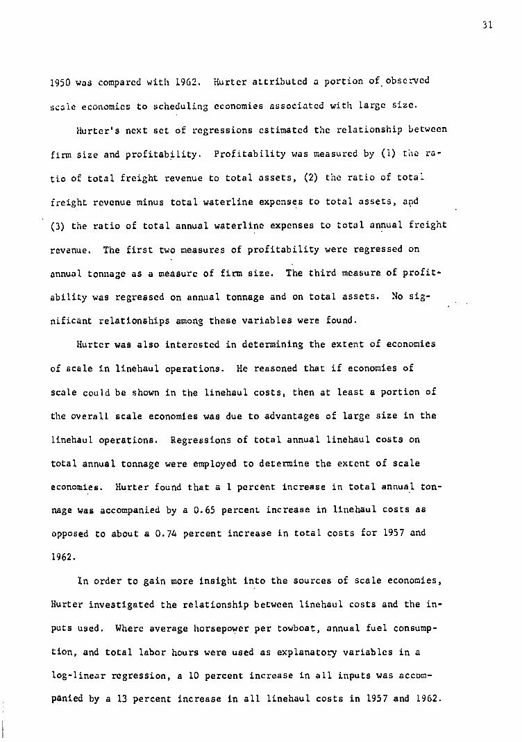
1950 was compared with 1962. Hurter attributed a portion of observed

scale economies to scheduling economies associated with large size.

Hurter's next set of regressions estimated the relationship between

firm size and profitability. Profitability was measured by (1) the ra-

tio of total freight revenue to total assets, (2) the ratio of total

freight revenue minus total waterline expenses to total assets, and

(3) the ratio of total annual waterline expenses to total annual freight

revenue. The first two measures of profitability were regressed on

annual tonnage as a measure of firm size. The third measure of profit-

ability was regressed on annual tonnage and on total assets. No sig-

nificant relationships among these variables were found.

Hurter was also interested in determining the extent of economies

of scale in linehaul operations. He reasoned that if economies of

scale could be shown in the linehaul costs, then at least a portion of

the overall scale economies was due to advantages of large size in the

linehaul operations. Regressions of total annual linehaul costs on

total annual tonnage were employed to determine the extent of scale

economies. Hurter found that a 1 percent increase in total annual ton-

nage was accompanied by a 0.65 percent increase in linehaul costs as

opposed to about a 0.74 percent increase in total costs for 1957 and

1962.

In order to gain more insight into the sources of scale economies,

Hurter investigated the relationship between linehaul costs and the in-

puts used. Where average horsepower per towboat, annual fuel consump-

tion, and total labor hours were used as explanatory variables in a

log-linear regression, a 10 percent increase in all inputs was accom-

panied by a 13 percent increase in all linehaul costs in 1957 and 1962.

31

A 10 peicont increase in all inputs was also associated with a 28 per-

cent increase in annual tonnage in 1962. These findings seemed to in-

dicate the existence of scale economies in 1957 but not in 1962; tfie

latter year, it will be recalled, showed positive scale economies - when

tonnage was regressed on linehaul costs. Further support for posiffNie

. . economies of scale was gained from the set of regressions In which

stock inputs (boats and barges) and flow inputs (fuel and labor) were

regressed on linehaul costs. ,

Hurter has also provided an analysis of terminal cost, but'dis-

cussion of that is omitted here since the emphasis of this research

is on linehaul operations. Omitted also is a discussion of a barge

scheduling model by Hurter and A. Victor Cabot.13

Reference to the

model is made later in the chapter on the tow process function, where

it is indicated how one might determine firm costs through use of the

tow process function and the Cabot-Hurter scheduling model.

Some general comments on the foregoing research may be appropriate

now. The tow process function, as has been pointed out, is incomplete ,

as a description of the barge linehaul process. This is primarily due

to the absence of any consideration of linehaul delays but is also due

to omission of any consideration of non-constant operating speeds.

Whether or not these are important omissions, and if so what to do

• , 4

about them, are questions taken up in Chapter IV of this dissertation.

The cost functions derived from the Howe tow process function are, of

course, subject to the same reservations as affect the process func-

32

tion.

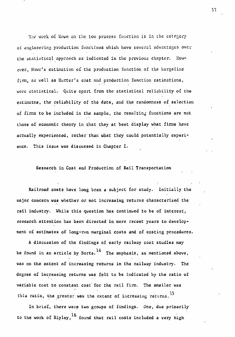
The work of Howe on the tow process function is in the category

of engineering production functions which have several advantages over

the statistical approach as indicated in the previous chapter. How-

ever, Howe's estimation of the production function of the bargeline

firm, as well as Hurter's cost and production function estimations,

were statistical. Quite apart from the statistical reliability of the

estimates, the reliability of the data, and the randomness of selection

of firms to be included in the sample, the resulting functions are not

those of economic theory in that they at best display what firms have

actually experienced, rather than what they could potentially experi-

ence. This issue was discussed in Chapter I.

Research in Cost and Production of Rail Transportation

Railroad costs have long been a subject for study. Initially the

major concern was whether or not increasing returns characterized the

rail industry. While this question has continued to be of interest,

research attention has been directed in more recent years to develop-

ment of estimates of long-run marginal costs and of costing procedures.

A discussion of the findings of early railway cost studies may

be found in an article by Borts. 14 The emphasis, as mentioned above,

was on the extent of increasing returns in the railway industry. The

degree of increasing returns was felt to be indicated by the ratio of

variable cost to constant cost' for the rail firm. The smaller was

this ratio, the greater was the extent of increasing returns.15

In brief, there were two groups of findings. One, due primarily

- to the work of Ripley, 16 found that rail costs included a very high

33

.•

proportion of constant costs. Typically variable expenses were esti-

mated to constitute less than half the operating expenses and about

one-third the total expenses. The other group of findings consisted

of those studies which reported that the cost ratio was really much

higher than one half. These studies are exemplified by the work of

Ford K. Edwards17

and M. 0. Lorenz.18

It was this body of research, - , . . . , -

principally the work of Edwards, from which were obtained the ideas

and methods employed by the Interstate Commerce Commission in its rail

- •, , costing procedure.

19 The Interstate Commerce Commission approach 6)

rail cost analysis may serve as the culmination of the earlier cost

studies referred to above. A brief exposition and critique of the

Interstate Commerce Commission costing procedure is now presented.

A method was developed to estimate the extent of variability of '

railway expenses with traffic volume. A simple linear regression was

used. The dependent variable was operating expense, and the indepen-

dent variable was gross ton-miles. Both variables were deflated by •

miles of road in order to eliminate scale effects. The data were

total operating expenses, rents, and taxes for a cross section of

U.S. rail systems. The intercept value, which may be interpreted as

fixed cost, was subtracted from the average value of the dependent

variable, which may be interpreted as total cost; the remainder may

be viewed as total variable cost. This remainder, expressed as a

percentage of total cost, as defined above, was used to measure the

percentage of variability among all railway operating expenses. A

similar procedure was used to determine the variability of road and • ■

equipment capital investment, to which was then applied a cost-of-

• X

34

money factor.

The Interstate Commerce Commission approach to rail costing out-

lined briefly above has been subjected to some severe criticisms.20

A summary of these is presented now. It is contended that the very

aggregative nature of the cost data hides important details. In addi-

tion, the application of an average percentage variable to the cost of

a specific railroad may result in error if the railroad has a consis-

tent error of observation in its costs, resulting in a, consistent

under or overstatement of variable costs. Also, when used separately

with .component categories of operating expense, the Interstate Com-

merce Commission method assumes the percentage variable is constant

in all these categories. Finally, it is necessary for all subcategories

of total operating expense to vary with gross tpn-miles, whereas other

units may be superior for other categories, e.g., engine miles for

measuring the variability of engine maintenance expense. .

Meyer, Peck, Stenason, and Zwick (MPSZ) sought to present an ap-

proach to rail cost analysis that would answer some of the criticisms

leveled at earlier studies and particularly the Interstate Commerce .

Commission method of rail costing. 21 The approach used by MPSZ in

rail cost determination is quite simple in concept. 22 Statistical

cost relations .of the following form were fitted to the data:

E = f(Q, S), (2.5)

' f

where E represents an expense or cost account .

Q indicates quantity of output Jr traffic variable

S designates size variable.

3 5

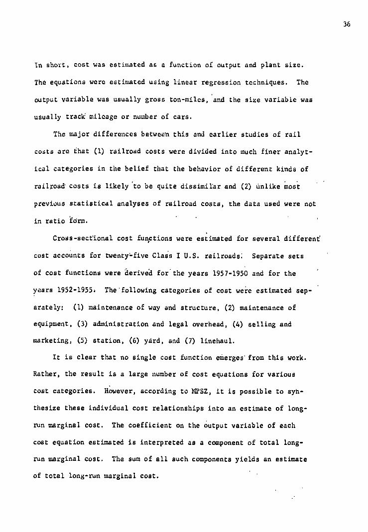
In short, cost was estimated as a function of output and plant size.

The equations were estimated using linear regression techniques. The

output variable was usually gross ton-miles, and the size variable was

usually track' mileage or number of cars.

The major differences betweeh this and earlier studies of rail

costs are that (1) railroad costs were divided into much finer analyt-

ical categories in the belief that the behavior of different kinds of

railroad costs is likely to be quite dissimilar and (2) unlike most

previous statistical analyses of railroad costs, the data used were not

, in ratio 'fcirm.

Cross-sectional cost functions were estimated for several different

cost accounts for twentyl-five Class I U.S. railroads: Separate sets

of cost functions were ilerivea for theyears 1957-1950 and for the

years 1952-1955i The'following categories of cost were estimated sep-

arately: (1) maintenance of way and structure, (2) maintenance of

equipment, (3) administration and legal overhead, (4) selling and

marketing, (5) station, (6) yard, and (7) linehaul.

It is clear that no single cost function emerges from this work.

Rather, the result is a large number of cost equations for various

cost categories. However, according to NPSZ, it is possible to syn-

thesize these individual cost relationships into an estimate of long-

run marginal cost. The coefficient on the output variable of each

cost equation estimated is interpreted as a component of total long-

run marginal cost. The sum of all such components yields an estimate

of total long-run marginal cost.

36

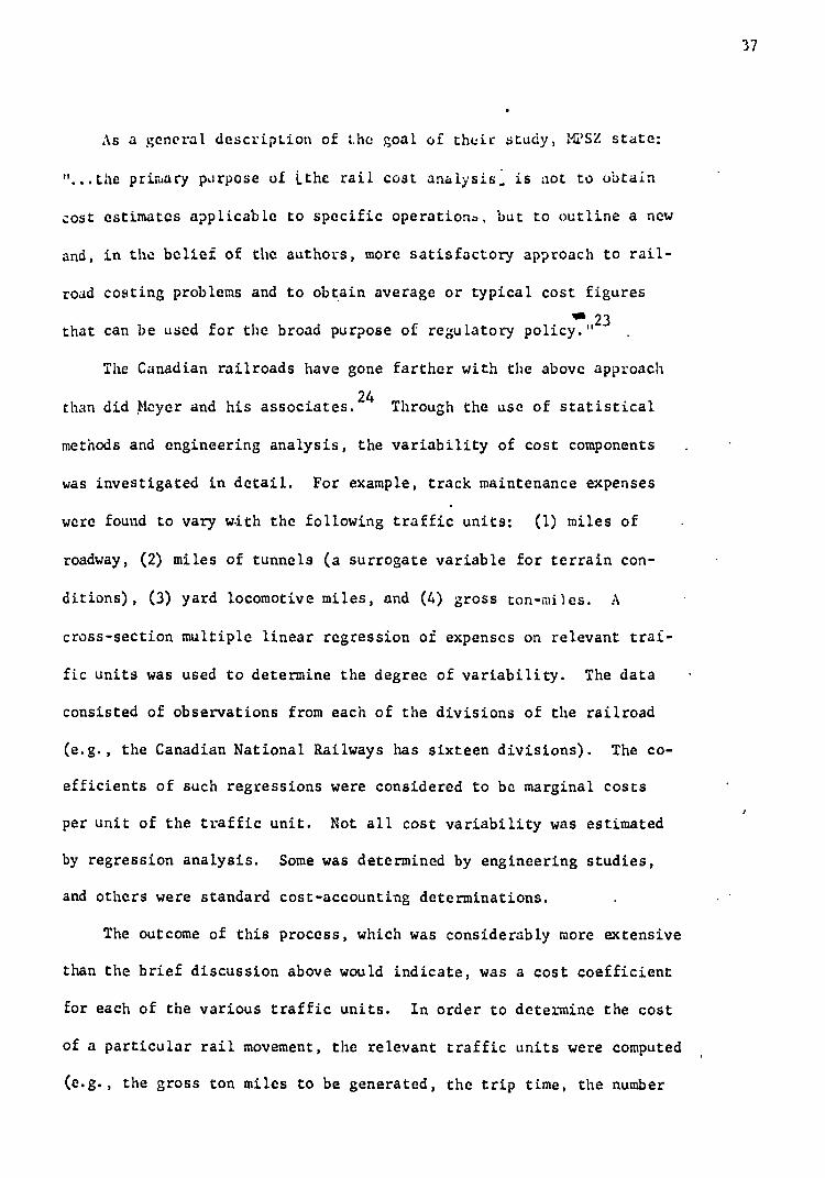
As a general description of the goal of their study, MPS?. state:

"...the primary porpose of Lthe rail cost analysis, is not to obtain

cost estimates applicable to specific operation., but to outline a new

and, in the belief of the authors, more satisfactory approach to rail-

road costing problems and to obtain average or typical cost figures

" 23 that can be used for the broad purpose of regulatory policy." .

The Canadian railroads have gone farther with the above approach

than did Neyer and his associates. 24 Through the use of statistical

methods and engineering analysis, the variability of cost components .

was investigated in detail. For example, track maintenance expenses

were found to vary with the following traffic units: (1) miles of -

roadway, (2) miles of tunnels (a surrogate variable for terrain con-

ditions), (3) yard locomotive miles, and (4) gross ton-miles. A .

cross-section multiple linear regression of expenses on relevant traf-

fic units was used to determine the degree of variability. The data .

consisted of observations from each of the divisions of the railroad

(e.g., the Canadian National Railways has sixteen divisions). The co-

efficients of such regressions were considered to be marginal costs

per unit of the traffic unit. Not all cost variability was estimated

by regression analysis. Some was determined by engineering studies,

and others were standard cost-accounting determinations. .

The outcome of this process, which was considerably more extensive

than the brief discussion above would indicate, was a cost coefficient

for each of the various traffic units. In order to determine the cost

of a particular rail movement, the relevant traffic units were computed .

(e.g., the gross ton miles to be generated, the trip time, the number

37

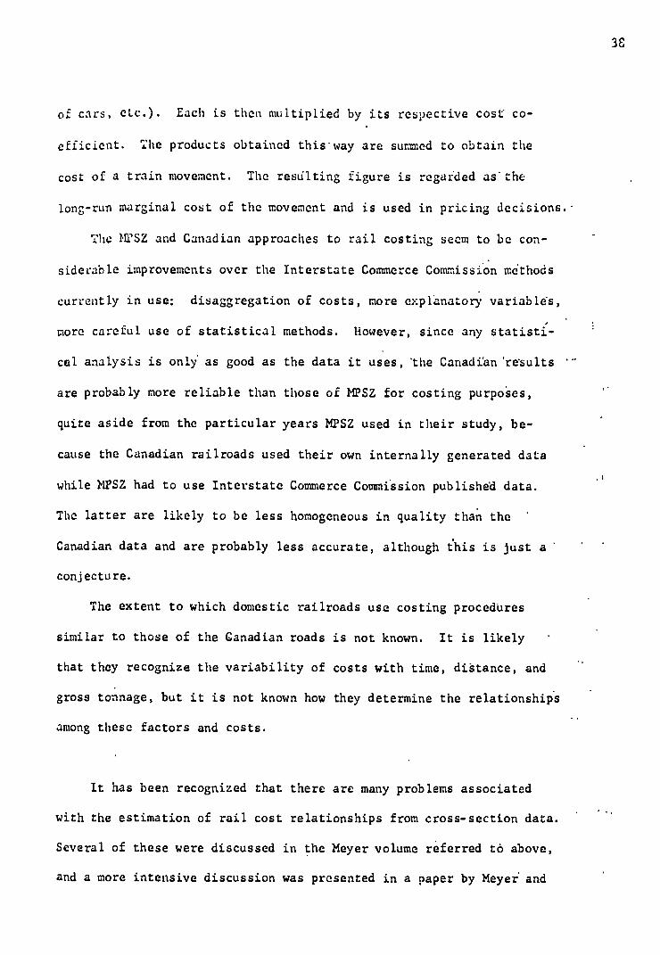
o f cars, etc.). Each is then multiplied by its respective cost co-

efficient. The products obtained this . way are summed to obtain the

cost of a train movement. The resdlting figure is regarded as the

long-run marginal cost of the movement and is used in pricing decisions. -

Thc MPSZ and Canadian approaches to rail costing seem to be con-

siderable improvements over the Interstate Commerce Commission methods

currently in use: disaggregation of costs, more explanatory variables,

more careful use of statistical methods. However, since any statisti-

cal analysis is only as good as the data it uses, the Canadian 'results -

are probably more reliable than those of MPSZ for costing purposes,

quite aside from the particular years MPSZ used in their study, be-

cause the Canadian railroads used their own internally generated data

while MPSZ had to use Interstate Commerce Commission published data.

The latter are likely to be less homogeneous in quality than the "

Canadian data and are probably less accurate, although this is just a '

conjecture.

The extent to which domestic railroads use costing procedures

similar to those of the Canadian roads is not known. It is likely -

that they recognize the variability of costs with time, distance, and

gross tonnage, but it is not known how they determine the relationships

among these factors and costs.

It has been recognized that there are many problems associated

with the estimation of rail cost relationships from cross-section data.

Several of these were discussed in the Meyer volume referred to above,

and a more intensive discussion was presented in a paper by Meyer' and

38

Kraft.25 . In addition, Borts has also been concerned with the problem

raised by the attempts to estimate rail costs from cross-section data

and has proposed a method of statistical analysis which he regards as

an improvement over current methods.26 Borts argued that biases have

crept into statistical cost estimation primarily because the size of .

the firm has been treated incorrectly in previous studies. He pro-

posed as a .solution stratification of firms by size.

To illustrate his proposal Borts presented a stratified cost func-

tion estimated from a cross-section sample of firms. He also strati-

fied by region. For each size class, estimates were made of average

cost, marginal cost, and the elasticity of cost. (Cost elasticity is ..

defined as the percentage variation in cost accompanying a 1 percent .

change in output.) Further, the marginal cost and. elasticity of cost .

between cost classes have been computed as a check on the possible..

error of estimating a function which is not the true long-run cost . .

function. .

The basic cost-output relation (estimated by least-squares) was

of the following form: ,

C = a + bX + c(Z/X), (2.6)

where C = freight operating expenditures .

X = total loaded and empty freight car miles

Z = total freight carloads.

The variable r (Z/X) maybe viewed as a measure of carload density; its

reciprocal cap be interpreted as a measure of the average length of

39

haul. The variable (Z/X) was used instead of Z alone in order to avoid

high correlation between the independent variables and to permit non-

linearity into the function. .

With this formulation of the cost function, Borts was able to

examine (1) the marginal cost of carloads for a given average length

of haul, (2) partial cost elasticities with respect to X and Z, (3)

the marginal cost of car miles for a given level of carloads, and (4)

the partial cost elasticity with respect to length of haul.

Three size classes were determined based on cost of reproduttion

and track mileage. Regions used were East, South, and West. Data .

used were Interstate Commerce Commission rail cost data for the year

1948. Allocations of freight costs were made by Borts. "Elements of

cost were eliminated where they did not appear related to the produc-

tion of freight service. Whenever possible, items of cost were ex-

cluded when they were shared jointly between freight and passenger

service."27

It was found that long-run, increasing cost prevailed only in. the

Eastern region, while long-run decreasing and constant costs occurred

in the South and West. Cost elasticities computed between size classes

confirMed these findings.

It is doubtful whether any real conclusions can be drawn from

the rail cost analysis of Sorts, if only because the data were four-

teen years old when his article was published and because they were

annual costs cross-sectionally for one year only. Additionally, the

cost allocations were done by the author, and the degree of arbitrari-

ness is unclear. -It is unfair to be too critical of Borts regarding

40

'1 J.

the independent variables in his estimation equations, for he was at-

tempting to determine the effects of size and region on cost. Never-

theless, using only car miles and carloads (the latter deflated by

tae former) seems a tremendous oversimplification of cost-determining

factors. Even Botts himself, in a different article (to be discussed

below), used a much more disaggregative approach and many more explan-

atory variables. Borts' real contribution would seem to lie in his

use of covariance analysis in the study of costs. This is a statis-

tical technique that permits investigation Of the effects on regres-

sion equations of various categorizations of the data. It is particu-

larly useful when comparisons between categories is desired but the

number of sample observations is small.28

The only estimation of rail production functions to be found in

the economics literature is the work of Borts.29

His study was de-

signed to determine whether increasing returns existed in the rail-

way industry. A model of production was specified for two processes

in railway technology, and a production function was estimated from

cross --section, data for each process. ,

It wah 4poLneblzed that railway technology consisted of the si-

multaneous operation of three distinct processes which were physically

connected. The three processes were loading of cargo cars, switching

of cargo cars, and the transfer of assembled trains between terminals

(linehaul). Because a large proportion of loading activity was car-

ried on by other than transport firms, models of production relations

were constructed for the switching and linehaul processes only.

In the switching process--which consists of picking up, assembling,

and sorting cargo cars into trains--the following input services were

employed: labor, fuel, equipment, and fixed plant. Output was measured .

by number of trahsferred cargo cars. In addition to the inputs given

above, the following were used: (I) - switch engine miles, to account

for the distance over which the switch engine must travel, which will

vary from yard to yard; and (2) switch-engine hours, to account for

- circuity in routing of switch locomotives required by the scatter of

• cargo cars.

In the linehaul process--which consists of the transfer of loaded

and empty cargo cars between terminals--the following inputs were used:'

labor, fuel, equipment, and fixed plant.' The outputs considered were

loaded cargo miles, loaded transported cars, and empty cargo car miles.

The form of the production relations for both processes was the

same:

Y . . f.(zl'

z 2' ..., z ) ' i . 1, ...; m (2.7)

L 1 n

where the Y's represent the minimum values of the variable inputs, and

the 'Vs reptesent the outputs and the fixed inputs. In both models

four variable inputs were specified. For the linehaul process the

variable inputs were (1)- labor services; (2) fuel consumption; (3) -

flow of equipment services, measured by expenditures on maintenance

of freight equipment, exclusive of depreciation; and (4) flow of track •

and structure services, Measured by expenditures on maintenance of

track and structure for freight service purposes, exclusive of

42

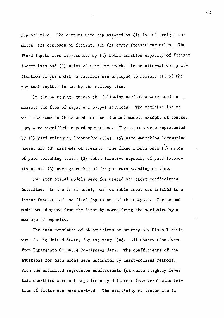
deprecL.tion. The ,outputs were represented by (1) loaded freight car

miles, (2) carloads of freight, and (3) empty freight car miles. , The

fixed inputs were represented by (1) total tractive capacity of freight

locomotives and (2) miles of mainline track. In an alternative speci-

fication of the model, a variable was employed to measure all of the

physical capital in use by the railway firm.

in the switching process the following variables were used to ,

measure the flow of input and output services. The variable inputs

were the same as those used for the linehaui model, except, of course,

they were specified to yard operations. The outputs were represented

by (1) yard switching locomotive miles, (2) yard switching locomotive

hours, and (3) carloads of freight. The fixed inputs were (1) miles

of yard switching track, (2) total tractive capacity of yard locomo-

tives, and (3) average number of freight cars standing on line.

Two statistical models were formulated and their coefficients

estimated. In the first model, each variable input was treated as a

linear function of the fixed inputs and of the outputs. The second ,

model.was derived from the first by normalizing the variables by a

measure of capacity. .

The data consisted of observations on seventy-six Class I rail-

ways in the United States for the year 1948. All observations were

from Interstate Commerce Commission data. The coefficients of the

equations for each model were estimated by least-squares methods.

From the estimated regression coefficients (of which slightly fewer

than one-third were not significantly different from zero) elastici-

ties of factor use•were derived. The elasticity of factor use is

43

defined to be the percentage change in factor use accompanying a

1 percent change in all of-the output variables, holding constant the

stocks of equipment. Decreasing returns to scale are implied by a

value of the elasticity coefficient which is greater than unity; in-

creasing returns are implied by a value of the coefficient which is

less than unity. The elasticity of variable cost was also estimated.

This is defined as the percentage change in variable cost accompanying

a 1 percent chahge in the output variables, holding constant the stock

of equipment. This particular elasticity was calculated by takihg a

weighted ailerage of the factor-use elasticities, where the weights '

consisted of the proportion of total variable cost expended on the

particular inputs. These proportions were derived from the aggregate

expense accounts of all the' railway firms.

The models of the switching process indicated a cost elasticity

not significantly different from unity, implying constant returns td

scale. For the linehaul process, there was a considerable difference

between the cost elasticity coefficients indicated by the two models:'

the first model , exhibited a coefficient close to unity, but the second

showed a coefficient of one-half, implying increasing returns to scale.

As:in the cost study discussed previously, Sorts used annual

Interstate Commerce Commission cross-section data for the year 1948.

In addition, the variable cost proportions were based onligures summed'

across firms, and" it Is possible that the-proportion used have little '

'relevance to the actual proportions of individual firms. Finally, it

should be mentioned again that slightly fewer than one-third of the

estimated coefficients were not significantly different from zero.

44

Moreover, the form of the production relations estimated by Borts per-

mits little flexibility. Input elasticities may be calculated, but a

process function which relates inputs to outputs does not emerge.

Factor substitutability cannot be examined, nor can marginal or total

productivities be calculated. Returns to scale are investigated in-

directly through factor elasticities rather than directly by means of

a well-articulated production or process function.

In summary, it seems that past rail cost analyses have been de-

signed to answer one of two questions: (1) What is the extent of in-

creasing returns in the railway firm? and (2) What is the long-run

marginal cost of the railway firm? Attempts to answer the first ques-

tion are exemplified by the work of the early railway economists, as

noted above, and also by later economists such as Borts. The second

question has been pondered by the Interstate Commerce Commission,

John Meyer and his associates, and the railroads themselves, as exem-

plified by the Canadian approach to rail costing. Because of the

difference in approach between the two groups of researchers, the

results of the one have not aided in answering the question posed by

the other. Were it possible to derive the long-run average cost

curve of the railroad firm, then both questions could be answered by

the same study. This has not yet been accomplished. However, the

rail process function of Chapter V will be used to derive along-run

cost curve for the linehaul activities of the rail firm, and it will

be shown how to integrate this with statistical cost analysis to

determine the firm's short and long..run average costs. The only

45

other production analysis of rail is the work of Borts which was dis-

cussed above.30

As noted, his approach was to divide the rail firm's

activities into non-overlapping processes and to analyze each sepa-

rately via statistical methods. No attempt was made to determine cost

curves; but, as noted, cost elasticities were calculated.

46

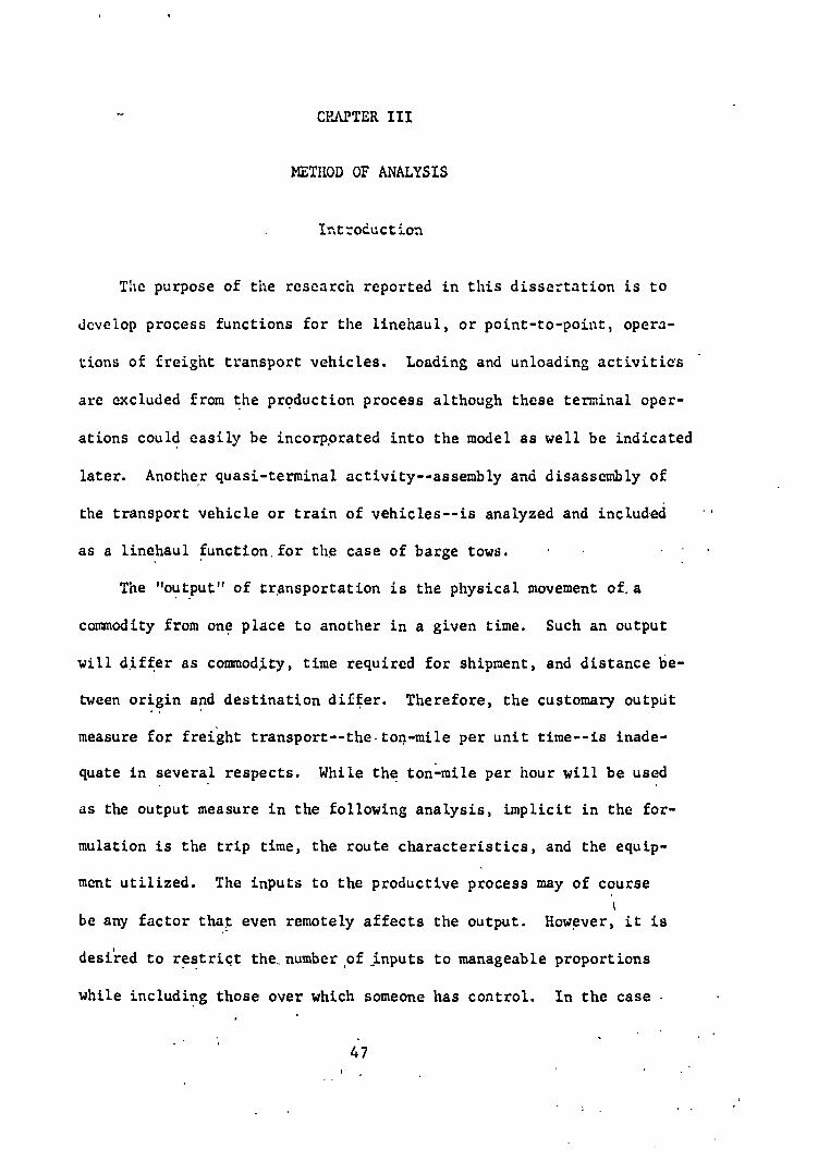
CRAFTER III

METHOD OF ANALYSIS

Introduction

The purpose of the research reported in this dissertation is to

develop process functions for the linehaul, or point-to-point, opera-

tions of freight transport vehicles. Loading and unloading activities

are excluded from the production process although these terminal oper-

ations could easily be incorpprated into the model as well be indicated

later. Another quasi-terminal activity--assembly and disassembly of

the transport vehicle or train of vehicles--is analyzed and included

as a linehaul function, for the case of barge tows.

The "output" of transportation is the physical movement of.a

commodity from one place to another in a given time. Such an output

will differ as commodity, time required for shipment, and distance be-

tween origin and destination differ. Therefore, the customary outpdt

measure for freight transport--the,ton-mile per unit time--is inade-

quate in several respects. While the ton .-mile per hour will be used

as the output measure in the following analysis, implicit in the for-

mulation is the trip time, the route characteristics, and the equip-

ment utilized. The inputs to the productive process may of course

be any factor that even remotely affects the output. However, it is

desired to restrict the, number of _inputs to manageable proportions

while including those over which someone has control. In the case -

47

Q = e , (3. 1) •

of transportation, the inputs controlled by the productive unit may

be such factors as the horsepower of the motive unit, the size and

type of carrying capacity, labor, fuel, etc. Some factors not control-

lable by the productive unit are delays en route due to weather, break- . .

down, etc. Some inputs may be under the control of one mode and not

controllable by another. '"Roadbed" is an example of this kind of in-

put. Barging firms, for example, have no direct control over the

depth, width, and stream velocity of the waterways on which they op-

erate. .Railroads, on the other hand, may alter the roadbeds over which

they travel. The inputs of the productive processes will be discussed

more fully later. In the next sections the method of articulating a

linehaul transportation process function will be developed. In later'

chapters this method will be applied to water and rail transport.

Form of Linehaul Process Function

The ton-miles per hour generated by a transportation vehicle is

the product of the cargo tonnage and the average speed at which the

vehicle travels between origin and destination. Cargo 'tonnage and

average speed are functions of the size and type of cargo-carrying

units comprising the transport vehicle. Important inputs for these

functions will be specified below; this discussion is focused on the

form of the production relationship.

The process function has the following form;

48

T =T +T , t r s

(3.2) '

in which T f = time during which the vehicle operates at "full" speed,

"" . . • . i.e., the equilibrium speed of the vehicle for a given power input

T time required for vehicle to accelerate from a stop to

in which Q = ton-miles per hour

C = cargo tonnage

Vc = average (effective) speed.

Since a transport vehicle must be in ons of four states (at rest, at

constant velocity, accelerating, or decelerating) at any moment of

1 time, the following travel time expression may be defined:

49

in which Tt = travel time of vehicle

Tr = running time of vehicle, i.e., time during which the vehicle is moving

Ts = delay time of vehicle, i.e., time during which the

vehicle is stopped for one reason or another..

This travel-time expression may be further disaggregated as follows:

(3.3) T =T r f aa dd'

full speed

Na

= number of accelerations occurring during a trip

Td = time required for vehicle to decelerate from full speed

to a complete stop

Nd

= number of decelerations occurring during a trip.

It will be convenient to define Tf as follows:

50

(3.4) T f = D f/V f = (D - DaNa - DdNd)/V

f'

in which D f = distance traveled at full speed during a trip

D = distance to be traveled during a trip

Da = distance traveled during one acceleration

Dd = distance traveled during one deceleration

Vf = full speed of vehicle, i.e., the equilibrium speed of

the vehicle for a given power input.

Finally, the travel-time expression may be written

Tt = [(D - D

aNa

- DdNd)/Vf] + TaNa + T

dNd + T

s. (3.5)

The total trip time, T. required to travel distance D is the sum of

four terms: (1) the time during which the vehicle travels at maximum -

speed, (2) the additional time required because the vehicle accelerates,

(3)the additional time required because the vehicle decelerates, and

(4)the amount of time during which the vehicle is stopped. "

Effective speed may now be defined as

V = D/Tt =D{[(D -DN -DN)/V ] + TaNa +.

TdNd + T

s} e a a d d (3.6)

If it is desired to divide D into I segments of length'D i each,' then

I

Ve

= D

(

:DUD. - N -D N )/V ] + TaiNai

+ TdiNdi

+ Ts. j a. a. d i di fi

(3.7)

- Q = CD [(D/V f) + (3.10)

Equation (3.7) allows for the possibility that factors affecting trip

time may not be constant over the entire distance D but are constant

over the length D i .

The Process function, then, takes the following form

C.D r4(D. - D N - D )/V ] +T N- +T N + a a

T ( 1. a i a i d. d. f.

11 1 i i d. d. s.)

1 1 i=1 (3.8)

Of course, Equation (3.8) may be simplified considerably. If, for

example, it were decided that acceleration and deceleration were un-

important but that route segmentation were important, the linehaul

process function would become

51

- 1 ,

-1

Q = C.D [1] (D./V f ) +T i=1

. (3.9)

In addition, if it were decided to ignore the effects of variability

in route characteristics, the process function would take the follow-

ing form:

Analysis of Transportation Vehicle in Motion2

• Introduction. This subsection discusses the determination-of the , .

constant running speed, V , the acceleration time and distance, Ta

and

Da' and the deceleration time and distance, Td and D

d. For the purpose

of analyzing the motion of a transport mode, the vehicle, or train of

F = Ft (v) - Fd (v) = m(dvidt), (3.11)

vchicles, is considered to be a point moving in a straight line. This

assumptiodis standard in physics and engineering, and should not mate-

rially affect the result. Constant velocity, acceleration, and decel-

eration will be discussed in that order.

Constant Velocity State. The cruising speed of a vehicle depends

on the resistance characteristics or drag forces acting on the vehicle

and the tractive-effort or motive properties of the propulsion system.

These forces are each functions of velocity as well as vehicle charac-

teristics, "roadbed," etc. The equation of motion for the vehicle is 3

52

' in which F = resultant force

Ft (v) = tractive force

Fd(v) = drag force

dv/dt = acceleration.

Equation (3.11) is a form of Newton's second law of motion: force is

the product of mass and acceleration. An alternative statement is

dv/dt = [Ft (v) - Fd (v);/m. (3.12)

If the vehicle is operating at limiting velocity Vf , i.e., the maximum

attainable velocity for a given power input, then dv/dt = 0, and it may

be possible to * solve Equation (3.12) for v = V. For water transporta-

tion vehicles Vf must be adjusted for stream velocity in order to ob-

tain V f' which ik speed relative to the land. For land transportation

vehicles' Vf

Vf

.

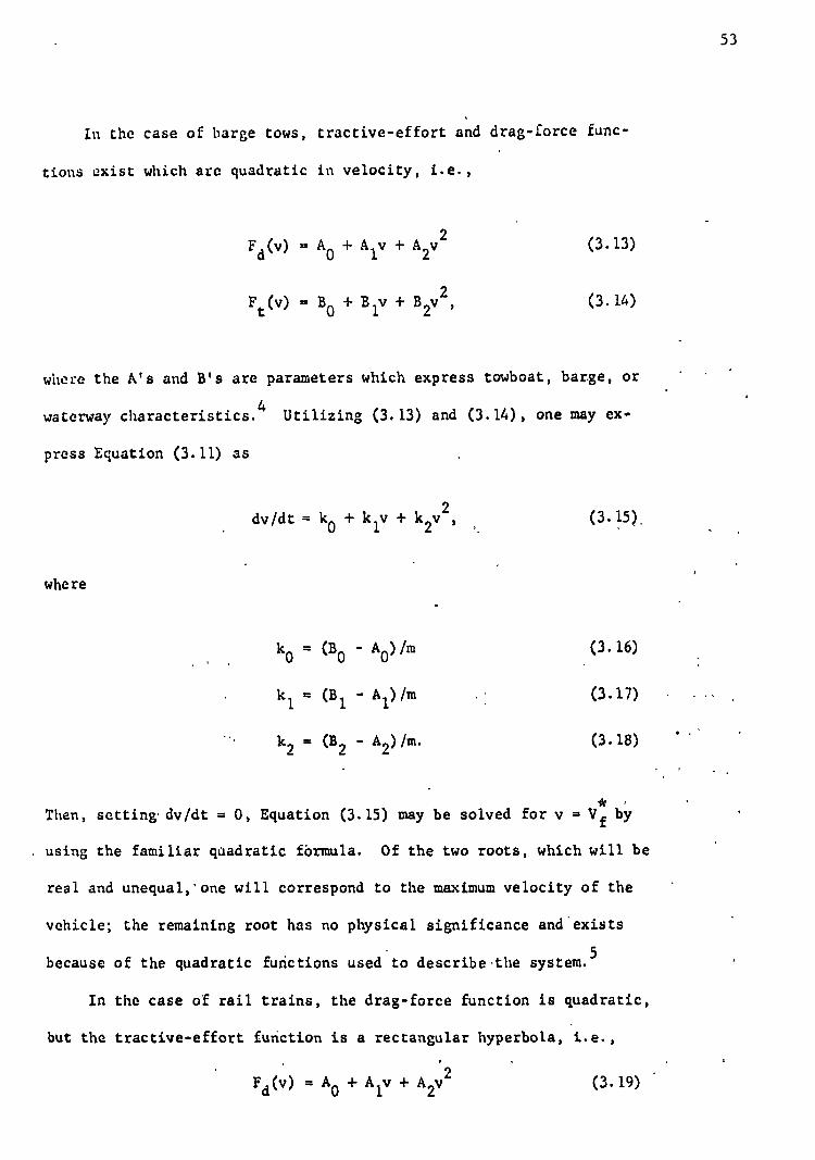
(3. 16)

(3.17)

(3.18)

Fd (v) = AO + A lv + A2v

2 (3.19)

In the case of barge tows, tractive-effort and drag-force func-

53

tions exist which are quadratic in velocity, i.e.,

Fd(v) = A

O + A

lv + A

2v2

Ft(v) = B

O + B

lv + B

2v2

'

(3.13)

(3.14)

where the A's and B's are parameters which express towboat, barge, or

waterway characteristics.4

Utilizing (3.13) and (3.14), one may ex-

press Equation (3.11) as

dv/dt =k0 +k1v+k2 v

2 '

where

k0 = (B0

- 0

k 1 = (B 1 -

k2 = (B 2 - A

2)/m.

(3.15)

* Then, setting.dv/dt = 0, Equation (3.15) may be solved for v = V f by

, using the familiar quadratic formula. Of the two roots, which will be

real and unequal,'one will correspond to the maximum velocity of the

vehicle; the remaining root has no physical significance and exists

because of the quadratic functions used to describe -the system.5

In the case of rail trains, the drag-force function is quadratic,

but the tractive-effort function is a rectangular hyperbola, i.e.,

54

Ft(v) = B/v. 6

(3.2(;)

Therefore, the equation of motion for the system is

dv/dt = i.(B/v) - (A0 + A lv + A2v2)]/m.

When dv/dt = 0, Equation (3.21) will have the following form

v3 + k

2v2 + k

1 v + k

o = 0

'

(3.21)

(3.22) '

where k = -B/A2'

k1 = A

0/A

2' and k

2 = A

1/A

2' which may be solved for 0

v = V f . Of the resulting roots, one will be real and positive and will

be the equilibrium speed of the train. 7

Acceleration State. It is desired to determine estimates of a

vehicle's acceleration time and the distance traveled during an accel-

eration from v = 0 to v = V. The formulas derived below could be

generalized to include acceleration from any one speed to any other.

However, these situations are not emphasized here, for they are ignored'

in the linehaul-process functions. If the differential equation con-

stituting the vehicle equation of motion, Equation (3.12): could be

solved for velocity as a function of time (yielding an "acceleration-

speed-time" function),8

then the above time and distance estimates

could be obtained. ,Specifically, if v = v(t) were the acceleration

curve, then, in order to:determine acceleration time, one would obtain

the inverse function t = t(v). The time required to accelerate from

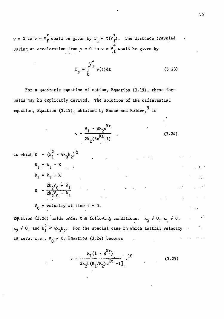
* Ey f

D = i v(t)dt. Da 6

(3.23)

55

... * v = 0 to v = V f

would be given by Ta = t(V f). The distance traveled

. *

during an acceleration from v = 0 to v = Vf would be given by

.

For a quadratic equation of motion, Equation (3.15), these for-

mules may be explicitly derived. The solution of the differential

equation, Equation (3.15), obtained by Haase and Holden,9

is

R1 - SlyKt

v - , 2k2 (Se

Kt-1)

, , .

L in which K = (k

2 - 4k k ) .2

1 0 2

R1 7 k1

- K , . .

R = k + K 2 1 .

2k2V0 + R

1 S - ' 2k

2V0 + R

2

V0 = velocity at time t . = 0. '

(3.24)

Equation (3.24) holds under the following, conditions: ko 4 0, 1( 1 4 0,

k2 4 0, and k2 > 4k,0k2. For the special case in - which initial velocity - 1

is zero, i.e.,,V0.= 0,. Equation (3.24) becomes

R1 (1 7 e ' Kt) 10 . (3.25) v=

", :,

The graphical expression of Equation (3.25) is known as an accelera-

tion speed-time curve and is given schematically in Figure 3.1.11

v

56

Figure 3.1. Acceleration Speed-Time Curve

It would be desirable to let v = Vf in Equation (3.25) and solve

for t, which would give an expression for the time required to accel-

• - erate from zero to V f . However, because of the quadratic nature of

Equation (3.15), this is not possible, i.e., an attempt to solve for

acceleration time results in an indeterminate form because the accel-

* eration speed-time relationship approaches V

f asymptotically. There-

* , fore, a velocity pV f is defined, where 0 < < 1. .Setting v = pV f

and solving Equation (3.25) for t = T a (i.e., the .time required to

acceleration from zero to 100 percent of limiting speed), one obtains

(3.26)

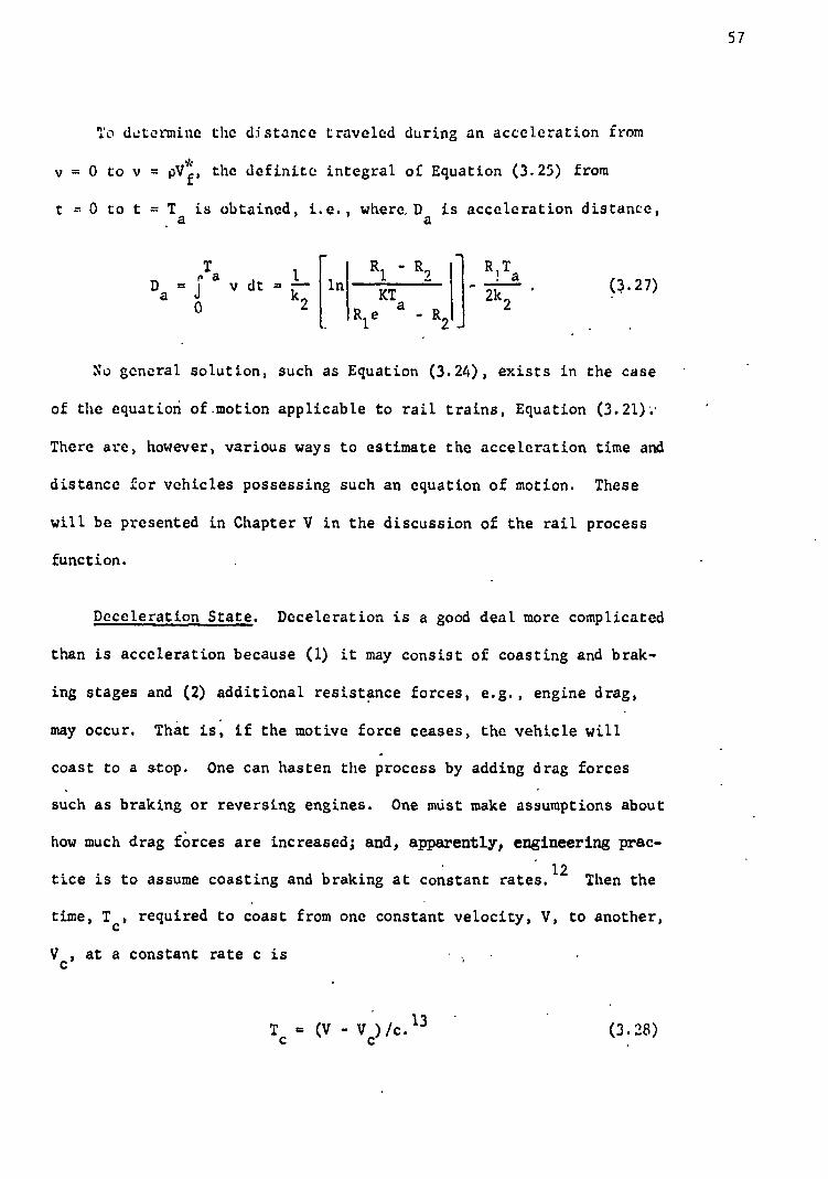
r a D = v dt = .L In a k2 0

(3.27) Ri - R9 R 1 Ta

KTa

I 2k2 e - R2 KTa IR

2

Tc = (V - V)/c. 13 (3.28)

To dotermine the distance traveled during an acceleration from

v = 0 to v = plq, the definite integral of Equation (3.25) from

t 0 to t = Ta is obtained, i.e., where. D

a is acceleration distance,

57

No general solution, such as Equation (3.24), exists in the case

of the equation of.motion applicable to rail trains, Equation (3.21) .. -

There are, however, various ways to estimate the acceleration time and

distance for vehicles possessing such an equation of motion. These

will be presented in Chapter V in the discussion of the rail process

function.

Deceleration State. Deceleration is a good deal more complicated

than is acceleration because (1) it may consist of coasting and brak-

ing stages and (2) additional resistance forces, e.g., engine drag,

may occur. That is, if the motive force ceases, the vehicle will

coast to a stop. One can hasten the process by adding drag forces

such as braking or reversing engines. One mist make assumptions about

how much drag forces are increased; and, apparently, engineering prac-

tice is to assume coasting and braking at constant rates. 12 Then the

time, T c , required to coast from one constant velocity, V, to another,

Vc, at a constant rate c is

Tb = Vc/b.

15 (3.30) '

And the distance traveled, Dc , during a coasting phase is

14 D = CV - ct)dt = VT

c - 1/2cT

c2

. C 0

58

(3.2q)

The braking phase of the deceleration may be handled in the same

manner as above. Suppose braking occurs at the rate b at the end of

the coasting phase until the vehicle comes to a stop. Then the time,

Tb'

required to brake from a velocity Vc to a velocity zero is '

The distance traveled, Db. during the braking ph.ise is given by

. T 16 , Db = j

bbT

bdt = -,21)T

b2

.

0 (3.31)

Of course the method by which a vehicle decelerates depends on

the type of vehicle and the accepted practice of its operators. De-

celeration characteristics would therefore have to be determined for

each vehicle-type studied. If, in addition, the constant rates of

coasting and braking did not turn out to be good approximations, then

other formulations, such as exponential or quadratic, could be used.

Delays and Cargo Capacity

In the preceding sections of this chapter, expressions concern-

ing maximum speed, acceleration time and distance, deceleration time

and distance were presented. It was shown above how these

relationships enter the linchaul process function. In the next two

chapters, specific forms for each of these relationships will be

derived for rail and inland water transportation modes. In order,

however, to specify a complete linehaul process function for each

mode, two further relationships are required as indicated above.

A transport vehicle may be required to stop en route for a vari-

ety of reasons. Therefore, delays must be analyzed. .There does not

appear, however, to be a general theory of delay that would be appli-

cable to all transportation modes for all types of delays. Different

transportation modes need not encounter the same types of delays, nor

will the same factor affect different modes identically. Therefore,

it seems necessary to analyze individual delays separately for each

mode. This will be done in the next two chapters.

The second relationship required to complete the process function

is the cargo-tonnage function. The cargo carrying capability of a

transportation vehicle will vary with the size, type, and number of

units comprising the whole vehicle. In addition, cargo tonnage may

vary with commodity characteristics such as weight per unit volume

and with institutional constraints such as load limits. It seems

impossible to develop . a general cargo tonnage relationship that wovld

be applicable to all modes. Therefore ., the derivation of cargo func-

tions is postponed to the next two chapters.

59

CHAPTER IV

LINEHAUL PROCESS FUNCTION FOR BARGE TOWS

Introduction

A barge tow consists of a flotilla of barges rigidly lashed to-

1 gether and pushed by a towboat. The flotilla may consist of any num-

ber of barges from one to more than forty. Barges are constructed in

a variety of models; e.g., Open and covered hopper barges, 'tank barges,

deck barges, etc'. The shape is similar for most barges a rectangular. '

steel box with two raked ends. So-called integrated tows, however, con-

, sist of square-end barges inserted between a front barge with a raked

bow and square stern and a rear barge with a raked stern and square

bow. Semi-integrated tows consist of partly integrated sections and

partly non-integrated sections. Integrated 'tows offer liss resistance

to the water and therefore travel faster than comparable non-integrated

tows for a given horsepower towboat. Integrated and semi-integrated

tows are generallyused only for trips that are to be made repeatedly;

for square-end barges when not part of an integrated unit create much

resistance and slow the tow. The barge type in most common use is the

Jumbo (195 'feet by 35 feet) open or' closed hopper with bow and stern

rakes. The analysis to follow deals exclusively with this type of

barge, but it will be shown how other types and sizes may be handled.

A trip by barge tow may be thought of as consisting of several

phases. Before the linehaul movement can begin, the barges intended

60

to comprise the flotilla must be gathered and assembled into a unit;

this process is known as "making tow." Once the tow is made, it be-

gins the trip by-accelerating to its cruising speed. The time required

to accelerate and the distance covered during acceleration depend on

the power of the towboat, the number-and draft of barges - (determined .

by size, tare weight, and cargo weighWand waterway characteristics.

If there were no delays en route the rest of the trip would take place

at the maximum cruising speed of the tow. !rows typically operate at

maximum attainable speed, although they will occasionally reduce speed

in certain situations such as light fog. It should be pointed out that .

the maximum attainable speed of the tow need not be a constant- fOr'a

trip. Rather, the speed will be greatly influenced by waterway char-

acteristics such as depth, width, and stream current, all of which

may vary over the length of a trip. For this' reason, it has become

common in the -barging industry to divide waterways into segments hav-

ing fairly uniform characteristics. 'This procedure.is adopted in the

following analysis-to -account for- the variability'of waterway tharad-

teristics. .A typical trip is interrupted by many delays such as lock-

ing, bad weather, ice, and running aground, 'so that most trips do not

proceed from origin to destination at maximum attainable speed. In

addition, each stop has an acceleration and a deceleration associated

with it. When the tow reaches its destination it disassembles the

flotilla ("break tow"). While it is common practice for a towboat to ,

assemble and disassemble its own .tai; the larger ports offer assis-'

tance in the lorm of a harbor boat'. ,- The towbdat will not usually wait '

while barges are loaded or unloaded; ' • ' -

61

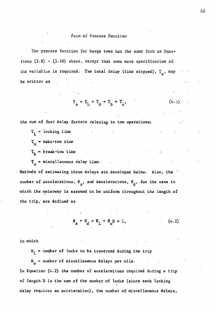
Ts =T

L +T

m +T

b +T

(4 -. 1)

N =N =N +ND+ 1, a • d L- o (4.2)

Form of Process Function

The process function for barge tows has the same form as Equa-

tions (3.8) - (3.10) above, except that some more specification of

the variables is required. The total delay (time stopped), T s , may :

be written as

62

the sum of four delay factors relating to tow operations:

TL

= locking, time

• Tm = make-tow time

• Tb

= break-tow time

To = miscellaneous delay time.

• Methods of estimating these delays are developed below. Also, the '

number of accelerations, Na' and decelerations, N d'

for the case in

which the waterway is assumed to be uniform throughout the length of

the trip, are defined as

in which

NL = number of locks to be traversed during the trip

No = number of miscellaneous delays per mile.

In Equation (4.2) the number of accelerations required - during a trip

of length D is the sum of the number of locks (since each locking

delay requires an acceleration), the number of miscellaneous delays,

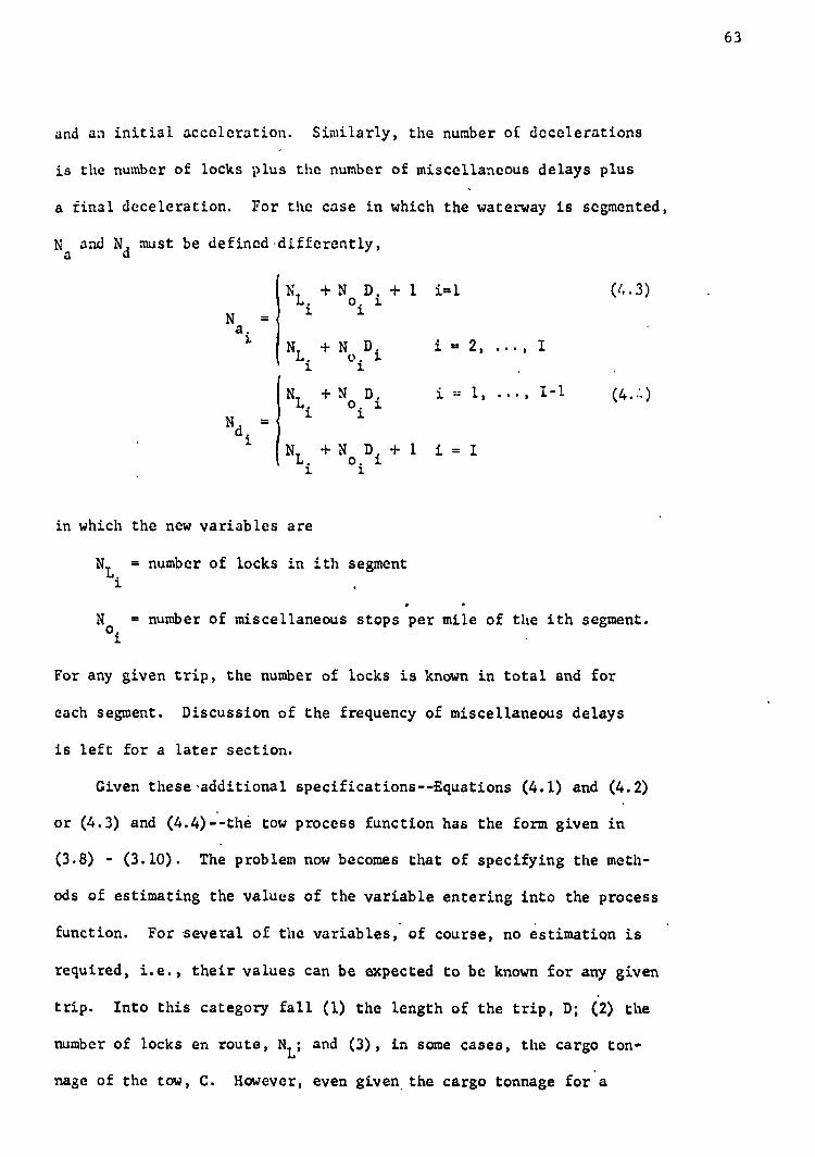
N = a. 1 ( N + N D.

L. 0i

3.3.

i = 2, ..., I

NL. +N

o.Di + 1 i=1

i i (4.3)

and an initial acceleration. Similarly, the number of decelerations

is the number of locks plus the number of miscellaneous delays plus

a final deceleration. For the case in which the waterway is segmented,

Na and N

d must be defined differently,

63

NL.

+ No.D i

i = 1, ..., I-1 1 1

NL. +N

o.Di + 1 i = I

i 1

Nd. = i

(4.:.)

in which the new variables are

NL.

= number of locks in ith segment i .

No.

= number of miscellaneous stops per mile of the ith segment. i

For any given trip, the number of locks is known in total and for

each segment. Discussion of the frequency of miscellaneous delays

is left for a later section.

Given these additionalspecifications--Equations (4.1) and (4.2)

or (4.3) and (4.4)--the tow process function has the form given in

(3.8) - (3.10). The problem now becomes that of specifying the meth-

ods of estimating the values of the variable entering into the process

function. For several of the variables, of course, no estimation is

required, i.e., their values can be expected to be known for any given

trip. Into this category fall (1) the length of the trip, D; (2) the

number of locks en route, NL; and (3), in some cases, the cargo ton-

nage of the tow, C. However, even given the cargo tonnage for a

particular . trip', that tonnage may be achieved in a variety of ways;

e.g., fewer barge& with-deeper drafts, more barges' with smaller drafts,

and different . arrangements-of 4 given number of barges. It is desir.;.

able, therefore, to have a formulation of C that will aceount for '

these possible alternatives. This is discussed in the next section.

There remain a large number of components of the tow process function

for which methods of eitimation must be developed. Functional forms

for Vf' Da,.D

d' Ta'

and Td

are developed below based upon the analysis

of Chapter III and specific tractive-effort and drag-force functions

applicable to barge tows. This chapter also develops procedures for

estimating TL, T

m, T

b, T

o, and N. Locking time is estimated by a

relatively simple queuing model. Make-tow and break-tow time are es-

timated from towboat log data by least-squares procedures. Miscel-

laneous delay 'time is estimated from aggregate delay data provided by •

a barging firm and, in addition, utilizes the analysis of a tow in

motion which was developed in an earlier section of this chapter.

Finally, an estimate of No is obtained from towboat log data. More- .

over, these formulations of the inputs to the process function will .

be amenable to changes in variables under control of the firm (e.g.,.

horsepower of towboat, draft of barges, number of barges comprising .

a flotilla, etc.) as well as variables under control of the Army ,

Corps of Engineers (e.g., waterway depth, waterway width, stream

velocity, and size of locks).

64

Wc = -605,120 + 380,000 H + 2,210 H

(125) (100)

2 (4.5)

Cargo Capacity of Tow

In the following analysis only one barge size will be used, that

of the Jumbo (195 feet by 35 feet) double-raked hopper barge. As

was mentioned earlier, this particular barge is probably the most.

common model in use today. Nevertheless, the general applicability

of the analysis to follow is restricted somewhat by the above assump-

tion, however, perhaps less than might be thought. Most double-

raked barges, no matter what type and size, have essentially the same

hull shape. The most important differences among barge types are

tare weight. These differences introduce little difficulty into the

following analysis. It will be seen that the operative variables

with respect to the flotilla of barges are (1) length of flotilla, L;

(2) breadth of flotilla, B; and (3) draft of flotilla, E., Given L

and B and the barge type comprising the flotilla, one can easily de-

termine the number of barges in the flotilla, whether the barge type

is Jumbo hopper or some other. Moreover, there is a regular relation-

ship between the cargo weight and the draft of a barge, which can be

estimated quite accurately by a second degree polynomial in H. For

the Jumbo hopper barge, the relationship is

65

in which W c = cargo weight of barge, in pounds; H = draft of flotilla,

in feet; coefficient of determination = . 0.99; standard errors are

given in parentheses; and sample size was 109. Equation (4.5) was

ostimated from a capacity cable for the Jumbo hopper barge.2

From

capacity tables for other barge types and sizes, similar relationships

could be developed. So, knowing the length, breadth, and draft of a

flotilla of barges of given size and type, one can determine the

cargo capacity of the flotilla; or, in symbols,

C = C(L, B, H) = Nb (L, B).W c (H) = Nb (-605,120 + 380,000 H (4.6)

+ 2,210 H2)

in which N . = the number of barges in the flotilla, as determined by the length and breadth of the flotilla

Wc = cargo weight of a barge as determined from Equation (4.5)

or similar relations for other barge types and sizes.

Formulating the cargo capacity of the flotilla in this manner

brings out three implicit assumptions which are somewhat restrictive

and intractable. They are: (1) the barges comprising the flotilla are

of the same size and type; (2) the configuration of barges in the

flotilla is rectangular; and (3) all barge's in the flotilla are loaded

to the same draft. These assumptions are not always fulfilled in

practice. Nevertheless, it will be argued below that these assump-

tions do not adversely affect the tow speed prediction equation.

66

Analysis of Tow in Motion

Introduction. In order to apply the relationships developed in

Chapter III, tractive-effort and drag-force functions must be obtained

for barge tows. Several drag-force functions (generally called re-

sistance functions for water vehicles) have been developed. These

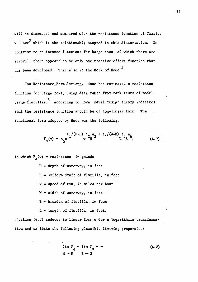
lim Fd = lim F

d =

H D B --W

(4.8)

will be discussed and compared with the resistance function of Charles

W. Howe3 which is the relationship adopted in this dissertation. In

contrast to resistance functions for barge tows, of which there are

several, there appears tobe only one tractive-effort function that

has been developed. This also is the work of Howe.4

Tow Resistance Formulations. Howe has estimated a resistance

function for barge tows, using data taken from tank tests of model

barge flotillas.5 According to Howe, naval design theory indicates

that the resistance function should be of log-linear form. The

67

functional form adopted by Howe was the following:

a /(D-H) a h a3 4

+ a,/(W-B) L a5

B a6

1 , F

d(v) = a

0 e v

(4.7) .

in which Fd(v) = resistance, in pounds

D = depth of waterway, in feet

H = uniform draft of flotilla, in feet

' v = speed of tow, in miles per hour

W = width of waterway, in feet •

B = breadth of flotilla, in feet

L = length of flotilla, in feet.

Equation (4.7) reduces to linear form under a logarithmic transforma-

tion and exhibits the following plausible limiting properties:

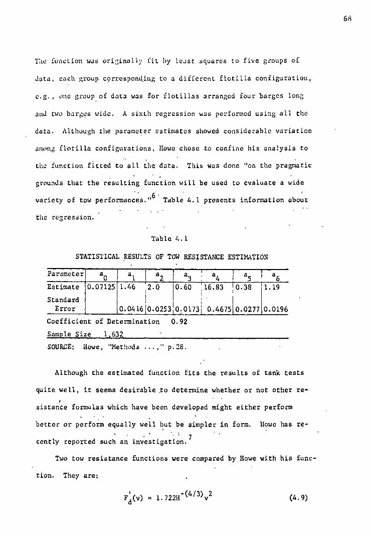
The function was originaliy fit by least squares to five groups of

data, each group corxespond,ing to a different flotilla configuration,

e.g., one group of data was for flotillas arranged four barges long

and two barges wide. A sixth regression was performed using all the

. data. Although the parameter estimates showed considerable variation

among flotilla configurations, Howe chose to confine his analysis to

the function fitted to all the data. This was done "on the pragmatic

grounds that the resulting function will be used to evaluate a wide

- variety of tow performances.'

,6 Table 4.1 presents information about

the regression.

Table 4.1

STATISTICAL RESULTS OF TOW RESISTANCE ESTIMATION

i 1 Parameter ao

al a2 1 a3 . a4 1 a5 a6

Estimate 0.07125 1.46 2.0 10.60 :16.83 !0.38 1.19

Standard 1 I

Error 0 . 041610 . 0253 ! 0 . 01731 0.467510.0277 0.0196 , 1 Coefficient of Determination 0.92

Sample Size L632

SOURCE: Howe, "Methods ...," p.28.

Although the estimated function fits the results of tank tests

quite well, it seems desirable .to determine whether or not other re-

sistance formulas which have been developed might either perform

better or perform equally well but be simpler in form. Howe has re-

cently reported such an investigation. 7

Two tow resistance functions were compared by Howe with his func-

68

tion. They are:

Fd(v) = 1.722H -(4/3)v2 (4.9)

Fd (v) = 100.838 (A/L)v

2,

and

69

in which A is gross displacement of flotilla, in short tons; the

other variables are as defined before. The F' function is due to

Langbein,8 and the F" function is the work of Rouse.

9

Howe tested all three of the functions against tank test data,

using the reported model resistance as the norm. In all cases in

volving deep-water tests, Howe's function was markedly superior to

the other two. .Specifically, the following statistics were all lower

for the Howe function than for the other two: (1) the arithmetic

average difference of predicted from actual, (2). the average absolute

difference of predicted from actual, and (3) the maximum absolute

difference of,predicted from actual: For example, the average-abso-

lute deviations ranged from 11 to 25 percent of the data-set averages

for Howe's function and over 100 percent of the data-set averages for

the others. Shallow-water comparisons could only be made against

Langbein's functions since Rouse's function applies solely to deep-

water operations. Here, again, Howe's resistance function appears

decidedly superior; in all cases the three statistics were markedly

lower for the Howe-function predictions than for the Langbein-

function predictions.

In the process of performing the above tests, Howe discovered

that his resistance function consistently produced large errors

for those cases in which flotilla width approached channel width, in

which flotilla draft approached channel depth, or in which speeds

were greater than 11 miles per hour. Using the data subseta for which

v 11 miles per hour and W maximum (28, 225 feet), Howe modified

his resistance fuuction as follows:

Fd(v) = 0.072891.46/(D-H)

v2.0HL

0.38E1.19

. (4.11)

The modified function performed well on the test data subsets for

which the above conditions were met. The Fd function as given by

Equation (4.11) is used in the remainder of this chapter.

Howe has further refined his resistance function to account for

a factor known as slope-drag.10

When a tow is proceeding upstream

there is a loss of speed, in addition to that due to the stream cur-

rent, because the unit is actually going uphill. The reverse is the

case for downstream movements. Howe feels that the slope-drag adjust-

ment could become important for tow operations on waterways with a

steep gradient. This may well be true, and, if so, the slope-drag

adjustment could easily be incorporated into the process function;

however, it is not used here.

Tractive-Effort Function. Howe has estimated a tractive-effort,

or effective-push, function for barge tows. It has the following

form .

70

Ft(v) b HP + b

2HP 2 + b

3HP.D + b

4v2 + b r v.HP.

1

in which Ft(v) ='tractive-effort, or effective-push, in pounds

HP = rated brake horsepower of towboat

D = depth of waterway, in feet

v .= speed of tow, in miles per hour.

(4.12)

The 'a:2 term allows for increasing or decreasing effectiveness of

horsepower in determining push. The cross-product term, HP.D, re-

fleets the fact that gains from greater depth are greater for larger •

boats and vice versa. The v.H2 term reflects the fact that bF/bv,

evaluated at a given speed, is a decreasing function of horsepower, a

fact that was determined from plots of the data. Waterway width was

not found to be an important variable in determining effective push.

Equation (4.12) was estimated by least squares; Table 4.2 con-

tains information about the estimates.

Table 4.2

STATISTICAL RESULTS OF TOW EFFECTIVE-PUSH ESTIMATION

Parameter i 1) 1 I b2 b3 b4 ! b5 1

itiirae -t31.82i 0:0039 : 0.379 -172.05 . -1.14 -_---

Standard ;

Error: i 0.961 0.0003 1 0.058i 11.50 1 0.07 Coefficient of Determination 0.98

Sample Size 145

SOURCE: Howe, 'Tlethods ...," p.29.

The data used in the estimation of Equation (4.12) were obtained

from barging firms and contained observations on eleven towboats rang-

ing in horsepower from 500 to 3500. Observations included a range of

waterway depths of from 15 to 26 feet and a range of towboat speeds

up to 14 miles per hour. While the estimation is quite good, it is

impossible to compare the function with others as was done for the

resistance function, for there are no others. Rather, the predictive

ability of the speed function determined from the resistance and

11

B2

= 172.05. (4.14)

effective-push functions will be examined below. The speed function

is derived in the next section, and some tests are presented in a

following section,

Constant Velocity State. Given resistance and tractive-effort

functions, the results obtained in Chapter III may be applied to barge

tows.

Equation (3.13), the quadratic drag-force function, becomes Howe's

resistance runction when

72

A0 = 0

Al = 0 •.i

A2 = 0.07289e1.46/(D-H)

H0.6+50/(W-B)

L0.38

B1.19

. . ( 4. 1 3 )

Equation (3.14), the quadratic tractive-effort function, becomes

Howe's effective-push relation when .

Bo

= 31.82HP - 0.0039HP 2 + 0.38HP'D

B 1 = 1.14HP

Defining

1. 1 .. k = --.) = --(31.82HP - 0.0039HP 2

+ 0.38Hp.D) 0 mOm . .

1. 1 k 1

= —.3 = —.(-1.14HP) m 1 m

= —1 1.

2 1t

, k -172.05 - 0.07289e

2 m = — m (4.15)

= Vf

=V - 6S6Sw

(4.17)

73

then from the earlier discussion the limiting velocity of a tow is

given by

* (k

1 + K)

1 + J) V - - f 2k2 2j2

(4.16)

where

2 K = (k

2 - 4k

0 k 2 )2 and J (j

1 - 4j

0j2) 1/2 , which is the familiar

1

quadratic formula. Note that the m's cancel out.

Equation (4.16) gives the speed of a tow relative to the water.

In order to obtain the speed relative to the land, V f , an adjustment •

for stream current is. required;

in which

Sw

= stream velocity, in miles per hour

I upstream 6

-1 downstream.

Tests of Tow Speed Function. Although the effective-push and

drag-force functions estimated by Howe seem to be quite good statis-

tically and although the resistance function seems to be better than

any other available, it remains to be shown that the speed function

is capable of approximating speeds of tows under actual working condi-

tions. In addition, several simplifying assumptions were made: uni-

form waterway depth, width, and stream velocity; uniform draft of

barges comprising the flotilla; and rectangular configuration of

ilotilla. These assumptions will not always.:be realized in ptactice,

anj one would like to know whether the formula can be applied without .

resulting in large errors.

Howe's. •speed function has been applied ta two sets of data. The

first is composed of tests performed by the Army Corps of Engineers

with a 1500-horsepower towboat pushing tows of 4 and 8 fully integrated

and semi-integrated barges 'These tests were performed in 1947 on

reaches of the lower Illinois and Upper Mississippi. All variables

necessary to the application of Howe's formula were carefully recorded

by Corps personnel, except for stream velocity. Stream velocity was

assumed to be 2 feet per second or 1.36 miles per hour. This assump-

tion was based on discussions with two Corps hydrology experts who in-

dependently advanced this figure as a good "approximate average." A

better estimate of stream velocity would require obtaining the dis-

charge of the waterway (in cubic feet per second), obtaining an approxi-

mation of the cross section of the waterway (in square feet), and di-

viding the latter into the former. The resulting velocity in feet per

second could then be transformed into a mile-per-hour equivalent.

While such a calculation is possible, it would add little, for the

tests all occurred within a few days of one another over the same

stretches of the two waterways involved. These data contained 24 ob-

servations, half upstream and half downstream. The ranges of the vari-

ables are shown below:

(1) ifor-sepOWCI-1- 1500— " "1 • , (21-1.epgth of,flotilla: ..390 feet and 780 feet

Zet.a 1.111"l a teLL

0 ialyS

eet Or one 11 (3) r)readth of tlotfta: . / 'f one .v:. •

• (A) Width of channel: • 700 feet-1500 feet servaT-4ons. ialz - (7), Stream velocity: 1.36 miles per hour (assumed).

ar , •

74

.RS•_fjoti7.1.4; (5)'- Depth - of igAer . 91".S.-1 le'ety-'36.15" feet

Vf

-0.35 + 1.01V f ,

(0.87) (0.11)

(4.18) .

75 .

As a test of the relationship between actual speeds attained by

the tows, V, their predicted speeds; V, straight line was fit

r, , f'

to the data points by the method of least squares. As far as deter-

mining the extent of linear correlation between the two sets of speeds,

it is immaterial which variable is used as the "dependent" and which

the "independent" variable. However, if hypothesis testing and pre-

diction are desired, then there are good statistical reasons for using

a V f as the independent variable and V r as the dependent variable. 12

If Equation (4.17) provided a perfect prediction of actual speed

and if actual speed were measured without error, the least-squares

line would possess a slope coefficient of unity and an intercept co-

efficient of zero. This statement is strictly true only if all tows

used to generate the actual speeds were non-integrated (i.e., all

barges comprising the flotillas were double-raked), for this was the

condition under which Howe's resistance function was estimated. Since

the prototype data are for fully and semi-integrated tows, one would

expect a priori a negative intercept, i.e., the prediction equation

will consistently underestimate the actually attained speeds.

The estimated relationship is as follows:

with (1) coefficient of determination= 0.79 (2)standard error of estimate = 0.69 (3) sample size = 24 (4)standard errors shown in parentheses under the estimated

coefficients.

11.

A V f = V f + .35. (4.12) .

Upon testing the hypotheses indicated above, it was found that

the slope coefficient was not significantly different from unity .

(t = 0.09) and that the intercept coefficient was not . significantly

different from zero (t = 0.40). Both of these t values are so small

that the null hypotheses could not be rejected at any conventional-

level of significance. As was expected on a priori grounds, the pre-

diction equation consistently underestimated the actual values by

about 0.35 miles per hour. As an illustration of how the tow-speed

prediction equation could be corrected for different tow types, the

following relation could be used to estimate the speed of fully and

semi-integrated tows:

76

If such a correction were going to be used in practice, it would be

desirable to have many more observations over a wider range of.vari-

ables than the data provided. In addition, one would undoubtedly

wish separate adjustments for fully integrated tows as against semi-

integrated tows. Nevertheless, this serves as an example of the

applicability of the previous analysis to different tow types.

To provide tests of his function, Howe obtained a set of 224

movements gathered from towboat log books of Ohio River operations.13

The log data gave actual tow characteristics--length, breadth, and

draft--which are required for the use of Equation (4.16). Average ..

tow speeds were calculated from the log data because the speed . of

the tow was not recorded directly in the logs. Port delays and

Vf = 2.12 + 0.94Va

(0.27) (0.06)

(4.20)

77

waiting time at locks were excluded from the trip times, but unfor-

tunatdly, time actually spent in locks could not be excluded.

The range of variables was as follows:

(1)Horsepower of towboat: 1400-3200 (2)Length of flotilla: 350 feet-1180 feet (3)Breadth of flotilla: 35 feet-135 feet (4)Draft of flotilla: 1 foot-9.3 feet (5)Depth of water: 13.2 feet, 14.5 feet, and 18.3 feet

(assumed) (6)Width of channel: 500 feet and 550 feet (assumed) (7)Stream velocity: 0.61 miles per hour-4.0 miles per

hour (assumed).

The values of the last three variables for each of the 224 observa-

tions had to be assumed, for there were no data in the logs pertain-

ing to depth, width, and stream velocity of the waterway. 14

As before, predicted speed was regressed on actual speed with

the following results:

in which (1) coefficient of determination = 0.49 (2) standard error of estimation = 2.19 (3) sample size = 224 (4)standard errors shown in parentheses under the

estimated coefficients.

In this case, as in the other, the slope coefficient is not signifi-

cantly different from unity (t = 1) for any conventional level of

significance. Of course, the intercept is significantly greater

than zero (t = 7.85) which was to be expected since locking time was

included in the average speed observations.

These two sets of data fail to provide adequate tests of the hy-

pothesis that the intercept term in the regression equations is zero,

for in the first case tows were semi- and fully integrated and in

the second locking time was included. An ideal test would involve

obtaining carefully collected observations (like those of the proto-:

type data above) on operations of non-integrated tows composed of .

Jumbo hopper barges. Nevertheless, the results of the tests ard.in ,

the right direction: the intercept being negative for the case in

which it was expected the predictions would understate actual speeds

and positive for the case in whiCh overstatement was expected. The '

two sets of data do confirm the unit slope of the fitted line. This

confirmation indicates that the tow speed prediction equation, Equa-

tion (4.17), forecasts actual speeds without.bias.

In summary, the tests performed and reported here seem to pro- ,

vide convincing evidence in favor of the predictive quality of Equa-

tion (4.17). Conclusive evidence has by no means been presented,

however. Better data would be needed for that. In addition, a

method has been demonstrated for adapting the model to fit situations

other than those for which it was designated, as illustrated-by Equa-

tion (4.19). . '

On the basis of the very good statistical estimation equations

derived by Howe for the resistance and tractive-effort functions of

barge tows, on the basis of the favorable comparative tests of Howe's

resistance function with others, and on the basis of .the predictive

quality of the speed function as indicated by the previous analysis,

there seems sufficient evidence favorable to the continued use of

Howe's resistance and tractive-effort functions in the analysis of'

tow movements.

78

Acceleration and Deceleration. The acceleration time and dis-

tance formulas were presented in Chapter III above and are given in

Equations (3.26) and (3.27). Using the definitions of k 0, k k

2,

and K given in (4.15) and an appropriate value of these formulas

may be applied to barge tows. Since Lows typically operate at full •

throttle,15 accelerat:ons from velocities other than zero to veloc-

ities other than V f were not considered.

The method of obtaining the factor ; was as follows: Equation

(3.25), as applied to barge tows, was plotted for three sets of tow-

waterway characteristics. These graphs are shown in Figures 4.!,

4.2, and 4.3. A velocity of 0.99Vf seemed to include most of the

time required for acceleration while not including a large amount of

time on the asymptotic portion of the acceleration curve.

Examples of acceleration times and distances as predicted by

Equations (3.26) and (3.27) are given in Table 4.3 for five differ- ,'

ent flotilla combinations. In all five cases the waterway character-

istic a are assumed to be the same, viz., width equal to 225 feet and

depth equal to 12 feet. These values could easily be changed; the

particular values presumably typify the Illinois Waterway.16

Horse-

power of the towboat was assumed to be 3000 and flotilla draft was

assumed to be 8.5 feet. These also could be varied. Five flotilla

sizes were assumed: (1) a four-barge flotilla, arranged two barges

long and two barges wide (2 x 2); (2) a nine-barge flotilla, arranged

three barges long and three barges wide (3 x 3); (3) a twelve-barge

flotilla, arranged four barges long and three barges wide (4 x 3); .

(4) a fifteen-barge flotilla, arranged five barges long and three

79

HP 3000

- 12

- 225

• H - 8.5

L - 390

- 70

V. 6.19

.99V1 - 6:13

a

0

3.5 4.0

/

VI

;

• I

0.5 1.0 1.5 2.0 2.5 3.0 Time (min.)

. •

Fig. 4.1 7- Acceleration-Speed-Time Curve for Barge Tow .

(3000-Horsepower Towboat, 4 Jumbo Open-Hopper Barges)

80

- . •

0 CJ

2.0

HP 3000

D 12

IV - 225

H - 8.5

L 585

B 105

2 3 4 Time (mm.)

1 5

o

4. 5 1■110 Vf

4.0

3.5

3.0

1.5 4.46

.99 V1 4.41

1 .0

0.5

Fig. 4.2 -- Acceleration-Speed-Time Curve for Barge Tow ' (3000-Horsepower Towboat., 9..lumbo Open-Hopper Barges)

81

3.5

3.0

1.5

5.. 2.0

7,

1 .5

HP . 3000

D = 12

, 225

H - 8.5

L - 1170

B = 105

VI = 3.99

.99V1 = 3.95

1 1 1 1 II 1 1 2 3 4 5 6

Time (min.) 1

■••••••• 4.0

7 8

1 .0

0.5

Fig. 4.3 -- Acceleration-Speed-Time Curve for Barge Tow (3000-Horsepower Towboat, 18 Jumbo Hopper Barges)

82

2 x 2 3 x 3 4 x3 5 x 3 6 x 3

2.75 1,127

4.15 1,218

5.23 1,464

6.26 1,690 _1,901 7.25

bar.,-,eb wide (5 x 3); and (5) an eighteen-barge flotilla, arranged sic .

barges long and three barges wide (6 x 3). The configurations corre-

spond to typical tows operating on the Illinois Waterway.

Table 4.3

ACCELERATION TIMES AND DISTANCES FOR BARGE TOWS

83

Flotilla Configuration Acceleration

(no. barges long Time by no. barges wide) 1 (min.)

Acceleration Distance (ft.)

The figures in Table 4.3 seem to correspond well with the industry

rule of thumb that a tow can accelerate from a stop to full speed in

1'1-2 times the length of the tow.17

Moreover, and most importantly,

the figures. indicate the relative insignificance of acceleration time

and distance per acceleration. Since the frequency of stops en route

is not likely to be large, as will be shown below, the error introduced

by ignoring acceleration altogether is slight. Moreover, since tows .

typically decelerate by reversing towboat engines at full throttle,

deceleration time and distance will be even less than acceleration

time and distance; the rule of thumb in this case is that it requires

1-1 1i times a tow length to bring the tow to a stop from full speed.18

The insignificance of acceleration time and distance, as discussed

above, applies a fortiori to the case of deceleration of barge tows.

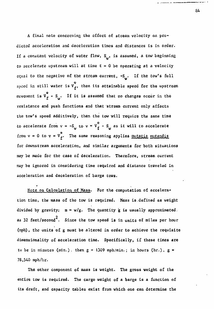
......•••••••••••••••••-•• ■•• •....• 1

A final note concerning the effect of stream velocity on pre-

dicted acceleration and deceleration times and distances is in order.

If a constant velocity of water flow, S w , is assumed, a tow beginning

to accelerate upstream will at time t = 0 be operating at a velocity

equal to the negative of the stream current, -Sw. If the tow's full

speed in still water is V f , then its attainable speed for the upstream

movement is Vf

- Sw. If it is assumed that no changes occur in the

resistance and push functions and that .stream current only affects

the tow's speed additively, then the tow will require the same time

to accelerate from v = -Sw to v = V f - S

w as it will to accelerate

from v = 0 to v = Vf. The same reasoning applies mutatis mutandis

for downstream acceleration, and similar arguments for both situations

may be made for the case of deceleration. Therefore, stream current

may be ignored in considering time required and distance traveled in

acceleration and deceleration of barge tows.

Note on Calculation of Mass. For the computation of accelera-

tion time, the mass of the tow is required. Mass is.defined as weight

divided by gravity: m = wig. The quantity k is usually approximated.

as 32 feet/second2. Since the tow speed is in units of miles per hour

(mph), the units of g must be altered in order to achieve the requisite

dimensionality of acceleration time. Specifically, if these times are

to be in minutes (min.). then g = 1309 mph/min.; in hours (hr.), g =

78,540 mph/hr.

The other component of mass is weight. The gross weight of the

entire tow is required. The cargo weight of a barge is a function of

its draft, and capacity tables exist from which one can determine the

84

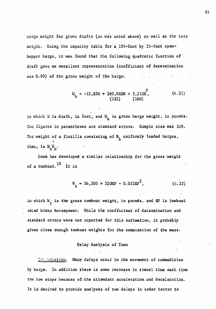
cargo weight for given drafts (as was noted above) as well as the tare

weight. Using the capacity table for a 195-foot by 35-foot open-

hopper barge, it was found that the following quadratic function of •

draft gave an excellent representation (coefficient of determination

was 0.99) of the gross weight of the barge:

85

2 Wb

= -15,830 + 380,060H + 2,21011, (125) (100)

(4.21)

in which H is draft, in feet, and W b is gross barge weight, in pounds.

The figures in parentheses are standard errors. Sample size was 109.

The weight of a flotilla consisting of Nb uniformly loaded barges,

then, is NbWb.

.

Howe has developed a similar relationship for the gross weight

of a towboat.19

It is

Wt = 24,300 + 35011P - 0.02111P

2, (4.22)

in which Wt

is the gross towboat weight, in pounds, and HP is towboat

. rated brake horsepower. While the coefficient of determination and

standard errors were not reported for this estimation, it probably

gives close enough towboat weights for the computation of the mass.

Delay Analysis of Tows

Many delays occur in the movement of commodities

by barge. In addition there is some increase in travel time each time

the tow stops because ofthe attendant acceleration and deceleration.

It is desired to provide analyses of tow delays in order better to

Delay Category

Percentage of Active

Time

predict the time required for travel by barge between origin and des-

tination.

In subsequent usage delay will mean any period of time during -

which the tow is not moving. Such delays result from a variety of '

factors. One classification of delays and the relative importance

of them is given in Table 4.4

Table 4.4

PERCENTAGE OF ACTIVE TIME ACCOUNTED FOR BY VARIOUS DELAYS FOR NINETEEN TOWBOATS,

1960-64

86

1. Locking: waiting for and being serviced by a lock 7.29

2. Weather: unnavigable weather conditions such as fog, ice, and snow 2.35

3. Repair: Minor repairs (major overhauls not included) 3.94

4. Supplies: taking on supplies 0.65

5. Waiting barges: Frequently barges are transferred from one towboat to another. When one of the boats arrives late, •the other is delayed. 1.87

6. Load and unload: towboat waiting while barges are loaded and unloaded 0.75

7.Bridges: waiting for lift bridges to operate 0.12

8. Running aground 0.24

9. Make and break tow: assembly of tow at beginning of trip and disassembly at end 3.16

10.Other: includes waiting for orders, waiting for arrival of crew, and wait- ing for clear channel 3.91

SOURCE: Common carrier barge firm which requested not to be identified.

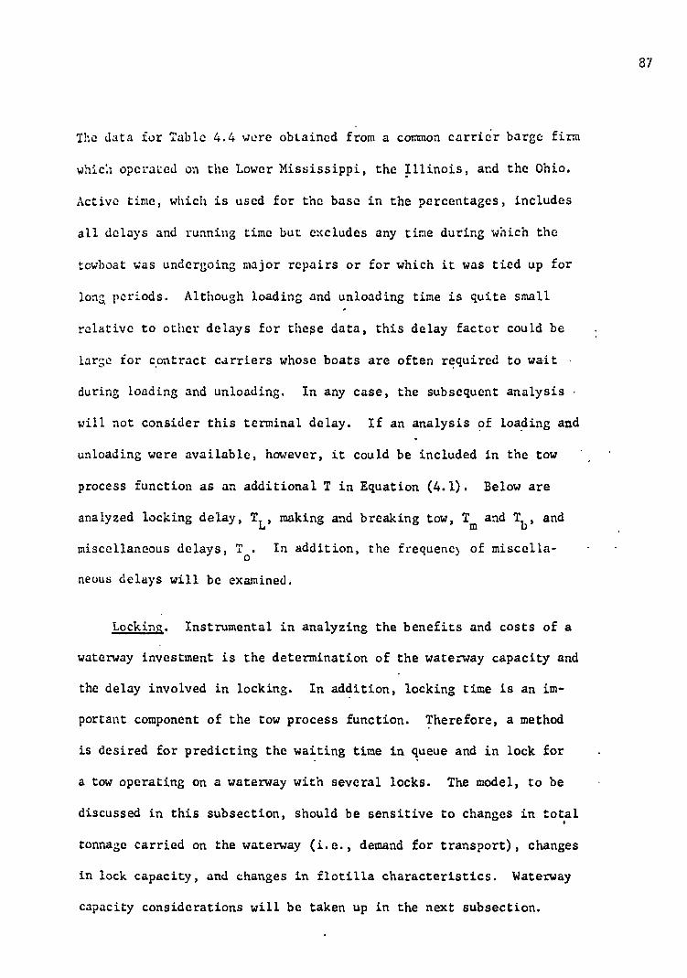
The data for Table 4.4 were obtained from a common carrier barge firm

which operated on the Lower Mississippi, the Illinois, and the Ohio.

Active time, which is used for the base in the percentages, includes

all delays and running time but excludes any time during which the

towboat was undergoing major repairs or for which it was tied up for

long periods. Although loading and unloading time is quite small

relative to other delays for these data, this delay factor could be

large for contract carriers whose boats are often required to wait .

during loading and unloading. In any case, the subsequent analysis •

will not consider this terminal delay. If an analysis of loading and

unloading were available, however, it could be included in the tow

process function as an additional T in Equation (4.1). Below are

analyzed locking delay, T L , making and breaking tow, Tm and Tb , and

miscellaneous delays, T. In addition, the frequenc) of miscella-

neous delays will be examined.

Locking. Instrumental in analyzing the benefits and costs of a

waterway investment is the determination of the waterway capacity and

the delay involved in locking. In addition, locking time is an im-

portant component of the tow process function. Therefore, a method

is desired for predicting the waiting time in queue and in lock for

a tow operating on a waterway with several locks. The model, to be

discussed in this subsection, should be sensitive to changes in total

tonnage carried on the waterway (i.e., demand for transport), changes

in lock capacity, and changes in flotilla characteristics. Waterway

capacity considerations will be taken up in the next subsection.

87

P(t) (X*O ne-\*t

- n! (4.25)

Given the tonnage, 0, to be carried on the waterway and the ton- _

nage, C, of an optimal or average tow, one can determine the number

of trips required to achieve 0, viz.,

X = 0/E, (4.23)

where X is the number of trips per time period. A trip is defined as

any point-to-point movement. While X is the number of trips required

to produce a waterway tonnage of 0, there may not be a one-to-one re-

lationship between X and the number of trips by tows operating on the

waterway because of the possibility of trips involving empty tows.

This consideration may be accounted for by adjusting k by the factor

(1 + p), where p represents the percentage of unproductive trips (i.e.,

with unlcadedbargee) which requires an empty barge backhaul. Let ?.*

be the adjusted trip rate:

X* = (1 + p)X, (4.24)

where 0 p 1. .

It is assumed that the possibility of a tow's being at any given

point on the waterway is independent of the time since the last tow

was there. This implies a Poisson distribution for the arrival of

taws; that is, the probability that n arrivals occur within an inter-

' val of time of duration t is given by .

88

This probability distribution corresponds to completely random arriv-

als. The mean of the distribution is '4* and is identified with the

':k discussed above. In queuing theory Equation (4.25) is called an

arrival distribution and is an important input to a model capable of

.20 predicting waiting time.

Suppose a lock exists through which all tows must pass in order

to complete a trip. The number of tows that are handled by the lock

in a given period of time is called the service rate of the lock. .

Several operations are included in the "service" of a tow through a

lock: (1) preparation of the lock, (2) rearrangement of the tow for

locking, (3) entrance of tow, (4) locking, (5) rearrangement of tows

for departure, and (6) departure of tow. Since . each of these opera-

tions is likely to be stochastic in its duration, it is plausible to .

treat the service rate of the lock as a, random variable. Specifically,

it is assumed that the service rate has a Poisson distribution whose

mean, the average service rate, is denoted by p. Such a distribution'

implies that the probability of prolongation of service is independent

of how long ago the service began. Many service operations exhibit

a Poisson distribution, e.g., telephone conversations, grocery check-

out facilities, various repair operations, etc. 21 In addition, use

of a Poisson service rate coupled with a Poisson arrival rate permits

the resulting queuing model to be relatively simple. Furthermore, it

will be possible to judge the quality of the'resulting model to see

if undue error is caused by these assumptions.

It seems -likely that p, the average service rate, can be closely

approximated for a proposed lock by experience with locks already in ,

vi

1 TL L - X* (4.26)

X* T - Lq p(p X*) ' (4.27)

existence. For example, the locks on the Illinois River have been

intensively studied, and their service rates are likely to apply to

similar newly-built locks on other waterways. A complicating factor

here concerns single versus multiple locking procedures. It is typi-

cal, for example, on the Illinois River for tows to -be composed of

16 barges. Since the locks are 600 feet by 110 feet, the tow is

locked in two passes, the first consisting of 9 barges, the second of

7 barges and the towboat. It would be desirable therefore, to know

the service rate of the lock for each type of locking procedure, i.e.,

single, double, or triple (though the latter is not common practice

at this time). One could then evaluate different locking procedures.

This sort of information should not be very difficult to obtain. In

any case, p is taken as given and no analytical procedure as to how

it might be estimated is presented here.

Given X* and p and assuming Poisson distributions for the arrival

rate and service rate, queuing theory may be used to derive an esti-

mate of the expected waiting time in queue and in service for a tow

at a lock. In particular, the relevant formulas are 22

90

and

where TL

is the expected total locking time and TLq

is the expected

waiting time in queue. The expected service time is given by the re-

ciprocal of p. So far the analysis is applicable only to waterways

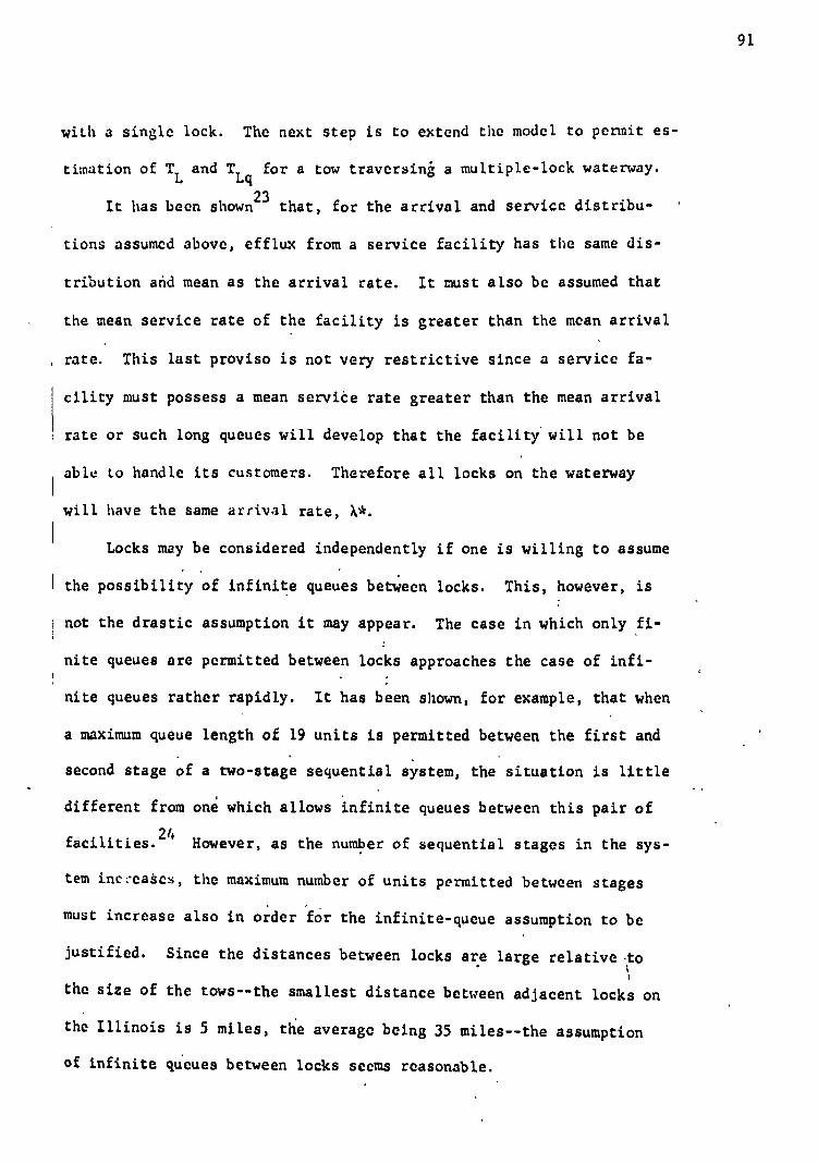
with a single lock. The next step is to extend the model to permit es-

timation of TL

and TLq

for a tow traversin; a multiple-lock waterway.

It has been shown23

that, for the arrival and service distribu-

tions assumed above, efflux from a service facility has the same dis-

tribution and mean as the arrival rate. It must also be assumed that

the mean service rate of the facility is greater than the mean arrival

rate. This last proviso is not very restrictive since a service fa-

cility must possess a mean service rate greater than the mean arrival

! rate or such long queues will develop that the facility' will not be

able to handle its customers. Therefore all locks on the waterway

will have the same arrival rate, X*.

Locks may be considered independently if one is willing to assume

1 the possibility of infinite queues between locks. This, however, is

i not the drastic assumption it may appear. The case in which only fi-

nite queues are permitted between locks approaches the case of infi-

nite queues rather rapidly. It has been shown, for example, that when

a maximum queue length of 19 units is permitted between the first and

second stage of a two-stage sequential system, the situation is little

different from one which allows infinite queues between this pair of

24 facilities. However, as the number of sequential stages in the sys-

tem inc:eaSes, the maximum number of units permitted between stages

must increase also in order for the infinite-queue assumption to be

justified. Since the distances between locks are large relative to

the size of the tows--the smallest distance between adjacent locks on

the Illinois is 5 miles, the average being 35 miles--the assumption

of infinite queues between locks seems reasonable.

91

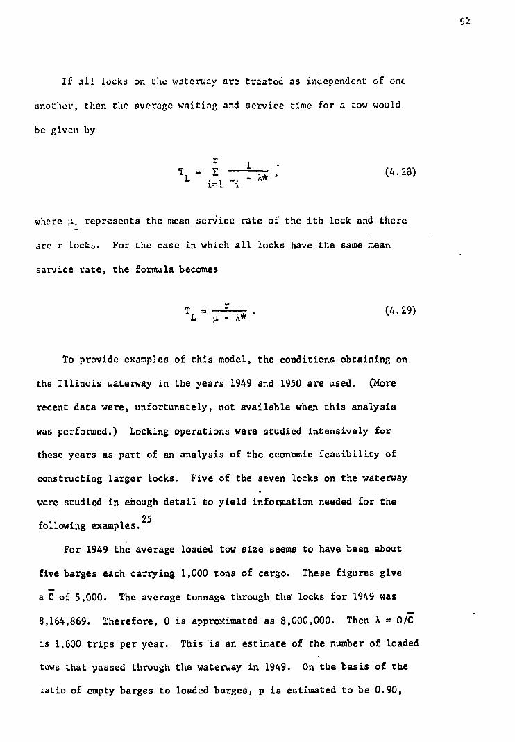
TL

1 r i=1i

(4.28)

(4. 29) TL - X* '

If all locks on the waterway arc treated as independent of one

another, then the average waiting and service time for a tow would

be given by

92

where ui represents the mean serNiice rate of the ith lock and there

arc r locks. For the case in which all locks have the same mean

service rate, the formula becomes

To provide examples of this model, the conditions obtaining on

the Illinois waterway in the years 1949 and 1950 are used. (More

recent data were, unfortunately, not available when this analysis

was performed.) Locking operations were studied intensively for

these years as part of an analysis of the economic feasibility of

constructing larger locks. Five of the seven locks on the waterway

were studied in enough detail to yield information needed for the

following examples.25

For 1949 the average loaded tow size seems to have been about

five barges each carrying 1,000 tons of cargo. These figures give

a C of 5,000. The average tonnage through the locks for 1949 was

8,164,869. Therefore, 0 is approximated as 8,000,000. Then X =

is 1,600 trips per year. This Is an estimate of the number of loaded

tows that passed through the waterway in 1949. On the basis of the

ratio of empty barges to loaded barges, p is estimated to be 0.90,

- r

Predicted Reported .Predicted Reported Total Total Time in

Waiting Time Waiting Time Queue (min.) (min.) (min.) Lock

Time in Queue

i.e., 90 percent of all loaded tows make a return trip empty. This

statement is not strictly true, for undoubtedly many tows contained

both loaded and empty barges. This does not change the analysis, how-

ever; and it is easier to speak of empty and full tows rather than

tows some of whose barges may be full and others empty. Therefore,

X* is approximately 3,000 tows per year or 0.34 tows per hour.

The average service times per tow for each of the five locks are

available from the Corps study. Thus the waiting times, TL

and TLq

may be calculated. These quantities are presented in Table 4.5 along

with the actual values of these variables for 1949.

Table 4.5

AVERAGE LOCKING TINE PER TOW FOR FIVE LOCKS ON THE ILLINOIS WATERWAY, 1949 i

Lockport 75.9 68.4 22.8 ' 15.3 Brandon Road 89.5 I 75.8 . 30.2 16.5 Dresden Is. . 57.7 55.5 14.3 12.1 Marseilles ' . 70.6 64.2 20.1 13.7 Starved Rock . 47.6 50.1 10.1 12.6 . _.. SOURCE: Interim Survey Report: Duplicate Locks ) Illinois

Waterway.

For 1950 the average tow size seemed about the same as for 1949,

but the average tonnage per loaded barge was larger at about 1200.,

Therefore, C is 5,000 for 1950. Total tonnage on the waterway was

also larger in 1950, averaging 10,457,127 through the five locks.

Therefore, 0 is approximated as 10,500,000 tons, and X becomes 1,750

- trips peryear.. It appears that empty hauls were 85 percent of

93

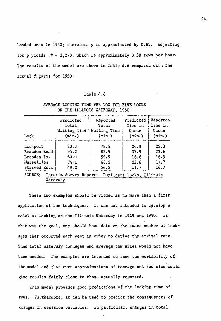
loaded ones in 1950; therefore p is approximated by 0.85. Adjusting

for p yields * = 3,278, which is approximately 0.38 tows per hour.

The results of the model are shown in Table 4.6 compared with the

actual figures for 1950.

Table 4.6

AVERAGE LOCKING TIME PER TOW FOR FIVE LOCKS ON THE ILLINOIS WATERWAY, 1950

C

Predicted Total

Waiting Time (min.)

Reported Total

Waiting Time (min.)

Predicted Reported Time in Time in Queue Queue (min.) (min.) Lock

80.0 78.4 26.9 25.3

_ Lockport Brandon Road Dresden Is. Marseilles Starved Rock

95.2 82.9

60.0 59.9

74.1 68.2

49.2 54.2

35.9 23.6

16.6 16.5

23.6 17.7

11.7 16.7 -

SOURCE: Inteiim Survey Report: Duplicate Locks Illinois Waterway.

These two examples should be viewed as no more than a first

application of the techniques. It was not intended to develop a

model of locking on the Illinois Waterway in 1949 and 1950. If

that was the goal, one should have data on the exact number of lock-

ages that occurred each year in order to derive the arrival rate.

Then total waterway tonnages and average tow sizes would not have

been needed. The examples are intended to show the workability of

the model and that even approximations of tonnage and tow size would

give results fairly close to those actually reported.

This model provides good predictions of the locking time of

tows. Furthermore, it can be used to predict the consequences of

changes in decision variables. In particular, changes in total

t¼ - ;e carried on thc waterway will bo reflected in the arrival rate

of tows and thereby in the locking time involved. Changes in tow size

will be reflected in the arrival rate also. Finally, changes in lock

sizes will be reflected in the service rate,

Note on Capacity of a Waterway and Optimal Tolls. The model of

locking employed above might be used to determine the capacity of a

waterway and to measure the congestion which ensues from having an

additional tow on the waterway.

As noted above, locking consists of the operations of (1) wait-

ing for permission to approach the lock, (2) approaching the lock and

maneuvering into the chamber, (3) filling or emptying the lock, (4)

multiple locking if necessary, and (5) leaving the lock and maneuver-

ing out into the channel. Operations (1) and (3) will be independent

of the number of barges in the tow, but the other operations will be

directly related to the number of barges. One might show this rela-

tionship, TL(Nb), as in Figure 4.4 where TL is the total service time

(assuming a constant amount of time is spent in queue) and N b is the

number of barges in the tow. Note that there are sharp discontinuities

when double or triple locking is necessary, for part of the tow must

be tied off, the lock must go through one cycle empty, the rest of

the tow must be pulled into or out of the lock from the shore, and

the tow must be reassembled.

One measure of the capacity of a waterway would be the maximum

feasible number of barges that could be locked through in a given

period of time. This idea was explored earlier by Bottoms. 26 Since

95

96

TL

N 8760 T T

L(Nb) '

(4.30)

NB

= NTNb

. (4.31)

-2; Single Double Locking Locking

Fig. 4.4 -- Locking time

T(Nb) is the time, in hours, it takes to service a tow of N. barges,

the number of tows that could be locked through in a year, N T , is

Nb

where 8,760 is the number of hours in a year, and it is assumed all

tows have Nb barges. The number of barges that could be serviced in

a year, NB , under the same assumptions, is given in Equation (4.31)

The most efficient tow size, from the standpoint of the lock, is prob-

ably that involving no more than a single locking.

While the above NB is one measure of the capacity of a waterway,

it is a capacity that would never be attained in practice. Tows are

not uniform; therefore, capacity would depend on the distribution of

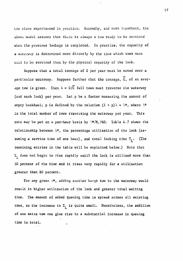
Low sizes experienced in practice. Secondly, and more i:Jportant, the

above model assumes that there is always a tow ready to be serviced

when the previous lockage is completed. In practice, the capacity of

a waterway is determined more directly by the time which tows must

wait to be serviced than by the physical capacity of the lock.

Suppose that a total tonnage of 0 per year must be moved over a _

particular waterway. Suppose further that the tonnage, C, of an aver-

age tow is given. Then k = ofE full tows must traverse the waterway

(and each lock) per year. Let p be a factor measuring the amount of

empty backhaul; p is defined by the relation (1 + p)% = 'A*, where Vie

is the total number of tows traversing the waterway per year. This

rate may be put on a.per-hour basis by \*/8,760. Table 4.7 shows the

relationship between.X*) the percentage utilization of the lock (as-

suming a service time of one hour), and total locking time T L. (The

remaining entries in the table will be explained below.) Note that

TL does not begin to rise rapidly until the lock is utilized more than

50 percent of the time and it rises very rapidly for a utilization

greater than 80 percent.

For any given .\*, adding another barge tow to the waterway would

result in higher utilization of the lock and greater total waiting

time. The amount of added queuing time is spread across all existing

tows, so the increase in TL

is quite small. Nonetheless, the addition

of one extra tow can give rise to a substantial increase in queuing _

time in total.

07

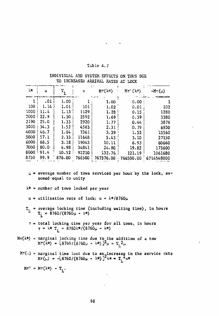
u TL 1 Mi(X*) . MTI(X*) -MT()

Table 4.7

INDIVIDUAL AND SYSTEM EFFECTS ON TOWS DUE TO INCREASED ARRIVAL RATES AT LOCK

1 ,

1 ; .01 1.00i 1 100 i 1.14 - 1.01 1 101'

1000 I 11.4 1.13 ! 1129

2000 1 22.9 1.30 i 2592

2190 : 25.0 1.33 I 2920

3000 1 34.3 1.52 1 4563

4000 1 46.7 1.84 1 7361

5000 I 57.1 2.33 i 11648

6000 68.5 3.18 I 19043 7000 80.0 - 4.98 i 34841

8000 91.4 10.52 1 92210

1.00 0.00

1.02 ' 0.01

1.28 I 0.15

1.69 I 0.39 1

1.77 ; 0.44

2.31 ! 0.79

3.39 ' 1.55

5.43 ! 3.10 I

10.11 1 6.93 I

24.80 . 19.82

132.76 1 121.19

1 102

1280 3380 3876 6930

13560 27150 60660 173600

1061680 8750 99.9 876.00766500:

l767376.00.

1 766500.00 6714548000

- -. . ...-

p. . average number of tows serviced per hour by the lock, as-sumed-equal to unity

X* .. number of tows locked per year

u . utilization rate of lock: u = X*/8760p

T = average locking time (including waiting time), in hours L T. = 8760/(8760.A - X*) L

T = total locking time per year for all tows, in hours 7 = .h* T = 8760h*/(8764, - X*)

L

MT(X*) . marginal locking time due to the addition of a tow NY(0) = 18760/(8760.d. - J. = TL2 .11

MT(.) = marginal time lost due to an oincrease in the service rate = -L8760/(8760w, - X*)] '4* . TL2 Ate

MI" = MT(X*) - Tv

98

Aso iven in Yahle 4.7 is T = X*TL'

the total waiting time for

all tows dLrin3 the year. The increase in total waiting time due to

an extra tow is, therefore,

2

dT.dA* = MT(X*) - (Vi7o ,8760

." (4.32) 0, -

This figure is shown in the table as MT(*). Note that Mr(t) rises

very rapidly as the percentage of utilization rises.

From the above discussion, it is clear that an additional tow im-

poses a cost (in terms of additional waiting time) of MT(*) on all

existing operations. Even one tow increases congestion. In practice,

an additional tow does experience some part of the cost of this con-

gestion, for TL

increases. However, the cost to all tows is consider-

ably greater than the cost borne by the individual tow. The social

or system cost of an additional tow is MT(*); the private cost (that

borne by the extra tow) is TL'

The difference between social and

private cost is '

mT(X*) - TL = MT 1 (X*). (4.33)

On a waterway at any given time, congestion would be decreased.

and the savings to the whole system would be MT'('*), if a single tow

were permladed to exit. If it costs CT dollars per,hour,to operate a

tow, then the system would be willing to pay C_MT 1 (X*) to any tow if

9

it would leave the system. Alternatively, each tow should be charged

a like amount if it insists o.1 staying. Thus, each tow on the water-

way is costing all other users M7'(i.le) hours, and rational allocation

of resources requires that a tow not be operated unless it is generat-

ing C_11 7"(‘*) in profit.

Note that the above formulation gives TL

and T as functions of

'*, p, and lock capacity. For a given lock capacity, one could deter-

mine how much equipment would be required to move a given number of

bargeloads per year. Note further that this analysis provides a way

of optimizing lock capacity. MT(X*) is the increment to total wait-

ing time from the last tow. One can define Mr(.) = dT/dp. which will

measure the change in total waiting time as the service time is

changed. This is

100

9

(

.

8760 141T() = - 8760p -

(4.34)

One would then expand capacity until the cost to tows of waiting an

additional hour equals the cost of expanding the lock to save that

hour.

An example will demonstrate how to determine when a lock should

be expanded on the basis of the queuing model and its extensions de-

veloped above. Assume it costs $17,000,000 to build new locks twice

as large as the old locks. (The figure $17,000,000 is the average

estimated cost, of building second locks of twice the capacity of the

existing seven locks on the Illinois Waterway.) 27 It is assumed

that doubling the size of the lock doubles the service rate. If

double locking is the practice on the waterway before the change,

the increased service rate may in fact be achieved by doubling the

size of the locks. If some other situation prevails, it may not be

possible to increase the service rate so dramatically. The principle

develope below will be the same, however. Next assume that the annual

cost of the lock is $656,000. (Again, this is the average cost of the

boven proposed Illinois Waterway locks.)28

If there is a single lock on the waterway and the cost per hour

of tows is $100,29 then the lock should be improved if at least 6,500

tow-hours can be saved per year. Such a saving can be obtained if

'.* = 5,000. For this number of tows operating on the waterway, 7, the

total locking time, will be 11,650 at the old service rate ... = 1 per

hour. At the new service rate p. = 2, 7 will be 3,450, a saving of

8,200 tow-hours which exceeds the amount required to justify the lock.

Note that this example implies that a lock should be expanded, given

the above assumptions, when that lock's utilization is approximately

57 percent.

Another extension of the above analysis is the determination of

the optimal toll for the use of the lock. In general, the optimal

toll per tow is. the additional cost imposed on all other tows, i.e.,

M- '(%*)-CT,

where CT

is the per-hour cost of a tow and MT 1 (A*) is de-

fined above. For the previous example NT'(*) = '6.27, after lock

expansion, CT = $100, so the toll per tow should be $27. Before im-

provement of the lock M1!(.*) = 3.10, so the optimal toll should have

been $310 per tow. .

101

The government should incur the cost of lock expansion (accord-

ing to the above criterion) only if barge traffic is behaving in

accordance with the toll scheme outlined above. Given the number of

tows on the waterway (all of which are paying MTTA*).C T or could pay

it), the waterway ought to be expanded according to the rule developed

above, i.e., expand lock capacity until the cost to tows of waiting

an additional hour equals the cost of expanding the lock to save that

hour.

The discussion has been in terms of a single lock only. However,

as was shown above, under reasonable assumptions, all locks on a water-

way may be treated independently. Therefore, if tows arrive completely

independently of each other, and if locks are sufficiently far enough

apart, at least several times the length of a tow, then the above

analysis may be applied individually to each lock on a multiple-lock

waterway.

A caveat should be issued at this point. In the preceding dis-

cussion, the term optimal toll was used to designate a toll that, if

imposed, would equate private and social costs. The idea of using a

toll (or, for that matter any kind of tax or subsidy) for this purpose'

is, of course, well known in the literature of welfare economics.30

In the above case, the external diseconomy imposed on all other tows

by a single tow's operations is "internalized" by means of the toll.

However, the adjective optimal may be misleading. If it were true

that all the marginal conditions for achieving a Pareto optimum would

be satisfied,.except for the existence of an external diseconomy such

as the one described above, then the proposed toll scheme would indeed

,,)_

1)(2. ooti:..“1. 31 If, on the other hand, it were not true or one werc

no:. wi:ling to assume that the marginal conditions would be satisfied,

then the toll scheme above would not achieve a Pareto optimum and, in

that sense, would not be optimal.

Making and Breaking Tow. At the beginning and end of each trip,

the flotilla of barges must be assembled and disassembled. As Table

4.4 shows, these processes--known as making and breaking tow--com-

prised 3.19 percent of the active time over a five-year period for

all boats of the barge firm which supplied the data. This is the

fourth largest delay-causing factor in Table 4.4, and it is the sec-

ond largest of non-miscellaneous delays. It is desired, therefore,

to present some analysis of this major delay category so that one

might be able to predict the time required to assemble and disassemble

tows.

Data on making and breaking tows were collected from two towboat

logs which were supplied by a barging firm. A towboat log reports

in detail on a year's operations of a towboat; in particular, delay

times and causes are given. It was possible to collect a large num-

ber of making and breaking times with the attendant number of barges

involved.

In the case of making tow, 242 observations were obtained. The

average time required to make tow was 1.7 hours; the number of barges

included in the sample tows ranged from I to 24, and the average tow

size was 3.4 barges. In the cases of breaking tow, 247 observations

were obtained. The average time to break tow was about 1 hour; the

number of barges involved ranged from 1 to 16, and the average tow

1 . 1

I

si,:e was 3.1 bares. The small average tow size is due to the fact

that the observations contain mans , additions to or subtractions fro:'

tows of only one or a few barges at a time. These "drops" and "adds"

oo,.nteLl because they occur frequently and the time required should

not differ importantly from that required in making or breaking tows

of only one or a few barges. An examination of the data showed:

(1) on the average, making tow required considerably more time than

breaking tow and (2) both making and breaking tow were affected by

the number of barges involved in the process. Both of these points

seemed plausible a priori. The possible reason for (1) is that in

assembling the barges the towboat captain attempts to achieve a flo-

tilla configuration that reduces resistance of the tow. On the other

hand, when the destination is reached, the flotilla may be disassembled

in any order. Point (2) seems even more obvious. Since each barge

must be collected and tied securely either to the towboat or to other

barges, the time required to do this is clearly a function of the

number of the barges comprising the tow. In the case of breaking

tow, the barges may be let Off individually or in two's at the termi-

nal. Again, the time required for this procedure would seem to be a

function of the number of barges.

With these ideas in mind, two linear regressions were performed:

(1) making-tow time regressed on number of barges added to the tow

and (2) breaking-tow time regressed on_number of barges dropped from

the tow. The results are,

where Tm = time required to make tow

Tb

= time required to break tow

134

:•ta "

(4.35)

(4.)6)

Nb

= number of barges added or removed

I

Tm = 0.21 + 0.44N

b' (0.061) (0.015)

with (1) coefficient of determination = 0.78

(2) standard error of estimate = 0.97

(3) F statistic = 848;

Tb = 0.34 + 0.20N

b' (0.029) (0.010)

with (1) coefficient of determination = 0.63

(2) standard error of estimate = 0.53

(3) F statistic = 411.

Both regressions are highly significant, which means that the esti-

mated time to assemble or disassemble a flotilla consisting of a given

number of barges obtained from Equations (4.35) and (4.36) is a better

prediction than using the average sample values. In addition, the

linearity of the estimating equations was corroborated by log-linear

regressions not reported here.

Miscellaneous Delays. _Estimation procedures for two of the most

important delay causes have been developed above. It is conceivable

that similar approaches could be used in analyzing each of the remain-

ing delay categories given in Table 4.4. However, this procedure

would be impossible given the data availability. A simpler approach

and one amenable to the available data is, therefore, desired.

To simplify the analysis all delay-causing factors other than

locking, load-unload, and make-break tow are aggregated into a single

category to be called "miscellaneous delays." On the basis of the

delay categorization of Table 4.4, miscellaneous delays include all

delays due to weather, repair, supplies, waiting barges, waiting

bridges, running aground, and other. These delays were approximately ,

13 percent of active time for the total of 59 boat-year observations

summarized in Table 4.4. Note that for any given trip, the expected

locking time and the expected assembly and disassembly time for the

tow may be predicted using the analyses reported above. Now, it is

desired to know how much additional time might be expected because

of all other delays en route.

Two types of data are available for estimating miscellaneous

delay time:

1. Point-to-point data: These data are derived from logs

of two towboats for the year 1964. The logs give infor-

mation on the number of stopsmade each day, the dura-

tion of each stop, where each stop occurred, and, in

most cases, the cause of the stop. .

2. Aggregate delay data: These data consist of summary

sheets which show the total delay time for each of

the ten delay categories discussed above. In addi-

tion, the total active time for each boat per year ,

is given. Observations are available for 19 towboats

across 5 years, giving 59 towboat-year combinations ,

in all (not all towboats operated each year). Table 4.4

1;LP,

is based on these data. They were obtained from tow-

boat logs just as the other data were.

Two types of analyses of miscellaneous delays are possible. On

the one hand, one might take a very detailed aPproach using the logs.

These data have the advantage of indicating the location of a tow-

boat at the time the delay occurred. This information could be used

to investigate the relationship between location and frequency and

duration of delay. Such analysis could provide a detailed relation-

ship between the characteristics of the waterway (as specified by the

location of the towboat) and the total miscellaneous delay time.

Analysis conducted in this detail would require many logs represent-

ing the various waterways.

On the other hand, a more aggregate analysis might be used.

Here locational differences could not be investigated. Such an anal-

ysis would prove to be more tractable and could be done with the sec-

ond type of data discussed above. A sample observation of the ag-

gregate data contains the same information (but without the details)

as is available from the logs. For example, if one wishes to know -

how long a given towboat was delayed because of bad weather in a cer-

tain year, this time could be found by reading it directly from the

summary sheet for the particular boat and year, or it could be deter-

mined by looking up the time lost for each weather delay for an en-

tire year.

The aggregate delay data are easier to use and available in

. much greater quantity than are the log data. On the other hand, only

the log data can be used to infer the relationship between waterway

107

Dependent on Waterway Independent of Waterway Percentage of Active

Time Delay

Percentage . of Active,

Time Delay

Total 4.01 Total . 9.07

characteristics and delays. Therefore, in order to justify using the

aggregate data in the following analysis, it is necessary to presume

that the waterway characteristics have little effect on delay time.

On an a priori basis, it seems that some of the miscellaneous delays

would depend on waterway characteristics while others would not.

Table 4.8

WATERWAY-DEPENDENT AND WATERWAY-INDEPENDENT MISCELLANEOUS DELAYS

Weather 2.35 Repair 3.94 . Bridge .12 Supply .65

Running aground .24 Waiting barge 1.87 One-third of "other" 1.30 Two-thirds of "other" 2.61

Source: Table 4.4 above.

In order to get an upper bound on the error introduced by ne-

glecting waterway characteristics, the following percentages were

calculated: (1) total waterway-dependent miscellaneous delays ex-

pressed as a percentage of total active time and (2) total waterway-

independent miscellaneous delays expressed as a percentage of total

active time. Table 4.8 shows the breakdown into dependent and inde-

pendent delays and the percentages of active time involved. The

"other" category consists of the following three delay factors:

(1) waiting orders, (2) waiting for crew, (3) waiting for a clear

channel. Since the only one of these that is likely to be affected

by waterway characteristics is (3) and since the relative magnitudes

106

of the three are unknown, one-third of the "other" category is al-

locatod to waterway-dependent delays and two-thirds to waterway-

independent delays. When this is done, it is seen that total waterway-

dependent delays cannot amount to more than 4.01 percent of active

pimc, while total waterway-independent delays amount to 9.07 percent

of active time. Or, in other words, a maximum of one-third of mis-

cellaneous delays may be waterway dependent. This seems to be an

upper bound and that in all likelihood the proportion is much lower

than one-third, for not every weather delay, running-aground delay,

and waiting-clear-channel delay is dependent on waterway character-

istics. Moreover, these delays are not ignored in the following

analysis, but, rather, they are assumed to be equally spread among

waterways regardless of waterway characteristics.

Next, a framework is established in which the aggregate delay

data may be used to estimate the miscellaneous delay time for indi-

vidual trips. The following relationship among the aggregate vari-

ables is defined:

109

10

tt =t +t =t + 1: t . anr in

i=1

(4.37)

in wnich tt = total time in a year, in hours, (observable from

data)

ta = total active time in a year, in hours (observable

from data)

• tn = total inactive time in a year, in hours (observ-

able from data)

tr = total running time in a year, in,hours (observable

from data) -

t. = total delay time in a year for the ith delay, in i hours, i - 1, ..., 10 (observable from data).

10

tr = t - t..

a i i=1

(4.38)

t T y r

j=1

(4.39)

Tr = T

f + T

aNa + T

dNd'

(4.40)

t = t.. o a i=1

(4.41)

i/l, 6, 9

Equation (4.37) divides the total :Lim! in a year into the sum of the

tin.o. during which a towboat is actually making trips and the time dur-

ing which it is inactive because of major repairs or lack of business.

From Equation (4.37) running time is the difference between active

time and total delay time.

110

The aggregate running time may be related to individual trip time by

inwhichTrj is the time required to make the jth trip, and there are

J trips in a year. Note that the previous analysis of the tow in mo-

tion permits the estimation of trip running time.' Repeating Equation

(3.3) above.

i.e., for any given trip, the running time'is the sum of the time dur-

ing which the tow operates at full speed, Tf , and the time during

which it is accelerating or decelerating, T aNa + TdNd .

Define total miscellaneous delay time in a year as

10

I., .

ILI

T o natio, a, of total miscellaneous delays per year to total yearly

ruaning time is defined:

a = t It . o r (1..42)

Note also that to =

cit . Since the previous analysis permits the es-

timation of Tr'

which is the point-to-point counterpart of tr, an

.!stimate of miscellaneous delay time expected to be encountered on

any given trip, To , is

To = aT

r. (4.43)

The factor of proportionality, a, must be estimated from the aggregate

delay data. Note that to and t r are available from the aggregate data

for each of the 59 boat-year observations. A sample of a's, defined

as in Equation (4.42), are therefore available.

The central limit theorem leads one to believe that the distri-

bution of a should be approximately normal, for miscellaneous delays

are the sum of seven independent random variables. The data were .

tested for normality with a standard chi-square test employing seven

cells. With four degrees of freedom, the calculated statistic is

0.12; the statistic would have to exceed 9.49 for significance of

conventional levels. Therefore, it is concluded that the distribu-

tion of miscellaneous delays is not significantly different from

normal. . ,

Given a normally 'distributed random variable, probably the best

estimate of the mean for most purposes is the sample arithmetic mean.

To

= -ce-Tf'

(4.44)

Xore confidence may be attached to this estimate if the distribution —

has a small variance. The aggregate delay data give a - 14 percent

with a standard deviation of 5 percent. The standard deviation is

large relative to the mean, however, but this seems the best that can

be done given the data.

In summary, the miscellaneous delay time for any given tow trip

may be estimated by To

=r, where a = 0.14 and T

r is estimated from

the relationships developed above. Note that T r contains acceleration

and deceleration time as well as time during which the tow travels at

full throttle. It was noted above that, for long trips and/or those

in which few locks are encountered, acceleration and deceleration time

is likely to be insignificant relative to the time during which the

tow is operating at full speed. If this is the case, the miscellaneous

delay time for a trip may be estimated by

112

— in which a = 0.14 as before, but T f is the time required to make the trip

at full speed. In either formulation, T o. enters the tow process func-

tion as shown earlier. See Equation (4.1).

Note on Frequency of Miscellaneous Delays. Recall from earlier

sections that in order to adjust for acceleration and deceleration

time lost and distance traveled incidental to each stop, the number

of stops en route must be known. The number of locking stops should

be known for any given trip. Uhile there must be an acceleration at

No

= 0.01D, (4.45)

tile beginning of the trip and a deceleration at the end, it is not

known how many stops are due to miscellaneous delays.

In order to get an idea of the frequency of miscellaneous de-

lays, the two towboat logs were examined. For each day, the number

O f stops due to miscellaneous factors, still using the term "miscel-

laneous" in the manner described above, was counted and the miles

traveled that day were recorded. It turned out that the average

number of miscellaneous stops per mile was 0.01, with a standard

deviation of 0.02. In other words, there is on average one stop

due to miscellaneous delay factors for every 100 miles of travel, .

and in most cases the number of miscellaneous stops will be between

zero and 3 for 100 miles of travel. As a point estimate of No, the

number of stops due to miscellaneous delay factors, the following

relationship could be used:

113

where D is, as before, the length of the trip, in miles. In most

cases No would be a rather small number. Moreover, since it has

been determined that accelerations and decelerations take little

time and account for little distance traveled for most trips, it

is probably best to ignore the slight adjustment factor of Equa-

tion (4.45).

Recapitulation of Tow Linehaul Process Function

The output of a barge tow is the cargo ton-miles per hour gen-

erated in the process of hauling commodities from one point to

another. Ton-miles per hour may be expressed as the product of

(1) the cargo tonnage of the tow and (2) average effective speed

of the tow between origin and destination. It is the latter of

these two that has required considerable analysis in the preceding

sections of this chapter.

Cargo tonnage of a tow was expressed as a simple relationship

between number of barges and their draft. Average speed, on the

other hand, was seen to be dependent in complicated ways on a wide

variety of variables. In the development of a method of determin-

ing the average speed of a tow, it was convenient to think of any 1

tow trip as consisting of various phases and to develop models for

predicting the time spent in any phase. Given the time spent by

the tow in each phase of the trip and the length of the trip, then

the average effective speed is determined. This, as was pointed out

above, when multiplied by the cargo tonnage of the tow, provided the

ton-miles per hour generated by the transport vehicle. Analyses

were required concerning such things as acceleration, deceleration,

cruising speed, locking time, assembly and disassembly time, and

other delay times.

The analyses of acceleration, deceleration, and cruising speed

were based on estimated tractive-effort and drag-force functions

for barge tows. It was found that the time spent in acceleration

1 L,r

115 ,

was quite small relative to the time during which the tow would typi-

z.dly operate at its cruising speed. Also, it was found that the

distance traveled by a tow during acceleration was small relative to

typical trip distances. Likewise, deceleration was determined to be

insignificant. The model predicting the cruising speed of the tow,

then, is the major input to the process function as far as tow move-

ment is concerned. That would be the end of things were it not for

the fact that tows are delayed en route. Delays occur because of,

locking, assembly and disassembly of the tow, and other miscellaneous

reasons. Locking delay was handled by a simple queuing model A

delay relationship for making and breaking tow was estimated from .

towboat log data. Finally, all other linehaul delays were grouped

together and estimated from delay data collected by a common carrier

barge firm.

Given the above relationships, the ton-miles per hour generated

by any given tow for any given trip may be estimated. .Moreover, the

predicted ton-miles per hour figure is amenable to changes in vari-

ables under the control of barging firms (e.g., horsepower of tow-

boats) as well as variables under the control of the Corps of Engi-

neers (e.g.., depth, width, and stream velocity of waterway; lock

size). In addition, as will be shown in the next section, cost per

ton-mile may be determined with the aid of the process function de-

veloped above.

Productivity relationships and isoquants will not be investi-

gated for the tow process function. As was noted in Chapter II,

Howe has investigated these relationships for his tow process

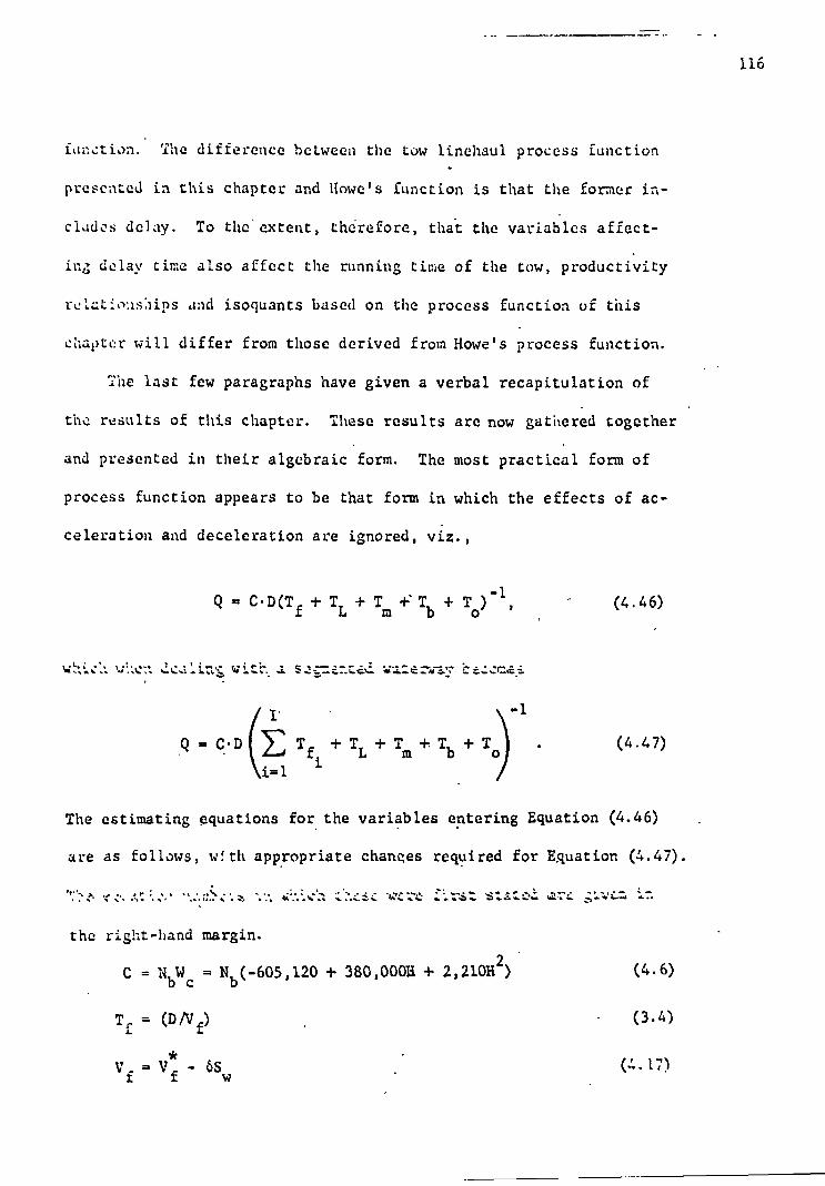
116

function. The difference beiween the tow linehaul process function

presented in this chapter and Howe's function is that the former in-

cludes delay. To the extent, thdrefore, that the variables affect-

ing delay time also affect the running time of the tow, productivity

relationships and isoquants based on the process function of this

chapter will differ from those derived from Howe's process function.

The last few paragraphs have given a verbal recapitulation of

the results of this chapter. These results are now gathered together

and presented in their algebraic form. The most practical form of

process function appears to be that form in which the effects of ac-

celeration and deceleration are ignored, viz.,

Q=C•D(T_+T +T +*T t L mb o'

1.it.....,..,„:;•. ,./...,c-.1 ac.a'-ir,s with. a se--7.enzed ...;a7..e...n.-1,7

1- -1

Q = C•D (E T f. + T

L +T + T

b + T

o .

i i=1 "

(4.46)

(4.47)

The estimating equations for the variables entering Equation (4.46) .

are as follows, w!th appropriate changes required for Equation (4.47).

the right-hand margin.

C = NbWc = Nb

(-605,120 + 380,000H + 2,210E2)

T r = (Div f)

* V_ = V - OS t f w

(4.6)

(3.4)

(4.17)

117

t •

* 1 V. = -

1 - J2

r 1

T = 1

i=1

%* . (1 + p)

‘ = 0/E

T = 0.21 + 0.44Nb m

T1 = 0.34 + 0.20Nb

To = 0.14T

f

(4..;,,

(4. 2S)

(4.24)

(4.23)

(4.33)

(L.44)

The variables are defined as follows:

Q = ton-miles per hour _

C = cargo tonnage of tow, in short tons

D = distance of trip, in miles

Tf = time required to travel D at full speed, in hours

TL = locking time, in hours

Tm = make-tow time, in hours

Tb

= break-tow time, in hours

To = miscellaneous delay time, in hours

Nb = number of barges in tow ,

. Wc = cargo tonnage of a barge, in short tons

H = draft of barges, in feet

Vf = full speed of tow, in miles per hour, adjusted for

stream current

* V full speed of tow, in miles per hour, in still water

= 1 upstream 6

= -1 downstream

S -, speed of water, in miles per hour W

HP = rated brake horsepower of towboat

D = depth of channel, in feet

W = width of channel, in feet

B = breadth of flotilla of barges, in feet

L = length of flotilla of barges, in feet

r = number of locks to be traversed during trip

. = service rate of ith lock, in tows per hour .p.. 2.

X* . arrival rate at locks, in tows per hour

0 = total waterway tonnage required to pass through locks in a given period of time

— C = cargo tonnage, in short tons, of an average tow

p = percentage of trips requiring empty backhaul.

Obtaining Costs from Process Function for Barge Tows

The tow process function provides an estimate of the ton-miles

per hour generated by a tow, Q. In order to convert this into the

cost per ton-mile of operating the tow, two more inputs are needed:

(1) the cost per hour of operating towboats of various horsepower,

Ct'

and (2) the cost per hour of a Jumbo hopper barge, C b . Both of _ these items are available from the Corps of Engineers, which collects

cost data from barging firms and calculates the per-hour costs, C t

and Cb. In addition, the Corps has per-hour costs of various other

barge types as well. And, as was indicated above, the process func-

tion may be adapted with little difficulty to other barge types.

118

Given Q, Ct'

and Cb

and knowing the number of barges in the tow,

Nb

then the cost per ton-mile of a to trip, C, may be determined tm .

119

from

Ct + N

bCb

Ctm

- Q

(4.48)

Note that the cost per ton-mile given by Equation (4.48) refers

only to a point-to-point movement. Such a cost, therefore, does not

take into consideration any adjustments in the barging firm's other

transportation activities. If the firm, for example, had to divert

barges from some other traffic to make a .given trip, then the real

cost per ton-mile might not be reflected in the cost per ton-mile

for the point-to-point movement. Moreover, a change in the depth of

a waterway, for example, would affect the cost per ton-mile of the

point-to-point barge movement over that waterway, but might also af-

fect the operations on other waterways as well. The effect of these

other adjustments would not be reflected in the point-to-point cost

per ton-mile over the improved waterway.

In order to determine the cost per ton-mile of the firm's opera-

tions, one would need to know the entire distribution of tow trips

undertaken by the firm. In addition, to know the change in the firm's

costs due to a waterway improvement, one would again need information

on the firm's entire activities. In order, therefore, to know firm

costs as opposed to individual trip costs, the tow process function

must be incorporated into a scheduling model of the barging firm.

Simple scheduling problems, such as contract carriage, can be handled

by the above analysis, but for more complex problems such as those

of a common carrier, a scheduling model for the barge firm has been

developed by Hurter and Cabot.32

Without going into detail, the

model provides optimal scheduling of barges and towboats in order to

satisfy the transport demands on the firm and to maximize the firm's

profits. An important input into the Cabot-Hurter model is the time

required for any tow to travel between ports designated in the model.

This information could be supplied by the point-to-point analysis de-

tailed above. Tow cost analysis will not be pursued further here.

120

CHAPTER V

RAIL LINEHAUL PROCESS FUNCTION

Introduction

In Chapter III a method of formulating a linehaul process func-

tion for a transportation mode was presented. The method was ap-

plied to barge tows in Chapter IV. In this chapter a linehaul pro-

cess function for rail freight transportation is presented. The

next section develops the form of the rail linehaul process function.

Functions are developed for the cargo weight and light weight of.a

train in the following sections. A subsequent section analyzes the

train in motion, including constant velocity, acceleration, and de-

celeration. There is no discussion of tests of the speed prediction

function as there was in the chapter on barge tows, for the tractive-

effort and drag-force functions employed in the train process func-

tion are both well-known relationships that have received wide ap-

proval and use. A section on rail linehaul delays provides hardly

anything that is new. This is in marked contrast to the comparable

sections in the last chapter. This should not be taken to imply

that linehaul delays are unimportant for rail or that the definitive

delay analysis has been done. Quite the contrary, rail linehaul de-

lays are important, as will be shown; and almost no one would agree

that no more analysis is needed on them. Nevertheless, that analysis

is not provided in this dissertation. Concluding sections contain

1 •) )

econoinic analysis of the rail linchaul process function, including

various productivity relationships, isoquants, and cost curves. The

final section includes a derivation of the railroad firm's cost

curves using both engineering and statistical methods. This last

should be viewed as merely an example of what can be done and not as

an attempt to estimate present day rail costs since the data on which , the statistical results are based are a decade old.

Form of Rail Linehaul Process Function

The process fuuction for rail trains has the same form as Equa-

tions (3.8)-(3.10) above. Recall that Equation (3.8) allows for

the effects of acceleration and deceleration on the output produced

by the vehicle, whereas Equations (3.9) and (3.10) are the process

functions when these factors are ignored. Also, note that the pro-

cess function allows for the trip mileage to be segmented. This was

done to account for variability of factors en route that may affect

the vehicle's performance. In the case of barge tows, such vari-

ables as depth, width, and stream velocity can vary over a route

between two points. In order to account for variability, the route

may be divided into many segments, each of which is fairly uniform

with respect to depth, width, and stream velocity.

In the case of railroads, the primary factors that are likely

to vary over the length of a trip are the grade of terrain and the

degree of track curvature. The operating characteristics of a

freight train will vary considerably with these two factors. The

method for dealing with grade and curvature is to divide the trip

122

into segments with respect to these variables. For example, suppose

a train is engaged in a trip of length ten miles of which the first

two-mile stretch has an upgrade of 2 percent, the next two miles a

downgrade of 1 percent, and the remaining six miles are on level

ground. The trip would consist of three segments over which the

spved and, therefore, the ton-miles per hour generated by the train

would be different. The trip may be further segmented with respect

to curvature since the length and degree of each curve encountered

can be determined. Of course, the two factors of curvature and

grade will be combined on several segments, e.g., a half-mile curve

of two degrees may occur on a 1 percent grade.

Another factor that must be considered in the rail linehaul

process function is the speed limit. Any existing speed limit must

be added as a constraint to the function. For example, the analysis

may indicate a feasible speed of 100 miles per hour, whereas the

speed limit is 75 miles per hour. Again, the route may be segmented

into sections over which the speed limit constraint is operative and

over which it is not.

In the process function, time spent delayed en route is repre-

sented by T s . It was convenient to disaggregate delay time into

several components for the tow analysis. However, in the case of

rail all delays en route could perhaps be treated as one. Delay

time due to acceleration and deceleration will also be examined, be-

low. If these delays are found to be large relative to total trip

time, then they may be integrated into the rail process function

by using forms of the function which include acceleration and

123

• i

deceleration, Equation (3.8). Moreover, some analysis of the num-

ber of stops en route would be required in order to include the

effects of acceleration and deceleration on a train's output.

Cargo Capacity and Light Weight of Rail Train

Recall that the linehaul process function is the product of

two terms: (1) the cargo tonnage of the vehicle and (2) the aver-

age speed of the vehicle between origin and destination. The second

of these terms will be developed in the next and following sections -

of this chapter for the case of rail. The cargo tonnage of a train

will be discussed in this section beginning first with a discussion

of the cargo tonnage of a rail car and then generalizing this dis-

cussion to the cargo tonnage of a rail train. The remarks made here

concerning the cargo tonnage of rail trains are applicable to all

different types of rail cars and to trains composed of a variety of

types of cars. Note that this was not the case in the tow process

function. In the analysis of tow cargo capacity, a particular barge

type was selected and used exclusively in the analysis, although

methods were suggested for generalizing this procedure. The use of

one type of barge was necessitated by the fact that the tow resis-

tance formulation had been estimated for only one barge type. In

the case of rail, on the other hand, the resistance function is not

based solely on one rail car type, nor is_it dependent on a partic-

ular configuration of rail cars, i.e., the order of the rail cars

comprising a train does not affect the total resistance.

124

There are several types of freight cars and many sizes for each

type. For each size and type of car, one can determine the cargo

capacity in cubic feet, the light weight, and the load limit.1

Load

limits, set by the Association of American Railroads (AAR), may not

be exceeded and are generally much less than the actual cubic capa-

city would permit. For example, a 50-foot general box car may have

a capacity of 5000 cubic feet but a load limit of 70 tons. A typi-

cal medium density commodity, such as corn, may weigh 45 pounds per

cubic foot. This means that if the above box car were loaded to

capacity, the cargo weight would be 112.5 tons which far exceeds the

load limit. However, a low density commodity like oats, which weighs

about 26 pounds per cubic foot, would be space-limited rather than

weight-limited, for the freight car when filled to capacity would

weigh 65 tons, less than the load limit of 70 tons.

To put this argument into symbols, the following definitions

are needed:

Kij = capacity of ith car for jth commodity, in tons

L. = load limit of ith freight car, in tons

x4 = cargo volume oi ith car, in cubic feet

. = weight of jth commodity per unit volume, in tons g3 per cubic foot

k. = proportion of capacity of ith car utilized, 0 ki 1

C. = cargo weight of ith car, in tons.

Capacity is defined as follows:

K.. = min (L., x g.). (5.1) ij L i j

195

Then the cargo weight of the ith car for the jth commodity is

c. kJ(.., () k. 5. 1. (5.2)

An example will illustrate the above relationships. Suppose for a

given freight car and a given commodity, the following hold:

L. = 70 tons

. = 0.01 tons/cu. ft. gj

x. = 5000 cubic feet. 1

ThenKij = min (70 tons, 50 tons) = 50 tons; i.e., the car is space

limited for the assumed commodity, and the cargo weight of the car

is given by Equation (5.2), where ki refers to the fraction of the

ith car's capacity utilized. If another, denser commodity is con-

sidered, say the rth commodity, where g r = 0.025, then K min

(70, 125) = 70, and the car is weight limited. The cargo weight is

again given by Equation (5.2).

The cargo weight of a train of freight cars will be the sum of

the cargo, weights of the individual freight cars comprising the

• train, or, in symbols,

126

Nc

Nc

C=Ec.=I: kKij' i=1 i=1

(5.3)

where Nc

is the number of cars in the train and j represents the

commodity with which the car is loaded. This formulation allows '

for N cars, Nc different commodities (but only one to a

car) and Nc different utilization rates. If all cars were identical

C = NckL.

Wt = w

t.' (5.5)

i= 1

and hauled the same amounL of the samc: commodity, and if thv cars

ere weight-limited for that commodity, then the cargo weight of a

train would be given by

127

In addition to the cargo weight of a train, it will be neces-

sary in the subsequent analysis to know the tare or light weight of

the cars and the gross weight of the locomotive. Again, for any

given freight car, one can easily determine the tare weight of the

car, w . 2 Therefore, for any given train of cars, one can deter-L. 1

mine the light weight of the train of cars

where Nc is the number of cars in the train. The gross weight of

one freight car is

(5.6) WC. = C. Wt.

, 1

1

and the gross weight of the train of cars is

W = C + Wt

. (5.7)

The gross weight of a locomotive may be similarly obtained.3. How-

ever, the gross weight of a locomotive seems to be related to its

horsepower and number of axles, i.e., for a given number of axles

(4, 6, or 8), the weight of the locomotive is an increasing func-

tion of horsepower. And for any given horsepower, weight is an in-

creasing function of number of axles. In the subsequent analysiz,

it will prove convenient to have a functional relationship among

horsepower, weight, and axles. The following relationship will be

used:

-26

(5.8) w . -3.62 + 0.00834HP + 27.140a L L . L (0.00194) (1.724)

in which wL = weight of locomotive unit in tons

HPL = horsepower of locomotive unit

aL = number of axles of locomotive unit.

Both coefficients are significantly different from zero. The t -values

for horsepower and axles are, respectively, 4.3 and 15.7. Standard

errors are given in parentheses below the estimates to which they

relate. The coefficient of determination is 0.98. This relationship

was obtained by regression analysis applied to 24 sample observations

of diesel-electric locomotives contained in Car & Locomotive Cyclo-

pedia. It should prove applicable to present day, United States and

Canadian .diesel-electric locomotives. . .

Horsepower may be added to a train in one of two ways: (1) us-

ing a larger horsepower locomotive and (2) using additional locomo-

tives. For example, a motive force of 6,000 horsepower may be ob-

tained from one 6,000-horsepower locomotive or from four 1,500-

horsepower locomotives. It would be-interesting to be able to

investigate these alternative methods of obtaining horsepower. This

w.w.

+w L c z_d L. t.

3. T 1=1 1 i=1 i=1

(5.10)

can be accmplished by derinin,,!, 2ocomotive gross weight W L . as

NL

W" = i=1

129

(5.9)

where NL

is the number of locomotive units and w L. is the weight of

1 the ith locomotive unit. If NL= 1, then W L

= wL.

This formulation

will permit investigation of the effect of changing horsepower on

the ton-miles per hour generated by the train, where horsepower can

be changed either by adding locomotives or b) using a locomotive of

ereater horsepower.

The gross weight of the trdin is expressed as

NL

N Nc

The preceding discussion has developed a formulation of the

cargo and gross weight of a train. Both of these are components of

the train process function, for the cargo tonnage transported by the

train certainly affects the ton-miles per hour produced by the vehi-

cle, and the gross weight of the train affects the speed at which it

may travel.. In the next section the analysis of a train in motion

is begun. This analysis is necessary in determining the average

effective speed of the train between origin and destination. Another

factor affecting average speed--delays en route--will be taken up in

a later section.

Ft (v) = 375(HP - HP a)(e/v), (5.11)

Ft (v) = (30811P)/v. (5.12)

Analysis of Train in Motion

Introduction. In order to apply the relationships developed in

Chapter III, tractive-effort and drag-force functions must be obtained

for rail trains. This is a. much easier task than it was for the case

of barge tows, for there already exist in the railroad engineering

literature well-known and accepted functions.

Tractive-effort Function. A general tractive-effort functiOn for

diesel-electric locomotives is derivable from the definition of horse-

power. Moreover, it takes account of mechanical and electrical losses

from auxiliary units of the locomotive. This function is 4

130

in which Ft (v) = tractive effort, in pounds

HP = total rated horsepower of locomotive units

HPa = horsepower used by auxiliaries

e = an efficiency factor,.mechanical-electrical, taken as 82.2 percent

v = velocity, in miles per hour.

When these factors are given numerical values from conventional de-

sign and operation, the tractive-effort equation reduces to

Dra.;-force Function. The most commonly used drag-force function

in railroad engineering is the Davis formulation.5 This relationship

is usually presented as follows, applicable both to rail cars and

1

locomotives;

Fd(v) = (1.3 + 29/w + by + SXv

2 /wa)wa, (5.13)

in which Fd(v) = drag-force, or resistance of car or locomotive,

w = weight per axle of car or locomotive, in tons

a = number of axles

b = coefficient of flange friction = 0.045 for freight cars; 0.03 for locomotives

S = drag coefficient of air = 0.0025 for locomotives; , 0.0005 for freight cars

X = cross-sectional area = 105-120 square feet for loco-motives; 85-90 square feet for freight cars.

Frontal area could be determined for each particular locomotive and

car, but since the subsequent analysis is to be applied to a large

variety of cars and locomotives and since the range of variation of

X is small,'it will be assumed to be equal to 112.5 for locomotives

and 87.5 for freight cars (the arithmetic averages of the end points

of the ranges of variation).

Equation (5.13) may be put into a more useful form if the im-

plied multiplication of the bracketed expression by wa is carried

out. Note that wa is the gross weight of the vehicle. Substituting

the values of b, S, and X, two drag-force functions are obtained,

one for a locomotive and one for a .freight car, viz.,

in pounds

FL(v) = 1.3w + 29aL + 0.03wL v + 0.28125v2 (5.14)

and

F(v) = 1.3wc + 29a 0.045wc

v + 0.04375v2

, (5.15)

in which F(v) = drag-force of locomotive, in pounds

F(v) = drag-force of freight car, in pounds

wL = gross weight of locomotive, in tons

wc = gross weight of freight car, in tons

aL = number of axles of locomotive

a number of axles of freight car

v = velocity of locomotive or car, in miles per hour.

The above formulas give resistance of only one locomotive and

one freight car. Total train resistance is the sum of the locomotive

resistance and the resistances of all the freight cars, or

Nc NL

Fd (v) = V F

L (v) + 1: F

c (v), L...., d. - d. 3. 3. i=1 i=1

where Fd (v) = total train resistance

Fd. (v) = locomotive resistance of ith unit

NL = number of locomotive units in train

Fd. (v) = freight car resistance of ith car

Nc = number of freight cars in train.

(5 16)

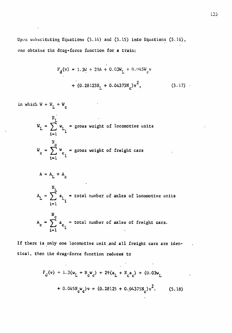
".1'. 1.-IJ

Upon substituting Equations (5.14) and (5.15) into Equations (5.16),

one obtains the drag-force function for a train:

Fd(v) = 1.3W + 29A + 0•03WL

+ 0.045W v c

+ (0.28125NL + 0.04375cv2

, (5.17)

in which W = WL +W

c

NL .

WL = 1: wL = gross weight of locomotive units

i i=1

'Nc

W = w = gross weight of freight cars c c. i i=1

A=A L +A

c

NL

AL = 12 aL. = total number of axles of locomotive units i

i=1

Nc A = 1: a = total number of axles of freight cars. C C.

i=1 1 •

If there is only one locomotive unit .and all freight cars are iden-

tical, then the drag-force function reduces to

Fd (v) = 1.3(wL + N cwc) + 29(aL + Nca c) + (0.03wL

+ 0.045Ncwc)v + (0.28125 + 0._04375Nc)v2 . (5.18)

Fs = 20Ws, (5.19)

Adiustment for Grade and Curvature. In the case of barge tows,

there were several factors concerning the "foadbcd" that•ffected

the speed, e.g., depth, width, and stream velocity of the waterway.

The only factors comparable to these for the case of the rail are

the gradient of the tefrain and the degree of track curvature.

It is not difficult to adjust the preceding drag-force function

to account for the effect of grade. Let the extra resistance on the

train due to grade be denoted by Fs , which may be negative or posi-

tive depending upon whether the train is going downhill Or uphill, -

respectively. Fs is equal to 20 pounds per ton per percentage of

grade. 6 For example, a train climbing a 2 percent grade encounters

additional resistance equal to 40 pounds per ton of train weight.

The relationship among grade resistance, train weight, and percent-

age grade may be expressed as

134

in which F grade resistance, in pounds

W = total weight of train (engine. and cars) in tons

s = percentage gradient of terrain.

In order to obtain total train drag force including grade re-

sistance, one need merely add the grade resistance to the train re-

, sistance, i.e.,

Fds

(v) = Fd(v) + F

s,

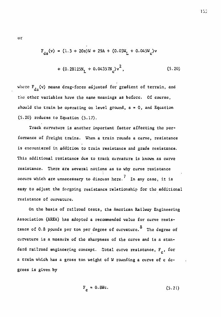
Fc

= 0.8Wc. (5.21)

or

1S3

Fds(v) = (1.3 + 20s)W + 29A + (0.03W L + 0.045W c)v

+ (0.28125NL + 0.04357N c)v2

, (5.20)

where Fds

(v) means drag-force adjusted for gradient of terrain, and

the other variables have the same meanings as before. Of course,

should the train be operating on level ground, s = 0, and Equation

(5.20) reduces to Equation (5.17).

Track curvature is another important factor affecting the per-

formance of freight trains. When a train rounds a curve, resistance

is encountered in addition to train resistance and grade resistance.

This additional resistance due to track curvature is known as curve

resistance. There are several notions as to why curve resistance

occurs which are unnecessary to discuss here. 7 In any case, it is

easy to adjust the forgoing resistance relationship for the additional

resistance of curvature.

On the basis of railroad tests, the American Railway Engineering

Association (AREA) has adopted a recommended value for curve resis-

tance of 0.8 pounds per ton per degree of curvature. 8 The degree of

curvature is a measure of the sharpness of the curve and is a stan-

dard railroad engineering concept. !Total curve resistance, F c , for

a train which has a gross ton weight of W rounding a curve of c de-

grees is given by

+ 0.04375N c) v2 . , (5.22)

Ft (v) - F

dsc (v) =0. (5.23)

136

Curve resistance, like grade resistance, enters the resistance func-

tion additively. The resistance function adjusted for curve and

grode is, therefore,

Fdsc (v) = Fd (v) + F + F = (1.3 + 2Us + 0.8c)W + 29A s c

+ (0.03WL + 0.045W c)v + (0.28125NL

Constant Velocity State. Given the tractive-effort function of

Equation (5.12) and the drag-force function of Equation (5.22), the

analysis developed in Chapter III may now be applied to rail trains.

The equation of motion for a rail train operating at cruising speed

i s

Substituting the functional forms for Ft and Fdsc , one obtains the

following cubic equation:

308HP - [(1.3 + 20s + 0.8c)W + 29A]v - (0.03WL + 0.045Wc)v 2

- (0.28125NL + 0.04375N c

)v3 = O.

. (5.20

Solving this cubic equation for velocity will yield the cruising speed,

Vf' of a rail train as a function of HP, s, c, W, A, WL'

NL

and

Fortunately, a solution to a cubic equation of this form exists, and

a standard computer program is available for obtaining it. Of the

three possible sets of roots that may be obtained from cubic equations

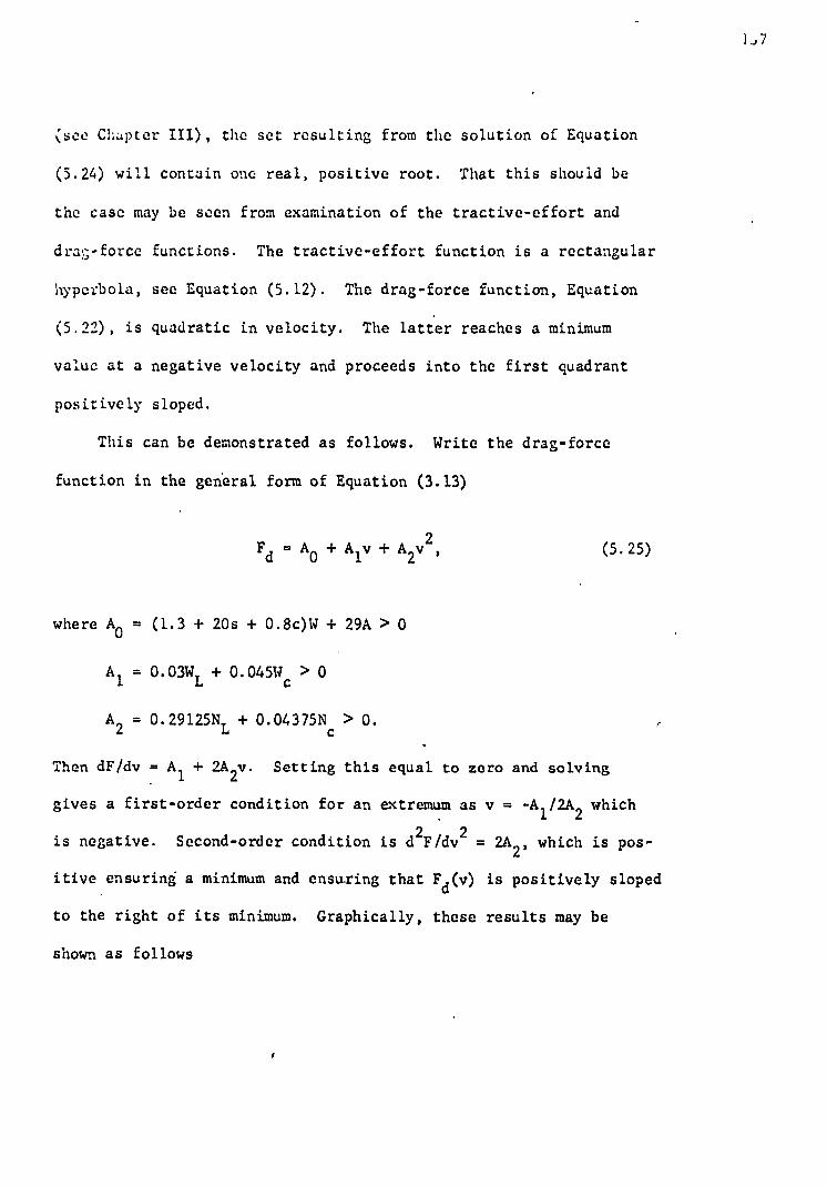
Fd = AO + Alv + A2

v2

' (5.25)

(sec Chapter III), the set resulting from the solution of Equation

(5.24) will contain one real, positive root. That this should be

the case may be seen from examination of the tractive-effort and

drag-force functions. The tractive-effort function is a rectangular

hyperbola, sec Equation (5.12). The drag-force function, Equation

(5.22), is quadratic in velocity. The latter reaches a minimum

value at a negative velocity and proceeds into the first quadrant

positively sloped.

This can be demonstrated as follows. Write the drag-force

function in the general form of Equation (3.13)

where A0 = (1.3 + 20s + 0.8c)W + 29A > 0

A1 = 0.03WL + 0.045Wc > 0

A2 = 0.29125N + 0.04375N c

> 0.

Then dF/dv = A1 + 2A

2v. Setting this equal to zero and solving

gives a first-order condition for an extremum as v = -A1/2A

2 which

is negative. Second-order condition is d 2F/dv

2 = 2A2 , which is pos-

itive ensuring a minimum and ensuxing that F d (v) is positively sloped

to the right of its minimum. Graphically, these results may be

shown as follows

0 VI

133

F .

Fd(v)

F (v) t v

Fig. 5.1 -- Determination of cruising speed of train

These characteristics of the two functions ensure an intersection

in the first quadrant (therefore a real, positive root). The other

2 two roots may be conjugate and imaginary (if 4A 0A2 > Al); real, neg-

ative, and unequal (if 4A0 A2

< A2

'). and real, negative, and equal

1 2

(if 4A0A2 = A

1).

Acceleration. The following acceleration equations are com-

monly found in railroad engineering literature: 9

Ta = (95.6/F 1 )(V - V 1)

a 2 1

and

Da = (70/F 1 )(V

2 - V

2)

a 2 1 '

where Ta = acceleration time, in seconds

Da = acceleration distance, in feet

(5.26)

(5.27)

V 1 = initial velocity, in miles per hour

V2 = final velocity, in miles per hour

F' = force available for acceleration, in pounds per ton. a

F' is obtained as follows: (1) calculate the tractive effort, in a

pounds, of the motive units minus the resistance, in pounds, of the

motive units; (2) calculate the resistance, in pounds, of the train ,

of cars; (3) divide the resulting figure by the weight, in tons, of

the entire train. The figure obtained by the operation described

in (1) is commonly referred to as "drawbar pull"; it is the amount

of pulling force left after the resistance of the locomotive units

is accounted for. All of these computations are made for a given

speed, usually the mean obtained over the entire interval considered.

If one were interested in the time and distance required to accelerate

from a speed of V 1 to V 2 , then (1) and (2) could be calculated using

(V2

- V 1)/2. This would represent a linear approximation to the

acceleration curve and would result in an underestimate of accelera-

tion time and distance. Better estimates could be obtained by using

smaller speed intervals and then adding up the resulting magnitudes.

For example, if one were interested in the time required to accelerate

from 0-20 miles per hour, the time required to accelerate from 0-2, '

2-4, 4-6, ..., 18-20 could be calculated and the resulting time fig-

ures added together to get the required result.

Such a procedure is followed by Hay in determining the accel-

eration characteristics of a' train of fifty 70-ton cars pulled by

four 2,000-horsepower diesel-electric units. 10 Using the equations

for acceleration time and.distance given above, Equations (5.25)

139

and (5.26), and 2-miles-per-hour speed intervals, Hay calcul'ates it

would require 49,295 feet and 694.29 seconds to achieve the cruis-

speod of 60 miles per hour. While these appear to be large -

figures, it is interesting to calculate the error resulting from

ignoring acceleration. Suppose it is determined the train operates

at a cruising speed of 60 miles per hour. At this speed the time

required to cover 49,295 feet is 560 seconds. Therefore, the error

in ignoring acceleration time is an underestimate by the amount 134

seconds or slightly over 2 minutes. Distance traveled would be

overestimated by 10,777 feet or less than 2 miles. It would seem

that unless one were concerned with short trips and/or those in-

volving frequent stops, acceleration time and distance can be ig-

nored with only small resulting error.

Deceleration. There exist in the railroad engineering litera-

ture formulas for obtaining the time required and the distance trav-

eled in the deceleration of trains. For example, Hay derives quite

complicated deceleration relationships by equating the kinetic en-

ergy of the train with the work done in stopping the vehicle. 11 In

this derivation, consideration is made of such things as the time

required for brakes to act, weight of train, brake cylinder pressure,

etc.

An alternative, and much simpler, procedure for obtaining esti-

mates of deceleration time and distance was outlined in Chapter III.

Assume a constant rate of deceleration d; e.g., 0.75 miles per hour

per second, suggested in Car and Locomotive Cyclopedia. Then the

11' . Vf /d = (4/3)V f , (5.28)

time required to stop a train from full speed is

141

where Td

is in seconds. The distance traveled in such a deceleration

is given by

2 2 2 Ad

= (1/2)dTd

= Vf/2d = (2/3)V f , (5.29)

where Dd

is in feet.

The deceleration figures produced by Equations (5.27) and (5.2S)

are likely to be overestimates of actual deceleration time and dis-

tance. This observation is based on actual braking tests reported

in Hay.12

The tests were performed on a train consisting of fifty

70-ton freight cars pulled by four 2,000-horsepower locomotives.

The distance traveled in stopping from 60 miles per hour on various

grades ranged. from about 900 feet to 1350 feet; the time required to

stop varied from 20 seconds to about 28 seconds. Unless one were

concerned with short trips involving many stops or slow-downs, it

scams safe to omit calculations of deceleration times and distances

in determining the time required to make a trip.

Rail Linchaul Delays

Introduction. In the general form of the process function of

a transport mode, there is a term to represent the time during which

the unit is stopped. Sac Equations (3.8) - (3.10). In the case of

barge tows, it was found convenient to disaggregate total delay time

Tf = D/V f . ' (5.30)

per trip into several components, e.g., make tow, break tow, locking,

etc. But some tow delays were best treated by lumping them together

into a single category which was called "miscellaneous delays."

These miscellaneous delays were those due to weather, running aground, . •

waiting for bridges, etc. In the case of rail, for a given level of

traffic, the delays encountered en route are similar to those in the

miscellaneous category for barge tows, i.e., there are a large number

of random and independent delay-causing factors which may be combined

for treatment. However, train delays are also related to congeition

en route.

In the next subsection, a brief discussion of delay-estimating •

procedures is presented. Some data obtained from a railway are alio

discussed to give an idea of the magnitude of linehaul delays.

Apart from delays en route, trains are detained at terminals for in- '

spection and assembly. Although this category of delay will not be

discussed below, several studies - of yard operations are available, 13

the results of which could be incorporated into the rail linehaul

process function in the same manner in which make and break tow de-

lays were incorporated into the tow linehaul process function.

Delays en Route. The time in hours, Tf , required to travel the

distance D miles at cruising speed of V i miles per hour was given

in Equation (3.4) as

l42

143

Preceding sections have examined the relationships required to ob-

tain Vf' i.e., the tractive-effort and drag-force functions. Since

D is assumed known for any given trip, the trip time would be deter-

mined from Equation (5.29) were it not for delays.

In reality, for a given level of traffic, there is a dispersion

of trip times about an average, and the average itself increases as

traffic congestion rises. Since thc variations in conditions af-

fecting trip time are largely random--being primarily speed varia-

tions due to weather, individual engine efficiency, and operator pro-

cedures--the plot of the relative frequencies of vehicles against

trip time has been approximated by a normal distribution. 14

While, for a given level of traffic, the delay time is distrib-

uted about a mean delay, the average delay itself is a function of

the level of traffic. In railroad parlance, "interference time"

increases as more trains operate on the same route. This interfer-

ence time is primarily due to trains pulling into sidings to allow

on-coming trains to pass, but it may also result from trains being

retarded behind more slowly moving units.

These ideas have been incorporated into an analysis of line-

haul delays.15.

The following trip-time expression is postulated:

Tt = T

f +

where T t = road time, in hours '

T f = minimum road time, in hours

5 = delay factor, in hours per train

(5.31)

Nt = number of trains on a given route in a 24-hour period. The

factors governing T f have already been given considerable attention;

I_ is the time that would result if there were no delays en route.

In practice, an "average" train is considered for which i f is calcu-

lated. The average train is usually selected as that train whose

cargo weight is the average of all those trains traversing the route

in a given period of time. Next, a sample of actual road times

ollected along with the corresponding number of trains operating

on that route in a 24-hour period, i.e., for each observation on

road time, Tt' there is an associated measure of traffic density,

Nt . These observations are collected either from test results or

dispatchers' records. From these data are calculated the average

— road time, T t' and the average number of trains per day, Nt. Then

144

the delay factor is obtained as

(7it Tf) (5..32)

An alternative procedure for obtaining an estimate of delays would'

be to perform a simple regression of road time, T t ,- on traffic den-

sity, N t . An estimate of trip time would be obtained in the same

manner as before: calculate Tf and add to it 0 N

t' where is the

slope coefficient in the regression. Although this is a feasible

alternative to the former approach, no instance of its use has been

found in the railroad engineering literature. On the other hand,

the former procedure for estimating trip time seems to have become

the accepted approach by railroad engineers. Another estimate of

delay time would be simply the arithmetic average delay time over a

sample of train trips. This, of course, ignores congestion and

would relate to a specific route only.

In order to get an idea of the magnitude of linchaul delays, a

sample of 100 unit-train movements was obtained. These data all re-

late to the same origin-destination combination: a one-way distance

of 227 miles. Information on the composition of each train was ob-

tained, specifically: (1) number of cars, (2) tare weight of cars,

(3) loaded weight of cars, (4) number of axles on each car, (5) num-

ber of locomotive units, (6) horsepower of each locomotive unit, and

(7) number of axles on each locomotive unit. Detailed terrain anal-

ysis of the route was made by the railway; it was decided that there

was no appreciable gradient or curvature along the route. Given

this information--train characteristics and route characteristics--

it was possible to determine the speed of each sample train from the

solution to Equation (5.24) above. Applying Equation (5.24) to each

of the 100 data points in turn yielded 100 predicted speeds V i and,

by Equation (5.29), 100 predicted trip times, Ti. These were then

subtracted from the observed trip times supplied by the railway.

The result in'each case was an estimate of delay time en route. It

should be stressed that no terminal time was included in these ob-

servations; therefore, assuming the predicted times are correct,

deviations from predicted trip times are due to delays en route in-

volving slow-downs as well as stops. The results are shown in

Table 5.1.

145

Table 5.1

STATISTICAL ANALYSIS OF TRIP TIMES AND DELAY TIMES FOR 100 UNIT TRAIN MOVEMENTS

1 .

Predicted Actual Delay 1 1 Trip Time 1 Trip Time 1 Time 1 !

(hours) i (hours) (hours) 1 1 I Range . 7.17 - 9.41 1 8.42 - 22.58 ! 0.61 - 14.32

I Mean 8.15 1 12.13 4.14 Standard 47 0 Deviation' ! _i ' ' 3.26 i 3.92 ._ SOURCE: Midwestern Railway which requested not to be

identified.

An estimate of the average delay time per train is 4.14 hours

for the 100 sample movements. The standard deviation is large rela-

tive to the mean, however, indicating, as does the range of actual

trip times, a great dispersion from the mean. .Unfortunately, the

data did not disclose the nature of the delays, and it was impossible

to deduce delay-causes except for a few cases. Based on an examina-

tion by railroad personnel of some of the very large trip times, it

can be concluded that some atypical delays occurred, e.g., a derail-

ment. Removing these observations from the sample reduces the mean

delay time to 3.85 hours and the standard deviation to 3.09 hours.

Even with these observations removed, however, the mean delay is

large relative to the predicted mean trip time of 8.15 hours and to

the delay standard deviation. This signifies the importance of

linehaul delays, even for unit-train movements which are supposed

to . be unimpeded en route. However, while recognizing the importance

of linehaul delays, no additional analysis of these will be provided

here. Rather, economic analysis of the linehaul process function,

146

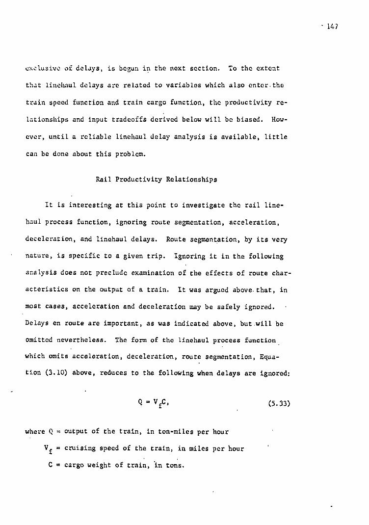
'147

exclusive of delays, is begun in the next section. To the extent

that linehaul delays are related to variables which also enter.the

train speed function and train cargo function, the productivity re-

lationships and input tradeoffs derived below will be biased. How-

ever, until a reliable linehaul delay analysis is available, little

can be done about this problem.

Rail Productivity Relationships

It is interesting at this point to investigate the rail line-

haul process function, ignoring route segmentation, acceleration,

deceleration, and linehaul delays. Route segmentation, by its very

nature, is specific to a given trip. Ignoring it in the following

analysis does not preclude examination of the effects of route char-

acteristics on the output of a train. It was argued above, that, in

most cases, acceleration and deceleration may be safely ignored. •

Delays en route are important, as was indicated above, but will be

omitted nevertheless. The form of the linehaul process function .

which omits acceleration, deceleration, route segmentation, Equa-

tion (3.10) above, reduces to the folloWing when delays are ignored:

Q = VC,

where Q = output of the train, in ton-miles per hour

V f - - cruising speed of the train, in miles per hour

C = cargo weight of train, in tons.

(5.33)

• 14'd

Each of the terms Vf and C represents a function. In general, they

may be specified as follows:

V f = f(HPL.'

NL'

aL.

, s, c, N, a , k., x., g.) (5.34) c c. j j 3

C = g(Nc , kj , Li , xi , g i )

i = 1, ..., NL

j = 1, ..., Nc , (5.35)

in which HPL = horsepower of ith locomotive unit

NL = number of locomotive units

aL. = number of axles per ith locomotive unit

3.

s = gradient of terrain, in percent

c = degree of curvature, in degrees

Nc = number of cars

ac = number of axles per jth car .. 3

= proporticn of the jai car loaded, 0 3

L..= load limit of jth car, in tons

x. = cargo volume of jth car, in cubic feet 3

g. weight weight of jth commodity per unit volume, in • tons per cubic foot.

Note that the above formulation is quite general, allowing for

almost any conceivable combination of the inputs. To simplify mat-

ters somewhat, the following assumptions are made: (1) all freight

C = NckL. (5.37)

cars in the train are identical; (2) all locomotive units on a ,given

train are identical; (3) eath freight car contains the same amount

of cal%4o weight as each of the others in a given train; (4) freight

cars are weight-limited rather than space-limited; another way of

stating this is that the commodities being transported are so dense

that the load limit of a freight car is reached before its cubic

capacity is exhausted. 16 These assumptions permit the following

simplification of the speed and cargo functions:

145

(5.36) Vf = h(HPNa N L)

L' L' L" s c ' c' a c" k

With the aid of a production function, one may examine the ef-

fect of the individual inputs on the productive unit's output, given

constant levels of the other inputs. In the economist's parlance,

productivity relationships may be investigated. One is concerned

with the total, average, or marginal productivity of the productive

unit with respect to a particular input. In addition, the substi-

tution possibilities between inputs may be investigated through the

production function. That is, isoquants may be determined. From

these and the related input costs, expansion paths and cost func-

tions may be obtained.

These properties of a production function may be determined

analytically if the production function relation is sufficiently

simple to permit this. Functional forms may be obtained for such

things as productivity curves, isoquants, and expansion paths.

nowever, in the case of the rail linchaul process function developed

above, such analytical treatment is precluded by the complexity of

the relationship. (Recall that the function V f results from the

solution of a cubic equation.) The alternative method of obtaining

the desired results is to characterize the function numerically us-

ing tables and graphs. This is the procedure followed below.

In the case of rail, the most important effects to be examined

seem to be (1) the effect of the locomotive input on train perfor-

mance, and (2) the effect of the car input on train performance.

The most important input substitution to consider is that between

locomotive power and cars. In addition to these relationships it

is also of interest to investigate the effect of terrain, as repre-

sented by gradient and curvature, on train performance. Finally,

one might like to know the effect upon train output of less-than-

carload shipments. All of these are discussed below.

First, the relationship between the locomotive input and the

train's output is investigated. The locomotive input in the process

function ie represented by three variables: (1) horsepower of a

locomotive unit, (2) number of axles of a locomotive unit, and (3)

number of locomotive units. It is total horsepower of the motive

unit(s) that determines the tractive effort of the vehicle. (See

Equation (5.12).) Under the assumptions stated above, horsepower

' may be obtained in either of two ways. A given horsepower may be

achieved by using a single locomotive unit or several locomotive

units of the same horsepower. (Recall that unequally-powered loco-

motive units for a given train are excluded by assumption.)

1:)0

Figure 5.2 displays total productivity of cars for various lev-

els of horsepower. The values of the variables entering the process

function are given in the box accompanying the figure. They repre-

sent one locomotive pulling standard, fully loaded 70-ton box cars

over straight, level track. These cars have a light weight of 30

tons each. The following observations are Made. (1) The total pro-

ductivity curves for fixed horsepower are strictly concave, i.e., the

marginal productivity of cars is monotone decreasing, or (2Q/a;N

2) < 0.

(2) The marginal productivity of horsepower diminishes. This is seen

from Figure 5.2 by the curves getting closer together as one moves

upward from a given number of cars, i.e., (A2Qi)HP

2) < 0. (3) The

marginal products of both inputs remain positive within the ranges

considered, i.e., (oQ/HP) > 0 and (N/BNc) > 0 for 500 HP 6000

and 10 Nc 100. It is likely that the marginal product of cars

would become negative at some point beyond a train length of 100 cars,

at least for the low horsepower trains. The positivity of the mar-

ginal products means that as the train gets larger and larger, the

resulting decrease in speed is more than offset by the resulting in-

crease in additional carrying capacity.

The productivity curves of Figure 5.2 also permit the examina-

tion of substitution possibilities between the car and locomotive in-

puts. By selecting a particular rate of output and drawing at that

level of output a horizontal line across the family of total product

curves, the combinations of the two inputs yielding the given level

of output are obtained. The curve drawn through such a collection

of points is called an isoproduct curve or isoquant.

1;1

200

! 175 '— i

-, 1 9, D 0

,- ._

- c)

:- 6'. 100

.:, — . _ E 1 C c)

i- 751—

50 r

24-

1

0 0 20 40 60 80 .

Number of cars

Fig. 5.2 -- Productivity Curves for Rail Linehaul Process Function

100

152

ny examining the isoquants shown in Figure 5.3, a couple of in-

teresting properties of rail transportation may be determined. The

isoquants arc negatively sloped throughout, indicating that the two

inputs are technical substitutes for one another, i.e., if fewer

cars are used, more horsepower must be used in order for total out-

put to remain unchanged. Moreover, the isoquants are convex to the

origin, which means that, while the two inputs are technical substi-

tutes, they, are not perfect substitutes. More cars will just compen-

sate for smaller and smaller amounts of horsepower and vice versa.

Finally, isoquants can be used to investigate the returns to

scale exhibited by the productive process. The term returns to scale

describes the output response to a proportionate increase in all in-

puts. If output increases in the same proportion, returns to scale

are constant. They are increasing if output increases in greater

proportion and decreasing if it increases in smaller proportion than

the increase in inputs. 17 There are two equivalent ways one may de-

termine which of these three categories prevails when an isoquant

graph is available. In both methods straight lines must be drawn

from the origin of the horsepower-car axes into the plane. Three of

these are •hown in Figure 5.3. Upon measuring the distance along a

line from the origin between points on successive isoquants which

increase by a constant amount, one will find that these distances

become smaller. This shows that a given increment in output may be

obtained with a proportionately smaller increase in both inputs, a

condition of increasing returns to scale. This condition prevails

along all of the lines drawn in Figure 5.3. Alternatively, one could

15";

N 1

a 1 -- 6

TON-MILES/ HOUR a c -- 4

1 / ..---- 1,

. ...-----

10 20

/ /

/ / / /

/// \<:______,.• ,

..-- -,--'

..."-- ..---

// / ..----

.--. __

50,000 100,000 • / /

/

_L___ _L_ ___ _ 1_ ___ _L _ _ _ _I_ _ . L ______ 50 60 70 80 90 100

Number of cars

Fig. 5.3 -- Isoquants of Rail Linehaul Process Function

150,000

_L L

30 40

200,000 k r 1

L = - 70

w f - 30

c ' 0

3

Hor

sep

ow

er (

in t

hou

sand

s)

note the points along a line from the origin which represent given

proportionate increases in inputs. These are shown in Figure 5.3

by dots along the three straight lines. The first set of dots were

selected to lie on the isoquant representing 50,000 ton-miles per

hour. Successive sets of dots represent, respectively, increases of

100 percent, 50 percent, and 33-1/3 percent. It can be observed that

the isoquants representing increases in output of 100, 50, and 33-1/3

, percent respectively, lie below the corresponding points on the line 1 , 1 : from the origin. Moreover, the isoquants lie increasing distances

1 below these points the greater is the rate of output. Again, this 1

situation indicates increasing returns to scale because proportion-

ate increases in all inputs are accompanied by greater than propor-

tionate increases in output. It is interesting to note that Howe

I found decreasing returns to scale for tow production. 18 This prop-

erty of the tow process function was attributed to the ,increased re-

sistance encountered as the tow widened relative to the width of the .

waterway. There is no factor comparableto the width of the water-

way in the train process function, and the absence of such a resist-

ing factor may account for the apparent increasing returns observed.

A qualification of the above results should be voiced at this

point. Recall that it was assumed in the above calculations that

only one locomotive unit was employed. Thus motive power was added . . ..

to a train by using a more powerful locomotive. The rail process

function allows for the possibility of multiple locomotive units,

and the assumption of a single unit was made for simplification only.

Multiple units would typically be used when total motive power

155:

Ton-miles per Hour

Total Horsepower

2000 4000 6000

Multiples of 2000-HP (4-axle locomotives) Single Unit

101,374 (4 axles) 155,108 (6 axles) 193,909 (8 axles)

101,374 152,765 187,600

exceeded 6,000 horsepower, for at present the largest locomotive

units are of that size. However, it is also conceivable that multi-

ple locomotive units would be employed even where the total horse-

power could be obtained from one unit. This could occur for two

reasons. First, scheduling problems might dictate the use of multi-

ple units where a single unit would be more efficient. Second, in

certain circumstances, multiple units might be more efficient than

a comparable single unit. Such a situation occurs whenever the to-

tal weight of the multiple units is less than that of a comparable

single unit and when the total number of axles of the multiple unit

is less than or equal to that of a single unit. This is so because

both weight and number of axles enter the train resistance function

positively (see Equation (5.22)); and, thus, increases in these fac-

tors, certeris paribus, decrease output. In most instances, how- .

ever, for total horsepower less than 6,000, single locomotive units

will be more efficient than multiple units. In any case, the pro-

cess function may be used to rule out inefficient alternatives. ,

Table 5.2 illustrates how certain multiple units compare with their

corresponding single unit locomotives in pulling a given train.

Table 5.2

EFFECT OF HORSEPOWER ON TRAIN PERFORMANCE FOR SINGLE AND MULTIPLE LOCOMOTIVE UNITS FOR 50-CAR TRAIN

156

0 .5

1.0 1.5 2.0 2.5 3.0

101,374 32,600 18,540 12,903 9,885 8,009 6.731

28.96 9.31 5.30 3.69 2.82 2.29 1.92'

Gradient (percent)

Speed miles/hour

Output ton-miles/hour)

157'

In the examination of barge tows, it was found that the tow's

output was materially affected by characteristics of the waterway,

namely, width, depth, and stream velocity. The comparable variables

in the case of rail transportation are the gradient and curvature of

the track. The effect of gradient of terrain on train performance

is illustrated in Table 5.3. The train whose output is examined in

that table consists of fifty fully-loaded, 70-ton freight cars pulled

by one 2,000-horsepower locomotive. The table ends with a grade of

3 percent because few grades exceed that amount.19

Table 5.3.

EFFECT OF GRADIENT ON TRAIN PERFORMANCE FOR FIFTY 70-TON BOX CARS PULLED BY 2000-HORSEPOWER LOCOMOTIVE

Curvature, the other terrain factor to be considered, also im-

pedes train performance, although not so dramatically is does grad-

ient. The following table illustrates the effect of curvature on

train performance for the same train considered above. Hay reports

that railroad curves for high speed traffic--70 to 100 miles per

hour--are held, to 1 to 2 degrees and 2 to 3 degrees for 'moderate

speeds of 45 to 69 miles per hour. Curvature may go as high as 30

to 40 degrees, but curvature above 20 degrees is not recommended.20

0 •.

.5 1.0 1.5 2.0 2.5 3.0 3.5 4.0 4,5 5.0

Curvatures of greater than 5 degrees are not considered in the table.

Table 5.4

EFFECT OF CUaVATURE ON TaAIN PERFORMANCE FOR FIFTY 70-TON BOX CARS PULLED BY 2000-HORSEPOWER LOCOMOTIVE

Curvature Speed 1 Output (degrees) (miles/hour) 1 (ton-miles/hour)

158

101,374 95,137 89,334 84,092 79,235 74,734 70,706 66,970 63,546 60,404 57,517

The final factor to be investigated is the effect of loading on

train performance. It is common knowledge that less-than-full car-

loadings are discriminated against in rail transport p-icing. While

this is surely a question of relative costs of transporting carloads

versus less.-than-full carloads, it . is of interest to look at this

question from the production side in order possibly to obtain some

evidence on it.- The process function permits investigation of this

point, for it has built into it a variable representing the loading

characteristics of a train. Recall that the simplifying assumptions

,given earlier require that all cars be loaded to the same extent.

The process function, however, permits investigation of any conceiv-

able loading condition, if desired.

28.96 27.18 25.54 24.03 22.64 21.37 20.20 19.13 18.16 17.26 16.43

Table 4 shows, for the same train considered above, what hap-

pens to speed and output as loading varies from empty to full.

Table 5.5

EFFECT 07 CARLOADIZ ON TRAIN RERFORMANCE FOR FIFTY 70-TON BOX.CA'aS PULLED BY 2000-HORSEPOWER LOCOMOTIVE

Proportion Loaded: Speed Output (percent) I (miles/hour) (ton-miles/hour)

159

0' 40.90 10 39.25 20 37.74 30 • 36.34 40 35.05 50 33.85 60 32.73 70 31.67 80 I 30.72 90 29.81 100 I 28.96

0 13,738 26,416 38,156 49,063 59,229 68,734 77,644 86,021 93,91:6 101,374

Although output increases considerably as the cars become fuller,,

there is diminishing marginal productivity associated with the fac-

tor "proportion loaded." If hourly Operating costs of the train were

constant no matter what the load, Chen unit cost (i.e., colt per ton-

mile) would be decreasing throughout as would marginal cost'. This

would constitute-an argument in favor of pricing so as to achieve

full carloading.

Rail Costs

Introduction. -In the preceding sections of this chapter a rail

linehaul process function has been developed. Some properties of the

process function were investigated in the last section. Now it' is

desired to use the process function as an aid in determining the

hohavior of rail costs. First, the costs of the linehaul process

are investigated by deriving a family of short-run average cost

curves. These are analogous to the plant unit cost curves of the

f,rm. However, here the "plant" is a railroad freight train, and

plant "scale" varies as the size of the locomotive changes. Infor-

mation on the extent of economies of scale is provided by the enve-

lope to the short-run unit cost curves. Secondly, the railway

firm's costs are investigated by means of the linehaul process func-

tion and some statistical cost analysis. In this case the rail

linehaul process function - again provides the basis for the analysis

of linehaul costs, but the costs comprising the railway firm's ac-

tivities other than linehaul are provided by the statistical cost

analysis. The rail firm's short-run average cost curves are obtained,

and again the implied long-run envelope curve is used to draw conclu-

sions about economies of scale.

This last exercise, that of grafting the linehaul costs obtained

via the process function onto the other costs obtained from a statis-

tical analysis, should be viewed as merely an example of how one

might obtain cost curves for the firm when process functions do not

exist for all the processes comprising the firm's activities. A

pure process function approach to obtaining the rail firm's costs

would be better, in this writer's view, than the "mongrel" approach

illustrated below. The reasons for this belief are the same as those

given in Chapter I for preferring an engineering approach to a sta-

tical one in the examination of production and cost functions.

The technological approach is inherently more flexible than the

160

statistical, and in addition, does not require the assumption of long-

run er,uilibrium necessary to statistical estimations of long-run costs.

Production functions based on technological data more closely approach

the long-run production functions of economic theory than do statisti-

cal estimations based solely on observed behavior. It is unfortunate,

therefore, that similar technological information has not been success-

f11 , 1 ,, Qmpl,wed f.q- thki other cost components of train (1.,)cratinns.

Co:.t.b of Linchaul Process. Aside from depreciation and interest,

the primary components of linehaul costs are crew wages and fuel ex-

penses. Others such as lubricants and water are so small as to be

safely ignored.21

In order to determine the train's cost curves,

methods of estimating the individual cost components must be developed.

A typical freight train crew consists of an engineer, a conductor,

and two brakemen. 22 The rate at which crew members are paid is based

upon the distance traveled. Time is converted into distance by the

assumption of an average freight-train speed of 12.5 miles per hour.

Therefore, än 8-hour period is equivalent to a 100-mile trip. For

purposes , of determining the crew cost of a trip, the first 100 miles

is charged at one rate and the remaining miles at another, lower rate.

These mileage rates are effectively independent of the actual trip

time involved. If, however, the train actually attains an average

speed for the trip of less than 12.5 miles per hour, then "overtime"

is paid on the basis of the miles that could have been traveled at a

speed of 12.5 miles per hour. Thus, if a 125-mile trip which "should"

have taken 10 hours, actually takes 12 hours, then it is equivalent

to a 150-mile trip for crew-wage purposes. The additional 25 miles

161

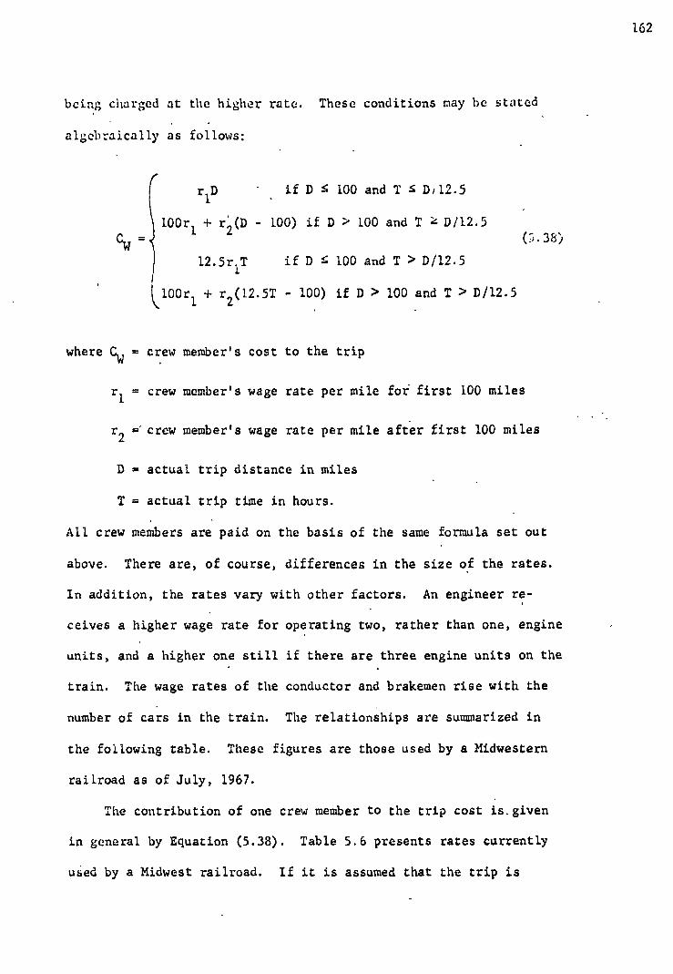
. if D 100 and T D/12.5

100r1 + r2

'(D - 100) if D > 100 and T k D/12.5

if D 1". 100 and T > D/12.5 I 100r1 + r2 (12.5T - 100) if D > 100 and T > D/12.5

r1D

12.5r T 1

being charged at the higher rate. These conditions may be stated

algebraically as follows:

(r).38)

where C = crew member's cost to the trip W

r 1 = crew member's wage rate per mile for first 100 miles

r2 ='crew member's wage rate per mile after first 100 miles

D = actual trip distance in miles . .

T = actual trip time in hours.

All crew members are paid on the basis of the same formula set out

above. There are, of course, differences in the size of the rates.

In addition, the rates vary with other factors. An engineer re-

ceives a higher wage rate for operating two, rather than one, engine

units, and a higher one still if there are three engine units on the

train. The wage rates of the conductor and brakemen rise with the

number of cars in the train. The relationships are summarized in

the following table. These figures are those used by a Midwestern

railroad as of July, 1967.

The contribution of one crew member to the trip cost is.given

in general by Equation (5.38). Table 5.6 presents rates currently

used by a Midwest railroad. If it is assumed that the trip is

162

Rates/Mile for First 100 Miles

Rates/Mile after First 100 Miles Crew Momber

Engineer 1 engine unit 2 engine units

. 3 engine units 4 engine units

Conductor 1-81 cars 82-105 cars 106-125 cars 126-145 cars 146-165 cars over 165 cars

Brakeman 1-81 cars 82-105 cars ' 106-129 cars 126-145 cars 146-165 cars ' over 165 cars

$ .2564 .2657

. .2775 .2840

.2216

.2251

.2291

.2316

.2326 a

.2104

.2139

.2179

.2204

.2214 a

$ .2389 .2482 .2575 .2665

.2041

.2076

.2116

.2141

.2151 a

.1860

.1895

.1935

.1 4 60

.1470 a

Table 5.6

FREIGHT TRAIN CREW WAGE RATES, 1967

a$.20 for each additional block of 20 cars or *portion thereof.

SOURCE: Midwestern railroad which requested not to be identified.

100 miles in length and that the crew consists of an engineer, a con-

ductor and two brakemen, then the following total crew costs for the

trip are defined:

1. If train speed is less than 12.5 miles per hour, then crew

cost is given by .

a. 1 - 81 cars: $11.235T b. 82 - 105 cars: 11.366T c. 106 - 125 cars: 11.516T d. 126 - 145 cars: 11.610T e. 146 - 165 cars: 11.648T f. 166 - 185 cars: 11.723T ' g. 186 - 205 cars: 11.798T

163

2545HP 0.25 =

(139,000)n (5.39)

2. If train speed is greater than or equal to 12.5 miles per

hour, then the crew cost is given by

a. 1 - 81 cars: $89.88 b. 82 - 105 cars: 90.93 c. 106 - 125 cars: 92.13 d. 126 - 145 cars: 92.88 c. 146 - 165 cars: 93.18 f. 166 - 185 cars: 93.78 g. 186 - 205 cars: 94.38.

Fuel cost is the second major component of train expenses. The

amount of fuel consumed on a trip is primarily a function of the

horsepower, thermal efficiency of the engine units, and the energy

content of the fuel. A formula is developed for predicting train

fuel consumption per hour. Knowing this and the price per gallon of

fuel, the fuel cost per hour may be calculated.

The AREA Manual states that the thermal efficiency, defined as

the ratio of work performed to energy consumed of rail diesel en-

gines, is 25 to 30 percent. 23 This may be stated in symbols as W,E =

0.25, where W is work performed and E is energy consumed. In order

that W and E be in the same units, work (which is defined as the

product of.horsepower and time) is converted to Btu. by the follow-

ing relation: 2545 Btu. = 1 horsepower-hour. Since there are ap-

proximately 139,000 Btu. in a gallon of diesel fuel, 24 the energy

content of N gallons is E = 139,000N. Thus, the number of gallons

consumed per hour, n, by a diesel engine of HP horsepower is obtained

from the foliowing expression

164

Cf = p•n = 0.073pHP. (5.41)

which when solved for n yields

n = 0.073HP. (5.40)

Equation (5.40) gives the number of gallons per hour that will be

consumed by engine units generating HP horsepower.

Given the price p per gallon of fuel oil, fuel cost per hour

(C.) is obtained as

165

! In general, fuel cost per hour is given by Equation (5.41). Fuel

cost per trip may be found by multiplying trip time in hours by the

fuel cost per hour. If it is assumed that p = $0.10, i.e., that

diesel fuel is $0.10 per gallon, 25 then fuel cost per trip is given

by

F = $0.0073HP.T. (5.42)

This expression is true regardless of the rated horsepower of the

engine units. However, since the horsepower actually geneiated by

the locomotive units over the entire trip cannot be known, it will

be assumed to be equal to the rated horsepower of the engine units.

What this means is that the train is assumed to operate at full power

during those periods when it is moving at all. This is clearly an

oversimplification and will result in an over-estimate of fuel . con-

sumption and cost when actual utilized horsepower departs from the

C = -4.313 + 0094HP • L L

(0.007) (5.43)

maximula attainable horsepower of the engine units.26 Since 'trains

utilize full throttle whenever possible, 27 this assumption should not

do too much violence to the facts, however.

The next cost 'to be associated with linehaul operations is de-

preciation of equipment. Cars and locomotives depreciate partly

through use and partly through the passage of time. No distinction

is made between these two causes of depreciation, however. Moreover,

for convenience, straight-line depreciation is assumed. While this

assumption is justified only under certain circumstances,28 it is

quite common accounting practice and is used here merely for conven-

ience.

Table 5.7 shows freight car prices by car types. These figures

are averages of actual purchase prices reported to the Interstate

Commerce Commission by railroads. Prices will vary for cars of a

given type as size and other factors vary, but these figures should

serve where more exact ones are not available.

The following equation represents diesel locomotive prices as

a function of horsepower. The equation is a least-squares regres-

sion based on 22 saMple observations from Interstate Commerce Com-

mision data. 29 . Locomotive cost (CL) is in thousands of dollars.

C

166

Again, better information could be obtained for specific locomotive

types, but estimates based on the above equation should be fairly

accurate. The F value of 188 indicates a significant relationship

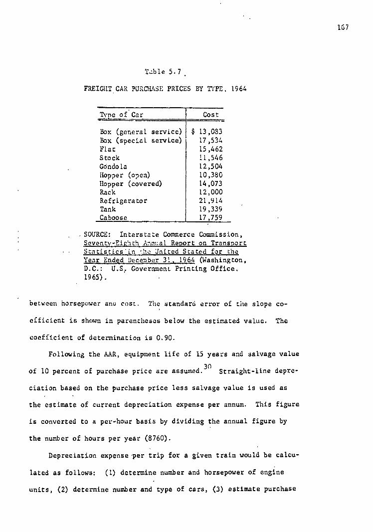
T..:ble 5.7 •

FREIGHT CAR PURCHASE PRICES BY TYPE. 1964

167

Cost Type of Car

Box (general service) $ 13,083 Box (special service) 17,534 Flat 15,462 Stock 11,546 Gdndola 12,504 Hopper (open) 10,380 Hopper (covered) 14,073 Rack 12,000 Refrigerator 21,914 Tank 19,339 Caboose 17,759

.SOURCE: Interstate Commerce Commission, Seventv-Eiehth Annual Report on Transport Statistics 'in United Stated for the Year Ended December 31. 1964 (Washington, D.C.: U.S.. Government Printing Office. 1965). •

between horsepower anu cost. The standard error of the slope co-

efficient is shown in parentheses below the estimated value. The

coefficient of determination is 0.90.

Following the AAR, equipment life of 15 years and salvage value

of 10 percent of purchase price are assumed.30

Straight-line depre-

ciation based on the purchase price less salvage value is used as

the estimate of current depreciation expense per annum. This figure

is converted to a per-hour basis by dividing the annual figure by

the number of hours per year (8760).

Depreciation expense 'per trip for a given train would be calcu-

lated as follows: (1) determine number and horsepower of engine

units, (2) determine number and type of cars, (3) estimate purchase

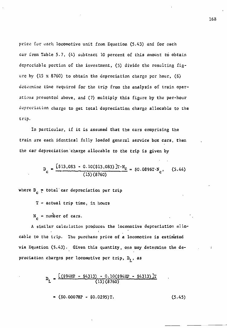
price for each locomotive unit from Equation (5.43) and for each

car from Table 5.7, (4) subtract 10 percent of this amount tO obtain

depreciable portion of the investment, (5) divide the resulting fig-

ure by (15 x 8760) to obtain the depreciation charge per hour, (6)

determine time required for the trip from the analysis of train oper-

ations presented above, and (7) multiply this figure by the per-hour

depreciation charge to get total depreciation charge allocable to the

trip.

In particular, if it is assumed that the cars comprising the

train are each identical fully loaded general service box cars, then

the car depreciation chargeallocable to the trip is given by

[$13,083 - 0.10($13,083)]T.N_ . ‘ $0.0896T•N c , (5.44) D

c =

(15)(8760)

where D= total'car depreciation per trip c •

T = actual trip time, in hours

Nc = nuMber of cars. .

A similar calculation produces the locomotive depreciation allo-

cable to the trip. The purchase price of a locomotive is estiMated

via Equation (5.43). Given this quantity, one may determine the de-

preciation charges per locomotive per trip, DL,

as

[($9411P - $4313) - 0.1009411P - $4313),IIT D L (15)(8760)

168

= ($0.0007HP - $0.0295)T. (5.45)

The final cost to be allocated to the linehaul process is in-

terest on investment in road equipment. Here, as with depreciation,

the total interest charge over the life of the equipment will be re-

duced to a per-hour amount and allocated to the linehaul process on

the basis of the time required to complete the trip.

The total interest charge incurred over the life of the equip-

ment will be estimated by the following relation.

= !.341,r, (5.46)

, where I = total interest charge

W = purchase price of unit of capital equipment

L = length of life of unit of capital equipment

r = annual interest rate.

Equation (5.46) gives the total interest paid (or foregone) on the

investment of W dollars for L years at an annual interest rate r.

It assumes that the amount W is paid off at the rate W/L continuously

over the life of the equipment and is paid off completely at time L.

This assumption may not be justified in practice, but alternatives

to it would be equally suspect. In any case, Equation (5.46) is

quite commonly used for costing purposes 31 and is very easy to apply.

Again, it is desired to express I on a per-hour basis and relate

it to specific units of equipment. Assume r = 0.065; no justifica-

tion is given for this rate. It may, however, be regarded as the

rate paid to bondholders by the firm. Then assuming L years equip-

ment life and using the locomotive purchase price equation, Equation

(5.43), the per-hour interest cost allocable to a locomotive unit,

169

= $0.000351HP - $0.016003. (5.47)

IT

= (ILNL

+ IcNc)T ' (5.49)

170

IL' is given by

(0.5)($94HP L - $4313)(L)(r)

8760L

Sii:.;:arly, using the purchase price in Table 5.7, the hourly interest

cost of a standard box car, l c , is given by

(0.5)($13,083)(L)(r) Ic

- - $0.048367. 8760L (5.48)

Thus, the total interest cost of equipment to be allocated to a trip

of T hours is

where IT = total interest cost of equipment for the trip

NL = number of locomotive units

Nc = number of cars.

In summary. per-hour estimation equations for crew expenses,

fuel expenses, depreciation, and interest have been derived above.

Therefore, to determine the cost of a particular train trip, one

needs to know the trip time in hours as well as the hourly cost com-

ponents. The product of trip time and hourly cost gives total trip

cost. Note that trip cost is a function of (1) trip time, (2) num-

ber of cars, (3) number of locomotives, and (4) horsepower of each

locomotive. See Equations (5.38), (5.42), (5.44), (5.45), and

(5.49). In addition, recall that trip time is given by Equation

(5.30) and is itself a function of (1) trip distance, (2) locomotive

horsepower, (3) number of locomotives, (4) number of axles on each

locomotive, (5) gradient of terrain, (6) degree of curvature, (7)

number of cars, (8) number of axles on each car, (9) loading per-

centage of r , and (10) load limit of each car. See Equation

(5.36) above. Given these relationships, the cost behavior of trains

un,e: a variety of circumstances may be investigated.

Cast Curves for Linehaul Process. Given the cost estimation

equations of the preceding subsection and the train linehaul process

function, it is possible now toinvestigate the cost behavior of a

train in the process of hauling freight between two points. Specif-

ically, it is desired to develop short-run and long-run unit cost

curves for the freight train. Unit cost will be measured in the

units of dollars per ton-mile and will be composed of all major line-

haul expenses including interest and depreciation on equipment (no

distribution of administrative expenses is included, however). The

output measure is the ton-mile per hour. A "plant" consists of a

locomotive of given horsepower; output varies in the short run as

the number of cars comprising the train varies. In the long run the

locomotive horsepower as well as the number of cars can vaty. This

is expressed by a family of short-run unit cost curves

senting a given horsepower. The implied envelope curve to this

family of short-run cost curves represents the long-run unit cost

curve of the linehaul process.

171

, each repre-

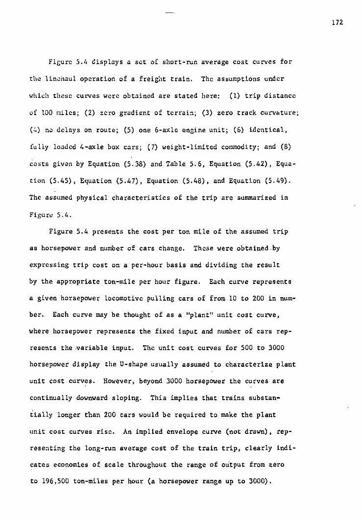
Figure 5.4 displays a set of short-run average cost curves for

the linehaul operation of a freight train. The assumptions under

which these curves were obtained are stated here: (1) trip distance

of 100 miles; (2) zero gradient of terrain; (3) zero track curvature;

(4) no delays on route; (5) one 6-axle engine unit; (6) identical,

fully loaded 4-axle box cars; (7) weight-limited commodity; and (8)

costs given by Equation (5.38) and Table 5.6, Equation (5.42), Equa-

tion (5.45), Equation (5.47), Equation (5.48), and Equation (5.49).

The assumed physical characteristics of the trip are summarized in

Figure 5.4.

Figure 5.4 presents the cost per ton mile of the assumed trip

as horsepower and number of cars change. These were obtained.by

expressing trip cost on a per-hour basis and dividing the result

by the appropriate ton-mile per hour figure. Each curve represents

a given horsepower locomotive pulling cars of from 10 to 200 in num-

ber. Each curve may be thought of as a "plant" unit cost curve,

where horsepower represents the fixed input and number of cars rep-

resents the variable input. The unit cost curves for 500 to 3000

horsepower display the U-shape usually assumed to characterize plant

unit cost curves. However, beyond 3000 horsepower the curves are

continually downward sloping. This implies that trains substan-

iially longer than 200 cars would be required to make the plant

unit cost curves rise. An implied envelope curve (not drawn), rep-

resenting the long-run average cost of the train trip, clearly indi-

cates economies of scale throughout the range of output from zero

to 196,500 ton-miles per hour (a horsepower range up to 3000).

172

2.0

1■■•

1 .5

P■a.

1 .0

Co

st p

er to

n-m

ile

(mill

s)

:00)

0.5

11•—■•

316 0 L 0

W.] .)

1 sa.)

. , r"" . i 2 .1:10

4); )

Horsepower:

" ,f7 • 1

a

1 _ 100 150 200 250 300

Ton-miles pel hour (in thousands)

Fig. 5.4 -- Rail Linehaul Cost Curves

N - 1

a L 6

N c 10, ..., 200

a c 4

A 1

L -- 70

30

•- 0

C • 0

r- 100

No delays

Economics of scale, in fact, seem to persist throughout the range

of output shown on the graph although at a much diminished rate be-

yond an output of 196,500 ton-miles per hour.

Curves such as those of Figure 5.4 can be derived for any pro-

posed trip by specifying the necessary values of the appropriate

variables. The results could be used in the selection of equipment

for various train trips. In addition the linehaul costs generated

via the process function could be used with other cost determination

methods for the remaining rail processes to estimate the rail firm's

costs of a train trip. One way of achieving this last suggestion is

illustrated in the next section.

Cost Curves for Railway Firm. Meyer, Peck, Stenason, and Zwick

(MPSZ) have estimated the long-run marginal cost of freight train

transportation. 32 Their general approach was to divide total rail

operating costs into several components. Each component account was

then subjected to individual analyses. These analyses consisted in

cross-section regressions of cost on output and size variables. The

output variables were usually gross ton-miles of freight and of pas-

senger traffic, although other output variables were used where they

seemed appropriate or gave better results. The size variable was,

usually, miles of track, although, again, others were used.

The components of total operating cost were: train (linehaul)

expenses, station expenses, yard expenses, traffic (selling and mar-

keting) expenses, general (administrative and legal overhead) expenses,

variable portion of maintenance expenses, variable portion of depre-

ciation expenses, and variable portion of capital costs.

174

The analyses of t'aese cost categories were synthesized to yield

over-all relationships between cost and output. MPSZ did this by em-

ploying certain assumptions about the relationships between ton-miles

and certain other operating :Icasures such as yard hours and train

miles. Based on these assumptions and the statistical analyses, the

long-run marginal costs shown in Table 5.8 are obtained. Using MPSZ's

results, if one wanted to estimate the long-run marginal cost of a

freight train trip, he would determine the amount of gross ton-miles

to be generated and multiply this by 4.28 mills, which is the price-

corrected version of the MPSZ figure. Such a calculation would re-

quire knowledge of the distance to be traversed by the train, the

cargo tonnage of the train, and the tare weight of the train.

MPSZ say, in reference to the above sort of calculation, "It

should be noted that these estimates are based on a sort of central

tendency and are typical figures that will apply to freight movements

only of a very average or ordinary kind." 33 The reason for this is

in part due to the nature of the estimation procedure and in part due

to the assumptions required to use some of the results. The varia-

bility of costs with output was investigated, as mentioned above, by

means of linear regression analysis. This by its very nature makes

the estimates "sort of central tendencies." In addition, certain

assumptions were employed to achieve the figure of long-run marginal

cost on a gross ton-mile basis. For example, it was assumed that it

required "approximately 24 minutes to originate, classify, and termi-

nate the typical merchandise car, that this car goes approximately

400 miles, and that it has a load of 25 tons." 34 These assumptions

1.75

Tab1e 5.8

LONG-RUN MARGINAL COST OF RAIL FREIGHT TRANSPORTATION

, Cost Per Gross Ton-Mile of Percentage Cost Category Freight_ Traffic ,

b of .,_

1947-50 Mills, 1965 Mills Total

Traina

0.411000 0.809670 18.90 SLation 0.001799 0.003544 0.08 Yard 0.268441 0.528829 12.34 Traffic 0.070860 0.139594 3.26 General 0.126000 0.236400 5.52 Maint. of Way

& Struct. 0.284000 0.559480 13.06 Freight Car

Maint. 0.162000 0.319140 7.45 Yard Engine

Maint. 0.004000 0.007880 0.18 Road Engine

Maint. 0.151000 0.297470 6.94 Joint Equip.

Repair 0.088900 0.175133 4.09 Equip. Repreci-

ation 0.165360 0.325759 7.60 Road Struct. Depreciation 0.046640 0.091881 2.14

Capital 0.401100 0.790167 18.44

Totals 2.175100 4.284947 100.00

aTo be estimated from an engineering production function.

bThe price indices used for corretting the 1947-50 figures

were obtained from Association of American Railroads, Railway, Statistics Manual (Washington, 1964), p. 10.14, "Indexes of Average Charge-Out Prices of Railway Material and Supplies and Straight Time Hourly Wage Rate Class I Railroads," for the period to 1963, and from Association of American Railroads, "Indexes of Railroad Material Prices and Wage Rates (Railroads of Class I)," Series Q4IPW-51, May 17, 1966, for the period 1963-65.

SOURCE: John R. Meyer et al., The Economics of Competition in the Transportation Industries (Cambridge, Mass., 1960), pp..46-47, 51, 56, 60, 62, Appendix B.

176

were used to reduce yard expenses to .1 gross ton-mile basis. Later,

it was assumed "that any shipment under analysis is normal in t'le

sense that it approximates the 1947 to 1950 averages of having 3,0(o

ross ton-miles of freight moved for every road mile of diesel engine

operations and requiring one diesel engine yard hour for every

gross ton-miles of freight traffic." 35 These assumptions were used

to translate the yard engine and road engine maintenance figures into

gross ton-mile equivalents.

It is possible even within the context of the MPSZ work to avoid

making such assumptions. For example, MPSZ provide equations from

which can be estimated yard time. 36 If one does not necessarily wish

to relate all costs to a gross ton-mile basis, the original estimat-

ing equations can be used rather than the aggregate figures of Table

5.8. In most cases, they will be no different because the gross ton-

mile is the predominant output variable used, but in some cases, for

example, road engine maintenance, other variables are included in the

estimation, necessitating either assumptions such as those used by

MPSZ or actual values for a particular situation.

While it is possible to use MHZ results without some of their

assumptions, it is not possible to use them and avoid the central-

tendency aspect mentioned above. One way to avoid this problem is

to provide an alternative cost estimation procedure for some or all

of the components of total operating expenses. Clearly one of the

most important of the cost categories is train expenses. It is pro-

posed, therefore, to estimate train expenses by use of the rail pro- .

cess function and direct costs for crew and fuel. The train expenses

177

69,000

obtained this way may then be added on to the other operating expenses

as estimated by MPSZ, yielding a . combined engineering-statistical cost'

estimate.

It is proposed to substitute direct estimates of certain costs

for those estimates of MPSZ. Specifically, the following costs will

be estimated directly: (1) train expenses, i.e., crew costs and fuel

costs, and (2) locomotive and car depreciation expenses. Another

cost that could be estimated directly, locomotive and car capital ex-

penses, will not be. The reason for this is that the MPSZ estimate

of capital cost includes not only locomotives and cars but investment

in road as well. It would be difficult to disentangle the various

capital items in the MPSZ analysis, and therefore, it is more con-

venient to use their capital cost estimate exclusively. Those other

costs for which the MPSZ figures will be used are: station, yard,

traffic, general, maintenance of way and structure, freight car main-

tenance, joint equipment repair, and road structure depreciation.

Directly estimated costs (train and equipment depreciation) comprise

about 25.5 percent of the total, based on Table 5.8.

For any given trip, crew wages may be determined from Equation

(5.38) and Table 5.6, with the following additional information:

trip distance, number of engine units, number of cars, and trip time.

Fuel cost for a trip may be calculated from Equation (5.42) if one

• knows trip time, engine horsepower, and price per gallon of diesel

fuel. Equipment depreciation expenses allocable to the trip may be

determined from Equation (5.45) for locomotives and Equation (5.44)

for boxcars. (If one were interested in a different type of freight

178

ear, an equation similar to Equation (5.44) could be developed with

the use of Table 5.7, freight car prices.)

For those costs not estimated as described above, the price-

corrected figures of MPSZ are used. 37 Referring to Table 5.8, it is

seen that MPSZ have estimated long-run marginal cost per gross ton-

mile of freight to be 4.28 mills. Train and equipment depreciation

expenses were estimated by MPSZ to be 1.13 mills per gross ton-miles

of freight. In order, then, to find the contribution to the firm's

total Costs of an additional trip (excluding crew, fuel, and equip-

ment depreciation costs of a trip), one must determine the gross ton-

miles to be generated during the trip and multiply this figure by

3,15 mills. Note that this assumes marginal cost equal to average

cost. It is not in general true that marginal cost times output

yields total cost. However, since MPSZ claim they have estimated

long-run marginal cost, the identification of marginal with average

is justified in this case.

Putting the preceding discussion into symbols, one may express

the cost (C) to the firm of a train trip as follows:

179

(5.50) C = W + F + Dc + D

L +A

,

where W = crew wages

F = fuel cost

Dc = depreciation of cars

DL = depreciation of locomotives

A = all other costs.

The estimating methods for each of the first four cost components

were presented above. Utilizing the MPSZ estimate, corrected for

price changes, all other costs of the train trip may be estimated by

A = $0.00315 (gross ton-miles). . (5.51)

The rail process function estimates train speed and the ton-

miles per hour produced by the train. The inputs required for the

use of the process function are (1) number of cars, (2) tare weight

of each car, (3) load limit of each car (if commodity to be trans-

ported is not very dense, then cubic capacity of each car and weight

per cubic foot of the commodities must be known), (4) proportion of

each car filled, (5) number of axles on each car, (6) horsepower of

locomotive(s), (7) number of locomotives, (8) number of axles on each

locomotive, (9) gradient of terrain, and (10) degree of curvature.

Given the speed of the train from the process function, the trip

time is easily calculated, assuming no delays. If an estimate of de-

lay time is available, this may be used in conjunction with train

speed to determine trip time. For any given routeand any given train,

the trip cost may be determined from the cost estimation procedures

discussed above, using the train process function to estimate trip

time and to calculate the rate of output (in ton-miles per hour) pro-

duced by the train. Moreover, the behavior of cost as horsepower and

number of cars vary may be observed.

In addition to the assumptions made above, it is further assumed

for purposes of the example presented below: (1) there are no delays

180

en route, (2) there is no grade, (3) there is no track curvature,

(4) the commodities are dense enough that the cars.are weight limited

r,,ther than space limited, (5) all cars are fully loaded, (6) trip

length is 100 miles, (7) cars are standard box cars with tare weight

of 30 tons each and load limit of 70 tons each, and (3) only one

locomotive is used.

Figure 5.5 presents the cost per ton-mile of the assumed trip

as horsepower and the number of cars change. These were obtained

by expressing trip cost on a per-hour basis and dividing the result

by the appropriate ton-mile per hour figure. Each curve represents

a given horsepower locomotive pulling cars of from 10 to 200 in num-

ber. Each curve may be thought of as a "plant" unit cost curve,

where horsepower represents the fixed input and number of cars repre-

sents the variable input. The unit cost curves for 500 to 2500 horse-

power display the U-shape usually assumed to characterize plant cost

curves. However, beyond 2500 horsepower the curves are continually

downward sloping. This implies that trains substantially longer than

200 cars would be required to make the unit cost curves rise. An

envelope curve could be drawn to the individual unit cost curves.

This would represent the long-run average cost of the train trip to

the firm. Although such a curve is not drawn in Figure 5.5, it is

clear that economies of scale exist in the range of output from zero

to 180,000 ton-miles per hour (a horsepower range of from 500 to

2500). Economies of scale, in fact, seem to persist throughout the

range of output shown on the graph although at a much diminished rate

beyond an output of 180,000 ton-miles per hour.

181

7.25

7.00

6.75

6.50

Co

st p

er t

on

-mil

e (m

;11s

)

6.25

6.00

5.75

5.50

5.25

5.00

4.75 1.)0(4 3 -0)) 3 .1.0

JL I 300 3.50

1 250

V41 S 1).1 V0.1 ,:. ■ I I

cal I I I i

0 50 100 150 200

Ton-miles pet hour (in thousands)

Fig. 5.5 -- Railway Firm Cost Curves

Summary. In this section, an attempt has been made to show how

the rail linehaul process function may be used to generate linehaul

costs. Linchaul plant unit cost curves were derived and some impli-

caLions of them discussed. An example was also provided to show how

an engineering-type process function could be used in conjunction

with statistical analysis to provide estimates of the rail firm's

costs. Unit cost curves were again derived and their implications

discussed.

183

CHAPTER VI

SUMMARY AND CONCLUSIONS

The purpose of this dissertation is to provide a method for de-

veloping process functions for the linehaul operations of transport

modes and to apply that method to two modes. An introductory chapter

, distinguishes between a production, function and a process function,

the latter being used throughout the dissertation to describe a pro-

duction function for one process out of several that comprise the

production activities of a transport mode. The derivation of cost

functions from production functions is discussed in the introduction

with an eye on the future use to be made of this discussion in Chapter

V. A distinction is made between the statistical approach to esti-

mating production and cost functions and the engineering approach.

It is argued the latter possesses several advantages over the former.

The engineering approach is followed in the dissertation.

Chapter II contains a rather detailed and complete survey of the

previous research in cost and production relationships for inland

waterway and rail transportation. Emphasis is on method but results

are thoroughly discussed. Criticisms are made where they seem appro-

priate, but the review is a survey rather than a critique.

The method of analysis to be used throughout the remainder of

the study is contained in Chapter III. This chapter details the

form of the transportation linehaul process function which in its

most general form makes provision for acceleration, deceleration, •

184

1

185

and delays as well as cruising speed of the vehicle. The general

equation of motion of a vehicle is presented, and specific forms of

it to be used later are also discussed. General acceleration equa-

tions arc obtained for the case of a quadratic equation of motion,

to be applied later to the case of barge tows. A brief discussion

of delays and cargo capacity concludes the chapter. Since the latter

two items .c. specific to a transport mode, no general delay or cargo

analyses are provided.

Chapter IV contains the application of methods developed in

Chapter III to the case of barge tows. Much of the analysis in this

chapter relies on the work of Charles W. Howe. Howe's analysis is

deficient in that no consideration of delays or of acceleration and ,

deceleration is presented. This chapter rectifies those deficiencies

by providing analyses of locking, making and breaking tow, miscel-

laneous delays (e.g., weather, running aground, etc.) as well as ac-

celeration and deceleration.

It was found that the industry rule of thumb concerning acceler-

ation is probably correct, i.e., it requires a distance of 1' 2 to 2,

times the length of the tow to reach cruising speed from a stopped

position. This ordinarily involves distances of between 1,000 and

2,000 feet. In the examples given in the text, acceleration time

ranged from about 2k minutes to 1-4 minutes. It was concluded that,

. unless trips were very short or involved many stops and starts, ac-

celeration could be ignored in the linehaul process function. A com-

parable deceleration analysis was not provided, but the conclusions

reached for acceleration, which takes longer than deceleration, ,

should apply a fortiori.

Of the myriad delays encountered by tows, locking and tow as-

sembly and disassembly account for the major portion of delay time.

A simple queuing model is developed for predicting locking delay.

The locking model estimates the amount of time a tow can expect to

spend in the process of locking on any given trip. The model is

sensitive to the number of tows operating on the waterway (which is

estimated from total tonnage to be transported on the waterway, aver-

age tow size, and an empty backhaul factor) and to the characteris-

tics of the locks themselves. The model is checked against actual

average locking times and found to predict well.

The time involved in assembly and disassembly of tows is found

to be accurately estimated by linear relationships in which the num-

ber of barges comprising the tow is the independent variable. That

is, making and breaking tow each requires a constant amount of time

irrespective of the number of barges in the tow and an amount of

time proportionate to the number of barges in the tow.

All other delay time (e.g., that due to weather, running

aground, etc,) is classified as miscellaneous. The time consumed

by miscellaneous.delays is found to be proportionate to tow running

time, the factor of proportionality being estimated as 14 percent.

• That is, a trip which would require 10 hours with no delaya could be

expected to encounter miscellaneous delays amounting to 1.4 hours.

Given these delay analyses, the tow linehaul process function

is complete and may be used to estimate productivity and cost

186

relationships in the same manner in which these were performed by

Howe for the incomplete tow process function. Howe found decreasing

..- vturns to scale for his tow process function, i.e., cquiproportionate

incrcnves in the barge and towboat inputs resulted in less than pro-

po .rtionate increases in output. While similar computations are not

made above, there is no reason to believe Howe's result is changed -.' '

In :act, it deems likely that a gleater degree of decreasing returns

to scale would be exhibited by the linehaul process function indlu-

sive of delays, for delay time is in all cases positively related to

the number of barges in the tow. Making and breaking tow require

more time the greater the size of the tow, and a larger towboat would

not likely help very much in reducing that time (although this con-

jecture is 'net investigated in the preceding analysis). Likewise,

locking time will-increase as tow size increases; this is especially

true where -double and triple locking would be required from increases

in tow size. Finally, even miscellaneous delays are likely to be

greater as tow size increases. It was found that miscellaneous de-

lay time is proportionate to running time, but running time is likely

to be greater for large tows than for smaller ones since the former

will travel glore slowly.. This may be thought to be offset to 'some

extent by large towboats but, since Howe found decreasing returns to

scale and diminishing returns to the towboat input, this offset is .

not likely to exist. All in all, it seems reasonable to say.that the

tow process function (including delays) will exhibit decreasing re-

turns to scale. It is also likely, based on the above discussion,

that Howe's conclusion of a flat long-run unit cost curve over a

1.67

wide range of output would have to be altered. This would probably

result in a U-shaped long-run average cost curve, which if flat at .

all would be flat over a narrower range of output possibilities. Of

course, the level of the curve would be higher than that calculated

by Howe, even if the same input costs were used, simply because of .

the inclusion of delay time. .

Though not a component of the tow process function, an analysis

of waterway capacity and tolls is presented in Chapter IV. This is

an outgrowth of the locking model and may be viewed as an applica-

tion of welfare economics to tow and waterway operations. The anal- , ysis provides a method of measuring the capacity of a waterway in ,

terms of the utilization of its locks. A method of calculating the

optimal toll to be charged for use of the waterway is also developed.

The toll is optimal in the sense that if imposed it would equate

private and social coats. Methods are, of course, provided for cal-

culating these costs. A recapitulation of resurts ends the chapter.

Chapter V is an application of the method of Chapter III to the

case of rail freight trains. For the purpose of the rail analysis,

there is no previously existing process function as there was for

the case of barge tows. However, there are, much more widely accepted

and well known engineering relationships available for rail opera-

tions than there are for barge operations. The chapter proceeds to

.exploit these relationships in developing the rail linehaul process \

function. .

The two most important functions in determining, the speed of a

rail train are, as discussed in Chapter III, the tractive-effort.

188

function and the drag-force function. Both of these have been esti-

1.....ted, and their forms are well known in the railroad engineering

lItcrature. The tractive-effort function is taleen over from the lit-

erature without modification. The drag-force function, however, is

modified to include variables such as number of cars, number of loco-

motives, gradient of terrain, and degree of track curvature.

Given these two functions, one can determine the cruising speed ,

of a train as a function of many interesting variables. The cruis-

ing speed of a train multiplied by the cargo tonnage of the train .

gives the ton-miles per hour produced by that vehicle, ignoring ac-

celeration, deceleration, and delays and assuming that the train

operates at full throttle. The implications and importance of these

assumptions are discussed in Chapter V. No analysis of delays is .

provided in this chapter. A discussion of acceleration and decelera-

tion, along with some estimating equations, is presented but no use

is made of them in the remainder of the chapter. It may be noted .

that the rail linehaul process function, exclusive of delays and,ac-

celeration-deceleration, is similar to the original tow process func-

tion of Howe. That is, it is incomplete in several respects but may

be used to provide insights into rail freight operations.

The chapter proceeds to investigate various productivity rela-

tionships of the rail freight train. Under certain simplifying as-

sumptions, it is found that the marginal productivity of the car in-

put is'monotouu decreasing. It is further shown that the marginal

productivity of the locomotive input diminishes. The marginal prod-

ucts of both inputs remain positive within the ranges considered.

189

Isoquants between car and locomotive inputs are drawn and returns to

scale investigated. It is found that the inputs are technical sub-

stitutes, but not perfect substitutes, and that the process function

exhibits slightly increasing returns to scale. In addition to these

findings, effects of gradient of terrain and track curvature on

train performance are investigated. Increases in both of these fac-

tors result in decreases in train output, most notably for gradient

where very small increments result in very large reductions in out-

put. Finally the effect of carloading on train performance is in-

vestigated. A rationale is provided for the less-than-carload dis-

criminatory pricing practiced by railroads.

Finally, the rail linehaul process function is used to estimate

rail costs. In order to do this, however, the cost components of

linehaul operations must be investigated. This leads to develop-

ment of methods for estimating crew costs, fuel costs, interest cost

on equipment, and equipment depreciation costs. All of these costs

relate to the linehaul movement of commodities; there are no station

expenses; administrative costs, etc. Given these cost estimation

relationships and the rail linehaul process function, it is then

possible to produce unit cost curves for the train trip. A short

run average cost curve is developed by assuming a locomotive of

190

given size but varying numbers of cars. A family

. obtained by varying the size of locomotives. The

U-shaped average cost curve is obtained for small

of such curves is

typically assumed

horsepower locomo-

tives. But as locomotive horsepower increases (i.e., "firm" size

increases) the short-run average cost curves become flatter and

flatter. An envelope curve may be drawn to this family of short-run

curves. Such an envelope represents the long-run unit cost curve of

the train. The implied envelope curve indicates great economies of

scale at low levels of output but much smaller economies at higher

levels of output.

It is also shown in Chapter V how one might use both statistic-

ally derived costs and the rail process function to estimate the

rail firm's costs of a train trip. In order to illustrate this the

' statistical cost analysis of Meyer, Peck, Stenason, and Zwick is

employed. They had divided total rail operating costs into several

categories, e.g., train (linehaul), station, yard, etc. Each cate-

gory was analyzed individually by means of regression analysis, with

the goal of synthesizing the resulting relationships into an esti-

mate of the rail firm's costs.

Since the analysis of this dissertation provides a method for

estimating the train expense portion of the firm's costs as described

above, that analysis was substituted for the statistical estimation

of Meyer, Peck, Stenason, and Zwick. Thus, it was possible to gen-

erate cost curves for the rail firm in a manner similar to that

described above. Were process functions available for other cost

categories, such as yard operations, these could be incorporated

into the statistical analysis as train expenses were. Thus it is

seen that a combination of statistical and engineering costing may

be used to generate the firm's cost curves.

The reader should be reminded that in the rail linehaul pro-

cess function delays were ignored. Therefore, the productivities

191

reported in the dissertation will in fact be lower if delays occur. .

In like manner cost curves will be higher than those shown above.

Moreover, to the extent that delays are themselves functions of some

of the same variables in the process function, then productivities

and cost curves may assume different forms than those shown in Chap-

ter V. It is difficult to say anything more on a priori grounds

about the effect of delays on the shape of the productivity and cost

curves. It is left to someone else to provide the required delay

analysis for rail.

In conclusion, it might be said that the results of this dis-

sertation should be of interest to two groups of people: to those ,

who are interested in seeing examples of the "engineering approach"

to the development of production functions and to those who are

interested in the costing of rail and water freight transportation.

- It is hoped that the former group will be satisfied. Indeed, it is

further hoped that they will see the possibilities of applying the

method developed here to. other transportation modes as well. Un-

fortunately for the latter group, the last word has by no means

been said. It is hoped, however, that they recognize an approach

to costing that could be fruitful and which is comparable across

modes. .

192

FOOTNOTES

Chapter I

1. Unless otherwise noted, the discussion in this and in the next subsection may be found in any intermediate price-theory text-book, e.g., James M. Henderson and Richard E. Quandt, Micro-economic Theory: A Mathematical Approach (New York, 1958), pp. 42-75.

2. The distinction between process and production functious math_ in the text may be found in A. A. Walters, "Production and Cost Functions: An Econometrlc Survey," Econometrica, XXXI (jan.- Apr. 1963), pp. 11-14. An alternative use of the term is found in Alan S. Manne and Harry M. Markowitz (eds.), Studies in Pro-cess Analysis: Economy-Wide Production Capabilities (New York, 1963). To Manne and Markowitz "'process analysis' always refers to the construction and use of industry-wide, multi-industry, and economy-wide models which attempt to predict production re-lationships on the basis of technological structure." (p.4)

3. See Walters, p.13.

4. See Henderson and Quandt, p. 55 and the example on pp. 66-67.

5. An example of this approach may be found in Charles W. Howe, "Process and Production Functions for Inland Waterway Trans-portation" (Institute for Quantitative Research in Economics and Management, Paper No. 65, Purdue University, 1964), pp. 2U-31.

6. Kurt Ehrke, Die Uebererzeugung in der Zementindustrie von 1858- 1913 (Jena, 1933).

7. Theodore O. Yntema, United States Steel Corporation T.N.E.C. pa2cal_112marising the Pamphlets and Charts Submitted by United States Steel Coaoration to the Temporary National Economic Com-mittee (Washington, 1940), I, 223-301.

8. Joel Dean, Statistical Determination of Costs with Special Refer-ence to Marginal Costs (Chicago, 1963).

9. C. W. Cobb and P. H. Douglas, "A Theory of Production," American Economic Review, XVIII (Ma..ih 1928), 139-65.

193

10. M. Bronfenbrenner and P. H. Douglas, "Cross Section Studies in the Cobb-Douglas Function," Journal of Political Economy, XLVII (Dec. 1939), 761-85.

11. Temporary National Economic Committee, "The Relative Efficiency of Large, Medium-sized, and Small Business," Monograph 13 (Washington, 1941).

12. J. Dean and R. W. James, "The Long-run Behavior of Costs in a Chain of Shoe Stores," Studies in Business Administration, XV (Chicago, 1942).

13. H. B. Chenery, "En1;ineecing Production Functions," Quarterly Journal of Economics, LXIII (Nov. 1949), 507-31.

14. Allan R. Ferguson, "Commercial Air Transportation in the United States," Studies in the Structure of the American Economy, ed. Wassily Leontief (New York, 1953), pp.. 412-47.

15. Statistical estimation of cost and production functions has been subjected to a great deal of scrutiny. One of the best surveys on this subject, in addition to the Walters article cited above,, is John R. Meyer and Gerald Kraft, "The Evaluation of Statisti-cal Costing Techniques as Applied to the Transportation Industry," American Economic Review, LI (May 1961), 313 ,34.

16. See Vernon L. Smith, Investment and Production; A Study in the Theory of Capital-Using Enterprise (Cambridge, Mass., 1966) pp. 24-30.

17. Walters, p. 12.

18. This classification has been used in statistical estimation of a rail production function. See George H. Borts, "Production Relations in the Railway Industry," Econometrica, XX (Jan. 1952), 71-79.

19. See, for example, Nancy Lou Schwartz,‘"Economic Transportation Fleet Composition and Scheduling, with Special Reference to Inland Waterway Transport" (Institute for Research in the Be-havioral, Economic, and Management Sciences, Paper No. 91, Purdue University, 1964); M. L. Burstein, et al., The Cost of Trucking; Econometric Analysis (Dubuque, 1965).

20. See, for examplu, Charles R. Carr and Charles W. Howe, Quanti-, tative Decision Procedures in Management and Economics; Deter-ministic Theory and Applications (New York, 1964), pp. 10-20.

21. Smith, pp. 45-55.

194

4rr IJJ

22. See, for an elaboration of this distinction, Jack Uirshleifer, "The Firm's Cost Function: A Successful Reconstruction?" Journal of Business, XXXV (July 1962), 235-55.

23. The'latter of these is examined in Chapter V.

Chapter II

1. Howe, "Process and Production Functions ...." The porLion of this paper relating to the process function hz:s been puhlisued, as "Methods for Equipment Selection and Benefit Evaluation in inland Waterway Transportation," Water Resources, I (First Quarter 1965), 25-39. Citations will be made to the first of these papers.

2. A more general treatment of this assertion is presented in Chapter III.

3. Howe, p. 10.

4. See, for example, Henderson and Quandt, p. 46.

5. Howe, p. 29.

6. Charles W. Howe, "The Performance of Barge Tows: A Mathemat-ical Representation" (unpublished paper, Resources for the Future, inc., 1966).

7. Howe, "Process and Production Functions ...," pp. 35-61.

8. Ibid., p. 48.

9. Ibid., p. 60.

10. Charles W. Howe, "Models of a Barge Line: An Analysis of Returns to Scale in Inland Waterway Transportation" (Institute for Re-search in the Behavioral, Economic, and Management Sciences, Paper No. 77, Purdue University, 1964).

11. Arthur P. Hurter, Jr., "Production Relationships for Inland Waterway Operations on the Mississippi River: 1950, 1957, 1962" (unpublished paper, The Transportation . Center, Northwestern University, 1965).

12. Arthur P. Hurter, Jr., "Cost Relationships for Inland Waterways Operations on the Mississippi River: 1950, 1957, 1962" (un-published paper, The Transportation Center, Northwestern Uni-versity, 1965).

13. A. V.ctor Cabot and Arthur P. Hurter, Jr., "Equipment Schedul-ing IA River System liansportation" (unpublished paper, The Transportation Center, Northwestern University, 1965).

14. George H. Borts, "Increasing Returns in the Railway Industry," Journal of Political Economy, LXII (Aug. 1954), 316-33, esp. pp. 318-21.

15. As Borts points out, much of the work done on rail costs was done before the long-rud envelope curve of economic theory had been developed. There is, therefore, little distinction made between long-run and short-run costs. Borts feels that the dichotomy between "variable" costs and "constant" costs is identical to the current economics usage only when the short-run cost function is linear. Otherwise, the early railway economists were including some variable cost in their constant cost category. The extent of increasing returns, as this term . was used by the early railway economists, referred to the rela-tionship between fixed and variable costs and is not the "econ-omies of scale" resulting from firm size. See Borts, pp. 318- 21.

16. W. Z. Ripley, Railroads, Rates, and Regulation (New York, 1927).

17. Rail Freight Service Costs in the Various Rate Territories of the United States (Washington, 1943).

18. "Cost and Value of Service in Railroad Rate Making," Quarterly Journal of Economics, XXX (Feb. 1916), 109-12.

19. The I.C.C. cost analysis is explained in I.C.C. Bureau of Ac-counts, Explanation of Rail Cost Finding Procedures and Prin-ciples Relating to the Use of Costs, Statement No. 7-63 (Wash-ington, 1963), Chs. 1 and 2. References to the work of early railway economists are found in these chapters also.

20. See, for example, John R. Meyer, et al., The Economics of Com-petition in the Transportation Industries (Cambridge, Mass., 1960), Appendix A, pp. 274-76. Also see, W. J. Stenason and R. A. Bindeen, "Transportation Costs and Their Implications: An Empirical Study of Railway Costs in Canada," Transportation Economics (New York, 1965), pp. 121-23.

21. Meyer, et al., pp. 33-63, 177-320

22. Only a brief description of Meyer's study will be given here, for a much more detailed discussion is presented in Chapter V in illustrating the integration of statistical cost analysis with the engineering process function for rail.

23. Meyer, et al., p. 43.

196

24. The discussion of the Canadian rail costing methods is based on Stenason and Bandeen, pp. 123-38, and on Royal Cormaission on Transnortation, III (Ottawa, 1962), pp. 193-365. Discussions with Msars. George Hanks and Victor Alalouf of the Canadian National Railways were very helpful also.

Mover and Kraft, pp. 313-40.

25. George H. Borts, "The Estimation of Rail Cost Functions," Economet rica, XXVIII (Jan. 1960), 108-31.

27. Ibid., p. 118, n. 13.

28. Ibid., p. 120, See also G. W. Snedecor, Statistical Methods (Ames, Iowa, 1946), pp. 318-74.

29. George H. Borts, "Production Relations in the Railway Industry," pp. 71-79.

30. Soberman has provided a rail linehaul simulation model as part of a larger study being performed at Harvard University. While the Sobennan model provides neither a production function nor a cost function for rail transport, it does use some of the basic engineering relationships to be employed below. Richard Soberman, "A Railway Performance Model" (unpublished paper, Harvard Trans-portation and Economics Seminar, Paper No. 45, Harvard University, 1966).

Chapter III

1. Travel - tine expressinns imil to those in the toxt may be found • in R. H. Haase and W. H. T. 11, ',ter:, Performance of Land Trans-

portation Vehicles, RAND Memorandum RN-3966-RC (Santa Monica, 1964), pp. 11-13 and Appendix D. These expressions are not re-lated by Haase and Holden to any sort of transportation produc-tion analysis.

2. Some of the notation of Haase and Holden has been adopted in this section. Where specific analysis of theirs is used, this will be indicated by individual citations.

3. Haase and Holden, p. 4.

4. The actual' functions will be given in Chapter IV.

• 5. Haase and Holden, p. 97.

6. The actual functions will be given in Chapter V.

197

2.

7. There are in fact three different possible sets of roots: (1) one real, two conjugate imaginary; (2) three real of which at least two are equal; and (3) three real and unequal roots. See Robert C. Weast et al. (eds;), Handbook of Mathematical Tables (Cleveland, 1964), p. 464. The fact that a unique real, posi-tive root results from the solution of the rail equation of motion is discussed in Chapter V.

S. Haase and Holden, p. 107ff.

9. Ibid., p. 96.

10. Ibid.

11. See Haase and Holden, p. 107ff; also see Figures 4.1 to 4.3 below.

• 12. Haase and Holden, p. 121.

13. Ibid. •

14. Ibid.

15. Ibid., p. 123.

16. Ibid.

Chapter IV

1. Much of the descriptive material in this subsection is based on talks with personnel of barging firms and on the voluMe LiLg. Load Afloat (Washington, 1956) prepared by the American Water- Ways Operators, Inc.

2. Such a capacity table is reproduced in Howe, "Methods ...," p. 39.

3. Ibid., pp. 25-39.

4. Ibid.

. 5. U.S. Army Engineer Division, Ohio River, Corps of Engineers, Cincinnati, Ohio, Resistance of Barge Tows: Model and'IProto-type Investigation, August, 1960.

6. Howe, "Methods...," p. 27.

7. Howe, "The Performance of Barge Tows ...," pp. 3-11.

198

8. W. B, Langbcin, Uydroulics of River Channel:, dE P.clated to 1;avi-ability, Geological Survey Water-Supply Paper 1539-W (Washington, 1962). •

Hunter Rouse, Elementary Fluid Mechanics, (New York, 1946), p. 234ff.

10. Howe, "The Performance of Barge Tows ...," p. 14.

11. U.S. Army Division, Up i.er Mississippi Valley Division, Memorandum Report on Prototype Barge Resistance Tests, September 21, 1949.

12. See Robert H. Strotz and Robert AL Coen, "Estimating Explanatory Variables in Single and Simultaneous Equation Models" (unpublished paper, Northwestern University, n.d.), pp. 1-6.

13. Howe, "The Performance of Barge Tows ...," p. 22, Appendix C.

14. Ibid., pp. 14-17

15. Based on discussions with personnel of barging firms and with personnel of towboat and barge construction firms.

16. The Illinois Waterway project width and depth arc given respec-tively as 225 ft. and 9 ft. in Big Load Afloat, p. 73. However, personnel of the Army Corps of Engineers suggested a depth of 12 ft. would be a better approximation.

17. Confirmed in a letter to the author from A. M. Martinson, Jr., Chief Marine Engineer, Dravo Corporation, Feb. 24, 1967.

18. Dravo Corporation, Push Towins, Bulletin No. 250 (Pittsburgh, n.d.), p. 5. Also letter from Martinson cited above.

19. Howe, "The Pdrformance of Barge Tows ...," p. 13.

20. See, for example, Philip M. Morse, Queues, Inventories, and Maintenance (New York, 1958), pp. 12-13.

21. Ibid., pp. 7-12.

22. Ibid., p.'22

23. Gordon C. Hunt, "Sequential Arrays of Waiting Lines," Journal of the Operations Research Society of America, IV (Dec.. 1956), p. 676.

24. Ibid. p. 6S2.

25. Al' data are from U.S. Army Corps of Engineers, Chicago Dis-trict, Interim Survey Report: Duilicate Locks Illinois Waterway, Jan. 25, 1967.

•

9.

200

26. Eric Bottoms, "Practical Tonnage Capacity of Canalized Waterways," Journal of the Waterwa s and Harbors Division Proceedin- , s of the American Society of Civil Engineers, XCII (Feb. 1966), 33-46.

27. U.S. Army Engineers Division, Chicago District, Interim Survey Report ..., pp. A-8 to A-21.

28. Ibid.

29. Hourly tow operating costs may range from about $25.00, for a low-horsepower boat pushing one small barge, to over $500,_for a large boat pushing a number of large expensive barges (e.g., liquid sulfur barges). These cost figures are based on Corps of Engineers data which are priviledged. Therefore, more speci-fic information on tow operating costs cannot be given here. The figure of $100 used in the text is, of course, only for il-lustrative purposes.

30. See, for example, A. C. Pigou, Economics of Welfare 4th ed. (London, 1932), Part II, Chs. IX-XI.

31. For a discussion of the marginal conditions required to achieve a Pareto optimum, see M. W. Reder, Studies in the Theory of Wel-fare Economics (New York, 1947), pp. 21-38. A discussion of ex-ternalities may be found in ibid., pp. 62-67.

32. See Chapter II.

Chapter V

1. See C. L. Combes (ed.), 1966 Car and Locomotive Cyclopedia of American Practice (Chicago, 1966).

2. Ibid.

3. Ibid.

4. See W. W. Hay, An Introduction to Transportation Engineerin (New York, 1961), pp. 200-201.

5. W. V. Davis, "Tractive Resistance of Electric Locomotives and Cars," General Electric Review, XXIX (Oct. 1926), 685-,708. See also Hay, pp. 174-75.

6. For a derivation of the grade-adjustment factor, see W. W. Ray, Railroad Engineering (New York, 1953), I, 82-83.

7. But see ibid., pp. 52-55.

S. American Railway Engineering Association, Manual (Chicago, 1961), PP. 16-3-35.

9. For a derivation of the:-.e. equations, see Hay, Railroad Enr , ineer-

ia , PP. 134-39.

10. ibid., p. 139.

11. Ibid., pp. 141-46.

12. Ibi.d., pp. 146-47.

13. E;:amples arc: (!) M. Beckmann, C. B. McGuire. il . -1,1 C. B. 14:L..1st:en, Studies in the E.:ono:its of Tra:.sportation (Ncw Haven, Ch.. VIII; (2) David Nippert, "Si:aulation of TerminaL Operations," Simulation of Railroad Operations (Chicago, 1966), pp. 169-79.

14. Such an approximation is found in several places. See, for ex-ample, Hay, An IntrodIxtion to Transportation Engineering, p. 267 or E. E. Ki:aball, "Track Capacity and Train Performance," American Railwu Engineeriry, Association Bu:letin, XTVITI (Nov. L946), 133. It has been questioned by Mostafa K. K. Mosi - afa, "Actual Track Capacity of a Railroad Division - (unpublit;hed D. Thesis, Department of Civil Engineering, University of Illinois, 1951), Ch. III. Mostafa .-.:aggests a Pearson's Type III Frequency Curve to fit the data.

• 15. This approach to estimating train linehaul delays is based pri-

marily on the work of Kimball, pp. 125-44. The article referred to was a report of Committee 16, Economics of Railway Location and Operation, to the American Railway Engineering Association. The same approach was adupted, except for the minor criticism noted above, 1):: Mostafa. Some additional applications of the approach arc given in E. E. Kimball, "Report on Assignment 1: Revision of Manual," American Railway Engineering Association Proceedin^,s, XLIX (March 1948), 2-14. The approach has been . enshrined in a textbook by,Hay, An Introduction to Trans ortation Engineering, pp. 266-71.

16. An additional assumption, of less importance, is that the number of axles •s six. As was shown in Eq. (5.8) the number of axles is related to the weight of the locomotive. The above assump-tion tends to overestimate the weight of locomotives whose horse-powers range from 500 to 2,000, since these usually have four axles, and to underestimate the weight of locomotives whose horsepowers range from 4,500 to 6,000, since these usually have eight axles.

17. See Henderson and Quandt, p. 62.

18. Howe, "Methods ...," p. 32.

201

19. Hay, An Introduction to Transportation Engineering, p. 22].

20. Ibid., p. 445.

21. In 1965 the following expense categories relatin, solel y to freight linehaul service for all rail districts ;:mount.ed to $1,005,631,294: enginomen ($278,777,773), trainmen ($451,420,683), fuel ($258,117,538), water ($500,377), and lubricants ($16,824,923). The labt two items constituted 1.7 percent of the total of these five cost categories. See Interstate Commerce Commission, Seventy-Ninth Annual Report of Transport Statistics in the United States 1:or the Year Ended December 31, 1965 (Washington, 1966), Part 1, p. 93.

22. The description of train crew make-up, method of payment, and wage rates contained in this subsection were obtained from a Midwest-ern railroad.

23. American Railway Engineering Association, p. 16-3-35.

24. The figure used in the text for the Btu. content of a gallon of diesel fuel was obtained from the Marketing Department of the American Oil Company's Chicago Office. The range of variation was given as 135,680 to 141,700 Btu.'s per gallon.

25. This figure was used in the A.A.R. See Association of American Railroads, Incremental Railroad Costs in the Tennessee-Tombigbee (unpublished report, March 9, 1966), p. 22.

26. This, of course, assumes that thermal efficiency remains constant, ' an assumption which is implicitly made in engineering textbooks. See, for example, Robert G. Hennes and Martin I. Eske, Fundamentals of Transportation Engineering (New York, 1955), pp. 339-40.

27. Railroad engineers assume full power operation of trains in their calculations of trip time and average speed. See the discussion of plotting a "velocity profile" in any transportation engineer-ing textbook, e.g., Hennes and Eske, p. 336.

28. See Vernon L. Smith, Investment and Production (Cambridge, Mass., 1961), p. 109.

29. Interstate Commerce Commission, Seventy-Eighth Annual Report on Transport Statistics in the United States for the Year Ended

. December 31, 1964 (Washington, 1965).

30. See Association of American Railroads, p. 22.

31. See Association of American Railroads, pp. 22-23. The Army Corps of Engineers also uses this method for calculating the capital cost of barges and towboats. See, for example, "Estimated Costs of Operating Towboats on Mississippi River System, January 1966," '

202

203 .

(unpublished report, Jan. 1966). This report and a similar one for barges are prepared annually by the Transportation Economics section.

32. A full reference citation to this work is contained above in note 20 to Ch. II.

33. Mcycr, ct al.. i.

p. 4.

35. Illid., p. 52.

36. nid., pp. 308-15.

37. The price-adjusted cost figures in the te::t do not reflect tech-nological and institutional improvements that occurred in the intervening years. Since such improvements did occur, it is likely that the price-adjusted figures are 1.00 high. Ideally, one would want to perform the statistical analysis using more recent data, but this is precluded here by the magnitude of the task. Moreover, the purpose of this subsection is primarily to illustrate a method of combining statistical and engineering cost analysis. No claim is made that current rail costs arc estimated.

BIBLIOGRAPHY

American Railway Engineering Association. Manual. Chicago, 1961.

American Waterways Operators, Inc. Big Load Afloat: U.S. Inland Water Transportation Resources. Washington, 1965.

Association of American Railroads. Incremental Railroad Costs in the Tennessee-Tombigbee Area. Unpublished report, 1966.

. Railway Statistical Manual. Washington, 1964.

Baler, L. A. Supplement to Resistance of Barge Tows: Model and Prototype Investigations. Cincinnati, 1963. •

Beckmann, Martin, C. B. McGuire, and C. B. Winsten. Studies in the Economics of Transportation. New Haven, 1956.

Borts, George H. "Increasing Returns in the Railway Industry,'! Journal of Political Economy,..LXII (Aug. 1954), 316-33

. "Production Relations in the Railway Industry," Econo- metrica, XX (Jan. 1952), 71-79.

. "The Estimation of Rail Cost Functions," Econometrica, XXVIII (Jan. 1960), 108-31.

Bottoms, Eric. "Practical Tonnage Capacity of Canalized Waterways," Journal of the Waterways & Harbors Division Proceedin s of the American Society of Civil Engineers, XCII (Feb. 1966), 33-46.

Bronfenbrenner, M. and P. H. Douglas. '!Cross Section Studies in the Cobb-Douglas Function," Journal of Political Economy, XLVII (Dec. 1939), 761 -85. '

Bureau of Railway Economics, Association of American Railroads. A Guide to Railroad Cost Analysib. Washington, 1964.

.Burstein, M. L., A. Victor Cabot, John W. Egan, Arthur P. Hurter, Jr., and Stanley L. Warner. The Cost of Trucking: Econometric Analysis. Dubuque, Iowa, 1965.

Cabot, A. Victor and Arthur P. Hurter, Jr. "Equipment Scheduling in River System Transportation." The Transportation Center. North-western University, 1965.

204

Carr, Charles R. and Charles W. Howe. Quantitative Decision Pro-du Lvs in Management and Economics: Deterministic Theory and

Aon1ications. New York, 1966.

Cobb, C. W. and P. 11. Douglas. "A Theory of Production," American Economic Review, XVIII (March 1928), 138-65.

Combos, C. L. (ed.). 1966 Car and Locomotive Cyclopedia of American Practice. Chicago, 1966.

Davis, W. V. "Tractive Resistance of Electric Locomotives and Cars," General Electric Review, XXIX (Oct.,1926), 685-708.

Dean, Joel and R. W. James. "The Long-run Behavior of Costs in a Chain of Shoe Stores," Studies in Business Administration. Chicago, 1942.

. Statistical Determination of Costs with Special Reference to Marsinal Costs. Chicago, 1963.

Dravo Corporation. Personal letter from A. M. Martinson, Jr., Chief Marine Engineer. Feb. 24, 1967.

. Push Towing. Bulletin No. 260. Pittsburgh, n.d.

Edwards, Ford K. Rail Freight Service Costs in the Various Rate Territories of the United States. Washington, 1943.

Ehrke, Kurt. Die Cebecerzeugung in der Zementindustrie you 1858-1913. Jena. 1933.

Ferguson, Allan R. "Commercial Air Transportation in the United . States," Studies in the Structure of the American Economy. Ed.

by Wassily Leontief. New York, 1953.

Haase, R. H. and W. H. T. Holden. Performance of Land Transporta-tion Vehicles. RAND Memorandum RN-3966-RC. Santa Monica, 1964. ,

Hay, William W. An Introduction to Transes•ation Engineering. New York, 1961. ' •

. Railroad Engineering. Vol. I. New York, 1953.

Henderson, James 14. and Richard E. Quandt. Microeconomic TheaELL A Mathematical Approach. New York, 1958.

; Hennes. Robert. G. and Martin I. Eska. Fundamentals of TransOrtation

Enzineering. New York, 1955.

Hirshleifer, Jack. "The Firm's Cost Function: A Successful Recon-- struction?" Journal of Business, XXXV (July, 1962), 235-55.

205

Howe, Charles M... "Methods for Equipment Selection and Lenefit Evaluation in Inland Waterway Transportation," Water Resources Research, I (First Quarter 1965), 25-39.

. --- "Models of a Bargelinc: An Analysis of Returns to Scale in Inland Waterway Transportation." Institute for Research in the Behavioral, Economic, and Management Sciences, Paper No .. 77. Purdue University, 1964 . .

. "Process and Production Functions for Inland Waterway Transportation." Institute for Quantitative Research in Economics . and Management, Paper No. 65. Purdue University, 1964.

"The Performance' of Barge Tows: A Mathematical Represen- tation." Unpublished paper. Resources for the Future, Inc., 1966.

Hunt, Gordon C. "Sequential Arrays of Waiting Lines," Operations Research, IV (Dec. 1956), 674-83.

Hurter, Arthur P., Jr. "Cost Relationships for Inland Waterways Operations on the Mississippi River:, 1950, 1957, 1962." The Transportation Center. Northwestern University, 1965.

. "Production Relationships for Inland Waterway Operations on the Mississippi River: 1950, 1957, 1962." The Transportation Center. Northwestern University, 1965.

Interstate Commerce Commission, Bureau of Accounts. Explanation of Rail Cost Finding Procedures and Principles Relating to the Use of Costs. Statement No. 7-63. Washington, 1963.

. Seventv-Eighth Annual Report of Transport Statistics in in the United States for the Year Ended December 31. 1964. Wash-. ington, 1965.

. Sevent -Ninth Annual Re.ort of Trans.ort Statistics in the United States for the Year Ended December 31 1965. Washing-ton, 1966.

Johnston, J. Statistical Cost Analysis. New York, 1960..

Kimball, E. E. "Report on Assignment 1: Revision of Manual," American Railway Engineering Association Proceedings, XLIK (March,. 1948), 2-14. :

. "Track Capacity and Train Performance," American Railway * Engineering . Association Bulletin, XLVIII (Nov. 1946), 125-44.

Langbein, W. B. hydraulics of River Channels as Related to Navi a bility: Geological Survey Water-Supply Paper 1539-W. Washington, 1962.

206

Le,mtief, Wassily (ed.). Studies in the Structure of the American Economy. New York, 1953.

Loren-4. n. .o. "Cost and Value of SCEVICC in RaLiroad Rate Making," tuarterly Journal of Economics, XXX (Feb. 1916), 109-12.

Mane, Alan S. and Harry M. Markowitz (cds.). S:- udlils in Process

Anal ,'sis: Economy-Wide Production Capabilities. New York, 1..,63.

Meyer, John R. and Gerald Kraft. "The Evaluation of Statistical Costing Techniques as Applied in the Transportation Industry," The American Economic Revicw, LI (May 196 .1), 313-40.

Meyer, John R., Merton J. Peck, John Stenason, and Charles Zwick. The Economics of Com etition in the Trans.ortation Industries. Cambridze, 1960.

Morse, Philip M. Queues, Inventories and Maintenance: The Analysis of Operational Systems with Variable Demand and Supply. New York, 1958.

Mostafa, Mosta2a K. K. "Actual Track Capacity of a Railroad Divi-sion." Unpublished Ph. D. Thesis. Department of Civil Engineer-ing, University of Illinois, 1951.

National Bureau of Economic Research. Transportation Economics. New York, 1965.

Nippert, D. "Simulation of Terminal Operations," Simulation of Rail-road Operations. Chicago, 1966.

7igou, A. C. Economics of Welfare. 4th ed. London. :932.

Railway SysteMs and Management Association. Simulation of Railroad Operations Chicago, 1966.

Rader, M. W. Studies in'the Theory of Welfare Economics. New York, 1947.

Ripley, W. Z. Railroads, Rates, and Regulation. New York, 1927.

Rouse, Hunter. Elementary Fluid Mechanics. New York, 1946.

Royal Commission on Transportation. 3 Vols. Ottawa, 1961.

Schwartz, Nancy Lou. "Economic Transportation Fleet Composition and schedalin,;, wil, Special Refcrence to Inland Waterway Transport." Institute fo: Research in the Behavioral, Economic, and Management Sciences, Paper No. 91. Purdue University, 1964.

Smith, Vernon L. Investment and Production. Cambridge, 1961.

207

Soberman, Richard. "A Railway Performance Model." Unpublished paper, Harvard Transportation and Economics Seminar, Paper No. 45. Harvard University, 1966.

Stenason, W. J. and R. A. Bandeen. "Transportation Costs and Their' Implications: An Empirical Study of Railway Costs in.Cahada,"- Tra:tsportation Economics. New York, 1965.

Strotz, Robert H. and Robert M. Coen. "Estimating Explanatory Vari-ables in Single and Simultaneous Equation Models." Unpublished paper. Northwestern University, n.d.

Temporary National Economic Committee. "The Relative Efficiency of Large, Medium-sized, and Small Business." Monograph 13. Washing-ton, 1941.

U. S. Army Corps of En.:,...neers, Chicago District. Interim Suryev Re-vrt: Duplicate Locks, Illinois Waterway. Chicago, 1967.

U.S. Army Corps of Engineers. Resistance of Barge Tows: Model and Prototype Investigations. Cincinnati, 1960.

U.S. Army Corps of Engineers, Upper Mississippi Valley Division. Memorandum Report on Prototype Barge Resistance Tests. Unpublished report. U.S. Army Corps of Engineers, 1949.

Walters, A. A. "Production and Cost Functions: An Econometric Sur-vey," Econometrica, XXXI ((Jan.-April 1963), 1 - 66.

Weast, Robert C., Samuel M. Selby, and Charles D. Hodgman (eds.). Handbook of Mathematical Tables. 2nd ed. Cleveland, 1964.

Yntema, Theodore 0. United States Steel Carporation T.N.E.C. Papers, Comuisina_the_Pamphlets and Charts Submitted by United States Steel Corporation to the Temporary National Economic Committee. Washingtbn, 1940.

208

VITA

Joseph S. DeSalvo was born on August 6, 1938, in Jacksonville,

Florida. He attended primary and secondary schools there. After

graduation from high school in 1956, he attended the University of

Florida. Following the receipt of a B.A. in Economics in 1960, Mr.

DeSa/vo entered graduate school in the field of Economics at the

University of Florida, where he was awarded a master's degree in

1961. Mx. DeSalvo accepted an Instructorship in Economics at The

Virginia Military Institute and taught there for two years. While .

at V.M.I., he was awarded an Economics-in-Action Fellowship by

Case Institute of Technology and spent the summer of 1962 at that

institution. Mr. DeSalvo left V.M.I. to enter the Northwestern

graduate program in 1963, from which he received a Ph.D. in Econom-

ics in June, 1968. Mr. DeSalvo is at present a member of the pro-

fessional staff of The RAND Corporation. He is married and has two

children.

209

NORTHWESTERN UNIVERSITY

ESTIMATION OF PRODUCTION AND COST FUNCTIONS

FOR INLAND WATERWAY TRANSPORTATION

A DISSERTATION

SUBMITTED TO THE GRADUATE SCHOOL

IN PARTIAL FULFILLMENT OF THE REQUIREMENTS

for the degree

DOCTOR OF PHILOSOPHY

Field of Economics

By

LELAND STEWART CASE

Evanston, Illinois

August 1968

ACKNOWLEDGMENTS '

This work was performed under a contract between the Econometric

Research Center, Northwestern University and the U. S. Army, Corps of

Engineers. I would like to express my appreciation to the members of

my committee, Professor Leon N. Moses, Professor Arthur P. Hurter, and

Dean Robert H. Strotz, for the many helpful comments I received from

them. A special note of appreciation is due Professor Lester B. Lave,

friend and critic, whose patient comments and encouragement were most

helpful. Finally, I would like to thank the seven inland waterway

carriers and their representatives for providing the data needed for

this study and for assisting me in interpreting the information.

r

1 4 4744-: rt..‘"

ii

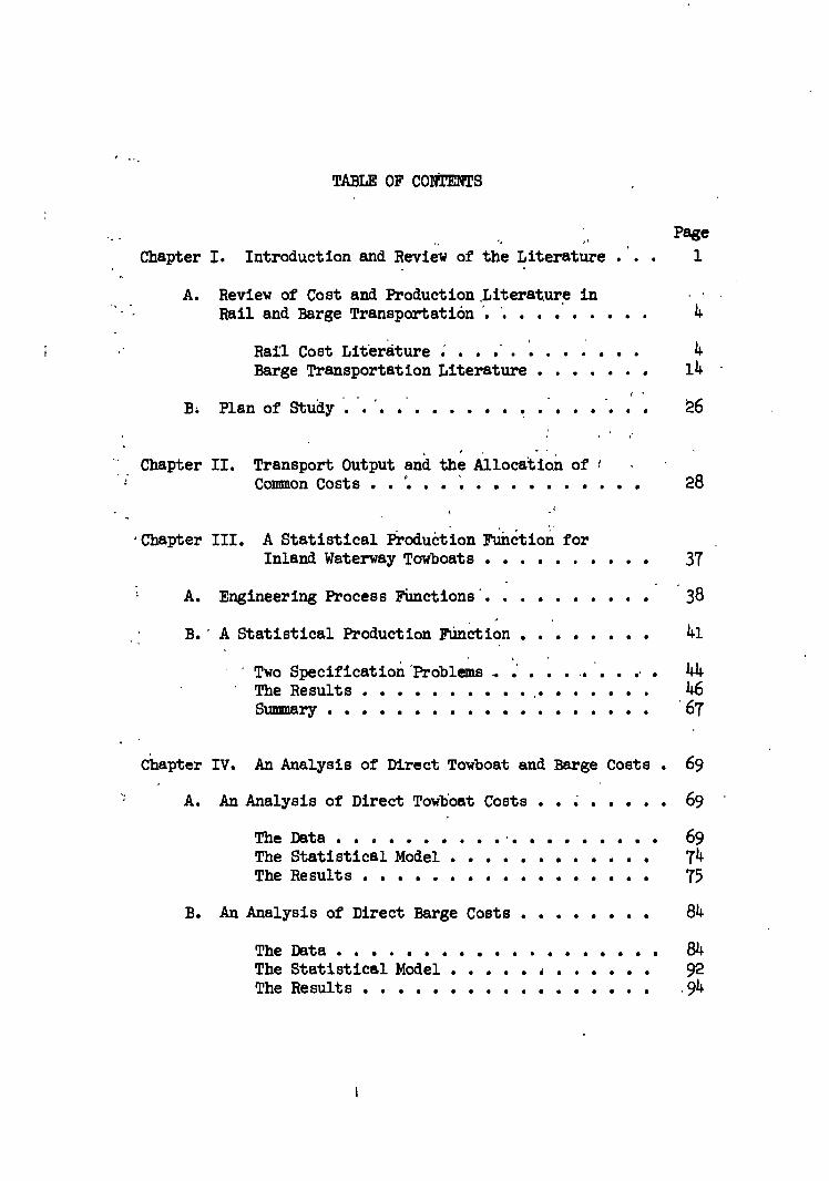
84 92

.94

TABLE OF COIMETS

Page

Chapter I. Introduction and Review of the Literature . . . 1

A. Review of Cost and Production .Literature in Rail and Barge Transportation ' 4

• Rail Cost Literature ' 4 Barge Transportation Literature 14 -

B. Plan of Study ' ' 26

. . . Chapter II. Transport Output and the Allocation of (

Common Costs '

'Chapter III. A Statistical ProduCtion Function for Inland Waterway Towboats 37

' A. Engineering Process Functions' '38

: B. A Statistical Production Function 41

Two Specification 'Problems • 44 The Results 46 Summary 67

Chapter IV. An Analysis of Direct Towboat and Barge Costs . 69

A. An Analysis of Direct Towboat Costs 69

The Data 69 The Statistical Model 74 The Results 75

B. An Analysis of Direct Barge Costs 84

28

The Data The Statistical Model The Results

Table of Contents - Cont'd Page

Chapter V. A Time Series Analysi's of Barge Firm Costs • . . 106

A. The Data 106 B. The Statistical Model 110 C. The Results 111

' Direct Barge Costs 112 Indirect Costs V 118 Direct Terminal Costs•••.•••.. OOOOO • 122

Chapter VI. A Cross Section Analysis of Firm Costs . • • • 124

A. The Data 124 B. The Statistical Model . 128 C. The Results 129

Indirect Costs 129 Total and Direct Costs .134

Chapter VII. Summary and Conclusions 141 . . •

A. Returns to Scale 141 B. Technological Change 144 C. Costs and Rate .Structure 147 D. Cost Finding Techniqdes - 149

Footnotes 152

• " .Bibliography . , 156

CHAPTER I

INTRODUCTION AND REVIEW OF THE LITERATURE

What is the cost of moving a ton of freight from some origin A to

some destination B? Answers to this question are necessarily complex

since they depend upon the mode of transport used, the length of haul,

the commodity shipped, and whether a backhaul is required. This study

examines this question for one mode of transport: Barge transportation

on inland waterways.

Essentially, two different methods can be employed to arrive at

estimates of transport cost. One method is based on the use of engi-

neering production functions. The engineering relationship shows the

technological substitution possibilities between the various inputs

(which should be stated in stocks and flows) required to perform a given

task (for barge transportation, the point-to-point movement of commodities

and equipment). If the prices of the inputs are known, long-run and

short-run cost relationships can be derived. In the case of barge trans-

portation, one needs the costs associated with various kinds of equipment

(towboats and barges), costs of a crew,.the characteristics of the water-

way, and a measure of delay time. With this information the cost of a

particular point-to-point movement can be determined. An engipeering

relationship developed in this way could ,be termed a "process function"

since it describes the alternative ways of performing a particular task.

It does not describe the production relationship when several tasks are

1

2

performed either simultaneously, or sequentially (under some conditions

it can be aggregated), nor does it describe the cost-output relationship.

The second method is the use of statistical estimation procedures. ,• •

This is a more direct and traditional approach to obtaining cost estimates.

"Basically, statistical methods are a substitute for experimental controls

in attempting to establish and measure causal relationships, statistical

techniques being used when controls are either unavailable or too expen-.

The statistical approach is based on observed rates of output

and expenditure collected by firms. Cross-section Or time-series data

are used in the framework of an appropriate statistical model to deter-

mine the parameter values. The selection of the model may be based on

theortticai or technological knowledge, or simply on'goodness of fit.

The two methods are no mutually exclusive. Statistical methbds

are frequently employed in deriving the technological parameter estimates

Of•engineering relationships; knowledge of technological constraints can

be used to select the appropriate model for statibtical production or cost

estimates. The two approaches do, however, possess different interprets-

tiOns. The engineering relationships, as they embody the available tech-

nology, describe the set Of alternative ways of performing a partioular

' task independent of the relative prices of the inputs. Tht engineering

relationships thus desCribe the teChnologically most efficientways of

accomplishing the task. Given the prices of the various inputs, the

economically efficient production method can be selected, that is, the

. method which produces a given output at the least cost. Cost relation-

ships obtained in this war, then, represent the coSt'curves Of economic

theory.

*All footnotes appear following text, beginning on p. 152.

3

On the other hand, the statistical cost-output relationships, since

they are based on actual rates of output and expenditure, are a summary

of the average operating conditions for the period observed. Since they

do not carry the interpretation of technological-efficiency or cost mini-

mization at each output level, they do not represent the cost relation-

ships of economic theory.

Nevertheless, statistical relationships, if properly interpreted,

can yield extremely useful information about the operations. of a firm.

One could assume, as is frequently done, that the observed data do repre-

sent minimum cost points, that is, that the firm is at, or near, an

optimum. The estimated results can then be interpreted as the long-run

costs of economic theory. This, however, is not likely to be true: The

observations will most-certainly reflect the operation of a firm where

some short run adjustments are still taking place. Another interpretation

seems more reasonable: Assume that the observations represent a certain

. average level of efficiency which has been achieved.in the past and is

likely to prevail- for some time. The-cost. relationships could then be

used to draw conclusions, for example, about the expected effects of

- increasing firm size. -

. Since statistical relationships are derived from the operations of

firms, one can be sure that these functions represent actual operations.

No such guarantee can be given for engineering functions. We.know that

some inputs (such as management) are omitted. Even the engineering

process functions are simplifications rather than the exact physical

relations. Thus, there is no guarantee that these relations can be

realized in actual operations.

4

Both the engineering and statistical methods have been employed

in studies of rail and barge transport cost. A summary of the more

• significant studies, in this area is presented below.

A. Review of Cost and Production Literature in Rail and Barge Transportation

• Rail Cost Literature

Considerable attention has been devoted in the past to studies of

rail transport costs. Although the primary concern or this study is the

cost of barge transportation, investigators of rail cost have dealt with

problems common to both modes.. For this reason a survey of the more

recent studies of rail cost have been included in this review.

Meyer, Peck, Stenason, and Zwick (MPSZ) have estimated long-run

cost relationships for freight and .passenger rail traffic. 2 Their study

is distinguished from those done in the past in two ways. The first is

that they stratify railroad costs into much finer categories than in the

past. This is a recognition that railroad transportation is a many

faceted operation. "Specifically, total railroad operating expense in-

cludes all the labor, fuel, and miscellaneous variable costs associated

with the operation of trains, yards,. and stations . . ." (p. 34).- In

addition there are the costs of marketing, supervision, and maintenance.

Obviously the behavior of cost in relation to output will be quite dif-

ferent for different parts of the operation. Also a single output

measure will not adequately describe the activities of all aspects of

• • • - rail transport.

• , Five categories of operating cost are included by MPSZ: general

(administrative and legal overhead), traffic (selling and marketing),

station, train (line-haul), and yard. Maintenance cost, depreciation,

5

and capital Outlays are also treated as separate categories. The data

used were cross-section observations on the twenty-seven largest United

States class I rail systems (excepting the New York Central and the

Pennsylvania Railroad). The sample was taken from data collected by the

Interstate Commerce Commission from 1947 to 1955.

The second distinguishing feature of the MPSZ study is that the

data are not used in ratio form. A difficulty with cross-section studies

is that almost all the differences between observations in a saiple seem

to be due to the influence of firm size. A common method employed to

eliminate this influence has been to deflate the cost and output obser-

vations by the size of the firm. An important consequence of this pro-

cedure for linear regression equations is to overstate the constant term

and hence overstate the extent of scale economies. According to MPSZ,

. . . these scale economies probably are best attributed to nonOptimal

factor proportions at lower levels of output . . ." (p. 38).

As noted above, the MPSZ study is based on cross-section data. As

a result, the authors consider their estimates to represent long-run cost

relationships. The possibility of transient short -run influences in Cross-

section data are recognized; however, these influences are discounted by

the authors because, ". . . interfirm . variance over the cross section is

almost surely many times the intnafirm variance attributable to these

short-run influences . . ." (p. 41). This is particularly true in the

MPSZ case, since the authors use WO and four year averages in estimating

their cost functions.

The authors estimate relationships for each cost category. A

description of the procedures followed for each category ofcost would

necessarily be extremely detailed and has been omitted.' The procedure

6

followed was to regress each cost category on its associated output

measure. Linehr regression equations were employed.

The authors simplify their analysis of different cost components

into "typical" over-all relationships between costs and gross ton-miles.

This is done by making "normative" assumptions about the relationships

between gross ton-miles and the other output measures (such as yard

. hours or train-miles) .employed in the individual category regressions.

These normative assumptions are apparently industry rules-.-of-thumb

obtained from discussions with railroad operating officials.

, The results of this summarization are presented in Table 1. To

obtain the total cost of a particular trip, one calculates the number of

gross ton-miles to be generated and then multiplies this by the relevant

total long-run marginal cost coefficient. The coefficients can be ad-

justed by price indices when considering subsequent periods. In this

way, the total cost (or cost of particular operations) can be determined

for freight and passenger rail traffic; however, as the authors point out,

reasonable caution should be employed in making such estimates. "It

should be noted that these estimates are based on a sort of central ten-

dency and are typical figures that will apply to freight movements only -

of a very average or ordinary kind." .(p. 63). This is due primarily to

the nature of the normative assumptions that were made. In reducing yard

expenses to a gross ton-mile basis, for example, the authors assume that

twenty-four minutes are required . . to originate, 'classify, and ter-

minate the typical merchandise car, [and] that this car gOes approximately

400 miles, and that it has a load of 25 tons . . ." (p. 48). Nevertheless, -

the MPSZ results are potentially quite useful in determining the cost of

typical railway traffic and should be useful in making.regulatory.deci-

6.6190 2.826 7.03

4.50

1.53

1.00

1.700

0.910

.216

4.2330

1.4100

0.9760

1.4079 0.445 1.48

TABLE 1

SUMMARY ESTIMATES OF RAILROAD OPERATING COSTS THAT VARY IN THE LONG RUN*

1947-1950 results (1947-1950 mills)

1952-1955 results (1952-1955 mills)

Per Per . Per G.T.M. of G.T.M. of G.T.M. of freight passenger freight traffic traffic traffic

Per G.T.M. of passenger traffic

Long-run marginal train, station, yard, traffic, and general expenses... 0.8721

User cost portion of main- tenance costs... .6900

Variable portion of de- preciation expenses... .2120

Total long-run marginal operating costs... 1.7741

Variable portion of cap- ital costs at 6 1/2 percent interest rate... 0.4011

Total long-run marginal operating and capital costs... 2.1752 • 8.0269 3.271 8.51

*Source: John R. Meyer et al., The Economics of Competition in the Transportation Industries (Cambridge, Mass.: Harvard University Press, 1964), p. 62.

7

8

sions particularly with respect to rate making. Finally as the authors

point out, even if their results are not perfect they may represent the

best alternative approach to determining rail costs, and ". . . cost

determination is almost always not a matter of obtaining an exact answer

but of getting the best available answer." (p.44). 3

Borts4 argues that the use of cross-section data in statistical

cost estimation can produce biases in the measurement of returns to

scale. After discussing the source of these biases, Borts outlines a

method for avoiding them and applies this method to cross-section data

for United States railroads.

His argument is illustrated in Figure 1. (Borts, p. 110). C(X)

is the long-run total cost function for each firm in the.industry. S 1

and S2 are short-run total cost curves for two plants, one large and

one small. X1 isthe output where the firm begins to experience increas-

ing returns to scale. If all of the observations of a cross-section

data set lie on C(X), and if all of the observations are for plant sizes

below X1,

then the intercept term of a simple linear regression equation

will provide a reasonable estimate of return to scale in the industry.

However, it is more likely that the data will represent points such

as b, c, d, and e in Figure 1. In this case, the estimated regression

equation will lie above C(X) throughout its range yielding an over-estimate . •

of the intercept term. According to Borts, the most frequently employed

method of correcting for this problem is to explicitly introduce some

measure of plant size in the regression equation. The l,size coefficient

can then be interpreted as meaning ". . . the extent to which the firm

is operating above its long-run cost function as well as the position of

the plant curve relative to the envelope." (p. 109).

FIGURE •

C (X)

■

9

10

Results obtained in this way, however, may be misleading due to

the influence of the regression fallacy. Firms are subject to random

fluctuations in the demand for their product. As a result, the output

produced by each firm is a random variable and the variation of output

about the mean value is not controlled by the firm. The firm then

tries to optimize its plant size for the production of some distri-

bution of outputs. When firms are observed at a point in time, as

in cross-section data, firms with the largest outputs are most likely

to be producing at unusually high output levels (such as points c and

e in Figure 1). The opposite is likely to be true for firms with the

lowest output. Thus, classification of the firms by actual output,

may lead to an understatement or overstatement of the firm's long-run

(planned) output rate. "Under these conditions, the interpretation of

the estimated size coefficient is ambiguous." (p. 110). For example,

a positive sign for the coefficient of firm size may indicate - that

abnormally large expenditures.were incurred which are attributable to

a divergence, of the planned and actual output rates. It may not indi-

cate, according to the usual interpretation, that the firm could reduce

its cost by selecting a smaller size plant.

Borts proposes an alternative method of cost estimation, that of

stratifying the observations by firm size. Besides avoiding the bias

due to the regression fallacy, this approach ". . . permits a test of

the presence of the regression fallacy through a comparison of between

size- and within size-class estimates of marginal and average costs . . ."

(p. 114).

This method is applied by . Borts to a cross-section of sixty-one

United States railroads. Linear regression techniques are employed.

11

The effects of two types of classification are examined: the size of

firm and the region in which the railroad operates. The regional

classification is used to account for spatial price differences, and

regional differences in physical operating conditions. Due to the

small sample size, shift parameters are used to take account of re-

gional and size differences. Covariance analysis is then used to

examine the influence of these variables. The hypotheses tested are

that the cost-output relationships are significantly affected by both

the size of firm arid the region of operation. . .

Two types of cost behavior are observed in Borts results; each is

associated with different regions in Borts classification. "It was

found that long-run increasing costs prevailed only in the Eastern re-

gion, while long-run decreasing or constant costs occurred in the South

and West." (p. 116). According to Borts, this evidence on regional

differences suggests that different regulatory policies should be de-

signed to meet the varying conditions among regions. In the East, .

” . . . the question of basing charges on identifiable cost can be

reopened, once it is possible to ignore the problem of allocating in-

direct expenses . . . [In the West and South] the evidence indicates

a continuation of the historical problems raised by overbuilding, be-

cause of the possibility of continued increasing returns." (p. 128).

In a study of railroad cost in Canada, Stenason and Bandeen

provide a critique of current cost finding techniques of the Interstate

1 Commerce Commission. 5 The authors present an alternative costing

system used by the Canadian National Railroad and the Canadian Pacific

Railroad Company.

12

According to the authors,

. . . the ICC procedures are a compromise between the need of the accountant to record all the costs in a specific set of accounts, often on a somewhat arbitrary basis, and the desire of the economist to trace expenses to the output that occasions them, in order to determine the costs associated with specific changes in service or

: output. .(p. 122). -

Current ICC cost finding techniques are based on eighty year old cost

classifications which succeed in assuring uniform reporting of expenses

by the carriers, but are not adaptable t6 cost analysis.

In the ICC procedures total cost in each category is allocated to

live service areas (linehaul, switching, station, special services, and

overhead). The allocation is quite arbitrary. For example, an analysis

of time spent in different stations by trains is used to allocate sta-

tion labor costs among different service categories. To determine the

variable portion of total expense, simple linear regression techniques

are employed using cross-section data. The procedure is to regress total

. operating expense per mile of road on gross ton-miles per mile of road

(density). The intercept coefficient of the regression equation is then

subtracted from the average value of expense for United States railroads.

The figure derived from this calculation is expressed as a percent of

the average value of expense per mile of road. This percentage is then

interpreted as the percent of total expense which varies with output. .-

The authors find this procedure unacceptable for several reasons.

One .is that the arbitrary allocation of costs to separate service cate-

, gories does not allow ". . . an estimate of the extent to which total

expenses will change as a result of change in traffic volume or in its

mix." (p. 123). A second criticism is that the use of ratios in the

13

regression equations will produce biased results unless the numerator

and denominator of the ratio are homogeneously distributed. In addi-

tion, the authors point out that even in the absence of statistical

bias, the regression procedure is invalid as it ignores the length of

haul, traffic volume, traffic density, and the commodity carried.

Finally, the authors note that the association of variable costs with

'a single output meastre, gross ton-miles, ignores the multi-product

' 'Character of railroad output.

The authors are led to reject the ICC procedures for use on

Canadian railroads. They describe research conducted in Canada which

has resulted in a more sophisticated cost finding procedure. This

procedure has been adopted by Canadian regulatory agencies .for their

cost analysis. The procedure is based on actual recorded costs in the

Canadian system of railroad accounts and a knowledge of technical engi-

neering and operating features of railroad systems.

The procedure is to first define and quantify measures of output

corresponding to different aspects of the transport process and which

are applicable to particular categories of traffic. For example, a

determination was made of the number of minutes required to switch

freight cars of different types and having particular origins and des-

tinations. The principle output meaiures (traffic units) analyzed are:

switching minutes per car, gross ton-miles, train miles, diesel unit

miles (reflecting the number of diesel units used on 'a train for each

train run), car.-days, and car-miles. ,

The next step was to develop a set of cost faciprs or coefficients

which reflect expenses that are variable with respect to the different

output measures. "This involved estimating many hundreds of regression

14

models and selecting those which best fitted, the many tests made of

them." (p. 127)..

Once the service or work requirements of particular shipments

are known and knowing, the marginal cost associated with each type of

service, the marginal cost of any particular point-to-point movement

can be calculated. The various factors and procedures have been for-

malized so that they can easily be applied An particular circumstances.

Quite apparently, such a cost finding technique is superior to the one

employed by the ICC. It avoids arbitrary allocations and recognizes

the complexity of the rail transportation process.

Barge Transport Literature

The work of Charles W. Howe and Arthur P. Hurter represents the

• entire body of literature concerned with production and cost relation-

ships for barge transportation.

Howe6 has developed a production function for the point -to-point

movement of a barge tow based upon engineering relationships taken from

naval design theory. His approach is to solve a system of equations

for the equilibrium speed of a tow. The model, in 'functional notation,

is: . '

(1) R= f (L, B, H, S, D, W)

- '(2) EP = g (HP, S, D)

(3) EP = R

where: R = resistance of flotilla in tow-rope horsepower 1

EP = effective push of towboat

D = depth of waterway in feet

H =s draft of barge in ,feet

15

S = speed in miles per hour

W = width of waterway in feet

B = breadth of flotilla in feet

L = length of flotilla in feet

HP = horsepower of the towboat

The resistance of a flotilla as it is pushed through the waterway

depends on its velocity, the characteristics of the flotilla (length,

breadth, and draft), and the characteristics of the waterway (depth, and

width). The push generated by a towboat depends upon the horsepower

and speed of the boat and the depth of the waterway. The equilibrium

condition, given in (3), must hold for a tow operating at a constant

speed.

Since naval design theory does not provide the exact form - of

either the resistance function or the effective push function, it was

necessary for Howe to estimate the parameters of the two relationships

statistically. The data used to estimate the functions were derived

from tank and prototype tests conducted by the U. S. Army Corp of

Engineers and barge equipment manufacturers, and speed tests conducted

with actual equipment by barge operators.

According to Howe, "Extensive use of regression analysis showed

that the following functional form fitted the resistance test data

quite well:" (p. 27).

sa2 Ha3 + a4 L 5 Ba6

(1/W-B) a . (4) R.= ao eal (1/D-0

This, Howe used as a modified log-linear resistance function which is

n . . . consistent with what is known about resistance phenomena." (p. 27).

16

The resistance data were stratified into five groups according to

flotilla configuration. Equation (4) was then estimated for each con-

figuration separately and again for a weighted average of the five

groups. His results show significant parameter difference among the

stratified regressions. Nevertheless, Howe adopts the combined re-

gression to use in his analysis. Howe recognizes that this is a

questionable procedure since structural differences have been observed,

however, he proceeds ". . . on the pragmatic grounds that the resulting

function will be used to evaluate a wide variety of tow characteristics."

' (p. 27).

The effective push relationship Vias examined in a similar fashion.

The adopted form was:

2 (5) EP = B1HP + B2HP + B3HP.D + B4S 2 + B5S.HP

2 According to Howe, "The HP term allows for increasing or decreasing

2 effectiveness of HP in determining push. [The coefficient of HP was

negative, indicating diminishing productivity of HP in higher HP ranges.]

The cross-product term, HP.D, reflects the fact that gains from greater

depth are greater for larger boats and vice versa. [The coefficient of

HP.D was positive, an indication that this prediction of navel design

theory is correct.] Finally, the S•HP term reflects the fact that

ap/as is a decreasing function of HP . . ." (p. 29). The coefficient

of S.HP was negative, indicating that the push generated by a towboat

of given horsepower declines as the velocity of the tow increases.

Using the estimated relationships (1) and (2) and the equilibrium

condition for constant speed (3), Howe was able to solve the system of

equations for the equilibrium speed, S. In functional notation, we have:

17

(6) S = h(HP, L, B, H, D, W)

The actual form of the equilibrium speed relationship is very complex

and has been omitted. However, it should be noted that when L, B,

and H are specified, the cargo tonnage of the tow is also specified.

Thus by rewriting the function (6), we can derive the output of the tow

in cargo ton-miles per hour:

(7) TM(HP, L, B, H, D, W,) m. S(HP, L, B, H, D, W) • T(L, B, H)

' where TM represents the output of the tow measured in net cargo (short)

ton-miles per hour. Such a function is of considerable interest since

it relates the tow's output to (1) waterway characteristics under the

control of the Army Corp of Engineers, and (2) to he tow inputs (horse-

power and flotilla configuration) under the control of the individual

barge firm.

To derive the unit cost functions from his analysis, Howe defined

his productive inputs to be horsepower of the towboat (assuming that

labor and fuel costs are proportional to horsepower) and the deck area

of the barge input. Howe then obtained ftom barge firms average daily

operating costs of towboats of various horsepowers and of open hopper

jumbo barges.

Using (7) and the related cost information, Howe was able to gen-

erate (1) total product curves as a function of flotilla area for vari-

ous horsepowers, holding waterway characteristics constant, (2) iso-quants

for horsepower and deck area, holding waterway characteristics constant,

(3) a family of average cost curves for particular flotillas, allowing

horsepower to vary, and (4) the effects on tow performance of changes in

waterway characteristics, W and D.

18

Since the function (7) is discontinuous in the barge inputs, it

was necessary to evaluate the function over a set of specified values

of all inputs. According to Howe, "these values cover farily well the

range of operating conditions found on the Ohio, Upper Mississippi,

Missouri, Illinois Waterway, and the Gulf Intracoastal Canal." (p. 30).

The set of derived relationships exhibits reasonable properties.

In particular it was discovered that, (1) both the tow boat and barge

inputs showed diminishing productivity (2) the tow shows "decreasing

returns to scale" which can be attributed to the waterway inputs, and

(3) "U-shaped" average cost curves, costs rising beyond some point

. . because speed reductions more than offset the effects of addi-

tional carrying capacity." (p. 36).

Howe recognized that his process function was not adequate for

describing the activities of a barge firm in organizing its traffic

into tows and in scheduling the movement of those tows across the

waterway. As was demonstrated by the process function, the point-to-

point operation of a tow was subject to decreasing returns to scale

due.to the limitations of the waterway. However, the firm " . . . may

experience constant returns because Of its ability to duplicate

individual operating units as total output grows." 7

Howe then turns to developing production functions for the barge

firm. Of particular interest is his discussion of how the capital

inputs should enter the production function. Howe argues that the

entire capital stock in barge transportation is not alwas used at any

one time. Observed current output is thus related to the portion of

the capital stock actually used. It is not related to the capital

19

stock which remains idle. Under these circumstances, "It would not be

adequate to measure capital utilization simply by counting the number

of units which were utilized • • ." (p. 40). The appropriate measure

for the capital input is thus the flow of capital services. Howe

called a function estimated using capital services a production function.

The idle capital stock, however, is important for meeting the firm's

overall objectives. This can easily be seen when it is realized that

barge firms (and other transport firms as well) are subject to random

fluctuations in the demand for their services. Firms must make deci-

sions about the optimal stock of equipment to have on hand as well as

what equipment to use in meeting current demands. Thus, the relation-

ship between capital stock and output is also of interest. However,

Howe recognizes that such a relationship extends beyond the technolog-

ical constraints embodied in a production function, involving ". . .

all of the variables which must be considered in dynamic long-run profit

maximization." (p. 40). Howe refers to such a relationship as a "plan-

ning function."

The two relationships are viewed as providing complimentary infor-

mation on the firm's operation. The two functions can be compared to

gain insights into returns to scale. That is, suppose the firm has

increasing returns to the production process (because a large cargo

volume allows for a high proportion of larger more efficient tows),

but experiences decreasing returns reflected through the planning

,function. This might indicate increasing complexities in scheduling

so that the stock of capital must be greatly increased as the rate of -

output increases.

20

Howe estimates both kinds of functions. His production function

uses monthly time-series data for three firms representative of different

operating conditions on the Mississippi River System. The production

function estimated was:

(S) TM = aoBa le2p

where: TM = cargo ton-miles

B = equivalent barge days underway, full and empty

H = operating horsepower hours

The log-linear form of the function was estimated. Note that the inputs

are measured as flows. The function was estimated separately for each

firm.

Howe's planning function uses combined cross-section, time-series

data for six firms. The estimated function was:

(9) TM = ace lliPc42Ta3p

where: TM = annual cargo ton-miles

B = number of equivalent jumbo barges owned or leased

by the firm

T = time (1950 = 01, 1962 = 13)

Once again the log-linear form of the function was estimated. The inputs

are measured as stocks.

The results for the production function exhibited reasonable pro-

perties for two of the firms in the sample. The coefficients of H and

B were significant for these firms and showed constant 'or slightly in-

creasing returns to scale for the capital input. The third firm had

neither significant coefficients nor reasonable parameter estimates

(the sign of the barge input was negative).

21

The planning function also exhibited reasonable properties and had

significant parameter estimates. The results indicate decreasing returns _

to scale when the firm's stock of equipment is considered. The time trend

coefficient was positive, an indication of technological improvements in

the industry.

A possible conclusion is that scheduling difficulties increase as

the volume of output grows, making, additions to the capital stock less

productive overall. Although Howe's process function showed decreasing

returns, the results for the production function indicate that the firm

is able to schedule tows out of a fixed stock of equipment subject to

increasing returns, as would be expected. However, the planning func-

tion indicated that as the firm adds to its capital stock to meet the

requirements of growing demand (i.e.,as the total number of tows to be

scheduled increases) it does so subject to decreasing returns.

In the work of Hurter, statistical cost and production relation-

ships were estimated for three years (1950, 1957, 1962) using annual

Interstate Commerce Commission data on Class A certificated waterway

carriers operating on the Mississippi River.

Hurter's production study 8 followed closely the methodology devel-

oped by Howe. Hurter estimated six production relationships, three of

which he characterizes as planning functions in the sense in which Howe

employed the term. The stated objective of Hurter's study is to describe

the production and planning functions applicable to the firms in the

sample and to make "year-wise" comparisons in order to determine ". . .

the change in input combinations that have taken place in response to

technological and environmental change."9 The six relationships are:

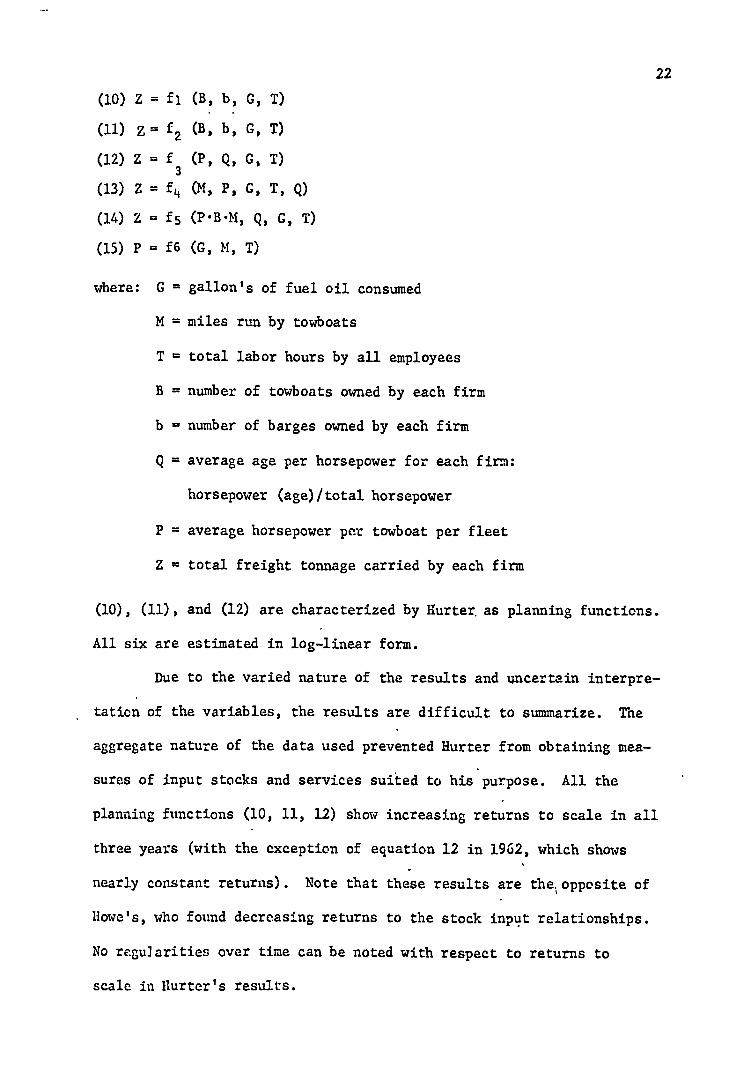
22

(10)Z = fi (B, b, G, T)

(11)z= f2 (B, b, G, T)

(12)Z = f3 (P, Q, G, T)

(13)Z = f4 (M, P, G, T, Q)

(14)Z = f5 (P•B.M, Q, G, T)

(15)P = f6 (G, M, T)

where: G = gallon's of fuel oil consumed

M = miles run by towboats

T = total labor hours by all employees

B = number of towboats owned by each firm

b = number of barges owned by each firm

Q = average age per horsepower for each firm:

horsepower (age)/total horsepower

P = average horsepower per towboat per fleet

Z = total freight tonnage carried by each firm

(10), (11), and (12) are characterized by Hurter, as planning functions.

All six are estimated in log-linear form.

Due to the varied nature of the results and uncertain interpre-

tation of the variables, the results are difficult to summarize. The

aggregate nature of the data used prevented Hurter from obtaining mea-

sures of input stocks and services suited to his purpose. All the

planning functions (10, 11, 12) show increasing returns to scale in all

three years (with the exception of equation 12 in 1962, which shows

nearly constant returns). Note that these results are the. oppositeof

Howe's, who found decreasing returns to the stock input relationships.

No regularities over time can be noted with respect to returns to

scale in Hurter's results.

23

Of the production functions, (13, 14, 15), equation (15) produced

no statistically meaningful results. (13) exhibited increasing returns

to scale each year. On the other hand, (14) showed decreasing returns

for 1957 and 1962.

Finally, Hurter tests the hypotheses that there are no significant

differences between the three years in the sample for each estimated

relationship. Applying the standard tests developed- by Chow, 10 Hurter

found that significant differences did, indeed exist between 1950-57 and

1950-62 for all relationships. Only (10) showed a significant difference

for 1957-62. Hurter thus concluded that significant adjustment in the

productive process had taken place up to 1957. .

Hurter then turned his attention to estimating cost relationships.11

Once again, the data used were annual cross-section observations for

Class A carriers operating on the Mississippi system in 1950, 1957, and

1962. His work can be summarized in three parts: The first part relates

annual water line expense to each of two measures of firm size (total

annual cargo tonnage, and asset size of firm). Both linear and log-linear

results were obtained although Hurter preferred the lordinear results

since the firm size coefficient will .be biased for the linear regressions.

All four regressions indicated the existence of economies of scale in .

each year. Hurter attributes these scale economies to the barge firm's

scheduling operations. However, only stacistically significant firm size

coefficients were obtained for 1957 and 1962 for all'four relationships.

The regressions using total output in ton-miles (linear and log-linear)

and the linear regressions of cost on asset size did not produce signi-

ficant results and had extremely low coefficients of determination

(.12 to .24).

24

The sccond part of Hurter's cost study was an attempt to relate

firm size to "profitability." Three measures of profitability were

used: (1) the ratio of total freight revenue to total assets; (2) the

ratio of net revenue to assets; and, (3) the ratio of total waterline

costs to total freight revenue (the so-called "operating ratio"). No

significant relationships were found.

For the third part of the cost study, Hurter separated out annual

line-haul costs from total waterline expense. Linear and log-linear

estimates were made of line-haul expense on annual tonnage. Signifi-

cantly higher scale economies were indicated by the results for the

line-haul operation relative to the terminal and administrative oper-

ations. Once again, scheduling economies are a possible source of

these scale economies.

Hurter also related line-haul costs to inputs used in the line-

haul operations (average horsepower per towboat, annual fuel consumption,

and total labor hours). These variables represent the input flow vari-

ables of Hurter's production functions. A log linear relationship was

estimated. It was found that a 10 percent increase in all

accompanied by a 13 percent increase in all line-haul costs in 1957 and

1962. At the same time, a 10 percent increase in all inputs was found

to be associated with a 28 percent increase in total output for 1957;

a 10 percent increase in total output in 1962. This indicates strong

economies of scale in 1957, but does not support scale economies for

1962. Additional support for positive scale economies was obtained

by relating the stock input variables to line-haul costs.

One of the difficulties that have beset investigators of the

barge industry has been the unavailability of important (and relevant)

inputs was

25

sources of data. Despite the use of sophisticated statistical tech-

niques, Hurter's cost and production studies produced few important

results. This stems partly from the data he used; partly from a seem-

ing,lack of theoretical justification for many of his estimated rela-

tionships. The latter criticism, no doubt, stems from the first.

Hurter was simply not able to obtain direct measures of the variables

of interest and had to make do with less than satisfactory surrogates.

The data used by Hurter, and to a lesser extent by Howe, are

taken from the annual KA reports submitted by common carriers to the

ICC. The information is highly aggregate and it is not possible to

separate certain cost and output quantities into relevant categories.

For example, total labor expenses may include terminal labor, line-

haul labor, maintenance labor (of all sorts, from barge and towboat

maintenance to repairs of office structures), janitorial services,

administrative clerks, and so on. Fuel costs include fuel for harbor

tugs as well as linehaul boats. The reports do not consider measures

of towboat or barge services which can be related to different acti-

vities or services offered by the firm (for example, ton-miles carried

of each commodity on each waterway). .

The reports are designed to relate to the common carriage portion

of a firm's business. By the nature of the record keeping process, how-

ever,'it is difficult for the firms to assign a portion of total cost

to the common carriage part of their operation. The 'reports, at best,

represent industry guesswork as to the correct cost allocation.

The barge operators themselves have little respect for the infor-

mation reported. Many firms do, however, collect quite detailed data

on their operations. Unfortunately, this data has not been made gener-

26

ally available to investigators of barge operations in the past. Access

to the records of the barge firms would allow a detailed analysis of

several aspects of their operations. Common costs, for example, could

be allocated to different types of service offered by the firm. Use of

heretofore unavailable data in examining these questions is one of the

major contributions of this study.

II. Plan of Study.

As noted above, this study presents the results of statistical cost

and production functions estimated using actual operating and cost data

from several inland waterway operators. Chapter II considers the pro-

blem of selecting an output measure for barge transportation. The rest

of the paper outlines the statistical methods and results. Chapter III

presents a statistical production function which draws upon engineering.

knowledge, but which differs from engineering production functions such

as Rowe's in that it describes actual operations. Chapter IV is an

analysis of direct operating costs for towboats and barges. One would •

expect that the costs of operating each type of equipment will bear a

different relationship to the work performed. Thus, a separate cost

analysis has been made for both types of equipment. Chapter V is a

detailed analysis of the costs of a single firm using time-series data.

It was possible to obtain extremely detailed data for this on firm

including ton-miles of each commodity transported by•river district.

Thus, it has been analyzed separately. Chapter VI reports on a combined

cross-section, time-series analysis of five barge firms. Chapter VII

summarizes and expands on the major coLclusions of the study.

The reader should note several themes running throughout the

entire study. One is the importance of the operating environment in

which the firm operates, the waterway. This is shown to have a sig-

. nificalt effect on cost and output. Second, is the multi-product

. character of barge transport. This is especially evident in Chapter

V, where the detailed data on cost and output make it possible to

examine the problem of common costs. Finally, a third theme, is the

lack of adequate output measures to describe all of the many services

performed by barge firms (and transport firms in general).

27

CHAPTER II

TRANSPORT OUTPUT AND THE ALLOCATION OF COMMON COSTS

For the firm producing a'single, homogeneous product under con-

ditions of perfect competition, short-run and long-run cost relation-

ships are easily defined. At the other extreme is the multiproduct

firm. The costs associated with the production of each of many

products and services are complex, interdependent,.and difficult to

measure.

A real difficulty arises in the case of joint costs: when a

given expenditure is associated with the production of multiple pro-

ducts in fixed proportions. In this case, it is impossible to com-

pletely separate the costs of producing each _product. For example,

if a barge firm produces services by moving commodities in one

direction, it necessarily must produce the service of a return haul.

Allocation of cost between the trips is necessarily arbitrary. As a

result, an arbitrary element enters the rate structure; no particular

pricing policy can be justified on the basis of marginal cost. Price

is then determined by the conditions of demand, or "what the traffic

will bear."

A system of rates, such as the actual railroad . rate Structure in

the United States, constitutes an elaborate system of price discrimi-

nation. This price discrimination, however, is not easy to disentangle

28

29

from variations in rates based on variations in the cost of different

services provided.

More frequently encountered is the situation where multiple pro-

ducts or services can be produced in varying proportions by a single

operating unit. Certain expenditures may be shared by (or common to)

all products, as in the joint cost case. However, since the output of

the individual products are capable of independent variation, it is

possible, at least conceptually, to determine the marginal costs asso-

ciated with each by varying the output of one product, and fixing the

outputs of all other products. Note that the marginal cost schedules

obtained for each product may depend upon the level of output of all

other products.

A major difficulty in examining the cost of services provided by

transport firms is that the services cannot be measured along a'single

dimension. The service performed in handling, for example, a ton-mile

of coal is not the same as the service performed.in handling a ton-mile

of steel wire. This is true even though the same equipment may be used

and the same route traveled in both cases. The character of the output

(and the cost-output relationship) may vary because of time requirements

to be met, special handling, or equipment necessary for certain commod-

ities, route traveled, and amount of empty backhaul.

As a result, many of the costs that are incurred cannot directly

be attributed to any one particular type of service provided by the firm.

This problem of common costs occurs at several levels of analysis, de-

pending upon how one disaggregatea the firm's output. Looking at the

problem of common costs at the highest level of output aggregation

30

(taking, for example, ton-miles as a single measure of total output)

some costs can be directly identified as "due" to particular shipments

that are made. Such costs are referred to in the barge industry as

"direct" or "operating" costs. These are the costs associated with

actually moving and handling the freight:. fuel, maintenance, labor,

etc. Such costs vary directly with the total number of ton-miles

produced.

• Additional costs, however, are incurred which cannot be identi-

fied with a general output measure such as ton-miles. These are the

costs associated with the sale of services, record keeping, and general

office and administrative expense. Such costs are generally termed

"indirect" costs. At this level of output aggregation these indirect

costs cannot be allocated to particular shipments, although certain

shipments may have been more costly than others.

Most barge firms analyze their costs exactly in this way. That

is, individual expense items are aggregated into the two categories,

direct and indirect expense. ' However, analyzing costs in this way

obscures many important relationships.

This can be seen by disaggregating'total output (ton-miles) in

various ways. As has already been argued, a ton-mile of one commodity

is not the same as a ton-mile of a different commodity. A ton-mile on

one route, or over one river district, may have a different relation-

ship with cost than a ton-mile on other river districts. When output

is disaggregated, the direct costs also take on the attribute of

commonness. A profit maximizing firm would need information on the

marginal costs associated with these different outputs. That is, if

it were possible to allocate direct costs to particular types of

31

service the firm would want to set the marginal cost of each type of

service equal to the marginal revenue derived from the sale of that

service.

The problem of allocating common costs then, may be approached

by segregating costs that are directly associated with particular ship-

ments. It may be possible to allocate other costs, if not to individual

shipments, at least to classes of shipments. One might think of a

hierarchy of costs ranked by the degree of output aggregation. Some

costs are allocable to individual shipments, others to classes of ship-

ments somehow defined, while still others are not easily allocable to

any services provided.

The crucial question is, what is the marginal cost of the ser -

vice? What would be saved if the service was not provided? For example,

the extra wear on a barge from carrying certain commodities is allocable

as the cost of that shipment.

In examining the question of output measures for transportation,

Wilson2 provides an example of such an allocation for the case of motor

freight transport. Wilson argues that transport firms provide a wide

variety of services. This heterogeneity of transport output is, how-

ever, frequently collapsed into a single output measure, the ton-mile.

II • • • it But the ton-mile is itself a heterogenous output measure.

is evident that the costs for 100 ton-miles must differ, depending on

the proportion of tons and miles involved." (p. 272)..

Examining ICC cost data for various combinations of weight and

distance, Wilson is able to derive total and average'cost schedules

for weight and distance. He finds that average cost declines as either

tons or miles increases, holding one variable constant. He also finds

32

• cost interdependence, that is ". . . the percent variability of weight

(or distance) is greater the greater the constant distance (or weight)

which one uses." (p. 274).

Several measures of current transport output are available:, tons,

ton-miles (cargo or gross), number of trips or barge loads, and equivalent

barge miles (EBM). None of the output measures are completely satisfac-

tory in describing waterway transport output. This is because the

character of the output measured, for example, in ton-miles, varies with

respect to the commodity handled, equipment used, length of haul, size

of shipment, route taken, special handling required, and time spent in

transit. In general, these dimensions cannot be collapsed into a single

variable such as ton-miles. An "ideal" single output measure would be

an index, calculated by weighting in some fashion the different aspects

of the services performed. Since no such comprehensive weighting scheme

exists it is neceSsary to use one of the "standard" output measures.

One measure has recently received considerable attention: the

EBM. The EBM is a measure of output designed to determine the relative

amount of towboat effort (and thus towboat cost) required to move barges .

of various sizes and loads over waterways with different characteristics.

This concept is of particular interest since it has been adopted by the

ICC as part of its cost-finding procedure. 3 An EBM is defined by the

ICC as the movement of a fully loaded jumbo barge one mile. To this

definition should be added the characteristics of the waterway in which

the movement occurs.

The EBM is a recognition of the fact, well established in engi-

neering relationships and confirmed by operator experience, that tow-

33

boat output, or effort, is not proportional to the number of tons or

ton-miles being pushed. In particular, a towboat does not expend twice

the "effort" in pushing a barge loaded with 1200 tons of cargo as it

does with 600 tons of cargo. Yet, for each mile towed, twice as many

ton-fliiles ,are produced by towing the 1200 ton barge. This tends to

make costs rise more than in proportion to increases in output. This

is because the relationship between the draft of the barge (as deter-

mined by the weight of the cargo in the barge) and the resistance of

the flotilla is not proportional. As draft increases, the amount of

turbulence in the water also increases, thus regniring increasing mar-

ginal effort by the towboat to achieve any given speed. There is an

additional interaction with waterway depth: In general, the deeper the

' water the less severe the turbulence for any draft.

In addition to this engineering phenomena, two additional factors

alter the draft, or cargo load, and output relationship: waterway con-

gestion and locking time. If, for example, a large portion of the total

time taken on any trip is spent navigating locks, an empty or partially

loaded barge becomes just as difficult to push as does a fully loaded

barge. .

All of these factors are closely related to the waterway condit-

ions which prevail for any movement (thus the insistence above on in-

cluding waterway characteristics in the EBN definition). The number of

EBN's per hour produced by a given boat will vary with the physical con-

ditions of the waterway (depth, width, stream flow), average congestion

experienced, and With the time required to pass through locks. It

should be noted that, viewed in this way, the EBM provides a way of

. dividing the river systems into uniform river districts.

34

A number of reasons for preferring the EBM as an output measure can

be cited. It is only slightly more difficult to Calculate than a measure

such as cargo ton-miles (or gross ton-miles). More importantly, it re-

presents an attempt to account for the effort expended in pushing empty,

or partly loaded barges. Over a uniform stretch of waterway, a towboat

should generate the same number of EBM's per hour, no matter how many

barges are being pushed, or what the amount of cargo is. If fewer

barges are being pushed, or the barges contain less cargo, the speed of

the flotilla increases. The EBM concept can be thought of as describ-

ing the relationship between number of barges, cargo weight, and the

speed of the flotilla (waterway characteristics, congestion, and tow-

boat characteristics held constant). Needless to say, these relation-

ships are more complicated than those embodied in the ICC formulation;

the latter must be viewed as an approximation over a reasonable range.

The EBM, then, is itself an output index, although it is still

imperfect as an output measure. However, it does attempt to collapse

certain features of waterway transport output into a single measure by

recognizing characteristics of waterway transportation that have an

important influence on the relationship between costs and output.

Because of these reasons, and because considerable interest has

been generated in the barge industry regarding its use, the EBM has

been selected as the measure of current output for this study.

In attempting to allocate the costs of the barge firm to each

shipment it carries, one would have to specify, at least, what commod-

ity was being carried, the length of the haul, the size and configu-

ration of the flotilla, the characteristics of the equipment used, the

route traveled, and the current level of total output. Allocations at

35

this level of disaggregation are extremely difficult to obtain, parti-

cularly when a single output index is used. In addition, results would

be extremely detailed, relating only to the specific traffic being con-

sidered.

However, it is possible to examine interesting questions relating

to the expenses of the firm by taking an intermediate position in the

cost-output hierarchy. The approach taken in this study is to look at

the total output of the firm (measured in EBM's) and attempt to analyze

the effect on costs of providing certain classes of transport service

(assuming an average length of haul, and an average collection of

equipment).

. For example, we would certainly expect that the type of traffic

the firm chooses to carry will influence its cost-output relationship.

Certain liquid bulk material, for example, must be carried in relatively

expensive, specialized barges often built specifically for a single

commodity. If the firm chooses to haul some combination of bulk commod-

ities, such as coal and grain, extra cost will be incurred in cleaning

and preparing the barges for the grain movement. In addition, the kind

of traffic will influence labor costs'to the extent special handling

is involved in either the terminal or the "on-line" operation.

We know from the engineering production function that an impor-

tant input into the barge transport process is the physical operating

environment for the tow. In examining the cost-outpui relationship

it is of interest to determine the effect of changes in operating

environnent on cost. Once again the aggregative point of view can

be taken. Specifying an average or typical barging operation, one

looks at the operation under a variety of physical conditions. It

is possible then, to relate systematically the observed physical con-

ditions to the estimated differences in cost.

36

CHAPTER III

A STATISTICAL PRODUCTION FUNCTION FOR INLAND WATERWAY TOWBOATS

A firm producing transportation on inland waterways must make

optimizing decisions similar to those made by any transportation firm.

Freight is offered at various points along the waterway for transpor-

tation to other points. The firm must determine what equipment Is to

be used in a movement and the way in which the service is to be per-

formed. In particular, the firm must allocate barges to haul the

freight, it must decide how deeply to load the barges, how many barges

to include in a tow, what size towboat to use in pushing the tow and

when to schedule the movement. - ,

Two types of exogenous factors influence the firm's decisions.

One type is under no one's control (for example, weather conditions).

The second type is under the control of the U. S. Army Corps of Engi-

neers (such as, waterway characteristics, including depth and width,

distance between locks and amount of traffic on the waterway). In

order to make waterway transportation efficient, the Corps of Engineers

must adjust public investment in waterways in accordance with the de-

mand for waterway transportation, the equipment and operating decisions

of carriers and dxogenous factors. , ,

The resistance of a flotilla of barges increases as the draft and

breadth of the flotilla increase and decreases as the depth and width of

37

38

the waterway increase. Other factors influencing towboat performance

include the speed of the current, the amount of congestion and the

distance between locks. To produce water transportation cheaply, the

firm must optimize the 'factors under its control: towboat horsepower,

towboat features (including the age and special features), crew size

and various operating rules. These decisions must be tailored to the

nature of demand and the characteristics of the waterway.

Here, these optimization decisions are approached by estimation

of a statistical production function for a towboat. This function ex-

plains the productivity of a towboat in terms of towboat characteristics

(such as horsepower), waterway characteristics, and seasonal variation,

as shown in Tables 2-7,. By estimating this function with data from a

number of firms, it may be possible to gain insight into the decisions

necessary to optimize waterway transportation.

A. Engineering Process Functions

In order to optimize the barge firm's operation, one must have a .

function which holds constant all other factors while focusing on the

effect of varying a single parameter. Two techniques have been used to

generate data of this nature. One technique involves performing speed

tests with actual equipment under carefully controlled conditions. A

flotilla is run over a course (generally pooled water) with speed, water-

way and flotilla characteristics carefully noted. These prototype data

are exceedingly useful, although quite expensive to obtain:. Furthermore,

it is difficult to get a waterway which is uniform and displays charac-

teristics of interest.

39

A second way of generating data involves the construction of

laboratory test facilities. Test tanks and scale model towboats and

barges are constructed. The models are propelled through the tank

with measurements taken of the resistance of the flotilla. It is

comparatively inexpensive. to try many new designs.and ideas. The

basic limitation of these tests is that they are only simulations.

One is never sure whether a result is an abberation due to the test

procedure or a true indication of the performance that might be ex-

, pected in a.prototype test.

Between laboratory and prototype tests, it has been possible to

estimate towboat process functions.1

These engineering functions re-

late the speed of a flotilla to the characteristics of flotilla and

waterway. Such a function is extremely useful in optimizing the depth

to which barges should be loaded, and the number of barges that should

be placed in a flotilla. To a lesser extent, this function is also

useful in deciding what size towboat is optimal for a firm's operation.

Unfortunately, a whole host of additional considerations intrude in the

latter decision. Towboats must operate on many different waterways,

under a vast number of conditions. The function could determine which

boat is best for any particular conditions, but it is not easily adapted

to determining the best boat for a range of operations.

Equipment selection must take into account the entire matrix of

the firm's shipments. The demands for transport services presented to

the firm vary as to commodity hauled, length of haul, frequency of ship-

ment, and shipper requirements. The major role of the firm is the co-

ordination of many such point -to-point movements. Time, for example,

is an important element in equipment selection. If the firm's demands

40

are presented infrequently, or if shippers do not require immediate

delivery, a smaller towboat may be optimal for the firm even though a

larger boat would yield greater speed for a given waterway.

In addition, the firm must operate the same equipment over water-

ways which have widely varying characteristics. Thus, what may be an

optimal piece of equipment for a particular point-to-point movement may

not be satisfactory when viewed from the standpoint of the firm's sched-

uling requirements.

Another difficulty with the engineering approach is the nature of

the approximation it makes. The technological constants in the function

are based upon a tow moving through still water and over a waterway of

uniform depth and width. Actual waterway profiles are quite irregular.

A "9 foot" waterway refers to the minimum controlling depth. The actual

depth varies between nine feet and several hundred feet. Thus, when one

evaluates a tow's performance with the engineering function based, for

example, upon a nine foot "bathtub" one is introducing a downward bias

of unknown size.

The engineering process function describes the 'speed of a flotilla

under carefully specified conditions. •There is a vast set of conditions

which are encountered during normal operations. One might apply the

engineering function to each of these and then aggregate them in some

fashion to get a measure of "normal operation." Such a task would be

tedious and it is not evident what weights should be Used for aggregation.

Finally, there is some question about the accuracy with which the process

function would predict the actual speed that would be observed.

The last difficulty can be handled by observing that the engineer-

ing process function is likely to be accurate for small changes, in the

41

variables, even if it is not accurate for predicting absolute speeds.

One way to use the engineering process function would be to observe the

speed of a ton under a particular set of conditions and then use the ,

function to predict the change in speed that would occur by changing one

or more conditions. This technique could be used both to optimize the

operating characteristics of a flotilla (including the derivation of a

specific measure of marginal cost associated with changing character-

istics) and to determine the marginal benefit to be derived by improving

various Waterway characteristics.

There is no easy way of adapting the engineering process function

, to describe actual operations. The engineering relation is an ideal one,

iuch like the productiOn and cost functions of economic theory. Actual

operations consist of equipment which is outmoded or not operating at

peak efficiency; it consists of bad weather and channels which are more

shallow than they are supposed to be. Some adjustments can ba made,

such as incorporating a delay.analysis; but, basically, it is evident

that the engineering relation does not describe actual operations. The question

of how closelY it approximates actual operations is an empirical one.

B. A Statistical Produttion Function

Economists have estimated statistical production functions for

many industries.2

After obtaining observations on each of many pro-

duction units, multivariate techniques can be used to isolate the

effect of each input factor on output. The estimated furiction is

especially valuable in that it estimates the production relation pre-

sently in existence, that is, the one which applies for firms cur-

rently going about their business. This relation is not the optimal

production relation of the economics textbook.

42

Along with its advantages, the statistical production function also

has a number of drawbacks. Firms tend to cluster around one set of equip-

ment and operating rules (that representing "current practices"). Insofar

as this is true, there will be no observations on other techniques of pro-

duction. Even where some differences can be observed, firms are unlikely

to impose a Latin-square experimental design on their operations. Thus,

the observations on most variables will show limited range and many vari-

ables will be collinear. While a vast number of techniques have been

developed for estimation, it remains true that there is basically no an-

swer to the problems of collinearity and limited range of observations.

There are two ways to estimate production functions. One involves

building in all a priori information in order to get the best possible

estimates. A second way is to make use of none of the a priori infor-

mation and simply let the estimates come out as they will. The former

technique generates better estimates. However, there is always a ques-

tion about what is known a priori, and what is only convention. A

priori information often consists of ranges of reasonable parameter

values rather than single values. One reason for using the second

approach is that any a priori information can be used to check the

estimated parameters. For example, one can check the estimated pro-

duction function against the accumulated experience of men who have

worked in the industry. In the .case of Barge Transportation, some of

this experience has been quantified in ICC cost findirig procedures.

Finally, there are investigations of the physical-engineering rela-

tions between changes in such characteristics as towboat horsepower •

and tow size and the resulting change in tow speed.

43

Three major inland waterway firms provided data for the period

1964-66. An observation consists of the operations of a particular

towboat for a one-month period. Roughly. 100 towboats . were observed

ta operating on sixteen river districts over this period. For each tow- ..

boat month, data were available on: (1) the amount of time it operated

in each river district (broken down by the time going downstream and --

time going upstream), (2) the horsepower of the towboat, (3) whether

it was equipped with Kort nozzles, (4) the size of the crew, (5) the

time it had 'received its last major overhaul, and (6) the number of

EBM's per hour produced on each river district during operation. (A

towboat operates 24 hours a day unless it is in drydock for repairs

or is deactivated). A number of variables were tried with both linear .-

and log-linear specifications.

_ The horsepower of the towboat has been chosen as,a measure of

the capital input. • Towboat..sizes are most frequently stated in terms

of horsepower. In addition, one would expect that, ceteris paribus,

the greater the horsepower, the larger the output of the towboat.

Crew size represents the labor input; it generally varies di-?

rectly with the number of barges being towed and the horsepower of ,

the towboat. It varies directly with the age of the towboat. Any

particular towboat,-however, tends to have the same crew size over "

time.

A dummy variable which increases linearly with the age of the

towboat has also been included to pick up the effect of two reinforcing

phenomena. The first is the expectation that newer boats have better

engineering characteristics and more efficient engines. The second is

the physical deterioration of the boat. The age of the towboat is

44

taken from the data of its last major overhaul. This implicity as-

sumes that an overhaul restorer; a boat to "new" efficiency.

Another dummy variable indicates the presence or absence of Kort

nozzles on the towboat. Kort nozzles are tunnels which surround the

towboat's propellers and are designed to reduce turbulence around the

propellers and hence to improve performance.

The operations of an inlanel waterway company are quite sensitive

to seasonal variations in waterway conditions and to the demand for

transport services. A set of dummy variables has been included to esti-

mate this element of seasonal variation. Stream flow and weather con-

ditions are determinants of the maximum draft and number of barges that

can be included in a tow. In addition, during peak seasons we should

observe a more intensive use of capital stock as reflected in increased

-tow sizes and average load of barges. To the extent that this occurs

on particular river districts, the coefficients for those districts will

generally be larger. Likewise, if the increase in output is distributed .

more generally over the entire firm's operations, the coefficients for

these peak seasons should be larger than the coefficients for less

active periods.

Two Specification Problems

The river districts differ markedly in physical characteristics

affecting towboat operations. One way to measure this effect is

to use the output produced on each waterway (corrected for

differences in tow and towboat characteristics) as the dependent

variable in a regression. Differences in output would be attributed \

to changes in such characteristics as the depth, width, stream flow,

number of locks and amount of traffic on each river diitrict. In

such a regression, the coefficients of each characteristic variable

would measure the change in output resulting, for example,

45

from changing depth or stream flow. Such a model would provide a direct

way of estimating the effect of changes in waterway characteristics on

barge operations and costs. This approach is empirically direct and

simple.

There are also a number of disadvantages. This analysis is essen-

tially a reworking of the investigation of the physical engineering re-

lationship. While the direct approach might be desirable under some

conditions, it is much simpler than the engineering relationship and .

could hardly be expected to be as good.

• A second method, the one used in this analysis, it to include a

set of dummy variables for each river district on which the towboat

operated: The coefficient of the dummy variable associated with a par-

ticular river ClistriCt would show how the production surface should be

shifted when a towboat of given characteristics is operated on that.

river district. 3 The coefficients would represent a relative evaluation

of the "difficulty" or the "penaltY" to be attached to operating on each

waterway. This "penalty" is due both to physical constrictions in the

waterway (such as shallow - stretches) and to congestion resulting from

other traffic.

A second problem is involved in specifying production function

changes when the tow is headed upstream rather than downstream. While

there is no particular reason to suspect that the form of the produc-

tion function changes as the waterway input changes, the 'same may not

be true of the direction the towboat is traveling, that is, upstream

or downstream. The standard approach is to correct for direction by

subtracting the speed of the stream. However, this ignores the effects

46

on performance of additional turbulence due to stream flow and the

downward slopeof the waterway in the direction of stream flow.

To determine the effect of direction on performance,'a dummy

variable has been included. Also, separate runs were made for the

upstream and downstream data. In this way, it is possible to test

the hypothesis that the performance of a towboat, upstream and down-

stream, differs only by the magnitude of stream flow.

The Results

The first problem investigated was the similarity of the produc-

tion functions for upstream and downstream movements. The null hypoth-

esis is that the production functions are identical, except for a dummy

variable indicating direction. (The effect of the dummy variable is

to shift the entire production surface depending on whether the move-

ment was upstream or downstream). This hypothesis was tested with an

analysis of covariance.4

After taking account of the degrees of

freedom, an F-test showed that the variance of the residual in the

regression using the pooled data was significantly greater than the

sum of the variances of the residuals in the two separate regressions.

Therefore, the null hypothesis of identical production functions is

rejected. (The value of F was always significant well beyond the .01

level.)

As indicated earlier, a predetermined concept of the specification

of the function was not formed. Thus, both linear and log-linear spec-

ifications were estimated for each company separately and for all com-

panies together. Since the production function for upstream movement

differed from that for downstream movement separate estimations were

47

made for each. (In the log-linear regression the dummy variables were

left untransformed.) .

The next hypothesis was that the production functions for all

companies were identical, except for a dummy variable. The null hypoth-

esis is that the production functions for all three companies are iden-

tical. Again, an analysis of covariance was performed; again the null

hypothesis was rejected at a level of significance beyond .01 for all

regressions (upstream and downstream; linear and log-linear specifi-

cations).

The results of this test are somewhat surprising. Firms perform-

ing similar services on similar waterways should arrive at similar

operating practices. There seems to be two possible explanations for

these differences.

The first . is measurement error. Firms may compile their data in

different ways, leaving errors of unknown size. Certainly, some errors

of this sort do occur. The basic data are the towboat logs that each

captain keeps. It is possible that some captains keep less accurate

logs--or have divergent interpretations of the reporting method. But,

there is no reason to suspect that such errors are systematically re-

lated to different companies. .

In gathering the data, one cannot help but be impressed by the

uniformity of the methods employed by the different companies in their

individual data collection. (Thus minimizing the imporiance of the

measurement error.) The division of the Mississippi River System into

river districts was, with one exception, the same for all companies.

All companies gathered towboat performance data monthly, by towboat

and direction. All companies used the same definition of operating

48

hours and all reported cargo ton-miles, tare ton-miles and empty ton-

miles.

A more plausible hypothesis about the firm differences is that

ther are, in fact, basic differences in each firm's operation that

; affect overall performance. Different rules-of-thumb may be applied

toidetermine how full the barges are to be loaded, how many barges are t!'l l'.." putAn a flotilla and in what configuration. There are differences in 1l'

the type of traffic handled, the amount of empty backhaul, the average

length of haul and the distribution of the firm's total traffic among

the various river districts. One would expect that average performance

would improve the greater the length of haul. A firm which operates

N' mady unit-tows will experience a different level of performance than a

carrier which deals primarily in common carriage. Thus, it is argued

that the difference between companies is really a difference in the

primary type of service performed.

The final specification problem involves choosing between linear

and log-linear forms of the equations. So far as the coefficient of

; determination is concerned, there is little to differentiate the two

forms; both are quite large. The two specifications gave statistically

comparable results, with one exception:- the river district coefficients

for the linear specification accorded more closely with a priori ex-

pectations (see discussion below). The results of both the linear and

the log-linear specifications are reported in Tables.2-7. With these

specification problems out of the way, the individual parameter esti-

mates can be discussed.

The most striking variable is horsepower. In all 16 regressions,

the coefficient is highly significant. Furthermore, the coefficients

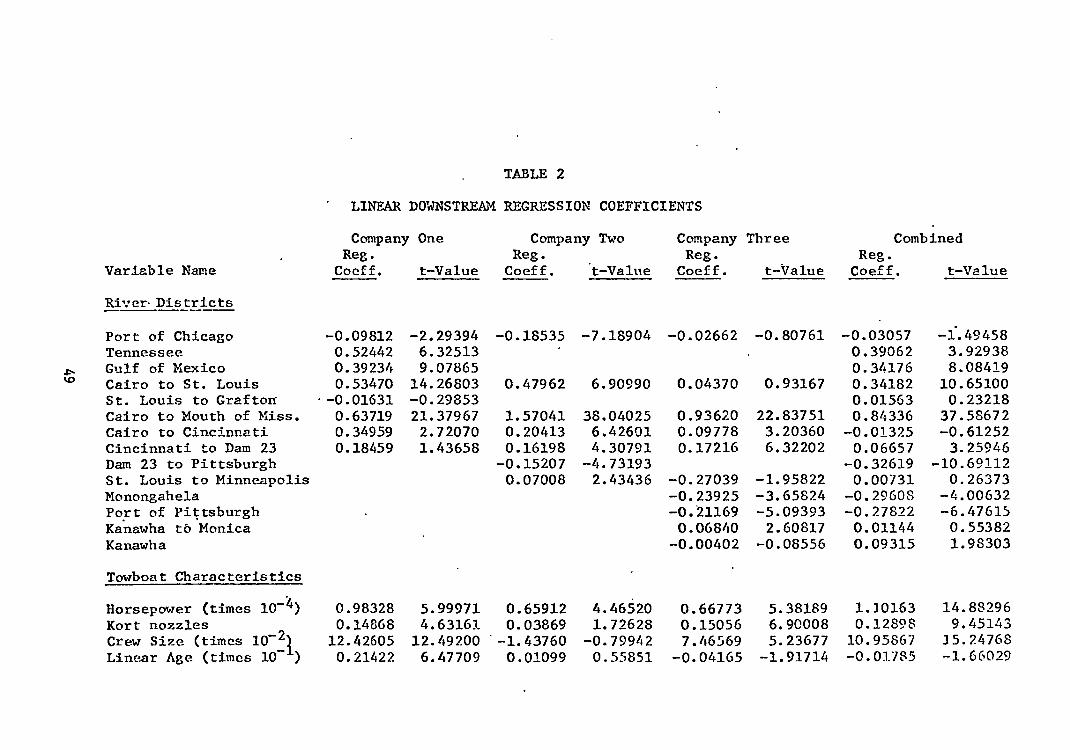
Variable Name

Riven Districts

TABLE 2

• LINEAR DOWNSTREAM REGRESSION COEFFICIENTS

Company One Company Two Reg. Reg. •

Coeff. t-Value Coeff. t-Value

Company Three Reg.

Coeff. t-Value

Combined Reg.

Coeff. t-Value

Port of Chicago Tennessee

•Ps Gulf of Mexico Cairo to St. Louis St. Louis to Grafton Cairo to Mouth of Miss. Cairo to Cincinnati Cincinnati to Dam 23 Dam 23 to Pittsburgh St. Louis to Minneapolis Monongahela Port of Pittsburgh Kanawha to Monica Kanawha

-0.09812 -2.29394 -0.18535 -7.18904 -0.02662 -0.80761

0.52442 6.32513

0.39234 9.07865

0.53470 14.26803 0.47962 6.90990 0.04370 0.93167 .-0.01631 -0.29853

0.63719 21.37967 1.57041 38.04025 0.93620 22.83751

0.34959 2.72070 0.20413 6.42601 0.09778 3.20360

0.18459 1.43658 0.16198 4.30791 0.17216 6.32202 -0.15207 -4.73193 0.07008 2.43436 -0.27039 -1.95822

-0.23925 -3.65824 -0.21169 -5.09393

0.06840 2.60817 -0.00402 -0.08556

-0.03057 0.39062 0.34176 0.34182 0.01563 0.84336

-0.01325 0.06657

-0.32619 0.00731

-0.29608 -0.27822 0.01144 0.09315

-1.49458 3.92938 8.08419 10.65100 0.23218 37.58672 -0.61252 3.25946

-10.69112 0.26373

-4.00632 -6.47615 0.55382 1.98303

Towboat Characteristics

Horsepower (times 10-4) 0.98328 5.99971 0.65912 4.46520 0.66773 5.38189 1.10163 Kort nozzles 0.14868 4.63161 0.03869 1.72628 0.15056 6.90008 0.12898 Crew Size (times 10-21 12.42605 12.49200 -1.43760 -0.79942 7.46569 5.23677 10.95867 Linear Age (times 10-i) 0.21422 6.47709 0.01099 0.55851 -0.04165 -1.91714 -0.01785

14.88296 9.45143

35.24768 -1.66029

TABLE 2 - -Continued

Variable Name

Company One Company Two Company Three Combined -Reg. Reg. Reg. Reg. Coeff. t-Value Coeff. t-Value Coeff. t-Value Coeff. t-Value

Month

January r0.09467 -1.99514 -0.00216 -0.06290 0.05099 1.65056 -0.01450 -0.58075 February r0.03891 .40.81306 0.04613 1.34226 -0.04813 -1.34091 -0.04669 -1.77957 March 0.01414 0.28470 0.15455 4.67984 0.11426 3.99957 0.10489 4.34597 April 0.13571 2.76299 0.16941 5.05616 0.04423 1.55179 0.09581 3.96492 May 0.09132 1.84063 0.12123 3.63094 0.01709 0.58761 0.O5076 2.07837 June • 0.03406 0.67575 0.02241 0.67366 -0.00812 -0.26075 -0.01904 -0.75635 July 0.06176 1.21282 0.06165 1.87044 -0.05611 -1.85428 -0.01385 -0.55796 August -0.01479 -0.29935 -0.00720 -0.22459 -0.06414 -2.18826 -0.05428 -2.25129

U' September r0.04621 -0.92748 -0.00126 -0.03900 -0.06429 -2.25589 -0.05254 -2.19421 c) October ' 0.09766 2.02642 0.02592 0.77830 -0.04337 -1.54912 -0.01959 -0.82146 November 0.06293 1.29246 0.04308 1.30676 -0.05799 -2.03624 -0.02041 -0.84936

Year

1964 -0.21201 -6.29756 -0.03236 -1.98050 -0.08948 -5.90145 1965 -0.05493 -1.98258 -0.00679 -0.40592 0.00368 0.27902 -0.00789 -0.69192

Dependent Variable; , EBM/HR (times 10- ')

r2 .9083 .9173 .6660 .7934 Standard error • 0.17423 0.18346 0.19253 0.22815 Intercept r1.593'6 0.3317 -0.6925 -1.2064 Sample size 349 743 951 2043

TABLE 3

LINEAR UPSTREAM REGRESSION COEFFICIENTS

Variable Name

Company One Reg.

Coeff. t-Value

Company Two Reg. Coeff. t -Value

Company Three Reg.

Coeff. t-Value

Combined Reg. Coeff. t-Value

River Districts

-0.08867 -3.6550 -0.07878 -5.2396

0.11258 2.6597

0.13774 5.6821

0.14082 8.6864 0.07237 3.5261 St. Louis to Grafton -0.09143 -3.3125 Cairo to Mouth of Miss. 0.10975 6.9720 Cairo to Cincinnati 0.31634 4.3052 Cipcinnati to Dam 23 0.31634 4.3052 Dam 23 to Pittsburgh 0.05134 0.6987 St. Louis to Minneapolis Monongahela Port of Pittsburgh Kanawha to Monica Kanawha . •

Towboat-Characteristics

-0.05663 -2.6645 -0.07245 -6.5343

0.05999 1.2294

0.09404 4.1014

-0.07615 -3.0041 0.06334 5.2752

-0.08522 -2.5995

0.13086 5.0100 0.14583 12.3962

0.03784 1.9238 0.01014 0.9031

0.11593 6.5340 0.08181 7.8515 -0.20124 -13.0902

-0.21721 -2.3636 -0.01582 -1.0042

-0.12843 -4.2121 -0.13576 -4.9823

-0.11342 -5.2281 -0.12128 -7.1618

0.01615 0.9291 0.00561 0.5006

0.03503 1.1173 0.03188 1.2013

Port of Chicago Tennessee Gulf of Mexico Cairo to St. Louis

0.28593 12.5021

0.02303 1.2805

0.02947 1.5548 -0.19278 -10.4603 -0.00435 -0.2380

Horsepower (times 10-4) 0.95214 10.5881 Kort nozzles 0.08541 5.2319 Crew Size (times 10-2) 3.67580 6.8629 Linear Age (times 10-1) 0.05939 3.4153

1.00327 12.3443 0.69701 8.7461 0.79823 23.4626 0.04936 3.7269 0.10134 7.4298 0.07455 10.5093

-1.87375 -1.7595 5.05772 5.5754 3.52121 9.2280 -0.00235 -0.1998 0.01091 0.7926 0.02511 4.5262

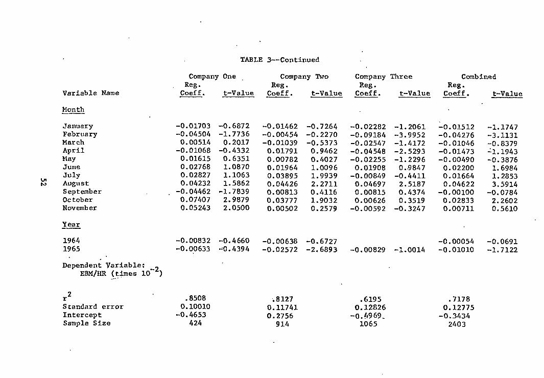
Variable Name

Month

TABLE 3 - -Continued

Company One . Company Two Company Three Combined . Reg. Reg. Reg. Reg. Coeff. t-Value Coeff. t-Value Coeff. t-Value Coeff. t-Value

January -0.01703 -0.6872 -0.01462 -0.7264 -0.02282 -1.2061 -0.01512 -1.1747 February -0.04504 -1.7736 -0.00454 -0.2270 -0.09184 -3.9952 -0.04276 -3.1131 March 0.00514 0.2017 -0.01039 -0.5373 -0.02547 -1.4172 -0.01046 -0.8379 April -0.01068 -0.4332 0.01791 0.9462 -0.04548 -2.5293 -0.01473 -11.1943 May 0.01615 0.6351 0.00782 0.4027 -0.02255 -1.2296 -0.00490 -0.3876 June 0.02768 1.0870 0.01964 1.0096 0.01908 0.9847 0.02200 1.6984 July 0.02827 1.1063 0.03895 1.9939 -0.00849 -0.4411 0.01664 1.2853

t.n tv August 0.04232 1.5862 0.04426 2.2711 0.04697 2.5187 0.04622 3.5914

September -0.04462 -1.7839 0.00813 0.4116 0.00815 0.4374 -0.00100 -0.0784 October 0.07407 2.9879 0.03777 1.9032 0.00626 0.3519 0.02833 2.2602 November 0.05243 2.0500 0.00502 0.2579 -0.00592 -0.3247 0.00711 0.5610

Year

1964 -0.00832 -0.4660 -0.00638 -0.6727 -0.00054 -0.0691 1965 -0.00633 =0.4394 -0.02572 -2.6893 -0.00829 -1.0014 -0.01010 -1.7122

Dependent Variable: -2 EBM/HR (times 10 )

• r2

.8508 ..8127 .6195 .7178 Standard error 0.10010 0.11741 0.12826 0.12775 Intercept -0.4653 0.2756 -0.4969_ -0.3434 Sample Size 424 914 1065 2403

TABLE 4

LOG-LINEAR DOWNSTREAM REGRESSION COEFFICIENTS

Variable Name

Company One Company Two Company Three Combined Reg. Reg. Reg. Reg.

aoeff. t-Value Coeff. t-Value Coeff. t-Value Coeff. t-Value

River Districts

Port of Chicago -0;54509 -17.6538 -0.35729 -18.0708 -6.05272 -1.9048 -0.27553 -17.7132 Tennessee 0.18771 3.1880 0.02529 0.3761 Gulf of Mexico 0.20224 6.5469 . 0.09006 3.1687 Cairo to St. Louis 0.32578 12.2768 0.26647 6.7716 0.00590 0.1564 0.21324 9.8909 St. Louis to Grafton -0.05671 -1.4566 -0.05121 -1.1348 Cairo to Mouth of Miss. 0.35008 16.6685 0.53185 24.1166 0.42878 13.1628 0.37325 25.6628 Cairo to Cincinnati 0.30644 3.3684 0.10746 5.9932 0.03020 1.2384 0.03392 2.3656 Cincinnati to Dam 23 0.20203 2.2207 0.09929 4.6668 0.09368 4.2514 0.09012 6.5840 La Dam 23 to Pittsburgh -0.18636 -10.1112 -0.22849 -11.2003 St. Louis to Minneapolis 0.04656 2.7743 -0.43020 -3.8911 0.03269 1.7431 Monongahela -0.31412 -5.9855 -0.30059 -6.0635 Port of Pittsburgh -0.28760 -8.5705 -0.26997 -9.3431 Kanawha to Monica 0.00941 0.4405 0.02541 1.8294 Kanawha -0.01803 -0.4844 0.03710 1.1757

Towboat Characteristics

logio Horsepower (times 10-4) 0.47509 7.8211 0.51673 10.2347 0.58533 9.9264 0.44742 14.9251

Kort Knozzles 0.11426 4.9445 0.05847 4.4951 0.14983 8.6605 0.10644 11.6179 loglo Crew Size

(times 10-2) • 2.44631 15.8897 -0.18005 -0.7556 1.36704 4.1702 1.81511 16.4901 Linear Age (times 10-1) 0.06357 2.9427 0.00263 0.2.479 -0.09113 -5.6954 -0.00186 -0.2620

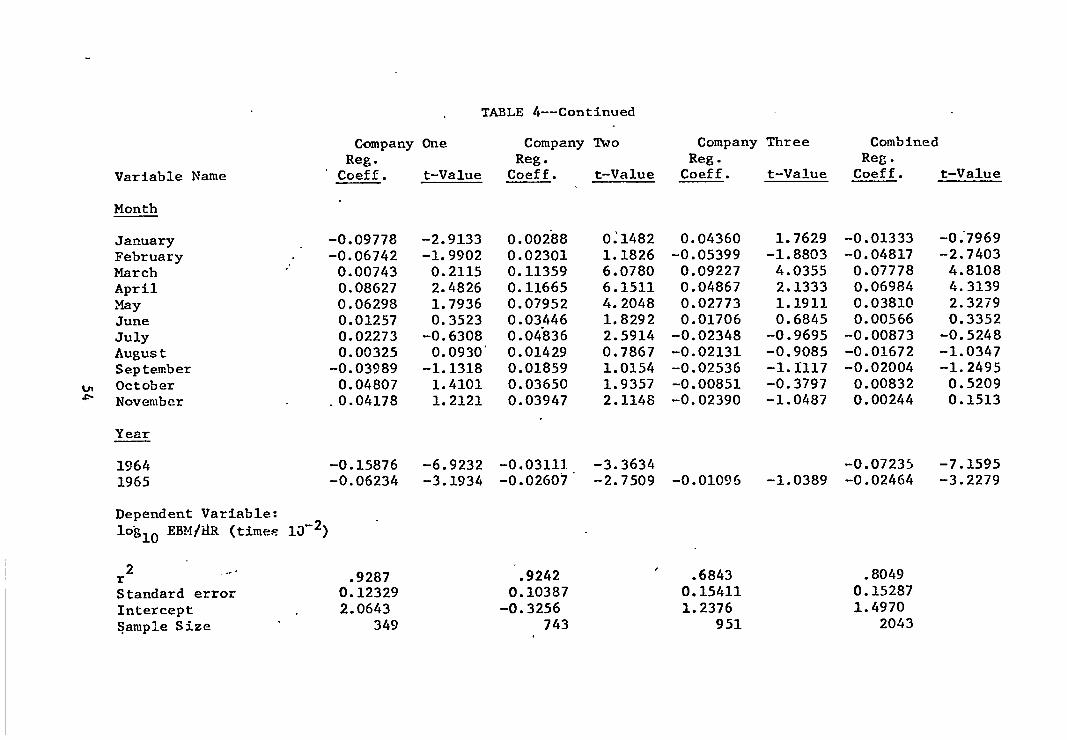
TABLE 4 - -Continued

Variable Name

Company One Company Two Company Three Combined Reg. Reg. Reg. Reg.

' Coeff. t-Value Coeff. t-Value Coeff. t-Value Coeff. t-Value

Month

January -0.09778 -2.9133 0.00288 0:1482 0.04360 1.7629 -0.01333 -0.7969 February • -0.06742 -1.9902 0.02301 1.1826 -0.05399 -1.8803 -0.04817 -2.7403 March 0.00743 0.2115 0.11359 6.0780 0.09227 4.0355 0.07778 4.8108 April 0.08627 2.4826 0.11665 6.1511 0.04867 2.1333 0.06984 4.3139 May 0.06298 1.7936 0.07952 4.2048 0.02773 1.1911 0.03810 2.3279 June 0.01257 0.3523 0.03446 1.8292 0.01706 0.6845 0.00566 0.3352 July 0.02273 -0.6308 0.04836 2.5914 -0.02348 -0.9695 -0.00873 -0.5248 August 0.00325 0.0930 0.01429 0.7867 -0.02131 -0.9085 -0.01672 -1.0347 September -0.03989 -1.1318 0.01859 1.0154 -0.02536 -1.1117 -0.02004 -1.2495

u, October 0.04807 1.4101 0.03650 1.9357 -0.00851 -0.3797 0.00832 0.5209 '°- November .0.04178 1.2121 0.03947 2.1148 -0.02390 -1.0487 0.00244 0.1513

, Year

1964 -0.15876 -6.9232 -0.03113 -3.3634 -0.07235 -7.1595 1965 -0.06234 -3.1934 -0.02607 -2.7509 -0.01096 -1.0389 -0.02464 -3.2279

Dependent Variable: 16gio EBM/AR (times 13-2)

• , ...

r2

.9287 .9242 .6843 .8049 Standard error 0.12329 0.10387 0.15411 0.15287 Intercept 2.0643 -0.3256 1.2376 1.4970

. Sample Size 349 743 951 2043

,

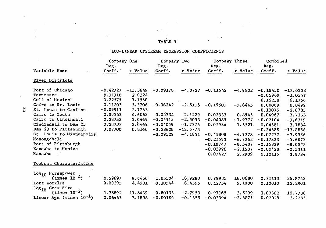
Variable Name

River Districts

TABLE 5

LOG-LINEAR UPSTREAM REGRESSION COEFFICIENTS

Company One Company Two Company Three Combined . Reg. Reg. Reg. Reg.

Coeff. - t-Value Coeff. t-Value Coeff. t-Value Coeff. t-Value

Port of Chicago -0.42727 -13.3649 -0.09178 -4.0727 -0.11542 -4.9902 -0.18450 -13.0303 Tennessee 0.11110 2.0324 -0.05969 -1.0557 Gulf of Mexico . 0.22575 7.1560 0.16238 6.1756 Cairo to St. Louis 0.11203 5.3706 -0.06242 -2.5115 -0.15601 -5.8465 0.00069 0.0499

t" St. Louis to Grafton vi -0.09911 -2.7763 -0.10076 -2.6783 Cairo to Mouth . 0.09343 4.6062 0.05734 2.1229 0.02333 0.8545 0.04967 3.7365 Cairo to Cincinnati 0.28732 3.0469 -0.05512 -2.5053 -0.04085 -1.9777 -0.02704 -1.6319 Cincinnati to Dam 23 0.28732 3.0469 -0.04059 -1.7374 0.02934 1.5521 0.04581 3.7884 Dam 23 to Pittsburgh 0.07700 0.8166 -0.28628 -12.5773 -0.24588 -13.8858 St. Louis to Minneapolis -0.09529 -4.1851 -0.45808 -4.7778 -0.07227 -3.9586 Monongahela -0.21593 -6.7262 -0.17823 -5.6873 Port of Pittsburgh -0.19747 -8.5437 -0.15629 -8.0822 Kanawha to Monica -0.03998 -2.1537 -0.00428 -0.3311 Kanawha - ' 0.07427 2.2909 0.12115 3.9784

Towboat Characteristics

loglo Horsepower (times 10-4) 0.59697 9.6466 1.05504 18.9280 0.79985 16.0680 0.71113 26.8758

Kort nozzles 0.09395 4.4501 0.10544 6.4395 0.12754 9.1000 0.10010 12.2901 log io Crew Size

(times 10-2) 1.78892 11.8469 -0.80135 -2.7953 0.97165 3.5299 1.07602 10.7736 Linear Age (times 10-1) 0.06463 3.1898 -0.00186 -0.1355 -0.03394 -2.5871 0.02029 3.2285

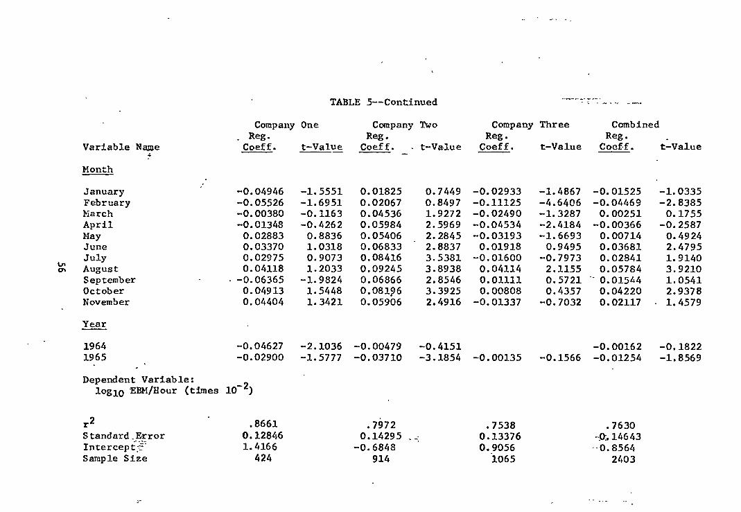
TABLE 5--Continued

- Company One Company Two Company Three Combined . Reg. Reg. Reg. Reg. .

Variable Name Coeff. t-Value Coeff. . t-Value Coeff. t-Value Coeff. t-Value

Month

January -0.04946 -1.5551 0.01825 0.7449 -0.02933 -1.4867 -0.01525 -1.0335 February -0.05526 -1.6951 0.02067 0.8497 -0.11125 -4.6406 -0.04469 -2.8385 March -0.00380 -0.1163 0.04536 1.9272 -0.02490 -1.3287 0.00251 0.1755 April -0.01348 -0.4262 0.05984 2.5969 -0.04534 -2.4184 -0.00366 -0.2587 May 0.02883 0.8836 0.05406 2.2845 -0.03193 -1.6693 0.00714 0.4924 June 0.03370 1.0318 0.06833 2.8837 0.01918 0.9495 0.03681 2.4795 July 0.02975 0.9073 0.08416 3.5381 -0.01600 -0.7973 0.02841 1.9140

ON August 0.04118 1.2033 0.09245 3.8938 0.04114 2.1155 0.05784 3.9210 September • -0.06365 -1.9824 0.06866 2.8546 0.01111 0.5721 - 0.01544 1.0541 October 0.04913 1.5448 0.0846 3.3925 0.00808 0.4357 0.04220 2.9378 November 0.04404 1.3421 0.05906 2.4916 -0.01337 -0.7032 0.02117 1.4579

Year

1964 -0.04627 -2.1036 -0.00479 -0.4151 -0.00162 -0.1822 1965 -0.02900 -1.5777 -0.03710 -3.1854 -0.00135 -0.1566 -0.01254 -1.8569

Dependent Variable: log lo EBM/Hour (times 10-2)

r2 .

.8661 .7972 .7538 .7630 Standard_Error 0.12846 0.14295 .... 0.13376 -0.14643 Intercept-: 1.4166 -0.6848 0.9056 0.8564 Sample Size 424 914 1065 2403

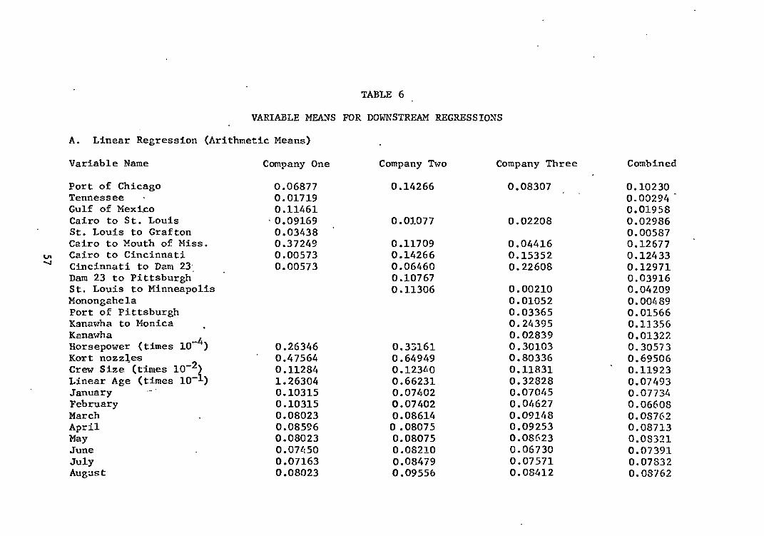
TABLE 6 .

. VARIABLE MEANS FOR DOWNSTREAM REGRESSIONS

A. Linear Regression (Arithmetic Means) .

Variable Name Company One Company Two Company Three Combined

Port of Chicago Tennessee - Gulf of Mexico Cairo to St. Louis St. Louis to Grafton Cairo to Mouth of Miss.

t..n Cairo to Cincinnati .....1 Cincinnati to Dam 23'

Dam 23 to Pittsburgh St. Louis to Minneapolis Monongahela Port of Pittsburgh Kanawha to Monica . Kanawha Horsepower (times 10-4 ) Kort nozzles Crew Size (times 10-2) Linear Age (times 10-1) January February March April May June July August

0.06877 0.01719 0.11461 0.09169 0.03438 0.37249 0.00573 0.00573

0.26346 • 0.47564

0.11284 1.26304 0.10315 0.10315 0.08023 0.08596 0.08023 0.07450 0.07163 0.08023

0.14266 0.08307 0.10230 0.00294 - 0.01958

0.01077 0.02208 0.02986 0.00587

0.11709 0.04416 0.12677 0.14266 0.15352 0.12433 0.06460 0.22608 0.12971 0.10767 0.03916 0.11306 0.00210 0.04209

0.01052 0.00489

0.03365 0.01566

0.24395 0.11356

0.02839 0.01322 0.3:3161 0.30103 0.30573 0.64949 0.80336 0.69506 0.12360 0.11831 - 0.11923 0.66231 0.32828 0.07493 0.07402 0.07045 0.07734 0.07402 0.04627 0.06608 0.08614 0.09148 0.08762 0.08075 0.09253 0.08713 0.08075 0.08623 0.08321 0.08210 0.06730 0.07391 0.08479 0.07571 0.07832 0.09556 0.08412 0.08762

...-

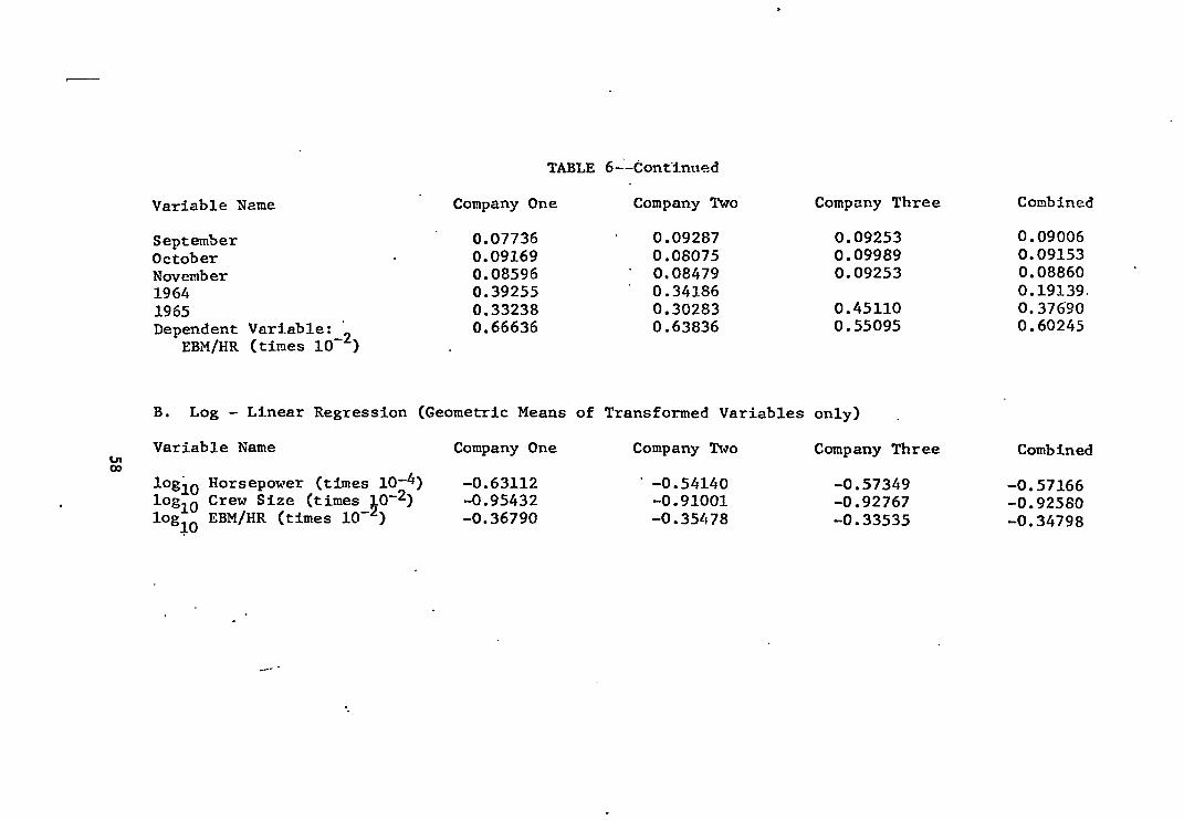
Variable Name Company One Company Two Company Three

Company One Company Three

-0.63112 -0.95432 -0.36790

Company Two

' -0.54140 -0.91001 -0.35478

-0.57349 -0.92767 -0.33535

Variable Name

logio Horsepower (times 10-4 ) logio Crew Size (times.10 -2) 1°g10 EBM/HR (times 10-2 )

Combined

-0.57166 -0.92580 -0.34798

TABLE 6--Continued

September October November 1964 1965 Dependent Variable: 2

EBM/HR (times 10 - )

0.07736 0.09169 0.08596 0.39255 0.33238 0.66636

0.09287 0.08075

• 0.08479 0.34186 0.30283 0.63836

0.09253 0.09989 0.09253

0.45110 0.55095

Combined

0.09006 0.09153 0.08860 0.19139 0.37690 0.60245

B. Log - Linear Regression (Geometric Means of Transformed Variables only)

TABLE 7

VARIABLE MEANS FOR UPSTREAM REGRESSIONS

A. Linear Regression (Arithi.etic Means)

Variable Name Company One Company Two Company Three Combined

Port of Chicago - 0.05896 0.11816 0.07418 Tennessee 0.01887 Guld of Mexico 0.09906 Cairo to St. Louis 0.19575 0.08425 0.03286 St. Louis to Grafton 0.03774 Cairo to Mouth of Miss. 0.33255 0.09847 0.04319 Cairo to Cincinnati . 0.00472 ' 0.14004 0.15211 Cincinnati to Dam 23 0.00472 0.09519 0.22535

LA Dam 23 to Pittsburgh 0.00472 0.10722 %.0 St. Louis to Minneapolis 0.08643 0.00188 Monongahela 0.02254 Port of Pittsburgh 0.06667 . Kanawha to Monica 0.21878 Kanawha 0.02441 Horsepower (times 10

-4) 0.27719 0.34560 0.30168

Kort nozzles 0.52123 0.70022 0.80845 Crew Size (times 10-2) 0.11406 0.12430 0.11840 Linear Age (times 10-I) 1.28891 0.68359 1.30854 January 0.09670 0.07440 0.07887 February _ • ' 0.08962 0.07659 0.04413 March 0.08255 0.08972 0.09671 April . 0.09670 0.09737 0.09484 May --

0.08255 0.08643 0.08826 • June 0.08019 0.08534 0.07230 July 0.08019 0.08425 0.07418 August 0.06604 0.08534 0.08263

0.08822 0.00333 0.01748 0.08115 0.00666 0.11527 0.12151 0.13691 0.04161 0.03371 0.00999 0.02955 0.09696 0.01082 0.31406 0.71660 0.11988 1.06737 0.08032 0.06450 0.01955 0.09613 0.08656 0.07865 0.07907 0.08073

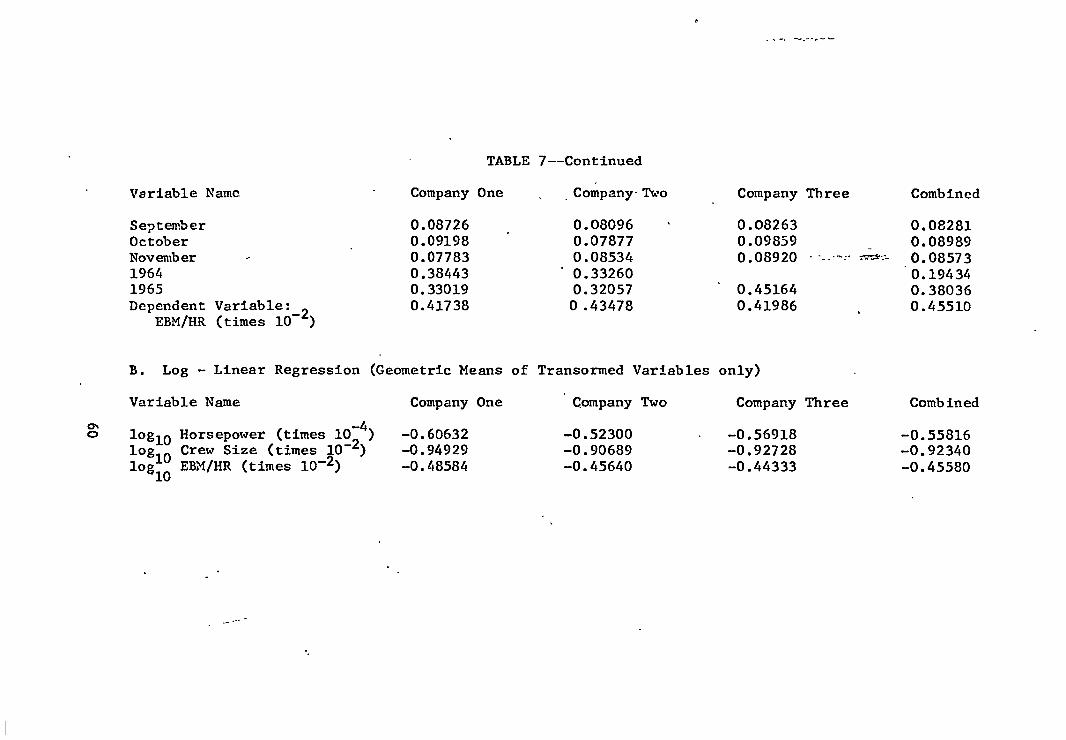
Company Two

-0.52300 -0.90689 -0.45640

Company Three

-0.56918 -0.92728 -0.44333

Combined

-0.55816 -0.92340 -0.45580

TABLE 7--Continued

Variable Name Company One Company-TWo . Company Three Combined

September October November 1964 1965 Dependent Variable: 2

EBM/HR (times 10- )

0.08726 0.09198 0.07783 0.38443 0.33019 0.41738

0.08096 0.07877 0.08534 0.33260 0.32057 0 .43478

0.08263 0.08281 0.09859 0.08989 0.08920 - 0.08573

0.19434 0.45164 0.38036 0.41986 0.45510

B. Log - Linear Regression (Geometric Means of Transormed Variables only)

Variable Name Company One

log10 Horsepower (times 10-4 ) -0.60632 log Crew Size (times 10-2) -0.94929 logio EBM/HR (times 10-2 ) -0.48584

10

61

are roughly comparable across all companies (see Table 2) and for both

upstream and downstream. Apparently, horsepower is just as useful for

a tow heading doWnstream as it is for a tow heading upstream. At first,

this result may seem paradoxical. After all, in heading downstream the

current is doing much of the work. However, horsepower is required to

control the tow (by steering and power backing). Carriers find that

using a towboat on a downstream run can achieve high speeds, but it

also has a high probability of having an accident.

With the exception of company two, the coefficient of crew size

is always positive and significant. The negative sign for company two

is implausible since it indicates that additional crew members decrease

the productivity of a towboat. In attempting to explain this sign, one

should note that company two operates larger crews than either of the

other companies. Thus, it is quite possible that they are at the point

of negative marginal productivity. Alternatively, one might note that

company two operates larger boats and pushes larger tows than do the

other two companies. This is most evident in the newest large boats

where automated equipment has replaced several crew functions. Since

company two operates larger boats, it is quite possible that larger

outputs are associated with smaller crew sizes (that is, a negative

coefficient for crew size).

The coefficient for labor is much larger for the downstream re-

gressions than for the upstream regressions. According to the estimates,

labor is four times as productive on downstream runs. In part, this

additional productivity comes from higher average speed on the downstream

run; there is more work for the crew per hour of running time.

62

A towboat is an expensive piece of capital equipment (costing

between 1/2 million and 1 million dollars when new) and can be assum-

ed to embody the best technplogy available when it was constructed

(or had a major overhaulinsofar as this technology has improved

over time, newer boats should be more productive. Thus, a linear

measure of the age of a towboat should have a negative coefficient.

In looking at the results, only company one has a significant coef-

ficient. Two of six coefficients are negative, and coefficients of

companies two and three change signs between the upstream and down-

stream regressions. Apparently, there have not been significant im-

provements in design over this period.

This lack of significance in design inprovements was checked with

naval architects. They expressed the opinion that there has been only

one major improvement: the Kort nozzle. These impressions are con-

firmed by the regressions. In all cases, the coefficient of Kort nozzles

is positive and significant.. Again, they seem to add more to productiv-

ity in downstream runs than in upstream runs.

Over the last two or three decades, the price of waterway trans-

portation either remained constant or declined slightly. Over this

same period, the price of fuel has risen sharply, as has the cost of

equipment and crew. Apparently, there has been a significant increase

in productivity over this period. The increased productivity could

be due to: (1) changes in equipment design, (2) improvements in labor

productivity or (3) changes in operating rules, such as the number of

barges in a tow. If the increased productivity took the form of im-

proved equipment, it could, be thought of as "capital embodied techno-

logical change." 5 If the productivity were due to labor, it would be

63 •

termed "labor embodied technological change." If it can be ascribed to

neither capital nor labor, it is "neutral technological change."

The age of the towboat gives a general indication of capital em-

bodied technological change. As pointed out above, there is little

evidence that this change is important. A particular measure of capital

embodied technological change is the presence of Kort nozzles. These

seem to be effective in improving the productivity of towboats. Over

the last three decades, crew size has fallen (holding towboat size con-

stant). However, this change took place before 1964, when the data

series began. A measure of labor embodied technological change has

not been pursued. However, the experience of operators is that this

effect has not been significant.

Insofar as capital embodied technological change has been account-

ed for, any remaining increase in productivity must be classified as

labor embodied or neutral. In fact, a more direct measure of neutral

technological change is available. Controlling for capital and labor

variables, how did towboat productivity change between 1964 and 1966?

This question is answered by looking at the year dummy variables. Since

1966 is omitted, it is defined as having a coefficient of zero (to serve

as a base of comparison). In the downstream regression for company one,

the coefficient of 1964 is -.20 and for 1965 -.05. Thus, 1966 experi-

enced a neutral technological improvement of .21 over 1964 and .05 over

1965. These coefficients indicate an impressive amount' of neutral tech-

nological change. 6

For the river district dummy variables, the omitted district was

the Lower Illinois River (which thus has a coefficient of 0). The

estimated coefficients carry the interpretation of being corrections

64

to the productivity experienced on the Lower Illinois River. For exam-

ple, the Port of Chic.ago has a lower productivity (equal to about .09

EBM's per hour) after accounting for all other factors. In contrast,

the Lower Mississippi River (downstream) gives about .6 more EBM's per

hour. Any river district which is more "difficult" to operate on than

the Lower Illinois River should have a negative coefficient; positive

coefficients indicate rivers which are "easier" to operate on.

The estimated coefficients indicate the penalty to he assigned to

operating on each river district. Thus, if a company were offered

freight in the Port of Chicago, which is to be delivered in the Port of

Chicago, the price per ton-mile should be relatively higher (other

things held equal) because it is more difficult to operate there. (These

coefficients give quantitative information as to the size of the penalty

to be attached to each river district.)

One way of checking these river district coefficients is to rank

them and compare this ranking with a similar one embodied in Barge Form

C. Table 8 presents a ranking of the coefficients for both upstream

and downstream mOvements of the company one linear regression. The . rank-

ing varies between the two as expected. Some river districts are com-

pletely enclosed by locks. Current is minimal, and it makes little

difference whethei a tow is headed upstream or downstream. Other river

districts have completely open water (such as the lower Mississippi).

For example, in the upstream run, the lower Mississippi probably has

the most rapid current, while the Ohio River is completely dammed up

(except during spring flood). For operations on the °hie, River it

should prove as easy to go one way as the other.

-

TABLE 8

COMPANY ONE LINEAR REGRESSION RIVER DISTRICT COEFFICIENT COMPARISON

, . Districts

Downstream:

Coefficient Empty Barge Factor

.275: - Cairo to Mouth of Miss.

0 .6

0 Cairo to St. Louis ' .6 Tennessee 0.524* .7 Gulf of Mexico 0.392* .7 Cairo to Cincinnati 0.349* .7 Cincinnati- to Dam 23 - 0.184 .7 Lower Illinois 0.000 .7 St. Louis to Graf ton -0.016 .7 Port of Chicago -0.098* 1.0

Upstream':

Cincinnati to Cairo • , 0.316* .7 Cincinnati to Dam 23 0.316* .7 Cairo to , St. Louis . 0.141* .6 Gulf of Mexico 0.138* .7

. Tennessee 0.113*" .7 Cairo to Mouth of Miss. 0.110* .6

- Dam. 23 to'Pittsburgh • .0.051 .75 . Lower Illinois 0.000 .7 Port of Chicago. -0.089* 1.0

• St. Louis to Grafton -0.091* .7

*Indicates that coefficient was significant (t-value greater than +2.0)

65

66

Barge Form C contains a table of the relative weight given to

towing an empty barge on each river district. The lowest weight indi-

cates that (on the Lower Mississippi) an empty barge requires about

60 per cent of the effort required to push a full barge. The highest

weight indicates that (for the Port of Chicago) it takes the same

effort to push an empty barge as a full one. In the port of Chicago,

average speed is governed by congestion and a towboat can never use

all of its power to gain speed.

In general, the higher the weight assigned to an empty barge, the

more congested the river district will be. These weights also tend to

reflect shallow water, swift current and locking delays as well as con-

gestion. These factors are approximately the same as would be expected

to produce penalties in our estimation scheme. For downstream move-

ments, river districts are ranked identically by both the river district

coefficients and the Barge Form C weights. On upstream movements the

ranking is less perfect. While this rank correlation tends to strengthen

one's faith in the estimated conditions, it slrould be pointed out that the

Barge Form C weights are somewhat arbitrary and do not represent any

systematic collection of data. . .

These estimated coefficients are of direct interest to waterway

carriers. They provide a measure of the relative difficulty of operating

in each waterway. These coefficients might be used to modify the rate

structure to bring price more closely in line with marginal cost. Ceteris

paribus, the price (per ton-mile) of carrying freight on each river dis-

trict should reflect these operating penalties.

The final set of variables accounts for seasonality in operations.

The month of December is defined to have a coefficient of zero; each of

67

the other monthly coefficients indicates the relative difficulty of ,

operating in that month. The changes between the months appear to .

establish a regular pattern. The winter months have negative.coef-

ficients, indicating difficulties of icing and bad weather. The spring

and early summer months have large positive coefficients, indicating

they are the easiest months in which to operate. Finally, the early

fall carries a negative coefficient due to low water (in genexal.there

is little rain in summer and so river depth falls). Again, these month-

ly variables could be used to redesign the rate structure to bring

prices in line with costs. .

Summary

A statistical production function for towboats on inland waterways

was estimated from data from three companies over a three-year period;

approximately 4500 observations on 100 towboats operating on 16 river

districts were used. Both linear and log-linear relationship were esti-

mated.

The reduction function for downstream operations was found to

differ significantly from that for upstream movements. It was also

found that the production functions differed between companies.

The productivity of a towboat (measured in terms of the number of

EBM's per hour produced) was regressed on the horsepower and also age

of the towboat, its crew size and whether it had Kort nozzles. Addi-

tional variables were the river in which it operated and the month and

year of the observation. Horsepower is a measure of the size of the

towboat and had a consistently positive, significant coefficient. With

the exception of one company, crew size had positive, significant coef-

68

ficients. The age of the towboat added little to the regression, indi-

cating few improvements in towboat design in recent years. The one

significant improvement was the Kort nozzle; thus there is evidence of

some capital embodied technological change (in the Kort nozzles). There

was also evidence of neutral technological change. The variables for

river district and month showed effects consistent with the experience

of waterway operators.

CHAPTER IV

AN ANALYSIS OF DIRECT TOWBOAT AND BARGE COSTS

Inland waterway firms are the operating managers of large, varied,

and costly assortments of floating equipment. This study is an attempt

to determine the influence of the operating environment of inland water-

way barge firms upon the direct Operating costs associated with their

towboat and barge fleets.

A. An Analysis of Direct Towboat Costs

The cost of operating a towboat should be directly related to the

amount of "work" (measured in EBM's or ton-miles) the boat performs.

However, towboats possess a range of capabilities (as measured by their

horsepower and other physical characteristics). In addition, the en-

vironment in which the towboat operates (the waterway) directly affects

the output of the towboat. Thus, one cannot look simply at the average

cost of an EBM. The approach used here is to specify how average cost

varies with output (EBM's) as the characteristics of the equipment and

of the waterway are changed.

The Data

Data on _towboat costs have been gathered from six inland waterqay

operators. The services performed by these six firms are widely dis-

tributed over the entire Mississippi and Gulf River systems. The six

firms are varied as to size and type of traffic carried. Together, the

69

■■•■••.••••■•••

70

six Lirms operate a towboat fleet which possess a wide range of - enysical

ch.:.1.:3cLer1stics.

The observations range over a period of five years, from lci62 to

ló3. Annual costs were obtained for each towboat the firms actually

operated during each year. In addition, information was gathered on

the number of hours that each towboat operated on each river district

in the Mississippi and Gulf River systems during each year in the sam-

ple. 1

From the standpoint of determining costs, there are two dominant

features of towboat operations. The first feature is the characteris-

tics of the equipment itself. The most general indicator of towboat

size (and thus of its productive capacity) is its horsepower. As larger

horsepower towboats are used to produce a given output, one would expect

total cost to rise (due to increased fuel consumption, greater mainte-

nance expense, etc). However, since certain components of total cost,

such as fuel consumption, wages, and maintenance, would not be expected

to increase in proportion to horsepower (and since some components of

total cost are not even related to horsepower, e.g., radio repair) one

would expect that increases in total cost would be less than proportional

to increases in horsepower. Therefore, we would expect average cost to

fall, ceterus paribus as horsepower increases.

It is to be expected that the age of a towboat will directly affect

the cost of operating it. An old boat is a less efficient resource than

a new boat. One would expect costs to be higher for older boats. A

linear measure of towboat age was used in the statistical production

function without much success. Here, the effect of age has been included ■

71

with the use of dummy variables. Towboat ages were grouped into five

year intervals. A dummy variable was assigned to each group. In the

regression the dummy variable for the newest boats was excluded. If

our age hypothesis is correct, the coefficients of the remaining dummy

variables should all be positive.

Other characteristics of the towboat most certainly will affect

cost in some way. Some features, such as the extent of automation in

the engine operation will affect cost directly by reducing the amount.

. of the labor input and hence wage cost (there will of course be an

increase in cost for the capital input). Other features., such as elec-

tronic guidance equipment, will serve to improve the average performance

of the boat and lower cost for any given output. Most of these factors

are extremely hard to quantify and-have not been included in the statis-

tical model. Information on one feature, the Kort nozzle, is available

and has been included in the analysis. The Kort nozzle is a tunnel

which surrounds the towboat's - propellers and creates a channel through

which the water is propelled. Its purpose is to reduce power loss due

to turbulence and thus improve performance. Its effect on cost is of

interest since some controversy among naval architects surrounds its use.

The presence of Kort nozzles on a boat in our sample is denoted by a

dummy variable. If the Kort nozzle does perform as expected we would

expect the dummy variable associated with its presence to have a nega-

tive sign. .

The second dominant feature of towboat operations is the operating

environment provided by the waterway. The physical characteristits of

the waterway (depth, width, stream flow) affect the speed at which a

72

given towboat can travel and thus help determine the maximum output the

towboat can produce per unit-time. Other features of the waterway, such

as the number of locks and conjestion, will affect the average level of

performance of the boat over many trips. -

Towboats generally do not operate on one river district alone:

Rather, their operations may be spread over three or four districts.

From time-to-time the assignments of the towboats will change and the

boats will be assigned to a different set of river districts. One would

expect the cost of operation for any towboat to vary with its assignment.

That is, one would expect that average costs will be lower for operations

on a less restrictive waterway than for operations on a river district

'with a narrow channel and congested traffic. Thus, in estimating a cost

relationship for towboats, an allowance must be made for where the tow-

boat boat operated. .

One way to include the effect of river districts would be to look

at the distribution of total output among river districts, measUred in

EBM's, for each towboat in each year. However, this approach is not

satisfactory because the period over which the output is produced is

not known. It could be argued that the dumber of EBM's produce - on a •I

river district and the time spent operating on a river district for any

one boat will be highly correlated. This will in general be true. But,

in comparing towboats cross-sectionally, an implicit assumption would be

introduced: that each boat spends the same number of hoUrs in operation

during the year. This is, however, a poor approximation to actual oper-

ations. Towboats will typically spend time "tied up" either for repairs

or in waiting for business. This time may-vary from a few hours due to

severe ice on the waterway, to several weeks for a major overhaul. 2

73

A more direct method, and the one employed in this study, is to

weight a towboat's operation on the various river districts by the

number of operating hours spent on each river district. This is done

in the statistical model by calculating the percent of total hours of

operation spent on each river district. A set of variables has been

included in the statistical model which represent the relative operating

time spent on each river district for each boat. The interpretation of

these variables wOuld be similar to that of dummy variables. One of

the percentages must be excluded. Then, the question could be posed:

How would costs change if the towboat operated 1% more of the time on

river district X1 and 1% less on the excluded river district? The

answer would, of course, depend upon the magnitude and sign of the

coefficient of X1

(note that a 1% increase, in this case, is not the

same as a one percentage point increase. For example, if a boat spent

50% of its time on the Lower Illinois River, an increase of 1% of time

spent on this river district would be a .5 percentage point increase).

Thus, the river district coefficients should show the,"costliness" of

operating-on each river district relative to the excluded river dis-

trict.

In summary, an observation for the towboat cost function consists

of the operating cost of a towboat for each year in the sample, the

characteristics of the towboat (its horsepower, age, and whether it has

Kort nozzles), the total output of the towboat for the.year (measured

in EBM's), and the distribution of the time spent in actual 'Inperation

for twenty-one river districts of the Gulf and Mississippi River systems. • . , ,

74

The Statistical Model

A statistical cost function has been estimated with the above

described data. The form of the function is:

20 loa°10 Cost/EBM = log ioa o + a l log ioHF + a2 log 10EBM + a 3KN + E B.R +

i=1 .

3 5 4 E y.A. + E 6,C, + E A n y n

j=1 J k=1 1' L=1

where: Cost = annual total direct towboat cost for each boat .

EBM = Equivalent Barge Miles produced by each boat in each year

'BF = towboat horsepower

KN = Kort nozzle dummy variable (1 = presence of Kort nozzles)

R. = percent time towboat operated on ith river district

(Lower Illinois excluded)

A = dummy variables for towboat age (A1 = 1 indicates the tow-

boat was built prior to 1050. 1960-1965 excluded)

Ck = dummy variables for each company

y = dummy variables for year (Y1 = 1 is 1962, etc., 1966 ex-

cluded)

In many regression models in econpmics, economic theory does not

indicate the correct specification of the function to be estimated.

Frequently, however, statistical theory indicates a choice. One model

may be preferred in particular circumstances because it avoids statis-

tical biases which may occur due to the nature of the data. One example

of this is the choice between the total and average functional forms

for cost estimation.

75

In using; for example,, cross-Section cost data, it is frequently

the case that the variance of total cost increases as output increases.

This phenomena is known as heteroscedasticity. This would be depicted

by a "fanning-out" of the scatter of points in the cost-output plane

as output increases. The presence of . heteroscedasticity will produce

biases in the estimated function.' One way of correcting 'for this bias

is to deflate cost by output,. that is, to specify the average cost

function.

Plots of the towboat cost data indicate that-the data tend to

disperse at higher outputs. Thus, the average form of the function

was specified. •

. A second specification problem involves the choice between the

linear and log-linear forms. The.log-linear form is more likely to

approximate true average costs than the linear,form if the average

. cost curve is "U-shaped." Both linear and log;-linear forms were esti-

mated. The results bear out the expectation of U-shaped average costs.

For example, the r 2 for the linear regression was .16; the standard

error . of the estimate was .14, which can be compared to the mean value

of the dependent variable of .19. Thus, the log-linear form op the

average cost function was specified. •

The Results

The results of the log-linear estimation are presented in Table

9. Note that the dummy variables for year have been omitted. An F-

teSi was performed to determine the significance of each variable or

set of variables. The results of these tests are repotted in Table

10. As can be seen from Table 10, all variables, or sets of variables,

Variable Name Mean

Kort Nozzles 0.60150

Regression Coefficient -

-0.07181

t -Value

-2.96398

TABLE 9

TOWBOAT COST REGRESSION RESULTS

• r2 = .85 Sample Size = 266 Standard Error of Estimate = 0.14883 Intercept =.-0.36759

Towboat Age 1956 - 1960 1951 - 1955 Before 1950

0.27820 0.21053 0.33835

-0.03936 0.01693 0.06774

-0.92493 0.44163 1.98602

River Districts ,

2 (percent ties 10 m ) .

Chicago Port 0.08023 0.01841 0.25051 Tennessee 0.00598 0.18884 . 0.46628 West Intercostal Canal 0.02857 -0.16024 -1.63870 East Intercostal Canal 0.00241 -1.21041 -1,45835 Gulf of Mexico 0.01857 -0.07897 ' -0.83839 Cairo to St. Louis , 0.06481 , -0..18085 -1.44655

' St. Louis to Grafton 0.00402 0.82517 0.87359 Cairo to Mouth of. Mississippi 0.18763 0.03639 0.57067 Cincinnati to Cairo 0.04395 ' 0.06897 0.50527 Dam 23 to Cincinnati 0.03207 0.17160 0.81126 Pittsburgh to Dam 23 0.04797 6.00230 0.62480 Port of Pittsburgh 0.00526 1.37323 0.69112 St. Louis to Minnesota 0.07530 0.01127 0.15281 • Dam 23 to Cairo . 0.08252 -0.07361. -0.87499 Kanawha River ' 0.00752 ' 0.04017 0.25541 Monongahela 0.00421 0.35108 0.48631 Missouri 0.00361 0.64024 1.09926 Unit Tow Movement . 0.06177 0.23119 3.84230 Kanawha to Monaca 0.04241 -0.20394 -0.67019 Missouri to Ohic, to Tennessee 0.01410 0.23829 0.60023

-4

Company Dummy Variables Company 1 Company 2 Company 3 Company 4 Company 5

log io Horsepower (tiles log io EBM (times 10- )

0.11654 -0.03766 • -062727

0.19173 0.15438 3.80294

0.02632 0.19398 2.91415

0.18421 -0.00853 -0.19389 • 0.01880 -0.3126 -0.81462

-0.61664 -026136 -2.23274

-0.73099 -0.53895 -19.21339

Dependent Variable: log ioCost/EBM

(times. 100) 0.19820 •

76 '

_ . 4 230

River District Percentages None

.05551

.02216 ' 25051

(.99) 20

230

TABLE 10 ..

F-TESTS FOR TOWBOAT COST REGRESSIONS '

•

-Excluded Variables

Yearly Dummy Variables None

Towboat Dummy Age Variables .' None .

Degrees Of Mean Freedom 1511E2.

.02132

.02216

3 .09292

230 . .02216

F-Value (Significance Level)

0.962I (Not Significant)

4.1931 (.99)

Firm Dummy Variables None

5 .11424 5.1550

230 .02216 (.99)

,,, •

77

. 78

are significant at the .99 level, except for year (which has an F-value

of less than one). Thus, the function was re-estimated excluding year.

Looking first at the results for towboat characteristics, we see

that the coefficient of log io horsepower is negative and significant.

One would expect the horsepower of a towboat to be one of the most

significant elements in determing towboat cost. The negative sign for

horsepower indicates that the.average cost of an-EBM declines as larger

boats are employed. It is possible to think of horsepower as a measure

of "plant" size. The curve of the function traced out by increasing

horsepower (allowing EBM's to adjust optimally) could . be viewed as a

long-run average cost curve. This curve would be downward sloping

. . throughout the range of actual operations'. Viewed in this way, towboat

operations exhibit long-run decreasing costs. . • .

Care should be exercised, however, in making this observation. We . ..

know, from the production function, that for operations on a given river

district, horsepower exhibits diminishing productivity. Thus, it must

be true that the average cost curve will turn up after some point. That

is, it is certainly not possible to increase horsepower indefinitely

and expect long-run average costs to fall. There is, nevertheless,

reason to believe that average towboat costs are falling throughout a

wide range of current operations.

The results for Kort nozzles show that the presence of this feature

on a towboat has a significant influence on average cot. The coefficient

for Kort nozzles is negative and significant. Use of the Kort nozzle

implies an overall reduction of 15% in average cost. For example, multi-

plying mean average cost and mean EBM, the total cost of mean EBM (almost

79

200,000 EBM per year) comes to about $300,000 per year. A 15% cost

reduction for Kort nozzles would be $45,000 per year.

The results for towboat age are generally consistent with expec-

tations. Age of the boat was taken from the date it was built, or the

date of its last major overhaul. Newer boats represent an investment

in a newer technology. To the extent that there has been any techno-

logical improvement in towboats, costs for newer boats should be lower.

An implicit assumption is that when a boat is overhauled the technology

current at the time of overhaul is incorporated into the towboat. The

newest boats (dated from 1961 to 1966) represent the omitted dummy

variable.

The,results show that the next newest boats (dated from 1955 to

1960) have lower average costs than the newest boats, although the

coefficient for this variable is not significant. The coefficients

for boats built from 1951 to 1955 is positive (.01693). The coefficient

for the oldest boats (built prior to 1951) is positiVe and significant,

and is larger algebraically (.06774), than the coefficients for any of

the newer boats. The oldest boats are 17% more costly to operate than

the newest boats. •

The river district variables are ranked by the algebraic magnitude

of their coefficients in Table 11. Also shown, in Table 11 for each

river district, are the empty barge factors from ICC Barge Form C. The

factors are a rough indication of the "difficulty" or "penalty" to be

attached to that river district depending upon the restrictiveness of

the channel and delays necessary to pass through any locks. The rank-

ings are generally consistent. However, it is apparent that the Barge

River District Regression Coefficients

Barge FormC Empty Factors

' TABLE 11

RANKING OF RIVER DISTRICT COEFFICIENTS FOR TOWBOAT COST REGRESSION

Port of Pittsburgh ' 1.373 1.0 St. Louis to Grafton 0.825 .7 Missouri. 0.640 .9 Monongahela 0.351 .9 . Missouri to Ohio to Tennessed 0.238 Unit Tow Movement 0.231 Tennessee 0.189 .7 Dam 23 to Cincinnati 0.172 .7 Cairo to Mouth of Mississippi 0.036 ' .6 Port of Chicago . 0.018 1.0 St. Louis to Minnesota 0.011 .7 Pittsburgh to Dam 23 0.002 .75 Lower Illinois 0.000 .7 Dam 23 to Cairo —0.074 .7 Gulf of Mexico -0.079 .7 West Intercostal Canal -0.160 . .7 Cairo to St. Louis -0.181 .6 Kanawha to Monaca -0.204 .7 East Intercostal Canal -1.210 .7

80

81

Form C weights have limited accuracy. One would expect, for example,

that operating conditions are not the same for the Tennessee River and

the Gulf of Mexico, yet both have a weight of .7. The factors are in-

cluded merely as a rough check on the tendencies shown by the river

district coefficients.

In looking at the river district coefficients, there is only one

that is quite surprising. That is the coefficient shown for the Lower

Mississippi. Since the Lower Mississippi is probably the least restric-

tive of all river districts and contains no locks, one would expect it

to have a relatively large, negative coefficient. Other than the coef-

ficient for the Lower Mississippi, the relative magnitudes of the river

district coefficients appear reasonable.

It is worth noting that, although individually some of the coef-

ficients are not significant, nevertheless they are significant as a

group (see Table 10). In addition, from an economic standpoint, most

of the river district coefficients are significant relative to average

cost. For example, by increasing operations on the Central Ohio

(Cincinnati to Dam 23) 10 percentage points (reducing operations by

a like amount on the Lower Illinois) average cost will fall by 4% at

all levels of output. Taking, once,again, $300,000 as the representa-

tive annual total cost, this change would increase total cost by $12,000.

That the results show significant differences existing between

firms is no surprise. One would expect the cost to Vary due to region-

al differences in wage contracts and other prices; differences in typical

operating conditions (river districts where the firm is licensed to

operate, rules concerning how deeply to load barges, flotilla make-up,

82

and frequency of equipment maintenance); differences in the type of

commodity carried; and differences in equipment used. Due to the

varied circumstances it is difficult to draw definite conclusions

from the firm dummy variable coefficients. For example, company .

three, with the largest positive (and significant) coefficient is a

specialized company dealing with common carriage almost exclusively,

and operates to a great eXtent on some of the more restrictive water-

ways. Company four, on the other hand, is one of the largest firms

in the industry, carries almost exclusively bulk commodities and has

several unit tow operations. One would expect its cost to be generally

lower than the other firms.

Finally, the coefficient of log10 EBM is negative, indicating an

inverse relationship between total output and average cost. Viewing

the towboat as a firm once again, the relationship between EBM's and

Cost per EBM can be characterized as short-run cost. Holding horse-

power (firm size) constant and varying EBM's a family of short run

curves can be derived. •

At the point of means the average cost of an EBM is $1.578. A

more intuitive feel for this figure can.be gained by recalling the

definition of an EBM: An EBM is the movement of a fully loaded barge

for one mile under given physical operating conditions. A fully loaded

barge will weigh about 1400 tons. Thus, an EBM, ignoring its special

physical characteristics is approximately equal to 1400'ton7miles.

Meyer reports the total average cost of a ton-mile in the 'barge indus-

• try to be about two to two and one-half mills.

3 This is a cost per

1400 ton-miles of $2.80 to $3.50. No indication is given in the Meyer

study as to the level of output to which his estimate corresponds.

However, our figure of $1.578 does appear qufte reasonable. One

would have to add an estimate of direct barge expense and indirect

expense to our estimate to make it directly comparable to Meyer's

*figure.

In summary, the results for the towboat cost function are quite

generally consistent with a priori expectations and result in reason-

able overall predictions of average cost. The evidence presented

indicates that there is strong dependence of cost upon towboat char-

acteristics and the physical characteristics of the various waterways.

Both long-run and short-run average costs are declining, indicating

,• that if output was to be expanded, a major category of total average ,

cost would be declining, at least for a wide range of output.

83

B. An Analysis of Direct Barge Costs •

In the analysis of towboat costs reported in the previous section,

cost was related to equipment and waterway characteristics, as well as

the general output level. It was found, in particular, that significant

cost differences existed for shipments on different waterways. A further

attempt is made in this section to allocate a general cost category (dir-

ect barge costs) to classes of service barge firms perform. In addition

to equipment and waterway characteristics, the effect of the actual com-

modity shipped is examined.

Direct barge costs are primarily maintenance costs. Maintenance

is required for two reasons: (1) physical deterioration due to the .

passage of time, and (2) wear occasioned by actual use. Maintenance

cost due to time should be related to the age of the barge. One would

expect that wear due to use would be systematically related to the com-

modity carried and the waterway over which the movement occurs. In

addition, cost is related to the size and type of barge as well as the

total output of each barge.

The Data

. Data on individual barge costs have been obtained from one inland

waterway operator for a period of three years. Although cross-section

data would be preferable it was not possible to gather equivalent data

from other firms. However, due to the homogeniety of the equipment,

there is no reason to suspect that barge costs should vary systematically

with different companies. In addition, i strong ariument can be made

that the data obtained are representative of the entire industry.

84

85

The firm in the sample operates a large and varied selection of

barges, including both standard and jumbo open and covered barges,

various types of tank barges, and several deck barges. The size of

the fleet in each year is about 330 barges, an average size for the

major freight carriers.

Although it is generally thought to be primarily a general cargo

carrier, the firm in the sample derived an average of 49.2% of its

revenue from bulk commodities for the period of the study (1964-1966).

The distribution of its output (in cargo ton-miles) between all bulk

commodities and general cargo was 61.3% and 38.7% respectively. In

addition, the firm's operations cover the major portions of the Gulf

' and Mississippi River Systems.

The observations range over a period of•three years from 1964 to

1966. Annual costs were obtained for each barge the firm actually

operated during the year (including long-term charters). In addition,

the total number of cargo ton-miles carried by each barge during a

year was obtained as a measure of work performed (Empty barge movements

by river district for each barge were not available. As a result the

EBM measure could not be calculated).' • .

Several types of barges are in use on the inland waterways. Prior

to about 1950 the most common type of barge in use was the "standard"

size barge. Standard barges arc generally 175 feet long and 26 feet

wide. The size of the barge was a reflection of the lock sizes then

in use on most waterways. Locks were usually 56 feet or 80 feet wide

and thus would allow two or three standard size barges to pass abreast

through the lock. Several hundred of these standard barges are still

in use.

86

The most common type of barge in use today is the "jumbo!' barge.

Jumbo barges are 195 feet in length and 35 feet wide. Several reasons

might account for the use of these larger barges. A "tow" consists of

several barges lashed together. The fewer the number of barges required

to make up any given tow size, the more stable or rigid the tow will

tend to be. This is an advantage, not only in tow make-up time, but

the stability also serves as an aid to navigation. In addition, most

modern locks, constructed in the past decade, have length and width

conforming to multiples of the 195 by 35 foot barge. Also, large ship-

ment sizes are almost certainly cheaper to handle in one barge than in

two.. Cost per shipment would be lower because of reductions in loading

and unloading time and the shifting of fewer barges. If shippers have

also tended to increase shipment size, further savings will have accrued

to the scheduling operation.

Other barges in use, primarily tank barges, are specialized in

use to one or two particular commodities. Tank barges are generally

custom built to meet special shipper requirements. Certain acid barges,

for example, have special corrosion resistant tank linings. Other

barges may contain heating or refrigeration equipment for .special car-

•,0s.

One would expect that these differences between barge types would

have an effect on the cost-output relationship. This is especially true

since the major part of barge cost is expenditure on maintenance of the

hull and ancillary equipment. For example, both standard and jumbo

barges come with or without covers. The covers are expensive metal lids

which are easily damaged. One would expect that barges with covers

87

would tend to be slightly higher cost barges than those without the

covers.

As a result each of the barges in the sample has been classified

into nine types (see Table 14).- In the statistical model each type is

identified by a dummy variable. Thus, it will be possible to determine

the relative cost of operating barges with different physical character-

istics.

Two additional aspects af barge freight operations should be

significant elements in barge cost determination. The two aspects can

be seen as different ways of partitioning total output into types of

special services produced by the firm.

The first way of partitioning total output is by commodity shipped.

Barge cost should be quite sensitive to the commodity being shipped for

several reasons. One reason is found in the way commodities are loaded

and unloaded. Coal, for example, is generally unloaded by bucket clam-

shells which are dropped into the barge. Even when reasonable care is

exercised the buckets frequently damage the sides and bottom of the

barge. 'Eventually, the hull damage will require that the barge spend

time in dry-dock to be patched. Occasionally, the buckets will drop

through the bottom or side of the barge requiring substantial structural

repair.

Grain, on the other hand, is loaded and unloaded by more "gentle"

equipment. However, grain shipments require special handling in that

barges used for shipping grain must be cleaned of other bulk materials

and also must be covered to prevent mildew of the grain.

Bulk commodities, including coal, generally tend to be more

abrasive than, for example, grain. In addition, some bulk commodities

88

come in large size pieces, such as coal and some ores, whereas others,

such as sand or grain, come in small particles. As bulk commodities,

are loaded into a barge, generally by dumping, the large size corn-

modities can inflict additional damage on the hull.

As mentioned earlier, -liquid commodities are shipped in tank

barges. Some tanks are used to ship more than a single commodity.

To prevent contamination when this occurs, tank barges must be clean-

ed. In addition, some liquid commodities are corrosive, thus tanks

may have to be occasionally relined.

To capture the effect of commodity shipped on cost, information .

on the number of ton-miles of each commodity shipped by each barge

has been obtained. Commodities are classified in the barge industry

according to one of several standard commodity classifications. The

classification used by the firm in this sample is the ICC "Standard

Commodity Classification for Transportation." This commodity code is

an extremely disaggregate taxonomy of bulk, agricultural, and manu-

factured products. The sample firm carried an average of 60 commodi-

ties, as listed in the commodity code, in each of the three years in

• the sample.

. To reduce the problem to manageable proportions the sixty de-

tailed commodities were combined into six commodity groups. A two-fold

classification is frequently used in the barge industry: general cargo

and bulk commodities. However, there are important commodity differences

which this classification would obscure. Bulk commodities were classi-

fied into five types, general cargo becoming the sixth type, as follows:

1. grain

2. coal

89

3. other bulk

4. petroleum products

5. other liquid bulk

6. general cargo

This classification is a reasonable reflection of differences

among commodities as to commodity characteristics and special handling

required.

After aggregating the commodities into the six groups for each

barge in each year, on the basis of cargo-ton-miles, the group percent-

ages for each barge were calculated. This yields a measure of the

relative output produced by each barge of the six commodity groups.

When the percentages are used in this way in the statistical

model, the coefficients of each type of service will yield a measure

of the relative "costliness" of producing each class of service. The

interpretation of the coefficients for these variables is the same as

dummy Variables. One variable must be excluded to prevent singularity

of the variance -- covariance matrix. The question can then be posed:

How 1411 costs be affected if the firm ships 1% more grain (and 1% less

of the excluded commodity)? The answer will, of course, depend upon

the sign and magnitude of the grain coefficient.

An additional variable, relating to commodities, has been included:

the number of commodities shipped by each barge during the year. As

mentioned earlier, barges must frequently be cleaned before different

commodities can be shipped. It would be possible, of course, for the

firm to avoid such expenses by always using the barge in the same ser-

vice. This would be done, however, at the expense of increased sched-

90

uling costs. In addition, the firm would most likely have to maintain

a larger barge fleet. Scheduling costs cannot be determined here, how-

ever, one would expect direct barge costs to be higher the greater

number of commodities carried by each barge.

The second point of view that can be taken in disaggregating total

output is by the geographic area of operation. The inland waterways do

not represent a homogeneous "roadbed" for freight operations. This is

especially important in considering towboat costs where the physical

characteristics of the waterway have been shown to have a significant .

effect on output and cost (see the previous section).

These effects should be evident for the barge fleet as well,.parti-

cularly when maintenance cost is considered. Barge equipment faces a

continual rust problem. To prevent rust, each barge is treated with a

special rust-resistant paint. These treatments can be quite expensive,

often running in excess of $5,000 for any one barge. One.would expect

that waterways with relatively higher salt content (or other corrosive

material) such as the entire Gulf River System would also have higher

barge costs associated with movements on them.

. Barges also receive additional wear due to physical contact with

other barges or structures such as locks and piers. Such effects are

quite likely to be associated with the river district over which a

barge operates. For example, a river district which has a large number

of locks that must be travermiand difficult navigation conditions will

tend to have a higher incident of collision and scraping. Barge damage

and thus barge maintenance cost will be higher for such river districts.

A similar Argument could be made for river districts with conjested

traffic.

In addition, river districts with shallow stream depths present

a persistent problem for barge navigation. Barges are frequently

loaded to 8 1/2 foot or 9 foot drafts. On a nine-foot waterway, such

as the Illinois River, a barge may frequently scrape along the river

bottom or may clear the bottom only by a few inches. In addition to

wear on the barge from scraping, any obstruction encountered under

these conditions can inflict considerable damage on the barge.

The total output of.each barge (in cargo ton-miles) was obtaine4

for each of twelve river districts over which it operated during each .

year in the sample. The twelve districts cover the major portion of

the Mississippi and Gulf River Systems. The percent cargo-ton-miles

by river district was calculated for each barge. The interpretation

of these percent variables is the same as for the percent commodity

variables described above. •

Additional information has been obtained on the characteristics

of each barge, in particular, barge age and cubic capacity. Barge

age would attempt to capture two reinforcing phenomena. First, if

there has been embodied technological change in barge construction

one would expect newer barges to have generally lower costs. Secondly,

newer barges may require less maintenance to the extent that barge

wear is cumulative with time. Thus, newer barges should be associated

with lower costs.

The cubic capacity of two barges of the same type is.not neces-

sarily the same. Variations occur due to the number of rakes, hull

construction, and height of combing. The capacity variable could be

viewed as a measure of "plant" size. The relationship described by

91

92

increasing cubic capacity (allowing cargo ton-miles to adjust optimally)

could be viewed as long run cost.

The barge type dummy variables really serve two purposes.. Its

major purpose is as an indicator of design or physical differences be-

tween barges. The second use of barge type could be as a discrete '

measure of barge capacity. However, there are variations in capacity

within any one barge type, with some overlapping of sizes. In addition,

the discrete nature of barge type does not lend itself to analysis in

a long-run cost framework. Thus, in order to obtain a more meaningful

cost-capacity relationship, the continuous cubic capacity measure has

been included in the model.

In summary, an observation for the barge cost study consists of

a barge (identified by type, age, and cubic capacity); the total number

of cargo ton-miles carried during each year by each barge; the percent

cargo ton-miles carried by eaCh barge of six commodity groups and the

total number of comModities carried; the percent cargo ton-miles carried

by each barge for twelve river districts; the annual expense for each

• barge; and the year in which the observation was made.

The Statistical Model

A,statistical cost function for barges has been estimated using

the data described above. The form of the function is: ..

11 • log Cost/CTM = log,„ 0 a +a1log10 a2l

CTM + og10S +aN+E B.R + 10 lu

3 i=1 1 i

5 8 2 E o.C. +E 6,T, +Z Ay j=1 J J k=1 K K L=1 L L

93

where: Cost = annual total direct barge operating coot for each barge

CTM = cargo ton-miles carried by each barge in each year

S = barge size, measured in cubic feet of cargo space

N = number of different commodities carried by each barge

during one year

R. = percent CTM carried by each barge on the ith river district

(Lower Mississippi excluded)

C. = percent CTM carried by each barge of six commodity groups '

(general -cargo excluded)

Tk

= dummy variables for barge type (jumbo coirered excluded)

y = dummy variables for year (1966 excluded)

. Once again, the average form of the function has been specified.

The reasons for this specification are the same as given in the preceding

section on towboat costs. The log-linear form is used to take into

account the expected curvature of the average cost curve.

Note that in the above specification the variables for barge age

have been omitted. Two ways of including barge age were tried. The

first uas a linear index, which increased with barge age. The coef-

ficient of the linear age measure was riot significant (t-value of .97) .

and was excluded.

The second way of including age was to partition barge ages into

five year groups by using dummy variables. An F-test performed on this

set of dummy variables led to the failure to reject the null hypothesis

(F-value of less than one). Thus, the function was re-estimated ex-

cluding the age variables.

Several factors could explain the absence of significc.nt efforts

due to barge age. First, if no embodied technological change has occurred

94

in barge construction over the range of ages in our sample the coeffi-

cients of the dummy age variables would show no significant differences

between age groups. A jumbo hopper barge is a fairly simple piece of

equipment. According to naval architects, few design changes in barge

construction have taken place since World War II.

Second, if bargesreceivepreventative maintenance to arrest cor-

rosion and hull damage, rather than being allowed to deteriorate until

maintenance is absolutely necessary, the effects of age on maintenance

cost would disappear. Casual inspection of the firms' records indicates

that this may be the case, many barges receiving, for example, painting

in successive years.

Table 13 presents the results of F-tests performed on each variable

finally included. With the exception of cubic capacity, all variables

are significant at the .999 level of probability. Although the F-value

of the cubic capacity variable was not significant, a one-tailed t-test

performed on the capacity coefficient yields a significant value at the

.90 level of probability. Because of interest in the capacity variable

as a quasi-plant size measure it has been included in.fhe results below.

The Results

The results of the log-linear estimation are presented in Table

12. Looking first at the results for total current output, we see

that the coefficient' of cargo ton-miles is negative and significant.

•The negative sign for cargo ton-miles is an indication that the average

cost of a cargo ton-mile declines throughout the range of current out-

put actually experienced. If one takes the view that each barge is a

"plant" for the production of cargo ton-miles of freight, the average

Variable Name

1964 1965

Barge Type

TABLE 12

BARGE COST REGRESSION RESULTS

r 2 = .63 Sample Size = 991 Standard Error of Estimate = 0.31022 Intercept = -0.72980

Regression Mean Coefficient t-Value

0.31382 0.12851 4.90390

0.34511 0.05558 2.26840

• Standard Opea 0.08073 -0.14828 -1.75352 .Standard Cover 0.16448 -0.13739 -2.04134 Jumbo Open 0.03734 0.09554 1.76755 Gulf 0.04743 0.17957 1.19173 Petroleum 0.03027 0.66234 4.53281 Acid 0.01514 -1.58922 -10.08618 Chemical 0.04036 0.29873 2.13220 Deck 0.00303 0.53075 2.26636

River Districts (percent times 10 -2)

Illinois River Port of Chicago Upper Mississippi Ohio River Tennessee River Cumberland River West Intercostal Canal East Intercostal Canal Gulf of Mexico Lake Michigan Atchtafalaya River

0.20800 0.32822 5.69710

0.03466 0.36686 2.66019

0.15879 0.13617 1.89436

0.03268 -0.06366 -0.29551

0.00700 -0.01193 -0.02137

0.00010 0.12623 0.02746

0.03322 0.40043 2.12541

0.00359 2.88486 1.59912

0.01365 0.20679 0.35863

0.00103 -0.41600 -0.21558

0.00944 0.52900 0.74934

95

Variable Name Regression

Mean Coefficient t-Value

TABLE 12--Continued

BARGE COST REGRESSION RESULTS

Commodity Shipped (percent times 10-2)

Grain 0.34030 0.05175 1.22945 Coal 0.01290 0.21012 1.45622 Other Bulk 0.09413 0.03337 0.56460 Petroleum 0.02249 -0.90644 -3.73632 Liquid Bulk 0.06181 -0.09444 -0.67989

loc,° Cubic Feet of Capacity 10 (times 10-5) , -0.27828 -0.30018 -1.30661

log io Cargo Ton-Mile (times 10-1 ) -0.46448 -0.45160 -12.39779 NumSer of Commodities Shipped

(times 10-1) 0.39364 0.24000 3.46528

Dependent Variable: log lo Cost/Cargo Ton-Mile (times 10 0 ) -0.16661

96 '

TABLE 13

F-TESTS FOR BARGE COST REGRESSIONS

Degrees Of Mean F-Value 'Excluded Variables Freedom Square (Significance Level)

Yearly Dummy Variable 2 • 1.1588 12.0403' None 961 0.0962 • .999)

Barge Type Dummy Variables 8 5.3195 55.2734 None 961 0.0962 (.999)

River District Percentages 11 0.4669 4.8516 None 961 0.0962 (.999)

Commodity Group Percentages 5 0.4646 4.8271 None 961 0.0962 (.999)

Cubic Capacity 1 0.1643 1.7071 None 961 0.0962 (Not significant)

I

97

98

cost-cargo ton-mile relationship would have the interpretation of short-

run average costs. A family of short-run relationships exists for each

plant size (cubic capacity). Average cost at the point of means is .68

mills/CTM.

Continuing with the plant analogy, we note also that the coeffi-

cient of cubic capacity is negative. Viewed in this way, barging oper-

ations exhibit long-run decreasing costs.

If these short and long-run relationships hold true for the entire

range of output two predictions can be made for barge operations, one in

the short-run and one in the long-run. The long-run tendency would be

toward employing larger sized barges. In the previous discussion of

barge size the limiting factor on the use of large barge sizes seemed to

be the physical waterway characteristics, especially the size of locks.

However, as lock size has been increased and as waterways have been deep-

ened there has in fact been a tendency to use larger barges.

Unfortunately, the extent of this tendency cannot be easily deter-

mined. Nevertheless, barge size could not be expected to increase in-

definitely even with accomodating changes in waterway characteristics.

A major limitation on the optimal size barge is shipment size and

scheduling costs. One could conceive of an extremely large barge

sufficient in size to carry the entire cargo load of a flotilla of 16

jumbo barges. Typical shipment sizes presented to the firm, however,

would not fill such a flotilla. A large flotilla; at any one time,

will be carrying a variety of commodities with different igins and

'destinations. Barges are added and dropped from tie flotilla as it

moves along the waterway. Unless 'shipment size increases accordingly,

scheduling costs for such a barge :ould rise considerably, and would

99

tend to rise with increases in barge size. The firm in co-ordinating

its shipments and selecting its equipment has to trade off the scale .

economies and the additional scheduling costs due to increases in

barge size.

The short-run expectation is due to the indication of falling

short-run average costs. If, for any given barge size, the average

cost of a CTM falls, one would expect a tendency for barges to be load-

ed to capacity (as determined either by the cubic capacity of the barge

or the depth of the waterway). This in fact seems to be the industry

practice. Various operating rules-of-thumb have been developed in the

industry as a result of experience. One rule-of-thumb expressed by

all operators is that barges are loaded to within about 6 inches of the

river bottom. Use of such a rule usually results in some barges scrap-

ing the river bottom in shallow stretches. That is, the rule says load

barges as deeply as you can and still be able to navigate the river.

During periods of high water the average load per barge tends to in-

crease. One operator indicated that if the waterway channel was deep-

ened he would immediately begin loading his barges to deeper drafts.

Once again, it is necessary to point out that this relationship

holds only over a reasonable range of output. We know from the engi-

neering production function for towboats that tow speed is a decreasing

function, inter alia, of the draft of the flotilla. As draft increases

speed falls and costs will rise. However, it is reasonable to conclude

that falling short-run barge costs are consistent with expectations and

appear to be confirmed by actual industry practice.

Table 14 ranks the coefficients for each of the barge types. Jumbo

covered barges, the omitted type, has a "coefficient" of zero. The rank-

Type of Barge Regression Coefficients

TABLE 14

BARGE TYPE REGRESSION COEFFICIENTS

Petroleum 0.66234 Deck 0.53075 Chemical 0.29873 Gulf 0.17957 Jumbo Open 0.09554 Jumbo Covered 0.00000 Standard Covered -0.13739 Standard Open -0.14828 Acid -1.58922

. 100

101

ing is quite consistent with a priori expectations. Standard barges

tend to be lower cost than the larger jumbos with covered standards

being slightly more expensive. Jumbo open hopper barges are very

slightly more expensive than jumbo covered barges. There might be a

tendency for this to occur since covered barges carry mostly grain

and general cargo whichprobably contribute less to barge maintenance

problems than coal, for example, which often moves in the open hopper

barges.

Gulf barges, a jumbo size barge with higher sides to allow deep

water operations in the Gulf of Mexico,are higher cost barges. This

is to be expected since gulf barges operate almost entirely in salt

water areas where the corrosive environment requires frequent pre-

ventative maintenance.

Tank barges, with the exception of the acid barges, are high cost

barges. This is certainly a reflection of the additional cost required

to maintain the more sophisticated design of such barges.

Acid barges present a problem, in that their coefficient is the

lowest, by an order of magnitude, than the coefficient for the other

types and has a t-value significant at the .9995 level of probability.

In checking the records for these barges it is apparent that little 1

maintenance is performed on them. However, all of the acid barges are

operated under a long term lease. A possible explanation is that any

maintenance is performed by the leasing agency. .

Tables 15 and 16 present rankings for the river district and com-

modity.variables respectively. These two sets of variables, it should

be recalled, represent alternative ways of dis-aggregating total output.

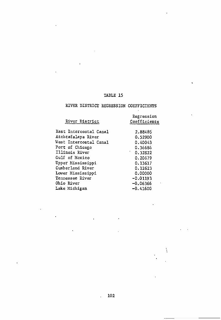
TABLE 15

RIVER DISTRICT REGRESSION COEFFICIENTS

River District

East Intercostal Canal Atchtafalaya River West Intercostal Canal Port of Chicago Illinois River Gulf of Mexico Upper Mississippi Cumberland River Lower Mississippi Tennessee River Ohio River Lake Michigan

Regression Coefficients

2.88486 0.52900 0.40043 0.36686 0.32822 0.20679 0.13617 0.12623 0.00000

-0.01193 -0.06366 -0.41600

. 102

TABLE 16

PERCENT COMMODITY REGRESSION COEFFICIENTS

Regression Commodity Group Coefficients

Coal 0.21012 Grain 0.05175 Other Bulk 0.03337 General Cargo 0.00000 Liquid Bulk -0.09444 Petroleum -0.90644

103

104

The coefficients of each set represent the relative cost of maintaining

- the barge fleet in the different types of service.

The relative order of the coefficients in both sets are consistent

with reasonable expectations. For example, the Gulf, the East Inter-

coastal Canal, the West intercoastal Canal, waterways with high salt

content, are all high cost service areas. In addition both the East

and West Canals are constricted waterways containing several locks.

An example perhaps best illustrates the use of the service vari-

bles. Looking at the commodity coefficients, suppose the firm has an

opportunity to expand its coal operation. In the short-run this ex-

pansion will mean a reduction of the amount of some other service it

offers. What will be the effect on barge costs of an increase in coal

service?

Increasing coal service by 10 percentage points (decreasing by

the same amount the output of general cargo) would increase average

costs per cargo ton-mile by 5% at all levels of output. If the coal

service was increased by reducing the amount of "other bulk" materials

shipped (instead of general cargo) the net effect would be to increase

the average cost of the mean output per barge by .029 mills/CTM, an

increase of 4.3%. This represents an average increase in total barge

operating expense of $98 per barge, or an increase in total barge cost

of $32,500 per year for the entire fleet. Adding to this figure changes

in other direct and indirect costs would yield an average measure of

marginal cost which could be compared with the marginal revenue to be

derived from the new business. .

Finally, the coefficient for the number of commodities shipped

per barge is positive and significant. The results show that if one

105

barge was to ship one more commodity, average costs for that barge would

increase by about 5% at all output levels. This represents an average

increase of about $116 for each barge which carries an additional com-

modity.

For both towboat and barge operating costs it appears that many

of the costs incurred by the firm in providing freight transport ser-

vices are sensitive to the exact nature of the service performed. In

particular, it has been found that for both towboat and barge costs,

changes in equipment and waterway characteristics produce significant

differences in marginal cost. In addition, for the barge analysis,

the effect of the commodity carried on barge maintenance costs indicates

that competitive rate differentials between commodities can be justified

on the basis of differences in marginal cost.

CHAPTER V

A TIME SERIES ANALYSIS OF BARGE FIRM COSTS

In the preceding parts of this study, the costs associated

with the linchaul equipment have been analyzed. As has been pointed

out, however, this equipment must be co-ordinated by the barge firm

in order to satisfy, at the least cost, the demands presented to it.

In this chapter, the analysis is extended to cost relationships for

the barge firm. As in the two preceding chapters, the approach

is to examine how variations in waterway characteristics, commodity

shipped, and seasonality are related to changes in the cost of

transporting freight.

• A. The Data

Detailed monthly cost and production data have been gathered

from a single firm for a period of three years. The selected firm

is among the major inland waterway operators. In terms of total

output the firm operates at the mid-range for the industry. The

firm operates a wide selection of floating equipment, varied as to

age and size. Its operations cover a major portion of the Gulf

and Mississippi River systems. Approximately 60% of its output

(in cargo ton-miles) is bulk freight. Its revenue is derived in

about equal proportions from bulk commodities and general cargo.

The total expenses of the firm have been broken down into

three expense categories: overhead expense, direct barge expense,

and direct terminal expense. Direct barge costs are all those

costs related to the actual movement of freight. Included here

106

107

are the costs of operating and maintaining'their floating equipment

and fees or expenses incurred in moving barges (mooring charges,

port expenses, etc.). Overhead expenses are all those expenses

which cannot directly be assigned to the freight operation .(management

and office salaries, building rents, sales expenses, etc.). Terminal

costs are the direct operating expenses, primarily labor and

maintenance, associated with the operations of terminals owned

by the firm. Terminal expenses do not include the cost of loading

and unloading all of the companies' cargo. Many terminal services

are performed for the firm by other companies or by independent

' operators. The cost of these services are borne by the shipper

and do not enter the analysis (nor are they part of direct barge

costs). These expense categories are standard for the industry.

The sample firm adhered strictly to the "Uniform System of Accounts

for Carriers by Inland and Coastal Waterways" in accordance with

I.C.C. regulations. These accounts represent a detailed reporting

method which most firms in the industry use.

The number of EBM's produced on each of eleven river districts

where the firm operates have been 'calculated for each month. The

question to be asked of the river district variables is: How will

costs be affected if the firm produces more services on one river

district and less on another river district? To accomplish this

task a Measure of the relative output the firm produced on each

river district is necessary. This is done by calculating the

percent of EBM's produced on each river district. These

percent variables are similar in nature to dummy variables. Using

1

108

the coefficient for one river district it is possible to determine

the change in cost occasioned by increasing the proportion of total

output produced on that river district. This method provides a link

between all river districts for determining the effect on cost of

relative shifts in the firms operation from one part of the waterway

to another.

Detailed records of the firm's shipments were obtained for

the three years in the sample. These records provide information on

the number of tons and ton-miles of each commodity carried by the

firm. The sample firm carried over sixty different commodities

each year as detailed by the I.C.C. "Standard Commodity Classification

for Transportation." Due to the small sample size it was necessary

to aggregate the commodities in some fashion.

Freight can be loosely classified into bulk freight and

general cargo. Bulk freight is perhaps best characterized by

commodities which can be dumped or poured into a barge. Bulk

commodities represent the "bulk" of the traffic handled by the

barge industry. General cargo is freight which has undergone some

processing and is usually "packaged" In some way.

This two-fold classification, however, obscures some

important differences. Bulk commodities, for example, coma in both

liquid and solid form. Coal, usually carried under long term

contracts which specify frequency of delivery, is often carried

in unit tows (i.e., with equipment "dedicated" to that particular

traffic). Equipment used in unit tows can be scheduled separately

from the rest of the firm's traffic. Special cleaning and

preparation of barges is necessary for grain shipments. The basic

differences in handling and in equipment used for the commodities

carried by the firm suggest that the following classification would

be a reasonable approximation to capturing the special features of

transporting different commodities:

1. grain products

2. coal

3. other solid bulk (primarily ores)

4. petroleum and petroleum products

5. other liquid bulk

6. general cargo

The commodities carried by the firm were aggregated, on the

basis of cargo ton-miles, into one of the six groups above for each

month in the sample. Percentages for each category were calculated.

The interpretation of these percent variables is the same as for the

river district percentages described above.

Casual observation would lead one to expect that costs for

general cargo will be higher than for most bulk products. General

cargo requires special handling which would raise terminal costs.

The loading and unloading of general cargo frequently damages barges.

Also, since general cargo is specialized as to specific commodity,

shipper, and origin and destination, one would expect that sales

expenses and scheduling costs will be generally higher than for the

bulk commodities. Of the bulk commodities, one would expect that

the costs of shipping coal would be the lowest of all the commodity.

groups considered. This is due to the ease of scheduling and absence

109

of special handling or preparation of barges.

Finally, a measure of firm size has been included. At the

conceptual level, several measures can be suggested. Among these are

total horsepower, number of barges, barge carrying capacity in cubic

feet or cargo tons, horsepower or number of barges weighted by age.

With the exception of the age weighted variable all of the proposed

measures are essentially identical, as measured by their simple

correlation coefficients. The age weighted variables proved to be

unrelated to the dependent variables and were excluded on statistical

grounds. The measure selected was cargo tons of barge capacity. One

might argue that this is a better measure of firm size than, for

example, cubic feet of cargo space since commodities typically

carried in barges have high weight to volume ratios. This assumes

then, that the relevant constraint in loading barges is cargo

weight, rather than the cargo's volume.

In summary, an observation for the single firm study consists

of the monthly percent distribution of cargo ton-miles among six

commodity groups; the monthly distribution of EBM's among eleven

river districts; total EBM's per month, a measure of firm size, and

a set of dummy variables denoting the month. For the terminal costs,

total cargo tons was substituted for EBM's. EBM's are calculated to

correct for conditions peculiar to the linehaul operation and do not

relate to the loading and unloading of cargo.

B. The Statistical Model

Separate statistical cost functions have been estimated for

the three cost categories. The general form of the functions

170

estimated was the same for all three categories. The general form

used was:

11 log io Cost/EBMi = logioao + allogioEBMi + u2log10Si +i E l aiMi +

10 5 .EyR +ZAr. 313 ij k=1-k-ik

where: UM. = the number of equivalent barge miles produced each

month

Si = firm size measured in total net tons of barge

carrying capacity

M. = monthly dummy variables (December excluded) 1

R.. = percent of total EBM's produced oa river district j 3.3

in the ith month (Lower Mississippi excluded)

Cik = percent of total ton-miles carried of kth commodity

'group in the ith month (general cargo excluded)

The reasons for the Specification of the average cost function in a

log-linear form are given in Chapter IV.

As noted above, the measure of output used in the terminal

analysis was cargo tonnage. In the estimation of overhead costs

use of the monthly dummy variables resulted in an F-value for the

regression which was not significant at the .90 probability level.

Thus, the monthly dtimmy variables are excluded for the overhead

results.

• C. The Results

Results for each cost category are presented in Tables 17 -19.

Before examining the results, a general comment on the regressions is

111

112

in order. The sample size is quite small (36 observations). With

the relatively large number of variables used the number of degrees

of freedom is quite small. On the positive side it is worth noting

that the regression results are significant. F-values for the analysis

of variance of the three regressions are presented in Table 20.

Although care must be exercised in using the regressions for

predictive purposes, the results are quite consistent with a

priori expectations and can be used to estimate the direction and

magnitude of changes in cost due to specified changes in the variables.

Direct Barge Costs

The results for the direct barge cost estimation are presented

in Table 17. Direct barge costs include all those costs we would

expect to change if one additional ton of cargo was transported. As

expected, short-run average costs are falling as current output

increases. The range of output produced by the firm is between

200,000 and 400,000 EBM's. Average cost for this firm thus varies

from $2.86 per EBM to $1.54 per EBM. Assuming an EBM to be 1400

cargo ton-miles, average cost per ton-mile ranges from 2.1 mills

to 1.1 mill. Recall that the costs reported by Meyer ranged from

2 to 2.5 mills per ton-mile? These estimates reported here are to be

preferred to Meyer's, first, since they are more current and -

secondly, because the relationship between average cost and output

is explicit.

The relationship of the estimates presented here and past

estimates, such as Meyer's, that are available,Imme been influenced

in three important ways. First, the barge industry has experienced

Variable Name Regression

Mean Coefficient t-Value

TABLE 17

DIRECT BARGE EXPENSE

r2 = .94 •

Sample size = 36 Standard Error of Estimate = 0.03498 Intercept = -0.23800

Commodity Shipped (percent times 10-2)

Grain 0.30111 -0.22344 -1.06479 ' Coal 0.00806 -1.05039 -0.69376

Other Bulk 0.12583 -0.15056 -0.55241 Petroleum products 0.08917 -0.48547 . . -0.85037 Other liquid bulk 0.08861 -0.40087 -0.98271

.River Districts (percent times 10-2 )

tower Illinois 0.14694 0.21486 0.27631 Chicago Port 0.02417 1.77304 1.04040 Tennessee 0.04111 -0.49696 -0.30993

WICC 0.04250 -1.16258 -0.88053 , E1CC ' 0.00222 -2.14679 -0.72300 Gulf . 0.06833 -0.64112 -1.12297 i Cairo - St. Louis 0.10556 -0.47782 -.0.35987 . St. Louis - Grafton 0.02278 -4.28935 -1.75228 Grafton - Minneapolis 0.00278 -1.75541 -0.56699 Cairo - Cincinnati - 0.03833 2.04464 1.65515

Monthly Dummy Variables •

January 0.08333 -0.11094 -1.46574 February 0.08333. -0.09831 -1.94714 March 0.08333 -0,07816 -1.76284 Apr-Li 0.08333 -0.03305 -0.59840 May 0.08333 -0.07039 -1.25853 June ' 0:08333 -0.12112 -1.90933 July 0.08333 -0.08488 -1.54296 August 0.08333 -0.02014 -0.40840 September 0.08333 -0.03360 -0.43063 October . 0.08333 -0.04345 -0.91529 November 0.08333 -0.04931 -1.28813

1 logio EBM (times 10-6 ) -0.56578 -0:90051 -3.49150 logio Net Tons of Cargo ,

Capacity (times 10 -') 0.56021 -0.74976 -0.22836 Dependent Variable: logio

Cost/EBM (times 10°) 0.33743 .

113

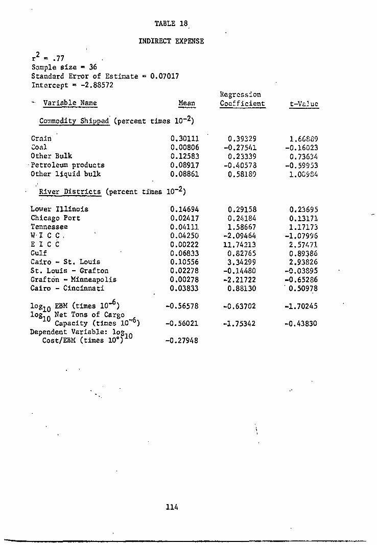
- Variable Name Regression

Mean Coefficient t-Va2ue

TABLE 18,

INDIRECT EXPENSE

r2 = .77 . Sample size = 36 Standard Error of Estimate = 0.07017 Intercept = -2.88572

Commodity Shipped (percent times 10 -2)

Grain 0.30111 0.39329 1.66889 Coal 0.00806 -0.27541 -0.16023 Other Bulk 0.12583 0.23339 0.73634 Petroleum products 0.08917 -0.40578 -0.59953 Other liquid bulk 0.08861 0.58189 1.06984

• River Districts (percent times 10 -2 )

Lower Illinois 0.14694 0.29158 0.23695 Chicago Port 0.02417 0.24184 0.13171 Tennessee 0.04111 1.58667 1.17173 WI C C •

.

0.04250 -2.09464 -1.07996 E I C 6 0.00222 11.74213 2.57471

- Gulf 0.06833 0.82765 0.89386 Cairo - St. Louis 0.10556 3.34299 2.93826 St. Louis - Grafton 0.02278 -0.14480 -0.03895 Grafton - Minneapolis 0.00278 -2.21722 -0.65286 Cairo - Cincinnati 0.03833 0.88130 0.50978

loglo EBM (times 10-6 ) -0.56578 -0.63702 -1.70245 loglo Net Tons of Cargo ,

Capacity (times 10') -0.56021 -1.75342 -0.43830 Dependent Variable: log io

Cost/EBM (times 10 ° ) -0.27948

1

114

Variable Name Regression Coefficient t-Value Mean

-0.17086 -0.00568 0.02756 0.05754

-0.11066 -0.15505 -0.17728 -0.00378 -0.55436 -0.30962 -0.15355

-0.27221

-3.09194

-0.83604 0.04666 0.23059 0.39828

-0.72972 -0.90426 -1.09764 -0.02837 -2.50447 -2.53681 -1.56261

-0.42996

-0.32019

TABLE 19

TERMINAL EXPENSE

9 r- = .91 . Sample Size = 36 Standard Error of Estimate = 0.09458 Intercept = -1.92645

Commodity Shipped (percent times 10 -2 )

Grain Coal -

. Other bulk* . . Petroleum products Other liquid bulk

0.30111 0.00806 0.12583 0.08917 0.08861

-0.93996 6.80497

-1.77043 -0.62837 -0.50185

-1.56756 1.68074 -2.41563 -0.40276 -0.45147

River Districts (percent times 10-2 )

Lower Illinois Chicago Port Tennessee West Intcrcoastal Canal East Intercoastal Canal Gulf Cairo - St. Louis St. Louis - Grafton Grafton - Minneapolis ' Cairo - Cincinnati

0.14694 0.02417 0.04133 0.04250 0.00222 0.06833 0.10556 0.02278 0.00278 0.03833

3.51629 -0.41507 5.89744 -4.42486 2.38680

-4.78775 4.11378 1.07093 0.72734

-5.15640

1.97465 -0.08936 1.37863 -1.21512 0.31098 -3.05355 1.10961 0.15063 0.08133 -1.49995

Monthly Dummy Variables

January February March April May. June July August September October November

log Cargo Ton-miles (times 10 Nat log INet 'ions of Cargo 10Capacity (times 10- )

Dependent Variable: logio Cost/EBM (times 10

0.08333 0.08333 0.08333 0.08333 0.08333 0.08333 0.08333 0.08333 0.08333 0.08333 0.08333

10-9 )-0.72592

-0.56021

-0.17567

115

TABLE 20

F-TESTS FOR TIME-SERIES COST REGRESSIONS

Degrees Of Mean F-Value Source Of Variation Freedom Square (Significance Level)

1. Direct Cost Regression •

Due to Regression 28 .00482 3.9412 Deviation About Regression 7 .00122 (.95)

2. Overhead Cost Regression

Due to Regression 18 .01615 3.2806

Deviation About Regression 17 .00492 ' (.99)

3. Terminal Cost Regression .

-Due to Regression 28 .02444 2.7328 Deviation About Regression 7 .00894 -(.90) '

116

117

considerable growth in the past twenty years. This is reflected by

both a growi.h in total output of the industry and a growth in the

size of individual firms. In terms of the model presented here,

this means there has been both a shift (to the right) in the short

run cost curve, and a movement along any one short-run curve to

higher output levels.

Secondly, the barge industry has experienced considerable

technological progress due to the kinds and characteristics of

equipment used, changes in operating methods (for example, unit

tows), and in the scheduling of barge movements. Thus, ceterus

paribus, one would expect to find the short-run cost curves estimated

from actual data to shift downward over time. To the extent that

the prices of inputs used in barge transportation have increased,

however, the cost curves would have shifted upward. Since our cost

estimates are lower, in general, than the figures given by Meyer,

one might tentatively conclude that the first two factors have offset

the effect of rising input prices.

. Controlling for price changes, the above arguments would

indicate that barge transportation experiences long-run decreasing

costs. Although the period of time over which our sample is taken

is too short to allow definite conclusions to be drawn, the hypothesis

of decreasing costs is given tentative support. by the fact that the

coefficient estimated for firm size has a negative sign. .

The coefficients for the commodity variables conform quite

closely to expectations. The results indicate that each of the

commodity groups can be shipped for lower average cost than general

cargo, the excluded category. The average cost of shipping coal, in

particular is considerably lower than the cost of general cargo. For

example, increasing coal shipments by one percentage point, costs per

EBM would fall, at all levels of output, by 2.4%. At typical output

levels for this firm, a 2.4% average cost reduction would reduce

total cost by over $15,000 per month.

The coefficients for the river district percentages show a

wide range of values. Unfortunately, the coefficients do not show

significant statistical differences from the omitted river district

(the Lower Mississippi). The coefficients for S. Louis to Grafton,

and Cairo to Cincinnati however, are significant for a one-tailed

t-test at the .95 level of probability. Economically, however, the

coefficients indicate that large cost differentials may exist between ..

operations on different river districts. A one percentage point

increase, for ,example, of traffic in the Port of Chicago would

increase average cost by more than 4% at all output levels.

Indirect Costs

Indirect costs represent the portion of total cost which

cannot directly be assigned to particular outputs. These are

the costs primarily associated with the scheduling of equipment

and the sale of services. The estimates can serve two purposes.

First, it may be possible to associate variations in indirect cost

with variations in particular services offered. Secondly, the

estimates could be used to supplement the other statistical '

estimates of direct cost (both direct barge and direct terminal)

to arrive at a measure of total firm cost. The estimates could

118

119

also be used in conjunction with direct cost estimates derived from an

engineering production function.

Substantial difficulties are inherent in attempting to estimate

the indirect cost associated with a,movement of cargo. Cargo must be

found and coordinated. In general, the balance of traffic and

coordination are much less than perfect and a high percentage of

barge miles are taken up with empty barges. The scheduling problem

is the major difficulty in estimating indirect costs. One might view

the firm as an organization designed to coordinate various point-to-

point movements; Various demands are presented to the firm and the

scheduling problem is to manage to satisfy the demands with its

current equipment at the least cost. In practice, this generally

involves carrying as many shipments as possible given the stock of

equipment. . .

Estimates of direct cost can come from two sources. The first

source is the direct operating expense reported by a firm. The

results presented in the preceding section are of this type. These

, direct barge costs are related to the commodity shipped and the

location of services provided. The advantage of these estimates is

that they reflect the average actual performance of the firm for the

broad characteristics of its operation.

A second source of direct cost is the engineering production

function. The engineering function relates the output of a tow

directly to the physical characteristics of the waterway (depth,

width, stream flow) and the characteristics of the flotilla (length,

breadth, draft). The advantage of this approach is its disaggregative

120

nature. Having determined the output of a tow, one can go on to

calculate the direct cost associated with a particular movement.

There is a cost associated, with each piece of equipment (which can be

expressed on an hourly basis); knowing output (expressed in ton-miles

per hour), one can calculate the cost per ton-mile. This cost is

only part of the marginal cost of the movement; no provision is

made for scheduling or other overhead costs or for empty backhaul.

Changes in output, and hence changes in cost, can be 'calculated,

for example, by adding a barge, or by loading it to a deeper draft.

Thus, the engineering function can be used to provide estimates of

direct cost for any particular point-to-point movement that might be

of interest. Using estimates of indirect cost obtained from the

statistical model together with the direct cost of a point-to-point

movement would provide an estimate of the total cost associated with

that movement.

The EBM might be integrated into the engineering production

function. The function can then be used to generate an estimate of

the number of EBM's per hour produced by any towboat on any river dis-

trict. An analysis of delay times could be included to modify this

estimate to take account of locks and congestion.

Using this estimate of EBM's per hour produced by a towboat

provides considerable simplification in planning the operations of the

towboat.. Since EBM's per hour are constant, one can easily calculate

the effect of adding additional barges or cargo. It should be noted,

however, that estimates obtained in this way would be most relevant

for determining the cost of a marginal movement (adding one more barge

121

to an already scheduled tow). Two kinds of scheduling costs can be

identified: Indirect supervisory costs, and direct operating costs

due to the necessity of shipping extra empty barges. Since the

engineering estimate would not include the latter kind of cost its

most appropriate use would be for the marginal movement where the

marginal direct scheduling cost is zero. The results of the indirect

cost estimation are presented in Table 18. Looking at the coefficient

for firm size we find that it has a negative sign. Firm size should

be an important determinant of scheduling costs. In general, we

should expect economies of scale in the scheduling of barges.

The coefficient of EBM's is also negative. This is not

surprising since average costs will continually fall until total

cost begins to rise at an increasing rate. This is certainly not

what we would expect total indirect .costs to do. In fact, we should

expect total indirect cost to remain fairly constant over wide ranges

of output. We can infer the shape of the total cost function from

our results. The coefficient of logioEBM is interpreted as the

elasticity of the average cost curve. If the coefficient were equal

to -1.0 the total cost curve would be constant over all output values.

The coefficient is equal to -.63702 which would indicate that total

indirect cost increases at a decreasing rate with respect to output,

although it is by no means constant.

Note also that it is possible to use these estimates to

allocate part of indirect cost to particular services the firm renders.

In the statistical model these effects are derived by looking at the

coefficients for the commodity, and river district percentages and

122

the monthly dummy variables. Several examples have already been given

of the use of these variables. .

Direct Terminal Costs

Very little is known about the cost associated with terminal

operations in inland waterway transportation. This is primarily due

to the high degree of specialization of terminal facilities. Speciali-

zation occurs at two levels. First, different commodities require

their own particular terminal services. Secondly, different concepts

in the provision of terminal services can be applied depending upon

the rate of output required, the nature of the interface (whether the

terminal connects with truck, rail, or both) and the size and topology

of the terminal location. Different types of facilities are also

required for loading and unloading. As a result of the specilization

it is extremely difficult to make any generalizations about terminal

cost.

The firm in our sample, however, operates two terminals which

are devoted entirely to general cargo. Terminal facilities for

handling general cargo are less specialized than terminals for bulk

commodities. In addition, the same facilities can be used at both

ends of the handling operation. Input requirements are fairly

standard: lift trucks, one or two cranes (an extra crane is generally

kept on a standby basis since only one crane can be used at a time

on any one barge), and stevedores. The process of general cargo

handling is labor intensive relative to the handling of bulk

commodities.

The terminal results are quite tentative, particularly since

an adequate output measure is not available. Cargo ton-miles,

however, should.be highly correlated with cargo tons. Since the

coefficient of the sUrrogate measure is negative, short run terminal

costs are falling over the range of the sample. (See Table 19.).

We would expect to observe falling short-run average costs for

terminal operations due to the necessity for considerable excess :

capacity. The demand for terminal services is random. As a result,

terminals must be of sufficient size to handle peak loads or else- .

lengthy (and costly) queues will form. For a given size facility,

then, average costs will be lower the greater the volume of cargo .

handled.

123

CHAPTER VI

, A CROSS SECTION ANALYSIS OF FIRM COSTS

This chapter presents the results of a statistical investigation

of the relationship between output and costs for five major inland

waterway operators. The data used are actually combination cross- .

section and time-series. Quarterly observations over a period of five

years have been employed.

Chapter V reported the results of a detailed examination of cost-

output relationships for a single firm. The approach taken in Chapter

V was to relate categories of firm cost to special:types of service

offered by inland waterway carriers. In this study it has not been

possible to dbmaregate output in the same way. Instead, a more tradi-

tional approach has been employed; the costs of the firms in the sample

have been related to their total current output and the size of the

firm, adjusting the observations for the passage pf time.

A. The Data

As mentioned above, the data consist of quarterly observations of

cost, output, and firm size for a period of five years for five inland

waterway operators. The cost data have been separated into direct and

indirect components. Separate cost relationships have been estimated

for each cost category and for total cost. Once again, the measure

of current output used in the statistical model was the EBM.

124

125

The five firms in the sample represent major inland waterway

- carriers. Taken as a group, their barging operations are highly

d:versified. They operate on all of the navigable tributaries of

the Mississippi and Gulf Intercostal River Systems, including the

Missouri River, the Gulf of Mexico, and Lake . Michigan. In addition,

the five firms offer essentially a complete range of water transport

services, both with respect to commodities handled, and equipment

available for freight transportation.

Although the firms in the sample are among the largest firms in ,

the industry (measured either in current output and revenue, or by

size of equipment stocks), nevertheless, there are considerable dif-

ferences in their absolute size. For example, the largest firm, as

measured by total 'available horsepower, wag on the average 3.3 times

larger' than the smallest iirm'in the sample.

Several surrogate measures could be used to correct for firm

size in the statistical model. Since the firm size-cost relationship

carries the interpretation of long-run costs, the measure selected

should be a reflection of the productive capacity of the firm at any

one time. That is, any paired cost-size observation. should represent

the least cost way of operating a firm of particular size. It should

be noted, however, ,that when historical data are used in statistical

cost estimation these theoretical efficiency assumptions are not

necessarily met. The data, in general, do not describe the least

cost solution for a particular firm; rather they represent the actual -

cost of operating particular firm sizes included - in the sample.

One could assume that the observations do represent minimum cot

points and interpret the estimated results as the long-run costs of

126

economic theory. This, however, is certainly not likely to be true.

That is, the observations will reflect the operation of a firm where

some short-run adjustments are still taking place. Another inter-

pretation is possible: Assume that the observations made represent a

certain average level of efficiency which has been achieved in the past

and is likely to prevail for some time. The long-run relationship could

then be used to draw conclusions, for example, about the expected effects

of increasing firm size.

Four measures of firm size are readily available. These measures

are also reflections of the firm's productive capacity: towboat horse-

power, number of towboats, cargo tons of barge capacity, and the number

of barges. Since no a priori judgement can be made as to which of the

measures is the "correct one," all four have been gathered for each

firm in the sample. Each could then be tried in the statistical model

and the results compared. If the four measures yield similar results

we would gain some confidence in the use of the variables as measures

of firm size. -

. Since the observations range over a period of five years, it is

of interest to ask how costs have changed over time. This period is

reputed to be one in which the industry made substantial efforts to im-

prove its efficiency. As a result considerable attentiOn has been paid

to the equipment used, to scheduling, and other operating rules-of-thumb.

One reflection of this movement is the increasing Use of sophisticated

cost accounting techniques (for example, much of the data used in this

study was simply not available before 1962, at least in a form which

would be useful as a guide to production control). To attempt to mea-

127

sure the extent of this activity, a dummy variable which increases

linearly with time has been included in the statistical model. This

variable should indicate the extent of neutral technological change

which has taken place during the sample period. If the hypothesis of

positive neutral technological change is correct, this. variable should

have a negative coefficient. According to representatives in the in-

dustry, the period reported in our sample did not experience significant

amounts of inflation for inputs important to barge transport (a major

labor contract was renegotiated in 1967, after our sample period). As

a result, the data have not been deflated.

An additional time measure has been included: the quarter the

observation was made. This is done by assigning a dummy variable to

each quarter. In the statistical model, one dummy variable must be

excluded. The coefficients of the remaining variables will reflect

the shift in the cost relationship to be attributed to operations at

that time of year relative to the omitted quarter. This, then, will

give an indication of seasonal variation in water transport costs.

The fourth calendar quarter was the omitted dummy variable.

These variations may occur for two basic reasons: One is that the

volume of cargo offered to the firm varies seasonally (for example, the

grain products). Secondly, operating conditions vary during the year

due to weather (icing, fog, etc.), steamflow, and water level. Season-

ality of the firm's - demand will affect cost primarily by increasing

scheduling difficulties at peak periods and by requiring the employment

of less efficient factors. • Operating conditions affect cost primarily

by affecting towboat performance. (See Chapter III.)

128

Thus, an observation for the cross-section study consists of a

measure of current output (EBM's); a measure of firm size (total tow-

boat horsepower, number of towboats, net tons of barge cargo capacity,

and the number of barges); a linear annual time trend; a set of dummy

variables to identify the quarter of the year; and quarterly costs;

total costs and two subdivisions of total cost; direct operating (or

linehaul costs) and indirect operating expense.

B. The Statistical Model

Separate statistical cost functions have been estimated for three

categories of cost: indirect, direct, and total cost, each for the

four measures of firm size. The general form of all twelve functions

estimated is the same:

3 • Cost

log 10 EBM.. = lor,010 a +alog EBM +alo,, S.. +aT+E B.Q. 0 1 10 ijk 2 10 ijk 3 1j k =

ij 3 3

where: EBMijk = current output, measured in EBM's, for the ith firm,

during the jth year and kth quarter

S.. = a measure of firm size, either total towboat horse- ' ijk

power, number of towboats, net tons of barge cargo

capacity, or number of barges for the ith firm, during

the jth year and kth quarter

T = annual time trend variable (1962 = 1, . . . 1966 = 5)

Qk = quarterly dummy variables (fourth quarter omitted)

The estimating equations are linear in logarithms (the time trend

variables, however, are left untransformed). The average cost and log-

129

linear form of- the functions have been specified. The arguments for

this specification have already been given in Chapter IV.

- % C. The Results

Results for all cost categories are presented in Tables 21-23.

Four regressions are presented for each category of cost, one for each

alternative measure of firm size, to allow comparison. With the ex-

ception of indirect cost there is little to distinguish between the

four regressions for each cost category. Since the results using the

number of barges as the firm size variable appear to be generally

better, these results have been used in the discussion below.

Indirect Costs

Indirect costs represent expenses incurred by the firm which

cannot be allocated to particular levels of output. These are the

costs associated with general office and management expense, record . .

keeping, sale of services, and the scheduling, and cbordination of

shipments and equipment. .

. Table 21 presents the indirect cost results for each of the

firm size measures. In comparing the results across firm size mea-

sures, an apparent contradiction is evident in the firm size coeffi-

cients. The two towboat measures show a strong positive relationship

with average indirect cost, whereas the two barge measures show a

strong negative relationship with average indirect cost.

It would be expected, ceterus paribus, that if the "correct"

firm size measure was used, average indirect costs wbuld fall as

firm size increased. For example, we would expect to find economies

1

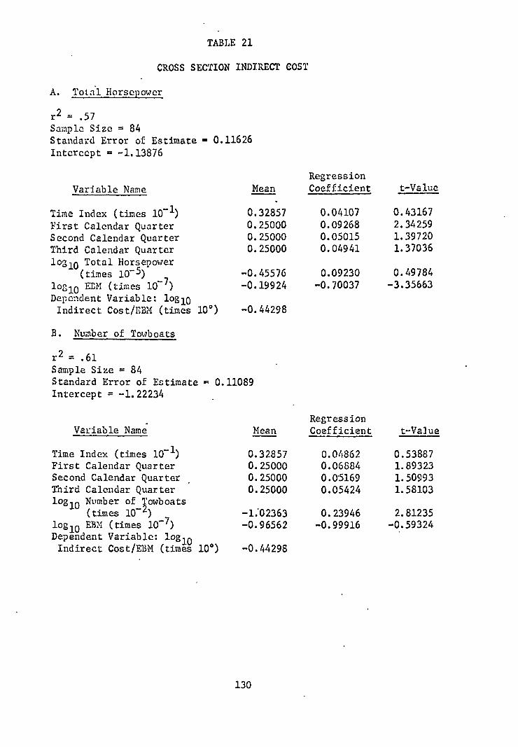
Regression Coefficient t-Va]ue

0.04862 0.53887

0.06884 1.89323

0.05169 1.50993

0.05424 1.58703

0.23946 2.81235

-0.99916 -0.59324

TABLE 21

CROSS SECTION INDIRECT COST

A. Total Horsepower

r 2 = .57 Sample Size = 84 Standard Error of Estimate = 0.11626 Intercept = -1.13876

Variable Name

Time Index (times 10-1) First Calendar Quarter Second Calendar Quarter Third Calendar Quarter log Horsepower

(times 10-5) lo0c, 10 ELM (times 10-7 ) Dependent Variable: log 10 Indirect Cost/EBM (times 10 ° )

Regression Mean Coefficient t-Value

•

0.32857 0.04107 0.43167

0.25000 0.09268 2.34259

0.25000 0.05015 1.39720

0.25000 0.04941 1.37036

-0.45576 0.09230 0.49784

-0.19924 -0.70037 -3.35663

-0.44298

B. Number of Towboats

r 2 = .61 Sample Size = 84 Standard Error of Estimate = 0.11089 Intercept = -1.22234 _

Variable Name

Time Index (times 10-1) First Calendar Quarter Second Calendar Quarter , Third Calendar Quarter 1°810 Number of Towboats

(times 10-2) -2

1°8 10 EB`i (times 10-7) Dependent Variable: log lo

Indirect Cost/EBM (times 10 ° )

Mean

0.32857 0.25000 0.25000 0.25000

-1:02363 -0.96562

-0.44298

130

TABLE 21--Continued

CROSS SECTION INDIRECT COST

C. Net Tons of Barge Capacity

/ r- = .65 Sample.Size = 84 . Standard Error of Estimate = 0.10520 Intercept = -0.91246 .

Variable Name

, Time Index (times 10- 1) '

.First Calendar Quarter Second Calendar Quarter Third Calendar Quarter log io Net Tons of Barge

-t Capacity (times 1O, ) . . . log io EBM (times 10-1 ) Dependent Variable: log io

Indirect Cost/EBM (times 10 ° )

Regression Mean Coefficient t-Value

0.32857 0.01911 0.22338

0.25000 0.33510 3.99459

0.25000 0.04656 1.43373

0.25000 0.04145 1.27516

-0.37330 -0.66452 -4.16424

-0.96562 -0.16503 -1.36981

-0.44298

D. Number of Barges

r 2 .64 Sample Size = 84 Standard Error of Estimate = 0.10626 Intercept = 0.10626

Variable Name

Time Index (times 10 -1) . First Calendar Quarter Second Calendar Quarter Third Calendar Quarter . lor,'3 Number of Barges 10

(times 10-3) 1oa°10 EBM (times 10-7 ) Dependent Variable: logio Indirect Cost/EBM (times 10°)

Regression Mean Coefficient t-Value

0.32857 -0.02011 -0.22993

0.25000 0.13822 4.00942

0.25000 0.04630 1.41121

0.25000 0.04095 1.24661

-0.45985 -0.64527 -3.93314

-0.96562 -0.12424 -0.91772

-0.44293

131

132

of scale in both the scheduling of equipment and the sale of services.

We would also expect to find little association of indirect cost and

current output (EBM's). This is in fact what we find for the barge-

firm size regressions; both coefficients of BBM being small and insig-

nificant, both barge-firm size measures are negative and significant.

For the towboat-firm size regressions, however, the EEM coefficients

are large and significant, the towboat-firm size measure coefficients

are positive.

A clue to the explanation of this apparent contradiction can be

found in the fact that the contradiction occurs across the two sets of

firm size measures, each representing two different types of productive

capacity. No one of the firm size measures can be said to be better

than any of the others. These measures represent inputs to the produc-

tive process that are quite different and enter the production function

in quite different ways.

Suppose that the barge measure was the "correct" one, that is,

every firm in the industry uses barges in their production function in

exactly the same way. Suppose also, that the same is not true for tow-

boats. In particular, suppose that the barge fleet is used to capacity;

excess barges being chartered to other firms. On the other hand, tow-

boats are not used to capacity; if no work is available for a boat it

is allowed to sit in port. Under these assumptions, one would expect

larger increases in output from increasing the barge fleet by 10% than

from increasing the towboat input a proportional amount. Controlling

for output (EBM's) we would than expect to find lower average costs

per EBM to be associated with increases in the barge fleet; higher costs

per EBM to be associated with larger towboat fleets.

133

Indirect cost is the same for towboats and barges whether they

are in or out of service. If towboats or barges are out of service,

they produce no EBM's. The greater the non-.scrvice time of towboats

or barges, the higher the indirect costs per EBM will be. If towboats

are not used to capacity, increasing the number of towboats will in-

crease total idle time and increase indirect cost per EBM. If barges,

on the other hand, are fully utilized, increasing the number of barges

will increase the number of EBM's produced. With relatively constant

indirect cost, indirect cost per EBM will fall as the size of the barge

fleet increases.

This argument is consistent with the operation Of the lease mar-

kets for towboat and barge equipment. Barges are extremely portable

between firms. They are frequently chartered, even for short periods.

This is less true for towboats (except indirectly through outside tow-

ing). The results may then reflect the fact that there is a more active

market fot barges than for towboats.

If the above argument3about the firm size measures are valid, the

best (although not perfect) measure of firm size would be one of the

barge size measures. For either one of the barge size measures, indirect

cost is relatively constant at all current output levels. (The coeffi-

cient for both barge measures are also not significantly different from

zero.) Average indirect cost at the point ol means is $.35 per EBM

(about .2 mills per cargo ton-mile).

These indirect cost estimates provide a supplement to other esti-

mates of direct cost that can be made. In particular, it is possible

to obtain from the engineering production function the direct costs

134

associated with any particular trip. Direct cost estimates obtained in

this way represent the cost for the most efficient way of providing that

individual trip.. The firm, however, must sell and coordinate this ship-

ment with the many others that it produces. Thus, a measure of per unit

indirect costs can be added to the engineering direct cost estimate to

yield a measure of the Marginal cost of an additional trip. The indirect

cost estimate would have to be adjusted for the level of output at which

the additional trip occurred, as well as for the size of firm making the

shipment.

Total and Direct Costs

Both the direct cost and total cost results are quite similar.

This is not surprising since direct cost is about 75% of total cost.

Only the average direct cost results will be discussed, however, the

discussion will also be applicable to total average costs.

As expected, the average direct cost of an EBM falls as output

increases. The coefficient of EBM's is negative and significant for

all regressions. Evidently, upward short run adjustments in output

can be accomplished with lower per unit costs over a wide range of

output actually experienced. Average direct cost per EBM at the point

of means is $2.08 (about 1.5 mills per cargo ton-mile).

A puzzling result is once again obtained for the firm size mea-

sures. The coefficients for all measures are positive. Larger firms

appear to be associated with higher costs. This is certainly strange

in view of results obtained in other parts of this study which indi-

cate substantial amounts of technological change occurring in the

industry, and that economies of scale are to be expected with respect

Regression Mean Coefficient t-Value

0.32857 0.25000 0.25000 0.25000 -0.45576

-0.12615 -3.80639

0.02181 1.58225

0.01044 0.83503

0.00472 0.37566

0.19924 3.09328

-0.96562 -0,44389 -6.10697 0.31778

Regression Coefficient t-Value

-0.13265 -4.06703

0.02517 1.91486

0.01035 0.83632

0.00383 0.30897

0.10369 3.36840

-0.40251 -7.20547

Mean

0.32857 0.25000 0.25000 0.25000 -1.02363

-0.96562 0.31778

TABLE 22

CROSS SECTION DIRECT COST

A. Total Horsepower

1 2 = 0.68 • Sample Size = 84 Standard Error of Estimate = 0.04050 Intercept = 0.01241

Variable Name

Time Index (times 10-1

) First Calendar Quarter ,

Second Calendar Quarter Third Calendar Quarter logio Total Horsepower

(times 10-5 ) logio EBM (times 10 -7 ) Dependent Variable: logio

Direct Cost/EBM (times 10 0 )

B. Number of Towboats

r2 = .69 Sample Size = 84 - Standard Error - of Estimate = 0.04069 Intercept = 0.06900

Variable Name

Time Index (times 10 -1) ' First Calendar Quarter Second Calendar Quarter Third Calendar Quarter loglo Number of Towboats

• ' (times 10 -2 ) logio EBM . (times 10-7 ) Dependent Variable: . log io

Direct Cost/EBM (times 10 0 ) .

135

Regression Mean Coefficient t-Value

0.32857 0.25000 0.25000 0.25000

-0.37330

-0.13201 -4.24030

0.02546 2.06905

0.01072 0.90738

0.00342 0.28936

0.25913 4.46305

-0.95562 -0.40072 4.14191 0.31778

Regression Mean Coefficient t-Value

TABLE 22--Continued

CROSS SECTION DIRECT COST

C. Net Tons of Barge Capacity

r 2 = .72 Sample Size = 84 Standard Error of Estimate = 0.03827 Intercept = 0.06104

Variable Name

Time Index (times 10-1) First Calendar Quarter Second Calendar Quarter Third Calendar Quarter logio Net Tons of Barge

Capacity .(times 10 -6 ) login EBM (times 10 -7 ) Dependent Variable : log in

Direct Cost/EBM (times 10 0 )

D. Number of Barges

r2 = .73 Sample Size = 84 Standard Error of Estimate = 0.03701 Intercept = 0.04806

Variable Name

Time Index (times 10-1) 0.32857 -0.11298 -3.70748 First Calendar Quarter 0.25000 0.02172 , 1.80837 Second Calendar Quarter . 0.25000 0.01105, 0.96735 Third Calendar Quarter 0.25000 0.00407 0.35596 login Number of Barges -0.45985 0.29494 5.16078

(times 10-3 ) login EBM (times 10 -7 ) -0.96562 -0.44869 --9.51454 Dependent Variable: login 0.31778

Direct Cost/EBM (times 100)

136

TABLE 23

CROSS SECTION DIRECT COST

A. Total Horsepower

9 r - = .69 - Sample Size = 84

, Standard Error of Estimate = 0.04428 Intercept = 0.05131

1 .‘

Variable Name

' Time Index (times 10 -1 ) First Calendar Quarter. Second Calendar Quarter Third Calendar Quarter

Total Horsepower 010 (times 10-5) -

1o , EBM (times 10 - ') - 070 Dependent Variable: loglo

Direct Cost/EBM (times 10 ° )

Regression Mean Coefficient t-Value

0.32857 -0.10722 -2.95923

0.25000 0.03143 2.08579

0.25000 0.01370 1.00215

0.25000 0.00928 0.67572

-0.45576 0.17761 2.51543

-0.46311 -5.82781 -0.96562 0.39592

B. Number of Towboats •

r2 = .74 Sample Size = 84 Standard Error of Estimate = 0.04091 Intercept = 0.07273

Variable Name Regression

Mean Coefficient t-Value

- Time Index (times 10-1) • . 0.32857 -0.11022 -3.31178 First Calendar Quatter 0.25000 0.02773 2.06743 Second Calendar.Quarter - 0.25000 0.01403 1.11135 Third Calendar Quarter _ , . 0.25000 ,0.00987 0.77999 lor, Number of Towboats -1.02363 0.014262 4.54054

'10 (times 10-2 ) '

logio EBM (times 1077)-0.96562 -0.51004 -8.94762 Dependent Variable: logo 0.39592

Direct Cost/EBM (times 10°)

137

Regression Mean Coefficient t-Value

0.32857 -0.13380 -3.36856

0.25000 0.03759 2.64764

0.25000 0.01368 1.00371

0.25000 0.00760 0.55689

-0.37330 0.17431 2.50220

-0.96562 -0.38789 -7.67006 0.39592

TABLE 23--Continued

CROSS SECTION DIRECT COST

C. Net Tons of Barge Capacity

r2 = .70 Sample Size = 84 Standard Error of Estimate = 0.04416 Intercept = 0.10912

Variable Name .

Time Index (times 10 -1 ) First Calendar Quarter Second Calendar Quarter Third Calendar Quarter logio Net Tons of Barge

Capacity (times 10-6) logio EBM (times 10-7 ) Dependent Variable: logio

Direct Cost/EBM (times 10 ° )

D. Number of Barges

r2 = .71 Sample Size = 84 • Standard Error of Estimate = 0.04343 Intercept = 0.09785

Variable Name

Time Index (times 10 -1 ) First Calendar Quarter Second Calendar Quarter Third Calendar Quarter logio Number of larges

(times 10-') logm ELM (times 10-7 ) Dependent Variable: log io

Direct Cost/ELM (times 10 ° )

Regression Mean Coefficient t-Value

0.32857 -0.10020 -2.80227

0.25000 0.03453 2.45018

0.25000 0.01396 1.04077

0.25000 0.00814 0.60595

-0.45985 0.20771 3.09741

-0.96562 -0.42705 -7.71734 0.39592

138

139

to scheduling. In addition, we observe a recent trend toward individ-

ual firm expansion along with considerable merger activity. Unless

gross irrationality exists in the industry, another explanation of the

results must be found,

, A possible explanation may be found in the hypothesis that large

firms offer a wider range of special services than smaller firms. The

problem may then be with the output measure. It is not an adequate

measure of. the work done by the firm. The EBM (as well as the ton-mile)

is a measure of, work done by the carrier's equipment in the linehaul

operation, not of services performed by the carrier for customers. A

large firm may be more willing to allow commodities to be stored in a

barge at port for long periods; it may provide special handling of

particular commodities; it may incur a higher percentage of empty barge

movements, that is. , it may be quite willing. to accomodate certain cus-

tomers with equipment on demand. It will, of course, perform these

services at additional expense, but it also will receive additional

revenue.

Smaller firms may attempt to only haul traffic with a -short turn

around time and with little extra service. Larger firms may find it

more profitable tooffer these special services. It will do so at the

expense of some efficiency in the strictly line-haul part of their

operation, th'at is, for a higher cost, per EBM. It can be argued, there-

fore, that the association of higher average costs with larger firms

comes as a result of the failure of the output measure used in the

statistical models to incorporate the special aspects of water trans-

port services.

140

Looking at the time variables, it is worth noting that average

costs have fallen significantly over the five year period in the sample.

An average decrease of about 2 1/2 percent per year is indicated.

The quarterly dummy variables show average cost declining steadily

throughout the year. This accords reasonably well with a priori expec-

tations. The first quarter (the only dummy variable which proves to be

statistically different from the omitted variable) has significantly

higher costs than other quarters. This is to be expected since the

winter months represent generally adverse operating conditions for tows.

In summary, it appears that the barge industry is capable of ex-

panding its output over a wide range at lower unit costs in the short

run. In addition there is evidence that the industry has experienced

'considerable cost saving reductions over the past few years. The re-

sults for the cost-size relationship are mixed, yet they point to at

least two interesting issues. One is the indication that the different

types of operating equipment (towboats and barges) are not used with

equal efficiency. This may in part be due to imperfections in the mar-

ket for chartered towboats. .

The second issue is the difficulty of obtaining satisfactory

measures of the output and size of transport firms. The EBM does

represent an improvement as it corrects for differences in equipment

and operating conditions. It does not correct, however, for special

features of waterway transport service which apparently have signif-

icant effects upon the operating costs of the industry.

:CHAPTER VII

SUMMARY AND CONCLUSIONS

The major results obtained in this study and their implications

are summarized below in three sections: (A) returns of scale, (B)

technological change,'and . (0 , costs and the rate structure. Following

this summary, two methods of obtaining-estimates of cost using these

results are discussed.

A. Returns to Scale

Two indications of returns to scale can be obtained from the

statistical results. One relates to the major operating unit of

waterway transportation, the towboat. The second indication of re-

turns to scale relates to the firm.

With respect to the towboat, we find in the towboat production

function a general indication of increasing returns to scale, as

measured by the capital and labor inputs. The sum of the capital and

labor coefficients of the log-linear regressions are greater than one

for companies one and three and the combined regressions, both up-

stream and downstream.

Company two is a notable exception; for both the upstream and

-downstream regressions, firm two shows decreasing. returns for the

towboat. This seeming contradiction, however, may be an important

indication of the extent of scale economies in towboat size. One

141

would predict, from the horsepower coefficients alone, that there is

some upper limit to increases in horsepower. Horsepower consistently

shows diminishing productivity (with the single exception of the com-

pany two upstream coefficient, 1.05). It is evident that the labor

input alone is sufficient to assure constant or increasing returns

for companies one and three and the combined production functions.

However, it must be remembered that the results are derived

from the limited range of actual practice. Although, proportional

increases in the labor and horsepower inputs for companies one and

three indicate increasing returns we may not be able to extrapolate

this result beyond the ranges of labor and horsepower used by the

two companies. A priori, we would expect eventual decreasing re-

turns for very high horsepower and labor input combinations.

A possible explanation for the company two results is that com-

pany two in fact operates in the range where decreasing returns have

set in. Note that company two has both the highest average crew size

and towboat horsepower. In addition, firm two, which has the smallest

towboat fleet of all companies, has the largest number (four) of very _

large towboats (6000 horsepower and above). Firms one and three each

have only one towboat as large as 5500 horsepower.

If the above arguments are true, decreasing returns to towboat

size must become important for towboats in the 4000-6000 horsepower

range and for crew sizes of 12 men and above.

Supporting evidence on returns to scale for towboats is found in

the estimation of towboat cost. Towboat cost declines throughout the

range of actual horsepowers, as would be expected. Note however, that

142

143

the coefficients of the dummy variables for two companies (two and three)

are positive and significant, indicating that these firms have the high-

est towboat costs of all firms in the sample,. Company two is the same

as company two in the production function. Company three is similar

company two in that it also operates a small fleet (eight boats) of very

large horsepower towboats (average towboat size is 4300 horsepower, even

higher than that for company two). While these coefficients do not

measure returns to scale, it does appear that decreasing returns have

already been attained for some firms in their current operations.

Measures of returns to scale for the firm are given in both the

- single firm and the cross-section regressions. In the single firm

;study the coefficient of firm size (cargo tons of barge capacity) is

negative for both the direct and indirect cost regressions. Moderate

increasing returns are indicated; however, the coefficients are not

significantly different from zero.

In the cross-section results, four different measures of firm size

were employed in estimating direct, indirect, and total cost per EBM.

They were (1) total available horsepower, (2) number of towboats, (3)

total available barge capacity, measured in net .cargo tons, and (4) the

number of barges. The results were quite surprising. For the direct

and total cost regressions, all four measures'of firm size have positive

and significant coefficients. In addition both of.the towboat firms

. size measures were positive for the indirect cost regressions.

The most plausible interpretation of these results seems to be

that large firms offer a diversity of high cost services. The measure

of output used, however, is an index of work done in actually moving

co=odities. This may represent only part of the work performcd for

the customer, excluding such services as storage, special handling,

and fascr delivery. If the numbersof these services are expanded as

the firm grows, its cost (but also. its revenue) per EBM will increase.

Thus, neither the single firm nor the cross section results can be

used to draw unambiguous conclusions about returns to scale for barge

firms. '

B. Technological Change

The several parts of this study contain various measures of

capital embodied and neutral technological change (labor embodied

technological change was not examined). The results are remarkable

for their consistency.

Two measures of capital embodied technological change for tow-

boats were examined in the towboat production and cost functions:

towboat age and Kort nozzles. The results for towboat age indicate

that there have been no significant changes in towboat design for the

range of ages in thcsample (about 25 years). This indication has

been confirmed by naval architects.

However, it is possible that Minor changes have occurred that

would not Show up in our data. For example, newer towboats are gen-

erally equiped'with sophisticated navigation and communication equip-

ment as they are built. Such equipment should tend to raise the pro-

ductivity of the towboat. The improvements, however, are easily

installed on older boats. In fact, almost all the boats in the sample

were so equiped by the beginning of our sample period. Thus, our

analysis is not capable of picking up these effects.

144

145

. The coefficients of the dummy variables for towboat age in the

towboat cost regression do indicate that the very oldest boats are

less efficient than the newest boats. Boats built prior to 1950 are

approximately 17% more costly to operate than the newest boats. Boats

built between 1950 and 1955 are 4% more costly to operate, although

the coefficient of the 1950-55 dummy variable is not significant. How-

ever, for boats built between 1956 and 1960, the results indicate a

reduction in operating cost of 9% over the newest boats. The latter

coefficient is also not significant.

A dummy variable for the Kort nozzle was included in both the

towboat cost and towboat production functions. For the combined log

regressions of the towboat production function, Kort nozzles improved

average productivity by more than 26% for-both upstream and downstream

movements. Both coefficients are significant. The Kort nozzle coef-

ficients are positive for all six of the individual company log regress- .

ions. Four of the six coefficients are significant. The range of

improvement for the individual companies is from 14% to 41%. The linear

regressions indicate that Kort nozzles may be slightly more important

for downstream movements.

Supporting evidence of Kort nozzles is obtained from the towboat

cost function. Here, the Kort nozzle coefficient is negative and

significant. A 15% reduction in average towboat cost is indicated for

. use of the Kort nozzle.

As reported in Chapter Iv, an attempt was made to measure capital

embodied technological change for the barpequipment.. Both a linear

age index and dummy variables for age groups were tried. F-tests per-

formed on these variables indicated that no significant cost differences

146

were present with respect to barge age. Thus, we may conclude that

there have not been significant technological improvements in barge

design for the period of our sample (about 30 years). This, once

again, is confirmed by the opinion Of naval architects.

Evidence on neutral technological change can be obtained from

the towboat production function, the barge cost function, and the

cross-section firm cost analysis. The results are quite consistent,

showing considerable neutral technological improvement for the period

of our sample (five years in the cross-section study).

In the cross-section study, the effect of time was embodied in

a linear index which increased with time (ranging from one to five).

For all of the average direct operating cost and total cost regressions,

the coefficients of the index were negative and significant, (The re-

sults for indirect cost are inconclusive; one coefficient was negative,

but three were positive; none were significant). An average annual

cost reduction of 2.3% to 3% is indicated.

In the barge cost results dummy variables were used to denote the

passage of time. 1966 was the omitted dummy variable, and thus has

a "coefficient" of zero. The coefficients of the 1964 and 1965 dummy

variables are positive and significant. The coefficients become less

positive over time, thus cost falls during this period. An average

annual reduction in direct barge operating cost of 12% is indicated.

It should be pointed out that the indicated cost savings may be

understating the real reductions. This is because the cost data are not

deflated for price changes, since inflation of barge factor input prices

was not found to be significant for the period of our sample. To the

extent any inflation did occur, the reductions in cost would be greater.

147

Supporting results for neutral technological change are given

in the towboat production function. Dummy variables arc used to denote

the year. Once again, 1966 was the omitted year, thus to show produc-

tivity increases, all the dummy variable coefficients should have nega-

tive signs. In-looking at the. results, the dummy variables for 1964

and 1965 are negative in all 16 regressions, with one exception. In

general, the coefficients become less negative over time. Average

annual increases in productivity appear to be in the range of 5% to

9% for the combined downstream regressions.

The barge industry appears, to have experienced considerable tech- .

nological improvement over the past few years. A possible source of

these improvements is the scheduling of equipment. Barge firms typically

have difficulty in scheduling their equipment and are constantly seeking

improvements in their methods To the extent they have been successful _

we would expect the productivity of the.towboat, measured in EBM's per

hour, to rise (as unnecessary empty movements are eliminated), and the

cost per EBM to fall.

C. Costs and the Rate Structure

A major objective of this study was to examine the problem of

common costs. In particular, one would expect cost to vary with the

commodity carried, the waterway on which the shipments are made, the

time of year, and the length of haul. All of these represent aspects . of the actual transport process which can be identified with each ship-

ment made. To the extent costs are different for each of l these vari-

ables, we would expect different rates to be charged (with competitive

markets) which reflect these cost differences.

l

148

it was not possible to pursue the question of the length of haul

in this study. Implicitly, then, an average trip length has been

assumed. However, the other three effects have been examined. The

towboat production function, for example, employs dummy variables to

determine productivity shifts between sixteen river districts. Dummy

variables arc also used for each month to capture seasonal output

variations. The direct barge cost and single firm cost studies include

a set of variables for the commodity shipped, as well as the seasonal

and river district variables. . .

When taken together, the results are extremely detailed. That is,

it is possible to determine the marginal cost, at any output level, for

shipments of particular commodities, river districts, and season's (16

river districts, times 12 months, times 6 commodity groups, yields 1152

possible cost estimates). In addition, these costs can be adjusted for

the equipment (towboats and barges) used.

It is impossible to summarize all the results here. The individual

results are discussed in each chapter. In general, it was found that

these variables had significant effects on cost. F-tests were performed

on each group of dummy variables to see if they could be excluded from

the individual regressions. The hypothesis of no significant differences

in the residual regression variance was consistently rejected. The

coefficients were found to generally accord with a priori expectations

as to their signs and magnitudes.

If the barge industry was characterized by perfect competition we

would expect the rate structure to reflect these differences in marginal

cost. Barge rates, however, are not always competitive ones. Many

commodities are, of course, regulated by the ICC and various state trans-

149

port agencies. A considerable amount of traffic, however, is carried

exempt from regulation or under contract, where presumably competitive

rates are established. The cost estimates that can be derived from ,

this study could be used as a guide to these rate-making decisions.

As just one example, consider the effect on cost of shipping

additional grain on the Lower Illinois relative to its cost on the

Lower Mississippi (using the single firm results). Suppose we allow

traffic on the Lower Illinois River to increase by 1%. (Recall that

the river district variables are in terms of percentages. Thus, a 1%

increase in traffic on the Illinois, at its mean value, represents a

.147 percentage point increase).

A 1% increase in Illinois River traffic will result in a .23%

increase in cost over the Lower Mississippi for any level of output. 1 ,

Marginal cost of shipments on the Illinois, then, are .23% higher than

for the Lower Mississippi. For roughly comparable distances, however,

the price per ton-mile of grain on the Illinois is 11% higher than on

the Lower Mississippi, according to one industry representative. Illi-

nois grain rates are regulated by the state. In the absence of such

regulation one would predict that the rate for grain would fall.

. • D.. •Cost Finding Techniques •

It should be noted-that the cost finding procedure implicit in

this study can be combined with other methods of cost estimation to

obtain particular results. One possibility is to use estimates of

direct cost derived from the engineering production function.

For example, consider a marginal shipment from Cairo to New

Orleans (ene extra barge). The engineering function is capable of

150

providing direct cost estimates of this sort, taking into account water-

way cho.racteristics, and the change in tow configuration. To this esti-

mate of direct cost could be added the indirect cost of the additional

movement based on the statistical indirect cot function. One diffi-

culty with the estimate made is that part of indirect cost is due to

scheduling. There is no scheduling problem for this one barge, thus a

slight over estimate would be made. In this case one would have an

. accurate direct cost estimate, and a less accurate indirect cost esti-

mate. .

Alternatively, the statistical towboat and barge cost functions

could be used to provide a direct cost estimate for this movement.

Again, the statistical indirect cost estimate could be added to the

direct cost figure to determine the marginal cost of the trip. In

this case, however, the direct cost estimate is less satisfactory,

'since the statistical direct cost functions do not take into account

changes in tow configuration..

For the "average" movement, that is, viewing the problem from the

standpoint of the firm that has demands it must satisfy at a certain

time, it would be possible to use the .engineering function to determine

cost. However, direct scheduling costs would be left out of account.

The best cost finding procedure in this case would be the statistical

one. The estimates obtained would be representative of the costs the

firm would actually experience for the conditions which prevail.

The resultspresented in this study permit a wide variety of

cost estimates to be made. These estimates are sensiiive to changes

in the commodity shipped, the type of equipment used, the waterway

characteristics and seasons] -changes. The results should be of interest

15]

to inland waterway operators, since they can be employed in rate making

and in examining sources of extra profit. In addition, the results

should be of assistance to the Army Corp of Engineers in calculating

the costs and benefits of additional investment in waterway projects.

I

FOOTNOTES

CHAPTER I

1John R. Meyer and Gerald Kraft, "The Evaluation of Statistical Costing Techniques as'Applied in the Transportation Industry," A. E. R., LI (May, 1961), 313.

2John R. Meyer, Merton J. Peck, W. John Stenason, and Charles Zwick, The Economics of Competition in the Transportation Industries (Cambridge, Mass.: Harvard University Press ) 1964). Subsequent refer-ences to this edition will appear in the text.

3It should be noted that if superior estimates of long-run marginal cost could be found for any'particular cost category, these estimates could be substituted for the values estimated by MPSZ. A recent study (Joseph S. DeSalvo and Lester B. Lave, "A Statistical-Engineering Approach To Estimating Railway Cost Function," P-3781, Rand Corporation, March, 1968.) suggests the possibility of replacing two of MPSZ's estimates (train expense, and locomotive and car depreciation expense) by COSE estimates obtained via an engineering production function for the point-to-point movement of a train. This approach would yield an estimate of cost for the two categories which could be associated with particu-lar train movements (specifying the characteristics of the locomotive, the type and number of cars, and the roadbed over which the train travels). Thus, a more specific estimate of long-run incremental costs could be obtained.

4George H. Borts, "The Estimation of Rail Cost Function," Econometri-

ca, XXVIII, No. 1 (Jan., 1960), 108-131. Subsequent references to this article will appear in the text.

5W. John Stenason and R. A. Bandeen, "Transportation Costs and Their Implications: An Empirical Study of Railway Costs in Canada," Transportation Economics, National Bureau of Economic Research, Special Confereace 17 (New York: Columbia University Press, 1965), pp. 121-138. Subsequent references to this edition will appear in the text.

6Charles W. Howe, "Methods for Equipment Selection and Benefit Evaluation in Inland Waterway Transportation," Water Resources Research, I, No. 1 (1965), 25-39; and Charles W. Howe, "Proceis and Production Functions for Inland Waterway Transportation," Institute for Quantita-tive Research in Economics and Management (Herman C. Krannert Graduate School of Industrial Administration, Purdue University, Institute Paper No. 65, January, 1964). CMimeographed.) Subsequent references to Howe, 1965, will appear in the text.

152

153

Footnotes--Continued

7Howe, Jan., 1964, p. 36. Subsequent references to this paper will appear in the text.

8Arthur P. Hurter, Jr., "Production Relationships for Inland Water-way Operations on the Mississippi River 1950, 1957, 1962 for the project The Economics of Inland Waterway Transportation" (Transportation Center, Northwestern University, September, 1965). (Mimeographed.)

9 Ibid., p. 8.

10Gregory C. Chow, "Tests of Equality Between Sets of Coefficients in Two Linear Regressions," Econometrica, XXVIII, No. 3 (July, 1960), 591-605. A brief explanation of the Chow test also appears in J. John-ston, Econometric Methods (New York: McGraw-Hill, 1963), pp. 136-138.

11Arthur P. Hurter, Jr., "Cost Relationships for Inland Waterways Operations on the Mississippi River 1950, 1957, 1962 for the project The Economics of Inland Waterway Transportation" (Transportation Center, Northwestern University, September, 1965). (Mimeographed.)

CHAPTgR II

'Direct expenses are usually further subdivided into those costs • associated with towboats and those associated with barges. In the case of barges, the expense is primarily for maintenance. Separate analyses of towboat and barge direct costs are made in Chapter iv.

2George W. Wilson, "On the Output Unit in Transportation," Land Economics, XXXV (Aug., 1959), 266-276. Subsequent references to this article will appear in the text.

3Interstate Commerce Commission Bureau of Accounts, "Formula for Determining the Cost of Transporting Freight by Barge Lines," Prepared by the Cost Finding Section (Barge Form C), Washington D.C., September, 1964.

An EBM is defined as the movement:of a jumbo barge for one mile when loaded to a draft of 8.5 feet (with 1,350 net tons of cargo). Such a barge movement would have an EBM weight of 1.00. Conceptually, dif-ferent weight can be attached to each barge movement depending upon:

1. The characteristics of the barge (its size and capacity) 2. The size of the load in the barge, in tons 3. The river district, that is, the characteristics of the water-

way over which the movement occurs (depth, stream flow, width, number of locks, congestion, etc.)

Barge Form C considers only (1) and (2) above, listing weighting schemes for:

1. Each type of barge, fully loaded with an average density

154

Footnotes--Continued

commodity. 2. The amount of cargo in a barge. There is an empty barge weight

for each river district. A simple formula is given for inter-polating the weights for loads between empty and completely full. The formula makes the EBM weight of any specific load a linear function of the draft of the vessel.

No detailed account is given of the derivation of the weights. . They were apparently taken from tank tests made at the University of

Michigan by Professor L. A. Baler and from individual carrier experience.

CHAPTER III

1Howe, Water Resources Research, I, No. 1 (1965), 25-39, and Howe, "Process and Production Functions , . ," January, 1964.

2A. A. Walters, "Production and Cost Functions: An Econometric. Survey," Econometrica, XXI (Jan.-April, 1963), 1-66.

3It is assumed that other parameters of the production function re-main the same across all River Districts. -Thus, the river district dummy variables represent a shift in the whole production surface.

4See: J. Johnston, Econometric Methods (NeW York: McGraw Hill, 1963), pp. 136-138.

5For a discussion of technological change see: Lester B. Lave, Technological Change: Its Conception and Measurements (Englewood Cliffs: Prentice Hall, 1966).

Chap. 4. This can be compared to an overall rate of tech-nological change in manufacturing of.about 2 1/2% per year.

CHAPTER IV

. . IA river district is a stretch of the waterway system which has

roughly the same characteristics (depth, width, and stream flow) over its length. All of the firms in the sample collect information on their operations by river district (ton-miles produced, towboat hours of operation, etc.) This information is taken from the towboat logs that a, captain keeps for each boat. Fortunately, the definition of the various river districts (about 27 in all) is, with one exception, the same for all the firms. The same definitions are found also in Interstate Commerce Commission literature about the baige industry (See I.C.C. Barge Form C).

Footnotes--Continued

This is also why the total EBMs produced by each boat have been included as a separate independent variable. That is, it might be argued that since towboat and waterway characteristics have been spe-cified, the number of EBMs/Hour produced is determined, and thus total EBMs need not be included separately. In general, this is true. How-ever, since towboats do not operate the same number of hours in a year the number of EBMs per year is not determined. Thus, total EBMs have been included as a separate explanatory variable.

3Meyer et al., The Economics of Competition . . . , p. 121..

CHAPTER V

11b id.

155

: BIBLIOGRAPHY

Rail Cost Literature

Borts, George H. "The Estimation of Rail Cost Function," Econorktrica, XXVIII, No 1 (Jan., 1960), 108-131.

"A Statistical-Engineering Function," P-3781, Rand Cor-

DeSalvo, Joseph S., and Lave, Lester B. Approach To Estimating Railway Cost poration, March 1968.

Meyer, John R., et al. The Economics of tation Industries. Cambridge, Mass. 1964.

Competition in the Tranuor- : Harvard University Press,

Stenason, W. John, and Bandeen, R. A. "Transportation Costs and Their Implications: An Empirical Study of Railway Costs in Canada," Transportation Economics. National Bureau of Economic Research, Special Conference 17. New York: Columbia University Press, 1965.

Barge Literature

American Waterways Operators. Bis Load Afloat: U.S. Inland Water Trans-portation Resources. Washington, 1965.

Howe, Charles W. "Methods for Equipment Selection and Benefit Evalua-tion in Inland Waterway Transportation," Water Resources Research, I, No. 1 (1965), 25-39.

. "Process and Production Functions for Inland Waterway Trans- portation." Institute for Quantitative Research in Economics and Management. Herman C. Krannert Graduate School of Industrial Administration, Purdue University, Institute Paper No. 65, January, 1964. (Mimeographed.)

Hurter, Arthur P., Jr. "Cost Relationships for Inland Waterways Oper-ations on the Mississippi River 1950, 1957, 1962 for the project The Economics of Inland Waterway Transportation." Transportation Center, Northwestern University, September, 1965. (Mimeographed.)

. "Production Relationships for Inland Waterway Operations on the Mississippi River 1950, 1957, 1962 for the project The Economics of Inland Waterway Transportation." Transportation Center, North-western University, September, 1965. (Mimeographed.)

156

157

Bibliography--Continued

Interstate Commerce Commission Bureau of Accounts. "Formula for Determining the Cost of Transporting Freight by Barge Lines." Prepared by the Cost Finding Section (Barge Form C), Washington, D.C., September, 1964.

Statistical Methods

Anderson, R. L., and Bancroft, T. A. Statistical Theory in Research. New York: McGraw-Hill, 1952.

Chow, Gregory C. "Tests of Equality Between Sets of Coefficients in Two Linear Regressions," Econometrica, XXVIII, No. 3 (July, 1960), 591-605.

Johnston, J. Econometric Methods. New, York: McGraw-Hill, 1963.

Meyer, John R., and Kraft, Gerald. "The Evaluation of Statistical Cost-,. ing Techniques as applied in the Transportation Industry," A. E. R.,

LI (May, 1961), 313-340.

• Suits, Daniel B. "Use of Dummy Variables in Regression Equations," Journal of the American Statistical Association, LII (December, 1957), 548-551.

Walters, A. A. ."Production.and Cost Functions: An Econometric Survey," Econometrica, XXI (Jan.-April, 1963), 1-66.

General Literature

Lave, Lester B. Technological Change: Its Conception and Measurements.' Englewood Cliffs: Prentice Hall, 1966.

Transportation Economics. A Conference of the Universities-National Bureau Committee for Economic Research. Special Conference 17. New York: Columbia University Press, 1965.

Wilson, George W. "On the Output Unit in Transportation," Land Econ-omics, XXXV 1959), 266-276.

VITA

Name: Leland Stewart Case

Birth Place: Salt Lake City, Utah

Date of Birth: August 28, 1942

Education:

University of Utah, September 1959 to June . 1963.

B. S. Degree in EconoMics received June, 1963.

Northwestern University, September 1963 tO June 1967.

M. A. Degree in Economics received June, 1967.

Ph. D. Degree in Economics received August, 1968.

158

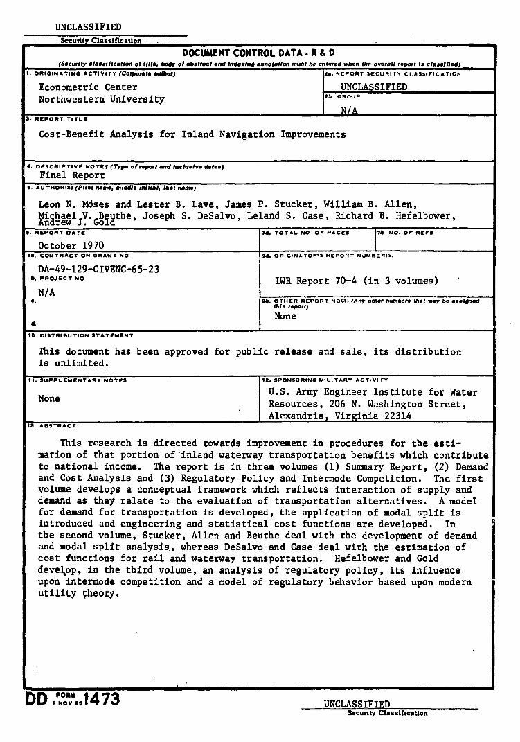
DDIFIR„m8.1473 UNCLASSIFIED

UNCLASSIFIED Security Classification

. DOCUMENT CONTROL DATA- R &D (Security classification of title, body of abstract and indexing annotation must be entered when the overall report is classified)

I. ORIGINATING ACTIVITY (Corporal* author) te. REPORT SECURi iv CLASSIFICATIOt ,

Econometric Center UNCLASSIFIED Northwestern University 2b GROUP

NA

3. REPORT TITLE

Cost-Benefit Analysis for Inland Navigation Improvements

4. DESCRIPTIVE NOTES (Type of report and inclusive dates)

• Final Report S. AU THORISI (First name, middle initial, last name)

• Leon N. Mdses and Lester B. Lave, James P. Stucker, William B. Allen,

Egatly.diathe, Joseph S. DeSalvo, Leland S. Case, Richard B. Hefelbower,

O. REPORT DATE 7. TOTAL NO Or PAGES lb NO. OF REFS

October 1970 SS. CONTRACT OR GRANT NO 94. ORIGINATOR'S REPORT NUMBERIS;

DA-49-129-CIVENG-65-23 It PROJECT NO IWR Report 70-4 (in 3 volumes) " N/A

C. 96. OTHER REPORT NO(S) (Any other numbers Met may be assigned this report)

None cl.

10 DISTRIBUTION STATEMENT

This document has been approved for public release and sale, its distribution is unlimited.

11. SUPPLEMENTARY NOTES 12. SPONSORING MILITARY AC Ts Vi TY

U.S. Army Engineer Institute for Water None Resources, 206 N. Washington Street, Alexandria Virginia 22314 13. ABSTRACT

This research is directed towards improvement in procedures for the esti-mation of that portion of inland waterway transportation benefits which contribute to national income. The report is in three volumes (1) Summary Report, (2) Demand and Cost Analysis and (3) Regulatory Policy and Intermode Competition. The first volume develops a conceptual framework which reflects interaction of supply and demand as they relate to the evaluation of transportation alternatives. A model for demand for transportation is developed, the application of modal split is introduced and engineering and statistical cost functions are developed. In the second volume, Stucker, Allen and Beuthe deal with the development of demand and modal split analysis, whereas DeSalvo and Case deal with the estimation of cost functions for rail and waterway transportation. Hefelbower and Gold develipp, in the third volume, an analysis of regulatory policy, its influence upon intermode competition and a model of regulatory behavior based upon modern utility theory.

'

' . . •

Secunty Classification

UNCLASSIFIED Security Classification

IC LINK A LINK B LINK C KEY WORDS

ROLE WT ROLE WT ROLE WT

Transportation Alternative Transportation Demand Modal Split Discriminant Analysis Regression Analysis Benefits Transportation Benefits National Income Benefits Process Cost Functions Line Haul Cost Functions Joint Costs Production Function of Transportation Modes Engineering Cost Functions Statistical Cost Functions Intermodal Competition Private Costs Public Costs Externalities ' Regulatory Behavior

•

UNCLASSIFIED Security Classification