J Mol Evol (1992) 35:60-76 Journal of Molecular Evolution ~) Springer-Verlag New York lnc, 1992

A Derivation of All Linear Invariants for a Nonbalanced Transversion Model

Trang Nguyen and T.P. Speed

Department of Statistics, University of California at Berkeley, Berkeley, CA 94720, USA

Summary. The method of linear invariants dis- covered by Lake is a way of inferring phylogenies by testing statistical hypotheses. The main advan- tage of the method is that substitution rates for po- sitions along the DNA sequence do not have to be identical. The assumptions and the algebraic back- ground necessary for the applications of the method were clearly laid out in two papers by Cavender, who also described a way to derive a basis for the space of all linear invariants for rooted trees linking four species when the substitution process satisfies the assumption of balanced transversions. Cavender noted a generalization of linear invariants to certain more general substitution models. In this paper we give a simple explicit description of a basis for all linear invariants for a slight variant of Cavender's more general model, which applies to rooted trees linking any number of species. Bases for rooted trees linking five species are enumerated and the method applied to a problem concerning RNA polymerase sequence data.

Key words: Invariants -- Phylogenetic inference

Introduction

The problem of inferring phylogenetic relations among a group of species, or among individuals within a species, is one of continuing interest to researchers in the field of molecular evolution. A variety of approaches in current use are reviewed by Swofford and Olsen (1990), and this paper con- cerns methods that are based upon simple proba-

Offprint requests to: T.P. Speed

bilistic models for nucleotide substitution. Such methods were introduced by Jukes and Cantor (1969) and Neyman (1971) and since that time have been developed by a number of authors, including Ki- mura (1980, 1981, 1983), Felsenstein (1981), Ta- var6 (1986), and Barry and Hartigan (1987). Most of these authors recommend the use of the method of maximum likelihood in its standard or in a mod- ified form.

The method of linear invariants discovered by Lake (1987) is a way of inferring phylogenies by testing statistical hypotheses. This method is con- cerned with the topology of the tree and not any other attributes such as branch lengths, rates, and times of divergence. A linear invariant is a linear function of the observed pattern frequencies of the data whose expected values are identically zero un- der one possible topology and usually non-zero un- der other possible topologies. The main advantage of the method of linear invariants is that substitu- tion rates for positions along the DNA sequences do not have to be identical. Test statistics based on linear invariants have the same asymptotic null dis- tribution under these more general assumptions as they do under the assumption of identical distri- bution, see Navidi et al. (1992).

Cavender (1989) described a mechanical method of generating all linear invariants assuming a bal- anced transversion probability model for the sub- stitution process. His method was computationaUy intensive, requiring the formation of a very large spanning set for the vector space of expected fre- quencies from which is obtained the smallest linear subspace that contains all expected frequencies. Us- ing this method, Cavender found all linear invari- ants for four-species rooted trees. Lake's linear in- variants are just a subset of Cavender's invariants.

61

In this paper we describe a simple me thod o f gen- erating a complete set o f linear invariants for any s-species rooted tree, assuming a "beyond balanced t ransvers ion" probabil i ty model similar to that o f Cavender (1989). The balanced t ransversion model o f Lake (1987) and Cavender (1989, 1991), the mod- el o fHasegawa et al. (1985), and the model used in the D N A M L program in the P H Y L I P compute r package (Felsenstein 1989) are all special cases o f this nonbalanced transversion model.

Definitions and Notation

Suppose that we have aligned D N A sequence data for s species. Only the substi tution process is con- sidered; possible deletions and insertions are sup- posed to have been dealt with separately. At each position o f the D N A sequence, each species 1, 2 , . . . , s can be in one o f four possible states: A, G, C, T. Thus there are 4 s possible pat tern at each position. Here a pat tern A G C . . . A means that species, 1, 2, 3 . . . . and s have bases A, G, C . . . . and A, respec- tively. The 4s-dimensional vectors that contains the observed frequencies o f the patterns is called the observed spectrum of the D N A sequence, and we denote this vector by y. We follow Cavender (1989) as far as possible in our nota t ion and terminology, referring to this and other papers in the references for full details concerning the construct ion o f the probabil i ty model for the Markovian substi tut ion process.

In this paper we assume that the transit ion ma- trices have the "beyond balanced t ransvers ions" form of Cavender (1989). In o ther words, the tran- sition matrices along the edges o f the tree o f our model are all o f the form

c d 3e fig h

where we suppose in addi t ion that

and

f(~-a-)+e(1 +3)=g(1 +3)+h(1 +a)

Here the dots down the diagonal replace the entry required to ensure that row sums are one. The two linear constraints are somet imes called the semi- group closure constraints because they are needed to ensure mult ipl icat ive closure o f these matrices. Because we would like to include the identi ty matr ix

as an e lement o f our semigroup, the above con- straints are different f rom those o f Cavender (1989). The balanced transversion model o f Lake (1987) and Cavender (1989) is the special case o f this model with a = 3 = 1. The model o fHasegawa et al. (1985) and Felsenstein's (1989) model in his D N A M L pro- gram in the P H Y L I P compute r package are also special cases o f this nonbalanced transversion mod- el with a = 7rT/71" C and 3 = 7rc,/~rA, where 7rA, ~ro, 7rc, and ~rT are the stat ionary base frequencies. Any sto- chastic matr ix o f the above form is a linear com- binat ion o f the following seven matrices:

P 1 - - 0 1

O0

P2 =

1 + a /~(1 + a ) 0 0 0 I + 3 0 0 (1 + a)(1 + 3) 0 0 0

P3 =

0 0 1 + 3 1 + a 3(1 + a ) 0

0 0 (1 + a)(1 + 3) 0 0 0

1 3(1 + 3) 0

P 4 = 1 + 3 fl 2 0 0 0 1 + 3 + f l 2 0 0 0

P5 =

(1 + a)(1 + r ) 0 0 (1 + a)(1 + 13)

1 + a fl(1 + a) 0 0

P6 =

(1 + c0(1 4- 3) 0 0 (1 +a ) (1 + 3 ) 0 0

1 + a 3(1 + a )

I 1 + a + a 2 0

P7 = 0 1 + a + a 2 0 0 0 0

o a(1 + 3)

0 (1 + a)(1 + 3)

a(1 + 3) o o ]

(1 + a)(1 + 3)

° l 0 0

1 + f l + f l 2

o o] 0 0 0 0

I +3 ~(I +3)

0 0

I + B 0

0 0 1

l + a

0] 0

~(1 + 3) 0

° l 0

a(1 + a) OL 2

A vector v is a linear invariant o f a topology i f E((v, Y)w) =- 0, where y denotes the observed spec- t rum. Here E denotes expectat ion relative to prob-

62

7

1 2 3 4

I

7

1 2 3 4

IV

7

2 1 3 4

VII

7

A 3 4 1 2

X

7

A 4 3 1 2

XIII

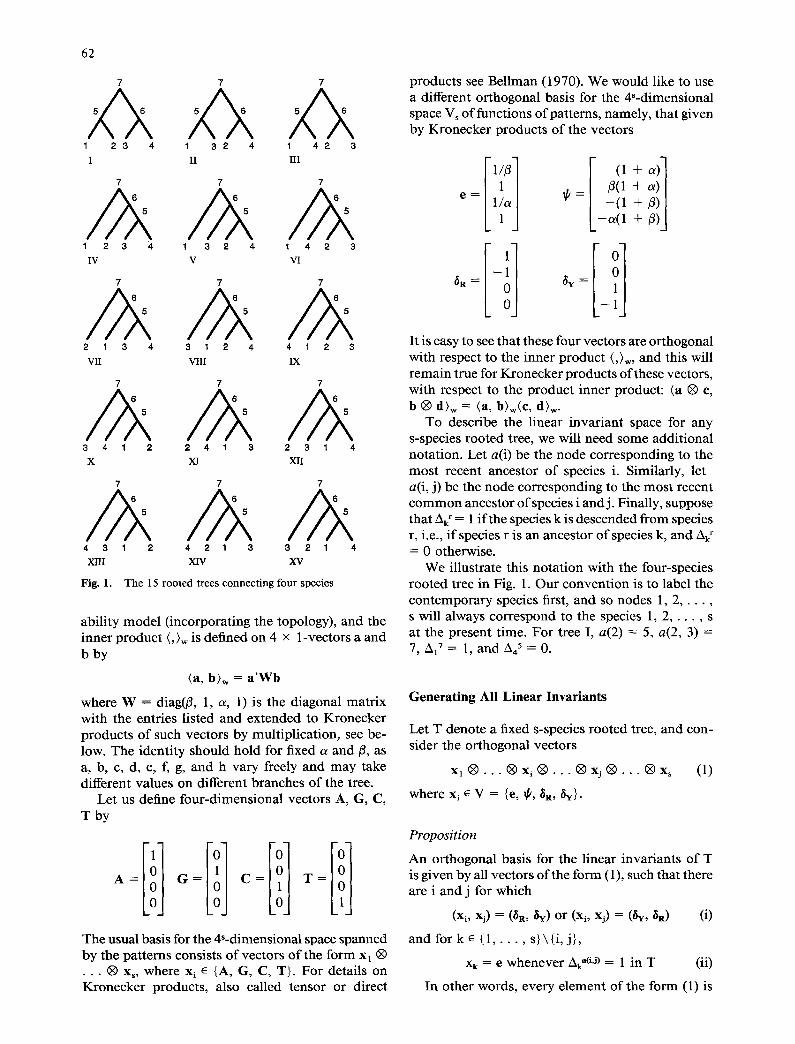
Fig. 1.

7 7

1 3 2 4 1 4 2 3

II III

7 7

1 3 2 4 1 4 2 3

V VI

7 7

3 1 2 4 4 1 2 3

VIII IX

7 7

A A 2 4 1 3 2 3 1 4

X] XII

7 7

A A 4 2 1 3 3 2 1 4

X1V XV

The 15 rooted trees connect ing four species

ability model ( incorporating the topology), and the inner p roduc t (,)w is defined on 4 x 1-vectors a and b by

(a, b)w = a 'Wb

where W = diag(fl, 1, a, 1) is the diagonal matr ix with the entries listed and extended to Kronecker products o f such vectors by multiplication, see be- low. The identi ty should hold for fixed a and/3, as a, b, c, d, e, f, g, and h vary freely and may take different values on different branches o f the tree.

Let us define four-dimensional vectors A, G, C, T by

A = G = C = T =

The usual basis for the 4s-dimensional space spanned by the patterns consists o f vectors o f the form x I (~ . . . ® xs, where x i c {A, G, C, T}. For details on Kronecker products, also called tensor or direct

products see Bellman (1970). We would like to use a different or thogonal basis for the 4 ' -dimensional space Vs o f functions o f patterns, namely, that given by Kronecker products o f the vectors

e =

~R ~

/3(1 + c 0

l l / . l ~'= - ( 1 + fl) --o~(1 + /3)

It is easy to see that these four vectors are or thogonal with respect to the inner product (,)w, and this will remain true for Kronecker products of these vectors, with respect to the product inner product: (a ® c, b ® d)w - (a, b)w(C, d)w.

To describe the linear invariant space for any s-species rooted tree, we will need some addit ional notat ion. Let a(i) be the node corresponding to the most recent ancestor of species i. Similarly, let a(i, j) be the node corresponding to the most recent c o m m o n ancestor o f species i andj . Finally, suppose that Akr = 1 i f the species k is descended f rom species r, i.e., i f species r is an ancestor o f species k, and Akr = 0 otherwise.

We illustrate this nota t ion with the four-species rooted tree in Fig. 1. Our convent ion is to label the con temporary species first, and so nodes 1, 2 . . . . . s will always correspond to the species 1, 2 , . . . , s at the present time. For tree I, a(2) = 5, a(2, 3) = 7, A17 ~- l , and A45 = 0.

Generating All Linear Invariants

Let T denote a fixed s-species rooted tree, and con- sider the orthogonal vectors

Xl ~ . . . ~ X i @ . . . ~ X j @ . . . ~ X s (1)

w h e r e X i E V = {e, ~, ~R, ~Y}"

Proposition

An orthogonal basis for the linear invariants of T is given by all vectors o f the form (1), such that there are i and j for which

(Xi, Xj) = (~R, ~Y) or (xi, x j) = (fly, ~R) (i)

and for k e ( 1 , . . . , s} \{i , j} ,

Xk = e whenever Ak"(iJ) = 1 in T (ii)

In other words, every element of the form (1) is

63

either a l inear invariant o f T or a m e m b e r o f the expected spectra space for T.

In a lecture in July 1990 that we attended, Dr. J. Cavender described a result similar to the hal f o f this proposi t ion which states that vectors o f the form (1) satisfying (i) and (ii) are linear invariants.

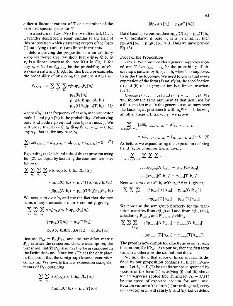
Before proving the proposi t ion for an arbi t rary s-species rooted tree, we show that e ® ~R ® ~Y ® x4 is a linear invariant for tree XIII in Fig. 1, for any x4 e V. Let fblb2b3b4 be the probabil i ty o f ob- serving a pat tern babzb3b4 for this tree. For example, the probabi l i ty o f observing the pattern A A G T is

fAAm" = ~ ~ ~ r(by)P6,7(b6 I bT) b7 b5 b6

"Ps,6(b5 [b6) • p~,5(A [ bs)P2,5(A I bs)

• P3,6(G[b6)P4,7(T [b7) (2)

where r(b7) is the frequency o f base b7 at the ancestor node 7, and pij(bi[ b j) is the probabil i ty o f observing base bi at node i given that base bj is at node j. We will p rove that E{(e ® ~R ® ~Y ® x4, Y)w} = 0 for any x4, that is, for any base b4,

[O~/~fblmCb4 - - /~fblmTb4 - - O~fblGfb4 -~- fblGTb4 ] = 0 ( 3 ) bl

Expanding the left-hand side o f this expression using Eq. (2), we begin by factoring the c o m m o n terms as follows:

~ ~ ~ r(b7)P4,7(b4[b7)P6,7(b6[bT) b7 b 6 bs bl

• [otpa,6(Clb6) - P3,6(TIb6)]Ps,6(b5 [b6)

• [Bp2,5(AIbs) - p2,~(Glbs)]pl,5(b~ I bs)

We next sum over b~ and use the fact that the row sums o f any transaction matr ix are unity, giving,

~ ~ r(b7)P4,7(b4 [b7)P6,7(b6 I b7) b7 b6 b 5

"[aP3,6(f[b6) - P3,6(TIb6)]

'Pa,6(b5 [b6)[/3P2,5(mlbs) - P2,5(G[ bs)]

Because Pz,6 = Ps,6P2,5, and the transit ion matr ix P2,5 satisfies the semigroup closure assumption, the transit ion matr ix P2,6 also has the form supposed in the Definit ions and Notation• (This is the only place in this p r o o f that the semigroup closure assumption comes in.) We rewrite the last expression using ele- ments o f P2,6 obtaining

~ r(b7)P4,e(b4 ] b7)P6,7(b6 [be) b7 b 6

• [oLp3,6(C [b6) - P3,6(T [b6)]

• [/3P2,6(AIb6) - P2,6(G[b6)]

But i f base b 6 is a purine, then aP3,6(C [ b6) - p3,6(T [br) = 0. Similarly, i f base b 6 is a pyrimidine, then /3P2,6(Alb6) - P2,6(Glb6) = 0. Thus we have p roved Eq. (3)•

P r o o f o f the Proposi t ion Part 1. We now consider a general s-species root-

ed tree T. Let fb~b2 " " bs be the probabil i ty o f ob- serving a pat tern by bib 2 . . . b, when T is supposed to be the true topology. We need to prove that every expression o f the form (1) satisfying the specification (i) and (ii) o f the proposi t ion is a linear invariant for T.

C h o o s e i ~ { 1 . . . . , s } a n d j ~ { i + 1 . . . . . s} .We will follow the same argument as that just used for a four-species tree. In this general case, we sum over the bases bk at posit ions k with ~k a0'~) = 1, leaving all other bases arbitrary, i.e., we prove

[~fu,...A...¢...~ - ~ f ~ , . . . . ~ . . . ¢ . . . ~

b k if Aka(i' J)= 1

- afb,...a...c...bs + fbl...O...r...bs] = 0 (4)

AS before, we expand using the expression defining f and factor c o m m o n terms, giving

b k if Aka(i' j)= 1

• ..{~Pi,a(i)[Alba(i)] -- Pi,a(0[Glba(i)]}

•..{~Pj,~o)[CIb~G)] - pj,~0)[TIb~G)]}. •.

Next we sum over all bk with Aka(i,J) = 1, giving

~ ~ • . . { / ~ P i , a ( i ) [ h [ b a ( i ) ] - - P i , a ( i ) [ a [ b a ( i ) ] }

• . .{o~pj,a(j)[C]ba(j)] - p j , a 0 ) [ T l b ~ o ) ] } . • .

We now use the semigroup proper ty for the tran- sition matrices f rom a(i, j) to i and f rom a(i, j) to j, calculating Pi,a(i, j) and Pj,~(~, j), yielding

~ ~.-.{/3Pl,a(i,j)[A I bao,j)] - Pi,a(i,j)[Glba0,j)]} ba(i,j)

• • .{~pj,a(i,j)[C I ba(i,j)] - pj,a(i,j)[T I ba(i,j)]}.. •

The p ro o f is now comple ted exactly as in our simple illustration, for ifba(i, j) is a purine, then the first te rm vanishes; otherwise the second one does.

We now show that space o f linear invariants de- fined by our proposi t ion contains all linear invari- ants. Let Ls = Ls(T) be the linear space spanned by vectors o f the form (1) satisfying (i) and (ii) above for an s-species rooted tree T, and let Hs = Hs(T) be the space o f expected spectra for same tree. Because vectors o f the form (1) are orthogonal, every such vector in L~ will satisfy (i) and (ii). Let us define

64

Table 1. Basis for H :

e ® e =

_ a + 3a ~ + a 3 + fl + 4aft + 9a2fl + 3a3fl + 3t32 + 9a/32.(1, a( l + a)2/3(i + /3) 2 1, e)

140t~fl 2 + 5a3fl ~ 4- /33 -4- 3aft 3 4- 50Z2fl 3 + 2ot3fl ~ - *(1, 1, e)

+ (a + 0~/3)-1.(1, 2, e) + (,~ + a/3)-~.(1, 3, e) + o~ - /3 afl(l + fl) *(1, 4, e)

+ (/3 + a/3)-~*(1, 5, e) + (fl + a3) ' . (1 , 6, e) a(~ ~ :/3¢(1, 7, e)

e ® ~ k =

2(a - fl)(-1 + aft) a(1, 1, e) - *(1, 2, e) - o'(1, 3, e)

(l + a)(1 + fl)

2(1 + a) .. + ] - _ ~ . t , , 4 , e ) + . ( 1 , 5 , e ) + a ( 1 , 6 , e) 2 ( 1 + /3)*(1' 7' + a

~k®e =

~ b @ ~ = " - (1 + a)~ . (1 ,3 , e) + - -

- a(1 + fl)*(1, 6, e) + - -

2or 3 + otfl + 3aZfl + l la3 f l + a4fl + f12 + 6aflZ + 12a2f12 *(1, 1, e) a(1 + a)2(1 + /3) 2

q 22a3f12 + 3ot4f12 _ /33 _ 3a/33 _ 3ot2f13 + 7a3/33 + 2a3f14 , , m,~, 1, e)

a(1 + a)2fl(1 + fl)2

(1 +o0/3 , ~ 3 + a f t (I + a ) ( a + / 3 + 3a f l - /32 ) . (1 ' l + a(1 + fl)*(l, 2, e) + a + aft *(1' 3, e) + a/3(1 + /3)2 4, e)

_ 2or(1 + fl)2 .. a(1 + fl) *(1, 5, e) a(1 + fl) *(1, 6, e) + (1 + ,~)fl (1 + ~)3 ~ * t ~ , 7, e)

ce + fl + 2a/3 2, e) a(1 + a)fl(1 +/3)¢(2,

2(a2 + 3c?fl + f12 + 3a/32 + &x2fl2 + a~/32 + a2f13) ¢(1, 1, e) - (1 + o0/3.(1 , 2, e)

(1 + ~)(1 + fl)

2(1 + ~)2fl*(1, 4, e) - a(1 + fl)*(1, 5, e)

1 +

2a(1 + fl)z¢(1, 7, e)

l + a

~®~R =

~ ® ~ y =

(1 + or)(-- 1 + fl)flg(1, 1, e) + (1 + a ) ( - 1 + f l)g(1, 4, e) + g(2, 1, e) - / 3 ~ ( 3 , 1, e)

l + f l l + f l

(1 - a)a(1 +f l )a (1 , 1, e) --~----(1 +a ) f l ' 2, e ) - (1 +cOil 1 + ,~ ~ (1+/3) *('' ~(1 +/3)-0, ' 3, e)

(1 + ~)fl ,~ - *(1, 5, e) - a(1, 6, e) + (1 -l+oea)(1 + /3)*(1, 7, e) + ~ ( - - ~ - - ~ . ~ z , 1, e)

(1 + a ) f l ,~ + ~ . t ~ , 1, e) + (1 + a)*(5, 1, e)

(I + ~X)(-- 1 + fl)/3.(1, 1, e) + a(1, 2, e) - f t . ( l , 3, e) + (1 + a ) ( -1 + /3)o-(1, 4, e)

l + f l l + f l

[/3 + (1 + /3)-']*(1, 1, e) -- (1 + fl)-l .(1, 4, e)

(1 oL) o((l + fl).(1, 1, e) + ~ . ( 1 , 5, e) - ,~(1, 6, e) + (1 - a)(1 + f l ) . (1 , 7, e)

l + a l + a

1 + + a2¢(1, 1, e) - (1 + a ) -~ (1 , 7, e)

l + a

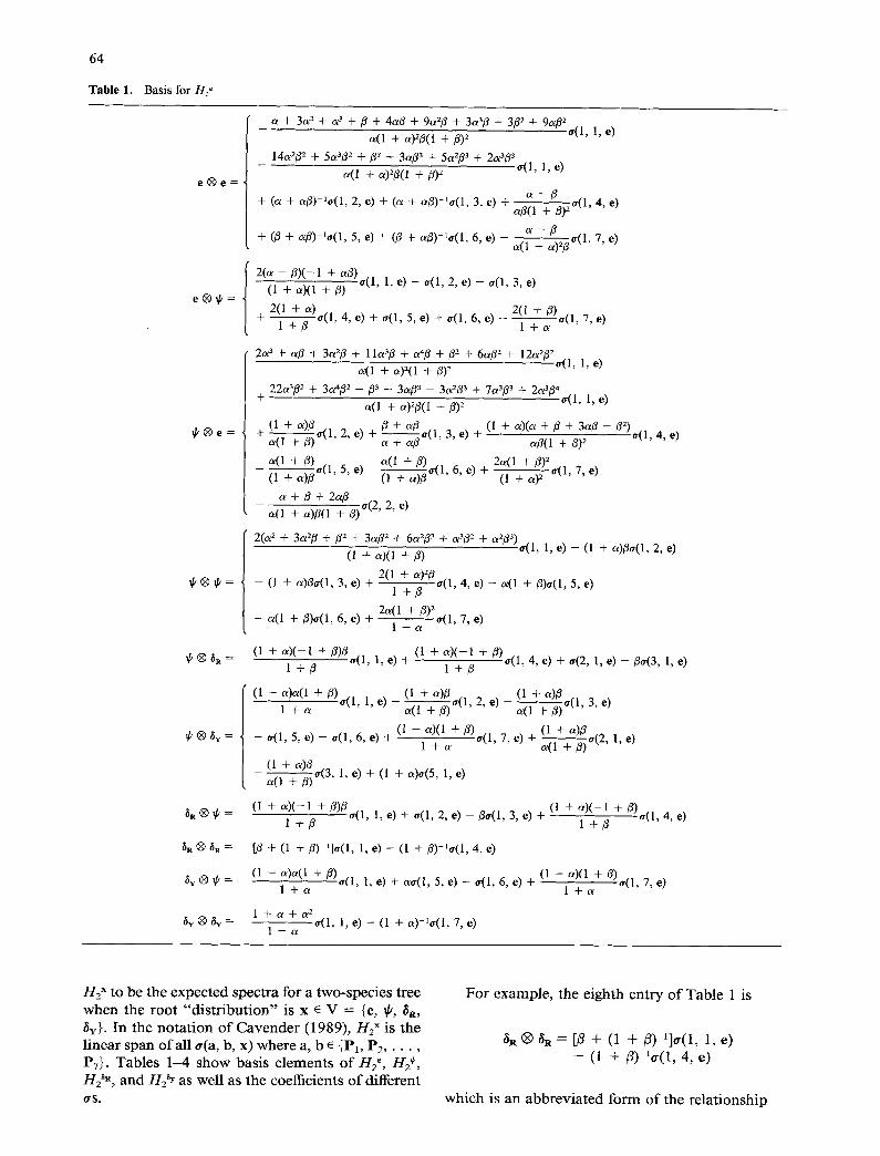
H2 x to be the e x p e c t e d spectra for a t w o - s p e c i e s tree w h e n the r o o t "d i s t r ibut ion" is x e V = {e, ~k, 6R, ~y}. In the n o t a t i o n o f C a v e n d e r (1989) , H2 x is the l inear span o f all or(a, b, x) w h e r e a, b e {P1, P2 . . . . . P7). Tab le s 1 - 4 s h o w bas is e l e m e n t s o f H : , /-/2 +, H2 ~R, a n d H : y as we l l as the coef f ic ients o f different orS.

F o r e x a m p l e , the e ighth entry o f Tab le 1 is

aR ® aR = [fl + (1 + f l ) -qa(1 , 1, e) - (1 + ~)-'or(1, 4, e)

w h i c h is an a b b r e v i a t e d f o r m o f the re la t ionsh ip

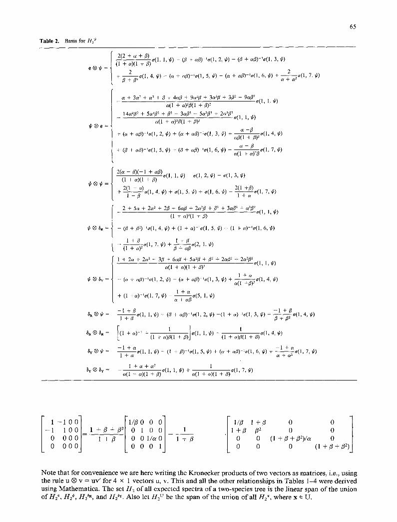
Table 2. Basis f o r / / 2 ~

65

2(2 + a + 1 3 ) ,, e ® ~k = (1 + ~)-(1 ~_7)at~, 1, ¢) - (t3 + a/3) ~,r(1, 2, ¢) - (13 + a/3)-'a(1, 3, ¢)

2 2 + ~ .--7--=a(1, 4, ~b) - (a + c~3)-1~r(1, 5, @) - (or + ~/3) a~r(1, 6, ¢) + "--7--7a(1, 7, ¢)

i f ® e =

c~ + 3a ~ + cP + /3 + 4a/3 + 9a2/3 + 3cP/3 + 3fl ~ + 9a/3 2 a(1, 1, ~P)

~(1 + a)23(1 + /3)2

14a2/32 + 5a3/32 + /33 + 3a/33 + 5a2/33 + 2a3•3 - ,r(l, 1, ¢)

~(1 + .)~/3(1 +/3)~

a -3fl)a(1, 4, ~) + (a + a3)-~a(1, 2, ¢) + (c~ + a/3)-~a(1, 3, ¢) + a/3-~ +

+ 03 + a/3)-'~r(1, 5, ¢) + (/3 + o~/3)-1o'(1, 6, ¢) a(1 z/3~r(1, 7, ¢)

2(c~ 3)(-1 + c~/3)~r(1, 1, ¢) - ~r(1, 2, ¢) - a(1, 3, ¢)

(1 + ~x)(1 + /3) ~ ® ~ = + --c~____..~j a ( 1 , 2 ( 1 + 4, ¢) + a(1, 5, ¢) + ~(1, 6, ¢) 2(1--+~a(1, 7, if)

1 + / 3 l + a

2 + 5a + 2e~ 2 + 2fl + 6oL/3 + 20'2/3 + f12 + 3a32 + 0/2/32 - a(1, 1, ¢)

(1 + c02(1 + /3)

® ~R = • - - (~ ~- /32)--~a(1, 4, ~) + (1 + o0-1o-(1, 5, ~) + (1 + o~)-1o(1, 6, ¢)

1 _+ e o'(1,7,¢) + ~ e ( 2 1,¢) (1 + a ) ~ /3~c~o '

[ 1 +_.2_~ + 2.~ + 3/3 + 6~/3 + 5~:/3 + 3 ~ + 2a/3 ~ + 2.~/3~ ( 1 1, ~) . . . . ~-l--+-c~ f --_7--/3)5- - -

l + c ~ @ ~y = # -- (O~ -}- Ot/3)-10"(1, 2, ¢) -- (Ce + a/3)-'cr(1, 3, ¢) + ~ a ( 1 , 4, if)

l + c ~ + (1 +o0-1o'(1, 7, if) -- - - 1, ¢) a + a/3'T(5'

-1_+._3],. - 1 +/3 ~(1, 1, ¢) + (/3 + a/3)-~a(1, 2, ¢) - (1 + o~)-1o'(1, 3, ¢) + -~ - - -~ -a (1 , 4, ¢)

[ I ) ] a ( l ' l ' ~ ) 1 / 3 ) ~ ( 1 , 4 , 7 ¢) (1 + c 0 ~ + ( 1 +c0/3(1 +/3 (1 +a)/3(1 +

- l + a - l + a a(1, 1, ¢) - (1 + /3) 'a(1, 5, ¢) + (c~ + o//3)-1~r(1, 6, ~) + --~--~--~: a(1, 7, ~) + ~ 1

I + a + O ~ 2 1 c~(1 + o0(1 + /3)a(1, 1, ~,) + o~(1 + ~e)(1 +/3)(r(l, 7, ~)

~R® ~ -

~y® ¢ -

ii10 1 i;00 ] 0 0 l - 1 1 0 = 1 + / 3 + / 3 2 1 0 1 . 1 + / 3 f12 0 0 0 O0 1 + fl 0 1/oe 1 + /3 0 0 (1 + f l+ /32) /a 0 0 O 0 0 0 0 0 0 ( 1 + / 3 + 3 2 )

N o t e that for c o n v e n i e n c e w e are here wri t ing the K r o n e c k e r produc t s o f t w o vec tor s as matr ices , i .e., us ing the rule u ® v = uv' for 4 x 1 vec tor s u, v. T h i s a n d all the o ther re la t ionsh ips in Tables 1 - 4 were d e r i v e d us ing M a t h e m a t i c a . T h e set H2 o f all e x p e c t e d spectra o f a t w o - s p e c i e s tree is the l inear span o f the u n i o n o f / / 2 e , / / 2 ~ , / / 2 % a n d H2 "Y. A l s o let H2 v be the span o f the u n i o n o f a l l / / 2 x, w h e r e x • U .

66

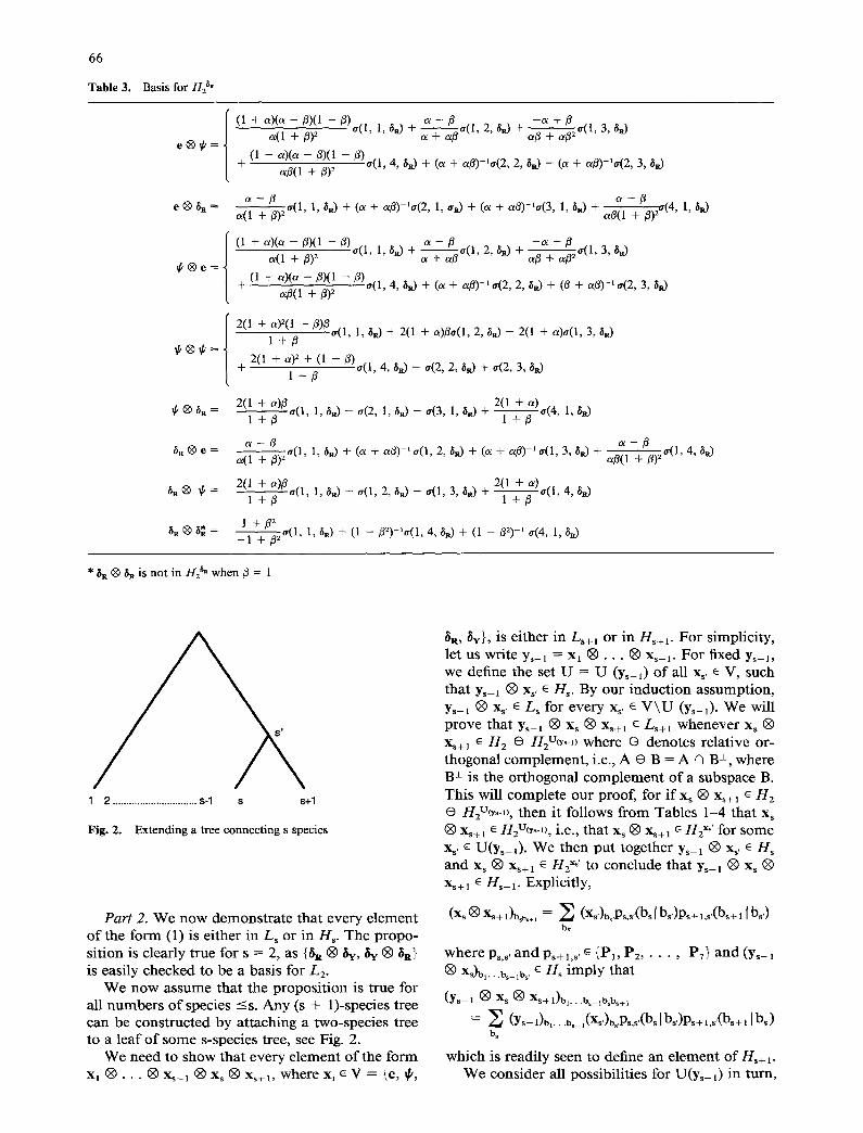
Table 3. Basis for H2 5"

~ ® e =

~ ® ~ =

~R @ e =

$~® ~ =

~a ® ~R* =

(1 + a)(a-- fl)(1 - fl).(1, 1,6a) + a - / 3 - a + fl "1 " a(1 + fl)~ a + a3 0(1' 2, ~ + a-~--~afl~ ~rt , o, ~ )

+ (1 + a)(a - fl)(1 - fl)*(1, 4, 6R) + (a + a3)-lff( 2, 2, 5~) -- (a + a/~)-'*(2, 3, ~R) ~3(1 + 3)=

a - 3 ) . ( 1 , a - 3 * ( 4 , 1 , ~ a 0 ~ 1, ~ ) + (a + afl)-~*(2, 1, .~) + (a + otfl)-l*(3, 1, ~R) + a3(1 +

aa@aB - a + 3 ,, (1 + a)(a - fl)(1 - B).(1, 1,/~) + ~(1, 2, ~a) + - - - ,3, rid

+ (l + a)(a - /3)(1 - / 3 ) . ( 1 , 4, 610 -I- (a + a3) - t * (2 , 2, 6~ -I- (/3 + a3) - ' * (2 , 3, $~) a3(l + 3)=

2(1 + ~x) 2(l fl)3.(1, 1, ~D + 2(1 + a)3*(1, 2, 610 - 2(1 + a)*(1, 3, ~ )

I + B 2(1 + a ) 2 + ( 1 -

+ 3).(1, 4, ~) - .(2, 2, ~R) + .(2, 3, ~D 1 + 3

2(11++3 )3.(1' 1, ~R) -- *(2, 1, ~) -- a(3, 1, 6R) + ~ * ( 4 , 1, ~)

) . (1 , l, ~) + (~ + ~ ) - i .(1, 2, ~) + (~ + ~ ) - , .(1, 3, ~) + ~(~fi -,.~.=.(1,p~ 4, ~.9

2(1 + a) .. 2(11+ + )f t . ( l , 1, ~R) -- *(1, 2, 6D -- *(1, 3, ~ ) + ~ * t ' , 4, ft.)

1 + 3 ~ 3 . (1 , l, ~.) + (1 - 3b- ' . (1, 4, ~) + (1 - ~ ) - ' .(4, l, ~) +

* ~R ® ~ is not in H2 ~ when 3 = 1

1 2 ............................... s-1 s s+l

Fig. 2. Extending a tree connecting s species

P a r t 2. W e n o w d e m o n s t r a t e t ha t eve ry e l e m e n t o f the f o r m (1) is e i ther in L~ or in H~. T h e p r o p o - s i t ion is c lear ly t rue for s = 2, as { ~ ® &¢, &¢ ® 6R} is eas i ly c h e c k e d to be a bas i s for L2.

W e n o w a s s u m e tha t the p r o p o s i t i o n is t rue for all n u m b e r s o f species - s . A n y (s + D-spec ies t ree can be c o n s t r u c t e d b y a t t ach ing a two-spec ie s t ree to a l ea f o f s o m e s-species tree, see Fig. 2.

W e n e e d to show tha t eve ry e l e m e n t o f the f o r m X 1 ® • • . ® Xs__ 1 ® X s ® K s + l , w h e r e x i e V = {e, ~,

~a, g~}, is e i ther in Ls+~ or in Hs+l . F o r s impl ic i ty , let us wr i te y~_l = x~ ® . . . ® X~_l. F o r fixed y~_~, we def ine the set U = U (Ys-~) o f all x~, e V, such t ha t y~_l @ x,, e H~. By o u r i nduc t ion a s s u m p t i o n , y,_~ @ x~, ~ Ls for eve ry xs, e V \ U (y~_~). W e will p r o v e t ha t y~_~ ® xs ® x~+~ e L~+I w h e n e v e r x~ ® x~+~ e H2 (3 H2u(,,-L) whe re (3 deno te s re la t ive or - t hogona l c o m p l e m e n t , i.e., A (3 B = A N B ±, whe re B J- is the o r t h o g o n a l c o m p l e m e n t o f a subspace B. T h i s will c o m p l e t e o u r p roof , for i f xs @ x~+~ e H2 e H2U(,~-l), t hen it fo l lows f r o m Tab l e s 1 -4 t ha t x~ ® x~+l e H2U(,s-,, i.e., t ha t x~ ® xs+ 1 e H2x,' for s o m e Xs, ~ U ( y ~ - 0 . W e t h e n p u t t oge the r Y~-I ® xs, ~ Hs a n d x~ ® X~+l e H2x¢ to conc lude tha t y ,_l ® x~ ®

xs+l e H~+l. Expl ic i t ly ,

(xs ® Xs+ 1)b.b.+, = ~ (X¢)b.,Ps,s'(bs [ bs,)Ps+l ,s,(bs+ 1 Ibm,) bs'

w h e r e p~,~, a n d P~+l,s, e {P1, P2, - • • , P7} a n d (y~_~ ® X~)b,...b~_,b,, e H~ i m p l y t ha t

(Ys-l ® x~ ® x~+~)b .... b~ ,b.b.,

= ~ (Ys--~)b .... b._,(X~')b~,P.x(b~ I b~,)P~+~,~,(bs+~ Ibm,) b s,

which is read i ly seen to def ine an e l e m e n t o f Hs+~. W e cons ide r all poss ib i l i t ies for U ( y . _ 0 in turn ,

Table 4. Basis fo r / / 2 ~

67

e ® ~ =

e ® ~ y =

q~®e= {

- - - ~ + 3 "' 2-fft~ (1 a)(a /3)(1 + /3)a(1, 1, ~v) + a~3 + aZ3 . - ~ . + (1 + a)~/3 . . . . a t i , 5, ~.) + a(l , 6, ~v)

(1 - ,~)(~ - 3)(1 + 3) + a(l, 7, fir) + (13 + a/3)-'a(5, 5, fly) - (3 -~'a/3)--lo'( 5, 6, ~) a(1 + a)23

' ~ - 3 a - 3 (f-+--a~/3a(1, 1, ~v) + (3 +a/3) ~a(5, 1, ~,) + (3 + a3) *a(6, 1, ~ ) a(]" ~" ~z3a (7 ' 1, 6v)

- - a + / 3 (r(1,5, b ~ ) + a ~ - 3 o - ( 1 6, 8 0 (1 oO(a - 3)(1 + 3)a(1, l , by) + a3 + a2----'-~ 3 ~- ~0 ' (1 + ,~)~/3

+ (1 - a)(a - /3)(1 + 3 ) ( 1 ' 7, ~v) + (3 + a/3)-~a(5, 5, 6v) + (a + o~/3)-1 o-(5, 6, Sy) a(1 + a)Z3

f f ® ~ =

2(1 - a)a(1 + fl)~ a(1, 1, ~r) - 2(1 + 3)a(1 , 5, t~)

l + a

+ 2a(1 + 3)a(1, 6, 6y) + 2(1 - a)(1 + /3)za(1, 7, ~ ) + a(5, 5, ~ ) - o-(5, 6, ~ ) l + a

~ ® f i v = m 2 ~ 1 +

3)a(1, 1, 6v) + 0-(5, 1, (~v) + o(6, 1, (~v) 2 ( 1 ) 3 , o.(7 , + 1, ~.) l + a l + a

6 v ® e =

~y® ~ =

a 2 /3 a(1 1, ~v) + (3 + otfl)-lo'(1, 5, ~¥) + (/3 + O~fl)-lo-(1, 6, fly) d + ~)~ '

~ 2 ~ 1 + /3)a(1, 1, ~v) + a(1, 5, 6v) + a(1, 6, ~v)

l + a

2(1 + 3)o-(1, 7, ~v)

l + a

a - 3 a(1 + a)2fl ~(1' 7, ~v)

1 +o¢ 2 ot2o-(l, 1, fly) + (1 - o t2 ) - lo ' (1 , 7 , ~v) + (1 -- a2)-~a(7, I, ~y) +

* ~v ® g~ is not in Hz ~ when a = 1

referring to Tables 1--4 for the coefficients that show our asser t ions to be true.

i) I f U ( y s _ 0 = V, then HzU~- -, = H 2 and there is nothing to prove.

ii) I fU(ys_ l ) = {~k, 6R, ~v}, then we can de te rmine f rom Tables 2 -4 that H2 e H2tr~,s-, = span{e ® e}. Because e e U(ys_0, y~_x ® e e L~, and by our rule there are leaves i and j such that A ,-0J) = 1. But by the rule again we mus t have y~_l ® e @ e e L~+I and this case is proved.

iii) I f U ( y , _ 0 = {e, if, ~y}, then we find f rom Tables 1, 2, and 4 that H2 e HzU~ys-, = span{e ® 6R, ~a ® e}. Because 6R ~ U(Y~_0, Ys-1 ® 61~ ~ L~, and by our rule there m u s t be a l ea f i with xi = ~ . Again by the rule, we mus t have Xk = e whenever Aka~'s') = 1, and then Y~-I ® e ® ~R e L~+~ because A~ "~i,s+~) = 1. Similarly, we deal with y~_~ ® ~l~ ® e.

iv) I f U(y~_1) = (e, if, ~R}, we can argue along the same lines as those jus t given.

v) I f U(y~_I) = {~k, ~ } , then f rom Tables 2 and 4 we find t h a t / / 2 (3 H2U~,-, = span{e ® e, e ® ~R, 6R ® e}. We then argue as we did in cases ii and iii above.

vi) I fU(ys_0 = {~k, 6~}, then we argue as in case v. vii) I fU(y~_l ) = {~}, then f rom Table 2 we see

t ha t / 42 (3 H 2 U(y~-l) = span{e ® e, e ® fiR, 6R ® e,

e ® 6v, ~v ® e}. We can then argue as in cases iv and v.

viii) I t follows f rom our l inear invar iant rule that no subset U(ys_l) is possible o ther than those con- sidered, and the p r o o f is thus complete . QED.

Examples and Discussion

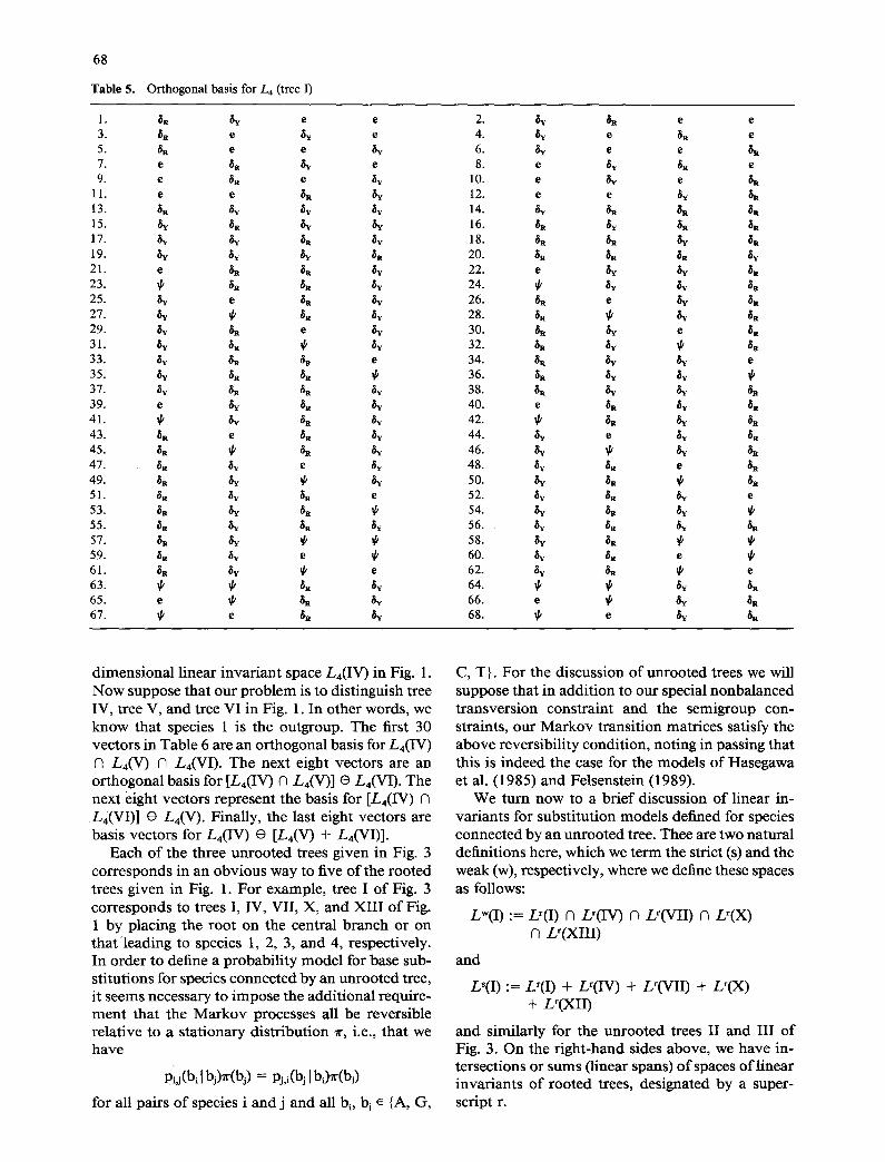
We begin by enumera t ing bases for the two types o f rooted trees linking four species (cf. Cavender 1989). Table 5 shows the or thogonal basis for the 68-di- mens iona l l inear invaf ian t space L4 (tree I) o f tree I in Fig. 1. For simplicity, we omi t the symbol ®.

Using this or thogonal basis, it is very easy to see the relat ionships between the l inear invar iant spaces for different topologies. For example , suppose that our p rob l em is to distinguish the first three trees in Fig. 1. Let us denote the space L4 (tree i) o f l inear invar iants o f tree i by L4 (i), i = I, I I . . . . . The first 20 vectors in Table 5 cor respond to an or thogonal basis for L4(I) n L4(II) 0 L4(III). The next 18 vec- tors represent an or thogonal basis for [L4(I) f3 L4(II)] @ L4(III). The next 18 vectors are basis vectors for [L4(I) n L4(III)] e L4(II). Finally, the last 12 vectors are basis vectors for L4(I) e [L4(II) + L4(III)].

Table 6 shows the or thogonal basis for the 54-

68

Table 5. Orthogonal basis for L4 (tree I)

1. 8a ~Y e e 3. 8~ e ~ e 5. ~R e e 7. e 8s ge e 9. e ~R e ~y

11. e e ~R ~y 13. ~ ~v ~v 15. t~ ~a t~ t~ 17. ~v ~y 6 R ~y 19. ~ &z ~ ~s 21. e ~ ~R 23. ~ ~R ~ 25. ~v e ~R 27. ~v ~ ~R 29. ~v ~a e &~ 31. ~v ~a ~k ~Y 33. ~v ~a ~a e 35. ~v ~a ~a 37. ~ ~ ~R 39. e ~v ~a ~Y 41. 4' ~ ~a 43. ~s e ~a 45. ~a $ ~ ~v 47. ~ ~v e ~ 49. 6a ~ ~ 51. &~ ~v ~t e 53. ~R ~Y ~R 55. ~ ~v ~R 57. ~R ~v 1// 59. ~ ~v e $ 61. 8~ ~v ~k e 63. ~k xk ~ ~v 65. e ~ ~ 67. ~ e ~R

2. ~ 6~ e e

4. ~ e bR e

6. ~ e e t~

8. e ~ ~ e

I0. e ~ e ~a

12. e e ~ ba

14. ~ 5R ~a ~R 16. bR ge ~ 18. ~ ~R ~ 8~ 20. 5R bR ~ 22. e 5y ~ ~t 24. ~ ~v ~ ~R 26. ~R e 5v ~R 28. ~R ~ ~v ~R 30. ~R ~v e ~ 32. ~ ~v ~ ~ 34. 5R ~v 5v e 36. ~ ~v ~ 38. 8~ ~ ~ 40. e ~a ~ ~n 42. ~ ~ ~v ~R 44. ~v e ~ ~ 46. ~v Xb ~v ~R 48. ~ ~ e ~R 50. t~ ~ ~ 52. ~v ~ ~v e

54. ~v ~ ~ 56. ~v ~R ~v ~ 58. ~v ~ $ 60. ~v ~a e ~,

62. ~v ~a ~ e 64. $ ~ ~v ~a 66. e ~ ~ ~ 68. ~k e ~ /$~

dimens iona l l inear invar ian t space L4(IV) in Fig. 1. N o w suppose that our p rob l em is to distinguish tree IV, tree V, and tree VI in Fig. 1. In other words, we know that species 1 is the outgroup. The first 30 vectors in Table 6 are an or thogonal basis for L4(IV) n L4(V ) n L4(VI). The next eight vectors are an or thogonal basis for [L4(IV) O L4(V)] ~ L4(VI). The next eight vectors represent the basis for [L4(IV ) n L4(VI)] O L4(V ). Finally, the last eight vectors are basis vectors for L4(IV) e [L4(V) + L4(VI)].

Each o f the three unroo ted trees given in Fig. 3 cor responds in an obv ious way to five o f the rooted trees given in Fig. 1. For example , tree I o f Fig. 3 cor responds to trees I, IV, VII , X, and X I I I o f Fig. 1 by placing the root on the central b ranch or on tha t ieading to species 1, 2, 3, and 4, respectively. In order to define a probabi l i ty mode l for base sub- st i tut ions for species connected by an unroo ted tree, it seems necessary to impose the addi t ional require- m e n t that the M a r k o v processes all be reversible relat ive to a s ta t ionary dis t r ibut ion ~r, i.e., that we have

Pij(bi [bj)zr(bj) = Pj,i(bj I b0~r(b.3

for all pairs o f species i and j and all bi, bj e {A, G,

C, T}. For the discussion o f unroo ted trees we will suppose that in addi t ion to our special nonbalanced t ransvers ion constraint and the semigroup con- straints, our M a r k o v transi t ion matr ices satisfy the above reversibi l i ty condit ion, noting in passing tha t this is indeed the case for the models o f Hasegawa et al. (1985) and Felsenstein (1989).

We turn now to a b r i e f discussion o f l inear in- var iants for subst i tut ion models defined for species connected by an unroo ted tree. Thee are two natural definit ions here, which we t e rm the strict (s) and the weak (w), respectively, where we define these spaces as follows:

Lw(I) :-- Lr(I) n Lr(IV) n Lr(VII) n Lr(X) (q L~(XIII)

and

L*(I) := L~(I) + L~(IV) + L~(VII) + Lr(X) + Lr(XII)

and similar ly for the unroo ted trees I I and I I ! o f Fig. 3. On the r ight -hand sides above, we have in- tersections or sums (linear spans) o f spaces o f l inear invar iants o f rooted trees, designated by a super- script r.

Table 6. Orthogonal basis for L 4 (tree IV)

69

1. ~ ~, e e 3. ~R e ~ e 5. ~ e e ~,

7. e ~R ~ e 9. e ~. e

11. e e ~R g~ 13. &~ e ~ 15. ~ ~ e gg 17. ~ e ~R 19. ~p e /~R 2 i. ¢ ~Y ~R e 23. ~ ~y ~Z e 25. ~. ~ ~ e 27. ~ ~v e ~R 29. &¢ ~ e ~R 31. ~¢ ~ ~ ~R 33. e ~R ~a 35. ~ ~R ~ ~V 37. ~ ~R ~ g~ 39. ~ ~ ~R 41. e ~IR ~ /~R 43. ~ ~R g~ ~R 45. ~ ~a ~ ~R 47. &~ ~ ~ h 49. g/ ¢ ~R 51. ~ ¢ ~,, 53. e ¢ ~a ~g

2. ~ ~R e e 4. ~v e ~R e 6. ~v e e ~R 8. e ~ ~R e

10. e g¢ e 5R 12. e e ~ ~R 14. ~ e ~ g~ 16. ~a ge e #a 18. 5R e ~ 5R 20. ff e g~ 5a 22. ff ~R g~ e 24. ~a ~a gz e 26. ~ 5a g~ e 28. ~' ~R e 30. ~ ~ e 32. ~R ~ ~R 34. e ~ ~ ~R 36. ¢/ ~ g¢ ~ 38. ~a ~ g~ 5R 40. ~. ~ ~ ~ 42. e ~ ~. ~y 44. ff ~ ~ ~v 46. ~R ~ ~R g~ 48. ~R ~ ~R 50. ~R ~ ~ ~R 52. ~ ~ ~ ~R 54. e ff 8v ~R

1 3 1 2 1 2

N / N / N / / \ / \ / N

2 4 $ 4 4 3 Fig. 3. The three unrooted trees connecting four species

The linear spaces L w have dimension 16 (for four species), and we will discuss them in detail shortly, whereas the spaces L ~ have dimension 92. In es- sence, the larger, strict set o f constraints demands that the probabil i ty model for substi tut ion on the unrooted tree is compat ible with every possible rooting o f the tree, whereas the smaller, weak set o f constraints gives only those that are c o m m o n to all o f the models corresponding to different rootings o f the tree.

We now describe the linear spaces Lw(I), Lw(II), and Lw(III). It is not hard to check that

Lw(I) • Lw(II) n Lw(III) = s p a n { v 1 , . . . , v~2}

where v~ . . . . . v12 denotes the first 12 vectors in Table 5. Denot ing the above intersection by M, with or thogonal complement M ±, we can further check that

Lw(I) n Lw(II) N M ± = span{v37 , V3s}

Lw(II) N Lw(III) O M ± = span(%5, v56}

Lw(II) N Lw(III) N M ± = span{v', v"}

where v37, v3s, v55, and v56 are f rom Table 5, and v' = ~, ® ~v ® ~g ® ~g, and v" = ~R ® 6R ® &," ®

6v have not been previously ment ioned. Finally, we can check that

Lw(I) ~ [Lw(II) + Lw(III)] = (0)

i.e., Lw(I) = M • span{v37, V38 , Y55, V56}, with similar expressions for Lu(II) and Lo(III).

We conclude that for unrooted trees, with the weak sense constraints, we have 12 linear invariants that permi t a check on the validity o f our balance (or imbalance) assumptions, whereas each o f the three pairs o f trees has 2 l inear invariants that con- strain the model for that pair, but not for the other tree. These are the phylogenetically informat ive lin- ear invariants, and we remark that 737 + 738, 755 + v56 and v' + v" are just the original l inear invariants defined by Lake (1987).

Similar decomposi t ions o f the spaces Ls(I), Ls(II), and L~(III) could be described, but for brevi ty we omi t the details. We simply note at this point that these spaces coincide with the spaces o f linear in- variants for the K imura two-parameter model de- fined over any o f the corresponding rooted trees [see Evans and Speed (1992) for further details].

7O

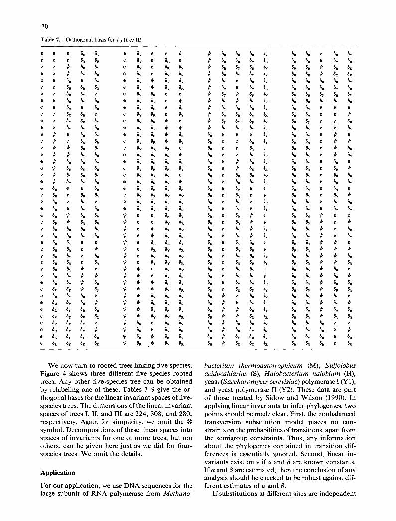
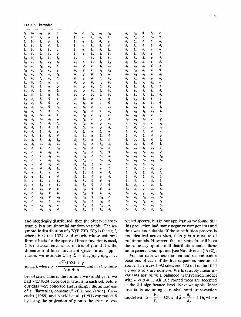
Table 7. Orthogonal basis for L5 (tree II)

e e e ~R 8Y e fy e e fR e e e fy fR e ~y e fR e e e ~ fR fY e ~y e ~R ~Y e e ~ ~Y ~R e ~y e f~ ~R e e ~R e ~y e fy ~ ~R f~ e e fR ~R ~Y e fY ~ ~Y ~R e e ~a f~ e e ~y ~R e e e e ~R ~Y ~R e 8y fR e e e ~ e ~R e fy 8a e ~R e e fv ~a e e fy 6 8 e fy e e ~Y ~R ~Y e ~Y ~s ~ e

e e ~ fy fR e ~y fR ~ e ~ e fR ~Y e f~ f~ ~ ~R e ~ e ~y fR e ~Y ~R ~

e ~ ~ ~R ~Y e ~Y ~R fR e

e ~ ~ fy f~ e fY fR fR e ~ fR fR ~Y e #Y ~R ~R ~R e ~ ~R ~Y ~ e ~Y fR ~R fY e ~ ~y ~a ~ e fy f~ f~ e e 6 ~y f~ f~ e ~ #R ~Y e ~R e e ~y e ~Y ~R ~Y ~R e ~R e ~R ~ e ~y ~R 5Y f~ e fR e 8y e e ~Y ~Y fa fY e fs e fY fR e ~Y fY fY ~R e ~a ~ fa ~ ff e e ~R ~Y e ~s ~ ~Y ~R ~ e e ~y f. e fR fR ~R fV ~ e ~ fR fY e ~R ~a fY fR ~ e ~ fY ~R e ~R fv e e ~ e ~R ~R ~v e ~R ~Y e ~ ~ e 8a ~Y fR e ~R ~Y e ~R ff e ~ fR fY e fR ~Y e f~ ff e fy fY ~R e 8R ~Y ff e ff ff e ~R ~Y e ~R fY ~ ~ ~ ~ e ~Y fR

e ~R ~Y ~ ~)Y ~ ~ ~ {~Y ~R e ~R ~Y fR e ~ ~ fR fR ~Y e fs ~y ~R ff ff ~ ~R ~Y ~R e ~R ~Y fR ~a ~ ~ fY ~R fY

e ~R fY ~Y e ~ ~R e ~R fY e ~R ~Y fY ff ff ~a e fY ~R e fa ~Y ~Y ~a ff ~R ff ~ ~Y e ~R ~Y fY ~Y ~ ~R ~ ~Y fR

fR ~R fR ~Y fR ~R e ~R fY ~R fR ~Y 6R ~R ~R e ~Y fR ~R ~Y fR ~ ~R fR ~ ~R ~Y ~a fY ~Y fR ~R fs ~ ~Y ~a fy e ~R ~Y fR ~R ~R fR fY ~y e fY ~R f~ ~a ~R fY fR ~Y ~ ~R ~Y ~R fR fY ~a fY fY ~ fY fR fR fR ~Y ~Y fa fY ~R 5a ~y f~ fy e e e ~Y fR ~Y ~R ~R ~Y e e fY ~Y ~R fY ~R fY e e ~R ~Y ~Y fY ~R fR fY e e fy

fa e e e ~y ~R ~Y e ~ e 8R e e 6R ~Y ~R ~Y e ~ ~R e e fly e 8R fY e ~ ba fR e e fY fR fR fY e ~ ~y ~R e ~ fR ~Y fR ~Y e fR e ~R e ~ ~y bR ~R ~Y e fR ~R e ~R ~R fY ~a fY e ~R ~R fR e ~R fY ~R fR ~Y e ~Z fY ~R e fy e e ~ fy e ~y e ~R e f~ e ~ fR ~Y e f~ ~R e ~ e f~ ~ fy e f~ ~R fR e ~y e fy fa fy e ~ ~ ~R e fv ~ e ~R f~ ~ e e

fR e f~ ~ ~ fR 8~ ~ e

fR e ~ ~ f~ fR f~ ~ e ~ ~R e fy fiR e fir fY ~ ~ e

~R e ~Y ~R fR fR ~Y ~ ~ ~R fR e 8y fa fY fa ~Y ~ ~ ~Y fR e fv fy e fR ~Y ~ ~R e ~R e fY ~Y ~ ~a ~Y ~ ~R fa e ~Y ~Y fa fa ~Y ~ fR ~R fR e ~Y ~Y ~Y ~R ~Y ¢ ~R ~Y ~R ~ e ~R fY ~a fY ~ ~Y e ~R ~ e fY ~R fR ~Y ~ fY

fR ¢ ¢ ~Y fR ~a ~Y ¢ fY ~Y fR ~ ~R fR ~Y ~R ~Y fR e e ~S ~ ~R fY fa fa fY ~a e ~R ~ f~Y fR ~Y fR ~ ~R e 8R fR ~ ~Y ~Y ~s ~R ~Y 8R e fy

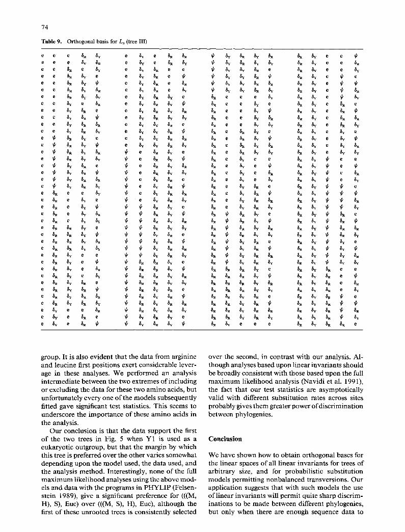
w e n o w t u r n to r o o t e d trees l inking five species. F igure 4 shows three different f ive-species roo t ed trees. A n y o the r f ive-species tree can be ob t a ined b y relabel ing one o f these. Tab les 7 -9 give the or- t h o g o n a l bases for the l inear i nva r i an t spaces o f five- species trees. T h e d i m e n s i o n s o f the l inear i nva r i an t spaces o f trees I, II , a nd I I I are 224, 308, a n d 280, respect ively . Aga in for s impl ic i ty , we o m i t the ® symbo l . D e c o m p o s i t i o n s o f these l inear spaces in to spaces o f i nva r i an t s for one o r m o r e trees, bu t no t others , can be g iven here jus t as we d id for four- species trees. W e o m i t the details.

A p p l i c a t i o n

F o r our appl ica t ion , we use D N A sequences for the large subun i t o f R N A p o l y m e r a s e f r o m Methano-

bacterium thermoautotrophicum (M), Sulfolobus acidocaldarius (S), Halobacterium halobium (H), yeas t (Saccharomyces cerevisiae) p o l y m e r a s e I (Y 1), and yeas t p o l y m e r a s e I I (Y2). These da t a are par t o f those t rea ted by S idow and Wi l son (1990). I n app ly ing l inear inva r i an t s to infer phylogenies , two po in t s shou ld be m a d e clear. First , the n o n b a l a n c e d t r ansve r s ion subs t i tu t ion m o d e l places no con- straints on the probabi l i t ies o f transit ions, apar t f r o m the s e m i g r o u p cons t ra in ts . Thus , any i n f o r m a t i o n a b o u t the phylogenies c o n t a i n e d in t rans i t ion dif- ferences is essential ly ignored. Second, l inear in- va r i an t s exist on ly i f a and /3 are k n o w n cons tants . I f a and/3 are es t imated , t hen the conc lus ion o f any analysis shou ld be checked to be robus t against dif- ferent es t imates o f ~ and/3 .

I f subs t i tu t ions at different sites are i n d e p e n d e n t

71

Table 7. Extended

~R ~Y ~R ~ e ~y e ~R ~R ~R ~R ~Y ~R ~ ~ ~y e ~R ~R ~Y ~R ~Y ~R ~ ~R ~y e ~R ~v e ~R ~Y ~R ~ ~Y ¢~y e ~R ~Y ~R ~Y ~R ~R e av e ~R ~Y ~R ~R ~Y ~R ~R ~ ~y e ~R ~Y ~Y

~R ~Y ~R ~R ~Y ~y e ~Y ~Y ~R ~R ~Y ~ ~v e ~ ~ e ~g ~Y

~" ~Y ~R ~Y ~R ~Y ~ ~ ~R ~Y ~R ~Y ~R ~Y ~Y ~Y ~ ~ ~W ~R ~R ~Y ~W e e ~Y ~ ~R ~R ~Y ~R ~Y ~Y e ~ ~Y ~ ~R ~Y ~R ~R ~Y ~Y e ~S ~Y ~ ~Y ~S ~Y ~R ~v ~v e ~y ~Y ~ ~Y ~Y ~R ~R 5y ~y ~ e ~v ~R e e e ~R ~Y ~Y ~ ~ ~Y ~R e e 6R ~Y ~Y ~ 6R ~Y ~R e e ~R ~R ~Y #Y ~ ~Y ~Y ~z e e ~y ~R ~W ~Y ~R e 6v ~R e ~ e ~R ~Y ~Y ~R ~ ~Y ~S e ~ ~R ~Y ~Y ~R ~R ~Y ~R e ~ ~R ~R ~Y ~Y 6R ~Y ~Y ~R e ~ #v ~R #v 6v ~v e ~v ~R e ~R e ~R ~Y ~V ~Y ~ 6y 6R e ~R 8R ~Y ~Y ~Y 6R ~V ~R e ~R ~R ~R ~Y ~Y ~Y ~Y ~Y ~R e ~R ~Y 6y e e e #R ~g 6R e ~v e ~v e e ~R e ~Y ~R e ~v ~v e e ~R ~Y ~Y ~R e ~Y ~R ~y e e ~y ~R ~Y ~R e ~y ~y ~y e ~ ~R 6y 8y ~a ~ e e

~g e ~R e e ~y ~ ~ e ~s 8v e 6R e ¢ 8Y ~R ~ e ~y 8y e 8R e ~R ~y ~ ~ ~ e

~y e ~R ~ ~R ~Y ~ ~ ~R e

~y e ~R ~R e ~Y ~R ~ ~R ~R ~y e ~R ~R ~ ~Y ~R ~ ~R ~Y

~Y ~R ~ ~Y e

~Y ~R ~R e e ~Y ~R ~g e #g ~R ~a e #a ~g ~R ~R e ~y ~Y ~R ~R ~ e

~v ~R ~R ~ ~v ~V ~R ~R ~R e

~V ~R ~R 6R ~R ~v ~R ~R ~R 6y ~v 6. ~R ~Y e

~v ~a #a #v ~R ~y 6R 6R ~y ~y ~Y ~R ~Y e e ~Y ~R ~ e ~Y ~R ~Y e ~R

~v 6R ~v ~ ~R

~Y ~R ~V ~R e

~Y ~R ~v ~R ~a ~Y ~R ~Y ~R ~Y 6~ ~R ~v ~v e ~Y ~a ~v ~Y ~v ~R ~v ~v ~R ~Y ~R ~Y ~Y ~Y ~y ~y e 6~ ~ 6y ~y e ~v ~a ~Y ~V ~ ~R 6y ~Y ~Y ~ ~Y ~R ~Y ~Y ~R ~R ~Y ~Y ~Y ~R ~Y ~R ~y ~y ~y 6R ~y ~Y ~Y ~Y ~Y ~R

and identically distributed, then the observed spec- t rum y is a mul t inomial r andom variable. The as- ympto t ic distribution o fy 'V(V '~V) -~V 'y is then Xd 2, where V is the 1024 × d matrix whose columns form a basis for the space o f linear invariants used, Z is the usual covariance matrix o f y, and d is the d imension of linear invariant space. In our appli- cation, we estimate ~ by ~ = diag(n151, nl~2, • • . ,

~ /~/1024 + Yi n~1o24), where 15 i = V n + n , and n is the num-

ber o f sites. This is the formula we would get if we had Vrn/1024 prior observations in each cell before our data were collected and is simply the ad hoc use o f a "flattening constant ," cf. G o o d (1965). Cav- ender (1989) and Navid i et al. (1991) est imated by using the projection o f y onto the space o f ex-

pected spectra, but in our application we found that this projection had m a n y negative components and thus was not suitable. I f the substitution process is not identical across sites, then y is a mixture o f multinomials. However, the test statistics still have the same asymptot ic null distribution under these more general assumptions [see Navidi et al. (1992)].

For our data we use the first and second codon positions o f each o f the five sequences ment ioned above. There are 1392 sites, and 375 out o f the 1024 elements o f y are positive. We first apply linear in- variants assuming a balanced transversion model with a = fl = 1. All 105 rooted trees are accepted at the 0.1 significance level. Next we apply linear invariants assuming a nonbalanced transversion

modelwith& = ~ 0.89and~ = =-= 1.16, where 7F C 7F A

72

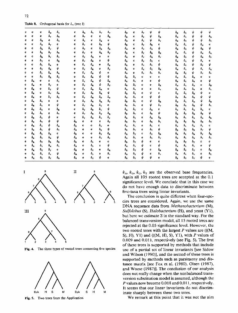
Table 8. Orthogonal basis for Ls (tree I)

e e e ~R ~Y e ~R ~Y ~Y ~Y e e e ~Y ~R e ~y e e ~R e e ~a e ~y e ~y e ~ e e e 8a ~y e e ~y e ~. e e ~R ~v ~ e ~y e ~ ~R e e ~R ~Y ~R e ~y e ~R (~Y e e ~ ~y ~y e ~v 8a e e e e 8~ e ~R e ~Y ~R e e e ~ ~a e e ~y ~R e ~a e e ~ ~R ff e ~Y ~R e ~y e e ~ ~R ~R e ~ 6. ~ e

e e ~Y ~R 8y e 8y ~R ~ e ~. e e ~y e ~y ~a 6 ~R e ~ e ~y e e ~ ~a ~ ~ e 8s e ~ ~ e ~y ~R ~a e e ~a e ~Y ~a e ~y ~a ~ e ~ e ~y ~y e ~i ~R ~R ~R e ~ ~y e e e ~Y ~S ~ ~Y e ~ ~y e ¢ e ~y ~ ~y e e ~R ~Y e ~ e ~y ~ ~ e ~R ~v e 6y e ~Y ~R ~Y ~R e ~R ~Y ~ e e ~y ~a ~ ~g e ~R ~Y ~ ~ ~R e e e ~y e ~ ~y ~ ~R ~R e e ~ e e ~R ~Y ~ ~Y ~R e e ~y e ~R (~y 6 R e ~ e e ~y 6~ e ~R ~y ~R ~ ~R e e ~y ~y e ~R ~y ~R ~R ~R e ~ e e e ~R ~Y ~R ~Y ~R e ~y e e ~R ~Y ~ e ~ e ~v e ~R

e ~R ~ ~y ~R ~. e ~ ¢ e

~R e ~ ~ ~ ~ ~ ~ ~ ~. e ~Y ~R ~R ~R ~Y ~ ~R ~R

~s e ~y ~y e ~R ~V ~ ~Y e

~R e ~Y ~Y ~R ~R ~Y ~ ~Y ~R ~R e ~Y ~Y ~Y ~R ~Y ~ ~Y ~Y ~R ~y e e e 6R ~Y 6R e e ~R ~Y e e ~ ~R ~Y ~R e ~R ~y e e ~ ~R ~v ~g e ~R ~R ~y e e ~ ~R ~y ~R e

6R ~Y e ~ e ~R ~Y ~ ~ e ~R ~ e ~ ~ ~R (~Y ~R ~

~R ~Y e ~a e ~R ~Y ~R ~R e ~ ~ e ~. ~ ~R ~Y ~R ~R ~s ~Y e ~ ~R ~R 6y 8 R ~R 6R ~R 6y e 6a 6 v ~a ~Y 8R ~R 6y ~R ~Y e ~g e #R ~Y ~R ~Y e

8~ ~y e 8y ~ 8R 8y ~R 8y ~R 8y e 6Y ~R 8R ~ ~R ~Y ~R ~R ~Y e ~Y ~ ~S ~Y ~a ~Y ~Y ~ ~y ~ e e ~ ~y ~g e e ~R ~Y ~ e ~ ~R ~Y ~Y e ~a ~Y ~ e ~R ~R ~Y ~Y e ~S ~a 6y ~ e ~v ~R ~Y 6y e ~y ~a ~ ~ ~ e ~ ~y ~ ~ e

I 9

1 2 3 4 5

II 9

1 2 3 4 5

III 9

1 2 3 4 5

Fig. 4. The three types o f rooted trees connecting five species

Euk H S M Euk S H M

Fig. 5. Two trees f rom the Applicat ion

~A, ~G, ~C, 7rT are the observed base frequencies. Again all 105 rooted trees are accepted at the 0.1 significance level. We conclude that in this case we do not have enough data to discriminate between five-taxa trees using linear invariants.

The conclusion is quite different when four-spe- cies trees are considered. Again, we use the same D N A sequence data f rom Methanobacterium (M), Sulfolobus (S), Halobacterium (H), and yeast (Y1), but here we estimate ~ in the s tandard way. For the balanced t ransversion model , all 15 rooted trees are rejected at the 0.05 significance level. However , the two rooted trees with the largest P values are (((M, S), H), Y1) and (((M, H), S), Y1), with P values o f 0.009 and 0.011, respectively (see Fig. 5). The first o f these trees is supported by methods that include use o f a partial set o f linear invariants [see Sidow and Wilson (1990)], and the second o f these trees is supported by methods such as pars imony and dis- tance matr ix [see Fox et al. (1980), Olsen (1987), and Woese (1987)]. The conclusion of our analysis does not really change when the nonbalanced trans- version substi tut ion model is assumed, although the P values now become 0.018 and 0.011, respectively. It seems that our linear invariants do not discrim- inate sharply between these two trees.

We remark at this point that it was not the aim

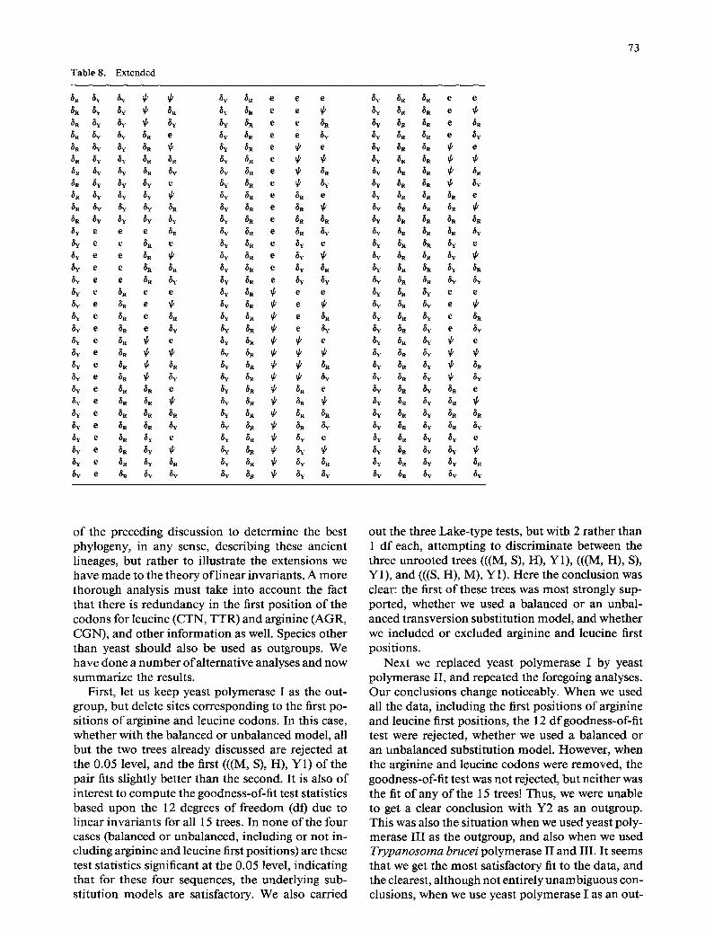
Table 8. Extended

~R ~Y ~Y ~ ~ ~Y ~R e e ~R ~Y ~Y ~ ~R ~Y #R e e ~R ~Y ~Y ~ ~Y ~Y ~R e e ~R ~Y ~Y ~R e ~g ~R e e ~a ~Y ~Y ~R ~ ~y 6R e ~R ~Y ~Y ~R ~R ~Y ~R e ~R ~Y ~Y ~R ~Y ~Y ~R e ~R ~Y ~y ~Y e ~Y ~R e ~R ~Y ~Y ~Y ~ ~V ~R e ~R ~R ~V ~Y ~Y ~R ~y 6R e ~. ~R ~Y ~Y ~Y ~Y ~Y ~R e ~R ~y e e e ~R ~Y 6R e ~a 6g e e ~R e ~y ~. e ~ 6y e e ~. ¢ ~Y ~R e ~y 6v e e ~R ~a ~Y ~R e ~ #y e e ~R ~Y ~Y ~R e ~ 6y e #R e e ~y ~ ~ e #~ e ~ e ¢ ~y ~R ¢ e #y e ~R e #R ~Y ~R ~ e ~y e ~R e ~y ~ ~R ~ e ~y e ~R ~ e ~Y ~R ~ #y e ~R ¢ ¢ ~ ~R ¢ ~y e 6R ~ ~R ~Y ~R ~

~y e ~R ~s e ~Y #a ~ ~a ~v e ~R ~S ~ ~g ~R ~ ~R ~y e ~R ~R ~R ~Y ~R ~ ~R ~ e ~ ~R ~ ~Y ~ ¢ #R ~y e ~R ~Y e ~y ~ ~ ~y #y e ~a 6y ~ ~Y ~R ~ 6y ~y e ~a #y ~a ~y ~ ~ ~y 8~ e ~R ~Y ~Y ~Y ~R ~ ~Y

e ~Y ~R ~R e e

~R ~Y ~a ~R e ~R ~Y ~Y ~R ~R e ~y e ~Y ~R ~R ~ e

e ~Y ~a ~a ~a e

~a #g ~a ~a ~a #R ~y 6y ~R ~R ~R 6y e ~Y ~R ~R ~Y e

~R ~Y ~Z ~a ~Y ~R

e ~Y ~R ~v e e ~v ~ ~v e

~R ~y 6R ~ e ~a ~Y ~Y ~a ~Y e ~g e ~Y #~ #v ~ e

~Y ~R ~Y ~ ~R ~Y ~R ~W ~ ~R

e ~Y ~R ~Y #R e ~Y ~R ~Y ~R

~R ~Y ~s ~Y ~R ~R ~Y ~Y ~R ~ ~R ~Y e ~Y ~R ~Y ~Y e

~Y ~R ~Y ~Y ~R ~Y ~R ~Y ~Y ~R ~Y ~Y ~R ~Y ~Y ~V

73

o f the preceding discussion to de te rmine the best phylogeny, in any sense, describing these ancient lineages, but ra ther to illustrate the extensions we have m a d e to the theory o f l inear invariants . A m o r e thorough analysis mus t take into account the fact that there is r edundancy in the first posi t ion o f the codons for leucine (CTN, T T R ) and arginine (AGR, CGN) , and other in fo rmat ion as well. Species other than yeast should also be used as outgroups. We have done a n u m b e r o f a l ternat ive analyses and now s u m m a r i z e the results.

First, let us keep yeast po lymerase I as the out- group, but delete sites corresponding to the first po- sitions o f arginine and leucine codons. In this case, whether with the balanced or unbalanced model , all but the two trees already discussed are rejected at the 0.05 level, and the first (((M, S), H), Y1) o f the pair fits slightly bet ter than the second. I t is also o f interest to compu t e the goodness-of-f i t test statistics based upon the 12 degrees o f f reedom (dO due to l inear invar iants for all 15 trees. In none o f the four cases (balanced or unbalanced, including or not in- cluding arginine and leucine first posit ions) are these test statistics significant at the 0.05 level, indicating that for these four sequences, the underlying sub- st i tution models are satisfactory. We also carried

out the three Lake- type tests, but with 2 ra ther than 1 d f each, a t tempt ing to d iscr iminate between the three unroo ted trees (((M, S), H), Y1), (((M, H), S), Y1), and (((S, H), M), Y1). Here the conclusion was clear: the first o f these trees was mos t strongly sup- ported, whether we used a balanced or an unbal- anced t ransvers ion subst i tut ion model , and whether we included or excluded arginine and leucine first posit ions.

Next we replaced yeast po lymerase I by yeast po lymerase II, and repeated the foregoing analyses. Our conclusions change noticeably. When we used all the data, including the first posi t ions o f arginine and leucine first posit ions, the 12 dfgoodness-of - f i t test were rejected, whether we used a balanced or an unba lanced subst i tut ion model . However , when the arginine and leucine codons were r emoved , the goodness-of-f i t test was not rejected, but nei ther was the fit o f any o f the 15 trees! Thus, we were unable to get a clear conclusion with Y2 as an outgroup. This was also the si tuat ion when we used yeast poly- merase I I I as the outgroup, and also when we used Trypanosoma bruce/polymerase I I and III . I t seems that we get the m o s t sat isfactory fit to the data, and the clearest, a l though not entirely unambiguous con- clusions, when we use yeast po lymerase I as an out-

74

Table 9. Orthogonal basis for L5 (tree III)

e e e ~a ~ e ~y e ~R ~R e e e ~ ~R e ~v e ~R ~Y e e ~R e 5y e 6Y ~R e e e e ~R ~v e e 6y 5R e e e ~R ~Y ~ e ~y ~R e ~R e e ~R SY ~R e ~Y ~R e ~y e e ~. ~y 6y e 6Y 6R ~Y e e e ~v e ~R e ~y ~R ~Y e e ~y ~s e e ~Y ~R ~V 6R e e ~Y ~R ~ e ~Y ~R ~Y ~Y e e ~Y ~a ~a e ~Y ~Y ~R e e e ~Y ~R ~Y e ~Y ~Y ~R e ~ 6s ~ e e ~y ~y ~R ~R e ~ ~R ~Y ~ e (~Y ~Y ~R ~Y e ~ ~R ~Y ~R ~ e ~s ~y e e ~ ~R ~Y ~w ~ e ~s ~w e ~ ~Y ~R e ~ e ~a 6Y ~a

e ~ ~Y #R ~a ~ e ~ ~R e e ~ ~Y #R ~V ~ e ~ ~a e ~R e e ~v ~ e ~ ~a ~R e 6 R e ~y e ~ e ~Y ~R ~v e 6a e ~Y ~ ~ ~ ~R 5Y e e 6R e ~Y ~R ~ ~ ~R ~Y

e ~R ~R ~Y e ~ ~ ~R ~y ~y e ~R ~R ~Y ~ ~ ~ ~V ~R e e ~ ~R ~Y ~R ~ ~ ~V ~R e ~R ~R ~Y ~Y ~ ~ ~Y ~R ~R e ~R #Y e e ~ ~ ~Y ~t ~Y e ~. ~y e ~ ~ ~. ~R ~ e e ~R ~ e ~R ~ ~R ~a ~Y e ~R ~Y e ~ ~ 6R ~R ~Y ~R e ~R ~ ~R e ~ ~R ~R ~Y ~Y e ~R ~ ~R ¢ ¢ ~R ~Y ~Z e e ~R ~ ~R ~R ~ ~R ~Y ~R

e ~ e e ~. ~ ~Z ~ ~R ~Y e ~y e ~S e ~ ~Y ~R ~Y e e ~y e ~R ~ 6 ~Y ~R ~Y

G 6~ ~ ~s ~R ~ e e ~Y ~s ~Y ~ ~a ~Y e e ~R ~Y ~Y ~R e ~a ~Y e e ~y ~y ~y 6R ~ ~R ~ e ~ e

6R e e e ~ ~R ~ e ¢ ~v ~ e e ~y e ~R ~Y e ~ e

6R e e 5Y ~R ~R ~V e ~R ~R 6~ e e 5Y ~v ~R ~Y e ~R 6V ~ e 6~ ~y e ~R ~Y e ~y e ~R e ~R ~Y ~ ~ ~y e ~y ~ e ~n ~Y ~R ~R 6~ e ~ ~R ~R e 6~ ~y ~ ~ ~ e ~y ~ ~R e 6v e e ~n 6Y ~ e e 6a e 5~ e ~ ~R ~V ¢ e

6a e 6y e ~ ~ ~ ~ e ~ ~R e ~ ~R e ~. ~ ~ ~ e

~R e ~Y ~R ~R ~R ~Y ~ ~ 6R ~R e ~Y ~R ~Y ~R ~Y ~ ~ ~Y ~R ~ ~R ~Y e ~R ~Y ~ ~R e ~R ~ ~ ~ ~ ~R ~ ~ ~R ~R ~ ~Z ~Y ~R ~R ~Y ~ ~R ~Z ~R ~ ~R ~Y ~Y ~R ~Y ~ ~R (~Y ~. ¢ ~ ~. e ~ ~y ¢ t~ e

~R ~ ~Y ~S ~t ~R ~Y ~ ~Y ~R

~g ~R ~R ~Y e ~R ~Y 8R e e ~R ~R 8R ~Y ~ ~R ~Y ~R e ~R ~R ~R ~Y ~a ~t ~Y ~R e ~R ~R ~R ~R ~Y ~Y ~R ~ ~. e ~ ~R ~R ~Y ~R e ~R ~ ~ ¢ e ~R ~R ~ ~R ~ ~R ~ ~R ~ ~R ~R ~Y ~R ~R ~R ~Y ~R ~ ~R ~R ~R ¢~ ~R ~Y ~R ~Y ~R ~ ~Y ~R ~Y e e e 6s 6~ ~R ~ e

group. It is also evident that the data f rom arginine and leucine first posit ions exert considerable lever- age in these analyses. We performed an analysis intermediate between the two extremes of including or excluding the data for these two amino acids, but unfortunately every one o f the models subsequently fitted gave significant test statistics. This seems to underscore the impor tance o f these amino acids in the analysis.

Our conclusion is that the data support the first o f the two trees in Fig. 5 when Y1 is used as a eukaryotic outgroup, but that the margin by which this tree is preferred over the other varies somewhat depending upon the model used, the data used, and the analysis method. Interestingly, none of the full m a x i m u m likelihood analyses using the above mod- els and data with the programs in P H Y L I P (Felsen- stein 1989), give a significant preference for (((M, H), S), Euc) over (((M, S), H), Euc), al though the first o f these unrooted trees is consistently selected

over the second, in contrast with our analysis. Al- though analyses based upon linear invariants should be broadly consistent with those based upon the full m a x i m u m likelihood analysis (Navidi et al. 1991), the fact that our test statistics are asymptotically valid with different substitution rates across sites probably gives them greater power o f discrimination between phylogenies.

C o n c l u s i o n

We have shown how to obtain orthogonal bases for the linear spaces of all linear invariants for trees o f arbitrary size, and for probabilistic substitution models permitt ing nonbalanced transversions. Our application suggests that with such models the use o f linear invariants will permit quite sharp discrim- inations to be made between different phylogenies, but only when there are enough sequence data to

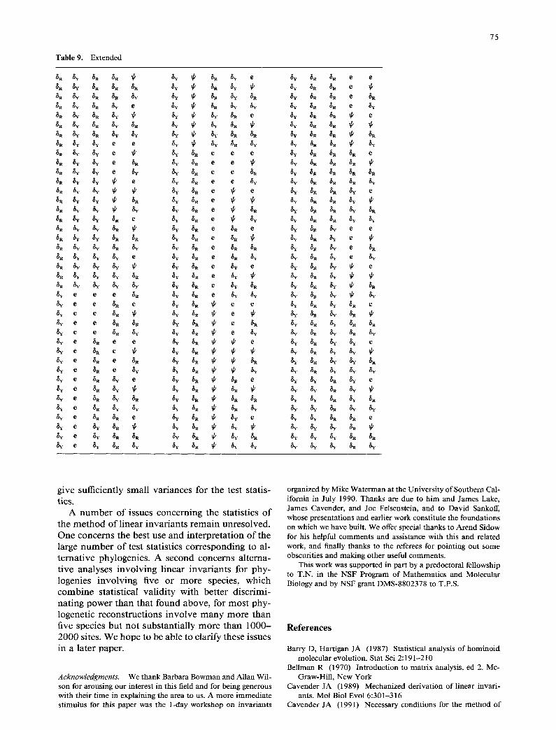
Table 9. Extended

~R ~Y ~R ~R ~ ~Y ~ ~R ~Y e ~R ~Y ~R ~R ~R ~Y ~ ~R ~Y

~ ~y ~ #~ e ~v ¢ ~ ~g ~y ~R ~Y ~R ~Y ~ ~y ~ ~v #~ e ~R ~Y ~R ~Y ~R ~Y ~ ~Y ~S ~R ~Y ~R ~Y ~Y ~g ~ ~Y ~a ~R ~R 6y ~y e e ~v ~ ~Y ~R ~Y ~R ~Y ~Y e ~ ~Y 6a e e e ~a ~Y ~Y e ~R ~g ~R e e

~R ~Y ~Y ~ e ~Y ~R e e ~y ~R ~Y ~Y ~ ~ ~Y 6R e ~ e ~R ~Y ~Y ~ 6R 6y ~R e ~ 6 R ~V ~V ~ ~V 6y 6R e ~ 6R ~R ~Y ~Y ~R e ~Y ~R e ~ ~y ~R ~Y ~Y ~R ~ ~Y ~R e ~R e ~R ~Y ~Y ~R ~R ~Y ~S e #a ~R ~Y ~Y ~R ~Y ~y ~a e 6a ~a ~R ~Y ~Y ~Y e 6Y ~a e 63 6. 8a ~v ~v 8y ~ 6y 6R e ~y e 6R ~Y ~Y ~Y ~R ~y 6R e ~y 6R 6Y ~V ~V ~V 6y ~R e 6y ~R ~V e e e ~R ~Y ~R e 6v 6y ~y e e ~R e ~v ~R ~ e e ~y e e ~R ~ ~Y ~R ~ e ~y e e ~s ~ ~w ~ ~ e ~ ~v e e ~R 6v 6v 6R ~ e ~v ~y e ~R e e ~Y ~R ~ ~ e ~y e ~R e ~ ~Y ~R ~ ~ ~y e ~R e ~R ~W ~R ~ ~ ~R ~y e ~R e ~y ~w ~R ~ ~ ~Y 8y e ~R ~Y e ~v ~R ~ ~R e ~y e ~a ~v ~ ~y ~ ~ ~s ~y e ~ ~Y ~R ~Y ~R ~ ~R ~R ~v e ~a ~Y ~Y ~Y ~R ~ ~R ~Y #y e ~a ~R e ~Y ~R ~ ~V e ~y e ~v ~R ~ ~Y ~R ~ ~Y ~v e ~v ~R ~R ~v ~R ~ ~v 6R ~y e 6y ~R ~Y 8y ~R ~ ~Y 6y

~Y ~R ~R e e ~Y ~R ~R e ~g ~R ~a e ~R ~Y ~a ~R e ~y ~Y ~R ~ ~ e ~ ~R ~R ~ ~Y ~R ~R ~ ~R ~g ~R ~R ~ ~Y 6y ~R ~R ~R e ~Y 6R ~R ~R ~v ~a ~a #a ~R 6v 63 63 ~a ~v ~Y 6R ~S ~Y e

~Y ~R ~R ~Y ~R 6y ~ ~R ~V ~V ~Y ~R ~Y e e ~Y ~R ~Y e #Y ~R ~Y e 6R ~Y ~R ~Y e ~y ~Y ~R ~Y ~ e ~Y ~R ~Y ~

~Y ~g 6y ~ ~y ~Y ~R ~Y ~R e

~Y ~R ~Y ~R ~R ~Y ~R ~Y ~R ~Y ~Y ~R ~Y ~Y e ~Y ~R ~Y ~Y ~Y ~R ~Y ~Y 6R ~Y ~R ~W ~Y ~Y ~Y ~Y ~a ~Y e

~Y ~Y ~R ~V ~R 6~ ~y ~R ~v ~Y 6Y ~v ~R ~R e ~V ~Y ~Y ~R

~Y ~Y ~v ~R ~v

75

give sufficiently smal l va r i ances for the test statis-

tics. A n u m b e r o f issues c o n c e r n i n g the stat is t ics o f

the m e t h o d o f l inear i n v a r i a n t s r e m a i n un reso lved .

O n e conce rns the bes t use a n d i n t e r p r e t a t i o n o f the

large n u m b e r o f test s tat is t ics c o r r e s p o n d i n g to al- t e r n a t i v e phylogenies . A second conce rns a l t e rna-

t ive ana lyses i n v o l v i n g l inea r i n v a r i a n t s for phy-

logenies i n v o l v i n g five or m o r e species, wh ich c o m b i n e s ta t is t ical va l id i ty wi th be t te r d i s c r imi -

n a t i n g power t h a n tha t f o u n d above , for m o s t phy- logenet ic r e cons t ruc t i ons i n v o l v e m a n y m o r e t h a n

five species b u t n o t subs t an t i a l l y m o r e t h a n 1 0 0 0 - 2000 sites. We hope to be able to clarify these issues in a la ter paper .

Acknowledgments. We thank Barbara Bowman and Allan Wil- son for arousing our interest in this field and for being generous with their time in explaining the area to us. A more immediate stimulus for this paper was the 1-day workshop on invariants

organized by Mike Waterman at the University of Southern Cal- ifornia in July 1990. Thanks are due to him and James Lake, James Cavender, and Joe Felsenstein, and to David Sankoff, whose presentations and earlier work constitute the foundations on which we have built. We offer special thanks to Arend Sidow for his helpful comments and assistance with this and related work, and finally thanks to the referees for pointing out some obscurities and making other useful comments.

This work was supported in part by a predoctoral fellowship to T.N. in the NSF Program of Mathematics and Molecular Biology and by NSF grant DMS-8802378 to T.P.S.

R e f e r e n c e s

Barry D, Hartigan JA (1987) Statistical analysis of hominoid molecular evolution. Stat Sci 2:191-210

Bellman R (1970) Introduction to matrix analysis, ed 2. Mc- Graw-Hill, New York

Cavender JA (1989) Mechanized derivation of linear invari- ants. Mol Biol Evol 6:301-316

Cavender JA (199l) Necessary conditions for the method of

76

inferring phylogeny by linear invariants. Math Biosci 103:69- 75

Evans SN, Speed TP (1992) Invariants of some probability models used in phylogenetic inference. Ann Star (in press)

Felsenstein J (1981) Evolutionary trees from DNA sequences: a maximum likelihood approach. J Mol Evol 17:368-376

Felsenstein J (1989) Phylogenetic inference programs (PHY- LIP) manual, version 3.2. University of Washington, Seattle

Fox GE, Stackenbrandt E, Hespell RB, Gibson J, Maniloff J, Dyer JA, WolfRS, Balch WE, Tanner RS, Magrum L J, Zahlen LB, Blakemore R, Gupta R, Bonen L, Lewis BJ, Stahl DA, Luehrsen KR, Chert KH, Woese CR (1980) The phylogeny of prokaryotes. Science 209:457-463

Good IJ (1965) The estimation of probabilities: an essay on modem Bayesian methods. MIT Press, Cambridge MA

Hasegawa M, Kishino H, Yano T (1985) Dating of the human- ape splitting by a molecular clock of mitochondrial DNA. J Mol Evol 22:160-174

JukesTH, CantorC (1969) Evolution ofproteinmolecules. In: Munro HN (ed) Mammalian protein metabolism. Academic Press, New York, pp 21-132

KimuraM (1980) A simple method for estimating evolutionary rates of base substitution through comparative studies of nu- cleotide sequences. J Mol Evol 16:111-120

Kimura M (1981) Estimation of evolutionary sequences be- tween homologous nucleotide sequences. Proc Natl Acad Sci USA 78:454--458

Kimura M (1983) The neutral theory of molecular evolution. Cambridge University Press, Cambridge

Lake JA (1987) A rate-independent technique for analysis of

nucleic acid sequences: evolutionary parsimony. Mol Biol Evol 4:167-191

Navidi W, Churchill GA, yon Haeseler A (1991) Methods for inferring phylogenies from nucleic acid sequence data by using maximum likelihood and linear invariants. Mol Biol Evol 8: 128--43

Navidi W, Churchill GA, yon Haesler A (1992) Phylogenetic inference: linear invariants and maximum likelihood. Bio- metrics (in press)

Neyman J (1971) Molecular studies of evolution: a source of novel statistical problems. In: Gupta SS, Yackel J (eds) Sta- tistical decision theory and related topics. Academic Press, New York, pp 1-27

Olsen GJ (1987) Earliest phylogenetic branchings: comparing rRNA-based evolutionary trees inferred with various tech- niques. Cold Spring Harbor Syrup Quant Biol 52:825-837

Sidow A, Wilson AC (1990) Compositional statistics: an im- provement of evolutionary parsimony and its application to deep branches of the tree of life. J Mol Evol 31:51-68

Swofford DL, Olsen GJ (1990) Phylogeny reconstruction. In: Hillis DM, Moritz C (eds) Molecular systematics. Sinauer Associates, Sunderland MA, pp 411-501

Tavar6 S (1986) Some probabilistic and statistical problems in the analysis of DNA sequences. In: Miura R (ed) Lectures on mathematics in the life sciences. American Mathematical Society, Providence RI, lap 57-86

Woese CR (1987) Bacterial evolution. Microbiol Rev 51:221- 271

Received July 24, 1991/Revised and accepted February 21, 1992