A congestion model for cell migration

arX

iv:1

102.

0147

v1 [

mat

h.N

A]

1 F

eb 2

011

Manuscript submitted to Website: http://AIMsciences.orgAIMS’ JournalsVolume X, Number 0X, XX 200X pp. X–XX

A CONGESTION MODEL FOR CELL MIGRATION

Julien Dambrine and Nicolas Meunier

MAP5, UFR de Mathematiques et InformatiqueUniversite Paris Descartes, 45 rue des Saints-Peres, 75270 Paris Cedex 06

Bertrand Maury and Aude Roudneff-Chupin

Laboratoire de Mathematiques d’Orsay, Universite Paris-Sud, 91405 Orsay Cedex

(Communicated by the associate editor name)

Abstract. This paper deals with a class of macroscopic models for cell mi-gration in a saturated medium for two-species mixtures. Those species tend toachieve some motion according to a desired velocity, and congestion forces themto adapt their velocity. This adaptation is modelled by a correction velocitywhich is chosen minimal in a least-square sense. We are especially interestedin two situations: a single active species moves in a passive matrix (cell migra-tion) with a given desired velocity, and a closed-loop Keller-Segel type model,where the desired velocity is the gradient of a self-emitted chemoattractant.

We propose a theoretical framework for the open-loop model (desired ve-locities are defined as gradients of given functions) based on a formulation inthe form of a gradient flow in the Wasserstein space. We propose a numericalstrategy to discretize the model, and illustrate its behaviour in the case of aprescribed velocity, and for the saturated Keller-Segel model.

1. Introduction, modelling aspects. We propose a model to handle interactionsbetween organisms such as unicellular organisms e.g. bacteria or amœbia. The be-havior of an entity is based on a will to move with its desired velocity, regardless ofothers, but the fulfillment of individual wills is made impossible because of conges-tion. We consider here the case of two organisms (see Section 4 for a straightforwardextension to several populations). We describe the densities by measures ρ1 and ρ2.We assume global saturation of the domain, i.e. ρ1 + ρ2 = 1. In order to take intoaccount the individual tendencies together with congestion constraints, we considerthat individuals have two velocities, namely a desired velocity that will be denotedby U1 (resp. U2) and a common correction velocity that will be denoted by w.Densities ρ1 and ρ2 satisfy:

∂tρi +∇ · (ρi (Ui +w)) = 0 i = 1, 2. (1)

We consider the correction velocity which minimizes L2 norm among all those ve-locity fields which ensure preservation of the saturation constraint ρ1 + ρ2 = 1,which can be expressed in a dual, Darcy-like, form:

w +∇p = 0∇ ·w = −∇ · (ρ1U1 + ρ2U2) .

(2)

2000 Mathematics Subject Classification. Primary: 58F15, 58F17; Secondary: 53C35.Key words and phrases. Congestion, Chemotaxis, Aggregation, Optimal transport.The first and second authors are supported by the European Project ARTreat FP7 - 224297.

1

http://arxiv.org/abs/1102.0147v1

2 FIRST-NAME1 LAST-NAME1 AND FIRST-NAME2 LAST-NAME2

This basic model corresponds to a competition between two species which tendto achieve a prescribed motion, and realize a sort of compromise. We shall beespecially interested in the following situations:

(i) Competition between species which tend to minimize a given function: Ui isdefined as −∇Di, with ρ1U1 + ρ2U2 not feasible (i.e. leading to violation ofthe saturation constraint) in general. This setting, which extends the modelproposed in [11] to a two-population situation with distinct tendencies, shallbe the core of the theoretical analysis proposed in section 2.

(ii) Desired velocity for species 2 is zero, and U1 is prescribed as the gradient ofa given function S (concentration of a chemoattractant). Note that this case,which corresponds to the migration of cells in a passive biological matrix, asencountered in the developpment of atherosclerosis, is a particular case of (i).

(iii) Keller-Segel model with congestion (closed-loop version of the basic model):U2 is again 0, andU1 is defined as∇S, where S is a chemotactic agent createdby the species 1 itself. Assuming S diffuses in the mixture domain, we shallconsider

∂tS −∆S = ρ1,

or, assuming diffusion is instantaneous, −∆S = ρ1.

The question of boundary conditions rises delicate issues. Setting equation inthe whole space amounts to deal with infinite quantities of 1 and/or 2 (the sum ofdensities is equal to 1), which rules out standard tools for theoretical analysis andnumerical simulation. One may consider that both populations occupy a bounded,moving domain Ω(t), on the boundary of which pressure is zero. It is then naturalto consider that the boundary of Ω moves with a normal velocity which identifiesto the normal velocity of the mixture (ρ1U1 + ρ2U2 + w) · n. This approach issurely relevant in some situations, yet we shall not consider it in this paper. Letus give an idea of one of the difficulties which are likely to occur: consider themonodimensional situation with initial condition and desired velocities:

ρ1 = 1(0,1) , ρ2 = 1(−1,0) , U1 = 1 , U2 = 0.

Translation of those intervals at constant speed 1/2 is obviously a solution to ourproblem (with piecewise affine pressure, 0 at both ends, 1/2 at the interface). Nowconsider the scenario where 1 runs away with velocity 1, and 2 stays where it is(both species are separated, and the domain Ω(t) is no longer convex). One caneven imagine that half of 1 (initially located in 1(1/2,1)) takes off with velocity 1,while the other half of 1 trails 2 at speed 1/3. In this spirit, one can create aninfinite number of scenarios which all seem to be, in a reasonable sense, solutions toour problem. Note that those problems are likely to occur in the case of expansionfields, as the one considered previously, because of the loss of monotonicity of theunderlying evolution equation.

Another approach consists in considering a fixed domain Ω, delimited by rigidwalls. This assumption is reasonable if one considers migration phenomena in livingorganisms. The boundary condition for Darcy equations is of Neumann type: no-flux condition at walls leads to (ρ1U1 + ρ2U2 +w) · n = 0, i.e.

∂p

∂n= (ρ1U1 + ρ2U2) · n.

This condition ensures no-flux for the mixture, but not for both species indepen-dently; it may allow some out- or in-flux of either 1 or 2, which calls for further

A CONGESTION MODEL FOR CELL MIGRATION 3

prescriptions on the boundary. The situations we shall consider in next sectionssuggest that, at least in the case U2 = 0, the model tends to create pure zones (ei-ther 1 only, or no 1 at all) in the neighbourhood of boundaries. As a consequence,global no flux conditions turn into no flux conditions for both species. Yet, in 2 or 3dimensions and for non zero desired velocities, one may have to consider more gen-eral situations. To overcome those difficulties, we shall consider in the theoreticalpart (Section 2) the fully periodic setting.

In a different context, such saturated two-component mixtures have been studiedin [13], with a motion driven by chemical potentials. In the biological context, aKeller-Segel model with logistic sensitivity (KSLS) has been proposed recently [6, 4].This KSLS model reads

∂tρ+∇ · (ρ (1− ρ)U) = 0, (3)

where the “desired” velocity U is of the chemotactic type:

U = ∇S , ∂tS −∆S = ρ.

First of all, in one dimension (say Ω = (0, 1)) with no-flux boundary conditionsat x = 1, our model reads

∂tρ+ ∂x (ρ(U − ∂xp)) = 0 ,

−∂xxp = −∂x(ρU)

with (no flux condition) ρU − ∂xp = 0 at 1, so that ∂xp = ρU in the whole interval,and therefore it identifies exactly with KSLS. Note that in case the velocity is givenand constant, we recover an inviscid Burgers equation.

Both models are different for d ≥ 2. Yet, they present some common structurewhich can be described as follows: consider (situation (iii) above) the case of zerovelocity for species 2, and velocity for 1 given as the gradient of a density S ofchemoattractant created by 1 itself. We consider the biperiodic setting, and de-fine ∆−1 as the operator which maps a function g with zero mean value over thebiperiodic domain onto the zero mean value solution to

∆u = g.

The pressure in our model can then be written p = ∆−1∇ · (ρU), so that transportequation for species 1 becomes

∂tρ+∇ ·(

ρ(

U−∇∆−1∇ · (ρU)))

= 0.

which is formally equivalent to KSLS model (3) with identity operator replaced byHelmoltz projection∇∆−1∇· (projection onto the space of irrotational fields). Non-locality of the latter operator differentiate both models. Yet both PDE’s systemsare quite similar from the spectral point of view.

As for modelling aspects, they rely on different assumptions: KSLS model canbe seen as standard KS model with a reduced velocity U = (1 − ρ)∇S, which canexpress for example the fact that when entities reach some critical density (set to1 here), they disturb each other and are no longer able to sense the underlyinggradient. In our approach, we consider that entities continue to exert some actionwhich would lead them in the right direction if they were alone, but they are (me-chanically) prevented from fulfilling their purpose, because of the presence of otherentities (possibly with different “strategies”). The model is in some way less con-strained as motion of saturated zones is possible, but also more constrained because


the other species (which replaces empty space in KSLS) has to be swept away, atsome price, by species 1.

2. Theoretical framework. We consider in this section the case of 2 species inthe flat torus Ω = S1 × S1, with desired velocities prescribed as follows

U1 = −∇D1, U2 = −∇D2,

where D1 and D2 are given smooth functions over Ω. The system corresponding tothis situation writes

∂tρ1 +∇ · (ρ1(U1 +w)) = 0

∂tρ2 +∇ · (ρ2(U2 +w)) = 0

w = −∇p

−∆p = −∇ · (ρ1U1 + ρ2U2).

(4)

Although concentrations for both species automatically admit a density whichis in L∞ (thanks to the congestion constraint), we shall keep the general settingof measures, which is usually adopted in optimal transport, and which allows forgeneralisations (e.g. relaxing the congestion constraint in some zones). Besides,we disregard normalization to obtain probability measures: we shall consider thatρ1⊗ρ2 belongs to P(Ω×Ω), although the total mass is not 1. Similarly, we considerthat ρi ∈ P(Ω).

In what follows, regularity of functions defined over Ω accounts for periodicconditions. In particular H1(Ω) is defined as the set of biperiodic functions withH1 regularity (closure for the H1 norm of biperiodic regular functions).

Definition 2.1 (Weak solutions). We say that (ρ1, ρ2) is a weak solution of (4)with initial condition (ρ01, ρ

02) if ρ1 + ρ2 = 1 for a.e. t, and if there exists p ∈ H1(Ω)

such that for all ϕ1, ϕ2 ∈ C∞c ([0, T [×Ω), for a.e. t ∈ (0, T ), and for all q ∈ H1(Ω),

we have∫ T

0

∫

Ω

(∂tϕ1 +∇ϕ1 · (U1 −∇p)) dρ1 +

∫

Ω

ϕ1(0, .)dρ01 = 0

∫ T

0

∫

Ω

(∂tϕ2 +∇ϕ2 · (U2 −∇p)) dρ2 +

∫

Ω

ϕ2(0, .)dρ02 = 0,

∫

Ω

∇p · ∇q =

∫

Ω

∇q ·U1 dρ1 +

∫

Ω

∇q ·U2 dρ2.

Let ρ = ρ1⊗ρ2 for a.e. t, U = (U1,U2). We can rewrite the previous formulationas follows: for all ϕ ∈ C∞

c ([0, T [×(Ω× Ω))∫ T

0

∫

Ω×Ω

(∂tϕ+ 〈U− (∇p,∇p),∇ϕ〉) dρ +

∫

Ω×Ω

ϕ(0, .) dρ0 = 0.

and for a.e. t ∈ (0, T ), all q ∈ H1(Ω),∫

Ω

∇p · ∇q =

∫

Ω×Ω

〈(∇q,∇q),U〉 dρ.

Let us state the main result of this section:


Theorem 2.2 (Existence of a solution). If D1 and D2 are Lipschitz functions, and(ρ01, ρ

02) positive measures that satisfy ρ01 + ρ02 = 1 a.e., then equation (4) admits at

least a weak solution, according to definition 2.1.

The proof of this theorem relies on the notion of gradient flow in the Wassersteinspace (see e.g. [1]). Theoretical analysis of a similar problem in the context of crowdmotions was proposed in [11]. The proof proposed therein is quite general, and thesame approach could be carried out in the present context. Yet, to avoid sometechnicalities and to give a clearer view of the underlying gradient flow structure,we propose here an alternative approach which is directly based on the main exis-tence and characterization theorems in [1]. The rest of this section describes themain outlines of this approach, which is based on theories of optimal transport andgradient flows, which we will use to prove theorem 2.2. For more details, see thebooks of Villani [17], [18], and Ambrosio et al. [1], [2]. See also the recent appli-cation of this framework [7] to recover entropic solutions to the Burgers’ equation(which identifies in some way to the proposed model for d = 1, as pointed out inthe introduction).

We define a discrete scheme for (4):

Definition 2.3 (JKO scheme). Let τ > 0 be given, and ρ0 = ρ01 ⊗ ρ02 ∈ P(Ω× Ω)an initial density. We define ρ1, . . . , ρn (we drop the dependence upon τ to alleviatenotations) recursively according to

ρn ∈ argminρ∈P(Ω×Ω)

(

J(ρ) + IK(ρ) +1

2τW 2

2 (ρ, ρn−1)

)

(5)

where J is given by

J(ρ) =

∫

Ω×Ω

(D1(x1) +D2(x2))dρ(x1, x2)

and K is the set of admissible densities

K = µ ∈ P(Ω× Ω) : µ = µ1 ⊗ µ2, µ1 + µ2 = 1 a.e..

The notation IK stands for the indicatrix function of K, i.e.

IK(ρ) =

0 if ρ ∈ K+∞ if ρ 6∈ K.

This is a well-known scheme in gradient flow theory (see [5], [8], [3], [1], [2]), whichhas been widely used to prove existence theorems. Taking a minimizing sequenceof the right-hand side of (5), we can verify that every of these minimizing problemsadmit at least a solution.

Let us underline that here the JKO scheme is only a tool to prove the existenceof a solution to our problem, and has not been used for numerical purposes. Asa matter of fact, the numerical resolution at each time step of the minimisationproblem leads to many difficulties, and we have chosen a totally different approachfor the numerical tests in section 3.

Proposition 1 (Distance between two product measures). If µ = µ1 ⊗ µ2, ν =ν1 ⊗ ν2, then

W 22 (µ, ν) = W 2

2 (µ1, ν1) +W 22 (µ2, ν2).

Moreover, if r1 (resp. r2) is the optimal transport between µ1 and ν1 (resp. µ2 andν2), then r = (r1, r2) is the optimal transport between µ and ν.


Proof. As (r1, r2) transports µ to ν, the previous definition of W2 gives W 22 (µ, ν) ≤

W 22 (µ1, ν1)+W 2

2 (µ2, ν2). To obtain the converse inequality, we simply use the dualdefinition of W2 with Kantorovich potentials (see [17]).

Thanks to the previous proposition, the JKO scheme can be rewritten as follows

(ρn1 , ρn2 ) ∈ argmin

ρ1+ρ2=1

(∫

Ω

D1dρ1 +

∫

Ω

D2dρ2 +1

2τW 2

2 (ρ1, ρn−11 ) +

1

2τW 2

2 (ρ2, ρn−12 )

)

(6)

Proposition 2 (Convergence of the JKO scheme). Let ρτ be the piecewise constantinterpolation (in time) of the sequence (ρn)n defined by the JKO scheme(5) for thetime step τ . Under the assumptions of theorem 2.2, there exists a subsequence of(ρτ )τ which converges weakly to a weak solution of the transport equation

∂tρ+∇ · (ρu) = 0

where u verifies

u ∈ −∂(J + IK)(ρ).

Proof. We have to verify that the functionnal Φ := J+IK satisfies the assumptionsof the theory developed by Ambrosio et al. in [1]. Φ is clearly proper and lowersemicontinuous, and its sublevels [Φ(ρ) ≤ c] are compact. Moreover, we can provethat Φ is regular according to definition 10.1.4 in [1], i.e. for all sequence ρn =(ρn1 ⊗ ρn2 ) ∈ K, for all un ∈ ∂Φ(ρn) such that (ρn) narrowly converges towardsρ in P(Ω× Ω), and

supn

||un||L2(µn) < +∞, un u weakly

then u ∈ ∂Φ(ρ). All assumptions of Prop. 2.2.3, Th. 2.3.1, and Th. 11.1.3 of [1] aresatisfied, therefore there exists a subsequence of (ρτ )τ which converges to a weaksolution of

∂tρ+∇ · (ρu) = 0,

withu ∈ −∂Φ(ρ) for a.e. t.

Proposition 3. The limit of (ρτ )τ in proposition 2 is actually a weak solution ofequation (4).

Proof. It is quite easy to verify that when τ converges to 0, the properties ρ(t, .) =ρ1(t, .)⊗ ρ2(t, .) with ρ1(t, x) + ρ2(t, x) = 1 for a.e. x, and u(x, y) = (u1(x),u2(y))still hold true. Therefore, the continuity equation rewrites

∂tρ1 +∇ · (ρ1u1) = 0∂tρ2 +∇ · (ρ2u2) = 0

, (7)

and the condition ρ1 + ρ2 = 1 gives the following equation on u1 and u2

∇ · (ρ1u1 + ρ2u2) = 0.

We now use the fact that −u is a strong subdifferential, i.e. that for all transportmap r, we have

Φ(ρ)−

∫

Ω×Ω

〈u, r− id〉ρ ≤ Φ(r#ρ) + o(

||r− id||L2(ρ)

)

.


Let us underline that if r#ρ 6∈ K, the previous inequality does not give any infor-mation, as Φ(r#ρ) = +∞.

We define the set of admissible velocities as follows

Cρ := v = (v1,v2) ∈ L2(ρ1)× L2(ρ2) : ∇ · (ρ1v1 + ρ2v2) = 0.

We just proved that u ∈ Cρ. Let v ∈ Cρ, ε 6= 0, and rε = id + εv. In mostcases, we have rε#ρ 6∈ K. However, it is possible to find a transport tε such that

(tε rε)#ρ ∈ K, and W2((tε rε)#ρ, r

ε#ρ) = o(ε). The subdifferential inequality

applied to tε rε gives∫

Ω×Ω

(D1 +D2) dρ−

∫

Ω×Ω

〈u, tε rε − id〉 dρ

≤

∫

Ω×Ω

(D1 +D2)(tε rε)#ρ+ o

(

||tε rε − id||L2(ρ)

)

.

Using estimates between (tε rε)#ρ and rε#ρ, we get∫

Ω×Ω

(D1 +D2) dρ−

∫

Ω×Ω

〈u, rε − id〉 dρ ≤

∫

Ω×Ω

(D1 +D2)rε#ρ+ o(ε),

which implies∫

Ω×Ω

〈−∇D − u, εv〉 dρ ≤ o(ε).

Letting ε go to 0 from positive and negative values, we obtain∫

Ω×Ω

〈−∇D − u,v〉 dρ = 0,

which means that −∇D − u ∈ C⊥ρ . As u ∈ Cρ, u is indeed the projection of

−∇D = (U1,U2) onto Cρ, i.e.

u = argminv∈Cρ

∫

Ω×Ω

|U− v|2dρ.

This minimizing problem can be written as a saddle-point problem for which wecan prove existence and uniqueness of a solution (u, p) which satisfies

u+ (∇p,∇p) = U,

i.e.

u1 = U1 −∇p

u2 = U2 −∇p.

Moreover, since ∇ · (ρ1u1 + ρ2u2) = 0, the equation on p is given by

−∆p = −∇ · (ρ1∇p+ ρ2∇p) = −∇ · (ρ1U1 + ρ2U2).

If we replace the expression of u in equations (7), we finally get

∂tρ1 +∇ · (ρ1(U1 −∇p)) = 0

∂tρ2 +∇ · (ρ2(U2 −∇p)) = 0

−∆p = −∇ · (ρ1U1 + ρ2U2)

,

i.e. ρ is a solution of (4).


Remark 1. (Uniqueness) We focused here on the proof of existence of a solution.Under reasonable assumptions on D1 and D2, it is to be expected that the JKOprocess leads to a unique solution (see [11] for remarks regarding uniqueness in asimilar setting). Yet, as we pointed out in the introduction, the system is undersome conditions equivalent to the standard inviscid Burgers’ equation, which rulesout uniqueness in general. It is natural to wonder whether the JKO scheme selectsa particular solution, namely the entropic one. This delicate question is still widelyopen, but a recent work on Burgers equation ([7]) suggests a positive answer.

3. Numerical methods and results. We consider here the transport model withcongestion, with one active species only (U1 = U, U2 = 0) expressed in terms ofthe active species only:

∂tρ+∇ · (ρ (U +w)) = 0 , (8)

w = −∇p , (9)

−∆p = −∇ · (ρU ) . (10)

3.1. Discretization and maximum principle. First, a time discretization of thesystem (8)-(10) is given. We set tn = n δt, and

ρn(x) ∼ ρ(tn, x) , wn(x) ∼ w(tn, x) , Un(x) ∼ U(tn, x) , pn(x) ∼ p(tn, x) .

Equation (8) is approached by using a backwards Euler finite difference method.Semi-discretized version of System (8)-(10) hence reads:

ρn+1 = ρn − δt∇ · (ρn (Un +wn)) , (11)

wn = −∇pn , (12)

−∆pn = −∇ · (ρn Un) . (13)

For the sake of simplicity, we only give the 1D spatial discretization of (11)-(13),the extension to 2D or 3D on cartesian grids being straightforward.

We introduce:

xi = i δx , i = 1, . . . , Nx .

Since the equations of the model are written in a conservative form, the naturalframework to be used for the spatial discretization of (11)-(13) is the finite volumeframework. We hence introduce the control volume defined by:

Ci =(

xi− 12, xi+ 1

2

)

.

We denote by (ρni )i and (pni )i the piecewise constant approximations of densitiesand pressures at time tn (i.e. ρni stands for the value of ρ at cell center xi, at timetn). As for flux variables, we define approximate values at interfaces: wn

i (resp.Un

i ) stands for w (resp. U) at interface xi− 12,

By integrating (11) over Ci and by using the divergence theorem, we obtain∫

Ci

ρn+1 dx =

∫

Ci

ρn dx− δt [ρn(Un +wn)]xi+1

2xi− 1

2

. (14)

We approximate the integral terms in the following way:∫

Ci

ρn+1 dx ∼ ρn+1i δx ,

∫

Ci

ρn dx ∼ ρni δx .


An upwind discrete flux is then introduced to approximate the remaining flux termin (14):

ρn(xi− 12)(

Un(xi− 12) +wn(xi− 1

2))

∼ Aup(

Uni , ρ

ni−1, ρ

ni

)

+Aup(

wni , ρ

ni−1, ρ

ni

)

(15)

where the numerical flux Aup is defined by

Aup(u, ρ−, ρ+) =

u ρ− if u > 0 ,

u ρ+ if u < 0 .

We finally obtain ;

ρn+1i = ρni −

δt

δx

(

Aup(

Uni+1, ρ

ni , ρ

ni+1

)

−Aup(

Uni , ρ

ni−1, ρ

ni

))

−δt

δx

(

Aup(

wni+1, ρ

ni , ρ

ni+1

)

−Aup(

wni , ρ

ni−1, ρ

ni

))

. (16)

It is important to notice that fluxes ρU and ρw were treated separately in (15).As we will see, this plays an essential role in preserving the maximum principle onρ for the numerical solution. This advection scheme is stable under the Courant-Friedrichs-Lewy condition :

δt <1

2·

δx

|Un|∞ + |wn|∞. (17)

Eq. (13) is discretized in space with

pni+1 − 2 pni + pni−1

δx2=

1

δx

(

Aup(

Uni+1, ρ

ni , ρ

ni+1

)

−Aup(

Uni , ρ

ni−1, ρ

ni

))

. (18)

Finally, by using an Euler finite difference scheme in (12), correction velocity w isapproximated with

wni = −

pni − pni−1

δx. (19)

Proposition 4. The numerical scheme (16)-(19) satisfies the following maximumprinciple:

if 0 ≤ ρ0i ≤ 1 , ∀ i = 1, . . . , Nx

then 0 ≤ ρni ≤ 1 , ∀ i = 1, . . . , Nx ∀n.

Proof. For the sake of simplicity, only periodic boundary conditions are consideredin the following proof:

ρn1 = ρnNx,

pn1 = pnNx.

Note that, in practical, the proposition remains true if the no-flux boundary con-dition (mentioned in Section 1) is taken over p. In this case, appropriate boundaryconditions have to be taken upon ρ in the upwind scheme:

Aup (u1, ρ0, ρ1) = 0 ,

Aup (uNx+1, ρNx, ρNx+1) = 0 .

First the positivity of the numerical scheme is given by the well known positivity ofthe upwind scheme under the C.F.L. condition (17). For the upper bound ρni ≤ 1,


the proof relies on the positivity of µni := 1−ρni , that is given by a similar numerical

scheme. Indeed, equation (16) implies

µn+1i = µn

i +δt

δx

(

Aup(

Uni+1, ρ

ni , ρ

ni+1

)

−Aup(

Uni , ρ

ni−1, ρ

ni

))

+δt

δx

(

Aup(

wni+1, 1− µn

i , 1− µni+1

)

−Aup(

wni , 1− µn

i−1, 1− µni

))

.

Since Aup(u, 1− ρ+, 1− ρ−) = u−Aup(u, ρ+, ρ−) we have

µn+1i = µn

i +δt

δx

(

Aup(

Uni+1, ρ

ni , ρ

ni+1

)

−Aup(

Uni , ρ

ni−1, ρ

ni

))

+δt

δx

(

wni+1 −wn

i

)

−δt

δx

(

Aup(

wni+1, µ

ni , µ

ni+1

)

−Aup(

wni , µ

ni−1, µ

ni

))

.

By replacing the values of wni with the discrete gradient of p as shown in (19), one

gets

µn+1i = µn

i +δt

δx

(

Aup(

Uni+1, ρ

ni , ρ

ni+1

)

−Aup(

Uni , ρ

ni−1, ρ

ni

))

−δt

δx

(

pni+1 − 2 pni + pni−1

δx

)

−δt

δx

(

Aup(

wni+1, µ

ni , µ

ni+1

)

−Aup(

wni , µ

ni−1, µ

ni

))

. (20)

We recognize in the first terms of the right hand side of (20) the exact discreteexpression of (18). Hence the numerical scheme satisfied by µ is

µn+1i = µn

i −δt

δx

(

Aup(

wni+1, µ

ni , µ

ni+1

)

−Aup(

wni , µ

ni−1, µ

ni

))

,

which is an upwind discretization of the advection problem: ∂tµ + ∇ · (µw) = 0.Thanks to the positivity of the upwind scheme under the C.F.L. condition (17) wededuce the discrete maximum principle for ρ.

3.2. Numerical results. In this section we present several numerical simulationsperformed for the migration model (8)-(10) with the numerical scheme (16)-(19)introduced above. First, in order to validate the numerical method, two 1D testcases for which the exact solution is known are presented. Then 2D simulationsare shown for two types of situations: first the case where the desired velocity U isknown, and then the case where U is given as a function of ρ.

3.2.1. 1D simulations. In this section the domain is the interval (0, 1), the desiredvelocity is U = 1, and we consider the following boundary conditions for p:

pn(x = 0) = 0 , ∂xpn(x = 1) = ρn(1)Un(1) . (21)

Two different initial conditions are considered:

ρ0 =1

21[0.1 , 0.9] + 1[0.9 , 1] (see Fig. 1a) , (22)

andρ0 = 1[0.3 , 0.5] (see Fig. 2a). (23)

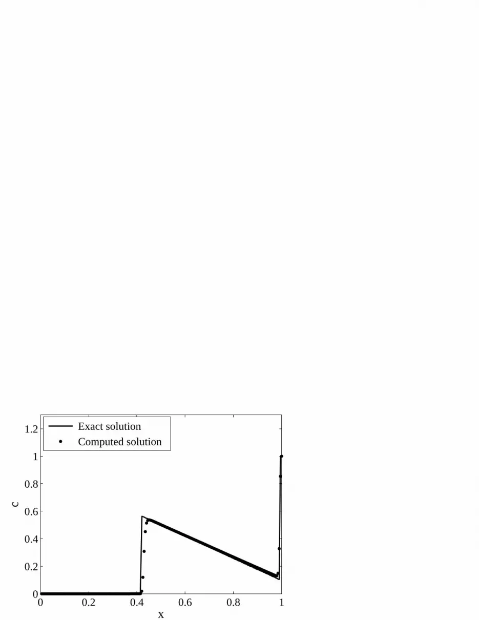
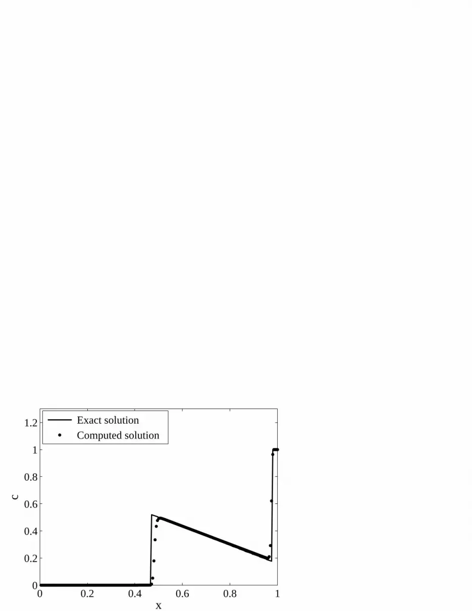
As we can see on Figures 1b-c and 2b-c, errors between the computed and theexact solution happen mostly near the points of discontinuity of the exact solution,except when we reach steady state. Discontinuities of steady states are indeedcaptured with striking accuracy (see Figs 1d and 2d), whereas upwinding might be


a) b)

0 0.2 0.4 0.6 0.8 10

0.2

0.4

0.6

0.8

1

1.2

x

c

Exact solution

Computed solution

0 0.2 0.4 0.6 0.8 10

0.2

0.4

0.6

0.8

1

1.2

x

c

Exact solution

Computed solution

c) d)

0 0.2 0.4 0.6 0.8 10

0.2

0.4

0.6

0.8

1

1.2

x

c

Exact solution

Computed solution

0 0.2 0.4 0.6 0.8 10

0.2

0.4

0.6

0.8

1

1.2

x

c

Exact solution

Computed solution

Figure 1. Evolution of the concentration ρ for the initial datadefined in (22), with the “wall” boundary condition (21). Exactsolution (plain) and discrete solution (dotted line). Simulationsperformed for Nx = 200.

expected to diffuse fronts: it is due to the behavior of the model we consider, whichtends to sweep ρ toward the discontinuity, inducing permanent correction of thenumerical diffusion.

3.2.2. 2D simulations for a constant desired velocity U. In this section we performsome numerical simulations for the migration model (8)-(10), in the case where thedesired velocity U is given and constant in time. In all the cases shown here, thedomain Ω is bounded and surrounded by walls, so that p verifies Neumann boundaryconditions:

∂p

∂n= ρU · n. (24)

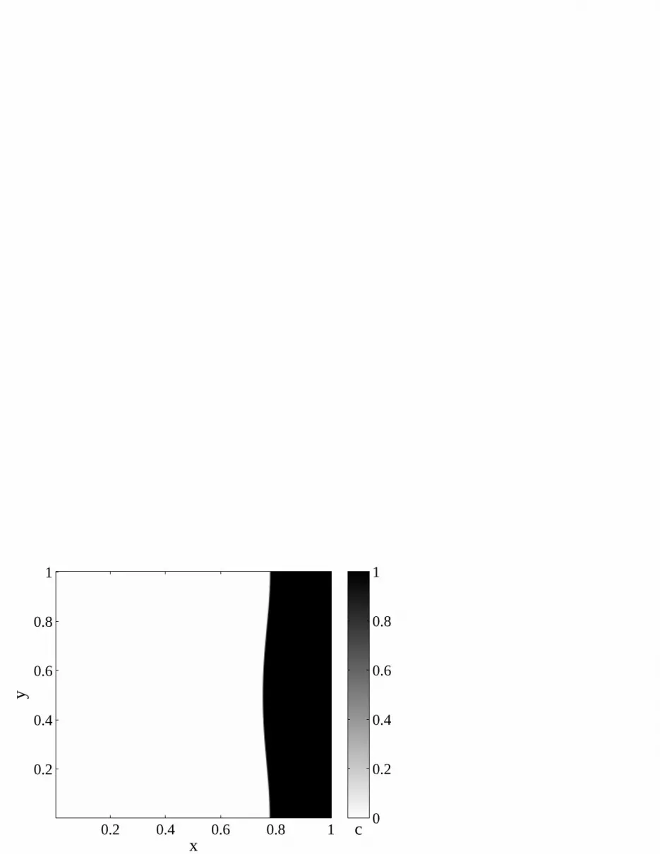
The first situation studied here is a direct 2D extension of the 1D test case describedpreviously, see Fig. 2. The domain is the unit square Ω = (0 , 1)× (0 , 1). We alsoprescribe the following desired velocity: U = 1. Figure 3 shows the evolution of ρfrom the initial condition (Fig. 3a) to the steady state (Fig. 3f) given by a numericalsimulation performed in the situation described above. The same way as in the 1Dsituation (Fig. 2b), the evolution of ρ begins with the spreading of a mixing zonealong the x axis (Figs. 3b-c). Along with the evolution of the mixing zone, the


a) b)

0 0.2 0.4 0.6 0.8 10

0.2

0.4

0.6

0.8

1

1.2

x

c

Exact solution

Computed solution

0 0.2 0.4 0.6 0.8 10

0.2

0.4

0.6

0.8

1

1.2

x

c

Exact solution

Computed solution

c) d)

0 0.2 0.4 0.6 0.8 10

0.2

0.4

0.6

0.8

1

1.2

x

c

Exact solution

Computed solution

0 0.2 0.4 0.6 0.8 10

0.2

0.4

0.6

0.8

1

1.2

x

c

Exact solution

Computed solution

Figure 2. Evolution of the concentration ρ for the initial datadefined in (23), with the “wall” boundary condition (21). Exactsolution (plain) and discrete solution (dotted line). Simulationsperformed for Nx = 200.

solution also tends to spread along the y axis. Hence, a real difference is shown herebetween our model and Burgers-type models. When the mixing zone reaches thewall, a congested zone instantly appears and develops backwards (Fig. 3d-e). Thesteady state is reached when all the right side of the domain is saturated with theactive species (Fig. 3f).

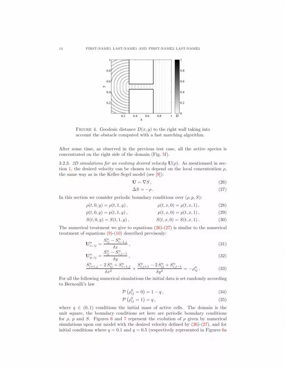
The second situation studied in this section involves a more complex geometryfor the domain, which is defined by

Ω = (0 , 1)× (0 , 1)\ ([0.3 , 0.7]× [0 , 0.45] ∪ [0.3 , 0.7]× [0.55 , 1]) , (25)

which corresponds to two rectangular rooms joined by a thin corridor (see Fig. 4).The desired velocity is set to U = −∇D, where D(x, y) represents the geodesicdistance from (x, y) to the right wall. In practice D is computed thanks to thetoolbox provided by [15], which is based on the Fast-Marching method (see [10]).Figure 5 represents the simulated evolution of the concentration ρ with the settingdescribed above. The initial condition is shown in figure 5a. As we can see acongested zone rapidly forms near the entrance of the corridor (figure 5b), whichsize decreases in time as the matter runs through it (figures 5c-e). We notice that aquasi-homogeneous flow regime tends to be established in the corridor (Fig. 5d-e),


a) b)

x

y

0.2 0.4 0.6 0.8 1

0.2

0.4

0.6

0.8

1

c0

0.2

0.4

0.6

0.8

1

x

y

0.2 0.4 0.6 0.8 1

0.2

0.4

0.6

0.8

1

c0

0.2

0.4

0.6

0.8

1

c) d)

x

y

0.2 0.4 0.6 0.8 1

0.2

0.4

0.6

0.8

1

c0

0.2

0.4

0.6

0.8

1

x

y

0.2 0.4 0.6 0.8 1

0.2

0.4

0.6

0.8

1

c0

0.2

0.4

0.6

0.8

1

e) f)

x

y

0.2 0.4 0.6 0.8 1

0.2

0.4

0.6

0.8

1

c0

0.2

0.4

0.6

0.8

1

x

y

0.2 0.4 0.6 0.8 1

0.2

0.4

0.6

0.8

1

c0

0.2

0.4

0.6

0.8

1

Figure 3. Evolution of the concentration ρ in the case of a con-stant desired velocity U = 1, with the “wall” boundary condi-tion (24). Mesh resolution: Nx ×Ny = 300× 300.

where a constant concentration ρ ∼ 0.5 is observed. It illustrates conservation ofspecies 2 (in white in the figures): as the domain is bounded by walls, flow of 1to the right has to be balanced by an opposite flow of 2 to the left. As we definethe correction velocity in the least-square sense, actual speeds for 1 and 2 are close,so that the mixture is necessarily balanced for global mass conservation reasons.


x

y

0.2 0.4 0.6 0.8 1

0.2

0.4

0.6

0.8

1

D0

0.2

0.4

0.6

0.8

1

Figure 4. Geodesic distance D(x, y) to the right wall taking intoaccount the obstacle computed with a fast marching algorithm.

After some time, as observed in the previous test case, all the active species isconcentrated on the right side of the domain (Fig. 5f).

3.2.3. 2D simulations for an evolving desired velocity U(ρ). As mentionned in sec-tion 1, the desired velocity can be chosen to depend on the local concentration ρ,the same way as in the Keller-Segel model (see [9]):

U = ∇S , (26)

∆S = −ρ . (27)

In this section we consider periodic boundary conditions over (ρ, p, S):

ρ(t, 0, y) = ρ(t, 1, y) , ρ(t, x, 0) = ρ(t, x, 1) , (28)

p(t, 0, y) = p(t, 1, y) , p(t, x, 0) = p(t, x, 1) , (29)

S(t, 0, y) = S(t, 1, y) , S(t, x, 0) = S(t, x, 1) . (30)

The numerical treatment we give to equations (26)-(27) is similar to the numericaltreatment of equations (9)-(10) described previsouly:

Unx, ij =

Snij − Sn

i−1,j

δx, (31)

Uny, ij =

Snij − Sn

i,j−1

δy, (32)

Sni+1,j − 2Sn

ij + Sni−1,j

δx2+

Sni,j+1 − 2Sn

ij + Sni,j−1

δy2= −ρnij . (33)

For all the following numerical simulations the initial data is set randomly accordingto Bernoulli’s law

P(

ρ0ij = 0)

= 1− q , (34)

P(

ρ0ij = 1)

= q , (35)

where q ∈ (0, 1) conditions the initial mass of active cells. The domain is theunit square, the boundary conditions set here are periodic boundary conditionsfor ρ, p and S. Figures 6 and 7 represent the evolution of ρ given by numericalsimulations upon our model with the desired velocity defined by (26)-(27), and forinitial conditions where q = 0.1 and q = 0.5 (respectively represented in Figures 6a


a) b)

x

y

0.2 0.4 0.6 0.8 1

0.2

0.4

0.6

0.8

1

c0

0.2

0.4

0.6

0.8

1

x

y

0.2 0.4 0.6 0.8 1

0.2

0.4

0.6

0.8

1

c0

0.2

0.4

0.6

0.8

1

c) d)

x

y

0.2 0.4 0.6 0.8 1

0.2

0.4

0.6

0.8

1

c0

0.2

0.4

0.6

0.8

1

x

y

0.2 0.4 0.6 0.8 1

0.2

0.4

0.6

0.8

1

c0

0.2

0.4

0.6

0.8

1

e) f)

x

y

0.2 0.4 0.6 0.8 1

0.2

0.4

0.6

0.8

1

c0

0.2

0.4

0.6

0.8

1

x

y

0.2 0.4 0.6 0.8 1

0.2

0.4

0.6

0.8

1

c0

0.2

0.4

0.6

0.8

1

Figure 5. Evolution of the concentration ρ in the case of a con-stant desired velocity U = ∇D (see Fig. 4), with the “wall” bound-ary condition (24). Mesh resolution: Nx ×Ny = 300× 300.

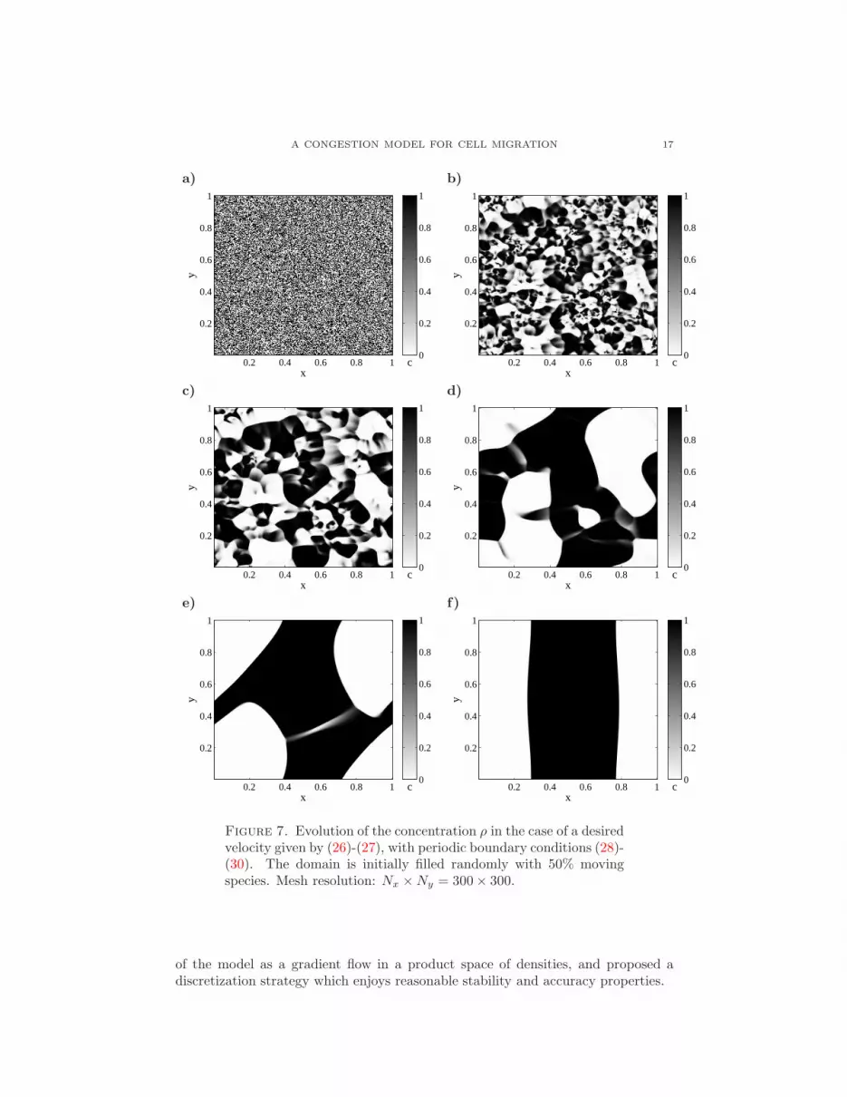
and 7a). In each case we see aggregation of bigger and bigger structures as timegoes (Figs. 6b-e and 7b-e). Two different steady states are shown, both involvinga steady, fully congested zone. In the case q = 0.1 the steady state congested zoneis a disc, whereas in the case q = 0.5 a band has formed because of the periodicboundary conditions we chose to consider.


a) b)

x

y

0.2 0.4 0.6 0.8 1

0.2

0.4

0.6

0.8

1

c0

0.2

0.4

0.6

0.8

1

x

y

0.2 0.4 0.6 0.8 1

0.2

0.4

0.6

0.8

1

c0

0.2

0.4

0.6

0.8

1

c) d)

x

y

0.2 0.4 0.6 0.8 1

0.2

0.4

0.6

0.8

1

c0

0.2

0.4

0.6

0.8

1

x

y

0.2 0.4 0.6 0.8 1

0.2

0.4

0.6

0.8

1

c0

0.2

0.4

0.6

0.8

1

e) f)

x

y

0.2 0.4 0.6 0.8 1

0.2

0.4

0.6

0.8

1

c0

0.2

0.4

0.6

0.8

1

x

y

0.2 0.4 0.6 0.8 1

0.2

0.4

0.6

0.8

1

c0

0.2

0.4

0.6

0.8

1

Figure 6. Evolution of the concentration ρ in the case of a desiredvelocity given by (26)-(27), with periodic boundary conditions (28)-(30). The domain is initially filled randomly with 10% movingspecies. Mesh resolution: Nx ×Ny = 300× 300.

4. Conclusion, extensions. We proposed a model to describe the motion of mix-tures of cell populations in a saturated medium with a constraint on the localdensity. We provided an adapted theoretical framework, based on a reformulation


a) b)

x

y

0.2 0.4 0.6 0.8 1

0.2

0.4

0.6

0.8

1

c0

0.2

0.4

0.6

0.8

1

x

y

0.2 0.4 0.6 0.8 1

0.2

0.4

0.6

0.8

1

c0

0.2

0.4

0.6

0.8

1

c) d)

x

y

0.2 0.4 0.6 0.8 1

0.2

0.4

0.6

0.8

1

c0

0.2

0.4

0.6

0.8

1

x

y

0.2 0.4 0.6 0.8 1

0.2

0.4

0.6

0.8

1

c0

0.2

0.4

0.6

0.8

1

e) f)

x

y

0.2 0.4 0.6 0.8 1

0.2

0.4

0.6

0.8

1

c0

0.2

0.4

0.6

0.8

1

x

y

0.2 0.4 0.6 0.8 1

0.2

0.4

0.6

0.8

1

c0

0.2

0.4

0.6

0.8

1

Figure 7. Evolution of the concentration ρ in the case of a desiredvelocity given by (26)-(27), with periodic boundary conditions (28)-(30). The domain is initially filled randomly with 50% movingspecies. Mesh resolution: Nx ×Ny = 300× 300.

of the model as a gradient flow in a product space of densities, and proposed adiscretization strategy which enjoys reasonable stability and accuracy properties.


In terms of modelling, as mentioned in the introduction, any number N of speciescan be handled, as far as equations are considered (possible issues concerning bound-ary conditions are disregarded here). Saturation writes simply ρ1 + · · · + ρN = 1,we have an advection equation for each species

∂tρi +∇ · (ρi (Ui +w)) = 0 , i = 1, . . . , N,

and the common correction velocity verifies

∇ ·w = −∇ ·

(

N∑

i=1

ρiUi

)

.

It could be of particular importance to include also proliferation phenomena. De-noting by βi the local rate of creation (possibly depending explicity upon ρi or otherdensities), conservation equations become

∂tρi +∇ · (ρi (Ui +w)) = βi , i = 1, . . . , N,

and the constraint on w accounts for mass creation:

∇ ·w =N∑

i=1

βi −∇ ·

(

N∑

i=1

ρiUi

)

.

Note that, in this situation, global non conservation rules out the use of no-fluxconditions (or periodic setting). Considering a bounded domain Ω one can con-sider its boundary as a free outlet (interaction pressure is set at 0), so that a nonconservative flux through boundary can compensate the unbalance of mass in thedomain. In case of mass creation (βi > 0), one can expect outflow through theboundary, so that no additional condition is needed for the advection equations. Incase some individual velocitiesUi+w may point inward the domain, the system hasto be complemented with appropriate conditions (e.g. prescribed value of ingoingdensities).

As for theoretical issues, non conservation rules out the standard framework ofgradient flow in the Wasserstein space, which is dedicated to measures with constanttotal mass. Yet, as suggested in [11], generalizations of the JKO scheme, in thespirit of prediction-correction algorithms (or catching-up algorithms for sweepingprocesses, see for example [12]) might be expected to provide well-posedness results.

One may also wonder whether it could be possible to recover evolution equationsfor a single species, as in the case of crowd motion models ([11]). In this situation,species 2 is replaced by empty space, which can be moved at no cost. Our proposedmodel could be seen as an attempt to replace a unilateral constraint ρ1 ≤ 1 (whichis quite delicate to handle, see again [11]), by an equality ρ1 + ρ2 = 1 with ρ2 ≥ 0.It can be done formally by lowering the importance of species 2, more precisely bydefining the correction velocity as the one which minimizes a weighted L2 norm:

w = argmin

∫

Ω

kε(ρ1, ρ2)|v|2,

where the minimum is taken among all those fields which satisfy∇·w = −∇·(ρ1U1)(in the case U2 = 0), and

kε(ρ1, ρ2) = ρ1 + ερ2.

One recovers formally an evolution equation for ρ1 with unilateral constraint ρ1 ≤ 1,yet with a significant difference: if one considers a saturated zone of 2 surroundedby a saturated zone of 1, the asymptotic (ε → 0) model sees the inclusion as globallyincompressible, which is not the case if one imposes simply ρ1 ≤ 1.


REFERENCES

[1] L. Ambrosio, N. Gigli, G. Savare, Gradient flows in metric spaces and in the space of proba-

bility measures, Lectures in Mathematics, ETH Zurich (2005).[2] L. Ambrosio, G. Savare, Gradient flows of probability measures, Handbook of differential

equations, Evolutionary equations, 3 (ed. by C.M. Dafermos and E. Feireisl, Elsevier, 2007).[3] J.-D. Benamou, Y. Brenier, A computational fluid mechanics solution to the Monge-

Kantorovich mass transfer problem, Numer. Math., 84(3) (2001) 375–393.[4] A.L. Dalibard, B. Perthame, Existence of solutions of the hyperbolic Keller-Segel model,

Trans. Amer. Math. Soc., 361(5) (2009), 2319–2335.[5] E. De Giorgi, New problems on minimizing movements, Boundary Value Problems for PDE

and Applications, C. Baiocchi and J. L. Lions eds. (Masson, 1993) 81–98.[6] Y. Dolak, C. Schmeiser, The Keller-Segel model with logistic sensitivity function and small

diffusivity, SIAM J. Appl. Math., 66(1) (2005), 286–308.[7] N. Gigli, F. Otto, Entropic Burgers’ equation via a minimizing movement scheme based on

the Wasserstein metric, submitted.[8] R. Jordan, D. Kinderlehrer, F. Otto, The variational formulation of the Fokker-Planck equa-

tion, SIAM J. Math. Anal., 29(1) (1998) 1–17.[9] E.F Keller, L.A. Segel, Model for chemotaxis, J. Theor. Biol., 30 (1971) 225–234.

[10] R. Kimmel, J. Sethian, Fast marching methods for computing distance maps and shortest

paths, Technical Report 669, CPAM, Univ. of California, Berkeley (1996).[11] B. Maury, A. Roudneff-Chupin, F. Santambrogio, A macroscopic crowd motion model of

gradient flow type, Math. Mod. Meth. Appl. Sci., to appear.[12] J.J. Moreau, Evolution problem associated with a moving convex set in a Hilbert space, J.

Differential Equations, 26 (3), 347?374, 1977.[13] F. Otto, Weinan E., Thermodynamically driven incompressible fluid mixtures, J. Chem. Phys.

107, 10177 (1997).[14] B. Perthame, PDE models for chemotactic movements: parabolic, hyperbolic and kinetic,

Appl. Math., 49(6) (2004) 539–564.[15] G. Peyre, Toolbox Fast Marching - A toolbox for Fast Marching and level sets computations

(2008), software.[16] M. Renardy, R.C. Rogers, An introduction to partial differential equations, Texts in App.

Math., 13, Springer-Verlag, New York (2004).[17] C. Villani, Topics in optimal transportation, Grad. Stud. Math., 58 (AMS, Providence 2003).[18] C. Villani, Optimal transport, old and new, Grundlehren der mathematischen Wissenschaften,

338 (2009).

Received xxxx 20xx; revised xxxx 20xx.

E-mail address: [email protected]




x

y

0.2 0.4 0.6 0.8 1

0.2

0.4

0.6

0.8

1

c0

0.2

0.4

0.6

0.8

1

0 0.2 0.4 0.6 0.8 10

0.2

0.4

0.6

0.8

1

1.2

x

c

Exact solution

Computed solution

x

y

0.2 0.4 0.6 0.8 1

0.2

0.4

0.6

0.8

1

c0

0.2

0.4

0.6

0.8

1

0 0.2 0.4 0.6 0.8 10

0.2

0.4

0.6

0.8

1

1.2

x

c

Exact solution

Computed solution

A congestion model for cell migration

Documents

Transcript of A congestion model for cell migration