BioMed CentralBMC Bioinformatics

ss

Open AcceResearch articleA comparison of random forest and its Gini importance with standard chemometric methods for the feature selection and classification of spectral dataBjoern H Menze1,2, B Michael Kelm1, Ralf Masuch3, Uwe Himmelreich4, Peter Bachert5, Wolfgang Petrich6,7 and Fred A Hamprecht*1,6

Address: 1Interdisciplinary Center for Scientific Computing (IWR), University of Heidelberg, Heidelberg, Germany, 2Computer Science and Artificial Intelligence Laboratory (CSAIL), Massachusetts Institute of Technology, Cambridge/MA, USA, 3Micro-Biolytics GmbH, Esslingen, Germany, 4Biomedical NMR Unit, Department of Medical Diagnostic Sciences, KU Leuven, Leuven, Belgium, 5Department of Medical Physics in Radiology, German Cancer Research Center, Heidelberg, Germany, 6Department of Astronomy and Physics, University of Heidelberg, Heidelberg, Germany and 7Roche Diagnostics GmbH, Mannheim, Germany

Email: Bjoern H Menze - bjoern.menze@iwr.uni-heidelberg.de; B Michael Kelm - michael.kelm@iwr.uni-heidelberg.de; Ralf Masuch - masuch@micro-biolytics.com; Uwe Himmelreich - uwe.himmelreich@med.kuleuven.be; Peter Bachert - p.bachert@dkfz-heidelberg.de; Wolfgang Petrich - wolfgang.petrich@roche.com; Fred A Hamprecht* - fred.hamprecht@iwr.uni-heidelberg.de

* Corresponding author

AbstractBackground: Regularized regression methods such as principal component or partial leastsquares regression perform well in learning tasks on high dimensional spectral data, but cannotexplicitly eliminate irrelevant features. The random forest classifier with its associated Gini featureimportance, on the other hand, allows for an explicit feature elimination, but may not be optimallyadapted to spectral data due to the topology of its constituent classification trees which are basedon orthogonal splits in feature space.

Results: We propose to combine the best of both approaches, and evaluated the joint use of afeature selection based on a recursive feature elimination using the Gini importance of randomforests' together with regularized classification methods on spectral data sets from medicaldiagnostics, chemotaxonomy, biomedical analytics, food science, and synthetically modified spectraldata. Here, a feature selection using the Gini feature importance with a regularized classification bydiscriminant partial least squares regression performed as well as or better than a filteringaccording to different univariate statistical tests, or using regression coefficients in a backwardfeature elimination. It outperformed the direct application of the random forest classifier, or thedirect application of the regularized classifiers on the full set of features.

Conclusion: The Gini importance of the random forest provided superior means for measuringfeature relevance on spectral data, but – on an optimal subset of features – the regularizedclassifiers might be preferable over the random forest classifier, in spite of their limitation to modellinear dependencies only. A feature selection based on Gini importance, however, may precede aregularized linear classification to identify this optimal subset of features, and to earn a doublebenefit of both dimensionality reduction and the elimination of noise from the classification task.

Published: 10 July 2009

BMC Bioinformatics 2009, 10:213 doi:10.1186/1471-2105-10-213

Received: 23 February 2009Accepted: 10 July 2009

This article is available from: http://www.biomedcentral.com/1471-2105/10/213

© 2009 Menze et al; licensee BioMed Central Ltd. This is an Open Access article distributed under the terms of the Creative Commons Attribution License (http://creativecommons.org/licenses/by/2.0), which permits unrestricted use, distribution, and reproduction in any medium, provided the original work is properly cited.

Page 1 of 16(page number not for citation purposes)

BMC Bioinformatics 2009, 10:213 http://www.biomedcentral.com/1471-2105/10/213

BackgroundThe high dimensionality of the feature space is a charac-teristic of learning problems involving spectral data. Inmany applications with a biological or biomedical back-ground addressed by, for example, nuclear magnetic reso-nance or infrared spectroscopy, also the number ofavailable samples N is lower than the number of featuresin the spectral vector P. The intrinsic dimensionality Pintrof spectral data, however, is often much lower than thenominal dimensionality P – sometimes even below N.

Dimension reduction and feature selection in the classification of spectral dataMost methods popular in chemometrics exploit this rela-tion Pintr < P and aim at regularizing the learning problemby implicitly restricting its free dimensionality to Pintr.

(Here, and in the following we will adhere to the algorith-mic classification of feature selection approaches from[1], referring to regularization approaches which explicitlycalculate a subset of input features – in a preprocessing,for example – as explicit feature selection methods, and toapproaches performing a feature selection or dimensionreduction without calculating these subsets as implicit fea-ture selection methods.) Popular methods in chemomet-rics, such as principal component regression (PCR) orpartial least squares regression (PLS) directly seek for solu-tions in a space spanned by ~Pintr principal components(PCR) – assumed to approximate the intrinsic subspace ofthe learning problem – or by biasing projections of leastsquares solutions towards this subspace [2,3], down-weighting irrelevant features in a constrained regression(PLS). It is observed, however, that although both PCRand PLS are capable learning methods on spectral data –used for example for in [4] – they still have a need to elim-inate useless predictors [5,6]. Thus, often an additionalexplicit feature selection is pursued in a preceding step toeliminate spectral regions which do not provide any rele-vant signal at all, showing resonances or absorption bandsthat can clearly be linked to artefacts, or features which areunrelated to the learning task. Discarding irrelevant fea-ture dimensions, though, raises the question of how tochoose such an appropriate subset of features [6-8].

Different univariate and multivariate importance meas-ures can be used to rank features and to select themaccordingly [1]. Univariate tests marginalize over all butone feature and rank them in accordance to their discrim-inative power [9,10]. In contrast, multivariate approachesconsider several or all features simultaneously, evaluatingthe joint distribution of some or all features and estimat-ing their relevance to the overall learning task. Multivari-ate tests are often used in wrapper schemes incombination with a subsequent classifier (e.g. a globaloptimization of feature subset and classifier coefficients

[11]), or by statistical tests on the outcome of a learningalgorithm (e.g. an iterative regression with test for robust-ness [12,13]). While univariate approaches are sometimesdeemed too simplistic, the other group of multivariatefeature selection methods often comes at unacceptablyhigh computational costs.

Gini feature importanceA feature selection based on the random forest classifier[14] has been found to provide multivariate featureimportance scores which are relatively cheap to obtain,and which have been successfully applied to high dimen-sional data, arising from microarrays [15-20], time series[21], even on spectra [22,23]. Random forest is an ensem-ble learner based on randomized decision trees (see [24]for a review of random forests in chemometrics, [14] forthe original publication, and [25-28] for methodologicalaspects), and provides different feature important meas-ures. One measure is motivated from statistical permuta-tion tests, the other is derived from the training of therandom forest classifier. Both measures have been foundto correlate reasonably well [28]. While the majority ofthe prior studies focused on the first, we will focus on thesecond in the following.

As a classifier, random forest performs an implicit featureselection, using a small subset of "strong variables" for theclassification only [27], leading to its superior perform-ance on high dimensional data. The outcome of thisimplicit feature selection of the random forest can be vis-ualized by the "Gini importance" [14], and can be used asa general indicator of feature relevance. This featureimportance score provides a relative ranking of the spec-tral features, and is – technically – a by-product in thetraining of the random forest classifier: At each node τwithin the binary trees T of the random forest, the optimalsplit is sought using the Gini impurity i(τ) – a computa-tionally efficient approximation to the entropy – measur-ing how well a potential split is separating the samples ofthe two classes in this particular node.

With being the fraction of the nk samples from

class k = {0,1} out of the total of n samples at node τ, the

Gini impurity i(τ) is calculated as

Its decrease Δi that results from splitting and sending the

samples to two sub-nodes τl and τr (with respective sample

fractions and ) by a threshold tθ on varia-

ble θ is defined as

pknkn=

i p p( )τ = − −1 12

02

plnln= pr

nrn=

Page 2 of 16(page number not for citation purposes)

BMC Bioinformatics 2009, 10:213 http://www.biomedcentral.com/1471-2105/10/213

In an exhaustive search over all variables θ available at thenode (a property of the random forest is to restrict thissearch to a random subset of the available features [14]),and over all possible thresholds tθ, the pair {θ, tθ} leadingto a maximal Δi is determined. The decrease in Gini impu-rity resulting from this optimal split Δiθ (τ, T) is recordedand accumulated for all nodes τ in all trees T in the forest,individually for all variables θ:

This quantity – the Gini importance IG – finally indicateshow often a particular feature θ was selected for a split,and how large its overall discriminative value was for theclassification problem under study.

When used as an indicator of feature importance for anexplicit feature selection in a recursive elimination scheme[1] and combined with the random forest itself as classi-fier in the final step, the feature importance measures ofthe random forest have been found to reduce the amountof features. Most studies using the Gini importance[22,29] and the related permutation-based feature impor-tance of random forests [16,18,20,21,23] together withrandom forests in a recursive feature elimination scheme,also showed an increases in prediction performance.(Only [17] reports a constant performance, but withgreatly reduced amount of features.) While these experi-ments indicate the efficiency of the Gini importance in anexplicit feature selection [24] one might raise the questionwhether a random forest – the "native" classifier of Giniimportance – with its orthogonal splits of feature space is

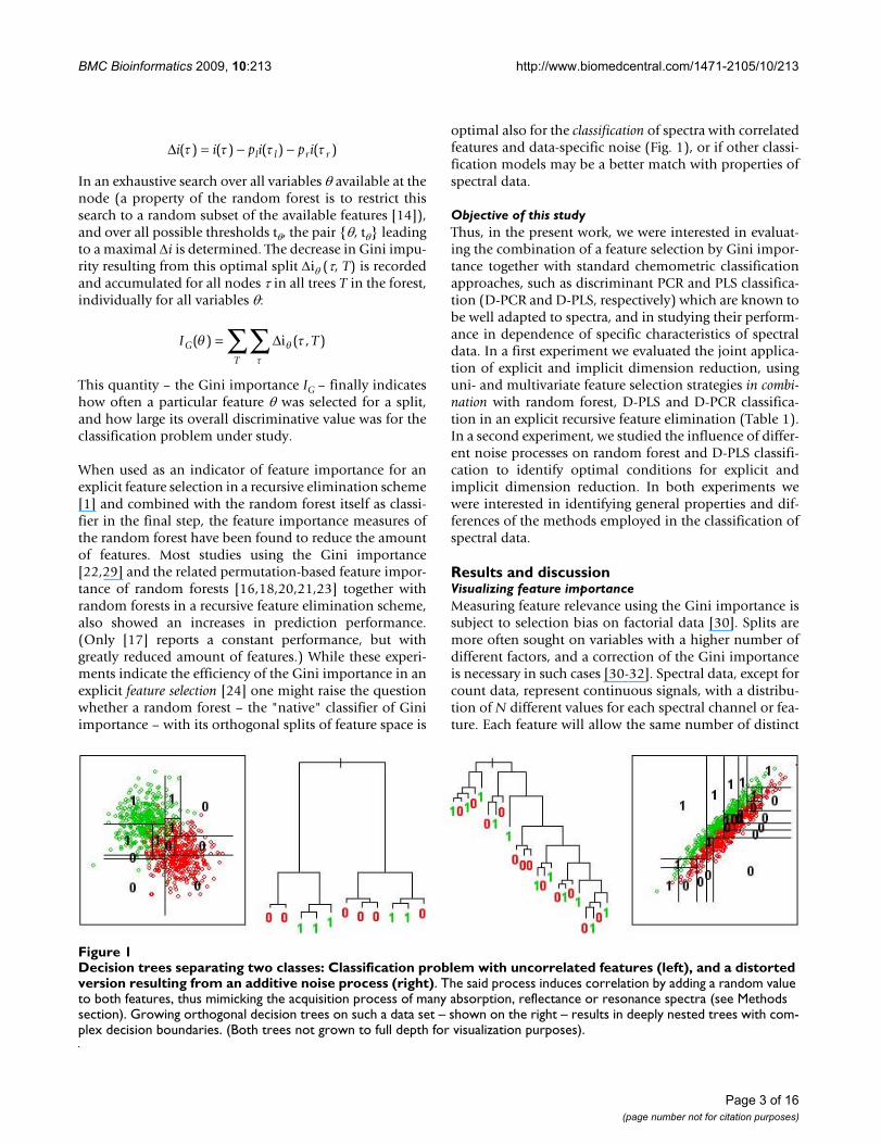
optimal also for the classification of spectra with correlatedfeatures and data-specific noise (Fig. 1), or if other classi-fication models may be a better match with properties ofspectral data.

Objective of this studyThus, in the present work, we were interested in evaluat-ing the combination of a feature selection by Gini impor-tance together with standard chemometric classificationapproaches, such as discriminant PCR and PLS classifica-tion (D-PCR and D-PLS, respectively) which are known tobe well adapted to spectra, and in studying their perform-ance in dependence of specific characteristics of spectraldata. In a first experiment we evaluated the joint applica-tion of explicit and implicit dimension reduction, usinguni- and multivariate feature selection strategies in combi-nation with random forest, D-PLS and D-PCR classifica-tion in an explicit recursive feature elimination (Table 1).In a second experiment, we studied the influence of differ-ent noise processes on random forest and D-PLS classifi-cation to identify optimal conditions for explicit andimplicit dimension reduction. In both experiments wewere interested in identifying general properties and dif-ferences of the methods employed in the classification ofspectral data.

Results and discussionVisualizing feature importanceMeasuring feature relevance using the Gini importance issubject to selection bias on factorial data [30]. Splits aremore often sought on variables with a higher number ofdifferent factors, and a correction of the Gini importanceis necessary in such cases [30-32]. Spectral data, except forcount data, represent continuous signals, with a distribu-tion of N different values for each spectral channel or fea-ture. Each feature will allow the same number of distinct

Δi i p i p il l r r( ) ( ) ( ) ( )τ τ τ τ= − −

I TG

T

( ) ( , )θ τθτ

= ∑∑ Δi

Decision trees separating two classes: Classification problem with uncorrelated features (left), and a distorted version resulting from an additive noise process (right)Figure 1Decision trees separating two classes: Classification problem with uncorrelated features (left), and a distorted version resulting from an additive noise process (right). The said process induces correlation by adding a random value to both features, thus mimicking the acquisition process of many absorption, reflectance or resonance spectra (see Methods section). Growing orthogonal decision trees on such a data set – shown on the right – results in deeply nested trees with com-plex decision boundaries. (Both trees not grown to full depth for visualization purposes).

Page 3 of 16(page number not for citation purposes)

BMC Bioinformatics 2009, 10:213 http://www.biomedcentral.com/1471-2105/10/213

splits in a random forest classification, and, hence, ameasurement of the relevance of spectral regions for a spe-cific classification problem will be unaffected by thispotential source of bias.

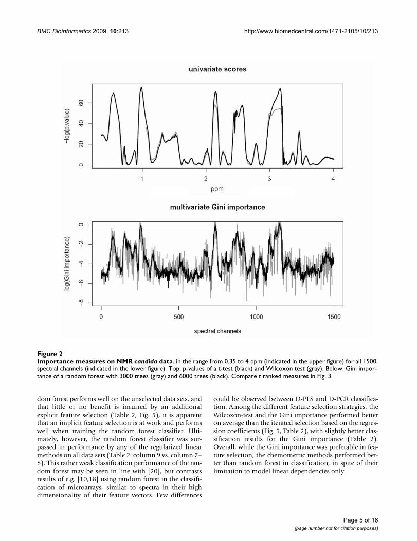
Both univariate tests for significant class differencesreturned smooth importance vectors when employed onthe spectral data (Fig. 2, top). The smoothness of the Giniimportance was dependent on the size of the random for-est (Fig. 2, bottom) – small forests resulted in "noisy"importance vectors, only converging towards smooth vec-tors when increasing the overall number of trees in theforest or the overall number of splits. As such changesinfluence the absolute value of this measure, the Giniimportance could not be interpreted in absolute terms –like the p-values of the univariate tests – but only allowedfor a relative comparison. For such a comparison betweendifferent variables and between different measures, thefeatures were ranked according to their importance score(Fig. 3A). Here, univariate importance measures and Giniimportance agreed well in many, although not all, spectralregions (Fig. 3A, rows 2 and 3). An example of the mostprominent differences between univariate feature impor-tance and multivariate Gini importance are highlighted inFig. 3B. Spectral regions deemed unimportant by the uni-variate measures – with complete overlap of the marginaldistributions as shown in Fig. 3B – may be attributed highimportance by the multivariate importance measure (Fig.4), indicating spectral regions with features of higherorder interaction.

Inspecting the Gini feature importance we observed –similar to [32] – that some spectral regions were selectedas a whole, suggesting that correlated variables wereassigned similar importance. Thus, the importance meas-ure may be interpreted like a spectrum, where neighbour-ing channels of similar importance may be considered asrepresentatives of the same peak, absorbance or resonance

line. This can be used in an exploratory visualization offeature relevance (Figs. 2 and 3A, top row). As the randomforest prefers splits on correlated variable over splits onuncorrelated ones [28] it should be noted, however, thatthis "importance spectrum" may be somewhat biasedtowards overestimating the importance of major peaksspanning over many spectral channels.

Feature selection and classificationThe classification accuracies provided by the first experi-ment based on the real data allowed for a quantitativecomparison of the methods applied and for testing for sta-tistically significant differences between results on the fullset of features in comparison to the subselected data sets(Table 2, "stars"). On one half of the data, the featureselection hardly changed the classification performance atall (Tables 2 and 3, tumor and candida data), while on theother half a feature selection improved the final result sig-nificantly (Tables 2 and 3, wine and BSE data), almostindependently of the subsequent classifier. In the lattergroup optimally subselected data typically comprisedabout 1–10% of the initial features (Table 3, Fig. 5). Sucha data dependence in the benefit of a preceding featureselection is well known (e.g. [33]). Different from [33],however, we did not see a relation to the apparent degreeof ill-posedness of the classification problem (i.e., a lowratio N/P of the length of the spectral vector P and thenumber of available samples N leading to an underdeter-mined estimation problem – he BSE and candida data, forexample, are nearly identical in dimensionality – PBSE =1209, Pcandida = 1500 – and number of training samples –NBSE = 2 * 96, Ncandida = 2 * 101).

Random forest, the only nonlinear classifier applied, per-formed slightly better than the linear classifiers on theunselected data sets (BSE and wine data, Fig. 5), butimproved only moderately in the course of the featureselection (Fig. 5, Table 3: p-value > 10-3). Given that ran-

Table 1: Recursive feature selection.

1. Calculate feature importance on the training dataa. Gini importanceb. absolute value of regression coefficients (PLS/PCR)c. p-values from Wilcoxon-test/t-test

2. Rank the features according to the importance measure, remove the p% least important3. Train the classifier on the training data

A. Random forestB. D-PLSC. D-PCR

and apply it to the test data4. Repeat 1.–4. until no features are remaining5. Identify the best feature subset according to the test error

Workflow of the recursive feature selection, and combinations of feature importance measures (1.a-1.c) and classifiers (3.A-3.C) tested in this study. Compare with results in Table 2 and Fig. 4. Hyper-parameters of PLS/PCR/random forest are optimized both in the feature selection (1.) and the classification (3.) step utilizing the training data only. While Gini importance (1.a) and regression coefficients (1.b) have to be calculated within each loop (step 1.–4.), the univariate measures (1.c) have only to be calculated once.

Page 4 of 16(page number not for citation purposes)

BMC Bioinformatics 2009, 10:213 http://www.biomedcentral.com/1471-2105/10/213

dom forest performs well on the unselected data sets, andthat little or no benefit is incurred by an additionalexplicit feature selection (Table 2, Fig. 5), it is apparentthat an implicit feature selection is at work and performswell when training the random forest classifier. Ulti-mately, however, the random forest classifier was sur-passed in performance by any of the regularized linearmethods on all data sets (Table 2: column 9 vs. column 7–8). This rather weak classification performance of the ran-dom forest may be seen in line with [20], but contrastsresults of e.g. [10,18] using random forest in the classifi-cation of microarrays, similar to spectra in their highdimensionality of their feature vectors. Few differences

could be observed between D-PLS and D-PCR classifica-tion. Among the different feature selection strategies, theWilcoxon-test and the Gini importance performed betteron average than the iterated selection based on the regres-sion coefficients (Fig. 5, Table 2), with slightly better clas-sification results for the Gini importance (Table 2).Overall, while the Gini importance was preferable in fea-ture selection, the chemometric methods performed bet-ter than random forest in classification, in spite of theirlimitation to model linear dependencies only.

Importance measures on NMR candida dataFigure 2Importance measures on NMR candida data. in the range from 0.35 to 4 ppm (indicated in the upper figure) for all 1500 spectral channels (indicated in the lower figure). Top: p-values of a t-test (black) and Wilcoxon test (gray). Below: Gini impor-tance of a random forest with 3000 trees (gray) and 6000 trees (black). Compare t ranked measures in Fig. 3.

Page 5 of 16(page number not for citation purposes)

BMC Bioinformatics 2009, 10:213 http://www.biomedcentral.com/1471-2105/10/213

The two linear classifiers of this study generally seek forsubspaces ck maximizing the variance Var of the explana-tory variables X in the subspace c

in case of PCR or the product of variance and the(squared) correlation Corr

with the response y in case of PLS [2,3]. Thus, for a betterunderstanding of D-PCR and D-PLS, both Corr(x, y) andVar(x) were plotted for individual channels and for indi-vidual learning tasks in Fig. 6 (with the absolute value ofthe coefficients of c encoded by the size of the circles inFig. 6). On data sets which did not benefit greatly from thefeature selection, we observed variance and correlation to

c Var c xkc

Corr c x c x j k

T

TjT

= ( )=

( )= <

arg max| |

, ,

1

0

c Corr c x y Var c xkc

Corr c x c x j k

T T

TjT

= ( ) ( )=

( )= <

arg max ,| |

, ,

1

0

2

Comparison of the different feature selection measures applied to the NMR candida 2 data (3A)Figure 3Comparison of the different feature selection measures applied to the NMR candida 2 data (3A). Multivariate fea-ture importance measures can select variables that are discarded by univariate measures (3B). Fig. 3A, from top to bottom: Gini importance, absolute values; Gini importance, ranked values, p-values from t-test, ranked values. Fig. 3B: Feature impor-tance scores below (black: Gini importance, gray: t-test). Perhaps surprisingly, regions with complete overlap of the marginal distributions (3B bottom, indicated by vertical lines), are assigned importance by the multivariate measure (3B top). This is indicative of higher-order interaction effects which can be exploited when used as a feature importance measure with a subse-quent classifier.

Page 6 of 16(page number not for citation purposes)

BMC Bioinformatics 2009, 10:213 http://www.biomedcentral.com/1471-2105/10/213

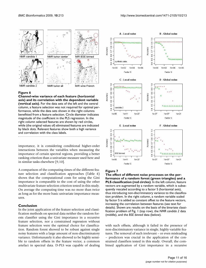
be maximal in those variables which were finally assignedthe largest coefficients in the regression (indicated by thesize of the black circles in Fig. 6). Conversely, in data setswhere a feature selection was required, features with highvariance but only moderate relevance to the classificationproblem (as indicated by a low univariate correlation ormultivariate Gini importance) were frequently present inthe unselected data (Fig. 6, black dots). This might be seenas a likely reason for the bad performance of D-PCR andD-PLS when used without preceding feature selection onthe BSE and wine data: Here the selection process allowedto identify those features where variance coincided withclass-label correlation (Fig. 6, red circles), leading to asimilar situation in the subsequent regression as for thosedata sets where a feature selection was not required (Fig.6, compare subselected features indicated red in the leftand central row with features in the right row).

In summary, observing that the degree of ill-posedness isnot in itself an indicator for a required feature selectionpreceding a constrained classification, it might be arguedthat non-discriminative variance – hindering the identifi-cation of the optimal subspace in PCR, and disturbing theoptimal trade-off between correlation and variation inPLS – may be a reason for the constrained classifiers' fail-

ing on the unselected data and, consequently, a require-ment for a feature selection in the first place.

Feature selection and noise processesThe first experiment advocated the use of the Gini impor-tance for a feature selection preceding a constrainedregression for some data sets. Thus, and in the light of theunexpectedly weak performance of the random forestclassifier, we studied the performance of the D-PLS andthe random forest classifier as a function of noise proc-esses which can be observed in spectral data (see Methodssection for details) to identify optimal situations for thejoint use of explicit and implicit feature selection.

In this second experiment, random forest proved to behighly robust against the introduction of "local" noise, i.e.against noise processes affecting few spectral channelsonly, corresponding to spurious peaks or variant spectralregions which are irrelevant to the classification task (bothon the synthetic bivariate classification problem, Figs. 1left, 7A; and the modified real data, Fig. 7CE). The ran-dom forest classifier was, however, unable to cope withadditive global noise: Already random offsets that werefractions of the amplitude S of the spectra (Fig. 7DF; S =10-2) resulted in a useless classification by the random for-est. As global additive noise stretches the data along the

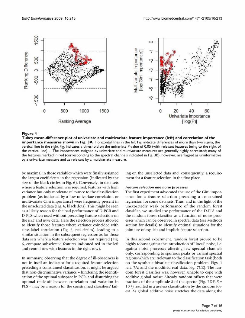
Tukey mean-difference plot of univariate and multivariate feature importance (left) and correlation of the importance measures shown in Fig. 3AFigure 4Tukey mean-difference plot of univariate and multivariate feature importance (left) and correlation of the importance measures shown in Fig. 3A. Horizontal lines in the left Fig. indicate differences of more than two sigma, the vertical line in the right Fig. indicates a threshold on the univariate P-value of 0.05 (with relevant features being to the right of the vertical line). -. The importances assigned by univariate and multivariate measures are generally highly correlated; many of the features marked in red (corresponding to the spectral channels indicated in Fig. 3B), however, are flagged as uninformative by a univariate measure and as relevant by a multivariate measure.

Page 7 of 16(page number not for citation purposes)

BMC Bioinformatics 2009, 10:213 http://www.biomedcentral.com/1471-2105/10/213

high dimensional equivalent of the bisecting line (Fig. 1),the topology of its base learners may be a disadvantage forthe random forest in classification problems as shown inFig. 1. Single decision trees, which split feature space in abox-like manner orthogonal to the feature direction areknown to be inferior to single decision trees splitting thefeature space by oblique splits [34] (although they have aconsiderable computational advantage). Random offsetsoften occur in spectral data, for example resulting frombroad underlying peaks or baselines, or from the normal-ization to spectral regions that turn out to be irrelevant tothe classification problem. Thus, one might argue that the"natural" presence of a small amount of such noise may

lead to the rather weak overall performance of the randomforest observed in the first experiment (Table 2, Fig. 5).

Partial least squares performed slightly better than ran-dom forests on all three data sets at the outset (Fig. 7). Incontrast to the random forest, PLS was highly robustagainst global additive noise: On the synthetic classifica-tion problem – being symmetric around the bisecting line– the random offsets did not influence the classificationperformance at all (Fig. 7B). On the real data – with morecomplex classification tasks – the D-PLS classification stillshowed to be more robust against random offsets than therandom forest classifier (Fig. 7DF). Conversely, localnoise degraded the performance of the D-PLS classifica-

Table 2: Average cross-validated prediction accuracy.

no selection Univariate selection Multivariate selection (Gini importance) multivariate selection (PLS/PC)

PLS PC RF PLS PC RF PLS PC RF PLS PC RF

MIR BSE orig 66.8 62.9 74.9 80.7 80.7 76.7 84.1 83.2 77.4 68 63.5 75.5- - - *** *** * *** *** ** **

binned 72.7 73.4 75.3 80.4 80.7 76.6 86.8 85.8 77.3 85 82.1 75.6- - - *** *** ** *** *** ** *** ***

MIR wine French 69.5 69.3 79.3 83.7 83.5 82.2 82.4 81 81.2 66.9 70.0 79.8- - - *** ** *** ** *

grape 77 71.4 90.2 98.1 98.7 90.3 98.4 98.4 94.2 91.7 88.5 90.4- - - *** *** *** *** ** *** ***

NMR tumor all 88.8 89 89 89.3 89.3 90.5 90.0 89.6 89.6 89.3 89.2 89.1- - - * *** ** *

center 71.6 72.3 73.1 73.9 72.7 73.9 72.6 72.0 74.3 71.8 72.7 73.3- - - ** *

NMR candida 1 94.9 94.6 90.3 95.1 94.9 90.6 95.6 95.3 90.3 95.3 95.2 90.7- - -

2 95.6 95.2 93.2 95.8 95.7 93.7 95.6 95.5 93.5 96.0 95.9 94.1- - - *

3 93.7 93.8 89.7 93.7 93.8 89.9 94.2 93.8 89.9 94.0 94.0 90.2- - - * * *

4 86.9 87.3 83.9 87.8 87.3 84.0 88.2 87.6 84.3 87.7 87.6 84.1- - - *

5 92.7 92.6 89.2 92.7 92.6 89.9 92.5 92.5 90.3 92.8 92.6 90.0- - -

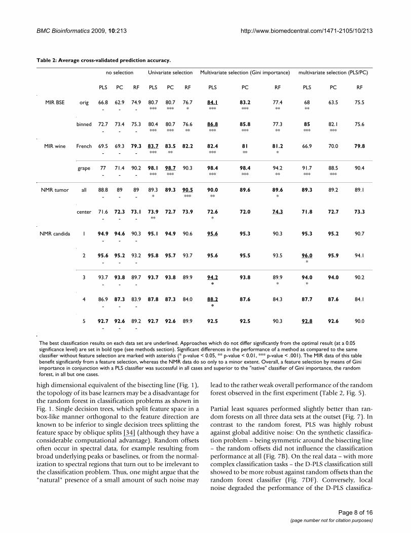
The best classification results on each data set are underlined. Approaches which do not differ significantly from the optimal result (at a 0.05 significance level) are set in bold type (see methods section). Significant differences in the performance of a method as compared to the same classifier without feature selection are marked with asterisks (* p-value < 0.05, ** p-value < 0.01, *** p-value < .001). The MIR data of this table benefit significantly from a feature selection, whereas the NMR data do so only to a minor extent. Overall, a feature selection by means of Gini importance in conjunction with a PLS classifier was successful in all cases and superior to the "native" classifier of Gini importance, the random forest, in all but one cases.

Page 8 of 16(page number not for citation purposes)

BMC Bioinformatics 2009, 10:213 http://www.biomedcentral.com/1471-2105/10/213

Page 9 of 16(page number not for citation purposes)

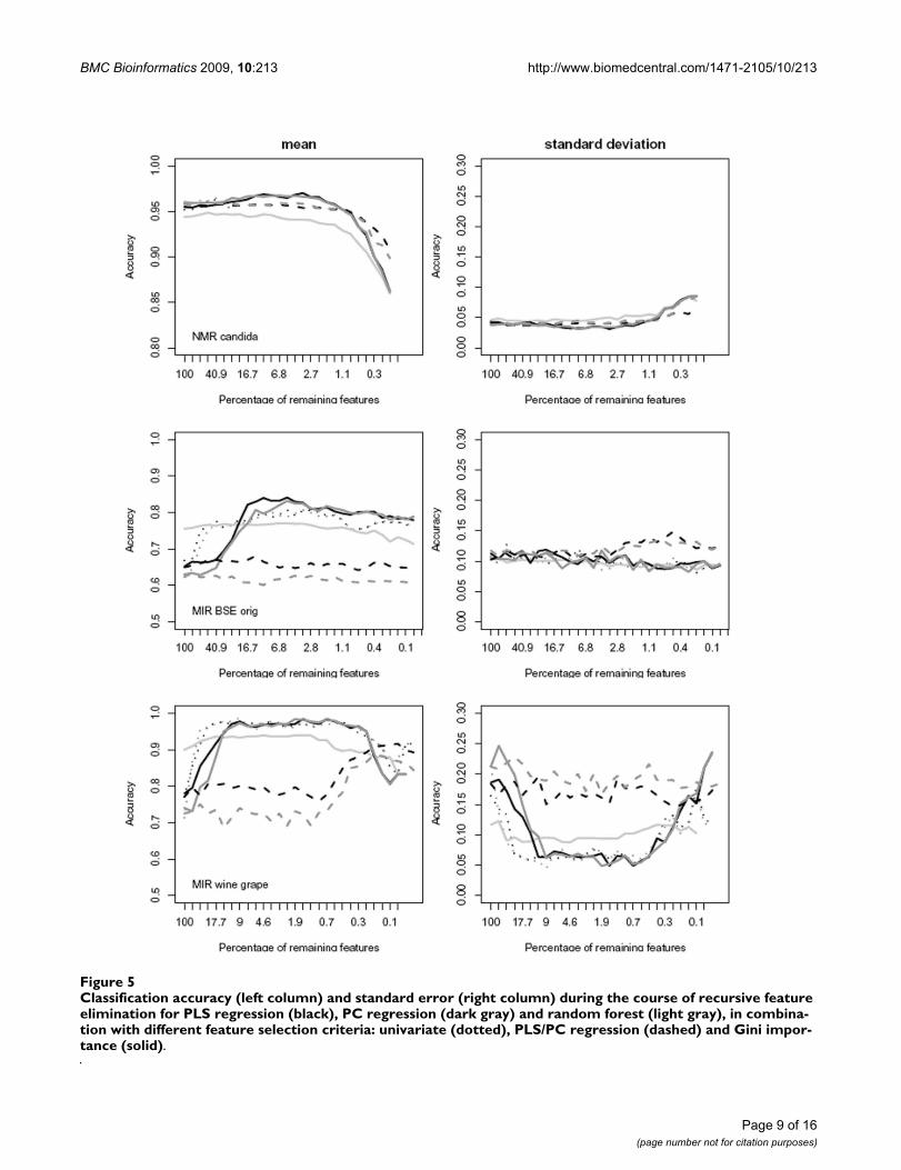
Classification accuracy (left column) and standard error (right column) during the course of recursive feature elimination for PLS regression (black), PC regression (dark gray) and random forest (light gray), in combination with different feature selection criteria: univariate (dotted), PLS/PC regression (dashed) and Gini importance (solid)Figure 5Classification accuracy (left column) and standard error (right column) during the course of recursive feature elimination for PLS regression (black), PC regression (dark gray) and random forest (light gray), in combina-tion with different feature selection criteria: univariate (dotted), PLS/PC regression (dashed) and Gini impor-tance (solid).

BMC Bioinformatics 2009, 10:213 http://www.biomedcentral.com/1471-2105/10/213

tion (Fig. 6ACE, although for rather large values of Sonly). The D-PLS classifier seemed to be perfectly adaptedto additive noise – splitting classes at arbitrary obliquedirections – but its performance was degraded by a largecontribution of non-discriminatory variance to the classi-fication problem (Figs. 6 &7ACE).

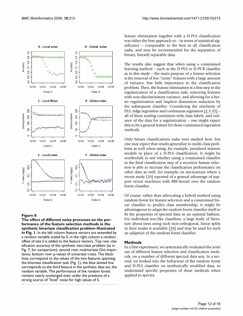
In the presence of increasing additive noise, both univari-ate and multivariate (i.e., the Gini importance) featureimportance measures lost their power to discriminatebetween relevant and random variables at the end (Fig.8DF), with the Gini importance retaining discriminativepower somewhat longer finally converging to a similarvalue for all three variables correlating well with a randomclassification and an (equally) random assignment of fea-ture importance (Fig. 8D). When introducing a source oflocal random noise and normalizing the data accordingly,the univariate tests degraded to random output (Fig. 8E),while the Gini importance measure (Fig. 8CE) virtually

ignored the presence and upscaling of the non-discrimi-natory variable (as did the random forest classifier in Fig.7ACE).

Feature selection using the Gini importanceOverall, we observed that the random forest classifier –with the non-oblique splits of its base learner – may notbe the optimal choice in the classification of spectral data.For feature selection, however, its Gini importanceallowed to rank non-discriminatory features low and toremove them early on in a recursive feature elimination.This desirable property is due to the Gini importancebeing based on a rank order measure which is invariant tothe scaling of individual variables and unaffected by non-discriminatory variance that does disturb D-PCR and D-PLS. Thus, for a constrained classifier requiring a featureselection due to the specificities of the classification prob-lem (Table 2, Fig. 5), the Gini feature importance mightbe a preferable ranking criterion: as a multivariate feature

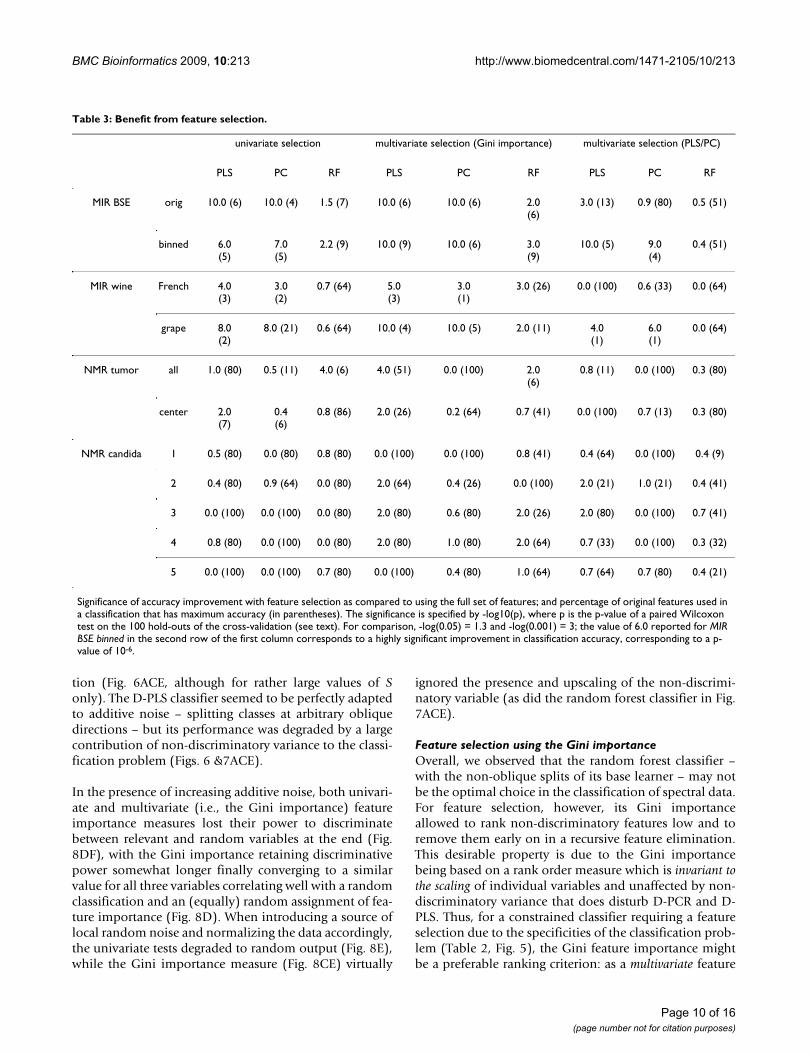
Table 3: Benefit from feature selection.

univariate selection multivariate selection (Gini importance) multivariate selection (PLS/PC)

PLS PC RF PLS PC RF PLS PC RF

MIR BSE orig 10.0 (6) 10.0 (4) 1.5 (7) 10.0 (6) 10.0 (6) 2.0(6)

3.0 (13) 0.9 (80) 0.5 (51)

binned 6.0(5)

7.0(5)

2.2 (9) 10.0 (9) 10.0 (6) 3.0(9)

10.0 (5) 9.0(4)

0.4 (51)

MIR wine French 4.0(3)

3.0(2)

0.7 (64) 5.0(3)

3.0(1)

3.0 (26) 0.0 (100) 0.6 (33) 0.0 (64)

grape 8.0(2)

8.0 (21) 0.6 (64) 10.0 (4) 10.0 (5) 2.0 (11) 4.0(1)

6.0(1)

0.0 (64)

NMR tumor all 1.0 (80) 0.5 (11) 4.0 (6) 4.0 (51) 0.0 (100) 2.0(6)

0.8 (11) 0.0 (100) 0.3 (80)

center 2.0(7)

0.4(6)

0.8 (86) 2.0 (26) 0.2 (64) 0.7 (41) 0.0 (100) 0.7 (13) 0.3 (80)

NMR candida 1 0.5 (80) 0.0 (80) 0.8 (80) 0.0 (100) 0.0 (100) 0.8 (41) 0.4 (64) 0.0 (100) 0.4 (9)

2 0.4 (80) 0.9 (64) 0.0 (80) 2.0 (64) 0.4 (26) 0.0 (100) 2.0 (21) 1.0 (21) 0.4 (41)

3 0.0 (100) 0.0 (100) 0.0 (80) 2.0 (80) 0.6 (80) 2.0 (26) 2.0 (80) 0.0 (100) 0.7 (41)

4 0.8 (80) 0.0 (100) 0.0 (80) 2.0 (80) 1.0 (80) 2.0 (64) 0.7 (33) 0.0 (100) 0.3 (32)

5 0.0 (100) 0.0 (100) 0.7 (80) 0.0 (100) 0.4 (80) 1.0 (64) 0.7 (64) 0.7 (80) 0.4 (21)

Significance of accuracy improvement with feature selection as compared to using the full set of features; and percentage of original features used in a classification that has maximum accuracy (in parentheses). The significance is specified by -log10(p), where p is the p-value of a paired Wilcoxon test on the 100 hold-outs of the cross-validation (see text). For comparison, -log(0.05) = 1.3 and -log(0.001) = 3; the value of 6.0 reported for MIR BSE binned in the second row of the first column corresponds to a highly significant improvement in classification accuracy, corresponding to a p-value of 10-6.

Page 10 of 16(page number not for citation purposes)

BMC Bioinformatics 2009, 10:213 http://www.biomedcentral.com/1471-2105/10/213

importance, it is considering conditional higher-orderinteractions between the variables when measuring theimportance of certain spectral regions, providing a betterranking criterion than a univariate measure used here andin similar tasks elsewhere [9,10].

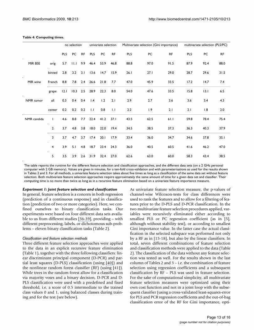
A comparison of the computing times of the different fea-ture selection and classification approaches (Table 4)shows that the computational costs for using the Giniimportance is comparable to the cost of using the othermultivariate feature selection criterion tested in this study.On average the computing time was no more than twiceas long as for the more basic univariate importance meas-ures.

ConclusionIn the joint application of the feature selection and classi-fication methods on spectral data neither the random for-ests classifier using the Gini importance in a recursivefeature selection, nor a constrained regression withoutfeature selection were the optimal choice for classifica-tion. Random forest showed to be robust against singlenoisy features with a large amount of non-discriminatoryvariance. Unfortunately it also showed to be highly sensi-ble to random offsets in the feature vector, a commonartefact in spectral data. D-PLS was capable of dealing

with such offsets, although it failed in the presence ofnon-discriminatory variance in single, highly variable fea-tures. The removal of such irrelevant – or even misleading– predictors was crucial in the application of the con-strained classifiers tested in this study. Overall, the com-bined application of Gini importance in a recursive

Channel-wise variance of each feature (horizontal axis) and its correlation with the dependent variable (vertical axis)Figure 6Channel-wise variance of each feature (horizontal axis) and its correlation with the dependent variable (vertical axis). For the data sets of the left and the central column, a feature selection was not required for optimal per-formance, while the data sets shown in the right columns benefitted from a feature selection. Circle diameter indicates magnitude of the coefficient in the PLS regression. In the right column selected features are shown by red circles, while (the original values of) eliminated features are indicated by black dots. Relevant features show both a high variance and correlation with the class labels.

The effect of different noise processes on the performance of a random forest (green triangles) and a PLS classification (red circles)Figure 7The effect of different noise processes on the per-formance of a random forest (green triangles) and a PLS classification (red circles). In the left column, feature vectors are augmented by a random variable, which is subse-quently rescaled according to a factor S (horizontal axis), thus introducing non-discriminatory variance to the classifica-tion problem. In the right column, a random variable scaled by factor S is added as constant offset to the feature vectors, increasing the correlation between features (see text for details). Shown are results on the basis of the bivariate classi-fication problem of Fig. 1 (top row), the NMR candida 2 data (middle), and the BSE binned data (below).

Page 11 of 16(page number not for citation purposes)

BMC Bioinformatics 2009, 10:213 http://www.biomedcentral.com/1471-2105/10/213

feature elimination together with a D-PLS classificationwas either the best approach or – in terms of statistical sig-nificance – comparable to the best in all classificationtasks, and may be recommended for the separation ofbinary, linearly separable data.

The results also suggest that when using a constrainedlearning method – such as the D-PLS or D-PCR classifieras in this study – the main purpose of a feature selectionis the removal of few "noisy" features with a large amountof variance, but little importance to the classificationproblem. Then, the feature elimination is a first step in theregularization of a classification task, removing featureswith non-discriminatory variance, and allowing for a bet-ter regularization and implicit dimension reduction bythe subsequent classifier. Considering the similarity ofPLS, ridge regression and continuum regression [2,3,35] –all of them trading correlation with class labels, and vari-ance of the data for a regularization – one might expectthis to be a general feature for these constrained regressionmethods.

Only binary classifications tasks were studied here, butone may expect that results generalize to multi-class prob-lems as well when using, for example, penalized mixturemodels in place of a D-PLS classification. It might beworthwhile to test whether using a constrained classifierin the final classification step of a recursive feature selec-tion is able to increase the classification performance onother data as well, for example on microarrays where arecent study [20] reported of a general advantage of sup-port vector machines with RBF-kernel over the randomforest classifier.

Of course, rather than advocating a hybrid method usingrandom forest for feature selection and a constrained lin-ear classifier to predict class membership, it might beadvantageous to adapt the random forest classifier itself tofit the properties of spectral data in an optimal fashion.For individual tree-like classifiers, a large body of litera-ture about trees using such non-orthogonal, linear splitsin their nodes is available [34] and may be used for suchan adaption of the random forest classifier.

MethodsIn a first experiment, we systematically evaluated the jointuse of different feature selection and classification meth-ods, on a number of different spectral data sets. In a sec-ond, we looked into the behaviour of the random forestand D-PLS classifier on synthetically modified data, tounderstand specific properties of these methods whenapplied to spectra.

The effect of different noise processes on the performance of the feature selection methods in the synthetic bivariate classification problem illustrated in Fig. 1Figure 8The effect of different noise processes on the per-formance of the feature selection methods in the synthetic bivariate classification problem illustrated in Fig. 1. In the left column feature vectors are extended by a random variable scaled by S, in the right column a random offset of size S is added to the feature vectors. Top row: clas-sification accuracy of the synthetic two-class problem (as in Fig. 7, for comparison); second row: multivariate Gini impor-tance, bottom row: p-values of univariate t-test. The black lines correspond to the values of the two features spanning the bivariate classification task (Fig. 1), the blue dotted line corresponds to the third feature in the synthetic data set, the random variable. The performance of the random forest remains nearly unchanged even under the presence of a strong source of "local" noise for high values of S.

Page 12 of 16(page number not for citation purposes)

BMC Bioinformatics 2009, 10:213 http://www.biomedcentral.com/1471-2105/10/213

Experiment 1: Joint feature selection and classificationIn general, feature selection is a concern in both regression(prediction of a continuous response) and in classifica-tion (prediction of two or more categories). Here, we con-fined ourselves to binary classification tasks. Ourexperiments were based on four different data sets availa-ble to us from different studies [36-39], providing – withdifferent preprocessing, labels, or dichotomous sub-prob-lems – eleven binary classification tasks (Table 2).

Classification and feature selection methodsThree different feature selection approaches were appliedto the data in an explicit recursive feature elimination(Table 1), together with the three following classifiers: lin-ear discriminant principal component (D-PCR) and par-tial least squares (D-PLS) classification (using [40]) andthe nonlinear random forest classifier (RF) (using [41]).While trees in the random forest allow for a classificationvia majority votes and a binary decision, D-PCR and D-PLS classification were used with a predefined and fixedthreshold, i.e. a score of 0.5 intermediate to the trainedclass values 0 and 1, using balanced classes during train-ing and for the test (see below).

As univariate feature selection measure, the p-values ofchannel-wise Wilcoxon-tests for class differences wereused to rank the features and to allow for a filtering of fea-tures prior to the D-PLS and D-PCR classification. In thetwo multivariate feature selection procedures applied, var-iables were recursively eliminated either according tosmallest PLS or PC regression coefficient (as in [5],although without stability test), or according to smallestGini importance value. In the latter case the actual classi-fication in the selected subspace was performed not onlyby a RF as in [15-18], but also by the linear classifiers. Intotal, seven different combinations of feature selectionand classification methods were applied to the data (Table2). The classification of the data without any feature selec-tion was tested as well. For the results shown in the lastcolumn of Tables 2 and 3 – i.e. the combination of featureselection using regression coefficients and a subsequentclassification by RF – PLS was used in feature selection.For the sake of computational simplicity, all multivariatefeature selection measures were optimized using theirown cost function and not in a joint loop with the subse-quent classifier (using a cross-validated least-squares-errorfor PLS and PCR regression coefficients and the out-of-bagclassification error of the RF for Gini importance, opti-

Table 4: Computing times.

no selection univariate selection Multivariate selection (Gini importance) multivariate selection (PLS/PC)

PLS PC RF PLS PC RF PLS PC RF PLS PC RF

MIR BSE orig 5.7 11.1 9.9 46.4 53.9 46.8 88.8 97.0 91.5 87.9 92.4 88.0

binned 2.8 3.2 3.1 13.6 14.7 15.9 26.1 27.1 29.0 28.7 29.6 31.5

MIR wine French 8.8 7.8 2.4 26.6 21.8 7.7 47.0 45.9 33.5 17.2 14.7 7.4

grape 12.1 10.3 2.5 28.9 22.3 8.0 54.0 47.6 33.5 15.8 13.1 6.5

NMR tumor all 0.3 0.4 0.4 1.4 1.2 2.1 2.9 2.7 3.6 3.6 3.4 4.3

center 0.2 0.2 0.2 1.1 0.8 1.1 2.2 1.9 2.1 2.1 1.8 2.0

NMR candida 1 4.6 8.8 7.7 22.4 41.2 37.1 43.5 62.5 61.1 59.8 78.4 75.4

2 3.7 4.8 3.8 18.0 22.0 19.4 34.5 38.5 37.3 36.3 40.3 37.9

3 3.7 4.7 3.7 17.4 20.1 17.9 33.4 36.0 34.7 34.6 37.8 35.1

4 3.9 5.1 4.8 18.7 23.4 24.3 36.0 40.5 60.5 41.6 46.2 47.0

5 3.5 3.9 2.6 31.9 32.4 27.0 62.6 63.0 60.0 58.3 43.4 38.5

The table reports the runtime for the different feature selection and classification approaches, and the different data sets (on a 2 GHz personal computer with 2 GB memory). Values are given in minutes, for a ten-fold cross-validation and with parameterisations as used for the results shown in Tables 2 and 3. For all methods, a univariate feature selection takes about five times as long as a classification of the same data set without feature selection. Both multivariate feature selection approaches require approximately the same amount of time for a given data set and classifier. Their computing time is no more than twice as long as in a recursive feature elimination based on a univariate feature importance measure.

Page 13 of 16(page number not for citation purposes)

BMC Bioinformatics 2009, 10:213 http://www.biomedcentral.com/1471-2105/10/213

mized over the same parameter spaces as the respectiveclassifiers). For both univariate filters and multivariatewrappers, 20% of the remaining features were removed ineach iteration step. Prior to classification all data was sub-ject to L1 normalization, i.e. to a normalization of the areaunder the spectrum in a predefined spectral region.

DataData set one, the BSE data set, originates from a study con-cerning a conceivable ante-mortem test for bovine spong-iform encephalopathy (BSE). Mid-infrared spectra of N =200 dried bovine serum samples (Npos = 95, Nneg = 105)were recorded in the spectral range of 400–4000 cm-1 withP = 3629 data points per spectrum. Details of the samplepreparation and of the acquisition of spectra are reportedin Refs. [14,31]. The same spectra were used in a secondbinary classification task after a smoothing and downsam-pling ("binning"), and thus by reducing the number ofdata points per spectrum to Pred = 1209.

Data set two, the wine data set, comprised N = 71 mid-infrared spectra with a length of P = 3445 data points fromthe spectral region of 899–7496 cm-1, sampled at a resolu-tion of approx. 4 cm-1 interpolated to 2 cm-1, originatingfrom the analysis of 63 different wines using an auto-mated MIRALAB analyzer with AquaSpec flow cell. In thepreprocessing a polynomial filter (Savitzky-Golay, length9) of second order was applied to the spectra. Labelsassigned to these data were the type of grape (Nred = 30,Nwhite = 41) in a first learning task and an indicator of thegeographic origin of the wine (NFrench = 26, NWorld = 45) ina second.

Data set three, the tumor data set, comprised N = 278 invivo 1H-NMR spectra with a length of P = 101 data pointsfrom the spectral region between approximately 1.0 ppmand 3.5 ppm, originating from 31 magnetic resonancespectroscopic images of 31 patients, acquired at 1.5 T withan echo time of 135 ms in the pre-therapeutic and post-operative diagnostics of (recurrent) brain tumor (Nhealthy =153, Ntumor border = 72, Ntumor center = 53) [31,32]. Two binarygroupings were tested, either discriminating healthy vs.both tumor groups (tumor all), or the spectral signature ofthe tumor center vs. the remaining spectra (tumor center).

Data set four, the candida data set, comprised N = 581 1H-NMR spectra of cell suspensions with a length of P = 1500data points in between 0.35–4 ppm, originating from achemotaxonomic classification of yeast species (Candidaalbicans, C. glabrata, C. krusei, C. parapsilosis, and C.tropicalis). A subset of the data was originally publishedin [34]. Its five different subgroups of sizes N = {175, 109,101, 111, 85} allowed to define five different binary sub-problems ("one-against-all").

ComparisonIn the evaluation, 100 training and 100 test sets were sam-pled from each of the available data sets, in a ten timesrepeated ten-fold cross validation [42,43], following theoverall test design in [19]. In order to obtain equal classpriors both in training and testing, the larger of the twogroups of the binary problems was subsampled to the sizeof the smaller if necessary. Where dependence betweenobservations was suspected, e.g. in the tumor data wheremore than one spectrum originated for each patient, thecross-validation was stratified to guarantee that all spectraof a correlated subset were exclusively assigned to eitherthe training or the test data [42,43].

The random forest parameters were optimized in logarith-mic steps around their default values [41] (using 300trees, and a random subspace with dimensionality equalto the rounded value of the square of the number of fea-tures) according to the out-of-bag error of the random for-est, while the number of latent variables γ in the linearclassifiers was determined by an internal five-fold cross-validation for each subset, following the 1σ rule forchoosing the γ at the intersection between the least error(at γopt) plus an interval corresponding to the 1σ standarddeviation at γopt, and the mean accuracy.

The classification accuracy was averaged over all 100 testresults and used as performance measure in the compari-son of the different methods. While all feature selectionand all optimization steps in the classification were per-formed utilizing the training data only, test result wererecorded for all feature subsets obtained during the courseof feature selection (Fig. 4). To verify significant differ-ences between the test results, a paired Cox-Wilcoxon testwas used on the accuracies of the 100 test sets as proposedin [42,43]. Such paired comparisons were performed foreach classifier between the classification result obtainedfor the full set of features, and the best result when appliedin conjunction with a selection method (i.e. the resultswith highest classification accuracy in the course of featureselection). Feature selection approaches leading to a sig-nificant increase in classification performance were indi-cated accordingly (Table 2, indicated by stars). Once thebest feature selection and classification approach hadbeen identified for a data set (as defined by the highestclassification accuracy in a row in Table 2), it was com-pared against all other results on the same data set. Resultswhich were indistinguishable from this best approach (nostatistical difference at a 5% level) were indicated as well(Table 2, indicated by bold values).

Experiment 2: PLS and RF classification as a function of specific data propertiesD-PLS reportedly benefits from an explicit feature selec-tion on some data sets [33]. Random forest reportedly

Page 14 of 16(page number not for citation purposes)

BMC Bioinformatics 2009, 10:213 http://www.biomedcentral.com/1471-2105/10/213

performed well in classification tasks with many featuresand few samples [15-18], but was outperformed by stand-ard chemometrical learning algorithms when used to clas-sify spectral data. Thus, to identify reasons for thesedifferences and to corroborate findings from experimentone, we decided to study the performance of both meth-ods in dependence of two noise processes which are spe-cific to spectral data.

Noise processesWe identified two sources of unwanted variation (noiseprocesses) which can be observed in spectral data, andwhich can jeopardize the performance of a classifier.

First, there are processes affecting few, possibly adjacent,spectral channels only. Examples for such changes in thespectral pattern are insufficiently removed peaks andslight peak shifts (magnetic resonance spectroscopy), thepresence of additional peaks from traces of unremovedcomponents in the analyte, or from vapour in the lightbeam during acquisition (infrared spectroscopy). Identi-fying and removing spectral channels affected by suchprocesses is often the purpose of explicit feature selection.We refer to this kind of noise as "local noise" in the fol-lowing, where the locality refers to the adjacency of chan-nels along the spectral axis.

Second, there are processes affecting the spectrum as awhole. Examples for such noise processes may be the pres-ence (or absence) of broad baselines, resulting in a ran-dom additional offset in the spectrum. Variation may alsoresult from differences in the signal intensities due tochanges in the concentration of the analyte, variation inreflectance or transmission properties of the sample(infrared spectroscopy), or the general signal amplitudefrom voxel bleeding and partial volume effects (magneticresonance spectroscopy), leading to a scaling of the spec-trum as a whole, and – after normalization – to randomoffsets in the spectrum. Such processes increase the nom-inal correlation between features and are the main reasonfor the frequent use of high-pass filters in the preprocess-ing of spectral data (Savitzky-Golay filter, see above). Itmight be noted that this noise does not have to offset thespectrum as a whole to affect the classification perform-ance significantly, but may only modify those spectralregions which turn out to be relevant to the classificationtask. Nevertheless, we refer to this kind of noise as "globalnoise" here.

Modified and synthetic data setsFor visualization (Fig 1, left), we modelled a synthetictwo-class problem, by drawing 2*400 samples from twobivariate normal distributions (centred at (0,1) and (1,0),respectively, with standard deviation 0.5). The two fea-tures for the two-dimensional classification task were aug-

mented by a third feature comprising only random noise(normally distributed, centred at 0, standard deviation0.5), resulting in a data set with N = 800, P = 3 and bal-anced classes. To mimic local noise, we rescaled the third,random feature by a factor S, for S = 2{0,1,...,20}. In real spec-tra one might expect S – the ratio between the amplitudeof a variable that is relevant to the classification problem,and a larger variable introducing non-discriminatory var-iance only – to be of several orders of magnitude. Here,changing S gradually increased the variance of the thirdfeature and the amount of non-discriminatory variance inthe classification problem. To mimic global noise, weadded a constant offset (normally distributed, centred at0, standard deviation 0.5), also scaled by S = 2{0,1,...,20}, tothe features of every sample as an offset. This increased thecorrelation between the features and, along S, graduallystretched the data along the bisecting line (Fig. 1, right).

In addition to the synthetic two-class problem of Fig. 1,we modified two exemplary real data sets (candida 2 andBSE binned) by these procedures in the same way, hereusing S = 10{-6,-4,...,16}, using the largest amplitude of aspectrum as reference for a shift by S = 1, or a rescaling ofthe random feature (N(0,.5)).

ComparisonGini importance and univariate importance (t-test) werecalculated along S for the features of the synthetic data set.PLS and random forest classification were applied to alldata sets, for all values of S, after a L2-normalization of thefeature vector. (Which may be a closer match with thenoise statistic than the L1 normalization used in the realdata in the first experiment.) Classification accuracy wasdetermined according to the procedure described above(Experiment 1).

Authors' contributionsBHM performed the design of the study and drafted themanuscript. FAH contributed significantly to the manu-script. RM, UH, PB, WP acquired data for the study. Allauthors participated in the analysis of the results. BHM,BMK, WP, FAH conceived of the study and participated inits coordination. All authors read and approved the finalmanuscript.

AcknowledgementsBHM acknowledges support from the German Academy of Sciences Leopoldina through the Leopoldina Fellowship Programme (LPDS 2009-10). FAH acknowledges support by the German Research Foundation (DFG HA-4364).

References1. Guyon I, Elisseeff A: An introduction to variable and feature

selection. J Mach Learn Res 2003, 3:1157-82.2. Stone M, J R, Brooks Continuum regression: Cross-validated

sequentially constructed prediction embracing ordinary

Page 15 of 16(page number not for citation purposes)

BMC Bioinformatics 2009, 10:213 http://www.biomedcentral.com/1471-2105/10/213

Publish with BioMed Central and every scientist can read your work free of charge

"BioMed Central will be the most significant development for disseminating the results of biomedical research in our lifetime."

Sir Paul Nurse, Cancer Research UK

Your research papers will be:

available free of charge to the entire biomedical community

peer reviewed and published immediately upon acceptance

cited in PubMed and archived on PubMed Central

yours — you keep the copyright

Submit your manuscript here:http://www.biomedcentral.com/info/publishing_adv.asp

BioMedcentral

least squares, partial least squares and principal componentsregression. J Roy Stat Soc B (Meth) 1990, 52:237-269.

3. Frank IE, Friedman JH: A statistical view of some Chemometricsregression tools. Technometrics 1993, 35:109-135.

4. Bylesjö M, Rantalainen M, Nicholson JK, Holmes E, Trygg J: K-OPLSpackage: Kernel-based orthogonal projections to latentstructures for prediction and interpretation in feature space.BMC Bioinformatics 2008, 9:106.

5. Westad F, Martens H: Variable selection in near infrared spec-troscopy based on significance testing in partial least squaresregression. J Near Infrared Spectrosc 2000, 117:117-124.

6. Nadler B, Coifman RR: The prediction error in CLS and PLS:the importance of feature selection prior to multivariate cal-ibration. J Chemometrics 2005, 19:107-118.

7. Denham MC, Brown PJ: Calibration with many variables. ApplStat 1993, 42:515-528.

8. Baumann K, von Korff M, Albert H: Asystematic evaluation of thebenefits and hazards of variable selection in latent variableregression. Part I. Search Algorithm, theory and simula-tions. J Chemometrics 2002, 16:339-350.

9. Hastie T, Tibshirani R, Eisen MB, Alizadeh A, Levy R, Staudt L, ChanWC, Botstein D, Brown P: 'Gene shaving' as a method for iden-tifying distinct sets of genes with similar expression patterns.Genome Biol 2000, 1:3.

10. Zeng XQ, Li GZ, Yang JY, Yang MQ, Wu GF: Dimension reductionwith redundant gene elimination for tumor classification.BMC Bioinformatics 2008, 9:S8.

11. Leardi R: Genetic algorithms in chemometrics and chemistry:a review. J Chemometrics 2001, 15:559-569.

12. Centner V, Massart DL, de Noord OE, de Jong S, Vandeginste BM,Sterna C: Elimination of uninformative variables for multivar-iate calibration. Anal Chem 1996, 68:3851-58.

13. Forina M, Casolino C, Millan CP: Iterative predictor weighting(IPW) PLS: a technique for the elimination of useless predic-tors in regression problems. J Chemometrics 1999, 13:165-84.

14. Breiman L: Random forests. J Mach Learn 2001, 45:5-32.15. Jiang H, Deng Y, Chen H-S, Tao L, Sha Q, Chen J, Tsai C-J, Zhang S:

Joint analysis of two microarray gene-expression data sets toselect lung adenocarcinoma marker genes. BMC Bioinformatics2004, 5:1-12.

16. Diaz-Uriarte R, Alvarez de Andres S: Gene selection and classifi-cation of microarray data using random forest. BMC Bioinfor-matics 2006, 7:1-25.

17. Li S, Fedorowicz A, Singh H, Soderholm SC: Application of therandom forest method in studies of local lymph node assaybased skin sensitization data. J Chem Inf Comp Sci 2005,45:952-64.

18. Geurts P, Fillet M, de Seny D, Meuwis M-A, Malaise M, Merville M-P,Wehenkel L: Proteomic mass spectra classification using deci-sion tree based ensemble methods. Bioinformatics 2005,21:313-845.

19. Dudoit S, Fridlyand J, Speed TP: Comparison of discriminationmethods for the classification of tumors using gene expres-sion data. J Am Stat Assoc 2002, 97:77-88.

20. Statnikov A, Wang L, Aliferis CF: A comprehensive comparisonof random forests and support vector machines for microar-ray-based cancer classification. BMC Bioinformatics 2008, 9:319.

21. Shen KQ, Ong CJ, Li XP, Zheng H, Wilder-Smith EPV: A FeatureSelection Method for Multi-Level Mental Fatigue EEG Clas-sification. IEEE Trans Biomed Engin 2007, 54:1231-1237.

22. Menze BH, Petrich W, Hamprecht FA: Multivariate feature selec-tion and hierarchical classification for infrared spectroscopy:serum-based detection of bovine spongiform encephalopa-thy. Anal Bioanal Chem 2007, 387:801-1807.

23. Granitto P, Furlanello C, Biasioli F, Gasperi F: Recursive FeatureElimination with Random Forest for PTR-MS analysis ofagroindustrial products. Chem Intell Lab Sys 2006, 83:83-90.

24. Svetnik V, Liaw A, Tong C, Culberson JC, Sheridan RP, Feuston BP:Random Forest: A Classification and Regression Tool forCompound Classification and QSAR Modeling. J Chem InfComp Sci 2003, 43:1947-58.

25. Lin Y, Jeon Y: Random Forests and adaptive nearest neighbor.J Am Stat Assoc 2006, 101:578-590.

26. Biau G, Devroye L, Lugosi G: Consistency of Random Forestsand Other Averaging Classifiers. J Mach Learn Res 2008,9:2015-2033.

27. Breiman L: Consistency for a simple model of random forests.In Technical Report 670 Technical report, Department of Statistics,University of California, Berkeley, USA; 2004.

28. Strobl C, Boulesteix A-L, Kneib T, Augustin T, Zeileis A: Condi-tional variable importance for random forests. BMC Bioinfor-matics 2008, 9:307.

29. Jiang R, Tang W, Wu X, Fu W: A random forest approach to thedetection of epistatic interactions in case-control studies.BMC Bioinformatics 2009, 10(Suppl 1):S65.

30. Strobl C, Boulesteix AL, Zeileis A, Hothorn T: Bias in RandomForest Variable Importance Measures: Illustrations, Sourcesand a Solution. BMC Bioinformatics 2007, 8:25.

31. Sandri M, Zuccoletto P: A bias correction algorithm for the Ginivariable importance measure in classification trees. J CompGraph Stat 2008, 17:611-628.

32. Archer KJ, Kimes RV: Empirical characterization of randomforest variable importance measures. Comp Stat Data Anal2008, 52:2249-2260.

33. Gauchi J-P, Chagnon P: Comparison of selection methods ofexplanatory variables in PLS regression with application tomanufacturing process data. Chem Intell Lab Sys 2001, 58:171-93.

34. Murthy SK, Kasif S, Salzberg S: A System for Induction of ObliqueDecision Trees. J Artif Intell Res 1994, 2:1-32.

35. Bjorkstrom A: A generalized view on continuum regression.Scand J Stat 1999, 26:17-30.

36. Martin TC, Moecks J, Belooussov A, Cawthraw S, Dolenko B, EidenM, Von Frese J, Kohler W, Schmitt J, Somorjai RL, Udelhoven T, Ver-zakov S, Petrich W: Classification of signatures of bovine spong-iform encephalopathy in serum using infrared spectroscopy.Analyst 2004, 129:897-901.

37. Menze BH, Lichy MP, Bachert P, Kelm BM, Schlemmer H-P, Ham-precht FA: Optimal classification of long echo time in vivomagnetic resonance spectra in the detection of recurrentbrain tumors. NMR in Biomedicine 2006, 19:599-60.

38. Menze BH, Kelm BM, Heck D, Lichy MP, Hamprecht FA: Machinebased rejection of low-quality spectra and estimation ofbrain tumor probabilities from magnetic resonance spectro-scopic images. In Proceedings of BVM Edited by: Handels H, EhrhardtJ, Horsch A, Meinzer H-P, Tolxdorff T. Springer, New York;2006:31-35.

39. Himmelreich U, Somorjai RL, Dolenko B, Lee OC, Daniel HM, Mur-ray R, Mountford CE, Sorrell TC: Rapid identification of candidaspecies by using nuclear magnetic resonance spectroscopyand a statistical classification strategy. Appl Environm Microbiol2003, 69:4566-74.

40. Mevik B-H, Wehrens R: The pls Package: Principal Componentand Partial Least Squares Regression in R. J Stat Software 2007,18:1-24.

41. Liaw A, Wiener M: Classification and Regression by random-Forest. R News 2002, 2:18-22.

42. Hothorn T, Leisch F, Zeileis A, Hornik K: The design and analysisof benchmark experiments. J Comp Graph Stat 2005, 14:575-699.

43. Demsar J: Statistical comparisons of classifiers over multipledata sets. J Mach Learn Res 2006, 7:1-30.

Page 16 of 16(page number not for citation purposes)