A comparison of pollen counts: Light versus scanning electron microscopy

A comparison of pollen counts: Light versus scanning electronmicroscopy

GRETCHEN D. JONES1 & VAUGHN M. BRYANT, JR.2

1Areawide Pest Management Research Unit (APRMU), Agricultural Research Service (ARS), United States Department of

Agriculture (USDA), College Station, Texas, USA, 2Palynology Laboratory, Department of Anthropology, Texas A & M

University (TAMU), College Station, Texas, USA

AbstractPalynologists use compound light microscopy (LM) for pollen identification and interpretation and scanning electronmicroscopy (SEM) for morphological comparisons and taxonomy. As we are unaware of any published reports comparingLM and SEM pollen counts and identifications of the same sample, we decided to examine a surface soil sample using bothmicroscopes. Standard palynological extraction techniques were used. Two, 300 grain counts were made using LM, andtwo, 300 counts with SEM. Pollen grains viewed with SEM were also divided into three categories, ‘‘identifiable,’’‘‘obscured,’’ and ‘‘virtually impossible to identify’’. Eighty-six (86) percent of the pollen grains counted with SEM wereclassified as ‘‘identifiable’’ or ‘‘obscured.’’ Pollen concentration values ranged from 385,714 (LM Count #2) to 900,000(SEM Count #1) per gram of soil. Regardless of the microscope used, Ligustrum spp., Myrtaceae-type, and Tilia spp. hadthe greatest number of pollen grains. A total of 73 taxa were found. A scan of the unexamined portion of the stubs resultedin 20 additional taxa. There were no significant differences between the counts made with the two microscopes (ANOVA,pw0.05, F50.18, df576). However, there were significantly more taxa found with SEM than with LM (t-test, T50.05).Sample preparation and the time needed to count, analyze, photograph and print the micrographs are the same regardless ofthe microscope used. The sample, information needed, and funding will determine which technique to use.

Keywords: Pollen analyses, scanning electron microscopy, light microscopy, soil analysis

Palynologists rely on light microscopy (LM) to

identify and interpret the pollen spectrum of a

particular sample. Scanning electron microscopy

(SEM) is not normally used for counting and

identifying pollen grains. Instead, SEM is mainly

used for morphological comparisons and taxonomy

where the increased resolution of SEM makes

differentiation of pollen grains and taxa more

obvious (for example The Northwest European

Pollen Flora I–VIII (Punt, 1976; Punt & Clarke,

1980, 1981, 1984, 1988; Punt & Blackmore, 1991;

Punt et al., 1995; Blackmore et al., 2003), Pollen et

spores d’Europe et d’Afrique du Nord Series (Reille,

1992, 1995, 1998, 1999), and in Grayum’s con-

tribution, 1992) and as an aid in taxonomy (Skvarla

& Larson, 1965; Ridgeway & Skvarla, 1969).

Scanning electron microscopy of pollen is also used

to create new terminology for describing pollen

ornamentation (Rowley et al., 1988; Vezey &

Skvarla, 1990; Vezey et al., 1991), developing a

numerical approach to pollen sculpturing (Vezey et

al., 1991), and even computer analysis of the exine

(Vezey & Skvarla, 1990).

Some modern palynological textbooks include

SEM micrographs of pollen (Ogden et al., 1974;

Moore et al., 1991); however, the majority focuses

only on LM (Herrera & Urrego, 1996; Beug, 2004).

Likewise, some atlases include SEM micrographs

(Nilsson et al., 1977; Bassett et al., 1978; Moar,

1993; Qiao, 2005) and only a few solely use SEM

Correspondence: Gretchen D. Jones, Areawide Pest Management Research Unit (APMRU), ARS United States of Agriculture, 2771 F&B Road, College

Station, TX 77845, U.S.A. E-mail: [email protected]

(Received 2 March 2006; accepted 12 December 2006)

Grana, 2007; 46: 20–33

ISSN 0017-3134 print/ISSN 1651-2049 online # 2007 Taylor & Francis

DOI: 10.1080/00173130601173897

micrographs for the pollen presentation (Adams &

Morton, 1972, 1974, 1976, 1979; Bambara & Leidy,

1991; Jones et al,. 1995; Wei et al., 2003).

Most entomopalynological (study of pollen on/in

insects) studies use LM for pollen analyses (Jones &

Coppedge, 1998). However, SEM is better for

examining the pollen that adheres to insects, such

as moths and butterflies (Lepidoptera). Since much

of that pollen is on the proboscis, legs, thorax and

head (Bryant et al., 1991), the samples can be

mounted on SEM stubs and examined without

processing. In these types of SEM studies, pollen

identification is used to determine migration and

dispersal routes, insect source zones and examine

feeding resources (Hendrix et al., 1987; Benedict et

al., 1991; Hendrix & Showers, 1992; Gregg, 1993;

Lingren et al., 1993, 1994; Del Socorro & Gregg,

2001; Gregg et al., 2001).

Van Laere et al. (1969) saw the promise of SEM

in such studies and even suggested that SEM might

be an important technique for analyzing honey.

Chen and Shen (1990) used SEM to examine the

pollen of Formosan honey. However, they did not

use SEM to make counts and pollen identifications.

Blackburn and Ford (1993) used SEM micrographs

of filtered honey to determine the abundance of each

pollen type in the honey. The abundance was

calculated by placing a 1 cm2 acetate grid over each

micrograph. Unfortunately, there is no information

about the actual pollen counts or pollen diversity.

Regardless, SEM is not routinely used in palynol-

ogy and is seldom used to make pollen counts or

pollen identification. In some situations the lack of

availability and/or lack of funding may prevent the

use of SEM. Nevertheless, if both LM and SEM

were available, which should be chosen to conduct a

pollen analysis of a single sample? We could not find

any published comparisons between LM and SEM

pollen counts and pollen identifications of the same

sample, or any information about using SEM for

sediment samples. The purpose of this research was

to test and determine the advantages and disadvan-

tages of each technique (LM and SEM), and to

compare the pollen counts and pollen identifications

from the same sample.

Material and methods

A surface sample (3.0 g) was collected following

Adam and Mehringer (1975) in Tirana, Albania by

mixing 30 individual ‘‘pinches’’ from the uppermost

layer of soil at different locations within a 10 km2

area. Unless otherwise stated, the sample was always

centrifuged for 3 min at 10606g., the supernatant

decanted, and resulting residue mixed (vortexed) on

a vortex stirrer for 30 s after each step.

Pollen extraction

One-half of the soil sample (1.5 g) was examined for

pollen. One tablet of Lycopodium clavatum L. spores

(Figure 1A) was dissolved in 5 drops of concen-

trated hydrochloric acid (HCl) for 5 min then added

to the sample. The beaker containing the spores was

rinsed twice with 95% ethyl alcohol (ETOH), and

the rinse added to the sample.

The sample was then rinsed with glacial acetic

acid.

Five ml of an acetolysis mixture (Erdtman, 1960)

was added to the subsample. The subsample was

heated for 6 min at 80˚C in a pre-heated hot block.

After which 5 ml of glacial acetic acid were added.

The subsample was rinsed with glacial acetic acid

followed by two distilled water rinses. After each

rinse the sample was centrifuged, decanted, and

vortexed.

Four ml of zinc bromide (ZnBr2) (specific gravity

of 1.9) was added, and then thoroughly mixed into

the subsample for one min. Afterwards, an addi-

tional 5 ml of ZnBr2 was mixed into the subsample.

The subsample was centrifuged for 5 min at 2126g,

and then for 5 min at 10606g. The dark band of

material (pollen residue) that formed on the surface

after centrifugation was removed. It consisted of

about 2 ml of fluid.

To reduce the specific gravity of the removed pollen

residue, 40 ml of 95% ETOH (specific gravity of

0.79) were added to the pollen residue. The pollen

residue was concentrated using centrifugation.

The sample was rinsed twice with 95% ETOH.

One drop of the pollen reside was pipetted onto a

SEM stub that was previously coated with

TEMPFIXH adhesive. Three stubs were made, each

with a single drop of the pollen residue.

Several drops of safranin-O stain and 8 ml of 95%

ETOH were added to the remaining pollen residue.

After centrifuging, decanting, and vortexing, the

residue was transferred to a one-dram, glass vial.

Five drops of glycerin were stirred into the vial and

the vial was placed on a warm hot plate at 27˚Covernight.

LM preparation

Before making each slide, the pollen residue was

vortexed for 30 s (Jones & Bryant, 1998). One drop

of residue was placed on a glass slide, allowed to

spread, then covered with a cover slip, and the slide

sealed.

SEM preparation

Stubs were coated with 400 A of gold palladium in a

Hummer II sputter coater. Marks for repositioning

A comparison of pollen counts: LM vs. SEM 21

of the stub were added before and after coating.

Marks made prior to coating included numbers or

letters added to the sides, top, and bottom of the stub

with a permanent marker. Marks made after coating

included a drop of glitter nail polish (Figure 1B), an

‘‘i’’ made with a pair of forceps (Figure 1C), or a ‘‘+’’

made with a diamond scribe (Figure 1D). Stubs were

examined in a JEOL JSM-6400 scanning electron

microscope using an operating voltage of 15 kV and a

working distance of 15 mm.

LM and SEM analyses

Four 300-grain pollen counts were made. One count

was made from each of the two prepared glass slides,

and one from each of two of the three prepared SEM

stubs.

Pollen grains viewed with SEM were put into

three categories. Grains where most of the diagnostic

features could be seen were placed into Category 1

‘‘identifiable’’ (Figure 1A). Grains in Category 2

were labeled ‘‘obscured’’. Pollen in this category

included grains that were sufficiently covered by

debris so that many key ornamentation and/or

aperturation details were partially obscured or were

in a poor orientation (Figure 2A).

Category 3 grains were considered ‘‘virtually

impossible to identify’’. This category included

grains that were badly degraded, severely broken,

crumpled, badly folded, or so obscured by debris

that sufficient morphological details were not visible

(Figure 2B).

Pollen identification

Pollen identifications were made utilizing the USDA

Areawide Pest Management Research Unit

(APMRU) Modern Pollen Reference Collections,

the Texas A & M University Palynology Laboratory

Modern Pollen Reference Collection (TAMU), and

comparisons with images in a number of published

pollen atlases.

Figure 1. (A) Lycopodium clavatum L. spore that was added as a tracer; (B) SEM after-coating mark made with nail polish; (C) SEM after-

coating mark made with a pair for forceps; (D) SEM after-coating mark made with a diamond probe. Scale bars – 20 mm (A); 200 mm (B,

D); 100 mm (C).

22 G. D. Jones and V. M. Bryant, Jr.

For SEM analyses, when a pollen grain’s orna-

mentation looked different from other grains in the

same family or genus, it was considered to represent

a different taxon. Several different pollen types in the

genera Ligustrum, Tilia, and Plantago were distin-

guishable during SEM analyses but were not initially

apparent during LM analyses. During the SEM

analyses, the pollen in each genus was separated into

species or groups called ‘‘types.’’ To make the

counts comparable, the number of pollen grains for

the different types of Ligustrum, Tilia, and Plantago

are lumped together in a genus ranking. For

example, three different types of Tilia pollen were

apparent during the SEM analyses but not during

the LM. Therefore, there is a Tilia SEM total that is

a summation of the number of pollen grains from

each of the three Tilia types.

Asteraceae. The sunflower plant family is the largest

vascular plant family with over 1,525 genera and

over 22,750 species (Mabberley, 1997). Assigning

specific genera to the pollen in this vast group is

difficult even though each species has its own unique

morphology. Nevertheless, some broad pollen

groups were used. These groups included

Artemisia, and Cichorioideae, both of which are

distinguishable.

Martin (1963) split the pollen of the subfamily

Asteroideae into two major groups based on the

length of the surface ‘‘spines.’’ Asteroideae pollen

with surface ‘‘spines’’ longer than 2.5 um were

categorized as a high ‘‘spine’’ (HS) group, and those

with shorter ‘‘spines’’ were put into a low ‘‘spine’’

(LS) group.

Myrtaceae. This large family of tropical and

subtropical plants contains over 130 genera and

more than 4,600 species (Mabberley, 1997). Since

the 1800s, members of this family have been

exported as ornamental or timber trees to tropical

and subtropical regions of the world. Most of the

pollen types in the Myrtaceae share similar

morphological characteristics. However, with SEM,

different Myrtaceae pollen grains were initially

separated into distinctive types. Similar to

Ligustrum, Tilia, and Plantago for comparison

between LM and SEM counts, there is a

Myrtaceae SEM total that is a summation of the

number of pollen grains from each Myrtaceae type.

Pollen statistics

The number of taxa was totalled for each technique

(LM and SEM), a grand total was summed, and

pollen concentration values were calculated using

the following formula:

number pollen grains countedð Þ| number of tracer spores addedð Þnumber of grams of sample processedð Þ| number tracer spores countedð Þ

ANOVA and t-tests were used to compare the

Figure 2. Two pollen grains from the SEM studies. (A) A Category 2 pollen grain ‘‘obscured’’ by a poor orientation for identification; (B) A

Category 3 pollen grain ‘‘virtually impossible to identify’’ is so obscured by debris that identification is extremely difficult. Scale bar – 10 mm.


number of taxa among the counts and between the

two techniques (Jones & Bryant, 2001, 2004).

Results and discussion

SEM analysis

Prior to examining the first stub, a palynologist using

SEM for pollen analyses must decide two main

things. First, the palynologist must decide which

type of photomicroscopy medium to use. Secondly,

the palynologist must determine how to reposition a

stub if the count is interrupted and the stub must be

removed and replaced at a later time.

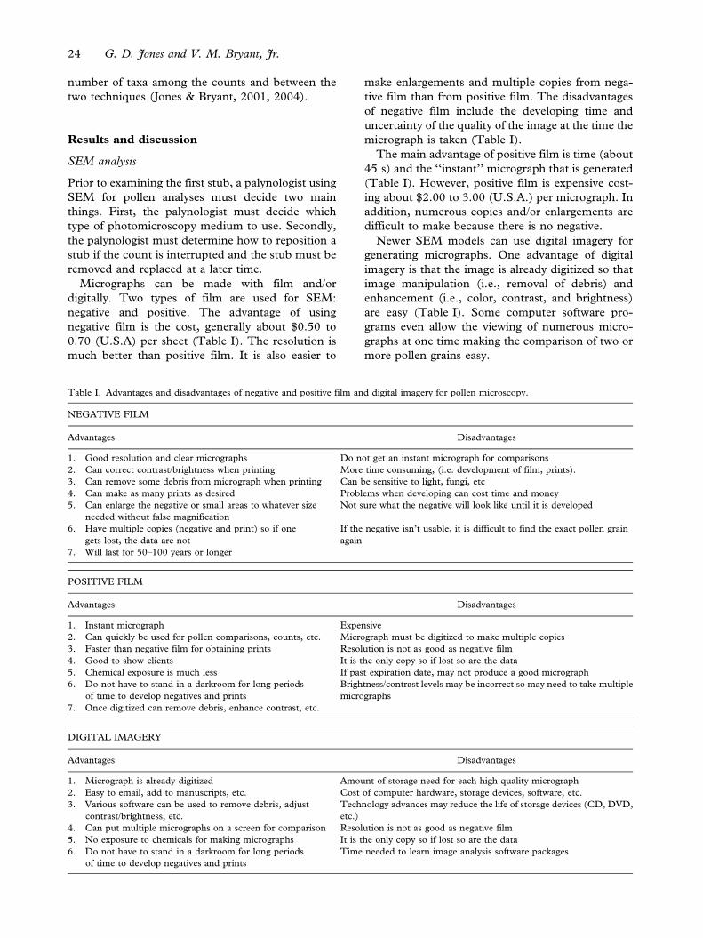
Micrographs can be made with film and/or

digitally. Two types of film are used for SEM:

negative and positive. The advantage of using

negative film is the cost, generally about $0.50 to

0.70 (U.S.A) per sheet (Table I). The resolution is

much better than positive film. It is also easier to

make enlargements and multiple copies from nega-

tive film than from positive film. The disadvantages

of negative film include the developing time and

uncertainty of the quality of the image at the time the

micrograph is taken (Table I).

The main advantage of positive film is time (about

45 s) and the ‘‘instant’’ micrograph that is generated

(Table I). However, positive film is expensive cost-

ing about $2.00 to 3.00 (U.S.A.) per micrograph. In

addition, numerous copies and/or enlargements are

difficult to make because there is no negative.

Newer SEM models can use digital imagery for

generating micrographs. One advantage of digital

imagery is that the image is already digitized so that

image manipulation (i.e., removal of debris) and

enhancement (i.e., color, contrast, and brightness)

are easy (Table I). Some computer software pro-

grams even allow the viewing of numerous micro-

graphs at one time making the comparison of two or

more pollen grains easy.

Table I. Advantages and disadvantages of negative and positive film and digital imagery for pollen microscopy.

NEGATIVE FILM

Advantages Disadvantages

1. Good resolution and clear micrographs Do not get an instant micrograph for comparisons

2. Can correct contrast/brightness when printing More time consuming, (i.e. development of film, prints).

3. Can remove some debris from micrograph when printing Can be sensitive to light, fungi, etc

4. Can make as many prints as desired Problems when developing can cost time and money

5. Can enlarge the negative or small areas to whatever size

needed without false magnification

Not sure what the negative will look like until it is developed

6. Have multiple copies (negative and print) so if one

gets lost, the data are not

If the negative isn’t usable, it is difficult to find the exact pollen grain

again

7. Will last for 50–100 years or longer

POSITIVE FILM


1. Instant micrograph Expensive

2. Can quickly be used for pollen comparisons, counts, etc. Micrograph must be digitized to make multiple copies

3. Faster than negative film for obtaining prints Resolution is not as good as negative film

4. Good to show clients It is the only copy so if lost so are the data

5. Chemical exposure is much less If past expiration date, may not produce a good micrograph

6. Do not have to stand in a darkroom for long periods

of time to develop negatives and prints

Brightness/contrast levels may be incorrect so may need to take multiple

micrographs

7. Once digitized can remove debris, enhance contrast, etc.

DIGITAL IMAGERY


1. Micrograph is already digitized Amount of storage need for each high quality micrograph

2. Easy to email, add to manuscripts, etc. Cost of computer hardware, storage devices, software, etc.

3. Various software can be used to remove debris, adjust

contrast/brightness, etc.

Technology advances may reduce the life of storage devices (CD, DVD,

etc.)

4. Can put multiple micrographs on a screen for comparison Resolution is not as good as negative film

5. No exposure to chemicals for making micrographs It is the only copy so if lost so are the data

6. Do not have to stand in a darkroom for long periods

of time to develop negatives and prints

Time needed to learn image analysis software packages


Some disadvantages of digital imagery include

the large amount of memory needed for each

micrograph, disk storage space needed (hard disk,

CDs or DVDs), and the initial cost for computer,

software, etc. Obtaining a high quality resolution

micrograph took about 4 min. The resolution of the

printed digital image was not a good as the same

images taken with either negative or positive film.

The JEOL SEM used for this manuscript is over 15

year old. No doubt there have been many improve-

ments in the digital imagery system of newer SEM

scopes.

Printing compound photographic plates from

digital images was difficult. Trying to match the

contrast and brightness for each print was time

consuming and used a lot of photographic printer

paper and ink. Putting four micrographs together to

be printed on one photographic sheet was not an

option in the software used to generate micrographs

for this manuscript. Therefore no matter how large

or small the final micrograph, a whole sheet of paper

had to be used. Finally, the heat press used to attach

a print and adhesive to a mounting board scratched,

melted, and scarred the micrograph made from the

computer regardless of how low the temperature

was. This is most likely due to the heat sensitivity of

the ink used for most computer printers. There are

other types of techniques such as spray adhesives

that can be used to put micrographs made from

computer printers onto plates for publication and

exhibition.

Because the objective of this study was to compare

LM and SEM pollen counts and identifications, it was

important to have instant access to the different pollen

types. Therefore, positive film was used for the SEM

analyses. The positive micrographs were put into

plastic photo holders, placed into a 3-ring binder, and

arranged by ornamentation then aperaturation. This

binder was kept next to the SEM so that new grains

could be compared to previously photographed ones.

Over 200 LM and over 150 SEM pollen micrographs

were taken during the counts.

Pollen counting. Re-positioning the SEM stub in the

exact location to continue a count is next to

impossible. To allow exact repositioning, marks

were made prior and after coating the stub.

Marking prior to coating did not work because the

coating covered the marks that were made on the top

and sides of the stub. Marks on the bottom of the

stub were not covered by the coating but were

hidden when the stub was put in the specimen

holder making re-positioning impossible.

The after-coating mark made with the nail polish

(Fig. 1 B) was the easiest to apply because a drop of

nail polish could be added without picking up and

holding the stub. Once applied, the nail polish had

to dry for several days before the stub could be

examined. Unfortunately, the nail polish mark was

the most difficult mark to use to consistently

reposition the stub in the same location. In addition,

there was concern that the drop may obscure

important pollen types.

Marking with the forceps worked well

(Figure 1C). However, several forceps were bent

during the marking process. If forceps are used, they

should be a coarse type that does not easily bend.

The ‘‘i’’ made with the forceps was easily seen but

could be mistaken as an accidental scratch on the

stub by an inexperienced technician.

Marking with a diamond scribe worked best

(Figure 1D). Diamond scribes are common in

palynological laboratories and are used for marking

numbers or codes on vials and glassware. Virtually

any type of mark can be made with a diamond

scribe. The ‘‘t’’ made with the diamond probe was

more obvious when examining the stub (Figure 1D)

than the ‘‘i’’ (Figure 1C) made with the forceps.

Also, the cross bars of the ‘‘t’’ helped in re-

positioning the stub correctly each time.

Pollen data interpretation and LM/SEM comparison.

Debris in a pollen sample is common and something

palynologists work around. When using glycerine

and LM, a pollen grain usually can be separated

from the debris by gently rolling it around. Debris on

the stub can partially or entirely cover a pollen grain.

When the diagnostic features are hidden,

identification of the pollen grain can be impossible.

To calculate the difficulty in pollen identification

during SEM analyses, pollen grains seen with the

SEM were put into three categories: Category 1

‘‘identifiable’’ (Figure 1A), Category 2 ‘‘obscured’’

(Figure 2A) and Category 3, ‘‘virtually impossible to

identify’’ (Figure 2B).

Overall, the majority of the pollen grains counted

with the SEM (86%) were classified as either

Category 1 or 2 (calculated from Table II). Only

14% of the grains were considered to be in Category

3.

In the SEM Pollen Counts #1 and #2, over

50% of the grains were classified as Category 1

(54 and 70% respectfully, Table II). Category 3

contained the fewest number of pollen grains in

both SEM counts (16 and 12%, respectfully,

Table II).

All of the pollen in Category 1 was identified or in

a few cases some were listed as unknown types. The

unknown category was used for pollen grains that

were identifiable provided there were sufficient SEM

images to match the unknown type.


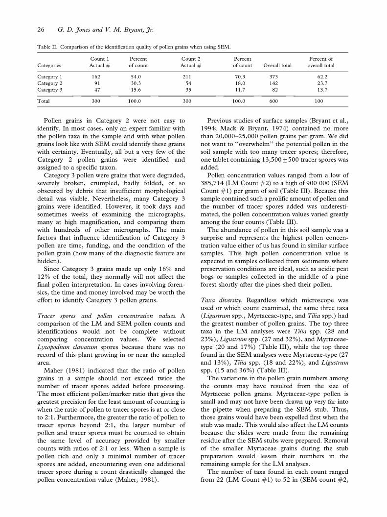
Pollen grains in Category 2 were not easy to

identify. In most cases, only an expert familiar with

the pollen taxa in the sample and with what pollen

grains look like with SEM could identify these grains

with certainty. Eventually, all but a very few of the

Category 2 pollen grains were identified and

assigned to a specific taxon.

Category 3 pollen were grains that were degraded,

severely broken, crumpled, badly folded, or so

obscured by debris that insufficient morphological

detail was visible. Nevertheless, many Category 3

grains were identified. However, it took days and

sometimes weeks of examining the micrographs,

many at high magnification, and comparing them

with hundreds of other micrographs. The main

factors that influence identification of Category 3

pollen are time, funding, and the condition of the

pollen grain (how many of the diagnostic feature are

hidden).

Since Category 3 grains made up only 16% and

12% of the total, they normally will not affect the

final pollen interpretation. In cases involving foren-

sics, the time and money involved may be worth the

effort to identify Category 3 pollen grains.

Tracer spores and pollen concentration values. A

comparison of the LM and SEM pollen counts and

identifications would not be complete without

comparing concentration values. We selected

Lycopodium clavatum spores because there was no

record of this plant growing in or near the sampled

area.

Maher (1981) indicated that the ratio of pollen

grains in a sample should not exceed twice the

number of tracer spores added before processing.

The most efficient pollen/marker ratio that gives the

greatest precision for the least amount of counting is

when the ratio of pollen to tracer spores is at or close

to 2:1. Furthermore, the greater the ratio of pollen to

tracer spores beyond 2:1, the larger number of

pollen and tracer spores must be counted to obtain

the same level of accuracy provided by smaller

counts with ratios of 2:1 or less. When a sample is

pollen rich and only a minimal number of tracer

spores are added, encountering even one additional

tracer spore during a count drastically changed the

pollen concentration value (Maher, 1981).

Previous studies of surface samples (Bryant et al.,

1994; Mack & Bryant, 1974) contained no more

than 20,000–25,000 pollen grains per gram. We did

not want to ‘‘overwhelm’’ the potential pollen in the

soil sample with too many tracer spores; therefore,

one tablet containing 13,500¡500 tracer spores was

added.

Pollen concentration values ranged from a low of

385,714 (LM Count #2) to a high of 900 000 (SEM

Count #1) per gram of soil (Table III). Because this

sample contained such a prolific amount of pollen and

the number of tracer spores added was underesti-

mated, the pollen concentration values varied greatly

among the four counts (Table III).

The abundance of pollen in this soil sample was a

surprise and represents the highest pollen concen-

tration value either of us has found in similar surface

samples. This high pollen concentration value is

expected in samples collected from sediments where

preservation conditions are ideal, such as acidic peat

bogs or samples collected in the middle of a pine

forest shortly after the pines shed their pollen.

Taxa diversity. Regardless which microscope was

used or which count examined, the same three taxa

(Ligustrum spp., Myrtaceae-type, and Tilia spp.) had

the greatest number of pollen grains. The top three

taxa in the LM analyses were Tilia spp. (28 and

23%), Ligustrum spp. (27 and 32%), and Myrtaceae-

type (20 and 17%) (Table III), while the top three

found in the SEM analyses were Myrtaceae-type (27

and 13%), Tilia spp. (18 and 22%), and Ligustrum

spp. (15 and 36%) (Table III).

The variations in the pollen grain numbers among

the counts may have resulted from the size of

Myrtaceae pollen grains. Myrtaceae-type pollen is

small and may not have been drawn up very far into

the pipette when preparing the SEM stub. Thus,

those grains would have been expelled first when the

stub was made. This would also affect the LM counts

because the slides were made from the remaining

residue after the SEM stubs were prepared. Removal

of the smaller Myrtaceae grains during the stub

preparation would lessen their numbers in the

remaining sample for the LM analyses.

The number of taxa found in each count ranged

from 22 (LM Count #1) to 52 in (SEM count #2,

Table II. Comparison of the identification quality of pollen grains when using SEM.

Categories

Count 1

Actual #Percent

of count

Count 2

Actual #Percent

of count Overall total

Percent of

overall total

Category 1 162 54.0 211 70.3 373 62.2

Category 2 91 30.3 54 18.0 142 23.7

Category 3 47 15.6 35 11.7 82 13.7

Total 300 100.0 300 100.0 600 100


Table III. Family, taxon, actual grain counts (NOG), and the percentage of each taxon in the count (POG) made with light (LM) and

scanning electron (SEM) microscopy. LM/SEM total represents the actual pollen count from LM and the summed total for all the types in

that category made from SEM.

Family Taxon or type

LM SEM

Count 1 Count 2 Count 1 Count 2

NOG POG NOG POG NOG POG NOG POG

Aceraceae Acer 1 0.3

Arecaceae 1 0.3

Asteraceae Cichorioideae type 2 0.7

Asteraceae Asteroideae LS type 2 0.7 3 1.0

Asteraceae Asteroideae HS type 1 0.3 1 0.3

Berberidaceae 1 0.3

Betulaceae Carpinus 5 1.7 3 1.0 5 1.7 3 1.0

Betulaceae Alnus 1 0.3 1 0.3 2 0.7 3 1.0

Betulaceae Betula 3 1.0 2 0.8

Brassicaceae 1 0.3 1 0.3 1 0.3

Caprifoliaceae Lonicera 2 0.7

Caryophyllaceae 1 0.3

Chenopod./Amar. Cheno-Ams 3 1.0 3 1.0 2 0.6

Cupressaceae 2 0.7 2 0.7 11 3.7 4 1.4

Cupressaceae Juniperus 1 0.3

Ericaceae 1 0.3 1 0.3

Ericaceae SEM type 1 1 0.3

Ericaceae SEM type 2 1 0.3

Fabaceae Acacia 1 0.3 1 0.3

Fabaceae Melilotus 1 0.3 1 0.3 1 0.3

Fabaceae SEM type 2 1 0.3 1 0.3

Fagaceae Castanea 5 1.7 3 1.0 4 1.3 2 0.6

Fagaceae Fagus 1 0.3 3 1.0

Fagaceae Quercus 1 0.3 1 0.3 5 1.7 4 1.4

Juglandaceae Juglans 1 0.3

Liliaceae Erythronium 1 0.3

Liliaceae 1 0.3

Malvaceae 1 0.3

Myrtaceae LM/SEM total 60 20.1 50 16.7 82 27.3 40 13.3

Myrtaceae SEM type 2 52 17.3 33 11.0



Myrtaceae SEM type 4 1 0.3

Myrtaceae SEM type 5 2 0.7

Oleaceae Ligustrum LM/

SEM total

80 26.8 96 32.0 46 15.3 108 36.0

Oleaceae Ligustrum SEM type

1

10 3.3 5 1.7


2

31 10.3 97 32.3


3

5 1.7 6 2.0

Oleaceae Olea 12 4.0 20 6.7 20 6.7 19 6.4

Oleaceae Syringa vulgaris 3 1.0 6 2.0

Pinaceae Pinus - Diploxylon

type

1 0.3 1 0.3

Pinaceae Pinus - Haploxylon

type

1 0.3 1 0.3

Pinaceae Undetermined type 19 6.4 14 4.7 14 4.7 11 3.6

Plantaginaceae Plantago LM/SEM

total

1 0.3 1 0.3 12 4.0 7 2.5

Plantaginaceae Plantago SEM type 1 2 0.7

Plantaginaceae Plantago SEM type 2 10 3.3 5 1.7

Plantaginaceae Plantago SEM type 3 2 0.8

Poaceae 13 4.4 12 4.0 19 6.3

Poaceae Zea 1 0.3

Polygonaceae Rumex 2 0.7

Ranunculaceae Caltha palustris 1 0.3 2 0.6


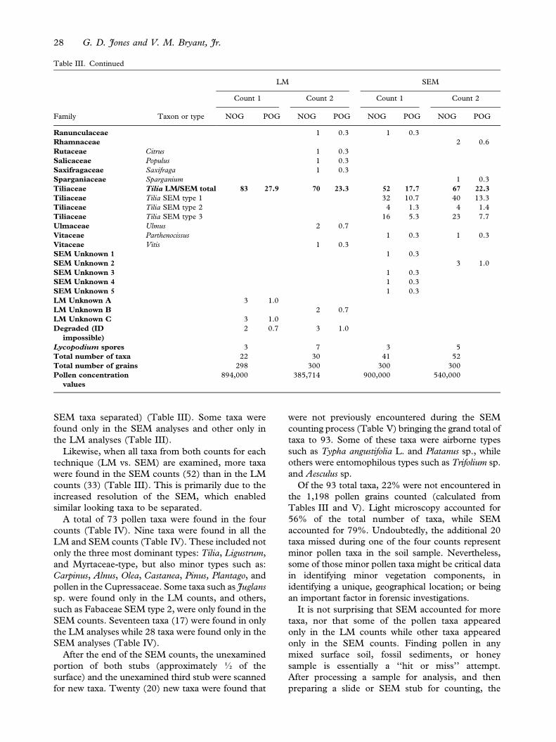
SEM taxa separated) (Table III). Some taxa were

found only in the SEM analyses and other only in

the LM analyses (Table III).

Likewise, when all taxa from both counts for each

technique (LM vs. SEM) are examined, more taxa

were found in the SEM counts (52) than in the LM

counts (33) (Table III). This is primarily due to the

increased resolution of the SEM, which enabled

similar looking taxa to be separated.

A total of 73 pollen taxa were found in the four

counts (Table IV). Nine taxa were found in all the

LM and SEM counts (Table IV). These included not

only the three most dominant types: Tilia, Ligustrum,

and Myrtaceae-type, but also minor types such as:

Carpinus, Alnus, Olea, Castanea, Pinus, Plantago, and

pollen in the Cupressaceae. Some taxa such as Juglans

sp. were found only in the LM counts, and others,

such as Fabaceae SEM type 2, were only found in the

SEM counts. Seventeen taxa (17) were found in only

the LM analyses while 28 taxa were found only in the

SEM analyses (Table IV).

After the end of the SEM counts, the unexamined

portion of both stubs (approximately K of the

surface) and the unexamined third stub were scanned

for new taxa. Twenty (20) new taxa were found that

were not previously encountered during the SEM

counting process (Table V) bringing the grand total of

taxa to 93. Some of these taxa were airborne types

such as Typha angustifolia L. and Platanus sp., while

others were entomophilous types such as Trifolium sp.

and Aesculus sp.

Of the 93 total taxa, 22% were not encountered in

the 1,198 pollen grains counted (calculated from

Tables III and V). Light microscopy accounted for

56% of the total number of taxa, while SEM

accounted for 79%. Undoubtedly, the additional 20

taxa missed during one of the four counts represent

minor pollen taxa in the soil sample. Nevertheless,

some of those minor pollen taxa might be critical data

in identifying minor vegetation components, in

identifying a unique, geographical location; or being

an important factor in forensic investigations.

It is not surprising that SEM accounted for more

taxa, nor that some of the pollen taxa appeared

only in the LM counts while other taxa appeared

only in the SEM counts. Finding pollen in any

mixed surface soil, fossil sediments, or honey

sample is essentially a ‘‘hit or miss’’ attempt.

After processing a sample for analysis, and then

preparing a slide or SEM stub for counting, the


LM SEM

Count 1 Count 2 Count 1 Count 2

NOG POG NOG POG NOG POG NOG POG

Ranunculaceae 1 0.3 1 0.3

Rhamnaceae 2 0.6

Rutaceae Citrus 1 0.3

Salicaceae Populus 1 0.3

Saxifragaceae Saxifraga 1 0.3

Sparganiaceae Sparganium 1 0.3

Tiliaceae Tilia LM/SEM total 83 27.9 70 23.3 52 17.7 67 22.3

Tiliaceae Tilia SEM type 1 32 10.7 40 13.3



Ulmaceae Ulmus 2 0.7

Vitaceae Parthenocissus 1 0.3 1 0.3

Vitaceae Vitis 1 0.3

SEM Unknown 1 1 0.3

SEM Unknown 2 3 1.0

SEM Unknown 3 1 0.3

SEM Unknown 4 1 0.3

SEM Unknown 5 1 0.3

LM Unknown A 3 1.0

LM Unknown B 2 0.7

LM Unknown C 3 1.0

Degraded (ID

impossible)

2 0.7 3 1.0

Lycopodium spores 3 7 3 5

Total number of taxa 22 30 41 52

Total number of grains 298 300 300 300

Pollen concentration

values

894,000 385,714 900,000 540,000

Table III. Continued


Table IV. The total number of pollen grains (NOG) and percentage (POG) of grains per taxon for the LM and SEM counts and an over all

total number of each taxon pollen grains and its percentage. LM totals do not include degraded grains.


LM Totals SEM Totals Overall Total

NOG POG NOG POG NOG POG

Aceraceae Acer 1 0.1 1 0.1

Arecaceae 1 0.2 1 0.1

Asteraceae Cichorioideae type 2 0.3 2 0.2

Asteraceae Asteroideae LS type 5 0.8 5 0.4

Asteraceae Asteroideae HS type 2 0.3 2 0.2

Berberidaceae 1 0.2 1 0.1

Betulaceae Carpinus 8 1.3 8 1.3 16 1.4

Betulaceae Alnus 2 0.3 5 0.9 7 0.6

Betulaceae Betula 5 0.9 5 0.5

Brassicaceae 1 0.2 2 0.3 3 0.2

Caprifoliaceae Lonicera 2 0.3 2 0.2

Caryophyllaceae 1 0.2 1 0.1

Chenopod./Amar. Cheno-Ams 3 0.5 5 0.8 8 0.6

Cupressaceae 4 0.7 15 2.5 19 1.6

Cupressaceae Juniperus 1 0.2 1 0.1

Ericaceae Ericaceae 2 0.3 2 0.2

Ericaceae SEM type 1 1 0.1 1 0.1

Ericaceae SEM type 2 1 0.1 1 0.1

Fabaceae Acacia 1 0.2 1 0.1 2 0.2

Fabaceae Melilotus 1 0.2 2 0.3 3 0.2

Fabaceae SEM type 2 2 0.3 2 0.2

Fagaceae Castanea 8 1.3 6 0.9 14 1.1

Fagaceae Fagus 4 0.7 4 0.4

Fagaceae Quercus 2 0.3 9 1.5 11 0.9

Juglandaceae Juglans 1 0.2 1 0.1

Liliaceae Erythronium 1 0.2 1 0.1

Liliaceae 1 0.1 1 0.1

Malvaceae 1 0.2 1 0.1

Myrtaceae LM/SEM total 110 18.4 122 20.3 232 19.4






Oleaceae Ligustrum LM/SEM total 176 29.4 155 25.7 331 27.6

Oleaceae Ligustrum SEM type 1 15 2.5 15 1.3



Oleaceae Olea 32 5.4 39 6.5 71 5.9

Oleaceae Syringa vulgaris 9 1.5 9 0.7

Pinaceae Pinus - Diploxylon 2 0.3 2 0.2

Pinaceae Pinus - Haploxylon 2 0.3 2 0.2

Pinaceae Pinaceae - Undetermined 33 5.5 25 4.1 58 4.8

Plantaginaceae Plantago LM/SEM total 2 0.3 19 3.2 22 1.8




Poaceae Poaceae 25 4.2 19 3.2 44 3.7

Poaceae Zea mays 1 0.2 1 0.1

Polygonaceae Rumex 2 0.3 2 0.2

Ranunculaceae Caltha palustris 3 0.4 3 0.2

Ranunculaceae 1 0.2 1 0.2 2 0.2

Rhamnaceae 2 0.3 2 0.1

Rutaceae Citrus 1 0.2 1 0.1

Salicaceae Populus 1 0.2 1 0.1

Saxifragaceae Saxifraga 1 0.2 1 0.1

Sparganiaceae Sparganium 1 0.1 1 0.1

Tiliaceae Tilia LM/SEM total 153 25.6 119 19.8 272 22.7





potential for finding or missing a specific pollen

type will depend on the amount of the sample

examined and the number of pollen grains actually

counted (Traverse, 1988).

The results of the present study confirm similar

results from an earlier study (Jones and Bryant,

1998) where five drops were extracted from a single

processed honey sample. For each drop, a total of

500 pollen grains were counted. Once the counts

were finished, a cursory examination of the slide was

made to find taxa that were not previously recorded.

The results of that study showed that none of the

five, 500-grain counts accounted for more than 60%

of the total 130 taxa present in the sample.

Like the results in this study, Jones and Bryant

(2004) found that some taxa only occur in one count

of a sample while others occur in all the counts.

Furthermore, the number of newly discovered taxa

increased as the size of the total pollen count

increases.

How long one spends looking for new taxa

depends on the amount of funding and the

information needed from the study. Obviously, if

only the majority of taxa are needed and the top 2 or

3 taxa are the most important, then doing a 1200+grain count is not needed. However, if looking for a

particular pollen taxon or determining the complete

pollen taxa diversity in the sample is warranted, then

a 1200 grain count is not sufficient.

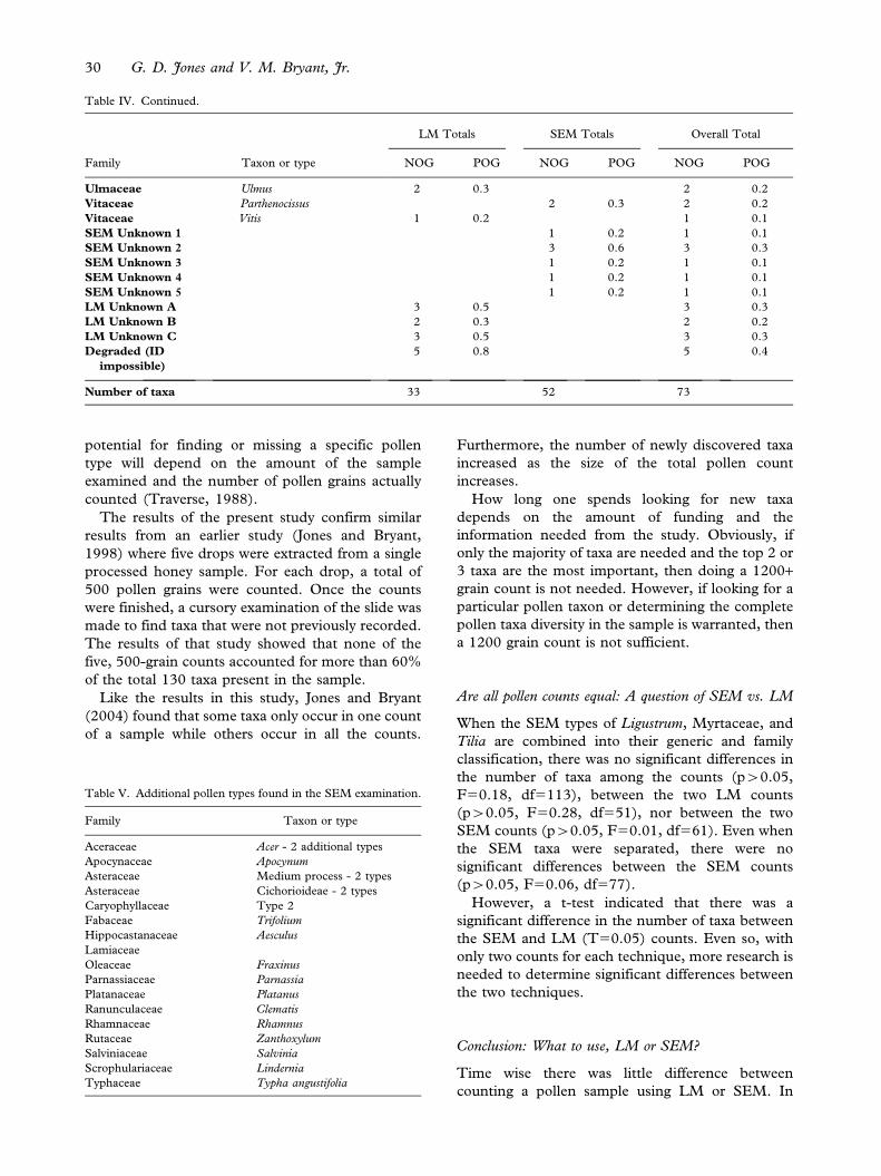
Are all pollen counts equal: A question of SEM vs. LM

When the SEM types of Ligustrum, Myrtaceae, and

Tilia are combined into their generic and family

classification, there was no significant differences in

the number of taxa among the counts (pw0.05,

F50.18, df5113), between the two LM counts

(pw0.05, F50.28, df551), nor between the two

SEM counts (pw0.05, F50.01, df561). Even when

the SEM taxa were separated, there were no

significant differences between the SEM counts

(pw0.05, F50.06, df577).

However, a t-test indicated that there was a

significant difference in the number of taxa between

the SEM and LM (T50.05) counts. Even so, with

only two counts for each technique, more research is

needed to determine significant differences between

the two techniques.

Conclusion: What to use, LM or SEM?

Time wise there was little difference between

counting a pollen sample using LM or SEM. In


LM Totals SEM Totals Overall Total

NOG POG NOG POG NOG POG

Ulmaceae Ulmus 2 0.3 2 0.2

Vitaceae Parthenocissus 2 0.3 2 0.2

Vitaceae Vitis 1 0.2 1 0.1

SEM Unknown 1 1 0.2 1 0.1





LM Unknown A 3 0.5 3 0.3

LM Unknown B 2 0.3 2 0.2

LM Unknown C 3 0.5 3 0.3

Degraded (ID

impossible)

5 0.8 5 0.4

Number of taxa 33 52 73

Table IV. Continued.

Table V. Additional pollen types found in the SEM examination.


Aceraceae Acer - 2 additional types

Apocynaceae Apocynum

Asteraceae Medium process - 2 types

Asteraceae Cichorioideae - 2 types

Caryophyllaceae Type 2

Fabaceae Trifolium

Hippocastanaceae Aesculus

Lamiaceae

Oleaceae Fraxinus

Parnassiaceae Parnassia

Platanaceae Platanus

Ranunculaceae Clematis

Rhamnaceae Rhamnus

Rutaceae Zanthoxylum

Salviniaceae Salvinia

Scrophulariaceae Lindernia

Typhaceae Typha angustifolia


addition, the sample extraction, processing time,

and micrograph production were the same regard-

less of which microscope was used. One major

advantage of LM is convenience and the major

advantages of SEM are increased resolution and

number of taxa.

When using LM, several things should be remem-

bered. First, there is a possibility of lumping two or

more different taxa into one category. How much

this effects the overall interpretation of the data

depends on the sample and what information is

needed from the sample. Second, LM analyses

accounted for the least diversity of pollen taxa.

Again, the importance of the pollen taxa diversity

depends on the type of information needed.

When using SEM, several things should be

considered. First, at least two micrographs should

be taken of each pollen taxon, one of the whole grain

and the second of a close up of the ornamentation of

the grain.

Second, the micrographs should be taken at similar

magnifications. For example, all pollen grains classi-

fied as Tilia should be taken at 1,500–1,800X and the

high magnification of the ornamentation at 5,000X.

This standard magnification will change according to

the taxon and the family. For example, at 1,500X, a

whole Malvaceae pollen grain will not fit on the

negative. On the other hand, at 1,500X, Mimosa

strigillosa Torr. & A. Gray is still very small and the

whole grain needs to be photographed at 5,000X.

Third, micrographs generated should be housed

in a dry, cool area where they can be kept for future

use. Digital images also must be cared for and kept

in a secure and dry location. When cared for

properly, micrographs and negatives should last for

at least 50+ years. How long digital imagery will last

depends on technology. At the current rate of new

computer technology, common types of storage

(CD, DVD) may be obsolete and unreadable in

10–20 years. By keeping the micrographs for years,

regardless of their format, there is the chance that an

unknown pollen type in the sample will be identified

at a later date.

Whenever confronted with the need to decide

whether or not to examine a pollen sample using

LM, SEM, or both, the sample, the information

needed from the sample, and the cost will most likely

dictate whether to use LM, SEM, or both.

Additional factors for deciding which type of

microscope to use are the availability of a SEM,

the deadline for the project, and whether precise

(genera, species, or sub species levels) or general

(genera or family levels) pollen data are needed. For

the moment, we suggest that those who are

comfortable using LM should continue using LM

and those who like to use SEM and have the

availability and funding needed for SEM analyses

should consider using SEM for statistical pollen

counts and identifications.

Acknowledgements

We appreciate the help of Dr. Matthew Cimino,

Curator and Charles O. Wingo, Jr. Herbarium,

Salisbury University. We are indebted to Ester F.

Wilson, Ashley Johnson, and Bianca Johnson

(USDA-ARS, APMRU) for their help with devel-

oping and printing all of the LM and SEM

micrographs created from this research. We also

appreciate Drs. David M. Jarzen (Florida Museum

of Natural History) and John G. Jones (Washington

State University) for their support and review of the

manuscript. We are grateful to the Texas A & M

Microscopy and Imaging Center for use of their

SEM. Finally, we appreciate the anonymous

reviewers that reviewed this manuscript.

References

Adam, D. P. & Mehringer, P. J., Jr. (1975). Modern pollen

surface samples: An analysis of subsamples. J. Res. U.S. Geol.

Surv., 3, 733–736.

Adams, R. J. & Morton, J. K. (1972–1979). An atlas of pollen of the

trees and shrubs of eastern Canada and the adjacent United States.

Waterloo, ONT: Dept Biol. Univ. Waterloo.

Bambara, S. B. & Leidy, N. A. (1991). An atlas of selected pollen

important to honey bees in the eastern United States. Raleigh, NC:

N. Carol. St. Beekeep. Assoc.

Bassett, I. J., Crompton, C. W. & Parmelee, J. A. (1978). An atlas

of airborne pollen grains and common fungus spores of Canada.

Quebec: Thorne Press Ltd, Can. Dept. Agric. Res. Br. Monogr. 18.

Benedict, J. H., Wolfenbarger, D. A., Bryant, V. M., Jr. & George,

D. M. (1991). Pollens ingested by boll weevils (Coleoptera:

Curculionidae) in southern Texas and northeastern Mexico. J.

Econ. Entomol., 84, 126–131.

Beug, H.-J. (2004). Leitfaden der Pollenbestimmung fur Mitteleuropa

und angrenzende Gebiete. Munchen: F. Pfeil.

Blackburn, J. S. & Ford, J. B. (1993). A study of the foraging

behavior of honeybees (Apis mellifera) by the scanning electron

microscopic analysis of pollen in honey. Bee Craft, 75,

170–175.

Blackmore, S., Hoen, P. P., Stafford, P. J. & Punt, W. (Eds).

(2003). The Northwest European Pollen Flora. VIII. New York:

Elsevier. (http://www.bio.uu.nl/,palaeo/Research2/NEPF/nepf.htm).

Bryant, V. M., Jr., Holloway, R. G., Jones, J. G. & Carlson, D. L.

(1994). Pollen preservation in alkaline soils of the American

Southwest. In A. Traverse (Ed.), Sedimentation of organic

particles (pp. 47–58). Cambridge, UK: Cambridge Univ. Press.

Bryant, V. M., Jr., Pendleton, M., Murray, R. E., Lingren, P. D.

& Raulston, J. R. (1991). Techniques for studying pollen

adhering to nectar-feeding corn earworm (Lepidoptera:

Noctuidae) moths using scanning electron microscopy. J.

Econ. Entomol., 84, 237–240.

Chen, S.-H. & Shen, C. (1990). An ultrastructural study of

Formosan honey pollen (I). Taiwania, 35, 221–239.


Del Socorro, A. P. & Gregg, P. C. (2001). Sunflower (Helianthus

annuus L.) pollen as a marker for studies of local movement in

Helicoverpa armigera (Hubner) (Lepidoptera: Noctuidae).

Aust. J. Entomol., 40, 257–263.

Erdtman, G. (1960). The acetolysis method. Sv. Bot. Tidskr., 54,

561–564.

Grayum, M. H. (1992). Comparative external pollen ultrastruc-

ture of the Araceae and putatively related taxa. Lawrence, KS:

Allen Press Inc, Monogr. Syst. Bot. Mo. Bot. Gard. 43.

Gregg, P. C. (1993). Pollen as a marker for migration of

Helicoverpa armigera and H. punctigera (Lepidoptera:

Noctuidae) from western Queensland. Aust. J. Ecol., 18,

209–219.

Gregg, P. C., Del Socorro, A. P. & Rochester, W. A. (2001). Field

test of a model of migration of moths (Lepidoptera:

Noctuidae) in inland Australia. Aust. J. Ecol., 40, 249–256.

Hendrix, W. H., III. & Showers, W. B. (1992). Tracing black

cutworm and armyworm (Lepidoptera: Noctuidae) northward

migration using Pithecellobium and Calliandra pollen. Entomol.

Soc. Am., 21, 1092–1096.

Hendrix, W. H., III., Mueller, T. F., Phillips, J. R. & Davis, O. K.

(1987). Pollen as an indicator of long-distance movement of

Heliothis zea (Lepidoptera: Noctuidae). Environ. Entomol., 16,

1148–1151.

Herrera, F. & Urrego, L. E. (1996). Atlas de polen de plantas utiles y

cultivadas de la Amazonia colombiana. Santafe de Bogota:

Tropenbos Colombia & Fund. Erigaie, Estud. Amazonia

Colomb. 11.

Jones, G. D. & Bryant, V. M., Jr. (1998). Are all counts created

equal? In V. M. Bryant, Jr & J. H. Wrenn (Eds), New

developments in palynomorph sampling, extraction, and analysis

(pp. 115–120). Dallas, TX: AASP Found.

Jones, G. D. & Bryant, V. M., Jr. (2001). Is one drop enough? In

D. K. Goodman & R. T. Clark (Eds), 9th Int. Palynol. Congr.

Proc (pp. 483–487). Dallas, TX: AASP Found.

Jones, G. D. & Bryant, V. M., Jr. (2004). The use of ETOH for

the dilution of honey. Grana, 43, 174–182.

Jones, G. D. & Coppedge, J. R. (1998). Pollen analyses of the boll

weevil exoskeleton. In V. M. Bryant, Jr & J. H. Wrenn (Eds),

New developments in palynomorph sampling, extraction, and

analysis (pp. 121–125). Dallas, TX: AASP Found.

Jones, G. D., Bryant, V. M., Jr., Lieux, M. H., Jones, S. D. &

Lingren, P. D. (1995). Pollen of the southeastern United States:

with emphasis on melissopalynology and entomopalynology. Dallas,

TX: Am. Assoc. Stratigr. Palynol. Found.

Lingren, P. D., Bryant, V. M., Jr., Raulston, J. R., Pendleton, M.,

Westbrook, J. K. & Jones, G. D. (1993). Adult feeding host

range and migratory activities of corn earworm, cabbage

looper, and celery looper (Lepidoptera: Noctuidae) moths as

evidenced by attached pollen. J. Econ. Entomol., 86,

1429–1433.

Lingren, P. D., Westbrook, J. K., Bryant, V. M., Jr., Raulston, J.

R., Esquivel, J. F. & Jones, G. D. (1994). Origin of corn

earworm (Lepidoptera: Noctuidae) migrants as determined by

citrus pollen markers and weather systems. Environ. Entomol.,

23, 562–570.

Mabberley, D. J. (1997). The Plant-Book. Cambridge, UK:

Cambridge Press.

Mack, R. N. & Bryant, V. M., Jr. (1974). Modern pollen spectra

from the Columbia Basin, Washington. Northw. Sci., 48,

183–194.

Maher, L. (1981). Statistics for microfossil concentration

measurements employing samples spiked with marker grains.

Rev. Palaeobot. Palynol., 32, 153–191.

Martin, P. S. (1963). The Last 10,000 Years: A Fossil Pollen Record

of the American Southwest. Tucson, AZ: Univ. Arizona Press.

Moar, N. T. (1993). Pollen grains of New Zealand dicotyledonous

plants. Lincoln, Canterb., N.Z.: Manaaki Whenua Press.

Moore, P. D., Webb, J. A. & Collinson, M. E. (1991). Pollen

Analysis. 2nd Ed. London: Blackwell Sci. Publ.

Nilsson, S., Praglowski, J. & Nilsson, L. (1977). Atlas of Airborne

pollen grains and spores in northern Europe. Natur & Kultur,

Sweden.

Ogden, E. C., Raynor, G. S., Hayes, J. V., Lewis, D. M. &

Haines, J. H. (1974). Manual for sampling airborne pollen. New

York: Hafner Press.

Punt, W. (Ed.). (1976). The Northwest European Pollen Flora. I.

Amsterdam/Oxford/New York: Elsevier. (http://www.bio.uu.nl/

,palaeo/Research2/NEPF/nepf.htm).

Punt, W. & Clarke, G. C. S. (Eds). (1980). The Northwest

European Pollen Flora. II. Amsterdam/Oxford/New York:

Elsevier. (http://www.bio.uu.nl/,palaeo/Research2/NEPF/nepf.

htm).


European Pollen Flora. III. Amsterdam/Oxford/New York:



European Pollen Flora. IV. Amsterdam/Oxford/New York:



European Pollen Flora. V. Amsterdam/Oxford/New York/

Tokyo: Elsevier. (http://www.bio.uu.nl/,palaeo/Research2/

NEPF/nepf.htm).

Punt, W. & Blackmore, S. (Eds). (1991). The Northwest European

Pollen Flora. VI. Amsterdam/Oxford/New York/Tokyo:

Elsevier. (http://www.bio.uu.nl/,palaeo/Research2/NEPF/nepf.

htm).

Punt, W., Blackmore, S. & Hoen, P. P. (Eds). (1995). The

Northwest European Pollen Flora. VII. Amsterdam/Lausanne/

New York/Oxford/Shannon/Tokyo: Elsevier. (http://

www.bio.uu.nl/,palaeo/Research2/NEPF/nepf.htm).

Qiao, B.-S. (2004). Color atlas of air-borne pollen and plants in

China. Beijing: Peking Union Med. Coll. Press.

Reille, M. (1992). Pollen et spores d’Europe et d’Afrique du Nord.

Marseille: Lab. Bot. Hist. & Palynol. URA CNRS/Univ.

Marseille III.


Suppl. 1. Marseille: Lab. Bot. Hist. & Palynol. URA CNRS/

Univ. Marseille III.


Suppl. 2. Marseille: Lab. Bot. Hist. & Palynol. URA CNRS/

Univ. Marseille III.


Index. Marseille: Lab. Bot. Hist. & Palynol. URA CNRS

Univ./Marseille III.

Ridgeway, J. E. & Skvarla, J. J. (1969). Scanning electron

microscopy as an aid to pollen taxonomy. Ann. Mo. Bot.

Gard., 56, 121–124.

Rowley, J. R., Skvarla, J. J. & Vezey, E. L. (1988). Evaluating

the relative contributions of SEM, TEM, and LM to

the description of pollen grains. J. Palynol. (India), 23–24,

27–28.

Skvarla, J. J. & Larson, D. A. (1965). An electron microscopic

study of pollen morphology in the Compositae with special

reference to the Ambrosiinae. Grana, 6, 210–269.

Traverse, A. (1988). Palaeopalynology. London: Unwin/Hyman.

Van Laere, O., Lagasse, A. & Mets, M., de. (1969). Use of

the scanning electron microscope for investigating pollen

grains isolated from honey samples. J. Apicult. Res., 8,

139–145.

Vezey, E. L. & Skvarla, J. J. (1990). Computerized feature analysis

of exine sculpture patterns. Rev. Palaeobot. Palynol., 64,

187–196.

Vezey, E. L., Skvarla, J. J. & Vanerpool, S. S. (1991). Characterizing

pollen sculpture of three closely-related Capparaceae species

using quantitative image analysis of scanning electron


micrographs. In S. Blackmore & S. J. Barnes (Eds), Pollen

and spores: Patterns of diversification (pp. 291–300). Oxford:

Clarendon Press, Syst. Assoc. Sp. Vol. 44.

Wei, Z.-X. (Ed.), Wang, H., Gao, L.-M., Zhang, X.-L., Zhou,

L.-H. & Feng, Y.-X. (2003). Pollen flora of seed plants.

Kunming: Yunnan Sci. & Technol. Press.

USDA-ARS Disclaimer

Mention of trade names or commercial products in this

publication is solely for the purpose of providing specific

information and does not imply recommendation or endorsement

by the U.S. Department of Agriculture.


A comparison of pollen counts: Light versus scanning electron microscopy

Documents

Transcript of A comparison of pollen counts: Light versus scanning electron microscopy