A Comparative Study on Optimal Structural Dynamics Using Wavelet Functions
11
Research Article A Comparative Study on Optimal Structural Dynamics Using Wavelet Functions Seyed Hossein Mahdavi and Hashim Abdul Razak StruHMRS Group, Department of Civil Engineering, University of Malaya, 50603 Kuala Lumpur, Malaysia Correspondence should be addressed to Hashim Abdul Razak; [email protected] Received 2 April 2014; Accepted 8 October 2014 Academic Editor: Shuenn-Yih Chang Copyright © 2015 S. H. Mahdavi and H. Abdul Razak. is is an open access article distributed under the Creative Commons Attribution License, which permits unrestricted use, distribution, and reproduction in any medium, provided the original work is properly cited. Wavelet solution techniques have become the focus of interest among researchers in different disciplines of science and technology. In this paper, implementation of two different wavelet basis functions has been comparatively considered for dynamic analysis of structures. For this aim, computational technique is developed by using free scale of simple Haar wavelet, initially. Later, complex and continuous Chebyshev wavelet basis functions are presented to improve the time history analysis of structures. Free-scaled Chebyshev coefficient matrix and operation of integration are derived to directly approximate displacements of the corresponding system. In addition, stability of responses has been investigated for the proposed algorithm of discrete Haar wavelet compared against continuous Chebyshev wavelet. To demonstrate the validity of the wavelet-based algorithms, aforesaid schemes have been extended to the linear and nonlinear structural dynamics. e effectiveness of free-scaled Chebyshev wavelet has been compared with simple Haar wavelet and two common integration methods. It is deduced that either indirect method proposed for discrete Haar wavelet or direct approach for continuous Chebyshev wavelet is unconditionally stable. Finally, it is concluded that numerical solution is highly benefited by the least computation time involved and high accuracy of response, particularly using low scale of complex Chebyshev wavelet. 1. Introduction Generally, results integrated from dynamic analysis of struc- tures are the main reliable criteria for design of solids and structures. e technique for a solution of general dynamic equilibrium can become very expensive if a com- plex loading (e.g., an unknown earthquake excitation) is being applied on large-scaled structures [1, 2]. In general, procedure of dynamic analysis is categorized into the two solution methods: first, mode superposition method. Second, direct and indirect integration methods, for example, central differences, family of Newmark-, Houbolt, and Wilson- fall under direct integration schemes and Fourier transformation and wavelet analysis have been introduced as indirect integra- tion approaches. In addition, the choice as to which method to use for an effective solution is governed by the dynamical problem considered [3, 4]. eoretically, aforesaid numerical integration methods lie in case of either conditionally stable or unconditionally stable procedures. An integration method is unconditionally stable if the solution for any initial condi- tions does not grow without a band for any time step while will be conditionally stable if it does grow. In other words, stability of results is achieved at any time interval and there is no restriction on using Δ smaller than a particular value. As a result, optimal solution for dynamic analysis is accomplished using long intervals [5–7]. Nowadays, orthogonal polynomials are being widely implemented as a practical analysis of time dealing problems in engineering, particularly in the form of wavelet analysis. Obvious effectiveness from property of orthogonality is that the repeated components with similar characteristics are neglected in the analytical process [8, 9]. Consequently, computational calculations are being considerably decreased and computation time involved is being therefore reduced, hence, accuracy of responses will be more desirable [10, 11]. Practically, considerable attention has been given for the use of wavelet method for the solution of time dependent prob- lems such as dynamic analysis or identification of systematic Hindawi Publishing Corporation Mathematical Problems in Engineering Volume 2015, Article ID 956793, 10 pages http://dx.doi.org/10.1155/2015/956793
Transcript of A Comparative Study on Optimal Structural Dynamics Using Wavelet Functions
Research ArticleA Comparative Study on Optimal StructuralDynamics Using Wavelet Functions
Seyed Hossein Mahdavi and Hashim Abdul Razak
StruHMRS Group Department of Civil Engineering University of Malaya 50603 Kuala Lumpur Malaysia
Correspondence should be addressed to Hashim Abdul Razak hashimumedumy
Received 2 April 2014 Accepted 8 October 2014
Academic Editor Shuenn-Yih Chang
Copyright copy 2015 S H Mahdavi and H Abdul Razak This is an open access article distributed under the Creative CommonsAttribution License which permits unrestricted use distribution and reproduction in any medium provided the original work isproperly cited
Wavelet solution techniques have become the focus of interest among researchers in different disciplines of science and technologyIn this paper implementation of two different wavelet basis functions has been comparatively considered for dynamic analysis ofstructures For this aim computational technique is developed by using free scale of simple Haar wavelet initially Later complexand continuous Chebyshev wavelet basis functions are presented to improve the time history analysis of structures Free-scaledChebyshev coefficient matrix and operation of integration are derived to directly approximate displacements of the correspondingsystem In addition stability of responses has been investigated for the proposed algorithm of discrete Haar wavelet comparedagainst continuous Chebyshev wavelet To demonstrate the validity of the wavelet-based algorithms aforesaid schemes have beenextended to the linear and nonlinear structural dynamics The effectiveness of free-scaled Chebyshev wavelet has been comparedwith simple Haar wavelet and two common integration methods It is deduced that either indirect method proposed for discreteHaar wavelet or direct approach for continuous Chebyshev wavelet is unconditionally stable Finally it is concluded that numericalsolution is highly benefited by the least computation time involved and high accuracy of response particularly using low scale ofcomplex Chebyshev wavelet
1 Introduction
Generally results integrated from dynamic analysis of struc-tures are the main reliable criteria for design of solidsand structures The technique for a solution of generaldynamic equilibrium can become very expensive if a com-plex loading (eg an unknown earthquake excitation) isbeing applied on large-scaled structures [1 2] In generalprocedure of dynamic analysis is categorized into the twosolutionmethods first mode superpositionmethod Seconddirect and indirect integration methods for example centraldifferences family ofNewmark-120573 Houbolt andWilson-120579 fallunder direct integration schemes and Fourier transformationandwavelet analysis have been introduced as indirect integra-tion approaches In addition the choice as to which methodto use for an effective solution is governed by the dynamicalproblem considered [3 4] Theoretically aforesaid numericalintegration methods lie in case of either conditionally stableor unconditionally stable procedures An integrationmethod
is unconditionally stable if the solution for any initial condi-tions does not grow without a band for any time step whilewill be conditionally stable if it does grow In other wordsstability of results is achieved at any time interval and there isno restriction on usingΔ119905 smaller than a particular value As aresult optimal solution for dynamic analysis is accomplishedusing long intervals [5ndash7]
Nowadays orthogonal polynomials are being widelyimplemented as a practical analysis of time dealing problemsin engineering particularly in the form of wavelet analysisObvious effectiveness from property of orthogonality is thatthe repeated components with similar characteristics areneglected in the analytical process [8 9] Consequentlycomputational calculations are being considerably decreasedand computation time involved is being therefore reducedhence accuracy of responses will be more desirable [10 11]Practically considerable attention has been given for the useof wavelet method for the solution of time dependent prob-lems such as dynamic analysis or identification of systematic
Hindawi Publishing CorporationMathematical Problems in EngineeringVolume 2015 Article ID 956793 10 pageshttpdxdoiorg1011552015956793
2 Mathematical Problems in Engineering
problems [12] Several attractive mathematical characteris-tics of wavelets such as efficient multiscale decompositionslocalization properties in physical and wave-number spacesand the existence of recursive and fast wavelet transformshave obtained practice of this efficient tool for the numericalsolution of partial differential equations (PDEs) and ordinarydifferential equations (ODEs) [13ndash15]
Significantly accuracy of responses is directly related tothe basis function of mother wavelet depending on the kindof objectives Fundamentally in the structural dynamicscompatibility of a wavelet basis function is premised uponon not only the degrees of freedom but also the similarityof basic functions to the lateral loading emphasizing onfrequency contents Considerably less computational costof calculations in advanced time history analysis throughthe compatible wavelet functions makes distinction of thisapproach over other numerical methods For instance forthe purpose of time history analysis a simple basis functionof Haar wavelet was indirectly applied on its own free-scaled functions [16] It is inferred that because of theinherent simple shape function of Haar wavelet accuracyof responses was undesirable even employing large-scaledfunctions Furthermore to improve inadequacy of Haarwavelet known as the simplest and two-dimensional (2D)wavelet basis function it is indispensable to employ three-dimensional (3D) and adaptive wavelet basis functions [1718] Moreover there is no consideration reported on thestability of responses calculated using Haar wavelet functionscompared with other basis functions
Mathematically adaptive wavelets are those that grow inthree dimensions which in the current definition dimensionsare time scale and frequency respectively For instanceChebyshev Legender and Symlet are some basis functionswith compatible characteristics [19] Basically Chebyshevpolynomials are presented as continuous basis function ofwavelet [20 21] The most popular characteristic of thiswavelet is various weight functions of Chebyshev polynomi-als that directly influence stability and accuracy of responses[22ndash24] However it is reported that stability of resultscomputed by Chebyshev wavelet are independent from initialaccelerations Furthermore compatibility is being satisfiedthrough the capturing of broad frequency of complex excita-tions by oscillated shape functions of free-scaled Chebyshevwavelet [25]
Subsequently themain contributions of this study (whichreceived little attention in the literature) are composedof the following (i) a numerical assessment of structuraldynamic problems using free-scaled simple and complexwavelet functions with the emphasis on the large scalesof wavelets (ii) numerical stability analysis of an indirectalgorithm using family of discrete Haar wavelets establishedas 2D wavelet functions (iii) stability analysis of continuousChebyshev wavelet functions with respect to the third-ordered derivation of time (iv) a comparative evaluation ofcomputational efficiency of simple and complex wavelets forsmooth and wide-band frequency contents of loading and(v) capability evaluation of Haar and Chebyshev wavelets inlinear and nonlinear structural dynamic problems Accord-ingly to achieve the proposed objectives of this paper
the second-ordered differential equation of motion is indi-rectly solved by free scale of Haar wavelet and later free-scaledChebyshevwavelet functions are directly implementedto compute responses For this aim a brief background ofwavelet is discussed in Section 2 of this study In additioncoefficientmatrices of wavelet and operationmatrices of inte-gration corresponding to complex scales of efficient Cheby-shev wavelet are formulated and presented in this section InSection 3 the computational procedure is developed for anoptimal dynamic analysis Section 4 is allocated to numericalstability analysis of responses corresponding to the indirectmethod proposed for Haar and direct scheme proposedfor Chebyshev wavelet functions Accordingly stability ofresponses has been comparatively presented Section 5 isdevoted to investigation of the validity and effectiveness ofresults For this purpose various scales of Chebyshev andHaar wavelet functions are considered for dynamic analysisFinally efficiency and accuracy of results have been comparedin this section
2 Fundamental of Wavelet
21 Haar Wavelet The simple family of Haar wavelet waspresented by Alfred Haar in 1910 for 119905 isin [0 1] as follows[16 18]
119867119898minus1
(119905) =
1 119905 isin [119896
2119895
119896 + 05
2119895]
minus1 119905 isin [119896 + 05
2119895
119896 + 1
2119895]
0 otherwise
(1)
where
119898 = 2119895 + 119887 + 1 119895 ge 0 0 le 119887 le 2119895 minus 1 (2)
where 119872 = 2119895 (119895 = 0 1 119895) denotes the order of wavelet119887 = 0 1 119872 minus 1 is the value of transition In (1) 119898 = 1and 119898 = 2 indicate scale function and mother wavelet ofHaar respectively In this study 2119872 indicates the number ofsegmentations in each global time interval regarding the scaleof proposed wavelet which refers to segmentation method(SM) For example in the case of Haar wavelet 2119872 = 2119895+1
denotes the 2119895th scale of Haar wavelet [18]Basically signal 119891(119905) can be expanded in Haar series as
[16]
119891 (119905) cong2119872
sum119894=0
119888119894ℎ119894(119905) (3)
Accordingly Haar coefficients 119888119894(119894 = 0 1 2 ) are
defined by
119888119894= 2119895 int
1
0
119891 (119905) ℎ119894(119905) 119889119905 (4)
Hence 1198672119872
is a square matrix (2119872 times 2119872) including thefirst 2119872 scale of Haar wavelet Haar coefficients are directlygiven as
119888119894= 119891 (119905) 119867minus1
2119872(119905) (5)
Mathematical Problems in Engineering 3
Equivalently signal 119891(119905) may be rewritten as
119891 (119905) cong 1198881198792119872
1198672119872
(119905) (6)
Subsequently integration of 1198672119872
is obtained by Haarseries with new square coefficient matrix of integration 119875
2119872
as [16 18]
int1
0
1198672119872
(119905) 119889119905 asymp 1198751198672119872
(119905) (7)
Pointed out that local times are calculated relatively to thescale of wavelet as
120591119897=
119897 minus 05
2119872 119897 = 1 2 2119872 (8)
Finally the local time divisions (120591119897) are adapted to the
global domain Assumption of 119889119905as global time interval we
have [16 18]
119905119897119905
= 119889119905(120591119897) + 119905119905
997904rArr 120591119897=
119905119905minus 119905119897119905
119889119905
119897 = 1 2 2119872 (9)
22 Chebyshev Wavelet In mathematics families of contin-uous wavelet transforms (CWT) are considered as follows[22 24]
CWT (ScalePosition)
= int 119891 (119905) Ψ (ScalePosition) 119889119905(10)
where CWT denotes corresponding wavelet transform Aslong as wavelet function Ψ(119905) is supposed as mother waveletthe continuous wavelet transform of a signal 119891(119905) is obtainedas
CWTΨ119878
(119886 119887) =1
radic|119886|int 119891 (119905) Ψlowast
119886119887(119905) 119889119905 (11)
where 119887 119886 indicate the transition and the scale of wavelet andlowast indicates the complex conjugate form of Ψ(119905) respectively
In general the Chebyshev polynomials named afterPafnuty Chebyshev are a sequence of orthogonal polyno-mials defined as two kinds The general expression forChebyshev polynomials of the first kind (119879
119899) is defined as
follows [20 21]
119879119899
(119909)
= (119899
2)1198992
sum119896=0
((minus1)119896
119899 minus 119896 minus 1
119899 minus 2119896119896times (2119909)
119899minus2119896)
119899 = 1 2 3
(12)
In addition the variable weight functions of 119879119899is defined
as 120596(119909)
[25]
120596(119909)
=
1
radic1 minus 1199092 |119909| lt 1
0 |119909| ge 1(13)
Mathematically the Chebyshev wavelet arguments aredefined as
Ψ119899119898
= Ψ (119896 119899 119898 119905)
119899 = 1 2 2119896minus1 119898 = 0 1 119872 minus 1 119896 = 1 2 3
(14)
where positive integer 119896 denotes the value of transition 119905indicates the time 119898 is degree of Chebyshev polynomials forthe first kind and 119899 denotes the considered scale of waveletChebyshev wavelets are formulated with substituting the firstkind 119879
119899with relevant weight functions for each scale and
transition in (11) as follows [22 25]
120595119898
(119905)
=
(21198962) times 119879119898
(2119896 (119905) minus 2119899 + 1) 119899 minus 1
2119896minus1lt 119905 le
119899
2119896minus1
0 Otherwise(15)
where 119879119898in (15) is obtained as
119879119898
(119905) =
1
radic120587 119898 = 0
119879119898
times radic2
120587 119898 gt 0
(16)
Thus weight functions corresponding to different scalesare obtained as
120596119899
(119905) = 120596 (2119896 sdot 119905 minus 2119899 + 1) (17)
Regarding the idea of SM method 119863 is number ofpartitions in the global time 119872 is the order of Chebyshevpolynomials that is derived as
2119896minus1119872 = 119863 997904rArr 119872 =119863
2119896minus1 (18)
Numerically the signal119891(119905) can be expandedwithCheby-shev wavelets as [19 22]
119891 (119905) asymp2119896minus1
sum119899=1
119872minus1
sum119898=0
119862119899119898
120595119899119898
(119905) = 119862119879 sdot 120595 (119905) (19)
Here 119862 and 120595(119905) are obtained as two vectors
119862 = [1198881 1198882 1198883 119888
2119896minus1]119879
2119896minus1119872times1
(20)
where
119862119894= [1198881198940
1198881198941
1198881198942
119888119894119872minus1
]119879
(21)
Chebyshev coefficients matrix is defined as
120595 (119905) = [1205951 1205952 1205953 120595
2119896minus1]119879
2119896minus1119872times1
(22)
4 Mathematical Problems in Engineering
where
120595119894(119905) = [120595
1198940(119905) 1205951198941
(119905) 1205951198942
(119905) 120595119894119872minus1
(119905)]119879
(23)
where 119894 = 1 2 4 2(119896minus1)Local time 119905
119897for collocation points are considered as
follows [25]
119905119897= (
1
2119896minus1119872) (119897 minus 05) 119897 = 1 2 3 2119896minus1119872 (24)
Subsequently a 119863 times 119863-dimensional square matrix of120601119899119898
(119905) is derived as
120601119899119898
(119905) = [120595 (1199051) 120595 (119905
2) sdot sdot sdot 120595 (119905
119894)]2119896minus1119872times2119896minus1119872
(25)
For instance assumption of 119872 = 4 and 119896 = 2lies on the first four equations of Chebyshev wavelet cor-responding to eight collocation points (in referring to theSM method) Accordingly coefficient matrix of free-scaledChebyshevwavelet of120601
88(119905) corresponding to 2119872 local times
is improved as follows
120601119863times119863
=
[[[[[[[[[[[[[[[[[[[[[[[[
[
12059510
12059510
0 le 119905 lt 05 12059510
12059510
12059510
12059510
05 le 119905 lt 1 12059510
12059510
12059511
12059511
12059511
12059511
119899 minus 1
2119896minus1∢119905local∢
119899
2119896minus1
12059512
ZERO
12059513
119899 = 1 d 119899 = 1
sdot sdot sdot sdot sdot sdot sdot sdot sdot sdot sdot sdot sdot sdot sdot d sdot sdot sdot sdot sdot sdot sdot sdot sdot sdot sdot sdot sdot sdot sdot
12059520
12059520
sdot sdot sdot 12059520
12059520
d sdot sdot sdot
12059521
119899 minus 1
2119896minus1∢119905local∢
119899
2119896minus1
12059522
ZERO
1205952119896minus1times119872minus1
119899 = 2 119899 = 2 120595
2119896minus1times119872minus1
]]]]]]]]]]]]]]]]]]]]]]]]
]
(26)
where
in 120595119899119898
997888rarr 119899 = 1 2 2119896minus1
119863 = 2119896minus1 times 1(27)
Local times (119905119897) for 119872 = 4 and 119896 = 2 are calculated on
2119872 = 8 points as
119905119897= [00625 01875 03125 04375 05625 06875
08125 09375] (28)
As can be seen from the matrix of (26) column of 119894threfers to120595
119894and integration of120595(119905) in the local time is obtained
as
int119905
0
120595 (120591) 119889120591 asymp 119875 sdot 120595 (119905) (29)
where 119863 times 119863-dimensional 119875 and 120591 denote the operationmatrix of integration and local time respectively Accord-ingly operation matrices of integration [24] are improved asfollows
119865120572 =1
119898120572 sdot Γ120572 + 2
times
[[[[[[
[
119886 1205851
1205852
sdot sdot sdot 1205852119896minus1119872minus1
119886 1205851
sdot sdot sdot 1205852119896minus1119872minus2
119886 sdot sdot sdot 1205852119896minus1119872minus3
Symetric d
1205852119896minus1119872
]]]]]]
]2119896minus1119872times2119896minus1119872
(30)
where
Γ (120572 + 1) = 120572 120572 = 0 1 2 3 (31)
And respectively
120585119896
= (119896 + 1)120572+1 minus 2119896120572+1 + (119896 minus 1)
120572+1 119886 =120572 + 1
2 (32)
Hence the operation matrix of integration is obtained as
119875120572 = 120601 times 119865120572 times 120601minus1 (33)
Mathematical Problems in Engineering 5
3 Dynamic Analysis of Equation of Motion
31 Haar Wavelet Theoretically (1) reveals one major short-coming of Haar wavelet where at the point of 05 thereis no continuity In other words the second derivation isnot existed at this point As a result it is not possible touse this simple wavelet function directly Consequently toutilize free scale of Haar wavelet functions for solution ofsecond-ordered ODE of motion an alternative procedure isimplemented indirectly
After discretization of external loading 119865(119905) to the 119899equal partitions the dynamic equilibrium governing oncorresponding mass (119898lowast) damping (119888lowast) and stiffness (119896lowast) isconverted to the local time analysis as follows (related to the2119872 points of SM method) [16]
(119905) +119888lowast
119898lowast sdot 119889119905
sdot (119905) +119896lowast
119898lowast sdot 119889119905
sdot 119906 (119905)
=1
119898lowast sdot 119889119905
sdot 119865 (119905119899
+ 119889119905120591)
(34)
where terms of velocity and acceleration are considered as
= 119889119905sdot V (35)
(119905) = minus119888lowast
119898lowast sdot 119889119905
sdot (119905) minus119896lowast
119898lowast sdot 119889119905
sdot 119906 (119905)
+1
119898lowast sdot 119889119905
sdot 119865 (119905119899
+ 119889119905120591)
(36)
Or equivalently are expanded as
V = 119887119875119867 + V119899119864 = 119886119867
= 119889119905119887119875119867 + 119889
119905V119899119864 = 119886119867
119906 = 119886119875119867 + 119906119899119864
(37)
Here 119886 and 119887 are row vectors with dimension of 2119872for multiplying with aPH or bPH a unit vector is suffixed as1198641times2119872
Finally 119906119899 V119899are initial and boundary conditions at
119905 = 119905119899 that are obtained with linear interpolation of 119906
1in the
current interval and 1199062119872
calculated from previous interval2119872 times 2119872-dimensional 119875 and 119867 also represent operationof integral matrix of Haar and coefficient matrix of Haarrelevant to the collocation points respectively Assumptionof 119884 = 119864119867minus1 it gives vector of 119886
1times2119872as [16]
119886 = 119889119905119887119875 + 119889
119905V119899119884 (38)
where 119864 = [1 1 1]12119872
Substituting (38) into (37) vector of 1198871times2119872
is developed as
11988712119872
= [minus (119896lowast sdot 1198892119905
sdot V119899
sdot 119884 sdot 119875
119898lowast) minus (
119888lowast sdot 119889119905sdot V119899
+ 119896lowast sdot 119889119905sdot V119899
119898lowast)
sdot 119884 +1198910
sdot 119891119905119899
+ 119889119905120591 sdot 119889119905sdot 119867minus1
119898lowast] sdot sdot sdot
times [119896lowast sdot 11988921199051198752
119898lowast+ 119868 +
119888lowast sdot 119889119905sdot 119875
119898lowast]
minus1
(39)
Here 119868 denotes 2119872-dimensional identity matrix Finallysubstituting (38) and (39) into (36) and (37) vectors of accel-eration velocity and displacement being calculated in eachcollocation point A schematic view of results calculated withHaarwavelet is depicted in Figure 1This figure shows a stairs-shaped plot for responses corresponding to all collocationpoints of Haar wavelet
32 Chebyshev Wavelet A linear dynamic system can beexpressed as
119898lowast (119905) + 119888lowast (119905) + 119896lowast119906 (119905) = 119865 (119905) (40)
According to (19) accelerations are numerically approxi-mated with Chebyshev wavelet as follows
(119905) = 119862119879 times 120595 (119905) (41)
Vector of velocity is therefore approximated multiplyingby operation of integration (119875) as follows
(119905) = 119862119879 times 119875 times 120595 (119905) + V119899 (42)
Next displacements are numerically expanded as well asthe following
119906 (119905) = 119862119879 times 1198752 times 120595 (119905) + 119906119899 (43)
where in (42) and (43) V119899and 119906
119899represent initial condition
of each global time approximated with Chebyshev waveletas a constant value For this purpose the unity is beingexpanded by the Chebyshev wavelet as [25]
1 cong 119868lowast times 120595 (119905)
cong (radic120587
2) times [1 0 0 1 0 0 ] times 120595 (119905)
(44)
Therefore initial displacements and velocities areimproved as
V119899
= 1198781198791
times 120595 (119905)
119906119899
= 1198781198792
times 120595 (119905) (45)
6 Mathematical Problems in Engineering
where 1198781198791and 119878119879
2are 2119896minus1119872 times 1 dimension vectors that are
obtained by Chebyshev wavelet as follows
1198781198791
cong V119899(0)
times (radic120587
2) times [1 0 0 1 0 0 ]
119879
1198781198792
cong 119906119899(0)
times (radic120587
2) times [1 0 0 1 0 0 ]
119879
(46)
Substituting (45) into (42) and (43) vectors of velocityand displacement are defined as
(119905) = 119862119879 times 119875 times 120595 (119905) + 1198781198791
times 120595 (119905)
119906 (119905) = 119862119879 times 1198752 times 120595 (119905) + 1198781198791
times 119875 times 120595 (119905) + 1198781198792
times 120595 (119905) (47)
Additionally external excitation is approximated withChebyshev wavelet as
119865 (119905) = 119891119879 times 120595 (119905) (48)
Equivalently the coefficient matrix of load is numericallyobtained by
1198911198791times2119896minus1119872
=1198651times2119896minus1119872
120601(2119896minus1119872)times(2
119896minus1119872)
(49)
Furthermore quantities of dynamic system are modifiedcorresponding on local times as
(119905) = 119889119905sdot V
(119905) = 119889119905sdot 119865 (119905119899
+ 119889119905sdot 120591 119906 V)
(50)
Finally rearranging (40) after algebraic simplificationsthe dynamic equilibrium is numerically developed as follow-ing algebraic system
119898lowast sdot [119862119879] + 119888lowast sdot 119889119905sdot [119862119879119875 + 119878119879
1]
+ 119896lowast sdot 1198892119905
sdot [1198621198791198752 + 1198781198791119875 + 1198781198792] = 1198911198791198892
119905
(51)
Equation (51) represents an algebraic system calculating119862119879 and substituting into (42) and (43) displacements andvelocities are obtained at any time instant respectively
A schematic view of responses computed with Chebyshevwavelet is depicted in Figure 1 This figure shows a linearplot for responses corresponding to all collocation points ofChebyshev wavelet
4 Stability Analysis
In general displacements velocities and accelerations havebeen transferred step-by-step from 119905th step to the (119905 + Δ119905)thstep of integration schemes In other words the relationbetween quantities from previous state to the current state isexpressed as follows [25]
119905+Δ119905
= [119860] 119905 + [119871] 119891
119905+120592 (52)
where in (52) 119905+Δ119905
represents solution quantities that havebeen transferred with amplification matrix of 119860 from thoseon the previous step of
119905119871 is load operators to relate external
load 119891119905+120592
to the current quantities known as 119905+Δ119905
120592 standson coefficient of Δ119905 and may be 0 Δ119905 or 120579Δ119905 related to eachnumerical integration method
To determine the stability criterion of the proposedscheme for Haar wavelet the behavior of numerical inte-gration should be examined for any initial conditions Forthis purpose the dynamic equilibrium governing on a freevibrated SDOF system in (40) is evaluated Accordingly (40)is rearranged in terms of damping ratio (120585) and naturalfrequency (120596) as
(119905) + 2120585120596 (119905) + 1205962119906 (119905) = 0 (53)
Equation (39) and therefore (38) are rearranged for theinitial velocity (V
119899= 119905minusΔ119905) as follows
119887 = 119905minusΔ119905 (120581120583minus1)
119886 = 119905minusΔ119905120578(54)
where
120581 = minus1205962 (Δ119905) 119884 minus 2120585120596 (Δ119905) 119884 minus 1205962 (Δ119905)2 119884119875
120583 = 2120585120596 (Δ119905) 119875 + 119868 + 1205962 (Δ119905)2 1198752
120578 = (Δ119905) 120581120583minus1119875 + (Δ119905) 119884
(55)
Note that 120583 and 119868 (identity matrix) are 2119872 times 2119872-dimensional matrix 120581 and 120578 are 1times2119872-dimensional vectorsrespectively Equivalently (52) when no load is applied(119891119905+120592
= 0) is developed as
[
[
119905
119905
119906119905]
]
= [
[
0 1198891015840 + 1198901015840 1198881015840
0 1198861015840 00 1198871015840 1198921015840
]
]
[
[
119905minusΔ119905
119905minusΔ119905
119906119905minusΔ119905]
]
(56)
As it is shown in Figure 1 Haar wavelet functionscalculate constant responses on all 2119872 collocation pointsConsequently components of amplification matrix of 119860computed in (56) represent mean value of 2119872 points in eachtime interval and we have
1198861015840 = mean (120581120583minus1119875119867(119905)
+ 119864)
1198871015840 = mean (120578119875119867(119905)
)
1198921015840 = mean (119864) = 1
1198891015840 = mean (minus2120585120596 (120581120583minus1119875119867(119905)
+ 119864))
1198901015840 = mean (minus120578119875119867(119905)
1205962)
1198881015840 = mean (minus1198641205962)
(57)
Figure 1 and (56) demonstrate that responses in each timeinterval have been independently calculated by solver of Haar
Mathematical Problems in Engineering 7
002040608
1
44 46 48 5 52 54 56 58
Disp
lace
men
t (cm
)
Time (s)
Haar waveletChebyshev wavelet
minus02minus04minus06minus08
Figure 1 A schematic view of results calculated with waveletfunctions
from initial accelerations Although the same behavior isreported forChebyshevwavelet [25] the amplificationmatrixof 119860 and (52) is modified for Chebyshev wavelet in order tobe dependent on initial accelerations as
[[[
[
119909119905
119905
119905
119909119905
]]]
]
=[[[
[
0 119886120601 (119905) 119887120601 (119905) 119888120601 (119905)0 119889120601 (119905) 119890120601 (119905) 119891120601 (119905)0 119892120601 (119905) 119894120601 (119905) 119895120601 (119905)0 119902120601 (119905) 119903120601 (119905) 119911120601 (119905)
]]]
]
[[[
[
119909119905minusΔ119905
119905minusΔ119905
119905minusΔ119905
119909119905minusΔ119905
]]]
]
(58)
where
119886 = 120581120583minus1
119887 = 120578120583minus1
119888 = Υ120583minus1
119889 = 119868lowast + 120581120583minus1119875
119890 = 120578120583minus1119875
119891 = Υ120583minus1119875
119892 = 119868lowast119875 + 120581120583minus11198752
119894 = 119868lowast + 120578120583minus11198752
119895 = Υ120583minus11198752
119902 = 119868lowast1198752 + 120581120583minus11198753
119903 = 119868lowast119875 + 120578120583minus11198753
119911 = 119868lowast + Υ120583minus11198753
(59)
where
120581 = minus119868lowast minus 2120585120596 (Δ119905) 119868lowast119875 minus 1205962 (Δ119905)2 119868lowast1198752
120578 = minus2120585120596 (Δ119905) 119868lowast minus 1205962 (Δ119905)2 119868lowast119875
Υ = minus1205962 (Δ119905)2 119868lowast
120583 = 119875 + 2120585120596 (Δ119905) 1198752 + 1205962 (Δ119905)2 1198753
(60)
where 120601(119905) denotes 2119872 times 2119872-dimensional coefficient matrixof Chebyshev wavelet 119868lowast and 119875 imply (44) and operation
012345
0 025 05 075 1 125 15 175 2 225 25Spec
tral
radi
us
Linear accelerationAverage accelerationCentral differenceChebyshev wavelet
Haar wavelet
Wilson (120579 = 14)
ΔtT
Figure 2 Comparison of spectral radius for proposed methods and4 other integration schemes
matrix of integration of Chebyshev wavelet Note that 120583 is2119872 times 2119872-dimensional matrix 120581 120578 and Υ are 1 times 2119872-dimensional vectors respectively The spectral decomposi-tion of 119860 = [Φ][120582][Φ]minus1 is considered for stability and[Φ] contains eigenvectors of 119860 and [120582] is a diagonal matrixincluding eigenvalues of 119860 In the pursuit of stable solutionthe spectral radius of 119860 that equaled by maximum norm ofelements [120582] should be less than unity as follows [5]
120588 (119860) = max (10038171003817100381710038171205821
1003817100381710038171003817 10038171003817100381710038171205822
1003817100381710038171003817 10038171003817100381710038171205823
1003817100381710038171003817) le 1 (61)
where 120588(119860) is the spectral radius of the amplification matrix119860 computed as a function of Δ119905 by (56) for the solverof Haar or (58) for the Chebyshev wavelet This value iscalculated for some integration schemes including Wilson-120579 central difference Newmark-120573 (both linear and averageacceleration integration procedure) and the second scale (theleast scale) of Chebyshev and Haar wavelet Results that havebeen plotted in Figure 2 based on 120585 = 0 show that thecentral difference method and linear acceleration methodas two explicit methods are conditionally stable whereasthe proposed scheme for simple Haar wavelet or complexChebyshev wavelet is unconditionally stable even in the firsttwo scales of corresponding waveletsTherefore no restraints(such as Δ119905 critical value) are placed on time step Δ119905 usedin the analysis from the viewpoint of numerical stabilityconsiderations
As it is shown in Figure 2 variation of spectral radiusin terms of variation of Δ119905119879 illustrates that Wilson-120579 andaverage acceleration method are also unconditionally stablewith no requirements made on the time step Δ119905 used in theanalysis
5 Numerical Applications
In the following section validity of proposed methods isexamined through the comparison of results calculated withdiverse scale of Chebyshev wavelet Haar wavelet Duhamelmethod and Wilson-(120579) method Two examples are con-sidered including a fixed beam under harmonic loadingand a nonlinear SDOF system under a wide-frequency-content base acceleration The corresponding scale of eachwavelet function is designated by 2119872 For instance 211987264implies on 64th scale of correspondingwavelet Furthermoreto evaluate optimal structural dynamic computation timeinvolved for eachmethod is also consideredwhere it has been
8 Mathematical Problems in Engineering
c
F(t)
m
IPB300
k
100
300
0 5 10 15 20 25 30F(t)
Time (s)
F(t) = 300 (2t) Nmoment of inertia IPB300 = 25170 cm4sinE = 210GPa mass = 4000 kg 120585 = 5 k = 200Ncm L = 350 cm
minus100
minus300
Figure 3 A fixed beam under sinusoidal loading 119865(119905) applied in vertical direction
0005
01
0 1 2 3 4 5 6 7 8 9 10
Disp
lace
men
t (cm
)
Time (s)
DuhamelHA(2M4)
CH(2M4)HA(2M64)
minus005
minus01
Figure 4 The first 10 sec of vertical displacement of the mid node(HA = Haar wavelet CH = Chebyshev wavelet)
034
2603
0007 098 0 0102030
010203040
CH(2M4) HA(2M4) CH(2M64) HA(2M64) Duhamel
Time consumptionTotal average errors ()
Figure 5 Computation time involved (sec) and percentile totalaverage error for proposed methods (HA = Haar wavelet CH =Chebyshev wavelet)
recorded with the same hardware Similarly for nonlinearanalysis of structures recessive proceeding is developed thatis provisions in the previous step are new initial conditions inthe current step for each nonlinear behavior such as stiffnessor damping of structure
51 A Fixed Beam Figure 3 shows a fixed I-shaped beamunder sinusoidal loading at the center The characteristics ofconsidered system including section mass dynamic loadingdamping ratio and spring stiffness are shown in this figureIt should be noted that all degrees of freedom are neglectedexcept vertical displacement of the center node
The first 10 sec time history displacement of the centernode is plotted in Figure 4 calculated using the proposedmethods of Haar (21198724 and 211987264) and Chebyshev wavelet(21198724) and compared with results of Duhamel method
It can be seen from figure that accurate results arecalculated by 4th scale of Chebyshev wavelet and 64th Haarwavelet Significantly this figure shows that result computed
Table 1 Absolute errors and calculation time of free-scaled Cheby-shev wavelet and Duhamel (example 51)
Chebyshev wavelet DuhamelSM point (Δ119905 = 005 s) (Δ119905 = 001 s)
Δ119890 119905 (sec) 119905 (sec)2119872 = 4 340119864 minus 03 28654
8527
2119872 = 8 891119864 minus 04 534752119872 = 32 176119864 minus 04 933212119872 = 64 732119864 minus 05 3639182119872 = 128 800119864 minus 05 7886232119872 = 256 823119864 minus 06 1411936
by 4th scale of Haar wavelet is almost rejected but fromits optimization point of view we still accept result of Haarwavelet In addition absolute errors and computational timesdue to the free scale of Chebyshev wavelet consist of 4th8th 32nd 256th against Duhamel method is tabulated inTable 1 for 10 seconds of loading It is pointed out that thelong interval of Δ119905 = 005 s and short time step of Δ119905 = 001 shave been utilized for time increment of wavelet solver andDuhamel scheme respectively
Table 1 confirms that high scales of Chebyshev waveletanalyze lateral loading more accurately than low scalesHowever computational time gave the maximum value of14119 s Furthermore it is shown in Table 1 that after 64thscale of Chebyshev wavelet accuracy of responses roughlyremained constant However cost of analysis is considerablyincreased from the low scales to high scales of Chebyshevwavelet For the purpose of comparison percentile errors andcomputational times have been plotted in Figure 5 for twodifferent scales of Haar and Chebyshev wavelet comparedwith Duhamel integration method
It is shown in Figure 5 that cost of calculation whichbelongs to the 4th scale of Chebyshev wavelet gave 034errors after 286 sec whereas the least accuracy computed for4th scale of Haar wavelet with 2603 in 162 sec Figure 5shows that the cost of Duhamel method reached the thirdhighest value of 852 sec As can clearly be compared com-putation time involved in the high scale of Chebyshev waveletshown in Table 1 and Figure 5 is not desirable In other wordsfor a harmonic loading known as a smooth one the desirableresponses are calculated with 4th or 8th scale of Chebyshev
Mathematical Problems in Engineering 9
03
08
0 2 4 6 8 10
Acce
lera
tion
(g)
Time (s)
minus02
minus07
minus12
S(t)
2IPB240
Ib = infin
m = 3000 kg120585 = 5 E = 210GPa
Figure 6 A SDOF system subjected to the El-Centro acceleration at the base
wavelet Overall Duhamel results compared with responsesof low scale of Chebyshev wavelet demonstrate the efficiencyof this basis wavelet even for the low scale of 2119872 = 4 withthe least cost of computation albeit high-scaled Chebyshevwavelet analyzes the lateral loading accurately
52 A Nonlinear SDOF System Subjected to the GroundAcceleration Figure 6 shows a SDOF system subjected to El-Centro accelerationThe characteristics of considered systemincluding two 4m columnrsquos sectionmass damping ratio andground acceleration are shown in this figure Nonlinearlydynamic analysis is carried out and it is assumed that thenonlinear stiffness (119896lowast) is defined in term of displacement as
119896lowast =4000
radic119886119887119904119906 + 1 (62)
Nonlinear time history horizontal displacement of theconsidered mass using Chebyshev and Haar wavelet for timeincrement of Δ119905 = 005 sec compared with Wilson-120579 methodfor Δ119905 = 005 and 0001 sec is plotted in Figure 7 It is shownin the figure that results computed even with low scale ofHaar wavelet are closer than results calculated for a largetime increment ofWilson-120579 In addition this figure illustrateshigh accuracy of low-scaled Chebyshev wavelet and large-scaled Haar wavelet in comparison with long time incrementof Wilson-120579 method
Furthermore computation time involved and percentiletotal average errors are plotted in Figure 8 for proposedschemes andWilson-120579 method For the purpose of compari-son time history responses calculated withWilson-120579methodwith time increment of Δ119905 = 0001 sec are supposed asexact results and errors are presented compared with exactresponses
Considerably Figure 8 illustrates that optimal dynamicanalysis has been achieved by 4th scale of Chebyshev waveletSignificantly cost of analysis is reduced by 698 sec andaccuracy of 297 of errors Moreover Figure 8 shows aninefficient nonlinear analysis for Haar wavelet particularlyencountering with broad-frequency-content excitation (El-Centro acceleration shown in Figure 6) Imprecise approx-imation of high frequency components by Haar waveletand using an alternative solver significantly affects the costof analysis Consequently the applicability of the proposedapproaches is demonstrated by given numerical examples inwhich that the linear and nonlinear time history analysis of
001003005
0 1 2 3 4 5 6 7 8 9 10
Disp
lace
men
t (cm
)
Time (s)
CH(2M4)HA(2M4)
HA(2M64)
minus001minus003minus005
Wilson-120579(Δt = 0001)
Wilson-120579(Δt = 005)
Figure 7 The first 10 sec horizontal displacement of the SDOFsystem (HA = Haar wavelet CH = Chebyshev wavelet)
297
3803
0063 301321698
577748236302
0 02040
050
100
CH(2M4) HA(2M4) CH(2M64) HA(2M64)
Time consumptionTotal average errors ()
Wilson-120579
Figure 8 Computation time involved (sec) and percentile totalaverage error for proposed methods HA = Haar wavelet CH =Chebyshev wavelet (Δ119905 = 005) Wilson-120579 (Δ119905 = 0001)
the smooth parts and broadband frequency contents of theexternal loading are optimally accomplished using moderatescales of the simple Haar and low scales of the complexChebyshev wavelets respectively
6 Conclusion
In this paper procedure of dynamic analysis of structuresis developed using wavelet functions For this aim imple-mentation of two different wavelet basis functions includingfree-scaled complex and 3D Chebyshev and simple 2D Haarwavelet has been comparatively considered Accordingly forthe simple and discrete shape function of Haar waveletan indirect solver has been applied for structural dynam-ics thus computation time involved has been considerablyincreased although accuracy of results was desirable forsmooth loadings Moreover dynamic equation of motionhas been analyzed through the accurate approximation ofcomplex loading using 3D Chebyshev wavelet It is shownthat the solver of continuous Chebyshev wavelet is directly
10 Mathematical Problems in Engineering
implemented therefore evaluation of the equation of motionis optimally achieved In other words an adaptive numericalscheme has been developed to be capable of capturingdetails in the vicinity of highly varying structural responsesEventually it is demonstrated that the proposed methods forboth wavelet functions lie on unconditional stable methods
Despite accurate responses for large scales of Chebyshevwavelet due to the inherent ability of this wavelet the opti-mumresultswere computed using its low-scaled functions Inactual fact practice of several basis functions in the proposedapproach yielding an adaptive wavelet approach varies fromcases to cases Consequently compatible analysis is satisfiedusing 2D and simple functions to analyze the smooth partsof loading and employing 3D and complex wavelet functionsto analyze wide-frequency-contents parts simultaneouslyIt is recommended to employ the proposed methods forthe solution of optimization problems where the objectivefunctions of dynamic equilibrium governing to the large-scaled structural systems are considered for satisfaction ofvarious constraints
Conflict of Interests
The authors declare that there is no conflict of interestsregarding the publication of this paper
Acknowledgments
The authors wish to acknowledge the financial support fromthe University of Malaya (UM) and Ministry of Educationof Malaysia (Grant nos PG0782013B and UMC6251HIRMOHEENG55)
References
[1] K J BatheFinite Element Procedures Prentice-Hall EnglewoodCliffs NJ USA 1996
[2] T J Hughes The Finite Element Method Linear Static andDynamic Finite Element Analysis Prentice-Hall EnglewoodCliffs NJ USA 1987
[3] A K Chopra Dynamic of Structures Theory and Applicationsto Earthquake Engineering Prentice Hall Englewood Cliffs NJUSA 1995
[4] M A Dokainish and K Subbaraj ldquoA survey of direct time-integration methods in computational structural dynamics IExplicit methodsrdquo Computers amp Structures vol 32 no 6 pp1371ndash1386 1989
[5] K J Bathe and E L Wilson ldquoStability and accuracy analysis ofdirect integrationmethodsrdquo International Journal of EarthquakeEngineering and Structural Dynamics vol 1 no 3 pp 283ndash2911972
[6] S-Y Chang ldquoExplicit pseudodynamic algorithm with uncon-ditional stabilityrdquo Journal of EngineeringMechanics vol 128 no9 pp 935ndash947 2002
[7] G Rio A Soive and V Grolleau ldquoComparative study ofnumerical explicit time integration algorithmsrdquo Advances inEngineering Software vol 36 no 4 pp 252ndash265 2005
[8] C F Chen and C H Hsiao ldquoWavelet approach to optimizingdynamic systemrdquo IEE ProceedingsmdashControl Theory and Appli-cations vol 146 no 2 pp 213ndash219 1999
[9] T Fang X L Leng and C Q Song ldquoChebyshev polynomialapproximation for dynamical response problem of randomsystemrdquo Journal of Sound and Vibration vol 266 no 1 pp 198ndash206 2003
[10] E Salajegheh and A Heidari ldquoTime history dynamic analysisof structures using filter banks and wavelet transformsrdquo Com-puters and Structures vol 83 no 1 pp 53ndash68 2005
[11] S H Mahdavi and H A Razak ldquoOptimum dynamic analysis of2D frames using free-scaled wavelet functionsrdquo Latin AmericanJournal of Solids and Structures vol 11 no 6 pp 1036ndash10482014
[12] N Chen Z Qian and X Meng ldquoMultistep wind speed fore-casting based on wavelet and gaussian processesrdquoMathematicalProblems in Engineering vol 2013 Article ID 461983 8 pages2013
[13] C Cattani ldquoHaar wavelets based technique in evolution prob-lemsrdquo Proceedings of the Estonian Academy of Sciences PhysicsMathematics vol 53 no 1 pp 45ndash63 2004
[14] L A Dıaz M T Martın and V Vampa ldquoDaubechies waveletbeam and plate finite elementsrdquo Finite Elements in Analysis andDesign vol 45 no 3 pp 200ndash209 2009
[15] S U Islam I Aziz and F Haq ldquoA comparative study ofnumerical integration based on Haar wavelets and hybridfunctionsrdquoComputers ampMathematics with Applications vol 59no 6 pp 2026ndash2036 2010
[16] S H Mahdavi and S Shojaee ldquoOptimum time history analysisof SDOF structures using free scale of Haar waveletrdquo StructuralEngineering and Mechanics vol 45 no 1 pp 95ndash110 2013
[17] U Lepik ldquoHaar wavelet method for solving stiff differentialequationsrdquo International Journal of Mathematics and Computa-tion vol 14 no 1 pp 467ndash481 2009
[18] U Lepik ldquoNumerical solution of differential equations usingHaar waveletsrdquoMathematics and Computers in Simulation vol68 no 2 pp 127ndash143 2005
[19] E Babolian and F Fattahzadeh ldquoNumerical computationmethod in solving integral equations by using Chebyshevwavelet operational matrix of integrationrdquoAppliedMathematicsand Computation vol 188 no 1 pp 1016ndash1022 2007
[20] L Fox and I B Parker Chebyshev Polynomials in NumericalAnalysis Oxford University Press London UK 1968
[21] J C Mason and D C Handscomb Chebyshev PolynomialsChapman amp HallCRC 2003
[22] E Babolian and F Fattahzadeh ldquoNumerical solution of differ-ential equations by using Chebyshev wavelet operationalmatrixof integrationrdquo Applied Mathematics and Computation vol 188no 1 pp 417ndash426 2007
[23] M Ghasemi and M T Kajani ldquoNumerical solution of time-varying delay systems by Chebyshev waveletsrdquo Applied Math-ematical Modelling vol 35 no 11 pp 5235ndash5244 2011
[24] Y Li ldquoSolving a nonlinear fractional differential equation usingChebyshev waveletsrdquoCommunications in Nonlinear Science andNumerical Simulation vol 15 no 9 pp 2284ndash2292 2010
[25] S H Mahdavi and H Abdul Razak ldquoA wavelet-based approachfor vibration analysis of framed structuresrdquo Applied Mathemat-ics and Computation vol 220 no 1 pp 414ndash428 2013
Submit your manuscripts athttpwwwhindawicom
Hindawi Publishing Corporationhttpwwwhindawicom Volume 2014
MathematicsJournal of
Hindawi Publishing Corporationhttpwwwhindawicom Volume 2014
Mathematical Problems in Engineering
Hindawi Publishing Corporationhttpwwwhindawicom
Differential EquationsInternational Journal of
Volume 2014
Applied MathematicsJournal of
Hindawi Publishing Corporationhttpwwwhindawicom Volume 2014
Probability and StatisticsHindawi Publishing Corporationhttpwwwhindawicom Volume 2014
Journal of
Hindawi Publishing Corporationhttpwwwhindawicom Volume 2014
Mathematical PhysicsAdvances in
Complex AnalysisJournal of
Hindawi Publishing Corporationhttpwwwhindawicom Volume 2014
OptimizationJournal of
Hindawi Publishing Corporationhttpwwwhindawicom Volume 2014
CombinatoricsHindawi Publishing Corporationhttpwwwhindawicom Volume 2014
International Journal of
Hindawi Publishing Corporationhttpwwwhindawicom Volume 2014
Operations ResearchAdvances in
Journal of
Hindawi Publishing Corporationhttpwwwhindawicom Volume 2014
Function Spaces
Abstract and Applied AnalysisHindawi Publishing Corporationhttpwwwhindawicom Volume 2014
International Journal of Mathematics and Mathematical Sciences
Hindawi Publishing Corporationhttpwwwhindawicom Volume 2014
The Scientific World JournalHindawi Publishing Corporation httpwwwhindawicom Volume 2014
Hindawi Publishing Corporationhttpwwwhindawicom Volume 2014
Algebra
Discrete Dynamics in Nature and Society
Hindawi Publishing Corporationhttpwwwhindawicom Volume 2014
Hindawi Publishing Corporationhttpwwwhindawicom Volume 2014
Decision SciencesAdvances in
Discrete MathematicsJournal of
Hindawi Publishing Corporationhttpwwwhindawicom
Volume 2014 Hindawi Publishing Corporationhttpwwwhindawicom Volume 2014
Stochastic AnalysisInternational Journal of
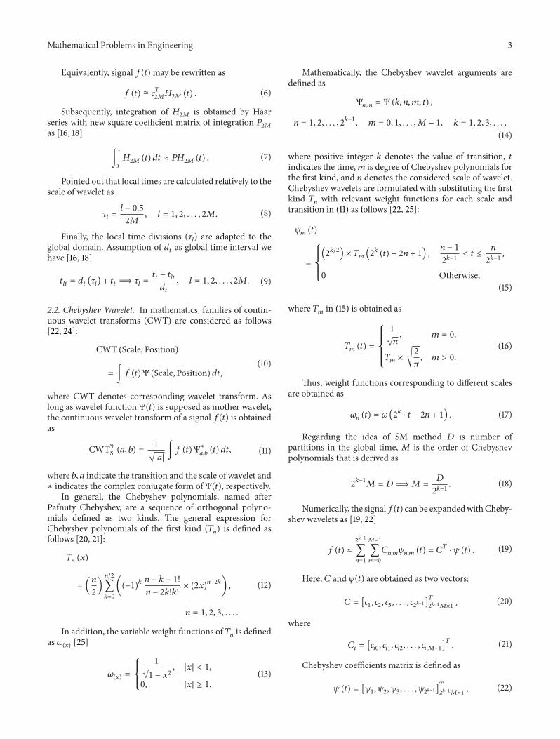
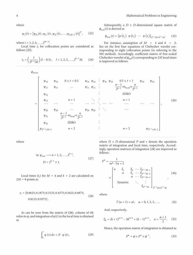
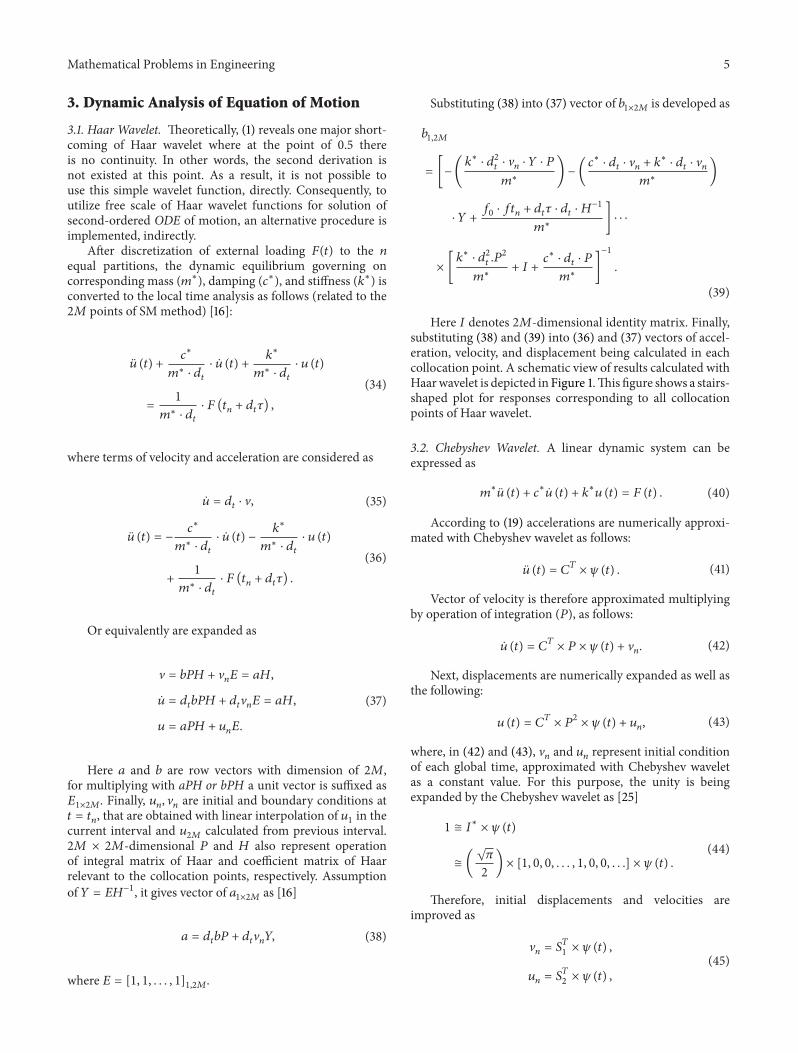
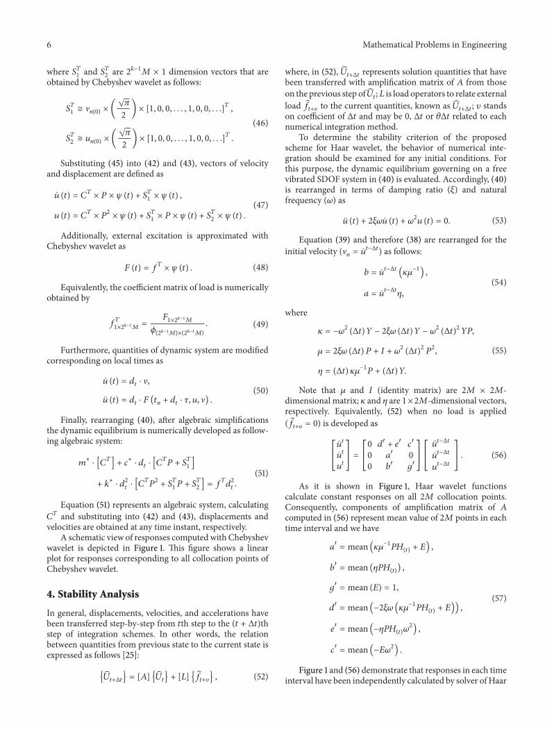
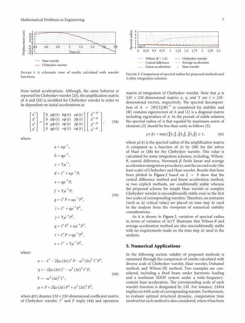
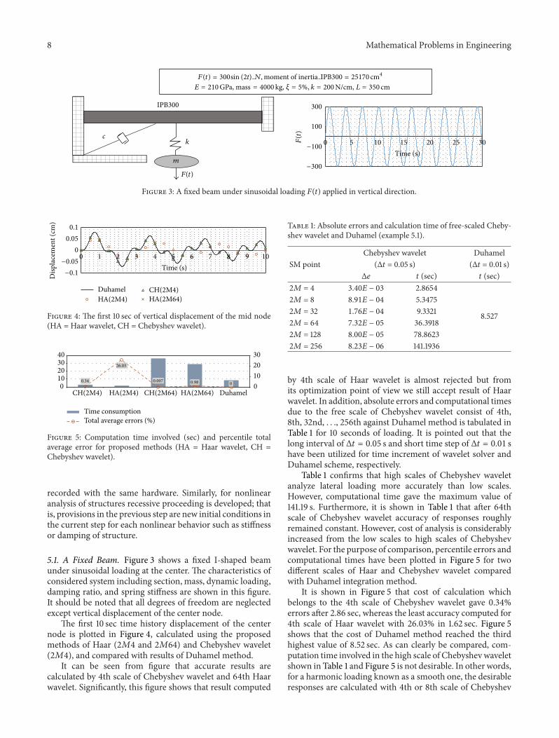
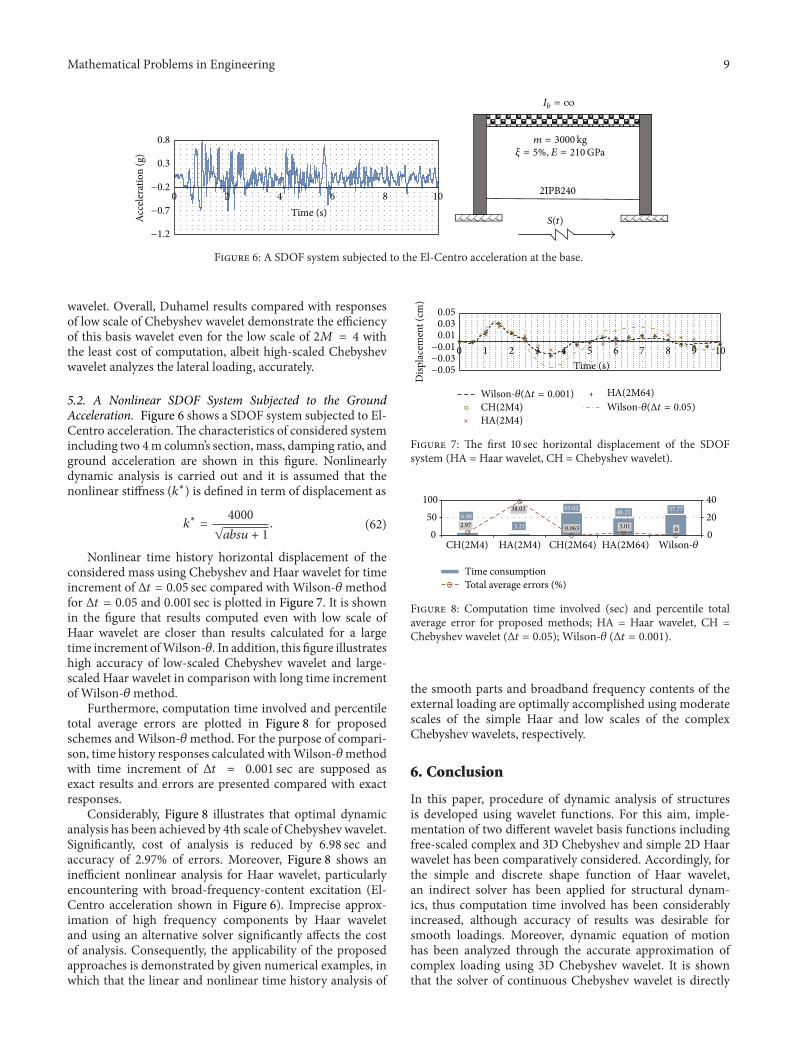
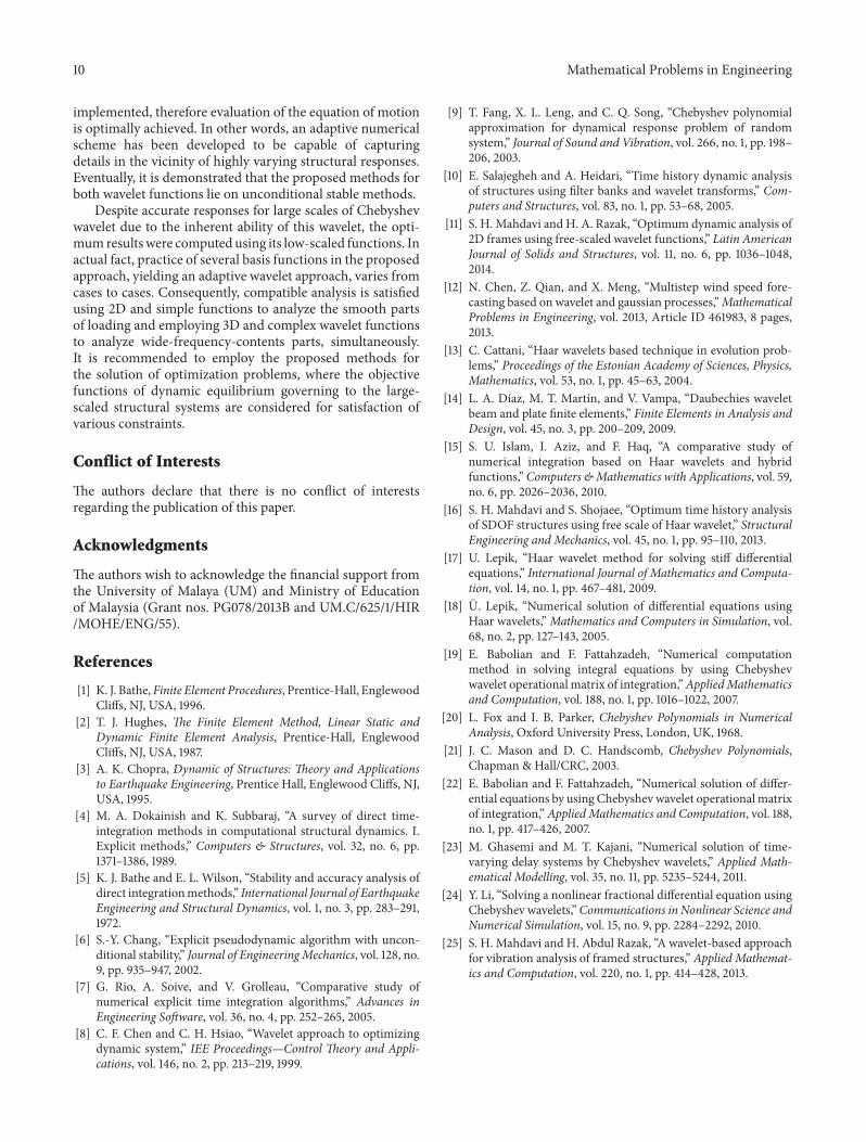