A comparative study of some methods for color medical images segmentation

RESEARCH Open Access

A comparative study of some methods for colormedical images segmentationLiana Stanescu*, Dumitru Dan Burdescu and Marius Brezovan

Abstract

The aim of this article is to study the problem of color medical images segmentation. The images representpathologies of the digestive tract such as ulcer, polyps, esophagites, colitis, or ulcerous tumors, gathered with thehelp of an endoscope. This article presents the results of an objective and quantitative study of threesegmentation algorithms. Two of them are well known: the color set back-projection algorithm and the localvariation algorithm. The third method chosen is our original visual feature-based algorithm. It uses a graphconstructed on a hexagonal structure containing half of the image pixels in order to determine a forest ofmaximum spanning trees for connected component representing visual objects. This third method is a superiorone taking into consideration the obtained results and temporal complexity. These three methods weresuccessfully used in generic color images segmentation. In order to evaluate these segmentation algorithms, weused error measuring methods that quantify the consistency between them. These measures allow a principledcomparison between segmentation results on different images, with differing numbers of regions generated bydifferent algorithms with different parameters.

Keywords: graph-based segmentation, color segmentation, segmentation evaluation, error measures

1 IntroductionThe problem of partitioning images into homogenousregions or semantic entities is a basic problem for iden-tifying relevant objects. Some of the practical applica-tions of image segmentation are medical imaging, locateobjects in satellite images (roads, forests, etc.), facerecognition, fingerprint recognition, traffic control sys-tems, visual information retrieval, or machine vision.Segmentation of medical images is the task of parti-

tioning the data into contiguous regions representingindividual anatomical objects. This task is vital in manybiomedical imaging applications such as the quantifica-tion of tissue volumes, diagnosis, localization of pathol-ogy, study of anatomical structure, treatment planning,partial volume correction of functional imaging data,and computer-integrated surgery [1,2].This article presents the results of an objective and

quantitative study of three segmentation algorithms.Two of them are already well known:

- The color set back-projection; this method wasimplemented and tested on a wide variety of imagesincluding medical images and has achieved good resultsin automated detection of color regions (CS).- An efficient graph-based image segmentation algo-

rithm known also as the local variation algorithm (LV)The third method design by us is an original visual

feature-based algorithm that uses a graph constructedon a hexagonal structure (HS) containing half of theimage pixels in order to determine a forest of maximumspanning trees for connected component representingvisual objects. Thus, the image segmentation is treatedas a graph partitioning problem.The novelty of our contribution concerns the HS used

in the unified framework for image segmentation andthe using of maximum spanning trees for determiningthe set of nodes representing the connectedcomponents.According to medical specialists most of digestive

tract diseases imply major changes in color and less intexture of the affected tissues. This is the reason whywe have chosen to do a research of some algorithmsthat realize images segmentation based on color feature.

* Correspondence: [email protected] of Automation, Computers and Electronics, University of Craiova,200440, Romania

Stanescu et al. EURASIP Journal on Advances in Signal Processing 2011, 2011:128http://asp.eurasipjournals.com/content/2011/1/128

© 2011 Stanescu et al; licensee Springer. This is an Open Access article distributed under the terms of the Creative CommonsAttribution License (http://creativecommons.org/licenses/by/2.0), which permits unrestricted use, distribution, and reproduction inany medium, provided the original work is properly cited.

mailto:[email protected]

http://creativecommons.org/licenses/by/2.0

Experiments were made on color medical imagesrepresenting pathologies of the digestive tract. The pur-pose of this article is to find the best method for thesegmentation of these images.The accuracy of an algorithm in creating segmentation

is the degree to which the segmentation corresponds tothe true segmentation, and so the assessment of accu-racy of segmentation requires a reference standard,representing the true segmentation, against which itmay be compared. An ideal reference standard forimage segmentation would be known to high accuracyand would reflect the characteristics of segmentationproblems encountered in practice [3].Thus, the segmentation algorithms were evaluated

through objective comparison of their segmentationresults with manual segmentations. A medical expertmade the manual segmentation and identified objects inthe image due to his knowledge about typical shape andimage data characteristics. This manual segmentationcan be considerate as “ground truth”.The evaluation of these three segmentation algorithms

is based on two metrics defined by Martin et al.: GlobalConsistency Error (GCE), and Local Consistency Error(LCE) [4]. These measures operate by computing thedegree of overlap between clusters or the cluster asso-ciated with each pixel in one segmentation and its “clo-sest” approximation in the other segmentation. GCEand LCE metrics allow labeling refinement in either oneor both directions, respectively.The comparative study of these methods for color

medical images segmentation is motivated by the follow-ing aspects:- The methods were successfully used in generic color

images segmentation- The CS algorithm was implemented and studied for

color medical images segmentation, the results beingpromising [5-8]- There are relatively few published studies for medi-

cal color images of the digestive tract, although thenumber of these images, acquired in the diagnostic pro-cess, is high- The color medical images segmentation is an impor-

tant task in order to improve the diagnosis and treat-ment activity- There is not a segmentation method for medical

images that produces good results for all types of medi-cal images or applications.The article is organized as follows: Section 2 presents

the related study; Section 3 describes our originalmethod based on a HS. Sections 4 and 5 briefly presentthe other two methods: the color set back-projectionand the LV; Section 6 describes the two error metricsused for evaluation; Section 7 presents the experimental

results and Section 8 presents the conclusion of thisstudy.

2 Related studyImage segmentation is defined as the partitioning of animage into no overlapping, constituent regions that arehomogeneous, taking into consideration some character-istic such as intensity or texture [1,2].If the domain of the image is given by I, then the seg-

mentation problem is to determine the sets Sk ⊂ Iwhose union is the entire image. Thus, the sets thatmake up segmentation must satisfy:

I =K⋃k=1

Sk (1)

Where Sk ∩ Sj = ∅ for k ≠ j and each Sk is connected[9].In an ideal mode, a segmentation method finds those

sets that correspond to distinct anatomical structures orregions of interest in the image.Segmentation of medical images is the task of parti-

tioning the data into contiguous regions representingindividual anatomical objects. This task plays a vital rolein many biomedical imaging applications: the quantifica-tion of tissue volumes, diagnosis, localization of pathol-ogy, study of anatomical structure, treatment planning,partial volume correction of functional imaging data,and computer-integrated surgery.Segmentation is a difficult task because in most cases

it is very hard to separate the object from the imagebackground. Also, the image acquisition process bringsnoise in the medical data. Moreover, inhomogeneities inthe data might lead to undesired boundaries. The medi-cal experts can overcome these problems and identifyobjects in the data due to their knowledge about typicalshape and image data characteristics. But, manual seg-mentation is a very time-consuming process for thealready increasing amount of medical images. As aresult, reliable automatic methods for image segmenta-tion are necessary.It cannot be said that there is a segmentation method

for medical images that produces good results for alltypes of images. There have been studied several segmen-tation methods that are influenced by factors such asapplication domain, imaging modality, or others [1,2,10].The segmentation methods were grouped into cate-

gories. Some of these categories are thresholding, regiongrowing, classifiers, clustering, Markov random field(MRF) models, artificial neural networks (ANNs),deformable models, or graph partitioning. Of course,there are other important methods that do not belongto any of these categories [1].


of 12

In thresholding approaches, an intensity value calledthe threshold must be established. This value will sepa-rate the image intensities in two classes: all pixels withintensity greater than the threshold are grouped intoone class and all the other pixels into another class. Ifmore than one threshold is determined, the process iscalled multi-thresholding.Region growing is a technique for extracting a region

from an image that contains pixels connected by somepredefined criteria, based on intensity information and/or edges in the image. In its simplest form, region grow-ing requires a seed point that is manually selected by anoperator, and extracts all pixels connected to the initialseed having the same intensity value. It can be used par-ticularly for emphasizing small and simple structuressuch as tumors and lesions [1,11].Classifier methods represent pattern recognition tech-

niques that try to partition a feature space extractedfrom the image using data with known labels.A feature space is the range space of any function of

the image, with the most common feature space beingthe image intensities themselves. Classifiers are knownas supervised methods because they need training datathat are manually segmented by medical experts andthen used as references for automatically segmentingnew data [1,2].Clustering algorithms work like classifier methods but

they do not use training data. As a result they are calledunsupervised methods. Because there is not any trainingdata, clustering methods iterate between segmenting theimage and characterizing the properties of each class. Itcan be said that clustering methods train themselvesusing the available data [1,2,12,13].MRF is a statistical model that can be used within seg-

mentation methods. For example, MRFs are often incor-porated into clustering segmentation algorithms such asthe K-means algorithm under a Bayesian prior model.MRFs model spatial interactions between neighboring ornearby pixels. In medical imaging, they are typicallyused to take into account the fact that most pixelsbelong to the same class as their neighboring pixels. Inphysical terms, this implies that any anatomical struc-ture that consists of only one pixel has a very low prob-ability of occurring under a MRF assumption [1,2].ANNs are massively parallel networks of processing

elements or nodes that simulate biological learning.Each node in an ANN is capable of performing elemen-tary computations. Learning is possible through theadaptation of weights assigned to the connectionsbetween nodes [1,2]. ANNs are used in many ways forimage segmentation.Deformable models are physically motivated, model-

based techniques for outlining region boundaries usingclosed parametric curves or surfaces that deform under

the influence of internal and external forces. To outlinean object boundary in an image, a closed curve or sur-face must be placed first near the desired boundary thatcomes into an iterative relaxation process [14-16].To have an effective segmentation of images using

varied image databases the segmentation process has tobe done based on the color and texture properties ofthe image regions [10,17].The automatic segmentation techniques were applied

on various imaging modalities: brain imaging, liverimages, chest radiography, computed tomography, digi-tal mammography, or ultrasound imaging [1,18,19].Finally, we briefly discuss the graph-based segmenta-

tion methods because they are most relevant to ourcomparative study.Most graph-based segmentation methods attempt to

search a certain structures in the associated edgeweighted graph constructed on the image pixels, such asminimum spanning tree [20,21], or minimum cut[22,23]. The major concept used in graph-based cluster-ing algorithms is the concept of homogeneity of regions.For color segmentation algorithms, the homogeneity

of regions is color-based, and thus the edge weights arebased on color distance. Early graph-based methods [24]use fixed thresholds and local measures in finding asegmentation.The segmentation criterion is to break the minimum

spanning tree edges with the largest weight, whichreflect the low-cost connection between two elements.To overcome the problem of fixed threshold, Urquhar[25] determined the normalized weight of an edge usingthe smallest weight incident on the vertices touchingthat edge. Other methods [20,21] use an adaptive criter-ion that depends on local properties rather than globalones. In contrast with the simple graph-based methods,cut-criterion methods capture the non-local propertiesof the image. The methods based on minimum cuts in agraph are designed to minimize the similarity betweenpixels that are being split [22,23,26]. The normalized cutcriterion [22] takes into consideration self-similarity ofregions. An alternative to the graph cut approach is tolook for cycles in a graph embedded in the image plane.For example in [27], the quality of each cycle is normal-ized in a way that is closely related to the normalizedcuts approach.Other approaches to image segmentation consist of

splitting and merging regions according to how welleach region fulfills some uniformity criterion. Suchmethods [28,29] use a measure of uniformity of aregion.In contrast, [20,21] use a pairwise region comparison

rather than applying a uniformity criterion to each indi-vidual region. A number of approaches to segmentationare based on finding compact clusters in some feature


of 12

space [30,31]. A recent technique using feature spaceclustering [30] first transforms the data by smoothing itin a way that preserves boundaries between regions.Our method is related to the works in [20,21] in the

sense of pairwise comparison of region similarity. Weuse different measures for internal contrast of a con-nected component and for external contrast betweentwo connected components than the measures used in[20,21]. The internal contrast of a component C repre-sents the maximum weight of edges connecting verticesfrom C, and the external contrast between two compo-nents represents the maximum weight of edges connect-ing vertices from these two components. Thesemeasures are in our opinion closer to the human per-ception. We use maximum spanning tree instead ofminimum spanning tree in order to manage externalcontrast between connected components.

3 Image segmentation using an HSThe low-level system for image segmentation describedin this section is designed to be integrated in a generalframework of indexing and semantic image processing.In this stage, it uses color to determine salient visualobjects.The color is the visual feature that is immediately per-

ceived on an image. There is no color system that isuniversally used, because the notion of color can bemodeled and interpreted in different ways. Each systemhas its own color models that represent the systemparameters.There exist several color systems, for different pur-

poses: RGB (for displaying process), XYZ (for colorstandardization), rgb, xyz (for color normalization andrepresentation), CieL*u*v*, CieL*a*b* (for perceptualuniformity), HSV (intuitive description) [2,32].We decided to use the RGB color space because it is

efficient and no conversion is required. Although it alsosuffers from the non-uniformity problem where thesame distance between two color points within the colorspace may be perceptually quite different in differentparts of the space, within a certain color threshold it isstill definable in terms of color consistency. We use theperceptual Euclidean distance with weight-coefficients(PED) as the distance between two colors, as proposedin [33]:

PED(e, u) =√wR(Re − Ru)

2 + wG(Ge − Gu)2 + wB(Be − Bu)

2 (2)

the weights for the different color channels, wR, wG,andwB verify the condition wR + wG + wB = 1.Based on the theoretical and experimental results on

spectral and realworld datasets, in [25] it is concludedthat the PED distance with weightcoefficients (wR =0.26, wG = 0.70, wB = 0.04) correlates significantly

higher than all other distance measures including theangular error and Euclidean distance.In order to optimize the running time of segmentation

and contour detection algorithms, we use a HS con-structed on the image pixels, as presented in Figure 1.Each hexagon represents an elementary item and the

entire HS represents a grid-graph, G = (V, E), whereeach hexagon h in this structure has a correspondingvertex v Î V. The set E of edges is constructed by con-necting pairs of hexagons that are neighbors in a 6-con-nected sense, because each hexagon has six neighbors.The advantage of using hexagons instead of pixels as

elementary piece of information is that the amount ofmemory space associated to the graph vertices isreduced. Denoting by np the number of pixels of theinitial image, the number of the resulted hexagons isalways less than np = 4, and then the cardinal of bothsets V and E is significantly reduced.We associate to each hexagon h from V two impor-

tant attributes representing its dominant color and thecoordinates of its gravity center. For determining theseattributes, we use eight pixels contained in a hexagon h:six pixels from the frontier and two interior pixels. Weselect one of the two interior pixels to represent withapproximation the gravity center of the hexagon becausepixels from an image have integer values as coordinates.We select always the left pixel from the two interior pix-els of a hexagon h to represent the pseudo-center of thegravity of h, denoted by g(h).The dominant color of a hexagon is denoted by c(h)

and it represents the mean color vector of the all eightcolors of its associated pixels. Each hexagon h in thehexagonal grid is thus represented by a single point, g(h),6 having the color c(h).The segmentation system creates an HS on the pixels

of the input image and an undirected grid graph havinghexagons as vertices, and uses this graph in order toproduce a set of salient objects contained in the image.In order to allow an unitary processing for the multi-level system at this level we store, for each determinedcomponent C:- an unique index of the component;

Figure 1 HS constructed on the image pixels.


of 12

- the set of the hexagons contained in the region asso-ciated to C;- the set of hexagons located at the boundary of the

component.In addition for each component a mean color of the

region is extracted. Our HS is similar to quincunx sam-pling scheme, but there are some important differences.The quincux sample grid is a sublattice of a square lat-tice that retains half of the image pixels [34]. The keypoint of our HS, that also uses half of the image pixels,is that the hexagonal grid is not a lattice because hexa-gons are not regular. Although our hexagonal grid isnot a hexagonal lattice, we use some of the advantagesof the hexagonal grid such as uniform connectivity. Inour case, only one type of neighborhood is possible,sixth neighborhood structure, unlike several types as N4and N8 in the case of square lattice.

3.1 Algorithms for computing the color of a hexagon andthe list of hexagons with the same colorThe algorithms return the list of salient regions fromthe input image. This list is obtained using the hexago-nal network and the distance between two colors in theRGB color space. In order to obtain the color of a hexa-gon a procedure called sameVertexColour is used. Thisprocedure has a constant execution time because allcalls are constant in time processing. The color informa-tion will be used by the procedure expandColorArea tofind the list of hexagons that have the same color.3.1.1 Determination of the hexagon colorThe input of this procedure contains the current hexa-gon hi, L1–the colors list of pixels corresponding to thehexagonal network: L1 = {p1,...,p6n}. The output is repre-sented by the object crtColorHexagon.Procedure sameVertexColour (hi, L1)

initializecrtColorHexagon;

determine the colors for the six ver-tices of hexagon hi

determine the colors for the two ver-tices from interior of hexagon hi

calculate the mean color value meanCo-lor for the eight colors of vertices;crtColorHexagon.colorHexagon <-meanColor;

crtColorHexagon:sameColor <- true;for k <- 1 to 6 do

if colorDistance(meanColor, color-Vertex[k]) > threshold then

crtColorHexagon:sameColor <-false;

break;end

end

return crtColorHexagon;In the above function, the threshold value is an adap-

tive one, defined as the sum between the average of thecolor distances associated to edges (between the adja-cent hexagons) and the standard deviation of these colordistances.3.1.2 Expand the current regionThe function expandColourArea is a depth-first traver-sing procedure, which starts with an specified hexagonhi, pivot of a region item, and determines the list of alladjacent hexagons representing the current region con-taining hi such that the color dissimilarity between theadjacent hexagons is below a determined threshold.The input parameters of this function is the current

region item, index-CrtRegion, its first hexagon, hi, andthe list of all hexagons V from the hexagonal grid.Procedure expandColourArea (hi, crtRegionI-

tem, V)push(hi);while not(empty(stack)) doh <- pop();for each hexagon hj neighbor to h do

if not(visit (V[hj])) thenif colorDistance(h, hj) < threshold

thenadd hj to crtRegionItemmark visit (V[hj])push (hj)

endend

endendThe running time of the procedure expandColourArea

is O(n) where n is the number of hexagons from aregion with the same color [35].

3.2 The algorithm used to obtain the regionsThe procedures presented above are used by the listRe-gions procedure to obtain the list of regions.This procedure has an input which contains the vector

V representing the list of hexagons and the list L1.The output is represented by a list of colors pixels and

a list of regions for each color.Procedure listRegions (V, L1)colourNb <- 0;for i <- 1 to n do

initialize crtRegionItem;if not(visit(h_ i)) then

crtColorHexagon <- sameVertexCo-lour (L1, hi);

if crtColorHexagon.sameColor thenk <- findColor(crtColorHexagon.

color);if k < 0 then


of 12

add new color ccolourNb to list C;k <- colourNb++;indexCrtRegion <- 0;

elseindexCrtColor <- k;indexCrtRegion<-

findLastIndexRegion(indexCrtColor);

indexCrtRegion++;endhi.indexRegion <- indexCrtRegion;hi.indexColor <- k;add hi to crtRegionItem;

expandColourArea(hi, L1,V,indexCrtRegion, indexCrtColor,

crtRegionItem);add new region crtRegionItem to

list of element k from Cend

endendThe running time of the procedure list Regions is O(n)

2, where n is the number of the hexagons network [35].Let G = (V, E) be the initial graph constructed on the

HS of an image. The color-based sequence of segmenta-tions, Si = (S0, S1,..., St), will be generated by using acolor-based region model and a maximum spanningtree construction method based on a modified form ofthe Kruskal’s algorithm [36].In the color-based region model, the evidence for a

boundary between two regions is based on the differ-ence between the internal contrast of the regions andthe external contrast between them. Both notions ofinternal contrast or internal variation of a component,and external contrast or external variation between twocomponents are based on the dissimilarity between twocolors [37]:

ExtVar(C′,C′′) = max(hi,hj)∈cb(c′,c′′)

w(hi, hj) (3)

IntVar(C) = max(hi,hj)∈c

w(hi, hj) (4)

where cb(C’, C“) represents the common boundarybetween the components C’ and C“ and w is the colordissimilarity between two adjacent hexagons:

w(hi, hj) = PED(c(hi), c(hj)) (5)

where c(h) represents the mean color vector associatedwith the hexagon h.The maximum internal contrast between two compo-

nents is defined as follows [37]:

IntVar(C′,C′′) = max(IntVar(C′), IntVar(C′′)) + r (6)

where the threshold r is an adaptive value defined asthe sum between the average of the color distancesassociated to edges and the standard deviation, r = μ +s.The comparison predicate between two neighboring

components C’ and C“ determines if there is an evi-dence for a boundary between them [37].

dif fcol(C′,C′′) ={true,ExtVar(C′,C′′) > IntVar(C′,C′′)false,ExtVar(C′,C′′) ≤ IntVar(C′,C′′) (7)

The color-based segmentation algorithm represents anadapted form of a Kruskal’s algorithm and it builds amaximal spanning tree for each salient region of theinput image.

4 The color set back-projection algorithmColor sets provide an alternative to color histograms forrepresenting color information. Their utilization is basedon the assumption that salient regions have not morethan few equally prominent colors [38].The color set back-projection algorithm proposed in

[38] is a technique for the automated extraction ofregions and representation of their color content.The back-projection process requires several stages:

color set selection, back-projection onto the image,thresholding, and labeling. Candidate color sets areselected first with one color, then with two colors, etc.,until the salient regions are extracted. For each imagequantization of the RGB color space at 64 colors isperformed.The algorithm follows the reduction of insignificant

color information and makes evident the significant CS,followed by the generation, in automatic way, of theregions of a single color, of the two colors, etc.For each detected region the color set, the area and

the localization are stored. The region localization isgiven by the minimal bounding rectangle. The regionarea is represented by the number of color pixels, andcan be smaller than the minimum bounding rectangle.The image processing algorithm computes both the

global histogram of the image, and the binary color set[7,32]. The quantized colors are stored in a matrix. Tothis matrix a 5 × 5 median filter is applied which hasthe role of eliminating the isolated points. The processof regions extraction is using the filtered matrix and itis a depth-first traversal described in pseudo-code in thefollowing way:Procedure FindRegions (Image I, colorset

C)InitStack(S)Visited = ∅


of 12

for *each node P in I doif *color of P is in C thenPUSH(P)Visited <- Visited ∪ Pwhile not Empty(S) doCrtPoint <- POP()Visited <- Visited ∪ CrtPointFor *each unvisited neighbor S of

CrtPoint doif *color of S is in C thenVisited <- Visited ∪ S

PUSH(S)end

endend* Output detected region

endendThe total running time for a call of the procedure Fin-

dRegions (Image I, colorset C) is O(m2 × n2) where m isthe width and n is the height of the image [7,32].

5 Local variation algorithmThis algorithm described in [20] is using a graph-basedapproach for the image segmentation process. The pix-els are considered the graph nodes so in this way it ispossible to define an undirected graph G = (V, E) wherethe vertices vi from V represent the set of elements tobe segmented. Each edge (vi, vj) belonging to E has asso-ciated a corresponding weight w(vi, vj) calculated basedon color, which is a measure of the dissimilaritybetween neighboring elements vi and vj.A minimum spanning tree is obtained using Kruskal’s

algorithm [36]. The connected components that areobtained represent image regions. It is supposed thatthe graph has m edges and n vertices. This algorithm isdescribed also in [39] where it has four major steps thatare presented below:Sort E=(e1,..., em) such that |et| < |e′t| ∪ t

<t’Let S0 = ({x1},..., {xn}) be each initial

cluster containing only one vertex.For t = 1,..., m

Let xi and xj be the vertices con-nected by et

Let Ct−1xi be the connected component

containing point xi on iteration t-1 and

li = maxmstCt−1xi be the longest edge in

the minimum spanning tree of Ct−1xi . Likewise

for lj.

Merge Ct−1xi and Ct−1

xj if

|et| < min{li + kCt−1xi

, lj + kCt−1xj

} where k is a

constant.S = Sm

The existence of a boundary between two componentsin segmentation is based on a predicate D. This predi-cate is measuring the dissimilarity between elementsalong the boundary of the two components relative to ameasure of the dissimilarity among neighboring ele-ments within each of the two components. The internaldifference of a component C ⊆ V was defined as the lar-gest weight in the minimum spanning tree of a compo-nent MST(C, E):

Int(C) = maxe∈MST(CE)w(e) (8)

A threshold function is used to control the degree towhich the difference between components must be lar-ger than minimum internal difference. The pairwisecomparison predicate is defined as:

D(C1,C2) ={true, ifDif (C1,C2) > MInt(C1,C2)false, otherwise

(9)

where the minimum internal difference Mint isdefined as:

MInt(C1,C2) = min(Int(C1) + τ (C1), Int(C2) + τ (C2)) (10)

The threshold function was defined based on the sizeof the component: τ(C) = k/|C|. The k value is set takinginto account the size of the image. For images havingthe size 128 × 128 k is set to 150 and for images withsize 320 × 240 k is set to 300. The algorithm for creat-ing the minimum spanning tree can be implemented torun in O(m log m) where m is the number of edges inthe graph. The input of the algorithm is represented bya graph G = (V, E) with n vertices and m edges. Theobtained output is a segmentation of V in the compo-nents S = (C1,..., Cr). The algorithm has five major steps:Sort E into π = (o1, , otπ) by non-decreas-

ing edge weightStart with a segmentation SD, where each

vertex vi is in own componentRepeat step 4 for $q = 1, . . . , m$Construct Sq using Sq-1 and the internal

difference. If vi and vj are in disjoint com-ponents of Sq-1 and the weight of the edgebetween vi and vj is small compared to theinternal difference then merge the two com-ponents otherwise do nothing.Return S = Stπ

Unlike the classical methods this technique adaptivelyadjusts the segmentation criterion based on the degreeof variability in neighboring regions of the image.


of 12

6 Segmentation error measuresA potential user of an algorithm’s output needs to knowwhat types of incorrect/invalid results to expect, assome types of results might be acceptable while othersare not. This called for the use of metrics that arenecessary for potential consumers to make intelligentdecisions.This section presents the characteristics of the error

metrics defined in [4]. The authors proposed twometrics that can be used to evaluate the consistency of apair of segmentations, where segmentation is simply adivision of the pixels of an image into sets. Thus a seg-mentation error measure takes two segmentations S1and S2 as input and produces a real valued output inthe range [0...1] where zero signifies no error.The process defines a measure of error at each pixel

that is tolerant to refinement as the basis of both mea-sures. A given pixel pi is defined in relation to the seg-ments in S1 and S2 that contain that pixel. As thesegments are sets of pixels and one segment is a propersubset of the other, then the pixel lies in an area ofrefinement and the local error should be zero. If there isno subset relationship, then the two regions overlap inan inconsistent manner. In this case, the local errorshould be non-zero. Let \ denote set difference, and |x|the cardinality of set x. If R(S,pi) is the set of pixels cor-responding to the region in segmentation S that con-tains pixel pi, the local refinement error is defined as in[4]:

E(S1, S2, pi) =|R(S1, pi)/R(S2, pi)|

|R(S1, pi)| (11)

Note that this local error measure is not symmetric. Itencodes a measure of refinement in one direction only:E(S1, S2, pi) is zero precisely when S1 is a refinement ofS2 at pixel pi, but not vice versa. Given this local refine-ment error in each direction at each pixel, there are twonatural ways to combine the values into an error mea-sure for the entire image. GCE forces all local refine-ments to be in the same direction. Let n be the numberof pixels:

GCE(S1, S2) =1nmin{

∑i

E(S1, S2, pi),∑i

E(S2, S1, pi)} (12)

LCE allows refinement in different directions in differ-ent parts of the image.

LCE(S1,S2) =1n

∑i

min{E(S1, S2, pi),E(S2, S1, pi)} (13)

As LCE ≤ GCE for any two segmentations, it is clearthat GCE is a tougher measure than LCE. Martin et al.showed that, as expected, when pairs of human

segmentations of the same image are compared, boththe GCE and the LCE are low; conversely, when randompairs of human segmentations are compared, the result-ing GCE and LCE are high.

7 Experiments and resultsThis section presents the experimental results for theevaluation of the three segmentation algorithms anderror measures values.The experiments were made on a database with 500

medical images from digestive area captured by anendoscope. The images were taken from patients havingdiagnoses such as polyps, ulcer, esophagites, colitis, andulcerous tumors.For each image, the following steps are performed by

the application that we have created to calculate theGCE and LCE values:Obtain the image regions using the color set back-

projection segmentationObtain the image regions using the LVObtain the image regions using the algorithm based

on the HSObtain the manually segmented regionsStore these regions in the databaseCalculate GCE and LCEStore these values in the database for later statisticsIn Figure 2 the images for which we present some

experimental results are presented. Figures 3 and 4 pre-sent the regions resulted from manual segmentation andfrom the application of the three algorithms presentedabove for the images displayed in Figure 2.In Table 1 the number of regions resulted from the

application of the segmentation can be seen.In Table 2 the GCE values calculated for each algo-

rithm are presented.In Table 3 the LCE values calculated for each algo-

rithm are presented.If two different segmentations arise from different per-

ceptual organizations of the scene, then it is fair todeclare the segmentations inconsistent. If, however, seg-mentation is simply a refinement of the other, then theerror should be small, or even zero. The error measurespresented in the above tables are calculated in relationwith the manual segmentation which is considered truesegmentation. From Tables 2 and 3 it can be observedthat the values for GCE and LCE are lower in the caseof hexagonal segmentation. The error measures, foralmost all tested images, have smaller values in the caseof the original segmentation method which use a HSdefined on the set of pixels.Figure 5 presents the repartition of the 500 images

from the database on GCE values. The focus point hereis the number of images on which the GCE value isunder 0.5.


of 12

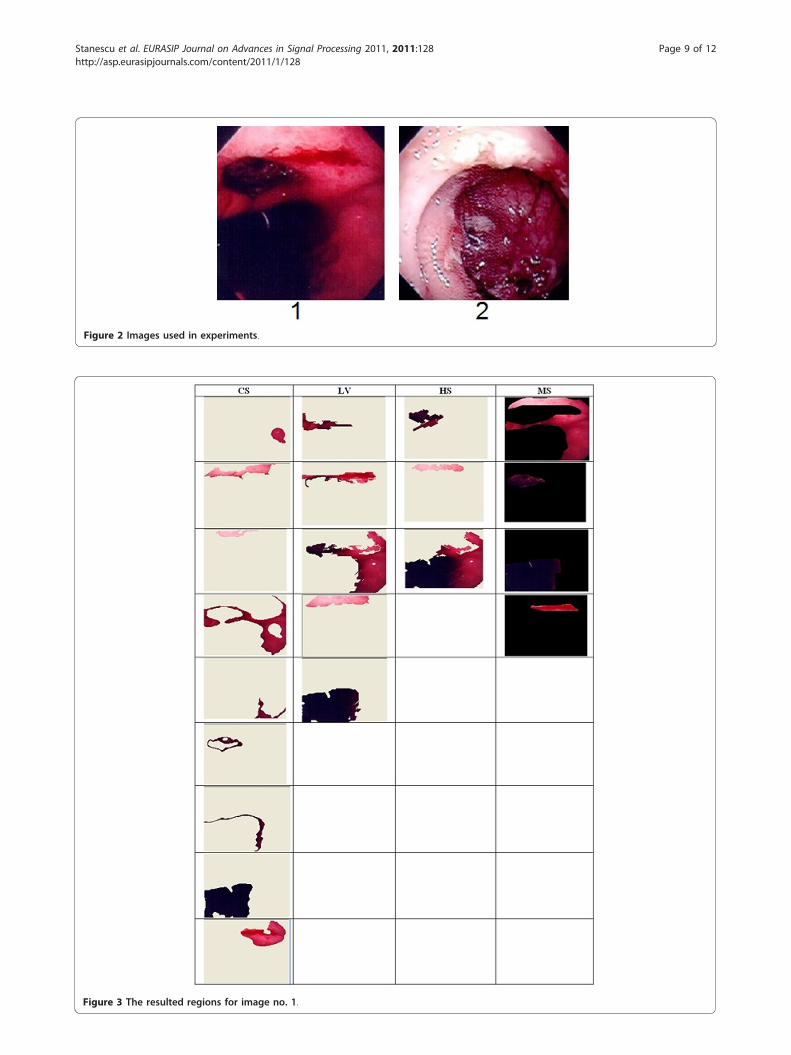
Figure 2 Images used in experiments.

Figure 3 The resulted regions for image no. 1.


of 12

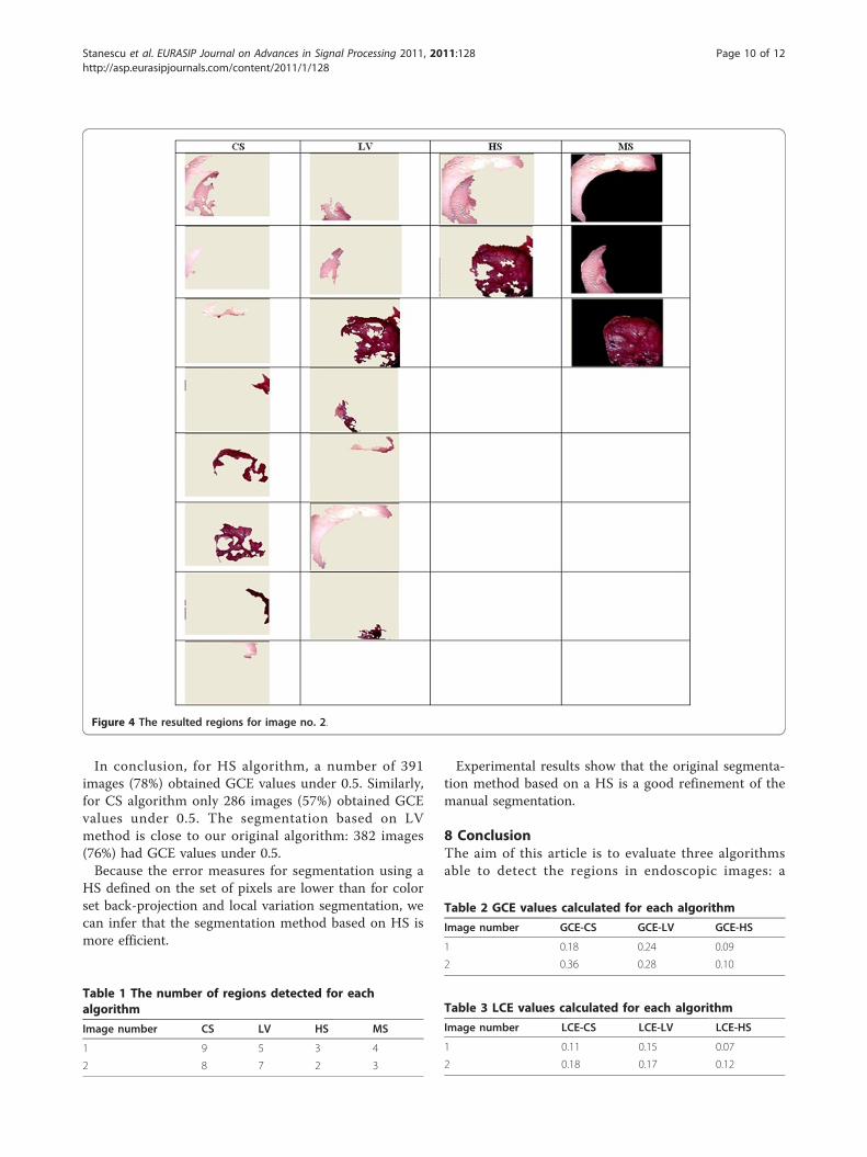
In conclusion, for HS algorithm, a number of 391images (78%) obtained GCE values under 0.5. Similarly,for CS algorithm only 286 images (57%) obtained GCEvalues under 0.5. The segmentation based on LVmethod is close to our original algorithm: 382 images(76%) had GCE values under 0.5.Because the error measures for segmentation using a

HS defined on the set of pixels are lower than for colorset back-projection and local variation segmentation, wecan infer that the segmentation method based on HS ismore efficient.

Experimental results show that the original segmenta-tion method based on a HS is a good refinement of themanual segmentation.

8 ConclusionThe aim of this article is to evaluate three algorithmsable to detect the regions in endoscopic images: a

Figure 4 The resulted regions for image no. 2.

Table 1 The number of regions detected for eachalgorithm

Image number CS LV HS MS

1 9 5 3 4

2 8 7 2 3

Table 2 GCE values calculated for each algorithm

Image number GCE-CS GCE-LV GCE-HS

1 0.18 0.24 0.09

2 0.36 0.28 0.10

Table 3 LCE values calculated for each algorithm

Image number LCE-CS LCE-LV LCE-HS

1 0.11 0.15 0.07

2 0.18 0.17 0.12


of 12

clustering method (the color set back-projection algo-rithm), as well as other two methods of segmentationbased on graphs: the LV and our original segmentationalgorithm.Our method is based on an HS defined on the set of

image pixels. The advantage of using a virtual hexagonalnetwork superposed over the initial image pixels is thatit reduces the execution time and the memory spaceused, without loosing the initial resolution of the image.In comparison to other segmentation methods, ouralgorithm is able to adapt and does not require neitherparameters for establishing the optimal values, nor setsof training images to set parameters.Furthermore, the article presents a method that

enables the assessment of the segmentation accuracy.The role of this review is to find out which segmenta-

tion algorithm gives the best results for medical imagesfrom digestive area captured by an endoscope.First, the correctness of segments resulted after the

application of the three algorithms described above iscompared. Concerning the endoscopic database all thealgorithms have the ability to produce segmentationsthat comply with the manual segmentation made by amedical expert. Then for evaluating the accuracy of thesegmentation error measures are used. The proposederror measures quantify the consistency between seg-mentations of differing granularities. Because humansegmentation is considered true segmentation the errormeasures are calculated in relation with manual seg-mentation. The GCE and LCE demonstrate that theimage segmentation based on an HS produces a bettersegmentation than the back-projection method and theLV.The future research will focus on developing our seg-

mentation algorithm so as to include the texture featurealong with the color feature and reducing the algorithmcomplexity at O(n log n), where n represents the num-ber of image pixels.

AcknowledgementsThe support of The National University Research Council under Grant CNC-SIS IDEI 535 is gratefully acknowledged.

Competing interestsThe authors declare that they have no competing interests.

Received: 15 May 2011 Accepted: 9 December 2011Published: 9 December 2011

References1. DL Pham, C Xu, JL Prince, Current methods in medical image

segmentation. Annu Rev Biomed Eng. 2, 315–337 (2000). doi:10.1146/annurev.bioeng.2.1.315

2. L Stanescu, D Burdescu, M Brezovan, in Chapter Book: Multimedia MedicalDatabases, Biomedical Data and Applications, Series: Studies in ComputationalIntelligence, vol. 224, ed. by Sidhu AS, Dillon T, Bellgard M (Springer, 2009)

3. SK Warfield, KH Zou, WM Wells, Simultaneous truth and performance levelestimation (STAPLE): an algorithm for the validation of image segmentation.Med Imag IEEE Trans. 23(7), 903–921 (2004). doi:10.1109/TMI.2004.828354

4. D Martin, C Fowlkes, D Tal, J Malik, A database of human segmentednatural images and its application to evaluating segmentation algorithmsand measuring ecological statistics, in Proceedings of the Eighth InternationalConference On Computer Vision (ICCV-01). 2, 416–425 (2001)

5. DD Burdescu, L Stanescu, A new algorithm for content-based region queryin databases with medical images, in Conference of International Council onMedical and Care Compunetics, Symposium On Virtual Hospitals, Symposiumon E-Health, Proceedings in Studies In Health Technology and Informatics. 114,132–133 (2005). Medical and Care Compunetics 2

6. DD Burdescu, L Stanescu, A new algorithm for content-based region queryin multimedia database, in 16th International Conference on Database andExpert Systems Applications, Proceedings in Lectures Notes in ComputerScience. 3588, 124–133 (2005)

7. DD Burdescu, L Stanescu, Color image segmentation applied to medicaldomain. Intell Data Eng Autom Learn. 4881, 457–466 (2007). doi:10.1007/978-3-540-77226-2_47

8. L Stanescu, DD Burdescu, Medical image segmentation–a comparison oftwo algorithms, in International Workshop on Medical Measurements andApplications (2010)

9. JR Smith, Integrated spatial and feature image systems: retrieval,compression and analysis, PhD thesis, Graduate School of Arts and SciencesColumbia University, (1997)

10. H Muller, N Michoux, D Bandon, A Geissbuhler, A review of content-basedimage retrieval systems in medical applications–clinical benefits and futuredirections. Int J Med Inf. 73(1), 1–23 (2004). doi:10.1016/j.ijmedinf.2003.11.024

11. C Jiang, X Zhang, M Christoph, Hybrid framework for medical imagesegmentation. Lecture Notes in Computer Science. 3691, 264–271 (2005).doi:10.1007/11556121_33

Figure 5 Number of images relative to GCE values.


of 12

http://www.ncbi.nlm.nih.gov/pubmed/11701515?dopt=Abstract

http://www.ncbi.nlm.nih.gov/pubmed/11701515?dopt=Abstract

12. S Belongie, C Carson, H Greenspan, J Malik, Color and texture-based imagesegmentation using the expectation-maximization algorithm and itsapplication to content-based image retrieval. in ICCV 675–682 (1998)

13. C Carson, S Belongie, H Greenspan, J Malik, Blobworld: image segmentationusing expectation-maximization and its application to image querying. IEEETrans Pattern Anal Mach Intell. 24(8), 1026–1038 (2002). doi:10.1109/TPAMI.2002.1023800

14. L Ballerini, Medical image segmentation using Genetic snakes, Applicationsand Science of Neural Networks, Fuzzy Systems, and Evolutionary ComputationII, (Denver Co, 1999)

15. S Ghebreab, AWM Smeulders, Medical images segmentation by strings, inProceedings of the VISIM Workshop: Information Retrieval and Exploration inLarge Collections of Medical Images (2001)

16. S Ghebreab, AWM Smeulders, An approximately complete stringrepresentation of local object boundary features for concept-based imageretrieval, in IEEE International Symposium on Biomedical Imaging (2004)

17. S Gordon, G Zimmerman, H Greenspan, Image segmentation of uterinecervix images for indexing in PACS, in Proceedings of the 17th IEEESymposium on Computer-Based Medical Systems, CBMS (2004)

18. H Lamecker, T Lange, M Seeba, S Eulenstein, M Westerhoff, HC Hege,Automatic segmentation of the liver for preoperative planning ofresections, in Proceedings of Medicine Meets Virtual Reality, Studies in HealthTechnologies and Informatics. 94, 171–174 (2003)

19. H Muller, S Marquis, G Cohen, PA Poletti, CL Lovis, A Geissbuhler, Automaticabnormal region detection in lung CT images for visual retrieval. Swiss MedInf. 57, 2–6 (2005)

20. PF Felzenszwalb, WD Huttenlocher, Efficient graph-based imagesegmentation. Int J Comput Vis. 59(2), 167–181 (2004)

21. L Guigues, LM Herve, LP Cocquerez, The hierarchy of the cocoons of agraph and its application to image segmentation. Pattern Recogn Lett.24(8), 1059–1066 (2003). doi:10.1016/S0167-8655(02)00252-0

22. J Shi, J Malik, Normalized cuts and image segmentation. in Proceedings ofthe IEEE Conference on Computer Vision and Pattern Recognition 731–737(1997)

23. Z Wu, R Leahy, An optimal graph theoretic approach to data clustering:theory and its application to image segmentation. IEEE Trans Pattern AnalMach Intell. 15(11), 1101–1113 (1993). doi:10.1109/34.244673

24. C Zahn, Graph-theoretical methods for detecting and describing gestalclusters. IEEE Trans Comput. 20(1), 68–86 (1971)

25. R Urquhar, Graph theoretical clustering based on limited neighborhoodsets. Pattern Recogn. 15(3), 173–187 (1982). doi:10.1016/0031-3203(82)90069-3

26. Y Gdalyahu, D Weinshall, M Werman, Self-organization in vision: stochasticclustering for image segmentation, perceptual grouping, and imagedatabase organization. IEEE Trans Pattern Anal Mach Intell. 23(10),1053–1074 (2001). doi:10.1109/34.954598

27. I Jermyn, H Ishikawa, Globally optimal regions and boundaries as minimumratio weight cycles. IEEE Trans Pattern Anal Mach Intell. 23(8), 1075–1088(2001)

28. M Cooper, The tractibility of segmentation and scene analysis. Int J ComputVis. 30(1), 27–42 (1998). doi:10.1023/A:1008013412628

29. T Pavlidis, Structural Pattern Recognition (Springer, 1977)30. D Comaniciu, P Meer, Robust analysis of feature spaces: color image

segmentation. in Proceedings of the IEEE Conference on Computer Vision andPattern Recognition 750–755 (2003)

31. A Jain, R Dubes, Algorithms for Clustering Data (Prentice Hall, 1988)32. L Stanescu, Visual Information. Procecessing, Retrieval and Applications

(Sitech, Craiova, 2008)33. A Gijsenij, T Gevers, M Lucassen, A perceptual comparison of distance

measures for color constancy algorithms, in Proceedings of the EuropeanConference on Computer Vision. 5302, 208–2011 (2008)

34. X Zhang, X Wu, Image coding on quincunx lattice with adaptive lifting andinterpolation. in Data Compression Conference 193–202 (2007)

35. DD Burdescu, M Brezovan, E Ganea, L Stanescu, A new method forsegmentation of images represented in a HSV color space. in ACIVS606–617 (2009)

36. MT Goodrich, R Tamassia, Data Structures and Algorithms in Java, 4th edn.(John Wiley and Sons, Inc, 2006)

37. M Brezovan, DD Burdescu, E Ganea, L Stanescu, Boundary-basedperformance evaluation of a salient visual object detection algorithm, inProceedings of the WorldComp IPCV (2010)

38. JR Smith, SF Chang, Tools and techniques for color image retrieval, Proc.SPIE Storage retrieval for still image and video databases, IV. 2670, 426–437(1996)

39. C Pantofaru, M Hebert, A comparison of image segmentation algorithms,Technical Report CMU-RI-TR-05-40, Robotics Institute, Carnegie MellonUniversity, Pittsburgh, PA, (2005)

doi:10.1186/1687-6180-2011-128Cite this article as: Stanescu et al.: A comparative study of somemethods for color medical images segmentation. EURASIP Journal onAdvances in Signal Processing 2011 2011:128.

Submit your manuscript to a journal and benefi t from:

7 Convenient online submission

7 Rigorous peer review

7 Immediate publication on acceptance

7 Open access: articles freely available online

7 High visibility within the fi eld

7 Retaining the copyright to your article

Submit your next manuscript at 7 springeropen.com


of 12

http://www.springeropen.com/

http://www.springeropen.com/

A comparative study of some methods for color medical images segmentation

Documents

Transcript of A comparative study of some methods for color medical images segmentation