A tensorial framework for color images
20
A tensorial framework for color images Leticia Rittner a, * , Franklin C. Flores b , Roberto A. Lotufo a a School of Electrical and Computer Engineering, University of Campinas (UNICAMP), C.P. 6101, 13083-852 Campinas (SP), Brazil b Department of Informatics, State University of Maringá (UEM), Bloco 19, 87020-900 Maringá (PR), Brazil article info Article history: Available online 3 October 2009 Keywords: Color image Gradient Tensor Mathematical morphology Watershed transform Segmentation abstract This paper proposes a new tensorial color representation, obtained by making a correspondence between color models (HSL, IHSL, HSV, RGB and CIELUV) and tensors. Based on this representation, a proposed ten- sorial morphological gradient (TMG), defined as the maximum dissimilarity over the neighborhood, was tested using several tensor similarity measures. Experimental results illustrate which color models are more suitable to the proposed tensorial representation and which measures give best results in the TMG computation. The watershed transform was used to demonstrate that the proposed representation and the TMG can be applied to segment color images. A quantitative analysis of segmentation results was also conducted. Ó 2009 Elsevier B.V. All rights reserved. 1. Introduction The image edge enhancement by gradient computation is an important step in morphological image segmentation via wa- tershed (Beucher and Meyer, 1992; Soille and Vincent, 1990; Fal- cão et al., 2004; Cousty et al., 2009). For grayscale images, the morphological gradient (Dougherty and Lotufo, 2003) is a very good option and its computation is simple: for each point in the image, a structuring element is centered to it and the difference be- tween the maximum and the minimum graylevels inside the struc- turing element is computed. For grayscale images, it is possible to compare the intensities among themselves in order to find the maximum and the minimum in a set of intensities. Such intensities are usually represented by integers, and the set of integers has a to- tal order relation, i.e., any two integers are comparable and one of them is greater than or equal to the other one. The dissimilarity information exploited to compute the morphological gradient is the intensity difference among pixels inside the structuring element. Color information lacks a total order relation – it is not possible to compare two colors, for instance red and blue, and conclude which of them is the greatest one. Therefore, such concept does not extend naturally to color images. Although the dissimilarity information is richer in color images than in grayscale ones, the de- sign of methods to edge enhancement in color images is complex. Also note that if one considers the color space as a complete lattice (Talbot et al., 1998; Chanussot and Lambert, 1998), the order rela- tion is not total and even if a total order is imposed to this space, it will be not natural for the human eye. One option to construct color gradients relies on the design of measures to compute them (Flores et al., 2004, 2006). Such mea- sures exploit the dissimilarity information in color images, usually collected from each band, and then compute the gradient based on the distance of the colors inside a given connected region: the higher the dissimilarity among the colors inside this region, the higher is its gradient. The dissimilarity measures impose a total or- der relation and the gradient may be computed. An alternative measure is the one based on tensorial algebra (Danielson, 2003; Bishop and Goldberg, 1980). Using tensors to represent colors in images bring us the possibility to make use of all the tensor theory. Given a tensorial representation of colors, it is possible to compute the gradient of a color image by computing the dissimilarity among the tensors. Some approaches of color rep- resentation based on tensors can be found in the literature. The gradient of Di Zenzo (1986) is a well known application of tensor to compute color gradient. Others utilize the Structure Tensor (or a modified version of it) to represent RGB color images and use this representation to comply different tasks, such as: feature extrac- tion (Weijer et al., 2004; Weijer et al., 2004), computation of opti- cal flow (Bigun et al., 1991) and segmentation (de Luis Garcia et al., 2005). This paper proposes a new tensorial framework for color images. Based on a tensorial representation of color images using the HSL color model (Rittner et al., 2007), new color representa- tions are obtained by building a correspondence between some color models and tensors. The tensorial morphological gradient (TMG) for color images is also a new proposal to compute color gradients based on tensorial algebra. Several ways to compute 0167-8655/$ - see front matter Ó 2009 Elsevier B.V. All rights reserved. doi:10.1016/j.patrec.2009.09.030 * Corresponding author. Tel.: +55 19 3521 3706; fax: +55 19 3521 3845. E-mail address: [email protected] (L. Rittner). Pattern Recognition Letters 31 (2010) 277–296 Contents lists available at ScienceDirect Pattern Recognition Letters journal homepage: www.elsevier.com/locate/patrec
Transcript of A tensorial framework for color images

Pattern Recognition Letters 31 (2010) 277–296
Contents lists available at ScienceDirect
Pattern Recognition Letters
journal homepage: www.elsevier .com/locate /patrec
A tensorial framework for color images
Leticia Rittner a,*, Franklin C. Flores b, Roberto A. Lotufo a
a School of Electrical and Computer Engineering, University of Campinas (UNICAMP), C.P. 6101, 13083-852 Campinas (SP), Brazilb Department of Informatics, State University of Maringá (UEM), Bloco 19, 87020-900 Maringá (PR), Brazil
a r t i c l e i n f o a b s t r a c t
Article history:Available online 3 October 2009
Keywords:Color imageGradientTensorMathematical morphologyWatershed transformSegmentation
0167-8655/$ - see front matter � 2009 Elsevier B.V. Adoi:10.1016/j.patrec.2009.09.030
* Corresponding author. Tel.: +55 19 3521 3706; faE-mail address: [email protected] (L. Rit
This paper proposes a new tensorial color representation, obtained by making a correspondence betweencolor models (HSL, IHSL, HSV, RGB and CIELUV) and tensors. Based on this representation, a proposed ten-sorial morphological gradient (TMG), defined as the maximum dissimilarity over the neighborhood, wastested using several tensor similarity measures. Experimental results illustrate which color models aremore suitable to the proposed tensorial representation and which measures give best results in theTMG computation. The watershed transform was used to demonstrate that the proposed representationand the TMG can be applied to segment color images. A quantitative analysis of segmentation results wasalso conducted.
� 2009 Elsevier B.V. All rights reserved.
1. Introduction
The image edge enhancement by gradient computation is animportant step in morphological image segmentation via wa-tershed (Beucher and Meyer, 1992; Soille and Vincent, 1990; Fal-cão et al., 2004; Cousty et al., 2009). For grayscale images, themorphological gradient (Dougherty and Lotufo, 2003) is a verygood option and its computation is simple: for each point in theimage, a structuring element is centered to it and the difference be-tween the maximum and the minimum graylevels inside the struc-turing element is computed. For grayscale images, it is possible tocompare the intensities among themselves in order to find themaximum and the minimum in a set of intensities. Such intensitiesare usually represented by integers, and the set of integers has a to-tal order relation, i.e., any two integers are comparable and one ofthem is greater than or equal to the other one. The dissimilarityinformation exploited to compute the morphological gradient isthe intensity difference among pixels inside the structuringelement.
Color information lacks a total order relation – it is not possibleto compare two colors, for instance red and blue, and concludewhich of them is the greatest one. Therefore, such concept doesnot extend naturally to color images. Although the dissimilarityinformation is richer in color images than in grayscale ones, the de-sign of methods to edge enhancement in color images is complex.Also note that if one considers the color space as a complete lattice(Talbot et al., 1998; Chanussot and Lambert, 1998), the order rela-
ll rights reserved.
x: +55 19 3521 3845.tner).
tion is not total and even if a total order is imposed to this space, itwill be not natural for the human eye.
One option to construct color gradients relies on the design ofmeasures to compute them (Flores et al., 2004, 2006). Such mea-sures exploit the dissimilarity information in color images, usuallycollected from each band, and then compute the gradient based onthe distance of the colors inside a given connected region: thehigher the dissimilarity among the colors inside this region, thehigher is its gradient. The dissimilarity measures impose a total or-der relation and the gradient may be computed.
An alternative measure is the one based on tensorial algebra(Danielson, 2003; Bishop and Goldberg, 1980). Using tensors torepresent colors in images bring us the possibility to make use ofall the tensor theory. Given a tensorial representation of colors, itis possible to compute the gradient of a color image by computingthe dissimilarity among the tensors. Some approaches of color rep-resentation based on tensors can be found in the literature. Thegradient of Di Zenzo (1986) is a well known application of tensorto compute color gradient. Others utilize the Structure Tensor (ora modified version of it) to represent RGB color images and use thisrepresentation to comply different tasks, such as: feature extrac-tion (Weijer et al., 2004; Weijer et al., 2004), computation of opti-cal flow (Bigun et al., 1991) and segmentation (de Luis Garcia et al.,2005).
This paper proposes a new tensorial framework for colorimages. Based on a tensorial representation of color images usingthe HSL color model (Rittner et al., 2007), new color representa-tions are obtained by building a correspondence between somecolor models and tensors. The tensorial morphological gradient(TMG) for color images is also a new proposal to compute colorgradients based on tensorial algebra. Several ways to compute

Fig. 1. Ellipse representing a tensor.
278 L. Rittner et al. / Pattern Recognition Letters 31 (2010) 277–296
the dissimilarity between tensors have been published (Pierpaoliand Basser, 1996; Alexander et al., 1999; Jones et al., 1999; Basserand Pajevic, 2000; Wiegell et al., 2003; Ziyan et al., 2006; Pennecet al., 2006). Six of them are used in this work to compute the ten-sorial morphological gradient.
Previously, the TMG was applied to compute gradients of diffu-sion tensor images and segment them (Rittner and Lotufo, 2008).Now, segmentation of color images is performed using the wa-tershed transform on the computed TMG. Quantitative analysis isconducted to compare segmentations obtained by different TMGs.
This paper is organized as follows: Section 2 describes the pro-posed tensorial representation of color images based on HSL colormodel. Section 3 discusses the behavior of the proposed represen-tation applied to other color models. Section 4 presents dissimilar-ity measures commonly used to compare tensors and introducesthe TMG, based on tensors and their dissimilarities. Section 5 com-pares the segmentation results obtained by watershed applied onseveral TMGs, obtained by different combinations of color modelrepresentation and similarity functions. Finally, Section 6 con-cludes the paper.
2. Tensorial representation of color images based on HSL colormodel
A tensor is the mathematical idealization of a geometric orphysical quantity whose analytic description, relative to a fixedframe of reference, consists of an array of numbers. In other words,it is an abstract object expressing some definite type of multi-lin-ear concept. Their well-known properties can be derived from theirdefinitions and the rules for manipulation of tensors arise as anextension of linear algebra to multilinear algebra (Danielson,2003).
Our tensorial framework for color images is based on second or-der tensors. In practice, a bi-dimensional second order tensor is de-noted by a 2� 2 matrix of values:
T ¼T11 T12
T21 T22
� �; ð1Þ
and can be reduced to principal axes (eigenvalue and eigenvectordecomposition) by solving the characteristic equation:
T � ðk � IÞe ¼ 0; ð2Þ
where I is the identity matrix, k are the eigenvalues of the tensorand e are the normalized eigenvectors. If the tensor is symmetric,i.e., T12 ¼ T21, the eigenvalues will always be real. Moreover, thecorresponding eigenvectors are perpendicular (Bishop and Gold-berg, 1980). In this case, the tensor can be represented by an ellipse,where the main axes lengths are proportional to the eigenvalues k1
and k2ðk1 P k2Þ and their direction correspond to the respectiveeigenvectors (Fig. 1).
It is possible to describe an ellipse by choosing its attributesfrom the corresponding tensor. The ratio between eigenvalues ofa tensor determines the shape (eccentricity) of the ellipse that rep-resents it, their sum defines the scale (also called trace) of the el-lipse and its principal eigenvector direction defines the angle ofthe ellipse in relation to the reference axis. Put differently, for a gi-ven 2� 2 tensor, the shape and trace of the ellipse can be calcu-lated as follows:
Shape ¼ 1� k2
k1; ð3Þ
Trace ¼ ðk1 þ k2Þ: ð4Þ
By establishing a relationship between the ellipse attributes(principal eigenvector direction, shape and trace) and the attri-butes of the HSL color model (hue, saturation and luminance), it
is possible to represent a color in terms of a tensor (Rittner et al.,2007). In other words, interpreting the hue of a color as the princi-pal eigenvector direction (PED) of the tensor, the saturation as theshape of the ellipse and the luminance as the trace, for each colorof the HSL model there will be a tensor for its description. Fig. 2 de-picts this representation proposal.
Fig. 2a shows the tensorial representation of different colorsð0 6 h 6 p=2Þ, with same saturation ðs ¼ 0:5Þ and same luminanceðl ¼ 0:5Þ. Starting at red color (hue ¼ 0), represented by an ellipseoriented along the horizontal axis, changes in color (hue) keepingthe same saturation and luminance cause changes only in the ori-entation of the ellipse. Fig. 2b depicts colors with same hue ðh ¼ 0Þand luminance ðl ¼ 0:5Þ and different saturation values ð0 6 s 6 1Þ.In this case, changes in saturation determine changes in the shapeof the ellipse. The more saturated is the color, the more elliptical isthe tensor that represents it. In one extreme ðs ¼ 1Þ, the color (red)is represented by a line segment. In the other extreme, color withno saturation (grayscale) is represented by a circle ðs ¼ 0Þ, meaningthat the orientation of the ellipse (h) does not matter. Finally,Fig. 2c presents colors with fixed hue ðh ¼ 0Þ and saturationðs ¼ 0:5Þ and luminance varying between 0 and 1ð0 6 l 6 1Þ. Colorswith null luminance (black) are represented by a point. Once againthe orientation of the ellipse (h) does not matter. As the luminancerises, the trace of the ellipse also grows (without changing itsshape).
Fig. 3 illustrates the proposed tensorial representation of colorsthrough an example. Color information, given by its red, green andblue components (under the RGB color model) or by its hue, satu-ration and luminance values (under the HSL color model), is nowrepresented by a tensor. This tensor is described in terms of ellip-ses attributes: PED, shape and trace. Fig. 3b depicts the tensorialrepresentation for a small region indicated by a white square inthe original image (Fig. 3a). For each pixel of the selected regionthere is an ellipse representing the tensor that describes its color.
Looking carefully, it is possible to distinguish four major regionsin Fig. 3b: a red region in the left side, a green region in the upperright corner, a blue one, in the bottom right corner and a transitionregion in the middle of the figure. Ellipses in the red border (leftside) of Fig. 3b are similar in shape, size and PED. They representcolors with high saturation (ellipses with high eccentricity) andrelative low luminance (small ellipses). In the green border (upright) ellipses are similar in shape and size to the ones in the redregion. This means that the saturation and luminance of the greenpixels are similar to the red ones. The only difference between theellipses representing them are their PED, responsible to define thecolor (in this case, red or green). The bottom left corner contain

Fig. 2. Tensorial representation of HSL color information.
Fig. 3. Example of the tensorial representation of a color image.
L. Rittner et al. / Pattern Recognition Letters 31 (2010) 277–296 279
bigger and less eccentric ellipses, indicating that the blue repre-sented by them is not so saturated and more intense. Their PEDare different too, corresponding to the blue color. The fourth regioncan be found moving toward the center of Fig. 3b, where the ellip-ses become more circular, losing therefore its principal direction.That is because they are responsible for the transition effect be-tween the three other regions and represent less saturated colors(almost achromatic ones).
3. Tensorial representation of color images based on other colormodels
A color model is an abstract mathematical model describing theway to represent a color using a tuple of numbers, typically asthree or four values or color components. There are a considerablenumber of color models in common usage depending on the partic-ular industry and/or application involved. For example, human vi-sion determines color by parameters such as brightness, hue, and
saturation. On computers it is more common to describe color bythree components, normally red, green, and blue. Another similarsystem geared more towards the printing industry uses cyan, ma-genta, and yellow to specify color (Gonzalez and Woods, 1992).
Although the tensorial representation proposed in Section 2was first designed for color images using the HSL color model (Ritt-ner et al., 2007), any other color model with three color compo-nents could be used. By creating a direct correspondencebetween the ellipse attributes and the color model components,any color described by the chosen color model can be representedby a tensor. But, some color models are more suitable to the tenso-rial representation than others. Because of the angular attribute ofthe ellipse (PED), any color model that has an angular component(hue, for example, in HSL color model) is more likely to be well rep-resented by an ellipse.
In order to extend the tensorial representation concept to othercolor models it suffices to establish a relation between the ellipseattributes (PED, shape and trace) and the attributes of the desiredcolor model. In the case of the HSV and IHSL color models, hue, sat-uration and value (or luminance) have to be associated to PED,shape and trace, respectively. The HSV (hue, saturation, value)can be thought of conceptually as an inverted cone of colors (witha black point at the bottom, and fully-saturated colors around a cir-cle at the top). The IHSL color model was proposed by Hanbury(Hanbury, 2003) to guarantee that the saturation is independentof the brightness and it is low-valued for all achromatic colors,since it does not occur in cylindrically-shaped versions of the HSLand HSV spaces. While hue in HSL, HSV and IHSL refers to the sameattribute, their definitions of saturation differ dramatically. Never-theless, results obtained using any of these three color models arequite similar for tensorial representation purposes and their nuan-ces will not be discussed here.
Whereas for the above mentioned color models the extension ofthe proposed tensorial representation is obvious, for the RGB colormodel the correspondence is not well defined. Since it has no angu-lar component, any of the three components, R, G or B can be cho-sen to be associated to PED, shape and trace. In this work, wedefined the R component as the PED of the ellipse, the G compo-nent as the shape and the B component as the trace of the ellipse.When R ¼ 0, the ellipse is oriented parallel to the horizontal axis,and as R grows to 255, the PED grows counterclockwise until p.Its important to notice that, while in the tensorial representationof HSL, the minimum and maximum values of color componentsare coherently represented by a point, a vector or a circle, in thetensorial representation of RGB, the meaning of minimum valuesis not translatable. Therefore, we had to avoid null tensors by fixingat 1 and 256 the limits of the RGB components associated withshape and trace of the ellipse. Otherwise, colors with B ¼ 0 and dif-ferent R and G components would be all represented by a point andcolors with G ¼ 0, same B and distinct R would be all representedby the same circle.
By changing the channel that corresponds to PED, to the shapeor to the trace of the ellipse the tensorial representation of each

Table 1Correspondence between ellipse attributes and color models components.
HSL HSV IHSL RGB CIELUV
PED h h h R v�Shape s s s G u�
Trace l v l B L�
280 L. Rittner et al. / Pattern Recognition Letters 31 (2010) 277–296
individual color is modified, but the representation of a color imageremains conceptually the same. Experiments with different corre-spondence between RGB components and ellipse attributes leadedto similar gradient and segmentation results. Also, the correspon-dence between the PED of the ellipse and the color componentcould be made differently: the minimum value of the color compo-nent could be assigned to a null PED (parallel to horizontal axis)and the maximum value of the color component could correspondto a PED equal to p=2 (parallel to vertical axis). This could solve theproblem of two distinct colors being represented by the same el-lipse. For example, a color with R ¼ 0 and a color with R ¼ 255would be represented by the same tensor, since both PED ¼ 0and PED ¼ p lead to an ellipse horizontally oriented and wouldbe represented by distinct ellipses if R ¼ 255 corresponded toPED ¼ p=2. In the other hand, distance between colors would beshortened and could deteriorate dissimilarity measurements.
Also for the CIELUV color model (L� for luminance, u�v� – chro-maticity space), the only obvious correspondence is between theluminance component and the trace of the ellipse. Since it has noangular component, the PED has to be associated to one of thechromaticity components: u� or v�. In the experiments presentedin this paper, the channel u� was associated with the PED andthe v� channel was associated with the shape of the ellipse. Theminimum value of u� corresponds to a null PED (parallel to hori-zontal axis) while the maximum u� is translated as PED ¼ p. Inver-tion in this association (u ¼ shape and v� ¼ PEDÞ does not changethe overall results.
To better illustrate these possible extensions of the proposedtensorial representation, a synthetic color vector was created andrepresented using three different color models: HSL, RGB, CIELUV(Fig. 4).
Fig. 4a was obtained by creating a vector of colors originally inthe HSL model, for which the saturation was set to 0.7, the lumi-nance to 0.3 and the hue varied from 0 to 1 (in intervals of 0.1).Then, the respective color vector were converted to the two othercolor models (RGB and CIELUV) and a tensorial representation wasobtained from the correspondence between the color componentsand the ellipse attributes. The established correspondence is indi-
HSL RGB Luv
Fig. 4. Extension of the tensorial repres
cated in Table 1. The result is a vector of fixed colors being repre-sented by different tensors (depending on the chosen color model).
The first column is the original tensorial color representation,using the HSL color model, as presented in Section 2. In the secondand third columns of Fig. 4a it is possible to observe that the ob-tained tensorial representations using the RGB and the CIELUVmodels do not demonstrate any coherence at first glance. But to af-firm that these representation are not suitable for color images, itis necessary to analyze under what circumstances they would beused.
Similarly, first column of Fig. 4b was obtained setting saturationto 0.7 and luminance to 0.5 and varying hue from 0 to 1, in inter-vals of 0.1. Then, all others columns of Fig. 4b were obtainedassigning the same values (0.7, 0.5 and from 0 to 1) to the first, sec-ond and third components of each color model. By doing so, thetensors are fixed and what changes are the colors represented bythem. The resulting figure is composed of color tables in all threecolor models, generated by a single tensor color table.
Fig. 4b shows that the first color model (HSL) present somecoherence in this tensor color table. One evidence is that the firstand the last color of the first column are the same. This coherenceis not preserved in the RGB model (Fig. 4b – second column), be-cause when the PED varies from 0 to p, it means that the R compo-nent varies from 0 to 255. It explains why the first and the lastcolor represented in the second column are not the same, as ob-served in the first column. As explained before, this could be over-come by modifying the representation of colors in RGB space (PEDvarying only between 0 and p=2), but this would cause very dis-tinct colors to be represented by not so distinct tensors. The lastcolumn, the CIELUV model, shows also that the variation of p in
HSL RGB Luv
entation to different color models.

L. Rittner et al. / Pattern Recognition Letters 31 (2010) 277–296 281
the PED does not lead to a comprehensible color palette, sincewhat is being changed is the v� component, from 0 to 1.
Another way to visualize the differences between tensorial col-or representations based on different color models is to chose threedifferent values for the hue component (for example: red, greenand blue) and three different saturation levels for each one of thechosen hue (s ¼ 1, 0.5 and 0.05). Then, the same nine resulting col-ors are represented by tensors using the tensorial color representa-tion based on the three different color models previouslydescribed. Fig. 5 shows that the obtained tensorial representationsare distinct in shape, orientation and scale. Nevertheless, some of
Fig. 5. Tensorial representation of colors based on different color models.
them are intuitive or, at least, comprehensible whereas othersseem uncorrelated or, at least, confusing.
By observing Fig. 5a, for example, it is easy to notice that tensorsrepresenting colors with identical hue components present thesame orientation. As the saturation decays, the tensor approxi-mates to a circle.
Fig. 5b shows a completely distinct configuration, compared tothe first representation. The R component corresponds to the PED,and is not trivial to infer which color has a higher R component justlooking at the PED of the ellipses. The G component defines theshape of the ellipse, which explains why the green colors corre-spond to more elliptical tensors than the blue and red colors, rep-resented by more circular tensors. Finally, the B componentdetermines the trace of the ellipse. That is why the blue colorsare represented by bigger tensors than the green and red tones.
The last representation (Fig. 5c) shows that the tensors obtainedby the CIELUV color model present a coherence, although its inter-pretation is not intuitive. However, the validity of this color repre-sentation, as well as the remaining representations, can beconfirmed after choosing a specific application and running someexperiments.
4. Tensorial morphological gradient (TMG)
In the following we present several analysis and discussionabout the choice of color models and tensorial metrics for compu-tation of the tensorial morphological gradient. Section 4.1 de-scribes some tensorial similarity measures. These measurementsare discussed in Section 4.2 regarding to color comparison. TheTensorial Morphological Gradient (TMG) is proposed in Section4.3, and the comparison of results achieved by the application ofseveral similarity measures in TMG computations is shown in thissubsection as well.
4.1. Tensorial similarity measures
Although tensors are used in several different problems fromgeometry and physics, most of the tensor similarity measures dis-cussed here derived from Diffusion Tensor Imaging (DTI) studies, aMagnetic Resonance Imaging (MRI) modality that became recentlya powerful technique to investigate the tissue microstructurein vivo. Since a key factor in DTI analysis is the proper choice ofthe similarity measure to be used, several works have been pub-lished on the subject (Pierpaoli and Basser, 1996; Alexanderet al., 1999; Jones et al., 1999; Ziyan et al., 2006; Basser and Pajevic,2000; Wiegell et al., 2003; Pennec et al., 2006).
Given two tensors T i e T j, the most simple comparison betweentwo tensor quantities, used by Ziyan et al. (2006) to segment thethalamic nuclei from diffusion tensor images, is the dot productbetween the principal eigenvector directions:
d1ðT i;T jÞ ¼ je1;i � e1;jj; ð5Þ
where e1;i and e1;j are the principal eigenvectors of tensors T i e T j,respectively. The absolute value of the dot product solves the prob-lem with the sign ambiguity of the eigenvectors.
Another simple similarity measure, presented by Pierpaoli andBasser (1996) as an intervoxel anisotropy index and used by Alex-ander et al. (1999), is the tensor dot product:
d2ðT i;T jÞ ¼ k1;ik1;jðe1;i � e1;jÞ2 þ k2;ik2;jðe2;i � e2;jÞ2: ð6Þ
In (Alexander et al., 1999) a number of tensor similarity mea-sures are presented. Their purpose was to match pairs of diffusiontensor images (DTI) and the proposed measures were based on the
0
0.1
0.2
0.3
0.4
0.5
0.6
0.7
0.8
0.9
0 < h < 3600 < h < 180
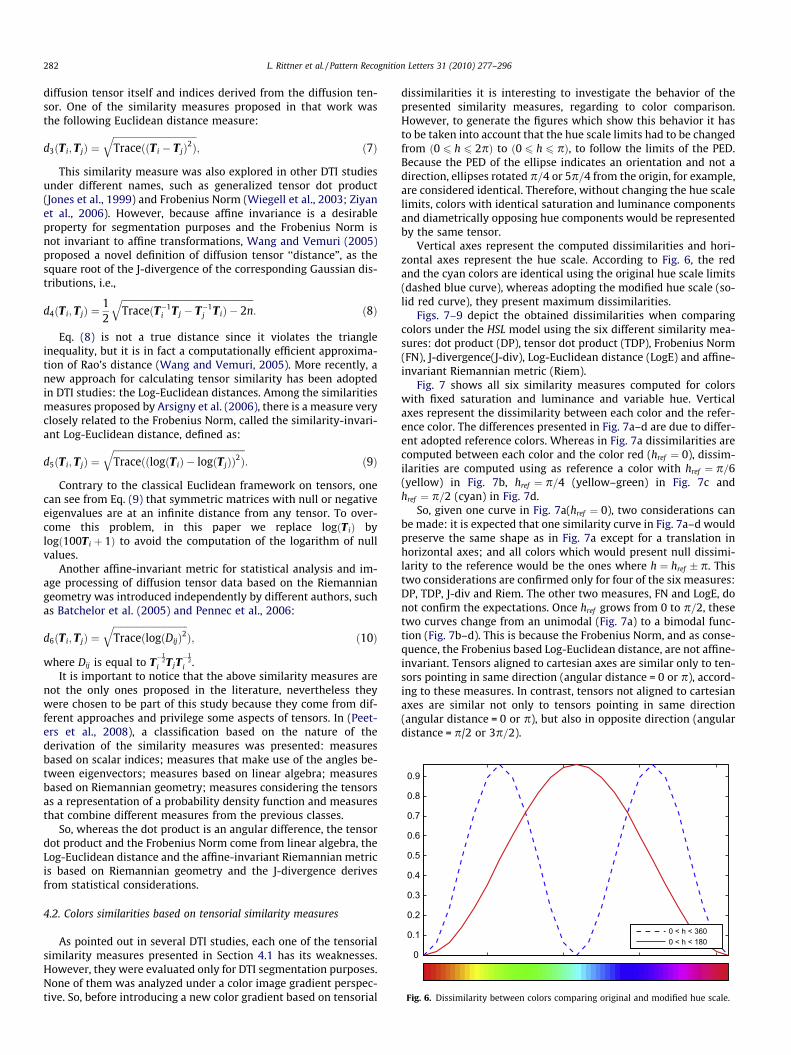
Fig. 6. Dissimilarity between colors comparing original and modified hue scale.
282 L. Rittner et al. / Pattern Recognition Letters 31 (2010) 277–296
diffusion tensor itself and indices derived from the diffusion ten-sor. One of the similarity measures proposed in that work wasthe following Euclidean distance measure:
d3ðT i; T jÞ ¼ffiffiffiffiffiffiffiffiffiffiffiffiffiffiffiffiffiffiffiffiffiffiffiffiffiffiffiffiffiffiffiffiffiffiffiffiTraceððT i � T jÞ2Þ
q; ð7Þ
This similarity measure was also explored in other DTI studiesunder different names, such as generalized tensor dot product(Jones et al., 1999) and Frobenius Norm (Wiegell et al., 2003; Ziyanet al., 2006). However, because affine invariance is a desirableproperty for segmentation purposes and the Frobenius Norm isnot invariant to affine transformations, Wang and Vemuri (2005)proposed a novel definition of diffusion tensor ‘‘distance”, as thesquare root of the J-divergence of the corresponding Gaussian dis-tributions, i.e.,
d4ðT i; T jÞ ¼12
ffiffiffiffiffiffiffiffiffiffiffiffiffiffiffiffiffiffiffiffiffiffiffiffiffiffiffiffiffiffiffiffiffiffiffiffiffiffiffiffiffiffiffiffiffiffiffiffiffiffiffiffiffiffiffiffiffiTraceðT�1
i T j � T�1j T iÞ � 2n
q: ð8Þ
Eq. (8) is not a true distance since it violates the triangleinequality, but it is in fact a computationally efficient approxima-tion of Rao’s distance (Wang and Vemuri, 2005). More recently, anew approach for calculating tensor similarity has been adoptedin DTI studies: the Log-Euclidean distances. Among the similaritiesmeasures proposed by Arsigny et al. (2006), there is a measure veryclosely related to the Frobenius Norm, called the similarity-invari-ant Log-Euclidean distance, defined as:
d5ðT i; T jÞ ¼ffiffiffiffiffiffiffiffiffiffiffiffiffiffiffiffiffiffiffiffiffiffiffiffiffiffiffiffiffiffiffiffiffiffiffiffiffiffiffiffiffiffiffiffiffiffiffiffiffiffiffiffiffiffiffiffiffiTraceððlogðT iÞ � logðT jÞÞ2Þ
q: ð9Þ
Contrary to the classical Euclidean framework on tensors, onecan see from Eq. (9) that symmetric matrices with null or negativeeigenvalues are at an infinite distance from any tensor. To over-come this problem, in this paper we replace logðT iÞ bylogð100T i þ 1Þ to avoid the computation of the logarithm of nullvalues.
Another affine-invariant metric for statistical analysis and im-age processing of diffusion tensor data based on the Riemanniangeometry was introduced independently by different authors, suchas Batchelor et al. (2005) and Pennec et al., 2006:
d6ðT i; T jÞ ¼ffiffiffiffiffiffiffiffiffiffiffiffiffiffiffiffiffiffiffiffiffiffiffiffiffiffiffiffiffiffiffiffiTraceðlogðDijÞ2
qÞ; ð10Þ
where Dij is equal to T�12
i T jT�1
2i .
It is important to notice that the above similarity measures arenot the only ones proposed in the literature, nevertheless theywere chosen to be part of this study because they come from dif-ferent approaches and privilege some aspects of tensors. In (Peet-ers et al., 2008), a classification based on the nature of thederivation of the similarity measures was presented: measuresbased on scalar indices; measures that make use of the angles be-tween eigenvectors; measures based on linear algebra; measuresbased on Riemannian geometry; measures considering the tensorsas a representation of a probability density function and measuresthat combine different measures from the previous classes.
So, whereas the dot product is an angular difference, the tensordot product and the Frobenius Norm come from linear algebra, theLog-Euclidean distance and the affine-invariant Riemannian metricis based on Riemannian geometry and the J-divergence derivesfrom statistical considerations.
4.2. Colors similarities based on tensorial similarity measures
As pointed out in several DTI studies, each one of the tensorialsimilarity measures presented in Section 4.1 has its weaknesses.However, they were evaluated only for DTI segmentation purposes.None of them was analyzed under a color image gradient perspec-tive. So, before introducing a new color gradient based on tensorial
dissimilarities it is interesting to investigate the behavior of thepresented similarity measures, regarding to color comparison.However, to generate the figures which show this behavior it hasto be taken into account that the hue scale limits had to be changedfrom ð0 6 h 6 2pÞ to ð0 6 h 6 pÞ, to follow the limits of the PED.Because the PED of the ellipse indicates an orientation and not adirection, ellipses rotated p=4 or 5p=4 from the origin, for example,are considered identical. Therefore, without changing the hue scalelimits, colors with identical saturation and luminance componentsand diametrically opposing hue components would be representedby the same tensor.
Vertical axes represent the computed dissimilarities and hori-zontal axes represent the hue scale. According to Fig. 6, the redand the cyan colors are identical using the original hue scale limits(dashed blue curve), whereas adopting the modified hue scale (so-lid red curve), they present maximum dissimilarities.
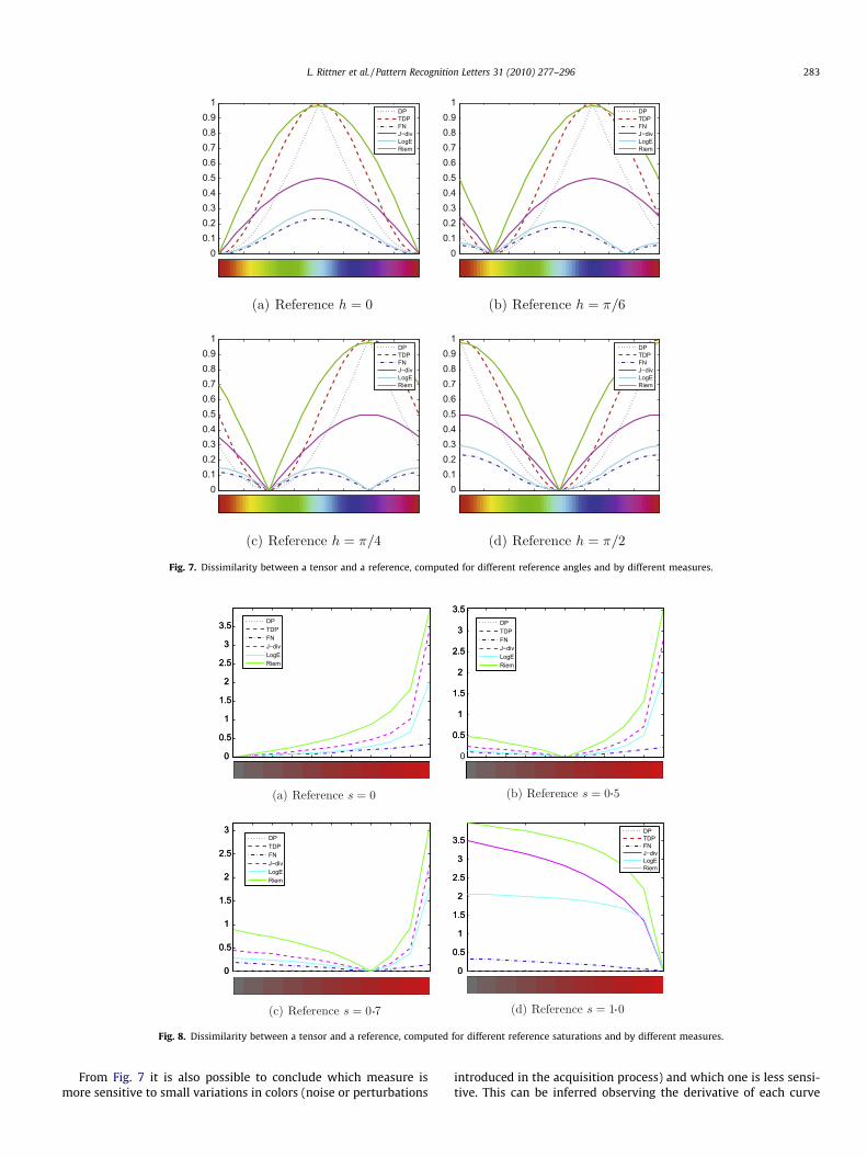
Figs. 7–9 depict the obtained dissimilarities when comparingcolors under the HSL model using the six different similarity mea-sures: dot product (DP), tensor dot product (TDP), Frobenius Norm(FN), J-divergence(J-div), Log-Euclidean distance (LogE) and affine-invariant Riemannian metric (Riem).
Fig. 7 shows all six similarity measures computed for colorswith fixed saturation and luminance and variable hue. Verticalaxes represent the dissimilarity between each color and the refer-ence color. The differences presented in Fig. 7a–d are due to differ-ent adopted reference colors. Whereas in Fig. 7a dissimilarities arecomputed between each color and the color red (href ¼ 0), dissim-ilarities are computed using as reference a color with href ¼ p=6(yellow) in Fig. 7b, href ¼ p=4 (yellow–green) in Fig. 7c andhref ¼ p=2 (cyan) in Fig. 7d.
So, given one curve in Fig. 7a(href ¼ 0), two considerations canbe made: it is expected that one similarity curve in Fig. 7a–d wouldpreserve the same shape as in Fig. 7a except for a translation inhorizontal axes; and all colors which would present null dissimi-larity to the reference would be the ones where h ¼ href � p. Thistwo considerations are confirmed only for four of the six measures:DP, TDP, J-div and Riem. The other two measures, FN and LogE, donot confirm the expectations. Once href grows from 0 to p=2, thesetwo curves change from an unimodal (Fig. 7a) to a bimodal func-tion (Fig. 7b–d). This is because the Frobenius Norm, and as conse-quence, the Frobenius based Log-Euclidean distance, are not affine-invariant. Tensors aligned to cartesian axes are similar only to ten-sors pointing in same direction (angular distance = 0 or p), accord-ing to these measures. In contrast, tensors not aligned to cartesianaxes are similar not only to tensors pointing in same direction(angular distance = 0 or p), but also in opposite direction (angulardistance = p/2 or 3p=2).
00.10.20.30.40.50.60.70.80.9
1DPTDPFNJ−divLogERiem
00.10.20.30.40.50.60.70.80.9
1DPTDPFNJ−divLogERiem
00.10.20.30.40.50.60.70.80.9
1DPTDPFNJ−divLogERiem
00.10.20.30.40.50.60.70.80.9
1DPTDPFNJ−divLogERiem
Fig. 7. Dissimilarity between a tensor and a reference, computed for different reference angles and by different measures.
0
0.5
1
1.5
2
2.5
3
3.5
0
0.5
1
1.5
2
2.5
3
3.5 DPTDPFNJ−divLogERiem
0.5
1
1.5
2
2.5
3
3.5
0
0.5
1
1.5
2
2.5
3
3.5DPTDPFNJ−divLogERiem
0
0.5
1
1.5
2
2.5
3
0
0.5
1
1.5
2
2.5
3DPTDPFNJ−divLogERiem
0
0.5
1
1.5
2
2.5
3
3.5DPTDPFNJ−divLogERiem
0
0.5
1
1.5
2
2.5
3
3.5DPTDPFNJ−divLogERiem
Fig. 8. Dissimilarity between a tensor and a reference, computed for different reference saturations and by different measures.
L. Rittner et al. / Pattern Recognition Letters 31 (2010) 277–296 283
From Fig. 7 it is also possible to conclude which measure ismore sensitive to small variations in colors (noise or perturbations
introduced in the acquisition process) and which one is less sensi-tive. This can be inferred observing the derivative of each curve

1
2
3
4
5
6
7DPTDPFNJ−divLogERiem
0
1
2
3
4
5DPTDPFNJ−divLogERiem
1
2
3
4
5
6DPTDPFNJ−divLogERiem
00
1
2
3
4
5
6
7DPTDPFNJ−divLogERiem
Fig. 9. Dissimilarity between a tensor and a reference, computed for different reference luminances and by different measures.
1 The hue scale was converted to degrees only to make the graph more intuitive.
284 L. Rittner et al. / Pattern Recognition Letters 31 (2010) 277–296
near the origin. The Riem and the J-div have the larger derivativesnear the origin, therefore, they are more sensitive to any kind ofperturbation. The LogE and the TDP are less sensitive to small vari-ations than the J-div and the Riem, nonetheless have more sensitiv-ity than the DP and the FN.
But even this sensitivity to noise changes, depending on the ref-erence color. Fig. 7b shows that for a reference tensor withhref ¼ p=6, the LogE turns out to be more sensitive to noise, fol-lowed by the FN, the J-div and the Riem. As a consequence, theTDP and the DP become the less sensitive measures. This changein sensitivity is a direct consequence of the FN not being affine-invariant, therefore, changing the curve derivative when the refer-ence color is rotated.
Fig. 8 shows also all six similarity measures, this time computedfor colors with fixed hue and luminance and variable saturation.Vertical axes represent the dissimilarity between each color andthe reference color. Once again, the adopted reference color is dif-ferent in each of the four plots (Fig. 8a–d). Whereas in Fig. 8a dis-similarities are computed between each color and the red with nullsaturation (sref ¼ 0), dissimilarities are computed using as refer-ence a red color with sref ¼ 0:5 in Fig. 8b, sref ¼ 0:7 in Fig. 8c andsref ¼ 1 in Fig. 8d.
The conclusion extracted from Fig. 8 is that measures like theDP and the TDP are not suitable for color comparison. Color withno saturation at all and full saturated are perfectly similar, accord-ing to these measures. In the other hand, the J-div, the LogE and theRiem measures present much higher derivatives in the right part ofthe plot (s < 0:5) than in the left part (s > 0:5). This characteristic isdesirable when comparing diffusion tensors, where small satura-tion can be translated as low anisotropy and should be ignoredin DTI analysis. But for color comparison, this increasing derivativecauses a distortion in the obtained results.
Two colors with the same hue, same luminance and with asmall difference in a high saturation, for example, s ¼ 0:9 ands ¼ 0:95 would be considered much more dissimilar by the J-div,
the LogE and the Riem measures than two other colors with thesame hue, same luminance and the same small difference in alow saturation, for example, s ¼ 0:1 and s ¼ 0:15. That would nothappen when comparing these two pairs of colors using the FN,since it presents a constant derivative, suggesting that the FN hasthe best behavior with respect to saturation differences.
Finally, Fig. 9 depicts the behavior of the similarity measures inthe presence of variable luminance. The indicated figure was ob-tained fixing hue and saturation components and varying the lumi-nance. Once again, vertical axes represent the dissimilaritybetween each color and the reference color and the adopted refer-ence color is different in each of the four plots (Fig. 9a–d). Whereasin Fig. 9a dissimilarities are computed between each color and thered with null luminance (lref ¼ 0), dissimilarities are computedusing as reference a red color with lref ¼ 0:5 in Fig. 9b, lref ¼ 0:7in Fig. 9c and lref ¼ 1 in Fig. 9d.
Conclusions from Fig. 9 are similar to the ones presented forFig. 8. The DP and the TDP do not seem to be ideal for color com-parison, due to their null gain and the J-div, the LogE and the Riemmeasures, due to their decreasing derivative. The measure thatpresented better behavior regarding luminance variation in colorcomparison is the FN, because of its constant derivative.
Previous discussed plots were obtained fixing two parametersof the colors and changing only one (for example, fixed saturationand luminance and variable hue). To have a more complete idea ofthe behavior of the metrics applied to color comparisons, oneshould observe it by varying all parameters.
Fig. 10 depicts the Frobenius Norm computed between all colorsand a chosen reference color. Axes correspond to the three colorcomponents – hue, saturation and luminance – varying from 0 to1.1 The color inside the cube (grayscale) represents the computeddissimilarity, where black corresponds to null dissimilarity. Lighter
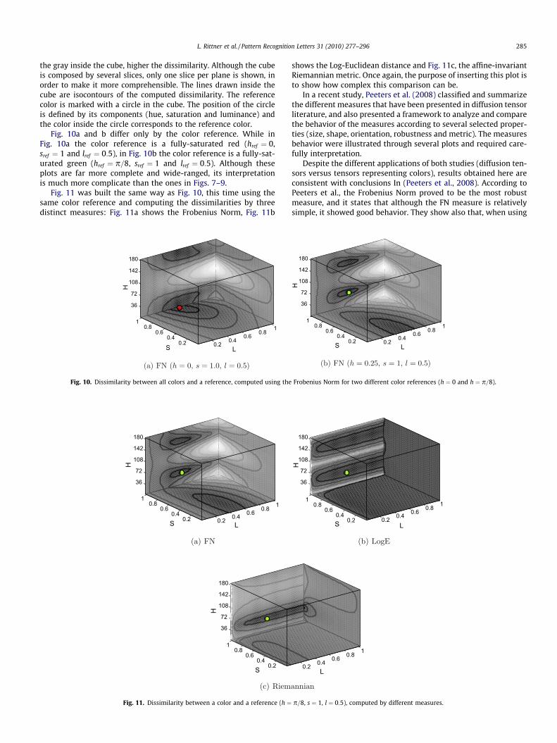
L. Rittner et al. / Pattern Recognition Letters 31 (2010) 277–296 285
the gray inside the cube, higher the dissimilarity. Although the cubeis composed by several slices, only one slice per plane is shown, inorder to make it more comprehensible. The lines drawn inside thecube are isocontours of the computed dissimilarity. The referencecolor is marked with a circle in the cube. The position of the circleis defined by its components (hue, saturation and luminance) andthe color inside the circle corresponds to the reference color.
Fig. 10a and b differ only by the color reference. While inFig. 10a the color reference is a fully-saturated red (href ¼ 0,sref ¼ 1 and lref ¼ 0:5), in Fig. 10b the color reference is a fully-sat-urated green (href ¼ p=8, sref ¼ 1 and lref ¼ 0:5). Although theseplots are far more complete and wide-ranged, its interpretationis much more complicate than the ones in Figs. 7–9.
Fig. 11 was built the same way as Fig. 10, this time using thesame color reference and computing the dissimilarities by threedistinct measures: Fig. 11a shows the Frobenius Norm, Fig. 11b
0.20.4
0.60.8
1
0.20.4
0.60.8
1
36
72
108
142
180
LS
H
Fig. 10. Dissimilarity between all colors and a reference, computed using the
0.2 0.4 0.6 0.8 1
0.20.4
0.60.8
1
36
72
108
142
180
LS
H
0.20.4
0.60.8
1
36
72
108
142
180
S
H
Fig. 11. Dissimilarity between a color and a reference (h ¼
shows the Log-Euclidean distance and Fig. 11c, the affine-invariantRiemannian metric. Once again, the purpose of inserting this plot isto show how complex this comparison can be.
In a recent study, Peeters et al. (2008) classified and summarizethe different measures that have been presented in diffusion tensorliterature, and also presented a framework to analyze and comparethe behavior of the measures according to several selected proper-ties (size, shape, orientation, robustness and metric). The measuresbehavior were illustrated through several plots and required care-fully interpretation.
Despite the different applications of both studies (diffusion ten-sors versus tensors representing colors), results obtained here areconsistent with conclusions In (Peeters et al., 2008). According toPeeters et al., the Frobenius Norm proved to be the most robustmeasure, and it states that although the FN measure is relativelysimple, it showed good behavior. They show also that, when using
0.20.4
0.60.8
1
0.20.4
0.60.8
1
36
72
108
142
180
LS
H
Frobenius Norm for two different color references (h ¼ 0 and h ¼ p=8).
0.2 0.4 0.6 0.8 1
0.20.4
0.60.8
1
36
72
108
142
180
LS
H
0.2 0.4 0.6 0.8 1
L
p=8, s ¼ 1, l ¼ 0:5), computed by different measures.
286 L. Rittner et al. / Pattern Recognition Letters 31 (2010) 277–296
measures like the J-div, the LogE and the Riem, one has to be care-ful with the sensitivity to small shape and size changes close to thedegenerate cases.
4.3. Definition of the tensorial morphological gradient (TMG)
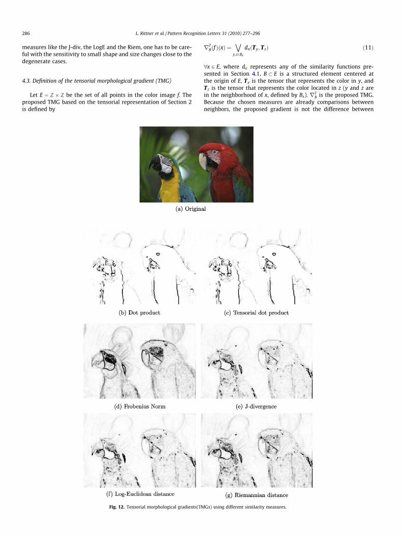
Let E ¼ Z� Z be the set of all points in the color image f. Theproposed TMG based on the tensorial representation of Section 2is defined by
Fig. 12. Tensorial morphological gradients(TM
rTBðf ÞðxÞ ¼
_y;z2Bx
dnðTy; TzÞ ð11Þ
8x 2 E, where dn represents any of the similarity functions pre-sented in Section 4.1, B � E is a structured element centered atthe origin of E, Ty is the tensor that represents the color in y, andTz is the tensor that represents the color located in z (y and z arein the neighborhood of x, defined by Bx). rT
B is the proposed TMG.Because the chosen measures are already comparisons betweenneighbors, the proposed gradient is not the difference between
Gs) using different similarity measures.

L. Rittner et al. / Pattern Recognition Letters 31 (2010) 277–296 287
the maximum and the minimum values, but only the maximum va-lue. In other words, the computed gradient in a neighborhood givenby a structuring element is the maximum dissimilarity among allpairwise dissimilarities.
Fig. 12 depicts the original image and the TMGs computed byDP, TDP, FN, J-div, LogE and Riem. All gradients were computedusing a 3� 3 diamond structuring element and using the tensorialrepresentation based on the HSL model and were negated for a bet-ter presentation. The gradients based on DP (Fig. 12b) and TDP(Fig. 12c) presented smoother borders and lost important parts(such as the left parrots head), therefore it is expected that the seg-mentation result provided by them will not be good. The borders inthe TMG using the FN (Fig. 12d), the J-div (Fig. 12e), the LogE(Fig. 12f) and the Riem (Fig. 12g) were sharper and should providebetter results in the application of watershed technique.
Fig. 13 contains TMGs computed by different measures andbased on different color model representations. First row of the re-ferred figure (Fig. 13a–c) shows computed TMGs using the TDPmeasure, based in HSL, IHSL and CIELUV tensorial representations,respectively. Although all three gradients are similar, i.e., presentthe same borders of the original image, the first two (Fig. 13aand b) are much more stronger than the third one. This resultcan be explained by the nature of the TDP measure and the charac-teristic of the CIELUV color model. The TDP measure compares basi-cally the eigenvectors directions of the tensors and in the HSL andthe IHSL tensorial representation the eigenvectors directions have asignificant meaning, due to their angular component (hue). In con-trast, in the CIELUV tensorial representation, eigenvectors direc-tions have a questionable meaning, since they are associated tothe v component (not an angular information).
The same conclusion cannot be extended to the other two linesof Fig. 13. That is because they were obtained using the FN and theLogE measures, functions that take into account not only the eigen-vectors directions, but also the shape and trace of the ellipse repre-senting colors. Therefore, gradients based on the CIELUV tensorial
Fig. 13. Tensorial morphological gradients(TMGs) using dif
representation are more likely to present satisfactory segmenta-tion results, when computed using the FN and the LogE measures.In contrast, gradients based on HSL and IHSL tensorial representa-tions computed using different similarity measures look very sim-ilar and is not possible to make any statement about theirsegmentation performance just looking at them.
5. Segmentation experiments
This section presents the hierarchical segmentation achieved bythe combination of tensorial representation of colors, tensorialmorphological gradient, watershed from markers (Beucher andMeyer, 1992; Vincent and Soille, 1991; Falcão et al., 2004; Coustyet al., 2009) and extinction values computation (Vachier andMeyer, 1995; Grimaud, 1992; Najman and Schmitt, 1996; Meyer,1996). The images used in this section were obtained from theBerkeley Segmentation Dataset (BSDS) (Martin et al., 2001), a data-base of 300 natural images, manually segmented by a number ofdifferent subjects. The watershed transform, the extinction func-tions and other morphological functions can be found in the‘‘SDC Morphology Toolbox for MATLAB” (Dougherty and Lotufo,2003). The hierarchical segmentation is done by classifying struc-tures in the TMG image according to an extinction function andselecting them – by marker imposition – in order to compute thewatershed from markers.
In the first experiment, images were segmented by the wa-tershed transform over the TMG computed using all six similarityfunctions. After calculating the TMG of the original image, the nstructures in the image which have the greatest volume extinctionvalues were automatically selected. The n markers assigned tothese regions were then used in the watershed transform, whichsegmented the TMG in n regions.
Different color models were used and all tensorial measurespresented were applied to the TMG computation. Likewise Section
ferent similarity measures and different color models.

288 L. Rittner et al. / Pattern Recognition Letters 31 (2010) 277–296
3, that showed that each one of the tensorial color representationbased on distinct color models has significant differences and Sec-tion 4.2, that analyzed several aspects of the different tensorialsimilarity functions, pointing out their divergences, this sectionhas the intention to show the differences in segmentation resultingfrom distinct similarity measures associated to different tensorialcolor representations. As in Section 4.3, all gradients were com-puted using a 3� 3 diamond structuring element, except the gra-dient proposed by Zenzo (1986), that used a 3� 3 square.
Fig. 14 depicts watershed segmentation results obtained apply-ing all similarity measures in a HSL tensorial representation of the‘‘parrots” image. The image was segmented in 25 regions and theresults confirmed what was expected by analyzing Fig. 12 (Section4.3). The TMG using the FN (Fig. 14c) resulted in a better segmen-tation, in comparison to the DP (Fig. 14a), TDP (Fig. 14b) and J-div(Fig. 14d) measures. The TMGs using the LogE (Fig. 14e) and theRiem (Fig. 14f) had a good performance too, although inferior tothe one using the FN. Basically, the three measures were able tosegment the parrot from the right, but only the segmentation ob-tained by the FN was able to delineate the head of the parrot fromthe left.
The number of regions – 25 – was chosen because, taking intoaccount the complexity of the Parrots image, 25 regions was a rea-sonable number to illustrate the impact of the TMG choice in the
Fig. 14. Watershed segmentation of the ‘‘parr
segmentation of such image. A greater number of regions wouldnot highlight the differences among the TMGs and a lesser numberwould not provide a meaningful segmentation to be discussed.
In Fig. 15 only a detail of the ‘‘parrots” image is segmented.Fig. 15a shows the original image and the selected region to be seg-mented is in Fig. 15b. The selected image detail was segmented inthree regions using the five distinct similarity measures applied tothe HSL tensorial representation. Fig. 15c depicts the five TMGs ob-tained and the respective segmentation obtained by each one. Thegradients were negated for a better presentation. Because the threemain regions are represented by tensors with very distinct PEDs,all similarity measures were able to segment them, even the DPand the TDP, that do not take into account the full tensor informa-tion. The obtained watershed lines were a little bit distinct, none-theless all segmentations presented satisfactory results.
The first line of Fig. 15d shows different TMGs obtained by thesame measure (FN) applied to tensorial representations using threedifferent color models. The second line of the same figure containsthe segmentation results obtained for each of the three computedTMGs. It shows that the obtained watershed lines differ from eachother, nevertheless all are able to correctly segment the threeregions.
Another detail of the ‘‘parrots” image can be seen in Fig. 16, thistime to better illustrate the differences among the TMGs computed
ots” image with 25 regions using TMGs.

Fig. 15. Negated TMG gradients and segmentation results of a detail of the ‘‘parrots” image. The TMGs were computed using different similarity measures and different colormodels.
L. Rittner et al. / Pattern Recognition Letters 31 (2010) 277–296 289
by distinct measures. It helps also to understand why some seg-mentation results are superior than others and in which circum-stances this happens.
Fig. 16a shows the original image, where the detail is marked bya white rectangle. Fig. 16b depicts only the chosen detail with thetensorial representation for each pixel (ellipses). Although thereare significant differences among ellipses, an easier way to identifyand analyze the differences is to plot separately each property ofthe ellipses – PED, shape and trace – i.e., the color components -hue, saturation and luminance. They can be found in Fig. 16c–e,respectively. Based on Fig. 16c, it can be observed that, although
in the image the colors from the blue neck of the parrot look verydifferent from the colors of the white background, their hue are al-most the same. That means that any measure that only takes intoaccount the hue of the color, i.e., the PED of the tensors, would notbe able to segment it. Fig. 16h and i confirm that, showing that theTMG computed using the DP or the TDP preserve only the borderbetween the yellow and the blue part of the neck, because is whereFig. 16c presents a strong border, dividing the two regions withdistinct hues.
Fig. 16f and g presents the results of the segmentation basedon the TMG computed using the Frobenius Norm and the

Fig. 16. Detail of the parrot image – color components, watershed results and TMGs.
290 L. Rittner et al. / Pattern Recognition Letters 31 (2010) 277–296
affine-invariant Riemannian metric, respectively. The lines obtained bythe watershed over the FN–TMG contain the border between theneck and the background, as opposed to the Riemannian-TMG, thatdoes not contain it. The explanation comes from analyzing Fig. 16d,e, j and m.
Fig. 16d shows that the saturation of colors that belong to theblue region is not constant, on the contrary, presents small varia-tions. The same can be observed inside the white region, wherethe saturation of colors assume a range of values significantly low-er than the ones from the blue region. In Fig. 16j it is possible toidentify that the TMG obtained using the FN contains a strong gra-dient (lighter line) where the border of the neck and the back-ground should be. It confirms that the FN recognizes that thesaturation oscillation inside the regions are not so strong as thesaturation difference between the regions, thanks to the constantderivative of the FN previously discussed (Fig. 8). On the otherhand, Fig. 16m shows that the gradient computed by the Riemann-ian metric inside the blue region (high saturation) is almost as
strong as the gradient in the border between the blue and thewhite regions. That is due to the high derivative of the Riemannianmetric with the saturation (Fig. 8). The same behavior is observedin Fig. 16k and l, consequence of their high derivatives as well. Sim-ilar reasoning can be done for the luminance (Fig. 16e).
It is important to note that the Frobenius Norm would not beable to segment object and background if their color were per-pendicular and have identical saturation and luminance. Despiteof that, it presented the best segmentation results, mainly be-cause real images are unlikely to have objects and backgroundwith completely uniform colors (null variation of hue, saturationand luminance). And probably if the color of some pixels of theobject were perpendicular to the color of some pixels of thebackground, the TMG computed for the pixels in that region(using the FN) would not be null, since the TMG takes into ac-count the dissimilarities not only between a pair of pixels butwithin a neighborhood (defined by the structuring element)and takes the maximum.

L. Rittner et al. / Pattern Recognition Letters 31 (2010) 277–296 291
Fig. 17 presents segmentation results using some possible com-binations of similarity measures and tensorial representation usingdifferent color models. The image was segmented in 25 regions forevery combination and the watershed lines were overlaid on theoriginal image. The obtained results confirm the expectations.Aside from certain combinations of tensorial representation andsimilarity measure that are not adequate (for example, Fig. 17c),all obtained segmentation can be considered satisfactory. Natu-rally, some specific combinations presented superior results thanthe rest (Fig. 17d and e), however, this superiority can vary accord-ing to the image to be segmented. In other words, for a coarse seg-mentation, almost any combination of a tensorial representationand a similarity measure can be used. Conversely, for a fine seg-mentation, the combination should be carefully chosen. Anyway,the best segmentations would most likely result from combina-
Fig. 17. Watershed segmentation results based on TMGs computed
Fig. 18. Two images from the Ber
tions of tensorial representations containing angular components(HSL, HSV e IHSL) and measures using full tensor information (FN,J-div, LogE and Riem).
To confirm our observations about the segmentation resultsusing TMGs based on different similarity measures, quantitativeevaluation tests were performed. The segmentation evaluationsconducted were proposed by Borsotti et al. (1998). Segmentationresults using different measures for the computation of the TMGwere compared. Hierarchical segmentations using the color gradi-ent proposed by Di Zenzo (1986) were also performed, and thesesegmentation were evaluated as well. A qualitative analysis ofthe TMG was done, using as benchmarking segmentation algo-rithms contained at the Berkeley Segmentation Dataset (BSDS)(Martin et al., 2001). Fig. 18 presents two examples of images ofthis Dataset.
using different similarity measures and different color models.
keley segmentation dataset.

Fig. 19. Evaluation of segmentation results for image 42,049.
292 L. Rittner et al. / Pattern Recognition Letters 31 (2010) 277–296
The segmentation evaluations were done by applying two func-tions proposed by Borsotti et al. (1998) to assess segmentation ofcolor images. Both functions assess segmentation of color imagesaccording to heuristic criteria such as homogeneity and simplicity.When comparing segmentation results, the lower results are pro-vided by the best segmentation. Both functions are stated asfollows:
F 0ðIÞ ¼ 110; 000� N �M
�
ffiffiffiffiffiffiffiffiffiffiffiffiffiffiffiffiffiffiffiffiffiffiffiffiffiffiffiXMax
A¼1
RðAÞ1þ1=A
vuut �XR
i¼1
e2iffiffiffiffiffiAip ð12Þ
Fig. 20. Evaluation of segmentation results for 22 images. (a) and (b) Segmentation e
and
QðIÞ ¼ 110;000� N �M
�ffiffiffiRp�XR
i¼1
e2i
1þ log Aiþ RðAiÞ
Ai
� �2" #
ð13Þ
where N and M are, respectively, the height and width of the image,RðAÞ is the number of regions having area equals to A, Max is thegreatest segmentation area, R is the number of regions the imagewas segmented, Ai is the area of region i and ei is the average colorerror for region i (see Borsotti et al. (1998) for more details).
Fig. 19 shows an example of the segmentation assessment ofthe TMGs. The five proposed TMGs were applied to images underthe HSL, IHSL and L�U�V� color models. Hierarchical segmentationswere done selecting the desired number of regions and then thevalues for F 0 and Q were computed. The comparison was done tak-ing into account that the lesser the evaluation a segmentation re-ceives, the better is the achieved segmentation. Under theconditions pointed above, the TMG using the Frobenius Normachieved the best segmentations in all tested color spaces. WhileF 0 was between 30 and 39 for the Frobenius Norm, it was between44 and 337 for all TMGs based on other measures. It also per-formed better than segmentations based on the Di Zenzo gradient(F 0 ¼ 223:6813 and Q ¼ 3641:596). Similar results were obtainedfor the Q value, that ranged from 371 to 585 for the TMG usingthe Frobenius Norm and from 658 and 6374 for all other TMGs.The superiority of the Frobenius Norm over other TMGs was con-firmed in all segmentation experiments conducted for otherimages from the same dataset.
From Fig. 19 it is also possible to observe that there was almostno difference between the HSL and the IHSL color model represen-tation, and that they performed better than the L�u�v�. In all other
rror for each test case; (c) and (d) Amount of lowest errors for each TMG metric.
L. Rittner et al. / Pattern Recognition Letters 31 (2010) 277–296 293
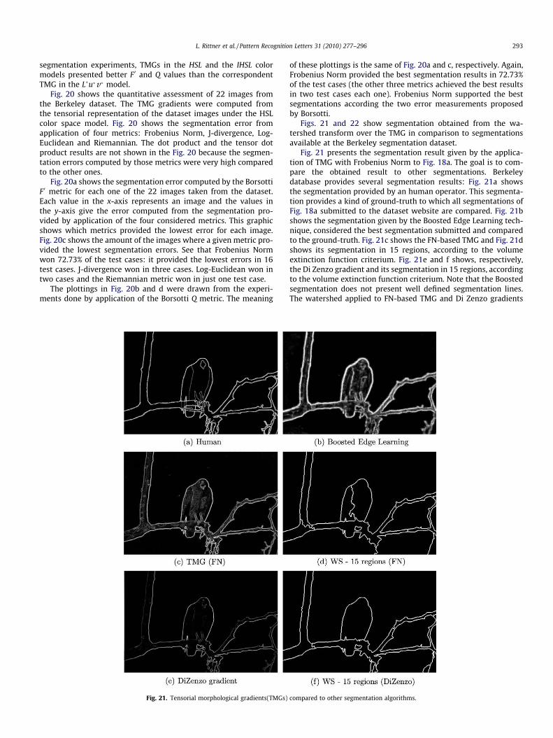
segmentation experiments, TMGs in the HSL and the IHSL colormodels presented better F 0 and Q values than the correspondentTMG in the L�u�v� model.
Fig. 20 shows the quantitative assessment of 22 images fromthe Berkeley dataset. The TMG gradients were computed fromthe tensorial representation of the dataset images under the HSLcolor space model. Fig. 20 shows the segmentation error fromapplication of four metrics: Frobenius Norm, J-divergence, Log-Euclidean and Riemannian. The dot product and the tensor dotproduct results are not shown in the Fig. 20 because the segmen-tation errors computed by those metrics were very high comparedto the other ones.
Fig. 20a shows the segmentation error computed by the BorsottiF 0 metric for each one of the 22 images taken from the dataset.Each value in the x-axis represents an image and the values inthe y-axis give the error computed from the segmentation pro-vided by application of the four considered metrics. This graphicshows which metrics provided the lowest error for each image.Fig. 20c shows the amount of the images where a given metric pro-vided the lowest segmentation errors. See that Frobenius Normwon 72.73% of the test cases: it provided the lowest errors in 16test cases. J-divergence won in three cases. Log-Euclidean won intwo cases and the Riemannian metric won in just one test case.
The plottings in Fig. 20b and d were drawn from the experi-ments done by application of the Borsotti Q metric. The meaning
Fig. 21. Tensorial morphological gradients(TMGs)
of these plottings is the same of Fig. 20a and c, respectively. Again,Frobenius Norm provided the best segmentation results in 72.73%of the test cases (the other three metrics achieved the best resultsin two test cases each one). Frobenius Norm supported the bestsegmentations according the two error measurements proposedby Borsotti.
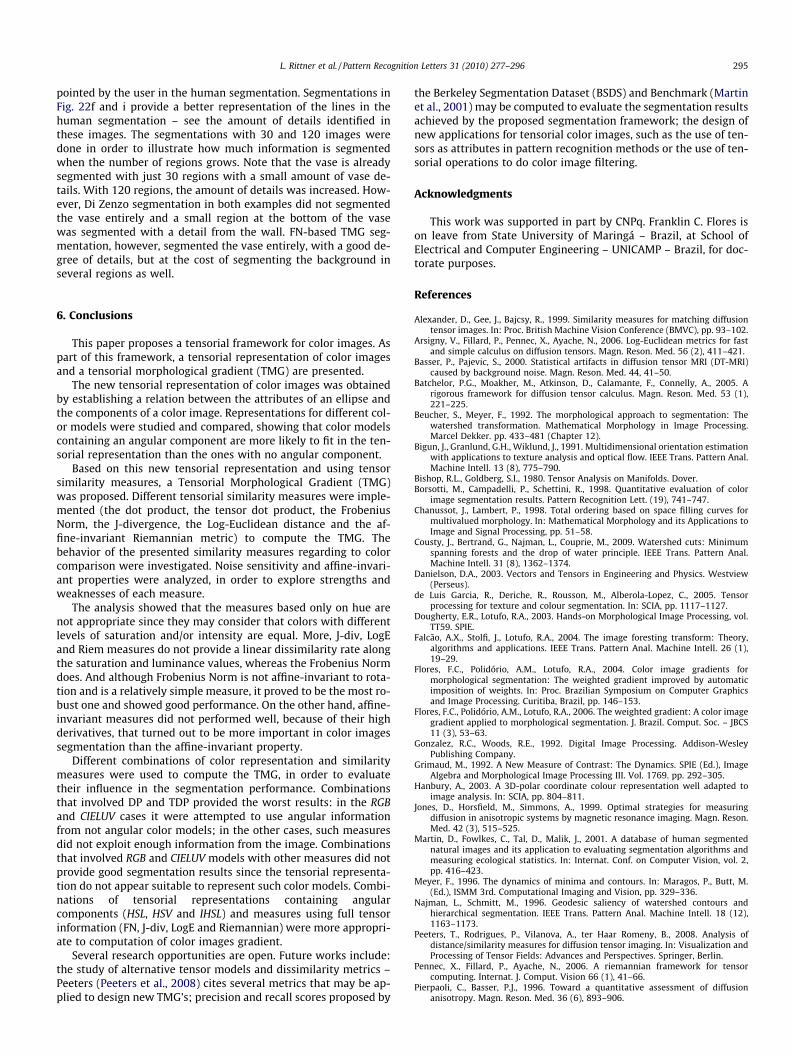
Figs. 21 and 22 show segmentation obtained from the wa-tershed transform over the TMG in comparison to segmentationsavailable at the Berkeley segmentation dataset.
Fig. 21 presents the segmentation result given by the applica-tion of TMG with Frobenius Norm to Fig. 18a. The goal is to com-pare the obtained result to other segmentations. Berkeleydatabase provides several segmentation results: Fig. 21a showsthe segmentation provided by an human operator. This segmenta-tion provides a kind of ground-truth to which all segmentations ofFig. 18a submitted to the dataset website are compared. Fig. 21bshows the segmentation given by the Boosted Edge Learning tech-nique, considered the best segmentation submitted and comparedto the ground-truth. Fig. 21c shows the FN-based TMG and Fig. 21dshows its segmentation in 15 regions, according to the volumeextinction function criterium. Fig. 21e and f shows, respectively,the Di Zenzo gradient and its segmentation in 15 regions, accordingto the volume extinction function criterium. Note that the Boostedsegmentation does not present well defined segmentation lines.The watershed applied to FN-based TMG and Di Zenzo gradients
compared to other segmentation algorithms.

294 L. Rittner et al. / Pattern Recognition Letters 31 (2010) 277–296
provided a more precise segmentation. Note that these lines ap-pear more with the lighters lines in the human segmentation thatthe ones in the Boosted segmentation. Segmentations in Fig. 21dand f are quite similar, and each one segments different regionsin a more detailed way. FN-based TMG supported a detailed seg-mentation of the wing and the tree. Dizenzo gradient supporteda better segmentation of the branches.
Fig. 22 presents another comparison with an image from Berke-ley dataset. Fig. 22a shows the original image, a vase with severaldrawings. Fig. 22b and c show, respectively, the human segmenta-
Fig. 22. TMGs compared to othe
tion and the one provided by the Global Probability of Boundarytechnique. Fig. 22d–f shows, respectively, the FN-based TMG ofthe vase, and its segmentation in 30 and 120 regions, accordingto the volume extinction function criterium. Fig. 22g–i shows,respectively, the Di Zenzo gradient and its segmentation in 30and 120 regions, according to the volume extinction function crite-rium. The goal is to visually evaluate the segmentation results andto comment the impact in the selection of the number of regions inthe hierarchical segmentation. Note that Global Probability ofBoundary segmentation does not enhance the main features
r segmentation algorithms.
L. Rittner et al. / Pattern Recognition Letters 31 (2010) 277–296 295
pointed by the user in the human segmentation. Segmentations inFig. 22f and i provide a better representation of the lines in thehuman segmentation – see the amount of details identified inthese images. The segmentations with 30 and 120 images weredone in order to illustrate how much information is segmentedwhen the number of regions grows. Note that the vase is alreadysegmented with just 30 regions with a small amount of vase de-tails. With 120 regions, the amount of details was increased. How-ever, Di Zenzo segmentation in both examples did not segmentedthe vase entirely and a small region at the bottom of the vasewas segmented with a detail from the wall. FN-based TMG seg-mentation, however, segmented the vase entirely, with a good de-gree of details, but at the cost of segmenting the background inseveral regions as well.
6. Conclusions
This paper proposes a tensorial framework for color images. Aspart of this framework, a tensorial representation of color imagesand a tensorial morphological gradient (TMG) are presented.
The new tensorial representation of color images was obtainedby establishing a relation between the attributes of an ellipse andthe components of a color image. Representations for different col-or models were studied and compared, showing that color modelscontaining an angular component are more likely to fit in the ten-sorial representation than the ones with no angular component.
Based on this new tensorial representation and using tensorsimilarity measures, a Tensorial Morphological Gradient (TMG)was proposed. Different tensorial similarity measures were imple-mented (the dot product, the tensor dot product, the FrobeniusNorm, the J-divergence, the Log-Euclidean distance and the af-fine-invariant Riemannian metric) to compute the TMG. Thebehavior of the presented similarity measures regarding to colorcomparison were investigated. Noise sensitivity and affine-invari-ant properties were analyzed, in order to explore strengths andweaknesses of each measure.
The analysis showed that the measures based only on hue arenot appropriate since they may consider that colors with differentlevels of saturation and/or intensity are equal. More, J-div, LogEand Riem measures do not provide a linear dissimilarity rate alongthe saturation and luminance values, whereas the Frobenius Normdoes. And although Frobenius Norm is not affine-invariant to rota-tion and is a relatively simple measure, it proved to be the most ro-bust one and showed good performance. On the other hand, affine-invariant measures did not performed well, because of their highderivatives, that turned out to be more important in color imagessegmentation than the affine-invariant property.
Different combinations of color representation and similaritymeasures were used to compute the TMG, in order to evaluatetheir influence in the segmentation performance. Combinationsthat involved DP and TDP provided the worst results: in the RGBand CIELUV cases it were attempted to use angular informationfrom not angular color models; in the other cases, such measuresdid not exploit enough information from the image. Combinationsthat involved RGB and CIELUV models with other measures did notprovide good segmentation results since the tensorial representa-tion do not appear suitable to represent such color models. Combi-nations of tensorial representations containing angularcomponents (HSL, HSV and IHSL) and measures using full tensorinformation (FN, J-div, LogE and Riemannian) were more appropri-ate to computation of color images gradient.
Several research opportunities are open. Future works include:the study of alternative tensor models and dissimilarity metrics –Peeters (Peeters et al., 2008) cites several metrics that may be ap-plied to design new TMG’s; precision and recall scores proposed by
the Berkeley Segmentation Dataset (BSDS) and Benchmark (Martinet al., 2001) may be computed to evaluate the segmentation resultsachieved by the proposed segmentation framework; the design ofnew applications for tensorial color images, such as the use of ten-sors as attributes in pattern recognition methods or the use of ten-sorial operations to do color image filtering.
Acknowledgments
This work was supported in part by CNPq. Franklin C. Flores ison leave from State University of Maringá – Brazil, at School ofElectrical and Computer Engineering – UNICAMP – Brazil, for doc-torate purposes.
References
Alexander, D., Gee, J., Bajcsy, R., 1999. Similarity measures for matching diffusiontensor images. In: Proc. British Machine Vision Conference (BMVC), pp. 93–102.
Arsigny, V., Fillard, P., Pennec, X., Ayache, N., 2006. Log-Euclidean metrics for fastand simple calculus on diffusion tensors. Magn. Reson. Med. 56 (2), 411–421.
Basser, P., Pajevic, S., 2000. Statistical artifacts in diffusion tensor MRI (DT-MRI)caused by background noise. Magn. Reson. Med. 44, 41–50.
Batchelor, P.G., Moakher, M., Atkinson, D., Calamante, F., Connelly, A., 2005. Arigorous framework for diffusion tensor calculus. Magn. Reson. Med. 53 (1),221–225.
Beucher, S., Meyer, F., 1992. The morphological approach to segmentation: Thewatershed transformation. Mathematical Morphology in Image Processing.Marcel Dekker. pp. 433–481 (Chapter 12).
Bigun, J., Granlund, G.H., Wiklund, J., 1991. Multidimensional orientation estimationwith applications to texture analysis and optical flow. IEEE Trans. Pattern Anal.Machine Intell. 13 (8), 775–790.
Bishop, R.L., Goldberg, S.I., 1980. Tensor Analysis on Manifolds. Dover.Borsotti, M., Campadelli, P., Schettini, R., 1998. Quantitative evaluation of color
image segmentation results. Pattern Recognition Lett. (19), 741–747.Chanussot, J., Lambert, P., 1998. Total ordering based on space filling curves for
multivalued morphology. In: Mathematical Morphology and its Applications toImage and Signal Processing, pp. 51–58.
Cousty, J., Bertrand, G., Najman, L., Couprie, M., 2009. Watershed cuts: Minimumspanning forests and the drop of water principle. IEEE Trans. Pattern Anal.Machine Intell. 31 (8), 1362–1374.
Danielson, D.A., 2003. Vectors and Tensors in Engineering and Physics. Westview(Perseus).
de Luis Garcia, R., Deriche, R., Rousson, M., Alberola-Lopez, C., 2005. Tensorprocessing for texture and colour segmentation. In: SCIA, pp. 1117–1127.
Dougherty, E.R., Lotufo, R.A., 2003. Hands-on Morphological Image Processing, vol.TT59. SPIE.
Falcão, A.X., Stolfi, J., Lotufo, R.A., 2004. The image foresting transform: Theory,algorithms and applications. IEEE Trans. Pattern Anal. Machine Intell. 26 (1),19–29.
Flores, F.C., Polidório, A.M., Lotufo, R.A., 2004. Color image gradients formorphological segmentation: The weighted gradient improved by automaticimposition of weights. In: Proc. Brazilian Symposium on Computer Graphicsand Image Processing. Curitiba, Brazil, pp. 146–153.
Flores, F.C., Polidório, A.M., Lotufo, R.A., 2006. The weighted gradient: A color imagegradient applied to morphological segmentation. J. Brazil. Comput. Soc. – JBCS11 (3), 53–63.
Gonzalez, R.C., Woods, R.E., 1992. Digital Image Processing. Addison-WesleyPublishing Company.
Grimaud, M., 1992. A New Measure of Contrast: The Dynamics. SPIE (Ed.), ImageAlgebra and Morphological Image Processing III. Vol. 1769. pp. 292–305.
Hanbury, A., 2003. A 3D-polar coordinate colour representation well adapted toimage analysis. In: SCIA, pp. 804–811.
Jones, D., Horsfield, M., Simmons, A., 1999. Optimal strategies for measuringdiffusion in anisotropic systems by magnetic resonance imaging. Magn. Reson.Med. 42 (3), 515–525.
Martin, D., Fowlkes, C., Tal, D., Malik, J., 2001. A database of human segmentednatural images and its application to evaluating segmentation algorithms andmeasuring ecological statistics. In: Internat. Conf. on Computer Vision, vol. 2,pp. 416–423.
Meyer, F., 1996. The dynamics of minima and contours. In: Maragos, P., Butt, M.(Ed.), ISMM 3rd. Computational Imaging and Vision, pp. 329–336.
Najman, L., Schmitt, M., 1996. Geodesic saliency of watershed contours andhierarchical segmentation. IEEE Trans. Pattern Anal. Machine Intell. 18 (12),1163–1173.
Peeters, T., Rodrigues, P., Vilanova, A., ter Haar Romeny, B., 2008. Analysis ofdistance/similarity measures for diffusion tensor imaging. In: Visualization andProcessing of Tensor Fields: Advances and Perspectives. Springer, Berlin.
Pennec, X., Fillard, P., Ayache, N., 2006. A riemannian framework for tensorcomputing. Internat. J. Comput. Vision 66 (1), 41–66.
Pierpaoli, C., Basser, P.J., 1996. Toward a quantitative assessment of diffusionanisotropy. Magn. Reson. Med. 36 (6), 893–906.

296 L. Rittner et al. / Pattern Recognition Letters 31 (2010) 277–296
Rittner, L., Lotufo, R., 2008. Diffusion tensor imaging segmentation by watershedtransform on tensorial morphological gradient. In: Proc. XXI BrazilianSymposium on Computer Graphics and Image Processing. Campo Grande,Brazil, pp. 196–203.
Rittner, L., Flores, F., Lotufo, R., 2007. New tensorial representation of color images:Tensorial morphological gradient applied to color image segmentation. In: Proc.XX Brazilian Symposium on Computer Graphics and Image Processing. BeloHorizonte, Brazil, pp. 45–52.
Soille, P., Vincent, L., 1990. Determining watersheds in digital pictures via floodingsimulations. Visual Communications and Image Processing, vol. 1360. SPIE, pp.240–250.
Talbot, H., Evans, C., Jones, R., 1998. Complete ordering and multivariatemathematical morphology: Algorithms and applications. In: MathematicalMorphology and its Applications to Image and Signal Processing, pp. 27–34.
Vachier, C., Meyer, F., 1995. Extinction value: A new measurement of persistence.Proc. 1995 IEEE Workshop on Nonlinear Signal and Image Processing, vol. I.IEEE, pp. 254–257.
Vincent, L., Soille, P., 1991. Watersheds in digital spaces: An efficient algorithmbased on immersion simulations 13 (6), 583–598.
Wang, Z., Vemuri, B.C., 2005. DTI segmentation using an information theoretictensor dissimilarity measure. IEEE Trans. Med. Imaging 24 (10), 1267–1277.
Weijer, J., Gevers, T., 2004. Tensor based feature detection for color images. In: 12thColor Imaging Conf.: Color Science and Engineering Systems, Technologies,Applications, vol. 12, pp. 100–105.
Weijer, J., Gevers, T., Smeulders, A., 2004. Robust photometric invariant featuresfrom the color tensor. IEEE Trans. Image Process 15 (1), 118–127.
Wiegell, M., Tuch, D., Larson, H., Wedeen, V., 2003. Automatic segmentation of thalamicnuclei from diffusion tensor magnetic resonance imaging. NeuroImage 19, 391–402.
Zenzo, S.D., 1986. A note on the gradient of a multi-image. Computer VisionGraphics Image Process. 33, 116–125.
Ziyan, U., Tuch, D., Westin, C.-F., 2006. Segmentation of thalamic nuclei from DTIusing spectral clustering. In: Ninth Internat. Conf. on Medical Image Computingand Computer-assisted Intervention (MICCAI’06). Lecture Notes in ComputerScience, vol. 4191. Copenhagen, Denmark, pp. 807–814.