Robotics and Autonomous Systems 34 (2001) 23–38

A robot self-localization system based onomnidirectional color images

Alessandro Rizzi∗, Riccardo CassinisDepartment of Electronics for Automation, University of Brescia, Via Branze 38, I-25123 Brescia, Italy

Received 7 July 1998; received in revised form 15 March 2000; accepted 11 April 2000

Abstract

A self-localization system for autonomous mobile robots is presented. This system estimates the robot position in previouslylearned environments, using data provided solely by an omnidirectional visual perception subsystem composed of a camera andof a special conical reflecting surface. It performs an optical pre-processing of the environment, allowing a compact represen-tation of the collected data. These data are then fed to a learning subsystem that associates the perceived image to an estimate ofthe actual robot position. Both neural networks and statistical methods have been tested and compared as learning subsystems.The system has been implemented and tested and results are presented. © 2001 Elsevier Science B.V. All rights reserved.

Keywords:Self-localization; Omnidirectional sensor; Visual navigation; Mobile robots

1. Introduction

In the field of visual guidance of autonomousrobots, omnidirectional image sensors have beenintensively studied [19,20,22]. Having an omnidi-rectional field of view in a single camera shot is anappealing feature, but an omnidirectional device addsheavy geometric distortions to the perceived scene.In this case, a geometrical model based on naviga-tion method originates complex tasks, thus wastingthe acquiring facilities of the omnidirectional device.Exploration and map building using this approachhave the same problem as well [9].

A first simplification derives from the use of quali-tative methods [17]. Complex visual navigation tasks

∗ Corresponding author. Tel.:+39-030-3715-469;fax: +39-030-380014.E-mail addresses:alessandro.rizzi@unibs.it (A. Rizzi),riccardo.cassinis@unibs.it (R. Cassinis).

in real environments can be managed more easilyby not trying to recognize objects around the robot,but simply memorizing snapshots from specific placesand then correlating them with the currently perceivedimage [6,12]. The typical problem of this approachis the large amount of memory needed for learning aroute in an environment.

An omnidirectional image can be obtained by meansof different devices. Besides fish-eye lenses [15], sev-eral mirror-based devices such as COPIS [18,19,21],MISS [20] and HOV [22] have been developed andstudied taking into account the different geometricviewfield distortions, but little attention has been paidto the reflectance characteristics of the various devices.

The central idea of the present work is to use a con-ical device, similar to COPIS, but with a different re-flecting surface that allows the collection of simplifiedomnidirectional visual information (Fig. 2).

The proposed system derives from an earlier jointresearch program started at the Laboratory of Automa-tion, University of Besançon (France) [1,2] and then

0921-8890/01/$ – see front matter © 2001 Elsevier Science B.V. All rights reserved.PII: S0921-8890(00)00103-2

24 A. Rizzi, R. Cassinis / Robotics and Autonomous Systems 34 (2001) 23–38

continued at the Department of Electronics for Auto-mation, University of Brescia (Italy) [3–5].

2. Aim and structure of the system

The aim of the system is to support the navigationof an autonomous mobile robot estimating its positionin a previously learned working area.

Neither conditioning of the environment around theworking area nor accurate distance measurements arerequired and no explicit and detailed maps of the worldsurrounding the robot are made.

An interesting feature of the proposed system isits ability to work even if the learned environmentchanges. This holds true, provided that changes af-fect only limited portions of the whole vision field[5] (e.g. people walking around, objects that werenot present during the training phase or that wereremoved thereafter, etc.).

The system is designed to work on a car-like au-tonomous mobile robot and thus its position in atwo-dimensional space can be described by threeco-ordinates〈x, y, θ〉, representing the position of thecenter point of the robot and its rotation with respectto a fixed reference system. The system provides only〈x, y〉 co-ordinates. In order to make things simplerθ has not been taken into account so far and theheading of the robot has been kept constant by othermeans. However, due to the system robustness, smallundetected rotations (less than 5◦ in either direction)can be easily tolerated [5].

Fig. 1. Structure of the system.

The whole system can be split into three sub-systems: an optical subsystem that collects andmodifies the omnidirectional visual information, apre-processing subsystem that further simplifies thedata and a learning subsystem. The overall systemstructure is shown in Fig. 1.

3. The visual perception subsystem

The visual information reflected by the cone isgrabbed with a CCD color camera facing upwards.The cone-shaped mirror is placed at a known distance,coaxially to the camera lens and the camera is focusedon the cone surface. The conical mirror collects infor-mation from the environment around the robot in eachdirection orthogonal to the cone–camera axis. Theresulting image is an omnidirectional view of a hor-izontal section of the environment around the robot.

The cone surface reflectance characteristics and thegeometric distortions in the perceived image do notallow the vision system to identify any object andthe self-localization is obtained from the perceivedimage without any attempt to detect and recognizeobjects in the scene. In fact the surface of the cone isnot a perfect mirror and the perception system is notdesigned to obtain a perfect image of the environment.Fig. 2 shows five conical mirrors with different surfacefinishing (the smoothest at top left) and the way theyreflect the same scene.

A large amount of details in the image obtained bya perfect mirror would increase the image elaboration

A. Rizzi, R. Cassinis / Robotics and Autonomous Systems 34 (2001) 23–38 25

Fig. 2. Images from different cone surfaces.

complexity. As high spatial frequencies are less in-fluent on the performance of the learning system, itis convenient to enhance the image blur. The surfacediffusion acts as a low-pass filter [11] and is responsi-ble for the loss of information related to those objectsin the environment that are small or far away fromthe robot. For these reasons, it was decided to use theroughest available surface (bottom right in Fig. 2).

Diffused and constant lighting conditions are ini-tially assumed in order to eliminate the effects oftime-varying and space-varying or color-varyinglighting. Pollicino has been devised for indoor en-vironments such as offices, where the main sourceof lighting is artificial and can be considered almostconstant. As any vision system, even this one is not

completely independent from changes in the environ-ment illumination geometry.

4. The image pre-processing subsystem

The main goal of the image pre-processing is toextract only a small amount of meaningful data fromthe grabbed omnidirectional image.

Two kinds of pre-processing are performed on theenvironment data: an optical pre-processing due to thereflectance characteristics of the cone surface, beforethe image grabbing, and a subsequent extraction of themean angular chromatic value from the grabbed im-age. As it can be seen in Fig. 2, as the surface specular-

26 A. Rizzi, R. Cassinis / Robotics and Autonomous Systems 34 (2001) 23–38

Fig. 3. The image pre-processing.

ity decreases, the image of each angular sector tendsto be a vertical superimposition of all the perceivedobjects in a given direction. With the decrease of spec-ularity fewer single objects are recognizable and theonly perceived information is the mean color of theseobjects. The information obtained with a non-specularcone enhances the color and the brightness reflectedby large surfaces in the environment, and large sur-faces are more useful than small ones in determiningrobot localization.

After the image grabbing, the pre-processing sub-system divides the perceived image into the RGB chro-matic components. The pixels around the center of thecone do not carry useful information and are discarded(Fig. 3).

A reference system transformation is then appliedfrom rectangular to polar coordinates and the circle ofthe original image is mapped onto a rectangle (Fig. 3).Each vertical stripe of the rectangle contains pixelsrepresenting the chromatic characteristics perceivedin the related direction. Then each chromatic channelimage is split into 360 sectors of 1◦. For each sectorand for each channel the mean chromatic lightnessvalue is extracted.

5. System operation

Pollicino uses the data extracted by the omnidirec-tional vision system in two different ways. In fact the

system operation involves two phases: the supervisedlearning of the working areas, and the autonomousnavigation of the robot in the learned areas.

5.1. Learning phase

During the learning phase the mobile robot is guidedall around the operating area. In this phase, the systemmust acquire a number of images at known positionsin order to train the learning subsystem.

These data should be collected, either in a regularor irregular way, all around the area to learn. The tests,presented in the following sections, use regular gridsto acquire the images to train the learning subsystem.Variations in the shape of these grids do not affect thesystem performance. Influence of image acquisitiondensities for the learning set in the output error hasbeen investigated.

If the area to be learned is large, complexity canbe kept low by splitting the area into several sections.The learning phase can be realized by teleoperated orexternally guided procedures.

5.2. Execution phase

During the execution phase, the mobile robot canuse Pollicino to localize itself in the previously learnedarea. Once an image from the environment has beengrabbed, the localization system uses the informa-tion organized and stored in the learning subsystem toobtain an estimate of the actual position.

A. Rizzi, R. Cassinis / Robotics and Autonomous Systems 34 (2001) 23–38 27

If the robot enters a new subsection of a long path,the corresponding new mapping data, instead of theold ones, will be used for the learning subsystem. Thesystem can easily switch between different learned ar-eas, partially superimposed, when the estimated posi-tion falls near the border of the current area.

6. The learning subsystem

The learning subsystem carries out an inverse map-ping between the position of the mobile robot in asubsection of the working area and the data extractedfrom the omnidirectional image corresponding to thatposition. The performance of the whole localizationsystem is measured by the error between the actualposition and the one estimated by the system.

Alternative learning systems based on neural net-works and on statistical methods have been tested.

6.1. Neural network approach

The tested neural networks are supervised learning,feed-forward, and back-propagation neural networks.This kind of network is often used to map an arbitraryinput space to an output space when output values cor-responding to teaching input are available [14]. If theteaching input patterns are not too different, the kindof proposed network provides a useful generalizationproperty that maps similar input patterns into similaroutput ones. This type of network also exhibits a prop-erty of graceful performance degradation that allowsa correct operation of the learning system even if theinput pattern is partially corrupt [14]. This implies thatthe system can localize the robot even if the environ-ment changes, provided that the changes affect limitedportions of the whole vision field [5]. All these proper-ties enable the neural network to build an approxima-tion of the desired mapping function using a limitednumber of sample patterns in the learning phase.

6.2. Statistical approach

Two well-known statistical methods have been com-pared with the neural networks: multiple linear regres-sion (MLR) [13] and principal component regression(PCR) [10]. The same set of images used to train the

neural networks has been used to calibrate the modelsobtained by statistical methods. In order to compareall the different methods, the same performance in-dex set was used to evaluate models. Multiple linearregression is tested here to predict co-ordinate valuesfrom a linear combination of the chromatic character-istics perceived, used as independent variables. ThePCR method applies the MLR to the same variables ina changed space allowing a reduction of the numberof such variables.

6.3. The first learning system

The first learning system, called STDBP and used inearly stages of the research, was a feed-forward neuralnetwork, trained with a back-propagation algorithm[14]. Its structure is the same as STD3BP, presentedin the sequel, but, due to the fact that the first systemused a b/w CCD sensor, with an input layer simplifiedto 360 input units, each one corresponding to the meanlightness value of each 1◦ angular sector.

6.4. A neural network for color images

A modified version of the first neural network hasbeen developed to deal with color images. It is calledSTD3BP and, as the previous one, it is a feed-forwardneural network trained with a back-propagation algo-rithm. STD3BP derives directly from STDBP, with aninput layer three times larger. It is composed of 360×3units, one for each 1◦ wide angular sector and for eachchromatic channel. This network, shown in Fig. 4, hastwo hidden layers and an output layer of two outputunits for the robot co-ordinates. Each hidden layer iscompletely connected to the following layer and it iscomposed of units with a sigmoidal activation func-tion. Each unit in the first hidden layer gets its inputsonly from a group of units of the input layer, thusforming a cluster, with input clusters partially super-posed. This superimposition makes the neural networkmore dependent on the angular position of the values,allowing a more precise estimate of the robot position.

6.5. Opponent color model neural network

The last neural network, called BIONET, is inspiredby a color perception theory and its input layer is real-

28 A. Rizzi, R. Cassinis / Robotics and Autonomous Systems 34 (2001) 23–38

Fig. 4. STD3BP structure.

ized according to the relative neural model of the hu-man visual system (retina and cortex) [8,16], shown inFig. 5. This model can be divided into two stages. Thefirst stage collects chromatic inputs coming from thethree different types of retinal cones, long (L), inter-mediate (I) and short (S). The tri-stimulus theory as-sociates them approximately with the RGB chromaticchannels. The following stage of the model is madeof two “opposite chromatic” units (red–green [r–g]and yellow–blue [y–b]) and one “opposite achromatic”unit (black–white [w–bk]). The links between the twostages are realized by excitatory (+) and inhibitory (−)connections. This model is implemented in BIONET

Fig. 5. Opponent color perception neural connections model(BIONET).

like in Fig. 6, with non-adaptive connections betweenthe input layer and the first hidden layer.

6.6. Statistical methods

The same image data sets that were used for neuralnetwork tests were also used for the statistical meth-ods. For these methods it was not possible to use 360sectors as in neural network tests, since the averagenumber of acquired images was not enough for thecalibration. For both MLR and PCR methods a choicecriteria for the number of sectors to use has been

Fig. 6. BIONET structure.

A. Rizzi, R. Cassinis / Robotics and Autonomous Systems 34 (2001) 23–38 29

adopted. It is presented in Section 9 and the resultingvalues are shown in the tables of Section 9. Accord-ing to the number of sectors, to the density and to thechromatic component, the average pixel values in eachsector has been computed and used as angular data.

The MLR method uses the patterns in the trainingset to find the coefficients of the linear function thatestimates robot co-ordinates. This method performs amapping from themD-space of the input patterns tothe 2D-space of the output co-ordinates. The numberof input variablesm depends on the number of patternsin the training set that must be greater thanm.

Two functionsfx, fy : Rm → R are seek, sepa-rately one for each of the two co-ordinatesx andy sothat

fx(vi) ∼= xi, fy(vi) ∼= yi,

wherevi ∈ Rm is the image vector and(xi, yi) theestimate point. The 2m coefficients of the two linearregressions

xi∼=

m∑

j=1

ajvij , yi∼=

m∑

j=1

bjvij

are determined using the least squares method as fol-lows:

a1···m = (XX′)−1Xxxx, b1···m = (XX′)−1Xyyy,

wherexxx andyyy are the training set image co-ordinatesand the matrixX[m×m] contains all thevi patterns ofthe same training set.

The second statistical method, PCR, uses the prin-cipal component analysis (PCA) technique to reducethe dimensions of the input space on which MLR isthen computed [7].

For the PCR the new components have been com-puted and the number of principal components to usehave been chosen according to the criteria describedin Section 9. The MLR has been later applied on thevalues of the chosen principal components.

6.7. Memory requirements

Each image, pre-processed as it was said in Sec-tion 4, requires 1080 bytes, since it consists of 36024-bits samples. The amount of memory required tostore all the image vectors to learn an area depends

on the chosen learning density (see Section 7). Fora typical navigation task, 20–50 kbytes can be a rea-sonable estimate. In the tests discussed in Section 7,the neural networks described above have been real-ized with Stuttgart Neural Network Simulator (SNNS),but can be implemented with a standard programminglanguage. A program that realizes the neural networkneeds a floating point variable for each node and foreach link. The number of bits for each variable affectsthe precision of the system. STD3BP has 1138 nodesand 2920 links; using a long double (12 bytes usinggccon Pentium under Linux), the total amount of memoryis less than 50 kbytes. BIONET has the same struc-ture with an added level that performs the opponentcolor computation, and with a larger second hiddenlayer. Its nodes are 1262 and its links are 11 736. Thememory required in this case is less than 160 kbytes.

7. Test of the system

The system has been tested with the acquisition de-vice mounted on the robot, as visible in Fig. 7, andthe computations have been performed off-line and onboard as well.

Some indoor environments have been chosen andimages all over the test areas have been collected reg-ularly over a grid scheme and in some random points.

A subset of the collected images has been used as atraining set for the learning systems, while the othershave been used to test the system performances. Polli-cino was also tested at random points. In order to fullyunderstand the meaning of the tests, it should be keptin mind that Pollicino is not a complete navigationsystem by itself, but only a self-localization modulethat should be integrated with other sensors to provideactual navigation and obstacle avoidance capabilities.

In order to test the system performance, the data cor-responding to the pre-processing of each image havebeen fed to the learning system and the difference be-tween the system output and the expected output hasbeen collected.

All the neural networks and statistical methodschosen have been tested on different sets, in differentconditions. The system performances in several testedindoor environment have always shown comparableresults. Thus, only two representative test areas (A1and A2) have been reported.

30 A. Rizzi, R. Cassinis / Robotics and Autonomous Systems 34 (2001) 23–38

Fig. 7. The mounted acquisition device.

7.1. A1 test area

The A1 test area is a an indoor environment (therobotics lab) with no conditioning. The objects havetheir normal color and position and their disposition

Fig. 8. A1 test area.

can be seen in Fig. 8. 27 images were taken over asampling regular grid. From these 27 images threelearning sets with different sampling densities havebeen chosen. The high density set is composed of 15images, the mid density of 12 images and the low

A. Rizzi, R. Cassinis / Robotics and Autonomous Systems 34 (2001) 23–38 31

Fig. 9. A2 test area.

density of nine images. The total area dimension is270× 90 cm2.

7.2. A2 test area

Test area A2 (Fig. 9) is settled in a briefing roomwith tables and chairs. It is smaller than A1 and amore accurate sampling has been done. 96 imageswere taken in a rectangular test area along a regulargrid and at some random points. In the same way asA1 three density sets have been chosen, with 48, 16and 9 images. The total area size is 110× 70 cm2.

Table 1A1 test resultsa

Color components High density Mid density Low density Learning system

Err. Dev. Err. Dev. Err. Dev.

R 13.28 4.95 14.63 4.95 15.53 9.23 STDBPG 15.30 5.63 16.65 6.98 16.20 6.98 STDBPB 22.95 10.13 20.93 10.35 28.80 11.70 STDBPBk/W 18.00 8.10 17.33 7.43 17.10 8.78 STDBPRGB 11.25 5.18 15.98 4.95 13.05 7.43 STD3BPHSL 22.50 9.45 27.68 14.85 23.85 12.15 STD3BPRGB 8.10 3.60 15.08 7.60 18.00 7.65 BIONET

aLocalization errors in centimeter.

8. Neural networks results

In this section the localization results of the system,tested using neural networks in the learning subsys-tem, are presented.

8.1. A1 results

As can be seen in Fig. 8, the first tested area A1is an indoor environment in which a robot can easilynavigate. In Table 1 the results obtained from STDBPusing the single chromatic channels or the Bk/W input,from STD3BP and from BIONET are shown. All these

32 A. Rizzi, R. Cassinis / Robotics and Autonomous Systems 34 (2001) 23–38

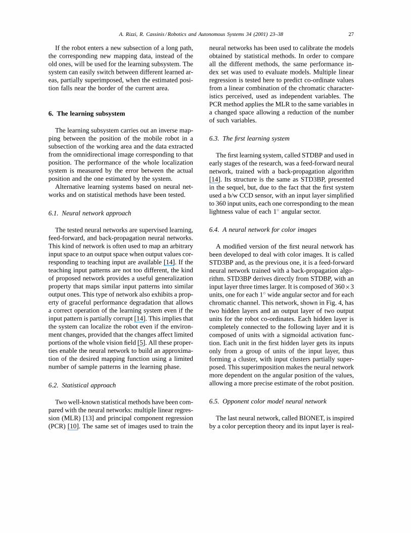
Fig. 10. A1 result comparison (cm).

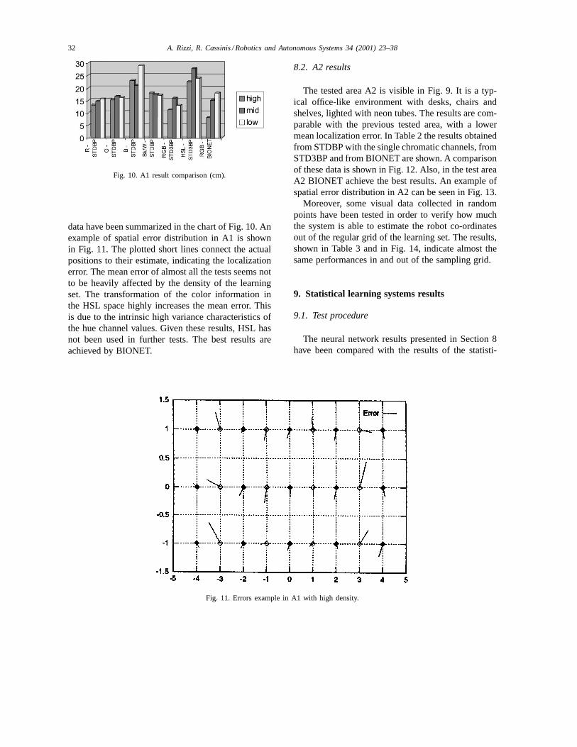
data have been summarized in the chart of Fig. 10. Anexample of spatial error distribution in A1 is shownin Fig. 11. The plotted short lines connect the actualpositions to their estimate, indicating the localizationerror. The mean error of almost all the tests seems notto be heavily affected by the density of the learningset. The transformation of the color information inthe HSL space highly increases the mean error. Thisis due to the intrinsic high variance characteristics ofthe hue channel values. Given these results, HSL hasnot been used in further tests. The best results areachieved by BIONET.

Fig. 11. Errors example in A1 with high density.

8.2. A2 results

The tested area A2 is visible in Fig. 9. It is a typ-ical office-like environment with desks, chairs andshelves, lighted with neon tubes. The results are com-parable with the previous tested area, with a lowermean localization error. In Table 2 the results obtainedfrom STDBP with the single chromatic channels, fromSTD3BP and from BIONET are shown. A comparisonof these data is shown in Fig. 12. Also, in the test areaA2 BIONET achieve the best results. An example ofspatial error distribution in A2 can be seen in Fig. 13.

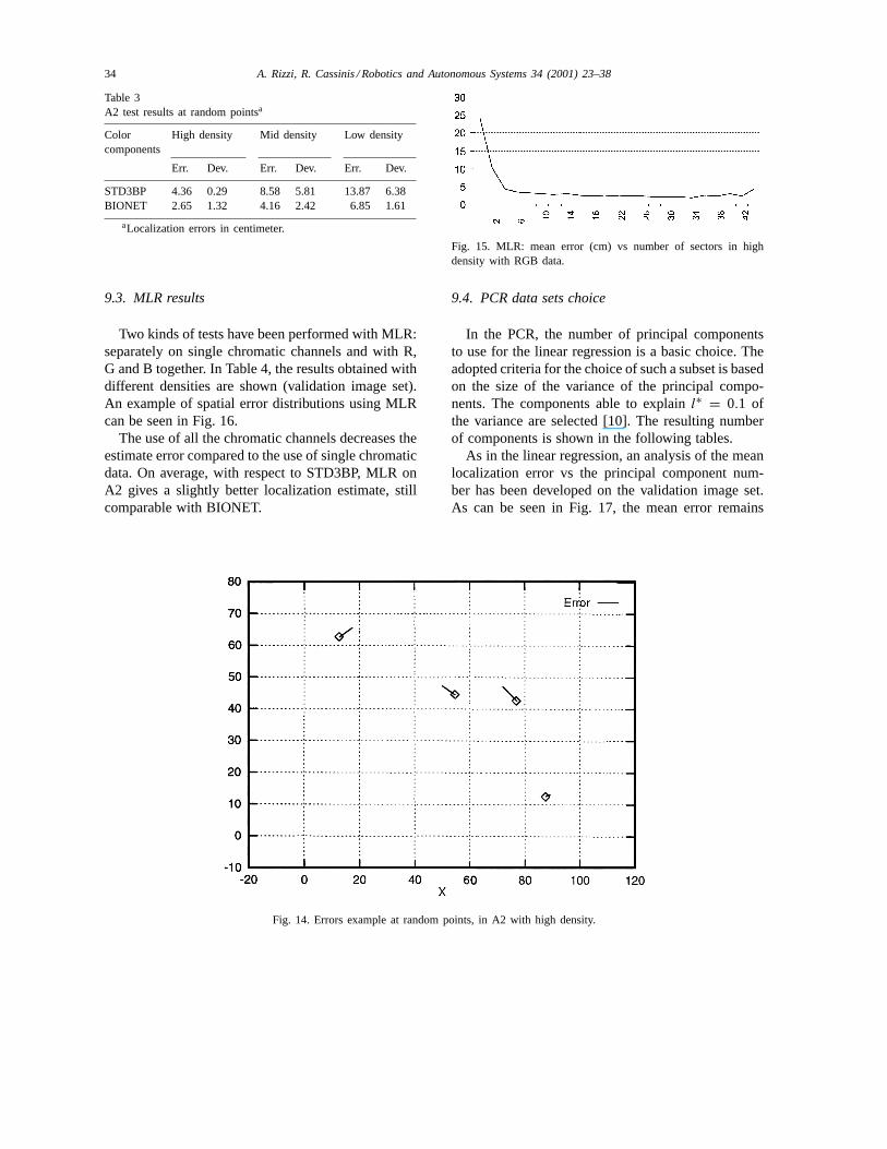
Moreover, some visual data collected in randompoints have been tested in order to verify how muchthe system is able to estimate the robot co-ordinatesout of the regular grid of the learning set. The results,shown in Table 3 and in Fig. 14, indicate almost thesame performances in and out of the sampling grid.

9. Statistical learning systems results

9.1. Test procedure

The neural network results presented in Section 8have been compared with the results of the statisti-

A. Rizzi, R. Cassinis / Robotics and Autonomous Systems 34 (2001) 23–38 33

Table 2A2 test resultsa

Color components High density Mid density Low density Learning system

Err. Dev. Err. Dev. Err. Dev.

R 5.42 3.70 7.55 5.12 9.59 5.66 STDBPG 3.84 2.46 8.06 4.47 10.65 5.06 STDBPB 7.53 4.19 10.04 6.14 13.34 8.65 STDBPRGB 4.00 2.64 7.77 4.45 13.61 9.98 STD3BPRGB 2.70 1.55 4.96 2.96 7.59 4.08 BIORETE

aLocalization errors in centimeter.

Fig. 12. A2 result comparison (cm).

cal methods described. The pre-processed images aredivided into a number of sectors lower than the neuralnetwork tests, as they are the independent variablesof a model that have to be calibrated by a small

Fig. 13. Errors example in A2 with high density.

number of images. The number of sectors is fixedin about half the number of calibration images. Thedependent variables are still the robot co-ordinates.Only the tests performed in the area A2 arepresented.

9.2. MLR data sets choice

The mean localization error vs sector number inhigh density is shown in Fig. 15. The fitting curveof these data is very smooth and for a wide rangeof sector number the mean localization error remainsalmost steady. This fact supports the selecting criteriaof the number of sectors chosen above. The resultingnumber of components, according to this criteria, isshown in the following tables.

34 A. Rizzi, R. Cassinis / Robotics and Autonomous Systems 34 (2001) 23–38

Table 3A2 test results at random pointsa

Colorcomponents

High density Mid density Low density

Err. Dev. Err. Dev. Err. Dev.

STD3BP 4.36 0.29 8.58 5.81 13.87 6.38BIONET 2.65 1.32 4.16 2.42 6.85 1.61

aLocalization errors in centimeter.

9.3. MLR results

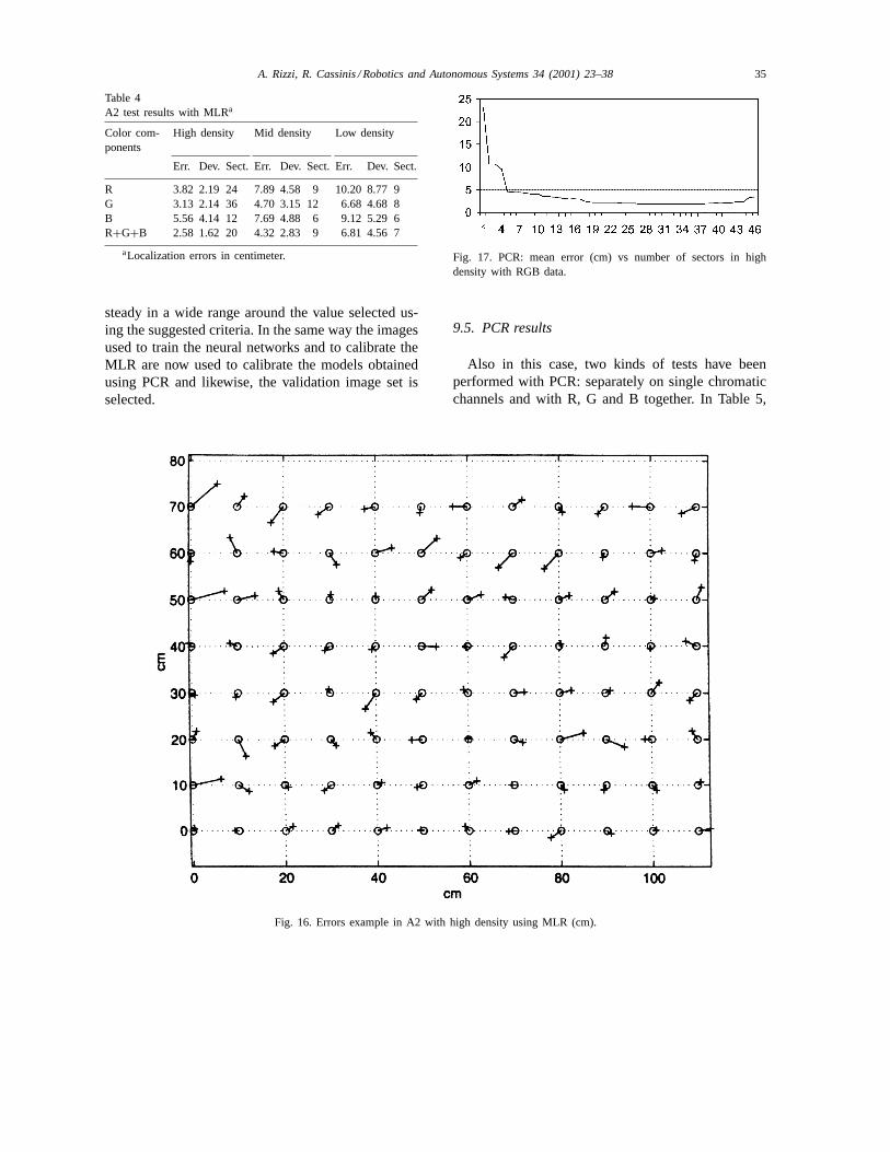
Two kinds of tests have been performed with MLR:separately on single chromatic channels and with R,G and B together. In Table 4, the results obtained withdifferent densities are shown (validation image set).An example of spatial error distributions using MLRcan be seen in Fig. 16.

The use of all the chromatic channels decreases theestimate error compared to the use of single chromaticdata. On average, with respect to STD3BP, MLR onA2 gives a slightly better localization estimate, stillcomparable with BIONET.

Fig. 14. Errors example at random points, in A2 with high density.

Fig. 15. MLR: mean error (cm) vs number of sectors in highdensity with RGB data.

9.4. PCR data sets choice

In the PCR, the number of principal componentsto use for the linear regression is a basic choice. Theadopted criteria for the choice of such a subset is basedon the size of the variance of the principal compo-nents. The components able to explainl∗ = 0.1 ofthe variance are selected [10]. The resulting numberof components is shown in the following tables.

As in the linear regression, an analysis of the meanlocalization error vs the principal component num-ber has been developed on the validation image set.As can be seen in Fig. 17, the mean error remains

A. Rizzi, R. Cassinis / Robotics and Autonomous Systems 34 (2001) 23–38 35

Table 4A2 test results with MLRa

Color com-ponents

High density Mid density Low density

Err. Dev. Sect. Err. Dev. Sect. Err. Dev. Sect.

R 3.82 2.19 24 7.89 4.58 9 10.20 8.77 9G 3.13 2.14 36 4.70 3.15 12 6.68 4.68 8B 5.56 4.14 12 7.69 4.88 6 9.12 5.29 6R+G+B 2.58 1.62 20 4.32 2.83 9 6.81 4.56 7

aLocalization errors in centimeter.

steady in a wide range around the value selected us-ing the suggested criteria. In the same way the imagesused to train the neural networks and to calibrate theMLR are now used to calibrate the models obtainedusing PCR and likewise, the validation image set isselected.

Fig. 16. Errors example in A2 with high density using MLR (cm).

Fig. 17. PCR: mean error (cm) vs number of sectors in highdensity with RGB data.

9.5. PCR results

Also in this case, two kinds of tests have beenperformed with PCR: separately on single chromaticchannels and with R, G and B together. In Table 5,

36 A. Rizzi, R. Cassinis / Robotics and Autonomous Systems 34 (2001) 23–38

Table 5A2 test results with PCRa

Colorcomponents

High density Mid density Low density

Err. Dev. Sect. Err. Dev. Sect. Err. Dev. Sect.

R 3.53 2.01 24 5.66 3.40 8 8.05 4.80 7G 2.89 2.90 22 4.35 2.84 7 8.22 5.32 4B 4.46 2.56 23 7.67 5.00 7 11.03 6.41 8R+G+B 2.42 1.67 29 3.66 2.37 7 6.11 3.75 5

aLocalization errors in centimeter.

the results obtained with different chromatic input anddensity are shown. An example of spatial error distri-butions of the PCR can be seen in Fig. 18. In averagePCR shows performances comparable with the othermethods, but less dependent from the learning density.

Also using PCR, some visual data collected in ran-dom points have been tested in order to verify thesystem estimate out of the regular grid of the learn-ing set. The results, shown in Table 6, indicate almostthe same performances in and out of the samplinggrid.

Fig. 18. Errors example in A2 with high density using PCR (cm).

Table 6A2 test results at random points using PCRa

Colorcomponents

High density Mid density Low density

Err. Dev. Err. Dev. Err. Dev.

PCR 4.93 3.12 5.11 1.15 13.52 6.38

aLocalization errors in centimeter.

10. System robustness against rotations

Pollicino does not measure the robot rotation inthe fixed reference system defined in the learningphase. While a programmed turn of the robot canbe easily compensated with a pattern shift, an un-wanted heading change due to skidding or otherexternal unpredictable reasons can result in an ex-tra localization error. Tests were made to investigatethe sensitivity of the system to undetected rotations.As it can be seen in Tables 7 and 8, small rota-tions are well tolerated. As the unwanted rotationsgets higher (more than 5◦), the system performancesensibly decreases, but such high rotations could be

A. Rizzi, R. Cassinis / Robotics and Autonomous Systems 34 (2001) 23–38 37

Table 7Clockwise rotation test resultsa

Clockwiserotations (deg.)

High density Mid density Low density

Err. Dev. Err. Dev. Err. Dev.

2 4.56 1.76 8.46 4.06 12.43 1.865 6.73 0.50 10.84 3.76 17.08 8.81

10 14.28 4.51 20.21 1.17 24.89 5.1315 15.24 3.30 23.90 7.47 30.67 1.3120 17.02 5.10 29.37 1.00 27.44 1.0445 40.32 4.48 30.45 4.17 35.23 1.99

aLocalization errors in centimeter.

Table 8Counterclockwise rotation test resultsa

Counter-clockwiserotations (deg.)

High density Mid density Low density

Err. Dev. Err. Dev. Err. Dev.

2 4.30 1.78 9.11 4.27 9.92 2.295 6.26 0.65 11.72 3.94 15.50 12.71

10 13.05 4.26 22.03 1.09 24.87 7.1915 13.92 3.17 26.09 8.02 31.80 1.4620 15.52 4.79 32.11 0.90 27.93 1.0645 36.49 4.23 33.29 4.39 37.28 2.48

aLocalization errors in centimeter.

managed if the robot keeps track of its heading in thereference system by other means (e.g. magnetic orgyrocompass).

11. Conclusions and perspectives

A self-localization system for autonomous robot hasbeen presented. The main features of this system are:it is a completely passive system, it does not requireany environment conditioning and it works even if thelearned environment changes moderately (e.g. peoplewalking, moved objects, etc.). The precision of thelocalization estimate is acceptable and, especially withhigh density learning sets, the localization error is low,compared to the needs of a navigating mobile robot.

Pollicino has been implemented with low cost com-ponents and it does not require powerful computa-tional resources. In fact the presented system has beenimplemented on low cost PC (e.g. 486) with responsetime almost instantaneous in relation with the sam-pling time of the low cost camera (about eight framesper second).

Regarding the learning subsystem choice, a com-parative analysis of the results indicates that all thetested methods have comparable performances. More-over, the randomness of the error direction suggest thatan iterative estimate could further increase the overallsystem performance.

The use of the system in environments with heavylighting changes, that might affect the system per-formance, should be investigated, and automaticlearning procedure should be developed in order torealize an autonomous guidance system able to drivethe robot back from unknown places visited onlyonce.

References

[1] E. Bideaux, P. Baptiste, C. Day, D. Harwood, Mapping witha backpropagation neural network, in: Proceedings of theIMACS-IEEE/SMC Symposium, Lille, France, 1994.

[2] R. Cassinis, D. Grana, A. Rizzi, A perception system formobile robot localization, in: Proceedings of the WAAP’95Workshop congiunto su Apprendimento Automatico ePercezione, Ancona, Italy, 1995.

[3] R. Cassinis, D. Grana, A. Rizzi, Self localization usingan omnidirectional image sensor, in: Proceedings of theSIRS’96, Fourth International Symposium on IntelligentRobotic Systems, Lisbon, Portugal, 1996.

[4] R. Cassinis, D. Grana, A. Rizzi, Using colour informationin an omnidirectional perception system for autonomousrobot localization, in: Proceedings of the EUROBOT’96,First Euromicro Workshop on Advanced Mobile Robots,Kaiserslautern, Germany, 1996.

[5] R. Cassinis, D. Grana, A. Rizzi, V. Rosati, Robustnesscharacteristics of Pollicino system for autonomous robotself-localization, in: Proceedings of the EUROBOT’97,Second Euromicro International Workshop on AdvancedMobile Robots, Brescia, Italy, 1997.

[6] B. Crespi, C. Furlanello, L. Stringa, Memory basednavigation, in: Proceedings of the IJCAI Workshop onRobotics and Vision, Chambéry, France, 1993, p. 1654.

[7] W.R. Dillon, M. Goldstein, Multivariate Analysis: Methodsand applications, Wiley, New York, 1984.

[8] D.S. Falk, D.R. Brill, D.G. Stark, Seeing the Light, Harperand Row, New York, 1986.

[9] M.O. Franz, B. Scholkopf, H.A. Mallot, H.H. Bulthoff,Learning view graphs for robot navigation, AutonomousRobots 5 (1) (1998) 111–125.

[10] I.T. Jollife, Principal Component Analysis, Springer, NewYork, 1986.

[11] S.K. Nayar, K. Ikeuchi, T. Kanade, Surface reflection:physical and geometrical perspectives, IEEE Transactions onPattern Analysis and Machine Intelligence 13 (1991).

38 A. Rizzi, R. Cassinis / Robotics and Autonomous Systems 34 (2001) 23–38

[12] T. Ohno, A. Ohya, S. Yuta, Autonomous navigation for mobilerobots referring pre-recorded image sequence, in: Proceedingsof the IEEE/RSJ IROS’96, 1996.

[13] P.G. Hoel, Introduction to Mathematical Statistics, Wiley,New York, 1947.

[14] D.E. Rumelhart, J.L. McClelland, Parallel DistributedProcessing: Explorations in the Microstructure of Cognition,MIT Press, Cambridge, MA, 1986.

[15] S. Shah, J.K. Aggarwal, Mobile robot navigation and scenemodeling using stereo fish-eye lens system, Machine VisionApplications 10 (4) (1997) 159–173.

[16] G. Wyszecki, W.S. Stiles, Color Science, Wiley, New York,1982.

[17] Y. Yagi, S. Fujimura, M. Yashida, Route representationfor mobile robot navigation by omnidirectional routepanorama Fourier transformation, in: Proceedings of theIEEE International Conference on Robotics and Automation,Leuven, Belgium, 1998.

[18] Y. Yagi, Y. Nishizawa, M. Yashida, Map based navigation ofthe mobile robot using omnidirectional image sensor copis,in: Proceedings of the IEEE International Conference onRobotics and Automation, Nice, France, 1992.

[19] Y. Yagi, Y. Nishizawa, M. Yashida, Map based navigationfor a mobile robot with omnidirectional image sensor copis,IEEE Transactions on Robotics and Automation 11 (5) (1995)634–648.

[20] Y. Yagi, H. Okumura, M. Yashida, Multiple visual sensingsystem for mobile robot, in: Proceedings of the IEEEInternational Conference on Robotics and Automation, SanDiego, CA, Vol. 2, 1994, pp. 1679– 1684.

[21] Y. Yagi, M. Yachida, Real-time generation of environmentalmap and obstacle avoidance using omnidirectional imagesensor with conic mirror, in: Proceedings of the IEEEConference on Computer Vision and Pattern Recognition,1991.

[22] K. Yamazawa, Y. Yagi, M. Yachida, Omnidirectionalimaging with hyperboloidal projection, in: Proceedings of theIEEE/RSJ IROS’93, Vol. 2, 1993, pp. 1029–1034.

Alessandro Rizzi graduated in Informa-tion Science from the University of Milanin 1992 and got his Ph.D. in InformationEngineering from the University of Bres-cia (Italy). From 1992 to 1994 he workedas a contract researcher at the Universityof Milan in the Image Laboratory, studyingthe problem of color constancy and its ap-plication in computer graphics. From 1994to 1996 he worked as a contract professor

of Information Systems at the University of Brescia. Since 1994he has been working with Professor Riccardo Cassinis at the Ad-vanced Robotics Laboratory studying problems of self-localizationand navigation using color information, omnidirectional devicesand biologically inspired models. In 1999 he worked as a con-tract professor of Computer Graphics at Politecnico of Milano.He is presently researching on color appearance models appliedto robotic visual navigation and image correction.

Riccardo Cassinisreceived his degree inElectronic Engineering in 1977 from thePolytechnic University of Milan. In 1987he was appointed as an Associate Profes-sor of Robotics and of Numerical SystemsDesign at the University of Udine. Since1991 he is working as an Associate Profes-sor of Computer Science and of Roboticsat the University of Brescia. He has beenworking as a Director of the Robotics Lab-

oratory of the Department of Electronics in Milan, of the RoboticsLaboratory of the University of Udine, and is now the Directorof the Advanced Robotics Laboratory of the University of Bres-cia. Since 1975 he has been working on several topics related toindustrial robots, and since 1985 he is involved in navigation andsensing problems for advanced mobile robots. His current interestsinclude mobile robots for exploring unknown environment, withparticular attention to problems related to humanitarian de-mining.