Segmentation of Brain Images Using Adaptive Atlases withApplication to Ventriculomegaly

Navid Shiee1, Pierre-Louis Bazin1, Jennifer Cuzzocreo1, Ari Blitz2, and Dzung L. Pham1,3

1The Laboratory of Medical Image Computing, Johns Hopkins University, USA2Department of Radiology and Radiological Science, Johns Hopkins University, USA3Center for Neuroscience and Regenerative Medicine, Henry M. Jackson Foundation, USA

AbstractSegmentation of brain images often requires a statistical atlas for providing prior informationabout the spatial position of different structures. A major limitation of atlas-based segmentationalgorithms is their deficiency in analyzing brains that have a large deviation from the populationused in the construction of the atlas. We present an expectation-maximization framework based ona Dirichlet distribution to adapt a statistical atlas to the underlying subject. Our model combinesanatomical priors with the subject’s own anatomy, resulting in a subject specific atlas which wecall an “adaptive atlas”. The generation of this adaptive atlas does not require the subject to havean anatomy similar to that of the atlas population, nor does it rely on the availability of anensemble of similar images. The proposed method shows a significant improvement over currentsegmentation approaches when applied to subjects with severe ventriculomegaly, where theanatomy deviates significantly from the atlas population. Furthermore, high levels of accuracy aremaintained when the method is applied to subjects with healthy anatomy.

1 IntroductionAutomated algorithms for the segmentation of magnetic resonance (MR) brain imagesprovide valuable tools for analyzing human brain structure. The incorporation of priorinformation is often required in many of these algorithms. One of the most commonly usedtypes of prior information are statistical atlases that use a selection of training examples (i.e.manual delineations) from multiple subjects to model the spatial variability of the structuresof interest [1, 22, 8, 17, 2]. These atlases can be utilized within a Bayesian framework toguide the algorithm as to where a structure is likely to appear within the image. Suchapproaches offer several advantages, including enhanced stability and convergence, as wellas providing the ability to distinguish between structures with similar intensities. However,one of the major drawbacks of algorithms that use such statistical atlases is their inability toaccurately model subjects whose brain anatomy deviates from the atlas population to a greatextent. In some diseases and neurodegenerative conditions such as hydrocephalus, largechanges take place in the geometry of the brain, potentially resulting in wildly inaccuratesegmentations when using atlases derived from healthy populations.

Few methods have been proposed to effectively employ spatial atlases when population-specific training data is unavailable. Bhatia et al. [3] proposed a combined segmentation-registration method for atlas based brain segmentation in a group of subjects that areanatomically different from the atlas subjects. Riklin-Raviv et al. [19] avoided the use of astatistical atlas by introducing latent atlases generated from an image ensemble. The mainlimitation of these approaches is their dependency on the existence of a group of images thatimplicitly are needed to represent similar anatomy. Liu et al. utilize a generativesegmentation model combined with a discriminative classifier to reduce dependency on an

NIH Public AccessAuthor ManuscriptInf Process Med Imaging. Author manuscript; available in PMC 2012 October 22.

Published in final edited form as:Inf Process Med Imaging. 2011 ; 22: 1–12.

NIH

-PA Author Manuscript

NIH

-PA Author Manuscript

NIH

-PA Author Manuscript

atlas [10]. However, this method focused on diseases that possess relatively modestgeometric changes in brain structure.

Our approach for the segmentation of MR brain images is based on Gaussian MixtureModels (GMMs), similar to many other approaches (cf. [1, 22]). In GMMs, the intensityvalues of each cluster are assumed to have a Gaussian distribution whose parameters can beestimated by maximum likelihood (ML) using the expectation maximization (EM) algorithm[6]. The mixing coefficients of the GMM in brain segmentation algorithms can be given bya statistical atlas registered to the image space [22]. Consequently, if the difference betweenthe subject and the training data used in the construction of the atlas can not be captured bythe registration algorithm, these algorithms are unable to generate an accurate segmentation(Fig. 1). In other image processing applications, several approaches have been introduced toderive the mixing coefficients from the image itself. The concept of spatially varying mixingcoefficients was first introduced by Sanjay-Gopal and Hebert [20]. In their work, a GibssMRF-based prior was assumed on the mixing coefficients whose maximum a posteriori(MAP) estimates were computed by means of a generalized EM algorithm. Several otherapproaches have been proposed based on this model(see [12, 13]). Although theseapproaches are not biased to a statistical atlas, they can not effectively model separatestructures with similar intensity values, such as sulcal and ventricular cerebrospinal fluid(CSF). This is a major advantage of methods employing a statistical atlas.

In this work, we propose a new framework that combines the desirable properties of both ofthese models. We model the mixing coefficients by a Dirichlet distribution whoseparameters are derived from a statistical atlas of healthy subjects. Employing this modelwithin an EM framework, we estimate an “adaptive” atlas which is updated iteratively bycombining the original statistical atlas with information from the image under study. Sincethe adaptive atlas is informed by a statistical atlas, clusters with similar intensities can beembedded in our adaptive atlas. At the same time, the influence of the data on the adaptiveatlas removes the bias toward the statistical atlas to a great extent. The resulting adaptiveatlas is specific to the subject and therefore, does not limit the atlas based segmentation ofthe image. Unlike the approaches of [3, 19], our model does not require an ensemble ofimages and automatically adapts the statistical atlas to a single subject. It is worthmentioning that two recent works have incorporated a Dirichlet model in imagesegmentation algorithms in a different context [13, 11].

We test and validate our method both on subjects with normal brain anatomy and subjectssuffering from hydrocephalus. Hydrocephalus patients can have severe ventriculomegalywhich are not well modeled by statistical atlases generated from normal subjects. Because ofthe specific interest in ventricular size and shape in hydrocephalus patients [18, 4],traditional three-class brain segmentation approaches are not appropriate. For thisapplication, we employ a four tissue class model, consisting of gray matter (GM), whitematter (WM), sulcal CSF, and ventricular CSF. Our results demonstrate that our methodapplied to brains with severe ventriculomegaly has superior performance over state-of-the-art atlas-based methods, while it achieves similar accuracy in the segmentation of brainswith normal anatomy.

2 MethodsIn this section, we first review the Gaussian mixture model (GMM) with spatially varyingmixing coefficients introduced in [20] before presenting our work on incorporating adaptiveatlases in the segmentation of brain MR images. In a standard atlas approach, the mixingcoefficients represent our atlas, providing the prior probability that a tissue class occurs at avoxel. The central idea of this paper is to employ a Dirichlet distribution as a prior to the

Shiee et al. Page 2

Inf Process Med Imaging. Author manuscript; available in PMC 2012 October 22.

NIH

-PA Author Manuscript

NIH

-PA Author Manuscript

NIH

-PA Author Manuscript

mixing coefficients, where the mode of the distribution is given by a statistical atlasconstructed from healthy subjects. In so doing, the estimated mixing coefficients can deviatesignificantly from the original statistical atlas and adapt to the subject data.

2.1 Gaussian mixture model with spatially varying mixing coefficientsOur goal is to segment the brain into K structures. We assume that the intensity distributionof each structure follows a Gaussian distribution. Hence the observed MR image(s) can bemodeled by a GMM. Let xj be the Cx1 vector of the observed intensities where j ∈ {1, 2, …,N} represents the voxel location in the image and C represents the number of input channels.Also let θk = {μk, Σk} be the parameters of the Gaussian distribution associated withstructure k (k ∈ {1, 2, …, K}). Here, μk is the Cx1 mean vector and Σk is the CxCcovariance matrix.

The label of each voxel j is denoted by a Kx1 vector zj. If voxel j belongs to structure k, zj =ek where ek is a Kx1 vector whose kth component is 1 and all of its other components are 0.We model the prior distribution of zj’s as a multinomial distribution with the Kx1 vectorparameter πj, i.e. f (zjk = 1) = πjk where the second letter in the subscript denotes the vectorcomponent index. The πjk’s are called the mixing coefficients of GMM and they represent

the possibility that voxel j belongs to structure k a priori (by construction, ).With the assumption of the independence of zj’s, we can write the prior on z = (z1, z2, …,zN) as:

(1)

In [20], it was assumed that the observations xj’s are independent, hence the conditionaldistribution of the complete data y = (x1, x2, …, xN, z1, z2, …, zN) is given by:

(2)

where Ψ = (π1, π2, …, πK, θ1, θ2, …, θK) and G(,; θk) is a Gaussian distribution withparameter θk. Sanjay-Gopal and Hebert derived an EM algorithm for ML estimation of theGaussian parameters θk’s and πjk’s in (2):

(3)

(4)

The posterior probabilities given by (3) are used to associate each voxel to one of thestructures by choosing the one that has the largest posterior probability wjk.

It is worth mentioning here that the two other common assumptions on πjk’s are:

i. πjk = πk, ∀j, which is the classical mixture model approach.

Shiee et al. Page 3

Inf Process Med Imaging. Author manuscript; available in PMC 2012 October 22.

NIH

-PA Author Manuscript

NIH

-PA Author Manuscript

NIH

-PA Author Manuscript

ii.πjk = pjk, where pjk is given by a statistical atlas and .

2.2 GMM with adaptive atlasesA major drawback of using (2) in the segmentation of the brain structures is theinsufficiency of this model in distinguishing structures with similar intensities from oneanother. Assumption (ii) in the previous section resolves this problem to some extent.However, if the underlying image largely differs from the subjects used in the constructionof the atlas, this assumption hinders the correct segmentation of the image. Here we describea MAP framework to solve this limitation of atlas-based segmentation algorithms.

To incorporate a statistical atlas within a framework that estimates the mixing coefficientsbased on the subject data, we treat πj as a random vector with a distribution whoseparameters are derived from the statistical atlas. As the vector πj lives on a K-dimensionalsimplex, we should choose a distribution with simplex support as a prior on πj. The naturalchoice for such a distribution is a Dirichlet distribution:

(5)

where B(·) is a Beta function and αj is the Kx1 vector parameter of the distribution. In ourmodel, we have a statistical atlas generated from training data pjk, that provides us the apriori probability of a structure j occurring at voxel k in a healthy population (as will bedescribed later in Sec 2.4). We therefore employ a Dirichlet prior with parameter αjk = 1 +δpjk, ∀k. The parameter δ is non-negative and we describe its selection later in this section.For the case of δ = 1, the values pj = (pj,1, pj;2, …, pj,K) represent the mode of the Dirichletprior probability function.

As the brain structures often form a connected region, we incorporate a Markov RandomField (MRF) as a prior on zj’s. In this work, we utilize a model similar to the one employedin [22, 16], which yields the following prior on z:

(6)

where π = (π1, π2, …, πN), Nj is the 6-connected neighborhood of voxel j, β is theparameter controlling the effect of the prior, and ZMRF is the normalizing factor. It is worthmentioning that we assume uniform prior on θk’s.

With these assumptions, the conditional distribution of the complete data in our model isgiven by:

(7)

2.3 Estimation AlgorithmIn this section we derive the estimation algorithm for the parameters in (7) using ageneralized EM algorithm. The EM algorithm is an iterative approach for the estimation ofmodel parameters that involves two steps: (i) an E-step in which, given the parameterestimates from the previous iteration, the conditional expectation of the complete data

Shiee et al. Page 4

Inf Process Med Imaging. Author manuscript; available in PMC 2012 October 22.

NIH

-PA Author Manuscript

NIH

-PA Author Manuscript

NIH

-PA Author Manuscript

likelihood function is computed; and (ii) a M-step in which the new estimate of the modelparameters is computed to increase or maximize the conditional expectation computed in E-step [6]. We provide here the E-step and M-step for (7). If Ψ(t) is the set of estimatedparameters from iteration t, then we have:

E-Step

(8)

The main component in (8) is computing . Due to the MRF prior on z,

computing analytically is computationally intractable. Using a mean field approximationyields (see [16]):

(9)

M-step—In this step, we want to find the set of parameters Ψ(t+1) that maximizes (8). This

can be done independently for and . For , we first derive the equation for

and then for . As we assume uniform priors on θk’s, the solution for issimilar to (4):

(10)

Because of the constraint on πjk’s, we use Lagrange multiplier to maximize (8) with respectto πjk:

(11)

Hence:

(12)

Using the constraint on πjk’s and pjk’s and (9) λ is given by:

(13)

Therefore the update for is given by:

Shiee et al. Page 5

Inf Process Med Imaging. Author manuscript; available in PMC 2012 October 22.

NIH

-PA Author Manuscript

NIH

-PA Author Manuscript

NIH

-PA Author Manuscript

(14)

The statistical atlas, by construction, should be a smooth probability map that represents thepopulation under study. Although pjk’s are given by a smooth statistical atlas, wjk’s do nothave this desirable smooth property. To enforce the spatial smoothness on wjk’s and makethe mixing coefficients reffective of a population that the subject is drawn from, weconvolve wjk’s with a spatial Gaussian kernel in (14):

(15)

where G is a Gaussian kernel (we used a kernel size of 2.5 mm in all our experiments). Thisprovides our model for generating the adaptive atlas. Although the Gaussian filteringdeviates from our statistical framework, simple smoothing of parameter estimates haspreviously been shown to offer good convergence properties and computational advantagesover explicit smoothing priors when used within the EM algorithm [14].

Eq. (15) has an intuitive interpretation of being a weighted average of the original atlas withthe subject atlas. We call in (15) the adaptation factor, which controls the influence ofthe image on the adaptive atlas. For instance, k = 0 results in case (ii) of Sec 2.1 (a non-adapted statistical atlas), whereas k = 1 results in a smooth version of (4) (no influence fromthe statistical atlas). In particular, k = 0.5, which we used in all our experiments, enforces themode of the Dirichlet prior on πj to be equal to pj. Fig. 2 shows how the adaptive atlaschanges during the segmentation algorithm.

2.4 Implementation DetailsStatistical atlas—The statistical atlas we used in this work is built from a set of 18manual delineations of the structures of interest, based on the IBSR data set [23]. For eachimage in the atlas, the delineation is rigidly aligned with the current atlas image, and asmooth approximation of the probabilities is accumulated. The smoothing replaces the stepedge at the boundary of each structure in their binary delineation by a linear ramp over aband of size ε (which we set to 10 mm in our work) [2]. In this work, the statistical atlascontains prior information for sulcal-CSF, ventricles, GM, and WM, however it can beeasily extended to more structures.

Atlas registration—The statistical atlas needs to be registered to the image space for thesegmentation task. We used a joint segmentation and registration technique that alternatesbetween estimating the segmentation given the current atlas position, and then updating thetransformation given the current segmentation. The registration maximizes the correlation ofthe mixing coefficients with the posterior probabilities. The transformation is updated ateach iteration of the algorithm. We used affine transformations in this work.

Initializing the EM algorithm—To initialize the intensity centroids of the differentstructures, we first estimate the robust minimum and maximum of the intensity (the intensityvalues at 5% and 95% of the histogram, respectively), and normalize the profiles such that 0corresponds to the minimum and 1 to the maximum. We then initialized the centroids toempirically determined values stemming from the expected intensities of the tissue classesfor the appropriate pulse sequence.

Shiee et al. Page 6

Inf Process Med Imaging. Author manuscript; available in PMC 2012 October 22.

NIH

-PA Author Manuscript

NIH

-PA Author Manuscript

NIH

-PA Author Manuscript

Convergence criteria—We used the maximum amount of change in posteriorprobabilities as the measure of convergence of the EM algorithm. We set a threshold of 0.01on this maximum in our work.

3 ExperimentsWe evaluated the performance of the introduced method on both brains with healthyanatomy and hydrocephalus brains which suffer from ventriculomegaly. We compared theperformance of our method to an in-house implementation of a standard atlas-based EMsegmentation algorithm (which we refer to as the atlas EM segmentation algorithm in thissection). The only difference between this implementation and our proposed method lies inthe use of a conventional statistical atlas instead of the introduced adaptive atlas. Brainimages were preprocessed to extract the brain and correct for inhomogeneities. Somemanual refinement of the brain mask was necessary on some cases. We also compared theperformance of our method in the segmentation of the ventricles of hydrocephalus brainswith the Freesurfer software [8], which employs a nonstationary MRF model and aprobabilistic atlas updated using nonlinear registration. Finally we compared our method toa registration based segmentation algorithm which uses Hammer [21], a state-of-the-artdeformable registration algorithm, to label the ventricles. We used Dice overlap coefficient[7] and false negative ratio (for the ventricle segmentation experiment) between theautomated segmentation and the ground truth as the accuracy measures.

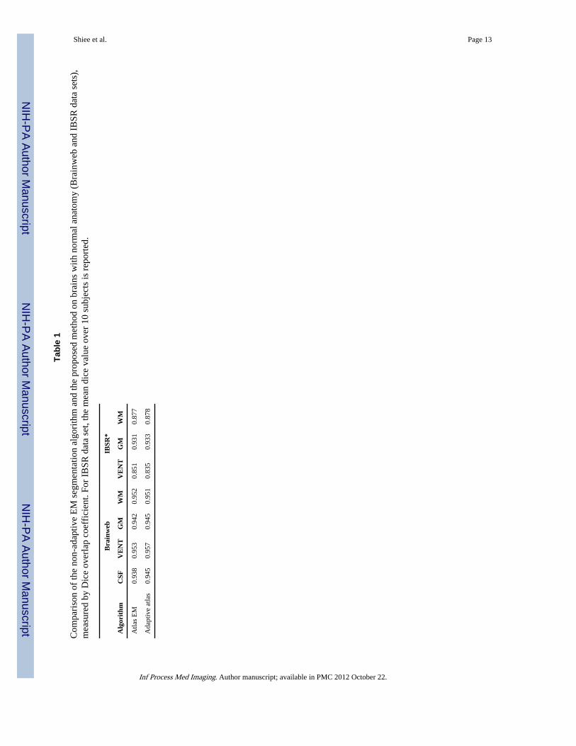
3.1 Normal BrainsTo study the performance of the algorithm on brains with normal anatomy, we used bothsimulated and real data sets. In our first experiment, we used the simulated T1 brain fromthe Brainweb phantom [5] with 3% noise and no inhomogeneity. As Brainweb truth modeldoes not have a separate segmentation for the ventricles, we manually separated the sulcal-CSF from the ventricles on the ground truth image. As Table 1 demonstrates, our methodhas slightly better overall accuracy in segmenting the simulated brain in comparison to thenon-adaptive EM segmentation algorithm.

In the second experiment, we used the IBSR database [23] which contains MR brain imagesof 18 real subjects. As we also use this database to create our statistical atlas, we separatedthe subjects to two non-overlapping groups of 8 and 10 subjects. We used the first group tocreate the statistical atlas and then used that atlas to validate the algorithms on the 10 othersubjects. As the manual segmentation of this data set does not contain sulcal-CSF andincludes it inside the GM segmentation, we combined the sulcal-CSF and GM labels in theautomated segmentation results before comparing to the manual segmentation. The accuracyof our method and the non-adaptive atlas EM segmentation algorithm in the segmentation ofthis data set are very similar (Table 1).

3.2 Brains with ventriculomegalyThe main advantage of our approach using the adaptive atlases over other atlas-basedsegmentation algorithms is its ability in the segmentation of images that largely deviate fromthe atlas population. To study this unique aspect of our adaptive method, we evaluated theperformance of the proposed method, the atlas EM segmentation algorithm, Freesurfer, andHammer on the segmentation of ventricles of 14 patients with hydrocephalus. Our data sethas 9 subjects with moderate and 5 subjects with marked ventricular dilatation, as diagnosedby a neuroradiologist. This allows us to be able to study the effect of large deviations fromthe atlas population on the performance of each algorithm more thoroughly. Also, in

addition to Dice overlap coefficient, we computed the false negative ratio ( )between the automatically segmented ventricles (Seg) and the manual delineation by an

Shiee et al. Page 7

Inf Process Med Imaging. Author manuscript; available in PMC 2012 October 22.

NIH

-PA Author Manuscript

NIH

-PA Author Manuscript

NIH

-PA Author Manuscript

expert (Ref) for each method. We found FNR very informative in our validation, as theerrors in the segmentation of the ventricles in this data set are mostly due to amisclassification as other structures.

The validation results (Table 2) show that our method has superior accuracy on all thesubjects in comparison to other methods. As expected, the atlas EM segmentation algorithm,Freesurfer, and the Hammer based segmentation perform significantly worse on subjectswith marked ventriculomegaly, whereas the performance of our approach is not alteredsignificantly by the amount of the dilatation. Freesurfer failed (did not complete or resultedin a nearly empty image) in the processing of 3 subjects with severe structural anomalies dueto problems in its brain extraction step. We also note that Freesurfer attempts to segment amuch larger number of structures and is therefore at a disadvantage trying to solve a moredifficult problem. Also it is worth mentioning that for the approach based on Hammer, wefirst used FANTASM [15] to classify the image voxels as CSF, GM, or WM. We then usedthe atlas provided with the Hammer software [9] to segment the ventricles. Although thisatlas contains 101 regions of interest, we grouped all of these regions into sulcal-CSF,ventricles, GM, and WM in our experiments.

Fig. 3 shows that even in the cases of moderate ventriculomegaly, the atlas EMsegmentation algorithm, Freesurfer and Hammer are not able to segment the ventricles asaccurately as the adaptive approach.

4 DiscussionWe have presented a new statistical framework for the atlas based segmentation of MR brainimages based on adaptive atlases. Our approach addresses the segmentation of images thatdeviate from the atlas population to a great extent. The validation results confirm that ouralgorithm has a superior performance in the segmentation of such subjects, whilemaintaining high level of accuracy in the segmentation of brains with healthy anatomy. Onthe hydrocephalus data, our

method was shown to have some advantages when compared to a deformable registrationapproach (Hammer), as well as an atlas-based approach that employs deformableregistration to update its atlas (Freesurfer). Deformable registration approaches are prone tolocal optima when the target is highly dissimilar from the template. Furthermore, theproposed approach leads to computationally e3-cient atlas updating (a Gaussian filter andsimple averaging) when compared to deformable registration. The introduced adaptive atlasprovides a general model for the computation of the mixing coefficients of a GMM model;for instance the conventional approach of using a statistical atlas as the mixing coefficientsis a special case of this model. Although we described the adaptive atlas concept as part of aGMM model, our approach can be easily incorporated in other atlas-based probabilisticsegmentation methods.

In computing the adaptive atlas, we included a smoothing step within EM iterations to makethe adaptive atlas reffective of a population that the subject is drawn from. We willinvestigate explicitly modeling this property as a hierarchical prior on the mixingcoefficients.

References1. Ashburner J, Friston K. Multimodal image coregistration and partitioning–a unified framework.

NeuroImage. 1997; 6(3):209–17. [PubMed: 9344825]

2. Bazin PL, Pham DL. Homeomorphic brain image segmentation with topological and statisticalatlases. Med Image Anal. 2008; 12(5):616–25. [PubMed: 18640069]

Shiee et al. Page 8

Inf Process Med Imaging. Author manuscript; available in PMC 2012 October 22.

NIH

-PA Author Manuscript

NIH

-PA Author Manuscript

NIH

-PA Author Manuscript

3. Bhatia, KK.; Aljabar, P.; Boardman, JP.; Srinivasan, L.; Murgasova, M.; Counsell, SJ.; Rutherford,MA.; Hajnal, J.; Edwards, AD.; Rueckert, D. Groupwise combined segmentation and registrationfor atlas construction. In: Ayache, N.; Ourselin, S.; Maeder, A., editors. Proc of MICCAI. p.532-40.Lecture Notes in Computer Science. Springer; Berlin / Heidelberg: 2007.

4. Clarke MJ, Meyer FB. The history of mathematical modeling in hydrocephalus. Neurosurg Focus.2007; 22(4):E3. [PubMed: 17613192]

5. Collins DL, Zijdenbos AP, Kollokian V, Sled JG, Kabani NJ, Holmes CJ, Evans AC. Design andconstruction of a realistic digital brain phantom. IEEE Trans Med Imaging. 1998; 17(3):463–468.[PubMed: 9735909]

6. Dempster A, Laird N, Rubin D. Maximum likelihood from incomplete data via the EM algorithm. JRoyal Stat Soc. 1977; 39(1):1–38.

7. Dice L. Measures of the amount of ecologic association between species. Ecology. 1945; 25(3):297–302.

8. Fischl B, Salat DH, van der Kouwe AJW, Makris N, Ségonne F, Quinn BT, Dale AM. Sequence-independent segmentation of magnetic resonance images. NeuroImage. 2004; 23 (Suppl 1):S69–84.[PubMed: 15501102]

9. Kabani N, McDonald D, Holmes CJ, Evans AC. 3D anatomical atlas of the human brain. Proc ofHBM, NeuroImage. 1998; 7(4):S717.

10. Liu CY, Iglesias JE, Toga A, Tu Z. Fusing adaptive atlas and informative features for robust 3Dbrain image segmentation. Proc of ISBI. 2010:848–851.

11. Maddah M, Zollei L, Grimson W, Wells W. Modeling of anatomical information in clustering ofwhite matter fiber trajectories using Dirichlet distribution. Proc of MMBIA. 2008:1–7.

12. Nikou C, Galatsanos NP, Likas AC. A class-adaptive spatially variant mixture model for imagesegmentation. IEEE Trans Image Process. 2007; 16(4):1121–30. [PubMed: 17405442]

13. Nikou C, Likas AC, Galatsanos NP. A bayesian framework for image segmentation with spatiallyvarying mixtures. IEEE Trans Image Process. 2010; 19(9):2278–89. [PubMed: 20378472]

14. Nychka D. Some properties of adding a smoothing step to the EM algorithm. Stat Probabil Lett.1990; 9(2):187–193.

15. Pham DL, Prince JL. Adaptive fuzzy segmentation of magnetic resonance images. IEEE TransMed Imaging. 1999; 18(9):737–52. [PubMed: 10571379]

16. Pham, D.; Bazin, PL. Unsupervised tissue classification. In: Bankman, I., editor. Handbook ofMedical Image Processing and Analysis. 2. Elsevier; 2008. p. 209-221.

17. Pohl KM, Bouix S, Nakamura M, Rohlfing T, McCarley RW, Kikinis R, Grimson WEL, ShentonME, Wells WM. A hierarchical algorithm for MR brain image parcellation. IEEE Trans MedImaging. 2007; 26(9):1201–12. [PubMed: 17896593]

18. Preul C, Hübsch T, Lindner D, Tittgemeyer M. Assessment of ventricular reconfiguration afterthird ventriculostomy: what does shape analysis provide in addition to volumetry? AJNR Am JNeuroradiol. 2006; 27(3):689–93. [PubMed: 16552017]

19. Riklin-Raviv T, Van Leemput K, Menze BH, Wells WM, Golland P. Segmentation of imageensembles via latent atlases. Med Image Anal. 2010; 14(5):654–65. [PubMed: 20580305]

20. Sanjay-Gopal S, Hebert TJ. Bayesian pixel classification using spatially variant finite mixtures andthe generalized EM algorithm. IEEE Trans Image Process. 1998; 7(7):1014–28. [PubMed:18276317]

21. Shen D, Davatzikos C. HAMMER: hierarchical attribute matching mechanism for elasticregistration. IEEE Trans Med Imaging. 2002; 21(11):1421–39. [PubMed: 12575879]

22. Van Leemput K, Maes F, Vandermeulen D, Suetens P. Automated model-based tissueclassification of MR images of the brain. IEEE Trans Med Imaging. 1999; 18(10):897–908.[PubMed: 10628949]

23. Worth, A. Internet brain segmentation repository. 1996. http://www.cma.mgh.harvard.edu/ibsr/

Shiee et al. Page 9

Inf Process Med Imaging. Author manuscript; available in PMC 2012 October 22.

NIH

-PA Author Manuscript

NIH

-PA Author Manuscript

NIH

-PA Author Manuscript

Fig. 1.Results of an atlas-based GMM segmentation algorithm on a subject with large ventricles(sulcal-CSF, ventricles, GM, and WM are represented by dark red, light red, orange, andwhite, respectively).

Shiee et al. Page 10

Inf Process Med Imaging. Author manuscript; available in PMC 2012 October 22.

NIH

-PA Author Manuscript

NIH

-PA Author Manuscript

NIH

-PA Author Manuscript

Fig. 2.Evolution of the adaptive atlas from the initial statistical atlas. It originally is biased by thetraining data but eventually converges to the subject’s geometry.

Shiee et al. Page 11

Inf Process Med Imaging. Author manuscript; available in PMC 2012 October 22.

NIH

-PA Author Manuscript

NIH

-PA Author Manuscript

NIH

-PA Author Manuscript

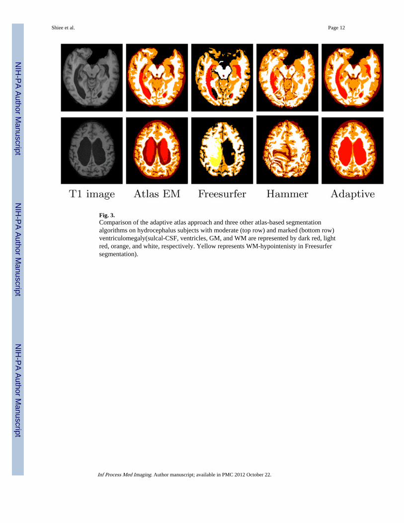
Fig. 3.Comparison of the adaptive atlas approach and three other atlas-based segmentationalgorithms on hydrocephalus subjects with moderate (top row) and marked (bottom row)ventriculomegaly(sulcal-CSF, ventricles, GM, and WM are represented by dark red, lightred, orange, and white, respectively. Yellow represents WM-hypointenisty in Freesurfersegmentation).

Shiee et al. Page 12

Inf Process Med Imaging. Author manuscript; available in PMC 2012 October 22.

NIH

-PA Author Manuscript

NIH

-PA Author Manuscript

NIH

-PA Author Manuscript

NIH

-PA Author Manuscript

NIH

-PA Author Manuscript

NIH

-PA Author Manuscript

Shiee et al. Page 13

Tabl

e 1

Com

pari

son

of th

e no

n-ad

aptiv

e E

M s

egm

enta

tion

algo

rith

m a

nd th

e pr

opos

ed m

etho

d on

bra

ins

with

nor

mal

ana

tom

y (B

rain

web

and

IB

SR d

ata

sets

),m

easu

red

by D

ice

over

lap

coef

fici

ent.

For

IBSR

dat

a se

t, th

e m

ean

dice

val

ue o

ver

10 s

ubje

cts

is r

epor

ted.

Bra

inw

ebIB

SR*

Alg

orit

hmC

SFV

EN

TG

MW

MV

EN

TG

MW

M

Atla

s E

M0.

938

0.95

30.

942

0.95

20.

851

0.93

10.

877

Ada

ptiv

e at

las

0.94

50.

957

0.94

50.

951

0.83

50.

933

0.87

8

Inf Process Med Imaging. Author manuscript; available in PMC 2012 October 22.

NIH

-PA Author Manuscript

NIH

-PA Author Manuscript

NIH

-PA Author Manuscript

Shiee et al. Page 14

Tabl

e 2

Segm

enta

tion

accu

racy

mea

sure

s on

hyd

roce

phal

us d

ata

set.

Subj

ect

Dic

e ov

erla

p co

effi

cien

tF

alse

neg

ativ

e ra

tio

Atl

as E

MF

rees

urfe

rH

amm

erA

dapt

ive

Atl

as E

MF

rees

urfe

rH

amm

erA

dapt

ive

Mod

erat

e 1

0.90

80.

884

0.78

60.

977

0.15

10.

156

0.32

00.

015

Mod

erat

e 2

0.96

40.

929

0.88

90.

972

0.05

00.

053

0.15

40.

038

Mod

erat

e 3

0.96

10.

930

0.86

40.

967

0.04

00.

043

0.18

70.

023

Mod

erat

e 4

0.95

90.

911

0.82

70.

970

0.05

60.

061

0.25

10.

026

Mod

erat

e 5

0.95

30.

889

0.82

40.

962

0.05

10.

108

0.23

60.

030

Mod

erat

e 6

0.94

10.

890

0.84

70.

949

0.06

30.

083

0.20

30.

035

Mod

erat

e 7

0.89

80.

753

0.86

40.

970

0.16

30.

362

0.19

40.

026

Mod

erat

e 8

0.93

70.

923

0.86

00.

958

0.10

60.

065

0.19

10.

073

Mod

erat

e 9

0.95

10.

922

0.57

60.

977

0.08

00.

079

0.58

00.

022

Mea

n0.

941

0.89

20.

815

0.96

70.

084

0.11

20.

257

0.03

2

Mar

ked

10.

496

Faile

d*0.

119

0.97

70.

670

Faile

d*0.

936

0.04

3

Mar

ked

20.

494

Faile

d*0.

154

0.96

20.

671

Faile

d*0.

915

0.06

4

Mar

ked

30.

561

Faile

d*0.

111

0.96

70.

608

Faile

d*0.

941

0.04

6

Mar

ked

40.

798

0.15

20.

190

0.97

00.

333

0.91

70.

893

0.04

4

Mar

ked

50.

863

0.25

80.

417

0.98

10.

233

0.84

90.

731

0.02

1

Mea

n0.

642

0.20

50.

198

0.97

10.

503

0.88

30.

883

0.04

4

Mea

n (A

ll)0.

835

0.76

70.

595

0.96

80.

234

0.25

20.

481

0.03

6

* Alg

orith

m f

aile

d du

e to

pro

blem

s in

the

skul

l-st

ripp

ing

step

.

Inf Process Med Imaging. Author manuscript; available in PMC 2012 October 22.