A 3D Live-Wire Segmentation Method for Volume Images Using Haptic Interaction

A 3D Live-Wire Segmentation Method for

Volume Images Using Haptic Interaction

Filip Malmberg1, Erik Vidholm2, and Ingela Nystrom2

1 Centre for Image Analysis, Swedish University of Agricultural Sciences, Uppsala,Sweden

2 Centre for Image Analysis, Uppsala University, Uppsala, Sweden{filip, erik, ingela}@cb.uu.se

Abstract. Designing interactive segmentation methods for digital vol-ume images is difficult, mainly because efficient 3D interaction is muchharder to achieve than interaction with 2D images. To overcome thisissue, we use a system that combines stereo graphics and haptics to fa-cilitate efficient 3D interaction. We propose a new method, based on the2D live-wire method, for segmenting volume images. Our method con-sists of two parts: an interface for drawing 3D live-wire curves onto theboundary of an object in a volume image, and an algorithm for connect-ing two such curves to create a discrete surface.

1 Introduction

Fully automatic segmentation of non-trivial images is a difficult problem, anddespite decades of research there are still no robust methods for automaticallysegmenting arbitrary images. This is mainly due to the fact that it is hard toidentify objects from the image data only. Often, we also need some high-levelknowledge about the type of objects we are interested in. This is recognizedin [1], where the segmentation process is divided into two steps: recognition anddelineation. Recognition is the task of roughly determining where in the imagethe objects are located, while delineation consists of determining the exact ex-tent of the object. Human users outperform computers in most recognition tasks,while computers are often better at delineation. Semi-automatic segmentationmethods take advantage of this fact by letting a human user guide the recogni-tion, while the computer performs the delineation. A successful semi-automaticmethod minimizes the user interaction time, while maintaining tight user controlto guarantee the quality of the result.

Many semi-automatic segmentation methods exist for two-dimensional (2D)images, but in most cases it is not obvious how to extend these methods towork efficiently for three-dimensional (3D) images. One problem is that efficientinteraction with a 3D image is much harder to achieve than interaction with a2D image. In this project, we have used a system that simplifies 3D interaction.The system supports 3D input, stereo graphics, and haptic feedback through asensing probe. The haptic feedback allows the user to feel where surfaces andstructures in the volume are located, making it easier to navigate within the

A. Kuba, L.G. Nyul, and K. Palagyi (Eds.): DGCI 2006, LNCS 4245, pp. 663–673, 2006.c© Springer-Verlag Berlin Heidelberg 2006

664 F. Malmberg, E. Vidholm, and I. Nystrom

volume. Haptic feedback has previously been used in the context of interactiveimage segmentation in, e.g. [2] and [3]. Our system gives us new possibilitiesto create efficient user interfaces for interacting with volume images. The aimis to investigate how these new possibilities can be used to extend an existingsemi-automatic segmentation method to also handle volume images efficiently.

Live-wire [1, 4] is a popular semi-automatic segmentation method that hasbeen used successfully for many 2D problems. Various ways of extending thismethod to segment volume images have been proposed in the literature. Mostof these methods are based on using the 2D live-wire method on a subset of2D slices in the volume, and then reconstructing the entire object using thisinformation. Examples of such approaches can be found in [5, 6, 7, 8]. While thereconstruction algorithms might take 3D information into account, all user in-teraction is performed in 2D. This restriction gives rise to problems, e.g., howto handle cases where a single object has different numbers of connected compo-nents in consecutive slices. The method presented in this paper is a step towardsa more direct 3D approach that may overcome these problems.

In our method, the user still draws live-wire curves, but these curves are notrestricted to planes. Pairs of such curves are then connected by a surface in thefollowing way: using the image foresting transform (IFT) [9], a large number oflive-wire curves are computed between the original curves. The areas betweenthese curves are covered by polygons which are then rasterized to produce atunnel-free discrete surface between the two curves that well approximates theboundary of the underlying object.

2 Environment

Our setup consists of a Reachin desktop display [10] which combines a PHAN-ToM desktop haptic device [11] with a stereo-capable monitor mounted over a

Fig. 1. The Reachin desktop display [10]. The PHANToM device [11] is positionedbeneath a semi-transparent mirror. The graphics are projected through the mirror toobtain co-location of graphics and haptics.

A 3D Live-Wire Segmentation Method for Volume Images 665

semi-transparent mirror. See Figure 1. The PHANToM is a 3D input device thatalso provides the user with haptic feedback. It is designed as a stylus, and thehaptic feedback is given at one point, the tip. It provides six degrees of freedom(DOF) for input and three DOF for output, i.e., the input is the position andorientation of the stylus, and the output is a force vector.

We have implemented our software using the Reachin API 3.2 [10], which isa C++ API that combines graphics and haptics in a scene-graph environment.The workstation we use is equipped with dual 2.4 GHz Pentium IV processorsand 1GB of RAM.

3 The 2D Live-Wire Method

The basic idea of the live-wire method is that the user places a seed-point onthe boundary of an object. As the user moves the cursor in the image, a path(live-wire) is displayed in real-time from the current position of the cursor backto the seed-point. The wire is attracted to edges in the image and it will snaponto the boundary of the object. If the user moves too far from the original seed-point, the wire might snap onto an edge that does not correspond to the desiredobject. When this happens the user can move the cursor back a little and placea new seed-point. The wire from the old seed-point to the new then freezes, andthe tracking continues from the new seed-point. In this way, the entire objectboundary can be traced with a rather small number of live-wire segments. SeeFigure 2.

The live-wire algorithm is based on graph-searching techniques. Therefore, weconsider the image to be a graph where the nodes correspond to pixels and the

Fig. 2. In the live-wire method, the user segments an image by interactively placingseed-points along the boundary of an object. As the user moves the cursor throughthe image, a path from the last seedpoint to the current cursor position is displayed inreal-time. The path attempts to follow edges in the image, and will thus snap onto theboundary of the object. Here, the liver in a slice of a magnetic resonance (MR) imageis being segmented.


graph edges correspond to paths between pixels. For every edge, a cost is assignedto represent the “likelihood” that the edge belongs to a desired boundary in theimage. How this cost function should be chosen is discussed in, e.g., [1]. Whenthe user places a seed-point, Dijkstra’s algorithm [12] is used to compute theoptimal path to the seed-point from all other points in the image. Once thesepaths have been computed, it is possible to display the live-wire in real-timewith virtually no computational cost as the user moves the cursor through theimage.

4 Our 3D Live-Wire Method

In the 2D live-wire method, the user interacts with the program by placing seed-points which are then connected by curves in a 2D plane. Our 3D analogy ofthis is to let the user create curves, which are then automatically connectedby discrete surfaces in 3D space, a process we call bridging. An entire objectin a volume image can be segmented by drawing a relatively small number oflive-wire curves on the boundary of the object.

After a tunnel-free surface representing the boundary of the desired object hasbeen created, the entire region occupied by the object can be found by taking thecomplement of all connected background components that touch the border ofthe volume. To create this segmentation method, we need to solve two problems:(1) how to draw live-wire curves in 3D, and (2) how to connect two closed curvesto form a tunnel-free discrete surface.

4.1 Drawing Live-Wire Curves in 3D

To extend the live-wire algorithm to draw closed curves in 3D, there are againtwo issues that we need to consider. First, we need to transform the volumeimage to a graph so that we can apply the shortest path calculation. This can beachieved in a number of ways, and we will see that the choice of graph structurewill affect the performance of the shortest-path calculation. The second issue ishow to design the user interface so that seed-points can easily be placed on theboundary of an object.

Defining a 3D Graph. In the literature on 2D live-wire, various ways of con-structing a graph from the image have been used by different authors. Mortensenand Barrett [13] construct the graph by placing a node at the center of each pixel,with edges passing from each node to the nodes of all neighboring pixels. Anotherway of constructing the graph is proposed by Falcao et al. [1] where the nodesare instead placed at the pixel vertices, and the pixel edges are used as directedgraph edges. The latter graph formulation has the advantage that thin (evenone pixel wide) structures can be traced as a closed boundary, and the directednature of the graph allows us to use cost functions that depend on the directionin which the edge is traversed. Both these 2D graph models are illustrated inFigure 3.


(a) (b)

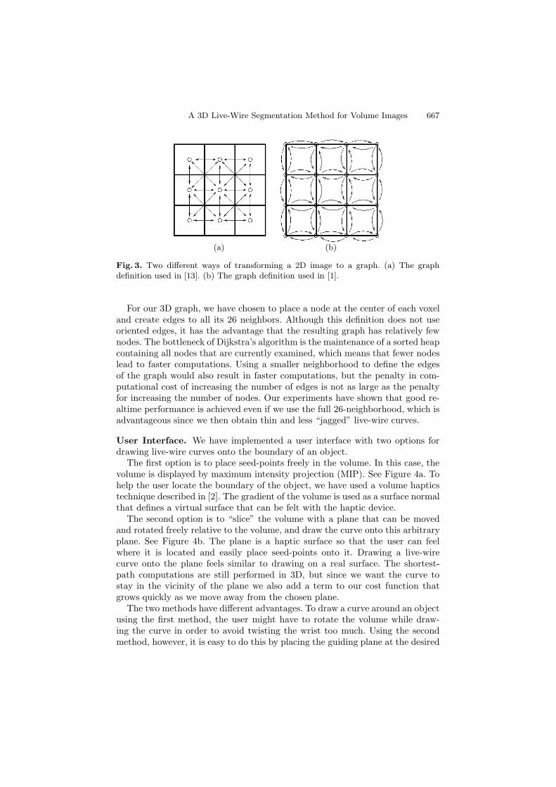
Fig. 3. Two different ways of transforming a 2D image to a graph. (a) The graphdefinition used in [13]. (b) The graph definition used in [1].

For our 3D graph, we have chosen to place a node at the center of each voxeland create edges to all its 26 neighbors. Although this definition does not useoriented edges, it has the advantage that the resulting graph has relatively fewnodes. The bottleneck of Dijkstra’s algorithm is the maintenance of a sorted heapcontaining all nodes that are currently examined, which means that fewer nodeslead to faster computations. Using a smaller neighborhood to define the edgesof the graph would also result in faster computations, but the penalty in com-putational cost of increasing the number of edges is not as large as the penaltyfor increasing the number of nodes. Our experiments have shown that good re-altime performance is achieved even if we use the full 26-neighborhood, which isadvantageous since we then obtain thin and less “jagged” live-wire curves.

User Interface. We have implemented a user interface with two options fordrawing live-wire curves onto the boundary of an object.

The first option is to place seed-points freely in the volume. In this case, thevolume is displayed by maximum intensity projection (MIP). See Figure 4a. Tohelp the user locate the boundary of the object, we have used a volume hapticstechnique described in [2]. The gradient of the volume is used as a surface normalthat defines a virtual surface that can be felt with the haptic device.

The second option is to “slice” the volume with a plane that can be movedand rotated freely relative to the volume, and draw the curve onto this arbitraryplane. See Figure 4b. The plane is a haptic surface so that the user can feelwhere it is located and easily place seed-points onto it. Drawing a live-wirecurve onto the plane feels similar to drawing on a real surface. The shortest-path computations are still performed in 3D, but since we want the curve tostay in the vicinity of the plane we also add a term to our cost function thatgrows quickly as we move away from the chosen plane.

The two methods have different advantages. To draw a curve around an objectusing the first method, the user might have to rotate the volume while draw-ing the curve in order to avoid twisting the wrist too much. Using the secondmethod, however, it is easy to do this by placing the guiding plane at the desired


(a) (b)

Fig. 4. (a) Placing seed-points freely in the volume using volume rendering and volumehaptics to locate the boundary of the object. (b) Drawing a live-wire curve onto aguiding plane.

cross-section of the object. When testing the application we have mainly usedthe second method for drawing curves, while the first method has been used forplacing single points (which are also considered to be closed curves).

4.2 Bridging Algorithm

We have based our bridging algorithm on the image foresting transform (IFT)[9]. The IFT is essentially Dijkstra’s algorithm, modified to allow an arbitrarynumber of seed-points as input for the computations. The result of using morethan one seed-point is that we find the shortest path from all pixels in the imageto any of the seed-points.

Using the IFT, it is quite straightforward to create a rough “wire-frame” ofthe surface we are looking for. To do this, we compute the optimal curves fromeach voxel in one of the curves, using all voxels of the other curve as seed-points.An illustration of the result is shown in Figure 5c.

Since the curves we compute are independent of each other, the result isgenerally not a tunnel-free surface. To fill the gaps between the curves we define apolygonal surface between adjacent curves, as shown in Figure 6. These polygonsare then rasterized using the method described in [14] to obtain a discrete surface.The result is exemplified in Figure 5d. Algorithm 1. shows the pseudo-code forour bridging algorithm.

Since all points on the second curve are not necessarily the “closest” point toa point on the first curve, a surface generated using our method is unfortunatelynot guaranteed to fit the “goal” curve exactly. In the worst case, all points onthe first curve have the same closest point on the second curve, in which casethe second curve will be approximated by this point only. Our current solutionto this is to apply the algorithm from both directions and return the union ofthe results, i.e., run the algorithm starting from one of the curves and then run


Algorithm 1. Bridging AlgorithmInput: Two sets of voxels, curve1 and curve2, that represent the initial curves.Output: A set of voxels, output, that represents the generated surface.Additional variables: Two sets of voxels, current curve and next curve that will beused to store intermediate curves. A voxel next voxel.

• current curve← curve1while next curve contains voxels that are not in curve2 do• next curve← emptyfor every voxel v in current curve do• next voxel← vif v is not in curve2 then• calculate the optimal path from v to curve2• set next voxel to be the next voxel along this path

end ifif next curve is not empty then• rasterize the polygon between the last voxel of next curve and the two

last voxels of current curve• add the resulting voxels to output• rasterize the polygon between next voxel and the last voxels of next curveand current curve• add the resulting voxels to output

end if• add next voxel to next curve

end for• rasterize the polygon between next voxel, the first voxel of next curve and thelast voxel of current curve• add the resulting voxels to output• rasterize the polygon between the first voxels of current curve and next curveand the last voxel of current curve• add the resulting voxels to output• current curve← next curve

end while

it again starting from the other curve. The result then always contains the twooriginal curves. However, if the shapes of the two curves differ to much “pockets”may be produced on the surface, as illustrated in Figure 7. In most cases whenthis happens, it is possible to reduce the error by drawing additional curvesinbetween the two original curves.

4.3 Performance

For a moderately sized volume (128x128x100) our algorithm runs in approxi-mately 1–20 seconds. The exact times depend on the length of the curves weare bridging and the distance between them. A number of things can be doneto improve the performance. For example, our current implementation uses aheap data structure to manage the sorted queue when computing the IFT, but


(a) (b) (c) (d)

Fig. 5. (a) A synthetic object. (b) Two closed curves on the boundary of the object.(c) Result of connecting the two curves by live-wires. (d) Result of using our proposedalgorithm.

Fig. 6. To obtain a tunnel-free surface, all live-wire curves generated between the twouser-defined curves are connected to their adjacent curves by triangular polygons

Fig. 7. If the shapes of the two curves differ too much, the surface produced by ourbridging algorithm may contain pockets


(a)

(b)

Fig. 8. (a) Segmentation of the liver in a 153x153x161 CT image of a human, obtainedwith our method by drawing 7 live-wire curves onto the boundary of the liver. (b)Surface rendering of the segmentation result.


according to [4] better performance can be achieved by using a circular queuestructure instead.

Tests on large volumes have not been possible due to the current memory-inefficient implementation where big amounts of data are stored redundantlyduring the shortest-path calculations. In future work, this will be made moreefficient.

5 Discussion and Future Work

Despite the issues mentioned in Section 4.2, preliminary tests of our appli-cation show promising results. We have segmented objects of varying com-plexity using a varying number of live-wire curves. In most cases, the closeddiscrete surfaces obtained are satisfactory representations of the underlying ob-ject. Figure 8 shows an example of a segmentation result obtained with ourmethod. The total segmentation time for this example, including user interac-tion, was approximately 3 minutes.

As stated in [1], a semi-automatic method should ultimately be measured byhow much it reduces the time it takes for the user to achieve a correct segmen-tation result. To verify the efficiency of our method, it would be therefore be ofinterest to make a user study to compare it with other segmentation methods.

Acknowledgements

Prof. Gunilla Borgefors at the Centre for Image Analysis, Swedish Universityof Agricultural Sciences, Uppsala, Sweden is acknowledged for her scientificsupport.

References

1. Falcao, A.X., Udupa, J.K., Samarasekera, S., Sharma, S.: User-steered imagesegmentation paradigms: Live wire and live lane. Graphical Models and ImageProcessing (60) (1998) 223–260

2. Vidholm, E., Tizon, X., Nystrom, I., Bengtsson, E.: Haptic guided seeding of MRAimages for semi-automatic segmentation. In: Proceedings of IEEE InternationalSymposium on Biomedical Imaging (ISBI’04). (2004) 278–281

3. Harders, M., Szekely, G.: Enhancing human-computer interaction in medical seg-mentation. Proceedings of the IEEE, Special Issue on Multimodal Human Com-puter Interfaces 9(91) (2003) 1430–1442

4. Falcao, A.X., Udupa, J.K., Miyazawa, F.K.: An ultra-fast user-steered image seg-mentation paradigm: Live wire on the fly. IEEE Transactions on Medical Imaging19(1) (2000) 55–62

5. Falcao, A.X., Udupa, J.K.: A 3D generalization of user-steered live-wire segmen-tation. Medical Image Analysis 4(4) (2000) 389–402

6. Knapp, M., Kanitsar, A., Groller, M.E.: Semi-automatic topology independentcontour based 2 1/2 D segmentation using live-wire. Journal of WSCG 20(1–3)(2004)


7. Schenk, A., Prause, G., Peitgen, H.O.: Efficient semiautomatic segmentation of3D objects in medical images. In: Proceedings of MICCAI 2000, Springer-Verlag(2000) 186–195

8. Hamarneh, G., Yang, J., McIntosh, C., Langille, M.: 3d live-wire-based semi-automatic segmentation of medical images. In: Proceedings of SPIE Medical Imag-ing: Image Processing. Volume 5747. (2005) 1597–1603

9. Falcao, A.X., Bergo, F.P.G.: Interactive volume segmentation with differentialimage foresting transforms. IEEE Transactions on Medical Imaging 23(9) (2004)

10. Reachin Technologies: (http://www.reachin.se) Accessed 23 January 2006.11. Technologies, S.: (http://www.sensable.com) Accessed 23 January 2006.12. Dijkstra, E.W.: A note on two problems in connexion with graphs. Numerische

Mathematik 1 (1959) 269–27113. Mortensen, E.N., Barrett, W.: Interactive segmentation with intelligent scissors.

Graphical Models and Image Processing 60(5) (1998) 349–38414. Kaufman, A.: Efficient algorithms for scan-converting 3D polygons. Computers

and Graphics 12(2) (1988) 213–219

A 3D Live-Wire Segmentation Method for Volume Images Using Haptic Interaction

Documents

Transcript of A 3D Live-Wire Segmentation Method for Volume Images Using Haptic Interaction