Intensity-Adaptive Segmentation of Single-EchoT1-Weighted Magnetic Resonance Images

Reza Momenan,1* Daniel Hommer,2 Robert Rawlings,2 Urs Ruttimann,2

Michael Kerich,2 and Daniel Rio2

1MedData Research, Vienna, Virginia 221822Laboratory of Clinical Studies, Division of Intramural Clinical & Biological Research, National

Institutes on Alcohol Abuse and Alcoholism, National Institutes of Health,Bethesda, Maryland 20892-1256

r r

Abstract: A procedure for segmentation of intracranial tissues, including cerebrospinal fluid surroundingthe brain, cortical and subcortical gray matter, and white matter, in a T1-weighted magnetic resonanceimage of the brain, has been developed. The proposed method utilizes information from the histogram ofpixel intensities of the intracranial image. Based on this information, an unsupervised K-means clusteringprocedure separates various tissue regions. Information about the approximate location of anatomicalregions within the intracranial space is used to detect ventricles and the caudate nuclei. First a descriptionand justification for the procedure is presented. Then the performance of the procedure is evaluated byanalysis of variance. In conclusion, the results of applying this procedure to 31 healthy subjects arepresented and future improvements are discussed.Hum. BrainMapping 5:194–205, 1997. r 1997Wiley-Liss,Inc.†

Key words: brain volume; gray matter; white matter; ventricle; clustering; region growing

r r

INTRODUCTION

Researchers in the clinical neurosciences are greatlyinterested in accurately measuring the volumes ofvarious compartments of the brain using magneticresonance images (MRI). However, automated segmen-tation of brain MRI into cerebrospinal fluid (CSF), graymatter (GM), and white matter (WM) is very difficult.Alternatively, manual outlining of these segments foreach of many slices of an MRI scan is time-consumingand tedious. Furthermore, because of inhomogeneitiesin the intensity of various areas as a result of partialvolume effects or the presence of mixed tissue, even a

trained rater or researcher cannot always accuratelydifferentiate regions of CSF, GM, and WM. Note thatthroughout this paper, the terms ‘‘partial volume’’ and‘‘mixed tissue’’ are used interchangeably. Investigatorshave also reported other sources of inhomogeneitiesdescriptively called ‘‘shading artifacts’’ [Zijdenbos andDawant, 1994]. Shading artifacts are seen as gradientsin the image introduced by the MRI acquisition sys-tem. However, shading artifacts will not be addressedin this paper since they were not observed in any of theimages we processed.Some researchers have attempted to automate seg-

mentation of MRI brain scans using double-echo MRIscans [Cohen et al., 1992; Harris et al., 1994; Cheng,1994; Ardekani et al., 1994; Byrum et al., 1996]. Othershave implemented methods based on adaptive con-tours [Fuchs et al., 1994; Warfield et al., 1996] orstatistical methods [Herndon et al., 1996; Wells et al.,

*Correspondence to: Reza Momenan, The National Institutes ofHealth 10/3C112, 10 Center Dr., MSC 1256, Bethesda, MD 20892-1256. E-mail:rezam@nih.govReceived for publication 18 November 1996; accepted 10 April 1997

r HumanBrain Mapping 5:194–205(1997)r

r 1997Wiley-Liss, Inc. †This article is a US Government workand, as such, is in the public domain in the United States of America.

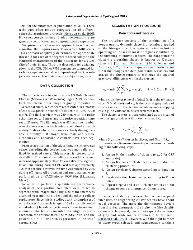
1994] for the automated segmentation of MRIs. Thesetechniques often require coregistration of differentspin-echo acquisition protocols [Herndon et al., 1996].However, coregistration and adaptive contouring aregenerally complicated and computationally expensive.We present an alternative approach based on an

algorithm that requires only T1-weighted MRI scans.This approach adaptively determines the appropriatethreshold for each of the segments based solely on thestatistical characteristics of the histogram for a givenslice of brain image. Thus, the thresholds for assigningpixels to the CSF, GM, or WM segment are computed foreach slice separately anddonotdependonglobal intersub-ject variations such as brain shape or subject diagnosis.

DATA COLLECTION

The subjects were imaged using a 1.5 Tesla GeneralElectric (Milwaukee, Wisconsin) Signa MRI scanner.Each volumetric brain image originally consisted of124 coronal slices, which were represented in a matrixof 2563 256 pixels (or voxels of size 0.937 3 0.937 3 2.0mm3). The field of view was 240 mm, with the pulseecho time set to 5 msec and the pulse repetition timeset to 25 msec. The flip angle was 45°, and the numberof excitationswas one. Each volume contained approxi-mately 75 sliceswhere the brainwas clearly distinguish-able. Currently, 100 images from male and femalealcoholics and nonalcoholic controls have been seg-mented.Prior to application of the algorithm, the intracranial

space, excluding the cerebellum, was manually out-lined by trained raters. This process is referred to asdeshelling. Themanual deshelling process for a trainedraterwas approximately 30 sec for each slice. The segmen-tation time during normal CPU load was approximately1.25min per slice; however, this timewas reduced by 20%during off-hours. All processing and computations wereperformed on a VAXStationr 4000/90A (Maynard,Mass.).In order to perform a quantitative performance

analysis of the algorithm, two raters were trained tosegment brain images manually. One of the raters wasa second-year medical student and the other a collegesophomore. Since this is a tedious task, a sample set ofonly 6 slices from each image of 8 (4 alcoholic and 4nonalcoholic) female subjects was chosen to segmentmanually. The 6 slices included 2 contiguous sliceseach from the anterior third, the middle third, and theposterior third of the brain, as presented in the set ofcoronal slices.

SEGMENTATION PROCEDURE

Basic tools and theories

The procedure consists of the combination of anonparametric dynamic clustering technique appliedto the histogram, and a region-growing techniqueoperating on the initial mask of regions identified bythe clustering of individual slices. The nonparametricclustering algorithm chosen is known as K-meansclustering [Tou and Gonzalez, 1974; Coleman andAndrews, 1978]. This technique uses an iterative algo-rithm that assigns the data points into K clusters andadjusts the cluster-centers to minimize the squaredgray-level differences within the clusters:

en 5 minoi51

N

oj51

M

(x ijn 2 ckn)2, k 5 1, 2, . . . K (1)

where xijn is the gray level of pixel (i, j) in the nth imageslice (N 3 M size) and ckn is the central gray value ofcluster k in slice n. The iterations continue until a stoppingrule, e.g., no variation in cluster centers, ismet.The cluster centers, ckn, are calculated as the mean of

the pixel gray-values within each cluster, i.e.,

ckn 51

Nkno

i,j[Skn

x ijn. (2)

where Skn is the kth cluster in slice n, and Nkn 5 #Skn.In summary, K-means clustering is performed accord-

ing to the following steps:

1. Assign K, the number of clusters (e.g., 2 for CSFand brain).

2. Assign K means or cluster centers to initialize theclustering procedure.

3. Assign pixels to K clusters according to Equation1.

4. Recalculate the cluster center according to Equa-tion 2.

5. Repeat steps 3 and 4 until cluster centers do notchange or some minimum condition is met.

K-means clustering performs best when the pixelintensities of neighboring cluster centers have aboutequal variance. The more the distributions deviatefrom this ideal assumption, the higher the false classifi-cation rate. In general, one cannot expect the varianceof gray and white matter volumes to be the same[Jackson et al., 1994]. However, with the right numberof tissue types selected, and segmentation within a

r AutomatedSegmentation ofT1-WeightedMRI r

r 195 r

slice, deviations from the ideal situation are not severe.Therefore, the nonparametric technique will performadequately under these conditions. The results of oursegmentation indicate that this is indeed the case.

Deshelling procedure

Each slice is manually deshelled to contain only theintracranial space. Deshelling means that the brain isseparated from scalp, skull, and the tissue layer underthe skull. A binary mask of the deshelled area, includ-ing brain and CSF, but excluding cerebellum, is gener-ated to limit the subsequent segmentation steps to theintracranial space.

CSF from brain segmentation

The histograms of intracranial images are usuallybimodal, where one peak corresponds to CSF/ventricu-lar regions and the other to the brain parenchyma

(gray/white matter) region (Fig. 1a). Hence, a K-meansclustering with K 5 2 was applied to separate CSFfrom parenchymal regions. However, since the K-means algorithm is very sensitive to the distributionalshape [Momenan, 1989], the distribution tails must beremoved to prevent their undue effect on the estima-tion of cluster centers. This is accomplished by apply-ing an initial threshold to the image that truncateshigher gray values and then this threshold. The thresh-old was determined from the average and standarddeviation of the intracranial histogram (Fig. 1b). Thebest results, in terms of the amount of CSF included ineach slice, were obtained with the threshold set to

Tn 5 µn 1 0.5sn (3)

where µn was the mean and sn the standard deviationof the intracranial pixel values for slice n. Applicationof the K-means algorithm (K 5 2) on the deshelledimage produced two clusters of pixel values. The

Figure 1.Segmentation of intracranial CSF from brain. a: Deshelling contour. b: Histogram of pixels insidedeshelling contour. c: Binary mask of segmented CSF. d: Binary mask of segmented brain.

r Momenan et al.r

r 196 r

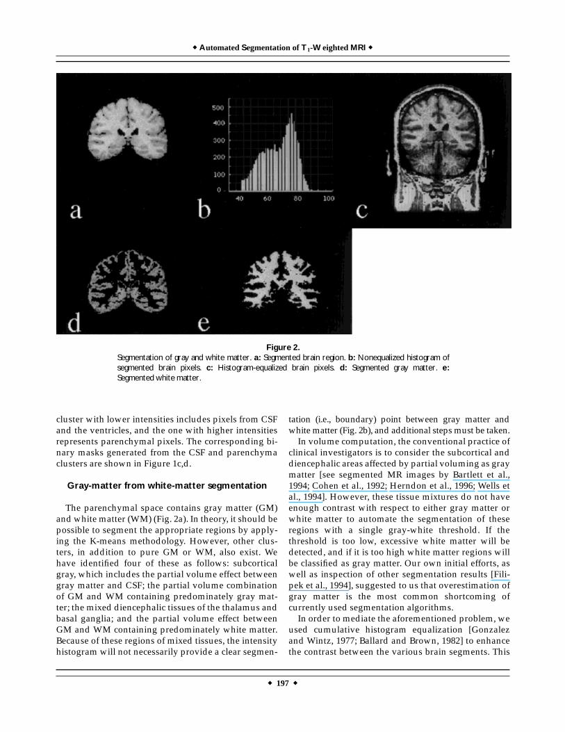
cluster with lower intensities includes pixels from CSFand the ventricles, and the one with higher intensitiesrepresents parenchymal pixels. The corresponding bi-nary masks generated from the CSF and parenchymaclusters are shown in Figure 1c,d.

Gray-matter from white-matter segmentation

The parenchymal space contains gray matter (GM)andwhite matter (WM) (Fig. 2a). In theory, it should bepossible to segment the appropriate regions by apply-ing the K-means methodology. However, other clus-ters, in addition to pure GM or WM, also exist. Wehave identified four of these as follows: subcorticalgray, which includes the partial volume effect betweengray matter and CSF; the partial volume combinationof GM and WM containing predominately gray mat-ter; the mixed diencephalic tissues of the thalamus andbasal ganglia; and the partial volume effect betweenGM and WM containing predominately white matter.Because of these regions of mixed tissues, the intensityhistogram will not necessarily provide a clear segmen-

tation (i.e., boundary) point between gray matter andwhitematter (Fig. 2b), and additional stepsmust be taken.In volume computation, the conventional practice of

clinical investigators is to consider the subcortical anddiencephalic areas affected by partial voluming as graymatter [see segmented MR images by Bartlett et al.,1994; Cohen et al., 1992; Herndon et al., 1996; Wells etal., 1994]. However, these tissue mixtures do not haveenough contrast with respect to either gray matter orwhite matter to automate the segmentation of theseregions with a single gray-white threshold. If thethreshold is too low, excessive white matter will bedetected, and if it is too high white matter regions willbe classified as gray matter. Our own initial efforts, aswell as inspection of other segmentation results [Fili-pek et al., 1994], suggested to us that overestimation ofgray matter is the most common shortcoming ofcurrently used segmentation algorithms.In order to mediate the aforementioned problem, we

used cumulative histogram equalization [Gonzalezand Wintz, 1977; Ballard and Brown, 1982] to enhancethe contrast between the various brain segments. This

Figure 2.Segmentation of gray and white matter. a: Segmented brain region. b: Nonequalized histogram ofsegmented brain pixels. c: Histogram-equalized brain pixels. d: Segmented gray matter. e:Segmented white matter.

r AutomatedSegmentation ofT1-WeightedMRI r

r 197 r

allows us to map a histogram h(g1) with the interval ofgray levelsDg1 into an approximately uniformly distrib-uted histogram h(g2) with the Dg2 interval such that

h(g1)Dg1 5 h(g2)Dg2 (4)

where gi represents the gray values and the intervalsDgi are chosen to increase the dynamic range of theimage. The ranges of g1 and g2 are kept equal, resultingin a more uniform histogram compared to the original.As a result of this procedure, pixel values in the middleregion of the histogram are mapped toward either end,which results in an enhanced contrast between grayand white matter. Figure 2c shows the histogram-equalized image which can be compared with theoriginal image in Figure 1a. This demonstrates thathistogram equalization stretches the difference be-tween pixel values and, hence, cluster centers of graymatter and white matter. Note that all segmentationprocesses at this step are performed on areas limited tothe parenchymal mask as shown in Figure 1d.Histogram equalization, however, creates an un-

wanted side effect in that it also increases image noise

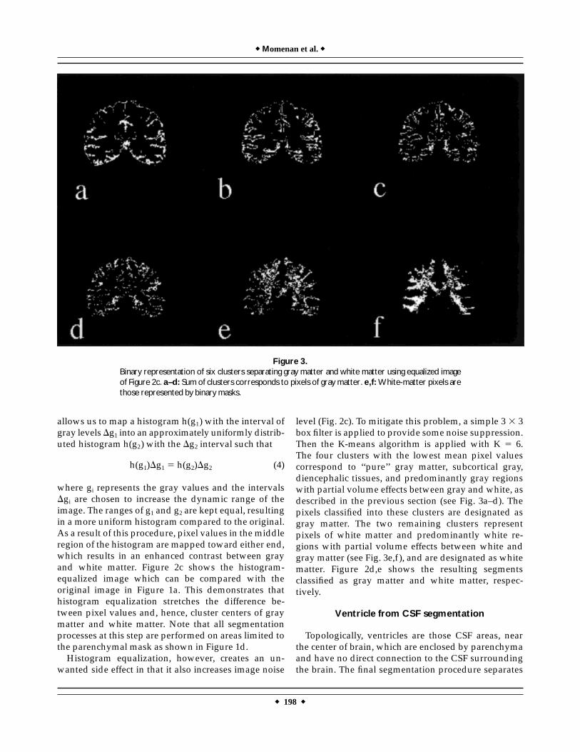
level (Fig. 2c). To mitigate this problem, a simple 3 3 3box filter is applied to provide some noise suppression.Then the K-means algorithm is applied with K 5 6.The four clusters with the lowest mean pixel valuescorrespond to ‘‘pure’’ gray matter, subcortical gray,diencephalic tissues, and predominantly gray regionswith partial volume effects between gray and white, asdescribed in the previous section (see Fig. 3a–d). Thepixels classified into these clusters are designated asgray matter. The two remaining clusters representpixels of white matter and predominantly white re-gions with partial volume effects between white andgray matter (see Fig. 3e,f), and are designated as whitematter. Figure 2d,e shows the resulting segmentsclassified as gray matter and white matter, respec-tively.

Ventricle from CSF segmentation

Topologically, ventricles are those CSF areas, nearthe center of brain, which are enclosed by parenchymaand have no direct connection to the CSF surroundingthe brain. The final segmentation procedure separates

Figure 3.Binary representation of six clusters separating gray matter and white matter using equalized imageof Figure 2c. a–d: Sum of clusters corresponds to pixels of gray matter. e,f:White-matter pixels arethose represented by binary masks.

r Momenan et al.r

r 198 r

ventricles from CSF. A region-growing algorithm isapplied to the intracranial CSF in order to segment theventricles from CSF.Region growing is an image processing technique

that uses a similarity criterion to partition an imageinto contiguous segments with similar properties[Gonzalez and Wintz, 1977]. In our application, thesimilarity criterion is that a pixel must have beenclassified as CSF. If the pixel under examination is CSFand is attached to other pixels with the same property,the algorithm continues to examine the neighboringpixels until it fails to find any additional pixels with asimilar property. This process continues until all CSFpixels in the center of the brain are examined.To initiate region growing, a seed point must be

specified. For each slice this seed point was chosen tobe the center of the parenchyma, found by calculatingfirst-order moments from the binary mask of theparenchymal space. These moments are determinedfrom the projection of this binary mask along thehorizontal and vertical axes. If a region touches theboundary of the parenchymal mask, it is considered to

be part of the surrounding CSF; otherwise, it is consid-ered to be ventricular. This process continues until allCSF pixels enclosed within the area of the parenchy-mal mask are processed as above.A source of error in applying this procedure is due to

CSF segments within sulci that appear to be discon-nected from the CSF covering the periphery of thebrain. Such sulci are usually found in slices near theoccipital or frontal poles. Although the detection ofventricles in our test set was for the most part success-ful and errors occurred infrequently, the differentiationof ventricles from peripheral CSF is problematic inslices near the poles and requires review and manualediting. However, in all cases the region-growingprocess greatly expedites this manual task.

COMPARISON OF AUTOMATED VS. MANUALSEGMENTATION

For facilitation in reading the following section, afew terms are defined here. A region is an area seg-mented by a clinical researcher or a segmentationprocedure and can refer to CSF, ventricle, gray matter,or white matter. Machine refers to the automatedprocedure. Rater refers to the operator of the segmenta-tion method, either human or machine.Given the nature of the problem, no investigator can

claim error-free (automated or even nonautomated)segmentation of MR images. Therefore, we chose tovalidate our segmentation by investigating whetherthe error due to automation is acceptable in compari-son with human raters’ variability in segmentingdifferent tissue types. Hence, we did not attempt to testthe accuracy of human raters or the machine, butrather investigated whether the performance of themachine is compatible with that of any human rater.However, the following steps were carried out toensure the reliability of the segmentation by the trainedraters.

TABLE I. Interaction between three raters (two humanand one machine) and four regions (CSF, ventricles, gray

matter, and white matter)

Slice

Raters 3 regions interaction(Ps 5 0.01)

F(2,14) P

1 16.6405 0.00022 10.4062 0.00173 7.5410 0.00604 2.3913 0.12795 5.1861 0.02066 7.2381 0.0069Total volume 32.0439 0.000006

TABLE II. Rater effect for CSF

Slice

Raters for CSF(Prs 5 0.0025)

Rater 1 vs. machine(Prsr 5 0.0008)

Rater 1 vs. rater 2(Prsr 5 0.0008)

Rater 2 vs. machine(Prsr 5 0.0008)

F(2,14) P F(1,7) P F(1,7) P F(1,7) P

1 33.26713 .000005 22.40430 .002124 25.88730 .001418 42.52281 .0003282 24.01402 .000030 13.57756 .007810 17.17625 .004325 32.92805 .0007073 25.96745 .000019 21.55361 .002362 15.78316 .005373 32.17038 .0007574 50.62461 .000000 53.35694 .000162 27.39970 .001207 55.38285 .0001445 9.83231 .002151 5.03916 .059653 56.72588 .000134 13.35830 .0081256 10.19486 .001853 5.46001 .052100 38.31860 .000450 14.60621 .006527Total volume 36.21698 .000003 22.91439 .001996 33.98872 .000644 45.65225 .000263

r AutomatedSegmentation ofT1-WeightedMRI r

r 199 r

First, each rater segmented nonventricle-CSF, ven-tricle-CSF, gray matter, and white matter by outliningthe areas of these tissue types. Then, binary masks ofeach tissue type were generated and color representa-tions were transparently laid over the MR images. Theraters were then asked to use their best judgment indetermining the accuracy of each tissue type at thepixel level. This means that the raters were able toinspect the accuracy of their segmentation by alterna-tively removing the mask or ‘‘seeing through’’ it untilthey were confident about their segmentation result. Inthat way, pixels in the segmentation masks could beedited such that they reflected the raters’ judgmentsregarding tissue types.Machine performance was qualitatively validated

by visually inspecting the masks of each region trans-parently laid over the original images.Quantitative assessment of machine performance

relative to the two trained human raters, when we willhereafter call rater 1 and rater 2, was performed asfollows. An often-used measure of comparison is thecorrelation coefficient between the number of pixels incorresponding regions (segmented by different raters).It measures the interrater reliability in terms of total

tissue volume detected [Zijdenbos and Dawant, 1994],and in this context indicated whether the machine andhuman raters in general agreed on the criteria fordetermining the various tissue types. The correlationof the number of pixels in each region (CSF, ventricu-lar, and gray and white matter) among all three raterswas fairly high (r . .70) in every case. However, thecorrelation coefficient alone is not a sufficient measureof similarity [Bland and Altman, 1986] or of overlapamong corresponding segments. The fact that themachine and human raters are highly correlated inselecting more of one tissue type and less of anotherfrom slice to slice, or from subject to subject, does notindicate whether they agree on the absolute amounts.To compare the discrepancy among the raters in termsof the absolute amounts of tissues classified, we per-ormed a two-way repeated-measures analysis of vari-ance (ANOVA) with respect to the repeated factors:regions (CSF, ventricles, GM, and WM) and raters(rater 1, rater 2, and machine).Table I presents the results of testing the interaction

between raters and regions. In order to correct for theseven multiple tests (for six slices and the total volumeof the six slices), the level of significance chosen was

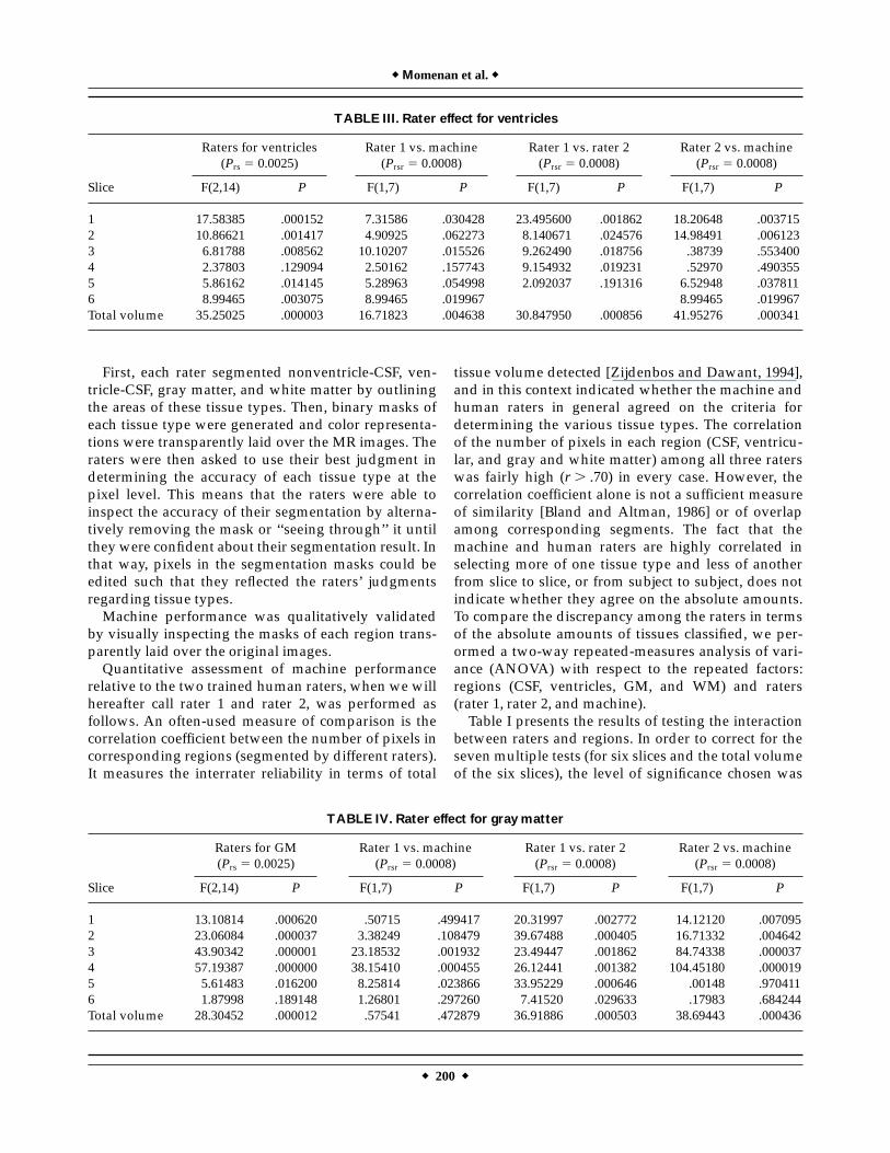
TABLE III. Rater effect for ventricles

Slice

Raters for ventricles(Prs 5 0.0025)

Rater 1 vs. machine(Prsr 5 0.0008)

Rater 1 vs. rater 2(Prsr 5 0.0008)

Rater 2 vs. machine(Prsr 5 0.0008)

F(2,14) P F(1,7) P F(1,7) P F(1,7) P

1 17.58385 .000152 7.31586 .030428 23.495600 .001862 18.20648 .0037152 10.86621 .001417 4.90925 .062273 8.140671 .024576 14.98491 .0061233 6.81788 .008562 10.10207 .015526 9.262490 .018756 .38739 .5534004 2.37803 .129094 2.50162 .157743 9.154932 .019231 .52970 .4903555 5.86162 .014145 5.28963 .054998 2.092037 .191316 6.52948 .0378116 8.99465 .003075 8.99465 .019967 8.99465 .019967Total volume 35.25025 .000003 16.71823 .004638 30.847950 .000856 41.95276 .000341

TABLE IV. Rater effect for gray matter

Slice

Raters for GM(Prs 5 0.0025)

Rater 1 vs. machine(Prsr 5 0.0008)

Rater 1 vs. rater 2(Prsr 5 0.0008)

Rater 2 vs. machine(Prsr 5 0.0008)

F(2,14) P F(1,7) P F(1,7) P F(1,7) P

1 13.10814 .000620 .50715 .499417 20.31997 .002772 14.12120 .0070952 23.06084 .000037 3.38249 .108479 39.67488 .000405 16.71332 .0046423 43.90342 .000001 23.18532 .001932 23.49447 .001862 84.74338 .0000374 57.19387 .000000 38.15410 .000455 26.12441 .001382 104.45180 .0000195 5.61483 .016200 8.25814 .023866 33.95229 .000646 .00148 .9704116 1.87998 .189148 1.26801 .297260 7.41520 .029633 .17983 .684244Total volume 28.30452 .000012 .57541 .472879 36.91886 .000503 38.69443 .000436

r Momenan et al.r

r 200 r

conservatively set to Ps 5 0.01 (approximately 0.1 foroverall level of significance). From this table it is clearthat except for perhaps slices 4 and 5, there aredisagreements among the raters in determining thetissue types. We then tested for simple effects, i.e., wecompared the raters for each individual region todetermine the significance of the disagreement insegmenting each tissue type separately.Tables II–V show the repeated-measures ANOVA

results on raters vs. a particular region and the resultsof the pairwise comparison. Note that the P value forthe raters vs. a given region is now calculated from

Prs 5 Ps/4 5 0.0025, where the denominator 4 is usedbecause there are four regions (CSF, ventricle, GM, andWM). For pairwise comparison we computed the Pvalue as Prsr 5 Prs/3 5 0.0008 because there are threeraters (two human raters plus the machine). Then, anyP value greater than those presented above indicatessimilar segmentation performance.These results indicate that rater 1 and the machine

performed similarly in almost all cases. Furthermore,there are significant differences in the performance ofrater 1 vs. rater 2 in some of the slices regarding CSFand WM segmentation. There are also quite a few

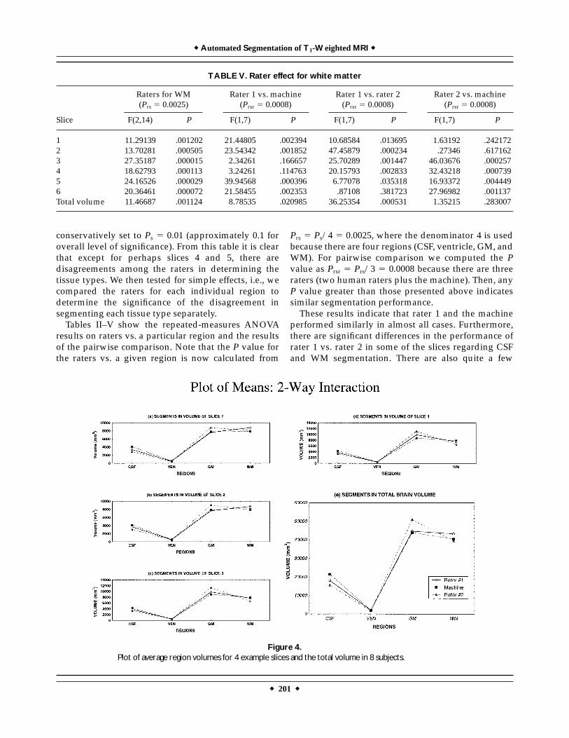
TABLE V. Rater effect for white matter

Slice

Raters for WM(Prs 5 0.0025)

Rater 1 vs. machine(Prsr 5 0.0008)

Rater 1 vs. rater 2(Prsr 5 0.0008)

Rater 2 vs. machine(Prsr 5 0.0008)

F(2,14) P F(1,7) P F(1,7) P F(1,7) P

1 11.29139 .001202 21.44805 .002394 10.68584 .013695 1.63192 .2421722 13.70281 .000505 23.54342 .001852 47.45879 .000234 .27346 .6171623 27.35187 .000015 2.34261 .166657 25.70289 .001447 46.03676 .0002574 18.62793 .000113 3.24261 .114763 20.15793 .002833 32.43218 .0007395 24.16526 .000029 39.94568 .000396 6.77078 .035318 16.93372 .0044496 20.36461 .000072 21.58455 .002353 .87108 .381723 27.96982 .001137Total volume 11.46687 .001124 8.78535 .020985 36.25354 .000531 1.35215 .283007

Figure 4.Plot of average region volumes for 4 example slices and the total volume in 8 subjects.

r AutomatedSegmentation ofT1-WeightedMRI r

r 201 r

significant differences for CSF, GM, and WM regionsbetween rater 2 and the machine. Note that thedifference between rater 1 and rater 2 for all regions oftotal volume is significant, whereas none of the totalregion volumes differed significantly between rater 1and the machine. Even though rater 1 and rater 2 havea very high correlation (CSF, r . 0.86; ventricles,r . 0.98, GM, r . 0.72; and WM, r . 0.86) for theirregion segmentation, the mean values of their seg-mented areas are significantly different. Figure 4 showsthe plots of mean value of regions in several slices andthe total volume. It is clear that there are only smalldifferences in the slice-by-slice volumes of the ven-tricles between the three raters. Also note that typicallythe machine determined the mean value of each regioncloser to rater 1 than to rater 2.The fact that the differences between human raters

were more often significant than those between themachine and either of the raters is interesting and canbe explained by the following observations. Althoughboth human raters were trained to segment regionsbased on the same criteria, rater 1 utilized a priori

knowledge of brain anatomy in outlining the segmentsinstead of relying solely on the gray values of thepixels as displayed. This means, e.g., that if rater 1observed an image pixel to be within the range for graymatter, but knew from prior knowledge that anatomi-cally it should represent white matter, it was picked aswhite, and visa versa. By comparison, rater 2 strictlytrusted the differences in the displayed image intensi-ties. Themachine, as a result of the histogram equaliza-tion procedure, could detect more subtle intensitydifferences, and performed more similarly to rater 1.

RESULTS AND DISCUSSION

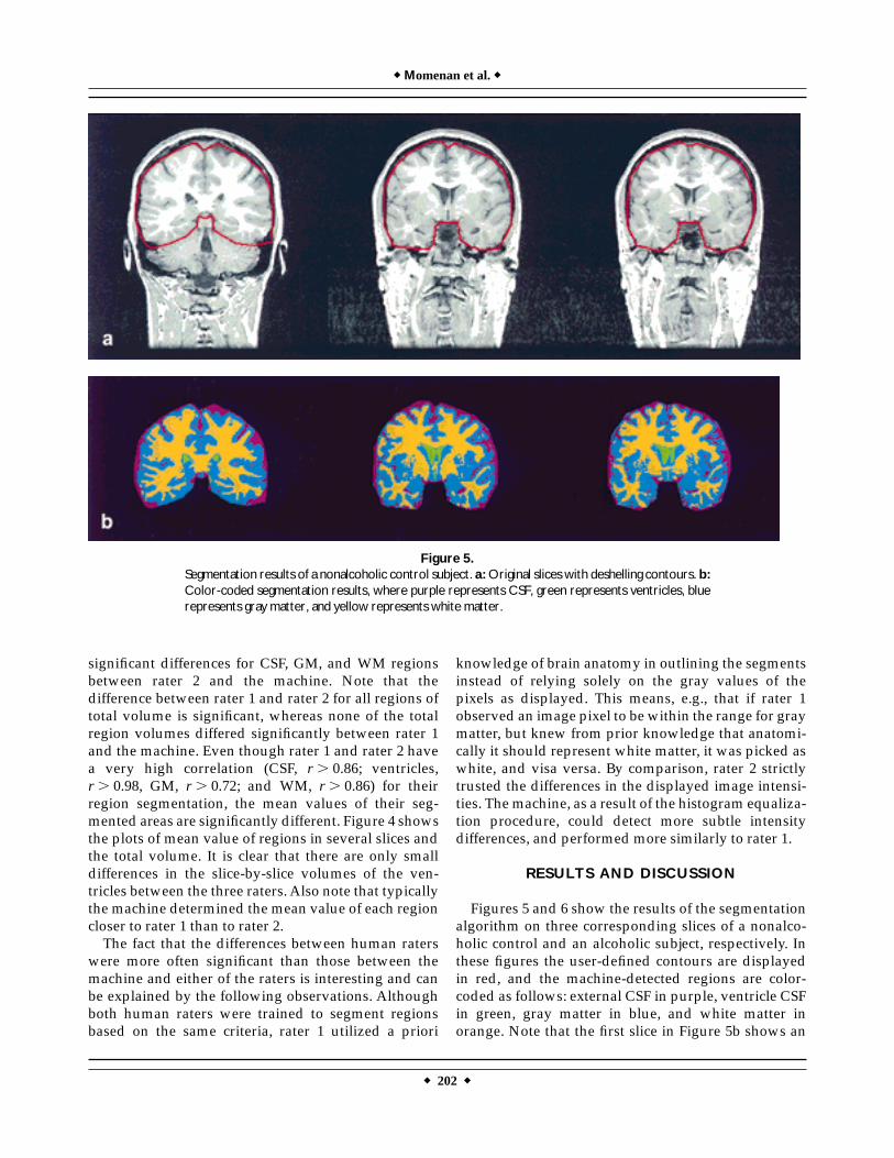
Figures 5 and 6 show the results of the segmentationalgorithm on three corresponding slices of a nonalco-holic control and an alcoholic subject, respectively. Inthese figures the user-defined contours are displayedin red, and the machine-detected regions are color-coded as follows: external CSF in purple, ventricle CSFin green, gray matter in blue, and white matter inorange. Note that the first slice in Figure 5b shows an

Figure 5.Segmentation results of a nonalcoholic control subject. a:Original slices with deshelling contours. b:Color-coded segmentation results, where purple represents CSF, green represents ventricles, bluerepresents gray matter, and yellow represents white matter.

r Momenan et al.r

r 202 r

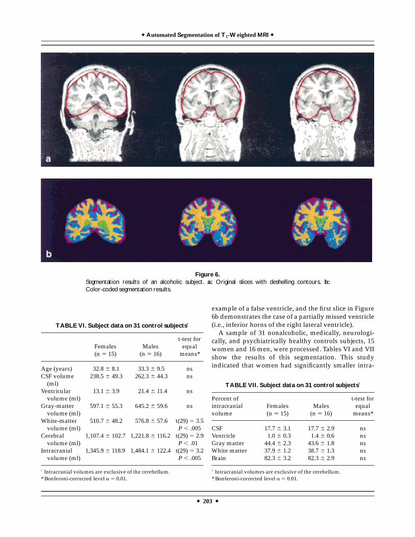
example of a false ventricle, and the first slice in Figure6b demonstrates the case of a partially missed ventricle(i.e., inferior horns of the right lateral ventricle).A sample of 31 nonalcoholic, medically, neurologi-

cally, and psychiatrically healthy controls subjects, 15women and 16 men, were processed. Tables VI and VIIshow the results of this segmentation. This studyindicated that women had significantly smaller intra-

TABLE VII. Subject data on 31 control subjects†

Percent ofintracranialvolume

Females(n 5 15)

Males(n 5 16)

t-test forequalmeans*

CSF 17.7 6 3.1 17.7 6 2.9 nsVentricle 1.0 6 0.3 1.4 6 0.6 nsGray matter 44.4 6 2.3 43.6 6 1.8 nsWhite matter 37.9 6 1.2 38.7 6 1.3 nsBrain 82.3 6 3.2 82.3 6 2.9 ns

† Intracranial volumes are exclusive of the cerebellum.* Bonferoni-corrected level a 5 0.01.

Figure 6.Segmentation results of an alcoholic subject. a: Original slices with deshelling contours. b:Color-coded segmentation results.

TABLE VI. Subject data on 31 control subjects†

Females(n 5 15)

Males(n 5 16)

t-test forequalmeans*

Age (years) 32.8 6 8.1 33.3 6 9.5 nsCSF volume(ml)

238.5 6 49.3 262.3 6 44.3 ns

Ventricularvolume (ml)

13.1 6 3.9 21.4 6 11.4 ns

Gray-mattervolume (ml)

597.1 6 55.3 645.2 6 59.6 ns

White-mattervolume (ml)

510.7 6 48.2 576.8 6 57.6 t(29) 5 3.5P , .005

Cerebralvolume (ml)

1,107.4 6 102.7 1,221.8 6 116.2 t(29) 5 2.9P , .01

Intracranialvolume (ml)

1,345.9 6 118.9 1,484.1 6 122.4 t(29) 5 3.2P , .005

† Intracranial volumes are exclusive of the cerebellum.* Bonferoni-corrected level a 5 0.01.

r AutomatedSegmentation ofT1-WeightedMRI r

r 203 r

cranial volumes than men. Similarly, the volume ofwhite matter was also significantly smaller in women.When segmented brain volumes were converted topercentages of intracranial volume, men and womenhad virtually identical proportions.The results of our segmentation are similar to results

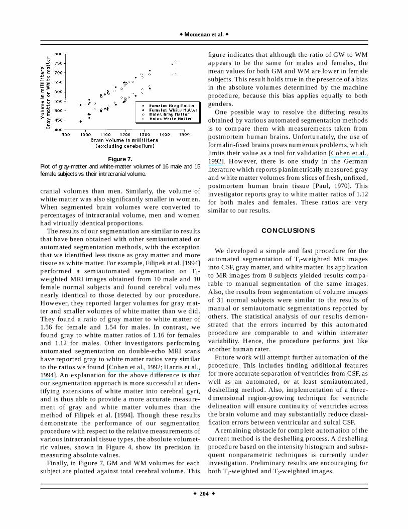
that have been obtained with other semiautomated orautomated segmentation methods, with the exceptionthat we identified less tissue as gray matter and moretissue as white matter. For example, Filipek et al. [1994]performed a semiautomated segmentation on T1-weighted MRI images obtained from 10 male and 10female normal subjects and found cerebral volumesnearly identical to those detected by our procedure.However, they reported larger volumes for gray mat-ter and smaller volumes of white matter than we did.They found a ratio of gray matter to white matter of1.56 for female and 1.54 for males. In contrast, wefound gray to white matter ratios of 1.16 for femalesand 1.12 for males. Other investigators performingautomated segmentation on double-echo MRI scanshave reported gray to white matter ratios very similarto the ratios we found [Cohen et al., 1992; Harris et al.,1994]. An explanation for the above difference is thatour segmentation approach is more successful at iden-tifying extensions of white matter into cerebral gyri,and is thus able to provide a more accurate measure-ment of gray and white matter volumes than themethod of Filipek et al. [1994]. Though these resultsdemonstrate the performance of our segmentationprocedure with respect to the relative measurements ofvarious intracranial tissue types, the absolute volumet-ric values, shown in Figure 4, show its precision inmeasuring absolute values.Finally, in Figure 7, GM and WM volumes for each

subject are plotted against total cerebral volume. This

figure indicates that although the ratio of GW to WMappears to be the same for males and females, themean values for both GM andWM are lower in femalesubjects. This result holds true in the presence of a biasin the absolute volumes determined by the machineprocedure, because this bias applies equally to bothgenders.One possible way to resolve the differing results

obtained by various automated segmentation methodsis to compare them with measurements taken frompostmortem human brains. Unfortunately, the use offormalin-fixed brains poses numerous problems, whichlimits their value as a tool for validation [Cohen et al.,1992]. However, there is one study in the Germanliterature which reports planimetrically measured grayandwhite matter volumes from slices of fresh, unfixed,postmortem human brain tissue [Paul, 1970]. Thisinvestigator reports gray to white matter ratios of 1.12for both males and females. These ratios are verysimilar to our results.

CONCLUSIONS

We developed a simple and fast procedure for theautomated segmentation of T1-weighted MR imagesinto CSF, gray matter, and white matter. Its applicationto MR images from 8 subjects yielded results compa-rable to manual segmentation of the same images.Also, the results from segmentation of volume imagesof 31 normal subjects were similar to the results ofmanual or semiautomatic segmentations reported byothers. The statistical analysis of our results demon-strated that the errors incurred by this automatedprocedure are comparable to and within interratervariability. Hence, the procedure performs just likeanother human rater.Future work will attempt further automation of the

procedure. This includes finding additional featuresfor more accurate separation of ventricles from CSF, aswell as an automated, or at least semiautomated,deshelling method. Also, implementation of a three-dimensional region-growing technique for ventricledelineation will ensure continuity of ventricles acrossthe brain volume and may substantially reduce classi-fication errors between ventricular and sulcal CSF.A remaining obstacle for complete automation of the

current method is the deshelling process. A deshellingprocedure based on the intensity histogram and subse-quent nonparametric techniques is currently underinvestigation. Preliminary results are encouraging forboth T1-weighted and T2-weighted images.

Figure 7.Plot of gray-matter and white-matter volumes of 16 male and 15female subjects vs. their intracranial volume.

r Momenan et al.r

r 204 r

Although the automated separation of ventriclesfrom CSF is not perfect, given the results we have hadso far, even personnel without anatomical knowledgecan be easily trained to perform the task of reviewingand editing the automated results.

ACKNOWLEDGMENTS

The authors thank Cristine Bernard and RebeccaHommer for their tireless work of segmenting theimages for comparisons with this procedure. We alsoappreciate the hard work of Cristina Souto in outliningthe intracranial volumes of many of our subjects.

REFERENCES

Ardekani BA, Braun M, Kanno I, Hutton BF (1994): Automaticdetection of intradural spaces in MR images. J Comput AssistTomogr 18:963–969.

Ballard DH, Brown CM (1982): Computer Vision, Englewood Cliffs,NJ: Prentice Hall.

Bartlett TQ, Vannier MW, McKeel DW, Gado M, Hildebolt CF,Walkup R (1994): Interactive segmentation of cerebral graymatter, white matter, and CSF: Photographic and MR images.Comput Med Imaging Graphics 18:449–460.

Bland JM, Altman DG (1986): Statistical methods for assessingagreement between two methods of clinical measurement. Lan-cet 1:307–310.

Byrum CE, MacFall JR, Charles HC, Chitilla VR, Boyko OB, Up-church L, Smith JS, Rajagopalan P, Passe T, Kim D, Xanthakos S,Ranga K, Krishnan R (1996): Accuracy and reproducibility ofbrain and tissue volumes using a magnetic resonance segmenta-tion method. Psychiatry Res 67:215–234.

Cheng KH (1994): In vivo tissue characterization of human brain bychisquares parameter maps: Multiparameter proton T2-relax-ation analysis. Magn Reson Imaging 12:1099–1109.

Cohen G, Andreasen NC, Alliger R, Arndt S, Kuan J, Yuh WTC,Ehrhardt J (1992): Segmentation techniques for the classificationof brain tissue usingmagnetic resonance imaging. Psychiatry Res45:33–51.

Coleman GB, Andrews HC (1978): Image segmentation by cluster-ing. Proc IEEE 67:773–785.

Filipek PA, Richelme C, Kennedy DN, Caviness VS (1994): Theyoung adult human brain: An MRI-based morphometric analy-sis. Cereb Cortex 4:344–360.

Fuchs M, Wagner M, Wischmann HA, Ottenberg K, Dossel O (1994):Possibilities of functional brain imaging using a combination ofMEG and MRT. In: C. Pantev Oscillatory Event-Related BrainDynamics. New York: Plenum Press 435–457.

Gonzalez RC, Wintz P (1977): Digital Image Processing, Reading,MA: Addison-Wesley.

Harris GJ, Barta PE, Peng LW, Lee S, Brettschneider PD, Shah A,Henderer JD, Schlaepfer TE, Pearlson GD (1994): MR volumesegmentation of gray matter and white matter using manualthresholding: Dependence on image brightness, Am J Neurol Res15:225–230.

Herndon RC, Lancaster JL, Toga AW, Fox PT (1996): Quantificationof white matter and gray matter volumes from T1 parametricimages using fuzzy classifiers. J Magn Reson Imaging 6:425–435.

Jackson EF, Narayana PA, Falconer JC (1994): Reproducibility ofnonparametric feature map segmentation for determination ofnormal human intracranical volumes with MR images data. JMagn Reson Imaging 4:693–670.

Momenan R (1989): Quantitative Detection and Display of Multidi-mensional Information in Diagnostic Ultrasound, Dissertation.Washington, DC: George Washington University.

Paul F (1971): BiometrischeAnalyse der Frishvolumina der Großhirn-rinde und des Prosencephalon von 31 menschlichen, adultenGehirnen. Anat Entwickl Gesch 133:325–368.

Tou JT, Gonzalez RC (1974): Pattern Recognition Principles,Waltham,MA: Addison-Wesley.

Warfield S, Dengler J, Zaers J, Guttmann CRG, Wells WM, EttingerGJ, Hiller J, Kikinis R (1996): Automatic identification of greymatter structures from MRI to improve the segmentation ofwhite matter lesions. Journal of Image Guided Surgery, vol. 1,No. 6:326–338.

Wells WM, Grimson WEL, Kikinis R, Jolesz FA (1994): Statisticalintensity correction and segmentation of MRI data. SPIE 2359:13–24.

Zijdenbos AP, Dawant BM (1994): Brain segmentation and whitematter lesion detection in MR images. Crit Rev Biomed Eng22:401–465.

r AutomatedSegmentation ofT1-WeightedMRI r

r 205 r