a comparative analysis of dairy production systems in New ...
257
Copyright is owned by the Author of the thesis. Permission is given for a copy to be downloaded by an individual for the purpose of research and private study only. The thesis may not be reproduced elsewhere without the permission of the Author.
-
Upload
khangminh22 -
Category
Documents
-
view
2 -
download
0
Transcript of a comparative analysis of dairy production systems in New ...

Copyright is owned by the Author of the thesis. Permission is given for a copy to be downloaded by an individual for the purpose of research and private study only. The thesis may not be reproduced elsewhere without the permission of the Author.

Measuring performance in farming: A comparative analysis
of dairy production systems in New Zealand and Chile
A thesis presented in partial fulfilment of the requirements for the degree of
Master of AgriScience
at Massey University, Turitea, Palmerston North,
New Zealand
Licy Maren Beux Garcia
2013


i
Abstract
The purpose of this work was to identify, examine, and compare the key performance indicators and
drivers of success of pasture-based dairy systems in New Zealand and Chile. Key similarities and
differences between dairy farming systems in these countries were identified by analysing data
provided by DairyBase and, its Chilean counterpart, TodoagroBase. Comparable observations were
nested using country-specific classification systems based on existing knowledge, followed by the
estimation of efficiency scores for each individual observation within these classes using Data
Envelopment Analysis (DEA). Efficiency scores were then attached to the original datasets and used
as the response variable in several country-specific Regression Partitioning Trees. This procedure
identified the most relevant benchmarks in each country and showed that there are various pathways
to high efficiency. Knowledge gains provided by this research are expected to influence farming
practices and management, research and extension, and to encourage future cooperation between the
two countries.
Dairy farmers in New Zealand and Chile benefit from low-cost production advantages because of
their favourable environment for pasture-based dairying, efficiently and profitably producing milk at
a lower cost than the world’s average. However, a large variability in farming systems within the
countries was identified, as were different benchmarks. In New Zealand, herd productivity and
labour played key roles in defining efficiency, while in Chile, herd productivity and supplements fed
per litre of milk produced were key indicators explaining efficiency. In New Zealand, operating cost
per kg of milk solids, return on Assets (ROA), operating profit margin (OPM), operating profit per
hectare, and asset turnover (ATR) were also major indicators. In Chile, gross farm revenue per cow,
cost of production per litre of milk produced, wages per litre, operating profit per cow and ATR
were also highlighted. The absence of indicators such as ROA in Chile was noticeable.
Reasons for different key performance indicators occurring in each country stem from history to
geography, and have resulted in differences in values and goals. New Zealand farmers are
profitability and cost-focused, looking alternatively to both OPM and the capital invested. Chilean
farmers are revenue-focused and respond strongly to milk:feed price ratio and to the efficiency in the
use of supplement. In both countries, the systems are evolving in similar ways, gradually increasing
intensification levels and specialisation. In both countries, consistently high performing farms are
efficient at producing both milk and revenue, and are more likely to have higher herd productivity
and labour efficiency than poorer performers. In New Zealand, consistently efficient farms also had
significantly better asset use as reflected by their ROA and ATR. In Chile better performers used
significantly less supplement per litre of milk produced.
Keywords: pasture-based, farming system, efficiency, benchmarks, New Zealand, Chile

ii

iii
Acknowledgements
Many thanks go to the New Zealand Ministry of Foreign Affairs and Trade and to Sylvia
Hooker and her beautiful team: Olive, James, Leuiana, and Sue from the NZAID programme. A
special thank you, too, to Natalia Benquet from the International Support Office; Alfredo and I
will always be grateful to and remember you all.
Thank you to all the direct and indirect contributors to this study. After being introduced to
Nicola Shadbolt in 2010 by Daniel Conforte, I got to know Nicola as an advisor, a professor,
and as a supervisor. For a number of reasons, Nicola taught me what kiwi humility really
means. Ever since 2010, it has been an honour; thank you. Special thanks to Elizabeth Dooley
for being my supervisor, for looking after me, and for teaching and guiding me during the highs
and lows of this process. Thanks also to Chris Dake and Jonathan Godfrey for sharing a bit of
your brilliant minds and ideas with me. From the department, thanks Lee-Anne, Kate, Linda,
and Denise Stewart for always being willing to help. From Uruguay, Ariel Asuaga has been a
friend and a great source of inspiration and confidence.
At Massey, during my first year in New Zealand, I had the pleasure of assisting to the classes of
Marta Camps, Dave Gray, Michael Hedley, David Horne, Matthew Irwin, Peter Kemp, Cory
Matthews, Alan Palmer, Ranvir Singh, and Mike Tuohy. Thank you also to Lisa Haarhoff and
Ian Furkert. In particular, I am grateful to Tania, Julia Rayner, Jacqui Burne, and Lois
Wilkinson from the Centre for Teaching and Learning, for your time and patience; you have
been a great help all the way!
Thanks to the Modelling and Breeding Club for sharing your knowledge and experiences; to
some of you also for being our friends. To my office mate, Federico: it has been good fun
despite the ‘disturbed environment’. Thank you to the Kay (one special thought goes to our
favourite chestnut, Squash, and grey, Saigo), the Lane, the Claridge, and the Guscott families
for helping us to understand several aspects of New Zealand farming systems, combining both
fun and work.
To our ‘gringo’ friends: the Wier (incredible Harry and Chloe, Laura, Tessa, Peter, and the
lovely Ashley), the Charteris, and the Dobson (including all your beautiful horses) families.
Thanks Aotearoa. Haere ra. Finally, we offer a special acknowledgement to our friends from the
Latin American community at Massey University and Palmerston North.
Finally, thanks go to our many friends in Uruguay, including Quique Iturralde and Carlos
Bautes, who are gone forever. To our families; you are always in our hearts and thoughts. Thank
you for coming and sharing this awesome place and also for patiently waiting for us to come
back home, including ‘abuela Marficia’,… somewhere. Licy Maren

iv

v
TABLE OF CONTENTS
ABSTRACT .................................................................................................................................. i
ACKNOWLEDGEMENTS ....................................................................................................... iii
LIST OF TABLES ..................................................................................................................... ix
LIST OF FIGURES ................................................................................................................... xi
1. INTRODUCTION. . ................................................................................................................ 1
1.1 The Country Context ............................................................................................................... 3
1.2 Research Motivation ............................................................................................................... 4
1.3 Statement of Purpose ............................................................................................................... 4
1.4 Research Questions and Specific Objectives .......................................................................... 4
1.5 Outline of the Study ................................................................................................................ 5
2. LITERATURE REVIEW. . .................................................................................................... 7
2.1 Pasture–Based Dairy Systems ................................................................................................. 7 2.1.1 Milk output from pasture. ................................................................................................. 8
2.1.1.1 Seasonality. ............................................................................................................. 10 2.1.1.2 Feeding strategies. .................................................................................................. 11 2.1.1.3 Stocking rate. ........................................................................................................... 12 2.1.1.4 Calving systems. ...................................................................................................... 13 2.1.1.5 Genotype. ................................................................................................................ 14 2.1.1.6 Economics. .............................................................................................................. 15 2.1.1.7 Diversification or specialisation strategy? ............................................................. 16
2.1.2 The challenges. ............................................................................................................... 16
2.2 Farming Systems Approach .................................................................................................. 19 2.2.1 Values and goals............................................................................................................. 19
2.2.1.1 Lifecycle stage and age of the business. .................................................................. 20 2.2.1.2 Business operator’s age. ......................................................................................... 21
2.2.2 Structure. ........................................................................................................................ 21 2.2.2.1 Land ownership. ...................................................................................................... 22
2.2.3 Family businesses. .......................................................................................................... 23 2.2.4 Management in farm businesses. ................................................................................... 24
2.2.4.1 The manager’s entrepreneurial orientation. ........................................................... 27
2.3 Metrics Used for Success Appraisal in Pasture–Based Systems ........................................... 28 2.3.1 Physical Key Performance Indicators (KPIs). ................................................................ 28

vi
2.3.2 Financial KPIs. ............................................................................................................... 30 2.3.2.1 Profitability. ............................................................................................................ 30 2.3.2.2 Solvency, liquidity, and wealth. ............................................................................... 34 2.3.2.3 Resilience measures. ............................................................................................... 36
2.4 Macro-environment ............................................................................................................... 38 2.4.1 Economic factors. ........................................................................................................... 38 2.4.2 Political and legal factors. .............................................................................................. 42 2.4.3 Ecological and climate factors. ...................................................................................... 43 2.4.4 Socio-cultural and consumer factors. ............................................................................. 46 2.4.5 Technological factors. .................................................................................................... 48
2.4.5.1 New Zealand dairy farming systems. ...................................................................... 49 2.4.5.1.1 The pasture resource and feeding systems. ...................................................... 52 2.4.5.1.2 New Zealand dairy calving systems. ................................................................ 53 2.4.5.1.3 New Zealand breeds. ........................................................................................ 54
2.4.5.2 Chilean dairy farming systems. ............................................................................... 55 2.4.5.2.1 The pasture resource and feeding systems. ...................................................... 57 2.4.5.2.2 Chilean dairy calving systems and breeds. ...................................................... 57
2.4.5.3 Milk payment systems. ............................................................................................. 58 2.4.5.4 Recent empirical research. ...................................................................................... 60
2.5 Benchmarking Farming Systems .......................................................................................... 63 2.5.1 Why benchmark?............................................................................................................ 64 2.5.2 Benchmarking and benchmarks. .................................................................................... 64
2.5.2.1 Benchmarking forms and types. .............................................................................. 65 2.5.2.2 Benchmarking as a farm management tool. ............................................................ 66 2.5.2.3 Data envelopment analysis (DEA): a method for benchmarking. ........................... 67 2.5.2.4 Regression or Recursive partitioning Tree ............................................................. 71
2.5.3 Generic competitive strategies. ...................................................................................... 72 2.5.3.1 Differentiation. ....................................................................................................... 73 2.5.3.2 Focus. ..................................................................................................................... 73 2.5.3.3 Overall cost leadership. .......................................................................................... 73 2.5.3.4 Competitiveness within groups. ............................................................................... 75 2.5.3.5 Competitiveness across groups. .............................................................................. 75
2.5.4 The International Farm Comparison Network. .............................................................. 76
3. METHOD. .............................................................................................................................. 79
3.1 Research Strategy .................................................................................................................. 79
3.2 Materials and Data Analysis Methods .................................................................................. 79 3.2.1 DairyBase and TodoagroBase overview. ....................................................................... 80
3.2.1.1 Data quality and limitations. ................................................................................... 80 3.2.2 Review of methods. ........................................................................................................ 82
3.2.2.1 DEA models. ............................................................................................................ 82 3.2.2.2 Recursive partitioning tree. ..................................................................................... 83 3.2.2.3 Metafrontier envelope. ............................................................................................ 85
3.2.3 Procedure: the data analysis. .......................................................................................... 85

vii
3.2.3.1 Sampling. ................................................................................................................. 86 3.2.3.2 Variable correction and creation. ........................................................................... 88 3.2.3.3 The NZ classification system. .................................................................................. 89 3.2.3.4 The Chilean classification system. .......................................................................... 93 3.2.3.5 Class-specific DEA. ................................................................................................. 94 3.2.3.5 Recursive Partitioning Trees fitting and KPI selection. .......................................... 96 3.2.3.6 Benchmarks sets. ..................................................................................................... 96 3.2.3.7 Metafrontier analysis. ............................................................................................. 97
4. INTERNATIONAL FARM COMPARISON NETWORK RESULTS. .......................... 99
4.1 Typical NZ and Chilean Dairy Farms Comparison ............................................................... 99
4.2 Discussion and concluding comments on the IFCN comparison ........................................ 103
5. NEW ZEALAND RESULTS. ............................................................................................ 109
5.1 Data Envelopment Analyses ............................................................................................... 109
5.2 Recursive Partitioning Trees results .................................................................................... 115 5.2.1 Milk Solids Results ...................................................................................................... 115 5.2.2 Gross Farm Revenue Results. ...................................................................................... 120 5.2.3 The fifth NZ tree .......................................................................................................... 125
5.3 NZ Benchmarks Set ............................................................................................................ 125
6. CHILEAN RESULTS. ........................................................................................................ 133
6.1 Data Envelopment Analyses (DEA).................................................................................... 133
6.2 Regresion Partitioning Tree results ..................................................................................... 135 6.2.1 Milk results. ................................................................................................................. 135 6.2.2 GFR results. .................................................................................................................. 140 6.2.3 The fifth Chilean tree ................................................................................................... 145
6.3 Chilean Benchmarks Set ..................................................................................................... 146
7. METAFRONTIER ANALYSES. ...................................................................................... 153
7.1 New Zealand Metafrontier Results ..................................................................................... 154
7.2 Chilean Metafrontier ........................................................................................................... 157
7.3 Metafrontier across countries .............................................................................................. 161
8. GENERAL DISCUSSION. ................................................................................................ 163
8.1 The Non-financial Benchmarks .......................................................................................... 165

viii
8.2 The Financial Benchmarks .................................................................................................. 170
8.3 The Benchmark Sets Applied to Different Performance Groups ........................................ 176
8.4 The Metafrontier Analyses .................................................................................................. 179
8.5 The Metafrontier Across Countries ..................................................................................... 181
8.6 Review of Method ............................................................................................................... 182
9. CONCLUSIONS. ................................................................................................................ 187
10. REFERENCES. ................................................................................................................ 189
APPENDICES. ....................................................................................................................... 215
Appendix One: DairyBase variables and ratios ........................................................................ 216
Appendix Two: TodoagroBase Variables and Ratios ............................................................... 224
Appendix Three: R Codes ......................................................................................................... 228
Appendix Four: The NZ Classification System, an Iterative Process ....................................... 229
Appendix Five: IFCN Results ................................................................................................... 239
Appendix Six: 5th Chilean Tree Including Assets as Input Variable ......................................... 240
Appendix Seven: 5th NZ Tree Using ROA as Response Variable ............................................ 241
Appendix Eight: Frequency of Consistently Efficient Farms ................................................... 242

ix
List of Tables
Table 1 Average Figures for Normal Raw Milk at 20oC ................................................................. 9 Table 2 Basic Comparative Figures.............................................................................................. 39 Table 3 Economic Indicators of Selected Countries .................................................................... 40 Table 4 Dairy Industry Facts ........................................................................................................ 46 Table 5 Advantages and Disadvantages of Respective Dairy Industries ..................................... 47 Table 6 Operating Structure of Dairy Farms in Both Islands and at the National Level .............. 51 Table 7 Frontier Methods Taxonomy .......................................................................................... 68 Table 8 Comparison of Representative Dairy Systems ................................................................ 77 Table 9 Sustainability Areas and Indicators for Dairy Farms Worldwide .................................... 78 Table 10 Original NZ and Chilean Samples .................................................................................. 87 Table 11 Number of DMUs Included in the Analysis per Year and Country ................................ 88 Table 12 Estimated Seasonal Prices for Output (MS) ................................................................. 89 Table 13 Averaged Indicators Showing the Relevance of Grouping into Farming System ......... 90 Table 14 NZ Classification System ............................................................................................... 92 Table 15 Chilean Classification system ........................................................................................ 94 Table 16 Inputs Included in the Output DEA Models by Country ................................................ 95 Table 17 Weighted Averages for DEA Results by Year .............................................................. 109 Table 18 DEA Results per Class Within Season 2006/07 ........................................................... 111 Table 19 DEA Results per Class Within Season 2007/08 ........................................................... 112 Table 20 DEA Results per Class Within Season 2008/09 ........................................................... 112 Table 21 DEA Results per Class Within Season 2009/10 ........................................................... 113 Table 22 DEA Results per Class Within Season 2010/11 .......................................................... 114 Table 23 Key Performance Indicators as Revealed by MS Trees ............................................... 120 Table 24 Key Performance Indicators as Revealed by GFR Trees .............................................. 124 Table 25 NZ Benchmarks Set Comprising Physical and Financial KPIs ...................................... 126 Table 26 Descriptive Statistics on Selected Physical KPIs .......................................................... 127 Table 27 Comparison of Means for the Output Produced per Cow Indicator ........................... 128 Table 28 Comparison of Means for the Output produced per Labour Unit Indicator ............... 128 Table 29 Descriptive Statistics on Selected Financial KPIs......................................................... 129 Table 30 Comparison of Means for Dairy ROA .......................................................................... 130 Table 31 Comparison of Means for Operating Profit Margin ................................................... 130 Table 32 Comparison of Means for Operating Profit per Hectare ............................................ 131 Table 33 Comparison of Means for Operating Expenses per Kg of Output ............................... 131 Table 34 Comparison of Means for Assets Turnover Ratio in Different Classes ........................ 131 Table 35 Weighted Averages for DEA Results by Year .............................................................. 133 Table 36 DEA Results per Class for the Period 2007-11 ............................................................ 134 Table 37 Key Performance Indicators (KPIs) as Revealed by MS Trees .................................... 140 Table 38 Key Performance Indicators as Revealed by GFR Trees .............................................. 144 Table 39 Chilean Benchmarks Set Comprising Physical and Financial KPIs .............................. 146 Table 40 Descriptive Statistics in Physical KPIs.......................................................................... 147 Table 41 Comparison of Means for Litres per Cow Indicator (L/cow) ....................................... 148

x
Table 42 Comparison of Means for Supplement Used Per Litre of Milk produced (g/L) ........... 148 Table 43 Descriptive Statistics of Financial Indicators .............................................................. 149 Table 44Comparison of Means for the Wages ratio (CLP$/L) ................................................... 150 Table 45 Comparison of Means for the Production Cost Indicator (CLP$/L) ............................. 151 Table 46 Comparison of Means for the Operating Profit per Cow Indicator (CL$/Cow) ........... 151 Table 47 Descriptive Statistics and Inputs/Output used for Metafrontier Efficiency in New Zealand ...................................................................................................................................... 154 Table 48 Comparison of Means for the Metafrontier Scores .................................................... 155 Table 49 Comparison of Means for the CPI -adjusted Gross Farm Revenue ............................. 156 Table 50 Comparison of Means for the CPI-Adjusted Indicator Operating Expenses .............. 156 Table 51 Descriptive Statistics and Inputs/Output used for Metafrontier Efficiency in Chile ... 157 Table 52 Comparison of Means for the Metafrontier Scores .................................................... 158 Table 53 Comparison of Means for the CPI-Adjusted Gross Farm Revenue .............................. 159 Table 54 Comparison of Means for the CPI-Adjusted Operating Expenses .............................. 159 Table 55 Comparison of Means for the Physical Input Cows .................................................... 160 Table 56 Comparison of Means for the Physical Input Supplements per Cow .......................... 160 Table 57 Comparison of Means for the Metafrontier across Countries .................................... 162 Table 58 Production, Labour and Feed Benchmarks ................................................................. 165 Table 59 Financial Benchmarks and Similarities Across Countries ............................................ 171
List of Tables in Appendices
Table A-1 List of Variables DairyBase Analyses ......................................................................... 216 Table A-2 List of variables TodoagroBase Analyses .................................................................. 224 Table A-3 Descriptive Regional Analysis of Selected KPIs.......................................................... 230 Table A-4 Descriptive Seasonal Analysis of Selected KPIs ......................................................... 232 Table A-5 Descriptive Farming System analysis of selected KPIs............................................. 233 Table A-6 IFCN Approach New Zealand Versus Chile ................................................................ 239 Table A-7 Frequency of Consistently Efficient Farms Across Years, Region, Farming System, Irrigation and Size ........................................................................................................ 242

xi
List of Figures
Figure 1. NZ$ versus US$ exchange rate. .................................................................................... 40 Figure 2. Chilean $ versus US$ exchange rate. ........................................................................... 41 Figure 3. New Zealand trend in the average herd size and number of herds............................. 42 Figure 4. New Zealand and Chile dairy regions and latitudes. .................................................... 44 Figure 5. Evolution in MS production per cow and per effective area since 1992/93. .............. 49 Figure 6. CRS and VRS DEA envelopes. ....................................................................................... 71 Figure 7. Averaged farm operating expenses within NZ classes. ................................................ 93 Figure 8. Economic performance of the typical NZ farm relative to the world’s average. ......... 99 Figure 9. Economic performance of the typical Chilean farm relative to the world’s average. . 99 Figure 10. NZ strong and weak profile. ..................................................................................... 101 Figure 11. Chile strong and weak profile. ................................................................................. 101 Figure 12. Typical Chilean dairy farm compared to the typical NZ dairy farm. ........................ 103 Figure 13. MS DEA partitioning tree. ........................................................................................ 116 Figure 14. Modified MS DEA partitioning tree. ......................................................................... 118 Figure 15. GFR DEA partitioning tree. ....................................................................................... 121 Figure 16. Modified GFR DEA partitioning tree......................................................................... 123 Figure 17. MS DEA partitioning tree. ........................................................................................ 136 Figure 18. Modified MS DEA partitioning tree. ......................................................................... 138 Figure 19. GFR DEA partitioning tree. ....................................................................................... 141 Figure 20. Modified GFR DEA partitioning tree......................................................................... 143 Figure 21. Boxplot of metafrontier efficiency across countries. ............................................... 161
List of Figures in Appendices
Figure A-1. Herd size by region and intensification level .......................................................... 234 Figure A-2. Stocking rate by region and intensification level.................................................... 235 Figure A-3. FTEs per hectare by region and intensification level .............................................. 235 Figure A-4. Milk solids per hectare by region and intensification level. ................................... 236 Figure A-5. Milk solis per cow by region and intensification level. ........................................... 236 Figure A-6. Operating expenses per hectare by region and intensification level. .................... 237 Figure A-7. Operating profit per hectare by region and intensification level. .......................... 237 Figure A-8. Operating profit margin (%) by region and intensification level. ........................... 238

xii

Chapter I: Introduction
1
1. Introduction.
A farming system might simplistically be defined as the particular combination of resources
operating over time, under similar socioeconomic conditions and producing a certain set of
outputs (Cochet & Devienne, 2006; National Research Council, 2010). Most importantly,
farming systems are complex entities, exposed and sensitive to all types of external fluctuations
and particularly prone to potential rapid change in system drivers. Research in this field has
often been identified as high-priority, and, as such, it continues to be encouraged. The National
Research Council [NRC] (2010) stated:
Agricultural research and development programs should aggressively fund and pursue
integrated research and extension on farming systems that focus on interactions among
productivity, environmental, economic and social sustainability outcomes. Research
should explore the properties of farming systems and how they could make the systems
robust and resilient over time (p. 22).
Support for these concepts can be found worldwide and in almost every industry, coming from
major entities that promote extension and research such as Dairy NZ (2010) and Consorcio
Lechero (2010). Irrespective of the industry, the availability of relevant information is
increasingly needed, since the farm business ability to succeed and sometimes to survive rests
on making informed decisions (Dillon, Hennessy, Shalloo, Thorne, & Horan, 2008). Some of
this information may be provided by empirical research, and particularly by the long term
assessment of different farming systems (NRC, 2010). According to Thorne and Fingleton
(2006), there is an increasing requirement for transparency and information-sharing around the
world in response to increasing trade liberalisation and globalisation which have led to farmers
seeking more resilient and profitable farming systems. International efficiency analyses and
benchmarking activities have the added value of encouraging increased sampling of firms from
a range of geographies, policies and market contexts, allowing comparisons of performance and
the development of methods for improved systems (McGuckian, 1996). This suggests that
international comparisons of business performance are actually useful excercises.
Dairy farming is important for a number of reasons including the nutritional value of milk, the
significance of its global production, and the trade that the sector underpins. Milk is perhaps the
most important single agricultural commodity in the world: 40 per cent of the world’s
population consumes milk daily (Blasko, 2011), contributing significantly to human health and
food security (Swinnen & Squicciarini, 2012). The milk industry is large and has a strong
growth forecast; according to Blasko (2011), 711 million tonnes of milk were produced in 2010,

Chapter I: Introduction
2
and future production may rise to over 794 million tonnes in 2017. This increase in supply
would be supported by a demand that is projected to escalate in both developing and developed
countries (Popp, 2010). As a consequence, the dairy sector has a promising outlook, even
though additional supply is expected to drive prices down from current levels beyond 2012
(Ministry of Agriculture and Forestry [MAF], 2011; Organisation for Economic Co-operation
and Development [OECD], 2011).
Increasingly, milk producers operate in a global economy, interacting through diverse linkages
boosted by free trade policies. This setting provides both opportunities and threats, and forces
successful farmers to continually assess their external environment and internal resources to
meet their long term goals (Kay, Edwards, & Duffy, 2012; Olson, 2010). Focusing on the
positive side of this dichotomy, globalisation represents an opportunity for those farming
systems, countries and regions to specialise where they have a comparative advantage. For
producers of commodities in general and dairy farmers in particular, cost advantage provides a
competitive strength, and low-cost leadership is the generic strategy that best fits their external
environment (Langemeier, 2010; Olson, 2010; Shadbolt, 2011). As pasture is the cheapest
source of ruminant feed, pastoral farming systems are well-suited to that strategy of cost
leadership. In particular, dairy farming systems show a strong inverse relationship between
costs and grazing because feed is the highest single cost component (Dillon, et al., 2008;
Lapple, Hennessy & O’Donovan, 2012; van Vuuren, 2006). Therefore, the recognition of the
advantage of low-cost production is important and dairy producers that benefit from a
favourable climate for pasture production need to exploit this as a comparative advantage
(Lapple, et al., 2012).
Furthermore, pasture-based farming systems are less controversial than supplement intensive
farming systems in terms of human food security, animal welfare, and environment.
Consequently, pasture is used worldwide as the main source of feed for a range of animal
production systems including dairying. However, given the biological nature of agriculture great
variation can still be found among pasture-based systems. A particular farming system can be
distinguished from the rest, in terms of environment and technology, by looking at the resources
available and system configuration. Griliches (1987) defined technology as the state of
knowledge concerning ways of converting resources or inputs into product or output. The
output achieved by using that knowledge, relative to the maximum amount of output physically
achievable by mastering a given technology and inputs, is defined as efficiency (Diewert &
Lawrence, 1999). Exogenous conditions that are likely to affect efficiency are soil, climate, and
other physical parameters (Fraser & Cordina, 1999) which vary across the terrain and affect the
technology adopted (Sumner & Wolf, 2002). Therefore, assuming the existence of different

Chapter I: Introduction
3
technologies is customary in inter-country comparisons in the same way that the spatial
dimension is clearly significant in terms of efficiency (Alston, 2002).
1.1 The Country Context Many rural economies have developed with agricultural production as their main activity,
including those in New Zealand (NZ) and Chile. The urban and rural populations are distributed
similarly in both countries (86% NZ, 89% Chile), but the labour force occupied in agriculture in
Chile is almost double that of NZ (13% to 7%) (Central Intelligence Agency [CIA], 2011). In
turn, the contribution of agriculture to Gross Domestic Product (GDP), including downstream
activities, is around 15% in both countries. The countries also have a number of other
commonalities relevant to the macro-environment in which they operate. NZ exports are
delivered to more than 150 countries as a consequence of a consolidated modern open market
system; developing countries are the main destination while key markets are China, the United
States (US), Japan, and the European Union (EU) (Blasko, 2011). Similarly, Chile has shown a
longstanding commitment to trade liberalisation, having 59 bilateral or regional trade
agreements with various regions and countries including the EU, the US, MERCOSUR1, China,
India, South Korea, Mexico, Singapore, and New Zealand (Agosin & Bravo Ortega, 2009).
NZ’s land area is about one third that of Chile and its population less than one quarter of Chile’s
population (CIA, 2011). In addition, the adjusted self-sufficiency in milk supply data shows
that, while NZ’s contribution to dairy world trade is large, the Chilean contribution is negligible
(CIA, 2011). The level of development in the dairy industry is a major difference between the
two countries. NZ accounts for just over 2% of the total world milk production, but makes up to
one-third of the world’s cross-border trade in dairy products (Blasko, 2011). Nationally and
internationally, the NZ dairy industry is seen as a pastoral giant, where cohesiveness and co-
operation abound and the transparency of milk pay-outs operates as a powerful driver for
collective action (MAF, 2011). Virtually all NZ milk is processed into dairy products and
exported. The NZ Institute of Economic Research (2011), estimates that the dairy industry
contributes NZ$ 10.4 billion of export earnings or 2.8% of the national GDP including
downstream activities such as marketing and transport to the economy. In contrast, dairy
production in Chile has traditionally supplied the domestic market demand but several factors
including social, political, and economic instability have adversely affected the development of
its dairy industry (Dobson, 2003). In 1977, Chile produced 1,003 million litres of milk that were
100% internally marketed (Zegers & von Baer, 1978), and nowadays dairy still provides a 1 MERCOSUR stands for Mercado Comun del Sur, meaning The Southern Common Market. It is an association between Argentina, Brazil, Paraguay, Uruguay and Venezuela, as full members. Bolivia, Chile, Ecuador and Peru have the status of associated countries, while Mexico is also included as an observer. The objectives of MERCOSUR are to allow for the free movement of goods, services and factors of production between the countries through the elimination of customs duties and non-tariff restrictions; to establish a common external tariff and to adopt a common trade policy in relation to third States or groups of States (MERCOSUR, n.d.)

Chapter I: Introduction
4
minor input into the Chilean government revenue (Banco Central de Chile [BCCL], 2012).
However, dairying is seen as a sector full of growth opportunities, with Chile having recently
become a net exporter of milk products (Barton, Gwynne & Warwick, 2007).
1.2 Research Motivation This research is motivated by the need for further knowledge about pasture-based dairy farming
systems. A major premise is that a rigorous analysis of the past may contribute to knowledge
gains, which could directly influence future farming practices and management, policy making,
research, and marketing programmes. A second premise is that NZ and Chilean pastoral dairy
farming systems may mutually benefit from being benchmarking partners. Therefore, an
exploration of these systems was proposed here based on key metrics testing performance. This
summary set of performance indicators allowed the different farming systems to be compared.
Despite the use of only quantitative measures to analyse the farming systems, this thesis aims
for a holistic view by incorporating rich contextual information. This study intends to use a
systems approach, including external environment considerations and diagnoses of the techno-
economic performance, to search for the reasoning behind common practices leading to the
production of milk.
1.3 Statement of Purpose The purpose of this study is to identify, examine and compare key performance indicators and
drivers of efficiency of pasture-based dairy systems within New Zealand and Chile. This will be
achieved using standardised metrics and methodology to look at empirical data generated by
two national databases over five consecutive seasons.
1.4 Research Questions and Specific Objectives The research questions in this study were:
1. Which are the most relevant benchmarks to assess and compare dairy farming systems in
Chile and NZ?
2. Are these benchmarks the same in both countries?
3. If the benchmarks were not the same, why this would be?
4. How can ‘performance’ best be measured in NZ and Chile?
5. What is the relative efficiency of the normal NZ and Chilean pasture-based dairy farming
system?

Chapter I: Introduction
5
The specific objectives were:
1. To gain a deeper understanding of pastoral based dairy farming systems in NZ and Chile, in
terms of their internal resources, key performance indicators, and drivers of success.
2. To identify differences and similarities between the country-specific farming systems.
Some key assumptions were:
1. A farming system may be described with reasonable accuracy, after understanding physical
and socio-economic factors as part of the whole agrarian system context, and through
reviewing accounting records.
2. The use of large databases would allow general conclusions to be drawn from statistical
inference.
3. Benchmarks can be used to identify performance gaps, while benchmarking practices can
identify how to close these gaps (for example, imitation of superior practices or correction
of low-grade practices) (Camp, 1989)
4. The assessment of the external environment and the on-farm competitive advantages, are
important for reaching meaningful conclusions. The environment and strategic management
both influence a farming system’s structure and shape competitive advantages (Porter, 1985,
in Shadbolt, 2011), which if effectively exploited, will allow a farm to outperform
competitors and exhibit greater performance over time (Pertusa-Ortega, Molina-Azorin &
Claver-Cortes, 2010).
1.5 Outline of the Study The justification and purpose for the study have been set out in this chapter. In Chapter Two, the
relevant literature on pasture-based dairy systems, farming systems approaches, performance
measurement, the macro-environment, and benchmarking as a farm management tool, is
discussed. The method used to assess performance and answer the research questions is
presented in Chapter Three. The results and summary statistics for the major performance
indicators are presented in Chapter Four, Five and Six. The results of the metafrontier analyses
and the cross-country comparison are described in Chapter Seven. In Chapter Eight the main
findings are discussed and compared with the literature. Finally, in Chapter Nine the
conclusions from this study are drawn and areas of improvement and further research are
suggested.

Chapter I: Introduction
6

Chapter II: Literature Review
7
2. Literature Review.
In this chapter the generalities of pasture-based dairying are described and the farming systems
approach is conceptualised; these ideas build up the research framework for introducing a
summary of commonly used metrics for appraisal in pasture-based systems, including physical,
financial, and efficiency indicators. This is followed by an overview of the NZ and Chilean
macro-environments and dairy industries which sets the scene and enables a richer discussion
about specific key features that, in one way or another, have shaped dissimilar dairy farming
systems. Finally, this literature review addresses the competitiveness of pastoral systems and the
applications of benchmarking on farm management and farming systems research.
2.1 Pasture-Based Dairy Systems Pasture-based dairy systems have always been dominant in Oceania and most parts of South
America. Recently, these systems have gained interest in other parts of the world where dairies
have traditionally been based on confinement systems. Pastoral dairies typically feature outdoor
herds all year round, have a match between milk production and pasture growth, and generally
have lower feed, culling and total production costs than other systems (Harris & Kolver, 2001).
Consistently, in Oceania and South American countries, this type of dairy farming has below
world’s average costs and a share of feed around 60% of total costs, while in the world this
share ranges between 45-74% (IFCN, 2011).
The criteria for systems to be described as ‘pasture-based’ can vary, partly due to pasture
production differing by regions due to differences in plant growth which depends upon climate
and soil. According to Taylor and Foltz (2006), pasture-based dairy systems are those which use
pasture as the primary feed source during the grazing period. Other authors are more specific
and require animals to directly obtain a minimum of 40% of their forage needs during the
summer months from pasture (Hanson, Cunningham, Ford, Muller, & Parsons, 1998).
Alternatively, a ‘grazing operation’ may be one where at least 25% of the annual forage
requirement is obtained via pasture and the animals graze for at least four months of the year
(Dartt, Lloyd, Radke, Black, & Kaneene, 1999). Pasture-based farming systems are physically
feasible only if there is a suitable climate throughout the year, and they are optimally established
in the temperate regions (Holmes, 2003). Temperate pastoral systems, like those developed in
Oceania and South America, typically show a higher commitment to grazing, which usually
makes up more than 70% of the diet (IFCN, 2011).
In addition, pasture is also a flexible description that encompasses low to highly productive
swards and poor to high quality botanical mixtures or monocultures (Waghorn, Burke, &

Chapter II: Literature Review
8
Kolver, 2007). Typical temperate species are usually C3 2 , with best performances at an
optimum temperature of 20-25°C, outside which photosynthesis and, hence, production
decreases considerably below 10 and above 30°C. Conner, Hamilton, Sheehy, Stuth, and
Kreuter (1998) defined the temperate zone as regions where the annual mean sits around 15°C
and where winter temperatures that may fall below 5°C. Characteristically, the average rainfall
across the temperate zone fluctuates from 500 to 1,000 mm (although large deviation can be
expected), evapotranspiration may vary greatly between seasons, and water deficit in the
summer may be more or less important as it interacts with soil properties. Four well-defined
seasons with potentially large seasonal amplitude, soil water retention ability and rainfall
patterns through the seasons are the other vital features defining a temperate environment
(Carter, Murphy, & Cheal, 2003).
Overall, temperate grasslands include a variety of environments resulting from factors such as
season, latitude, altitude, aspect, and distance from the sea. In spite of this highly variable
environment, the normal conditions are very favourable for livestock production. Consequently,
temperate grasslands around the globe have developed relatively low input systems shaped by
several different management strategies that cope with this natural variability. These strategies,
in turn, have logically allowed for a range of farming systems to take place differing, for
example, in how much pasture they grow, supplement they use, and the amount of desirable and
undesirable outputs they produce.
2.1.1 Milk output from pasture. This section reviews the definition of milk and milk components, as well as some aspects
related to milk quality and measurement. Milk is the normal mammary secretion of milking
mammals, including all commercially available types from cows, goats, sheep, and mares. Raw
milk is that which has not been in any way processed, reconstituted, or recombined (Draaiyer,
Dugdill, Bennett, & Mounsey, 2009). The composition and characteristics of milk largely vary
as a function of species, breed, and other factors. Table 1 focuses only on raw bovine milk and
presents average figures for parameters of interest.
2 According to the online Dictionary of Botany, C3 is a type of plant that produces phosphorglyceric acid as the first step in photosynthesis, which contains three carbon atoms. Most C3 plants exhibit photorespiration when temperature is greater than 25oC and, therefore, are relatively inefficient photosynthetically compared to C4 plants, particularly at higher temperatures.

Chapter II: Literature Review
9
Table 1
Average Figures for Normal Raw Milk at 20oC
Adapted from: Draaiyer et al., 2009.
Milk is both a suspension and a solution, fundamentally composed of water and solids that are
mainly fat, protein, and lactose. As a result, milk quantity can be measured in volume or weight
and, on average, one litre of milk produced by a Friesian type cow weighs 1.03 kg (Porter,
1991). Most payment systems in the world are based on volume as fluid milk is required for
home consumption. However, as even these systems include milk solids (MS) in some way, it is
also appropriate to measure the mass of milk solids, or the weight of milk (Draaiyer et al.,
2009). MS content can be measured by using estimation readings from the lactometer, or by
drying the milk and weighing the solids, and by using rapid testing methods (Siddique &
Gulfraz, 2009). While fat has traditionally been the first compositional quality parameter to be
included in a milk payment system, non-fat solids (SNF3) has recently become an important
parameter.
Milk composition and hygiene are major quality factors, and, as such, milk payment systems
often offer bonuses or penalties based on quality grading systems. The somatic cell count
(SCC) measures the number of somatic cells (SC) present in a sample of milk, typically
comprising three quarters white blood cells and one quarter epithelial cells from the secretory
3 SNF are the portion of MS minus the fat component; SNF includes proteins, lactose and minerals.
Parameter Value range (%)
Water 85.5 - 89.5
Fat 3.2 - 5.5
Solids Non-Fat 8.2 - 10.0
Total Solids or Milksolids 10.5 - 14.5
Protein 2.6 - 3.6
Lactose 4.6 - 5.0
Acidity 6.6 - 6.7
pH 0.14 - 0.18
Specific gravity 1.032
Somatic Cell Count (000) 100 - 300

Chapter II: Literature Review
10
tissue of the udder (Draaiyer et al., 2009). A high concentration of SC per millilitre of milk
indicates an abnormal condition in the udder and can make the milk susceptible to rejection (Le
Marechal, Thiery, Vautor, & Le Loir, 2011).
Milk output from pasture shows distinct variability both in volume and quality, affecting
production costs and returns. A lower degree of control over intake and diet quality can be
expected in pasture-based feeding systems, along with poorer individual cow performance
(Gazzarin, Frey, Petermann, & Hoeltschi, 2011). Milk produced from pasture also shows higher
variability in fat and protein contents over time; a lower proportion of saturated fatty acids
(Wyss, Mauer, Frey, Reinhard, Bernet, & Hofstetter, 2011) and lower total somatic cell counts
than milk from indoor systems (Pedernera, Garcia, Horagadoga, Barchia, & Fulkerson, 2008;
Wyss et al., 2011). All of these vary for the different farming systems but they particularly vary
over time responding to seasonality, a common attribute of all pasture-based dairy systems.
2.1.1.1 Seasonality. Supply fluctuation is a common feature among food commodities, although it is not always part
of a seasonal pattern. Milk production from pasture is seasonal in nature. Seasonality can be the
result of natural, economic, social, or institutional causes, and is defined as the systematic, but
not necessarily regular, movement or set of movements within a year or less that happen in a
temporal series (Marin, Cavalheiro, & Anschau, 2011). In Chile, seasonality can be expressed
as the ratio, litres of milk produced in Spring-Summer relative to litres produced in Autumn-
Winter (Lerdon, Baez, & Azocar, 2008). Season affects not only milk volume, but also milk
quality; composition, fat, protein, and lactose content; and the herd’s reproductive performance.
From an industry standpoint, seasonality influences the milk processing ability, the final product
class, and even the monthly milk prices (Holmes et al., 2003). Consequently, there is an overall
negative effect on the standardisation ability of the industry that begins with the heterogeneity
of milk supply. In addition, seasonality is also a challenge with respect to scheduling and
utilisation of plant infrastructure because the handling of the milk during the peak season
requires an adequate processing capacity while plants are often idle during autumn and winter
months (Holmes, 2003). This excess capacity adds substantial processing costs to the system,
which are paid by all, dairy producers and processors.
Boehlje and Schiek (1998) suggest that complex matters like these need to be studied using a
complete systems approach, placing emphasis on the entire value chain. Several strategies have
been designed to cope with the issue of seasonality, directed to improve the non-seasonal yield
of milk. In NZ, these strategies are generally based on a proportion of the herd calving in the
autumn and bonus payment schemes for winter milk production (Holmes et al., 2003). In Chile,
bonus payments for winter milk can be accompanied by penalties for spring milk (Lerdon et al.,

Chapter II: Literature Review
11
2008). However, pursuing a more level production pattern is costly to farmers, and although
fresh winter milk usually gets rewarded, marketing arrangements sometimes provide little
incentive for such activities. In conclusion, seasonality of milk production is the most common
pattern for pasture-based dairying and one of the biggest challenges for the milk industry as a
whole.
2.1.1.2 Feeding strategies. Maximising the grass utilisation and animal performance from grazed pasture has been cited as
one of three key areas of innovation important for the sustainability of dairy farming (Dillon et
al., 2008). The most typical and appealing characteristic about pastoral systems is that milk can
be produced from inexpensive pasture at lower costs; as demonstrated by the data for nine
countries, a higher proportion of pasture in the diet is negatively correlated with cost of
production (Dillon et al., 2005). This finding has been supported by broader sample studies
(IFCN, 2010; 2011; 2012). In addition, supplements integrated with the pasture supply add
flexibility to the systems and may produce extra milk and extra profit. As a consequence, the
optimum balance between pasture and supplements is often system-specific and has proven to
be difficult to find.
There are different feeding strategies aimed at several objectives: exploiting the natural
production peak after calving; increasing the milk fat or protein content; extending the lactation;
or improving the body condition score over the dry period (Dairy NZ, 2011). The diet
influences not only volume of production and every aspect of milk quality and composition, but
also reproductive performance which, in turn, affects the whole system’s physical and economic
efficiencies. Feeding strategies concerned with both productive and reproductive performance
have to deal with the negative association between milk yield and fertility (de Vries & Risco,
2005; Washburn, Silvia, Brown, McDaniel, & McAllister, 2002). This is, in part, explained by
the antagonist correlation between milk yield and fertility, and in part, explicated by the energy
partition and balance of the lactating cow (Hansen, 2000).
The theory and practice of grazing management and feeding supplementary feed sometimes
conflict and add complexity to these matters. Feeding strategies for pasture-based dairy systems
have been developed looking at both grazing management and supplementary feed research;
however, grazing management research has proven to be difficult, resulting in slower progress
in strategy development. Research in this area has partially removed subjectivity from grazing
management, propagating the use of certain rules, such as target pasture mass at key times and
optimum seasonal grazing management (MacDonald & Penno, 1998). Although these rules
meet the dual objective of feeding the herd while maintaining healthy swards and quality, the
persistent dualism has determined that grazing management stays sub-exploited and

Chapter II: Literature Review
12
underdeveloped. Meanwhile, the use of a wide range of supplements continues to gain
popularity across the most diverse dairy regions in the world. Milk production responses of
grazing cows offered supplements reported in the literature vary between 30 and 150 g of milk
solids per kg of dry matter intake, however, positive quadratic responses to increasing amounts
of supplement have been observed for yield of milk (Auldist, Marett, Greenwood, Hannah,
Jacobs, Wales, 2013).
2.1.1.3 Stocking rate. Stocking rate, also known as stocking density, is the number of animals supported per hectare or
other unit of area. Although the weaknesses of the simplest ratio, ‘cows/ha’, are widely
recognised, it has persisted because of its simplicity rather than its accuracy. The stocking rate
(SR) a farm may support is limited by the availability of pasture and the intensity of the use of
supplements (Penno, McGrath, Macdonald, Coulter, & Lancaster, 1999). Potential for pasture
production depends mostly on the quality of the land. In pastoral systems, the reliance on
pasture production means that SR affects not only physical and economic performance, but also
a farm’s risk profile (Penno, 1999). Usually, most types of risk associated with farming are
positively correlated with increasing SR. Recent work by Anderson and Ridler (2010) analysed
the optimisation of resource allocation in dairy production systems in NZ and found that there is
less financial risk when a farm is slightly under-stocked than when it is highly stocked.
Stocking rate is, therefore, an effective management tool since it can be manipulated to provide
a wide variety of management options. SR adjustments throughout the seasons are common
place for most farmers, and often the potential of the land is challenged by the available
supplement cropped or purchased. In general terms, the milk production response for an
incremental SR change is negative on a per cow basis, while a strong positive relationship exists
to a point between SR and milk production per ha (McCarthy, Delaby, Pierce, Journot, &
Horan, 2011; Penno, 1999). Also, a farm may be able to carry more cows (smaller) per hectare,
in which case a financial disadvantage per head may be partly or completely offset by higher
stock numbers and performance per hectare.
Physical resource constraints, such as soil type, have real and significant negative impacts on
the probability of increasing SR because of their effects on pasture production (Penno, 2000).
MacDonald, Penno, Lancaster, and Roche (2008), after conducting a three-year-study on a
seasonal calving system, concluded that there is a tendency for most production variables to
behave quadratically with increasing SR. They showed the need for a more robust measure than
cows per hectare and introduced the concept of a comparative SR. Using this concept, the
carrying capacity of the farm is defined by the live weight of the cows and the potential of the
land to produce pasture. According to Macdonald, Penno, Nicholas, Lile, Coulter, and Lancaster

Chapter II: Literature Review
13
(2001), for NZ farming systems, the economically optimum comparative SR appears to lie
between 80 and 90 kg of live weight (LW) per tonne of dry matter (DM) produced.
2.1.1.4 Calving systems. A calving system is defined by time and pattern of calving, two key elements in the construction
of any pastoral dairy farming system. The dairy cow can conceive, calve and lactate
successfully at any time of year as long as enough energy can be provided when it is required
(Garcia & Holmes, 1999). Therefore, the calving system can be used as a management tool.
This offers complete flexibility in the selection of a calving system. However, such flexibility is
partially offset by the seasonality of pasture production that implies greater restrictions in
respect to the times at which economical feed can be provided in the required quantities. Hence,
there is a considerable productive challenge in meeting feed supply with the increased demands
of pregnancy and lactation considering the herd need to get in calf again soon after calving. The
combination of management strategies, production, and fertility governs the pressure of animal
demand on the grazing area, shapes the lactation curve, and regulates the animal performance,
all of which affects farm’s profit (Steinwidder et al., 2011).
A compact calving pattern at the appropriate time is the major reproductive target for the
seasonal dairy farm (Holmes et al., 2003). Cost-focused dairy pastoral systems in NZ tend to
implement a location-adjusted strategy which requires a labour efficient, concentrated spring
calving that matches the animal demand with availability of forage resources (Adams, Clark,
Klopfenstein, & Volesky, 1996). This strategy has been quoted as one of three key areas for the
sustainable development of dairy farming (Dillon et al., 2008). According to Garcia and Holmes
(1999), early spring calving ensures sufficient feed in early lactation and more days in milk than
a later calving pattern.
Nonetheless, a variety of results suggest that for maximum profitability, no calving time is
optimal in all environments. Alternative systems are autumn calving, a combination of both
spring and autumn, and all year round calving. All three systems can be found in Chile, but the
combined spring-autumn tends to predominate in pasture-based dairies (Lerdon, Baez &
Azocar, 2008). In general, one or other of these may be particularly suitable if pasture growth is
slower in summer than in winter; if affordable supplements can be fed at any time of the year;
and if there is a price incentive for winter-milk (Hodgson & Chesnutt, 1999). Production results
show that autumn calving systems can have very good annual milk yields, mainly sustained on
longer milking periods, and higher yields in late lactation. A review of comparisons between
autumn and spring calving systems showed that autumn-calved cows require more supplements
during winter and usually have lower daily milk yields at peak lactation than spring-calved
cows (Garcia & Holmes, 1999). According to Garcia, Cayzer, Holmes, and MacDonald, (1998),

Chapter II: Literature Review
14
economic results are diverse and are mainly a function of the premium received for milk
produced in winter and the prices paid for supplements.
2.1.1.5 Genotype. The use of profitable high quality genetics to increase the herd’s performance from grazed
pasture has been mentioned as one of the three crucial areas of improvement important for the
sustainability of milk production (Dillon et al., 2008). There are so many interactions that the
choice of a suitable cow genotype for a particular farming system remains a large and
continually evolving area of research. The value of certain breeds depends on the system’s
configuration and resources. However, the breed itself does not completely explain genetic
merit as it does when strain is also taken into account.
The NZ breeding programme managed by the Livestock Improvement Corporation (LIC) has
put emphasis on milk solids (MS) production and, therefore, has produced a strain of Holstein-
Friesian (HF) cow which yields higher MS and increased protein:fat ratio than overseas’ HF.
McCarthy et al. (2007) compared the economic efficiency of three divergent strains of HF cows;
high-production North American (HP), high-durability North American (HD), and New Zealand
(NZ) across a variety of Irish pasture-based production systems. The economic performance of
each strain and feed system was affected by different production scenarios, milk quotas,
predicted future prices, costs, and potential land availability. The results showed that in a fixed
milk quota scenario, the NZ strain returned the highest profitability while the HD strain proved
to be the next most profitable. The HP animals were least profitable in all systems because the
productivity gains achieved were outweighed by associated increases in reproductive costs.
Typically, in a different environment to what cows were bred for, genetic selection solely for
increased milk production may result in reduced farm profitability.
South American dairy production systems have been highly influenced by genotypes from
North America whose strains are typically capable of very high milk yields with low MS
produced by mobilising large amounts of body reserves. On pasture alone, this metabolic effect
reduces lactation length and leads to reproductive issues (Harris & Kolver, 2001; Harris &
Winkelman, 2000). Thomson, Turner, Lopez-Villalobos and Glassey (2005) evaluated the effect
of genotype on milk composition, milk value, and dairy farm profitability by means of a trial
including a low and a high merit strain from NZ, and another high merit strain from America.
Their results clearly showed that, within the same breed and under the NZ payment system, the
American strain resulted in high milk production but lower farm profitability than the NZ strain.
Overall, the potential for improving the performance of different dairy systems through breed
substitution and by identifying the more appropriate strains has been frequently examined
(Piccand, Cutullic, Schori, Keckeis, Gazzarin, Wanner, & Thomet, 2011). Crossbreeding,

Chapter II: Literature Review
15
breeding and multi-factorial selection are increasingly valid options to include in any farming
system’s design. The results presented above reinforce the economic value of genetic
improvement based on a selection index pertinent to the production environment.
2.1.1.6 Economics. Empirical data has demonstrated that pasture-based dairy systems consistently have lower costs
than other farming alternatives (IFCN, 2011). This organisation also indicated a mean world
cost of milk production of US$40/100 kg milk in 20104 in a study which included all major
producers and farming systems in the world. Long term experiments by White, Benson,
Washburn, and Green (2002) on pasture-based systems showed what may be considered a
regular pattern: lower milk production per cow, inferior feed and culling costs and lower labour,
plant and equipment costs. This has been supported by other authors who claim that pastoral
systems exhibit consistently higher net returns per cow than confinement systems (Rust,
Sheaffer, Eidman, Moon, & Mathison, 1995). However, there is often controversy when
undertaking these sorts of comparisons because the attributes to be measured and the
appropriate metrics to be used are often system-specific. For instance, return on feed cost is less
relevant if analysing a pasture-based system due to the inherent difficulty in estimating dry
matter cost from long lived pasture (Barnard & Boehlje, 1998). In contrast, some financial
indicators, including solvency and liquidity measures, have been regarded as mandatory
(Barnard & Boehlje, 1998; Hanson et al., 1998). This is consistent with the inherent cash flow
difficulty in all land-based industries (Oltmans, 2007).
Profitability, which is possibly the most important determinant of long term business
performance, has several indicators which cannot be considered in isolation and which need to
be contextualised adequately. There are several financial indicators, and depending on the
indicator and the context where it is used, an empirical comparison might exhibit conflicting
results. For instance, in the US where a vast range of dairy farming systems coexist, a pasture-
based system may exhibit a higher gross margin than a confinement system (Parker, Muller &
Buckmaster, 1992; Tozer, Bargo, & Muller, 2004). Yet, the confinement system can be found to
have the highest profit measured as net income per cow when the milk:feed price ratio is
favourable (Tozer, Bargo, & Muller, 2003). In NZ, the same pattern was found by Jensen,
Clark, and Macdonald (2005) who analysed different levels of intensification within pasture-
based systems. They found that increased input systems sustained greater SR and were able to
duplicate the output, while the indicator return on assets revealed that profitability was governed
by the relationship between milk payout:feed price. When the payout was low at NZ$3.50/kg
MS, the low input system was competitive irrespective of land price ($18,000 or $37,000/ha) or
4 Considering all cash and non-cash costs and including indoor and outdoor systems from 49 countries.

Chapter II: Literature Review
16
supplement cost (18c or 24c/kg DM). Conversely, at a higher payout of NZ$4.5/kg MS, the
higher input systems showed higher profitability.
2.1.1.7 Diversification or specialisation strategy? Milk production usually represents more than 85% of the total dairy farm’s income, which
originates from a multi-product system resulting from vertical diversification, which may
include feed or stock sales (IFCN, 2011). Assuming that the rationale for portfolio
diversification is to decrease non-systematic risk, this multiplicity of outputs can be seen as an
advantage due to effective diversification (Rumelt, 1982). However, according to Ethier (1982),
it can also be perceived as a disadvantage due to a lack of specialisation. In some cases, certain
outputs are actually by-products, such as bobby calves 5 and cull cows, and not deliberate
diversification. According to Rumelt (1982), true diversification occurs when a firm produces or
sells a product which has zero or close to zero cross price-elasticity with each of the firm’s other
products. Different diversification strategies that exist in farming can be classified according to
variations in their related or unrelated activities. The latter, also called primary diversification, is
perhaps the most common practice for farmers all over the world, and usually involves those
activities that share common skills or resources.
However, why would pasture-based dairy farmers choose specialisation instead of
diversification? Many factors influence this decision, and the perceived risk and attitudes
towards risk play a major role (Chatterjee & Wernerfelt, 1991). Risk averse farmers are more
likely to increase portfolio diversification. Initial farm size and current levels of diversification
are also likely to influence future diversification decisions: large farm size may be associated
with greater diversification of unrelated farming activities. Chatterjee and Wernerfelt (1991)
also demonstrated that the resource profile can partially explain the type of diversification
strategy the firms engage. Therefore, some resources and core skills can be taken as competitive
advantages (Porter, 1985) and also as key factors explaining diversification. A resource-based
approach would consider three classes of resources: physical, financial, and intangibles.
Typically, financial resources are more flexible than the other two. In contrast, physical
resources usually have fixed capacity, and excess physical capacity will lead to related
diversification. Similarly, the presence of intangible assets also leads to related diversification,
and conversely, the availability of internal funds, equity capital or unused debt capacity, will
favour unrelated diversification (Chatterjee & Wernerfelt, 1991).
2.1.2 The challenges. Pastoral dairy farmers, regardless of their setting in the world, face several diverse challenges.
These may be classified into at least three areas: productive, environmental, and consumers or
5 In NZ, these are calves up to five days old.

Chapter II: Literature Review
17
general. Those challenges from the productive area are often addressed and researched.
Challenges concerning to the environment and consumers areas are possibly even more complex
than those related to production, and are probably among the most debated in modern
agriculture. Both are closely connected because environmental issues are likely to influence
preferences, public opinion, and consumer trends. The present section briefly addresses some of
these challenges.
Among the production challenges, ensuring an adequate feed supply to high-yielding dairy cows
in a highly variable environment would be the greatest challenge (Ferris, 2007). Feasible
grazing systems require the use of high quality, high yielding pastures aimed at increasing either
farm productivity, profitability, or both (Waghorn et al., 2007). In the future, land availability
may limit the expansion of pasture-based dairy systems so that the maximisation of productivity
per hectare could become critical (Shalloo, Dillon, O’Loughlin, Rath, & Wallace, 2004, cited in
Patton, Shalloo, Pierce & Horan, 2012). A more general, and for some perhaps greater
challenge, is how to get the most out of the existing competitive advantages by using a number
of options spatially across the farm and temporally across the seasons (Lapple, et al., 2012).
Plenty of alternatives have been designed to buffer the systems and cope with variability,
mainly by spreading and increasing feed supply (Valentine & Kemp, 2007). Despite these
alternatives existing, and variability being intrinsic to most pasture-based farming systems, not
all farmers adjust their tactics and strategies to match heterogeneity and uncertainty.
Sustainable profitability is a challenge that combines the productive and environmental aspects.
As Beale (2006) claimed in the Financial Times6, contemporary businesses want not just large
dividends, but also want them to be ethically driven, environmentally concerned and
ecologically sustainable. Pasture-based dairy farming is required to be profitable on a
sustainable basis; this means establishing high, lasting, and economic productivity and
improving the quality of life without damaging the environment (Derpsch & Moriya, 1998;
McGuckian, 1996). McGuckian (1996) also emphasised the enhancement of the natural
resource base over time as a condition for sustainability. Therefore, farm sustainability is only
achieved when all objectives, obligations and requirements associated with the farm system are
fulfilled in a reconciliatory way (van Eijk, 1998). On-going financial and environmental
problems related to agriculture prove that the reconciliation of all factors linked to farm
sustainability is if not the greatest challenge, at least a difficult proposition.
Many common practices in farming have the potential to negatively impact on the atmosphere,
water or land qualities. Among environmental challenges, agriculturally produced greenhouse
6 The Financial Times is one of the world's leading business news and information organisations, publishing in several countries and languages worldwide.

Chapter II: Literature Review
18
gases stand out as a current concern (Surinder, Bolan, Bhandral, Hedley & Luo, 2004). Methane
(CH4) is a greenhouse gas over 20 times more effective in trapping heat in the atmosphere than
carbon dioxide (CO2), and is emitted from a variety of natural and human-influenced sources.
However, 18% of total greenhouse emissions are produced by fermentative processes in the
digestive system of ruminants (FAO, 2006). The quantification and management of these
undesirable outputs is under study, as well as other interrelated bodies of research dedicated to
understanding and generating mechanisms to cope with global warming and its consequences
(Fischer, Shah, & van Velthuizen, 2002). In the meantime, environmental regulations threaten
the image and competitiveness of pastoral farming systems.
Environmental impacts affecting land and water are more ‘conventional’ and longstanding, but
not less challenging issues. Relatively recently, regulatory agencies, environmental groups, and
concerned citizens have focused their attention on livestock operations potentially harmful to
the environment. This is significant because, in any industry, the public perception influences
present and future consumption and trends, sways the people willing to take part in the business,
and contributes to the growing development of environmental standards and regulations (Hicks
& Dietmar, 2007). For example, agriculture through historic over-application of phosphorous
and nitrogen from commercial fertilizers and organic wastes, has contributed to many off-site
impacts through surface runoff and subsurface transport. Consequently, wastewater and
fertiliser-related pollution problems have regularly been reported as resulting from farm
operations (Nahuelhual, Engler, Carrillo, Moreira, & Castro 2009). Dairy farms are particularly
critical because of the high organic matter and nutrient levels contained in dairy effluent, which
can have detrimental effects on drinking water, water supplies, fish resources, and recreation if
not adequately managed (Rahelizatovo & Gillespie, 2004).
Finally, there are the challenges around the adoption or adaptation of technology to a changing
world, markets and regulations. Griliches (1987) defined technology as the state of knowledge
concerning ways of converting inputs or resources into outputs or product. Land-based
industries, soils, climate, and landscape, in particular, are likely to affect efficiency and impose
restrictions on the selection and type of technology used. Therefore, technology is not only
limited but also shaped by the environment in which it is applied (Alston, 2002). According to
Sumner and Wold (2002), land differences influence the amount and type of resources, the
opportunity cost of land, and the level of scale economies. Pasture-based systems developed on
superior land classes have the potential to produce more pasture and milk, outperforming other
poorer-resourced systems. More importantly, well-managed and resource-rich pastoral farms
could generate fewer adverse environmental impacts and, thus, would be socially more
acceptable (Benson, 2008). Conversely, less well-managed farms or farms making use of more
marginal, fragile land types could be easily damaged under pressure. Increased pressure on

Chapter II: Literature Review
19
existing resources may only be tolerable if it is both profitable and sustainable in the long term.
Consequently, if significant increases in milk production are to be made from higher
productivity grasslands, this may require efficiency increases, technology adjustments, or even
paradigm changes.
2.2 Farming Systems Approach Farming systems are multi-factorial, complex entities that may not be able to be properly
assessed unless their drivers are fully understood (Kristensen & Jakobsen, 2011). The systems
based on pasture may exhibit additional intricacy, resulting from biotic and abiotic components,
economic and genetic factors, and environmental and management functions. Many
relationships explaining variation in dairy performance can be assessed through financial data
analysis, but others may only be explained by contextual factors and managerial behaviours.
According to Garcia and Holmes (1999), due to the large number of relationships and
interactions present in pasture-based systems, meaningful research should only be approached
by means of systems research.
The first premise of systems research is holism. Wilson and Morren (1990) proposed that the
first step towards system thinking and practice is to develop the ability to explore experiences
holistically, assuming that no matter how the individual parts are studied, the emergent
properties within the whole cannot be understood, nor can the original complex situation be
improved, unless it is studied in its entirety. A farming systems approach may contribute
significantly not only to the data analysis, but also to the understanding of actual farming
practices (Tripp, Anandajayasekeram, Byerleee, & Harrington, 1990). The use of hard,
empirical data enables unbiased studies, while the systems approach may be needed to reach
significant conclusions. These conclusions may in turn contribute to the continuous
development and acquisition of relevant technology, since the processes related to technology
mastering or advancement need to be grounded in a full knowledge of the specific farming
system into which it is to be implemented (van Eijk, 1998). According to Ronan and Clearly
(2000), a systems approach and appropriate participatory activities that include active farmers
are central for any rural industry to be able to react proactively and appropriately to most
challenges. This may be the case within the dairy sector, where these types of initiatives have
been increasingly promoted at both national and international levels.
2.2.1 Values and goals. Performance is a relative term and how to gauge it depends on the businesses’ values and goals,
along with other important factors such as its lifecycle stage and age. The complex nature of the
interactions within a farming system and the significant influence that the farmer, the family and

Chapter II: Literature Review
20
the values and goals involved have on the operation of the farming system must be recognised
(Tripp, 1991). Gasson (1973) defined values as
… a more permanent property of the individual, less liable to change with time and
circumstances. A value is a conception of the desirable referring to any aspect of a
situation, object or event that has a preferential implication of being good or bad, right
or wrong. Values are felt to be justified by reason, moral or aesthetic judgements. …are
ends in themselves, pursued for their own sake. They serve as standards influencing the
selection from among available modes, means and ends of action. (p. 522)
So, why values and goals are so important in practice? Olsson (1988) affirmed that farmers with
well-established values follow a structured decision-making process, which provides them with
the greatest opportunity to succeed. Four major categories related to dominant values that are
likely to be associated with farming were created by Gasson (1973). If instrumental values
predominate, then farming is viewed as a means of obtaining income and security. Similarly, if
prevailing values are social in nature, farming is undertaken for the sake of interpersonal
relationships. However, the dominance of expressive values means that farming is used as a
means of self-expression or personal fulfilment. Finally, if intrinsic values outweigh other
values, then farming is valued as an activity in its own right. Later, Gasson and Errington (1993)
stated that typical goals in farming were maximising profits, controlling a larger farm, reducing
levels of debt, having a well-managed tidy farm and improving lifestyle. Nowadays, these goals
might still be a sound representation of typical values for most farmers around the world. The
vision and mission statements encouraged across many industries, including agriculture, are
related to both values and goals, and act as long term expressions of the basic purposes and
values of the business (Steiner, 1997).
2.2.1.1 Lifecycle stage and age of the business. Lifecycle describes the development of the business over time. To assess a lifecycle’ stage, two
aspects must be considered: the business’ age and the business operator’s age. According to
Gale (1994), a factor that contributes to considerable variability in the farm sector is the
interaction between the farm and the farmer life cycles, which may be related but are not
necessarily in synchrony. Boehlje (1973; 1992) identified three stages that can apply to both the
farm and the farmer: establishment, growth and survival, and disinvestment. Each stage can last
for several years, may have particular characteristics including objectives and goals, and would
require specific skills or management.
In most industries and particularly in farming, the age of the business is an important factor
when understanding its goals and objectives, and for interpreting its results. Theoretical and
empirical works have shown that a business’ growth’ rate usually declines with age (Evans,

Chapter II: Literature Review
21
1987; Jovanovic, 1982). Similarly, there is a well-established pattern which shows that failure
rates also fall as businesses age (MacDonald, 2007). Moreover, well-established businesses
have greater survival prospects than younger businesses (MacDonald, Korb, & Hoppe, 2007).
The importance of a business’ age holds, irrespective of the farm size, whereby large farms are
more likely to succeed, but the effects of a business’ age are generally even larger than the
effects of farm size and can be similar to the implicit of business’ operator’s age. Apparently,
know-how and business’ networks seem to provide an important advantage to well-established
firms, regardless of their size.
2.2.1.2 Business operator’s age. The operator’s age has a profound impact on the firm’s performance. Despite the existence of
mixed results, a general consensus is that farms operated by middle-aged managers are more
likely to survive and grow (Gale, 1994). Gale also partially explained this, suggesting that while
older farmers generally lack the motivation for growth, new and young farmers encounter
financial constraints that limit the size of the farm they operate. The farm’s lifecycle hypothesis
suggests that farms entering the industry should have younger operators than farms exiting the
industry, which has been supported by Gale’s results (1994). Experience continues to matter at a
diminishing rate as farm managers’ age. In addition, according to Perkin (1992), older farmers
are more risk averse than younger ones, possibly due to previous negative experience and/or
because they are close to retirement. Also, young farmers may need to take more risk to get
higher returns and get ahead Perhaps 45-year old farmers and older also attach more importance
to social goals and values (Gasson, 1973).
2.2.2 Structure. In the context of this research, the business’s structure refers to the configuration of a firm’s
internal resources, which are associated with production, ownership, and management factors.
The business’s structure is regarded as being pertinent because it may uncover those values and
goals that are likely to be prevalent in a particular farm. According to Spulber (2004), whatever
the structure, it has to enhance implementation of the firm’s strategy; consequently, changes in
the goals or strategic shifts have to be reflected in the business structure, sometimes favouring
some business units to the detriment of others. In New Zealand farming systems, ‘structure’
describes the farm’s ownership. According to Dairy NZ (2012) business in NZ are as follows:
Owner operator: The operator owns both cows and land or leases them from an external party;
typically these are family businesses. This business structure may have a manager.
Owner with 50-50 sharemilker: The operator ownw the land but not the herd and contracts a
sharemilker or equivalent. A variation is when the operator owns the herd but not the land and
receives a variable milk income that generally fluctuates between 40 – 60%.

Chapter II: Literature Review
22
Owner with contract milker: The owner of the land and the cows and contracts either
contracts a milker or a variable order sharemilker to milk the cows who receive a percentage of
income.
Operator variable order sharemilker: The operator is a variable order sharemilker and gets
approximately 22% of milk income. The owner owns the land and cows.
Other or Diverse: The operator can be in any other ownership type, typically with a
combination of more than one role or activity. It could also relate to companies and equity
partnerships that are either corporate or family-centred with a number of equity partners that
own shares. Any of these may have a manager; otherwise one of the equity partners may operate
the farm.
Some of these categories are NZ specific as these business structures are relatively unique to
this country. Other structures, such as ‘owner-operator’ and ‘diverse’, are common to most
countries. Whatever the case, it is generally accepted that ownership, and particularly land-
ownership, causes noise when analysing the economics of essentially land-based businesses.
Therefore, a proper separation from production activities is needed prior to any analysis
(Gardner & Hargreaves, 1987; Oltmans, 2007). Land tenancy will be discussed further because
of the importance of land, both as an input for production and as an asset for investment.
2.2.2.1 Land ownership. For most agricultural activities, land is the single largest asset accounting for more than 40% of
total assets in Oceania and most countries in South America, including Chile. In part because of
this, there is an inherent cash flow difficulty in all land-based industries. Correspondingly, debt
on real estate tends to dominate the liability side of the balance sheet in farming (Oltmans,
2007). In theory, a business should generate a return commensurate with the investment and the
risk involved, as well as being able to meet all outgoings. In other words, the market price must
maintain a strong relationship with the estimated price by capitalizing expected farm income at
current prices (Decimavillaa, San Juanb, & Sperlichc, 2008). According to Schönhaut (1999 in
ODEPA, 2009) land quality is just one factor affecting the dynamic price of the land; other
factors are demand, location, potential land uses and versatility, size of the property,
improvements incorporated to the property, public infrastructure in the area, among others. As a
consequence, the relationship between income and value has not been traditionally that clear
with farm land. Some of the factors just mentioned can be summarized in what has been called
the lifestyle market effect. In NZ for example, the significantly higher market value of land in
the Waikato region is influenced by the demand for dairy and for other purposes (IFCN, 2012).
Land not only has ‘productive’ value but also a ‘place value’ that creates problems when

Chapter II: Literature Review
23
analysing the pure farm business (Oltmans, 2007). Sometimes, the place value may exceed the
productive value, and different tools have been put in place to overcome this undesirable effect.
Leasing is a process by which a firm can obtain the use of land or other fixed assets, for which it
must pay a series of contractual, periodic, tax deductible payments called rent. The lessor is the
owner of the asset, and the lessee is the one who benefits from the use of the assets under the
lease contract. According to Gardner and Hargreaves (1987), the reasons for lease land from the
lessee’s standpoint are as follows:
• It is a step to farm ownership;
• It may improve capital utilisation through scale increase;
• It can provide flexibility, minimise risk, and increase profits; and
• It can allow for return on limited capital.
According to Gardner and Hargreaves (1987), farmers have traditionally preferred to own rather
than lease farm land. However, the long term option in the buying or leasing decision depends
upon the actual relationship between interest rates, rents and land values, and upon the
expectations a farmer has about these variables in the future. The perceived uncertainties about
each of these play a role, as does the risk involved in the expected variation in the return on
investment (Gardner & Hargreaves, 1987).
Wealth generation, defined as the increase in equity is achieved in NZ farming through a
number of land purchases and sales during the life cycle of a farm business (Gardner &
Shadbolt, 2005). Therefore, it is evident that the related concepts of wealth, assets and equity
have significant importance in NZ farming systems. In contrast, these concepts are expected to
be less important in Chile where no reports on wealth creation related to farming have been
found. In Chile, land often has a share of total assets greater than the 40% estimated by IFCN
(2011). Survey information provided by Chilean dairy farmers showed that land was the main
component of total assets (70%), followed by capital in cattle (16%), machinery (7%) and
construction (7%) (Silva, 1997). Farming in Chile is characterised by far more stable farm
ownership patterns with fewer opportunities to purchase land, since land is held by farming
families for many generations.
2.2.3 Family businesses. The family business model is the most commonly in use in New Zealand. A farm business may
be classified as a family business if ownership is combined with managerial control; the
household is identified with the work place; and/or the family provides a significant part of the
labour requirements. According to Gasson and Errington (1993), this definition has changed
over time because the labour criterion has become less relevant, as the principle switched from

Chapter II: Literature Review
24
labour to capital. A family business is a partnership of people who are, in a social sense, already
partners (Robbins & Wallace, 1992). If this is so, then, as noted by Gersick, Davis, McCollom,
Hampton, and Lansberg (1997), a three dimensional model may be a sound conceptual
representation of the family business. This multi-dimensional model comprises three
independent subsystems: the family, the business itself, and the ownership on its own as an
investment. As the subsystems coexist and overlap, they also generate subsequent combinations,
totalling seven zones, including a multiple combination of the three subsystems. These special
configurations, exemplify the complexity of this distinctive type of business. Such complexity
needs to be acknowledged in order to understand or predict the drivers and the management
process.
Family farm businesses exhibit clear advantages, such as flexibility in responding to the
environment or a greater confidence in the family working team (Gasson & Errington, 1993).
The degree of elasticity in task allocation may be a positive factor comparable to that related to
the cash flow; reliance on family labour may signify that wages do not have to be paid rigidly.
This also features positively from a liquidity point of view, especially during unfavourable
periods provoked, for example, by depressed markets. Moreover, as the firm’s goals and values,
the business nature, and the operator and employees all build a business’s level of performance,
a higher level of commitment is expected from family members than for strangers which, in
turn, may at least partially compensate any other disadvantage (Gersick et al., 1997).
However, although common identity, values, and language provide strength to the family
business, at the same time they can work against the executive behaviour of the employed
family. Furthermore, the family business also exhibits weaknesses, such as conflict of interests
and lower rationality, than other types of businesses because the different demands are
linked,and family and business responsibilities do not naturally mix (Robbins & Wallace, 1992),
but tend to overlap and often to conflict. In addition, the family business is typically less
rational than other firm’s structures that often behave according to more objective, unemotional
management. Another drawback of family employment is that in some cases it can result in a
smaller range of skills being available than if human resources were supplied from the market.
If the range of skills were broader than needed, sometimes the opportunity cost for family
labour could also be neglected (Gasson & Errington, 1993).
2.2.4 Management in farm businesses. The importance of management in farm businesses is such that sometimes a change can result in
a lift in profitability greater than that expected from the adoption of new technology. From a
management perspective, if the existing technology is used to its full potential through
optimising technical efficiency, the savings achieved are translated into a farm’s higher chance

Chapter II: Literature Review
25
of surviving and prospering (Bravo-Ureta & Rieger, 1991). According to Bennett (1982),
management research used to common in early farm economic research but it has gradually lost
importance as research moved towards more quantitative theory and methodology. However,
the human factor is a determinant of performance given certain technology or productive
environment. Agriculture, being based on three major resources, land, labour, and capital,
without the contribution of management farming would be random (Nuthall, 2006).
According to Spulberg (2004), the management strategy is defined as a broad plan of action to
achieve the business goals, and includes the following five main components:
1. Business goals;
2. External environment;
3. The competitive advantages;
4. The competitive strategy; and
5. Business structure
In turn, management as a process, rather than as a strategy, is defined in a slightly different way.
It is typically represented by effective knowledge, planning, and control. The management
process has been shown to be able to be used to develop more successful farming systems than
other approaches (van Eijk, 1998). According to Barry, Ellinger, Hopkin, and Baker (2000), the
strategic management process can be organized into the following systematic set of six
interconnected steps:
1. Developing the firm’s mission;
2. Formulating its objectives;
3. Assessing the firm and its environment;
4. Building and implementing a strategy;
5. Evaluating its performance; and
6. Implementing any corrective action.
Impediments to the management process sometimes arise from the management style itself, or
from limitations in observation skills and the ability to order, analyse, and process complex
information (Barry et al., 2000). Decision-making is an input component in the complex
management process. The farmer’s decisions are influenced by many interconnected factors:
values, financial and non-financial goals, knowledge, and previous experience are well-known
factors providing strong guidance in successful decision-making. Willock et al. (1999) pointed
out that attitudes towards stress, risk, technology, and nature, and also personality and other
psychological characteristics, play an important role. Stress levels and control, innovativeness

Chapter II: Literature Review
26
and intelligence have proven to be significant in determining a farmer’s success in decision
making (Willock et al., 1999).
Individual characteristics related to the manager’s style and skills in the context of farm
management have been the subject of different studies and types of taxonomy. In NZ, multiple
management styles, ages and gender differences were identified by Fairweather and Keating
(1990) through an empirical study of farmers. Dissimilarities were found not only in values and
objectives, but also in preferences, likes, and dislikes. Three management styles were identified
resulting from this variability. The Dedicated Producer is associated with young men who
thrive on hard farm work, with achievement, and a high quality of production. Their means are
full time work and care in planning and financial management. In contrast, the Flexible
Strategist tends to be older and female. This style thrives on being conscious about nature,
responding to the environment, reducing work load, and pursuing off-farm ventures. Its means
are higher level understanding, effective marketing, and asset diversification. Thirdly, and
lastly, Lifestyler’s are oldest and comprise both males and females who allocate even higher
value on nature, and thrive in working with family and sustaining or increasing lifestyle by
several means.
Regardless of the world setting, variation in farm profitability is a consequence of interacting
outputs, inputs and prices, but especially a result of business skills applied to available resources
(Kay & Edwards, 1999; Wilson, 2011). The external environmental plays a major role as a
determinant of success or failure in pastoral farming, but the variability of results within a
particular environment has suggested that the role of farmers as general managers and their
managerial abilities need to be observed (de Lauwere, 2005). According to Olson (2010), the
functions farmers accomplish are many, diverse, and related to major areas such as production,
marketing, finance and human resource management. Farmers need to be effective, and unlike
managers in other sectors, versatile. Covey (1989) highlighted seven habits of highly effective
people in general, that could also be applied to managers and operators in the farming sector:
1. To be proactive;
2. To be goal minded (principle centred);
3. To prioritise (put first things first);
4. To be positive;
5. To seek understanding first and then to be understood;
6. To synergise (seek interdependence and put value in team work); and
7. Sharpen the saw (cultivate observation skills).
The farm management literature states that a successful farm manager requires a broad set of
skills as reported by Boehlje, Dobblins, and Miller (2001): strategic, procurement and selling,

Chapter II: Literature Review
27
relationship, leadership, and risk management skills. Nuthall (2010) also identified that
observation, keeping of records, and the use of a scoring system of facts were core skills in farm
management. According to Barry et al. (2000), superior managers show a methodical approach
to the strategic management process, strong analytical skills, decisiveness, and the capacity to
admit the consequences and to review decisions as conditions warrant. From the skills listed
above, some may be referred also to as contributors to a particular characteristic known as
entrepreneurship.
2.2.4.1 The manager’s entrepreneurial orientation. Entrepreneurial orientation refers to behaviours, processes, or practices that lead to a sustainable
competitive advantage, especially when this involves proactiveness, innovativeness, and
financial risk taking. In economic theory, an entrepreneur is defined as a the person who makes
judgement decisions about the management of scarce resources (Gasson & Errington, 1993).
According to van Praag (1999), entrepreneurs are held responsible for economic development
by introducing and implementing innovative ideas, including product, processesing, market and
organisational innovations. Taken to the extreme, an entrepreneur may be that person who has a
single objective of profit maximisation and always selects the appropriate means to attain this
goal. As this is not prevalent in farming, the pure definition of entrepreneur is ignored while
entrepreneurial orientation is discribed as another management style.
Entrepreneurial orientation influences performance and is an important factor enabling firms to
create, modify, and apply their resources in more efficient ways. However, both the resource
configuration and the environment may modify the impact of entrepreneurship. Recent research
indicates that, despite many others characteristics being evaluated, only proactiveness has
shown a significant positive contribution to business performance (Kraus, Rigtering, & Hughes,
2012). Although numerous forces drive the entrepreneurial orientation in agriculture,
information and knowledge are important contributors. As in other industries characterised by
negotiated or personal linkages, those individuals with unique and accurate information and
knowledge have greater power and control. This would imply having greater capabilities to
transfer risk to other less capable individuals (Boehlje & Schiek, 1998). According to de
Lauwere (2005), performance in farming depends on many internal and external conditions, but
the role of the agricultural entrepreneur is extremely critical in doing this. A study of Dutch
farmers showed that the positive entrepreneurial characteristics were achievement-orientation,
market-orientation, perseverance, creativity, leadership, initiative, self-criticism, and inspiration,
which were highly correlated, as were the negative entrepreneurial characteristics, ‘love of ease’
and ‘passivity’. In addition, the farmers who scored higher in the positive characteristics
exhibited better performance measured as annual income and expectations achieved (de
Lauwere, 2005).

Chapter II: Literature Review
28
2.3 Metrics Used for Success Appraisal in Pasture-Based Systems Ensuring and enhancing farm performance requires effective management, and measurement of
both financial and physical resources (Dairy NZ, 2011). The selection of the best measure of
performance in farming can be controversial because the way success is gauged depends on the
particular business and its goals. Parmenter (2010) distinguished between a key result indicator
(KRI) and a key performance indicator (KPI): a KRI tells what has been done and can be either
a financial or non-financial measure, while a KPI tells what can be done to increase
performance dramatically and is always a non-financial measure. However, in this research KPI
are quantitative measures that can be financial or non-financial, and serve as testimony of the
past, reflect in some essential way the purpose of a firm, and can be used to encourage
improvement (Hansen, Stokstad, Hegrenes, Sehested, & Larsen, 2005).
Despite being useful, KPIs have some intrinsic limitations (Bogetoft & Otto, 2011). A limitation
of these indicators is that KPIs make assumptions about the relationship between inputs and
outputs. For instance, when businesses of different sizes are compared, constant returns to scale
(CRS) are assumed. A second limitation of the KPI approach is that it usually involves partial
evaluations. Often, a substitution effect between inputs can be expected and this is why partial
benchmarks can lead to misleading comparisons. To avoid these, the use of certain
combinations of benchmarks may be required. A third limitation is known as the Fox’s paradox,
which suggests that even if one firm has higher values in all its partial benchmarks, it might
have poorer overall results than other firms. This paradox highlights the importance of
achieving the right combination of outputs so that to do well, a firm must make adequate use of
those sub processes that have relatively higher productivity than others, and not just perform
each process well. In this section, an approach to success appraisal in pasture-based dairy
farming is proposed based on the review of relevant literature. This includes physical and
financial key performance indicators particularly suited for pasture-based farming systems.
2.3.1 Physical Key Performance Indicators (KPIs). Physical performance indicators, especially ratios, often assist financial indicators in providing a
more holistic view of the business by showing how certain resources have been allocated
(Rawlings, 1999). Physical indicators are valuable for tracking performance over time and help
to identify strengths and areas for improvement. Measurements are often given in metric units
and many have been defined by Fingleton (1995) for European farming systems. They may be
set as targets to monitor and control in the short term, and also used retrospectively to make
comparisons between seasons, farms, or competitors.
Production measures and indicators defining the system such as grazing area, pasture supply,
use of supplements, or stocking rate, must be included in a basic set of physical KPIs as follows:

Chapter II: Literature Review
29
1. Dairy area (may or may not exclude dry stock): sometimes acres; usually hectares (ha);
2. Herd size: peak milked cows as in New Zealand or total cows as in Chile;
3. Labour input: total full time equivalent (FTE) (corresponding to 24,000 hours of work
time); these can be paid FTEs, non-paid FTEs, or ratios such as cows/FTE or kgMS/FTE;
4. Production: total litres, kg MS, Energy Corrected Milk (ECM) (kg);
5. Production ratios: any of the previous measures on a per cow, area, or labour unit basis;
such as Litres per cow (L/cow); Litres per hectare (L/ha) (Bywater, 2010); and
6. Stocking rate: cows/ha, Animal unit/ha, Livestock unit/ha, kg Live weight/ton grass grown.
Many of these indicators, such as area, herd size, or labour units, are self-explanatory inputs,
and all are common, significant and well known as physical indicators. Outputs have more
variation across countries, but commonly, production is expressed as litres (L) or kilogram (kg)
of milk. Dairy systems analysed using a raw milk volume do not account for possible variation
in milk constituents. In such cases, the resulting conclusions may be biased in favour of those
producers with lower levels of milk solids. To overcome this, two standard measures of
production have been proposed: kg MS (which ignores volume of milk), and energy corrected
milk (ECM) which normalises different milk qualities to match a MS content of 4.0% fat and
3.3% protein (IFCN, 2011, 2012).
Production may be better expressed as annual litres of milk per cow or dairy area if the payment
system rewards volume, for example, L/ha/year and L/cow/day. In Chile, production of milk (L)
per year and per unit of area has been indicated as the most reliable indicator to measure dairy
farm efficiency (Bywater, 2010; Department of Agricultural Economics at the Catholic
University of Chile, 1991, cited in Silva, 1997). Bywater (2010) also recommended the use of
litres per cow in Chile. Under European conditions where cows are housed, the ratio per cow
has been indicated as significantly more important than the ratio per hectare (Hansen et al.,
2005). A Brazilian study of a pastoral dairy system also found the indicator per cow to be more
important in explaining variability in return on capital (Neto, Campos, de Olivera, & Gomes,
2012). Macdonald et al. (2008) went further, and proposed including cow size by expressing
production relative to size or body weight (for example, kgMS/kg LW).
Estimates of how much pasture is available or eaten in terms of dry matter per unit of area (kg
DM/ha), how much feed energy each hectare produces (Mega Joules of Metabolizable
Energy/ha), and how many supplements the cows eat (kg DM/cow/year) are also valuable
indicators. In pasture-based systems, these indicators, although valuable, are based on
information that is usually unavailable or unreliable (Smit, Taweel, Tas, Tamminga, &
Elgersma, 2005). Cases where indicators are accessible often depend on backwards’

Chapter II: Literature Review
30
calculations, so their reliability needs to be addressed (Bywater, 2010; Mattiauda, Tamminga,
Gibb, Soca, Bentancur, & Chilibroste, 2013).
2.3.2 Financial KPIs. The observation and study of causes underlying differences in performance began in the early
1900s and marked the foundation of farm management and farm business analysis (Kay &
Edward, 2012). A financial KPI is often a ratio of an output to an input and, although most
industries have very specific KPIs, some financial indicators are used generically. These include
Return on Assets (ROA), Gross margin, and Debt ratios (Bogetoft & Otto, 2011). The Farm
Financial Standards Council (FFSC) (1997) developed and published recommendations for the
preparation of farm financial performance measures which many organisations have adopted as
a guide. Later a task force created by the American Agricultural Economics Association
developed guidelines for the estimation of farm commodity costs and returns. In addition,
groups in New Zealand and other countries have developed their own sets of KPIs to be applied
within their particular farming systems.
Nowadays, differences in methodology, terminology, and definitions remain across countries,
especially when farming systems vary. Furthermore, recent research has demonstrated that no
single dominant measure describes a farming system’s performance over a reasonably long
period. Hadrich and Olson (2011) suggested that a single indicator, such as ROA, may not
capture enough variability, and multiple indicators should be used jointly to determine a farm’s
performance.
2.3.2.1 Profitability. In this section, a basic set of profitability indicators is presented and explained. Profitability
may be the closest to an efficiency measure of all the financial indicators because it captures
both inputs and outputs. Several measures of profitability have been recommended by
specialised entities around the world. The FFSC (1997) recommended examining profitability
based on four major indicators: the Net farm income (NFI) as an absolute measure; and three
relative measures: Operating Profit Margin (OPM), ROA, and ROE. In New Zealand, Operating
Profit (OP) per hectare, Farm Working Expenses (FWE) per kgMS, ROA, and ROE are
important KPIs for dairy farming systems (DairyBase, 2009).
Net Farm Income (NFI) is one aspect of profitability, and encompasses Gross Farm Income
(GFI) - (Total farm expenses + Depreciation). Depreciation is an imputed cost based on market
values and a standard depreciation rate depending on the asset. NFI is an useful measure for
comparing profitability year to year within a business, but is not suited for comparative analysis
of firms of different size. NFI represents the returns to unpaid labour, management, and the

Chapter II: Literature Review
31
owner’s equity (Olson, 2010). It is the amount by which revenue exceeds expenses plus any
ordinary gain or loss on the sale of capital assets (Kay & Edwards, 2012).
Other farm financial ratios can be derived from NFI, such as the relationship between operating
expenses and gross farm income, also called the Revenue ratio. Kohl and Wilson (1997)
indicated that a revenue ratio greater than 80% denotes a weak financial position; a ratio
between 80 and 65% would be considered stable; and less than 65% indicates a strong position.
These threshold values increase by five to ten per cent when assets are mostly leased rather than
owned. From NFI, operating profit (OP) can be derived. OP can be summarised as:
OP = NFI – Livestock-Labour-Management-Feed Adjustments + Debt Interest + Other Farm
Income. OP is the return after the livestock inventory change adjustment, non-paid labour, and
management adjustments; supplementary feed inventory change; and depreciation, all of which
are included in the calculation of operating expenses (DairyBase, 2009).
Although OP is a measure of business performance, it is not an indicator of operating efficiency
(Shadbolt & Gardner, 2005). In New Zealand, owned run-off adjustment is also included in the
OP calculation and the use of relative measures expressing OP per kilogram of milk solids, cow,
or per hectare is encouraged. Operating profit margin (OPM) can be calculated from OP relative
to gross farm revenue (GFR); it is the ratio OP/GFR, and thus, is an expression of the
input/output ratio. When leasing costs are not deducted, OPM is an accurate indicator of the
business’s operating efficiency in producing profit from its revenue (Shadbolt, 2011). By
definition, it is also an indicator of how well costs are controlled. Kohl and Wilson (1997)
indicated the following reference values for OPM positions: strong, >25%; stable, 10-25%; and
weak, <10%.
Anderson and Ridler (2010) studied resource allocation optimisation in dairy farming systems
to determine the importance of assessing expenses as well as production and income to optimise
profit through resource allocation. Farm cost measures and detailed expenditure contain
valuable information whose value increases with intensification. In Norway, for example, the
most important KPIs are both fixed and variable feed costs, and the difference between milk
income and variable feed costs (Hansen et al., 2005). Relevant KPIs are Operating Expenses
(OpEx), including both cash and non-cash expenditure, and Farm Working Expenses (FWE),
which only includes cash expenditure (Shadbolt & Gardner, 2005). The distinction between
cash costs and economic costs is particularly important when comparative analysis is
undertaken and both need to be used when appropriate. According to Dillon et al. (2008) and
Lobos, Soto, Zenteno, and Prizant (2001), total economic costs are considered to be the leading

Chapter II: Literature Review
32
indicator of the sector’s ability to compete, adapt, and expand. Total economic costs include all
resource input costs, including family labour, equity capital, and owned resources, such as land.
Based on this, operating expenses are a priori preferable over FWE. Both, OpEx and FWE can
be expressed in absolute value ($), as a ratio using unit of output such as FWE/kgMS, or as a
ratio using unit of input such as OpEx/ha. Thorne and Fingleton (2006), based on Fingleton
(1995), proposed working under the format of expenses relative to kilograms of milk solids
rather than area to examine the competitiveness of Irish milk production.
In Chile, production costs and direct costs of production are both important indicators measured
in CLP$ per L of total milk produced (Lerdon et al., 2008). ‘Direct costs’ involve only costs
directly related to the management of the herd, the milking facility or dairy shed, feed, taxes,
rent and labour costs, including wages and social security. ‘Production cost’ includes several
items as follows:
• wages,
• electricity,
• fuels and lubricants,
• contributions and rent,
• maintenance of machinery, buildings, milking facility, fences, roads, etc.,
• fertilizers, chemicals, seeds and forage conservation,
• concentrates and off-farm grazing,
• animal health and milk control,
• insemination,
• replacement and purchase of cows,
• depreciation,
• administration,
• general expenditure, including overheads, compensation manager, freight, and livestock
sales fees.
Relative profitability indicators are widely used across many industries and types of businesses.
ROA and ROE are the recommended indicators of the earning capacity of the asset or equity
base (Doehring, 2001). ROA represents the average interest rate being earned on all investments
in the business. If assets are valued at market value, ROA can be looked at as the opportunity
cost of farming versus alternate investments (Olson, 2010). Its calculation is as follows:
ROA = (Net Farm Income + Debt Interest – Management/Unpaid labour reward + Other Farm
Income) / Total Opening Farm Assets

Chapter II: Literature Review
33
ROA is the term used by the FFSC, but it can also be referred to as Return on Investment (ROI)
or Operating Return on Dairy Assets and hence, it is the return on assets employed at the
beginning of the year to generate the income. It is the dairy operating profit plus owned run-off
adjustment less rent, divided by opening assets (DairyBase, 2009). In contrast, Kay and
Edwards (2012) recommended the use of average assets, calculated as the average of the
beginning and ending total assets at market valuation. In Chile, return on total assets, including
land, is calculated by using average assets and market valuation (Lerdon et al., 2008).
Because the ROA shows profitability per dollar of assets, it can be used to compare businesses
of different sizes and even belonging to different industries (Boehlje, 1994). As ROA is affected
by opportunity costs (labour and/or management), care is needed in calculating it. According to
Kohl and Wilson (1997), there are different critical values when benchmarking ROA, depending
on the ownership of the assets. A strong position is indicated by ROA greater than 5% where
assets are mostly owned, but higher than 12% if assets are mostly leased. Similarly, a weak
position is indicated by 1 and 3%, respectively.
ROE is a measure of the return achieved by the owner’s equity; in other words, it is the interest
rate earned on the farm’s net worth (Olson, 2001). ROE is calculated similarly to ROA and is
defined as the dairy OP plus owned run-off adjustment, plus net off-farm income, less rent and
interest, as a percentage of opening equity. A crucial relationship exists between ROA and
ROE, which tells whether or not acquired assets are generating a return greater than the cost of
borrowing (Doehring, 2001). If ROA is greater than the cost of debt, then ROE is greater than
ROA; conversely, if ROA is less than the cost of debt, then ROE is less than ROA. ROE is very
sensitive to the cyclical nature of agricultural production and, with both ROE and ROA, the
absolute difference between the two values depends on the debt to equity ratio and the standing
interest rate. Long term, the ROE should be higher than the ROA because it is assumed that the
manager is using debt leverage advantageously. Therefore, there is a trade-off between a high
return on equity and high risk as the two are positively correlated.
A downside to ROA and ROE is their reliance on asset valuations. A sound representation of
asset valuation, such as government valuations must be used consistently to ensure a that
meaningful interpretation is derived from these measures. Other indicators that may be largely
affected by asset valuation are measures of financial efficiency, such as Asset Turnover Ratio
(ATR). This is calculated as the relationship GFR/Average total farm assets. According to Kohl
and Wilson (1997), there are no critical values for ATR defining strong, stable, or weak
positions since these depend on the type of operation and whether assets are owned or leased.

Chapter II: Literature Review
34
2.3.2.2 Solvency, liquidity, and wealth. Solvency is a financial performance indicator of ownership risk (Shadbolt & Gardner, 2005). A
business is solvent if assets exceed liabilities and insolvent if vice versa. Ratios in the area of
solvency are designed to measure the long-term solvency of a farm and are concerned with the
levels of equity and debt. According to Kay and Edwards (2012), solvency measures the
liabilities of an operation relative to the amount of the owner’s equity invested in the business. It
also provides an indication of the ability to pay off all the business’s financial obligations. The
most commonly used measure of financial risk is the leverage ratio, from which other indicators
can be derived. Therefore, both solvency ratios, Debt:Assets and Equity:Assets, are strongly
related. The Debt:Asset ratio can be defined as:
Debt:Asset Ratio = Total Farm Liabilities / Total Farm Assets.
Trading in an insolvency situation is illegal since this is a high-risk situation for any lender.
According to Barry et al. (2000), the desirable value for the Debt:Assets ratio should be lower
than 0.5, and the optimum leverage ratio may vary but increases with farm size and leased land.
The critical value for this ratio relates to the firm’s ability to meet all the expenses and service
the debt with an acceptable margin of safety. If a farm business is efficient and has a high return
on assets, then it would be desirable to have a certain level of debt in order to ‘lever up’ return
on equity. Kohl and Wilson (1997) stated that there is nothing inherently wrong with high levels
of debt, provided the operation is able to service that debt. Therefore, a Debt:Assets ratio of zero
is not necessarily desirable, but can represent a lower financial risk. If debt payments get first
claim on profits and equity is a residual return, Debt:Assets will need a relatively higher return
to compensate for higher risk.
According to Shadbolt and Gardner (2005), while profitability could be considered an opinion,
cash is a fact and therefore, liquidity is very important. They also claimed that lack of liquidity
is the most common reason for farm business failure. Chatterjee and Wernerfelt (1991) stated
that all the standard measures of liquidity can be used as proxy for availability of unused
internal capital. Four liquidity indicators are commonly used in farming: Working capital,
Current ratio, Operating cash, and Disposable income. The available Working capital and the
Current ratio are measures of liquidity that show the ability of a business to meet financial
commitments. Both are relatively easy to understand and are straightforward calculations:
Working Capital = Total Current Farm Assets - Total Current Farm Liabilities;
Current Ratio = Total Current Farm Assets/Total Current Farm Liabilities.
A positive value for working capital is desirable, but too high a value may indicate that too
many lazy assets are being held (Kohl &Wilson, 1997). The Current ratio shows the number of

Chapter II: Literature Review
35
times the current assets cover the cost of the current liabilities; hence, a ratio below one could
indicate a potential developing cash flow problem. A very high value may not be desirable
either because it may indicate that too many assets are tied up in conservative investments that
have lower rates of return. Both the absolute measure of Working capital, and the ratio, are
relevant because they show whether or not an operation can cash in its current assets without
compromising its operational status. These indicators express the business’s health; if fixed
assets have to be sold to cover current liabilities then the operation is affected in undesirable
ways. Bankruptcy occurs when a business is unable to cover its commitments without
liquidating fixed assets (Barry et al., 1995). These measures are usually snapshots at the end of
the year, which do not tell the story of seasonal fluctuations, and therefore, their usefulness for
farm seasonal dairy businesses is limited.
In farm businesses where indebtedness is high, Debt servicing capacity has proven to be another
useful liquidity indicator (Shadbolt & Gardner, 2005). There are various methods for calculating
Debt servicing capacity, being the following the most comprehensive:
Debt servicing capacity = (Interest + Principal paid + Rent) /Gross farm revenue
Financial attributes may affect operational efficiency, both on a daily and on a long term basis.
Nasr, Barry, and Ellinger (1998) explained the different theories about the relationships between
financial structure and technical efficiency. They noted that the Agency Cost hypothesis implies
a negative relationship between debt and efficiency. Similarly, the Free Cash Flow theory
implies that excess cash flow results in more relaxed management, and thus lower efficiency.
The Credit Evaluation theory postulated that more efficient farms are expected to require
investment, and hence, are likely to have higher debt levels. Chavas and Aliber (1993) earlier
suggested the Embodied Capital hypothesis, which implies that indebted farmers are more
focused and tend to have higher efficiency levels. Bierlen and Featherstone (1998) investigated
the effects of financial constraints in farm investment and concluded that a trade-off between
financial stability and efficiency may exist. Supporting this, Handley et al. (2001) found a
negative relationship between indebtedness and technical efficiency. Lopez, Featherstone,
Langemeier, and Grunewald (2006) found that mean technical efficiency was lower when farms
faced financial constraints, whereas allocative efficiency was found to be greater for financially
constrained farms. They additionally noted that farm size influences these relationships. Hallam
and Machado (1996) reported that larger farms tend to be more efficient. Weersink, Turvey, and
Godah (1990) found that efficiency was positively associated with size but at a decreasing rate.

Chapter II: Literature Review
36
Operating farm cash surplus or deficit, and discretionary income are also regarded as relevant
liquidity indicators in New Zealand. Farm cash operating surplus is calculated as a farm’s total
cash income from sales, minus the sum of purchases and cash expenses (FWE) generated
through the year. Makeham and Malcom (1993) suggested that cash surplus/deficit is the best
liquidity measure for a seasonal business. An alternative to discretionary income is known as
Discretionary Cash (Martin, 2009). In New Zealand, Discretionary cash is considered to be an
important KPI, representing the cash available to meet capital purchases, debt repayments,
drawings, and extraordinary expenses. Discretionary cash t can be defined thus:
Discretionary cash = Cash operating surplus – (Rent + Interest + Tax) + (Net non-dairy cash
income + Income equalisation + Net off-farm income)
This calculation excludes interest, rent, and taxes, which, in contrast, are included in the
definition of discretionary Income. Hence, farm cash surplus can be calculated by subtracting
net debt paid, drawings, and net capital investments from the disposable income on adding in
existing off-farm income. This is the indicator of cash available to meet debt repayment,
personal or family requirements, and to invest after having paid imputable taxes, leasing, and
debt obligations (Shadbolt & Gardner, 2009).
The relative importance of wealth and wealth creation in farming is different in NZ and Chile.
However, the standard measure of absolute wealth, equity, is international. Wealth creation may
be represented by a positive change in equity, which is commonly taken as a measure in New
Zealand (Shadbolt & Gardner, 2009). Growth in equity can be calculated as the change in
owner’s equity over the year as a percentage of opening equity. A positive change can be the
result of an appreciation in value or the retention of increased earnings. Conversely, a negative
change in wealth may be the result of depreciation of the value of the assets or negative returns.
2.3.2.3 Resilience measures. Resilience may be defined as a system’s capability to absorb shocks, avoid crossing a threshold,
and reorganise after an adverse effect (Resilience Alliance, 2009). The concept emerged to
conceptualise human-environment systems in sustainability science, and was originally used in
relation to the robustness of populations and ecosystems (Folke, 2006). Earlier, Walker, Hollin,
Carpenter, and Kinzig (2004) defined resilience as the on-going capacity of a system to cope
with whatever the future may bring without experiencing undesirable changes. Resilience
applied to farming systems in the area of farm management is a relatively novel concept that has
been defined as the capability to adapt to alterations in the environment and to take advantage of
opportunities created by them, while maintaining productive capacity despite potential

Chapter II: Literature Review
37
variability in financial, market, and production related factors (Shadbolt, Rutsito, & Gray,
2011). Maintaining farm viability in the long run depends on the ability of the system to adjust
to change in a way that still generates a profit without compromising land integrity and
environmental quality. Overall, resilience is a desirable attribute of farming systems and relates
to what ecology and biology have defined as robustness, plasticity, and rusticity (Sauvant &
Perez, 2010). Aven (2011) pointed out that a key difference between robustness and resilience is
that the first relates to a fixed threat, whereas resilience applies to any type of potential event
and associated uncertainties in a given environment.
Rodriguez, deVoil, Power, Cox, Crimp, and Meinke (2011) claimed that flexible farming
systems are more resilient than more rigid systems. Research suggests that flexibility is an
important attribute for farming systems, just as phenotypic plasticity is a key element in the
functioning of organisms (DeWitt & Schneider, 2004). Rodriguez et al. (2011) explained that
where farm management is highly contingent on, for instance, environmental conditions, farm
managers often vary crops and inputs based on the availability of limited and variable resources
(land, water, finances, labour, machinery) and signals from the operating environment (rainfall,
markets), with the objective of achieving a number of often competing objectives such as
reduced risk or increased profits. According to this, the ability to respond quickly to changes
from the external environment is critical in maintaining profit margins and extracting profits
from variability. Dairy NZ (2009) has noted that:
The need to compete against low cost producers in a volatile international market means
that dairy farmers must remain focused on resilient farming systems with relatively low
fixed costs (p. 6).
This means that businesses with a higher proportion of variable costs may be more responsive to
changing market conditions. Conversely, firms with higher proportions of fixed, structural costs
may not be able to adjust to change. Information management and quick recognition of
volatility, followed by appropriate adjustments and corrections, are vital, and resilience studies
may help farmers to identify strong and weak areas (Rodriguez et al., 2011). However, there are
two key issues around resilience studies on farming systems. First, the observation of resilience
in the farm management discipline is a difficult task since it requires empirical data for a
minimum period which depends upon the variability of the environment; it cannot rely on
snapshots as resilience implies behaviour, which needs to be observed over time. To overcome
this, alternative methodologies, including the use of modelling, have been proposed. Second,
indicators or surrogate variables able to offer an appropriate empirical measure of resilience are
needed (Bennett, Cumming, & Peterson, 2005). Walker et al. (2004) postulated that latitude,
resistance, and precariousness are three major attributes of a system’s resilience. Latitude may

Chapter II: Literature Review
38
be defined as the amount of stretch that a system may support without losing the ability to
recover its original form; in other words, its flexibility. Resistance may be defined as the ease
required to create a change in the system. Precariousness is the closeness of the system to the
point that leads to permanent change. Shadbolt et al., (2011) proposed that these attributes can
be estimated through surrogates commonly found among key performance indicators in regular
use in farming: liquidity can be assimilated to latitude; efficiency to resistance; and solvency
can express the degree of precariousness (Shadbolt et al., 2011). Resilient farms are expected to
be efficient overall, have increased liquidity, vary according to market conditions, and have a
low Debt:Assets ratio under unfavourable market conditions. Along with this, Scholz, Blumer,
and Brand (2012) pointed out that resilience is linked to risk and vulnerability; it incorporates
the capability of a system to cope with the adverse effects or risks that a system has been
exposed to.
2.4 Macro-environment Farm businesses are an integral part of the food and fibre industries and sit within the wider
national and international macro-environment (Nell & Napier, 2005). The IFCN (2011) noted
that the viability of dairy farms internationally rest on their ability to cope with the risk to which
they are exposed. There are several types of risks, from productive to political risk, from
technical to financial risk, and from personal to market risk. Robinson and Barry (1987) defined
a risk as that situation whose outcome is not known with certainty and which alters the decision-
maker’s well-being. The EPEST approach has been recommended for the macro-environment
assessment in farming because farming systems are naturally exposed to many risks. This
approach, alternatively and systematically, looks at economic factors (E), the political and legal
environment (P), ecological and climate factors (E), social-cultural and consumer aspects (S),
and technological issues (T). Farming systems often depend on the external environment and,
therefore, need to be highly responsive to it. To enhance this responsive ability, it is advisable to
understand the external environment dynamics and to monitor emerging or potential strategic
opportunities and threats. This section presents the country background using the EPEST
approach, with an emphasis on the New Zealand and Chilean dairy farming systems and
industries, and also focusing on some relevant empirical research in both countries.
2.4.1 Economic factors. Different social realities exist in New Zealand and Chile, beside peculiar economies, currencies,
and farming systems. Social realities have been shaped by particular cultures, histories, and
contemporary characteristics. As a consequence, the New Zealand and Chilean dairy industries
differ in their development and importance to their economies (Challies, & Murray, 2006),
despite having many similarities, such as shared geographical characteristics, climatic features,

Chapter II: Literature Review
39
production patterns, and ideological convergence around free trade. Table 2 provides a
comparative description of the two countries.
Table 2
Basic Comparative Figures
Source: CIA (2012); *Robobank (2012)
New Zealand has a land area just over one third that of Chile, with a population density of 16
people per square kilometre compared to 23 in Chile, and an agricultural labour force occupied
approximately half that of the Chilean one. Directly, agriculture contributed to 4.6% of the New
Zealand Gross Domestic Product (GDP) (Statistics NZ, 2012) and 5.1% of Chile’s (INDEX
Mundi, 2012). Table 2 shows that the dairy sector directly and indirectly throughout dairy-
related activities contributed to 16% and 15% of the New Zealand and Chilean economies.
However, farming, and particularly dairy, has always been of far greater importance to New
Zealand than to Chile (Painter, 2007). Table 3 shows the contrasting macroeconomic indicators
of the target countries.
Country New Zealand Chile
Land area (1000 km2) 268 744
Population (million) 4 17
Population density (person/km2) 16 23
Labour force occupied in Agriculture 7% 13.2%
*Agriculture contribution to GDP (%) 16 15
*Self-sufficiency in milk supply (%) >1000 115

Chapter II: Literature Review
40
Table 3
Economic Indicators of Selected Countries
Source: CIA (2011)
Table 3 presents figures in US$ because there is no exchange rate between New Zealand and
Chile and some type of standardisation is needed to compare the two countries. GDP per head
and average wages have typically been much higher in New Zealand, but the inflation rate
fluctuates in both countries under inflation targeting regimes. Both countries are important
commodity exporters, having a similar degree of trade openness in their economies. The
promotion of free trade has been a longstanding policy that enjoys wide support in both
countries, based on the belief that every country has a comparative advantage which must be
used to develop a trade pattern for its own benefit and that of its trading partners (OECD, 2011).
Figure 1 presents the NZ$ to US$ exchange rate, which shows a clear increasing trend for the
same period (1999 to 2012).
Figure 1. NZ$ versus US$ exchange rate.
Adapted from Robobank (2012).
The NZ$ has appreciated against the US$ since 1998, reaching its historical maximum value in
2011. Sharples (1990) warned that, especially when making international comparisons, the
Country New Zealand Chile
Per capita GDP (US$) 27,900 16,100
Average wage rate (US$/hr) 11 3
Inflation rate (%) 4.5 3.3

Chapter II: Literature Review
41
exchange rate used may affect the conclusions. The author clarified that volatile exchange rates
may show very high or low competitiveness relative to other countries, and therefore advises the
use of averages over a certain length of time when comparing measures of competitiveness.
Harrison and Kennedy (1997) noted that exchange rates may influence competitiveness
measurements in the way that devaluation of the domestic currency results in a decrease in the
price of domestically-produced goods sold on the world market, and thus, an increase in
domestic firms’ profits and market shares. This is also stressed by Krugman (1994), who points
out that a nation’s competitiveness may be falsely created by devaluing the domestic currency,
thus increasing the value of exports, whereas the nation’s standard of living may actually
decline if the purchasing power is not favourable. Brinkman (1987) explained that when the
demand for the currency of a competitive country is high, this actually strengthens its exchange
rate. Chile has traditionally shown higher level of international trade openness than New
Zealand, with the greatest absolute difference being greater than 20% in 2008. Thereafter, the
continually declined, reaching very similar stable levels by 2010 (OECD, 2011). Interestingly,
almost all credits and deposits are denominated in local currency: the NZ dollar (NZ$) and the
Chilean peso (CLP$). Figure 2 shows the Chilean exchange rate to US$ from 1999 to 2012.
Figure 2. Chilean $ versus US$ exchange rate.
Adapted from: Central Bank of Chile, (2012).
The exchange rate between the CLP$ and the US$ has had an erratic trend, sharply devaluing
from 1998 to 2003, appreciating thereafter until 2008, when again the exchange rate abruptly
reached CLP$650. This level of variability and volatility makes converting local currency into
US$ for analytical purposes problematic. Bureau, Butault, and Hoque, (1992) pointed out that
comparing production costs between countries is also made difficult by the variation in
exchange rates across time periods.

Chapter II: Literature Review
42
2.4.2 Political and legal factors. Political and legal factors in New Zealand and Chile are similar. The deregulation of the New
Zealand economy in the 1980s generated the conditions for restructuring the agricultural sector
and for changing farming practices towards higher efficiency. This is recognised as an important
turning point that affected the relative profitability of agricultural industries, forced successful
farmers to become internationally more competitive and pushed less successful farmers out of
the business (Frangley & Engelbrecht, 1998). Illustrating this, Figure 3 shows the evolution for
the last 30 seasons in number of dairy herds and their average size.
Figure 3. New Zealand trend in the average herd size and number of herds.
Source: NZ dairy statistics 2010/11, LIC & Dairy NZ (2011)
In New Zealand over the last 30 years, the number of herds has decreased from 16,000 to less
than 12,000; conversely, the average herd size has increased from just over 120 cows to more
than 380 cows. Amalgamations for bigger scale were common across the country, resulting in
these trends (Journeaux, 2002). Jaforullah and Devlin (1996) pointed out that the average herd
size also increased because land holdings and herds owned by corporate farms increased,
especially in the South Island. This process of amalgamation was not in isolation from other
phenomena of similar relevance associated to the pattern of land use and the manufacturing
industry. Conversions from sheep and beef farms to dairy units following the changes in relative
profitability of these agricultural activities provoked a clear change in land use (Jaforullah &
Devlin, 1996; Johnston & Frengley, 1994). Johnston and Frengley (1994) indicated that
following deregulation, sheep and beef farming was displaced by dairying or forestry. The
manufacturing industry also suffered dramatic changes after a series of mergers and acquisitions
took place. The number of manufacturing cooperatives decreased from 30 in 1980, to 16 in
1996, and four at beginning of the 21st Century (Holmes, 2003). According to the Fonterra

Chapter II: Literature Review
43
Cooperative Group’s Annual Report 2002, economies of scale, efficiency of transport, and the
retention or gain associated with market share were major reasons for the amalgamations.
Similar changes were occurring in Chile and worldwide. Zwanenberg (2001) stated that in the
1990s a worldwide dairy industry consolidation took place and highlighted the key drivers for
this as being milk demand growing faster than supply, and increasingly powerful customers
having more requirements. A similar dairy expansion accompanied by conversions happened in
Chile, but the turning point occurred later, in 1994. According to Escobar, Mladinic, Sanhueza,
and Diaz (2006), the beginning of the change for the dairy sector occurred when it was
announced that Chile would join the MERCOSUR. Before that, the Chilean dairy industry
showed a sustained rate of slow growth, a result of a stable macroeconomic policy and
appropriate sectorial policies, including specific tariffs on imports, implementation of standards,
sanitary rules, and technology transference programmes. However, since 1995, the dairy sector
has grown significantly, particularly in the Central–Southern territory as a consequence of the
modifications to the strategy after joining the MERCOSUR.
2.4. 3 Ecological and climate factors. New Zealand and Chile share a number of ecological and climatic factors, including latitudes,
mountainous landscapes, soils originating from volcanic ash, and similar lithology, climate, and
isolation (Challies & Murray, 2006). Geographic location and associated features mean that
both countries benefit from a complete set of natural barriers. While New Zealand is a group of
islands in Oceania in the South Pacific Ocean, Chile is located in Southwest South America,
with the Pacific Ocean coastline stretching more than 4,300 kilometres long to the west; the
Andes7 to the east; the Atacama which is the world’s most arid desert to the North; and the
Antarctic to the south. Due to the geographic isolation, strict border controls, and similar
farming practices, both countries are free from a range of diseases that are endemic in the rest of
the world.
The variability in the New Zealand climate is due to its turbulent mid-latitude location, which is
influenced by many features from the Tropics to the sub-Antarctic (National Institute for Water
and Atmospheric Research [NIWA], 2010). Much of the variability in the New Zealand climate
originates from the interactions of global air circulation and orography being the west to east
gradient in rainfall the most notable effect. Evenly distributed, frequent damaging events can
include floods, droughts, wind storms, and heat waves (NIWA, 2010).
7 The Andes is the longest continental mountain range in the world, being a continuous range of highlands along the western coast of South America. This range is about 7,000 km long, about 200 km to 700 km wide, with an average height of about 4,000 metres.

Chapter II: Literature Review
44
Chile extends between 22 and 55 degrees of latitude South, with strong climatic influences form
the sea and the Andes. A large area has a mountain climate with perpetual snow and glaciers.
However, a large percentage of the population lives where agriculture thrives in the lowlands of
Central and Southern Chile. This part of Chile tends to be wet all year round, with changeable
weather (Escobar et al., 2006). Annual precipitation can be as high as 5,000 mm (200"), much
of which falls as snow farther south and on the higher mountains. On the coast, winters are
rarely extremely cold, but summers are cool and cloudy. Figure 4 shows the countries, their
latitudes, with their key dairy farming regions highlighted in darker shading.
Figure 4. New Zealand and Chile dairy regions and latitudes.
Adapted from: Challies & Murray (2006)
In New Zealand, grassland occupies approximately 45% of the country’s area and can be grown
and intensively grazed all year round (McCall & Clark, 1999). However, NZ grasslands still

Chapter II: Literature Review
45
show large variation in land characteristics, winter temperatures, and summer soil moisture
(Hodgson, 1999; Holmes, 2003). In the majority of the New Zealand’s non-mountainous
territory the climate is temperate. Mean daily temperatures range from 8°C in July to 17°C in
January, but summer temperatures can reach over 30°C in many places (NIWA, 2011). The
average rainfall ranges widely from less than 400 mm in the Central South Island (Otago) to
around 1,000mm in most regions (Gaul & Hughes, 1996). For the majority of the North Island
and northern South Island, the driest season is summer (December–February), but for much of
the South Island, winter (June–August) is the driest season.
Over the period 2006 to 2011, NIWA reported that there were several extreme events. The
2006/07 was a good climatic year, but the 2007/08 summer was the driest in a century in parts
of the North Island, particularly in the Waikato region and the eastern South Island (Dairy NZ,
2009). Pasture growth, pasture covers, milk production, and stock body condition were severely
affected by the drought. Dairy NZ (2010) indicated that the 2008/09 season was fairly typical
climatically in most regions, but dry weather was again a factor in some major dairying regions,
such as the Waikato and Bay of Plenty, and also in the Auckland region, Northland, central
North Island, and the north and east of the South Island. In contrast, it was a wet year in
Gisborne, Manawatu, and parts of Westland. A Dairy NZ economic survey (2011), reported that
2009/10 was a difficult climatic year for most regions, mainly due to a late summer/autumn
drought affecting most of the upper North Island and some parts of the South Island. These
widespread autumn droughts resulted in early drying-off of dairy herds in many regions,
although the effects of the drought were less severe in the South Island as many Canterbury
farms irrigated their pastures and parts of Otago–Southland had 42% more rainfall than average
in early 2010.
The Chilean southern plains and their temperate grasslands extend south from 38º Latitude S up
to approximately 44º S. Mean monthly temperatures range between 5 ºC in the winter months
and 12-15 ºC in summer (Vera, 1996). Rainfall increases in the north to south direction from
about 1,400 mm to over 2,000 mm, with 70% of the rain concentrated from early autumn to
early spring (Balocchi & Lopez, 2001). Summer rainfall represents between 10 to 17% of this
total in the north and south, respectively. This wheather pattern creates a brief water deficit
during peak summer in the northern part of the region, which does not exist at the southern end.
Over the period 2007 to 2011, according to the Dirección Meteorologica of Chile (2007, 2008,
2009, 2010 and 2011), rainfall patterns were varied. In 2007, key dairying regions such as
Valdivia and Osorno were drier than normal (about 1,200 mm of rain in Valdivia and just less
than 900 mm in Osorno). In 2008, rainfall was 1,995 mm and 1,028 mm respectively, while in
2009, Valdivia had 1,950 mm and Osorno a maximum of 1,345 mm. In 2010, Valdivia had an

Chapter II: Literature Review
46
annual rainfall closer to average of 1,491 mm and Osorno also totalled 1,041 mm, similar to
those observed in 2011: 1,618 mm and 995 mm respectively.
2.4.4 Socio-cultural and consumer factors. The New Zealand and Chilean dairy industries have been through similar economic transitions.
However, the development of the industry, the government paradigm shifts, and the trade and
production strategies have been very different. New Zealand dairying has always been
principally an export-oriented activity, while the Chilean dairy sector emerged to supply the
domestic market. The basic dichotomy that brought about the two contrasting dairy industries in
New Zealand and Chile remains in force today and is reflected in the information summary
presented in Table 4.
Table 4
Dairy Industry Facts
Source: IFCN (2011)
Chile has many more, considerably smaller dairy farms than New Zealand. The number of
milking cows in Chile is approximately one tenth of those in New Zealand. The Chilean
industry is made up of mostly heterogeneous and small-scale farms, close to market,
representing around 80% of producers and 40% of the dairy herd. In New Zealand, given the
external market focus, location close to domestic markets is not imperative, farm structure is
relatively similar, and herds are markedly larger. New Zealand produces not only more milk
Country
Profile 2009 2010 2009 2010
Dairy farms 11691 15903
Cows (000) 4253 4397 466 423
Average herd size 376 27
Protein (%) 3.7 3.36
Fat (%) 4.91 3.74
Milk solids (%) 8.61 7.1
Milk yield (t/cow) 4.36 4.36 4.91 5.72
Land (USD/ha) 22315 11000
New Zealand Chile

Chapter II: Literature Review
47
than Chile but a different type of milk that yields higher milk solids (MS) and is more suited to
industrial processes. Recently, milk solids content has become part of the Chilean development
strategy, which states that the country needs to produce milk higher in MS, with a view to more
efficient industrial processing into milk powder (Consorcio Lechero, 2012). The goal is to
increase MS from the current value of 7.1% to 7.6% at a rate of 0.05% per year. Although it is
clear that industry guidance is needed, how to achieve the goals remains unclear. Several
variables, such as season and time of calving, breed, and diet, are being evaluated since these
are major factors which can affect milk composition.
According to Winkler (1999), both countries have some disadvantages and many benefits in
dairying as shown in Table 5.
Table 5
Advantages and Disadvantages of Respective Dairy Industries
In Chile, the advantages are clearly lower wages and capital costs due to cheaper land than New
Zealand. A major advantage in New Zealand is that virtually all processing is dominated by a
farmer-owned cooperative (Painter, 2007; Willis, 2004), Fonterra, which became the largest
dairy exporter in the world after the New Zealand Dairy Board, the New Zealand Dairy Group,
and Kiwi Cooperatives merged to create a single entity (Fonterra Cooperative Group, 2002).
According to the same source, this consolidation has resulted in greater efficiency in operating
scale, transport, and labour management, while securing milk supply, access to capital, market
share and power, and ensuring New Zealanders and not foreigners receive the potential benefits.
This means that there is great capacity and limited industry competition within NZ, with
Fonterra having a 89% share of the market, down from 98% in 2010 (Fonterra, 2012).
Chile has two major companies, Nestlé and Soprole, which account for approximately half of
the total milk processing, and many more, smaller competing processors (ODEPA, 2012). There
Country Advantages Disadvantages
New Zealand Labour productivity Cost of capital
Industry vertically integrated Public concerns about dairy farming
Dairy specialization
Chile Cost of labour Industry structure
Cost of capital Politic-Economic environment

Chapter II: Literature Review
48
is strong competition between companies that engage in vertical and horizontal integration to
control the oligopolistic market (Amtmann & Blanco, 2003). According to Consorcio Lechero
(2012), production and seasonality have increased steadily. The industry structure has also
changed, with the number of companies decreasing from 25 to 14, and processing plants from
38 to 25. In the period 1977-2011, the fluid milk production increased by 2.8 times, mainly in
the form of sterilised milk; milk powder production has increased 2.4 times, and whey powder
has also had a significant increase.
In 2011, the total processing capacity of the industry for fluid milk reached 12.5 million litres
(L) per day, and milk powder, fluid milk, and cheese, reached 6, 4.7 and 1.95 million L a day,
respectively. The regional distribution shows that the processing capacity in the South (X, XIV
regions) is 78% of full capacity, at 98% of milk powder production, 88% of cheese production
capacity, and 35% for processing fluid milk. The Central zone is at 65% capacity for fluid milk
processing. To maintain current growth conditions and seasonality, the processing capacity
would be adequate until 2020 for powdered milk and fluid milk, but is at limited capacity for
cheese making, which could be saturated by 2016. However, as plant capacity may be sensitive
to increases in volume and seasonality, this potential scenario may occur up to three years
earlier (Consorcio Lechero, 2012).
New Zealand and Chile are partners and competitors in more than one market and have signed
numerous and varied treaties in the search for promotion of longer-term synergies and
cooperation (Barton et al., 2007). The two dairy industries have been in direct competition since
2006 when the Trans Pacific Strategic Partnership came into force, whereby international tariffs
are expected to be fully suppressed by 2017. Trade liberalisation between the countries is
expected to promote efficiency, cooperation, and mutual technological advancement across a
broad range of sectors. These strategic cooperation and competition have been seen as a benefit,
but also as an issue, by some Chilean dairy farmers (Challies, & Murray, 2006). Other
interactions also exist, particularly in the form of New Zealand investment in Chile (Escobar et
al., 2006). Neither New Zealand nor Chile is of major significance to the other in terms of trade.
Until 2005, bilateral trade between the countries had been minor (Challies, & Murray, 2006). As
cooperation and competition occur at the country level and extend to the individual farms within
and between countries, an approach to generic competitive strategies becomes relevant and is
addressed later in this chapter.
2.4.5 Technological factors. Technology is defined as the systematic knowledge and set of features that provide context to
actual farming practices, while technique refers to skills and performance in a more mechanical

Chapter II: Literature Review
49
context (Villano, Boshrabadi, & Fleming, 2010). The estimation of technical efficiency
determines the scope for improving farm performance through better farming practices, but is
subject to existing technological constraints. Any comparison across countries acknowledges
that the underlying technology is different since it is shaped by such issues as ecological and
climatic factors, industry, logistics, policies, and human resources.
2.4.5.1 New Zealand dairy farming systems. This section addresses New Zealand’s export-oriented dairy industry and the key technological
aspects of New Zealand dairy farming systems. As discussed before, the dairy industry has
expanded rapidly over the last few decades, with the national herd doubling between 1980 and
2009. Traditionally, dairy farming was restricted to summer-safe, flat to rolling land with mean
annual rainfall over 2,000 mm a year. However, the expansion has moved into regions that
receive 600-1,000 mm rainfall, and which are highly reliant on access to irrigation in summer
months or are subject to high drought risk. New Zealand dairy farming systems are based on a
seasonal operation, a compact spring calving pattern of eight to 12 weeks, and a completely dry
milking herd for at least eight weeks a year (Holmes, 2003). The distance and associated costs
of transport between New Zealand and its main export markets, combined with an environment
suitable for pastoral production, has resulted in a focus on efficient dairy production systems
(Moot, Mills, Lucas & Scott, 2010). The principles of this system are pasture feeding, a 12-
month calving interval, and owner–operated low labour units (LIC & DairyNZ, 2011).
However, increasing use of imported feed has been observed, which has allowed for higher
stocking rates, leading to an escalation in the production per hectare and in the use of the fixed
assets. Figure 5 presents the milk solids production ratios, per cow, and per effective hectare,
since 1992/93.
Figure 5. Evolution in MS production per cow and per effective area since 1992/93.
Source: LIC & Dairy NZ,(2010)

Chapter II: Literature Review
50
The increasing trend, the seasonal variation in production in response to climate and rainfall,
and the increased gap between production per cow and per hectare since 2003/04 are worth
noting. Using ‘herd’ as the sample unit, the average annual increase in MS production since
2001/02 has been 4,721 kilograms. According to LIC & Dairy NZ (2011), this annual growth
rate of 4.5% from 2001/02 to 2010/11 has several contributing factors:
• More hectares dedicated to dairy-annual growth in milking area of 3.8 ha (+3.1% per year);
• Larger herds – annual growth of 12.8 cows per herd (+3.9% per year);
• Higher stocking rate – annual growth of 0.02 cows per ha (+0.8% per year);
• More MS per cow – annual growth of 1.7 kg (+0.5% per year); and
• More MS per hectare – annual growth of 11.8 kg (+1.4% per year).
The annual growth in cows per farm has been slightly faster than the growth in milking hectares
per farm, and therefore stocking rate has increased slightly over the last 10 years. This increase
in stocking rate, coupled with the small growth in MS per cow, has resulted in a greater annual
increase in MS per milking hectare. These continuing increases in production, and the New
Zealand approach to pastoralism, have generated interest from farmers all around the world.
Since the beginning, the New Zealand dairy industry has had a strong export focus, easily
supplying the limited domestic market demand, which today sits around 5% of total NZ
production (Dairy NZ, 2009). Most dairy production is sold at international market prices,
resulting in milk prices that closely track the prices of commodities on the world market.
Exports are directed to a variety of countries in approximately 200 different product forms. New
Zealand is the largest butter exporter in the world (Indexmundi, 2012) and also an important
exporter of whole and skim milk powders, contributing 44%, 38%, and 27% respectively to
world trade (FAO, 2010).
New Zealand’s primary producers have a strong cost leadership focus shaped by low milk
prices at the farm gate (Holmes, 2003). Low-cost milk production is supported by the
availability of pasture all year round, direct grazing, and a the match between maximum herd
feed demand and peak pasture production in spring. As a consequence, New Zealand dairy
farmers have become world cost leaders and diversified along the value chain into the
processing and marketing of dairy products through a farmer-owned industrial sector (Painter,
2007). Developments in New Zealand’s dairy farming have included: a focus on productivity
and labour saving technologies; the use of nitrogen fertiliser and supplements; on-going
adaptation to new technologies; and larger farm sizes (Emerson & Rowarth, 2009). Some other
factors have also been branded as critical to the New Zealand dairy sector: international market
access; effective national and international political support; effective adaptability of industry

Chapter II: Literature Review
51
structure; maintaining a disease–free status; and the farmers themselves (Conforte, Garnevska,
Kilgour, Locke, & Scrimgeour, 2008).
The New Zealand dairy farmers’ engagement, not only in their managerial role, but also in the
farm operation, makes them invaluable human capital for the country. The farmers’
commitment is well complemented by other characteristics such as people on farm being
energetic, technically skilful, and optimistic (Holmes, 2003). It is debatable whether or not
human capability is a limiting factor in New Zealand already but it is undebatable that labour is
increasingly becoming an issue (LIC, 2011). Herringbone milking structures are common, and
rotary sheds are incrasingly being adopted to increase labour productivity. These innovations
have been regarded as cost efficient, competitive, simple, and profitable (Dobson, 1996), and
assumed to be the consequence of particularly well-honed management skills resulting from
world market exposure (Painter, 2007). Table 6 presents a summary of the regional and national
statistics showing the operating structure of dairy farms in NZ.
Table 6
Operating Structure of Dairy Farms in Both Islands and at the National Level
Source: Adapted from LIC & Dairy NZ Statistics 2010/11 (2011)
The majority of NZ dairy farms have traditionally been family owned and operated (Sankaran &
Luxton, 2003). According to the LIC and Dairy NZ statistics (2011), in 2010/11, 65% of dairy
farms functioned under an owner-operator structure. Another 35% of all herds were operated by
sharemilkers or under other structures. Interestingly, the same source reports that, on average,
sharemilkers on less than 20% agreements have the larger farms, the highest production per
herd and per effective hectare.
Business structure
Owner Operator 5,830 76% 1,847 24% 7,677 65%
Share milker 50/50 1,815 81% 434 19% 2,249 19.2%
Others 1,302 72% 507 28% 1,809 15%
Total 8,949 2,788 11,735
Total 76% 24% 100%
NZSouth IslandNorth Island

Chapter II: Literature Review
52
A noticeable characteristic is that New Zealand farmers typically challenge the status quo: they
like seeking growth in profit and efficiency by using different strategies and by being innovative
(Williams, 2006). One of these strategies is the separation of actual milk production from
breeding, production of replacement heifers, and feed production (Robertson, 2010). This
specialisation phenomenon occurs through contracting arrangements: a dairy operator may own
the milking facilities but contract out part of the feed production and replacement heifer
growing phases. Some advantages of this separation are human and capital resource
specialisation, economies of scale, and increased overall efficiency (Purdy, Langemeier, &
Featherstone, 1997). A further dimension of this separation can be observed in the ownership
and operation of the resources, which is also relevant for sharemilking agreements. Although
the specialisation in resource use decreases flexibility, the participation in only one stage may
increase the options for negotiating with partners. According to Boehlje and Schiek (1998), the
specialisation strategy allows farmers to leverage volume by investing funds in only part of the
needed total fixed assets, while maintaining a certain degree of control of the other phases
through contract specification.
2.4.5.1.1 The pasture resource and feeding systems. The grassland resources, which occupy approximately 45% of the country’s area and can be
grown and intensively grazed all year round, play a major role in New Zealand’s farming
success (McCall & Clark, 1999). However, these grasslands show large variation in pasture
production mainly determined by land characteristics, winter temperatures, and summer soil
moisture (Hodgson, 1999; Holmes, 2003). The profile of pasture production for most regions
typically peaks in spring and, to a lesser extent, in early autumn (Robinson, 1999). Furthermore,
pasture growth patterns are location-specific. For instance, Gaul and Hughes (1996) noted that
pasture growth in Canterbury and North Otago more closely matched this seasonal pattern of
production than other regions of New Zealand. This production pattern and the widespread use
of irrigation have made dairy farming viable in the Canterbury region.
New Zealand pastures have traditionally been sown in perennial ryegrass (Lolium perenne) and
white clover (Trifolium repens) (Robertson, 2010) that allow an annual productivity ranging
from nine to 18 tonnes of dry matter per hectare (tonDM/ha) (Valentine & Kemp, 2007).
Nationally, and at a commercial level, mean annual pasture has been reported as 12 tonnes
DM/ha/yr, while top quality production may range from 10-16 ton DM/ha/yr (Holmes, 2003).
New Zealand feeding systems have predominantly been reliant on direct grazing of pasture, or
crops, such as oats, brassicas, swedes, chicory, and fodder beet, along with variable
contributions of hay, maize silage, palm kernel, meals, or other supplements (Harris et al., 1998;
Penno et al., 1999). According to Holmes (1998), conventional farms in the past were self-

Chapter II: Literature Review
53
contained for feed, but by 1998, most farms were using some kind of imported feed, including
grazing off-farm. More recently, DairyNZ 8 classified New Zealand dairy feeding systems
according to the use of imported feed and/or off farm cow grazing as follows:
• System 1: Self-contained – no imported feed: All stock on the dairy platform and all
supplement harvested off the milking area.
• System 2: 4-14% of total feed imported or grazing off farm: generally for dry stock and
replacements with large variation in quantity depending on the region. This system
overlaps in part with system three and must be identified by the objectives and the pattern
in the use of supplements.
• System 3: 10-20% of total feed imported with imported feed used to extend lactation in
autumn or to winter the herd.
• System 4: 20-30% of total feed imported and used during both early and late lactation.
• System 5: More than 30% of total feed imported and used at all times of the year, including
lactation and dry period.
2.4.5.1.2 New Zealand dairy calving systems. In New Zealand, 90% of dairy farming systems are based on spring–calving herds supported by
seasonal-supply, pasture-based feeding systems (Garcia & Holmes, 1999; Holmes, 2003).
Spring-calving herds offer many advantages to management, such as synchrony between pasture
growth and feed demand, and a simple work schedule, although it requires a higher seasonal,
concentrated labour input. Other advantages are concerned with animal welfare and animal
health (Holmes, 1986). The seasonal calving system allows for calf rearing in groups instead of
the individual rearing of calves. First calving usually takes place at 24 months and the calving
interval is 364 days ± 31 days (Macmillan & Moller, 1977). Calving dates differ between
regions with a clear gradient from a median calving date in the first week of August in the north,
to a median calving date 30 days later in the south (Holmes, 2003). In some areas where very
dry summer conditions are common, split calving has been adopted to smooth feed demand
(Robinson, 1999). However, research at the farm and commercial levels has shown that a range
of autumn and spring calving systems (from 100% of cows in autumn through to 100% of cows
in spring) can be operated successfully in New Zealand, depending on local climate and
resources (Holmes, Brookes, Garrick, Mackenzie, Parkinson & Wilson, 2003).
8 DairyNZ is the dairy industry organisation representing farmers and is funded by a levy on milk solids and through government investment. Its purpose is to enhance the profitability, sustainability, and competitiveness of New Zealand dairy farming (DairyNZ, 2012).

Chapter II: Literature Review
54
2.4.5.1.3 New Zealand breeds. The prevalence and main characteristics of New Zealand dairy breeds have changed over time.
Nowadays, the New Zealand Holstein–Friesian (HF) is predominant, making up 42% of total
dairy cows, followed by 36% Holstein–Friesian and Jersey crossbred cows, and 13% Jersey
(Dairy NZ, 2011). The remaining 9% is made up of other breeds, including 0.8% Ayrshire.
According to Porter (1991), the Holstein–Friesian originated in North America (NA) from
imported Dutch black and white cows through selection as specialist milk producers in
confinement systems. This resulted in a larger, single purpose dairy cow which can produce a
very high volume of milk low in MS content. The New Zealand Friesian differs from the NA
Friesian, being a smaller biotype and producing milk with a higher MS content. The third breed
of importance, the Jersey, is a dairy biotype that originated in the British Islands of the English
Channel. It has the notable ability to adapt to diverse climates, phenotypically a good dairy
conformation, moderate milk yields of very high MS content and it is less suited to meat
production than other breeds (Porter, 1991). Finally, Ayrshire is a dairy breed native to Scotland
that typically provides good milk and meat on low-cost forage, has an excellent udder, and can
adapt to a wide range of climates (Porter, 1991).
The shifts in breed use and crossbreeding9 feature strongly in the history of New Zealand
dairying (Holmes, 2001). By the early 1970s, the dominant breed had changed from Jersey, to
Friesians that had been bred under local conditions from animals imported from the USA before
1925 (Harris & Kolver, 2001). Since the 1960s, northern hemisphere Holstein-Friesian genetics
were introduced again with an expectation that traits for very high milk production would be
expressed in New Zealand conditions. However, this breed did not yield expected results and
crossbreeding was later adopted to reduce the impacts of ‘Holsteinisation’ (Harris & Kolver,
2001), which included shorter lactations and reproductive issues (Lucy, 2001). Farmers have
focused on breeding cows more suited to pasture–based systems (Montgomerie, 2004) including
crossbreeding to take advantage of heterosis effects comprising improved fertility (Harris,
2005). More recently, semen from elite Jersey–Friesian crossbred sires (‘KiwiCross’) has been
commercially available, not just in New Zealand, but also around the world.
According to LIC and Dairy NZ (2011), in the 2010/11 season, Holstein–Friesian and
crossbreed cows exhibited the highest MS production (kg), while the HF cows produced more
protein. Jerseys produced the highest percentages of milk fat and protein and lowest absolute
milk volume as shown by the average per cow statistics for each region. North Canterbury had a
larger proportion of Holstein and HF than the rest of the country, and recorded the highest per
cow milk volume (4,916 litres), milk fat (221 kg), and protein (186 kg). In turn, Taranaki, with a
9 A crossbreed is defined as having, at most, 13/16 of any one breed (LIC & DairyNZ, 2011)

Chapter II: Literature Review
55
larger proportion of Jersey cows, recorded the highest percentage for milk fat (5.07%) and milk
solids (8.95%).
2.4.5.2 Chilean dairy farming systems. Dairy farming is among the most important agriculture sectors in Chile, being particularly
significant in the Southern regions (Escobar et al., 2006; Lobos et al., 2001). The dairy farming
systems in Chile vary by region, tending towards smaller, more intensive operations in the
Northern regions and larger, export-oriented and more seasonal operations in the South
(Challies & Murray, 2006). At the country level, Chilean dairy farming systems can be grouped
into three or more classes, ranging broadly from confinement to pasture–based systems. The
pastoral systems may also house the cows over the winter period, and all three classes rely to
some extent on the use of supplements all year round (Smith, Moreira, & Latrille, 2002).
Evidence suggests that most farm businesses can be classified as System 4 or 5 according to the
DairyNZ classification system.
The Northern farming systems are often confined or semi-confined dairies, where animals are
fed on concentrates, irrigated lucerne, and maize or grass silage (Challies & Murray, 2006;
Smith et al., 2002). These operations are domestic market-oriented with all year round
production supplying Santiago de Chile, the capital city, and its six million citizens. The
proximity to the metropolitan region allows relatively small-scale, intensive, and niche
production to occur, and as such, the price paid to producers is often higher than the national
average (Challies & Murray, 2006). Domestic market-oriented producers supply the raw milk
for a range of high value-added products, such as yoghurts and flavoured milks (Barton, et al.,
2007). In this context, dairy producers are usually classified as small (up to 50 L per day),
medium (100 to 700 L per day), or large (more than 700 L per day), according to the volume of
milk delivered (Salas, 1995).
The southern central regions of Bio-Bio, also called VIII, La Araucania (or IX), Los Lagos (X),
and Los Rios (XIV) have the potential to establish successful pasture based dairy systems. In
these regions, land values are lower and more extensive dairying occurs almost naturally
(Bravo-Ureta & Fuentes, 2003 and Troncoso & Tobar, 2005, cited in ODEPA, 2009). The
distance from the major market means that less perishable items, such as cheeses and milk
powder, are more likely to be produced (Barton, et al., 2007).
The pasture-based dairy farm in Chile is usually family owned, but frequently not owner-
operated, mostly because of absentee landlords (Anrique & Latrille, 1999). Even owners who
have completed agricultural studies tend to focus on professional or advisory careers rather than

Chapter II: Literature Review
56
on-farm management (Smith et al., 2002). At the operational level, human capability is often a
limiting factor because of lack of skills and education, the poor social status of contract milkers,
and sub-standard working conditions on farms (Vargas, 2001). Frequently, workers and farmers
have little, if any, training in currently accepted management techniques. In terms of
infrastructure, herringbone milking sheds are the most common, and twice a day milking is
common (Carrillo, Moreira, & González, 2011).
Heterogeneity characterises Chilean dairy farming systems, and this heterogeneity is not just
limited to variation across regions, but also intra-regionally (Carrillo et al., 2011). In the
southern regions, low-technology dairies co-exist with technologically sophisticated enterprises
across all systems. According to Smith et al., (2002), the greatest variability is found among the
medium-sized farms. As a result of this heterogeneity, the costs of milk production are
extremely variable, depending on the area, the intensification level, the technology used, and the
management skills of farmers (Salas, 1995). According to Escobar et al. (2006), technological
changes represent the most important development within the dairy sector in the last few years,
and only the producers that have successfully incorporated hard and soft technologies have been
able to remain competitive. In contrast, those farmers who were unable to change exited the
industry, or converted to sheep and beef farming.
Chilean dairy farms are often not specialised, and usually allocate land to a variety of
agricultural activities, such as beef or cropping, which generally occupy more than 50% of the
total land area (Anrique et al., 2004; Lerdon, Munoz, & Moreira, 2010). In particular, the beef
and dairy markets are closely related, mutually influencing the decision-making process. For
most specialised farming systems, any change from dairy to beef is a long-term decision;
however, for Chilean dairy systems which tend to be not specialised, it can be either a long- or a
short-term decision (Winkler, 1999). However, what can be advantageous for the farmer can
also be a serious disadvantage for the industry as a whole, mainly because this type of
diversification policy increases both price and volume instability. This policy may have
contributed to limiting the necessary specialisation for export production. However, the current
situation minimises the risk, with a portfolio of products instead of one product marketed into a
portfolio of importing countries. However, according to Escobar et al. (2006), medium and large
producers tend to specialise and to incorporate technology to pursue higher standards of milk
quality (hygiene and milk solids content). Recently, foreign investment that originated in New
Zealand has come to dominate Chilean dairy product processing, triggering an export-
orientation, and more seasonal operations have increased in number as a result (Escobar et al.,
2006).

Chapter II: Literature Review
57
2.4.5.2.1 The pasture resource and feeding systems. Pasture–based Chilean dairy systems are characterised by grazing herds with a variable
percentage of the diet being supplements of various classes (Smith et al., 2002). These systems
utilise ‘natural’ 10 and sown pastures year round, forage or pasture hay and silage, and different
types of concentrates (Schnettler, Lopez, & Barchiesi, 2002). Very wet winters and short-term
soil water deficits during peak summer are the major restrictions to pasture growth and grazing
all year round in most southern-central regions. The pasture depending upon soil characteristics
and management may comprise spontaneous clovers (Trifolium sp.), Lotus sp., and fine grasses
(Balocchi & Lopez, 2001). Typical sown pastures rely on some naturalised species, such as
Trifolium repens, Bromus catharticus, and Dactylis glomerata, but most frequently include
Lolium perenne, and sometimes Festuca arundinacea. Short-lived pastures, such as annual
ryegrass and red clover pastures, are also common. Pastures in central-south Chile may yield
between 12 and 18 tonnes DM/ha.year (Teuber, 1996). Well-managed natural pastures can
provide similar yields and equivalent nutritional quality (Balocchi & Lopez, 2001).
In Chile and other parts of the world, supplements are a way to improve milk yields, both per
cow and per hectare, and at the same time, reduce climatic risk associated with pasture–based
systems (Edwards & Parker, 1994). Moreover, under grazing conditions, dry matter intake is
frequently insufficient to meet dairy cows’ high genetic potential and supplements are needed
(Kolver & Muller, 1998). However, supplements increase the cost of production, and the
profitability of their use depends on the milk:feed prices ratio and the response in milk
production per gram or kilogram of feed fed to the cows. Milk production responses of grazing
cows offered supplements reported in the literature vary between 30 and 150 g of milk solids
per kilogram of dry matter intake, but positive quadratic responses to increasing amounts of
supplement have been observed for yield of milk, energy-corrected milk (ECM), and fat and
protein (Auldist et al., 2013).
2.4.5.2.2 Chilean dairy calving systems and breeds. Dairy calving systems in Chile are diverse, from all year round calving to concentrated spring,
autumn or both (Smith et al., 2002; Winkler, 1999). First calving usually takes place at 26 to 32
months, and the calving interval is 365 to 400 days. Artificial insemination is widespread
(Ferreira, Mujica, Uribe, Lanuza, Quinteros, & Concha, 2010; Winkler, 1999). An important
feature of the Chilean farming systems is that there is no veal market, which means that male
and female calves have to be raised (Winkler, 1999). This affects the selection of the type of
breed; there is a tradeoff between milk and meat production which is consistent with the multi-
product system and the diversification strategy explained earlier. 10 ‘Natural pasture’ means that pasture species are spontaneous or naturalised but not necessarily native.

Chapter II: Literature Review
58
Traditionally, Chilean dairy farming systems have used predominantly dual purpose breeds,
such as British Friesian and German Red, although these breeds becoming less important due to
their lower milk production potential. Currently, herds are largely based on Holstein cattle, with
a smaller proportion of European type dual purpose breeds and crosses. The main Chilean breed
is now the American Holstein and North American farm management principles are
predominant with Litres per cow (L/cow) being the industry standard benchmark for efficiency
(Ferreira et al., 2010). However, increasingly “the health of the herd tied up with the genetic
improvement is very much linked to the search of higher solid content of the milk” (Escobar et
al., 2006, p.45). This means that crossbreeding and the use of other breeds is increasingly being
considered due to the industry objective of increasing MS content before 2020 (Consorcio
Lechero, 2010).
2.4.5.3 Milk payment systems. This section describes the different milk payment systems in New Zealand and Chile. If strong
industry guidance is required for dairy farming systems to succeed, there is no clearer signal
from the market than that coming from the milk payment system. According to Draaiyer et al.
(2009), understanding the reasons for different payment systems can be gained through
consideration of the following factors:
• Stage of development of milk collection in the country or region;
• Level of trust in the relationship between producers and the industry;
• Educational level of farmers;
• Readiness of farmers to accept payment systems;
• Present dairy legislation;
• The hygienic quality of the milk available;
• Existing adulteration practices;
• Obtainable products from the raw milk; and
• Available testing methods.
Ideally, a payment system must be accepted and understood by the producers and all parties
need to be convinced that the payment system introduced is the most appropriate. Moreover,
dairy legislation is something to carefully consider before introducing a payment system, and
national and local regulations might dictate what a payment system can or cannot do. A
payment system must address the strengths and weaknesses of the surrounding productive
environment; for instance, if hygienic conditions at milk collection are low, a payment system
based on hygienic quality is a priority and, conversely, if these conditions are high, testing and
paying for hygienic quality might not be the highest priority. Similarly, if adulteration practices
are known, then testing and payment systems should be adjusted accordingly.

Chapter II: Literature Review
59
Accordingly, farmers must consider the final market for the products made from the milk they
produce and consider this market in their decisions (Boehlje & Schiek, 1998). In the future,
milk producers may be increasingly called upon to produce milk of varying composition for
specific food uses. As milk solids content determines the yield of milk in dairy products, if the
market for these is greater than the market for fluid milk, the industry might have a payment
system based on individual components or total MS. However, in many countries, a difficulty in
developing such a system is the ability to measure the components in the milk coming off the
farm (Draaiyer et al., 2009). Therefore, any payment system should be based on raw milk
testing methods that are available, trusted, and economical.
New Zealand has a small domestic market compared to its export markets, and therefore, far
greater demand for dairy products than fluid milk. Consequently, the New Zealand system
rewards dairy farmers for producing milk solids and penalises water content. Milk containing
higher MS results in reduced processing costs for a given level of production, and therefore,
increased profitability within the dairy industry as a whole (Bates, 1998). In addition, very high
hygiene requirements at collection means farmers and processing firms have a strong focus on
testing and information availability which is vital for meeting quality standards and avoiding
commercial issues and penalties. Whenever possible the processing companies send information
back to producers (even on a daily basis), allowing farmers to make changes in management to
favour the production of one component or another.
For most New Zealand dairy farmers, milk income is derived from two sources of income as a
result of a dominant, fully vertical, integrated cooperative with farmer owning shares in the
processing company, matching kilograms of milk solid produced in a 1:1 ratio with shares.
Thus, the typical milk pay-out for the farmer-owned cooperative, Fonterra, has two components:
firstly, that due to the individual farm output and, secondly, that due to the company’s
performance in the international market. Nevertheless, it is worth noting that milk price is
completely separate from dividends. A farmer’s monthly income reflects the estimates of milk
price for the season, while the share dividend is received in February and November each year
and reflects the added value component of the product generated by the company performance
in the previous season (exports). The milk component of the price is paid partially in advance by
the monthly estimates, with a final payment at the end of a 15-month period (Fonterra, 2012).
The minority of the processing industry is made up of an investor-owned company, which
reward producers just for the amount of MS delivered.
Overall, two clearly different payment systems in New Zealand and Chile have promoted the
production of dissimilar types of milk and have contributed shaping the different farming
systems. In Chile, the milk is currently paid on volume and composition. Between 1997 and

Chapter II: Literature Review
60
2007, the Chilean Agricultural Census showed an increase in the volume of milk produced and
a reduction in the size of the national dairy herd; this is consistent with the way producers are
rewarded. Farmers have responded by increasing the individual cow productivity to the
detriment of herd size and MS content (Ferreira et al., 2010). However, there is no single raw
milk payment system in Chile; milk is paid for under several arrangements according to the
company, and there are also differences between producers within a company. Milk is paid on a
volume basis (L), using a base price and several other factors to make up the final price.
Annually, each farmer negotiates the base price per L, and the final price includes bonuses and
penalties according to:
• Somatic Cells Count < 3 million cells/ml;
• Colony forming units < 90.000 /ml;
• Volume supplied (L);
• Winter milk bonus;
• Protein > 3.0%;
• Fat > 3.0%; and
• Presence/absence of a cooling tank (Prolesur, 2011).
The base price relates to the litres of milk produced, with 3.0% fat and 3.0% of protein. The
final price is only known after the bonuses and penalties have been applied. The 3.0% milk fat
and 3.0 % milk protein have a built in bonus, resulting in a fixed amount paid per Kg of fat
protein above 3.0%. Analyses to determine MS content are undertaken fortnightly, not daily.
The value of protein is almost four times higher than the value of fat (Prolesur, 2011); this is
also true for NZ and other countries. Other bonuses relate to the hygienic quality of the farm and
the milk itself.
2.4.5.4 Recent empirical research on pasture-based farming systems. Empirical research requires direct and indirect experience or observation (Hand, Mannila, &
Smith, 2001). Empirical evidence has shown that pasture-based dairy farming systems in
temperate regions have lower production costs per unit of output through lower feed and labour
expenses (IFCN, 2010). These attributes are fully expressed where:
• pasture production potential is high;
• variability in seasonal pasture supply and quality is low;
• milk production itself accounts for a large proportion of total production; and
• large areas of land are readily available at relatively low cost.

Chapter II: Literature Review
61
This last attribute is particularly true in Chile where the cost of pasture land is approximately
half that for similar quality land in New Zealand (CIA, 2012). Other relevant costs, such as
wages and supplementary feed, are much higher in New Zealand than in Chile, triggering
correspondingly higher labour efficiency (IFCN, 2011; Winkler, 1999). However, both pasture-
based farming systems allow higher labour efficiencies than other more intensively capitalised
systems. Research on resilience has suggested that this should add greater global sustainability
in a scenario of increased supply and possibly lower prices. Pasture–based systems are expected
to not only be more sustainable, but also have increased product quality and improved animal
welfare (Benson, 2008; Dillon, et al., 2005).
Acknowledging the value of empirical data, DairyBase11 was established in 2003 by Dairy NZ
and has been addressing issues existing in the New Zealand dairy industry, such as the lack of
robust information, terminology inconsistencies, and different approaches to the calculation of
key performance indicators (Shadbolt, 2009). DairyBase collects and stores large amounts of
data functional to the levy paying New Zeland dairy farmers and the industry as a whole.
Statistics New Zealand is another source of hard data from a more random selection of NZ dairy
farmers of national coverage. Every year, information from both DairyBase and Statistics New
Zealand is used in different studies.
Dairy NZ is also a routine user of both the DairyBase and Statistics New Zealand datasets. A
recent study has showed that milk production has consistently increased over the last decade,
but at the same time, the average annual total factor productivity has declined by 0.5% (Dairy
NZ, 2012). This apparent contradiction is explained by the fact that the extra production
averaged 5.6% per year as a result from a 6.1% annual increase in inputs, such as farm working
inputs, land, and cows. Over the same period, labour productivity, measured as additional cows
per full time equivalent (FTE) per year, has increased at a rate of 3.1%. Therefore, farm working
inputs other than labour that resulted in decreased total factor productivity need to be identified
from the inputs.
Recent research based on the Dairy NZ farm systems classification using the amount of
imported feed, investigated the drivers of financial success for each of the different systems.
The study concluded that the cost leadership strategy was pursued by all the five systems in
New Zealand through effective cost control over the period of analysis, and that the most
important measure of profit was ROE (Shadbolt, 2011). Higher input systems also consistently
produced more milk per hectare, but were less able to cope with deteriorating market conditions
exhibiting inferior performance under depressed milk price scenarios. The author concluded
11 DairyBase is supported by the New Zealand Institute of Chartered Accountants and the NZ Institute of Primary Industry Management.

Chapter II: Literature Review
62
that, regardless of the adopted feeding system, better performers are those that have both high
capital and superior operating efficiencies.
Rouse, Harrison, and Chen (2010) applied a non-parametric efficiency analysis to a case study
of New Zealand dairy farms data for 2004/05. They found that farms within the Waikato region
were more efficient than Taranaki farms, and concluded that the differences were mostly
explained by herd size. Their results revealed that around 300 cows was optimum herd size, and
farms associated with higher soil quality combined with less hilly contours were more efficient.
Econometric studies have also played a role in analysing DairyBase information (many actually
analysing its precursor, ProfitWatch). According to Laca-Viña (2010), empirical evidence
suggests that a variety of farming systems have emerged as a result of dairy farming
geographical expansion in New Zealand. Encouraged by this evidence, Laca-Viña tested for
differences in technology between regions of New Zealand and studied the robustness of the
different stochastic production functions responding to input/output selection (Laca-Viña,
2010). The author reported that sample farms from Farm Monitoring data located in the South
Island of New Zealand were, on average, more productive than those farms in the Waikato–
Taranaki region. Given the differences in technology and scale, it was not clear from his results
which factor influenced his conclusions the most. The author also claimed that the high levels of
technical efficiency of farms in both regions suggests that the industry could not expect to
achieve major productivity gains through efficiency improvements; rather, these efficiency
gains may only be achieved through technical progress or technology gains that increase both
labour and capital productivity. The robustness of farm technical efficiency estimates to the
input/outputs chosen was addressed by comparing farm level estimates obtained by the different
models using the Pearson and Spearman correlation coefficients. Evidence suggested that
efficiency estimates were not very sensitive to the choice of input/output set.
Motivated by the proposed Emissions Trading Scheme and its effects on dairy farming, Jiang
(2011) looked at the regional efficiency performance of dairy farming in New Zealand using the
stochastic frontier framework for the period 1998/99 to 2006/07. It was found that, given the
different climate, soil, and farming history, the North and South Islands do not share the same
technology. The subsamples in both islands did exhibit similarities, like decreasing returns to
scale, but dairy farming technologies are markedly different. For example, labour and electricity
were relatively more important for dairying in the North Island, while farming systems in the
South Island relied more heavily on capital and fertiliser. Interestingly, when evaluated against
their own regional frontiers, the North Island farming systems had higher technical efficiencies
than those in the South Island. However, a direct comparison between North and South Islands

Chapter II: Literature Review
63
showed that farming technology was more advanced in the South Island. Jiang concluded that
efficiency encouragement in the South Island should focus on lifting individual technical
performance, while a technological change is required in the North Island to lift the whole
region’s efficiency frontier.
Empirical data shows that Chilean dairy farming systems have traditionally shown greater
variability in efficiency, profitability, and other variables’ results. A study conducted in the
Central area estimated a range between 3.3 and 13.6% of return on invested capital for dairies
with varying levels of technology (Aichele, 1979). Similarly, in the Central area, Campos et al.
(1995) determined that the average return on capital investment for the production of milk
ranged between 5 and 14.9%. Another study by Silva (1997) surveyed 28 dairy producers in the
VII Region and reported that return on assets for the larger producers fluctuated between 10 and
12%, but both variability and profitability observed with the medium producers were higher,
ranging from 10 to 17% ROA. Diaz and Williamson (1998) looked at profitability,
infrastructure, and management of pasture-based dairy farms in Southern Central Chile during
1995 and 1996, and observed a 3% ROA for producers with medium sized dairies and 8% for
large producers. They concluded that the effect of scale on farm profitability was significant.
They also found that size was positively correlated with management improvements and
infrastructure.
According to several studies cited in Lobos et al. (2001), the most important factors determining
the economic performance of a dairy farm are feed, genetics, reproductive results, animal
health, scale, production per cow, pasture grown per hectare, cost control, and investment. In
Chile, the evidence suggests that a series of management factors directly controlled by the
farmer determine efficiency (Lerdon, Muñoz, & Moreira, 2010). This study revealed that costs
of production, stocking rate, and quality of the milk were the key factors determining the
productive success of the farm. Moreira and Bravo-Ureta (2003) measured technical efficiency
and technological change using a highly unbalanced panel of 48 Chilean dairy farms from
1996/97 to 2001/02. They found that mean technological efficiency varied from 69% to 77%.
Over the same period, but using a different methodology, stochastic metafrontier analysis, the
same authors evaluated technical efficiency and the technological gap of dairy farms in
Uruguay, Argentina, and Chile (Moreira & Bravo-Ureta, 2010). They found an even lower
mean technical efficiency of 66% in Chile, which was the lowest in the region.
2.5 Benchmarking Farming Systems This section addresses the motivation behind comparative analysis as well as relevant
definitions and applications of benchmarking found in the management and efficiency literature.

Chapter II: Literature Review
64
2.5.1 Why benchmark? Recording information and benchmarking are of particular importance in agriculture, and both
have developed to varying degrees, depending on the country and the industry (Whitehead,
2008). According to recent studies, the smaller the scale of the farms, the greater the industry
guidance in the form of technical and economic recommendations is needed (Bernard, Le Gal,
Triomphe, Hostiou, & Moulin, 2011). This form of leadership from the industry has included
benchmarking, monitoring, process control, and other extension activities have been included
(van Eijk, 1998). Similarly, information, analysis, and evaluation are necessary for the enhanced
design and management of viable and robust farming systems (NRC, 2011). This implies the
acknowledgement of others doing well at something, the necessity for shared information, and
the drive for excellence through continuous learning and improvement. The practice of
benchmarking has had broad application in various contexts, including problem solving,
planning, goal and strategy setting, process improvement, and innovation.
2.5.2 Benchmarking and benchmarks. Benchmarking is the exercise or process of searching for best practices that lead to superior
performance (Camp, 1989). Accordingly, it is defined as an on-going process that involves
learning and benefitting from others’ experience, leading to superior performance (Bogan &
English, 1994). McGuckian (1996) is supportive of these definitions and also stated that a firm
can develop methods to improve its own by looking at the performance of other businesses.
Anderson and McAdam (2007) pointed out that many definitions are valid for benchmarking
and argued that they essentially share the same common ideas. According to Jack and Boone
(2009), a comprehensive definition of benchmarking should include information sharing, trust,
collaboration, learning, and adoption of best practices to improve performance. However, to
undertake these activities, a comprehensive benchmarking system, including a range of
benchmarks, is needed.
Benchmarks are metrics that may be used as operating statistics to identify performance gaps
and the competitive position of a particular business (Martin, Zwart, Gardner, & Parker, 2005).
According to Benson (2008), necessary physical and financial performance benchmarks for
pasture–based farming systems include ratios per cow, per unit of milk sold, and per unit of land
area. The stated objective of benchmarking studies is to get insight through comparative
evaluation; relative performance is assessed for firms which transform the same type of
resources (inputs) into the same type of products (outputs) (Bogetoft & Otto, 2011).
Benchmarking can be used to make longitudinal panel comparisons, where the performance of
firms in different time periods is compared. Other stated objectives and uses of this practice
may include decision making, coordination, control, and motivation (Bogetoft & Otto, 2011).

Chapter II: Literature Review
65
2.5.2.1 Benchmarking forms and types. Martin et al. (2005) stated that benchmarking activities may be classified according to
objectives in or four recognised forms as follows:
Industry group benchmarking: Comparative analysis where various benchmarks from a business
operation are contrasted to similar measures in other businesses belonging to the same industry
group.
Best practice benchmarking: “A particular systematic approach in which a business evaluates its
own operations and procedures through a detailed comparison with those of another business, in
order to establish best practice and to improve performance” p. 60 (Jack & Boone, 2009).
Competitive benchmarking: This is the study of a competitor without their cooperation, for the
purposes of product or process quality improvement. This form is unlikely to reveal practices
for improving performance.
Cooperative benchmarking: This is the study of production functions aimed at improving
performance. It is done between benchmarking partners. This form has the potential to reveal
innovative practices.
Similarly, Martin et al. (2005) suggested three distinctive types of benchmarking:
Process benchmarking: This type focus on acquiring the know how to achieve operating
practices of excellence. In agriculture, this tends to focus on technical issues.
Performance benchmarking: This type concentrates at the tactical level on results that are
consistently being achieved, and seeks to identify the practices that deliver such results.
Strategic benchmarking: This type concentrates on longer term, strategic decisions that have
been made in a business, involving the triggers and the positive outcomes that resulted from the
change. It is usually long-term focused and rarely industry-specific.
The most common use of benchmarks for diagnostic purposes and performance analysis in what
is also called ‘comparative analysis’ (Jack & Boone, 2009) or industry group benchmarking
(Martin et al., 2005). Watson (1993) identified four key components to benchmarking: the
planning stage; conducting the research; analysing the data; and adapting, improving, and
implementing the findings. The process of benchmarking involves a definition in the scope of
the study and the selection of a benchmarking partner; determination of the relevant indicators
or benchmarks; data collection; analysis focusing on strengths and weaknesses; discussion of
results and implications; and seeking new benchmarks.

Chapter II: Literature Review
66
2.5.2.2 Benchmarking as a farm management tool. Benchmarking has been a longstanding and widespread practice. Discussion groups and monitor
farms, started in France in the 1940s and in New Zealand in the 1980s, respectively, are
considered early examples of benchmarking to inform, transfer technology, and motivate
learning and action (Campbell, 2008). According to the Food Chain Centre (FCC, 2007),
farmers value benchmarking because for: cost understanding, working practices improvement,
understanding business drivers, increasing returns, and improving quality of products and
processes. Benchmarking has been reported as a common exercise among top performing dairy
farmers (Wilson, 2011). Verissimo and Woodford (2005) stated that top farmers are generally
information-rich and use many strategies to acquire and filter relevant information, including
benchmarking. Benchmarking as a farm management method can help identify the necessary
changes to improve financial position and is also useful for strategic planning.
However, while benchmarking is widely used, its adoption does not appear to influence
profitability (Gloy & LaDue, 2003). Benchmark data are powerful diagnostic and research tools
which enable the assessment of the prevailing farm management performance, as well as a
monitoring the trends and changes in farming (Jack & Boone, 2009). Benchmarking, and the
search for competitive advantage, can address whether differences in performance are due to
random events or to managerial ability (Langemeier, 2010). Langemeier (2010) also indicated
that it is hard to perform well consistently, and concluded that benchmarking over several
seasons is essential for determining competitive advantages. In addition, according to Benson
(2008), judgements about relative performance of one or more particular farming systems
should be based on a large sample from different regions and various practices.
Benchmarking can be used to assess an individual farm business’s performance, and to examine
the relative competitiveness of different farming systems. However, Makeham and Malcom
(1993) criticised benchmarking, pointing out that the emphasis on accounting and recording
leaves out the critical technical and human aspects of management, and it also has a past, not a
future orientation (Anderson & McAdam, 2004). Barnard and Nix (1979) cited in Fleming,
Farrel, Villano, and Fleming (2006) noted five key problems with comparative analysis
benchmarking identified in the academic literature:
1. It was not a holistic approach;
2. It failed to incorporate some key economic principles;
3. It failed to establish causal relations between farming practices and performance;
4. It had limited scope for action; and
5. It neglected the effect of risks and uncertainty in farm decision–making.

Chapter II: Literature Review
67
According to Fleming et al. (2006), failure to identify causal relationships between performance
and factors such as input-output prices or rainfall often led analysts into interpretative errors.
Therefore, a holistic approach is needed to adequately contextualise benchmarks. Possibly the
most damaging criticism of comparative analysis was that it neglected economic principles.
Malcom (2004) postulated that economics is the core discipline of farm management, and
without its contribution results from comparative analysis have little prescriptive value.
Benchmarking businesses to identify differences and similarities in financial and productive
farm performance may not be enough to comprehensively assess a farming system (Anderson &
Ridler, 2010). A farming systems approach interpreting the outcomes of the comparative
analysis may overcome these faults. However, according to Fleming et al. (2006),
benchmarking partial performance measures means that benchmarks may only convey partial
information on the farm’s performance. A more comprehensive measure is then needed to get
an accurate picture of the whole farm performance.
2.5.2.3 Data envelopment analysis (DEA): a method for benchmarking. The literature reviewed has shown that most performance measures are system-specific and that
there is no consensus on the best set of benchmarks to concisely describe a dairy farming
system. However, efficiency can fulfil the role of being a simple, comprehensive, and versatile
indicator that naturally stands out as a benchmark because it is always a relative measure.
Efficiency measures the ability of a certain business to use the existing technology or set of
resources in the best possible way. Using an output-oriented perspective, it is the observed
output of a particular farm compared to the maximum attainable output that can be produced
under the current production frontier or technology set (Farrel, 1957). Villano et al. (2010)
defined efficiency as the ratio of the observed output to the corresponding technological frontier
or benchmarking peer, conditional on the level of inputs used. Although it is debatable whether
technical efficiency is the ultimate measure of performance as claimed by Diewert and
Lawrence (1999), it is undoubtedly important because if a firm does not attain technical
efficiency, it means that resources are being wasted.
It is important to distinguish between efficiency and productivity. Jiang (2011) highlighted the
differences and similarities between both terms, and claimed that these were not interchangeable
since productivity is an absolute measure. DairyNZ (2012) defined productivity as the ratio,
aggregated inputs to aggregated outputs. However, Bravo-Ureta (1986) warned that the
aggregation of inputs and outputs is subjective and can affect the conclusions. Despite
differences in methodology, warnings, and acknowledged limitations, modern benchmarking
analyses increasingly use best practice or frontier analysis methods. Table 7 presents a
taxonomy of frontier methods adapted from Bogetoft and Otto (2011).
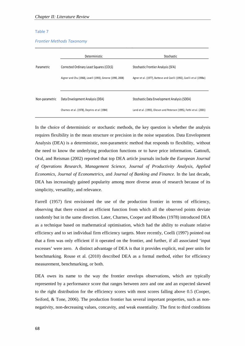
Chapter II: Literature Review
68
Table 7
Frontier Methods Taxonomy
In the choice of deterministic or stochastic methods, the key question is whether the analysis
requires flexibility in the mean structure or precision in the noise separation. Data Envelopment
Analysis (DEA) is a deterministic, non-parametric method that responds to flexibility, without
the need to know the underlying production functions or to have price information. Gattoufi,
Oral, and Reisman (2002) reported that top DEA article journals include the European Journal
of Operations Research, Management Science, Journal of Productivity Analysis, Applied
Economics, Journal of Econometrics, and Journal of Banking and Finance. In the last decade,
DEA has increasingly gained popularity among more diverse areas of research because of its
simplicity, versatility, and relevance.
Farrell (1957) first envisioned the use of the production frontier in terms of efficiency,
observing that there existed an efficient function from which all the observed points deviate
randomly but in the same direction. Later, Charnes, Cooper and Rhodes (1978) introduced DEA
as a technique based on mathematical optimisation, which had the ability to evaluate relative
efficiency and to set individual firm efficiency targets. More recently, Coelli (1997) pointed out
that a firm was only efficient if it operated on the frontier, and further, if all associated ‘input
excesses’ were zero. A distinct advantage of DEA is that it provides explicit, real peer units for
benchmarking. Rouse et al. (2010) described DEA as a formal method, either for efficiency
measurement, benchmarking, or both.
DEA owes its name to the way the frontier envelops observations, which are typically
represented by a performance score that ranges between zero and one and an expected skewed
to the right distribution for the efficiency scores with most scores falling above 0.5 (Cooper,
Seiford, & Tone, 2006). The production frontier has several important properties, such as non-
negativity, non-decreasing values, concavity, and weak essentiality. The first to third conditions
Deterministic Stochastic
Parametric Corrected Ordinary Least Squares (COLS) Stochastic Frontier Analysis (SFA)
Aigner and Chu (1968), Lovel l (1993), Greene (1990, 2008) Agner et a l . (1977), Battese and Coel l i (1992), Coel l i et a l (1998a)
Non-parametric Data Envelopment Analysis (DEA) Stochastic Data Envelopment Analysis (SDEA)
Charnes et a l . (1978), Deprins et a l (1984) Land et a l . (1993), Olesen and Petersen (1995), Fethi et a l . (2001)

Chapter II: Literature Review
69
are obvious in their meanings, while the weak essentiality property means that the production of
positive output is impossible without the use of at least one input (Coelli, Prasada Rao,
O’Donnell, & Battese, 2005).
DEA models separate the data variables into input or output types such that input variables are
causal factors to the outputs. The proper treatment of inputs and outputs in efficiency studies
has been regarded as being very important; the variables have to be consistent with the
phenomena they are supposed to capture. According to Coelli et al. (2005), inputs may be
classified into five categories: capital (K); labour (L); energy (E); material inputs (M); and
services (S). Often E, M and S categories are aggregated into a single category ‘EMS’. Capital,
unlike the other variables which are consumed in the production process, is a durable input
which may be measured from the various assets of a particular Decision Making Unit (DMU) or
farm. In farming, K is typically composed of land, livestock, buildings, and plant. Labour
constitutes another primary input, normally measured using a single variable which aggregates
paid and unpaid labour and management. It may be expressed in physical full-time-equivalent
units, hours of work, or in monetary terms. None of these measures take into account the
composition and quality of the labour force such as skills, age, gender, and education levels
(Coelli et al., 2005).
Moreover, the number of efficient DMUs relies on the number of inputs plus outputs (Cinca &
Molinero, 2004). The greater the dimensionality of the production function the more constraints
the model has and the less discerning the analysis (Jenkins & Anderson, 2003). The analysis
ought only to include inputs and outputs that are definitely relevant to the proposed study.
According to Rouse et al (2010) there are some other rules about their proportion:
1. The number of farms (firms or decision-making units) must exceed a minimum of three
times the number of inputs plus outputs; or
2. The number of farms must be higher than the product of inputs and outputs.
One important point to note is that inputs need to represent a production function or technology
set such that the proposed output is achievable (Coelli et al., 2005). Another rule is that input
variables should be controllable variables. The transformation of multiple inputs into outputs is
affected by controllable and non-controllable variables, as well as observable and non-
observable managerial characteristics. Therefore, there is a lack of information about the true
underlying technology that needs to be acknowledged. This, in turn, leads to an efficiency
estimate that is always higher than the real value of efficiency. The efficient DMUs (peers)
resulting from a DEA provide concrete evidence of performance improvement targets for both
inputs and outputs. As peer units are usually interpreted as those demonstrating how a firm can

Chapter II: Literature Review
70
improve, it is relevant that changes are actually feasible, which is only possible if inputs are
fully controllable. The analysis of the DEA peers is out of the scope of this study; exploring the
explicit, real peer units would be a field for further research.
Economic or ‘overall’ efficiency (EE) is one of the major factors explaining differences in firm
survival and growth (Olson & Vu, 2009). It has two components: price or ‘Allocative’
Efficiency (AE) and technical efficiency (E), such that
EE = E x AE (Farrel, 1957; Olson & Vu, 2009).
AE reflects the ability of a business to use inputs and produce outputs in optimal proportions to
maximise profit, given their respective prices (Farrell, 1957). In turn, E is a measure of how a
business transforms inputs into physical outputs and includes two components: pure technical
efficiency (TE) and scale efficiency (SE) (Moreira & Bravo-Ureta, 2010). According to Barnard
and Boehlje (1998), economic efficiency is determined to a large extent by pure technical
efficiency because it reflects managerial ability especially in smaller firms. Allocative, scale,
and pure technical efficiencies all impact profit, but the first is always related to changes in
input and/or output prices, neither of which are controlled by farmers. In contrast, technical
efficiency refers only to discretionary variables or those variables that can be influenced by
someone’s discretion, judgement, or preference (Harrison, Rouse & Amstrong, 2012).
According to Latruffe (2010), in most circumstances an improvement in technical efficiency can
result from a more competent use of the existing technology: that is by producing the same
output by using less inputs or more output with the same level of inputs. A second way to
improve efficiency is through economies of scale. Figure 6 shows a graphical representation of
both constant (CRS) and variable returns to scale (VRS) DEA envelopes for one output and one
input condition.

Chapter II: Literature Review
71
Figure 6. CRS and VRS DEA envelopes.
Adapted from: Coelli (1997)
Scale refers to a firm’s size; scale efficient firms have a scale elasticity of one and work under
Constant Returns to Scale (CRS), while scale inefficient firms could exploit either scale
economies or diseconomies, which imply Variable Returns to Scale (VRS), including both
decreasing (DRS) and increasing returns to scale (IRS) (Coelli, 1997). DRS takes place when a
proportionate increase in all inputs results in a less than proportional increase in output; the
latter conversely happens when increased inputs lead to a more than proportionate increase in
output. ‘Scale’ interacts with technical efficiency in predictable ways: in larger scale operations,
managerial input can be spread too widely and this might generate inefficiencies, while
excessively small scale operations can result in high costs, because the fixed investment is
spread over relatively low output levels (Barnard & Boehlje, 1998). TE, when measured under
the assumption of CRS, only represents the true technical efficiency if the firm has an optimal
scale of operation (Rouse, Harrison, & Chen, 2010). Otherwise, the pure TE component, which
refers solely to management practices rather than the firm’s operating scale, must be calculated
under the VRS assumption. SE may also be of interest, and can be calculated as the ratio
CRS:VRS. Different DEA assumptions define diverse DEA methods that differ in the ex-ante
assumptions involved. A major DEA assumption is that data is measured without error, and
thus, differences in efficiency scores are due to inefficient transformation of input into outputs,
not allowing for noise or error. The free disposability assumption stipulates that unnecessary
inputs and unwanted outputs can be freely discarded.

Chapter II: Literature Review
72
2.5.2.4 Regression or Recursive Partitioning Tree. Regression partitioning tree is a data mining method that recursively partitions data into sets,
each of which is simply modelled using regression methods (Witten & Frank, 2000). RPT is a
non-parametric statistical technique used to classify observations into homogeneous groups
(Godfrey, 2011). DEA efficiency scores can be used as the response variable in a second stage
approach, to find the best summary set of benchmarks that explains a dairy system’s
performance. Since often the databases provided many more variables than those required to
build such a summary set, an effective reduction of the multidimensionality of the datasets is in
most cases desirable. RPT can regress discretionary and non-discretionary inputs on its analysis.
This approach not only generated a ranking of variables, but also revealed the interaction
between independent variables, which it is not possible to do with other forms of multivariate
analysis (Curran et al., 1993). RPT approach can identify the relationships between different
variables of interest as reported by Hansen et al. (2005). Rossi et al. (2005) also pointed out that
RPT provides a variable ranking that is more stable than stepwise variable selection.
2.5.3 Generic competitive strategies. Competitiveness is defined as the ability to profitably produce and provide value at an equal or
lower cost than that of other sellers in a specific market (Harrison & Kennedy, 1997). Since a
competitive advantage is not in itself a guarantee of achievement, in order to be successful, a
firm needs to define the position and the competitive strategy that it is pursuing. By defining
these position and strategy, firms get closer to the best way to succeed in a particular industry.
Similarly, by executing a generic competitive strategy, the business is able to put its competitive
advantage into practice. The competitive advantage of a firm is the extra value it creates and this
is the difference between the value created by the firm and the potential value created by its
competitors (Spulber, 2004).
Prosperous farm businesses are increasingly utilising and embracing well-known concepts and
principles to improve their competitive position, efficiency, and productivity. However, the
traditional techniques for being efficient, which are reducing cost and increasing margins, are
not always sufficient to ensure successful agricultural production (Boehlje & Schiek, 1998).
Three positive ways to achieve the best possible strategy, differentiation, focus, and overall cost
leadership, are determined by the firm’s competitive advantages (Porter, 1980). The first step
towards defining the best strategy is to scan the external business environment and assess the
business's internal resources and capabilities. According to Gray and Boehlje (2004), once the
activities upon which a business may build a competitive advantage have been identified, the
strategic position from the three options above can be defined.

Chapter II: Literature Review
73
2.5.3.1 Differentiation. The transition of agriculture from a commodity industry to one of differentiated products
indicates a dramatic paradigm shift in the industry (Boehlje & Schiek, 1998). The main aim of
the differentiation strategy is to be perceived as unique industry-wide. Differentiation can be
gained by selecting one or more attributes that clients perceive as important and trying to
position the firm in such a way that the attributes of its products are considered by the consumer
to be different from the rest of the industry’s products. Some of the most common attributes that
consumers perceive as different are the firm’s delivery service and marketing approach (Porter,
1985). Differentiation takes many forms including design or brand image, special features,
customer services, and technology. Differentiated firms have a low level of competition and
rivalry as consumers have a lower sensitivity to price due to brand loyalty.
2.5.3.2 Focus. Boehlje and Schiek (1998) stated that differentiation in the commodity industry has been
particularly noteworthy when combined with a focus on the consumer and manufacturing
approach to production. Focus strategy is based on choosing a market segment or group of
segments in the industry by product line or geographic market. Once the market segment is
chosen, the firm’s efforts should be focused to serve that segment to the exclusion of others.
The focus approach can achieve low-cost or differentiation for that market segment, but not for
the whole market (Porter, 1985).
2.5.3.3 Overall cost leadership. This strategy has a broad scope and is used in agriculture and many other industries and
industry segments. A business has a cost advantage if cost efficiencies allow it to consistently
outperform competitors and earn greater economic profits (Porter, 1980). In order to achieve
and maintain a cost leadership position, an aggressive construction of efficient scale processes
and on-going cost minimisation through innovation is required (Spulber, 2004). More
specifically, Barney and Hesterly (2006) indicated that there are six main sources of cost
advantages for firms that successfully adopt cost leadership as described below:
1. Size differences and economies of scale;
2. Size differences and diseconomies of scale;
3. Experience differences and learning-curve economies;
4. Differential low-cost access to productive inputs;
5. Technological advantages independent of scale; and
6. Policy choices.

Chapter II: Literature Review
74
Further, the authors explain that the ability of a valuable cost leadership strategy to create a
sustainable competitive advantage is conditional upon the strategy being difficult and costly to
imitate. At the farm level, cost structures are explained by fixed and variable costs. According to
economic theory and empirical research, the cost explanatory variables are U shaped, meaning
that costs of production decrease to a minimum point where economies of scale are achieved.
Subsequently, diseconomies of scale occur and costs increase (Smyth, Butler, & Hennessy,
2008).
Agricultural systems’ cost advantages are seen in those countries or regions where the particular
climate, soil conditions, or labour supply advantages allow more efficient farming than in other
regions (Kay, Edwards, & Duffy, 2012). The competitive strategy that best represents pasture–
based dairy farming systems is cost leadership due to typically low feeding costs, since feed is
the highest single cost component for these farming systems (IFCN, 2011). Low variable costs,
and particularly low feed costs, have been reported as being important underlying causes of
efficiency at the farm level which are responsible for achieving a high gross margin (Flaten &
Giaever, 1998, cited in Hansen et al., 2005).
The New Zealand dairy industry has historically adopted a strategy of “broadly-targeted cost
leadership” (Akoorie & Scott-Kennel, 1999, p.12). This strategy has been used throughout the
New Zealand dairy industry to compete against other players in the global marketplace. Under
the cost-leadership strategy farmers decide on the combination of inputs they wish to use and
they make these decisions in order to minimise costs. In other words, if the input market is in
perfect competition and under a cost-leadership strategy, the best technically feasible input-
output combination is that which minimise production costs. These assumptions are considered
to be appropriate for countries where farmers cannot accurately predict the volume of output,
take input market prices as given and do not have any control over milk pay-out such as NZ and
Chile.
Shapiro (1985) discussed the nature of the ‘fit’ between a firm’s logistics system and its overall
strategic focus. He considered three possible foci (product innovation, differentiation through
customer service, and cost-leadership) that were broadly related to Porter’s (1998) typology of
strategies. For each focus, Shapiro clarified the nature of the task that logistics needed to
accomplish. Thus, under a strategy of cost leadership, the logistics function should seek to
minimise costs while keeping service at an acceptable level. Further, the ways suggested to
control costs include, but are not limited to: exploitation of economies of scale; centralisation of
inventories to the extent possible; lowest cost routing; and automation of materials handling and
order processing. The need for a strategic fit between a firm’s competitive strategy and its
supply chain strategy was also espoused by Chopra and Meindl (2001).

Chapter II: Literature Review
75
2.5.3.4 Competitiveness within groups. The competitiveness of a particular firm or a group of firms can be defined as the ability to face
competition and to be successful when doing so. According to Latruffe (2010), competitiveness
may be the capability to sell products that meet demand requirement, such as price, quality, and
quantity. In addition, this capability must result in profits over time and enable the firm to
prosper. Competitiveness is a relative measure, and a broad concept with many definitions and
disagreements about how to measure it precisely. However, there is consensus that in order to
evaluate the competitiveness of a given farm or farming systems, it is necessary to have data
from peers that allow benchmarking to occur.
Data envelopment analysis (DEA) has proven to be an effective tool for analysing productive
efficiency, and benchmarking the competitiveness of agricultural units and farming systems
(Coelli, 1995). A wide range of benchmarking approaches and frameworks are described in the
literature, which are often based on non-parametric methods, such as DEA (Bogetoft & Otto,
2011). This method allows the estimation of individual farm technical efficiency (TE) relative to
the maximum feasible production possibilities, given certain technology availability to a
particular group.
2.5.3.5 Competitiveness across groups. Benchmarking across groups that have different production opportunities can still be achieved
using DEA, although it needs to be taken further using a metafrontier approach. O’Donnell et al.
(2008) used this extended methodology to compare the TE of firms that could be classified into
different groups. They used data drawn from FAO Statistics, containing observations from 97
countries classified into four groups (Africa, America, Asia, and Europe) from 1986 to 1990.
The data set comprised observations on just one output variable, representing the aggregation of
185 commodities, and five input variables related to agricultural production. This study showed
that African and European countries produced agricultural outputs under conditions that were
more restrictive than in other regions of the world with an average metatechnology ratio that
indicated they could at best produce only 89% of the output that could be produced using the
unrestricted metatechnology. America could produce 91% at best, and Asia (including Australia
and New Zealand) could produce 93% of the output that could be produced using the
unrestricted metatechnology.
Likewise, Moreira and Bravo-Ureta, (2010) used a single–output, multi–input approach and
found different TE and metatechnology ratios for dairy farms in Chile, Argentina, and Uruguay.
They also suggested that technical efficiency can be interpreted as a relative measure of
managerial ability given certain technologies or productive environments. The findings from
this study were that technology was indeed different for each country and that the average
metafrontier efficiencies were 79.6%, 83.8%, and 91.4%, for Chile, Argentina, and Uruguay

Chapter II: Literature Review
76
respectively. However, metatechnology ratios were much closer with 65.8%, 72.8%, and 73.4%,
respectively. One attribute of the whole pooled sample was that farms were all operating at a
sub-optimal size.
2.5.4 The International Farm Comparison Network. The International Farm Comparison Network (IFCN) is an organisation that benchmarks farms
across the world. In 2010, 90 countries that accounts for 98% of the world’s total milk
production were benchmarked (IFCN, 2011). The IFCN vision is to be “…the leading, global
knowledge organization in milk production” (p. 8), while the mission advocates for the creation
of “…a better understanding of milk production worldwide” (p. 8). The IFCN has been defined
as a global network of dairy researchers from companies and other stakeholders in the dairy
supply chain with a focus on milk production. The IFCN particularly addresses the dairy chain’s
resources and costs, emissions created, and the political challenges that come from producing
milk itself.
In 2010, the typical farms’ analysis comprised 157 dairy farms from 60 regions and 49
countries, which accounted for 87% of total milk production. Typical farms under the IFCN
method represent those that produce the highest share of milk within their region. Table 8 shows
a comparison of selected measures for both Typical New Zealand and Chilean dairy farms. Note
that these figures are from actual farms representing each country’s distinct dairy farming
system and are not national averaged values.

Chapter II: Literature Review
77
Table 8
Comparison of Representative Dairy Systems
ECM kg = Milk kg corrected to 8.5% MS; Stocking rate: 1 Livestock unit = 650 kg LW
Source: IFCN (2011)
The IFCN has specific methods for the calculation of major KPIs. Net farm income (NFI) is
obtained by deducting total expenses from total cash income and then making the necessary
non-cash adjustments. Milk price is calculated by dividing the milk returns by the total
kilograms of ECM sold. The costs calculation for the dairy enterprise consists of the following
costs: milk production, raising replacement heifers, and home grown feed production cost
and/or cost of feed purchased for dairy cows and replacements. Total costs are composed of
expenses included in the profit cash and non-cash costs, including depreciation and opportunity
costs for factors of production such as family labour, own land, and own capital. Both returns
and total costs are expressed in US$ and per hundred kilograms of Energy Corrected Milk
(ECM). Cost of production includes farm working expenses, wages, and debt servicing, but
excludes management wages and depreciation. The cost of labour (US$/100 kg milk) is similar
Country NZ Chile
Location Waikato Region X
Herd size (cows) 348 421
Stocking rate 3.3 1.0
Labour units 2.3 7.1
Kg MS/cow 394 685
Kg MS/ha 945 753
Total assets (US$/100 kg) 126 48
Total Capital cost (US$/100 kg) 2.4 0.5
Equity 70 100
Milk price (US$/100 kg) 34 35
Cost of Production (US$/100 kg) 34 27
Average wages on farm (US$/hr) 18 6
Cost of labour (US$/100 kg) 6 6
Labour productivity (kg/hr) 290 100

Chapter II: Literature Review
78
in both countries despite the number of labour units being more than three times higher in Chile
than in New Zealand. This is explained by labour productivity which is almost three times
higher in NZ. These considerable differences in labour units could be afforded in Chile because
the average wage was US$ 6 per hour while in NZ this was US$ 18 per hour.
The entrepreneur’s profit measures the financial sustainability of the typical farm and shows the
total profitability of the dairy enterprise. It is calculated by subtracting the opportunity costs for
factors of production as above from the NFI. The return to labour, in turn, indicates how much
profit an employee or farmer generates per hour of farm work. It is calculated by adding wages
for hired labour and the opportunity costs of family labour to the entrepreneur’s profit, and
dividing this partial result by the total hours of labour used for the dairy enterprise. It is driven
by the wage level of the country, the labour input on the farm, and the economic performance of
the farm. Average wages on the farm include the gross salary plus any social costs the employer
has to cover. For hired labour, the cash labour costs effectively incurred are used, and for unpaid
family labour, the average wage rate which a hired worker would be paid to perform a similar
task in the same region is used.
The IFCN also studies the sustainability of dairy farming worldwide. Seven areas, where
economic, social and environmental sustainability stand out, are considered. Table 9 presents
the areas of importance, their indicators and their sustainability scale numbers (IFCN, 2011).
Table 9
Sustainability Areas and Indicators for Dairy Farms Worldwide
Considering the indicators in Table 9 and the data available in Table 8 the typical NZ farm is in
a more risky situation than the Chilean farm. This is mainly due to a lower entrepreneur’s profit
and higher intensification. Also of interest is noting that among the benchmarks chosen to
measure sustainability, many of them are commonly used and of easy quantification.
AREA INDICATOR UNIT GOOD BAD
ECONOMIC Entrepreneur's profit US$/100 kg milk ECM > 1 < -1
RISK Operating profit margin % > 15% < 12%
COMPETITIVENESS Return to labour % > 110% < 90%
EMISSIONS Carbon footprint g CO2/100 kg milk ECM 0 - 130 > 140
RESOURCE USE Water footprint L/kg milk ECM 0 - 1800 > 2000
INTENSIFICATION Stocking rate LU/ha < 1 > 1.2
JOB CREATION Employees /100 ton of milk Labour units >1.1 <0.9

Chapter III: Method
79
3. Method.
Farming systems and their available technology are shaped by natural resources; the physical,
economic, and social environment; policies; the characteristics of the labour force; and the
existing market for potential outputs. Hence, it is expected that farmers in different regions or
countries face different production opportunities and make choices from different sets of
feasible input-output combinations. This chapter presents the research method used in this study
which was in accordance with these concepts that is framed by a systems approach but makes
use of predominantly quantitative methods.
3.1 Research Strategy To answer the research questions posed in this research, a variety of methods were used after
reviewing the literature which provided the background to better understand the three dairy
databases used in this research. The first part of the study was straightforward and compared
two dairy farms from NZ and Chile. The second part of the study required grouping and
classifying observations from the country-specific dairy bases. Country-specific classifications
for production systems in NZ and Chile were developed on an annual basis for NZ (June-May)
and Chile (January-December). After the existing observations were classified into the most
appropriate ‘system’ based on the review of supplementary feed and regional information, a
comprehensive measure of performance was found for individual observations by applying an
efficiency analysis separately to each class. Corresponding efficiency scores were then
associated with the DMU in the original data set and a regression method was applied to
determine the relative importance of independent variables in determining efficiency in each
dataset. Finally, an overall measure of efficiency combining both datasets was calculated for
each observation to give the metafrontier for the final comparative analysis.
3.2 Materials and Data Analysis Methods This section introduces the sources of data and the methods applied to the present study. The
International Farm Comparison Network (IFCN) provided data for the farm to farm comparison
from its world-wide dataset for 2011. Data was analysed using specific features within the TIPI-
CAL 5.3 spread sheet. The country-specific datasets were “DairyBase” from NZ and
“TodoagroBase” from Chile. R statistical software was used to analyse data from these two
datasets. Computerised statistical packages such as R are time savers for both quantitative and
qualitative research (Patton, 2002). R software was used for the core part of this research, to
calculate the efficiency scores and to run the regression that identified the key performance
indicators. The R statistical software system for Windows was used because of its versatility

Chapter III: Method
80
and flexibility in undertaking a range of tasks with large datasets, including both statistical and
non-statistical analyses. The R codes12 used rpart and lpSolve packages. The data analysis
combined input oriented Data Envelopment Analysis (DEA), followed by Recursive or
Regression Partitioning Trees (RPTs), descriptive statistics, and a metafrontier approach, which
together provided the means for extracting relevant conclusions from the data available.
3.2.1 DairyBase and TodoagroBase overview. Databases typically record historical information through systematic collection and, if required,
conversion of quantitative and qualitative observations into numbers or codes. DairyBase and
TodoagroBase are independent data collections of dairy farm data, annually produced at the end
of each season or year. These datasets created by industry-owned and private agricultural
advisory services in NZ and Chile respectively, were used in this research as secondary data
sources. Each year, farm businesses are included on a voluntary basis; therefore, the cooperating
units are self-selected rather than a random sample. The information, validated at the time of
entering, has been made available for research purposes. Each database contained unbalanced
panel data as the total number of participants varied throughout the seasons, years, farming
systems, regions, and countries.
DairyBase included information for five consecutive years: 2006/07, 2007/08, 2008/09,
2009/2010, and 2010/11, while TodoagroBase comprised information for five consecutive
production years: 2007, 2008, 2009, 2010, and 2011. Participants represented diverse locations
across NZ’s North and South Islands, and Central-South Chile. The datasets only shared a few
common variables but most of those were expressed in different units (for example, milk output
was expressed as kilograms of milk solids for DairyBase and as litres of milk for
TodoagroBase). Financial variables and most ratios were often exclusive to one or the other
dataset. Shared and unshared variables acquired relevance at the final stage of this study,
particularly in the cross-country comparison. For most analyses, the datasets were analysed
separately and the original data were preferred; data conversions were only made when
necessary.
3.2.1.1 Data quality and limitations. Data quality and appropriateness are just as important as the analytical techniques themselves
because regardless of how powerful a technique may be, it cannot overcome problems that
fundamentally reside in the data (Coelli et al., 2005). Inaccuracy of production data, a chronic
problem to be aware of, may or may not be evident to the analyst. A priori, the quality of the
available data was considered high because farmers volunteer their data to the databases, and
therefore, have a vested interest in both the collection and the use of accurate data. 12 The R codes written by Lecturer and PhD in Statistics, Jonathan Godfrey (Statistics and bioinformatics group Massey University) can be found in Appendix 3

Chapter III: Method
81
DairyBase supplied New Zealand farm-level data consisting of information on more than 200
variables and ratios (Appendix 1). Each observation consists of a set of records; the database
originally contained 2,616 sets of financial records and 657 sets of physical observations
records throughout the period. A balanced panel would have included the same 523 farms each
year and totalled 2,615 observations. However, the dataset was unbalanced, with only 39 farms
consistently surveyed every year across the whole period. A similar situation was found among
Chilean observations, and although the lack of balance in both databases was acknowledged and
managed accordingly, the small proportion of farms present each year was a limitation in this
research. This posed the question of how much of the inter-annual variation found was
attributable to the relative ‘weight’ of different farms present each year. Non-random, missing
data on DairyBase was not a concern because the sets of observations were complete for the
variables of interest.
TodoagroBase supplied Chilean farm-level data consisting of information on more than 90
variables and ratios (refer to Appendix 2). The database originally contained 1082 sets of
combined financial, economic and physical records for a range of farming systems, from
exclusively pasture-based farms to supplement intensive systems feeding up to 4,734 kilograms
of supplement per cow per year. After reviewing the literature, a cut-off value of 2,700
kg/cow/year fed was used to define a pasture-based system; this resulted in 1,028 pasture-based
cases being available for further study (95% of the original sample). Missing data was a concern
when it involved important variables for the dairy enterprise. Missing data was an issue, and
included observations on depreciation, and remuneration among others. This was important in
calculating ratios or as part of operating expenses. The value of assets was calculated backwards
using the original profitability value but this resulted in another issue which was incoherent
data. This issue was a concern when involved variables used for the efficiency analysis because
implied a lower confidence in the data. Case deletion was applied in a few cases. However, the
most drastic measure was complete variable exclusion with the assets, whose calculated value
was not used in the main DEA analyses.
In summary, there were a few concerns which prevented the research from reaching fully
generalizable conclusions regarding a respective class or farming system. There were two major
issues: unbalance and non-randomness in the two datasets. Due to non-random sampling it was
uncertain whether the samples were fully representative of the NZ and Chilean pastoral dairy
farms populations. The second concern was that presumably, in both NZ and Chile, the samples
comprised above-average-managed dairy farms. In NZ, available information showed that the
DairyBase sample had been above average in indicators of interest. According to Jiang (2012),
differences in production have traditionally existed between DairyBase farms, and the national

Chapter III: Method
82
statistics. While DairyBase samples have traditionally consisted of farms with management and
performance above the average, there has not been a big difference in the direction and
magnitude of the bias between regions. Therefore, since a large sample does not necessarily
prevent bias (Hawley, 2010) efficiency estimates and other outcomes should be interpreted with
care as they may not reflect the true situation in the respective farming systems.
3.2.2 Review of methods. Quantitative research permits the diagnosis of historical and current situations, and developing
trends (Taylor, 2005). In order to achieve the objectives of this research, this study used a
combination of predominantly quantitative methods, both parametric (descriptive statistics) and
non-parametric, enabling valid, objective descriptions and conclusions. This section describes
the data envelopment analysis models, the recursive partitioning technique, and the metafrontier
approach in the order in which they were applied.
3.2.2.1 DEA models. DEA owes its name to the way the frontier envelops observations, which are typically
represented by a performance score that ranges between zero and one (Cooper, Seiford, & Tone,
2006). In DEA terminology, all observations are so-called decision making units or DMUs. The
envelopment identifies those efficient DMUs (those with a score=1) and locates them on the
frontier; in that way they serve as benchmarks to rank all the inefficient DMUs. The term
‘frontier’ is used to emphasise the fact that the function gives the maximum output that is
technologically feasible. The maximum value of one means that the DMU has achieved
maximum output with minimum expendable inputs or resources; in contrast, a minimum of zero
means nothing is achieved by using certain inputs (which is hard to find in practice). DEA uses
mathematical optimisation or linear programming (LP) to calculate efficiency scores, based on
one or more outputs and commonly utilises multiple inputs.
DEA can operate on either input or output orientation, but both models estimate the same
frontier, identifying exactly the same set of DMU’s as being efficient (Farrel, 1957). In contrast,
the efficiency scores associated with inefficient DMU’s may differ between the two methods
(Coelli, 1997). The frontier may also be determined assuming a transformation of inputs into
outputs under constant returns to scale (CRS) proposed by Charnes et al. (1978), or variable
returns to scale (VRS) reported and explained by Banker, Charnes and Cooper (1984) and later
by Fare, Grosskopf, and Lovell, (1994). Under the latter assumption, decreasing (DRS) and
increasing returns to scale (IRS) may occur. DRS takes place when an increase in inputs results
in a less than proportional increase in output; conversely, IRS happens when increased inputs
lead to a greater than proportional increase in output. In this research, DEA models were set up
to use VRS and an input-oriented approach. The use of VRS is customary in agriculture and

Chapter III: Method
83
commonly preferred in related studies. The input orientation was used in this study since a
manager has greater control over inputs than over outputs, which are influenced by external
factors such as climate and prices.
The selection of Regression Partitioning Tree as the best possible method to use in a second
stage DEA was the end result of an iterative process that started looking at linear models. After
reviewing the literature, linear models were chosen as it was necessary to incorporate multiple
predictors to predict efficiency and the Gauss-Malcom theory behind them is robust and well
understood (Hazelton, pers. com.). The multi-dimensionality in the dataset required a method
capable of handling several parameters; therefore, multiple linear regression (MLR) was tested
to regress efficiency scores attached to the original sets of observations previously cleaned of
trivial variables. The NZ dataset was used to test the parametric model (MLR) behaviour, which
was set up to capture main effects and also interactions which were considered unavoidable.
After a primary cleaning of trivial variables, the number of variables was still large (81) and
hence MLR failed to achieve the expectations. According to Strobl, Malley, and Tutz (2009),
standard regression methods commonly fail in these conditions and recursive partitioning trees
are an alternative approach.
3.2.2.2 Regression or Recursive partitioning tree. Regression partitioning is a technique that produces either classification or regression trees,
depending on whether the dependent variable is categorical or numeric, respectively (Strobl et
al., 2009). In this study DEA efficiency scores were used as the response variable in a second
stage approach, to find the best summary set of indicators that explains a dairy system’s
performance. Since the databases provided many more variables than were required to build
such a set, and following the principle of parsimony, an effective reduction of the
multidimensionality of the datasets was pursued. In a second stage RPT, DEA scores from the
first stage were regressed on discretionary and non-discretionary inputs in a country-specific but
common-to-all-groups analysis. This approach not only generated a ranking of variables, but
also revealed the interaction between independent variables, which it was not possible to do
with other forms of multivariate analysis (Curran et al., 1993).
RPT generates a flow-chart structure or tree which has a root node, secondary and tertiary nodes
and so on, and finally terminal nodes called leaves. Trees reveal the variables’ ranking of
importance with the root node representing the top level indicator. Each node provided
information on the splitting criteria (variable’s name) and the threshold value above or below
which a class is defined. Each leaf presents the class’s mean efficiency, and the number of
DMUs included (n). To reach a leaf node, the pathway starts at the root node. From each non-

Chapter III: Method
84
leaf node the procedure splits the data to the left, or to the right, based on the condition and
value of a certain variable, whose index is stored in the observed node. If the observed value
satisfies the condition, the procedure goes to the left, otherwise, to the right.
The partition is created such that observations with similar efficiency values are grouped by a
set of rules. Once a rule is selected and splits a node into two, the same process is applied to
each “child” node which is why RPT is called a recursive procedure (Witten & Frank, 2000). In
general, splitting and stopping follow the principle of impurity reduction, whereby each split
results in a child node which is more pure than the parent node. In each node, the variable that is
most strongly associated with the response variable (y) is selected for the next split (Strobl et al.,
2009). Finally, a response class is predicted in each terminal node of the tree (leaf or class).
Splitting stops when the software detects that no further gain can be made, or some pre-set
stopping rules are met. In this research at each node the recursive procedure stopped splitting
the node further in any of the following cases:
1. The number of observations in the node was less than the specified value (n = 50);
2. All the samples in the node belonged to the same class (or, in the case of regression, the
variation was too small), because it was not statistically possible to split the node
further; or
3. The best split found did not give any noticeable improvement compared to a random
choice.
The pathway to any particular leaf showed the main effects and the interactions between
variables. The RPT operates as a reduction, classification, and prediction tool for observations
meeting certain set of rules. A key property of this technique is that it is possible to compute the
importance or relative decisive power of each participating variable (Strobl et al., 2009). A
variable may be present more than once, and this only reinforces its importance. To avoid the
analytical or the prediction procedure getting stuck in a certain node, the technique also
provides so-called surrogate splits, in addition to the best ‘primary’ split (Strobl et al., 2009).
These surrogate splits can be used for observations with incomplete records and yield nearly the
same results as the primary splits. If a farm fulfils all the node or partitioning conditions on a
particular pathway, then it is likely with 95% of confidence that its efficiency will be mean
efficiency at leaf +/- deviance.
In summary, RPTs were expected to identify important benchmarks or indicators defining
efficiency classes and also to present a number of pivotal values to expose the pathway or
combination of conditions useful to predict technical efficiency. These pivotal values were the
thresholds indicating a single feature, which may split the dataset such that the variance of

Chapter III: Method
85
subsamples in each partition is less than their variance in the whole dataset. The pathway from
the root to a leaf node was a sequence of decision-making steps, and the leaf node function was
evaluated to provide a numerical prediction of the averaged value of efficiency for each leaf.
3.2.2.3 Metafrontier envelope. The measurement of efficiency across groups is only possible if efficiency is measured relative
to a common metafrontier which is the boundary of a metatechnology or unrestricted
technology that envelops the restricted group frontiers (Battese & Prasada Rao, 2002;
O’Donnell et al. 2008). This study used a metafrontier to compare dairy farm efficiencies in NZ
and Chile. By definition, a metafrontier envelops all farms and all group frontiers. In this
research, the main reason for using a metafrontier envelope was to provide comparable
efficiency scores for businesses operating in different environments existing either across
seasons, regions and countries. The metafrontier also enabled the technology gaps to be
estimated for firms under different technologies, relative to the potential technology available to
the industry as a whole (Battese, Prasada Rao & O’Donnell, 2004). A priori, the mean technical
efficiencies relative to the metafrontier are always expected to be smaller than those calculated
from the group frontiers. The difference between the group scores (E1) and the metafrontier
scores (E2) represented the restrictive nature of the particular environment. There is a gap
between a farm and the group frontier, which represents the differences in performance between
the efficient farms (TE = 1) and the particular DMU, and is called ‘d’. Then, there is another
gap ‘e’ between this DMU and the metafrontier. Both indicators may be used to calculate the
metatechnology ratio as the relationship d/e (Battese & Prasada Rao, 2002; O’Donnell et al.
2008). This ratio is of considerable interest because it measures the potential improvement in
performance resulting from changes in the production environment.
3.2.3 Procedure: the data analysis. The data analysis comprised five key stages including sampling, grouping, efficiency analysis,
RPT, metafrontier, and benchmarking. The procedure in more detail is presented in
chronological order as follows:
1. Analysing IFCN data relevant to the countries of interest, NZ and Chile;
2. Developing a classification system for each country’s data which yielded 27 NZ and 10
Chilean classes using a combination of season/year, region and supplements use;
3. Running the DEA (VRS) separately for each class which created a DEA score for each
observation so that the multiple effects of season/year, region and system were
minimised in the complete data set for that country;
4. Obtaining DEA scores (0-1) for each observation within each class and adding these
scores to the original databases;

Chapter III: Method
86
5. Testing stepwise MLR using DEA scores as response variables with all non-trivial
variables contained in the datasets as predictors;
6. Looking for alternatives to MLR, which was discarded due to the high dimensionality
of the dataset plus multi-collinearity13 and missing data issues;
7. Substituting MLR with RPT in the second stage, using efficiency scores as the response
and input variables as predictors;
8. Identifying country-specific sets of major KPIs for NZ and Chile based on RPT outputs;
9. Describing the samples using descriptive statistics on the identified KPIs;
10. Standardising the output and input variables to be used on the metafrontier envelop to a
common currency when necessary; then running the VRS DEA code in R on the
combined NZ-Chilean data using these variables.
11. Summarising the differences between farming systems, within, and between countries,
using selected variables with the highest explanatory power, and the metafrontier
scores.
3.2.3.1 Sampling. Since the research is based on existing datasets, this section actually refers to the original and
final configuration of the samples after cleaning the data. The samples in the databases
consisted of dairy farms across the countries over five agricultural years, where the sampling
unit was the dairying enterprise. The original number of observations contained in the NZ and
Chilean datasets for each season is shown in Table 10.
13 This is a term commonly applied to the statistical phenomenon in which two or more predictor variables are highly correlated. In this situation the coefficient estimates may change erratically in response to small changes in the model or the data (Adler & Golany, 2001).

Chapter III: Method
87
Table 10
Original NZ and Chilean Samples
The NZ data were allocated to eight NZ regions based on the DairyBase clustering criterion.
The number of observations for the period 2006-11 is shown in brackets for each region from
the top of the North Island to the bottom of the South Island as follows: Northland (268),
Waikato (864), Bay of plenty (215), Taranaki (292), Lower North Island (182), West Coast-
Tasman (226), Marlborough-Canterbury (324), and Otago-Southland (243). Waikato farms
represented 33% of the original sample, which shows the importance of this region to the NZ
dairy industry. Similarly, the southern central dairy territory in Chile consisted of five agro-
ecological zones: Llano Central Sur (404), Ribera de Los Lagos (308), Litoral Sur (82), IX Sur
and XIV Norte (221), and Los Angeles-Angol (66). The first two regions comprised more than
66% of the total data, thus demonstrating their significance to the Chilean dairy industry.
Observations were excluded from the raw data for the following reasons:
• Business structure other than owner operators (NZ data only);
• Extreme outlier data;
• Important missing data that could not be inferred or interpolated;
• Incoherent data (Chilean data only); and
• Systems other than pasture-based, that is using above 270014 kg supplement per cow per
year (Chilean data only).
Only data for owner operators were analysed in the NZ data to attain a homogeneous possible
sample which was representative of this type of business which is the most prevalent business
14 Equivalent to 45% of the diet based on supplements (year round).
Season DairyBase TodoagroBase
2006/07 625 259
2007/08 628 245
2008/09 497 237
2009/10 567 205
2010/11 297 135
Period 2614 1081

Chapter III: Method
88
structure in NZ. Table 11 shows the number of observations included in the analysis at the end
of this cleaning process.
Table 11
Number of DMUs Included in the Analysis per Year and Country
3.2.3.2 Variable correction and creation. For the purpose of this study, it was appropriate to adjust the variables for inflation that
occurred throughout the period even though inflation rates for the period were negligible in both
countries. Since TodoagroBase provided Consumer Price Index (CPI) corrected values for the
year 2011, variable correction was only needed for the NZ dataset and it was carried out using
the same criterion to be equivalent to the Chilean index15 and an appropriate CPI coefficient for
each year published by Statistics New Zealand (2012). The general CPI for the ‘all groups’
index was selected. The available price deflators were as follows: 20060/07 (1.119); 2007/08
(1.067); 2008/09 (1.065); 2009/10 (1.055); and 2010/11 (1).
The next step was to check TodoagroBase and to decide which variables in the NZ data should,
and could, be created based on the available information. The following set of variables was
created:
- Farm Working Expenses (FWE) and ratios (FWE/cow; FWE/ha);
- Operating Expenses (OpEx) and ratios (OpEx/cow; OpEx/ha);
- Operating Profit (OpProfit) and ratios (OpProfit/cow; OpProfit/ha);
15 A more correct adjustment would have been to use the dairy Producers Price Index as the adjuster which shows that on-farm inflation on dairy farms over the period was generally higher than measured by the CPI, and hence using the CPI under-deflated the figures.
Season DairyBase TodoagroBase
2006/07 619 245
2007/08 614 231
2008/09 496 231
2009/10 564 197
2010/11 295 125
Period 2588 1029

Chapter III: Method
89
- Milk price:Feed price ratio;
- Operating Profit margin (OPM);
- Cash Operating surplus;
- Discretionary Cash + Tax;
- Total Assets; and
- Asset Turnover ratio.
3.2.3.3 The NZ classification system. Battese et al. (2004) pointed out that farms operating in different regions or under different
technologies are not strictly comparable unless a special methodology is used to analyse the
data. However, in such cases, the observations can be grouped according to similarities and
differences in technology, and other conditions among the nominated periods or regions
(Haghiri, Nolan, & Tran, 2004). For instance, the seasons 2007/08 and 2010/11 both had
exceptionally high milk prices as shown in Table 12.
Table 12
Estimated Seasonal Prices for Output (MS)
The physical information contained in DairyBase also suggested that farmers responded to price
information by feeding more supplements to the herd in higher milk price years, which led to
farming systems shifting towards greater use of imported feed. Physical input was also used to
improve the understanding about dairy farming systems in the different regions. The most feed-
Season Milk ($/kgMS) % Average
2006/07 4.15 0.69
2007/08 7.36 1.22
2008/09 5.22 0.86
2009/10 6.16 1.02
2010/11 7.36 1.22
Period 6.05 1.00
Estimated price (NZ$)

Chapter III: Method
90
intensive region in NZ, measured as supplement imported per hectare, was found to be
Canterbury, followed by the Lower North Island and Waikato regions. The least intensive
region was Tasman-West Coast, closely followed by Northland and Taranaki, which are the
regions with the highest rainfall averages. The Dairy NZ Farming systems (reviewed in Chapter
II) in the NZ dataset had a mean of 2.9 and a median of 3, with the most representative regions
being Bay of Plenty and Southland. The use of imported feed was positively associated with
stocking rate, measured as both Cows/ha and LWT/ha. The correlation was significant at the 1%
Pearson coefficient, so is moderately high in both cases (0.629 and 0.642 respectively). In the
period under study (June 2006 to May 2011), farming systems were characterized by quite
distinctive indicators, as presented in Table 13.
Table 13
Averaged Indicators Showing the Relevance of Grouping into Farming System
The clear rainfall gradient shows that the volume of rain is negatively associated with the use of
imported feed, and hence, the farming system in place. In contrast, the farming system is
associated positively with the use of nitrogen (kg/ha) and feed grown (ton/ha), as well as with
production of milk solids per unit of labour (kgMS/FTE). These findings supported the need to
recognise the year and region effects, as well as their interactions with use of imported feed.
Therefore, the samples were grouped by year and then classified into several sub-samples
representing location and farming system, ensuring as much homogeneity of exogenous
conditions as possible within sample group.
Indicator 1 2 3 4 5
Rainfall (mm) 1764 1766 1301 1346 1187
Nitrogen (kg/ha) 70 116 202 169 169
Hay (%) 20 17 13 11 7
Supplement (ton/ha) 0.23 0.71 1.45 3.19 5.44
Pasture&Crop (ton/ha) 10.69 11.31 12.1 12.79 13.61
MS/FTE 45811 48670 53997 60045 62570
Farming system

Chapter III: Method
91
There was an iterative process that guided the classification systems in both countries. In order
to decide on the best categorization system for existing differences in technology across NZ, the
three approaches to nesting were evaluated: Regional consisting of regions (8) across five years
and five DairyNZ farming systems; Seasonal consisting of years across region and systems; and
Farming systems regardless of year or region. Three intensification levels (IL) were made by re-
coding DairyNZ farming systems so that farming systems 1 and 2 composed LOW, 3
represented MEDIUM, while 4 and 5 composed HIGH intensification levels. After the
evaluation process, observations contained in DairyBase were classified according to year of
record, region and intensification level. The classification process is partially explained in this
chapter and complemented by information contained in Appendix 4. Finally, the NZ
classification system consisted of 27 classes (Table 14), with half of them being a combination
of year, region, and farming system, and the other half, a combination of year and region. The
latter can be observed for those classes where the number of observations did not allow for a
further split at the intensification level criterion. The NZ classification system is presented in
Table 14.
A priori, concerns regarding all the mentioned classification systems were identified. One
concern when categorising by year was whether or not the underlying technology changes over
time in a relatively short period. It was found that some particularly responsive variables
showed both intra- and inter-annual variation. These variables included: input and output prices,
pasture growth, use of imported feed, and rainfall, which were highly variable between seasons.
A second concern was that the dataset was unbalanced with only 39 firms present across all
seasons, which prevented a fully meaningful comparison between seasons. Similarly, issues
around categorisation by Dairy NZ farming systems were recognised. Previous empirical work
had shown little or non-significant differences between systems in efficiency, which were
explained by greater variation in intra- than in inter-feeding systems. In addition, other factors
were prone to affect the farming system, meaning that a variety of technologies could be
represented by the same feeding system. Also, there were difficulties when categorising by
region alone because of large intra-region variability.

Chapter III: Method
92
Table 14
NZ Classification System
Season Class (code) Regions Farming Systems
2006-07 67 16 Northland-TasmanWestCoast All
67 78 Canterbury-Otago All
67 2345LOW Bay of Plenty, Waikato, Taranaki, Lower NI 1 and 2
67 2345MEDIUM Bay of Plenty, Waikato, Taranaki, Lower NI 3
67 2345HIGH Bay of Plenty, Waikato, Taranaki, Lower NI 4 and 5
2007-08 78 16 Northland-TasmanWestCoast All
78 7 Canterbury All
78 8 Otago All
78 2345 LOW Bay of Plenty, Waikato, Taranaki, Lower NI 1 and 2
78 2345MEDIUM Bay of Plenty, Waikato, Taranaki, Lower NI 3
78 2345HIGH Bay of Plenty, Waikato, Taranaki, Lower NI 4 and 5
2008-09 89 16 Northland-TasmanWestCoast All
89 78 Canterbury-Otago All
89 2345 LOW Bay of Plenty, Waikato, Taranaki, Lower NI 1 and 2
89 2345 MEDIUM Bay of Plenty, Waikato, Taranaki, Lower NI 3
89 2345 HIGH Bay of Plenty, Waikato, Taranaki, Lower NI 4 and 5
2009-10 910 16 Northland-TasmanWestCoast All
910 7 Canterbury All
910 8 Otago All
910 2345LOW Bay of Plenty, Waikato, Taranaki, Lower NI 1 and 2
910 2345MEDIUM Bay of Plenty, Waikato, Taranaki, Lower NI 3
910 2345HIGH Bay of Plenty, Waikato, Taranaki, Lower NI 4 and 5
2010-11 1011 16 Northland-TasmanWestCoast All
1011 78 Canterbury-Otago All
1011 2345LOW Bay of Plenty, Waikato, Taranaki, Lower NI 1 and 2
1011 2345MEDIUM Bay of Plenty, Waikato, Taranaki, Lower NI 3
1011 2345HIGH Bay of Plenty, Waikato, Taranaki, Lower NI 4 and 5

Chapter III: Method
93
The final combined classification approach was useful in overcoming the heterogeneity faults in
the dataset as shown in Figure 7 for total operating expenses (NZ$ thousands).
Figure 7: Averaged farm operating expenses within NZ classes.
As Figure 7 shows there was huge variability across classes. The greatest variability was found
when comparing across regions, especially when Canterbury (region 7) and Southland (region
8) are taken into account. The year effect was also evident with operating expenses increasing
steadily from 2006/07 to 2008/09, then stabilising in 2009/10 and decreasing slightly in
2010/11. The classification system normalised these and other effects, such as asset value and
land quality (refer to Appendix 4). However, it was still complex, comprising 27 combinations
of year, region, and intensification level. By performing DEA for each of these combinations
separately, this study recognised differences in the environment (year effect), and farm specific
characteristics related to region and intensification level. This provides more relevant efficiency
estimators as farms are scored only with respect to their peers.
3.2.3.4 The Chilean classification system. A similar approach categorizing by year and farming systems to give a comparable
classification system was used for the Chilean grouping criteria. Observations contained in
TodoagroBase were grouped into a classification system based on a combination of year and
use of supplement per cow. This combined approach was similar to that used for NZ but was
restricted by sample size, and thus, could not discriminate by regions. However, it was
considered appropriate and sufficient for the Chilean dataset. Two intensification levels
(MEDIUM and HIGH) were drawn by grouping according to the use of supplements looking at
the variable ‘Supplement kg/Cow’. The critical value for MEDIUM was below 2000

Chapter III: Method
94
kg/cow/year fed which was arbitrarily selected to generate classes of similar size. The final
classification system is presented in Table 15.
Table 15
Chilean Classification system
3.2.3.5 Class-specific input oriented DEA. After developing these classification systems, each country-specific class was analysed to
calculate efficiencies using input oriented DEA. All input and output variables were read by a
DEA code in R software. This code allowed for CRS, VRS, or both models to be run and
efficiency scores to be calculated in any of the mentioned model orientations. However, in this
study, only VRS was used. The first step to set up for DEA is to classify variables as inputs or
outputs, such that input variables are causal factors to the outputs. DEA assumes precise
knowledge regarding which variables are outputs and inputs. The output selection were
straightforward: the milk physical production indicators, expressed as kilograms of milk solids
in NZ or litres of milk in Chile, and the financial indicator gross farm revenue were used
separately in a single-output approach. These outputs were user-defined and were used so that
each of them captured different effects.
Year Class (code) Regions Farming Systems
2007 2007 MEDIUM All 3 and 4
2007 HIGH All 5 or more
2008 2008 MEDIUM All 3 and 4
2008 HIGH All 5 or more
2009 2009 MEDIUM All 3 and 4
2009 HIGH All 5 or more
2010 2010 MEDIUM All 3 and 4
2010 HIGH All 5 or more
2011 2011 MEDIUM All 3 and 4
2011 HIGH All 5 or more

Chapter III: Method
95
Input variables were classified into controllable and non-controllable variables. The selection of
inputs used is very important in efficiency studies and therefore, variables were selected with
care. First, DEA input variables were selected from the sub-set of controllable variables and,
second, they were consistent with the phenomena they were supposed to capture, for example
milk production in the physical analyses (using either milksolids or litres depending on the
country). Several inputs were meaningful from a productive standpoint, but some were omitted
following the principle of parsimony and to avoid multi-collinearity16. The first principle, also
called simplicity, states that large numbers of variables in DEA may lead to over-estimation of
relative efficiency (Adler & Golany, 2001). In this study, the ratio between numbers of DMUs
and total inputs plus outputs was kept much higher than 3:1 which, according to Bowlin (1998)
and Rouse et al. (2010), ensures reliability of the results. Golany and Roll (1989) state that the
number of DMUs should be at least twice the number of inputs and outputs considered and
Dyson et al. (2001) recommend a total of two times the product of the number of input and
output variables. These conditions were met in this study and all finally selected inputs were
standard production factors including capital, labour, operating costs and cows as presented in
Tables 16.
Table 16
Inputs Included in the Output DEA Models by Country
*Full time paid and unpaid labour Equivalents: 1=2,400 hours of work a year
The variables presented in Table 16 were selected because they represent different aspects of the
farming systems. Capital is a standard candidate variable in farming that typically includes land,
livestock, buildings and plant. It may be represented by equity plus liabilities, as was done for
NZ, or by the sum of various assets, as could have been done for Chile if data was more
16 Inputs that correlate highly with one another were eliminated based on correlation analysis.
NEW ZEALAND CHILE
Cows (peak number of cows milked) Cows (mass cow; all cows on farm)
Labour (FTE*) Supplement (kg/cow)
Operating Expenses (NZ$) Wages paid (CLP $)
Opening Equity (NZ$) Operating Expenses (CLP $)
Opening Liabilities (NZ$)

Chapter III: Method
96
reliable. However, incoherent data made impossible the inclusion of assets as a DEA input in
the Chilean model. Labour was another primary input included in both country’s analyses, but
expressed differently in NZ and Chile. In NZ, it was a single physical variable which aggregated
paid and non-paid labour and management in full time equivalents (FTE). In Chile, it was
expressed in monetary terms due to the lack of a physical indicator, and only accounted for paid
labour; therefore, unpaid labour and management were not reflected on this measure. Both, the
labour and the supplement variables did not reflect quality of the input in any way because de
databases did not contain information on these regards.
3.2.3.5 Recursive Partitioning Trees fitting and KPI selection. Both the milk and revenue efficiency scores obtained in the DEA stage were subsequently used
in a series of country-specific RP Trees as the response variable y. The same procedure was
followed separately with both, the DairyBase and the TodoagroBase datasets. First, a milk
efficiency y1 and a revenue efficiency y2 were attached to the original datasets. All the variables
available in the respective datasets were used as predictor variables. The first and second RPTs
used DEA scores based on the physical output milk (kg of milk solids or litres depending on the
country). Tree one regressed DEA estimates on all existing variables, including discretionary
and non-discretionary inputs and ratios, in a common-to-all-groups second stage which involved
all DMUs. Tree two was subsequently carried out after all milk-related ratios were removed (for
example MS/cow, MS/FTE, MS/ha; Milk fat/cow, Protein/cow, Milk L/cow, L/ha). The third
and fourth trees used DEA scores based on the economic output GFR. Tree three included all
the dataset’s existing variables, while tree four used all the same variables but was carried out
after all efficient farms (DEA score = 1) were removed from the dataset. The reason for this was
to increase the discriminant power in the analysis and uncover potentially new variables that had
not been revealed by tree number three.
Two more trees, one per each country are presented in the respective sections and called ‘the
fifth tree’. These were used to fullfill different requeriments in both countries. The fifth NZ tree
included all existing variables in DairyBase and used return on assets as the response variable to
show what could be done without DEA by using a major variable instead of efficiency as y.
The fifth Chilean tree included backward calculated assets to evaluate what could have been
done and found with better quality information in TodoagroBase.
3.2.3.6 Benchmarks sets. After running the R codes, a series of trees were available for interpretation and they revealed
those benchmarks used for further analysis in this study. Only the roots, plus the second and
third level splits in the multiple trees provided enough benchmarks, which were grouped in two
sets: NZ-specific KPIs and Chile-specific KPIs. No common KPIs were primarily identified.

Chapter III: Method
97
The sets included well known KPIs for each country and were used for intra-country
comparisons.
The benchmark sets were expected to provide answers to the research questions and were used
to analyse each database, provided that they were selected as the best possible measures of
performance for dairy farming systems in each country. Instead of analysing the pooled
samples, the datasets were split based on the efficiency scores gained in the first stage of DEA.
All efficient farms (DEA scores = 1) overlapping in both milk and revenue efficiency analyses,
were set apart. The NZ group consisted of 644 DMUs while doubly efficient DMUs in Chile
were 276. In both countries these figures were roughly equivalent to one quarter of the analysed
total observations. In addition two other groups were of interest. A second class was drawn
from the efficient group by ordering the database using farm ID and setting apart the farms
efficient three or more years. For obvious reasons all those efficient farms that were not present
in the survey for at least three years were not part of this group. Finally, a third class comprised
only the inefficient DMUs (DEA score < 1), or more precisely all those DMUs that were not
able to be ‘milk’ and ‘revenue’ efficient simultaneusly.This was just a criterion and it is
acknowledged here that things could have been done differently, for example, by relaxing the
cut-off value and considering efficient those virtually efficient observations with score > 0.95.
In NZ, the group of farms efficient three or more years was reduced to 41, represented by 142
observations which were only 5.5% of the sample. In Chile, the proportion was larger,
increasing to 7.4% with 76 observations and less than 20 farms. In both countries, these farms
were actually consistent in their efficiency score and, therefore, called the group of resilient
farms. All three groups (inefficient, efficient, resilient) were analysed in depth and compared
looking at the KPIs revealed by the RPTs. The comparisons were made by means of one-way
ANOVA and Schaffe significance tests.
3.2.3.7 Metafrontier analysis. The metafrontier approach was capable of investigating whether variations in technical
efficiency responded solely to technical limitations or whether differences in technology
contributed to some extent to the alleged inefficiency (Battese et al., 2004). Metafrontier is the
boundary of an unrestricted technology that envelops the restricted group frontiers (Battese &
Rao, 2002); therefore, instead of relying on separate frontiers for each class within countries,
technical efficiency was estimated in respect to a common frontier (Moreira & Bravo-Ureta,
2010). The relative efficiency scores across regions and countries were estimated by means of a
common metafrontier. The overarching metafrontier was achieved through linear optimisation
as for DEA and by pooling all the data under the same set of output (GFR) and input (cows,

Chapter III: Method
98
supplement kg/cow, wages, and operating expenses other than wages) combinations (Battese et
al., 2004). Data from both databases needed to be modified in order to obtain comparable inputs
and outputs to be used in the models. For instance, to allow for differences in milk solids
content, variable standardisation was needed but there was not enough information to use the
IFCN method for energy corrected milk (ECM) (IFCN, 2012), which could still have been used
by making several assumptions. Finally, GFR was preferred over the physical output milk
because its transformation to US$ was straightforward and it is also a standard practice when
comparing across countries. The same procedure, using an annualised exchange rate and CPI
indexes was repeated for all input and output variables of interest.

Chapter IV: IFCN Results
99
4. International Farm Comparison Network Results.
This section presents information on NZ and Chilean dairy farming systems extracted from the
database developed by the International Farm Comparison Network (IFCN) 17. In 2011, the
database comprised information from 171 farms from 61 regions and 51 countries, representing
90% of the world’s total milk production. Data from this secondary data source was used to
compare one typical pasture-based dairy farm in NZ with a typical dairy farm from Chile; since
only key findings are highlighted the reader is directed to Appendix 5 for more detailed
information. This Chapter sets the scene for the general discussion in Chapter VIII.
4.1 Typical NZ and Chilean Dairy Farms Comparison The typical NZ farm had a herd size of 348 cows, a forage area of 120 hectares, and a stocking
rate of 3.3 livestock units per hectare (LU/ha), whereas the typical Chilean farm had 421 cows,
a forage area of 520 ha, and a stocking rate of 1 LU/ha. The typical NZ farm had a production
per cow of 4,300 kg of energy corrected milk (ECM) and a land productivity of 12,000 kg ECM
per hectare whereas the typical Chilean farm produced 9,300 kg ECM per cow and 8,000 kg
ECM/ha. Figures 8 and 9 show different indicators in comparing the behaviour of these farms
and their positioning relative to typical farms analysed in 2011 for all countries. The world
mean is represented by the value at 0%; a value greater than the mean will compare positively
(to the right), while a value below the world mean will compare negatively (to the left).
Figure 8: Economic performance of the typical NZ farm relative to the world’s average.
Figure 9: Economic performance of the typical Chilean farm relative to the world’s average.
17 Information on this organisation and its particular TIPI-CAL approach was presented in Chapter II. Two typical farms from traditional pasture-based dairy regions in both countries were selected from the IFCN sample.

Chapter IV: IFCN Results
100
Figure 8 shows that only farm income was positive for the typical NZ farm; in contrast, all
indicators were positive for the typical Chilean farm (Figure 9)18. The farm income reflects the
total revenue left after all expenses including rent and interest have been paid, and non-cash
adjustments (depreciations) have been made. The entrepreneur’s profit and the farm income
relate to milk price, while return to labour relates to the regional level of wages. The
entrepreneur’s profit was calculated by subtracting the opportunity costs of farm owned factors
from the FI. The NZ farm income was US$161,400, which is about 30% above the world mean,
while the Chilean farm income was US$552,3000, which is about 40% above the world’s mean.
This indicator is driven by milk price and farm productivity. In NZ milk price is lower than in
Chile, but similar in the fact that in both countries it is lower than the world mean. Therefore,
differences are mainly explained by land productivity and farm size.
Entrepreneur’s profits were markedly different, being US$-4,5000 in NZ and US$312,600
thousands in Chile. Also of interest are the returns on investment calculated using the market
values on all assets, this was 4% for the typical NZ farm and 9% for the Chilean farm. The
differences in return to labour between the typical farms from NZ and Chile were even more
noticeable. The return to labour indicates how much profit an employee, or farmer, generates
per hour of work on the farm and is calculated by adding wages for hired labour and opportunity
costs for family labour to Entrepreneur’s profit, and dividing this partial result by total hours of
labour used for the dairy enterprise. It is driven by the wage level of the country, the labour
input on the farm and the economic performance of farm. The return to labour was negative for
the typical NZ farm, while the typical Chilean farm had a very high positive value. Note that the
return to labour positions the typical farm relative to the world sample and to their own local
peers, since it uses the national wages to build a ratio. Also of interest is that the average wage
on the typical Chilean farm was US$ 5.9 per hour and on the typical NZ farm the average wage
was US$ 17.64 per hour.
Figure 10 and 11 provide some explanations for these differences. The NZ and Chilean strong
and weak profile respectively, compared to the world’s average, again represented by the 0%
position. The slim vertical lines indicate the bounds where the particular farm is compared to
the IFCN distribution (weakest 10%, weakest 25%, strongest 10% and strongest 25%). The
returns profile is presented on top, the profitability indicators are at the bottom, and the costs
profile is in between.
18 Note that, as explained in Chapter II, all indicators, farm income (FI), entrepreneur’s profit and return to labour, are relative to their local prices.

Chapter IV: IFCN Results
101
Figure 10: NZ strong and weak profile.
Figure 11: Chile strong and weak profile.
The return profiles for both countries are quite similar, with both in the segment of the 25%
weakest, with minor differences favourable to the NZ farm in the variable ‘other returns’, and

Chapter IV: IFCN Results
102
also minor differences favourable to the Chilean farm in milk and cattle returns. According to
IFCN (2012), a rise in beef prices significantly increased the dairy farm income in most world
regions. However, the overall result for NZ and Chilean farms were only slightly affected by
changes in non-milk returns.
The differences between the typical farms from NZ and Chile, as shown in Figures 8 and 9, in
return to labour and profitability were clearly explained by two significantly different cost
profiles. The typical NZ farm had two major weaknesses when compared to the world sample’s
mean, land and capital costs, whereas the typical Chilean farm was weak in land cost only due
to its large size. Under the IFCN approach, land cost consists of regional rent prices for owned
land, or rents currently paid by the farmers for rented land per hectare. Capital cost is calculated
as a percentage of the sum of owned capital, defined as value of assets excluding land, plus
circulating capital; the real interest rate is assumed to be 3% or 6% for borrowed funds. The
Chilean land cost is higher than the world’s mean but it is far below the NZ land value. The
share of land as a proportion of total costs in NZ is very high compared to the Chilean farm due
to the relatively higher price of land for dairy. These reflect a land purchase price around
US$24,000 per hectare in NZ, and around US$12,000 per hectare in Central southern Chile
(IFCN, 2011). The negative comparison of the typical NZ farm relative to the world’s sample in
capital cost is driven by higher asset values and a lower equity ratio, which lifts the interest rate
used from 3 to 6%.
Both the NZ and Chilean farms revealed their major strength in relatively low costs of
production. Since these typical farms represented pasture-based farming systems, they both
compared positively against the world mean when feed, stock, machinery, energy, building and
other costs are considered. ‘Labour’, ‘Other’ and ‘Quota’ compare positively in both NZ and
Chile. Quota costs do not exist in either of the two countries. The family farm income compared
negatively for the NZ farm and positively for the Chilean farm. The entrepreneur’s profit in both
countries compared more favourably than the farm income, due to lower opportunity costs in
these countries compared to the world’s average. Return to labour indicates how competitive the
farm is relative to the cost of the labour it is using; note that the average wage in NZ is higher
than the world’s average of wages. Return to labour features highly positive in both countries,
but indicates greater labour efficiency in NZ than in Chile given the wages in each country.
Figure 12 shows a direct comparison between Chilean and NZ typical farms, where the
horizontal axis contains the deviations with respect to the NZ values in percentage terms.

Chapter IV: IFCN Results
103
Figure 12: Typical Chilean dairy farm compared to the typical NZ dairy farm.
The typical Chilean farm compares favourably against the NZ farm in all but ‘Other returns’,
‘Machinery cost’, ‘Fuel, energy, water’ and ‘Return to labour’. The typical Chilean farm had
higher milk and cattle returns due to more milk and beef produced respectively; also had higher
total returns. Land, capital, animal health, building, labour and other costs all are higher in NZ,
being land costs the biggest contributor to total costs. Overall, the bottom line also compares
very positive for the typical Chilean farm against the NZ farm.
4.2 Discussion and concluding comments on the IFCN comparison Pasture-based systems are a competitive advantage for those countries or regions that have the
potential to grow grass all year round. These systems have recently re-gained worldwide interest
due to their generally lower production costs compared to other systems, along with their more
environmentally friendly profile (Dillon, et al., 2005; Benson, 2008). Temperate grasslands
have a variety of environments as a result of factors such as season, latitude, altitude, aspect and
distance from the sea. Their normal conditions are sufficiently favourable for livestock
production to operate relatively low input systems. The variety in natural conditions also allows
a range of farming systems to be used, differing, for example, in how much pasture they grow,

Chapter IV: IFCN Results
104
supplement they use, or stock they carry per unit of area. According to expectations, despite
some important similarities between NZ and Chilean dairy farming systems, the differences
revealed by the results presented in this chapter were significant.
In 2011, both the cost of milk production and the profitability of dairying increased on average
compared to the previous year (IFCN, 2012). This costs increase was found to be mainly due to
escalating land, feed and energy prices. The opportunity cost for land also increased in this year
relative to 2010 since cropping competed with dairy land because of very high prices for cereals
and oilseeds. A longer term analysis showed “a sharp increase in cost of milk production in
most world regions” (IFCN, 2012, p. 13). However, the relative strength in local currencies in
many countries reduced the impact of rising energy and fertiliser prices. Profitability improved
mainly driven by the high world milk price, consequence of a strong unsatisfied demand for
milk products, which lasted until mid-2011 (IFCN, 2012).
Discussion groups and monitor farms are considered early examples of benchmarking. These
activities started in France, after the Second World War, and in NZ in the 1980s, in order to
share information, transfer technology and motivate learning and action among farmers
(Campbell, 2008). The IFCN provides a modern version of monitor farms at the international
level. ‘Typical’ farms under the IFCN approach represent those that produce the highest share
of milk within a region, rather than the majority or average of farms in a country. Clearly, the
NZ farm, located within a traditional dairy region (Waikato), was representative of both its
region and the country (LIC & Dairy NZ, 2011). The ‘typical’ Chilean farm, also belonged to a
traditional dairy area (X Region, Osorno), however, the farm was not particularly distinctive of
its country which is characterised by many heterogeneous, smaller dairy farms that represent
around 80% of producers, 40% of the dairy herds, and 20% of the total production (Consorcio
Lechero, 2010). Although in Chile, the bigger producers have the greater share of total
production (Escobar et al., 2006), according to all the background information reviewed, the
typical NZ farm would still be larger than the normal Chilean dairy farm. In contrast, the IFCN
Chilean farm had 21% more cows than a typical NZ farm and 400% more land dedicated to
dairy. This suggests that the IFCN approach works well representing the average NZ farm, but
only represents one segment of the Chilean dairy sector.
Both Chilean and NZ farms had significant differences in most physical parameters including
production per cow, stocking rate, and land and farm productivity. The Chilean farm had greater
cow and farm productivity than the NZ farm, but lower land productivity due to a significantly
lower stocking rate (1 to 3.3 LU/ha). The stocking rate a farm can support is limited by the
availability of pasture and the intensity of supplements used, while the potential for pasture
production depends mostly on the quality of the land (Penno, 1999; Smith, et al., 2009). Several

Chapter IV: IFCN Results
105
ecological and geographical factors such as latitude, soils and weather patterns are similar in
Southern Chile and New Zealand (Challies & Murray, 2006). Hence, the quality of the land
would not be expected to be more than three times higher in production of pasture as reflected
in stocking rate differences. In NZ, the mean annual pasture production at the commercial level
has been reported at 12 tonnes of dry matter per hectare and year (Holmes, 2003). The quantity
of grass grown in Chile would in fact be lower than in NZ. This lower pasture production in
Southern Chile may be due to a series of factors reported by Pinochet (2003) including low
phosphate and pH values, and poor grazing management.
However, the large difference observed in stocking rates is only partially explained by lower
pasture yields on similar quality land. Another component of this difference may be explained
by the breeds and strains used for dairying in each country and the ‘Livestock unit’ employed
by IFCN in its database. Stocking rate describes the number of animals supported per hectare or
other unit of area and is expressed on a per head ratio, animal unit, or other pre-defined entity
basis. A smaller NZ cow would allow more ‘livestock units’ per hectare. Conversely, the bigger
Chilean Holstein type will reduce that figure. In other words, the relationship may be 1 to 2.419
(rather than 1 to 3.3) if the stocking rate was measured directly in cows per hectare. Also of
interest are the implications of the stocking rate values on the different risk profiles of the farms.
According to Penno and Kolver (2000), and Anderson and Ridler (2010), since most types of
risk associated with farming are positively correlated with increasing stocking rate, the typical
NZ farm will have a more risky profile than the Chilean farm.
In order to completely understand the systems, the stocking rate needs to be related not only to
land productivity but also to supplements fed to the cows. For an increment in stocking rate, the
milk production response on a per hectare basis is positive and, conversely, it is negative on a
per cow basis (McCarthy, Delaby, Pierce, Journot, & Horan, 2011). The typical Chilean farm
had very high milk yields per cow (9,300 kg ECM) which can only be achieved on pasture by
using significant amounts of supplements (Gazzarin, Frey, Petermann, & Hoeltschi, 2011;
National Research Council, 2001). Moreover, the fact that the typical Chilean farm had double
the milk yields per cow of the NZ farm suggests that a higher genetic merit for milk production
is being well capitalised through the use of concentrates or other supplements in Chile,
favouring individual cow performance rather than land performance. It is also likely that the
typical Chilean farm has grown its own supplementary feed on the effective grazing area.
Comparative benchmarking is particularly valuable for understanding returns, cost, and business
drivers (FCC, 2007). The differences between the typical NZ and Chilean farms were clear
19 According to an adult live weight relationship of 400 kg (NZ crossbreed) and 550 kg (American Holstein) and the Livestock unit equivalence used by IFCN LU = 650 kg LW

Chapter IV: IFCN Results
106
when comparing physical results but not as evident when comparing revenues, costs and results.
The return profiles shown in Figure 12 showed minor differences in most indicators under
analysis for total, milk, cattle and other returns. The Chilean farm of 520 ha and 421 cows had
higher cattle, milk and total returns than the typical NZ farm of 120 ha and 348 cows. This was
due to higher farm productivity as a result of larger scale in both, effective dairy area and herd
size, and also higher production per cow. In contrast, ‘other returns’ were higher for the typical
NZ farm due to the dividends generated by shares owned by the farm under the distinctive NZ
payment system.
In both countries, dairy farms operated as price takers under conditions similar to perfect
competition. According to Holmes (2003), given low milk prices at the farm gate, primary
producers need a strong cost leadership focus. The cost profiles for the two countries showed
differences in the order of 7% in total costs, explained mainly by higher land and capital costs in
NZ compared to Chile, with NZ having also slightly higher feed, animal health, building and
labour costs. Land cost was the biggest contributor to total costs in NZ because of the higher
land and rent market values connected to stocking rate and land productivity. Capital costs are
also related to the value of the assets which are significantly higher in NZ as are the levels of
debt. The costs of feed and animal health were confounding factors because the supplementary
feed used was expected to be lower in NZ than in Chile. A higher proportion of pasture in the
diet of the cows was expected in NZ, which, according to Dillon et al., 2005, correlates
negatively with total cost of feed. The NZ farm had higher feed cost due to high price per unit of
supplement rather than volume used. Similarly, animal health was expected to be lower in NZ
than in Chile, where housing increases the animal health issues and the herd was larger.
However, it was again more costly for the NZ farm, presumably due to higher veterinary and
animal health costs. Higher building costs in NZ may be explained by more infrastructures other
than housing to maintain in NZ than in Chile. Finally, labour costs were not surprisingly higher
in the typical NZ farm, mainly due to significantly higher wages than in Chile. As expected the
typical NZ farm was less mechanized, used less fuel, energy and water, and also demonstrated a
higher labour efficiency as reflected by a return to labour greater than that for Chile. Despite
these, the bottom line represented by family farm income and entrepreneur’s profit compared
very positively for the Chilean farm, being more than 3% and 6% higher respectively.
In summary, the IFCN provided valuable background information for both countries. The farms
studied shared a series of characteristics and exhibited some differences. One similarity was that
both countries produce at low cost although it is not clear if both countries pursued a cost-
leadership strategy. NZ pastoral systems are well delineated pasture-based systems and clearly
pursue cost-leadership. In contrast, the Chilean example showed to be also low-cost but by
producing a lot of milk rather than using low inputs. Both also were exposed to climatic and a

Chapter IV: IFCN Results
107
price shocks due to natural variability and the absence of subsides and quotes. The differences
between the countries were mostly in the cost profiles as previously explained, and in the risk
profiles as a result of very different stocking rates in similarly uncertain productive
environments. However, the comparison of these ‘typical’ farms for only one particular year did
not allow a good characterisation of pasture-based dairy farming systems in NZ and Chile. This
reinforces the need for a more comprehensive study, including a broader sample from a wider
geographic coverage.

Chapter IV: IFCN Results
108

Chapter V: DairyBase Results
109
5. New Zealand Results.
This chapter presents the NZ results, consisting of the data envelopment analyses and the
second stage recursive partitioning analyses.
5.1 Data Envelopment Analyses This section presents the NZ results for the data envelopment analysis. Table 17 presents a
summary of the NZ results over a five year period from 2006/07 to 2010/11 showing
corresponding weighted averages for the outputs milk solids (MS) and gross farm reveue (GFR)
while Tables 18, 19, 20, 21 and 22 show the class results for both MS and GFR analyses per
season over the five-year period.
Table 17
Weighted Averages for DEA Results by Year
Results per class are not strictly comparable since several DEA have been carried out
independently, and sample sizes and DMUs observed are not the same over the period.
Therefore, significance tests would only encourage misleading comparisons, and have not been
conducted. A score of 1 represents full efficiency; the range from 0.95 to 1 is referred to as
virtually efficient; the range from 0.90 to 0.95 is considered very high efficiency; and from 0.85
to 0.90 is high. From June 2006 to May 2011 the NZ efficiency proved to be high to very high
with fluctuations over the period. The milk solids weighted efficiency for the owner-operators
Season n MS GFR
2006/07 616 0.885 0.877
2007/08 609 0.884 0.854
2008/09 492 0.892 0.867
2009/10 558 0.884 0.876
2010/11 323 0.92 0.918
Period 2598 0.89 0.88
Weighted Averages

Chapter V: DairyBase Results
110
suveyed in DairyBase ranged from 0.884 to 0.920 and the gross farm revenue weighted
efficiency ranged from 0.854 to 0.918.
The similarity between MS and GFR efficiencies values was expected since the correlation
between these variables was very high (0.95), and GFR was driven to a large extent by MS and
milk price. The results suggest that milk efficiency was also driven by price relationships such
as the milk:feed ratio, and by the presence/absence of weather related shocks such as droughts
or flooding. Over the period milk and feed prices as well as the climate showed marked
variability. International milk prices were exceptionally high in 2007 and the beginning of 2011,
and a pronounced drop was observed in June 2009 (IFCN, 2012).
This study looked at the DairyBase physical data to gain context and better interpret the results.
The DairyBase physical data comprised 657 observations across the period (88 observations in
2006/07, 151 in 2007/08, 156 in 2008/09, 187 in 2009/10 and 75 in 2010/11). Seasons 2006/07,
2007/08, and 2009/10 had lower rainfall than 2008/09 and 2010/11, which led to lower pasture
growth and quality, and also lower total feed eaten and productivity in terms of milk solids per
cow per day. Further consequences of the lower pasture growth were a higher share of
supplements in total feed eaten, lower annual productivity per cow, and less days in milk.
Consequently, the lower physical efficiency found in 2006/07, 2007/08 and 2009/10 years than
in 2008/09 and 2010/11 was expected.
In 2006/07 and 2007/08, the weighted mean efficiency converting inputs into milk was high
(0.885, 0.884) and the conversion of inputs into revenue was lower but still high (0.877, 0.854).
In response to milk price, in 2008/09 and despite a high mean physical efficiency (0.892), the
revenue efficiency was again significantly lower (0.867). In 2009/10, the mean milk efficiency
was high (0.884), while the revenue efficiency was identical to that of the previous year (0.867).
Season 2010/11 showed a very high overall efficiency; converting inputs into physical product
was high (0.920) as was the revenue efficiency (0.918), with both being well above the means
for the five-year period (0.89 and 0.88, respectively). During the whole period revenue
efficiency was below milk efficiency, which is also reflected in the general mean for the period.
Table 18 shows the DEA outcomes for season 2006/07 (mean efficiencies and standard
deviations for each class).

Chapter V: DairyBase Results
111
Table 18
DEA Results per Class Within Season 2006/07
In 2006/07, Rest of North Island-LOW had the lowest efficiency (0.857) and the greatest
variability as denoted by standard deviation 20. Attention is drawn to the higher efficiency
classes, Canterbury/Southland (0.902) and Rest of North Island-MEDIUM (excluding
Northland and using medium levels of imported feed; 0.900). The mean efficiencies were very
close to each other, but Canterbury/Southland had a narrower efficiency range and lower
variability. For the gross farm revenue results, Rest of North Island-LOW (0.849) had the
lowest efficiency and was largest variability class. It is interesting to note that
Canterbury/Southland’s (0.883) ranking went from being the most efficient class producing MS
to only third best producing revenue after Rest of North Island-MEDIUM (0.898) and HIGH
(0.908). Also of interest is that greater variability is found among the revenue results than
among the milk scores.
Table 19 shows the DEA outcomes for season 2007/08.
20 The standard deviation (SD) of the mean measures the spread of values in a distribution being calculated as the square root of the variance. The spread of a distribution is also referred to as ‘dispersion’ and ‘variability’. All three terms mean the extent to which values in a distribution differ from one another.
Season 2006-07 n M SD M SD
Rest of North Island - Low use of supplements 189 0.857 0.111 0.849 0.116
Northland-Tasman/West coast 119 0.887 0.101 0.878 0.100
Rest of North Island - High use of supplements 67 0.897 0.097 0.908 0.094
Rest of North Island - Medium use of supplements 106 0.900 0.100 0.898 0.096
Canterbury/Southland 135 0.902 0.085 0.883 0.097
MS oriented efficiency GFR oriented efficiency

Chapter V: DairyBase Results
112
Table 19 DEA
Results per Class Within Season 2007/08
The 2007/08 season exhibited a similar pattern to that of 2006/07. The milk solids output shows
that the lower efficiency classes, on average, were Northland-Tasman/West Coast (0.863) and
Rest of North Island-LOW (0.863) for a second time, while higher efficiency classes were again
Canterbury (0.928) and Southland (0.948). For the revenue results, attention is drawn to the
consistency among the lower and higher efficiency classes. Rest of North Island-LOW (0.812)
and Northland-Tasman/West Coast (0.817) had lower efficiencies again and also showed the
larger variabilities. Canterbury (0.930) and Southland-Otago (0.923) produced revenue very
efficiently, just under the mean score reached producing milk. Greater variability was once
again found among the revenue results than among the milk scores.
Table 20 shows the DEA outcomes for season 2008/09.
Table 20
DEA Results per Class Within Season 2008/09
Season 2007-08 n M SD M SD
Northland-Tasman/West coast 117 0.863 0.111 0.817 0.139
Rest of North Island - Low use of supplements 157 0.864 0.112 0.812 0.121
Rest of North Island - High use of supplements 90 0.871 0.109 0.870 0.098
Rest of North Island - Medium use of supplements 119 0.886 0.107 0.855 0.112
Canterbury 73 0.928 0.081 0.930 0.079
Southland 53 0.948 0.068 0.923 0.090
MS oriented efficiency GFR oriented efficiency
Season 2008-09 n M SD M SD
Rest of North Island - Low use of supplements 109 0.866 0.111 0.888 0.109
Rest of North Island - High use of supplements 63 0.878 0.120 0.868 0.119
Northland-Tasman/West coast 92 0.887 0.112 0.862 0.132
Rest of North Island - Medium use of supplements 123 0.899 0.101 0.869 0.113
Canterbury/Southland 105 0.925 0.083 0.845 0.127
MS oriented efficiency GFR oriented efficiency

Chapter V: DairyBase Results
113
In 2008/09, the lowest milk efficiency class was Rest of North Island-LOW (0.863), while the
highest mean was exhibited by Canterbury and Southland-Otago classes (0.925). For Rest of
North Island-HIGH, the variability of these results was much higher than that observed in the
previous season. For the revenue results, note the dramatic change in ranking compared to both,
the milk results and the previous seasons. Rest of North Island-LOW (0.888) exhibited the
highest revenue efficiency. Conversely, Canterbury and Southland-Otago (0.845) showed the
lowest mean efficiency and a very high standard deviation.
Table 21 shows the DEA outcomes for season 2009/10.
Table 21
DEA Results per Class Within Season 2009/10
In 2009/10, the lowest milk efficiency class was Northland-Tasman West Coast (0.847),
followed very closely by Rest of North Island-HIGH (0.850), with both exhibiting moderately
high milk efficiency. In contrast, Southland was virtually efficient (0.951) with a low standard
deviation. Canterbury had the same pattern, having a very high milk efficiency (0.939). In
between, Rest of North Island-LOW and MEDIUM exhibited very high efficiency and moderate
variability. The ranking for milk results almost perfectly matched the ranking for the revenue
results. However, the lowest refficiency class changed to Rest of North Island-HIGH (0.845),
which was at that lowest position for the first time in the series.
Table 22 shows the DEA outcomes for season 2010/11.
Season 2009-10 n M SD M SD
Northland-Tasman/West coast 105 0.847 0.126 0.853 0.120
Rest of North Island - High use of supplements 96 0.850 0.126 0.845 0.115
Rest of North Island - Low use of supplements 121 0.878 0.099 0.863 0.103
Rest of North Island - Medium use of supplements 110 0.888 0.103 0.892 0.097
Canterbury 74 0.939 0.076 0.910 0.092
Southland 52 0.951 0.063 0.930 0.083
MS oriented efficiency GFR oriented efficiency

Chapter V: DairyBase Results
114
Table 22
DEA Results per Class Within Season 2010/11
In 2010/11, mean efficiencies for both MS and GFR were markedly higher than for the previous
seasons. The MS results show that the lower efficiency class were Rest of North Island-HIGH
(0.908) and LOW (0.910), but these values were still in the range of very high milk efficiency
range. In contrast, Canterbury and Southland exhibited a very high average efficiency (0.947)
with a low standard deviation. This highest efficiency class also kept its place when looking at
the revenue results (0.937), although the rest of the ranking did change. Interestingly, Rest of
North Island-HIGH (0.924) jumped from last to the second best efficiency class and conversely,
Rest of North Island-LOW went from very high efficiency to bottom of the table (0.899).
In summary, variability was evident in both milk and revenue efficiencies throughout the period
but the variability was greater among the GFR results than among the MS scores. The best year
of the series clearly was 2010/11 due to a favourable milk price scenario and the absence of
weather shocks. The lowest efficiency class for both milk and revenue for most years was
Northland-Tasman/West Coast, while Canterbury and Southland had the higher milk efficiency
almost every year but failed to deliver the same good results when revenue efficiency was
analysed.
The 2007/08 season exhibited a similar pattern to that of 2006/07, but the milk price was
significantly higher and thus, attention is drawn to the fact that lower and higher milk efficiency
classes exactly matched the revenue efficiency class rankings. Rest of North Island-LOW
(0.812) and Northland-Tasman/West Coast (0.817) had lower efficiencies again and also
showed the larger variabilities. Canterbury (0.930) and Southland/Otago (0.923) produced
revenue very efficiently, with just under the mean score reached producing milk. Greater
variability was once again found among the GFR results than among the MS scores. In 2008/09
(Table 20), a year characterised by a high initial milk price followed by a pronounced drop
Season 2010-11 n M SD M SD
Rest of North Island - High use of supplements 73 0.908 0.095 0.924 0.089
Rest of North Island - Low use of supplements 67 0.910 0.103 0.899 0.106
Rest of North Island - Medium use of supplements 63 0.913 0.089 0.914 0.080
Northland-Tasman/West coast 57 0.923 0.095 0.916 0.097
Canterbury/Southland 63 0.947 0.065 0.937 0.076
MS oriented efficiency GFR oriented efficiency

Chapter V: DairyBase Results
115
when the season was well under way, the lower MS efficiency classes generally had the higher
revenue efficiency averages. In 2008/09, clearly only those who effectively managed the change
in milk price scenario were able to maintain efficiency producing revenue. In 2009/10 the MS
results positioned Northland-Tasman West Coast (0.847) as the lowest efficiency class, closely
followed by Rest of North Island-HIGH (0.850). In contrast, Southland was virtually efficient
(0.951) with a low standard deviation and Canterbury exhibited the second best efficiency
(0.939) and also low variability. Interestingly, the ranking for MS results almost perfectly
matched the ranking for the GFR results. In 2010/11 mean efficiencies were markedly higher
than for 2009/10. The efficiency at producing milk had an inverse relationship with the
efficiency at producing revenue in some classes in the North Island of NZ. In contrast, classes in
the South Island had a direct association between milk and revenue efficiency.
5.2 Recursive Partitioning Trees results Both the milk and revenue efficiency scores obtained in the DEA stage were incorporated into
the original dataset including all years and regions, and subsequently used in a series of country-
specific RP trees with the efficiency values used as the response variable y. This section
presents the milk trees first and later the revenue trees, followed by a summary of key
performance indicators identified.
5.2.1 Milk Solids Results Figure 1321 represents a milk solids tree, obtained from the regression of DEA estimates on a
dataset that included all 176 discretionary and non-discretionary inputs and ratios contained in
DairyBase (refer to Appendix 1). A general concept useful to navigate and understand the trees,
was that right branches always cluster the subsample with the highest mean efficiency and, on
the contrary, left branches contains the lowest mean efficiency class. Figure 13 shows 13
terminal nodes within two major branches split by a top level or root variable.
21 See Chapter III: Method for more detail in trees’ structure and how to navigate them.

Chapter V: DairyBase Results
116
Figure 13: MS DEA partitioning tree.

Chapter V: DairyBase Results
117
Milk solids measured in kilograms per cow (MS/cow) was the root variable. Based on a
threshold value of 338.5 kg, MS/cow split the sample into left and right branches. The left
branch which accounted for 1,150 DMUs or observations that produced less than the pivotal
value (339 kg MS/cow) resulted in eight leaves. A virtually efficient class (0.9525) contained
those 150 DMUs with total labour units lower than 1.305 full time equivalents (FTE). On the
outer left side, total FTE interacted with a third split on MS/FTE, which led to two fourth level
variables, Closing Total Assets and dairy return on assets (dROA). Following the outer track,
the two lower efficiency classes clustered 258 DMUs. The lowest efficiency leaf (0.7075) was
composed of observations that produced less than the threshold MS/cow (294 kg), further split
by operating profit margin (OPM) at a critical value of 22.5%.
The right branch clustered those DMUs with production levels higher than 339 kg MS/cow into
four leaves containing 1,438 observations. This branch revealed four more partitioning levels
using the same variables as in the left branch. However, these variables all acted at different
levels, revealing varied main effects and interactions between them. Again MS/cow was the
second order split and in itself was able to define an outer leaf; this was the largest class (n =
462), and was virtually efficient (0.9664), with production levels greater than 406 kgMS per
cow. On the inner side, the second split led to the third level variable, FTE, which revealed the
most efficient class (0.9734; n = 141); this had a combination of moderate yields per cow
(between 339 and 406 kg MS/cow), employed less than 1.56 FTE, and comprised just under
10% of the sub sample.
MS/cow, FTE, and MS/FTE were very dominant in Figure 13, and it was considered that this
could be masking some interesting relationships among other less strong variables; hence, a
modification was proposed. Figure 14 shows a second tree generated using the same DEA
scores based on the physical output MS with twelve of the milk-related ratios excluded from
the dataset (MS/cow, MS/FTE, MS/ha; Milk fat, MFat per cow and ha, Protein, Protein/cow,
Protein/ha, Total milk, Milk litres per cow and L/ha). The analysis regressed DEA estimates on
163 variables, yielding 13 terminal leaves, as shown in Figure 14.

Chapter V: DairyBase Results
118
Figure 14: Modified MS DEA partitioning tree.

Chapter V: DairyBase Results
119
The modified tree exposed relationships among variables that had not appeared before. There
were 1,427 observations with a dROA lower than the threshold value of 4.5% which were split
to the left ending in nine leaves drawn by means of six levels of partition. The second split on
the left branch FTE created a virtually efficient (0.9529), medium sized class (n = 154), having
less than 4.5% of dairy ROA and fewer than 1.3 FTEs. In parallel, following the outer track the
sample was further split by operating expenses ratio expressed in NZ dollars per kgMS
(OpEx/kgMS) at the threshold value of NZ$ 4.935/ kgMS. Net milk sales (NZ$) was at the next
level down, splitting at two different pivotal values. The lowest efficiency class (n = 114,
0.7247) had an intermediate value for net milk sales, a value of equity equal or greater than
NZ$1.043 million and paid more than NZ$ 1.99 per kgMS in interest and rent. In parallel, the
left inside third level split also led to net milk sales, then to liabilities ratio (NZ$/kgMS), and
finally to gross farm revenue per hectare (GFR/ha), defining four leaves ranging in efficiency
from 0.9222 to 0.8003.
The root variable dROA also split 1,161 observations for those having a threshold value greater
than 4.5% to the right branch. On the outer side, OpEx was a second level variable at the pivotal
value of NZ$ 4.385/kgMS clustered observations into the most efficient (0.9599) and largest
class (n = 582): 22.5% of the sample fitted into this leaf. On the inner pathway, a further split
originated on the third level variable, Assets Turnover Ratio (ATR), at a threshold value of
24.5%. Again, on the outer side, a virtually efficient class (0.9548) comprised of 149
observations which were very profitable, as indicated by the dROA, but less cost efficient,
however, they made good use of their assets as indicated by ATR.
Table 23 highlights the order and frequency of appearance of the variables exposed by both
trees based on milk solids DEA which were located from the root to the fourth level split in
Figures 13 and 14.

Chapter V: DairyBase Results
120
Table 23
Key Performance Indicators as Revealed by MS Trees
A key property of the RPT approach is that it identified the relative importance of each variable.
Not only is the order of entrance of a particular variable important, but also its reappearance at
different levels and combination with other variables. Table 23 shows the strong variables, such
as MS/COW, FTE, dROA, and OpEx, which appeared at least twice and sometimes
‘participated’ in building up other ratios like MS/FTE. When this is the case, the significance of
the relevant variable was reinforced.
5.2.2 Gross Farm Revenue Results. The following trees (Figures 15 and 16) used DEA scores based on the economic output GFR
instead of MS. Figure 15 included all DMUs and all variables used for the first tree MS.
KPI LEVEL
MS/Cow 1ST
MS/Cow 2ND R
FTE 2ND L
Figure 13 FTE 3RD R
MS/FTE 3RD L
OPM 4TH R
dROA 4TH L
CTASS 4TH L
dROA 1ST
OpEx/kg 2ND R
FTE 2ND L
Figure 14 ATR 3RD R
OpEx/kg 3RD L
OpEx/HA 4TH R
Net milk sales 4TH L
Closing Equity 4TH L

Chapter V: DairyBase Results
121
Figure 15: GFR DEA partitioning tree.

Chapter V: DairyBase Results
122
Figure 15 exposed 13 terminal nodes, six levels of partition, and overall, was very similar to
Figure 14. Similarly, the top level variable was the ratio dROA at the same critical value of
4.5%, which split the sample into the left branch (n = 1427) and the right branch (n = 1161).
Nine leaves were drawn from the left subsample, which had the same structure and complexity
as those shown in tree number two (Figure 15). The second level variables were again total FTE
and OpEx/kgMS, although the threshold values were slightly different. In short, Figure 16
revealed that the highest efficiency class (0.9552) on the right branch, was attainable by having
higher than 4.5% dairy ROA and operating costs lower than $ 4.295/kgMS. This was the
situation for 520 observations which was approximately 20% of the whole sample. In contrast,
one tenth of the sample was included in the lowest efficiency class (0.732) which had ROA
below 4.5%, total FTE above 1.36 and produced less than 315.6 kgMS/cow. This lowest
efficiency class also had higher closing Equity than the pivotal value and an operating profit
margin lower than 22.5%.
Figure 16 shows a tree based only on inefficient farms, that is those non-efficient DMUs left
after the 570 efficient farms (DEA score = 1) were removed from the dataset so as to search for
new interactions.

Chapter V: DairyBase Results
123
Figure 16: Modified GFR DEA partitioning tree.

Chapter V: DairyBase Results
124
This tree yielded 11 terminal leaves, by means of five partitioning levels. Similar to tree number
one (Figure 13), the root node split 659 observations to the left and 1131 to the right based on
the ratio MS/cow. On the right branch and to the outer side, the highest efficiency class (0.8793)
was also the largest (n = 513) comprising 27% of the whole sample; it was defined by an
operating profit per hectare greater than the critical value of NZ$ 953 and a production per cow
higher than 355.7 kgMS. The second highest efficiency class (0.8737) was found on the inner
left branch. This was a small class (n = 50) having less than 320 kgMS/cow, more than 23.5%
OPM and a high labour productivity (> 5228 kgMS/FTE). In contrast, the lowest efficiency
class (0.6778) which was also on the left branch was determined by less than 23.5% OPM, more
than 1.705 FTE and a production per cow lower than 281 kg MS.
Table 24 highlights the order and frequency of appearance of the variables exposed by Figures
15 and 16.
Table 24
Key Performance Indicators as Revealed by GFR Trees
In summary, the RPT approach identified those indicators which were important in defining
efficiency classes in New Zealand; presented a number of threshold or pivotal values that
KPI LEVEL
dROA 1ST
OpEx/kg 2ND R
FTE 2ND L
Figure 15 MS/Cow 3RD R
MS/Cow 3RD L
Opening Equity 4TH R
Closing Equity 4TH L
Operating profit/ha 4TH L
MS/Cow 1ST
Operating profit/ha 2ND R
OPM 2ND L
Figure 16 Opening Land&Building Assets 3RD R
MS/Cow 3RD R
FTE 3RD L
MS/FTE 3RD L
MS/Cow 4TH L
Closing Total Assets 4TH L

Chapter V: DairyBase Results
125
determine the pathway and the class where a particular DMU is likely to sit; and ultimately
exposed the pathway, or combination of indicators, that identified homogenous groups
accounting for different dairy performance in NZ (p = 0.05 as pre-defined in RPT code). These
results show that there is no one pathway to attain high efficiency, and that many variable
combinations of good practices can result in high and very high efficiency scores. The variable
MS/cow was revealed as a multiple order indicator that came out in different trees and levels,
sometimes more than once. Similarly FTE was found in all studied trees and also the
relationship MS/FTE appeared as a third and fourth level indicator, reinforcing the importance
of both physical production and labour. dROA appeared repeatedly, from top to fourth order.
OPM came up four times, as a second, fourth and sixth level indicator in several trees, having
the higher level in the last tree which excluded the efficient farms and looked for a more
discerning analysis. ATR was revealed once, as a third level indicator, as did OpEx/kg.
5.2.3 The fifth NZ tree A fifth NZ tree used ROA as the response variable instead of efficiency scores. This is
presented in Appendix seven since it is out of the scope of this work. However, it was
considered to be an effective way to show relationships between variables without the need for
estimating efficiency scores using DEA. Such a tree could also be used as a prediction tool,
even with a different New Zealand dataset, for example, for appraisal of past or future seasons.
5.3 NZ Benchmarks Set The NZ benchmark sets, identified in the previous analyses, consisted of key performance
indicators that acted at the first, second and third level variables, on the trees presented earlier.
Table 25 presents this set split into two groups, one column showing the physical and other
column showing the financial indicators drawn from the trees. It is worth noting that the present
set can be expanded by adding as many levels as required.

Chapter V: DairyBase Results
126
Table 25
NZ Benchmarks Set Comprising Physical and Financial KPIs
This set of benchmarks, which comprises three physical and five financial indicators, was next
used to describe the data contained in DairyBase. The NZ sample was grouped according to the
following criteria: inefficient DMUs, with a score < 1 in any of the MS or GFR analyses, made
up the largest group (n = 1944), and efficient DMUs, whose score = 1 overlapping in both
analyses. This second group was further split into two sub sets by ordering observations using
farm ID: those farms which were efficient just once or twice over the five year period were set
apart (n = 502) from those which were consistently efficient three or more times over the same
period (n = 142). These resulting groups are thereafter referred to as Inefficient, Efficient, and
Resilient respectively.
Table 26 presents a summary of the descriptive statistics for the physical indicators for each
group. This is followed by indicator-specific tables (Tables 27 and 28) where significance tests
are presented.
Physical KPIs Financial KPIs
MS/COW (kg) dROA (ratio)
FTE (units) OPERATING PROFIT/HA ($)
MS/FTE (kg) OPM (ratio)
OpEx/kgMS ($)
ATR (ratio)
Benchmarks set

Chapter V: DairyBase Results
127
Table 26
Descriptive Statistics on Selected Physical KPIs
As shown in Table 26, resilient farms had greater variability in MS/cow and FTE, but on
average, they produced more output, both per cow and per labour unit expressed in kg of milk
solids, than the other groups. Differences in total FTE between groups were minor and not
significant. Tables 27 and 28 show the means’ comparison for the production ratios of interest.
The layout indicates no significant differences in the means when these are shown in the same
column. The columns represented the number of subsets of means drawn for a confidence value
of 95%. Significance Schaffe tests for unequal group sizes, were conducted to compare the
groups by using one-way ANOVA.
Resilient 142 391 88 213 650
Efficient 502 376 64 178 564
Inefficient 1944 342 56 118 525
Total 2588 351 62 118 650
Resilient 141 3.04 2.62 .58 12.44
Efficient 502 3.13 2.45 .69 17.56
Inefficient 1944 2.95 1.48 .77 13.24
Total 2587 2.99 1.79 .58 17.56
Resilient 141 59294 19098 16260 102677
Efficient 502 59024 20764 18522 143826
Inefficient 1944 48293 14707 13593 120172
Total 2587 50975 16957 13593 143826
MIN MAX
N M SDMS/cow
Total FTEs
MS/FTE
Chapter V: DairyBase Results
128
Table 27
Comparison of Means for the Output Produced per Cow Indicator
Table 28
Comparison of Means for the Output produced per Labour Unit Indicator
The differences in production per cow and labour unit were large and significant, especially
between the group of resilient farms and the inefficient group. The differences between the
groups found in absolute and statistical terms support the relevance of the selected physical
indicators as KPIs in NZ. In a similar layout, financial KPIS will be presented.
Table 29 shows the summary on selected financial KPIs followed by the indicator-specific
tables (Tables 30 to 34).
Class n
Inefficient 1944 342
Efficient 502 376
Resilient 142 391
MS/Cow
Class n
Inefficient 1944 48293
Efficient 502 59024
Resilient 141 59294
MS/FTE

Chapter V: DairyBase Results
129
Table 29
Descriptive Statistics on Selected Financial KPIs
Resilient 142 .081 .076 -.030 .495
Efficient 502 .072 .066 -.111 .664
Inefficient 1944 .041 .033 -.087 .287
Total 2588 .049 .047 -.111 .664
Resilient 142 2920 2024 -2654 10431
Efficient 502 2711 1788 -1207 8624
Inefficient 1944 1871 1493 -2498 8860
Total 2588 2092 1632 -2654 10431
Resilient 142 .341 .173 -.275 .715
Efficient 502 .328 .155 -.252 .616
Inefficient 1944 .251 .161 -.479 .714
Total 2588 .271 .164 -.479 .715
Resilient 142 4.49 1.15 2.33 8.43
Efficient 502 4.55 1.08 1.98 9.07
Inefficient 1944 4.97 1.09 2.54 10.72
Total 2588 4.86 1.11 1.98 10.72
Resilient 142 .268 .237 .068 1.444
Efficient 502 .246 .222 .046 1.802
Inefficient 1944 .151 .064 .020 .978
Total 2588 .176 .132 .020 1.802
Operating Profit/ha ($.ha)
Operating Profit margin (ratio)
MIN MAXDairy Return on Assets (ratio)
N M SD
Operating Expenses/kgMS ($/kg)
Asset turnover (ratio)

Chapter V: DairyBase Results
130
For all the analysed financial variables, the resilient farms showed greater variability as
indicated by standard deviations. They were also consistently more profitable than the other
groups, and exhibited lower operating expenses and better use of assets. Efficient DMUs tended
to be similar to the resilient group, but sometimes exhibited lower minimum and higher
maximum values. Differences between resilient and inefficient observations were noticeable in
all the indicators, but were more marked for dairy ROA where resilient farms had twice the
return of inefficient observations. Furthermore, resilient farms had 77% higher ATR and 56%
greater profitability per hectare than the group of inefficient observations. Table 30 shows the
means’ comparison for the profitability ratio Dairy return on assets (d ROA).
Table 30
Comparison of Means for Dairy ROA
As expected because of the large gap in returns between the resilient farms and the groups of
inefficient and efficient, the differences in ROA were significant between all groups. In absolute
terms, the efficient observations were closer to the resilient than to the inefficient group, but still
a difference of 0.009 can be considered large for this particular indicator. Table 31 shows the
statistical comparison for another profitability ratio, operating profit margin.
Table 31
Comparison of Means for Operating Profit Margin
In operating profit margin, both in absolute and statistical terms, efficient observations behaved
very similarly to the resilient farms. This measure indicates how well a farm generates profit
from its revenue and/or how effective cost control is. Table 31 clearly demonstrates that
resilient and efficient groups are performing much better than the Inefficient DMUs. Taking this
into consideration, Operating Profit per hectare was also expected to be significantly different,
at least between two groups. Table 32 shows the comparisons carried out on that indicator.
Class n
Inefficient 1944 0.041
Efficient 502 0.072
Resilient 142 0.081
DairyreturnAssets
Class n
Inefficient 1944 0.25
Efficient 502 0.33
Resilient 142 0.34
OpProfitMargin

Chapter V: DairyBase Results
131
Table 32
Comparison of Means for Operating Profit per Hectare
As shown in Table 32, the Operating Profit per hectare demonstrated that, in absolute and
statistical terms, efficient observations behaved very similarly to the resilient farms, and both
groups were again far away from the inefficient group. Two columns set these apart from
efficient and resilient observations, which were clustered together by much higher levels of
profit per hectare. These results may be in part explained by lower operating costs, as shown in
Table 33.
Table 33
Comparison of Means for Operating Expenses per Kg of Output
Resilient and efficient observations, as seen in Table 33, had approximately 10% lower
operating costs, which were statistically different than those for inefficient DMUs. Two
columns were drawn from the means’ comparison for this variable, indicating that efficient and
resilient observations had no significant differences in operating expenses per kg of output. The
last indicator in the NZ benchmark set measures how well a farm generates dairy revenue from
its assets. The results for this indicator are presented in Table 34.
Table 34
Comparison of Means for Assets Turnover Ratio in Different Classes
Class n
Inefficient 1944 1871
Efficient 502 2711
Resilient 142 2920
Operating Profit/ha ($.ha)
Class n Operating Expenses/kgMS ($/kg)
Inefficient 1944 4.97
Efficient 502 4.55
Resilient 142 4.49
Class n
Inefficient 1944 0.15
Efficient 502 0.25
Resilient 142 0.27
Asseturnover

Chapter V: DairyBase Results
132
Table 34 supports to the considerable differences between resilient farms and inefficient
observations. Inefficient DMUs had an ATR of 0.15 versus 0.25 and 0.27 for the efficient and
resilient, respectively, which is a difference 40% more favourable to these two groups
(differences between them did not allow for statistical significance). As has happened with
physical indicators, the differences found in absolute and statistical terms support the relevance
of the selected financial KPIs for NZ dairy farming.

Chapter VI: TodoagroBase Results
133
6. Chilean Results.
This chapter presents the Chilean results, consisting of the Data Envelopment Analyses (DEA) and a second stage DEA using recursive partitioning analyses. It follows the same structure and order of Chapter 5, but employs fewer tables given the smaller size of the Chilean sample.
6.1 Data Envelopment Analyses (DEA) This section presents the Chilean data envelopment analysis results. Table 35 presents a summary for the five year period from 2007 to 2011, while Table 36 shows the results for both milk (L) and gross farm revenue (GFR) analyses for each class22. As in Chapter 5, results per class were not strictly comparable since DEA were carried out independently, so significance tests were not attempted at this stage. The considerations about milk and input prices made in Chapter 5 over the period are valid for the present section. According to the Dirección Meteorological of Chile (2007, 2008, 2009, 2010, and 2011), there was a diverse rainfall pattern for the period. In 2007, Valdivia had more than 1,200 mm of rain and Osorno had just less than 900 mm. In 2008, rainfall was 1,995 mm and 1,028 mm, respectively, while in 2009, Valdivia had 1,950 mm and Osorno a maximum of 1,345 mm. In 2010, Valdivia had annual rainfall closer to the average of 1,491 mm, while Osorno totalled 1,041 mm which was similar to the results observed in 2011 which were 1,618 mm and 995 mm, respectively.
Table 35
Weighted Averages for DEA Results by Year
22 Note that the Chilean classification system has been explained in the Method chapter; the system comprises ten classes derived from splitting the sample into years and classifying observations into LOW or HIGH intensity, depending on the supplement feed to the cows, with a cut off value of 2,000 kg/cow/year.
Year n MILK GFR
2007 245 0.893 0.877
2008 231 0.895 0.885
2009 231 0.894 0.880
2010 197 0.898 0.894
2011 124 0.879 0.881
Period 1028 0.893 0.883
Weighted Average

Chapter VI: TodoagroBase Results
134
In the results where a score of 1 represents ‘full’ efficiency; the range from 0.95 to 1 is referred
to as ‘virtually efficient’; the range from 0.90 to 0.95 is considered ‘very high efficiency’; and
from 0.85 to 0.90 is ‘high efficiency’. In 2007 and 2008, the weighted mean milk efficiency was
high (0.893, 0.895), and the conversion of inputs into revenue (GFR) was lower but still high
(0.877, 0.885). In 2009, the mean physical efficiency was again high (0.894), and the revenue
efficiency was considerably lower (0.880). In 2010, both weighted averages increased, but GFR
efficiency improved significantly with respect to the previous year; the mean efficiency
converting inputs into physical product was 0.898, and the efficiency producing revenue was
0.894. In 2011, there was a distinct fall in physical efficiency (0.879), along with a drop in
revenue efficiency to the level experienced in 2009 (0.881). In the whole period, 2007-2011, the
weighted mean efficiency was greater producing milk (0.893) than producing revenue (0.883).
Overall, in 2007, 2008, 2009, and 2010, the revenue efficiency was below the physical
efficiency, though this relationship was inverted in 2011. Table 36 shows more detailed
information on the DEA outcomes for the period 2007-11.
Table 36
DEA Results per Class for the Period 2007-11
Table 36 shows mean efficiencies and standard deviations for the ten Chilean classes. The milk
results ranged from 0.84 (moderately high) to 0.92 (very high), while the standard deviations
n
Chilean class M SD M SD
2007-LOW use of supplements 131 0.87 0.11 0.85 0.12
2007-HIGH use of supplements 114 0.92 0.07 0.91 0.07
2008-LOW use of supplements 113 0.88 0.10 0.87 0.11
2008-HIGH use of supplements 118 0.91 0.08 0.90 0.08
2009-LOW use of supplements 143 0.87 0.10 0.86 0.11
2009-HIGH use of supplements 88 0.92 0.06 0.92 0.06
2010-LOW use of supplements 113 0.88 0.11 0.88 0.11
2010-HIGH use of supplements 84 0.92 0.07 0.91 0.08
2011-LOW use of supplements 66 0.84 0.14 0.85 0.14
2011-HIGH use of supplements 58 0.92 0.08 0.92 0.09
MILK efficiency GFR efficiency

Chapter VI: TodoagroBase Results
135
fluctuated between a relatively low 0.06 to a high 0.14. Similarly, the revenue results ranged
from a high 0.85 to a very high 0.92, while the standard deviation fluctuated within the same
range. Interestingly, the higher efficiency classes in both milk (0.92) and revenue analyses
(0.92) were found in two contrasting years from the milk price stand point, 2009 and 2011, in
classes with a HIGH use of supplements. These were followed by other very high efficiency
classes in 2007 and 2010, again using HIGH levels of supplements (0.92 and 0.91). Results in
all these four classes were tight and standard deviations were consistently low. Also of interest
is the fact that the lowest milk efficiency class (0.84) was found in 2011, comprising
observations with a LOW use of supplements. This class was only slightly better at producing
revenue from the same inputs (0.85). The other lower efficiency class producing revenue (0.85)
was found in 2007, also using LOW levels of supplements and producing milk at a higher
efficiency level (0.87). Despite a tendency to higher physical than revenue efficiencies, the
Chilean milk and revenue scores were very close. The variability tended to be greater in revenue
than in milk efficiency and, consistently, all LOW classes showed higher standard deviation
values in both measures of efficiency.
6.2 Recursive Partitioning Tree results As explained in Chapter 5, both the milk and revenue efficiency scores obtained in the Chilean
DEA stage were attached to the complete original dataset and subsequently used to develop a
series of country-specific RP trees using the efficiency scores as the response variable y. This
section presents the milk trees first and later the revenue trees, followed by a summary with the
identified indicators.
6.2.1 Milk results. Figure 17 shows the milk efficiency tree obtained from the regression of DEA estimates on all
90 discretionary and non-discretionary inputs and ratios contained in the TodoagroBase (refer
Appendix 2). The diagram shows 11 terminal nodes on two major branches split by the root
variable, litres of milk per cow (L/Cow), at a threshold value of 4,664 L.

Chapter VI: TodoagroBase Results
136
Figure 17. MS DEA partitioning tree.

Chapter VI: TodoagroBase Results
137
The root variable, litres per cow, split the sample into right and left branches. The right branch
accounted for more than two thirds of the sample, clustering those DMUs producing more than
4,664 L/cow and year. One virtually efficient class (0.954, n = 235) was drawn as the result of a
second split made by the ratio wages paid per litre of milk. The threshold value was
CLP$16.22/L, equivalent to NZ$0.4123 per 10 L of milk24. The second best efficiency class
(0.9375; n=236) in this branch had a higher wages ratio and used less than 295.7 g/L of
supplements, but almost offset these with a gross farm revenue per cow greater than CLP$1.087
million, equivalent to NZ$2,764 per cow. These two large classes made up almost half of the
total sample.
The root variable split just over one third of the Chilean sample into the left branch. The least
efficient class (n = 56) was found on this branch at the end of the outer pathway. It had an
average efficiency of 0.7228, which resulted from the combination of lower production per cow,
a higher than the threshold value for production costs and wages, and also a higher total cost,
including rent and interests. The second split on this branch was the ratio production costs per
litre of milk, which is a Chile-specific variable similar to the well-known farm working
expenses in New Zealand (see definition Chapter II). The critical value was CLP$121.80/L,
equivalent to NZ$3.10 per 10 L of milk. The third split was again the wages ratio at the
threshold value of CLP$17.79/L, equivalent to NZ$0.45 per 10 L of milk produced.
Following the same reasoning as with the New Zealand sample, a modification was carried out
to expose any hidden relationships among the less strong variables. Figure 18 shows a second
tree generated by using the same DEA scores based on the milk output, with six milk-related
ratios excluded from the dataset (the analysis regressed DEA estimates on 84 variables).
23 Based on an exchange rate of CLP$394.65 per NZ$. 24 Based on the assumption that 10 litres of Chilean milk (3.4% Protein, 3.7% Fat) would be roughly equivalent to one kilogram of milk solids.

Chapter VI: TodoagroBase Results
138
Figure 18. Modified MS DEA partitioning tree.

Chapter VI: TodoagroBase Results
139
Figure 18 revealed new relationships, but these were fewer than expected. Only two different
variables came out compared to those in Figure 17: operating profit per cow, and litres produced
per milked cow. It is worth clarifying that ‘milked cows’ are the average number of cows
effectively milked throughout the year, which is different from ‘total cows’ which includes
milked, pregnant, and empty cows on the farm. These new variables appeared at the third and
fourth levels, respectively. The root variable changed from L/cow, which was exempt from
available variables, to gross farm revenue per cow, confirming a strong association between
these two ratios.
The right branch clustered 625 observations that had gross farm revenue per cow higher than
CLP$956,500, equivalent to NZ$2,424. The second level split was made by the ratio
Supplement fed per litre of milk, at the threshold value of 295.3 g/L. DMUs using lower levels
of supplement were further split to the outer side. Following this pathway, operating profit
created the highest efficiency class (0.9572, n = 251), exhibiting a profit per cow greater than
CLP$303,200, equivalent to NZ$768/cow. The third highest efficiency class (0.9254)
comprised those 184 observations that had a lower profit than the threshold and also produced
more than 6,574 L/milked cow.
The root variable also split 403 observations to the left branch. Surprisingly, the second best
efficiency class (0.9472) was located on this branch, at the end of a very different pathway than
that followed to reach the best performing leaf. This second best class had a lower revenue per
cow than the threshold, but this was offset by a lower than CLP$13.39 or NZ$0.34 per 10 L
value for wages per litre of milk produced. In contrast, the lowest efficiency class also had a
lower revenue per cow, but a much higher value of wages per litre at CLP$20.44 or NZ$0.52
per 10 L; this infers that paid labour was 53% less productive on these low efficient
observations. This class was also affected by higher direct costs of production, and again, GFR
CLP$/cow. Table 37 highlights the order and frequency of appearance of the variables exposed
by both trees based on milk DEA results, from root to fourth level split as revealed by Figures
17 and 18.

Chapter VI: TodoagroBase Results
140
Table 37
Key Performance Indicators (KPIs) as Revealed by MS Trees
Benchmarks, such as L/Cow, GFR/cow, Supplement g/L, and Wages/L, appeared as very strong
variables at the first, second, third, and fourth levels, and repeatedly played a role in the
physical–oriented trees. The structure of these trees is more or less similar to that found for the
New Zealand trees. The milk production ratio per cow consistently appeared on top fo the tree,
and labour, expenditure, and profit also came out as strong variables.
6.2.2 GFR results. The following results used DEA scores based on the economic output, GFR, instead of milk
production. Figure 19 presents a tree based on an analysis that included all Chilean DMUs,
ratios, and variables.
KPI Level
L/cow 1ST
Wages CLP$/L 2ND R
Production cost CLP$/L 2NDL
Supplement g/L 3RD R
Wages CLP$/L 3RD L
GFR CLP$/cow 4TH R
Total cost CLP$/L 4TH L
GFR CLP$/cow 1ST
Supplement g/L 2ND R
Wages CLP$/L 2NDL
Operating profit CLP$/cow 3RD R
Production cost CLP$/L 3RD L
L/VO 4TH R
Total cost CLP$/L 4TH L
Figure 17
Figure 18

Chapter VI: TodoagroBase Results
141
Figure 19. GFR DEA partitioning tree.

Chapter VI: TodoagroBase Results
142
Figure 19 exposed 11 terminal nodes and four levels of partition. The top level variable was
again gross farm revenue per cow at the critical value of CLP$952,400/cow, equivalent to
NZ$2,413. The sample was split into the right (n = 631) and the left branch (n = 394). The 631
observations on the right branch had GFR per cow higher than the threshold value and were
clustered into five leaves. The second split on supplement fed to the cows (g/L) led to the
largest class (0.9535, n =266), comprising the observations that combined lower than 293.9 g/L
use of supplement, with an operating profit higher than CLP$289,200/cow, equivalent to
NZ$733.
On the left branch, six small classes were drawn, including the highest efficiency class (0.955, n
= 58). DMUs at lower than the threshold value for the root variable were further split by direct
production cost per litre at the critical value of CLP$121.50. The highest efficiency class
comprised observations with lower production costs that paid less than CLP$8.014 million or
NZ$20,307 in total wages. In contrast, the lowest efficiency class (0.6954, n = 55) was found at
the end of the outer pathway and had a higher production cost; it paid more than CLP$20.26/L
on wages and exhibited a GFR lower than CLP$75,100 or NZ$1,964 per cow.
In the search for new interactions and replicating the succession of steps taken with the New
Zealand data, a modified tree was proposed based only on inefficient farms. This subsample,
consisting of 807 DMUs with revenue efficiency score below 1, was set apart from 222 efficient
farms (DEA score = 1). Figure 20 presents a tree including all Chilean ratios, and variables but
excluding all efficient (score = 1) observations.

Chapter VI: TodoagroBase Results
143
Figure 20. Modified GFR DEA partitioning tree.

Chapter VI: TodoagroBase Results
144
Figure 20 presents the fourth tree of the series. Similar to Figures 18 and 19, it had gross farm
revenue per cow as the root node at a lower threshold of CLP$827,500, and it split the sample
into 605 observations to the right and 202 to the left. In fact, the variables were almost the same
as those that appeared in the previous trees, but the critical values all tended to be lower.
Interestingly, ‘Year’ came out as a fourth level variable, which never happened before in the
previous trees. This suggests that in 2011 (b) and 2007 (d), there was a price component
affecting revenue efficiency that could not be removed by the class-specific DEA. Table 38
highlights the order and frequency of appearance of the variables exposed by both trees based
on revenue DEA results, from root to fourth level split as revealed by Figures 19 and 20.
Table 38
Key Performance Indicators as Revealed by GFR Trees
In summary, as in the NZ case the RPT approach applied to TodoagroBase showed multiple
pathways to achieve a high efficiency; revealed those important indicators in defining efficiency
classes; presented a number of threshold or pivotal values that determine the pathway and the
KPI Level
GFR CLP$/cow 1ST
Supplement g/L 2ND R
Production cost CLP$/L 2NDL
Operating profit CLP$/cow 3RD R
Wages CLP$ 3RD L
L/cow 4TH R
Wages CLP$/L 4TH L
GFR CLP$/cow 1ST
Operating profit CLP$/cow 2ND R
Subtotal Prod,Adm Costs CLP$ 2NDL
L/VO 3RD R
Wages CLP$/L 3RD L
Year 2008 and 2007 4TH R
Figure 19
Figure 20

Chapter VI: TodoagroBase Results
145
class where a particular DMU may sit; and ultimately exposed the pathway or combination of
indicators that identified homogenous groups accounting for different dairy performances in
Chile.
6.2.3 The fifth Chilean tree The striking absence of return on assets (ROA), and return on equity (ROE) in the Chilean trees
was addressed by running a final tree that only included 862 observations whose asset values
were considered reliable. The tree is presented in Appendix 5, and shows assets turnover (ATR)
came out as the root variable at the pivotal value of 29.5%, accompanied by the ratio production
costs per litre of milk and, again, ATR at the second level. The persistent absence of ROA
coming out as a KPI was noticeably and a possible explanation will be addressed in the
discussion (Chapter VIII).

Chapter VI: TodoagroBase Results
146
6.3 Chilean Benchmarks Set The previous analyses suggested a set of benchmarks appropriate to describe the Chilean
sample. These comprised variables and ratios that acted at the first, second, and third levels on
the trees presented earlier. Table 39 shows this set divided into two groups depending on
whether they were physical or financial indicators.
Table 39
Chilean Benchmarks Set Comprising Physical and Financial KPIs
The tree presented in Appendix five used efficiency scores estimated using backwards
calculated assets as an input in DEA for a small group of observations for which there was more
confidence in the reliability of the data. Appendix five shows that ATR comes out as the root
variable and again at the second level would suggest that the methodology was sensitive to the
inclusion/exclusion of assets. It also meant that ATR could be included in the list of financial
benchmarks. However it was not because there was little confidence in the asset values and,
therefore, it could not be included as a key descriptor.
The Chilean sample was grouped using the previously explained criteria to classify DMUs:
inefficient, efficient, and resilient DMUs. Inefficient observations (score < 1 in any of two milk
or revenue efficiencies) were set apart and made up the largest group (n = 752). The remaining
276 efficient DMUs (score = 1 in both milk and revenue efficiencies) were clustered by farm ID
and split into efficient once or twice (n = 200), and consistently efficient or resilient three or
more times (n = 76, called) over the five year period. As happened in the NZ case, the fact that
TodoagroBase contains unbalanced panel data could have resulted in a resilient farm being
classified as non-resilient just because it had insufficient number of records (minimum of three).
Results are presented as a summary (Table 40) containing descriptive statistics of physical
indicators for each class, followed by indicator–specific significance tests. Statistical
Physical KPIs Financial KPIs
L/cow GFR CLP$/cow
Supplement g/L Wages CLP$/L
Production cost CLP$/L
Operating profit CLP$/cow
Benchmarks set

Chapter VI: TodoagroBase Results
147
significance was reflected in the number of subsets of means drawn for a p value of 0.05.
Significance Schaffe tests for unequal class sizes were conducted to compare the groups by
using one way ANOVA. Financial indicators were then introduced in a similar layout.
Descriptive statistics of physical variables of interest are shown in Table 40.
Table 40
Descriptive Statistics in Physical KPIs
Table 40 shows that over the five year period, all groups produced, on average, almost the same
output per cow. However, differences can be found looking at subsamples’ characteristics other
than the mean: the groups of the resilient and efficient showed greater variability than inefficient
DMUs, as indicated by the standard deviation values. Resilient DMUs also exhibited the highest
minimum and a moderately high maximum. Interestingly, the efficient DMUs exhibited the
highest maximum and the lowest minimum, along with the greatest variability.
All classes achieved these results by using variable levels of supplement per litre of milk
produced. Again, the greatest variability is shown by the efficient DMUs. These, and the
resilient farms, used less supplement than the sample mean (215 grams per litre), with some
DMUs not using supplements at all. In contrast, the Inefficient DMUs used supplements at
levels well above the mean with a minimum of 16 g/L. Also of interest were the maximum
values for by each class: resilient farms used up to 330 g/L; efficient DMUs used up to 465 g/L;
and the group of inefficient observations exhibited a maximum of 527 g/L. Tables 41 and 42
show the comparison of means for the indicators of interest.
n M SD MIN MAX
L.cow (VM) Resilient 44 5472 1842 2029 8971
Efficient 154 5450 1886 1706 10552
Inefficient 830 5437 1327 1735 8910
Total 1028 5441 1447 1706 10552
Supplement (g/L) Resilient 44 183 98 0 330
Efficient 154 176 102 0 465
Inefficient 830 224 78 16 527
Total 1028 215 85 0 527

Chapter VI: TodoagroBase Results
148
Table 41
Comparison of Means for Litres per Cow Indicator (L/cow)
The comparison of means identified no significant differences between the groups for the
physical indicator of production ‘L/cow’. Table 41 shows that the figures that looked very
similar at a glance, were not significantly different one from another. Table 42 shows the
ANOVA for the indicator ‘Supplement g/L’
Table 42
Comparison of Means for Supplement Used Per Litre of Milk produced (g/L)
The mean use of supplement per litre of milk produced was significantly different between the
resilient and efficient, and the inefficient groups. On average, inefficient DMUs used 22.4%
more supplements than the resilient farms and 27.3% more than the efficient observations.
Considering that production per cow from the inefficient group averaged 5,437 L/cow, the extra
supplement is equivalent to an extra 223 and 261 kilograms of feed per cow, respectively.
Descriptive statistics on financial indicators of interest are shown in Table 43.

Chapter VI: TodoagroBase Results
149
Table 43
Descriptive Statistics of Financial Indicators
Similar to that observed for the physical indicator, ‘L/cow,’ differences in mean GFR per cow
were small between the groups. The comparison of means using the Schaffe test indicated that
there were no statistical differences either. Again, only differences were found by looking at
N M SD MIN MAX
GFR CLP$/cow Resilient 44 1057330 383865 343785 1772877
Efficient 154 1086500 466702 318046 3856439
Inefficient 830 1051410 286250 300090 1833900
Total 1028 1056920 323907 300090 3856439
Wages CLP$/L Resilient 44 17.5 7.3 5.7 35.9
Efficient 154 15.6 6.4 5.3 48.0
Inefficient 830 21.1 8.3 4.6 106.6
Total 1028 20.2 8.3 4.6 106.6
Production cost CLP$/L Resilient 44 124.0 25.9 66.5 185.0
Efficient 154 115.3 29.1 57.9 258.5
Inefficient 830 131.9 27.6 67.2 279.0
Total 1028 129.1 28.4 57.9 279.0
SubTot Prod,Adm CLP$/L Resilient 44 137.0 26.2 78.0 195.3
Efficient 154 127.9 29.1 72.6 261.2
Inefficient 830 146.0 28.7 88.0 356.6
Total 1028 142.9 29.4 72.6 356.6
OpProfit CLP$/Cow Resilient 44 264565 188129 -117156 589697
Efficient 154 332365 242094 -309328 945882
Inefficient 830 206434 208872 -1126574 814844
Total 1028 227787 217936 -1126574 945882

Chapter VI: TodoagroBase Results
150
other descriptive measures. The resilient and efficient observations showed much greater
variability than the group of inefficient DMUs, as denoted by the standard deviation values.
Interestingly, the resilient farms had the smallest range, with the highest minimum and the
lowest maximum. Also of interest was that the efficient DMUs had the highest maximum and
the second lowest minimum, along with the greatest standard deviation.
Differences were significant when the other indicators were analysed. The three classes spent
very differently as demonstrated by results on three different cost ratios per litre of milk
produced: wages, direct costs of production, and the sum of production and administration
costs. The group of resilient farms showed an intermediate behaviour in all indicators
considered, having the lowest standard deviation in the production, and production plus
administration cost ratios. This group also showed the lowest variability in operating profit per
cow. The efficient DMUs performed well overall: they exhibited the highest mean revenue and
profit, but also the lowest minimum cost ratios. Their weakness as a group is their high
variability in all these parameters as demonstrated by they low minimums and high maximums,
which in almost all cases resulted in high standard deviations.
Table 44 shows the comparison of means for the wages ratio.
Table 44
Comparison of Means for the Wages ratio (CLP$/L)
The wages paid per litre of milk produced were not significantly different between the resilient
and efficient DMUs, and both had significantly lower wage ratios than the inefficient group.
This pattern changed when more inclusive ratios were taken into account.
Table 45 present the comparison of means for the indicator of direct production costs.

Chapter VI: TodoagroBase Results
151
Table 45
Comparison of Means for the Production Cost Indicator (CLP$/L)
Production cost per litre of milk produced as well as the subtotal of production plus
administration cost showed a similar behaviour. Tables 45 shows that the resilient and efficient
groups had no significant differences in terms of expenditure, with only the efficient group
having a mean significantly lower than the inefficient group.
Table 46 shows the comparison of means for the operating profit per cow indicator
Table 46
Comparison of Means for the Operating Profit per Cow Indicator (CL$/Cow)
The resilient farms had no significant differences regarding mean operating profit per cow when
compared against the efficient observations. However, neither had any differences related to the
inefficient group. In turn, the mean operating profit exhibited for this last group was
significantly lower when compared against the group of efficient DMUs.

Chapter VI: TodoagroBase Results
152

Chapter VII: Metafrontier analyses Results
153
7. Metafrontier Analyses.
Chapter 7 presents the individual New Zealand and Chilean metafrontier results, followed by a
metafrontier analysis across both countries for two selected years of interest. A ‘good’ year was
represented by the 2010/11 season in New Zealand and the 2011 year in Chile, while the
contrasting ‘poor’ year was the 2008/09 season in New Zealand and the 2009 year in Chile.
Inputs used in these analyses were only three: herd size (cows), supplements (kg/cow), and
CPI–adjusted operating expenses expressed in US$. The selection of inputs was reduced to the
variables present in both databases that were reliable, and were selected to keep consistency
with the previous efficiency analyses. Assets were deliberately excluded from the metafrontier
analyses because of the unreliability of the backwards calculation in TodoagroBase.
Despite the default output in this type of technical efficiency analysis is ‘milk’, expressed either
in kilogram of milk solids or in litres, the metafrontier output was CPI-adjusted gross farm
revenue, also expressed in US$. The use of this variable so affected by output price was the
straightforward option given the lack of information about milk solids’ content in
TodoagroBase. Alternatives to this could have been the use of several assumptions to correct
litres of milk contained in TodoagroBase to energy corrected milk (ECM) using the IFCN
methodology. However, the revenue option avoided using the assumptions, while price
information meant the results could be contextualised in the discussion.
Similar to Chapters 5 and 6, a summary table per country shows the descriptive statistics for the
metafrontier results and the inputs/outputs used, followed by a series of tables showing
statistical differences revealed ANOVA and Schaffe tests.

Chapter VII: Metafrontier analyses Results
154
7.1 New Zealand Metafrontier Results The New Zealand metafrontier used all the observations, across all years, totalling 2,588 DMUs.
Table 47 presents the descriptive statistics for the metafrontier results first, then the output and
the three inputs used in the New Zealand metafrontier efficiency analysis.
Table 47
Descriptive Statistics and Inputs/Output used for Metafrontier Efficiency in New Zealand
n M SD MIN MAX
Metafrontier efficiency
200607 618 0.37 0.11 0.16 1
200809 496 0.37 0.11 0.19 1
200910 564 0.41 0.11 0.22 1
201011 296 0.48 0.12 0.28 1
200708 614 0.51 0.14 0.25 1
Period 2588 0.42 0.13 0.16 1
GFR CPI US$
200809 496 702,635 576,887 62,802 4,621,358
200910 564 850,997 653,930 90,615 5,116,878
200708 614 1,029,702 864,510 131,996 7,367,019
200607 618 569,488 426,677 74,268 3,981,424
201011 296 1,024,704 852,500 195,351 6,316,417
Period 2588 817,605 702,279 62,802 7,367,019
CPI OPEX US$
200809 496 560,311 492,399 57,822 4,168,995
200910 564 542,761 414,478 68,872 3,489,759
200708 614 562,436 450,873 57,245 3,975,797
200607 618 400,064 307,174 79,361 3,137,947
201011 296 573,093 465,332 113,133 3,058,534
Period 2588 520,186 428,666 57,245 4,168,995
Peakcows
200809 496 459 353 60 2,894
200910 564 461 318 55 2,800
200708 614 424 310 60 2,966
200607 618 408 281 99 2,800
201011 296 444 338 87 3,100
Period 2588 437 318 55 3,100
Supplement kg/cow
200809 496 313 232 0 2,308
200910 564 339 249 0 1,936
200708 614 329 258 0 2,029
200607 618 335 234 0 1,781
201011 296 317 222 0 1,545
Period 2588 328 242 0 2,308

Chapter VII: Metafrontier Analyses
155
As expected, the metafrontier scores were lower than the individual year results presented in
Chapter 5, which were in the range of 0.8 to 0.9. The highest average efficiency was observed in
2007/08, and the lowest in 2006/07. The standard deviation values were relatively low though,
which suggests moderate variability and consistent results. The lowest minimum value (0.16)
was recorded in 2006/07, and the highest minimum value was estimated in 2010/11 (0.28). The
years with lower efficiencies had lower milk prices and, conversely, the higher efficiency years
had higher milk prices.
Table 48 shows the annual comparison of means for the metafrontier efficiency scores.
Table 48
Comparison of Means for the Metafrontier Scores
Efficiency producing revenue over all the years were significantly different from each another,
except for 2006/07, which was statistically similar to 2008/09. Efficiency was relatively low
during 2006/07 (0.37) due to a comparatively low milk price, then efficiency peaked in 2007/08
(0.51) and came back to the 2006/07 level in 2008/09 (0.37). In 2009/10, it was significantly
higher again (0.41), and continued to increase in 2010/11 (0.48). A similar pattern can be
observed in Table 49 for the metafrontier output, CPI-adjusted gross farm revenue.
Class n
200607 618 0.37
200809 496 0.37
200910 564 0.41
201011 296 0.48
200708 614 0.51
Metafrontier efficiency

Chapter VII: Metafrontier analyses Results
156
Table 49
Comparison of Means for the CPI -adjusted Gross Farm Revenue
The comparison of means shows a similar pattern to the average metafrontier scores through the
period, except for years 2007/08 and 2010/11 that were similar in statistical terms. Interestingly,
the CPI-adjusted GFR increased 81% from the beginning to the end of the period, whereas
efficiency only improved by 38%. Table 50 presents the comparison of means for the CPI-
adjusted operating expenses.
Table 50
Comparison of Means for the CPI-Adjusted Indicator Operating Expenses
Total operating expenditure, on average, was only statistically different from other years in
2006/07. It is interesting that even when facing a bad milk price scenario in 2008/09, expenses
were not significantly lower or higher than other more favourable years. This suggests a high
share of fixed costs in total expenses in New Zealand. Throughout the period, and under
ANOVA and Schaffe tests, there were no significant differences in the average size of the herd
or in the use of supplements per cow, which were two inputs also used in the metafrontier
analysis.
Class n
200607 618 569,488
200809 496 702,635
200910 564 850,997
201011 296 1,024,704
200708 614 1,029,702
CPI GFR US$
Class n
200607 618 400064
200910 564 542761
200809 496 560311
200708 614 562436
201011 296 573093
CPI OPEX US$

Chapter VII: Metafrontier Analyses
157
7.2 Chilean Metafrontier The Chilean metafrontier used the observations across all years, totalling 1,028 DMUs. Table
51 presents descriptive statistics of results, output and inputs used .
Table 51
Descriptive Statistics and Inputs/Output used for Metafrontier Efficiency in Chile
n M SD MIN MAX
Metafrontier efficiency
2007 245 0.68 0.11 0.47 1
2008 231 0.74 0.10 0.51 1
2009 231 0.56 0.12 0.34 1
2010 197 0.67 0.12 0.42 1
2011 124 0.72 0.11 0.47 1
Period 1028 0.67 0.13 0.34 1
CPI GFR US$
2007 245 569,645 509,866 37,934 4,079,934
2008 231 674,610 543,042 38,001 4,276,795
2009 231 403,872 371,571 18,120 2,591,149
2010 197 685,142 617,539 44,454 4,289,108
2011 124 904,760 919,340 50,684 5,972,281
Period 1028 618,536 595,916 18,120 5,972,281
CPI OPEX
2007 245 426,303 389,302 27,097 3,536,960
2008 231 477,375 386,868 26,105 2,998,412
2009 231 359,477 320,961 16,398 1,956,635
2010 197 554,249 483,154 40,191 2,990,723
2011 124 657,845 698,207 33,940 4,596,861
Period 1028 475,211 452,043 16,398 4,596,861
Cows
2007 245 250 182 25.3 1207
2008 231 251 167 22 1225
2009 231 270 199 29.2 1404
2010 197 292 221 32 1738
2011 124 369 306 24 2118
Period 1028 277 212 22 2118
Supplement Kg/cow
2007 245 1252 671 3 2697
2008 231 1323 660 2 2652
2009 231 1128 651 0 2680
2010 197 1152 591 0 2609
2011 124 1370 606 4 2683
Period 1028 1235 647 0 2697

Chapter VII: Metafrontier analyses Results
158
As expected, the metafrontier scores were lower than the individual year results presented in
Chapter 6, with most of these in the range 0.8 to 0.9. The highest and lowest average
efficiencies were recorded in 2008 (0.74) and 2009 (0.54). The results were consistent as shown
by relatively low standard deviation values. The lowest minimum value (0.34) was recorded in
2009, and the highest minimum value was estimated in 2011 (0.51). Table 52 shows the
comparison of means for the metafrontier efficiency scores.
Table 52
Comparison of Means for the Metafrontier Scores
The metafrontier efficiency in 2009 was significantly lower than the rest of the period. The
years 2010 and 2007 were characterised by intermediate mean efficiencies, while the years 2011
and 2008 stood out with higher mean efficiencies. Throughout the period, there were alternative
highs and lows, which may reflect the influence of weather and price shocks. Overall, New
Zealand and Chile behaved in similar ways: the New Zealand 2008/09 season can be compared
to the Chilean 2009 year, even if not exactly the same time period. Correspondingly, the New
Zealand 2010/11 season can be compared to the Chilean 2011 year. Table 53 shows the
comparison of means for the CPI-adjusted gross farm revenue.
Class n
2009 231 0.56
2010 197 0.67
2007 245 0.68
2011 124 0.72
2008 231 0.74
Metafrontier efficiency

Chapter VII: Metafrontier Analyses
159
Table 53
Comparison of Means for the CPI-Adjusted Gross Farm Revenue
The mean GFRs in 2009 and 2007 were not statistically different. In addition, 2007 was found
to be statistically no different from 2008 and 2010. The 2011 year was clearly different from the
others, exhibiting very high mean revenue. Interestingly, the CPI-adjusted GFR was 59% higher
in 2011 than at the beginning of the period (2007), and more than doubled the US$403,872
average in 2009. As in the New Zealand analysis, the changes in efficiency were smoother than
the fluctuations observed in mean gross farm revenue; in addition, the greatest difference
between maximum and minimum efficiencies was in the order of 32%. Table 54 presents the
comparison of means for the CPI-adjusted operating expenses.
Table 54
Comparison of Means for the CPI-Adjusted Operating Expenses
From 2007 to 2011, despite fluctuations, there was an overall trend in increasing operating
expenses over time. However, there were no statistical differences in operating expenditure in
the first three years of the period. Similarly, operating expenses in 2007, 2008, and 2010 were
Class n
2009 231 403,872
2007 245 569,645 569,645
2008 231 674,610
2010 197 685,142
2011 124 904,760
CPI GFR US$
Class n
2009 231 359,477
2007 245 426,303 426,303
2008 231 477,375 477,375
2010 197 554,249 554,249
2011 124 657,845
OPEX US$

Chapter VII: Metafrontier analyses Results
160
not statistically different, while the expenditure in 2010 was similar to that of 2011. The
minimum mean expenditure was recorded in 2009, and the maximum in 2011. Table 55
presents the comparison of means for the input variable, herd size.
Table 55
Comparison of Means for the Physical Input Cows
Herd size showed an increasing trend. However, only the last year of the period was
significantly different from the rest of the years. This trend to increasing numbers of cows in the
herd was accompanied by a similar tendency towards intensification, as denoted by the higher
use of supplements per cow found in Table 56.
Table 56
Comparison of Means for the Physical Input Supplements per Cow
The beginning of the period in 2007 showed a moderate use of supplements at 1,252 kg/cow on
average. This was not statistically different from the supplements used in 2008, 2009, 2010, and
2011. However, there were differences between supplement feed to the cows in 2011 relative to
2009 and 2010, which were at a lower level in response to an unfavourable milk:feed price ratio.
Class n
2007 245 250
2008 231 251
2009 231 270
2010 197 292
2011 124 369
Cows
Class n
2009 231 1128
2010 197 1152
2007 245 1252 1252
2008 231 1323 1323
2011 124 1370
Supplement Kg/cow

Chapter VII: Metafrontier Analyses
161
7.3 Metafrontier across countries The last section in this Chapter presents the metafrontier across countries, using CPI-adjusted gross farm revenue (US$) as the single output. CPI-adjusted operating expenses (US$), cows, and supplement (kg/cow) were used as inputs. Descriptive statistics for these output and inputs can be found in the previous sections.
The cross-country metafrontier addresses the research question of which country is more efficient and why. From the previous analyses, two contrasting years were chosen and metafrontier analyses conducted separately for them. These years are considered contrasting because of both price and climate: in both countries, 2008/09 and 2009 represent a poor year for New Zealand and Chile, respectively, and 2010/11 and 2011 a good year. Note that a relatively less favourable weather scenario affected the New Zealand pastoral season in 2010/11, with officially declared areas of drought across the country (MAF, 2011). Therefore, the metafrontier results must be interpreted with care. In addition, it must be remembered that the years do not refer to exactly the same period, since New Zealand uses the agricultural year (June-May), while Chile uses a calendar year (January-December). In addition, results across years are not strictly comparable since different farms made up the samples each year. Figure 21 shows the descriptive statistics for the two New Zealand years, 2008/09 and 2010/11, and their Chilean counterparts, 2009 and 2011.
Figure 21. Boxplot of metafrontier efficiency across countries.
The horizontal lines across the boxes in the box plot represent the medians for each country–year combination. Those in the top quartile (25%) with the higher efficiency are shown by the top ‘whisker’ and dots. Dots usually represent outliers but, in this case, these are DMUs with distinctively high efficiency scores. Conversely, the bottom ‘whisker’ represents the lower quartile and, although they may occur, there were no low efficiency dots in any of the country-

Chapter VII: Metafrontier analyses Results
162
year combinations. The whiskers ends show the minimum values present in each subset. The poor year, 2008/09, severely affected revenue efficiency in New Zealand (mean = 0.38), which was consistently below the mean for the whole period (0.41), with a relatively low standard deviation (0.11) in a relatively large sample (n = 494). In the equivalent year in Chile (2009), the Chilean sample (n = 231) had a lower efficiency (0.37) and also greater variability (0.18) than the New Zealand sample. Differences in average efficiencies between DairyBase and TodoagroBase samples during the poor year were not significant. Table 57 presents the comparison of means for the metafrontier across countries in the selected years of interest.
Table 57
Comparison of Means for the Metafrontier across Countries
The good year, 2010/11 in New Zealand and 2011 in Chile, showed a recovery in efficiency for both countries. The mean efficiencies were both significantly higher than those observed in the poor year. New Zealand’s mean efficiency (0.49) was also significantly higher than the Chilean mean efficiency (0.41) and, despite the smaller samples, the variability in the results was greater on average, as shown by standard deviation values of 0.13 (New Zealand) and 0.15 (Chile). The minimum metafrontier efficiency score observed in New Zealand in 2008/09 was 0.19 and in Chile in 2009, it was 0.16. The minimum estimates in the good years were 0.28 and 0.18, respectively. It is clear that in these types of years, there are Chilean observations doing very well, and also very badly, as demonstrated by standard deviations.
Means comparison were also carried out with the inputs used in the construction of the metafrontier, which were the same as those used in the country-specific metafrontier (refer to Tables 47 and 51). The significance tests showed that in the poor year, gross farm revenue was significantly lower in Chile compared to New Zealand, and both revenues were significantly lower than those observed in 2011, but not significantly different one from the other. However, in 2009, the mean expenditure was also significantly lower in Chile than the expenditure means for the other three country-year combinations (no difference between them). In addition, the use of supplements was significantly lower in New Zealand than in Chile for all the years under review
Class n
CHILE 2009 231 0.37
NZ 0809 494 0.38
CHILE 2011 124 0.41
NZ 1011 293 0.49
Metafrontier efficiency

Chapter VIII: General Discussion
163
8. General Discussion.
The purpose of this study was to describe and compare key drivers of NZ and Chilean pasture-
based dairy farming systems. These countries are natural benchmarking partners, since farms in
both of them transform similar inputs or resources, into similar outputs or products (Bogetoft &
Otto, 2011). The systems were assessed in terms of their internal resources, key performance
indicators, and drivers of success. This chapter discusses the key findings presented in the
results (Chapters 5, 6 and 7) and their implications. Three independent sources of data were
used to assess and benchmark the NZ and Chilean pastoral systems. The International Farm
Comparison Network data was used at the individual farm businesses level, while at the farming
systems level, the research used longitudinal panel data from DairyBase from NZ and
TodoagroBase from Chile.
The IFCN farm to farm comparison (Chapter 4) confirmed the expected international level of
competitiveness and the cost advantages in both countries. The typical farms in each country
were able to profitably produce milk at a lower cost than the world’s average. These farms
demonstrated Porter’s (1980) cost efficiencies, effectively outperforming other farms in the
IFCN comparison when their cost profiles were analysed, and exhibiting technically feasible
input-output combinations. The cost advantages in agricultural systems are found in those
countries or regions where particular climate, soil conditions, or labour supply allow more
efficient farming than in other regions (Kay, Edwards & Duffy, 2012). Both countries exhibited
all these characteristics in their non-mountainous territory (approximately half of the total area)
which contributes to them being lower cost producers compared to the world’s average.
The assumption of perfect competition was considered appropriate in the context of NZ and
Chile, where farmers do not have any control over milk pay out, accept input market prices as a
given, and seek to minimise expenditure in variable inputs. The NZ dairy industry in particular,
has adopted a widely used strategy of cost leadership (Akoorie & Scott-Kennel, 1999; Shadbolt,
2011). The IFCN data also showed that the farms’ returns for both countries were well below
the world’s average due to milk prices that more (NZ) or less (Chile) closely track international
prices and the absence of quotas and subsidies. Efficient-scale processes and an on-going cost
minimisation throughout innovation can be assumed for both countries given the farm sizes and
cost profiles. According to Spulber (2004) these processes are critical in order to achieve and
maintain a cost-leadership position. However, NZ and Chilean farming systems demonstrated
that a good international positioning can be achieved by using a set of inputs in different
quantities or by approaching the cost-leadership strategy in different ways. For instance, while

Chapter VIII: General Discussion
164
expenditure in fertiliser on average is higher in NZ than in Chile, conversely, expenditure in
supplementary feed on average is greater in Chile. Shadbolt (2011) explained two basic
different basic approaches to the cost-leadership strategy, one is the low-input approach and the
other is the high-output approach. The first one is typically associated with NZ farming systems
and is self-explanatory. The latter is the Chilean approach and is based on reducing the cost per
unit by producing larger amounts of product.
The comparison carried out using IFCN data confirmed that larger samples, including data
recorded over several years, were needed to really assess farming systems in the respective
countries. Langemeier (2010) indicated that benchmarking over several seasons was required to
determine competitive advantages given the evident difficulty in consistent farming
performance. Therefore, judgements about the relative performance of one or more farming
systems may be better if based on large samples from different regions (Benson, 2008). In
addition, individual farm performance will naturally fluctuate over time and thus, snapshots of
performance can be misleading. In any year, a downturn or upturn in performance may be
found, which in part could be explained by an industry-wide trend, a general economic
circumstance, or weather related factors that are out of the control of the manager. According to
Fleming et al. (2006) failure to identify causal relationships between performance and factors
such as rainfall and input-output prices has often led analysts into interpretative errors.
In this study, the relevance of weather and market-related shocks in isolation, and in
combination, was apparent depending on the magnitude of the event. For example, over the
period 2006-11 there were good and poor years, climatically and economically. both in NZ and
Chile. The NZ results (Chapter 5) show those years of high milk prices affected milk efficiency
and especially revenue efficiency. Conversely, a poor climatic year was more likely to affect the
physical efficiency than the revenue efficiency depending on the input:output price ratio. The
summer 2007/08 was the driest in a century in parts of the North Island and South Island of NZ
(NIWA, 2012). The following year (2008/09) was again dry: some regions in the North Island,
and also the South Island had near record low annual rainfalls. The 2009/10 season was also a
difficult climatic year for most regions, mainly due to a late summer/autumn drought (Dairy
NZ, 2011). However, 2007/08 had exceptionally high milk prices, only comparable to the high
milk price observed in 2010/11, and this helped farmers to overcome the climatic shocks. In
contrast, the 2008/09 season in NZ showed how a really poor year can result from the
combination of both low yields and low product prices.
DairyBase and TodoagroBase provided the data to characterise NZ and Chilean pasture-based dairy farming systems over the 2006/07-2010/11 period. Country-specific key metrics were identified and used as operating statistics to identify performance gaps, and the competitive

Chapter VIII: General Discussion
165
position of the systems and particular groups of businesses. Before getting into this discussion, it is worth reviewing the methodology and some fundamental steps to understand and interpret these results. Motivated by the need to compare only similar (peer) farms the data in both databases were nested into several classes using country-specific classification systems. The NZ one (27 classes) included a combination of year, region and three levels of intensification, while the Chilean one (10 classes), limited by dataset size, combined just year and two levels of intensification. DEA within these classes meant that data was normalised to remove differences between seasons, regions and intensification level which were expected from reading the literature.
8.1 The Non-financial Benchmarks The three key non-financial benchmarks identified in DairyBase were the milk solids production measure (kgMS/cow), the labour input measure (FTE) and a productivity of labour measure (MS/FTE). In TodoagroBase, the key metrics identified were a milk production measure (L/cow), the wages paid relative to production and the feed input measure, supplement feed to the cows also relative to production (grams/L). Therefore, some physical benchmarks found for NZ, and Chile where similar while others were different. The countries shared similar indicators for milk production and labour, however, labour and labour productivity were very important in NZ while in Chile supplementary feed was key in defining efficiency. Table 58 summarises the findings discussed in this section.
Table 58
Production, Labour and Feed Benchmarks
25
25 DairyBase data was only at level one so did not have the level two indicator KgDM eaten per Kg MS.
INDICATOR NZ CHILE SIMILAR
PRODUCTION MS/cow L/cow yes
LABOUR FTE Wages CLP$/L yes
Paid wages yes yesPaid management yes no Family labour yes no Family management yes no Share of Operating Expenses 20% 14%
PRODUCTIVITY OF LABOUR MS/FTE WAGES/L yes
FEED no g/L no

Chapter VIII: General Discussion
166
Table 58 presents non-financial benchmarks, except the Chilean labour indicator presented here
to facilitate the comparison with the physical NZ indicator full time equivalent (FTE). All the
non-financial metrics are discussed in this section while the indicator Wages/L is discussed at
the beginning of the financial benchmarks section.
Since milk is both a suspension and a solution, it can be measured in either volume or weight
(Draaiyer et al., 2009). In NZ, the driver for dairy production is milk solids for export, rather
than fluid milk to supply the small domestic market. Therefore, the dominance of kilograms of
milk solids rather than litres (which also was available in the data) in NZ was not surprising
given the country-specific payment system. In NZ, farmers are rewarded for milk solids content
and penalised for volume (Bates, 1998). In contrast, in Chile milk is measured and paid for in
litres and, thus, this was the obvious production measure to be expected. The largely domestic
market for milk, results in a payment system based on the reverse of the NZ system, rewarding
volume and providing bonuses for milk composition (Prolesur, 2011). This is why milk solids
content is not even recorded in TodoagroBase. The threshold values at which these indicators
came out of the trees were between 320 and 406 kg MS/cow in NZ, and between 4,700 and
5,300 L/cow in Chile (roughly equivalent26 to 470 and 530 kg MS). These values suggested that
the production per cow in Chile was greater than in NZ. However, the difference was not as
large as the observed gap between the IFCN farms (discussed earlier in Chapter 4), for which
the Chilean farm has been shown here to be less typical than assumed.
The dominance of the production measure ‘per cow’ rather than ‘per hectare’, could have turned
out to be a controversial factor, especially in NZ. The indicators kg MS/cow and L/cow are
measures traditionally associated more with supplement intensive systems than with pastoral
farming (Hansen et al., 2005). In pasture-based systems the tendency is make the most out of
the first limiting factor which usually is land, to the detriment of productivity per cow. In NZ,
the ratio milk solids produced per hectare has been regarded as the ultimate measure of physical
performance (Holmes et al., 2002). In Chile, the Department of Agricultural Economics at the
Catholic University of Chile (1991), quoted in Silva (1997), identified the most reliable
indicators of efficiency for a dairy farm as being production of milk per hectare and year. Other
authors, however, have challenged these traditional views about pasture-based farming systems
and their ultimate production benchmark. Ferreira et al. (2010) explained that L/cow is the
industry standard benchmark for efficiency in Chile because the main breed is the American
Holstein and North American farm management principles predominate. Lerdon et al., (2008)
and Lobos et al. (2001) do not mention productivity per hectare in the list of factors considered
particularly important as determinants of results for Chilean dairy farms but included milk 26 Based on the assumption that 10 litres of Chilean milk (3.4% Protein, 3.7% Fat) would be roughly equivalent to one kg of MS

Chapter VIII: General Discussion
167
production per cow among the measures. Neto, et al. (2012), found in the largest milk-
producing region in Brazil that the productivity of the herd was more strongly correlated to
return on capital than the productivity of the land. Benson (2008) suggested that relative
indicators per cow, and per unit of land, were both necessary physical performance benchmarks
for pasture-based farming systems regardless of the world’s setting.
In this study, milk production per cow in both countries was strongly associated with technical
efficiency but milk production per hectare did not come through as a KPI in the trees. Far from
being controversial, this was expected considering the research method (Chapter 3). Two factors
were involved that may have had variable weight identifying these ‘per cow’ key benchmarks
rather than ‘per hectare’. Firstly, the classification system for each country may have partially
removed the land and the stocking rate effects on production by nesting into year-region-
intensification combinations for analysis. Once these factors were removed, the trees picked up
the key variable from what was left. After the nesting, and from the literature, a similar
production per hectare (within a range) was expected within the classes and major variability
could only be explained by individual cow productivity. The second factor is that efficiency
scores are slightly biased towards the variables used as inputs or outputs, which has been
pointed out as a weakness of the second stage DEA procedures by Simar and Wilson (2007).
Following their reasoning, our results would be biased towards ‘cows’ rather than ‘hectares’
(the latter was excluded from the DEA inputs to avoid multi-collinearity). However, evidence in
this study suggested that the estimated efficiency scores and their ranking were highly reliable,
which indicates that the first methodological factor had the greater weight in determining the
results. This particular point will be addressed further at the end of this chapter where methods
are reviewed and discussed.
The second important physical benchmark in NZ was total labour measured as full time
equivalents (FTE), suggesting that after milk production, labour cost and labour productivity are
the key drivers for efficiency in NZ. A weakness of this indicator is that despite including both
paid and unpaid labour and management, it does not distinguish the quality of the input.
Winkler (1999) concluded that high minimum wages might be a weakness of NZ dairy farming
systems compared to lower-wages systems in developing countries. While this high labour cost
may be beneficial as part of an effective social welfare policy (Bonoli, 2001) and trigger
correspondingly higher labour efficiency (IFCN, 2011) than in other countries, it also threatens
NZ’s international competitiveness when competing against lower labour cost countries. The
dairy industry repeatedly considers the labour issue when looking for options for dairy farming
in NZ, with farmers adopting labour saving systems such as once-a-day milking, and investing
in technology such as bigger rotary sheds, milking robots (Robertson, 2010), or looking at
fence-less systems (Emerson & Rowarth, 2009).

Chapter VIII: General Discussion
168
Owner-operated family businesses have traditionally been the predominant structure in NZ
farming systems, with the ownership of the assets combined with managerial control. This
offers some advantages from the labour perspective. Typically in family businesses, the family
provides a significant part of the labour requirements (Robbins & Wallace, 1992). A clear
advantage from the labour stand point is that greater confidence in the family working team and
elasticity in task allocation can be expected. This is also advantageous because what is a
typically fixed cost can become a variable cost by employing family members as required.
Fixed costs remain constant for a business regardless of production levels and are mutually
exclusive with variable costs unless the labour agreement is flexible which is possible in family
teams. However, perhaps the most positive factor relates to the cash flow advantage: reliance on
family labour means that wages do not have to be paid rigidly and can be reduced in poor
income years (Gersick et al., 1997). All these labour-related factors may be significant in
defining the business and the labour structures that characterise the NZ dairy industry.
The importance of labour-related variables in NZ is seen by the fact that labour came out in the
analyses as an absolute measure (total labour) and as a ratio (productivity per FTE). The drivers
of total FTE are size of the business and intensification level. This suggested that different
scales or labour intensities affect efficiency in a major way. However, there was no clear pivotal
value of FTE to predict high efficiency, with the indicator appearing at different levels in
several trees and exhibiting threshold values ranging from 0.58 to 12.44 total FTEs (most
commonly between 1.305 and 1.705) suggesting that medium size farms were on average more
efficient. However, this research found that business size was not a limitation to efficiency in
NZ over the period 2006/07-2010/11. Farms employing 12.44 FTE were as efficient as those
employing only 0.58 FTE. Thus, scale should not be a big concern for dairy business since what
really matters is having the right combination of inputs. The farm management literature has
traditionally reported the opposite, emphasising the importance of economies of scale in
farming (Fox, Bergen, & Dickson, 1993; Olson & Vu, 2009; Purdy et al., 1997). This apparent
contradiction may be explained by the fact that most NZ dairy farms are already large enough to
display significant economies of scale. Moreover, Jiang’s results (2011) show that the
subsamples of dairy farms from both islands in NZ, on average, exhibited decreasing returns to
scale. Earlier work by Rouse et al. (2010) found that in 2004/05 the herd size for optimum
performance was around 300 cows. In our sample of dairy farms over the 2006/07-2010/11
period, the average herd size was larger than 400 cows with an associated labour input over two
FTEs, or 200 cows per labour unit in most regions. National data as reported by LIC and
presented in Figure 3 also demonstrates that, over the same period, herd size has increased from
340 cows to approximately 390 on average, and that more than 50% of the herds are already
larger than 300 cows.

Chapter VIII: General Discussion
169
The third and last non-financial benchmark of importance in NZ was a combination of a
production and a labour measure, commonly known as labour productivity, expressed as milk
solids produced per labour unit (kg MS/FTE). Over the last decade, labour productivity in NZ,
measured as cows per full time equivalent, has increased at an annual rate of 3.1% (Dairy NZ,
2012). The main driver for this has been the progressive trend to increase herd size, since labour
in most cases behaves like an indivisible factor of production. Across NZ, efficient farms were
likely to have higher production per unit of FTE than less efficient farms. Although the
relevance of this indicator was found for the whole of the DairyBase sample, some regional
differences were detected in previous efficiency analyses. Jiang (2011) looked at the regional
efficiency performance of dairy farming in New Zealand over the period 1998/99 to 2006/07,
and found that the different climate, soil, and farming history between the North and South
Island of NZ resulted in markedly different dairy farming technologies, and that labour was
relatively more important in determining technical efficiency in the North Island, while farming
systems in the South Island relied more heavily on capital and fertiliser. Laca Vina (2010)
suggested that given the high levels of technical efficiency of NZ farms in most regions, the
industry could only expect to achieve major productivity gains through technical progress that
increases labour and capital productivity. These concordant findings support the results of the
present study.
In summary, to perform efficiently a dairy farm in NZ needed to produce a given amount of
milk solids with as few labour units as possible. Production per cow within the range of 340 to
400 kg MS/cow, combined with a value for labour efficiency of around 45,000 kg MS/FTE,
ensured high technical efficiency in producing milk solids in NZ dairy farms from 2006/07 to
2010/11. In countries such as Chile, where the level of wages is lower than in NZ, the expected
importance of labour in the overall performance of a dairy farm was lower.
The second important physical benchmark identified in the TodoagroBase data was supplement
fed to the cows measured as g/L of milk produced. The importance of supplements in defining
efficiency in Chile is such that it could not be removed by the classification system. Pasture-
based dairy farming systems in Chile are characterized by grazing herds with a variable
percentage of the diet being supplements of various types (Smith, Moreira, & Latrille, 2002). A
Chilean pastoral farm may also house cows fed on concentrates, maize or grass silage and hay
over the winter period, and rely to some extent on the use of supplements all year round
(Challies & Murray, 2006; Smith, et al., 2002).
All of these facts suggest that most dairy farm businesses in Chile could be classified as System
4, 5 or above using the Dairy NZ classification system, which was verified in this research. In

Chapter VIII: General Discussion
170
addition, it is well reported that the feed cost was the largest proportion of the total cost in most
dairy farming systems in the world, including Chile, and total cost of feed has a direct and
positive relationship with the use of supplements (IFCN, 2010, 2011 and 2012). Therefore, the
importance of this benchmark in Chilean farming systems is well justified and was not a
surprising finding. This raises the question of whether the Chilean agricultural systems behave
more like confinement systems than like typical pasture-based systems. However, this question
was not considered a fundamental one since the answer depends on how relaxed the criteria
used to define ‘pasture-based farming systems’ are.
The Chilean indicator, grams of supplement fed to the cows per litre of milk produced, allows
for the calculation of response to the use of supplements. Milk production responses of grazing
cows offered supplements reported in the literature are positive, and quadratic, varying between
30 and 150 g of milk solids per kg of dry matter intake (Auldist et al., 2013). Given this large
variability and the cost of supplementary feed in NZ, it may be important to consider the
relevance of the Chilean indicator, grams used per unit of output, at high intensification levels
(farming systems 4 and 5).
8.2 The Financial Benchmarks Fleming et al. (2006) warned that the use of partial benchmarks would not provide an accurate
picture of whole-farm performance unless these are contextualised adequately. Whole farm
measures would be valid indicators of economic performance while partial measures would not.
The tree analyses showed that to predict an efficiency class, in most cases, physical indicators
needed to be assisted by financial benchmarks. Two exceptions to this rule were MS/cow alone,
and in combination with MS/FTE, as shown in Figure 13. Thereafter, non-physical benchmarks
which include expense and revenue measures will be referred to as financial benchmarks. The
NZ trees revealed five financial benchmarks: return on assets (ROA), operating profit (OpP/ha),
operating profit margin (OPM), operating expenses (OpEx/kgMS), and asset turnover (ATR).
The Chilean trees also revealed five benchmarks as follows: gross farm revenue (GFR/cow),
wages (CLP$/L), production costs (CLP$/L), and operating profit (CLP$/cow).
Given that there are some similarities between the physical NZ benchmark ‘FTE’ and the
Chilean benchmark for labour, ‘wages CLP$/L’ (Table 57) will be discussed first. The literature
showed conflicting opinions about the relevance of this indicator. Neto et al., (2012) found that
regardless of the operating scale, labour, and labour productivity, were only weakly correlated
with return on capital in Brazilian dairy farms where most labour is provided on low wages
similar to Chile (IFCN, 2011, 2012). In contrast, labour cost per litre of milk has been regarded
as an important indicator in Chile (Bywater, 2010). Along with this our findings show that

Chapter VIII: General Discussion
171
labour input was also a very important indicator for Chilean farming systems. As in NZ, the
Chilean pasture-based dairy farm is usually family owned but the concepts discussed earlier
about the family labour input are not particularly relevant to the Chilean context. Since the
wages are low, the Chilean family farm frequently has absentee land lords and thus, it is not
owner-operated (Anrique & Latrille, 1999). For the same reason, in the majority of the cases the
contribution of the children and/or the partner is negligible.
The lack of a physical measure for labour in TodoagroBase makes the cost of ‘wages’ the only
recorded measure of labour input. According to the IFCN (2011) the family input as a
percentage of total labour input on a typical Chilean dairy farm would be 7%, and thus, wages
would be a sound approximation to total labour input. In this research, TodoagroBase revealed
that the average share of wages in the direct cost of production was 16%, and in total cost only
14%. Although this is not a high proportion, this variable was second in relative importance
after feed cost (41% of total cost on average including concentrate and pasture cost). Therefore,
the one indicator that was not to appear in the Chilean sample was necessary in explaining an
important part of the total variability in efficiency as it did with the NZ sample. Table 59
summarises the findings discussed in this section.
Table 59
Financial Benchmarks and Similarities Across Countries
** Fifth Chilean tree refer to Appendix five
Dairy return on assets was the most important financial benchmark revealed by the NZ trees
which concurs with the dairy industry view of the farm business (DairyBase, 2009). Other
research in NZ has indicated that the most important measure of profit is ROE, which according
to the Du Pont model, is fundamentally similar and closely linked to ROA (Shadbolt, 2011). In
this research it was shown that ROA was the closest to an efficiency measure of all the financial
indicators (including ROE) because it has a relatively high focus on the capital used for
INDICATOR NZ CHILE SIMILAR
PROFITABILITY ROA no noOPM ATR** no
Operating Profit/ha Operating profit/cow yesper unit input per unit input
EXPENDITURE Opex/kgMS Production cost/L yesper unit output per unit output
REVENUE no GFR/cow noper unit input

Chapter VIII: General Discussion
172
production, and captures multiple inputs and outputs in the same way that DEA did. Note that
this benchmark was highly correlated with both milk and revenue efficiency, and consistently
came through with the threshold value of 4.5% in the trees. The partitioning into the left and
right branches where ROA acted as a root variable (Figures 14 and 15) suggested that most NZ
dairy farms are in a strong to medium position related to ROA27. ROA is widely used across
many industries and types of businesses, and is recommended as the leading indicator of the
earning capacity of the asset (Boehlje, 1994; Doehring, 2001). If assets are valued at market
value, ROA can be looked at as the opportunity cost of farming relative to alternate investments
(Olson, 2010). In NZ, its calculation uses the value of opening assets, while in Chile annual
averaged values are used following American farm management principles (Ferreira et al.,
2010). The most common concern associated with the ROA measure is its reliance on asset
valuations. However, this is not an issue in NZ since the asset value is defined using market
values and there is confidence in the valuation of the properties.
The results presented in Chapter 5 also indicated that ROA, at the pivotal value of 4.5%,
interacted with physical indicators such as MS/cow and MS/FTE to create efficiency classes, as
well as with other financial ratios such as rent and interest paid, and equity. ROA also interacted
strongly with the operating expenses ratio at a critical value of NZ$ 4.39/kg MS. For instance,
in Figure 14, more than one-fifth of the DairyBase sample (582 observations) were found to be
virtually efficient at producing milk (DEA efficiency score 0.96) following the pathway of ROA
> 4.5% and relatively low operating expenses (< $4.39/kg MS). All these interactions were
logical, as was the fact that ROA came through as a key performance indicator closely linked to
efficiency. Two major strengths of ROA are firstly that it is a comprehensive indicator in which
cash and non-cash expenses are truly represented, and secondly that it allows for comparison of
farms which pay family wages with those than do not, or the comparison of farms which own
run-offs to those that do not (DairyBase, 2009).
Operating profit per hectare was the second financial benchmark of importance revealed by the
NZ trees. This indicator was not completely normalised by the classification system (as it
happened with the kg MS/ha) which could suggest that it was stronger at defining efficiency
than milk production per hectare (kg MS/ha). Its use is not as widely spread as the use of ROA
or net farm income, but in NZ it has been postulated as being critical for dairy farming systems
(DairyBase, 2009). In NZ, the use of relative measures expressed on a per kilogram of milk
solids, per cow or per hectare basis is encouraged to make comparisons between different sized
businesses possible. Operating profit is a very comprehensive indicator, calculated after several
adjustments have been made to the net farm income including depreciation. The presence of 27 Based on Kohl and Wilson (1997) where strong > 5% when assets are mostly owned and > 12% if assets are leased; weak < 1% and < 3% respectively.

Chapter VIII: General Discussion
173
Operating Profit/ha among the key performance indicators suggests that it is strongly correlated
with technical efficiency, and more precisely, with revenue efficiency. However, it has been
stated that although operating profit is undoubtedly a measure of business performance, it is not
always an indicator of operating efficiency (Shadbolt & Gardner, 2005).
Operating profit margin was the third benchmark of importance revealed by the NZ trees. It is
one of four major indicators recommended in NZ for measuring profitability in farming (along
with net farm income, ROA, and return on equity) (DairyBase, 2009). OPM measures the firm's
ability to generate revenues and control costs. Since its major drivers are operating profit and
gross farm revenue, OPM becomes the most comprehensive expression of the input/output ratio.
When leasing costs are not deducted, OPM is an accurate indicator of the business’s operating
efficiency in producing profit from its revenue (Shadbolt, 2011). In this research, OPM was
strongly associated with kg MS/cow suggesting that farmers who get the most out of their cows
are also financially more efficient. The pivotal values in the trees for OPM were between 22.5%
and 26.5%, indicating a strong to stable position28 for most NZ farms through the 2006/07-
2010/11 period. For each dollar of revenue earned, most NZ dairy farmers were above the
pivotal values, and thus retained more than one fifth of returns as profit with the rest being
expenses.
Operating expenses ratio per kilogram of milk solids was the fourth benchmark to come through
in the NZ trees. The importance of a cost measure was not unexpected. The importance of
assessing costs as well as production and income to optimise profit has been well highlighted in
the literature (Anderson & Ridler, 2010). A strong to stable position in OPM indicated an ability
to control costs effectively, and also suggested a clear cost control focus. In general, information
on farm production cost and detailed information about expenditure may be valuable for all
farming systems. However, the importance of detailed expenditure may become higher at
increasing intensification levels, scale and complexity of the business.
The predominance of operating expenses (OpEx) over farm working expenses (FWE) was not a
surprise after the importance shown by labour in determining efficiency. OpEx is a more
comprehensive measure than FEW, and may include unpaid labour, if relevant, in a manner
similar to total economic costs, which is the indicator suggested as the leading indicator of a
sector’s ability to compete, adapt and expand since it includes all resource input costs, including
family labour, equity capital and owned land (Dillon et al., 2008; Lobos et al., 2001). Both FWE
and OpEx are, nonetheless, leading indicators of farm expenditure in the NZ dairy industry
(DairyBase, 2009; Shadbolt & Gardner, 2009). OpEx and FWE can be both expressed in
28 Kohl and Wilson (1997) indicated the reference for OPM reflecting a strong (0.25), stable (0.10-0.25) or weak position (<10%).

Chapter VIII: General Discussion
174
absolute terms ($), or as ratios per unit of output such as FWE/kg MS or unit of input such as
dairy grazing area, for example OpEx/ha. Fingleton (1995) and Thorne and Fingleton (2006), in
examining the competitiveness of Irish milk producers, opted for expenses relative to kilograms
of milk solids rather than area, to allow for differences in the potential of the land for milk
production.
Asset turnover ratio was the fifth and last benchmark revealed in the NZ trees. This came
through twice, in two different trees (Figures 14 and 15), at the threshold values of 25% and
15%. In general, asset value has an inverse relationship with the ATR and ROA value, and a
direct relationship with operating profit margin. Some authors suggest that a low profit margin
can be tolerated if there is a high asset turnover ratio (Kohl & Wilson, 1997). This supports our
findings in Chapter 5, where it was shown that a dairy farm in NZ may have high operating
expenses and still be very efficient, simply by making better use of the assets as indicated by the
interaction with Assets Turnover ratio (ATR) at a threshold value of 25%. This would be the
case with irrigated, supplement-intensive farms in the South Island of NZ where the land is less
expensive than in most NZ regions. However, when a lower ATR value was combined with a
low profit margin, a low efficiency operation was always identified. Therefore, the pivotal value
for ATR which defines a strong, stable or weak position strongly depended on the type of
operation, and whether assets were owned or leased. A key point to note from the results in this
study is that there was no one pathway to efficient performance, and that many variable
combinations of good practices could result in high and very high efficiency scores. Also, these
results demonstrate that strong, stable and weak threshold levels of measures cannot be taken as
general truths.
The relationship between ATR and OPM also relates to the competitive strategy. In this study,
farms following the low-cost strategy are likely to have lower ATR and ROA, and a higher
OPM. More intensive farms such those found in Chile and some in NZ, however, are likely to
behave in the opposite manner. For example, the efficiency literature in NZ consistently found
that technical efficiency was, on average, higher in the South Island than in the North Island,
which was also found in this research. Without exception, all efficiency analyses have included
land capital as an input. We found that North Island farms were able to be as efficient as South
Island farms through having a lower ROA but higher OPM. Therefore, when facing the
dilemma of whether to look at overall efficiency (ROA) or operating efficiency (OPM) in
choosing just one indicator, the answer would be that it depends on the values and goals in the
farming business.
The Chilean trees revealed three financial benchmarks, as shown in Table 59: gross farm
revenue per cow (GFR CLP$/cow), production costs per litre (PC CLP$/L), and operating profit

Chapter VIII: General Discussion
175
per cow (OpP CLP$/cow). GFR per cow was highly correlated with net milk sales per cow, and
thus, it is ultimately correlated with physical milk production. The importance of this
benchmark suggested that Chilean farmers are revenue maximising. This assumption has been
found in the literature for those situations where the level of inputs, especially land, operator
and family labour, is considered fixed in the short run (Olson & Vu, 2009). Both the literature
reviewed and the evidence in this study all indicated that an important driver for milk
production in all countries is milk price. This is perhaps more clear in Chile, where farmers may
be more reactive to milk price information than a NZ farmer. The reason for the strong
influence of this variable is because it is easily quantifiable, resulting in a direct incentive to
improve production and increase revenue when milk price is high, or to reduce costs per unit of
output when the price is low. This ability to respond rapidly to milk price is a fundamental
difference between pastoral and supplement intensive farming systems. In this respect, Chilean
farming systems are more likely to behave like confinement systems than like pasture-based
systems.
Lerdon et al., (2008) studied the interactions between different social, productive, economic and
financial variables in dairy farms in Chile during two consecutive years, 2000 and 2001. They
found a strong correlation between milk production and milk price in both periods, explaining
more than 60% of the variation in milk production. The authors also found that milk price was
of higher importance in planning and decision making than profitability and cost per litre. The
physical information contained in DairyBase and TodoagroBase, and used in this study, clearly
indicated that farmers responded to price information by feeding more supplements to the herd,
which led to farming systems shifting towards greater use of imported feed in years of higher
prices.
In both countries, a price crisis would produce discontent and then uncertainty, which may
stimulate variable cost reduction. This is likely to negatively affect production in the same way
that a high milk price will stimulate production. However, only in Chile would a price crisis
encourage the search for new alternatives by diversifying the production portfolio. The literature
reports that one basic difference between NZ and Chilean dairy farming systems is that NZ
farmers have long opted for specialisation in dairying, while Chilean farmers have opted for
diversification. For most specialized farming systems, any change from dairy to beef production
is a long-term decision, however, for the Chilean dairy systems it can be either a long or a short-
term decision (Winkler, 1999). Chilean dairy farms often allocate land to a variety of
agricultural activities such as beef or cropping. These non-dairying activities generally occupy
more than 50% of the total land area (Anrique et al., 2004; Lerdon, Munoz & Moreira, 2010). In
particular the beef and the dairy markets are negatively correlated, mutually influencing the
decision-making process. While this can be advantageous for the farmer, it becomes a serious

Chapter VIII: General Discussion
176
disadvantage for the Chilean dairy industry because it increases both price and volume
instability.
In Chile, milk price was strongly related to physical milk production (L/cow), and this to gross
farm revenue per cow and farm efficiency. The second financial benchmark to emerge from the
trees was production costs which is closely linked to the other benchmark yet to be discussed
that is operating profit per cow. Production cost per litre of milk produced was 90% on average
of the total production cost averaged in the TodoagroBase data over the 2007-2011 period. The
structure of the Chilean trees was similar to the NZ trees, in that production, labour, cost and
profit variables came out in almost the same order as in the NZ trees. Operating profit per cow
was a variable created as part of this study to test whether or not this NZ-specific variable was
relevant for Chilean farming systems. No literature exists suggesting that this might be the
situation. In this particular case, the farmers’ focus on Operating profit per cow can be discarded
as a causal agent of the measure being so relevant. Therefore, the strong association between
operating profit (per hectare and per cow) and technical efficiency revealed by the trees for both
countries was reinforced. The fact that in Chile it is expressed as a relative measure on a per
cow basis is also compatible with the industry view, where the preference is for cow rather than
per hectare measures in Chile.
8.3 The Benchmark Sets Applied to Different Performance Groups The corresponding benchmarks for each country were used to comprehensively describe the
five-year NZ and Chilean samples, which were divided into three sub-groups according to their
efficiency scores. The ability to have an efficiency score of one in producing both milk, and
revenue, for three or more years, as explained in Chapters 5 and 6 was recognised as resilient
efficiency. Top performers were described as ‘resilient’ which implies robustness and the
capability to adapt to alterations in the environment and to take advantage of opportunities,
while maintaining productive capacity despite variability in financial, market and production
related factors (Shadbolt, Rutsito & Gray, 2011). Aven (2011) pointed out that a key difference
between robustness and resilience is that the first relates to a fixed threat, whereas resilience is
relevant to any type of potential shock and uncertainties given a certain environment. This is
why the term ‘resilience’ was preferred over ‘robustness’. Scholz, Blumer, and Brand (2012)
pointed out that resilience is linked to risk and vulnerability; it incorporates the capability of a
system to cope with the adverse effects or risks that a system has been exposed to.
The percentage of resilient farms in Chile (4.3% extracted from Table 40) was lower than in NZ
(5.6% extracted from Table 26). This may be more likely explained by a higher percentage of
the farms being in the NZ database for three or more years, as the criterion for defining resilient
farms indicated, or/and by a better overall management among NZ dairy farmers than among

Chapter VIII: General Discussion
177
Chilean farmers. In Chile, along with a higher use of supplements there is a lower dependence
on rainfall and pasture production to feed the herds. This may have the effect of increasing
resilience since supplements are well known as a way to, simultaneously, improve milk yields
and reduce the climatic risk associated with pasture-based systems (Edwards & Parker, 1994).
According to the IFCN criteria (2011) presented in Table 9, and recent research by Anderson
and Ridler (2010), due to climatic risk NZ farms have a more risky profile than Chilean farms.
Therefore, if resilience refers to the capability of a system to cope with risks, under comparable
scenarios the ‘natural’ resilience of NZ dairy farms would be more challenged than under other
less risky situations.
Rodriguez, deVoil, Power, Cox, Crimp and Meinke (2011) claimed that flexible farming
systems express greater resilience than more rigid farming systems. Research suggests that this
flexibility is an important attribute for farming systems, likewise ecologists have long identified
that phenotypic plasticity as a key element in the functioning of organisms (DeWitt &
Schneider, 2004). Rodriguez et al. (2011) explained that where farm management is highly
contingent on, for instance, environmental conditions, farm managers often vary crops and
inputs based on the availability of limited and variable resources (land, water, finances, labour,
machinery), and signals from its operating environment (rainfall, markets), with the objective of
achieving a number of often competing objectives, such as reduce risk or increase profits. This
is similar to what the Chilean farmers do with their diversification strategy by considering beef
and cropping as complements but also as alternatives to dairying. Therefore, farmers in Chile
with a higher proportion of variable costs may be more responsive to changing market
conditions than NZ farmers. This is what is likely to be expected from a supplement intensive
farming systems versus a pasture-based system. However, given the current environment it may
be advisable for NZ farming systems to find mechanisms to be more responsive to changing
conditions in general and to milk price in particular.
In NZ, the observed frequency of resilient farms in the 2010/11 season was significantly higher
than the expected value. Similarly, the Otago-Southland region, farming system number five,
irrigated farms, and dairy farms larger than 600 cows dairy farms showed a higher frequency of
resilient farms (Appendix 8). In Chile there was no difference between the observed and
expected frequency of resilient farms by year and farming system (identified by use of
supplements) but there were differences in region and scale. The observed frequency of resilient
farms was significantly higher in the Bio-Bio region, and in farms larger than 600 cows
(Appendix 8).
Interestingly, for many of the analysed variables in NZ and Chile, consistent top farms showed
greater variability than poorer performers. This suggests that in both countries, the overall

Chapter VIII: General Discussion
178
ability to perform well consistently did not depend on the size of the business. This reinforces
the discussion about economies of scale in NZ presented earlier. This finding has not been noted
yet for Chilean dairy farming systems; on the contrary the opposite was found by authors in
several studies. Although traditionally Chilean dairy farming systems have shown considerable
variability in efficiency, profitability, and other variables (Aichele, 1979; Campos et al., 1995;
Silva, 1997), generally increasing returns to scale have been found (Diaz & Williamson, 1998;
Moreira 1999; Schilder and Bravo-Ureta, 1994). The long time gap between these results and
the findings presented in this research makes it believable that the norm has changed for
pasture-based dairy farms over this period.
In NZ and Chile, top performers, on average, produced the same or more output per cow than
the other groups. The resilient top performers in NZ produced about 391 kg MS/cow on
average, with a minimum of 213 kg MS/cow and a maximum of 650 kg MS/cow. The labour
productivity of resilient farms was in the order of 60,000 kg MS/FTE, which means that
variable herd productivity needed to be accompanied by very high labour productivity to
consolidate resilient farm efficiency. Labour productivity was crucial and showed a mean
significant difference in the order of 15% between resilient and poorer performers. In Chile, a
resilient farm could also produce a very similar output per cow compared to an average farm
(about 5,300 L/cow), but would do this with higher efficiency in the use of supplements.
Supplement fed to the cows was the key defining efficiency and resilience among Chilean dairy
farms. Resilient performers used less supplement than the mean (215 grams per litre), with
some not using supplements at all to achieve resilient efficiency. In contrast, the poorer
performers all used supplements and most were heavy users. Under Chilean conditions, and
with Chilean dairy breeds and strains, dry matter intake of pasture may often be insufficient for
the high genetic merit cows to meet their potential, and therefore supplements are needed
(Kolver & Muller, 1998). This implies dependence on the use of supplements which can result
in inefficient farmers being cost-inefficient if the milk:feed prices ratio is unfavourable. On
average, the resilient performers used 22.4% less supplement per cow than the poorer
performers. Milk production responses of grazing cows offered supplements varied and positive
quadratic responses to increasing amounts of supplement have been observed for yield of milk
(Auldist et al., Wales, 2013). The resilient farms, may be achieving higher responses to
supplement in milk production than poorer performers. They may also be more flexible in
adjusting to unfavourable milk:feed prices ratio by using breeds and strains more suited to a
pasture-based feeding strategy, or by better grazing management .
Interestingly, despite lower reliance on supplements, the direct cost of production expressed in
CLP$/L achieved by the resilient performers in Chile on average was not significantly different

Chapter VIII: General Discussion
179
from that achieved by the non-resilient observations. Most Chilean farmers may be maintaining
a relatively low-cost status by reducing cost per unit through the denominator effect by
producing larger volumes of milk. However, resilient farms on average had significantly higher
profitability per cow with the lowest variability, and also had wages per litre of milk produced
which were significantly lower than the inefficient performers. This is consistent with the fact
that generally higher intensification levels (exhibited by inefficient observations) require higher
labour input.
In NZ, resilient farms were consistently more profitable than non-resilient farms, exhibiting
10% lower operating expenses per kilogram of milk solids on average, and better use of assets,
as reflected by dairy ROA and ATR results. Profitability per hectare was also markedly higher
among resilient performers, and OPM in absolute and statistical terms was also higher,
indicating that these generate more profit from their revenue by effectively controlling costs.
Shadbolt, Rutsito and Gray (2011) proposed that efficiency measured as profitability could be
equated to resistance, one desirable attribute clearly exhibited by resilient farms in this study. In
NZ and Chile, resilient performers remain production- and cost-focussed simultaneously,
achieving greater profitability than non-resilient performers no matter what milk price, feed
price or rainfall received. Resilient farms are flexible enough to take advantage of upside risk
and cope with downside risk.
8.4 The Metafrontier Analyses The purpose of the metafrontier analyses within countries was to compare efficiencies scores
across a number of years, regions and farming systems in NZ and Chile, separately. In addition,
the metafrontier analysis across countries compared efficiencies of dairy farms across countries
for two selected years of interest.
The country-specific analyses found that the countries benefited from high technical efficiencies
relative to their own frontiers, with efficiency estimates averaging around 0.90. Thus, in each
country there were a number of farms operating relatively close to the technical efficiency
frontier. However, when compared to a metafrontier, broadly representing the pasture-based
technology set shared by both countries averages showed very low technical efficiency scores.
This reinforces the idea that within each country, a range of diverse and sometimes contrasting
farming systems can coexist.
All metafrontier analyses used herd size (cows), supplements (kg/cow) and CPI adjusted
operating expenses expressed in US$ as inputs. The selection of inputs was reduced to the
reliable variables present in both databases that were reliable, with the set chosen to keep
consistency with the previous efficiency analyses. Assets were deliberately excluded from the
metafrontier analyses because of the unreliability of the backwards calculation of return on

Chapter VIII: General Discussion
180
assets in the TodoagroBase. The default output in this type of technical efficiency analyses is
‘milk’, expressed either in kilogram of milk solids or in litres. However, the metafrontier output
was CPI adjusted gross farm revenue, also expressed in US$. The use of this variable affected
by production and milk price was the straightforward option given the lack of information about
milk solids content in the TodoagroBase.
The fact that some inputs and outputs are expressed in US$ (because physical measures were
recorded in different units in DairyBase and TodoagroBase), deflated by average price indices
per country may introduce problems in comparison between countries. In addition to issues
related to relative prices, the movements of the respective exchange rate can affect the
conclusions (Sharples, 1990). Real movements in exchange rates tend to be associated with
changes in the competitive position of a country. In particular, real appreciation of local
currency means, ceteris paribus, that the goods produced are comparatively more expensive
domestically, which is a situation associated with a loss of competitiveness (Harrison &
Kennedy, 1997). For example, the NZ$ has appreciated against the US$ following an increasing
trend since 1998, reaching its historical maximum value in 2011 (Figure 6) while the Chilean
peso has been erratic behaviour over the same period (Figure 7). This might mean data
limitations might have weakened the metafrontier results, and therefore, some interpretative
caution is required.
The NZ metafrontier used all the observations, across all years, a total of 2,588 DMUs. Not
surprisingly, the years with lower efficiencies had lower milk price, and conversely, the higher
efficiency years had higher milk prices. Overall, efficiency tracked fluctuations in GFR which
suggests a similar consumption of inputs throughout the period. Operating expenditure on
average was only statistically different in 2006/07 from the rest of the period. It is interesting to
note that even when facing an average milk price scenario in 2009/10, expenses were not
significantly lower than in other more favourable years. This suggests a high fixed costs
proportion in total expenses in NZ. In 2008/09 expenses were not significantly different from
other more favourable milk price years because milk price dropped half way through the season
when the majority of the costs were already locked in.
Throughout the period, there were no significant differences between years in the average herd
size or in the use of supplement per cow. These suggest that NZ dairy farming systems may
benefit from being more reactive to milk:feed prices ratio which could be achieved by
increasing or decreasing expenditure per unit of output as a function of the price received for
milk. Despite feed being more expensive in NZ than the world’s average, it would make sense
to have higher use of supplements at higher milk prices. This may be very challenging for
isolated farmers, but may possibly be achieved by using a complete systems approach involving

Chapter VIII: General Discussion
181
the entire value chain, encouraging more cropping under contract and other arrangements that
make more feed available to farmers.
The Chilean metafrontier used the observations across all years, totalling 1,028 DMUs. Through
the period there were highs and lows alternatively, which may reflect the influence of weather
and price shocks. The metafrontier efficiency in 2009 was significantly lower than the rest of
the period, explained by an observed milk price well below the expectations that farmers had at
the beginning of the production year. Average years, such as 2010 and 2007, showed
intermediate mean efficiencies, while the years 2011 and 2008, had noticeably higher mean
efficiencies due to record high milk prices. Overall, NZ and Chile behaved in a similar way; the
NZ 2008/09 season can be compared to the Chilean 2009 year, even if it was not exactly the
same time period. Correspondingly, the NZ 2010/11 season can be compared to the Chilean
2011 year.
In both countries, the changes in efficiency were smoother than the fluctuations observed in
mean gross farm revenue. In Chile, the greatest difference between maximum and minimum
mean efficiencies were in the order of 32%, while the maximum mean revenue was almost
double the minimum. From 2007 to 2011, despite fluctuations there was an overall trend in
increasing operating expenses over time. The minimum mean expenditure was recorded in
2009, and the maximum recorded in 2011. This suggests that Chilean farmers are milk price
focused and react to it by increasing or decreasing variable costs. Herd size showed an
increasing trend over the period, but only the last year of the period was significantly different
from the rest of the years. This trend to increase numbers of cows in the herd was accompanied
by a similar tendency towards intensification, as denoted by the higher use of supplements per
cow. The beginning of the period (2007) had a moderate use of supplements of 1,252 kg/cow on
average. This was not statistically different from the supplement used in 2008, 2009, 2010 and
2011. However, there were differences between supplement fed to the cows in 2011, relative to
2009 and 2010, in response to more favourable milk: feed ratio.
8.5 The Metafrontier Across Countries The metafrontier across countries for two selected years of interest addressed the research
question ‘What country is more technically efficient regarding dairy farming and why?’ From
the previous analyses, two contrasting years were identified by both price and climate. A ‘good’
year was represented by 2010/11 in NZ and 2011 in Chile, while the contrasting ‘poor’ year was
2008/09 in NZ and 2009 in Chile. Metafrontier analyses were conducted separately for those
years. Note that a relatively less favourable weather scenario affected the NZ pastoral season in
2010/11, with officially declared areas of drought across the territory (MAF, 2011). In addition,
it must be remembered that the years do not refer to the same period, since NZ uses the

Chapter VIII: General Discussion
182
agricultural year (June-May) while Chile uses a calendar year (January-December). It also is
worth noting that results across years within countries are not strictly comparable since different
farms made up the samples each year.
Significance tests showed that in the poor year, gross farm revenue was significantly lower in
Chile compared to NZ. Both countries’ poor year’s revenues were significantly lower than those
observed in 2011, but were not significantly different from each other. In contrast, mean
expenditure for Chile in 2009 was also significantly lower than the expenditure means for the
rest of the country-year combinations (but not significantly different between them). The use of
supplements was significantly lower in NZ than in Chile for both years under review. In both
countries, efficiency was highly affected by input/output prices and climate. Highly correlated
world market prices for milk, feed and oil, as well as rainfall, are important drivers of efficiency
of milk production in both NZ and Chile. Particularly for milk price, exceptionally high values
occurred at the end of 2007 and the beginning of 2011, while low values were observed in June
2009 and 2012 (IFCN, 2012).
The low milk price and poor climatic year, 2008/09, severely affected revenue efficiency in NZ
(mean = 0.38), which was consistently below the mean for the whole period (0.41). The
equivalent year for the Chilean sample (2009) demonstrated a lower efficiency (0.37), and also
greater variability (0.18), than the NZ sample. However, differences on average efficiencies
between DairyBase and TodoagroBase samples for the poor year were not significant. The
IFCN (2012) and Tozer, Bargo, and Muller (2003) both remark that a low milk:feed prices ratio,
as observed in 2008/09 (below 1.5), may benefit low input farming systems with moderate milk
yield levels. In NZ, the same pattern was found by Jensen, Clark, and Macdonald (2005) who
analysed different levels of intensification within pasture-based systems. At a higher milk
payout (NZ$4.5/kg MS), the higher input systems showed higher profitability. The metafrontier
showed that in NZ and Chile, a good year (2010/11 in NZ and 2011 in Chile) allowed for a
recovery in efficiency. The mean efficiencies in both countries were significantly higher than
those observed in 2009. The difference between NZ mean efficiency (0.49) and the Chilean
mean efficiency (0.41) was also significant.
The metafrontier across countries results indicated that there is a very large variability within
countries, and even larger variability between them. To the best of our knowledge, this is the
only possible explanation for the fact that the metafrontier scores were very low compared to
the class-specific scores. The metafrontier across countries also suggests that both NZ and
Chilean samples had similar mean efficiency during the poor year, but differences were
expressed in the good 2011 year. This would suggest that NZ farmers had greater ability to
capitalise a high milk price as revenue, by using fewer inputs that their Chilean counterparts.

Chapter VIII: General Discussion
183
8.6 Review of Method This section provides a review of data envelopment analysis with recursive partitioning as a
second stage approach. Despite criticism of DEA models applied to agriculture, this research
relied to a large extent on DEA estimates of efficiency. Major criticism has been that DEA does
not account for random errors, is sensitive to nesting and input/output selection, and it usually
ignores undesirable outputs (Coelli et al., 2005).
Random factors that affect production, such as rainfall, can have a large impact and are
particularly important in pasture-based farming systems. These random factors can affect the
relative performance scores calculated by DEA, which attributes all movement away from the
frontier of the scores to inefficiency rather than providing some allowance for random effects.
Typically, operating conditions, and environmental and contextual variables such as climate or
land attributes, are assumed to be non-discretionary inputs and are rarely included in a given
dataset. If the environmental impact component can be identified, its separation from
managerial inefficiency is advised. Otherwise the DMUs can be penalised for the uncontrollable
conditions they face. Several efforts to include non-discretionary inputs in the DEA are
testament not only to their importance, but also to the difficulty of satisfactorily incorporating
their impact in any evaluation of performance.
In this research, this limitation was addressed and its undesirable effect reduced through the
country-specific classification system. Nesting DMUs is one way researchers have attempted to
adjust for heterogeneity in operating conditions when estimating DEA efficiency scores, since
the discriminatory power of DEA, and to some extent its validity, relate to the homogeneity of
the sample (Semoneiko & Osei-Bryson, 2008). However, DEA typically has a high level focus,
and the use of aggregated information is actually one of its strengths (Rouse, Harrison &
Turner, 2011). When there are multiple ways to nest the observations, DEA can yield very
different results which is undesirable. This study found heterogeneity within the DairyBase and
TodoagroBase data rather than homogeneity, and used a nesting process to group naturally
occurring peers based on the literature, normalising the sample against the larger sources of
heterogeneity. This was done at the year, region and feeding system levels. This disaggregation
proved to be of benefit in estimating efficiency scores and was the most important step in the
process because all the successive steps relied on it.
DEA is known to be sensitive to the selection of inputs, outputs and to the presence of outliers.
In this research, we determined the relative importance of competing explanatory factors
without a built-in test based on their appropriateness and reliability and avoiding multi-
collinearity. This is an issue when inputs are highly collinear, which can lead DEA into the
second error type. In contrast, when inputs have very low correlations, DEA is more likely to

Chapter VIII: General Discussion
184
view each DMU as being unique, and therefore fully efficient, especially when there are limited
observations resulting in the loss of discriminatory power. Moreover, the flexibility of the
envelope underlying normal DEA may be a cause of upward bias, especially for limited sample
sizes (Pedraja-Chaparro et al., 1997). This research acknowledged this limitation and tested the
robustness of DEA estimates for the benefit of this discussion, evaluating the influence of
including the input ‘hectares’, rather than ‘cows’, in the DEA applied to the largest class in the
study ‘Rest of North Island’ (n = 189; NZ, season 2006/07). The influence of this on the
efficiency scores was minor as reflected on a Spearman correlation coefficient of 0.884,
significant at the 0.001. A second test evaluated the impact of including hectares and cows
simultaneously in the same NZ class. The impact of this on the efficiency scores was also
negligible, as reflected by a Spearman correlation coefficient of 0.968, significant at the 0.001.
These mean that the reliability of efficiency estimators calculated in the first place was high, as
was the validity of our results.
Another major limitation of DEA is the existence of undesirable outcomes, often not measured
or included in the databases, and therefore, excluded from the analyses. Lack of information
about undesirable outputs in this study may have led to a misclassification of a DMU as
efficient when it is actually inefficient because it may produce large quantities of undesirable
outcomes. According to Seiford and Zhu (2002), these undesirable outcomes should be included
as outputs when performing efficiency analyses. Frequently ignored undesirable outputs could
include pollutants and wastes. However, these are often difficult to quantify which is why they
are not included. For instance, FAO (2006) attributed to agriculture 18% of the world’s total
anthropogenic greenhouse gases, and the IFCN (2012) estimated that dairy farming systems
worldwide have on average a carbon footprint of 1.36 kg CO2 equivalent per kg of energy
corrected milk. In the last few years, there has been an increasing tendency for people to be
more conscious of undesirable outputs and other issues derived from agricultural activities. This
trend should help to increase work in this area, which, in the near future may generate measures
and identify techniques to quantify undesirable outputs, making the information more available
for the debate on how to deal with them.
In this research bias was expected to vary between the classes within the country-specific
classification systems. It was expected to be lower in larger classes where there were enough
efficient or near-efficient observations to delineate the frontier adequately, and to be higher
when the class had fewer DMUs. Banker (1993) pointed out that in DEA two possible types of
error may occur: firstly, falsely classifying an efficient unit as inefficient, and secondly, falsely
classifying an inefficient unit as efficient. At smaller sample sizes, the frontier is thinly
populated and DEA is particularly liable to fall into the latter error (Banker, 1993). This means
that the frontier estimator is biased below the theoretical frontier for a finite sample size and that

Chapter VIII: General Discussion
185
the bias approaches zero for large samples. Kittelsen (1995) addressed the problem of bias in
DEA and concluded that even though bias may be an intrinsic limitation of the methodology, it
is at least predictable such that it increases with dimensionality and decreases at higher average
efficiency, sample size, and concentration of observations adjacent to the frontier. Hawley
(2010) in contrast, suggested that the use of a large sample would not necessarily prevent bias,
which is an intrinsic property of, and a limitation, in DEA. In this research, bias was not only
expected, but also tolerated, as is the measurement error in the explanatory variables.
This research explicitly ignored other potential applications of DEA, such as slacks, peers or
scale efficiency scores. These, although acknowledged valuable information, were out of the
scope of this study. For time constraint reasons, individual farm analyses were not feasible,
while peer information using DEA efficient DMUs was neither analysed and nor taken into
account. DEA provides a formal method of performance measurement that addresses some of
the problems encountered in the use of conventional accounting methods of such measurement.
In particular, it enables comparisons to be made of relative performance where multiple
performance measures exist, but the appropriate weightings to be applied to those measures are
not known or cannot be agreed upon (that is, where the production function is unknown), and
where nonfinancial, as well as financial, measures are important.
Finally, second stage DEA in general, including the analysis presented in this study using
regression trees, has many supporters, but also critics, because of its limitations. Many authors
have used DEA efficiency scores in a two-stage analysis for various purposes (Banker &
Natarajan, 2008; Olson & Vu, 2009; Simar & Wilson, 2007). The first, and stronger, argument
against the second stage DEA approach states that if the variables in the second stage were
expected to affect the performance, they should have been included in the original DEA model
(Grosskopf, 1996). Grosskopf also draws attention to the likelihood of bias and inconsistency in
the second stage due to the correlation with the factors included from the first stage. Other
detractors of this approach also claim that efficiency scores are inevitably biased, and often
strongly correlated with the variables used as inputs or outputs (Siman & Wilson, 2007). For
example, peak cows milked was used in DEA as an input, rather than the effective dairy area
(ha), and both were expected to affect performance since they both represent dairy farm size and
have a very high correlation, so one had to be discarded. The second stage revealed that the ratio
per cow was in fact dominant over the ratio per hectare, although it is uncertain how much of
this is due to the nesting process or to the correlation between DEA inputs and the trees’ results.
We also addressed this limitation by applying RPT to DairyBase and TodoagroBase using the
first split variables ROA and GFR/cow, respectively, as response variables to re-test consistency
and relevance of the respective benchmark sets. These trees, which are briefly discussed in the

Chapter VIII: General Discussion
186
appendices, showed the desired consistency and relevance. These regression trees could be used
as prediction tool for ROA without the need to estimate efficiency scores with similar results.
In addition, and related to the recursive partitioning trees (RPT), Strobl et al., (2009) explain
that an undesirable side effect of the trees is that an entire tree structure could be altered if the
root variable or its cut-off point was chosen differently because of a small change in the dataset.
A solution to this instability problem was also provided by these authors, who suggest the use of
a series of trees instead of a single tree, where there are reliability concerns that could affect the
consistency of the results. In this research, this limitation was addressed by using multiple trees
for each country, and only selecting the benchmarks that were consistent across the trees.

Chapter IX: Conclusions
187
9. Conclusions.
This research focused on New Zealand and Chilean dairy farming systems and particularly on
the interactions between inputs, outputs, and the macro-environment. It was in response to the
need for greater understanding of the farming systems and demand for information-sharing,
triggered by both globalisation and increased market risk.
In New Zealand, well-delineated pastoral systems following the cost-leadership strategy were
confirmed regardless of the intensification level. Herd and labour productivity played key roles
in defining efficiency. The operating cost per kilogram of milk solids, return on assets,
operating profit margin, operating profit per hectare, and asset turnover, joined the production
measures in the final set of KPIs that adequately described and explained the variability in
efficiency in New Zealand farming systems. In Chile, supplement-intensive systems based on
pasture were identified. Herd productivity and supplement fed to the cows played the most
important roles in defining efficiency. Chile benefits from temperate grasslands just like New
Zealand, and has the advantage of a low cost labour supply and land, both of which place Chile
in a very good competitive position internationally as a milk producer. The absence of return on
assets in Chile was noticeable, but may be justified by the fact that the main asset, land, is not
actively marketed since land belongs to families for sucesive generations and there is little
chance in disinvesting from farming to invest in any other activity. From these findings, it may
be concluded that operating profit should be included as an indicator in Chile since it was the
only profitability indicator that came out from the regression trees (operating profit was not
originally available in TodoagroBase). Similarly, in New Zealand it may be interesting to study
the relevance of including a similar KPI to that found in Chile (g supplement/L milk produced),
to evaluate performance in the use of supplements in Farming systems 4 and 5.
The fact that different KPIs were identified for each country indicates that metrics should not be
used to benchmark across systems without a previous evaluation. It has been proven here that
system-specific benchmarks can objectively be identified. Other conclusions also extracted from
this work are that New Zealand farming systems are more dependent on weather-related factors
and may have a riskier profile than Chilean farming systems due to higher stocking rates and
greater reliance on pasture as feed. Furthermore, New Zealand farmers may be technologically
more advanced at managing pasture, while Chilean farmers may be better at managing
supplements since they have traditionally used them more intensively. Chilean farmers are more
revenue focused and respond to milk:feed ratio and response to the use of supplement, while
New Zealand farmers are profitability and cost-focused looking at both the OPM and capital
invested. This suggests a greater orientation towards entrepreneurship in New Zealand than in
Chile, as well as differences in values and goals.

Chapter IX: Conclusions
188
New Zealand and Chile are natural benchmarking partners for pasture-based dairy systems since
they produce similar outputs, trade under similar market conditions, and consume similar inputs
although in different proportions, and efficiently and profitably produce milk at a lower cost
than the world’s average. Their systems are also evolving in similar ways through efficient-scale
processes, innovation, and gradual increases in average intensification levels and specialisation.
Other similarities are that, despite being heterogeneous groups, the consistent top performers in
both countries were more likely to be bigger, to produce on average the same or more output per
cow, and to have higher labour productivity than poorer performers. Interestingly, the
consistently top performers in Chile, on average, used significantly less supplements per litre of
milk produced than the poorer performers. Similarly, New Zealand’s top performing farmers
had significantly lower operating expenses ratios than the other groups. They also used assets
better, and had higher operating profit margins and profitability per hectare. This is important in
terms of sustainability because dairy farms with a higher profitability have a lower risk of being
unsuccessful when faced with a turbulent environment.
Benchmarking has been criticised as being ‘just’ backward looking. The innovative second
stage DEA and RPT approach could be used as a prediction tool in each country using actual
pivotal values found in this research. For extension and education purposes RPT may be also
useful to graphically show relationships between key variables of interest rather than using the
standard multivariate regression method.
A natural follow up for this research could be further exploring the outcomes of this study.
Peers and slacks from the data envelopment analyses, surrogate splits from the trees and
metatechnology ratios from the metafrontier results which were out of the scope of this work,
could be used to gain more insight into the studied farming systems and the virtues of the
method. Another direction for future investigation based on this work would be qualitative
research both in New Zealand and Chile, to identify the key management factors and the
different pathways that lead to consistent efficiency.
The identification of a few KPIs among all the measures currently available may permit a better
focus on the really key metrics. This is important for at least two reasons. Firstly, because all the
measures and available information at times might be overwhelming and secondly, because a
better focus on just few KPIs could allow time and resources to identify and measure other
variables needed for improved farming systems such as undesirable outputs that threaten
sustainability and resilience. If that were possible the differences in results when undesirable
outputs, such us greenhouse gases or soil degradation, would need to be included in future
estimations of efficiency in agriculture.

Chapter X: References
189
10. References.
Adams, D. C., Clark, R. T., Klopfenstein, A. & Volesky C., (1996). Matching the cow with
forage resources. Rangelands 18 (2):57-62.
Adler, N. & Golany, B., (2001). Evaluation of deregulated airline networks using data
envelopment analysis combined with principal component analysis with an application
to Western Europe. European Journal of Operational Research 132(2):260-273.
Agosin, M., & Bravo Ortega, C., (2009). The Emergence of New Successful Export Activities
in Latin America: The Case of Chile. Research Network Working Paper, 552, Banco
Interamericano de Desarrollo [Interamerican Bank of Development] (BID).
Aichele, O., (1979). Estudio de casos en predios lecheros ubicados entre Valparaíso y
Llanquihue [Case studies in dairy farms located between Valparaiso and Llanquihue].
Tesis de Licenciado en Ciencias Agrarias [Bachelor Thesis in Agricultural Sciences].
163p. Universidad Austral de Chile, Facultad de Ciencias Agrarias, Valdivia, Chile.
Akoorie M. & Scott-Kennel J., (1999). The New Zealand Dairy Board: A Case of Group-
Internalization or a Monopolistic Anomaly in a Deregulated Free Market Economy.
Asia Pacific Journal of Management 16(1):127-156.
Alston, J. M., (2002). Spillovers. The Australian Journal of Agricultural and Resource
Economics 46(3):315-346.
Amtmann, C. & Blanco, G., (2003). Expansión transnacional y nueva ruralidad: Conflictos del
sector lechero en el sur de Chile [Transnational expansion and new rurality: Conflicts
in the dairy sector in southern Chile]. In Bendini M. & Steimbreger N., Eds Cuaderno
del GESA 4: Los espacios sociales y la organización de la agricultura. Buenos Aires: La
Colmena.
Anderson, K. & McAdam, R. (2007). Reconceptualising benchmarking development in UK
organisations: the effects of size and sector. International Journal of Productivity and
Performance Management 56 (7):538-58.
Anderson, W. J. & Ridler, B. J., (2010). Application of resource allocation optimisation to
provide profit options for dairy production systems. Proceedings of the New Zealand
Society of animal production 70 (1):291-295.

Chapter X: References
190
Anrique, R., & Latrille, L. (1999). Caracterización del Chile lechero. [Characterisation of
Chilean Dairy sector]. Producción animal 1:140-157.
Anrique, R., Latrille, L, Balocchi, O., Alomar, D., Moreira, V., Smith, R., Pinochet, D. &
Vargas, G., (2004). La produccion de leche en Chile: caracterizacion tecnica a nivel
predial [Milk production in Chile: technical characterization at the farm level].
Valdivia: Facultad de ciencias Agrarias, Universidad austral de Chile.
Auldist, M.., Marret, A., Greenwood, Hannah, Jacobs, Wales, (2013). Effects of different
strategies for feeding supplements on milk production responses in cows grazing a
restricted pasture allowance. Journal of Dairy Science 96 (2):1218-1231.
Aven, T., (2011). On some recent definitions and analysis frameworks for risk, vulnerability,
and resilience. Risk Analysis 31(4):515-522.
Balocchi, O., & López, I., (2001). Rol de las especies pratenses nativas y naturalizadas en las
praderas permanentes del Sur de Chile [Role of native and naturalized pasture species in
permanent pasture of Southern Chile]. Proceedings, Simposio Internacional en
Producción Animal y Medio Ambiente. Santiago: Departamento de Zootecnia, Facultad
de Agronomía, Pontificia Universidad Católica de Chile:285-299.
Banker, R. D. (1993). Maximum likelihood, consistency and Data Envelopment Analysis - A
statistical foundation. Management Science 39(10):1265-1273.
Banker, R. D., Charnes, A. & Cooper, W. W., (1984). Some models for estimating technical and
scale inefficiencies in Data Envelopment Analysis. Management science 30:1078-1092.
Barnard, F. L., & Boehlje, M., (1998-99). The financial troubleshooting of farm businesses: A
diagnostic and evaluation system. Journal of the American Society of Farm Managers
and Rural Appraisers:6-14.
Barney, J. B., & Hesterly, W. S. (2006). Strategic management and competitive
advantage.Upper Saddle River, New Jersey: Pearson Education.
Barry, P. J., Ellinger, P. N., Hopkin, J. A. & Baker, C. B., (1995). Financial management in
agriculture. Illinois, USA: Interstate publishers, Inc.
Barry, P. J., Ellinger, P. N., Hopkin, J. A. & Baker, C. B., (2000). Financial management in
agriculture. Illinois, USA: Interstate publishers, Inc.

Chapter X: References
191
Barton, J. R., Gwynne, R. N., & Murray, W. E. (2007). Competition and co-operation in the
semi-periphery: closer economic partnership and sectoral transformations in Chile and
New Zealand. Geographical Journal 173:224-241.
Bates, S. A. E. (1998). Issues arising from the milk pricing mechanisms of the New Zealand
dairy sector. Farm Management 10(2): 55-62.
Battese, G. E., & Prasada Rao, D. S. P., (2002). Technology gap, efficiency and a stochastic
metafrontier function. International Journal Business Economy, 1(1): 87-93.
Battese, G. E., Prasada Rao, D. S. P. & O’Donnell, C. J., (2004). A metafrontier production
function for estimation of technical efficiencies and technology gaps for firms operating
under different technologies. Journal of Productivity Analysis, 21(1): 91-103.
BCCL Banco Central de Chile, (2012). Official Reports serie, Retrieved March 2012
from: http://www.bcentral.cl/eng/press/releases/index.htm.
Bennett, E. M., Cumming, G. S., & Peterson, G. D., (2005). A system models approach to
determining resilience surrogates for case studies. Ecosystems 8:945-947.
Bennett, J. W., (1982). Of time and enterprise: North American family farm management in a
context of resource marginality. Minneapolis: University of Minnesota Press.
Benson, G., (2008). Pasture-based and confinement dairy farming in the United States: An
assessment. Journal of International farm management 4(2).
Bernard, J., Le Gal, P. Y., Triomphe, B., Hostiou, N., & Moulin, C. H. (2011). Involvement of
small-scale dairy farms in an industrial supply chain: when production standards meet
farm diversity. Animal, 5(6), 961-971.
Bierlen, R., & Featherstone, A. M., (1998). Fundamental q, Cash Flow, and Investment:
Evidence from panel data. The Review of Economics and Statistics 80:427-435.
Blasko, B., (2011). World importance and present tendencies of dairy sector: a thesis presented
in partial fulfilment of the requirements for Doctor of Philosophy (Applied Economics
and Rural Development) University of Debrecen, Budapest.
Boehlje, M., (1973). The Entry-Growth-Exit Processes in Agriculture. Southern Journal of
Agricultural Economics, 5(1), 23-36.

Chapter X: References
192
Boehlje, M., (1992). Alternative models of structural change in agriculture and related
industries. Agribusiness 8(1), 219-231.
Boehlje, M., (1994). Evaluating farm financial performance. Journal of the American society of
farm managers and rural appraisers, 57, 4-9
Boehlje, M. & Schiek, W. (1998). Critical Success Factors in a Competitive Dairy Market.
Journal of dairy science 81(6):1753 – 1760.
Boehlje, M. D., Dobblins C. & Miller, A., (2001). Are your farm business management skills
ready for the 21st Century?: Self-assessment checklists to help you tell. Retrieved in
March 2012 from: http://ceplacer.ucdavis.edu/files/47701.pdf
Bogan, C. E., & English, M. J., (1994). Benchmarking for best practices: winning through
innovative adaptation. New York: McGraw-Hill.
Bogetoft, P. & Otto, L., (2011). Benchmarking with DEA, SFA, and R. International series in
Operation research and management science 157 (1).
Bravo-Ureta, B. E., (1986). Technical efficiency measures for dairy farms base don a
probabilistic frontier function model. Canadian Journal of Agricultural Economics
34(3):399-415.
Bravo-Ureta, B. E., & Rieger, L., (1991). Dairy farm efficiency measurement using stochastic
frontiers and neoclassical duality. American Journal of Agricultural Economics 73:421-
428.
Bureau, J. C., Butault, J. P., Hoque, A., (1992). International comparisons of costs of wheat
production in the EC and United States. Staff Report - Economic Research Service,
United States Department of Agriculture (9222):21p.
Bywater, A. C., (2010). Analisis de indicadores: Proyecto M1P2, Identificacion y monitoreo de
sistemas de produccion de leche por macrozonas lecheras en Chile [Indicator analysis:
Project M1P1, Identification and monitoring of dairy farming systems in Chile]. Dairy
Consortium Report.
Camp, R. C., (1989). Benchmarking: the search for industry best practices that lead to superior
performance. Wisconsin, USA: ASQC Quality press.

Chapter X: References
193
Campbell, B., (2008). Benchmarking medieval economic development: England, Wales,
Scotland, and Ireland. Economic historic review 61(4):896-945.
Campos, A., Beck, A., & Hausdorf, S., (1995). Análisis económico de la producción lechera en
predios de la zona Central de Chile [Economic analysis of dairy farming in the Chilean
Central área]. Agricultura técnica 55:140-146.
Carrillo, B. L., Rosas D., Moreira V. H., Lerdon, J. (2010). Milk payment system in southern
Chile: minimum and maximum milk price to farmer Esquemas de pago de leche en el
sur de Chile: precio minimo y maximo a productor. Idesia 28(3):61-67.
Carrillo, B., Moreira, V. & Gonzalez, J., (2011). Caracterizacion y tipificacion de sistemas
productivos de leche en la zona centro-sur de Chile: un analisis multivariable.
[Characterization and classification of milk production systems in the central-southern
Chile: a multivariate analysis]. IDESIA Chile 29(1):71-81.
Carter, O., Murphy, A. M. & Cheal, D., (2003). Natural Temperate Grassland. Flora Ecology
Research. Arthur Rylah Institute for Environmental Research Department of Natural
Resources & Environment (Victoria).
Central Bank of Chile [BCCL], (2012). Exchange rate CLP$:US$. Retrieved July 2012
from: http://si3.bcentral.cl/Indicadoressiete/secure/Indicadoresdiarios.aspx.
Central Intelligence Agency (CIA), (2012). The world factbook. Retrieved March 2012
from: https://www.cia.gov/library/publications/the-world-factbook.
Challies, E. & Murray, W., (2006). Productive transformations and bilateralism in the semi-
periphery: A comp. political economy of the dairy complexes of NZ and Chile. Asia
Pacific viewpoint 47 (3):351-365.
Charnes A, Cooper W., Rhodes E., (1978). Measuring the efficiency of Decision Making Units.
European Journal of Operational Research 2:429-444.
Chatterjee, S. & Wernerfelt, B. (1991). The link between resources and type of diversification:
Theory and evidence. Strategic management journal 12 (1):33-48.
Chavas, J. P., & Aliber, M., (1993). An Analysis of Economic-Efficiency in Agriculture – a
Non-parametric approach. Journal of Agricultural and Resource Economics 1:1-16.

Chapter X: References
194
Chopra, S. & Meindl, P. (2001). Suppy chain management: Strategy, Planning and Operation.
Prentice Hall, Upper Saddle River: 457 p.
Cinca, C. S. & Molinero, C. M., (2004). Selecting DEA Specifications and Ranking Units Via
PCA. Journal of RS 55(5): 521-528.
Cochet, H. & Devienne, S., (2006). Operation and economic performance of farming systems:
A regional approach. Cahiers Agricultures 15 (6):578-583.
Coelli, T. J., (1997). A guide to DEAP Version 2.1: A Data envelopment analysis (computer)
program. CEPA Working paper 96(8). Department of Economics, University of New
England, Armidale.
Coelli, T. J., Prasada Rao, D., O’Donnell, C. & Battese, G., (2005). An introduction to efficiency
and productivity analysis (2nd Ed.). Springer, USA.
Conforte, D., Garnevska, E., Kilgoure, M., Locke, S. & Scrimgeour, F., (2008). Diary: The key
elements of success and failure in the NZ Dairy industry, December 2008, The
Agribusiness Research and Education Network (AREN). Retrieved 1st of March 2012
from: http://www.agmardt.org.nz .
Conner, J. R., Hamilton, W. T., Sheehy, D. P., Stuth, J. W. & Kreuter, U. P., (1998). Grassland-
based livestock production in temperate zones. World animal review 90: 6-13.
Consorcio Lechero, (2012). Estrategia del desarrollo competitivo del sector lácteo chileno.
[Dairy Consortium. Competitive development strategy for the Chilean dairy sector].
Retrieved from: http://www.consorciolechero.cl/chile/docs/Estrategia-Desarrollo-
Sectorial-2010-2020.pdf.
Cooper, W.W., Seiford, L. M., Tone, K., (2006). Introduction to Data envelopment analysis and
its uses. USA, Springer Science+Business media, Inc.
Covey, S. R., (1989). The seven habits of highly effective people : restoring the character ethic.
New York: Fireside Book.
Curran, W., Scott, C. B., Horton, J., N. James, Weinstein, A. S., Fischbach, J., Chang, C. H.,
Rotman, M., Asbell, S., Krisch, R. & Nelson, D., (1993). Recursive Partitioning
Analysis of Prognostic Factors in Three Radiation Therapy Oncology Group Malignant
Glioma Trials. Journal National Cancer Institute 85(9):704-710.

Chapter X: References
195
DairyBase, (2010). Report description handbook (last update). Retrieved January 2011
from: http://www.dairybase.co.nz/page/pageid/2145841079/Reports.
DairyNZ, (2009). Strategy for New Zealand dairy farming 2009/20. Retrieved April 2012
from: http://www.dairynz.co.nz/file/fileid/28814.
DairyNZ, (2010). Annual report 2009/10. Retrieved April 2012
from: http://www.dairynz.co.nz/Publications/AnnualReport/2009.
DairyNZ, (2011). Annual report 2010/11. Retrieved March 2012
from: http://www.dairynz.co.nz/page/pageid/2145866853/Dairy_Industry.
DairyNZ, (2012). Economic survey 2010/11. Retrieved August 2012
from http://www.dairynz.co.nz.
Dartt, B. A., Lloyd, J. W., Radke, B. R., Black, J. R. & Kaneene, J. B., (1999). A comparison of
profitability and economic efficiencies between management-intensive grazing and
conventionally managed dairies in Michigan. Journal of dairy science 82:2412–2420.
de Lauwere, C. C. (2005). The role of agricultural entrepreneurship in Dutch agriculture of
today. Agricultural Economics 33(2):229-238.
de Vries, A. & Risco, C.A., (2005). Trends and seasonality of reproductive performance in
Florida and Georgia dairy herds from 1976 to 2002. Journal of dairy science 88(1):
3155–3165.
Decimavilla, E., San Juan, C., & Sperlich, S., (2008). Land prices with urban sprawl: a model
for Spain. Economia Agraria y Recursos Naturales 8 (1):3-20.
Derpsch, R., & Moriya, K., (1998). Implications of no-tillage versus soil preparation on
sustainability of agricultural production. Advances in Geoecology 31:1179-1186.
DeWitt, T. J., & Schneider, S. M., (2004). Phenotypic plasticity: Functional and conceptual
approaches. New York: Oxford University Press.
Diaz, C., & Williamson, C., (1998). Trade agreements and competitiveness: evidence from the
Chilean dairy sector. Pontificia Universidad Catolica de Chile, School of Management.
Studies in Business. ABANTE Journal 1:58-88.

Chapter X: References
196
Diewert, E., & Lawrence, D., (1990). Measuring New Zealand’s productivity. Treasury working
paper 99/5, report prepared for the Department of Labour, Reserve Bank of New
Zealand and The Treasury.
Dillon, P., Hennessy, T., Shalloo, L., Thorne, F., & Horan, B. (2008). Future outlook for the
Irish dairy industry: a study of international competitiveness, influence of international
trade reform and requirement for change. Proceedings paper International Journal of
Dairy Technology 61(1):16-29.
Dillon, P., Roche, J. R., Shalloo, L. & Horan, B., (2005). Optimizing financial return from
grazing in temperate pastures. Utilization of grazed grass in temperate animal systems.
Proceedings of a satellite workshop of the XXth International Grassland Congress,
Cork, Ireland, July 2005:31-147.
Dirección Meteorológica de Chile, (2008). Anuario climatologico 2007. Retrieved February
2013 from http://164.77.222.61/climatologia/.
Dirección Meteorológica de Chile, (2008). Anuario climatologico 2008. Retrieved February
2013 from http://164.77.222.61/climatologia/.
Dirección Meteorológica de Chile, (2010). Anuario climatologico 2009. Retrieved February
2013 from http://164.77.222.61/climatologia/.
Dirección Meteorológica de Chile, (2011). Anuario climatologico 2010. Retrieved February
2013 from http://164.77.222.61/climatologia/.
Dirección Meteorológica de Chile, (2012). Anuario climatologico 2011. Retrieved February
2013 from http://164.77.222.61/climatologia/.
Dobson, W., (2003). Developments in the Dairy Industries of Mexico, Central America,
Argentina, and Brazil: Implications for the U.S. Dairy Sector. Babcock Institute for
International Dairy Research and Development, Discussion Paper, 37616.
Doehring, T. A., (2001). Analyzing the profitability of your operation. Retrieved March 2012
from: http://www.centrec.com/Articles/FinAnalysisFarmRanches/Profitability.pdf.
Dooley, A. E., (2002). Milk segregation on dairy farms: a thesis presented in partial fulfilment
of the requirements for the degree of Doctor of Philosophy in Agricultural systems and
Management at Massey University, Palmerston North, New Zealand.

Chapter X: References
197
Draaiyer, J., Dugdill, B., Bennett, A. & Mounsey, J., (2009). Milk testing and payment systems.
Food and Agriculture Organization, Resource book. Rome: Publishing and Multimedia
service.
Emerson, A. & Rowarth, J., (2009). Future food farming: New Zealand Inc. meeting
tomorrow’s markets. Wellington, New Zealand: NZX Ltd.
Escobar, G., Mladinic, C., Sanhueza, R., & Diaz, O. (2006). Rural territorial development: The
milk territory in Southern Chila. Rimisip. Retrieved September 2012
from www.rimisip.org.
Ethier, W. J., (1982). National and international returns to scale in the modern theory of
international trade. American Economic Review 72(3):389-405.
Evans, D.S., (1987). Tests of Alternative Theories of Firm Growth. Journal of Political
Economy 95:657-7.
Fairweather, J. & Keating, N. (1990). Management styles of Canterbury farmers. Canterbury
NZ: Lincoln University Agrigusiness and Economics research unit, Research report
205.
Fare, R., Grosskopf, S. & Lovell, C. A. K., (1994). Production Frontiers. Cambridge:
Cambridge University Press.
Farm Financial Standards Council (FFSC), (1997). Financial guidelines for agricultural
producers: Recommendations of the Farm Financial Standards Council. Retrieved
December 2011 from: http://agmarketing.extension.psu.edu/Business/PDFs/
FinGuidAgProd.pdf
Farrell, M. J., (1957). The measurement of productive efficiency. Journal of Royal Statistical
Society, Series A, CXX, 253-281.
Ferreira, O., Mujica, F., Uribe, H., Lanuza, F., Quinteros, G., & Concha, C., (2010). Chilean
milk recording and its importance for the national herd genetic improvement. Agro Sur
38(3): 178-193.
Ferris, C. P., (2007). Sustainable pasture-based dairy systems - meeting the challenges.
Canadian Journal of Plant Science 87(4): 723-738.

Chapter X: References
198
Fingleton, W. A., (1995). Comparative costs and returns for milk production in EU countries.
Annual conference of the agricultural economics society of Ireland, Dublin, October
1995.
Fischer, G., Shah, M., & van Velthuizen, H., (2002). Climate change and agricultural
vulnerability: A special report, prepared by the International Institute for Applied
Systems Analysis. United Nations Institutional Contract Agreement No. 1113 on
Climate Change and Agricultural Vulnerability. World Summit on Sustainable
Development, Johannesburg 2002.
Fleming , E., Farrell, T., Villano, R. & Fleming, P., (2006). Is farm benchmarking the new
acceptable face of comparative analysis?. Australasian Agribusiness Review 14(1).
Folke, C., (2006). Resilience: The emergence of a perspective for social-ecological systems
analyses. Global Environmental Change-Human and Policy Dimensions 16(3):253-267.
Fonterra, (2012). Fonterra annual report 2011. Retrieved August 2012
from: http://www.fonterra.com/wps/wcm/connect/fonterracom/fonterra.com/Home/Sear
ch+Results?search_query=report+2011&x=0&y=0.
Food and Agriculture Organisation of the United Nations (FAO), (2006). Greenhouse gas
emissions from the dairy sector: A life cycle assessment. Retrieved December 2012
from: http://www.fao.org/docrep/012/k7930e/k7930e00.pdf
Food Chain Centre (FCC), (2007). Farm Benchmarking: Lessons from the past five years.
Retrieved March 2012 from: www.foodchaincentre.com.
Fox, G., Bergen, P. A., & Dickson, E., (1993). Why are some farms more successful than
others? A review. In Size, Structure, and the Changing Face of American Agriculture,
Ed., Hallam Boulder CO: Westview Press.
Frangley, A. G., & Engelbrecht, R. (1998). Economic deregulation and the adjustments of New
Zealand farmers. Choices First Quarter:14-18.
Fraser, I., & Cordina, D., (1999). An application of data envelopment analysis to irrigated dairy
farms in Northern Victoria, Australia. Agricultural Systems 59: 267-282
Gale, H. F., (1994). Longitudinal analysis of farm size over the farmer's life cycle. Review of
agricultural economics 16 (1):113-123.

Chapter X: References
199
Garcia, S. C., Cayzer, F. J., Holmes, C. W. & MacDonald, A., (1998). The effect of calving
season on milk production: A system study. Proceedings of the NZ Society of animal
production 58.
Garcia, S. C., & Holmes, C. W., (1999). Effects of time of calving on the productivity of
pasture‐based dairy systems: A review. New Zealand Journal of Agricultural Research
42(3): 347-362.
Gardner, J. W. & Hargreaves, B., (1987). The economics of leasing farm land. NZ Farmer,
August 13:60-61
Gardner, J. & Shadbolt, N., (2005). Wealth creation. In Farm Management in New Zealand,
edited by N. Shadbolt and S. Martin, Oxford University Press, Melbourne.
Gasson, R., (1973). Goals and values of farmers. Journal of Agricultural Economics 24(3):521-
542.
Gasson, R. & Errington, A. (1993). The farm family business. Wallingford, Oxon: CAB
International
Gattoufi S, Oral M, Reisman A. (2002). Data Envelopment Analysis literature: A Bibliography
Update (1951-2001). Working Paper SUGSM – 02-08, Sabanci University, Istanbul,
Turkey.
Gaul, P., & Hughes, T., (1996). Canterbury diary farming – fitting feed supply to herd demand.
Dairy farming annual 48:4-9
Gazzarin, C., Frey, H. J., Petermann, R. & Hoeltschi, M., (2011). Pasture feeding or cowshed
feeding - which is more economical? Agrarforschung schweiz, 2, (9), 418-423
Gersick, K. E., Davis, J., McCollom Hampton, M. & Lansberg, I., (1997). Generation to
generation : life cycles of the family business. Boston: Harvard Business School Press
Gloy, B. A., & LaDue, E. L., (2003). Financial management practices and farm profitability.
Agricultural Finance Review 63, (2), 157-174.
Godfrey, J. (2011). Statistics advice on principal component analysis and regression
partitioning. In J. Bensemann (Ed.). Palmerston North.
Griliches, Z., (1987). Productivity measurement problems. In The New Palgrave: A Dictionary
of Economics, Ed. By J. Eatwell, M. Milgate, and P. Newman. New York: Macmillan.

Chapter X: References
200
Hadrich, J. C., & Olson, F., (2011). Joint measurement of farm size and farm performance: a
confirmatory factor analysis. Agricultural Finance Review 71(3):295-309.
Haghiri, M., Nolan, J. F. & Tran, K. C., (2004). Assessing the impact of economic liberalisation
across countries: A comparison of dairy industry efficiency in Canada and the United
States. Applied Economics 36(11):1233-1243.
Hallam, D., & Machado, F., (1996). Efficiency Analysis with Panel Data: A Study of
Portuguese Dairy Farms. Foundation for the European Review of Agricultural
Economics 23(1):79-93.
Handley D., Shankar, B, Thirtle, C., & Coelli, T., (2001). Financial Exposure and Farm
Efficiency: Evidence from the England and Wales dairy Sector. Paper Presented at the
annual meetings of the American Agricultural Association, Chicago, August 5-8, 2001.
Hansen, L.B., (2000). Consequences of selection for milk yield from a geneticist's viewpoint.
Journal dairy science 83(1):1145–1150.
Hansen, B. G., Stokstad, G., Hegrenes, A., Sehested, E. & Larsen, S. (2005). Key performance
indicators on dairy farms. Journal of international farm management 3(1).
Hanson, G. D., Cunningham, L. C., Ford, S. A., Muller, L. D., & Parsons, R. L., (1998).
Increasing Intensity of Pasture Use with Dairy Cattle: An Economic Analysis. Journal
Production Agriculture 11(2): 175–179.
Harris, B.L., (2005). Breeding dairy cows for the future in New Zealand. New Zealand
veterinary journal (53):384-389.
Harris, B. L., Kolver, E. S., (2001). Review of Holsteinization on intensive pastoral dairy
farming in New Zealand. Journal of dairy science 84:E56-E61.
Harris, B. L. & Winkelman, A. M., (2000). Influence of North American Holstein genetics on
dairy cattle performance in New Zealand. Proceedings of the Large Herds Australia
Conference:122-136.
Harrison, W. R., & Kennedy, L. P., (1997). A neoclassical economic and strategic management
approach to evaluating global agribusiness competitiveness. Competitive review 7(1),
14-27.

Chapter X: References
201
Hicks, C. & Dietmar, R. (2007). Improving cleaner production through the application of
environmental management tools in China. Journal of Cleaner Production 15(5):395-
408.
Hodgson R., & Chestnut K., (1999). Northern Wairoa experimental and demonstration farm
calving systems trial results. Dairy farming Annual, Massey University, 159 p.
Holmes, C. W.. (1986). Calving dates and their importance to the dairy farmer. Dairy farming
annual 1:55-67.
Holmes, C. W., (2001). Managing fertility in the New Zealand dairy herd. Proceedings of the
New Zealand Society of Animal Production 61:135-140.
Holmes, C. W., (2003). Low cost production of milk from grazed pastures: An outline of dairy
production systems in NZ. Palmerston North, NZ: Massey University.
Holmes, C. W., Brookes, I. M., Garrick, D., Mackenzie, D.S., Parkinson, T.J., & Wilson, G.F.,
(2003). Milk production from pasture. Principles and practices. Massey University,
Palmerston North, New Zealand.
International farm comparison network (IFCN), (2010). Dairy report 2009: For a better
understanding of milk production world-wide. IFCN Dairy research Center, Germany.
International farm comparison network (IFCN), (2011). Dairy report 2010: For a better
understanding of milk production world-wide. IFCN Dairy research Center, Germany.
International farm comparison network (IFCN), (2012). Dairy report 2011: For a better
understanding of milk production world-wide. IFCN Dairy research Center, Germany.
INDEX Mundi, (2012). GDP composition by sector, Retrieved March, 2012
from: http://www.indexmundicom/chile/gdpcomposition_by_sector.html.September
Jack, L. & Boone, J., (2009). Sustainable change and benchmarking in the food supply chain. In
L. Jack (Ed.), Benchmarking in food and farming (p. 132). Surrey, England: Gower
Publishing Limited.
Jaforullah, M. & Devlin, N. (1996). Technical efficiency in the NZ dairy industry: A frontier
production approach. New Zealand Economic Papers 30(1):1-17.

Chapter X: References
202
Jensen, R. N. ; Clark, D. A. ; Macdonald, K. A.(2005). Resource efficient dairying trial:
measurement criteria for farm systems over a range of resource use. Proceedings of the
New Zealand Grassland Association 67:47-52.
Jiang, N. (2011). Efficiency analysis of NZ dairy farming and the issue of climate change
policy. A stochastic frontier analysis. A thesis submitted for the degree of Doctor of
Philosophy at the University of Auckland, New Zealand.
Johnson, R. W., & Frengley, G. A., (1994). Economic adjustments and changes in the financial
viability of the farming sector: The NZ experience. American Journal of Agricultural
Economics 76(4):1034-1040.
Journeaux, P., (2002). Dairy farming – Trends over time. Proceedings of the 5th Annual
conference of the New Zealand Agricultural and Resource Economics Society:1-13.
Jovanovic, B., (1982). Selection and Evolution of Industry. Econometrica 50: 649-70.
Kay, R. D. & Edwards, W. M., (1999). Farm management. Seventh edition. New York:
McGraw-Hill.
Kay, R. D., Edwards, W. M. & Duffy, P. A. (2012). Farm management. Fourth edition. New
York: McGraw-Hill.
Kay, R. D., Edwards, W. M. & Duffy, P. A. (2012). Farm management. Seventh edition. New
York: McGraw-Hill.
Kohl, D. & Wilson, T., (1997). Understanding key financial ratios and benchmarks. Northwest
Farm Credit Services, Business Tools Bulletin, Spokane, Washington.
Kristensen, E. & Jakobsen, E. B., (2011). Challenging the myth of the irrational dairy farmer;
understanding decision-making related to herd health. New Zealand Veterinary Journal
59:1-7.
Kolver, E.S., & Muller, L.D., (1998) .Performance and nutrient intake of high producing
Holstein cows consuming pasture or a total mixed ration. Journal of Dairy Science
81:1403–1411.
Kraus, S., Rigtering, C. & Huges, M., (2012). Entrepreneurial orientation and the business
performance of SME’s: a quantitative study from the Neatherlands. Rev Management
science 6:161-182.

Chapter X: References
203
Laca-Viña, H. R., (2010). An application of Malmquist productivity index to compare
technological and growth differences between traditional and non-traditional dairy
regions in New Zealand : a thesis presented in partial fulfilment of the requirements for
the degree of PhD in Agribusiness at Massey University, Palmerston North, New
Zealand.
Langemeier, M., (2010). Persistence in financial performance. Journal of international farm
management, 5 (2).
Lapple, D., Hennessy, T., & O'Donovan, M. (2012). Extended grazing: A detailed analysis of
Irish dairy farms. Journal of Dairy Science 95(1):188-195.
Latruffe, L. (2010). Competitiveness, productivity and efficiency in the agricultural and agri-
food sectors. OECD Food, Agriculture and Fisheries Working Papers 30: 63 p.
Le Marechal, C., Thiery, R., Vautor, E., Le Loir, Y., (2011). Mastitis impact on technological
properties of milk and quality of milk products-a review. Dairy Science & Technology
91(3):247-282.
Lerdon, J., Báez, A., & Azócar, G., (2008). Relationship between social, productive and
economical variables of sixteen small dairy farms of the Valdivia Province, Chile. Arch
Med Vet 40:179-185.
Livestock Improvement Corporation (LIC) & DairyNZ, (2011). New Zealand dairy statistics
2010-11. Retrieved April 2012 from: www.lic.co.nz/pdf/DAIRY%20STATISTICS
%2010-11-WEB.pdf.
Lobos, G., Soto R., Zenteno, N., & Prizant, A. (2001). Analisis de eficiencia y rentabilidad
economica en dos lecherias de la Region del Maule, Chile [Efficiency and profitability
analisis for two dairy farms in the Maule Region, Chile]. Agricultura tecnica 61:367-
378.
Lopez Andreu, M., Featherstone, A. M., Langemeier, M. R., & Grunewald, O., (2006). Impact
of Financial Variables on Production in Kansas Farms Efficiencies. Selected Paper
prepared for presentation at the American Agricultural Economics Association Annual
Meeting, Long Beach, California, July 23-26, 2006.
Macdonald, J. M., (2007). Experience counts - farm business survival in the U.S. Retrieved June
2012 from: http://www.ers.usda.gov/AmberWaves/April07/PDF/ April07.pdf

Chapter X: References
204
MacDonald, M., Korb, P & Hoppe, R., (2007). Experience counts: Farm business survival in the
US. Economic Research Service USDA 5(2):10-15.
Macmillan, K. L. and K. Moller (1977). Aspects of reproduction in New Zealand dairy herds. 2.
Calving interval, breeding period and non-pregnancy rates. New Zealand veterinary
journal 25(8):220-224.
MacDonald, K. A. & Penno, J. W., (1998). Management decision rules to optimise milksolids
production on dairy farms. Proceedings of the New Zealand Society of Animal
Production 58:132-135.
MacDonald, K. A., Penno, J. W., Nicholas, P. K., Lile, J. A., Coulter, M., & Lancaster, J. A.,
(2001). Farm systems - Impact of stocking rate on dairy farm efficiency. Proceedings of
the NZ Grassland Association: 223-227.
MacDonald, K. A., Penno, J. W., Lancaster, J. A. S., Roche, J. R., (2008). Effect of stocking
rate on pasture production, milk production, and reproduction of dairy cows in pasture-
based systems. Journal of Dairy Science 91:2151-2163.
Makeham, J. P, & Malcom, L. R., (1993). The farming game now. Cambridge, England:
Cambridge University press.
McCall, D. G. & Clark, D. A., (1990). Optimised dairy grazing systems in the Northeast United
States and NZ. System Analysis. Journal of Dairy Science 82:1795-1807.
Malcom, B., (2004). Where is the economics?. Australian Journal of Agricultural and Resource
Economics, 48 (3): 395-417.
Marin, S. R., Cavalheiro, A. G., Anschau, D., (2011). Sazonalidade do preço do leite no Rio
Grande do Sul (1986-2009) [Milk Price seasonality in Rio Grande do Sul]. Ciencia
Rural 41(2):361-364.
Martin, S., Zwart, T., Gardner, J. & Parker, W., (2005). Introduction. In N. Shadbolt & S.
Martin (Eds.). Farm Management in New Zealand (pp. 95-122). Melbourne, VIC:
Oxford University Press.
Mattiauda, D. A., S. Tamminga, S., Gibb, M. J., Soca, P., Bentancur, O., & Chilibroste, P.,
(2013). Restricting access time at pasture and time of grazing allocation for Holstein
dairy cows: ingestive behaviour, dry matter intake and milk production. Livestock
Science 152(1):53-62.

Chapter X: References
205
McCarthy, S., Horan, B., Dillon, P., O’Connor, P., Rath, M. & Shalloo, L., (2007). Economic
comparison of divergent strains of Holstein-Friesian cows in various pasture-based
production systems. Journal of Dairy Science 90(3):1493-1505.
McCarthy, B., Delaby, L., Pierce, K. M., Journot, F., Horan, B., (2011). Meta-analysis of the
impact of stocking rate on the productivity of pasture-based milk production systems.
ANIMAL 5 (5):784-794.
McGuckian, (1996). Benchmarking sustainable farming systems. Victoria: Agricultural and
management consultants.
Ministry of Agriculture and Forestry (MAF), (2011). Situation and outlook for New Zealand
agriculture and forestry. Wellington: MAF publisher.
Montgomerie, W. A., (2004). Future genetic progress of dairy cattle in New Zealand.
Proceedings of the New Zealand Society of Animal Production 64:96-100.
Moot D, Mills A, Lucas R and Scott W (2010). New Zealand: Country forage
profiles. http://www.fao.org/ag/AGP/AGPC/doc/Counprof/newzealand/newzealand1.ht
m.
Moreira, V., (1999). Analisis del costo de produccion de leche en los sistemas productivos
lecheros en Chile. [Production costs analysis in Chilean dairy farming systems]. Estudio
de casos. Competitividad de la produccion lechera nacional, p.221-258. Universidad
Austral de Chile, Facultad de Ciencias agrarias, Santiago de Chile.
Moreira, V. H. and B. E. Bravo-Ureta (2010). Technical efficiency and metatechnology ratios
for dairy farms in three southern cone countries: a stochastic meta-frontier model.
Journal of Productivity Analysis 33(1):33-45.
Nahuelhual, L., Engler, A., Carrillo, B., Moreira, V. H., & Castro, I. (2009). Adoption of
cleaner production practices by dairy farmers in southern Chile. Ciencia e Investigacion
Agraria 36(1): 97-106.
Nars, R., Barry, P., & Ellinger, P., (1998). Financial structure and efficiency of grain farms.
Agricultural Finance Review 58:33-48.
National research council, (2001). Nutrient requirements of dairy cattle, 10th rev. Edited
National Academy of Sciences, Washington D. C. USA.

Chapter X: References
206
National research council (NRC), (2010). Toward sustainable agriculture systems in the 21st
century. Washington, DC: National Academy Press.
Nell, W. T. & Napier, R. J., (2005). Strategic approach to farming success. South Africa: Will
Nell Agricultural management consultant.
Neto, M. C., Campos, J. M. D., Soares de Oliveira, A., Texeira Gomes, S., (2012). Identification
and quantification of benchmarks of milk production systems in Minas Gerais. Revista
Brasileira De Zootecnia [Brazilian Journal of Animal Science] 41(10):2279-2288.
New Zealand Institute of Economic Research, (2011). New Zealand exports: more diverse than
commonly thought. Retrived April 2012
from: http://nzier.org.nz/sites/nzier.org.nz/files.
New Zealand Statistics, (2012). New Zealand in profile: 2012. Retrieved August 2012
from: http://www.stats.govt.nz/browse_for_stats/snapshots-of-nz/nz-in-profile-
2012.aspx.
NIWA, (2010). State of the climate 2010: A snapshot of recent climate in New Zealand. NIWA
Science & Technology Series No56. Retrieved October 2012
from: http://www.niwa.co.nz.
Nuthall, P. L., (2010). Farm business management: The core skills. Oxforshire, UK: CABI
Head Office.
O'Donnell, C. J., Prasada Rao, D. S., & Battese, G. E., (2008). Metafrontier frameworks for the
study of firm-level efficiencies and technology ratios. Empirical Economics 34(2):231-
255.
Oficina de Estudios y Politicas Agrarias (ODEPA) [Office of studies and agrarian policies],
(2012). Leche: produccion, recepcion, precios y comercio exterior. Retrieved March,
2012 from: http://www.odepa.gob.cl/odepaweb/serviciosinformacion/Lacteos/informe_
lacteo_1211.pdf
Olson, K. D., (2010). Economics of farm management in a global setting. USA: John Willey &
sons, Inc.
Olsson, R. (1988). Management for success in modern agriculture. European Review of
Agricultural Economics 15(2/3):239-259.

Chapter X: References
207
Olson, K. & Vu, L. (2009). Economic efficiency in farm households: Trends, explanatory
factors, and estimation methods. Agricultural Economics 40(5):587-599.
Oltmans, A. W., (2007). A new approach in farm business analysis to fit a changing farmland
investment market. Proceedings of the 16th International farm management congress.
Cork, Ireland.
Organization of Economic Cooperation and Development (OECD), (2011). Fostering
Productivity and Competitiveness in Agriculture. Retrieved December 2012
from: http://www.oecd.org/agriculture/agricultural-policies/ .
Organization of Economic Cooperation and Development (OECD), (2011). OECD-FAO
Agricultural Outlook 2011-2020. Retrieved March, 2012 from: http://www.agri-
outlook.org/dataoecd/13/2/48186214.pdf.
Painter, M. (2007). A comparison of the dairy industries in Canada and New Zealand Journal
of International Farm Management, 4(1).
Parker, W. J., Muller, L. D., & Buckmaster, D. R., (1992). Management and Economic
Implications of Intensive Grazing on Dairy Farms in the Northeastern States. Journal of
Dairy Science 75:2587–2597.
Parmenter, D. (2010). Key Performance Indicators: Developing, implementing and using
winning KPIs [Second Edition] New Jersey, US: John Wiley & Sons, Inc.
Patton, D., Shalloo, L., Pierce, K., M., & Horan, B., (2012). A biological and economic
comparison of two pasture-based production systems on a wetland drumlin soil in the
northern region of Ireland. Journal of Dairy Science 95(1): 484-495.
Pedernera, M., Garcia, S. C., Horagadoga, A., Barchia, I. & Fulkerson, W. J., (2008). Energy
balance and reproduction on dairy cows fed to achieve low or high milk production on a
pasture-based system. Journal of dairy science 91(10):3896-3907.
Penno, J. (1999). Stocking rate for optimum profit. Proceedings of the South Island dairy
Event:25-43.
Penno, J. (2000). Profitable milk production from pasture. Irish Grassland and Animal
Production Association Journal 34:78-86.

Chapter X: References
208
Penno, J., McGrath, J. M., Macdonald, K. A., Coulter, M., Lancaster, J. A., (1999). Increasing
milksolids production with supplementary feeds. Proceedings of the New Zealand
Society of Animal Production 59(0):188-191.
Perkin, P., (1992). An investigation into the relationship between farm and farmer
characteristics and objectives among a sample of Berkshire farmers. University of
reading, Department of Agriculture, unpublished PHD thesis.
Pertusa-Ortega, E. M., Molina-Azorin, J. F., Claver-Cortes, E., (2010). Competitive strategy,
structure and firm performance: A comparison of the resource-based view and the
contingency approach. Manage decis 48(7-8):1282-1303.
Piccand V., Cutullic, E., Schori, F., Keckeis, K., Gazzarin, C., Wanner, M. & Thomet, P.
(2011). Which cow for pasture-based production systems?: production, reproduction
and health. Recherche Agronomique Suisse 6:252-257.
Popp, J. (2010). Which kind of milk will we drink in 2018? Haszon Agrar Magazin, Retrieved
March 2012 from: http://www.haszon.hu/agrar/allattenyesztes/390-milyentejet-iszunk-
2018-ban.html.
Porter, M. E., (1980). Competitive strategy : Techniques for analysing industries and
competitors. New York: Free Press.
Porter, M. E., (1985). Competitive Advantage: Creating and sustaining superior performance.
New York: Free Press.
Porter, V., (1991). Cattle: A handbook to the breeds of the world. XX: Christopher Helm Ltd.
PROLESUR (Productores de Leche del Sur), (2011). Resumen pauta de pago de leche [Pattern
of milk payment abstract]. Retrieved June 2012 from: http://www.prolesur.cl.
Purdy, B. M., Langemeier, M. R., & Featherstone, A. M. (1997). Financial performance, risk,
and specialization. Journal of Agricultural and Applied Economics 29(1):149-161.
Robobank, (2012). Exchange rate NZ$:US$. Retrieved July 2012
from: http://www.rbnz.govt.nz/statistics/exandint/b1/download.html
Rahelizatovo, N. C., & Gillespie, J. M., (2004). Factors influencing the implementation of best
management practices in the dairy industry. Journal of Soil and Water Conservation
59(4):166-175.

Chapter X: References
209
Rawlings, K. M., (1999). Key performance indicators for goal attainment in Dairy Farming:
essential elements for monitoring farm business performance: a thesis presented in
partial fulfilment of the requirements for Master’s Degree at Massey University,
Palmerston North, New Zealand.
Resilience alliance (2009). About RA. Retrieved August 2012
from: http://www.resalliance.org/index.php/about_ra
Robbis, B. & Wallace, D., (1992). The family business: How to successfully manage a family
business. Melbourne: Business Library.
Robison, L., & Barry, P. (1987). The Competitive Firm's Response to Risk. New York:
Macmillan Publishing Company.
Robertson, M. (2010) 2010 Food Security from Sustainable Agriculture. Proceedings of the
15th ASA Conference, 15-19 November 2010, Lincoln, New Zealand.
Rodriguez, D., deVoil, P., Power, B., Cox, H., Crimp, S. & Meinke, H., (2011). The intrinsic
plasticity of farm businesses and their resilience to change. An Australian example.
Field Crops Research 124(2):157-170.
Ronan, G., & Cleary, G. (2000). Best practice benchmarking in Australia: issues and challenges,
Agribusiness perspectives 2000. Retrieved from http://www.agrifood.info/Review/
Perspectives/2000_Ronan/2000Ronan.htm.
Rouse, P., Harrison, J. & Chen, L. (2010). Data Envelopment Analysis: A Practical Tool to
Measure Performance. Australian Accounting Review 20(2):165-177.
Rumelt, R. P. (1982). Diversification strategy and profitability. Strategic Management Journal,
3(4):359-369.
Rust, J. W., Sheaffer, C. C., Eidman, V. R., Moon, R. D., Mathison, R. D., (1995). Intensive
rotational grazing for dairy cattle feeding. American Journal of Alternative Agriculture
10(4):147-151.
Salas, L. 1995. Current status and prospects of the dairy sector. Border Agricultural Journal 3
(1):81-88.

Chapter X: References
210
Sankaran, J. K. & Luxton, P., (2003). Logistics in relation to strategy in dairying: The case of
New Zealand dairy. International Journal of Operations & Production Management
23:522 – 545.
Sauvant, D. & J. M. Perez (2010). Robustness, hardiness, flexibility, plasticity, resilience ... new
quality criteria for animals and farming systems Foreword. Productions Animales 23(1).
Schnettler B., López P. & Barchiesi, P. et al. (2004). Rentabilidad económica de sistemas
lecheros con distinta inversión y financiamiento en la región de La Araucania, Chile:
Estudio de casos. Agricultura Técnica 64:192-204.
Scholz, R. W., Blumer, Y. & Brand, F. (2012). Risk, vulnerability, robustness, and resilience
from a decision theoretic perspective. Journal of Risk Research 15(3):313-330.
Shadbolt, N. (2009). DairyBase: building a Best Practice Benchmarking System. In L. Jack
(Ed.), Benchmarking in food and farming (pp. 39-48). Surrey, England: Gower
Publishing Limited.
Shadbolt, N. (2011). Competitive strategy analysis of NZ pastoral farming systems.
www.ifmaonline.org: 18th International Farm Management Congress [Conference
Paper in Published Proceedings]:122-132.
Shadbolt, N. M. & Gardner, J., (2005). Financial management. In N. Shadbolt & S. Martin
(Eds.). Farm Management in New Zealand (pp. 95-122). Melbourne, VIC: Oxford
University Press.
Shadbolt, N., Rutsito, B. & Gray, D., (2011). Defining and Measuring Resilience for New
Zealand Dairy Farmers. Retrieved March 2012
from: https://www.ifama.org/events/conferences/2011/cmsdocs/2011SymposiumDocs/3
11Symposium %20Paper.pdf .
Shalloo, L., Dillon, P., O’Loughlin, J., Rath, M. & Wallace, M. (2004). Comparison of a
pasture-based system of milk production on a high rainfall, heavy-clay soil with that on
a lower rainfall, free draining soil. Grass Forage Science 59:157–168.
Shapiro, R. D. and J. L. Heskett (1985). Logistics strategy : cases and concepts. St. Paul,
Minnesota, West Publishers.
Siddique, F. & Gulfraz, M. (2009). Quality Assessment of Fresh Milk Obtained From Different
Sources. Pakistan Journal of Zoology 41(4):316-319.

Chapter X: References
211
Silva, R. 1997. Estudio de rentabilidad de sistemas mixtos con predominancia lechera de la VII
Región. [Profitability study on mixed farming systems with prevalence of dairying
within the VII Region]. Engineer Agronomist thesis. Universidad de Talca, Facultad de
Ciencias Agrarias, Talca, Chile.
Smit, H. J., Taweel, H. Z., Tas, B. M., Tamminga, S., Elgersma, A., (2005). Comparison of
techniques for estimating herbage intake of grazing dairy cows. Journal of Dairy
Science 88:1827–1836.
Smith, R.; Moreira, V.; Latrille, L., (2002). Caracterización de sistemas productivos lecheros en
la X Región de Chile mediante análisis multivariable. Agricultura Técnica 62: 375-395.
Smyth, P., Butler, A. M., & Hennessy, T., (2008). Analysing the Economic Performance of Irish
Dairy Farmers 1998-2006. The 82nd Annual Conference of the Agricultural Economics
Society Royal Agricultural College, 31st March to 2nd April 2008
Spulber, D. F., (2004). Management strategy. New York: McGraw – Hill.
Statistics New Zealand, (2012). New Zealand in profile: 2012. Retrieved
from: http://www.stats.govt.nz/browse_for_stats/snapshots-of-nz/nz-in-profile-
2012.aspx.
Steiner, G. A. (1997). Strategic planning : what every manager must know. New York, Free
Press Paperbacks.
Steinwidder, A., Starz, W., Podstatzky, L., Gasteiner, J., Pfister, R., Rohrer, H. & Gallnbock,
M., (2011). Effects of time of calving on pasture-based dairy systems in mountainous
regions. Zuchtungskunde 83(3):203-215.
Strobl, C., Malley, J. & Tutz, G., (2009). An introduction to recursive partitioning. Technical
report 55, Department of Statistics, University of Munich.
Sumner, D. A., & Wolf, C. A., (2002). Diversification, vertical integration, and the regional
patter of dairy farm size. Review of Agricultural Economics 24(2):442-457.
Surinder Saggar, N. S. Bolan, R. Bhandral, C. B. Hedley & J. Luo (2004). A review of
emissions of methane, ammonia, and nitrous oxide from animal excreta deposition and
farm effluent application in grazed pastures. New Zealand Journal of Agricultural
Research 47(4):513-544.

Chapter X: References
212
Swinnen, J., & Squicciarini, P. (2012). Mixed Messages on Prices and Food Security. [Editorial
Material]. Science 335(6067):405-406.
Taylor, J., & Foltz, J. (2006). Grazing in the Dairy State: Pasture Use in the Wisconsin Dairy
Industry, 1993– 2003. Department of Agricultural and Applied Economics, University
of Wisconsin, Madison US.
Teuber, N. (1996) La pradera en el llano longitudinal de la X región (Valdivia-Chiloé). In I.
Ruiz, ed,. Praderas para Chile, 2nd edition. Santiago: Instituto de Investigaciones
Agropecuarias.
Thomson, N. A., Turner, S. A., Lopez-Villalobos, N. & Glassey A., (2005). The effect of
genotype on milk composition, milk value, and dairy farm profitability. Proceedings of
the New Zealand Society of Animal Production 65:276-282.
Thorne, F. S., & Fingleton, W. (2006). Examining the relative competitiveness of milk
production: An Irish case study (1996 – 2004). Journal of International Farm
Management, 3(4).
Tozer, P. R., Bargo, F., & Muller, L. D., (2003). Economic analyses of feeding systems
combining pasture and total mixed ration. Journal of Dairy Science 86(3):808-818.
Tozer, P. R., Bargo, F., Muller, L. D., (2004). The effect of pasture allowance and
supplementation on feed efficiency and profitability of dairy systems. Journal of Dairy
Science 87(9):2902-2911.
Tripp, R., (1991). The farming systems research movement and on-farm research. In Tripp, R.
Ed. Planned change in farming systems: Progress in on-farm research. John Widely
and sons, West Sussex: 3:16
Tripp, R., Anandajayasekeram, P., Byerleee, D. & Harrington, L., (1990). Farming systems
research revisited. In Eicher C. and Staatz J. Eds. Agricultural development in the third
world. The Johns Hopkins University press, Baltimore and London, 384-99
Valentine, I. & Kemp, P. D., (2007). Pasture and supplement resource. In Pasture and
supplements for grazing animals, edited by P. V. Rattray, I. M. Brookes and A. M.
Nicol. New Zealand Society of animal production Ocassional publication 14.
van Eijk, T., (1998). Farming research and spirituality; an analysis of the foundations of
professionalisim in developing sustainable farming systems: a thesis presented in partial

Chapter X: References
213
fulfilment of the requirements for Doctor of Philosophy at Wageningen Agricultural
University, Wageningen, The Neatherlands.
van Praag, C.M., (1999). Some classic views on entrepreneurship. De Economist 147(3):311-
335.
van Vuuren, A. M., & Pol-van Dasselaar, A., (2006). Grazing systems and feed
supplementation. Fresh herbage for dairy cattle: the key to a sustainable food chain:
85-101.
Vargas, G., (2001). Cambio estructural en el sector lechero Chileno: Potencial exportador y
desafíos, [Structural Change in the Chilean dairy industry: export potential and
challenges]. Ciencia e Investigacion Agraria 28(3):117 – 129.
Vera, R. (1996). Country pasture: Chile. Forage resource profiles FAO. Retrieved May 2012
from: www.fao.org/ag/AGP/AGPC/doc/Counprof/Chile/cile.htm.
Verissimo, A. & Woodford, K., (2005). Top performing farmers are information rich: case
studies of sheep and cattle farmers in the South Island of New Zealand. Proceedings of
the Fifteenth International Farm Management Association Congress, Campinas, Brazil,
August 2005(1): 365-368.
Villano, R., Boshrabadi, M. H., & Fleming, E., (2010) When Is Metafrontier Analysis
Appropriate? An Example of Varietal Differences in Pistachio Production in Iran.
Journal of Agricultural Science and Technology 12(4): 379-389.
Waghorn, G. C., Burke, J. L. & Kolver, E. S., (2007). Principles of feeding value. In Pasture
and supplements for grazing animals, edited by P. V. Rattray, I. M. Brookes and A. M.
Nicol. New Zealand Society of animal production, Ocassional publication 14.
Walker, B., Hollin, C. S., Carpenter, S. R., & Kinzig, A., (2004). Resilience, adaptability and
transformability in social-ecological systems. Ecology and Society 9(2).
Washburn, S. P., Silvia, W.J., Brown, C.H., McDaniel, B.T. & McAllister, A.J., (2002). Trends
in reproductive performance in Southeastern Holstein and Jersey DHI herds. Journal of
dairy science 85(1):244–251.
Watson, G. H. (1993). Strategic benchmarking: how to rate your company’s performance
against the world’s best. New York: John Wiley and sons, Inc.

Chapter X: References
214
Weersink A., Turvey C. G., & Godah, A., (1990). Decomposition Measures of Technical
Efficiency for Ontario Dairy Farms. Canadian Journal of Agricultural Economics
38(3): 439-456.
White, S. L., Benson, G. A., Washburn, S. P., & Green, J. T., (2002). Milk Production and
Economic Measures in Confinement or Pasture Systems Using Seasonally Calved
Holstein and Jersey Cows. Journal of Dairy Science 85(1):95–104.
Whitehead, P., (2008). Farm benchmarking in the UK: An assessment by the Food chain
Centre, 2002-7. In Benchmarking in food and farming (p. 132). Surrey, England:
Gower Publishing Limited.
Wilson, K. & Morren, G. E., (1990). System approaches for improvement in agriculture and
resource management. New York: Macmillan Publishing Company.
Williams, T., (2006). 101 ingenious Kiwis: How New Zealanders changed the world. Reed
Publishing Ltd.: New Zealand.
Willock, J., Dearyb, I. J., McGregor, M. M., Sutherlanda, A., Edwards-Jones, G., Morgana, O.,
Dentc, B., Grieved, R., Gibsone, G. & Austine, E., (1999). Farmers' attitudes,
objectives, behaviors, and personality traits: The Edinburgh Study of Decision Making
on Farms. Journal of Vocational Behavior 54(1): 5-36.
Winkler, D. K., (1999). Comparison of the Chilean and New Zealand milk production costs. A
thesis presented in partial fulfilment of the requirements for the degree of Masters in
Applied Economics in Agribusiness, Massey University, Palmerston North, New
Zealand.
Wyss, U., Mauer, J., Frey, H., Reinhard, T., Bernet, A. & Hofstetter, P., (2011). Comparative
milk production system of Hohenrain. Aspects of milk quality and seasonality of milk
suppliers. AGRARFORSCHUNG SCHWEIZ 2(9):412-417.
Zegers, C., & von Baer, H. (1978). The dairy industry in Chile [Die Milchwirtschaft in Chile].
Deutsche Molkerei-Zeitung 99(25):862-863.
Zwanenberg, A., (2001). Consolidation in the Dairy Industry: Industry Note. Rababank
International, Netherlands.

Appendices
215
APPENDICES

Appendices
216
Appendix One: DairyBase variables and ratios (Source: DairyBase handbook)
Table A-1
List of Variables DairyBase Analyses
DairyBase Variable status ACC ORIGINAL All Dairy Sheds ORIGINAL Animal Health ORIGINAL Asseturnover ORIGINAL BREED ORIGINAL Breeding & Herd Testing ORIGINAL Business profit before tax ORIGINAL CalfRearing(Excluding Labour) ORIGINAL Calving Season ORIGINAL Cash Operating Surplus ORIGINAL Cash surplus/deficit ORIGINAL Change in Dairy Livestock Value ORIGINAL Change in Non-dairy livestock Value ORIGINAL ChangeDairyLivestock ORIGINAL Close Liabilities.kg MS ORIGINAL Closing Dairy Investments ORIGINAL Closing.Equity ORIGINAL ClosingDairy Livestock value ORIGINAL ClosingDairyAssets ORIGINAL ClosingDairyLandBuildings ORIGINAL ClosingTotalAssets$ ORIGINAL Cows.ha ORIGINAL CowsMilked.FTE ORIGINAL Dairy Gross Farm Revenue ORIGINAL Dairy Operating Profit ORIGINAL DairyreturnAssets ORIGINAL DebttoAsset % BM ORIGINAL Decision making unit (Farm ID+Season) ORIGINAL Discretiory cash ORIGINAL Drawings ORIGINAL EffDAIRYArea (Ha) ORIGINAL Effective Area : Non-Dairy (Ha) ORIGINAL Effective Area : Run-off Area (Ha) ORIGINAL EFs introduced funds ORIGINAL EFS: Dairy Operating Profit (EFS) ORIGINAL EqGrowthCapital ORIGINAL EqGrowthProfit ORIGINAL Equity Growth from Profit ORIGINAL Estimated $.kg MS ORIGINAL Extraordiry expenses ORIGINAL Farm ID ORIGINAL Farm System ORIGINAL Farm Working Expenses ORIGINAL

Appendices
217
FarmDairyExpenses ORIGINAL Feed Inventory Adjustment ORIGINAL FeedInvAdj ORIGINAL Fertiliser ORIGINAL FEW ORIGINAL FEW.kg MS ORIGINAL FreightgeneralFWE ORIGINAL Fuel & Oil ORIGINAL GFR.ha ORIGINAL GFR/kg MS ORIGINAL Grazing and Run-off Expenses ORIGINAL GrowthEquity ORIGINAL GrowthEquity % ORIGINAL IL CREATED Income Equalisation ORIGINAL Interest ORIGINAL Interest & Rent.GFR ORIGINAL Interest & Rent.kg MS ORIGINAL IRRIGATION ORIGINAL LabAdj-Management ORIGINAL LabAdj-Non-paid ORIGINAL Labour Adjustment ORIGINAL Labour Expenses (adjusted) ORIGINAL Liabilities.kg MS ORIGINAL Milk Fat composition ORIGINAL Milk fat/cow ORIGINAL Milk fat/ha ORIGINAL Milk litres/cow ORIGINAL Milk litres/ha ORIGINAL Milking interval ORIGINAL MS.cow ORIGINAL MS.FTE ORIGINAL MS.ha ORIGINAL MSComposition ORIGINAL Net Adjustments ORIGINAL Net Capital Expenditure ORIGINAL Net Cash Income ORIGINAL Net cost of leased runoff land ORIGINAL Net Debt ORIGINAL Net heifer/General grazing ORIGINAL Net Livestock (adjusted) ORIGINAL Net Milk Sales ORIGINAL Net Non-Dairy Cash Income ORIGINAL Net Off-farm income ORIGINAL Net revenue from dairy livestock ORIGINAL Net winter grazing ORIGINAL NetMilkSales ORIGINAL NetRDairyLivestock ORIGINAL Nitrogen ORIGINAL Non-Dairy (Ha) ORIGINAL Non-dairy operating profit ORIGINAL

Appendices
218
Non-DairyCashIncome ORIGINAL Non-DairyOpEx ORIGINAL Non-dairyOpProfit ORIGINAL Number of replacement calves reared ORIGINAL Off Farm Income ORIGINAL Opening Dairy Investments ORIGINAL OpeningDairyLandBuildings ORIGINAL OpeningDairyLivestockValue ORIGINAL OpeningTotalAssets ORIGINAL OpEquity ORIGINAL OpEx.ha ORIGINAL OpEx.kg MS ORIGINAL OpProfit(EFS).ha ORIGINAL OpProfit(EFS).kg MS ORIGINAL OpProfitMargin ORIGINAL Overheads ORIGINAL Owned Run-off Adjustment ORIGINAL Owned Run-off Adjustment ORIGINAL Paid FTEs ORIGINAL PEAKCOWS ORIGINAL Protein Composition ORIGINAL Protein/cow ORIGINAL Protein/ha ORIGINAL RatesLandwater ORIGINAL Region ORIGINAL Rent ORIGINAL Repairsmaintenance ORIGINAL repairsmaintenanceLand&Buildings ORIGINAL ReturnEquity ORIGINAL Run-off (Ha) ORIGINAL Season ORIGINAL suppl.ha ORIGINAL Suppl.PurchasedMadeCropped ORIGINAL Supplementary Feed Expenses ORIGINAL Tax ORIGINAL Tax/ha ORIGINAL TotAdmEx ORIGINAL Total Area : Milking Platform (Ha) ORIGINAL Total Dairy Operating Expenses ORIGINAL Total Depreciation ORIGINAL Total fat for KPIs ORIGINAL Total FTEs ORIGINAL Total Grazing & Run Off Expenses ORIGINAL Total milk for KPIs ORIGINAL Total Other Dairy Farm cash revenue ORIGINAL Total Other Working Expenses ORIGINAL Total Overheads ORIGINAL Total protein for KPIs ORIGINAL Total Stock Expenses ORIGINAL Total Supplement Expenses ORIGINAL TotalArea (Ha) ORIGINAL

Appendices
219
TotalFixedAssetsClosing ORIGINAL TotalMSProduced ORIGINAL TotalrrigationEx ORIGINAL TotCostPastureRenovation ORIGINAL TotCurrentAssetsClosing ORIGINAL TotCurrentLiabilitiesClosing ORIGINAL TotDairyOpEx ORIGINAL TotDepreciation ORIGINAL TotFarmElectricity ORIGINAL TotFarmInsurance ORIGINAL TotFarmVehExexcludingfuel ORIGINAL TotFeedEx ORIGINAL TotFixedAssets-Opening ORIGINAL TotGraz&RunOffEx ORIGINAL TotLabExpenses ORIGINAL TotOpEx ORIGINAL TOTOpPROFIT ORIGINAL TotOtherDairyFarmcashR ORIGINAL TotOtherFWE ORIGINAL TotOverheads ORIGINAL TotreturnAssets ORIGINAL TotreturnEquity ORIGINAL TotStockExpenses ORIGINAL TotSupplExpenses ORIGINAL TotTerm LiabilitiesClosing ORIGINAL Ungrazeable area ORIGINAL UnpFamilyLabour ORIGINAL UnpFamilyManag ORIGINAL Wages (incl ACC, less subsidies) ORIGINAL Wages(inclACClesssubsidies) ORIGINAL Weed and Pest ORIGINAL Winter milk ORIGINAL Youngstock area ORIGINAL
Production System: The type of production system as defined by the amount of imported feed and/or off farm dry cow grazing (irrespective of young stock grazing).
Calving Season: The calving season for the herd. 1 Spring only. 2 Autumn only. 3 Spring and Autumn. 4 Other, including year round and extended lactation.
Milking Interval: Describes milking frequency: 1 TAD Twice a day milking for majority of milking season. 2 OAD Once a day milking for majority of milking season. 3 Mixed – OAD for between 16 and 30 weeks of milking season. 4 Other eg 3 times in 48 hours for majority of milking season.
Winter Milk: Describes whether the herd is milked during the winter months of June and July.
Region: DairyBase has 8 regions across the country: 1 Northland. 2 Waikato. 3 Bay of Plenty. 4 Taranaki. 5 Lower North Island. 6 West Coast-Tasman. 7 Marlborough-Canterbury. 8 Otago-Southland (refer to the website www.dairybase.co.nz for a map showing regions).

Appendices
220
% Milking Area Irrigated: Describes the proportion of the Milking Area (C31) that is irrigated. 1 No irrigation. 2 Some irrigation – but less than 30% of the Milking Area is irrigated. 3 More than 30% of the Milking Area is irrigated.
Farm Dairy Type: The farm dairy type followed by the number of sets of cups. H = Herringbone R = Rotary. O = Other
Predominant Dairy Breed: The main (predominant) breed of the herd. 1 Friesian. 2 Crossbred. (Under 70% of 1 specific breed). 3 Jersey. 4 Other (Ayrshire, Brown Swiss, Guernsey, Milking Shorthorn etc.)
Peak Cows Milked: The highest number of cows milked at any time during the season.
Stocking Rate (Cows/ha): The number of Peak Cows Milked divided by Milking area.
Replacement Calves Reared: The total number of heifer calves reared as herd replacements for the year.
Non-replacement Calves Reared: The total number of beef (non-replacement) calves reared in both the spring and autumn (includes dairy heifers raised for sale).
Full Time paid labour Equivalents: 1 FTE = 2,400 hours of work a year. All paid farm employees hours as a proportion of the working year (2,400 hours). Includes labour for calf rearing, relief milking and casual workers as well as paid farm managers. Excludes any specific contract work such as cultivation or fencing etc which is attributed to another category.
Full Time unpaid labour Equivalents: 1 FTE = 2,400 hours of work a year. All unpaid (usually family labour) farm labour hours as a proportion of theworking year (2,400 hours). Includes unpaid labour for calf rearing and relief milking. A maximum of 0.5 FTEs will be added to unpaid labour from unpaid management due to different treatments to calculator labour adjustment.
FTE unpaid Management: 1 FTE = 2,400 hours of work a year. The Full Time Equivalent (FTE) of all unpaid (usually family) farm management. The number of FTEs displayed for unpaid management could be up to a maximum of 1.0. Management FTEs over 1.0 will be added to unpaid labour (C23) up to a maximum of 0.5 FTEs. Note: it is possible to have less than 1.0 FTE unpaid management.
Total FTEs: Total paid and unpaid labour hours as a proportion of the working year (2,400 hours).
Total Dairy area: Total surveyed dairy farm area (freehold and leasehold) excluding run-off.
Ungrazeable area: The area on the Total Farm that can not be grazed. This includes waste areas, waterways, races, fences, drains, buildings and forestry.
Effective Dairy area: Total Dairy area less Ungrazeable area. Essentially this is the area available for grazing and/or cropping.
Defined Young Stock area: The Effective area assigned to young stock over 3 months of age. (based on a 25% replacement rate). For young stock raised to 10 months; 4% of Effective area For young stock raised from 10 to 22 months, 11% of Effective area. For young stock raised from 3 to 22 months, 15% of Effective area
Milking area: Effective area less Defined Young Stock area. It is the pasture and/or cropping area available for milking cows. This figure is used to calculate per ha KPI's.
Dairy Run-off effective area: Effective run-off area (freehold and leasehold) used to support the milking area. Note: this does not include the area used for non-dairy related production.

Appendices
221
Non-dairy effective area: Any effective run-off area (freehold and leasehold) not used for the dairy cows within the business. Include: Effective area used for grazing non-dairying livestock, grazing dairy stock on a contract basis, forestry, horticulture, viticulture and cash cropping,
Total – Total for the farm
Per ha – Total divided by Milking area
Per cow – Total divided by Peak Cows Milked
Composition – Kg of milk solids (fat, protein, total MS) divided by Milk Litres. This shows the milk composition proportion per litre of milk supplied
Milk litres: Total volume of milk supplied to dairy company plus milk fed to non-replacement calves.
Fat Kg: Total milk fat supplied to dairy company plus milk fat fed to non-replacement calves.
Protein Kg: Total milk protein supplied to dairy company plus milk protein fed to non-replacement calves.
Financial year - Milk solids Kg: Total Fat Kg produced plus total Protein Kg produced Total milk solids supplied to dairy company plus milk solids fed to non-replacement calves. This is for the financial year e.g. May June. This figure is used to calculate per Kg Milk solid KPI’s in the financial reports
Non-replacement Calf Milk (litres): Milk (excluding colostrum) from the vat fed to non-replacement calves.
Non-replacement Calf Milk (Kg): Milk litres for Non-Replacement Calves converted to Kgs MS using the total Kg MS supplied to the dairy company for the season divided by total litres supplied to the dairy company for the season.
Stocking Rate: Peak Cows Milked divided by Milking area.
Kg Milk solids/ha: Milk solids Kg divided by Milking area.
Kg Milk solids/cow: Milk solids Kg divided by Peak Cows Milked
Cows/FTE: Peak Cows Milked divided by Total FTEs
Kg MS/FTE: Total Milk solids Kg produced divided by Total FTEs.
Gross Farm Revenue/ha: Dairy Gross Farm Revenue (GFR) - cash and non cash from net milk, net livestock (adjusted) and other dairy farm related revenue divided by milking area.
Operating Expenses/ha: Total Dairy Operating Expenses (E29) - cash and non cash- divided by Milking area.
Operating Profit (EFS)/ha: Dairy Gross Farm Revenue per ha (K06) less Total Dairy Operating Expenses per ha.
Gross Farm Revenue/Kg MS: Dairy GFR divided by Milk solids Kg.
Operating Expenses/Kg MS: Total Dairy Operating Expenses - cash and non cash divided by Milk solids Kg.
Operating Profit (EFS)/Kg MS: Dairy Gross Farm Revenue per Kg MS less Total Dairy Operating Expenses per Kg Ms.

Appendices
222
FWE/Kg MS: Farm Working Expenses divided by Milk solids Kg.
Operating Profit Margin %: Dairy Operating Profit as a percentage of Dairy Gross Farm Revenue. This measures how well a farm generates profit from its revenue.
Asset Turnover %: Dairy Gross Farm Revenue as a percentage of Opening Dairy Assets. Note: Opening assets are Closing assets from the previous year. The rate of asset turnover measures how well a farm generates dairy revenue from its assets.
Operating Return on Dairy Assets %: Dairy Operating Profit plus owned run-off adjustment less rent as a percentage of Opening Dairy Assets. Note: Opening Dairy Assets are Closing Dairy Assets from the previous year . The RoDA measures the profit generated from the dairy assets employed
Interest and Rent/Total Revenue: Interest and Rent (excluding run-off rent) paid as a percentage of Total Revenue: Total GFR + Net off-farm income.
Interest and Rent/Kg MS: Interest and Rent (excluding run-off rent) paid divided by Milk solids Kg.
Total Return on Assets %: Total Operating Profit plus owned run-off adjustment less rent plus change in capital value divided by Opening Total Assets. Note: Opening Total Assets are Closing Total Assets from the previous year. The TRoA is the profit generated by the assets employed plus capital gains and losses. It measures the overall financial performance of the business.
Change in Capital Value: Closing Total Assets less Opening Total Assets less Net Capital Purchases less Value of Change in Dairy Livestock. Note: Opening Total Assets are Closing Total Assets from the previous year
Return on Equity % (excluding change in capital value): Total Operating Profit plus owned run-off adjustment plus net off-farm income less rent less interest as a percentage of Opening Equity. Note: Opening Equity is Closing Equity from the previous year. The RoE measures the return on the funds of the owner but does not include the change in capital value.
Total Return on Equity %: Operating Profit plus owned run-off adjustment plus net off farm income less rent less interest plus change in capital value as a percentage of Opening Equity. Note: Opening Equity is Closing Equity from the previous year (Y-1). The TRoE measures the return on thefunds of the owner including the change in capital value.
Net Cash Income: Net Cash income from milk sales; net (sales-purchases) dairy livestock sales and other dairy farm related revenue. Note: this is net cash income from dairy operations only and does not include the value of the change in dairy livestock numbers.
Farm Working Expenses: Total dairy farm cash expenditure, including labour, stock, feed, other working expenses and overheads.
Cash Operating Surplus: Net Cash Income less Farm Working Expenses. It is the cash available from dairying after paying for farm working expenses.
Discretionary Cash: This is the cash available from dairy, non-dairy and off-farm operations to meet capital purchases, debt repayments, drawings, and extraordinary expenses (discretionary items). The calculation is Cash Operating Surplus less rent, interest and tax plus net non-dairy cash income, change in income equalisation and net off-farm income.
Cash Surplus/Deficit: The cash surplus from dairy, non-dairy and off-farm operations over the year. It is measured by total discretionary cash plus introduced funds less net capital purchases, net change in debt, drawings and extraordinary expenses.

Appendices
223
Closing Dairy Assets $: The value of all dairy related assets at close of the financial year. 1 Closing land and buildings (includes all improvements used for dairying eg fences, races, dairy shed and the house value) valued at current market value by applying an adjustment based on Quotable Value sales to the latest Rateable Capital Value. Alternatively an assessed market value can be entered for open and close. 2 plus plant, machinery and vehicles at book value, 3 plus dairy livestock valued at NAMV, 4 plus any dairy related farm investments eg dairy company shares and shares in dairying related companies eg fertiliser, meat, animal breeding and trading companies) at market value. Note: Closing Dairy Assets does not include current assets eg bank, savings accounts, sundry debtors.
Closing Total Assets $: The total value of all business assets at closen Closing Dairy Assets 2 plus any non-dairy farm land and buildings 3 plus the book value of any plant, machinery and vehicles not included in Dairy Assets, 4 plus all non-dairy livestock valued at NAMV, 5 plus the market value of any off-farm assets and investments eg off-farm houses, commercial buildings, boats, aeroplanes Note: Closing Total Assets does not include current assets eg bank, savings accounts, sundry debtors.
Closing Total Liabilities $: Closing long-term liabilities + (current liabilities – current assets). Note: debt to family is included in liabilities if there is an expectation that it will be repaid. A long-term liability is one where the term for repayment is longer than 1 year. This also includes hire purchases for more than 1 year.
Closing Total Equity $: This is sometimes referred to as Net Worth as it is the value of the owner’s share of the assets. Closing Assets–Closing Liabilities.
Growth in Equity $: The change in owner’s equity during the year.Closing Equity – Opening Equity. Note: Opening Equity is Closing Equity from the previous year.
Equity Growth from Profit $: Dairy operating profit plus the adjustment for non-paid family labour and management plus the adjustment for owned run-off, plus non dairy operating profit plus net off-farm income less extraordinary expenses, rent (excluding run-off), interest, drawings and tax.
Growth from Capital $: Growth in Equity less Growth from Profit. It includes capital gain and introduced funds.
Growth in Equity %: Closing Equity – Opening Equity as a percentage of Opening Equity. Note: Opening Equity is Closing Equity from the previous year.
Debt to Assets %: Closing Total Liabilities as a percentage of Closing Total Assets. This measures the proportion of the business value that is borrowed by the owners. Note: the Equity to Asset ratio is the inverse of the Debt to asset ratio and thus the 2 measures sum to 100%.
Liabilities per Kg MS: Opening: Total Liabilities divided by Milk solids Kg. Note: Opening Total Liabilities is Closing Total Liabilities from the previous year (Y-1).

Appendices
224
Appendix Two: TodoagroBase variables and ratios
Table A-2
List of Variables TodoagroBase Analyses
TodoagroBase Variable status Adm, freights, others US$ CREATED Administration, freights and others ORIGINAL Animal health CLP$ CREATED Animal health CLP$.L ORIGINAL Arriendo $.L ORIGINAL Assets CLP$ CREATED AssetsUSD CREATED AssetsUSD.ha CREATED ATR CREATED Cash I.ha US$ CREATED Cash income CLP$ CREATED Cash income CLP$.L ORIGINAL Cash Income.ha ORIGINAL Cash Op Surplus US$ CREATED Cash Op Surplus.ha US$ CREATED Cash operating surplus CREATED CL$/US$ CREATED Contribuciones CLP$.L ORIGINAL Contribution CLP$ CREATED Cow.ha CREATED Cows ORIGINAL Decision making unit (Farm ID+Year) CREATED Depreciation CREATED Depreciation $.L ORIGINAL Discretionary cash plus tax CREATED Effdairy area (ha) ORIGINAL Electricity CLP$ CREATED Electricity CLP$.L ORIGINAL Farm ID ORIGINAL FEW (PROD+ADM-DEPR) CREATED FEW US$ CREATED FEW.Cow CREATED FEW.cow US$ CREATED FEW.ha CREATED FEW.ha US$ CREATED Fuel & oil CLP$.L ORIGINAL Fuel & oil CLP$ CREATED Gastosadmin $.L ORIGINAL Gastosfinancieros CREATED

Appendices
225
GFR CLP$ ORIGINAL GFR CLP$.cow ORIGINAL GFR US$ CREATED GFR. US$ cow CREATED GFR.ha US$ CREATED Inseminación CREATED Insemination $.L ORIGINAL L.cow ORIGINAL L.ha ORIGINAL L.milked cow ORIGINAL Livestock sold (heads) ORIGINAL MantencionCosts CLP$ CREATED Margen Neto CLP$ ORIGINAL Meat price CLP$/kg ORIGINAL Milk control CLP$ CREATED Milk control CLP$.L ORIGINAL Milk price (CLP$/L) ORIGINAL Milk price (US$/L) CREATED Milk:Feed prices ratio CREATED Milked cow/Total cow ORIGINAL Milked cows ORIGINAL Net milk sales CLP$ ORIGINAL Net MS US$ CREATED Net MS US$.ha CREATED Off farm forage ORIGINAL Operating Profit $ CREATED Operating Profit US$ CREATED OpEx (Total-Int-Rent) CREATED OpEX US$ CREATED OpEX US$.ha CREATED OpProf Margin CREATED OpProfit $.Cow CREATED OpProfit $.ha CREATED OpProfit.cow US$ CREATED OpProfit.ha US$ CREATED Pasture renov.&others CLP$ CREATED Pasture renov.&others CLP$.L ORIGINAL Prod+Aminsitration $ CREATED Production cost CLP$.L ORIGINAL Profitability % ORIGINAL Region ORIGINAL Rent CLP$ CREATED Resultado CLP$.L ORIGINAL ROA % CREATED SubTotCostprodGastosAdmin $.L ORIGINAL SubTotMantencion CLP$.L ORIGINAL

Appendices
226
Supplement (g.L) ORIGINAL Supplement CLP$/kg ORIGINAL Supplement kg/cow ORIGINAL Supplements CLP$ CREATED Supplements CLP$.L ORIGINAL Total Cost $ CREATED Total cost CLP$.L ORIGINAL Total Interest CLP$ CREATED Total production cost $ CREATED TotProd US$ CREATED TotProd US$.L ORIGINAL UAxHa ORIGINAL Wages CLP$ CREATED Wages CLP$.L ORIGINAL Year ORIGINAL
Season: period between the 1st of January each year until the 31st of December.
Dairy Area (ha): indicates the area under dairy, including run-off and crops.
Milk production (L): milk produced annually by each farm.
Cows: the average obtained between beginning and ending inventory of dairy cows (heads) per year.
Annual production per cow (L/cow): milk production in the period in relation to the mass number of cows.
Annual production per milked cow (L/milked cow): milk produced per cow milked.
Milk equivalent (L): Milk plus the meat produced in the Dairy area “converted” to L of milk. Meat is obtained from the sum of income from meat (calves and cull cows sold or transferred to fattening area, inventory difference, and new born calves). This is converted to ‘milk’ by dividing into the average price received per L of milk. ‘Litres’ resulting from this calculation are added to the milk produced on the farm.
Milk per hectare (L/ha): is equivalent milk production divided by dairy area.
Stocking (AU/ha): is the number of cows (expressed in animal unit (AU)) for the Dairy area.
Use of concentrate: variable measured by the consumption of concentrate per cow (kg concentrate/cow) and also by the grams of concentrate used per liter of milk produced (g of concentrate/L of milk).
Production costs (CLP$/L): includes wages, energy (electricity, fuels and lubricants), contributions and leases, maintenance (machinery, buildings, parlor, fences, roads and other), grassland and fodder at (fertilizers, chemicals, seeds, forage conservation, among others), concentrates and forages external health and milk control, insemination, replacement and purchase of cows, depreciation and administration and expenditure item general, which includes overhead, personal retreats, compensation manager, freight and sales commissions of animals;
Direct Costs (CLP$/L): involves costs related to the management of the herd, such as animal health, inputs to the parlour, insemination, own fodder production, fodder and concentrates bought, taxes, rent and labor costs, which involve direct wages and social security;

Appendices
227
Indirect Costs (CLP$/L): includes energy costs as defined above, indirect wages, water, telephone, repairs of buildings and machinery of the property, depreciation, overheads, freight and commissions sold animals, administration and personal retreats (two criteria were used for allocating indirect costs: a) sales allowance, which is to distribute indirect costs according to the relative importance of dairy item sales in relation to total sales of the company, b) animal unit allowance assigns the relative costs of the item dairy animal units, relative to the total units of the venture animals.
Gross Farm Revenue (CLP$): product sales plus the value of milk consumed by calves plus inventory variation.
Total Capital (CLP$): is the total value of investments in land, machinery, equipment, buildings, animals and working capital (only considers the investment in pastures).
Net income: revenue less production costs and administrative expenses including bank interest payments as the debt level of the producers is not related to production efficiency.
Profitability (%): Different from return on assets. This indicator is obtained by dividing net income between total assets (land, machinery, equipment, buildings, animals and operating capital)
(Source: Lerdon, Baez & Azocar, 2008)

Appendices
228
Appendix Three: R codes
Data Envelopment Analysis (*requires lpSolve package to be installed).
source("CRS.r")
source("VRSInput.r")
source("VRSOutput.r")
source("Additive.r")
Data = read.csv("EXAMPLE.csv",sep=",",header=T)
Outputs= Data[,1]
Inputs = Data[,2:6]
EXAMPLECRS = CRS(InputMat = Inputs, OutputMat = Outputs, ResultsFilename = "EXAMPLEResultsCRS", ResultsFileType="csv")
EXAMPLEVRSI = VRSInput(InputMat = Inputs, OutputMat = Outputs, ResultsFilename = "EXAMPLEVRSI", ResultsFileType="csv")
EXAMPLEVRSO = VRSOutput(InputMat = Inputs, OutputMat = Outputs, ResultsFilename = "EXAMPLEVRSO", ResultsFileType="csv")
EXAMPLEAdd = Additive(InputMat = Inputs, OutputMat = Outputs, ResultsFilename = "EXAMPLEResultsAdd", ResultsFileType="csv")
Recursive Partitioning Trees (requires the rpart package to be installed).
Data = read.csv("EXAMPLE.csv",sep=",",header=T)
str(Data)
library(rpart)
Model = rpart(RESPONSE VARIABLE ~.,data=Data,control=c(minbucket=50))
sink("RPartOutput.txt",append = FALSE)
print(Model)
summary(Model)
sink()

Appendices
229
Appendix Four: The NZ classification system, an iterative process
This section describes the iterative process leading to the final classification system in NZ,
which in turn, guided the selection of the Chilean classification system. After reviewing the
literature it was evident that a combined approach was required. To split the sample according
to year was the first straightforward decision. Some particular, very responsive variables were
certainly likely to show both intra and inter-annual variation. Examples of these are pasture
growth and use of imported feed both highly responsive to rainfall which shows high variability
in inter-annual comparisons. Issues around categorisation by DairyNZ farming systems were
that previous empirical work has been done where differences between systems in efficiency
terms were not recognized. The sample was split into three intensification levels (IL), created by
re-coding DairyNZ farming systems such that farming systems 1 and 2 composed LOW,
farming system 3 represented MEDIUM and farming systems 4 and 5 composed HIGH.
A preliminar analysis was conducted to evaluate the variability across regions. The regional
analysis included the whole dataset, which comprises 2,614 observations across the period 2006
to 2011. The dataset was highly unbalanced in the size of sample per region as it is shown in
Table 1 by the n value. The variables analysed were herd size, stocking rate, FTEs, MS/ha,
MS/cow, Operating expenses and Operating profit per hectare. A second preliminar analysis
was then conducted to evaluate variability across seasons. The seasonal analysis included the
whole dataset or pooled sample (n=2614). Data was available for seasons 2006/07, 2007/08,
2008/09, 2009/10 and 2010/11. A third preliminar analysis was conducted to evaluate whether
or not the DairyNZ’s farming systems approach based on the use of imported feed was relevant.
The analysis included the whole dataset, which comprises n observations across all regions and
seasons (n = 2611). More than 65% of the sample was composed of Farming systems 2 and 3.

Appendices
230
Table A-3: Descriptive Regional Analysis of Selected KPIs
1 268 349.0 218.2 13.3 84.0 1850.0
2 864 384.4 280.7 9.5 55.0 3100.0
3 215 357.3 162.6 11.1 99.0 1030.0
4 292 295.2 138.1 8.1 93.0 1160.0
5 182 394.0 254.8 18.9 106.0 1800.0
6 226 392.7 247.5 16.5 114.0 1710.0
7 324 819.5 455.1 25.3 155.0 2966.0
8 243 527.2 264.8 17.0 126.0 1989.0
Total 2614 437.2 317.4 6.2 55.0 3100.0
1 268 2.5 .5 .0 1.3 4.1
2 864 3.0 .5 .0 1.5 5.3
3 215 3.0 .5 .0 1.7 5.3
4 292 2.9 .5 .0 1.8 4.8
5 182 2.9 .4 .0 1.9 4.5
6 226 2.5 .6 .0 1.2 3.8
7 324 3.5 .5 .0 2.2 6.3
8 243 2.8 .4 .0 1.6 4.2
Total 2614 2.9 .6 .0 1.2 6.3
1 268 2.7 1.4 .1 .6 9.7
2 864 2.6 1.5 .1 .4 13.2
3 215 2.5 1.1 .1 .7 7.7
4 292 2.3 1.0 .1 .7 6.0
5 182 2.7 1.5 .1 .8 9.8
6 226 3.0 1.6 .1 .9 12.4
7 324 5.0 2.5 .1 1.5 17.6
8 243 3.4 1.5 .1 .7 11.2
Total 2614 3.0 1.8 .0 .4 17.6
1 268 773.9 211.5 12.9 341.7 1631.0
2 864 1025.7 295.6 10.1 348.8 2888.8
3 215 1026.9 237.7 16.2 523.6 2195.7
4 292 981.8 239.8 14.0 7.7 1743.1
5 182 1006.3 287.1 21.3 275.8 2239.6
6 226 867.9 225.0 15.0 9.6 1634.6
7 324 1443.6 294.3 16.3 6.1 3028.2
8 243 1123.0 208.0 13.3 513.3 1760.0
Total 2614 1040.9 316.9 6.2 6.1 3028.2
1 268 309.5 50.9 3.1 183.0 451.8
2 864 334.4 59.1 2.0 178.1 649.5
3 215 344.1 41.8 2.9 200.3 472.2
4 292 338.0 49.1 2.9 2.8 563.9
5 182 349.0 70.2 5.2 118.2 603.4
6 226 348.7 54.2 3.6 4.2 507.8
7 324 408.7 54.4 3.0 2.0 539.5
8 243 398.4 52.1 3.3 222.2 550.9
Total 2614 350.4 62.9 1.2 2.0 649.5
1 268 3936.9 1258.8 76.9 1515.0 8852.1
2 864 4599.2 1631.3 55.5 1259.1 15354.4
3 215 4652.3 1498.2 102.2 1815.0 13854.3
4 292 4246.5 1174.7 68.7 1818.5 9321.7
5 182 4530.9 1536.4 113.9 1774.8 11379.5
6 226 4083.7 1451.7 96.6 1463.8 9873.4
7 324 6441.3 1647.8 91.5 3291.7 14871.1
8 243 4762.6 1408.0 90.3 1979.9 13650.7
Total 2614 4690.5 1655.3 32.4 1259.1 15354.4
1 268 1186.8 1270.1 77.6 -1463.2 5258.6
2 864 1904.4 1350.8 46.0 -2491.7 9794.0
3 215 2016.7 1276.1 87.0 -1096.5 6067.6
4 292 2017.5 1317.4 77.1 -1487.6 6725.8
5 182 1876.2 1406.5 104.3 -1295.0 6920.1
6 226 1398.2 1148.5 76.4 -1282.2 4598.6
7 324 2972.7 2167.6 120.4 -2345.8 8319.3
8 243 2287.7 1502.1 96.4 -1258.2 6912.6
Total 2614 1975.0 1536.9 30.1 -2491.7 9794.0
Operating Profit (EFS)/ha
Peak cows milked
Cows/ha
FTEs including Unpaid Labour
Milksolids/ha Production year
Milksolids/cow Production year
Operating Expenses/ha
Descriptives
N Mean Std. Deviation Std. Error Minimum Maximum

Appendices
231
Beyond the differences in the absolute value of the variables presented in Table 1, the regional
analysis of means using one way ANOVA and Schaffe tests, showed statistical differences
between the majority of the regions in every studied variable. Herd size presented significant
differences in 16 out of the 28 pairs compared. Stocking rate and MS/ha was significantly
different for 21 out of the same 28 pairs. FTEs and Operating profit/ha presented statistical
differences in 19 out of 28, while Operating Expenses/ha were significantly different in 18 out
of 28 paired comparisons. Interestingly, Regions 2 and 3 performed statistically equal in all
analysed variables, while region 3 and 5 statistically performed identical. Similarly, Region 3
showed to have similarities with 4, which did not present significant differences for all variables
except for OpEx/ha that was significant different and higher in Region 3 than in 4. Regions 1
and 6 performed not significantly different in five out of seven variables. The variables that did
show differences were related to MS production; both per hectare and cow, demonstrated to be
statistically different and higher in Region 6. In contrast, Regions 7 and 8 proved to be unique
performing different in all variables and paired comparisons.
When efficiency scores were studied, Region 2 performed with the minimum efficiency and it
showed to be different from all other regions. The higher efficiencies were shown by Regions 3,
4, 7 and 8 and proved to have not significant differences. Region 1 was found to be different to
all Regions except for number 5. Regions 1 and 5 behaved somewhere in between close to the
averaged efficiency for all region and the whole period. Region 6 proved to be different from
regions 1, 2, 3, 7 and 8.

Appendices
232
Table A-4
Descriptive Seasonal Analysis of Selected KPIs
Unbalance is clearly reflected in the following: firstly the last season comprises only 217
DMU’s while previous years’ numbers were between 497 and 628 and secondly, just 39 firms
are present across all seasons. The latter in particular prevents from truly meaningful
comparison between seasons. There are minimum absolute differences in herd size across the
period reflected in few significant differences when pairs where tested. The 06/07 season
presented differences when compared to season 08/09 and 09/10. Stocking rate was not
affected, without significant differences across the period. Similarly, Labour did not vary much
67 625.00 408.28 280.98 11.24 99.00 2800.00
78 628.00 424.51 308.83 12.32 60.00 2966.00
89 497.00 458.91 353.11 15.84 60.00 2894.00
910 567.00 460.60 317.99 13.35 55.00 2800.00
1011 297.00 443.51 338.11 19.62 87.00 3100.00
Total 2614.00 437.16 317.35 6.21 55.00 3100.00
67 625.00 2.90 0.56 0.02 1.20 5.32
78 628.00 2.94 0.57 0.02 1.30 5.27
89 497.00 2.96 0.58 0.03 1.25 5.22
910 567.00 2.96 0.58 0.02 1.43 6.25
1011 297.00 2.98 0.59 0.03 1.50 5.13
Total 2614.00 2.94 0.58 0.01 1.20 6.25
67 625.00 2.85 1.71 0.07 0.69 17.56
78 628.00 2.90 1.73 0.07 0.38 15.16
89 497.00 3.10 1.96 0.09 0.69 15.53
910 567.00 3.13 1.76 0.07 0.58 13.75
1011 297.00 3.01 1.75 0.10 0.77 13.24
Total 2614.00 2.99 1.78 0.03 0.38 17.56
67 625.00 1056.21 287.56 11.50 341.67 2385.71
78 628.00 999.76 317.04 12.65 275.84 2888.85
89 497.00 1052.12 306.56 13.75 375.00 2362.24
910 567.00 1031.89 339.91 14.27 6.10 3028.21
1011 297.00 1094.37 337.25 19.57 434.41 2494.45
Total 2614.00 1040.93 316.93 6.20 6.10 3028.21
67 625.00 361.26 54.49 2.18 181.67 591.55
78 628.00 336.58 63.22 2.52 118.22 649.50
89 497.00 353.17 57.93 2.60 190.21 593.21
910 567.00 344.51 71.32 2.99 2.01 603.38
1011 297.00 363.67 62.63 3.63 220.36 578.39
Total 2614.00 350.43 62.88 1.23 2.01 649.50
67 625.00 3754.47 1085.29 43.41 1259.08 8612.31
78 628.00 4866.05 1660.82 66.27 1699.92 14469.50
89 497.00 5119.70 1793.74 80.46 1604.97 15354.37
910 567.00 4801.93 1546.98 64.97 1514.97 14871.10
1011 297.00 5357.71 1788.52 103.78 2269.00 13910.59
Total 2614.00 4690.46 1655.28 32.38 1259.08 15354.37
67 625.00 1117.59 711.51 28.46 -1283.22 3459.02
78 628.00 3156.67 1523.31 60.79 -792.85 9793.97
89 497.00 781.06 1016.46 45.59 -2491.72 4173.01
910 567.00 2002.72 1209.85 50.81 -1237.95 6595.95
1011 297.00 3225.77 1363.97 79.15 -315.60 6725.77
Total 2614.00 1975.01 1536.94 30.06 -2491.72 9793.97
Operating Profit (EFS)/ha
Peak cows milked
Cows/ha
FTEs including Unpaid Labour
Milksolids/ha Production year
Milksolids/cow Production year
Operating Expenses/ha
Descriptives
N Mean Std. Deviation Std. Error Minimum Maximum

Appendices
233
and showed just minor differences in absolute value only being significantly different when
season 06/07 was matched to season 09/10.
The comparison of means yielded four out of 10 pairs of seasons that behaved statistically
different from each other when Milk solids, both per hectare and per cow, were analysed.
Season 06/07 was significantly different from 07/08, which showed differences when compared
to 08/09 and 10/11. Season 09/10 was also different from 10/11. Despite of these, differences
did exist for 90% of the pairs when Operating Expenses and Operating profit as ratios were
considered. Efficiency was also calculated on a seasonal basis using DEA. Results showed that
mean efficiency for dairy farms across all New Zealand were statistically not different in season
06/07, 08/09 and 10/11. In addition, season 07/08 was not significantly different from 09/10. In
contrast, mean efficiency scores for season 06/07 proved to be different from seasons 07/08 and
09/10. Similarly, season 07/08 also demonstrate differences with season 08/09 and 10/11, which
were both different from seasons 09/10.
Table A-5
Descriptive Farming System Analysis of Selected KPIs
1 270 279.85 138.65 8.44 55.00 980.00
2 803 354.50 202.96 7.16 93.00 1620.00
3 921 481.26 347.01 11.43 87.00 3100.00
4 476 561.88 393.79 18.05 76.00 2966.00
5 141 499.54 363.61 30.62 128.00 2800.00
Total 2611 437.13 317.48 6.21 55.00 3100.00
1 270 2.56 .48 .03 1.25 4.45
2 803 2.76 .49 .02 1.20 4.40
3 921 2.99 .52 .02 1.47 5.16
4 476 3.21 .53 .02 1.59 5.27
5 141 3.56 .72 .06 2.21 6.25
Total 2611 2.94 .58 .01 1.20 6.25
1 270 813.37 217.86 13.26 7.73 1764.51
2 803 919.89 213.06 7.52 352.33 1626.00
3 921 1053.88 280.89 9.26 9.57 2494.45
4 476 1225.71 294.89 13.52 411.47 2361.89
5 141 1453.82 485.21 40.86 6.10 3028.21
Total 2611 1040.72 316.96 6.20 6.10 3028.21
1 270 317.10 56.20 3.42 2.83 469.80
2 803 334.05 53.07 1.87 182.86 525.00
3 921 350.54 57.47 1.89 4.23 550.68
4 476 380.69 58.11 2.66 205.74 550.87
5 141 403.69 93.45 7.87 2.01 649.50
Total 2611 350.38 62.90 1.23 2.01 649.50
1 270 3523.66 1032.91 62.86 1259.08 7585.96
2 803 3970.78 1043.36 36.82 1463.83 9886.88
3 921 4787.19 1378.57 45.43 1774.83 13910.59
4 476 5659.44 1627.04 74.58 1979.87 13854.28
5 141 7099.48 2560.50 215.63 2256.47 15354.37
Total 2611 4689.33 1654.10 32.37 1259.08 15354.37
1 270 1632.56 1230.95 74.91 -1237.95 5593.53
2 803 1753.87 1262.42 44.55 -1463.19 6721.47
3 921 1995.23 1533.73 50.54 -2007.98 7541.46
4 476 2336.89 1781.27 81.64 -2345.84 8319.31
5 141 2525.90 2129.26 179.32 -2491.72 9793.97
Total 2611 1974.44 1537.30 30.09 -2491.72 9793.97
Descriptives
N Mean Std. Deviation Std. Error Minimum Maximum
Operating Profit (EFS)/ha
Peak cows milked
Cows/ha
Milksolids/ha Production year
Milksolids/cow Production year
Operating Expenses/ha

Appendices
234
Herd size’s means showed not significant differences when FS 5 was compared to 3 and 4
although statistical differences between 3 and 4 did exist. Operating Profit/ha proved to be
significantly not different for FS 1 and 2; equally, FS 4 proved to behave similarly than FS 5.
When efficiency scores were studied, FS 5 presented the highest averaged efficiency score and
it was found to be different to all FS except for number 4. FS 4 performed with the second best
mean efficiency and it showed to be different from FS 2 and 3 which showed the lowest
averaged efficiency scores. Interestingly, FS 1 showed not significant differences with FS 4
despite of being somehow contrasting farming systems.
These results are essentially different to those found by Dake, Shadbolt and Dooley (2011
unpublished) who analysed all five farming systems in the Waikato and the Canterbury regions
for the 2010/11 season. They found all systems performed similarly in terms of efficiency
scores, estimated using DEA under VRS. Differences can be explained by sample size, regional
distribution, the use of a pooled sample including five seasons instead of one and the inclusion
of different inputs.
A combination of region (1 to 8) and intensification level (LOW, MEDIUM, HIGH) based on
the DairyNZ’s farming systems’ classification was evaluated. This yielded 2614 observations
classified in 27 groups. The variables analysed were herd size, stocking rate, FTEs, MS/ha,
MS/cow, Operating expenses, Operating profit per hectare, Operating profit margin. There is a
clear trend relating to level of intensification (LI) and herd size as shown in Graph 1.
Figure A-1: Herd size by region and intensification level
LI tends to increase with herd size or the other way round, at increased herd size, the use of
imported feed increase. Region 1 shows the exception to this rule among all other regions
explained by the existence of outliers. The variable stocking rate measured in cows/ha
consistently responds to intensification level in all regions as presented in Graph 2.

Appendices
235
Figure A-2: Stocking rate by region and intensification level
The lowest values are exhibited by regions 1 and 6 while region 7 shows the highest mean and
the maximum value for a particular observation: 6.25 cows/ha at 7-HIGH. There is an
observable trend between input labour and intensification level as shown in Graph 3.
Figure A-3: FTEs per hectare by region and intensification level
However, Regions 1 and 4 escape to the rule showing maximum labour input at MEDIUM
levels of intensification. The highest, both mean and individual, observations are found at 7-
HIGH. This is consistent with the high correlation observed in the same dataset, between
stocking rate and FTEs. Production measured in MS/ha consistently responds to intensification
level in all regions as presented in Graph 4. The response shows a very similar shape than the
variable stocking rate, consistent with the high correlation between these two variables.

Appendices
236
Figure A-4: Milk solids per hectare by region and intensification level.
Production measured in MS/cow also responds to intensification level in all regions but some
differences are not significant. Regions 3,5, 6 and 7 show very similar means when levels LOW
and MEDIUM are compared.
Figure A-5: Milk solis per cow by region and intensification level.
Operating Expenses per hectare consistently responds to intensification level in all regions as
revealed by Graph 5.

Appendices
237
Figure A-6: Operating expenses per hectare by region and intensification level.
The lowest mean is found in region 1 closely followed by mean OpEx/ha in region 4, 5, and 6 at
the LOW intensification level. Region 2 shows the minimum and maximum individual
observations at the LOW and HIGH level respectively, and thus the greatest standard deviation
as a region.
There is an observable trend between Operating profit per hectare and IL as shown in Graph 6,
where the OpP/ha increases with intensification.
Figure A-7: Operating profit per hectare by region and intensification level.
However, regions 3, 5, 6 and 7 present mixed results as shown in Graph. In region 3 the highest
likelihood to maximise the result is found at the LOW IL. In regions 6 and 7 maximum values
appear associated to MEDIUM IL.

Appendices
238
There is another observable but opposed trend between Operating profit margin and IL as
shown in Graph 7.
Figure A-8: Operating profit margin (%) by region and intensification level.
Differences in operating profit margin are not significant between IL in region 1. Otherwise, the
consistent trend is to observe lower margin at the higher intensification levels. The highest mean
is found in region 3-LOW and the lowest is found at 6-HIGH. JUSTIFICATION FOR USING
MILKSOLIDS AS AN OUTPUT There is little divergence in the use of outputs in the DEA
literature. Candidate outputs are usually GFR, Dairy and non-dairy cash income, Milk solids or
financial performance measures. This research proposes the use of physical output in the form
of MS/ha to keep the milk price effect out. To be consistent, whenever possible, inputs such as
labour are also expressed in physical units.

Appendices
239
Appendix Five: IFCN results
Table A-6
IFCN Approach New Zealand Versus Chile

Appendices
240
Appendix Six: 5th Chilean tree including assets (input variable)

Appendices
241
Appendix Seven: 5th NZ tree using ROA as response variable

Appendices
242
Appendix Eight: Frequency of consistently efficient farms
Table A-7
Frequency of Consistently Efficient Farms Across Years, Region, Farming systems, Irrigation and Size
YEAR TOTAL RESILIENT NUMBER RESILIENT FREQUENCY YEAR TOTAL RESILIENT NUMBER RESILIENT FREQUENCY
2008/09 496 102 0.21 2007 245 68 0.28
2009/10 564 124 0.22 2008 231 68 0.29
2007/08 614 118 0.19 2009 231 55 0.24
2006/07 618 113 0.18 2010 197 51 0.26
2010/11 295 93 0.32 2011 124 35 0.28
REGION TOTAL RESILIENT NUMBER RESILIENT FREQUENCY REGION TOTAL RESILIENT NUMBER RESILIENT FREQUENCY
Bay of Plenty 214 40 0.19 Llano Central Sur 379 99 0.26
Lower North Island 178 43 0.24 Ribera de los Lagos 299 78 0.26
Marl-Canterbury 322 77 0.24 Litoral Sur 73 16 0.22
Northland 268 49 0.18 IX Sur and XIV Norte 215 53 0.25
Otago-Southland 240 70 0.29 Los Angeles-Angol 59 28 0.47
Taranaki 289 43 0.15
Waikato 853 172 0.20 COWS TOTAL RESILIENT NUMBER RESILIENT FREQUENCY
West Coast-Tasman 224 55 0.25 < 300 673 187 0.28
300-600 299 59 0.20
FARMING SYSTEM TOTAL RESILIENT NUMBER RESILIENT FREQUENCY > 600 56 30 0.54
1 268 52 0.19
2 796 152 0.19 SUPPLEMENT kg/Cow TOTAL RESILIENT NUMBER RESILIENT FREQUENCY
3 910 191 0.21 < 1300 555 146 0.26
4 474 109 0.23 > 1300 473 130 0.27
5 140 47 0.34
IRRIGATION TOTAL RESILIENT NUMBER RESILIENT FREQUENCY
< 30% 58 10 0.17
>30% 446 112 0.25
NOT IRRIGATED 2084 429 0.21
PEAKCOWS TOTAL RESILIENT NUMBER RESILIENT FREQUENCY
< 300 1040 250 0.24
300-600 1030 143 0.14
> 600 518 158 0.31
DAIRYBASE TODOAGROBASE