A Case Study of a Langer Beam Bridge - DiVA-Portal
137
-
Upload
khangminh22 -
Category
Documents
-
view
1 -
download
0
Transcript of A Case Study of a Langer Beam Bridge - DiVA-Portal
Measurement Evaluation andFEM Simulation of Bridge Dynamics
- A Case Study of a Langer Beam Bridge
by
Andreas Andersson and Richard Malm
January 2004Technical Reports from
Royal Institute of TechnologyDepartment of Mechanics
SE-100 44 Stockholm, Sweden

Kungliga Tekniska Hogskolan i Stockholm, Valhallavagen 79, Stockholm.c©Andersson and Malm 2004
Preface
The research presented in this thesis was initiated by the structural engineeringcompany Tyrens AB and the Department of Mechanics at the Royal Institute ofTechnology, KTH. It was carried out at the Department of Mechanics from June toDecember 2003 under the supervision of Adjunct Prof. Dr. Per-Olof Thomasson.
The field measurements of the train induced strain were performed by Stefan Tril-lkott and Claes Kullberg of the Department of Civil and Architectural Engineering.The field measurements of the train induced acceleration were performed by KentLindgren of the Department of Aeronautical and Vehicle Engineering. We would liketo thank them for letting us take part in the measurements and for their support inanalysing the results.
We give our sincere appreciation and gratitude to Adjunct Prof. Dr. Per-OlofThomasson for introducing us to this project and foremost for his invaluable advice,guidance and support through this thesis.
We would especially like to thank and express our deepest thankfulness and admi-ration to Professor Anders Eriksson for spreading his knowledge and founding ourinterest in structural mechanics through his courses at KTH. His encouragementand enthusiasm has been a great inspiration for us.
A special thanks goes to Doctoral Student Mehdi Bahrekazemi at the Division ofSoil- and Rock Mechanics for his help concerning signal analysis and time integrationmethods.
We would also like to thank all the people at the Department of Mechanics that hasshown interest in our work and helped us and we would especially like to thank Dr.Jean Marc Battini for always taking time to help us analyse the dynamic effects andDr. Gunnar Tibert for his valuable support throughout the thesis.
Stockholm, January 2004
Andreas Andersson and Richard Malm
iii


Abstract
The aim of this thesis is to analyse the effects of train induced vibrations in a steelLanger beam bridge. A case study of a bridge over the river Ljungan in Angehas been made by analysing measurements and comparing the results with a finiteelement model in ABAQUS. The critical details of the bridge are the hangers thatare connected to the arches and the main beams. A stabilising system has beenmade in order to reduce the vibrations which would lead to increased life length ofthe bridge. Initially, the background to this thesis and a description of the studiedbridge are presented. An introduction of the theories that has been applied is givenand a description of the modelling procedure in ABAQUS is presented.
The performed measurements investigated the induced strain and accelerations inthe hangers. The natural frequency, the corresponding damping coefficients and thedisplacement these vibrations leads to has been evaluated. The vibration-inducedstresses, which could lead to fatigue, have been evaluated. The measurement wasmade after the existing stabilising system has been dismantled and this results inthat the risk of fatigue is excessive. The results were separated into two parts: trainpassage and free vibrations. This shows that the free vibrations contribute moreand longer life expectancy could be achieved by introducing dampers, to reduce theamplitude of the amplitude of free vibrations.
The finite element modelling is divided into four categories: general static analysis,eigenvalue analysis, dynamic analysis and detailed analysis of the turn buckle in thehangers. The deflection of the bridge and the initial stresses due to gravity load wereevaluated in the static analysis. The eigenfrequencies were extracted in an eigenvalueanalysis, both concerning eigenfrequencies in the hangers as well as global modesof the bridge. The main part of the finite element modelling involves the dynamicsimulation of the train passing the bridge. The model shows that the longer hangersvibrate excessively during the train passage because of resonance. An analysis ofa model with a stabilising system shows that the vibrations are damped in thedirection along the bridge but are instead increased in the perpendicular direction.The results from the model agree with the measured data when dealing with stresses.When comparing the results concerning the displacement of the hangers, accuratefiltering must be applied to obtain similar results.
Keywords: dynamic, railway, finite element analysis, vibration, measurement, fre-quency, fatigue
v

Contents
Preface iii
Abstract v
1 Introduction 1
1.1 Introduction . . . . . . . . . . . . . . . . . . . . . . . . . . . . . . . . 1
1.2 Properties of the Bridge . . . . . . . . . . . . . . . . . . . . . . . . . 2
1.3 Aims of the Study . . . . . . . . . . . . . . . . . . . . . . . . . . . . 4
1.4 Structure of the Thesis . . . . . . . . . . . . . . . . . . . . . . . . . . 4
2 Evaluation Methods 7
2.1 Structural Dynamics . . . . . . . . . . . . . . . . . . . . . . . . . . . 7
2.1.1 Undamped Free Vibration . . . . . . . . . . . . . . . . . . . . 7
2.1.2 Viscously Damped Free Vibration . . . . . . . . . . . . . . . . 9
2.1.3 Resonance . . . . . . . . . . . . . . . . . . . . . . . . . . . . . 10
2.1.4 Half-Power (Band-Width) Method . . . . . . . . . . . . . . . 11
2.1.5 2D Continuous Beams . . . . . . . . . . . . . . . . . . . . . . 11
2.1.6 Rayleigh Damping . . . . . . . . . . . . . . . . . . . . . . . . 14
2.2 Signal Analysis . . . . . . . . . . . . . . . . . . . . . . . . . . . . . . 16
2.2.1 Fourier Analysis . . . . . . . . . . . . . . . . . . . . . . . . . . 16
2.2.2 Discrete Fourier Transform (DFT) . . . . . . . . . . . . . . . 16
2.2.3 Filtering . . . . . . . . . . . . . . . . . . . . . . . . . . . . . . 17
2.2.4 Windowing . . . . . . . . . . . . . . . . . . . . . . . . . . . . 17
2.3 Time Integration Methods . . . . . . . . . . . . . . . . . . . . . . . . 18
vii

2.3.1 Numerical Approximation Procedures . . . . . . . . . . . . . . 18
2.3.2 Newmark Beta Methods . . . . . . . . . . . . . . . . . . . . . 19
2.3.3 Hilber-Hughes-Taylor Alpha Method . . . . . . . . . . . . . . 20
2.4 Fatigue . . . . . . . . . . . . . . . . . . . . . . . . . . . . . . . . . . . 21
3 Creating Finite Element Models 25
3.1 Modelling Procedures in ABAQUS/CAE . . . . . . . . . . . . . . . . 25
3.1.1 Modules . . . . . . . . . . . . . . . . . . . . . . . . . . . . . . 25
3.1.2 Elements . . . . . . . . . . . . . . . . . . . . . . . . . . . . . . 26
3.1.3 Analysis Type . . . . . . . . . . . . . . . . . . . . . . . . . . . 27
3.1.4 Contact Methods . . . . . . . . . . . . . . . . . . . . . . . . . 29
3.1.5 Explicit versus Implicit Methods . . . . . . . . . . . . . . . . 30
3.1.6 Contact Conditions for Train Simulations . . . . . . . . . . . . 30
4 Measurements 31
4.1 Introduction . . . . . . . . . . . . . . . . . . . . . . . . . . . . . . . . 31
4.1.1 Strain Gauge . . . . . . . . . . . . . . . . . . . . . . . . . . . 32
4.1.2 Accelerometers . . . . . . . . . . . . . . . . . . . . . . . . . . 33
4.2 Frequency Analysis . . . . . . . . . . . . . . . . . . . . . . . . . . . . 36
4.2.1 Free Vibration Test . . . . . . . . . . . . . . . . . . . . . . . . 36
4.2.2 Train Induced Vibration . . . . . . . . . . . . . . . . . . . . . 39
4.2.3 Structural Damping . . . . . . . . . . . . . . . . . . . . . . . . 43
4.3 Displacement . . . . . . . . . . . . . . . . . . . . . . . . . . . . . . . 46
4.3.1 Errors due to Integration . . . . . . . . . . . . . . . . . . . . . 46
4.3.2 Correction of Errors . . . . . . . . . . . . . . . . . . . . . . . 47
4.3.3 Final Displacements . . . . . . . . . . . . . . . . . . . . . . . 48
4.4 Plane Stress Variation . . . . . . . . . . . . . . . . . . . . . . . . . . 55
4.5 Fatigue . . . . . . . . . . . . . . . . . . . . . . . . . . . . . . . . . . . 59
4.5.1 Assessing the Risk of Stress Concentrations . . . . . . . . . . 62
4.5.2 Fatigue Evaluation . . . . . . . . . . . . . . . . . . . . . . . . 65
viii

5 Modelling Results 67
5.1 Modelling Results in ABAQUS . . . . . . . . . . . . . . . . . . . . . 67
5.1.1 The Models . . . . . . . . . . . . . . . . . . . . . . . . . . . . 67
5.1.2 Model Simplifications . . . . . . . . . . . . . . . . . . . . . . . 71
5.1.3 Modelling of Rail Vehicle Components . . . . . . . . . . . . . 71
5.1.4 The Train Model . . . . . . . . . . . . . . . . . . . . . . . . . 73
5.2 General Static Analysis . . . . . . . . . . . . . . . . . . . . . . . . . . 74
5.3 Eigenvalue Analysis . . . . . . . . . . . . . . . . . . . . . . . . . . . . 78
5.4 Dynamic Analysis . . . . . . . . . . . . . . . . . . . . . . . . . . . . . 79
5.4.1 Convergence of the Results . . . . . . . . . . . . . . . . . . . . 80
5.4.2 Rayleigh Damping . . . . . . . . . . . . . . . . . . . . . . . . 82
5.4.3 Variation of the Train Parameters . . . . . . . . . . . . . . . . 84
5.4.4 Deformation of the Hangers . . . . . . . . . . . . . . . . . . . 85
5.4.5 Stabilisation of the Hangers . . . . . . . . . . . . . . . . . . . 92
5.4.6 Stress Variation in the Hangers . . . . . . . . . . . . . . . . . 97
5.5 Study of the Turn Buckle . . . . . . . . . . . . . . . . . . . . . . . . 99
5.5.1 The Static Model . . . . . . . . . . . . . . . . . . . . . . . . . 99
5.5.2 The Dynamic Model . . . . . . . . . . . . . . . . . . . . . . . 101
6 Conclusions 103
6.1 Discussion . . . . . . . . . . . . . . . . . . . . . . . . . . . . . . . . . 103
6.2 Measurements . . . . . . . . . . . . . . . . . . . . . . . . . . . . . . . 103
6.3 Finite Element Modelling . . . . . . . . . . . . . . . . . . . . . . . . 104
6.4 Future Research . . . . . . . . . . . . . . . . . . . . . . . . . . . . . . 105
Bibliography 107
A Measurement Results 109
A.1 Measurement Results . . . . . . . . . . . . . . . . . . . . . . . . . . . 109
A.1.1 Accelerations . . . . . . . . . . . . . . . . . . . . . . . . . . . 109
A.1.2 Stress Variation . . . . . . . . . . . . . . . . . . . . . . . . . . 112
ix

A.1.3 Frequency Response . . . . . . . . . . . . . . . . . . . . . . . 116
A.1.4 Displacement . . . . . . . . . . . . . . . . . . . . . . . . . . . 118
A.1.5 Plane Stress Results . . . . . . . . . . . . . . . . . . . . . . . 122
A.1.6 Fatigue Results . . . . . . . . . . . . . . . . . . . . . . . . . . 124
x

Chapter 1
Introduction
1.1 Introduction
This thesis deals with the dynamic effects on a Langer beam bridge during trainpassages. The bridge is located in Ange municipality in central Sweden. It wasconstructed in 1959 by request from the Swedish Railway Association (SJ). In 1967fatigue fractures in the bridge were repaired. In 1984 further improvements had tobe made, to stabilise the hangers of the bridge, which were vibrating during trainpassages. It was still not guaranteed to work as intended, and due to the complexityof the problem, no further confirmation could be made. Measurements of the bridgewere performed in June 2003 using accelerometers and strain gauges.Here the new data has been analysed to gain further information about the stressesand motions of the bridge and to draw conclusions concerning the risk of fatigue inthe hangers. A finite element approach has also been made, using the commercialsoftware ABAQUS [11]. The intention of the finite element model is to get a moredetailed understanding of the behaviour of the bridge and to compare the resultswith the measured data.
Figure 1.1: Langer beam bridge.
1
CHAPTER 1. INTRODUCTION
1.2 Properties of the Bridge
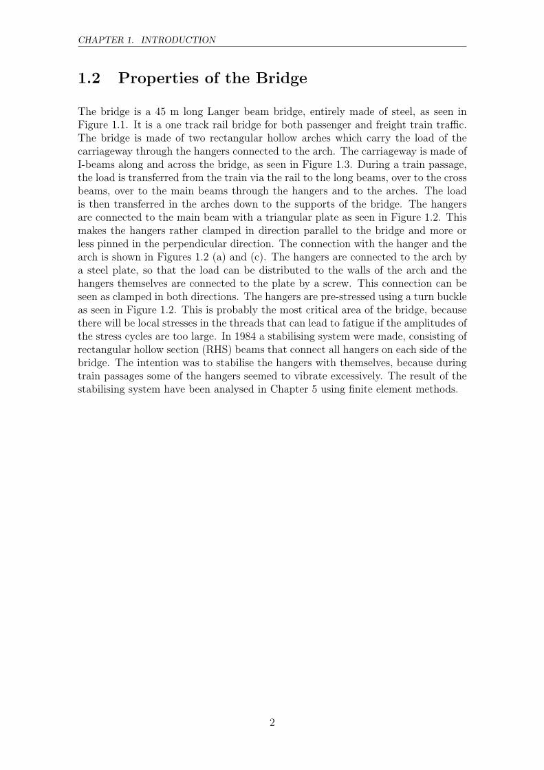
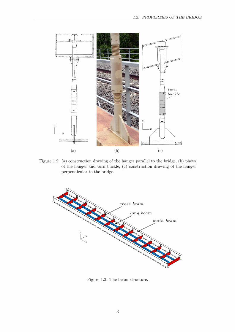
The bridge is a 45 m long Langer beam bridge, entirely made of steel, as seen inFigure 1.1. It is a one track rail bridge for both passenger and freight train traffic.The bridge is made of two rectangular hollow arches which carry the load of thecarriageway through the hangers connected to the arch. The carriageway is made ofI-beams along and across the bridge, as seen in Figure 1.3. During a train passage,the load is transferred from the train via the rail to the long beams, over to the crossbeams, over to the main beams through the hangers and to the arches. The loadis then transferred in the arches down to the supports of the bridge. The hangersare connected to the main beam with a triangular plate as seen in Figure 1.2. Thismakes the hangers rather clamped in direction parallel to the bridge and more orless pinned in the perpendicular direction. The connection with the hanger and thearch is shown in Figures 1.2 (a) and (c). The hangers are connected to the arch bya steel plate, so that the load can be distributed to the walls of the arch and thehangers themselves are connected to the plate by a screw. This connection can beseen as clamped in both directions. The hangers are pre-stressed using a turn buckleas seen in Figure 1.2. This is probably the most critical area of the bridge, becausethere will be local stresses in the threads that can lead to fatigue if the amplitudes ofthe stress cycles are too large. In 1984 a stabilising system were made, consisting ofrectangular hollow section (RHS) beams that connect all hangers on each side of thebridge. The intention was to stabilise the hangers with themselves, because duringtrain passages some of the hangers seemed to vibrate excessively. The result of thestabilising system have been analysed in Chapter 5 using finite element methods.
2
1.2. PROPERTIES OF THE BRIDGE
y
z
(a) (b)
x
z
turn
buckle
(c)
Figure 1.2: (a) construction drawing of the hanger parallel to the bridge, (b) photoof the hanger and turn buckle, (c) construction drawing of the hangerperpendicular to the bridge.
x
yz
main beam
long beam
cross beam
Figure 1.3: The beam structure.
3
CHAPTER 1. INTRODUCTION
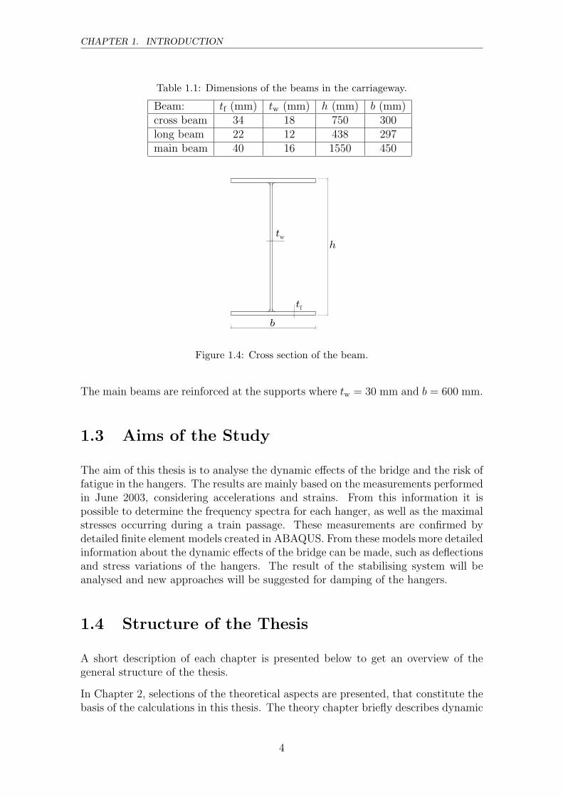
Table 1.1: Dimensions of the beams in the carriageway.
Beam: tf (mm) tw (mm) h (mm) b (mm)cross beam 34 18 750 300long beam 22 12 438 297main beam 40 16 1550 450
tw
tf
h
b
Figure 1.4: Cross section of the beam.
The main beams are reinforced at the supports where tw = 30 mm and b = 600 mm.
1.3 Aims of the Study
The aim of this thesis is to analyse the dynamic effects of the bridge and the risk offatigue in the hangers. The results are mainly based on the measurements performedin June 2003, considering accelerations and strains. From this information it ispossible to determine the frequency spectra for each hanger, as well as the maximalstresses occurring during a train passage. These measurements are confirmed bydetailed finite element models created in ABAQUS. From these models more detailedinformation about the dynamic effects of the bridge can be made, such as deflectionsand stress variations of the hangers. The result of the stabilising system will beanalysed and new approaches will be suggested for damping of the hangers.
1.4 Structure of the Thesis
A short description of each chapter is presented below to get an overview of thegeneral structure of the thesis.
In Chapter 2, selections of the theoretical aspects are presented, that constitute thebasis of the calculations in this thesis. The theory chapter briefly describes dynamic
4

1.4. STRUCTURE OF THE THESIS
properties of a basic structural model in order to visualise the methods such asthe Half-Power method and Rayleigh damping that are used to analyse the traininduced vibrations. Other important theoretical aspects that are discussed are thesignal analysis, time integration methods and fatigue. The signal analysis sectionincludes subjects such as Fourier transform, filtering and windowing.
The procedure of creating finite element models in ABAQUS/CAE is presented inChapter 3. The algorithms within ABAQUS that are used in this thesis are brieflypresented and the different dynamic analysis approaches are compared. The use ofcontact formulations in ABAQUS is also presented.
In Chapter 4, the equipment used in the field measurements and the different trainpassages that were measured are presented. The main part of Chapter 4 describesthe analysis of the measurements and the effect of the train induced vibrations. Theanalyses that have been made are frequency response of the hangers and their damp-ing properties from both a free vibration test and excitation from train passages.Other important results are the displacements in the hangers and the train inducedstress. Long term effects of the train induced vibrations are considered with fatigueanalysis. The results of the finite element modelling in ABAQUS are presented inChapter 5 and the analyses are divided into static analysis, eigenvalue analysis anddynamic analysis. The whole bridge is analysed during train passages and a detailedstudy of the turn buckle is performed. A comparison of the results is made with themeasurements and conclusions of the modelling are drawn.
Chapter 6 contains a discussion of the results and presents the main results. Somerecommendations for further research are also suggested.
Appendix A includes results from the measurements of some train passages thatillustrate the behaviour of the bridge.
5

Chapter 2
Evaluation Methods
2.1 Structural Dynamics
There is an extensive amount of literature concerning the theory of structural dy-namics and it is beyond the scope of this thesis to review this literature to anylarger extent. However, some of the theoretical aspects that are used in this thesisare presented in this section. The intention of this section is to provide a backgroundthat can be useful when analysing dynamic properties of train induced vibrationsand other problems in structural dynamics. All of the Figures in this Section arereproduced from Battini [2] except Figure 2.9 which is reproduced from Clough andPenzien [4].
2.1.1 Undamped Free Vibration
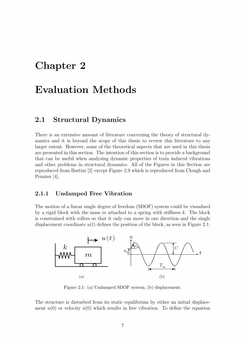
The motion of a linear single degree of freedom (SDOF) system could be visualisedby a rigid block with the mass m attached to a spring with stiffness k. The blockis constrained with rollers so that it only can move in one direction and the singledisplacement coordinate u(t) defines the position of the block, as seen in Figure 2.1.
k
m
)(tu
(a)
ou
u
nT
u
t
C
.o
(b)
Figure 2.1: (a) Undamped SDOF system, (b) displacement.
The structure is disturbed from its static equilibrium by either an initial displace-ment u(0) or velocity u(0) which results in free vibration. To define the equation
7
CHAPTER 2. EVALUATION METHODS
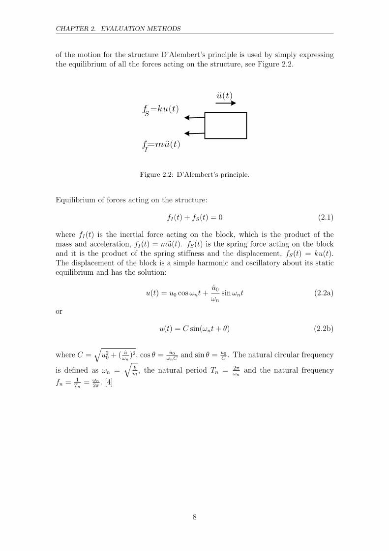
of the motion for the structure D’Alembert’s principle is used by simply expressingthe equilibrium of all the forces acting on the structure, see Figure 2.2.
fS=ku(t)
u(t)
fI=mu(t)
..
..
Figure 2.2: D’Alembert’s principle.
Equilibrium of forces acting on the structure:
fI(t) + fS(t) = 0 (2.1)
where fI(t) is the inertial force acting on the block, which is the product of themass and acceleration, fI(t) = mu(t). fS(t) is the spring force acting on the blockand it is the product of the spring stiffness and the displacement, fS(t) = ku(t).The displacement of the block is a simple harmonic and oscillatory about its staticequilibrium and has the solution:
u(t) = u0 cos ωnt +u0
ωn
sin ωnt (2.2a)
or
u(t) = C sin(ωnt + θ) (2.2b)
where C =√
u20 + ( u
ωn)2, cos θ = u0
ωnCand sin θ = u0
C. The natural circular frequency
is defined as ωn =√
km
, the natural period Tn = 2πωn
and the natural frequency
fn = 1Tn
= ωn
2π. [4]
8
2.1. STRUCTURAL DYNAMICS
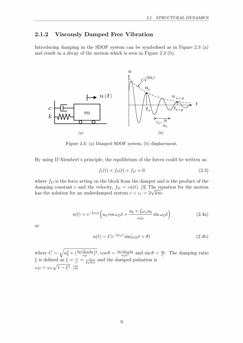
2.1.2 Viscously Damped Free Vibration
Introducing damping in the SDOF system can be symbolised as in Figure 2.3 (a)and result in a decay of the motion which is seen in Figure 2.3 (b).
m
)(tu
k
c
(a)
nt pnt +
nu
pnu+
u
t
te nC
D
DT2π
=
−ξω
ω
(b)
Figure 2.3: (a) Damped SDOF system, (b) displacement.
By using D’Alembert’s principle, the equilibrium of the forces could be written as:
fI(t) + fS(t) + fD = 0 (2.3)
where fD is the force acting on the block from the damper and is the product of thedamping constant c and the velocity, fD = cu(t). [3] The equation for the motionhas the solution for an underdamped system c < cr = 2
√km:
u(t) = e−ξωnt(u0 cos ωDt +
u0 + ξωnu0
ωD
sin ωDt)
(2.4a)
or
u(t) = Ce−ξωnt sin(ωDt + θ) (2.4b)
where C =√
u20 + ( u0+ξωnu0
ωD)2, cos θ = u0+ξωnu0
ωDCand sin θ = u0
C. The damping ratio
ξ is defined as ξ = ccr
= c2√
kmand the damped pulsation is
ωD = ωn
√1 − ξ2. [2]
9

CHAPTER 2. EVALUATION METHODS
2.1.3 Resonance
When a structure is subjected to a time varying force, it will after a while vibratewith the same frequency as the applied force. This is called steady state response.The amplitude of the vibration is equal to the product of the static deformationmultiplied with a dimensionless dynamic factor Rd:
Rd =1√[
1 − ( ωωn
)2]2
+ (2ξ ωωn
)2
(2.5)
where ωn is the natural circular frequency of the structure and ω is the circularfrequency of the load. For an undamped structure, ξ = 0, the dynamic factor tendsto infinity as the frequency ratio approaches unity, i.e. ω
ωn→ 1. As the damping
coefficient ξ increases, the value of the dynamic factor reduces, as seen in Figure 2.4.Steel bridges have normally a very low material damping coefficient, ξ ≤ 0.02.According to Johnson [12] the damping of large steel structures is commonly assumedto be 0.5%, independent of the mode and the amplitude of the vibration. If ξ = 0.02,the dynamic deformation at the resonance frequency is 25 times larger than the staticone.
0 0.5 1 1.5 2 2.5 30
1
2
3
4
5
6
ω/ωn
Rd
ξ=0.5
ξ =0.2
ξ=0.1
ξ =0
Figure 2.4: Variation of dynamic factor with damping and frequency.
It is seen in Figure 2.4 that the maximum steady-state response amplitude oc-curs at a frequency ratio slightly less than unity. Resonance is reached whenω = ωn
√1 − 2ξ2 [4].
10
2.1. STRUCTURAL DYNAMICS
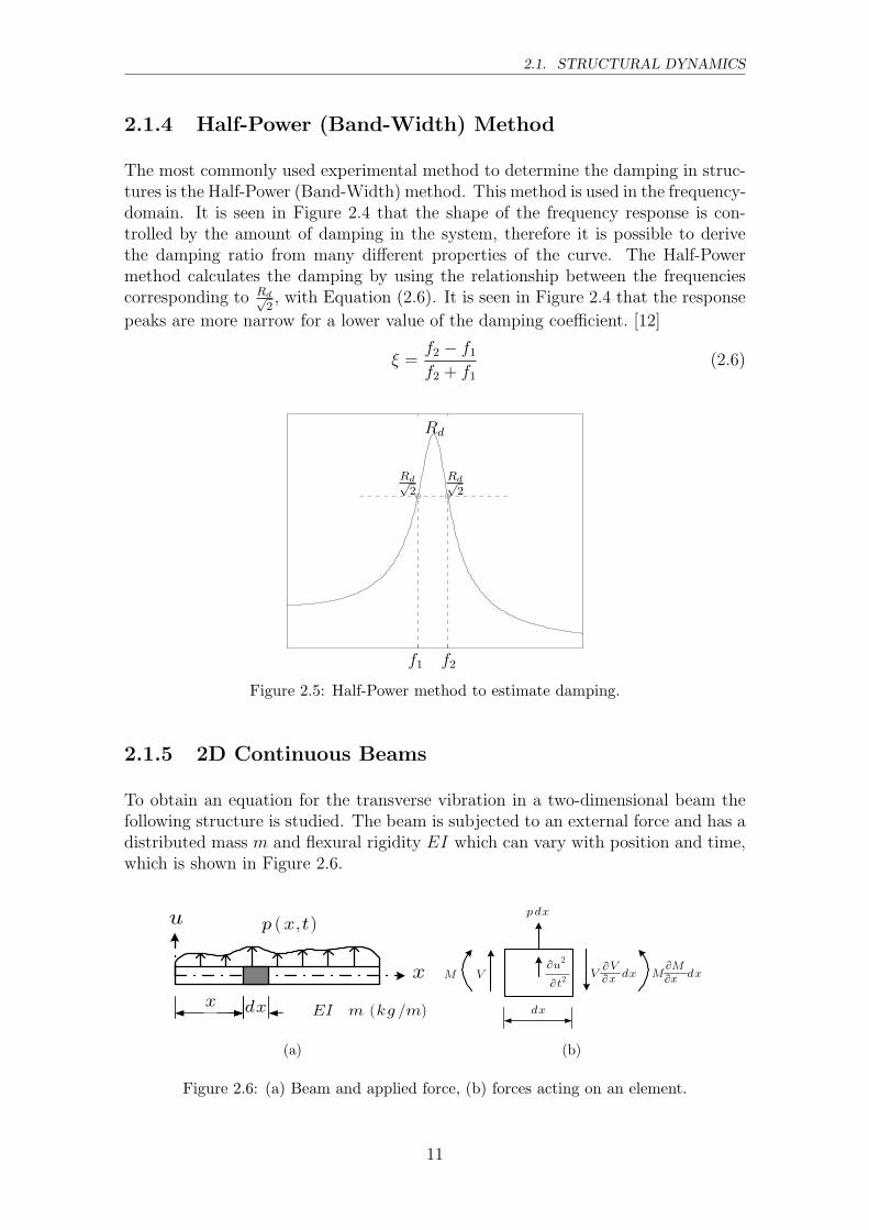
2.1.4 Half-Power (Band-Width) Method
The most commonly used experimental method to determine the damping in struc-tures is the Half-Power (Band-Width) method. This method is used in the frequency-domain. It is seen in Figure 2.4 that the shape of the frequency response is con-trolled by the amount of damping in the system, therefore it is possible to derivethe damping ratio from many different properties of the curve. The Half-Powermethod calculates the damping by using the relationship between the frequenciescorresponding to Rd√
2, with Equation (2.6). It is seen in Figure 2.4 that the response
peaks are more narrow for a lower value of the damping coefficient. [12]
ξ =f2 − f1
f2 + f1
(2.6)
Rd√2
Rd√2
f2f1
Rd
Figure 2.5: Half-Power method to estimate damping.
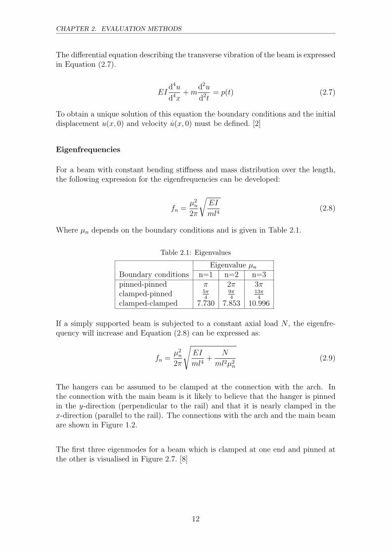
2.1.5 2D Continuous Beams
To obtain an equation for the transverse vibration in a two-dimensional beam thefollowing structure is studied. The beam is subjected to an external force and has adistributed mass m and flexural rigidity EI which can vary with position and time,which is shown in Figure 2.6.
u )( tx,p
x dx
x
(kg /m)mEI
(a)
2
2
t
uxx
VV d xx
MM d
dx
VM
xpd
∂∂
∂∂
∂
∂
(b)
Figure 2.6: (a) Beam and applied force, (b) forces acting on an element.
11
CHAPTER 2. EVALUATION METHODS
The differential equation describing the transverse vibration of the beam is expressedin Equation (2.7).
EId4u
d4x+ m
d2u
d2t= p(t) (2.7)
To obtain a unique solution of this equation the boundary conditions and the initialdisplacement u(x, 0) and velocity u(x, 0) must be defined. [2]
Eigenfrequencies
For a beam with constant bending stiffness and mass distribution over the length,the following expression for the eigenfrequencies can be developed:
fn =µ2
n
2π
√EI
ml4(2.8)
Where µn depends on the boundary conditions and is given in Table 2.1.
Table 2.1: Eigenvalues
Eigenvalue µn
Boundary conditions n=1 n=2 n=3pinned-pinned π 2π 3πclamped-pinned 5π
49π4
13π4
clamped-clamped 7.730 7.853 10.996
If a simply supported beam is subjected to a constant axial load N , the eigenfre-quency will increase and Equation (2.8) can be expressed as:
fn =µ2
n
2π
√EI
ml4+
N
ml2µ2n
(2.9)
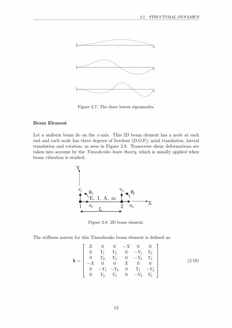
The hangers can be assumed to be clamped at the connection with the arch. Inthe connection with the main beam is it likely to believe that the hanger is pinnedin the y-direction (perpendicular to the rail) and that it is nearly clamped in thex-direction (parallel to the rail). The connections with the arch and the main beamare shown in Figure 1.2.
The first three eigenmodes for a beam which is clamped at one end and pinned atthe other is visualised in Figure 2.7. [8]
12
2.1. STRUCTURAL DYNAMICS
Figure 2.7: The three lowest eigenmodes.
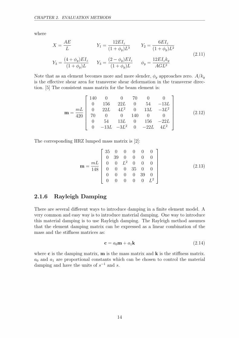
Beam Element
Let a uniform beam lie on the x-axis. This 2D beam element has a node at eachend and each node has three degrees of freedom (D.O.F); axial translation, lateraltranslation and rotation, as seen in Figure 2.8. Transverse shear deformations aretaken into account by the Timoshenko beam theory, which is usually applied whenbeam vibration is studied.
Y
X1u 2u
1v 2v1 2
E, I, A, m
L1 2
θ θ
Figure 2.8: 2D beam element.
The stiffness matrix for this Timoshenko beam element is defined as:
k =
X 0 0 −X 0 00 Y1 Y2 0 −Y1 Y2
0 Y2 Y3 0 −Y2 Y4
−X 0 0 X 0 00 −Y1 −Y2 0 Y1 −Y2
0 Y2 Y4 0 −Y2 Y3
(2.10)
13
CHAPTER 2. EVALUATION METHODS
where
X =AE
LY1 =
12EIz
(1 + φy)L3Y2 =
6EIz
(1 + φy)L2
Y3 =(4 + φy)EIz
(1 + φy)LY3 =
(2 − φy)EIz
(1 + φy)Lφy =
12EIzky
AGL2
(2.11)
Note that as an element becomes more and more slender, φy approaches zero. A/ky
is the effective shear area for transverse shear deformation in the transverse direc-tion. [5] The consistent mass matrix for the beam element is:
m =mL
420
140 0 0 70 0 00 156 22L 0 54 −13L0 22L 4L2 0 13L −3L2
70 0 0 140 0 00 54 13L 0 156 −22L0 −13L −3L2 0 −22L 4L2
(2.12)
The corresponding HRZ lumped mass matrix is [2]:
m =mL
148
35 0 0 0 0 00 39 0 0 0 00 0 L2 0 0 00 0 0 35 0 00 0 0 0 39 00 0 0 0 0 L2
(2.13)
2.1.6 Rayleigh Damping
There are several different ways to introduce damping in a finite element model. Avery common and easy way is to introduce material damping. One way to introducethis material damping is to use Rayleigh damping. The Rayleigh method assumesthat the element damping matrix can be expressed as a linear combination of themass and the stiffness matrices as:
c = a0m + a1k (2.14)
where c is the damping matrix, m is the mass matrix and k is the stiffness matrix.a0 and a1 are proportional constants which can be chosen to control the materialdamping and have the units of s−1 and s.
14
2.1. STRUCTURAL DYNAMICS
Mass proportional a1=0
Stiffness proportional a0=0
Combined
ωn
ξn
ωm
ξm
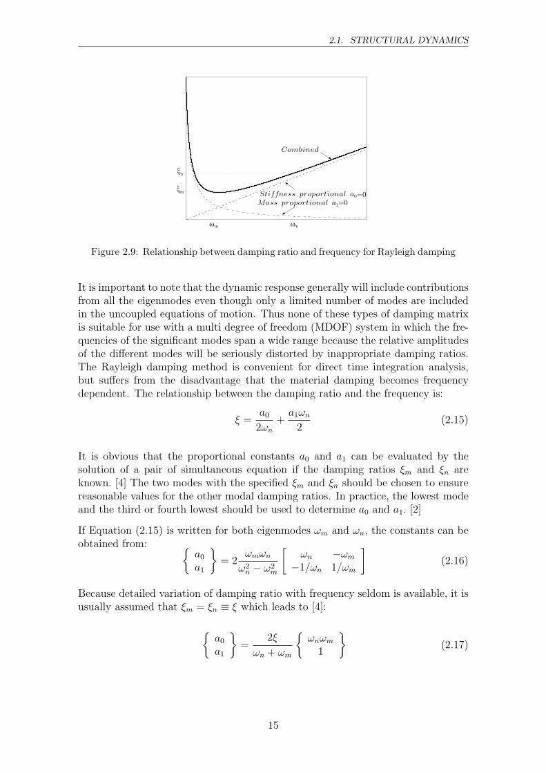
Figure 2.9: Relationship between damping ratio and frequency for Rayleigh damping
It is important to note that the dynamic response generally will include contributionsfrom all the eigenmodes even though only a limited number of modes are includedin the uncoupled equations of motion. Thus none of these types of damping matrixis suitable for use with a multi degree of freedom (MDOF) system in which the fre-quencies of the significant modes span a wide range because the relative amplitudesof the different modes will be seriously distorted by inappropriate damping ratios.The Rayleigh damping method is convenient for direct time integration analysis,but suffers from the disadvantage that the material damping becomes frequencydependent. The relationship between the damping ratio and the frequency is:
ξ =a0
2ωn
+a1ωn
2(2.15)
It is obvious that the proportional constants a0 and a1 can be evaluated by thesolution of a pair of simultaneous equation if the damping ratios ξm and ξn areknown. [4] The two modes with the specified ξm and ξn should be chosen to ensurereasonable values for the other modal damping ratios. In practice, the lowest modeand the third or fourth lowest should be used to determine a0 and a1. [2]
If Equation (2.15) is written for both eigenmodes ωm and ωn, the constants can beobtained from: {
a0
a1
}= 2
ωmωn
ω2n − ω2
m
[ωn −ωm
−1/ωn 1/ωm
](2.16)
Because detailed variation of damping ratio with frequency seldom is available, it isusually assumed that ξm = ξn ≡ ξ which leads to [4]:
{a0
a1
}=
2ξ
ωn + ωm
{ωnωm
1
}(2.17)
15

CHAPTER 2. EVALUATION METHODS
2.2 Signal Analysis
2.2.1 Fourier Analysis
The response of a system acted upon by an arbitrary force can be determined bythe time domain analysis procedure for any single degree of freedom system. Itis sometimes more convenient to transform the signal to frequency domain. Thisis especially suitable when the equation of motion contains parameters which arefrequency dependent. Such parameters can be the stiffness k or the damping c.
A simple periodic function can be separated into harmonic components by usingFourier series:
p(t) = a0 +∞∑
n=1
(an cos ωnt + bn sin ωnt
)(2.18)
In which the natural circular frequency ωn = nω1 = n 2πTn
and Tn represent theperiod. [4]
The Fourier coefficients are:
a0 =1
Tn
∫ Tn
0
p(t)dt (2.19)
an =2
Tn
∫ Tn
0
p(t) cos(ωnt)dt n = 1, 2, 3 . . . (2.20)
bn =2
Tn
∫ Tn
0
p(t) sin(ωnt)dt n = 1, 2, 3 . . . (2.21)
The periodic function can also be written as:
p(t) = c0 +∞∑
n=1
(cn sin(ωnt + φn)
)(2.22)
The coefficients are: c0 = a0, cn =√
a2n + b2
n and φn = arctan an
bn
The Fourier coefficient cn represents the magnitude and φn is the phase angle. Aplot of magnitude versus frequency is known as the Fourier amplitude spectrum. [10]
2.2.2 Discrete Fourier Transform (DFT)
Note that the time function is denoted by lowercase letter and the Fourier transformof the function by the same letter in uppercase. The frequency domain analysis ofa dynamic response requires that both the Fourier transform of p(t) and the inverse
16
2.2. SIGNAL ANALYSIS
Fourier transform of the complex response amplitude U(t) are determined. Analyt-ical evaluation of these direct and inverse Fourier transforms is not possible exceptfor excitations described by simple functions applied to structural systems. The in-tegrals have to be evaluated numerically for excitations varying arbitrary with time,complex vibratory systems, or situations where complex frequency response (or unitimpulse response) is described numerically. Numerical evaluation requires truncat-ing these integrals over infinite range to a finite range, and becomes equivalent toapproximating the random time-varying excitation p(t) by a periodic function. Thediscrete Fourier transform is defined as [3]:
Pn =1
N
N−1∑m=0
p(tm)e−i 2πnmN (2.23)
where t = tm = m∆t m = 1, 2, 3, . . . , N
2.2.3 Filtering
Filtering is often used to minimize high frequency signals (noise) in order to makethe primary pulse more readable. Filtering can attenuate the unimportant parts ofthe signal, but it can also be misapplied if the signal is over-filtered. This will leadto a distortion of the data, which normally reduces the signal peak amplitude. Toprevent over-filtering, the filter frequency should be at least five times greater thanthe highest frequency of interest.
The most common type of filter is a low-pass filter, which attenuates the highfrequency signals while the low frequency signals are unmodified. Another commontype of filter is a band-pass filter which attenuates signals with frequencies thatnot are within a specified interval. Filters can either be mechanical or applieddigitally. Mechanical (analogue) filters are used when measuring the signal, whiledigital filtering only is possible when the signal has been digitalised, such as withPC-based instrumentation systems. Digital filtering is accomplished in three steps.First the signal has to be Fourier transformed and then the signals amplitude infrequency domain should be multiplied by the desired frequency response. Finallythe transferred signal must be inversely Fourier transformed back into time domain.The advantage with a digital filter is that it does not introduce any phase errorsand that the original unfiltered signal still can be stored. [10]
2.2.4 Windowing
The Fourier transform has been described for a periodic signal, but a measured sig-nal is obviously not periodic. Fourier transform of a non-periodic signal can resultin several spurious amplitudes. [12] Windowing is the multiplication of the inputsignal by a weighted function to reduce spurious oscillations in the frequency do-main, which forces the signal to be periodic. Signals obtained from measurementsare made over finite time intervals, while Fourier transforms are defined of infinite
17
CHAPTER 2. EVALUATION METHODS
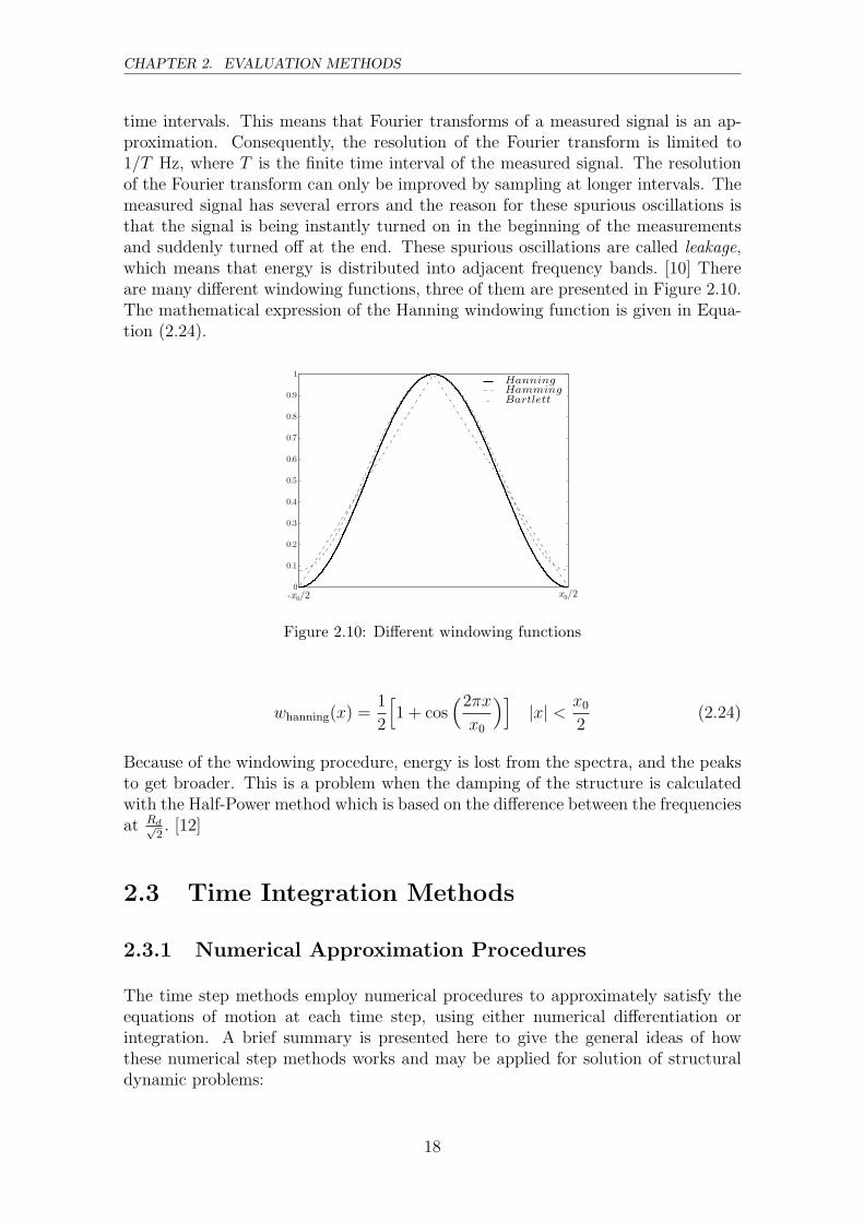
time intervals. This means that Fourier transforms of a measured signal is an ap-proximation. Consequently, the resolution of the Fourier transform is limited to1/T Hz, where T is the finite time interval of the measured signal. The resolutionof the Fourier transform can only be improved by sampling at longer intervals. Themeasured signal has several errors and the reason for these spurious oscillations isthat the signal is being instantly turned on in the beginning of the measurementsand suddenly turned off at the end. These spurious oscillations are called leakage,which means that energy is distributed into adjacent frequency bands. [10] Thereare many different windowing functions, three of them are presented in Figure 2.10.The mathematical expression of the Hanning windowing function is given in Equa-tion (2.24).
x /20
0.1
0.2
0.3
0.4
0.5
0.6
0.7
0.8
0.9
1HanningHammingBartlett
0-x /20
Figure 2.10: Different windowing functions
whanning(x) =1
2
[1 + cos
(2πx
x0
)]|x| <
x0
2(2.24)
Because of the windowing procedure, energy is lost from the spectra, and the peaksto get broader. This is a problem when the damping of the structure is calculatedwith the Half-Power method which is based on the difference between the frequenciesat Rd√
2. [12]
2.3 Time Integration Methods
2.3.1 Numerical Approximation Procedures
The time step methods employ numerical procedures to approximately satisfy theequations of motion at each time step, using either numerical differentiation orintegration. A brief summary is presented here to give the general ideas of howthese numerical step methods works and may be applied for solution of structuraldynamic problems:
18
2.3. TIME INTEGRATION METHODS
1. The method may be classified as either explicit or implicit. In an explicitmethod, the result in each step depends only on the quantities obtained in thepreceding step, so the analysis proceeds directly from one step to the next.The implicit method on the other hand is based on that the expression fora certain step includes one or more values pertaining to the same step. Thismeans that trial values of the necessary quantities must be guessed and theseare refined by successive iterations. Even though the equations required foreach step are very simple, the cost of iteration within a step may be ruling.
2. The primary factor to be considered in selecting a step method is efficiency,which concerns the computational effort required to achieve the desired levelof accuracy over the range of time for which the response is needed. Accuracyalone cannot be a criterion since any level of accuracy can be obtained withany method if the time step is small enough, but with obvious increase ofcosts. In any case the time steps must be made short enough to provide anadequate definition of the loading and the response history. A high frequencyinput or response cannot be defined with large time steps.
3. Factors that may contribute to errors in the results obtained from well definedloadings include:
(a) Round off: resulting from calculations being done using number expressedby too few digits. This is normally not any problem with the computerprograms used today.
(b) Instability: caused by amplification of the errors from one step duringthe calculations of subsequent steps. Stability of any method is improvedby choosing a smaller time step.
(c) Truncation: using too few terms in series expressions of quantities.
4. Errors resulting from any causes may be manifested by either or both of thefollowing effects:
(a) Phase shift or apparent change of frequency in cyclic results.
(b) Artificial damping, in which the numerical procedure removes or addsenergy to the dynamically response system.
2.3.2 Newmark Beta Methods
A general step method was proposed by Newmark and the equations for the velocityand displacement in step i is defined as:
ui = ui−1 + (1 − γ)∆tui−1 + γ∆tui (2.25a)
ui = ui−1 + ∆tui−1 +(1
2− β
)∆t2ui−1 + β∆t2ui (2.25b)
19
CHAPTER 2. EVALUATION METHODS
The factor γ provides a linearly weighting between the influence of the initial and thefinal accelerations on the change of velocity and β provides the same weighting be-tween the initial and final accelerations for the displacements. According to Cloughand Penzien, [4], studies of this formulation has shown that the factor γ controls theamount of artificial damping induced by the step procedure and if γ = 1/2 thereis no artificial damping. Direct time integration methods based on the Newmarkformula are summarised in Table 2.2. [4]
Table 2.2: Different Newmark methods.
Method Type β γTrapezoidal rule Implicit 1/4 1/2Linear acceleration Implicit 1/6 1/2Central difference Explicit 0 1/2
The stability criterion for Newmark’s method is:
∆t
Tn
≤ 1
π√
2
1√γ − 2β
(2.26)
For the Trapezoidal rule,γ = 12
and β = 14, this condition is presented in Equa-
tion (2.27). [3]∆t
Tn
< ∞ (2.27)
This means that the Trapezoidal rule is stable for any time increment.
2.3.3 Hilber-Hughes-Taylor Alpha Method
The Hilber-Hughes-Taylor Alpha method is used when damping is introduced inthe Newmark method, without degrading the order of accuracy. The method isbased on the Newmark equations, whereas the time discrete equations are modifiedby averaging elastic, inertial and external forces between both time instants. Theparameters γ and β are defined:
γ =1 − 2α
2(2.28a)
β =(1 − α)2
4(2.28b)
where the parameter α is chosen so that:
α ∈[− 1
3, 0
](2.29)
The result of this is an unconditional stable second-order scheme and it is a log-ical replacement of the Newmark algorithm for non-linear problems in which it isnecessary to control the damping during the integration. [8]
20
2.4. FATIGUE
2.4 Fatigue
Loads suddenly applied to structures are termed shock or impact loads and result indynamic loading . This also includes rapidly moving forces such as those caused by arailroad train passing over a bridge. Structural members subjected to repeated fluc-tuating, or alternating stresses, which are smaller than the ultimate tensile strengthσu or even the yield strength σyp, may nevertheless manifest diminished strengthand ductility. This is termed fatigue and is mainly influenced by minor structuraldiscontinuities, the quality of the surface finish and the chemical nature of the en-vironment. Generally the fatigue fracture has its origin at points with high stressconcentrations. This type of failure, through the involvement of slip planes andspreading cracks, is progressive in nature. Tensile stress, and to lesser degree shear-ing stress, lead to fatigue crack propagation, while compressive stress probably doesnot. [15]
The dynamic loads are normally loads from moving vehicles and/or wind loads. Aload that is time-dependent will induce stress variations in the structure and if theyare large and many they could lead to fatigue fractures. When designing for fatiguethe stress range σrd is used. Stress range is the difference between maximum andminimum stress in the studied point during the stress variation. The stress range σrd
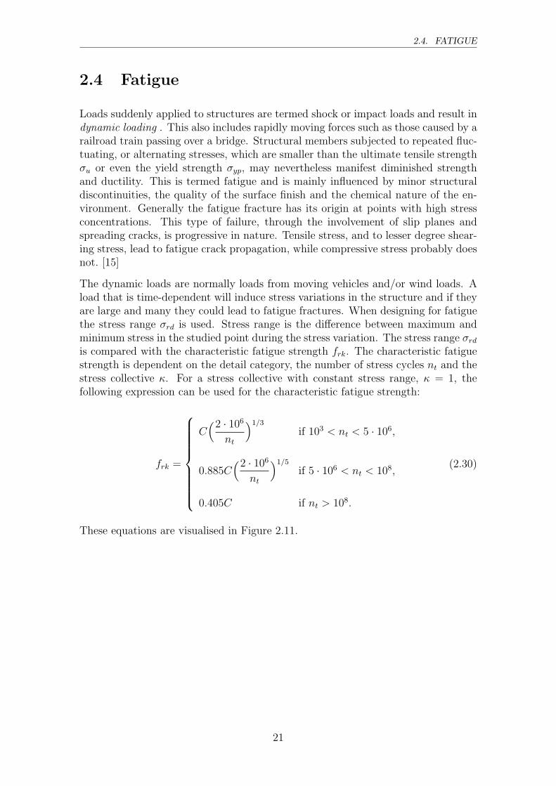
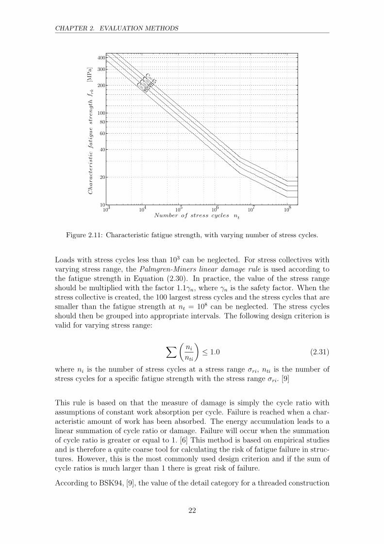
is compared with the characteristic fatigue strength frk. The characteristic fatiguestrength is dependent on the detail category, the number of stress cycles nt and thestress collective κ. For a stress collective with constant stress range, κ = 1, thefollowing expression can be used for the characteristic fatigue strength:
frk =
C(2 · 106
nt
)1/3
if 103 < nt < 5 · 106,
0.885C(2 · 106
nt
)1/5
if 5 · 106 < nt < 108,
0.405C if nt > 108.
(2.30)
These equations are visualised in Figure 2.11.
21
CHAPTER 2. EVALUATION METHODS
103
104
105
106
107
10810
20
40
60
80
100
200
300
400
C=45
C=40
C=35
C=30
Number of stress cycles nt
Characteristic
fatigue
strength
frk
[MPa]
Figure 2.11: Characteristic fatigue strength, with varying number of stress cycles.
Loads with stress cycles less than 103 can be neglected. For stress collectives withvarying stress range, the Palmgren-Miners linear damage rule is used according tothe fatigue strength in Equation (2.30). In practice, the value of the stress rangeshould be multiplied with the factor 1.1γn, where γn is the safety factor. When thestress collective is created, the 100 largest stress cycles and the stress cycles that aresmaller than the fatigue strength at nt = 108 can be neglected. The stress cyclesshould then be grouped into appropriate intervals. The following design criterion isvalid for varying stress range:
∑ (ni
nti
)≤ 1.0 (2.31)
where ni is the number of stress cycles at a stress range σri, nti is the number ofstress cycles for a specific fatigue strength with the stress range σri. [9]
This rule is based on that the measure of damage is simply the cycle ratio withassumptions of constant work absorption per cycle. Failure is reached when a char-acteristic amount of work has been absorbed. The energy accumulation leads to alinear summation of cycle ratio or damage. Failure will occur when the summationof cycle ratio is greater or equal to 1. [6] This method is based on empirical studiesand is therefore a quite coarse tool for calculating the risk of fatigue failure in struc-tures. However, this is the most commonly used design criterion and if the sum ofcycle ratios is much larger than 1 there is great risk of failure.
According to BSK94, [9], the value of the detail category for a threaded construction
22

2.4. FATIGUE
element should be less than 45. A rolled thread and thread turned in a lathe should,respectively, have 90% and 70% of the dimensioning value frd at C = 45.
23

Chapter 3
Creating Finite Element Models
This chapter deals with the modelling techniques that are used to analyse the bridgein the commercial software ABAQUS. A brief summary of the different routines thathave been used are presented, how they were used and the advantages of differentanalysis approaches. The finite element models were created in ABAQUS/CAEwhich includes the Graphical User Interface (GUI). This method of creating modelsis easier than coding an input file, especially when the models are large, as in thecase with 3D models and dealing with solid elements.
3.1 Modelling Procedures in ABAQUS/CAE
The ABAQUS/CAE environment is divided into different modules, where each mod-ule defines a logical aspect of the modelling process; for example, defining the ge-ometry, defining material properties, and generating a mesh. The GUI interfacegenerates an input file with all information of the model, to be submitted to thesolver, using ABAQUS/Standard or ABAQUS/Explicit routines. The solver per-forms the analysis and sends the information back to ABAQUS/CAE for evaluationof the results.
3.1.1 Modules
Most models created in ABAQUS/CAE are assembled from different parts. Parts arecreated separately in the part module. Different parts may need different materialproperties, which are defined in the property module. ABAQUS provides a fullrange of material properties, such as elastic and plastic behaviour, as well as thermaland acoustic behaviour. The model is then assembled in the assembly module, bycombining the different parts. In the step module the analysis is divided in differentanalysis step, such as static and dynamic analyses. These can be combined in a wayto resemble the physical problem that is to be analysed. At this stage, the partsin the model do not interact with each other. In the interaction module the partsare connected to each other using constraints, by defining the degrees of freedom
25
CHAPTER 3. CREATING FINITE ELEMENT MODELS
to be connected with another part. Interactions between parts are also defined,such as contact methods and friction behaviour. Connector elements can also bedefined, to simulate for example spring or dashpot behaviour. The loads acting onthe model are defined in the load module, as well as boundary conditions. Theloads and the boundary conditions can be defined to vary over time as well as overdifferent steps. Physical kinematical behaviour, such as velocity, can be appliedeither as boundary condition or field procedure. Velocity is generally more stablewhen defined as boundary condition than field variables. The whole model is thenmeshed in the mesh module. The meshing techniques vary with the element typeand the geometry of the model. Different meshing techniques can be applied tothe same part if partitioning is used. This is useful when regions of the same partrequires different accuracy, or if the geometry is complicated.
3.1.2 Elements
All elements used in ABAQUS are divided into different categories, depending onthe modelling space. The element shapes available are beam elements, shell elementsand solid elements and the modelling space is divided into 3D space, 2D planar spaceand axisymmetric space.
Beam Elements
A beam element is an element in which assumptions are made so that the problemis reduced to one dimension mathematically. The primary solution variable is thenfunctions of the length direction of the beam. For this solution to be valid, the lengthof the element must be large compared to its cross-section. There are two maintypes of beam element formulations, the Euler-Bernoulli theory and the Timoshenkotheory.The Euler-Bernoulli theory assumes that plane cross-sections, initially normal tothe beams axis, remain plane, normal to the beam axis, and undistorted. All beamelements in ABAQUS that use linear or quadratic interpolation are based on thistheory. The Timoshenko beam theory allows the elements to have transverse shearstrain, so that the cross-sections do not have to remain normal to the beam axis.This is generally more useful for thicker beams. [11]
Shell Elements
The shell elements defined in ABAQUS are divided into three categories: thin,thick and general-purpose elements. The thin shell elements are based on the Kir-choff shell theory and the thick shell elements are based on the Mindlin shell theory,which includes shear deformation and therefore are better suited for thicker ele-ments. The general-purpose shell elements can provide solutions for both thin andthick shell elements. In ABAQUS/Standard all three types are available, whileABAQUS/Explicit only provides general-purpose elements. [11]
26
3.1. MODELLING PROCEDURES IN ABAQUS/CAE
Solid Elements
ABAQUS provide solid elements in two and three dimensions. The two-dimensionalsolid elements allow modelling of plane and axisymmetric problems. In three di-mensions the isoparametric hexahedra element are most common, but in some casescomplex geometry may acquire tetrahedron elements. Those elements are generallyonly recommended to fill in awkward parts of the mesh. ABAQUS provide bothfirst-order linear and second-order quadratic interpolation of the solid elements.The first-order elements are essentially constant strain elements, while the second-order elements are capable of representing all possible linear strain fields and aremore accurate when dealing with more complicated problems. [11]
3.1.3 Analysis Type
ABAQUS provides several different analysis types which are divided in two maingroups: general and linear perturbation. General analysis defines a sequence ofevents and the state of the model at the end of one step provides the initial statefor the next step. Linear perturbation analyses provide the linear response of themodel about the state reached at the end of the last general nonlinear analysis. InABAQUS/CAE those different analysis types are managed under the step module.
General Static Analysis
The general static analysis can involve both linear and nonlinear effects and is per-formed to analyse static behaviour such as deflection due to a static load. A criterionfor the analysis to be possible is that it is stable. A static step uses time increments,not in a manner of dynamic steps but rather as a fraction of the applied load. Thedefault time period is 1.0 units of time, representing 100% of the applied load. Ifnonlinear effects are expected, such as large displacements, material nonlinearities,boundary nonlinearities, contact or friction, the NLGEOM command should beused. When dealing with an unstable problem, such as in buckling or collapse, themodified Riks method can be used. It uses the load magnitude as an additional un-known, and solves simultaneous for loads and displacements. This method providesa solution even if the problem is nonlinear. [11]
Linear Eigenvalue Analysis
Linear eigenvalue analysis is used to perform an eigenvalue extraction to calculate thenatural frequencies and the corresponding mode shapes of the model. The analysiscan be performed using two different eigensolver algorithms, Lanczos or subspace.The Lanczos eigensolver is faster when a large number of eigenmodes are requiredwhile the subspace eigensolver can be faster for smaller systems. When using theLanczos eigensolver, one can choose the range of the eigenvalues of interest whilethe subspace eigensolver is limited to the maximum eigenvalue of interest. [11]
27
CHAPTER 3. CREATING FINITE ELEMENT MODELS
Dynamic Implicit Analysis
The dynamic implicit analysis method is used to calculate the transient dynamicresponse of a system, e.g. a moving body interacting with other parts of the model.When nonlinear dynamic responses are studied, a direct time integration of thesystem must be used. In linear analysis, modal methods can be used to predict theresponse of the system, using eigenmode extraction. This is generally less expensivethan direct integration, because in direct integration the global equations of motionof the system must be integrated through time.
Implicit schemes solve the dynamic quantities at time t + ∆t and the nonlinearequations must be solved. This method uses the Hilber-Hughes-Taylor operator,which is an extension of the trapezoidal rule. If the equations are highly nonlinear,it may be difficult to obtain a solution. Nonlinearities are easier to handle in dynamicprocedures than in static ones, which make the implicit scheme applicable in mostcases that do not deal with extreme nonlinearities. The time step used in theimplicit scheme can be controlled by the “half step residual”, introduced by Hibbitand Karlsson (1979). The half-step residual is the equilibrium residual error halfwaythrough a time increment, t+∆t/2 and once the solution at t+∆t has been obtained,the accuracy of the solution can be assessed and the time step adjusted appropriately.The choice of the time increment depends on the type of analysis performed. Indynamic problems, a smaller time increment than the stable one might be used, toget an accurate result depending on the variations in the structure. In a static modelon the other hand, the time increment usually does not have the same physicalmeaning and corresponds to a fraction of the applied load rather than physicaltime. The time increment can be defined using either the automatic or the fixedincrementation. The automatic incrementation is based on the half step residualand is recommended for most analysis except in cases when the problem is wellunderstood, or when convergence is not achieved with the automatic incrementation.Even if convergence is achieved, the results are not guaranteed to be correct. Theautomatic time increments are chosen by defining initial, minimum and maximumincrement sizes. If no convergence can be found with the initial increment, a smallerone is used until convergence is achieved, down to the minimum increment defined.If the solution converges with the initial increment size, an attempt with a larger onewill be used. No increments will be attempted that are larger than the maximumstated. The routine for these procedures are based on empirical studies. [11]
Dynamic Explicit Analysis
The dynamic explicit analysis available in ABAQUS/Explicit is to be used withshort dynamic response time and extremely discontinuous processes. It also allowsgeneral contact conditions. Due to its large deformation theory, models are allowedto be heavily deformed, such as in explosions or collisions. The dynamic explicitroutine performs a large number of small time increments efficiently using an explicitcentral difference time integration rule. In this method, each increment is relativelyinexpensive compared to the direct-integration method because there is no solution
28
3.1. MODELLING PROCEDURES IN ABAQUS/CAE
for a set of simultaneous equations.The explicit central difference operator satisfies the dynamic equilibrium equationsat the beginning of the increment, t and the accelerations calculated at time t areused to advance the velocity solution to time t+∆t/2 and the displacement solutionto time t+∆t. The stability increment limit is given in terms of the highest frequencyof the system as ∆t ≤ 2/ωmax. When introducing damping to the system, the timeincrement is given by
∆t ≤ 2
ωmax
(√
1 + ξ2max − ξmax), (3.1)
where ξmax is the fraction of critical damping in the mode with the highest frequency.An approximation to the stability limit can be written as the smallest transit timeof a dilatational wave across any of the elements in the mesh, ∆t ≈ Lmin/cd, whereLmin is the length of the smallest element in the mesh and cd is the dilatational wavespeed. [11]The wave speed for steel is approximately 6000 m/s. If the smallest element size is0.1 m, the stable time increment becomes 17 µs.
3.1.4 Contact Methods
Contact methods are used in ABAQUS to define contact either between bodies orwith the body itself. Contact between bodies can be made with both rigid and de-formable bodies. There are two types of contact algorithms in ABAQUS/Explicit:kinematic and penalty method.The kinematic contact method does not allow any penetration of the contact bodieswhile the penalty method does. When defining a contact between two bodies, oneserves as a slave body and the other one as master. When contact occurs betweenthese two bodies, it is determined which slave nodes penetrates the master surface,the depth of each penetration and the mass associated with it. The force requiredto move the slave nodes to the master surface is then calculated. This force isdistributed to the master surface without deforming it and is used to adjust theacceleration of the nodes. A second adjustment is then performed to ensure that noother parts overlap each other.When using hard kinematic contact method it is still possible for the master surfaceto penetrate the slave surface after the correction. Such penetrations can be min-imised by refining the mesh on the slave surface.If softened kinematic contact is used, it will allow penetrations since its correctionsare made to satisfy the pressure-overclosure relationship at the slave nodes, not thecondition of zero penetration.
Sliding Formulation
There are three approaches to account for the relative motion concerning contactformulations: finite sliding, small sliding and infinitesimal sliding. Finite slidingis the most general and allows any arbitrary motion of the surfaces, small sliding
29
CHAPTER 3. CREATING FINITE ELEMENT MODELS
assumes relatively small relative motions between the contact surfaces, although thebodies themselves have large motions.The infinitesimal sliding and rotation assumes that both relative and absolute mo-tions are small. The last two types cannot be used with the penalty contact algo-rithm. [11]
3.1.5 Explicit versus Implicit Methods
Using the dynamic implicit scheme instead of the explicit can reduce the solutiontime radically. The main difference lies in the definition of the stable time increment.As discussed in Section 3.1.3, the stable time increment for the explicit analysis isLmin/cd, where Lmin is the smallest element in the mesh and cd is the dilatationalwave speed. This is generally most useful when dealing with models that suffer fromlarge deformation during a short time interval, e.g. explosions, collisions or bucklinganalysis. The train simulation in this thesis does not have any large deformationand have rather long time duration, more than 10 seconds. In the explicit schemeit is recommended to use automatic incrementation to achieve convergence, becausechanging the size of the increment easily makes the solution diverge. When usingthe implicit scheme it is also recommended to use the automatic incrementation,but convergence can be accomplished with a fixed time increment if the problem iswell understood. Even if the solution converges it is not guaranteed that the resultsare accurate, so it must be verified with different sizes of the increment.
3.1.6 Contact Conditions for Train Simulations
The dynamic simulations of the train in this thesis were mostly performed with dy-namic implicit scheme because the calculation time is just a fraction of the time forthe explicit routine. Both the train and the rail were made of solid elements withcontact formulation. Contact was set with a penalty friction formulation with thefriction constant µ = 0.1 in the tangential direction. In the normal direction thecontact was set with hard contact and no allowance to separate after contact. Thecontact was performed with a surface to surface contact method, with each wheelas a separate master surface and the rail as slave surface. The rail was constrainedwith the sleepers using a TIE connection to constrain every degree of freedom. Thebridge was then made in the same model with either 3D beam elements or 3D shellelements.The simulation was made with both automatic and fixed time increments with differ-ent time steps to achieve accurate results, which are further presented in Chapter 5.The loads, in this case gravity load from the bridge and the train load, were made inthe static step and then propagated into the dynamic step. If the load was createdin the dynamic step it was applied in a dynamic manner, causing the structure tooscillate severely before equilibrium was reached.
30

Chapter 4
Measurements
4.1 Introduction
The field measurements were performed at the Langer beam bridge in Ange andtook place in 24–25 June 2003. This project was initiated because it had beendetected that the hangers on the bridge vibrated excessively during train passagesand evaluation of the effect of these vibrations had to be made. To analyse themeasurements the software MATLAB was used. The five different train passageswere measured are presented in Table 4.1.
Table 4.1: Measured train types.
Type of train ID number locomotive number of Velocitycarriages [km/h]
freight 009 Rc4 24 85freight 011 Rc4 10 75passenger 012 Rc6 6 75passenger 018 Rc6 6 70freight (copper train) 019 Rc4 19 80
All of the results presented are taken from the last train passage with the coppertrain, ID019, since this train induced the largest vibrations and strains in the bridge.The results from a selection of the other train passages are displayed in Appendix A.The two types of measurements that were performed on the hangers measured theinduced strain and acceleration.
The instruments used to measure the train induced acceleration were:
• DAT-recorder -Sony PC216AX
• Amplifier-UNO-MWL 006
• Low-pass filter-PCP-848 LP-filter 20Hz
• Accelerometers-Terra Technology
31

CHAPTER 4. MEASUREMENTS
The instrumentation used to measure the train induced strain was:
• Amplifier-Hottinger MGCplus
• Strain gauges-N11-FA-5-120-11
The signals from the accelerometers and strain gauges had, respectively, the samplefrequency of 6000 Hz (samples/s) and 2000 Hz (samples/s).
The accelerometer and the strain gauge used for these measurements are shown inFigure 4.1.
(a) (b)
Figure 4.1: (a) Strain gauge attached to a hanger, (b) three accelerometers.
4.1.1 Strain Gauge
The strain was measured with four foil strain gauges assembled 90◦ apart and 100mm above the threaded section on the perimeter of each hanger. There are 11hangers on each side of the bridge and they are numbered from 1 to 11, where hanger1 and 11 are shortest and hanger 6 is the longest. The strain gauges were attachedto hanger 2 to 5. The gauges were numbered from 1 to 16, where the odd numbersmeasured bending parallel to the rail, x-direction, and even numbers perpendicularto the rail, y-direction. The assembly of the gauges is shown in Figure 4.2.
9
10
11
12
5
6
7
8
13
14
15
16
1
2
3
4hanger 2hanger 3hanger 4hanger 5
Figure 4.2: Placement of the strain gauges.
32
4.1. INTRODUCTION
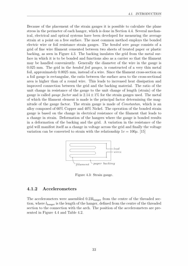
Because of the placement of the strain gauges it is possible to calculate the planestress in the perimeter of each hanger, which is done in Section 4.4. Several mechan-ical, electrical and optical systems have been developed for measuring the averagestrain at a point on a free surface. The most common method employs the bondedelectric wire or foil resistance strain gauges. The bonded wire gauge consists of agrid of fine wire filament cemented between two sheets of treated paper or plasticbacking, as seen in Figure 4.3. The backing insulates the grid from the metal sur-face in which it is to be bonded and functions also as a carrier so that the filamentmay be handled conveniently. Generally the diameter of the wire in the gauge is0.025 mm. The grid in the bonded foil gauges, is constructed of a very thin metalfoil, approximately 0.0025 mm, instead of a wire. Since the filament cross-section ona foil gauge is rectangular, the ratio between the surface area to the cross-sectionalarea is higher than of a round wire. This leads to increased heat dissipation andimproved connection between the grid and the backing material. The ratio of theunit change in resistance of the gauge to the unit change of length (strain) of thegauge is called gauge factor and is 2.14± 1% for the strain gauges used. The metalof which the filament element is made is the principal factor determining the mag-nitude of the gauge factor. The strain gauge is made of Constantan, which is analloy composed of 60% Copper and 40% Nickel. The operation of the bonded straingauge is based on the change in electrical resistance of the filament that leads toa change in strain. Deformation of the hangers where the gauge is bonded resultsin a deformation of the backing and the grid. A variation in the resistance of thegrid will manifest itself as a change in voltage across the grid and finally the voltagevariation can be converted to strain with the relationship 1v = 100µ. [15]
filament
lead
wires
paper backing
Figure 4.3: Strain gauge.
4.1.2 Accelerometers
The accelerometers were assembled 0.23lhanger from the centre of the threaded sec-tion, where lhanger is the length of the hanger, defined from the centre of the threadedsection to the connection with the arch. The position of the accelerometers are pre-sented in Figure 4.4 and Table 4.2.
33

CHAPTER 4. MEASUREMENTS
Table 4.2: Length of the hangers and the position of the accelerometers.
Hanger ltot (m) lhanger (m) 0.23lhanger (m) lacc(m)2 4.613 4.043 0.93 1.5453 6.244 5.674 1.30 1.9184 7.356 6.786 1.55 2.1725 8.003 7.433 1.70 2.320
x
z
turn
buckle
accelero-
meters
ltot
lacc
lhanger
Figure 4.4: Position of the accelerometers.
Each cylinder has three accelerometers, one for each direction in space, as seenin Figure 4.1. The accelerometers are piezoelectric. This type is primary madeof piezoelectric materials, i.e. natural or man-made quartz, which produce electriccharges in response to the strain in the material. By applying a seismic mass ofknown value to the piezoelectric material, a known force due to the acceleration ofthe seismic mass is created. The piezoelectric material has a force-voltage strainresponse which produces an electric charge proportional to the acceleration. Sincethe force-voltage strain response is nearly quadric it requires either a static load, oras in this case, a DC bias voltage to centre the response in a linear range. Thereforethe frequency may be constant all the way down to 0 Hz. All accelerometers have aparticular sensitivity, which refers to the ratio of electrical output to the mechanicalinput. Thus it is possible to calculate the acceleration by measuring the outputcharge or voltage from the accelerometer. [10]
A low-pass (LP) filter was used on train passages ID018 and ID019 to reduce thefrequencies above 20 Hz. This will show in the acceleration graphs were the mea-
34
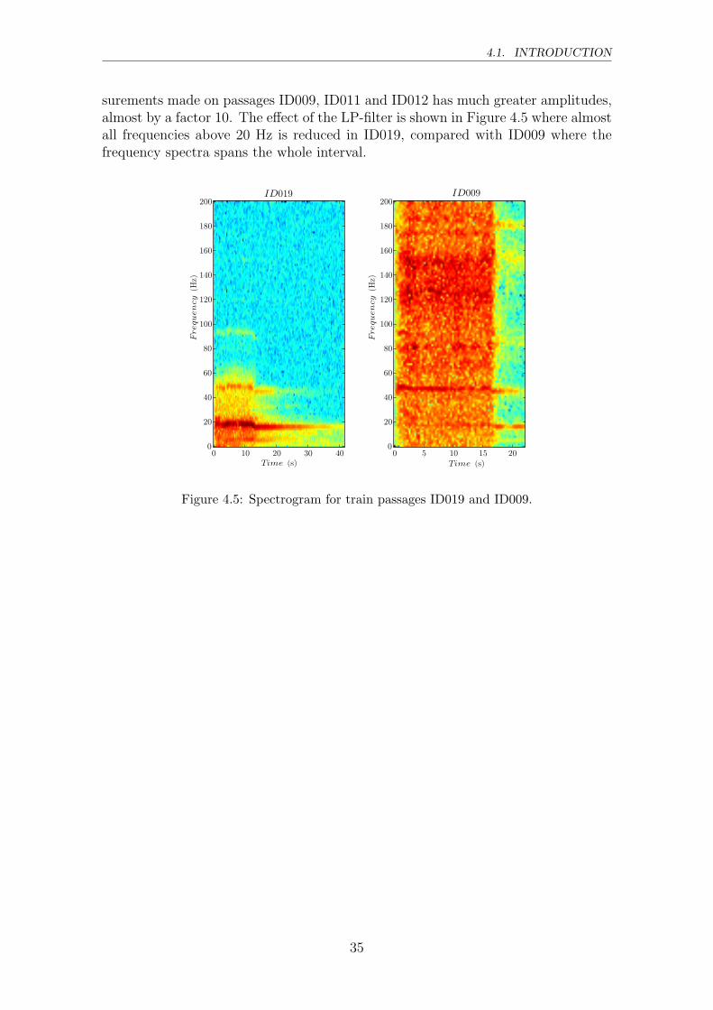
4.1. INTRODUCTION
surements made on passages ID009, ID011 and ID012 has much greater amplitudes,almost by a factor 10. The effect of the LP-filter is shown in Figure 4.5 where almostall frequencies above 20 Hz is reduced in ID019, compared with ID009 where thefrequency spectra spans the whole interval.
Time (s)
Frequency
(Hz)
0 10 20 30 400
20
40
60
80
100
120
140
160
180
200
Time (s)
Frequency
(Hz)
0 5 10 15 200
20
40
60
80
100
120
140
160
180
200ID019 ID009
Figure 4.5: Spectrogram for train passages ID019 and ID009.
35
CHAPTER 4. MEASUREMENTS
4.2 Frequency Analysis
The frequency analysis was made according to the theory in Section 2.2 whereEquation (2.23) was used to transform the measured signal from time domain tofrequency domain. The result from this procedure is a complex number and whentaking the absolute value of it, the Fourier magnitude is created. The frequencyspectra should have the interval ∆f and is obtained by the number of samples Nand the sampling rate, by the relation ∆f = N · rate.
During the field measurements it was detected that the entire arch vibrated perpen-dicular to the rail. This is shown in the frequency spectrum as several frequencyresponses in the y-direction during and after a train passage.
To estimate the eigenfrequencies of the hangers, Equation (2.8) was used whichproduced the results shown in Table 4.3.
Table 4.3: Estimated eigenfrequencies.
x-direction y-directionHanger Mode 1 [Hz] Mode 2 [Hz] Hanger Mode 1 [Hz] Mode 2 [Hz]
2 17.32 47.74 2 11.94 38.683 9.45 26.06 3 6.51 21.114 6.81 19.23 4 4.70 15.215 5.75 13.53 5 3.97 12.85
These eigenfrequencies were calculated with the assumption that the hangers areclamped in the connection with the arch in both x- and y-directions. In the con-nection with the main beam it were assumed that the hangers are clamped in thex-direction and pinned in the y-direction. A connection is almost impossible todesign so that it is clamped. Hence, the eigenfrequencies in Table 4.3 are overesti-mated. The eigenfrequencies are calculated using the entire lengths of the hangers,defined as ltot in Table 4.2.
4.2.1 Free Vibration Test
To determine the eigenfrequencies of each hanger, free vibration tests were per-formed. The free vibration was initiated by a swift knock on each hanger. Thismade it possible to easily view the eigenfrequencies from the hangers without dis-turbance from global eigenmodes of the bridge. The result from the free vibrationtest is presented in Figures 4.6– 4.9.
36

4.2. FREQUENCY ANALYSIS
0 5 10 15 20 250
0.5
1
1.5
f (Hz)
a/amax
15.96
acc2x
0 5 10 15 20 250
0.5
1
1.5
f (Hz)
a/amax
10.94
acc2y
Figure 4.6: Frequency analysis of the accelerations in hanger 2.
0 5 10 15 20 250
0.5
1
1.5
f (Hz)
a/a
max
7.86 23.09
acc3x
0 5 10 15 20 250
0.5
1
1.5
f (Hz)
a/a
max
6.15
18.84
acc3y
Figure 4.7: Frequency analysis of the accelerations in hanger 3.
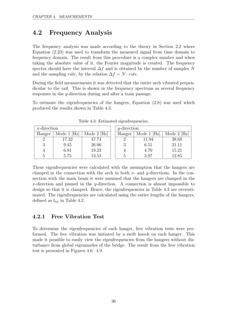
37
CHAPTER 4. MEASUREMENTS
0 5 10 15 20 250
0.5
1
1.5
f (Hz)
a/amax
7.21
19.23
acc4x
0 5 10 15 20 250
0.5
1
1.5
f (Hz)
a/amax
6.04 16.50
acc4y
Figure 4.8: Frequency analysis of the accelerations in hanger 4.
0 5 10 15 20 250
0.5
1
1.5
f (Hz)
a/a
max
4.31
13.53
acc5x
0 5 10 15 20 250
0.5
1
1.5
f (Hz)
a/a
max
3.61
11.40
acc5y
Figure 4.9: Frequency analysis of the accelerations in hanger 5.
38
4.2. FREQUENCY ANALYSIS
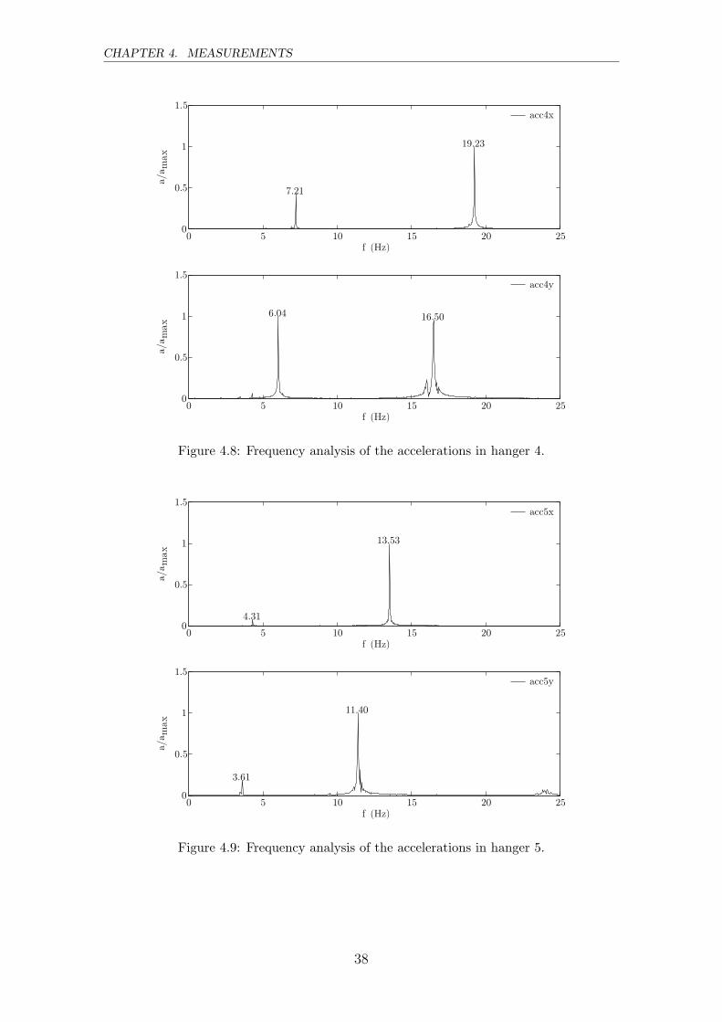
4.2.2 Train Induced Vibration
During excitation from the train the hangers are forced to vibrate with the frequencyinduced by the train. After the train has passed, the hangers are in free vibrationand vibrate with their natural frequencies.
The frequency response obtained from the accelerometers after the train passageare presented in Figures 4.10– 4.13. The frequency response from the strain gaugesassembled on hanger 5 is shown in the Figure 4.14, while the frequency responses ofthe other hangers are shown in Appendix A.
In the frequency response graphs of hangers 4 and 5, obtained from the accelerome-ters, the second eigenmode is generally dominating, while the graphs from the straingauges show the first eigenmode as the largest peak. The acceleration is higher whenthe hangers are vibrating with the second eigenmode than with the first and this isseen in the frequency response graphs as a higher peak. The reason for this is that ahigher eigenfrequency means that the hanger vibrates with more cycles per secondand because of this it has a higher acceleration. The frequency response obtainedfrom the strain gauge shows which eigenmode that causes the largest strain in thehangers. The motion of the hangers will be further discussed in Section 4.3.
0 5 10 15 20 250
0.5
1
1.5
f (Hz)
a/a
max
16.07
acc2x
0 5 10 15 20 250
0.5
1
1.5
f (Hz)
a/a
max
2.17
8.45 9.48
11.10
acc2y
Figure 4.10: Frequency analysis of the accelerations in hanger 2.
39
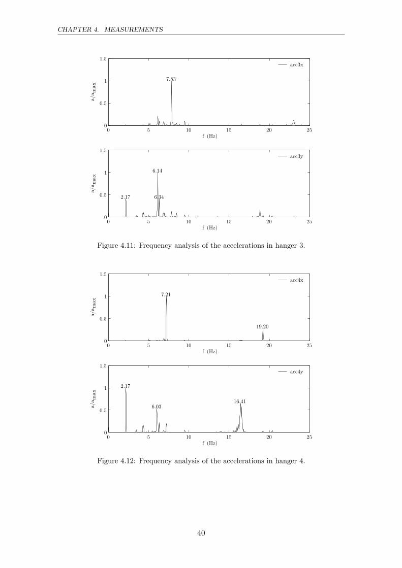
CHAPTER 4. MEASUREMENTS
0 5 10 15 20 250
0.5
1
1.5
f (Hz)
a/amax
7.83
acc3x
0 5 10 15 20 250
0.5
1
1.5
f (Hz)
a/amax
2.17
6.14
6.34
acc3y
Figure 4.11: Frequency analysis of the accelerations in hanger 3.
0 5 10 15 20 250
0.5
1
1.5
f (Hz)
a/a
max
7.21
19.20
acc4x
0 5 10 15 20 250
0.5
1
1.5
f (Hz)
a/a
max
2.17
6.0316.41
acc4y
Figure 4.12: Frequency analysis of the accelerations in hanger 4.
40

4.2. FREQUENCY ANALYSIS
0 5 10 15 20 250
0.5
1
1.5
f (Hz)
a/amax
4.31
13.55
acc5x
0 5 10 15 20 250
0.5
1
1.5
f (Hz)
a/amax
2.17
3.62
9.48
11.41
acc5y
Figure 4.13: Frequency analysis of the accelerations in hanger 5.
0 5 10 15 20 250
0.5
1
1.5
f (Hz)
ε/ε m
ax 2.163.62
4.3211.41 24.00
gauge 13
0 5 10 15 20 250
0.5
1
1.5
f (Hz)
ε/ε m
ax 4.32
13.57
gauge 14
0 5 10 15 20 250
0.5
1
1.5
f (Hz)
ε/ε m
ax 2.163.62
4.329.46 11.41 24.00
gauge 15
0 5 10 15 20 250
0.5
1
1.5
f (Hz)
ε/ε m
ax 4.32
13.57
gauge 16
Figure 4.14: Frequency analysis from strain gauges in hanger 5(gauges 13 and 15 correspond to the x-axis and 14 and 16 to the y-axis).
All of the signals from the train induced vibration have been subjected to windowing,which forces them to be periodic and makes the frequency response more legible.
41
CHAPTER 4. MEASUREMENTS
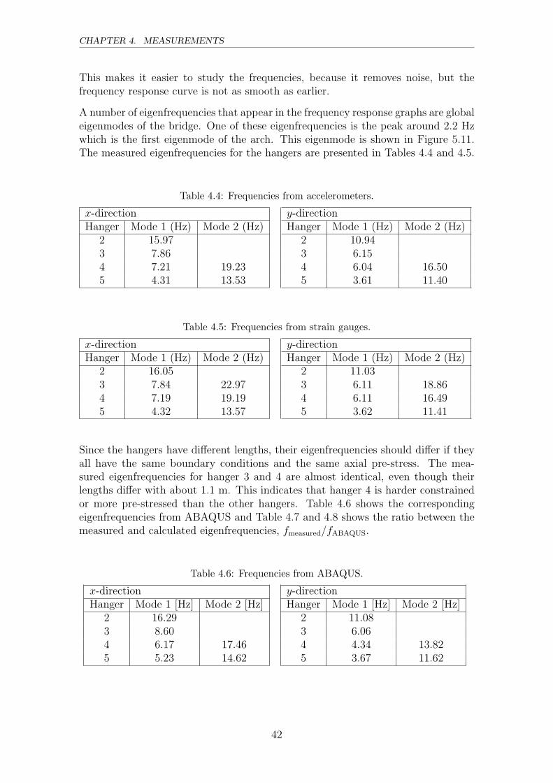
This makes it easier to study the frequencies, because it removes noise, but thefrequency response curve is not as smooth as earlier.
A number of eigenfrequencies that appear in the frequency response graphs are globaleigenmodes of the bridge. One of these eigenfrequencies is the peak around 2.2 Hzwhich is the first eigenmode of the arch. This eigenmode is shown in Figure 5.11.The measured eigenfrequencies for the hangers are presented in Tables 4.4 and 4.5.
Table 4.4: Frequencies from accelerometers.
x-direction y-directionHanger Mode 1 (Hz) Mode 2 (Hz) Hanger Mode 1 (Hz) Mode 2 (Hz)
2 15.97 2 10.943 7.86 3 6.154 7.21 19.23 4 6.04 16.505 4.31 13.53 5 3.61 11.40
Table 4.5: Frequencies from strain gauges.
x-direction y-directionHanger Mode 1 (Hz) Mode 2 (Hz) Hanger Mode 1 (Hz) Mode 2 (Hz)
2 16.05 2 11.033 7.84 22.97 3 6.11 18.864 7.19 19.19 4 6.11 16.495 4.32 13.57 5 3.62 11.41
Since the hangers have different lengths, their eigenfrequencies should differ if theyall have the same boundary conditions and the same axial pre-stress. The mea-sured eigenfrequencies for hanger 3 and 4 are almost identical, even though theirlengths differ with about 1.1 m. This indicates that hanger 4 is harder constrainedor more pre-stressed than the other hangers. Table 4.6 shows the correspondingeigenfrequencies from ABAQUS and Table 4.7 and 4.8 shows the ratio between themeasured and calculated eigenfrequencies, fmeasured/fABAQUS.
Table 4.6: Frequencies from ABAQUS.
x-direction y-directionHanger Mode 1 [Hz] Mode 2 [Hz] Hanger Mode 1 [Hz] Mode 2 [Hz]
2 16.29 2 11.083 8.60 3 6.064 6.17 17.46 4 4.34 13.825 5.23 14.62 5 3.67 11.62
42
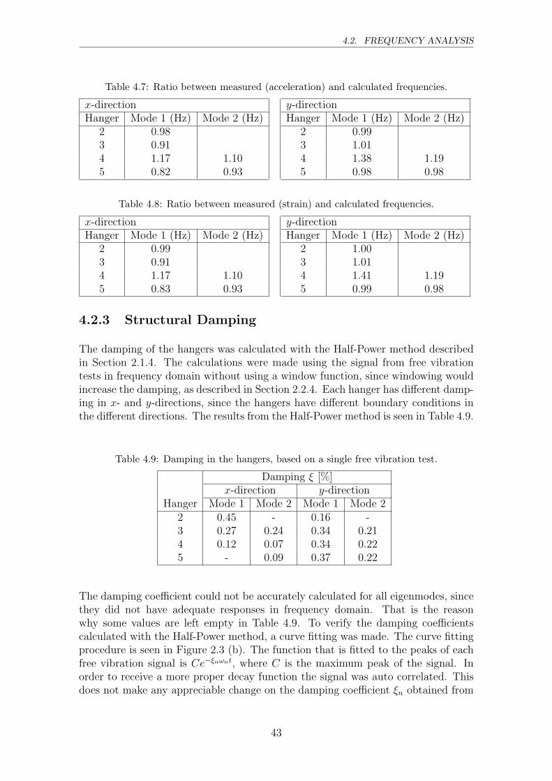
4.2. FREQUENCY ANALYSIS
Table 4.7: Ratio between measured (acceleration) and calculated frequencies.
x-direction y-directionHanger Mode 1 (Hz) Mode 2 (Hz) Hanger Mode 1 (Hz) Mode 2 (Hz)
2 0.98 2 0.993 0.91 3 1.014 1.17 1.10 4 1.38 1.195 0.82 0.93 5 0.98 0.98
Table 4.8: Ratio between measured (strain) and calculated frequencies.
x-direction y-directionHanger Mode 1 (Hz) Mode 2 (Hz) Hanger Mode 1 (Hz) Mode 2 (Hz)
2 0.99 2 1.003 0.91 3 1.014 1.17 1.10 4 1.41 1.195 0.83 0.93 5 0.99 0.98
4.2.3 Structural Damping
The damping of the hangers was calculated with the Half-Power method describedin Section 2.1.4. The calculations were made using the signal from free vibrationtests in frequency domain without using a window function, since windowing wouldincrease the damping, as described in Section 2.2.4. Each hanger has different damp-ing in x- and y-directions, since the hangers have different boundary conditions inthe different directions. The results from the Half-Power method is seen in Table 4.9.
Table 4.9: Damping in the hangers, based on a single free vibration test.
Damping ξ [%]x-direction y-direction
Hanger Mode 1 Mode 2 Mode 1 Mode 22 0.45 - 0.16 -3 0.27 0.24 0.34 0.214 0.12 0.07 0.34 0.225 - 0.09 0.37 0.22
The damping coefficient could not be accurately calculated for all eigenmodes, sincethey did not have adequate responses in frequency domain. That is the reasonwhy some values are left empty in Table 4.9. To verify the damping coefficientscalculated with the Half-Power method, a curve fitting was made. The curve fittingprocedure is seen in Figure 2.3 (b). The function that is fitted to the peaks of eachfree vibration signal is Ce−ξnωnt, where C is the maximum peak of the signal. Inorder to receive a more proper decay function the signal was auto correlated. Thisdoes not make any appreciable change on the damping coefficient ξn obtained from
43

CHAPTER 4. MEASUREMENTS
the Half-Power method. The auto correlated signals and the corresponding fittedfunction are displayed in Figure 4.15.
0 2 4 6
-0.5
0
0.5
1
ξ= 0.45%
0 5 10 15 20 25
-0.5
0
0.5
1
ξ= 0.16%
0 10 20 30 40
-0.5
0
0.5
1
ξ= 0.15%
0 5 10 15 20
-0.5
0
0.5
1
ξ= 0.21%
0 10 20 30 40
-0.5
0
0.5
1
ξ= 0.07%
0 10 20 30
-0.5
0
0.5
1
ξ= 0.34%
0 10 20 30 40
5
0
0.5
1
ξ= 0.06%
0 5 10 15 20
-0.5
0
0.5
1
ξ= 0.22%
time [s]
x-direction
hanger 2
y-direction
time [s]
time [s] time [s]
time [s] time [s]
time [s] time [s]
hanger 3
hanger 5
hanger 4
a/a
max
a/a
max
a/a
max
a/a
max
a/a
max
a/a
max
a/a
max
a/a
max
-0.
Figure 4.15: Free vibrations and the fitted decay functions.
Table 4.10: Damping in the hangers, based on a curve fitting on the free vibrationtest
Damping ξ (%)x-direction y-direction
Hanger Mode 1 Mode 2 Mode 1 Mode 22 0.45 - 0.16 -3 - 0.15 - 0.214 - 0.07 0.34 -5 - 0.06 - 0.22
44

4.2. FREQUENCY ANALYSIS
The eigenfrequency with the largest frequency response in the free vibration testdominate the signal in time domain. It is only possible to determine one dampingcoefficient in the curve fitting procedure, unless the signals are filtered to attenuateall eigenmodes except the one of interest. The values obtained in the Half-Powermethod and the values from the curve fitting method correspond quite well. TheHalf-Power method was also used to determine the damping of the signals obtainedfrom the train passage ID019, where the damping coefficient of the arch could bedetermined to 0.8%.
45
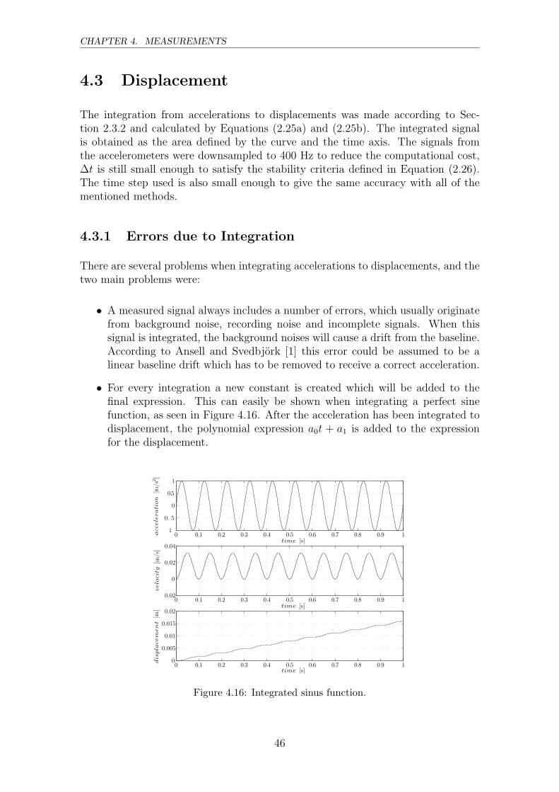
CHAPTER 4. MEASUREMENTS
4.3 Displacement
The integration from accelerations to displacements was made according to Sec-tion 2.3.2 and calculated by Equations (2.25a) and (2.25b). The integrated signalis obtained as the area defined by the curve and the time axis. The signals fromthe accelerometers were downsampled to 400 Hz to reduce the computational cost,∆t is still small enough to satisfy the stability criteria defined in Equation (2.26).The time step used is also small enough to give the same accuracy with all of thementioned methods.
4.3.1 Errors due to Integration
There are several problems when integrating accelerations to displacements, and thetwo main problems were:
• A measured signal always includes a number of errors, which usually originatefrom background noise, recording noise and incomplete signals. When thissignal is integrated, the background noises will cause a drift from the baseline.According to Ansell and Svedbjork [1] this error could be assumed to be alinear baseline drift which has to be removed to receive a correct acceleration.
• For every integration a new constant is created which will be added to thefinal expression. This can easily be shown when integrating a perfect sinefunction, as seen in Figure 4.16. After the acceleration has been integrated todisplacement, the polynomial expression a0t + a1 is added to the expressionfor the displacement.
0 0.1 0.2 0.3 0.4 0.5 0.6 0.7 0.8 0.9 11
0. 5
0
0.5
1
time [s]
acceleration
[m/s
2]
0 0.1 0.2 0.3 0.4 0.5 0.6 0.7 0.8 0.9 10.02
0
0.02
0.04
time [s]
velocity
[m/s]
0 0.1 0.2 0.3 0.4 0.5 0.6 0.7 0.8 0.9 10
0.005
0.01
0.015
0.02
time [s]
displacem
ent[m
]
Figure 4.16: Integrated sinus function.
46
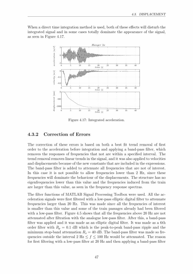
4.3. DISPLACEMENT
When a direct time integration method is used, both of these effects will disturb theintegrated signal and in some cases totally dominate the appearance of the signal,as seen in Figure 4.17.
0 5 10 15 20 25 30 35 40-5
0
5Hanger 2x
time [s]
acceleration
[m/s
2 ]
0 5 10 15 20 25 30 35 40
-0.2
-0.1
0
time [s]
velocity
[m/s]
0 5 10 15 20 25 30 35 40
-1000
-500
0
time [s]
displacem
ent[m
m]
Figure 4.17: Integrated acceleration.
4.3.2 Correction of Errors
The correction of these errors is based on both a best fit trend removal of firstorder to the acceleration before integration and applying a band-pass filter, whichremoves the responses of frequencies that not are within a specified interval. Thetrend removal removes linear trends in the signal, and it was also applied to velocitiesand displacements because of the new constants that are included in the expressions.The band-pass filter is added to attenuate all frequencies that are not of interest.In this case it is not possible to allow frequencies lower than 2 Hz, since thesefrequencies will dominate the behaviour of the displacements. The structure has noeigenfrequencies lower than this value and the frequencies induced from the trainare larger than this value, as seen in the frequency response spectras.
The filter functions of MATLAB Signal Processing Toolbox were used. All the ac-celeration signals were first filtered with a low-pass elliptic digital filter to attenuatefrequencies larger than 20 Hz. This was made since all the frequencies of interestis smaller than this value and some of the train passages already had been filteredwith a low-pass filter. Figure 4.5 shows that all the frequencies above 20 Hz are notattenuated after filtration with the analogue low-pass filter. After this, a band-passfilter was applied and it was made as an elliptic digital filter. It was made as a 6thorder filter with Rp = 0.1 dB which is the peak-to-peak band-pass ripple and theminimum stop-band attenuation Rs = 40 dB. The band-pass filter was made so fre-quencies outside the interval 2 Hz ≤ f ≤ 100 Hz would be attenuated. The reasonfor first filtering with a low-pass filter at 20 Hz and then applying a band-pass filter
47

CHAPTER 4. MEASUREMENTS
with an upper limit of 100 Hz is that the band-pass filter could be ill-conditioned fornarrow frequency interval, according to the MATLAB manual, [13] . The maximumupper limit of the band-pass filter is the Nyquist frequency which is half the samplingfrequency. The downside of the band-pass filtering is that because of the lower limitat 2 Hz the total displacement will not be visible. This means that the obtaineddisplacement is the displacement of the hanger relative to the global deflection ofthe bridge. The total displacement could be visualised in the results from ABAQUS,which is shown in Chapter 5. It is very important to study the frequency responseof the calculated displacement and verify that no unfamiliar frequencies are presentthat could lead to distortion of the displacements.
The measurements made with the analogue low-pass filter, i.e. ID018 and ID019,shows smaller displacements than the measurements without. The two different pas-senger trains, ID012 and ID018, were similar since both were of the same type, hadthe same number of carriages and almost the same velocity. Despite the similarities,there is a great difference in the calculated displacements from the two trains. Thedisplacement from these trains are displayed in Appendix A. The two train passagesID009 and ID019 should also show displacements that are similar to each other butthere is a large difference between them.
4.3.3 Final Displacements
As seen in Table 4.2, the accelerometers were placed on different positions of eachhanger. To find where the maximum displacement in the hangers occurs, was theposition of the accelerometer compared with the position of maximum displacementfor the first eigenmode. The maximum displacement in y-direction of the hangercan be calculated using the eigenmodes shown in Figure 2.7, and multiplying thedisplacements with a factor based on the ratio between the mode based max dis-placement and the mode based displacement at the point of the accelerometer. Thesame procedure is then made to obtain maximum displacement in x-direction, wherethe displacements are multiplied with corresponding mode based displacement factorfor a beam that is clamped in both ends.
The frequency response spectra obtained from the calculated displacements showsa peak at about 5 Hz, which only occurs during the train passage. A band-passfilter was applied which only consider frequencies close to this value and it showsthat the displacements of the hangers during a train passage are dominated by thisfrequency. After the train has passed, the displacement induced by this frequencyis insignificant. This frequency is most likely induced in the hangers by the train.
48
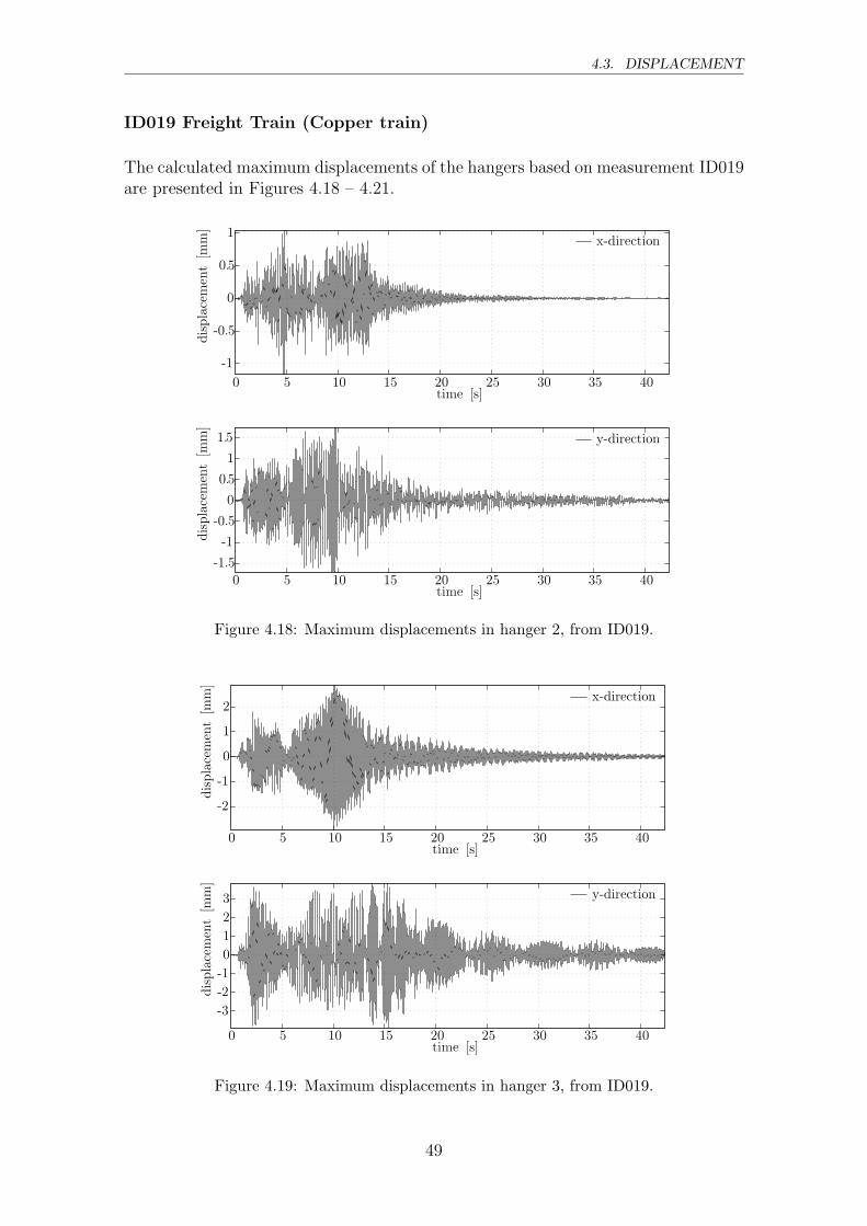
4.3. DISPLACEMENT
ID019 Freight Train (Copper train)
The calculated maximum displacements of the hangers based on measurement ID019are presented in Figures 4.18 – 4.21.
0 5 10 15 20 25 30 35 40
-1
-0.5
0
0.5
1
time [s]
displacement[m
m]
x-direction
0 5 10 15 20 25 30 35 40
-1.5
-1
-0.5
0
0.5
1
1.5
time [s]
displacement[m
m]
y-direction
Figure 4.18: Maximum displacements in hanger 2, from ID019.
0 5 10 15 20 25 30 35 40
-2
-1
0
1
2
time [s]
displacement[m
m]
x-direction
0 5 10 15 20 25 30 35 40
-3
-2
-1
0
1
2
3
time [s]
displacement[m
m]
y-direction
Figure 4.19: Maximum displacements in hanger 3, from ID019.
49
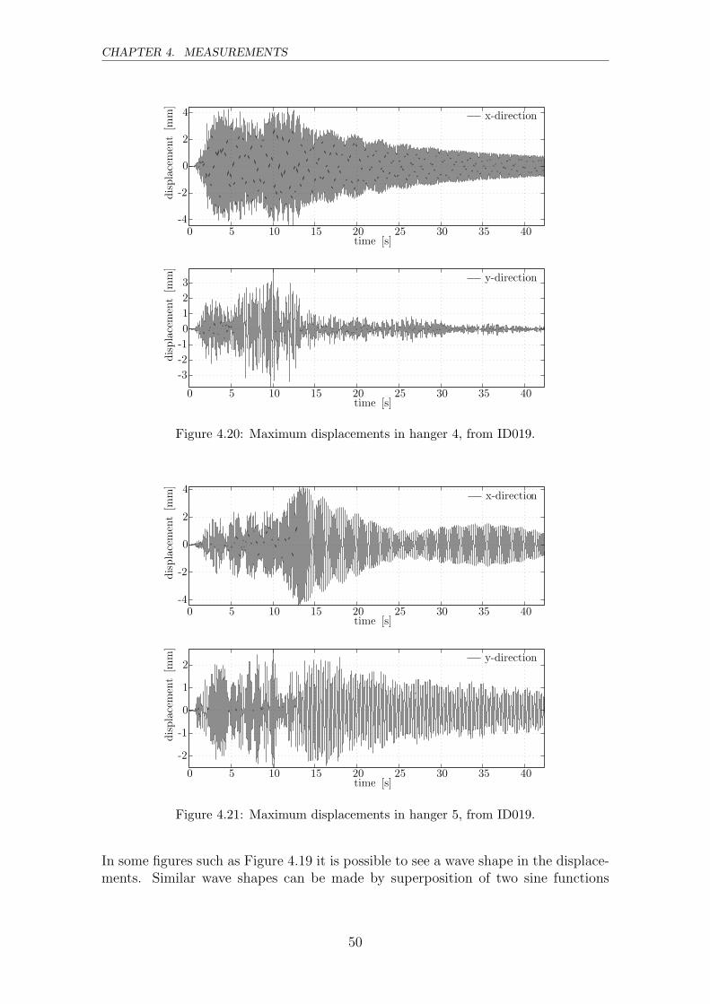
CHAPTER 4. MEASUREMENTS
0 5 10 15 20 25 30 35 40-4
-2
0
2
4
time [s]
displacement[m
m]
x-direction
0 5 10 15 20 25 30 35 40
-3
-2
-1
0
1
2
3
time [s]
displacement[m
m]
y-direction
Figure 4.20: Maximum displacements in hanger 4, from ID019.
0 5 10 15 20 25 30 35 40-4
-2
0
2
4
time [s]
displacement[m
m]
x-direction
0 5 10 15 20 25 30 35 40
-2
-1
0
1
2
time [s]
displacement[m
m]
y-direction
Figure 4.21: Maximum displacements in hanger 5, from ID019.
In some figures such as Figure 4.19 it is possible to see a wave shape in the displace-ments. Similar wave shapes can be made by superposition of two sine functions
50
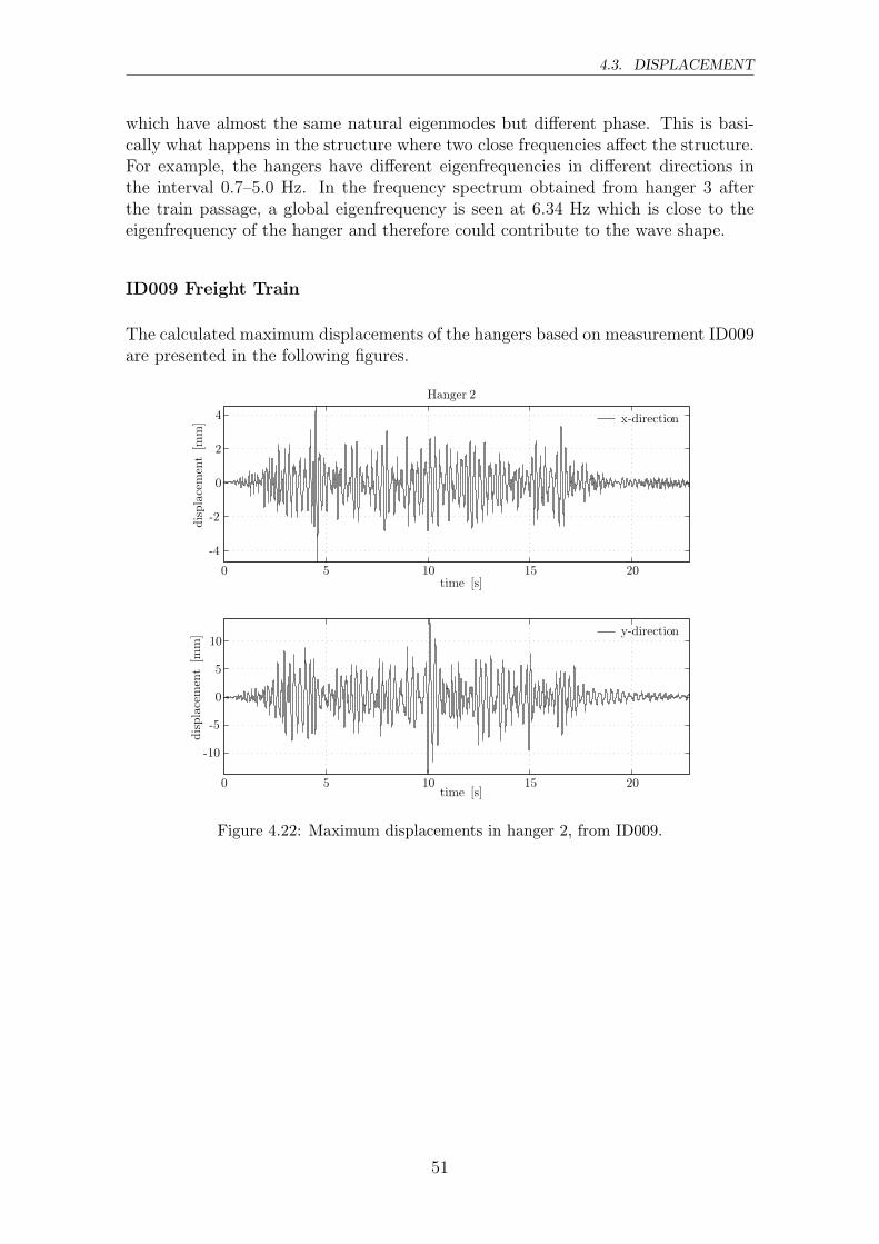
4.3. DISPLACEMENT
which have almost the same natural eigenmodes but different phase. This is basi-cally what happens in the structure where two close frequencies affect the structure.For example, the hangers have different eigenfrequencies in different directions inthe interval 0.7–5.0 Hz. In the frequency spectrum obtained from hanger 3 afterthe train passage, a global eigenfrequency is seen at 6.34 Hz which is close to theeigenfrequency of the hanger and therefore could contribute to the wave shape.
ID009 Freight Train
The calculated maximum displacements of the hangers based on measurement ID009are presented in the following figures.
0 5 10 15 20
-4
-2
0
2
4
time [s]
displacement[m
m]
Hanger 2
x-direction
0 5 10 15 20
-10
-5
0
5
10
time [s]
displacement[m
m] y-direction
Figure 4.22: Maximum displacements in hanger 2, from ID009.
51

CHAPTER 4. MEASUREMENTS
0 5 10 15 20
-4
-2
0
2
4
time [s]
displacement[m
m]
Hanger 3
x-direction
0 5 10 15 20
-10
-5
0
5
10
time [s]
displacement[m
m] y-direction
Figure 4.23: Maximum displacements in hanger 3, from ID009.
0 5 10 15 20
-10
-5
0
5
10
time [s]
displacement[m
m]
Hanger 4
x-direction
0 5 10 15 20
-30
-20
-10
0
10
20
30
time [s]
displacement[m
m] y-direction
Figure 4.24: Maximum displacements in hanger 4, from ID009.
52

4.3. DISPLACEMENT
0 5 10 15 20-8
-6
-4
-2
0
2
4
6
time [s]
displacement[m
m]
Hanger 5
x-direction
0 5 10 15 20
-15
-10
-5
0
5
10
15
time [s]
displacement[m
m] y-direction
Figure 4.25: Maximum displacements in hanger 5, from ID009.
The two different measurements have basically the same displacements in the x-direction which is parallel to the rail. In the y-direction the displacements are muchgreater in the freight train ID009 and especially some amplitudes are unrealisticlarge. The most accurate displacements should probably be the signals from trainpassages ID018 and ID019, since these measurements were made with an analoguelow-pass filter that attenuated the uninteresting frequencies. It is very difficult todigitally define a low-pass filter that has the same properties as the analogue.
The frequency response of the acceleration, velocity and displacement shows thesame eigenfrequencies. In the frequency response from accelerations, generally thesecond eigenmode is the largest and for the displacement the first eigenmode is dom-inating, as seen in Figure 4.26. The reason for this is that the second eigenmode hasa higher acceleration magnitude since they are vibrating faster, but the displace-ments of these vibrations are rather small. On the contrary, the first eigenmodeshould have a smaller acceleration, which would induce larger displacement in thehangers, i.e. the first eigenmode contribute with a large area in the integration.The frequency response from the displacements have the same appearance as thefrequency response from the strain gauges and they both show that the hangers aremainly vibrating in the first eigenmode, as shown Figure 2.7.
53
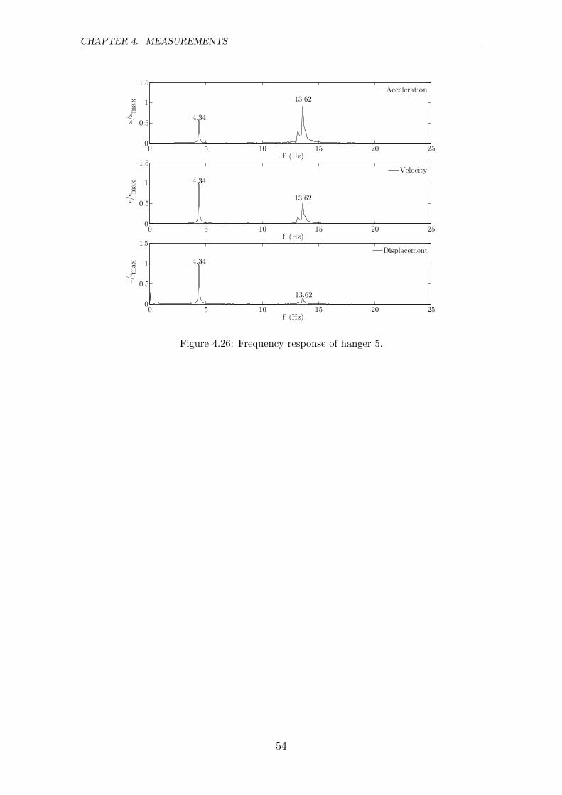
CHAPTER 4. MEASUREMENTS
0 5 10 15 20 250
0.5
1
1.5
f (Hz)
a/amax
4.34
13.62
Acceleration
0 5 10 15 20 250
0.5
1
1.5
f (Hz)
v/vmax 4.34
13.62
Velocity
0 5 10 15 20 250
0.5
1
1.5
f (Hz)
u/umax 4.34
13.62
Displacement
Figure 4.26: Frequency response of hanger 5.
54

4.4. PLANE STRESS VARIATION
4.4 Plane Stress Variation
The stresses obtained from the strain gauges on hanger 5 are shown in Figure 4.27.
0 5 10 15 20 25-10
-5
0
5
10
15
20
time [s]
stress
σ[M
Pa]
gauge13
0 5 10 15 20 25
-20
-10
0
10
20
30
time [s]
stress
[MPa]
gauge14
0 5 10 15 20 25
-5
0
5
10
15
20
time [s]
stress
σ[M
Pa]
gauge15
0 5 10 15 20 25-20
-10
0
10
20
30
time [s]
stress
[MPa]
gauge16
σσ
Figure 4.27: Measured stress in hanger 5.
The attached strain gauges may not show the maximum stresses in the hangers,which depend on the direction the hangers are vibrating in. Because of the positionof the gauges is it possible to calculate the stress in any point in the plane that isdefined by the strain gauges. The stress variation in the plane is defined by Navier’sequation:
σ =N
A+
Mxy
Ix
− Myx
Iy
(4.1)
Where N is the axial force, A is the cross-sectional area and Mx and My are thebending moments and Ix and Iy are the moments of inertia. For a circular cross-
section is Ix = Iy = πr4
4. The cross section of the hanger and the forces acting on it
are displayed in Figure 4.28.
55
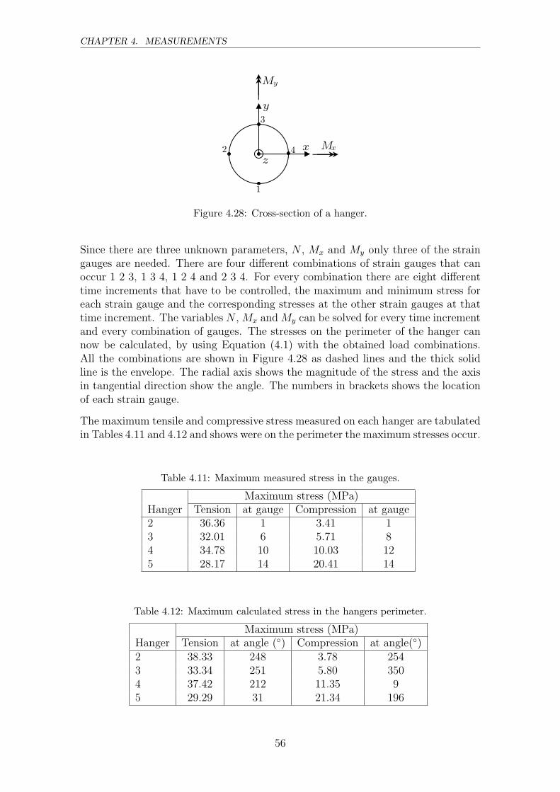
CHAPTER 4. MEASUREMENTS
y
xz
1
2
3
4
My
Mx
Figure 4.28: Cross-section of a hanger.
Since there are three unknown parameters, N , Mx and My only three of the straingauges are needed. There are four different combinations of strain gauges that canoccur 1 2 3, 1 3 4, 1 2 4 and 2 3 4. For every combination there are eight differenttime increments that have to be controlled, the maximum and minimum stress foreach strain gauge and the corresponding stresses at the other strain gauges at thattime increment. The variables N , Mx and My can be solved for every time incrementand every combination of gauges. The stresses on the perimeter of the hanger cannow be calculated, by using Equation (4.1) with the obtained load combinations.All the combinations are shown in Figure 4.28 as dashed lines and the thick solidline is the envelope. The radial axis shows the magnitude of the stress and the axisin tangential direction show the angle. The numbers in brackets shows the locationof each strain gauge.
The maximum tensile and compressive stress measured on each hanger are tabulatedin Tables 4.11 and 4.12 and shows were on the perimeter the maximum stresses occur.
Table 4.11: Maximum measured stress in the gauges.
Maximum stress (MPa)Hanger Tension at gauge Compression at gauge2 36.36 1 3.41 13 32.01 6 5.71 84 34.78 10 10.03 125 28.17 14 20.41 14
Table 4.12: Maximum calculated stress in the hangers perimeter.
Maximum stress (MPa)Hanger Tension at angle (◦) Compression at angle(◦)2 38.33 248 3.78 2543 33.34 251 5.80 3504 37.42 212 11.35 95 29.29 31 21.34 196
56
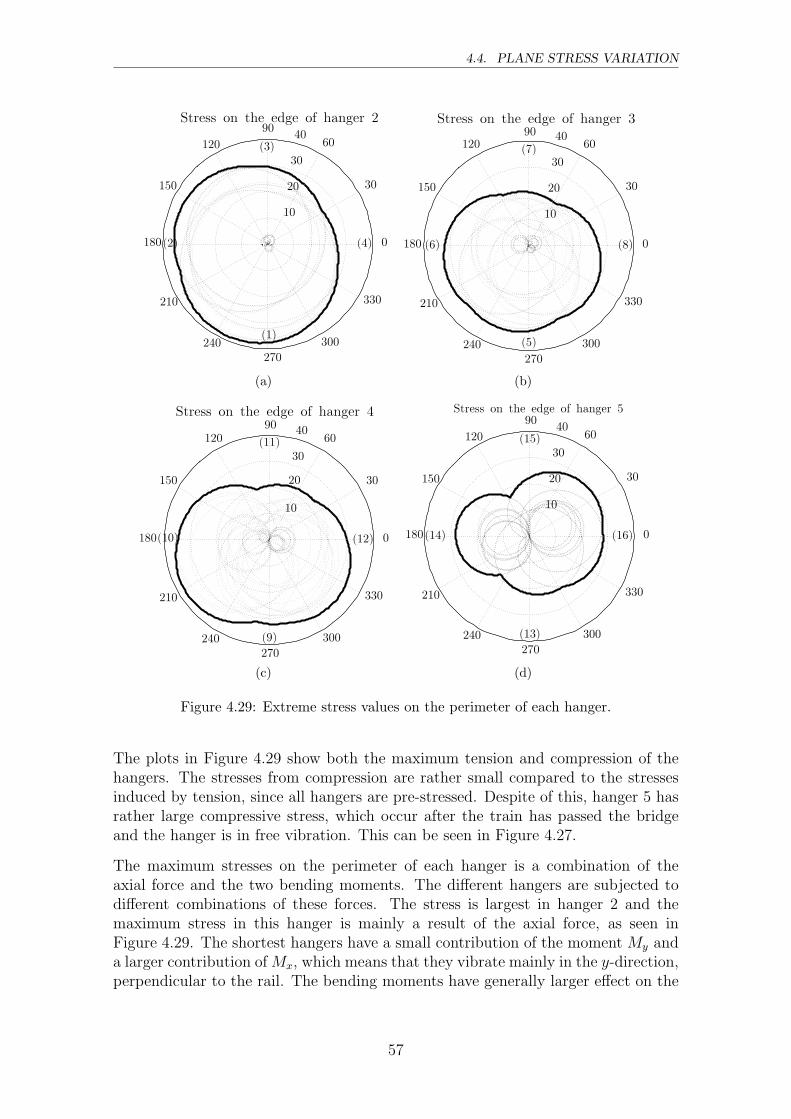
4.4. PLANE STRESS VARIATION
10
20
30
40
30
210
60
240
90
270
120
300
150
330
180 0
Stress on the edge of hanger 2
(1)
(2)
(3)
(4)
(a)
10
20
30
40
30
210
60
240
90
270
120
300
150
330
180 0
Stress on the edge of hanger 3
(5)
(6)
(7)
(8)
(b)
20
30
40
30
210
60
240
90
270
120
300
150
330
180 0
Stress on the edge of hanger 4
(9)
(10)
(11)
(12)
10
(c)
20
30
40
30
210
60
240
90
270
120
300
150
330
180 0
Stress on the edge of hanger 5
(13)
(14)
(15)
(16)
10
(d)
Figure 4.29: Extreme stress values on the perimeter of each hanger.
The plots in Figure 4.29 show both the maximum tension and compression of thehangers. The stresses from compression are rather small compared to the stressesinduced by tension, since all hangers are pre-stressed. Despite of this, hanger 5 hasrather large compressive stress, which occur after the train has passed the bridgeand the hanger is in free vibration. This can be seen in Figure 4.27.
The maximum stresses on the perimeter of each hanger is a combination of theaxial force and the two bending moments. The different hangers are subjected todifferent combinations of these forces. The stress is largest in hanger 2 and themaximum stress in this hanger is mainly a result of the axial force, as seen inFigure 4.29. The shortest hangers have a small contribution of the moment My anda larger contribution of Mx, which means that they vibrate mainly in the y-direction,perpendicular to the rail. The bending moments have generally larger effect on the
57
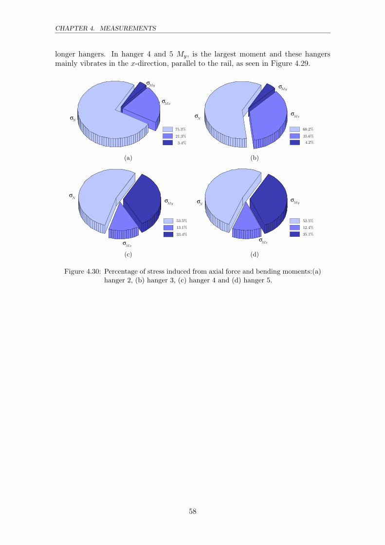
CHAPTER 4. MEASUREMENTS
longer hangers. In hanger 4 and 5 My, is the largest moment and these hangersmainly vibrates in the x-direction, parallel to the rail, as seen in Figure 4.29.
σMx
σMy
σN
75.3%
21.3%
3.4%
(a)
σMx
σMy
σN
60.2%
35.6%
4.2%
(b)
σMy
σMx
σN
53.5%
13.1%
33.4%
(c)
σMy
σMx
σN
52.5%
12.4%
35.1%
(d)
Figure 4.30: Percentage of stress induced from axial force and bending moments:(a)hanger 2, (b) hanger 3, (c) hanger 4 and (d) hanger 5.
58
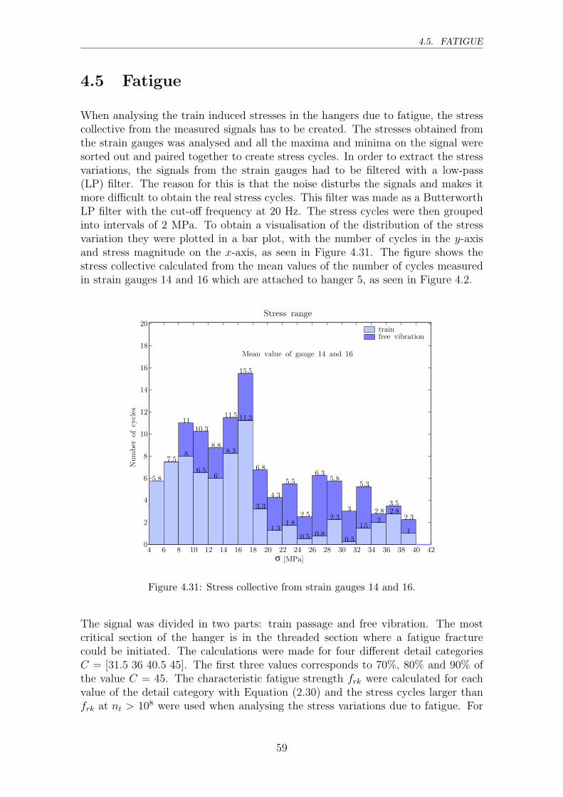
4.5. FATIGUE
4.5 Fatigue
When analysing the train induced stresses in the hangers due to fatigue, the stresscollective from the measured signals has to be created. The stresses obtained fromthe strain gauges was analysed and all the maxima and minima on the signal weresorted out and paired together to create stress cycles. In order to extract the stressvariations, the signals from the strain gauges had to be filtered with a low-pass(LP) filter. The reason for this is that the noise disturbs the signals and makes itmore difficult to obtain the real stress cycles. This filter was made as a ButterworthLP filter with the cut-off frequency at 20 Hz. The stress cycles were then groupedinto intervals of 2 MPa. To obtain a visualisation of the distribution of the stressvariation they were plotted in a bar plot, with the number of cycles in the y-axisand stress magnitude on the x-axis, as seen in Figure 4.31. The figure shows thestress collective calculated from the mean values of the number of cycles measuredin strain gauges 14 and 16 which are attached to hanger 5, as seen in Figure 4.2.
4 6 8 10 12 14 16 18 20 22 24 26 28 30 32 34 36 38 40 420
2
4
6
8
10
12
14
16
18
20
Stress range
Number
ofcycles
[MPa]
Mean value of gauge 14 and 16
5.8
7.58
11
6.5
10.3
6
8.88.3
11.5 11.3
15.5
3.3
6.8
1.3
4.3
1.8
5.5
0.5
2.5
0.8
6.3
2.3
5.8
0.3
3
1.5
5.3
22.8
3.5
1
2.3
trainfree vibration
σ
2.8
Figure 4.31: Stress collective from strain gauges 14 and 16.
The signal was divided in two parts: train passage and free vibration. The mostcritical section of the hanger is in the threaded section where a fatigue fracturecould be initiated. The calculations were made for four different detail categoriesC = [31.5 36 40.5 45]. The first three values corresponds to 70%, 80% and 90% ofthe value C = 45. The characteristic fatigue strength frk were calculated for eachvalue of the detail category with Equation (2.30) and the stress cycles larger thanfrk at nt > 108 were used when analysing the stress variations due to fatigue. For
59

CHAPTER 4. MEASUREMENTS
the stress cycles larger than fatigue strength, the total number of stress cycles for allthe train passages during the lifetime of the bridge was calculated. It was calculatedfor 1 to 10 train passages a day and with a bridge life length of 10 to 100 years andfinally summarised in a table. The design criterion, displayed in Equation (2.31),was finally used to view the risk of fatigue failure.
This calculation was made for all of the signals from the strain gauges and wasalso made for the mean value from the gauges that measured bending in the samedirection on each hanger, since those two strain gauges has a small difference inthe number of stress cycles obtained. The bar plot over the stress collective for themean value of gauges 14 and 16 is shown in Figure 4.31 and the results from fatigueassessment is shown in Tables 4.13– 4.16. The values in bold font style is over 1.0and that load combination could therefore lead to failure in the threaded section ofthe hanger.
Table 4.13: Mean value of gauges 14 and 16, C=45.Lifetime Number of train passages per day(years) 1 2 3 4 5 6 7 8 9 10
10 0.02 0.04 0.06 0.08 0.10 0.12 0.14 0.16 0.18 0.2020 0.04 0.08 0.12 0.16 0.20 0.24 0.28 0.32 0.36 0.4030 0.06 0.12 0.18 0.24 0.30 0.36 0.42 0.48 0.54 0.6040 0.08 0.16 0.24 0.32 0.40 0.48 0.56 0.64 0.72 0.8050 0.10 0.20 0.30 0.40 0.50 0.60 0.70 0.80 0.90 1.0060 0.12 0.24 0.36 0.48 0.60 0.72 0.84 0.96 1.08 1.2170 0.14 0.28 0.42 0.56 0.70 0.84 0.98 1.12 1.27 1.4180 0.16 0.32 0.48 0.64 0.80 0.96 1.12 1.29 1.45 1.6190 0.18 0.36 0.54 0.72 0.90 1.08 1.27 1.45 1.63 1.81100 0.20 0.40 0.60 0.80 1.00 1.21 1.41 1.61 1.81 2.01
Table 4.14: Mean value of gauges 14 and 16, C=40.5.Lifetime Number of train passages per day(years) 1 2 3 4 5 6 7 8 9 10
10 0.03 0.06 0.09 0.12 0.15 0.18 0.21 0.24 0.27 0.3020 0.06 0.12 0.18 0.24 0.30 0.36 0.42 0.48 0.55 0.6130 0.09 0.18 0.27 0.36 0.45 0.55 0.64 0.73 0.82 0.9140 0.12 0.24 0.36 0.48 0.61 0.73 0.85 0.97 1.09 1.2150 0.15 0.30 0.45 0.61 0.76 0.91 1.06 1.21 1.36 1.5160 0.18 0.36 0.55 0.73 0.91 1.09 1.27 1.45 1.64 1.8270 0.21 0.42 0.64 0.85 1.06 1.27 1.48 1.70 1.91 2.1280 0.24 0.48 0.73 0.97 1.21 1.45 1.70 1.94 2.18 2.4290 0.27 0.55 0.82 1.09 1.36 1.64 1.91 2.18 2.45 2.73100 0.30 0.61 0.91 1.21 1.51 1.82 2.12 2.42 2.73 3.03
60
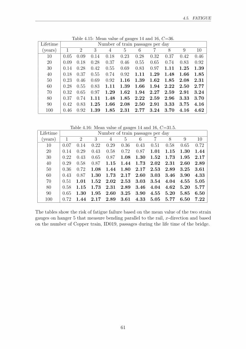
4.5. FATIGUE
Table 4.15: Mean value of gauges 14 and 16, C=36.Lifetime Number of train passages per day(years) 1 2 3 4 5 6 7 8 9 10
10 0.05 0.09 0.14 0.18 0.23 0.28 0.32 0.37 0.42 0.4620 0.09 0.18 0.28 0.37 0.46 0.55 0.65 0.74 0.83 0.9230 0.14 0.28 0.42 0.55 0.69 0.83 0.97 1.11 1.25 1.3940 0.18 0.37 0.55 0.74 0.92 1.11 1.29 1.48 1.66 1.8550 0.23 0.46 0.69 0.92 1.16 1.39 1.62 1.85 2.08 2.3160 0.28 0.55 0.83 1.11 1.39 1.66 1.94 2.22 2.50 2.7770 0.32 0.65 0.97 1.29 1.62 1.94 2.27 2.59 2.91 3.2480 0.37 0.74 1.11 1.48 1.85 2.22 2.59 2.96 3.33 3.7090 0.42 0.83 1.25 1.66 2.08 2.50 2.91 3.33 3.75 4.16100 0.46 0.92 1.39 1.85 2.31 2.77 3.24 3.70 4.16 4.62
Table 4.16: Mean value of gauges 14 and 16, C=31.5.Lifetime Number of train passages per day(years) 1 2 3 4 5 6 7 8 9 10
10 0.07 0.14 0.22 0.29 0.36 0.43 0.51 0.58 0.65 0.7220 0.14 0.29 0.43 0.58 0.72 0.87 1.01 1.15 1.30 1.4430 0.22 0.43 0.65 0.87 1.08 1.30 1.52 1.73 1.95 2.1740 0.29 0.58 0.87 1.15 1.44 1.73 2.02 2.31 2.60 2.8950 0.36 0.72 1.08 1.44 1.80 2.17 2.53 2.89 3.25 3.6160 0.43 0.87 1.30 1.73 2.17 2.60 3.03 3.46 3.90 4.3370 0.51 1.01 1.52 2.02 2.53 3.03 3.54 4.04 4.55 5.0580 0.58 1.15 1.73 2.31 2.89 3.46 4.04 4.62 5.20 5.7790 0.65 1.30 1.95 2.60 3.25 3.90 4.55 5.20 5.85 6.50100 0.72 1.44 2.17 2.89 3.61 4.33 5.05 5.77 6.50 7.22
The tables show the risk of fatigue failure based on the mean value of the two straingauges on hanger 5 that measure bending parallel to the rail, x-direction and basedon the number of Copper train, ID019, passages during the life time of the bridge.
61
CHAPTER 4. MEASUREMENTS
4.5.1 Assessing the Risk of Stress Concentrations
The stresses will become more concentrated where the hanger section passes overto the threaded part. The reason for this is seen in Equation (4.1), where boththe area and the moment of inertia decreases with a smaller diameter. The innercross-sectional area of the threaded section is smaller and has a diameter of 74.4mm. Because of the decreased area, the stresses from pure axial stress will increasewith the factor (
dhanger
dthread)2 ≈ 1.16. If Equation (2.30) is expressed as:
nt =
C3 · 2·106
σ3rd
if σrd > 0.737C
(0.885C)5 · 2·106
σ5rd
if 0.4047C < σrd < 0.737C
∞ if σrd < 0.4047C
(4.2)
It shows that an increasing stress range, σrd, will reduce the number of stress cyclesnt that would lead to failure proportional to 1
σ3rd
or 1σ5
rd. This means that if the stress
range increases with 16%, the hanger will reach failure for half the number of stresscycles if 0.4047C < f < 0.737C.
The measured stresses are also dependent on the bending moment in the cross-section, as seen in Figure 4.30. The decrease of the diameter will increase thestresses due to the bending moment with the factor (
dhanger
dthread)3 ≈ 1.26.
The method described in Section 4.4 could be used to divide the stress obtainedfrom the strain gauges at every time increment into three parts, σN , σMx and σMy,as seen in Figure 4.30. Instead of calculating the stress on the perimeter, the stressat each gauge is recalculated, where the stress components are multiplied with thefactors due to the area decrease in the threaded section and combined again. Thestress collective from the risk of fatigue, based on the increased stress, is presentedin Figure 4.32.
62

4.5. FATIGUE
4 6 8 10 12 14 16 18 20 22 24 26 28 30 32 34 36 38 40 42 44 46 48 500
2
4
6
8
10
12
14
16
Stress range
Number
ofcycles
[MPa]
Mean value of gauge 14 and 16
3.5
6.3
4.85
5.8
7.5
4.5
7.8
5.5
8.8
5.3
8 8
11 10.8
12.8
2
5.8
1
2.8
1.5
5.8
1
3
0.8
5.3
0.8
2.5
1
4.5
1.3
4.3
1.3
4
1.8
3.5
2.3
4
1.3
0.5 0.3
trainfree vibration
σ
Figure 4.32: Stress collective from strain gauge 14 and 16, with consideration of thesmaller area of the threaded section.
The maximum stress cycles obtained from the mean value of gauges 14 and 16have increased from 40 MPa in Figure 4.31 to 50 MPa. The new risk of fatigue, ispresented for detail category C = 45 in Table 4.17. The risk of fatigue is now almosttwice as high as earlier.
Table 4.17: Mean value of gauges 14 and 16, C = 45 and increased stress due toarea decrease in the threaded section.
Lifetime Number of train passages per day(years) 1 2 3 4 5 6 7 8 9 10
10 0.04 0.08 0.12 0.16 0.20 0.23 0.27 0.31 0.35 0.3920 0.08 0.16 0.23 0.31 0.39 0.47 0.55 0.63 0.70 0.7830 0.12 0.23 0.35 0.47 0.59 0.70 0.82 0.94 1.06 1.1740 0.16 0.31 0.47 0.63 0.78 0.94 1.10 1.25 1.41 1.5750 0.20 0.39 0.59 0.78 0.98 1.17 1.37 1.57 1.76 1.9660 0.23 0.47 0.70 0.94 1.17 1.41 1.64 1.88 2.11 2.3570 0.27 0.55 0.82 1.10 1.37 1.64 1.92 2.19 2.47 2.7480 0.31 0.63 0.94 1.25 1.57 1.88 2.19 2.50 2.82 3.1390 0.35 0.70 1.06 1.41 1.76 2.11 2.47 2.82 3.17 3.52100 0.39 0.78 1.17 1.57 1.96 2.35 2.74 3.13 3.52 3.91
All calculations have been made without consideration of the safety factor γn = 1.2.This factor has to be used if a new bridge would be designed to make sure that the
63
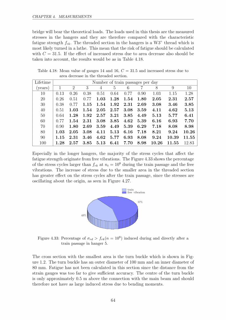
CHAPTER 4. MEASUREMENTS
bridge will bear the theoretical loads. The loads used in this thesis are the measuredstresses in the hangers and they are therefore compared with the characteristicfatigue strength frk. The threaded section in the hangers is a W3” thread which ismost likely turned in a lathe. This mean that the risk of fatigue should be calculatedwith C = 31.5. If the effect of increased stress due to area decrease also should betaken into account, the results would be as in Table 4.18.
Table 4.18: Mean value of gauges 14 and 16, C = 31.5 and increased stress due toarea decrease in the threaded section.
Lifetime Number of train passages per day(years) 1 2 3 4 5 6 7 8 9 10
10 0.13 0.26 0.38 0.51 0.64 0.77 0.90 1.03 1.15 1.2820 0.26 0.51 0.77 1.03 1.28 1.54 1.80 2.05 2.31 2.5730 0.38 0.77 1.15 1.54 1.92 2.31 2.69 3.08 3.46 3.8540 0.51 1.03 1.54 2.05 2.57 3.08 3.59 4.11 4.62 5.1350 0.64 1.28 1.92 2.57 3.21 3.85 4.49 5.13 5.77 6.4160 0.77 1.54 2.31 3.08 3.85 4.62 5.39 6.16 6.93 7.7070 0.90 1.80 2.69 3.59 4.49 5.39 6.29 7.18 8.08 8.9880 1.03 2.05 3.08 4.11 5.13 6.16 7.18 8.21 9.24 10.2690 1.15 2.31 3.46 4.62 5.77 6.93 8.08 9.24 10.39 11.55100 1.28 2.57 3.85 5.13 6.41 7.70 8.98 10.26 11.55 12.83
Especially in the longer hangers, the majority of the stress cycles that affect thefatigue strength originate from free vibrations. The Figure 4.33 shows the percentageof the stress cycles larger than frk at nt = 108 during the train passage and the freevibrations. The increase of stress due to the smaller area in the threaded sectionhas greater effect on the stress cycles after the train passage, since the stresses areoscillating about the origin, as seen in Figure 4.27.
57%
43%
trainfree vibration
Figure 4.33: Percentage of σrd > frk(n = 108) induced during and directly after atrain passage in hanger 5.
The cross section with the smallest area is the turn buckle which is shown in Fig-ure 1.2. The turn buckle has an outer diameter of 100 mm and an inner diameter of80 mm. Fatigue has not been calculated in this section since the distance from thestrain gauges was too far to give sufficient accuracy. The centre of the turn buckleis only approximately 0.5 m above the connection with the main beam and shouldtherefore not have as large induced stress due to bending moments.
64
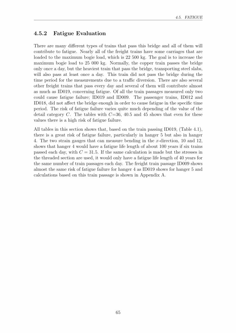
4.5. FATIGUE
4.5.2 Fatigue Evaluation
There are many different types of trains that pass this bridge and all of them willcontribute to fatigue. Nearly all of the freight trains have some carriages that areloaded to the maximum bogie load, which is 22 500 kg. The goal is to increase themaximum bogie load to 25 000 kg. Normally, the copper train passes the bridgeonly once a day, but the heaviest train that pass the bridge, transporting steel slabs,will also pass at least once a day. This train did not pass the bridge during thetime period for the measurements due to a traffic diversion. There are also severalother freight trains that pass every day and several of them will contribute almostas much as ID019, concerning fatigue. Of all the train passages measured only twocould cause fatigue failure; ID019 and ID009. The passenger trains, ID012 andID018, did not affect the bridge enough in order to cause fatigue in the specific timeperiod. The risk of fatigue failure varies quite much depending of the value of thedetail category C. The tables with C=36, 40.5 and 45 shows that even for thesevalues there is a high risk of fatigue failure.
All tables in this section shows that, based on the train passing ID019, (Table 4.1),there is a great risk of fatigue failure, particularly in hanger 5 but also in hanger4. The two strain gauges that can measure bending in the x-direction, 10 and 12,shows that hanger 4 would have a fatigue life length of about 100 years if six trainspassed each day, with C = 31.5. If the same calculation is made but the stresses inthe threaded section are used, it would only have a fatigue life length of 40 years forthe same number of train passages each day. The freight train passage ID009 showsalmost the same risk of fatigue failure for hanger 4 as ID019 shows for hanger 5 andcalculations based on this train passage is shown in Appendix A.
65

Chapter 5
Modelling Results
5.1 Modelling Results in ABAQUS
In this chapter the results from the finite element modelling in ABAQUS is pre-sented. The purpose of the modelling is to compare the results from measurementson the actual bridge with FEA and give a better understanding of how the stressesand displacements act and appear.Three different models have been created: a beam element model, a shell model anda solid model. The types of analyses performed are static, eigenvalue and dynamicanalysis. The static analysis involves the deformation of the bridge due to gravityload and a static train load. The eigenfrequencies of the hangers have been analysedin the eigenvalue analysis and are compared with the results from the field measure-ments. The train passage has been simulated in the dynamic analysis using contactinteractions.
5.1.1 The Models
All models have been created in three dimensions. When performing a static anal-ysis, the accuracy and behaviour are best seen when using solid or shell elements.The bridge mainly consists of I-beams that have a thickness much smaller than thewidth or the length. Those parts are best modelled with shell elements and a bettermesh can be achieved than when using 3D solid elements. The main reason forcreating a beam element model is to speed up the dynamic simulations. A dynamicsimulation of 10 carriages passing a 45 m bridge at 25 m/s takes at least 10 secondsif free vibrations are to be studied. The frequencies of interest in this case are inthe interval 0 to 20 Hz. This means that the smallest time increment should be lessthan 1/20 = 0.05 s. By using a 3D beam element model, the number of DOF canbe reduced from 100 000 in the solid model to 20 000 in the beam element model.
The main interest is to achieve a realistic response in the hangers from the train.The success in this matter depends mainly on two things; that the model of thebridge behaves as the real bridge and that the vibrations from the train are created
67
CHAPTER 5. MODELLING RESULTS
in a way that resembles the reality. The dynamic behaviour of the hangers dependson the length, the cross section and the boundary conditions. In the beam elementmodel, the hangers are connected only to a single node in the arch and the mainbeam. The only way to control the boundary conditions is to lock a certain degreeof freedom in that specific node, or to create a partly restraint connection. Whenusing a 3D shell model this connection can be modelled as it looks on the real bridgeand therefore give a more accurate result in the dynamic simulations. This is furtherconfirmed in the eigenfrequency analysis. Another important aspect concerning thebridge is how the damping of the structure is defined. In this case the behaviourof the damping is rather well known, because it is based on the measurements.The damping is defined in ABAQUS as a material damping based on the Rayleighdamping behaviour presented in Section 2.1.6. The damping is frequency dependentand therefore depends on the structure, so the hangers might have different dampingdepending on their length and their boundary conditions, but the model has beensimplified with the same damping for the entire model.
The Beam Element Model
The beam element model is the most simplified one, because all elements consistof three dimensional beam elements. The beam elements have been assigned di-mensions according to the construction drawings [14]. The connections betweenthe different beams are supposed to be continuous. The connections between thehanger and the main beams are connected through a triangular plate on the realbridge. This construction can be assumed to be clamped in the direction parallelto the bridge but simply supported in the direction perpendicular to the bridge.The connection between the arch and the hanger is assumed to be clamped, becauseit is connected by a rather stiff plate on the inside of the arch that connects thehanger with a bolt. The sleepers, the rail and the train model are represented bysolid elements. The reason for this is to be able to create an accurate interactionformulation between the train and the rail. The disadvantage is that the number ofDOF increases when inserting more carriages.
68
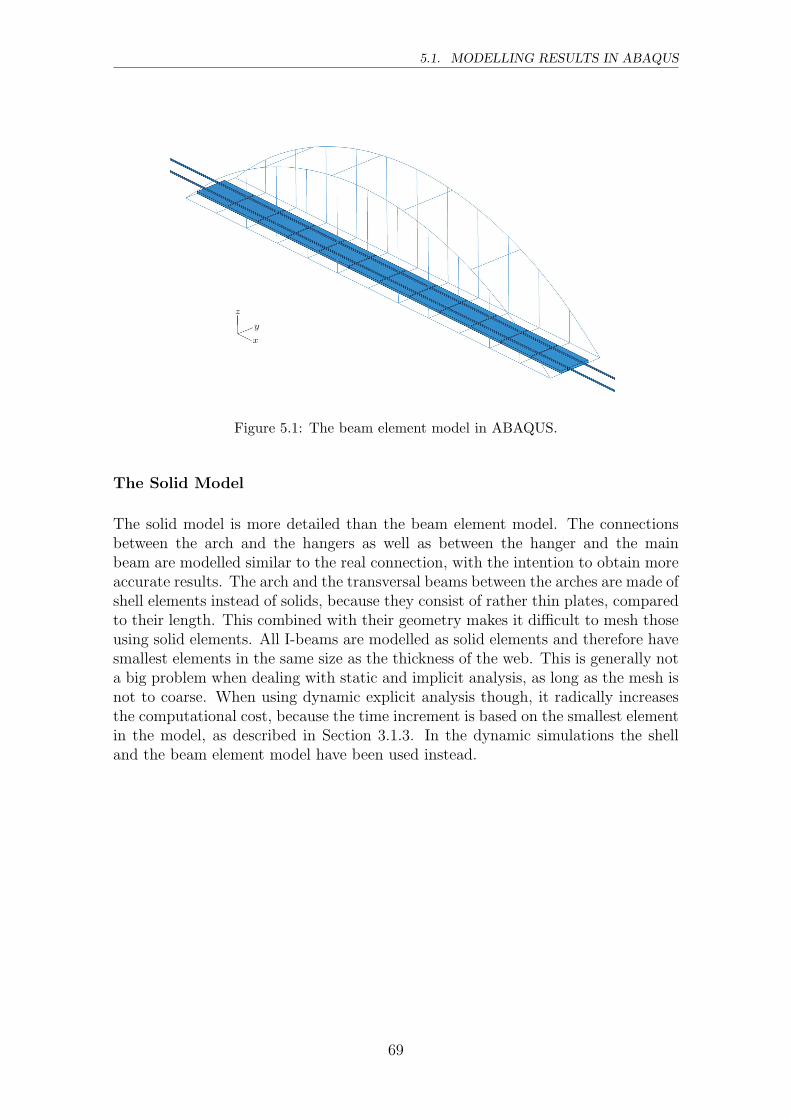
5.1. MODELLING RESULTS IN ABAQUS
x
y
z
Figure 5.1: The beam element model in ABAQUS.
The Solid Model
The solid model is more detailed than the beam element model. The connectionsbetween the arch and the hangers as well as between the hanger and the mainbeam are modelled similar to the real connection, with the intention to obtain moreaccurate results. The arch and the transversal beams between the arches are made ofshell elements instead of solids, because they consist of rather thin plates, comparedto their length. This combined with their geometry makes it difficult to mesh thoseusing solid elements. All I-beams are modelled as solid elements and therefore havesmallest elements in the same size as the thickness of the web. This is generally nota big problem when dealing with static and implicit analysis, as long as the mesh isnot to coarse. When using dynamic explicit analysis though, it radically increasesthe computational cost, because the time increment is based on the smallest elementin the model, as described in Section 3.1.3. In the dynamic simulations the shelland the beam element model have been used instead.
69

CHAPTER 5. MODELLING RESULTS
x
y
z
Figure 5.2: The solid model in ABAQUS.
x
y
z
(a)
x
zy
(b)
Figure 5.3: (a) The hanger connection with the main beam, (b) the hanger connec-tion with the arch.
The Shell Model
The shell model consists of 3D shell elements everywhere except at the hangers thatare made of solid elements, because they have a solid cross section. Shell elementsare well suited for structures that are significantly smaller in one direction, e.g. I-beams. The thickness of the shell elements are defined parameters and therefore donot have any elements in that directions. When using the dynamic explicit analysis,the time increment is significantly reduced compared to the implicit analysis. Whendynamic implicit is used, the computer time can be compared to the beam elementmodel but with a more detailed and accurate result. The stresses can be studied in
70
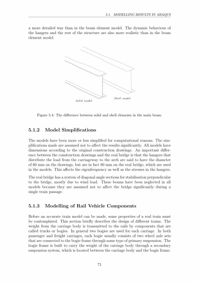
5.1. MODELLING RESULTS IN ABAQUS
a more detailed way than in the beam element model. The dynamic behaviour ofthe hangers and the rest of the structure are also more realistic than in the beamelement model.
Solid modelShell model
Figure 5.4: The difference between solid and shell elements in the main beam.
5.1.2 Model Simplifications
The models have been more or less simplified for computational reasons. The sim-plifications made are assumed not to affect the results significantly. All models havedimensions according to the original construction drawings. An important differ-ence between the construction drawings and the real bridge is that the hangers thatdistribute the load from the carriageway to the arch are said to have the diameterof 60 mm on the drawings, but are in fact 80 mm on the real bridge, which are usedin the models. This affects the eigenfrequency as well as the stresses in the hangers.
The real bridge has a system of diagonal angle sections for stabilisation perpendicularto the bridge, mostly due to wind load. These beams have been neglected in allmodels because they are assumed not to affect the bridge significantly during asingle train passage.
5.1.3 Modelling of Rail Vehicle Components
Before an accurate train model can be made, some properties of a real train mustbe contemplated. This section briefly describes the design of different trains. Theweight from the carriage body is transmitted to the rails by components that arecalled trucks or bogies. In general two bogies are used for each carriage. In bothpassenger and freight carriages, each bogie usually consists of two wheel axle setsthat are connected to the bogie frame through some type of primary suspension. Thebogie frame is built to carry the weight of the carriage body through a secondarysuspension system, which is located between the carriage body and the bogie frame.
71
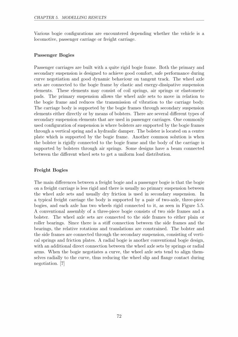
CHAPTER 5. MODELLING RESULTS
Various bogie configurations are encountered depending whether the vehicle is alocomotive, passenger carriage or freight carriage.
Passenger Bogies
Passenger carriages are built with a quite rigid bogie frame. Both the primary andsecondary suspension is designed to achieve good comfort, safe performance duringcurve negotiation and good dynamic behaviour on tangent track. The wheel axlesets are connected to the bogie frame by elastic and energy-dissipative suspensionelements. These elements may consist of coil springs, air springs or elastomericpads. The primary suspension allows the wheel axle sets to move in relation tothe bogie frame and reduces the transmission of vibration to the carriage body.The carriage body is supported by the bogie frames through secondary suspensionelements either directly or by means of bolsters. There are several different types ofsecondary suspension elements that are used in passenger carriages. One commonlyused configuration of suspension is where bolsters are supported by the bogie framesthrough a vertical spring and a hydraulic damper. The bolster is located on a centreplate which is supported by the bogie frame. Another common solution is whenthe bolster is rigidly connected to the bogie frame and the body of the carriage issupported by bolsters through air springs. Some designs have a beam connectedbetween the different wheel sets to get a uniform load distribution.
Freight Bogies
The main differences between a freight bogie and a passenger bogie is that the bogieon a freight carriage is less rigid and there is usually no primary suspension betweenthe wheel axle sets and usually dry friction is used in secondary suspension. Ina typical freight carriage the body is supported by a pair of two-axle, three-piecebogies, and each axle has two wheels rigid connected to it, as seen in Figure 5.5.A conventional assembly of a three-piece bogie consists of two side frames and abolster. The wheel axle sets are connected to the side frames to either plain orroller bearings. Since there is a stiff connection between the side frames and thebearings, the relative rotations and translations are constrained. The bolster andthe side frames are connected through the secondary suspension, consisting of verti-cal springs and friction plates. A radial bogie is another conventional bogie design,with an additional direct connection between the wheel axle sets by springs or radialarms. When the bogie negotiates a curve, the wheel axle sets tend to align them-selves radially to the curve, thus reducing the wheel slip and flange contact duringnegotiation. [7]
72
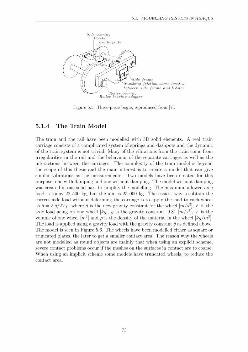
5.1. MODELLING RESULTS IN ABAQUS
Side bearingBolster
Centerplate
Roller bearing adapterRoller bearing
Side frameSnubbing friction shoes located
between side frame and bolster
Figure 5.5: Three-piece bogie, reproduced from [7].
5.1.4 The Train Model
The train and the rail have been modelled with 3D solid elements. A real traincarriage consists of a complicated system of springs and dashpots and the dynamicof the train system is not trivial. Many of the vibrations from the train come fromirregularities in the rail and the behaviour of the separate carriages as well as theinteractions between the carriages. The complexity of the train model is beyondthe scope of this thesis and the main interest is to create a model that can givesimilar vibrations as the measurements. Two models have been created for thispurpose; one with damping and one without damping. The model without dampingwas created in one solid part to simplify the modelling. The maximum allowed axleload is today 22 500 kg, but the aim is 25 000 kg. The easiest way to obtain thecorrect axle load without deforming the carriage is to apply the load to each wheelas g = Fg/2V ρ, where g is the new gravity constant for the wheel [m/s2], F is theaxle load acing on one wheel [kg], g is the gravity constant, 9.81 [m/s2], V is thevolume of one wheel [m3] and ρ is the density of the material in the wheel [kg/m3].The load is applied using a gravity load with the gravity constant g as defined above.The model is seen in Figure 5.6. The wheels have been modelled either as square ortruncated plates, the later to get a smaller contact area. The reason why the wheelsare not modelled as round objects are mainly that when using an explicit scheme,severe contact problems occur if the meshes on the surfaces in contact are to coarse.When using an implicit scheme some models have truncated wheels, to reduce thecontact area.
73
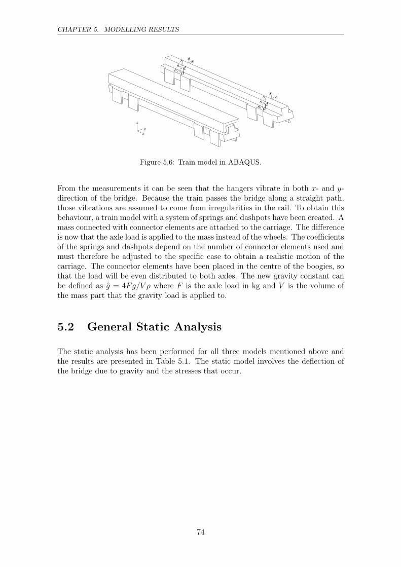
CHAPTER 5. MODELLING RESULTS
sss s
s
s d
sd
ss
s
x
y
z
dd
Figure 5.6: Train model in ABAQUS.
From the measurements it can be seen that the hangers vibrate in both x- and y-direction of the bridge. Because the train passes the bridge along a straight path,those vibrations are assumed to come from irregularities in the rail. To obtain thisbehaviour, a train model with a system of springs and dashpots have been created. Amass connected with connector elements are attached to the carriage. The differenceis now that the axle load is applied to the mass instead of the wheels. The coefficientsof the springs and dashpots depend on the number of connector elements used andmust therefore be adjusted to the specific case to obtain a realistic motion of thecarriage. The connector elements have been placed in the centre of the boogies, sothat the load will be even distributed to both axles. The new gravity constant canbe defined as g = 4Fg/V ρ where F is the axle load in kg and V is the volume ofthe mass part that the gravity load is applied to.
5.2 General Static Analysis
The static analysis has been performed for all three models mentioned above andthe results are presented in Table 5.1. The static model involves the deflection ofthe bridge due to gravity and the stresses that occur.
74
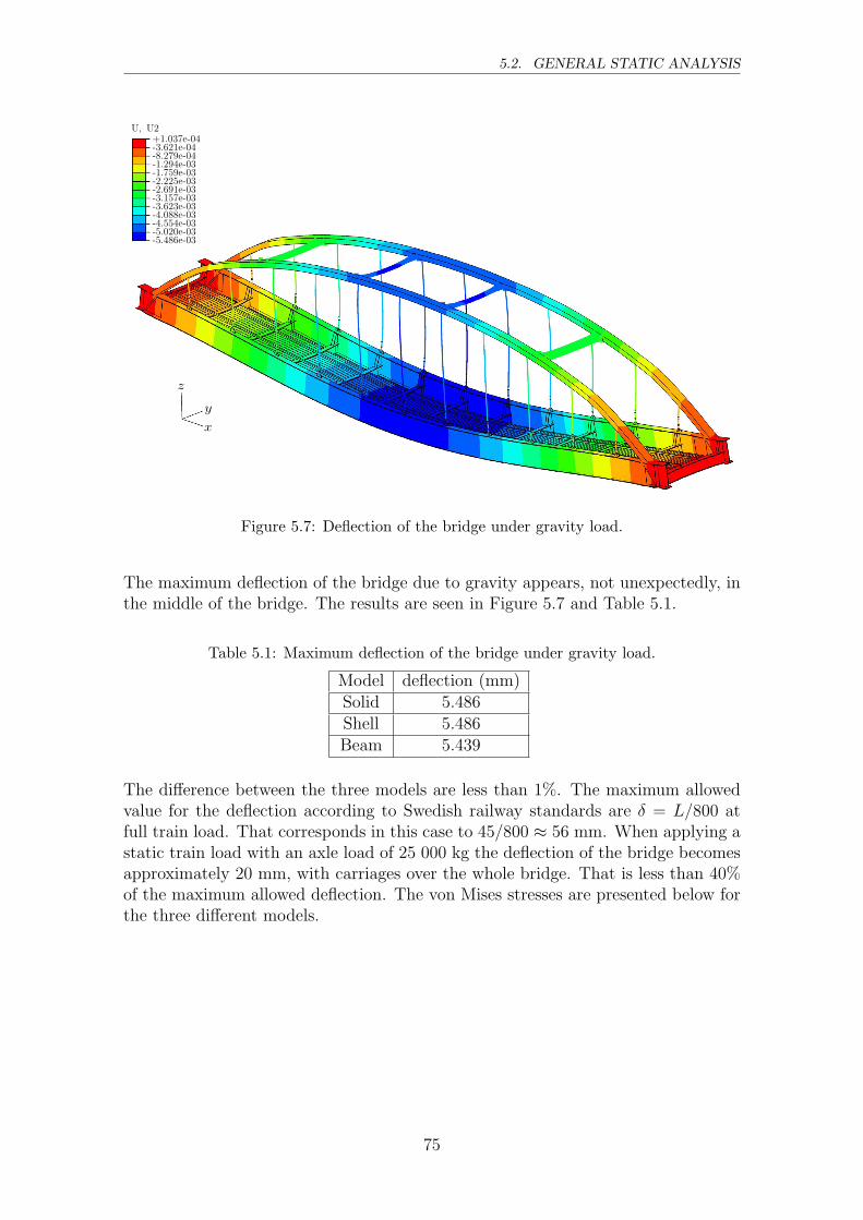
5.2. GENERAL STATIC ANALYSIS
U, U2
-5.486e-03-5.020e-03-4.554e-03-4.088e-03-3.623e-03-3.157e-03-2.691e-03-2.225e-03-1.759e-03-1.294e-03-8.279e-04-3.621e-04+1.037e-04
x
y
z
Figure 5.7: Deflection of the bridge under gravity load.
The maximum deflection of the bridge due to gravity appears, not unexpectedly, inthe middle of the bridge. The results are seen in Figure 5.7 and Table 5.1.
Table 5.1: Maximum deflection of the bridge under gravity load.
Model deflection (mm)Solid 5.486Shell 5.486Beam 5.439
The difference between the three models are less than 1%. The maximum allowedvalue for the deflection according to Swedish railway standards are δ = L/800 atfull train load. That corresponds in this case to 45/800 ≈ 56 mm. When applying astatic train load with an axle load of 25 000 kg the deflection of the bridge becomesapproximately 20 mm, with carriages over the whole bridge. That is less than 40%of the maximum allowed deflection. The von Mises stresses are presented below forthe three different models.
75

CHAPTER 5. MODELLING RESULTS
x
z
y
(Ave. Crit.: 75%)
S, Mises
+5.882e+06+7.351e+06+8.821e+06+1.029e+07+1.176e+07+1.323e+07+1.470e+07+1.617e+07+1.764e+07
+2.787e+03+1.473e+06+2.942e+06+4.412e+06
(Ave. Crit.: 75%)S, Mises
+1.519e+07+1.899e+07+2.279e+07+2.658e+07+3.038e+07+3.418e+07+3.798e+07+4.177e+07+4.557e+07
+1.554e+03+3.799e+06+7.597e+06+1.139e+07
(Ave. Crit.: 75%)S, Mises
+1.680e+07+2.099e+07+2.518e+07+2.938e+07+3.357e+07+3.777e+07+4.196e+07+4.616e+07+5.035e+07
+1.786e+04+4.212e+06+8.406e+06+1.260e+07
Figure 5.8: Von Mises stresses in the solid model, shell model and beam elementmodel.
From the legends in Figure 5.8 it can be seen that the maximum stress are muchhigher in the solid and shell model than in the beam element model. This dependson local stress concentrations near connections between different parts that mightbe insufficiently meshed, such as the connection between the hanger and the bridge.This does not appear in the beam element model, because of the more coarse el-ements. The stresses of more importance are instead those in the arch. The loadfrom the bridge is transported from the carriageway through the hangers and viathe arch down to the supports of the bridge. This produces the largest stresses nearthe supports of the arch of about 17 MPa in all three models. The distribution ofthe stress in the arch is shown in Figure 5.9. The stresses in the hangers are notuniformly distributed and the hangers nearest to the end supports have larger stressthan those in the middle, as shown in Figure 5.10.
76
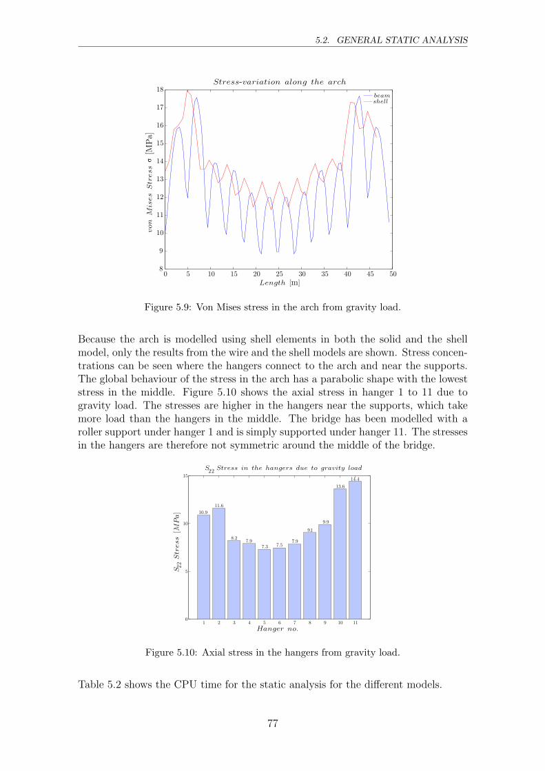
5.2. GENERAL STATIC ANALYSIS
0 5 10 15 20 25 30 35 40 45 508
9
10
11
12
13
14
15
16
17
18Stress-variation along the arch
Length [m]
von
Mises
Stress
σ[M
Pa]
beamshell
Figure 5.9: Von Mises stress in the arch from gravity load.
Because the arch is modelled using shell elements in both the solid and the shellmodel, only the results from the wire and the shell models are shown. Stress concen-trations can be seen where the hangers connect to the arch and near the supports.The global behaviour of the stress in the arch has a parabolic shape with the loweststress in the middle. Figure 5.10 shows the axial stress in hanger 1 to 11 due togravity load. The stresses are higher in the hangers near the supports, which takemore load than the hangers in the middle. The bridge has been modelled with aroller support under hanger 1 and is simply supported under hanger 11. The stressesin the hangers are therefore not symmetric around the middle of the bridge.
1 2 3 4 5 6 7 8 9 10 110
5
10
15
Hanger no.
S22Stress
[MPa]
S22
Stress in the hangers due to gravity load
10.9
11.6
8.27.9
7.3 7.57.9
9.1
9.9
13.6
14.4
Figure 5.10: Axial stress in the hangers from gravity load.
Table 5.2 shows the CPU time for the static analysis for the different models.
77
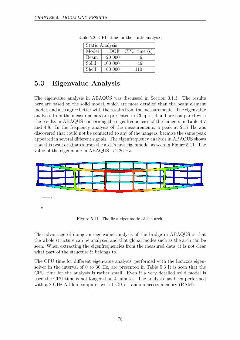
CHAPTER 5. MODELLING RESULTS
Table 5.2: CPU time for the static analyses.
Static AnalysisModel DOF CPU time (s)Beam 20 000 6Solid 100 000 46Shell 60 000 110
5.3 Eigenvalue Analysis
The eigenvalue analysis in ABAQUS was discussed in Section 3.1.3. The resultshere are based on the solid model, which are more detailed than the beam elementmodel, and also agree better with the results from the measurements. The eigenvalueanalyses from the measurements are presented in Chapter 4 and are compared withthe results in ABAQUS concerning the eigenfrequencies of the hangers in Table 4.7and 4.8. In the frequency analysis of the measurements, a peak at 2.17 Hz wasdiscovered that could not be connected to any of the hangers, because the same peakappeared in several different signals. The eigenfrequency analysis in ABAQUS showsthat this peak originates from the arch’s first eigenmode, as seen in Figure 5.11. Thevalue of the eigenmode in ABAQUS is 2.26 Hz.
x
y
Figure 5.11: The first eigenmode of the arch.
The advantage of doing an eigenvalue analysis of the bridge in ABAQUS is thatthe whole structure can be analysed and that global modes such as the arch can beseen. When extracting the eigenfrequencies from the measured data, it is not clearwhat part of the structure it belongs to.
The CPU time for different eigenvalue analysis, performed with the Lanczos eigen-solver in the interval of 0 to 30 Hz, are presented in Table 5.3 It is seen that theCPU time for the analysis is rather small. Even if a very detailed solid model isused the CPU time is not longer than 4 minutes. The analysis has been performedwith a 2 GHz Athlon computer with 1 GB of random access memory (RAM).
78

5.4. DYNAMIC ANALYSIS
Table 5.3: Acquired CPU time for the eigenvalue analyses.
Eigenvalue AnalysisModel DOF No. of Modes CPU time (s)Beam 12 500 123 32Shell 60 000 114 236Solid 64 000 109 222
5.4 Dynamic Analysis
The dynamic simulations are based on the beam element model and the shell model.Both explicit and implicit dynamics have been used. The explicit scheme appearedto be very computationally demanding and is more appropriate to use when thetime interval is very small. However it is easier to achieve convergence based onan explicit scheme if the behaviour of the structure is unknown. In this case thebehaviour has been studied from the measurements. The advantage of the implicitscheme is that it only takes a fraction of the time compared to the explicit method.
The time step is chosen by the user either as automatic or fixed time increment, asexplained in Section 3.1.3. A different size of the time increment has been performeduntil the results seem to converge. Different analyses have been performed with dif-ferent type of damping in the structure, concerning spring and dashpot dampers inthe train and Rayleigh damping of the structure. Trains with different damping,velocity and load have been modelled to see how they affect the structure. Froma dimensional point of view maximum train load and velocity has been applied,because that seem to be case that gives the largest stresses in the bridge. The max-imum velocity has been set to 25 m/s and is assumed to lie in the interval from20 to 25 m/s. The dynamic behaviour of the bridge in the perpendicular direc-tion depends on the behaviour of the train carriages. Different values of the traindamping have therefore been studied to achieve a similar behaviour compared tothe measurements. Due to the size of the model not more than 10 carriages havebeen modelled, compared with up to 24 carriages at the measurements.The main purpose with the dynamic model is to show the behaviour of the bridgeduring the train passage and compare the results with the measurements. Whenthe field measurements were performed, the stabilising system connecting the hang-ers, were dismantled to make the results from the measurements less complex. Inthe finite element models the effect of the stabilising system can be analysed in amore accurate way, because the deflections do not have to be integrated from theaccelerations, as in the case of the signal analysis.
A rather wide range of different behaviours of the hangers can be created dependingon how the train and bridge are modelled, or the analysis method used. Most ofthe results from the dynamic analysis are based on the implicit scheme, because ofthe advantages in this case, both concerning the computational cost and the abilityto combine it with a static analysis. The results that are presented are mainlyfrom the shell model as it seemed to give the most accurate result compared to
79
CHAPTER 5. MODELLING RESULTS
the measurements. A comparison is made between the shell and the beam elementmodel, to see if both models are accurate enough to be used.
The implicit analysis were performed in two different steps, first a static analysisthat calculates the stresses and deformations of the bridge as a result of the gravityload. In the next step, a dynamic implicit analysis with fixed time incrementshas been performed. Material damping has been used by defining the Rayleighcoefficients a0 and a1 from the measurements, as presented in Section 2.1.6. If nomaterial damping is introduced, the decay motion will be unrealistic low, althoughthe damping in this case is very low. When using the dynamic implicit scheme withfixed time increments, the results must be verified to converge to the same result,otherwise a smaller time increment must be used. If the time increment on the otherhand is to low, the simulation is often terminated due to the inability to handle largefiles. The result file can be reduced by extracting only the results that are of interest,e.g. stresses and displacements. This will also reduce the computational time.
Loads defined in a static step are applied linearly from 0 to 100%, in order to findequilibrium. A load defined in a dynamic step is applied instantaneously and causevibrations in the structure before equilibrium is reached. The loads in the modelare therefore applied in the static step and then propagated in the dynamic step.
5.4.1 Convergence of the Results
It was shown from the measurements that the hangers mainly vibrated with its firsteigenmode and that the highest first eigenmode in the hangers had an eigenfrequencyof 16 Hz, occurring in hanger 2. It was also shown that the longest hangers werethose who suffered greatest risk of fatigue. Because of their length both the first andthe second eigenfrequency are below 20 Hz. The first choice of the time incrementis therefore taken as 0.05 seconds which corresponds to the sample frequency of20 Hz. A time increment of 0.02, 0.01 and 0.005 seconds were then performed,corresponding to a sample frequency of 50 Hz, 100 Hz and 200 Hz. According toShannon’s sampling theorem [10], the sample frequency of a signal should be atleast twice the highest frequency of interest in the structure, fs ≥ 2fh; otherwiseit can cause lower peak amplitudes. That would in this case correspond to a timeincrement of 0.025 seconds.
The results with the different time increments are shown in Figure 5.12. The resultsseem to converge with a sample frequency of 100 Hz which are used in the followinganalyses. The train consists of 10 carriages and the whole train set has left the bridgeafter 7 seconds when travelling at 25 m/s. After that, the hangers are assumed tobe in free vibration.
The signal corresponding to a sampling frequency of 20 Hz seems to have faded outalmost entirely after 11 seconds, after just 4 seconds of free vibrations. It was seenfrom the measurements see Figure 4.20 that the hangers were still vibrating after 20seconds of free vibration. Convergence seems to be found when the time incrementis 0.01.
80
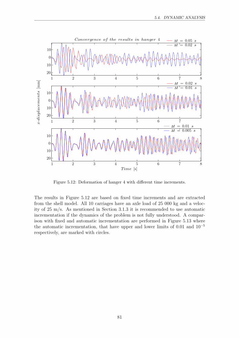
5.4. DYNAMIC ANALYSIS
1 2 3 4 5 6 7 8
20
10
0
10
x-displacem
ents
[mm]
∆t = 0.05 s∆t = 0.02 s
2 3 4 5 6 7
20
10
0
10
∆t = 0.02 s∆t = 0.01 s
2 3 4 5 6 7 8
20
10
0
10
Time [s]
∆t = 0.01 s∆t = 0.005 s
Convergence of the results in hanger 4
1
1
Figure 5.12: Deformation of hanger 4 with different time increments.
The results in Figure 5.12 are based on fixed time increments and are extractedfrom the shell model. All 10 carriages have an axle load of 25 000 kg and a veloc-ity of 25 m/s. As mentioned in Section 3.1.3 it is recommended to use automaticincrementation if the dynamics of the problem is not fully understood. A compar-ison with fixed and automatic incrementation are performed in Figure 5.13 wherethe automatic incrementation, that have upper and lower limits of 0.01 and 10−5
respectively, are marked with circles.
81
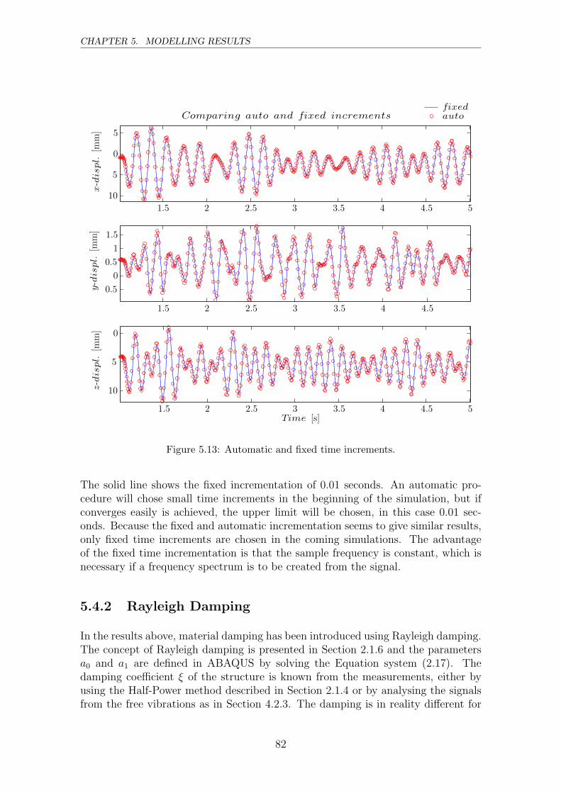
CHAPTER 5. MODELLING RESULTS
1.5 2 2.5 3 3.5 4 4.5 5
10
5
0
5
x-displ.
[mm]
1.5 2 2.5 3 3.5 4 4.5
0.5
0
0.5
1
1.5
y-displ.
[mm]
1.5 2 2.5 3 3.5 4 4.5 5
10
5
0
Time [s]
z-displ.
[mm]
fixedautoComparing auto and fixed increments
Figure 5.13: Automatic and fixed time increments.
The solid line shows the fixed incrementation of 0.01 seconds. An automatic pro-cedure will chose small time increments in the beginning of the simulation, but ifconverges easily is achieved, the upper limit will be chosen, in this case 0.01 sec-onds. Because the fixed and automatic incrementation seems to give similar results,only fixed time increments are chosen in the coming simulations. The advantageof the fixed time incrementation is that the sample frequency is constant, which isnecessary if a frequency spectrum is to be created from the signal.
5.4.2 Rayleigh Damping
In the results above, material damping has been introduced using Rayleigh damping.The concept of Rayleigh damping is presented in Section 2.1.6 and the parametersa0 and a1 are defined in ABAQUS by solving the Equation system (2.17). Thedamping coefficient ξ of the structure is known from the measurements, either byusing the Half-Power method described in Section 2.1.4 or by analysing the signalsfrom the free vibrations as in Section 4.2.3. The damping is in reality different for
82

5.4. DYNAMIC ANALYSIS
different parts of the structure, but is simplified in the model by using the samedamping for the whole structure. The damping used in ABAQUS is based on thedamping of hanger 4, which is 0.4%. This gives the parameters a0 = 3.41 · 10−2 anda1 = 5.38 · 10−6, based on the first and the third eigenmodes of that hanger.
0 1 2 3 4 5 6 7 8 9 10 112
1
0
1
2
0 1 2 3 4 5 6 7 8 9 10 110.4
0.2
0
0.2
0.4
0 1 2 3 4 5 6 7 8 9 10 112
1
0
1
No dampingRayleigh dampingRayleigh Damping of hanger 4
Time [s]
x-displ.
[mm]
y-displ.
[mm]
z-displ.
[mm]
Figure 5.14: The influence of Rayleigh damping.
Figure 5.14 shows that the Rayleigh damping has very little influence on the am-plitude of the signal. This depends on the low damping coefficient, ξ = 0.4% thathave been used, as the entire structure is made of steel. Because the damping isso low, the signal has been filtered according to its first eigenmode using an ellipticband-pass filter, to be able to see the influence of the damping at all. No aspectshave been made concerning the damping of the sleepers. The effect of the Rayleighdamping are difficult to see from the ABAQUS models because the time of free vi-brations are to short and the damping is very low. Because the computational timeis significantly larger when using Rayleigh damping, the total simulation time of themodel must be reduced. The Rayleigh damping in this case are rather superfluous,because of the size of the model and the duration time needed, in contrast to thecomputational cost that can be reduced if no damping is used, as seen in Table 5.4.
Table 5.4 shows how the time increment affects the calculation time. The simulations
83
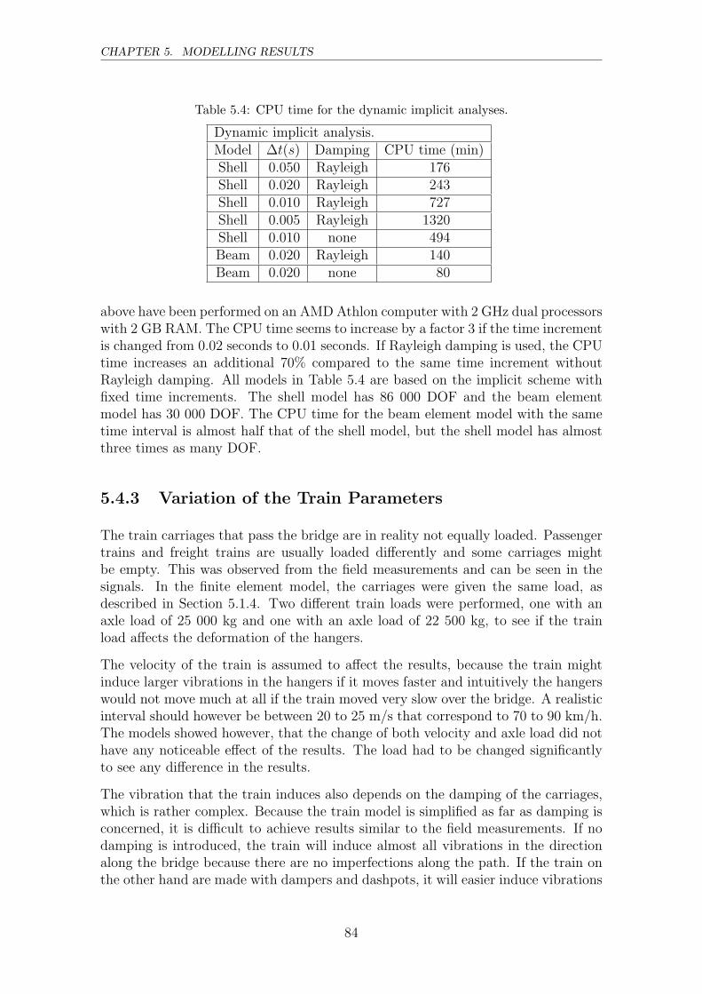
CHAPTER 5. MODELLING RESULTS
Table 5.4: CPU time for the dynamic implicit analyses.
Dynamic implicit analysis.Model ∆t(s) Damping CPU time (min)Shell 0.050 Rayleigh 176Shell 0.020 Rayleigh 243Shell 0.010 Rayleigh 727Shell 0.005 Rayleigh 1320Shell 0.010 none 494Beam 0.020 Rayleigh 140Beam 0.020 none 80
above have been performed on an AMD Athlon computer with 2 GHz dual processorswith 2 GB RAM. The CPU time seems to increase by a factor 3 if the time incrementis changed from 0.02 seconds to 0.01 seconds. If Rayleigh damping is used, the CPUtime increases an additional 70% compared to the same time increment withoutRayleigh damping. All models in Table 5.4 are based on the implicit scheme withfixed time increments. The shell model has 86 000 DOF and the beam elementmodel has 30 000 DOF. The CPU time for the beam element model with the sametime interval is almost half that of the shell model, but the shell model has almostthree times as many DOF.
5.4.3 Variation of the Train Parameters
The train carriages that pass the bridge are in reality not equally loaded. Passengertrains and freight trains are usually loaded differently and some carriages mightbe empty. This was observed from the field measurements and can be seen in thesignals. In the finite element model, the carriages were given the same load, asdescribed in Section 5.1.4. Two different train loads were performed, one with anaxle load of 25 000 kg and one with an axle load of 22 500 kg, to see if the trainload affects the deformation of the hangers.
The velocity of the train is assumed to affect the results, because the train mightinduce larger vibrations in the hangers if it moves faster and intuitively the hangerswould not move much at all if the train moved very slow over the bridge. A realisticinterval should however be between 20 to 25 m/s that correspond to 70 to 90 km/h.The models showed however, that the change of both velocity and axle load did nothave any noticeable effect of the results. The load had to be changed significantlyto see any difference in the results.
The vibration that the train induces also depends on the damping of the carriages,which is rather complex. Because the train model is simplified as far as damping isconcerned, it is difficult to achieve results similar to the field measurements. If nodamping is introduced, the train will induce almost all vibrations in the directionalong the bridge because there are no imperfections along the path. If the train onthe other hand are made with dampers and dashpots, it will easier induce vibrations
84
5.4. DYNAMIC ANALYSIS
in the perpendicular direction. Because the hangers can be seen as simply supportedin that direction, it will need a smaller load to excite them in that direction than inthe direction along the bridge. This behaviour is also seen in the measurements.
5.4.4 Deformation of the Hangers
The deformations of the hangers are presented for the dynamic implicit analysis witha fixed time increment of 0.01 seconds. The nodes to be analysed are taken at thepoint that has the largest displacement. The results from ABAQUS are comparedwith the results from the measurements in Figure 5.15 for hanger 4. The ABAQUSmodel with 10 carriages is compared with the measured signal from the freight train,ID019 that had 24 carriages. The results seem to be more or less comparable in thex-direction along the bridge, but the signal perpendicular the bridge is much largerfrom the measurements than from ABAQUS. The difference depends on the numberof carriages and how the train is modelled. Non-uniform loads on the real train setmight create more vibrations in the perpendicular direction than in the models.
The integration of the acceleration signal to displacements from the measurementsdepends very much on the filtering technique that is used, as discussed in Section 4.3.The dynamic analysis performed in ABAQUS with the shell model has a durationtime of 10 seconds, compared with up to 40 seconds from the measurements. Alonger time interval has not been modelled in ABAQUS due to the increased CPUtime. Another problem is the size of the results file. All simulations performedwhere the results file (*.ODB) exceeded 2 GB, crashed. This problem can in somecases be avoided by reducing the number of output variables to be extracted andthe density of the output signal.
85
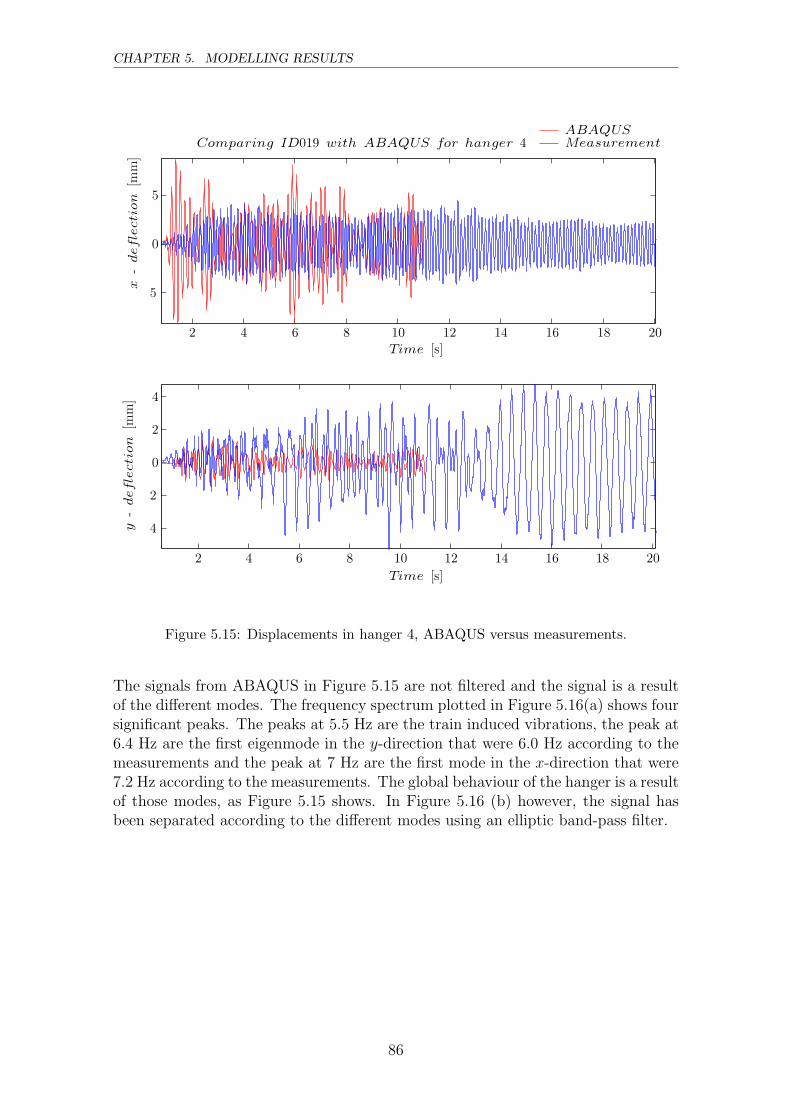
CHAPTER 5. MODELLING RESULTS
2 4 6 8 10 12 14 16 18 20
5
0
5
Time [s]
x-deflection
[mm]
ABAQUSMeasurement
2 4 6 8 10 12 14 16 18 20
4
2
0
2
4
Time [s]
y-deflection
[mm]
Comparing ID019 with ABAQUS for hanger 4
Figure 5.15: Displacements in hanger 4, ABAQUS versus measurements.
The signals from ABAQUS in Figure 5.15 are not filtered and the signal is a resultof the different modes. The frequency spectrum plotted in Figure 5.16(a) shows foursignificant peaks. The peaks at 5.5 Hz are the train induced vibrations, the peak at6.4 Hz are the first eigenmode in the y-direction that were 6.0 Hz according to themeasurements and the peak at 7 Hz are the first mode in the x-direction that were7.2 Hz according to the measurements. The global behaviour of the hanger is a resultof those modes, as Figure 5.15 shows. In Figure 5.16 (b) however, the signal hasbeen separated according to the different modes using an elliptic band-pass filter.
86
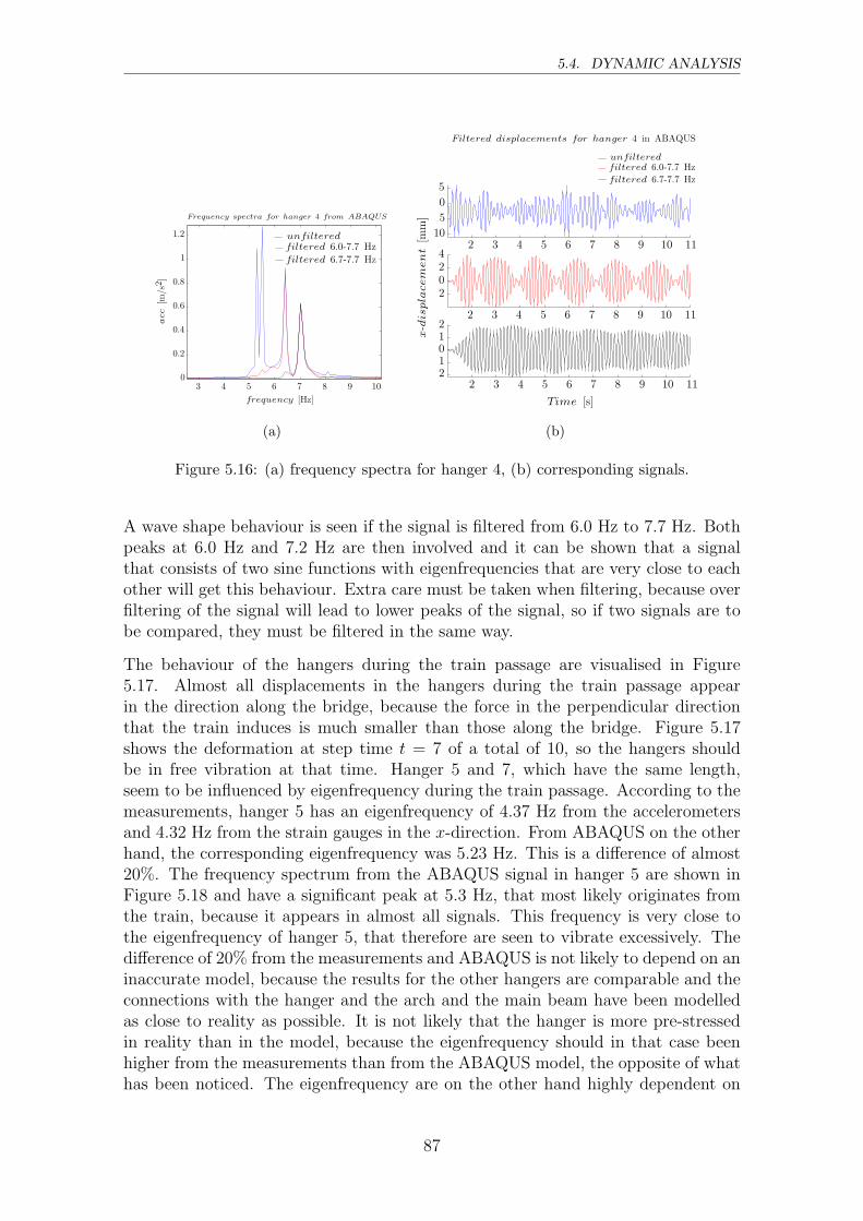
5.4. DYNAMIC ANALYSIS
3 4 5 6 7 8 9 100
0.2
0.4
0.6
0.8
1
1.2
frequency [Hz]
acc
[m/s2]
Frequency spectra for hanger 4 from ABAQUS
unfilteredfiltered 6.0-7.7 Hz
filtered 6.7-7.7 Hz
(a)
2 3 4 5 6 7 8 9 10 1110
5
0
5
2 3 4 5 6 7 8 9 10 11
2024
2 3 4 5 6 7 8 9 10 1121012
Time [s]
x-displacem
ent[m
m]
Filtered displacements for hanger 4 in ABAQUS
unfilteredfiltered 6.0-7.7 Hz
filtered 6.7-7.7 Hz
(b)
Figure 5.16: (a) frequency spectra for hanger 4, (b) corresponding signals.
A wave shape behaviour is seen if the signal is filtered from 6.0 Hz to 7.7 Hz. Bothpeaks at 6.0 Hz and 7.2 Hz are then involved and it can be shown that a signalthat consists of two sine functions with eigenfrequencies that are very close to eachother will get this behaviour. Extra care must be taken when filtering, because overfiltering of the signal will lead to lower peaks of the signal, so if two signals are tobe compared, they must be filtered in the same way.
The behaviour of the hangers during the train passage are visualised in Figure5.17. Almost all displacements in the hangers during the train passage appearin the direction along the bridge, because the force in the perpendicular directionthat the train induces is much smaller than those along the bridge. Figure 5.17shows the deformation at step time t = 7 of a total of 10, so the hangers shouldbe in free vibration at that time. Hanger 5 and 7, which have the same length,seem to be influenced by eigenfrequency during the train passage. According to themeasurements, hanger 5 has an eigenfrequency of 4.37 Hz from the accelerometersand 4.32 Hz from the strain gauges in the x-direction. From ABAQUS on the otherhand, the corresponding eigenfrequency was 5.23 Hz. This is a difference of almost20%. The frequency spectrum from the ABAQUS signal in hanger 5 are shown inFigure 5.18 and have a significant peak at 5.3 Hz, that most likely originates fromthe train, because it appears in almost all signals. This frequency is very close tothe eigenfrequency of hanger 5, that therefore are seen to vibrate excessively. Thedifference of 20% from the measurements and ABAQUS is not likely to depend on aninaccurate model, because the results for the other hangers are comparable and theconnections with the hanger and the arch and the main beam have been modelledas close to reality as possible. It is not likely that the hanger is more pre-stressedin reality than in the model, because the eigenfrequency should in that case beenhigher from the measurements than from the ABAQUS model, the opposite of whathas been noticed. The eigenfrequency are on the other hand highly dependent on
87

CHAPTER 5. MODELLING RESULTS
the boundary conditions and a little change in the enforcement could change theeigenfrequencies for the longer hangers.
(Ave. Crit.: 75%)S, Mises
+2.873e+03+5.613e+06+1.122e+07+1.683e+07+2.244e+07+2.806e+07+3.367e+07+3.928e+07+4.489e+07+5.050e+07+5.611e+07+6.172e+07+6.733e+07
x
y
z
x
z
Figure 5.17: Behaviour of the bridge, scale factor 100, t = 7 s.
The eigenfrequency of hanger 5 in the y-direction are about 3.7 Hz, according toboth the measurements and ABAQUS and the difference between them are less than1%. That means that hanger 5 only suffers from eigenfrequency in the x-direction,as seen in Figure 5.17.
88
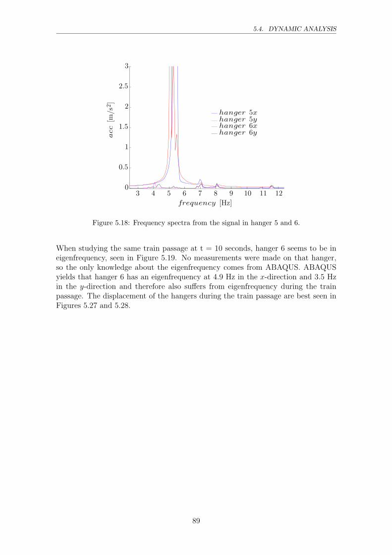
5.4. DYNAMIC ANALYSIS
3 4 5 6 7 8 9 10 11 120
0.5
1
1.5
2
2.5
3
frequency [Hz]
acc
[m/s2]
hanger 5xhanger 5yhanger 6xhanger 6y
Figure 5.18: Frequency spectra from the signal in hanger 5 and 6.
When studying the same train passage at t = 10 seconds, hanger 6 seems to be ineigenfrequency, seen in Figure 5.19. No measurements were made on that hanger,so the only knowledge about the eigenfrequency comes from ABAQUS. ABAQUSyields that hanger 6 has an eigenfrequency at 4.9 Hz in the x-direction and 3.5 Hzin the y-direction and therefore also suffers from eigenfrequency during the trainpassage. The displacement of the hangers during the train passage are best seen inFigures 5.27 and 5.28.
89

CHAPTER 5. MODELLING RESULTS
(Ave. Crit.: 75%)
S, Mises
+5.062e+03+6.575e+06+1.314e+07+1.971e+07+2.628e+07+3.285e+07+3.942e+07+4.599e+07+5.256e+07+5.913e+07+6.570e+07+7.227e+07+7.884e+07
x
z
x
y
z
Figure 5.19: Behaviour of the bridge, scale factor 100, t = 10 sec.
The deflection of hanger 1 to 6 are plotted in Figures 5.20 and 5.21 along a path thatfollows each hanger, for the times 6.65 and 10 seconds, in both x and y-directions.The Figures are plotted with a normalised length to compare all hangers, where thepaths are taken from the main beam at length 0 and are connected to the arch atthe unit length 1.All hangers seem to deflect according to the first eigenmode in the x-direction andhave a clamped behaviour in the connections with both the arch and the main beam.In the y-direction on the other hand, the hangers are more or less simply supportedwith the main beam. Some of the longer hangers seem to deflect according to thesecond eigenmode, especially hanger 6 that have an eigenfrequency of 11 Hz in thatdirection.
90
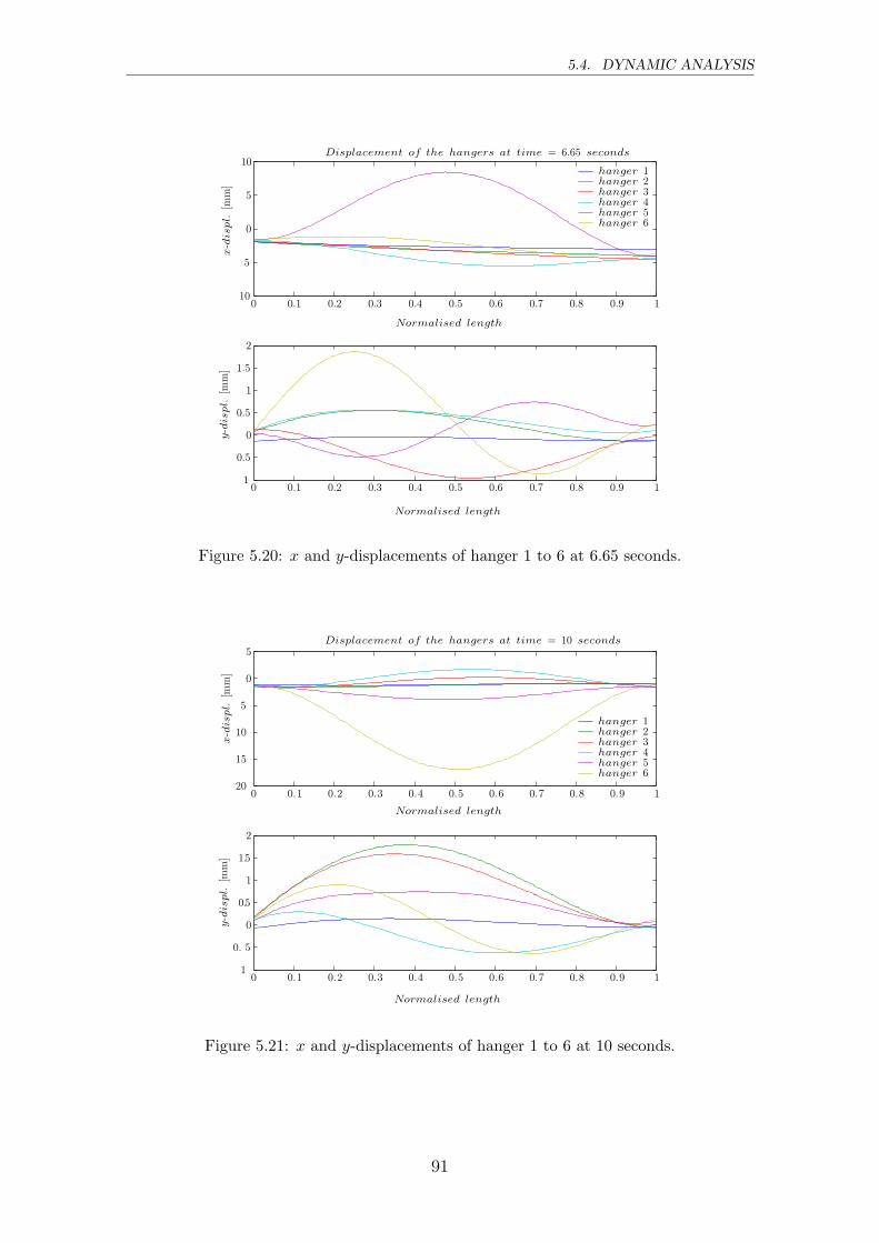
5.4. DYNAMIC ANALYSIS
0 0.1 0.2 0.3 0.4 0.5 0.6 0.7 0.8 0.9 110
5
0
5
10
0 0.1 0.2 0.3 0.4 0.5 0.6 0.7 0.8 0.9 11
0.5
0
0.5
1
1.5
2
Normalised length
x-displ.
[mm]
y-displ.
[mm]
hanger 1hanger 2hanger 3hanger 4hanger 5hanger 6
Displacement of the hangers at time = 6.65 seconds
Normalised length
Figure 5.20: x and y-displacements of hanger 1 to 6 at 6.65 seconds.
0 0.1 0.2 0.3 0.4 0.5 0.6 0.7 0.8 0.9 120
15
10
5
0
5
Normalised length
x-displ.
[mm]
0 0.1 0.2 0.3 0.4 0.5 0.6 0.7 0.8 0.9 11
0. 5
0
0.5
1
1.5
2
y-displ.
[mm]
hanger 1hanger 2hanger 3hanger 4hanger 5hanger 6
Displacement of the hangers at time = 10 seconds
Normalised length
Figure 5.21: x and y-displacements of hanger 1 to 6 at 10 seconds.
91
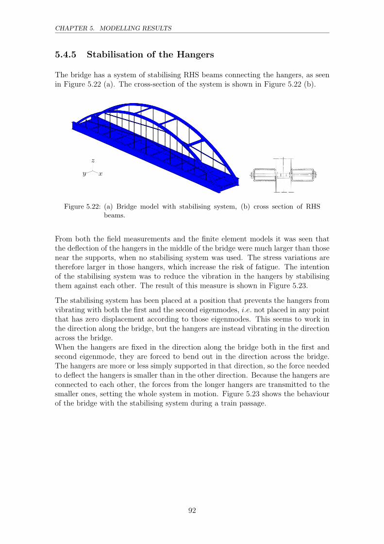
CHAPTER 5. MODELLING RESULTS
5.4.5 Stabilisation of the Hangers
The bridge has a system of stabilising RHS beams connecting the hangers, as seenin Figure 5.22 (a). The cross-section of the system is shown in Figure 5.22 (b).
y x
z
Figure 5.22: (a) Bridge model with stabilising system, (b) cross section of RHSbeams.
From both the field measurements and the finite element models it was seen thatthe deflection of the hangers in the middle of the bridge were much larger than thosenear the supports, when no stabilising system was used. The stress variations aretherefore larger in those hangers, which increase the risk of fatigue. The intentionof the stabilising system was to reduce the vibration in the hangers by stabilisingthem against each other. The result of this measure is shown in Figure 5.23.
The stabilising system has been placed at a position that prevents the hangers fromvibrating with both the first and the second eigenmodes, i.e. not placed in any pointthat has zero displacement according to those eigenmodes. This seems to work inthe direction along the bridge, but the hangers are instead vibrating in the directionacross the bridge.When the hangers are fixed in the direction along the bridge both in the first andsecond eigenmode, they are forced to bend out in the direction across the bridge.The hangers are more or less simply supported in that direction, so the force neededto deflect the hangers is smaller than in the other direction. Because the hangers areconnected to each other, the forces from the longer hangers are transmitted to thesmaller ones, setting the whole system in motion. Figure 5.23 shows the behaviourof the bridge with the stabilising system during a train passage.
92

5.4. DYNAMIC ANALYSIS
(Ave. Crit.: 75%)
S, Mises
+2.098e+03+5.482e+06+1.096e+07+1.644e+07+2.192e+07+2.740e+07+3.288e+07+3.836e+07+4.384e+07+4.932e+07+5.480e+07+6.028e+07+6.576e+07
x
z
y
x
z
y
y
xz
Figure 5.23: The deformation of the stabilising system, scale factor 100.
The frequency spectra for the train passage are shown in Figure 5.24. Figure 5.24(a) shows the frequency response in hanger 5 at a point in the middle betweenthe stabilising system and the connection with the arch. The dominating mode inthe x-direction is at about 11.5 Hz, which presumably corresponds to the secondeigenmode. That frequency does not seem to exist in Figure 5.22 (b), that is takenat a point in the hanger near the stabilisers. The behaviour of the structure ismore complicated to analyse when the stabilisers are applied because all hangersare connected and interact. The signal from ABAQUS mostly consists of the traininduced vibrations so the frequencies of the structure are mixed with the frequenciesof the train.
93
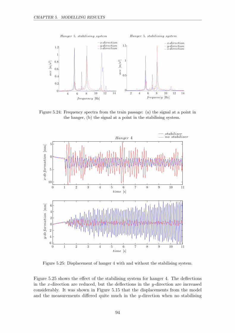
CHAPTER 5. MODELLING RESULTS
4 6 8 10 12 14
0.2
0.4
0.6
0.8
1
1.2
frequency [Hz]
acc
[m/s
2]
Hanger 5, stabilising system
x-directiony-directionz-direction
2 4 6 8 10 12 140
0.5
1
1.5
frequency [Hz]
acc
[m/s
2]
Hanger 5, stabilising system
x-directiony-directionz-direction
0
Figure 5.24: Frequency spectra from the train passage: (a) the signal at a point inthe hanger, (b) the signal at a point in the stabilising system.
0 1 2 3 4 5 6 7 8 9 10 11
10
5
0
5
time [s]
x-deform
ation
[mm]
0 1 2 3 4 5 6 7 8 9 10 116
4
2
0
2
4
6
time [s]
y-deform
ation
[mm]
stabiliserno stabiliserHanger 4
Figure 5.25: Displacement of hanger 4 with and without the stabilising system.
Figure 5.25 shows the effect of the stabilising system for hanger 4. The deflectionsin the x-direction are reduced, but the deflections in the y-direction are increasedconsiderably. It was shown in Figure 5.15 that the displacements from the modeland the measurements differed quite much in the y-direction when no stabilising
94
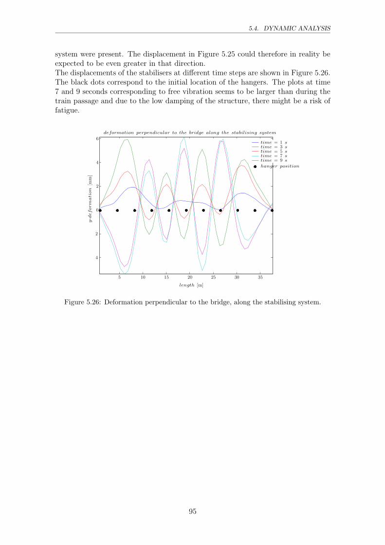
5.4. DYNAMIC ANALYSIS
system were present. The displacement in Figure 5.25 could therefore in reality beexpected to be even greater in that direction.The displacements of the stabilisers at different time steps are shown in Figure 5.26.The black dots correspond to the initial location of the hangers. The plots at time7 and 9 seconds corresponding to free vibration seems to be larger than during thetrain passage and due to the low damping of the structure, there might be a risk offatigue.
5 10 15 20 25 30 35
4
2
0
2
4
6
length [m]
y-deform
ation
[mm]
deformation perpendicular to the bridge along the stabilising system
time = 1 stime = 3 stime = 5 stime = 7 stime = 9 s
hanger position
Figure 5.26: Deformation perpendicular to the bridge, along the stabilising system.
95
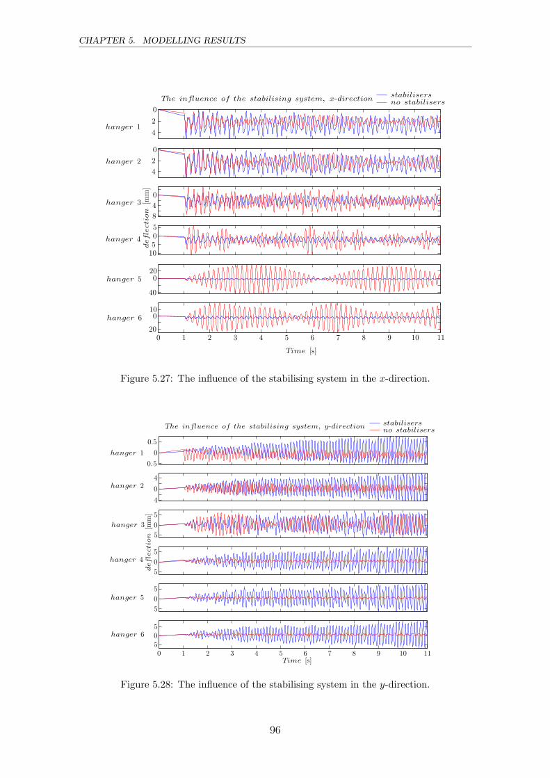
CHAPTER 5. MODELLING RESULTS
4
2
0
Time [s]
4
2
0
Time [s]
8
4
0
Time [s]
10505
Time [s]
40
020
Time [s]
0 1 2 3 4 5 6 7 8 9 10 1120
010
Time [s]
deflection
[mm]
stabilisersno stabilisersThe influence of the stabilising system, x-direction
hanger 1
hanger 2
hanger 3
hanger 4
hanger 5
hanger 6
Figure 5.27: The influence of the stabilising system in the x-direction.
0.5
0
0.5
Time [s]
4
0
4
Time [s]
5
0
5
Time [s]
5
0
5
Time [s]
5
0
5
Time [s]
0 1 2 3 4 5 6 7 8 9 10 1150
5
Time [s]
stabilisersno stabilisers
The influence of the stabilising system, y-direction
deflection
[mm]
hanger 1
hanger 2
hanger 3
hanger 4
hanger 5
hanger 6
Figure 5.28: The influence of the stabilising system in the y-direction.
96
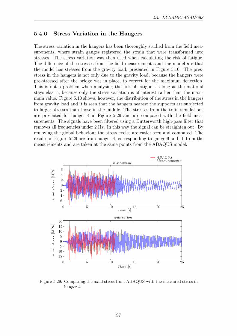
5.4. DYNAMIC ANALYSIS
5.4.6 Stress Variation in the Hangers
The stress variation in the hangers has been thoroughly studied from the field mea-surements, where strain gauges registered the strain that were transformed intostresses. The stress variation was then used when calculating the risk of fatigue.The difference of the stresses from the field measurements and the model are thatthe model has stresses from the gravity load, presented in Figure 5.10. The pres-stress in the hangers is not only due to the gravity load, because the hangers werepre-stressed after the bridge was in place, to correct for the maximum deflection.This is not a problem when analysing the risk of fatigue, as long as the materialstays elastic, because only the stress variation is of interest rather than the maxi-mum value. Figure 5.10 shows, however, the distribution of the stress in the hangersfrom gravity load and it is seen that the hangers nearest the supports are subjectedto larger stresses than those in the middle. The stresses from the train simulationsare presented for hanger 4 in Figure 5.29 and are compared with the field mea-surements. The signals have been filtered using a Butterworth high-pass filter thatremoves all frequencies under 2 Hz. In this way the signal can be straighten out. Byremoving the global behaviour the stress cycles are easier seen and compared. Theresults in Figure 5.29 are from hanger 4, corresponding to gauge 9 and 10 from themeasurements and are taken at the same points from the ABAQUS model.
0 5 10 15 20 25
6
4
2
0
2
4
6
Time [s]
Axia
lstress[M
Pa]
0 5 10 15 20 25
15
10
5
0
5
10
15
20
Time [s]
Axia
lstress[M
Pa]
x-direction
y-direction
MeasurementsABAQUS
Figure 5.29: Comparing the axial stress from ABAQUS with the measured stress inhanger 4.
97
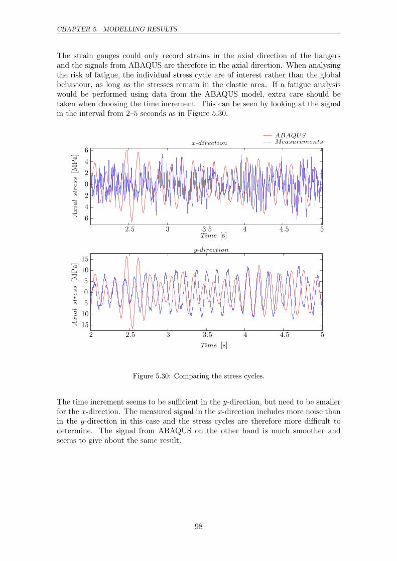
CHAPTER 5. MODELLING RESULTS
The strain gauges could only record strains in the axial direction of the hangersand the signals from ABAQUS are therefore in the axial direction. When analysingthe risk of fatigue, the individual stress cycle are of interest rather than the globalbehaviour, as long as the stresses remain in the elastic area. If a fatigue analysiswould be performed using data from the ABAQUS model, extra care should betaken when choosing the time increment. This can be seen by looking at the signalin the interval from 2–5 seconds as in Figure 5.30.
2 2.5 3 3.5 4 4.5 5
15
10
5
0
5
10
15
2.5 3 3.5 4 4.5 5
6
4
2
0
2
4
6
Time [s]
Axia
lstress[M
Pa]
Time [s]
Axia
lstress[M
Pa]
x-direction
y-direction
MeasurementsABAQUS
Figure 5.30: Comparing the stress cycles.
The time increment seems to be sufficient in the y-direction, but need to be smallerfor the x-direction. The measured signal in the x-direction includes more noise thanin the y-direction in this case and the stress cycles are therefore more difficult todetermine. The signal from ABAQUS on the other hand is much smoother andseems to give about the same result.
98
5.5. STUDY OF THE TURN BUCKLE
5.5 Study of the Turn Buckle
The most critical part of the bridge is most likely the turn buckle that connects thehanger with the main beam. It was seen from the analysis of the measurementsthat there was a great risk of fatigue in the threaded section of the hangers, whenneglecting the turn buckle. When the area change in that region were taken intoconsideration, the risk was even greater. A detailed finite element model has beencreated to investigate the stress concentrations in the threads of the turn buckle,where fatigue cracks can be expected to appear. The stress variation is assumed tobe elastic and the purpose is just to see the distribution of the stresses.
The connection can be divided into three parts, the hanger connected to the arch,the hanger connected to the main beam and the turn buckle connecting these two.The stresses were measured with strain gauges, placed 10 cm above the threadedpart of the hanger. The maximum stresses are expected to appear in the turnbuckle that has a smaller cross-sectional area, but local stress concentrations mayalso appear in the contact with the threads.The interactions of the threads is in reality a complicated contact problem andone approach in ABAQUS is to create a contact formulation between the surfacesin contact, using a dynamic implicit scheme. This is rather computer demanding,both because the complexity of the surfaces in contact and that a very refined meshmust be used, if the stresses in the threads are to be studied.
An easier approach can be made by neglecting the stresses that occur due to contactbetween the threads and instead assume that the largest global stress will appearin the middle of the turn buckle where the cross-sectional area is smallest. Furthersimplifications can be made by using an axisymmetric model and applying boundaryconditions so that it can move only in the axial direction.Because the stress increase is of importance, rather than the stress cycle, a staticmodel with a constant load can be used. The results can be applied to the fatigueanalysis based on the field measurements, by scaling the signal with the factor thatthe stresses are increased due to stress concentrations in the threads. The detailcategory that has been used in the fatigue analysis was adapted to the threadedsection when the stresses in the solid hanger were known. When the stresses canbe calculated in the threads, the detail category should be that for solid steel, e.g.C = 125.
5.5.1 The Static Model
The maximum stress occurring in the hangers were obtained from the strain gaugeswhen the hangers were in free vibration. The stresses were oscillating with anamplitude of 40 MPa. In the static model, the load was applied to give the samestress in the area where the strain gauge were placed and compare them with themaximum stress occurring in the threads. No contact interactions were used andthe model was made in one part. The part was revolved 360 ◦ and Figure 5.31 showsa cross-section of the part.
99
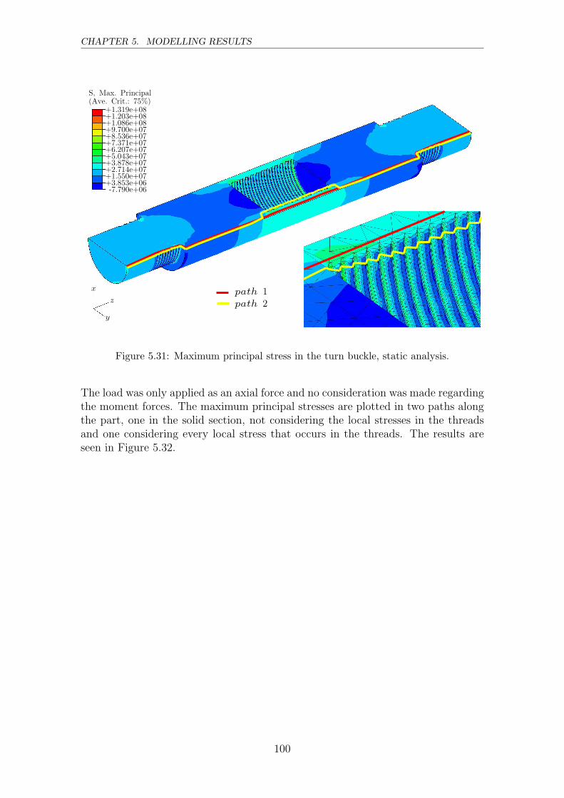
CHAPTER 5. MODELLING RESULTS
(Ave. Crit.: 75%)S, Max. Principal
-7.790e+06+3.853e+06+1.550e+07+2.714e+07+3.878e+07+5.043e+07+6.207e+07+7.371e+07+8.536e+07+9.700e+07+1.086e+08+1.203e+08+1.319e+08
x path 1path 2z
y
Figure 5.31: Maximum principal stress in the turn buckle, static analysis.
The load was only applied as an axial force and no consideration was made regardingthe moment forces. The maximum principal stresses are plotted in two paths alongthe part, one in the solid section, not considering the local stresses in the threadsand one considering every local stress that occurs in the threads. The results areseen in Figure 5.32.
100
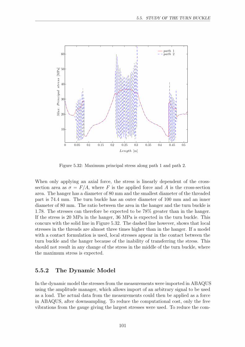
5.5. STUDY OF THE TURN BUCKLE
0 0.05 0.1 0.15 0.2 0.25 0.3 0.35 0.4 0.45 0.5
10
20
30
40
50
60
Length [m]
Max.Prin
cipalstress
[MPa]
path 1path 2
Figure 5.32: Maximum principal stress along path 1 and path 2.
When only applying an axial force, the stress is linearly dependent of the cross-section area as σ = F/A, where F is the applied force and A is the cross-sectionarea. The hanger has a diameter of 80 mm and the smallest diameter of the threadedpart is 74.4 mm. The turn buckle has an outer diameter of 100 mm and an innerdiameter of 80 mm. The ratio between the area in the hanger and the turn buckle is1.78. The stresses can therefore be expected to be 78% greater than in the hanger.If the stress is 20 MPa in the hanger, 36 MPa is expected in the turn buckle. Thisconcurs with the solid line in Figure 5.32. The dashed line however, shows that localstresses in the threads are almost three times higher than in the hanger. If a modelwith a contact formulation is used, local stresses appear in the contact between theturn buckle and the hanger because of the inability of transferring the stress. Thisshould not result in any change of the stress in the middle of the turn buckle, wherethe maximum stress is expected.
5.5.2 The Dynamic Model
In the dynamic model the stresses from the measurements were imported in ABAQUSusing the amplitude manager, which allows import of an arbitrary signal to be usedas a load. The actual data from the measurements could then be applied as a forcein ABAQUS, after downsampling. To reduce the computational cost, only the freevibrations from the gauge giving the largest stresses were used. To reduce the com-
101
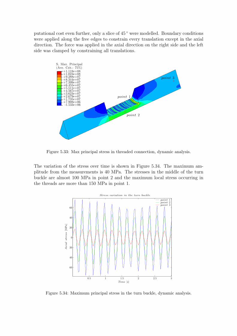
putational cost even further, only a slice of 45 ◦ were modelled. Boundary conditionswere applied along the free edges to constrain every translation except in the axialdirection. The force was applied in the axial direction on the right side and the leftside was clamped by constraining all translations.
(Ave. Crit.: 75%)S, Max. Principal
-1.533e+06+7.908e+06+1.735e+07+2.679e+07+3.623e+07+4.567e+07+5.511e+07+6.455e+07+7.399e+07+8.344e+07+9.288e+07+1.023e+08+1.118e+08
point 2
point 1
point 3
Figure 5.33: Max principal stress in threaded connection, dynamic analysis.
The variation of the stress over time is shown in Figure 5.34. The maximum am-plitude from the measurements is 40 MPa. The stresses in the middle of the turnbuckle are almost 100 MPa in point 2 and the maximum local stress occurring inthe threads are more than 150 MPa in point 1.
0.5 1 1.5 2 2.5 3
60
40
20
0
20
40
60
Time [s]
Axia
lstress
[MPa]
Stress variation in the turn buckle
point 1point 2point 3
Figure 5.34: Maximum principal stress in the turn buckle, dynamic analysis.
Chapter 6
Conclusions
6.1 Discussion
The purpose of this thesis was to study the train induced vibrations based on bothfield measurements and finite element analysis. The parts of main interest were thehangers, concerning stress variation and displacements due to vibrations from thetrain.
An important aspect of the thesis was to compare the results from the measurementswith the finite element models, to see if it was possible to obtain similar results. Thesuccess in this manner depends both on the evaluation method of the measured dataand the accuracy of the model. The main difficulty in the finite element model wasto create an accurate train model that induces similar vibrations compared to themeasurements.
6.2 Measurements
The main interest of the measurements was to study the vibrations in the hangersand analyse if these vibrations could lead to fatigue. The measurements were madewith the stabilising system dismantled, since it was assumed that it did not stabilisethe structure enough. All of the results from the measurements could not be shownin the thesis, but some supplementary results are shown in Appendix A. Resultshave been sorted out since they did not contribute with any additional information.
The results obtained from the accelerometers and strain gauges showed that the firsteigenfrequency of the hangers varies from 3.6 to 16.0 Hz. The frequency responseshows that hanger 4 appears to be more pre-stressed than all the other hangers.Hanger 4 had almost the same eigenfrequencies as hanger 3 even though it is 1.1m longer. The frequency response also showed that the frequency induced fromthe train is approximately 5 Hz. This frequency is quite close to the natural eigen-frequency of hanger 5 in the x-direction, parallel to the rail, which could causeresonance problems. The damping in the hangers varies in the interval 0.1–0.5%
103
CHAPTER 6. CONCLUSIONS
depending on the different hangers and which direction and eigenmode the hangersvibrate with.
There are several difficulties when integrating displacements from measured accel-erations. This is because a measured signal is never perfect; it contains some errorssuch as background noise and new constants are created in the integration. It isimportant to verify that no unfamiliar peaks in frequency-domain appear. Thecalculated displacements differ from the measured ones that were made with andwithout an analogue low-pass filter. The unfiltered signals are filtered in MATLABto attenuate frequencies in the same interval as the analogue low-pass filter. Themaximum amplitude of the vibration was almost 10 mm in the measurements madewith the analogue low-pass filter.
The maximum stress due to tension in the hangers was almost 40 MPa and themaximum stress due to compression was 20 MPa. Both of these values are muchsmaller than the yielding stress. However, these stresses had large stress variationswhich can lead to fatigue. The fatigue analysis showed that to two freight trainpassages, ID009 and ID019, resulted in a high risk of fatigue in the two longesthangers that was measured, i.e. hanger 4 and 5. Based on the stress cycles inducedin hanger 5 from ID019 it would only have a life length of 70 years if two trainspassed every day. Hangers 4 and 5 also had a high risk for fatigue for highervalues on the detail category. The risk of fatigue would increase largely if thestress concentrations in the threaded section of the hangers are considered, wherethe bridge only would have a life length of 40 years for two train passages a day,according to both measurement ID009 and ID019. The majority of these largestress variations occurred as the hangers were in free vibration. The induced stressin hanger 2 is mainly a result of an axial load, while the stress in the longer hangershas a large contribution from the bending moments.
6.3 Finite Element Modelling
The aim of the finite element modelling was to get a detailed understanding of thedynamics of the bridge. The success in this manner depends mostly on how theinteraction between the train and the bridge is formulated. In this case the resultscould be compared with the field measurements to adjust the model. The partsof main interest are the hangers and the behaviour of these depends on how theboundary conditions are defined. A 3D shell model was therefore created so thatthe boundary conditions could be modelled in an accurate way. From the fieldmeasurements it was seen that the longer hangers were vibrating excessively duringthe train passage and the similar behaviour have been obtained from the finiteelement models. The frequency that the train induce in the bridge seems to beclose the eigenfrequencies of those hangers who therefore suffers from resonance, asdescribed in Section 2.1.3. Although a rather detailed model was made, the resultsdid not entirely correspond to the result from the measurements, mainly regardingthe displacements. The accuracy of the displacements from the field measurementswere however integrated from the accelerometers, which is not trivial. Just by
104
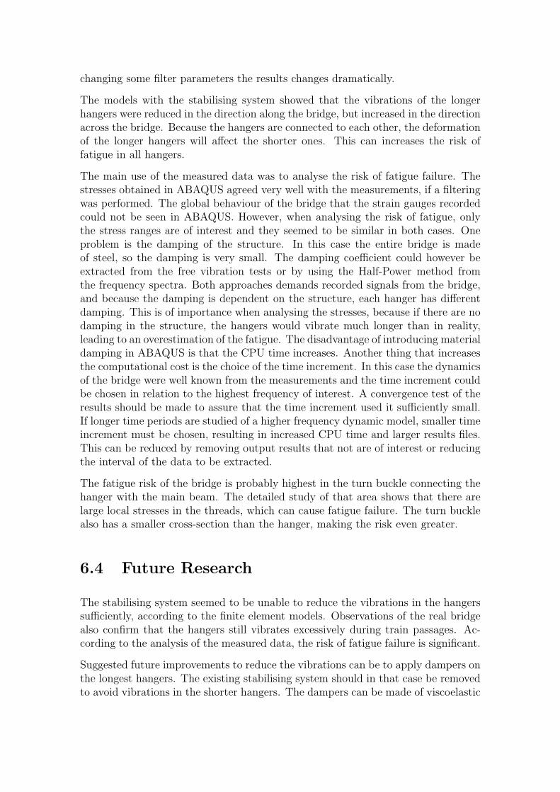
changing some filter parameters the results changes dramatically.
The models with the stabilising system showed that the vibrations of the longerhangers were reduced in the direction along the bridge, but increased in the directionacross the bridge. Because the hangers are connected to each other, the deformationof the longer hangers will affect the shorter ones. This can increases the risk offatigue in all hangers.
The main use of the measured data was to analyse the risk of fatigue failure. Thestresses obtained in ABAQUS agreed very well with the measurements, if a filteringwas performed. The global behaviour of the bridge that the strain gauges recordedcould not be seen in ABAQUS. However, when analysing the risk of fatigue, onlythe stress ranges are of interest and they seemed to be similar in both cases. Oneproblem is the damping of the structure. In this case the entire bridge is madeof steel, so the damping is very small. The damping coefficient could however beextracted from the free vibration tests or by using the Half-Power method fromthe frequency spectra. Both approaches demands recorded signals from the bridge,and because the damping is dependent on the structure, each hanger has differentdamping. This is of importance when analysing the stresses, because if there are nodamping in the structure, the hangers would vibrate much longer than in reality,leading to an overestimation of the fatigue. The disadvantage of introducing materialdamping in ABAQUS is that the CPU time increases. Another thing that increasesthe computational cost is the choice of the time increment. In this case the dynamicsof the bridge were well known from the measurements and the time increment couldbe chosen in relation to the highest frequency of interest. A convergence test of theresults should be made to assure that the time increment used it sufficiently small.If longer time periods are studied of a higher frequency dynamic model, smaller timeincrement must be chosen, resulting in increased CPU time and larger results files.This can be reduced by removing output results that not are of interest or reducingthe interval of the data to be extracted.
The fatigue risk of the bridge is probably highest in the turn buckle connecting thehanger with the main beam. The detailed study of that area shows that there arelarge local stresses in the threads, which can cause fatigue failure. The turn bucklealso has a smaller cross-section than the hanger, making the risk even greater.
6.4 Future Research
The stabilising system seemed to be unable to reduce the vibrations in the hangerssufficiently, according to the finite element models. Observations of the real bridgealso confirm that the hangers still vibrates excessively during train passages. Ac-cording to the analysis of the measured data, the risk of fatigue failure is significant.
Suggested future improvements to reduce the vibrations can be to apply dampers onthe longest hangers. The existing stabilising system should in that case be removedto avoid vibrations in the shorter hangers. The dampers can be made of viscoelastic

foam in contact with the hanger that absorbs the vibrations in order to damp thefree vibrations of the hangers. Similar methods have been used when damping othertypes of structures, e.g. the sports arena New Ullevi in Gothenburg and several cable-stayed bridges. The results are possible to verify using finite element methods in forinstance ABAQUS, where viscoelastic material properties can be defined.

Bibliography
[1] Ansell, A., and Svedbjork, G. Kompletterande dynamisk provning avkontinuerliga plattstrimlor av betong med armering av varierande seghet. Tech-nical report (2003).
[2] Battini, J.-M. Lecture notes in Structual Dynamics, Royal Institute of Tech-nology, 2002.
[3] Choppra, A. K. Dynamics of Structures, Theory and Applications to Earth-quake Engineering, 2nd ed. Prentice-Hall Inc, New Jersey, 2001.
[4] Clough, R. W., and Penzien, J. Dynamics of Structures, 2nd ed. McGraw-Hill, Singapore, 1993.
[5] Cook, R. D., Malkus, D. S., Plesha, M. E., and Witt, R. J. Conceptsand Applications of Finite Element Analysis, 4th ed. John Wiley & Sons, NewYork, 2002.
[6] Fatemi, A., and Yang, L. Cumulative fatigue damage and life predictiontheories: a survey of the state of the art for homgeneous materials. 9–11.
[7] Garg, V. K., and Dukkipati, R. V. Dynamics of Railway Vehicle Systems.Academic Press Canada, Ontario, 1984.
[8] Geradin, M., and Rixen, D. Mechanical Vibrations, Theory and Applicationto Structual Dynamics, 2nd ed. John Wiley & Sons, Chichester, 1997.
[9] Goransson, L., and Akerlund, S. Boverkets handbok omstalkonstruktioner. Boverket, Byggavdelningen, Karlskrona, 1994.
[10] Hall, L. Simulations and Analyses of Train-Induced Ground Vibrations. PhDthesis, Royal Institute of Technology, Department of Civil and EnvironmentalEngineering, Stockholm, Sweden, 2000.
[11] Hibbitt, Karlsson, and Sorensen. ABAQUS/Standard User’s Manual,6.3 ed. Hibbitt, Karlsson and Sorensen Inc, Pawtucket, 2002.
[12] Johnson, R. Progression of the dynamic properties of large suspension bridgesduring construction —a case study of the hoga kusten bridge. Licentiate thesis(1999).
[13] MathWorks. Signal Processing Toolbox, for use with MATLAB. 2000.
107

BIBLIOGRAPHY
[14] Tyrens AB. Design drawings for bridge over river Ljungan at Ange.
[15] Ugural, A. C., and Fenster, S. K. Advanced Strength and Applied Elac-ticity, 3rd ed. Prentice-Hall, New Jersey, 1995.
108

Appendix A
Measurement Results
A.1 Measurement Results
A.1.1 Accelerations
ID019 Freight Train (Copper train)
0 5 10 15 20 25 30 35 40-5
0
5
t (s)
a(m
/s)
2
acc2x
0 5 10 15 20 25 30 35 40-4
-2
0
2
4
t (s)
a(m
/s)
2
acc2y
0 5 10 15 20 25 30 35 40
-1
0
1
2
t (s)
a(m
/s)
2
acc2z
Figure A.1: Acceleration in hanger 2.
109
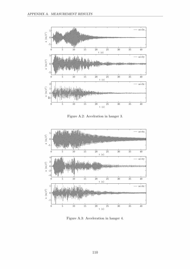
APPENDIX A. MEASUREMENT RESULTS
0 5 10 15 20 25 30 35 40
-5
0
5
t (s)
a(m
/s)
2
acc3x
0 5 10 15 20 25 30 35 40
-5
0
5
t (s)
a(m
/s)
2
acc3y
0 5 10 15 20 25 30 35 40
�-1
0
1
2
t (s)
a(m
/s)
2
acc3z
Figure A.2: Accelration in hanger 3.
0 5 10 15 20 25 30 35 40
-5
0
5
t (s)
a(m
/s2)
acc4x
0 5 10 15 20 25 30 35 40
-4
-2
0
2
4
t (s)
a(m
/s2)
acc4y
0 5 10 15 20 25 30 35 40
-1
0
1
t (s)
a(m
/s2)
acc4z
Figure A.3: Acceleration in hanger 4.
110
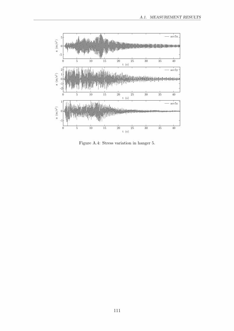
A.1. MEASUREMENT RESULTS
0 5 10 15 20 25 30 35 40
-5
0
5
t (s)
a(m
/s)
2
acc5x
0 5 10 15 20 25 30 35 40
-2
-1
0
1
2
t (s)
a(m
/s)
2
acc5y
0 5 10 15 20 25 30 35 40
-1
0
1
t (s)
a(m
/s)
2
acc5z
Figure A.4: Stress variation in hanger 5.
111
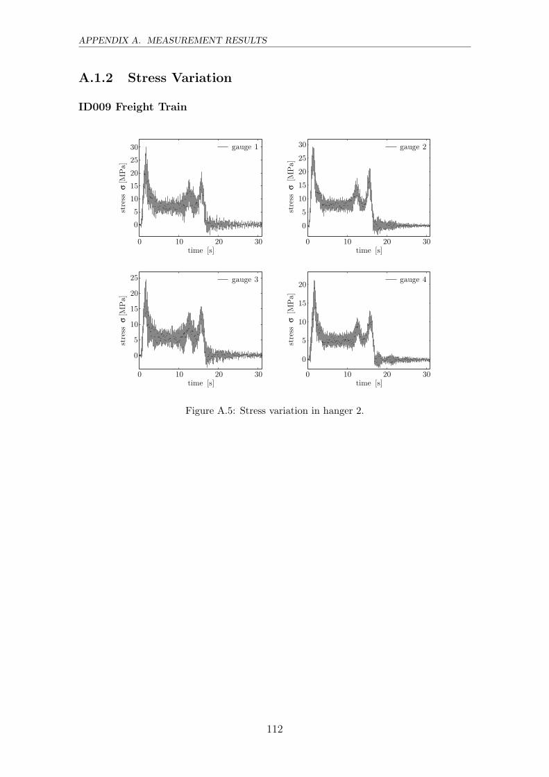
APPENDIX A. MEASUREMENT RESULTS
A.1.2 Stress Variation
ID009 Freight Train
0 10 20 30
0
5
10
15
20
25
30
time [s]
stress
σ[M
Pa]
gauge 1
0 10 20 30
0
5
10
15
20
25
30
time [s]
stress
σ[M
Pa]
gauge 2
0 10 20 30
0
5
10
15
20
25
time [s]
stress
σ[M
Pa]
gauge 3
0 10 20 30
0
5
10
15
20
time [s]
stress
σ[M
Pa]
gauge 4
Figure A.5: Stress variation in hanger 2.
112
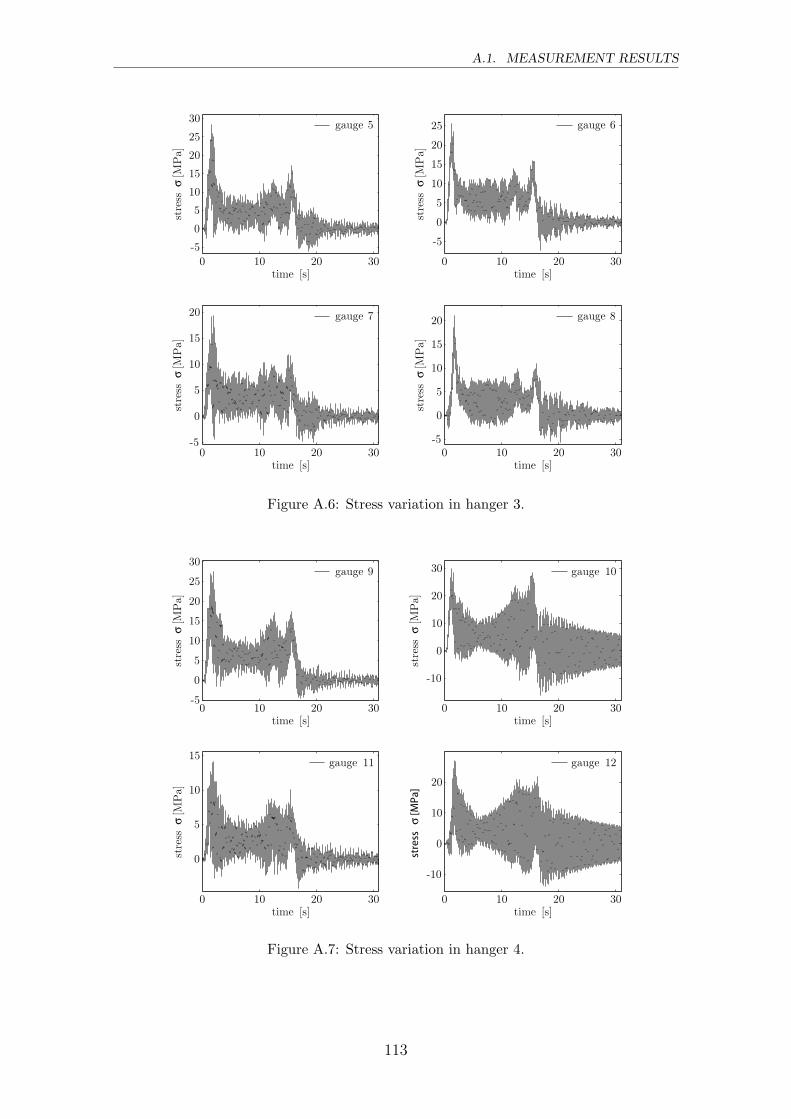
A.1. MEASUREMENT RESULTS
0 10 20 30
-5
0
5
10
15
20
25
30
time [s]
stress
σ[M
Pa]
gauge 5
0 10 20 30
-5
0
5
10
15
20
25
time [s]
stress
σ[M
Pa]
gauge 6
0 10 20 30-5
0
5
10
15
20
time [s]
stress
σ[M
Pa]
gauge 7
0 10 20 30-5
0
5
10
15
20
time [s]
stress
σ[M
Pa]
gauge 8
Figure A.6: Stress variation in hanger 3.
0 10 20 30-5
0
5
10
15
20
25
30
time [s]
stress
σ[M
Pa]
gauge 9
0 10 20 30
-10
0
10
20
30
time [s]
stress
σ[M
Pa]
gauge 10
0 10 20 30
0
5
10
15
time [s]
stress
σ[M
Pa]
gauge 11
0 10 20 30
-10
0
10
20
time [s]
stre
ssσ
[MPa
]
gauge 12
Figure A.7: Stress variation in hanger 4.
113
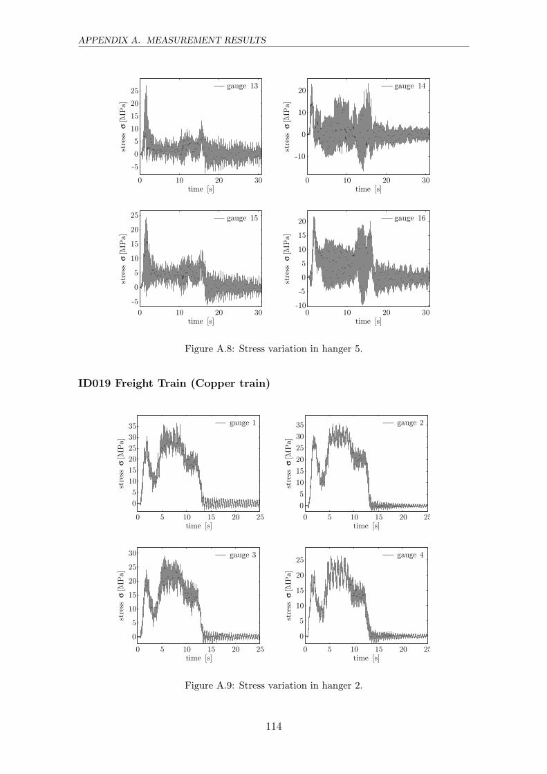
APPENDIX A. MEASUREMENT RESULTS
0 10 20 30
-5
0
5
10
15
20
25
time [s]
stress
σ[M
Pa]
gauge 13
0 10 20 30
-10
0
10
20
time [s]
stress
σ[M
Pa]
gauge 14
0 10 20 30
-5
0
5
10
15
20
25
time [s]
stress
σ[M
Pa]
gauge 15
0 10 20 30-10
-5
0
5
10
15
20
time [s]
stress
σ[M
Pa]
gauge 16
Figure A.8: Stress variation in hanger 5.
ID019 Freight Train (Copper train)
0 5 10 15 20 25
0
5
10
15
20
25
30
35
time [s]
stress
σ[M
Pa]
gauge 1
0 5 10 15 20 25
0
5
10
15
20
25
30
35
time [s]
stress
σ[M
Pa]
gauge 2
0 5 10 15 20 25
0
5
10
15
20
25
30
time [s]
stress
σ[M
Pa]
gauge 3
0 5 10 15 20 25
0
5
10
15
20
25
time [s]
stress
σ[M
Pa]
gauge 4
Figure A.9: Stress variation in hanger 2.
114
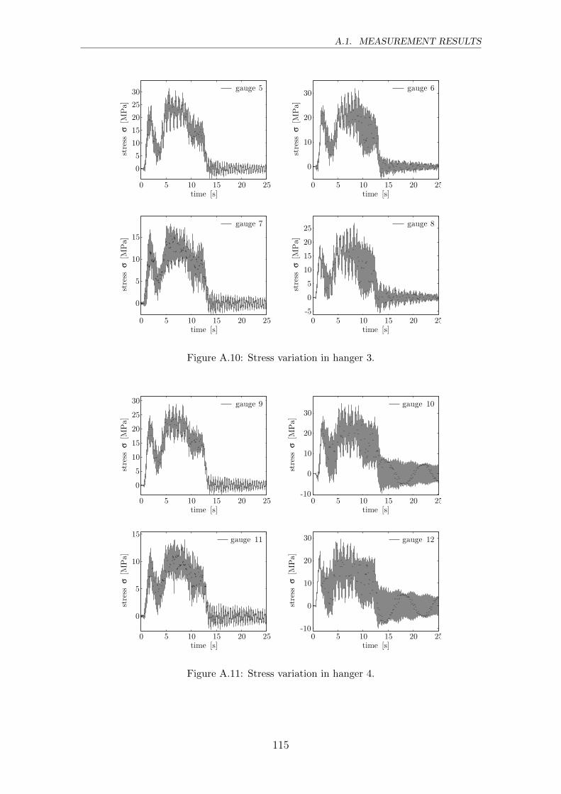
A.1. MEASUREMENT RESULTS
0 5 10 15 20 25
0
5
10
15
20
25
30
time [s]
stress
σ[M
Pa]
gauge 5
0 5 10 15 20 25
0
10
20
30
time [s]
stress
σ[M
Pa]
gauge 6
0 5 10 15 20 25
0
5
10
15
time [s]
stress
σ[M
Pa]
gauge 7
0 5 10 15 20 25-5
0
5
10
15
20
25
time [s]
stress
σ[M
Pa]
gauge 8
Figure A.10: Stress variation in hanger 3.
0 5 10 15 20 25
0
5
10
15
20
25
30
time [s]
stress
σ[M
Pa]
gauge 9
0 5 10 15 20 25-10
0
10
20
30
time [s]
stress
σ[M
Pa]
gauge 10
0 5 10 15 20 25
0
5
10
15
time [s]
stress
σ[M
Pa]
gauge 11
0 5 10 15 20 25-10
0
10
20
30
time [s]
stress
σ[M
Pa]
gauge 12
Figure A.11: Stress variation in hanger 4.
115
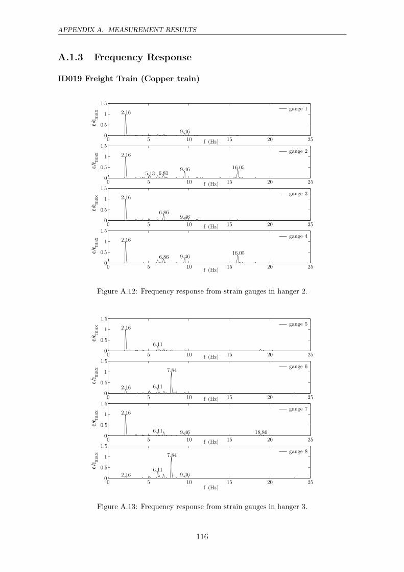
APPENDIX A. MEASUREMENT RESULTS
A.1.3 Frequency Response
ID019 Freight Train (Copper train)
0 5 10 15 20 250
0.5
1
1.5
f (Hz)
ε/ε m
ax 2.16
9.46
gauge 1
0 5 10 15 20 250
0.5
1
1.5
f (Hz)
ε/ε m
ax 2.16
5.13 6.819.46 16.05
gauge 2
0 5 10 15 20 250
0.5
1
1.5
f (Hz)
ε/ε m
ax 2.16
6.869.46
gauge 3
0 5 10 15 20 250
0.5
1
1.5
f (Hz)
ε/ε m
ax 2.16
6.86 9.4616.05
gauge 4
Figure A.12: Frequency response from strain gauges in hanger 2.
0 5 10 15 20 250
0.5
1
1.5
f (Hz)
ε/ε m
ax 2.16
6.11
gauge 5
0 5 10 15 20 250
0.5
1
1.5
f (Hz)
ε/ε m
ax
2.16 6.11
7.84gauge 6
0 5 10 15 20 250
0.5
1
1.5
f (Hz)
ε/ε m
ax 2.16
6.11 9.46 18.86
gauge 7
0 5 10 15 20 250
0.5
1
1.5
f (Hz)
ε/ε m
ax
2.166.11
7.84
9.46
gauge 8
Figure A.13: Frequency response from strain gauges in hanger 3.
116
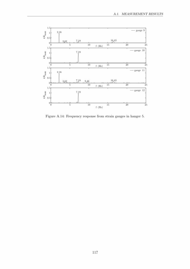
A.1. MEASUREMENT RESULTS
0 5 10 15 20 250
0.5
1
1.5
f (Hz)ε/
ε max 2.16
3.62 7.19 16.43
gauge 9
0 5 10 15 20 250
0.5
1
1.5
f (Hz)
ε/ε m
ax 7.19gauge 10
0 5 10 15 20 250
0.5
1
1.5
f (Hz)
ε/ε m
ax 2.16
3.62 7.19 9.46 16.43
gauge 11
0 5 10 15 20 250
0.5
1
1.5
f (Hz)
ε/ε m
ax 7.19gauge 12
Figure A.14: Frequency response from strain gauges in hanger 5.
117
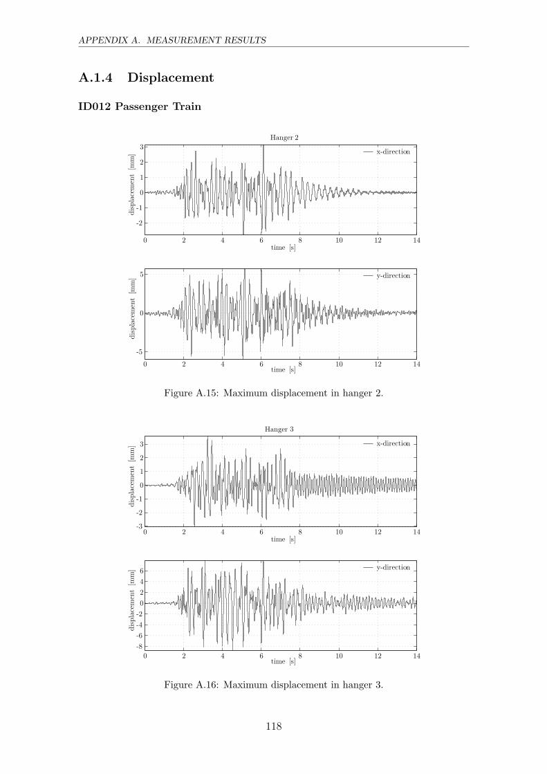
APPENDIX A. MEASUREMENT RESULTS
A.1.4 Displacement
ID012 Passenger Train
0 2 4 6 8 10 12 14
-2
-1
0
1
2
3
time [s]
displacement[m
m]
Hanger 2
x-direction
0 2 4 6 8 10 12 14
-5
0
5
time [s]
displacement[m
m] y-direction
Figure A.15: Maximum displacement in hanger 2.
0 2 4 6 8 10 12 14-3
-2
-1
0
1
2
3
time [s]
displacement[m
m]
Hanger 3
x-direction
0 2 4 6 8 10 12 14
-8
-6
-4
-2
0
2
4
6
time [s]
displacement[m
m] y-direction
Figure A.16: Maximum displacement in hanger 3.
118
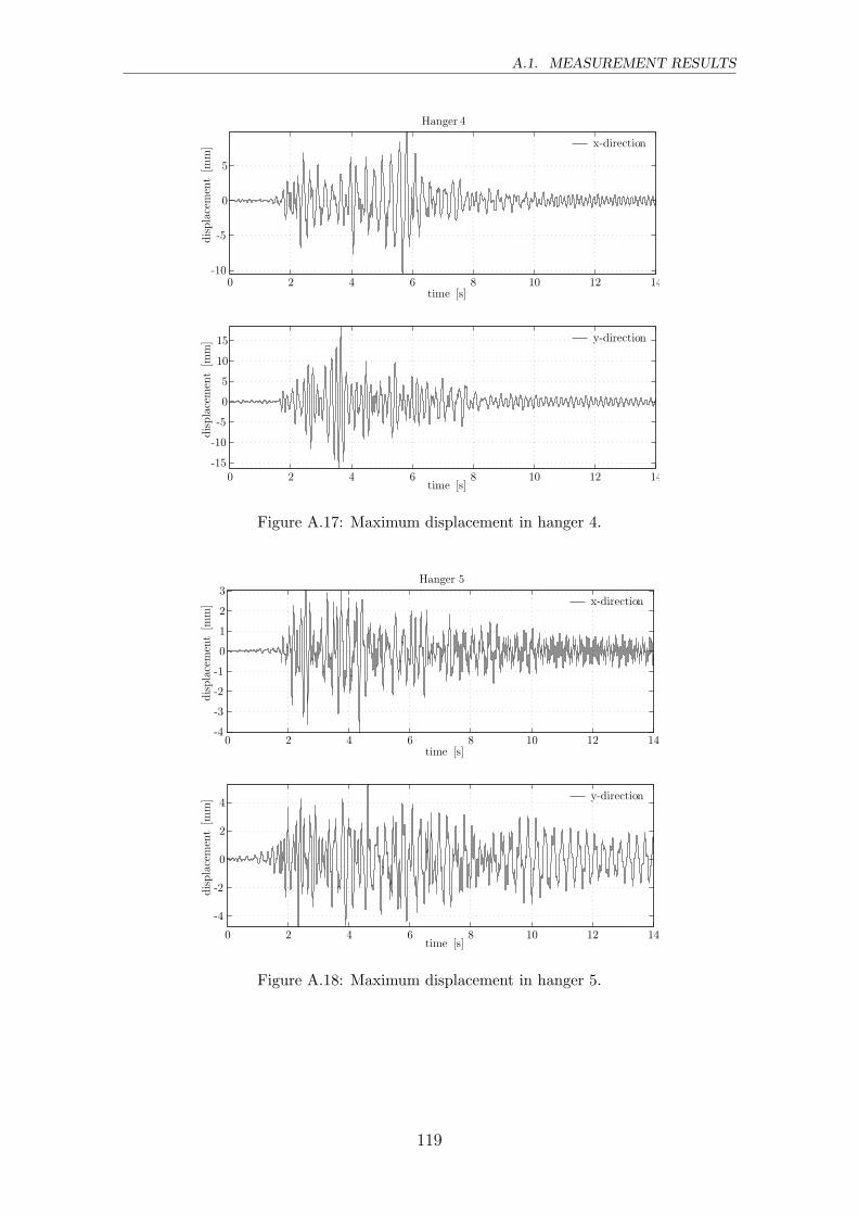
A.1. MEASUREMENT RESULTS
0 2 4 6 8 10 12 14-10
-5
0
5
time [s]
displacement[m
m]
Hanger 4
x-direction
0 2 4 6 8 10 12 14-15
-10
-5
0
5
10
15
time [s]
displacement[m
m] y-direction
Figure A.17: Maximum displacement in hanger 4.
0 2 4 6 8 10 12 14-4
-3
-2
-1
0
1
2
3
time [s]
displacement[m
m]
Hanger 5
x-direction
0 2 4 6 8 10 12 14
-4
-2
0
2
4
time [s]
displacement[m
m] y-direction
Figure A.18: Maximum displacement in hanger 5.
119
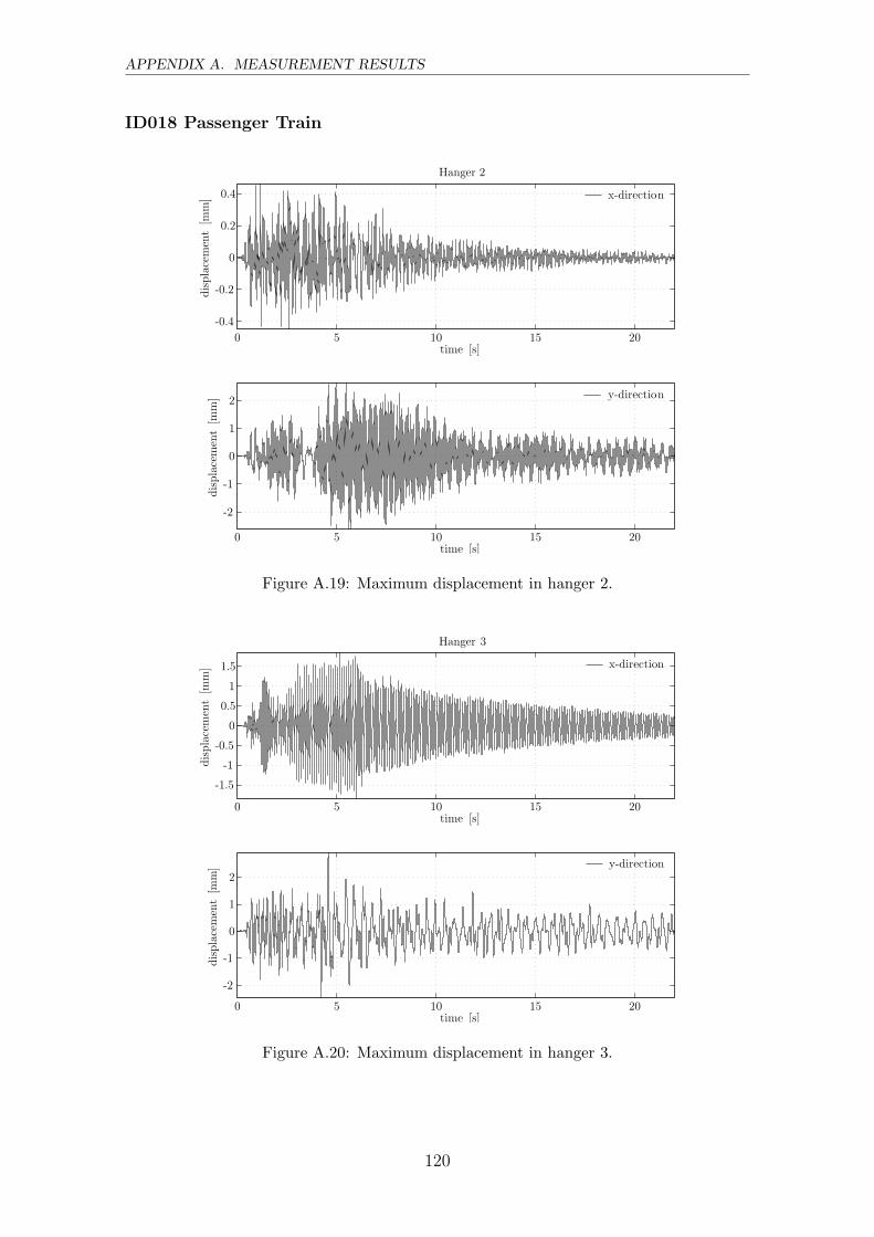
APPENDIX A. MEASUREMENT RESULTS
ID018 Passenger Train
0 5 10 15 20
-0.4
-0.2
0
0.2
0.4
time [s]
displacement[m
m]
Hanger 2
x-direction
0 5 10 15 20
-2
-1
0
1
2
time [s]
displacement[m
m] y-direction
Figure A.19: Maximum displacement in hanger 2.
0 5 10 15 20
-1.5
-1
-0.5
0
0.5
1
1.5
time [s]
displacement[m
m]
Hanger 3
x-direction
0 5 10 15 20
-2
-1
0
1
2
time [s]
displacement[m
m] y-direction
Figure A.20: Maximum displacement in hanger 3.
120
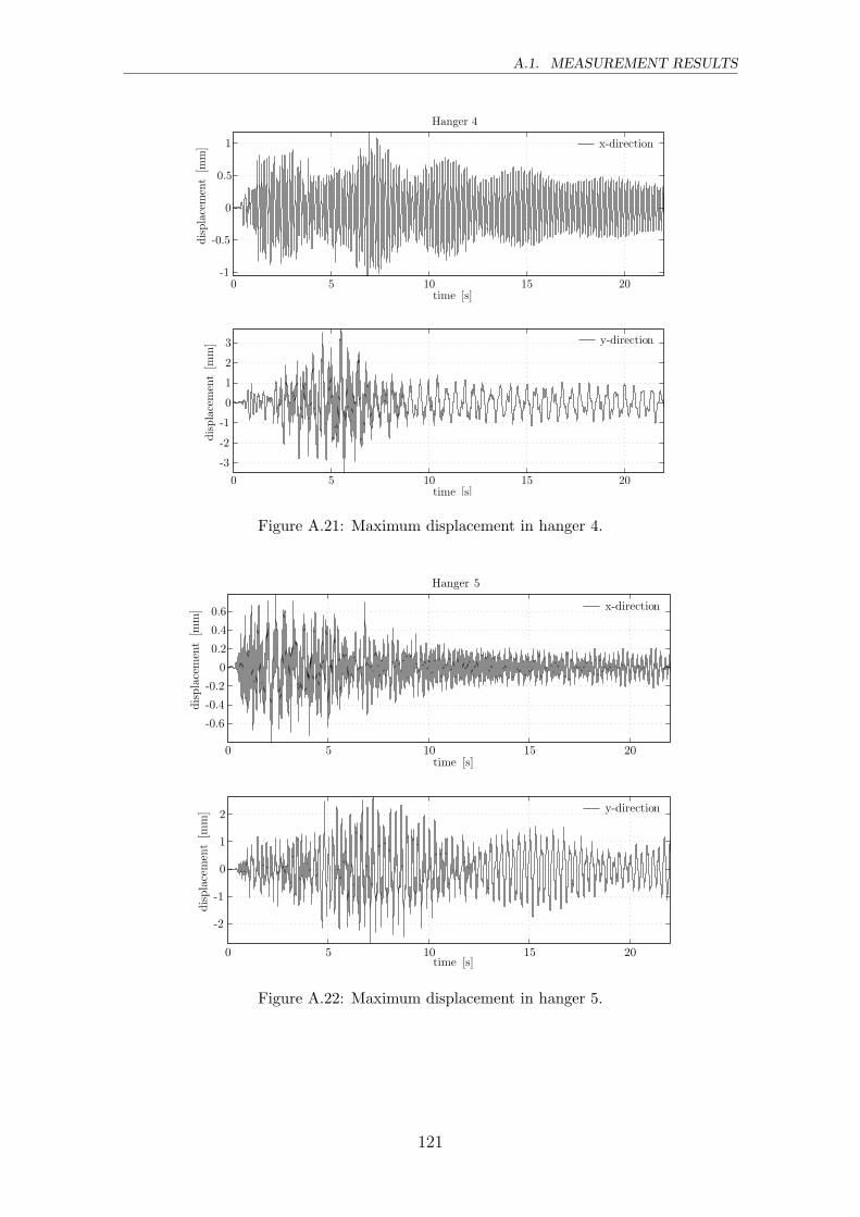
A.1. MEASUREMENT RESULTS
0 5 10 15 20-1
-0.5
0
0.5
1
time [s]
displacement[m
m]
Hanger 4
x-direction
0 5 10 15 20
-3
-2
-1
0
1
2
3
time [s]
displacement[m
m] y-direction
Figure A.21: Maximum displacement in hanger 4.
0 5 10 15 20
-0.6
-0.4
-0.2
0
0.2
0.4
0.6
time [s]
displacement[m
m]
Hanger 5
x-direction
0 5 10 15 20
-2
-1
0
1
2
time [s]
displacement[m
m] y-direction
Figure A.22: Maximum displacement in hanger 5.
121
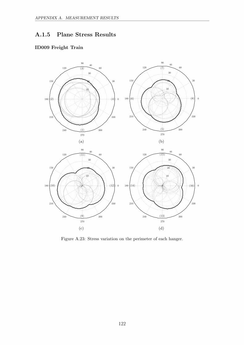
APPENDIX A. MEASUREMENT RESULTS
A.1.5 Plane Stress Results
ID009 Freight Train
10
20
30
40
30
210
60
240
90
270
120
300
150
330
180 0
(1)
(2)
(3)
(4)
(a)
10
20
30
40
30
210
60
240
90
270
120
300
150
330
180 0
(5)
(6)
(7)
(8)
(b)
10
20
30
40
30
210
60
240
90
270
120
300
150
330
180 0
(9)
(10)
(11)
(12)
(c)
10
20
30
40
30
210
60
240
90
270
120
300
150
330
180 0
(13)
(14)
(15)
(16)
(d)
Figure A.23: Stress variation on the perimeter of each hanger.
122
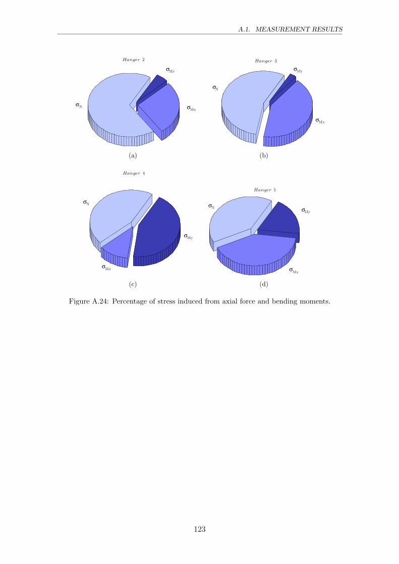
A.1. MEASUREMENT RESULTS
σMx
σMy
σN
Hanger 2
(a)
σMx
σMy
σN
Hanger 3
(b)
σMy
σMx
σN
Hanger 4
(c)
σMy
σ Mx
σN
σ
Hanger 5
(d)
Figure A.24: Percentage of stress induced from axial force and bending moments.
123

APPENDIX A. MEASUREMENT RESULTS
A.1.6 Fatigue Results
ID009 Freight Train
4 6 8 10 12 14 16 18 20 22 24 26 28 30 32 34 36 380
5
10
15
20
25
30
35
40
45
50Stress range
Number
ofcycles
σ [MPa]
ID009 strain gauge 10
4
88.5
1315
22.5
13.5
35
14.5
38.5
12
26
7
17.5
7
14
7
13.5
79 8.5
10
67
0.51.5
trainfree vibration
4 6 8 10 12 14 16 18 20 22 24 26 28 30 32 34 36 380
5
10
15
20
25
30
35
40
45
Stress range
Number
ofcycles
σ [MPa]
ID009 strain gauge 12
2.5
1515.5
6.5
15.5
24
13
38
14.5
30
14.5
32.5
6
18
7.5
16.5
10
14.5
10.512.5
6.58.5
trainfree vibration
Figure A.25: Stress collective from strain gauges 10 and 12.
4 6 8 10 12 14 16 18 20 22 24 26 28 30 32 34 36 380
5
10
15
20
25
30
35
40
45
Stress range
Number
ofcycles
σ [MPa]
Mean value of gauge 10 and 12
3.3
11.512
9.8
15.3
23.3
13.3
36.5
14.5
34.3
13.3
29.3
6.5
17.8
7.3
15.3
8.5
14
8.810.8
7.59.3
33.5
0.30.8
trainfree vibration
Figure A.26: Stress collective from strain gauges 10 and 12.
124
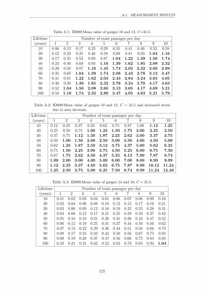
A.1. MEASUREMENT RESULTS
Table A.1: ID009:Mean value of gauges 10 and 12, C=31.5.
Lifetime Number of train passages per day(years) 1 2 3 4 5 6 7 8 9 10
10 0.06 0.12 0.17 0.23 0.29 0.35 0.41 0.46 0.52 0.5820 0.12 0.23 0.35 0.46 0.58 0.69 0.81 0.93 1.04 1.1630 0.17 0.35 0.52 0.69 0.87 1.04 1.22 1.39 1.56 1.7440 0.23 0.46 0.69 0.93 1.16 1.39 1.62 1.85 2.08 2.3250 0.29 0.58 0.87 1.16 1.45 1.74 2.03 2.32 2.60 2.8960 0.35 0.69 1.04 1.39 1.74 2.08 2.43 2.78 3.13 3.4770 0.41 0.81 1.22 1.62 2.03 2.43 2.84 3.24 3.65 4.0580 0.46 0.93 1.39 1.85 2.32 2.78 3.24 3.70 4.17 4.6390 0.52 1.04 1.56 2.08 2.60 3.13 3.65 4.17 4.69 5.21100 0.58 1.16 1.74 2.32 2.89 3.47 4.05 4.63 5.21 5.79
Table A.2: ID009:Mean value of gauges 10 and 12, C = 31.5 and increased stressdue to area decrease.
Lifetime Number of train passages per day(years) 1 2 3 4 5 6 7 8 9 10
10 0.12 0.25 0.37 0.50 0.62 0.75 0.87 1.00 1.12 1.2520 0.25 0.50 0.75 1.00 1.25 1.50 1.75 2.00 2.25 2.5030 0.37 0.75 1.12 1.50 1.87 2.25 2.62 3.00 3.37 3.7540 0.50 1.00 1.50 2.00 2.50 3.00 3.50 4.00 4.50 5.0050 0.62 1.25 1.87 2.50 3.12 3.75 4.37 5.00 5.62 6.2560 0.75 1.50 2.25 3.00 3.75 4.50 5.25 6.00 6.75 7.5070 0.87 1.75 2.62 3.50 4.37 5.25 6.12 7.00 7.87 8.7480 1.00 2.00 3.00 4.00 5.00 6.00 7.00 8.00 8.99 9.9990 1.12 2.25 3.37 4.50 5.62 6.75 7.87 8.99 10.12 11.24100 1.25 2.50 3.75 5.00 6.25 7.50 8.74 9.99 11.24 12.49
Table A.3: ID009:Mean value of gauges 14 and 16, C = 31.5.
Lifetime Number of train passages per day(years) 1 2 3 4 5 6 7 8 9 10
10 0.01 0.02 0.03 0.04 0.05 0.06 0.07 0.08 0.09 0.1020 0.02 0.04 0.06 0.08 0.10 0.12 0.15 0.17 0.19 0.2130 0.03 0.06 0.09 0.12 0.16 0.19 0.22 0.25 0.28 0.3140 0.04 0.08 0.12 0.17 0.21 0.25 0.29 0.33 0.37 0.4250 0.05 0.10 0.16 0.21 0.26 0.31 0.36 0.42 0.47 0.5260 0.06 0.12 0.19 0.25 0.31 0.37 0.44 0.50 0.56 0.6270 0.07 0.15 0.22 0.29 0.36 0.44 0.51 0.58 0.66 0.7380 0.08 0.17 0.25 0.33 0.42 0.50 0.58 0.67 0.75 0.8390 0.09 0.19 0.28 0.37 0.47 0.56 0.66 0.75 0.84 0.94100 0.10 0.21 0.31 0.42 0.52 0.62 0.73 0.83 0.94 1.04
125
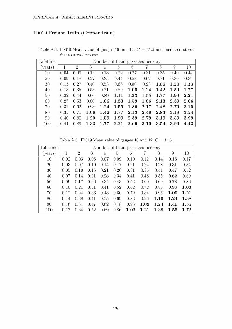
APPENDIX A. MEASUREMENT RESULTS
ID019 Freight Train (Copper train)
Table A.4: ID019:Mean value of gauges 10 and 12, C = 31.5 and increased stressdue to area decrease.
Lifetime Number of train passages per day(years) 1 2 3 4 5 6 7 8 9 10
10 0.04 0.09 0.13 0.18 0.22 0.27 0.31 0.35 0.40 0.4420 0.09 0.18 0.27 0.35 0.44 0.53 0.62 0.71 0.80 0.8930 0.13 0.27 0.40 0.53 0.66 0.80 0.93 1.06 1.20 1.3340 0.18 0.35 0.53 0.71 0.89 1.06 1.24 1.42 1.59 1.7750 0.22 0.44 0.66 0.89 1.11 1.33 1.55 1.77 1.99 2.2160 0.27 0.53 0.80 1.06 1.33 1.59 1.86 2.13 2.39 2.6670 0.31 0.62 0.93 1.24 1.55 1.86 2.17 2.48 2.79 3.1080 0.35 0.71 1.06 1.42 1.77 2.13 2.48 2.83 3.19 3.5490 0.40 0.80 1.20 1.59 1.99 2.39 2.79 3.19 3.59 3.99100 0.44 0.89 1.33 1.77 2.21 2.66 3.10 3.54 3.99 4.43
Table A.5: ID019:Mean value of gauges 10 and 12, C = 31.5.
Lifetime Number of train passages per day(years) 1 2 3 4 5 6 7 8 9 10
10 0.02 0.03 0.05 0.07 0.09 0.10 0.12 0.14 0.16 0.1720 0.03 0.07 0.10 0.14 0.17 0.21 0.24 0.28 0.31 0.3430 0.05 0.10 0.16 0.21 0.26 0.31 0.36 0.41 0.47 0.5240 0.07 0.14 0.21 0.28 0.34 0.41 0.48 0.55 0.62 0.6950 0.09 0.17 0.26 0.34 0.43 0.52 0.60 0.69 0.78 0.8660 0.10 0.21 0.31 0.41 0.52 0.62 0.72 0.83 0.93 1.0370 0.12 0.24 0.36 0.48 0.60 0.72 0.84 0.96 1.09 1.2180 0.14 0.28 0.41 0.55 0.69 0.83 0.96 1.10 1.24 1.3890 0.16 0.31 0.47 0.62 0.78 0.93 1.09 1.24 1.40 1.55100 0.17 0.34 0.52 0.69 0.86 1.03 1.21 1.38 1.55 1.72
126