A Bayesian Approach for Predicting Building Cooling ... - AIVC

A BAYESIAN APPROACH FOR PREDICTING BUILDING COOLING AND HEATING CONSUMPTION

Bin Yan, and Ali M. Malkawi

School of Design, University of Pennsylvania, Philadelphia PA 19104, United States

ABSTRACT This research proposes a Bayesian approach to include uncertainty that arises from modeling process and input values when predicting cooling and heating consumption in existing buildings. Our approach features Gaussian Process modeling. We present a case study of predicting energy use through a Gaussian Process and compare its accuracy with a Neural Network model. As an initial step of applying Gaussian Processes to uncertainty analysis of system operations, we evaluate the impact of uncertain air-handling unit (AHU) supply air temperature on energy consumption. We also explore the application of Bayesian analysis to building energy diagnosis and fault detection. In concluding remarks, we briefly discuss advantages of the proposed approach.

INTRODUCTION Making a prediction typically involves dealing with uncertainties. Improving uncertainty analyses remains a challenge in building simulation (Augenbroe, 2002). Uncertainty and sensitivity analysis have been extensively applied in science and engineering. However, their applications to building systems are still limited. Uncertainty enters a model in various contexts. One way to categorize is to consider uncertainty that arises from modeling process and input values associated with predictions. Most uncertainty studies focus on uncertainty in input values for predictions. Monte Carlo experiment is a widely used method for analyzing input uncertainty (Hamby, 1995). Several studies use Monte Carlo method with building simulation to study building and system design with input uncertainty (de Wit & Augenbroe, 2002; Domínguez-Muñoz et al., 2010). We found three areas where could be improved in current uncertainty research in building simulation. First, uncertainty in the modeling process is seldom quantified. There are assumptions, simplifications and approximations in a model. The data used to build or calibrate a model might not cover the whole input domain and could be corrupted with sensor noise and measurement errors. Therefore, it is important to include modeling uncertainty when making predictions.

Second, when building simulations are computationally expensive, a more efficient method for uncertainty analysis is desirable. Monte Carlo experiment requires a large number of model evaluations. As the dimension of input variables increases, the number of simulations required increases significantly. Techniques such as parameter screening and Latin hypercube sampling help reduce the number of model evaluations. However, it would be beneficial if the time cost of uncertainty analysis could be further reduced. Last, few existing studies have covered uncertainty related to system controls in operations. Measurements in system operations are usually corrupted by sensor noise. For example, measurements of temperature, humidity, air flow and water flow are typically noisy. Furthermore, few systems perform as intended. Usually there is a discrepancy between intended and actual performance. The main purpose of this research is to include uncertainty that arises from modeling process and input values when predicting cooling and heating consumption in existing buildings. We propose a Bayesian approach which features Gaussian Process modeling. This paper is an extension of previous work (Yan & Malkawi, 2012). In this paper, we explain the types of uncertainties covered by Gaussian Processes. In order to evaluate the prediction accuracy, we test a Gaussian Process with metered data and compare its results with another widely used machine learning method, Neural Networks. As an initial step of applying Gaussian Processes to uncertainty analysis of system operations, we present a case study of predicting energy use with uncertain AHU supply air temperature. Compared with the previous work, we expand the case studies in these two sections to both cooling and heating energy consumption predictions. Additionally, we explore the application of Bayesian analysis in building energy diagnosis and fault detection in this paper, which is an innovative part. In the concluding remarks, we briefly discuss the advantages of our proposed method and future research topics.

MODELING METHOD The use of Gaussian Processes has grown significantly after the works of (Neal, 1995 &

3URFHHGLQJV�RI�%6��WK�&RQIHUHQFH�RI�,QWHUQDWLRQDO�%XLOGLQJ�3HUIRUPDQFH�6LPXODWLRQ�$VVRFLDWLRQ��&KDPEpU\��)UDQFH��$XJXVW��

��

Rasmussen, 1996) in machine learning community. Gaussian Process regression has been successfully applied to various predicting tasks. The goal is to find the distribution of a nonlinear function � � to underlie data points, each of which is composed of input � and target � . Then we can use the distribution of � �� to predict the value of ��. We denote � input vectors �� by � and the set of corresponding target values �� by the vector �. Using Bayes’ theorem, the posterior probability distribution of � � is

� � � �� (1)

In a regression problem, �� , the distribution of the target values given the function � � is usually assumed to be Gaussian. The prior � � � is placed on the space of functions, without parameterizing � � (MacKay, 2003). A Gaussian process is specified by a mean function (usually a zero function) and a covariance function �� . The choice of covariance function in this study is a Gaussian kernel,

�� (2)

Where

� � �� (3)

Inputs that are judged to be close by the covariance function are likely to have similar outputs. A prediction is made by considering the covariance between the predictive case and all the training cases (Rasmussen, 1996). For a noise-free input ��, the predictive distribution of � �� is Gaussian with mean � �� and variance �� (Rasmussen & Williams, 2006)

� �� (4)

�� (5)

� �� is the �� vector of covariance functions between training inputs � and the new input ��. � is the �� matrix of covariance functions between each pair of training inputs. �� denotes the variance

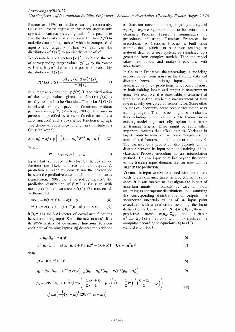
of Gaussian noise in training targets �. ��, �� and �� are hyperparamters to be trained in a Gaussian Process. Figure 1 summarizes the procedures of using Gaussian Processes for predictions. A Gaussian Process is built upon training data, which can be sensor readings or metered data of a real system, or simulated data generated from complex models. Then the model takes new inputs and makes predictions with uncertainty. In Gaussian Processes, the uncertainty in modeling process comes from noise in the training data and distance between training inputs and inputs associated with new predictions. One source of noise in both training inputs and targets is measurement noise. For example, it is reasonable to assume that time is noise-free, while the measurement of flow rate is usually corrupted by sensor noise. Some other sources of uncertainty could account for the noise in training targets. The process might be stochastic, thus including random elements. The features in an existing model might not fully explain the variance in training targets. There might be some other important features that affect outputs. Variance in targets might be reduced if we could recognize some more related features and include them in the model. The variance of a prediction also depends on the distance between its input point and training inputs. Gaussian Process modeling is an interpolation method. If a new input point lies beyond the scope of the training input domain, the variance will be large in the prediction. Variance in input values associated with predictions leads to an extra uncertainty in predictions. In some cases, it is our interest to investigate the impact of uncertain inputs on outputs by varying inputs according to appropriate distributions and examining the corresponding distributions of outputs. To incorporate uncertain values of an input point associated with a prediction, assuming the input distribution is Gaussian �� , then the predictive mean � �� and variance �� of a prediction with noisy inputs can be computed according to equations (6) to (10) (Girard et al., 2003):

� �� (6)

�� (7)

with

� � �� (8)

��

� �� (9)

��

��

��

��

��

��

��

(10)

3URFHHGLQJV�RI�%6��WK�&RQIHUHQFH�RI�,QWHUQDWLRQDO�%XLOGLQJ�3HUIRUPDQFH�6LPXODWLRQ�$VVRFLDWLRQ��&KDPEpU\��)UDQFH��$XJXVW��

��

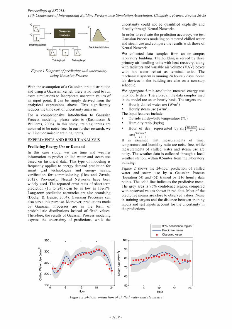
Figure 1 Diagram of predicting with uncertainty

using Gaussian Process With the assumption of a Gaussian input distribution and using a Gaussian kernel, there is no need to run extra simulations to incorporate uncertain values of an input point. It can be simply derived from the analytical expressions above. This significantly reduces the time cost of uncertainty analysis. For a comprehensive introduction to Gaussian Process modeling, please refer to (Rasmussen & Williams, 2006). In this study, training inputs are assumed to be noise-free. In our further research, we will include noise in training inputs.

EXPERIMENTS AND RESULT ANALYSIS

Predicting Energy Use or Demand In this case study, we use time and weather information to predict chilled water and steam use based on historical data. This type of modeling is frequently applied to energy demand prediction for smart grid technologies and energy saving verification for commissioning (Heo and Zavala, 2012). Previously, Neural Networks have been widely used. The reported error rates of short-term prediction (1h to 24h) can be as low as 1%-5%. Long-term prediction accuracies are also promising (Dodier & Henze, 2004). Gaussian Processes can also serve this purpose. Moreover, predictions made by Gaussian Processes are in the form of probabilistic distributions instead of fixed values. Therefore, the results of Gaussian Process modeling express the uncertainty of predictions, while the

uncertainty could not be quantified explicitly and directly through Neural Networks. In order to evaluate the prediction accuracy, we test Gaussian Process modeling on metered chilled water and steam use and compare the results with those of Neural Network. We collected data samples from an on-campus laboratory building. The building is served by three primary air-handling units with heat recovery, along with radiators and variable air volume (VAV) boxes with hot water reheat as terminal units. The mechanical system is running 24 hours 7 days. Some lab devices in the building are also on a non-stop schedule. We aggregate 5-min-resolution metered energy use into hourly data. Therefore, all the data samples used in the model are on an hourly basis. The targets are � Hourly chilled water use (W/m2) � Hourly steam use (W/m2). The input features include � Outside air dry-bulb temperature (°C) � Humidity ratio (kg/kg) � Hour of day, represented by ��

�� and

�� .

It is assumed that measurements of time, temperature and humidity ratio are noise-free, while measurements of chilled water and steam use are noisy. The weather data is collected through a local weather station, within 0.5miles from the laboratory building. Figure 2 shows the 24-hour prediction of chilled water and steam use by a Gaussian Process (Equation (4) and (5)) trained by 216 hourly data points. The solid line indicates the predictive mean. The grey area is 95% confidence region, compared with observed values shown in red dots. Most of the predictive means are close to observed values. Noise in training targets and the distance between training inputs and test inputs account for the uncertainty in the predictions.

Figure 2 24-hour prediction of chilled water and steam use

0 6 12 18 24150

200

250

300

350

Hour

Chille

d W

ater

Use

(W/m

2 )

0 6 12 18 2450

60

70

80

90

100

Hour

Stea

m U

se (W

/m2 )

95% confidence regionPredictive meanObserved value

Proceedings of BS2013: 13th Conference of International Building Performance Simulation Association, Chambéry, France, August 26-28

- 3139 -

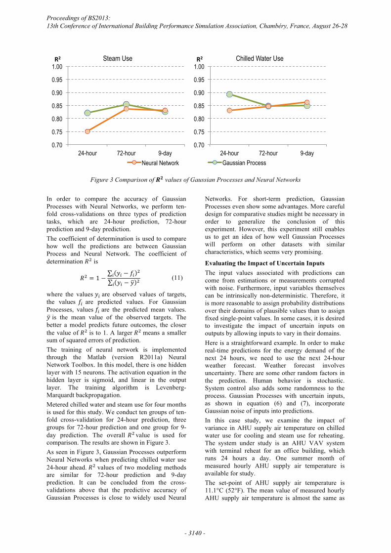
Figure 3 Comparison of �� values of Gaussian Processes and Neural Networks

In order to compare the accuracy of Gaussian Processes with Neural Networks, we perform ten-fold cross-validations on three types of prediction tasks, which are 24-hour prediction, 72-hour prediction and 9-day prediction. The coefficient of determination is used to compare how well the predictions are between Gaussian Process and Neural Network. The coefficient of determination �� is

��

(11)

where the values �� are observed values of targets, the values �� are predicted values. For Gaussian Processes, values �� are the predicted mean values. � is the mean value of the observed targets. The better a model predicts future outcomes, the closer the value of �� is to 1. A larger �� means a smaller sum of squared errors of prediction. The training of neural network is implemented through the Matlab (version R2011a) Neural Network Toolbox. In this model, there is one hidden layer with 15 neurons. The activation equation in the hidden layer is sigmoid, and linear in the output layer. The training algorithm is Levenberg-Marquardt backpropagation. Metered chilled water and steam use for four months is used for this study. We conduct ten groups of ten-fold cross-validation for 24-hour prediction, three groups for 72-hour prediction and one group for 9-day prediction. The overall �� value is used for comparison. The results are shown in Figure 3. As seen in Figure 3, Gaussian Processes outperform Neural Networks when predicting chilled water use 24-hour ahead. �� values of two modeling methods are similar for 72-hour prediction and 9-day prediction. It can be concluded from the cross-validations above that the predictive accuracy of Gaussian Processes is close to widely used Neural

Networks. For short-term prediction, Gaussian Processes even show some advantages. More careful design for comparative studies might be necessary in order to generalize the conclusion of this experiment. However, this experiment still enables us to get an idea of how well Gaussian Processes will perform on other datasets with similar characteristics, which seems very promising.

Evaluating the Impact of Uncertain Inputs The input values associated with predictions can come from estimations or measurements corrupted with noise. Furthermore, input variables themselves can be intrinsically non-deterministic. Therefore, it is more reasonable to assign probability distributions over their domains of plausible values than to assign fixed single-point values. In some cases, it is desired to investigate the impact of uncertain inputs on outputs by allowing inputs to vary in their domains. Here is a straightforward example. In order to make real-time predictions for the energy demand of the next 24 hours, we need to use the next 24-hour weather forecast. Weather forecast involves uncertainty. There are some other random factors in the prediction. Human behavior is stochastic. System control also adds some randomness to the process. Gaussian Processes with uncertain inputs, as shown in equation (6) and (7), incorporate Gaussian noise of inputs into predictions. In this case study, we examine the impact of variance in AHU supply air temperature on chilled water use for cooling and steam use for reheating. The system under study is an AHU VAV system with terminal reheat for an office building, which runs 24 hours a day. One summer month of measured hourly AHU supply air temperature is available for study. The set-point of AHU supply air temperature is 11.1°C (52°F). The mean value of measured hourly AHU supply air temperature is almost the same as

0.70

0.75

0.80

0.85

0.90

0.95

1.00

24-hour 72-hour 9-day

�� Steam Use

Neural Network

0.70

0.75

0.80

0.85

0.90

0.95

1.00

24-hour 72-hour 9-day

�� Chilled Water Use

Gaussian Process


- 3140 -

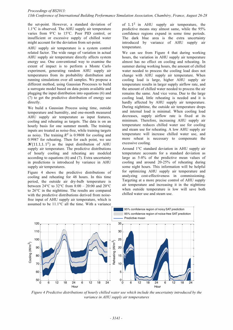
the set-point. However, a standard deviation of 1.1°C is observed. The AHU supply air temperature varies from 9°C to 15°C. Poor PID control, or insufficient or excessive supply of chilled water might account for the deviation from set-point. AHU supply air temperature is a system control related factor. The wide range of variation in actual AHU supply air temperature directly affects system energy use. One conventional way to examine the extent of impact is to perform a Monte Carlo experiment, generating random AHU supply air temperatures from its probability distribution and running simulations over all samples. We propose a different method, using Gaussian Processes to build a surrogate model based on data points available and plugging the input distribution into equations (6) and (7) to get the predictive distribution of energy use directly. We build a Gaussian Process using time, outside temperature and humidity, and one-month measured AHU supply air temperature as input features, cooling and reheating as targets. The data is on an hourly basis for one summer month. The training inputs are treated as noise-free, while training targets as noisy. The training �� is 0.9808 for cooling and 0.9987 for reheating. Then for each point, we use �� as the input distribution of AHU supply air temperature. The predictive distributions of hourly cooling and reheating are modeled according to equations (6) and (7). Extra uncertainty in predictions is introduced by variance in AHU supply air temperatures. Figure 4 shows the predictive distributions of cooling and reheating for 48 hours. In this time period, the outside air dry-bulb temperature is between 24°C to 32°C from 8:00 – 20:00 and 20°C to 26°C in the nighttime. The results are compared with the predictive distributions derived from noise-free input of AHU supply air temperature, which is assumed to be 11.1°C all the time. With a variance

of �� in AHU supply air temperature, the predictive means stay almost same, while the 95% confidence regions expand in some time periods. The dark blue area is the extra uncertainty introduced by variance of AHU supply air temperature. We can see from Figure 4 that during working hours, the variation in AHU supply air temperature almost has no effect on cooling and reheating. In summer during working hours, the amount of chilled water needed to process the cooling load does not change with AHU supply air temperature. When cooling load is large, higher AHU supply air temperature results in larger supply airflow rate, and the amount of chilled water needed to process the air remains the same. And vice versa. Due to the large cooling load, little reheating is needed and it is hardly affected by AHU supply air temperature. During nighttime, the outside air temperature drops and internal load is minimal. When cooling load decreases, supply airflow rate is fixed at its minimum. Therefore, increasing AHU supply air temperature reduces chilled water use for cooling and steam use for reheating. A low AHU supply air temperature will increase chilled water use, and more reheat is necessary to compensate the excessive cooling. Around 1°C standard deviation in AHU supply air temperature accounts for a standard deviation as large as 5-8% of the predictive mean values of cooling and around 20-25% of reheating during some night hours. This information will be helpful for optimizing AHU supply air temperature and analyzing cost-effectiveness in commissioning. Targeting at a more precise control of AHU supply air temperature and increasing it in the nighttime when outside temperature is low will save both chilled water use and steam use.

Figure 4 Predictive distributions of hourly chilled water use which include the uncertainty introduced by the

variance in AHU supply air temperatures

0 6 12 18 24 6 12 18 2450

60

70

80

90

100

110

120

Hour

Cool

ing

(W/m

2 )

0 6 12 18 24 6 12 18 240

5

10

15

20

25

30

35

Hour

Rehe

atin

g (W

/m2 )

95% confidence region of noisy SAT prediction95% confidence region of noise-free SAT predictionPredictive mean


- 3141 -

The example above shows how to use Gaussian Processes to study the uncertainty introduced by uncertain inputs. With the assumption that the input distributions are Gaussian, the predictive distribution can be computed directly without Monte Carlo experiment. It is necessary that the training set should cover most of the input domain. Otherwise, the uncertainty introduced by the modeling process itself would be too large. Usually this is not an issue if data is generated from simulation. It might be challenging when building a Gaussian Process based on observations from actual performance. The example above uses measured AHU supply air temperature to ensure a realistic pattern, while energy use for cooling and reheating is simulated data by EnergyPlus since metered data is not available at this point.

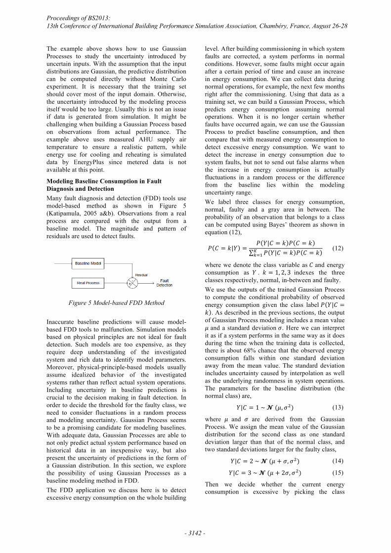
Modeling Baseline Consumption in Fault Diagnosis and Detection Many fault diagnosis and detection (FDD) tools use model-based method as shown in Figure 5 (Katipamula, 2005 a&b). Observations from a real process are compared with the output from a baseline model. The magnitude and pattern of residuals are used to detect faults.

Figure 5 Model-based FDD Method

Inaccurate baseline predictions will cause model-based FDD tools to malfunction. Simulation models based on physical principles are not ideal for fault detection. Such models are too expensive, as they require deep understanding of the investigated system and rich data to identify model parameters. Moreover, physical-principle-based models usually assume idealized behavior of the investigated systems rather than reflect actual system operations. Including uncertainty in baseline predictions is crucial to the decision making in fault detection. In order to decide the threshold for the faulty class, we need to consider fluctuations in a random process and modeling uncertainty. Gaussian Process seems to be a promising candidate for modeling baselines. With adequate data, Gaussian Processes are able to not only predict actual system performance based on historical data in an inexpensive way, but also present the uncertainty of predictions in the form of a Gaussian distribution. In this section, we explore the possibility of using Gaussian Processes as a baseline modeling method in FDD. The FDD application we discuss here is to detect excessive energy consumption on the whole building

level. After building commissioning in which system faults are corrected, a system performs in normal conditions. However, some faults might occur again after a certain period of time and cause an increase in energy consumption. We can collect data during normal operations, for example, the next few months right after the commissioning. Using that data as a training set, we can build a Gaussian Process, which predicts energy consumption assuming normal operations. When it is no longer certain whether faults have occurred again, we can use the Gaussian Process to predict baseline consumption, and then compare that with measured energy consumption to detect excessive energy consumption. We want to detect the increase in energy consumption due to system faults, but not to send out false alarms when the increase in energy consumption is actually fluctuations in a random process or the difference from the baseline lies within the modeling uncertainty range. We label three classes for energy consumption, normal, faulty and a gray area in between. The probability of an observation that belongs to a class can be computed using Bayes’ theorem as shown in equation (12),

� � � ��

�� (12)

where we denote the class variable as � and energy consumption as � . � � �� indexes the three classes respectively, normal, in-between and faulty. We use the outputs of the trained Gaussian Process to compute the conditional probability of observed energy consumption given the class label � �� . As described in the previous sections, the output of Gaussian Process modeling includes a mean value � and a standard deviation �. Here we can interpret it as if a system performs in the same way as it does during the time when the training data is collected, there is about 68% chance that the observed energy consumption falls within one standard deviation away from the mean value. The standard deviation includes uncertainty caused by interpolation as well as the underlying randomness in system operations. The parameters for the baseline distribution (the normal class) are,

�� (13)

where �� and � are derived from the Gaussian Process. We assign the mean value of the Gaussian distribution for the second class as one standard deviation larger than that of the normal class, and two standard deviations larger for the faulty class,

�� (14)

�� (15)

Then we decide whether the current energy consumption is excessive by picking the class


- 3142 -

assignment � with the highest posterior probability � � � �� :

� � �� (16)

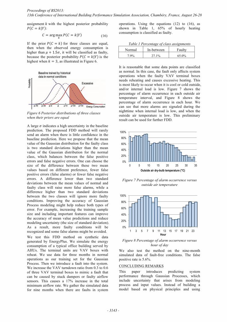
If the prior � � � � for three classes are equal, then when the observed energy consumption is higher than � � ��, it will be classified as faulty, because the posterior probability � � � �� is the highest when � � �, as illustrated in Figure 6.

Figure 6 Posterior distributions of three classes when their priors are equal

A large � indicates a high uncertainty in the baseline prediction. The proposed FDD method will rarely send an alarm when there is little confidence in the baseline prediction. Here we propose that the mean value of the Gaussian distribution for the faulty class is two standard deviations higher than the mean value of the Gaussian distribution for the normal class, which balances between the false positive errors and false negative errors. One can choose the size of the difference between these two mean values based on different preference, fewer false positive errors (false alarms) or fewer false negative errors. A difference lower than two standard deviations between the mean values of normal and faulty class will raise more false alarms, while a difference higher than two standard deviations between the two classes will ignore more faulty conditions. Improving the accuracy of Gaussian Process modeling might help reduce both types of error. For example, increasing the training sample size and including important features can improve the accuracy of mean value predictions and reduce modeling uncertainty (the size of standard deviation). As a result, more faulty conditions will be recognized and some false alarms might be avoided. We test this FDD method on synthetic data generated by EnergyPlus. We simulate the energy consumption of a typical office building served by AHUs. The terminal units are VAV boxes with reheat. We use data for three months in normal operations as our training set for the Gaussian Process. Then we introduce a fault into the system. We increase the VAV turndown ratio from 0.3 to 0.6 of three VAV terminal boxes to mimic a fault that can be caused by stuck dampers or faulty airflow sensors. This causes a 17% increase in the total minimum airflow rate. We gather the simulated data for nine months when there are faults in system

operations. Using the equations (12) to (16), as shown in Table 1, 65% of hourly heating consumption is classified as faulty.

Table 1 Percentage of class assignments

Normal In-between Faulty 7.9% 27.1% 65.0%

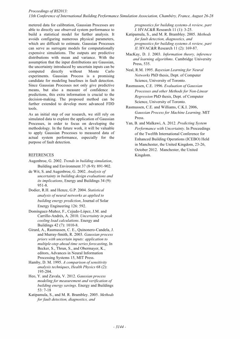
It is reasonable that some data points are classified as normal. In this case, the fault only affects system operations when the faulty VAV terminal boxes needs reheating and causes excessive heating. This is most likely to occur when it is cool or cold outside, and/or internal load is low. Figure 7 shows the percentage of alarm occurrence in each outside air temperature interval, and Figure 8 shows the percentage of alarm occurrence in each hour. We can see that more alarms are signaled during the nighttime when internal load is low, and when the outside air temperature is low. This preliminary result can be used for further FDD.

Figure 7 Percentage of alarm occurrence versus

outside air temperature

Figure 8 Percentage of alarm occurrence versus

hour of day We also test the method on the nine-month simulated data of fault-free conditions. The false positive rate is 5.6%.

CONCLUDING REMARKS This paper introduces predicting system performance through Gaussian Processes, which include uncertainty that arises from modeling process and input values. Instead of building a model based on physical principles and using

0%

20%

40%

60%

80%

100%

0 5 10 15 20 25 30 35 Outside air dry-bulb temperature (°C)

0%

20%

40%

60%

80%

100%

1 3 5 7 9 11 13 15 17 19 21 23 Hour


- 3143 -

metered data for calibration, Gaussian Processes are able to directly use observed system performance to build a statistical model for further analysis. It avoids configuring numerous physical parameters, which are difficult to estimate. Gaussian Processes can serve as surrogate models for computationally expensive simulations. The outputs are predictive distributions with mean and variance. With the assumption that the input distributions are Gaussian, the uncertainty introduced by uncertain inputs can be computed directly without Monte Carlo experiments. Gaussian Process is a promising candidate for modeling baselines in fault detection. Since Gaussian Processes not only give predictive means, but also a measure of confidence in predictions, this extra information is crucial to the decision-making. The proposed method can be further extended to develop more advanced FDD tools. As an initial step of our research, we still rely on simulated data to explore the application of Gaussian Processes, in order to focus on developing the methodology. In the future work, it will be valuable to apply Gaussian Processes to measured data of actual system performance, especially for the purpose of fault detection.

REFERENCES Augenbroe, G. 2002. Trends in building simulation,

Building and Environment 37 (8-9): 891-902. de Wit, S. and Augenbroe, G. 2002. Analysis of

uncertainty in building design evaluations and its implications, Energy and Buildings 34 (9): 951-8.

Dodier, R.H. and Henze, G.P. 2004. Statistical analysis of neural networks as applied to building energy prediction, Journal of Solar Energy Engineering 126: 592.

Domínguez-Muñoz, F., Cejudo-López, J.M. and Carrillo-Andrés, A. 2010. Uncertainty in peak cooling load calculations. Energy and Buildings 42 (7): 1010-8.

Girard, A., Rasmussen, C. E., Quinonero-Candela, J. and Murray-Smith, R. 2003. Gaussian process priors with uncertain inputs: application to multiple-step ahead time series forecasting, In Becker, S., Thrun, S., and Obermayer, K., editors, Advances in Neural Information Processing Systems 15, MIT Press.

Hamby, D. M. 1995. A comparison of sensitivity analysis techniques, Health Physics 68 (2): 195-204.

Heo, Y. and Zavala, V. 2012. Gaussian process modeling for measurement and verification of building energy savings. Energy and Buildings 53: 7-18

Katipamula, S., and M. R. Brambley. 2005. Methods for fault detection, diagnostics, and

prognostics for building systems-A review, part I. HVAC&R Research 11 (1): 3-25.

Katipamula, S., and M. R. Brambley. 2005. Methods for fault detection, diagnostics, and prognostics for building systems-A review, part II. HVAC&R Research 11 (2): 169-87.

MacKay, D. J. 2003. Information theory, inference and learning algorithms. Cambridge University Press, 535.

Neal, R.M. 1995. Bayesian Learning for Neural Networks PhD thesis, Dept. of Computer Science, University of Toronto.

Rasmussen, C.E. 1996. Evaluation of Gaussian Processes and other Methods for Non-Linear Regression PhD thesis, Dept. of Computer Science, University of Toronto.

Rasmussen, C.E. and Williams, C.K.I. 2006, Gaussian Process for Machine Learning. MIT Press.

Yan, B. and Malkawi, A. 2012. Predicting System Performance with Uncertainty. In Proceedings of the Twelfth International Conference for Enhanced Building Operations (ICEBO) Held in Manchester, the United Kingdom, 23-26, October 2012. Manchester, the United Kingdom.


- 3144 -

A Bayesian Approach for Predicting Building Cooling ... - AIVC

Documents

Transcript of A Bayesian Approach for Predicting Building Cooling ... - AIVC