67th HGS Colorado Springs, Colorado 2016
661
-
Upload
khangminh22 -
Category
Documents
-
view
0 -
download
0
Transcript of 67th HGS Colorado Springs, Colorado 2016


67th Highway Geology Symposium
HGS 67 | Program-ii
Dedication The Proceedings of the 67th Highway Geology Symposium
are dedicated to
Vern C. McGuffey 1934-2016
Vern C. McGuffy was born December 15, 1934 in Accord, New York. He obtained his Bachelor of Civil Engineering and Masters of Engineering degrees from Rensselaer Polytechnic Institute in Troy, NY, in 1956 and 1958 respectively. He started working for the New York State (NYS) Department of Public Works in 1958 as a Junior Engineer and retired from The NYS Department of Transportation (DOT) as the Geotechnical Engineer Bureau Assistant Director in 1993.
Vern was always trying to advance the fields of Civil Engineering and Engineering Geology through class and field training. He would take new employees into the field and teach them the power of observation. Vern was the person who was instrumental in convincing the New York DOT to host the 42nd Highway Geology Symposium in 1991. He also was on the symposium committee for the 60th Highway Geology Symposium in 2009, held in Buffalo, NY. Vern attended the 66th HGS held in Sturbridge, Mass in 2015. He remained involved in HGS more than 20 years after he retired.
Vern was very active in his professional field as a geotechnical engineer. He contributed to the Transportation Research Board (TRB) as task force chair, committee chair, and section chair over a period of 50 years. He helped organized a new committee for the American Society for Testing and Materials (ASTM). He developed standards of practice for the NYSDOT, ASTM, TRB, and the American Association of State Highway and Transportation Officials (AASHTO). He contributed over 20 technical papers to the TRB and the American Society of Civil Engineers (ASCE), and he wrote articles for professional magazines. He was an organizer and contributing author to TRB report 247 “Landslides: Investigation and Mitigation” (1996), TRB Special Report 6 “Transportation Earthworks”(1997), and was coauthor of the Federal Highway Administration (FHWA) manual on “Engineering Fabrics” (1981unpublished but used as a basis for present FHWA manuals and guides for Geosynthetics).
Vern will always be remembered for his dedication to improving Geotechnical knowledge and his willingness to help others.

67th Highway Geology Symposium
HGS 67 | Program-1
Contents Dedication ............................................................................................ ii
67th HGS Local Organizing Committee .................................................. 2
Grateful Acknowledgments ................................................................... 2
At-A-Glance Schedule of Events ............................................................ 3
Transportation Research Board Midyear Session 2016........................... 9
Cheyenne Mountain Resort Floorplan ................................................. 10
Booth Locations in Exhibit Hall and Commons Foyer ........................... 10
Highway Geology Symposium: History, Organization, and Function ...... 11
HGS Medallion Award Winners............................................................ 15
Young Author Award Winners ............................................................. 16
Emeritus Members of the Steering Committee ..................................... 16
HGS National Steering Committee ....................................................... 17
HGS Symposium Contact List ............................................................. 18
Opening Session Speakers……………………………..………………….19
Banquet Keynote Address ................................................................... 20
Symposium Sponsors and Exhibitors .................................................. 21
Abstracts and Notes ……………………………………………………….. Abstracts

67th Highway Geology Symposium
HGS 67 | Program-2
67TH HIGHWAY GEOLOGY SYMPOSIUM JULY 11 – 14, 2016
Cheyenne Mountain Resort COLORADO SPRINGS, COLORADO
67th HGS Local Organizing Committee Ty Ortiz (Chair) Ben Arndt Ghislain Brunet Jamie Javier John Kalejta Nicole Oester Roger Pihl Becky Roland
Barry Siel Beau Taylor David Thomas Nate Thompson Mark Vessely Jon White Kim Wyatt
Grateful Acknowledgments HGS Steering Committee HGS Local Organizing Committee Brad Bauer, CDOT Cave of the Winds Cheyenne Mountain Resort
Colorado DOT Colorado Geological Survey Garden of the Gods Phantom Canyon Brewery Pikeview Quarry
On the cover: Post flood work at Waldo Canyon (a 2016 field trip stop). Right: Pikeview Quarry Failure

67th Highway Geology Symposium
HGS 67 | Program-3
At-A-Glance Schedule of Events Monday, July 11 – Thursday, July 14, 2016
Monday, July 11th
8:00 AM – 12:00 PM GeoHazard Professionals Committee Meeting Location: Arkansas Non-members welcome
11:00 AM – 5:00 PM Highway Geology Symposium Registration OPEN
1:00 PM – 4:00 PM Transportation Research Board Midyear Session 2016 “Geological Modeling: Methods and Methodologies” Location: Colorado II
5:00 PM – 8:30 PM Highway Geology Symposium Exhibit Hall OPEN
4:30 PM – 6:00 PM HGS Steering Committee Meeting Location: Rio Grande/Gunnison
6:30 PM – 8:30 PM Ice Breaker Social – Sponsored by Access Ltd. Location: Colorado I
Tuesday, July 12th
6:30 AM – 8:00 AM Breakfast Location: Mountain View Dining Room
6:30 AM – 5:00 PM Highway Geology Symposium Registration OPEN
8:00 AM – 5:00 PM Highway Geology Symposium Exhibit Hall OPEN
8:00 AM – 9:00 AM Welcome and Opening Remarks Ty Ortiz, HGS Organizing Committee Chair Dave Noe, Colorado Geological Survey – Retired Josh Laipply, Chief Engineer, Colorado Department of Transportation Location: Colorado II
Highway Geology Symposium Guest Field Trip to Colorado Springs/Manitou Springs 9:00 AM – 3:00 PM Transportation Pick-up Location: Resort Lobby

67th Highway Geology Symposium
Tuesday, July 12th cont.
HGS 67 | Program-4
Technical Sessions I – Young Authors Location: Colorado II Chris Ruppen, Moderator
9:00 AM – 9:15 AM Emergency Repair of a Failing MSE Wall Utilizing Hollow Bar Soil Nails and Compaction Grouting Presenter: Justin Petersen 9:15 AM – 9:30 AM Claystone, Steep Slopes, and Water, Not Again! The SR 2018 West Smithfield Street Landslide Remediation, Allegheny County, PA Presenter: Stephanie Chechak
9:30 AM – 9:45 AM Understanding Rockfall Behaviors Using Wireless Sensor Network System Through Laboratory Experiments Presenter: Prapti Giri
9:45 AM – 10:00 AM Comparison of 2D and 3D Rockfall Modeling for Rockfall Mitigation Design Presenter: Brett Arpin
10:00 AM – 10:30 AM Morning Coffee Break – Sponsored by Ameritech Location: Colorado I
Technical Sessions I – Young Authors cont. Location: Colorado II Chris Ruppen, Moderator
10:30 AM – 10:45 AM K-7 Highway Realignment in Cherokee Co. Kansas - the Past, Present and Future Presenter: Kyle Halverson 10:45 AM – 11:00 AM Geologic Exploration for Ground Classification of the I-70 Veterans Memorial Tunnels Presenter: Todd G Hansen and Samantha Sherwood
11:00 AM – 11:15 AM 3D Monitoring of Rockfall Sources in Colorado Presenter: Cole Christiansen
11:15 AM – 11:30 AM Glenwood Canyon Rockslide Emergency Response and Construction in a Major Interstate Corridor Presenter: Nicole Oester 11:30 AM – 11:45 AM Use of Anchored Drilled Shafts to Stabilize a Landslide: Construction and Instrumentation Presenter: David Vara
11:45 AM – 12:00 PM Roller Coaster Highways - The Implementation and Execution of Settlement Monitoring Program at Two Colorado Highway Projects Presenter: JG McCall
12:00 PM – 1:15 PM Lunch Location: Mountain View Dining Room

67th Highway Geology Symposium
Tuesday, July 12th cont.
HGS 67 | Program-5
Technical Sessions II – Slopes and a Sinkhole Location: Colorado II Barry Siel, Moderator
1:15 PM – 1:30 PM Umbrella Structures for Avalanche Protection Per Western North American Snow Conditions Designed according to the Swiss Guidelines Presenter: Luca Bobbin
1:30 PM – 1:45 PM A Cost Effective Design for Stabilization of a 40-Year-Old Landslide: Construction and Instrumentation Presenter: Khalid Mohamed
1:45 PM – 2:00 PM Rapid Response to Post Fire Debris Flow Event Presenter: Mallory Jones
2:00 PM – 2:15 PM Nanos Cattle Pin Embankment Instability Investigation SH 99 in Osage Co. Oklahoma Presenter: James Nevels
2:15 PM – 2:30 PM Plymouth Road over Plymouth Creek A Sinkhole that Stopped Traffic Presenter: Sarah Mclnnes
2:30 PM – 2:45 PM Turkey Creek Stream Bank Stabilization, Mission, Kansas, July 2015 Presenter: Levi Sutton
2:45 PM – 3:15 PM Afternoon Break
Technical Sessions III – Geological and Geotechnical Exploration Location: Colorado II Peter Ingraham, Moderator
3:15 PM – 3:30 PM Concerns about Siting an Aggregate Quarry in a Dolomite Reef Deposit, Central Indiana Presenter: Terry West
3:30 PM – 3:45 PM Geotechnical Aspects of an Off-line Walkway Addition to the Route 28 Project Presenter: Chris Ruppen
3:45 PM – 4:00 PM Electrical Resistivity in the Kansas Ozarks: US 166 Bridges in Cherokee County Presenter: Neil Croxton
4:00 PM – 4:15 PM How not to Build on Karst - A Case History Presenter: Joseph Fischer
4:15 PM – 4:30 PM Value Engineering the Sunbelt Rentals Equipment Yard Rehabilitation Presenter: John C. Folts

67th Highway Geology Symposium
HGS 67 | Program-6
Tuesday, July 12th cont. 4:30 PM – 4:45 PM Utility Mapping Using Multichannel 3D GPR Array Technology Presenter: Manuel Celaya, PhD
4:45 PM – 5:00 PM Overview of HGS Field Trip on July 13 Presenter: Jon White
6:00 PM Optional Colorado Luau – Sponsored by BGC Engineering Location: Resort Lakeside
Wednesday, July 13th 7:00 AM – 8:00 AM Breakfast Location: Mountain View Dining Room
Highway Geology Symposium Field Trip 8:00 AM Meet on Mountain View Terrace for Area Geology Overview 8:15 AM – 4:00 PM Field Trip Lunch sponsored by GeoBrugg, afternoon beverages sponsored by Golder Associates Buses load from Resort Lobby
5:30 PM – 6:30 PM Highway Geology Symposium Social Hour – Sponsored by IDSNA Location: Cheyenne Courtyard
Highway Geology Symposium Banquet Dinner 6:30 PM – 9:30 PM Keynote Address – Colorado Roadside Extinctions by Dr. James Hagadorn, Denver Museum of Nature & Science Location: Grand Rivers Ballroom
Thursday, July 14th 6:30 AM – 7:45 AM Breakfast Location: Mountain View Dining Room
8:00 AM – 10:30 AM Highway Geology Symposium Exhibit Hall OPEN Exhibitors need to break down after morning coffee break

67th Highway Geology Symposium
HGS 67 | Program-
Thursday, July 14th cont.
Technical Sessions IV – Geohazard Management and Monitoring Location: Colorado II Beth Widmann, Moderator
7:45 AM – 8:00 AM Remote Sensing Model - Drone flight over Waldo Canyon Presenter: Cole Christiansen and Beau Taylor
8:00 AM – 8:15 AM Displacement Measurement of Slow Moving Landslides using Sub-mm LIDAR Scanning Presenter: Norbert Maerz
8:15 AM – 8:30 AM An Introduction to NCDOT's Performance-Based Geotechnical Asset Management Program Presenter: Jody Kuhne
8:30 AM – 8:45 AM Probabilistic Geohazard Assessment: Accounting for Engineered Mitigation Presenter: Alex Strouth
8:45 AM – 9:00 AM Utilization of a Geotechnical Asset Management Program - Lessons Learned from a Highway Improvement Project in Alaska Presenter: John Thornley
9:00 AM – 9:15 AM Proposed Rockslope and Rockfall Design Guidelines and Proposed Geotechnical Asset Management Methods for Evaluating Rockfall Sites Presenter: Ben Arndt
9:15 AM – 9:30 AM The Contribution of Satellite and Terrestrial Radar to the Management of Geohazards Presenter: Alfredo Rocca
9:30 AM – 10:00 AM Morning Coffee Break Location: Colorado I

67th Highway Geology Symposium
HGS 67 | Program-
Technical Sessions V – Rockfall Location: Colorado II Ben Arndt, Moderator
10:00 AM – 10:15 AM Single Rope Access Presenter: John Duffy
10:15 AM – 10:30 AM D3 Rockfall Mitigation Project, Interstate 15, Helena to Great Falls, Montana Presenter: Benjamin George
10:30 AM – 10:45 AM Logistics and Considerations Surrounding the Opening of Glenwood Canyon After a Major Rockfall Event Presenter: Cameron Lobato
10:45 AM – 11:00 AM Rockfall Barrier Foundations and Challenges Associated with Estimating Design Basis Loads Presenter: Dave Scarpato
11:00 AM – 11:15 AM Inner-City Rockfall Hazards - Systematic Investigations of Rock Slopes in the City of Hamilton Ontario Presenter: Gabriele Mellies
11:15 AM – 11:30 AM Rockfall Hazard Assessment and Mitigation for the TH-53 Bridge over the Rouchleau Mine Pit near Virginia, Minnesota Presenter: John Turner
11:30 AM – 11:45 AM Attenuator’s for Controlling Rockfall: First Results of a State-of-the-Art Full-Scale Testing Program Presenter: Tim Shevlin, PG
11:45 AM – 12:00 PM Emergency Response to Rockfall on Oklahoma Interstate 35 Presenter: Marty Woodard
12:00 PM – 12:15 PM Closing Remarks Ty Ortiz

67th Highway Geology Symposium
HGS 67 | Program-9
Transportation Research Board Midyear Session 2016 Engineering Geology and Exploration and Classification of Earth Materials Committees
“Geological Modeling: Methods and Methodologies” Monday, July 11, 2016 | Colorado II
The Transportation Research Board (TRB) Standing Committee on Geotechnical Site Characterization (AFP20) and the Standing Committee on Engineering Geology (AFP10), traditionally hold their midyear session during the Highway Geology Symposium. This year’s theme is “Geological Modeling: Methods and Methodologies”. The session will include four 30 minute invited presentations followed by a 30 to 45 minute open discussion on the state of practice in the transportation industry.
Agenda
1:00 pm to 1:30 pm
Alexandra Wayllace, PhD - Colorado School of Mines - “Infiltration-induced instability of an embankment along interstate highway near the Colorado continental divide”
1:30 pm to 2:00 pm
Paolo Mazzanti, PhD – NHAZCA - “On the importance of displacement monitoring for the prediction of landslide time of failure”
2:00 pm to 2:30 pm
Dave Gauthier, PhD - BGC Engineering – “Rock slope monitoring and rockfall prediction from LiDAR and photogrammetry: state of art”
2:30 pm to 3:00 pm
Paco Gomez, PhD - University of Missouri – “Modeling implications from observations of rockfall and earth slope movements using ground-based interferometric RADAR”
3:00 pm to 3:15 pm BREAK 3:15 pm to 4:00 pm Open Discussion 4:00 pm
Adjourn

67th Highway Geology Symposium
HGS 67 | Program-10
Cheyenne Mountain Resort Floorplan
Booth Locations Exhibit Hall

67th Highway Geology Symposium
HGS 67 | Program-11
Highway Geology Symposium: History, Organization, and Function
Inaugural Meeting Established to foster a better understanding and closer cooperation between geologists and civil engineers in the highway industry, the Highway Geology Symposium (HGS) was organized and held its first meeting on March 14, 1950, in Richmond, Virginia. Attending the inaugural meeting were representatives from state highway departments (as referred to at that time) from Georgia, South Carolina, North Carolina, Virginia, Kentucky, West Virginia, Maryland, and Pennsylvania. In addition, a number of federal agencies and universities were represented. A total of nine technical papers were presented.
W.T. Parrott, an engineering geologist with the Virginia Department of Highways, chaired the first meeting. It was Mr. Parrott who originated the Highway Geology Symposium.
It was at the 1956 meeting that future HGS leader, A.C. Dodson, began his active role in participating in the Symposium. Mr. Dodson was the Chief Ge- ologist for the North Carolina State Highway and Public Works Commission, which sponsored the 7th HGS meeting.
East and West Since the initial meeting, 64 consecutive annual meetings have been held in 33 different states. Between 1950 and 1962, the meetings were east of the Mississippi River, with Virginia, West Virginia, Ohio, Maryland, North Carolina, Pennsylvania, Georgia, Florida, and Tennessee serving as host state. In 1962, the symposium moved west for the first time to Phoenix, Arizona, where the 13th annual HGS meeting was held. Since then, it has alternated, for the most part, back and forth from the east to the west.
The Annual Symposium has moved to different locations as listed on the next page.
Organization Unlike most groups and organizations that meet on a regular basis, the Highway Geology Sympo- sium has no central headquarters, no annual dues, and no formal membership require- ments. The governing body of the Symposium is a steering committee composed of approximately 20 – 25 engineering geologists and geotechnical engineers from state and federal agencies, colleges and universities, as well as private service compa- nies and consulting firms throughout the country. Steering committee members are elected for three- year terms, with their elections and re-elections being determined principally by their interests and participation in and contribution to the Symposium. The officers include a chairman, vice chairman, secretary, and treasurer, all of whom are elected for a two-year term. Officers, except for the treasurer, may only succeed themselves for one additional term.
A number of three-member standing committees conduct the affairs of the organization. The lack of rigid requirements, routing, and relatively relaxed overall functioning of the organization is what attracts many participants.
Meeting sites are chosen two to four years in ad- vance and are selected by the Steering Committee following presentations made by representatives of potential host states. These presentations are usually made at the steering committee meeting, which is held during the Annual Symposium.
Upon selection, the state representative becomes the state chairman and a member pro-tem of the Steering Committee.

67th Highway Geology Symposium
HGS 67 | Program-12
List of Highway Geology Symposium Meetings
No. Year HGS Location No. Year HGS Location 1st 1950 Richmond, VA 2nd 1951 Richmond, VA 3rd 1952 Lexington, VA 4th 1953 Charleston, WV 5th 1954 Columbus, OH 6th 1955 Baltimore, MD 7th 1956 Raleigh, NC 8th 1957 State College, PA 9th 1958 Charlottesville, VA 10th 1959 Atlanta, GA 11th 1960 Tallahassee, FL 12th 1961 Knoxville, TN 13th 1962 Phoenix, AZ 14th 1963 College Station, TX 15th 1964 Rolla, MO 16th 1965 Lexington, KY 17th 1966 Ames, IA 18th 1967 Lafayette, IN 19th 1968 Morgantown, WV 20th 1969 Urbana, IL 21st 1970 Lawrence, KS 22nd 1971 Norman, OK 23rd 1972 Old Point Comfort, VA 24th 1973 Sheridan, WY 25th 1974 Raleigh, NC 26th 1975 Coeur d'Alene, ID 27th 1976 Orlando, FL 28th 1977 Rapid City, SD 29th 1978 Annapolis, MD 30th 1979 Portland, OR 31st 1980 Austin, TX 32nd 1981 Gatlinburg, TN 33rd 1982 Vail, CO 34th 1983 Stone Mountain, GA 35th 1984 San Jose, CA 36th 1985 Clarksville, TN 37th 1986 Helena, MT 38th 1987 Pittsburgh, PA 39th 1988 Park City, UT 40th 1989 Birmingham, AL 41st 1990 Albuquerque, NM 41st 1991 Albany, NY 43rd 1992 Fayetteville, AR 44rd 1993 Tampa, FL 45th 1994 Portland, OR 46th 1995 Charleston, WV 47th 1996 Cody, WY 48th 1997 Knoxville, TN 49th 1998 Prescott, AZ 50th 1999 Roanoke, VA 51st 2000 Seattle, WA 52nd 2001 Cumberland, MD 53rd 2002 San Luis Obispo, CA 54th 2003 Burlington, VT 55th 2004 Kansas City, MO 56th 2005 Wilmington, NC 57th 2006 Breckinridge, CO 58th 2007 Pocono Manor, PA 59th 2008 Santa Fe, NM 60th 2009 Buffalo, NY 61st 2010 Oklahoma City, OK 62nd 2011 Lexington, KY 63rd 2012 Redding, CA 64th 2013 North Conway, NH 65th 2014 Laramie, WY 66th 2015 Sturbridge, MA 67th 2016 Colorado 68th 2017 Georgia

67th Highway Geology Symposium
HGS 67 | Program-13
HGS History, Organization, and Function cont. The symposia are generally scheduled for two and one-half days, with a day-and-a-half for technical papers plus a full day for the field trip. The Sympo- sium usually begins on Wednesday morning. The field trip is usually Thursday, followed by the annu- al banquet that evening. The final technical session generally ends by noon on Friday. In recent years, this schedule has been modified to better accom- modate climate conditions and tourism benefits.
The Field Trip The field trip is the focus of the meeting. In most cases, the trips cover approximately 150 to 200 miles, provide for six to eight scheduled stops, and require about eight hours. Occasionally, cultural stops are scheduled around geological and geotechnical points of interests.
To cite a few examples: in Wyoming (1973), the group viewed landslides in the Big Horn Moun- tains; Florida’s trip (1976) included a tour of Cape Canaveral and the NASA space installation; the Idaho and South Dakota trips dealt principally with mining activities; North Carolina provided stops at a quarry site, a dam construction site, and a nuclear generation site; in Maryland, the group visited the Chesapeake Bay hydraulic model and the Goddard Space Center. The Oregon trip includ- ed visits to the Columbia River Gorge and Mount Hood; the Central mine region was visited in Texas; and the Tennessee meeting in 1981 provided stops at several repaired landslide in Appalachia regions of East Tennessee.
In Utah (1988), the field trip visited sites in Provo Canyon and stopped at the famous Thistle Land- slide, while in New Mexico, in 1990, the emphasis was on rockfall treatments in the Rio Grande River canyon and included a stop at the Brugg Wire Rope headquarters in Santa Fe.
Mount St, Helens was visited by the field trip in 1994 when the meeting was in Portland, Oregon, while in 1995 the West Virginia meeting took us to the New River Gorge Bridge that has a deck eleva- tion of 876 feet above the water.
In Cody, Wyoming, the 1996 field trip visited the Chief Joseph Scenic Highway and the Beartooth Uplift in northwest Wyoming. In 1997, the meet- ing in Tennessee visited the newly constructed future I-26 highway in the Blue Ridge of East Ten- nessee. The Arizona meeting in 1998 visited the Oak Creek Canyon near Sedona and a mining ghost town at Jerrome, Arizona. The Virginia meeting in 1999 visited the “Smart Road” Project that was un-
der construction. This was a joint research project of the Virginia Department of Transportation and Virginia Tech University. The Seattle Washington meeting in 2000 visited the Mount Rainier area. A stop during the Maryland meeting in 2001 was the Sideling Hill road cut for I-68 which displayed a tightly folded syncline in the Allegheny Mountains.
The California field trip in 2002 provided a field demonstration of the effectiveness of rock netting against rock falls along the Pacific Coast Highway. The Kansas City meeting in 2004 visited the Hunt Subtropolis, which is said to be the “world’s largest underground business complex,” created through the mining of limestone using the room and pillar method. The Rocky Point Quarry provided an opportunity to search for fossils at the North Car- olina meeting in 2005. The group also visited the US-17 Wilmington Bypass Bridge, which was under construction. Among the stops at the Pennsylvania meeting, were the Hickory Run Boulder Field, the No. 9 Mine and Wash Shanty Museum, and the Lehigh Tunnel.
The New Mexico field trip in 2008 included stops at a soil nailed wall along US-285/84 north of Santa Fe, and a road cut through the Bandelier Tuff on highway 502 near Los Alamos, where rockfall mesh was used to protect against rockfall. The New York field trip in 2009 visited the Niagara Falls Gorge and the Devil’s Hole Trail. The Oklahoma field trip in 2010 toured through the complex geology of the Arbuckle Mountains in the southern part of the state along with stops at Tucker’s Tower and Turner Falls.
In the bluegrass region of Kentucky, the 2011 HGS field trip included stops at Camp Nelson which is the site of the oldest exposed rocks in Kentucky near the Lexington and Kentucky River Fault Zones. Additional stops at the Darby Dan Farm and the Woodford Reserve Distillery illustrated how the local geology has played such a large part in the success of breeding prized Thoroughbred horses and made Kentucky the “Birthplace of Bourbon.”
In Redding, California, the 2012 field trip includ- ed stops at the Whiskeytown Lake, which is one in a series of lakes that provide water and power to northern California. Additional stops included Rocky Point, a roadway construction site contain- ing Naturally Occurring Asbestos (NOA), and Ore- gon Mountain where the geology and high rainfall amounts have caused Hwy 299 to experience local and global instabilities since first constructed in 1920.

67th Highway Geology Symposium
HGS 67 | Program-14
HGS History, Organization, and Function cont. The 2013 field trip of New Hampshire highlighted the topography and geologic remnants left by the Pleistocene glaciations that fully retreated approx- imately 12,000 years ago. The field trip included stops at various overlooks of glacially-carved valleys and ranges; the Old Man of The Mountain Memorial Plaza, which is a tribute to the famous cantilevered rock mass in the Franconia Notch that collapsed on May 3, 2003; lacustrine deposits and features of the Glacial Lake Ammonoosuc; views of the Presidential Range; bridges damaged during Tropical Storm Irene in August 2011; and the Willey Slide, located in the Crawford Notch where all members of the Willey family homestead were buried by a landslide in 1826.
2014 presented a breathtaking tour of the geology and history of southeast Wyoming, ascending from the high plains surrounding Laramie at 7,000 feet to the Medicine Bow Mountains along the Snowy Range Scenic Byway. Visible along the way were a Precambrian shear zone, and glacial deposits and features. From the glacially carved Mirror Lake and the Snowy Range Ski Area, the path wound east to the Laramie Mountains and the Vedauwoo Recreational Area, a popular rock climbing and hiking area, before returning to Laramie.
Technical Sessions and Speakers At the technical sessions, case histories and state-of-the-art papers are most common; with highly theoretical papers the exception. The papers presented at the technical sessions are published in the annual proceedings. Some of the more recent papers may be obtained from the Treasurer of the Symposium. Banquet speakers are also a highlight and have been varied through the years.
Member Recognition Medallion Award. A Medallion Award was initiat- ed in 1970 to honor those persons who have made significant contributions to the Highway Geology Symposium over many years. The award is a 3.5 inch medallion mounted on a walnut shield and appropriately inscribed. The award is presented during the banquet at the annual Symposium. The selection was and is currently made from the members of the national steering committee of the HGS.
Emeritus Members. A number of past mem- bers of the national steering committee have been granted Emeritus status. These individuals, usually retired, resigned from the HGS Steering Committee, or are deceased, have made significant contributions to the Highway Geology Symposium. Emeritus status is granted by the Steering Com- mittee. A total of 34 persons have been granted Emeritus status. Fourteen are now deceased.
Dedications. Several Proceedings volumes have been dedicated to past HGS Steering Committee members or others who have made outstanding contributions to HGS. The 36th HGS Proceedings were dedicated to David L. Royster (1931 - 1985, Tennessee) at the Clarksville, Indiana meeting in 1985. In 1991, the Proceedings of the 42nd HGS held in Albany, New York were dedicated to Burrell S. Whitlow (1929 – 1990, Virginia). In 2013, the Proceedings of the 64th HGS held in North Conway, New Hampshire were dedicated to Earl Wright and Bill Lovell. The 2014 Proceedings of the 65th HGS held in Laramie, Wyoming were dedicated to Nicho- las Michiel Priznar. The 2015 Proceedings of the 66th HGS were dedicated to Michael Hager, and the 67th HGS Proceedings are dedicated to Vern McGuffey.

67th Highway Geology Symposium
HGS 67 | Program-
HGS Medallion Award The Medallion Award was instituted in 1969 to recognize individuals who have made significant contributions to the Highway Geology Symposium over many years. The award is a 3.5” medallion mounted on a walnut shield and appropriately inscribed. The Medallion Award is presented during the banquet at the annual symposium.
Medallion Award recipient Year Hugh Chase* 1970 Tom Parrott* 1970 Paul Price* 1970 K. B. Woods* 1970 R. J. Edmonson* 1972 C. S. Mullin* 1974 A. C. Dodson* 1975 Burrell Whitlow* 1978 Bill Sherman 1980 Virgil Burgat* 1981 Henry Mathis 1982 David Royster* 1982 Terry West 1983 Dave Bingham 1984 Vernon Bump 1986 C. W. “Bill” Lovell* 1989 Joseph A. Gutierrez 1990 Willard McCasland 1990 W. A. “Bill” Wisner 1991 David Mitchell 1993 Harry Moore 1996 Earl Wright 1997 Russell Glass 1998 Harry Ludowise* 2000 Bob Henthorne 2004 Michael Hager 2005 Joseph A. Fischer 2007 Ken Ashton 2008 David Martin 2008 Richard Cross 2009 Mike Vierling 2009 John Szturo 2009 Jeff Dean 2012 Chris Ruppen 2012 Eric Rorem 2014 John Pilipchuk 2015

67th Highway Geology Symposium
HGS 67 | Program-
Young Author Award Winners 2014 Simon Boone - Performance of Flexible Debris Flow Barriers in a Narrow Canyon
2015 Cory Rinehart - High Quality H20: Utilizing Horizontal Drains for Landslide Stabilization
Emeritus Members of the Steering Committee
R. F. Baker* John Baldwin David Bingham Vernon Bump Virgil E. Burgat* Robert G. Charboneau* Hugh Chase* Dick Cross A. C. Dodson* Walter Fredericksen Brandy Gilmore Robert Goddard Joseph Gutierrez
Mike Hager Rich Humphries Charles T. Janik John Lemish Bill Lovell* George S. Meadors, Jr.* Willard MaCasland David Mitchell Harry Moore W. T. Parrot* Nicholas Priznar* Paul H. Price* David L. Royster*
Bill Sherman Willard L Sitz Mitchell Smith Steve Sweeney Sam Thornton Berke Thompson* Burrell Whitlow* W. A. “Bill” Wisner Earl Wright* Ed J. Zeigler
* - Deceased

67th Highway Geology Symposium
HGS 67 | Program-17
HGS National Steering Committee
Ken Ashton (Membership) CHAIRMAN West VA Geological Survey PO Box 879 Morgantown, WV 26507 Phone: (304) 594-2331 Fax: (304) 594-2575 Email: [email protected]
Krystle Pelham VICE-CHAIRMAN New Hampshire Dept. of Transportation O Box 483 Concord, NH 03302 Phone: (603) 271-1657 Email: [email protected]
Bill Webster SECRETARY CalTrans 5900 Folsom Blvd. Sacramento, CA 95819 Phone: (916) 662-1183 Fax: (916) 227-1082 Email: [email protected]
Russell Glass TREASURER (Publications & Proceedings) NCDOT (Retired) 100 Wolf Cove Asheville, NC 28804 Phone: (828) 252-2260 Email: [email protected]
Vanessa Bateman USACE 801 Broadway #A540 Nashville, TN 37202-1070 Phone: (615-736-7906 Email: [email protected] Jim Coffin Wyoming Department of Transportation Geology Program 5300 Bishop Blvd. Cheyenne, WY 82009-3340 Phone: (307) 777-4205 Fax: (307) 777-3994 Email: [email protected]
Jeff Dean Oklahoma DOT (Retired) 2412 Cedar Oak Dr. Edmond, OK 73013 Phone: (405) 503-1463 Email: [email protected] John D. Duffy Caltrans (Retired) 128 Baker Ave. Shell Beach, CA 93449 Phone: (805) 440-9062 Email: [email protected]
Tom Eliassen State of Vermont, Agency of Transportation Materials & Research Section National Life Building, Drawer 33 Montpelier, VT 05633 Phone: (802) 828-6916 Fax: (802) 828-2792 [email protected] Bob Henthorne Materials and Research Center 2300 Van Buren Topeka, KS 66611-1195 Phone: (785) 291-3860 Fax: (785) 296-2526 Email: [email protected]
Peter Ingraham Golder Associates Inc. 670 North Commercial Street, Suite 103 Manchester, NH 03101-1146 Phone: (603) 668-0880 Fax: (603) 668-1199 Email: [email protected] Richard Lane NHDOT (Retired) 213 Pembroke Hill Rd. Pembroke, NH 03275 Phone: (603) 485-3202 Email: [email protected]
Henry Mathis (By-Laws) Terracon 561 Marblerock Way Lexington, KY 40503 Cell: (859) 361-8362 Fax: (859)455-8630 Email: [email protected] John Pilipchuk NCDOT Geotechnical Engineering Unit 1589 Mail Service Center Raleigh, NC 27699-1589 Phone: (919) 707-6850 Fax: (919) 250-4237 Email: [email protected]
Victoria Porto PA DOT Bureau of Construction and Materials (Retired) 1080 Creek Road Carlisle, PA 17015 Phone: (717) 805-5941 Email: [email protected] Erik Rorem Geobrugg North America, LLC Phone: (505) 771-4080 Fax: (505) 771-4081 Email: [email protected]

67th Highway Geology Symposium
HGS 67 | Program-18
HGS National Steering Committee cont.
Christopher A. Ruppen (Connections) (YAA) Michael Baker Jr., Inc. 4301 Dutch Ridge Rd. Beaver, PA 15009-9600 Phone: (724) 495-4079 Cell: (412) 848-2305 Fax: (724) 495-4017 Email: [email protected] Stephen Senior Ministry of Transportation, Ontario 1201 Wilson Ave. Rm. 220, Bldg. C Downsview, ON M3M 1J6 Canada Phone: (416) 235-3734 Fax: (416) 235-4101 Email: [email protected]
Deana Sneyd Golder Associates 3730 Chamblee Tucker Rd. Atlanta, GA 30341 Phone: (770) 496-1893 Fax: (770) 934-9476 Email: [email protected] Jim Stroud (Appt.) Subhorizon Geologic Resources LLC (SGR) 4541 Araby Ln. East Bend, NC 27018 Cell: (336) 416-3656 Email: [email protected] Steven Sweeney 105 Albert Rd. Delanson, NY 12053 Email: [email protected]
John F. Szturo (Medallion) HNTB Corporation 715 Kirk Drive Kansas City, MO 64105 Phone: (816) 527-2275 (Direct Line) Cell: (913) 530-2579 Fax: (816) 472-5013 Email: [email protected]
Michael P. Vierling 323 Boght Road Watervliet, NY 12189-1106 Phone: (518) 233-1197 Email: [email protected]
Terry West (Medallion) Earth and Atmospheric Science Dept. Purdue University West Lafayette, IN 47907-1297 Phone: (765) 494-3296 Fax: (765)496-1210 Email: [email protected]
HGS Symposium Contact List
2009 New York Mike Vierling [email protected]
2010 Oklahoma Jeff Dean [email protected]
2011 Kentucky Henry Mathis 859-455-8530 [email protected]
2012 California Bill Webster 916-277-1041 [email protected]
2013 New Hampshire Krystle Pelham 603-271-1657 [email protected]
2014 Wyoming Jim Coffin 307-777-4205 [email protected]
2015 Massachusetts Peter Ingraham 603-688-0880 [email protected]
2016 Colorado Ty Ortiz 303-921-2634 [email protected] 2017 Georgia Deana Sneyd 770-496-1893 [email protected]

67th Highway Geology Symposium
HGS 67 | Program-19
Opening Session Speakers Dr. Dave Noe, Retired Colorado Geological Survey
Dave Noe is a fourth-generation Coloradan. He is a graduate of the University of Northern Colorado, University of Texas at Austin, and Colorado School of Mines. He is recently retired from the Colorado Geological Survey (CGS), where he served as Chief Engineering Geologist and managed Colorado’s STATEMAP geologic mapping program.
Dr. Noe has been involved in many types of geologic studies during his 35+ year professional career. These include resource exploration, site reviews, hazard characterization and mitigation, geologic mapping, and investigations of sedimentary depositional environments, genetic stratigraphy, coastal geomorphology, and paleoseismology.
Dr. Noe's work with expansive soil and rock has garnered several national awards. He is lead author of A Guide to Swelling Soil for Colorado Homebuyers and Homeowners, which is the most-sold publication of any from the state geological surveys: over 400,000 copies have been distributed to Colorado residents.
Josh Laipply, Chief Engineer, Colorado Department of Transportation
Josh Laipply is the Chief Engineer for the Colorado Department of Transportation (CDOT). He is responsible for integrated transportation program development functions including planning, engineering, design and construction. He oversees all project development and delivery functions, control engineering and construction contracts and manages resulting claims and liabilities. Josh has been CDOT’s Chief Engineer since July 2014. He also served as CDOT’s Bridge Engineer for 2 years. Josh also has experience in the private sector; he spent 17 years in consulting engineering, working on infrastructure projects and innovative delivery methods across the nation. Notable projects include Denver Union Station, Colorado Bridge Enterprise Program Management, SR 202 corridor in Arizona and other large corridor projects in Illinois, and Washington. Josh holds a Bachelor’s degree in Civil Engineering from Colorado School of Mines and is a licensed Professional Engineer in the State of Colorado. CDOT currently holds memberships with a number of professional affiliations including the American Association of State Highway Transportation Officials (AASHTO) and the Western Association of State Highway Officials (WASHTO).

67th Highway Geology Symposium
HGS 67 | Program-20
Banquet Keynote Address “Colorado’s Roadside Extinctions”
Dr. James Hagadorn, Tim and Kathryn Ryan Curator of Geology, Denver Museum of Nature & Science
James Hagadorn is currently the Tim and Kathryn Ryan Curator of Geology at the Denver Museum of Nature & Science. Although originally hailing from California he has been fortunate to have also lived in Pennsylvania, Montana, Massachusetts and Texas. Everything about "deep time" fascinates him, and he has spent the last twenty years studying modern and ancient environments all over the world. Much of his research has focused on the latest part of the Precambrian (700-542 million years ago) and the early parts of the Paleozoic (542-450 million years ago), intervals of time that witnessed some of the most profound changes in environments and biota in all of earth history. Through fieldwork, labwork, and collaboration with academic and citizen scientists, he has studied ancient sedimentary environments, large volcanic deposits, weird minerals, extinct creatures, and a variety of enigmatic 'whatsits'. Although this work contributes to improving our understanding of ancient earth systems, Hagadorn is cognizant of the need to leverage our understanding of ancient earth to better understand future earths. In particular, how will our earth change in the future, as a result of human activities? And how can we convey this geologic information to the public?
Dr. James W. Hagadorn

67th Highway Geology Symposium
HGS 67 | Program-21
Symposium Sponsors and Exhibitors The following companies have graciously contributed toward the sponsorship of the Symposium. The HGS relies on sponsor contributions for refreshment breaks, field trip lunches, and other activities. We gratefully appreciate the contributions made by these generous sponsors.
Platinum Sponsors
Swiss company Geobrugg is the global leader in the supply of safety nets and meshes made of high-tensile steel wire. Many years of experience and intensive collaboration with universities and research institutes have made Geobrugg a reliable partner when it comes to protection and safety solutions.
A global network with branches and partners in over 50 countries ensures fast, thor- ough, and cost-effective solutions for customer requirements. With production facili- ties on four continents and more than 300 employees worldwide, Geobrugg combines short delivery times with local support for customers. We are partners, consultants, developers, and project managers for our customers.
Geobrugg North America, LLC 22 Centro Algodones Algodones, NM 87001 USA
Phone: +1 505 771 4080 Mobile: +1 505 228 6425 geobrugg.com
67th Highway Geology Symposium
HGS 67 | Program-22

67th Highway Geology Symposium
HGS 67 | Program-23
Golder is respected across the globe for providing consulting, design and construction services in our specialist areas of earth and environment. Our highly skilled engineers, scientists, project managers and other technical specialists are committed to helping clients achieve project success. Uniquely employee owned since formation in 1960, we now employ over 6000 people, working on projects around the globe.
Our engineering design services include:
• Site characterization • Innovative rock mechanics design and analysis • Geological hazard and terrain analysis • Landslide/slope stability studies • Foundation design for bridges and other structures • Engineering tunnels and dams design
Pete Ingraham
Golder Associates Inc.
670 North Commercial Street, Suite 103
Manchester, New Hampshire 03101
Phone +1 603 668 0880
Email [email protected]
www.golder.com

67th Highway Geology Symposium
HGS 67 | Program-24
Gold Sponsors
BGC Engineering Inc. provides specialized engineering and geoscience services for a wide variety of transportation applications, including highway, railway, and pipeline. We specialize in corridor-scale and site-specific geohazard risk assessment and management, remote sensing and monitoring, and mitigation design.
BGC Engineering Inc. Suite 500, 980 Howe Street Vancouver, BC Canada V6Z 0C8
Phone: 604 684 5900 ext. 41182
Mobile: 778 385 6763 Fax: 604 684 5909 www.bgcengineering.ca
Ameritech Slope Constructors, Inc. is a multi-state licensed, specialty geotechnical construction firm located in Asheville, North Carolina. Our services include: manual rock scaling, high angle drilling, installation of rockfall barriers and rockfall drapes, as well as slope stabilization systems using soil nails and high strength mesh. Ameritech also installs rock bolts, cable anchors, rock dowels, and rock drains. Whether it is a rock face with loose debris or an unstable soil slope, we can install the system that is nec- essary to provide protection for people and property. The company is proud to offer a team of highly skilled professionals with over 100 years of combined experience in the rockfall and slope stabilization industry.
Ameritech Slope Constructors, Inc. P.O. Box 2702 Asheville, NC 28802
Phone: 828 633 6352 Fax: 828 633 6353 www.ameritech.pro

67th Highway Geology Symposium
HGS 67 | Program-25

67th Highway Geology Symposium
HGS 67 | Program-26
Silver Sponsors
Located in San Luis Obispo, CA, Access Limited Construction is a General Contractor specializing in rockfall mitigation and slope stabilization systems, and is considered to be an industry leader in designing and installing rockfall protection, slope stabilization systems, and performing difficult access drilling throughout the United States.
Access Limited Construction Co. 225 Suburban Rd San Luis Obispo, CA 93401
Phone: (805) 592-2230 Email: [email protected] accesslimitedconstruction.com
IDS GeoRadar is a world leader, designing and providing radar products for subsurface and surficial investigations. Various GPR and InSAR instruments are available.
IDS North America Inc. 14828 W. 6th Ave., Ste. 12-B, Golden, CO 80401, United States
Phone: +1 303-232-3047 Ext. 121 Fax: +1 720 519 1087 [email protected] www.idscorporation.com/na

67th Highway Geology Symposium
HGS 67 | Program-27

67th Highway Geology Symposium
HGS 67 | Program-28
Exhibitors
Acadia Mountain Guides Climbing School PO Box 121 92 Main Street Orono, ME 04473 Phone: 1-888-232-9559 [email protected] http://www.acadiamountainguides.com
Access Limited Construction Co. 225 Suburban Rd San Luis Obispo, CA 93401 Phone: 805-592-2230 Brian McNeal, President P: 805-331-7648 E: [email protected] Kevin Wiesman, Vice-President P: 517-605-6296 E: [email protected] http://www.accesslimitedconstruction.comaccesslimitedconstruction.com
AMS 105 Harrison Street American Falls, ID 83211 Phone: 800-635-7330; 208-226-2017 Fax: 208-226-7280 [email protected] Website: www.ams-samplers.com
The Association of GeoHazard Professionals Becky Slaybaugh Executive Administrator 1934 Commerce Lane Suite 4 Jupiter, Florida 33458 Phone: 561-768-9487 [email protected] www.GeohazardAssociation.org
Ameritech Slope Constructors, Inc. P.O. Box 2702 Asheville, NC 28802 Phone: 828-633-6352 Fax: 828-633-6353 www.ameritech.pro
Atlas Pipe Piles 1855 E 122nd St Chicago, IL 60633 Phone: 312-262-1962 atlaspipepiles.com
BASALITE CONCRETE PRODUCTS, LLC 4900 Race Street Denver, CO 80216 Phone: 303-292-2345 www.basalite.com

67th Highway Geology Symposium
HGS 67 | Program-
Canary Systems 5 Gould Road, PO Box 2155 New London, NH 03257 USA Phone: 603-526-9800 http://canarysystems.com/
Canyon Equipment 109 – 2799 Gilmore Avenue Burnaby, BC Canada V5C 6S5 Phone: 604-299-1123 [email protected] www.canyonequipment.com
Central Mine Equipment Company 4215 Rider Trail North Earth City, MO 63045-1106 Phone: 800-325-8827; 314-291-7700 [email protected] Web: www.cmeco.com
Colorado Geological Survey 1801 19th Street Golden, CO 80401 Phone: 303-384-2655; 800-945-0451 [email protected] http://coloradogeologicalsurvey.org
Gannett Fleming, Inc. 207 Senate Avenue Camp Hill, PA 17011-2316 Phone: 717-763-7211; 800-233-1055 www.gannettfleming.com
Geokon, Inc. 48 Spencer Street Lebanon, NH 03766 Phone: 603-448-1562 Fax: 603-448-3216 geokon.com
Geobrugg North America, LLC 22 Centro Algodones Algodones, NM 87001 USA Phone: +1 505-771-4080 Mobile: +1 505-228-6425
geobrugg.com
Golder Associates Inc. 670 N Commercial St., Ste. 103 Manchester, NH 03101 Phone: 603-668-0880 [email protected] Golder.com

67th Highway Geology Symposium
HGS 67 | Program-
GeoStabilization International P.O. Box 4709 Grand Junction, CO 81502
Phone: 970-210-6170 Fax: 970-245-7737 http://www.geostabilization.com
Hayward Baker
11575 Wadsworth Blvd.
Broomfield, CO 80020
Phone: 800-864-4328; 303-469-1136
Fax: 303-469-3581
www.haywardbaker.com
HI-TECH
HI-TECH Rockfall Construction, Inc. 2328 Hawthorne
St Forest Grove, OR 97116
Phone: 503-357-6508 hitechrockfall.com
IDS North America Inc.
14828 W. 6th Ave., Ste. 12-B, Golden, CO 80401, United States
Phone: +1 303-232-3047 Ext. 121
Fax: +1 720-519-1087
www.idscorporation.com/na
KANE GeoTech
7400 Shoreline Drive, Suite 6 Stockton, California 95219
Phone: 209-472-1822
[email protected] www.kanegeotech.com
Maccaferri, Inc. 10303 Governo Lane Blvd
Williamsport,MD 21795 Phone: (01-233-6910 maccaferri-usa.com
Renishaw Inc. 5277 Trillium Blvd Hoffman Estates Illinois, IL 60192
Phone: +1 847-286-9953
Fax: +1 847-286-9974
usa @ renishaw.com
http://www.renishaw.com
RST Instruments
11545 Kingston Street, Maple Ridge, BC Canada V2X 0Z5
Phone: 604-540-1100 (Local);
303-993-9230
Fax: 604-540-1005
http://www.rstinstruments.com

67th Highway Geology Symposium
HGS 67 | Program-
Scarptec, Inc. PO Box 326 Monument Beach, MA 02553 Phone: 603-361-0397 www.scarptec.com
SIMCO Drilling Equipment 802 Furmas Dr Osceola, IA 50213 Phone: 800-338-9925 simocodrill.com
TenCate PO Box 1955 Burlington, CT 06613 Phone: 860-305-4441 tencate.com
Trumer NA 14900 Interurban Ave S., Suite 271 #19 Seattle, Washington 98168, USA Toll Free: + 1.855.732.0325 Local: + 1.604.732.0325 [email protected] www.trumer.cc
Williams Form 251 Rooney Road Golden, CO 80401 Phone: 303-216-9300 Fax: 303-216-9400 http://www.williamsform.com/
Joseph Erickson Technical Sales Rep. 720-425-7087 (Cell) 303-273-1005 (Direct)
Cole J Trout West Coast Tech. Manager 888-762-5265 (toll free) 303-216-9300 ext. 60 402-980-0586 (mobile)
Yeh and Associates, Inc. 2000 Clay Street – Ste 200Denver, CO 80211 Phone: 303-781-9590 http://yeh-eng.com

Electrical Resistivity in the Kansas Ozarks:
US 166 Bridges in Cherokee County
Neil M. Croxton
Kansas Department of Transportation 3825 Yost Drive Salina, KS 67401 (785) 827-3964 [email protected]
Prepared for the 67th Highway Geology Symposium July, 2016

Acknowledgments
The author would like to thank the following individuals for their assistance with this paper:
Scott Otipoby—KDOT Graphic Design Supervisor Tyson LeSage—KDOT Geologist, Chanute
Disclaimer
Statements and views presented in this paper are strictly those of the author, and do not necessarily reflect positions by the Kansas Department of Transportation, the Highway Geology
Symposium, or the individuals acknowledged above. The mention of trade names does not imply the approval or endorsement by HGS.
Copyright Notice
Copyright © 2016 Highway Geology Symposium (HGS)
All rights reserved. Printed in the United States of America. No part of this publication may be reproduced or copied in any form or by any means—graphic, electronic, or mechanical,
including photocopying, taping, information storage and retrieval systems—without prior written permission of the HGS. This excludes the original author.

Abstract In the fall of 2015, the Geology Section of the Kansas DOT used electrical resistivity surveys to supplement bridge foundation investigations at a project near Baxter Springs. The realignment and widening of US 166 in the far southeast corner of the state will require new bridges at 6 locations. The geology of the area is karstic, part of the Springfield Plateau of the Ozark Mountains, characterized by thick sequences of cherty limestone and dolomite. The presence of large pieces of chert, both within the rock and as gravel layers in the overburden, damages drill bits and often limits attainable borehole depths. Karst features such as pinnacles and cavities can be kept hidden by unlucky placement of borings. In addition, steep, wooded terrain prevents easy access by drill rigs at some locations. If earth resistivity were able to help profile the geology at these bridge locations, drilling could be scaled back. The primary field challenge of these resistivity surveys was dry surface soils, that compromised contact resistance and wearied the workers who placed electrodes. Very shallow bedrock also complicated data collection at some locations. Overall data quality was good; the usefulness of the inversion profiles was mixed. Groundwater near the bedrock contact interfered with the interpretation of geology at several places.

Introduction
In autumn of 2015, the KDOT Geology Section began foundation investigations for 9 bridges east of Baxter Springs as part of a realignment project for US 166. When built, a modern divided 4-lane highway will nearly connect US 400 with Interstate 44 in Cherokee County. As part of the geology survey, we used our SuperSting® 8-channel earth resistivity meter, which was purchased in 2006. By using resistivity, we hoped to supplement our drilling program by identifying any unusual features in the subsurface.
Geology of the Project
Hidden in the extreme southeast corner of Kansas is about 55 square miles of the Ozark
Plateau (Figure 1). The geology of the Ozarks is dominated by cherty Late Mississippian limestones and dolomites. This part of the state averages over 40 inches of rain a year, and that water percolates through the joints and fractures of the limestones, creating typical karst features: pinnacles, sinkholes and caves. Because the chert is so much more resistant than the carbonates, bedrock on ridges and hillsides is usually covered with a significant layer of chert gravel. Stream valleys are steep; clear, spring-fed streams are filled with this gravel. The dry, rocky uplands have thin topsoil and are heavily forested with hardwoods such as hickory, white oak, and post oak.
Figure 1: Project location (red dot). The extreme southeast corner of Kansas is considered part of the Springfield Plateau region of the Ozarks.

The Kansas DOT has known for decades the difficulties of exploration drilling in this part of the state. Expensive diamond bits can be ruined by the chert in a matter of minutes; carbide bits are often unable to cut through the overlying chert gravel to even reach bedrock. The scope of the investigations can’t be reduced because caverns and pinnacles beneath proposed foundations must be found. For these reasons, KDOT added electrical resistivity to traditional shallow exploration methods with a 4-pin system in the 1960’s. The Investigation
Seven of the proposed bridges cross a perennial stream (an unnamed tributary to the Spring River), while the other two structures carry traffic over the new 4-lane. Preliminary drilling and past projects showed us that depth to the Warsaw-Keokuk Limestone at these locations varies from 2 feet to over 30 feet, but at most foundation elements the depth is 10 to 20 feet (Figure 2). There were two concerns about the resistivity survey; the biggest uncertainty was the groundwater level. If the ground was saturated at or above the bedrock contact, it would likely be impossible to discern any useful information about the configuration of the limestone. Also, do dry chert gravel and dry limestone have such similarly high resistivities that would prevent discerning shallow interfaces in the upland locations? On the other hand, a dry bedrock contact should stand out because of the high contrast between limestone and clay, such as might be found in the valleys. With these questions in mind, we set our electrode spacing at 2 feet, to get the highest resolution in the 10 to 20 foot depth range.
Figure 2: Simplified geologic section of the stream crossings on the project.

In late August, we began collecting data with a 3-man crew. There had been heavy rain throughout the area, so contact resistance was good during that first week and ample current was being injected. Driving the electrodes in areas where chert gravel was close to the surface proved time-consuming, but steady progress was made through the end of summer. Raw data was excellent to acceptable. At the locations of the 3 twin bridge pairs, we ran continuous roll-along surveys across the abutment or pier locations of both structures. Where the ground is forested, lines had to be surveyed and then cleared. The crew contended with thick poison ivy and impressive numbers of ticks. Uncharacteristically, there was no more rain across the project site for the remainder of our survey, which continued off-and-on into early October. As the soil dried, it became more and more difficult to inject current into the ground. We mixed and applied salt-bentonite slurry to the electrodes, sometimes more than once during data collection. At times, the only answer to this problem was to drive the electrodes deeper into the ground, through the cherty layers. Despite our efforts, the quality of data deteriorated as the ground continued to dry. Another, more predictable challenge arose as we attempted to collect data on the side of a steep, rocky ridge. The western abutments and piers of one pair of twins fall in this area, which is heavily wooded and will not permit drill rig access. Placing the electrodes into the thin, rocky soil proved too much—no amount of slurry was able to help get enough current into the ground to provide any useful resistivity information. We resorted to using picks and shovels to give an estimate of the depth to bedrock. Once the site is cleared and graded during construction, our crews can reevaluate the geology and make any minor revisions to foundation design, if needed. Interpretation and Conclusions
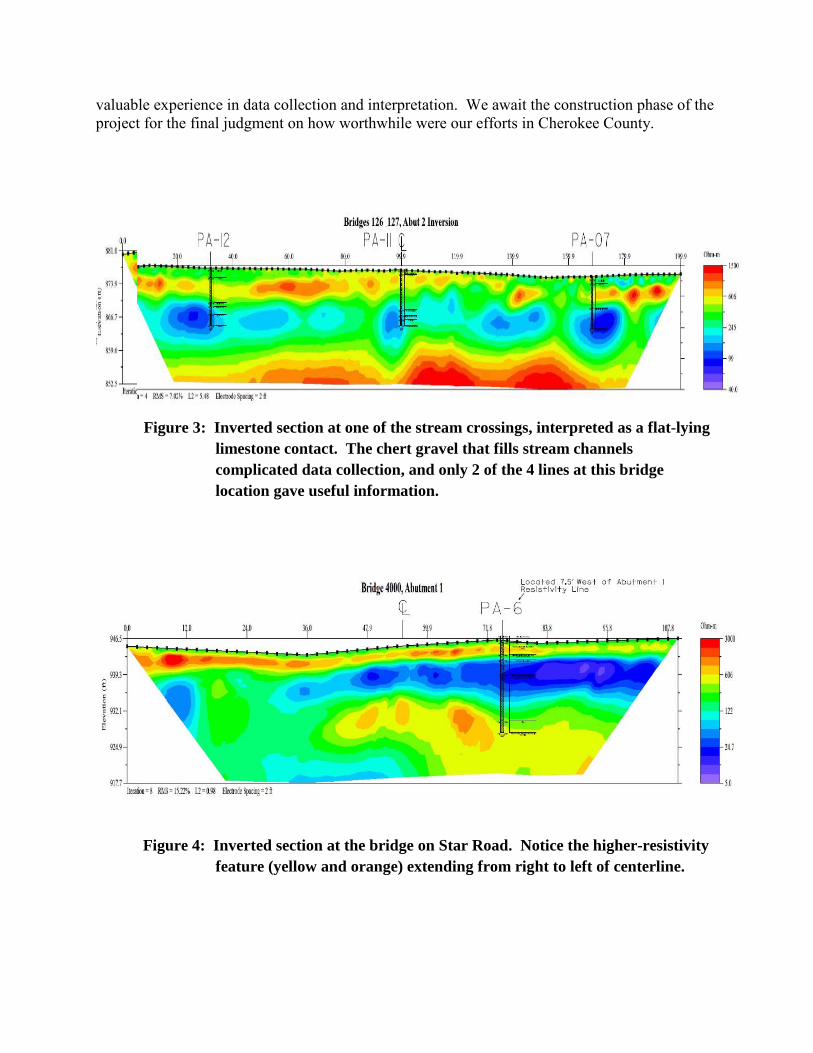
Twenty-four lines with good data were inverted. The inversions were overlain with drill holes; four are shown here. As we feared, the water table in several locations was close to the bedrock contact eliminating the needed contrast between highly-resistive limestone and the overburden. Some inversions showed flat-lying changes in apparent resistivities, which was interpreted as flat-lying geology (Figure 3). This coincided with drill soundings indicating a planar bedrock contact, although the inversion could also simply be showing the water table. Relatively flat-lying geology was seen in several of the inverted resistivity sections.
At other locations, such as the west abutment of the Star Road bridge (Figure 4), some distinctive high-resistance features are evident; this line was taken across a wooded slope, well above the water table. The irregular yellow contour follows the 500 Ohm-meter line, and may approximate the top of limestone. On the west abutment of the US 400 bridge, at the far west end of the proposed project (Figure 5), a large low-resistance feature to the right of centerline could not readily be explained. The pile locations at both of these abutments will be predrilled in order to ensure adequate pile penetration; pile lengths will likely vary significantly at these locations.
Finally, Figure 6 shows the south abutment of the K-26 bridge over the proposed realignment. This location is slightly above influence by the water table. To the left of centerline at the surface are layers of highly-resistive buried bricks. Otherwise, the inverted section is a jumble that does not match nearby drill holes. Despite having theoretically good data, this line was meaningless to the author.
In conclusion, our resistivity work on US 166 was typical of what we often find using this method: some of the results were very helpful, and some were not. The work gave us
valuable experience in data collection and interpretation. We await the construction phase of the project for the final judgment on how worthwhile were our efforts in Cherokee County.
Figure 3: Inverted section at one of the stream crossings, interpreted as a flat-lying
limestone contact. The chert gravel that fills stream channels complicated data collection, and only 2 of the 4 lines at this bridge location gave useful information.
Figure 4: Inverted section at the bridge on Star Road. Notice the higher-resistivity feature (yellow and orange) extending from right to left of centerline.

Figure 5: Inverted section at US 400 bridge over US 166. The large bullseyes of low resistivity (blue and purple) could not be easily explained.
Figure 6: Inverted section at K-26 over US 166. The high-resistance areas (red) near the surface left of centerline are buried bricks. The remainder of the interpretation eluded the author.

Emergency Repair of a Failing MSE Wall Utilizing Hollow Bar Soil Nails and Compaction Grouting
Justin Petersen, P.E. Regional Engineer
GeoStabilization International 543 31 Road
Grand Junction, CO 81504 [email protected]
Prepared for the 67th Highway Geology Symposium, July, 2016

Emergency Repair of a Failing MSE Wall Utilizing Hollow Bar Soil Nails and Compaction Grouting – Justin Petersen, P.E.
2
Acknowledgements
The authors appreciate the support of Mesa County Engineering Department and the Orchard Mesa Irrigation District.
Disclaimer
Statements and views presented in this paper are strictly those of the author(s), and do not necessarily reflect positions held by their affiliations, the Highway Geology Symposium (HGS), or others acknowledged above. The mention of trade names for commercial products does not
imply the approval or endorsement by HGS.
Copyright Notice
Copyright © 2016 Highway Geology Symposium (HGS)
All Rights Reserved. Printed in the United States of America. No part of this publication may be reproduced or copied in any form or by any means – graphic, electronic, or mechanical,
including photocopying, taping, or information storage and retrieval systems – without prior written permission of the HGS. This excludes the original author(s).

Emergency Repair of a Failing MSE Wall Utilizing Hollow Bar Soil Nails and Compaction Grouting – Justin Petersen, P.E.
3
ABSTRACT
This paper summarizes the emergency stabilization repair of a newly constructed roadway section originally designed and constructed using a Mechanically Stabilized Earth (MSE) wall to create 40-ft of additional roadway width, including a bike lane and pedestrian walkway. The new roadway section, located on 38 Road, near Palisade, Colorado, began to show signs of movement just days before the ribbon cutting ceremony was marked on the calendar. The movement accelerated rapidly over the next few days and became an emergency situation as the tension cracks in the roadway created hazards to motorists and cyclists.
The MSE wall consisted of a wire-faced basket type and appeared to be internally
stable. The movement observed in the MSE wall suggested a problem in the foundation soils that the MSE was placed on. In addition to this poor foundation, an approximately 12-ft wide “buttress” of soil was placed at the toe of the finished MSE Wall. This buttress was placed too high on the slope and was over-steepened. This was thought to be another contributing factor in overloading the foundation soils. The approach to mitigate the movement of the existing retaining wall consisted of designing and installing a pattern of hollow bar soil nails, up to 50-ft in length, through the existing wall face and reinforced fill into the shale bedrock. Additionally, the design included reshaping the fill previously placed in front of the newly constructed wall. Reshaping consisted of regrading the mass of the previous over-steepened “soil buttress” downhill, to a more suitable configuration making the mass more useful to resist the movement.
During the drilling process, the wall continued to move until enough of the installed
soil nails began to take load and “catch” the wall’s movement. Once the combined resistive forces in the soil nails as well as the fill below the wall were at or above equilibrium with the driving forces of the failure, the wall movement quickly reduced to almost zero. Since the wall experienced significant movement for approximately one (1) week, as well as being purportedly founded on less than suitable foundation material, it was then decided to implement a more comprehensive solution and improve the foundation materials as well as increase the density of the sub-grade materials using compaction grouting methods. Compaction grouting was used in the subgrade soils below the roadway to re-densify the soil behind the MSE fill to help mitigate any settlement or reflection cracking that could occur in the roadway after repaving.

Emergency Repair of a Failing MSE Wall Utilizing Hollow Bar Soil Nails and Compaction Grouting – Justin Petersen, P.E.
4
INTRODUCTION In June of 2015, Mesa County officials approved plans for the reconstruction of 38 Road near the Orchard Mesa Power Plant. The 2,660 linear foot section of roadway was designed to increase the roadway width to nearly 60-ft, which would also provide a 10-ft wide pedestrian and cyclist lane. The additional width and reconstruction of the roadway was needed to provide a safe route for the increase in vehicle traffic and the interaction between motorists and pedestrians/cyclist that access East Orchard Mesa. The widening of the roadway created a safer alignment and width for the mixed use of produce truck traffic, local residents, tourists, and cyclists. However, the engineering challenges included steep terrain as well as preservation and avoidance of critical infrastructure such as the Orchard Mesa Irrigation District (OMID) siphon. The additional roadway width was achieved by constructing a Mechanically Stabilized Earth (MSE) wall. The MSE wall consists of wire basket facing that connects to the reinforcing strips layered horizontally, 2-ft vertical spacing, throughout the granular wall backfill. The 2-ft layers were compacted during construction to increase the confinement and friction of the granular fill. East Orchard Mesa is a plateau located on the East end of the Grand Valley that is home to over 4,300 acres of farmland that produces famous peaches and a host of other agricultural products. OMID manages and maintains the 30 miles of irrigation canals that provide water to the 4,300 acres of farmland. The OMID power station located at 668 38 Road in Palisade, Colorado provides 3 megawatts of electricity to Xcel Energy and also delivers the water required, through additional pump house penstocks, to operate hydraulic pumps to feed the East Orchard Mesa Irrigation canals. After the power station uses the required flow to operate the turbines, the remaining water flows through 4 additional penstocks that feed the pump house, shown in Figure 1. The pump house penstocks provide hydraulic energy that powers pumps that deliver water to the upper (canal 2) and lower (canal 1). Canal 1 then travels towards the 38 Road MSE Wall in a pipe system before the siphon carries the water under 38 Road. The siphon is a 54” bell and spigot pipe system, likely constructed in the 1960’s, that transfers the irrigation water directly below 38 Road to the 4,300 acres of farmland that surrounds the lower canal. Palisade, Colorado is known as the “Peach Capital of Colorado.” The local farmers and community take pride in growing and celebrating peaches along with many other products that fill roadside fruit stands and local grocery stores. The farming culture of Palisade is centered on the mild climate, 78% of days with sunshine, and fertile fields that provide the backdrop for a tradition in growing and providing farm to table products to the region. None of the agriculture would be possible without access to the Colorado River and the irrigation water that is provided by the canal systems operated by Orchard Mesa Irrigation District (OMID). The integrity of the irrigation canals is critical to the maintaining the farming culture of the area.

Emergency Repair of a Failing MSE Wall Utilizing Hollow Bar Soil Nails and Compaction Grouting – Justin Petersen, P.E.
5
FIG. 1. Orchard Mesa Irrigation Pump House Penstocks
EXISTING CONDITIONS In the fall of 2014, Mesa County decided to move forward with the bidding process to design and construct the retaining wall system to widen 38 Road for an overall section length of 2,660 feet. The bid specifications outlined the project as “The 38 Road Safety Improvement Project” which called for the complete reconstruction of 38 Road between the Orchard Mesa Irrigation District Tailrace and the intersection of Solbre El Rio. Primary features of the project included widening lanes to 14 feet, adding shoulders, storm drain facilities, retaining walls, concrete rockfall mitigation barriers (K rail barriers) and a 10-foot wide concrete path for pedestrians and cyclists. The project was successfully bid and constructed per the bid documents during the summer and fall of 2015. Within days of the ribbon cutting ceremony, the roadway surface began to show signs of distress. The tension cracks in the new pavement indicated that the global stability of the newly constructed wall was in jeopardy. If a catastrophic failure occurred and 38 Road had to be closed to through traffic, the detour for access to the East Orchard Mesa area would travel through the business district of Clifton, Colorado. The detour would traverse 18 miles through Clifton and narrow country roads. Country roads that were not designed to handle high volumes of traffic would be inundated with high volumes of motorists. C ½ Road is a narrow country road that travels through communities and farmland in East Orchard Mesa. One example of the detour affecting the community/local

Emergency Repair of a Failing MSE Wall Utilizing Hollow Bar Soil Nails and Compaction Grouting – Justin Petersen, P.E.
6
farmers would be Talbott Farms. Talbott Farms is the largest producer of fruit in the area and located only 0.5 miles from the 38 Road MSE wall. Figure 2 shows the anticipated detour route.
Figure 2 – Anticipated 38 Road Detour Route
The MSE wall movement also threatened the Canal 1 siphon below 38 Road. This siphon was replaced in the mid 1960’s and was reaching the end of its service life. Additional stress from the retaining wall movement accelerated the disrepair of the current siphon and separated the joints. The separation caused significant flow from the siphon pipe that increased the level of saturation in the lower fill material, which added to the driving forces of the retaining wall failure. DESIGN After GeoStabilization International (GSI) received a call from the contractor regarding the failing wall and potential loss of the 38 Road section, GSI engineers visited the site the same day and began performing a site reconnaissance to assess the situation and determine the appropriate slide mitigation. Early in the site reconnaissance it was determined that the wall movement was contained in the outboard lane of the roadway. The location of the tension cracks in the roadway correlated with the back of the MSE wall reinforcement material according to the as-built information provided by the prime contractor during onsite conversations. GSI engineers also determined that the wall instability could pose a risk to the travelling public and a catastrophic failure of the wall could result in a multiple-week road closure and a complete loss or shutdown of water to canal 1. In an effort to proceed as quickly as possible, GSI provided the County with an initial proposal for the soil nail repairs within 24 hours of the initial site visit. The proposal was founded on available information of the site and local geology with the idea that the design would be evaluated and changes if needed based on the information gathered during the soil nail drilling.

Emergency Repair of a Failing MSE Wall Utilizing Hollow Bar Soil Nails and Compaction Grouting – Justin Petersen, P.E.
7
The extra width provided by the MSE wall construction required the wall to be founded on competent bearing material to support the additional surcharge applied to the system by the retaining wall facing, backfill and traffic. The typical cross-section below in Figure 3 shows the geometry of the MSE wall construction with the estimated subsurface layers. Due to the emergency nature of the repair and the possibility that the wall could experience a catastrophic failure at any moment, there was not sufficient time to provide additional subsurface borings and geotechnical data before GSI’s design could be finalized and implemented. GSI design engineers provided a preliminary design for the emergency repair based from past geotechnical data and experience with the local geology, as well as a back calculation of existing conditions. The preliminary design provided a foundation for field engineering and allowed flexibility during the construction process to address changes in conditions that may occur.
Figure 3 - Preliminary Typical Cross-Section It was determined, by investigative drilling using the soil nail installation rig, that the front edge of the constructed MSE wall was not founded on competent material. According to the county and the MSE wall contractor, the original excavation for the construction of the wall was likely terminated at a depth where the back edge of the MSE wall reinforcement reached competent material. Due to the angles in the soil stratigraphy, the outside face of the retaining wall appeared to be founded on cast material placed during the original 38 Road construction. Each individual layer was verified during soil nail installation procedures. After further investigation, the material that the outside face of the MSE wall was founded on was classified

Emergency Repair of a Failing MSE Wall Utilizing Hollow Bar Soil Nails and Compaction Grouting – Justin Petersen, P.E.
8
as unconsolidated shale colluvium that had been cast down the slope during the original construction of 38 Road. In addition to being unconsolidated, the material near the outward face of the wall at the base had moisture content at the approximate plastic limit. The additional moisture in the unconsolidated shale material directly above the bedded shale reduced the particle friction along the potential failure surface. The design for the wall failure utilized hollow bar soil nails (HBSN) that increased the resisting forces to counteract the driving forces of the failure. The HBSNs designed for the repair were installed in various lengths as shown in the elevation view in Figure 4 below. The soil nails are installed directly through the wire basket face, through the granular fill of the existing MSE wall and into the undisturbed material near the inboard edge of the roadway. The soil nails penetrated through the wall fill into the undisturbed material and were embedded past the failure zone and successfully confined the failing material wedge behind the MSE fill to stable material. The HBSNs were drilled using neat cement grout as the drilling fluid. This method of drilling created higher bonds strengths than typical methods in a granular material as encountered on this site. The continuous injection of grout during the drilling process creates additional layers of grout dispersion as seen in Figure 5 below. Typical cased-hole methods would only achieve the neat cement grout zone and open-hole drilling would not likely be achievable in the granular fill of the MSE wall. The HBSN drilling methods bond strengths are increased due to the soil and cement mixing that occurs as well as the roughness of the drilled hole associated with this installation method. The actual effective grout column can be significantly larger than the drill bit diameter. The soil and cement mixing, paired with the densified ground that is achieved, result in bond strengths that develop the required tensile force for the soil nail elements. The soil nails can then be used effectively to resist the driving forces of the retaining wall and roadway failure.
Figure 4 – As-Built Elevation View

Emergency Repair of a Failing MSE Wall Utilizing Hollow Bar Soil Nails and Compaction Grouting – Justin Petersen, P.E.
9
Figure 5 – Typical Cross Section for HBSN Grout Column
In Figure 6, the subsurface conditions were modified based on the drill logs acquired from the soil nail installation. The undisturbed shale bedrock layer was found to be located farther below the bottom of the constructed MSE wall system than initially expected. The engineering team then modified the soil nail repair system to account for the change in conditions without additional cost to Mesa County.

Emergency Repair of a Failing MSE Wall Utilizing Hollow Bar Soil Nails and Compaction Grouting – Justin Petersen, P.E.
10
Figure 6 - Typical Cross-Section Repaired Model w/ Micropile The cross section above represents a typical view of the proposed soil nail repair that was designed and installed by GSI crews. The soils nails vary in length from 30-50 feet according to the output information from the limited equilibrium modeling software. The micropiles shown in this image represent a design iteration that was field engineered once the bedrock was located. In lieu of the micropiles as shown above, compaction grouting techniques were implemented to provide the required bearing capacity needed to satisfy global stability. Figure 7 shows the Factor of Safety (FoS) of the repair solution without the micropiles for additional bearing support.
Figure 7 - Typical Cross-Section Repaired Model The compaction grouting design was developed to remediate two main areas of the wall repair. The first and most critical portion of the compaction grouting design was developed to provide additional bearing capacity at the base of the wall. The soil nails provided the required lateral

Emergency Repair of a Failing MSE Wall Utilizing Hollow Bar Soil Nails and Compaction Grouting – Justin Petersen, P.E.
11
resistance to the stability while the compaction grouting at the base provided the required bearing capacity to aid in resisting the settlement. The second location for compaction grouting was located directly below the roadway platform. During the initial wall failure, lateral and vertical movements created voids at the interface between the wall backfill and the existing roadway fill. The low slump grout material was strategically installed in the trouble areas to fill the voids and densify the soil. The grouting procedures were carefully monitored to avoid unwanted heaving or displacement of the roadway or wall. Figure 8 shows the compaction grouting zone near the base of the wall.
Figure 8 - Typical Cross-Section Repaired Model CONSTRUCTION The graph below in Figure 9 represents the outside wall face displacement in relation to date of each survey. Prior to the GSI repair, survey targets were installed on August 13, 2015 once tension cracks in the new pavement began to develop. The targets were routinely surveyed to monitor the movement and eventually provide Mesa County proof that a mitigation plan was necessary. The movement increased in a linear trend until August 26th when crews installed 5,940 lineal feet of soil nails into the failing section of the MSE wall. Through decisive and quick thinking from the County, the wall could be stabilized at the current alignment and height. If the movements were allowed to continue, global failure would have resulted in a catastrophic collapse of the wall and roadway platform, as well as the Orchard Mesa Irrigation District siphon. Due to the severity and consequence of failure and not knowing when the inevitable collapse would occur, the engineering team decided that the center and worst area of the wall should be stabilized first. That decision turned out to be correct when the siphon water line finally compromised enough by the movement to severely leak, inundating the site with irrigation water. Figure 9 shows the movement of the wall was counteracted between August 24, 2015 and August 26, 2015. That is important because August 24, 2016 was the day the fill material below

Emergency Repair of a Failing MSE Wall Utilizing Hollow Bar Soil Nails and Compaction Grouting – Justin Petersen, P.E.
12
the wall became fully saturated and moved vertically 4 feet. The drastic movement of the fill material below the wall tried to “drag” the retaining wall down the slope, but the installed soil nails provided the resistance needed to support the wall and roadway surface. The roadway was never closed during the soil nail installation and the irrigation siphon was only shutdown for 6 days, which saved the late season crops in the area. Total construction time for the soil nails, reinforced shotcrete and compaction grouting was 6 weeks. The repair included 6,540 feet of soil nails, 250 square feet of steel reinforced shotcrete and approximately 10 cubic yards of compaction grouting material. The combination of the techniques mentioned above resulted in a stabilization repair system for the 38 Road retaining wall and roadway.
Figure 9 - Wall Face Displacements at Station 26+00 CONCLUSION The reconstruction of the 2,660 lineal foot section of 38 Road to provide additional width faced global stability concerns that developed days after the ribbon cutting ceremony for the reopening. GSI engineers and crews were able to mobilize to the emergency situation and mitigate the MSE wall failure before the condition turned catastrophic. Decisive action from the Prime Contractor and County plus quick response from GSI and continuous cooperation from OMID proved to be the winning combination that saved this section of 38 Road.
0
0.1
0.2
0.3
0.4
0.5
0.6
0.7
August13,2015
August14,2015
August15,2015
August16,2015
August17,2015
August18,2015
August19,2015
August20,2015
August21,2015
August22,2015
August23,2015
August24,2015
August25,2015
August26,2015
August27,2015
August28,2015
August29,2015
Del
ta D
ispl
acem
ent (
in)

Use of Anchored Drilled Shafts to Stabilize a Landslide:
Construction and Instrumentation
David A. Varathungarajan, P.E. Shannon & Wilson, Inc.
1321 Bannock Street, Suite 200 Denver, CO 80204
(303) 825-3800 [email protected]
Kyle D. Murphy Shannon & Wilson, Inc.
1321 Bannock Street, Suite 200 Denver, CO 80204
(303) 825-3800 [email protected]
Paul R. Macklin, P.E. Shannon & Wilson, Inc.
1321 Bannock Street, Suite 200 Denver, CO 80204
(303) 825-3800 [email protected]
Gregory R. Fischer, Ph.D., P.E. Shannon & Wilson, Inc.
1321 Bannock Street, Suite 200 Denver, CO 80204
(303) 825-3800 [email protected]
Matthew C. Kurle, P.E. North Dakota Department of Transportation
300 Airport Road Bismarck, ND (701) 328-6900 [email protected]
Prepared for the 67th Highway Geology Symposium, July, 2016

67th HGS 2016: Varathungarajan et al. 2
Acknowledgements
The authors would like to thank Jeff Jirava and Colter Schwagler (both of the North Dakota Department of Transportation) for their review of this manuscript.
Disclaimer
Statements and views presented in this paper are strictly those of the author(s), and do not necessarily reflect positions held by their affiliations, the Highway Geology Symposium (HGS), or others acknowledged above. The mention of trade names for commercial products does not
imply the approval or endorsement by HGS.
Copyright Notice
Copyright © 2016 Highway Geology Symposium (HGS)
All Rights Reserved. Printed in the United States of America. No part of this publication may be reproduced or copied in any form or by any means – graphic, electronic, or mechanical,
including photocopying, taping, or information storage and retrieval systems – without prior written permission of the HGS. This excludes the original author(s).

67th HGS 2016: Varathungarajan et al. 3
ABSTRACT
A 500-foot wide by 700-foot long landslide occurred in the Badlands of North Dakota, affecting the westbound lanes of Interstate Highway I-94, about 30 miles west of Dickinson. The landslide had been active for a number of years, and the adjacent stretch of roadway had a history of slope instability dating back to the original interstate construction. Because of right-of-way limitations associated with the adjacent Theodore Roosevelt National Park, the North Dakota Department of Transportation elected to mitigate the landslide using a structural support system consisting of a single row of drilled shafts and a row of post-grouted ground anchors connected to the drilled shafts via a reinforced concrete cap beam.
The slope stabilization system was constructed in 2015. The techniques used to construct
the project, including challenges associated with the installation of ground anchors and drilled shafts in an active landslide and post-grouting of ground anchors are summarized.
Construction of the project included the installation of instrumentation consisting of
inclinometer casings in drilled shafts, load cells on ground anchors, and elasto-magnetic force sensors in the anchor bond zone. Crosshole sonic log tests were conducted on a number of the drilled shafts. The project also included the completion of two verification tests on instrumented sacrificial post-grouted anchors. Data from the verification tests and sacrificial ground anchors is presented and evaluated. Data from post-construction monitoring of the project instrumentation is also presented and evaluated.

67th HGS 2016: Varathungarajan et al. 4
INTRODUCTION
The Painted Canyon Landslide is an approximately 500-foot wide landslide that occurred in the Badlands of North Dakota, affecting the westbound lanes of I-94, about 30 miles west of Dickinson (see Figure 1). The landslide had been active for a number of years, and the adjacent stretch of roadway has a history of landslide movement dating back to the original interstate construction. Because of right-of-way limitations associated with the adjacent Theodore Roosevelt National Park (the Park), the North Dakota Department of Transportation (NDDOT) elected to stabilize the landslide using a structural system consisting of a single row of drilled shafts and a row of post-grouted ground anchors connected to the drilled shafts via a reinforced concrete cap beam.
Figure 1 – Site Location
This paper summarizes the techniques used to construct the project and lessons learned
from the construction. This paper also presents post-construction geo-structural monitoring data and results from two verification tests on instrumented sacrificial ground anchors. SITE HISTORY
Since the construction of I-94 in 1964, the roadway has experienced several significant episodes of landslide activity in the vicinity of the project. The first landslide occurred in 1970, approximately 1,000 feet east of the project site. The 1970 landslide was repaired by grading the landslide mass to a 4H:1V (horizontal:vertical) slope and installing subsurface drainage features. In 1979, a smaller landslide occurred just to the west of the 1970 landslide repair. The 1979
Approximate Site Location
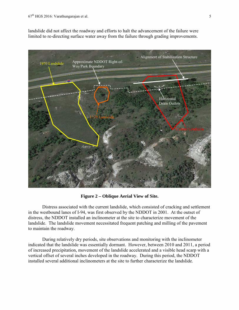
67th HGS 2016: Varathungarajan et al. 5
landslide did not affect the roadway and efforts to halt the advancement of the failure were limited to re-directing surface water away from the failure through grading improvements.
Figure 2 – Oblique Aerial View of Site.
Distress associated with the current landslide, which consisted of cracking and settlement in the westbound lanes of I-94, was first observed by the NDDOT in 2001. At the outset of distress, the NDDOT installed an inclinometer at the site to characterize movement of the landslide. The landslide movement necessitated frequent patching and milling of the pavement to maintain the roadway.
During relatively dry periods, site observations and monitoring with the inclinometer
indicated that the landslide was essentially dormant. However, between 2010 and 2011, a period of increased precipitation, movement of the landslide accelerated and a visible head scarp with a vertical offset of several inches developed in the roadway. During this period, the NDDOT installed several additional inclinometers at the site to further characterize the landslide.
1970 Landslide
Current Landslide
Approximate NDDOT Right-of-Way/Park Boundary
Alignment of Stabilization Structure
Horizontal Drain Outlets
1979 Landslide

67th HGS 2016: Varathungarajan et al. 6
In 2012, the NDDOT installed 14 horizontal drains with lengths up to 300 feet at the site. Although several of the drains initially produced significant volumes of water after installation, movement of the landslide continued, albeit it a slightly decreased rate.
Following ongoing movement of the landslide and concerns that movement could
eventually impact the safety of the traveling public, the NDDOT retained Shannon & Wilson in 2013 to evaluate several options to mitigate the landslide. Based on the evaluation, the NDDOT selected a structural support stabilization system consisting of anchored drilled shafts and horizontal drains to protect the interstate. Subsequently in 2014, the NDDOT retained Shannon & Wilson and Kadrmas, Lee & Jackson, Inc. (KLJ) to design the repair and prepare bid documents for the project. SITE GEOLOGY AND SUBSURFACE CONDITIONS Regional Geology
The site is located in the Fryburg Northwest Quadrangle, for which there is a 1:24,000 geology map (1). The site is mapped as a landslide. The mapped landslide area is about twice the size of the landslide considered herein. The geologic map indicates that the landslide continues eastward well into the Park. The geologic map also indicates that the area surrounding the landslide is underlain by bedrock of the Sentinel Butte Formation, which is described as “alternating beds of gray to grayish brown, variably lithified sandstone, siltstone, mudstone, claystone, clinker and lignite. Calcite-cemented sandstone concretions, siderite nodules, and petrified wood are common.” The sediments accumulated in a basin far from their source rocks during the Paleocene Epoch about 60 million years ago.
Outcrops of in-place bedrock were not observed in the mapped landslide area. Nearly all
of the bedding that was exposed in surrounding terrain appeared to be near-level. Subsurface Conditions Between 2001 and 2013, the NDDOT completed 13 borings at the site to characterize subsurface conditions. The borings were completed with inclinometer casing to allow monitoring of the landslide. In 2014, Shannon & Wilson completed two supplementary borings at the site. Both borings were completed with inclinometer casing. Additionally, multiple levels of nested vibrating wire piezometers (VWPs) were attached to the outside of the inclinometer casing and installed in the boreholes to monitor groundwater conditions.
The rock at the site is poorly lithified. It was capable of being drilled with auger drilling equipment and sampled with a split-spoon and thin-wall samplers. The median N-value in the bedrock was 36 blows per foot and the median undrained shear strength measured in unconsolidated-undrained triaxial compression tests was approximately 5,000 pounds per square foot. For purposes of engineering behavior, the rock is described herein as soil.
The rock underlying the site is dominated by light and dark gray, fat clay which contains many carbonaceous fragments. The average liquid limit of samples tested was 70, with a maximum of 110. However, based on the authors’ experience with the formation, bentonite-rich

67th HGS 2016: Varathungarajan et al. 7
seams with liquid limits in excess of 200 may be present. Locally, the clay is lean. Silt layers are randomly interbedded with the clay. Coal lenses/partings and carbonaceous fragments were observed in many of the samples. Slickensides were observed in numerous samples from the borings.
Bedrock at the site is mantled by relatively thin (typically less than 15-feet thick) deposits
of aeolian soil or landslide debris. Aeolian soils are present on the slope and typically consist of loose to medium dense, silty sand to sandy silt. On the upper portion of the slope, fill may have been placed during construction of I-94. Grading plans provided by NDDOT indicate that up to 15 feet of fill was placed beneath the WB lanes, while about 10 feet of cut was required to construct the eastbound (EB) lanes. The fill appears to be similar to the native aeolian soils and may consist of reworked native material or aeolian soils imported from the vicinity of the site. Most of the sand was iron-oxide stained, indicative of a fluctuating water level. Landslide debris is present on the lower portion of the slope and typically consists of medium stiff to very stiff, lean clay. The landslide debris may be a block of material that detached from the upper portion of the landslide.
The groundwater data show groundwater levels are typically in the bedrock.
Measurements from nested VWPs suggest the presence of confined aquifers, i.e., measurements from VWPs installed at different depths in the same borehole show different groundwater levels. During site visits, some seepage was observed near the toe of the slope. LANDSLIDE REPAIR AND INSTRUMENTATION In 2014, the NDDOT retained Shannon & Wilson and KLJ to complete the design and prepare bid documents for the stabilization of the landslide. The salient landslide stabilization components consisted of the following: • A single row of 60, 4-foot diameter, 70-foot long drilled shafts, spaced at 12 feet center-to-
center, and installed from an existing bench about 25 feet below the roadway. At the location of the drilled shafts, the depth of the slip surface was estimated to range from about 45 feet near the west end of the repair to about 10 feet near the east end of the repair (directions refer to I-94 alignment).
• A reinforced concrete cap beam installed atop the drilled shafts. The total length of the cap beam was 712 feet.
• A single row of 79 five-strand ground anchors installed through the cap beam with a spacing of 9 feet center-to-center, designed for a factored load of 191 kips, and a lock-off load of 147 kips. The ground anchors had a free length of 95 feet and bond length of 45 feet. The project specifications required at least one cycle of post-grouting for the ground anchors.
• Two sacrificial 7-strand ground anchors installed at each end of the repair. • A total of 12 horizontal drains installed from four different locations about 100 feet
downslope of the cap beam.
The approximate location of the alignment of the structure is shown in Figure 2. A typical section showing a schematic of the repair is shown in Figure 3. A plan and elevation view of the structure are also shown in Figure 4.

67th HGS 2016: Varathungarajan et al. 8
Figure 3 – Schematic Cross-Section of Repair
The bid documents for the project also included the installation of instrumentation for construction-phase and post-construction monitoring of the structure. Specifically, the instrumentation consisted of the following: • Inclinometer casing tied to the inside of the drilled shaft rebar cage. The inclinometers were
proposed to measure deflections in the drilled shafts. • Load cells installed at the head of the ground anchor. The load cells were proposed to
measure post-construction loads in the ground anchors. • Two DYNA Force ® elasto-magnetic sensors installed in the bond zone of anchors at
locations 15 and 30 feet from the end of the free length. The elasto-magnetic sensors were proposed to measure the mobilization and distribution of load in the bond zone of the ground anchors.
The above instruments were installed at four different instrumentation installations located
along the length of the wall (see Figure 5). The load cells and elasto-magnetic sensors are currently being monitored with a data acquisition system, while the NDDOT is taking manual readings of the inclinometers.
Approx. Bedrock Contact
Bond Zone

67th HGS 2016: Varathungarajan et al. 9
Figure 4 – Plan and Elevation View of Landslide Stabilization Structure (instrument
locations shown in pink).
CONSTRUCTION NDDOT awarded the contract for construction of the Project to Veit & Company (Veit) of Rogers, Minnesota in March 2015. Jensen Drilling Company (JDC) of Eugene, Oregon was subcontracted to Veit to install ground anchors and horizontal drains. Key dates in the construction schedule are summarized below: • July 29, 2015: Installation of drilled shafts begins. • September 19, 2015: Installation of drilled shafts completed, construction of cap beam
begins. • October 21, 2015: East sacrificial ground anchor tested. • October 23, 2015: West sacrificial ground anchor tested. • November 2, 2015: Construction of cap beam completed. • November 3, 2015: Installation of production ground anchors begins. • December 21, 2015: Installation of production ground anchors completed. • December 29, 2015: Installation of horizontal drains begins.

67th HGS 2016: Varathungarajan et al. 10
• December 31, 2015: Installation of horizontal drains completed. • Spring 2016: Project cleanup and closeout.
The following sections summarize the techniques used to construct the Project and lessons learned during construction. Drilled Shafts Installation Veit excavated the shafts using a CZM EK 200 hydraulic drill rig, equipped with soil augers of varying diameters as needed to install temporary casing (see below). During drilling, overburden and disturbed bedrock materials above the slip surface were susceptible to caving and seepage (groundwater was encountered in 36 of 60 drilled shafts). To stabilize these materials and to seal the excavation from seepage, Veit constructed the drilled shafts using temporary telescoping casing. Veit typically utilized three pieces of telescoping casing, the bottom of which extended to a depth of about 40 feet. After installing the temporary casing through caving and water-bearing materials, Veit then drilled the remaining portion of each drilled shaft using open-hole techniques. The use of the telescoping casing produced an adequate groundwater seal, such that all of the drilled shafts could be bailed or pumped dry to a degree that permitted free-fall placement of concrete. None of the drilled shafts required tremie concrete placement under water. Lessons Learned During drilled shaft installation, four access tubes were installed in 10 different drilled shafts to complete cross-hole sonic log (CSL) testing. Subsequent CSL testing of these shafts allowed the design team and the NDDOT to confirm the effectiveness of the drilled shaft installation methods. The CSL results were classified in accordance with the following criteria from the project specifications:
Table 1 – CSL Classification from Project Specifications
Concrete Rating Test Result
Satisfactory (G) Good
First Arrival Time (FAT) increase 0 to 10% and Energy Reduction < 6 decibels
Anomaly (Q) Questionable
FAT increase 11 to 20% and Energy Reduction < 9 decibels
Flaw (P/F) Poor/Flaw
FAT increase 21 to 30% or Energy Reduction between 9 and 12 decibels
Defect (P/D) Poor/Defect
FAT increase > 31% or Energy Reduction > 12 decibels
The specifications required that 1) flaws must be addressed if they occur in 3 or more
profiles at the same elevation, 2) defects must be addressed if they occur in more than one profile at the same elevation, and 3) flaws or defects covering the entire cross section require repair.

67th HGS 2016: Varathungarajan et al. 11
The CSL testing indicated that 9 of the 10 the drilled shafts had an “anomaly” that was classified near the threshold of the “satisfactory” rating. These anomalies were typically located in the temporarily cased portion of the drilled shaft and did not correspond to issues of concern observed during construction. Test results indicated two “flaws”, both of which were in a single shaft and in the same tube pair, but at different depths. The locations of the flaws corresponded to locations where clods of soil were observed to fall into the fresh concrete as the temporary casing was extracted. Based on the project specifications, as well as construction observations, the flaws did not warrant further action. Good field observations and documentation proved to be crucial in the design team’s and NDDOT’s evaluation of the CSL test results and confirming the acceptability of the drilled shafts. Without the field observations, the design team and NDDOT would have been more likely to require additional testing, remediation, or analysis where anomalies and flaws were detected, all of which could have adversely affected the project schedule and increased costs.
Based on the authors’ experience on this project, as well as others, it may be feasible to simplify the CSL testing classification into two categories (see Table 2), particularly in cases where good construction observation is completed. Considering these criteria, where results classify satisfactory, no additional action would typically be required, and where results classify as poor/defect, further evaluation would be completed.
Table 2 – Proposed CSL Classification
Test Result Concrete Rating
Velocity Reduction ≤ 20% and Energy Reduction ≤ 9 dB Satisfactory
Velocity Reduction > 20% or Energy Reduction > 9 dB Poor/Defect
Ground Anchors Installation After the reinforced concrete cap beam was constructed atop the drilled shafts, the ground anchors were drilled and installed through block-outs in the cap beam. Secondary block-outs were provided in the cap beam as a contingency in the event that installation of a primary anchor could not be completed or load testing of a primary anchor did not satisfy acceptance criteria. Ground anchor installation began with the installation of two sacrificial anchors for verification testing (see below for further discussion). JDC drilled the ground anchors using a Boart Longyear DB 102 drill rig equipped with a 6-inch diameter polycrystalline diamond compact (PDC) fixed-head bit and a series of smooth and fluted drill rods. The upper 50 to 60 feet of each ground anchor was installed through silty sand, with the remaining portion installed in bedrock. JDC elected to utilize 6.625-inch outside diameter (OD) permanent casing that was

67th HGS 2016: Varathungarajan et al. 12
advanced with the PDC drill bit, but rotated in the opposite direction, to stabilize the borehole. JDC circulated air, water, and polymer drilling fluid through the drills rods and bit, with cuttings being ejected from the annulus between the drill rods and casing. The production ground anchors included a 0.75-inch diameter tube attached to the outside of the anchor sheath for primary grouting and two 0.75-inch diameter post-grout tubes. Each post-grout tube was installed with a 20-foot long section with tube-a-manchette (TAM) ports spaced at 4 feet. One post-grout tube was installed with the TAM ports in the upper 20-foot segment of the bond zone, while the second post-grout tube was installed with the TAM ports in the lower 20-foot segment of the bond zone. After completing initial grouting and allowing the grout to cure for 24 hours, JDC completed one or two post-grouting cycles (see below), with a 24 hour period between each cycle. A flow meter and pressure gage were used during all grouting operations. During each cycle of post-grouting, JDC separately pumped grout into each of the post-grout tubes. Typical grout takes during each cycle were on the order of 40 to 60 gallons per tube, at pressures between approximately 400 and 700 pounds per square inch. Between the first and second cycles of post-grouting, JDC flushed the post-grout tubes with water circulated through a pipe pushed to the bottom of the post-grout tube.
Figure 5 – Photo Showing Installation of Production Ground Anchors through Cap Beam
(Note drill rig in background and uncoiler in foreground).

67th HGS 2016: Varathungarajan et al. 13
Lessons Learned
During the installation of production ground anchors, the contractor typically drilled and grouted adjacent odd numbered anchors on a given day and adjacent even numbered ground anchors on the following day (i.e. drilling occurred 18 feet from a ground anchor that had been grouted the same day). At the outset of the project, communication was observed between nearby ground anchors drilled and grouted in the same day (18-foot clear distance between anchors). During anchor drilling, drilling fluids ejected fluid grout from nearby recently grouted anchors. This issue was exacerbated when the annulus between the drill rods and steel casing became plugged, resulting in pressurized drilling fluids migrating to adjacent ground anchors. JDC mitigated the issue by maintaining circulation through the borehole annulus as each anchor was drilled. Additionally, during post-grouting of several anchors, grout returns were observed from the nearby recently drilled ground anchor. To limit such occurrences, specifications could incorporate a minimum distance between ground anchors that are drilled and grouted in the same day.
The use of a grout flow meter and pressure gage was necessary to identify issues that occurred during anchor grouting. The flow meter indicated that during grouting of the anchor encapsulation, the grout take far exceeded the volume of the encapsulation. Field observations also indicated that grout placed in the encapsulation was returned from the annulus between the steel casing and ground anchor. In the authors’ opinion, the hydrostatic pressures during grouting of the 140-foot long anchors probably ruptured the corrugated sheathing, most likely at the pre-grout window. (The bottom 2 feet of encapsulation was factory grouted to stiffen the anchor. To grout this portion of the anchor, a small window was cut into the encapsulation near the bottom of the anchor during the anchor assembly process. The window was then patched after grouting by the anchor manufacturer.) To reduce the likelihood of rupturing the encapsulation, specifications for projects with relatively long ground anchors could require either 1) multi-stage grouting of the encapsulation to reduce hydrostatic pressures inside the anchor or 2) simultaneous grouting of the encapsulation and annulus around the outside of the anchor such that hydrostatic pressures acting on the encapsulation are minimized.
Following the first cycle of post-grouting it was difficult to flush the grout tube. In about
18 different grout tubes (each in different ground anchors), either a substantial volume of grout leaked from the grout tube after disconnecting the grout hose or rinse water pumped through the post-grout tube failed to produce clear returns. In these cases, it appears that the TAM ports did not reseal after the initial post-grout cycle. Thus, these tubes were capped and abandoned after the first cycle of post-grouting. In the authors’ opinion, it would be prudent to design post-grouted ground anchors assuming each post-grout tube is viable for only one cycle of post-grouting. GROUND ANCHOR TESTING During the design phase of the project, a nominal load transfer of 4.3 kips per foot (equivalent to a nominal bond strength of 2.7 kips per square foot (ksf) over a 6-inch diameter bond zone) was assumed for the analysis and design of the landslide stabilization. However, there was uncertainty in the actual bond strength that could be developed in the field due to the

67th HGS 2016: Varathungarajan et al. 14
lack of ground anchor projects completed in the Sentinel Butte Formation. There was also concern that creep could occur in the high plasticity bedrock present at the site. Therefore, the completion of two verification tests at the outset of ground anchor installation was specified in the project contract documents, to assess the actual bond strength and creep behavior of the proposed ground anchors. The sacrificial ground anchors were installed using methods similar those previously described for the production ground anchors. A sacrificial anchor was installed at each end of the proposed improvements (Sacrificial Anchor 1 (S1) at the east end and Sacrificial Anchor 2 (S2) at the west end). Each anchor was installed with 0.75-inch diameter initial grout tube and two 0.5-inch diameter post-grout tubes with tube-a-manchette (TAM) grout ports spaced at 5-foot intervals along the bond length. Unlike the production anchors, the TAM ports on each grout pipe were located along the full length of the bond zone. Based on the results of the verification testing, the locations of the TAM ports was revised for the production anchors as discussed below. Two cycles of post grouting were completed on each anchor. Additionally, each sacrificial ground anchor was installed with three elasto-magnetic sensors in the bond zone to measure the distribution and mobilization of load in the bond zone. The sensors were installed at locations 5, 20, and 40 feet behind the beginning of the bond zone. During testing, each anchor was stressed against a temporary reaction frame to a maximum load of 330 kips (load transfer of 7.3 kips per foot), 80 percent of the anchor minimum ultimate tensile strength (MUTS). The load was increased in increments equal to 10 percent of the MUTS, with each load increment held for a period of 60 minutes. During testing, a load cell as well as a calibrated pressure gage connected to the hydraulic loading jack was used to monitor the load applied to the anchor. A dial gage was used to measure displacement at the head of the anchor. An angle finder was also attached to the anchor bearing plate to measure rotation of the plate during loading. The elasto-magnetic sensors were read with a manual readout during the load test.
Results for the tests are presented in Figures 6 and 7 for each anchor as plots of force versus displacement and creep displacement. The force-displacement plots also include conventional minimum and maximum apparent free length criteria, where the minimum apparent free length is assumed equal to the jack length plus 80 percent of the design free length and the maximum apparent free length is assumed equal to 100 percent of the free length plus 50 percent of the bond length plus the jack length. Creep data are provided for a load of 200 kips (the load increment closest to the factored design load of 191 kips).

67th HGS 2016: Varathungarajan et al. 15
0.0
1.0
2.0
3.0
4.0
5.0
6.0
7.0
8.0
9.0
10.0
11.0
0 50 100 150 200 250 300 350
Dia
l Gau
ge R
eadi
ng (i
n)
Applied Load (kips)
Figure 6 – Sacrificial Anchor 1 Test Results Figure 7 – Sacrificial Anchor 2 Test Results
0.0
1.0
2.0
3.0
4.0
5.0
6.0
7.0
8.0
9.0
10.0
11.0
0 50 100 150 200 250 300 350D
ial G
auge
Rea
ding
(in)
Applied Load (kips)
0.00
0.01
0.02
0.03
0.04
0.05
0.06
0.1 1.0 10.0 100.0
Mov
emen
t (in
)
Time (minutes)
0.00
0.01
0.02
0.03
0.04
0.05
0.06
0.1 1.0 10.0 100.0
Mov
emen
t (in
)
Time (minutes)
Creep at 200 kips
Creep at 200 kips

67th HGS 2016: Varathungarajan et al. 16
Data obtained from the elasto-magnetic gages installed in the bond zone are presented in Figure 8 as mobilized bond resistance for four segments in the bond zone versus applied load (jacking force). The load readings obtained from the gages were converted to mobilized bond resistance assuming no load transfer in the free length, linear load transfer between adjacent gages, and a bond diameter of six inches.
Figure 8 – Verification Test Results, Mobilized Bond Resistance by Segment of
Bond Zone During testing, S1 was capable of holding the final test load of 330 kips for 60 minutes, while S2 experienced a pull-out failure (i.e. the applied load could no longer be held or increased) 30 minutes after applying the 330 kip load. Both anchors exhibited satisfactory creep behavior at the factored design load.
As shown in Figure 8, both anchors mobilized the majority of their resistance in the front 5 feet of the bond zone, where the maximum mobilized bond strength ranged from about 16 to 19 ksf. Substantially less resistance was mobilized in the next segment of the bond zone (5 to 20 feet), where the maximum mobilized bond strength ranged from 3 to 6 ksf. Essentially no load was mobilized in the back 5 feet of the bond zone in either anchor. However, as pull out failure occurred in S2, about 3 ksf of bond strength was mobilized at the back of the bond zone.
Despite anchor S2 pulling out, the bond strength mobilized at the back of the anchor was
substantially less than the bond mobilized at the front of the anchor. Although it is unclear if the full bond strength was mobilized at the back of the bond zone (the full travel of the hydraulic jack was expended when the anchor began pulling out), the authors postulate that during post-grouting, only a few TAM ports opened, most likely the ports near the front of the bond zone,
0
2
4
6
8
10
12
14
16
18
20
0 50 100 150 200 250 300 350
Mob
ilize
d B
ond
Zone
Res
ista
nce
(kip
s/ft
2 )
Applied Load (kips)
S1: 0-5 feet
S2: 0-5 feet
S1: 5-20 feet
S2: 5-20 feet
S1: 20-40 feet
S2: 20-40 feet
S1: 40-45 feet
S2: 40-45 feet
Anchor and Bond Zone Segment

67th HGS 2016: Varathungarajan et al. 17
resulting in significantly higher resistance at the front of the bond zone. The relatively high bond strength measured at the front of the bond zone could also be the result of a continuous grout column that formed and extended into a portion of the unbonded zone, on the outside of the anchor. Thus, to improve the distribution of grout, the design was adjusted to use two post-grout tubes per anchor, one with TAM ports in the front 20 feet of the bond zone and one with TAM ports in the back 20 feet of the bond zone. Otherwise, the techniques used to install the production anchors were similar to those used to install the sacrificial anchors. POST-CONSTRUCTION INSTRUMENTATION READINGS Post-construction data from the ground anchor load cells and elasto-magnetic sensors installed in the anchor bond zones are shown in Figure 9. Additionally, representative data from one of the four inclinometers installed in drilled shafts are shown in Figure 10 as a plot of cumulative displacement versus depth. In reviewing the data, it should be noted that past monitoring of the landslide indicates that the greatest slope movement typically occurs in June and July. The monitoring data is currently limited to December through May, a period where the landslide movement is comparatively less. However, NDDOT will continue to monitor the instrumentation on a quarterly basis. Indications of distress in the pavement in the landslide area have not been observed since project completion.
Figure 9 – Post-construction Monitoring Data, Load Cells and Bond Zone Force Gages The four instrumented ground anchors were locked off between December 15 and December 17, 2015. Following lock off of the instrumented ground anchors, stressing of the remaining anchors continued through December 21, 2015. The data show a reduction of about
0
5
10
15
20
110
115
120
125
130
Bond Zone L
oad (kips)L
oad
Cel
l at A
ncho
r H
ead
(kip
s)
GA 18 LC GA 27 LC GA 29 LC GA 48 LCGA 18 DF 1 GA 27 DF 4 GA 29 DF 7 GA 48 DF 10GA 18 DF 2 GA 27 DF 5 GA 29 DF 8 GA 48 DF 11
30 ft into bond zone
15 ft into bond zone
Anchor Head

67th HGS 2016: Varathungarajan et al. 18
20 to 30 kips in the measured anchor load as adjacent ground anchors were tested and locked off. About one week after the anchors were all locked off, the load in the instrumented anchors had essentially stabilized. Since then, the anchor loads have held relatively steady, except for minor diurnal fluctuations that are likely temperature-related.
Similar to the sacrificial ground anchors, the monitoring data suggests that the majority of load transfer occurs near the front of the bond zone. Although only two gages were installed in each of the instrumented production anchors, at 15 and 30 feet in the bond zone, about 90 percent of the anchor load has transferred to the ground in the front 15 feet of the bond zone. Essentially no load has been mobilized in the back 15 feet of the bond zone.
Figure 10 – Inclinometer Installed in Drilled Shaft 22, Cumulative Displacement
The inclinometers installed in the drilled shafts were initialized in November 2015, about 1 ½ months before the ground anchors were stressed and locked off. The data show that the drilled shafts moved about ¼ inch uphill as the anchors in the cap beam were stressed and locked off. However, subsequent readings show continued uphill movement, although at a decreasing rate, with essentially no movement after March 2016. Interestingly, the load cells did not

67th HGS 2016: Varathungarajan et al. 19
indicate a substantial loss of load in the ground anchors during this time period. Total uphill movement through May 5, 2016 is about ¼ to ½ inch for the instrumented drilled shafts.
The post-lock-off movement of the drilled shafts could be related to lateral creep of the
drilled shafts. However, there is uncertainty in the cause of the apparent movement and regarding why a reduction in ground anchor load corresponding to drilled shaft movement was not observed. CONCLUSIONS Anchored drilled shafts have been used to stabilize a large landslide in low strength, high plasticity bedrock in the Badlands of North Dakota. Verification testing of post-grouted anchors installed at the project site indicated nominal load transfer on the order of 7.3 kips per foot, with the majority of bond strength mobilized in the front 5 feet of the bond zone. Post-construction monitoring of the structure has shown that loads in the ground anchors have remained steady at loads about 20 to 30 kips less than the lock off load of 147 kips, with the majority of the reduction in load occurring during stressing and lock off of adjacent anchors. Deflection of the drilled shafts through May 2016 has been in the uphill direction and on the order of ¼ to ½ inch, with the majority of the deflection occurring as the anchors were stressed. Following anchor lock off, uphill drilled shaft deflection continued but at a decreasing rate, until essentially stopping in March 2016. Since construction of the stabilization structure, roadway distress at the landslide area has not been observed. The NDDOT will continue to monitor the instrumentation installed at the site.

67th HGS 2016: Varathungarajan et al. 20
REFERENCES
1. Gonzalez, M. A., and Biek, R. F., Geologic Map of the Fryburg NW Quadrangle, North Dakota, North Dakota Geological Survey, Scale 1:24,000, 2003.

How Not To Build In Karst – A Case History
By: Joseph A. Fischer & Joseph J. Fischer Geoscience Services
1741 Route 31 Clinton, NJ 08809
908-221-9332 Email: [email protected]
Prepared for the 67th Highway Geology Symposium, July 2016

Copyright 2016 Highway Geology Symposium
All Rights Reserved. Printed in the United States of America. No part of this publication may be reproduced or copied in any form or by any means – graphic, electronic, or mechanical,
including photocopying, taping, or information storage and retrieval systems – without prior written permission of the HGS. This excludes the original authors.

ABSTRACT
A large industrial park was built in an area of complex geology in the Valley Ridge Province of eastern Pennsylvania. A large portion of the industrial park is atop faulted and folded karst. The
developer hired a local geotechnical consultant who performed a nominal subsurface investigation for a facility to be built within the industrial park. Although the possibility of
sinkholes and remedies for sinkhole repair were noted in their report, there were no recommendations regarding construction atop the karst. The only “bedrock” encountered in
borings and test pits was classified as “granite gneiss” or “gray” rock. Shortly after the tenant moved into the building, an apparent sinkhole formed below the subsurface stormwater detention basin in the main parking lot. Repairs were made to the system, but apparently not much effort was made to prevent future sinkholes. Subsequently, another sinkhole formed within the system not far from the original one. Detention/retention and especially infiltration basins in the area are a recognized problem in karst (1). The industrial park landlord, apparently tired of the expense of sinkhole repair at this system, told the tenant that he will make repairs and charge the tenant the cost of remediation under a “parking lot repair” clause in the lease agreement. The tenants
engineer hired the authors to observe the system’s removal and subsequent sinkhole “repairs” to ensure that they were performed in accordance with good engineering practice and to have a
professional familiar with the operations in case the issue went to court. The subsurface stormwater system was removed revealing karst conditions. The area was backfilled and borings
were drilled to investigate areas of concern noted during the system removal as well as other areas where the building was showing signs of excessive settlement. Low mobility grouting was
then performed in areas deemed of concern by the landlord’s site engineers.

INTRODUCTION This paper is based upon a report written to provide a summary of our observations and opinions of a subsurface stormwater detention system removal and remedial grouting operations performed at a facility near Bethlehem, Pennsylvania that has a strong chance of being the basis for a lawsuit. We were asked to observe and record the operations in response to repeated sinkhole formation in a parking area adjacent to a building. Beneath this parking area and also affected by the sinkholes was a subsurface stormwater detention system with nine, 116-foot-long, 60-inch diameter, HDPE laterals bedded in stone. The entire system including the manifolds and manholes encompasses an area of 132 feet (north/south) by 68.5 feet (east/west) and the system subgrade was approximately 18 feet below parking lot grade. The authors did not observe the reported sinkholes, but some photographs were shown to us by our client. SITE GEOLOGY AND GEOTECHNICAL STUDIES Our review of the available geologic information (2 & 3) shows that the site is underlain by the Leithsville Formation, The Leithsville is described as:
“Thin- to thick-bedded dolomite containing subordinate siliciclastic rocks. Upper part is medium- to medium-dark-gray, fine- to medium-grained, pitted, friable, mottled and massive dolomite. Middle part is medium-gray, stylolitic, fine-grained, thin- to medium-bedded dolomite that is interbedded with shaly dolomite and, less commonly, vari-colored quartz sandstone, siltstone, and shale. Lower part is medium-gray, medium-grained, medium-bedded dolomite containing quartz-sand grains in stringers and lenses near the contact with the Hardyston Quartzite. Archaeocyathids of Early Cambrian age suggest an intraformational disconformity separating rocks of Middle and Early Cambrian age. Thickness approximately 305 m (1,000 ft).” (4)
In our experience, the Leithsville is prone to sinkhole formation in many areas, though not as susceptible as some other carbonate bedrock formations in the region. Karst-related sinkholes and depressions maps are available from the Pennsylvania Geological Survey (2 & 3). Neither of these sources indicate such features on the site, but some are nearby and the newer data available from Reference 3 shows many more depressions around the Routes 78 and 412 interchange. Presumably this newer data indicates the negative impact that man’s activities, such as construction, can have on a site underlain by carbonate bedrock. Prior to construction, a “Soils and Foundation Investigation” was performed by a local consultant. In our opinion the investigation methods used were inadequate for identifying the possible risks at a site underlain by carbonate bedrock and even fails to recognize that the site is underlain by carbonate rock. Although a number of test pits and borings were performed, the bedrock was identified as “granite gneiss” and “gray rock” on the logs. Within the body of the report is the statement “Even though the rock is not KARST material, we still suggest that you follow considerations on pages…” Those are sections on “Preventative Measures Against Sinkholes” and “General Procedures for Sinkhole Repair”.

In general, we believe that the original “Soils and Foundation Investigation” was apparently not performed with consideration for the carbonate bedrock mapped below the site. The report misidentifies the bedrock below at least a portion of the site, but offers generic advice in case of sinkhole occurrence, while making no mention of the readily available and reliable State data showing that the site is underlain by a sinkhole prone bedrock formation. We understand that the developer’s site engineer logged the drilling of 16 test borings at various points around the building to depths ranging from 8 to 50.6 feet below grade. The borings were drilled without the knowledge of the authors between the time of the subsurface stormwater system removal and the remedial grouting programs. The borings were presumably drilled to investigate suspect areas within the removed system area as well as around various portions of the building where settlement was noted. We inspected many of these locations, both interior and exterior of the building. In general, we believe that the areas remediated during the grouting program were at locations that the test borings indicated poor subsurface conditions. We did not understand why no action was taken near where a pair of the borings were drilled. Major differences between those two borings may indicate what is affecting the settlement near that portion of the building. We also felt that additional study should have been performed in other parts of the building that appeared to be experiencing settlement. The auger techniques used in both test boring programs may be state-of-the-practice, but rotary-wash boring techniques that have long been promulgated by experienced karst investigators (e.g., 5), would have likely further indicated the solutioned nature of the bedrock and more adequately indicated the less favorable conditions above the bedrock. BUILDING INSPECTION Settlement cracks and related distress can be seen in the exterior masonry, interior sheetrock, windows and columns in a portion of the complex used for offices. One of the authors toured the interior of the building and was shown numerous examples of settlement. In summary, there are both major and minor signs of settlement along walls. The authors did notice settlement in an area not investigated by the developer’s geotechnical engineer. In addition, a couple of interior columns supporting a factory crane have settled more than others and circular cracks were noted in the concrete floor of the manufacturing portion of the building. SUBSURFACE STORMWATER DETENTION SYSTEM REMOVAL In late 2015, the authors visited the site early in the process of removing the subsurface stormwater detention system. All of the asphalt above the system had been removed and excavation of the system was taking place at one end. The work was being performed by a local contractor and overseen by the developer’s site engineer (different than the geotechnical consultants who performed the original investigation). The removal of the subsurface stormwater system was performed in stages. The backfilling of the areas excavated was performed in stages governed by the limited area to work within. After a portion of the system was removed it was backfilled with materials either stockpiled during

removal or removed from the subsequent area being excavated. The backfill was generally compacted in roughly 12-inch lifts. However, as a result of the limited area to work in, compaction was likely uneven and often on shallow slopes. A ridge of Leithsville Formation bedrock, trending in an east-southeast/west-northwest direction, was revealed below the system during excavation. This ridge extended from about the southeasterly corner of the system to some 20 feet north of the southwesterly corner of the system. A few obvious karst concerns were noted adjacent to the northerly-side of this ridge as well as within a channel that seemed to divide the ridge in some locations. Two small voids were noted, one below the system and one adjacent to an exposed bedrock pinnacle in the west excavation wall. It is apparent that bedrock removal would have been necessary to reach basin subgrade, though the method of removal could not be determined. Our observations during system removal showed several distressed and collapsed sections of the laterals. If one divided the system into four quarters by north/south and east/west lines, the distressed laterals were generally in (but not limited to) the southwesterly quadrant of the system. However, evidence of past and present sinkhole activity within the basin subgrade and sidewalls were noted along almost the entire width of the system in relation to the ridge of exposed bedrock. Laterals in the south-central portion of the system were underlain and partially surrounded by flowable fill. This would appear to be remnants of past sinkhole repair or measures to provide additional support to laterals in this area. However, the authors could not determine if the flowable fill was placed prior to construction or as part of one of the later system repairs. REMEDIAL GROUTING After the removal of the stormwater system and the second set of test borings were drilled, the authors observed the majority of the grout-hole drilling and grouting operations until they were completed. The procedures used were described as “pressure grouting”. Two “rules of thumb” for pressure grouting have been advanced. The American rule of thumb is 1 pound per square inch (6.9 kilopascals) of injection pressure per foot of depth interval being treated. The European rule of thumb is 1kilogram per square centimeter (roughly 4.4 pounds per square inch) per foot of depth interval being treated. However, the American rule of thumb is often considered conservative as it only seems to consider the weight of the overburden materials and not their strength (6). The drilling equipment was an air-track with separate compressor using a 3-inch bit. We recorded a summary of the subsurface conditions encountered in the grout holes observed. Grout was reportedly a mix consisting of 2 (sand) to 1 (cement) provided to the site by a local supplier. The authors estimate that the grout had a 1- to 2-inch slump upon exiting the concrete truck. The grout was delivered to the hole by a piston pump and introduced into the subsurface under pressure through steel casing placed in the drilled holes. Grouting generally started above the rock, although was sometimes started below the bedrock surface.

An effort was made to obtain the grouting specifications for the project, but no document was received. However, the developer’s geotechnical engineer in the field said that they were grouting in two-foot stages using a 300 psi pressure limit per stage and a 1.5 cubic yard (cy) per stage injection cutoff. The grout hole spacing was generally 10-feet with the adjacent rows offset some five feet. Interior floor and/or ground heave were monitored during the grouting operations. Parking Area As noted previously, drilling through the fills placed after removal of the subsurface stormwater detention system indicated that compaction during placement was likely uneven. However, no soft soils were noted within the fill materials during the observed drilling. In general, the areas chosen for remediation by the developer’s site engineer were areas of concern. Without the benefit of surveying equipment, they appeared to be in the general areas of concerns noted during the stormwater system removal. The grout takes were significantly over hole volume in most of the grout holes drilled in these areas. Office Building Five grout holes were drilled near a settling section of a wall to the office building. Three of the grout holes were drilled at a roughly 30 degree angle aimed to pass under the buildings footings and interior. Two others were drilled vertically in an offset pattern from the first three, further from the building. The same grouting volume cutoff and pressure “specifications” as used in the parking area were used below the building. Two of the three holes angled under the building encountered significant voids and soft soils zones. One other hole had a section of blaster’s primer cord “blown” up with the drill cuttings. The five grout holes took more than 40 cubic yards (30.6 cubic meters) of grout combined, even with the volume cutoff. While grouting these five holes, the volume cutoff of 1.5 cubic yards (1.1 cubic meters) per 2-foot (0.6-meter) stage was reached 19 times. One grout hole, presumably at the location of one of the more recent test borings, took the most grout (20+ cubic yards/15.3+ cubic meters) and reached the volume cutoff 12 times. During the grouting of the holes closest to the office building, the building floor reacted by lifting to the grouting of four of these holes. Exterior ground heave was experienced in another hole drilled to grout near the building. CONCLUSIONS Although there is little doubt that the subsurface stormwater detention basin contributed to the sinkhole formation at the site, it appears to have been constructed as designed and approved. However, the placement of any subsurface stormwater system at a site underlain by carbonate bedrock is usually ill-advised, especially when solutioned carbonates are likely shallow. The backfill placed after the removal of the system was not closely controlled and appeared to be uneven as a result of the limited work space. This would seem to be evidenced by the somewhat

inconsistent drilling rates observed while drilling grout holes through the fills. However, we feel that the overall compactive effort was likely adequate for the areas planned use as a parking area. Evidence of previous blasting was noted in one probe hole drilled between the building and the subsurface stormwater system (an angle hole oriented to drill below the building foundation and under the building). We are unaware if blasting was used for rock removal at this site, but our experience shows that uncontrolled blasting in solutioned carbonate rocks commonly increases the possibility for sinkhole formation. However, from observations made during the removal of the subsurface stormwater detention system, we know that rock was removed from excavations at the site, yet no one appeared to recognize that the bedrock was a solution-prone carbonate formation. We believe that the remediation performed in the parking area may be incomplete because the areas grouted at the western-most grouting location appeared to be limited to the basin excavation area and did not extend along the previously discussed bedrock trend to the west. We also would have preferred more check holes near some of the locations with larger grout-takes. In our opinion, the area to be restored for parking above the removed stormwater system may have been adequately protected from future sinkhole occurrence by the remedial operations performed there. Significant grout was placed in these areas and compacted, low-permeability fill covers the area. As our confidence level in the grouting operation in this area is not strong, we recommended continued monitoring of that entire area for unusual settlements. We also recommended that any significant subsidence noted in the pavement should be cordoned off, avoided by people, cars and machinery, and reported to the responsible parties. We believe that grouting performed in the five holes nearest the office building west wall was incomplete for two reasons. The first is the 1.5 cubic yard (1.1 cubic meter) per 2-foot (0.6-meter) stage volume cutoff. That leaves many sections not completely grouted and the possibility that more grout is needed to replace founding materials eroded into bedrock cavities or that there are bedrock cavities partially ungrouted. Secondly, we believe that the conditions encountered in this area warranted the addition of more grouting locations, especially considering that it is below a structure already showing signs of excessive settlement. In general, we also believe that the bedrock trend noted in the parking lot excavations and during the drilling of the grout holes should be explored further. The sinkhole formation experienced in the past and the reaction of the building in combination with the data from drilling the grout holes indicates that the primary areas of concern seem related to this bedrock trend. Further, we believe that other portions of the site are of concern and should have been further explored and possibly remediated. There were a number of open questions on the overall nature of the subsurface and the thoroughness of the remedial efforts.

REFERENCES
1. Nicholson, L. and T. Pallis. Assessment of the Potential for Sinkhole Formation with Stormwater Detention and Infiltration in the Carbonate-Rock Aquifers of New Jersey. New Jersey Geological and Water Survey, 5/10/13.
2. Kochanov, W.E., 1986. Sinkholes and Karst Related Features of Lehigh and Northampton Counties, Catasaqua Quadrangle, Pennsylvania Geological Survey.
3. Pennsylvania Geological Survey on-line geology, http://www.gis.dcnr.state.pa.us/geology/index.html. Accessed 12/3/2016.
4. United States Geological Survey, http://mrdata.usgs.gov/geology/state/sgmc-unit.php?unit=NJCAl;8. Accessed 4/14/2016.
5. Fischer, J.A. and R. Canace. Foundation Engineering Constraints in Karst Terrane. American Society of Civil Engineers, Foundation Engineering: Current Principles and Practices, v. 1. 1989.
6. Weaver, Kennth D. A Critical Look at Use of “Rules of Thumb” for Selection of Grout Injection Pressures. American Society of Civil Engineers, Advances in Grouting and Ground Modification, Geotechnical Special Publication Number 104. 2000, pp 173-180.

Inner-City Rockfall Hazards – Systematic Investigation of Rock Slopes in the City of Hamilton, ON
Gabriele Mellies Golder Associates Ltd.
6925 Century Avenue, Suite 100 Mississauga ON L5N 7K2, Canada
+1 905 567 4444 [email protected]
Mark Telesnicki Golder Associates Ltd.
6925 Century Avenue, Suite 100 Mississauga ON L5N 7K2, Canada
+1 905 567 4444 [email protected]
Rafael Sandoval City of Hamilton
City Hall 71 Main Street West
Hamilton ON L8P 4Y5, Canada +1 905 546 2424
Prepared for the 67st Highway Geology Symposium, July 2016

67th HGS 2016: Gabriele Mellies, Mark Telesnicki and Rafael Sandoval 2
Acknowledgements
The authors would like to thank the City of Hamilton for its support of this work.
Disclaimer
Statements and views presented in this paper are strictly those of the author(s), and do not necessarily reflect positions held by their affiliations, the Highway Geology Symposium (HGS), or others acknowledged above. The mention of trade names for commercial products does not
imply the approval or endorsement by HGS.
Copyright Notice
Copyright © 2016 Highway Geology Symposium (HGS)
All Rights Reserved. Printed in the United States of America. No part of this publication may be
reproduced or copied in any form or by any means – graphic, electronic, or mechanical, including photocopying, taping, or information storage and retrieval systems – without prior
written permission of the HGS. This excludes the original author(s).

67th HGS 2016: Gabriele Mellies, Mark Telesnicki and Rafael Sandoval 3
ABSTRACT
The City of Hamilton in Ontario is located on the Niagara Escarpment, a large forested ridge with steep slopes that reach heights of up to 50 metres and form the most prominent topographical feature and the main source for natural rockfalls in Southern Ontario. Various roadways within the City of Hamilton traverse through the escarpment and many of them were built in close proximity to the slopes. Over the past years, the City has experienced rockfalls on various scales, from small single pieces of rock to large scale falls that included massive blocks of rock, which impacted the use of the roadways and resulted in damage and road closures.
In the past, the response to these events was reactive and remedial measures were
planned and carried out after rockfall events had happened. After an accumulation of rockfalls in 2014/2015, the decision was made by the City to be proactive and have measures in place to help mitigate future rockfalls and minimize their impact on the roads and the public. A systematic investigation of 20 sites was carried out in 2015 that included site inspections and preparation of individual inspection records for each site. Site specific information was gathered including rock characteristics, slope geometry and potential failure mechanisms as well as road and traffic details. Recommendations for remedial measures were developed for each site. A rockfall hazard rating system was applied to the collected data to prioritize the remedial measures in order to address the most problematic sites in the short-term, while accounting for budget constraints. The applied rating system proved to be effective after rockfall events from high ranked sites occurred in 2016.

67th HGS 2016: Gabriele Mellies, Mark Telesnicki and Rafael Sandoval 4
INTRODUCTION
The City of Hamilton (City) is located at the western tip of Lake Ontario within the area
of the Niagara Escarpment, a large forested escarpment ridge that separates the City in a lower part at the toe of the escarpment and an upper part located on top of the ridge. Several roadways cross the escarpment to connect the upper city area with Hamilton’s downtown area and the major highway located at the shore of Lake Ontario. The crossings were cut through the escarpment rock and many of these roads were built in close proximity to the rock faces or rock slopes. Figure 1 shows an example of a roadway crossing through the escarpment. Every year, the City of Hamilton experiences rockfalls that impact traffic on the roads and result in road closures and damage to structures and vehicles.
Figure 1: Roadway crossing through the Niagara Escarpment
After a series of rockfall events over the past years, which resulted in several temporary
road closures, the City of Hamilton decided to implement a slope maintenance plan that would allow the City to address the existing rockfall hazards within the City proactively and in a controlled way. In 2015, the City of Hamilton retained Golder Associates Ltd. to develop this maintenance plan including a comprehensive investigation of the escarpment crossings.
The project objective was to assess the stability of a defined number of rock slopes for
potential rockfall hazards and the associated risk to the public and to public infrastructure. Accounting for budgetary constraints, priorities had to be defined based on the evaluation criteria. Recommendations for maintenance measures and remediation work were to be developed for each individual site.
BACKGROUND
The Niagara Escarpment
The Niagara Escarpment is a large forested ridge of approximately 1600 km total length
that forms the weathered edge of an ancient sea. The escarpment runs through parts of the United States and Canada, from New York State through Ontario, Michigan, Wisconsin and Illinois,

67th HGS 2016: Gabriele Mellies, Mark Telesnicki and Rafael Sandoval 5
thereby partly shaping the basins of Lake Ontario, Lake Huron and Lake Michigan (see Figure 2). The escarpment is the most prominent feature of southern Ontario, where it spans over a length of approximately 725 km from the Niagara Peninsula, to the Bruce Peninsula and Manitoulin Island. At the western end of Lake Ontario the escarpment crosses through several Canadian cities including the City of Hamilton.
Figure 2: Location of the Niagara Escarpment [1]
In the Hamilton area, the Niagara Escarpment rises to a maximum height of about 250
metres above sea level with rock slopes along the road within the City of up to 50 metres in height. Typically, the rock faces of the ridge are oriented towards north in the direction of Lake Ontario. Figure 3 shows an aerial view of the rock faces of the ridge in the Town of Grimsby in Ontario, just east of the City of Hamilton.
Figure 3: Aerial View of the Niagara Escarpment in Grimsby near Hamilton [1]
The City of Hamilton is located at the western tip of Lake Ontario. Hamilton’s northern
part including the downtown area is located at the toe of the Niagara Escarpment towards the
Hamilton

67th HGS 2016: Gabriele Mellies, Mark Telesnicki and Rafael Sandoval 6
lake shore, whereas the southern part of the city as well as rural neighborhoods extend on top of the escarpment. Several roadways cross through the escarpment to connect the upper city areas with the downtown area and with the major highway that runs along the shore of Lake Ontario. Figure 4 shows a map of Hamilton with the Niagara Escarpment (marked with a red line) that divides the City into a northern part and a southern part.
Figure 4: Map of the City of Hamilton, showing the location of the Niagara Escarpment [2]
Some of these escarpment crossings are multi-lane roads with relatively wide shoulders
and ditches, but most of the crossings are narrow roads that were cut through the escarpment or built in close proximity to the escarpment slopes. Rockfalls from the slopes often reach the roadways creating hazards for traffic and causing road closures and sometimes damage to adjacent structures or to vehicles travelling the roads, which often result in claims for damages. The escarpment crossings are bottlenecks for the traffic in the City and the unplanned temporary closures of the roads after rockfall events, to allow for road clean-up or for scaling of the rock faces, frequently last for several days. These road closures cause long traffic delays and major traffic back-ups in adjacent neighborhoods, which in turn result in frustrations and resentment with residents and commuters.
Geology of the Niagara Escarpment in Hamilton
The Niagara Escarpment is a massive ridge of sedimentary rock comprising of dolostone
and limestone formations that were formed in turns with layers of sandstone and shale, the latter often with limestone interbeds. A typical section of the escarpment rock stratigraphy is shown in Figure 5. The exposed rock faces of the road cuts along Hamilton’s escarpment crossings typically consist of dolostone and limestone layers at the top of the faces that are overlaying shale layers, often with limestone interbeds.
Hamilton
Niagara Escarpment
Lake Ontario

67th HGS 2016: Gabriele Mellies, Mark Telesnicki and Rafael Sandoval 7
Figure 5: Stratigraphic Section of the Niagara Gorge [3]
Typical Rockfall Events
Rockfalls from the rock faces within the City of Hamilton range from individual pieces of
rock that ravel from the faces, to large amounts of smaller blocks caused by a surficial failure of a section of blocky rock, to failure of large blocks from the more massive layers often present at the top of the escarpment slopes. Examples of typical failures are shown in Figure 6. Note that the photos in these Figures show the rockfall areas after the rock debris was removed from the road. In areas where retaining structures were erected to protect the roadways from rockfalls, these structures can also be affected by the failure of the rock as shown in Figure 7.
Goat Island Mb.
Gasport Mb.
Irondequoit Fm.
Thorold Fm.
Grimsby Fm.
Cabot Head Fm.
Whirlpool Fm.
Queenston Fm.
Reynales Fm.
Rochester Fm.
Decew Fm.
Lockport Fm.
Neahga Fm.
Shale
Mudstone
Dolostone
Limestone
Sandstone
Mid
dle
Silu
rian
Ord
ovi
cian
Up
per
Silu
rian
Vertical Scale
met
res
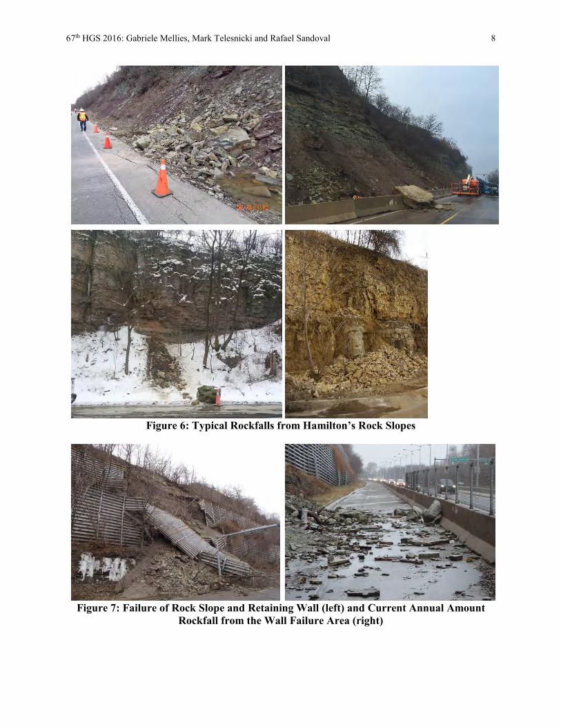
67th HGS 2016: Gabriele Mellies, Mark Telesnicki and Rafael Sandoval 8
Figure 6: Typical Rockfalls from Hamilton’s Rock Slopes
Figure 7: Failure of Rock Slope and Retaining Wall (left) and Current Annual Amount
Rockfall from the Wall Failure Area (right)

67th HGS 2016: Gabriele Mellies, Mark Telesnicki and Rafael Sandoval 9
MATERIAL AND METHODS
In total, 20 different rock slope sites were inspected throughout the City of Hamilton as
listed below. The sites comprised various types of rock slopes including near-vertical rock cuts comprising dolostone and limestone faces, inclined rock slopes consisting of shale and limestone interbeds often with vertical faces at the top, and forested overburden slopes with rock outcrops. Figure 8 shows examples of typical layouts of the investigated sites.
Fifty Road McNeilly Road Dewitt Road New Mountain Road Centennial Parkway (up-bound) Centennial Parkway (down-bound) Kenilworth Access Sherman Cut South Sherman Cut North Sherman Access East
Sherman Access West Claremont Access Jolley Cut up-bound Jolley Cut down-bound James Street Beckett Drive Wilson Street Old Dundas Road Highway 8 Sydenham Road
Figure 8: Examples of Typical Rock Slopes (near-vertical rock faces, overburden slopes
with rock outcrops, inclined rock slopes with rock faces at the top)
General Procedure Data for each site was collected to (i) assess the individual slopes, (ii) develop individual
maintenance and remedial measures, and (iii) compare and rate the slopes to prioritize the work and ensure that the most hazardous slopes were addressed first.
The analysis of the field data aimed to assess the slopes individually to provide
recommendations that are tailored for each site. Furthermore, the slopes were compared to each other and a rating system had to be applied to assess the rockfall hazards and the risk to the public and to prioritize the required work to ensure that the City’s funds that are available for slope maintenance work are assigned in a systematic and cost-effective way.
Wilson Street Kenilworth Access
Centennial Parkway

67th HGS 2016: Gabriele Mellies, Mark Telesnicki and Rafael Sandoval 10
Data Collection
Visual Inspections
The goal of the inspections was to collect a comprehensive data set for each site. The preparation of the field inspection work focused on the identification of the data required to subsequently allow a comparison and rating of the sites. The collected data included the following information:
Geometry of the slope (inclination, height, length, etc.) Rock mass structure (orientation of joints and bedding, etc.) Vegetation and water Failure mechanisms Ditch and road shoulder, existing barriers (width, depth, etc.) Road and traffic (road width, bike lanes, amount of traffic, etc.)
The field inspections comprised visual assessments of the exposed rock conditions,
mapping of relevant features of the slopes (e.g., major jointing, seepage, etc.) and an assessment of the potential failure modes. Measurements of slope heights and slope inclinations, as well as photographs were taken at each site. The inspections were carried out, without restricting traffic, from accessible areas at the bottom or top of the slopes, usually from the ditch or shoulder areas of the roads.
Data Analysis
Application of Rockfall Hazard Rating System
The Ontario Rockfall Hazards Rating (RHRON) system [4] was used to assess the inspected sites and assign priorities to the remediation of the individual slopes. The RHRON system was developed by the Ministry of Transportation, Ontario (MTO) with the goal to “systematically identify, prioritize and remediate rockfall hazards”. The system was developed based on the Oregon Department of Transportation’s Rockfall Hazard Rating System (RHRS) with certain modifications to adjust the system to the conditions in Ontario.
The RHRON system comprises of two versions: a detailed RHRON and a basic RHRON.
While the basic system is used for preliminary evaluation of rockfall hazards, the detailed system is used for a subsequent detailed rating of a site. The detailed system is based on the same four evaluation factors as the basic system; however, a larger number of observations is used to obtain the rating factors. For the assessment of the Hamilton slopes the basic RHRON system was used, which is based on the following four criteria:
F1 Magnitude (estimated amount of rock that might come down in a rockfall event) F2 Instability (estimated frequency of rockfalls) F3 Reach (estimated reach of rock debris in a rockfall event) F4 Consequences (estimated consequences of a rockfall event)

67th HGS 2016: Gabriele Mellies, Mark Telesnicki and Rafael Sandoval 11
The slope rating is carried out by assessing the four factors and assigning a rating on a scale from 0 (‘good’) to 9 (‘bad’) to each factor. The four ratings are then averaged to obtain an overall rating, based on the following:
Overall Rating F = (F1+F2+F3+F4)/4
As requested by the City of Hamilton, a Slope Criticality Rating (SCR) was assigned to
each of the inspected sites that rank the rock slopes with respect to the risk that is associated with each site. The ranking was defined as follows:
Table 1: Slope Criticality Rating (SCR)
Slope Criticality Rating (SCR) Description Range of Overall
RHRON Rating (F)
1 very low risk F 2 2 minor risk 2 < F 4 3 moderate risk 4 < F 6 4 high risk 6 < F 8 5 very high risk 8 < F 9
Development of Remedial Measures
Based on the site inspections, maintenance and remedial measures were developed for each inspected site to address the existing rockfall hazards. The measures were primarily aimed at addressing the short-term maintenance of the slopes to reduce the potential for rockfalls and risk to the public. Typical maintenance measures included regular manual or machine scaling of the rock faces, installation of passive rockfall barriers, as well as ditch maintenance.
RESULTS
Site Observations
During the visual inspections, comprehensive information was gathered for all 20 sites.
The following summarizes the most relevant findings:
Slope Dimensions:
Slope types comprised near-vertical rock cuts, inclined rock slopes and forested overburden slopes with rock outcrops.
Slope lengths ranged between 25 metres and 500 metres. Slope heights varied between 10 metres and 30 metres; slope inclinations ranged between
near-vertical rock cuts to 50° to 70° inclined rock slopes and 30° to 60° inclined overburden slopes.
Talus slopes of various heights comprising rock debris that has ravelled from the rock faces have formed at the toe of many slopes.

67th HGS 2016: Gabriele Mellies, Mark Telesnicki and Rafael Sandoval 12
Although the inspection of the overburden slopes focused on the rockfall hazards pertaining to the rock outcrops rather than failures of the overburden slopes, notes of visual evidence for slope instabilities or overburden failures were recorded too.
Rock Mass Structure of Exposed Rock Faces
Near-horizontally bedded limestone and dolostone rocks with distinctive near-vertical cross jointing.
A near-vertical joint set running near-parallel to the exposed rock faces parallel to the roadways was noted at many sites.
Orthogonal joints at other sites results in a “saw tooth” rock face configuration Bedding spacing and joint spacing typically thin to thick. Wider bedding and joint spacing
was noted along the crest of several slopes. Horizontal bedding and closely spaced near-vertical cross jointing result in very blocky,
‘brick wall type’ rock faces. Figure 9 shows the typical blocky rock faces.
Figure 9: Typical Blocky Rock Face Conditions
Weathering Processes Observed On Site
Freeze-thaw cycles: Fractured rock with water present in open discontinuities is often subjected to ice jacking during cold periods. When water turns to ice, it increases in volume, thus applying a ‘jacking’ force within the discontinuity, which further opens the discontinuity. This force may lead to block instability through progressively jacking apart of blocks that may eventually slide or topple. Intact rock susceptible to frost action may flake and crumble in response to freeze-thaw cycles.

67th HGS 2016: Gabriele Mellies, Mark Telesnicki and Rafael Sandoval 13
The blocky rock mass structure and the many open discontinuities in the rock that were observed at most of the inspected sites indicate a high susceptibility of the rock mass to freeze-thaw processes.
Differential Weathering: Differential weathering occurs from variations in weathering susceptibility of the rock. Weak, more susceptible formations weather more rapidly and thereby undercutting more competent overlying rock formations. With ongoing undercutting, the overhanging rock above may eventually fail. Differential weathering was observed at several of the inspected sites where underlying layers of thinly layered shale or shaley limestone weather at a faster rate than the overlying more massive limestone layers resulting in undermined sections of rock. The undermined blocks of rock are often detached from the rock face at the back due to the near-vertical jointing parallel to the rock faces.
Vegetation: Roots can penetrate fractures in the rock mass and gradually wedge (or jack) the sides apart. This process is of particular importance at many of the investigated rock cuts where the rock mass contains very blocky fractured rock. Vegetation was observed growing in fractures on many of the inspected sites, in particular along the crest of the rock cuts and slopes.
Water: Water (groundwater and surface water) plays a significant role in slope stability, with most instability mechanisms as well as weathering processes aggravated by the presence of water. Groundwater seepage was observed at the inspected rock cuts and slopes mostly from bedding planes near the top of the shale layers along the bottom part of the rock faces. Seepage contributes to the ongoing erosion of the shale layers and, hence, to the undercutting of the overlying rock. Surface water was observed only locally during the inspections; however, some run-off areas were noted. Reportedly, and based on previous site visits at different times of the year, surface water is present at many of the sites.
Failure Mechanisms Observed On Site
Ravelling and Gravity Falls: The most significant failure mechanisms observed on site were ravelling and gravity falls. Ravelling is described as the fall of small individual pieces of deteriorated rock from the rock faces, whereas gravity falls describe the falling of overhanging pieces of rock from the rock faces or along the crest. These failures occur as a result of the weathering processes as described above and due to past excavation operations.

67th HGS 2016: Gabriele Mellies, Mark Telesnicki and Rafael Sandoval 14
Toppling: Potential for toppling failures was noted at several sites along the crest of the rock cuts as well as along the faces, involving individual rock blocks or groups of blocks. Toppling describes the rotational fall of rock blocks from a steep rock surface. Toppling failure may develop when a rock mass contains multiple, parallel, steeply dipping continuous geologic structures, such as continuous joints/foliation planes, that strike nearly parallel to the strike of the slope face.
Road and Ditch Conditions
Roadways comprised one-lane to multi-lane roads, some with bike lanes along the upslope or downslope side of the road.
Various catchment conditions, including some roads without any ditch or catchment area to roads with narrow road shoulders and roads with wide ditch and shoulder areas.
Visibility of potential rockfall debris on the roads usually poor due to the winding nature of many of the escarpment crossings.
Information regarding traffic volumes on the affected roadways was provided by the City of Hamilton. Traffic volume was mostly high throughout the days, except for few roadways that are connecting less densely populated areas at the outskirts of the City.
Accumulations of rockfall debris noted in several ditch or catchment areas causing reduced catchment capacities and increased risks of rockfall overspill onto the roads (see Figure 10).
Figure 10: Examples of Catchment Areas filled with Rockfall Debris
Existing Rockfall Barriers
While along most of the inspected sites there are no barriers separating the slopes from the roadways, along a few roadways concrete barriers have been put in place at the toe of the slope to prevent rockfall debris overspill onto the travelled portion of the road. Along two roads, the overspill prevention included a permanently closed lane that is separated from the travelled lanes with concrete barriers.
Kenilworth Access
Kenilworth Access

67th HGS 2016: Gabriele Mellies, Mark Telesnicki and Rafael Sandoval 15
Previous Maintenance Work
Maintenance scaling and barrier installation has been carried out in the past years at some of the inspected sites after rockfalls had occurred from these slopes. As much as possible, information about previous maintenance work was included in the assessment. At some site, previous remedial work included manual or machine scaling of the rock faces as well as the installation of concrete barriers.
Field Inspection Sheet
An individual field inspection sheet was developed for each of the 20 inspected rock
slopes summarizing the site observations (see Figure 11). The same type of data was presented for each site in a systematic manner to serve as reference for future inspections and long-term monitoring of the individual sites and to facilitate the comparison of the sites.
The inspection sheet also included annotated photographic records of the slope layout and
of site areas or features that were of particular interest or concern. In addition, a site map with the inspected slope area marked was provided with the field sheets for future reference.
Figure 11: Example of Field Inspection Sheet
Rock Hazard Rating
The overall RHRON rating of the slopes ranged from F = 2.9 to F = 6.6 (see Figure 12),
corresponding to a Slope Criticality Rating of 2 (low risk) to 4 (high risk) (Figure 13). None of the slopes were considered as very low or very high risk.

67th HGS 2016: Gabriele Mellies, Mark Telesnicki and Rafael Sandoval 16
Figure 12: Total Rating F
Figure 13: Slope Criticality Rating SCR
The individual ratings for the four criteria F1 Magnitude, F2 Instability, F3 Reach and F4
Consequences are presented in Figure 14.
0
1
2
3
4
5
6
7
8
9
RH
RO
N O
vera
ll R
atin
g F
(0 =
'go
od
' to
9 =
'bad
')
Total Rating F
0
1
2
3
4
5
Slo
pe
Cri
tica
llity
Rat
ing
(SC
R)
Slope Criticality Rating SCR
SCR Description1 Very Low Risk2 Low Risk3 Moderate Risk4 High Risk5 Very High Risk

67th HGS 2016: Gabriele Mellies, Mark Telesnicki and Rafael Sandoval 17
Figure 14: Rating Criteria F1 Magnitude, F2 Instability, F3 Reach and F4 Consequences
As shown in the graphs, the rating for the expected magnitude of rockfalls was highly
variable between 0 and 8, corresponding to rockfall amounts between 1 m3 and 60 m3, whereas the instability rating was relatively consistent with ranges between 4 and 6, corresponding to an annual to monthly frequency of falls. The rating for the reach of the rockfalls, as a combination of slope angle and overspill onto the road, ranged between 2 and 5.5, indicating that rockfalls will likely block only on parts of the roadways. The rockfall consequences, as a combination of traffic density and visibility, were rated relatively high for all sites (between 5 and 9).
RECOMMENDED MAINTENANCE AND REMEDIAL MEASURES
The recommended maintenance and remedial measures were tailored individually for
each of the 20 sites. The recommended measures included the following:
Regular Slope Inspections Regular inspections of the slopes should be carried out to identify changed conditions and
potential rockfall hazards. Depending on the site conditions and level of concern associated with a specific site, regular inspections should be carried out every 1 to 5 years. In addition, it is also recommended that rockfall or overburden failure events be recorded systematically for all slopes
0
1
2
3
4
5
6
7
8
9R
HR
ON
Rat
ing
F1 (
0 =
'go
od
' to
9 =
'bad
')
Rating F1 Magnitude of Rockfalls
0
1
2
3
4
5
6
7
8
9
RH
RO
N R
atin
g F2
(0
= 'g
oo
d' t
o 9
= 'b
ad')
Rating F2 Instability
0
1
2
3
4
5
6
7
8
9
RH
RO
N R
atin
g F3
(0
= 'g
oo
d' t
o 9
= 'b
ad')
Rating F3 Reach
0
1
2
3
4
5
6
7
8
9
RH
RO
N R
atin
g F4
(0
= 'g
oo
d' t
o 9
= 'b
ad')
Rating F4 Consequences

67th HGS 2016: Gabriele Mellies, Mark Telesnicki and Rafael Sandoval 18
in order to obtain information about rockfall frequencies and magnitudes. This would allow for a more precise planning of future maintenance and inspection work.
Regular Rock Scaling
Regular scaling of loose rock was recommended for several of the inspected sites. Since
scaling is a temporary measure, it will have to be carried out regularly depending on the weathering rate of the rock. Based on the observations that were made over the past years regarding the weathering rate of the rock, which in some cases indicate a relatively fast weathering rate of the rock, it was recommended for several sites that regular maintenance scaling be carried out at least every 2 to 3 years. With further information regarding the actual rockfall events and regular inspections of the sites, the frequency of rock scaling could be adjusted for individual site conditions. Depending on site access and site conditions, manual or machine scaling was recommended.
It is important that the scaling does not create additional hazards by adversely altering the
slope geometry or the slope conditions, for example by inclining vertical rock faces or creating ledges that would allow rock debris to slide or bounce and be projected towards the roadways. Removal of vegetation that grows on overburden slopes and slope toe areas and provides erosion control or retention of rockfall debris should also be avoided.
Passive Rockfall Protection
The installation of rockfall protection mesh was recommended for several of the near-
vertical rock faces that are in close proximity to a roadway. The recommendations for rockfall protection mesh include regular removal of rock debris accumulated behind the mesh in order to reduce the loading on the mesh and prevent damage to the mesh. Debris removal from the mesh should be carried out typically every 5 to 7 years or as required.
For several slopes, the installation of concrete barriers or rockfall fences along the
roadway was recommended to prevent falling rock from reaching the roadway. However, due to the often limited space at the toe of the slopes, this measure is not applicable to some of the inspected sites. Several inspected sites already have barriers installed along the slope toe. Maintenance of the barriers and removal of accumulated debris behind the barriers has to be carried out regularly.
Ditch Maintenance
Regular removal of accumulated debris from existing ditch or catchment areas along the
slope toes is essential to provide room for future rockfall debris and to prevent rockfall overspill onto the roadways.

67th HGS 2016: Gabriele Mellies, Mark Telesnicki and Rafael Sandoval 19
DISCUSSION
The systematic approach of data collection that ensured that the same data was collected
for all 20 sites (including information about rock mass, failure mechanisms and evidence of previous failures, slope and catchment configurations as well as information regarding road and shoulder widths, existing structural elements and traffic volume) proved to be suitable to provide comparable data for relatively different slope types.
The individual field inspection sheets that summarize the slope conditions at the time of
the inspection serve as the basis for the recommended maintenance and remedial measures, but they also provide a reference for future inspections and long-term monitoring of the sites. The inspection sheets allow the City to identify easily the particular condition and areas of concern of each site to assist with general maintenance work.
The comparison of the different slope types with many varying parameters not only
regarding the slope configuration but also regarding previous maintenance work, existing rockfall protection, etc. was complex. In addition, the Ontario Rockfall Hazard Rating (RHRON) system that was applied to the inspected sites was developed by the MTO for rock cuts along Ontario’s highways. However, its application to inner-city roads with dense traffic worked well for the purpose of assessing the rockfall hazards and prioritizing the sites and the rating of the 20 sites as described in this paper was confirmed to be suitable based on the fact that several recent rockfall events occurred at sites which were identified as high-priority sites.
Engineering judgement had to be used regarding some of the rating parameters, including
the assessment of previous rockfalls and their frequency and reach, since previous rockfall events were not always recorded.
The City of Hamilton’s approach to systematically and proactively address the rockfall
hazards at the escarpment crossings will help to reduce unscheduled road closures and mitigate the risk of rockfalls onto the often narrow roadways. Going forward, it is recommended that all rockfall events, including failures of small single blocks that appear to be of minor relevance, be reported and systematically recorded to allow for a better assessment of the required maintenance and inspection measures and frequencies.
Also, regular systematic geotechnical inspections of the sites would help to get a better
understanding regarding the weathering rate of the rock and to adjust the frequency for maintenance of the slopes in order to prevent rockfalls by addressing the rockfall hazards proactively.
The project was primarily targeted toward the short-term maintenance of the inspected
rock slopes and did not account for long-term solutions to remediate the rockfall hazards. Long-term solutions should be considered, which could include for example realignment of sections of road, retaining walls, permanent lane closures, rockfall mesh or rockfall fences, although it is acknowledged that these measures are not applicable to all sites. Some sites do not allow for the installation of retaining structures or barriers, in particular due to the narrow road conditions, and these sites will likely have to be addressed by regular temporary measures such as rock scaling.

67th HGS 2016: Gabriele Mellies, Mark Telesnicki and Rafael Sandoval 20
SUMMARY AND CONCLUSIONS
The chosen methodology proved to be suitable to reach the project goal of collecting
comparable field data for 20 rock slope sites, providing individual recommendations for maintenance measures and prioritizing the maintenance work for the inspected sites.
The results of the slope investigations and ratings are currently in the process of being
implemented. The City of Hamilton started the maintenance program in 2015 and has carried out rock scaling and rockfall protection mesh installation at the most hazardous sites that ranked in the top on the priority list. Currently the second round of rock scaling as well as installation of rockfall barrier and rockfall protection mesh is in progress.
The City’s rock slope maintenance plan is an excellent tool to address existing rockfall
hazards proactively and in a systematic manner. It helps to reduce the rockfall hazards and the risk of unscheduled road closures. The rockfall mesh installation at the Sherman Access East rock slope that is scheduled for this year will contribute to the goal.
The possibilities for more permanent measures such as the installation of retaining
structures to prevent weathering of the slopes and, hence, rockfalls onto the roadways should be investigated and implemented were possible.
In a further step, the City of Hamilton’s Capital Works Group is currently looking into
adapting a similar approach of systematic investigation and assessment of rock and overburden slopes below roadways that cross the Niagara Escarpment. This program would also include the investigation of locally existing retaining structures below and above the roadways that are supporting the roads and the rock faces. As for the rock slopes above the roads, the project goal would be to provide recommendations for the remediation of slopes and existing structures including prioritization of the work but would also include the identification of areas for new retaining structures that would help to protect motorists and infrastructure.
REFERENCES
1. Wikipedia. Niagara Escarpment. www.wikipedia.org. Accessed May 21, 2016. 2. Google Maps. Hamilton. www.google.ca/maps. Accessed May 20, 2016. 3. Thurston, P.C.; Williams, H.R.; Sutcliffe, R.H and Stott, G.M. (Eds.). Geology of
Ontario in Ontario Geological Survey. Special Volume 4, Part 2, Ministry of Northern Development and Mines, Ontario, 1992.
4. Ministry of Transportation Ontario. RHRON, Rock Hazard Rating System for
Ontario, Field Procedures Manual. Report M1 – draft. Ministry of Transportation Ontario, Engineering Materials Office. September, 1998.

Probabilistic Geohazard Assessment: Accounting for Engineered Mitigation
Alex Strouth, Matt Lato, Martin Zaleski BGC Engineering Inc.
710 10th Street – Suite 170 Golden CO 80401
(303)-727-0996 [email protected] [email protected]
Prepared for the 67th Highway Geology Symposium, July, 2016

67th HGS 2016: Strouth, Lato, and Zaleski 2
Acknowledgements
The authors would like to thank the following individuals and entities for their contributions in the work described:
Rocky Wang, Rishi Adhikari, Roger Skirrow – Alberta Transportation
Dominique Sirois – Iron Ore Company of Canada
Disclaimer
Statements and views presented in this paper are strictly those of the author(s), and do not necessarily reflect positions held by their affiliations, the Highway Geology Symposium (HGS), or others acknowledged above. The mention of trade names for commercial products does not
imply the approval or endorsement by HGS.
Copyright Notice
Copyright © 2016 Highway Geology Symposium (HGS)
All Rights Reserved. Printed in the United States of America. No part of this publication may be reproduced or copied in any form or by any means – graphic, electronic, or mechanical,
including photocopying, taping, or information storage and retrieval systems – without prior written permission of the HGS. This excludes the original author(s).
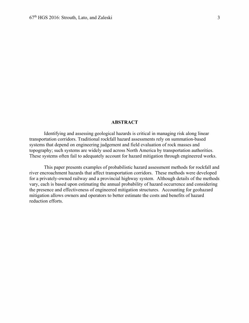
67th HGS 2016: Strouth, Lato, and Zaleski 3
ABSTRACT
Identifying and assessing geological hazards is critical in managing risk along linear transportation corridors. Traditional rockfall hazard assessments rely on summation-based systems that depend on engineering judgement and field evaluation of rock masses and topography; such systems are widely used across North America by transportation authorities. These systems often fail to adequately account for hazard mitigation through engineered works.
This paper presents examples of probabilistic hazard assessment methods for rockfall and
river encroachment hazards that affect transportation corridors. These methods were developed for a privately-owned railway and a provincial highway system. Although details of the methods vary, each is based upon estimating the annual probability of hazard occurrence and considering the presence and effectiveness of engineered mitigation structures. Accounting for geohazard mitigation allows owners and operators to better estimate the costs and benefits of hazard reduction efforts.

67th HGS 2016: Strouth, Lato, and Zaleski 4
INTRODUCTION
Highway and railway transportation agencies have finite resources to manage geologic hazards. In recent decades, transportation agencies have been moving towards proactive methods for managing geologic hazards (1,2). This includes “geotechnical asset management” which uses concepts of risk and life-cycle analysis to manage performance of the transportation corridor (e.g. 3). For rockfall hazards, variations of the Rockfall Hazard Rating System (RHRS) have been widely applied to systematically inventory and prioritize hazardous rock slopes adjacent to transportation infrastructure (1,2).
Many transportation agencies have successfully applied RHRS to obtain consistent and
comparable information for a large number of rock slopes leading to improved allocation of resources for operational improvements, safety improvements, and reduced maintenance costs. Detailed RHRS ratings involve characterization of rock slope geometry, traffic and road geometry, geological conditions, and climate, water, and rockfall history. Scores are assigned to each characterized parameter and the rockfall hazard rating is assigned to the rock slope by summation of the parameter scores. Rock slopes with the highest rating are interpreted to have the highest rockfall risk, and agencies typically prioritize high rated slopes for implementation of rockfall mitigation measures, such as scaling, installation of drape mesh or fences, or improving ditch effectiveness (1,2).
Ideally, mitigated slopes would be rated again after implementing mitigation measures
and the risk reduction achieved would be demonstrated by the updated RHRS rating score. However, the RHRS rating often does not reflect the risk reduction achieved by mitigation, and the benefits of the mitigation are not readily quantified. This creates challenges for transportation agencies that need to compare costs and benefits of mitigation measures, and justify the use of resources.
RHRS scores often fail to account for hazard mitigation because of the summation-based
calculation of the RHRS rating. In summation-based calculations, large changes in a single category score have a relatively small effect on the overall RHRS score. For example, one could nearly eliminate the possibility of rockfall reaching the transportation corridor by construction of a 100% effective ditch or slope covering, but reduce the RHRS score by less than 20%.
This paper presents two examples of hazard assessment systems that overcome this
limitation of RHRS, including a rockfall hazard assessment method developed for a privately-owned railway, and a river encroachment hazard assessment system developed for the Alberta provincial highway network. Each system is based upon estimating the annual probability of the hazard occurring and intersecting the transportation corridor. Each explicitly considers the presence and effectiveness of engineered mitigation structures. Accounting for engineering mitigation allows owners and operators to better estimate their costs and benefits.
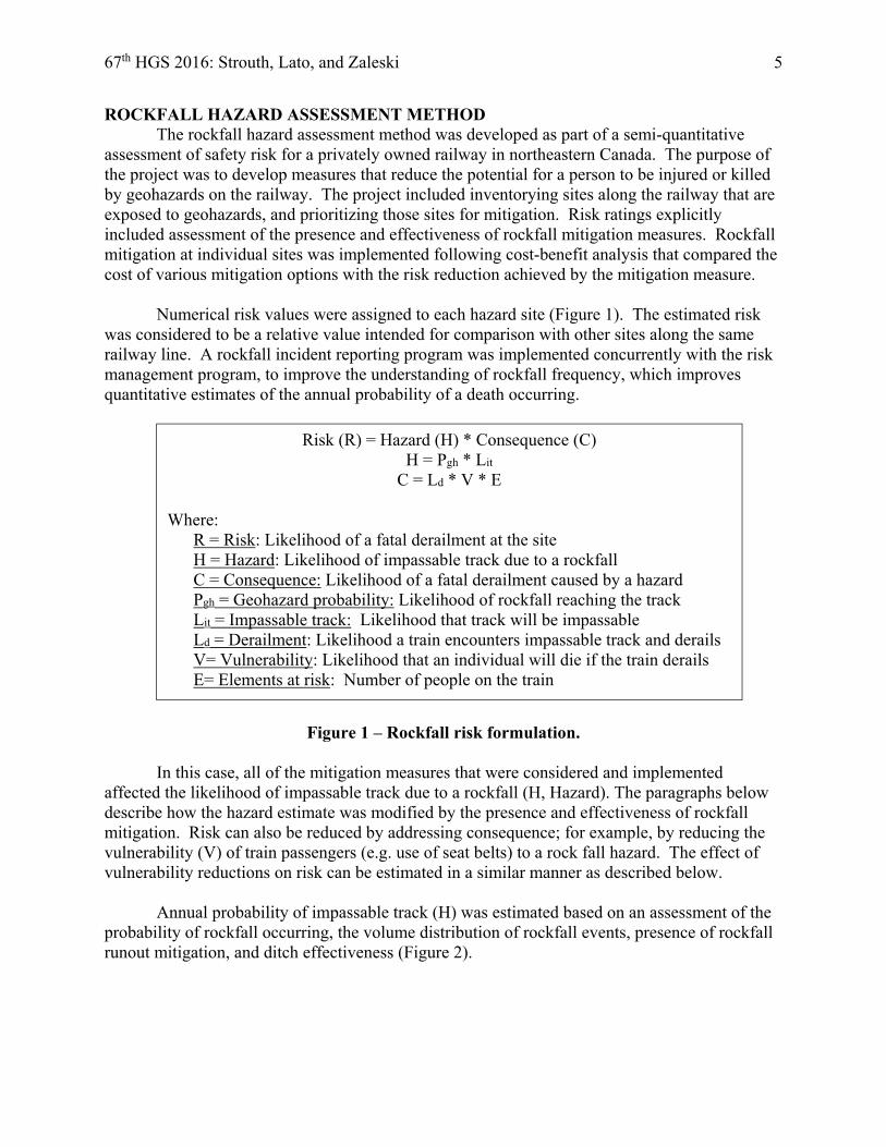
67th HGS 2016: Strouth, Lato, and Zaleski 5
ROCKFALL HAZARD ASSESSMENT METHOD The rockfall hazard assessment method was developed as part of a semi-quantitative
assessment of safety risk for a privately owned railway in northeastern Canada. The purpose of the project was to develop measures that reduce the potential for a person to be injured or killed by geohazards on the railway. The project included inventorying sites along the railway that are exposed to geohazards, and prioritizing those sites for mitigation. Risk ratings explicitly included assessment of the presence and effectiveness of rockfall mitigation measures. Rockfall mitigation at individual sites was implemented following cost-benefit analysis that compared the cost of various mitigation options with the risk reduction achieved by the mitigation measure.
Numerical risk values were assigned to each hazard site (Figure 1). The estimated risk
was considered to be a relative value intended for comparison with other sites along the same railway line. A rockfall incident reporting program was implemented concurrently with the risk management program, to improve the understanding of rockfall frequency, which improves quantitative estimates of the annual probability of a death occurring.
Figure 1 – Rockfall risk formulation. In this case, all of the mitigation measures that were considered and implemented
affected the likelihood of impassable track due to a rockfall (H, Hazard). The paragraphs below describe how the hazard estimate was modified by the presence and effectiveness of rockfall mitigation. Risk can also be reduced by addressing consequence; for example, by reducing the vulnerability (V) of train passengers (e.g. use of seat belts) to a rock fall hazard. The effect of vulnerability reductions on risk can be estimated in a similar manner as described below.
Annual probability of impassable track (H) was estimated based on an assessment of the
probability of rockfall occurring, the volume distribution of rockfall events, presence of rockfall runout mitigation, and ditch effectiveness (Figure 2).
Risk (R) = Hazard (H) * Consequence (C) H = Pgh * Lit
C = Ld * V * E
Where: R = Risk: Likelihood of a fatal derailment at the site H = Hazard: Likelihood of impassable track due to a rockfall C = Consequence: Likelihood of a fatal derailment caused by a hazard Pgh = Geohazard probability: Likelihood of rockfall reaching the track Lit = Impassable track: Likelihood that track will be impassable Ld = Derailment: Likelihood a train encounters impassable track and derails V= Vulnerability: Likelihood that an individual will die if the train derails E= Elements at risk: Number of people on the train

67th HGS 2016: Strouth, Lato, and Zaleski 6
Figure 2 –Hazard probability formulation.
Annual Probability of Rockfall Occurrence (P)
At each site, the annual probability of rockfall is assigned from estimates of typical past rockfall frequency, without considering travel distance or trajectory, as follows:
1.0 – Rockfall has typically occurred several times per year 0.63 – Rockfall has typically occurred about once per year 0.1 – Rockfall has typically occurred once every several years 0.01 – Rockfall has typically occurred less frequently than once per decade
Annual probability of rockfall occurrence was estimated at each site based on field
inspection and the recorded history of rockfall events. Field inspections considered factors such as slope condition (similar to RHRS systems), presence of rocks in the ditch or toe of slope, and presence and effectiveness of rock bolts, pinned mesh, or other slope coverings that reduce the occurrence of rockfall. This parameter also directly accounted for the effects of scaling, in that a slope that had recently been scaled and had few visible loose blocks received a lower probability estimate. The effectiveness of proposed rockfall mitigation measures was assigned subjectively, based on judgement and understanding of the character and scale of the measure.
Ideally, the annual probability of rockfall occurrence would be assigned based on a
record of rockfall events and data that demonstrates the effectiveness of various mitigation measures, but this record is incomplete. Instead, all care was taken to assign parameter values consistently across the project. This method is effective for ranking and prioritizing sites, although it is important that end users recognize the large uncertainties in the assigned values.
Volume Class (V1, V2, V3)
The possibility of the track becoming blocked by a rockfall event depends heavily on the volume (also called ‘magnitude’) of the rockfall event. Typically, at any given site, small rockfall events will occur much more frequently than large events, but the small events are less likely to cause harm. An understanding of the likely magnitude of rockfall events at each site is needed. In this study, three volume classes were considered:
V1 – less than 1 cubic meter, unlikely to block the track V2 – between 1 and 3 cubic meters, could block the track V3 – greater than 3 cubic meters, likely to block the track

67th HGS 2016: Strouth, Lato, and Zaleski 7
The proportion of all rockfall events that would fall within each volume class (V1+V2+V3 = 100%) was assessed for each site, based on visual inspection of the rock slope (e.g. joint spacing, block size, volume of recorded events, volume of rockfall deposits in ditch) and on a typical rockfall frequency-magnitude relationship from literature (4). Hungr et al. (4) present a rockfall frequency-magnitude curve for transportation corridors in Western Canada that corresponds approximately to: V1 (50%), V2 (30%), V3 (20%).
Figure 3 –Schematic rockfall frequency-magnitude relationship.
Runout Mitigation (Mv1, Mv2, Mv3)
The runout mitigation term considers the effectiveness of measures designed to limit rockfall travel distance, including drape mesh, rockfall fences, and earth berms. Values range from 0 to 1. A value of 0.5 indicates that approximately half of the rocks that reach the barrier will pass the barrier, and a value of 0.1 indicates that 10% of rocks that reach the barrier will pass the barrier. A value of 1 is assigned when runout mitigation measures are absent.
Values were assigned based on the expected effectiveness of the existing or proposed measure, and varied for each rockfall volume class. For example, a lightweight rockfall fence may be capable of stopping nearly all small-volume events (Mv1=0.01), but ineffective at stopping large-volume events (Mv3=0.9).
Ditch Effectiveness (Dv1, Dv2, Dv3)
The ditch effectiveness term assesses the likelihood that a rockfall event will travel to the track based on the slope height, slope angle, and ditch geometry. Each slope and ditch was individually assessed. Values were assigned from FHWA design charts (5). The value can range from 0 to 1, and is the inverse of the “Percent Rockfall Retained” reported on the design charts.

67th HGS 2016: Strouth, Lato, and Zaleski 8
For example, a value of 0.1 (indicating that 10% of rocks pass the ditch) would be used for a scenario in which the design chart shows 90% retention for the site’s slope height, slope angle, ditch width, and ditch slope. Likelihood of Impassable Track (Lit) This value represents the likelihood that the rockfall event that reaches the track will make the track impassable to a train moving at a normal track operating speed. A constant value was assigned based on the event volume class, and independent of the site specific conditions, as follows:
Lit(V1) – 0.03 (unlikely) Lit(V2) – 0.3 (likely) Lit(V3) – 0.93 (very likely)
Example Rockfall Hazard Calculation An example calculation is presented below for the rock slope shown in Figure 4.
Figure 4 –Example rock slope.
Step 1: Estimating Rock Fall Probability and Volume Class
Rockfall impact scars were observed at track level, and detachment scars were observed
on the rock slope. No rock bolts or slope mesh were present. Maintenance records indicate that rockfalls have occurred approximately once per year. Annual probability of rockfall occurrence, P, of 0.63 was assigned.
The distribution of potential rockfall volumes in the source zone was estimated by visual inspection, as follows:
Less than 1 m3: 10% Between 1 m3 and 3 m3: 10% Greater than 3 m3: 80%

67th HGS 2016: Strouth, Lato, and Zaleski 9
Typical rockfall frequency-magnitude relationships (4) suggest that smaller-volume events are more likely than larger events. The following distribution was applied to this site:
Less than 1 m3: 50% Between 1 m3 and 3 m3: 30% Greater than 3 m3: 20%
The proportion of rockfall events in each volume class at this particular slope was estimated
by averaging the estimated rockfall volumes and typical rockfall frequency-magnitude values. The annual probability of rockfall in each volume class was estimated as follows:
P*V1 = 0.63 x (0.5 + 0.1)/2 = 0.19
P*V2 = 0.63 x (0.3 + 0.1)/2 = 0.13
P*V3 = 0.63 x (0.2 + 0.8)/2 = 0.32
Step 2: Estimating Spatial Probability of Reaching Track The site had no rockfall runout mitigation, such as drape mesh or rockfall fences, at the time of the initial rating; therefore, 100% of rocks should follow a natural trajectory:
MV1 = 1
MV2 = 1
MV3 = 1
The rock slope height is 28 m with an average gradient of 4V:1H with a 2 m wide flat ditch.
According to the FHWA design guide (5) this ditch has an estimated retention capability of 62% (or 38% exceedance):
DV1 = 0.38
DV2 = 0.38
DV3 = 0.38
Step 3: Estimating the likelihood of impassable track (default values)
L1 = 0.03
L2 = 0.3 L3 = 0.93
Step 4: Estimating the Annual Probability of Impassable Track (H)
Based on Figure 2:
h1 = (0.19 x 1 x 0.38 x 0.03) = 0.002
h2 = (0.13 x 0.38 x 0.3) = 0.011
h3 = (0.32 x 0.38 x 0.93) = 0.113
Therefore:
H = h1 + h2 + h3 H = 0.002 + 0.011 + 0.113 H = 0.126

67th HGS 2016: Strouth, Lato, and Zaleski 10
An annual probability of impassable track of 0.13 associated with rock fall for this specific
rock slope suggests that impassable track may be expected along this railway segment about once every eight years, on average. Maintenance records can be used to calibrate these estimates.
RIVER ENCROACHMENT RISK ASSESSMENT METHOD Encroachment hazards are present where highways are near the outside banks of river
bends (Figure 5). The river encroachment hazard assessment method was developed as part of a semi-quantitative assessment of highway closure risk for the Alberta provincial highway network. The purpose of the project was to reduce the potential for bank erosion or bank slope failures to migrate towards a highway resulting in partial or complete road closure. The complete assessment included inventorying bank erosion sites along the road network, and prioritizing those sites for construction of bank erosion mitigation measures. Risk ratings explicitly included assessment of the presence and effectiveness of bank erosion mitigation measures. It is intended that bank erosion mitigation at individual sites will be implemented following cost-benefit analysis that compares the cost of various mitigation options with the risk reduction achieved by the mitigation measure.
Figure 5 –Examples of encroachment in Alberta.
Encroachment risk was estimated using a quantitative format allowing numerical risk
values to be assigned to each hazard site (Figure 6). The risk estimate was considered to be a relative value intended for comparison with other sites in the highway network. More than 500 sites were rated. Encroachment risk ratings were based primarily on desktop review of geologic maps, Google Earth and Google Streetview imagery, and LiDAR-derived digital elevation models.

67th HGS 2016: Strouth, Lato, and Zaleski 11
Figure 6 – River encroachment risk formulation. Baseline Event Probability (B) The baseline event probability was assigned based on the setback ratio, D, defined as the number of equivalent bank full widths between a river and the road embankment. Distances were measured from orthophotos and LiDAR-derived digital elevation models.
D = d / W (d) is the shortest distance from the channel bank to the toe of the road embankment. (W) is the bankfull width of the main channel.
The baseline encroachment hazard probability assigned to each setback ratio was originally developed from a numerical bank-erosion model that considers grain size and shear stress, which was then calibrated using historical records. The baseline case applies to unconfined, braided or wandering river systems with sand and gravel banks. D B 0 1/5 0.5 1/10 1 1/20 2 1/40 5 1/100 10 1/1000
Risk (R) = Hazard (H) * Consequence (C) H = B*(T*G*S*I*M)
C = V * E
Where: R = Risk: Road closure caused by river encroachment H = Hazard: Likelihood of the river bank reaching the road prism C = Consequence: Duration of road closure and vehicles affected B = Baseline event frequency: Return period of encroachment reaching the road, assuming a braided river system eroding sand and gravel banks. T = Channel type: Channel morphology G = Geometry: Severity of channel bend S = Soil erodibility: Composition of channel bank I = Instability: Evidence of bank or roadway instability M = Mitigation: Existing engineered encroachment mitigation measures V = Vulnerability: Likelihood that roadway is damaged given river erosion E = Exposure: Traffic volume

67th HGS 2016: Strouth, Lato, and Zaleski 12
Channel Type (T) Channel type is controlled by sediment supply and channel gradient. Different channel types have different typical rates of bank erosion. Braided channels tend to have the highest erosion rates, and were considered the baseline case. Other channel types have lower typical erosion rates. The following adjustment factors for channel type were applied:
Braided = 1 Wandering = 0.8 Anastomosing = 0.6 Sinuous = 0.3
Geometry (G) Rivers tend to erode their outer banks at bends. At tighter bends, the river’s flow tends to be concentrated along its outside bank, so most of the erosion typically occurs there. At straight reaches, flow concentration and erosion rate is typically about equal for each bank. The following geometry factors were applied:
Severe bend = 1 Moderate bend = 0.75 Gentle bend = 0.5 Straight = 0.5
Soil Erodibility (S) The rate at which a bank erodes toward a highway depends, in part, on the erodibility of the soil and rock between them. Loose, cohesionless silts, sands, and gravels erode relatively quickly. Soils that are dense or stiff (e.g. tills or pre-glacial deposits compacted by ice loading), cohesive (clays and some silts), or coarse-grained (e.g. talus or riprap) are less erodible. Bank soils were classified by typical grain size and genesis. The classification was informed by orthophoto imagery and published surficial geologic maps. The following soil erodibility factors were applied:
Modern floodplain sand and gravel = 1 Glacial fluvial and fan deposits = 0.8 Modern overbank or till (clay, silt, and sand) = 0.6 Coarse colluvium, talus, or glaciolacustrine clay = 0.4 Bedrock = 0.1
Instability (I) A riverbank or road prism with landslides should erode at a higher rate in a given event than one without, as high flows will undermine those landslides. Existing landslide features, including headscarps, tension cracks, and slide scars were identified on orthophotos and digital elevation models, and the following instability factors were applied.
Evidence of instability = 1.5 No evidence of instability = 1

67th HGS 2016: Strouth, Lato, and Zaleski 13
Mitigation (M) Some sites are protected from encroachment by engineered mitigation structures. Mitigation measures typically reduce the likelihood that a given flood event causes bank erosion that reaches the road prism. Typical mitigation structures include flow control structures (e.g. jetties, riprap, spurs) and bank erosion protection (e.g. river bank armor, vegetated slopes). Orthophotos and Google Maps Streetview images were reviewed to identify existing mitigation structures, and the following mitigation factors were applied.
None = 1 Basic = 0.5 Engineered = 0.25
Vulnerability (V) Vulnerability is the likelihood that the roadway is damaged given that erosion reaches the road embankment. Erosion that reaches the road embankment can cause varying levels of damage to the roadway depending on the channel size and site geometry. Weighting scores were assigned based on estimates of the proportion of typical traffic passage that would be permitted if the road was damaged.
High (Full road closure for more than 24 hours) = 0.9 Moderate (Partial road closure, traffic can pass) = 0.5 Low (Erosion is unlikely to cause traffic interruption) = 0.1
Exposure (E) Exposure describes the number of vehicles affected. In this case the average summer daily traffic volume (number of cars per day) was used. CONCLUSIONS This paper presents examples of multiplication-based, probabilistic geohazard assessment methods. The methods incorporate evaluation of geohazard mitigation measures and have been used to efficiently evaluate hundreds of geohazard sites along transportation corridors. Explicit incorporation of mitigation effectiveness in the assessment allows hazard sites to be rated before and after mitigation implementation, facilitates comparison of cost and benefit of various mitigation alternatives, and allows transportation agencies to demonstrate the benefit of geohazard mitigation in terms of highway performance goals.

67th HGS 2016: Strouth, Lato, and Zaleski 14
REFERENCES: 1. Pierson LA. Rockfall Hazard Rating Systems. In Rockfall: characterization and control,
TRB Miscellaneous Publication, National Research Council, Washington, DC. 2012. pp. 56-71.
2. Pierson LA and Turner AK. Implementation of Rock Slope Management Systems. In Rockfall: characterization and control, TRB Miscellaneous Publication, National Research Council, Washington, DC. 2012. pp. 72-112.
3. Vessely M. Geotechnical asset management: Implementation concepts and strategies. Federal Highways Administration publication No. FHWA-CFL/TD-13-003. 2013.
4. Hungr O, Hazzard J, and Evans SG. Magnitude and frequency of rock fall and rock slides along the main transportation corridors of southwestern British Columbia. Can. Geotech. J. 36: 224-238. 1999.
5. Pierson LA, Gullixson CF, and Chassie R. Rockfall Catchment Area Design Guide – Final Report. Oregon Department of Transportation and Federal Highway Administration. Report No. FHWA-OR-RD-02-04.

UTILITY MAPPING USING MULTICHANNEL 3D GPR ARRAY TECHNOLOGY
Manuel Celaya, PhD Project Manager
Advanced Infrastructure Design 1 Crossroads Drive, Hamilton, NJ 08691-3389 Tel: 609-838-2216 Email: [email protected]
Alexandre Novo, PhD
GeoSystems Business Unit Manager IDS North America Inc
14828 West 6th Avenue, Suite 12-B, Golden, CO 80401 Tel: 303 232 3047 Fax: 720-519-1087; Email: [email protected]
Mark Sray, PE, CME
Senior Associate, Municipal & County Services Hatch Mott MacDonald. Water & Wastewater Division 833 Route 9 North Cape May Court House, NJ 08210
Tel: 609-465-9377 Fax: 609-465-5270; Email: [email protected]
Kaz Tabrizi, PhD, PE Vice President
Advanced Infrastructure Design 1 Crossroads Drive, Hamilton, NJ 08691-3389 Tel: 609-838-2216 Email: [email protected]
Enrico Boi, MSCE
Vice President IDS North America Inc
14828 West 6th Avenue, Suite 12-B, Golden, CO 80401 Tel: 303 232 3047 Fax: 720-519-1087; Email: [email protected]
Prepared for the 67th Highway Geology Symposium, July 11-14, 2016

Celaya, Novo, Sray, Tabrizi and Boi 2
Acknowledgements
The authors wish to gratefully acknowledge the support of Hatch Mott MacDonald and the Municipality of Lower Township in Cape May County, New Jersey, for the assistance and
guidance on this project.
Disclaimer Statements and views presented in this paper are strictly those of the author(s), and do not
necessarily reflect positions held by their affiliations, the Highway Geology Symposium (HGS), or others acknowledged above. The mention of trade names for commercial products does not
imply the approval or endorsement by HGS.
Copyright Notice Copyright © 2016 Highway Geology Symposium (HGS)
All Rights Reserved. Printed in the United States of America. No part of this publication may be reproduced or copied in any form or by any means – graphic, electronic, or mechanical, including
photocopying, taping, or information storage and retrieval systems – without prior written permission of the HGS. This excludes the original authors.

Celaya, Novo, Sray, Tabrizi and Boi 3
ABSTRACT Utility designation and location procedures are critical tasks during excavation operations for construction projects. To avoid project delays and minimize cost overruns, fully identifying and locating all utilities early in the project planning and design process (preferably prior to excavation) is highly desirable.
Utility excavation and test pits are tools extensively used to determine the exact horizontal and vertical location of existing utilities. These methods are expensive and require opening the surface of the pavement. Nondestructive techniques are readily available and minimize traffic disruption. Among these, electromagnetic methods are commonly used for this practice.
Ground Penetrating Radar (GPR) is an electromagnetic method that has been used since
the 1960s for utility detection. Initially, GPR systems included single antenna devices and required highly trained personnel and extensive expertise. Recent developments in the form of GPR array systems and user friendly analysis software have addressed some of GPR’s disadvantages.
In this study a section of a municipal road in New Jersey was comprehensively evaluated
with a high density GPR array system to identify existing utilities and other underground anomalies under the pavement surface. Particularly, the location of a large storm drain pipe within the limits of this project needed to be obtained. A total of 2,600 ft of road and more than 1,000 ft of sidewalks were investigated. The utility suspected of being the storm drain pipe was highlighted and more than three hundred utilities were found. After a cross-check with exiting utility base maps, it was concluded that about 90% of the utilities that were shown on the utility maps were found. Additional utilities that were not displayed on the base map were identified by the GPR array system.

Celaya, Novo, Sray, Tabrizi and Boi 4 INTRODUCTION The lack of reliable underground utility information has long been a troublesome problem for highway engineers. In the United States, department of transportation staff typically utilize consultants to identify the quality of subsurface utility information needed for highway plans, and to acquire and manage that level of information during the development of highway projects. This engineering practice is known as Subsurface Utility Engineering (SUE). SUE has evolved considerably over the past few decades and combines civil engineering, surveying, and geophysics. It utilizes several technologies, including vacuum excavation and surface geophysics. Its use has become a routine requirement on highway projects in many states. Since 1991, the Federal Highway Administration (FHWA) has been encouraging the use of SUE on highway projects as an integral part of the preliminary engineering process (1).
Ensuring a proper and successful application of SUE investigation (which can require much effort and additional expense) is greatly beneficial, because unnecessary utility relocations are avoided, thus reducing costly relocations and project delays. Unexpected conflicts with utilities are minimized or avoided since exact locations of virtually all utilities can be determined and accurately shown on construction plans. Better data reduces construction delays caused by cutting, damaging, or discovering unidentified utility lines and minimizes contractor claims for delays resulting from unexpected encounters with utilities. Moreover, safety is enhanced during excavation or grading work.
There are four recognized quality levels of underground utility information ranging from
Quality Level D (the lowest level) to Quality Level A (the highest level). For example, Quality Level D comes solely from existing utility records or verbal recollections, which are typically unreliable sources. On the other hand, Quality Level A involves the full use of SUE services. It provides information for the precise plan and profile mapping of underground utilities through the nondestructive exposure of these utilities. It also provides the type, size, condition, material and other characteristics of underground features (1). This highest level of accuracy is generally not needed at every point along a utility's path, but only where conflicts with highway design features are most likely to occur. Quality Level B is typically applied throughout the entire project limits.
Quality Level B involves the application of appropriate surface geophysical methods to
determine the existence and horizontal position of virtually all utilities within the project limits. In this case, the information obtained is typically surveyed to project control. It addresses problems caused by inaccurate utility records, abandoned or unrecorded facilities, and lost references. This increases the likelihood that conflicts with existing utilities can be successfully avoided. Information provided by this Level B can assist the design process and produce substantial cost savings.
Different geophysical techniques are readily available for conducting the Quality Level B
utility identification. The proper selection and application of surface geophysical techniques for achieving this Quality Level data is critical. The current version of the American Society of Civil Engineers (ASCE) “Standard Guidelines for the Collection and Depiction of Existing Subsurface Utilities” (2) contains an appendix on surface geophysical techniques that may be useful in the evaluation of providers' equipment lists.

Celaya, Novo, Sray, Tabrizi and Boi 5
The most common geophysical methods for utility location include electromagnetic
methods. Other methods less commonly used are resistivity measurements, magnetic methods, elastic waves (acoustics/sound/mechanical), borehole geophysics, microgravitational techniques, isotopic (radiometric) methods and chemical techniques (3).
Among the electromagnetic methods, pipe and cable locators (time-domain electromagnetics) are the most common instruments for detecting and tracing underground utilities. Conventional pipe-location systems introduce a current onto a pipe or cable, and the associated magnetic field is measured at the surface with an antenna. This equipment is easy to use and has many manufacturers; however, it still requires some level of expertise and the level of success depends on the equipment specifications and the type of utility that needs to be identified. There are many instruments available with general frequencies ranging from 60 Hz to 480 kHz. It may be necessary to have equipment in all of these frequency ranges to effectively detect and trace a particular utility.
Ground Penetrating Radar (GPR) is another geophysical electromagnetic tool in the radio
wave range. The use of GPR research for utility detection began in the 1960s with the introduction of plastic gas pipes. GPR works by sending an electromagnetic pulse into the ground. Some ratio of this pulse signal is transmitted through boundaries and some is reflected from the boundaries back to the receiving antenna. With GPR, detection of target occurs when the target’s (i.e., utility) dielectric constant differs from that of the surrounding soil. A dielectric constant that differs significantly from the surrounding soil would produce the highest reflection. To identify utilities, the frequency spectrum of GPR antennas typically ranges between about 50 MHz and 800 MHz. While GPR has been used to a lesser extent for conventional locating, it is becoming more common as equipment costs drop, ease of use improves and multi-sensor platforms or antenna arrays are being developed.
In this study, a subsurface evaluation was performed on a roadway and sidewalk section
in Lower Township, Cape May County, New Jersey with a multichannel 3D GPR array system. The objective of this investigation was to identify existing and abandoned underground utilities that may exist within the limits of this project. Another objective was to clearly identify the location and depth of a large storm drain pipe. It should be noted that the section investigated was scheduled to be reconstructed, thus reliable utility mapping data was needed. The area of interest included the main lane of Roseann Avenue in Lower Township and a selected area on one of the adjacent sidewalks. The approximate length of the project was about 2,600 ft and the width (curb to curb) of Roseann Avenue was about 32 ft. The area investigated on the sidewalk included a section about 900 ft. long. Overall, a total of three hundred targets were found with the GPR system. Targets that were identified included point targets (i.e., manholes, inlets, others), linear targets (i.e., pipes, utilities) and areas with anomalies (i.e., suspected voids, utilities). The utilities identified were compared to the utility maps available (unknown accuracy) for the area and it was found that 90% of the utilities that were shown on existing utility maps were identified. It is to be noted that the utility base maps consisted of as-built and planned maps of utilities for the area. Additionaly, the location and approximate depth of the storm drain pipe was clearly obtained.

Celaya, Novo, Sray, Tabrizi and Boi 6 METHODOLOGY GPR is a popular non-destructive tool for many different applications (4). Among them, it is routinely used as part of an arsenal of tools to locate and map buried utilities. The standard methodology is based on real-time interpretation of 2D profiles and onsite spray marking of the detected utilities. Rarely, grids are set up for subsequent three-dimensional processing and generation of CAD maps of the detected utilities. These two methods are mainly based on hyperbolae detection; however, not all of these hyperbolae may be related to the presence of utilities, but to other underground features such as tree roots, fractures, cavities, and stones. Some expertise is required to achieve reliable results. One facet of this practice is creating high-resolution plane view GPR images capable of showing utilities as linear features across the survey area, so that someone less familiar with GPR interpretation analysis can regularly interpret them. Multichannel 3D GPR Technology for High-Resolution Images In 2005, full-resolution images using single-channel GPR systems were first published (5). However, the extra time needed for collecting this type of data has minimized its use. Multichannel GPR instruments provide fast full-resolution data recording, however, until the last five years their use had been limited by the quality of the data and complex data processing. Wildly different frequency responses of the multichannel antenna prevented useful amalgamation of the individual profiles into useful images. However, in the last few years, most of the multichannel manufacturers have provided GPR systems where the antenna responses of the individual elements are much closer (6). Among the different hardware providers, Ingegneria Dei Sistemi (IDS) has developed modular multichannel 3D GPR array systems which have greatly improved the speed and areal coverage of the ground together with precise images of the subsurface targets. Such modularity allows for flexible configurations to adapt to different terrains and applications: Highways (7); Sidewalks (8), or Archaeological sites (9). Data Acquisition The equipment used in this study was a multichannel GPR array system marketed as STREAM EM by IDS. The STREAM EM (see Figure 1a) is a dual-frequency (200-600MHz) and dual-polarized (HH and VV) system which acquires full-resolution data (6cm in between profiles). This allows complete surveying while driving the system in only one direction without stopping traffic. The system covers an area about 6 ft. wide with each pass or swath, and can be used up to a speed of 10 mph, thus requiring only a backup attenuator truck to provide Maintenance and Protection of Traffic (MPT). For the sidewalk acquisition, (not suited for the trailer mounted GPR), four antennas of dual-frequency (200-600 MHz) were assembled onto a field survey push-cart as shown in Figure 1b. This system, which contains 4 antennas, was fitted with a GPS RTK system to provide accurate positioning. Data analysis and processing were conducted using advanced processing software specifically designed for an easy and efficient interpretation of the data. Key features include automatic and manual data processing, as well as 2D/ 3D tomography for an immediate visualization of pipes or utilities, and automated data transfer to CAD/GIS maps.

Celaya, Novo, Sray, Tabrizi and Boi 7 Data positioning A crucial issue regarding data collection is positioning. Real-time kinematic (RTK) GPS or robotic total station systems can be interfaced with acquisition software to mark system trajectory in order to correctly position data on the XY plane during the follow-up analysis stage. Integration with Inertial Measurement Systems (IMU) platforms is probably the near future solution for urban environments. For the study presented in this paper, an RTK system with centimeter accuracy was fitted to the GPR system to provide accurate positioning (see Figure 1 for details).
Preferrably, data collection should follow some basic principles: adjacent swaths have to partially overlap in order not to leave any gap and to assure proper mapping of features situated on the edge of adjacent swaths, and trajectories have to be as straight as possible, avoiding any wandering.
a) Multichannel GPR Array System
b) Push-cart GPR System
Figure 1. GPR Systems Used in this Study.
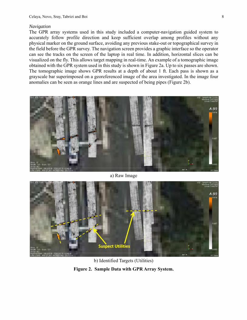
Celaya, Novo, Sray, Tabrizi and Boi 8 Navigation The GPR array systems used in this study included a computer-navigation guided system to accurately follow profile direction and keep sufficient overlap among profiles without any physical marker on the ground surface, avoiding any previous stake-out or topographical survey in the field before the GPR survey. The navigation screen provides a graphic interface so the operator can see the tracks on the screen of the laptop in real time. In addition, horizontal slices can be visualized on the fly. This allows target mapping in real-time. An example of a tomographic image obtained with the GPR system used in this study is shown in Figure 2a. Up to six passes are shown. The tomographic image shows GPR results at a depth of about 1 ft. Each pass is shown as a grayscale bar superimposed on a georeferenced image of the area investigated. In the image four anomalies can be seen as orange lines and are suspected of being pipes (Figure 2b).
a) Raw Image
b) Identified Targets (Utilities)
Figure 2. Sample Data with GPR Array System.

Celaya, Novo, Sray, Tabrizi and Boi 9 SITE DESCRIPTION AND PRESENTATION OF RESULTS Site Description For the purpose of detecting existing utilities and the location of the storm drain pipe, AID used its multichannel 3D GPR technology for an active design project Roseann Avenue in Lower Township, Cape May County, New Jersey. The area of interest included the main lane of Roseann Avenue from Amhurst Road to Clearwater Drive (shown in red in Figure 3). Roseann Avenue carries one lane of traffic for both Eastbound and Westbound directions. In addition, parking lanes are located on both sides of the street. The approximate length of the project was about 2,600 ft and the width (curb to curb) of Roseann Avenue was about 32 ft. The area investigated on the sidewalk included the south sidewalk from Croydon Drive to Clearwater Drive (shown in blue in Figure 3). A 25 ft. swath in the front yards from the face of curb was carried out. The approximate length of sidewalk investigated was 900 ft. It should be noted that the location of the storm drain pipe was suspected to be within the limits of the sidewalk.
The pavement structure within the project limits was unknown, but it was observed that the pavement surface was comprised of flexible pavement. General views of the project site are shown in Figure 4.
Figure 3. Aerial Image of Project Site and Project Limits
Field Test Details and Typical Results Data collection was conducted on the main lane and south sidewalk of Roseann Ave. For the main lane a total of six passes with the Multichannel GPR Array System were conducted to ensure complete coverage of the test area. For the case of the sidewalk, multiple passes were obtained with the push-cart system in both longitudinal and transverse direction to ensure enough coverage. Two days were used to completely scan the project limits. For the GPR Array System, tests were conducted with the GPR system at a speed of about 10 mph. An attenuator truck was used to provide MPT. It should be noted that for each lane-mile of tested area, about 3 GB of data was recorded with the GPR system.

Celaya, Novo, Sray, Tabrizi and Boi 10
After data collection was completed, analysis was carried out with the manufacturer’s
software and results were compiled and summarized. A total of 120 man hours were needed to complete the analysis. Three types of point targets were identified: Point Targets that were associated with manholes, steel covers and inlets, Linear Targets that corresponded to pipes, conduits or linear utilities and areas with Anomalies to identify areas with suspected voids or other anomalies.
A typical example of the data collected with the trailer mounted GPR system is shown in
Figure 5a. Up to six passes are shown on a section of Roseann Avenue. The images shown on the bottom and upper right (depicted in grayscale) correspond to GPR line scans from the array of antennas positioned along the direction of data collection (longitudinal line scan, named as “Cut 3”) and across (transverse line scan, named as “Cut 2”). The horizontal axis is related to linear distance and the vertical axis to depth. On the bottom image (longitudinal line scan), up to three inverted hyperbolae are seen at depths between 2 and 6 ft. These features are associated with utilities crossing transversely beneath the road. It should be noted that the vertex of each hyperbola corresponds to the depth of the top of each utility. An area with unknown anomalies at depths of about 1.5 ft. is also highlighted in the figure. Note that to obtain the depth scale, a subsurface dielectric of 8 was used. This dielectric was adjusted based on ground truth depth of targets provided by the client (total of 4 test pits). With these subsurface properties, GPR signal penetration was found to be about 12 ft. within the limits of this project.
In this study, anomalies were defined as areas where the GPR signal was not definitive
enough to clearly identify targets. An anomaly is clearly seen close to the surface on the upper right image (transverse line scan). This anomaly is associated with a manhole, steel cover, or inlet (strong surface reflection). The image shown on the top (or tomographic view) illustrates a top down view of the area investigated at the selected depth (0.4 ft. in this case). Each pass is shown as a grayscale bar superimposed on a georeferenced image of the area investigated. In this case, the horizontal and vertical axes represent linear distance. The area shown in this image is from 460 ft. to 620 ft. east of Croydon Dr. In the image, the anomaly associated with a manhole is highlighted.
A view from the same location with a depth of about 4 ft. is shown in Figure 5b. In this
case one longitudinal utility is clearly identified in the horizontal line scan (seen as a horizontal band). On the other hand, longitudinal utilities are seen as inverted hyperbolae on the upper right image (transverse line scan). In this case, two inverted hyperbolae are seen. After careful examination and coordination with existing base maps, it was found that the larger hyperbola corresponded to the storm drain pipe. The depth of this utility (vertex of hyperbola) at this location was about 4.1 ft. For the case of the tomographic view, the suspected storm drain pipe is seen as an orange linear feature. Previously selected utilities are also identified as blue lines (for linear utilities) or red polygons (for other anomalies). For the case of the suspected storm drain pipe, a different color (purple line) was selected to identify this utility.
The summary of findings (utilities, manholes, anomalies) for the area selected in Figure 5
is depicted in Figure 6. Four longitudinal utilities (including the storm drain pipe), six transverse utilities, one manhole, and four areas of unknown anomalies are shown.

Celaya, Novo, Sray, Tabrizi and Boi 11
a) View from Roseann Avenue at Amhurst Road, Looking East
b) View from Roseann Avenue at Clearwater Drive, Looking West
c) View from Roseann Avenue at Clearwater Drive, Looking East
Figure 4. General View of the Project Site

Celaya, Novo, Sray, Tabrizi and Boi 12
a) Tomographic, Longitudinal and Transverse GPR Views at 0.4 ft. Manhole, Anomalies and Transverse
Utilities Identified
b) Tomographic, Longitudinal and Transverse GPR Views at 4.1 ft. Longitudinal Utility Identified
Figure 5. Typical Results with the GPR Trailer Mounted System
After careful evaluation and analysis of all GPR passes conducted on the main lane and
sidewalks of Roseann Avenue, results were compiled and summarized. A total of three hundred (300) targets, including suspected utilities, manholes, and other anomalies were found. All findings were combined into an AutoCAD file with the New Jersey State Plane Coordinate system of reference. As previously indicated, all data was georeferenced with centimeter accuracy.

Celaya, Novo, Sray, Tabrizi and Boi 13
Figure 6. Typical Summary of Findings with the GPR Trailer Mounted System
In addition, a georeferenced Google Earth file was prepared separately for easy reference.
This file was provided as a complementary way of representing the data along with the AutoCAD file and this report. In that file, the same color scheme and features used in the GPR software to identify all targets was used. For longitudinal and transverse utilities, blue lines were used, for anomalies red polygons, and for point targets (i.e. manholes, inlets), a push pin was selected. The suspected storm drain pipe was highlighted as a purple line for easy reference. A close up view of all targets found at the intersection of Clearwater Drive and Roseann Avenue (west end of the project) is shown in Figure 7.
Figure 7. Typical Summary of GPR Findings Presented as a Google Earth File

Celaya, Novo, Sray, Tabrizi and Boi 14 CONCLUSIONS In this study a section of a local road and adjacent sidewalk of a municipality in New Jersey were comprehensively evaluated with a high density GPR array system to identify existing utilities under the pavement surface. A total of 2,600 ft long section of road and about 900 ft of sidewalk were investigated. Forty-eight hours of field data collection and 120 man hours of analysis were required to complete the utility mapping of the project limits. Six (6) passes were collected with the trailer mounted GPR system on Roseann Avenue and multiple passes were collected with the push-cart GPR system on the south sidewalk of Roseann Avenue.
It was found that GPR array systems are capable of collecting and detecting utility data in a timely manner. For this study, more than three hundred targets were found with the system. The utility suspected of being the storm drain pipe was also highlighted. After a cross-check with exiting utility base maps, it was concluded that about a 90% success rate was obtained with the GPR system. In this comparison there were some utilities found using the GPR system that were not included in the utility base maps.

Celaya, Novo, Sray, Tabrizi and Boi 15 ACKNOWLEDGEMENTS The authors wish to gratefully acknowledge the support of Hatch Mott MacDonald and Municipality of Lower Township, New Jersey for the assistance and guidance on this study. REFERENCES 1. Federal Highway Administration (FHWA) webpage, Subsurface Utility Engineering:
www.fhwa.dot.gov/programadmin/sueindex.cfm#s01 2. Standard Guidelines for the Collection and Depiction of Existing Subsurface Utilities
American Society of Civil Engineers, Standards ASCE/CI 38-02 (2002). 3. Sterling, R. L. , Anspach, J., Allouche, E., Simicevic, J., Rogers, C. D. F., Weston, K. and
Hayes, K. Encouraging Innovation in Locating and Characterizing Underground Utilities. Strategic Highway research Program Report, SHRP 2 Report S2-R01-RW (2009).
4. Daniels, D. J. Ground Penetrating Radar. The Institution of Engineering and Technology, London, UK, 2004, 726 pp.
5. Grasmueck, M., R. Weger, and H. Horstmeyer. Full-resolution 3D GPR imaging. Geophysics, Vol. 70, No 1, 2005, K12-K19 pp.
6. Novo, A., J. Leckebusch, D. Goodman, G. Morelli, S. Piro, and G. Catanzariti. Advances in GPR Imaging with Multi-channel Radar Systems. Journal of Surveying and Mapping Engineering, Vol. 1, No 1, 2013, pp. 1-6.
7. Simi A., G. Manacorda, M. Miniati, S. Bracciali, and A. Buonaccorsi. Underground asset mapping with dual-frequency dual-polarized GPR massive array. In 13th International Conference on Ground Penetrating Radar, Lecce, Italy, 2010. 1001-1005 pp.
8. Coll, M., A. Novo, C. Simmonds, and G. Morelli. Nueva metodología para cartografiar servicios enterrados bajo aceras mediante georadar multi-canal. In 7AHPGG: Proceedings, San Sebastian, Spain, 2012.
9. Novo A., M. Dabas, and G. Morelli. The STREAM X Multichannel GPR System First Test at Vieil-Evreux (France) and Comparison with Other Geophysical Data. Archaeological Prospection, Vol 19, 2012, 179-189 pp.

Turkey Creek Stream Bank Stabilization,
Mission, Kansas, July 2015
Levi Sutton Engineering Associate II
1290 Enterprise Dr.
Olathe, KS 66051
913-669-0829
Prepared for the 67th
Highway Geology Symposium July 11-14 2016

67th
HGS 2016: Sutton 2
Disclaimer
Statements and views presented in this paper are strictly those of the author(s), and do not
necessarily reflect positions held by their affiliations, the Highway Geology Symposium (HGS),
or others acknowledged above. The mention of trade names for commercial products does not
imply the approval or endorsement by HGS.
Copyright Notice
Copyright © 2016 Highway Geology Symposium (HGS)
All Rights Reserved. Printed in the United States of America. No part of this publication
may be reproduced or copied in any form or by any means – graphic, electronic, or mechanical,
including photocopying, taping, or information storage and retrieval systems – without prior
written permission of the HGS. This excludes the original author(s).

67th
HGS 2016: Sutton 3
ABSTRACT
Turkey Creek is a stream located in the Kansas City Metro area that flows under the US-
69 bridges alongside I-35. The embankment supporting the northbound US-69 bridge has been
suffering erosion damage from the creek and has been regularly monitored by KDOT for some
time.
In the spring of 2014 the erosion became severe enough that the KDOT Bureau of
Structures and Geotechnical Services requested an emergency project to protect the slope with
rip rap while the permanent repair project was finalized. The permanent repair consisted of a soil
nail wall combined with a cast-in-place wall. The emergency repair was completed in the spring
of 2014. The permanent repair project was let in the fall of 2014 and construction began in July
2015.
During construction of the project there were a number of complications that delayed
construction and required contract changes. Some of these were known ahead of time, but others
were discovered after construction began. Known issues were: a massive AT&T utility line that
intersects the wall, limited access to the work area, a cramped work space, and close proximity to
a creek that is prone to flooding. New issues that arose during construction included: an
unusually wet construction season, an area of loose fill rock, and the location of the AT&T fiber
optic line differing greatly from the plans.

67th
HGS 2016: Sutton 4
PROJECT HISTORY:
The US69/I635 highway in the Kansas City Metro area is the primary connection
between the City of Mission and the rest of the Kansas City Metro area. About 70,000 people
travel on this road every day. The bridge over Turkey Creek that connects northbound US 69 to
I-635 is located over a bend in the creek that makes the south embankment highly susceptible to
erosion. This problem has been known to KDOT for some time and was under observation by
the KDOT Bureau of Structures and Geotechnical Services.
Figure 1: Image of Turkey Creek before any construction.
In the spring of 2014 the erosion became so severe that the Bureau of Structures and
Geotechnical Services decided that corrective action was needed. They suggested an emergency
repair in order to stabilize the slope and prevent further erosion damage while a permanent repair
design was finalized. This temporary repair consisted of a large amount of rip rap stone placed
on the embankment. The emergency repair was completed less than a month after KDOT called
for it, and was in place until the summer of 2015 when construction on the permanent repair
started.
Figure 2: Emergency Repair of Embankment

67th
HGS 2016: Sutton 5
PROJECT OVERVIEW:
The permanent repair consists of a Cast in Place (CiP) retaining wall set in front of a soil
nail retaining wall. The design for the CiP wall was finalized by August 2014 and the project was
let in October 2014. The contract was awarded to Philips Hardy as the prime contractor, with
TerraFirm (formerly Judy Company) subcontracted to do the soil nail wall. A preliminary design
for the soil nail wall was included in the contract but with the provision that the soil nail
contractor would need to finalize the design and have it approved by KDOT before work could
start. The preliminary design called for 190 soil nails at 44’ each, for a total of 8,400 linear feet
of soil nails. Due to the instability of the soil, TerraFirm’s finalized design called for 304 soil
nails of varying lengths, for a total of 11,000 linear feet.
KNOWN COMPLICATIONS:
Going into the project there were a couple of known complications that would make
completing the project more difficult: cramped working conditions, close proximity to Turkey
Creek, and an AT&T fiber conduit that intersects the proposed wall.
Of these, the cramped working conditions seemed like they would be the most difficult
thing to deal with. The soil nail wall is located in the embankment just 9 ft in front of the
abutment and only 3 ft from the bottom of the bridge girders. The embankment was too narrow
and too unstable to serve as a work platform for the drill rig. Large vertical fissures in the face of
the embankment made working on or around it too dangerous. Even if the embankment was
stable, it was still too narrow to work on. The embankment only extended 9 feet from the front of
the soil nail wall before dropping off to form a vertical face and TerraFirm needed 18 ft in order
to operate their drill rig.
Figure 3: Embankment drop off and growing crack.
In order to fix both of these issues, Philips Hardy placed a large amount of rip rap stone
against the face of the embankment in order to prevent it from collapsing and to widen the area
that TerraFirm had to work on. This rock would be later used as the rip rap surrounding the walls

67th
HGS 2016: Sutton 6
when the project was finished, (after being cleaned). In addition to those issues, there was also a
lack of vertical space when working on the first row of nails. The distance from the bottom of the
bridge girders to the excavated work area was only 9 feet. The drill rig had no issues working in
this space, but the excavator operators had to be very mindful of the bridge girders when they
were excavating for the first couple lifts.
Figure 4: Rip rap placed to create a workable area.
Figure 5: Work area for top row of nails.
While the operator did a good job of avoiding the girders on the first couple rows of soil
nails, he did slip up once on the 3rd
row. While excavating for the 4th
row, the excavator bucket
caught one of the old timber piles that were left from when the bridge was built (see Figure 3
above), and when the pile snapped it knocked the excavator arm up into one of the girders. The
damage to the girder was minor; no rebar was exposed, and it was repaired before the project
was completed.

67th
HGS 2016: Sutton 7
While the lack of space was expected to be the worst issue the contractor faced, it turned
out to be not as stressful as anticipated. As the project progressed and the contractor excavated
more and more rock, the size of the work area continued to increase. After the first row was
completed, there really wasn’t an issue with space when working under the bridge anymore. So
what was initially assumed to be a major issue was more of a temporary inconvenience.
While the cramped work space wasn’t as difficult as anticipated, the AT&T conduit and
Turkey Creek proved to be much more difficult to deal with. Because the soil nail wall and CiP
wall footing extended below the creek level, the plans called for temporary shoring to keep the
creek out of the work area. But temporary shoring couldn’t be installed because the creek bed is
solid shale on top of limestone; there wasn’t any way the contractor could drive metal sheeting in
deep enough to hold back the creek. Instead, the contractor came up with a way to use the unique
site conditions to divert Turkey Creek without driving metal sheeting.
The section of Turkey Creek that was adjacent to the work area has a very low flow rate
when not flooding, but the water pools up to 12 feet deep right under the bridge. Most of that
water just sits there like a pond and the small trickle of water flowing in flows right over the top
and over the natural rock berm on the downstream side. Philips Hardy decided that they would
use an inflatable damn to block the small amount of flow, the dam sat on top of three 12-inch
steel pipes that connected to a flume chute that would transport the water flow past the work site,
and then they would use two 6-inch water pumps to pump the standing water over the natural
rock berm. This set up could only handle the normal flow of Turkey Creek; it couldn’t handle the
flow after even a mild rain event. If there was rain in the forecast then the system would need to
be removed and reinstalled after the flood water receded.
Figure 6: Dam and flume system fully installed.
In addition to this, when the contractor excavated for the last 2 rows of soil nails they
only excavated wide enough for the drill rig to get down to the right elevation, (about 35 feet for
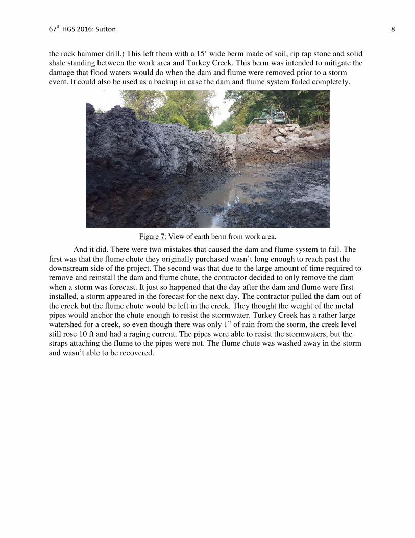
67th
HGS 2016: Sutton 8
the rock hammer drill.) This left them with a 15’ wide berm made of soil, rip rap stone and solid
shale standing between the work area and Turkey Creek. This berm was intended to mitigate the
damage that flood waters would do when the dam and flume were removed prior to a storm
event. It could also be used as a backup in case the dam and flume system failed completely.
Figure 7: View of earth berm from work area.
And it did. There were two mistakes that caused the dam and flume system to fail. The
first was that the flume chute they originally purchased wasn’t long enough to reach past the
downstream side of the project. The second was that due to the large amount of time required to
remove and reinstall the dam and flume chute, the contractor decided to only remove the dam
when a storm was forecast. It just so happened that the day after the dam and flume were first
installed, a storm appeared in the forecast for the next day. The contractor pulled the dam out of
the creek but the flume chute would be left in the creek. They thought the weight of the metal
pipes would anchor the chute enough to resist the stormwater. Turkey Creek has a rather large
watershed for a creek, so even though there was only 1” of rain from the storm, the creek level
still rose 10 ft and had a raging current. The pipes were able to resist the stormwaters, but the
straps attaching the flume to the pipes were not. The flume chute was washed away in the storm
and wasn’t able to be recovered.
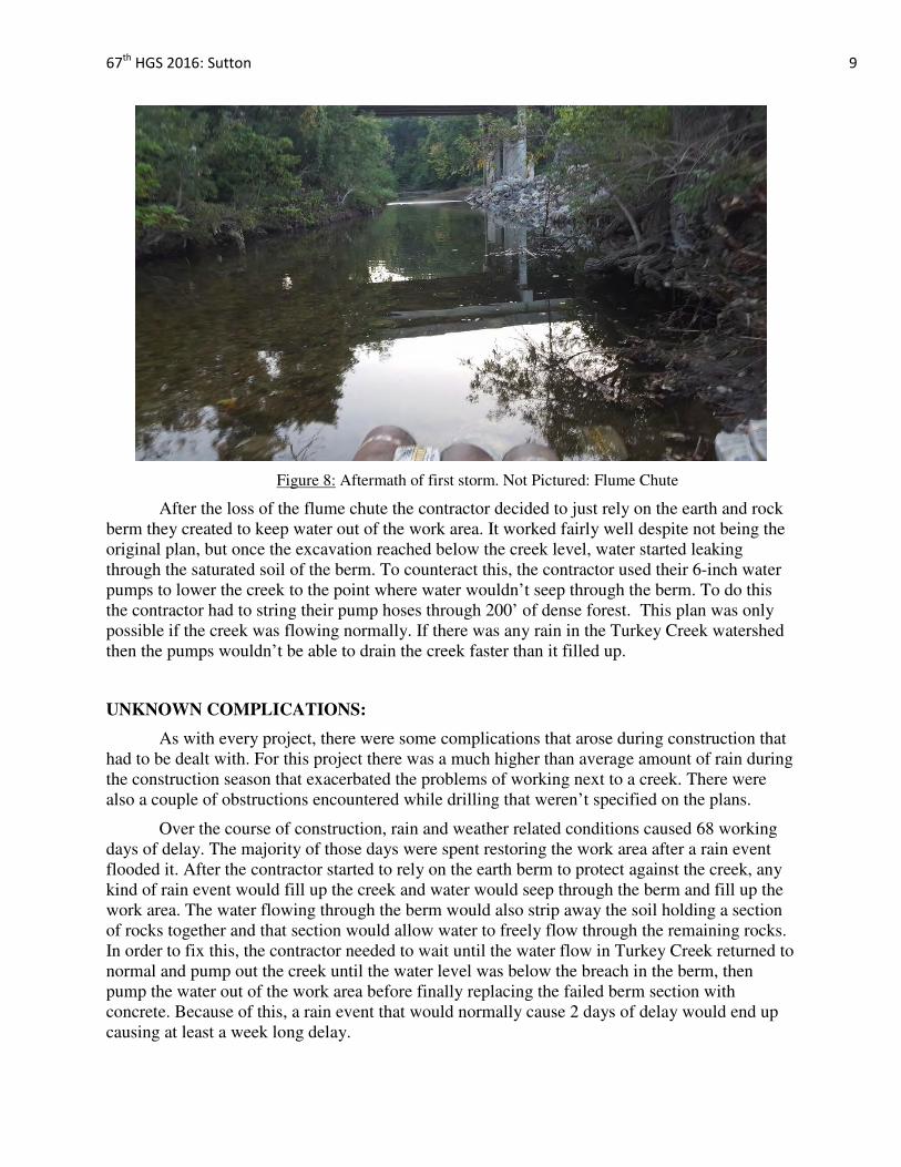
67th
HGS 2016: Sutton 9
Figure 8: Aftermath of first storm. Not Pictured: Flume Chute
After the loss of the flume chute the contractor decided to just rely on the earth and rock
berm they created to keep water out of the work area. It worked fairly well despite not being the
original plan, but once the excavation reached below the creek level, water started leaking
through the saturated soil of the berm. To counteract this, the contractor used their 6-inch water
pumps to lower the creek to the point where water wouldn’t seep through the berm. To do this
the contractor had to string their pump hoses through 200’ of dense forest. This plan was only
possible if the creek was flowing normally. If there was any rain in the Turkey Creek watershed
then the pumps wouldn’t be able to drain the creek faster than it filled up.
UNKNOWN COMPLICATIONS:
As with every project, there were some complications that arose during construction that
had to be dealt with. For this project there was a much higher than average amount of rain during
the construction season that exacerbated the problems of working next to a creek. There were
also a couple of obstructions encountered while drilling that weren’t specified on the plans.
Over the course of construction, rain and weather related conditions caused 68 working
days of delay. The majority of those days were spent restoring the work area after a rain event
flooded it. After the contractor started to rely on the earth berm to protect against the creek, any
kind of rain event would fill up the creek and water would seep through the berm and fill up the
work area. The water flowing through the berm would also strip away the soil holding a section
of rocks together and that section would allow water to freely flow through the remaining rocks.
In order to fix this, the contractor needed to wait until the water flow in Turkey Creek returned to
normal and pump out the creek until the water level was below the breach in the berm, then
pump the water out of the work area before finally replacing the failed berm section with
concrete. Because of this, a rain event that would normally cause 2 days of delay would end up
causing at least a week long delay.

67th
HGS 2016: Sutton 10
Figure 9: Work area before a rain event.
Figure 10: Work Area after a rain event.
This wait-and-repair process happened five times during the course of the project. The
first time was on October 24, 2015 when a storm caused the first breach in the berm. Restoring
the work area to a functional state took until November 6, 2015. The second and third times
happened on November 17th and November 26th
. On November 17th
a very strong thunderstorm
caused Turkey Creek to actually overtop the berm instead of flowing through it. It took until
November 25, the Wednesday before Thanksgiving, to restore the work area, but over the
holiday weekend it stormed again and re-flooded the site before any work could be done. It

67th
HGS 2016: Sutton 11
wasn’t until December 6th
that the contractor was able to restore the site and perform any work.
They were then able to work for a full week and were able to pour the first part of the footing for
the CiP wall. Then over the weekend of December 12th
it rained again and flooded the site for the
fourth time.
Figure 11: Turkey Creek frozen
Figure 12: Work area frozen.
For the next two weeks the contractor tried their best to lower the water level of the
creek, but they weren’t able to make any progress. They decided to wait until after the Winter
Holiday Period, December 23rd
to January 3rd
, to try again. They resumed pumping on January
4th
and were able to make some progress, but two days later on the 6th
it rained for four straight
days. The Monday after the rain, Jan. 11th
, everything froze. The creek, the work area, even the
hoses for the pumps were all frozen solid. The contractor couldn’t operate the pumps without

67th
HGS 2016: Sutton 12
damaging them, and they couldn’t remove the frozen hoses without driving heavy machinery
through the forest the hoses were laid in.
Figure 12: Left: Hose for one of the pumps. Middle: The forest the hoses are laid in. Far Right: Project
work area.
So their only choice was to wait for the hoses to thaw out naturally. And since the
contractor couldn’t dewater the project while everything was frozen, construction halted until the
project thawed and the forecasted temperatures were consistently above freezing. This didn’t
happen until Feb. 12th
, a month later. Once the pump hoses thawed the contractor was able to
pump out the water and restore the project site to a workable condition by the end of the week.
After they returned to work they were able to build the bottom half of the CiP wall and backfill it
above creek level before another rain event delayed work. During construction of the remaining
part of the CiP wall, and the other work items, there were no further complications encountered
and the project was completed without incident.
The other unexpected complication was the discovery of a pocket of loose rock fill when
excavating for the 3rd
row of soil nails. The drill rig the contractor was using was intended for
use in soil that’s easy to drill through and doesn’t collapse when the auger is removed. The clay
soil they were previously drilling through was perfect for this, but the new rocky fill took them
twice as long to drill through and then the holes would collapse as soon as they pulled the auger
out. They tried using a couple different auger types they had on hand, but none of them were able
to perform well enough to meet the KDOT specifications for drilling. They ended up renting a
dual string drill rig from California that was able to use cased augers. The plan was that the
casing would hold the hole open while the soil nail was installed and would be removed as grout
was poured in the hole.
While the dual string drill was able to keep the hole open after it was drilled, it also took
longer to drill the holes than the original drill rig. Using the original drill rig, the contractor could
drill a 40’ hole in about 30 minutes. But using the dual string drill it took 2.5 hours for each hole.
On top of that, the grout the contractor used was thin enough that it seeped down through the

67th
HGS 2016: Sutton 13
rock fill instead of filling the hole. Instead of using 2/3 yd3
of grout per hole, it took over 3 yd3
for each hole in the top row in the rock fill. In the lower section of the rock fill all of the grout
actually bound the entire section of fill into a solid piece. This allowed the contractor to use their
hammer drill to punch through it without needing to use the slow dual string drill.
Figure 13: Solidified section of rock fill.
Figure 14: Close up of rock fill grouted together.

67th
HGS 2016: Sutton 14
AT&T UTILITY CONDUIT COMPLICATIONS:
Going into the project the AT&T utility conduit was expected to be a problem, but no one
realized just how big a problem it would actually be. Before the design was finalized, KDOT
hired a surveying contractor to measure the elevation of the conduit at various points in order to
complete the design. That contractor wasn’t allowed to measure the elevation of the conduit
within the project limits because the slope it was under was too unstable to put equipment on.
But they were able to locate and measure the conduit on the north side of Turkey Creek and
along the road at the top of the embankment south of the project. The results of these shots
showed the conduit snaking towards Turkey Creek from the north, dipping under the creek bed,
and then showing up 200 feet further south next to the highway. The 200-foot survey gap
contains the entirety of the project limits. The plans show an assumption that the conduit makes a
straight line between the 2 points on either side of the project, but that alignment was unlikely
when compared to the rest of the conduit. The plans also made it explicitly clear that the
location shown was an estimate and that the contractor would need to field locate the conduit in
order to work around it.
Figure 15: The stations of the measured elevations along US 69. Marked Area: The project limits.
Based on the locations available, it was clear that even though the conduit intersects the
wall in the bottom two rows, it sloped up drastically behind the wall and could possibly be in the
path of the soil nails in rows 4 through 8. Because of this, the contractor needed to confirm the
location and the depth of the conduit at several locations behind the wall in order to ensure they
wouldn’t drill into it. This proved to be extremely difficult. Utility locators were brought out to
the project three times to mark out the location. The first time their markings were nothing like
what the plans and existing utility flags indicated, so they were called out a second time to verify
the first. But the second time their marks were much closer to what the plans showed so they
were called out for a third time just to be absolutely sure. The third time their marks matched
what they located the second time so those were what the contractor worked with. The locators
weren’t able to legally provide a depth using their sensor, so that responsibility fell on the prime
contractor. They decided that the best method of confirming the depth and location of the conduit
was to simply excavate down until they found it. The conduit is encased in 3-inches of concrete,
so if the drill hit it there theoretically wouldn’t be any immediate damage to it. After a lot of
work (and safety briefings) the contractor was able to excavate two sections of the conduit on the
slope behind the wall. They were also able to locate a third section of it in front of the wall.

67th
HGS 2016: Sutton 15
While the prime contractor was locating the conduit, the wall contractor continued to
work. Since the conduit was encased in concrete they would have a lot of warning before they
damaged it. The augers they used were capable of drilling through rock/concrete, but not fast
enough to go through 3-inches of concrete with warning. So the drilling contractor decided that
they would continue to drill in areas where the conduit might be, but if they hit something solid
they would stop immediately and move on to the next hole until they could be certain it wasn’t
the conduit. For the first 3 rows, they didn’t encounter any obstructions while drilling and they
were able to drill without problems. On the 4th
row they ran into obstructions 20’ behind the wall
on the last 5 nails. Fearful that the obstruction was the conduit, the contractor decided to not drill
through it. By the time they got to the 5th
row the conduit location was confirmed and there were
no issues.
Figure 16: Slope behind the soil nail wall.

67th
HGS 2016: Sutton 16
Figure 17: The 3 pot holes excavated on the slope. The conduit was found in only the closest 2.
Figure 18: The conduit at the bottom of the excavation.
Once the prime contractor confirmed those three locations, they had a surveyor measure
the elevation and location of the conduit and sent that information to the soil nail wall design
contractor. Their engineers changed the design of the wall in order to account for the actual
location of the utility conduit. The design change consisted of cutting off the first column of nails
on the east end of the wall and angling the next column of nails 15° away from the duct bank to
avoid hitting it. This plan was submitted to and approved by KDOT in September 2015. After
this plan was approved and everyone involved was satisfied that hitting the conduit was not a
concern, the rest of the drilling operation progressed without major incident.

67th
HGS 2016: Sutton 17
Figure 19: Utility conduit intersecting the soil nail wall.
COMPLETED PROJECT:
Construction of the soil nail wall was started on July 7, 2015 and was completed on
November 13, 2015. Construction of the cast-in-place wall began on November 16, 2015 and
finished on March 28, 2016. The other work items: backfilling between the walls, placing rip rap
stone around the walls, final grading, seeding, and the project punch list were all completed on
April 28, 2016.
Figure 20: View from the west of the completed project.

67th
HGS 2016: Sutton 18
Figure 21: View of the front of the cast-in-place wall.
Figure 22: View between soil nail wall and CiP wall.

67th
HGS 2016: Sutton 19
Figure 23: View from east side of the walls.

D3 Rockfall Mitigation Project
Interstate 15, Helena to Great Falls, Montana
Benjamin George, P.E., C.E.G., R.G. Landslide Technology
10250 SW Greenburg Road, Suite 111 Portland, Oregon 97223
503-452-1200 [email protected]
Brent Black, C.E.G., R.G. Landslide Technology
10250 SW Greenburg Road, Suite 111 Portland, Oregon 97223
503-452-1200 [email protected]
John Sharkey, P.G. Montana Department of Transportation – District 3 Geotechnical
2701 Prospect Avenue Helena, MT 59620
406-444-6286 [email protected]
Prepared for the 67th Highway Geology Symposium, July 2016

67th HGS 2016 – George, Black & Sharkey
Acknowledgements
The authors would like to thank the individuals for their contributions in the work described:
Blair Nordhagen – Montana Department of Transportation Randy Aafedt – Montana Department of Transportation Jim Sullivan – Montana Department of Transportation Ben Lavoie – Montana Department of Transportation
April Gerth – Robert Peccia & Associates Trish Bodlovic – Robert Peccia & Associates
Kevin Severson – Landslide Technology Collin McCormick – Landslide Technology
Disclaimer
Statements and views presented in this paper are strictly those of the author(s), and do not necessarily reflect positions held by their affiliations, the Highway Geologic Symposium (HGS), or others acknowledged above. The mention of trade names for commercial products does not
imply the approval or endorsement by HGS.
Copyright
Copyright © 2016 Highway Geology Symposium (HGS)
All Rights Reserved. Printed in the United States of America. No part of this publication may be reproduced or copied in any form or by any means – graphic, electronic, or mechanical,
including photocopying, taping, or information storage and retrieval systems – without prior written permission of the HGS. This excludes the original author(s).

67th HGS 2016 – George, Black & Sharkey
ABSTRACT
Numerous rock slopes adjacent to Interstate 15 (I-15) between Helena and Great Falls, Montana have a history of hazardous rockfall activity requiring high levels of maintenance. The Montana Department of Transportation (MDT) is in the process of reducing the rockfall hazards in this corridor. In January 2011, MDT Geotechnical Section evaluated historical performance and existing conditions of the rock slopes in the corridor to develop rockfall ratings for prioritizing mitigation.
MDT retained Landslide Technology (LT) of Portland, Oregon to conduct an independent rockfall evaluation of the corridor, and 15 sites were chosen for mitigation. LT developed conceptual mitigation options for each site. MDT selected mitigation options for development of final designs and divided the project into three phases to accommodate funding. Final design work began in 2014 and is ongoing.
Mitigation includes slope scaling, rock bolting, draped mesh, rockfall attenuators, flexible rockfall barriers, and catchment area improvements via rock slope excavation. The development of temporary rockfall protection and traffic control designs was a significant challenge given the vital nature of the I-15 corridor and MDT’s requirement to perform the majority of the work, including scaling under live traffic.
Construction of Phase 1 began in 2015 and was completed in June of 2016. Phase 2 began construction in the spring of 2016 and is projected to be completed by the fall of 2016. LT provided construction engineering (CE) services for Phase 1 and is currently providing CE on Phase 2. LT is developing final plans, specifications and engineer’s estimate for the Phase 3 designs, which is currently projected to be let for construction in 2017.
As with any design and construction project, several lessons have been learned on this project including items such as: unique nature observation of construction efforts for rockfall mitigation measures

67th HGS 2016 – George, Black & Sharkey 1
INTRODUCTION
The District 3 (D3) Rockfall Mitigation project is located on Interstate 15 (I-15) in northern Lewis & Clark and southern Cascade Counties, Montana (Figure 1). I-15 is classified as a National Highway System Interstate and as such is a critical north-south corridor for travelers and commerce. The project begins near the Sieben Ranch at approximate mile post (MP) 218.0 and extends for roughly 27.5 miles ending near Hardy Creek Hill. Slopes within the corridor have a history of hazardous rockfall activity and require a high level of maintenance. Due to the critical nature of I-15, the Montana Department of Transportation (MDT) is reducing rockfall hazards within the corridor.
Figure 1 – Vicinity and Location Map.

67th HGS 2016 – George, Black & Sharkey 2
Background
The purpose of the project is to increase the safety of the traveling public by reducing the potential for rockfall along I-15. MDT’s design goal for this project required mitigation measures that are capable of preventing 93% of possible rockfalls from reaching the highway (or 93% rockfall retention in the roadside ditch). Retention of rock is measured as the number of simulated rocks passing the edge of the travel lane (i.e. fog line). Given that I-15 is such a critical north-south corridor for travelers and commerce in Montana, another important consideration was to limit traffic disruption and delays during construction of the rockfall mitigation measures.
Overview of Rockfall Hazards
Rockfalls are naturally occurring hazards below steep rock slopes or road cuts. They are characterized by the rapid falling of rock blocks that become loose due to natural processes such as tree movement in the wind, root growth, ice jacking, hydrostatic pressure in cracks, loss of support due to differential weathering, and/or loss of strength along discontinuities (natural or man-made breaks in the intact rock) from weathering and creep (1).
Methods of rockfall mitigation typically fall into three categories, stabilization, protection, and avoidance. Stabilization measures include holding blocks in place or removing them in a controlled manner to eliminate the hazard. Protection measures are used to intercept and control rocks that have come loose and are actively falling. Avoidance measures include relocating the roadway out of harm’s way, but this option is generally impractical for most situations due to the cost and Right of Way restrictions.
For many rock slopes, it may be impractical to stabilize all potentially unstable rocks. In these situations, the likelihood of rocks reaching the road should be evaluated and reasonable protection measures considered. In either case, the consequences of the hazards and cost of continued road maintenance should be weighed against the cost of mitigation. Typically, a combination of stabilization and protection measures provide an optimal combination of hazard reduction and lower maintenance frequency based on the required investment.
Project Development
In early 2011, MDT’S Geotechnical personnel evaluated rock slopes along I-15 from Sieben Ranch to Hardy Creek Hill to develop ratings for potential rockfall hazard. MDT maintenance staff were met on-site to provide historical perspectives on the frequency and magnitude of rockfall events. MDT retained Landslide Technology (LT) of Portland, Oregon to conduct an independent evaluation of the slopes and potential rockfall hazard ratings. LT’s ratings were based on scores reported in MDT’s rockfall hazard classification and mitigation system (2), site observations of geologic conditions and rockfall potential, maintenance ratings, and conceptual mitigation measures and costs. A comparison of the two evaluations was provided to the District 3 office for review. Sites that received a 1 or 2 rating were selected for further project development, including 13 sites. Ratings were on a scale of 1 to 5, representing high to low potential hazard. Field review of the selected sites resulted two additional sites being selected based MDT maintenance input. The 15 sites considered in the project are detailed on Table 1.

67th HGS 2016 – George, Black & Sharkey 3
In late 2012 through 2013, preliminary information was collected relevant to the geotechnical and materials issues associated with the project. This work included a review of existing geologic and geotechnical information, delineation of rockfall mitigation limits at the 15 sites, helicopter reconnaissance for collection of aerial oblique images, site reconnaissance to perform geologic and geotechnical evaluations, specialized photogrammetry to collect geologic discontinuity information, installation of crackmeters on key larger blocks and rock columns at select sites for stability monitoring, laboratory testing of rock samples, and geotechnical analyses of the gathered information.
Table 1: Rock Slope Site Information
Site No. Mile Post MDT
Rating LT Rating
Approx. Length1 (feet)
Approx. Height1
(feet)
Approx. Northing
Approx. Easting
1 218.0 NB 1 1a 650 150-200 979302 1314123 2 218.2 NB 1 1a 520 250-275 980085 1314763 3 218.4 NB 1 1 560 300-325 980600 1315265 4 218.5 SB 2 2 450 150-190 981728 1315105 5 219.5 SB 1 1 930 175-200 986640 1313856 6 220.1 SB 2 2 960 70-190 988891 1312812 7 223.0 SB 2 2 910 140-170 1000602 1321214 8 225.4 SB 1 1 990 150-160 1011098 1325807 9 227.0 SB 2 2 1,350 130-200 1014915 1329853 10 238.5 NB 2 2 395 200 1056617 1365629 11 242.5 NB 2 1 1,015 250 1061957 1384595 12 244.5 NB 2 1a 620 370 1067437 1389445 13 244.7 NB 2 2 900 275 1067793 1389996 14 245.1 NB 2 2 400 50-160 1067968 1390237 15 245.5 NB 2 2 1,120 100-160 1069932 1392353
1Site lengths and heights delineated by LT and varied from the original approximate lengths and heights determined by MDT.
In early 2014 the project designs were advanced from conceptual to final design. Additional field reconnaissance was conducted to: evaluate if conditions had changed since 2012, confirm preliminary interpretations, and finalize conceptual rockfall mitigation designs. The selected conceptual mitigation options were reviewed at each site for effectiveness as compared to any changes in the rockfall activity and constructability of the mitigation element. The mitigation measures that were selected for final design are included on Table 2. All steel products were required to be American made and stained with a weathering agent to minimize visual impacts in the scenic canyon.
As requested by MDT planned scaling efforts and targets were reviewed to estimate the possibility of reducing this quantity to decrease the impacts of these activities on the traveling public since fewer temporary traffic delays were desired. This reduction also provided more cost efficient final designs. Traffic control options were reviewed in an attempt to optimize the cost

67th HGS 2016 – George, Black & Sharkey 4
of traffic control measures by grouping the sites. Sites with similar proposed mitigation measures were also grouped together in an attempt to maximize efficiency by process consistency (selection of a single specialty contractor).
During final design the project was split into three units to accommodate available funding and traffic control concern. Unit #1 included Sites 1-6 (construction began in 2015), Unit #2 included Sites 8, 11, and 12 (construction began in early 2016), and Unit #3 included Sites 7, 9, 10, 13, 14 and 15 (construction to be determined).
Table 2: Selected Rockfall Mitigation Measures
Site No. Rockfall Mitigation Phase (Construction Season) 1 Flexible Rockfall Barrier Phase 1 (2015-2016)
2 Scaling, Rock Bolts, Rockfall Attenuator Phase 1 (2015-2016)
3 Scaling, Rock Bolts, Rockfall Attenuator Phase 1 (2015-2016)
4 Scaling, Rock Bolts, Rockfall Attenuator, Draped Mesh Phase 1 (2015-2016)
5 Scaling, Draped Mesh Phase 1 (2015-2016)
6 Scaling, Draped Mesh Phase 1 (2015-2016)
7 Scaling, Draped Mesh, Concrete Barrier Rails Phase 3 (TBD)
8 Scaling, Rock Bolting, Rock Slope Excavation Phase 2 (2016)
9 Scaling, Rockfall Attenuator, Draped Mesh Phase 3 (TBD)
10 Scaling, Concrete Barrier Rails Phase 3 (TBD)
11 Scaling, Rock Slope Excavation Phase 2 (2016)
12 Scaling, Rock Slope Excavation, Flexible Rockfall Barrier Phase 2 (2016)
13 Scaling, Rock Bolts, Rockfall Attenuator Phase 3 (TBD)
14 Scaling, Rock Bolts, Rockfall Attenuator Phase 3 (TBD)
15 Shear Pins Phase 3 (TBD)

67th HGS 2016 – George, Black & Sharkey 5
GEOLOGIC AND GEOTECHNICAL EVALUATIONS
The sites selected by MDT were evaluated for rockfall potential by conducting a literature review, performing field reconnaissance, and conducing geotechnical analyses. Several techniques were employed on this project to help define the geologic character including structural mapping, joint set analysis, kinematic analysis and rock mass rating. A description of the regional geology and the analyses that were undertaken is offered below.
Regional Geology
The geology of the project can be divided into two sections: a southern section, which includes Sites 1 (MP 218.0) through 7 (MP 223.0) and a northern section, which includes Sites 8 (MP 225.4) through 15 (MP 245.5).
The southern section consists of the Precambrian Belt Supergroup sedimentary rocks, which are the northern extent of the Big Belt Mountains and the Belt Sedimentary Group (Figure 2) (3). Along the project corridor, the rocks mainly consist of argillites and thin beds of quartzite of the Spokane and Greyson Formations of the middle Proterozoic. They are recognizable by their burgundy-red and pastel-green colors for the Spokane Formation and dark-gray to light greenish-gray for the Greyson Formation. The bedding remains gently dipping overall with thrust faults and anticline and syncline structures trending generally NW-SE.
The northern section consists of Cretaceous clastic volcanic rocks and ash-flow tuffs, which overly the sedimentary rocks with exposures of soft shale and sandstone (Site 8 - MP 225.4); Cretaceous latites (Site 9 - MP 227.0); and rocks of the Adel Mountain Volcanics for the remaining sites (Figures 3 and 4), (4)(5). The Adel Mountain Volcanics are dark-grayish red, brownish-red, and dark-grayish green in color. The shonkinite units are made up of intrusive rocks and flows with porphyritic augite. Also included are purplish-gray to gray volcanic conglomerates with rounded to subrounded clasts of the shonkinite rock that vary in size from coarse sand to approximately two-foot diameter boulders and grey monzonite intrusive rock.
Field Reconnaissance
Several reconnaissance efforts were performed by LT representatives during 2012 and 2013. The objectives of the site visits were to: delineate the slope sections, evaluate local topography and geology, perform specialized photogrammetry, install monitoring instrumentation, collect geologic structural data, determine potential rockfall parameters (i.e. block sizes, slope properties) for computer simulations, observe existing ditch/fallout area geometries, and evaluate catchment effectiveness. During the reconnaissance and structural mapping, different rock units were characterized using standard description methods and the Rock Mass Rating (RMR) system. Hand samples were collected for laboratory testing to assist with RMR classifications. The type, frequency, orientation, spacing, persistence, and condition of rock discontinuities were measured and recorded. Potentially unstable rock blocks were evaluated and potential failure mechanisms estimated. Observed groundwater and seepage conditions were documented.

67th HGS 2016 – George, Black & Sharkey 6
Figure 2 – Regional geology surrounding Sites 1 through 8 (3).

67th HGS 2016 – George, Black & Sharkey 7
Figure 3 – Regional geology surrounding Site 9 (4).

67th HGS 2016 – George, Black & Sharkey 8
Figure 4 – Regional geology surrounding Sites 10 through 15 (5).

67th HGS 2016 – George, Black & Sharkey 9
Structural Mapping and Analysis
The presence, orientation, and condition of discontinuities in a rock slope have a major influence on the rockfall potential. With a better understanding of the structural character, the potential rockfall characteristics including the potential block size, block shape, and the likely mode(s) of failure can be more effectively estimated.
Structural mapping of was performed using geologic stratum compasses and using photogrammetric methods with the software program Sirovision® (version 5) (6). The program uses digital stereo-photographs to build three-dimensional (3D) images that are geo-referenced to the location where the photographs were collected. With these geo-referenced images, discontinuities can be mapped on a computer screen to obtain structural geologic data, i.e., discontinuity dip and dip direction. Structural measurements were also collected by hand in the field to verify the computer mapping results.
The structural data was plotted on equal-area equatorial stereonets using the RocScience computer program DIPS (version 6) (7). Joint sets were estimated by contouring the data and visually identifying concentrations of similar discontinuities. The range of discontinuity attitudes in the identified concentrations was averaged to represent a single geologic structure as a joint set. Once joint sets were identified, kinematic analyses were performed using DIPS, including tests for planar, wedge, and toppling potential. This analysis method compares the orientations and estimated friction angle of each joint set as well as the interactions of the joint sets to the cut slope orientation. If the joint set orientations and/or intersections of joint set orientations fall within specified critical zones, various failure modes are geometrically possible. These analyses provide an indication of the types of failures that may be possible, but do not give a factor of safety (FS) for failures nor do they take into account observed slope performance. The cut slope orientations used in the analyses were estimated from topographic maps and field observations. The friction angles were estimated based on field and slope performance observations and published literature for the rock types involved.
Instrumentation
Large open tensions cracks associated with large rock blocks and columns were observed at several sites during conceptual reconnaissance efforts in 2012. Five vibrating wire crackmeters with dataloggers were installed in 2013 with one at Site 1, two at Site 3, one at Site 4, and one at Site 7. Seasonal and temperature related movements have been observed in the instruments.
Laboratory Testing
Point load tests were conducted to estimate uniaxial compressive strength (UCS) as part of the RMR ratings. Collected samples were subjected to an increasing concentrated point load, applied through a pair of truncated, conical platens, until failure occurs. Hand specimen samples were tested as irregular lumps. Testing was conducted in orientations both perpendicular and parallel to planes of weakness to estimate rock mass strength in both directions. The tests were performed in general accordance with ASTM D 5731.
67th HGS 2016 – George, Black & Sharkey 10
Rock Mass Rating
To better understand the rock slopes and their potential for slope instabilities, the rock mass classification system based on Bieniawski’s 1973 RMR was used to categorize and evaluate the quality of exposed rock at each rockfall site. RMR provides an approximation of the anticipated rock mass performance based on an empirical evaluation. In hard rock, discontinuities largely govern the engineering behavior of slopes. For this reason, the RMR classification system relies heavily on information related to the discontinuities within the rock mass. The RMR system uses the following six parameters to classify a rock mass: uniaxial compressive strength (UCS), rock quality designation (RQD), spacing of discontinuities, condition of discontinuities, Groundwater conditions, and orientation of discontinuities.
Rockfall Modeling
Rockfall simulations provide an indication of the potential rockfall bounce heights, velocities, and kinetic energies at selected analysis points along a given cross section. This information is used to evaluate the likelihood of rockfall reaching the roadway at untreated sites and to determine the optimal location, height, and required capacity of conceptual rockfall mitigation measures. The cross sections used for modeling were developed from topographic maps based on aerial LiDAR data, provided by MDT. Cross sections were selected along anticipated critical rockfall paths based on their location relative to the roadway; their height, steepness, and the presence of launch features; and evidence of rockfall activity such as accumulated rockfall debris in the ditch or rockfall impacts on the pavement or guardrails. In general, the cross sections used represented worst-case scenarios.
The potential rockfall shapes and sizes were based on field observations and reported historical information where available. In general, a rock density of 160 pounds per cubic foot (pcf) was used for shonkinite and 165 pcf was used for argillite. Material parameters were selected based on observed slope materials and site conditions. Surface materials assigned to the modeled cross sections included bedrock outcrops, talus cover, soil with vegetation, and asphalt. Slope roughness was assigned based on site observations and experience modeling similar geologic materials. The models were calibrated using reported and/or observed rockfall results. Rockfall source areas, called initiation zones, were determined based on observed slope conditions. Rockfall initiation zones were typically distributed along bedrock outcrops in the modeled cross sections. Additional rockfall source areas may exist higher on the slope outside of the project limits; however, these where not modeled in our simulations. The analyses included 1,000 rockfall simulations for each slope configuration and rockfall size modeled for each rockfall path. Analysis points, also referred to as data collectors, were placed at the fog line adjacent to the rock slope and at other locations of interest along the cross-section to collect rockfall simulation data. In general, the fog line provided a more consistent reference point for each site due to the variability of the paved shoulder width.
Rockfall modeling was performed using the Rocscience statistical analysis program RocFall, (version 5). It should be noted that this program models individual rocks as points. The size and shape of the rock is only considered in calculating the rock mass for kinetic energy calculations and in assigning a roughness to the slope surface. The program does not account for interactions

67th HGS 2016 – George, Black & Sharkey 11
between falling rocks or the breaking apart of rocks as they descend. Thus, they retain their original size and mass, which typically yields greater rockfall energy and roll out results.
A summary of the geotechnical evaluations is provided as Table 3.
Table 3 – Summary of Rockfall Site Characteristics
Site Fallout Width (feet)
Adjusted RMR
Average UCS1 (psi)
Rock Block Size2 (feet)
Rock Type Cut Slope3
Controlling Potential
Failure Mode
1 20-45 39 20,340 9,290 // 1, 3 Argillite 69°/308° Toppling
2 15-30 37 15,330 30,685 // 1, 3 Argillite 70°/320° Toppling
3 10-20 40 22,840 13.720 // 1, 3 Argillite 70°/292° Toppling
4 12-18 35 17,055 19,664 // 1, 3, 5 Argillite 65°/040° Toppling
5 10-20 20 15,820 1, 3 Argillite 65°/115° 61°/080°
Diff. Weathering
6 13-18 50 8,246 29,520 // 1, 3 Argillite 62°/82° Diff.
Weathering
7 13-20 43 8,700 5,335 // 1, 3 Argillite 63°/080°
67°/095° Wedge
8 20-25 25 3,845 1, 4, 6 Shonkinite 57°/098° Wedge, Planar
9 14-35 32 13,875 1, 3 Adel Volcanics 63°/198° Toppling
10 15-20 53 6,160 1, 3 Shonkinite 61°/305° Planar, Wedge
11 14-18 58 9,100 1, 3, 5 Shonkinite 65°/314° Planar, Wedge
12 10-15 68 20,050 1, 3 Adel Volcanics 67°/343° Planar, Wedge
13 10-15 56 21,100 1, 3 Adel Volcanics 70°/340° Planar, Wedge
14 15-25 38 5,070 1, 3 Shonkinite 70°/320° Planar, Wedge
15 10-18 10 16,560 1, 3 Shonkinite 68°/285° Planar, Wedge 1Averged uniaxial compressive strengths were estimated from point load testing. Top number is perpendicular to plane of weakness, bottom number is parallel. 2Rockfall sizes were idealized. For example a 1-foot block was modeled as 1x1x1-foot cube. 3Cut slope attitude given as Dip/Dip Direction.

67th HGS 2016 – George, Black & Sharkey 12
ROCKFALL MITIGATION MEASURES
The results of the geologic and geotechnical evaluations were used to develop rockfall mitigation recommendations so that construction plans, specifications and engineer’s estimates could be developed. For this project, the rockfall mitigation measures generally fall into two major categories: 1) stabilization measures used to prevent rockfalls from occurring (i.e. removal such as scaling and excavation, or reinforcement such as rock bolting), and 2) protection measures used to limit rockfall energy and restrict falling rocks from reaching the roadway (i.e. improved catchment areas or ditches, draped mesh, flexible rockfall barriers, rockfall attenuators). Industry standard of practice was used for the design of each mitigation measure.
Traffic Control
To construct the recommended rockfall mitigation measures, traffic control (TC) was required for various reasons including but not limited to: protecting the traveling public from rockfall caused by on-slope construction activities; maintaining traffic flow through the construction sites; and providing temporary access for construction activities such as placement of temporary rockfall protection, catchment area for scaling operations, clearing of scaled rockfall debris, providing a work zone for construction equipment (i.e., outriggers on a crane) and/or staging areas, etc. It was recommended MDT implement one type of TC: two-lane closure with temporary traffic delays. This TC allows two-way traffic to continuously flow in the two open lanes on the opposite side of the highway from the work zone. To implement the recommended TC, entry and exit median crossovers were required. Where feasible, existing crossovers were utilized.
Temporary rockfall protection was used with activities that had a lower risk of causing a rockfall from the slope during construction such as scaling operations at lower elevations above the roadway, cleaning lower slope benches, and installing attenuator fences on lower slopes. During higher risk activities, flaggers and runners were available to assist with holding traffic for up to 20 minute temporary delays. Higher risk activities included but are not limited to: scaling operations at higher elevations above the roadway, excavation/blasting work, and other on-slope work that could produce rockfall that has the potential to bounce over or overwhelm the temporary rockfall protection. Any TC also included provisions to allow wide load passage at pre-assigned day(s) and time(s). Lane widths were temporarily adjusted to accommodate the wider vehicles.
Temporary Rockfall Protection
Temporary rockfall protection (TRP) was a critical aspect of this project in order to minimize impacts to traffic on I-15. TRP included placement of a moveable rockfall barrier (MRB) on the roadway directly below active on-slope work and suspension of rock containment nets (RCN) consisting of cable net panels backed with twisted wire mesh (Figure 5). Temporary traffic closures in both directions for up to 20 minutes were allowed during all scaling and excavation work. The contractor was limited to the number of days that temporary closures were allowed.
67th HGS 2016 – George, Black & Sharkey 13
Scaling
Two forms of scaling were recommended for this project: general and heavy scaling. The level of effort required for general scaling typically involves use of hand scaling bars without assistance of other mechanical or breaking means for removing loose material. Heavy scaling requires a more concentrated effort to remove specific rock blocks or less competent rock mass areas, which may require use of mechanical or rock breaking techniques (i.e. jacks, hydraulic splitters, air pillows, etc.). Figure 6 illustrates general scaling conducted in 2015 at Site 2.
Rock Bolting
Typically a key block rock bolting approach was used for this project. Stabilizing key rock blocks will generally improve the stability of surrounding rock blocks. Stabilization of areas not suitable for key block bolting was designed using a pattern bolting approach. Additional rock bolting was included to stabilize foundation areas for the rockfall attenuators (as discussed later). Locations requiring reinforcement were identified in the field and potential rock bolts were marked on topographic maps and photographs.
Rock block and slope area dimensions were evaluated along with documenting the following: rock type(s); measurement of geologic discontinuities and rock face orientation(s); observation of discontinuity character (i.e. type of discontinuity (i.e. bedding, jointing, faulting, etc.), spacing, aperture, length, persistence/continuity, roughness, infilling, presence of water, etc. Rock mass and discontinuity strength parameters were estimated based on field observations, experience, published literature, and back-calculations. This information was compiled to develop a slope stability model using computer software that analyzes planar and wedge modes of failure. Back analyses were conducted to simulate potential existing conditions at an approximate factor of safety of 1.0. The length and capacity of select rock bolts were then designed using the computer program. Bond zone requirements checked with hand calculations. Rock bolting was recommended at Sites 2, 3, 4, and 8. Figure 7 shows rock bolt drilling at Site 2.
Draped Mesh
Draped mesh is appropriate for rock slopes that are comprised of small block sizes (i.e. maximum dimension of less than or equal to one to five feet) or where the rock mass is moderately to highly fractured. Two forms of draped mesh were designed: high tensile strength mesh (HTS) and twisted wire mesh (TW). HTS mesh is typically used for block sizes on the order of four to five feet in maximum dimension; whereas TW mesh is typically used when the largest block sizes are on the order of two feet. Rock slopes exhibiting these types of features were identified in the field and marked on topographic maps and photographs. Rockfall simulations were used to optimize the ability of the draped mesh areas to control rockfall trajectories to improve effectiveness of ditch catchment. Final designs were achieved by refining the lateral extents and bottom elevations of the meshed sections. Design also considered constructability, public perception, and aesthetics. The slope areas and maximum slope distances were used to design anchor capacities and spacing using anticipated loading conditions (i.e. debris, impact and snow loads). Draped mesh was recommended at Sites 4, 5, 6 and 7. Figure 8 shows HTS mesh being placed at Site 5 with assistance of a helicopter.

67th HGS 2016 – George, Black & Sharkey 14
Figure 5 – MRB and RCN at Site 3 below an active scaling area.
Figure 6 – Active scaling at Site 2 with a MRB and RCN in place below work.
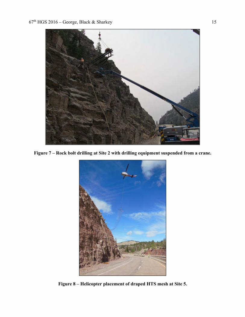
67th HGS 2016 – George, Black & Sharkey 15
Figure 7 – Rock bolt drilling at Site 2 with drilling equipment suspended from a crane.
Figure 8 – Helicopter placement of draped HTS mesh at Site 5.
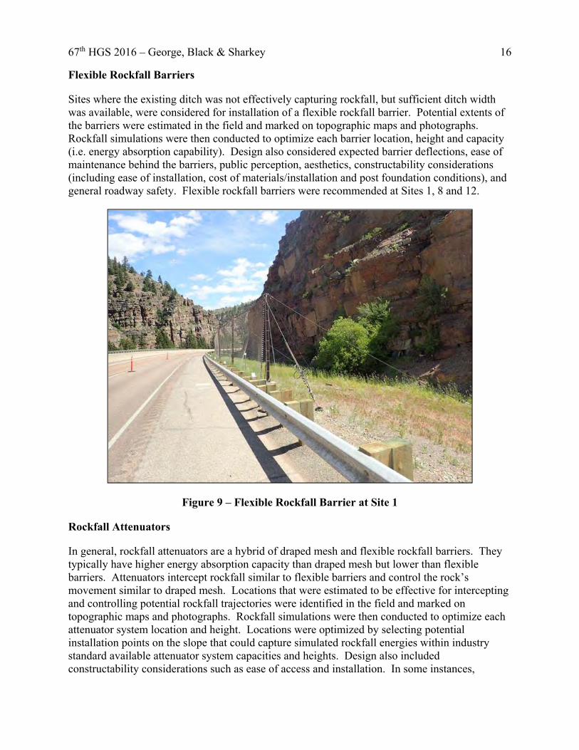
67th HGS 2016 – George, Black & Sharkey 16
Flexible Rockfall Barriers
Sites where the existing ditch was not effectively capturing rockfall, but sufficient ditch width was available, were considered for installation of a flexible rockfall barrier. Potential extents of the barriers were estimated in the field and marked on topographic maps and photographs. Rockfall simulations were then conducted to optimize each barrier location, height and capacity (i.e. energy absorption capability). Design also considered expected barrier deflections, ease of maintenance behind the barriers, public perception, aesthetics, constructability considerations (including ease of installation, cost of materials/installation and post foundation conditions), and general roadway safety. Flexible rockfall barriers were recommended at Sites 1, 8 and 12.
Figure 9 – Flexible Rockfall Barrier at Site 1
Rockfall Attenuators
In general, rockfall attenuators are a hybrid of draped mesh and flexible rockfall barriers. They typically have higher energy absorption capacity than draped mesh but lower than flexible barriers. Attenuators intercept rockfall similar to flexible barriers and control the rock’s movement similar to draped mesh. Locations that were estimated to be effective for intercepting and controlling potential rockfall trajectories were identified in the field and marked on topographic maps and photographs. Rockfall simulations were then conducted to optimize each attenuator system location and height. Locations were optimized by selecting potential installation points on the slope that could capture simulated rockfall energies within industry standard available attenuator system capacities and heights. Design also included constructability considerations such as ease of access and installation. In some instances,

67th HGS 2016 – George, Black & Sharkey 17
multiple attenuators were designed to provide continuous control of rockfall to the ditch elevations. The attenuator systems are based on the State of Washington Department of Transportation Cable Net Slope Protection Type 2 systems. Rockfall attenuators were recommended at Sites 2, 3, and 4.
Figure 10 – Rockfall Attenuators at Site 3
Rock Slope Excavation
At some sites benches are preset from the original cut slope construction, which could serve as launch features for potential rockfall. Excavation of such features will provide a larger rockfall catchment area (ditch), improve potential rockfall trajectories by removing launch features, and allow installation of addition mitigation due to increased ditch width. Sites with benches that could be removed were identified in the field and marked on topographic maps and photographs. Rockfall simulations were conducted to optimize cut slope and ditch configurations. Design included consideration of various cut slope angles, drilling offsets from the existing back slope, ditch geometries and locations for installation of flexible rockfall barrier (which were designed as discussed above) along with constructability and cost considerations.
At other sites, unsupported rock outcrops are present that cannot be effectively stabilized or controlled by the ditch or other protection measures (i.e. rockfall attenuator or flexible rockfall barrier). MDT elected to remove these outcrops to eliminate the potential for uncontrolled mobilization of this material towards the roadway. Optimization of the cut slope extents and geometry was conducted to compare level of effort for removing some or all of these outcrops so that MDT could decide how to proceed with the final design efforts.

67th HGS 2016 – George, Black & Sharkey 18
All excavations were designed with standard cut slope angles considering pre-splitting methods on a 2.5-foot hole spacing to reduce potential back break damage to surrounding rock outcrops and new rock faces. Excavation was recommended at Sites 8, 11, and 12.
Figure 11 – Rock Slope Excavation at Site 11
Concrete Barrier Rails and Guardrails
Concrete barrier rails can serve as a cost effective and simple rockfall mitigation measure when rockfall trajectories (i.e. bounce heights) and impact energies are low. Typically, other mitigation measures such as draped mesh and rockfall attenuators are installed in conjunction with these barriers to improve catchment capabilities of the ditch. Rockfall simulations were conducted to estimate locations where potential bounce heights and energies could be controlled by these barriers. Installation of these barriers along edge of pavement can complicate general roadway and ditch maintenance efforts along with hydraulics. To minimize impacts on maintenance requirements (i.e. snow removal) and roadway hydraulics, these barriers were not extensively recommended. Likewise, where possible these barriers were replaced with metal guardrail to decrease maintenance impacts and construction costs where clear zone protection was required. Concrete barrier rails were recommended at Sites 5, 7 and 10.

67th HGS 2016 – George, Black & Sharkey 19
CONCLUSIONS
As part of the National Highway System of Interstates, I-15 is a critical north-south corridor for travelers and commerce. This project is providing a major safety improvement for MDT and the traveling public. With construction completed on Phase 1, work proceeding according to schedule on Phase 2, and designs being finalized on Phase 3, the safety improvements will be noteworthy for years to come.
Lessons Learned
As with any project there are lessons learned on what could have been done in another way to improve the design, construction and project delivery. A few of the lessons learned on this project are offered below.
Rockfall mitigation is a niche sector of civil construction. As a result there are a limited number of contractors and construction inspectors that have experience with this work. To assure mitigation measures are installed in accordance with the designs, when possible it is recommended to have an on-site presence by a geotechnical specialist experienced with rockfall mitigation to assist the inspectors and contractor with construction. This is especially true for observing and directing scaling efforts; installation and testing of rock bolts; location selection, installation, and testing of anchors for rockfall mitigation measure such as: rockfall attenuators, flexible rockfall barriers, and draped mesh.
It was estimated the installation of post heights on the order of 6 feet would provide a cost savings to the project, which may be true from a material cost standpoint. However, the level of effort required to install a 6-foot post is about the same as installation of a 15-foot post and in some cases the shorter post may have a more complicated effort. A minimum post height of 10 feet could reduce the complications of construction while providing a reduced cost.
Installation of flexible rockfall barriers on concave horizontal alignments can promote system to fall towards the slope. This could be addressed by locating the flexible rockfall barriers on straight or convex horizontal alignments. If concave horizontal alignments are required additional down slope anchors could be installed to support the system.
Access for blasting is always a difficult item. Without prescribing the means and methods, it would be beneficial to provide guidance or descriptions of anticipated access requirements for blasting activities so that the contractor is aware of potential difficulties or equipment requirements. It is recommended to include requirements for slope rounding of any pioneered roads.

67th HGS 2016 – George, Black & Sharkey 20
REFERENCES
1. Transportation Research Board. Rockfall: Characterization and Control. Washington D.C., 2012.
2. Pierson, L.A., Beckstrand, D.L., and Black, B.A. Rockfall Hazard Classification and Mitigation System. FHWA/MT-05-011/8174. Research Programs – Montana Department of Transportation, Helena, MT, September 2005.
3. Lewis, R.S. Geologic Map of the Butte 1° x 2° Quadrangle. Open File MBMG 363. Montana Bureau of Mines and Geology, A Department of Montana Tech of the University of Montana, 1998.
4. Schmidt, R.G. Geologic Map of the Wolf Creek Quadrangle, Lewis and Clark County, Montana. Geologic Quadrangle Map GQ-974. United States Geological Survey, Department of the Interior, 1972.
5. Vuke, S.M. Geologic Map of the Great Falls South 30’ x 60’ Quadrangle, Central Montana. Open File MBMG 407. Montana Bureau of Mines and Geology, A Department of Montana Tech of the University of Montana, 2000.
6. CAE Mining Ltd. Sirovision R5. CAE Mining Corporate Ltd., Saint-Laurent, Quebec, Canada, 2012.
7. RocScience Inc. DIPS v6. RocScience Inc. Toronto, Ontario, Canada, 2015.

Concerns About Siting an Aggregate Quarry in a Dolomite Reef Deposit, Central Indiana
Terry West Purdue University
Department of Earth, Atmospheric, and Planetary Sciences 550 Stadium Mall Drive
West Lafayette, IN 47907-2051 (765)-494-3258
Prepared for the 67th Highway Geology Symposium, July, 2016

67th HGS 2016: West 2
Disclaimer
Statements and views presented in this paper are strictly those of the author(s), and do not necessarily reflect positions held by their affiliations, the Highway Geology Symposium (HGS), or others acknowledged above. The mention of trade names for commercial products does not
imply the approval or endorsement by HGS.
Copyright Notice
Copyright © 2016 Highway Geology Symposium (HGS)
All Rights Reserved. Printed in the United States of America. No part of this publication may be reproduced or copied in any form or by any means – graphic, electronic, or mechanical,
including photocopying, taping, or information storage and retrieval systems – without prior written permission of the HGS. This excludes the original author(s).

67th HGS 2016: West 3
ABSTRACT
Carbonates are the most desirable concrete aggregates in sedimentary terrains for many midwestern states, including Indiana. In northern Indiana thick glacial deposits cover the bedrock subcrop. Silurian age dolomite, comprising pinnacle reefs existing at higher elevations, are present in several counties north of Indianapolis along the strike of the bedrock. The Delphi Quarry, 20 miles north of Lafayette is located in a prominent dolomite reef. The quarry, nearly a century old, has provided much of the aggregate used in concrete and bituminous construction in a several county area. Recently it has supplied concrete for reconstruction of State Road 25 and foundations for wind turbines in the area. The Delphi quarry is located in a 400 foot thick reef of Silurian age and the aggregate produced there has one of the highest quality ratings in the state. A new quarry has been proposed, located five miles south of the existing quarry, in similar but perhaps not the same rock unit. Intense opposition to the new quarry has developed by nearby neighbors who have raised the following issues of concern: truck traffic, blasting, dust generation, disruption of groundwater supply, subsurface contamination, drainage and disposal of excavated materials. Another concern involves the quality of the rock at the proposed site. It may not be located on a pinnacle reef but adjacent to one, and a high purity dolomite will not be found and a thick black shale cover will have to be disposed of. Quarry development on agriculture-zoned land requires an exception and the issue has been brought before the local county zoning board. They have ruled against the rezoning for the quarry and an appeal is pending on their decision.

67th HGS 2016: West 4
INTRODUCTION
In many midwestern states, carbonate rocks provide the most desirable coarse aggregates for concrete construction. As such, limestone and dolomite commonly provide quality aggregates whereas shale and sandstones do not. Crushed stone aggregates in Indiana typically are superior to glacial gravels as these gravels tend to contain, weak, non-durable particles of low quality. In northern Indiana, thick glacial deposits are present which compounds the problem of finding suitable bedrock deposits for use in concrete. Dolomite reefs of Silurian age are prevalent along the strike from north to south near the center of the state and because of their resistance to weathering, stand at elevated positions into the overburden (Figure 1).
Figure 1 – Bedrock Map of Indiana

67th HGS 2016: West 5
The quarry in Delphi, Indiana, located 20 miles northeast of Lafayette provides an important aggregate supply for concrete construction for a several county area. It lies in southern Carroll County, just across the northeast corner of Tippecanoe County (Figure 2). Most recently, the upgrade to a four lane divided State Highway 25 from Lafayette to Logansport has been constructed using aggregate from the Delphi quarry as well as large foundation pads for several hundred wind turbines built in a nearby county. Crushed stone for concrete construction in Lafayette is also provided by this quarry.
Figure 2 – Tippecanoe County, Indiana
The dolomite reef in Delphi is 400 feet thick as indicated by rock coring performed by the Indiana Geological Survey in the 1970s and qualifies as one of the thickest reefs in the state. Near the center of the reef, 340 feet of the Huntington Lithofacies of the Wabash Formation, a

67th HGS 2016: West 6
recrystallized dolomite, is found, with the Salomonie, cherty dolomite below. The Huntington is a fine grained, massive, high purity dolomite, free of chert and argillaceous debris. Beyond the reef structure, rocks are capped by the Antrim Shale (equivalent of the New Albany Shale) and the Traverse Dolomite of Devonian age, and the Salina, Kenneth and Kokomo Limestones with the Wabash (Huntington Dolomite) below that, all of Silurian age. The Huntington Dolomite yields a high quality aggregate, with a low Los Angeles abrasion loss (in the 20 % range) and a high durability in freeze-thaw resistance. It qualifies as an AP aggregate by the Indiana Department of Transportation (INDOT), has a strong skid resistance for bituminous surfaces and is one of the highest quality concrete aggregates in Indiana.
A new quarry has been proposed for a site near the Wabash River, about five miles south of Delphi on old State Road 25 in Tippecanoe County, and only 15 miles from Lafayette, the population center for several adjacent counties. Intense opposition to quarry development by near-by property owners has developed as they conclude that a second quarry, with all the disruption it involves, is not necessary. Truck traffic, blasting, dust generation, disruption of groundwater supply and possible subsurface contamination have been pointed out in their opposition to the required zoning change. A boring for the site, drilled in 1979 by an earlier party, is provided as Figure 3 on the following page. Further discussion of these concerns are detailed in the following section.
DISCUSSION OF THE ISSUES
The quarry located at the edge of the Wabash River floodplain has the proposed footprint of 3100 feet by 1250 feet and will eventually be 420 feet deep. A full description of the subsurface of the site is not available as borings taken by the developer have not been made public. It is estimated based on a previous boring that 30 feet of alluvium with 40 feet of black shale lie above the carbonate bedrock. This yields a volume of 3100 X 1250 X70 =271.2 million cubic feet or 10 million cubic yards of soil and rock which has to be disposed of. The 5.7 million cubic yards of black shale yields a particular challenging problem that will be addressed later in this discussion. Also an increase in volume occurs when rock is excavated and placed in piles. Up to 15% increase of the 5.7 cubic yards of black shale or 6.5 million cubic yards would be involved.
Dewatering of the overburden will present a problem. It will cause a drawdown of neighboring wells in the floodplain when pumping is conducted in the quarry. The amount of drawdown is not known as the transmissibility of the overburden has not been determined. Groundwater will flow through the overburden and through the dolomite quarry walls. The Delphi quarry pumps up to 8 million gallons of water per day from their excavation. There are a number of homes located on the floodplain whose water supplies could be in impacted.
The developer has proposed to construct a slurry wall some 30 feet deep through the overburden into the black shale. Construction of a slurry wall can be difficult to accomplish as any holes in the wall yield concentrated flow into the excavation. It is not known if the shale cover over the dolomite is continuous for the whole site. A direct contact between the overburden and the dolomite would render the slurry wall ineffective. At the Delphi quarry, cover of the Anthrim Shale was very spotty and it is absent at the current quarry excavation.

67th HGS 2016: West 7

67th HGS 2016: West 8
Figure 3 – Boring Log at Proposed Site Black Shale is an undesirable material as it contains pyrite that is acid producing. Piles of excavated shale surrounding the quarry opening could produce acid drainage which should be isolated by a soil cover and neutralized by the addition of an alkaline material such as lime or limestone (Figure 4). This practice is used in current day highway construction when such shale is present in a road cut (Figure 5). Black shale also contains an elevated amount of radon which is another reason why the shale should be encapsulated by a soil cover. For safety purposes, soil berms must be built around the quarry. Since it is located on a floodplain, this would tend to reduce the floodway cross section during a high level flow of the Wabash River. Also there is a concern about the water pumped from the overburden and the bedrock. It must be contained in a settling pond to reduce turbidity. An NPDES permit would be required for any water to be released to the Wabash River.
The drilling log of a 218 ft. deep boring, taken at the site in 1979 by a former, interested party, shows the rock to be of much poorer quality than that claimed by the developer (see Figure 3). This resulted in that party abandoning the idea of developing a quarry at this location. The developer has stated that the rock is class A stone under INDOT specifications. The 1979 boring log disputes this conclusion as it shows the rock to contain chert and have a clayey nature. Both of these aspects yield a poor quality crushed stone of low durability.

67th HGS 2016: West 9
Figure 4 – Rock Cut in Black Shale, Eastern Tennessee
Figure 5 – Encapsulated Embankment, Black Shale

67th HGS 2016: West 10
Safety is another point of concern for the quarry site. A high fence around the site would be necessary. Quarries are an attractive nuisance and trespassing must be prevented. The developer at another quarry in Indiana had a problem with site invasion that involved a loss of several lives.
CONCLUSIONS
Construction of a rock quarry is a major endeavor requiring heavy construction, blasting and on- site development. By nature it has a disruptive effect on its surroundings even when located in a rural area that has limited housing development. Therefore, the need for such an enterprise must be established in order to convince local residents that it should come to pass. A zoning exception is required in Tippecanoe County to establish a quarry on agricultural land. The local citizens have expressed their concern over such a development and the county government has agreed that their concerns are reasonable. The zoning board denied the request to initiate the quarry and their decision has been appealed through the legal system.

Claystone, Steep Slopes, and Water, Not Again! The SR 2018 West Smithfield Street Landslide Remediation, Allegheny County, Pennsylvania
Stephanie M. Chechak, E.I.T.
Gannett Fleming, Inc. Foster Plaza 8, Suite 400
730 Holiday Drive Pittsburgh, PA 15220
(412) 922-5575 [email protected]
Brian F. Heinzl, P.E. Gannett Fleming, Inc.
Foster Plaza 8, Suite 400 730 Holiday Drive
Pittsburgh, PA 15220 (412) 922-5575
Prepared for the 67th Highway Geology Symposium, July, 2016

67th HGS 2016: Chechak and Heinzl 2
Acknowledgements The authors would like to thank the following individuals for their contributions to this paper:
Shane Szalankiewicz, P.E., District Geotechnical Engineer – PennDOT District 11-0 Greg Mumich, Geologic Specialist – PennDOT District 11-0
Disclaimer
Statements and views presented in this paper are strictly those of the authors, and do not necessarily reflect positions held by their affiliations, the Highway Geology Symposium (HGS), or others acknowledged above. The mention of trade names for commercial products does not
imply the approval or endorsement by HGS.
Copyright Notice
Copyright © 2016 Highway Geology Symposium (HGS)
All Rights Reserved. Printed in the United States of America. No part of this publication may be reproduced or copied in any form or by any means – graphic, electronic, or mechanical,
including photocopying, taping, or information storage and retrieval systems – without prior written permission of the HGS. This excludes the original authors.

67th HGS 2016: Chechak and Heinzl 3
ABSTRACT
Claystone beds commonly found throughout the geology of Southwestern Pennsylvania are generally soft, weak, and susceptible to landsliding. The Birmingham “Schenley” Redbed Claystone present at the SR 2018 West Smithfield Street project site in Allegheny County, Pennsylvania, is no exception. A landslide occurred above the roadway, cascading debris over the 40-to-50-foot near-vertical rock cut adjacent to the road. The size and volume of the landslide mass forced closure of the roadway. Gannett Fleming was tasked by the Pennsylvania Department of Transportation to provide a landslide treatment design that adequately stabilized the slope and prevented further debris from falling into the roadway. The “Schenley” Redbed Claystone encountered at the top of the near-vertical rock cut during the subsurface investigation measured up to 36 feet in thickness. Fluctuation of the groundwater table within the thick “Schenley” Redbed Claystone further softened and de-stabilized the claystone, complicating the task of stabilizing the slope. Several variations of the stability model were evaluated during the design phase to account for changing groundwater conditions. The final landslide treatment design incorporated flattening the slope to the edge of the near-vertical rock cut in combination with a soil nail slope treatment to provide additional reinforcement for the remaining soil and bedrock.
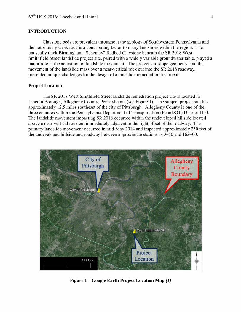
67th HGS 2016: Chechak and Heinzl 4
INTRODUCTION
Claystone beds are prevalent throughout the geology of Southwestern Pennsylvania and the notoriously weak rock is a contributing factor to many landslides within the region. The unusually thick Birmingham “Schenley” Redbed Claystone beneath the SR 2018 West Smithfield Street landslide project site, paired with a widely variable groundwater table, played a major role in the activation of landslide movement. The project site slope geometry, and the movement of the landslide mass over a near-vertical rock cut into the SR 2018 roadway, presented unique challenges for the design of a landslide remediation treatment. Project Location
The SR 2018 West Smithfield Street landslide remediation project site is located in Lincoln Borough, Allegheny County, Pennsylvania (see Figure 1). The subject project site lies approximately 12.5 miles southeast of the city of Pittsburgh. Allegheny County is one of the three counties within the Pennsylvania Department of Transportation (PennDOT) District 11-0. The landslide movement impacting SR 2018 occurred within the undeveloped hillside located above a near-vertical rock cut immediately adjacent to the right offset of the roadway. The primary landslide movement occurred in mid-May 2014 and impacted approximately 250 feet of the undeveloped hillside and roadway between approximate stations 160+50 and 163+00.
Figure 1 – Google Earth Project Location Map (1)

67th HGS 2016: Chechak and Heinzl 5
Project Statement
Gannett Fleming was tasked by PennDOT to provide final design services for the SR 2018 West Smithfield Street landslide remediation project. All final design services were performed under an accelerated schedule due to an Authorization for Emergency Procurement issued by the Deputy Secretary for Highway Administration. The Authorization for Emergency Procurement approves funding for expeditious landslide repair and was granted for the subject project based on: protecting the safety, health, and welfare of the traveling public; the forced closure of the roadway; the imminent potential for additional landslide movement; and the additional travel time required for emergency vehicles resulting from the roadway detour.
Gannett Fleming’s scope of work included: project site research; layout of the
geotechnical test borings; providing drilling inspection services during the geotechnical subsurface investigation; performance of a detailed stability analysis; development of a final landslide stabilization design as well as roadway restoration, drainage improvements and paving. Final Design engineering activities for the SR 2018 landslide remediation project began in late May 2014. PROJECT SITE DATA COMPILATION Office Research
Gannett Fleming performed office research pertaining to the existing project site soils, geology, and landslide history prior to locating the Final Design subsurface test borings. Published resources consulted during the office research period include: topographic mapping; structure contour and coal mine mapping; geologic mapping; soils mapping; and landslides and related features mapping.
Topographic and project site mapping indicate that the relief within the immediate project area is 110 feet, ranging between EL 930 and EL 1040 (2, 3). The elevation of SR 2018 ranges from EL 930 to EL 950 within the project limits. Structure contour mapping shows that the marker bed in closest proximity to the project site is the Pittsburgh Coal (4). Within the project limits, the base of the Pittsburgh Coal is located at approximate EL 1140. Therefore, the Pittsburgh Coal is located 100 feet above the uppermost limits of the project slope.
The geology of the project site was determined to lie within the Conemaugh Group of the
Casselman Formation based on the project site elevations, structure contour mapping, and the Generalized Geologic Section of Allegheny County (see Figure 2) (5). The specific rock strata anticipated to fall within the project site elevations include (in descending order): the Morgantown Sandstone; Wellersburg Coal and Clay; and the Birmingham “Schenley” Redbeds, Sandstone, and Shale.

67th HGS 2016: Chechak and Heinzl 6
Figure 2 – Generalized Geologic Section of Allegheny County (5)
Landslide mapping of the project site indicates that the entirety of the right offset slope is located within the limits of an “old landslide” (see Figure 3) (6). Soils located within the boundaries of an “old landslide” are sensitive to changes in groundwater condition. Movement of the “old landslide” may be reactivated by a fluctuating groundwater table. Soils mapping accessed through the U.S. Department of Agriculture (USDA) Web Soil Survey application indicates that the entirety of the project site soils lie within the Gilpin-Upshur Complex (GQF) (7). GQF soils are typically characterized as having very steep slopes, ranging from 25% to 75%, with a severe erosion hazard. The presence of the “old landslide” and the severe erosion hazard of the GQF soils are both indicators of soil slopes with high potential for landslide movement.
Base of Pittsburgh Coal EL 1140’
Project Location

67th HGS 2016: Chechak and Heinzl 7
Figure 3 – Landslide and Related Features Mapping (6) Field Reconnaissance
A field reconnaissance visit was performed in late May 2014 by Gannett Fleming, Inc., personnel in preparation for performance of the Final Design subsurface investigation. West Smithfield Street is a two lane roadway, with one eastbound lane and one westbound lane. The right offset slope consists of a near-vertical, 40-to-50-foot rock cut and is immediately adjacent to the eastbound travel lane.
The wooded hillside above the right offset rock cut failed, cascading the landslide mass
over the rock cut and into the SR 2018 roadway. The volume of material within the landslide mass impeded both travel lanes and forced closure of the roadway (see Figure 4). Groundwater seeps were observed throughout the active landslide area, indicating a seasonally high groundwater table.

67th HGS 2016: Chechak and Heinzl 8
Figure 4 – Landslide Mass and Right Offset Near-Vertical Rock Cut (June 2014) Final Design Subsurface Investigation
The Final Design subsurface investigation was performed in early June 2014 and
included a total of three test borings (GF-1, GF-2, and GF-3). Drilling services were provided by L.G. Hetager Drilling, Inc., with full-time drilling inspection services performed by a PennDOT-certified drilling inspector employed by Gannett Fleming, Inc. The test borings were located to form a subsurface cross section through the center of the active landslide mass (see Figure 5). Borings GF-1, GF-2, and GF-3 were advanced to evaluate the subsurface conditions near the toe, mid-section, and head scarp of the landslide mass, respectively. The subsurface conditions encountered during the Final Design subsurface investigation were utilized to verify the geologic data compiled during the office research period.
40-to-50-Foot Near-Vertical
Rock Cut

67th HGS 2016: Chechak and Heinzl 9
Figure 5 – Boring Location Plan Soil Conditions
The soil strata encountered in all three of the Final Design borings was comprised of colluvial lean clay and residual redbed claystone. Thickness of the soil strata ranged from 18.0 feet to 20.4 feet throughout the landslide mass. The colluvial and residual soils present in borings GF-1 and GF-2 were thicker and softer than those encountered in GF-3. Table 1 summarizes the colluvial and residual soil conditions in borings GF-1 and GF-2, as these borings were considered to exhibit the weakest soil properties.
GF-1
GF-3
GF-2
Boring Access Road
Approximate Extents of Landslide Parallel
to SR 2018
Approximate Landslide
Limits

67th HGS 2016: Chechak and Heinzl 10
Table 1 – GF-1 and GF-2 Soil Conditions
Soil Type Layer Thickness Range (ft.) Composition Density/
Consistency Average N160
(blows per foot)
Colluvium 9.4 – 15.4 Primarily Lean Clay, Little Silt, Trace Sand and Gravel
Medium Stiff to Stiff 27
Residual 5.0 – 9.4 Primarily Weathered Redbed Claystone, Trace Sand and Gravel
Very Stiff to Hard >50
Bedrock Conditions
The bedrock encountered in borings GF-1, GF-2, and GF-3 consisted of claystone, shale, and sandstone. As shown in Table 2, the Birmingham “Schenley” Redbed claystone was divided into two separate strata based on weathering, Rock Quality Designation (RQD), and depth from the existing ground surface. The upper portion of the “Schenley” Redbeds was highly weathered with 0% RQD, while the lower portion of the “Schenley” Redbeds exhibited minor weathering with >0% RQD.
Table 2 – GF-1, GF-2, and GF-3 Bedrock Conditions
Bedrock Type Unit Thickness
Range (ft.)
Unit Rock Quality Designation (RQD) Range
(%)
Bedrock Hardness
Bedrock Weathering
Highly Weathered Birmingham “Schenley”
Redbeds 7.5 – 36.0 0 Very Soft Highly
Weathered
Birmingham “Schenley” Redbeds 5.4 – 8.9 19 – 38 Very Soft Minor
Weathering
Birmingham Sandstone and Shale 3.6 – 13.6 77 – 92 Soft Fresh
Figure 2 indicates that the Birmingham “Schenley” Redbeds typically have a thickness
ranging between 5 feet to 15 feet; however, the “Schenley” Redbeds were much thicker beneath the SR 2018 project site. Boring GF-3 encountered a portion of the “Schenley” Redbeds with a thickness of 36 feet. This boring was terminated within the “Schenley” Redbed strata; as a result, the actual redbed claystone thickness may have exceeded 36 feet in this location. Numerous slickensides and healed fractures were noted at various depths throughout the “Schenley” Redbeds in all of the Final Design borings. Groundwater Conditions
The drilling inspector encountered difficulties while attempting to obtain accurate
groundwater level readings during the Final Design subsurface investigation. The high clay content of the colluvium resulted in a low permeability within the soil strata and artificially high

67th HGS 2016: Chechak and Heinzl 11
groundwater levels within the test borings. Consequently, accurate groundwater readings could not be obtained during the subsurface investigation. Information pertaining to the groundwater conditions within the project slope were based on project site observations. SUBSURFACE DATA ANALYSIS Laboratory Testing
Laboratory testing was performed on soil and bedrock samples obtained during the Final Design subsurface investigation to verify field classifications and determine material strength parameters. The SR 2018 landslide remediation project laboratory testing program included the following tests: soil classification and moisture content; unit weight testing; unconfined compressive strength testing of rock cores; and remolded direct shear testing.
Undisturbed Shelby tube samples were taken in holes offset from the three Final Design
test borings to obtain in-situ soil samples that would be used to develop shear strength parameters within the landslide mass. However, the sand and gravel fraction of the undisturbed Shelby tube samples was discovered to be high during extrusion of the samples in the laboratory, which would skew the results of the shear strength test. Therefore, the minus 3/4-inch portions of the Shelby tube samples and a bag sample of the colluvium obtained at the head scarp were remolded and utilized to perform remolded direct shear testing. Site Subsurface Model
The site subsurface model was constructed from data collected during the Final Design subsurface investigation, information from published resources, and project site observations. Due to the accelerated emergency project schedule, the Final Design laboratory testing program was performed in conjunction with the stability modeling and landslide treatment design. The laboratory testing results were received during finalization of the design process. Therefore, the laboratory testing results were used to verify the subsurface material properties selected during the initial subsurface modeling. Subsurface conditions encountered in borings GF-1, GF-2, and GF-3, coupled with observations made during the field reconnaissance visit, were used to model the stratigraphy of the project site.
Project site observations indicate variability of the groundwater table within the project
slope. Two groundwater tables were included in the site subsurface model to ensure representation of the varying groundwater conditions throughout the year. The normal groundwater table was located within the weathered redbed claystone strata. The elevated groundwater table is located within the colluvial and residual soils and is representative of springtime/thaw conditions when the groundwater table is temporarily high. The site subsurface model in Figure 6 includes both the normal and elevated groundwater tables.

67th HGS 2016: Chechak and Heinzl 12
Figure 6 – Project Site Subsurface Model The average N160 values, consistency/density ranges, and soil compositions shown in
Table 1 for the colluvial and residual soils were used in the determination of unit weights and friction angles. Cohesion was neglected for all site soils in order to more accurately model long term design conditions. Table 3 includes the material parameters selected as representative of the site colluvial and residual soils.
As previously discussed, two distinct zones were encountered within the thick
Birmingham “Schenley” Redbed claystone. The upper portion of the “Schenley” Redbeds, which was highly weathered with 0% RQD, was modeled as a separate strata from the lower portion, which displayed minor weathering with >0% RQD. The zones were differentiated in the subsurface model by assigning a lower friction angle to the highly weathered upper portion. The Birmingham Shale and Sandstone encountered beneath the “Schenley” Redbeds was fresh with a unit RQD of 88%. Field and Final Design subsurface investigation conditions indicate that the failure plane of the currently active landslide does not lie within the Birmingham Sandstone and Shale. High friction angle and cohesion values were selected for the Birmingham Sandstone and Shale to reflect the quality of this unit, as well as to prevent the stability model from failing through the competent bedrock.

67th HGS 2016: Chechak and Heinzl 13
Table 3 – Subsurface Material Properties
Material Type Moist Unit Weight γm (pcf)
Saturated Unit Weight γsat (pcf)
Cohesion c (psf)
Friction Angle ϕ (deg.)
Colluvium 100 110 0 16
Residual Redbeds 115 125 0 28
Highly Weathered Redbeds 135 140 0 28
Redbed Claystone 135 140 0 30
Shale/Sandstone Bedrock 140 140 10,000 40
GSTABL7 software was utilized to perform all stability analyses for the SR 2018
landslide remediation design. The stability of the existing site conditions was evaluated to verify the validity of the initial subsurface material properties selected for each strata. The existing slope stability was analyzed using both the normal and elevated groundwater tables to determine the impact of a fluctuating groundwater table. Stability of the existing slope under the normal groundwater table resulted in a FS = 0.96. This result indicates marginal stability of the slope. Stability of the existing slope under springtime/thaw conditions and an elevated groundwater table produced a FS = 0.80. This analysis indicates the level of slope de-stabilization caused by seasonal groundwater table variations. The material parameters selected for each subsurface strata were determined to be representative based on the results of the existing conditions subsurface stability analysis. LANDSLIDE REMEDIATION TREATMENT (STA. 160+80 TO STA. 162+95) Project Site Challenges The SR 2018 project site presented several unique challenges to the design of a landslide remediation treatment. The Birmingham “Schenley” Redbeds encountered in all three Final Design test borings was very soft with poor RQD and various degrees of weathering. The claystone was atypically thick for the “Schenley” Redbeds unit, with the highly weathered portions measuring up to 36 feet in thickness (3, 5). Numerous slickensides and healed fractures were noted throughout the “Schenley” Redbed strata. As previously discussed, redbed claystone is a contributing factor to many landslides throughout Southwestern Pennsylvania. The thickness and poor quality of the “Schenley” Redbed unit presented a major obstacle to designing a constructible and economical landslide remediation treatment.
The project site geometry also presented a unique challenge to the design of the landslide remediation treatment. The landslide occurred within an undeveloped hillside overlying a 40-to-

67th HGS 2016: Chechak and Heinzl 14
50-foot, near-vertical rock cut, immediately adjacent to the SR 2018 roadway. This slope geometry limited the amount of space available in which to design a viable landslide treatment. The number and type of feasible treatment options were constrained by the geometry and space limitations.
Variable groundwater conditions within the project slope contributed to the landslide remediation design challenges. As shown in the stability analyses of the existing slope conditions, the springtime/thaw groundwater table greatly impacts the marginally stable slope. Cycles of seasonal groundwater table fluctuation have weakened the already weak “Schenley” Redbed claystone present within the project slope. The landslide remediation treatment option selected for the project slope had to perform adequately and provide slope stability under all groundwater conditions.
Soil Nail Slope Treatment Design (Sta. 160+80 to Sta. 162+95)
Several treatment alternatives were considered for the remediation of the West Smithfield Street landslide. The potential treatment options considered for the project included a combination of excavation and a soil nailed slope or a slope with structural element inclusions. Only the final landslide remediation design will be discussed herein. The final landslide treatment design selected for the project incorporated flattening the slope to the edge of the near-vertical rock cut in combination with a soil nail slope treatment to provide additional reinforcement for the remaining soil and bedrock. This alternative was selected because it adequately addressed the aforementioned project site challenges while limiting disturbance to the project slope.
The soil nailed portion of the slope was designed to extend upslope from the back of the
flattened bench at a finished slope ratio of 1.5H:1V to reinforce the remaining colluvial soil mass. As shown in Figure 6, the colluvial soil/residual soil interface daylights at the slope face at approximate elevation 976. The control point for the front of the finished bench construction was based on the location of this interface. The slope flattening was proposed to occur within the residual soil. A finished slope ratio of 4H:1V, which is equivalent to a 14° slope, was determined to provide a stable finished bench. The finished bench was proposed to extend a minimum of 20 feet horizontally back into the slope from the toe of slope.
The design strength of the individual soil nails was evaluated based on the subsurface strata each nail was anticipated to encounter. A weighted average of the individual strata pullout resistance strengths was calculated based on the length of the soil nail modeled through the weakest series of strata. This weighted average pullout resistance strength was then assigned to all of the soil nails within the proposed configuration. Based on the location of the flattened bench, the thickest area of remaining colluvium was located at the top of the finished 1.5H:1V soil nail slope. Nail #1, the uppermost soil nail within the proposed layout, was determined to contact the thickest sections of the weakest subsurface strata. As a result, the weighted average allowable pullout resistance strength calculated for Nail #1 (1,386 psf), was applied to all soil nails in the stability model.

67th HGS 2016: Chechak and Heinzl 15
An iterative global stability analysis was performed using GSTABL7 to determine the proper soil nail configuration. Variables analyzed as part of the soil nail slope design included vertical and horizontal nail spacing, maximum number of rows of nails, nail length, and nail declination from horizontal. The iterative analysis was performed by changing a single variable, while holding the other variables constant, to evaluate the impact of modifying each variable. The stability of the soil nail slope was evaluated under both the normal and elevated groundwater tables to determine a slope design that performed adequately under all conditions. Global stability modeling of a soil nail slope with the following design elements achieved a FS = 1.50 under normal groundwater conditions and a FS = 1.43 under the elevated groundwater conditions:
• Soil Nail Spacing = 4 feet horizontally by 4 feet vertically • Maximum Number of Rows of Nails = 6 rows • Soil Nail Declination = 40° from horizontal • Soil Nail Length = 40 feet • Soil Nail Slope Finished Grade = 1.5H:1V • Soil Nail Size = No. 8 Bar (Diameter = 1 inch) • Total Soil Nail Diameter = 6 inches
Figure 7 shows the Soil Nail Treatment Typical Section that was included in the final drawings.
Figure 7 – Soil Nail Treatment Typical Section
Due to the accelerated project schedule, the laboratory testing results were received toward the end of the design phase. The testing results were used to verify the material parameters selected for design based on information collected from the subsurface investigation and published resources. Three sets of peak and residual friction angles were obtained for the

67th HGS 2016: Chechak and Heinzl 16
colluvial clay through remolded direct shear testing. The minimum friction angle resulting from laboratory testing of the colluvium was ϕ = 21°. Stability modeling of the slope included a friction angle of ϕ = 16° for the colluvium. Therefore, the initial friction angle assumptions for the colluvial clay were slightly lower than actual laboratory values. The laboratory testing results indicated that the moist and saturated unit weights of the site soils were much higher than those originally included in the subsurface model. The colluvial and residual soils were tested as having a moist unit weight of γm = 139 pcf and a saturated unit weight of γsat = 140 pcf. The final global stability analysis was re-evaluated using the laboratory unit weight results to verify that the heavier site soils did not negatively impact the slope stability. The modified stability analysis also resulted in a FS = 1.5, which verified that the proposed soil nail configuration performed adequately with the representative soil conditions.
The purpose of the soil nail slope system, as previously described, is to provide global stability of the landslide mass and prevent future slope movement. As shown in Figure 7, the soil nail slope system also includes a turf reinforcement mat (TRM) and high tensile steel wire mesh attached flush to the slope face by spike plates. The purpose of the TRM, high tensile steel wire mesh, and spike plates is to provide stability against local failure of the soil between the individual soil nails. The TRM also facilitates re-vegetation of the slope which further reinforces soil between nails and prevents future raveling.
The soil nail slope treatment design also includes a rock-lined drainage ditch at the back
of the finished 4H:1V bench/toe of 1.5H:1V soil nail slope interface. This rock-lined ditch extends the length of the soil nail treatment in order to provide drainage for the overall slope under elevated groundwater conditions. A series of pipes were connected to the ditch at various points through the treatment to divert the drainage over the slope and connect to the existing SR 2018 drainage system. CONSTRUCTION AND POST-CONSTRUCTION Bids were solicited in August 2014 to begin the Construction phase of the SR 2018 landslide remediation project. A total of six construction companies submitted bids and the bid opening was held on August 28, 2014. Allison Park Contractors, Inc., from Allison Park, Pennsylvania, submitted the winning bid which totaled $985,450.
Construction of the soil nail slope treatment, with associated drainage, began mid-September 2014 and was completed by mid-December 2014. The primary issue encountered during the Construction phase related to the appurtenances required for installation of the soil nail system. The hexagonal nuts submitted for tightening the spike plate/high tensile steel wire mesh/TRM/soil nail system to the slope face did not seat properly onto the spike plates. The hexagonal nut/spike plate interface was designed to act as a ball joint and allow for flexibility of spike plate installation angle at the slope face. The bottom of the hexagonal nuts initially submitted for installation was flat, which limited the angle of spike plate installation at the slope face. The issue was resolved through submittal of matching appurtenances for installation at the project site. Figures 8 and 9 show the finished soil nail slope treatment and the right offset slope, respectively, at the interim final construction inspection on December 15, 2014.

67th HGS 2016: Chechak and Heinzl 17
Figure 8 – SR 2018 Finished Soil Nail Slope Treatment
Figure 9 – SR 2018 and Right Offset Slope Post-Construction

67th HGS 2016: Chechak and Heinzl 18
REFERENCES 1. Google. Google Earth. Imagery date: October 18, 2015. Accessed May 2016. 2. U.S. Geological Survey. Topographic Map of the McKeesport, PA Quadrangle. 7.5 Minute
Series. Washington, DC: USGS 1960. Photorevised 1969.
3. Gannett Fleming, Inc. Geotechnical Engineering Report for Final Design – SR 2018, Section A04, West Smithfield Street Landslide Remediation. Revised July 30, 2014.
4. Pennsylvania Geological Survey. Coal Crop Lines and Structure Contours – McKeesport,
PA Quadrangle. Coal Resources of Allegheny County, Pennsylvania – Part 1. Coal Crop Lines, Mined-Out Areas, and Structure Contours – 4th series. Mineral Resource Report 89, 1985.
5. A.C. Ackenheil and Associates, Inc. Generalized Geologic Section – Allegheny County.
1954.
6. Davies, William E. Landslides and Related Features of the McKeesport, PA Quadrangle. U.S. Geological Survey – Open File Map 79-1314 (C-2), 1979.
7. Natural Resources Conservation Service. Web Soil Survey. U.S. Department of Agriculture.
http://websoilsurvey.sc.egov.usda.gov/App/WebSoilSurvey.aspx. Accessed May 2014.

67th HGS 2016: Graham, Turner, and Axtell 1
Rockfall Hazard Mitigation at the TH-53 Bridge, Virginia, Minnesota
David S. Graham, P.E. Project Engineer
108 Eveningside Drive Chattanooga, TN 37404
Dan Brown and Associates, PC (205) 427-0682
John P. Turner, Ph.D., P.E., PG, D.GE
Senior Principal Engineer 310 E Garfield Street Laramie, WY 82070
(307) 286-2958 Dan Brown and Associates, PC
Paul J. Axtell, P.E., D.GE Principal Engineer
10134 Glenwood St Overland Park, KS 66212
Dan Brown and Associates, PC (913) 744-4988
Prepared for the 67th Highway Geology Symposium, July, 2016

67th HGS 2016: Graham, Turner, and Axtell 2
Acknowledgments
The authors thank The Minnesota Department of Transportation, Parsons Transportation Group, Hoover Construction, Pacific Blasting and Demolition, and Kiewit Infrastructure Group for their
roles and support on the project. The authors also thank the following individuals for their contributions to this project:
Tim Siegel – Dan Brown and Associates Nathan Glinski – Dan Brown and Associates
Disclaimer
Statements and views presented in this paper are strictly those of the author(s), and do not necessarily reflect positions held by their affiliations, the Highway Geology Symposium (HGS), or others acknowledged above. The mention of trade names for commercial products does not
imply the approval or endorsement by HGS.
Copyright
Copyright © 2016 Highway Geology Symposium (HGS)
All Rights Reserved. Printed in the United States of America. No part of this publication may be reproduced or copied in any form or by any means – graphic, electronic, or mechanical,
including photocopying, taping, or information storage and retrieval systems – without prior written permission of the HGS. This excludes the original author(s).

67th HGS 2016: Graham, Turner, and Axtell 3
ABSTRACT The Trunk Highway 53 (TH-53) Relocation Project near Virginia, Minnesota, includes a new bridge across the currently inactive Rouchleau Mine Pit, one of many open pit iron ore mines on the Mesabi Range. Rockfall hazards associated with the existing highwall on the east side of the Rouchleau Pit were assessed and mitigated to ensure construction worker safety and long-term performance of the bridge. This paper provides a brief geologic background and describes the process of assessing and mitigating rockfall hazards at the TH-53 bridge site. Rockfall hazards were primarily assessed on the basis of observations made during site visits, including: geologic feature mapping, assessment of existing talus, identifying rockfall sources and travel paths, and run-out distance assessment via trial rolling of rocks. The influences of the local geologic conditions of the Biwabik Iron Formation at the site and the highwall geometry result in the potential for several mechanisms of rockfall hazard at this site, and the extreme northern climate contributes to the hazard through freeze-thaw conditions which initiate rockfall events. Rock bounce heights and velocities were analyzed using the Colorado Rockfall Simulation Program (CRSP). Mitigation elements for the protection of workers constructing the east pier of the bridge, which is located on a bench cut into the eastern pit highwall, include an attenuator fence system and combined wire mesh and cable net drapery covering portions of the highwall face. A soil berm will provide long-term protection for the eastern bridge pier. Details of the mitigation system and its construction are described, including: element selection and sizing, site-specific details, anchor design, challenges to construction, and quality control.

67th HGS 2016: Graham, Turner, and Axtell 4
INTRODUCTION AND BACKGROUND
Trunk Highway 53 (TH-53) southeast of Virginia, Minnesota, is being realigned to allow for future open-pit iron ore mining of land along the existing highway corridor. The new alignment follows the E-2 option shown in Figure 1. The new section of highway includes a three-span bridge across the currently inactive Rouchleau Mine Pit. The bridge is approximately 1,132 ft long with two abutments and two intermediate piers. The bridge is shown in elevation in Figure 2 and Figure 3 is a conceptual rendering of the bridge.
Construction of the 190-ft high pier column from the base of the East Highwall (circled in Figures 2 and 3) required excavation of a work pad into the toe of the highwall. Personnel and equipment needed to construct the pier and its foundations are therefore exposed to a significant construction-phase rockfall hazard. There is also a potential long-term rockfall hazard to the pier. The rockfall protection system employed a combination of cable net drapery with wire mesh backing, an attenuator fence, and catchment berms. The cable net and wire mesh drapery are suspended from two different levels, the top of the highwall and from an intermediate bench. The top of the lower drapery panels are suspended from an elevated top cable to form a 6-ft high attenuator fence. Berms were constructed around the perimeter of the Pier 1 work area, and the base of Pier 1 will be protected by a berm upon completion.
Figure 1 – Project Location and TH-53 Realignment.
Bridge Location
Rouchleau Pit

67th HGS 2016: Graham, Turner, and Axtell 5
Figure 2 – Bridge Elevation.
Figure 3 – Rendering of the TH-53 Bridge
GEOLOGY Geologic Setting The project is located in the Virginia Horn area of the Central Mesabi Iron Range. The Mesabi Range is a narrow belt of iron-bearing rocks in the Superior Upland physiographic province of northeastern Minnesota. The bedrock unit of interest at the bridge site is the Biwabik Iron Formation. Rocks of the Biwabik were formed between 1.85 and 1.93 billion years ago as sediments deposited in a shallow marine environment on the northern edge of the northward-migrating Animikie basin.
East Highwall
East Highwall

67th HGS 2016: Graham, Turner, and Axtell 6
Stretching roughly between the cities of Grand Rapids and Babbitt, the Biwabik Iron Formation is approximately 120 miles long and between 0.25 to 3.0 miles wide, as shown in Figure 4 (1). According to Severson et al. (1), the Biwabik Iron Formation is around 730-780 ft thick in the Virginia Horn area. The formation is subdivided into four units referred to as (from bottom to top): Lower Cherty member, Lower Slaty member, Upper Cherty member, and Upper Slaty member. The cherty members are typically characterized by a granular (sand-sized) texture and thick-bedding (beds ≥ several inches thick). The slaty members are typically fine-grained (mud-sized) and thin-bedded (≤ ½ in thick beds). “Slaty” is a local mining term indicating parting parallel to bedding in thin-bedded rocks and is not necessarily indicative of metamorphism or slaty cleavage (1). The cherty members are largely composed of chert and iron oxides with zones rich in iron silicates, while the slaty members are generally composed of iron silicates and iron carbonates with local chert beds. Both cherty and slaty iron-formation types are interlayered at all scales, but one rock type or the other predominates in each of the four informal members, and they are so named for this dominance. The repetition of the major cherty and slaty members is interpreted by geologists as being the result of transgressive and regressive ocean events.
The beds of the Biwabik Iron Formation generally strike approximately N75°E and dip gently south-southeast (2). The major exception to this orientation is the Virginia Horn, a reverse S-shaped bend in the central part of the formation near the cities of Virginia and Eveleth. The Virginia Horn is thought to be a broad, low-dipping anticline–syncline couplet (3). Although, the exact deformational processes resulting in the Virginia horn have never been definitively established (4).
Figure 4 – Map of the Mesabi Range (Biwabik Iron Formation) with the Duluth Complex shown to the east (1).

67th HGS 2016: Graham, Turner, and Axtell 7
Local Geologic Conditions The bridge site is located in the central part of the Virginia Horn “S”. Sub-horizontal bedding plane dip angles typically range from zero to 20 degrees with local variation. Dip direction varies but is predominantly northwest. Joints not associated with bedding planes are predominantly sub-vertical, typically dipping between 70 and 90 degrees. Two or three sub-vertical joint sets exist at locations across the site. The sub-horizontal bedding planes and sub-vertical joints form blocks. The blocks vary in size depending on the spacing of the bedding planes and the nature of the bedding plane contacts. Generally, the slaty layers are comprised of smaller blocks or chips and the cherty layers are comprised of larger blocks of several feet in dimension, as shown in Figure 5. The intact Biwabik rock is both strong and dense. Uniaxial compressive strength averaged 21,300 psi based on 117 laboratory tests. The average unit weight of the 117 test specimens was 191 lb/ft3. The density and strength of lab samples varied greatly.
Figure 5 – Exposed Cut Face showing Variations in Block Size.
Pencil
for
Scale
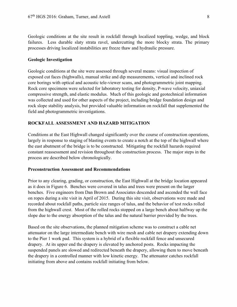
67th HGS 2016: Graham, Turner, and Axtell 8
Geologic conditions at the site result in rockfall through localized toppling, wedge, and block failures. Less durable slaty strata ravel, undercutting the more blocky strata. The primary processes driving localized instabilities are freeze thaw and hydraulic pressure. Geologic Investigation Geologic conditions at the site were assessed through several means: visual inspection of exposed cut faces (highwalls), manual strike and dip measurements, vertical and inclined rock core borings with optical and acoustic tele-viewer scans, and photogrammetric joint mapping. Rock core specimens were selected for laboratory testing for density, P-wave velocity, uniaxial compressive strength, and elastic modulus. Much of this geologic and geotechnical information was collected and used for other aspects of the project, including bridge foundation design and rock slope stability analysis, but provided valuable information on rockfall that supplemented the field and photogrammetric investigations. ROCKFALL ASSESSMENT AND HAZARD MITIGATION Conditions at the East Highwall changed significantly over the course of construction operations, largely in response to staging of blasting events to create a notch at the top of the highwall where the east abutment of the bridge is to be constructed. Mitigating the rockfall hazards required constant reassessment and revision throughout the construction process. The major steps in the process are described below chronologically. Preconstruction Assessment and Recommendations Prior to any clearing, grading, or construction, the East Highwall at the bridge location appeared as it does in Figure 6. Benches were covered in talus and trees were present on the larger benches. Five engineers from Dan Brown and Associates descended and ascended the wall face on ropes during a site visit in April of 2015. During this site visit, observations were made and recorded about rockfall paths, particle size ranges of talus, and the behavior of test rocks rolled from the highwall crest. Most of the rolled rocks stopped on a large bench about halfway up the slope due to the energy absorption of the talus and the natural barrier provided by the trees. Based on the site observations, the planned mitigation scheme was to construct a cable net attenuator on the large intermediate bench with wire mesh and cable net drapery extending down to the Pier 1 work pad. This system is a hybrid of a flexible rockfall fence and unsecured drapery. At its upper end the drapery is elevated by anchored posts. Rocks impacting the suspended panels are slowed and redirected beneath the drapery, allowing them to move beneath the drapery in a controlled manner with low kinetic energy. The attenuator catches rockfall initiating from above and contains rockfall initiating from below.

67th HGS 2016: Graham, Turner, and Axtell 9
Figure 6 – East Highwall Face, Existing Conditions Prior to Construction Operations.
The Colorado Rockfall Simulation Program (CRSP), Version 4, was used to evaluate the effectiveness of the attenuator concept, assess the attenuator location, and to determine the appropriate post height. The program CRSP simulates rocks tumbling down a slope, taking into account slope profile, rebound and friction characteristics of the slope surface, and rotational energy of falling rocks. Rock shape is idealized as being spherical, cylindrical, or disk-shaped. Rockfall can be generated from any location on the slope, and the program output consists of rock velocity, kinetic energy, and bounce height at each location along the slope. The percentage of generated rocks passing each point is also provided. The CRSP modeling methodology is described in further detail in the CRSP User Manual (5).
Bridge Centerline
250 ft

67th HGS 2016: Graham, Turner, and Axtell 10
CRSP was used to analyze three slope profiles corresponding to (a) the centerline of the bridge alignment, (b) the northern edge of the Pier 1 work area, and (c) the south edge of the Pier 1 work area. Each profile was established on the basis of surveyed topographic contours. The CRSP User Manual provides guidelines on ranges of the input parameters for various materials (5). For the preconstruction analyses, the values presented in Table 1 were used to represent the slope face materials. Each section of the slope surface was idealized as consisting of either glacial till overburden, bare rock, or talus slope (covered with rock debris). The required parameters include surface roughness, tangential coefficient that accounts for frictional interaction between falling rock and the slope surface, and the normal coefficient which accounts for rebound of rocks bouncing on the slope surface.
Table 1 – CRSP Input Parameters.
Slope Surface Geomateral
Category in CRSP User
Manual
Surface Roughness
(ft)
Tangential Coefficient,
Rt
Normal Coefficient,
Rn Glacial till overburden Firm soil slopes 0.20 0.70 0.16
Rock surfaces Bedrock; hard surfaces 0.33 0.95 0.80
Talus Talus 1.00 0.80 0.16 For each of the three profiles, CRSP was first used to analyze rockfall on the slope with no catchment system in place. The objective was to determine the locations where bounce height is minimized, which provides guidance and insight on where to locate the elevated cable net attenuator for optimum effectiveness. After several trial runs it was determined that elevation 1415 ft, which would be close to the west edge of the large intermediate bench, yields predicted bounce heights for all three profiles with maximum values less than 6 ft and average bounce heights of less than 1 ft. These results are consistent with our observations from rolling rocks, in which none of the rolled rocks passed the point corresponding to elevation 1415 ft. Note the rock rolling exercise was not a rigorously planned investigation with measurements of rock velocity, etc., but rather an informal exercise intended to provide general information. Next, a 6-ft high barrier was placed at elevation 1415 ft and the CRSP analysis was performed again. In each case zero rocks (out of 100 rocks generated) passed the barrier (Table 2). Based on these results, a cable net attenuator suspended from 6-ft high posts on the bench at elevation 1415 ft was recommended for protecting workers in the vicinity of Pier 1. It was planned to install the attenuator after scaling the upper portion of the East Highwall for the protection of workers constructing the attenuator.

67th HGS 2016: Graham, Turner, and Axtell 11
Table 2 – CRSP Results, 2-ft Diameter Spherical Rock and Input Parameters in Table 1.
Slope Profile Analyzed for Rockfall by CRSP
Bounce Height at EL 1415 ft Result of 6-ft High Attenuator @ EL 1415 ft Average Maximum
Bridge Centerline, Including Abutment Excavation 0.77 3.07 No rocks passing
attenuator North Edge of Work Pad
Excavation 0.69 5.09 No rocks passing attenuator
South Edge of Work Pad Excavation 0.69 3.55 No rocks passing
attenuator Upper Rockfall Protection Prior to installing the attenuator system, partial excavation for the East Abutment by blasting and scaling of the East Highwall above the attenuator bench were performed in July and August, 2015. Blast rock directed down the face of the highwall filled the benches to capacity with rock debris and removed the majority of trees that had previously acted as a partial barrier (Figure 7). Rocks launched from the crest now traveled significantly further than observed in the preconstruction test rolls. Additionally, it was observed that scaling alone was likely not sufficient for reducing the rockfall risk to personnel cleaning the benches, constructing the attenuator, and excavating the Pier 1 work area. In response to the altered conditions, draping the upper portion of the East Highwall was deemed the most safe and feasible means of providing the necessary rockfall protection. Recommendations for covering the upper portion of the slope with combined cable net and wire mesh drapery were provided to the contractor and the upper portion of the slope was covered down to the attenuator bench, as shown in Figure 8. Pier 1 Excavation and Attenuator Construction Pier 1 is founded on a bench excavated into the toe of the East Highwall by blasting and mechanical removal of blast rock in October and November, 2015. This work was performed in coordination with the attenuator construction. The attenuator posts and support cables were installed and drapery panels attached but not unrolled. Immediately following the Pier 1 excavation work, the attenuator drapery panels were deployed down the slope, extending to newly excavated Pier 1 work area, as shown in Figure 9. Berms were also constructed along the north, east, and west sides of the Pier 1 work area to create a catchment for rocks exiting from beneath the drapery.

67th HGS 2016: Graham, Turner, and Axtell 12
Figure 7 – Site Conditions after Initial Round of Blasting and Scaling.
Figure 8 – Upper Rockfall Drapery.
Blast Rock

67th HGS 2016: Graham, Turner, and Axtell 13
Figure 9 – Pier 1 Excavation and Attenuator Complete.
Upper Rockfall Protection, Removal and Replacement The drapery on the upper portion of the East Highwall was removed for final excavation of the East Abutment in January, 2016. The excavation work near the slope face was initially planned to be performed using only mechanical means or small controlled blasts; however, a least one blast resulted in significant rock debris being sent down the slope. Although the attenuator was not designed for such an event, it performed well, with relatively little damage. The post-blast conditions are shown in Figure 10. The following damage was observed during a site visit following the blast:
Severed top cable wires Severed support cable wires and strands Completely severed lacing cables Dented posts with chipped paint Torn double twist mesh Rocks protruding through the drapery

67th HGS 2016: Graham, Turner, and Axtell 14
Figure 10(a) – Attenuator Bench after East Abutment Excavation Blast.
Figure 10(b) – Damaged post support cable.

67th HGS 2016: Graham, Turner, and Axtell 15
Figure 10(c) – Rock protruding through drapery.
Figure 10(d) – Impacted post.

67th HGS 2016: Graham, Turner, and Axtell 16
During the blast, some rocks overtopped the attenuator, coming to rest in the Pier 1 work area. Prior to allowing construction operations to resume at Pier 1, the effectiveness of the attenuator was evaluated through a more rigorous program of trial rock rolling. Five rocks between approximately 6 and 18 inches in maximum dimension were rolled from multiple locations along the crest of the East Highwall. Additionally, some larger rocks were rolled using an excavator from two locations. Several trial rocks hit a small sloped bench above the attenuator bench that launched the rocks over the attenuator. This was primarily the case at the northern end of the attenuator, where the attenuator bench narrows and the attenuator fence is located closer to the upper highwall face. Reinstalling the previously installed drapery panels with some additional panels to increase the coverage area to the north was the safest, fastest, most feasible means of providing the necessary rockfall protection to personnel working in the Pier 1 area. Recommendations for reinstalling drapery along the upper portion of the East Highwall were provided to the contractor and the upper portion of the slope was covered down to the attenuator bench. Recommendations regarding repair of the attenuator and lower drapery were also made. ROCKFALL PROTECTION ELEMENTS
Combined Double Twist and Cable Net Drapery Given the wide range of rock sizes observed at the site, combined wire mesh backed cable net drapery was selected on the basis of guidance by Muhunthan et al. (6). The wire mesh provides small opening sizes needed to contain small fragments of rock and prevent erosion while the cable net provides the strength and weight per unit area required to restrain rocks exceeding 2 ft in dimension. Figure 11 is a photo showing the drapery product used for this project. Note that the double-twisted wire mesh is both galvanized and PVC coated, while all other steel components and hardware, including the cable mesh, are galvanized for corrosion protection. Attenuator Posts The top cable for the attenuator is elevated by 6-ft high anchored posts on 20-ft center-to-center spacing. The anchored post spacing is based on analysis of debris loads and snow load as recommended in Muhunthan et al. (6). The posts are W8x48 sections welded to foundation base plates, which are bolted to footings consisting of 24-inch diameter, 8-ft deep holes backfilled with concrete. The posts are connected to the anchors by cables at the top and bottom. This member size and the cable connections comprise a detail based on experience with cable net attenuator systems that were field tested and subject to direct impact (to the post) from falling rocks as described by Arndt et al. (7). The posts have axial and flexural resistances substantially greater than the service loads transmitted by the drapery. The additional strength allows the posts to remain serviceable after sustaining a direct impact, which actually occurred at some of the posts when blast rock was sent down the highwall. The posts are painted for corrosion protection.

67th HGS 2016: Graham, Turner, and Axtell 17
Figure 11 – Cable Net with Double-Twisted Wire Mesh Backing.
Anchors Anchors consisting of ¾-inch diameter cable centered in a hole drilled perpendicular to the ground surface and backfilled with grout were used to support the attenuator posts and to hang the upper drapery. The anchors are spaced 20 ft center-to-center. Anchors installed entirely in rock have a minimum 3-inch diameter drill hole to a minimum depth of 6 ft. Anchors installed in soil or in a mixed profile of soil over rock have a minimum 5-inch diameter hole to minimum depth of 10 ft or 6 ft into rock, whichever is less. Anchor spacing is based on analysis of debris loads and snow load as recommended by Muhunthan et al. (6). The anchors are design for an ultimate pullout resistance of 24 kips and a factor of safety of 2.5. Proof tests were conducted on nine of approximately fifty productions anchors to a pullout load of 24 kips. Quality Control Careful inspection of the rockfall protection elements was performed after each significant installation. This included repelling and climbing along the seams between panels for close visual inspection, as shown in Figure 12. The inspection included checking for:

67th HGS 2016: Graham, Turner, and Axtell 18
Correct materials and corrosion protection Proper drapery alignment and coverage Correct size of cables and cable clips Correct number and orientation of cable clips Correct lacing of seams Correct cable tension
LONG-TERM ROCKFALL PROTECTION The primary function of the drapery and attenuator is to provide a safe working environment during bridge construction. During construction, the drapery and attenuator will be maintained by the contractor. After construction, these elements will remain in place, but the owner does not plan on maintaining them. A 10-ft tall berm will be constructed around the base of Pier 1 to serve as long-term rockfall protection. CRSP analyses indicate that such a berm will provide adequate protection without any reliance on any of the other rockfall protection elements. The final configuration of the drapery and attenuator is shown in Figure 13.
Figure 12 –Drapery Inspection by DBA and MnDOT Personnel

67th HGS 2016: Graham, Turner, and Axtell 19
Figure 13 – Upper Drapery and Lower Attenuator, Final Configuration.
SUMMARY AND CONCLUSIONS A case history is described illustrating the successful application of rockfall mitigation technologies to provide worker safety under continually changing site conditions. Construction of the TH-53 Bridge across an iron ore open pit on the Mesabi Range in northern Minnesota required rockfall protection for workers involved in constructing a 190-ft high pier column at the base of one of the mine highwalls, while multiple stages of blasting were being conducted at the top of the highwall for abutment excavation. Coordinating the installation, removal, and reinstallation of rockfall protection elements with the construction sequence was critical to maintaining safe working conditions. CRSP modeling was found to be a useful evaluation tool; however, field observations and test rock rolling proved to be the best methods of performance evaluation. This case history also demonstrates the resiliency and robust nature of the rockfall protection system used at this site. The attenuator fence and drapery were subjected to extreme loading during an excavation blast. Some damage occurred, but the system remained intact and serviceable with relatively minor repairs.
Upper Drapery
Bench with Attenuator Posts
East Abutment
Pier 1 under
construction

67th HGS 2016: Graham, Turner, and Axtell 20
REFERENCES
1. Severson, M.J., R.W. Ojakangas, P. Larson, and P.K. Jongewaard. Geology and Stratigraphy of the Central Mesabi Iron Range. University of Minnesota Duluth, Duluth, 2010, 38.
2. French, B.M. Progressive Contact Metamorphism of the Biwabik Iron Formation. Geological Survey Bulletin 45, University of Minnesota, Minneapolis, 103.
3. Chandler, V.W., M.A. Jirsa, and R. S. Lively. "Chapter 4: Gravity and Magnetic Studies in the Virginia Horn Area." Contributions to the Geology of the Virginia Horn Area, St. Louis County, Minnesota. University of Minnesota, St. Paul, 2003, 103-135.
4. Morey, G.B. "Chapter 3: Paleoproterozoic Animikie Group, Related Rocks, and Associated Iron-ore Deposits in the Virginia Horn." Contributions to the Geology of the Virginia Horn Area, St. Louis County, Minnesota. University of Minnesota, St. Paul, 2003, 74-102.
5. Jones, C.L., Higgins, J.D., and Andrew, R.D. Colorado Rockfall Simulation Program,
Version 4.0, Colorado Department of Transportation, Denver, 2000, 127.
6. Muhunthan B., Shu, S., Sasiharan, N., Hattamleh, O.A., Badger, T.C., Lowell, S.M., and Duffy, J.D. Design Guidelines for Wire Mesh/Cable Net Slope Protection, Report No. WA-RD-612.2, Washington State Transportation Center (TRAC), Seattle, 2005, 60.
7. Arndt, B., Ortiz, T., and Turner, K.A. Colorado’s Full-Scale Field Testing of Rockfall Attenuator Systems, Transportation Research Circular E-C141, Transportation Research Board of the National Academies, Washington, D.C., 2009, 130.
A Cost Effective Design for Stabilization of a 40-Year Old Landslide on the Blue Ridge Parkway
Khalid Mohamed, P.E., PMP Federal Highway Administration
1200 New Jersey Ave, SE Washington, DC 20590
(202)-336-0886 [email protected]
Brian Lawrence, P.E. FHWA Maine Division
Edmund S. Muskie Federal Building 40 Western Avenue, Rm 614, Augusta, ME 04330
Thomas Shifflett, P.E., LS, PMP, DBIA Eastern Federal Lands Highway Division
21400 Ridgetop Circle, Sterling, VA 20166 [email protected]
Prepared for the 67th Highway Geology Symposium, July 2016

ABSTRACT
The National Park Service (NPS) staff first reported the beginnings of a landslide movement at Mile Post (MP) 270.3 on the Blue Ridge Parkway in Wilkes County, North Carolina in early 1970s. The landslide may have been active prior to this date. The Blue Ridge Parkway is a 469-mile (755 km) long National Scenic By-Way that began construction in 1935 and completed in 1987. A 340-foot (104 meters) long and 160 feet (49 meters) high section of the Parkway embankment began to settle creating cracks in the asphalt concrete (AC) paved road. Initial corrective measures consisted mainly of AC overlays to bring the roadway backup to grade. Previous slide corrective measures, consisted mainly of installing horizontal and vertical drains and shallow excavation, performed in 1978, 1981 and 1992 after observations of new slide movement and roadway settlement. The slide became active again in 1995 with observations of 5 inches (125 mm) new settlement.
Eastern Federal Lands Highway Division (EFLHD) Geotechnical Engineers listed four (4) repair options and recommended tensioned anchors with anchor blocks as the preferred option. A Value Analysis/Engineering (VA/VE) Study sponsored by NPS was performed, identifying a preferred option using tensioned anchors and anchor blocks. This was based on a number of factors that included resource disturbance, aesthetics, cost effectiveness, constructability, and long-term performance. A subsurface soil, rock and water investigation was performed consisting of test borings, rock coring and geophysical surveys. Data from earlier subsurface investigations were collected and evaluated with the new subsurface data. Subsurface materials consisted mainly of sand and silt (with some mica) fill over loose colluvium over sandstone and mica schist bedrock at depths ranging from 25 to 65 feet (7.5 to 20 meters). Slope stability and anchor design analysis were performed for optimal anchor distribution that meets stability requirements and to provide a cost effective solution. Construction of the anchor and block system was successfully completed in 2009 with few problems. No new slide movement has been observed since completion of construction.
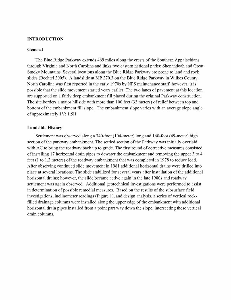
INTRODUCTION General
The Blue Ridge Parkway extends 469 miles along the crests of the Southern Appalachians through Virginia and North Carolina and links two eastern national parks: Shenandoah and Great Smoky Mountains. Several locations along the Blue Ridge Parkway are prone to land and rock slides (Bechtel 2005). A landslide at MP 270.3 on the Blue Ridge Parkway in Wilkes County, North Carolina was first reported in the early 1970s by NPS maintenance staff; however, it is possible that the slide movement started years earlier. The two lanes of pavement at this location are supported on a fairly deep embankment fill placed during the original Parkway construction. The site borders a major hillside with more than 100 feet (33 meters) of relief between top and bottom of the embankment fill slope. The embankment slope varies with an average slope angle of approximately 1V: 1.5H.
Landslide History
Settlement was observed along a 340-foot (104-meter) long and 160-foot (49-meter) high section of the parkway embankment. The settled section of the Parkway was initially overlaid with AC to bring the roadway back up to grade. The first round of corrective measures consisted of installing 17 horizontal drain pipes to dewater the embankment and removing the upper 3 to 4 feet (1 to 1.2 meters) of the roadway embankment that was completed in 1978 to reduce load. After observing continued slide movement in 1981 additional horizontal drains were drilled into place at several locations. The slide stabilized for several years after installation of the additional horizontal drains; however, the slide became active again in the late 1980s and roadway settlement was again observed. Additional geotechnical investigations were performed to assist in determination of possible remedial measures. Based on the results of the subsurface field investigations, inclinometer readings (Figure 1), and design analysis, a series of vertical rock-filled drainage columns were installed along the upper edge of the embankment with additional horizontal drain pipes installed from a point part way down the slope, intersecting these vertical drain columns.

Figure 1 - Inclinometer Readings
These measures slowed the slide for several years, but the slide reactivated in 1995. The various corrective measures performed had failed to eliminate the slide movement and ongoing maintenance was required on the Parkway pavement and shoulders. Additional settlement of up to 5 inches (125 mm) was measured in a period of 2 years from the last slide movement activation. During inspection of the slide area and drainage system in 1997 and 2000, consistent water flow was observed from four (4) of the sixteen (16) installed horizontal drains and water dripping was observed from another three (3) horizontal drains.
Site Geologic Setting
The landslide site is located within the Blue Ridge Belt. According to the “Geologic Map of North Carolina (1985),” the project site is predominantly underlain by finely laminated to thinly-layered gneiss of the Alligator Back Formation. This deposit locally contains massive gneiss and micaceous granule conglomeration, including schist, phyllite and amphibolite.

SUBSURFACE FIELD INVESTIGATIONS
EFLHD subsurface investigation team performed several subsurface investigation programs at the landslide site since the initial observation of slide movement in the 1970’s. Investigation records prior to 1990 are not available. Geophysical methods were also performed at the site to complement boring and coring log information. The details of the subsurface investigation are expounded below.
Borings and Rock Cores
Soil drilling and rock coring were performed at the site in the period between 1990 and 2003. This included site investigations on the following dates; 1) Five (5) C-series borings drilled during July 1990 by EFLHD, 2) Twelve (12) FD-series borings drilled during February 1991 by Froeling & Robertson, Inc., 3) Four (4) B270-series borings drilled during July 1997 by EFLHD to analyze the effectiveness of installed horizontal drains at draining the embankment fill, and 4) Three (3) B-series borings drilled during May 2003 by EFLHD to gather information at mid-slope. No borings were drilled at the toe of the slope because of problems accessing this location. (Figure 2).
Figure 2 - Subsurface investigation plan
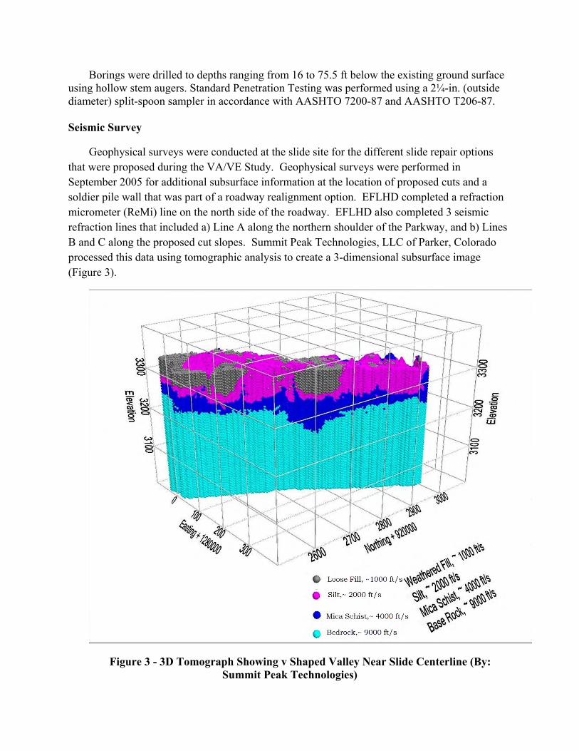
Borings were drilled to depths ranging from 16 to 75.5 ft below the existing ground surface using hollow stem augers. Standard Penetration Testing was performed using a 2¼-in. (outside diameter) split-spoon sampler in accordance with AASHTO 7200-87 and AASHTO T206-87.
Seismic Survey
Geophysical surveys were conducted at the slide site for the different slide repair options that were proposed during the VA/VE Study. Geophysical surveys were performed in September 2005 for additional subsurface information at the location of proposed cuts and a soldier pile wall that was part of a roadway realignment option. EFLHD completed a refraction micrometer (ReMi) line on the north side of the roadway. EFLHD also completed 3 seismic refraction lines that included a) Line A along the northern shoulder of the Parkway, and b) Lines B and C along the proposed cut slopes. Summit Peak Technologies, LLC of Parker, Colorado processed this data using tomographic analysis to create a 3-dimensional subsurface image (Figure 3).
Figure 3 - 3D Tomograph Showing v Shaped Valley Near Slide Centerline (By: Summit Peak Technologies)

EFLHD also conducted a geophysical refraction survey at the project site in September 2007
that consisted of three (3) seismic refraction survey lines. The seismic surveys were performed using a Smartseis S24 System with 24 channels. Geophones were spaced at either 15 or 20 feet (4.5 to 6 meters), and the total geophone array length ranged from 220 to 345 feet (67 to 105 meters). Shots were produced using a sledgehammer on a striker plate. Blackhawk – a Division of Zapata Engineering of Golden, Colorado, processed the geophysical data collected by EFLHD (Figure 4).
Figure 4 - 2D tomograph showing similar subsurface conditions (By: Zapata Engineering)
Subsurface Findings
The subsurface conditions encountered in the borings drilled at the slide site consisted mainly of four (4) layers as follows;
FILL - Fill consisting of brown and gray sand with silt and traces of mica gravel and small boulders was encountered from the ground surface to depths varying from 5 to 20 feet (4.5 to 6 meters). N-values recorded within the fill ranged between 2 and 15 blows per foot (bpf), indicating very loose to medium dense conditions.
COLLUVIUM – Colluvium material described as light brown to black sand with some silt and weathered sandstone fragments and traces of mica was encountered beneath the fill at depths ranging from 20 to 35 feet (6 to 10.7 meters). N-values recorded within this material ranged between 7 and 48 bpf, indicating loose to dense conditions.

SILT AND SAND (Saprolite) – Brown silt and sand with traces of mica was encountered beneath the fill or colluvium to depths ranging from 25 to 40 feet (6 to 12.2 meters). N-values recorded within the silt and sand ranged between 4 and 50 bpf, indicating very loose to very dense conditions.
BEDROCK – Light gray and brown (with some white) mica schist or sandstone was encountered beneath the silt and sand to the termination depth of the borings. The upper layer of mica schist consisted of a highly weathered layer to depths ranging from 26 to 44 feet (8 to 13.4 meters). N-values recorded within this stratum ranged from 22 to 50 bpf indicating medium dense to very dense conditions. Bedrock consisting of fine to medium textured, hard mica schist or sandstone was encountered below the silt or weathered material to depths ranging from 51 to 75 feet at boring termination. Rock quality designation (RQD) values varied from 51 to 100.
The tomographic image of the subsurface that was prepared based on the seismic survey results shows a valley into the bottom bedrock filled with soft material that deepens towards the southern end of the slide (Figures 3 & 4).
Groundwater
Groundwater was encountered in a number of borings at depths varying from 15 to 59.5 feet (4.5 to 18 meters). The drainage system appears to have lowered the groundwater table but the slide area continued to collect and concentrate groundwater from adjacent areas due to subsurface geology, such as the less pervious bedrock valley shown on the subsurface tomographic image. It was also observed that samples collected at the interface between the overburden material and top of rock were always in a wet condition. Based on these observations, the failure plane likely passes through this wet and soft subsurface zone.
Laboratory Testing
Laboratory testing was performed on representative rock core samples recovered during the subsurface exploration. Samples were tested for unconfined compressive strength (ASTM 2938). Test results are summarized in Table 1.
Table 1 - Summary of Laboratory Test Results.
Boring No. Sample No. Sample Depth
ft (m)
Unconfined Compressive Strength
psi (MPa) B-1 1 44.0 (13.4) 6,220 (42.89)
B-1 1 46.3 (14.1) 2,470 (17.03)
B-2 2 50.2 (15.3) 5,180 (35.71)
B-2 2 53.6 (16.3) 4,980 (34.34)
B-2 3 57.6 (17.6) 1,560 (10.76)

SLIDE REPAIR OPTIONS
EFLHD geotechnical engineers presented a number of slide repair options to the NPS, including a bridge option that was requested for consideration and evaluation by the NPS. Preliminary proposed repair options included:
a) Excavate and backfill b) Excavate and backfill with geosynthetic reinforcement, c) Roadway Realignment, d) Anchors with concrete blocks and e) A Bridge. The first two options were eliminated immediately since they did not meet the Park’s
requirements for environmental, limited disturbance and aesthetic considerations. The remaining options were further evaluated during a VA/VE Study in order to select the option that met the Park’s requirements and FLH design guidelines. The selection factors included;
1) Area of disturbance, 2) Construction impact, 3) Visual impact, 4) Risk, 5) Traffic control, and 6) Design and construction costs.
A summary of the final evaluated repair options is presented in Table 2
Table 2 - Summary of Slide Repair Options
Factor: Alternative 1 Realignment
Alternative 2 Anchor Blocks
Alternative 3 Bridge
Total Construction Cost
$5.9 m $2.5 m $4.0 m
Area of Disturbance; Acre (Hectare): Total Unpaved 0.64 (0.26) 0.32 (0.78) 0.33 (0.13)
Forested 0.10 (0.04) 0.68 (0.28) 0.00 (0.00) Grassy 0.54 (0.22) 0.10 (0.04) 0.33 (0.13)
Construction Impact: No. of Closed Lanes All 1 All
Tourist Seasons Affected 1 1 2
Risk: Slide Addressed N Y N
Road Affected by Continued Movement N Y N
Visual Impact: Cut Walls Temporary Tree Loss Bridge Appearance * Disturbance area in hectare/acre.

Based on the results of the VA/VE Study, anchors with anchor blocks was the preferred option since it enabled maintenance of one lane of traffic, it was cost effective, there is an ability to restore vegetation and natural site appearance, and there is less risk. The depth to rock made most of the other options not favorable.
DESIGN ANALYSIS
Design analysis was performed for the selected anchor and anchor block slide repair option based on the subsurface field investigations and laboratory test results, groundwater conditions and proposed site restoration geometry. Since depth to rock varied along and perpendicular to the roadway center line, and in order to provide an economical anchor design, the slide site was divided into zones. EFLHD prepared and analyzed a cross-section for each zone and determined the needed number of anchors to meet slope stability requirements.
Anchors and Anchor Blocks Design
Anchors were designed using principals for ground anchor design as presented in FHWA’s
Geotechnical Engineering Circular No. 4, 1999 (GEC 4). Anchors were designed for installation through the fill, colluvium, and weathered rock and into competent bedrock intersecting the failure plane. An allowable rock-grout bond stress of 50 psi (345 kPa) was calculated based on rock unconfined compressive strength laboratory test results.
Slope Stability Analysis
Slope stability analysis was performed for the selected critical cross sections. Soil strength properties were determined based on correlations to SPT N-values, laboratory test results, p-wave velocity and typical values in the literature. A summary of the determined soil and rock strength properties is provided in Table 3.
Table 3. Summary of Soil and Rock Strength Properties
Material type Unit Weight, Γ
lb/ft3 (kN/m3) Friction Angle, ϕ
Degrees Cohesion, C
lb/ft2 (kN/m2) FILL 115 (18.07 ) 30 --
Colluvium 120 (18.85) 32 --
Saprolite 125 (19.64) 25 300 (0.45)
Weathered rock 130 (20.42) 36 --
Bedrock 145 (22.78) 30 80000 (119.05)

Back analysis was used to refine calculated soil and rock strength parameters assuming an impending slope failure condition (using a safety factor of 1). Slope stability design models included the observed wet and soft or loose material at the interface between the overburden material and rock. The model was adjusted to simulate observed field conditions for the location of the crack at the top of the slope and the exit point of the failure plane at the toe of the slope (Figure 5). Computer software Slope/W (version 5) was used for running limit equilibrium design analysis and the Spencer method was selected because it satisfies both moment and force equilibrium.
Figure 5 - Slope stability design analysis results (Slope/W (v. 5))
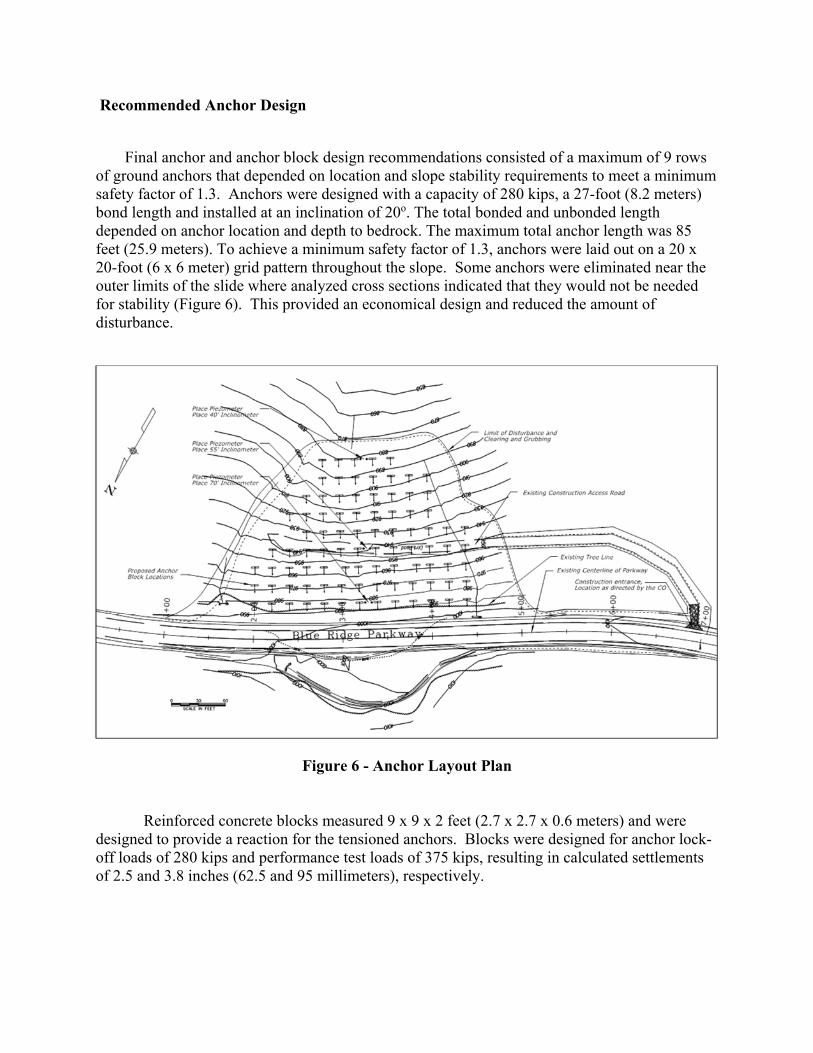
Recommended Anchor Design
Final anchor and anchor block design recommendations consisted of a maximum of 9 rows of ground anchors that depended on location and slope stability requirements to meet a minimum safety factor of 1.3. Anchors were designed with a capacity of 280 kips, a 27-foot (8.2 meters) bond length and installed at an inclination of 20o. The total bonded and unbonded length depended on anchor location and depth to bedrock. The maximum total anchor length was 85 feet (25.9 meters). To achieve a minimum safety factor of 1.3, anchors were laid out on a 20 x 20-foot (6 x 6 meter) grid pattern throughout the slope. Some anchors were eliminated near the outer limits of the slide where analyzed cross sections indicated that they would not be needed for stability (Figure 6). This provided an economical design and reduced the amount of disturbance.
Figure 6 - Anchor Layout Plan
Reinforced concrete blocks measured 9 x 9 x 2 feet (2.7 x 2.7 x 0.6 meters) and were
designed to provide a reaction for the tensioned anchors. Blocks were designed for anchor lock-off loads of 280 kips and performance test loads of 375 kips, resulting in calculated settlements of 2.5 and 3.8 inches (62.5 and 95 millimeters), respectively.

CONSTRUCTION Instrumentation
Instrumentation (observation wells and inclinometers) were installed during the design phase of the project. The contract also required the contractor to install additional instrumentation at three (3) locations along the centerline of the landslide slope in order to monitor the slide during and after completion of construction. Installed instrumentation consisted of piezometers and inclinometers that were installed at the top, middle and bottom of the slope prior to beginning of construction.
Construction Progress
The contractor began construction work by excavating a bench for the uppermost row of anchors in order to provide initial stability prior to accessing the lower steep toe of the slope. Heavy rainfall occurred after grouting anchors in the first row and prior to tensioning of these anchors. The rain, likely combined with stored construction materials and equipment loads at the top of the slope, triggered slide movement near the crest of the slope, causing a new crack to form and settlement on the road. This coincided with the inclinometer near the top of the slope showing significant ground movement during the first 4 weeks of construction. The contractor was advised to remove stored concrete blocks and heavy equipment from the roadway section located within the slide limits. After the uppermost two (2) rows of anchors were tensioned and stored material load had been removed from near the crest of the slope, visible movement ceased and inclinometer readings stabilized (Figure 7).

Figure 7 - Anchors and concrete anchor blocks installation during construction
Piezometer readings showed subsurface water condition changes during construction. A sharp and then steady increase of pore water pressure was observed as rows of anchors were tensioned (Figure 8). The increase was most apparent at the piezometers closest to the anchors being tensioned. Between the piezometer behavior and observations from anchor drillers, EFLHD deduced that there was at least one large, but discontinuous, confined pervious layer of weathered bedrock that was fed by groundwater discharged from the uplands and funneled into the V-shaped valley.

Figure 8 - Piezometer Reading Showing Subsurface Water Changes During Construction
As work progressed to near halfway down the slope, the contractor was placing blocks and drilling at the lowermost row of anchors. On one day, two of the holes drilled for anchors resulted in pressurized artesian fountains arcing from the drill hole at 4 to 6 feet into the air. This continued for several hours until there was a continuous trickle of water. The midslope and lower piezometers responded to this with a significant drop in water elevation. Shallow relief wells were installed on the lowermost row to allow for an outlet for water and to improve workability at those anchors.
After construction, the contractor hauled in fill to grade the slope, loamed, seeded, and planted larger vegetation between some of the blocks to create an engineered slope stabilization solution that is invisible to the observer.
Conclusions
A slowly progressing landslide at Milepost 270.3 on the Blue Ridge Parkway resisted attempts to be fixed for several decades. The first attempt focused on lowering the driving forces by lowering the elevation of the Parkway at the slide location. The next several remedial measures focused on reducing water pressures from the fill and upper slopes. These remedial measures incrementally improved the safety of the hillside, but were not enough to provide long-

term slope stability. Removing most of the water in the V-shaped subterranean bedrock valley would be a very difficult and costly solution. There were also intermittent confined layers within the saprolite that were not picked up during the investigations. The final anchor and block solution was able to address the instability by focusing primarily on providing active resisting forces to the slope, and designing with water present, assuming not all water could feasibly be removed. A benefit not foreseen in design was that punching 90 holes into bedrock resulted in at least temporary drainage of subsurface water. Finally, a significant aspect of this project has been achieving a context-sensitive solution that satisfied the NPS (Figure 8).
Figure 8 - Site Condition 2 Years After Completion of Construction
REFERENCES
Bechtel, R., 2005. When the Earth Moves. North Carolina Geological Survey, Information Circular 32: 24. Raleigh, NC.

Sabatini, P., Pass, D., Bachus, R., 1999. Ground Anchors and Anchored Systems. Publications No. FHWA-IF-99-015, Geotechnical Engineering Circular No. 4. Federal Highway Administration, Washington, DC.
Wightman, W., Jalinos, F., Sirless, P., Hanna, K. 2003. Applications of Geophysical Methods to Highway Related Problems. Publications No. FHWA-IF-04-021. Federal Highway Administration, Centeral Federal Lands Highway Division, Lakewood, CO.

Proposed Rock Slope and Rockfall Design Procedures and Methods for Evaluating Rockfall Sites within a Corridor
Ben Arndt, P.E., P.G. Yeh and Associates, Inc.
2000 Clay Street, Suite 200 Denver, CO 80211
(303) 781-9590 [email protected]
Brett Arpin, P.E. Yeh and Associates, Inc.
2000 Clay Street, Suite 200 Denver, CO 80211
(303) 781-9590 [email protected]
Prepared for the 67th Highway Geology Symposium, July, 2016

67th HGS 2016: Arndt and Arpin
Acknowledgements
The authors would like to acknowledge the input from the Colorado Department of
Transportation (CDOT) Geohazard and Geotechnical groups as well as the FHWA Resource Center and Central Federal Lands groups in discussions on this topic.
Disclaimer
Statements and views presented in this paper are strictly those of the author, and do not necessarily reflect positions held by their affiliations, the Highway Geology Symposium (HGS), or others acknowledged above. The mention of trade names for commercial products does not
imply the approval or endorsement by HGS.
Copyright Notice
Copyright © 2016 Highway Geology Symposium (HGS) All Rights Reserved. Printed in the United States of America. No part of this publication may be
reproduced or copied in any form or by any means – graphic, electronic, or mechanical, including photocopying, taping, or information storage and retrieval systems – without prior
written permission of the HGS. This excludes the original authors.

67th HGS 2016: Arndt and Arpin
ABSTRACT
Recent Federal legislation has linked asset management principles to transportation funding for pavements and bridges. Several transportation agencies are applying asset management principles to geological hazards and slopes. This has generated great interest in determining appropriate methods, designs, and guidelines for evaluating roadway corridors to address rock slope and rockfall design procedures and standards.
This paper presents the results of the previous discussion for roadway corridors within
Colorado. Proposed methods for evaluating rock slopes and rockfall potential include using the following concepts: 1) Rockfall Hazard Rating Systems (RHRS) or modified rating systems to evaluate the rock slope features that could potentially generate rockfall, 2) rock slope treatment based on rockfall potential (slope treatment includes such items as blasting methods, bolting, draped mesh, and pinned mesh), 3) expected percentages of rockfall catchment relative to rock slope treatment, and 4) catchment percentage requirements based on such factors as traffic volumes for a given corridor.

67th HGS 2016: Arndt and Arpin
BACKGROUND
Rock slopes and rockfall prone areas are common in mountainous terrain along transportation corridors in the United States. Two types of hazards confront geotechnical design efforts: rockfalls and rock slope stability. Both of these hazards are related but can also be independent variables. The potential to have a rockfall at a given site is dependent on many conditions and causes, all of which may result in rocks on the road. Rock slope stability may cause a rockfall to occur but is generally characterized by movement of a rock mass along a discontinuity such as a distinct kinematic-type failure (e.g., planar, wedge, or toppling). Both failure mechanisms create hazards to the traveling public and both mechanisms can result in rocks on the road and impacts to mobility.
Rock slope evaluations have generally relied on using the Rockfall Hazard Rating System
(RHRS) published in 1993 (1). Since then, many departments of transportation have either used RHRS as it was published or have modified it to incorporate other site-specific information. The original RHRS had ten (10) general categories that included the following:
Slope Height Ditch Effectiveness Average Vehicle Risk Percent of Decision Sight Distance Roadway Width Including Paved Shoulders Geologic Characteristics (Case 1 or Case 2) Block Size or Volume of Event Climatic and Water On Slope Rockfall History
The system provides a method to evaluate a given rock slope using the preceding categories
to apply an overall score. The higher the score presumably the worse the rock slope will perform. The score is relative to other rock slopes within a state or corridor. The best score that can be obtained in this system is 30, which presumably represents the best performing slope, while the worst score is 810, representing the worst performing slope.
Revised rating systems have also been used by many departments of transportation. The Colorado Department of Transportation developed the Modified Colorado Rockfall Hazard Rating System (MCRHRS) (2) which has twenty-one (21) categories to rate slopes that generally follow the RHRS but is more detailed. The best score that can be obtained is 63, which presumably represents the best performing slope. The worst score that can be obtained is 1701, which likely represents the worst performing slope.
Further research in rockfall ditch catchment was provided with the Rockfall Catchment Area Design Guide in 2001 (3). The design guide provided data from rolling more than 11,000 rocks off vertical; 0.25H:1.0V; 0.5H:1.0V; 0.75H:1.0V; and 1.0H:1.0V slopes of three different heights (40, 60 and 80 feet) into three differently inclined catchment areas (flat, 6H:1V and 4H:1V). The results were used to develop design charts that provide percentages of retained rockfall from 50% to 99% for a given ditch configuration.

67th HGS 2016: Arndt and Arpin
Rock slope evaluation and stability analysis presented in Rock Slopes Participants Manual
(4) generally follows Hoek and Bray (5). In this manual the mechanics of evaluating and designing rock slopes is outlined. Guidance is provided for assessing rock slopes and methods for stabilization such as rock bolting and other reinforcement options.
Common methods to mitigate an unstable rock slope or rockfall include but are not limited to:
Removal o Scaling o Blasting – presplitting techniques, flatter rock slope angles where unfavorable
discontinuities are present Stabilization
o Rock bolting o Pinned Mesh o Cable Lashing o Rock Gluing (Polyurethane Resin)
Protection o Draped Mesh Systems o Rockfall Barrier Fences o Attenuator Systems o Other Containment or Catchment Systems
The purpose of this paper is to propose using RHRS, ditch catchment, and common mitigation techniques in an integrated design process involving roadway designers to evaluate the best alternative. PRESENT STATE OF THE PRACTICE
Practitioners who design rock slopes and evaluate rockfall prone features generally use the
preceding FHWA documents to evaluate the rockfall potential and rock slope stability for existing and new roadway rock cuts. In lieu of specific AASHTO guidelines, which at present do not account for rock slopes or rockfall, a practitioner typically assumes these documents constitute the standard of practice. However, the question of standard of practice versus the standard for rock slopes and rockfall has recently arisen in Colorado in relation to flood damage issues and FEMA funding reimbursement for repair work. The following items are for consideration when a practitioner is designing a rock cut or rockfall mitigation feature for which specific AASHTO guidelines do not exist:
What is the minimum score from either the RHRS or modified systems that would
require mitigation action versus no action when dealing with rockfall or rock slope instability?
How can an RHRS or modified system be used to evaluate the potential for rockfall to occur? A higher rated slope would presumably create more rockfalls but can that be quantified with a number or a threshold?
The rockfall catchment design charts are useful but assume a rockfall will occur. How can rockfall frequency from a given slope be evaluated?

67th HGS 2016: Arndt and Arpin
What is the minimum global factor of safety (FOS) that a rock slope should be designed to when evaluating failure modes such as planar and wedge failures?
How can a new rock cut be evaluated prior to making the excavation such that mitigation and stabilization measures can be incorporated into the construction?
PROPOSED SYSTEM FOR ROCK SLOPE EVALUATION The following is a proposed set of procedures for updating and modifying the previous studies to incorporate newer roadway design standards and conditions in an iterative process that evaluates various rock slope and rockfall mitigation options and roadway layouts. Overview of Integrated Roadway and Rock Slope Design Current roadway design typically entails the roadway layout. Roadway layout uses AASHTO guidelines to determine traffic speeds, curves, super elevations, vertical alignments, horizontal alignments, recoverable shoulder slopes, grades, guardrail requirements, sight distances, etc. Given the multitude of roadway design requirements, rather than attempt to create new and redundant categories such as the site distance category in the RHRS, these features have been or can be addressed by roadway designers. Rock slope designers should work with the roadway designers to evaluate the best alternative both in terms of roadway layout and reduced likelihood of rockfalls reaching the roadway. For example, a roadway designer will establish a preliminary required shoulder distance from edge of travel lane with other features such as a recoverable slope angle and width for a new rock cut. At this point in the process, the rock slope designer would go through a design process such as the following and as is discussed in more detail in the following section:
Evaluate similar rock slopes and, through a geotechnical investigation, evaluate the likelihood and level that a proposed cut slope will generate rockfall and the potential for rock slope instability.
Evaluate the global and/or kinematic stability of the rock slope. Typically, a FOS of 1.30 is the design standard of practice, but can vary depending on site-specific conditions.
Evaluate if specific blasting methods (i.e. presplitting methods) will improve the stability of the rock cut
Evaluate whether the catchment ditch is of sufficient size to retain rockfalls and what percentage would be retained.
Evaluate mitigation methods to reduce rockfall potential and increase rock slope stability. Proposed Rock Slope and Rockfall Design Iteration Process Step 1 – After receiving the preliminary roadway layout, evaluate similar rock slopes and through a geotechnical investigation evaluate the likelihood and level that a proposed rock slope will generate rockfalls and the potential for rock slope instability. Many states and agencies have existing RHRS and other modified systems data that is available to a rock slope designer. It may be possible to isolate factors within the RHRS or other system that

67th HGS 2016: Arndt and Arpin
represent the potential for a slope to generate rockfalls. The following categories may provide such data. Geological Characteristics: This category may provide insight into the potential for a site to generate rockfalls. The RHRS provides two (2) sub-categories named Case 1 and Case 2 in which the structural condition, rock friction, and difference in erosion rates are evaluated. Climate and Persistence of Water on Slope: This category may be useful in evaluating rockfall potential given a fractured rock mass. Rockfall History: This category may not provide reasonable data to evaluate the likelihood and frequency of rockfalls due to the lack of reporting common in most agencies. Based on the preceding discussion, it may be reasonable to evaluate the likelihood of a rockfall event to occur from a rock slope based on the score of the Geological Characteristics category. The RHRS and modified systems typically use the 3, 9, 27, and 81 exponential rating systems with higher scores relating to conditions that are more likely to generate rockfall. As a starting point and after cursory review of historical systems, it seems that a rating lower than 9 likely is not as prone to generating rockfalls as a rating greater than 27. This could further be evaluated based on historical databases but the general idea would be as shown in Figure 1.
Figure 1. Likelihood of rockfall issues related to categories in RHRS
Step 2 – Evaluate the global and/or kinematic stability of the rock slope The global and kinematic stability of the rock slope can be evaluated as described in the Rock Slopes Participants Manual (4). Step 3 – Evaluate if specific blasting methods (e.g., presplitting) will improve the stability of the rock cut
0
10
20
30
40
50
60
70
80
90
Cat
egor
y S
core
Category Condition
Greater Potential Rockfall
Less Potential Rockfall
Better Worse

67th HGS 2016: Arndt and Arpin
FHWA publications such as Rock Blasting and Overbreak Control (6) are useful in evaluating whether specialized blasting techniques such as presplitting can improve the stability of a rock excavation. Step 4 – Evaluate whether the catchment ditch is of sufficient size to retain rockfall and what percentage is retained Once the potential for rockfall or an unstable rock slope condition has been established, then the catchment ditch can be evaluated. This is typically done using the information provided in the Rockfall Catchment Area Design Guide (3). The desired percentage of rock retained within the ditch will likely depend on many factors such as anticipated size of rocks, agency requirements, annual average daily traffic (AADT), and standard of practice. As an example of how AADT may influence the desired percentage of rock retained, Table 1 illustrates a relationship between AADT and percentage of rock retained. Obviously on interstates and high traffic volume areas the percent retained rock should be much higher. Any rock on the road, whether or not it can be avoided, will undoubtedly create a situation in which either a vehicle will hit the rock or hit another vehicle while trying to avoid a rock. The traffic volumes presented in this table are for discussion and could be adjusted according to corridor and agency requirements among other factors.
Table 1. Example AADT and Percent Rockfall Retained
Annual Average Daily Traffic
(AADT)
Percent Rockfall Retained
< 100 50% 101 to 1000 75% 1001 to 3000 80% 3,000 to 5,500 85% 5,500 to 10,000 90% 10,000 to 15,000 95%
> 15,000 99% Step 5 – Evaluate mitigation methods to reduce the rockfall potential and increase the rock slope stability If rockfall potential and rock slope stability are not satisfactory, mitigation methods can be evaluated to create a satisfactory rock slope. This will likely require an iterative design process as previously discussed. Simple examples of the design process iterations are provided below. Example 1. Given a rock slope is either unstable or can generate rockfall, the rock slope stability and ditch catchment are analyzed to evaluate if the catchment is within the project requirements. If rock slope stability and catchment are acceptable, then no further design evaluation is required. In this scenario, the rock slope can be excavated by any method and no further mitigation such as

67th HGS 2016: Arndt and Arpin
rock bolting or draped mesh is necessary. It would also be necessary to establish a target global stability factor of safety for the rock slope. Example 2. Given a rock slope is either unstable or can generate rockfalls and the ditch catchment effectiveness is not within the desired percentage retained, then further evaluation is necessary. Possible rock slope stability and rockfall mitigation options can be evaluated such as:
Increasing Ditch Catchment Presplit Blasting Methods Reducing Rock Slope Angle Rock Bolting Draped Mesh Rockfall Barrier Fences
SUMMARY
The overall intent of this process is to suggest a better defined process with a goal of
creating a standard for rock cuts with respect to slope stability and rockfall potential. It can be difficult for a licensed professional to provide rock slope and rockfall designs if no established standard exists and no well-defined process is in place. In many instances the practitioner is put in a position where mitigation options such as presplitting a rock slope are deemed visually unappealing for a given corridor and eliminated by others, which effectively transfers much greater liability to the design professional. The design professional is put in a position of maintaining safety to the traveling public versus requirements of the client or shareholder. Using the concepts outlined in this paper, the design professional would have the ability to demonstrate that if, for example, presplitting blasting methods are prohibited or draped mesh is not possible for aesthetic reasons, then other factors such as more ditch catchment is required. This seems reasonable since, for example, when recoverable slopes cannot be provided, the roadway design manual requires guardrail barrier. The liability of eliminating the safety feature (i.e., recoverable slope) is not transferred to the responsible roadway designer but is modified with another option (guardrail). Rock slope and rockfall design should be accorded similar design criterion and options to provide the best alternatives for agencies and the overall safety of the traveling public.

67th HGS 2016: Arndt and Arpin
REFERENCES
1. Pierson, L.A. and R. Van Vickle, R. Rockfall Hazard Rating System – Participant’s Manual. Report FHWA-SA-93-057. FHWA, U.S. Department of Transportation, 1993.
2. Russell, C.P., P. Santi, and J.D. Higgins. Modification and Statistical Analysis of the Colorado Rockfall Hazard Rating System, Report CDOT-2008-7. Colorado Department of Transportation, 2008.
3. Pierson, L.A, C.F. Gullixon, and R.G. Chassie. Rockfall Catchment Area Design Guide. Report FHWA-OR-RD-02-04. Research Group, Oregon Department of Transportation and FHWA, U.S. Department of Transportation, 2001.
4. Wyllie, D.C. and C.W. Mah. Rock Slopes – Participants Manual. Report FHWA-HI-99-007. NHI, FHWA, U.S. Department of Transportation, 1999.
5. Hoek, E. and J.W. Bray. Rock Slope Engineering. Institution of Mining and Metallurgy, 1996.
6. Konya, C.J. and E.J. Walter. Rock Blasting and Overbreak Control. Report FHWA-HI-92-001. FHWA, U.S. Department of Transportation, 1991.

Rapid Response to a Post Fire Debris Flow Event
Mallory A. Jones, GIT
KANE GeoTech, Inc.
7400 Shoreline Drive, Suite 6
Stockton, California 95219
(209) 472-1822
Richard A. Nack, PE
City of Camarillo
601 Carmen Drive
Camarillo, California 93010
(805) 388-5318
William F. Kane, PhD, PG, PE
KANE GeoTech, Inc.
7400 Shoreline Drive, Suite 6
Stockton, California 95219
(209) 472-1822
Prepared for Submission to the 67th Highway Geology Symposium
Colorado Springs, Colorado

67th HGS 2016, Jones, Nack, & Kane 2
ACKNOWLEDGEMENTS
The author(s) would like to thank the individuals/entities for their contributions in the work
described:
Access Limited Construction
City of Camarillo
Geobrugg North America
HI-TECH Rockfall Construction
Disclaimer
Statements and views presented in this paper are strictly those of the author(s), and do not necessarily reflect positions held by their affiliations, the Highway Geology Symposium (HGS), or others acknowledged above. The mention of trade names for commercial products does not
imply the approval or endorsement by HGS.
Copyright
Copyright © 2016 Highway Geology Symposium (HGS)
All Rights Reserved. Printed in the United States of America. No part of this publication may be reproduced or copied in any form or by any means – graphic, electronic, or mechanical,
including photocopying, taping, or information storage and retrieval systems – without prior written permission of the HGS. This excludes the original author(s).

67th HGS 2016, Jones, Nack, & Kane 3
ABSTRACT
In May, 2013, Ventura County, California was impacted by the Springs Fire that scorched approximately 24,000 acres. As a result of the fire, the area’s vegetative coverage and soil characteristics were drastically changed. These changes, along with heavy rainfall, caused a residential area located at the base of Conejo Mountain, Camarillo Springs, to experience two major debris flow events.
With all signs pointing to an El Nino year, and concern for the community, the City of Camarillo retained a team of geotechnical professionals to develop a mitigation design to minimize risk to life and property.
After completing the initial site investigation, analysis, and design, logistical issues arose delaying the original project. Alternate designs were considered but encountered conditions that could not be resolved with allotted time constraints. With time running out, on October 14, the original mitigation design was authorized for bidding.
With a contract completion date of January 25, 2016 and the constant threat of El Nino storms, the mitigation construction proceeded at an unprecedented pace. Five flexible barriers, six earth berms, and approximately 6.5 acres of slope grading were completed on January 4, 2016. On January 5, 2016, Ventura County experienced the heaviest rain of the season. The rains lasted three days and were the first test of the mitigation design. The barriers and berms performed as expected and prevented large amounts of material from impacting the homes below.

67th HGS 2016, Jones, Nack, & Kane 4
INTRODUCTION
Research on debris flows in the United States continues to provide new information and ideas on efficient and effective ways to mitigate them. Rigid debris flow barriers have been used for decades, but the idea of the flexible debris flow barrier has evolved after recent and extensive field testing and finite element modeling. These flexible debris flow barriers are an affordable option for debris flow mitigation and can be constructed quickly by qualified contractors.
After being impacted by the Springs Fire of 2013, the City of Camarillo (City), located in Ventura County, in Southern California, Figure 1, experienced two major rainfall events the following year causing devastating debris flows in the Camarillo Springs community, Figure 2. With the threat of El Nino impacting California during the winter of 2015-2016, the City’s geotechnical engineer contacted KANE GeoTech, Inc. (KANE GeoTech) to assess the hazard and develop a cost and time efficient mitigation plan.
Due to the topography and fast-track nature of the project, KANE GeoTech recommended the hazard be mitigated utilizing flexible debris flow barriers and earth berms. This option was the most efficient and cost effective with mitigation performance that has been tested and verified by one of the industry’s leading geohazard mitigation manufacturers, Geobrugg, North America.
Figure 1. Project Location Figure 2. Home buried after Decmeber 11, 2014 debris flow event.

67th HGS 2016, Jones, Nack, & Kane 5
HISTORY OF FLEXIBLE DEBRIS FLOW BARRIERS
Geobrugg Protection Systems began as part of a wire-rope manufacturing firm, Fatzer A.G., of Romanshorn, Switzerland. Early on, Brugg, as it was called then, began fabricating nets made from wire rope to use as snow nets for avalanche protection in the Swiss Alps. During spring season net maintenance, the nets were often observed full of rock from rockfall. The connection was made and Brugg began manufacturing barriers made of wire rope nets for the purpose of rockfall protection. In 1989, Brugg opened its first North American factory in Santa Fe, New Mexico to manufacture wire rope net rockfall barriers. In the early 1990s, the California Department of Transportation (Caltrans) began using the rockfall barriers with a high degree of success. Caltrans also experienced a number of debris flow events that were inadvertently stopped by the rockfall barriers. About the same time, ring net barriers, which were much stronger than wire rope nets and could absorb more energy, began to replace the rope nets in rockfall barriers. In the 1996, Caltrans; California Polytechnic University, San Luis Obispo; and the U.S. Geological Survey began flume experiments for the purpose of developing an understanding of the forces acting on a debris flow barrier. Meanwhile, similar research had begun in Europe and Japan. In the winter of 2005, devastating floods and debris flows impacted Switzerland. As a result, Brugg, now Geobrugg, and the Swiss Federal Institute for Forestry, Snow and Landscape Research, (WSL) embarked on a multi-year, several million Euro program to develop, test, and install debris flow barriers. These barriers were to be engineered according to the dynamics of debris flow. As a result of this research, Geobrugg developed two systems of engineered debris flow barriers. These barriers were designed to fit within stream flow channels, or chutes. They are engineered to absorb the initial dynamic impact forces and the subsequent static loads imposed on the barriers. Their flexible design allows for much of the impact energy to be absorbed in deformation of the flexible net and brake elements. The two barrier types are referred to as VX and UX barriers. VX barriers are intended for use in relatively narrow V-shaped chutes, up to about 15 meters wide. They consist of wire rope anchors between which are suspended wire rope support ropes with braking elements. High-strength steel ring nets are installed on the top, middle, and bottom support ropes, Figure 3. The system is designed to flex outward down slope on impact to absorb and dissipate energy of the debris flow. Consequently, the barrier must flex outward a few meters as it absorbs the energy. Any design must include this distance down slope of the barrier. It is also necessary for the barriers to be designed to withstand a static load after impact, similar to a retaining wall.

67th HGS 2016, Jones, Nack, & Kane 6
A UX barrier is similar in construction except that it includes two support steel column posts. It is designed for channels wider than the VX barrier limitations. UX barriers are intended for use in channels up to about 25 meters wide. The purpose of the posts is to maintain the height of the barrier across the channel. They are not intended to supply any additional structural functions. The barriers are engineered so that all loads are dissipated through the net, support ropes, brakes, and anchors. Shallow landslide barriers (SLBs) were developed for installations where no chute or channel is present or exceeds the maximum width of a conventional UX barrier. They rely on the same energy absorption principles as debris flow barriers. The major difference is that the top and bottom support ropes are anchored in the ground adjacent to the barriers. Debris flow barriers are now used around the world with installations in Switzerland and other parts of Europe, Malaysia, Japan, Hong Kong, Canada, Mexico, and South America among other places.
BACKGROUND
Camarillo Springs was impacted by the Spring Fire of 2013. Over 24,000 acres were burned, along with all the vegetation that covered the hillside, Figure 3. The Spring Fire also resulted in a change in soil conditions. The once permeable soil developed a waxy repellent beneath the scorched surface soil layer. This caused the top layer to become saturated during heavy rains, leading to rapid runoff and removal of the surface soil (GDI, 2015). Following the Spring Fire, Camarillo Springs experienced debris flows, including two major debris flow events with the first occurring on October 31 and the second on December 11, 2014. These debris flows
Figure 3. Geobrugg VX Debris flow barrier components.

67th HGS 2016, Jones, Nack, & Kane 7
impacted residences on the streets below, where ten homes were “red tagged” and unable to be re-built until a more permanent mitigation measure is in place.
Five major barrancas, or ravines, were identified as potential debris flow channels. Two of which, Barrancas 2 and 3, were the locations of the debris flow events of 2014. They were identified as being major hazards and the highest priority for mitigation by the City of Camarillo’s consulting geotechnical engineer. An apron between Barrancas 2 and 3, referred to as the Young Erosion Area, also showed evidence of producing massive amounts of material that could affect the homes below, (KANE, 2015). The debris flow event that occurred on October 31, 2014 consisted primarily of fine grained mud and ash. This saturated, surficial material, no longer anchored to the slope by vegetation, was mobilized by the runoff from the heavy rain that occurred during the storm. Rills varying in size were observed throughout the Young Erosion Area, showing contribution to the debris flow material. The December 11, 2014 debris flow was a higher energy flow resulting in the mobilization of larger material along with fine sediment. Observations following the December 11 debris flow reported the existing rills in the Young Erosion Area had drastically increased in size before the second event occurred (GDI, 2015).
Figure 4. National Park Service map showing Springs Fire burn area.

67th HGS 2016, Jones, Nack, & Kane 8
Since the debris flows occurred, studies have taken place to assess the probability of recurring debris flows and their potential volumes. Both of these factors have an influence on possible mitigation options. Due to the vast area and different depths to bedrock found throughout the area, estimating the amount of material that could potentially flow down-slope was investigated with the previous debris flows being worst-case scenarios. Topographic maps, as well as records of the material hauled away during clean up, were utilized for the material volume estimations. The values obtained after analysis were considered when finalizing the mitigation designs. After the October 31, 2014 debris flow event, a site inspection was performed by the Natural Resource Conservation Services (NRCS) staff to assess the damages and determine if the event qualified for the Emergency Watershed Protection (EWP) program. The assessment determined that the event met the EWP program requirements and was eligible for a 75 percent grant to construct intermediate mitigation measures to reduce the damage from future events. The EWP program required a public sponsor to receive the grant funds and the City of Camarillo accepted the role of sponsor.
The NRCS technical staff prepared an intermediate mitigation design consisting of a series of wood plank deflection devices, k-rails, sandbags, steel bar racks, and debris racks. The City advertised and bid the project in early December 2014 and awarded the construction contract at their council meeting on December 9. Due to the EWP grant requirement that the improvements must be constructed within 10 days, and given the rain forecast, the contractor began mobilizing on December 11, 2014.
During the early morning hours of December 12, 2014, a strong storm cell discharged over 0.2 inches of rain in 60 minutes which triggered the second major debris flow. The City staff worked with the contractor and the NRCS staff to develop a revised design that included the construction of three debris platforms, Figure 5. The revised design was completed December 18, 2014 and the contractor completed the construction on December 31, 2014.
Following construction of the debris platforms, the Camarillo Springs Home Owners’ Association petitioned for additional mitigation measures to be implemented by the City. The City, by the advice of their consulting geotechnical engineer, contacted KANE GeoTech to provide an additional engineering mitigation design.
KANE GeoTech visited the area in August 2015 to meet with the Camarillo Springs Homeowners’ Association and City personnel, including their consulting geotechnical engineer. During this visit, a field assessment was conducted to assess the hazards in each area and gather information for mitigation design and engineering analyses. This information was then utilized to design a mitigation plan using flexible debris flow barriers and earthen berms.
When the draft plans were near completion, the Camarillo Spring Homeowners’ Association decided to explore additional mitigation options, thus delaying the project. Alternate designs were considered but encountered conditions that could not be resolved with allotted time constraints. Following weeks of negotiation, the decision was made to move forward with the original d esign using the flexible debris flow barriers and berms.

67th HGS 2016, Jones, Nack, & Kane 9
As a result, of lost time while selecting a final mitigation design and the threat of a heavy rain season approaching quickly, the project was fast-tracked in hopes of completing final design revisions, bidding for contractors, and complete construction before the rainy season arrived.
RECONNAISSANCE AND SITE INVESTIGATION
Prior to the initial site investigation, KANE GeoTech reviewed existing reports written after the debris flows occurred. KANE GeoTech also utilized aerial images to perform a reconnaissance to become familiar possible mitigation options and locations before conducting the site investigation, Figure 6.
KANE GeoTech, along with City personnel, and their consulting geotechnical engineer, hiked the site to investigate areas of concern and verify possible mitigation locations. Once the locations were finalized, material property data and channel dimensions were collected. The site investigation also allowed additional mitigation options to be explored.
While on-site, KANE GeoTech designed a conceptual mitigation plan using flexible debris flow barriers and shallow landslide barriers (SLBs) within the barrancas, NCRS debris platforms, and earth berms on the Young Erosion Area. The general idea behind the mitigation design was to utilize the earth berms to intercept the high velocity runoff from the upper portions of the
Figure 5. NCRS designed debris flow platform at Barranca 3.

67th HGS 2016, Jones, Nack, & Kane 10
mountain and divert the water and eroded material into the barrancas. The eroded material from the upper property and the Young Erosion Area, along with eroded material produced from the barrancas themselves, would then be stored behind the flexible debris flow barriers and SLBs constructed within the barrancas and the debris platforms.
After developing the general concept, KANE GeoTech personnel gathered general channel and platform dimensions of each proposed barrier location using a measuring tape and a string level. These measurements would be used later for analysis and design purposes.
DEBRIS FLOW ANALYSIS AND DESIGN METHODOLOGY
Using the information gathered in during the site investigation and information provided from previous studies, a debris flow analysis was performed using one of the debris flow mitigation manufacturer’s analysis software, DEBFLOW. The DEBFLOW program has been developed by Geobrugg to aid in the analysis and application of their debris flow barriers, and was developed using field and lab testing data and finite element analyses.
Input parameters for the DEBFLOW analysis included channel dimensions, storage area behind the location of each barrier, amount of material and number of pulses expected for each debris flow event, channel gradient at each location, and the slope inclination of the channel sides. The results of the debris flow analysis provided the appropriate barrier type needed to mitigate the hazard at each proposed location, along with the barriers’ dimensions for design purposes.
Figure 6. Aerial image used to determine possible barrier locations prior to site investigation.

67th HGS 2016, Jones, Nack, & Kane 11
After the size and type of the barriers were established, additional engineering analysis was performed to determine the depth of the wire rope anchors. When needed, upslope retaining rope anchor depths, post foundations depths and dimensions were also determined.
After analyses is complete, the final plans and specifications were produced using the data output from the DEBFLOW program.
PRE-CONSTRUCTION BARRIER LAYOUT
As a result of the flexible debris flow technology being a relatively new concept, a formal barrier field layout methodology has yet to be developed for installation. KANE GeoTech has become familiar with information and parameters needed to be useful when ordering material for construction. KANE GeoTech has developed a methodology to accurately layout the flexible debris flow barriers while obtaining the final laid-out channel dimensions necessary for material purchasing purposes.
The methodology includes obtaining slope geometry and applying trigonometry to establish anchoring locations according to the manufacturer’s parameters. Barrier layout begins with obtaining slope angles on both sides of the channel. Multiple slope angle measurements are necessary if the channel side’s inclination changes. On one side of the channel, the top support rope length and anchor group locations are determined by measuring the maximum width, across the top of the channel. The maximum width is standardized by the manufacturer according to the designed system type. Winglet anchor locations are determined by calculating the slope distance (SD) using the Law of Sines, using the standardized 15 degrees horizontal offset, slope angle, and the top support rope length, Figure 7.
Bottom support rope anchor group locations are marked 12 inches above the bottom of the channel, 5 degrees vertical from the top support rope anchor group location. The barrier height is measured as the vertical height between the top and bottom support rope anchor group locations. The vertical height is then divided by the designed number of intermediate support rope sections. Intermediate support rope anchor group locations are marked at the section divisions, and in line with the 5 degrees offset down slope between top and bottom support rope anchor group locations, Figure 8. After anchor group locations on one channel side are laid out, straight-line lengths and anchor group locations on the other side of the channel can be determined. The support ropes are laid out in line directly across the channel and with a level and lengths are obtained with a tape measure. Slope angles are used to calculate slope distances between top and bottom support rope anchor group locations for border rope lengths.

67th HGS 2016, Jones, Nack, & Kane 12
CONSTRUCTION AND IMPACT OF THE DEBRIS FLOW BARRIERS, SHALLOW LANDSLIDE BARRIERS, AND EARTHEN BERMS
After all engineering analysis and barrier designs were completed, construction plans and specifications were produced for the Camarillo Springs project bidding process. The project was awarded to Access Limited Construction, LLC. Construction began November 16, 2015 and was scheduled to be completed no later than January 25, 2016.
In response to the stringent timeline, the more efficient option of utilizing a verification anchor test to verify the bond strength of the subsurface material at the site was decided to be drilled and performance tested, Figure 9. This verification anchor was located in the worst conditions encountered at the site to exhibit a worst-case scenario for the most conservative results possible. The verification anchor was drilled to 13 feet and passed the anchor test allowing the holes that were located in equally or more competent material to all be drilled to a depth of 13 feet, Figure 10.
Following drilling the anchor holes, the threadbar and wire rope anchors were then installed and grouted into place. Grout samples were taken by an outside contractor during every grout pour to verify the grout strength properties.
Figure 8. Wire rope anchor offset. (side view)
Figure 7. Slope distance equation.
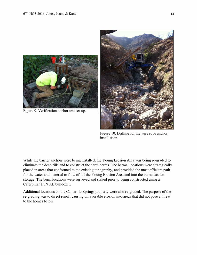
67th HGS 2016, Jones, Nack, & Kane 13
While the barrier anchors were being installed, the Young Erosion Area was being re-graded to eliminate the deep rills and to construct the earth berms. The berms’ locations were strategically placed in areas that conformed to the existing topography, and provided the most efficient path for the water and material to flow off of the Young Erosion Area and into the barrancas for storage. The berm locations were surveyed and staked prior to being constructed using a Caterpillar D6N XL bulldozer.
Additional locations on the Camarillo Springs property were also re-graded. The purpose of the re-grading was to direct runoff causing unfavorable erosion into areas that did not pose a threat to the homes below.
Figure 9. Verification anchor test set-up.
Figure 10. Drilling for the wire rope anchor installation.

67th HGS 2016, Jones, Nack, & Kane 14
Construction was completed on January 4, 2016, three weeks ahead of schedule. The day following the construction completion, Camarillo experienced the season’s heaviest rainfall. The storm event continued for three days and as a result, the newly constructed barriers and berms were impacted and performed as designed. The two barriers located upslope within the barrancas were approximately 75 percent and 90 percent filled by the time the rain ceased, Figure 11. The barriers located in the NCRS debris platforms were minimally impacted with debris filling approximately 5 percent to 10 percent of the barriers, Figure 12. The earth berms successfully diverted the high velocity water and material runoff into the barrancas where the material was stored behind the barriers and in the barrancas themselves. It should be noted that although erosion of these berms did occur, they were design to be temporary structures to aid in the reduction of rapid erosion of the Young Erosion Area until vegetation re-establishes.
The barriers were designed by the manufacturer and the Engineer for accessible clean-out and maintenance. All components can be re-used unless the rings are deformed or the break elements have been activated. In this case, the components that need replacement can be installed following the clean out of the debris accumulated.
Figure 11. Up slope barrier in Barranca 2 filled to approximately 90 percent of its capacity.

67th HGS 2016, Jones, Nack, & Kane 15
CONCLUSION
Following major debris flows, the threat of El Niño predicted for the upcoming rainy season, an innovative engineered mitigation design was put into action and constructed to mitigation future events. The project was delayed but then fast-tracked to be completed as soon as possible. The project was completed within an unprecedented timeframe and successfully mitigated what could have been a devastating debris flow event the day after construction completion. The conditions at the site have continued to improve with the growth of new vegetation, Figures 13 and 14.
Figure 13. Aerial image of the Project Area prior to mitigation.

67th HGS 2016, Jones, Nack, & Kane 16
REFERENCES
Geodynamics, Inc. (2015). “Geotechnical Reconnaissance of Debris Flow Risk, Gitana Avenue and San Como Lane, Camarillo Springs HOA, Camarillo, California, 93012.” April 14, 2015.
KANE GeoTech, Inc. (2015). “Camarillo Springs Debris Flow Investigation Report of Findings.” September 10, 2015.
National Parks Service. (2013). “2013 Springs Fire Burned Area Emergency Response Accomplishment Report.” National Parks Services. https://www.nps.gov/samo/learn/management/2013-springs-fire.htm.
Figure 14. Aerial image of the Project Area after mitigation construction was completed.

Understanding Rockfall Behaviors Using Wireless Sensor Network System
through Laboratory Experiments
Prapti Giri (Young Author) PhD Student
University of Wyoming 1000 E University Ave.
Laramie, WY 82071 (307)-761-3334 [email protected]
Kam Ng, PhD, PE Assistant Professor
University of Wyoming 1000 E University Ave.
Laramie, WY 82071 (307)-766-4388 [email protected]
William Phillips
Director of Operation Silent Solutions LLC Conifer, CO 80433
Christopher Robinson Software Engineer
Silent Solutions LLC Conifer, CO 80433
Marian Phillips President and CEO
Silent Solutions LLC Conifer, CO 80433
Prepared For:
“67th Highway Geology Symposium, July, 2016”

67th HGS 2016: Giri, Ng, Phillips, Robinson, and Phillips
Acknowledgements
The author would like to thank the organization for the financial support in the work described:
University of Wyoming Tier 1 Engineering Initiative
Disclaimer
Statements and views presented in this paper are strictly those of the author(s), and do not necessarily reflect positions held by their affiliations, the Highway Geology Symposium (HGS), or others acknowledged above. The mention of trade names for commercial products does not
imply the approval or endorsement by HGS.
Copyright Notice
Copyright © 2016 Highway Geology Symposium (HGS)
All Rights Reserved. Printed in the United States of America. No part of this publication may be reproduced or copied in any form or by any means – graphic, electronic, or mechanical,
including photocopying, taping, or information storage and retrieval systems – without prior written permission of the HGS. This excludes the original author(s).
i

67th HGS 2016: Giri, Ng, Phillips, Robinson, and Phillips
ABSTRACT
Slope failures result in property damage, environmental impacts, injury and death. Wireless sensor network (WSN) systems using Internet of Things (IoT) present the potential for quasi-real time landslide monitoring and advance notifications. The purpose of this research is to advance the WSN system, overcoming the limitations of conventional and existing technologies. Different types of failure modes, namely rock fall, soil and rock mass slide, and rock topple, are considered. However, this paper is limited to describing the framework of the WSN system and understanding the motion behavior of sensors through a series of laboratory rock fall experiments. The results from free fall experiments, where fall is preceded by sliding and rolling, are presented. Although the developed system consists of a network of sensors, only one sensor is currently deployed with the main objective of describing the different rock fall patterns. Based on laboratory experimental conditions, rock slide-fall failure, with a non-uniform motion of the mass before fall, exhibits some motion acceleration along with the measured acceleration in all three axes during the slide and a sudden drop down to zero acceleration during the fall. Simultaneously, the motion of sliding rock is confirmed by the change in magnetometer data. Likewise, rock roll-fall failure has a unique distinct acceleration pattern. Sensor data results obtained from these laboratory experiments help in identifying different types of movements. Knowing the failure type is conducive to alerting people about potential slope hazard, and necessary actions could be taken to avoid losses. This advancement will increase the safety of lives and properties.
ii

67th HGS 2016: Giri, Ng, Phillips, Robinson, and Phillips
INTRODUCTION
Geotechnical slope stability monitoring has been a serious concern and need of our society for decades after experiencing significant fatalities and loss of properties of significant value. For example, between 1995 and 2001, 34 fatalities that occurred at open pit mines were caused by slope instability, which is one of the leading causes of fatalities at surface mining operations in the United States (1). According to the Transportation Research Board (2), nearly every state of the United States suffer from landslides, and regions close to water bodies are more vulnerable to such hazard. In Wyoming there has been nearly $20 million in dam failure damage costs since 1906. Currently, more than 30,000 dams in Wyoming are aging (3). According to an estimate documented by Highland (2012) of the U.S. Geological Survey (4), the total direct costs of landslides in Colorado for the year 2010 were over $9 million, including nine casualties and four injuries.
Many scientific research works have been carried out for decades in the field of hazard monitoring, particularly landslide. The conventional technologies use inclinometers, strain gauges, tilt-meters, extensometers and other displacement measuring cabled systems for monitoring slope movements. These methods have many limitations, such as heavy drilling and boring required on unstable slopes for the device installation, vulnerability to harsh weather conditions, lack of real-time data collection and transmission, manual data recording and high cost of devices. A recent advancement of technology led to the development of wireless remote sensing devices that can overcome many limitations of some widely used conventional slope monitoring technologies. However, the wireless sensor network (WSN) system have not been deployed widely in the field of landslide monitoring, especially in USA. Also, this system has been used only as a tool to detect movement irrespective of its type and magnitude.
The purpose of this research is to identify different types of mass movement with the advancement of the WSN system and warning the users of facilities such as transportation, coal mines, and water structures of the impending slope failures. This paper particularly focuses on the results of laboratory experiments that were carried out to identify the typical pattern of rock fall led by rolling and sliding. By recognizing the type and magnitude of slope movement from the WSN system, the impending slope failures can be predicted, the extent of failure can be identified, and a cost-effective hazard warning system can be developed to alleviate the socioeconomic impact of the slope failure, minimizing the loss of lives and damage of properties.
BACKGROUND
In the process of monitoring slope failures and alerting people of impending slope failures, several systems beside the conventional technologies have been recently developed. Amongst all are fiber optic sensors, robotic total station, Ground-Based Interferometric Synthetic Aperture Radar (GB-InSAR) and wireless sensor network system. The fiber optic device designed by Li et al. (2012) is composed of a series of fiber optic sensors, including fiber bragg grating (FBG) strain gauge, FBG inclinometer, and FBG soil-pressure sensor (5). The system was designed to concentrate on the monitoring of anchor axial force using fiber grating anchors, internal displacement using optical inclinometers, and internal stress field variation using optical soil-pressure sensors. They are difficult to install in unstable slopes as the sensors need to be placed deep inside the soil/rock mass to monitor movements. Also, the system is vulnerable to
1

67th HGS 2016: Giri, Ng, Phillips, Robinson, and Phillips
rainfall, and the operation cost is high. Likewise, a robotic total station (6) may not be applicable to slopes with vegetative coverage that obstructs the view between a target and the total station. According to a recent case study in Børa, Norway, GB-InSAR was incapable of properly monitoring slope movements during snowfall as the coverage of slope face with snow obstructs the recording of exact slope movement (7). Also, the operation and handling cost is high so use of this system for continuous monitoring could be expensive.
Wireless sensor network system is a recent advancement in this field. It can overcome the shortcomings of many systems mentioned above, such as real-time monitoring, warning reliability, device installation, system installation cost, operation cost, and difficulty in system handling. The Sensor-based Landslide Early Warning System (SLEWS) developed by Azzam et al. (2010), and an internet-enabled WSN system consisting of accelerometer and soil moisture sensor in the sensor device by Smarsly et al. (2014), could overcome some of the limitations of conventional monitoring systems. However, their long-term application in field monitoring has not been justified, making it unclear if these systems could function well in all weather conditions especially during snowfall. Furthermore, these systems have not been deployed to monitor rock fall, which is more challenging to predict and a common failure mode in a mountainous region. The WSN system has not been pragmatically applied for slope monitoring in USA because 1) the system was mostly developed by other professions focusing on system development and data collection, 2) field data collected by WSN are not analyzed and interpreted to understand the slope movement and failure processes, and 3) the successful development of a reliable WSN system for slope monitoring requires a collaborative effort of multidisciplinary experts. The understanding of the sensor data is vital for describing the type of slope movement and accurately predicting the time and extent of a slope failure. Additionally, the application of WSN system in all-weather condition, including snowfall and rain, is necessary to confirm its uninterrupted operation during harsh weather or in a buried condition. To address these limitations, our ongoing research project began with the development of a feasible and efficient WSN system through laboratory experiments to understand the association between collected data and slope movement types. Due to space limitation, this paper presents some controlled laboratory experiments and rock fall experiments only.
There are several wireless sensor network systems developed in the recent years by different research teams that has future perspective and applicability in the real field monitoring. In 2007, Arnhardt et al. came up with the Sensor-based Landslide Early Warning System (SLEWS), which aims at development of a prototypic Alarm and Early Warning System (EWS) for real-time monitoring (8) and early warning of different types of landslides using wireless ad hoc network. Each sensor node facilitated with individual power supply- normal or solar powered rechargeable battery, transmission and receiving unit, microprocessor, and internal memory enables the sensor devices to perform independently and synchronize themselves with the system. The network structure ad modular setup of each sensor node are illustrated in Figure 1. A direct transmission of data packages from each node to the collection point is possible via radio. A multi-hop transmission could also be done i.e. over other nodes to the collection point in order to reduce long-range transmission and thus, the transmission power required (8). Each sensor node consists of 3-axis acceleration sensor, 2-axis inclination sensor, a barometric pressure sensor, and the displacement transducer. Low- cost sensors (Micro-Electro- Mechanical Systems (MEMS)) are adopted for measuring tilt, acceleration or spreading. The system is programmed to check for the errors in the data collection before activating warning system to
2

67th HGS 2016: Giri, Ng, Phillips, Robinson, and Phillips
avoid false alarms (8). The SLEWS system by Arnhardt et al. (2007) that was later on improvised by Fernandez-Steeher et al. (2008), was deployed to monitor landslide in “Elpandstein” mountains in Saxoney, Germany, since autumn 2009 (8).
(a)
(b) Figure 1 – (a) Structure of Self-organizing (Ad-Hoc), (b) Modular setup of a sensor node
(adopted from Azzam et al., 2010)
The alarm is sent to the concerned person(s) via emails. At first, warning message is sent when the slope is at marginally stable state and then, at actively unstable state of slope, an alarm message is sent. For this purpose, Smarsly et al. (2014) incorporated Java Mail Application Programming Interface (JavaMail API) in the software programs for sending emails.
Advantages:
1) It is completely autonomous system that requires no human involvement. 2) The devices consume low power. 3) The system can be controlled from remote location through web application allowing the
system to make necessary adjustments and enhance the accurate monitoring.
Limitations:
1) This system has been designed and tested for only one type of failure i.e. rainfall-induced failure characterized by slow deformation, therefore, limiting its use for monitoring slopes with different types of failures such as rock fall, topple, etc.
ARCHITECTURE AND FRAMEWORK OF THE SYSTEM
A wide number of sensors installed on the slope being monitored form a network. Any two sensor devices can be placed about 300 feet apart, at most, for data hopping. The general
3

67th HGS 2016: Giri, Ng, Phillips, Robinson, and Phillips
architecture of the sensor network system is as illustrated in Figure 2. Hardware and software are the two basic components of the system. Synapse provides RF modules to create a wireless mesh network between the sensors, and a gateway to allow monitoring of the network from a remote location. As per the testing done by our research team in Fairplay, CO, the data transmission distance using Synapse is about 2200m or more. The remote access range is expanded with the availability of both local (Ethernet or USB) and wireless (Cellular, Bluetooth or Wi-Fi) network connections, allowing control of sensor devices over the Internet. Likewise, 2.4GHz Standard receiver for sensor is another wireless technology that can transmit data over 100 m distance. Bluetooth Low Energy (BLE) or Bluetooth 4.0 communication toolset with the maximum communication distance of 100 m is another technology. Various wireless communication technologies can be used to send 6LoWPAN, which allows low-power devices (e.g. sensors) with limited processing capabilities to be in the network enabling data collection and exchange between the devices and the remote computer. The field monitoring makes use of these communication technologies based on the environment and distance from collection server. The primary software used are AngularJS for collecting data, Node-RED for design, and MongoDB for data storage. The hardware and software components of the system are explained in detail in the sections below.
(a) General Component of Sensor Network System
4

67th HGS 2016: Giri, Ng, Phillips, Robinson, and Phillips
(b) Hardware Component of Sensor Network System
(c) Software Component of Sensor Network System
Figure 2 – Architecture of the Sensor Network System
5

67th HGS 2016: Giri, Ng, Phillips, Robinson, and Phillips
Hardware Component
The hardware part of the landslide monitoring and warning system consists of two main components namely: capture server and sensors. The capture server is comprised of internet connection type, sensor communication devices, data storage devices and the ARM processor. Internet connection could be either wired or via cellular modem that provides wireless 3G or 4G connectivity to the computer. Communication between the local computer and the sensors can be facilitated either 2.4 GHz wireless receiver with a theoretical maximum range of 100m, 2.4 GHz BLE with theoretical maximum communication distance of 100m or, Synapse Serial over 2.4 GHz with theoretical maximum distance of 4800 m LoS outdoors. The primary storage device for Odroid could be eMMC (8GB to 64 GB) or Micro-SD (8GB to 128 GB) and secondary storage would be USB device with storage range of 8 GB minimum to maximum of 128 GB. Likewise, for Raspberry computer, primary and secondary storage devices are Micro-SD and USB, respectively. Odroid and Raspberry are the single-board computers that consist of single or multi- core CPUs with low power consumption, small size, lower cost and higher performance than normal computers.
The sensor device selected for meeting the requirement of this study had a minimum of 3-axis accelerometer, 3-axis gyroscope and a 3-axis magnetometer each, along with other additional sensors. As the name suggests, the accelerometer sensor measures the acceleration which is a resultant of gravity and linear/motion acceleration. Likewise, the magnetometer gives the strength of the magnetic field and the gyroscope measures angular velocity of the failure mass. These three parameters help in identifying the speed of the moving mass and position/tilt with respect to its initial condition or absolute co-ordinates. Thus, the sensor devices with a minimum of these three sensors are useful in detecting the movement behavior of the rock or soil mass and hence, predicting the time of failure.
Software Component
The software is required for two main purposes: 1) sensor data collection and 2) wiring the hardware devices and online services for device control and dissemination of interpreted sensor results and warning information. The program is written in AngularJS, which is an open-source web application framework and the language is JavaScript. Node-RED, which is a visual tool for wiring together the Internet of Things (IoT), and is also used for creating a simple and comprehensive user interface. In other words, Node-RED is used for the primary programming interface to allow ease of learning and understanding the logical flow of functions while programming. Node-red enables us to open a connection using a BLE, Synapse, or standard wireless USB dongle that allows bi-directional communication with the sensors. The Node-RED flows are created to control the sensors in the wireless sensor network system for start-up and end of data collection into the database, monitor the change in motion of sensor devices based on live graphing, and send warning signal(s) to the authorized personnel via email or text messages. Node-RED sends the data collected from the sensors to the MongoDB database for future retrieval as well as creating reports to send to authorized people at user defined interval of time.
6
67th HGS 2016: Giri, Ng, Phillips, Robinson, and Phillips
Warning System
Warning system is configured to send two types of signals – alert signal and warning signal. These signals will be sent in the form of email and/or cell-phone text message. Node-RED is used for creating this link with the online services and mobile phones. The Node-RED sends alert message(s) to the user(s) as soon as any initial movement exceeding the pre-defined acceleration and/or gyroscope threshold, in any of the sensor in the network, is observed. Also, the movement decision is made based on the motion data from more than one sensor node in the network. After notifying the authorized person of the initial movement, the sensors are monitored at higher sensor data output rate on recording the second movement within the next five seconds. This is when the acceleration phase is defined and the warning message is sent. At the beginning of the acceleration phase, the inverse velocity is plotted against time to obtain the predicted slope failure time based on each sensor motion. If no change in data is observed for next 10 seconds, the data output rate goes back to normal and another message of “non-immediate/long-term risk” is sent to the user. However, the system continues to plot the inverse velocity graph and predict the time to actual failure.
SENSOR FUSION
Sensor fusion refers to the combination of data collected from different types of sensors (e.g. accelerometer and gyroscope or accelerometer, gyroscope and magnetometer) to calculate measures that describes the orientation of device in 3-D space. In this research, we are interested in determining the motion acceleration and the heading of the sensor device. Since the raw acceleration data obtained from the accelerometer provides a resultant of gravity force and the acceleration of the device, it is necessary to separate gravity component from the raw accelerometer data. The motion acceleration can then be used to calculate the velocity and/or distance moved by the device in space. Heading is another important parameter to detect the motion of the sensor. Sensor fusion allows calculation of Euler angles (i.e. Roll, Pitch and Yaw) and/or Quaternion data which provide the heading of the sensor.
LABORATORY FALL EXPERIMENTS
Free fall of rock mass is one of the common slope failure modes, especially in a mountainous region. Fall often associates with a complex landslide at which at least two types of movement involved in the fall activity. In this paper, rock roll-rock fall and rock slide-rock fall were simulated in the laboratory. The purpose of the experiment is to understand the sensor data associated with typical movement patterns prior to and during fall. Beside acceleration measurements, each sensor device equipped with a gyroscope measures an angular velocity and a magnetometer identifies its absolute orientation with respect to earth’s magnetic north. Two types of fall experiments performed on two object models are described and the results are presented in the following sub-sections.
Both fall experiments used the same laboratory setup as illustrated in Figure 3, except the two different falling object models used in the roll-fall and slide-fall experiments. The experiment consisted of a wooden box (1.2m×1.2m) with a photoelectric sensor setup at the floor level (Figure 3 (b)) and the platform supported on a wooden post at a height of about 2.2 m above the floor level. The setup was made such that rolling or sliding of the object can be
7

67th HGS 2016: Giri, Ng, Phillips, Robinson, and Phillips
performed on a platform with variable slope angle and in a fixed path guided by two wooden walls along the platform. Two photoelectric sensors are provided on the platform (Figure 3 (a)). The photoelectric sensor-1 at the back indicates the initiation of sensor movement, the photoelectric sensor-2 on the edge defines the beginning of fall, and the photoelectric sensor-3 at the floor indicates the end of free fall as the sensor device passes through each of those photoelectric sensors (Figure 3 (b)).
(a) Fall Test Setup (Platform)
(b) Photoelectric Sensor Setup
Figure 3 – Experimental Setup for Fall Tests
Roll-Fall Experiment
To simulate the rolling of rock mass before the free fall, an absolute orientation sensor device was mounted onto a cylindrical object as shown in Figure 4. The platform built for roll-fall experiment was inclined at two different angles – about 3.5° and 5°, respectively. The object was made to roll over the platform under the influence of gravity. The test was repeated 5 to 6 times for each platform slope. However, the sensor orientation were slightly different during each test run for both platform slope experiments. This was done to check the repeatability of the movement pattern obtained for all the sensors within a sensor device irrespective of the sensor orientation as well as considering the time lag during different runs.
(a) At 5 Degree Slope
(b) At 3.5 Degree Slope
Figure 4 – Experimental setup for a roll-fall experiment
Photoelectric Sensor-2
Wooden walls
Photoelectric Sensor-1
Photoelectric Sensor-3 1.2 m
1.2 m
8

67th HGS 2016: Giri, Ng, Phillips, Robinson, and Phillips
The measured acceleration, linear acceleration, gravity, angular velocity, and the magnetometer results are plotted with respect to time for the test run with two slope angles. Due to the page limitation, only the results for the test run at 5 degree slope are presented. The gravity acceleration data plot with respect to time is sinusoidal in nature. It is true for all rolling action as the gravity acceleration represents the tilt. Hence, sinusoidal change in gravity with respect to time can be used as an indicator of rolling of the rock mass. During the full rolling cycle, the gravity ranges from -9.81m/s2 to 9.81m/s2. Based on the gravity data, the initial position or tilt of the sensor with respect to the direction of gravity can be easily identified. Likewise, the change in all three axes gives the information on the direction of sensor tilting and rolling. The sensor measured gravity acceleration during rolling was compared to the theoretical values at various tilt angles of the +x axis with respect to the horizontal (Figure 6). In this particular test, the positive x-axis of the sensor is initially at an angle of about 167 degrees (clockwise) with the horizontal line normal to the gravity (Figure 6). Then, it began to roll in the clockwise direction from 167 degrees (Ax = 2.2m/s2) to 180 degrees (Ax = 0m/s2) and to 270 degrees (Ax = -9.81m/s2) and so on completing about 1.75 cycles of rotation before the free fall. Likewise, Ay values also change in the same way as Ax, with the Ax lagging by 90 degrees. For example in Figure 5(c), when the Ax value changed to about -9.81m/s2 at 270 degrees rotation with respect to the horizontal, the perpendicular y-axis yielded Ay value of 0m/s2 and on further rotation from 270 degrees to 360 degrees, the Ax becomes 0m/s2 and Ay becomes 9.81m/s2. However, the gravity acceleration during fall does not show a distinct pattern representative of the fall action (Figure 5 (c)). Thus, during the free fall, the measured acceleration, which is the combination of gravity and motion acceleration, is referred. This is because during a free fall, all axes values for the measured acceleration come to zero with the motion and gravity being equal and opposite to each other as shown in Figure 5 (a). The motion acceleration data helps to understand is there is any acceleration or not. Usually in nature slope movements do not occur at a constant velocity. In this experiment, since the mass was allowed to roll down the slope by the gravitational pull, it experienced some motion acceleration (Figure 5 (b)). Based on the motion acceleration data, velocity and the displacement of the mass can be calculated. On the other hand, gyroscope reading explains the rotational speed; whether the rolling mass is moving with a constant revolution or accelerating. In Figure 5 (d), the slope at roll zone indicates acceleration of the rolling mass and a straight line represents constant rotation of the mass. Additionally, the change in magnetic flux (Figure 5 (e)) verifies the movement of the rock mass from the stationary position and the orientation of the moving mass with respect to earth’s magnetic north. The constant value of magnetic flux represents the stationary condition of the mass. Hence, a clear distinction between rolling data and fall data was observed during the experiment.
Similar results were obtained for the test conducted with 3.5 degrees of the slope angle. Due to the reduction in slope angle, the rolling speed slows down and hence, the time taken to roll to the edge of the platform increases. The gravity acceleration data followed the same sinusoidal pattern, but the amplitude of the sine curve was wider. In the same way, all other sensor results showed similar pattern to those for 5 degrees slope explained above.
The laboratory experiments showed that a rock fall led by rolling has a distinct pattern of motion, gravity, and measured acceleration data. Also, the gyroscope and the magnetometer results compliment the understanding of movement behavior and the confirmation of mass movement itself.
9

67th HGS 2016: Giri, Ng, Phillips, Robinson, and Phillips
-14-12-10-8-6-4-202468
101214161820
6 6.5 7 7.5 8 8.5 9 9.5 10
Mea
sure
d A
ccel
erat
ion
(m/s
2)
Time (s) (a) Measure Acceleration
Ax Ay AzROLL ZONE
FALL ZONE NO MOTION
ZONE
AFTER HITTING THE GROUND
-14-12-10-8-6-4-202468
101214
6 6.5 7 7.5 8 8.5 9 9.5 10
Mot
ion
Acc
eler
atio
n (m
/s2)
Time (s) (b) Motion Acceleration
Lx Ly Lz
ROLL ZONE
FALL ZONE
NO MOTION ZONE
AFTER HITTING THE GROUND
-14-12-10-8-6-4-202468
101214
6 6.5 7 7.5 8 8.5 9 9.5 10
Gra
vity
Acc
eler
atio
n (m
/s2)
Time (s) (c) Gravity Acceleration
Grx Gry Grz
ROLL ZONE
FALL ZONE
NO MOTION ZONE
AFTER HITTING THE GROUND
10
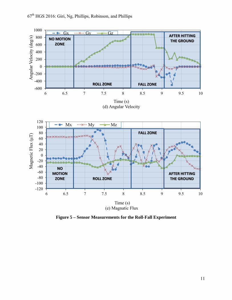
67th HGS 2016: Giri, Ng, Phillips, Robinson, and Phillips
Figure 5 – Sensor Measurements for the Roll-Fall Experiment
-600
-400
-200
0
200
400
600
800
1000
6 6.5 7 7.5 8 8.5 9 9.5 10
Ang
ular
Vel
ocity
(deg
/s)
Time (s) (d) Angular Velocity
Gx Gy Gz
ROLL ZONE FALL ZONE
NO MOTION ZONE
AFTER HITTING THE GROUND
-120-100-80-60-40-20
020406080
100120
6 6.5 7 7.5 8 8.5 9 9.5 10
Mag
netic
Flu
x (μ
T)
Time (s) (e) Magnatic Flux
Mx My Mz
ROLL ZONE
FALL ZONE
NO MOTION
ZONE
AFTER HITTING THE GROUND
11

67th HGS 2016: Giri, Ng, Phillips, Robinson, and Phillips
(a) Theoretical Gravity Acceleration
(b) Measured Gravity Acceleration
Figure 6 – Comparison of the Gravity Accelerations to Understand the Tilt and Rolling of the Sensor during Rolling
Slide-Fall Experiment
Slide-fall experiment was carried out by using the same setup that was used for the roll-fall experiment. In this experiment, however, the object used was a rectangular box that could slide easily on the platform before falling (Figure 7). The sensor device was placed inside the box and the box was pulled along the horizontal platform mechanically with the help of a string. The purpose of sliding the sensor mechanically was to observe the motion acceleration during the slide. The same three photoelectric sensors setup was used. Six runs of the experiment was conducted with the same setup.
Figure 7 – Experimental Setup for a Slide-Fall Experiment
-15
-10
-5
0
5
10
15
167 367 567 767
Theo
retic
al G
ravi
ty A
ccel
erat
ion
(m/s
2 )
Rotation (Degrees)
Gry-c Grx-c Grz-c
-15
-10
-5
0
5
10
15
6.722 7.222 7.722
Gra
vity
Acc
eler
atio
n (m
/s2)
Time (s)
Grx Gry Grz
12

67th HGS 2016: Giri, Ng, Phillips, Robinson, and Phillips
Results of the slide-fall experiment with +y axis facing forward in the direction of sliding, +y in the direction perpendicular to x in horizontal plane and +z in the direction of gravity, are presented in Figure 8. During the sliding phase, +z facing towards gravity yielded gravity acceleration data (Grz) equal to 1g (9.81m/s2), whereas x and y-axes being perpendicular to the direction of gravity yielded results (Grx and Gry) closer to zero. The discrepancy between expected and measured value was attributed to the wooden platform being not perfectly horizontal. Similar to the fall during roll-fall experiment, the measured acceleration values for all three axes become approximately zero. Figure 8 (a) shows a sudden change or drop of acceleration value in the axis along the direction of gravity from almost constant approximate value of 9.81m/s2 to close to zero. This is because of the same reason as explained earlier that during the free fall the gravity and motion acceleration measured by the sensor are equal and opposite resulting in zero measured acceleration. A small amount of the motion acceleration was observed during the slide (Figure 8 (b)). During the fall, the motion acceleration was observed to be approximately equal and opposite of the gravity acceleration (Figure 8 (c)). As expected, the gyroscope readings were almost equal to zero during the slide because of no rotation about any of the axes (Figure 8 (d)). However, the gyroscope experiences some rotation during the free fall and hence, the angular velocity of some magnitude was observed during the experiment. Likewise, the change in magnetometer readings during the slide and the fall indicates the motion of the sensor device and hence, the moving mass.
-6-4-202468
101214
0 1 2 3 4 5
Mea
sure
d A
ccel
erat
ion
(m/s
2)
Time (s) (a) Measured Acceleration
Ax Ay Az
FALL ZONE
SLIDE ZONE
NO
MO
TIO
N Z
ON
E
13

67th HGS 2016: Giri, Ng, Phillips, Robinson, and Phillips
-12-10-8-6-4-202468
1012
0 1 2 3 4 5
Mot
ion
Acc
eler
atio
n (m
/s2 )
Time (s) (b) Motion Acceleration
Lx Ly Lz
FALL ZONE
SLIDE ZONE N
O M
OTI
ON
ZO
NE
-12-10-8-6-4-202468
1012
0 1 2 3 4 5
Gra
vity
Acc
eler
atio
n (m
/s2 )
Time (s) (c) Gravity Acceleration
Grx Gry GrzFALL ZONE
SLIDE ZONE
NO
MO
TIO
N Z
ON
E
-600-400-200
0200400600800
100012001400
0 1 2 3 4 5
Ang
ular
Vel
ocity
(deg
/s)
Time (s) (d) Angular Velocity
Gx Gy Gz
FALL ZONE SLIDE ZONE
No
mot
ion
zone
14

67th HGS 2016: Giri, Ng, Phillips, Robinson, and Phillips
Figure 8 – Sensor Measurements for the Slide-Fall Experiment
CONCLUSION
This paper presents a WSN system to monitor rock fall movement. Past research works done in this field of landslide monitoring were mostly on the soil mass sliding (9) and few on the toppling failures (8). Also, the researches mainly focused on system development rather than understanding the change in movement that defines slope failure modes. Our research objective is to identify the movement types and hence, define failure modes accordingly. Recognizing the type and magnitude of slope movement from the WSN system, impending slope failures can be predicted, extent of failure can be identified, and a cost-effective hazard warning system can be developed to alleviate the socioeconomic impact of the slope failure, minimizing the loss of lives and damage of properties.
A basic framework of the WSN system designed for monitoring the landslides is presented in this paper. Experiments conducted in the laboratory supported the improvement of the performance and implementation of the WSN system developed for continuous and quasi-real time (up to 100 Hz of data processing speed) monitoring of the failure processes. All the experiments carried out in the laboratory were conducive to confirm the credibility of the sensors used in the WSN system for slope stability monitoring. Additionally, the laboratory experiments for the fall tests confirmed the repeatability of any experiment carried out for multiple runs.
The rock-fall experiments described in this paper improved our understanding of the data collected by the IMU sensor devices. Most importantly, the experiments where fall is preceded by rolling or sliding helped in understanding the pattern of the data followed during the rock mass movements. Roll-fall experiments showed a sinusoidal pattern of the gravity acceleration during the rolling phase. Some measured acceleration values were observed during the slide. This value becomes equal to gravity when there is a constant motion of the rolling or sliding mass causing the motion acceleration to be zero. On the other hand, during the slide-fall
-150-130-110-90-70-50-30-1010305070
0 1 2 3 4 5
Mag
netic
Flu
x (μ
T)
Time (s) (e) Magnetic Flux
Mx My Mz
FALL ZONE
SLIDE ZONE No
mot
ion
zone
15

67th HGS 2016: Giri, Ng, Phillips, Robinson, and Phillips
experiment, the gravity acceleration remains constant for all three axes. However, the application of non-uniform force to slide the object caused non-uniform speed and hence, generated some motion acceleration. The free fall exhibited a distinct pattern during both the roll-fall and the slide-fall experiments with a sudden drop of all axes’ measured acceleration values to zero during the free fall. Similarly, the gyroscope and magnetometer sensors were also very useful in detecting the movements as well as understanding the movement behavior. Hence, the combination of all the sensor results was found to be important for completely understanding any failure behavior and for landslide identification. The experimental data collected for the rockfall will provide the basis for establishing failure threshold values that are required in the development of a hazard warning system for slopes.
16

67th HGS 2016: Giri, Ng, Phillips, Robinson, and Phillips
REFERENCE
1. Girard, J.M., 2001. Assessing and Monitoring Open Pit Mine Highwalls. , p.13.
2. Norrish, N. I., & Wyllie, D. C. (1996). Rock slope stability analysis. Landslides: Investigation and Mitigation, Washington, DC, edited by: Turner, AK and Schuster, RL, Transportation Research Board, Special Report, 247, 391-425.
3. Wyoming Homeland Security. (2011). Wyoming Multi-Hazard Mitigation Plan: Chapter 4 – Dam Failures. June, pp. 4.1-4.10.
4. Highland, M.L. (2012). Landslides in Colorado, USA: Impacts and Loss Estimation for the Year 2010. Open-File Report 2012-1204, U.S. Geological Survey, U.S. Department of Interior, 54 p.
5. Li, F. et al., 2012. "Monitoring system for high steep slope based on optical fiber sensing technology". Advanced Sensor Systems and Applications V, 8561, pp.1–6.
6. Fung, W. H., Kinsil, R. J., Jamaludin, S., & Krishnan, S. (2014). Early warning and real-time slope monitoring systems in West and East Malaysia. In Landslide Science for a Safer Geoenvironment (pp. 569-575). Springer International Publishing.
7. Rouyet, L., 2013. "Monitoring and Characterization of Rock Slope Instabilities in Norway using GB-InSAR". Master Thesis, University of Lausanne.
8. Azzam, R., Arnhardt, C., & Fernandez-Steeger, T. M. (2010, February). Monitoring and early warning of slope instabilities and deformations by sensor fusion in self-organized wireless ad-hoc sensor networks. In International Symposium and the 2nd AUN/Seed-Net Regional Conference on Geo-Disaster Mitigation in ASEAN-Protecting Life from Geo-Disaster and Environmental Hazards, February (pp. 25-26).
9. Smarsly, K., Georgieva, K. & König, M., 2014. "An Internet-Enabled Wireless Multi-Sensor System for Continuous Monitoring of Landslide Processes". International Journal of Engineering and Technology, 6(6), pp.520–529.
10. Arnhardt, C., Asch, K., Azzam, R., Bill, R., Fernandez-Steeger, T. M., Homfeld, S. D. & Walter, K. (2007). Sensor based Landslide Early Warning System-SLEWS. Development of a geoservice infrastructure as basis for early warning systems for landslides by integration of real-time sensors. Geotechnologien science report, 10, 75-88.
11. Fernandez-Steeger, T. M., Arnhardt, C., Niemeyer, F., Haß, S. E., Walter, K., Homfeld, S. D., & Bill, R. (2008). Current Status of SLEWS-a Sensor Based Landslide Early Warning System. Universitätsgesellschaft Osnabrück eV: R & D-Programme Geotechnologien Status Report. Early Warning Systems in Earth Management.
17

Observations of Rockfall and Earth Slope Movements using Ground-Based Interferometric Radar
Brent L. Rosenblad Dept. of Civil Engineering, University of Missouri
Columbia, MO 65211 573-882-3736
Francisco Gomez Dept. of Geological Science, University of Missouri
Columbia, MO 65211 573-882-9744
J. Erik Loehr Dept. of Civil Engineering, University of Missouri
Columbia, MO 65211 573-882-6380
Joseph Gilliam Reitz & Jens, Inc.
1055 Corporate Square Dr. St. Louis, MO 63132
314-993-4132 [email protected]
Prepared for the 67th Highway Geology Symposium, July, 2016

67th HGS 2016: Rosenblad and Gomez
2
Acknowledgements
This material is based upon work supported by the National Science Foundation under Grant No. 1435889 and the Colorado Department of Transportation.
Disclaimer
Statements and views presented in this paper are strictly those of the author(s), and do not necessarily reflect positions held by their affiliations, the Highway Geology Symposium (HGS), or others acknowledged above. The mention of trade names for commercial products does not
imply the approval or endorsement by HGS.
Copyright Notice
Copyright © 2016 Highway Geology Symposium (HGS)
All Rights Reserved. Printed in the United States of America. No part of this publication may be reproduced or copied in any form or by any means – graphic, electronic, or mechanical,
including photocopying, taping, or information storage and retrieval systems – without prior written permission of the HGS. This excludes the original author(s).

67th HGS 2016: Rosenblad and Gomez
3
ABSTRACT
Rockfall events and earth slope movements are geotechnical hazards that can have serious economic consequences and impact the safety of the travelling public. There is a need for technologies that can detect hazards at an early stage and accurately monitor on-going movements. Differential radar interferometry is a remote sensing technology that uses phase shifts from pairs of radar scans to detect surface movements. Satellite-based radar interferometry has been successfully used for decades to measure large spatial-scale (km2) ground movements associated with events such as earthquakes and subsidence from oil and water extraction. In recent years, portable ground-based interferometric radar (GBIR) systems have been developed that can be used for monitoring movements of geotechnical features and structures. This technology can rapidly scan massive geotechnical features or landscapes and detect movements at sub-mm resolution. In this paper, results are presented from slope stability applications of GBIR, including: continuous monitoring of active slope movements, periodic monitoring of a potential rockfall site in Glenwood Canyon, Colorado, and a unique controlled study where individual boulders were moved and monitored using GBIR. The results demonstrate the capabilities of GBIR for slope stability applications.

67th HGS 2016: Rosenblad and Gomez
4
INTRODUCTION Surface deformation measurements are important for characterizing slope instability, detecting potential hazards, monitoring ongoing movements, and planning and verifying remediation measures. Technology for deformation measurements continue to improve and expand. Traditional survey tools, such as total stations, remain valuable for providing high-accuracy point measurements, but may not provide sufficient spatial sampling in many cases. Remote sensing methods, such as LiDAR and photogrammetry, provide excellent spatial coverage but lack the mm-scale deformation sensitivity that may be needed in some applications. Ground-based interferometric radar (GBIR) is a relatively new remote sensing technology that can provide some measurement capabilities that are not possible with other technologies. Over the past several years many potential applications of GBIR have been investigated, including: landslides (1, 2, 3), mine wall stability (4), dam movements (5, 6, 7), and civil structures (8, 9). This paper presents observations from recent studies of the application of GBIR to diverse slope stability issues. Three cases are presented, namely: continuous short-term monitoring of a slow moving landslide, periodic monitoring of a possible rockfall site, and a controlled study simulating detection of precursor rockfall movements. The results from these studies are discussed to illustrate the potential applications, advantages and limitations of GBIR for slope stability problems. OVERVIEW OF GROUND-BASED RADAR INTERFEROMETRY Ground-based interferometric radar (GBIR) is a remote sensing technology that can be used to detect and measure small (mm-scale) surface movements of natural landscapes or manmade structures. The technology is based on the same technology used in satellite-based interferometric radar platforms which have been in use for several decades. Ground-based interferometric radar (GBIR) systems operate by scanning the site of interest using a transmitting antennae and detecting the reflected radar returns using one or more receiving antennae, as illustrated in Fig. 1. As the GBIR scans the scene the intensity and phase of the radar return is recorded as a function of the range (distance) and azimuth (angle) from the radar. A radar image is created by plotting the radar return value (amplitude or phase) versus range and azimuth. Each pixel in the image contains information on the magnitude and phase of the reflected radar signal. Ground-based interferometric radar (GBIR) detects and measures deformation by comparing the phase values of two radar acquisitions obtained at different times. As illustrated in Fig. 1, a small movement of the surface causes a detectable shift in the phase of the reflected radar signal. The radar acquisition image collected at an initial time is mathematically combined with a later acquired image to determine changes in phase occurring between the two acquisition times. The time between image acquisitions can be minutes or months depending on the application. The mathematical combination of two radar images creates an interferogram, which is a two-dimensional image of differential phase values. The calculated phase values are wrapped, meaning they are in the range of 0 to ± and indicate the relative lead or lag in phase between the two images caused by movement towards or away from

67th HGS 2016: Rosenblad and Gomez
5
the radar. For the case of a Ku-band GBIR, as used in this study, one cycle (2of phase corresponds to about 8.6 mm of movement. The cumulative phase difference is determined by unwrapping the wrapped phase valueshe cumulative differential phase values can be related to the line-of-sight (LOS) displacements, as shown in Equation 1.
4LOS
(1)
where; δLOS = line-of-sight deformation λ = radar transmitting wavelength φ = cumulative differential phase value Because the deformations are determined from changes in phase and the wavelength of the Ku band system is small, the GBIR is very sensitive to small (mm-scale) surface deformations.
Figure 1 – Schematic illustrating phase shift in radar signal caused by surface deformations

67th HGS 2016: Rosenblad and Gomez
6
GROUND-BASED INTERFEROMETRIC RADAR USED IN THIS STUDY The Ku-band (17.1-17.3 GHz) GBIR at the University of Missouri is a second-generation, real-aperture system manufactured by GAMMA Remote Sensing in Switzerland. The GBIR consists of one transmitting antenna, two receiving antennas, a radio frequency controller, mounting frame, a stepping motor with tribrach, a portable tripod and a field computer. An anchored mast can also be deployed in lieu of the tripod if a more permanent platform is needed. The antennas are approximately two meters in length with slotted waveguide members. The radio frequency box generates the radar signal used for acquisition (Ku-band frequencies). A photograph of the GBIR system is shown in Figure 2. The site of interest is scanned by rotating the antennas as the system sends and receives the radar signal. Scan rates are typically in the range of 5 to 10 degrees per second. The spatial resolution of the radar image is a function of the radar bandwidth (200 MHz) and range distance. Spatial resolution in the range direction is approximately 0.75 m. Azimuthal resolution is a function of the range distance and decreases with increasing range distance. The azimuthal resolution is approximately 0.7 m at 100 m range and 7 m at 1 km range. The GBIR can be operated at range distances from 50 m to 10 km.
Figure 2 – Ground-based Interferometric Radar (GBIR) used in this study
CONTINUOUS SHORT-TERM MONITORING OF SLOPE USING GBIR The GBIR system at the University of Missouri was used to monitor a slow-moving landslide located in Granby, Colorado. The monitoring in this case was continuous and was performed over a time frame of about a day. The results from this study are presented to illustrate the

67th HGS 2016: Rosenblad and Gomez
7
information that can be derived from GBIR monitoring of large-spatial scale slope movements. A detailed description and analysis of this study can be found in Lowry et al, 2013 (3). This site is a slow moving landslide occurring beneath a landfill located near Granby, Colorado. Movement at this site has been observed since 2007. The measurements presented in this paper were performed in 2011, although subsequent measurements have also been performed. The total area of movement covers approximately 160,000 m2. The landslide has moved at a nominal velocity of about 50 cm/month. Measurements were performed over a span of 24 hrs in June, 2011 and over a span of 36 hrs in August 2011. The GBIR was set up about 500 m from the slide and radar scans of the site were performed at 15-minute intervals. A photograph of the GBIR scanning the site is shown in Fig. 3. The numerous radar scans collected allowed for the calculation of hundreds of interferograms over different increments of time. These interferograms were used to create displacement maps as well as displacement time series of specific points. A comparison of displacement maps from June and August is presented in Fig. 4, which shows a clear change in the rate of movement. Of particular note is the very small magnitude (mm-scale) of movement that is detected using the GBIR measurements. This measurement range is below the threshold that can be detected using other remote sensing technologies, such as photogrammetry and LiDAR. Measurements as small of 0.5 mm were detected in this case. Also of note is the clear delineation of the boundaries of movement, which may be difficult to obtain using point-by-point measurements. An example of a time series developed for two specific points is shown in Fig. 5, illustrating the ability to monitor hourly variations in the rate of movement.
Figure 3 – Ground-based Interferometric Radar (GBIR) with landslide in background

67th HGS 2016: Rosenblad and Gomez
8
Figure 4 – Displacement maps derived from continuous monitoring of a slow-moving landslide using the MU GBIR system (3)

67th HGS 2016: Rosenblad and Gomez
9
Figure 5 – Displacement time series from two points obtained during the August, 2011 measurements
PERIODIC MONITORING FOR ROCKFALL HAZARD DETECTION USING GBIR The case described above illustrated the use of GBIR for monitoring known slope instabilities where the region of interest is relatively large and the primary objective it to measure the rate of movement. The study described in this section is a very different application where the objective was to detect small and localized movements within a massive rockface. The Colorado Department of Transportation (CDOT) funded a project to monitor a site near Glenwood Springs, Colorado that has been the source of several rockfall events that impacted Interstate 70. Olson Engineering installed an IBIS-L GBIR system manufactured by IDS of Pisa, Italy. This system is a synthetic aperture radar (SAR) (unlike the real-aperture Gamma system) but in principle operates similarly to the GAMMA system used in this study. The IBIS system was installed on a cliff located across I-70 about 600 m from the rockface of interest. The IBIS system continuously monitored the potential rockfall site over a duration of about 2 months, taking radar scans every 5.5 minutes (10). The objective of this study was to detect small movements of the rock face that may be precursors to a rockfall event. CDOT also provided funding for periodic measurements of this site using the GAMMA GBIR system. The GAMMA system is not setup to operate unattended over months, so it was brought up to the site by helicopter at two-week intervals. A support mast was bolted to the rock at the edge of the cliff face and the GBIR components were installed on top of the mast. A photograph of the GBIR system installed on the cliff with the rockface of interest indicated in the background (dashed box), is shown in Fig. 6. Unlike the previous example, the spatial region of interest (rock blocks) was very small and it was not known if movements were occurring or where the movements would occur. In this case, the objective was to try to detect very small and very localized movements within this massive rockface.

67th HGS 2016: Rosenblad and Gomez
10
Figure 6 – Glenwood Canyon rock face and GBIR system installed on opposing cliff across
from Interstate 70. Radar scans were collected with the GAMMA system at about 15-minute intervals over the course of several hours. After the completion of the measurements, the equipment was removed from the site. Two return trips were performed, each separated by approximately two weeks. All of the measurements were performed concurrently with the continuous monitoring being performed by Olson Engineering. The radar images collected from the GAMMA GBIR were used to create interferograms and displacement maps spanning the two weeks between radar acquisitions. An example of one of the displacement maps superimposed on a digital elevation model (DEM) of the slope study area is shown in Fig. 7. As can be seen in this figure, the displacement map showed a uniform color indicating zero phase shift (and hence zero displacement) across the slope. Similar images were obtained from the other time intervals examined. It was concluded that no movements of the slope were detected over the time frame of the measurements using the GAMMA GBIR. In contrast, the continuous measurements obtained from Olson Engineering indicated several locations where movements were measured, some as much as 300 mm (10). A detailed presentation of the IBIS results can be found in Miller et al, 2013 (10). Based on the inconsistent findings from the two GBIR systems and the lack of ground truth at the site, it was not possible to evaluate if GBIR was an effective tool for this important application. This finding motivated the controlled study of individual boulder movements described in the next section.

67th HGS 2016: Rosenblad and Gomez
11
Figure 7 –Two-week interferogram of the Glenwood Canyon study site showing no movements of the rock face
CONTROLLED STUDY OF INDIVIDUAL BOULDER MOVEMENTS USING GBIR The inconclusive results from the Glenwood Canyon site described above motivated the need to perform a controlled study of GBIR for detecting movements of individual boulders. A rock slope site located outside Denver, Colorado was selected for the controlled study, as described below. The intent of the study was to document the effectiveness of GBIR as a means to detect minute movements of individual boulders within a massive landscape Site Description
The site of the controlled study is located approximately 50 km west of Denver, Colorado along a meander in Clear Creek. The control site was chosen based on good accessibility for equipment and personnel, clear vantage points to scan a large (approximately 20,000 m2) region, and availability of a wide variety of boulder sizes. A photograph of the site taken from one of the GBIR locations (GBIR2) is shown in Fig. 8. As can be seen in the photograph, the site consists predominately of outcropping rock surrounded by lightly vegetated regions, with some trees present. Two GBIR units (one borrowed from the University of Arkansas) were positioned on tripods at separate locations across Clear Creek from the rock slope. Twelve boulders ranging in approximate facial dimensions from less than 1 m to over 5 m were selected for this study. The boulder offsets ranged from about 70 m to over 150 m from the two GBIR locations. A Google Earth image of the site indicating the locations of the GBIR systems, as well as the twelve boulders (black circles), is shown in Fig. 9. In this paper representative results from the study are presented using incremental movements of Boulder 6 and Boulder 7. The locations of these boulders are identified in Figs. 8 and 9.

67th HGS 2016: Rosenblad and Gomez
12
Figure 8 – Field site of controlled boulder movements from vantage point of GBIR 2. The locations of Boulders 6 and 7, discussed later in this section, are outlined in the photo
Figure 9 – Google Earth image of field site showing the location of the GBIR systems and the twelve boulders moved in this study. Boulders B6 and B7 are labelled.
B7
B6
B6
B7
GBIR 2 GBIR 1

67th HGS 2016: Rosenblad and Gomez
13
Data Collection and Processing Procedures Two tripods were positioned over survey points marking the GBIR1 and GBIR2 locations. After the tripods were positioned the GBIR components were attached. The GBIR antennae were fixed at a 10° inclination from horizontal. A scanning swath for each GBIR was set such that the entire site containing the twelve boulders was scanned from each GBIR location. The rotational scanning rate was set to 5°/sec, resulting in the completion of each scan in under 30 sec. Four scans were performed after each increment of movement with data recorded from both the upper and lower antennae. Therefore, one scan set consisted of eight radar images. An example of a radar intensity image overlaid on the Google Earth image of the site is shown in Fig. 10. On the opposite side of Clear Creek the boulders were nudged slightly using pry bars for small boulders and air bag jacks for the larger boulders. A picture of an air bag jack being positioned behind one of the boulders is shown in Fig 11. Each boulder was moved in mm-scale increments. The intent was to limit each push to about 2 mm in magnitude, however, it proved difficult to precisely control the airbag pressure and increments were often several mm in magnitude. A total station was brought to the site to record ground truth movements. Unfortunately, the total station malfunctioned and another means to record ground truth measurements was improvised. Laser pointers placed a few meters away from the boulder were used to illuminate points on the boulder which were marked before and after each push increment. The distance between the marked points was measured using a steel ruler and the general push direction was measured using a compass. This approach provided reasonable ground truth values for comparison with the GBIR recordings, but due to the generally low accuracy in recording push direction and movement, as well as the contributions of rotation to the boulders movements, it was not possible to obtain high-quality ground truth measurements of line of sight displacement. After the completion of a series of incremental pushes on a given boulder, the air bag pressure was released and the boulder rebounded back towards the slope face. A final scan set was collected after the pressure release.
Figure 10 – Example of radar intensity scan collected from single scan set

67th HGS 2016: Rosenblad and Gomez
14
Figure 11 – Airbag jack being placed behind a large boulder
Interferograms were developed using scan set pairs spanning both single and multiple increments of movement. For each interval considered, eight individual interferograms were calculated using the eight radar images (4 scans with recordings on top and bottom antennae) recorded from each scan set. These eight interferograms were then averaged to produce a single interferogram. Results Example results from this study are presented using data collected from the GBIR2 system before the release of Boulder 6 and after the first incremental push of Boulder 7. In other words, the eight radar images collected prior to the release of Boulder 6 (moving away from the radar) were used with the eight radar images collected after Boulder 7 was moved a few mm (moving towards the radar), to produce a single interferogram. A photograph of Boulder 7 is presented in Fig. 12. The objective was to determine if these very small and very localized movements could be detected within the massive 20,000 m2 landscape. Based on ground truth data, Boulder 7 was moved about 3 mm in the direction of GBIR 2 and Boulder 6 rebounded several tens of mm. The raw interferogram produced from this interval is presented in Fig. 13. This figure is presented in radar coordinates, with the scan line azimuth presented on the y-axis and the range presented on the x-axis. As discussed above, if no movement occurs it is expected that a phase difference of zero (cyan color) should be recorded. As can be seen in this figure, most of the region is cyan color (indicating zero phase) but there are many portions of the image where the phase is non-zero. Most of these regions are associated with vegetated surfaces. Different approaches were studied to remove signals from non-rock surfaces from the image. The most effective approach was to calculate pixel-by-pixel coherence values from the eight radar images. Ideally more images would be used to provide a more reliable coherence value, but the eight images proved effective in separating rock from vegetation. Rock surfaces corresponded to very high coherence values (i.e. repeatable radar returns) while vegetated surfaces had much lower

67th HGS 2016: Rosenblad and Gomez
15
coherence values. Using a mask of 95% (i.e. pixels with coherence values greater than 0.95 were retained), the image shown in Fig. 14 was produced. As can be seen in this image, most of the non-zero phase regions were removed leaving a near uniform cyan (zero-phase) image. However, two clear phase anomalies remain in the image, as shown with the white arrows in Fig. 14. A zoomed in image of the interferogram is shown in Fig. 15. These two points correspond to the locations of the two boulders that were moved during the interval between scans. In Fig 16, the radar image is presented in rectangular coordinates and superimposed on the Google Earth image of the site. The locations of the anomalies are directly over the locations of Boulders 6 and 7. Phase values recorded using the GBIR from multiple push intervals of Boulder 7 were compared to expected phase values based on the line-of-sight movements calculated from the measured ground truth displacements and push direction. The comparison of the measured GBIR phase values with those expected based on the ground truth measurements are shown in Fig. 16. The GBIR phase values exhibit the expected wrapped pattern. The phase trends are slightly different than expected, which is likely attributable to inaccuracies in the ground truth measurements (particularly push direction), as discussed above.
Figure 12 – Close-up view of Boulder 7. The air bag was inserted in the vertical crack (white arrow) to initiate small outward movement of the rock mass.

67th HGS 2016: Rosenblad and Gomez
16
Figure 13 – Raw interferogram created from scans performed before release of pressure on Boulder 6 and after first increment of movement of Boulder 7. Colors indicates wrapped
phase values (in radians).

67th HGS 2016: Rosenblad and Gomez
17
Figure 14 – Interferogram after masking low coherence regions. Phase anomalies
associated with movements of Boulders 6 and 7 are indicated with white arrows. Colors indicates wrapped phase values (in radians).

67th HGS 2016: Rosenblad and Gomez
18
Figure 15 – Expanded view of phase anomalies in interferogram
Figure 16 – Interferogram presented in rectangular coordinates and superimposed over Google Earth image showing the phase anomaly locations are consistent with the locations
of Boulders 6 and 7.

67th HGS 2016: Rosenblad and Gomez
19
Figure 17 – Comparison of measured phase values to expected values for Boulder 7 based
on ground truth measurements. Discussion Detecting mm-scale movements of very localized regions is a difficult measurement problem and one that is important for geotechnical applications. Point-by-point survey methods often cannot provide the necessary spatial resolution to detect very localized movements. Remote sensing methods such as photogrammetry and LiDAR provide excellent spatial resolution but are not able to detect mm-scale changes. To illustrate this point, results are presented from LiDAR measurements of a boulder movement performed at the same site in a subsequent study. A photograph of the boulder is shown in Fig. 18. When the boulder movement was in the range of several cm, LiDAR provided excellent information on the magnitude and spatial distribution of movement, as shown in Fig 19(a). However, when the movement was in the mm range, the moving boulder could not be detected or differentiated from the non-moving boulder in the background, as shown in Fig. 19(b). Work is on-going using the complete data set of all boulders and push increments to determine the detection thresholds in terms of target size and range distance, and better understand data processing procedures that produce the best outcomes.

67th HGS 2016: Rosenblad and Gomez
20
Fig. 18 Boulder scanned using LiDAR
(a) 50 mm of movement (b) 6 mm of movement Fig. 19 LiDAR images showing displacement detected when boulder was moved (a) about 5 cm and (b) about 5 mm. In case (b) the boulder that was moved cannot be distinguished from the non-moving rock in the background.
No movement
6mm 3 mm
50 mm
35 mm

67th HGS 2016: Rosenblad and Gomez
21
CONCLUSIONS This paper has presented results from several diverse applications of GBIR for slope stability problems. The results from the first example demonstrate the excellent spatial coverage and measurement sensitivity that can be achieved with GBIR. Displacements as small as 0.5 mm were recorded and detailed displacement maps and time series were developed. Measurements at these small time and spatial scales can provide new insights into the mechanics driving slope instability. Rockfall hazard detection is a relatively new application of GBIR that requires further study. The results presented in this paper from a controlled study of rock movements monitored with GBIR demonstrate that GBIR can be an effective tool for detecting very small and very localized deformations that may not be detected using other techniques.

67th HGS 2016: Rosenblad and Gomez
22
REFERENCES:
1. Antonello, G., N. Casagli, P. Farina, D. Leva, G. Nico, A.J. Sieber, and D. Tarchi. Ground-based SAR Interferometry for Monitoring Mass Movements. Landslides, Vol 1 (1), 2004. pp. 21-28.
2. Casagli, N., F. Catani, C. Del Ventisette, and G. Luzi. Monitoring, Prediction, and Early Warning Using Ground-Based Radar Interferometry. Landslides, Vol 7 (3), 2010. pp. 291-301.
3. Lowry, B., F. Gomez, W. Zhou, M.A. Mooney, B. Held, and J. Grasmick. High
Resolution Displacement Monitoring of a Slow Velocity Landslide Using Ground Based Radar Interferometry. Engineering Geology, Vol 106, 2013, pp. 160-169.
4. Harries, N., D. Noon, and K. Rowley. Case Studies of Slope Stability Radar Used in
Open Cut Mines. Stability of Rock Slopes in Open Pit Mining and Civil Engineering Situations. Johannesburg: SAIMM, Symposium Series S44, 2006, pp. 335-342.
5. Alba, M., G. Bernardini, G., A. Giussani, P. Ricci, F. Roncoroni, M. Scaioni, P. Valgoi,
and K. Zhang. Measurement of Dam Deformations by Terrestrial Interferometric Techniques. Beijing, The International Archives of the Photogrammetry, Remote Sensing and Spatial Information Sciences, 2008.
6. Jenkins, W. S. Evaluation of Ground-Based Interferometric Radar for Civil Engineering
Applications, M.S. Thesis, Department of Civil and Environmental Engineering, University of Missouri, 2013.
7. Tarchi, D., H. Rudolf, G. Luzi, L. Chiarantini, P. Coppo, and A. J. Sieber, "SAR
Interferometry for Structural Changes Detection: A demonstration test on a dam", Proceedings IGARSS, pp. 1522-1524, 1999.
8. Pieraccini, M., D. Tarchi, H. Rudolf, D. Leva, G. Luzi, C. Atzeni. Interferometric Radar
for Remote Monitoring of Building Deformations. Electronic Letters, Vol 36 (6), pp. 569-570, 2000.
9. Pieraccini, M., M. Fratini, F. Parrini, G. Macaluso, and C. Atzeni. High-speed CW Step-
Frequency Coherent Radar for Dynamic Monitoring of Civil Engineering Stuctures. IEEE Electronic Letters, Vol 40(14), 2004.
10. Miller, P., M. Vessely, L. Olson, and Y. Tinkey. Slope Stability and Rock-Fall
Monitoring with a Remote Interferometric Radar System. In Proceedings ASCE Geo-Congress, San Diego, 2013. pp.304-318.

Comparison of 2D and 3D Rockfall Modeling for Rockfall Mitigation Design
Brett Arpin, P.E., G.I.T. Yeh and Associates, Inc.
2000 Clay Street, Suite 200 Denver, CO 80211
(303) 781-9590 [email protected]
Ben Arndt, P.E., P.G. Yeh and Associates, Inc.
2000 Clay Street, Suite 200 Denver, CO 80211
(303) 781-9590 [email protected]
Prepared for the 67th Highway Geology Symposium, July, 2016

67th HGS 2016: Arpin and Arndt 2
Acknowledgements
The authors would like to thank the Colorado Department of Transportation Geohazards Program for their contributions to this work.
Disclaimer
Statements and views presented in this paper are strictly those of the author(s), and do not necessarily reflect positions held by their affiliations, the Highway Geology Symposium (HGS), or others acknowledged above. The mention of trade names for commercial products does not
imply the approval or endorsement by HGS.
Copyright Notice
Copyright © 2016 Highway Geology Symposium (HGS)
All Rights Reserved. Printed in the United States of America. No part of this publication may be reproduced or copied in any form or by any means – graphic, electronic, or mechanical,
including photocopying, taping, or information storage and retrieval systems – without prior written permission of the HGS. This excludes the original author(s).
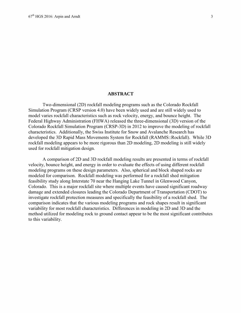
67th HGS 2016: Arpin and Arndt 3
ABSTRACT
Two-dimensional (2D) rockfall modeling programs such as the Colorado Rockfall Simulation Program (CRSP version 4.0) have been widely used and are still widely used to model varies rockfall characteristics such as rock velocity, energy, and bounce height. The Federal Highway Administration (FHWA) released the three-dimensional (3D) version of the Colorado Rockfall Simulation Program (CRSP-3D) in 2012 to improve the modeling of rockfall characteristics. Additionally, the Swiss Institute for Snow and Avalanche Research has developed the 3D Rapid Mass Movements System for Rockfall (RAMMS::Rockfall). While 3D rockfall modeling appears to be more rigorous than 2D modeling, 2D modeling is still widely used for rockfall mitigation design.
A comparison of 2D and 3D rockfall modeling results are presented in terms of rockfall
velocity, bounce height, and energy in order to evaluate the effects of using different rockfall modeling programs on these design parameters. Also, spherical and block shaped rocks are modeled for comparison. Rockfall modeling was performed for a rockfall shed mitigation feasibility study along Interstate 70 near the Hanging Lake Tunnel in Glenwood Canyon, Colorado. This is a major rockfall site where multiple events have caused significant roadway damage and extended closures leading the Colorado Department of Transportation (CDOT) to investigate rockfall protection measures and specifically the feasibility of a rockfall shed. The comparison indicates that the various modeling programs and rock shapes result in significant variability for most rockfall characteristics. Differences in modeling in 2D and 3D and the method utilized for modeling rock to ground contact appear to be the most significant contributes to this variability.

67th HGS 2016: Arpin and Arndt 4
INTRODUCTION
Rockfall modeling programs are widely used to evaluate rockfall characteristics such as velocity, energy, and bounce height for use in designing rockfall mitigation systems. A wide range of modeling programs are available that perform analysis in both two-dimensions (2D) and three-dimensions (3D). The Colorado Rockfall Modeling Program (CRSP-2D) is likely one of the most widely used 2D programs available. Based on the success of CRSP-2D, the Federal Highway Administration (FHWA) sponsored the development of the 3D version of the Colorado Rockfall Simulation Program (CRSP-3D) which was released in 2012. The Swiss Institute for Snow and Avalanche Research has developed the 3D Rapid Mass Movements System for Rockfall (RAMMS::Rockfall). While 3D modeling appears to be more rigorous than 2D modeling, 2D modeling is still widely used among designers of rockfall mitigation systems.
A major factor in evaluating whether rockfall modeling will be performed in 2D or 3D is
the availability of data required to perform the analysis. 2D programs are fairly simple and do not require detailed topographic data as do most 3D programs. Additionally, many designers have a comfort level with 2D programs that they have not developed with 3D programs.
Given that 2D programs are still widely used even though 3D programs appear to be
more rigorous, a comparison of the rockfall characteristics evaluated using 2D and 3D programs has been performed to help understand the potential variation in the results when using these different methods. Modeling was performed using CRSP-2D version 4.0 (1), CRSP-3D version 8 (2), and RAMMS::Rockfall version 1.6.52 (3). CRSP-3D version 8 is an updated version of the program released in 2012 and may not be commercially available. Additional updates and revisions of CRSP-3D are ongoing and were not available for this study.
Comparison Study Site
To facilitate the comparison, rockfall modeling was performed for a rockfall prone area along Interstate 70 (I-70) at approximate mile marker 125 near the Hanging Lake Tunnel in Glenwood Canyon, Colorado (Figure 1). Several rockfall events have caused significant roadway damage at this site.
Site Description and Geology
The highway at the base of the slope consists of two eastbound lanes and two westbound
lanes with shoulders. Additionally, a single lane eastbound off-ramp and a single lane westbound on-ramp are located in this section of the canyon. A multi-use path traverses through Glenwood Canyon and is located between the highway and Colorado River. The eastbound lanes are supported by a steel-girder bridge structure with a concrete deck. The westbound lanes and inside shoulder are constructed on a double-tee retaining wall, with part of the median deck cantilevered from the retaining wall. The concrete bridge deck for the eastbound lanes extends to abut the cantilevered median deck, providing a continuous concrete deck between the eastbound and westbound lanes. The roadway surface is about 35 feet above the surface of the Colorado River at this location. A typical cross section of the highway geometry at the study site in shown in Figure 2.

67th HGS 2016: Arpin and Arndt 5
Figure 1 – Study site location map
Figure 2 – Typical I-70 cross section at study site
Site
WB I-70 EB I-70 (Bridge)
Retaining Wall
Multi-Use Path
Existing Ground
Colorado River

67th HGS 2016: Arpin and Arndt 6
Natural slope angles range from 35 to 55 degrees extending approximately 900 feet above the highway at the study site. Based on mapping by the Colorado Geological Survey (4), bedrock beneath talus and other colluvial deposits on these slopes consists of Pre-Cambrian age (older than 542 Ma) biotite granite. Near vertical to vertical cliffs extend above the natural slopes for approximately 600 vertical feet. Upper Cambrian age (488 to 501 Ma) Sawatch Quartzite overlies the granite in an unconformity. The unconformity represents a 40-million-year gap in geologic time.
Above the Sawatch Quartzite is the Upper Cambrian Dotsero Formation which consists
of sandy dolomite, dolomitic sandstone, and limestone. The Lower Ordovician Manitou Formation (472 to 488 Ma) overlies the Dotsero Formation and is composed of limestone conglomerate, dolomite, and calcareous shale. Above the Manitou Formation is the Upper Devonian age Chaffee Group (359 to 385 Ma) consisting of quartzite, shale, dolomite, limestone, and sandstone. The slopes above the cliffs are composed of Mississippian Age (318 to 359 Ma) Leadville Limestone. Figure 3 illustrates the approximate contact locations for the geologic units present at the site.
Figure 3 – Photograph illustrating approximate geological unit contacts and rockfall source
areas
Pre-Cambrian Granite
Sawatch Quartzite Dotsero and Manitou Formations
Chaffee Group Leadville Limestone
March 2010 Source Area
November 2004 Source

67th HGS 2016: Arpin and Arndt 7
Significant Rockfall Events In November of 2004, rocks originating from approximately 1,150 feet above the
highway in an overhanging section of the Sawatch Quartzite (Figure 3) impacted the highway. The largest rock was approximately 15 feet across. Several holes were punched in the eastbound bridge deck with the largest hole being approximately 20 feet wide by 15 feet long. The highway was closed for one and a half days to allow for rock scaling and bridge deck repairs were completed in about two months.
In March 2010, 3 to 10-foot diameter rocks originating from the Pre-Cambrian Granite
approximately 500 feet above the highway (Figure 3) impacted the roadway (Figure 4). Again, several large holes were punched in the eastbound bridge deck (Figure 5). The highway was closed for four days following this event to allow for scaling and stabilization work. Bridge deck repairs were completed within about two months.
The detour available during both closures consisted of taking several US and state
highways totaling approximately 205 miles to surpass Glenwood Canyon.
Figure 4 – Large hole punched in the I-70 EB bridge deck by the March 2010 rockfall event
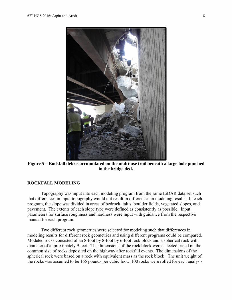
67th HGS 2016: Arpin and Arndt 8
Figure 5 – Rockfall debris accumulated on the multi-use trail beneath a large hole punched
in the bridge deck
ROCKFALL MODELING
Topography was input into each modeling program from the same LiDAR data set such that differences in input topography would not result in differences in modeling results. In each program, the slope was divided in areas of bedrock, talus, boulder fields, vegetated slopes, and pavement. The extents of each slope type were defined as consistently as possible. Input parameters for surface roughness and hardness were input with guidance from the respective manual for each program.
Two different rock geometries were selected for modeling such that differences in
modeling results for different rock geometries and using different programs could be compared. Modeled rocks consisted of an 8-foot by 8-foot by 6-foot rock block and a spherical rock with diameter of approximately 9 feet. The dimensions of the rock block were selected based on the common size of rocks deposited on the highway after rockfall events. The dimensions of the spherical rock were based on a rock with equivalent mass as the rock block. The unit weight of the rocks was assumed to be 165 pounds per cubic foot. 100 rocks were rolled for each analysis

67th HGS 2016: Arpin and Arndt 9
within each program. Results are presented for an analysis point on the slope approximately 30 feet above the highway. A discussion of the modeling follows the presentation of the results.
Rockfall Velocity
Rockfall velocities for the two rock dimensions selected were evaluated in each of the
three programs. The velocity results output from CRSP-3D appeared reasonable for the spherical rocks but did not appear reasonable for the rock block and have not been presented here. Attempts to calibrate the model did not improve the results. A summary of the average and maximum rockfall velocities is provided in Table 1.
Table 1 – Summary of Rockfall Modeling Velocities
Program Rock Rocks Passing Analysis Point
Ave. Velocity Max. Velocity (ft/s) (m/s) (ft/s) (m/s)
CRSP-2D Sphere
96 56.7 17.3 91.2 27.8 CRSP-3D 79 38.1 11.6 72.2 22.0 RAMMS 97 41.2 12.6 170.5 52.0 CRSP-2D
Block 94 54.3 16.5 80.4 24.5
RAMMS 27 81.6 24.9 161.9 49.4 The number of spherical rocks passing the analysis point in the CRSP-2D and RAMMS
models are fairly consistent while CRSP-3D indicates that fewer rocks travel past the analysis point. The average velocity of the spherical rocks reported by CRSP-3D and RAMMS are similar and are less than that reported by CRSP-2D. The maximum velocity reported by RAMMS is significantly greater than that reported by the CRSP models.
The number of rock blocks passing the analysis point in CRSP-2D versus RAMMS is
significantly different. This appears to be the result of the different modeling methods used to account for interaction between the rock and the slope as described in the Discussion section. RAMMS reports average and maximum velocities significantly higher than those reported by CRSP-2D. The results reported by CRSP-2D for spherical rocks and rock blocks are fairly consistent. RAMMS reports that the average velocity for a rock block is nearly double that of the spherical rock but the maximum velocities are fairly similar for the two rock shapes.
Rockfall Energy
Rockfall energies for the two rock dimensions selected were evaluated in each of the
three programs. Unfortunately, the energy results output from CRSP-3D did not appear reliable and are not presented here. Attempts to calibrate the model did not give results that appeared more plausible given the reasonable results output for rockfall velocity. A summary of the average and maximum rockfall energies from CRSP-2D and RAMMS are provided in Table 2.
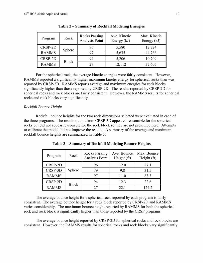
67th HGS 2016: Arpin and Arndt 10
Table 2 – Summary of Rockfall Modeling Energies
Program Rock Rocks Passing Analysis Point
Ave. Kinetic Energy (kJ)
Max. Kinetic Energy (kJ)
CRSP-2D Sphere
96 5,580 12,724 RAMMS 97 5,635 44,766 CRSP-2D
Block 94 5,206 10,709
RAMMS 27 12,112 37,605
For the spherical rock, the average kinetic energies were fairly consistent. However, RAMMS reported a significantly higher maximum kinetic energy for spherical rocks than was reported by CRSP-2D. RAMMS reports average and maximum energies for rock blocks significantly higher than those reported by CRSP-2D. The results reported by CRSP-2D for spherical rocks and rock blocks are fairly consistent. However, the RAMMS results for spherical rocks and rock blocks vary significantly.
Rockfall Bounce Height
Rockfall bounce heights for the two rock dimensions selected were evaluated in each of
the three programs. The results output from CRSP-3D appeared reasonable for the spherical rocks but did not appear reasonable for the rock block so they are not presented here. Attempts to calibrate the model did not improve the results. A summary of the average and maximum rockfall bounce heights are summarized in Table 3.
Table 3 – Summary of Rockfall Modeling Bounce Heights
Program Rock Rocks Passing Analysis Point
Ave. Bounce Height (ft)
Max. Bounce Height (ft)
CRSP-2D Sphere
96 12.0 27.1 CRSP-3D 79 9.8 31.5 RAMMS 97 11.0 83.3 CRSP-2D Block 94 12.3 22.6 RAMMS 27 22.1 124.2
The average bounce height for a spherical rock reported by each program is fairly
consistent. The average bounce height for a rock block reported by CRSP-2D and RAMMS varies considerably. The maximum bounce height reported by RAMMS for both the spherical rock and rock block is significantly higher than those reported by the CRSP programs.
The average bounce height reported by CRSP-2D for spherical rocks and rock blocks are
consistent. However, the RAMMS results for spherical rocks and rock blocks vary significantly.

67th HGS 2016: Arpin and Arndt 11
Rockfall Trajectory The rockfall trajectories reported for spherical rocks in CRSP-3D and RAMMS are
illustrated in Figure 6 using the rock velocity plots output from each program. Both models show that the majority of rocks follow a well-defined pathway downslope. This talus covered pathway is apparent in Figure 3. Both programs also show a small number of rocks that leave the well-defined pathway and traverse downslope towards the highway. This pathway is not well-defined but topographic data shows a shallow depression that rocks could potentially follow downslope.
Figure 6 – CRSP-3D and RAMMS rockfall trajectories for spherical rocks
The rockfall trajectories for spherical rocks and rock blocks output from RAMMS are
illustrated in Figure 7. The trajectories are similar in that the majority of rocks follow the well-defined pathway but there is slightly more disperse of the rock blocks than the spherical rocks. As with the spherical rock trajectories in CRSP-3D and RAMMS, a small number of rock blocks modeled in RAMMS follow the undefined pathway.

67th HGS 2016: Arpin and Arndt 12
Figure 7 – RAMMS rockfall trajectories for spherical rocks and rock blocks
DISCUSSION
Rockfall modeling results using CRSP-2D, CRSP-3D, and RAMMS for the Glenwood
Canyon study site are highly variable. While some results between programs are fairly consistent, other results vary significantly. CRSP-2D gives similar results whether modeling is performed using a spherical rock or rock block. This may be due to the simplicity of the program both in terms of modeling performed in 2D and the ease of developing a model. This simplicity does not appear to detract from the reliability of the results especially when compared to the 3D model results that generally require more effort to develop the model. As with all models, the quality of the results is highly dependent on the input parameters and model calibration among other factors.
RAMMS gives significantly different results when comparing spherical rocks to rock
blocks. This appears to be a result of how RAMMS models the interaction of the rock with the slope. The program utilizes a hard-contact, rigid body approach where contact forces are applied to the rock’s edges and points (3). For comparison, CRSP-2D utilizes a friction function and scaling factors that depend on coefficients of restitution (1) and CRSP-3D utilizes a visco-elastic contact model with inputs for stiffness and damping (2). With the hard-contact, rigid body approach the rockfall velocity, energy, bounce height, and trajectory are dependent on the rock shape. In general, rockfall velocities and energies reported by RAMMS are higher for the rock block than for the spherical rock. This may be a result of the rock block bouncing more and having less contact with the slope than is experienced by the spherical rock. The greater dispersion of the rockfall trajectories for the rock blocks compared to the spherical rocks also appears to be a result of the hard-contact, rigid body modeling approach.
The significant variation in the maximum velocity, energy, and bounce height reported by
RAMMS compared to the CRSP programs appears to be a single rock that launches over the

67th HGS 2016: Arpin and Arndt 13
majority of the slope and is in free-fall for a significant distance (Figure 8). This single rock also appears to skew the RAMMS results for average velocity and kinetic due to the relatively small number of rock blocks passing the analysis point. The presence of launching features that may not be captured in 2D modeling can have a significant effect on the modeling results.
Figure 8 – Single rock modeled in RAMMS with significant bounce height and free-fall
distance
Other potential sources of variability of the modeling results include differences in
defining slope types and also defining rockfall source areas within each model. Based on sensitivity analysis of varying surface roughness and hardness, it does not appear that differences in slope types between models would result in the significant differences in results that were observed in this study. Also, slight differences in defining the source area did not appear to provide significantly different results.
It is important to understand that most rockfall programs have been calibrated based on
observations of rockfall dynamics from rock rolling experiments. These experiments have typically been carried out with rocks smaller than those being modeled in this study. The rocks modeled in this study would be difficult to conduct experiments with due to their size. Modeling results should always be reviewed cautiously especially when modeling such large rocks.

67th HGS 2016: Arpin and Arndt 14
CONCLUSIONS Rockfall modeling results using CRSP-2D, CRSP-3D, and RAMMS for the Glenwood
Canyon study site are generally highly variable. Each program has advantages and limitations making it important for modelers to understand the program they are using and the needs of their specific project. CRSP-2D generally gives results similar to RAMMS when modeling a spherical rock. However, when a rock block and complex site are modeled using CRSP-2D and RAMMS the results vary significantly. Model calibration for site conditions and rock geometry appears to be the most important factor in obtaining reliable results.

67th HGS 2016: Arpin and Arndt 15
REFERENCES
1. Jones, C.L., J.D. Higgins, and R.D. Andrew. Colorado Rockfall Simulation Program, Version 4.0. Colorado Department of Transportation, Colorado Geological Survey, Colorado School of Mines, CDOT-SYMB-CGS-99-1, 2000.
2. Andrew, R., H. Hume, and R. Bartingale. CRSP-3D User’s Manual, Colorado Rockfall Simulation Program. Yeh and Associates, Inc., Federal Highway Administration, Central Federal Lands Highway Division, FHWA-CFL/TD-12-007, 2012.
3. Bartlet, P., C. Bieler, W. Bühler, M. Christen, L. Drier, W. Gerber, J. Glover, M. Schneider, C. Glocker, R. Leine, and A. Schweizer. RAMMS::ROCKFALL User Manual, v1.6. WSL Institute for Snow and Avalanche Research, 2015.
4. Kirkham, R.M., R.K. Streufert, and J.A. Cappa. Geologic Map of the Shoshone Quadrangle, Garfield County, Colorado. Map Series 35. Colorado Geological Survey, Department of Natural Resources, 2008.

Roller Coaster Highways
The Implementation and Execution of a Settlement Monitoring Program
at Two Colorado Highway Projects
JG T. McCall, EIT Kleinfelder, Inc.
4815 List Drive, Unit 115 Colorado Springs, Co 80919
(719)-632-3593 [email protected]
J. Kevin White, PE Kleinfelder, Inc.
4815 List Drive, Unit 115 Colorado Springs, Co 80919
(719)-632-3593 [email protected]
Prepared for the 67th Highway Geology Symposium, July, 2016

67th HGS 2016: McCall and White - DRAFT 2
Acknowledgements
The authors would like to acknowledge and sincerely thank each of the following individuals/entities for their contributions in the work described.
Craig Wieden – Colorado Department of Transportation
Kraemer North America – Edward Kraemer & Sons Flatiron Construction Corp.
Disclaimer
Statements and views presented in this paper are strictly those of the author(s), and do not necessarily reflect positions held by their affiliations, the Highway Geology Symposium (HGS), or others acknowledged above. The mention of trade names for commercial products does not
imply the approval or endorsement by HGS.
Copyright Notice
Copyright © 2016 Highway Geology Symposium (HGS)
All Rights Reserved. Printed in the United States of America. No part of this publication may be reproduced or copied in any form or by any means – graphic, electronic, or mechanical,
including photocopying, taping, or information storage and retrieval systems – without prior written permission of the HGS. This excludes the original author(s).

67th HGS 2016: McCall and White - DRAFT 3
ABSTRACT
We are all familiar with the infamous “bump” at the end of a bridge. After recent highway projects experienced significant differential settlement at bridge abutments, the Colorado Department of Transportation (CDOT) updated their specifications to address the problem. CDOT now requires contractors to monitor embankment settlement and verify the completion of primary settlement prior to allowing roadway paving. Kleinfelder, as part of design-build teams, was selected to provide geotechnical services for two highway interchange projects requiring settlement monitoring, and consulted each contractor on the implementation and execution of a settlement monitoring program.
Instruments were installed at the subgrade/foundation soils elevation, middle depth of the embankments, and at the final grade to determine the rate of settlement at each location within the embankment fill. Four instrument types were chosen based on subgrade soils and the installation height within the fill. Installation of the instruments required planning, cooperation, and communication with the prime contractor, sub-contractors, and CDOT representatives, to address the challenges of location selection during the fluid design-build process, avoiding and repairing damage to instruments, and field installation of the instruments. Settlement data was collected for analysis and submitted regularly throughout the construction process. Observed settlement data was compared to predicted and theoretical models. The settlement monitoring programs discussed are unique for Colorado highway projects, and presented are the challenges and lessons learned in implementing and executing settlement monitoring programs on two highway interchange projects.

67th HGS 2016: McCall and White - DRAFT 4
INTRODUCTION Nearly ten years after completion of one of the largest projects completed by Colorado’s Department of Transportation (CDOT), Region 2, the $150 million dollar Colorado Springs Metro Interstate Expansion (COSMIX) Project, located north of downtown Colorado Springs is still giving state engineers grief. The problem? Differential settlement along a stretch of Insterstate-25 at the Rockrimmon/Corporate Drive Interchange. Shortly after completion of the project, drivers began to complain about the dips in the road (1) at several of the bridge abutments along one of the off ramps and along the I-25 mainline. The first fix was completed by the design build team under the project warranty, a second fix was completed in 2009, and another round of repairs is currently in the works and expected to cost an additional $2 million dollars (2). With the persistent and costly repairs to the COSMIX area project in mind, CDOT added language to the RFP for a new I-25 design build interchange project in southern Colorado with the goal of reducing the differential settlement at the bridge abutments.
The RFP for the I-25 over Cimarron Design Build (Cimarron DB) project called for the contractor to monitor the embankment settlement and show completion of primary settlement prior to beginning paving operations. The inclusion of a settlement monitoring program at the RFP stage was uncommon for CDOT projects prior to the Cimarron DB project, and showed the agency’s emphasis on reducing the impacts of differential settlement. This emphasis was also seen on a second design build project being completed by CDOT region 2. The I-25 over Ilex Design Build (Ilex DB) project also included a settlement monitoring program. As part of the project approach the DB team proposed using fill material that was lower quality than the initial RFP specified. CDOT approved the proposed fill material with the requirement that the contractor monitor the settlement prior to paving operations.
Kleinfelder, as part of the design build team for each project, provided geotechnical engineering and design services including developing, implementing, and overseeing the two project settlement monitoring programs. With the emphasis on reducing settlement, Kleinfelder was involved from the proposal stage on each project and prepared a settlement monitoring plan to address the concerns expressed by CDOT. The team’s approach to monitor the settlement was a large factor in the selection criteria. To meet project goals and provide an alternative approach, Kleinfelder proposed utilizing 3 additional types of instruments to monitor the embankment settlement beyond the required settlement plate instrument. The instruments were chosen based on desired application, placement location to provide accurate data in key locations along the projects, and to provide system redundancy. The settlement monitoring programs were successfully implemented and the unique approach provided valuable data that went beyond CDOT’s expectations. INSTRUMENTATION SELECTION, INSTALLATION, AND COST Four instrument types were utilized as part of the settlement monitoring programs, each type of instrument was selected for various applications and desired readings. The instruments used on the projects included Vibrating Wire Manometers (VWM), Manual Manometers (MM), Settlement Plates (SP), and Survey Monuments (SM). Instruments were selected to measure settlement at the subgrade elevation, in the middle of the fill, and at the top of the fill. In general,

67th HGS 2016: McCall and White - DRAFT 5
the two manometers (VWM and MM) were planned as subgrade settlement monitors with a desired installation window just prior to the placement of fill materials. The settlement plates were planned to measure the settlement within the fill, with a target installation window mid-height of the fill embankment. The survey monuments were planned to measure the settlement at the surface of the fill and installed when the embankment reached the final grade. The four instrument types were used in conjunction to differentiate the subgrade settlement from settlement and consolidation within the fill embankment. The following paragraphs briefly discuss each instrument and provide a comparison of the various instruments utilized. To measure the subgrade settlement beneath the new embankments, vibrating wire manometers were installed near the subgrade elevation. The instrument consists of a pressure transducer mounted on a small steel plate that measures the pressure difference between the buried sensor and an outside reservoir. Two fluid filled tubes connect the buried sensor to a reservoir located outside the settlement area. Figure 1 shows the typical VWM transducer, plate, and associated wires and tubes. The pressure is automatically recorded via a data logger installed within the reservoir housing. Settlement of the transducer and plate are calculated from the pressure difference from the initial pressure reading recorded during installation of the system. Automatic recording of the sensor pressure can be set at a desired frequency and are stored on the data logger and simply downloaded for weekly processing. The use of the data logger allows for easy data collection at regular intervals. This ability to collect and store data at relatively high frequency, made the VWM an ideal instrument to be placed at critical areas identified in the pre-proposal phase. Critical areas include, large potential settlement areas, areas where time rate of settlement was a concern, or areas at critical structures such as bridge abutments.
Figure 1 – Typical VWM Transducer, Plate, and Tubing Similar to the VWM, manual manometers were also used on the projects to measure the subgrade settlement. The manual manometer consists of a simple U-tube manometer, with one end placed beneath the fill and the second end located outside the fill. Figure 2 shows the typical sensor end of the MM that is buried within the fill. The fluid level at either end of the manometer adjusts as the height of either end of the manometer changes. This direct measurement of the height at either end of the manometer allows for direct measurement of subgrade settlement when one end is placed beneath the embankment fill. In our application, one end of the

67th HGS 2016: McCall and White - DRAFT 6
manometer tube was attached to a plate buried beneath the fill. This elevation change of the buried plate and subgrade is observed in the manometer end located outside the fill, within a protected readout box. The manual manometers were chosen as a cost effective way to measure subgrade settlement when compared to the VWM, because of the ability to quickly assemble the instruments from locally sourced materials.
Figure 2 – Typical MM Sensor End Settlement plates are standard settlement monitoring instruments that have been widely used to measure settlement. The settlement plate is simple, cheap, and quick to install. Consisting of a 24-inch square steel plate with a 2-1/4 inch steel pipe welded orthogonal to the plate, as shown in Figure 3. The plate is placed at the desired location and the top of the steel pipe is surveyed. As the plate settles the elevation of the protruding pipe changes in elevation. Periodic surveys are taken to record the elevation change of the protruding pipe and corresponding plate. As fill is placed the steel pipe must be extended, additional pipe sections are connected with threaded couplings. For our application, settlement plates were installed near the mid-height of the embankment or at the subgrade elevation in areas with a relatively low embankment height.

67th HGS 2016: McCall and White - DRAFT 7
Figure 3 – Typical Settlement Plate The final instruments used on the projects were survey monuments (SM). The monuments consist of a single piece of steel rebar buried and encased in concrete, placed at the surface of the embankment. Figure 4 shows the typical survey monument used on the project. The monument is periodically surveyed to measure and record the elevation difference between successive measurements. Survey monuments were installed at the top of the embankment and used in conjunction with instruments installed at the subgrade, to ensure that the newly placed fill material was not settling.
Figure 4 – Typical Survey Monument
Installation and Placement Considerations The subgrade instruments, VWM and MM, are designed to be installed prior to placement of fill materials. In an active construction zone, it is not practical to place the instruments on the surface and let fill placement continue. Both of the subgrade instruments consist of a sensor end and a readout end connected by fluid filled tubes and communication wires. In order to protect the lines and wires, the ideal installation time was determined to be after the placement of 1 to 2 feet of fill. Following the placement of this protection layer of fill, the instruments and lines were trenched and buried within the existing fill. This allowed measurement of the subgrade settlement as the embankment is constructed while protecting the instruments and the associated lines to the readout unit. The readout units were installed in an area outside the fill, in an area that is protected from construction activities. The readout units were typically mounted on a 4x4 wood post founded in a 12-inch diameter, 3 feet deep, concrete filled base. Movement in the readout unit will affect the total settlement reading, therefore special care must be taken to minimize potential settlement. After installation, and prior to backfilling, the instruments must be surveyed to get baseline readings. In addition to the instrument sensor, the readout unit/post must also surveyed during installation to get a baseline elevation. The instruments installed near the subgrade elevation and buried beneath the fill were protected from construction activities at the surface. The units are much less likely to be damaged, and do not interfere with fill placement or other activities. The readout units are exposed to construction

67th HGS 2016: McCall and White - DRAFT 8
activities and should be placed in areas outside normal construction traffic and other site operations. When considering installation locations for the VWM and MM instruments, the relative elevation difference between the instrument and readout unit is a significant factor to consider. For the VWM, the fluid reservoir in the readout unit must be at a higher elevation than the sensor with a maximum elevation difference of about 20 feet. With regard to the MM, the readout unit and sensor end must be at the same elevation. For both instruments, the relative elevation difference requirements may be a limiting factor in the placement location. The VWM system is very sensitive to environmental conditions, and must be installed with precautions taken to keep the reservoir unit out of direct sunlight. The VWM system is also affected by electromagnetic radiation, and the system must be installed away for power lines. The settlement plates were placed within the embankment fill, or at the subgrade surface, in areas with relatively low embankment height. Installation requires excavating a 2 to 3 feet deep hole to place the steel base plate. The base plate is buried in 2 to 3 feet of fill to provide protection and stability of the instrument. The base plate and top of the steel pipe must be surveyed, and a PVC sleeve must be placed around the vertical steel pipe prior to backfilling. The PVC sleeve ensures that the settlement of the base plate is not influenced by down drag forces caused by the friction between the fill material and the sides of the pipe. The PVC sleeves were extended at a few feet above the top of the steel pipe, and painted orange to help keep the instrument visible during active construction of the embankment. The surface monuments were installed at the completion of fill placement, generally prior to the placement of pavement base materials. In order to allow for sufficient time to take the required number of measurements, the surface monuments were planned to be installed as soon as possible after the embankment reached final height. To protect the monument from equipment, and ensure the monument is not affected by the freeze/thaw cycle in the cold Colorado winter, surface monuments were placed a minimum of 3feet below the surface of the ground. A 6-inch diameter hole was advanced using a hand auger, or similar, to a depth of 3 feet, a 1/2-inch steel rebar was placed in the center of the hole, and backfilled with fast setting concrete. The rebar was brought about ½-inch above the existing ground surface and concrete mounded around the rebar. The top of rebar provided a consistent survey point, and survey of the rebar was completed at installation to provide a base reading. The settlement plate and the survey monument are both placed at or above the surface of the fill. This exposes the instruments to construction activities. Placement locations should consider the construction activities, and the location along the embankment, to ensure representative settlement observations (i.e. near the maximum height of the embankment). Cost Considerations
The cost of each instrument can be looked at from a variety of different ways: the initial cost of the instrument, labor cost during installation, collecting readings, and labor costs to evaluate, analyze, and repot the data. For the purposes of this paper we will keep pricing in terms of relative cost and budget numbers.

67th HGS 2016: McCall and White - DRAFT 9
The most expensive equipment in terms of initial equipment cost is the VWM. The instrument is purchased as part of a settlement system that includes the sensor, fluid filled tubes, control and communication wires, fluid reservoir, data logger, and housing unit. The system is calibrated by the manufacturer and requires a two to three week turnaround from ordering the units to delivery. Total cost of the system is a few thousand dollars and varies with the length of tube and data logger requirements. The VWM is delivered as a complete system from the manufacturer and requires minimal labor to set up prior to field installation of the system. The manual manometers used on the projects were fabricated by Kleinfelder, and the cost of materials were fairly cheap and on the order of a few hundred dollars. In addition to the cost of the raw materials, each MM required about 10 to 15 labor hours to purchase the supplies from local sources, construct the sensor unit, readout box, and pre-fill the tubes. The settlement plates were fabricated at a local machine shop, and each 24” by 24” base plate cost less than $100 for materials and welding. The steel extensions average about $10 per foot and includes cutting, threading, and couplers. Settlement plates required about 5 hours of labor to order and pick up the materials. Least expensive in terms of initial cost are the survey monuments, consisting of a single piece of rebar and couple bags of concrete. On each project the general contractor supplied scrap rebar that was left over onsite. More difficult to quantify is the labor required for each of the instruments after the initial cost of purchasing and fabrication of the instrument. Labor required for each instrument can be looked at in three different areas: installation, reading and collecting the data, and data evaluation and processing. The manual manometers required the most labor to install, about 10 to 16 labor hours in the field for installation. The location must be determined, excavations completed for the sensor area, and trench line excavated from the sensor to the readout box. Typical distance from the sensor to the readout box was about 100 to 200 feet. Figure 5 shows the typical excavated trench and installation of MM fluid lines. After the excavations were complete, the tubing was installed and the readout box mounted on the readout post. Following the installation, and prior to backfilling, the system and lines must be tested and verified. The manual manometers require field staff to read and record the fluid level in the tubes once a week, labor hours are about ½ an hour a week for each unit installed on the project and an additional ½ an hour per week is also required for data reduction, analysis and reporting.

67th HGS 2016: McCall and White - DRAFT 10
Figure 5 – MM Trench and Installation of Fluid Lines The vibrating wire manometer systems require similar labor hours as the manual manometers for field installation and testing. Similar to the MM the VWM sensor must be buried, the readout unit mounted to a post, and trenches excavated between the two. The average length of the VWM is also similar to that of the MM used on the projects at 100 to 200 feet. Field collection of data is quicker than the MM and only requires about 15 minutes of labor per unit to collect data from the data logger and record the fluid reservoir level. The data reduction and analysis requires more initial time than the MM and other instruments. The spreadsheets used for data analysis include the calibration information for each instrument and factors for sensor temperature, reservoir height, and readout post elevation. The amount of data is also substantially more than the other instruments that have a single reading each week, as the VWM system was set to record four daily readings. The data collected by the VWM system required an average of about ½ an hour to 1 hour of weekly processing time. Both the survey plate and the survey monument required minimal weekly labor to collect the data. The project surveyor took readings at each instrument and provided them to the project team for analysis. During fill placement, the settlement plates had to be extended by adding additional section of steel pipe and protective PVC sleeve in order to keep the top of the tube above the top of the fill. Throughout the project, adding the extensions averaged about ½ an hour of labor per week. The data reduction is also minimal for the settlement plates and the survey monuments. Processing and data analysis averaged about 15 minutes of labor per week for each instrument. DATA COLLECTION, REDUCTION, AND REPORTING Frequency of collection Throughout both of the projects, regular instrument readings were performed once a week, and planned for the same day each week. In addition to our readings, the project survey team performed weekly survey that included fill height, readout post elevations, and the top of the settlement plates and the survey monuments. The MM were checked once a week by field staff who recorded MM readings for processing. The VWM data logger data was downloaded once a week at the same time the MM readings were taken. Each week, the survey data and instrument readings were processed and interpreted by a staff level engineer. The VWM required the most processing, and included factors for sensor temperature, fluid height in the reservoir, and elevation of the read out post. Manual manometers required processing that included adjustments for fluid level and readout post elevation. Survey monuments and settlements plates required minimal processing, simply a comparison to past survey elevations. Weekly data was also checked for survey and readings errors during processing. Analysis and Reporting Analysis of the data was completed weekly following field collection of data. Analysis included careful interpretation of the data to determine the amount of settlement and to check for anomalies. Field data collected had a considerable amount of “noise” or variations in the readings. Noise in the reading may be attributed to several factors depending on the instrument

67th HGS 2016: McCall and White - DRAFT 11
type. The VWM and MM are both significantly affected by temperature fluctuations, and movement of the readout units. Factors for temperature and other environmental conditions can be applied to clean up some of the variation from these factors. The SP and SM data is completely dependent on the survey data, therefore, survey data required detailed analysis and interpretation. Variation in surveyed elevations were observed based on the location measured on the instrument and between different field staff completing the survey. During review and analysis of the data, we had to determine if the variations in the elevations were due to movement of the soil or other factors such as temperature fluctuation or survey discrepancy. During analysis of the data, we had to keep in mind the overall goal of the settlement programs was to determine if primary settlement was complete. With this in mind, the variations in the data attributed to “noise”, did not have a significant impact on the final conclusions of the data. Analysis of the data showed the general trend of the rate of settlement, and this was the final determination in deciding whether or not settlement was complete. Figure 6, shows an example of the settlement results collected with a VWM showing a very clear trend line.
Figure 6 – Observed Settlement of VWM installed at Subgrade Elevation
-1
0
1
2
3
4
5
6
7
8
9
105955
5960
5965
5970
5975
5980
5985
5990
5995
6000
6005
6010
01/1
6/16
01/2
3/16
01/3
0/16
02/0
6/16
02/1
3/16
02/2
0/16
02/2
7/16
03/0
5/16
03/1
2/16
03/1
9/16
03/2
6/16
04/0
2/16
04/0
9/16
04/1
6/16
SETT
LEM
ENT
(IN)
ELEV
ATIO
N (F
T)
Initial Ground Elevation (ft) Sensor Elevation (ft) Proposed Final Grade (ft)
Fill Elevation (ft) Observed Settlement (in)

67th HGS 2016: McCall and White - DRAFT 12
Figure 7 – Observed Settlement of VWM installed at Mid-Height of Embankment
From the data you can see the specific amount of settlement is difficult to determine within a ½ inch or so, however it is very clear that the rate of settlement is near zero. The installation of the instruments after placement of fill materials also made it very difficult to determine the total amount of settlement. The instruments measured settlement since installation, which in some cases, was near mid-height of the embankment. In these cases, the instruments were not installed prior to the application of the initial load. Without measuring the settlement due to the initial load, it was very difficult to determine the amount of total settlement experienced. Given that some amount of settlement was not observed, we were still able to show the rate of settlement and from the trend line determine if settlement was complete. Figure 7, shows the settlement curve for an area with similar amount of fill placed as Figure 6. The total settlement in these two areas were calculated/expected to be similar in magnitude. However, the total settlement observed in the instruments vary significantly, this is due to the installation location with regard to fill height. In Figure 7, the rate of settlement clearly trends toward zero, even though the amount of total settlement is much less. Following the analysis and processing of the weekly data, the results were reviewed by a senior level engineer and reported to the project team via upload to the file transfer site. Weekly data reported to the project team only included the processed data, a monthly letter summarizing the progress of the settlement monitoring program, and interpretation of results. As various locations within the project were completed, and the instruments showed completion of primary settlement, letters drafted by Kleinfelder were submitted for CDOT approval prior to beginning paving operations.
-1
0
1
2
3
4
5
6
7
8
9
105955
5965
5975
5985
5995
600511
/22/
15
11/2
9/15
12/0
6/15
12/1
3/15
12/2
0/15
12/2
7/15
01/0
3/16
01/1
0/16
01/1
7/16
01/2
4/16
01/3
1/16
02/0
7/16
02/1
4/16
02/2
1/16
02/2
8/16
03/0
6/16
03/1
3/16
03/2
0/16
03/2
7/16
04/0
3/16
04/1
0/16
04/1
7/16
OBS
ERVE
D SE
TTLE
MEN
T (IN
)
ELEV
ATIO
N (F
T)
Initial Ground Elevation (ft) Sensor Elevation (ft) Proposed Final Grade (ft)
Fill Elevation (ft) Observed Settlement (in)

67th HGS 2016: McCall and White - DRAFT 13
Data Quality The quality and precision of data that each instrument is able to provide was also considered in the selection of settlement systems and instruments. The vibrating wire manometers provided the most precise data and were accurate to about one-tenth of one inch. The VWM also allowed for the collection of much more data that in many cases showed a more detailed settlement curve compared to other instruments. The VWM also required little to no field measurement, because all readings were automated and stored in the logger. With that in mind, the VWM system also required more post-processing time, and the proper use of calibration and environmental factors, which if not properly accounted for could significantly affect the data quality. The manual manometers allowed for a precision of about one-quarter of an inch. The MM were highly sensitive to temperature changes and required field measurements and recordings that limited the number of readings. Weekly readings were chosen as the most practical frequency for measuring and recording the settlement data. The precision and quality of data available for the settlement plate and the survey monument is completely dependent on the surveyor. The precision of the survey on the project was about one-half of an inch. As with the MM, the settlement plates and monuments were measured once a week. There is little source of error during processing of the data because of the direct measurement of the settlement plate and monuments, provided the survey information is accurate. LESSONS LEARNED The settlement monitoring programs were unique for Colorado projects and unique for the each design build team. Throughout the process we learned a great deal about implementing a settlement monitoring program and some of the challenges working in a design-build environment. The monitoring programs were successful in completing the program goals and ensuring a quality product for the highway owner. The major takeaways from the programs are: the importance of constant communication with the contractor and owner, proper planning and pre-fabrication of instruments, and the importance of redundant systems. Communication and Coordination The most difficult part of the settlement monitoring programs was the coordination between all the various stake holders. To install a single instrument required the settlement plan to be written and approved by senior engineering staff at Kleinfelder, approval from CDOT and the design build team, and communication of the program to the Kleinfelder field staff. Following approval, the instrumentation had to be purchased and in some cases required a 2 to 3 week turnaround time for delivery, and several instruments had to be pre-fabricated prior to installation. Installation required planning and coordination with the general contractor, earth working contractor, and the project survey company. This amount of involvement from outside parties requires constant and clear communication throughout the project. From a consultant’s perspective, we found much better results when we were able to shift the mindset of the general contractor to take ownership of the settlement instruments. Alternatively, when the mindset of the contractor was such that the settlement instruments were Kleinfelder’s, the instruments were

67th HGS 2016: McCall and White - DRAFT 14
seen as an inconvenience and the installation and implementation of the settlement monitoring program was much more difficult. Communication is particularly important in the design build setting where the construction schedule may change daily. For example, we were prepping equipment for installation in one area of the project, when we were told fill placement was starting in a completely different area of the project the next day. By the time we were able to mobilize and prepare instruments for installation, the earth working contractor had placed over 10 feet of fill in certain areas. This was at the beginning of the project and the earth working contractor was not made aware of the location and timing for installation of the settlement monitoring equipment. In order to address this, we requested the earth working contractor be involved in settlement monitoring meetings from the beginning of the project, and have a copy of the instrumentation locations. When this approach was taken, the communication and timing of installation was much better. Communication regarding the project design plans is also critical to success of the settlement monitoring program. In the design build environment, the design process is very fluid and may be different than the proposal phase. On each project, we encountered an issue with the location of the readout unit, some areas that were outside the fill during the RFP stage were found to be areas of fill at the time of installation of the instruments. Communication with the contractor and design team was critical to ensure that the installation locations were chosen based on the most current set of plans. We found the installation locations were best determined by the prime contractor, who had the best understanding of the project. The contractor was best suited to determine locations that would likely be out if the way from construction activities. By letting the contractor approve the location of the instruments, we limited our exposure to future costs involved in replacing or moving the instruments if they were placed in a non-ideal location. Planning and Pre-fabrication Planning and pre-fabrication was the second takeaway we learned throughout the settlement monitoring programs. This is particularly true with the MM; without a well-planned installation procedure and pre-fabricated pieces, the installation and performance of the instruments suffered. The fluid filled lines must be completely free of air bubbles in order to provide accurate readings. During installation of the first couple of instruments on the project, we attempted to fill the lines in the field. We quickly found out that in the uncontrolled field environment, it was nearly impossible to properly fill the lines, and the instruments did not perform properly. Additionally, the cost savings observed in sourcing local, cheap raw materials, was diminished with the amount of labor required to install and troubleshoot the MM systems in the field. In order address the problems, we pre-filled the MM tubes in the lab prior to field installation. This allowed for the lines to be filled by gravity/siphon methods. Pre-filling the lines reduced the time required to fill the tubes, ensured the lines were completely free of entrained air, and resulted in more accurate readings. Redundancy
In addition to constant communication and proper planning, another takeaway from the project is the importance of redundancy. The field application of the instruments within an active

67th HGS 2016: McCall and White - DRAFT 15
construction site, specifically a design-build construction site, resulted in many unforeseen circumstances that required instruments to be abandoned. Instruments were abandoned because of damage caused by the construction activities, interference with structures, and instrument malfunction. With multiple instruments installed at each location, we were able to collect sufficient data to complete the overall project goals in the event that one or more instruments were abandoned or failed. The working instruments at any given location could be used in conjunction with surrounding locations to make a reasonable determination if primary settlement was complete. The loss of certain subgrade instruments did not allow us to accurately determine the amount of total settlement that occurred, however, we were still able to show that the rate of settlement had decreased and rate of movement was trending toward zero. Final Thoughts The settlement monitoring programs were successful in determining the completion of primary settlement, and the use of a wide range of instruments beyond the RFP requirements provided data that exceeded CDOT’s expectations for the monitoring programs (2). Program success required constant and clear communication with the stake holders, and realistic expectations of the data. The redundant systems proved to be a vital part of the program’s success, and we learned many valuable lessons during installation and fabrication of the instruments. Each of the four instruments used on the projects provided valuable data for the respective application. However, all in, the VWM in our application, provided the best value and most consistent data, provided proper time is devoted to analyze the large amount of data received from the system. The VWM worked very well in critical areas, and the ability to collect multiple daily readings, in our opinion, offset the initial cost of the system. The MM systems provided value for non-critical areas, however in general, the systems required a significant amount of labor and the data was much more variable than the VWM. We feel the settlement monitoring programs provide great value and quality assurance on large highway fill projects. The total cost of the monitoring programs were roughly 10 percent of the total geotechnical fee for the project. This cost is a small fraction of the overall project cost, and when implemented properly, has the potential to save millions of dollars in associated repairs and avoid public relations problems.

67th HGS 2016: McCall and White - DRAFT 16
REFERENCES:
1. Mckeown, Bill. Pesky Repairs Near I-25 Interchange are Nearly Complete. Colorado Springs Gazette. April 1, 2009.
2. Wieden, Craig. Region 2 Materials Engineer. Colorado Department of Transportation. Personal Interview. May 11, 2016.

Rockfall Barrier Foundations and Challenges Associated With Estimating Design Basis Loads
David J. Scarpato, P.E. Scarptec, Inc. P.O. Box 326
Monument Beach, Massachusetts, USA (603) 361-0397
Prepared for the 67th Highway Geology Symposium, July, 2016

67th HGS 2016: D. Scarpato 2
Acknowledgements
The author would like to thank the following individuals/entities for their contributions in the work described:
Mr. Kevin Coyle (GeoBrugg North America, LLC) Mr. Eric Seib (Merco, Inc.)
Disclaimer
Statements and views presented in this paper are strictly those of the author(s), and do not necessarily reflect positions held by their affiliations, the Highway Geology Symposium (HGS), or others acknowledged above. The mention of trade names for commercial products does not
imply the approval or endorsement by HGS.
Copyright Notice
Copyright © 2016 Highway Geology Symposium (HGS)
All Rights Reserved. Printed in the United States of America. No part of this publication may be reproduced or copied in any form or by any means – graphic, electronic, or mechanical,
including photocopying, taping, or information storage and retrieval systems – without prior written permission of the HGS. This excludes the original author(s).

67th HGS 2016: D. Scarpato 3
ABSTRACT
Rockfall barrier design is often complicated by the seeming disconnect between estimates of incoming rockfall kinetic energy and traditional approaches to foundation design. Engineering geologists can use industry-accepted rockfall modeling software to develop estimates for particle bounce height, kinetic energy, velocity, and limit of horizontal travel. Geotechnical engineers have well-established procedures for use with foundation design problems; however, how practitioners make the leap from input energy to development of barrier foundation design loads is less clear because of challenges associated with barrier behavior. Evaluation of rockfall impact force and probabilistic barrier impact location are critical for developing estimates of system load distribution and energy attenuation. Impact force is inversely proportional to stopping distance, and stopping distance can be considered an analog to system deflection. Barrier post impacts generate different system deflections (and hence input loads) than impacts in the mid-span portion of suspended netting; however, the probability of direct post impact is less than that of impacts to suspended netting. Loads are partially attenuated within the barrier system and a percentage of the incoming load is distributed to the foundation. These challenges further manifest themselves due to limited industry criteria on barrier foundation design, use of a wide range of input assumptions, and lack of widely available analysis tools for practicing geotechnical professionals. This paper will present practical guidance for dealing with the challenges associated with developing foundation loads during rockfall barrier selection and design, and will use project examples to highlight key points throughout. KEYWORDS Rockfall, Barrier, Foundation, Design, Impact Force, Kinetic Energy, Deflection

67th HGS 2016: D. Scarpato 4
INTRODUCTION
Rockfall barriers (“barriers”) have been used by industry for many years to either arrest falling pieces of rock or to significantly slow such rock down, as in the case of attenuator type systems. There are numerous barrier types produced by a series of manufacturers, both here in the U.S. and internationally. Barriers systems are now typically ordered pre-manufactured from vendors, based primarily on design evaluations provided by geotechnical engineers and/or engineering geologists. Minimum barrier height, impact energy capacity, plan limits, and deflection criteria are the parameters typically needed to design such a system. Industry-wide, there is very limited rockfall barrier design criteria available for geotechnical practitioners.
The use of individually designed and constructed systems (i.e. barriers designed for only
one specific project) has also been observed. The author is aware of four projects where individually designed and constructed barrier systems (“IDCBS”) are either in stages of construction or have recently been completed.
Design of the barrier system envelop requires input from multiple disciplines, including geotechnical engineers, engineering geologists, and civil/site. The civil/site engineer would assess site layout, traffic, lane width, and drainage. Traffic and lane width considerations are important with respect to system placement, as a barrier that deflects into traffic could be a disaster. Engineering geologists would assess rockfall source zones and estimate impact energy and bounce heights, for example. Geotechnical engineers would typically evaluate foundation details like minimum barrier post and anchorage embedment depths. (Note: Although structural engineers are not routinely enlisted during barrier design phases, it is thought that they could provide some useful insight with respect to research, assistance with development of design criteria, and especially with IDCBS)
When it comes to barrier support elements inclusive of the foundation and anchorage
systems, there is a considerable amount of difficulty deriving foundation anchorage loads from incoming dynamic impact energy (the term “foundation” when used herein refers to post foundation and any supporting anchorages). This holds true because the barrier system both distributes and attenuates energy as the impact load gets transmitted to the foundations (which is what it is supposed to do). But to many practitioners who may not have access or project budget capacity to support advanced numerical modeling, we must develop barrier foundation loads using the methods or criteria that are available to us – and there are not many! It is frequently found that barrier foundations designs are extremely conservative, resulting in either massive or very deep foundations. The remainder of this paper addresses how rockfall barrier system designers can develop reasonable estimates for foundation loads. CURRENT STATE OF PRACTICE
The current industry state-of-practice for barrier design here in the U.S. is based upon an evaluation of rockfall kinetic energy and bounce height. The bounce height can be used to develop required minimum barrier height, while estimates of rockfall kinetic energy can be used for design of barrier system energy attenuation capacity (1). Rockfall modeling software like the Colorado Rockfall Simulation Program (CRSP) or RocFall (from Rocscience©) can be used to

67th HGS 2016: D. Scarpato 5
generate two-dimensional rockfall trajectories along cross-sections of interest as shown in Figure 1. Although utilized less frequently here in the U.S., three-dimensional rockfall modeling software can be used, the likes of Hy-Stone and RAMMS, both of which rely on digital elevation models for development of trajectories.
Figure 1 – Example of output from a
2D CRSP rockfall simulation
Alternatively, for canopy type barriers under nearly vertical (free-fall) conditions, simple kinematic physics principles can be utilized to make conservative assessments of terminal velocity and resulting kinetic energy as shown in Table 1 below.
Table 1 – Example “free-fall” calculation
for rockfall on very steep slopes
FALL ENERGY
GRAV. ACC. VELOCITY KINETIC ENERGYG (M/S2) D (FT) D (M) V (M/S) KE (KJ)
9.8 285 87 41.3 1028
TERMINAL VELOCITY
KE = 0.5mv2v = √(2gd)
FALL DIST.

67th HGS 2016: D. Scarpato 6
Once rockfall bounce height and kinetic energy have been estimated based on the methods above, a barrier system will typically be selected. The selected barrier will consider the “rated” energy capacity and the minimum post height required to effectively maintain the design containment (usually expressed as a percentage, like 80% or 95% capture for example).
It should be mentioned that there is an inverse relationship between barrier deflection and
impact force; that is, when deflection is limited or hindered, impact forces are increased – which results in a corresponding increase in required geotechnical anchorage capacity. This can be shown by using a simple deflection analogy, where a free-falling rock penetrates a soil by the following “stopping distances”, as shown in Table 2.
Table 2 – Simple analogy of falling rock and impact
forces with respect to stopping distance
Some manufacturers (like GeoBrugg for example) offer anchor loading documents based on field-scale tests of barrier systems and finite element models of barrier behavior. This information comes in a simple table depending on barrier type, and shows forces transmitted at the anchor head for retaining ropes (i.e. tie-backs), lateral/end anchors, intermediate (i.e. rope separation) anchors, and post base plate anchors. These anchor forces documents are extremely helpful for geotechnical design of required barrier foundation systems.
Design of IDCBS requires an extra series of steps, where the barrier designer must evaluate system behavior and load distribution on their own, which can lead to very conservatively designed foundations with multiple degrees of redundancy. The author has seen some of these IDCBS which are impressive and could likely withstand impact from a Tomahawk cruise missile at close range; however, they are very expensive and likely largely over-designed. BARRIER FOUNDATION DESIGN
When available, the previously referenced anchor force documents are very helpful for design of barrier system anchorages; however, for the vertical post support system itself, requirements for concrete foundations are not as clearly defined. As a result, it is not uncommon to find post support foundations that are very large or deep. Many barriers are supported by anchorage elements (as opposed to direct embedment in the case of plunge columns or drilled shafts), and the impact loads are intended to be distributed to the anchors as the barrier deflects. It is work noting that for “off-the-shelf” barriers, the concrete foundations are secondary and merely intended to be an intermediary with which to accomplish the following:
KE (KJ) KE (FT-LBS) S (FT) Fi (LBS) Fi (KIPS)4 184391 1848 92195 9212 61464 6116 46098 4620 36878 3724 30732 31
IMPACT FORCEKINETIC ENERGY STOP DIST.
Fi = KE/S
1000 737562

67th HGS 2016: D. Scarpato 7
A. Construct the barrier and base plate on a sound, level surface; B. Distribute loads to the foundation anchorage elements.
When posts are directly constructed on sound bedrock, concrete or grout level pads may
not even be required. In which case, loads are transmitted directly to supporting anchorage elements. For cases in soil, “weak” rock, or other intermediate geomaterials, concrete foundations often become very large or very deep. Some of the reasoning behind such conservatively designed concrete barrier foundations may consist of the following:
A. “Zero deflection system” – This is a phrase that has been gaining usage in the industry, primarily among Owners, and is a misnomer. Barriers are intended to be flexible and deflect (i.e. deform) in order to efficiently distribute impact loads to the anchorage elements. In this regard, such deflection is actually a positive attribute. Note that even “rigid” rockfall barrier systems are intended to deflect. The only real system meeting (or almost meeting) this criteria is a structural wall.
B. “Shoe-horned” systems – Some rockfall barrier are proposed and constructed in locations that may not be realistic, for example, along highways with very limited shoulder width. This leads to the use of more conservative assumptions during design, which can result in larger concrete foundations.
C. Lack of experience – Rockfall barrier design and construction is a specialty field that requires experience for both the engineer and the contractor. Inexperience may lead to the use of very conservative foundation design assumptions. Traditional geotechnical engineers are excellent at foundation design, so concrete pedestal type foundations for barriers may be designed using analyses for spread shallow footings or deep foundations (e.g. piles, drilled shafts, etc.).
D. “No maintenance” system – Rockfall barriers are intended to be maintained over their intended service lifetime; however, in an era of reduced public infrastructure funding, it is likely that designers are over-designing barrier foundations to reduce long-term maintenance.
E. Use of IDCBS – Use of proprietary (not “off-the-shelf”) designs for a specific project can result in the use of very conservative assumptions, resulting in larger foundations.
F. Assumption of a Direct Post Strike – This assumption, if used as the primary basis of design for post foundations, may lead to very conservative (and costly) foundations. For example, assume a span between posts is approximately 10 m (33 ft.) by 4 m (13 ft.) in height, with an area of 40 sq. meters (429 sq. ft.). Assume the steel posts are 0.15 m (0.5 ft.) wide by 4 m (13 ft.) in height, with an exposed upslope facing surface area of 0.6 sq. meters (6.5 sq. ft.). The probability of a direct post strike based on exposed area of netting in use is approximately 1% to 2%. As the post spacing increases, the likelihood of a post strikes further diminishes.
G. Design for Large Rock Structures – We have seen cases where rockfall barriers are being used in less classic ways. For example, barriers have been used to resist large structural sliding slabs or wedges within close proximity (say 10 ft.) to the barrier.
H. Redundancy - Treatment of the concrete foundation as a fully independent system that has to bear the full load(s) described in the anchorage loading documents, or from loads derived from an independent analysis of foundations (taken at liberty by the designer).

67th HGS 2016: D. Scarpato 8
Item H from the list above describes the use of a redundant loading consideration, so it’s
worth expanding upon here. For the loads described in an anchor forces document provided by the manufacturer, traditional geotechnical engineers may be tempted to ask a few questions:
1. Are these anchor loads what a designer should also use to dimension a shallow footing
for a barrier post in soil? 2. Should the geotechnical designer develop their own loads to design the concrete post
support? If so, how does one estimate dynamic impact forces and the resulting attenuation and distribution of forces to the foundation?
3. How would you reliably estimate system deflection, either based on a direct post strike or netting capture?
CASE STUDY
To help answer some of the pertinent questions above and highlight the critical rockfall barrier foundation design issues, we have included a case study from a project in New Jersey. Delaware River Joint Toll Booth Commission (DRJTBC) Barriers
During the winter and spring of 2016, we were hired as the geotechnical engineer for design of rockfall barrier foundations at the DRJTBC facility in Phillipsburg, New Jersey. The facility houses a toll booth and maintenance building for the Route 22 Bridge which spans the Delaware River and connects Easton, Pennsylvania to Phillipsburg. Scarptec was retained for design of foundation and anchorage elements during construction, and the required barrier height and minimum energy capacity were designed by others. Site Summary
Two discrete barrier segments were constructed due to previous rockfall events at the site, and to help protect local traffic and roadway/bridge maintenance equipment. Both barrier segments were approximately 800 linear feet in plan length, with post heights set at approximately 6 ft. above existing grade. Additional barrier details consisted of the following:
A. GeoBrugg T-35 (Low Energy) Barrier – Constructed adjacent to lot line, upslope of main roadside barrier at approximately mid-slope height. This barrier segment was installed to arrest (and at least attenuate) pieces of falling rock from exposed slopes and debris from a residential development situated at the top of the hillside.
B. GeoBrugg GBE-500 A-R Barrier – Constructed at toe of slope adjacent to shoulder of roadway and ditch area. This segment of 500 kJ barrier is intended to stop rockfall events from entering the roadway.
The site generally consisted of two geologic units of interest during barrier design:

67th HGS 2016: D. Scarpato 9
A. Unit No. 1 – Soil unit overlying bedrock along the medial and upper reaches of the slope. Based on direct field observations and laboratory testing, the soil consisted of a 1 m (3.3 ft.) to 2.75 m (9.0 ft) thick, moist, sandy lean clay with gravel and cobbles;
B. Unit No. 2 – Based on direct field observation of outcroppings, bedrock was comprised
of fresh to moderately weathered, medium strong to strong dolomite and dolomitic limestone, with pervasively fractured intervals and periodic shaley interbeds.
T-35 Barrier Foundation Design
The T-35 barrier is a relatively simple low energy barrier, consisting of steel posts, upper and lower support ropes, and Tecco G65/3 mm netting spanning approximately 8 m (26 ft.) between each post (2). Posts can be “direct embedded” or attached to a base plate and bolted to the concrete or bedrock foundation. Based on initial geotechnical information, the upslope T-35 barrier was initially intended to be bolted to the bedrock using a two or three bolt arrangement as shown below in Figure 2.
Figure 2 – Foundation anchorage options for T-35 barrier. Image adapted from GeoBrugg Std. Dwg. GS-11393.1e (3)
Refined location-specific geotechnical data collected during construction indicated that
significant clayey soil thicknesses were present. It was subsequently decided that there would be a significant amount of surface preparation and grading required for the bolted foundation option. As a result, the direct embedment option was chosen instead, whereby the “tail” end of the post is embedded within a drill hole and backfilled with neat cement grout. A graphic depicting the direct embedment approach is shown below as Figures 3 and 4.

67th HGS 2016: D. Scarpato 10
Figures 3 and 4 – Showing direct column embedment in soil for T-35 barrier
Image adapted from GeoBrugg Std. Dwg. GS-10869.1e (4)
Direct embedment length in soil needed to be estimated based on limited geotechnical data relative to soil strength on the upper reaches of the slope. The manufacturer (GeoBrugg) provided guidance relative to minimum embedment depths in soil and bedrock, which indicated approximately 1.2 m (4.0 ft.) of embedment in “weak” soil and 1.0 m (3.3 ft.) of embedment in bedrock. Given that Scarptec was sealing the design and drawings, we chose to use these embedment depths as lower-end minimums, and run our own technical evaluations to help bracket reasonable embedment depths (as a “check”). Furthermore, the drilling was complicated by being on a sloped surface comprised of pockets of moist sandy clay, so drill hole depths needed to be minimized wherever practical. Based on real-time drill hole information, mixed ground conditions (i.e. soil and rock) were encountered in slope valleys.
In order to develop our own estimate for a reasonable column embedment depth in varied conditions consisting of full soil, mixed soil-rock, and all rock, we utilized a simplified version of Brom’s Method. This method is frequently used for determining required minimum embedment for sign posts along highways, for example, and is referenced in residential building codes for light pole embedment design. We assumed a “rigid post” with a “restrained head” condition, as the post is considered rigid with respect to ground conditions. The minimum required embedment (Dmin) can be found from the following formula (5):

67th HGS 2016: D. Scarpato 11
P is the incoming load, h is the height of load application above the base of the column (above grade), B is diameter of the embedded post, and S3 is allowable lateral soil bearing pressure, which can be estimated by using presumptive load bearing values and the following formula:
The variables shown above include Z for depth below grade, N which is an allowable “upscale” factor which can be used if 0.5-in. of deflection is tolerable (which it is for a rockfall barrier), and σLa which is allowable lateral bearing pressure. In order to arrive at a reasonable estimate for minimum embedment depth using this method, we had to make some simplifying assumptions:
1. Incoming load (P) needed to be estimated, as anchor loading document (5) only presented incoming anchor forces – not resolved foundation loads. Given that there were upwards of eight posts to be embedded per barrier segment, we took the incoming anchor design load (for each wire rope end and intermediate anchor) and divided the load by eight to distribute the load accordingly amongst posts.
2. Based on site observations, we needed to make reasonable and justifiable assumption that impact height (h) of the resultant load (P) was 1/3rd of the exposed height. Making more conservative assumptions (like at top of barrier) would drive embedment depths significantly upward.
3. We used weighted average approach to determination of S3 based on length of exposed rock and soil during drilling.
We arrived at the following minimum required barrier post embedment depths for mixed
conditions, as reflected in Table 3. Note that for all bedrock and no soil, the minimum embedment was found to be 3.5 ft. This is generally consistent with the manufacturer suggested guidelines, although for the case of soil or mixed ground conditions, the required embedment depth is up to 2.5 ft. higher.
Table 3 – Calculation of Dmin for mixed ground conditions
Zsoil (ft) Zrock (ft) Dmin (ft)1.0 3.0 4.02.0 2.7 4.73.0 2.4 5.44.0 2.0 6.05.0 1.5 6.5

67th HGS 2016: D. Scarpato 12
Figure 5 – Photo of completed T-35 upslope barrier, with GBE-500 in foreground. (Photo courtesy of Merco, Inc.)
GBE-500 A-R Barrier Foundation Design
The GBE-500 A-R was installed adjacent to the roadway, and post concrete bearing pads were constructed through upwards of 3.5 ft. or mixed fill and fractured bedrock. In instances where rock was at-grade, minor surface preparation was required to provide a relatively level bearing pad for post base plate placement and drilling of two vertical anchorage elements, as shown in Figure 6.
Figure 6 – Direct bolting to bedrock detail
for GBE-500 A-R rockfall barrier posts

67th HGS 2016: D. Scarpato 13
Where shallow fill or fractured bedrock were encountered down to a maximum depth of
approximately 3.5 ft., the material was excavated to top of rock and a 4 ft. wide by 3 ft. deep by 3 ft. long concrete “pedestal” was poured in-place. The barrier post base plate was seated atop the concrete pedestal for direct attachment.
Two 1.25-in. diameter (#10) grade 75 passive rock reinforcement elements were installed through the bedrock (or through the concrete pad) and embedded a minimum of 5 ft. in competent bedrock. Anchor forces were derived from manufacturer information for the barrier system (6, 7). A photo of the completed GBE-500 barrier system is shown as Figure 7 below.
Figure 7 – Photo of completed GBE-500 A-R
rockfall barrier (Photo courtesy of Merco, Inc.) CONCLUSIONS
Through the barrier foundation design case study shown above, we found that the use of reasonable assumptions can result in realistic foundation solutions. These assumptions included the following:
1. Anchor loads are intended to take the majority of the rockfall impact loads for most manufacturer supplied systems. Any concrete foundations that are needed are for attachment of barrier base plates on a flat level (and hard) surface. Highly plastic soils

67th HGS 2016: D. Scarpato 14
may require a slightly larger foundation, but under most circumstances, these barriers are designed with multiple levels of redundancy (numerous posts and anchorages).
2. Assuming that the full load will “make it” to the concrete foundation posts (or embedded column as in case of T-35) is overly conservative.
3. The probability of direct post strike is significantly less than rockfall impact on the suspended netting.
4. Reasonable (but realistic) engineering geologic assumptions relative to source zone frequency, block size, and bounce height can have a major impact on the design of the barrier foundation system.
5. Finally, far too frequently we lose sight of our engineering judgement and intuition. For example, when design calculations or models produce a 20 ft. embedment depth for a 6 ft. high post, we need to take a step back and ask ourselves “is this reasonable?”
Far too much emphasis being placed on the barrier alone, instead of it being part of an
overall rockfall mitigation system, which could include other elements like rock bolts, netting, more detailed scaling, or shotcrete. Rockfall barriers are often designed as a “catch all”, and are often tasked with being pushed beyond the limits of what is realistic and achievable.
When designing rockfall barrier foundations, reasonable assumptions matter and these assumptions have a profound effect on project cost and schedule. Through trial and error, we found that using very conservative assumptions would have resulted in excessively deep concrete pads and columns. REFERENCES:
1. Turner, A.K., Schuster, R.L., Rockfall – Characterization and Control, National Academy of Sciences, Transportation Research Board, Washington, D.C., 2012.
2. Geobrugg. Tecco T35 Roadside Fence for Low Energies.
3. Geobrugg. Standard Drawing, T35 Roadside Rockfall Barrier for Concrete/Rock/Soil, Dwg. No. GS-11393.1e, 4 March 2014.
4. Geobrugg. Standard Drawing, T35 Roadside Rockfall Barrier, Dwg. No. GS-10869.1e,
25 June 2015.
5. Coduto, D.P. Foundation Design – Principles and Practices (2nd Ed.), Prentice Hall, Upper Saddle River, NJ, 2001.
6. Geobrugg. GBE-500-A-R System Manual, 17 February 2014.
7. Geobrugg. Anchor Forces GBE-500-A-R, 20 August 2012.

67th HGS 2016: Johnson and Kuhne 1
An Introduction to NCDOT’s Performance-Based Geotechnical Asset
Management Program
Crystal Johnson
North Carolina Department of Transportation
Jody Kuhne, P.E., P.G.
North Carolina Department of Transportation
Prepared for the 67th Highway Geology Symposium, July 2016

2 67th HGS 2016: Johnson and Kuhne
Acknowledgements
The authors would like to thank the following individuals/entities for their contributions to this project:
Scott Anderson, FHWA
Ben Rivers, FHWA
Forrest Dungan, NCDOT
Disclaimer
Statements and views presented in this paper are strictly those of the author(s), and do not necessarily reflect positions held by their affiliations, the Highway Geology Symposium (HGS), or others acknowledged above. The mention of trade names for commercial products does not
imply the approval or endorsement by HGS.
Copyright Notice
Copyright © 2016 Highway Geology Symposium (HGS)
All Rights Reserved. Printed in the United States of America. No part of this publication may be reproduced or copied in any form or by any means – graphic, electronic, or mechanical,
including photocopying, taping, or information storage and retrieval systems – without prior written permission of the HGS. This excludes the original author(s).

3 67th HGS 2016: Johnson and Kuhne
ABSTRACT
Development of the Rockfall Hazard Rating System in the early 1990s provided tools and an approach to quantify rockfall problems and develop mitigation strategies. The mountains of Western North Carolina, due to climate and lower relief, present equal or more problems with other geo-hazards including landslides and embankment failures. The inclusion of all failure types into rating systems presents difficulties in two areas: defining the specific failure mechanisms relative to each site and defining the hazard and associated risk. Statistics show that North Carolina drivers have had very few incidents or injuries and no deaths due to highway geo-hazards over the past 35 years. The direct costs due to repairs and indirect costs due to closures and detours sum to several hundred million dollars.
When considering hazard ratings and Geotechnical Asset Management (GAM) programs, North Carolina Department of Transportation (NCDOT) was necessarily driven to emphasize the disruption factor and expense of slope failures more than an increase in safety. In addition to desired accumulation of historical documentation and institutional knowledge, NCDOT’s GAM program incorporates categories including route type, detour factor, average vehicle risk, groundwater presence, previous failure, previous remediation, and estimated repair time to assign numerical scores to sites. The applied multipliers attempt to differentiate sites relatively. The rating does not consider the failure mechanism, it assumes a complete geologic and engineering study has quantified the site. Each site is provided a recommendations report and/or mitigation plans and quantities for future repair- either to use preemptively or in case of failure.

67th HGS 2016: Johnson and Kuhne 1
INTRODUCTION
NCDOT is developing a rating system that encompasses the range of highway Geotechnical assets including rockslides, rockfalls, landslides, and embankment failures. The approach attempts to capture three tasks: 1. satisfy Federal mandates to develop GAM systems, 2. collect documentation and institutional knowledge concerning sites in digital and database format, and 3. quantify and qualify sites for potential preemptive mitigation or ongoing maintenance efforts. A new approach has been created to determine the ranked significance of these failure-prone areas with respect to traffic disruption and economic impact. The economic importance of managing and mitigating these areas has been well documented (1, 2). The economic loss associated with closing a main travel artery was documented after a major rockslide in 2009 in the Pigeon River Gorge along Interstate 40 near the North Carolina/Tennessee border. PROJECT AREA NCDOT Geotechnical Engineering Unit - Western Regional Office (WRO) is responsible for all GAM assets located west of Winston-Salem, NC and to the Tennessee border (Figure 1).
Figure 1: Initial GAM Assets Documented for Rating Development in the WRO project
area.

2 67th HGS 2016: Johnson and Kuhne
DATA CAPTURE, MAPPING AND DOCUMENTATION
Organization/visualization of GAM data was achieved using ArcMap 10.1, a Geographic Information System (GIS). A spatial database was created with descriptive attributes such as common name, GAM asset type, geographic coordinates, and specific links to information in the internal NCDOT network that includes images of the GAM site as well as descriptive geotechnical documents such as CADD files in addition to other documents, present and historic. Other attributes stored in the spatial database contain information specific for calculating the Average Vehicle Risk (AVR) as defined in 2004 by Budetta (3). The hazard length of each unstable slope was measured and confirmed in the field, while Average Daily Traffic (ADT) and posted speed limit were extracted from the NCDOT Integrated Statewide Road Network (ISRN) GIS data layer (4). Links to specific institutional documents stored on a permission-only internal network drive database including emails, CADD files, geotechnical information, or reports are included in the spatial database, and can be accessed by contacting the NCDOT Geotechnical Engineering Unit. The data is accessible both within the organization and publicly. Publicly, the GAM data can be viewed under “Geotechnical Asset Management – NCDOT” via ArcGIS Online (5) (Figures 3 and 4).
Figure 3: Data access page for GAM assets layer on the ArcGIS Online website.

3 67th HGS 2016: Johnson and Kuhne
Figure 4: ArcGIS Online map of GAM assets with attribute table.

4 67th HGS 2016: Johnson and Kuhne
For internal NCDOT use, the data is available via Spatial Data Viewer (SDV), a proprietary spatial data visualization software (Figure 5).
Figure 5: Screenshot of GAM data in Spatial Data Viewer (SDV).
RATING METHODOLOGY
In early, and likely final form, the Rating assumes that the site has been quantified from an Engineering Geology perspective; that is, trained and experienced staff have determined the potential failure mode and consequences. There is no attempt to determine probability of failure beyond an estimate of environmental contributions such as the effect of immediate or long-term rainfall. All sites are subjectively noted as having failure potential or have previously failed or shown instability. For initial comparison and modifying, the rating categories consist of sums or multipliers subjectively determined by their perceived level of contribution to the final Rating (Figure 6).

5 67th HGS 2016: Johnson and Kuhne
Figure 6: GAM Rating System Blank Worksheet.

6 67th HGS 2016: Johnson and Kuhne
The field data capture is as follows: 1) Route Type – The base score that determines the initial level of concern. The range is from Interstate to tertiary (dead-end) roads (Figure 7).
Figure 7: Route Hierarchy 2) Detour Factor – A multiplying factor that is a combination of the detour length multiplied by the level of service of the detour (Figure 8).
Figure 8: Detour Hierarchy, Combined With Length 3) Failure Type and Volume – Differentiates between Rockfall, Rockslide, Landslide and Embankment. The value for this category adds to the total and reflects the subtle impacts of each type. For example, a landslide rates lower than a rockfall due to the fact that NC has relatively few fast-moving landslides such as debris flows. They are typically slow moving and detectable before they become a larger threat. A rockslide of 100 yd3 would rate higher than a 100 yd3
landslide due to the instantaneous occurrence. This reflects a measure of the hazard but does not include any quantification of the risk. 4) Average Vehicle Risk (AVR) – This multiplier value captures a measure of the risk and potential disruption by incorporating Average Daily Traffic (ADT) with slope length and speed limit. These are inputs that are known to NCDOT or are readily measured in the field. The value comes from the following equation: AVR = {(ADT*Hazard Length (miles))/Speed Limit (MPH)}*0.01 This value is extremely sensitive to the Hazard Length and should denote only the specific anticipated length of roadway affected by the slope failure, not necessarily the full dimensions of the Asset.

7 67th HGS 2016: Johnson and Kuhne
5) Roadway Impedence –The amount of roadway blocked. This includes a category for shoulder width since embankments may require safety closure of some or all of the traffic lanes due to their nature. 6) Pavement Damage – Although the Rating is anticipated for use in preemptive mitigation, this category reflects surficial damage in an attempt to capture regular or repeated maintenance costs. This is a low additional factor that does not contribute greatly to the Rating. 7) Secondary Roadway Impact – The amount of time necessary to conduct a repair. This is a large multiplier that is not well defined at the time of this report. Depending on the previous factors for the importance of the route and detour factor this category could easily be expanded to give tolerable ranges for each of the route types. For example, it could be tailored such that a short-term closure of an Interstate could easily reflect a much higher rating than a short-term closure of a secondary road. Currently the Rating does not correspond to this directly. 8) Failure Incidence – This value is a multiplier, based on previous failures. It is recognized that many larger failures are preempted by previous failures at the same location (Figure 9).
Figure 9: Previous Failures at Site 9) Precipitation Amount – This value is an attempt to capture the sensitivity of each asset to a particular intensity rainfall event. Precipitation in Western NC ranges from approximately 40” per year to nearly 100” per year with periodic record events typically stemming from hurricane remnants. It is recognized that high intensity events do not affect rockfalls and rockslides as much as landslides and embankments. This category is currently only loosely defined since there is potentially a great deal of study and enhancement possible. NC is not highly seismically active or affected by long extremes of freeze-thaw so precipitation and inherent instability are the major triggers for failure. 10) Maintenance Frequency (per year) – This category is counter-intuitive due to its relation to the rating in #8, Failure Incidence. It attempts to capture the amount of time that an asset is regularly maintained (paving repair, rock cleanup, fence repair, etc.). Since a large and unstable slide is likely to present all of its effects relatively quickly, then it typically does not receive many visits for maintenance before a larger mitigation effort is needed. The Rating attempts to capture a higher value for higher frequency and ranges to a lower value for fewer since this is already captured by Failure Incidence. It also attempts to serve as an indicator for short-term developing failures; i.e., a slope may fail twice in a year (indicating both future failure and

8 67th HGS 2016: Johnson and Kuhne
increased repair) which would reflect two high multiplier values and push the rating up by a large percentage (Figure 10).
Figure 10: Required Attention by Maintenance 11) Groundwater (Seepage) – This value is determined by the presence of visible groundwater saturation of a slope or information determined by piezometer or other measurement. It is the final large multiplier of the Rating since it is the most likely failure trigger mechanism aside from inherent instability in the slope. It shows higher values for embankments and landslides than rockslides and rockfall due to the empirical observation of contributing factors to the hundreds of recorded slope failures in NC. 12) Previous Remediation – A reduction factor that indicates the amount of repair conducted at a site (Figure 11). It does not reduce any Rating to zero.
Figure 11: Reduction Factor for Mitigation Rating Examples
For the purposes of this investigation, 5 GAM assets were hand-picked to develop the Rating System (Figure 12).

9 67th HGS 2016: Johnson and Kuhne
Figure 12: Map of Initial Data Capture and Rating, Western NC

10 67th HGS 2016: Johnson and Kuhne
Interstate 40, Mile Marker 7
Figure 13: Rockslide along Interstate 40 at Mile Marker 7.
The rockfalls along Interstate 40 at Mile Marker 7 provides the basis for modelling rock
slide ratings (Figure 13). It has failed several times and blocked half the roadway, has undergone regular scaling and maintenance, and had control measures installed but not a complete engineered mitigation. It underwent complete design and reconstruction in 2016. This takes the emphasis from slope failure, which NCDOT anticipates, to overall performance of the slope as it relates to the highway.
The original rating was 1814.45. The rating after reconstruction is 102.78. The mitigation reduction factor of 0.2 brings the score down to the base value of the Route Type, essentially a benign rating that maintains the record in the database.

11 67th HGS 2016: Johnson and Kuhne
Interstate 40, Mile Marker 53
Figure 14: Example of control slope along Interstate 40 at Mile Marker 53.
Figure 14 is a slope located on Interstate 40 at Mile Marker 53. This slope is included in
the initial ratings as a control to study several of the categories other than highway blockage. It is 200 ft high, raveling, continuous groundwater seepage, mature root growth, Interstate, high ADT, but no maintenance incidents, notable failures or other repair in over 50 years. The rating is 179.37.

12 67th HGS 2016: Johnson and Kuhne
US 19, Maggie Valley
Figure 15: Slow-moving landslide located in Maggie Valley, NC along US 19. The site located in Maggie Valley, NC is a slow moving landslide with a very large
volume (Figure 15). Maintenance includes removing approximately 50 yds3 per year from the shoulder at the toe. Not practical to mitigate but also does not block travel lanes on this 5-lane highway. The low score reflects high LOS and maintenance scores versus the actual low impact of the failure progression: this is a large, high-volume, potentially high detour factor site that doesn’t experience spontaneous and crippling lane closures. The rating is 380.68.

13 67th HGS 2016: Johnson and Kuhne
US 276, Waynesville
Figure 16: Long-term embankment slump and lane drop on US 276, Waynesville, NC.
This site was a saturated over-steepened embankment that required regular yearly maintenance for shoulder sloughing and pavement drop, resulting in a 10’ thick buildup of asphalt (Figure 16). It was repaired by realignment and slope flattening. Although it was repaired before the GAM program it is used as a control to study embankments and detour factor. This was easily closed for repair because a tertiary loop is adjacent and the route is primary 2-lane commuter with low commercial traffic. The rating before stabilization was 872.26, after stabilization it is 134.19.

14 67th HGS 2016: Johnson and Kuhne
US 64, Winding Stair Gap
Figure 17: Repeat Hybrid Slide, US 64, Macon County, NC
The US 64 site was destabilized after a year of record rainfall in 2013 and despite being
heavily mitigated in 1989 (Figure 17). A hybrid slide, it provides a case study for a large slow landslide which is decoupling from and undermining weathered rock and rock above, which then rolls into the roadway. There is groundwater and the route is a strategic 2 lane with high detour factor. It rates high for Failure Frequency (#8) and low for Maintenance Incidence (#10). After cleanup this slope still rates 793.08. CONCLUSIONS
Developing a GAM program is immediately beneficial in graphically representing slide locations along with data digitization and accumulation of institutional knowledge. As presented here, developing a rating system focusing on system disruption requires full knowledge of failure sites, otherwise the incorporation of risk/hazard assessment becomes a very complicated individual rating. Adopting this particular program requires fully trained and experienced in-house staff or highly vetted and experienced outside consulting.
The vital question in asset management is “what to fix first”. How do you establish relativity between rankings and approach improvements in a systematic and prudent process? In developing this GAM system, NCDOT has noted the following:
With risk assessment de-emphasized, the tiers in the ratings relate to the importance of the route.
NCDOT, as with most DOT’s, has project development and improvement in the long term, with maintenance as roughly fixed cost per year. NCDOT maintenance does conduct active road building and improvement, either through contracting or with in-house equipment. This is typically for secondary roadways.

15 67th HGS 2016: Johnson and Kuhne
It is desirable to fix the biggest threat first. From a safety standpoint this is probabilistic and difficult to determine. For system improvement the Department needs to accept that this is an overall improvement approach and does not necessarily repair the greatest hazard or largest impact sites from the worst to the least-worst. Most people find this psychologically unsatisfactory- so the intent must be made clear. This is similar to the expectations and interpretation of structure ratings.
This rating system generates two tiers that are predicted to correspond with two levels of projects in NC. Slopes that rate between 1700 and 1900 and are on Interstates or other 4-lane routes should be considered first for project development and repair. Below 1500 these projects may be compared in cost and funding with higher ranking lesser routes. Two-lane primary and lesser routes should be prioritized at scores between 800 and 1,000.
When a site falls into the priority ranges then it should be studied and compared to discover the principal driving factors of the high rating. Those individual factors should be compared within the greater scope of funding, project development, safety or other subjective goals within the other projects in that rating range.
The NCDOT GAM rating system is currently evolving. The following steps are being
pursued:
Refinement is needed in the values for rating multipliers.
Input is needed from NCDOT units that may use this information outside of the Geotechnical Engineering Unit.
Complete the digitization of files and institutional knowledge. Provide executive summary of each site including Recommendations, plans, design information and cost estimates.

16 67th HGS 2016: Johnson and Kuhne
REFERENCES:
1. MacLeod, A., Hofmeister, R.J., Wang, Y., Burns, S., Landslide Indirect Losses: Methods and Case Studies from Oregon. Open-File Report O-05-X. Department of Geology and Mineral Industries, Portland, OR, 2005.
2. HDR Decision Economics, Economic Impact of Rockslides in Tennessee and North Carolina. 2010.
3. Budetta, P., Assessment of Rockfall Risk along Roads. Natural Hazards and Earth System Science, 2004, 4 (1), pp.71-81.
4. Connect NCDOT. GIS Data Layers. https://connect.ncdot.gov/resources/gis/Pages/default.aspx. Accessed May 11, 2015.
5. ArcGIS Online. Environmental Systems Research Institute (ESRI). http://www.arcgis.com/features/. Accessed April 27, 2016.

Displacement Measurement of Slow Moving Landslides using Sub-mm LIDAR Scanning
Norbert H. Maerz, Missouri University of Science and Technology, 1006 Kingshighway, Rolla, MO, 65409-0660,
[email protected], 573 201-4466
Kenneth J. Boyko, Missouri University of Science and Technology, 1006 Kingshighway, Rolla, MO, 65409-0660,
Ben J. Hill, Missouri University of Science and Technology, 1006 Kingshighway, Rolla, MO, 65409-0660,
Benjamin M. Herries, Missouri University of Science and Technology, 1006 Kingshighway, Rolla, MO, 65409-0660,
Marissa Hopkins, Missouri University of Science and Technology, 1006 Kingshighway, Rolla, MO, 65409-0660,
Chengxun Lu, Missouri University of Science and Technology, 1006 Kingshighway, Rolla, MO, 65409-0660,
Prepared for the 67th Highway Geology Symposium, July, 2016

67th HGS 2016: Maerz and Boyko 2
Acknowledgements
The authors would like to acknowledge funding provided by the Rock Mechanics and Explosives Research Center at Missouri University of Science and Technology for funding part of this work, and the Missouri Department of Transportation for permission to monitor the roadside landslide.
Disclaimer
Statements and views presented in this paper are strictly those of the author(s), and do not necessarily reflect positions held by their affiliations, the Highway Geology Symposium (HGS), or others acknowledged above. The mention of trade names for commercial products does not
imply the approval or endorsement by HGS.
Copyright Notice
Copyright © 2016 Highway Geology Symposium (HGS)
All Rights Reserved. Printed in the United States of America. No part of this publication may be reproduced or copied in any form or by any means – graphic, electronic, or mechanical,
including photocopying, taping, or information storage and retrieval systems – without prior written permission of the HGS. This excludes the original author(s).

67th HGS 2016: Maerz and Boyko 3
ABSTRACT
Most landslides do not happen instantly. Often there is advanced warning of imminent catastrophic failure. Because of creep phenomenon, slow slip movement has a steady state phase during which the movement, although small, can be observed and recorded. Slides in critical areas are usually recognized during this steady state phase. In those slopes that fail catastrophically, evidence of small movement is usually recognizable early on before the catastrophic failure begins.
Terrestrial LIDAR (Light Detection And Ranging) scanners are capable of creating a 3-D
map of a slope measuring up to a million data points per second at a single point accuracy of 6 mm. However displacement measurements over time are easily dwarfed by the growth and decay of vegetation cover. In addition, 6 mm accuracy is not enough to measure slow moving landslides. The authors have solved both problems by mounting spherical targets on rigid rods driven into the ground. The spherical targets have been demonstrated to have a position measurement accuracy of 0.3 mm. The rods place the targets above the vegetation. In addition, the use of two spherical targets on each rod is used to measure rotation of the target rods, thus giving insite into the nature of the below grade failure
Testing on an active highway site in Branson Missouri, scanned repeatedly over 2014-
2015, has shown the feasibility of this method, measuring total displacements of up to 75 mm over that period, and revealing also the directions of movement and information on the subsurface slide surface.

67th HGS 2016: Maerz and Boyko 4
INTRODUCTION Background
Soft slope landslides cost the world over one billion dollars annually [1]. It is estimated that globally there have been over 60,000 deaths from landslides during the 20th century, and almost 4 million people made homeless by landslides [2]. In addition, landslides cause transportation and logistical inconveniences by closing traffic arteries and disrupting supply chains. Geotechnical engineers have devised many methods to calculate the likelihood of landslides and corresponding factors of safety. Most commonly, limiting equilibrium methods are used, usually coded in computer algorithms. However, successful prediction of the risk and consequence of landslides depends on knowing the geometry of the slip surface as well as the landslide material and hydrological properties and their distribution.
Initial Indications of Slope Failure
Most landslides do not happen instantly. Often there is advanced warning of imminent catastrophic failure. Because of creep phenomenon (Figure 1) slow slip movement has a steady state phase during which the movement, although small, can be observed and recorded. Slides in critical areas are usually recognized during this phase. In those slopes that fail catastrophically, evidence of small movement is recognizable early on. Slides are often first identified by morphological features such as a small head scarp or tension crack at the top of the slide and small bulging at the toe (Figure 2). Additionally there may be indications of the lateral extent of the slide. The movement of the slope at this stage is small but measurable. On the Cruden and Varnes [3] timescale, slow means 5 x 10⁻³ mm/sec (17” per day) or less. (At this point there is still time to take remediating or mitigating actions.)
Figure 1: Time dependent deformation curve [4]. Primary or transient creep (I) changes to secondary or steady state creep (II) as the initial stress conditions have been relieved. This
phase can last a very short time or a very long time. As the material gets damaged over time it may enter the tertiary of accelerating creep phase (III) leading inevitably to
catastrophic failure.

67th HGS 2016: Maerz and Boyko 5
Figure 2: Morphology of a landslide [5]. An active landslide may have some or all the features noted in this image, including scarps or lateral tension cracks at the head of the slide area, tension cracks and bulging at the toe, and shear cracks along the flanks of the
slide.
Determining Landslide Characteristics During Steady State Creep Movements
During the steady state creep phase (phase II in Figure 1) it is possible to identify the characteristics that determine the stability of the slope. Important characteristics include:
1. The geological materials, their distribution, and their properties of shear resistance, 2. Water pressures acting on the slope and slide, 3. Potential seismic activity in the area, 4. Extent of the slide, and location of the slide surface (to define the general morphology
and volume of the slide), and, 5. Velocity of the slide.

67th HGS 2016: Maerz and Boyko 6
Figure 3: Types of movements in clay
slopes [6].
Figure 4: Types of complex movements [6].
Of all these parameters perhaps the most difficult to determine is the location of the slip surface. Figure 3 shows just how variable the single slip surface can be. Figure 4 shows that often there are multiple slip surfaces in a single composite slide. The knowledge of the morphology of the slip surface has significant consequences, including the major concern, the volume of material that may fail catastrophically. However, knowing the morphology of the slip surface also aids in determining the following:
1. Type of analysis to be used, 2. Input to modeling programs, 3. Decision on possible remediation/mitigation techniques.
Determining the Morphology of the Slide Surface
While forensic investigation of landslides after catastrophic failure can usually determine at least the approximate morphology of the slide slip surface, it is very difficult to determine this when the first indications of movements are observed. Surface observations [7] are useful to identify movement, but are not quantitative. While such devices such as extensometers, surveying techniques, and laser distance measuring devices can accurately measure the rate of movement [8-10], borehole inclinometers are the only reliable way of determining the location of slip surfaces (Figure 5). This is not an ideal solution since 1) boreholes are costly, 2) they reveal the slip surface ambiguously and only at a single point, and 3) putting a heavy drilling rig on an active landslide could accelerate the slip movement.

67th HGS 2016: Maerz and Boyko 7
Figure 5. Inclinometer vertical profile in a 6 m. vertical borehole. Profiles labeled a to k are inclinometer measurements at sequential times. This clearly indicates a slip plane at a
depth of about 5 m.
LIDAR MEASUREMENTS OF LAND SLIDES This paper presents a LIDAR (LIght Detection And Ranging) scanning based approach to
determine the slip surface, and to identify and measure the slip surface as well as measuring the extent and direction of small slip movements.
As a distance measuring device, LIDAR replaces traditional methods of laser surveying,
which take individual measurements, and require reflective targets to measure distances and angles. LIDAR is more analogous to radar, in that the scanning laser can make up to 1,000,000 point measurements per second, returning a point cloud, which can then be used by sophisticated software to create a very detailed surface map. Variants of the LIDAR unit include models used from airplanes to create detailed ground surface maps and terrestrial models that can be operated from stationary locations, and units in moving vehicles. At Missouri University of Science and Techology (S&T,) we have a Leica ScanStation II, a Leica HDS6000, and a Faro Focus3D, all terrestrial LIDAR models. These have a range of over several hundred meters, a sampling resolution of less than 1 mm, and a single measurement accuracy of 6 mm. In our work we have been able to consistently measure differences of 0.3 mm or less. Concept
Very small soft slope movements (sub-mm) are extremely difficult to measure using LIDAR and related technologies because there are typically no targets or “hard edges” on the moving part of the slope. (Surface erosion and vegetation growth over time can also totally obscure these small movements.) Contemporary authors cite 22 mm accuracy in distance measurement at up to 800 m [11] and 30 mm at up to 100 m distance [12]. Our experience is that sub-mm accuracy is achievable with spherical targets and oversampling.

67th HGS 2016: Maerz and Boyko 8
Figure 6: 12.7mm rebar driven into the ground with two 100 mm styrofoam balls.
Figure 7: In an old technique, quadrilaterals are stakes placed into the ground in a fixed pattern to allow manual measurement of
surface deformation [13].
Principle
The research presented here uses inexpensive rigid steel rods and Styrofoam balls mounted on the rods (Figure 6). These are the logical successors to “quadrilaterals” [8] which have been around for some time [13] (Figure 7) but which involve manual measurement. As we show below, it is possible to get sub-mm measurements on these balls using LIDAR. When these rods are installed into the slope, both inside and outside the slide area, the motion of the balls inside the slide area relative to the balls outside the slide area can be measured. Furthermore because there are two balls on the same rigid rod, rotation can be measured. Thus depending on whether the base of the rod is below or above the slip surface, different displacement/rotation will be measured (Figures 8-10). Because the rods and balls are inexpensive, hundreds can be placed at various depths and locations, above and below the slip surface to develop the slide morphology. Achieving Sub-mm Precision Essential to this proposal is the need to measure sub-mm precision on LIDAR measurement of the spherical target ball positions. We have repeatedly been able to demonstrate this level of accuracy. To increase the precision of a measurement, one common technique is to repeat the measurement multiple times, and compute an average of all the observations. This is basically

67th HGS 2016: Maerz and Boyko 9
the principle used to achieve sub-millimeter precision with LiDAR data. For change detection, precision (repeatability) is more important than absolute accuracy, since change is detected by
Figure 8: Idealized movement of styrofoam balls above a planar slip surface, when the base of the rigid rod is above the shear surface.
Figure 9: Idealized movement of styrofoam balls above a planar slip surface, when the base of the rigid rod is below the shear surface.
Figure 10: Idealized movement of styrofoam balls above a circular slip surface, when the base of the rigid rod is above the shear surface.
subtracting one set of observations from another. Any errors in absolute accuracy are canceled out, but the results depend on high precision or repeatability. The stated absolute accuracy of the Leica ScanStation II (single scan) (at 50 m) is 6 mm. This is derived from the accuracy of the horizontal and vertical angle encoders, and the LiDAR-generated distance measurements. The modeled surface precision/noise is 2mm at one sigma. When a spherical target is scanned, thousands of points are acquired representing the surface of the target. For a target such as a sphere, it is possible to mathematically describe the theoretical shape of the target, and compute a "best fit" to the set of thousands of LiDAR points in the point cloud representing that object.
Additionally, spherical targets have the unique property of omni-directional stability - no matter what angle the sphere is scanned at, the computed position of the sphere center will always be the same. This property is critical for applications where multiple scans separated over long periods of time are required. To compute the theoretical sphere center from a set of surface observations, a recursive algorithm was developed to find the (x,y,z) triplet which results in the smallest standard deviation of distances to each of the surface observations. This algorithm has been shown to be surprisingly resilient to noise and small physical irregularities in the spherical foam targets.
Tests have shown that precision is increased as the number of observations (points per
sphere) increases, but little improvement in precision is achieved beyond 1000 observations. By using approximately 1000 LIDAR points representing the scanned surface of a sphere, a resultant precision of 0.3 mm can be achieved. This is a marked improvement over the 6 mm precision achievable when using single-point measurements from the LIDAR point cloud.

67th HGS 2016: Maerz and Boyko 10
Figure 11: Apparatus to create small displacements of the 4 target balls. Motion is produced by turning a dial plate connected to a 10 threads per in inch screen. The
registration targets are stationary LIDAR MEASUREMENT ACCURACY TEST
An accuracy test showed an average measurement accuracy of about 0.3 mm can be
achieved. An apparatus that could accurately displace spherical targets a known distance, (accurate to 0.025 mm) was constructed (Figure 11). Four spherical foam target balls were mounted on a swinging metal plate at various distances from the fulcrum hinge) These could be moved by rotating a 10 thread per inch screw attached to a dial plate. Rotating the plate/screw 360º results in a displacement ranging from 2.323 mm for the top ball to 0.411 mm for the bottom ball. On the frame of the apparatus, four balls were mounted in a fixed position and were used for registration targets. The spherical foam targets were 100 mm in diameter.
The displacement apparatus was lined up 26 m from the LIDAR scanner and scanned once. Then the dial plate was rotated exactly one turn, and the LIDAR scanner was displaced 0.3 m to simulate a typical positional recovery error in the field, and the scan was repeated. After processing (for each target, the raw LIDAR points representing the hemi-spherical surface were
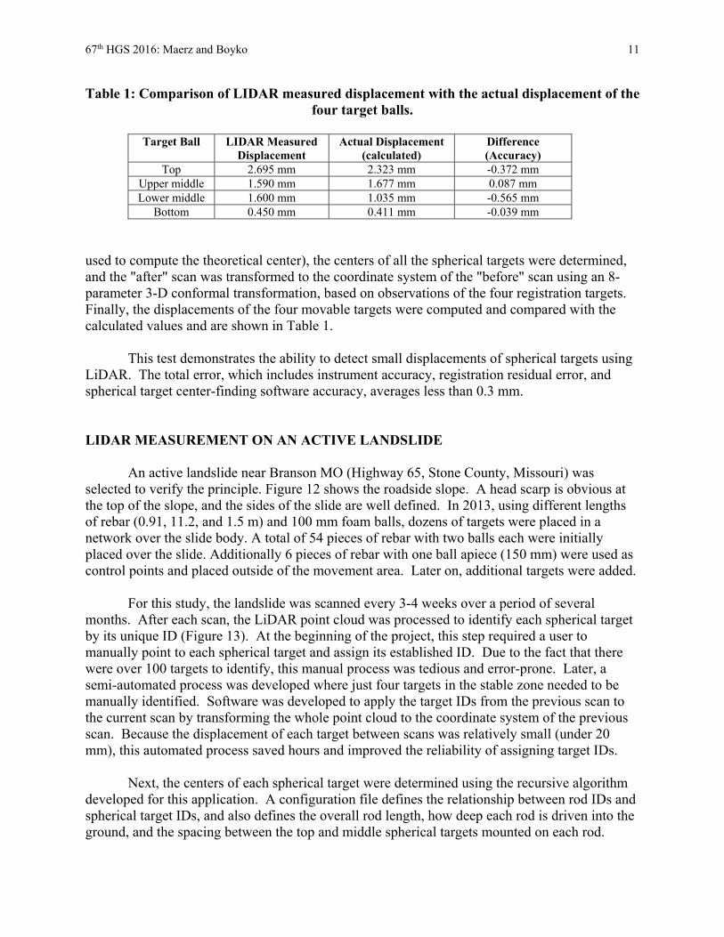
67th HGS 2016: Maerz and Boyko 11
Table 1: Comparison of LIDAR measured displacement with the actual displacement of the four target balls.
Target Ball LIDAR Measured
Displacement Actual Displacement
(calculated) Difference (Accuracy)
Top 2.695 mm 2.323 mm -0.372 mm Upper middle 1.590 mm 1.677 mm 0.087 mm Lower middle 1.600 mm 1.035 mm -0.565 mm
Bottom 0.450 mm 0.411 mm -0.039 mm used to compute the theoretical center), the centers of all the spherical targets were determined, and the "after" scan was transformed to the coordinate system of the "before" scan using an 8-parameter 3-D conformal transformation, based on observations of the four registration targets. Finally, the displacements of the four movable targets were computed and compared with the calculated values and are shown in Table 1.
This test demonstrates the ability to detect small displacements of spherical targets using LiDAR. The total error, which includes instrument accuracy, registration residual error, and spherical target center-finding software accuracy, averages less than 0.3 mm. LIDAR MEASUREMENT ON AN ACTIVE LANDSLIDE
An active landslide near Branson MO (Highway 65, Stone County, Missouri) was selected to verify the principle. Figure 12 shows the roadside slope. A head scarp is obvious at the top of the slope, and the sides of the slide are well defined. In 2013, using different lengths of rebar (0.91, 11.2, and 1.5 m) and 100 mm foam balls, dozens of targets were placed in a network over the slide body. A total of 54 pieces of rebar with two balls each were initially placed over the slide. Additionally 6 pieces of rebar with one ball apiece (150 mm) were used as control points and placed outside of the movement area. Later on, additional targets were added.
For this study, the landslide was scanned every 3-4 weeks over a period of several
months. After each scan, the LiDAR point cloud was processed to identify each spherical target by its unique ID (Figure 13). At the beginning of the project, this step required a user to manually point to each spherical target and assign its established ID. Due to the fact that there were over 100 targets to identify, this manual process was tedious and error-prone. Later, a semi-automated process was developed where just four targets in the stable zone needed to be manually identified. Software was developed to apply the target IDs from the previous scan to the current scan by transforming the whole point cloud to the coordinate system of the previous scan. Because the displacement of each target between scans was relatively small (under 20 mm), this automated process saved hours and improved the reliability of assigning target IDs.
Next, the centers of each spherical target were determined using the recursive algorithm
developed for this application. A configuration file defines the relationship between rod IDs and spherical target IDs, and also defines the overall rod length, how deep each rod is driven into the ground, and the spacing between the top and middle spherical targets mounted on each rod.

67th HGS 2016: Maerz and Boyko 12
Figure 12: Landslide on Highway 65 in Stone County Missouri, showing the layout of rods
and target balls. Location inset from Google Earth.
Figure 13: LIDAR image showing target balls (F) and control balls (C).
Once the sphere centers are known, the full 3-D position and orientation of each embedded rod can be established by utilizing the precise 3-D sphere center information along with the rod configuration information.

67th HGS 2016: Maerz and Boyko 13
Three assumptions are made in determining the projected position of the bottom of each
rod. The first assumption is that the rods are rigid, and remain rigid. This is a valid assumption, since most of the rods consist of 1/2" steel rebar. Rods driven to depths greater than 24" are 5/8" steel rebar, and control point rods in the stable zone are typically 3/4" steel rebar, driven to at least 30". With the inherent stiffness of these rods, and the low probability that differential forces exist that may bend the rods, the assumption of constant rigidity is valid.
The second assumption is that the relative positions of the spherical targets mounted on
the rods is not changing. This assumption is valid, as the spherical targets are glued with a weather-proof adhesive. Software was developed to monitor the distance between the targets mounted on each rod, and statistics are collected to monitor the relative displacements of targets along the rod axis. Analysis of these records show that targets are stable to 0.3 mm.
The third assumption is that the spherical targets do not rotate on the rod, and the rods do
not rotate in the ground. The spherical targets are mounted with the rod piercing their exact center, so even if the ball rotated on the rod, the apparent position of the sphere center would not shift. Nonetheless, the spherical targets are glued firmly to the rods, and no apparent looseness is evident even after over 18 months of exposure to the elements. The rods, being steel rebar with an external cross pattern, do not rotate once embedded into the soil. Periodic physical examination of the installed rods has shown them to remain tight.
After all the sphere-centers were determined, and the full rod geometry was established,
the control points in the stable zone were used to perform a 7-parameter conformal transformation of all data to bring it to the base coordinate system of the project site - usually the coordinate system used during the baseline scan. At this point, the displacements on a per-target and per-rod can be calculated and analyzed. Graphics are generated in two formats - VRML (Virtual Reality Modeling Language) and STL (StereoLithography). The resulting 3-D graphics can be exaggerated to show displacements and patterns of surface and sub-surface material flow.
PRELIMINARY RESULTS
Figure 14 shows the analysis of the planar view of the positions and downslope
displacement vectors of the ball targets based on scans taken July 19, 2015, July 29, 2015, August 8, 2015, and August 27, 2015. Displacements ranged from 7 to 75 mm over this period. Most of the targets have been stable over a period of 2 years.
Results show that the slide is moving downslope and slightly to the left. The fastest
movements are near the bottom at the left hand side of the slide, and total maximum displacement is approximately 75 mm.

67th HGS 2016: Maerz and Boyko 14
Figure 14: Downslope movement of the surface of the slide in plan view superimposed on a Google Earth image. Green arrows represent actual movement of targets; white arrows
are movements interpolated in a regular grid. White balls outside of the slide area are 150 mm control ball targets. Base image from Google Earth.
Figure 15 shows the positions and displacement vectors of the rods and balls in cross section over the same period of time. Figure 15 shows a cross section of the slope surface with three target rods aligned in the downslope direction. In this area there is displacement of about 50 mm downslope. The uppermost and lowermost target rods show more or less parallel downslope movement, which would indicate a planar failure surface. The centermost target rod shows some back rotation, which would indicate that at that point there is some circular rotation taking place.

67th HGS 2016: Maerz and Boyko 15
Figure 15: Downslope movement of 3 ball target pairs. Red and yellow are the before and after positions of the target; white arrows are the actual movement of targets; white dots
represent the scanned ground surface. All show downslope movement; the center rod shows back rotation as well
SUMMARY AND CONCLUSIONS:
The results of this have shown the ability of LIDAR to measure movements of as little as 0.3 mm based on temporal scanning. This can be used as an early warning system. It is also possible to measure small rotational changes in the target rods which is an indicator of the nature of the slide surface. In this landslide, both circular slip surfaces (target rods rotate backward) and surfaces parallel to the slope (target rods do not rotate) were indicated.
In future studies, target rods will be driven deeper into the ground. If the rods are driven
below the slide surface, the target rods will indicate that (target balls rotate forward).
REFERENCES:
1. Fleming, R. W. and Taylor, F. Estimating the costs of landslide damage in the United States, USGS Circular: 832, 1980, 30 pp.
2. Chowdhury, R. Flentje, P. and Bhattacharya, G. Geotechnical Slope Analysis, CRC Press, 2010, 737 pp.

67th HGS 2016: Maerz and Boyko 16
3. Cruden, D. and Varnes, J. Land slide types and processes. Landslides Investigation and Mitigation, Transportation Research Board Special Report 247, 1996, pp. 36-75.
4. Gonzales de Vallejo, L. I, and Ferrer, M. Geological Engineering. Taylor & Francis Group, London, UK, 2011, 678 pp.
5. AASHTO, Manual on Subsurface Investigation. American Association of State Highway and Transportation Official, Inc., Washington DC, 1988, 391 pp.
6. Sowers, G. and Royster, G. Field investigation. Landslide Analysis and Control. Transportation Research Board Special Report 176, 1978, pp. 81-111.
7. Keaton, J. and DrGraff, J. Surface observation and Geological Mapping. Landslides Investigation and Mitigation, Transportation Research Board Special Report 247, 1996, pp. 178-230.
8. Angeli, M. G. Pasuto, A, amd Silvano, S. A critical review of landslide monitoring experiences. Engineering Geology v. 55, 2000, pp. 133-147.
9. Segalini, A. and Carini, C. Underground landslide displacement monitoring: A new MMES based device. Landslide Science and Practice, V. 2. Spinger-Verlag, 2013, pp. 87-93.
10. Wilson, S. and Mikkelsen, A. Field instrumentation. Landslide Analysis and Control. Transportation Research Board Special Report 176, 1978, pp. 112-138.
11. Palenzuela, J. Irigary, C. Jimenez-Peralvarez, J, and Chacon, J. Application of Terrestrial Laser Scanner to the assessment of the evolution of diachronic landslides. Landslide Science and Practice, V. 2. Spinger-Verlag, 2013, pp. 517-523.
12. Panholzer, H. and Prokop, A. Assessing the capability of terrestrial laser scanning for monitoring slow moving landslides. Nat. Hazards Earth Systems Science V. 9, 2009, pp 1921-1928.
13. Baum, R. Johnson, A. and Fleming, R. Measurement of slope deformation using quadrilaterals. Landslide Processes in Utah-Observation and Theory. US Geological Survey Bulletin 1842, 1988, pp. B1-B23.

Emergency Response to Rockfall on Oklahoma Interstate 35
Martin J. Woodard, PhD PG PE GeoStabilization International
PO Box 4709 Grand Junction, CO 81502
(540) 315-0270 [email protected]
Prepared for the 67th Highway Geology Symposium, July, 2016

67th HGS 2016: Martin J. Woodard, Ph.D., P.G., P.E. 2
Acknowledgements
The author would like to thank the Oklahoma Department of Transportation, Mr. Ty Ortiz (Colorado Department of Transportation), Mr. Chad Lukkarila (Kleinfelder), Mr. Dan Conn (Kesco) for their contributions on this project.
Disclaimer
Statements and views presented in this paper are strictly those of the author(s), and do not necessarily reflect positions held by their affiliations, the Highway Geology Symposium (HGS), or others acknowledged above. The mention of trade names for commercial products does not
imply the approval or endorsement by HGS.
Copyright Notice
Copyright © 2016 Highway Geology Symposium (HGS)
All Rights Reserved. Printed in the United States of America. No part of this publication may be reproduced or copied in any form or by any means – graphic, electronic, or mechanical,
including photocopying, taping, or information storage and retrieval systems – without prior written permission of the HGS. This excludes the original author(s).

67th HGS 2016: Martin J. Woodard, Ph.D., P.G., P.E. 3
ABSTRACT
After heavy rains had impacted the Oklahoma region, a large rockslide occurred along a stretch of northbound I-35, a main traffic artery between Oklahoma City and Dallas, TX. A section of rock slope gave way; leaving large amounts of fallen debris that blocked the interstate and causing a significant safety hazard from additional slope failure. Remnants of the collapsed cliff above remained unstable and poised to fall at any time.
This paper discusses how a partnership between contractors and the State Department of Transportation resulted in safe reopening of the highway while solving significant engineering and operational challenges that occurred almost daily. Additionally the methodology used to develop the design mitigation plan is presented and described in detail.

67th HGS 2016: Martin J. Woodard, Ph.D., P.G., P.E. 4
INTRODUCTION
On June 18, 2015, a significant rockslide event occurred adjacent to the northbound lanes of I-35 that caused the closure of two northbound lanes of a divided interstate just north of Ardmore, Oklahoma. A location map is provided in Figure 1. The rockslide occurred in a road cut within the Arbuckle Mountains. The surface geology in this area contains folded and faulted limestones, dolomites, sandstones, and shales deposited from the Late Cambrian through Pennsylvanian time. After an unseasonably heavy spring rain a large failure occurred in the road cut. Figure 2 shows the rockslide as discovered the morning of June 18. News crews reported continuing large rockfall events for most of that day.
Figure 1 – Site Location
After conferring on site the day of the 18th, Oklahoma DOT contacted Daniel Journeaux
(GeoStabilization International) and Mr. Ty Ortiz (Colorado Department of Transportation) to arranged a site visit for the June 25. Prior to the site visit site photographs were provided and GSI developed a game plan ready for Mr. Ortiz to review upon his arrival. An example of details provided by GSI for the June 25th site visit can be seen in Figure 3.
After the rockslide it was apparent that a large dilated rock mass remained unsupported on
the upper portion of the slope that was still relatively unstable along with the remaining failed mass that was prone to continued and catastrophic failure. The first step of the game plan was to strategically blast the top structure in hopes that the vibrations and mass of materials added to the failed mass would be large enough to cause a significant portion of the larger, already mobilized,
Site Location

67th HGS 2016: Martin J. Woodard, Ph.D., P.G., P.E. 5
slide mass to come down from the slope. If the blast was successful it would not only make the upper portion of the slope more stable, but would also speed up the removal of the failed mass and construction sequence.
Figure 2 Image of site on June 18, 2015 after the failure
Initial Field Operations
A specialty blast consultant, Mr. Daniel Conn of Kesco, arrived on site to develop a blast design. The goal of the blasting plan was to dislodge enough of the rock mass at the top of the failed slope so that it would fall onto the already mobilized material to hasten the movement of material down to the base of the slope. The hope was that the blasting results would provide a good solid back slope to mitigate as well as significantly decrease excavation time. After Kesco developed the blasting plan, drilling of the holes commenced on July 2. This involved accessing the slope from the top and drilling holes in locations identified by Kesco. The blast was conducted and went off well and an image of the blast is shown in Figure 4. The results of the blast provided a good backslope, however the mass and vibrations were not significant enough in size to induce the failed mass still on the slope to mobilize down the slope.
Large remaining dilated rock mass

67th HGS 2016: Martin J. Woodard, Ph.D., P.G., P.E. 6
After the initial blast a significant amount of the failed rock mass remained on the slope
and was only marginally stable. The presence of the remaining mass still made the slope inaccessible to heavy earthwork equipment to remove the failed material.
At this point small drilling and blasting operations in conjunction with scaling material
were conducted until the toe of the slope was both safe enough to access with large excavation equipment and enough material was provided to allow excavation equipment to construct a ramp to remove all failed material. Over the next couple of weeks operations of scaling with periodic small strategic and controlled blasts were conducted.
Operations at this point were hampered by the temperature and humidity present in the
southern Oklahoma weather. With daytime temperatures in excess of 100o F and high humidity levels the GSI crews volunteered to conduct their activities at night. The nighttime temperatures were more conducive to working. Drilling, under the direction of Kesco occurred at night and periodic blasts were conducted in the early hours of the day. These operations continued until enough material was brought down to allow the earthwork contractor to construct a ramp and access the slope. At this point GSI demobilized from the site to allow the earthwork contractor access to the slope. Drilling, blasting, and scaling took approximately 1 month to conduct.
Figure 3 Image used in detail plans provided by GSI during June 25 site visit
Displacement Visible
Evaluate lateral extent of slide mass
Dilation visible in rock mass
Uppermost blocks require evaluation for overall and long-term stability
Need to evaluate lateral extent of slide mass

67th HGS 2016: Martin J. Woodard, Ph.D., P.G., P.E. 7
Figure 4 Initial blast conducted to remove large mass at the top of the failed area Final Slope Mitigation
After the earthwork contractor removed all the remaining failed material the slope was deemed temporarily safe for public use of the roadway. The roadway was opened and a follow up visit by Dr. Martin Woodard (GSI) and Mr. Chad Lukkarila (Kleinfelder) was conducted in the beginning of October to develop final, permanent designs for the remediation of the slope.
After the site had been exposed several blocks required reinforcement with the use of
rock anchors as well as an area on the southern end of the slope failure requiring a rockfall drape to mitigate against rockfall hazards. These blocks were initially checked scaled with scaling bars and a 50-ton airbag. Determining that they are stable in their present condition, but having the potential to release in the future they were additionally secured with a series of rock dowels for additional long-term protection. The broken rock mass on the southern end of the project was scaled and deemed sufficient. However, long term freeze and thaw cycles may effect this slope and additional protection for the roadway was provided with the use of a rockfall drape mesh. An image of the slope after the excavation of the failed area can be seen in Figure 5 as well as the mitigation strategy.

67th HGS 2016: Martin J. Woodard, Ph.D., P.G., P.E. 8
Figure 5 Final mitigation strategy imposed on an image of the slope after failed mass has
been removed. The final mitigation was completed by the end of October. The results of the final repair
were a permanently mitigated slope that was completed within the time period allocated and within the initial budget estimates for the project.
Rockfall Drape Estimate 15+ 10-ft rock dowels in drape area. Locations determined in the field.
10-ft rock dowels 15-ft rock dowels
20-ft rock dowels

67th HGS 2016: Halverson 1
K-7 HIGHWAY REALINGMENT IN CHEROKEE CO. KANSAS:
THE PAST, PRESENT, AND FUTURE
Kyle Halverson, P.G. Kansas Department of Transportation
101 SW Gage Boulevard Topeka, KS 66606
785-291-3862 E-mail: [email protected]
Prepared for the 67th Highway Geology Symposium, July 2016

67th HGS 2016: Halverson 2
Acknowledgements
Recognition is given to the following individuals for their assistance in facilitating and
compiling current and historic K-7 Highway data:
Bob Henthorne, P.G., Kansas Department of Transportation Chief Geologist Richard Ryan, P.G. Kansas Department of Transportation Regional Geologist (Retired)
Taylor Ree, G.A. Kansas Department of Transportation John Barker, P.G., Kansas Department of Transportation
Jim Burns, E.T. Sr., Kansas Department of Transportation
Disclaimer
Statements and views presented in this paper are strictly those of the author, and do not
necessarily reflect positions held by their affiliations, the Highway Geology Symposium (HGS), or others acknowledged above. The mention of trade names for commercial products does not
imply the approval or endorsement by HGS.
Copyright Notice
Copyright © 2016 Highway Geology Symposium
All Rights Reserved. Printed in the United States of America. No part of this publication
may be reproduced or copied in any form or by any means – graphic, electronic, or mechanical, including photocopying, taping, or information storage and retrieval systems – without prior
written permission of the HGS. This excludes the original authors.

67th HGS 2016: Halverson 3
ABSTRACT
K-7 Highway is a stretch of roadway in southeast Kansas that has seen its share of issues over the past 60 years. The site is notorious for restricted weight limits, catastrophic mine collapses, and hydrology problems; all due to the past mining of the Weir-Pittsburg coal bed.
In the 1960s, the State of Kansas recognized that the mining agreements for highway K-7
had not been followed, revealing that the area between Columbus and Cherokee had been significantly undermined. However, it wasn’t until the mid-1980s when roadway damage began to appear. In 1986, much to the dismay of the landfill and trash haulers, KDOT implemented a weight restriction of 24 tons due to the significant stresses being observed along K-7. At the same time, KDOT began the initial mine investigation to determine the extent and condition of the mine. This investigation took nearly 3.5 years to complete and in 1991 the remediation of K-7 began.
Today that stretch of K-7 Highway, where remediated, has performed extremely well.
However, it has been determined that to meet future growth, K-7 will need to be realigned through this problematic area. The realignment will predominately be within the existing right of way. However, much of the realignment will fall outside the past remediated areas.
A geotechnical investigation was requested in 2012 to determine the extent of the
undermined areas within the proposed new alignment. From the 2012 investigation, it was determined that a large part of the proposed realignment would need to be remediated prior to construction.
Currently the project is scheduled to let in March of 2016 with estimates for the mine
remediation alone exceeding $9 million. However, if the past is any indication of the future, the proposed remediation will support K-7 Highway well into the future.

67th HGS 2016: Halverson 4
INTRODUCTION
In May 2012, the Kansas Department of Transportation Geology Section was issued a request to conduct a geotechnical investigation along K-7 in Cherokee County, Kansas. The request was to investigate the subsurface geology and the extent of undermined areas under the proposed realignment of K-7 Highway. Historically, this section of K-7 has had numerous weight restrictions, catastrophic mine collapses, and hydrology problems, all due to the past mining of the coal bed within the Cabaniss Formation. At the time of the request, it was known that a large portion of the proposed project would be undermined due to past geotechnical investigations and remediations. Currently, the project has been let and the remediation of the undermined areas are set to begin in October 2016..
PROJECT LOCATION
The proposed K-7 realignment project is located in Cherokee County and stretches between the small towns of Columbus and Cherokee (Figure 1) in the far southeast corner of the state of Kansas. K-7 Highway is a major north-south highway running along the east side of the state that extends 228 miles from Cherokee Co. at the Kansas/ Oklahoma boarder to Doniphan Co. at the Kansas/Nebraska bordered. The proposed project is an 11.1 mile stretch that will widen the highway to a “Super Two” and will realign portions of the roadway to the east and west of the existing alignment.
Figure 1: Project Location

67th HGS 2016: Halverson 5
SITE HISTORY
In the late 1890’s through the early 1940’s southeast Kansas was mined commercially for coal, lead, and zinc. These ore minerals were mined predominately in relatively shallow subsurface mines, utilizing the “room and pillar” technique (Figure 2). When subsurface mining was the preferred method, there were two primary mining operations: Missouri-Kansas-Texas Railroad Company and St. Louis-San Francisco Railway Company. These companies were mining bituminous coal from the Weir-Pittsburg coal bed. The subsurface mining from these companies were so extensive, an estimated 60,000 acres of Cherokee and Crawford counties are underlain by subsurface mines. As the mining through the project area extended, the mining companies and the State of Kansas reached agreement that mining operations could extend to the state right of way line. Drifts could then be cut perpendicular to centerline of the highway to allow equipment to move to different parts of the mine without having to come to the surface.
By the 1930’s subsurface mining had dwindled to a few small “mom and pop” operations. These smaller mining companies had less oversight than the larger mining operations and were taking the coal from the roofs, floors, pillars and the unmined areas beneath K-7. As a result K-7 Highway and the surrounding areas became very hazardous. As surface strip mining became a more efficient and economical method of extracting coal in southeast Kansas, subsurface mining was slowly phased out. Strip mining allowed extraction of coal from seven different beds at a more economical and faster rate. Unfortunately, these methods of mining came with significant environmental impacts. Consequently, K-7 Highway in Cherokee County is now a reminder of those past mining operations and the problems associated with them.
Figure 2: Past mining techniques used to extract coal in S.E. Kansas
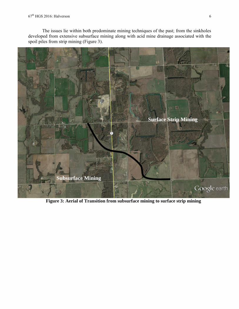
67th HGS 2016: Halverson 6
Figure 3: Aerial of Transition from subsurface mining to surface strip mining
Surface Strip Mining
Subsurface Mining
The issues lie within both predominate mining techniques of the past; from the sinkholes developed from extensive subsurface mining along with acid mine drainage associated with the spoil piles from strip mining (Figure 3).
N

67th HGS 2016: Halverson 7
GEOLOGIC SETTING
The proposed project is located in the far southeast corner of the state within the Cherokee Lowlands. This physiographic region is characterized by gently rolling hills, comprised of sandstones and shales hailing from the middle Pennsylvanian period. Over 300 million years ago, eastern Kansas was predominately at sea level with low-lying areas being covered with dense vegetation and brackish swamps. As a result, eight economically- important beds of bituminous coal were deposited and developed within the Cherokee Group (Figure 4), with the Weir-Pittsburg coal bed being the most significant because of its commercial importance.
During the geotechnical
investigation, the Cabaniss Formation was encountered across a majority of the site and was comprised of eight different coal beds and three distinguishable members. This formation can reach 220 feet at its extent, but in the project area the total thickness was undetermined. The “Cabaniss”, in the project area, consists mainly of sandy shale with a few thin areas of hard sandstone.
The south end of the K-7 realignment project is underlain by the Bluejacket Sandstone Member of the Krebs Formation. This unit consists of gray, fine to medium-grained sandstone and is weathered where exposed at the surface. When weathered the Bluejacket Sandstone turns to a soft, brown to reddish-brown material. The entire Bluejacket Sandstone Member is classified as rock excavation since it is difficult to predict any continuity of cementation and hardness in the sandstone. At some locations of the project, the sandstone is similar to a dense quartzite that can be very hard and difficult to excavate.
Figure 4: Stratigraphic Column for the State of Kansas

67th HGS 2016: Halverson 8
Figure 6: Boring location map from past geotechnical investigation
Figure 5: Boring location map from past geotechnical investigation
PAST GEOTECHNICAL INVESTIAGTIONS AND REMIDIATIONS Since the late 1960’s K-7 Highway was known to have been significantly undermined;
but due to the cost of remediation and no significant surface damage nothing was done along K-7 until the mid-1980s. In 1986, a weight restriction of 24 tons was implemented due to the significant deterioration of K-7 from the increase in traffic. Subsequently, KDOT Geology began a mine investigation to determine the condition and extent of the subsurface mines. The investigation took approximately 3.5 years to complete and consisted of borings approximately every 25 feet, alternating from edge of pavement to a few feet either side of centerline (Figure 5).
After the initial borings were completed and the undermined areas determined, larger, eight inch diameter borings were performed to obtain subsurface photos (Figure 6) and determine mine conditions across the project. The determination of the condition of the mine was critical in deciding how the mine should be remediated.
Figure 7: Mine condition from subsurface photographs

67th HGS 2016: Halverson 9
The remediation of K-7 began in May 1991. At that time it was determined that three different options for filling the subsurface mines would be considered. The options considered included: constructing grout columns using low slump concrete along centerline, build barrier walls along edge of pavement and fill the interior with high slump flowable fill, or a straight volume fill of the mines themselves. After considering the options, two options were selected based on mine conditions. Grout columns constructed with a low slump of 3 to 4 inches were used in areas where the mines were considered to be in “good condition” with minimal roof collapse, the mine floor relatively clear of debris, and where the roadway was being supported by deteriorating posts. These grout columns were spaced every 15 feet along centerline and were approximately 13.5 feet in diameter at the base and five feet in diameter at the contact of the mine roof (Figure 7). Each column was calculated to have approximately 12 to 14 cubic yards of concrete. Where the mine was considered to be in “poor condition”, with water present in the mine, the option was to build barrier walls and fill with a high slump grout. These areas were identified through the subsurface photographs and borings. During the remediation, the barrier walls were poured on 5 feet centers using the same method as the grout columns along the outside edge of both lanes. Then high-slump grout would be poured between barrier walls and spaced every 10 feet alternating from both lanes. The high slump grout was pumped to a predetermined pressure or when grout came up adjoining injection holes. At the end of the project, the overall cost to remediate the undermined areas beneath K-7 added up to be over $3 million or $12.50 per square foot of roadway.
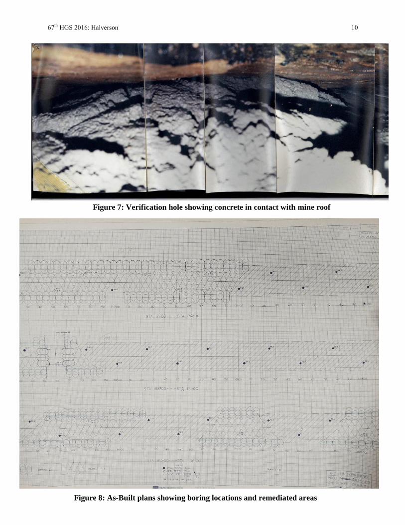
67th HGS 2016: Halverson 10
Figure 8: As-Built plans showing boring locations and remediated areas
Figure 7: Verification hole showing concrete in contact with mine roof

67th HGS 2016: Halverson 11
PROPOSED PROJECT
Today K-7 Highway because of the past remediations has performed extremely well under its current conditions. However, it has been determined to meet future growth K-7 will need to be realigned through this problematic area. The proposed changes include slight realignments to the east and west of the existing highway, widening, and grade changes throughout the extent of the project. These changes include 4 miles of undermined areas, and approximately 7 miles of abandoned strip mines.
Current plans indicate there will be four areas where the proposed alignment will shift to the
east or west of the existing alignment. Within these areas, the offset from the existing to the proposed centerline is relatively minor, with the furthest offset being 71 feet. The intent of these minor offsets to the alignment is to reduce cost by utilizing areas that have been previously remediated.
GEOTECHNICAL INEVSTIGATION AND RECOMMENDATIONS
In May 2014, KDOT Geology began its geotechnical investigation to determine the subsurface geology and the extent of undermined areas beneath the proposed new alignment for K-7. The investigation consisted of power auger soundings, site reconnaissance, and a review of past geotechnical investigations and boring logs. The historical borings proved to be an extremely invaluable tool due to the extensive amount of borings done during the previous investigations. All the past boring logs, which exceed 1,100, were recorded and kept on file for reference when sinkholes may appear within the right of way (Figure 9). For this investigation of the realignment of K-7, only a small number of additional borings were conducted; predominately where sinkholes had developed within the right of way.
Figure 9: Power auger soundings near a sinkhole that developed within state right of way

67th HGS 2016: Halverson 12
The recommendations from the Surface Geology Report provided to designers consisted of subgrading, material expected to be encountered during construction, cross-sections, profiles, recommended backslope designs, and hydrology issues related to roadway construction. The geology report also included locations where undermined areas are expected, along with areas of possible acidic water. These recommendations were issued within the initial Geology Report; and then followed up by a Final Design Geology Report. The Final Design Geology Report provided information regarding station-to-station undermined areas as well as the station-to-station location of strip ponds with recommendations to fill and/or remediate.
REMEDIATION PLANS
As part of the Final Design Geology Report, remediation recommendations were proposed along with a station-to-station breakdown of areas anticipated to be undermined. The Final Design Geology Report also provided estimate of costs, amount of borings needed, and grout quantities.
The proposed recommendation for remediating the undermined areas was to use a low
slump concrete to build barrier walls and then use a high slump concrete for in-fill. This method had been used in the previous remediation of K-7 Highway and has performed exceptionally well. This method was also appropriate because the alignment shifts where minor areas of past remediation could be utilized barrier walls. As locations and quantities were being determined for the remediation, there were only two locations identified along K-7 Highway that would not be able to utilize the past remediated areas. These areas are located where the proposed alignment shifting out of the existing right of way (Figure 10).
Figure 10: Plans Sheet showing alignment shifting to the east outside of existing right of way from
Station 358+90 to 385+00

67th HGS 2016: Halverson 13
The estimated concrete quantities for the mine filling were calculated using distance (stationing between undermined areas), offset from existing remediated area, and average void height. The barrier walls were calculated similarly. However, the area of the barrier was calculated by figuring the area of trapezoid: 𝐴 = ℎ (
𝑎+𝑏
2). Calculating the area of a trapezoid for
the barrier wall was because of the low slump of the concrete. The natural shape of the barrier wall would most resemble the shape of trapezoid when placed (Figure 11).
Figure 11: Simple schematic of barrier wall construction. NOT TO SCALE
Figure 12: Simple schematic of in-fill construction. NOT TO SCALE

67th HGS 2016: Halverson 14
Figure 13: Photograph from verification hole from past remediation
The proposed plan for the placement of concrete for the barrier walls will be to drill to the top of the mine void and pump low (two to four inch) slump concrete every 5 feet along the outside of the proposed shoulder. Similar to the previous remediation, each column for the barrier wall will take approximately 12-14 cubic yards of concrete. The plan for the placement of the in-fill concrete (Figure 12) will be to again drill to the top of the mine void every 20 feet alternating lanes and pump a high (eight to nine inch) slump concrete to a predetermined pressure or until concrete comes up in an adjacent injection hole. After the placement of the barrier walls and in-fill concrete, the contractor will be required to confirm through verification holes (Figure 13) that concrete is in contact or near the mine roof as well as competent concrete along the mine floor.
PROJECT STATUS
The proposed K-7 Highway realignment project’s original let date was scheduled for June 2015. However, budget shortfalls and lack of highway funding postponed the project until funding became available. Recently, the project was given funding and was let in March 2016. An open pre-bid meeting was held prior to letting allowing contactors to have a chance to meet with KDOT personnel, ask questions, and understand the full scope of the project. At the pre-bid meeting there were seven different contractors who attended, and three of those submitted bids. Topics that were noted from the pre-bid meeting included; specifications for concrete/grout, sequence of grouting, quantities (Figure 14), and under/over runs of concrete/grout. The other issue that was addressed during that meeting was a timeline and complete date requirement. According to the contract, the contractor must complete Phase 1 of the project within six months of the start date.
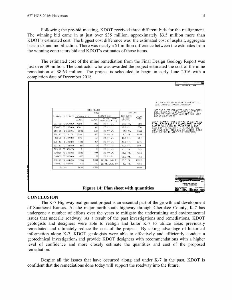
67th HGS 2016: Halverson 15
Following the pre-bid meeting, KDOT received three different bids for the realignment. The winning bid came in at just over $35 million, approximately $3.5 million more than KDOT’s estimated cost. The biggest cost difference was the estimated cost of asphalt, aggregate base rock and mobilization. There was nearly a $1 million difference between the estimates from the winning contractors bid and KDOT’s estimates of those items.
The estimated cost of the mine remediation from the Final Design Geology Report was just over $9 million. The contractor who was awarded the project estimated the cost of the mine remediation at $8.63 million. The project is scheduled to begin in early June 2016 with a completion date of December 2018.
CONCLUSION
The K-7 Highway realignment project is an essential part of the growth and development of Southeast Kansas. As the major north-south highway through Cherokee County, K-7 has undergone a number of efforts over the years to mitigate the undermining and environmental issues that underlie roadway. As a result of the past investigations and remediations, KDOT geologists and designers were able to realign and tailor K-7 to utilize areas previously remediated and ultimately reduce the cost of the project. By taking advantage of historical information along K-7, KDOT geologists were able to effectively and efficiently conduct a geotechnical investigation, and provide KDOT designers with recommendations with a higher level of confidence and more closely estimate the quantities and cost of the proposed remediation.
Despite all the issues that have occurred along and under K-7 in the past, KDOT is
confident that the remediations done today will support the roadway into the future.
Figure 14: Plan sheet with quantities

67th HGS 2016: Halverson 16
REFERENCES Zeller, Doris E, “The Stratigraphic Succession in Kansas”, Bulletin 189, Kansas Geological Survey, November 1998, Pages 23-24.
www.kgs.ku.edu/, Stratigraphic Succession in Kansas (1968), Plate 1-Classiffication of Rocks in Kansas, August 2005. http://www.fhwa.dot.gov/engineering/geotech/hazards/mine/workshops/kdot/kansas01.cfm, Brady, Lawrence L, Interstate Technical Group on Abandoned Underground Mines; Third Biennial Workshop, Mining History in Kansas. http://www.miningartifacts.org/Kansas-Mines.html, Kansas Mines, 2016. https://www.kshs.org/p/kansas-historical-quarterly-former-mining-communities/13222 Powell, William E., Former Mining Communities of the Cherokee-Crawford Coal Field of Southeastern Kansas, Summer 1972, Vol. 38, No. 2, Pages 187-199. Wilson, Frank W., “Highway Problems and the Geology of Kansas”, 21st Annual Highway Geology Symposium, April 1970, Pages 6-8

Geologic Exploration for Ground Classification:
Widening of the I-70 Veterans Memorial Tunnels
Todd G. Hansen, P.E. Yeh and Associates, Inc.
2000 Clay Street, Suite 200 Denver, CO 80211
(303) 781-9590 [email protected]
Samantha C. Sherwood, P.E. Yeh and Associates, Inc.
2000 Clay Street, Suite 200 Denver, CO 80211
(303) 781-9590 [email protected]
Prepared for the 67th Highway Geology Symposium, July, 2016

Acknowledgements
The authors would like to thank our colleagues who contributed to this project:
Howard Hume, Ph.D., P.G. – Yeh and Associates, Inc. Sylvia White – Yeh and Associates, Inc. Wade Hoon – Yeh and Associates, Inc.
Sara Hansen, P.E. – Yeh and Associates, Inc. Keith Asay – Yeh and Associates, Inc.
Disclaimer
Statements and views presented in this paper are strictly those of the author(s), and do not necessarily reflect positions held by their affiliations, the Highway Geology Symposium (HGS), or others acknowledged above. The mention of trade names for commercial products does not
imply the approval or endorsement by HGS.
Copyright Notice
Copyright © 2016 Highway Geology Symposium (HGS)
All Rights Reserved. Printed in the United States of America. No part of this publication may be reproduced or copied in any form or by any means – graphic, electronic, or mechanical,
including photocopying, taping, or information storage and retrieval systems – without prior written permission of the HGS. This excludes the original author(s).

67th HGS 2016: Hansen and Sherwood 1
ABSTRACT
The Colorado Department of Transportation (CDOT) recently completed widening of the Interstate 70 (I-70) Veterans Memorial Tunnels located one mile east of Idaho Springs, Colorado. As the geotechnical consultant, Yeh and Associates (Yeh) performed a detailed subsurface investigation to develop a rock mass classification using the Rock Mass Rating System (RMR) and Tunneling Quality Index (Q-rating). The goal of the investigation was to develop a rating system that could be used to predict the strength characteristics of the tunnel rock to be mined.
Following years of increasing traffic volume during the summer and winter tourist
seasons, CDOT implemented a plan to widen the existing eastbound tunnel an additional 21 feet in an effort to reduce persistent gridlock. The addition of an eastbound third lane on I-70 from East Idaho Springs to the bottom of Floyd Hill would reduce travel time and backups en route to the Denver-metro area. Yeh’s investigation began with a review of historical Colorado Highway Department (CHD) documents including geologic maps, technical memorandums and tunneling photos.
Yeh implemented traditional and specialty site investigation methods to characterize the
rock mass which would allow the tunnel design team to develop ground support and baseline conditions. Investigation methods included geologic and structural mapping of rock outcrops; drilling and logging rock core borings; borehole camera inspection of the drilled borings; and a three-dimensional seismic reflection tomography survey. Field data and lab test results correlated to observed conditions from the investigation were used to produce geologic maps showing estimated RMR, Q-ratings and rock types.
Using the geologic maps provided by Yeh, the other members of the tunnel design team
produced a ground classification map and associated excavation parameters. These documents were the foundation for preliminary cost estimates and project scheduling by the tunnel construction company. Following completion of the project, Yeh compiled a geologic map of observed as-built conditions of the eastbound bore to compare against predicted conditions.

67th HGS 2016: Hansen and Sherwood 2
INTRODUCTION
In 1961 the I-70 Twin Tunnels were constructed through a steep-sided ridge to improve the highway alignment through Clear Creek Canyon. Prior to the Interstate Highway Act, the only road serving the canyon was the single-lane U.S. 6 & U.S. 40 highway. Historically, there have been several routes which served as access to the Idaho Springs area such as rustic wagon trails, narrow-gauge railroads and paved automobile roads. Much of the U.S. 6&40 highway route followed the original railroad grade, but for the Interstate higher design speeds took precedence over easier construction. The old highway route bypassed the ridge but a tunnel would eliminate the sharp curves. Figures 1 and 2 show the location of the tunnels near Idaho Springs, Colorado. Unfortunately the construction documents detailing the tunnels did not record rock conditions encountered by the miners. Details that were useful to Yeh’s investigation came from the original geologic investigation documents.
Figure 1: I-70 Tunnel Widening Project in 2012. Note the yellow coloring of the rock at the west portal.
Powerline Pylon
East Portals
West Portals

67th HGS 2016: Hansen and Sherwood 3
Figure 2: View of the West Portals and Powerline Pylon from WB I-70, with observed fault (red).
The identical, two-lane, eastbound and westbound bores were burrowed through the promontory ridge of gneiss and pegmatite bedrock. Both bores were two-lane tunnels with a total width of 31 feet inside the liner. Almost 50 years following construction of the original Twin Tunnels the traffic volumes had increased to the point where the traffic volumes exceeded capacity. Traffic counts numbering as high as two thousand vehicles per hour routinely caused backups on eastbound I-70. To alleviate congestion several options were put forth including adding a third tunnel south of the current ones, blasting out an open cut through the ridge or widening the existing tunnels. Tunnel widening was selected as the most cost effective and feasible solution that would also keep the highway open during construction. The addition of the single lane would bring the interior width of each tunnel to 53 feet.
HISTORICAL BACKGROUND
Circa 1958 the CHD assessed the geologic and structural conditions of the bedrock, and working with the Bureau of Mines and Bureau of Public Roads developed plans and specifications for the proposed tunnels. A pilot bore was mined through the ridge circa mid-1959, and later that December two geologists from CHD performed an investigation and produced a geologic map of the proposed alignment. Available photographs from the CDOT archives showed steel sets and timber cribbing placed during tunnel excavation as well as wet seeps in the rock. Figure 3 shows a section of the fully excavated westbound tunnel, with the older pilot bore inside of it.
Powerline Pylon
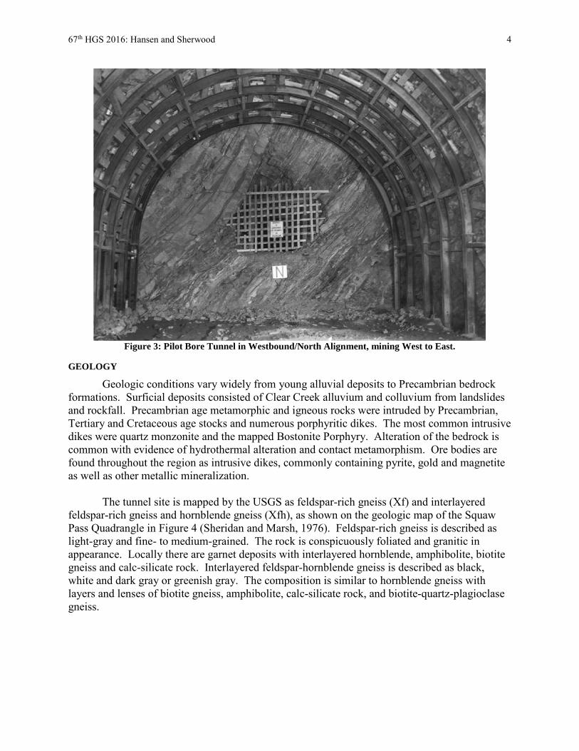
67th HGS 2016: Hansen and Sherwood 4
Figure 3: Pilot Bore Tunnel in Westbound/North Alignment, mining West to East.
GEOLOGY
Geologic conditions vary widely from young alluvial deposits to Precambrian bedrock formations. Surficial deposits consisted of Clear Creek alluvium and colluvium from landslides and rockfall. Precambrian age metamorphic and igneous rocks were intruded by Precambrian, Tertiary and Cretaceous age stocks and numerous porphyritic dikes. The most common intrusive dikes were quartz monzonite and the mapped Bostonite Porphyry. Alteration of the bedrock is common with evidence of hydrothermal alteration and contact metamorphism. Ore bodies are found throughout the region as intrusive dikes, commonly containing pyrite, gold and magnetite as well as other metallic mineralization.
The tunnel site is mapped by the USGS as feldspar-rich gneiss (Xf) and interlayered
feldspar-rich gneiss and hornblende gneiss (Xfh), as shown on the geologic map of the Squaw Pass Quadrangle in Figure 4 (Sheridan and Marsh, 1976). Feldspar-rich gneiss is described as light-gray and fine- to medium-grained. The rock is conspicuously foliated and granitic in appearance. Locally there are garnet deposits with interlayered hornblende, amphibolite, biotite gneiss and calc-silicate rock. Interlayered feldspar-hornblende gneiss is described as black, white and dark gray or greenish gray. The composition is similar to hornblende gneiss with layers and lenses of biotite gneiss, amphibolite, calc-silicate rock, and biotite-quartz-plagioclase gneiss.
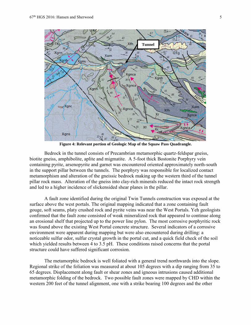
67th HGS 2016: Hansen and Sherwood 5
Figure 4: Relevant portion of Geologic Map of the Squaw Pass Quadrangle.
Bedrock in the tunnel consists of Precambrian metamorphic quartz-feldspar gneiss, biotite gneiss, amphibolite, aplite and migmatite. A 5-foot thick Bostonite Porphyry vein containing pyrite, arsenopyrite and garnet was encountered oriented approximately north-south in the support pillar between the tunnels. The porphyry was responsible for localized contact metamorphism and alteration of the gneissic bedrock making up the western third of the tunnel pillar rock mass. Alteration of the gneiss into clay-rich minerals reduced the intact rock strength and led to a higher incidence of slickensided shear planes in the pillar.
A fault zone identified during the original Twin Tunnels construction was exposed at the
surface above the west portals. The original mapping indicated that a zone containing fault gouge, soft seams, platy crushed rock and pyrite veins was near the West Portals. Yeh geologists confirmed that the fault zone consisted of weak mineralized rock that appeared to continue along an erosional shelf that projected up to the power line pylon. The most corrosive porphyritic rock was found above the existing West Portal concrete structure. Several indicators of a corrosive environment were apparent during mapping but were also encountered during drilling: a noticeable sulfur odor, sulfur crystal growth in the portal cut, and a quick field check of the soil which yielded results between 4 to 3.5 pH. These conditions raised concerns that the portal structure could have suffered significant corrosion.
The metamorphic bedrock is well foliated with a general trend northwards into the slope.
Regional strike of the foliation was measured at about 105 degrees with a dip ranging from 35 to 65 degrees. Displacement along fault or shear zones and igneous intrusions caused additional metamorphic folding of the bedrock. Two possible fault zones were mapped by CHD within the western 200 feet of the tunnel alignment, one with a strike bearing 100 degrees and the other
Tunnel

67th HGS 2016: Hansen and Sherwood 6
with a strike bearing 145 degrees. Groundwater flow rates were the highest in this western faulted area and dry by the east portal area. SITE INVESTIGATION
Yeh’s geologic investigation program included site reconnaissance, geologic and structural mapping, rock core drilling, borehole camera inspection and three-dimensional geophysical surveys. Laboratory testing of rock core and surficial samples was performed to determine strength of the rock for mining design and chemical properties for corrosion protection. Mapping
Field mapping was the essential component of the structural and geologic characterization. Structural features were measured including the dip angle and direction of foliation planes, joints and fractures. Areas that were mapped included the West (Figure 5) and East portals, the southernmost rock promontory (Figure 6), the slopes directly south of the portals and along the mineralized "vein" from the west portal to the power line pylon. Geologic mapping of the bedrock reached similar conclusions to those of the CHD. However, the original map indicated the fault dipped steeply to the north. Yeh’s geologists identified the fault to be dipping at a lower angle. Yeh geologists were able to access sites that would normally be inaccessible without specialized rope access. This allowed for a larger area to be mapped than the previous investigation. The rope access mapping also allowed for structural measurements of cliffs and overhangs, capturing video with helmet cameras to review for later analysis and identification of potential rockfall hazards to the tunnel portals and highway.
Figure 5: Mapping of the Eastbound West Portal encountered Altered Rock and Fault Zones.

67th HGS 2016: Hansen and Sherwood 7
Figure 6: Yeh’s Mapping Team explored the entire Rock Ridge.
Geotechnical Drilling
Twelve rock core borings were drilled for the investigation. Ten of the borings were drilled inside the eastbound tunnel; three horizontally in the pillar between the tunnels, three angled upwards in the south rib, two vertically in the tunnel back and two downwards into the pavement. The remaining two borings were drilled horizontally outside the West Portals; one in the pillar between and one south of the tunnels. The portal borings were drilled to observe the rock properties in a potentially weak bedrock area. A summary of the boring locations, orientations and lengths is presented in Table 1.

67th HGS 2016: Hansen and Sherwood 8
Table 1: Summary of Approximate Boring Orientations and Locations Measured from Portal Face.
Boring Depth (ft) Angle above or below horizontal Travel Lane Approximate Location
YA-T-01 20.1 Horizontal Left 77 ft East of West Portal, South Tunnel
YA-T-02 48.4 45 degrees above Right 77 ft East of West Portal, South Tunnel
YA-T-03 22.9 45 degrees above Right 50 ft East of West Portal, South Tunnel
YA-T-04 19.3 Horizontal Left 351 ft East of West Portal, South Tunnel
YA-T-05 20.0 Horizontal Left 47 ft West of East Portal, South Tunnel
YA-T-06 60.0 45 degrees above Right 351 ft East of West Portal, South Tunnel
YA-H-01 250.0 Horizontal Pillar between tunnels
20 ft South of WB West Portal between tunnels
YA-H-02 250.0 Horizontal South of tunnels 39 ft South, 1 ft West of EB West Portal edge of pavement
YA-T-07 31.1 90 degrees above Right 148 ft East of West Portal, South Tunnel
YA-T-08 29.7 90 degrees above Left 198 ft West of East Portal, South Tunnel
YA-TP-01 10.3 90 degrees below Left 197 ft West of East Portal, South Tunnel
YA-TP-02 7.8 90 degrees below Left 224 ft East of West Portal, South Tunnel
Rock core ranging in size from B (36.5 mm) to H (63.5 mm) was recovered using a skid-
mount Ingetrol Explorer 75E (Figure 7) for the horizontal and angled borings and a semi-trailer mounted Deets 1500 for the vertical roof borings. Drilling the angled borings required bolting the skid to the tunnel to develop drilling down pressure. Later the drill was mounted to a semi-trailer which greatly improved deployment and operation of the drilling program.
Drilling in the tunnels required single-lane closures which could only be performed at
night in winter. In the first week of exploratory drilling the core rig would reset every night on the same hole that had not been finished the previous night. In addition sub-freezing temperatures at night compounded the difficult drilling conditions. When it became clear that drilling could not be finished on time and within budget due to the night work limitations, CDOT allowed a 24-hour closure for one week to drill the entire tunnel. The drilling finished on schedule only after operations changed to two drill crews working 12-hour shifts. At least one boring was lost after freezing core water iced up the barrel which prevented flow and melted the bit into the rock mass. Water heaters were installed in the holding tanks which kept temperatures just above freezing.

67th HGS 2016: Hansen and Sherwood 9
Figure 7: Ingetrol Explorer 75E horizontal coring in the eastbound pillar, near the West Portal.
While drilling in the tunnel, a small hole was observed in the liner of the eastbound
tunnel in the left lane approximately 50 feet from the west portal. Further exploration by the engineers revealed that a large void with exposed rebar and steel sets was present behind the concrete liner shown in Figure 8. These findings were reported and the next day, a wider opening was cut to further evaluate the corroded state of the steel and concrete. The cut concrete ranged from 3 to 6 inches thick at the opening. Wood that had been used for blocking during construction was rotten and ice and frost were present inside the void. Several cobbles had fallen from the rock face and were resting on the inside of the liner. It appeared that when the tunnel liner was poured, the voids had not been completely filled with concrete. Fortunately, the liner materials were strong enough to stand for the life of the structure.

67th HGS 2016: Hansen and Sherwood 10
Figure 8: The conditions in the void included corroded steel sets, rotted cribbing, blasting half casts and ice.
Borehole Televiewing
Rock core provided samples for determining rock strength and quality and for developing an understanding of rock fabric, mineralogy and general character. Borehole televiewing allowed down-hole inspection of in-situ rock mass conditions and replaced the need for oriented core recovery. Borehole televiewing was able to correlate recovered core to the rock mass at depth. Ten of the twelve tunnel borings were inspected by Colog. Images were evaluated for discontinuities, foliation planes and other major rock mass features. Figure 9 is an example of a borehole photograph analysis. Dip angle and strike/dip direction of foliations and discontinuities were input into kinematic analysis programs to obtain pole plots and rose diagrams for each respective boring. Three of the borings were inspected to full depth and seven were blocked off at varying depths. Using Terzaghi weighting this data was then incorporated into the overall structural mapping of the rock mass. Joints that perpendicularly cross the survey area typically have more measurements taken. Therefore applying Terzaghi weighting accounts for the duplicate measurements of planar features.

67th HGS 2016: Hansen and Sherwood 11
Figure 9: Example of a borehole photo and selected rock features including foliation and joints.
Bedrock Seismic Tomography
A three-dimensional seismic refraction survey was performed by C-thru Ground, Inc. The intent of the survey was to identify weak rock, fracture zones and displaced faults on a larger scale possible than with exploratory drilling. Recovered rock core indicated blast-damaged bedrock up to five feet from the final excavation face. This, combined with the weak fault zones at the west end of the tunnel, was enough cause for the seismic assessment of the rock mass. To perform the investigation of the rock behind the reinforced concrete liner, 213 fiberglass dowels were installed through the liner into bedrock to ensure direct seismic connection between the sources and receivers. This required drilling each location, resin setting the dowel into rock, and adding foam insulation to the drill annulus for stability. In some areas dowel drilling encountered additional voids and weakened rock behind the liner. This information helped to estimate existing liner thickness (which varied from 1.5 to 3.6 feet) and void space along the tunnel.
The travel times for the direct seismic waves recorded in the EB Tunnel provided data for
building a general velocity model for seismic waves in the rock mass around the Tunnels. This velocity model was subsequently applied for mapping structural features in the ground. The measurements between the WB and EB Tunnels and also between the slope and the EB Tunnel provided complementary data about velocity distribution of seismic waves, and supporting

67th HGS 2016: Hansen and Sherwood 12
images of the local ground properties. Known discontinuities, either measured in 1959 or 2010, were used as a baseline calibration of the final analysis and added credibility to the overall results. Results of the survey are shown in Figure 10.
Figure 10: Plan view of the tomography anomalies with mapped discontinuities (C-Thru Ground, Inc., 2012)
The tomography survey was useful in capturing a low resolution model of the bedrock
structure, but several questions remained following the investigation. The mapped ground anomalies related to local weakness in the rock structure associated with fractures and weathered rock mass. However, the width of detected anomalies were exaggerated due to the image resolution and its relation to the length of the shortest measurable seismic waves (approximately 6 to 7 feet). Also, the orientation of the reflecting surfaces in the rockmass directly affected seismic wave return to the receivers. Sensor installation was limited to the tunnel liners and a few small outcrops outside the tunnel. Sections of the rockmass oriented away from receivers lost signal return and those areas suffered from reduced data recovery. The final model was only from one point of view and at a relatively poor resolution meaning that the size of possible anomalies could not be reliably estimated.
RMR & Q-RATINGS
Rock structure and composition varied the most in both the western end of the pillar and the southwest limb of the tunnel. The majority of weak zones were encountered in the western extent of the tunnel due to localized alteration. Weakened rock was prevalent in the immediate vicinity of faults, shear zones and dikes. Further east along the tunnel alignment the competency of the rock increased substantially.
RQD and core recovery information obtained from the geotechnical investigation is
presented in Table 2. The percent recovery and RQDs show averages over the entire length of

67th HGS 2016: Hansen and Sherwood 13
the core as well as values for the lowest and highest intervals in the core. In the case of long core runs where characteristics differed markedly along the entire length, the run was divided into zones of similar structural character in order to provide representative rock mass rating values for each of these zones rather than averaging these characteristics over the entire length of the run.
Table 2: RQD and Recovery Values from Tunnel Rock Core.
Boring Approx. Depth
(ft)
Recovery (%) RQD (%)
High Wtd. Ave Low High Wtd. Ave Low
YA-T-01 3-20 - 100 - 81 61 45 YA-T-02 3-48 100 87 59 100 63 7
YA-T-03 2-23 100 93 64 100 82 36 YA-T-04 2-19 - 100 - 80 64 52 YA-T-05 3-20 - 100 - 100 72 46
YA-T-06 2-60 100 98 90 94 61 32
YA-T-07 5-31 100 93 80 88 62 37
YA-T-08 3-30 100 100 98 94 84 64
YA-TP-01 3-10 100 87 65 54 40 17
YA-TP-02 2-8 100 89 80 82 52 28
YA-H-01
Zone 1 31-58 100 97 80 64 46 18
Zone 2 58-120 100 100 96 92 69 22
Zone 3 120-165 100 77 32 50 17 0
Zone 4 165-225 100 95 60 88 61 17
Zone 5 225-241 90 57 30 78 11 0
Zone 6 241-250 100 96 90 78 63 50
YA-H-02
Zone 1 15-43 100 79 0 74 27 0
Zone 2 43-161 100 91 0 96 60 0
Zone 3 161-210 100 81 40 56 16 0
Zone 4 210-250 100 99 80 94 69 32
Rock core discontinuity spacing and alteration continuously changed along the tunnel alignment. Due to the variable nature of the rock mass quality the ratings were based on grouping zones of similar material together. These zones and their characteristics directly affected the ground classification ratings.
Lab test data from Point Load, Unconfined Compressive Strength, and Brazilian Tensile
tests allow for rock samples from the logged and measured zones to represent quantifiable rock mass strengths. RMR and Q-ratings were developed independently of each other and cross checked using the Bieniawski (1989) equation. The correlated ratings confirmed our analysis and conclusions were accurate.

67th HGS 2016: Hansen and Sherwood 14
RMR and Q-ratings were calculated for the twelve core runs obtained from within and adjacent to the south tunnel and are shown in Tables 3 and 4. Values for Q-ratings were rounded to the nearest 10th and where the RMR class fell on the classification break, the weaker classification was selected.
Table 3 RMR Ratings of Drilled Borings.
Boring Strength RQD Joint
Spacing Joint Cond.
Groundwater Adj. for Joint
Orientation Rating RMR Class
1 2 3 4 5 YA-T-01 2 13 8 25 15 63 II YA-T-02 7 13 10 23 15 -10 58 III YA-T-03 7 17 10 25 15 74 II YA-T-04 7 13 8 25 15 -5 63 II YA-T-05 12 13 5 23 15 68 II YA-T-06 12 13 5 15 15 60 III YA-T-07 2 13 5 19 15 -10 44 III YA-T-08 7 17 8 18 15 -10 55 III YA-TH-01 Zone 1 12 8 8 25 15 68 II YA-TH-01 Zone 2 2 13 8 18 15 56 III YA-TH-01 Zone 3 4 3 5 11 15 38 IV YA-TH-01 Zone 4 7 13 8 16 15 -12 47 III YA-TH-01 Zone 5 4 3 5 13 15 -10 30 IV
YA-TH-01 Zone 6 4 13 8 24 15 -10 54 III
YA-TH-02 Zone 1 12 8 5 20 15 -10 50 III YA-TH-02 Zone 2 4 13 10 23 15 65 II YA-TH-02 Zone 3 2 3 5 14 15 39 IV YA-TH-02 Zone 4 12 13 8 22 15 70 II

67th HGS 2016: Hansen and Sherwood 15
Table 4: Q-Ratings of Drilled Borings.
Boring
Wtd. Ave. RQD
Jn Jr Ja Jw SRF Q* Approx.
Length (ft)
Joint Set Number
Joint Roughness
Number
Joint Alteration Number
Joint Water Reduction
Factor
Stress Reduction
Factor YA-T-01 3-20 61 9 2 1 1 2.5 5.4 YA-T-02 3-48 63 3 2 3 1 2.5 5.6 YA-T-03 2-23 82 6 1.5 0.75 1 1 27.3 YA-T-04 2-19 64 6 2 1 1 1 21.3 YA-T-05 3-20 72 9 3 1 1 1 24.0
YA-T-06 2-60 61 6 1.5 2 1 7.5 1.0
YA-T-07 5-31 62 2 0.5 2 1 7.5 1.0 YA-T-08 3-30 84 9 1.5 2 1 1 7.0 YA-H-01
Zone 1 31-58 46 4 1.5 2 1 1 8.6 Zone 2 58-120 69 4 1.5 3 1 2.5 3.5
Zone 3 120-165 17 6 1.5 4 1 10 0.1
Zone 4 165-225 61 9 1.5 4 1 10 0.3 Zone 5 225-241 11 12 1.5 3 1 5 0.09 Zone 6 241-250 63 9 1.5 2 1 1 5.3
YA-H-02 Zone 1 15-43 27 9 1.5 2 1 5 0.5 Zone 2 43-161 60 4 1.5 2 1 7.5 1.5 Zone 3 161-210 16 15 1.5 3 1 7.5 0.07 Zone 4 210-250 69 6 1.5 2 1 1 8.6
PRELIMINARY GROUND CLASSIFICATION
Bedrock structure and conditions were weakest from the West Portal to approximately 200 feet into the tunnel. Alteration and displacement of the bedrock appears to have been associated with the Bostonite Porphyry intrusive dike. Contact metamorphism features such as clay alteration, brecciated rock structure and highly variable mineral composition were encountered in the West Portal pillar and rock outcrops. The discontinuities varied widely throughout the tunnel, ranging from fresh joints and fractures to altered fault zones. Using the field data collected from Yeh’s geotechnical investigation as well as CHD historical documents Yeh estimated zones of RMR and Q-ratings with intact rock strength parameters. Yeh created an approximated three-dimensional geologic map which also showed anticipated rock quality, shown in Figure 11.

67th HGS 2016: Hansen and Sherwood 16
Figure 11: Three-dimensional ground condition map of the West Portal area.
These maps were provided to the tunnel design team in preparation for construction cost estimates and schedule. Based on Yeh’s data the rock was simplified into four possible conditions from which excavation sequence, round length, staging and appropriate support conditions were developed. The ground classifications were developed for anticipated ground behavior which included portal rock (TT-P), structurally controlled blocks (TT-1), slow raveling rock (TT-2 and TT-2S) and fast raveling or caving rock (TT-3). Figure 12 is an example of the ground class map produced for the three-dimensional tunnel map from the CDOT Bid Plans.
Figure 12: Ground class map of anticipated tunnel excavation requirements.

67th HGS 2016: Hansen and Sherwood 17
SUMMARY
Ultimately our site investigation program supported planning, design and construction. Many lessons were learned from our involvement with such a complex, rare and unique project to widen a tunnel. No one predicted how severely our investigation would impact traffic flow, which is an indication to the need for updating our national infrastructure. Data collected using non-invasive technology did not give us the level of detail we had hoped to achieve, but when combined with the rest of the investigation data it did help to fill in large gaps where drilling had not been performed. Lastly, reviewing the original CDOT design documents contributed greatly to Yeh’s understanding of the geologic conditions and construction methods. The Colorado Highway Department maps and memorandums contained important supplemental information.
Tunnel projects are a rare occurrence and widening existing tunnels for an active
roadway was unheard of in the Colorado transportation community. Yeh’s involvement with the initial investigation kept the authors on site in a design support role. After the eastbound tunnel was completed CDOT extended the project contract to widen the westbound tunnel. Overall rock conditions improved on the WB tunnel and only the West Portal side of the tunnel required special excavation attention. After completion of the project Yeh compiled as-built geologic maps of the tunnels based on photos provided by others.

67th HGS 2016: Hansen and Sherwood 18
REFERENCES: Barton N.R., Lien, R., and Lunde, J. 1974. Engineering Classification of Rock Masses For The Design Of Tunnel Support. Rock Mechanics, 6(4). Bieniawski, Z.T., 1989, Engineering Rock Mass Classifications. New York: Wiley. Colorado Department of Transportation, 2013. Highway Construction Bid Plans, Twin Tunnels, Clear Creek County, Construction Project Code No. 19036, Construction Package 2. Descour, J., 2012, Seismic Evaluation of the Ground Around I-70 Twin Tunnels, Idaho Springs, Colorado.
Sheridan, D.M. and Marsh, S.P., 1976, Geologic map of the Squaw Pass Quadrangle, Clear Creek, Jefferson, and Gilpin Counties, Colorado: U.S. Geological Survey, Geologic Quadrangle Map GQ-1337, scale 1:24000. Sherwood, S., Hansen, T., and White, S., 2012, Geologic Data Report CDOT I-70 Twin Tunnels Widening Project - Idaho Springs, Colorado. Sims, P.K., 1989, Ore Deposits of the Central City - Idaho Springs Area, Geological Society of America field trip guidebook, Colorado School of Mines Professional Contributions.

3D Monitoring of Rockfall Sources in Colorado
Cole Christiansen
BGC Engineering Inc. American Mountaineering Center
BGC Engineering Inc. 710 Tenth Street – Suite 170
Golden, CO 80401 [email protected]
720-598-5982
Dave Gauthier BGC Engineering Inc. 523 Frontenac Street
Kingston, ON K7K 4L9 [email protected]
613-893-4920
Nicole Oester Colorado Department of Transportation
4670 Holly Street, Unit A Denver, CO 80216
[email protected] 303-398-6603
Prepared for the 67th Highway Geology Symposium, July, 2016

67th HGS 2016: Christiansen, Gauthier, Oester
Acknowledgements
The authors would like to thank the following individuals for their contributions in the work described:
Ty Ortiz – CDOT
Beau Taylor – CDOT Alex Strouth – BGC
Disclaimer
Statements and views presented in this paper are strictly those of the author(s), and do not necessarily reflect positions held by their affiliations, the Highway Geology Symposium (HGS), or others acknowledged above. The mention of trade names for commercial products does not
imply the approval or endorsement by HGS.
Copyright Notice
Copyright © 2016 Highway Geology Symposium (HGS)
All Rights Reserved. Printed in the United States of America. No part of this publication may be reproduced or copied in any form or by any means – graphic, electronic, or mechanical,
including photocopying, taping, or information storage and retrieval systems – without prior written permission of the HGS. This excludes the original author(s).

67th HGS 2016: Christiansen, Gauthier, Oester
ABSTRACT Large rockfalls occurred in April and December 2014, impacting U.S. Route 24 near
Minturn, Colorado. Following these rockfall events, Colorado Department of Transportation (CDOT) commissioned a study to monitor and assess the rockfall source zones.
Oblique aerial photographs of the slope were collected from a moving helicopter on five
occasions between April and June 2015. From each oblique aerial photogrammetry (OAP) survey, BGC Engineering generated 3D models and completed 3D quantitative change-detection to determine model differences as small as 5 cm.
Analysis showed that a number of small rockfalls and debris slides occurred over the
course of the study. Additionally, results suggest that a large ‘cap block’ composed of at least three independent and detached blocks, ranging from 10 m3 to 100 m3, underwent downslope displacements from 5 to 15 cm.
OAP change-detection results were validated with a displacement signal from a
crackmeter that had been previously installed on the cap block. The OAP change-detection and the crackmeter data were in good agreement at this location, with both showing close to 5 cm of movement over the course of this study. Additional analysis showed that the block accelerated during a three-day precipitation event in early May, which came at the end of a prolonged period of freeze-thaw action.

67th HGS 2016: Christiansen, Gauthier, Oester 1
INTRODUCTION
Following a series of rockfall events along U.S. Route 24 (US 24) near Minturn, Colorado, the Colorado Department of Transportation (CDOT) initiated a project to assess the rockfall source zone using 3D topographic models developed from airborne LiDAR scans (ALS) and photogrammetric methods based on oblique aerial photographs (oblique aerial photogrammetry; OAP). The models were used to help visualize the terrain and understand the state of activity and mechanism(s) of rockfall hazards. The slope was re-photographed periodically, and 3D topographic models of each set of photographs were compared quantitatively to identify changes on the slope related to rockfall, debris flow, and slope deformation. This paper summarizes the results of the overall change-detection campaign and provides interpretations of displacements in the rockfall source zone. SITE BACKGROUND 2014 Rockfall Events
Notable rockfalls occurred in April and December 2014 (Figure 1, 2). In both events, individual blocks with volumes of about 10 m3 reached US 24. In each instance, rockfalls initiated from a relatively massive sandstone unit approximately 300 m (vertical) above the highway (“source area” in Figure 3). An aerial photograph of the source area (Figure 4) shows the large in-situ columnar block before it fell in December 2014; the columnar block rested on top of a blocky sandstone and shale “cap block”. An oblique model image (Figure 5) shows the source area in April 2015 after the columnar block had fallen.
Figure 1 – April 2014 US 24 rockfall event.

67th HGS 2016: Christiansen, Gauthier, Oester 2
Figure 2 – December 2014 US 24 rockfall event.
Figure 3 – Oblique OAP model image of the US 24 rockfall site. The white box indicates the main rockfall source area, and the focus of the current study. US 24 is approximately 300m
(vertical) below the rockfall source area.
Perspective view, scale varies. Source area
US 24 impact zone

67th HGS 2016: Christiansen, Gauthier, Oester 3
Figure 4 – Oblique aerial photograph of rockfall source area in 2014, showing the columnar block that fell in December 2014. An adjacent column fell in April 2014.
Figure 5 – Oblique OAP model image of the rockfall source area on April 8, 2015 displaying the “cap block,” “disrupted block,” and shaley beds.
Columnar block that fell in December 2014
Shaley beds
Perspective view, scale varies.
40 m
Source area as outlined in Figure 3
“Cap block” (20 m across) Blocky sandstone
“Disrupted block” Approximate Limit
(40 m x 35 m x 20 m)
“Cap block”

67th HGS 2016: Christiansen, Gauthier, Oester 4
METHODS AND DATA
The data for this project included ALS, OAP, in-situ crackmeter data, and historical weather data from a nearby station. Airborne LiDAR Scan (ALS)
Airborne LiDAR scans were collected by a commercial provider over the site and surrounding area on April 6, 2015, using a fixed-wing aircraft and Leica laser scanner. Raw and classified (bare earth and non-bare earth) point clouds were used in this analysis, to maximize the point density in non-vegetated areas. The ALS data were used as a baseline for spatial registration of the photogrammetry to geographic coordinates, and as a shape-accuracy check for the initial OAP models. A side-by-side comparison of ALS and OAP meshed surface models is shown in Figure 6.
Figure 6 – April 2015 meshed surface models, Airborne LiDAR scan (left) and Aerial
Photogrammetry (right).
Oblique Aerial Photogrammetry (OAP)
Oblique aerial photographs were collected on five occasions, as outlined in Table 1. In each case a 24 mega-pixel Nikon D5300 camera was used in combination with a Nikon 35 mm (prime) lens to collect the images. The images were collected at a range of several hundred meters, from a moving helicopter, either through an open door or window. Several hundred photos were captured in each campaign.
The digital photos were converted into 3D point clouds and surface models using the
software PhotoScan (1). Alignment tie-points were filtered, and only low-error and low-noise points were retained for the point cloud and model generation steps. The mesh generated from the April 8, 2015 OAP campaign is shown above in Figure 6.
10 m 10 m

67th HGS 2016: Christiansen, Gauthier, Oester 5
Change-detection was conducted for the time intervals between each consecutive field campaign, and for the overall time interval between the first and last photogrammetry campaigns (April 8 to June 24, 2015). The first OAP model (April 8, 2015) was registered in georeferenced coordinates, scaled, and oriented using the ALS point cloud as a baseline and the 3D iterative closest-point alignment algorithm available in the software Cloud Compare (2). Subsequent 3D models were co-registered using the same technique, with either the ALS or a previously registered OAP model as the base. The approach to OAP and change-detection that we used is outlined in detail by Gauthier et al. (3) and Gauthier et al. (4), and the reader is referred there for a more thorough explanation.
Table 1 – Oblique aerial photogrammetry campaign summary
Date Collected by
Number of Photos
Final Average Model Density (Points/m2)
April 8, 2015 BGC 275 700 April 22, 2015 CDOT 160 350 May 13, 2015 CDOT 363 1200 May 27, 2015 CDOT 206 1000 June 24, 2015 CDOT 277 900
Supplementary Analysis
To validate the photogrammetric change-detection results, and for better temporal resolution, we gathered data from a Celesco string potentiometer (crackmeter) and Specto WASP datalogger that had been installed at the rockfall source area prior to the ALS and OAP scans (Figure 7). Crackmeter readings were converted from raw signal (mA) to displacement length (mm) based on signal endpoint tolerances and full stroke range and according to Celesco SPD-12-3 specifications. To investigate possible meteorological triggering or conditioning factors, precipitation and temperature data were gathered from a weather station in Vail, Colorado, located 10 km NW of the site (5,6).
Figure 7 – Oblique aerial photograph of rockfall source area; approximate location of Celesco string potentiometer (crackmeter).
Approximate location of crackmeter

67th HGS 2016: Christiansen, Gauthier, Oester 6
RESULTS Change Detection
Change-detection was conducted for the time intervals between each consecutive field campaign, and for the overall time interval between the first and last photogrammetry campaigns. Basic observations for each interval are summarized in Table 2. The change-detection results for the interval between April 22 and May 13, and the interval between April 8 and June 24, are presented in the form of oblique views of the 3D surfaces with detected model differences highlighted in color (Figure 8, 9). Model differences may be due to:
small, widespread noise/error in the models and alignment which are typically not shown in
the figures, and upon which the lower ‘detection limit’ is based; spurious change, around poorly-modeled areas such as trees or occluded areas; and/or real change to the rock slope, in the form of discrete-block rockfalls (negative change),
erosion or debris slides (negative change), accumulation of material (positive change) and/or deformation of discrete areas of the slope (typically resulting in positive change).
Examples of each of the interpreted signal types (spurious change, rockfall, slow displacement, and debris slides) are shown in Figures 8 and 9.
Table 2 – Change-detection summary
Comparison Interval Detection Limit
Spurious Change Rockfall Slow Displacement Debris
Slides April 8 to April 22, 2015 14 days ± 10 cm Trees,
occlusions Yes (few) None evident Yes (one)
April 22 to May 13, 2015 21 days ± 10 cm Trees,
occlusions Yes (many) Possible (toppling block) Yes (few)
May 13 to May 27, 2015 14 days ± 10 cm Trees,
occlusions Yes (one) None evident None
May 27 to June 24, 2015 28 days ± 10 cm Trees,
occlusions None None evident None
April 8 to June 24, 2015 77 days ± 5 cm Trees,
occlusions Yes (many) Yes (toppling and sliding blocks) Yes (many)
The most active period of discrete rockfalls detected during the change-detection
campaign was April 22 to May 13, 2015. The source location for most rockfalls was a yellowish, blocky stratum below the cap block and shaley beds associated with the 2014 failures. Between April 22 and May 13, 2015 two prominent debris slide events occurred in the talus material below the main source of the 2014 rockfalls, as inferred from OAP change detection (Figure 8). These were between 50-100 m3, and were located at the top of discrete gullies. A relatively small amount (on the order of 5 cm) of positive model difference was detected during the interval of April 22 to May 13, 2015 in the area of the disrupted block. An area of positive (upward, in this case) model difference was located at the back of a portion of the cap block (Figure 8). This could be interpreted as an indication of a toppling motion during this 21-day interval, although confidence in this assessment came only after noting further movement of this and adjacent blocks over the entire study period.

67th HGS 2016: Christiansen, Gauthier, Oester 7
Figure 8 – April 22, 2015 to May 13, 2015. Change-detection and examples of signal types summarized in Table 2.
Over the entire study period – April 8 to June 24 (Figure 9, 10) – there was an area of
consistent positive model difference across the cap block and shaley strata below. This positive model difference was tentatively interpreted as true deformation, pending supporting evidence from instrumentation. Elsewhere, rockfall blocks typically less than 1 m3 in volume were detected, and likely ran out into the gulley leading to the highway, as no corresponding deposition was noted in the source area or reported at the highway. Often a long-term spatial pattern in small rockfalls delineates an incipient larger failure area, or a slowly moving block (7). The rockfalls detected throughout this study are stratigraphically below the main source area of the 2014 rockfalls, but otherwise no obvious spatial pattern is noted.
Example of spurious change (tree)
Perspective view, scale varies.
Debris slides
Example of rockfall
Small amount of positive model difference

67th HGS 2016: Christiansen, Gauthier, Oester 8
Figure 9 – April 8, 2015 to June 24, 2015. Change-detection and examples of signal types summarized in Table 2.
Figure 10 – OAP change-detection between April 8 and June 24, 2015. Typical model difference between 5 and 15 cm.
100
50
0
Mod
el D
iffer
ence
(cm
)
25
75
‐25
‐50
‐100 ‐75
Detection Limit +/- 5 cm
20
10
5
0
15
Mod
el D
iffer
ence
(cm
)
40 m
Example of debris slide
Example of spurious change (tree)
Example of slow displacement
Example of rockfall
Perspective view, scale varies.
Perspective view, scale varies.
20 m
“Cap block” (20 m across)

67th HGS 2016: Christiansen, Gauthier, Oester 9
Crackmeter and Weather Data
Figure 11 shows the displacement signal from the crackmeter between April 8 and June 24, along with the change detected over the entire study period. Note that the crackmeter is positioned at or below the shaley bed (Figure 7), which the OAP data suggest may have moved by about 5 cm, which is just detectable in the OAP method. In any case, the crackmeter and OAP change signal from that area are in good agreement, with both showing close to 5 cm of movement during the course of this study. The 3D analysis for the entire block shows up to 15 cm or more movement close to the top of the block (Figure 10).
Daily high and low temperature and 72-hour antecedent precipitation are plotted along
with the crackmeter data in Figure 11. The 72-hour antecedent precipitation signal reached its peak of approximately 35 mm between May 7 and 8, 2015, corresponding with an acceleration in the crackmeter displacement readings. The Vail weather station reported daily air temperatures above and below freezing every day between April 8 and May 3, 2015, which may have driven repeated freeze-thaw cycles at the Tennessee Pass site. May 4 was the first day temperatures did not drop below 0 C. Between May 4 and May 30, temperatures dropped below 0 C 12 out of the 27 days. Between May 31 and June 22, the temperature did not drop below 0 C.
Figure 11 – Crackmeter displacement, 72-hour antecedent precipitation, and daily high
and low temperatures between April 8, 2015 and June 24, 2015.

67th HGS 2016: Christiansen, Gauthier, Oester 10
DISCUSSION
OAP turned out to be the right monitoring tool for this location, where other remote sensing techniques would not have been feasible. Not only was OAP practicable, it was convenient. CDOT performed site inspections via helicopter and took photos regardless. With the addition of some guidance and a GPS, CDOT was able to take their own photos. With these photos, we generated 3D models, completed 3D quantitative change-detection, and identified rockfall, debris slides, and slow deformation within a detection limit of +/- 5 cm.
Rockfall
The most active period of rockfall was between April 22 and May 13, likely due a combination of snowmelt, daily freeze-thaw cycles, and an increase in precipitation. “Missing” rockfall blocks were detected down to sizes well below 1 m3. Block volumes and a 3D surface model of the slope allow for calibrated simulation of a range of rockfall scenarios. With calibrated estimates of bounce height and impact energy the efficacy of certain rockfall attenuators can be evaluated with less uncertainty.
In addition, a more detailed analysis including consideration of spatial and geological
correlations, as well as development of frequency-magnitude relationships, would be useful in characterizing the rock hazards in this area.
Debris Slides
The most active debris slide period was also between April 22 and May 13. Debris slides were more common during wetter weather, and were associated with seeps in the slope. Debris slides typically initiated in the talus material below the main source of the 2014 rockfalls. The most prominent debris slides initiated from the same area over two consecutive time intervals – April 8 to April 22 and April 22 to May 13. At this particular site, the debris slides that were detected were not an immediate threat to the highway. However, in places where thicker accumulations of debris are present, much larger slides are possible, in which case monitoring and estimation of potential failure volumes would be desired.
Slow Displacement
Previously we would have expected +/- 15 cm or more as the detection limit for the OAP change detection method. For smaller blocks, 15 cm would likely be larger than any pre-failure deformations – that is, they would be undetectable. The 5-15 cm of deformation we detected, and the sliding-toppling displacement mode suggests that the cap block is progressing toward failure; although, at this time it is not possible to say when it might release. The 3D models reveal a blocky, fractured rock mass in the cap block, and so if it fails it would likely break up into smaller blocks during its descent toward the highway, unlike the massive sandstone that fell previously.
The correlation between displacement and wet weather was not surprising. The longer-term influence is difficult to explain since the sliding block is completely disconnected from regional

67th HGS 2016: Christiansen, Gauthier, Oester 11
groundwater regime. However, our results do provide a basis for further analysis of the influence of seasonal and short-term weather on triggering any of the failure types we observed on the slope. Further monitoring of the cap block is planned for 2016, using OAP.
CONCLUSION
Overall, the OAP monitoring was a success. Analysis showed that a number of small rockfalls and debris slides occurred over the course of the study. Additionally, results suggest that a large ‘cap block’ underwent downslope displacements from 5 to 15 cm. OAP change-detection results were validated with a displacement signal from a crackmeter that had been previously installed on the cap block. The OAP change-detection and the crackmeter data were in good agreement at this location, with both showing close to 5 cm of movement over the course of this study. Additional analysis showed that the block accelerated during a three-day precipitation event in early May, which came at the end of a prolonged period of freeze-thaw action.
In general, this case history illustrates the usefulness and relative ease of assessing and
monitoring inaccessible or hazardous sites; while the scope of this paper is limited to data collection, interpretation, and validation of a known problem area, it could be taken a step further to inform predictions and quantitative risk assessments. Furthermore, monitoring can be expanded in scope from site-specific to corridor-scale monitoring for identifying source zones that require future detailed investigation. These applications are already being explored, and will likely become commonplace in monitoring of geohazards along transportation corridors across North America.

67th HGS 2016: Christiansen, Gauthier, Oester 12
REFERENCES: 1. Agisoft. PhotoScan Professional. 1.1. St. Petersburg, Russia, 2015. 2. GPL Software. Cloud Compare. 2.6.1. EDF R&D Telecom ParisTech, France, 2015. 3. Gauthier, D., Hutchinson, D.J., Morris, A.J., Wood, D. Rockfall source detection and volume
measurement from autonomous UAV acquired photogrammetry: A case study from a transportation corridor in northwestern Ontario, Canada. Proceedings: 65th Annual Highway Geology Symposium, Laramie, Wyoming, July 7-10, 2014.
4. Gauthier, D., Bunce, C., Edwards, T., Hutchinson, D.J., Lato, M., Wood, D. On the
precision, accuracy, and utility of oblique aerial photogrammetry (OAP) for rock slope monitoring and assessment. Proceedings: GeoQuebec 2015, Quebec, QC, September 20-23, 2015.
5. Precipitation – Climate Vail, Colorado.
http://www.usclimatedata.com/climate/vail/colorado/united-states/usco0738/2015/4. Accessed November 16, 2015.
6. Temperature – Climate Vail, Colorado.
http://www.usclimatedata.com/climate/vail/colorado/united-states/usco0738/2015/4. Accessed January 15, 2016.
7. Kromer, R., Hutchinson D.J., Lato, M., Gauthier, D., Edwards, T. Identifying rock slope
failure precursors using LiDAR for transportation corridor hazard management. Engineering Geology vol. 195, 10 September 2015, pp. 93-103. ISSN 0013-7952, http://dx.doi.org/10.1016/j.enggeo.2015.05.012.

67th HGS 2016: Duffy, Ingraham
Prepared for the 67th Highway Geology Symposium, July, 2016
Single Rope Slope Access
The Association of Geohazard Professionals
John D Duffy Yeh and Associates
391 Front Street Grover Beach, CA 93433
805-440-9062 mobile 805-481-9590 office [email protected]
Peter Ingraham
Principal & Senior Geological Engineer, Golder Associates Inc.
670 North Commercial Street, Suite 103 Manchester, New Hampshire, USA 03101
(603) 668-0880 office 603 785-0262 mobile

67th HGS 2016: Duffy, Ingraham
Prepared for the 67th Highway Geology Symposium, July, 2016
Acknowledgements
The author would like to thank these individuals for their contributions in the work described:
William C. B. Gates, PhD, PE, D.GE, PG, PEng Principal
McMillen Jacobs Associates 1109 First Ave. Suite 501 Seattle, WA 98101-2988
206-588-8176 office 206-496-4829 mobile [email protected]
Todd Hansen, PE
Project Geological Engineer Yeh & Associates, Inc.
2000 Clay Street, Suite 200 Denver CO 80211
303-781-9590 office 303-242-7452 mobile
Colby Barrett, P.E. President
Geostabilization (GSI) 543 31 Road
Grand Junction. Colorado 81504 303-909-6083 office 970-243-0580 mobile
Jon Tierney Acadia Mountain Guides, Inc.
Professional Climbing Instructors Association (PCIA) PO Box 200
Bangor, ME 04402 207-866-7562 office 207-461-4338 mobile

67th HGS 2016: Duffy, Ingraham
Prepared for the 67th Highway Geology Symposium, July, 2016
Acknowledgements Continued
Chris Ingram
Hi-Tech Rockfall Construction, Inc. P.O. Box 674
Forest Grove, OR 97116-0674 503-357-6508 office
mobile [email protected]
Bob Forbes Ameritech
21 Overland Industrial Blvd, Asheville, NC 28806 828-633-6352 office 828-506-5186 mobile

67th HGS 2016: Duffy, Ingraham
Prepared for the 67th Highway Geology Symposium, July, 2016
Disclaimer
Statements and views presented in this paper are strictly those of the author(s), and do not necessarily reflect positions held by their affiliations, the Highway Geology Symposium (HGS), or others acknowledged above. The mention of trade names for commercial products does not
imply the approval or endorsement by HGS.
Copyright Notice
Copyright © 2016 Highway Geology Symposium (HGS)
All Rights Reserved. Printed in the United States of America. No part of this publication may be reproduced or copied in any form or by any means – graphic, electronic, or mechanical,
including photocopying, taping, or information storage and retrieval systems – without prior written permission of the HGS. This excludes the original author(s).

67th HGS 2016: Duffy, Ingraham
Prepared for the 67th Highway Geology Symposium, July, 2016
ABSTRACT Safety protocols specifically developed for working at height on structures (such as off-shore oil rigs, buildings, monuments, dams, wind turbines, etc.) are being used to enter high angle slope access projects on a routine basis. Geohazard mitigation on high-angle slopes presents unique challenges and conditions not contemplated by the rope access protocols developed for structures. Geologic conditions, metastable slope conditions, and the need for maximum climber mobility necessitate development of a uniform approach for slope safety assessment, access protocols for high angle slope work in variable geologic terrain, and training of slope access personnel. The developed assessment, access, and training protocols need to incorporate the safety considerations of other programs, but be adaptive to geologic and site conditions that affect operations and safety. The purpose of this committee is to develop a standard of best practice that ensures safe and appropriate procedures for the geohazard industry. Standard training for recreational climbing, search and rescue, arborists, security, avalanche control, and structures are very task specific. The difference between working on slopes in the geohazard industry and working in these other fields is significant. Each requires different skills, techniques and equipment.
AGHP Position Accessing high angle slopes is regularly required in the occupational activities of the
geohazard professional. These activities often include site investigations, monitoring, construction, and on-slope inspection of geologic conditions that can reflect varying stages of stability. Performing this work on-slope, while maintaining feet on the ground, has been successfully accomplished by geologic and engineering professionals for decades. During this time, development of practical rope access techniques and safety procedures developed to meet the complex requirements of what workers on slopes were independently discovering was essential to successfully and efficiently perform their duties – unhindered mobility, intrinsic security, and safety. To maximize mobility to access difficult locations and avoid falling rocks, while not compromising safety standards necessary for fall protection, equipment and techniques from the rescue and recreational climbing communities were utilized to develop a generally-accepted procedure for high angle slope access that allowed geohazard professionals to work on slopes.
Many of these techniques and safety programs were developed independently, and while not nationally documented, many geohazard specialty companies have used written company procedures for slope access for many years. As part of a statewide program of slope assessment, stabilization, and maintenance, the California Department of Transportation (Caltrans) developed and documented their own slope access techniques and protocols, and assembled a code of safe operating practices and comprehensive training program for safe high angle slope access procedures. Caltrans procedures, recommended equipment, and safety protocols are summarized in the Caltrans Bank Scaling and Rock Climbing Manual, which has been used in conjunction with a 3-day field training course to successfully train thousands of Caltrans Employees since 1990. The Caltrans climbing technique, together with virtually all high-angle slope contractor procedures, incorporates a single rope for each person on slope, used with a rappelling device for positioning and a safety backup as fall protection. While not excluding additional ropes or belays, the single rope approach takes into consideration the primary need to maximize mobility and avoid additional encumbering equipment that could slow down movement on-slope during an emergency.

67th HGS 2016: Duffy, Ingraham
Prepared for the 67th Highway Geology Symposium, July, 2016
In practice, the climbing technique and required equipment is established once a slope work area assessment is performed by a designated lead climber, who is the “Climber of Record” (competent person). This assessment reviews important aspects of the slope work area pertinent to the type of high-angle slope work being performed including: anchoring, geologic slope conditions, unstable rock blocks, entry and exit routes, and other potential features that may affect the work. Currently the only publically available natural slope work area assessment procedure is that developed by the California Department of Transportation; however, many high-angle specialty slope contractors have developed their own proprietary high-angle safety programs and Job Safety Analysis (JSA) procedures.
Mobility has been proven time and again to be key to safely accessing metastable slopes with loose rock conditions – both from an access standpoint, and from the standpoint of being able to rapidly egress to avoid falling rocks or in emergencies. A proper slope work area assessment by an experienced “competent person” is also a key element of a successful high-angle slope access program. The single rope access technique has been safely used for several decades and has seen incorporation of new equipment and tools leading to over 1 million documented climbing hours without a single incident involving rope integrity or failure. The two primary causes of reported incidents have been operator error and failure to properly assess potential problems, usually geologic conditions, in slope work area. The training developed by Caltrans and others has sought to address and formalize slope work area assessment standards that are essential to choosing the appropriate technique and equipment for slope access and sequencing work on slope. The approaches developed also place the critical decision of the type of climbing technique, sequence of work, and identification of potential problems on slope in the hands of the lead climber, with input from the climbers themselves. The Bureau of Reclamation climbing guideline and Caltrans Bank Scaling and Rock Climbing Manual both identify the importance of the Climber of Record identifying the safest and most appropriate techniques to use on a slope-specific basis.
Currently, many end users are relying on in-place programs developed for different purposes that are either industrial-based methods for working on structures, recreational climbing programs, or rescue training programs. None of these programs have a slope work area assessment training/procedure that allows selection of techniques that incorporate the need to identify geologic conditions, maximize mobility to work around metastable rock formations, and provide intrinsically safe access procedures allowing workers to function on slope and not concentrate solely on climbing.
As a result, the Association of Geohazard Professionals is undertaking the development of a comprehensive program detailing appropriate techniques and applications for single rope slope access. This program will include slope access protocols and safety training specific to single rope techniques and will consider the specific site and geologic conditions that need to be addressed by climbers accessing natural and cut slopes. A critical component of this program will be a slope work area assessment. This protocol will serve as a metric by which the Climber of Record (lead climber) can justify a particular rope access technique for the job at hand.
The overall approach to this program is guided by the philosophy that in order to best serve the climbers working on the slope, the final decision on climbing technique should be made by the “Climber of Record.” The climbing technique chosen by the Climber of Record must be supported

67th HGS 2016: Duffy, Ingraham
Prepared for the 67th Highway Geology Symposium, July, 2016
with appropriate documentation. The program being developed by the Association of Geohazard Professionals is intended to serve as a published document which can be used by climbers as a basis for using single rope techniques appropriately to access natural and cut slopes.
REFERENCES:
1. Office of Geotechnical Design, Caltrans Bank Scaling and Rock Climbing Manual, California Department of Transportation, http://www.dot.ca.gov/hq/esc/geotech/references/Rockfall_References/13_Caltrans_Bank_Scaling_and%20Rock_V9.1_02-14-14.pdf, Accessed April 8, 2016.
2. Bureau of Reclamation, Guidelines for Rope Access Work, Department of the Interior, http://www.usbr.gov/ssle/safety/rope/Rope_Access.pdf, Accessed April 8, 2016.

Geotechnical Aspects of an Off-line Walkway Addition to the Route 28 Project
Shane Szalankiewicz
PennDOT, District 11-0 Bridgeville, PA 412-429-4904
E-mail: [email protected]
Chris Ruppen Michael Baker International, Inc.
Moon Township, PA 724-495-4079
E-mail: [email protected]
Don Gaffney Michael Baker International, Inc.
Moon Township, PA 412-269-2967
E-mail: [email protected]
John Lasko Michael Baker International, Inc.
Moon Township, PA 412-269-2078
E-mail: [email protected]
Prepared for the 67th Highway Geology Symposium, July 11-14, 2016

“67st HGS 2016” Szalankiewicz 1
Acknowledgements
The authors would like to thank the Pennsylvania Department of Transportation, District 11-0,
for allowing presentation of this paper.
Disclaimer
Statements and views presented in this paper are strictly those of the authors, and do not
necessarily reflect positions held by their affiliations, the Highway Geology Symposium (HGS),
or others acknowledged above. The mention of trade names for commercial products does not
imply the approval or endorsement by HGS.
Copyright Notice
Copyright © 2016 Highway Geology Symposium (HGS)
All Rights Reserved. Printed in the United States of America. No part of this publication may be
reproduced or copied in any form or by any means – graphic, electronic, or mechanical,
including photocopying, taping, or information storage and retrieval systems – without prior
written permission of the HGS. This excludes the original authors.

“67st HGS 2016” Szalankiewicz 2
ABSTRACT
Route 28 is the main artery accessing Pittsburgh from the northeast. The Pennsylvania Department of Transportation (PennDOT) sought to improve safety and mobility through the corridor when initiating the Route 28 (SR 28, East Ohio Street) Project. By engaging the public and stakeholders, the project was developed, which not only accomplishes these goals, but also carefully blended the highway in between a steep hillside, the Norfolk Southern Railroad, and the Allegheny River. Interestingly, Allegheny City’s East Ohio Street corridor was one of the earliest Croatian enclaves in the country. Understanding this rich culture, PennDOT worked closely with Preserve Croatian Heritage Foundation, Preservation Pittsburgh, Troy Hill Citizens and other area stakeholders throughout the planning, design, and construction stages of the project in order to document, preserve, and promote the area’s cultural legacy for future generations. The Saint Nicholas Catholic Parish, dating to 1894, is significant as the first Croatian national parish in the United States. The East Ohio Street church building and adjacent rectory were built in 1901. An elaborate hillside grotto, dedicated to Our Lady of Lourdes, was constructed in 1944, taking advantage of the surrounding terrain. After closure of the East Ohio Street church building in 2004, the building remained vacant until it was razed in January 2013 by the Diocese of Pittsburgh. After the removal of the church, PennDOT initiated design revisions to the Route 28 project. A significant priority was the desire for safe pedestrian access from the 31st Street Bridge to the North Side. In response, a major project alteration was replacing the standard sidewalk, adjacent to Route 28, with a wider walkway shifted away from the roadway. This walkway safely takes pedestrians from the Riverfront Trail across Route 28 via 31st Street and continues along Route 28 to the former site of Saint Nicholas Church. Here, the walkway was expanded to an octagonal area commemorating the church. Bordering the octagonal walkway area is a seating area and an architectural panel with an ashlar stone pattern and natural stone color stain reminiscent of the walls along the stairs that led to the grotto. A wider walkway then moves off-line from the roadway and ultimately terminates at a newly paved parking lot adjacent to Troy Hill Road and the Penn Brewery at the top of the hillside overlooking Route 28 and the Allegheny River. With the removal of numerous buildings along this walkway corridor, additional geotechnical investigation and design were needed. Existing subsurface information was extrapolated, supplemented with a detailed surface reconnaissance and review of historical documents. Over more than 150 years, buildings, walls and other features had been constructed on and in the hillside. As a result of study and analysis, detailed demolition and ground clearing plans and special provisions were developed for this area. These plans and specifications called for removal of potentially unstable features with minimal additional disturbance. A soldier pile wall over 900 feet long and averaging over 12 feet high was designed and built along the off-line walkway. This wall also provided a surface for six digitally-produced, sandblasted images to tell more of the local history. This paper will demonstrate successful transportation and pedestrian improvements along Route 28 while at the same time being sensitive to the geotechnical hazards and the rich local history and culture of the project area.

“67st HGS 2016” Szalankiewicz 3
PROJECT OVERVIEW
Route 28 is the main artery accessing Pittsburgh from the northeast. PennDOT sought to improve safety and mobility through the corridor when initiating the Route 28 (also referred to as SR 28 or East Ohio Street) Project. By engaging the public and stakeholders, the project was developed, which not only accomplishes these goals, but also carefully blended the highway in between a steep hillside, the Norfolk Southern Railroad, and the Allegheny River. Figure 1 shows the project location relative to Pittsburgh.
Figure 1, Project location The topic of this paper is just one small aspect of this project, an off-line walkway to connect the sidewalk along SR 28 with the historic community at the top of the hill via Troy Hill Road. This walkway area is shown in Figure 2. The walkway was added late in the final design process, and required additional surveys, geotechnical investigations, alignment and earthwork plans, and design of a retaining wall. The walkway starts at a parking lot on Troy Hill Road near the south end of the project, and connects with the standard sidewalk along SR 28 at its eastern terminus just under 2000 feet away. As it leaves the parking area, the walkway is 12 feet wide for approximately 150 feet. It then transitions to a 10-foot width that it maintains until it transitions to the standard 5-foot width approximately 200 feet from its eastern terminus at the roadside sidewalk.

“67st HGS 2016” Szalankiewicz 4
At the former site of Saint Nicholas Church and its hillside grotto, the walkway was expanded to an octagonal alcove area commemorating the church. The octagonal shape was taken from the shape of the dome on the church. Bordering the octagonal walkway area is a seating area and an architectural panel with an ashlar stone pattern and natural stone color stain reminiscent of the walls along the stairs that led to the grotto.
Figure 2, Location of off-line walkway The southern part of the walkway was constrained by existing buildings along Troy Hill Road, while the northern part of the walkway had a wider flat area along SR 28 and a steep hillside up to Troy Hill Road. At one time, Troy Hill Road and SR 28 were connected by a set of stairs constructed on the hillside near the eastern terminus, but those stairs had fallen into disrepair. The remnants of the stairs are closed to pedestrians, but provisions were included for their future reconstruction to tie into the walkway in the area where it transitions from 10 feet to 5 feet wide. SUPPLEMENTAL INVESTIGATIONS Historic aerial photos and maps were located, reviewed, and annotated. Aerial photos from 1939, 1957 and 1967 were poor quality, but still allowed determination of locations of key buildings erected and demolished over time between Troy Hill Road and SR 28 (East Ohio Street). Historic 1901 water and sewer maps indicated that an open reservoir used to exist at the

“67st HGS 2016” Szalankiewicz 5
top of Troy Hill, with a group of four penstocks varying from 12 to 36 inches in diameter to carry water from the Allegheny River to the reservoir. A historic image related to the reservoir showed a wall constructed between two outcrops above Troy Hill Road where the penstocks went down the hill (see Figure 3).
Figure 3, Location of penstocks above Troy Hill Road Other historic images showed conditions at a time when Pittsburgh slopes were only sparsely vegetated due to air pollution (see Figure 4). The nearly horizontal stratigraphy and poorer quality lower bedrock were evident in these images.

“67st HGS 2016” Szalankiewicz 6
Figure 4, Sparse vegetation and key features, East Ohio Street, 1921 In 1997, oblique aerial photography was obtained for the entire hillside within the project limits. These photographs showed conditions during the preliminary design phase of the project, and identified areas where property owners had encroached on the public hillside constructing terraces for gardens, vineyards and orchards. Recent demolitions could be tracked from the baseline established by these oblique photos. In addition to recent aerial photography obtained specifically for the project, both Google® and Bing® photography were reviewed for potentially significant site features. Bing® photography confirmed the property owner encroachment and construction of multiple terraces with low walls of questionable design and stability (see Figure 5). Google® photography allowed specific locations of recent demolitions to be determined.
TROY HILL ROAD
ST. NICHOLAS CHURCH

“67st HGS 2016” Szalankiewicz 7
Figure 5, Construction of terraces behind residences along Troy Hill Road (Bing® photo)
PROJECT-SPECIFIC GEOTECHNICAL INVESTIGATIONS Armed with information gleaned from historical research, a very detailed site reconnaissance was performed to document existing conditions on the slope between Troy Hill Road and East Ohio Street. Fifty-scale topographic plans were used as base maps for the reconnaissance notes. Besides natural conditions like bedrock outcrops, man-made alterations like walls and basements were documented. In addition to notes on the plans, many photographs were taken to document conditions. Refer to Figures 6 and 7 for examples.
Figure 6, Local wall in failure near SR 28, with accumulated talus and debris

“67st HGS 2016” Szalankiewicz 8
Figure 7, Failed stone block facing over bedrock; abandoned two-story building walls
The penstocks were found to be partially exposed on the slope above SR 28, below the area of wall construction along Troy Hill Road. Areas of previous demolition were checked, and sometimes found to be backfilled with trash or other debris (see Figure 8). Three large underground vaults were found extending into the hillside bedrock from the backs of basement walls (see Figure 9). These were explored as much as practicable, given safety concerns.
Figure 8, Basement backfilled with debris

“67st HGS 2016” Szalankiewicz 9
Figure 9, Arched top of entrance to underground vault Previous test borings in the area of concern were historic borings completed for alternative roadway improvements and borings for preliminary phases of this project design. A total of ten borings were identified, which allowed a total of six cross sections to be developed. Reconnaissance notes and historical records of the area were also considered in development of the cross sections. These cross sections were used in turn to develop a subsurface profile by interpolation. No laboratory testing was performed on samples collected from these borings. Consequently, soil and rock design parameters were based on experience with similar materials in the region and laboratory testing performed on similar materials for other parts of this project. Fill was modeled as granular material given its predominantly granular visual classification. Residuum above bedrock was modeled as cohesive material even though some of those samples were visually classified as granular, in recognition that claystone is its typical source material. These were generalized as the only two soil types in the area: fill and residuum. Claystone below the residuum was conservatively assumed to behave as a very stiff cohesive soil, not rock material. CONCLUSIONS AND RECOMMENDATIONS Bedrock consists of relatively flat-lying sedimentary units of the Pennsylvanian Conemaugh Group; see Figure 10 for the stratigraphic column. A prominent marker bed in the area is the

“67st HGS 2016” Szalankiewicz 10
Ames limestone, located slightly above the SR 28 roadway level. Massive claystone units are above and below the Ames, and these claystone units are prone to deterioration when exposed to air and water. However, in the past, these units have been cut vertically in areas along SR 28 for building construction and have exhibited minimal slope movement where they are protected by walls. It was observed that these walls have kept the claystone behind them from significant deterioration. Approximately mid-way up the claystone slope, the Duquesne limestone is present and is considered a rockfall generator.
Figure 10, Stratigraphic column

“67st HGS 2016” Szalankiewicz 11
The Birmingham sandstone and shale is above the claystone on the slope and forms a bluff at the top of the hill, with Troy Hill Road cutting up through it from west to east. Where this unit is below Troy Hill it also has the potential of creating rockfalls that would reach SR 28 or the pedestrian walkway. The reach of Troy Hill between SR 28 and Troy Hill Road does not have thick colluvium and is generally covered with a thin veneer of talus and dense vegetation. There were no deep seated landslide-type failures identified. Potential instabilities on the hillside arise from the thin veneer of talus/colluvium on top of the sloped, weathered face of claystone. The existing walls on the slope varied in height, construction and stability. Foundation and slope walls constructed by excavation into bedrock were typically stable, with the exception of raveling at the edges. There were sections of existing walls in various stages of collapse or failure. Localized slope walls, consisting of simple stacked stone with no mortar, have failed and damaged lower buildings in some areas. Further, where walls have begun to fail, the slopes behind them have also begun to weather and also move downslope. Since the existing slopes were deemed to be only marginally stable, disturbance to the existing slope and slope features was required to be minimized during construction. Special clearing and grubbing and demolition plans and details were developed to address this consideration. Rockfall hazard to the walkway was assessed through performance of Colorado Rockfall Simulation Program (CRSP) analyses. It was determined that a cantilevered soldier pile wall was required to improve public safety along the proposed pathway. As a result, catchment areas and / or a fence at the top of the proposed wall and barriers in certain locations were recommended to protect pedestrians further. Aesthetics were also a consideration, so these features were to be discreet and finished to blend in with the overall aesthetic/landscaping concept for the walkway. The proposed cantilevered soldier pile wall (designated for this project as Wall 21) was designed to be constructed in front of the existing slope features. The subsurface profile was developed at the location of the proposed wall, so that subsurface conditions could be tabulated at each caisson location, and design reaches for the wall determined from those conditions. The drilled shaft foundations for the soldier piles employed simplified termination criteria: no special material hardness, character, quality, or other special treatments were required. However, obstructions from debris fill were anticipated during shaft drilling, and where the wall crossed the alignment of the historical penstocks special construction was allowed to deal with the buried steel conflicting with caisson placement. AASHTO Number 57 aggregate was to be placed in the space (min 9”) between the existing slope feature (or embankment material placed behind the wall) and wall itself. Prefabricated drainage panels were to provide positive drainage from the

“67st HGS 2016” Szalankiewicz 12
aggregate to the combined foundation and pavement drainage network immediately in front of the wall. The walkway itself was kept almost entirely in fill throughout its alignment. This required benching and other embankment foundation preparation in the areas where its subgrade crossed other features. For example, materials found in backfilled basements of demolished buildings were to be removed and replaced with properly compacted embankment material after the existing basement floors were to be broken in place to destroy barriers to vertical sub-drainage. Other site constraints were identified that impacted construction. Petroleum contamination was identified associated with abandoned automotive dealerships and auto body facilities along existing SR 28. Excavated soils in these areas were subject to special handling in accordance with the Waste Management Plan for the project. The underground vaults were required to be filled with flowable concrete. Remnant building foundation walls and building return walls, the existing wooden fence, and loose debris along the slope above the existing walls were all to be removed. The remaining concrete walls built into the hillside were to be cleaned and stained brown to blend with their surroundings, again in keeping with the overall aesthetic concept. IMPLEMENTATION Recommendations for the walkway were developed in six integrated sets of plans: Existing Conditions and Demolition Plans, Geometric Layout Plans, Typical Sections, Contour Grading and Drainage Plans, Landscaping Plans, and Structure Plans for soldier pile retaining wall S-33485 (Wall 21). Each set of plans had associated special details. Standard PennDOT specifications were modified as necessary to control work on the hillside. Residences and structures along Troy Hill above the work area were subjected to pre-construction and post-construction surveys to document pre-existing and construction-related damage. Clearing and Grubbing was modified to include removal of objectionable material, rubbish, tires, and junk within the project limits. The Existing Conditions and Demolition Plans identified slope areas to be limited to select clearing instead of standard clearing and grubbing procedures. Select clearing included trimming of trees and brush flush with the ground surface behind and above existing walls at the limits of earthwork, trees and brush above earthwork where walls did not provide the upslope limit, and other individual trees that posed a safety risk to workers. The plans identified the walls to remain and receive pressure washing and staining. In addition, these Existing Conditions and Demolition Plans identified 14 discrete areas where specialized demolition was required. These various demolitions included removal of a grape arbor, removal of a steel beam and wood lagging wall, saw cut and removal of existing walls not retaining earth, backfill of existing open cellars and underground vaults with flowable concrete

“67st HGS 2016” Szalankiewicz 13
fill, removal of existing demolition debris in the church basement and proper backfill with compacted embankment material, and full demolition of the rectory and church garage, including a failed retaining wall externally braced against the rectory. These plans included details of specific demolitions in plan view, elevation view, and orthogonal view as necessary (see Figure 11).
Figure 11, Demolition detail
The Geometric Layout Plans, Typical Sections, and Contour Grading and Drainage Plans provided the construction direction for the walkway itself. The line and grade assured it would be constructed on embankment, and excavations into the hillside would be minimized. These roadway plans also included details for pedestrian railings, special single-faced barrier along the walkway (see Figure 12), and the octagonal alcove area near the former church area.

“67st HGS 2016” Szalankiewicz 14
Figure 12, Special single-faced barrier detail This walkway was to be aesthetically pleasing to the public from its initial inception. A full set of landscaping plans was developed, including decorative use of historic canal stones and placement of an interpretive marker at the former location of the church as well as special plantings of ornamental trees (see Figure 13).
Figure 13, Landscaping plan at the octagonal alcove
The Plans for Wall 21 called for it to be constructed by both top-down and bottom-up methods at various locations, supported by 114 42-inch diameter caissons. The wall plans and associated special provisions alerted the contractor to the need for two types of obstruction drilling for the caissons: Type A, defined as primarily concrete, block, stone, or brick, but may include welded wire fabric, rebars and other debris; and Type B, defined as primarily metal, iron, or steel, but may contain other debris. Soldier piles are W30 x 124, Grade 50 steel. Where risk of rockfall

“67st HGS 2016” Szalankiewicz 15
from above this wall was not reasonably reduced by the wall itself, a vinyl-coated steel protective fence was installed on top of the wall. The wall was provided with an architectural surface treatment to match that used on the single-faced barrier, except where six digital images depicting local events of historic significance were created in the wall face. SUCCESSFUL CONSTRUCTION Successful construction of the walkway and its wall is evident in Figures 14 and 15, showing the area soon after completion of construction in 2015.
Figure 14, Walkway, showing retaining wall with images, stained pre-existing walls, and protective fence

“67st HGS 2016” Szalankiewicz 16
Figure 15, Walkway with connection to Troy Hill Road in the distance. The completed walkway connection from SR 28 to Troy Hill promoted local pedestrian use and linked the community to the region’s expanding network of hiking and biking trails along the Allegheny River and throughout the City of Pittsburgh.

“67st HGS 2016” Szalankiewicz 17
BIBLIOGRAPHY A.C. Ackenheil and Associates, Inc. Mining and Physiography Study, Allegheny County. Board of County Commissioners, Allegheny County, 1968. Michael Baker Jr., Inc. Geotechnical Findings Report, S.R. 0028, Sections A09 & A10, East Ohio Street Improvement Project, City of Pittsburgh and Borough of Millvale, Allegheny County, Pennsylvania, Pennsylvania Department of Transportation, Engineering District 11-0, 2009. Michael Baker Jr., Inc. S.R. 0028 Section A53 Off-line Sidewalk, Existing Foundation Walls Station 113+25 to 119+25, Preliminary Geotechnical Review. Pennsylvania Department of Transportation, Engineering District 11-0, 2012. Michael Baker Jr., Inc. Documents for Construction of East Ohio Street Improvement Project, State Route 0028 Section A53 in Allegheny County, Commonwealth of Pennsylvania Department of Transportation, 2013.

Plymouth Road over Plymouth Creek: The Sinkhole that Stopped Traffic
Sarah McInnes, P.E.
Pennsylvania Department of Transportation, Engineering District 6-0 7000 Geerdes Boulevard
King of Prussia, PA 19406 610-205-6544
John Quirus, P.E.
HDR, Inc. 3025 Chemical Road, Suite 110 Plymouth Meeting, PA 19462
(484) 612-1104 [email protected]
Prepared for the 67th Highway Geology Symposium, July 2016

67th HGS 2016
2
Acknowledgements
The authors would like to thank the Pennsylvania Department of Transportation Engineering District 6-0; HDR Inc.; American Geotechnical & Environmental Engineering, Inc.; Enviroscan, Inc.; and Loftus Construction Company, Inc. for their work on the various aspects of this project.
Disclaimer
Statements and views presented in this paper are strictly those of the author(s), and do not necessarily reflect positions held by their affiliations, the Highway Geology Symposium (HGS), or others acknowledged above. The mention of trade names for commercial products does not
imply the approval or endorsement by HGS.
Copyright Notice
Copyright © 2016 Highway Geology Symposium (HGS)
All Rights Reserved. Printed in the United States of America. No part of this publication may be reproduced or copied in any form or by any means – graphic, electronic, or mechanical,
including photocopying, taping, or information storage and retrieval systems – without prior written permission of the HGS. This excludes the original author(s).

67th HGS 2016
3
ABSTRACT
The Plymouth Road bridge over Plymouth Creek in Montgomery County, Pennsylvania has always been plagued with sinkholes. In December 2014 a sinkhole surfaced adjacent to the downstream apron. By March of 2015 subsidence had migrated beneath the apron and east abutment and caused separation of the abutment from the superstructure and subsequently the bridge was closed on March 12th. Plymouth Road provides a vital link in the community due to its proximity to Interstates 276 and 476. The sudden closure required diversion of more than 15,500 motorists a day onto other heavily traveled roads in the region. Due to the extent of undermining and significant traffic impact of the closure, the Pennsylvania Department of Transportation decided to accelerate design and construction of the bridge replacement. A complete design package was delivered in a few short weeks and the project was moved to construction by April 27th. Construction was completed in August and included complete bridge replacement, a micropile foundation designed to withstand further sinkhole development beneath the bridge, repair of existing sinkholes, a concrete channel liner to control surface water, and grouting of the approach roadways and a portion of the downstream channel for stability in the karst terrain. Discussed in the paper are the history of sinkhole problems at the bridge, past remediation techniques, and the pertinent aspects of accelerated design and construction with a focus on the difficulties associated with karst terrain.

67th HGS 2016
4
INTRODUCTION
The Plymouth Road Bridge over Plymouth Creek is a Pennsylvania Department of Transportation (PennDOT) owned structure located in Plymouth Meeting, Pennsylvania, a northern suburb of Philadelphia approximately 15 miles from downtown and five miles from the northwestern city limits. Plymouth Road, State Route 3007, is classified as a minor arterial with average daily traffic of 15,600 vehicles per day. The Plymouth Creek Bridge is just east of the Pennsylvania Turnpike’s Mid-County Interchange, which links Interstate 276, the Pennsylvania Turnpike, to Interstate 476, locally called the Blue Route. Although classified as a minor arterial, Plymouth Road serves as a critical link to the interchange, multiple schools, the Plymouth Meeting Mall, and large residential neighborhoods. On March 12, 2015 the bridge was closed as a result of severe sinkhole damage. Due to the significant impact of the closure, it was determined accelerated design and construction would be undertaken to replace the structure. The bridge was required to be opened on August 31st, before the start of school.
HISTORY
Going as far back as anyone at the Department can remember, the sinkholes at the Plymouth Road bridge over Plymouth Creek have been at the least a nuisance and at times a serious threat to the structure. The Plymouth Road Bridge was built in 1962 as a 24’ single span reinforced concrete slab bridge on full height gravity-type abutments with 7 ft. wide footings. The Mid-County Interchange was constructed in the late 80’s to early 90’s and included a lined 1500’ long arch culvert conveying Plymouth Creek beneath the mainline Turnpike and associated ramps on significant embankment. The Turnpike culvert ends immediately upstream of the Plymouth Road bridge. Plymouth Creek flows south from north of the Turnpike, under the interchange, under Plymouth Road and continues southwest to the Schuylkill River. The interchange construction resulted in significantly altered local surface water conditions and directed considerable additional water to the creek, especially during storm events.
Plymouth Creek is riddled with sinkholes, ranging from small to very large. Over the course of the last five decades a significant sinkhole 300 feet downstream from the bridge has been monitored and observed to effectively swallow the creek except during large storm events. This sinkhole is so dramatic the scene is regularly used by Geotechnical Engineers and Geologists as an example of near surface karst activity. While it was known the local geology was prone to karst activity, significant unanticipated sinkhole repairs were needed during construction of the Turnpike interchange. It was reported that $750,000 was spent to fill in sinkholes (equivalent to $1.4 million in today’s dollars). Throughout the last few decades a few sinkhole events occurred at the bridge which resulted in significant repairs. In 1988 a sinkhole appeared upstream of the bridge between the wingwalls. This sinkhole was repaired using the traditional method of filling with concrete. In 1993, two sinkholes appeared on Department right of way, one upstream near the east wingwall and one in the center of the streambed beneath the bridge in conjunction with sinkholes on the adjacent Turnpike property. Photographs of this event show the sinkhole beneath the bridge was taking the entire flow of the creek. These were repaired using the method of filling the sinkhole with sandbags, “slurry concrete” and debris. This last event and the required repairs resulted in a decision by PennDOT to line the streambed from the end of the lined Turnpike culvert to the ends of the downstream wingwalls. Since the lining was placed in 1994, a few minor sinkholes emerged downstream but not adjacent to the bridge. In 2005

67th HGS 2016
5
attention was again brought to the bridge due to sinkhole activity downstream. Recommendations were made to continue the concrete liner 50 ft. downstream, provide rock protection of the existing stream and banks, channel stream flow away from the existing substructures and provide a grouting program to stabilize the existing structure and the surrounding area. This work was not completed.
Downstream sinkhole with the Plymouth Road Bridge and the I-476 overpass in the background.
Because of its history, the site was routinely observed by PennDOT Bridge and Geotechnical staff. In December of 2014 a sinkhole opened up immediately downstream of and adjacent to the end of the apron. On March 12, 2015 during a routine field visit, movement of the east abutment and southeast wingwall were observed and PennDOT bridge inspectors were immediately dispatched to the site for an emergency bridge inspection. Subsidence of the west abutment and rotation of the southwest wingwall were significant and as a result the Plymouth Road Bridge was closed.
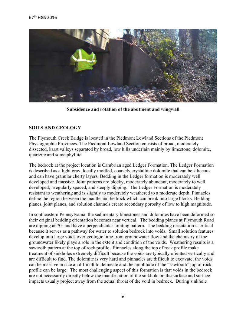
67th HGS 2016
6
Subsidence and rotation of the abutment and wingwall
SOILS AND GEOLOGY
The Plymouth Creek Bridge is located in the Piedmont Lowland Sections of the Piedmont Physiographic Provinces. The Piedmont Lowland Section consists of broad, moderately dissected, karst valleys separated by broad, low hills underlain mainly by limestone, dolomite, quartzite and some phyllite.
The bedrock at the project location is Cambrian aged Ledger Formation. The Ledger Formation is described as a light gray, locally mottled, coarsely crystalline dolomite that can be siliceous and can have granular cherty layers. Bedding in the Ledger formation is moderately well developed and massive. Joint patterns are blocky, moderately abundant, moderately to well developed, irregularly spaced, and steeply dipping. The Ledger Formation is moderately resistant to weathering and is slightly to moderately weathered to a moderate depth. Pinnacles define the region between the mantle and bedrock which can break into large blocks. Bedding planes, joint planes, and solution channels create secondary porosity of low to high magnitude.
In southeastern Pennsylvania, the sedimentary limestones and dolomites have been deformed so their original bedding orientation becomes near vertical. The bedding planes at Plymouth Road are dipping at 70° and have a perpendicular jointing pattern. The bedding orientation is critical because it serves as a pathway for water to solution bedrock into voids. Small solution features develop into large voids over geologic time from groundwater flow and the chemistry of the groundwater likely plays a role in the extent and condition of the voids. Weathering results is a sawtooth pattern at the top of rock profile. Pinnacles along the top of rock profile make treatment of sinkholes extremely difficult because the voids are typically oriented vertically and are difficult to find. The dolomite is very hard and pinnacles are difficult to excavate; the voids can be massive in size an difficult to delineate and the amplitude of the “sawtooth” top of rock profile can be large. The most challenging aspect of this formation is that voids in the bedrock are not necessarily directly below the manifestation of the sinkhole on the surface and surface impacts usually project away from the actual throat of the void in bedrock. During sinkhole

67th HGS 2016
7
repairs in the formation some voids have been observed to extend dozens of feet from the throat, further complicating repairs.
The Ledger formation is locally known as Public Enemy Number One for sinkhole formation. There are many mapped sinkholes and surface depressions along Plymouth Creek and in the general vicinity of the bridge. Sinkholes form when soil overburden collapses or is flushed into a cavity in the bedrock. At the Plymouth Road site, the depth to bedrock is shallow with visible pinnacles in the streambed, which provides the benefit of having a high degree of confidence that voids in the bedrock will be near the surface openings and our ability to repair them will be more successful. Unfortunately, the shallow bedrock also means sinkholes open frequently and grow quickly in the streambed. The water in Plymouth Creek, especially during storm events, flushes the overburden soil into the voids leaving little protection. Because of the significant quantities of water introduced into the creek during storm events, often filling the entire stream channel, the surface soils scour away leaving thin overburden. In conjunction with minimal overburden is the known significant size of voids locally. The massive downstream sinkhole is evidence of the large void size and is known to be explored by spelunkers. Other factors, including a nearby quarry (lowering the groundwater) and new development in the area (increasing runoff) have contributed to the frequency of sinkhole problems at the site. During the site reconnaissance undertaken after the closure, numerous unmapped sinkholes and surface depressions were observed. PROJECT DESCRIPTION
With the bridge closed and the commitment made to open the bridge by August 31st, significant work was now required to design and construct the bridge. The Department was able to utilize the services of an open-end agreement with HDR to obtain the necessary services to design the bridge. The team led by HDR as lead designer included American Geotechnical & Environmental Services, Inc.(AGES) as the geotechnical designer, Dawood Engineering to provide survey and Enviroscan who performed the geophysical investigation.
On March 13th an emergency proclamation was declared and the Department was then permitted to utilize an accelerated design and construction schedule to complete the project. The design schedule required a PS&E package to be delivered on April 2nd, an advertisement date of April 6th with a let date of April 16th. Notice to proceed was issued to the designer on March 23rd allowing them ten days to provide the design package. A directive was given by the Department to ensure structural stability of the bridge for its entire design life: the bridge was to be designed to withstand any future sinkhole development. In addition, other measures were to be recommended to mitigate future sinkhole development ensuring long term stability and managing surface water at the bridge.
Extraordinary coordination and cooperation was needed between the Department, designer, local officials and agencies, utility companies, the Pennsylvania Department of Environmental Protection (DEP), and private land owners to accomplish this 10-day goal. The typical drivers of design in this region are utility impacts and permitting. Even with ongoing coordination with the utility companies, the bridge was designed to avoid an 8-inch gas line that crosses the creek immediately downstream of the bridge just feet from the existing apron. The utility company

67th HGS 2016
8
decided later to replace this line; however, the wingwalls were located to avoid a direct impact to the line.
Probably the strongest example of the quick action and coordination between all stakeholders was the permitting. A field view was held early in the process with the DEP. At this meeting it was agreed the DEP would permit the project under an emergency permit with a formal permit to follow once construction was underway, including allowing the H&H analysis to be performed during construction. It was agreed the bridge would be replaced in its current location, holding the existing low chord, the span would be increased to provide a larger hydraulic opening and the streambed would be paved both upstream and downstream of the structure in order to minimize future development of sinkholes adjacent to the new structure. The design team then proposed a single span pre-stressed concrete spread box beam bridge supported by full height abutments with a clear span of 28’-6” and an out to out width of 43’-4.5”.
The subsurface exploration to evaluate the geotechnical conditions at the bridge commenced immediately and on March 16th Enviroscan performed their geophysics program. This was followed by the test boring program, overseen by AGES, which were completed between March 19th and April 2nd.
SUBSURFACE INVESTIGATION & SUBSURFACE CONDITIONS
Geophysical Study
An abbreviated geophysical study was conducted at the bridge site by Environscan, Inc., the intent of which was to provide guidance for test boring locations and identify possible karst-related subsurface conditions at the proposed foundation locations. Both microgravity and ground penetrating radar methods were used based on site conditions and topography. Geophysics were performed at the bridge, approach roadway and in flat areas southeast and southwest of the bridge.
The results of the study were provided on March 17th and indicated a general northwest to southeast trend of an anomaly at the proposed bridge location. This information was used to locate test borings.
Test Borings
The test boring program was developed by AGES engineers and preliminary consisted of 13 borings at the bridge. The intent was to add borings as needed based on the findings to delineate as many karst features as possible. Test Borings, performed by TRC Engineers, Inc. and inspected by AGES staff were completed between March 19th and April 2nd. The final subsurface investigation consisted of 424.4 feet of soil sampling and 725.1 feet of rock coring in twenty-four (24) borings, over 1100 linear feet drilled in two weeks. The boring locations peppered the site and were located at the proposed foundations, approach roadway, locations of known karst features and generally surrounding the bridge. While 24 borings are many more than the typical scope, the approach was to provide sufficient information to the contractor to minimize increased bid costs due to unknown conditions and the likelihood of delays and claims during construction.

67th HGS 2016
9
The borings identified a layer of sand and gravel fill underlain by a mixture of alluvial and highly disturbed residual soil, predominately sandy clay and clay, which extended to bedrock. Bedrock encountered in the borings is dolomite which confirmed the mapped Ledger Formation at the bridge location. The bedrock encountered in the borings is a predominantly medium hard to very hard, slightly weathered to fresh, broken to massive dolomite. Bedrock is thickly bedded with a sheer dip. Similarly, the joints are widely spaced and have a sheer dip.
Solutioning features and pinnacles in the bedrock are present and voids of similar dimension in the epikarst were encountered in the borings throughout the investigation area. Top of bedrock is highly variable. The depths at which epikarst features are no longer identified ranges from 15 to 36.5 feet. Above these elevations, zones of broken, moderately weathered rock and voids were identified in many of the borings. The weathered zones and voids are both air and soil filled.
Laboratory Testing Program
A laboratory testing program consisting of unconfined compressive strength testing of rock and classification testing of soil was performed for the borings conducted during the early phases of the subsurface exploration to ensure testing was completed prior the letting. Eight (8) unconfined compressive strength tests were performed on dolomite rock cores. The compressive strengths ranged from 4,009 to 26,531 psi. with an average of approximately 10,000 psi. Two (2) soil classification tests were performed on composited jar samples from the existing fill soils and were identified as silty gravel with sand.
Subsurface Profile at Abutment 1

67th HGS 2016
10
GEOTECHNICAL DESIGN
Foundation Type
Because of the time critical nature of the design a foundation type was selected by consensus of the Department and design team. Spread footings on soil were not considered due to the existing failure, known voids and the commitment to ensure long-term stability. Spread footings on rock, while possibly feasible, would have required significant and potentially excessive excavation to competent rock complicated by difficult excavation of the hard bedrock, extensive shoring and dewatering required and was also dismissed due to potential impacts to the construction schedule and unpredictable cost. Pre-drilled H-piles were also discussed but are difficult to install and seat in hard, steeply dipping, voided bedrock making obtaining tip resistance difficult. The Department has also experienced problems with driving and/or predrilling piles with the resulting holes creating a conduit for water and further destabilizing the existing conditions. There were further concerns with determining if a void is present below the pile adding uncertainty to the design.
A micropile foundation was agreed upon because it is known to provide support of the substructures below the epikarst and can provide side resistance in their bonded zone without requiring tip resistance for support. Voids in the bedrock can be identified while installing the micropiles so the bond could be specifically installed in a competent bedrock zone and if voids are encountered the bond zone can be easily lengthened. Additional micropiles can be installed during construction at the direction of the geotechnical engineer providing more certainty and load tests are required to ensure capacities are obtained.. The average recovery and RQD (Rock Quality Designation) in the bonded zone at Abutment 1 is 93% and 72%, respectively, and is 88% and 73% at Abutment 2. Micropiles also provide an easily constructible foundation providing economy and long term stability compared with other foundation types.
The bottom of pile cap elevation was selected by HDR based on minimum cover requirements and the proposed paved streambed channel adjacent to the pile cap. The elevation of the pile cap was placed as high as possible to minimize the need for rock excavation in the event dolomite pinnacles were encountered. The pile cap was not based on scour considerations because the stream channel will be concrete lined.
The most cost-effective micropile foundation design typically consists of larger, fewer piles. However, in consideration of the site conditions and the long term stability of this structure, the design included a larger number of smaller 7 inch diameter micropiles with a conservatively assumed 6 inch diameter rock socket. Increasing the number of piles provided a degree of redundancy and reduced the design load on each pile. This allowed for a minimized bonded length of seven feet to reduce the likelihood of encountering voids within the bonded zones and excess grout takes. The shorter bond zone and small diameter of the micropiles will also ensure they are installed at a tighter spacing in the pile cap that would normally be expected; this will allow for some level of redundancy in the foundations. The anticipated average pile length was 17 ft.

67th HGS 2016
11
The grout-to-ground bond strength of the dolomite is 0.225 ksi and the ultimate geotechnical resistance of the 7 foot bond zone with the 6 inch diameter rock socket is 356.3 kips. Using a resistance factor of 0.60, the factored geotechnical resistance was 213.8 kips per pile. HDR, Inc. recommended a No. 18 (Grade 75) reinforcing bar. The grout strength was 4 ksi. The ultimate structural resistance of the uncased portion was 325.2 kips. Therefore, the structural resistance of the uncased portion is 211.4 kips after applying a resistance factor of 0.65. The recommended factored resistance was conservatively 210 kips for the ABLRFD runs. Battered micropiles were recommended to support lateral loading. Verification static load tests were recommended at one micropile per abutment and loaded to twice the unfactored design load, or 180 kips. Proof tests were performed on two production piles to 1.5 times the unfactored design load, or 135 kips.
The micropiles were not designed for scour because the creek channel at the abutment locations will be lined with concrete. However, buckling analyses were conducted to account for an unsupported length of 13 feet in the event sinkholes develop after the bridge is constructed. The recommended unsupported length of 13 feet is the length from the bottom of pile cap to the lowest top of rock elevation encountered in the borings.
Sinkhole Mitigation
Several recommendations were made by the design team to deal with the existing sinkholes, unidentified sinkholes appearing during construction, and to minimize sinkhole potential once the project was complete. The objective of the sinkhole remediation recommendations was threefold: support the new bridge with robust foundations thereby reducing concerns for foundation failure; repair known sinkholes, and reduce the requirements for future maintenance of the area around the bridge.
Sinkhole Repair Details

67th HGS 2016
12
Repair of the existing sinkholes and any sinkholes that opened up during construction was anticipated to be fairly easy. Due to the shallow bedrock, once the existing bridge was removed and the pile cap excavation was complete the top of bedrock would be accessible with an excavator. The repair recommendation began with excavating all soil in the vicinity of the throat and flushing the sinkhole/throat with water to expose and clean the exposed bedrock surface. The voids would then be plugged with Class C concrete which would bond to the exposed rock and seal the throat off from surface water. It has been the Department’s experience that this is the best method to repair sinkholes in shallow bedrock. In the event the sinkhole throat was deeper than the excavator's reach, it was also recommended to be plugged with Class C concrete but understood the results would be less certain. The sinkhole remediation work was recommended to be conducted in advance of the micropile installation so the sinkholes could be readily identified and repaired without interference by other construction activities.
To minimize future development of sinkholes two additional recommendations were made, including a concrete channel liner and limited mobility grouting. An 8 inch concrete, wire mesh-reinforced channel liner placed on geogrid was recommended from the end of the Turnpike's culvert to 70 feet downstream of the bridge. The liner was also required at all side channels. The liner is intended to limit creek water from finding joints and fractures in the bedrock and to reduce scour of the creek bed soils. It is expected the channel liner will limit surface water from infiltrating into the karst but due to the high groundwater and shallow bedrock at the site it is likely joints and fractures in the bedrock will continue to create sinkholes below the channel lining. To further reduce potential for the development of sinkholes, limited mobility grouting was recommended to cap the top of rock surface in the epikarst zone. Limited mobility grouting was recommended in the approach embankments and also beyond the outfall of the channel lining to minimize localized sinkhole development as the creek water flows into the unlined stream. The grouting plan used primary and secondary grout holes with optional tertiary holes, a 1-inch slump, pumping pressure of 600 psi at the pump outlet and a maximum rate of 1.5 cubic feet per minute to avoid hydraulic fracturing. Grout injection was to begin at a depth of approximately 15 feet below top of rock and 1 foot below any large voids to encompass the epikarst. Grout was injected in 2 foot stages and injection terminated based on one of the following criteria: back pressure greater than 600 psi, 100 cubic feet of grout installed, or surface heave. If more than 50 cubic feet of grout was injected in two consecutive stages, the hole was terminated and the grout allowed to set. The hole was redrilled and grouting continued the next day. Grouting was terminated five feet from the ground surface. The grouting program was be verified by coring in areas as directed. The entire grouting operation was overseen by engineering staff from AGES. Grouting was restricted within 15 feet of an installed micropile.
CONSTRUCTION
Advertising the project for construction did not end the need for acceleration of the project. PennDOT shortened the typical advertisement period to ten days and issued award and NTP to the low bidder, Loftus Construction, Inc., within one week. In order to ensure the bridge was completed on time a $20,000/day penalty was included in the contract for each day past August 31st. Loftus Construction’s approach to the project was to focus on sinkhole closures and remediation around the bridge area, followed by the bridge and liner construction.

67th HGS 2016
13
With the road already under full detour Loftus got to work on the demolition immediately. Because the bridge was closed and would remain so for the duration of construction, the contractor had full access to both sides of the bridge. Construction began with removal of the bridge. The east abutment foundation excavation occurred first to allow access for the micropile operation to begin installing test piles. The west abutment foundation excavation occurred during the testing at the east abutment and when complete the testing operation moved across the creek. During this time the existing sinkholes in the streambed were repaired. With the micropiles successfully meeting the test criteria, the micropile installation operation began in earnest.
Once foundation construction was underway, the first challenge was managing surface water. The plan and proposed implementation of stream flow control was to block the creek at the outfall of the Turnpike arch culvert and pump the water around the site. Most days this method was adequate but after several significant spring storm events flooded the creek it was apparent that this method could only handle very low flows. A beneficial result of these spring storms was the appearance of additional sinkholes. The main sinkhole that undermined the bridge soon showed itself to be a monster. While inconvenient to construction it was quite fortunate the storms exposed the unobserved sinkholes so they could be remediated.
Repairing the “Monster” Sinkhole

67th HGS 2016
14
The largest sinkhole was at the southeast corner, where the bridge had failed. The contractor had difficulty locating the exact throat of the sinkhole. Rock was placed and the apparent opening concreted closed. Soon after the installation of the micropiles began, a significant rain event occurred and the sinkhole opened back up, this time larger than before. An additional micropile was installed at this location to provide added support for the bridge. Over the course of a few wet weeks in late May and early June several sinkholes presented themselves. This highlighted the ever-changing conditions the contractor had to deal with while keeping the construction moving along to meet the open date.
Southeast Sinkhole Second Opening
The work of repairing the sinkholes continued according to plan with successful flushing, choking and backfilling of known and new sinkholes. Fortunately, there were so many pumps on site to manage surface water it was simply a matter of moving a hose around to perform the flushing operations. A total of three known sinkholes were repaired along with five new ones that appeared during flooding of the excavation, all within the footprint of the bridge and
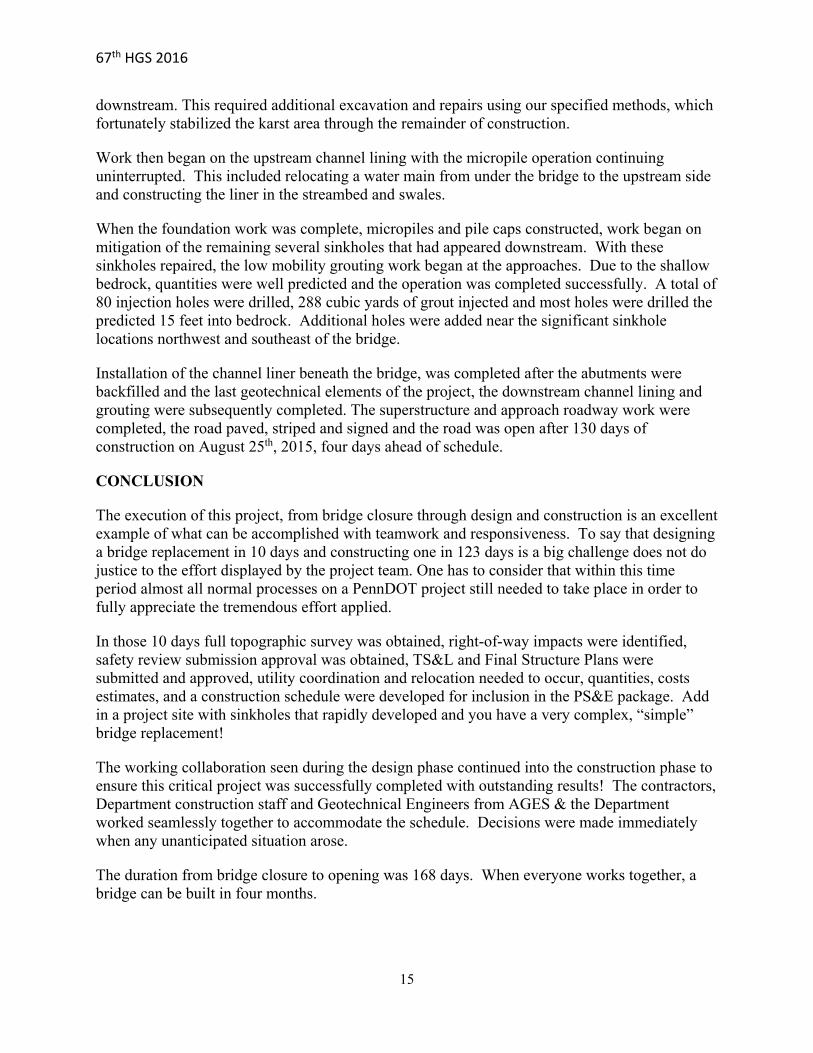
67th HGS 2016
15
downstream. This required additional excavation and repairs using our specified methods, which fortunately stabilized the karst area through the remainder of construction.
Work then began on the upstream channel lining with the micropile operation continuing uninterrupted. This included relocating a water main from under the bridge to the upstream side and constructing the liner in the streambed and swales.
When the foundation work was complete, micropiles and pile caps constructed, work began on mitigation of the remaining several sinkholes that had appeared downstream. With these sinkholes repaired, the low mobility grouting work began at the approaches. Due to the shallow bedrock, quantities were well predicted and the operation was completed successfully. A total of 80 injection holes were drilled, 288 cubic yards of grout injected and most holes were drilled the predicted 15 feet into bedrock. Additional holes were added near the significant sinkhole locations northwest and southeast of the bridge.
Installation of the channel liner beneath the bridge, was completed after the abutments were backfilled and the last geotechnical elements of the project, the downstream channel lining and grouting were subsequently completed. The superstructure and approach roadway work were completed, the road paved, striped and signed and the road was open after 130 days of construction on August 25th, 2015, four days ahead of schedule.
CONCLUSION
The execution of this project, from bridge closure through design and construction is an excellent example of what can be accomplished with teamwork and responsiveness. To say that designing a bridge replacement in 10 days and constructing one in 123 days is a big challenge does not do justice to the effort displayed by the project team. One has to consider that within this time period almost all normal processes on a PennDOT project still needed to take place in order to fully appreciate the tremendous effort applied.
In those 10 days full topographic survey was obtained, right-of-way impacts were identified, safety review submission approval was obtained, TS&L and Final Structure Plans were submitted and approved, utility coordination and relocation needed to occur, quantities, costs estimates, and a construction schedule were developed for inclusion in the PS&E package. Add in a project site with sinkholes that rapidly developed and you have a very complex, “simple” bridge replacement!
The working collaboration seen during the design phase continued into the construction phase to ensure this critical project was successfully completed with outstanding results! The contractors, Department construction staff and Geotechnical Engineers from AGES & the Department worked seamlessly together to accommodate the schedule. Decisions were made immediately when any unanticipated situation arose.
The duration from bridge closure to opening was 168 days. When everyone works together, a bridge can be built in four months.

67th HGS 2016
16
Completed Plymouth Road over Plymouth Creek

67th HGS 2016
17
REFERENCES
1. Geyer, McGlade and Wilshusen: "Engineering Characteristics of the Rocks of Pennsylvania", Pennsylvania Bureau of Topographic and Geologic Survey, 1982.
2. Pennsylvania DCNR, "The Geology of Pennsylvania", 1999.
3. American Geotechnical & Environmental Services, Inc., Structural Foundation Investigation Report for Final Design, prepared for SR 3007 Section SKH, April 2015.

1 67th HGS 2016: Gobbin, Giacchetti, Brunet.
Umbrella Structures for avalanches protection as per Western North America snow condition designed according to the Swiss
Guidelines
Luca Gobbin Maccaferri Canada Ltd.
400 Collier MacMillan Dr. Unit B Cambridge, Ont, Canada, N1R7H7
Telephone: 519-623-9990 [email protected]
Giorgio Giacchetti OFFICINE MACCAFERRI S.p.A.
Via Kennedy 10 40069 Zola Predosa
Ph: 01139051646000 [email protected]
Ghislain Brunet Maccaferri, Inc
10303 Governor Lane Blvd., Williamsport, MD 21795-3116
Ph: 301-223-6910 [email protected]
Prepared for the 67th Highway Geology Symposium, July 11 to 14 2016, Colorado Springs, CO

2 67th HGS 2016: Gobbin, Giacchetti, Brunet.
Disclaimer
Statements and views presented in this paper are strictly those of the author, and do not necessarily reflect positions held by their affiliations, the Highway Geology Symposium (HGS), or others acknowledged above. The mention of trade names for commercial products does not imply the approval or endorsement by HGS.
Copyright Notice
Copyright © 2016 Highway Geology Symposium (HGS)
All Rights Reserved. Printed in the United States of America. No part of this publication may be reproduced or copied in any form or by any means – graphic, electronic, or mechanical,
including photocopying, taping, or information storage and retrieval systems – without prior written permission of the HGS. This excludes the original authors.

3 67th HGS 2016: Gobbin, Giacchetti, Brunet.
ABSTRACT
In the Alps (Europe) infrastructure, buildings and human lives are usually protected from avalanches with snow fences, snow bridges, snow rakes and snow nets. The purpose of these fences is to prevent avalanches being triggered or, at a minimum, to prevent snow movements that could potentially lead to damage. Because of that, the snow fences are not designed to stop an avalanche during its motion, but they are developed to contain the slow initial movements of the snow creating an “upslope stagnation zone” parallel to the slope. This zone is characterized by very high compression stresses. For this reason, snow supporting structures must very strong and traditionally snow net systems made of posts and cable netting are used.
Umbrella Systems are another innovative solution for avalanches protection using the same design assumption as the traditional structures. These structures are made with an interception panel attached to a tubular strut: in this way the structure looks like an umbrella, hence their name. All the structures are connected to the ground by a single anchor and for this reason they are particularly suitable for intervention on very steep and potentially dangerous slopes. Also, their rapid installation makes them an appropriate solution when the construction period is very short such as in the mountain environment.
Umbrella structures have been used mainly in Europe for more than 20 years and are designed considering the typical snow unit weight of the Alps (approx. 270 kg/m3 [16.86 lb/ft3]) in accordance with the technical Swiss Guideline (2007).
This paper describes the new design criteria that need to be adopted to comply with the more severe snow conditions of to the Western North American Mountains. One of the major characteristics is the snow unit weight that is approximately two times higher than the one used in the Alps (approx. 400 to 600 kg/m3 [24.97 to 37.46 lb/ft3]).

4 67th HGS 2016: Gobbin, Giacchetti, Brunet.
INTRODUCTION An avalanche is a mass of snow and/or ice falling rapidly down a mountainside, progressively
swelling its volume and dragging everything in its path down with it. The behavior of the snow pack is similar to a viscous fluid characterized by a high density. The
density defines the weight (driving force) and consequently the movement of the snow. The properties of the fluid depend basically on temperature and the type of movement and stresses that occur within it. Compression, traction and shear stresses are developed in the snow pack. These stresses affect the movements and the deformations of the snow, and they define the possible collapse and resulting type of avalanche. The snow pack is a non-homogeneous and anisotropic body because it is generally composed of different layers. Its sliding and glide velocity, which define the shear stress, can vary between the layers. Moreover, the snow pack can modify its mechanic characteristic in function of the temperature.
As the snow cover moves constantly and slowly downslope, it is possible to define two main types of movement:
1. Creep: it is due to the weight of the snow, which defines the settlement and the shear deformation parallel to the slope:
2. Glide: it depends on the type of soil (roughness) and on the possible water presence at the interface between the soil and the snow. It is the downslope motion of the snow pack.
Figure 1 - Glide and creep velocity in the snow pack. Where: w = creep velocity normal to the slope; uu = glide velocity; u =
velocity component parallel to the slope (shear); v = resultant velocity vector. (Reference Fig. 4 of the Swiss Guideline, 2007).
For the most part, every avalanche consists of 3 distinct zones: - Detachment area (starting zone): it is the area where the avalanche originates. Normally it
is defined above the tree line, or by the mountain crests or ridges, or where there is a snow accumulation due to new snow falls or wind transport. In this area the unstable snow starts to move downslope. Creep movement and a subsequent glide mechanism can occur at the ground surface level. The movements depend on several factors, such as: slope inclination (generally between 30 and 60 degrees), snow thickness, soil roughness, type of snow (humidity, friction, unit weight, plasticity, etc.), wind and sun exposure, etc. (Figure 2, left).

5 67th HGS 2016: Gobbin, Giacchetti, Brunet.
- Sliding area: it is the area between the starting zone and the sticking area. In this zone the avalanche reaches its highest velocity. This area is normally characterized by high inclination and limited presence of vegetation (Figure 2, center).
- Sticking area: it is the area where the avalanche starts to reduce its velocity and stops its motion. In this zone high pressures (30+ kPa [4.35 PSI]) on the snow may occur (Figure 2, right).
Avalanches are generally classified worldwide following 2 different criteria: 1. Based on the morphology: UNESCO, International Commission on Snow and Ice, 1981; 2. Based on the magnitude: Canadian Avalanche Size Classification (McClung and Schaerer,
1993); and Japanese Avalanche Size Classification (Shimuzu, 1967).
Figure 2 - Photos of the 3 typical different areas of the avalanche. Left: starting zone; Centre: sliding zone; Right: sticking zone.
(Photos courtesy of Regione Autonoma Valle d’Aosta – Snow and Avalanches Dept.).
AVALANCHE PROTECTION SYSTEMS
The first tools used to reduce avalanche hazards are specific maps (Figure 3). Usually these plans identify potential areas affected by avalanche phenomena. These maps are based on historical and observed evidence, on geomorphological and geological parameters, on the type of vegetation and air photos, etc. These specific maps give all the information necessary to plan construction of new structures; (i.e., houses and other residential complexes), infrastructures; (i.e., roads, highways, railways, etc.) and ski areas; (i.e., lifts and ski slopes). Moreover, they allow strategic planning in order to locate the avalanche mitigation systems.

6 67th HGS 2016: Gobbin, Giacchetti, Brunet.
Figure 3 - Highlight of a cartographic map of avalanche risks. Legend: Va (in purple): areas exposed to avalanche phenomena; Vb (in pink): areas with high probability of avalanche; V1 (in red): area with high risk; V2 (in yellow): areas with medium risk;
V3 (in green): areas with low risk. (Avalanche map of Avise municipality, Aosta Valley Region (Italy). Courtesy of Geol. Stefano De Leo).
Once the maps of areas subject to avalanche hazards are defined protection measures can be
designed. Snow avalanche protection systems can be divided in: Temporary measures: normally they are used after exceptional meteorological events, (i.e.
snow falls, strong winds, storms, etc.). They might be subdivided in two categories: 1. By moving the affected development and/or infrastructure; 2. By using external systems able to guarantee the artificial detachment of an avalanche
(blasting). The blasting of avalanches is really common in the Western of the U.S. and Canada.
Permanent measures: the purpose of these types of mitigation systems is to reduce or limit the effects of an avalanche. They are divided in two categories:
1. Active protection systems: able to avoid the initiation of an avalanche. They are placed in the detachment zone in order to control the movement of the snow and reduce the possibility of avalanche detachment. These measures can be divided in 3 main interventions:
a. modification of the soil in order to increase the roughness of the slope and decrease the possibility of detachment;
b. control of the snow transported by the wind using structures; i.e. wind deflectors, or wind barriers) able to modify the wind flow and avoid the formation of dangerous snow accumulation;
c. holding the snow pack through installation of anti-avalanche structures (see Table 1). 2. Passive protection systems: able to limit damage and the consequences of avalanches. They
are placed in the sliding area or more commonly in the sticking zone. They allow detachment of the avalanche, but protect structures and infrastructure against the possible

7 67th HGS 2016: Gobbin, Giacchetti, Brunet.
consequences of the snow slip. As mentioned these structures are located in the sliding zone, where the velocity and the energy of the avalanche are really high, or in the stopping zone, where snow pressures are considerable. For these reasons passive protection systems are generally massive structures, such as concrete or reinforced soil structures. The goal of these interventions is to reduce the energy and the velocity of the moving snow, or to stop or to deflect the flow of the snow slide into safe areas.
The table below presents the main types of active avalanche protection systems.
Table 1 - Active protection systems (Swiss Guideline classification)
Type of structures
Description Example
Rigid When the creep and glide motions of the snow are arrested by a structure subjected to only slightly elastic deformations.
Snow Bridges Snow rakes
Flexible When the structure is able to follow and adapt itself to the snow movements (up to a certain level).
Snow nets Umbrella
structures
All the systems listed in the table above can be designed with either steel or wood or combined (wood and steel) elements. The type of system chosen must be consider different aspects, such as the morphology of the slope, the allowable risk, the type of structure to be protected, the type of snow, etc. Thus, all the advantages and the disadvantages of the different structure types must be well understood by designers. These supporting structures have the function to withstand mainly the snow pressures, and also possible dynamic forces.
UMBRELLA SYSTEM
As shown previously, several types of active retaining snow structures are available in the market. In recent years we have seen more and more projects using umbrella systems due to the speed and ease of installation. Umbrella structures are formed by modular mono-anchoring elements. The single unit is a cross-shaped structure made with beams supporting a facing composed of a wire rope panel combined with a double twist mesh. The connection between the front panel and the anchor is made through a tubular tie with the housing for a ball joint. The upslope bracing cables for load transfer connect the front panel with the anchor and the tubular tie. The anchor consists of a flexible double leg anchor.

8 67th HGS 2016: Gobbin, Giacchetti, Brunet.
Figure 4 - Lateral view of an Umbrella Structure (ErdoX).
The table below shows the advantages and the disadvantages of the Umbrella System:
Table 2 – Advantages and disadvantages of the Umbrella System supporting structure
Advantages
- Structures self-stable, modular and are provided with a single anchoring system that simplifies drilling operations;
- Easy and fast installation in the presence of snow; - Light structure (close to 300-400 kg [661-881 lb] for unit)
compared to traditional snow net, and well balanced, making transport by helicopter easier;
- If damaged, the structure can be easily replaced; - Easy layout operations; - More adaptable to ground morphology compared to traditional
snow net barriers.
Disadvantages
- Only one anchoring point: the acting forces on the single anchor are high;
- Upslope braces and tubular tie are in the maximum snow cover compression zone;
- The design has to be carried out by experts.
THE DESIGN APPROACH
The Swiss Guideline (Defence structures in avalanche starting zones – Technical Guideline as an aid to enforcement), issued in 2007 by the Swiss Federal Institute of Snow and Avalanche Research of Davos (SLF), represents worldwide the milestone for snow supporting structures

9 67th HGS 2016: Gobbin, Giacchetti, Brunet.
installed in the starting zone. The guideline defines all the aspects and the procedures to calculate and design, from a structural point of view, these types of avalanche mitigation systems.
Operating in accordance with such guidelines, the design of the homologated snow supporting structures must take into consideration several important aspects such as: - Inclination of the ground in the detachment zone (max value): ψ; - Glide factor, which depends on the roughness of the soil and the sun exposure: N. In the Alps
this value is between 1.2 (no sun exposure and high roughness) and 3.2 (sun exposure and low roughness);
- Altitude coefficient, which depends on the elevation of the site above the sea level: fc. In the Alps it is assumed between 1.0, if the elevation is equal or lower than 1,500 m [4,921.26 ft] a.s.l., and 1.3, if the elevation is more than 3,000 m [9,842.52 ft] a.s.l.;
- Effective thickness of the net: DK. The snow thickness measured perpendicular to the slope; (i.e., DK =2.0 to 4.0 m [6.56 ÷ 13.13 ft]);
- Minimum lateral distance between the structures along one alignment: A; - Average snow density: ρ = 270 kg/m3 [16.86 lb/ft3]. This value is obtained considering the
average unit weight of the snow in the Swiss Alps at an altitude of 1,500 m [4,921.26 ft] a.s.l. and an exposure of the slope WNW-N-ENE. Note that the variation of this parameter with altitude and slope exposure is taken into account using the fc and the N coefficients (section 3.10.6 and 3.10.5 of the Swiss Guideline, 2007). The generic formulas to define the forces and the pressures acting on the structure (Section 4
of the Swiss Guideline) are presented below. These stresses, which depend on the creep and the glide movement, are the base for dimensioning the components of the snow net. Even if these formulas represent a simplification of real snow behaviour, they are clear and easy to use. Moreover, in-situ experience shows that these equations give reliable results.
The pressure components of the snow parallel and perpendicular to the slope can be calculated as (per linear meter of structure):
S’N = ½ ρ . g . H2 . K . N . fs . fc (1) S’Q = S’N . a / (N . tanψ) (2) Where:
- S’N = snow pressure component in the line of slope per meter run of the supporting surface along the contour line [kN/m2];
- ρ = snow unit weight; - g = gravitational acceleration; - H = vertical snow thickness
H = HK = DK / cosψ (3)
- K = creep factor (function of the snow unit weight and slope gradient);

10 67th HGS 2016: Gobbin, Giacchetti, Brunet.
- N = glide factor; - fs = reduction factor for a flexible supporting structure (usually is 0.8, while for rigid structures
is 1.0); - fc = altitude coefficient; - a = factor that depends on the snow characteristic (it varies between 0.2 and 0.5); - S’N = Snow pressure component normal to the slope per meter run of the supporting surface along
the contour line [kN/m2]; - ψ = slope gradient.
Both these pressures are assumed to be distributed uniformly along the entire height of the
structure. This is a strong generalization because the pressure of the snow cover is extremely complex, even if the snow pack is quite homogeneous: formula (1) is a simplification of complex differential equations of the snow pack.
At this point it is possible to identify an incrementing load due to the fact that the snow net is not perpendicular to the ground surface (angle between the post and the slope surface generally equals 75 degrees), thus the weight of the snow prism formed between the supporting structure and normal to the surface has to be considered.
G’ = ½ ρ . g . D2 . tanδ (4) Where:
- D = snow thickness measured perpendicular to the slope; - δ = angle between the structure and the perpendicular to the slope.
The parallel and the normal component of G’ are respectively: G’N = G’ . sinψ (4.a) G’Q = G’ . cosψ (4.b) The marginal forces that act on the side of the structure can be taken into account with the
following equation (per ΔL of structure): S’R = fR . S’N (5) Where:
- fR = marginal factor that depends on the lateral distance between the structures (A), and the coefficient N;
- ΔL = length where S’R is acting, it depends on A.

11 67th HGS 2016: Gobbin, Giacchetti, Brunet.
Figure 5 - Simplified graph of the snow pressure distribution acting on an umbrella system. (Reference Fig. 17 of the Swiss Guideline, 2007).
At this point the overload that may act on the structure is identified: the proper weight of the
structure (W’) and the lateral thrust acting on both sides of the structure having a length (l), which can be expressed as:
SS = 0.10 . S’N . l (6) Finally, it is possible to obtain the resultant forces acting on the structure in the different
sections of the snow supporting system: intermediate (MF), interval (RF) and end (WF). R’N_MF = S’N + G’N + W’N (7) R’N_RF = S’N + G’N + W’N + S’R_RF (8) R’N_WF = S’N + G’N + W’N + S’R_WF (9) R’Q_MF = R’Q_RF = R’Q_WF = S’Q + G’Q + W’Q (10)
Figure 6 - Disposition of Umbrella structures: green dashes represent the position of interval and end sections (RF, WF); red
dashes represent the position of the intermediate section (MF).

12 67th HGS 2016: Gobbin, Giacchetti, Brunet.
UMBRELLA SYSTEM APPLICATION IN WESTERN NORTH AMERICA
Maccaferri has extensive experience worldwide in snow retaining structures such as snow nets. Based on this experience and considering environmental factors that affect installation issues, Maccaferri introduced a new type of structure, the umbrella system, to make these interventions more efficient: faster and easier to handle and install even in extreme environmental conditions.
As described in the previous paragraph, the umbrella structures are designed using standard parameters defined by the Swiss Guideline (2007). In the case where the in-situ local parameters of the protecting area differ from the ones adopted in the calculation, it is necessary to design the structures ad hoc, so that, the avalanche protection system will be able to resist the new larger forces and pressures.
In the Alps environment the parameters that can vary are generally: the inclination of the slope, the glide factor, the altitude and the snow thickness, while the snow density is generally considered constant (approx. 270 kg/m3 [16.86 lb/ft3]).
Figure 7 - Variation of the snow pressure (S’N) with different snow density values (ρ). The figure shows also the comparison between the Alps (ρ = 270 kg/m3 [16.86 lb/ft3]) and the North Western America environments (ρ = 450 kg/m3 [28.10 lb/ft3]).
(Castaldini, 2012).
The situation is different in Western North America (Pacific Coast of Canada and U.S.A.)
where the snow might have a unit weight that can reach values 2 times greater than the density measured in the Alps: it is not unusual to have snow density of 450-500 kg/m3 [28.10-31.22 lb/ft3] and more. This is due to the presence of the Pacific Ocean that increases the humidity ratio in the snow and consequently raises the snow unit weight.
The previous graph shows that the pressure components parallel to slope of the specific pressure of the snow (S’N) increases if the snow unit weight (ρ) increases as well. These increments follow a parabolic behaviour. It can be noted that with the increase in ρ the different curves (one

13 67th HGS 2016: Gobbin, Giacchetti, Brunet.
for each DK) diverge. Thus, it is evident that S’N is not directly related to the snow unit weight: a little variation in snow unit weight can provoke a big variation in snow pressure. For instance, by increasing the snow unit weight from the typical value of the Alps (270 kg/m3 [16.86 lb/ft3]) to the one recorded in Western North America (450 kg/m3 [28.10 lb/ft3]), the snow pressure value S’N almost doubles; (i.e., for a DK 3.5 the S’N changes from 68 kN/m2 [1,420.25 lb/ft3] to 133 kN/m2 [2,777.84 lb/ft3]). Consequently, umbrella structures are stressed with higher loads, which can cause damages or failures.
Three measures may be adopted to avoid potential collapse of the structure: 1. Reinforce all of the individual components of the structure; 2. Equip the beams of the umbrella with a special spherical joint aimed to reduce the stresses,
combined with a front wind bracing device to limit deformation; 3. Adapt the umbrella structure and the site conditions in order to reduce the pressure on the
structure.
Figure 8 – Umbrella structure: details.
CASE STUDY
An important avalanche prevention intervention was carried out in the area of Valsavarenche (AO, Italy) above the town of Les Thoules. The objective was to prevent the recurrence of incidents that in the past had caused causing a lot of damage, like: the destruction of telephone and electric poles, the damage to high voltage trellis structures, the burial of streets (Road S.R.23) and the destruction of 7 buildings and damage to 5 buildings.
The solution in this case was designed considering to the following data:
- the detachment area is at 2,450 meters (8,038 ft) above sea level; - the slope grade is everywhere is more than 40°; - The size of the detachment area could reach 350 m (1,148 ft); - The soft snow parts detached had a thickness of 1.5 m (5 ft); - The estimated volume of snow detached is about 50,000 m3 (1,765,733 ft3);

14 67th HGS 2016: Gobbin, Giacchetti, Brunet.
- The gap is about 900 m (2,953 ft).
Figure 9 - Location and schematic of the problem.
The solution to the problem was developed using the Umbrella structures: 718 elements for 2,600 total linear meters (8,530 ft) of developed area. All the structures were designed according to the Swiss Guideline. The duration of the job was 4 months and the total cost of it was about 2,000,000 €.
Figure 10 - View of the installed Umbrella structures.

15 67th HGS 2016: Gobbin, Giacchetti, Brunet.
CONCLUSION
The installation of active avalanche mitigation systems, such as umbrella structures, has continued to rise over the last 10-years to protect ski resorts, villages and infrastructure. Their success is linked to the high performance of these structures, as well as their cost-effectiveness. In 2007 the Swiss Federal Institute of Snow and Avalanche Research of Davos (Switzerland) (SLF), issued the Swiss Guideline (Defense structures in avalanche starting zones – Technical Guideline as an aid to enforcement). The guideline defines all the aspects and procedures to calculate and design, from a structural point of view, active avalanche supporting structures. In the case of Western North America (Pacific Coast of Canada and U.S.A.), the calculation approach must be adapted for the unit weight of the snow up to 400-500 kg/m3 (24.97-31.22 lb/ft3).
A consequence is the increasing of the pressure acting on the structures (i.e. for a DK 3.5, the parallel component of the snow pressure against the net can double by increasing the snow unit weight from 270 kg/m3 to 450 kg/m3 [16.86-28.10 lb/ft3]).
Despite the large pressure, snow umbrellas can be installed by reinforcing the structure, or reducing the stress on the junction point of the beams.
REFERENCES:
Castaldini R., 2010. Barriere fermaneve omologate UFAFP/SNV e NTC 2008. Review Lavori Pubblici n.43, March-April 2010.
Castaldini R., 2010. Barriere fermaneve omologate. Review Neve e Valanghe, n.70, August 2010. Castaldini R., 2012. Barriere fermaneve: pressione specifica del manto nevoso. Review Neve e
Valanghe, n.75, April 2012. Margreth S., 2008. New technical guideline on snow supporting structure in avalanche starting
zones. International Snow Science Workshop, Whistler (BC), Canada, September 2008. McClung, D.M and P.A. Schaerer. 1993. The Avalanche Handbook. Seattle, WA, The
Mountaineers. Shimizu, H. 1967. Magnitude of avalanche. In Physics of Snow and Ice. Proc. International Conf.
on Low Temp. Science, Sapporo, Japan. H. Oura, Ed., August 14-19, 1966, Vol. 1, Part 2. Swiss Guideline, 2007. Defense structures in avalanche starting zones – Technical guideline as
an aid to enforcement. Editors: Federal Office for the Environment (FOEN) & WSL Swiss Federal Institute for Snow and Avalanche Research (SLF), Bern.

16 67th HGS 2016: Gobbin, Giacchetti, Brunet.
UNESCO, 1981. Avalanche Atlas: Illustrated International Avalanche Classification. International Association of Hydrological Sciences, International Commission of Snow and Ice: Natual Hazards Series, Vol 2, Paris, France.

1
Nanos Cattle Pin Embankment Instability Investigation
SH 99 in Osage County, Oklahoma
By
James B. Nevels, Jr., Ph.D., P.E., PLLC
James B. Nevels, Jr., Ph.D., P.E., PLLC, Geotechnical Consultant
605 Mimosa Dr. Norman, OK 73069‐8622, USA
e–mail: [email protected]; Phone: 405.818.2897
And
Christopher R. Clarke, P.E.
Christopher R. Clarke, P.E., Geotechnical Engineer
Oklahoma Department of Transportation, Materials Division
200 N.E. 21st Street, Oklahoma City, OK 73105‐3204
e–mail: [email protected]; Phone: 405.522.4998.
Prepared for the 67th Highway Geology Symposium, July 2016

2
ACKNOWLEDGEMENTS
The Authors wish to thank Mr. Brian Rumsey, ODOT Osage County Superintendent District J, Division Eight for the help the maintenance crews during the field investigation for this project.
DISCLAIMER
Statements and views in this paper are strictly those of the author(s), and do not necessarily reflect positions held by their affiliations, the Highway Geology Symposium (HGS), or others acknowledged above. The mention of trade names for commercial products does not imply the approval or endorsement by HGS
COPYRIGHT © 2016 Highway Geology Symposium (HGS)
All Rights Reserved. Printed in the United States of America. No part of this publication may be reproduced or copied in any form or by any means – graphic, electronic, or mechanical, including photocopying, taping, or information storage or retrieval systems –without prior written permission of the HGS. This excludes the original author’s.

3
ABSTRACT
A highway embankment instability investigation was initiated along a segment of SH 99 located approximately 4.1 miles north of the junction US 60 and SH 99 in Osage County, Oklahoma by the Oklahoma Department of Transportation (ODOT) Division 8 Maintenance. The length of the embankment extent along SH 99 where persistent Division 8 maintenance repairs over a decade have been required is approximately 2300 feet. This paper looks only at Part A of this embankment instability extent between stations 379+60 to 382+16. According maintenance records there has never been an outright embankment slope failure at the site. However, the distress conditions observed in the pavement and side slopes indicates the symptoms of an incipient landslide. The assumption was concluded that the embankment instability could not be classified as a first time slope movement. The site condition showed that the embankment built in 1935 was constructed on the predominantly Steedman–Coweta complex, 15 to 25 percent slopes mapped soil series according to the USDA Natural Resources Conservation Service (NRCS) Web Soil Survey 3.1. The Steedman–Coweta complex is a residual soil consisting of shallow colluvial mantle underlain very heavy textured fat clay intermingled with rock fragments that overly a medium plasticity clay shale. The Steedman soil series profile was found to predominant the soil profile underlying the embankment based on cross–sectional borings. The embankment was constructed on the steep slope of a cruesta. The hillside geomorphology, surface distress indicators, and slope stability analyses point to the mechanism of a creep flow earth movement that is the cause of the Division 8 maintenance repairs. This case history concentrates on the terrain analysis that leads to the classification and mechanics of the embankment movement. A brief mention of the remedial repair recommendation for the embankment extent is presented, and a planned instrumentation to monitor to the creep rate of the Steedman soil series profile is also discussed.

4
INTRODUCTION This paper presents results of comprehensive forensic investigation for Part A of an
embankment instability problem designated as Slide 5. Part A was one five parts of the embankment extent investigated and is reported on in this presentation. The request for a geotechnical investigation for a station extent of SH 99 was made in a January 21, 2014 e‒mail by Mr. Michael Holloway, Oklahoma Department of Transportation (ODOT) Division Eight in Tulsa, Oklahoma. As presented in the initial January 21, 2014 e‒mail, the description of the roadway and embankment problems was primarily in the northbound lane for an approximately 700 foot lineal section of SH 99 in Osage County. Part A was from approximately station 379+60 to 382+16 (256 lineal feet in length), see location map in Figure 1. The purpose of this forensic investigation is to determine the following: a.) the nature of the geotechnical conditions at the site, b.) to determine the cause of the distress, and c.) make preliminary remedial repair recommendations. The scope of work for Part A as outlined by the Materials Division Geotechnical Branch involves the following:
a. Review of the pertinent original design plan sheets b. Assessment of site and subsurface condition c. A review of the surface soils and geology d. A field investigation (survey and borings) e. Embankment slope stability assessment and analysis f. Recommendations
SITE CONDITION The original design plans covering the embankment instability station extent are stamped in November 12, 1932, and the revised as‒built plans for Federal Aid Project No. 335 Section B are dated July 1934. The 1931 State Standard Specifications governed the project construction. The typical grading section and cross‒sections were not available for this old of a project. From the field investigation, the existing alignment of SH 99 through the approximate station extent 379+60 to 382+16 is a two lane 24 foot wide asphalt pavement with grass shoulders with an estimated 2:1 slope ratio cut and embankment grading section. Part A station extent is in shallow reverse shaped alignment in a climbing vertical curve. The alignment is in a predominantly climbing shallow fill transitioning to a side‒hill cut and fill grading section. The natural ground slopes from west to east and is the east facing slope of a cuesta (a hill or ridge with a steep face on one side and a gentle slope on the other). The surrounding land use along the existing alignment is predominantly ranch pasture.
SUBSURFACE CONDITION The subsurface conditions underlying the embankment extent consists of shallow residual
soils developed from shales and/or sandstones interbedded with clay, siltstone, or sandy shale on a hillside slope. The geomorphic province at this site in Osage County is the Eastern Sandstone Cuesta plains which consist of west‒dipping Pennsylvanian geologic aged sandstones that form cuestas that overlook broad shale plains, reference Oklahoma Geological Survey Educational Publication 9 (1).

5
Figure 1. Project location on Osage County Map Sheet 4, March 1995.
SITE TERRAIN The Part A station extent is along the lower flank of the steep slope of a cuesta. The project location is presented in the Nanos 7.5 minute topographic quadrangle in Figure 2. A cuesta is an asymmetrical ridge capped by resistant rock layers of slight to moderate dip (commonly less than 15 percent slopes); a type of homocline produced by differential erosion of interbedded resistant and weak rocks. The cuesta has a long gentle slope on one side (dip slope that roughly parallels the inclined beds; on the other side, it has a relatively short and steep or cliff like slope (scarp) that cuts through the titled rocks. The landform is controlled by erosion of the inclined top resistant rock layer (at the crest). The steep or cliff like slope (scarp) the cuesta topography is associated with the development and accumulation of shallow colluvial soil materials (2). Colluvium is defined as poorly sorted debris that has accumulated at the base of slopes, in depressions, or along small streams through gravity, soil creep, and local wash. It consists largely of material that has rolled, slid or fallen down the slope under the influence of gravity.
Site Location
Pawhuska, Oklahoma

6
Accumulations of rock fragments are called talus. The rock fragments in colluvium are usually, in contrast to the rounded, water-worn cobbles and stones in alluvium and glacial outwash.
Figure 2. Site location on a segment of the Nanos 7.5 minute topographic quadrangle.
The roadway grading typical section through station 379+60 to 382+16 is a shallow fill section in Area A. The grading section extent has been in place from approximately 1935 to 2016; approximately 81 years. Along the SH 99 alignment right of the center line of survey the grading of the back slope makes an approximate 2:1 cut into the cuesta hillside slope, and along this back
Station Reference ‒ Structure No. 39
EOP
BOP
AOI
Area A
BOP – Beginning of Slide 5 EOP – End of Slide 5 AOI – Area of Interest

7
slope a total of thirteen erosional features in drainage ways were observed exposing the composition and depths of the colluvial mantel intermingled with the underlying soil profile.
PAVEMENT and SLOPE DISTRESS The initial site visit to Part A of Slide 5 location and walkout of the embankment extent was made on March 12, 3014. The reference point for the layout of all the field investigation was the centerline of structure no. 39, (5 x 7 x 57 ft.) roadway reinforced concrete box (RCB) and SH 99, at station 406+51. Area A was identified in the walkout of the embankment extent between stations 379+60 to 382+16 to be investigated with regard to embankment slope instability Of the five areas, Area A was found to have the most significant embankment and slope distress. The major types of distress recorded at area A were as follows:
a. A scarp in the north bound lane with a few exceptions the scarp extending into the southbound lane, with a length of approximately 256 feet
b. Vertical displacements of the scarp ranged from 0.5 to 3 inches c. Significant longitudinal cracking and undulation of the pavement surface. d. Toe of the slide could not be determined e. Out of plumb right of way fence posts, leaning eastward.
At Area A location the toe of potential slide mass also could not be discerned. Interviews with Mr. Brian Rumsey, ODOT Osage County Superintendent, indicated that at location of Area A pavement and underlying subgrade were dug out to depths as much as 8 feet. The excavated embankment material from these Maintenance repairs was replaced with unidentified materials in attempts to stabilize the embankment these sections. Key site photographs of Area A for Slide 5 were taken to illustrate and supplement the report findings, see examples in Figures 3 and 4. Photographs were taken during the summer and winter time periods. Photographs also include the overall terrain and other features that are influencing the slope stability. Also of note is that the landscape throughout the extent of the cuesta seen in the site photographs is predominantly grass with few trees suggesting that the underlying geology is predominantly shale.
SURFACE SOIL DESCRIPTION A check with the United States Department of Agriculture (USDA) Natural Resources Conservation Service (NRCS) Web Soil Survey 3.1 (3) program indicates that there is one soil series complex that underlies Area A, and the soil series map unit 58 is the Steedman–Lucien complex, 15 to 25 percent slopes, see soil map on sheet 1 of the Web Soil Survey 3.1 in Figure 5.
HILLSLOPE GEOMORPHOLOGY At the site location, the amount of annual precipitation ranges from 35 to 40 inches, and the
Thornthwaite annual evapotranspiration indices range from 50 to 66. The climate can be characterized as B3 to B4 humid based on the mean Thornthwaite Moisture Index. A closer look at the average of the precipitation and evapotranspiration listed above indicates a ratio of 0.65 which more correctly defines the climate as dry–semi humid. The surface runoff for the Steedman

8
and–Lucien complex ranges from slow to rapid to very high. As can be seen in Figure 5, two soil map units have an impact on the embankment instability, and they are the following:
Figure 3. Area A scarp looking North along SH 99.
a. Map unit 58 – Steedman–Lucien complex, 15 to 25 percent slopes b. Map unit 13 – Lucien−Coyle complex, 3 to 8 percent slopes
Map unit 58 underlies the SH 99 grading within the right of way limits of Part A, and directly influences the embankment instability. The horizon depths for the soil series in map unit 58 are indicated in Figure 6 and 9 respectively. The map unit 13 is located on the ridge crest of the cuesta above Area A and has only an indirect affect in that it is an additional source of the colluvial mantle that makes up the predominant Steedman soil series A and parts and /or all of the Bt1 and Bt2 horizons. The colluvial mantle was shown in detail in Borings 21 and 22 where rock fragments are found to depths of 2.6 and to approximately 4.0 feet respectively in the soil profile. The percentage of rock fragments found in the (Steedman, Foraker, Coyle, and Lucien) soil series based on the NRCS Official Soil Description (OSD) that contribute to the colluvial mantle are as follows:
a. Steedman soil series: A horizon – Rock fragments less than 3 inch diameter 0 to 25 percent by volume. Rock fragments from 3 to 36 inch in diameter 0 to 50 percent.
b. Foraker soil series: A horizon – flat limestone rock fragments less than 3 inch in length 0 to 25 percent. Rock fragments greater 3 inch in length 0 to 50 percent. BA horizon: – Flat
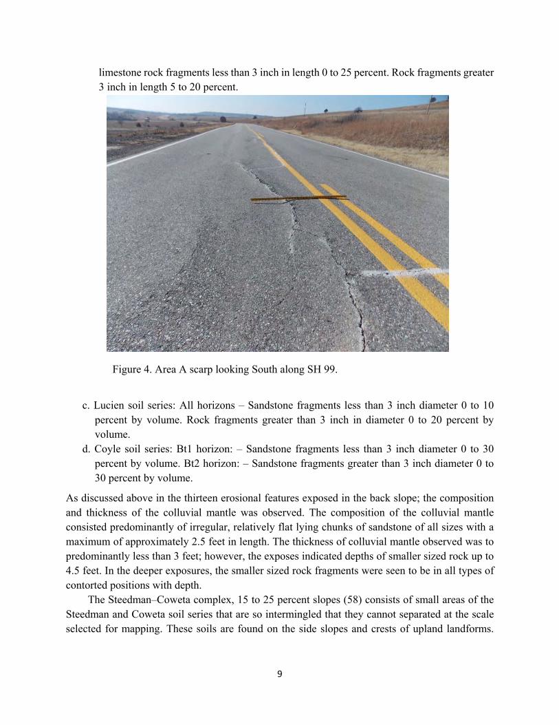
9
limestone rock fragments less than 3 inch in length 0 to 25 percent. Rock fragments greater 3 inch in length 5 to 20 percent.
Figure 4. Area A scarp looking South along SH 99.
c. Lucien soil series: All horizons – Sandstone fragments less than 3 inch diameter 0 to 10 percent by volume. Rock fragments greater than 3 inch in diameter 0 to 20 percent by volume.
d. Coyle soil series: Bt1 horizon: – Sandstone fragments less than 3 inch diameter 0 to 30 percent by volume. Bt2 horizon: – Sandstone fragments greater than 3 inch diameter 0 to 30 percent by volume.
As discussed above in the thirteen erosional features exposed in the back slope; the composition and thickness of the colluvial mantle was observed. The composition of the colluvial mantle consisted predominantly of irregular, relatively flat lying chunks of sandstone of all sizes with a maximum of approximately 2.5 feet in length. The thickness of colluvial mantle observed was to predominantly less than 3 feet; however, the exposes indicated depths of smaller sized rock up to 4.5 feet. In the deeper exposures, the smaller sized rock fragments were seen to be in all types of contorted positions with depth.
The Steedman–Coweta complex, 15 to 25 percent slopes (58) consists of small areas of the Steedman and Coweta soil series that are so intermingled that they cannot separated at the scale selected for mapping. These soils are found on the side slopes and crests of upland landforms.

10
Individual areas of the 58 mapping unit are 15 to 150 acres, and individual areas of each soil series within the map unit range from 4 to 15 acres.
Figure 5. Enlarged soil map from the Web Soil Survey 3.1 indicating the AOI, soil map units, and the beginning and ending of Slide 5.
EOP
BOP
Area A
BOP – Beginning of Slide 5 EOP – End of Slide 5 AOI – Area of Interest
AOI

11
The soil maps in the Web Soil Survey 3.1 have now been integrated with the block diagrams from the NRCS Soil Survey Geographic Database (SSURGO) into Google Earth, and the soil maps in Google Earth are inclusive and show all soil profile data historically found within a soil series map unit. As seen in the block diagrams in Figure 6, soil map unit 58 that underlies the embankment grading consists predominantly of the Steedman soils at approximately 55 percent of the map unit. Including the Foraker soil series shown in Figure 6, map unit 58 consists of approximately 65 percent of soils that develops from a shale parent material mixed with a clayey colluvial mantle with rock and fragments. Other inclusions are the Licien, Coyle, and Rock outcrop at collectively at 35 percent. The rock fragments observed on the ground surface above and below the right of way fence and in the existing eroded features of the side–hill cut–section west of the center line of survey within station extent 379+60 to 390+51 were all observed to be predominantly sandstone.
Soil Map Unit 58 Steedman‐Lucien complex, 15 to 25 percent slopes (SSURGO Export: 2014‐09‐19) Components within map unit 623453 Steedman (55%) Udertic Haplustalfs
hills hillslopes / Backslope
Lucien (20%) Udic Haplustolls
hills hillslopes / Backslope
Coyle (10%) Udic Argiustolls
hillslopes / Backslope hills
Foraker (10%) Udertic Argiustolls
hillslopes / Backslope hills
Rock outcrop (5%)
drainageways / Backslope hills
40 in
35 in
16 in
7 in
20 in
14 in
8 in
4 in
39 in
42 in
31 in
14 in
11 in
48 in
38 in
26 in
11
8 in
80 in
0 in 0 in 0 in 0 in
0 in
Figure 6. Block diagrams of the soils series map unit 58 in SSURGO Export 2014 ‒ 09 ‒ 19.

12
GEOLOGY The Soil Survey of Osage County (April 1979) (5) does not provide a geological map or description of the surface geology other than with the parent geology is following the soil series description. According to the Oklahoma Department of Transportation (ODOT) Engineering Classification of Geologic Materials, Division Eight, 1965 (Red Book) (6), the underlying geology for this site location is the Vamoosa Unit (Pvm).This unit consists predominantly of shale, which contains lenses of massive sandstone and a few limestones. The shale is gray, grayish−green, blue−gray, or maroon, and is silty to clayey. The sandstones are mostly soft to moderately hard, brown to tan, generally 10 to 25 feet or more thick and locally up to about 100 feet thick. Approximately 100 feet above the base of the unit, a 10 to 15 foot thick bed of hard sandstone is present. The thickness of the Vamoosa Unit ranges up to 100 feet. The Oklahoma Geological Survey Hydrological Atlas 7 by Roy H. Bingham and DeRoy L. Bergman, 1991 (7), the geology is recorded as the Vamoosa Group. The Vamoosa Group consists of alternating layers of shale and sandstone, tan to gray, with some thin limestones. The sandstone layers are thicker, coarser grained, and more numerous southward from the Kansas state line. The total thickness of the Vamoosa Group is about 630 feet. The Oklahoma Geological Survey does have a definitive current publication in Circular No. 76, “Shale and Carbonate‒Rock Resources of Osage County, Oklahoma”, by William H. Bellis and T. L. Rowland, 1976 (8), covering the site location. The Circular identifies the formation underlying the site location as the middle of the Vamoosa Formation as described above with the unnamed shale beds but five named sandstone marker beds. The Vamoosa Formation geology as described by the ODOT Red Book, Hydrological Atlas 7, and Circular No. 76 is deposited as relatively flat–lying beds, and the residual soil profiles develop on predominantly sloping surfaces.
BORINGS To access the geologic profile through the grading section representative of Area A, Borings 22, 13, 17, 12, 11, 18, and 21 were plotted in a cross‒sectional profile view at station 380+84 designated as profile A–A, see Figure 7. These seven borings were drilled and logged to determine the underlying ground condition and water table within the approximate station extent station 379+60 to 382+16 for Part A by the Materials Division Geotechnical Branch drill crew. These borings were of following three types:
a. Hand auger borings with continuous sampling b. A mix of drill and log and continuously sampled by the Standard Penetration Test (SPT)
to a point of refusal according to the current ASTM standard D 1586 (9) c. Continuously sampled with a SPT split spoon sampler.
A drilling pad at Areas A was constructed of asphalt millings was placed along and in the roadway ditch left and on the embankment slopes right of the existing SH 99 centerline by Osage County ODOT Maintenance crews to facilitate the field exploration. The boring logs are presented in a

13
gINT Version 8i format. For Borings 11, 17, 21, and 22 in profile A–A in Figure 7; the liquid limit, plastic limit, percent passing No. 200 sieve), and moisture contents for the samples tested with depth are reported within the boring log format. The characterization of the Steedman soils series is concentrated in Borings 21, 13, and 22. In these borings the Steedman soil series can be characterized as an over–consolidated, stiff and blocky structured with slickensides, high plasticity, and a dominantly moist residual soil with a thin colluvial mantle containing predominantly sandstone gravels and fragments in the upper horizons. Note that the residual clay is deeper than the attached Steedman soil series profile in Boring 21, and the difference can be explained in that Steedman pedon can have a BC horizon. Similarly in Borings 13 and 22 have deeper soil profiles. In Boring 13, the consistency of the underlying soil materials is gauged by the SPT N values with depth, and ranges from soft to very stiff. For borings 21 and 22, the consistency was gauged by the ASTM D 2488 Table 5 criteria where the range was also found to be from soft to very stiff. Attention was paid to structure description with depth in these Borings 21, 13, and 22 to detect zones containing slickensides. In drilling Boring 11, sandstone rock fragments and gravels that make up the colluvial mantle were found at the base of the embankment.
LABORATORY TESTING The SPT, grab, and hand auger samples obtained during the field exploration were transferred to the ODOT Materials Division for laboratory processing and testing. The laboratory tests performed on all samples were in accordance with the applicable ASTM test procedures (9) and AASHTO test procedures (10). The laboratory testing schedule included the determination of the natural moisture content (ASTM D 2216), Atterberg limits (ASTM D 4318) and), grain size distribution (ASTM D 422). The Atterberg limits and in‒place moisture contents are recorded in the gINT boring log format. To summarize the Atterberg limits and in‒place moisture contents as per group (compacted fill, residual soil, and underlying geology) with depth for Area A results are tabulated. The liquidity index (LI) is included in the tabulation because determining the natural in situ water content for fine–grained soils and relating it to the plastic and liquid limits provides an indication of soil consistency and/ or sensitivity potential. A LI with a low value or near zero value designates a low sensitivity (a stiff hard consistency), reference Braja M. Das (11). Negative LI values specify a desiccated hard soil. The tabulated LI values for the embankment soils are low with a few negative with depth, and for the residual soils, and underlying shales the LI values are all negative. At the Boring 21 location, an offset hand auger boring (2 feet north) designated as Boring 21A along cross‒sectional profile A‒A for Area A at station 380+84 was made to obtain samples with depth. These additional soil tests with depth were made to further characterize the Steedman soil series profile, and they include the following:
a. Atterberg limits, (ASTM D 4318) b. Clay fraction as determined from hydrometer (ASTM D 422) c. Specific gravity, (ASTM D 854)

14
d. Wet unit weight (AASHTO T 233)
The test results for the Atterberg limits, clay fraction, and wet unit weight from Boring 21A are presented graphically for Boring 21 with depth in Figure 8 and in a tabulated format for Boring 21at the end of the gINT boring logs. A soil profile of the Steedman soil series is attached to the Boring 21 gINT log description in Figure 9.

15
EMBANKMENT GRADING ASSESSMENT The soil parameters that affect compacted fill construction and the long term performance in a compacted fill for the (Steedman, Foraker, Coyle, and Lucien) the soil series from map units 58 are discussed as to their contribution to the causes of the embankment instability. The soils underlying the embankment grading assessment are the inclusive soil series found in the NRCS SSURGO map unit in Figure 6 for map units 58. A summary of the soil taxonomy is presented in Table 1. The characteristics and ratings are taken from the following:
Official Soil Description (OSD) Soil Survey of Osage County (April 1979) Web Soil Survey 3.1 local roads and streets extended soil data Soil taxonomy of the soil series in the Steedman–Coweta complex, 15 to 25 percent slopes
(58) Based on summary of all of the characteristics and ratings listed above the following summary
of factors for the (Steedman, Foraker, Coyle, and Lucien) soil series should have been considered in the construction grading:
1. The low strength for the (Steedman, Foraker, and Coyle) soil series is attributable to the depth of the colluvial mantle discussed above and a mollic epipedon depths reported in the soil taxonomy.
2. The shrink–swell potential for the Steedman and Foraker soil series 3. The shrink–swell potential for the Steedman and Foraker soil series 4. The Lucien and Coyle soil series are susceptible to perched water tables and/or wetness at
some periods of the year. 5. The Steedman and Foraker soil series have large stones. 6. The Steedman soil series has depth to a saturated zone due to a perched water table within
one foot of the ground surface during the months of November to March.
CREEP EVIDENCE Site specific photographs indicative of creep movement are seen in Figure 10. Creep is the imperceptibly slow steady downward movement of slope forming soil or rock. Movement is caused by the shear stress sufficient to produce permanent deformation but too small to produce a shear failure. Creep is also significantly influenced by the shrink–swell associated with the Steedman–Coweta complex, 15 to 25 percent slopes (58) map unit. The three types of creep recognized are as follows:
Seasonal – Where movement is within the depth affected by seasonal changes in soil moisture and soil temperature.
Continuous – Where the shear stress continuously exceeds the strength of the material. Progressive – Where slopes are reaching the point of failure as in other types of mass movement.
An approximate rate of slope movement is estimated from Figure 10. Here an ODOT standard right of way marker with a total nominal length of (4 ft – 6 in) embedded 3.2 feet into the ground

16
has moved out of plumb 0.9 foot over approximate 80 years of being in place. The rate of slope movement calculates to about 1.32 in/yr. The rate of the slope movement is judged to have been relatively slow.

17

18
3.33
Figure 9. Boring 21 gINT log and adjacent Steedman soil series profile.
Steedman Soil Series 0 Ft
3.33 Ft
0.58 Ft
1.33 Ft
2.92 Ft
A Horizon
Bt1 Horizon
Bt2 Horizon
Cr Horizon

19
Figure 10. Right of way marker leaning.
CONCLUSION The conclusions reached in this landslide investigation are based the site inspection, borings, soil property development, applied slope modeling, and analysis for back‒calculation of slope stability are as follows:
1. The root cause of the embankment distress is that the roadway alignment was constructed on a landform that is subject to creep movement. The very slow slope movement of approximately multiple translational types is occurring on a complex of old slip surfaces in the colluvium. The SH 99 embankment grading across the cuesta slope further stresses the colluvial sediment. The classification was determined to be a very slow compound seasonal to continuous soil creep flow based on the Varnes (1978) criteria (12).
2. The geomorphology of the hillside slope underlying the SH 99 alignment at the Slide 5 extent as determined by hand auger, SPT, and drill and log borings and the thirteen drainage way exposures in the back slope consists of an irregular and variable zone termed a

20
colluvial mantle. The colluvial mantle consists of the Steedman soil series A horizon and parts and/or all of the Bt1 and Bt2 horizons.
3. The soil properties in the colluvial mantle are reasoned to have approached a residual shear strength state of stress within the underlying Steedman soil series profile, based on the back–calculated residual friction angle (Фr') values from the slope stability analyses and the Stark and Hussain (2013) correlations (13).
4. The ground water was found to be erratic at the time of the investigation which leads to conservative water table case scenarios, but perched high water tables have most likely influenced the slope instability. The assumed water tables applied in the slope stability analyses does not seem to impact the back–calculated residual friction angle (Фr') values.
REFERENCES
1. Kenneth S. Johnson and Kenneth V. Luza, ''Earth Sciences and Mineral Resources of Oklahoma'', Oklahoma Geological Survey Educational Publication 9, Oklahoma Geologic Survey, Norman, Oklahoma, 2008.
2. Keith Turner and Robert L. Schuster, Transportation research Board Special Report 247, ''Landslides Investigation and Mitigation'', A., National Research Council, National Academy Press, Washington, D.C., 1996.
3. United States Department of Agriculture (USDA) Natural Resources Conservation Service (NRCS) Web Soil Survey 3.1, Washington D.C., 2013.
4. Keys to Soil Taxonomy, 12th Edition, United States Department of Agriculture (USDA) Natural Resources Conservation Service (NRCS) Web Soil Survey 3.1, Washington D.C., 2014.
5. Soil Survey of Osage County, United States Department of Agriculture (USDA) Natural Resources Conservation Service, April 1979.
6. L. D. Buie, Oklahoma Highway Department, ''Engineering Classification of Geologic Materials, Division Eight'', Research and Development Division, 1965.
7. Roy H. Bingham and DeRoy L. Bergman, ''Oklahoma Geological Survey Hydrological Atlas 7 '', Second Printing, 1991.
8. Oklahoma Geological Survey, Circular No. 76, “Shale and Carbonate‒Rock Resources of Osage County, Oklahoma”, by William H. Bellis and T. L. Rowland, 1976
9. 2011 Annual Book of ASTM Standards, Section 4, Construction, Volume 04.08. 10. American Association of State highway and Transportation Officials, Standard
Specifications Part 2B: Tests, 2010. 11. Braja M. Das, ''Principles of Geotechnical Engineering'', 7th Edition, Cengage Learning, Stamford CT, 2011. 12. Varnes, D. J.,''Slope Movement Types and Processes in Landslide Analysis and Control
'', Special Report 176, Transportation Research Board, Washington D.C., 1978. 13. Stark Timothy D. and Hussain, Manzoor, ''Empirical Correlations: Drained Shear
Strength for Slope Stability Analyses'', Journal of Geotechnical and Geoenvironmental Engineering, American Society of Civil Engineering, Vol. 139, No.6 , June 01, 2013, pp 853‒862.

Value Engineering The SunBelt Rentals Equipment Yard Rehabilitation
John C. Folts, PE (NY) Engineering Business Manager
TenCate Geosynthetics 1 Hall Avenue
Latham, NY 12110 (518) 728-8031
Prepared for the 67th Highway Geology Symposium, July, 2016

67th HGS 2016: Folts 2
Acknowledgements
The author would like to thank the individuals/entities for their contributions in the work described:
SunBelt Rentals Sargent Corp.
Chip Haskell - CES, Inc. Bob Martino – Mfg. Rep. TenCate Geosynthetics
Jason Potter & Glenn Cohen – A.H. Harris & Sons, Inc.
Disclaimer
Statements and views presented in this paper are strictly those of the author, and do not necessarily reflect positions held by their affiliations, the Highway Geology Symposium (HGS), or others acknowledged above. The mention of trade names for commercial products does not
imply the approval or endorsement by HGS.
Copyright Notice
Copyright © 2016 Highway Geology Symposium (HGS)
All Rights Reserved. Printed in the United States of America. No part of this publication may be reproduced or copied in any form or by any means – graphic, electronic, or mechanical,
including photocopying, taping, or information storage and retrieval systems – without prior written permission of the HGS. This excludes the original author.
67th HGS 2016: Folts 3
ABSTRACT
The equipment yard of the Sunbelt Rentals Equipment Agency in Bangor, ME needed a complete rehabilitation. The aggregate surfaced parking areas and drive lanes had been completely contaminated by the saturated clay subgrade soils. The owners had no place for the high groundwater to go, making the site a muddy mess during the spring thaw as the heavy construction equipment traveled across the parking areas.
The owner’s original plan was to remove and replace 12 inches of the clay mixed aggregate with a dense graded aggregate (DGA). After performing test pit excavations and dynamic cone penetrometer tests, the subgrade was found to have a California Bearing Ratio (CBR) of approximately 1.2%. This CBR value was extremely weak and would actually require approximately 32 inches of DGA to stabilize it. A value engineered alternative utilizing 2 layers of high strength geotextiles, an 8-inch layer of clean (open graded) stone and a 6-inch layer of DGA was determined to be the most economical solution. The use of the high strength geotextiles helped separate the subgrade and aggregate during construction and added reinforcing strength that will be maintained for the life of the section.

67th HGS 2016: Folts 4
INTRODUCTION
SunBelt Rentals is a company that rents all sorts of equipment for construction projects. The SunBelt Rentals storage yard in Bangor, ME was deteriorated to the point where the equipment was constantly rutting the ground surface and getting stuck in the mud during the Springtime (figure 1). They would routinely have to pull their rental equipment out of the mud and wash off the tires and tracks before renting. During the Spring they would have to load the equipment on the paved surface to keep the tractor trailers from having to drive on the unpaved areas. The owner contacted Sargent Corp., a local contractor, to rebuild the parking/loading and drive areas. They were hoping Sargent Corp. would be able to utilize a typical section of 12 inches of dense graded aggregate (DGA) over a light weight slit tape geotextile.
Figure 1 – Rutted Aggregate Surface
After performing test pit excavations and dynamic cone penetration tests, it was
determined that the proposed section would not be adequate for the heavy traffic loads. The subgrade consisted of approximately 18 inches of aggregate that had become mixed with clay over the years. Beneath the aggregate was saturated, gray silty clay. The dynamic cone penetrometer readings indicated the silty clay soils could have a CBR (California Bearing Ratio)

67th HGS 2016: Folts 5
value as low as 1.2%. Groundwater was also encountered at shallow depths making over excavation difficult. Under drains were not a viable option as there was no place to daylight.
DESIGN
A value engineered solution was sought after with the test pit excavations revealing gray, saturated, extremely low CBR, silty clay soils beneath the 18 inches of clay mixed aggregate. Unpaved road analyses were completed using the Giroud-Han geosynthetic reinforced design method for unpaved roads. The analyses showed that an unreinforced road section would require as much as 32 inches of undercut replaced with DGA to stabilize the subgrade.
The value engineered solution indicated that a section utilizing two layers of high
strength geotextiles (figure 2) and a total reduced section of 14 inches of aggregate would be sufficient. A high strength wicking geotextile was also evaluated, but with no place to drain the water, it was quickly passed over. Geogrids were also dismissed as separation was determined to be extremely important with such a low CBR value. The chosen design was to place the highest strength geotextile directly on the subgrade followed by 8-inches of open graded stone. The open graded stone was designed to help with water storage during the Spring thaws. A second layer of high strength geotextile (the lower strength of the two) was then placed perpendicular to the first layer. This was done to make sure there were no seams aligned that could potentially cause a failure. The wearing surface of the equipment yard was designed to be 6-inches of DGA.
Figure 2 – Two Layered Section

67th HGS 2016: Folts 6
The geotextiles used (TenCate Mirafi® RS280i and RS580i) were chosen based on their high tensile modulus (30,000 and 51,000 lbs/ft) at 2% strain, high flow rates (70 and 75 gal/min/ft2), high interaction coefficient (.89 and .90) and the pore size distribution at 050 (196 and 185 microns) and 095 (345 and 350 microns). The interaction of these four parameters are key factors in its superior performance.
CONSTRUCTION
Construction began with the excavation of approximately 14 inches of the existing clay contaminated aggregate. A layer of high strength geotextile was placed directly on the subgrade with a 3-foot overlap (figure 3). The large overlap was necessary due to the low CBR soils encountered. The geotextile roll widths utilized were 17 feet, which helped to reduce waste in the overlaps. The 8-inch layer of clean, open graded stone fill was then placed (figure 4) and compacted with a smooth drum, vibratory roller. At the time of construction, the subgrade was dry making it easier to install without causing deep ruts.
Figure 3 – High Strength Geotextile with 3-Foot Overlap
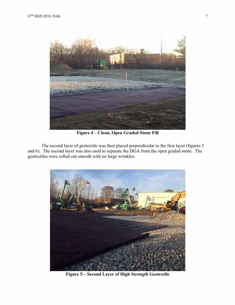
67th HGS 2016: Folts 7
Figure 4 – Clean, Open Graded Stone Fill
The second layer of geotextile was then placed perpendicular to the first layer (figures 5 and 6). The second layer was also used to separate the DGA from the open graded stone. The geotextiles were rolled out smooth with no large wrinkles.
Figure 5 – Second Layer of High Strength Geotextile

67th HGS 2016: Folts 8
Figure 6 – Second Layer of High Strength Geotextile
The DGA was placed on top of the second layer of high strength geotextile making sure the dozer pushed it in the direction of the overlap (figure 7) to minimize wrinkling and bunching of the geotextile. The final grade was also compacted using the smooth drum, vibratory roller.
Figure 7 – Dense Graded Aggregate Fill

67th HGS 2016: Folts 9
The project was accomplished in two phases to allow for moving the equipment out of the way. Upon completion of the two layered section, the equipment was immediately able to be parked on the DGA surface (figure 8).
Figure 8 – Finished DGA Surface (Equipment Parking Area)
CONCLUSION
Construction of the new parking/loading area and drives lanes was completed in the Fall of 2015. A site visit was made at the end of the Spring of 2016 to observe the rental yard surface. During the visit very little surface rutting and no “bird bath” depressions were observed (figure 9). The owner was very pleased with the results and the equipment operator could only say “Unbelievable..Unbelieveable!”
SunBelt Rentals is now able to load the equipment (figure 10) in the yard again with no
issues thanks to the use of the high strength geotextile reinforced DGA surfaced area that was constructed.

67th HGS 2016: Folts 10
Figure 9 – Finished DGA Surface (Drive Area)
Figure 10 – Finished DGA Surface (Loading Area)
The value engineered solution utilizing the 17-foot wide high strength geotextiles proved to be the most economical alternative to the traditional methods of undercutting and using low strength separation geotextiles.

67th HGS 2016: Folts 11
REFERENCES:
1. Giroud, J.P. and Han, J. “The Giroud and Han design method for geosynthetic-reinforced unpaved roads, Part 1: The method development and its calibration”, Geosynthetics, Vol. 30, No. 1, 2012, pp. 40-49.

Logistics and Considerations Surrounding Opening Glenwood Canyon
after a Major Rockfall Event
Cameron Lobato, P.E., P.Eng. GeoStabilization International
P.O. Box 4709 Grand Junction, CO 81502
(855) 579-0536 [email protected]
Prepared for the 67th Highway Geology Symposium, July, 2016
67th HGS 2015: Cameron Lobato 2
Acknowledgements
The author would like to thank the individuals/entities for their contributions in the work described:
Ty Ortiz, Geohazards Program Manager– Colorado Department of Transportation Nicole Oester, Geotechnical Engineer – Colorado Department of Transportation
Roger Phil, Senior Geologist – Golder Associates, Inc. Paul Martinez, President -- Martinez Excavating
Rampart Helicopters IDSNA—Radar Monitoring of Slope
John Vincent, Blaster – Yenter Companies
Disclaimer
Statements and views presented in this paper are strictly those of the author(s), and do not necessarily reflect positions held by their affiliations, the Highway Geology Symposium (HGS), or others acknowledged above. The mention of trade names for commercial products does not imply
the approval or endorsement by HGS.
Copyright Notice
Copyright © 2016 Highway Geology Symposium (HGS)
All Rights Reserved. Printed in the United States of America. No part of this publication may be reproduced or copied in any form or by any means – graphic, electronic, or mechanical, including
photocopying, taping, or information storage and retrieval systems – without prior written permission of the HGS. This excludes the original author(s).

67th HGS 2015: Cameron Lobato 3
ABSTRACT
This presentation highlights the efforts of those involved in opening I-70 through Glenwood Canyon after the February 15, 2016 rockfall event. Clearing rocks from the roadway is just one small step in what it takes to ensure traveller safety to the point of reopening the road. Blasting of boulders and trucking them away was not the number one priority on this emergency project. First, the slope had to be assessed for rocks that remained precarious and in eminent danger of falling to the roadway below. Helicopter access for safety scalers and their equipment was hampered by the weather in the first few days of this project, leaving the crew to pack in air bags, bars, and even compressed air canisters to begin the scaling operations. The interstate was closed to all travellers not working on this slide until the most dangerous rocks could be scaled from the slope. Steel bars, and airbags were used to dislodge the remaining boulders. With a full closure in place, many of the rocks were allowed to roll to both the West and Eastbound lanes of I-70. Some of the rocks came to rest in the lower deck or Eastbound lanes and still others made it all the way to the Colorado River, even with some temporary rockfall fences in place. With the opening of the interstate to intermittent traffic, further measures were taken to limit the continued destruction of the travel lanes and prevent large boulders from coming to rest in the eastbound lanes. Rocks in the lower deck would further delay reopening of the interstate to even limited traffic. After traffic was released in both directions on the Eastbound lanes, the work continued to stabilize areas of nested boulders that were not scaled down. This included cable lashing and netting to confine the nested boulders and prevent initiation of more rockfalls. This subsequent work required close coordination with the traffic flow in order to continue the use of the helicopter to assist in this work. Flight rules do not allow suspended loads under a helicopter with traffic below. Therefore, although traffic was released, there was still a need for intermittent stoppages of traffic during flights for tools and materials.

67th HGS 2015: Cameron Lobato 4
INTRODUCTION
Ever since Interstate 70’s construction was completed through the Glenwood Canyon along the Colorado River in 1992, this portion of the Interstate system has faced many challenges with regard to rockfalls. February 15, 2016 proved to be another one of these challenging closures for the Colorado Department of Transportation (CDOT). It is estimated that $1 Million dollars of interstate commerce through Glenwood Canyon is directly or indirectly affected each day the Interstate is closed
The only shortest suitable detour around the canyon is to go north to Highway 40 through Steamboat Springs then south again back to Interstate 70 (see Figure 1). This detour adds 138 miles and at least 3 hours to the trip between Wolcott, CO and Rifle, CO. That is until these 2-lane highways are flooded with the entire traffic load from each direction of the Interstate in which case the drive times are much longer than those given by typical navigational apps and devices.
Figure 1. Detour Map
The project site is located at Mile Post 124, approximately 8 miles east of Glenwood
Springs, Colorado (see Figures 2 &3 ). This particular rockfall event struck a car and immobilized a semi tractor-trailer. Although nobody was injured in the rockfall, the decks of both the Eastbound and Westbound lanes were heavily damaged. Some of the large rocks even came to rest on the south bank of the Colorado River.

67th HGS 2015: Cameron Lobato 5
Figure 2 – Vicinity Map (Google Earth 2016)
At 5:16 pm on February 15, GeoStabilization International (GSI) was called to assist
CDOT to scale the remaining unstable rocks, stabilize other rocks as needed, as well as to break down large boulders and remove fallen and scaled material. By 10:00 am the next morning GSI scalers ascended the slope with CDOT to begin assessing the imminent dangers and formulating a plan for mitigation.
Prior to scaling the slope, a Geohazard Slope Assessment was conducted to identify hazards and classify the slope access. The rating system used is relatively new and is being promoted and adopted by the Association of GeoHazard Professionals (AGHP). This slope was rated at a 5, given its geometry, rock size, chute orientation and geometry as well as many other factors related to the Geohazard Slope Assessment. This meant that the highest level of care and experience would be required to identify the rockfall hazards and begin work on this site. Such a rating system is somewhat analogous to a Job Hazard Analysis or JHA that is typically used to identify and communicate any particular hazards of a job site to the workforce involved.
The goal for all involved at this point was to safely remove the most immediate rockfall threats of subsequent rockfall in the immediate work zone and reopen the interstate again as soon as possible.

67th HGS 2015: Cameron Lobato 6
Figure 3 – Project Slope (Google Earth 2016)
LITHOLOGY OF GLENWOOD CANYON
The Sawatch Quartzite forms sheer cliffs 400 to 500 feet high in Glenwood Canyon, and cliffs nearly as high in the canyons of Deep, Grizzly, and Canyon Creeks, and the South Fork of the White River. The 75-foot dolomite unit forms a notch or shoulder in the cliffs and supports a scant growth of pine trees and many shrubs. The contact of the formation with the underlying Precambrian rocks is sharp at the few places where it is exposed. The boundary between the Sawatch Quartzite and the overlying Dotsero Formation is defined by relatively thick beds of quartzite below, and shale and thin beds of dolomite above.1 The unstable area at the site initiated in the Precambrian Granodiorite. Continued erosion and freeze-thaw cycles dislodge blocks causing the hazardous rockfall events in this canyon. Many of these rocks that have fallen over time have not made it all the way to the interstate, but rather collected as a jam in various chutes. These rock jams create a very serious hazard to mitigate. In the case of this particular rockslide, the challenge was deciding which rocks to remove by scaling and which of the nested rocks or groups of rocks to stabilize in place.
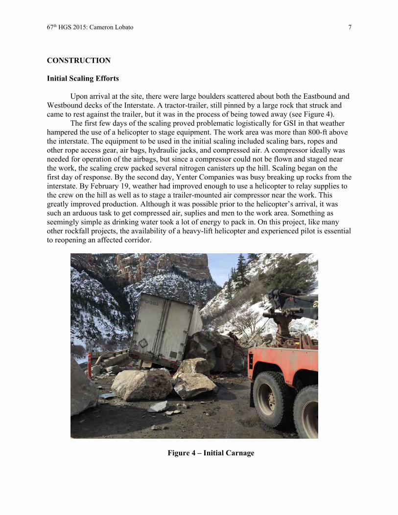
67th HGS 2015: Cameron Lobato 7
CONSTRUCTION Initial Scaling Efforts Upon arrival at the site, there were large boulders scattered about both the Eastbound and Westbound decks of the Interstate. A tractor-trailer, still pinned by a large rock that struck and came to rest against the trailer, but it was in the process of being towed away (see Figure 4).
The first few days of the scaling proved problematic logistically for GSI in that weather hampered the use of a helicopter to stage equipment. The work area was more than 800-ft above the interstate. The equipment to be used in the initial scaling included scaling bars, ropes and other rope access gear, air bags, hydraulic jacks, and compressed air. A compressor ideally was needed for operation of the airbags, but since a compressor could not be flown and staged near the work, the scaling crew packed several nitrogen canisters up the hill. Scaling began on the first day of response. By the second day, Yenter Companies was busy breaking up rocks from the interstate. By February 19, weather had improved enough to use a helicopter to relay supplies to the crew on the hill as well as to stage a trailer-mounted air compressor near the work. This greatly improved production. Although it was possible prior to the helicopter’s arrival, it was such an arduous task to get compressed air, suplies and men to the work area. Something as seemingly simple as drinking water took a lot of energy to pack in. On this project, like many other rockfall projects, the availability of a heavy-lift helicopter and experienced pilot is essential to reopening an affected corridor.
Figure 4 – Initial Carnage

67th HGS 2015: Cameron Lobato 8
To help minimize damage to the upper deck (Westbound) and the lower deck (Eastbound) during scaling operations, temporary movable rockfall barriers were provided by CDOT and placed by GSI (see Figures 5 - 6). These barriers, no doubt minimized some further destruction to the interstate’s decks and parapets during scaling, but many of the rocks proved to be too big and generated too much energy for the barriers. Most of the barriers were badly damaged and some of the barriers were breached by larger rocks. This was good information to have since there was a lot of pressure to open the interstate to traffic in any capacity. Without the assurance that the movable barriers would keep rocks from reaching the lower deck, the decision was made to keep scaling the worst of the potential rocks that might otherwise fall on their own before allowing any traffic to pass the work area.
On February 22, with continued pressure to get the interstate open, the plan was in place to get the most threatening rocks scaled. Traffic would be piloted each way running one lane of traffic alternating in each direction from the east side of Hanging Lake tunnel to the Grizzly Creek rest area.
Figure 5 – Moveable Barriers Before Scaling
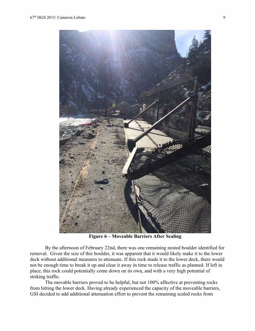
67th HGS 2015: Cameron Lobato 9
Figure 6 – Moveable Barriers After Scaling
By the afternoon of February 22nd, there was one remaining nested boulder identified for
removal. Given the size of this boulder, it was apparent that it would likely make it to the lower deck without additional measures to attenuate. If this rock made it to the lower deck, there would not be enough time to break it up and clear it away in time to release traffic as planned. If left in place, this rock could potentially come down on its own, and with a very high potential of striking traffic.
The movable barriers proved to be helpful, but not 100% affective at preventing rocks from hitting the lower deck. Having already experienced the capacity of the moveable barriers, GSI decided to add additional attenuation effort to prevent the remaining scaled rocks from

67th HGS 2015: Cameron Lobato 10
reaching the lower deck. GSI and Martinez Excavating collaborated to use two of Martinez’s tandem axle dump trucks to act as end posts for 150-LF of ring net to contain larger rocks (see Figure 7). Both GSI and Martinez knew the risks of the strategy, but were collectively willing to take that risk in order to release traffic. Rockfall behavior can be unpredictable as was observed in this case. The rock was released from the slope and with it, brought smaller rocks along the way. All of the rocks were caught or attenuated by either the ring net or the movable barriers. One large rock, however, climbed out of the fall line and struck one of the trucks. This was one of the larger rocks and it too was prevented from reaching the lower deck just 2 hours before the anticipated opening to escorted traffic. The trucks were unoccupied at the time and the immediate area was cleared during scaling. The truck was a total loss, but the interstate was reopened as planned to one-way, alternating, piloted traffic. Mission accomplished.
Figure 7 – Moveable Barriers and Ring Nets Between Trucks

67th HGS 2015: Cameron Lobato 11
Radar Monitoring of Slope IDS North America (IDSNA) was brought in to set up and monitor the slope for
movement using radar technology. IDS Ingegneria Dei Sistemi is headquartered in Pisa (Italy) with offices in six countries (Italy, UK, Brazil, Canada, USA and Australia) and around 500 employees worldwide. One of the challenges of using such instrumentation was finding a suitable area to place the radar station. This in itself was challenging in Glenwood Canyon given the steep terrain. It was finally decided that the most suitable place for the monitoring station was the south side of the Union Pacific tracks. There was a very specific area near the tracks that allowed enough area for the station setup and gave a clear view of the slope to be monitored. Placing this monitoring station presented its own logistical challenges. Not only would permission from the railroad need to be granted in order to place a facility on railroad property, but the railroad maintenance staff would be required to haul and place the cargo trailer that housed the radar station. This cargo trailer was approximately 16-foot by 8-foot single axel cargo trailer (see Figure 8-10). Data collected from this radar station was remotely monitored in real time through cellular data transmission for any large movements that may cause concern for the traffic below. Alarms were established so the team could decide whether or not to reclose the interstate if a subsequent impending large failure could be detected early.
Figure 8 – UPRR and IDSNA offloading radar-monitoring station

67th HGS 2015: Cameron Lobato 12
– Figure 9 Slope as seen from radar station
– – Figure 10 Slope as seen from site

67th HGS 2015: Cameron Lobato 13
Temporary rockfall fence After the initial safety scaling, CDOT had GSI install 140-LF of 500 KJ barrier (see Figure 11) at the bottom of the slope as an added precaution for any smaller rocks that may continue to fall during the continued construction and in anticipation of traffic back on the Westbound (Upper) deck. This barrier also afforded additional protection for the crews repairing the damaged deck structure. This fence was procured and arrived for installation within a couple of days prior to installation. Spotters were also utilized throughout the project to warn workers of any subsequent rockfall.
Figure 11 – 500 kJ Barrier shown behind crews working to repair westbound deck.

67th HGS 2015: Cameron Lobato 14
Final meshing, anchors and instrumentation After the scaling and temporary barrier installation came another tough task. By deciding that some of the nested rocks should be stabilized in place, the logistics of how to accomplish that task was magnified greatly. Scaling required scalers to access the area by ropes and dislodge precarious rocks using bars, air bags and other mechanical means. Stabilization requires, the safety scaling to be perform, but also additional tools, equipment and materials to be flown to the site. The plan was to secure the remaining nested boulders using Geobrugg Spider® Net, rock anchors and cable lashing. Golder Associates formalized the plan and also prescribed strain gauges for the cables associated with the cable lashing. Data was to be collected remotely with data boxes installed near the instrumentation. Each of 2 data boxes required a 1-1/2” diameter galvanized post to be drilled and grouted into rock as well as grounding rods drilled nearby. On helicopter days, the men were short-hauled to and from the work area as well (see Figure 12-13). This meant that men, two at a time, were clipped into the long-line of the helicopter and ferried to the work area to avoid the steep, time-consuming climb and allowed them to be more productive on anchor and mesh installation. A total of 20 each ¾”, 10-ft long wire rope anchors (see Figures 14-16) and 9,800 square feet of Spider® Net were installed. All of these materials and all of the tools required to install were ferried by helicopter to the work area.
Figure 12 – Short-Haul to Work Area

67th HGS 2015: Cameron Lobato 15
Figure 13 – Short-Haul to Work Area
Figure 14 – Preparing to drill Anchors

67th HGS 2015: Cameron Lobato 16
Figure 15 – Drilling Anchors
Figure 16 – Drilling Anchors

67th HGS 2015: Cameron Lobato 17
With all of the anchors installed, the mesh was flown to the work area and secured. (See Figues 17-19) The mesh used was Spider® Net from Geobrugg.
– Figure 17 Geobrugg Spider® Net
Figure 18– Final Mesh
Crew
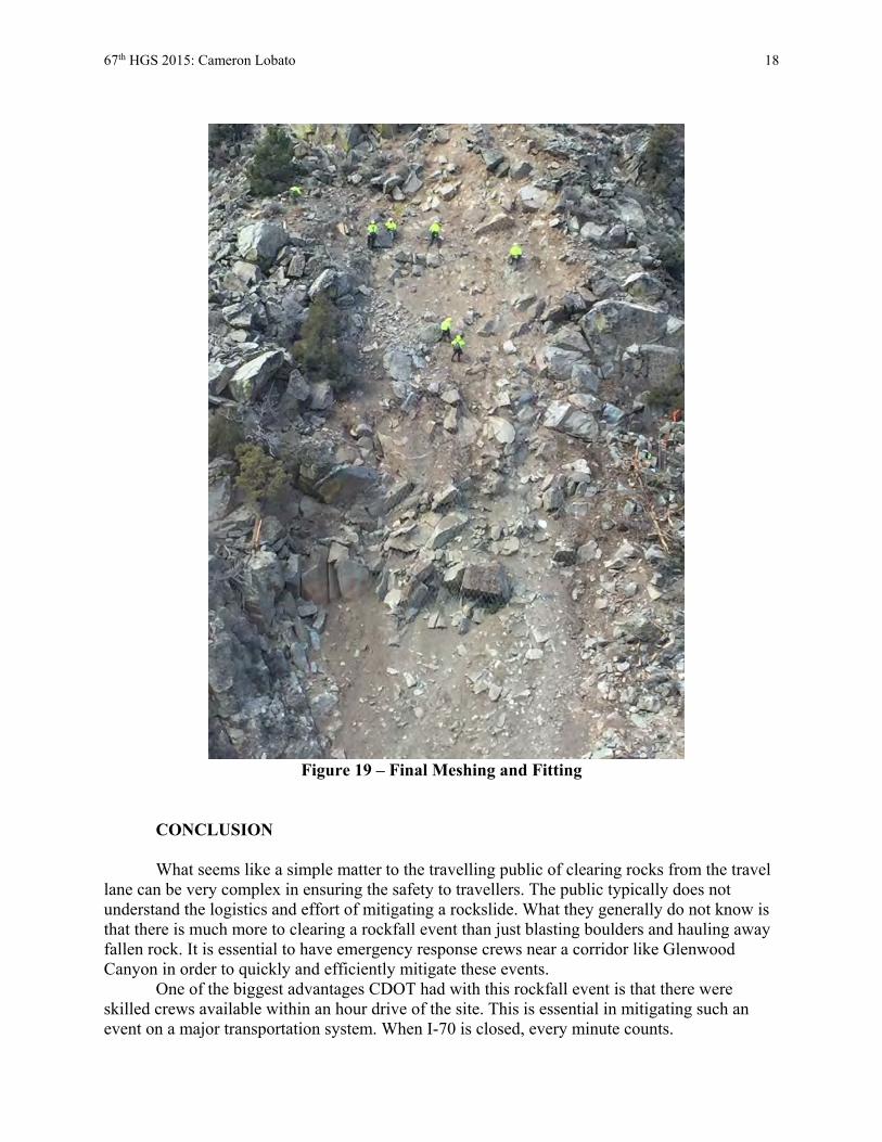
67th HGS 2015: Cameron Lobato 18
Figure 19 – Final Meshing and Fitting
CONCLUSION What seems like a simple matter to the travelling public of clearing rocks from the travel
lane can be very complex in ensuring the safety to travellers. The public typically does not understand the logistics and effort of mitigating a rockslide. What they generally do not know is that there is much more to clearing a rockfall event than just blasting boulders and hauling away fallen rock. It is essential to have emergency response crews near a corridor like Glenwood Canyon in order to quickly and efficiently mitigate these events.
One of the biggest advantages CDOT had with this rockfall event is that there were skilled crews available within an hour drive of the site. This is essential in mitigating such an event on a major transportation system. When I-70 is closed, every minute counts.

67th HGS 2015: Cameron Lobato 19
One of the biggest disadvantages to this rockfall event in Glenwood canyon is our dependence on the use of helicopters to make the mitigation efforts more efficient. While it is possible to hike in tools and compressed air by hand, the helicopter is much quicker in tool placement and placement of compressors near the work. When weather prohibits flight, we are left with brute-force manual methods. Additionally, having no easy detour around Glenwood canyon makes for a very thankless position in the eyes of the travelling public. Some understand, but many still think it is just a matter of clearing rocks from the roadway, without regard of knowing what it takes to stabilize the slope.
We can never prevent all rockfall from happening in the canyon, but we can safely manage events such as this one. Experienced crew with specialized equipment are necessary in being able to mitigate geohazards. Although the helicopter was eventually a critical component to this project, weather prevented its use in the first few days. Being able to hike in the compressed air for the air bags allowed the crews to get started with the scaling despite the grounded helicopter.
This project was successful given the amount of cooperation from all of the parties involved. Constructability, collaboration and logistics were key in opening the interstate as soon as it did. Without a knowledgeable staff in the CDOT Geohazards program and the collective efforts of the design and construction team, a project like this could drag on for weeks or worse yet, encounter injury to the crews or the travelling public.
Figure 20 – GeoStabilization International
Rockfall Deployment Crew

67th HGS 2015: Cameron Lobato 20
REFERENCES
1. Bass, N.W. and Northrop, S.A., Glenwood Springs Quadrangle and Vicinity Northwestern Colorado, Geological Survey Bulletin 1142-J, 1963

Utilization of a Geotechnical Asset Management Program – Lessons Learned from a Highway Improvement Project in Alaska
John D. Thornley, PE Golder Associates Inc.
2121 Abbott Road, Suite 100 Anchorage, AK, 99507
(907) 865-2538 [email protected]
Eric C. Cannon, CPG Golder Associates Inc.
2121 Abbott Road, Suite 100 Anchorage, AK, 99507
(907) 865-2525 [email protected]
Prepared for the 67th Highway Geology Symposium, July, 2016

67th HGS 2016: Thornley and Cannon 2
Acknowledgements
The authors would like to thank the Alaska Department of Transportation and Public Facilities – Southcoast Region and HDR Inc. for the opportunity to work with the Geotechnical Asset
Management Program for Alaska:
Mitch McDonald – ADOT&PF-Southcoast Region Lance Mearig, PE – ADOT&PF Statewide Design & Engineering Services
Christopher Croft, PE – HDR Inc.
Disclaimer
Statements and views presented in this paper are strictly those of the author(s), and do not necessarily reflect positions held by their affiliations, the Highway Geology Symposium (HGS), or others acknowledged above. The mention of trade names for commercial products does not
imply the approval or endorsement by HGS.
Copyright Notice
Copyright © 2016 Highway Geology Symposium (HGS)
All Rights Reserved. Printed in the United States of America. No part of this publication may be reproduced or copied in any form or by any means – graphic, electronic, or mechanical,
including photocopying, taping, or information storage and retrieval systems – without prior written permission of the HGS. This excludes the original author(s).

67th HGS 2016: Thornley and Cannon 3
ABSTRACT
Over the past several years, efforts by owners, including State Departments of Transportation, have been initiated to develop asset management databases. One subset of an asset management database that can be challenging to define is that of geotechnical assets. Geotechnical assets include rock slopes, soil slopes, and retaining structures, that can have very long design lives and show few signs of distress for years. For a highway improvement project in Ketchikan, Alaska, the authors used the Geotechnical Asset Management Program (GAMP) provided by the Alaska Department of Transportation and Public Facilities (ADOT&PF) to review the locations and characteristics of unstable rock slopes, unstable soil slopes, and retaining walls along the project alignment. Reviewing this information allowed the authors to prioritize locations for inspection, rock mass and discontinuity surveys, and sample collection. As a result of the baseline geotechnical asset information collected, field efforts were reduced, resulting in cost savings to the ADOT&PF. In addition, using the baseline data, additional data were collected and key locations were identified where future maintenance and capital efforts should be focused. Utilization of the GAMP information for this project also provided ADOT&PF with information that can improve the quality of information collected on future GAMP efforts in Alaska.

67th HGS 2016: Thornley and Cannon 4
INTRODUCTION
An asset management program is an important tool for identifying, characterizing, evaluating, and managing assets. State Departments of Transportation have historically maintained asset management programs only for select infrastructure assets, such as bridges and pavements. In recent years, geotechnical assets have been included in asset management programs for retaining walls and slopes. Geotechnical asset management (GAM) provides the opportunity to develop a uniform approach to managing geotechnical assets as part of an overall integrated transportation asset management program.
In this paper, we present the use of a geotechnical asset management program (GAMP)
provided by the Alaska Department of Transportation and Public Facilities (ADOT&PF) for a highway improvement project in Ketchikan, Alaska. We discuss reviewing the GAM database in preparation for and during completion of the fieldwork, efficiencies in fieldwork gained by using the GAM database, and lessons learned through using the GAMP on this project.
GEOTECHNIAL ASSET MANAGEMENT FUNDAMENTALS
GAM generally consists of four steps: identification, characterization, evaluation, and management. We discuss each of these steps below.
The first step in GAM is to identify the asset. This includes defining the category of the asset (e.g., a particular type of retaining wall). As part of identifying the asset, location is important. With improvements in Global Positioning System (GPS) equipment, it is possible to have highly-accurate location information included in a Geographic Information System (GIS) while in the field observing the asset.
The second step in GAM is to characterize the asset. This includes spatial and geographic characteristics of the asset, attributes of the asset at the location (e.g., length and height of a retaining wall), and temporal information (e.g., year of construction). This information can be recorded in a digital database in the field or on a field form to be entered back at the office.
The third step in GAM is to evaluate the asset. Evaluation systems can be in various forms, with results provided in a ranked format (e.g., good to poor). The evaluation process can be quantitative by using a formula to calculate a value; or qualitative by fitting the asset into a set of pre-defined terms.
By identifying, characterizing, and evaluating geotechnical assets, a lifecycle and condition awareness is developed for the assets that can be used to manage these assets, the fourth step, in terms of operations and maintenance, and to make decisions on whether maintenance or replacement of the assets will be considered as part of improvement projects. GAMP IN ALASKA
The GAMP in Alaska has been led by ADOT&PF through the efforts of Dave Stanley

67th HGS 2016: Thornley and Cannon 5
(retired) and Barry Benko of Statewide Materials. The geographic extent of Alaska and remote nature of the state’s limited road system makes developing and maintaining the GAMP a challenge.
Geotechnical assets identified in Alaska consist of material sources, rock slopes, soil
slopes, retaining walls, and geologic hazards. This information is maintained in a GIS system with the ability to display information through a World Wide Web interface. For example, information regarding rock and soil slopes is available from the Unstable Slope Management Program (USMP) developed by Landslide Technology (AKDOT-USMP, 2016). PROJECT EXAMPLE IN SOUTHEAST ALASKA
The ADOT&PF GAMP is being incorporated into a capital improvement project located on the South Tongass Highway in Ketchikan, Alaska (Figure 1). This project consists of an approximately 3-mile-long segment of highway connecting the communities of Ketchikan and Saxman. The existing highway is a two-lane, asphalt paved road. The road passes through commercial and residential areas, and bisects a United States Coast Guard facility. Current speed limits range from 20 mph to 45 mph. Rock cuts up to approximately 40 feet high are found on the left (northeast) side of the highway. On the right (southwest side) of the highway, a discontinuous pathway is present. Also, several types of short retaining walls, typically less than 10 feet tall, are generally found on the right (southwest side) as the ground surface drops steeply down to the shoreline.
The objectives of this highway improvement project are to reduce horizontal and vertical
curves to improve sight distances, widen the travel lanes, improve turn lanes, improve entrances and exits to the highway, make the pathway continuous, and improve rock slope performance. GEOLOGIC SETTING
The project alignment is located within the “Inside Passage” of southeast Alaska, a series of glacial fjords and channels that result in numerous islands. The glacial fjords and channels often follow faults. The southeast-trending project alignment follows the Tongass Narrows channel, an inferred bedrock fault (Gehrels and Berg, 1992). The bedrock geology of the area consists of Cretaceous and Jurassic volcanic rocks (Gehrels and Berg, 1992). These bedrock units are part of the Gravina Belt, a metamorphic belt located between the Alexander Terrane to the west and the Taku Terrane to the east (Gehrels and Berg, 1988). The Gravina Belt and the Alexander and Taku Terranes record the assembly of southeast Alaska from accretion of geologic terranes to the west coast of North America, metamorphism, and igneous activity.
Bedrock features in southeast Alaska are often a function of extensive glaciation. During the Last Glacial Maximum of the late Pleistocene, ice thickness in the Ketchikan area ranged from 3,000 to 4,000 feet (Coulter and others, 1962). The ice flowed generally to the southwest across the project area. Ice flow produced glacial scour and glacially-eroded bedrock, resulting

67th HGS 2016: Thornley and Cannon 6
Figure 1 – Location Map of Project Alignment. Images from http://sv.gina.alaska.edu
in shallow bedrock mantled with a thin, post-glacial veneer of sediments with an organic mat of temperate rain forest vegetation – spruce, hemlock, shrubs, Devil’s Club. In areas of poor drainage, muskeg deposits are present.
The present tectonic setting of the Ketchikan area consists of the Queen Charlotte fault located approximately 100-110 miles to the west of the project area. This fault is a right-lateral, oblique slip plate boundary fault that accommodates approximately 2 inches/year of movement between the Pacific oceanic plate and North American continental plate (Haeussler and Plafker, 2004).

67th HGS 2016: Thornley and Cannon 7
RETAINING WALLS
As stated previously, the current project includes an effort to widen an existing 3-mile section of road. As part of that effort, we were tasked with evaluating the condition of the retaining structures and providing recommendations on their reuse, rehabilitation, or removal. As part of our scoping efforts, we developed a level of effort cost proposal to perform this work. At the same time, a compilation of GAMP efforts in this area were becoming available. Previous GAMP efforts had developed a database of retaining wall locations, wall types, and a snapshot in time condition statement (Landslide Technology, 2015).
In preparation for the project field efforts, we obtained the GAMP for the project area. The information provided in the GAMP included GIS data defining wall locations and table of wall types and ratings. After a cursory review of the GAMP, we were able to reevaluate the level of effort in our cost proposal and reduce the number of field days required for the retaining wall condition assessment.
As part of the current project, we are tasked with answering the question: which walls can stay and which walls will need to be removed and replaced? Performing an initial field assessment is a key step in answering that question. Utilizing the GAMP database for retaining structures offered time savings in that we already knew going into the field where a majority of the retaining walls could be found. We also knew, based on the rating system, which walls we would need to evaluate first (i.e., “poor” rated walls). According to the GAMP database, there were a total of five retaining structures in “poor” condition, 14 retaining structures in “fair” condition, and 27 retaining structures “good” condition in our project area. The database did not include a sheet pile wall that has been included in our discussion.
In all, there are approximately 47 retaining walls along the alignment. The retaining walls generally classify as three types of walls: welded wire walls (Figure 2), soldier pile and wood lagging walls, and a sheet pile wall. Some of the characteristics of those walls are presented in the table below.
Table 1 – General Retaining Wall Inventory
Wall Type Number of Walls Height of Walls Welded Wire 42 0 to 6 feet Soldier Pile 4 0 to 4 feet Sheet Pile 1 5 to 7 feet
The current project aims to improve the roadway corridor for its users. With this there will be a balance of cuts upslope and fills downslope. Because the retaining walls are predominantly downslope, we evaluated the condition of these walls and asked ourselves one overarching question: should the existing walls be removed and replaced as needed, or is there any benefit gained by designing around them and leaving them in place? This question significantly differs from the question an inspector providing a GAM rating is interested in. In general, the GAM rater is interested in a snapshot in time and does not estimate the

67th HGS 2016: Thornley and Cannon 8
Figure 2 – Pathway Above a Welded Wire Retaining Wall that has Moved. remaining longevity of a wall. While this may be in the back of the inspector’s mind, we have rarely seen ratings that discuss the remaining design life of a structure.
Once in the field, we began by visiting the walls rated as “poor” first. From there, we continued to visit the remaining walls identified in the database. We were able to focus our efforts in the field because of the database and found the locations and ratings to be reasonable, especially from an asset management point of view. During our field visit, we took measurements of verticality, length, height, and condition.
While a majority of the walls we observed were in adequate condition to be serviceable for years to come, we found that there were very few retaining walls that should be considered adequate enough to remain in place as part of the current capital improvements project. We noticed that several walls have moved, primarily by rotation, with tension cracks and loss of material observed behind the walls (see Figure 2). These walls may not move further in the next few years, but incorporating them into a new design does not seem cost effective when compared with the risk of further movement.

67th HGS 2016: Thornley and Cannon 9
We do want to make note that, while in this case we do not find it beneficial to the project to design around a majority of the existing retaining structures, the GAM database was a very useful tool to our project. It should also be noted that these retaining walls are rather short, and in other cases, with significantly taller walls, it may be of value to collect years of data to evaluate movements. ROCK SLOPES
For this highway improvement project, one consideration is how existing rock slopes will be incorporated into the new alignment with a wider highway – will these rock slopes need to be modified? In this section, we discuss our use of the GAMP for reviewing rock slopes, and for planning and completing a field program.
Figure 3 – Example of Existing Rock Slope, View Northeast Approximately Perpendicular to Slope. Rectangular Clipboard on Slope is Approximately 1 Foot Tall for Scale. Overall
Rock Slope up to 15-20 Feet in Height.
The bedrock slopes along the proposed alignment consist of a micaceous phyllite, with steeply-dipping foliation to the northeast. The foliation is consistent with the overall structural grain of southeast Alaska resulting from accreted geologic terranes. The general trend of both

67th HGS 2016: Thornley and Cannon 10
the current highway and the proposed alignment is to the southeast. The relationship between the existing southwest-facing rock cut slopes, northeast-dipping foliation, and discontinuity sets results in toppling and wedge failures. Figure 3 provides a typical example of an existing rock cut, with foliations seen steeply dipping to the northeast into the cut as shown in Figure 4. In order to plan for a field program, we reviewed the GAM database in the project area.
Figure 4 – Example of Existing Rock Slope, View Northwest Approximately Parallel to Slope. Rectangular Clipboard on Slope is Approximately 1 Foot Tall for Scale. Note
Foliation Dipping Northeast Steeply Into the Rock Slope. Rock slope information included in the AKDOT-USMP (2016) database for individual
rock slopes consists of a unique milepost identification number, geographic coordinate of the rock slope, estimate of rock slope length and height, a description of the rock slope, condition of the rock slope using a good-fair-poor ranking system, and photographs of the rock slope for a point in time. In addition, hazard and risk factors are quantified. This information provides a base case for each rock slope in the GAM database.
We incorporated the GAM database into our project efforts in two ways. First, we
performed a desktop review of the database to become familiar with the characteristics of the rock slopes along the project alignment. The GAM database provided useful information that we

67th HGS 2016: Thornley and Cannon 11
used to target rock slopes for investigation in the field program. By reviewing the number of rock slopes, spatial extent, and conditions of the rock slopes, we were able to plan the field schedule to make efficient use of field time, resulting in cost savings to the project.
While in the field, we used the GAM database in digital and hardcopy map format to
make field observations at rock slopes. With the field sites already identified during pre-planning, we were able to start making detailed observations and measurements relatively quickly, as opposed to spending significant effort initially locating the rock slopes to be investigated. We used the spatial data related to the rock slopes to investigate site conditions, select locations to perform rock mass and discontinuity surveys, and to narrow down locations to collect bedrock samples for laboratory testing. Incorporating the GAM into pre-planning and fieldwork benefited our field efforts in terms of more efficient schedule and budget, and data collection to support project objectives. LESSONS LEARNED FROM USING THE GAMP We found the ADOT&PF GAM database to be a valuable tool for planning and completing our field investigations. The following are lessons learned from the project:
1. Understanding the Project Setting – The GAM database provides an introduction to assets within the project. In remote areas, information may be limited and the GAM may provide key information not otherwise available. Just as with geotechnical reports and geologic maps, reviewing the GAM database is an important part of the project cycle to learn about project-specific information and site conditions.
2. Pre-Planning – Using the GAM database for project planning offers many benefits. The database can be used to focus efforts, whether in the field or office, on specific assets. Field efforts can be ranked in terms of priority. This can bring efficiency to schedules and reduce project costs.
3. Change Detection – By comparing GAM data with project investigations, one can look for change over time, for example, deterioration of an asset. If change has occurred, factors can be investigated to understand why the change is occurring. If the GAM database contains an initial base case data set, this can be used to investigate change over one time interval. If the GAM database has a time series of data, one can investigate whether change has accelerated at a certain point, or if there are other patterns to the change (e.g., cyclic).
4. Updates to the GAM Database – By using the GAM database as baseline information, additional project-specific information collected can be considered for inclusion into the database. For example, the initial spatial extent of an asset may be refined through more detailed field investigations. Designing the database and having procedures to upload new data will allow the database to contain the most up-to-date information regarding the geotechnical assets. That way, the database is a living document where new project information and periodic updates can be incorporated regarding the geotechnical assets.

67th HGS 2016: Thornley and Cannon 12
SUMMARY
The GAMP offers a valuable tool to identify, characterize, evaluate, and manage geotechnical assets. We used a GAMP provided by ADOT&PF for a highway improvement project in Ketchikan, Alaska, focusing on the retaining wall and rock slope geotechnical assets of the project. We found that the GAM database was beneficial in providing an initial understanding of the assets in the area, assisting with pre-planning including scheduling and budgeting field work, and while conducting the field program. The GAMP contributed to the success of our field program, with data collected supporting the project objectives of improving the roadway corridor for users, and also for future updates to the database. The GAMP will play an important role in transportation projects in Alaska. REFERENCES AKDOT-USMP. AKDOT&PF Unstable Slope Management Program. Landslide Technology. http://akdot-usmp.com. Accessed May 15. 2016. Coulter, H.W., Hopkins, D.M., Karlstrom, T.N.V., Péwé, T.L., Wahrhaftig, Clyde, and Williams, J.R. Map showing extent of glaciations in Alaska: U.S. Geological Survey Miscellaneous Geologic Investigations Map 415, 1962. Gehrels, G.E., and Berg, H.C. A review of the regional geology and tectonics of southeastern Alaska. U.S. Geological Survey Open-File Report 88-659. 1988. Gehrels, G.E., and Berg, H.C. Geologic map of southeastern Alaska. U.S. Geological Survey Miscellaneous Investigations Series Map 1867, 1992. Haeussler, P.J., and Plafker, G. Earthquakes in Alaska. U. S. Geological Survey Open-File Report 95-624, 2004. Landslide Technology. AKDOT Geotechnical Asset Management Program Development – Interim Report – Draft. July 6, 2015.

Attenuators for controlling rockfall: first results of a state-of-the-art full-scale testing program
Tim Shevlin, PG Geobrugg North America, LLC
4676 Commercial Street SE Salem, OR 97302
503-423-7258 [email protected]
Duncan Wyllie, P.Eng. Wyllie & Norrish Rock Engineers
850 – 789 West Pender Street Vancouver, BC V6H 1C2
604-418-4617 [email protected]
James Glover, Ph.D.
Geomechanics, Mountain Geohazards, Global Risk Forum GRF Davos, Promenade 35,
CH-7270 Davos Platz, Switzerland
Prepared for the 67th Highway Geology Symposium, July, 2016

67th HGS 2016: Shevlin, Wyllie, and Glover 2
Acknowledgements
The author(s) would like to thank the individuals/entities for their contributions in the work described:
Tina Chen, Alastair Grogan - Wyllie & Norrish Rock Engineers
Jacob Serna – Geobrugg North America, LLC Amelia Hamilton
Emil Anderson Construction
Disclaimer
Statements and views presented in this paper are strictly those of the author(s), and do not necessarily reflect positions held by their affiliations, the Highway Geology Symposium (HGS), or others acknowledged above. The mention of trade names for commercial products does not
imply the approval or endorsement by HGS.
Copyright Notice
Copyright © 2010 Highway Geology Symposium (HGS) All Rights Reserved. Printed in the United States of America. No part of this publication may be
reproduced or copied in any form or by any means – graphic, electronic, or mechanical, including photocopying, taping, or information storage and retrieval systems – without prior
written permission of the HGS. This excludes the original author(s).

67th HGS 2016: Shevlin, Wyllie, and Glover 3
ABSTRACT
Rockfall attenuator systems are becoming one of the more popular systems for rockfall
mitigation. These systems are proven to be effective; however, full-scale testing with instrumentation has not been performed to the level of traditional rockfall barriers.
A joint testing program is being carried out by Wyllie & Norrish Rock Engineers Ltd.
and Geobrugg North America, LLC to measure and validate the performance of hybrid attenuator rockfall nets. A preliminary round of full-scale testing was performed in January 2015 and was continued with an extensive program in 2016 at the Nicolum Quarry in Hope, BC. The tests were documented with a high speed camera, load cells on the support cables, and rock motion sensors in the steel reinforced concrete cubes. This paper will present more detailed results of the extensive 2016 program where 84 rocks were rolled into different attenuator systems.

67th HGS 2016: Shevlin, Wyllie, and Glover 4
INTRODUCTION
Rockfall attenuator systems are becoming one of the more popular systems for rockfall mitigation in North America. They have been used successfully for a number of years, but the geometric variation of attenuator systems is broad and often site specific. Due to this, among other reasons, standard rockfall barrier testing guidelines are not applicable and performance benchmarks for attenuators do not exist.
With these challenges in mind, a state-of-the-art, full-scale joint testing program was
carried out by Wyllie & Norrish Rock Engineers Ltd. and Geobrugg North America, LLC to measure and validate the performance of hybrid attenuator rockfall systems. A preliminary round of full-scale testing was performed in 2015 and was continued with an extensive program in 2016 at the Nicolum Quarry in Hope, British Columbia, Canada. The testing series were documented with a high speed camera, load cells on the support cables, and rock motion sensors in steel reinforced concrete cubes. This paper will present initial results of the extensive 2016 program where 84 rocks were rolled into different attenuator systems.
As part of this testing program a tremendous amount of rockfall trajectory and attenuator
system loading data has been collected. To date a select number of the individual rock rolling experiments have been analyzed to determine the change in rockfall velocity and trajectory, and to evaluate the attenuator-rock interaction. The objective of the testing and analysis is to evaluate attenuator netting system performance and begin to develop an attenuator design methodology and performance criteria. This paper summarizes the continued findings of the joint testing program. ROCKFALL BARRIERS, DRAPERY SYSTEMS AND ATTENUATOR SYSTEMS
Flexible rockfall barrier systems are a protection measure that intercept falling rocks and
dissipate the rockfall impact energy through total system deflection until the rock has stopped. Another very common rockfall mitigation measure is a rockfall drapery system that has been employed since at least the 1950s in North America (Badger and Duffy, 2012). Rockfall draperies are passive mesh systems placed over the entire area where rockfall is anticipated in order to control the descent of falling rocks directing them to a planned catchment area at the base of the slope or mesh terminus (Badger and Duffy, 2012; Muhunthan et al., 2005; Wyllie and Norrish, 1996; Bertolo et al., 2007; Andrew, et al., 2011).
Rockfall attenuator systems do not completely halt falling rocks, but intercept the rockfall
trajectory and guide it under a tail drape (Figure 1 and 2). Attenuators are a combination of traditional rockfall barriers and draped net systems. The principal function of rockfall attenuator systems is to absorb only a portion of the impact energy and redirect the rock into the ground at the base of the slope where the rock is contained. In this way, the kinetic energy is only partially dissipated through barrier impacts deforming the netting and interaction with the slope during its passage to the base of slope (Glover et al., 2011). Attenuator systems hybridize the best features of both a traditional rockfall barrier and a slope drapery system. Hybrid drapery (attenuators) addresses rockfall source areas, both underneath and upslope of the installation, and controls the

67th HGS 2016: Shevlin, Wyllie, and Glover 5
rock’s descent under the mesh, combining the performance of standard unsecured draperies and flexible rockfall fences. (Fish et al., 2012; Eliassen, 2011; Badger et al., 2008).
Figure 1: Sketch of typical post supported attenuator system Vimp = impact velocity; Vexit = exit velocity (Image, J. Glover).
Figure 2: Catchment area of attenuating structure (left) and guided boulder along rock face (right) from Glover et al., 2012.
Standard North American attenuator systems typically exclude internal, side or bottom anchoring of the fabric, allowing for controlled deformation of the fabric and attenuation of the rockfall trajectory to the base of the installation (Fish et al., 2012). Similar to drapes, the tail of the netting is open, allowing the rocks to pass through the system while reducing their velocity and controlling their trajectory (Mumma, 2012). Rockfall attenuators are intended as low maintenance passive barrier systems (Glover et al., 2010; Badger et al., 2008).

67th HGS 2016: Shevlin, Wyllie, and Glover 6
Attenuator variations can include having the net partially restrained with vertical cables at
the net edges to contain rockfall impacts at the boundaries and to maintain the net width. Another variation includes an optional horizontal bottom cable at the base of the structural netting. Theoretically with this the horizontal deflection of the net is limited so that the system can be located low on the slope where it will not penetrate a defined clearance envelope. These configurations also provide a low maintenance system since rocks fall freely into the ditch without becoming entangled in the net.
Attenuator systems are suggested to be superior to other types of rockfall protection in several ways (Andrew et al., 2012):
The system is able to withstand much greater energies because it is designed to attenuate
the energy of the rockfall, not arrest the rock. The system slows and redirects the rock so that it can be captured in a catchment area. In areas of snow avalanches or debris flows, the flow can travel under the system without
causing damage. Rocks do not accumulate in the system but are allowed to pass through, resulting in less
maintenance.
PREVIOUS WORK Due to the dynamic nature of rockfall, similar to rockfall barriers, attenuator systems
need to be tested in full-scale conditions in order to fully understand their performance and analyze system function. A summary of published literature of attenuator testing, as well as a detailed description of standard rockfall barriers, rockfall drapery systems, and their combination as attenuator system was provided in the paper, Attenuators for controlling rockfall: Do we know how they work? Can we specify what they should do, by Wylie and Shevlin, 2015. This paper includes a summary of the 2015 proof of concept attenuator testing of the Nicolum Quarry test site. Attenuator Research Needs
This series of testing attempts to address some of the additional research work needing to be completed in the above mentioned studies:
Choice of netting properties (weight, length and mesh size) that are tailored to terrain properties.
Tests that focus on natural rockfall trajectories with both translational and rotational energy components are necessary over testing performed on inclined ropeway with no rotational energy to the block (Arndt et al., 2009; Glover et al., 2010).
Further testing is needed before definitive attenuator design guidelines can be developed (Arndt et al., 2009; Glover et al., 2012). Evaluation of (a) how the attenuator absorbs the initial impact in the “fence” portion of the system, and (b) how the “tail” portion of the system contribute to the further attenuation of the kinetic energy of the rockfall blocks as they pass through the system (Glover et al., 2010; Eliassen, 2011).

67th HGS 2016: Shevlin, Wyllie, and Glover 7
NICOLUM ATTENUATOR TESTING
The intent of the testing was to collate high quality data in order that an attenuator design tool can be developed. The complex nature of rockfall and especially the highly variable interaction between rocks and attenuator systems make this one of the most challenging tasks in rockfall today. More importantly with the broad spectrum of attenuator system geometries, choices of netting, and continuum of site condition; it was necessary to design the testing so that specific designable features of attenuator systems could be investigated. The Nicolum Site and Hanging Net style attenuator allows for rock net interactions to be isolated and the behavior of the netting under such contacts to be studied in detail.
The Nicolum Quarry in Hope, British Columbia was first identified as a suitable test site
in February 2013, partly based on previous tests carried out by the quarry owner, the British Columbia Ministry of Transportation and Infrastructure (MoTI) in the 1990’s (Figure 3, Figure 4).
The initial “proof of concept” full-scale attenuator testing series performed in 2014 and 2015 by Wyllie and Geobrugg confirmed the suitability of the Nicolum test site and the instrumentation systems utilized at that time. With the proof of concept established an expanded test series was planned and conducted in January 2016. Table 1 presents a summary of the two testing series. Table 1: Summary of Nicolum attenuator testing series
Year Total Tests System Netting Purpose 2014/2015 26 RXE-1000 (AT) ROCCO 7/3/300 Proof of Concept
2016 84 RXE-1000 (AT) ROCCO 7/3/300 and RCN S4-250
AT Design Data Collection
The 2016 series of full-scale tests include a number of improvements from the
preliminary testing performed in 2015. The new additions to the testing program include:
1. All support ropes outfitted with load cells, 2. Rock motion sensor instrumentation, 3. Testing of two different structural nets:
a. Rocco Ring Nets (7/3/300), b. Rolled Cable Nets (S4-250),
4. Restrained and unrestrained condition at the toe of the net, 5. Additional camera angles, 6. Tests with both natural blocks of rock and instrumented concrete cubes
This paper summarizes the results of the extended rockfall attenuator testing program
carried out from January 5 to 27, 2016 at Nicolum Quarry. Global Risk Forum Davos provided consultancy on experimental setup, data acquisition devices, and managing the test site set-up and overseeing the experiments. James Glover, Ph.D. was the primary site manager and person responsible for instrumentation and data acquisition.

67th HGS 2016: Shevlin, Wyllie, and Glover 8
Figure 3: Nicolum Quarry Location Hope, BC
Figure 4: Nicolum Quarry Test Site

67th HGS 2016: Shevlin, Wyllie, and Glover 9
Nicolum Site adaptations and performance
During the 2015 proof of concept testing, it was observed that many of the rocks took an eastward rockfall path due to slope topography often missing the attenuator system. Improvements to the rockfall pathway were made with trim blasting of the upper rock slope to better direct the rockfall toward the attenuator system (Figure 5). An additional goal was to smooth out the topography to reduce the energy losses due to impact on the rock face (Glover and Ammann, 2016).
In addition, anchorage for the high speed camera was drilled into the rock slope at the height of the expected rock-net impact for improving video analysis.
Figure 5: Trim blasting work for improvement to rockfall path alignment (Image, James Glover).
Nicolum Test Site Profile
The total fall height from the crest of the rock face to ground level was 180 ft. (55 m), although an additional fall height of about 16.5 ft. (5 m) could be achieved by extending the boom of the excavator to drop the blocks. The overall angle of the rock face was 60 degrees comprising two sloped benches and near vertical rock faces (Figure 6). Attenuator system design and construction
The tested attenuator system was Geobrugg’s RXE-1000A rockfall barrier modified to act as an attenuator (Figure 6). The system had a structural net length of approximately 36 ft (11 m) terminating approximately 3.25 ft (1 m) off the ground. The netting was hung vertically from a top support rope suspended from two steel posts each 26.25 ft (8 m) long, angled at 45 degrees. The steel posts were spaced at approximately 47.5 ft (14.5 m) and attached to the rock face using hinged bases so negligible forces are generated in the post foundations. Additional rope infrastructure included upslope anchor ropes, lateral ropes, and vertical side ropes. The support ropes were attached to the granite rock face with 6.5 ft (2 m) long wire rope cable anchors.

67th HGS 2016: Shevlin, Wyllie, and Glover 10
Figure 6: RXE-1000 Attenuator Net System from Geobrugg Protection Systems (left), slope
profile of the test site with location of the attenuator barrier (right).
The testing series was conducted using two different types of structural netting (Table 2). Additionally, a horizontal bottom rope was installed for optional attachment to anchors located at the toe of the slope. The anchors were concrete blocks spaced at approximately 75 feet.
Table 2: Netting condition evaluated. Bottom Rope Condition Structural Netting Restrained – bottom rope
attached to anchors RCN S4-250
Unrestrained – bottom rope unattached
ROCCO 7/3/300
INSTUMENTATION, PHOTOGRPAHY, AND DATA COLLECTION Test blocks
Natural granitic blocks up to approximately 1.5 ft (0.45 m) in diameter and cubic reinforced concrete blocks were used for testing (Figure 7). The concrete blocks were 14.88 ft3 (0.42 m3) and 35.28 ft3 (1 m3) cubes. The concrete blocks incorporated lifting eyes on two faces

67th HGS 2016: Shevlin, Wyllie, and Glover 11
and were painted yellow with emphasis on the corners, and each face numbered to maximize their visibility in the videos.
Figure 7: Granitic test rock (left) and concrete test blocks (right).
Data Acquisition System (DAS) and load cells
Ten tension load cells each with a capacity up to 450 kN were installed in all system support ropes of the test attenuator system. The load cells were calibrated in the field prior to testing. The calibration entailed making two lifts with a crane attaching each load cell to two different constant weights. The first lift was of a test block weighing 982 kg and the second lift was of two test blocks weighing in total 1920 kg. (Glover and Ammann, 2016).
Two high speed DAS systems were utilized to accommodate the ten load cells used for this testing. The selected DAS module was a QuantumX MX840-B with eight channels and a HBM Spider system. During the experimentation the DAS was set to record at 2.4 kHz and a force trigger of 0.5 kN was set on the system. (Glover and Ammann, 2016), Video Analysis
Video documentation of the tests was taken from a number of perspectives and frame rates. The primary cameras used for the video analysis were placed at the side and directly in front of the attenuator system. The main velocity analysis and observations of the rock-net interaction are performed using the data from the side view camera capturing video at a frame rate of 250 fps. The side view camera captures the initial rock impact trajectory, the rock-net interaction, and attenuated rock trajectory. The front view camera is used to document the netting hit location and the depth of field of the rock relative to the side view (Figure 8). Three additional cameras were utilized during the testing including a top view from the rock release position and two additional bottom views.

67th HGS 2016: Shevlin, Wyllie, and Glover 12
Figure 8: Video analysis performed using Kinovea motion analysis software. (Left) Side camera view and (Right) front camera view.
Rock Motion Sensor
As part of the expanded 2016 testing, in order to capture the full dynamics of the rock’s motion, a novel sensor bundle was employed to capture the full three-dimensional accelerations and rotations of the rock. To the author’s knowledge, this is the first time that rock-motion data of rotating block impacts into attenuator net systems has been collected. This begins to address previous researchers’ recommendations that testing with non-rotating blocks on inclined ropeways needs to be improved by natural rockfall trajectory impacts, having both translational and rotational energy components. (Arndt et al., 2009; Glover et al., 2010).
A Micro Slice rock motion sensor (RMS) from DTS technologies was implemented under the expertise of GRF Davos (Figure 9). The application of the rock motion sensor during the experiments has two main functions.
i) The first is to attain a measure of the rock’s rotation velocity, as to date this has only been possible in free flight from video analysis, allowing a complete examination of the total kinetic energy.
ii) To measure the rock’s accelerations both for slope contacts and for the periods of interaction with the netting.
The RMS was placed in the center of mass of the concrete test blocks and was capable of recording the rocks accelerations and rotational velocity. A custom built resin housing was used

67th HGS 2016: Shevlin, Wyllie, and Glover 13
to hold the RMS inside the concrete block (Figure 9). The RMS was a modular design with external battery power source and trigger switch and had the following technical capabilities:
Tri-axial accelerometer 500 g rated and measureable range of up to 750 g. Tri axis gyroscope measuring up to 18000 °/sec. Sampling rate is up to 20 kHz.
There were seven rockfall tests in which concrete blocks were equipped with a rock motion sensor placed in a resin housing.
Figure 9: (Left) DTS micro-slice Accelerometer and Gyroscope. (Right) The custom-resin housing. (Image, James Glover).
Rock Impact Locations
For each test, a record was made of the impact location on the net, as well as the final resting locations of the blocks relative to a grid system painted on the ground (Figure 4). Attenuator system impacts and un-attenuated (misses) rocks have allowed a very complete data set to be generated. This data is being analyzed currently and the results will be used to determine attenuation efficiency of the attenuator barrier system. Rockfall masses
The mass of the granitic blocks and the reinforced concrete blocks were determined by weighing each block after attenuation, and accounted for any loss of mass during impact with the rock face. This data is being used to determine impact forces and energies.

67th HGS 2016: Shevlin, Wyllie, and Glover 14
RESULTS
In all, 84 experiments were conducted in which rocks were rolled with the presence of an attenuator net system. Of the 84 tests there were 48 rock impacts with the net or other parts of the attenuator system (i.e. the system posts and support ropes). Even with the trim blasting and slope sculpting there was an impact rate of 57% into the attenuator system. In total there were 16 rocks that missed to the east and 11 that missed to the west of the attenuator netting. Some boulders also passed over the top of the barrier. This data set is invaluable to the future analysis and attenuator design tool development as it allows comparison of runout and attenuated performance. Rock Motion Sensor
The rotational kinetic energy is defined by the moment of inertia (I) of the rock and the rotational velocity (ω), and is given in the following:
kE 12Iω
Figure 11 plots the proportion of the rotational kinetic energy for each principal axis and
the Euclidean norm of the rotations experienced during the experiments. The variation in the rotational energy with time represents the tumbling motion of the concrete test block.
Figure 11: Plot of the rock’s total rotational kinetic energy and for each principal axis of
inertia (X, Y, and Z) (Glover and Ammann, 2016).

67th HGS 2016: Shevlin, Wyllie, and Glover 15
Analysis of high speed videos
The high speed videos running at 250 fps are being analyzed with ProAnalyst and Kinovea software that have the ability to measure both translational and rotational velocities frame-by-frame (Figure 12). The analyses require a dimension scale being visible in the image which was provided by the scales painted on the two support posts, with allowance being made for the changing perspective due the varying distance of the test blocks from each reference post. The impact angle is measured of initial impact with the netting. The position of the rock during free fall, and whilst in contact with the net is plotted over time. Net deflection is also obtained over the trajectory.
Figure 12: (Left) Video analysis software Kinovea applied to the side view camera. (Right) View from front camera (Image, James Glover).
Load cell results
The load cells record details of the magnitude and duration of the portion of the impact load that was transferred through the net into the support ropes. Integration of the load wave forms provide information of the impulse induced in each support rope, as well as the total impulse in all the support ropes. It is then possible to assess how the initial energy at the point of contact with the net was partitioned between the net, the support ropes, and the rockfall impact in the planned catchment area. It would appear that the variation in the load cell readings is related to the impact position on the net.

67th HGS 2016: Shevlin, Wyllie, and Glover 16
CONCLUSIONS
The 2016 series of attenuator system testing at the Nicolum Quarry expanded data from the previous proof of concept testing. There were improvements in quality and quantity of the video camera and load cell data collected in addition to the implementation of the state-of-the-art use of a rock motion sensor. The testing carried out at the Nicolum test site has provided very valuable information on attenuator design that has not been previously available. The collated data is currently being analyzed to create an attenuator design concept/tool.
An attenuator design tool is only one part of the attenuator rockfall mitigation equation. It takes a highly qualified design professional to understand the attenuator mitigation process in order to properly implement these systems. The designer will likely be using standard rockfall modeling design software for determining rockfall velocity and trajectory values. It is then necessary to select an appropriate location to position rockfall mitigation in the terrain. Proper attenuator mitigation requires placement, sizing, and a detailed understanding of rockfall entrance/exit trajectories and velocities. A properly tested and designed rockfall attenuator system, such as done at Nicolum, will need to handle the initial rockfall impact plus the multiple rock-net/slope interactions that will take place.
A performance basis of attenuators is not yet clearly defined such that exists for standard rockfall barriers. It is clear that successful mitigation using a standard rockfall impact barrier is one where the energy of the maximum anticipated rockfall is brought down to zero and the rock is stopped within the system. Attenuator systems do not stop rocks, but change the rockfall trajectory and limit rockfall velocity where the result is a rock still in motion when it exits the attenuator. The state-of-the-art data acquisition methods with 100 full-scale rockfall rolling experiments conducted over two seasons of testing at Nicolum Quarry are being used to develop a design method for Attenuators.

67th HGS 2016: Shevlin, Wyllie, and Glover 17
REFERENCES: Andrew, R.D., R. Barttingale, and H. Hume, 2011, Context Sensitive Rock Slope Design Solutions, Publication FHWA-CFL/TD-11-002. Federal Highway Administration, Central Federal Lands Highway Division, Lakewood, CO, 2011. Arndt, B., Ortiz, T., Turner, K., 2009, “Colorado’s Full-Scale Field Testing of Rockfall Attenuator Systems”, Transportation Research Circular E-C141, Transportation Research Board, October 2009. Badger, T.C., J.D. Duffy, F. Sassudelli, P.C. Ingrham, P. Perreault, B. Muhunthan, H. Radhakrishnan, O.S. Bursi, M. MolinarI, and E. Castelli, 2008, Hybrid Barrier Systems for Rockfall Protection, in A. Volkwein et al. (eds) Proceedings from the Interdisciplinary Workshop on Rockfall Protection, Morschach, Switzerland, 2008. pp. 10-12. Badger T.C. and J.D. Duffy, 2012, Drapery Systems In Rockfall: Characterization and Control Transportation Research Board, National Academy Press, Washington, D.C., 2012. pp 554-576. ETAG27, 2008, Guideline for European Technical Approval of Falling Rock Kits, (February, 2008), European Organisation for Technical Approvals, Brussels, Belgium, 2008. Eliassen, T.D., 2011, Evaluation of Hybrid Rockfall Barrier/Drape System Initial Report 2011. State of Vermont. 2011. P 17. Fish et al., B. Dobrev., S. Johnson, and T.C. Badger, 2012, Rock slope protection utilizing a new WSDOT designed hybrid drapery system in conjunction with traditional stabilization techniques, Proceedings, 63rd Highway Geology Symposium, 2012. Gerber, W., 2001, Guideline for the Approval of Rockfall Protection Kits. Swiss Agency for the Environment, Forests and Landscapes (SAEFL), and the Swiss Federal Institute (WSL), Berne, Switzerland, 2001. www.environment-switzerland.ch/publications. Glover, J., and Ammann, W., 2016, Geobrugg internal testing report No. 1-a, Rockfall Attenuator Testing Nicolum Quarry, Hope BC., Global Risk Forum Davos, GRF, Switzerland. Glover, J.; Volkwein, A.; Gerber, W.; Denk, M., 2011, Design criteria for rockfall attenuating systems. [Abstract] Geophys. Res. Abstr. 13: EGU2011-13273. Glover, J.; Volkwein, A.; Dufour, F.; Denk, M.; Roth, A., 2010, Rockfall attenuator and hybrid drape systems - design and testing considerations. In: Third Euro-Mediterranean Symposium on Advances in Geomaterials and Structures. Third Edition, Djerba, 2010. pp. 379-384. Muhuthan, B., S. Shu, N. Sasiharan, O.A. Hattamleh, T.C. Badger, S.L. Lowell, J.D. Duffy, 2005, Analysis and Design or Wire Mesh/Cable Net Slope Protection, Washington State Transportation Center, Seattle, Washington, WA-RD 612.1, p. 267.

67th HGS 2016: Shevlin, Wyllie, and Glover 18
Mumma, S., 2012. Research into and Application of Attenuator Rockfall Protection Systems Proceedings, 63rd Highway Geology Symposium, Redding, CA, May 2012. Wyllie, D.C. and Norrish, N.I., 1996. Stabilization of rock slopes. In Landslides: Investigation and mitigation Transportation Research Board, National Academy Press, Washington, D.C. pp 474-504. TRB Special Report 247. Wyllie D.W. and T. Shevlin, 2015, Attenuators for controlling rockfall: Do we know how they work? Can we specify what they should do?, Proceedings, 66th Highway Geology Symposium, Sturbridge, MA, September, 2015.

i

ii
i
67th Annual Highway Geology Symposium
Colorado Springs, Colorado
Field Trip Guidebook
July 13, 2016
Written, compiled, and edited
By
Jonathan L. White
With contributions by
Roger Pihl, M.L. (Mac) Shafer, Todd Schlitternhart, and Ben Arndt

ii
Historic USGS photograph by I.C. Russell from the 1890s is a north-facing view along strike of Fountain
Formation outcrops from Red Rock Canyon to across Fountain Creek. This linear formation of steep east-
dipping rock outcrops ends abruptly in the background (near the horizon), juxtaposed against weaker
Cretaceous strata along Rampart Range fault. Taller spires at Garden of the Gods in left background are back-
thrust slivers on the opposite (downthrown) side of the fault. Image is photographic plate XVII(a) from Darton
(1906).

iii
Table of Contents
Table of Contents ......................................................................................................................................... iii
Acknowledgements ...................................................................................................................................... iv
Introduction .................................................................................................................................................. 1
History of Colorado Springs, Transportation, and Mining ........................................................................ 2
History ................................................................................................................................................... 2
Transportation ...................................................................................................................................... 5
Mining ................................................................................................................................................... 5
Regional Geology ...................................................................................................................................... 6
Geologic History .................................................................................................................................... 7
Structural Geology .............................................................................................................................. 12
Geologic Hazards ................................................................................................................................. 13
Field Trip Road Log ...................................................................................................................................... 21
Field Trip Stop #1 -- Pikes Peak Quarry ................................................................................................... 23
Field Trip Stop #2 -- Chuckwagon Road, Flying W Ranch burn area ....................................................... 25
Field Trip Stop #3 -- Garden of the Gods Visitor Center ......................................................................... 27
Field Trip Stop #4 -- Lunch Stop at Phantom Canyon Brewery ............................................................... 29
Field Trip Stop #5 -- Cave of the Winds Visitor Center parking lot ......................................................... 31
Field Trip Stop #6 -- Waldo Canyon rockfall and debris flow mitigation ................................................ 32
Field Trip Stop #7 – Red Rock Canyon Open Space ................................................................................ 33
References .................................................................................................................................................. 35
Appendix A - Extended Abstracts……………………………………………………………….........................…………...….…A1
#1 Geologic Hazards of the Greater Broadmoor Area………………………………………………………………………A3
#2 Rockslide at Pikeview Quarry, Colorado Springs………………………….………………………….…………………..A7
#3 Garden of the Gods……………………………………………………………………………………..................……………A13
#4 Waldo Canyon Wild Fire and Manitou Springs Flooding……………………………………..……………………..A17
#5 Waldo Canyon Debris Flow Mitigation………………………………………………….………….……………………....A24
#6 Red Rock Canyon Open Space..………………………………….…………………………………….……………………….A27
Appendix B - 1:24,000-scale geologic maps……………………………………………………………………………………….….B1

iv
Acknowledgements The compilation and writing of this field trip guidebook for the 67th Annual Highway Geology
Symposium in Colorado Springs, Colorado was supported by the Colorado Department of Transportation
with additional assistance from the Colorado Geological Survey (CGS), Transit Mix, Golder Associates,
and Yeh and Associates. Sections of the guidebook benefited from reviews by Matt Morgan and
Jonathan Lovekin of the Colorado Geological Survey. Ty Ortiz, Becky Roland, and Barry Siel assisted with
the selection of field trip stops. Becky Roland created the guidebook cover and provided logistical
support managing transportation and lunch schedules.

1
Introduction The 67th Highway Geology Symposium field trip takes place in an urban setting along the western
edge of Colorado Springs and the vicinity of Manitou Springs in El Paso County, Colorado. Colorado
Springs is approximately 60 mi south of Denver and has the largest city-limit area in Colorado – 195 mi2.
The official elevation downtown is 6,035 ft, but within the city limits, elevations range from a low of
5,720 ft along Fountain Creek to a high of 9,212 ft on the flank of Cheyenne Mountain (White and Wait,
2003). Like much of the Front Range Urban Corridor, the climate of Colorado Springs is sunny (243 days
per year) and semi-arid with annual precipitation averaging 16 in/yr. Unlike other larger cities along the
Front Range Urban Corridor, Colorado Springs is a “plains” city with “mountain” problems. The western
city limits are located in rugged foothills that begin along the Ute Pass and Rampart Range faults, faults
that delineate the east edge of the Front Range of the Southern Rocky Mountains. Folded, steeply-
dipping sedimentary bedrock outcrop next to the range front where east-dipping ridges, hogbacks, and
fins and spires of vertically-rotated to overturned strata are the norm. The most famous rock exposures
lie within the Garden of the Gods Park (see historic photo in frontispiece). However, significant portions
of the west side of the city with steeply dipping strata appear relatively flat because those areas are
underlain by weak and highly expansive claystone bedrock that outcrop poorly, if at all.
The landforms of Colorado Springs, which vary from relatively flat areas covered in eolian
sediments out east to steeper hilly terrain along the western city limits, are exposed to almost the entire
list of geologic and natural hazards in a noncoastal environment: landslides, debris flow/flash flooding,
rockfall, swelling soils, heaving bedrock, collapsible (hydrocompactive) soils, elevated radon-gas levels,
mine subsidence, mill-tailings contamination, karst, earthquake potential, and wildfires. Interstate 25 is
the major highway in Colorado Springs that runs north-south, roughly parallel to the Front Range along
the Urban Corridor. US highway (US) 24, which runs west into the mountains from downtown Colorado
Springs and Manitou Springs, follows the Fountain Creek canyon where many old rock cuts excavated in
Pikes Peak Granite pose long term rockfall hazards for the Colorado Department of Transportation
(CDOT) Geohazards Program. Geologic hazards and land-use growth ranked this area high in need for
useful 1:24,000-scale geologic maps. The Colorado Geological Survey STATEMAP program mapped
quadrangles in this area beginning in 2000 (Appendix B) and work continues to this day (Figure 1).
The first stop is at the Pikeview Quarry where the quarry face failed near the Rampart Range fault.
The scars of the June 2012 Waldo Canyon fire occur above the quarry and the proximity of Colorado
Spring to mountain forests has brought keen focus on wildfire hazards. The field trip route will move
southward where the wildfire entered the city limits and entire neighborhoods were burned out. In the
Rampart Range, entire hydrologic basins were denuded by the huge 18,250-acre fire. Significant flash
floods and debris flows occurred in the area afterwards and remain a threat today. Another major field
trip stop will be at the Garden of Gods Visitor Center, which contains a breathtaking vista of the park’s
vertical rock formations set against the backdrop of Pikes Peak (Elev. 14,115 ft). The visitor center also
contains several geology and nature exhibits that can be viewed before we drive though the park. After
lunch in downtown Colorado Springs, we head west on US 24 into the Front Range foothills near
Manitou Springs. The afternoon stops will observe the Waldo Canyon fire burn area from the Cave of
the Winds visitor center and the lower Paleozoic strata at the Great Nonconformity with Precambrian
Pikes Peak Granite. Further west on US 24, the tour will visit rockfall and debris flow mitigation
structures. The return to Cheyenne Mountain Ranch down eastbound US 24 will, once again, pass

2
through the thin Lower Paleozoic stratigraphic section, and the tilted ridges of thicker Upper Paleozoic
“red beds.” The last stop will be at Red Rock Canyon with an opportunity to walk along some of the
steeply dipping red-bed outcrops and old rock quarries. From there the trip will pass though the
Mesozoic section to flatter lands underlain by the Cretaceous Pierre Shale. See Figure 2 map.
History of Colorado Springs, Transportation, and Mining
(Compiled from several sources including CDOT, Wikipedia.org, city-data.com, Terry and others (2003),
westernmininghistory.com, mindat.org, history.oldcolo.com, Historycolorado.org, and
redrockcanyonopenspace.org/)
History The site of modern-day Colorado Springs was home to the Ute People. Their name for Pike’s Peak
is Tavakiev, meaning Sun Mountain. They lived a nomadic, hunter-gatherer lifestyle. Summers were
spent in the mountains and winters at lower elevations. In the fall they would travel down Ute Pass and
visit the natural springs. Artifacts from up to 3,500 years ago, such as grinding stones, suggest the
groups would gather together after their hunt to complete the tanning of hides and processing of meat.
Figure 1. Location map of El Paso County and Colorado Springs. 1:24,000-scale geologic quadrangles are
shown by dashed line and listed in references of this guidebook.

3
Grinding stones found in the area from approximately 1330 B.C. are believed to have been used by the
Ute People. Arapaho, Cheyenne, and other tribes also gathered in present-day Manitou Springs and
Garden of the Gods areas. By 1882, the native people were displaced and moved to reservations.
The early history of the Colorado Springs area frontier settlements was tied to its close proximity to
mineral and geologic resources, and its scenic geographic location. The history of Colorado Springs is
actually a tale of two cities: Colorado City and Colorado Springs. Colorado City (now called Old Colorado
City) is located about 1 mile west of Colorado Springs and 1.5 miles east of Manitou Springs along the
banks of Fountain Creek.
Old Colorado City was the first camp along the old Colorado Trail (Ute Pass today), built in 1858-
1959 supplying prospectors during the early Pike’s Peak Gold Rush. Colorado City initially prospered as a
supply town, being second in size only to Denver. For a brief time, it vied with Denver to be the capital
of the Colorado Territory. A better road was built from Denver to the gold fields in South Park, and
travel through Colorado City and over Ute Pass slowed. Due to lack of trade and traffic, Colorado City
residents turned to agriculture and ranching to make ends meet. That changed after rich gold strikes
were discovered at Cripple Creek in the late 1880s.
Figure 2. Field trip route with stops shown. Red line is the perimeter of the June 2012 Waldo Canyon wildfire.
Purple shading is the city-limits area of Colorado Springs. Approximate view direction of Figure 4 oblique geologic
map is shown by dashed arrow. Basemap from ESRI ArcGIS USGS National Map catalog.

4
After the Civil War, General William Jackson Palmer arrived in Old Colorado City and became a
wealthy “captain of industry” who built many of the railroad, coal, and steel industries in the area. In
1886, Palmer founded Colorado Springs as a resort town on the broad terrace flat east of the confluence
of Monument and Fountain creeks. He had intended to build a resort town where the wealthy could
come and enjoy the healthful climate, the natural scenery of Pikes Peak, Garden of the Gods, and the
Soda Springs at the base of Ute Pass. Railroads brought wealthy tourists and visitors to the area from
other parts of the United States and abroad, especially England. Colorado Springs was also known for
mining exchanges and brokers for the Cripple Creek Gold Rush. The dry climate supported resorts and
sanatoriums for people with weak lungs or tuberculosis. The natural scenery of the area, clear air, and
climate attracted many tourists. The words to “America the Beautiful” were penned by Katherine Lee
Bates as she stood on the top of Pikes Peak in 1893 and looked out across the plains below. Colorado
Springs was called “Little London” because it had an aristocratic air with its English influence and ban on
alcohol.
Old Colorado City was the blue-collar, frontier town with saloons, gambling, and brothels. Quarries
for construction materials and gold-refining mills began operations nearby and Colorado City took
advantage as a waystation for rail and wagons to Manitou Springs and the gold fields west, as well as
becoming the red-light district for the townsfolk of Colorado Springs where liquor was banned. After
prolonged fights with the Women’s Christian Temperance Union, the political clout of fast-growing
Colorado Springs, and the Gazette editorial staff, public consumption of alcohol was banned and the
saloons and brothels outlawed in the years leading up to Colorado City’s annexation into Colorado
Springs in 1917.
In addition to founding Colorado Springs, Palmer also founded the town of Manitou Springs,
provided major funding for Colorado College, and founded the Colorado Springs Gazette newspaper.
General Palmer also built the Glen Eyrie estate at the mouth of Queens Canyon north of the Garden of
the Gods for his wife, who herself opened the first public school in Colorado Springs in 1871. Another
major industrialist and important philanthropist in Colorado Springs was Spencer Penrose, who made his
riches from mining in Cripple Creek and other holdings in Arizona and Utah. He financed construction of
the Broadmoor Hotel, the Cheyenne Mountain Zoo, the Will Rogers Shrine, and established the
charitable El Pomar Foundation in 1937.
Colorado Springs has a strong military presence. It is the location of Fort Carson Army Base
established in 1942 during World War II, Peterson Air Force Base (1948), the United States Air Force
Academy (1958), the near-by Schriever Air Force Base, and the North American Aerospace Defense
Command (NORAD) tunnel complex at the Cheyenne Mountain Air Force Base completed in 1966. The
outside of the NORAD underground facility is visible from the Cheyenne Mountain Resort.
The United States Olympic Committee developed the Olympic Training Grounds at Colorado Springs
in 1978. Other major tourist attractions include the Will Rogers Shrine, Cheyenne Mountain Zoo, Pike’s
Peak, the Pro Rodeo Hall of Fame, Garden of the Gods, Cave of the Winds, Cripple Creek, and Manitou
Springs. Today, Colorado Springs, with a population of about 450,000 is known for its military presence
and defense industry, religious institutions, tourism, and high-tech industry. It is also a popular home
for retired military personnel.
There is a local web site that may be of interest to the readers of this guidebook. The Colorado
Springs Historic Map Explorer at http://digitaldeepmap.com/cos/ has georeferenced many old maps,

5
including road, city, topography, and the geology map from the original Colorado Springs folio (Finley,
1916). The dates are on a sliding time bar and can be viewed in varying transparencies over the current
map of Colorado Springs and Manitou Springs.
Transportation The Colorado Springs area was noted for being the junction of several railways: Denver and Rio
Grande (1870); Denver and New Orleans Manitou Branch (1882); Colorado Midland (1886-1918) that
crossed Ute Pass; the local Colorado Springs and Interurban (1887-1932) horse/electric trolley system;
Atchison, Topeka, and Santa Fe (1889); and Chicago, Rock Island, and Pacific (1889). The Colorado
Springs and Cripple Creek railway “short line” route was built in 1900 and abandoned to become the
Corley Mountain Highway toll road. It was taken over by the U.S. Forest Service (USFS Road 370) in
1937. Known as Gold Camp Road, the historic origins of the rail line and the toll road are evident along
the route, and it continues to be a popular attraction for local residents and tourists. Another famous
railroad was the Manitou and Pikes Peak Cog railroad that tourists began to ride up to Pikes Peak in
1891. There is also a road to the summit of Pikes Peak. The first was a carriage road that opened in
1988 for only four years. The Pikes Peak Highway toll road was constructed in 1915, financed by
Spencer Penrose. The last of the gravel portion of the Pikes Peak road was finally paved in 2011.
The major highways approximated the alignments of the early wagon and stagecoach trails and
early automobile roads. The early, north to south roads from Denver, Littleton, Sedalia, Palmer Park,
Colorado Springs, to Pueblo, (old routes 3, 4 and 8 prior to 1923) became US Highways 85 and 87, which
has been supplanted by Interstate 25 that was completed in 1960. There is no east-to-west Interstate
that serves Colorado Springs. U.S. Highway 24 (old Route 18, US 40S) provides that vital east-west
connection for the Pikes Peak region and is the only major access to the mountains from Colorado
Springs. It follows the old Ute Trail and the Colorado Midland railroad alignment across Ute Pass and
through the mountains from the towns of Leadville, Minturn, Glenwood Springs, and Grand Junction to
the Utah border. Eastward, US 24 (old US 40S) passes to Limon where it now meets Interstate 70. In
the early automotive days this roadway was called the Pikes-to-Peak Ocean-to-Ocean Highway and was
one of the most important early automotive tourism routes into Colorado. A major effort by the
Colorado State Highway Department was made to improve US 24 from a dirt or graveled road to a paved
surface during the Great Depression. In 1964, major improvements and realignments were completed
and the four-lane Midland Expressway of US 24 was developed as a divided highway that ran on both
sides of Fountain Creek above the confluence with Waldo Canyon Creek, and realigned out of downtown
Manitou Spring to above (north of) town where deep, rock-excavated cutslopes were needed to
accommodate the design road grade. High rock excavations into the jointed and grussy granite along
the expressway in the steep Fountain Creek valley are now rockfall concerns for CDOT. Many slopes
have been mitigated with rock reinforcement, fences, and draped wire mesh and cable netting.
Mining The Cripple Creek mining district, about 20 mi southwest of Colorado Springs, was not only one of
the most famous gold camps in the world, it was one of the latest of all the western gold discoveries. It
is also distinctly different from the other districts of the Front Range in having ore deposits associated
with an extinct volcano of Oligocene age and in having had an exceedingly large output of gold-telluride
ores: Calaverite, AuTe2, the gold telluride is a metallic crystal, silver-white to bronzy yellow in color, and

6
44% gold by weight; Sylvanite, (Ag, Au)Te2, has a similar but lighter color with a higher silver content
(greater than 13.4%).
The historic rush of prospectors to Pikes Peak in 1859 resulted in no important discoveries. Initial
discoveries in 1874 that prospected the Cripple Creek district caused some excitement but nothing
major was ever found. Occasional prospecting was carried on in the district from 1880 to 1890 by Bob
Womack, who found some good ore and located the El Paso claim in Poverty Gulch. The first real
“strike” however, was made by W. S. Stratton, who sampled a ledge of granite on the slope of Battle
Mountain and found it to assay $380 to the ton. On July 4, 1891, he located the Independence Claim,
which later became one of the richest mines in the district. The combination of the lateness of the
discovery and the richness of the deposits make Cripple Creek an anomaly among mining districts of the
West. By 1900 there were over 500 mines operating in the Cripple Creek district. The famous Cresson
Vug from the Cresson Mine was discovered in 1914. This walk-in cavity (reportedly 14 ft wide, 23 ft
long, and 36 ft high) was lined with quartz, base-metal sulfides, sylvanite and calaverite, and pure
oxidized gold flakes. 20,000 ounces of gold were removed from the vug in a matter of days, with over
60,000 ounces in about 4 weeks (http://www.gemandmineral.com/cripple.html).
Refining mills opened in Colorado City to process the ore from Cripple Creek. At the time, coal
mines were open and producing along Austin Bluffs and Pikeview. It was felt by Mr. Penrose and other
investors that it made more sense to ship ore downhill to gold refining mills than shipping coal uphill to
the mines in Cripple Creek. Initially one of the largest was the Colorado-Philadelphia Reduction
Company located along the east end of Red Rock Canyon Park across Fountain Creek from Colorado City.
However, new cyanide refining technology at nearby Golden Cycle Mill forced it and other nearby mills,
to close in the early 1900s. The Golden Cycle Mill operated from 1906 to 1948 and processed up to 15
million tons of ore and produced approximately 483,000 pounds of gold. The mill received
approximately 40% of the ore by rail and cart that came out of the Cripple Creek Mining District. In 1948
the mill was dismantled and most of the machinery was relocated to Cripple Creek where a more
efficient mill was established and operated until 1962. The 11 to 14 million tons of tailings left after the
mill closed near Colorado City presents environmental concerns and is a major eyesore along US 24.
Now called Gold Hill Mesa, the large tailing pile is becoming a large 200-acre residential development.
The great wealth coming out of the mines turned Cripple Creek into a bustling and prosperous city
of over 35,000 people. Seventy-five saloons and numerous brothels helped separate miners from their
pay. A stock market was created to match remote investors with local mining interest. Cripple Creek
was also the site of some of the worst labor conflicts in American history, major strikes occurred in 1894
and 1903 where mine owners employed private armies and the state militia was called in. Like most
mining boom towns, Cripple Creek’s mining heydays were over by World War Two. However, the
Cresson Mine (now known as the Cripple Creek & Victor Gold Mine owned by Newmont Mining
Corporation) is still active with open-pit mine operations. Both leach pad and rod, ball, and flotation
milling processes are used at the mine to refine gold. Gambling was legalized in 1991, and like other old
mine towns in Colorado (Central City and Blackhawk), Cripple Creek has been reborn as a tourist center.
Regional Geology
Colorado Springs lies at the structural boundary of the Front Range and the Great Plains. Two
major faults, the Ute Pass and the Rampart Range faults, bound the east side of the mountain front

7
where Precambrian crystalline basement rocks have been thrusted upwards and steeply folded the
overlying package of Paleozoic and Mesozoic sedimentary rocks. This compressional mountain-building
episode occurred during the Laramide Orogeny, the last and furthest east of the west-to-east orogenies
that include the Nevadan (180 to 140 Ma) and the Sevier (140 to 50 Ma), which all formed the west
coast and the mountain ranges of the western U.S. The Laramide Orogeny began at the close of the
Cretaceous Period and slowed during the Cenozoic Eocene Epoch (about 75 to 40 Ma). Extensional re-
activation along the Ute Pass and Rampart Ranch faults subsequently occurred, possibly during the
Quaternary. The Colorado Springs area is one of the few places in Colorado where the entire
sedimentary rock record is exposed in close proximity, from the Great Nonconformity with underlying
Proterozoic basement rocks to the Tertiary Rocks that were formed from sediments shied off the
uplifted granite-cored mountains in the latter stages of the Laramide Orogeny.
Physiographically, Colorado
Springs lies within the Colorado
Piedmont section of Great Plains
along the base of the Front Range
foothills (Figure 3). The Piedmont is
the eroded surface of the Great Plains
where erosion of Tertiary and
mountain-front older sedimentary
rocks has lowered the base level of
the ground surface over a thousand
feet. The high area of the Colorado
Piedmont topography, ~7,500 ft in
elevation, is along the Palmer Divide,
about 18 mi north-northeast of
downtown Colorado Springs. Palmer
Divide, underlain by Dawson
Formation, is the drainage divide that
separates the Arkansas River basin to
the south from the South Platte River
basin to the north. The higher elevation climate there is suitable for the growth of Ponderosa pine
trees. Known as the Black Forest, it is the only pine forest that occurs on the Great Plains in Colorado.
Figure 4 is an oblique DEM draped with the 1:100,000-scale geologic map of the southern Front
Range Urban corridor by Trimble and Machette (1979) that shows the field trip route.
Geologic History
A generalized stratigraphic column of the Colorado Springs area is shown in Figure 5. This rock
record reveals a geologic past to 1.7 billion years ago when Proterozoic accretion of terranes moving
from the southeast to south onto the Archean Wyoming craton occurred, later intruded by the Pikes
Peak batholith. After a long period of erosion and flattening of the topography, early Paleozoic sea
transgression and deposits of sandstone and shallow sea carbonates created the basal Great
Nonconformable contact with the underlying crystalline basement rocks. Early in this time span was the
Figure 3. Physiographic provinces of Colorado. Image from
Colorado Geological Survey.

8
Figu
re 4
.

9
Figu
re 5
. G
ener
aliz
ed s
trat
igra
ph
ic c
olu
mn
an
d li
tho
logy
log
of
Co
lora
do
Sp
rin
gs a
rea.
Qu
ater
nar
y u
nit
s ar
e n
ot
sho
wn
. M
od
ifie
dfr
om
Him
mel
reic
h a
nd
No
e (1
99
9).

10
Cambrian explosion in animal evolution and marine fossils began to commonly occur in the rock record.
The early Paleozoic period was a time of shallow transgression and regression of seas, and periods of
nondeposition. However, there must have been periods of erosion during broad uplift and/or sea level
lowering since no Silurian beds reportedly occur in outcrop or the subsurface in Colorado. However,
there must have been because Silurian aged limestone rock fragments have been preserved and
identified in the breccia of later Devonian diamond-bearing Kimberlite pipes that intruded through them
in the northern Colorado Front Range near the Wyoming border (Chronic and others, 1969). The seas
reinvaded intermittently during the Devonian and Mississippian Periods when the Leadville Limestone
and other carbonates were deposited. The first major mountain building in the sedimentary rock record
occurred shortly thereafter.
The north-to-south trending Ancestral Rocky Mountain (Frontrangia) began to rise during the
Pennsylvanian Period. The cause of the Ancestral Rocky Mountain Orogeny remains poorly understood
but there was a chain of concurrent plate tectonic movements along a continent-continent boundary
between North American, South America, and Africa that occurred 310-280 Ma (the Alleghenian and
Ouachita-Marathon Orogenies) as the Pangea supercontinent was assembled. The ancestral uplift,
which lasted about 70 million years, presumably reactivated Precambrian basement faults as large
northwest-trending structures. Enormous block-faulted mountains formed as orogenic forces raised
and faulted the Uncompahgria and Frontrangia provinces west of Colorado Springs. Thick packages of
coarse-grained alluvial fan deposits were shed to the east and west of the ancestral mountain chain.
The thick “red beds” of conglomerate and sandstones (Fountain Formation) record this period of
mountain building, and erosion of those mountains, by the deposition of 4,000 ft of sediment (Keller and
others, 2003). In many areas to the north along the Front Range, the entire Paleozoic rock record was
uplifted and eroded out, with only crystalline basement rocks remaining. Examples occur at Red Rocks
Park near Denver where the Fountain Formation is in nonconformable contact with underlying
crystalline basement rocks. However, in the Colorado Springs/Manitou Springs areas, these lower
Paleozoic rocks were outside the major upthrown blocks of the Ancestral Rockies and so were
subsequently buried with “red-bed” sediments and spared from erosion to still exist in the rock record.
The Ancestral Rockies were subsequently eroded to near sea level and desert environment
predominated where mud flats, sabkhas, shallow restricted hypersaline seaways, and eolian dune sand
(ergs) covered the mountain roots.
As the North American continent split from Pangea and moved northward, the environment
became subtropical, and sediments eroded from the Nevadan Orogeny to the west were widely
deposited in flood plains of the Morrison Formation. This package of rocks are exposed as interbedded,
variegated colored, mudstones, riverine sandstones, and fresh-water limestones. The Morrison
Formation is famous for its dinosaur fossil collection sites. Further punctuated deposition of terrestrial
sediments continued, eroded from the west, forming the Purgatoire and Dakota Formations. As the
Cretaceous Period opened, significant tectonic events were occurring along the west coast subduction
zone that caused a wide structural sag in the center of the North American continent and transgression
of an epicontinental sea called the Cretaceous Western Interior Seaway.
As the mid-continent seaway opened and flooded Colorado, thousands of feet of marine shales and
limestones were deposited. Concurrent volcanic eruptions of the Sevier orogeny to the west caused
volcanic ash falls into the seaway. Weathering of this ash in sea water as it settled to the sea floor

11
formed bentonite and clay sediments with expansive clay mineralogy. As ground elevation was rising
(or sea levels were lowering) the regressive shore face of the Fox Hills Sandstone marked the eastward
receding of the mid-continent shoreline. Flood-plain sediments of the Laramie Formation followed that
included swamps where coal seams formed.
Near the end of the Cretaceous, mountain building of the Laramide Orogeny began, concurrent
with synorogenic development of the Denver Basin in eastern Colorado. As the Rocky Mountains were
thrusting up at the Ute Pass and Rampart Range faults, concurrent erosion washed thick deposits of
gravel, sand, and mud down streams to
coalescing alluvial fans out into the Denver
Basin in eastern Colorado (Figure 6). This
thick package of sediment became the Denver
Basin Group composed of subunits of the
Dawson Formation (Thorson, 2011). It was
during the deposition of the Denver Basin
Group sediment that the impact event
occurred at the Yucatan Peninsula in Mexico
(Chicxulub crater) that marked the end of the
Cretaceous Period. The KT boundary has
been verified by Denver Museum of Natural &
Science researchers at two Colorado Springs
locations in Cottonwood Creek and Jimmy
Camp Creek (Dechesne and others, 2011).
Later Tertiary sediments, up to the Neogene
Ogallala Formation, extended from the Rocky
Mountain front as an apron of clastic
sediments eastward into Nebraska and
Kansas, forming the gentle rise of the High
Plains. Within the Colorado Piedmont region
around Colorado Springs, much of those later
deposits, except for the small mesa remnants
Figure 6. Paleogeographic reconstructions of
the Front Range corridor during the Laramide
Orogeny. Top image is about 68-70 Ma when
the Fox Hills shoreface of the mid-continent sea
was regressing eastward with Laramie coal-
forming swamps and floodplains behind.
Second image from about 64-47 Ma shows fully
regressed sea and alluvial fans from the
upthrown mountain front beginning to cover
the Denver/Laramie floodplain within the
Denver Basin. Bottom image from 54-55 Ma
shows continued shedding of sediments from
the Front Range and filling of Denver Basin.
Images from Dechesne and others (2011).

12
around Castle Rock to the north, have been stripped away by erosion and sediment washed down
Monument Creek and Fountain Creek. Regional base-level lowering exposed earlier rock formation that,
in turn, have been variably mantled by episodic Quaternary pediment gravels and stream terraces.
Those Quaternary units are shown in Table 1 in both early nomenclature and that used in recent
mapping by CGS shown in Appendix B.
Age
Scott and Wobus (1973); Trimble and
Machette (1979)
Colorado Geological Survey Maps
Holocene Post-Piney Creek and Piney Creek Alluvium - Qp
Terrace alluvium 1 – Qt1
late Pleistocene Broadway Alluvium - Qb Terrace alluvium 2 – Qt2
late Pleistocene Louviers Alluvium – Qlo Terrace alluvium 3 – Qt3
middle Pleistocene Slocum Alluvium - Qs Pediment gravel 1 – Qg1
middle Pleistocene Verdos Alluvium - Qv Pediment gravel 2 – Qg2
middle? to early Pleistocene
Rocky Flats Alluvium - Qr Pediment gravel 3 – Qg3
late Pliocene-early Pleistocene
Nussbaum Alluvium - Qn Pediment gravel 4 – Qg4
Structural Geology
This structural geology section of the field trip guidebook is in part modified from Keller and others
(2003), Morgan and others (2003), and Siddoway and others (2013).
Two major fault systems control the mountain-front topography on the west side of Colorado
Springs: the Rampart Range fault in northwest Colorado Springs, and the Ute Pass fault in the southwest
part of the city along the eastern flank of Cheyenne Mountain that curves northwest to beyond Manitou
Springs (See figures 4 and 7). The Manitou Springs embayment is a structural and topographic feature
that formed in the transfer zone that accommodated differential motion between the northwest-
striking Ute Pass faulting of the upthrown Pikes Peak/Cheyenne Mountain block, and that of the north-
south striking Rampart Range faulting of the upthrown Rampart Range block. It remains unclear
whether both faults sole into a master or detachment fault at depth, and whether they are reactivations
of older faults from Ancestral Rocky Mountains (Frontrangia) building in the Pennsylvanian Period. Both
upthrown blocks, whether a high-angle reverse or thrust fault, or high-angle normal fault, have steeply
folded the adjacent sedimentary rocks along the east margin of the mountain front.
The Rampart Range fault is a north striking, high-angle reverse fault system that places upthrown
Precambrian igneous and metamorphic rocks against downthrown and force-folded sedimentary rocks
to dip eastward (see geologic maps B and C in appendix B). This was likely expressed as a large fault-
cored monoclinal system but erosion has removed the sedimentary rock cover from the upthrown block
except southward, nearing the Manitou Spring embayment at Glen Eyrie and Queens Canyon, where
Paleozoic rocks still drape the upthrown block. Where sedimentary rock exists on the upthrown block,
Table 1.

13
estimations of structural offset can be calculated using a nearby, uninterrupted stratigraphic rock
sequence above the Great Nonconformity. At the Glen Eyrie estate, the structural throw of the fault is
about 4,300 ft. The reverse fault propagation into Paleozoic and Mesozoic rock has force folded the
units steeply upwards, even overturned. Southward within the embayment, the fault system at the
surface lies entirely within sedimentary rock and is exposed as offset back-thrusted slivers in the Garden
of the God Park that is responsible for the spectacular, laterally-offset vertical “fins” of colorful
sandstone that make the park an attraction for geologists and tourists alike. South of Garden of the
Gods, the Rampart Range fault dies out near Fountain Creek, but is inferred to continue as a blind thrust
fault that cores the mapped monocline in the same general trend into Red Rock Canyon Open Space
(see geologic map figure 6-5 in Extended Abstract #6). This monocline, and the Paleozoic and lower
Mesozoic strata, is truncated against the Ute Pass fault, implying that movements along the Ute Pass
fault were contemporaneous, even outlasting activity along the Rampart Range fault.
The Ute Pass fault system is a zone of high-angle reverse faults that offsets upthrown Cheyenne
Mountain granodiorite against Mesozoic and Paleozoic rocks. However, the north-striking fault begins
to turn northwestward towards Manitou Springs and begins to cut down-section through Cretaceous,
Mesozoic, and Paleozoic rocks at the Manitou Springs embayment. This transition is marked by a linear
zone of deformation and shear reaching several hundred to a couple thousand feet in width. This thrust
sheet remnant between the Ute Pass fault trace and Fountain Formation contains massive tabular
sandstone and sandstone injectite dikes. Initially shown as Sawatch Sandstone in the Manitou Springs
quadrangle geologic map (shown in geologic maps B and C in appendix B), more recent work by
Siddoway and others (2013) proposed an alternative genesis of the sandstone bodies, which they have
informally named the “Tava sandstone”. These sandstone bodies are not Cambrian in age, but have
been reinterpreted as Proterozoic in age (800-660 Ma). How they have been overridden by older
crystalline Precambrian rock is likely seismically related to mass movement, liquefaction, and
remobilization (Siddoway and Gehrels, 2014).
The Ute Pass fault trend continues northwestward, cutting though the Great Nonconformity to
where Pikes Peak Granite is offset against Pikes Peak granite in the steep hills south of Fountain Creek
above Manitou Springs. Further to the northwest, the Ute Pass fault system structurally transitions to a
prominent faulted graben at Woodland Park (Temple and others, 2007).
Geologic Hazards
The geologic conditions discussed in the Regional Geology section above has left landforms and
adverse underlying geology that is amenable to exposure and risks to most types of geologic hazards in
Colorado Springs’ vicinity. Geologic mapping by the Colorado Geological Survey (CGS) emphases
mapping of surficial deposits (soils in engineering terms) because their modes of deposition can be
correlated, to some degree, to soil engineering properties. The CGS also completed applied geologic
hazard maps for the Colorado Springs area including landslide susceptibility, rockfall hazards, steeply
dipping expansive bedrock, coal mine subsidence maps, and maps of Quaternary-age faults. Those
coverages are shown in Figure 7.
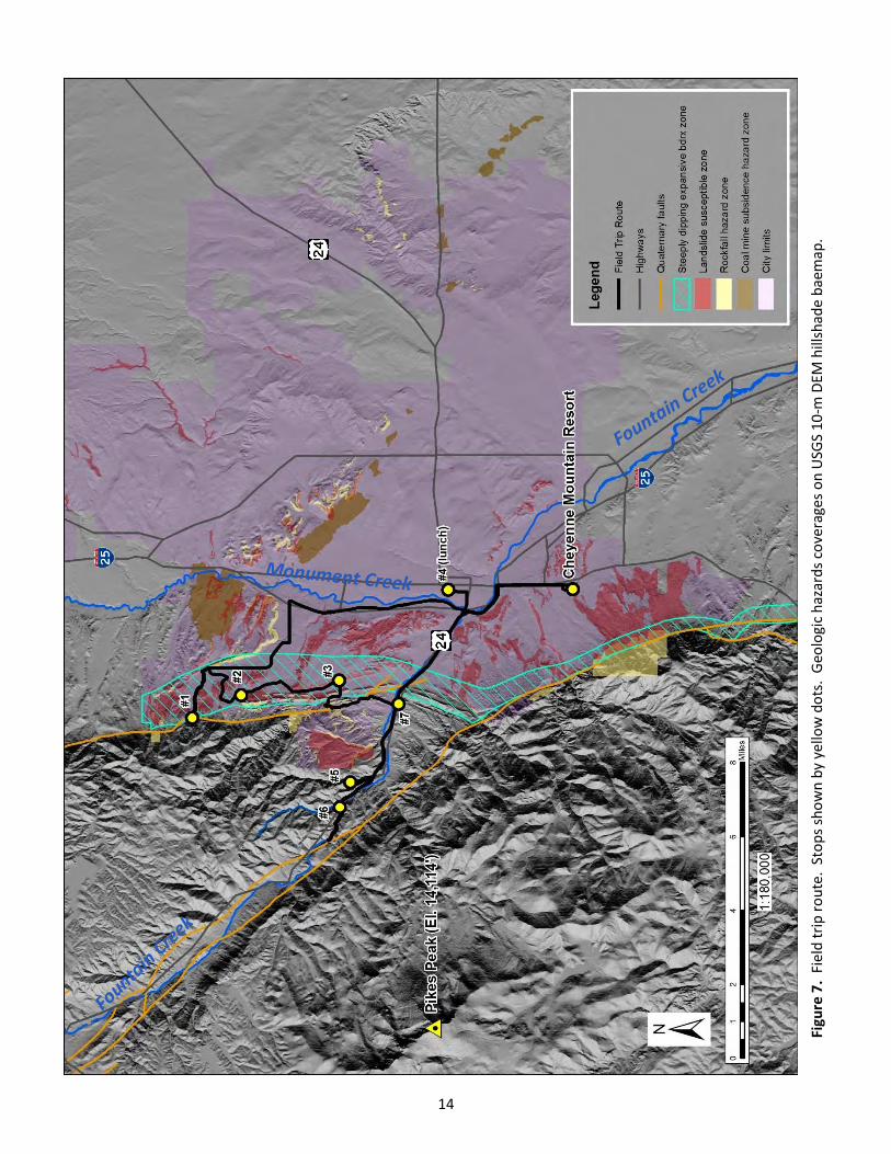
14
Figu
re 7
. Fi
eld
tri
p r
ou
te.
Sto
ps
sho
wn
by
yello
w d
ots
. G
eolo
gic
haz
ard
s co
vera
ges
on
USG
S 1
0-m
DEM
hill
shad
e b
aem
ap.

15
Landslides: Many areas of Colorado Springs are
underlain by weak clay shales. The most
potentially unstable areas in Colorado Springs are
the flanks of Cheyenne Mountain and Rampart
Range, and other hilly terrain underlain by the
Pierre Shale (Kp) west of Interstate 25. Another is
the Cedar Heights neighborhood that is underlain
by the Glen Eyrie Shale Member of the Fountain
Formation. These high-risk terrains are at higher
elevations with incredible views of Colorado
Springs and the eastern plains, so are desirable
for developers to build high-value residential
homes. However, in that terrain the eastward
strata dip direction approximates the slope
directions, which can cause dip-slope movements
where the ground can slip more easily along
formational bedding planes. Colorado Springs has
had several episodes of landslides activations and
reactivations of old landslides during high
precipitation periods (see extended abstract #1).
After a high-precipitation event in 1999 that
resulted in government buyouts for owners of
homes damaged or destroyed by landslides, the
CGS published a landslide susceptibility map of
Colorado Springs (White and Wait, 2003). The
spring of 2015 was also very wet and Colorado
Springs is having another news-worthy spate of
landslide activity (Figure 8). In the media, the
focus is on: where responsibility lies when the city
approves development in areas known for
landslide risk; risk isn’t disclosed to prospective
home buyers by the city, the engineering
consulting community, land developers, or real
estate agents; and should government funds be
used for buyouts for those people who have lost
their homes.
Rockfall: Steep outcrops of granite and dipping sedimentary rock along the mountain front and
sandstone bluffs can pose rockfall hazards. There is a published map of potential rockfall hazards in
Colorado Springs (Wait and White, 2006) where hazards are shown along the base of Pope’s Bluff, the
heights at Austin Bluffs and Palmer Park, and steep slopes near Cheyenne Mountain. Manitou Springs
also has risk of rockfall from the Fountain Formation “red beds” that are exposed as benchy cliffs in the
narrows of Fountain Creek valley (Figure 9). Transportations corridors are also exposed to potential
rockfall risk in canyons and along steep slopes, such as US 24 west of Manitou Springs.
Figure 8. Denver Post newspaper article about
landslides in Colorado Springs - April 24, 2016.

16
Steeply dipping expansive bedrock: The steeply dipping expansive bedrock coverage of Colorado
Springs shown in Figure 7 is from (Himmelreich and Noe, 1999). In addition to being low strength and
prone to instability, Cretaceous claystone commonly contain expansive clay minerals that can result in a
heaving bedrock phenomenon at the surface. Swelling clay soils are a common problematic soil
property along the entire Front Range piedmont corridor. However, along the flank of the mountains,
where bedding is steeply dipping (>30°) (Figure 10) and the soil mantle is thin, the swell differential in
shale beds can cause relatively narrow, linear heave features in bedrock that can severely damage
structures that span them (Figure 11). Only through trenching of near-surface bedrock, perpendicular
to strike, can an informed assessment be made of heave potential. Typical mitigation has been to
remove and replace the top 10 ft of bedrock when developing where this condition exists. For more
information, see Noe (1997), Noe and Dodson (1999), and Himmelreich and Noe (1999).
Figure 9. Large, joint-
controlled block of red Fountain
Formation sandstone and
conglomerate slipped and was
in precarious position in 1995,
directly above homes in
Manitou Springs. Block could
not be removed safely so was
initially restrained by 7/8-in
perimeter cables (top photo)
then anchored to additional
cables that fanned out to
anchor points in intact rock at
top of bluff.

17
Coal mine subsidence: Mining of subbituminous coal in the Laramie Formation was an important part
of Colorado Springs’ early history. There were 65 operating coal mines located in northern and eastern
Colorado Springs between 1883 and 1965, creating an undermined swath of land that extends
southeastward from the Rockrimmon neighborhoods, along the base of the Austin Bluffs and Palmer
Park, to the Jimmy Camp Creek basin. Coverages shown in Figure 7 are from Turney and Murray-
Williams (1983). Some of the areas where the coal mining was relatively shallow (<100 ft) have
experienced significant subsidence. Generally, areas where the mining occurred more than 100 ft below
the ground surface have not experienced as much subsidence (Terry and others, 2003a).
Earthquake potential: It is unclear what the seismic hazard is for Colorado Springs but both the
Rampart Range and Ute Pass faults have been assessed as having Quaternary movements. Earthquakes
up to a magnitude 4.5 have been recorded in the vicinity of Ute Pass fault, west of Colorado Springs
(Widmann and others, 1998). The traces of Rampart Range and Ute Pass faults are shown in Figure 7.
Earthquake shaking could have disastrous effects with potentially unstable landslide-susceptible slopes,
steep rocky slopes, and saturated fine-grained deposits.
The following potential geologic hazards are not shown on the Figure 7 map but also have a history
of impacting Colorado Springs.
Debris flow/flash flooding: Many alluvial fans are mapped at the mouths of most of the major steep
drainage basins in Cheyenne Mountain and the Rampart Range. The most notable debris flows occurred
along the flanks of Cheyenne Mountain in 1965 where there was significant damage to the Cheyenne
Expansive Steeply Dipping Bedrock
Steeply dipping sedimentary bedrock
Expansive soils and bedrock surface
Km Kn Jm PPf
Figure 10. Those formations that lie within the steeply dipping expansive bedrock zone where formation dip
exceeds 30°. Image modified from Noe and Dodson (1999).
Pl

18
Mountain Air Force Station (NORAD) and
Cheyenne Mountain Zoo, and flooding past
SH 115 into Fort Carson. There has been
renewed efforts to mitigate for debris flows
along Rampart Range, especially since the
2012 Waldo Canyon wild fire that denuded
many of the slopes of vegetation and the
Manitou Springs flood disaster that occurred
in June of 2013. An event in 2015, of similar
magnitude as 1965, again partially buried the
main portal entrance of the Air Force station,
accompanied by extensive flooding into the
neighborhood below. Large retention basins
with debris risers, concrete-lined flumes, and
cable-net structures spanning narrow chutes
have been constructed in Colorado Springs
and Manitou Springs. The CGS is currently
developing a debris-flow susceptibility map
for El Paso County using the latest LiDAR
data and modeling software.
Collapsible (hydrocompactive) soils: In
semi-arid Colorado Springs there are
relatively dry eolian and slope-wash deposits
that have an inherent low-density skeletal
fabric and can be susceptible to settlement if
they become wet. Wetting of dry soils cause
the breakage of meta-stable binding agents
that support soil grains, causing the loosened
soil grains to orient into a denser
configuration that can result in ground
settlement (White and Greenman, 2008).
Hydrocompactive soils (generally fine-
grained slope wash, fans, and eolian
sediments) have caused significant damage
to structures with shallow foundations in
Colorado Springs (Terry and others, 2003a;
White and Greenman, 2008).
Radon Gas and radioactivity: Radon gas is
the by-product of the natural decay of
uranium and radium. The Pikes Peak granite
can have higher levels of uranium, as does the widespread pediment gravels such as the Verdos alluvium
that is almost 100% composed of sediment eroded from the granite. Some parts of the Dawson
Formation may also have elevated uranium levels. It is recommended that all houses in Colorado
Figure 11. Illustrations from Noe (1997) showing
differences between typical clay (A) soil with expansive clay
minerals and two types of surface to near-surface bedrock
heave: B) differential heave of high-swell beds generally
along strike of strata, and C) fracture and bedding plane
thrusts. Note that fracture thrusts can have random
orientation at the ground surface.

19
Springs be tested for naturally occurring radon gas and if interior levels meet or exceed 4 pCi/L, active
mitigation measures should be installed. Some areas of the Dawson Formation have sufficient uranium
content that low-energy gamma radiation may also be a hazard (Terry and other, 2003a)
Mill-tailings: The field trip will pass next to the location of historic mills south of Old Colorado City.
The largest was Golden Cycle mill and its location is now called Gold Hill Mesa. All that remains of the
mill is a large embankment of mill tailings, estimated at 140 ft thick, composed of sand-sized particles
and mud slimes pumped into settling ponds from the milling process. The mills used coking (with coal
from nearby mines) as part of the smelting process of high-sulfate content ore. Golden Cycle also used
the more efficient cyanide leaching process. After the mill closure and dismantling in 1949, the tailings
were covered with a thin layer of dirt to prevent blowing and drifting of tailings sand. The land sat idle
with the expectation that the tailing would be reprocessed using new refining methods to recover an
estimated $300 million (2008 prices) worth of additional gold. In the meantime, despite periodic efforts
to revegetate portions of the tailing piles, the dirt cap was eroding, forming rills and gullies into the
underlying tailing, and surface flows were going directly into Fountain Creek. The EPA investigated the
grounds to determine if the tailings posed a serious risk to human health to be classified a Superfund
site. Though elevated concentrations of cyanide, copper, lead, mercury, silver and other heavy metals
were noted, it never received Superfund classification. Instead, it was labeled a “brownfield,” site with
problems that need addressing for future development. There is currently a settling basin at the toe of
the tailing embankment to temporarily capture runoff before it travels into Fountain Creek.
Karst: Lower Paleozoic carbonate rocks along the flanks of Rampart Range and near Manitou Springs
show evidence of dissolution. In addition to the Cave of the Winds cavern system, sinkholes and ground
depressions are mapped in the area (Keller and others, 2003 and Morgan and others, 2003). There are
also beds of gypsum that outcrop within the Lykins Formation strike valley in Old Colorado City, and
further to the south. Where gypsum was mined in Red Rock Canyon, the disturbed mined area was
converted to a reclaimed landfill that is mostly off limits. (See park map in extended abstract #6). There
is potential for sinkhole formation and ground subsidence from dissolution of both carbonate and
evaporate rocks (White, 2012).

20
Landslide warning system in Cedar Heights, Colorado Springs. The gated community of Cedar Heights
is underlain by the Glen Eyrie Member of the Fountain Formation. Eastward dip slopes of weak
mudstone strata have presented instability problems in the neighborhood. View is to the south.

21
Field Trip Road Log By
Jonathan L. White
Field trip begins at Cheyenne Mountain Resort
Overview of Cheyenne Mountain/Broadmoor Area of Colorado Springs
The decks of Cheyenne Mountain Resort have impressive views of the eastern flank of Cheyenne
where Precambrian granodiorite has been thrusted upwards along the Ute Pass fault. Many locations in
this area are exposed to significant risks from landslides and debris-flow flooding. See extended
abstract #1 in Appendix A and geologic map D in Appendix B.
Field trip route -- Cheyenne Mountain Resort to Pikeview Quarry (#1) – 14.3 miles
a) Broadmoor Valley Rd to E. Cheyenne Mountain Blvd., – 0.34 mile, turn right
b) E. Cheyenne Blvd to SH 115, 0.1 mile, turn left
c) SH 115 to NB on-ramp of I-25, 1.8 miles
Interstate 25 follows the Fountain Creek valley to US 24 near the confluence with Monument
Creek. There the interstate continues northward in the Monument Creek valley. The valley floor is
underlain by Holocene and late Pleistocene terraces (Qt) (See geologic map C in Appendix B).
Downtown Colorado Springs lies on one of the higher terrace surfaces. Within the recent incised
channel, the underlying Pierre Shale (Kp) is typically exposed in the strath terrace cut bank. To the
east Palmer Park and Austin Bluffs are the low bluffs underlain by the very coarse to conglomeritic
sandstones of the lower Tertiary/Late Cretaceous Dawson Formation (TKda). Where the terrain
flattens below the bluffs, the underlying bedrock is the coal-bearing Laramie Formation (Kl).
Neighborhoods of Colorado Springs along a northwest trending belt from Palmer Park to
Rockrimmon are undermined by abandoned coal mines that used “room and pillar” mining
techniques. Mine subsidence is a continuing hazard in those neighborhoods.
d) I-25 (NB) to off ramp to Garden of the Gods Rd., 6.3 miles, turn left
Pulpit rock can be seen in the hills to the northeast. This famous topographic point of Austin
Bluffs best exposes the gray-white sandstone strata of the Dawson Formation (TKda) (Figure 12).
e) Garden of the Gods Road to Centennial Blvd., 1.1 miles, turn right
To the north of Garden of the Gods Rd. is Popes Bluff. The resistant-to-weathering middle
sandstone unit of the Laramie Formation (Kls) has formed this cuesta (See Geologic Map A in
Appendix B). Outside of the steeply dipping bedrock zone, the formation dips are 5° to 10°.

22
Neighborhoods have been developed
along the mesa edge because of the view
lots that look over the Monument Creek
valley, and towards Garden of the Gods,
Cheyenne Mountain, and Pikes Peak.
Those neighborhoods situated below the
sandstone bluff are exposed to rockfall
hazards.
f) Centennial Blvd. to Allegheny Dr., 2.8
miles, turn left
Traveling north and west along
Centennial Boulevard one enters the
steeply dipping bedrock zone. Northward
on Centennial Blvd., as the road nears
Popes Bluff, the cuesta steepens to a ridgeline hogback where dips exceed 50°. Several coal adits
and tunnels serving the Rockrimmon/Pikeview coal field occur along the ridge line (Figure 13). The
Figure 12. Pulpit rock is a promontory of the Dawson Formation that is easily seen from I-25. Photo by V. Matthews.
Figure 13. Undermined areas of the Rockrimmon area of Colorado Springs. Several abandoned adits along the field trip route on Centennial Blvd. served the coal mines. These tunnel openings have been sealed and the surface mostly reclaimed.
Field Trip Route

23
tunnels are sealed and reclaimed but several small piles of mine spoils can still be seen along the
base of the ridge east of Centennial Blvd.
An excellent exposure of the tilted Laramie Formation can be seen at the cutslope of Allegheny
Drive where the field trip route takes a left turn to the quarry.
g) Allegheny Dr. to Quarry Office (safety meeting), 1.2 miles, 0.6 mile to Quarry floor.
Field Trip Stop #1 -- Pikes Peak Quarry
The Pikes Peak Quarry is an active aggregate mine so field trip attendees must stay in
designated areas that have been marked by the mine operator. Rockslides have been common at the
quarry but accelerated in late 2008; the most recent rockslide occurring in May 2015. See extended
abstract #2 in field trip appendix.
Field Trip route -- Pikeview Quarry to
Chuckwagon Rd. overview (#2) – 3.9
miles
a) Quarry to Centennial Dr., 1.8 miles,
turn right
b) Centennial Dr. to Flying W Ranch Rd.,
0.2 mile, turn right.
The Waldo Canyon wild fire
entered the city limits of Colorado
Springs along Flying W Ranch Road.
About 300 homes were destroyed in
the Mountain Shadows
neighborhoods on both sides of
Flying W Ranch Rd. See Figure 14
and 15.
c) Flying W Ranch Rd to Rossmere St.,
0.6 mile, turn right
d) Rossmere St to Chuckwagon Rd.,
1.33 miles, turn left and park along
Rd.
A
B
Figure 14. Total destruction of neighborhoods in Mountain
Shadows area near Flying W Ranch Road. Locations of oblique
photos are shown in Figure 15.

24
Figure 15. Colorado Springs Map of home destroyed or damaged in June 2012 Waldo Canyon wild fire. Arrows show view direction in photos A and B of Figure 14. Field trip route shown as heavy black line.
A
B
Cen
ten
nia
l Blv
d.
Field trip stop #2

25
Field Trip Stop #2 -- Chuckwagon Road, Flying W Ranch burn area
Chuckwagon Road leads to the Flying W Ranch. This working, mountain cattle ranch is also a
major tourist venue in Colorado Springs with chuckwagon dinners, theatre plays, and other western-
theme entertainment. The Waldo Canyon wild fire swept through the ranch and completely burned it
down June 26, 2012. The fire swept eastward down the drainageway south of the Chuckwagon Road
into the Mountain Shadow neighborhoods. The hogbacks of Cretaceous and Late Paleozoic strata are
now better exposed in the fire-swept hillsides (Figure 16).
Field Trip Route -- Chuckwagon Rd overview to Garden of the Gods Visitor Center (#3) – 3 miles
The prominent hogbacks at the Chuckwagon Road stop continue southward towards Garden of
the Gods. Unlike the Ute Pass fault to the south that faulted Cheyenne Mountain granodiorite
against soft Pierre Shale, near 30th St. and Garden of the Gods Boulevard, more resistant formations
from limestones of the Niobrara Formation to the Lyons Sandstone are exposed as prominent
hogbacks. See cross section in Figure 17.
a) Chuckwagon Rd to Flying W Ranch Rd., 0.16 mile, turn right
b) Flying W Ranch Rd to N. 30th St., 1.15 miles, turn right
c) N. 30th St. to Garden of the Gods visitor center, 1.7 miles
South on N. 30th St. steeply dipping hogbacks of gray to buff Niobrara Formation and Dakota
Sandstone appear on the west side. Through watergaps in the hogback, especially Camp Creek at
the entrance to The Navigators compound and Queens Canyon, one can see near vertical white and
pink rock spires and fins that become most pronounced at the Garden of the Gods Park.
Kpu – Purgatoire Fm. Kd – Dakota Ss.
Rampart Range
Ypp – Pikes Peak Granite
Figure 16. Dakota and Purgatoire hogback at Chuckwagon Road. Note burned trees that extend onto Rampart Range.
Exposed rock formations not labeled in right side of photo include the Lyons Ss. (white rocks) and the Fountain Fm.
(light red rocks). The drainageway below, as are many from basins in the Waldo Canyon burn area, is now prone to
flash flooding and mud/debris flows.

26
In the Navigators compound is Glen Eyrie, a castle built along the bank of Camp Creek at the
mouth of Queens Canyon by General William Jackson Palmer; the wealthy industrialist, rail
magnate, and philanthropist who founded Colorado Springs. Now owned by the Navigators
religious organization, Glen Eyrie estate is nestled around spires of vertical sandstone outcrops
where Queens Canyon exits Rampart Range. The Navigator’s grounds were luckily spared by the
Waldo Canyon wildfire. However, areas in proximity to the banks of Queens Canyon creek are now
at risk of post-burn debris-flow flooding (See extended abstract #4) and mitigation was quickly
installed after the 2012 fire (Figure 18).
Pediment Gravels - “The Mesa” Laramie and Dawson Fms. (Popes Bluff, Pulpit Rock, Austin Bluffs, and Palmer Park)
Figure 17. Cross section modified from Himmelreich and Noe (1999). Garden of the Gods Road can be seen in
Geologic Map B in Appendix B.
Figure 18. Debris-flow mitigation nets installed at Camp Creek in Queens Canyon after the Waldo Canyon wild
fire. Note men in right photo for scale. Grouted rip-rap and tiered gabion boxes were installed at anchors to
mitigate scour. Photos from Keaton and others (2013).

27
The bluff behind (east of) the Visitor Center is underlain by Pierre Shale but mantled with reddish
pediment gravel derived from coalesced mid-Pleistocene alluvial fans that were deposited along the
mountain front from erosion of Pikes Peak Granite in the foothills above. Known as Verdos
Alluvium, is has been more recently mapped as Qg2 gravels in CGS quadrangle mapping (Carroll and
Crawford, 2000, Thorson and others, 2001). The field trip encircles this broad alluvium remnant,
known as “The Mesa” on topographic maps. The bluff edges and slopes below are underlain by
Pierre Shale and are susceptible to landslides. Many have occurred, especially on the mesa’s east
slope where slope direction approximates dip direction. Many homes were damaged and
condemned in 1999.
Field Trip Stop #3 -- Garden of the Gods Visitor Center
See extended abstract #3 in appendix A.
Field Trip Route -- Garden of the Gods Visitor Center, through park to Phantom Canyon Brewery (#4,
Lunch) – 7.9 miles
a) Visitor center to Gateway Rd. and Juniper Way Loop, 0.55 miles, turn right (Figure 19)
The road entering Garden of the Gods from the visitor center crosses Camp Creek along a broad
swale underlain by soft Cretaceous shale and a small wall-like hogback of white Niobrara limestone
(Kn). These rock units are tilted into an almost vertical position. As the road nears Juniper Valley
Loop it crosses the roof fault of the Garden of the Gods. Juniper Valley Loop encircles the faulted
and upthrusted slivers of Lyons Sandstone and Fountain Formation. The field trip travels around the
upper west half of the loop. See extended abstract #3 and Geologic Map B for this corridor of the
field trip.
b) Juniper Way Loop to Ridge Rd., 1.7 miles, veer right
Though not easily seen, the turn off onto Ridge Road obliquely crosses the trend of Rampart
Range fault where the Fountain Formation is faulted against the Morrison Formation. Steeply
dipping red rocks of the Fountain Formation occur along Ridge Road. The low ridgelines
immediately to the east are formed by the Dakota Sandstone and, further to the east, the
prominent chalky-white limestones of the Niobrara Formation (see Figure 19).
c) Ridge Rd. to US 24 (EB), 1 mile, turn left
South of the intersection of US 24 and Ridge Rd. is the Red Rock Canyon Open Space, the last
stop of the field trip. Note the “red rock” spires of the Fountain Formation.

28
d) US 24 (EB), becomes W. Cimarron St. downtown to S. Nevada St., 3.9 miles, turn left
Approximately 3/10th of a mile east from the Ridge Rd. are well exposed, vertical to overturned
Lyons Sandstone and soft Lykins Formation strata in the US 24 highway cutslope. East of 31st Street,
the neighborhood on the north side of Fountain creek is Old Colorado City. Colorado City was the
original settlement of the area (see history of Colorado Springs in guidebook introduction).
Two miles east on US 24, past 21st Street, a wide embankment appears on the south side of the
highway that is heavily rilled and gullied (Figure 20). This is Gold Hill Mesa, the site of the historic
Golden Cycle Mining Company gold processing mill in Old Colorado City (See Mining History section
in guidebook).
The hilltop site has impressive 360-degree views so is being built out as a large residential
development called Gold Hill Mesa. While portions of the development have been built, much of the
north facing slopes are still rilled and gullied from runoff flowing into a drop-out detention pond
before entering Fountain Creek. Serious settlement issues are present on the thick mill tailings and
foundation damage is reportedly occurring in new homes of the development.
The confluence of the Monument Creek and Fountain Creek occurs just east of the Hwy 24
intersection with I-25.
Figure 19. Annotated north-facing oblique image of Garden of the Gods. Black line is field trip route. Fault traces are from Siddoway and others (2013). Thickest red line on the left is trace of Rampart Range fault, lighter red traces are oblique thrust sheets, and right red line is the roof thrust. See geologic map in Garden of the Gods extended abstract. Image created from Google Earth Pro™ urban high-resolution 3D imagery.
The Mesa Visitor Center
Glen Eyrie
PPf
Kd
Kn
Kp
Kcgg
Qg2
PPf

29
e) S. Nevada St. to E. Pikes Peak Ave., 0.5 miles, turn left
f) E. Pikes Peak Ave. to Phantom Canyon Brewery, 0.2 miles
Downtown Colorado Springs lies near the confluence of the Monument Creek and Fountain
Creek. The terrain of downtown is relatively flat because it lies on a higher alluvial terrace (Qt3),
also known as the Louviers Alluvium.
Field Trip Stop #4 -- Lunch Stop at Phantom Canyon Brewery
Field Trip Route -- Phantom Canyon Brewery to Cave of the Winds Parking Lot (#5) – 7.4 miles
a) S. Cascade Ave to W. Cimarron St./US 24, 0.5 miles, turn right
b) US 24 (WB) to Cave of the Winds exit, 6 miles, turn right
Westward of the Manitou Springs exit, US 24 climbs in grade. This portion of the highway was
realigned in the 1960s. Early roads and the original US 24 used to go through downtown Manitou
Springs. To keep a suitable road grade in the newer alignment, high rock-excavated cutslopes were
required on both sides of the highway. These rock excavations provide excellent exposures of
coarse-grained red-bed strata within eastward-dipping Pennsylvanian/Permain Fountain Formation
(Figure 21) (See Geologic maps B in Appendix B). This is the type locality for the Fountain
formation where it is at its thickest - 4,050 ft, representing a localized synorogenic depositional
center that flanked the Pennsylvanian Ancestral Rockies (Frontrangia) uplift. The formation thins
rapidly northward to only 650 ft thick at Glen Eyrie in Queens Canyon, which is about 3 miles north
on the other side of the Garden of the Gods Park (Keller and others, 2003).
Figure 20. Mill tailing of Golden Cycle Mining Company, now called Gold Hill Mesa. All that remains of the original mill
is the smokestack shown by white arrow. Note rills and gullies in the tailings embankment.

30
c) Cave of the Winds Rd. to parking lot, 0.9 miles
As the field trip turns right, note the high rock excavation in the heavily karstic, reddish stained
Hardscrabble Limestone Member of the Mississippian Leadville Limestone. The limestone has
undergone so much dissolution and brecciation that strata bedding is hard to distinguish.
Switch backs of the Cave of the Winds road climbs onto the Manitou Limestone, also heavily
karstic. Dissolution breccia is also exposed in rock excavations along the path to the visitor center.
The Cave of the Winds cavern is located within the Manitou Limestone. The Cave of the Winds was
discovered in 1881 and over the years has expanded to become a popular tourist attraction in the
Colorado Springs vicinity.
Figure 21. Tilted interbedded sandstone, conglomerate, and mudstone of the Fountain Formation in rock
excavation for US 24 alignment above Manitou Springs. Baseball cap in inset photo shows scale of cobble
conglomerate in some beds.

31
Field Trip Stop #5 -- Cave of the Winds Visitor Center parking lot
From the Cave of the Winds Visitor
Center parking lot, one can view the foothills,
the burn scars of the Waldo Canyon wild fire to
the west and northwest, and drainage
channels that flow to Fountain Creek and
Manitou Springs below. Flash floods also
scoured Williams Canyon (Figure 22) below
the visitor center and caused significant
damage to Manitou Springs in August 2013,
washing out the original historic road to Cave
of the Winds and flowing into neighborhoods
below. See extended abstract #4 about the
flooding effects of the intense August 9, 2013
precipitation event in the Waldo Canyon burn
area that impacted Manitou Springs.
Field Trip Route -- Cave of the Winds Parking
lot to Waldo Canyon (#6) – 1.9 miles
a) Cave of the Winds Rd to US 24 (WB), 0.9
mile, turn right.
Approximately 3/10th of a mile west
the Cave of the Winds turnoff, US 24
passes over the same nonconformity that
can be seen at two small irregular buttes
from the Cave of the Wind parking lot
(Figure 23) where tilted Cambrian Sawatch
Sandstone overlies heavily jointed, coarse
crystalline, 1.1 byp Pikes Peak Granite. Westward, the modern alignment of US 24 begins to follow
Fountain Creek canyon that is steeply incised into strongly jointed Pikes Peak granite. Natural steep
slopes and rock excavations for the 1964 highway widening are a persistent rockfall hazard.
Structurally, the Fountain Creek canyon parallels the Ute Pass fault zone, the trace of which is in the
foothills above (south of) Manitou Springs.
b) US 24 (WB) to pull out at Waldo canyon mouth, 1 mile
On August 9, 2013, a little more than a year after the Waldo Canyon wild fire, an intense
precipitation event caused several drainages along US 24 to flash flood. The debris/mud-flow
floods, very dark gray with entrained ash, flowed down the Highway 24 roadway and caused severe
erosion to highway embankments and flood damage to Manitou Springs. For additional
information see extended abstract #4.
Figure 22. Williams Canyon from Cave of the Winds. High bridge is SH 24. Manitou Springs is below at confluence with Fountain Creek. Ute Pass fault is behind town and curves in front of Cheyenne Mountain at left-center background.

32
Field Trip Stop #6 -- Waldo Canyon rockfall and debris flow mitigation
See extended abstract #5 in appendix about debris flow mitigation on US 24 at the mouth of
Waldo Canyon. Significant debris flows exited Waldo Canyon and, constrained by road-
separation barriers, flowed down the WB lanes. Figure 24 is a photo of the roadside cable-net
rockfall fence at Waldo Canyon taken shortly after the August 9, 2013 flooding event and shows
the height of debris that washed down the highway.
Field Trip Route -- Waldo Canyon to Red Rock Canyon Open Space (#7) – 5.7 miles
a) Waldo Canyon to Hwy 24 (WB) U-turn, 1.1 miles
Several rock slopes along US 24 in this corridor have been mitigated for rockfall, including rock
bolts and draped wire mesh.
b) Hwy 24 (EB) to Ridge Rd, 4.5 miles, turn right for 0.1 miles to entrance
The eastward dipping nonconformable contact of the Sawatch Sandstone can best be seen at
road level on the north side along SH 24 just above Manitou Springs when heading eastbound.
Tilted red beds of the Fountain Formation are exposed along Fountain Creek and US 24 to the
Red Rock Canyon Open Space (See Geologic Maps B and C in Appendix B)
Figure 23. Two irregular tilted buttes west of Cave of the Winds parking lot are capped by Lower Paleozoic
sedimentary rocks. The conspicuous gray-white bands are Sawatch Sandstone beds at the Great
Nonconformity with underlying Precambrian Pikes Peak Granite (brownish red slopes below). Note burned
forested area in Waldo Canyon watershed in the background.

33
Field Trip Stop #7 – Red Rock Canyon Open Space
This open space is locally popular, and the same geologic formations are exposed as at Garden
of the Gods, but isn’t the tourist draw and so doesn’t attracts the same crowds. A trail map and
same-scale geologic map of Red Rock Canyon Open Space is in extended abstract #6 as a guide for
a short hike though the park. The old quarries on the east side are a recommended visit.
Field Trip Route -- Red Rock Canyon Open Space to Cheyenne Mountain Resort – 6.9 miles
a) Ridge Rd. to US 24, 0.1 mile, turn right
b) US24 (EB) to I-25 (SB) on-ramp, 3.2 miles
c) I-25 (SB) to US 119 off ramp and cross S. Tejon St., 1.5 miles, turn right at SH 115
d) SH 115 to Cheyenne Mountain Resort off ramp and parking lot, 2.1 miles
End of Field Trip – Total Miles – 51 miles
Figure 24. August 9, 2013 debris flow caught by cable-net rockfall fence. Note barrier on the
opposite side of the WB lanes and height of the debris caught on the road side of the fence. Photo
from Keaton and others (2013).

34
High rock excavation for US 24 westbound lanes in Fountain Creek valley west of Manitou Springs.
Note level of jointing in Pikes Peak Granite. Rockfall mitigation includes rock bolt reinforcement and
draped wire netting.

35
References BAER Report, 2012, Waldo Canyon BAER Assessment -- Executive Summary Report, Online Burned Area Emergency
Response (BAER) Update, Pike & San Isabel National Forests, Cimarron & Comanche National Grasslands dated 7/20/2012, from http://inciweb.nwcg.gov/incident/article/2929/15218/
Carroll, C.J., and Crawford, T.A., 2000, Geologic map of the Colorado Springs quadrangle, El Paso County, Colorado: Colorado Geological Survey Open-File Report 00-3, scale 1:24,000, free download at: http://store.coloradogeologicalsurvey.org/product/geologic-map-of-the-colorado-springs-quadrangle-el-paso-county-colorado/
Chronic, J., McCallum, M.E., Ferris, C.S., Eggler, D.H., 1969, Lower Paleozoic rocks in diatremes, southern Wyoming
and northern Colorado: Geological Society of American Bulletin, v. 80, p. 149-156.
Darton, N.H., 1906, Geology and underground waters of the Arkansas Valley in eastern Colorado: U.S. Geological
Survey Professional Paper 52, 90 p.
Dechesne, M., Raynolds, R.G., Barkmann, P.E., and Johnson, K.R., 2011, Notes on the Denver Basin Geologic Maps:
bedrock geology, structure, and isopach maps of the Upper Cretaceous to Paleocene Strata between
Greeley and Colorado Springs, Colorado: Colorado Geological Survey Open File Report OF11-01, 35 p., 14
plates.
Finlay, G.I, 1916, Colorado Springs Folio, Geologic Atlas of the United States No. 203, U.S. Geological Survey, from
https://pubs.er.usgs.gov/publication/gf203
Himmelreich, J. W., Jr. , and Noe, D.C, 1999, Map of areas susceptible to differential heave in expansive, steeply
dipping bedrock, City of Colorado Springs, Colorado: Colorado Geological Survey Map Series 32, free
download at: http://store.coloradogeologicalsurvey.org/product/map-of-areas-susceptible-to-
differential-heave-in-expansive-steeply-dipping-bedrock-city-of-colorado-springs-colorado-2/
Keaton, J., Anderson, S., Santi, P., Dashti, S., 2013, Geotechnical effects on intense precipitation on August 9, 2013,
on slopes above Manitou Springs, Colorado, that were burned in the 2012 Waldo Canyon Fire:
Geotechnical Extreme Events Reconnaissance (GEER) Association, National Science Fountain, 136 p., free
download at:
http://www.geerassociation.org/index.php/component/geer_reports/?view=geerreports&id=33
Keller, J.W., Siddoway, C.S., Morgan, M.L., Route, E.E., Grizzell, M.T., Sacerdoit, R., and Stevenson, A., 2003, Geologic map of the Manitou Springs 7.5-minute quadrangle, El Paso and Teller Counties, Colorado: Colorado Geological Survey Open-File Report 03-19, scale 1:24,000, free download at: http://store.coloradogeologicalsurvey.org/product/geologic-map-of-manitou-springs-7-5-minute-quadrangle-el-paso-and-teller-counties-colorado/
Morgan, M.L., Siddoway, C.S., Rowley, P.D., Temple, Jay, Keller, J.W., Archuleta, B.H., Himmelreich, J.W., 2003, Geologic map of the Cascade quadrangle, El Paso County, Colorado: Colorado Geological Survey Open-File Report 03-19, scale 1:24,000, free download at: http://store.coloradogeologicalsurvey.org/product/geologic-map-of-the-cascade-quadrangle-el-paso-county-colorado/
Noe, D.C., 1997, Heaving-bedrock hazards, mitigation, and land-use policy: Front Range Piedmont, Colorado:
Colorado Geological Survey Special Publication SP-45, 57p.
Noe, D.C. and Dodson, M.D., 1999, Heaving bedrock hazards associated with expansive, steeply dipping bedrock,
Douglas County, Colorado: Colorado Geological Survey Special Publication SP-42, 80 p.

36
Siddoway, C., Myrow, P., and Fitz-Díaz, E., 2013, Strata, structures, and enduring enigmas: A 125th Anniversary
appraisal of Colorado Springs geology, in Abbott, L.D., and Hancock, G.S., eds., Classic Concepts and New
Directions: Exploring 125 Years of GSA Discoveries in the Rocky Mountain Region: Geological Society of
America Field Guide 33, p. 331–356.
Siddoway, C.S., and Gehrels, G.E., 2014, Basement-hosted sandstone injectites of Colorado: a vestige of the
Neoproterozoic revealed through detrital zircon provenance analysis: Geological Society of America
Lithosphere, December 2014, v.6, p. 403-408. Available on-line at:
http://lithosphere.gsapubs.org/content/early/2014/08/26/L390.1.full.pdf+html
Terry, T.A., Carroll, C.J., Lovekin, J.R., Andrew-Hoeser, K.A., and Hoffman, Jr., W.C., 2003a, Geology of Colorado Springs, Colorado, In Boyer, D.D., Santi, P.M., and Rogers, W.P., (eds.), Engineering geology in Colorado: contributions, trends, and case histories: Association of Engineering Geologists Special Publication 15 and Colorado Geological Survey Special Publication 55 on CD-ROM.
Terry, T.A., White, J.L., and Wait, T.C., 2003b, Cheyenne Mountain Quaternary deposits origins and engineering geology significance, In Boyer, D.D., Santi, P.M., and Rogers, W.P., (eds.), Engineering geology in Colorado: contributions, trends, and case histories: Association of Engineering Geologists Special Publication 15 and Colorado Geological Survey Special Publication 55 on CD-ROM.
Thorson, J.P., Carroll, C.J., and Morgan, M.L., 2001, Geologic map of the Pikeview quadrangle, El Paso County, Colorado: Colorado Geological Survey Open-File Report 01-3, scale 1:24,000, free download at: http://store.coloradogeologicalsurvey.org/product/geologic-map-of-pikeview-quadrangle-el-paso-county-colorado/
Thorson, Jon, P., 2011, Geology of Upper Cretaceous, Paleocene and Eocene Strata in the Southwestern Denver
Basin, Colorado: Colorado Geology Survey, 53 p., 3 plates.
Trimble, D.E., and Machette, M.N., 1979, Geological map of the Colorado Springs-Castle Rock area, Front Range Urban Corridor, Colorado: U.S. Geological Survey Miscellaneous Investigations Series Map I-857-F, scale 1:100,000, free download at: http://ngmdb.usgs.gov/Prodesc/proddesc_9754.htm
Turney, J.E., and Murray-Williams, L., 1983, Colorado Front Range Inactive Coal Mine Data and Subsidence
Information, El Paso County: Colorado Geological Survey, Plate 6 of 12, scale 1:50,000, free download at:
http://coloradogeologicalsurvey.org/wp-content/uploads/2013/08/ElPasoCounty.pdf
Verdin, K. L., Dupree, J. A., Elliott, J., 2012, Probability and volume of potential post-wildfire debris flows in the
2012 Waldo Canyon Burn Area near Colorado Springs, Colorado: U.S. Geological Survey Open-file Report
No. 1158., free download at: http://pubs.usgs.gov/of/2012/1158/
Wait, T.C., and White, J.L., 2006, Rockfall hazard susceptibility in Colorado Springs, El Paso County: Colorado Geological Survey Open-File Report 06-03, 1:24,000 scale, 2 plates.
White, J.L. and Wait, T.C., 2003, Colorado Springs landslide susceptibility map, El Paso County, Colorado: Colorado Geological Survey MS 42, includes 32 p. booklet, scale 1:24,000, 3 plates, free download at: http://store.coloradogeologicalsurvey.org/product/colorado-springs-landslide-susceptibility-map-el-paso-county-colo-2/
White, J.L., 2012, Colorado map of potential evaporate dissolution and evaporate karst subsidence hazards: Colorado Geological Survey Open File OF12-02D, 24 p., GIS data, scale 1:500,000, free download at: http://store.coloradogeologicalsurvey.org/product/colorado-map-of-potential-evaporite-dissolution-and-evaporite-karst-subsidence-hazards/
Widmann, B.L., Kirkham, R.M., and Rogers, W.P., 1998, Preliminary Quaternary fault and fold map and database of Colorado: Colorado Geological Survey Open- Report 98-8, 331 p

A1
Appendix A
The following extended abstracts offer more information about the 67th Highway Geology Symposium
field trip stops in the Colorado Springs area.

A2

A3
Abstract #1 - Geologic Hazards of the Greater Broadmoor Area by
Jonathan L. White (includes excerpts from White and Wait, 2003)
The decks of Cheyenne Mountain Resort have impressive views of the eastern flank of Cheyenne
where Precambrian granodiorite has been thrusted upwards along the Ute Pass fault. Pierre Shale is the
underlying bedrock on the east side of the fault. The proximity of the steep Cheyenne Mountain front
has exposed newer neighborhoods to geologic hazards. Unstable slopes, landslides, and debris-flows
are the major geologic hazards along the moderate slopes along the eastern flank of Cheyenne
Mountain. Other concerns are expansive Pierre Shale bedrock and its derived swelling soils, and
unknown potential for catastrophic rockslides, earth flows, and landslides if an earthquake were to
occur along Ute Pass fault, a risk not known at this time for what is inferred as a middle to late
Quaternary fault (Widmann and others, 1998). While difficult to see because of the weak nature of the
bedrock, claystone strata is folded steep upwards and dips to the east. Downcut by erosion and
subaerially exposed, the gently to moderately dipping weathered claystone surface is now mantled by
Pleistocene gravel pediments, a late Pleistocene to early Holocene large earth-flow complex that
extended to SH 115 (Terry and others, 2003), and more recent Holocene debris-fan sediments along the
steeper slopes at the base of Cheyenne Mountain (Figure 1-1).
Figure 1-1. Oblique 1(H):1(V) image of Cheyenne Mountain with view to the southwest. Orange-shaded strip is the zone of expansive steeply dipping bedrock from Himmelreich and Noe (1999) that is mostly covered by coalesced alluvial fans. Back end of the orange strip is the trace of the Ute Pass fault. Red-shaded polygons are mapped landslides from Carroll and Crawford (2000). Yellow stars are locations of landslide activity since 1995 that damaged homes or infrastructure. Blue arrows are debris-flow detention basins on active alluvial fans. For scale, mountain front is about 2 miles from SH 115 at label. Image created with ERDAS Imagine.
Cheyenne Mountain
Cheyenne Mountain
Resort
NORAD tunnel Portal
Broadmoor Mountain Golf Course landslide
Cheyenne Mtn. Earth-flow complex
Cull Reservoir
Cheyenne Mountain
Zoo
SH 115

A4
Debris-flow Hazards
Several steep drainage basins of
Cheyenne Mountain outlet onto the greater
Broadmoor residential areas that have been
developed since the early 1990s. Those steep
basins can be seen in figure 1-1. At the outlet
of all the mountain’s basins there is evidence
of geologically recent debris-flow activity,
including terminal lobate deposits on
mountain-front alluvial fans, flow diversion
and abandoned channels, lateral levees, and
boulder trains and piles stacked against larger
trees. Debris flows have occurred
historically, including very recently. In July
1965 debris-flow flooding occurred at the
mouth of every basin along the flank of
Cheyenne Mountain. These flows blocked
State Highway 115 and significantly impacted
the NORAD tunnel portal and the Cheyenne
Mountain Zoo (see Figure 1-2). Large
boulders from Cheyenne Mountain were
moved across State Highway 115 during this
event. A 2015 spring flooding, which
impacted much of the greater Broadmoor
area, also caused debris to, once again, block
the NORAD portal and damaged homes where
flows entered the neighborhood below.
Landslide Hazards
Dip-slope slope instability and landslides are a significant hazard in this area because of the
inherent weakness of the claystone bedrock and a general ground slope direction that approximates the
steep to moderate eastward dip of the strata (Figure 1-3). The Pierre Shale is a Cretaceous marine clay
shale with common thin bentonite beds. The erosion and removal of thousands of feet of overburden
along the Front Range Piedmont has now exposed an overconsolidated clayshale with significant
percentages of expansive clay minerals. Loss of overburden confinement and wetting has caused
rebound in the rockmass. In cores of “intact” claystone, slickensides have been observed by the author
in thin bentonite beds. The clayshale has been covered by a mantle of pediment gravel and alluvial fans.
These granular soils are highly permeable and ground water passes through quickly to the contact with
Figure 1-2. Archival pictures from July 1965 debris-flow
flooding along Cheyenne Mountain. Upper photo shows
bouldery debris-flow sediment at NORAD tunnel portal.
Lower photo shows VW van buried almost to roof by
debris-flow sediment at Cheyenne Mountain Zoo parking
lot. Photo attributions are unknown.

A5
the clayshale. There it perches, percolating into the clayshale and moving laterally down the
gravel/shale contact to the east. Ground underlain by dipping Pierre Shale is highly sensitive to
disturbance and landslides occur. Even modest cuts and fills have caused landslides in this area.
Landslide hazards in the Greater Broadmoor Area have been known by the engineering and
geological community for over three decades, although that didn’t dissuade developers and the city to
develop in the hilly terrain where valued view lots could be constructed. Most residents who built or
purchased homes in those areas were not aware of the risks. Larger landslides were regionally mapped
by USGS prior to the land development of many of the more problematic areas. Those and other
identified landslides have been mapped at better detail in the CGS 1:24,000-scale geologic mapping
program (see index map figure in the main field trip guidebook). The landslide boundaries at the base of
Cheyenne Mountain are shown in Figure 1-1. The most pronounced are: 1) the broad depression
northwest from the decks of Cheyenne Mountain Resort at the Broadmoor Mountain golf course, which
lies wholly within a large active landslide that extends from the mountain front almost to the resort lake
(Cull Reservoir), and 2) an ancient landslide complex further to the south where the flank of Cheyenne
Mountain, underlain by steeply dipping claystone and loaded by deposition of talus and alluvial fans,
had mobilized and spread to SH 115 as an earthflow that rafted granodiorite boulders down the size of
small homes (Terry and others, 2003b).
Figure 1-3. Generalized cross section at Cheyenne Mountain showing zone of expansive steeply dipping
bedrock (seen in figure 1) where bedrock can dip from slightly overturned to 30°. Bedrock bedding flattens
from 5° to 10° at SH 115. Illustration from Himmelreich and Noe (1999).

A6
New landslides and reactivations of older, existing landslides occurred during the wet spring of
1995. A brief flurry of media attention occurred after the landslides of that wet spring, and areas of
susceptibility were briefly discussed in a CGS field trip guide book in 1996. In 1999, another spring of
heavy precipitation triggered flooding, caused renewed landslide movement, and activated additional
landslides. Ground movements impacted several neighborhoods west of Interstate 25 and many homes
and properties were threatened, damaged, destroyed, or condemned. Although all of these
neighborhoods lie within landslide-susceptible areas, many had no history of landslide activity prior to
the 1999 events, and homeowners had no knowledge of the risk they were potentially exposed to.
Many of the homes and properties impacted were over 20 years old and apparently had no previous
problems with lateral earth movements. Because of the flooding and landslide movements, Colorado
Springs was declared a presidential disaster area. Many homes damaged by flooding and landslides
became eligible for a buy-out program. A FEMA grant funded an investigation and mapping of
landslides after the disaster and the Colorado Geological Survey published a landslide susceptibility map
of Colorado Springs in 2003 (White and Wait, 2003). Several years of movement dormancy ended in
2013 when another wet spring occurred. New landslides occurred and many of the existing landslides
reactivated. More homes, some recently built in susceptible areas known for landslide risks after 1999,
experience distress from lateral ground movements that continue today (2016). Areas of ground
movements from 1995 to 2016 in the greater Broadmoor area are shown by yellow stars in Figure 1-1.

A7
Abstract #2 - Rockslide at Pikeview Quarry, Colorado Springs By
Jonathan L. White and M.L. (Mac) Shafer
The Pikeview Quarry is located within the Rampart Range fault zone in northwest Colorado
Springs. The quarry was opened in 1905 to mine limestone for aggregate and concrete production and
over the last century the quarry has grown in size to about 200 acres. Transit Mix Concrete Co., a
subsidiary of Continental Material Corporation is the current owner and operator of the quarry. The
benched quarry walls create a large, easily seen excavation in the Rampart Range mountain front. As
the quarry enlarged over the years, and nearby neighborhoods have encroached as the City of Colorado
Springs expanded into the Pikeview and Rockrimmon areas, there have been the typical complaints of
mine operations near residential areas. However, the homes below the quarry have the disturbed
ground of the mine property to thank for stopping the 2012 Waldo Canyon wildfire and preventing it
from entering the Oak Valley Ranch and Peregrine neighborhoods, or potentially the heavily forests
neighborhoods of Rockrimmon across Centennial Blvd. further to the east (See mapped fire perimeter in
other illustrations in this guidebook. Other neighborhoods of Colorado Springs along the Rampart
Range front were not so lucky.
Mine geology and structural
conditions
The mine is located within the
north-striking trend of the of the
Rampart Range fault zone that marks
the Laramide tectonic boundary of the
Front Range mountain uplift with
flatter erosional landforms in the
sedimentary strata of the Colorado
Piedmont to the east. Geologically,
this is a structurally complex zone,
where five faults are mapped by
Morgan and others (2003) near, and
within, the mine boundary location
(Figure 2-1). The structural
surroundings of Pikeview Quarry can
be better seen in Geologic Map A in
Appendix B of the guidebook.
Movements of high-angle normal and
reverse, and strike-slip faults have
Figure 2-1. Geologic map of the mine and the immediate vicinity from Morgan and others (2003). Map scale is 1:24.000 (1 inch = 2,000 ft.).

A8
caused a 0.8 mile-long sliver of lower Paleozoic rocks to be folded upwards and structurally isolated.
Brittle deformation features are abundant within the Precambrian granite, sandstone, and limestone
outcrops in the vicinity of the fault zone (e.g., slickensides, deformation banding, altered zones,
fractures, and fault gouge), which indicate additional numerous, small, unmapped fault and shear zones
within the mine area. Subsequent Tertiary and Quaternary erosion, and differential topographic
lowering of the Piedmont along and east of the fault trend has exposed the Manitou Limestone (Om)
outcrop along the range front, which is the aggregate resource being mined. The west boundary of the
quarry has steep east-dipping (dips up to 70-80 degrees reported in the mine permit) Cambrian Sawatch
Sandstone (Єs) and Manitou Limestone (Om) against Precambrian Pikes Peak Granite (Ypp). At the base
of the quarry wall the eastward bedding flattens to 35° to 40°. At the east boundary of the mine,
another north-south trending high-angle fault occurs where over 6,000 feet of stratigraphic offset has
juxtaposed steep east-dipping Manitou Limestone (west) against structurally overturned Upper
Cretaceous Pierre Shale (Kp) strata of the downthrown block (east).
History of rock failures at the mine
The Pike View quarry has had a history of failures and significant rockslides. Morgan and
other’s (2003) cited that, “Numerous landslides have occurred in the Pikeview Quarry as a result of
mining operations exposing dipping carbonate layers of the Manitou Limestone.” The potential
instability of the quarry wall drove the application by the mine operator for a Special Use of forest
lands above the quarry. In 2001, the USFS authorized the mine operator to lay back the granite
slope above the steep quarry walls on forest lands in hopes that the layback of the top cut will
stabilizing the highwall and soften the visual impacts of the quarry face. Figure 2-2 shows the
quarry in 2008 during the excavation of the decomposed grussy granite over the corrugated
benches of the quarry walls.
On December 2, 2008, a large translational rockslide at the benched west wall of the quarry
failed (Figure 2-3). The rockmass quickly rubblized and behaved much like a soil-type rockslide,
exhibiting spreads at the toe and pressure ridges. The disturbed and deformed rockmass obscured
the original corrugated bench geometry as it slumped down the slope into the quarry floor and
heaved up against the active quarry bench being drill for production blasting at the time of failure
(Figure 2-4). There were no injuries or loss of equipment. The rockslide occurred either along the
Precambrian nonconformity or within bedding planes of steeply dipping sedimentary strata. The
rockslide was roughly triangular in shape and, at the apex of the landslide, the slip plane at the 40-ft
high scarp was observed at the contact of the Sawatch Quartzite and weathered, disturbed, and
grussified Pikes Peak Granite. Additional rock movements also occurred above the main landslide
scarp, evidenced by large tension cracks (insipient scarps) that extend into the weathered granite
above. Mining was suspended and Transit Mix developed a monitoring plan of the potentially
unstable blocks between the current headscarp and the tension cracks observed in the granite
above. An array of prisms were installed on the rock face and periodically read with a robotic total
station. Survey data showed continued creep of these areas. On September 13, 2009,

A9
Figure 2-3. Oblique aerial photo of quarry wall failure looking west. Yellow dashed lines show perimeter of rockslide. Red dashed lines are concurrent tension cracks and incipient scarps that also opened. Not all tension cracks are marked on photo. White arrow shows scarp location of visible exposure of Sawatch Quartzite and Precambrian granite. Black arrow shows active bench that was currently being mined. Photo taken December 5, 2008.
Working bench
Figure 2-2. Intact Pikeview Quarry in early winter of 2008. Pikes Peak is in the background. Note excavation into weathered Pikes Peak Granite above quarry benches and red-brown slope of grus on quarry benches. The Waldo Canyon wildfire of 2012 burn most of the forest above the quarry seen in this photo.

A10
Figure 2-4. Northwest view of rockslide (shown by dashed yellow line) showing pressure ridge against the active production bench that was being drilled at the time of failure. Note drill rig and blast hole pattern.
Rockslide toe
Pressure
ridge
Production bench in 2008

A11
large retrogressive reactivations of the rockslide began to occur. The tension cracks shown in Figure
3 developed into scarps with up to 50 feet in additional movement, large grabens formed, and a
large remnant of the benched quarry wall on the south side detached and slipped into the rubble
below (Figure 2-5). Creep movements continued into 2010 and 2011. The last major movement
occurred on May 11, 2015 where further displacement of the headscarp occurred and the entire
hanging block of the benched quarry wall below the south part of the scarp failed (Figure 2-6).
The quarry wall failures were likely a combination of 1) adverse steeply inclined strata dipping
towards the quarry floor, 2) the inherent weakness of the rockmass caused by the abundant
discontinuities related to the Rampart Range faulting, 3) continued quarrying of the Manitou Limestone
at the toe of the slope, 4) possibly loading the top of the quarry benches with spoils from the more
recent expansion and excavation into granite at the top of quarry, and 5) water introduction from the
drainage basins above; especially in the last movement in 2015 when flows rates were significantly
higher from the barren slopes after the Waldo Canyon wildfire.
Pikeview remains an active limestone quarry. The failures of the west quarry wall have been a
burden on the mine operation but there was never a threat to the adjacent neighborhoods. From afar,
the slopes of the failures rock faces today have less visual impact, compared to the original bench walls
that were most visible as a man-made non-natural corrugated surface.
Figure 2-5. Oblique aerial view of quarry in 2010. Note further loss of benched quarry wall within red dashed area compared to Figure 2-3. Black arrow approximates same arrow in figure 2-6.
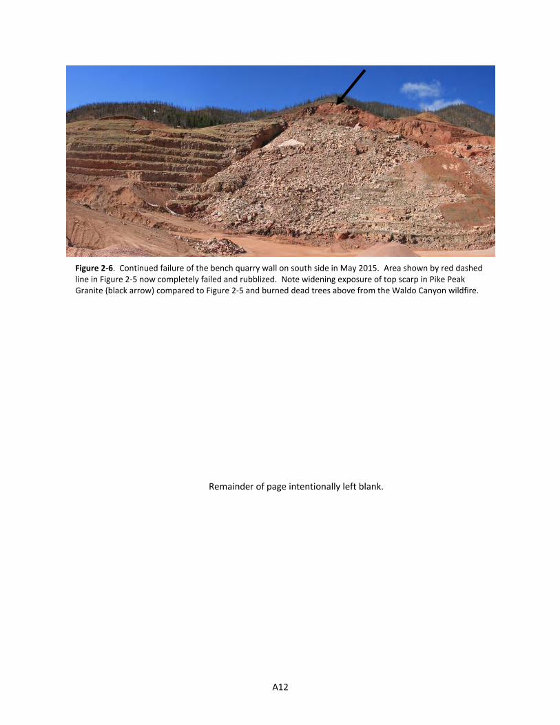
A12
Remainder of page intentionally left blank.
Figure 2-6. Continued failure of the bench quarry wall on south side in May 2015. Area shown by red dashed line in Figure 2-5 now completely failed and rubblized. Note widening exposure of top scarp in Pike Peak Granite (black arrow) compared to Figure 2-5 and burned dead trees above from the Waldo Canyon wildfire.

A13
Abstract #3 - Garden of the Gods Park By
Roger Pihl and Jonathan L. White
Park History
By the 1870’s, the railroads had forged their way west. In 1871, General William Jackson Palmer
founded Colorado Springs while extending the lines of his Denver and Rio Grande Railroad. In 1879,
General Palmer repeatedly urged his friend, Charles Elliott Perkins, the head of the Burlington Railroad,
to establish a home in the Garden of the Gods and to build his railroad from Chicago to Colorado
Springs. Although the Burlington never reached Colorado Springs directly, Perkins did purchase three
hundred and forty acres in the Garden of the Gods for a summer home in 1879. He later added to the
property but never built on it, preferring to leave his wonderland in its natural state for the enjoyment
of the public. Perkins died in 1907 before he made arrangements for the land to become a public park,
although it had been open to the public for years. In 1909, Perkins’ children, knowing their father’s
feelings for the Garden of the Gods, conveyed his four-hundred eighty acres to the City of Colorado
Springs. It would be known forever as the Garden of the Gods “where it shall remain free to the public,
where no intoxicating liquors shall be manufactured, sold or dispensed, where no building or structure
shall be erected except those necessary to properly care for, protect, and maintain the area as a public
park.“
Introduction
The story of the rocks seen in the Garden of the Gods Park begins over 300 million years ago
when a different set of Rocky Mountains existed here. This first set of Rocky Mountains is known as the
Ancestral Rockies (Frontrangia), which were composed of the same Pikes Peak Granite. There have
been two Phanerozoic mountain building episodes in the Pikes Peak area:
The ancestral Rockies occurred approximately 320 million years ago. The erosion of these first
Rocky Mountains created thick sediments that formed the sedimentary “red bed” Fountain
Formation sandstone and conglomerate layers followed by the Lyons Sandstone.
The Larimide Orogeny uplifted the Front Range, including Garden of the Gods. Sediments shed
from these mountains were deposited east to become the Denver Basin Group (See figure 6 in
guidebook introduction).
The Garden of the Gods Park is composed entirely of sedimentary rock layers, and is unique
because the rock layers have been tilted upright, laterally offset, and through millions of years of
differential erosion, exposed in dramatic fashion. The Garden of the Gods Park lies on four separate
geologic quadrangles mapping by the Colorado Geological Survey: Colorado Springs, Manitou Springs,
Cascade, and Pikeview (see geologic map B in appendix B).

A14
Formations in the Park
Sedimentary formations exposed in Garden of the Gods, from youngest to oldest, include the
Pierre Shale (Kp); the slope forming, combined Carlile Shale, Greenhorn Limestone, and Graneros Shale
unit (Kcgg); ridge forming limestones of the Niobrara Formation (Kn); the hogbacks and ridges of the
Dakota Sandstone (Kd) and Purgatoire Formation (Kpu); the slope forming Morrison and Ralston Creek
formations (Jmr); the red Lykins Formation (TR Pl); the resistant red and white sandstone beds of the
upper, middle, and lower units of the Lyons Sandstone (Plu, Plm, and Pll) that form the tallest rock spires
in the Park (and the most famous feature, the Kissing Camels); and the “red beds” of the Fountain
Formation (PIP f). As seen the geologic map in Figure 3-1, the bedrock units are highly faulted and
deformed within the Garden of the Gods. The formations and their relative thicknesses are shown in
the stratigraphic column in figure 5 of the Regional Geology section of the field trip guidebook
Figure 3-1. Larger-
scale geologic map of
Garden of the Gods.
Illustration from
Morgan and others
(2003).

A15
introduction. From the Visitors Center you can see that these rocks are not all restricted to the Garden
of the Gods area. They continue south in regimental rows across Fountain Creek into Red Rock Canyon
until they are cut off abruptly by the Ute Pass Fault, with the steep slopes of Cheyenne Mountain rising
behind.
A famous dinosaur skull was found in the Garden of the Gods in 1878 by a Colorado College
Professor named James Kerr. The fossil was recovered from the Lower Cretaceous Purgatoire Formation
and given to the famous dinosaur fossil collector O.C. Marsh in 1886. The fossil was misidentified and
sent to the Yale Peabody Museum where it safely rested for over 100 years, but forgotten in Colorado
Springs. As new park exhibits were being planned in 1994, the skull was remembered and borrowed by
the Denver Museum of Nature & Science to be examined and a cast made for the visitor center. At that
time, Dr. Carpenter, a long-time dinosaur expert at the museum, noticed irregularities with the original
assignment and further researched indicated that the skull was of a brand new genus and specie -
Theiophytalia kerri was named. The dinosaur fossil is so far the only dinosaur of this species found
anywhere in the world. An exhibit of the fossil is in the visitor center
(http://www.gardenofgods.com/educational/edu-2/theophytalia-kerri).
Faulting
Both Figure 3-1, figure 19 in the road log, and the geologic map B in Appendix B illustrates the
complexity of the Rampart Range fault system as it passes southward through the Garden of the Gods
Park and “dies out” below Fountain Creek. The Rampart Range fault is a high-angle thrust fault with the
up-thrown block on the west side. However, the southern segment of the north-south striking fault is
interpreted to contain both a floor thrust and roof thrust, creating a triangular zone cross section model
where east and west back-thrust sheets can be accommodated in a single structural system (Morgan
and others, 2003; Siddoway and others, 2013). See Figure 3-2.
The backthrusted slivers of rock have been rotated vertical to overturned and differential
erosion is responsible for the spectacular vertical “fins” of colorful sandstone outcrops that make the
park an attraction for geologist and tourist alike. Through the entire Park, the Rampart Range thrust
fault hanging wall is composed of steeply dipping Fountain Formation. The Rampart Range fault foot
wall, composed of vertical or overturned Lyons Sandstone, is further offset by the three faulted
backthrust slivers such that, along the fault in the park, the Fountain Formation is set against Lyons
though Morrison formations. These dipping faults, from north to south are the Hidden Inn Fault,
Kindergarten Rock Fault, and the South Fault (Figure 3-1).

A16
Figure 3-2. Conceptualized cross section using a triangular thrust model for the Rampart Range thrust fault at
the Garden of the Gods. Modified from Siddoway and others (2013).

A17
Abstract #4 - Waldo Canyon Wild Fire and Manitou Springs Flooding By
Jonathan L. White and Roger Pihl
This abstract has been written, in part, with text from the Geotechnical Extreme Events Reconnaissance (GEER) report (Keaton and others, 2013). The GEER report focused on a relatively small area northwest of Colorado Springs near Manitou Springs where a cloudburst storm on August 9, 2013 dropped high-intensity precipitation on burned watershed slopes. The background information regarding geology, topography, soils, the June 2012 Waldo Canyon fire, and post-fire precipitation events the next year provide context for descriptions of geotechnical mitigation in extended abstract #5.
Geology and Topography
The geology and geologic structure of the Manitou Springs area is discussed in the Geology section of the guidebook, and shown in the Figure 3 regional geologic map, the geologic maps in Appendix B, and formations shown in the stratigraphic column (Figure 5). Areas relevant to the 2013 flooding in Manitou Springs are the steep, watersheds of Pikes Peak Massif and those burned by the Waldo Canyon wild fire on Rampart Range, and Fountain Creek Canyon that passes through Manitou Springs.
Waldo Canyon Fire
The Waldo Canyon Fire initiated on June 23, 2012 and was contained on July 10, 2012. Approximately 18,247 acres, nearly entirely within foothills and mountains of the Rampart Range, were burned by this fire. There were two fatalities, 347 homes destroyed, and more than 32,000 people evacuated. The fire cost more than $16 million to fight and incurred a half billion dollars in insured losses. The initial Burned Area Emergency Response (BAER, 2012) assessment includes an executive summary report, as well as maps of fire progression, burn severity, and photographs of the burned areas. Figure 4-1 shows the USFS BAER soil burn severity map of the Waldo Canyon fire.
Nearly the entire 2012 Waldo Canyon fire perimeter lies within crystalline Precambrian rock in the Rampart Range, with a small area of the burn extending into Colorado Springs onto sedimentary rocks or surficial deposits (several images in the field trip guidebook show the perimeter of Waldo Canyon Fire).
Surficial deposits on slopes are important because they support the vegetation on the slopes that burned, can respond to the heat of the fire becoming hydrophobic, and produce sediment by erosion that contributes to damage in cloudburst storms. Alluvial deposits (silts, sands, gravels) accumulate in stream channels and on floodplains at varying rates; these deposits are available for erosion and remobilization during flash floods. Partially dissected remnants of older gravel deposits are present along Fountain and Monument Creek, and the Colorado Piedmont. Alluvial (fluvial) processes are dominant in stream channels and on flood plains, whereas gravity (colluvial) and sheetwash processes are dominant on ungullied hillslopes. Climate processes (freezing-thawing, wetting-drying, heating-cooling) act on mountain slopes, including exposed bedrock, and can produce substantial amounts of loose soil material (dry ravel) that moves downslope mainly by gravity, gradually and progressively. This sediment generation activity is accelerated where grussy pockets exists, caused by the partial to complete granular disintegration of the coarse-crystalline Pikes Peak Granite.

A18
Figure 4-1. Waldo Canyon BAER soil burn severity map from U.S. Forest Service

A19
Different types of hazardous geologic processes have been recognized by the Colorado Geological Survey in the Manitou Springs region (Keller and others, 2003; Morgan and others, 2003), including debris flows. Intense rainfall on steep slopes underlain by shallow bedrock can produce substantial runoff. Severe wildfire on steep drainage-basin slopes produces conditions for enhanced storm water runoff; even moderate storms are expected to produce increased flow volumes and velocities in channels that are capable of transporting sediment eroded from the slopes. Intense rainfall and increased runoff volume results in high potential for surficial deposits on steep slopes to move into drainages and be transported downstream. Large sediment and debris loads could become deposited within the lower-gradient channel reaches and at drainage devices, such as corrugated metal pipe or concrete box culverts. Channel capacities that are exceeded can result in peak discharge and hyperconcentrated flows diverting out of existing channels and being intercepted by roadways and being directed into downstream residential and commercial areas causing damage to property and threatening life and safety.
Runoff and sediment yield were identified as potential hazards within the first 3-7 years following the fire, until vegetation is reestablished on slopes in the majority of the burned area. Potential threats to health and safety of communities in the downstream perimeter of the burned area from increased post-fire watershed responses were immediately identified and treatment options were recommended (BAER, 2012). As part of a preliminary emergency assessment, and using the burn severity mapping, the probability and estimated volume of potential post-wildfire debris flows originating on slopes within the Waldo Canyon Burn Area were estimated by the U.S. Geological Survey (Verdin and others, 2012) (Figures 4-2).
August 9, 2013 Flash Flood Event
The storm that is the subject of the GEER report (Keaton and others, 2013) occurred on August 9, 2013. However, a storm occurred on July 1, 2013, that also caused local flooding in Manitou Springs. The precipitation during July 2013 contributed to antecedent soil moisture for the storm on August 9, 2013, but did not exceed the normal value by a wide margin, suggesting that the rainfall intensity of the August 9, 2013, storm may have been more important than the degree of saturation of the surficial soil deposits on the slopes in the burned watershed. Precipitation data compiled by Keaton (2013) indicates the August 9, 2013, storm was relatively fast-moving and localized; and the short-duration, high-intensity precipitation distribution (up to a 5-min intensity equaling 5 in/hr) appears to be represented reasonably well by the NEXRAD Doppler radar reflectivity. The southern part of the Waldo Canyon Burn Area experienced the heaviest precipitation. In about 30 minutes, 1.6 inches fell in Williams Canyon and 1.5 inches fell in Waldo Canyon. Examination of geologic maps reveals that most of the heaviest precipitation fell on burn areas of loose grussy slopes underlain by granitic rock (i.e., all of Waldo Canyon and the northern part of Williams Canyon). The southern part of Williams Canyon is underlain by metamorphic and Paleozoic sedimentary rocks. The burn areas were the source of most of the debris as evidenced by the very dark gray to black color of the debris-laden flood waters from the high concentrations of ash. The August 9, 2013 debris-laden flash floods was Manitou Springs’ worst disaster in decades, costing millions of dollars. There was one fatality. Flood damage occurred along Williams Canyon creek to the confluence with Fountain Creek, Waldo Canyon down westbound US24 and Manitou Avenue to Foundation Creek, and Fountain Creek itself. Manitou Springs is clustered tightly in the narrow Fountain Creek valley and many of the channels have been narrowed by walls, even directed into culverts in

A20
Figu
re 4
-2.
Esti
mat
ed p
rob
abili
ty o
f p
ote
nti
al p
ost
-wild
fire
deb
ris
flo
ws
in t
he
Wal
do
Can
yon
bu
rn a
rea.
Im
age
fro
m U
SGS
(Ver
din
an
d o
ther
s (2
01
2).

A21
town. Almost all of the culverts became blocked by debris so that creeks jumped their channels and washed down roadways. There are many videos on YouTube of the flooding of Manitou Springs. Bouldery debris washed down Williams Canyon and destroyed the historic original Cave of the Winds road (Figure 4-3) and many homes below (Figure 4-4). An extensive mitigation effort along Williams Canyon creek from the mouth of the canyon was completed in 2015 at a cost of $6.1 million. It included improved concrete flumes with elevated walls, a succession of cable-net debris catchment devices, and an enlarged detention basin at the mouth of the canyon (Figure 4-5). Future phases are still being planning as funding becomes available.
Figure 4-3. Cave of the Winds exit road completely washed out by flood of August 9th, Mortared rock wall in
photo was the retaining wall for the original road that was on right side. Creek originally flowed to left of rock
wall against rock face. This road has now been abandoned above the switch back to Geneva Trail road at the
approximate location of the photo. Photo from GEER report (Keaton and others, 2013).
Figure 4-4. Post-flood
image of neighborhood of
Manitou Springs near
mouth of Williams Canyon
showing size of boulder
debris that was washed into
town.

A22
The Waldo Canyon creek flooding didn’t enter Fountain Creek until within Manitou Springs. The debris-laden flows quickly plugged the US 24 culvert and redirected onto the highway, with the majority flowing down WB US 24 lanes (Figure 4-6) where the flow was constrained by the north valley wall and Type 4 barrier that divided the highway. Flows up to 4 feet deep washed ½ mile down the WB lanes floating several occupied cars (See figure 24 in road log). CDOT mitigated debris flooding at Waldo Canyon by the construction of a new wide concrete box culvert, excavation of a basin, and installation of cable-netting spanning the narrows near the mouth (See extended abstract #5).
Figure 4-5. Basin constructed at mouth of Williams Canyon after 2013 flood. Note cable-net spanning flume at
far end of detention basin. Image saved from Google Earth Pro™ Street View.

A23
Figure 4-6. Annotated image with
path of debris-laden flood down
US 24 from Waldo Canyon. Flood
path (yellow dashed arrow) was
predominately constrained by
CDOT concrete barriers (K-rail) that
divided east and westbound lanes
of US 24; leading to flows to be
concentrated on WB lanes to
underpass and onto Manitou
Avenue (old US 24). Image from
GEER report (Keaton and others,
2013)
Figure 4-6 (cont.) Annotated
image on left is at mouth of
Waldo Canyon near US 24 and
confluence with Fountain Creek
showing high water mark from
August 9, 2013 flood. Image
from GEER report (Keaton and
others, 2013)
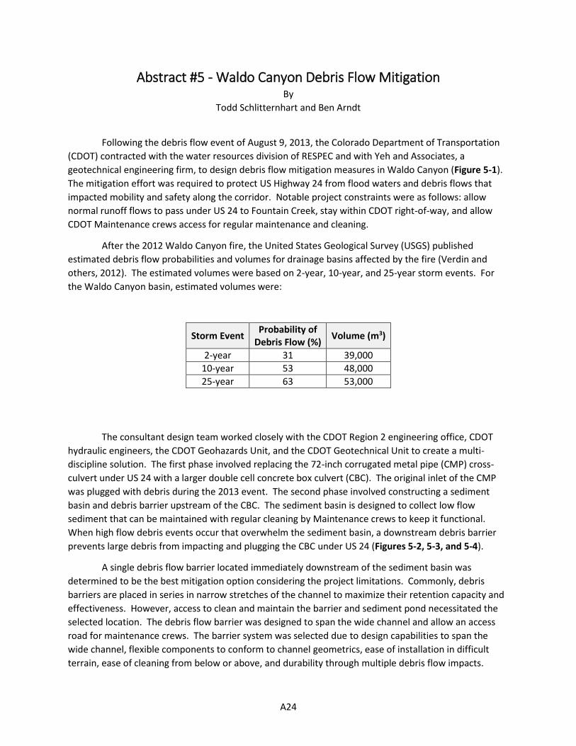
A24
Abstract #5 - Waldo Canyon Debris Flow Mitigation By
Todd Schlitternhart and Ben Arndt
Following the debris flow event of August 9, 2013, the Colorado Department of Transportation
(CDOT) contracted with the water resources division of RESPEC and with Yeh and Associates, a
geotechnical engineering firm, to design debris flow mitigation measures in Waldo Canyon (Figure 5-1).
The mitigation effort was required to protect US Highway 24 from flood waters and debris flows that
impacted mobility and safety along the corridor. Notable project constraints were as follows: allow
normal runoff flows to pass under US 24 to Fountain Creek, stay within CDOT right-of-way, and allow
CDOT Maintenance crews access for regular maintenance and cleaning.
After the 2012 Waldo Canyon fire, the United States Geological Survey (USGS) published
estimated debris flow probabilities and volumes for drainage basins affected by the fire (Verdin and
others, 2012). The estimated volumes were based on 2-year, 10-year, and 25-year storm events. For
the Waldo Canyon basin, estimated volumes were:
Storm Event Probability of
Debris Flow (%) Volume (m3)
2-year 31 39,000
10-year 53 48,000
25-year 63 53,000
The consultant design team worked closely with the CDOT Region 2 engineering office, CDOT
hydraulic engineers, the CDOT Geohazards Unit, and the CDOT Geotechnical Unit to create a multi-
discipline solution. The first phase involved replacing the 72-inch corrugated metal pipe (CMP) cross-
culvert under US 24 with a larger double cell concrete box culvert (CBC). The original inlet of the CMP
was plugged with debris during the 2013 event. The second phase involved constructing a sediment
basin and debris barrier upstream of the CBC. The sediment basin is designed to collect low flow
sediment that can be maintained with regular cleaning by Maintenance crews to keep it functional.
When high flow debris events occur that overwhelm the sediment basin, a downstream debris barrier
prevents large debris from impacting and plugging the CBC under US 24 (Figures 5-2, 5-3, and 5-4).
A single debris flow barrier located immediately downstream of the sediment basin was
determined to be the best mitigation option considering the project limitations. Commonly, debris
barriers are placed in series in narrow stretches of the channel to maximize their retention capacity and
effectiveness. However, access to clean and maintain the barrier and sediment pond necessitated the
selected location. The debris flow barrier was designed to span the wide channel and allow an access
road for maintenance crews. The barrier system was selected due to design capabilities to span the
wide channel, flexible components to conform to channel geometrics, ease of installation in difficult
terrain, ease of cleaning from below or above, and durability through multiple debris flow impacts.

A25
Although the calculated retention volume of the barrier (1,880 m3) is significantly less than the
anticipated debris flow volumes, through cooperative design elements and regular maintenance the
system has prevented debris flows from impacting the highway since construction completed in the Fall
of 2014.
Figure 5-1. Debris
barrier location prior
to construction
(3/6/2014).
Figure 5-2. Debris
barrier completed
(12/2/2014).

A26
Figure 5-3. Debris barrier partially inundated (5/21/2015).
Figure 5-4. Debris barrier cleaned out (9/9/2015).

A27
Abstract #6 - Red Rock Canyon Open Space by
Jonathan L. White
Red Rock Canyon Open Space includes tilted strata of the stratigraphic section from Fountain
Formation to limestone ridgelines of the Niobrara Formation. These formations are the same as at
Garden of the Gods Park but without the extensive structural deformation.
At both Red Rock Canyon and Garden of the Gods the Lyons Sandstone has been informally
subdivided into three units shown on the geologic map. The upper unit (Plu), middle unit (Plm), and
lower unit (Pll). Those units are easily seen at Red Rock Canyon. The lower unit (Pll) is in contact with
the Fountain Formation and is a massive resistant eolian sandstone. The middle unit is a softer, friable
micaceous arkosic conglomeritic sandstone and siltstone that does not outcrop well. The upper unit is a
hard, resistant, white to red sandstone with prominent planar beds of cross-bedded dune sand. The
Lyons Formation, where steeply dipping at both Garden of the Gods and Red Rock Canyon, outcrops as
two ridges of sand separated by a trough where the middle unit forms an intervening strike valley.
Red Rock Canyon Open Space is a popular hiking area with a trail network through the many
rock features. Notable sights in the open space are trails that meander through steep dipping spires and
fins of Fountain Formation sandstone on the west side. On the east side are benches, notches, and
steep walls from historic, long-abandoned quarries that cut into the lower Lyons Sandstone ridgeline for
dimension stone from the 1880s to 1910s (Figure 6-1). Those quarries, and world-class exposure of
planar bedded,
cross-set (dune)
sandstone
(Figures 6-2 and
6-3) are within
easily walking
distance from the
parking area. A
full-page trail
map (Figure 6-4)
of Red Rock
Canyon Open
Space and the
geologic map at
the same scale
(Figure 6.5) are in
the back of this
extended
abstract.
Figure 6-1. Historic quarry in lower Lyons Sandstone (Pll) at Red Rock Canyon Open
Space. Photo courtesy of F. Trenkler, www.cospringsstrails.com/hikes/redrock.html

A28
Figure 6-3. East-facing oblique image of quarry in figure 6-2 showing Lyons Sandstone lower unit (quarried
sandstone in bottom of image), middle unit strike valley, and upper unit at top of image. Note the exposures
of planar bedded strata with dune cross sets in exposure of upper unit. Beds are dipping about 75° to east.
Image created from Google Earth Pro™ urban high-resolution 3D imagery.
Figure 6-2. Oblique image of Red Rock Canyon showing location of historic quarry in steeply dipping Lyons
Sandstone approximately 6/10th of a mile from parking lot. View is to the north to northwest. Image created
from Google Earth Pro™ urban high-resolution 3D imagery.
Quarry
Fountain Fm. Lyons lower unit
Lyons middle unit
Lyons upper unit

A29
Figure 6-4.

A30
Geology from Keller and others (2003)
Figure 6-5.

B1
Appendix B
The enclosed geologic maps A, B, C, and D in this appendix are north to south geologic maps of
the Colorado Springs vicinity that were clipped from maps by the Colorado Geological Survey (CGS)
published from 2000 to 2003. An index map is shown in Figure 1. The maps are also listed in the
guidebook references. The map reproductions are in the same original 1:24,000-scale. These map are
available as free downloads of pdf-format map plate files and GIS data from the CGS publication web
site.

B2
Pikeview Quad
Thorson and others (2001)
Cascade Quad
Morgan and others (2003)
Geologic Map A

B3
Cascade Quad
Morgan and others (2003)
Manitou Springs Quad
Keller and others (2003)
Pikeview Quad
Thorson and others (2001)
Colorado Springs Quad
Carroll and Crawford (2001)
Geologic Map B

B4
Colorado Springs Quad
Carroll and Crawford (2001)
Manitou Springs Quad
Keller and others (2003)
Geologic Map C
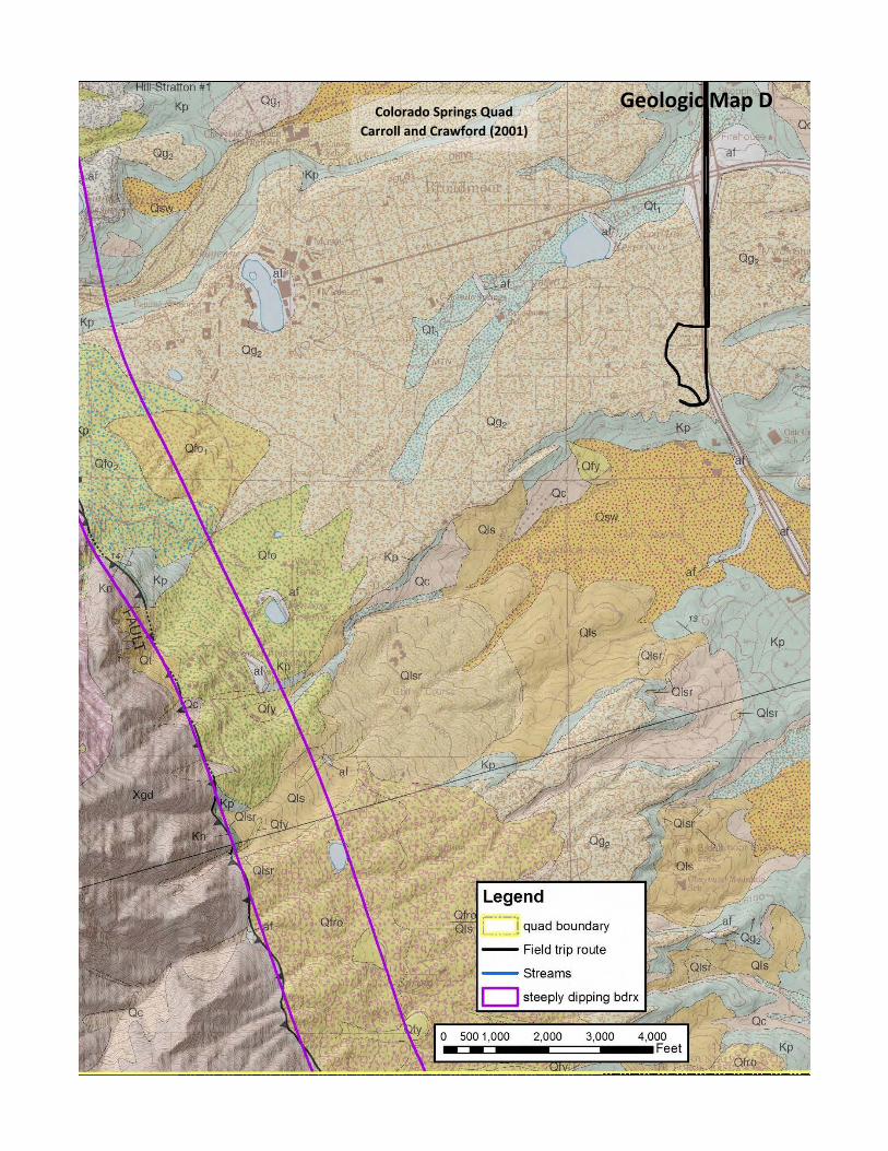
B5
Colorado Springs Quad
Carroll and Crawford (2001)
Geologic Map D