Institute of Parallel and Distributed SystemsUniversity of Stuttgart

UniversitätsstraSSe 38D–70569 Stuttgart

Masterthesis Nr. 3310

3D Video Tracking andLocalization of Underwater Swarm

Robots

Martin Antoni

Course of Study: INFOTECH

Examiner: Prof. Dr. rer. nat. habil. Paul Levi

Supervisor: Dipl.-Ing. Tobias Dipper

Commenced: 01.02.2012

Completed: 02.08.2012

CR-Classification: D.1.0, B.1.4, I.4.1

Abstract

Autonomous underwater vehicles (AUV) are robots, which usually estimate theirposition by localization the help of internal or external sensors. In this thesis, smallswarm robots from the CoCoRo are used as experimental platform. It is often use-ful, to know the exact position inside the testing area to evaluate swarm algorithms.Controlling the position of the robot should be possible as well.

A software is developed, which is able to track a robot inside an aquarium. Twocameras are install at each side of this aquarium for determining the 3D positionwhich includes the diving depth. Perspective distortions, which come from view-ing angle, are compensated with the help of image transformation. With the cor-rected image, the template matching algorithm with normalized cross-correlationis used to track the robot in the camera image.

A wireless connection is established between the computer and the robot to readout sensor data and to control the motors. Waypoints can be set by the user whichthe robot follows. The computer uses two independent controllers for rotationaland for distance control.

Zusammenfassung

Unbemannte Unterwasserfahrzeuge (AUV) sind Roboter, welche üblicherweise ihrePosition durch interne und externe Sensoren bestimmen. In dieser Masterarbeitwerden Schwarmroboter von dem CoCoRo Projekt als Testplattform benutzt. Esist sinnvoll, die genaue Position des Roboters zu wissen. Das macht es einfacher,bestimmte Schwarmalgorithmen zu testen. Weiterhin ist es nützlich, den Robotersteuern zu können.

In dieser Arbeit ist eine Software entwickelt worden, welche die Position desRoboters in einem Aquarium verfolgt. Zwei Kameras sind auf jeder Seite desAquariums angebracht. Damit ist es möglich, die 3D Position zu bestimmen, welchedie Tauchtiefe enthält. Perspektivische Verzerrungen, welche durch den Blick-winkel entstehen, werden mit einer Koordinatentransformation kompensiert. MitHilfe des ’Template matching’-Algorithmus und der normalisierten Kreuzkorrela-tion wird die Position des Roboters im Bild verfolgt.

Eine kabellose Verbindung zwischen dem Computer und dem Roboter überträgtdie Sensordaten und wird für die Motorsteuerung genutzt. Die Motorleistung wirddurch eine Drehungs- und Abstandsregelung vorgegeben. Durch Wegpunkte kanneine Route gesetzt werden, welche der Roboter abfährt.

Contents

List of Figures VI

List of Tables IX

1 Introduction 31.1 Task . . . . . . . . . . . . . . . . . . . . . . . . . . . . . . . . . . . . . . 41.2 Work description . . . . . . . . . . . . . . . . . . . . . . . . . . . . . . 4

2 Hardware 52.1 Robot . . . . . . . . . . . . . . . . . . . . . . . . . . . . . . . . . . . . . 52.2 Communication . . . . . . . . . . . . . . . . . . . . . . . . . . . . . . . 6

2.2.1 Blue light transmission . . . . . . . . . . . . . . . . . . . . . . . 62.2.2 USB RFM12 Bridge . . . . . . . . . . . . . . . . . . . . . . . . . 7

2.3 Sensors . . . . . . . . . . . . . . . . . . . . . . . . . . . . . . . . . . . . 82.3.1 Accelerometer . . . . . . . . . . . . . . . . . . . . . . . . . . . . 82.3.2 Digital compass . . . . . . . . . . . . . . . . . . . . . . . . . . . 92.3.3 Pressure sensor . . . . . . . . . . . . . . . . . . . . . . . . . . . 112.3.4 Distance measurement . . . . . . . . . . . . . . . . . . . . . . . 11

2.4 Actors . . . . . . . . . . . . . . . . . . . . . . . . . . . . . . . . . . . . . 122.5 Aquarium . . . . . . . . . . . . . . . . . . . . . . . . . . . . . . . . . . 122.6 Cameras . . . . . . . . . . . . . . . . . . . . . . . . . . . . . . . . . . . 12

3 Video Tracking 153.1 Perspective distortion . . . . . . . . . . . . . . . . . . . . . . . . . . . . 153.2 Gaussian elimination process . . . . . . . . . . . . . . . . . . . . . . . 183.3 Template matching . . . . . . . . . . . . . . . . . . . . . . . . . . . . . 183.4 Cross correlation . . . . . . . . . . . . . . . . . . . . . . . . . . . . . . 193.5 Calculation of the 3D position . . . . . . . . . . . . . . . . . . . . . . . 20

4 Robot control 274.1 Hydrodynamic equation . . . . . . . . . . . . . . . . . . . . . . . . . . 28

4.1.1 Forces under water . . . . . . . . . . . . . . . . . . . . . . . . . 284.1.2 Solving movement equation . . . . . . . . . . . . . . . . . . . . 29

4.2 Control strategie . . . . . . . . . . . . . . . . . . . . . . . . . . . . . . . 314.2.1 P-controller . . . . . . . . . . . . . . . . . . . . . . . . . . . . . 32

V

Contents

4.2.2 PD-Controller . . . . . . . . . . . . . . . . . . . . . . . . . . . . 32

5 Software 355.1 Main software . . . . . . . . . . . . . . . . . . . . . . . . . . . . . . . . 35

5.1.1 GUI . . . . . . . . . . . . . . . . . . . . . . . . . . . . . . . . . . 365.1.2 Flowchart . . . . . . . . . . . . . . . . . . . . . . . . . . . . . . 385.1.3 Algorithms . . . . . . . . . . . . . . . . . . . . . . . . . . . . . 40

5.2 Additional software . . . . . . . . . . . . . . . . . . . . . . . . . . . . . 435.2.1 Softwareimplementation of Gaussian elimination . . . . . . . 45

6 Experiments 496.1 Video tracking . . . . . . . . . . . . . . . . . . . . . . . . . . . . . . . . 496.2 Robot control . . . . . . . . . . . . . . . . . . . . . . . . . . . . . . . . 50

7 Summary 557.1 Outlook . . . . . . . . . . . . . . . . . . . . . . . . . . . . . . . . . . . . 55

Literatur A

VI

List of Figures

2.1 Submarine Toy . . . . . . . . . . . . . . . . . . . . . . . . . . . . . . . . 52.2 CoCoRo Robot . . . . . . . . . . . . . . . . . . . . . . . . . . . . . . . . 62.3 USB RFM12 bridge dataflow . . . . . . . . . . . . . . . . . . . . . . . . 72.4 USB RFM12 bridge . . . . . . . . . . . . . . . . . . . . . . . . . . . . . 82.5 Magnetic field of the earth . . . . . . . . . . . . . . . . . . . . . . . . . 92.6 Yaw, roll and pitch angle . . . . . . . . . . . . . . . . . . . . . . . . . . 102.7 Aquarium . . . . . . . . . . . . . . . . . . . . . . . . . . . . . . . . . . 122.8 Microsoft LifeCam HD-3000 . . . . . . . . . . . . . . . . . . . . . . . . 132.9 View of camera 1 . . . . . . . . . . . . . . . . . . . . . . . . . . . . . . 142.10 View of camera 2 . . . . . . . . . . . . . . . . . . . . . . . . . . . . . . 14

3.1 Image processing flow . . . . . . . . . . . . . . . . . . . . . . . . . . . 163.2 Vanishing point . . . . . . . . . . . . . . . . . . . . . . . . . . . . . . . 173.3 Template matching . . . . . . . . . . . . . . . . . . . . . . . . . . . . . 183.4 Snell’s Law . . . . . . . . . . . . . . . . . . . . . . . . . . . . . . . . . . 213.5 Optical path of the cameras in the aquarium . . . . . . . . . . . . . . 213.6 Skew lines . . . . . . . . . . . . . . . . . . . . . . . . . . . . . . . . . . 24

4.1 Real Position of the robot . . . . . . . . . . . . . . . . . . . . . . . . . . 304.2 Real Position of the robot . . . . . . . . . . . . . . . . . . . . . . . . . . 314.3 Controller overview . . . . . . . . . . . . . . . . . . . . . . . . . . . . . 32

5.1 Main software GUI . . . . . . . . . . . . . . . . . . . . . . . . . . . . . 365.2 Main software - Template settings . . . . . . . . . . . . . . . . . . . . 365.3 Main software - logging settings . . . . . . . . . . . . . . . . . . . . . 375.4 Main software - Waypoint settings . . . . . . . . . . . . . . . . . . . . 395.5 Main software - Robot information . . . . . . . . . . . . . . . . . . . . 405.6 Main software - Transformed camera picture . . . . . . . . . . . . . . 415.7 Main software flowchart (initialization) . . . . . . . . . . . . . . . . . 425.8 Main software flowchart . . . . . . . . . . . . . . . . . . . . . . . . . . 475.9 Transformation matrix solving GUI . . . . . . . . . . . . . . . . . . . . 48

6.1 Constast setting from left to right: 1, 2, 3 . . . . . . . . . . . . . . . . . 496.2 Reflections and Shading problems . . . . . . . . . . . . . . . . . . . . 506.3 Rotation controller up step response . . . . . . . . . . . . . . . . . . . 51

VII

List of Figures

6.4 Rotation controller down step response . . . . . . . . . . . . . . . . . 526.5 Waypoint route on the surface . . . . . . . . . . . . . . . . . . . . . . . 526.6 Waypoint route with 30cm diving depth . . . . . . . . . . . . . . . . . 536.7 Depth calculation . . . . . . . . . . . . . . . . . . . . . . . . . . . . . . 53

VIII

List of Tables

2.1 Data packet . . . . . . . . . . . . . . . . . . . . . . . . . . . . . . . . . 72.2 Sensors of the robot . . . . . . . . . . . . . . . . . . . . . . . . . . . . . 8

3.1 Perspective distortion vectors and angles . . . . . . . . . . . . . . . . 22

4.1 Approaches to control . . . . . . . . . . . . . . . . . . . . . . . . . . . 274.2 Forces under water . . . . . . . . . . . . . . . . . . . . . . . . . . . . . 28

5.1 Reqirements of the main software . . . . . . . . . . . . . . . . . . . . . 355.2 Logging file format . . . . . . . . . . . . . . . . . . . . . . . . . . . . . 375.3 Loggine file sample data . . . . . . . . . . . . . . . . . . . . . . . . . . 385.4 ’matrix.txt’ file format . . . . . . . . . . . . . . . . . . . . . . . . . . . 45

IX

1 Introduction

Autonomous underwater vehicles (AUV) are used in scientific application, likeanalysing an area of a reef or the sea ground. They can operate alone or with mul-tiple robots. When many robots act together, a swarm is created. Swarm robotshave the advantage, that if one fails, the group can continue operating. Multipledefects lead only to a smaller group. When using one big robot, which have thesame ability like the whole swarm, defects on the robot are much more harmful.

AUV’s navigate with the help of localisation and mapping. This includes esti-mating their position using sensors. Some robots can operate with a relative posi-tion, others needs the absolute position.

The development phase is a very critical phase where quick results are importantto get good results in a feasible time. All aids are welcome to the developer. Inthis thesis, a tool is discussed, which eases the testing and developing phase ofautonomous underwater vehicles (AUV).

The CoCoRo [coc] project deals with AUVs which are able to move in a swarm.These robots can estimate their positions with internal and external sensors. Cal-culations are made with the sensor data and control data from actors. The positioncan either be an absolute one or a relative position to other robots. To validatethe precision of the estimation, the real position has to be known. With this in-formation, parameters influencing the estimation can be optimized. Localisationof AUVs has two main approaches, visual and acoustic[PZ04]. In the visual ap-proach, cameras are installed in the robot to get a picture of the environment. Therobot can use stereo cameras[PZ04] to locate itself. Also, pattern recognition canbe used for localization[MCN]. These approaches have the problem, that the cam-era inside the robot is relatively big and processing the video stream needs a lotof computation power. In the CoCoRo project, robots with a size of about 12cm indiameter are used. They have only a small microcontroller for the basic controllingapplications. An onboard camera is therefore no option. The acoustic approachuses sound waves. In a small aquarium, a lot of reflections occur. This is very prob-lematic, because the waves add and subtract themselves. The localisation is almostnot possible.

3

1 Introduction

1.1 Task

For this thesis, the localisation area is an aquarium. A system is needed to getthe position of the robots inside this aquarium. This is done with external cameras.This method is chosen, because it does not disturb the movement of the robot. Withtwo cameras at different positions, it is possible to get the 3D position of the robot.One problem with this approach is refractions. Under water, light travels slowerthan in air. These refractions have to be considered in the position calculation pro-cess. With the knowledge of the corner points of the aquarium, a transformationmatrix can be created to compensate the viewing angles distortions.

The cameras are connected to a computer. Processing the video stream from thecameras is needed to locate an object inside a picture. Many algorithms exist forlocalisation. With the feature based approach[JH], borders and edges are used torecognise an object. This is not sufficient for this thesis, because the robot (see figure2.2) does not have many features. Other approaches use all pixel values to find anobject. In this thesis, the template matching algorithm [KB01] was chosen. With thehelp of internal sensor data from the robot, it is possible to get the heading of therobot.

To establish a connection between the robot and the computer to exchange data,a wireless system is needed. It is not possible to connect a cable to the robot, be-cause this would disturb its movement. All robots are equipped with a RF module.Transmitting data is done in the robots firmware. On the computer side, an inter-face is needed to connect the module to the computer. With the aid of waypoints,the robots should be able to drive a defined route without interaction of the user.

1.2 Work description

The task is to get a working solution, where two cameras point onto the aquariumand track the robots inside the aquarium. There has to be control of the positionof one robot over the computer software. Therefore, a connection to the robot hasto be established. All algorithms that are used are described in this thesis. In thefirst step, a camera is chosen for the video tracking system. This camera is selectedwith regards to the price and resolution. In the next step, a program to read outthe video stream is developed and the frame rate of the tracking has to be definedby the user. After setting up the cameras, a proper tracking algorithm is selectedand implemented. With the help of the tracking system, the control of the robot isdeveloped in the next step. First, the control of the rotation, then the distance con-trol is implemented. After motion control of the robot is established, the selectionof waypoints is implemented. Logging feature have to be implemented, to use thetracking data for later evaluation.

4

2 Hardware

There are two main parts of hardware used in this thesis, the AUV ’Lily’ and a com-puter. For the communication, a wireless system is used. For the video tracking,two cameras are installed. In the following sections, each part is described in detail.

2.1 Robot

The underwater robot that is used in this thesis is a modified toy submarine. Figure2.1 shows the original model, which can be bought in the internet or other stores.This toy can move backwards, forwards and dive. It also can turn on a spot, so it ispossible to move in each direction. For the CoCoRo project, this toy was modified.

Figure 2.1: Submarine Toy

The top was replaced by a custom made head. Motors and the on-off switch on thebottom part were not changed. In the inside, the custom main control board wasinserted and the batteries were changed to lithium polymere technology. Severalsensors are around the outside of the robot and on the mainboard. In figure 2.2,the final version of the robot is shown, which is used as experimenting platformduring this thesis. The pins on the top and on the side of the robot are electric fieldsensors, which are used in a different project and are not part of this thesis, so theyare ignored. The dark dots are photodiodes for the blue light sensor (see section2.3). This sensor also includes several blue light emitting diode (LED).

5

2 Hardware

Figure 2.2: CoCoRo Robot

2.2 Communication

The robot communicates mainly through two different channels. One channel isthe RF module and the other channel is the blue light sensor. In this thesis, theRF module is used most of the time, because it is more flexible than the blue lighttransmission and omnidirectional. Blue light has the problem, that it doesn’t workwith high distances between sender and receiver and is directional.On the otherhand, it is capable of higher data rates. For the RF module, a connection to thecomputer is needed, because the module has only a serial peripheral interface (SPI)for setup and data transmission. An interface is developed and described in section2.2.2.

2.2.1 Blue light transmission

The blue light sensor uses optical data transmission under water with a led assender and a photodiode as receiver. For the light color of the LED, there are manypossibilities. Blue was chosen, because it is less absorbed than other visible lightunder water[WSPZ97]. A photodiode was chosen, which is sensitive to this color.A multiprotocol transceiver chip (CS8130) is used which can drive two sendingLEDs and has one photodiode input. The transceiver has an UART interface toreceive and send data. It is also used to change the configuration of the CS8130.CMOS levels (3.3V) are used for transmission, so no level converter is needed toconnect this module directly to the main microcontroller. The communication vialight uses modulation to enhance the noise margin of the transmission and to rejectambient light and other parasitic light. Amplitude shift keying (ASK) modulationis used with a frequency of f = 500kHz. Section 2.3.4 describes, how the blue lightis also used for distance measurement.

6

2.2 Communication

2.2.2 USB RFM12 Bridge

The second and mainly used channel in this thesis uses wireless transmission witha 433MHz transmission frequency. This is a lower frequency when comparingZigBee[PB06] or BlueTooth[blu01], which work with a frequency of 2.4GHz. Theproblem is, that water absorbes the higher frequency more than the lower fre-quency. So, a lot more transmission power would be needed for the same trans-mission range. A RFM12 transceiver module is used in the robot because the band-width is sufficient for this application and also the price is very low. An additionaladvantage is that these modules are used by many people in the world and thedocumentation and tutorials are very good. To communicate with the RF module,the SPI interface is used, which cannot be directly connected to the computer. Theinterface in the developed bridge is a microcontroller from ST-Microelectronics, a32-Bit Cortex-M3 STM32F103CB. This chip has an integrated USB interface and aSPI interface. That makes the Cortex fitting perfectly this application.

PC Microcontroller

USB

RF

SPI

RF Microcontroller

SPI

Wirelesstransmittion

RobotUSB-RFM12

Figure 2.3: USB RFM12 bridge dataflow

Figure 2.3 shows the dataflow of data from the pc to the robot and backwards.Wireless systems have the problem, that the error rate is higher than wired systems[RK].

To compensate this, the data is wrapped inside a frame, which is controlled by achecksum. Table 2.1 shows a data packet with n bytes.

preamble preamble length data[0] data[1] . . . data[n] CRC16

Table 2.1: Data packet

The preamble consists of bit changes for optimal clock recovery of the receiver.0x55 and 0xAA are good values. Following the preamble, the data length is ap-pended. This has a advantage against fixed length transmission. If small packetsare sent, then no time is wasted while at the same time, longer packets can be sent.At the end of the data packet, a cyclic redundancy check (CRC) is added. Over thewhole packet, the CRC16[GG87] sum is counted. The receiver can then detect biterrors and discard the data packet.

Interfacing the computer software with the USB protocol is done with the freeLibUsb project. This is an open source implementation of USB functions to readand write to the interface. In fact that the C# programming language is used, a

7

2 Hardware

modification of the LibUsb project is used. A library for DotNet exists, it is calledLibUSBDotNet[lib]. To improve the transmission distance, a better antenna thanthe chip antenna is mounted. In figure 2.4, the final version of the bridge hardwareis shown. The pin header is used for programming and will be removed in thefinished version.

Figure 2.4: USB RFM12 bridge

2.3 Sensors

In table 2.2, all sensors are listed which are installed in or on the robot. The distancesensor is in brackets, because the main part for this sensor is communication. Allused sensors are discussed in more detail in the following sections.

Type SensorPosition Accelerometer

Digital compassElectric field sensor (not used)Pressure sensor

Status LEDs (no sensor, but indicator)Distance (Blue light sensor)

Table 2.2: Sensors of the robot

2.3.1 Accelerometer

The accelerometer has three axis, x-axis, y-axis and Z-axis. It is a LIS302DLH fromSTMicroelectronics. It is highly integrated. The acceleration is digitalized with aresolution of 12Bit with the build in analog-to-digital converter (ADC). All threeaxes can be read out over the I2C interface.

8

2.3 Sensors

Figure 2.5: Magnetic field of the earth

2.3.2 Digital compass

To get the heading or rotation of the robot, a digital compass in microelectric me-chanical system (MEMS) technology is used. This compass has the advantage ofbeing very small and consuming very little electrical power. There are differentcompass sensors available from manufactures like ST-Microelectronics and Honey-well. The robot has a Honeywell HMC5883L on its mainboard. This sensor is adigital three axis compass which uses mageto-resistive sensor elements to measurethe small magnetic field of the earth. Because the sensor has a very high integrationfactor, it can be installed very simply. A 12 Bit AD converter is on the chip and anI2C interface is used to read out the data. The vector of the magnetic field can beseen in figure 2.5. The strength depends on the location on the earth. In centralEurope, it has about 48microtesla(µT). The old unit for the magnetic field is gauss(G). 1G equals 100µT. With the compass, the field can be measured and all threefield vector components can be read independently.

To get the robot’s heading, some mathematical calculations have to be done.There are some cases, which require additional sensor data from a tilt sensor. Inthe simple case, the compass is level to the earth’s surface. Only the x and y com-ponents are needed to get the heading. A coordinate transformation between carte-sian and polar coordinates can be done with the following equation.

ϕ = arctanyx

(2.1)

where ϕ is the heading. One problem is that the arctan function cannot differ be-tween the quadrants of the coordinate system. This problem is solved by using thearctan 2 function.

ϕ = arctan 2(y, x) (2.2)

9

2 Hardware

This is just an extension to the normal arctan function, where the correct quad-rant of the coordinate system is considered. When the compass is not level to thesurface, a tilt error occur. This error can be compensated with a second sensor,which measures the tilt. It is possible to get the value of the tilt with the help ofan accelerometer. This has the restriction, that no additional acceleration than theearth’s gravity exists. Otherwise, errors would occur.

To get the tilting, the earth’s gravity is measured. The gravity vector is pointing

downwards to the earth surface. It has a strength of 9.81ms2 [for96]. The roll angle φ

and the pitch angle θ can be calculated by using all three axes from the accelerom-eter. Figure 2.6 shows, to which axis the angles belong to. The roll angle φ defines,how much the robot is tilted to the left or right. When tilting to the top or the bot-tom, the pitch angle θ is different from zero. The yaw angle ψ is the heading. In

X

Y

Z

pitch

yaw

roll

Figure 2.6: Yaw, roll and pitch angle

this thesis, the tilt compensation is applied. All equations given in this section arefrom an application note[com].

In the tilt compensation algorithm, the pitch and roll angle are calculated first.With these two angles, it is possible to rotate the magnetic field vector back to theearth’s surface. This is done by multiplication with rotation matrices.

The gravity vector is defined as

−→g =

gXgYgZ

(2.3)

and the magnetic field vector is defined as

−→b =

bXbYbZ

(2.4)

10

2.3 Sensors

The final equation for the roll angle is

φ = arctan(

gY

gZ

)(2.5)

and for the pitch angle

θ = arctan(

−gX

gY · sinφ + gZ · cosφ

)(2.6)

The pitch angle θ in equation 2.6 depends on the roll angle φ. This is due to the fact,that the rotation matrices are applied consecutively. It is also possible to calculatefirst the pitch and then the roll angle, but then, different solutions are given. To getthe heading ψ, the following equation is used.

ψ = arctan(

vZ · sinφ− vY · cosφ

vX · cosθ + vY · sinθ · sinφ + vZ · sinθ · cosφ

)(2.7)

2.3.3 Pressure sensor

The pressure sensor is used to measure the diving depth of the robot. It is an ab-solute pressure sensor which has a very high resolution of 1 Pascal (Pa). Each timethe robot is switched on, the sensor has to be calibrated to ambient pressure. Thisis done automatically in the firmware of the robot.

2.3.4 Distance measurement

To get the distance of an object or a wall, a light pattern is transmitted over the bluelight diode, gets reflected and the backscattered light is received with the photo-diode. A light modulation is used, otherwise every ambient light would alter themeasurement. The transceiver is set to a 500kHz ASK modulation. The microcon-troller sends a data pattern through the CS8130 transceiver. The data pattern 0xAAis randomly selected for this purpose. If the reflection is strong enough, then thelight received from the photodiode and is send back to the microcontroller over theCS8130. The transceiver has a variable gain amplifier implemented. To change thesensitivity of the photodiode, internal registers of the transceiver have to be repro-grammed. This feature is used for the actual distance measurement. The receptionthreshold is decreased until a valid data pattern is received. The distance can becalculated as follows:

d =Kambient

treshold2 (2.8)

Kambient is a constant, which depends on the environment. It includes the reflectioncoefficient of the object and also the light absorbtion of the water. Because of thisfact, a simple lookup table is used.

11

2 Hardware

2.4 Actors

Two electrical motors are mounted on the bottom back of the robot. They havesmall propeller to operate under water. If both motors are turned on, the robot isgoing forward or backwards, depending on the polarity. If only one motor is turnedon or both motors are turned on in opposite direction, the robot turns. This iscalled a differential system. To enable diving, the robot has a third motor installed,which drives a pump. The volume of air can be changed inside the robot and thebuoyancy adjusted. The volume of the robot changes and it is possible to controlthe float.

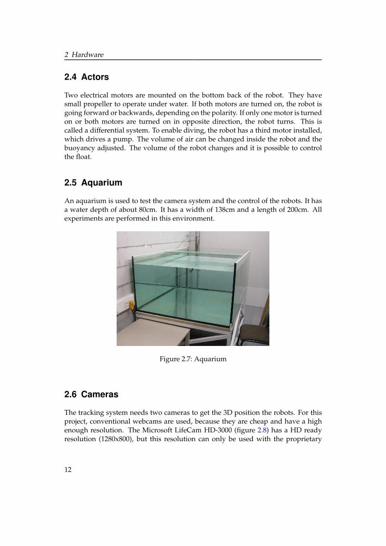
2.5 Aquarium

An aquarium is used to test the camera system and the control of the robots. It hasa water depth of about 80cm. It has a width of 138cm and a length of 200cm. Allexperiments are performed in this environment.

Figure 2.7: Aquarium

2.6 Cameras

The tracking system needs two cameras to get the 3D position the robots. For thisproject, conventional webcams are used, because they are cheap and have a highenough resolution. The Microsoft LifeCam HD-3000 (figure 2.8) has a HD readyresolution (1280x800), but this resolution can only be used with the proprietary

12

2.6 Cameras

software from microsoft. In the developed software, the resolution is limited to640x480. This is still high enough to get a position resolution of about 1cm.

Figure 2.8: Microsoft LifeCam HD-3000

The camera has a flexible leg, which can be mounted on the ceiling of the roomor at least above the aquarium. Both cameras have to be on the opposing sides ofthe aquarium to get a precise picture of the robot.

In figure 2.9 and figure 2.10, both sides of the aquarium can be seen. All cornersof the aquarium are in the picture. One obvious problem is the viewing angle,which distorts the picture. This can be compensated (see 3.1).

Webcams normally have an auto exposure feature, which means, the cameraadapts to ambient light changes. This can lead to problems, if the cameras are usedoutside a room with unsteady, environmental light. In section 3.3, this problem isdiscussed.

13

2 Hardware

Figure 2.9: View of camera 1

Figure 2.10: View of camera 2

14

3 Video Tracking

Video tracking is a method for tracking an object with a video camera. Trackingmeans that an algorithm extracts the position of an object. When this object moves,the algorithm has to recognize this and calculate the new position. For each frame,the position of the tracked object has to be calculated. This can be done with dif-ferent time intervals. More pictures per second means a higher motion resolutionof the object, but it also has a higher computational effort. Less pictures per sec-ond generate less data to be analysed, but the resolution is reduced. There is anoptimum between the frame rate (pictures per time interval) and resolution. If theobject moves very slow, then low rates can be used. In this thesis, an underwaterrobot is the object. It has a maximum velocity of about 10cm/s, so a frame rate of10Hz is sufficient.

To find an object in a picture, many different algorithms exist. In this thesis, thetemplate matching algorithm is chosen. Figure 3.1 shows the processing steps forthe video tracking system. The next sections discuss each step in detail. In the firststep, the video stream is read in a 10Hz frame rate. The following step correctsthe distortion, which comes from the camera perspective. In section 3.1, a solutionfor this is presented. Having a back transformed picture, the position is computedwith the template matching algorithm using cross-correlation. In the next step, theoutput of the normalized cross correlation is searched for its maximum. Once themaximum is found, the data from both cameras is combined and the real positionand diving depth of the robot are calculated. The last step is displaying the resultson the screen. The real position cannot be found by just one camera, if the robotdives. Both cameras give only a virtual 2D position of the robot, because refractionchanges the direction of the light

3.1 Perspective distortion

When a camera looks onto an object, distortions are present. The distortion de-pends on the viewing angle of the camera and the distance from the camera to theobject. Also, the focal length of the camera plays an important role. In this distor-tion, lines stay lines, but their angle changes. Figure 3.2 shows an example for thiskind of distortion. All parallel lines in reality meet in one vanishing point. Also, ob-jects near to the camera look bigger than object in the distance. In this project, bothcameras look from a different angle and distance onto the aquarium. So there are

15

3 Video Tracking

Video input

Coordinate transformation

Template matching

Maximum finding

Combining resultsfrom both cameras

Displaying results

Figure 3.1: Image processing flow

two different distortions. To correct the distortions, a mathematical transformationhas to be applied. The general transformation matrix has the form

M =

a b cd e fg h i

(3.1)

The last coefficient i, it is set to 1, it represents a scaling coefficient. The multi-plication of the original coordinates with the transformation matrix produces theundistorted coordinates. To multiply, the coordinates have to be extended with onedimension more, which represents a scaling factor.

Now, the equation looks like the following.x′

y′

1

= M ·

xy1

(3.2)

Solving equation 3.2 leads to equation 3.3 and 3.4.

x′ =a · x + b · y + cg · x + h · y + 1

(3.3)

16

3.1 Perspective distortion

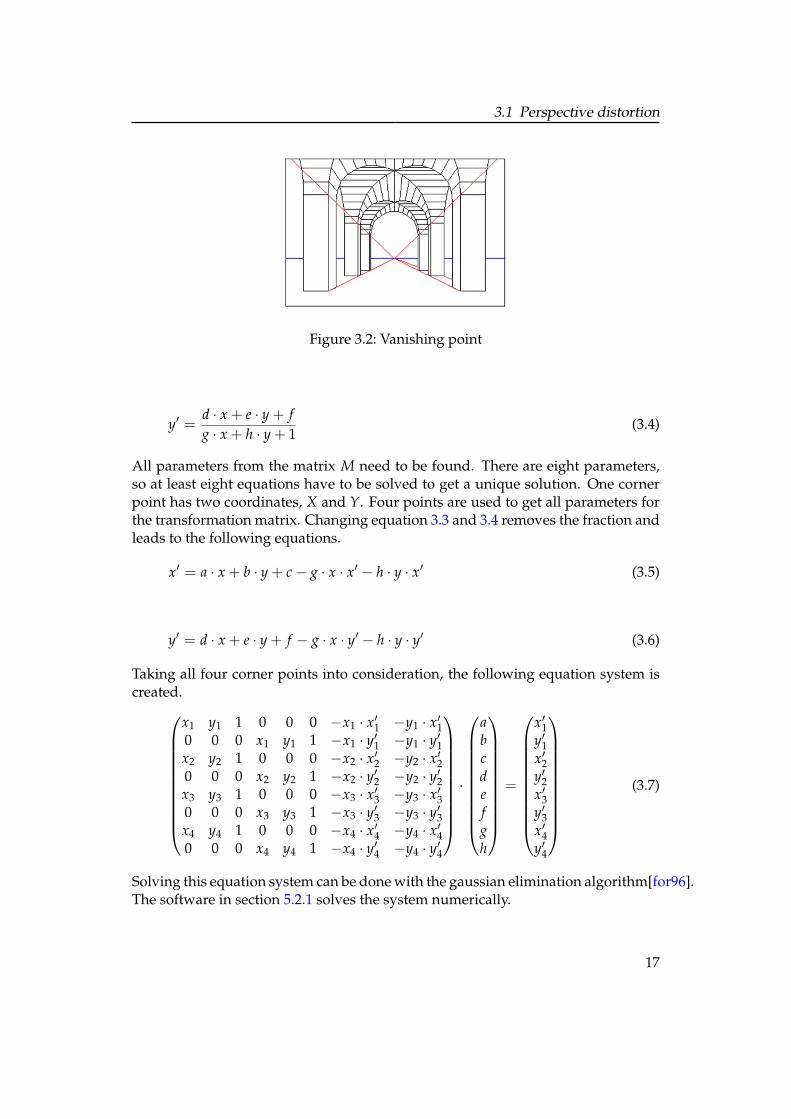
Figure 3.2: Vanishing point

y′ =d · x + e · y + fg · x + h · y + 1

(3.4)

All parameters from the matrix M need to be found. There are eight parameters,so at least eight equations have to be solved to get a unique solution. One cornerpoint has two coordinates, X and Y. Four points are used to get all parameters forthe transformation matrix. Changing equation 3.3 and 3.4 removes the fraction andleads to the following equations.

x′ = a · x + b · y + c− g · x · x′ − h · y · x′ (3.5)

y′ = d · x + e · y + f − g · x · y′ − h · y · y′ (3.6)

Taking all four corner points into consideration, the following equation system iscreated.

x1 y1 1 0 0 0 −x1 · x′1 −y1 · x′10 0 0 x1 y1 1 −x1 · y′1 −y1 · y′1x2 y2 1 0 0 0 −x2 · x′2 −y2 · x′20 0 0 x2 y2 1 −x2 · y′2 −y2 · y′2x3 y3 1 0 0 0 −x3 · x′3 −y3 · x′30 0 0 x3 y3 1 −x3 · y′3 −y3 · y′3x4 y4 1 0 0 0 −x4 · x′4 −y4 · x′40 0 0 x4 y4 1 −x4 · y′4 −y4 · y′4

·

abcdefgh

=

x′1y′1x′2y′2x′3y′3x′4y′4

(3.7)

Solving this equation system can be done with the gaussian elimination algorithm[for96].The software in section 5.2.1 solves the system numerically.

17

3 Video Tracking

Figure 3.3: Template matching

3.2 Gaussian elimination process

The Gaussian elimination is an approach to solve systems of linear equations. Elim-ination means, that out of all equations, two are added in such a way, that one vari-able is eliminated. Applying this to all equations a few times, it is possible to geta solution to one variable. After having one solution, this is substituted back to anequation with two variables and so on. A system of equation has the form

A · −→X =−→B (3.8)

where A is a coefficient matrix and B is a vector. X is the transformation vectorwhich contains the solution to this system. After applying the Gaussian eliminationprocess, the matrix A has all zeros under the first main diagonal. The next matrixis an example, where the elimination was applied.

A =

1 2 −40 1 30 0 1

(3.9)

In the last line of equation 3.9, all variables except one are zero.

3.3 Template matching

Template matching means, that a template is compared with a picture and the al-gorithm finds the point, where the template and the picture match the best. Figure3.3 shows an example. The left picture shows the input, in the center is the tem-plate and on the right side, the template is found in the input picture and markedwith a frame. The challenge during template matching is to make it robust againstpicture noise and other changes like brightness and scaling / rotation transforma-tions. There are two main approaches in template matching. One is called featurematching[JH]. Special features like corners, edges or other shapes are marked in

18

3.4 Cross correlation

the template. These features are then searched in the picture. It is only possible, ifthe template is not just plain but contains enough usable information.

The other approach is called template based. There, all pixel information fromthe template is used for comparison. Comparing can be done with difference values(SAD[sad], cross-correlation[KB01]). In this thesis, the cross-correlation is used astemplate matching approach.

3.4 Cross correlation

The cross-correlation is the summed product of two functions[tim06]. The formulaof the continuous cross-correlation is defined as follows:

Rxy(τ) =∫ ∞

−∞x(t) · y(t− τ)dt (3.10)

τ describes the replacement in time, x(t) and y(t) are the two functions, whichare compared to find a match. This is the global case, where both functions reachfrom −∞ to ∞. The result is a function, which maxima describe points, where agood matching in time exists. For image processing, the cross correlation is not onedimensional. There is not a replacement in time but two different replacements inx and y position. Furthermore, the images are in digital form, so a discrete solutionis needed. The next formula shows the 2D discrete cross correlation.

R f g(x, y) =W−1

∑i=0

H−1

∑j=0

f (i, j) · g(i + x, j + y) (3.11)

W is the width and H is the height of the template. The function f representsthe template and the function g is the picture. Both variables i and j representthe counting variables. For image processing, the cross-correlation is not workingvery good in some cases. If the contrast or the brightness changes, the matchingcoefficient R f g gets smaller and the peak from its curve is wider. The precision getslower. For compensating this, the normalized cross correlation (NCC) is used. Thefollowing equation shows the NCC.

R f g(x, y) =1

W · H ·W−1

∑i=0

H−1

∑j=0

( f (i, j)− f ) · (g(i + x, j + y)− g)σf · σg

(3.12)

When comparing equation 3.11 to equation 3.12, then the mean of the template fand the mean of the picture g is subtracted to the functions, which holds the pixeldata. If the brightness of the input picture gets higher, the mean of the picture isalso higher. That means, subtracting the mean compensated brightness changes.In the denominator of equation 3.12, the standard variation σ is a term. Contrastchanges in a picture changed also the standard deviation. But due to the division

19

3 Video Tracking

of the standard deviation in the NCC, contrast changes are also compensated. Themean of the function f (x, y) is defined as

f =1

W · H ·W−1

∑i=0

H−1

∑j=0

f (i, j) (3.13)

The standard deviation σ of the function f (x, y) is defined as

σ =

√√√√ 1W · H ·

W−1

∑i=0

H−1

∑j=0

( f (i, j)− f )2 (3.14)

From the equation 3.12, it can be seen, that there are many computations, espe-cially when the image size or the template size is high. For tracking applications,it is usually not necessary to cross-correlate the template with the whole input pic-ture. When the user selects the first time the template, the initial position of theobject is known. From this point, only a narrow surrounding has to be analysed,because the object does not move very far. This area can be very small, but it hasto be big enough, that the object cannot move outside the analysed area during oneframe interval. In the software in section 5.1, the area is only 10 by 10 pixels witha template size of 16 by 16, because the robot moves with a maximum of 10 cm/s.The frame rate is 10Hz, so between two frames, only 1cm (1 pixel) is moved.

3.5 Calculation of the 3D position

The two cameras look on the surface of the water to see the robot. But the problemis that the robot can dive. When diving, the cameras see the water surface, notdirectly the robot itself. When light goes from an optical thin medium to an opticalthick medium or the other way around, refraction occurs. Water has a refractioncoefficient of 1.33 [for96], while air has approximately 1.0 [for96]. This index isslightly depending on the temperature and more on the wavelength, but for theprecision of this work, this can be neglected. Because of the refraction, the realposition of the robot is not where it is seen on the surface.

The camera looks at any point of the aquarium with a different angle. WithSnell’s Law (figure 3.4), the refraction angle can be calculated. The incoming an-gle is β1 is refracted to the outgoing angle β2. When the material n2 is opticalthicker (higher refraction index) than material n1, the outgoing angle is refracted tothe normal. The relation between the two angles β1 and β2 is described in Snell’sLaw[for96].

sinβ1

sinβ2=

n2

n1(3.15)

20

3.5 Calculation of the 3D position

Water

Air

β1

β2

n1n2

Figure 3.4: Snell’s Law

Figure 3.5 shows the aquarium, where all rays are drawn and all vectors are named.The camera on the right is only indicated, but for the calculation process, only onecamera is regarded.

α

β

β'

α'

nview

u

u'

w

Figure 3.5: Optical path of the cameras in the aquarium

Table 3.1 describes all related angles and vectors to figure 3.5. In the center ofthe picture where all rays meet is the virtual position of the robot on the watersurface. The line u is the ray from the camera to the surface. This ray is refractedto the line u′. All angles which are needed to compute the position are shown. α isthe viewing angle from the left camera. For Snell’s Law, the angle to the normal isneeded, which is marked as β. The refracted angle then is β′ and the viewing angleunder water is α′. The viewing plane is needed to calculate the refracted ray. Thisplane is orthogonal to the XY plane (water surface) and contains the lines u, u′ and

21

3 Video Tracking

u Ray from camera to surfaceu′ Ray from surface to robotw Projected Ray u to the XY plane−→n Normal vector of the viewing planeα Viewing angleα′ Refracted angle to normalβ Viewing angle to normalβ′ Refracted viewing angle to normal

Table 3.1: Perspective distortion vectors and angles

w.For the line u, the following equation holds.

u = (−−−−−−−→Probot_sur f ace −

−−−→Pcamera) · j + Probot_sur f ace (3.16)

The line w has the equation 3.17.

u′ = (−−−−−−−→Probot_sur f ace −

−−−−−−−→Pcamera_bottom) · k + Probot_sur f ace (3.17)

To get the normal vector −→n , the vector product between the directional vectorfrom equation 3.16 and equation 3.17 has to be done.

−→n = (−−−−−−−→Probot_sur f ace −

−−−→Pcamera)× (

−−−−−−−→Probot_sur f ace −

−−−−−−−→Pcamera_bottom) (3.18)

With all three equations, the viewing plane equation can be written down.

p :

xyz

· −→n = 0 (3.19)

To calculate the viewing angle α, the following trigonometric functions are used.

sinα =|−−−−−−−→Probot_sur f ace −

−−−→Pcamera · −→n XY|

|−−−−−−−→Probot_sur f ace −−−−→Pcamera| · |−→n XY|

(3.20)

with the XY plane’s normal vector:

−→n XY =

001

(3.21)

The viewing angle with respect to the normal vector is

β = 90− α (3.22)

22

3.5 Calculation of the 3D position

With equation 3.16 and equation 3.19 it is possible to calculate the refracted rayu′. Two conditions hold for this ray: It has to lie in the viewing plane and its angleto the water surface has to be the refracted viewing angle α′.

Condition 1:

p :−−−−−→Probot_real −

−−−−−−−→Probot_sur f ace · −→n = 0 (3.23)

Condition 2:

β′ = arcsin(sin(α′) · 1

1.33) ∧ β = 90− β′ (3.24)

Condition 3.23 and 3.24 give two equations with two unknowns that can be solved.The result is the refracted line u′ which has the direction vector

−→u′ =

xyz

(3.25)

The last coordinate Z is set to −1. That means, the vector points downward. Thevalue−1 has the advantage, that in a later step the diving depth is calculated faster.The first condition from equation 3.23 leads to:

−→u′ · −→n = 0 (3.26)

Condition 2 leads to equation

sinα′ =

∣∣∣∣∣∣ x

y−1

·0

01

∣∣∣∣∣∣∣∣∣∣∣∣ x

y−1

∣∣∣∣∣∣ ·∣∣∣∣∣∣0

01

∣∣∣∣∣∣(3.27)

Solving equation 3.26 and equation 3.27, the component y has the following so-lution

y = ±

√√√√√√1

sin2α′

1 + (ny

nx)2

(3.28)

23

3 Video Tracking

Solving for x is similar. There are two solutions, which must be chosen correctlyfor each camera. The left camera looks in positive y direction, so the y-componentis positive. The right camera looks in a negative y direction, so the y-component isnegative.

All calculations have to be done for both cameras. The result is two line equationswhich are used for the final step. In this step, a point is found, which has theminimal distance to both lines u1 and u2. There are two cases. In the first case,which does not occur very often, both lines intersect in one point. This would bethe optimum case where the distance is zero. Due to the fact that all measurementsare inaccurate, this case is not considered and is also just a special case of the secondone.

For the second case, both lines do not intersect, they are skew lines. But it ispossible to find two points on the two lines, which have a minimum distance toeach other. Then, the real robot position lies near to those points. Figure 3.6 showstwo lines, which do not intersect. The plane p is parallel to the line g and the line hintersects this plane in one point Fh.

p

h

g

A

B

Fh

Fg

Figure 3.6: Skew lines

The vector n0 is defined as:−→n0 =

−→Fh −

−→Fg = −→v ×−→w (3.29)

The vector n0 is orthogonal to the line g and the line h. In equation 3.29, the direc-tion vector for line g is −→v and for line h the vector is −→w . To get the normal vectorof the plane p, the vector product between one direction vector and the vector n0 isdone. The plane p has the equation 3.30.

p : −→n0 ×−→v · (−→x −−→A ) = 0 (3.30)

In the next step, the point Fh is by with intersecting the plane p and the line h.

p : −→n0 ×−→v · (−→B +−→w · r1 −

−→A ) = 0 (3.31)

24

3.5 Calculation of the 3D position

The variable r is proportional to the diving depth. The same procedure is done tothe other point Fg with the equation 3.32.

p : −→n0 ×−→w · (−→A +−→v · r2 −

−→B ) = 0 (3.32)

Finally, the resulting points and the two diving depths have to be combined. Thiscan be done by taking one result or make an average. The average approach is thebetter one, because the error is minimized.

25

4 Robot control

The second task of this work is to have a position control of one robot. This isdone by setting waypoints in the software and the computer sends commands tothe robot that moves it to the destination point.

The manual control is an easy task. On pressing the forward key, both motorsshould drive forward, the backward key drives both motors backward and theturning keys drive both motors in opposing direction.

For the computer control there are many approaches. The next table shows threeof them. Each of the approaches has advantages and disadvantages. On the fol-

Approach 1 Approach 2 Approach 3Computertask

Send the current po-sition and a set ofwaypoints

Send the error to thenext waypoint

Sending motor con-trol commands

Robot task Waypoints and con-trol of the motors

Only control of themotors

-

Videotrackingsystem

Getting the position Getting the position Getting the position

Table 4.1: Approaches to control

lowing sections, these are discussed.

Approach 1

In the latest development step this approach is the best one. All calculations aredone by the robot itself. It gets only its current position and has to calculate allmotor control actions. The waypoints are also handled by the robot. The computersends all points once to the robot and then a start or stop command. If the way-points are meant to be changed dynamically, the computer can also send updatesof waypoints while the robot moves. One big disadvantage is that the control pa-rameters like PD parameters are hardcoded in the firmware of the robot. Changingthese parameters is a very time consuming part which includes reprogramming therobot. In the final phase, after sufficient testing / development, this approach canbe used. Another disadvantage is the computation complexity. All control mech-

27

4 Robot control

anisms have to work on a system with limited resources. But due to the modern32bit high performance microcontrollers, the disadvantage is not that big.

Approach 2

The second approach relocates the waypoint control to the computer. It is nowpossible to apply quicker changes in the planned route or the waypoints itself. Thecomputer makes the path planning and sends only the error to the next waypointto the robot. The robot still has to compute the motor control. Disadvantages arejust like in approach 1, the motor control parameters are still within the firmware.

Approach 3

All computations are done by the computer. On the robot, only the sensor han-dling is active. This approach is the most flexible. All parameters can be changedon the fly without reprogramming the robot. Also new control strategies can be im-plemented without reaching limits of computational power on the microcontroller.Waypoints can be easily set with the help of visualization on the computer screen.A the the advantages are numerous, this last approach is used in this thesis.

In section 4.1, a model for the robot is developed for future use. In this thesis,this model is..

4.1 Hydrodynamic equation

The hydrodynamics of the robot are useful to know, for setting up a model of therobot. Under water, the friction is very much lower than on the surface. The motorsturn relatively fast compared to the actual driving speed. Measuring the propellingtime, an estimation can be done, how far the robot drives.

4.1.1 Forces under water

To get an equation for the position of the robot, all forces which influence the mov-ing robot have to be known. Table 4.2 shows the most important forces.

Force Depends onInertial force Acceleration and massFriction in water VelocityPropelling force Motor speed and velocity

Table 4.2: Forces under water

28

4.1 Hydrodynamic equation

The inertial force FI is the same in water like on the surface. When the robot massis accelerated, this force is working.

The friction in water is more complex. This force depends on the fluid, herewater, on the shape of the robot and its squared velocity. There are also some otherdependencies like temperature, which changes the density of the water and otherfactors. But due to simplicity and importance, these factors are not considered. Theforce is called drag force FW .

For the propelling FM force, the velocity is also needed. When the propeller isturning and the robot is not moving, it generates a force. The higher the robot’svelocity gets, the smaller gets the relative velocity between the propeller and therobot. But this dependency is so small, it can be ignored.

All three forces have to be in equilibrium and the following equation shows thisstatement.

FI + FW = FM (4.1)

To get the position of the robot depending on all these forced, a differential equationis written.

The velocity is defined as

v(t) =ddt

(x(t)) = x′(t) (4.2)

and the acceleration is defined as

a(t) =ddt

(v(t)) = x′′(t) (4.3)

Inserting 4.3 and 4.2 in equation 4.1 leads to the following

x′′(t) ·m + (x′(t))2 · w = K (4.4)

where m is the mass of the robot, w is the water resistance factor and K is the motor

force. The units are [m] = kg, [w] =N

m/sand [K] = N

4.1.2 Solving movement equation

The equation 4.4 is a second order nonlinear differential equation. To solve thisequation, the homogeneous and particular solution has to be found. The homoge-neous solution is

xh(t) =m · log(C1 ·m + t · w)

w+ C2 (4.5)

29

4 Robot control

The non homogeneous solution is

xh(t) =

m · log

(cosh

(√K ·√

w · (C1 ·m + t)m

))w

+ C2 (4.6)

All coefficients have to be known to enable an exact estimation of the robots posi-tion. Some are easy to measure like the mass, others are more complex to calculate.In this case, an empirical method is used. Figure 4.1 shows the movement of therobot.

Figure 4.1: Real Position of the robot

The red line shows the x coordinate of the robot. The blue line the motor control.

In the next step, the parameters w, and K have to be varied, that the estimatedposition matches the real position. The mass m is known with mrobot = 0.43Kg.Figure 4.2 shows the estimated position of the robot with the blue line.

For better view, the estimated position has an offset of −5. The matching is verygood. For future use, more measurements have to be made and the parametershave to be optimized. It is shown, that the motion estimation can be used as goodmodel.

30

4.2 Control strategie

Figure 4.2: Real Position of the robot

4.2 Control strategie

Controlling the robots position is done with two independent controllers. One isfor the heading direction and one is for the distance control. When they are com-bined, it is possible to let the robot drive to each point in the water without userinteraction. Vehicle control underwater is quite different from normal robots on thesurface. When the propeller stops turning, the robot continues driving or drifting.There is no direct brake, only propelling backwards. Also the turning behavioris different. On the surface a robot can steer directly to a direction. Underwater,the robot turns, but continues to drive straight ahead. The speed of the robot in-creases, if the motors turn in the correct direction or decrease the speed to zero andgo backwards when continuing propelling. This behavior is like an integral one.The propelling time adds to the speed. So it can be said, the robot has an integralbehavior in case of moving. In the next parts, different controllers are shown andexplained, if they work for controlling underwater robots. All controllers are lim-ited to simple ones, fuzzy control or nonlinear controllers are not described. In thenext chart, the control scheme is shown.

On the left side, there are the two variables xSet and ySet. These come fromthe waypoint list and define the new target. From the video tracking system, thereal coordinates are measured. The difference of the desired target and the currentposition is the error for both coordinates.

31

4 Robot control

xSet

ySet

video tracking

Positionx

y

x

ysqrt(x²+y²)

x

yarctan(y/x)

Compass

PD distance

PD heading

I1

I2

M1=I1-I2

M2=I1+I2

e(t) distance

e(t) heading

Figure 4.3: Controller overview

There is a branch to the rotational controller and the distance controller. The rota-tional controller uses the arctan function to determine the angle, in which directionthe robot has to drive to reach the target. This angle is compared with the currentheading from the compass data. The angle difference is the error for the rotationPD-controller. On the other branch, the distance is calculated. It is error term forthe second PD controller. Both outputs from the controllers are connected togetherand for each motor, a signal is generated.

In the next sections, two controller types are described.

4.2.1 P-controller

The P-controller[reg05] is a very simple controller. The transfer function is

u(t) = P · e(t) (4.7)

where P is the constant and e(t) is the error. The output of the controller is u(t). Forunderwater robots, this controller is not sufficient. For example, if the robot drivesto a point and gets nearer, the error term e(t) gets smaller. At some point, the robotreaches the final position, so the error is zero. But now, the robot has still somevelocity. So it drives further. The error term starts to get bigger, but now in theopposite direction. The propellers drive backwards, the robot comes to a stop anddrives back to the destination. This goes on and on, the system is not stable. Theproblem is the low friction in water. Better results are achieved with a PD controller(see section 4.2.2).

4.2.2 PD-Controller

The PD-controller [reg05] has the transfer function

u(t) = D · ddt· e(t) + P · e(t) (4.8)

This is a very good approach for controlling the robot. In the transfer function, thedifferentiating part can cancel out the integrating part of the water, if the param-eters are set correctly. In the example from the P-controller, the robot drives near

32

4.2 Control strategie

to the destination point. The error term e(t) gets smaller. When differentiating theerror term, a negative value comes out. This negative part is added to the outputof the controller. At one point, the output gets negative, so the robot breaks. Thisbraking point is before reaching the target, not after the target. The PD controllercan have a steady error. But in water, the velocity of the robot is controlled not theposition. Therefore, this steady error does not affect the position control. This state-ment is only valid, when no current exists in the water. But inside the aquarium,the water is not moving.

33

5 Software

The software is written in C#. There are many programming languages, but C# waschosen because it is platform independent with the Microsoft .NET framework andthe coding style is like C or C++. C is a common programming language and isused for programming the firmware of the robots. Also designing a GUI is verysimple. Many libraries are free available on the internet available. For this project,the DirectShow and the LibUsbDotNet library are essentially.

Developing this software includs many steps. First, a list of requirement is cre-ated. Table 5.1 shows an overview.

Requirement ImportanceShow the robot position for each camera +Show the combined real position of the robot ++Show the robot angle relatively to the aquarium ++Show the diving depth ++Mark the robots position inside the pictures to check, if thetracking works correctly

++

Possibility to save all data to a file for later evaluation ++Camera number selection ++Show template +Import ini file with coefficients ++Contrast control with slider +Template rotation -Manual control of the robot -Set waypoints for a route of the robot +

Table 5.1: Reqirements of the main software

All features with a plus or more have to be implemented in the software. Thosewith a minus are optional. In section 5.1, the user interface is shown and explained

5.1 Main software

The main software is used to control the robot inside the aquarium. In the nextsections, a functional description is given.

35

5 Software

5.1.1 GUI

The developed software is shown in figure 5.1. Each part of the user interface isdiscussed in more detail in this section.

Figure 5.1: Main software GUI

The software consists of only one window, where everything can be controlled.

Figure 5.2: Main software - Template settings

Figure 5.2 shows the part of the GUI, where all settings for the template are madefor each camera. On the left side of the figure 5.2 is the template shown, which issearched for in the camera picture. To the right of the template, there are the co-ordinates for the corresponding camera. When the program starts, the coordinatesare set to zero.

On the right side is a checkbox to enable template update. If this checkbox isselected, the user can click in the camera picture to select the robot. The template isupdated and the checkbox is automatically unselected. The ’zero’ button is used toset the background picture, which will be subtracted during picture optimizing (seesection 5.1.3). Before taking any measurements with the robot inside the aquarium,the picture has to be zeroed.

Data logging is important for later evaluation. On the top of figure 5.3, a file-name has to be set. If the file already exists, then an increasing number is addedto the filename. For example, if the file ’log’ exists, the new file is called ’log0’ and

36

5.1 Main software

Figure 5.3: Main software - logging settings

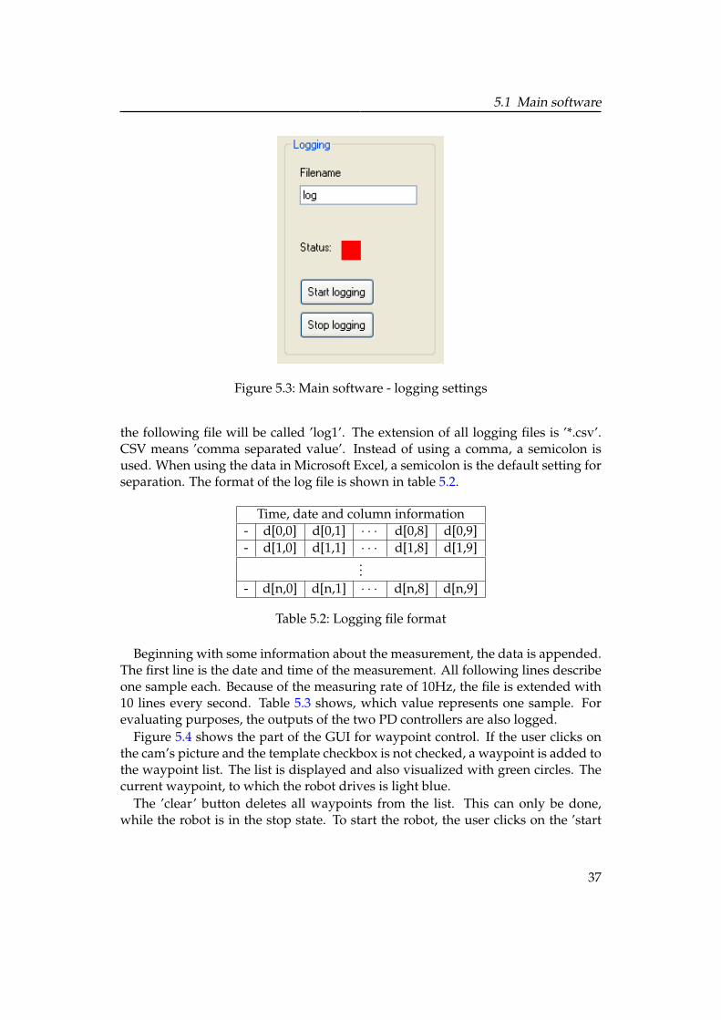
the following file will be called ’log1’. The extension of all logging files is ’*.csv’.CSV means ’comma separated value’. Instead of using a comma, a semicolon isused. When using the data in Microsoft Excel, a semicolon is the default setting forseparation. The format of the log file is shown in table 5.2.

Time, date and column information- d[0,0] d[0,1] · · · d[0,8] d[0,9]- d[1,0] d[1,1] · · · d[1,8] d[1,9]

...- d[n,0] d[n,1] · · · d[n,8] d[n,9]

Table 5.2: Logging file format

Beginning with some information about the measurement, the data is appended.The first line is the date and time of the measurement. All following lines describeone sample each. Because of the measuring rate of 10Hz, the file is extended with10 lines every second. Table 5.3 shows, which value represents one sample. Forevaluating purposes, the outputs of the two PD controllers are also logged.

Figure 5.4 shows the part of the GUI for waypoint control. If the user clicks onthe cam’s picture and the template checkbox is not checked, a waypoint is added tothe waypoint list. The list is displayed and also visualized with green circles. Thecurrent waypoint, to which the robot drives is light blue.

The ’clear’ button deletes all waypoints from the list. This can only be done,while the robot is in the stop state. To start the robot, the user clicks on the ’start

37

5 Software

d[x,0] Camera 1 X-Posd[x,1] Camera 1 Y-Posd[x,2] Camera 2 X-Posd[x,3] Camera 2 Y-Posd[x,4] Combined X-Posd[x,5] Combined Y-Posd[x,6] Diving depthd[x,7] Robot headingd[x,8] PD-controller rot.d[x,9] PD-controller dist.

Table 5.3: Loggine file sample data

drive’ button and the robot drives to the first waypoint. Stopping it is done withthe ’stop drive’ button.

In figure 5.5, the ’robot information’ field is shown. On the top, the calculatedaquarium coordinates of the robot are shown. Below this, the diving depth is dis-played. Further down, the robot’s rotation is shown. Left to it, the user can clickon the ’zero’ button to reset the current angle to zero degrees. This is useful, whenusing different locations for testing. Zero degrees is in the direction of the x-axis.

On the bottom, the ’Connect to robot’ button establishes the connection to therobot. Therefore, the USB library functions are called. Each USB device has aunique VID/PID (vendor ID and product ID)[pro] combination. This has to begiven to the functions to find the correct device.

In figure 5.6, one of the two transformed camera pictures is shown. The biggreen circles are the waypoints. One of the big circles is blue. This is the currentlyactivated waypoint. When the robot is near enough to the waypoint (radius 8cm),the next is automatically activated and the robot continues to the next one.

Clicking in the transformed camera picture has two different functions. One isto set a new waypoint and one is for template selection. Both click functions aredescribed above.

5.1.2 Flowchart

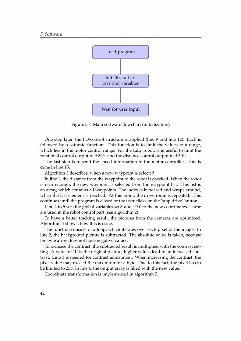
A flowchart gives a better understanding of the flow of the program. In figure 5.7,the initialization and start of the main program is shown.

After the program is started, all arrays have to be initialized and memory is allo-cated. The dynamic allocation would always create a new array and the memoryusage would rise constantly. In C#, the garbage collection could remove the un-used space, but this doesn’t work perfectly. All other variables, which are not setautomatically to zero, are initialized. The program is ready to accept any user inputlike clicking on a button. Figure 5.7 shows two flowcharts, which work in parallel.

38

5.1 Main software

Figure 5.4: Main software - Waypoint settings

Therefore, an event is created, which is triggered by incoming data. This is doneasynchronously to the main program.

The left flowchart shows the timer interrupt. In the first step, the data from thecamera is read and copied to an array. This is done for both cameras. There is atemporary array, which holds the RGB data from the cam. This is copied and in thesame step converted to black and white. The RGB24 format has three bytes, one forthe red, one for the green and one for the blue part. The black and white value iscalculated with the equation

BWvalue =R + G + B

3(5.1)

This is the average of all three color parts. In the second step, the transformationmatrix is applied to the array (see section 3.1). Then, the cross-correlation is done

39

5 Software

Figure 5.5: Main software - Robot information

and the maximum point is saved. The position is then averaged over four framesto have a smoother value and also for the D part of the distance controller (section4.2.2, intermediate values are better. In real application, the robot moves abouthalf a centimeter in each frame. Because the resolution is exactly one centimeter,each two frames is a step in the position. This would not lead to a sufficient motorcontrol.

The next step is to display the results. In the end of the function, the motorcontrol function is called. Parallel to this function, the receive data interrupt canoccur. Here, the data stream from the USB RFM12 bridge (section 2.2.2) is read.The data consists of all sensor data. From this stream, the data is saved to variablesand further processed.

5.1.3 Algorithms

The most important part of this thesis is the template matching. This is done withthe help of the cross-correlation. An implementation in software is shown in algo-rithm 1.

There are two for-loops. Due to efficiency, the cross correlation is only done isa small area (see section 3.4). Line 1 and line 2 show, that the for-loops iterateonly over this area. From line 6 to line 12, the two inner for-loops iterate over thetemplate size. In line 8, the first part of the nominator of equation 3.12 is calculated.Because this term is also needed in the denominator, it is saved in a temporaryvariable. Continuing, in line 9 the sum of the nominator is calculated. Line 10 isonly for calculation the standard variance 3.14 of the input picture. Now, the sumpart is ended for the current x-y position. Line 14 discards negative correlation

40

5.1 Main software

Figure 5.6: Main software - Transformed camera picture

coefficients. When this coefficient gets negative, the picture is inverted.From line 16 to line 17, the rest of equation 3.12 is calculated. The value 250 in

line 16 represents the scaling to a useful value. Because the array (output), whichholds the correlation data, has the type ’byte’, the value reaches from 0 to 255. Theoutput of the cross correlation is a value from 0 to 1. So, multiplying it with 250,almost the full scale is used. Due to rounding errors, a little space to 255 is held.

Line 19 finishes the function. The output array is filled with the correlation co-efficient. Within this algorithm, the maximum is continuously compared with thenew value. If the new value is bigger, the maximum is updated.

The algorithm 2 for the robot control has to be called each time, a new positionis calculated. It is called every 100ms. In line 1 and line 2, the errors for the x and ycoordinate are calculated. The realX and realY value comes from the video trackingsystem and the setX and setY variable is from the waypoint control. In line 4, theheading of the robot is calculated, where the robot should drive and in line 6, theangular error is calculated. In line 7, the error for the distance control is calculated.

41

5 Software

Load program

Initialize all ar-rays and variables

Wait for user input

Figure 5.7: Main software flowchart (initialization)

One step later, the PD-control structure is applied (line 9 and line 12). Each isfollowed by a saturate function. This function is to limit the values to a range,which lies in the motor control range. For the LiLy robot, is is useful to limit therotational control output to ±80% and the distance control output to ±50%.

The last step is to send the speed information to the motor controller. This isdone in line 15.

Algorithm 3 describes, when a new waypoint is selected.In line 1, the distance from the waypoint to the robot is checked. When the robot

is near enough, the new waypoint is selected from the waypoint list. This list isan array, which contains all waypoints. The index is increased and wraps around,when the last element is reached. At this point, the drive route is repeated. Thiscontinues until the program is closed or the user clicks on the ’stop drive’ button.

Line 4 to 5 sets the global variables setX and setY to the new coordinates. Theseare used in the robot control part (see algorithm 2).

To have a better tracking result, the pictures from the cameras are optimized.Algorithm 4 shows, how this is done.

The function consists of a loop, which iterates over each pixel of the image. Inline 2, the background picture is subtracted. The absolute value is taken, becausethe byte array does not have negative values.

To increase the contrast, the subtracted result is multiplied with the contrast set-ting. A value of ’1’ is the original picture, higher values lead to an increased con-trast. Line 3 is needed for contrast adjustment. When increasing the contrast, thepixel value may exceed the maximum for a byte. Due to this fact, the pixel has tobe limited to 255. In line 4, the output array is filled with the new value.

Coordinate transformation is implemented in algorithm 5.

42

5.2 Additional software

Algorithm 1 Normalized cross-correlation1: for y = area(top) to area(bottom), step + 1 do2: for x = area(top) to area(bottom), step + 1 do3: calculate mean of input4: SigmaPicture = 05: CC = 06: for v = 1 to TemplateHeight, step + 1 do7: for u = 1 to TemplateHeight, step + 1 do8: temp = input(x + u, y + v)− input9: cc+ = temp · (template(u, v)− template)

10: SigmaPicture+ = temp2

11: end for12: end for13: if CC < 0 then14: CC = 015: end if16: CC = CC · 250

SigmaPicture · SigmaTemplate

17: CC = CC · 1TemplateHigh · TemplateWidth

18: output(x + TemplateWidth/2, y + TemplateHeight/2) = CC19: end for20: end for

There are two loops, iterating over the width and the height of the output image.In line 3 and 4, the transformed coordinates are calculated. Then, in line 5, theoutput array is updated pixel wise with the new value. The variables a to h are thetransformation coefficients from equation 3.7.

5.2 Additional software

For the determination of the transformation matrix, the corner points of the aquari-um in the camera picture have to be known. Eight equations are needed to solved(see section 3.7). For this thesis, a software is developed, where the user can clickon the corner points and the transformation matrix is generated. All coefficientsare then stored to a file, which is used as a config file for the main software. Figure5.9 shows the GUI for this software.

The user has to click in the picture to select a point. In the red circle with no. 1,the coordinates are displayed. Also, the user has to select, which corner this pointbelongs to. In the circle no. 2, already determined corner points are displayed. Theleft bottom point marks the origin of the aquarium.

43

5 Software

Algorithm 2 Robot control1: errorX = setX− realX2: errorY = setY− realY3:4: robotHeadingSet = arctan2(errorY, errorX)5:6: errorHeading = robotHeadingSet− robotHeadingReal7: errorDistance =

√errorX2 + errorY2

8:9: urotation = P · errorHeading + D · (errorHeading− lastErrorHeading)

10: saturate(urotation)11:12: udistance = P · errorDistance + D · (errorDistance− lastErrorDistance)13: saturate(udistance)14:15: RobotSetMotors(urotation, udistance)

Algorithm 3 Waypoint control1: if errorDistance < 8 then2: selectnextwaypoint f romwaypointlist3:4: setX = newwaypoint.X5: setY = newwaypoint.Y6: end if

After selecting all corner points, the user has to click on the ’generate matrix file’button. In the same location as the program a text file with the name ’matrix.txt’ isgenerated. The file has the format described in table 5.4.

The letters a to h are from the equation system in section 3.7. Each line representsa coefficient. The type of the variable is a double with a comma as separator (ger-man notation). For the main software 5.1 it is needed to have two transformationmatrices because the two cameras have different positions. Therefore, this addi-tional software has to be started twice to get both matrices. The user can select thedesired camera from a combo box (circle no. 3). Before starting it the second time,the ’matrix.txt’ file has to be saved, because it will be overwritten.

In the figure 5.9, the aquarium is standing upside down. This is because the videostream is flipped. That is no problem, if the correct corner points are selected. Whenapplying the transformation matrix, the picture is corrected automatically. Havingall corner points selected, the program solves the equation system with the help ofGaussian elimination. This principle is explained in the section 3.2.

44

5.2 Additional software

Algorithm 4 Picture optimizing1: for i = 1 to PictureWidth · PictureHeight do2: PixelValue = |input(i)− background(i)| · ContrastSetting3: saturate(PixelValue)4: output(i) = PixelValue5: end for

Algorithm 5 Coordinate transformation1: for y = 0 to ArrayHeight do2: for x = 0 to ArrayWidth do

3: x′ =a · x + b · y + cg · x + h · y + 1

4: y′ =d · x + e · y + fg · x + h · y + 1

5: output(x, y) = input(x′, y′)6: end for7: end for

5.2.1 Softwareimplementation of Gaussian elimination

When using the computer to solve a system with the Gaussian elimination princi-ple, the algorithm 6 can be used.

The algorithm consists of two loops, one goes from line 1 to line 13. This is theelimination process. The second loop from line 14 to line 20 is the back substitution.From line 2 to line 5, the row with the greatest value at the top is found. This isimportant, because some equations have a leading zero, which will cause problemsin a later step. After finding the maxrow, this row is swapped with the first one (line7). In line 9 to line 11, two rows are subtracted, that one variable is eliminated. Thisis done for all remaining rows. In the next loop iteration of the first main loop, thisprocedure is repeated.

abcdefgh

Table 5.4: ’matrix.txt’ file format

45

5 Software

Algorithm 6 Gaussian Elimination1: for i = 0 to Nstep + 1 do2: for j = 1 to istep + 1 do3: if matrix(j, i) > matrix(maxrow, i) then4: maxrow = j5: end if6: end for7: Swapmatrix(maxrow, ∗)withmatrix(j, ∗)8: for j = i + 1 to Nstep + 1 do9: for k = N to istep− 1 do

10: matrix(j, k)− =matrix(i, k) ·matrix(j, i)

matrix(i, i)11: end for12: end for13: end for14: for j = N − 1 to 0step− 1 do15: temp = 016: for k = k + 1 to Nstep + 1 do17: temp+ = matrix(j, k) · output(k)

18: output(j) =matrix(j, N)− temp

matrix(j, j)19: end for20: end for

The second loop is for back substituting. For applying this algorithm, the matrixA has to contain the vector

−→B from equation 3.8 as additional column. The vector

−→X is the output.

46

5.2 Additional software

Timer tick interrupt

Read new framefrom cameras

Save frame datato grayscale array

Apply transfor-mation matrix

Run picture optimization

Apply the cross-correlation

Averaging thefound position

Draw the waypointsand robot position

Control the motors

Data receivedfrom RF module

Extract robot informa-tion from byte stream

Calculate roll and pitchangle of the robot

Calculate yaw an-gle of the robot

Figure 5.8: Main software flowchart

47

5 Software

Figure 5.9: Transformation matrix solving GUI

48

6 Experiments

The software in chapter 5 is tested, if the robot is recognized in all situation. Thisincludes floating on the water surface and diving. After evaluating the trackingsystem, the robot control is optimized. In section 6.2, the parameters for the con-trollers are optimized.

6.1 Video tracking

The video tracking system is evaluated by letting the robot drive through a set ofwaypoints. With the help of the logging file, the track of the robot is drawn into adiagram.

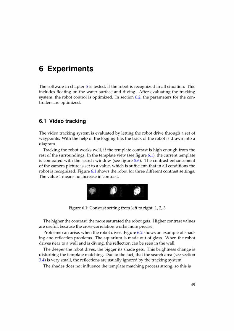
Tracking the robot works well, if the template contrast is high enough from therest of the surroundings. In the template view (see figure 6.1), the current templateis compared with the search window (see figure 5.6). The contrast enhancementof the camera picture is set to a value, which is sufficient, that in all conditions therobot is recognized. Figure 6.1 shows the robot for three different contrast settings.The value 1 means no increase in contrast.

Figure 6.1: Constast setting from left to right: 1, 2, 3

The higher the contrast, the more saturated the robot gets. Higher contrast valuesare useful, because the cross-correlation works more precise.

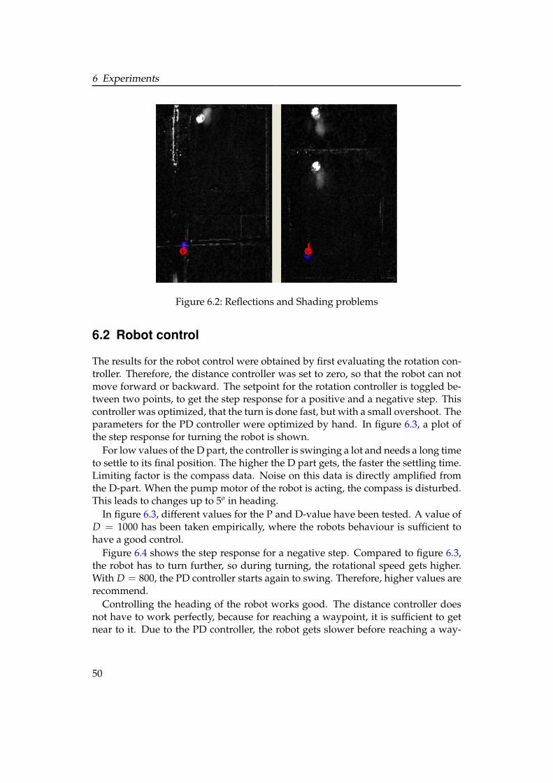
Problems can arise, when the robot dives. Figure 6.2 shows an example of shad-ing and reflection problems. The aquarium is made out of glass. When the robotdrives near to a wall and is diving, the reflection can be seen in the wall.

The deeper the robot dives, the bigger its shade gets. This brightness change isdisturbing the template matching. Due to the fact, that the search area (see section3.4) is very small, the reflections are usually ignored by the tracking system.

The shades does not influence the template matching process strong, so this is

49

6 Experiments

Figure 6.2: Reflections and Shading problems

6.2 Robot control

The results for the robot control were obtained by first evaluating the rotation con-troller. Therefore, the distance controller was set to zero, so that the robot can notmove forward or backward. The setpoint for the rotation controller is toggled be-tween two points, to get the step response for a positive and a negative step. Thiscontroller was optimized, that the turn is done fast, but with a small overshoot. Theparameters for the PD controller were optimized by hand. In figure 6.3, a plot ofthe step response for turning the robot is shown.

For low values of the D part, the controller is swinging a lot and needs a long timeto settle to its final position. The higher the D part gets, the faster the settling time.Limiting factor is the compass data. Noise on this data is directly amplified fromthe D-part. When the pump motor of the robot is acting, the compass is disturbed.This leads to changes up to 5o in heading.

In figure 6.3, different values for the P and D-value have been tested. A value ofD = 1000 has been taken empirically, where the robots behaviour is sufficient tohave a good control.

Figure 6.4 shows the step response for a negative step. Compared to figure 6.3,the robot has to turn further, so during turning, the rotational speed gets higher.With D = 800, the PD controller starts again to swing. Therefore, higher values arerecommend.

Controlling the heading of the robot works good. The distance controller doesnot have to work perfectly, because for reaching a waypoint, it is sufficient to getnear to it. Due to the PD controller, the robot gets slower before reaching a way-

50

6.2 Robot control

Figure 6.3: Rotation controller up step response

point. This is necessary, because if reaching the next waypoint includes a turn, therobot would overshoot. Its inertial force would let it drift further in the old direc-tion. Figure 6.5 shows a tracked route from the robot. In this case, the robot did notdive.

The waypoints are marked with circles. In the center of figure 6.5 is she startingpoint of the robot. Each waypoint is crossed nearly in the center.

The next experiment, the diving depth was set to 30cm. Figure 6.6 shows thetravelling path of the robot. The result is much different than the route with nodiving. A few time, the robot closely misses a waypoint, it has to turn aroundand drive in the opposite direction. This takes a lot of time. This problem comesfrom the side drift of the robot. Due to the low friction of the water, changing thedirection needs time.

To evaluate the tracking, the diving depth can be used as measure. The depthcontroller of the robot holds the diving depth in a range between 1cm up and down.Figure 6.7 shows the tracked diving depth for diving 30cm deep.

The maximum error is about 8cm. This error has its origin in the template match-ing algorithm. Viewing the robot from different angles, the center point of the robotchanges. For extreme viewing angles, only small differences in matching lead to agreat depth error.

51

6 Experiments

Figure 6.4: Rotation controller down step response

Figure 6.5: Waypoint route on the surface

52

6.2 Robot control

Figure 6.6: Waypoint route with 30cm diving depth

Figure 6.7: Depth calculation

53

7 Summary

In this thesis, a tracking system for underwater robot was developed and a robotcontrol feature was implemented. The robot can follow a route, which is set withwaypoints. All experiments are made with a small robot in a 140x200cm aquarium.

Two webcams are installed on the sides of this aquarium. The cameras are con-nected to a computer via USB. For the frame rate of the tracking system, 10Hz arechosen, because the robot moves with less than 10cm/s, which represents only afew pixel in the camera picture. Higher frame rates would bring a higher CPUutilisation, but no increase in performance.

A software was developed, which reads out the camera streams. The raw pic-tures contain perspective distortions. With a matrix transformation, the distortionsare compensated. In the following step, the picture is optimized, so that only rel-evant information are visible. The background is subtracted and the contrast isincreased.

Finding the robot in the camera picture is done with template matching. The nor-malized cross-correlation is used in the template matching algorithm. Contrast andbrightness changes in the picture have only a little effect on the cross-correlation,because the normalization compensated these changes.

The position seen by the cameras is only a virtual position when the robot dives.With the help of the second camera and refraction equations, the real position ofthe robot is determined.

In the second part, a controller for the robot was developed. Two independentcontrollers, one for the heading and one for the distance to the target, produce asignal, which is combined and send to the motor driver. Both controllers are testedand perform well with only low overshoot.

The tracking system is tested and it works for all robot positions. During diving,the contrast of the robot is high enough, to be found by the template matching.Shades and reflections do not have an effect on the performance of this system.The system works well in the aquarium, where it was tested. It is shown, that therobot can follow a route of waypoint with the help of the tracking software.

7.1 Outlook

For the future, the system should be tested in other areas than a small aquarium. Inthe room with the aquarium, the ambient light was constant. In other placed, this

55

7 Summary

might not be the case. So, the background subtraction may not work sufficient.The next point is regarding the tracking of multiple robots. In the developed

software, it is not possible to track more than one robot. It is mentioned, that theCPU utilization is so low, that tracking of more than one robot should be possiblewithout performance problems.

Problems can occur, if multiple robots drive at different depth but at the sameposition. The robots can shade each other and the tracking system can be confused.With the motion estimation, the shading problem could be solved.

The waypoint system is working, but has only limited functionality. Currently,the waypoints only accept 2D positions. The diving depth is constant in the drivingroute. For the future, each waypoint could be a 3D point.

56

Bibliography

[blu01] Bluetooth revealed: the insider’s guide to an open specification for global wire-less communication. Prentice Hall PTR Upper Saddle River, 2001.

[coc] Cocoro project.

[com] AN4248 - Implementing a Tilt-Compensated eCompass using Accelerometerand Magnetometer Sensors.

[for96] Formeln und Tabellen. paetec, 1996.

[GG87] G. Carlyle Stones Georgia Griffiths. The tea-leaf reader algorithm: anefficient implementation of crc-16 and crc-32. Technical report, Com-pusec, Inc., 1987.

[JH] R.C. Flemmer J.W. Howarth, H.H.C. Bakker. Feature-based object recog-nition. Technical report, Massey University.

[KB01] Uwe D. Hanebeck Kai Briechle. Template matching using fast normal-ized correlation. Technical report, TU Muenchen, 2001.

[lib] Libusbdotnet library.

[mat06] Mathematische Formelsammlung. Vieweg & Sohn Verlag, 2006.

[MCN] R. Garcia M. Carreras, P. Ridao and T. Nicosevici. Vision-based local-ization of an underwater robot in a structured environment. Technicalreport, University of Girona, ?

[PB06] Vince W.C. Chooka Stefano Chessab Alberto Gottab Y. Fun HuaPaolo Barontib, Prashant Pillaia. Wireless sensor networks: A surveyon the state of the art and the 802.15.4 and zigbee standards. Technicalreport, Mobile and Satellite Communication Research Centre, School ofEngineering, Design and Technology, University of Bradford, UnitedKingdom Wireless Networks Laboratory, Istituto di Scienza e Tecnolo-gie dell’Informazione, Pisa, Italy, Department of Computer Science,University of Pisa, Pisa, Italy, 2006.

[PCV07] Matthew Dunbabin Michael Hamilton Daniela Rus Peter Corke, Car-rick Detweiler and Iuliu Vasilescu. Experiments with underwater robot

A

localization and tracking. Technical report, CSIRO ICT Centre, Mas-sachusetts Institute of Technology, University of California, 2007.

[pro] USB protocol. http://www.usb.org.

[PZ04] Jason Gu Pifu Zhang, Evangelos E. Milios. Underwater robot localiza-tion using artificial visual landmarks. Technical report, Dalhousie Uni-versity, 2004.

[reg05] Regelungstechnik 1. Springer, 2005.

[RK] Kav’e Salamatian Ramin Khalili. Evaluation of packet error rate in wire-less networks. Technical report, Universit’e Pierre et Marie Curie.

[sad] Fast sum of absolute differences visual landmark detector. Technicalreport, Australian National University.

[tim06] Continuous-Time Signals. Springer, 2006.

[WSPZ97] Deric Gray W. Scott Pegau and J. Ronald V. Zaneveld. Absorption andattenuation of visible and near-infrared light in water: dependence ontemperature and salinity. Technical report, Optical Society of America,1997.

Declaration

All the work contained within this thesis,except where otherwise acknowledged, wassolely the effort of the author. At nostage was any collaboration entered intowith any other party.

(Martin Antoni)