Journal of Microscopy, 2012 doi: 10.1111/j.1365-2818.2012.03655.x

Received 27 February 2012; accepted 11 July 2012

3D multiscale segmentation and morphological analysis of x-raymicrotomography from cold-sprayed coatings

L . G I L L I B E R T ∗, C . P E Y R E G A ∗, D . J E U L I N ∗, V . G U I P O N T†& M . J E A N D I N†∗Centre de Morphologie Mathematique, Mathematiques et Sytemes, Mines ParisTech, France†Centre des Materiaux, Mines ParisTech, CNRS UMR, France

Key words. Cold-sprayed coatings, constrained segmentation, multiscale 3Dsegmentation, stochastic watershed.

Summary

X-ray microtomography from cold-sprayed coatings bringsa new insight on this deposition process. A noise-tolerant segmentation algorithm is introduced, based on thecombination of two segmentations: a deterministic multiscalesegmentation and a stochastic segmentation. The stochasticapproach uses random Poisson lines as markers. Results ona X-ray microtomographic image of aluminium particles arepresented and validated.

Introduction

The cold gas dynamic spray method or cold spray process isone of the more recent and innovative processes that has beenintroduced in the field of thermal spraying to achieve thickmetallic layers. To characterize the microstructure resultingfrom the plastic deformation of the sprayed metallic particlesby this process, X-ray microtomographic images of suchmaterials were made on the synchrotron at the ESRF (Guipontet al., 2010; Rolland et al., 2010).

Two algorithms to segment the particles on these 3Dimages were implemented from methods using mathematicalmorphology such as the watershed transform (Beucher& Lantuejoul, 1979; Beucher, 1994). The watershedtransformation used is an unbiased implementation based onhierarchical queues described in (Beucher, 2004).

The first algorithm is multiscale and consists of processingsuccessive deterministic constrained watershed transforms toextract all the boundaries of the particles. The second one isbased on the stochastic watershed segmentation which wasfirst introduced by Angulo and Jeulin in (Angulo & Jeulin,

Correspondence to: L. Gillibert, Centre de Morphologie Mathematique Mathe-

matiques et systemes, Mines ParisTech, 35, rue saint Honore Fontaineloeav, France.

Tel: +33164694792; Fax: +33164694707; e-mail: luc.gillibert@cmm.ensmp.fr

2007). The idea is to use a large number of realizations ofrandom markers to build a probability density function (PDF)of contours, starting from a standard watershed algorithmproducing oversegmentations. Here, random lines are used asmarkers. The material is anisotropic and therefore the lineswill have a specific orientation.

Finally, the combination of the two algorithms is used.Together, they provide a relevant segmentation, multiscaleand anisotropic.

The cold spray coating method

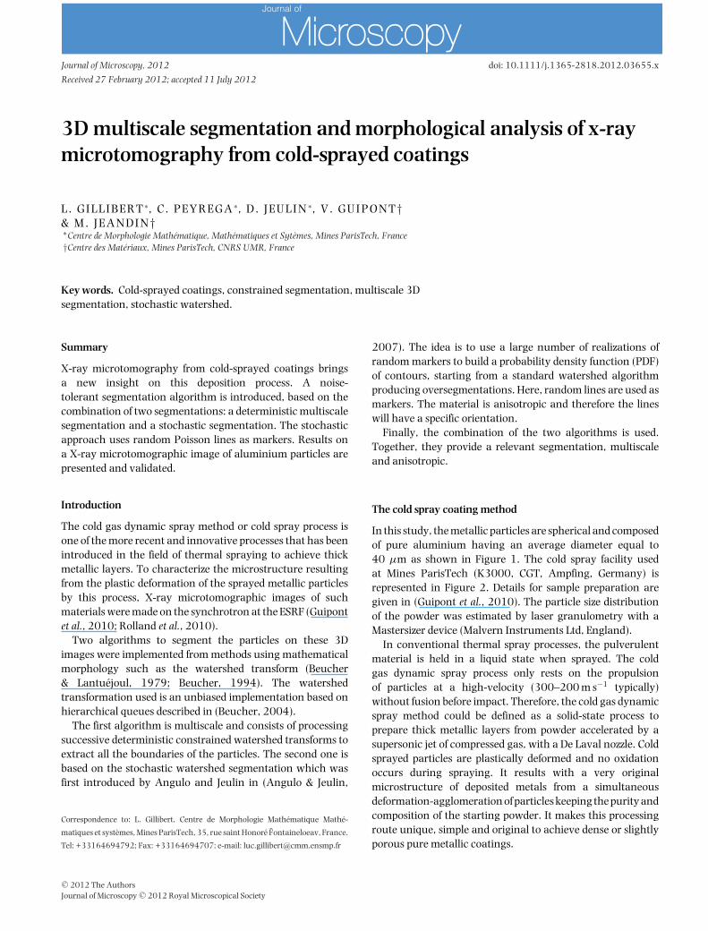
In this study, the metallic particles are spherical and composedof pure aluminium having an average diameter equal to40 μm as shown in Figure 1. The cold spray facility usedat Mines ParisTech (K3000, CGT, Ampfing, Germany) isrepresented in Figure 2. Details for sample preparation aregiven in (Guipont et al., 2010). The particle size distributionof the powder was estimated by laser granulometry with aMastersizer device (Malvern Instruments Ltd, England).

In conventional thermal spray processes, the pulverulentmaterial is held in a liquid state when sprayed. The coldgas dynamic spray process only rests on the propulsionof particles at a high-velocity (300–200 m s−1 typically)without fusion before impact. Therefore, the cold gas dynamicspray method could be defined as a solid-state process toprepare thick metallic layers from powder accelerated by asupersonic jet of compressed gas, with a De Laval nozzle. Coldsprayed particles are plastically deformed and no oxidationoccurs during spraying. It results with a very originalmicrostructure of deposited metals from a simultaneousdeformation-agglomeration of particles keeping the purity andcomposition of the starting powder. It makes this processingroute unique, simple and original to achieve dense or slightlyporous pure metallic coatings.

C© 2012 The AuthorsJournal of Microscopy C© 2012 Royal Microscopical Society

2 L . G I L L I B E R T E T A L .

Fig. 1. SEM image of pure aluminium particles ; spherical particles(average diameter: 40 μm).

Multiscale segmentation

Image acquisition

For this study, thick aluminium coatings have been achievedby cold gas dynamic spraying at the Material Research Center(Mines ParisTech). Moreover, an in-depth impregnation byan appropriate etching solution composed of gallium has beenachieved to reveal cold spray aluminium particles boundariesfor further image segmentations. To characterize themicrostructure of such a coating, 3D X-Ray microtomographyimages were obtained at the European Synchrotron RadiationFacility (ESRF). The resulting images were then processedto segment the deformed particles. The Figure 3(A) shows a3D X-ray microtomographic reconstruction of a cold sprayedcoating sample. The region of interest in Figure 3(B) is thesub-sample which was used to develop the segmentationalgorithms presented in this paper. The method is validatedon a second region of interest.

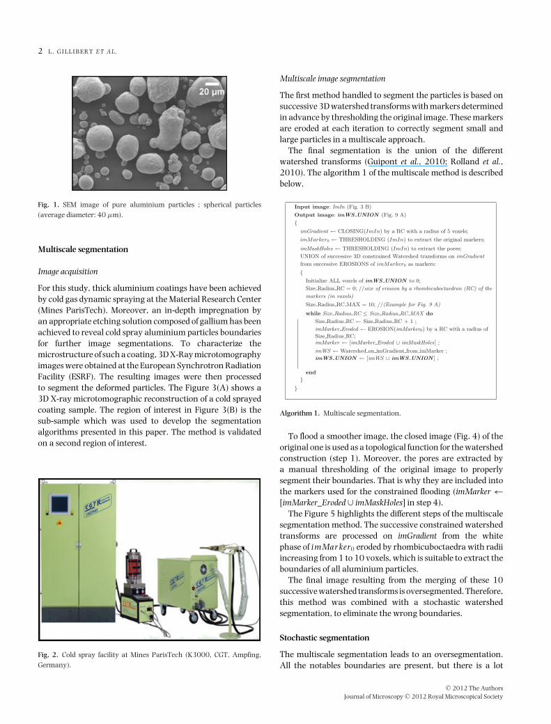
Fig. 2. Cold spray facility at Mines ParisTech (K3000, CGT, Ampfing,Germany).

Multiscale image segmentation

The first method handled to segment the particles is based onsuccessive 3D watershed transforms with markers determinedin advance by thresholding the original image. These markersare eroded at each iteration to correctly segment small andlarge particles in a multiscale approach.

The final segmentation is the union of the differentwatershed transforms (Guipont et al., 2010; Rolland et al.,2010). The algorithm 1 of the multiscale method is describedbelow.

Input image: ImIn (Fig. 3 B)

Output image: imWS UNION (Fig. 9 A)

{imGradient ← CLOSING(ImIn) by a RC with a radius of 5 voxels;

imMarker0 ← THRESHOLDING (ImIn) to extract the original markers;

imMaskHoles ← THRESHOLDING (ImIn) to extract the pores;

UNION of successive 3D constrained Watershed transforms on imGradient

from successive EROSIONS of imMarker0 as markers:

{Initialize ALL voxels of imWS UNION to 0;

Size Radius RC = 0; //size of erosion by a rhombicuboctaedron (RC) of the

markers (in voxels)

Size Radius RC MAX = 10; //(Example for Fig. 9 A)

while Size Radius RC ≤ Size Radius RC MAX do

Size Radius RC ← Size Radius RC + 1 ;

imMarker Eroded ← EROSION(imMarker0) by a RC with a radius of

Size Radius RC;imMarker ← [imMarker Eroded ∪ imMaskHoles] ;

imWS ← Watershed on imGradient from imMarker ;

imWS UNION ← [imWS ∪ imWS UNION ] ;

end

}}

Algorithm 1. Multiscale segmentation.

To flood a smoother image, the closed image (Fig. 4) of theoriginal one is used as a topological function for the watershedconstruction (step 1). Moreover, the pores are extracted bya manual thresholding of the original image to properlysegment their boundaries. That is why they are included intothe markers used for the constrained flooding (imMarker←[imMarker_Eroded ∪ imMaskHoles] in step 4).

The Figure 5 highlights the different steps of the multiscalesegmentation method. The successive constrained watershedtransforms are processed on imGradient from the whitephase of i mMarker0 eroded by rhombicuboctaedra with radiiincreasing from 1 to 10 voxels, which is suitable to extract theboundaries of all aluminium particles.

The final image resulting from the merging of these 10successive watershed transforms is oversegmented. Therefore,this method was combined with a stochastic watershedsegmentation, to eliminate the wrong boundaries.

Stochastic segmentation

The multiscale segmentation leads to an oversegmentation.All the notables boundaries are present, but there is a lot

C© 2012 The AuthorsJournal of Microscopy C© 2012 Royal Microscopical Society

S E G M E N T A T I O N O F M I C R O T O M O G R A P H Y F R O M C O L D - S P R A Y E D C O A T I N G S 3

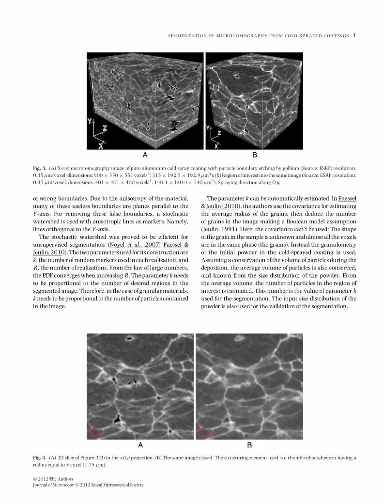
Fig. 3. (A) X-ray microtomography image of pure aluminium cold spray coating with particle boundary etching by gallium (Source: ESRF; resolution:0.35μm/voxel; dimensions: 900× 550× 551 voxels3; 315× 192.5× 192.9μm3); (B) Region of interest into the same image (Source: ESRF; resolution:0.35 μm/voxel; dimensions: 401× 401× 400 voxels3; 140.4× 140.4× 140 μm3). Spraying direction along O y.

of wrong boundaries. Due to the anisotropy of the material,many of these useless boundaries are planes parallel to theY-axis. For removing these false boundaries, a stochasticwatershed is used with anisotropic lines as markers. Namely,lines orthogonal to the Y-axis.

The stochastic watershed was proved to be efficient forunsupervised segmentation (Noyel et al., 2007; Faessel &Jeulin, 2010). The two parameters used for its construction arek, the number of random markers used in each realization, andR, the number of realizations. From the law of large numbers,the PDF converges when increasing R. The parameter k needsto be proportional to the number of desired regions in thesegmented image. Therefore, in the case of granular materials,k needs to be proportional to the number of particles containedin the image.

The parameter k can be automatically estimated. In Faessel& Jeulin (2010), the authors use the covariance for estimatingthe average radius of the grains, then deduce the numberof grains in the image making a Boolean model assumption(Jeulin, 1991). Here, the covariance can’t be used: The shapeof the grain in the sample is unknown and almost all the voxelsare in the same phase (the grains). Instead the granulometryof the initial powder in the cold-sprayed coating is used.Assuming a conservation of the volume of particles during thedeposition, the average volume of particles is also conserved,and known from the size distribution of the powder. Fromthe average volume, the number of particles in the region ofinterest is estimated. This number is the value of parameter kused for the segmentation. The input size distribution of thepowder is also used for the validation of the segmentation.

Fig. 4. (A) 2D slice of Figure 3(B) in the xO y projection. (B) The same image closed. The structuring element used is a rhombicuboctahedron having aradius equal to 5 voxel (1.75 μm).

C© 2012 The AuthorsJournal of Microscopy C© 2012 Royal Microscopical Society

4 L . G I L L I B E R T E T A L .

Fig. 5. Multiscale segmentation algorithm.

Stochastic watershed

The first method introduced for computing the stochasticwatershed is based on a large number of realizations of randommarkers to estimate a PDF of contours, or of surface boundariesin 3D.

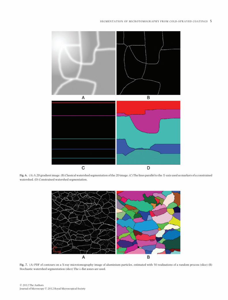
In the present case, the markers are random lines parallel tothe X-axis and lines parallel to the Z -axis. These markers willgive a high probability of detection of the boundaries parallelto the X-axis and the Z -axis and a low probability of detectionof the boundaries parallel to the Y-axis. As illustrated on a 2Dsimple example, if the markers of a realization are lines parallelto the X-axis, the boundaries parallel to the X-axis are detectedby a constrained watershed, but the the boundaries parallel tothe Y-axis disappear (Fig. 6).

As in the multiscale segmentation, the topological functionused for the watershed construction is a closing of the inputimage with a small rhombicuboctahedron (radius=1.75μm).For each set of markers, a constrained watershed is computed.Then, the Parzen window is used to estimate the PDF ofcontours (Parzen, 1962).

For a good estimation of the stochastic watershed,100 to 200 realizations are required (Angulo & Jeulin,2007). However, using λ-flat zones, a stochastic watershedsegmentation can be achieved with 50 realizations (Faessel& Jeulin, 2010). This number is low, but the computation of50 watersheds is very time consuming, especially on large 3Ddata sets. Here, 25 realizations with lines parallel to the X-axisand 25 realizations with lines parallel to the Z -axis are used.

From the PDF, it is possible to obtain the segmentation.The first approach uses this PDF as a topological function fora new watershed (Angulo & Jeulin, 2007). A more efficientapproach uses λ-flat zones to overcome the fact that theestimated PDF is not constant over each branch of contour(Faessel & Jeulin, 2010). Illustration of the PDF of contours isgive on Figure 7(A), the resulting segmentation is illustratedon Figure 7(B).

Graph-based stochastic watershed

Direct computation of the probability of a boundaryComputing a large number of watersheds from simulations

provides reliable results but is a slow process, especially in 3D .A more efficient solution for computing stochastic watershedsis to use a direct approach. Probability of boundaries is directlycomputed with a good approximation without the use of anyrealizations (Jeulin, 2008; Stawiaski & Meyer, 2010).

In the present case, we assume Poisson lines as markers. Allthe lines are parallel to a given axis denoted L . The probabilityof boundaries can be estimated from the surface area of theopaque projection of the regions on a plane perpendicular tothe axis L .

The opaque projection for the region i is denoted PL (i ) andthe surface area is denoted S(PL (i )).

Given two adjacent regions, the probability p(i , j ) of theboundary between regions i and j is obtained from thefollowing equation:

p(i , j ) = exp(−λS(PL (i ) ∩ PL ( j )))− 2 exp(−λS(PL (i )))

−2 exp(−λS(PL ( j )))+ 3 exp(−λS(PL (i ) ∪ PL ( j ))

+ exp(λS(PL (i ) ∩ PL ( j ))[exp(−λS(PL (i )))

+ exp(−λS(PL ( j )))

−2 exp(−λS(PL (i ) ∪ PL ( j )))],(1)

where λ is the Poisson lines intensity of the considered randomlines, and L is the orientation of the lines. When S(PL (i ) ∩PL ( j )) can be neglected with respect to S(PL (i )) and S(PL ( j )),the following approximation of Eq. (1), given in (Jeulin, 2008)

C© 2012 The AuthorsJournal of Microscopy C© 2012 Royal Microscopical Society

S E G M E N T A T I O N O F M I C R O T O M O G R A P H Y F R O M C O L D - S P R A Y E D C O A T I N G S 5

Fig. 6. (A) A 2D gradient image. (B) Classical watershed segmentation of the 2D image. (C) The lines parallel to the X-axis used as markers of a constrainedwatershed. (D) Constrained watershed segmentation.

Fig. 7. (A) PDF of contours on a X-ray microtomography image of aluminium particles, estimated with 50 realizations of a random process (slice) (B)Stochastic watershed segmentation (slice) The λ-flat zones are used.

C© 2012 The AuthorsJournal of Microscopy C© 2012 Royal Microscopical Society

6 L . G I L L I B E R T E T A L .

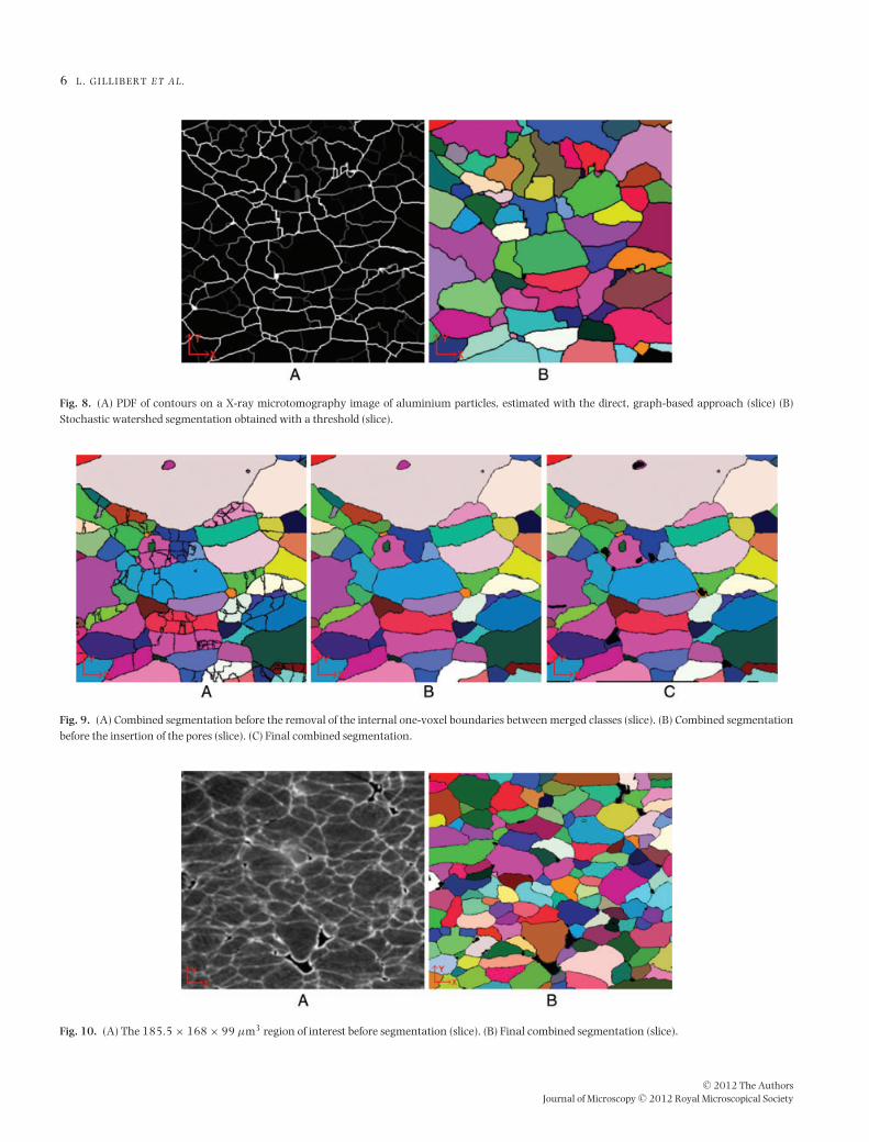
Fig. 8. (A) PDF of contours on a X-ray microtomography image of aluminium particles, estimated with the direct, graph-based approach (slice) (B)Stochastic watershed segmentation obtained with a threshold (slice).

Fig. 9. (A) Combined segmentation before the removal of the internal one-voxel boundaries between merged classes (slice). (B) Combined segmentationbefore the insertion of the pores (slice). (C) Final combined segmentation.

Fig. 10. (A) The 185.5× 168× 99 μm3 region of interest before segmentation (slice). (B) Final combined segmentation (slice).

C© 2012 The AuthorsJournal of Microscopy C© 2012 Royal Microscopical Society

S E G M E N T A T I O N O F M I C R O T O M O G R A P H Y F R O M C O L D - S P R A Y E D C O A T I N G S 7

Table 1. Computational cost of the stochastic watershed, the graph-based stochastic watershed, the multiscale image segmentation andthe combined segmentation. Times are given for the 140.4× 140.4×140 μm3 region of interest on a 3.00 GHz Pentium 4.

Algorithm Time

1 Simple watershed 3 min2 Stochastic watershed 2 h 32 min3 Graph-based stochastic watershed 8 min 40 s4 Multiscale image segmentation 31 min 40 s5 Combination of the partitions 1 min 50 s6 Combined segmentation (3+ 4+ 5) 42 min 10 s

is obtained, andcomment is used in the present segmentationof the cold-spray coating

p(i , j ) � 1− exp (−λS(PL (i )))− exp(−λS(P ( j )))+ exp (−λS(PL (i ) ∪ PL ( j ))). (2)

Graph-based algorithmWith the Eq. (2) and a graph-based approach, it is possible

to estimate the stochastic watershed by direct computation(Stawiaski & Meyer, 2010).

As before, the used topological function is a closing of theinput image with a small rhombicuboctahedron (radius =1.75μm). A first watershed is computed from the local minimaof the topological function. Again, a strong oversegmentationis obtained as a result of the presence of noise.

From this watershed, an adjacency graph is constructed.Vertices of the graph are associated to each basin ofthe watershed, connecting edges between adjacent regions.Values are given to the vertices corresponding to the surfacearea of the projection of the regions on a plane perpendicular tothe axis L . The projections PL (i ) of all regions i are computedand stored as binary images.

Each edge of the graph is labelled with the minimumof the topological function on the boundary between thecorresponding regions. This value corresponds to the heightof the gap where the two sources corresponding to the tworegions are meeting for the first time during the floodingprocess of the watershed. From this valued graph, a minimumspanning tree is extracted. Then the regions in the minimumspanning tree are merged, starting with the edge of lowestvalue.

This merging process corresponds to the natural order of theflooding process in the watershed. The merging process runsuntil all the nodes of the tree are merged. During this mergingprocess, the probability of the boundaries of the stochasticwatershed are estimated and the surface of the projections ofthe merged regions are updated.

When merging two regions i and j , the probability ofthe corresponding boundary in the stochastic watershed isestimated using the Eq. (2).

The values S(PL (i )) and S(PL ( j )) are already available.The value S(PL (i ) ∩ PL ( j )) is deduced from the projectionsPL (i ) and PL ( j ). The value S(PL (i ∪ j )) is computed, usingthe values S(PL (i )), S(PL ( j )) and S(PL (i ) ∩ PL ( j )), from

S(PL (i ∪ j )) = S(PL (i ) ∪ PL (i ))= S(PL (i ))+ S(PL ( j ))− S(PL (i ) ∩ PL ( j )). (3)

Then, the tree and the associated data are updated. Thenodes i and j are merged. The new node corresponds to theregion i ∪ j . Therefore, the valuation of this new region isS(PL (i ∪ j )), given by Eq. (3).

After the merging of all the nodes in the original minimumspanning tree, the probability of all the edges of the tree isknown. The result is projected from the tree on the graph andfrom the graph on the image.

Two directions are used tor the random lines, thereforetwo graph-based stochastic watersheds are computed: one for

Fig. 11. (A) Combined segmentation for the 140.4× 140.4× 140 μm3 region of interest. (B) And for the 185.5× 168× 99 μm3 region of interest.Spraying direction along O y.C© 2012 The AuthorsJournal of Microscopy C© 2012 Royal Microscopical Society

8 L . G I L L I B E R T E T A L .

0

20

40

60

80

100

0 50 100 150 200 250

% o

f VO

LUM

E

DIAMETER (micrometre)

GRANULOMETRY in VOLUME

Input granulometry (cumulated)Multiscale segmentation granulometry (cumulated)Combined segmentation granulometry (cumulated)

Fig. 12. Cumulative granulometry of the originalparticles used in the cold-sprayed coating and ofthe segmented image. Results are given for themultiscale segmentation algorithm and for thecombined segmentation algorithm on the 140.4×140.4× 140 μm3 region of interest. The Miles–Lantuejoul correction is used.

each direction. The average of the two PDFs is used as finalstochastic watershed.

With a large amount of memory, it is possible to computesingle graph-based stochastic watersheds, working withprojections in two directions at the same time. During themerging, the probability p(i , j ) of the boundary between thecorresponding regions i and j is estimated using the followingequation:

p(i , j ) � 1− exp [−λ(S(PX (i ))+ S(PZ (i )))]− exp [−λ(S(PX ( j ))+ S(PZ ( j )))]+ exp [−λ(S(PX (i ∪ j ))+ S(PZ (i ∪ j )))].

This approach provides uniform probability on each part ofboundary between two regions, as illustrated on Figure 8(A).Therefore, the λ-flat zones are useless and a simple thresholdcan be used for the segmentation, as explained later (Fig. 8B).A high threshold gives all boundaries which are not parallelto the Y-axis.

Combined segmentation

We have two segmentations, one stochastic and onemultiscale. In both cases, most of the true boundaries arepresent. In both cases, there is also some oversegmentation.

0

10

20

30

40

50

60

70

80

90

100

10 20 30 40 50 60 70 80 90

Num

ber

of p

artic

les

DIAMETER (micrometre)

GRANULOMETRY in NUMBER

Input granulometryMultiscale segmentation granulometryCombined segmentation granulometry

Fig. 13. Granulometry of the original particlesused in the cold-sprayed coating and granulometryof the segmented image (given as a histogramof number of particles). Small particles (with adiameter < 7 μm) are ignored. Results are given forthe multiscale segmentation algorithm and for thecombined segmentation algorithm on the 140.4×140.4× 140 μm3 region of interest.

C© 2012 The AuthorsJournal of Microscopy C© 2012 Royal Microscopical Society

S E G M E N T A T I O N O F M I C R O T O M O G R A P H Y F R O M C O L D - S P R A Y E D C O A T I N G S 9

0

20

40

60

80

100

0 50 100 150 200

% o

f VO

LUM

E

DIAMETER (micrometre)

GRANULOMETRY in VOLUME

Input granulometry (cumulated)Multiscale segmentation granulometry (cumulated)Combined segmentation granulometry (cumulated)

Fig. 14. Cumulative granulometry of the originalparticles used in the cold-sprayed coating and ofthe segmented image. Results are given for themultiscale segmentation algorithm and for thecombined segmentation algorithm on the 185.5×168× 99 μm3 region of interest. The Miles–Lantuejoul correction is used.

But the false boundaries present in the two segmentationsare very different. In the multiscale segmentation, we havemostly some planes parallel to the Y-axis. In the stochasticsegmentation, we have some very irregular boundaries in thelargest particles.

Therefore, it is possible to build a combination of the twosegmentations. Boundaries are kept if and only if they are inboth segmentations.

Due to some irregularity in the boundaries, it is impossible toachieve such a combination working only on the boundaries.Instead, we work on the partitions, using a supremum. Weuse the following process:

(i) Given two partitions, P1 and P2, we look for each class ofP1 its intersection with the classes in P2.

(ii) We label each class of P1 with the class in P2 itpredominantly belongs to.

(iii) Then we build the final partition F . It is a copy of P1, but iftwo classes in P1 predominantly belong to the same classof P2, they are merged.

As seen on Figure 9(A), this process is efficient for buildingthe supremum of two partitions, but does not remove theinternal one-voxel boundaries between merged classes. Forthis purpose, we use a last constrained watershed. The markersof this watershed are the merged regions and the topological

0

20

40

60

80

100

120

140

15 20 25 30 35 40 45 50

Num

ber

of p

artic

les

DIAMETER (micrometre)

GRANULOMETRY in NUMBER

Input granulometryMultiscale segmentation granulometryCombined segmentation granulometry

Fig. 15. Granulometry of the original particlesused in the cold-sprayed coating and granulometryof the segmented image (given as a histogramof number of particles). Small particles (with adiameter< 14μm) are ignored. Results are given forthe multiscale segmentation algorithm and for thecombined segmentation algorithm on the 185.5×168× 99 μm3 region of interest.

C© 2012 The AuthorsJournal of Microscopy C© 2012 Royal Microscopical Society

1 0 L . G I L L I B E R T E T A L .

AB

10

Y

X

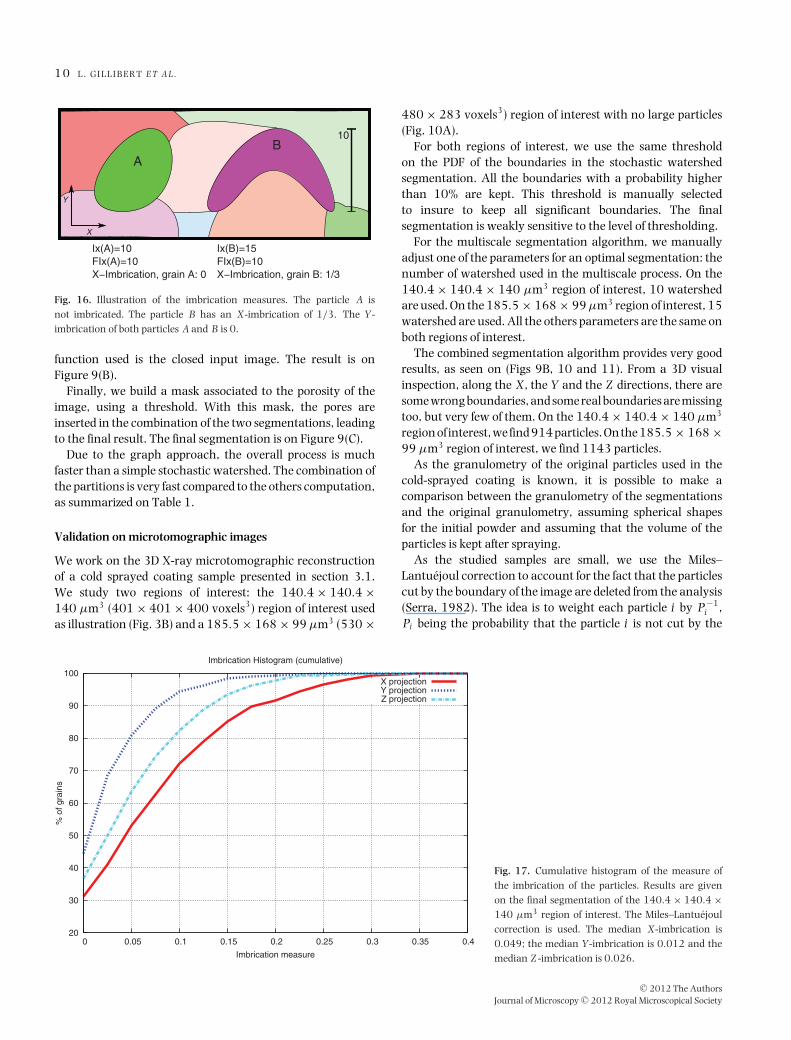
Ix(A)=10 FIx(A)=10X−Imbrication, grain A: 0

Ix(B)=15 FIx(B)=10X−Imbrication, grain B: 1/3

Fig. 16. Illustration of the imbrication measures. The particle A isnot imbricated. The particle B has an X-imbrication of 1/3. The Y-imbrication of both particles A and B is 0.

function used is the closed input image. The result is onFigure 9(B).

Finally, we build a mask associated to the porosity of theimage, using a threshold. With this mask, the pores areinserted in the combination of the two segmentations, leadingto the final result. The final segmentation is on Figure 9(C).

Due to the graph approach, the overall process is muchfaster than a simple stochastic watershed. The combination ofthe partitions is very fast compared to the others computation,as summarized on Table 1.

Validation on microtomographic images

We work on the 3D X-ray microtomographic reconstructionof a cold sprayed coating sample presented in section 3.1.We study two regions of interest: the 140.4× 140.4×140 μm3 (401× 401× 400 voxels3) region of interest usedas illustration (Fig. 3B) and a 185.5× 168× 99 μm3 (530×

480× 283 voxels3) region of interest with no large particles(Fig. 10A).

For both regions of interest, we use the same thresholdon the PDF of the boundaries in the stochastic watershedsegmentation. All the boundaries with a probability higherthan 10% are kept. This threshold is manually selectedto insure to keep all significant boundaries. The finalsegmentation is weakly sensitive to the level of thresholding.

For the multiscale segmentation algorithm, we manuallyadjust one of the parameters for an optimal segmentation: thenumber of watershed used in the multiscale process. On the140.4× 140.4× 140 μm3 region of interest, 10 watershedare used. On the 185.5× 168× 99 μm3 region of interest, 15watershed are used. All the others parameters are the same onboth regions of interest.

The combined segmentation algorithm provides very goodresults, as seen on (Figs 9B, 10 and 11). From a 3D visualinspection, along the X, the Y and the Z directions, there aresome wrong boundaries, and some real boundaries are missingtoo, but very few of them. On the 140.4× 140.4× 140 μm3

region of interest, we find 914 particles. On the 185.5× 168×99 μm3 region of interest, we find 1143 particles.

As the granulometry of the original particles used in thecold-sprayed coating is known, it is possible to make acomparison between the granulometry of the segmentationsand the original granulometry, assuming spherical shapesfor the initial powder and assuming that the volume of theparticles is kept after spraying.

As the studied samples are small, we use the Miles–Lantuejoul correction to account for the fact that the particlescut by the boundary of the image are deleted from the analysis(Serra, 1982). The idea is to weight each particle i by P−1

i ,Pi being the probability that the particle i is not cut by the

20

30

40

50

60

70

80

90

100

0 0.05 0.1 0.15 0.2 0.25 0.3 0.35 0.4

% o

f gra

ins

Imbrication measure

Imbrication Histogram (cumulative)

X projectionY projectionZ projection

Fig. 17. Cumulative histogram of the measure ofthe imbrication of the particles. Results are givenon the final segmentation of the 140.4× 140.4×140 μm3 region of interest. The Miles–Lantuejoulcorrection is used. The median X-imbrication is0.049; the median Y-imbrication is 0.012 and themedian Z -imbrication is 0.026.

C© 2012 The AuthorsJournal of Microscopy C© 2012 Royal Microscopical Society

S E G M E N T A T I O N O F M I C R O T O M O G R A P H Y F R O M C O L D - S P R A Y E D C O A T I N G S 1 1

20

30

40

50

60

70

80

90

100

0 0.05 0.1 0.15 0.2 0.25 0.3 0.35 0.4

% o

f gra

ins

Imbrication measure

Imbrication Histogram (cumulative)

X projectionY projectionZ projection

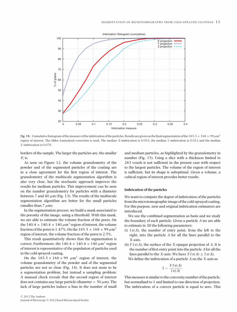
Fig. 18. Cumulative histogram of the measure of the imbrication of the particles. Results are given on the final segmentation of the 185.5× 168× 99μm3

region of interest. The Miles–Lantuejoul correction is used. The median X-imbrication is 0.052; the median Y-imbrication is 0.012 and the medianZ -imbrication is 0.078.

borders of the sample. The larger the particles are, the smallerPi is.

As seen on Figure 12, the volume granulometry of thepowder and of the segmented particles of the coating arein a close agreement for the first region of interest. Thegranulometry of the multiscale segmentation algorithm isalso very close, but the stochastic approach improves theresults for medium particles. This improvement can be seenon the number granulometry for particles with a diameterbetween 7 and 40 μm (Fig. 13). The results of the multiscalesegmentation algorithm are better for the small particles(smaller than 7 μm).

In the segmentation process, we build a mask associated tothe porosity of the image, using a threshold. With this mask,we are able to estimate the volume fraction of the pores. Onthe 140.4× 140.4× 140 μm3 region of interest, the volumefraction of the pores is 1.47%. On the 185.5× 168× 99 μm3

region of interest, the volume fraction of the pores is 2.5%.This result quantitatively shows that the segmentation is

correct. Furthermore, the 140.4× 140.4× 140 μm3 regionof interest is representative of the population of particles usedin the cold sprayed coating.

On the 185.5× 168× 99 μm3 region of interest, thevolume granulometry of the powder and of the segmentedparticles are not so close (Fig. 14). It does not seem to bea segmentation problem, but instead a sampling problem:A manual check reveals that the second region of interestdoes not contains any large particle (diameter > 50 μm). Thelack of large particles induce a bias in the number of small

and medium particles, as highlighted by the granulometry innumber (Fig. 15). Using a slice with a thickness limited to283 voxels is not sufficient in the present case with respectto the largest particles. The volume of the region of interestis sufficient, but its shape is suboptimal. Given a volume, acubical region of interest provides better results.

Imbrication of the particles

We want to compute the degree of imbrication of the particlesfrom the microtomographic image of the cold-sprayed coating.For this purpose, new and original imbrication estimators areintroduced.

We use the combined segmentation as basis and we studythe boundary of each particle. Given a particle A we are ableto estimate in 3D the following parameters:(i) I x(A), the number of entry point, from the left to the

right, into the particle A for all the lines parallel to theX-axis.

(ii) F I x(A), the surface of the X-opaque projection of A. It isthe number of first entry point into the particle A for all thelines parallel to the X-axis. We have F I x(A) ≤ I x(A).

We define the imbrication of a particle A on the X-axis as

1− F I x(A)I x(A)

.

This measure is similar to the convexity number of the particle,but normalized to 1 and limited to one direction of projection.The imbrication of a convex particle is equal to zero. This

C© 2012 The AuthorsJournal of Microscopy C© 2012 Royal Microscopical Society

1 2 L . G I L L I B E R T E T A L .

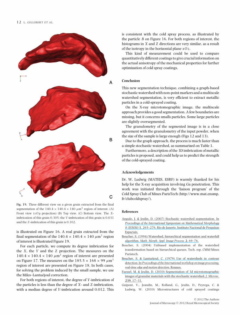
Fig. 19. Three different view on a given grain extracted from the finalsegmentation of the 140.4× 140.4× 140 μm3 region of interest. (A)Front view (xO y projection) (B) Top view. (C) Bottom view. The X-imbrication of this grain 0.305; the Y-imbrication of this grain is 0.031and the Z -imbrication of this grain is 0.102.

is illustrated on Figure 16. A real grain extracted from thefinal segmentation of the 140.4× 140.4× 140 μm3 regionof interest is illustrated Figure 19.

For each particle, we compute its degree imbrication forthe X, the Y and the Z projection. The measures on the140.4× 140.4× 140 μm3 region of interest are presentedon Figure 17. The measures on the 185.5× 168× 99 μm3

region of interest are presented on Figure 18. In both cases,for solving the problem induced by the small sample, we usethe Miles–Lantuejoul correction.

For both regions of interest, the degree of Y-imbrication ofthe particles is less than the degree of X- and Z -imbrication,with a median degree of Y-imbrication around 0.012. This

is consistent with the cold spray process, as illustrated bythe particle B on Figure 16. For both regions of interest, thehistograms in X and Z directions are very similar, as a resultof the isotropy in the horizontal plane xO z.

This kind of measurement could be used to comparequantitatively different coatings to give crucial information onthe actual anisotropy of the mechanical properties for furtheroptimization of cold spray coatings.

Conclusion

This new segmentation technique, combining a graph-basedstochastic watershed with non-point markers and a multiscalewatershed segmentation, is very efficient to extract metallicparticles in a cold-sprayed coating.

On the X-ray microtomographic image, the multiscaleapproach provides a good segmentation. A few boundaries aremissing, but it concerns smalls particles. Some large particlesare slightly oversegmented.

The granulometry of the segmented image is in a closeagreement with the granulometry of the input powder, whenthe size of the sample is large enough (Figs 12 and 13).

Due to the graph approach, the process is much faster thana simple stochastic watershed, as summarized on Table 1.

Furthermore, a description of the 3D imbrication of metallicparticles is proposed, and could help us to predict the strengthof the cold-sprayed coating.

Acknowledgements

Dr. W. Ludwig (MATEIS, ESRF) is warmly thanked for hishelp for the X-ray acquisition involving Ga penetration. Thiswork was initiated through the ‘liaison program’ of theCold Spray Club of Mines ParisTech (http://www.mat.ensmp.fr/clubcoldspray/).

References

Angulo, J. & Jeulin, D. (2007) Stochastic watershed segmentation. InProceedings of the International Symposium on Mathematical Morphology8 (ISMM) 1, 265–276. Rio de Janerio, Instituto Nacional de PesquisasEspaciais.

Beucher, S. (1994) Watershed, hierarchical segmentation and waterfallalgorithm. Math. Morph. Appl. Image Process. 2, 69–76.

Beucher, S. (2004) Unbiased implementation of the watershedtransformation based on hierarchical queues. Tech. rep. CMM/MinesParistech.

Beucher, S. & Lantuejoul, C. (1979) Use of watersheds in contourdetection. In Proceedings of the International workshop on image processing,real-time edge and motion detection. Rennes.

Faessel, M. & Jeulin, D. (2010) Segmentation of 3d microtomographicimages of granular materials with the stochastic watershed. J. Microsc.239, 17–31.

Guipont, V., Jeandin, M., Rolland, G., Jeulin, D., Peyrega, C. &Ludwig, W. (2010) Microstructures of cold sprayed coatings

C© 2012 The AuthorsJournal of Microscopy C© 2012 Royal Microscopical Society

S E G M E N T A T I O N O F M I C R O T O M O G R A P H Y F R O M C O L D - S P R A Y E D C O A T I N G S 1 3

investigated by x-ray microtomography. Ther. Spray Bull. 3, 140–147.

Jeulin, D. (1991) Modeles morphologiques de structures aleatoires et dechangement d’echelle. Ph.D. Thesis, University of Caen, France.

Jeulin, D. (2008) Remarques sur la segmentation probabiliste. Tech. Rep.N-10/08/MM CMM/Mines Paristech.

Noyel, G., Angulo, J. & Jeulin, D. (2007) Random germs and stochasticwatershed for unsupervised multispectral image segmentation. InProceedings of Knowledge-Based Intelligent Information and EngineeringSystems (KES). Vietri Sul Mare.

Parzen, E. (1962) On estimation of a probability density function andmode. Ann. Math. Stat. 33, 1065–1076.

Rolland, G., Guipont, V., Jeandin, M., Peyrega, C., Jeulin, D. & Ludwig,W. (2010) Microstructures of cold-sprayed coatings investigated by x-ray microtomography. In Proceedings of the International Thermal SprayConference and Exposition (ITSC). Singapore.

Serra, J. (1982) Image Analysis and Mathematical Morphology. AcademicPress, London.

Stawiaski, J. & Meyer, F. (2010) Stochastic watershed on graphs andhierarchical segmentation. In Proceedings ECMI 2010. Wuppertal.

C© 2012 The AuthorsJournal of Microscopy C© 2012 Royal Microscopical Society