“3D ENERGY MODELING OPTIMIZATION USING ...
170
BACHELOR THESIS “3D ENERGY MODELING OPTIMIZATION USING COMPUTATIONAL DESIGN SOFTWARE” TFG presented in order to obtain the Degree in Energy Engineering By Axel Paul Galpy-Massé Barcelona, 08 of June of 2016 Director: Jordi Torner Ribé Departament of EGE Universitat Politècnica de Catalunya (UPC)
-
Upload
khangminh22 -
Category
Documents
-
view
0 -
download
0
Transcript of “3D ENERGY MODELING OPTIMIZATION USING ...

BACHELOR THESIS
“3D ENERGY MODELING OPTIMIZATION USING
COMPUTATIONAL DESIGN SOFTWARE”
TFG presented in order to obtain the Degree in Energy Engineering
By Axel Paul Galpy-Massé
Barcelona, 08 of June of 2016
Director: Jordi Torner Ribé Departament of EGE
Universitat Politècnica de Catalunya (UPC)

VOLUME I
General Index, Memory
BACHELOR THESIS
“3D ENERGY MODELING OPTIMIZATION USING
COMPUTATIONAL DESIGN SOFTWARE
TFG presented in order to obtain the Degree in Energy Engineering
By Axel Paul Galpy-Massé
Barcelona, 08 of June of 2016
Director: Jordi Torner Ribé Departament of EGE
Universitat Politècnica de Catalunya (UPC)

General Index
“3D ENERGY MODELING OPTIMIZATION USING
COMPUTATIONAL DESIGN SOFTWARE
TFG presented in order to obtain the Degree in Energy Engineering
By Axel Paul Galpy-Massé
Barcelona, 08 of June of 2016
Director: Jordi Torner Ribé Departament of EGE
Universitat Politècnica de Catalunya (UPC)

GENERAL INDEX
General Index................................................................................... 1
VOLUME I
1: Memory Index .......................................................................... 3
VOLUME II
1: Budget ..................................................................................... 7
VOLUME III
1: Annexes ................................................................................... 9


- 3 -
MEMORY INDEX
ABSTRACT ............................................................................................. 5
RESUM .................................................................................................. 6
RESUMEN .............................................................................................. 7
Chapter 1: Introduction ....................................................................... 9
1.1 Description of the objective of the project ............................................. 9
1.1.1. General objective ........................................................................ 9
1.1.2. Specific objective ...................................................................... 10
1.2 Motivation ..................................................................................... 10
1.3 Scope ........................................................................................... 10
Chapter 2: Current Energetic situation ............................................... 13
2.1 World Global Warming ..................................................................... 13
2.2 World energy consumption in residential sector …………………………… …14
2.3 Energy consumption in the residential sector in Spain ........................... 14
2.4 Renewable energy sources applicable to a house ................................. 15
2.4.1. Solar Photovoltaic energy ............................................................ 15
2.4.1. Solar Thermal energy ................................................................. 16
2.4.1. Wind power ............................................................................. 17
2.4.1. Geothermal energy .................................................................... 18
2.5 Renewable Energies in Spain ............................................................ 19
2.6 Low-Energy Houses ........................................................................ 23
Chapter 3: Presentation of the software used .................................... 23
3.1 Rhino ........................................................................................... 23
3.2 Grasshopper .................................................................................. 23
3.2.1. Grasshopper components ............................................................ 24
3.2.2. Grasshopper Plugins .................................................................. 24
A) Python .................................................................................... 26
B) Daysim.................................................................................... 27
C) Radiance ................................................................................. 29
D) Ladybug .................................................................................. 30
E) VisualARQ ................................................................................ 31
Chapter 4: Program architecture for the study of a room ................... 31
4.1 Grasshopper .................................................................................. 31

3D Energy Modeling Optimisation using Computational Design Software
- 4 -
4.2 Honeybee ...................................................................................... 32
4.2.1. Building definition ..................................................................... 32
4.2.2. Schedules setting ...................................................................... 32
4.2.3. Loads setting ........................................................................... 33
4.2.4. Daylight simulation .................................................................... 34
4.2.5. Energy simulation ..................................................................... 35
4.2.6. Iterations ................................................................................ 35
A) Window glaze ratio iteration .......................................................... 35
B) Date of daylight simulation iteration ................................................ 36
C) Iteration order........................................................................... 36
D) Simulation run .......................................................................... 37
4.2.7. Simulation results ..................................................................... 37
Chapter 5: Room study ...................................................................... 39
5.1 Room 1 ......................................................................................... 39
5.1.1. Algorithm................................................................................ 39
5.1.2. Simulation results ..................................................................... 46
5.1.3. New algortihm ......................................................................... 46
5.1.4. New algorithm results ................................................................ 47
5.1.5. Optimisation with Galapagos ........................................................ 55
5.2 Room 2 ......................................................................................... 55
5.2.1. Algorithm................................................................................ 55
5.2.2. Simulation results ..................................................................... 55
5.2.3. Optimisation with Galapagos ........................................................ 58
5.3 Living Room .................................................................................. 59
5.3.1. Algorithm................................................................................ 59
5.3.2. Simulation results ..................................................................... 60
5.3.3. Optimisation with Galapagos ........................................................ 66
5.4 Room 3 ......................................................................................... 66
5.4.1. Algorithm................................................................................ 66
5.4.2. Simulation results ..................................................................... 68
5.4.3. Optimisation with Galapagos ........................................................ 74
5.5 Bathroom ...................................................................................... 74
5.5.1. Algorithm................................................................................ 74
5.5.2. Simulation results ..................................................................... 76
5.5.3. Optimisation with Galapagos ........................................................ 82
Chapter 6: Energetic study of the house ............................................ 83

3D Energy Modeling Optimisation using Computational Design Software
- 5 -
6.1 Home design ................................................................................. 83
6.2 House simulation algorithm .............................................................. 85
Chapter 7: House materials and insulation ......................................... 95
7.1 Construction materials in Grasshopper ............................................... 95
7.2 Materials impact on energy consumption ............................................ 97
7.2.1. Exterior wall material .................................................................. 97
7.2.2. Exterior window material .............................................................. 99
7.2.3. Roof material ............................................................................ 99
7.3 Final materials of the house ........................................................... 100
7.4 Construction costs ........................................................................ 101
Chapter 8: Renewable energy installation for the building .............. 105
8.1 Introduction ................................................................................ 105
8.2 Measuring of the photovoltaic installation 106
8.2.1. Energetic demand of the house .................................................... 106
8.2.2. Dimensions of the installation components ...................................... 107
8.2.3. Dimensions of the wire installation ................................................ 121
8.3 Demand and dimensiosn of the DHW ............................................... 124
8.3.1.Dimensions of the installation of solar thermal collectors ...................... 124
Chapter 9: Energy production legislation ........................................ 131
9.1 Definition of Net Metering and Self-Consumption ............................... 131
9.2 Legal application .......................................................................... 131
Chapter 10: Energy performance of the buildings ............................ 135
10.1 Performance certificate legislation ................................................. 135
10.2 Energy performance study ........................................................... 136
10.2.1. General Data ......................................................................... 136
10.2.2. Building definition ................................................................... 136
10.2.3. Installations .......................................................................... 138
10.2.4. Results ............................................................................... 140
Chapter 11: Gantt Chart ................................................................. 141
Chapter 12: Future projects ............................................................ 147
Chapter 13: Conclusions ................................................................. 149
Chapter 14: Bibliography ................................................................ 153
14.1 Bibliographic references ............................................................... 153
14.2 Search references ....................................................................... 155


3D Energy Modeling Optimisation using Computational Design Software
- 7 -
BUDGET INDEX
Chapter 1: Introduction .................................................................. 3
Chapter 2: Economic study of the technicities of the study .............. 5
2.1. Construction costs .............................................................. 5
2.1.1. Cost comparison between a glaze ratio optimized house and a non-optimized one..................................................................... 5
2.1.2. Cost comparison between an isolated house and a non-isolated one ..6
2.1.3. Isolation amortization ........................................................7
2.2. Renewable energy installation costs ...................................... 8
2.2.1. Photovoltaic installation ................................................. 8
A) Case A) ...................................................................... 8
B) Case B) ................................................................ 13
2.2.2. Thermo solar installation ....................................................... 17
2.3. Total cost ........................................................................ 18
2.4. Viability of the installations ................................................ 21
Chapter 3: Project cost ................................................................. 23
Chapter 4: Conclusions ................................................................. 27
Chapter 5: Bibliography ................................................................ 29


3D Energy Modeling Optimisation using Computational Design Software
- 9 -
ANNEXES INDEX
1.Photovoltaic panels’ datasheet .......................................................... 3
2.Batteries datasheet ......................................................................... 5
3. DC/DC Regulator datasheet ............................................................. 7
4. AC/DC Inverter datasheet ............................................................... 9
5. Solar thermal collector datasheet ................................................... 11
6. The reform of the Spanish electricity sector. Arturo Rojas and Pablo Mañueco ....................................................................................... 15
7.Methodology for the Energy Efficiency .............................................. 23
8. Energy Efficiency Study ................................................................ 25

Memory
“3D ENERGY MODELING OPTIMIZATION USING
COMPUTATIONAL DESIGN SOFTWARE
TFG presented in order to obtain the Degree in Energy Engineering
By Axel Paul Galpy-Massé
Barcelona, 08 of June of 2016
Director: Jordi Torner Ribé Departament of EGE
Universitat Politècnica de Catalunya (UPC)

- 1 -
MEMORY INDEX
ABSTRACT ............................................................................................. 5
RESUM .................................................................................................. 6
RESUMEN .............................................................................................. 7
Chapter 1: Introduction ....................................................................... 9
1.1 The project objective description ........................................................ 9
1.1.1. General objective ........................................................................ 9
1.1.2. Specific objective ...................................................................... 10
1.2 Motivation ..................................................................................... 10
1.3 Scope ........................................................................................... 10
Chapter 2: Current Energetic situation ............................................... 13
2.1 World Global Warming ..................................................................... 13
2.2 World Energy consumption in residential sector …………………………… …14
2.3 Energy consumption in the residential sector in Spain ........................... 14
2.4 Renewable energy sources applicable to a house ................................. 15
2.4.1. Solar Photovoltaic energy ............................................................ 15
2.4.1. Solar Thermal energy ................................................................. 16
2.4.1. Wind power ............................................................................. 17
2.4.1. Geothermal ............................................................................. 18
2.5 Renewable Energies in Spain ............................................................ 19
2.6 Low-Energy Houses ........................................................................ 23
Chapter 3: Presentation of the software used .................................... 23
3.1 Rhino ........................................................................................... 23
3.2 Grasshopper .................................................................................. 23
3.2.1. Grasshopper components ............................................................ 24
3.2.2. Grasshopper Plugins .................................................................. 24
A) Python .................................................................................... 26
B) Daysim.................................................................................... 27

Axel Paul Galpy Massé
- 2 -
C) Radiance ................................................................................. 29
D) Ladybug .................................................................................. 30
E) VisualARQ ................................................................................ 31
Chapter 4: Program architecture for the study of a room ................... 31
4.1 Grasshopper .................................................................................. 31
4.2 Honeybee ...................................................................................... 32
4.2.1. Building definition ..................................................................... 32
4.2.2. Schedules setting ...................................................................... 32
4.2.3. Loads setting ........................................................................... 33
4.2.4 Daylight simulation ..................................................................... 34
4.2.5. Energy simulation ..................................................................... 35
4.2.6. Iterations ................................................................................ 35
A) Window glaze ratio iteration .......................................................... 35
B) Date pf daylight simulation iteration ................................................ 36
C) Iteration order........................................................................... 36
D) Simulation run .......................................................................... 37
4.2.7. Simulation results ..................................................................... 37
Chapter 5: Room study ...................................................................... 39
5.1 Room 1 ......................................................................................... 39
5.1.1. Algorithm................................................................................ 39
5.1.2. Simulation results ..................................................................... 46
5.1.3. New algortihm ......................................................................... 46
5.1.4. New algorithm results ................................................................ 47
5.1.5. Optimisation with Galapagos ........................................................ 55
5.2 Room 2 ......................................................................................... 55
5.2.1. Algorithm................................................................................ 55
5.2.2. Simulation results ..................................................................... 55
5.2.3. Optimisation with Galapagos ........................................................ 58
5.3 Living Room .................................................................................. 59
5.3.1. Algorithm................................................................................ 59
5.3.2. Simulation results ..................................................................... 60
5.3.3. Optimisation with Galapagos ........................................................ 66
5.4 Room 3 ......................................................................................... 66
5.4.1. Algorithm................................................................................ 66
5.4.2. Simulation results ..................................................................... 68
5.4.3. Optimisation with Galapagos ........................................................ 74

3D Energy Modeling Optimisation using Computational Design Software
- 3 -
5.5 Bathroom ...................................................................................... 74
5.5.1. Algorithm................................................................................ 74
5.5.2. Simulation results ..................................................................... 76
5.5.3. Optimisation with Galapagos ........................................................ 82
Chapter 6: Energetic study of the house ............................................ 83
6.1 Home design ................................................................................. 83
6.2 House simulation algorithm .............................................................. 85
Chapter 7: House materials and insulation ......................................... 95
7.1 Construction materials in Grasshopper ............................................... 95
7.2. Materials impact on energy consumption ........................................... 97
7.2.1. Exterior wall material .................................................................. 97
7.2.2. Exterior window material .............................................................. 99
7.2.3. Roof material ............................................................................ 99
7.3. Final materials of the house .......................................................... 100
7.4. Construction costs ....................................................................... 101
Chapter 8:Renewable energy installation for the building ............... 105
8.1. Introduction................................................................................ 105
8.2. Measuring of the photovoltaic installation 106
8.2.1. Energetic demand of the house .................................................... 106
8.2.2. Dimensions of the installation components ...................................... 107
8.2.3. Dimensions of the wire installation ................................................ 121
8.3. Demand and dimensions of the DHW .............................................. 124
8.3.1.Dimensions of the installation of solar thermal collectors ...................... 124
Chapter 9: Energy production legislation ........................................ 131
9.1. Definition of Net Metering and Self-Consumption .............................. 131
9.2. Legal application ......................................................................... 131
Chapter 10: Energy performance of the buildings ............................ 135
10.1. Performance certificate legislation ................................................ 135
10.2. Energy performance study........................................................... 136
10.2.1. General Data ......................................................................... 136
10.2.2. Building definition ................................................................... 136
10.2.3. Installations .......................................................................... 138
10.2.4. Results ................................................................................ 140
Chapter 11: Gantt Chart ................................................................. 141
Chapter 12: Future projects ............................................................ 147
Chapter 13: Conclusions ................................................................. 149

Axel Paul Galpy Massé
- 4 -
Chapter 14: Bibliography ................................................................ 153
14.1. Bibliographic references .............................................................. 153
14.2. Search references ...................................................................... 155

- 5 -
ABSTRACT
The current tendency of the population is to live in cities. This urban exodus added to the fact that the world population is still increasing, with a growth expectation of 1.3% from 2016 to 20501, highlights the necessity of increasing the number of buildings in the world and, as a consequence, the increase of house energy consumption. Nowadays the sector of the computational design is growing with a diversity of products and scopes. The aim of this study is to use one of these software to optimize the characteristics of a house in order to reduce the energy consumption of the place people live in, work in and spend time in. The use of Grasshopper has permitted to simulate the energy consumption of a house located in Barcelona and thus to optimise its characteristics in order to reduce its energy consumption, with a final reduction of 2734kWh/year, which represents a reduction of 87.6% between the non-optimised house and the optimised one. This project shows that it has been possible to use the new computational design software in order to reduce the energy consumption of the studied house. The results obtained show that this study can be used in future larger-scale projects in order to reduce the energy consumption in the residential sector.

Axel Paul Galpy Massé
- 6 -
RESUM
La tendència actual de la població és d'anar a viure a les ciutats. Aquest èxode urbà afegit al increment de la població mundial previst del 1.3% entre 2016 i 2050, ressalta la necessitat d'augmentar el nombre d’habitatges en el món i, com a conseqüència, l'increment de l'energia consumida. Actualment el sector del disseny computacional està creixent amb una gran diversitat de producte i aplicacions. L'objectiu d'aquest projecte és el d'utilitzar un d'aquests programes per optimitzar les característiques d'una casa per tal de reduir el consum energètic del lloc on les persones viuen, treballen i passen temps. La utilització de Grasshopper ha permès simular el consum energètic d'una casa situada a Barcelona, i d'aquesta manera optimitzar les seves característiques per reduir el seu consum energètic, amb una reducció final de 2734kWh/any, que representa una reducció del 87.6% entre la casa no-optimitzada i la que si ho està. Aquest projecte mostra que ha estat possible utilitzar un programa de disseny computacional per reduir el consum energètic de la casa estudiada. Els resultats obtinguts fan que aquest estudi sigui apte a ser utilitzat en futurs projectes a major escala per tal de reduir el consum energètic en el sector residencial.

3D Energy Modeling Optimisation using Computational Design Software
- 7 -
RESUMEN
La tendencia actual de la población es la de ir a vivir a la ciudad. Este éxodo urbano junto con el incremento de la población mundial, que se prevé de un 1.3% entre 2016 y 2050, acarrea la necesidad de aumentar el número de viviendas en el mundo, y como consecuencia de ello, el incremento de la energía consumida. Además, actualmente, el sector del diseño computacional está creciendo con una gran diversidad de productos y aplicaciones. El objetivo de este proyecto es el de utilizar uno de estos programas para optimizar las características de una vivienda con el fin de reducir el consumo energético de este lugar en el que las personas viven, trabajan y pasan su tiempo. El uso de Grasshopper ha permitido simular el consumo energético de una casa situada en Barcelona, y de esta manera optimizar sus características para reducir su consumo energético, con una reducción de 2734kWh/año, que representa una reducción final del 87.6% entre la casa no-optimizada y la casa optimizada. Este proyecto muestra que es posible utilizar un programa de diseño computacional para reducir el consumo energético de la casa estudiada. Vistos los resultados obtenidos, este estudio es apto a ser aplicado en proyectos futuros a mayor escala con el fin de reducir el consumo energético en el sector residencial.


- 9 -
CHAPTER 1:
INTRODUCTION
« Globally, more people live in urban areas than in rural areas, with 54 per cent of the world’s population residing in urban areas in 2014. In 1950, 30 per cent of the world’s population was urban, and by 2050, 66 per cent of the world’s population is projected to be urban »2.
Everyday more than 1219 houses are built in France, which represents near to one house per second3. With this data, only in France, over 445 thousand new houses are build every single year.
Industrial pollution and vehicles greenhouses gas emissions are some of the greatest causes of pollution, however, the construction of houses have also to be taken into account, as the waste production during its construction or demolition, and the energy consumption during its lifespan are important.
A house or a living space has to be able to bring comfort to the ones that are in it, as temperature comfort, humidity comfort but also light and electricity for electronic supplies. The International Organisation for Standardization ISO 21930:20074 exposes the ecological level of a building, and the aim of new architecture and engineer companies is to minimize the energy consumption of every building by studding its optimum characteristics. Through the study of the sun path, depending on the localisation of the construction, the needs of each room of the building, the orientation of the building, the choice of construction materials and isolation, the energy consumption is wanted to be reduced.
1.1. The project objective description
1.1.1. General objective.
Nowadays, with the progress of the computational field, a multitude of different softwares are seeing the light for the first time, softwares that allow the user to realise economic studies, to realise 3D drawings and constructions, but also some of them are able to run simulations. The aim of this project is to use a software

Axel Paul Galpy Massé
- 10 -
that is able to run energetic simulations in order to study the energetic consumption of a house with the intention to optimise the construction, its architecture and its materials. Through the energetic simulations study, the main aim is to reduce the energy consumption using a computational design software.
1.1.2. Specific objective
In this project it has been decided that the building would be a house for living, a family house of 100 square meters with an occupancy of four people, a couple of adults and two children. Both children are studying and working, while the parents work from Monday to Friday. The house is located in Barcelona, Spain, in a planar surface, without any kind of obstruction around the horizon, without any object that could hypothetically bring a shadow to the construction. The house characteristics, the orientation, the room distribution, the window-wall ratio, the window position and the construction materials are going to be studied in order to find an optimisation to reduce the energy consumption.
Once the optimisation is realised, a photovoltaic and solar thermal installation is going to be studied in order to supply the electrical energy needed by the house in order to make it energetically independent. In this project, the localisation and the dimensions of the installation, are going to be studied as well as the electrical installation. Once both the optimisation and the installation are set, an economical study is going to be done in order to establish if this installation is economically viable or not. Finally, the jurisdiction of the solar installation and the energy performance will be studied.
1.2. Motivation All around the globe, the race to reduce the energy consumption has started, and as the number of buildings constructed is increasing and always will be due to the population increase, the house energy is one the sectors that can be relevant in order to achieve this reduction. People are increasingly trying to reduce their electrical consumption at home. Building houses which have an optimum architecture and characteristics will permit to achieve this goal from the basis. Moreover, nowadays, the use of technologies allows the engineers to make models and simulations in order to study some characteristics of a creation. In this way, some software have made possible the simulation and the study of the energetic behavior of a building depending on its characteristics to find the optimum shape and structure to minimize the energy consumption.
1.3. Scope This project is limited by the fact that the house that is being studied has some given characteristics about the location, the total area, the occupancy, the schedules, the shape and the rooms’ distribution. However, the energy consumption study of a building is not unique to this project, on the contrary, it may be used as a tool and a basis in order to study some other projects with different expectations, with a different location or with more complex geometries. Some of the observations and conclusions can and may be used in order to establish a pre-design of a new project, from a skyscraper to a simple house. This

3D Energy Modeling Optimisation using Computational Design Software
- 11 -
projects also allows to determine a path or the steps that can be followed for future studies using the chosen computational design software.


- 13 -
CHAPTER 2:
CURRENT ENERGETIC
SITUATION
In this chapter, first of all, the current energetic situation is going to be studied at the world and at the Spanish level, with their consequences to the world global warming. Then, the energetic consumption in the residential sector is going to be studied. And finally, the different renewable source of energy are going to be examined.
2.1. World Global Warming The UK Met Office5 published the 17th of December 2015 the global mean temperature forecast in which experts forecast the present year 2016 as one of the warmest years since 1996, with 1.14°C above pre-industrial temperatures due to the global warming with the effect of El Niño phenomena. This implies hard consequences for the organisms leaving on the earth but also for the lives of thousands of people that see their lives threaten by the consequences of such temperature increase, as drought, elevation of sea level, difficulty of access to water. Ethiopia, for example is facing one of the worst draught from decades, with an estimation of 10.2 million people that will need relief food assistance, the Doctors Without Borders say6.
Moreover, the UK Met Office forecast comes to the public less than a week after the UN summit in Paris in which it has been decided that the world’s temperature rise should reach at most 2°C to then maintain the rise to 1.5°C.

Axel Paul Galpy Massé
- 14 -
2.2. World Energy consumption in residential sector
In terms of energies, in 2010, 2068 Million Tonnes of Oil Equivalent were consumed in the world in the residential sector, which equals to 23.7 % of the total energy consumed in this year and a CO2 emission of 29’838 Mt of CO2. Meanwhile, in 2013, three year later, the same sector consumed 2’128 Million Tonnes of Oil Equivalent, so 22.8% of the total energy consumed through the year7.
Following those results, some observations can be done. Through these years, the energy consumption in the residential sector has increased about 2.9%, which equals to an increase of 865.3 Mt of CO2 emissions due to this unique sector. This increase can be explained by the increasing number of houses, the increasing level of life with more comfort and by consequence more electric equipment. The increasing wealth of the population and the level of style implies that the demand of this sector will continue increasing.
The importance of the reduction in residential energy consumption has then to be taken into account. For this, nowadays different solutions are proposed for the people in order to decrease the energy consumption. Some of the solutions are directly linked with the use or the way of life of the inhabitants, like for example the use of electric appliances that are more efficient, to shut them down and to turn off the light when they are not used, to consume less water in general and to limit the use of the heating. However, some other solutions are linked with the house itself, with the use of proper insulation for the walls as for the windows, the installation of renewable sources of energy for the house and also, the aim or the ideas of the passive houses.
2.3. Energy consumption of the residential sector in Spain According to the final report of the Planning and Studies department, the SECH-SPAHOUSEC project8, in Spain, the residential sector is a very important one in terms of energy as it represents 17% of the final energy consumption and 25% of the electric energy demand. These statistics come from the SECH project from the EU which purpose is to develop the energetic statistics in the residential sector for Member Countries.
In Spain, also according to the SECH-SPAHOUSEC, the mean house electric consumption is about 10.5kWh per year. However, in this average, the fact that a single family home consumes twice as much as a flat has to be taken into account. The electric appliances standby consumption is also relevant as it represents nearly 7% of the electric consumption.
The number of houses in Spain, like in the rest of the world, has increased from the 80’ and before, as for the energetic demand in Ktep (kilo tonnes of equivalent petrol) going from 8000 Ktep in 1980 to nearly 17000 Ktep in 2009, so twice the demand in thirty years.

3D Energy Modeling Optimisation using Computational Design Software
- 15 -
Fig. 2.1. Tendency of the energetic consumption in the residential sector in Spain8.
From these analyses it is possible to deduce the importance of finding a way in order to decrease the energy demand of the residential sector, moreover keeping in mind the fact that the number of households will keep increasing in Spain and in the World. To reduce the impact of this fact there are different ways, one of them is to reduce the demand of the house itself, but the use of renewable energy as electrical energy source has also to be taken into account
2.4. Renewable energy sources applicable to a house.
The different renewable energy sources that are used in constructions are going to be described and are ordered from the most to the less commonly used.
2.4.1. Solar Photovoltaic energy
The photovoltaic energy comes from the conversion of the radiance coming from the sun into electricity with the use of panels made by semiconductors materials. Each type of panel has its characteristics due to the size and the components from which they are done. This type of energy source is the most used in the residential domain due to its easy installation, its reasonable efficiency and its economic viability and accessibility.

Axel Paul Galpy Massé
- 16 -
Fig.2.2. Solar photovoltaic energy explanation9
2.4.2. Thermo solar energy
This type of energy comes from the conversion of the radiance coming from the sun into heat. Indeed, the sun heats fluids as water that is used for sanitary purposes but may also be used in order to heat the building or even to cool it.
Fig.2.3. Thermo solar energy explanation10
2.4.3. Wind power
The wind power comes from the conversion of the air flow force into a mechanical energy which is converted into an electric energy through windmills. These windmills can have different sizes and shapes, with horizontal or vertical blades and with rotational heads or fixed. This kind of source is not used really often in the case of urban houses due to the amount of space that the windmill needs and

3D Energy Modeling Optimisation using Computational Design Software
- 17 -
the fact that the buildings near to it can disturb the air flow and make it instable, which reduces its generating capacity.
Fig.2.4. Wind power explanation11
2.4.4. Geothermal energy
This technology, as for the thermo solar energy, uses the ground high temperature to heat a fluid, usually water in order to use it for sanitary purposes or as heating system. There are two types of geothermal installations, the vertical one, in which the installation goes deep into the ground vertically up to 50 meters deep, and the horizontal one in which the installation is placed at 2 meters deep horizontally. In the first case it does not need a vast surface but it has to be installed before the house construction when the second case needs a vast surface adjacent to the house but can be installed after and is easier to set.
Fig.2.5. Geothermal energy explanation12

Axel Paul Galpy Massé
- 18 -
2.5. Renewable Energies in Spain. In Spain, the amount of renewable energy installations has been increasing according to the Renewable Energy Production Association (APPA) as it is shown in the following figure.
Fig.2.6. Primary Energy in Spain (2007-2014)13
As shown in the graphs, from 2007 to 2014 the primary energy coming from the renewable energies have doubled from 7% to 14.4% while both the energy coming from the petroleum, the gasoil and the coal have decrease from 48.1% to 42.9%, from 21.5% to 20% and from 13.7% to 10.1% respectively. So the sector in which the difference of production between 2007 and 2014 is the biggest is in the renewable one. This could illustrate the current concern on the renewable energies. In 2014, the electric energy demand was distributed as following:
Fig.2.7. Coverage of the electric energy demand in 2014, Spain13

3D Energy Modeling Optimisation using Computational Design Software
- 19 -
The graph shows that the major part of the electric energy source was in 2014 coming from the nuclear production, with a total of 22%, followed by the windmill production with 20.3%. In the other hand, all the solar production only produces 5.1% of the electric energy.
2.6. Low-Energy houses From the analysis of the amount of energy consumed in the residential field, studies have been and are still being realised in order to decrease the consumption of a house. These studies imply the diminution of the electric consumption of the appliances of the house and the installation of proper insulation, in the case of the case of Low Energy Houses, or directly to define a new construction concept, the PassiveHouse, in which every component of the house is studied in order to get energy from it and to save energy from it.
According to the Passipedia ressources14, a passive house saves up to 90% of the heating and cooling energy in comparison with a standard building. This reduction is done by the recuperation of the heat of the energy sources that are in the building, like heat body or solar heat entering by the windows into the building, and by conserving it into it with an adequate insulation of the walls but also of the windows, to keep the house warm in winter and cool in summer. Moreover, a ventilation system is installed in order to supply fresh air into the house but without interfering in the room temperature.
Fig.2.8. Passive house heat transfer principe.14
In Passive Houses, the building envelope has to be insulated in a proper way in order to provide an indoor temperature comfort. In order to not let the outdoor temperature to vary the inside temperature as it could happen in winter when it is cooler outside than inside, the heat flow between the interior and the exterior has to be restrict, and it is done with the insulation.
In general, the surfaces through which the heat losses of house are the greatest are the exterior walls, about 35%, and the roof, about 25%. This means that both surfaces are the ones where the insulation is the major concern, as 60% of the house heat loss are from those two surfaces.

Axel Paul Galpy Massé
- 20 -
Fig.2.9. Heat losses in a house
The thermal transmittance U of the walls, of PassiveHouses have usually values between 0.10 and 0.15W/(m2K). The heat loss is obtained by multiplying the U-value by the area and the temperature difference between the indoor and the outdoor.
For example, for a central European small single-family house with a total external wall surface of 100m2, the heat loss rates would be as following:
Table 2.1. Relation between the U-value of the wall and the heat losses and costs14
The materials used for this insulation are different, and each material has a different thermal conductivity. In the next table, the material and the thickness of a wall of this material in order to have a U-value of 0.13W/(m2K), which is the typical value for Passivehouses, is shown:
U-value heat loss rate
annual heating losses
annual costs external wall only
W/m²K W kWh/yr €/yr1.00 3,3 7,8 515.000.80 2,64 6,2 409.000.60 1,98 4,7 310.000.40 1,32 3,1 205.000.20 660 1,6 106.000.15 495 1,2 79.000.10 330 800 53.00

3D Energy Modeling Optimisation using Computational Design Software
- 21 -
Table 2.2. U-values obtained with different construction materials.
thermal conducti
vity
thickness required for U=0.13 W/(m²K)
W/m2K mreinforced concrete 2.3 17.30
solid brick 0.80 6.02perforated brick 0.40 3.01
softwood 0.13 0.98porous brick, porous
concrete0.11 0.83
straw 0.055 0.41typical insulation
material 0.040 0.30
high-quality conventional insulation
material0.025 0.19
nanoporous super-insulating material normal pressure
0.015 0.11
vacuum insulation material (silica) 0.008 0.06
vacuum insulation material (high vacuum) 0.002 0.015
material


- 23 -
CHAPTER 3:
PRESENTATION OF THE
SOFTWARE USED
In this chapter, for each one of the software that have been used or studied, a presentation of its characteristics and functions is done.
3.1. Rhino The main software used in order to realise the design of the project is Rhinoceros 3D15, a Computer-Aided Design (CAD) software which allows trough some plug-ins to define the geometry of a building and then realise its energy study.
3.2. Grasshopper Grasshopper16 is a graphical algorithm editor integrated in the software Rhino 3D. It’s through the act of dragging components onto a canvas that the geometry of the building is defined. In this project Grasshopper is used as a platform for editing the program using Honeybee and Ladybug components, so Grasshopper itself is only used for the mathematical components, like sum, subtraction and comparison. However, it has also been used to define the geometry of the building of the project.
3.2.1. Grasshopper components.
There are several ways to define a geometry.
The first way is defining it by curves. With the main panel on Rhino 3D, a curve (a geometry) can be selected in order to link the Rhino geometry to a Grasshopper curve, which it’s possible to work with. However, if a change is wanted to be done in the dimensions, with this way of defining the geometry it would be necessary to

Axel Paul Galpy Massé
- 24 -
redraw the curve and re-link it to Grasshopper. In order to avoid this and in order to simplify possible changes, the geometry definition can be done parametrically, and this is the second way.
Directly from the grasshopper canvas it’s possible to define a geometry parametrically, defining its dimensions and allowing the user to easily change them through sliders.
Once the geometry of the building is set up, it is defined as a brep, in which the spatial characteristics are stored in order to be used.
3.2.2. Grasshopper Plugins.
In this project, the main components used are from different Grasshopper plugins that can be installed in this software. Some of them are software by themselves but their language has been set in order to be used with Grasshopper.
A) Python
x Introduction
Python is the programming language used by Grasshopper and its different plugins. Some of the important syntax is going to be studied in order to understand the logic of Grasshopper software and components.
x Variable definition.
Python works with four different variables types, the Boolean, which possible values are TRUE or FALSE, the integers that are wholes numbers, the floating numbers which are numbers with decimals, and finally the strings, which are text. A variable can be defined by a numeric, Boolean or integer value, and then can be compared to an other value in order to make a calculation or an iteration, but can also be modified or replaced.
For example, in order to modify a variable value:
#definition of the value of the variable x x=0 #the variable has to be increased by one x=x+1
#at this point x=1
x Comparison.
A value can be compared with an other value but both have to be of the same type. The main different operators are the followings:

3D Energy Modeling Optimisation using Computational Design Software
- 25 -
Table 3.1. Python operators.
x IF, ELSE conditioning operators.
Python also allows to make conditional operations which produces Boolean outputs, the TRUE and FALSE ones. If the condition is fulfilled, the output is TRUE, in the contrary the output is FALSE.
Fig.3.1: Conditioning in Python17
There are two statements for the conditional operation, IF and ELSE. The first one allows to define the mains conditions, and the second one defines the result if none of the IF conditions are fulfilled.
x Loop
In python, the statements are executed in a sequential way, the first statement is executed first, then the second, until the last statement is executed. However, in some situations, there is the need of repeating a statement a given number of times or until a condition is fulfilled.
Comparison operation
Python operators
Equal ==Larger >
Larger or equal >=Smaller <
Smaller or equal
<=
Different != or <>

Axel Paul Galpy Massé
- 26 -
Fig.3.2: Loop in Python17
The two main loop keywords are WHILE and FOR. The while keyword repeats the statement that is included into its loop until the WHILE condition is fulfilled, while the FOR keyword will make the sequence repeat a given number of times.
For example, if a statement is wanted to be done 5 times there are two ways of doing it.
#Using FOR:
FOR i in range (0,5):
statement
#Using WHILE:
i=0
WHILE i<5:
statement
i=i+1
x Lists
Python allows to work with lists, in which every value of the list is assigned to a position or index number. This allows to have a list of values in which it is possible to access and then to obtain the value of the list at a specific index. In this way, it is possible for example to compare each value of the list to a variable. In the Grasshopper simulations, the output values will be presented as lists.
B) Daysim
Daysim16 is a daylighting analysis software that uses the Radiance basis in order to make a model of the annual amount of daylight in a specific building, with all its architectural and use characteristics. This software is used by grasshopper and LadyBug to make all their computations.

3D Energy Modeling Optimisation using Computational Design Software
- 27 -
Fig.3.3: Daysim modeling18
C) Radiance
Radiance is a program that allows to analyse and visualise the lightning in a building, through the parameterisation of schedules, sky conditions, materials, room geometry. From this analyse it computes the radiance, the irradiance and the results can be given as values but also as images in order to get a visualisation of the different zones of the house and their behavior.
D) Honeybee
Honeybee19 is an open source plugin for Grasshopper that permits to connect this graphical algorithm editor to EnergyPlus, Daysim and Radiance. It permits to make some simulations as the energetic ones.
x Definition of the zone of study.
In the canvas of Grasshopper, dragging a brep (geometry) to “MassZone” introduce some structural information into the geometry. The vertical sides of the geometry will be defined as walls, while de lower horizontal side is defined as the ground floor, and the other horizontal sides as roofs. With this provided information, it is possible to introduce into the zone some programs, predefined programs by Honeybee. In the project that is studied, the zone has been programed as a “Midrise Apartment”. This means that from now, the geometry has turned to be a zone with architectural definition and some energetic information from the program, as “occupancy schedule”, “lightning schedule” and some other energetic information specific to a general Midrise Apartment. From now the geometry can be used in energetic simulations.
x Adjacent zones
In general, when a building is studied, multiple internal geometries are in contact, as for example some rooms with internal adjacent walls. With the “MassZone” studied before, in each geometry, all the verticals walls would be defined as external wall, with its properties, including material properties, however, in general the internal walls are not made of the same materials or have not the same characteristics as the external ones. In order to let the program define the adjacent walls as internal walls, the “SolveAdjacent” component is used. This permits to, automatically define the surfaces depending on their position and if they are adjacent to some other surfaces from other geometries, as walls of the building, as for example external walls, internal walls, but also air walls (in which case there

Axel Paul Galpy Massé
- 28 -
is no wall between both adjacent geometries), the windows, the roof, floors and the ground floor. Each of those new components have some characteristics which come from the “MidriseApartment” program that has been input in the previous “MassZone” component.
In order to verify how the “AdjacentZone” component has defined the different surfaces of the geometry, it is recommended to visualise the final result. For this, a Honeybee component is used, “Separate by Type”, which separates every surface by type, internal wall, external wall. Using some Grasshopper “preview” components it is then possible to have a visualisation of the final geometry with different colours for each type of surface and check if the geometry has been redefined correctly.
Once the zone is defined, some architectural components can be added, as for example some windows.
x Definition of windows
There are two ways of defining windows. The first one is creating a curve directly on Rhino 3D at the point where the window is wanted to be located, and from there drag the brep created to a window creator.
The second way is defining the glazing by ratio. The “glazingCreator” allows the user to enter the ratio windows-wall that is wanted in the walls. For a basic simulation, this component is sufficient, as it simplifies the calculations, but permits to study the global behavior of the room. However, if a value is directly entered in the “_glzRatio”, the room will have windows following this ratio in every wall.
In order to have a more precise windows definition the use of the some “glazingParameterList” is needed. In this component the exact value of the chosen parameter can be defined as a list, for each oriented wall. In this way, the glazing ratio can be defined for the southern, the northern, the eastern and western wall independently, as for the window height. It is also possible to allow the program to make one unique window or divide it in some multiple windows in order to achieve the wanted ratio.
From this point the geometry and the physical and energetic properties of the building are defined
x Definition of schedules.
Once the building construction is set, it is possible to generate some schedules of energy use, as for example occupancy schedule or light schedule.
A schedule is defined as a list of values, each value for each chosen time step. To transform a list of values into a schedule the “cvsSchedule” component is used. The value of the input depends on its representation. For example, on one hand, for an occupancy schedule, the value “1” represents that the occupancy is at its maximum for the indexed time, while the value “0” represents that the studied zone is empty during the indexed time. An intermediate value is also would represent the percentage of time the space would be used or the percentage of people would be into it. For example, a room that is defined to be for one person, could have an occupancy value of “2” at a determined indexed time if there is two people in it during that time.

3D Energy Modeling Optimisation using Computational Design Software
- 29 -
In an other hand, for example, the cooling and heating list value represents the minimal and maximal temperature that the room should have, which means that the heating system will be working until the room gets its minimal temperature value.
The light source schedule can be defined in two ways. One way is to define through the list when the light is switched on and off, by hour. This way the simulation is easier to compute.
An other way is by making a Boolean algorithm. In the present project, it has been wanted to turn on the light following a schedule, but taking into account the daylight. This way, even following the simplified light schedule, the new optimised schedule would only turn on the light if the room luminance is less than a determined value, which depends on the use of the room.
The daylight simulation is described in the Daylight part.
x Definition of Loads
Once the schedules are defined, it is possible to set the zone loads trough “setEPZoneLoads”. This component permits to define the loads characteristics of the zone, as for example the “equipment per area” which represents the electrical power needed by area, the “lightning density area” which takes into account the needed “light level” or the “luminous efficacy”.
x Energy Simulation.
At this point the geometry and the internal characteristics of the building are set, with energy properties, schedules and loads.
Honeybee permits to run an energy simulation with its “runEnergySimulation” component following some characteristics. In the first place, the location of the building can be set up through an epw. file, a weather file. The orientation of the building can be changed by defining a north vector as an input. In order to get a more focused energy simulation, the outputs from the simulation can be chosen with the input “EPoutput” with a determined time step.
Once the Energy Simulation is run, all the calculations are stored in a folder in grasshopper, which it is possible to read directly from the canvas with the “readEPResults” that classifies the data by simulation type, depending on the EPoutput chosen, for example the total thermal energy. In order to make the study more relevant it has been chosen to norm all results by floor area, this way the energy study does not depend on the total area of each room.
E) Ladybug
Ladybug19, like Honeybee, is an open source plugin for Grasshopper that permits to connect this graphical algorithm editor to EnergyPlus, Daysim and Radiance. It allows to make environmental simulations. It has also a wide variety of graphics that allow to represent the results of the different analysis studies.

Axel Paul Galpy Massé
- 30 -
x Daylight simulation
In order to establish the light schedule of each room of the studied building, the interior amount of daylight has been studied with a Ladybug component called “runDaylightAnalysis” which gives the daylight at given point for a period with a specified time step. This simulation can be based on different types of simulations as for example the image Based Simulation or the Daylight factor simulation. The gridBasedSimulation has been chosen in order to be able to study the daylight in a room which is separated as a grid. For this, some test points have to be specified through a grid size, in which the smaller is the grid size, the more precise is the simulation as the space between two test points decreases; and finally the height of those points.
F) VisualARQ
VisualARQ is an architectural software that can be used as a plug-in in Rhino3D and therefore in grasshopper. It allows to easily define the architectural components of a building, as its components are already define, this means that it is easy to draw the walls, the windows, stairs and other building components in a parametrical way, by dragging the selected component into the canvas and define it. However, if this plug-in allows to draw easily and precisely the architecture of the building, as this one is define by structure elements and not by zones, it is difficult and not practical to use the output building to realise energetic simulations, as there is too much information.

- 31 -
CHAPTER 4:
PROGRAM ARCHITECTURE
FOR THE STUDY OF A
ROOM
4.1. Grasshopper In this part, the Grasshopper algorithm is described.
4.1.1. Room design
In the design of the room it has been decided to enter the geometry in a parametrical way, in order to make it easy to change the dimensions of the room, just through value changes with sliders.
In the first part the floor surface has been design with four points, each one defined by its axial components (x, y, z).
The room surface used in the study for the general case has the following dimensions, 3m width by 3m long. Once the surface has been defined with the “Surface” component it is extruded through a vector which with an initial point and a final point characterises the way of extruding. In this case, it has been extruded vertically 5 meters from the base point.
In order to define the roof slope, the roof surface is defined as in the floor case, and extruded vertically. Finally, with both geometries, the final room geometry is obtained by a Boolean subtraction.

Axel Paul Galpy Massé
- 32 -
4.2. Honeybee In this part the Honeybee components used for the simulation are studied.
4.2.1. Building definition.
At first, in order to ensure that the adjacent zones will be studied correctly by the program, the “Intersect Mass” component has to be used in order to split the component surfaces of the geometry to make certain that the surfaces between the adjacent zones are matching. This is necessary in order to guarantee the correct conductive heat flow calculation in an energy simulation.
Once this step is realized, the “MassZones” component assigns to the input geometry all the properties needed to run them through energy simulations. Those properties can be chosen with a program selector. The HoneyBee plugin has a component with 13 building programs, (office, Retail, Midrise Apartment, Primary School, Secondary School, Small Hotel, Large Hotel, Hospital, Outpatient, Warehouse, Super Market, Full Service Restaurant and Quick Service Restaurant) and each program has different subzones, like for example a cafeteria in the case of a primary school. And each subzone program has internal properties as load schedules, occupancy schedules, occupancy per area and others. From this definition the closed geometry is set.
In order to define the windows, as the calculations that are going to be run by the simulation are heavy, it has been decided to define them by glaze ratio.
The objective of the project is to find the optimum ratio of the windows in the wall and the best orientation. In order to determine the windows properties in a parametric way, the ratio value is defined with a numerical slider which values are between 0 and 0.8. The study is set to start with four ratio values 0, 0.2, 0.5, 0.8 for each external wall in order to frame gradually the optimum glaze ratio for a minimum energy consumption.
4.2.2. Schedules setting
Once the room is totally defined, the properties that were initially set by the program can be modified.
The Honeybee component that allows to write a custom .csv schedule for EnergyPlus is Honeybee_Create CSV Schedule which has six different inputs. The values of the schedule depend of the type of schedule wanted, in the case of occupancy, the value 0 means that the room is empty and the value 1 means the room is occupied at 100% of its occupancy property, which is one in this room as it is design for only one person. However, if two people are in the room, the value of the schedule at that time would be 2, as its 200% of its original occupancy. The analysis period is only to set if the input units does not represent a full year, which is not the case of this project.
The room is assumed to be occupied either at 0% either at 100% as the amount of time that there will be more than one person is taken as negligible, so the Boolean TRUE value takes the value 1 and the Boolean value FALSE takes the value 0.

3D Energy Modeling Optimisation using Computational Design Software
- 33 -
The Boolean week list is converted into an integer list and then duplicated with the grasshopper component 5 times, one per day of the week. The same operation is done with the Boolean weekend list, but twice.
Both the output week list and the weekend list are joined into the data grasshopper component, as a single list of 168 values, one per hour of the week. This list is then duplicated 52 times, as a year has this number of weeks. However, a year is made of 8760 hours, and the output from the duplicate data does not reach this amount of hours, so an other data component is needed with as inputs the output of the last duplicate component, which needs to be flatten in order to end up with a single list containing all the items, and the list of one day, which has been chosen to be a week one. The study was intended to be for the year 2016, however, the program is not able to realise the energy simulation with more than 8760 hours, which would be the case of a leap year, so it has been realised for the year 2015.
The data obtained through this algorithm is the input of the CSV Schedule component.
The same steps have been followed in order to set the light schedule.
For this room, the light use has been defined as being switched on when the room is occupied. In the case of lightning, the value 0 means that the light is switched off and the value 1 means the light is switched on.
As for the occupancy schedule, the Boolean TRUE value takes the value 1, while the Boolean FALSE value takes the value 0. The final list is set following the same steps as for the occupancy schedule, with data duplications which ends with a list of 8760 values, one for each hour of the year. However, in order to save electric energy, the light is wanted to be switched on only if the schedule dictates it and if the room luminance is lower than a specific value, 300 lux in the case of a room. The room luminance is studied in the Ladybug section 4.2.4.
4.2.3. Loads setting
The loads of the room are a property that has been assigned to the geometry with the ZoneProgram Honeybee component, which means that the values of the loads are a generalisation. However, it is possible to set the loads for the specific case of the designed room. The loads setting is done through the “setEPZoneLoads” component, which has eight different inputs that define different properties and needs of the zone, where:
The equipment Load per Area is given by:
Area
TotalLoad loadperarea (4.1)
The lightning density area is set with the Lightning Density per area calculator component, in which the light level is set to be 300 lux, the minimum lightning value, and the luminous efficacy is set to 81 which represents the average luminous efficacy in homes.
The number of people per area is given by the quotient between the number of people in the room which is one and the total available surface. The number of people per area is then

Axel Paul Galpy Massé
- 34 -
Area
TotalPeople people
perarea (4.2)
4.2.4. Daylight simulation
In order to set the light schedule of the section 4.2.3, the daylight analysis of the room is run.
First of all, the period of study has to be set. The “date” component allows to set both the initial and final date that the Read Date component will go through, dividing the time in 8761 equal parts. In this way, the output is a list of time values with a time step of one hour, which is connected to a list item component and a slider in order to go all over the time options.
For each slider value a specific month, day, hour and minute is given, which is decomposed with the Decompose date component in order to connect it to the inputs of a Generate Standard CIE Sky ladybug component, which with a given weather file gives a sky file as output. This output is used to run a grid based simulation with the honeybee component with the same name. Test points are created into the zone with a component called Honeybee_Generate Zone Test Points. The inputs of this component are the zone of study, in this case the room, the grid size which is wanted to be maximal in order to have only one test point that will simplify the operations, and the distance of the point from the base surface, which is set to 1m, and finally, three types of simulation can be run, either luminance (with lux as unit or candela as unit) or radiance. In this project, the simulation type chosen is luminance in lux. The output analysis recipe is connected to the “Run Daylight Simulation” which computes the luminance at the test point for each hour of the year.
The light schedule algorithm is set in order to turn on the light if the use of the light is TRUE and if the luminance of the room is less than a given value, 300 lux in the case of a room20. The output of the “Run Daylight Simulation” component goes through a mathematical comparator, the “smaller” component, which sets the output value to TRUE if the input is less than 300. This output then goes through an integer component, giving as final output a list of integers with values of “1” if the room needs lights to get to the minimal luminance value, and “0” if the room daylight is over 300.
The final light schedule algorithm is set as a combination of the light use and the room daylight, and is as follow
#FOR i in range (0,i):
IF Light_use [i] ==1 AND Daylight [i] < 300:
THEN output [i]=TRUE
This Boolean output list is then transformed into an integer list with the value “1” for TRUE and “0” for FALSE, ending up with a list of 8760 values, each one for a specific hour of the year.

3D Energy Modeling Optimisation using Computational Design Software
- 35 -
4.2.5. Energy simulation
At this point the Honeybee zone is totally defined, from its final geometry to its loads and schedules, it also has all the energy properties set. The runEnergySimulation component allows to make the final energetic simulations. Its outputs of the simulation can be chosen, by a specific component in which it is possible to choose what simulations are going to be run. The more simulations are run, the longer the calculations are. At the beginning, only the thermal and light energy have been set to be calculated.
4.2.6. Iterations.
In order to go through all over the possibilities of possible ratio combinations it can be done by hand, however there is a plug in done by Mostapha Rosdari which is able to cycle through all the sliders connected to the component.
A) Window glaze ratio iteration.
In order to go through all over the possible combinations, the iterative slider is connected to a list item selector component. The inputs of this components are a multiple data list with the different glaze ratios that are wanted to be studied at different indexes, the integer slider, which goes from -1 to 3. The slider value indicates the item index that is wanted to be retrieved from the list which has the following values:
Table 4.1: Glaze ratio list
The slider goes from -1 to 3 in order to be sure that the slider takes into account the list value at index 0 and then goes through all over the possible ratio values.
If the item selector is set to TRUE in the input parameter, the index is wrapped to list bounds, which means that for the “-1” slider value, the output would be the value of the last item of the list. This would complicate the understanding of the results. In order to erase this possible confusion, the item selector component is set in order that the index in not wrapped to list bounds through a FALSE input in the wrap parameter. This allows that when the slider takes the value -1, as there is no index with this value in the list, the item selector component does not run, and the output is “null”. This “null” output means that it has “no type” and the glazing creator does not recognize this operand type, and then it does not run and has no output. This implies that none of the simulation can run.
For the case of the studied room, there are two external walls, the southern one and the western one, and for both of them, the possibility of having a window has to be studied. In this way, there is a glaze creator parameter for each of them, with the same possible ratio values.
Lis t I t e m I t e m v a lu e
0 01 0.22 0.53 0.8

Axel Paul Galpy Massé
- 36 -
This means that the west glaze parameter has as input the retrieved item from the list through the slider selector, but the south glaze parameter has as input an other retrieved item from an identical list with an other slider selector.
B) Date of daylight simulation iteration.
The date input of the sky generator component is between the selected date boundaries, from the 1st of January 2015 at 0am to the 1st of January at 0am. All dates are in a base list and the selection of the date is done with an item selector with a slider. This slider goes from -1 to 8760, one for each hour of the year.
As in the case of the ratio slider, the slider goes from -1 to be sure that the value of the list at index 0 is taken into account, and the wrap parameter of the item component is set to FALSE in order to stop the Daylight simulation when the value of the slider is -1.
C) Iteration order.
The iterative component is able to cycle through all the sliders with an order. In the case of two sliders, for example, the first one takes its first possible value, and the second slider will go through all its value. Once the slider two has reached its last value, then the first slider takes the next value and the second slider goes back to its first value and goes through all its possible values again, and so on until the first slider reaches its final value. Then the iteration stops. In a simplified Python script, it would be:
#We want to write in a list the value of both list in the following way: we want to, at each list 1 value, write in a 3 list first the list 1 value, and then all the list 2 values, and then the second list value, and once again all the list 2 values, and so on until the final list1 is reached.
#Slider 1 goes from -1 to 5
# a is the initial value of slider 1 and b is the final value of slider 1
#Slider 2 foes from -1 to 3
# x is the initial value of slider 1 and y is the final value of slider 1
a=-1
b=5
x=-1
y=3
While a<=b:
Print “a”
While x<=y:
Print “x”
x=x+1
a=a+1

3D Energy Modeling Optimisation using Computational Design Software
- 37 -
In the present case, the study is wanted to follow this order. In the first place the west window glaze ratio takes its first value, then the south window glaze ratio takes its first value, and then with those two window ratios, the daylight simulation is run for all the dates, once it’s done, then the south glaze ratio takes its following value, and the daylight simulation runs again, and so on until the south glaze ratio takes its final value. At this point, the west window glaze ratio takes its next value and all begins again. And so on until the first parameters reached is last value. In this way, all the possible combinations of glaze ratios are covered, and the results are easy to work with.
D) Simulation run.
In both daylight analysis and energy simulations, when one of the previous sliders takes the value -1, the simulation does not need to run, as the result would be “null”. For this it’s been used an algorithm that works as a bridge that only lets the program work if the input is not “null”. Each iterative slider is an input of a larger component, which is set to have a “TRUE” output when the input is larger or equal to 0. As none of the slider can be at -1, the AND component allows to determine if all the larger component outputs have the value “TRUE”. This output could be directly connected to the run simulation input of the different simulations, however, they would launch automatically every time a component of all the program is changed. In order to control that, a Boolean toggle is set and both its output and the output are connected to a final “AND” that is connected to the run input. That allows to set the toggle to FALSE and only set it to TRUE when all the corrections and changes have been done.
4.2.7. Simulation results
Once all the energy simulations are over, the results are stored into an Energy Plus format file. In order to read and extract the values from this file, the readEPResult component is used. It separates the data into the different chosen outputs, in this case into the total thermal energy used, the cooling and heating energy used, and finally the lightning energy consumption. With this values different ways of study and presentations are available. For example, it is possible to plot all the values into a graph, in this way the results can be seen through a 3D chart, with the date in the x axis, the hour of the day in the y axis and the amount of energy used in the z axis. It is also possible to change the colour of the floor depending on the use of energy, in order to see where the points where the consumption is the most important are. For a first simulation, it has been chosen to present the data by their mean for all the year, in order to see which is the aspect of the building that need more energy, the heating, the cooling or the lightning of the room. This mean is obtained by using the grasshopper “mean” component.


- 39 -
CHAPTER 5:
ROOM STUDY
Fig. 5.1. Plan of the house with Mysketcher
5.1. Room 1 The room in question has been said to be for a student of 22 years, which goes to university at morning and has some activities and work during the afternoon. So the use of the room is concentrated in the morning and the evening, when he is supposed to work for university.
5.1.1. Algorithm
In this chapter, it has been decided to study the energy simulation results of one single room depending on its characteristics. The studied characteristics are the orientation and size of the windows, the roof angle and the orientation of the room. This room is supposed to be the room 1 from the house.

Axel Paul Galpy Massé
- 40 -
In order to realise the simulation, the algorithm build follows all the steps presented in the previous chapter, and the final program is the following. For the explanations, it is set that the north is in the positive y axis.
Fig.5.2: Global vision of the algorithm
The Room1 is set to be 3 meters width, 4 meters long and 3 meters high in the north wall and 4 meters high in the opposite wall.
Fig.5.3: Parameterisation of the room dimensions
The room is set to be a Midrise Apartment zone, with all its characteristics, in order to make it possible to proceed with energy simulations with this zone.
Fig.5.4: Mass to Zone process

3D Energy Modeling Optimisation using Computational Design Software
- 41 -
Once the volume and the external walls are set, it is possible to define the window glaze. This room originally has an other room at its right and at its north, so the external wall would only be the southern and western ones. For this the windows parameterisations are only set for these two walls, with the following glaze ratio, 0, 0.2, 0.5 and 0.8 in this way it is possible to visualise some values from all the possible range of values.
Fig.5.5: Windows parameterisation
At this point the geometry is set, from now the schedules and the loads are going to be formalised as described in the previous chapter.
In order to get a precise simulation output, the energy schedules of the room have been set as following.
The presence of the person in that room has been set to be true from 0am to 8am, from 6pm to 7pm and from 10pm to 00am during the week, and true from 0am to 11am, from 5pm to 7pm and from 11pm to 0am during the weekend. The schedule of the occupancy of the room is then:
Table 5.1: Occupancy schedule
Time Week Weekend0 am -1 am TRUE TRUE1 am - 2 am TRUE TRUE2 am - 3 am TRUE TRUE3 am - 4 am TRUE TRUE4 am - 5 am TRUE TRUE5 am – 6 am TRUE TRUE6 am- 7 am TRUE TRUE7 am – 8 am TRUE TRUE8 am - 9 am FALSE TRUE9 am -10 am FALSE TRUE10 am- 11 am FALSE TRUE11 am- 0 pm FALSE FALSE0 pm-1 pm FALSE FALSE1 pm- 2 pm FALSE FALSE2 pm- 3 pm FALSE FALSE3 pm - 4 pm FALSE FALSE4 pm -5 pm FALSE FALSE5 pm- 6 pm FALSE TRUE6 pm- 7 pm TRUE TRUE7 pm- 8 pm FALSE FALSE8 pm- 9 pm FALSE FALSE9 pm -10 pm FALSE FALSE10 pm - 11 pm TRUE FALSE11 pm – 0 am TRUE TRUE

Axel Paul Galpy Massé
- 42 -
Fig.5.6: Room occupancy Schedule
The schedule of the lightning of the room is then:
Table 5.2: Lighting schedule
Fig.5.7: Room light Schedule
Time Week Weekend0 am -1 am FALSE FALSE1 am - 2 am FALSE FALSE2 am - 3 am FALSE FALSE3 am - 4 am FALSE FALSE4 am - 5 am FALSE FALSE5 am – 6 am FALSE FALSE6 am- 7 am FALSE FALSE7 am – 8 am TRUE FALSE8 am - 9 am FALSE TRUE9 am -10 am FALSE TRUE10 am- 11 am FALSE FALSE11 am- 0 pm FALSE FALSE0 pm-1 pm FALSE FALSE1 pm- 2 pm FALSE FALSE2 pm- 3 pm FALSE FALSE 3 pm - 4 pm FALSE FALSE4 pm -5 pm FALSE FALSE5 pm- 6 pm FALSE FALSE6 pm- 7 pm TRUE TRUE7 pm- 8 pm FALSE FALSE8 pm- 9 pm FALSE FALSE9 pm -10 pm FALSE FALSE10 pm - 11 pm TRUE FALSE11 pm – 0 am TRUE TRUE
Light�schedule�room1

3D Energy Modeling Optimisation using Computational Design Software
- 43 -
The daylight simulation is set as it has been described in the previous chapter.
Fig.5.8: Daylight simulation setting
The loads of Room1 are set with 4 equipment load per area, which corresponds to one or two computers, which is the usual load of a student room, and the number of people per area is computed and has a value of 0.083.
Fig.5.9: Load setting
Once the room is totally defined, the energy simulation can be run. Its outputs are the total thermal energy, the thermal energy balance, which gives with positive values the energy for heating and with negative values the energy for cooling, the heating and cooling energy and finally the load and light energy. In order to work with this values, it has been computed the mean value of each of these parameters.

Axel Paul Galpy Massé
- 44 -
Fig.5.10: Energy simulation and results.
As every energy simulation takes time, it has been decided to write the program in order that its computes all the possible combinations of window glaze ratio with the iterative components at once. In this way it is possible to launch the program and let it run some days in order to have all the results at once. In order to simplify the reading of the results it has been decided to connect the outputs to an excel, in this way the results are written in an excel in a given order.
Each column represents a specific simulation with specific parameters. And before every result a panel has been written in order that it writes the value that is behind. All the outputs go to a recorder component in order to have all the data in a single list from where the excel is written.
Fig.5.11: Writing the results
There are four outputs of the simulation, plus the two windows glaze ratio values. For each of them, there is a panel with the legend, which means that for each simulation there are twelve values to record, twelve values to put in a column, one per row before passing to the next column.
The total amount of values is counted with the list length component, and it gives the value of 300. This domain is divided into 25 equal segments domains through

3D Energy Modeling Optimisation using Computational Design Software
- 45 -
the Divide domain component in order to have as output 25 different domains that are the results for each of the 25 simulations.
The algorithm to set the number of columns is as following. Each domain goes though the “include” component that gives as output a list of Boolean values with the TRUE value set to accomplish the condition that the slider value is included into the domain or not. However, as the initial values are divided into 25 domains, the limits of the domains are included in next and previous domains. For example, if the slider takes the value 25, the output for the first and second domain are TRUE and for the rest FALSE. So, in order to be able to exclude or include the limit value into only one of both domains the decompose domain component has been used. Each of the 25 domains have been deconstructed with this component of same name in order to have every end value which is compared to the slider index. If the slider value is smaller than the ending domain value, the output is TRUE, if it is not, the output value is FALSE. Finally, both outputs of the previous components are dragged into an AND component, in order that if and only if both inputs are TRUE, the output is the TRUE. This output is converted into integers. The resulting list should have 25 different data with only one single 1 value and the rest 0. The index of the item with the positive value is found with the Member Index component, and this index is finally connected to an item selector. This item selector has as input a list with all the different column names of excel, going from A to Z, and the output of the member index gives the item index that is given as output by the item component. From this algorithm, the column is set for every value.
Fig.5.12: Column setting
The algorithm to set the number of columns is as following. At first, a multiple data panel is written with the value of the rows, from 1 to 12, one per value. This panel is repeated with the component of the same name in order to have a final pattern with the same length than the initial list, which is done by dragging the length as input into this component. The output is a list of 300 values from 1 to 12 repeated several times, and with a list item component, with the slider value as item index selector, the row number is taken from the list.
The row selector output and the column selector output are joined into a component with the same name. However, the output is, by definition set to put the numbers first and then the letter. However, the Excel way of selecting rows and columns is giving the letter first. For this the inputs of the Join are reversed, in order to reverse the order of the inputs. Finally, this output is dragged to the Excel Write component Sheet 1R parameter that is the range for recording in excel.

Axel Paul Galpy Massé
- 46 -
Fig.5.13: Row setting
5.1.2. Simulation results.
This program, then, makes, at first, a daylight simulation for a given test point for every hour of the day. With this output the light schedule is defined and the energy simulation runs. And then, the glaze ratio changes. Only with the different possible glaze ratios there are 25 different possible combinations, so 25 iterations for the energy simulation. However, with the previous daylight simulation, as it has 8760 hours to study, the final number of iterations would be of 219’000. The simulation required time for every daylight simulation is about 2 seconds, and the energy simulation about one minute, this means that the total amount of time needed to run all the iterations is about 7325 minutes, which is 5 days.
Taking into account that this program is written for only one of the 6 rooms of the house it has been decided to change the program in order to simplify the calculations. In this way the results might be lightly less accurate, but the time used to do the calculations is much less than with this previous program.
5.1.3. New Algorithm.
In order to simplify the calculus, the daylight simulation has been delated. However, in order to have the equivalence of the daylight analysis in order to set the lightning schedule, the algorithm has been set as following. In a first time, the zone goes through an energy simulation, but with the solar gain as output. This solar gain shows the amount of kWh that the sun brings to the room for each hour of the day, which means that at this time there is sunlight. Moreover, the resulting solar gain schedule has been compared to the daylight resulting schedule in order to set the minimum kWh value that would be equivalent to the minimum 300 lux needed in a room before the light is turned off, which turns to be about 0.007 kWh. This output, once passed through a comparator and then transformed from a Boolean list to a integer list as for the daylight analysis, gives the schedule of when the daylight is insufficient for the room needs and when the light should be turned on. As in the previous algorithm, this schedule is combined with the schedule of light use in order to set the final lightning schedule. This schedule is dragged into the new honeybee zone with which the final energy simulation is done, with the thermal energy outputs and the electric light output. In this way, both simulations take much less time and calculations and the results are just a little more inaccurate, but insignificantly.
Moreover, it has been decided to set directly to the program the possibility of changing the room orientation with a vector that is dragged as input into both energy simulation, in the “north” component. This vector has been set by defining in a panel 4 vectors, v1: (0,1,0), v2: (1,0,0), v3: (0,-1,0), v4: (-1,0,0) which corresponds to the fact that the north is at each one of the different external walls and so the windows will be orientated to different cardinal points.

3D Energy Modeling Optimisation using Computational Design Software
- 47 -
With this new parameter, the amount of possible iterations increases up to 125, but all the hypotheses are launched at the same time. Also, with the new addition, the excel writing program has to be changed. The north position is also recorded into the final panel from which all the excel values are taken. The excel writing program is not changed at its essence, only the values are changed. In this way, the slider now goes from -1 to 1624, the domain is divided into 125 sub domains instead of 25, the panel that sets the name of the column goes now from A to DZ.
5.1.4. New algorithm results
Several hypotheses have been formulated and studied through this simulation, the windows-wall ratio, the orientation of the window and the orientation of the room.
Fig.5.14: Orientation scenarios for Room1
Hypothesis 1: Energy variation by orientation.
Case a
For the west window: the more the glaze ratio is important, the more the cooling energy needed is important, going from 1.96Wh/m2 for a closed room, to 19.53Wh/m2 for a room with a glaze ratio of 0.8 in the west wall. So there is an increase of 896% of the cooling energy needed for an increase of 80% of the glaze ratio.
In terms of heating energy, the increase is smoother, going from 7.51Wh/m2 for a closed room to 8.67Wh/m2 for a room with a 0.8 glaze ratio. In this case the increase of the heating energy is about 15.44% for a glaze increase of 80%.
It is possible to see then that the changes are the west window ratio changes overall the cooling energy consumed.
For the south window, the more the glaze ratio is important, the more the cooling energy needed increases, going from 1.96Wh/m2 for a closed room to 16.55Wh/m2 for a 0.8 glaze ratio. For the south window, the need in cooling energy increases about 744%, while the heating energy decreases from 7.5Wh/m2 to 5.69Wh/m2, so decreases about 24% for a ratio change of 80%.

Axel Paul Galpy Massé
- 48 -
Case b
For the south window: the more the glaze ratio is important, the more the cooling energy needed is important, going from 1.95Wh/m2 for a closed room, to 19.14Wh/m2 for a room with a glaze ratio of 0.8 in the west wall. So there is an increase of 881.5% of the cooling energy needed for an increase of 80% for the glaze ratio.
In terms of heating energy, the energy deceases, going from 7.2Wh/m2 for a closed room to 6.4Wh/m2 for a room with a 0.8 glaze ratio. In this case the decrease of the heating energy is about 11 %.
For the east window, the more the glaze ratio is important, the more the cooling energy needed increases, going from 1.94Wh/m2 for a closed room to 12.97Wh/m2 for a 0.8 glaze ratio. For the south window, the need in cooling energy increases about 568%, while the heating energy decreases from 7.2Wh/m2 to 6.8Wh/m2, so decreases about 5% for a ratio change of 80%.
Case c
For the east window: the more the glaze ratio is important, the more the cooling energy needed is important, going from 2.08Wh/m2 for a closed room, to 15.1Wh/m2 for a room with a glaze ratio of 0.8 in the west wall. So there is an increase of 626% of the cooling energy needed for an increase of 80% for the glaze ratio.
In terms of heating energy, the energy increases, going from 7Wh/m2 for a closed room to 7.7Wh/m2 for a room with a 0.8 glaze ratio. In this case the increase of the heating energy is about 10 %.
For the north window, the more the glaze ratio is important, the more the cooling energy needed increases, going from 2.08Wh for a closed room to 6.37Wh/m2 for a 0.8 glaze ratio. For the south window, the need in cooling energy increases about 206%, while the heating energy increases from 7Wh/m2 to 9.26Wh/m2, so increases about 32% for a ratio change of 80%.
Case d
Finally, for the north window: the more the glaze ratio is important, the more the cooling energy needed is important, going from 1.95Wh/m2 for a closed room, to 6.94Wh/m2 for a room with a glaze ratio of 0.8 in the west wall. So there is an increase of 256% of the cooling energy needed for an increase of 80% for the glaze ratio.
In terms of heating energy, the energy increases, going from 7.2Wh/m2 for a closed room to 10.43Wh/m2 for a room with a 0.8 glaze ratio. In this case the increase of the heating energy is about 45 %.
For the west window, the more the glaze ratio is important, the more the cooling energy needed increases, going from 1.95Wh/m2 for a closed room to 16.78Wh/m2 for a 0.8 glaze ratio. For the south window, the need in cooling energy increases about 760%, while the heating energy increases from 7.2Wh/m2 to 7.59Wh/m2, so increases about 5.4% for a ratio change of 80%.
In order to simplify the previous explanations, a summarising table has been done:

3D Energy Modeling Optimisation using Computational Design Software
- 49 -
Table 5.3: Impact on the energy consumption of the orientation of Room1.
In the first column the case of study is specified, then the window orientation is specified the percent increase or decrease of energy for cooling and heating from a 0% ratio to an 80% ratio has been computed for each window, and then the total has been done for each window to finally have a total increase of energy for each change of orientation.
It is possible to see that in the first case, the case a) the total increase in energy need is of 1631%, while the total increase for the case c) is just 874%. This means that in the case c), the need in energy doesn’t vary as much as the case a) when the glaze ratio is changed.
Hypothesis 2: Energy variation by window ratio.
The total thermal energy is the sum of the cooling and the heating energy, and it is in Wh/m2.
The results of the first simulation are as following.
Case Window orientation Cooling percent (%) Heating percent (%) Subtotal (%) Total (%)
West 896,2 15,1 911,3South 743,9 -24,2 719,7South 883,3 -10,3 873,0East 566,2 -5,4 560,8East 626,1 9,4 635,5
North 206,4 31,9 238,4North 254,4 45,6 300,1West 757,2 5,9 763,1
b
c
d
1631,1
1433,8
873,9
1063,1
a


- 51 -
Fig.5.15: Impact on the average energy consumption of the glaze ratio for Room1.
CaseWest�window�ratio 0 0,2 0,5 0,8 0 0,2 0,5 0,8 0 0,2 0,5 0,8 0 0,2 0,5 0,8South�window�ratio 0 0 0 0 0,2 0,2 0,2 0,2 0,5 0,5 0,5 0,5 0,8 0,8 0,8 0,8
Total�thermal�Energy�(Wh/m2) 9,468 12,636 20,35 28,177 9,647 14,796 22,878 30,476 15,904 21,24 28,028 34,622 22,241 27,593 33,779 39,197Cooling�Energy�(Wh/m2) 1,961 5,995 13,022 19,536 5,022 9,269 15,749 21,643 11,109 15,259 20,227 24,953 16,549 20,661 24,962 28,449Heating�Energy�(Wh/m2) 7,507 6,641 7,328 8,641 4,625 5,527 7,129 8,833 4,795 5,982 7,801 9,669 5,692 6,932 8,817 10,748Electric�Light�(Wh/m2)� 1,883 1,45 1,179 1,125 1,474 1,196 1,124 1,091 1,204 1,135 1,089 1,08 1,175 1,103 1,078 1,067
Eletric�and�Heating�Energy�(Wh/m2) 9,39 8,091 8,507 9,766 6,099 6,723 8,253 9,924 5,999 7,117 8,89 10,749 6,867 8,035 9,895 11,815
a

- 52 -
It is possible to observe that depending on the glaze ratio, sometimes the cooling energy is greater than the heating one and some other times, even if its rarer, the contrary occurs, the heating energy is greater than the cooling one.
In this first case, the cooling and the heating energy demand grows at the same time that the opening in the wall for the window, going from, for example, 9.47Wh/m2 as total thermal energy for a room without windows to a demand of 39Wh/m2 if both windows are as big as possible (a ratio of 80%).
However, it is possible to observe that the cooling energy is in general much more important than the heating one, and that the resulting optimum glaze ratio would be to have a room without windows, which is not possible. For this it has been decided to take the assumption that the cooling energy wouldn’t be taken into account, as at the point that the room needs to be cooled, the windows would be opened in order to refresh the room. From this point, only the heating and the light energy are taken into consideration.
It is also important to take into account that the fact of having a single small room, with external walls has a different exchange process with the exterior than if that room is adjacent to an other room that is also heated.
Once the electric and the heating demand are added, the final energy is presented. In this case, for example, the optimum glaze ratio would be having a window that covers 50% of the southern wall and having no window in the western wall with an energy consumption of 6Wh/m2, while the worst case would be having both windows at their maximum dimensions where the consumption grows to 11.8Wh/m2.
Hypothesis 3: Energy variation by window ratio combined with orientation.
If both previous hypotheses are matched together, the results are as following:

- 53 -
Fig.5.16: Average energy variation by ratio for Room1. Case a)
Fig.5.17: Average energy variation by ratio for Room1. Case b)
CaseWest�window�ratio 0 0,2 0,5 0,8 0 0,2 0,5 0,8 0 0,2 0,5 0,8 0 0,2 0,5 0,8South�window�ratio 0 0 0 0 0,2 0,2 0,2 0,2 0,5 0,5 0,5 0,5 0,8 0,8 0,8 0,8
Total�thermal�Energy�(Wh/m2) 9,468 12,636 20,35 28,177 9,647 14,796 22,878 30,476 15,904 21,24 28,028 34,622 22,241 27,593 33,779 39,197Cooling�Energy�(Wh/m2) 1,961 5,995 13,022 19,536 5,022 9,269 15,749 21,643 11,109 15,259 20,227 24,953 16,549 20,661 24,962 28,449Heating�Energy�(Wh/m2) 7,507 6,641 7,328 8,641 4,625 5,527 7,129 8,833 4,795 5,982 7,801 9,669 5,692 6,932 8,817 10,748Electric�Light�(Wh/m2)� 1,883 1,45 1,179 1,125 1,474 1,196 1,124 1,091 1,204 1,135 1,089 1,08 1,175 1,103 1,078 1,067
Eletric�and�Heating�Energy�(Wh/m2) 9,39 8,091 8,507 9,766 6,099 6,723 8,253 9,924 5,999 7,117 8,89 10,749 6,867 8,035 9,895 11,815
a
CaseSouth�window�ratio 0 0,2 0,5 0,8 0 0,2 0,5 0,8 0 0,2 0,5 0,8 0 0,2 0,5 0,8East�window�ratio 0 0 0 0 0,2 0,2 0,2 0,2 0,5 0,5 0,5 0,5 0,8 0,8 0,8 0,8
Total�thermal�Energy�(Wh/m2) 9,142 10,27 18,163 25,598 10,854 13,766 21,5 28,28 15,005 18,894 26,591 32,659 19,776 23,507 30,125 36,738Cooling�Energy�(Wh/m2) 1,947 5,795 13,041 19,145 4,788 8,777 15,546 20,917 8,958 12,813 19,3 23,88 12,971 16,192 21,447 26,509Heating�Energy�(Wh/m2) 7,195 4,474 5,122 6,453 6,065 4,988 5,954 7,363 6,047 6,081 7,291 8,779 6,806 7,315 8,679 10,229Electric�Light�(Wh/m2)� 1,883 1,389 1,189 1,149 1,317 1,191 1,166 1,135 1,179 1,161 1,148 1,112 1,156 1,144 1,124 1,094
Eletric�and�Heating�Energy�(Wh/m2) 9,078 5,863 6,311 7,602 7,382 6,179 7,12 8,498 7,226 7,242 8,439 9,891 7,962 8,459 9,803 11,323
b

Axel Paul Galpy Massé
- 54 -
Fig.5.18: Average energy variation by ratio for Room1. Case c)
Fig.5.19: Average energy variation by ratio for Room1. Case d)
CaseEast�window�ratio 0 0,2 0,5 0,8 0 0,2 0,5 0,8 0 0,2 0,5 0,8 0 0,2 0,5 0,8North�window�ratio 0 0 0 0 0,2 0,2 0,2 0,2 0,5 0,5 0,5 0,5 0,8 0,8 0,8 0,8
Total�thermal�Energy�(Wh/m2) 9,099 11,471 16,95 22,781 10,51 13,517 18,714 24,093 13,004 16,341 21,208 25,943 15,634 18,879 23,589 27,778Cooling�Energy�(Wh/m2) 2,08 5,466 10,5 15,103 3,164 6,612 11,167 15,276 4,798 8,074 12,069 15,494 6,374 9,218 12,87 15,7Heating�Energy�(Wh/m2) 7,019 6,005 6,45 7,678 7,345 6,905 7,547 8,817 8,206 8,267 9,139 10,449 9,26 9,66 10,719 12,078Electric�Light�(Wh/m2)� 1,883 1,287 1,167 1,145 1,523 1,196 1,16 1,143 1,269 1,178 1,151 1,136 1,222 1,162 1,142 1,129
Eletric�and�Heating�Energy�(Wh/m2) 8,902 7,292 7,617 8,823 8,868 8,101 8,707 9,96 9,475 9,445 10,29 11,585 10,482 10,822 11,861 13,207
c
CaseNorth�window�ratio 0 0,2 0,5 0,8 0 0,2 0,5 0,8 0 0,2 0,5 0,8 0 0,2 0,5 0,8West�window�ratio 0 0 0 0 0,2 0,2 0,2 0,2 0,5 0,5 0,5 0,5 0,8 0,8 0,8 0,8
Total�thermal�Energy�(Wh/m2) 9,12 10,903 14,084 17,37 11,608 14,034 17,423 20,621 17,853 19,915 22,817 25,558 24,371 25,954 28,171 30,326Cooling�Energy�(Wh/m2) 1,958 3,215 5,146 6,94 5,281 6,492 8,118 9,516 11,171 11,834 12,668 13,382 16,783 16,893 16,962 16,98Heating�Energy�(Wh/m2) 7,162 7,689 8,938 10,429 6,328 7,542 9,305 11,105 6,682 8,081 10,149 12,176 7,587 9,061 11,209 13,345Electric�Light�(Wh/m2)� 1,883 1,474 1,247 1,2 1,511 1,264 1,188 1,142 1,218 1,164 1,117 1,103 1,144 1,12 1,099 1,091
Eletric�and�Heating�Energy�(Wh/m2) 9,045 9,163 10,185 11,629 7,839 8,806 10,493 12,247 7,9 9,245 11,266 13,279 8,731 10,181 12,308 14,436
d

- 55 -
Once all the possible scenarios have been studied, it is possible to establish the optimum window rate and orientation for this room. Indeed, the optimum design for the room would be the case b) without any window in the eastern wall, and a window that represents 20% of the southern wall. In this scenario the cooling energy added to the electric energy is about 5.86Wh/m2. In Barcelona the minimum glaze ratio for a room is 1/8 of the room surface21. In this case, the surface of the room is 12m2 so the window should be bigger than 1.5m2. The southern wall of the scenario b) has a total surface of 12m2, so the same surface than the floor, which means that the minimum glaze ratio should be of 1/8, so 12.5%, which is the case.
5.1.5. Optimisation with Galapagos
This first result has been found using some specific glaze ratio values, however, it is possible with Grasshopper to find the optimum value in order to minimize the energy consumption. For this, the component Galapagos is used. Galapagos is an evolutionary solver which means it tries to get a better solution over time on its own. It has two inputs, a list of genes which are sliders and a fitness function which is used to determine how good is one of the setup of the sliders compared to an other set up of the sliders. In the present study, it has been observed that the optimum ratio was just having a 20% glaze ratio at the southern wall in the case b). So it for this new program it has been decided to set to 0 the glaze ratio on the eastern wall and just change the southern value using Galapagos, with a slider that goes from 0 to 0.50 with a 0.01 step.
The result of this optimisation is that the optimum glaze ratio for the southern wall is of 26%. In this case, the total thermal energy is of 11.7Wh/m2, the heating energy is 4.48Wh/m2 and the electric energy is 1.2Wh/m2, so the heating energy added to the electric energy would give a consumption of 5.78Wh/m2, which would be 0.85Wh/m2 less than without the optimisation.
5.2. Room 2 The Room2 has also been said to be for a student of 22 years more or less that also goes to university and has some activities and work.
5.2.1. Algorithm
This room has the same dimensions as the previous room, the Room1, and has the same light schedule and the same occupancy schedule, so in terms of loads and schedules they are equal. However, the only difference between both rooms is that the Room2 has only one window as in the real case it has only one external wall and all the others are internal walls adjacent to Room1 and to the Living room. So the algorithm used is identical to the previous one but with a glaze ratio that only is taken into account for one wall.
5.2.2. Simulation results
As for the Room1, several hypotheses have been studied.

Axel Paul Galpy Massé
- 56 -
-
Fig.5.20: Orientation scenarios for Room2
Hypothesis 1: Energy variation by orientation
Like with Room1 the energy variation depending on each case has been studied, but this time instead of describing each case, the summarizing table has been directly done and the obtained values are as following:
Table 5.4: Impact on the energy consumption of the orientation of Room2.
As in this scenario there is only one variable which is one window, the calculations are easier. It is possible to observe that the cooling energy difference between the maximum and the minimum glaze ratio is at its maximum in the case d) while it’s at its lower value in case c). For the heating difference, the biggest difference is in the case c) with an increasing of the heating demand at the same time as the enlargement of the window and the lowest difference would be for the case b) where the heating demand decreases. For the heating demand, the best case would be the first case as the demand decreases nearly 25% with the enlargement of the aperture. However, when moth results are added, the case in which the energy difference between the extreme glaze ratio values is lower is in the case c).
Hypothesis 2: Energy variation by window ratio.
The results of the simulation of the Room2 are as following.
Case Window orientation Cooling percent (%) Heating percent (%) Total (%)
a South 743,9 -24,2 719,7b East 566,2 -5,4 560,8c North 206,4 31,9 238,4d West 757,2 5,9 763,1

3D Energy Modeling Optimisation using Computational Design Software
- 57 -
Fig.5.21: Impact on the average energy consumption of the glaze ratio for Room2.
As there is only one window as variable, the results are simpler that for the Room2. In this case, the cooling energy increases with the enlargement of the window while the heating energy and the electric light energy decrease. As in the previous case, the cooling energy is not taken into account in the following estimations as it has been set that the window opening would work as ventilation and cooling system.
When the electric and the heating demand are added, the final energy is presented. In this case, the optimum glaze ratio would be having a window that covers 50% of the southern wall which involves an energy consumption of 5.99Wh/m2, while the worst case would be having no window at all as both the heating and the electric light energy demand are at their maximum, which leads to a consumption of 9.39Wh/m2.
Hypothesis 3: Energy variation by window ratio combined with orientation.
If both previous hypotheses are matched together, the results are as following:
Fig.5.22: Average energy variation by ratio for Room2. Case a)
CaseSouth�window�ratio 0 0,2 0,5 0,8
Total�thermal�Energy�(Wh/m2) 9,468 9,647 15,904 22,241Cooling�Energy�(Wh/m2) 1,961 5,022 11,109 16,549Heating�Energy�(Wh/m2) 7,507 4,625 4,795 5,692Electric�Light�(Wh/m2)� 1,883 1,474 1,204 1,175
Eletric�and�Heating�Energy�(Wh/m2) 9,39 6,099 5,999 6,867
a
CaseSouth�window�ratio 0 0,2 0,5 0,8
Total�thermal�Energy�(Wh/m2) 9,468 9,647 15,904 22,241Cooling�Energy�(Wh/m2) 1,961 5,022 11,109 16,549Heating�Energy�(Wh/m2) 7,507 4,625 4,795 5,692Electric�Light�(Wh/m2)� 1,883 1,474 1,204 1,175
Eletric�and�Heating�Energy�(Wh/m2) 9,39 6,099 5,999 6,867
a

Axel Paul Galpy Massé
- 58 -
Fig.5.23: Average energy variation by ratio for Room2. Case b)
Fig.5.24: Average energy variation by ratio for Room2. Case c)
Fig.5.25: Average energy variation by ratio for Room2. Case d)
After studying all the possible combinations, it is possible to observe that the best combination would be the case a) having a window rate of 50% of the wall. In this case, the demand would be of 5.999Wh/m2, while in the worst of the cases, the case c) with a glazing ratio of 80% the demand would be of 10.48Wh/m2. For the rule of the 1/8 of the room surface, Room2 has a surface of 12m2, so the window should be bigger than 1.5m2. In the scenario a, the surface of the wall is 12m2, so if the 80% of the wall is a window, this last one would be of 9.6m2, which is more than the minimum window surface needed, so the rule is followed.
5.2.3. Optimisation with Galapagos
As in the case of Room 1, an optimisation has been studied with the Galapagos component. The previous results said that the optimum glaze ratio value was 50% for the western walls southern wall of the case a). In this case the gene input is
CaseEast�window�ratio 0 0,2 0,5 0,8
Total�thermal�Energy�(Wh/m2) 9,142 10,854 15,005 19,776Cooling�Energy�(Wh/m2) 1,947 4,788 8,958 12,971Heating�Energy�(Wh/m2) 7,195 6,065 6,047 6,806Electric�Light�(Wh/m2)� 1,883 1,317 1,179 1,156
Eletric�and�Heating�Energy�(Wh/m2) 9,078 7,382 7,226 7,962
b
CaseNorth�window�ratio 0 0,2 0,5 0,8
Total�thermal�Energy�(Wh/m2) 9,099 10,51 13,004 15,634Cooling�Energy�(Wh/m2) 2,08 3,164 4,798 6,374Heating�Energy�(Wh/m2) 7,019 7,345 8,206 9,26Electric�Light�(Wh/m2)� 1,883 1,523 1,269 1,222
Eletric�and�Heating�Energy�(Wh/m2) 8,902 8,868 9,475 10,482
c
CaseWest�window�ratio 0 0,2 0,5 0,8
Total�thermal�Energy�(Wh/m2) 9,12 11,608 17,853 24,371Cooling�Energy�(Wh/m2) 1,958 5,281 11,171 16,783Heating�Energy�(Wh/m2) 7,162 6,328 6,682 7,587Electric�Light�(Wh/m2)� 1,883 1,511 1,218 1,144
Eletric�and�Heating�Energy�(Wh/m2) 9,045 7,839 7,9 8,731
d

3D Energy Modeling Optimisation using Computational Design Software
- 59 -
only one sliders for the glaze ratio value of unique window that goes from 0.30 to 0.70 with a 0.01 step in order to set the optimum value with more precision.
The result of this optimisation is that the optimum glaze ratio for the southern walls is of 34%. In this case, the total thermal energy is of 12.32Wh/m2, the heating energy is 4.53Wh/m2 and the electric energy is 1.27Wh/m2, so the heating energy added to the electric energy would give a consumption of 5.79Wh/m2, which would be 0.2Wh/m2 less than without the optimisation.
5.3. Living Room The living room of the house is 9 meters by 5 meters and includes the kitchen which is not separated to the living room itself by a wall.
5.3.1. Algorithm
The algorithm for the living room is like the redesigned algorithm for the room 1 with some differences. The surface area is now 45 m2, 9x5m, and the windows can be located in the northern and southern walls. The living room, as a place used in a social way for breakfast, lunch and dinner but also as a place of meeting for the family, the light schedule and the occupancy is more important during the day. Moreover, the living room can also be lighted even if it is not occupied as this room has also the role of connection between different rooms, as for example the toilets. In this case, the present schedule and the lightning schedule have been set as following.
Table 5.5: Occupancy schedule for the Living room
Time Week Weekend0 am -1 am FALSE FALSE1 am - 2 am FALSE FALSE2 am - 3 am FALSE FALSE3 am - 4 am FALSE FALSE4 am - 5 am FALSE FALSE5 am – 6 am FALSE FALSE6 am- 7 am FALSE FALSE7 am – 8 am TRUE FALSE8 am - 9 am FALSE FALSE9 am -10 am FALSE TRUE10 am- 11 am FALSE TRUE11 am- 0 pm FALSE FALSE0 pm-1 pm FALSE FALSE1 pm- 2 pm FALSE FALSE2 pm- 3 pm FALSE FALSE3 pm - 4 pm FALSE TRUE4 pm -5 pm FALSE TRUE5 pm- 6 pm FALSE FALSE6 pm- 7 pm FALSE FALSE7 pm- 8 pm TRUE TRUE8 pm- 9 pm TRUE TRUE9 pm -10 pm TRUE TRUE10 pm - 11 pm TRUE TRUE11 pm – 0 am FALSE FALSE
Ocupancy�living�room

Axel Paul Galpy Massé
- 60 -
Table 5.6: Lightning schedule for the Living room
Taking into account that this zone is made by the kitchen and the living room, the loads of the zone are supposed to be as following22:
x A fridge of 100W x A washing machine of 350W x A TV of 50W x An oven of 790W x A stove 1200W
With this additional settings, the load per area is now of 55W/m2, and the number of people per area is set to be 0,044 which represents a mean value of occupancy of 2 people in this room.
5.3.2. Simulation results.
As in the previous room, different hypotheses have been set.
Fig.5.26: Orientation scenarios for Living room
Time Week Weekend0 am -1 am FALSE FALSE1 am - 2 am FALSE FALSE2 am - 3 am FALSE FALSE3 am - 4 am FALSE FALSE4 am - 5 am FALSE FALSE5 am – 6 am FALSE FALSE6 am- 7 am FALSE FALSE7 am – 8 am TRUE FALSE8 am - 9 am FALSE FALSE9 am -10 am FALSE TRUE10 am- 11 am FALSE TRUE11 am- 0 pm FALSE FALSE0 pm-1 pm FALSE FALSE1 pm- 2 pm FALSE FALSE2 pm- 3 pm FALSE FALSE3 pm - 4 pm FALSE TRUE4 pm -5 pm FALSE TRUE5 pm- 6 pm FALSE FALSE6 pm- 7 pm FALSE TRUE7 pm- 8 pm TRUE TRUE8 pm- 9 pm TRUE TRUE9 pm -10 pm TRUE TRUE10 pm - 11 pm TRUE TRUE11 pm – 0 am FALSE FALSE
Ocupancy�living�room

3D Energy Modeling Optimisation using Computational Design Software
- 61 -
Hypothesis 1: Energy variation by orientation.
As in the previous room the energy variation depending on each case has been studied, but this time instead of describing each case, the summarizing table has been directly done and the obtained values are as following:
Table 5.7: Impact on the energy consumption of the orientation of Living room
In this case the percentage of variation between the maximum and the minimum glaze ratio depending on the orientation is very important due to the big size of the room. In fact, the percentage where the changes are at their maximum is in the heating field as when the room is totally closed the heating energy needed is very close to zero. However, in this case it is possible to observe that in the third case, the case c) the total increase in energy need is of 39655%, while the total increase for the case d) is just 30715%. This means that in the case d), the need in energy doesn’t vary as much as the case c) when the glaze ratio is changed.
Hypothesis 2: Window ratio.
The total thermal energy is the sum of the cooling and the heating energy, and it is in Wh/m2.
The results of the second simulation are as following.
Case Window orientation
Cooling percent
(%)
Heating percent
(%)
Subtotal (%)
Total (%)
West 15,0 16236,8 16251,8South 97,4 18570,6 18668,0South 56,5 10386,3 10442,8East 67,4 21928,3 21995,7East 82,0 8814,8 8896,7North 20,4 30737,8 30758,2North 52,1 11292,1 11344,2West 77,0 19293,8 19370,8
30715,0
a
b
c
d
34919,8
32438,5
39655,0

- 62 -
Fig.5.27: Impact on the average energy consumption of the glaze ratio for Living room.
CaseNorth window ratio 0 0,2 0,5 0,8 0 0,2 0,5 0,8 0 0,2 0,5 0,8 0 0,2 0,5 0,8
South window ratio 0 0 0 0 0,2 0,2 0,2 0,2 0,5 0,5 0,5 0,5 0,8 0,8 0,8 0,8
Total thermal Energy (Wh/m2) 10,931 11,299 11,931 12,74 13,629 13,917 14,536 15,211 18,675 18,921 19,196 19,51 21,771 22,437 22,933 23,153
Cooling Energy (Wh/m2) 10,93 11,287 11,87 12,565 13,616 13,879 14,41 14,912 18,613 18,786 18,883 18,922 21,571 22,095 22,301 22,154
Heating Energy (Wh/m2) 0,001071 0,012 0,06 0,175 0,012 0,038 0,127 0,299 0,062 0,135 0,313 0,588 0,2 0,342 0,632 0,999
Electric Light (Wh/m2) 1,739 1,536 1,303 1,237 1,43 1,278 1,228 1,209 1,23 1,207 1,195 1,185 1,197 1,192 1,181 1,167
Electric and Heating Energy (Wh/m2) 1,740071 1,548 1,363 1,412 1,442 1,316 1,355 1,508 1,292 1,342 1,508 1,773 1,397 1,534 1,813 2,166
a

- 63 -
As in the previous case, it is possible to observe that depending on the glaze ratio, sometimes the cooling energy is in a general way greater than the heating one, so as before, the cooling energy has not been taken into account as for cooling the room the windows would be set to be opened as ventilation, so only the heating and the light energy are taken into consideration.
Once the electric and the heating demand are added, the final energy is presented. In this case, for example, the optimum glaze ratio would be having a window that covers 50% of the southern wall and having no window in the northern wall with an energy consumption of 1.29Wh/m2, while the worst case would be having both windows at their maximum dimensions where the consumption grows to 2.17Wh/m2.
Hypothesis 3: Window ratio combined with orientation.
If both previous hypotheses are matched together, the results are as following:

- 64 -
Fig.5.28: Average energy variation by ratio for Living room. Case a)
Fig.5.29: Average energy variation by ratio for Living room. Case b)
CaseNorth window ratio 0 0,2 0,5 0,8 0 0,2 0,5 0,8 0 0,2 0,5 0,8 0 0,2 0,5 0,8
South window ratio 0 0 0 0 0,2 0,2 0,2 0,2 0,5 0,5 0,5 0,5 0,8 0,8 0,8 0,8
Total thermal Energy (Wh/m2) 10,931 11,299 11,931 12,74 13,629 13,917 14,536 15,211 18,675 18,921 19,196 19,51 21,771 22,437 22,933 23,153
Cooling Energy (Wh/m2) 10,93 11,287 11,87 12,565 13,616 13,879 14,41 14,912 18,613 18,786 18,883 18,922 21,571 22,095 22,301 22,154
Heating Energy (Wh/m2) 0,001071 0,012 0,06 0,175 0,012 0,038 0,127 0,299 0,062 0,135 0,313 0,588 0,2 0,342 0,632 0,999
Electric Light (Wh/m2) 1,739 1,536 1,303 1,237 1,43 1,278 1,228 1,209 1,23 1,207 1,195 1,185 1,197 1,192 1,181 1,167
Electric and Heating Energy (Wh/m2) 1,740071 1,548 1,363 1,412 1,442 1,316 1,355 1,508 1,292 1,342 1,508 1,773 1,397 1,534 1,813 2,166
a
CaseWest window ratio 0 0,2 0,5 0,8 0 0,2 0,5 0,8 0 0,2 0,5 0,8 0 0,2 0,5 0,8
East window ratio 0 0 0 0 0,2 0,2 0,2 0,2 0,5 0,5 0,5 0,5 0,8 0,8 0,8 0,8
Total thermal Energy (Wh/m2) 11,029 11,931 14,51 17,403 13,404 14,142 16,314 18,789 16,382 18,03 19,173 20,968 18,769 20,614 22,264 23,26
Cooling Energy (Wh/m2) 11,027 11,918 14,456 17,255 13,385 14,09 16,172 18,491 16,276 17,836 18,793 20,331 18,456 20,14 21,506 22,166
Heating Energy (Wh/m2) 0,001421 0,012 0,054 0,149 0,019 0,051 0,142 0,298 0,106 0,194 0,38 0,637 0,313 0,474 0,758 1,095
Electric Light (Wh/m2) 1,739 1,475 1,278 1,174 1,35 1,214 1,17 1,13 1,214 1,187 1,143 1,112 1,189 1,167 1,13 1,104
Electric and Heating Energy (Wh) 1,740421 1,487 1,332 1,323 1,369 1,265 1,312 1,428 1,32 1,381 1,523 1,749 1,502 1,641 1,888 2,199
b

3D Energy Modeling Optimisation using Computational Design Software
- 65 -
Fig.5.30: Average energy variation by ratio for Living room. Case c)
Fig.5.31: Average energy variation by ratio for Living room. Case d)
CaseSouth window ratio 0 0,2 0,5 0,8 0 0,2 0,5 0,8 0 0,2 0,5 0,8 0 0,2 0,5 0,8
North window ratio 0 0 0 0 0,2 0,2 0,2 0,2 0,5 0,5 0,5 0,5 0,8 0,8 0,8 0,8
Total thermal Energy (Wh/m2) 11,102 13,023 16,875 20,301 11,588 13,531 17,205 20,673 12,572 14,469 17,806 21,21 13,708 15,463 18,487 21,613
Cooling Energy (Wh/m2) 11,101 13,015 16,842 20,202 11,57 13,491 17,1 20,444 12,462 14,292 17,48 20,656 13,368 14,999 17,78 20,589
Heating Energy (Wh/m2) 0,001099 0,008414 0,033 0,098 0,018 0,04 0,105 0,229 0,11 0,177 0,326 0,554 0,339 0,464 0,707 1,023
Electric Light (Wh/m2) 1,739 1,454 1,285 1,213 1,454 1,282 1,219 1,198 1,261 1,221 1,198 1,184 1,206 1,185 1,167 1,16
Electric and Heating Energy (Wh) 1,740099 1,462414 1,318 1,311 1,472 1,322 1,324 1,427 1,371 1,398 1,524 1,738 1,545 1,649 1,874 2,183
c
CaseEast window ratio 0 0,2 0,5 0,8 0 0,2 0,5 0,8 0 0,2 0,5 0,8 0 0,2 0,5 0,8
West window ratio 0 0 0 0 0,2 0,2 0,2 0,2 0,5 0,5 0,5 0,5 0,8 0,8 0,8 0,8
Total thermal Energy (Wh/m2) 11,135 12,861 15,41 17,098 12,476 14,065 16,747 19,788 16,145 17,249 19,081 21,108 19,997 20,71 21,903 23,32
Cooling Energy (Wh/m2) 11,133 12,848 15,35 16,93 12,458 14,013 16,596 19,462 16,046 17,063 18,699 20,447 19,71 20,269 21,166 22,222
Heating Energy (Wh/m2) 0,001475 0,013 0,061 0,168 0,019 0,052 0,151 0,327 0,099 0,186 0,382 0,661 0,286 0,442 0,738 1,098
Electric Light (Wh/m2) 1,739 1,396 1,257 1,199 1,421 1,21 1,183 1,169 1,202 1,143 1,129 1,119 1,14 1,114 1,102 1,093
Electric and Heating Energy (Wh) 1,740475 1,409 1,318 1,367 1,44 1,262 1,334 1,496 1,301 1,329 1,511 1,78 1,426 1,556 1,84 2,191
d

- 66 -
Once all the possible scenarios have been studied, it is possible to establish the optimum window rate and orientation for this room. Indeed, the optimum design for the room would be the case b) a window that represents 20% of the western and the eastern wall. In this scenario the cooling energy added to the electric energy is about 1.265Wh/m2. As before, the minimum glaze ratio in Barcelona for a room is 1/8 of the room surface20. In this case, the surface of the room is 45m2 so the window should be bigger than 5.6m2. The western wall of the scenario b) has a surface of 27m2 and the eastern wall has a surface of 36m2. So 20% of both surfaces represent 12.6m2, which is more than 5.6m2, and so the result is validated.
5.3.3. Optimisation with Galapagos
As in the case of Room 1, an optimisation has been studied with the Galapagos component. The previous results said that the optimum glaze ratio value were of 20% for the western and eastern walls of the case b). In this case the gene inputs are the two sliders for the glaze ratio value of the western and the eastern wall that go from 0.17 to 0.23 with a 0.01 step in order to set the optimum value with more precision.
The result of this optimisation is that the optimum glaze ratio for the eastern and the western walls are of 17%. In this case, the total thermal energy is of 13.95Wh/m2, the heating energy is 0.038Wh/m2 and the electric energy is 1.22Wh/m2, so the heating energy added to the electric energy would give a consumption of 1.258Wh/m2, which would be 0.007Wh/m2 less than without the optimisation.
5.4. Room3 Room3 is set to be for the parents of the family, two people that work every day with standard schedules, from 9am to 6 pm or so, so that are out of the house the major part of the day.
5.4.1. Algorithm
The room has a surface of 15 square meters, 5 meters long and 3 meters width, with the same kind of roof as the precedent rooms, one side the wall is taller than in the opposite side. So in the algorithm, in terms of zone setting, the only change that has to be done with respect to the algorithm for Room1 is to change the room dimensions.
As in the final construction in the reference case (a) this room is located on the south-eastern corner, the only walls that are external ones and that can then have windows are the southern and the eastern ones, so in the present algorithm, the glaze ratio sliders will be dragged into the correspondent input for both windows, with the same possible values, 0, 0.2, 0.5 and 0.8.
From this point the geometry of the room is set, however the loads and schedules also change.
The loads per area of this zone is set to 2W/m2 which represents the presence of one or two laptops, while the occupancy per area is given per the quotient of the

3D Energy Modeling Optimisation using Computational Design Software
- 67 -
number of persons in the room, 2, by the total area of the room, 15, which gives an occupancy per area of 0.13.
It is supposed that both parents have the same schedules either because they have exactly the same ones, or because the difference between both is negligible. It has been supposed that the occupancy schedule of the room is the following:
Table 5.8: Occupancy schedule for the Room3
The occupancy of this room is low because it has been supposed that during the day they are both out of the house, and in the afternoon and evening they would be in the living room or in the kitchen rather than in the room. For the lightning, the schedule is as following:
Time Week Weekend0 am -1 am TRUE TRUE1 am - 2 am TRUE TRUE2 am - 3 am TRUE TRUE3 am - 4 am TRUE TRUE4 am - 5 am TRUE TRUE5 am – 6 am TRUE TRUE6 am- 7 am TRUE TRUE
7 am – 8 am TRUE TRUE8 am - 9 am FALSE TRUE9 am -10 am FALSE FALSE
10 am- 11 am FALSE FALSE11 am- 0 pm FALSE FALSE0 pm-1 pm FALSE FALSE1 pm- 2 pm FALSE FALSE2 pm- 3 pm FALSE FALSE3 pm - 4 pm FALSE FALSE4 pm -5 pm FALSE FALSE5 pm- 6 pm FALSE FALSE6 pm- 7 pm FALSE FALSE7 pm- 8 pm FALSE FALSE8 pm- 9 pm FALSE FALSE
9 pm -10 pm FALSE FALSE10 pm - 11 pm FALSE FALSE11 pm – 0 am TRUE TRUE
Ocupancy�schedule�room3

Axel Paul Galpy Massé
- 68 -
Table 5.9: Lightning schedule for the Room3
5.4.2. Simulation results
As for the previous rooms, several hypotheses have been studied.
`
Fig.5.32: Orientation scenarios for Room3
Hypothesis 1: Energy variation by orientation
For Room3 the energy variation depending on each orientation case has been studied. The summarizing table is the following.
Time Week Weekend0 am -1 am TRUE TRUE1 am - 2 am FALSE TRUE2 am - 3 am FALSE FALSE3 am - 4 am FALSE FALSE4 am - 5 am FALSE FALSE5 am – 6 am FALSE FALSE6 am- 7 am FALSE FALSE7 am – 8 am TRUE FALSE8 am - 9 am FALSE TRUE9 am -10 am FALSE FALSE
10 am- 11 am FALSE FALSE11 am- 0 pm FALSE FALSE0 pm-1 pm FALSE FALSE1 pm- 2 pm FALSE FALSE2 pm- 3 pm FALSE FALSE
3 pm - 4 pm FALSE FALSE4 pm -5 pm FALSE FALSE5 pm- 6 pm FALSE FALSE6 pm- 7 pm FALSE FALSE7 pm- 8 pm FALSE FALSE8 pm- 9 pm FALSE FALSE
9 pm -10 pm FALSE FALSE10 pm - 11 pm FALSE FALSE11 pm – 0 am TRUE TRUE
Light�schedule�room1

3D Energy Modeling Optimisation using Computational Design Software
- 69 -
Table 5.10: Impact on the energy consumption of the orientation of Room3
It is possible to observe that the cooling energy difference between the maximum and the minimum glaze ratio is at its maximum in the case d) with a variation value of 1728% while it’s at its lower value in case c). For the heating difference, the biggest difference is in the case c) with an increasing of the heating demand at the same time as the enlargement of the window and the lowest difference would be for the case d). However, in the case a) even if the difference is big, about 32%, it is negative, which means that the heating energy variation decreases when the windows are made bigger. So the case in which the energy variation between the extreme glaze ratio values is lower is in the case b.
Hypothesis 2: Window ratio.
The total thermal energy is the sum of the cooling and the heating energy, and it is in Wh/m2.
The results of the simulation for the Room3 are as following.
Case Window orientation
Cooling percent (%)
Heating percent (%)
Subtotal (%) Total (%)
West 531,7 -16,0 515,8South 1183,8 -16,2 1167,6South 179,2 19,0 198,2East 798,4 3,9 802,4East 659,9 -4,0 656,0
North 310,1 47,5 357,7North 631,1 -35,1 596,0West 1097,7 15,8 1113,4
d 1709,4
a 1683,4
b 1000,6
c 1013,6

- 70 -
Fig.5.33: Impact on the average energy consumption of the glaze ratio for Room3
CaseEast�window�ratio 0 0,2 0,5 0,8 0 0,2 0,5 0,8 0 0,2 0,5 0,8 0 0,2 0,5 0,8South�window�ratio 0 0 0 0 0,2 0,2 0,2 0,2 0,5 0,5 0,5 0,5 0,8 0,8 0,8 0,8
Total�thermal�Energy�(Wh/m2) 9,101 9,967 12,573 16,022 9,87 12,363 16,371 19,929 18,249 20,631 24,291 27,744 25,972 27,765 30,583 33,703Cooling�Energy�(Wh/m2) 1,529 3,477 6,503 9,659 5,599 7,721 10,927 13,556 13,321 15,106 17,724 20,094 19,63 20,785 22,488 24,47Heating�Energy�(Wh/m2) 7,572 6,491 6,071 6,363 4,271 4,642 5,445 6,372 4,928 5,525 6,567 7,651 6,342 6,98 8,095 9,233Electric�Light�(Wh/m2) 1,547 1,227 1,183 1,17 1,296 1,193 1,175 1,166 1,188 1,174 1,165 1,157 1,171 1,166 1,157 1,155
Eletric�and�Heating�Energy�(Wh/m2) 9,119 7,718 7,254 7,533 5,567 5,835 6,62 7,538 6,116 6,699 7,732 8,808 7,513 8,146 9,252 10,388
a

- 71 -
It is observable that when the east window ratio increases the cooling energy demand increases while the electric light and the heating energy demand decreases. For the south window ratio, when it gets bigger, the cooling energy, the heating energy and the electric light demand variation are the same as for the eastern window. However, when both are matched, taking into account that the cooling energy consumption is not taken into account for the windows would be opened for this function, the best window ratio would be that the eastern wall has no windows, and the southern wall has a glaze ratio of 20%. In this case the heating energy demand and the electric light demand would be of 4.27Wh/m2 and 1.296Wh/m2 respectively, which gives a total demand of 5.567Wh/m2. The worst case would have a total energy demand of 10.399Wh/m2 and that would be if, like for the previous rooms, both windows were at their maximum opening ratio, which is 80%.
Hypothesis 3: Window ratio combined with orientation.
If both previous hypotheses are matched together, the results for each orientation are as following:

- 72 -
Fig.5.34: Average energy variation by ratio for Room3. Case a)
Fig.5.35: Average energy variation by ratio for Room3. Case b)
CaseEast�window�ratio 0 0,2 0,5 0,8 0 0,2 0,5 0,8 0 0,2 0,5 0,8 0 0,2 0,5 0,8South�window�ratio 0 0 0 0 0,2 0,2 0,2 0,2 0,5 0,5 0,5 0,5 0,8 0,8 0,8 0,8
Total�thermal�Energy�(Wh/m2) 9,101 9,967 12,573 16,022 9,87 12,363 16,371 19,929 18,249 20,631 24,291 27,744 25,972 27,765 30,583 33,703Cooling�Energy�(Wh/m2) 1,529 3,477 6,503 9,659 5,599 7,721 10,927 13,556 13,321 15,106 17,724 20,094 19,63 20,785 22,488 24,47Heating�Energy�(Wh/m2) 7,572 6,491 6,071 6,363 4,271 4,642 5,445 6,372 4,928 5,525 6,567 7,651 6,342 6,98 8,095 9,233Electric�Light�(Wh/m2) 1,547 1,227 1,183 1,17 1,296 1,193 1,175 1,166 1,188 1,174 1,165 1,157 1,171 1,166 1,157 1,155
Eletric�and�Heating�Energy�(Wh/m2) 9,119 7,718 7,254 7,533 5,567 5,835 6,62 7,538 6,116 6,699 7,732 8,808 7,513 8,146 9,252 10,388
a
CaseNorth�window�ratio 0 0,2 0,5 0,8 0 0,2 0,5 0,8 0 0,2 0,5 0,8 0 0,2 0,5 0,8East�window�ratio 0 0 0 0 0,2 0,2 0,2 0,2 0,5 0,5 0,5 0,5 0,8 0,8 0,8 0,8
Total�thermal�Energy�(Wh/m2) 9,143 10,121 11,739 13,612 11,201 12,742 14,968 17,059 16,981 18,288 20,14 21,908 23,042 23,95 25,28 26,618Cooling�Energy�(Wh/m2) 1,704 2,502 3,612 4,758 5,156 6,015 7,196 8,225 10,555 11,037 11,628 12,161 15,309 15,406 15,439 15,492Heating�Energy�(Wh/m2) 7,439 7,618 8,127 8,854 6,045 6,726 7,772 8,835 6,425 7,251 8,512 9,748 7,732 8,544 9,841 11,126Electric�Light�(Wh/m2) 1,547 1,458 1,326 1,25 1,194 1,189 1,185 1,18 1,167 1,166 1,162 1,16 1,156 1,156 1,155 1,155
Eletric�and�Heating�Energy�(Wh/m2) 8,986 9,076 9,453 10,104 7,239 7,915 8,957 10,015 7,592 8,417 9,674 10,908 8,888 9,7 10,996 12,281
b

3D Energy Modeling Optimisation using Computational Design Software
- 73 -
Fig.5.36: Average energy variation by ratio for Room3. Case c)
Fig.5.37: Average energy variation by ratio for Room3. Case d)
CaseWest�window�ratio 0 0,2 0,5 0,8 0 0,2 0,5 0,8 0 0,2 0,5 0,8 0 0,2 0,5 0,8North�window�ratio 0 0 0 0 0,2 0,2 0,2 0,2 0,5 0,5 0,5 0,5 0,8 0,8 0,8 0,8
Total�thermal�Energy�(Wh/m2) 8,713 10,251 14,51 19,363 10,512 12,622 16,858 21,358 13,774 16,181 20,084 24,081 17,204 19,556 23,125 26,636Cooling�Energy�(Wh/m2) 1,656 3,977 8,268 12,584 2,981 5,347 9,278 13,139 4,972 7,169 10,473 13,694 6,792 8,705 11,438 14,062Heating�Energy�(Wh/m2) 7,058 6,274 6,243 6,779 7,531 7,275 7,58 8,22 8,802 9,013 9,611 10,387 10,412 10,851 11,688 12,574Electric�Light�(Wh/m2) 1,547 1,525 1,336 1,253 1,365 1,311 1,249 1,225 1,245 1,229 1,207 1,194 1,204 1,196 1,192 1,188
Eletric�and�Heating�Energy�(Wh/m2) 8,605 7,799 7,579 8,032 8,896 8,586 8,829 9,445 10,047 10,242 10,818 11,581 11,616 12,047 12,88 13,762
c
CaseSouthwindow�ratio 0 0,2 0,5 0,8 0 0,2 0,5 0,8 0 0,2 0,5 0,8 0 0,2 0,5 0,8West�window�ratio 0 0 0 0 0,2 0,2 0,2 0,2 0,5 0,5 0,5 0,5 0,8 0,8 0,8 0,8
Total�thermal�Energy�(Wh/m2) 9,134 8,534 12,466 17,387 12,584 13,925 18,202 23,193 20,929 22,675 26,116 30,075 29,182 30,747 33,508 36,536Cooling�Energy�(Wh/m2) 1,72 3,773 8,115 12,575 6,194 8,581 12,753 17,148 13,797 15,782 18,845 22,124 20,6 22,106 24,295 26,579Heating�Energy�(Wh/m2) 7,413 4,761 4,351 4,812 6,39 5,344 5,448 6,046 7,132 6,893 7,27 7,951 8,581 8,641 9,213 9,957Electric�Light�(Wh/m2) 1,547 1,45 1,223 1,191 1,398 1,25 1,2 1,184 1,25 1,209 1,183 1,175 1,207 1,188 1,176 1,171
Eletric�and�Heating�Energy�(Wh/m2) 8,96 6,211 5,574 6,003 7,788 6,594 6,648 7,23 8,382 8,102 8,453 9,126 9,788 9,829 10,389 11,128
d

- 74 -
When all the results are studied, the best possible combination in which the addition of the electric and the heating energy demand is at its lowest. This happens for the case a) when the southern wall has a window ratio of 20% and the eastern wall has no window. This case has been studied in the previous hypothesis, and the total energy demand is 5.567Wh/m2. However, the worst scenario in which the addition is the greatest is not in the case a) with both windows at their maximum size anymore, but it is the case c) with both windows at their maximum opening, in which the total demand is of 13.762Wh/m2, which is more than twice as much as the best scenario. The minimum glaze ratio has to be of is 1/8 of the room surface. In this case, the surface of the room is 15m2 so the window should be bigger than 1.88m2. The southern wall of the scenario a) has a surface of 20m2, so 20% of the wall represents 4m2, which is more than 1.88m2, and so the result is validated.
5.4.3. Optimisation with Galapagos
An optimisation has been studied for Room3 with the Galapagos component. The previous results said that the optimum glaze ratio value were of 20% for the southern wall of the case a). In this case the gene inputs are the two sliders for the glaze ratio value of the southern and the eastern wall that go from 0.15 to 0.25 and from 0 to 0.20 respectively with a 0.01 step in order to set the optimum value with more precision.
The result of this optimisation is that the optimum glaze ratio for the southern and the eastern walls are of 24% and 1% respectively. In this case, the total thermal energy is of 11.05Wh/m2, the heating energy is 4.25Wh/m2 and the electric energy is 1.23Wh/m2, so the heating energy added to the electric energy would give a consumption of 5.483Wh/m2, which would be 0.084Wh/m2 less than without the optimisation. However, a window that covers 1% of the eastern wall has a surface of less than 0.12m2, so it’s so small that this window will not be considered in the final report.
5.5. Bathroom The bathroom of the house has a surface of 8 square meters, 4 meters long by 2 meters width and is located in the referential case, which is the case a), in the north-east corner.
5.5.1. Algorithm
In the algorithm, in terms of zone setting, the only change that has to be done with respect to the algorithm for the living room is to change the room dimensions.
Due to its situation in the house, the only wall that are external ones are, still in the referent case, the northern and eastern ones, so in the present algorithm, the glaze ratio sliders will be dragged into the correspondent input for both windows, with the same possible values, 0, 0.2, 0.5 and 0.8.
From this point the geometry of the bathroom geometry is set, however the loads and schedules also change.
It is supposed that in the bathroom there is no other loads than some electric appliances as razors or hair dryers that are rarely used, as the washing machine

3D Energy Modeling Optimisation using Computational Design Software
- 75 -
is in the kitchen. The loads per area of this zone is set to 2W/m2, while the occupancy per area is given per the quotient of the number of persons in the room, supposed to be one as usually only one person at a time uses the bathroom, by the total area of the room, 8, which gives an occupancy per area of 0.125.
For the schedules, as this room is used only by needs, it has been supposed that the room occupancy is mainly in the morning and at night, while during the day the use of this room is so unpredictable and so quick that it is nearly negligible. Moreover, in the case of the bathroom it has been supposed that the light is only switched n when it is in use, so that implies that both occupancy and lightning schedules are identical. They have been supposed to be as following:
Table 5.11: Occupancy and lightning schedule for the Bathroom
Time Week Weekend0 am -1 am FALSE FALSE1 am - 2 am FALSE FALSE2 am - 3 am FALSE FALSE3 am - 4 am FALSE FALSE4 am - 5 am FALSE FALSE5 am – 6 am FALSE FALSE6 am- 7 am FALSE FALSE
7 am – 8 am TRUE FALSE8 am - 9 am FALSE TRUE9 am -10 am FALSE FALSE10 am- 11 am FALSE FALSE11 am- 0 pm FALSE FALSE0 pm-1 pm FALSE FALSE1 pm- 2 pm FALSE FALSE2 pm- 3 pm FALSE TRUE3 pm - 4 pm FALSE FALSE4 pm -5 pm FALSE FALSE5 pm- 6 pm FALSE FALSE6 pm- 7 pm FALSE FALSE7 pm- 8 pm FALSE FALSE8 pm- 9 pm FALSE FALSE
9 pm -10 pm FALSE FALSE10 pm - 11 pm TRUE TRUE11 pm – 0 am FALSE FALSE
Ocupancy/LIght�schedule�Bathroom

Axel Paul Galpy Massé
- 76 -
5.5.2. Simulation results
For the bathroom several hypotheses have been studied.
Fig.5.38: Orientation scenarios for the Bathroom
Hypothesis 1: Energy variation by orientation
For the Bathroom the energy variation depending on each orientation case has been studied. The summarizing table is the following.
Table 5.12: Impact on the energy consumption of the orientation of the bathroom
From this table, the total cooling variation of the room when the glaze ratio goes from its minimum value to its maximum one is at its lowest in the case a) with a total variation of 1149% from its initial value. The case in which the variation is the biggest is the case c). For the total heating variation, the case with the lowest value is the case c) with a value of -7.9% while the case with the highest variation is the case b). Finally, when the addition is done, the results gives that the case where the total thermal energy variation is the lowest is the case a).
Case Window orientation
Cooling percent (%)
Heating percent (%)
Subtotal (%) Total (%)
West 463,1 36,1 499,2South 686,2 -12,0 674,2South 1387,3 14,2 1401,5East 225,9 16,2 242,1East 1452,2 -4,8 1447,4
North 842,2 -3,1 839,1North 999,6 7,1 1006,8West 760,3 -27,1 733,2
b 1643,6
c 2286,6
d 1739,9
a 1173,4

3D Energy Modeling Optimisation using Computational Design Software
- 77 -
Hypothesis 2: Window ratio.
The total thermal energy is the sum of the cooling and the heating energy, and it is in Wh/m2.
The results of the simulation for the Bathroom are as following.

- 78 -
Fig.5.39: Impact on the average energy consumption of the glaze ratio for the Bathroom
CaseNorth�window�ratio 0 0,2 0,5 0,8 0 0,2 0,5 0,8 0 0,2 0,5 0,8 0 0,2 0,5 0,8East�window�ratio 0 0 0 0 0,2 0,2 0,2 0,2 0,5 0,5 0,5 0,5 0,8 0,8 0,8 0,8
Total�thermal�Energy�(Wh/m2) 11,937 14,046 17,912 22,031 12,879 15,695 19,95 24,072 15,998 18,974 23,332 27,527 19,957 22,651 26,505 30,243Cooling�Energy�(Wh/m2) 1,354 2,96 5,41 7,624 3,531 5,18 7,364 9,252 7,095 8,492 10,353 11,97 10,645 11,607 12,831 13,867Heating�Energy�(Wh/m2) 10,583 11,086 12,501 14,407 9,348 10,515 12,585 14,82 8,903 10,482 12,98 15,557 9,312 11,044 13,675 16,375Electric�Light�(Wh/m2) 0,647 0,449 0,379 0,356 0,379 0,356 0,349 0,343 0,348 0,342 0,338 0,335 0,339 0,338 0,333 0,332
Eletric�and�Heating�Energy�(Wh/m2) 11,23 11,535 12,88 14,763 9,727 10,871 12,934 15,163 9,251 10,824 13,318 15,892 9,651 11,382 14,008 16,707
a

- 79 -
It is observable that when the North window ratio increases the cooling energy demand increases while the electric light and the heating energy demand decreases. For the east window ratio, when it gets bigger, the cooling energy, the heating energy and the electric light demand variation are the same as for the northern window. However, when both are matched, taking into account that the cooling energy consumption is not considered as the windows would be opened for this function, the best window ratio would be that the eastern wall had a glaze ratio of 50%, and the northern wall had no window. In this case the heating energy demand and the electric light demand would be of 8.9Wh/m2 and 0.348Wh/m2 respectively, which gives a total demand of 9.251Wh/m2. The worst case would have a total energy demand of 16.71Wh/m2 and that would be if, like for the previous rooms, both windows were at their maximum opening ratio, which is 80%.
Hypothesis 3: Window ratio combined with orientation.
If both previous hypotheses are matched together, the results for each orientation are as following for the bathroom.

- 80 -
Fig.5.40: Average energy variation by ratio for the bathroom. Case a)
Fig.5.41: Average energy variation by ratio for the bathroom. Case b)
CaseNorth�window�ratio 0 0,2 0,5 0,8 0 0,2 0,5 0,8 0 0,2 0,5 0,8 0 0,2 0,5 0,8East�window�ratio 0 0 0 0 0,2 0,2 0,2 0,2 0,5 0,5 0,5 0,5 0,8 0,8 0,8 0,8
Total�thermal�Energy�(Wh/m2) 11,937 14,046 17,912 22,031 12,879 15,695 19,95 24,072 15,998 18,974 23,332 27,527 19,957 22,651 26,505 30,243Cooling�Energy�(Wh/m2) 1,354 2,96 5,41 7,624 3,531 5,18 7,364 9,252 7,095 8,492 10,353 11,97 10,645 11,607 12,831 13,867Heating�Energy�(Wh/m2) 10,583 11,086 12,501 14,407 9,348 10,515 12,585 14,82 8,903 10,482 12,98 15,557 9,312 11,044 13,675 16,375Electric�Light�(Wh/m2) 0,647 0,449 0,379 0,356 0,379 0,356 0,349 0,343 0,348 0,342 0,338 0,335 0,339 0,338 0,333 0,332
Eletric�and�Heating�Energy�(Wh/m2) 11,23 11,535 12,88 14,763 9,727 10,871 12,934 15,163 9,251 10,824 13,318 15,892 9,651 11,382 14,008 16,707
a
CaseWest�window�ratio 0 0,2 0,5 0,8 0 0,2 0,5 0,8 0 0,2 0,5 0,8 0 0,2 0,5 0,8North�window�ratio 0 0 0 0 0,2 0,2 0,2 0,2 0,5 0,5 0,5 0,5 0,8 0,8 0,8 0,8
Total�thermal�Energy�(Wh/m2) 12,091 16,273 26,098 35,871 13,243 17,952 27,518 36,855 15,216 20,378 29,504 38,226 17,419 22,729 31,4 39,594Cooling�Energy�(Wh/m2) 1,607 7,03 15,931 23,901 2,498 7,89 16,299 23,763 3,875 9,066 16,776 23,54 5,238 10,125 17,19 23,354Heating�Energy�(Wh/m2) 10,484 9,242 10,167 11,97 10,746 10,062 11,22 13,091 11,341 11,312 12,728 14,686 12,181 12,604 14,21 16,241Electric�Light�(Wh/m2) 0,647 0,462 0,381 0,356 0,51 0,415 0,372 0,354 0,427 0,384 0,356 0,351 0,386 0,369 0,353 0,35
Eletric�and�Heating�Energy�(Wh/m2) 11,131 9,704 10,548 12,326 11,256 10,477 11,592 13,445 11,768 11,696 13,084 15,037 12,567 12,973 14,563 16,591
b

3D Energy Modeling Optimisation using Computational Design Software
- 81 -
Fig.5.42: Average energy variation by ratio for the bathroom. Case c)
Fig.5.43: Average energy variation by ratio for the bathroom. Case d)
CaseSouth�window�ratio 0 0,2 0,5 0,8 0 0,2 0,5 0,8 0 0,2 0,5 0,8 0 0,2 0,5 0,8West�window�ratio 0 0 0 0 0,2 0,2 0,2 0,2 0,5 0,5 0,5 0,5 0,8 0,8 0,8 0,8
Total�thermal�Energy�(Wh/m2) 11,514 13,212 23,254 32,513 13,325 17,014 27,219 35,989 18,149 22,559 32,46 40,996 23,662 28,035 36,923 45,421Cooling�Energy�(Wh/m2) 1,479 6,533 15,567 22,957 4,208 9,65 18,628 25,467 9,068 14,062 22,507 29,073 13,935 18,324 25,613 32,09Heating�Energy�(Wh/m2) 10,034 6,679 7,686 9,556 9,117 7,363 8,59 10,522 9,081 8,496 9,954 11,922 9,727 9,711 11,31 13,331Electric�Light�(Wh/m2) 0,647 0,398 0,348 0,34 0,552 0,369 0,345 0,338 0,432 0,359 0,342 0,337 0,388 0,349 0,342 0,335
Eletric�and�Heating�Energy�(Wh/m2) 10,681 7,077 8,034 9,896 9,669 7,732 8,935 10,86 9,513 8,855 10,296 12,259 10,115 10,06 11,652 13,666
c
CaseEast�window�ratio 0 0,2 0,5 0,8 0 0,2 0,5 0,8 0 0,2 0,5 0,8 0 0,2 0,5 0,8South�window�ratio 0 0 0 0 0,2 0,2 0,2 0,2 0,5 0,5 0,5 0,5 0,8 0,8 0,8 0,8
Total�thermal�Energy�(Wh/m2) 12,098 14,754 21,776 29,049 11,383 16,534 24,219 31,341 15,943 21,616 28,828 35,224 21,579 26,968 33,98 39,307Cooling�Energy�(Wh/m2) 1,621 5,848 12,254 17,825 3,919 8,675 14,59 19,605 8,919 13,423 18,438 22,498 13,946 17,93 22,601 25,498Heating�Energy�(Wh/m2) 10,477 8,906 9,522 11,224 7,464 7,859 9,629 11,736 7,024 8,193 10,391 12,726 7,633 9,038 11,38 13,809Electric�Light�(Wh/m2) 0,647 0,354 0,337 0,331 0,507 0,347 0,336 0,331 0,369 0,343 0,331 0,331 0,351 0,339 0,331 0,331
Eletric�and�Heating�Energy�(Wh/m2) 11,124 9,26 9,859 11,555 7,971 8,206 9,965 12,067 7,393 8,536 10,722 13,057 7,984 9,377 11,711 14,14
d

- 82 -
When all the results are studied, the best possible combination in which the addition of the electric and the heating energy demand is at its lowest. This happens for the case c) when the southern wall has a window ratio of 20% and the western wall has no window. In this case, the total energy demand is 7.077Wh/m2. However, the worst scenario in which the addition is the greatest is in the case b) with both windows at their maximum size, in which the total demand is of 16.591Wh/m2, which is more than twice as much as the best scenario. The minimum glaze ratio has to be of is 1/8 of the room surface. In this case, the surface of the room is 8m2 so the window should be bigger than 1m2. The southern wall of the scenario c) has a surface of 12m2, so 20% of the wall represents 2.4m2, which is more than 1.88m2, and so the result is validated.
5.5.3. Optimisation with Galapagos
An optimisation has been studied for the Bathroom with the Galapagos component. The previous results said that the optimum glaze ratio value were of 20% for the southern wall of the case c). In this case the gene inputs is one slider for the glaze ratio value of the southern wall that go from 0.15 to 0.40 with a 0.01 step in order to set the optimum value with more precision.
The result of this optimisation is that the optimum glaze ratio for the wall is of 23%. In this case, the total thermal energy is of 14.2Wh/m2, the heating energy is 6.69Wh/m2 and the electric energy is 0.38Wh/m2, so the heating energy added to the electric energy would give a consumption of 7.065Wh/m2, which would be 0.012Wh/m2 less than without the optimisation.

- 83 -
CHAPTER 6:
ENERGETIC SUTDY OF THE
HOUSE
In this chapter the results of all the previous simulations are going to be matched together in order to study the energetic consumption of the final house, and set the optimum architecture in order to reduce its energetic consumption.
6.1. Home design. After the study of each glaze ratio case and each orientation case for each room of the house, at first all the optimum combinations of the rooms have been put together in the following table:
Table 6.1. Optimum combinations of each room of the house
There are different observations that can be made. First of all, the surface. It has been said at the beginning of this project that the house would have a total surface of 100m2, and in the previous table, if all surfaces are added, the total surface obtained is of 92m2. This is due to the fact that the hall that goes by the rooms 1 and 2 and the hall that is just before the bathroom are not taken into account.
RoomSurface�(m2)
CaseWindow�
orientationGlaze�ratio�
(%)Energy�Wh/m2
Total�energy�Wh
Room1 12 b South 26 5,78 69,36Room2 12 a South 34 5,79 69,48Room3 15 a South 24 5,483 82,245
West 17East 17
Bathroom 8 c South 23 7,065 56,52Total 92 25,376 334,215
1,258 56,61Living�Room/Kitchen 45 b

Axel Paul Galpy Massé
- 84 -
This is due to the fact that it has been supposed that neither of them would need additional lightning that the one provided by the living room and the kitchen, and that there would not be any window. However, for the final result they will have to be taken into account as volumes. It is also possible to observe that in the previous table, different orientations cases have been matched together, which is impossible. This is due to the fact that there has only be shown each optimum case for each room without taking into account their orientation. They have been studied as isolated rooms with external walls and no adjacent ones between the rooms, which is impossible in the case of a house. So the final result, of 334,22Wh is only used as reference.
In order to make the study more real all the cases of all the rooms should match together. However, as there are two rooms with case a) and two rooms with case b) it is difficult to say at sight which final orientation would be the best. For this reason, both final orientations are going to be studied, taking the optimum glaze ratio for each room at the given orientation.
Table 6.2. Optimum combinations of each room of the house for the orientation case a)
Table 6.3. Optimum combinations of each room of the house for the orientation case b)
From the previous tables, in case a), when all the optimum scenarios for each room are added, the final energy consumption is about 355.78Wh, while in case b) the final energy consumption is about 373.82Wh. So for case b) the final energy is 39Wh more than the optimum case with different orientations, and 18Wh more that the case a), which is the best orientation for a minimum energy consumption of the house.
RoomSurface�(m2)
CaseWindow�
orientationGlaze�ratio�
(%)Energy�Wh/m2
Total�energy�Wh
Room1 12 a South 50 6 72Room2 12 a South 34 5,79 69,48Room3 15 a South 24 5,483 82,245
Bathroom 8 a East 50 9,251 74,008Total 92 27,814 355,783
South 50Living�Room/Kitchen 45 a 1,29 58,05
RoomSurface�(m2)
CaseWindow�
orientationGlaze�ratio�
(%)Energy�Wh/m2
Total�energy�Wh
Room1 12 b South 26 5,78 69,36Room2 12 b East 50 7,226 86,712Room3 15 b South 20 5,567 83,505
West 17East 17
Bathroom 8 b West 20 9,704 77,632Total 92 29,535 373,819
56,61Living�Room/Kitchen 45 b 1,258

3D Energy Modeling Optimisation using Computational Design Software
- 85 -
Knowing this, it is then possible to look for the optimum glaze ratio for all the rooms in case a). Both Room2 and Room3 have already been optimize for this orientation, the others room have also to be optimized in order to have the final optimization of the sum of the rooms.
Once the optimisations realized, the final glaze ratios for each window and the final energy consumption is the following.
Table 6.4. Final optimum combinations of each room of the house.
Following the previous results, the final average total energy consumed is of 352.63 Wh. With the final optimisation it has been possible to reduce the consumption about 3Wh from the previous case. It is possible to observe that all the windows are oriented to the south except for the bathroom, as it hasn’t any southern external wall.
The room with the biggest consumption is the bathroom, and the one with the lowest is the Living room, even if one is much bigger that the other.
However, it has to be kept in mind that this result is not the final one as the rooms have been studied isolated from each other. This optimisation has been realized in order to, in the case of the study of each room by separate, determine the optimum glaze ratio. This permits to have an initial idea of the final glaze ratio that can be set for each room in the final algorithm in order to make the simulations and the optimisations easier to compute.
However, from this point and the previous results it is possible to realize the energetic simulation of the entire house.
6.2. House simulation algorithm In this part the final simulation program is going to be studied.
The steps that have been followed are identical to the ones done for each room.
First the surfaces of the rooms have been parametrically set, the Room 1, the Room2, the Room3, the Living room and Kitchen, the bathroom, and the both spaces that are between the living room and the bathroom and the rooms, that will be called the Hall pre-bathroom and the hall of rooms, respectively.
RoomSurface�(m2)
CaseWindow�
orientationGlaze�ratio�
(%)Energy�Wh/m2
Totral�energy�Wh
Room1 12 a South 35 5,477 65,724Room2 12 a South 34 5,79 69,48Room3 15 a South 24 5,483 82,245
Bathroom 8 a East 47 9,248 73,984Total 92 27,358 352,633
a South 44 1,36 61,2Living�
Room/Kitch45

Axel Paul Galpy Massé
- 86 -
Fig.6.1. Room 1 and Room 2 surfaces parameterisation
Fig.6.2. Room 3 and Living room surfaces parameterisation
Fig.6.3. Bathroom surface parameterisation
Fig.6.4. Halls surface parameterisation

3D Energy Modeling Optimisation using Computational Design Software
- 87 -
Once the surfaces have been set, the rooms have been created with an extrude component, and delimited by a Boolean subtraction with the roof that has been parameterise as following.
Fig.6.5. Roof parameterisation
Once the geometries of the rooms set, they have been transformed into Honeybee Zones in order to make them usable for energy analysis.
Fig.6.6. Geometry creation and mass to zone process.
From this point, the windows have been created for each room with the optimum glaze ratio founded in the previous part of this chapter, so a southern window of 35%, 34%, 24% and 44% of the wall for Room1, Room2, Room3 and the living room, respectively, and an eastern window of 47% of the wall

Axel Paul Galpy Massé
- 88 -
Fig.6.7. Room 1 and Room 2 window parameterisation
Fig.6.8. Room 3 and Living Room parameterisation
Fig.6.9. Bathroom parameterisation
As for the algorithms for each room by separate, once the geometry of the building with its rooms have been parameterised in a tridimensional way, it is then possible to set the schedules and the loads for each room. The schedules used are the ones used in the previous cases and are as following.

3D Energy Modeling Optimisation using Computational Design Software
- 89 -
Table 6.5. Occupancy schedules for the rooms of the house
Fig.6.10. Occupancy schedules setting
Once the schedules and the loads set for the different rooms, it is then possible to proceed to the first energy simulation from which the glazing solar analysis is extracted.
Fig.6.11. Energy simulation to glazing solar analysis
Time Week Weekend Week Weekend Week Weekend Week Weekend Week Weekend0 am -1 am TRUE TRUE TRUE TRUE TRUE TRUE FALSE FALSE FALSE FALSE1 am - 2 am TRUE TRUE TRUE TRUE TRUE TRUE FALSE FALSE FALSE FALSE2 am - 3 am TRUE TRUE TRUE TRUE TRUE TRUE FALSE FALSE FALSE FALSE3 am - 4 am TRUE TRUE TRUE TRUE TRUE TRUE FALSE FALSE FALSE FALSE4 am - 5 am TRUE TRUE TRUE TRUE TRUE TRUE FALSE FALSE FALSE FALSE5 am – 6 am TRUE TRUE TRUE TRUE TRUE TRUE FALSE FALSE FALSE FALSE6 am- 7 am TRUE TRUE TRUE TRUE TRUE TRUE FALSE FALSE FALSE FALSE
7 am – 8 am TRUE TRUE TRUE TRUE TRUE TRUE TRUE FALSE TRUE FALSE8 am - 9 am FALSE TRUE FALSE TRUE FALSE TRUE FALSE FALSE FALSE TRUE
9 am -10 am FALSE TRUE FALSE TRUE FALSE FALSE FALSE TRUE FALSE FALSE
10 am- 11 am FALSE TRUE FALSE TRUE FALSE FALSE FALSE TRUE FALSE FALSE
11 am- 0 pm FALSE FALSE FALSE FALSE FALSE FALSE FALSE FALSE FALSE FALSE0 pm-1 pm FALSE FALSE FALSE FALSE FALSE FALSE FALSE FALSE FALSE FALSE1 pm- 2 pm FALSE FALSE FALSE FALSE FALSE FALSE FALSE FALSE FALSE FALSE2 pm- 3 pm FALSE FALSE FALSE FALSE FALSE FALSE FALSE FALSE FALSE TRUE3 pm - 4 pm FALSE FALSE FALSE FALSE FALSE FALSE FALSE TRUE FALSE FALSE4 pm -5 pm FALSE FALSE FALSE FALSE FALSE FALSE FALSE TRUE FALSE FALSE5 pm- 6 pm FALSE TRUE FALSE TRUE FALSE FALSE FALSE FALSE FALSE FALSE6 pm- 7 pm TRUE TRUE TRUE TRUE FALSE FALSE FALSE FALSE FALSE FALSE7 pm- 8 pm FALSE FALSE FALSE FALSE FALSE FALSE TRUE TRUE FALSE FALSE8 pm- 9 pm FALSE FALSE FALSE FALSE FALSE FALSE TRUE TRUE FALSE FALSE
9 pm -10 pm FALSE FALSE FALSE FALSE FALSE FALSE TRUE TRUE FALSE FALSE
10 pm - 11 pm TRUE FALSE TRUE FALSE FALSE FALSE TRUE TRUE TRUE TRUE
11 pm – 0 am TRUE TRUE TRUE TRUE TRUE TRUE FALSE FALSE FALSE FALSE
Living�room/�Kitchen BathroomOccupancy�Schedule
Room�1 Room�2 Room�3

Axel Paul Galpy Massé
- 90 -
In the case of multiple rooms, the output is a series of lists, so in order to be able to work which each list separately the “explode tree” component has been used as it separates the lists in different outputs, one for each room.
Fig.6.12. List of results being exploded
From the exploded list, for each room, the algorithm followed previously in order to set the light schedule is done using the schedules introduced by the user and the resulting daylight analysis from the first energy simulation. The lightning schedule for each room is the ones used for the study of each room separately and are as following.
Table 6.6. Lightning schedules for the rooms of the house
Time Week Weekend Week Weekend Week Weekend Week Weekend Week Weekend0 am -1 am FALSE FALSE FALSE FALSE TRUE TRUE FALSE FALSE FALSE FALSE1 am - 2 am FALSE FALSE FALSE FALSE FALSE TRUE FALSE FALSE FALSE FALSE2 am - 3 am FALSE FALSE FALSE FALSE FALSE FALSE FALSE FALSE FALSE FALSE3 am - 4 am FALSE FALSE FALSE FALSE FALSE FALSE FALSE FALSE FALSE FALSE4 am - 5 am FALSE FALSE FALSE FALSE FALSE FALSE FALSE FALSE FALSE FALSE5 am – 6 am FALSE FALSE FALSE FALSE FALSE FALSE FALSE FALSE FALSE FALSE6 am- 7 am FALSE FALSE FALSE FALSE FALSE FALSE FALSE FALSE FALSE FALSE7 am – 8 am TRUE FALSE TRUE FALSE TRUE FALSE TRUE FALSE TRUE FALSE8 am - 9 am FALSE TRUE FALSE TRUE FALSE TRUE FALSE FALSE FALSE TRUE9 am -10 am FALSE TRUE FALSE TRUE FALSE FALSE FALSE TRUE FALSE FALSE10 am- 11 am FALSE FALSE FALSE FALSE FALSE FALSE FALSE TRUE FALSE FALSE11 am- 0 pm FALSE FALSE FALSE FALSE FALSE FALSE FALSE FALSE FALSE FALSE0 pm-1 pm FALSE FALSE FALSE FALSE FALSE FALSE FALSE FALSE FALSE FALSE1 pm- 2 pm FALSE FALSE FALSE FALSE FALSE FALSE FALSE FALSE FALSE FALSE2 pm- 3 pm FALSE FALSE FALSE FALSE FALSE FALSE FALSE FALSE FALSE TRUE 3 pm - 4 pm FALSE FALSE FALSE FALSE FALSE FALSE FALSE TRUE FALSE FALSE4 pm -5 pm FALSE FALSE FALSE FALSE FALSE FALSE FALSE TRUE FALSE FALSE5 pm- 6 pm FALSE FALSE FALSE FALSE FALSE FALSE FALSE FALSE FALSE FALSE6 pm- 7 pm TRUE TRUE TRUE TRUE FALSE FALSE FALSE TRUE FALSE FALSE7 pm- 8 pm FALSE FALSE FALSE FALSE FALSE FALSE TRUE TRUE FALSE FALSE8 pm- 9 pm FALSE FALSE FALSE FALSE FALSE FALSE TRUE TRUE FALSE FALSE9 pm -10 pm FALSE FALSE FALSE FALSE FALSE FALSE TRUE TRUE FALSE FALSE10 pm - 11 pm TRUE FALSE TRUE FALSE FALSE FALSE TRUE TRUE TRUE TRUE11 pm – 0 am TRUE TRUE TRUE TRUE TRUE TRUE FALSE FALSE FALSE FALSE
Lightning�ScheduleRoom�1 Room�2 Room�3 Living�room/�Kitchen Bathroom

3D Energy Modeling Optimisation using Computational Design Software
- 91 -
Fig.6.13. Lightning schedules setting
Fig.6.14. General view of all the lightning schedules settings for each room
The lightning parameterisation is done as in the previous cases with the light level and the luminous efficacy. Here is the summarising table.
Table 6.7. Lightning characteristics of each room of the house
Once all the aspects of each room are entered in the program, like the surface, the window glaze ratio, the occupancy schedules, the loads, and finally the lightning schedules, it is then possible to realise the energy simulation in order to study the energy consumption of the final house.
Light�level�(lux)
Luminous�Efficacy�(lumens/Watt)
Lightning�density�per�area�(W/m2)
Room1 500 81 11,3Room2 500 81 11,3Room�3 300 81 6,8Living�Room 300 81 6,8Bathroom 300 81 6,8TOTAL

Axel Paul Galpy Massé
- 92 -
Fig.6.15. Energy simulation setting
As before the outputs of this simulation are the total thermal energy, the cooling energy, the heating energy and the electric energy used for the lightning. In order to be able to use the results it has been decided to work with the average values of each one of the outputs.
Fig.6.16. Total thermal energy and cooling energy results.
Fig.6.17. Heating energy and electric light energy result and final consumption of the house

3D Energy Modeling Optimisation using Computational Design Software
- 93 -
For the final study of the house energy consumption it has been decided that only the heating energy and the lightning energy would be taken into account, so in order to compute the total final energy consumption the values of those two parameters of each room have been added to have the final result of 0.029249kWh/m2.
Table 6.8. Average energy consumption per square meter.
Table 6.9. Average energy consumption.
In order to be able to use easily the values from the different energy simulations it has been decided to work with the average values, so all the values presented in the previous tables and figures are the average value of energy consumption. In order to have the real consumption, the one that has to be provided to the house, all the values have to be multiplied by the number of hours from which the average has been done, which is the number of hours per day, so twenty-four. Once this conversion has been done, it is possible to have the energy consumption per day.
Table 6.10. Energy consumption of the house.
It is possible to observe that the load energy consumption is of 41kWh/day which is not possible. It has been tried to change this value using load schedules in Honeybee, however the results weren’t valid neither as the energy for heating the room was then of 0, which is not possible due to the fact that changing the loads use cannot change the thermal energy consumption that much. So the final table with all the valid values would be the following.
Total�Thermal�Energy�(Wh/m2)
Cooling�Energy�(Wh/m2)
Heating�Energy�(Wh/m2)
Electric�Light�(Wh/m2)
Load�electric�energy�(Wh/m2)
Heating�and�Light�Consumption�(Wh/m2)
Heating�and�electricity�consumption�(Wh/m2)
Room1 11,808 8,16 3,648 1,721 2,632 5,369 8,001Room2 11,312 8,343 2,969 1,721 2,632 4,69 7,322Room�3 11,624 7,66 3,964 1,036 1,316 5 6,316Living�Room 17,863 17,863 0 1,036 36,185 1,036 37,221Bathroom 11,974 6,747 5,227 1,036 1,316 6,263 7,579Hall�pre-bathroom 14,277 9,872 4,406 0 0 4,406 4,406Hall�Rooms 6,557 4,072 2,485 0 0 2,485 2,485
SurfaceTotal�Thermal�Energy�(Wh)
Cooling�Energy�(Wh)Heating�Energy�(Wh)
Electric�Light�(Wh)
Load�electric�energy�(Wh)
Heating�and�Light�Consumption�(Wh)
Heating�and�electricity�consumption�(Wh)
Room1 12 141,696 97,92 43,776 20,652 31,584 64,428 96,012Room2 12 135,744 100,116 35,628 20,652 31,584 56,28 87,864Room�3 15 174,36 114,9 59,46 15,54 19,74 75 94,74Living�Room 45 803,835 803,835 0 46,62 1628,325 46,62 1674,945Bathroom 8 95,792 53,976 41,816 8,288 10,528 50,104 60,632Hall�pre-bathroom 2 28,554 19,744 8,812 0 0 8,812 8,812Hall�Rooms 6 39,342 24,432 14,91 0 0 14,91 14,91Total 100 1419,323 1214,923 204,402 111,752 1721,761 316,154 2037,915
SurfaceTotal�Thermal�Energy�(Wh/day)
Cooling�Energy�(Wh/day)
Heating�Energy�(Wh/day)
Electric�Light�(Wh/day)
Load�electric�energy�(Wh/day)
Heating�and�Light�Consumption�(Wh/day)
Heating�and�electricity�consumption�(Wh/day)
Room1 12 3400,704 2350,08 1050,624 495,648 758,016 1546,272 2304,288Room2 12 3257,856 2402,784 855,072 495,648 758,016 1350,72 2108,736Room�3 15 4184,64 2757,6 1427,04 372,96 473,76 1800 2273,76Living�Room 45 19292,04 19292,04 0 1118,88 39079,8 1118,88 40198,68Bathroom 8 2299,008 1295,424 1003,584 198,912 252,672 1202,496 1455,168Hall�pre-bathroom 2 685,296 473,856 211,488 0 0 211,488 211,488Hall�Rooms 6 944,208 586,368 357,84 0 0 357,84 357,84Total 100 34063,752 29158,152 4905,648 2682,048 41322,264 7587,696 48909,96

Axel Paul Galpy Massé
- 94 -
Table 6.11. Heating and Light energy consumption of the house.
The final consumption of the house would be 4.9kWh/day for heating and 2.68kWh/day for lightning, with a total of 7.587kWh/day.
In the case of the simulations done separately for each room, the final consumption was of 352.63Wh in average per hour, which would be 8.46kWh/day, so it is possible to observe that when the simulation is done for the whole building, the adjacencies of the walls of the rooms are taken into account, and the final consumption, the real one is smaller. The difference between both simulations is about 1kWh/day, which represents a difference of nearly 15%.
SurfaceHeating�Energy�(Wh/day)
Electric�Light�(Wh/day)
Heating�and�Light�conumption�(Wh/day)
Room1 12 1050,624 495,648 1546,272Room2 12 855,072 495,648 1350,72Room�3 15 1427,04 372,96 1800Living�Room 45 0 1118,88 1118,88Bathroom 8 1003,584 198,912 1202,496Hall�pre-bathroom 2 211,488 0 211,488Hall�Rooms 6 357,84 0 357,84Total 100 4905,648 2682,048 7587,696

- 95 -
CHAPTER 7:
HOUSE MATERIALS AND
INSULATION
In this chapter the construction materials of the house are going to be studied and chosen in order to determine their impact on the energy consumption of the house.
7.1. Construction materials in Grasshopper In Honeybee there are some different construction materials components that allow to change the materials of a selected zone with a pre-set material that is in the Honeybee library or a material that which properties are entered by the user.
As it has been studied in the second chapter of this project, the insulation material has an important role in the thermal energy consumption of a house. An insulation material is defined by its thermal transmittance U in W/(m2K), which should have the lowest value as possible
Honeybee has a predefined construction material which is specific for each surface type, the exterior wall, the interior wall, the exterior window, the exterior roof and the exterior floor. In order to be able to see what are made each of these surfaces, the “Decompose EP Construction” component is used, and it gives the different materials used in each layer of the wall. In the present case, the materials of the surfaces are as following.

Axel Paul Galpy Massé
- 96 -
Fig 7.1. Pre-set surfaces construction materials
The exterior wall is made of 5 different layers with a final 0.458622W/m2K U-value.
However, these construction materials can be changed in order to set the materials that are wanted to be studied in the simulation in order to see how the materials have influence in the final energy consumption.
In order to set new construction materials different Honeybee components are used.
In the first place, in order to be able to choose a correct wall material appropriated to the climate of the location of the project, the climate zone is needed. The earth has different climates and there has been an international climate zone definition in order to define them with different criteria.
Table 7.1. International Climate Zone definitions
Ladybug permits to find the climate zone of the project with different components. In the first place, the URL of the epw. file used in all the simulations has to be drag in a component called “Open EPW+Stat” which opens the stat file. This file can now be imported into grasshopper with the “import Stat” component, which has several outputs, like the climate zone, the extreme hot week, the typical hot week

3D Energy Modeling Optimisation using Computational Design Software
- 97 -
and more information about the climate of the location of the project. In this case, the climate zone is 3C. With this information, it is now possible to look for materials that are usable in this zone.
In the first place the materials have to be called from the EnergyPlus library with the component of the same name, and the dragged into the “Seach EP Construction” component. There is different standard that can be used, in this project the ASHRAE 90.1-2010 has been used, as it is the more recent one
Fig. 7.2. Parameterisation of construction materials search.
7.2. Material impact on energy consumption
7.2.1. External wall material.
In the first place the walls are going to be modified, so only the Wall type materials are wanted, which corresponds to a “0” input for “surface type”.
From this point, it is possible to select one of the materials of the library and see its characteristics and its composition with the “decompose EP Construction” component.
Fig.7.3. External Wall material selection.

Axel Paul Galpy Massé
- 98 -
The selected wall material is then dragged into a component that allows to modify the material called “Set EP Zones Construction” and from this point, the energy simulations can be realized.
The simulations have been realized for each material and the results are as following.
Table 7.2. Characteristics of the different wall materials and heat energy consumption.
After doing the simulations it is possible to see that the construction material of the Honeybee library with the lowest U-value is the ASHRAE Steel frame Climate Zone Alt-Res 2-6, with a U-value of 0,384316 W/m2K while the material with the highest value is the ASHRAE Mass Climate Zone 3, with 0,77997W/m2K. However, it is observable that the heat energy consumption does not match with the variation of the U-values, that is why it has been decided to study also the thickness of the wall, and the thicker wall is only 10.3 cm wide, while the wall with the lowest thickness is the pre-set material, with 37.4 cm wide. When both the lowest U-value is matched with the biggest width of the wall, the results do match. In this case, the second lowest U-value is the one of the Pre-set material with 0,458622 W/m2K, and it also has the widest wall with 0.374m thick. This brings a heat energy consumption of 0.316Wh. So this is the material chosen the exterior walls.
The same way it is possible to decompose EP construction with the Honeybee component, it is also possible to deconstruct the EP materials with a component with the same name, in order to know which materials compose the walls and their characteristics. The Pre-set construction wall has been deconstructed, and the result is as following.
Table 7.3. Composition of the Pre-set wall material.
Wall�Material U-value�(W/m2k) Thickness�(m) Heat�energy�(kWh)
ASHRAE�Mass�Climate�Zone�3 0,77997 0,290747 0,494683
ASHRAE�Mass�Climate�Zone��Alt-Res�3 0,647805 0,3035 0,466856
ASHRAE�Metal�Climate�Zone�3-4 0,513649 0,1057 0,5977
ASHRAE�Steelframe�Climate�Zone�3 0,513649 0,1097 0,589162
ASHRAE�Steelframe�Climate�Zone�Alt-Res�2-6 0,384316 0,14185 0,488543
ASHRAE�Woodframe�Climate�Zone�1-4 0,546725 0,10398 0,613511
Exterior�Wall�pre-set�material 0,458622 0,374 0,316154
Material Thickness�(m)� Conductivity�(kW/mK)
Layer�1 M01�100mm�brick 0,1016 0,89
Layer�2 M15�200�heavyweight�concrete 0,2032 1,95
Layer�3 I02�50�mm�insulation�board 0,0508 0,03
Layer�4 F04�Wall�air�space�resistance 0,0257
Layer�5 G01a�19�gypsum�board 0,019 0,16

3D Energy Modeling Optimisation using Computational Design Software
- 99 -
7.2.2. Exterior window materials
The same process is realised, with as only variation that the input in “surface type” in the “Search EP Construction” component will not be “0” anymore but “4”, which corresponds to the Window surface type.
The simulation has been done for both exterior windows available in the EP library, and the results are as following.
Table 7.4. Characteristics of the different window materials and heat energy consumption.
The thickness of both ASHRAE window materials is not specified by the program, and their U-value is the same, 3.691W/m2K. The material with the lowest U-value is the pre-set material with a value of 2.369W/m2K. However, the heat energy consumption result establishes that all the windows have the same impact on it. From this point two possible hypothesis can be established. The first one would be that the window type does not have any influence (or it is negligible) on the total heat energy consumption of the house, which is difficult to accept due to the huge surface of window in this project. The second hypothesis would be that the thickness of the ASHRAE materials is bigger than the pre-set material one, in a way that the lower U-value is compensated by the bigger width of the window and the final insulation characteristics of both windows are the same.
The material chosen for the windows is the pre-set one, and as for the wall, it has been decomposed in its materials, and the result is as following.
Table 7.5. Composition of the Pre-set window material.
7.2.3. Roof materials
For the roof the same process is realised, as for the previous surfaces, with as only variation that the input in “surface type” in the “Search EP Construction” component is “2”, which corresponds to the Roof surface type.
The simulation has been done for both roof available in the EP library and the pre-set roof material, and the results are as following.
Window�Material U-value�(W/m2K) Thickness�(m) Heat�Energy�(kWh)
ASHRAE�Metal�Climate�Zone�3 3,690871 UNKNOWN 0,316154
ASHRAE�Non�metal�Climate�zone�3 3,690871 UNKNOWN 0,316154
Window�pre-set�material 2,368986 0,0187 0,316154
Material Thickness�(m) Conductivity�(kW/mK)
Layer�1 Glazing 0,003 0,9
Layer�2 Air 0,0127 0,0257
Layer�3 Glazing 0,003 0,9

Axel Paul Galpy Massé
- 100 -
Table 7.6. Characteristics of the different roof materials and heat energy consumption.
In this case, the material with the smallest U-value is the ASHRAE IEAD Climate Zone 2-8, with a value of 0.283W/m2K, which is nearly 5 times less than the pre-set material. For the thickness, the roof material with the biggest one is once again the ASHRAE IEAD Climate Zone 2-8, with a roof 0.181m thick. Due to the two previous results, the material which implies the lowest heating energy consumption for the house is the ASHRAE IEAD Climate Zone 2-8, with a heating energy of 0,04414Wh, which is ten times less than with the pre-set roof material.
This heating energy difference is due to the fact that the roof of a house is where about 25% of the heat is lost.
In order to know from what is made this selected roof, the decompose material component has been used.
Table 7.7. Composition of the ASHRAE IEAD Climate Zone 2-8 material
It is possible to observe that the material that really brings the insulation is the IEAD Roof Insulation R-19.72 IP as its conductivity is the lowest one while its thickness is the biggest one, 17cm wide.
7.3. Final materials of the house. Once all the different surfaces have been studied for the different materials options, as the aim of this optimisation simulation is to reduce the energy consumption of the house, the materials which bring a decrease of this one have been chosen for the final house conception. The following table shows the final result of the surface types and the material used.
Table 7.8. Material used for each surface type and its characteristics
With this material optimisation it has been possible to reduce the energy consumption of about 86%, so 2382kWh/year.
Roof�Material U-value�(W/m2K) Thickness�(m) Heat�Energy�(kWh)
ASHRAE�Metal�Climate�Zone�2-5 0,326303 0,153 0,057867
ASHRAE�IEAD�Climate�Zone�2-8 0,283158 0,181 0,044142
Roof�pre-set�material 1,4492 0,12 0,316154
Material Thickness�(m)� Conductivity�(kW/mK)Layer�1 Roof�Membrane 0,0095 0,16Layer�2 IEAD�Roof�Insulation�R-19.72�IP 0,17 0,049Layer�3 Metal�Decking 0,0015 45
Surface�material U-Value�(W/m2K) Thickness�(m)
Walls Exterior�Wall�pre-set�material 0,458622 0,374
Windows Window�pre-set�material 2,368986 0,0187
Roof ASHRAE�IEAD�Climate�Zone�2-8 0,283158 0,181

3D Energy Modeling Optimisation using Computational Design Software
- 101 -
7.4. Construction costs Once all the materials have been chosen in order to reduce the heating energy consumption at its minimum, the economic viability of this has been studied. In the first place, the different surfaces of each surface type have been computed in order to have the final surface of external wall, window, floor and roof, and the result is as following.
Table 7.9. Areas of the different surface types
As a result, there are 32m2 of windows, 142.5m2 of exterior wall, 102m2 of roof and 100m2 of floor in this house.
All the materials of the different surface have been researched in the market in order to set the price of each one. When the exact material hasn’t been found, an equivalent one with the same characteristics (U-value and thickness) has been searched in order to have an approximate price. An important point is that in the price, only the material has been taken into account, so the human work has not been considered into the final price as this work would also be done in the case of any surface construction and in the contrary case, the working price is negligible in comparison with the final price. The following table shows every material that has been used, its price and the final price.
If the surfaces are studied separately, the walls cost 99.24€ per square meter, the windows cost 47.26€ per square meter and the roof costs 50.729€ per square meter, so the surface type that is the most expensive is the exterior wall. The total cost of the insulation of the house would be of 20846.03€
Exterior�surface�(m2) Window�surface�(m2) Wall�surface�(m2) Roof�Surface�(m2) Floor�Surface�(m2)Room�1 26 4,2 21,8Room�2 12 4,08 7,92Room�3 30,8 4,8 26Living�room 63 15,84 47,16Bathroom 18,4 3,008 15,392Hall�pre�bathroom 3 3Hall�rooms 21,2 21,2Total 174,4 31,928 142,472 102 100


- 103 -
Table 7.10. Prices of the different materials and final construction price
Surface Material Materials Surface�each�(m2)Number�of�material
Final�num�of�material
Price�each�(€) Total�Price�(€)
Brick Smooth�Brick 0,009 15830,2 15831 0,63 9973,53
Concrete�Block Concrete�Block 0,083 1716,5 1717 1 1717
Insulation�board Celotex�EL3000 7,2 19,8 20 75,59 1511,8
Air�Gap Delta�MS�Membrane�system 36,56 3,9 4 134,11 536,44
Gypsum�board Ultralight�Firecode�X 2,97 48,0 48 8,76 420,48
Window 31,928 Double�glazed�window Double�glazed�window�3/14/3 1 31,9 32 47,26 1512,32
Roof�Membrane Structural�reinforced�membrane 1 102,0 102 8 816
IEAD�Roof�Insulation�R-19.72�IPLinitherm�Pal�Sil.L 1 102,0 102 42,4 4324,8
Metal�Decking 20�Galvanized�Metal�Decking 1 102,0 102 0,33 33,66
Total 20846,03
142,472Walls
Material�characteristics
Roof 102


- 105 -
CHAPTER 8:
RENEWABLE ENERGY
INSTALLATION FOR THE
BUILDING
8.1. Introduction With the basic requirements and the installation of the studied building, the technical study and the economic study of the project has to be done. The aim is to set a sustainable installation in order to make the building be energetically independent and self-sufficient.
With the aim of evaluating its viability, the size of the installation has to be set as for the electric installation. Finally, the economic cost has to be studied in order to establish if the project is viable or not.
The house is made up of:
Two single rooms
One double room
A kitchen and a living room
A bathroom
It has been set that each room has one general light and one auxiliary light, while the kitchen and the living room have 3 lights in total. The bathroom has also 2 lights, one general and one auxiliary.
About the loads, there is a TV and the basic electrical appliances of a house.

Axel Paul Galpy Massé
- 106 -
It has been decided that all the batteries will be located in a garage next to the wall adjacent to the kitchen. In the design of the house, this garage hasn’t been taken into account as in fact it is an auxiliary place that does not need to follow the restrictions of temperature taking into account that the building is located in Barcelona and that the temperatures are not extreme. In the first place the photovoltaic installation will be studied for the demand in electric energy for the lightening and the electric loads and appliances, and in the second place the thermo solar installation will be studied for the Hot Sanitary Water and the heating energy consumption.
8.2. Measuring of the Photovoltaic installation
8.2.1. Energetic demand of the house.
For this part, the values of the total consumption of the house have to be estimated. Taking into account the loads, their time of use and the lights of the house established in the previous chapters it is possible to compute the total energy consumption. The power for the light is of 733.6W and it comes from the addition of all the light density of each room, which were as following:
Table 8.1. Light characteristics of each room of the house.
Knowing the light power of the installation, when the average of hours of light used per room and per day is computed, the result is that the average time of function of the light is about 3.7h/day, taking into account the variations of use between week days and weekend days.
Light�level�(lux)
Luminous�Efficacy�(lumens/Watt)
Lightning�density�per�area�(W/m2)
Surface�(m2) Light�power
Room1 500 81 11,3 12 135,6Room2 500 81 11,3 12 135,6Room�3 300 81 6,8 15 102Living�Room 300 81 6,8 45 306Bathroom 300 81 6,8 8 54,4TOTAL 733,6

3D Energy Modeling Optimisation using Computational Design Software
- 107 -
Table 8.2. Energetic consumption of the house22.
The total consumption of the house for lightning and the electric loads is then of 7719Wh/day.
8.2.2. Dimensions of the installation components.
In this part, the dimensions of all the components of the renewable energy installation are going to be studied one by one. In this context, the models with the characteristics and the price of the commercialised product are going to be determined in order to be able to set the whole installation.
For this eight steps are going to be followed:
x 1.- Determination of the nominal working voltage:
The studied installation has a total power of 3.39kW, and this value is between 1kW and 5kW, it is recommended to set the nominal voltage to 24V. However, in order to reduce the diameter of the wires and the current input in the DC/DC converter it has been chosen to set the photovoltaic installation voltage to 48V
VVnom 24 (8.1)
x 2.- Demand estimation and total electric energy consumption of the installation
The estimated consumption demand in Wh/day of the DC has been computed in the previous part for the DC and the AC appliances. The sum of both current type appliances gives the total energy consumption per day:
dayWhEEE ACDCtot 98.7721503798.2684 � � (8.2)
Once this value is obtained, if it is divided by the nominal voltage of the installation the consumed Ah per day is given by the following formula:
Power Voltage Time of function Units Consumption Cons. in DC Cons. in AC % Simult.
Load/Light (W ) (V) (h /día) - (Wh/day) (Wh/day) (Wh/day) (%) Power (W ) I (A) Power (W ) I (A)
Lightning 733,6 24,0 3,7 1 2685,0 2685,0 0,0 100 733,6 30,6 0,0 0,0
Oven 790,0 230,0 0,3 1 237,0 0,0 237,0 100 0,0 0,0 790,0 3,4
Stove 1 200,0 230,0 1,0 1 1200,0 0,0 1200,0 100 0,0 0,0 1200,0 5,2
Washing Machine 350,0 230,0 0,2 1 70,0 0,0 70,0 100 0,0 0,0 350,0 1,5
TV 50,0 230,0 2,0 1 100,0 0,0 100,0 100 0,0 0,0 50,0 0,2
Fridge 100,0 230,0 24,0 1 2400,0 0,0 2400,0 100 0,0 0,0 100,0 0,4
Computer 70,0 230,0 3,0 3 630,0 0,0 630,0 100 0,0 0,0 210,0 0,9
Others 100,0 230,0 2,0 2 400,0 0,0 400,0 100 0,0 0,0 200,0 0,9
3 633,60 7721,98 2684,98 5037,00 733,60 30,57 2900,00 12,61
(W ) (Wh/day) (Wh/day) (Wh/day) (W ) (A) (W ) (A)TOTAL
Total energetic consumption
DC with Simultaneity AC with Simultaneity

Axel Paul Galpy Massé
- 108 -
dayAhVEC
nom
totaltotal 75.321
2498.7721
(8.3)
However, from this value, the loses of the connexions have to be taken into account and they have a mean value of 10%. From this correction the Ah needed per day are more precise.
dayAhCC totalloss 17.3275.3211.01.0 � � (8.4)
dayAhCCC losstotalreq 92.35317.3275.321 � � (8.5)
x 3- Evaluation of the loses from the photovoltaic installation.
The estimated loses coming from the installation can be calculated by the following formula:
� �> @»»¼
º
««¬
ª �������
max,
11D
outAXRCBT P
DKKKKKK (8.6)
Where:
x KA: losses from the daily self-discharge of the battery at 20° (0.55%) x KB: losses from the battery efficiency (5%) x Kc: losses due to the efficiency of the DC/DA inverter (3%) x KR: losses due to the efficiency of the DC/DC converter (10%) x Kx: other losses like Joule effect (10%) x Daut: day of autonomy of the installation (2.5 days) x PD,max: maximum battery discharge depth (70%)
All the losses values are taken from average values. The days of autonomy have been set as 2 for the months from April to September and as 3 for the rest of the years. This values have been set taking into account that the home is located in Barcelona, which is a zone with regular sun presence with the influence of the Mediterranean climate. Using the values of the photovoltaic installation of the project the previous formula is as following:
� �> @ 7.07.0
5.20055.011.01.003.005.01 »¼
º«¬ª ������� TK (8.7)

3D Energy Modeling Optimisation using Computational Design Software
- 109 -
If these losses are applied to the required Ah per day, the final Ah required by the installation are obtained:
dayAhKC
CT
reqfinal 43.503
7.092.353
(8.8)
The following table presents the values obtained through all the previous calculations for each month.
Table 8.3. Summary of the values obtained from the tree previous steps for every month of the year
x 4- Decision of the optimum photovoltaic panels inclination
In order to calculate the best inclination for the photovoltaic installation, the annual maximal catchment criteria has been used. From the tables of CENSOLAR23 in which the inclination that provides the maximal annual catchment is given by province, it has been decided to set the inclination to the value 31°.
The geographic and the solar characteristics of the installation are presented in the following table:
Table 8.4. Geographic characteristics and panel inclination
The same CENSOLAR chart gives also the value of factor k. This factor represents the quotient between the total incident energy of a surface oriented to the equator and with a certain angle of inclination and a horizontal surface. This factor depends on the latitude of the installation and the angle of inclination of the panels. The values of k for the latitude of Barcelona are only given for the angle values of 30° and 35°, so for the study, as the selected angle for the project is 31°, the approximation will be done with the k values for an angle of 30°.
The irradiation H is the energy that arrives to a unity of surface in a given time, so:
³ � � 1
0
ttIrradiancedtIrradianceH (8.9)
E total C total % Energy C loss C req K A K B K C K R K X D aut P D,máx K T C' req
Month (Wh /day) (Ah /day) Losses (Ah /day) (Ah /day) (%) (%) (%) (%) (%) (days) (%) (Ah /day)January 7.721,98 321,75 10,0 32,17 353,92 0,55 5,0 3,0 10,0 10,0 3 70,0 0,70 503,43February 7.721,98 321,75 10,0 32,17 353,92 0,55 5,0 3,0 10,0 10,0 3 70,0 0,70 503,43March 7.721,98 321,75 10,0 32,17 353,92 0,55 5,0 3,0 10,0 10,0 3 70,0 0,70 503,43April 7.721,98 321,75 10,0 32,17 353,92 0,55 5,0 3,0 10,0 10,0 2 70,0 0,71 499,41May 7.721,98 321,75 10,0 32,17 353,92 0,55 5,0 3,0 10,0 10,0 2 70,0 0,71 499,41June 7.721,98 321,75 10,0 32,17 353,92 0,55 5,0 3,0 10,0 10,0 2 70,0 0,71 499,41July 7.721,98 321,75 10,0 32,17 353,92 0,55 5,0 3,0 10,0 10,0 2 70,0 0,71 499,41
August 7.721,98 321,75 10,0 32,17 353,92 0,55 5,0 3,0 10,0 10,0 2 70,0 0,71 499,41September 7.721,98 321,75 10,0 32,17 353,92 0,55 5,0 3,0 10,0 10,0 2 70,0 0,71 499,41
October 7.721,98 321,75 10,0 32,17 353,92 0,55 5,0 3,0 10,0 10,0 3 70,0 0,70 503,43November 7.721,98 321,75 10,0 32,17 353,92 0,55 5,0 3,0 10,0 10,0 3 70,0 0,70 503,43December 7.721,98 321,75 10,0 32,17 353,92 0,55 5,0 3,0 10,0 10,0 3 70,0 0,70 503,43
Total annual 92663,71 3.860,99 32,17 353,92 2,5 70,00 501,42
City BarcelonaLatitude (°) 41,2300
Geographic Characteristics
α 31Panels inclination

Axel Paul Galpy Massé
- 110 -
Table 8.5. Radiation characteristics for a plane at 30° of inclination
x 5- Calculation of the number of photovoltaic panels.
Once the inclination of the panels is set, and the consumption of the house is known, it is then possible to compute the number of panels that are need in series and in parallel. The characteristics of the panel are the following.
Table.8.6. Panels characteristics24
In order to compute the number of panels needed in parallel, the following formula is used:
1.8483.407.89.0
2442.501
,
, ���
�
���
�
panelnommp
batnomfinalpp VPSHI
VCn
K (8.10)
While in order to compute the number of panels in series, the formula used is the following one:
H k E PSHMonth (MJ /(m 2·day) 30 (MJ /(m 2·day)) (Peak Solar Hours)
January 6,2 1,35 7,86 2,18February 10,0 1,27 11,95 3,32March 13,6 1,18 15,09 4,19April 18,2 1,08 18,45 5,12May 21,3 1,01 20,20 5,61June 22,7 0,99 21,16 5,88July 22,4 1,02 21,44 5,95
August 19,0 1,09 19,43 5,40September 15,2 1,21 17,28 4,80
October 11,8 1,35 14,93 4,15November 6,9 1,44 9,35 2,60December 5,9 1,42 7,82 2,17
Total annual 14,42 15,41 4,3
ManufacturerModelPmax 325 WVmp 40,3 VImp 8,07 AVdc 49,7 VIsc 8,69 APtolerance -5/+0 %DimesionsPrice 366 €Distributor
Photovoltaic panel
KD325GXlLFBKyocera
1662mm/1320mm/46mm
Twenga
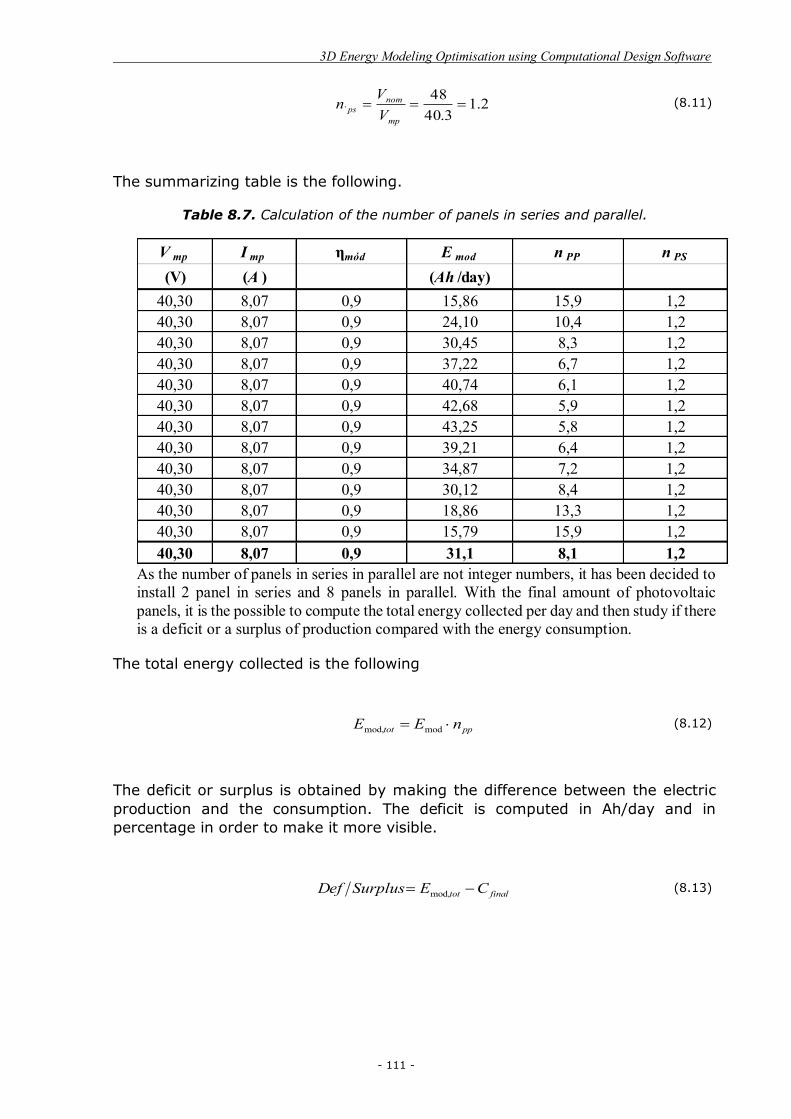
3D Energy Modeling Optimisation using Computational Design Software
- 111 -
2.13.40
48`
mp
nomps V
Vn (8.11)
The summarizing table is the following.
Table 8.7. Calculation of the number of panels in series and parallel.
As the number of panels in series in parallel are not integer numbers, it has been decided to install 2 panel in series and 8 panels in parallel. With the final amount of photovoltaic panels, it is the possible to compute the total energy collected per day and then study if there is a deficit or a surplus of production compared with the energy consumption.
The total energy collected is the following
pptot nEE � modmod, (8.12)
The deficit or surplus is obtained by making the difference between the electric production and the consumption. The deficit is computed in Ah/day and in percentage in order to make it more visible.
finaltot CESurplusDef � mod, (8.13)
V mp I mp ηmód E mod n PP n PS
(V) (A ) (Ah /day)40,30 8,07 0,9 15,86 15,9 1,240,30 8,07 0,9 24,10 10,4 1,240,30 8,07 0,9 30,45 8,3 1,240,30 8,07 0,9 37,22 6,7 1,240,30 8,07 0,9 40,74 6,1 1,240,30 8,07 0,9 42,68 5,9 1,240,30 8,07 0,9 43,25 5,8 1,240,30 8,07 0,9 39,21 6,4 1,240,30 8,07 0,9 34,87 7,2 1,240,30 8,07 0,9 30,12 8,4 1,240,30 8,07 0,9 18,86 13,3 1,240,30 8,07 0,9 15,79 15,9 1,240,30 8,07 0,9 31,1 8,1 1,2

Axel Paul Galpy Massé
- 112 -
Table 8.8. Calculation of the deficit or surplus in electric production of the photovoltaic installation of 16 panels.
In order to decrease the deficit of the installation in the months of winter, it could be possible to oversize it. If instead of 16 panels 18 panels are installed, 9 in parallel and 2 in series the deficit and surplus would be as shown in the following table.
Table 8.9. Calculation of the deficit or surplus in electric production of the photovoltaic installation of 18 panels.
With this new size, the installation would have an average surplus of 5.7kWh/day, so an average surplus of 74%, but with a lower deficit in the months of winter.
So from this study two cases of installation are possible.
E demand E produced Def./Surplus Def./SurplusMonth (Wh/day) (Wh /day) (Wh /day) (%)
January 7.721,98 6091,41 -1630,57 -21%February 7.721,98 9254,16 1532,18 20%
March 7.721,98 11691,90 3969,92 51%April 7.721,98 14290,63 6568,65 85%May 7.721,98 15645,96 7923,99 103%June 7.721,98 16390,18 8668,20 112%July 7.721,98 16607,56 8885,58 115%
August 7.721,98 15054,80 7332,82 95%September 7.721,98 13390,21 5668,23 73%
October 7.721,98 11565,42 3843,44 50%November 7.721,98 7242,05 -479,92 -6%December 7.721,98 6061,87 -1660,10 -21%Average 7.721,98 11.940,51 4.218,54 55%
E demand E produced Def./Surplus Def./SurplusMonth (Wh/day) (Wh /day) (Wh /day) (%)
January 7.721,98 6852,84 -869,14 -11%February 7.721,98 10410,93 2688,95 35%
March 7.721,98 13153,39 5431,41 70%April 7.721,98 16076,96 8354,98 108%May 7.721,98 17601,71 9879,73 128%June 7.721,98 18438,95 10716,97 139%July 7.721,98 18683,50 10961,53 142%
August 7.721,98 16936,65 9214,67 119%September 7.721,98 15063,98 7342,01 95%
October 7.721,98 13011,10 5289,12 68%November 7.721,98 8147,31 425,33 6%December 7.721,98 6819,61 -902,37 -12%Average 7.721,98 13.433,08 5.711,10 74%

3D Energy Modeling Optimisation using Computational Design Software
- 113 -
In the first case, the photovoltaic installation would be composed of 16 panels, but there would be a deficit of between 6% and 21% between November and February, while in the second case the installation would be composed of 18 panels, but the deficit would be reduced to 12% in the month of December and January.
The final photovoltaic installation of both cases would have the following characteristics:
Table 8.10: Photovoltaic installation dimensions of case a)
Table 8.11: Photovoltaic installation dimensions of case b)
x 6- Calculation of the total storage capacity of the batteries and calculation of the number of batteries.
The batteries installation is set to have a nominal voltage 24 V. In order to compute the total capacity that is needed for the batteries of the system the following formula is used, taking into account the days of autonomy and the maximum depth of discharge of the battery.
AhP
DCC
D
outfinalalm 39.895
7.05.271.250
max,
�
�
(8.14)
In order to compute the number of batteries that are needed first of all the characteristics of the chosen batteries have to be studied. The characteristics are as following:
Number of panels 16Number of panels in series 2,0
Number of panels in parallel 8Length of a panel (m) 1,662Width of a panel (m) 1,32
Total length of the installation (m) 3,324Total width of the installation (m) 10,56
Total surface (m2) 35,10
Number of panels 18Number of panels in series 2,0
Number of panels in parallel 9Length of a panel (m) 1,662Width of a panel (m) 1,32
Total length of the installation (m) 3,324Total width of the installation (m) 11,88
Total surface (m2) 39,49

Axel Paul Galpy Massé
- 114 -
Table.8.12. Batteries characteristics25
In order to compute the number of batteries in series and in parallel the following formula have been used.
3.03283
39.895
battery
storagebp C
Cn (8.15)
12224,
battery
instalnombs V
Vn (8.16)
The following table summarizes the computations for each month of the year.
Table 8.13. Calculation of the number of batteries in series and parallel.
ManufacturerModel
Nominal Voltage 2 V
Nominal Capacity
3283 A
Self-discharge 0,05 %
Dimensions
Distributor
Price 760,98 €
UZS3000-2Ultracell
Batteries
576mm/212mm/827mm
TuTiendaEnergética
nPS Cstor Cbat,nom nBP nBS(Ah) (Ah)
1,2 1078,77 3283,00 0,3 12,01,2 1078,77 3283,00 0,3 12,01,2 1078,77 3283,00 0,3 12,01,2 713,44 3283,00 0,2 12,01,2 713,44 3283,00 0,2 12,01,2 713,44 3283,00 0,2 12,01,2 713,44 3283,00 0,2 12,01,2 713,44 3283,00 0,2 12,01,2 713,44 3283,00 0,2 12,01,2 1078,77 3283,00 0,3 12,01,2 1078,77 3283,00 0,3 12,01,2 1078,77 3283,00 0,3 12,01,2 895,39 3283,00 0,3 12,0

3D Energy Modeling Optimisation using Computational Design Software
- 115 -
So, after studying the table, 12 batteries are going to be connected in series and 1 one parallel, with a total of 12 batteries.
x 7- Summarizing table
With all the dates of the installation that have been computed through all the previous steps it is then possible to summarise it all a table, and the result is as following.
The power of the batteries and the panels are given through the formula:
IVP � (8.17)
Table 8.14. Summarise of the installation for case a
Table 8.15. Summarise of the installation for case b
E demand E required in bateries E produced Def./Surplus Def./SurplusMonth (Wh/day) (Wh /day) (Wh /day) (Wh /day) (%)
January 7.721,98 12082,26 6091,41 -1630,57 -21%February 7.721,98 12082,26 9254,16 1532,18 20%March 7.721,98 12082,26 11691,90 3969,92 51%April 7.721,98 11985,81 14290,63 6568,65 85%May 7.721,98 11985,81 15645,96 7923,99 103%June 7.721,98 11985,81 16390,18 8668,20 112%July 7.721,98 11985,81 16607,56 8885,58 115%
August 7.721,98 11985,81 15054,80 7332,82 95%September 7.721,98 11985,81 13390,21 5668,23 73%
October 7.721,98 12082,26 11565,42 3843,44 50%November 7.721,98 12082,26 7242,05 -479,92 -6%December 7.721,98 12082,26 6061,87 -1660,10 -21%Average 7.721,98 12.034,04 11.940,51 4.218,54 55%
E demand E required in bateries E produced Def./Surplus Def./SurplusMonth (Wh/day) (Wh /day) (Wh /day) (Wh /day) (%)
January 7.721,98 12082,26 6852,84 -869,14 -11%February 7.721,98 12082,26 10410,93 2688,95 35%March 7.721,98 12082,26 13153,39 5431,41 70%April 7.721,98 11985,81 16076,96 8354,98 108%May 7.721,98 11985,81 17601,71 9879,73 128%June 7.721,98 11985,81 18438,95 10716,97 139%July 7.721,98 11985,81 18683,50 10961,53 142%
August 7.721,98 11985,81 16936,65 9214,67 119%September 7.721,98 11985,81 15063,98 7342,01 95%
October 7.721,98 12082,26 13011,10 5289,12 68%November 7.721,98 12082,26 8147,31 425,33 6%December 7.721,98 12082,26 6819,61 -902,37 -12%Average 7.721,98 12.034,04 13.433,08 5.711,10 74%


- 117 -
Table 8.14. Summarise table of the photovoltaic installation for case a)
January February March April May June July August September October November December
Photovoltaic Voltage (V) 48 48 48 48 48 48 48 48 48 48 48 48
Batteries Voltage 24 24 24 24 24 24 24 24 24 24 24 24
Total consumption (Wh/day) 7721,98 7721,98 7721,98 7721,98 7721,98 7721,98 7721,98 7721,98 7721,98 7721,98 7721,98 7721,98
Consumption without losses (Ah/day) 321,75 321,75 321,75 321,75 321,75 321,75 321,75 321,75 321,75 321,75 321,75 321,75
Consumption with losses (Ah/day) 503,43 503,43 503,43 503,43 503,43 503,43 503,43 503,43 503,43 503,43 503,43 503,43
Rad. H (KJ/m2) 6196 10006 13606 18170 21272 22734 22358 18966 15196 11764 6906 5862
HSP (30°) 2,18 3,32 4,19 5,12 5,61 5,88 5,95 5,40 4,80 4,15 2,60 2,17
Imp of the panel (A) 8,07 8,07 8,07 8,07 8,07 8,07 8,07 8,07 8,07 8,07 8,07 8,07
Ah/panel.day 15,86 24,10 30,45 37,22 40,74 42,68 43,25 39,21 34,87 30,12 18,86 15,79
Number of panels in parallel 15,9 10,4 8,3 6,8 6,2 5,9 5,8 6,4 7,2 8,4 13,3 15,9
Total number of panels installed in parallel 8 8 8 8 8 8 8 8 8 8 8 8
Total number of installed panels 16 16 16 16 16 16 16 16 16 16 16 16
Energy produced (Wh/day) 6091,4 9254,2 11691,9 14290,6 15646,0 16390,2 16607,6 15054,8 13390,2 11565,4 7242,1 6061,9
Deficit or surplus (kWh/day) -1,63 1,53 3,97 6,57 7,92 8,67 8,89 7,33 5,67 3,84 -0,48 -1,66
Deficit or surplus (%) -21% 20% 51% 85% 103% 112% 115% 95% 73% 50% -6% -21%
Days of autonomy 4 4 4 4 3 3 3 3 4 4 4 4
PD max 70% 70% 70% 70% 70% 70% 70% 70% 70% 70% 70% 70%
Capacity of the batteries (Ah) 3283 3283 3283 3283 3283 3283 3283 3283 3283 3283 3283 3283
Nuber of batteries in parallel 1 1 1 1 1 1 1 1 1 1 1 1
Total number of batteries 12 12 12 12 12 12 12 12 12 12 12 12

Axel Paul Galpy Massé
- 118 -
Table 8.14. Summarise table of the photovoltaic installation for case b)
January February March April May June July August September October November December
Photovoltaic Voltage (V) 48 48 48 48 48 48 48 48 48 48 48 48
Batteries Voltage 24 24 24 24 24 24 24 24 24 24 24 24
Total consumption (Wh/day) 7721,98 7721,98 7721,98 7721,98 7721,98 7721,98 7721,98 7721,98 7721,98 7721,98 7721,98 7721,98
Consumption without losses (Ah/day) 321,75 321,75 321,75 321,75 321,75 321,75 321,75 321,75 321,75 321,75 321,75 321,75
Consumption with losses (Ah/day) 503,43 503,43 503,43 503,43 503,43 503,43 503,43 503,43 503,43 503,43 503,43 503,43
Rad. H (KJ/m2) 6196 10006 13606 18170 21272 22734 22358 18966 15196 11764 6906 5862
HSP (30°) 2,18 3,32 4,19 5,12 5,61 5,88 5,95 5,40 4,80 4,15 2,60 2,17
Imp of the panel (A) 8,07 8,07 8,07 8,07 8,07 8,07 8,07 8,07 8,07 8,07 8,07 8,07
Ah/panel.day 15,86 24,10 30,45 37,22 40,74 42,68 43,25 39,21 34,87 30,12 18,86 15,79
Number of panels in parallel 15,9 10,4 8,3 6,8 6,2 5,9 5,8 6,4 7,2 8,4 13,3 15,9
Total number of panels installed in parallel 9 9 9 9 9 9 9 9 9 9 9 9
Total number of installed panels 18 18 18 18 18 18 18 18 18 18 18 18
Energy produced (Wh/day) 6852,8 10410,9 13153,4 16077,0 17601,7 18439,0 18683,5 16936,6 15064,0 13011,1 8147,3 6819,6
Deficit or surplus (kWh/day) -0,87 2,69 5,43 8,35 9,88 10,72 10,96 9,21 7,34 5,29 0,43 -0,90
Deficit or surplus (%) -11% 35% 70% 108% 128% 139% 142% 119% 95% 68% 6% -12%
Days of autonomy 4 4 4 4 3 3 3 3 4 4 4 4
PD max 70% 70% 70% 70% 70% 70% 70% 70% 70% 70% 70% 70%
Capacity of the batteries (Ah) 3283 3283 3283 3283 3283 3283 3283 3283 3283 3283 3283 3283
Nuber of batteries in parallel 1 1 1 1 1 1 1 1 1 1 1 1
Total number of batteries 12 12 12 12 12 12 12 12 12 12 12 12

- 119 -
x 8- Dimensions of the regulator
The regulator controls de charge process of the storage system, composed by the batteries from the photovoltaic installation, and the discharge process from the batteries to the load. The characteristics that define a regulator also called converter DC/DC are the output nominal voltage in DC, the nominal entering current to the regulator from the generator, the output nominal current to the load and the efficiency.
All the data needed for the measuring of the regulator are in the following tables.
The maximum incoming current that can be supported at the entrance of the regulator from the photovoltaic installation is given by:
mpppG InI � (8.18)
However, for reasons of security this value is incremented about 20%, so the final current would be:
AInI mpppG 16.8707.892.12.1 �� �� (8.19)
The total current consumption of the load has also to be taken into account. The way to compute it is the following. Knowing that
ACDCtotal PPP � (8.20)
Then
AVP
VP
Inom
DC
nominv
ACL 1.155
246.733
2493.02900
��
��
K
(8.21)
The regulator has to be able to support the maximum between the two previous currents, in this case the IG.
^ `LGreg III ,max (8.22)

Axel Paul Galpy Massé
- 120 -
Table.8.15. Summarize of necessary characteristics of the regulator
So,
AI reg 7.51 (8.23)
The chosen regulator for its characteristics is the following:
Table 8.16. Characteristics of the regulator26
x 9- Dimensions of the AC/DC inverter
The AC/DC inverters allows to convert de DC current coming from the regulator to a AC current in order to supply the loads. In order to set the dimensions of the inverter, the working power needed has to be computed.
WP
Pinv
ACinv 28.3118
93.02900
K
(8.24)
Table.8.17. Inverter Power characteristics.
Number of lines Num modules in parallel per line
Pmp 325 WVmp 40,3 Vηmód 0,9
Imp 8,07 AIGG per line 29,05 A
3
3 W PDC 733,6 WV PAC 2 900,0 W
Ptot 3 633,6 WA ηinv 0,97 A IL 155,1 A
Number of lines 3,0 IL per line 51,7 A
Ireg 51,7 A
3
ManufacturerModel
Entrance Voltage 48 VEntrance current 60 A
Exit Voltage 24 VEfficiency 90 %
Price 201 €Distibutor Amazone
Regulator 48Vdc/24VdcMorningStar
TrisTar
2 900 W0,93
12 900,00 W
3 118,28 WPAC per line
Number of lines
Inverter power
Inverter PowerPACηinv

3D Energy Modeling Optimisation using Computational Design Software
- 121 -
With this need in power, the inverter chosen for the installation is the following.
Table.8.18. AC/DC Inverter characteristics27
8.2.3. Dimensions of the wire installation.
In the first place the different currents of the house have to be computed with the voltage, the power.
VPI (8.25)
The wire installation is as following:
Fig.8.18. Wire installation
ManufacturerModel
Nominal Input Voltage 24 VDCNominal Output Voltage 230 VAC
Frequency 50 HzEfficiency 93 %
Nominal Power 3200 WPrice 1837 €
Distributor
AC/DC Inverter Apollo Solar
TSW3224
GreenEnergy

Axel Paul Galpy Massé
- 122 -
Table.8.19. Electric wiring information.
In all the following calculations, the current has been oversized about 20% for security reasons.
The current that goes from the photovoltaic panels to the regulator is, as computed previously:
AInI mplineppregpanels 05.2907.832.12.1 , �� � � (8.26)
The current that goes from the regulator to the batteries is, the same that the one that goes from the panels to the regulator.
AII regpanelsbattreg 05.29 �� (8.27)
The current that goes from the regulator to the invertor is computed using the number of lines that have been installed.
AVP
VP
Inom
DC
nominv
AClineL 7.51
31
246.733
2493.02900
31
, �¸¹·
¨©§ �
� �¸̧
¹
·¨̈©
§�
�
K (8.28)
The current in the DC line is follows this formula:
AVP
Inom
DCDC 7.36
246.733
2.12.1 � � (8.29)
While the current in the AC line is follows this formula:
CocinaDC/AC L V Power need (W) I (A)
DC 14 24 135,6 5,65AC 11 230 70 0,30DC 17 24 135,6 5,65AC 17 230 70 0,30DC 25 24 102 4,25AC 20 230 70 0,30
Living room/kitchen DC 15 24 306 12,75AC kitchen 8 230 2590 11,26
AC general use 15 230 100 0,43DC 15 24 54,4 2,27
AC general use 15 230 100 0,43
Room 3
Living room/kitchen
Bathroom
Circuits
Room 1
Room 2

3D Energy Modeling Optimisation using Computational Design Software
- 123 -
AV
PI
nominv
ACAC 13.15
23093.02900
�
�
K
(8.30)
The current that goes from the regulator to the AC/DC inverter is
AnumV
PI
linesnominv
ACinvreg 83.49
32493.02900
2.12.1 ��
� ��
� � K (8.31)
Now that the different currents are know, it is possible to compute the diameter of the different wires using the following formula.
U
ILS �� 0359.0 (8.32)
Where:
x L: length of the cable (m) x I: current of the line x U: maximum admissible voltage drop (V)
The maximum admissible voltage drop for each line used in this project are the ones recommended by CENSOLAR and are the followings.
Table 8.20. Tensions wires between the electronic devices of the photovoltaic installation
So the final sections of the wires of each line are presented in the following summarizing table.
CircuitNominal
Tens ion (V)
Admis s ible voltage drop
(%)Admis s ible
vo ltage drop (V)12 5 0,624 8 1,9248 10 4,812 0,5 0,0624 0,5 0,1248 1,5 0,7212 0,5 0,0624 1 0,2448 2 0,96
Light x 3 3x/100Loads x 5 5x/100
Panel-regulator
Regulator- batteries
Batteries - inverter

Axel Paul Galpy Massé
- 124 -
Table 8.21. Sections of the wires of the photovoltaic installation
8.3. Demand and dimensions of the DHW installation.
8.3.1. Dimensions of the installation of thermo solar collectors.
As an average, the Domestic Hot Water consumption is of 30 liters per day. This consumption has been reduced by 10% in the hot months of the year, which would be from May to September, as in this moment, the use of hot water is reduced. However, as the installation is done in order to be able to supply the DHW in the worst cases, which would be in winter, this reduction does not affect the final result. In this house, it has been said to be a family composed by four members, so the final consumption is DHW would be.
daylpersondaylpeopleDHW nconsumptioTot 120304,
�� (8.33)
It is established that the temperature of the DHW has to be of 60°C for sanitary reasons as the absence of microorganisms, and knowing the different temperature values of the water of the grid each month it is then possible to know the monthly demand of energy for heating the water. The formula used for this computation is the following.
)(00116.0 CWDHWdays TTQnumD ���� (8.34)
Where
x D: Demand (kWh) x Q: Volumetric flow rate (liters/day) x TDHW: Temperature of the Domestic Hot Water x TCW: Temperature of the cold water
Lines V nom (AC or DC)
∆V (%) U (V) Line lenght (m)
Current I (A)
Securrity current
(A)
Resulting section (mm2)
Normalized section (mm2)
Maximum admissible
current Iz (A)1.45 Iz (A)
Panels-Regulator 48 10 4,8 10 29,05 34,86 2,61 4 53,4 77,4Regulator-Batteries 24 0,5 0,12 5 29,05 34,86 52,25 70 46,7 67,7Regulador-Inversor 24 1 0,24 2 49,83 59,79 17,92 25 83,4 120,9
Regulator- Electrical Panel 24 3 0,72 3 30,57 36,68 5,50 6 40,0 58,0DC Room 1 and Room 2 24 3 0,72 17 11,30 13,56 11,52 16 18,8 27,3DC Living room/kitchen 24 3 0,72 15 12,75 15,30 11,47 16 21,4 31,0
DC Bathroom and Room 3 24 3 0,72 25 6,52 7,82 9,77 10 8,0 11,6Inverter-Electrical Panel 230 5 11,5 3 13,04 15,65 0,15 1 106,6 154,5AC Room 1 and Room 2 230 5 11,5 11 0,61 0,73 0,03 1 29,1 42,1AC Living room/kitchen 230 5 11,5 15 0,43 0,52 0,02 1 21,3 30,9
AC Bathroom and Room 3 230 5 11,5 20 0,74 0,89 0,06 1 16,0 23,2Kitchen loads 230 5 11,5 8 11,26 13,51 0,34 1 40,0 57,9

3D Energy Modeling Optimisation using Computational Design Software
- 125 -
Table 8.22. Demand in DHW
From the previous table it is possible to establish that the annual electric demand for the DHW is of 3913.7kWh.
However the heating energy of the house has been wanted to be provided with the thermo solar collectors, so the energy demand in heating should be added to the DHW demand.
The average heating energy demand is of 0,044142kWh, so.
yearkWhyear
daysday
hkWhndAnnualdema /68.38636524
044142.0 �� (8.35)
The total demand is then shown in the following table.
Table.8.23. Total DHW demand
The heating energy consumption is concentrated in the winter months, from October to march, when the exterior temperatures are at their minimum, so in this case, the inclination of the thermo solar collectors will be chosen in order to get the maximum possible radiation during those months. The factor that permits to establish which would be the optimum inclination is the k factor, which was, as a reminder, the quotient between the total incident energy of a surface oriented to
N Q TDHW TCW DMonth (days) (liters/day) (ºC) (ºC) (kWh)January 31 120 60 8 224,4February 28 120 60 9 198,8March 31 120 60 11 211,4April 30 120 60 13 196,3May 31 108 60 14 178,6June 30 108 60 15 169,1July 31 108 60 16 170,9
August 31 108 60 15 174,8September 30 120 60 14 192,1
October 31 120 60 13 202,8November 30 120 60 11 204,6December 31 120 60 8 224,4
Total annual 365,0 1.392 60,0 12,3 2.348,2
Demand (kWh/year)DHW 2.348,2
Heating Energy 386,68Total 2.734,92

Axel Paul Galpy Massé
- 126 -
the equator and with a certain angle of inclination and a horizontal surface. The different k factor values for this latitude are the following.
Table 8.24. K factor values depending on the inclination
The irradiation that is collected by the thermo solar collector is the following.
kHE �� 94.0 (8.36)
Where:
x E: Energy collected for the inclination of 30°(MJ/m2day) x H: Energy received for an horizontal plane x K: inclination factor
Table 8.25. Energy collected by the collector
Inclination (°) 35 40 45 50 55
January 1,38 1,4 1,42 1,42 1,42
February 1,29 1,3 1,3 1,3 1,28
March 1,18 1,18 1,6 1,14 1,12
April 1,07 1,05 1,03 0,99 0,95
May 0,99 0,96 0,93 0,88 0,83
June 0,96 0,93 0,89 0,84 0,79
July 0,99 0,96 0,93 0,88 0,84
August 1,08 1,06 1,04 1,01 0,97
September 1,22 1,22 1,21 1,19 1,17
October 1,38 1,41 1,41 1,41 1,41
November 1,49 1,52 1,55 1,56 1,57
December 1,47 1,5 1,52 1,54 1,54
angulo 30 °H k E E
(MJ/(m2·day) 45 (MJ/(m2·day)) (MJ/(m2·month))
6,196 1,42 8,27 256,38
10,006 1,30 12,23 342,37
13,606 1,60 20,46 634,37
18,17 1,03 17,59 527,77
21,272 0,93 18,60 576,48
22,734 0,89 19,02 570,58
22,358 0,93 19,55 605,91
18,966 1,04 18,54 574,78
15,196 1,21 17,28 518,52
11,764 1,41 15,59 483,35
6,906 1,55 10,06 301,86
5,862 1,52 8,38 259,64
14,4 15,46 5 651,99

3D Energy Modeling Optimisation using Computational Design Software
- 127 -
The collectors that have been chosen to be used are from Wolf and the model is CRK-12. The characteristics of those collectors are the following.
Table 8.26. Collectors’ technical datasheet28
From the received irradiation and the characteristics of the collectors, it is possible to compute the total efficiency of the installation
� �
ITTb
ITTa CWDHWCWDHW
2
0)( �
���
�� KK (8.37)
Where:
x n: Efficiency x a: Collector coefficient a x b: Collector coefficient b x THSW: Temperature of the HSW (°C) x Tamb: Ambient temperature (°C) x I: Radiation (W/m2)
The result of this computation for each month is as following:
ManufacturerModel
Inclination angle of installation 15-90 degresEfficiency 64,2 %
Coeficient a 0,885 W/(m2K)Coeficient b 0,001 W/(m2K)
Weight 37,6 KgDimensions
Price 2226 €Distributor Wolf Ibérica
1390mm/1640mm/100mm
Void tube collector
CRK-12Wolf

Axel Paul Galpy Massé
- 128 -
Table 8.27. Efficiency of the installation
With this results it is then possible to compute the usable energy for each square meter.
K� EEusable (8.38)
Table 8.28. Usable energy collected per m2
h I Tm Tamb η(SH) (W/m2) (ºC) (ºC) (%)4,81 477,97 60 9,40 54,3%5,82 583,44 60 9,90 56,2%6,45 881,06 60 12,30 59,2%7,33 666,37 60 14,60 57,9%7,87 656,28 60 17,70 58,2%8,73 604,94 60 21,60 58,3%10,00 542,93 60 24,40 58,2%9,10 566,17 60 24,20 58,4%7,30 657,68 60 21,70 58,8%5,81 745,91 60 17,50 58,9%4,87 574,32 60 13,50 56,7%4,45 522,63 60 10,20 55,3%
623,31 60,0 16,4 57,5%
E N E η Usable Energy Usable EnergyMonth (MJ/(m2·day) (days) (MJ/(m2·month) (%) (MJ/m2) (kWh/m2)January 8,27 31 256,38 54,3% 125,28 34,80February 12,23 28 342,37 56,2% 173,08 48,08March 20,46 31 634,37 59,2% 337,71 93,81April 17,59 30 527,77 57,9% 274,83 76,34May 18,60 31 576,48 58,2% 302,08 83,91June 19,02 30 570,58 58,3% 299,58 83,22July 19,55 31 605,91 58,2% 317,18 88,10
August 18,54 31 574,78 58,4% 301,99 83,89September 17,28 30 518,52 58,8% 274,51 76,25
October 15,59 31 483,35 58,9% 256,29 71,19November 10,06 30 301,86 56,7% 153,93 42,76December 8,38 31 259,64 55,3% 129,21 35,89
Total annual 185,57 365,0 5.651,99 57,5% 2945,66 818,24

3D Energy Modeling Optimisation using Computational Design Software
- 129 -
From the collectors and the power needed for the year it is possible to compute the surface needed in order to be able to produce the energy that is consumed. The energy consumed is
yearkWhDEconsumed /92.2734 (8.39)
The Energy collected per year and square meter is the following:
yearmkWhENU � ��� ��� 238.81146.15365575.025.025.0 K (8.40)
Where:
x η: efficiency of the system (%) x N: number of days per year x E: energy collected for the inclination
And the total surface of collection is given by the following formula, in which U and P have just been computed.
237.319.76792.2734 m
PUS (8.18)
The results have been summarised in the following table.
Table 8.29. Summary table
From the characteristics of each collector it is known that each one has a surface of 3.37m2, so it has been decided to install two collectors in order to be able to supply all the needs in DHW and heating. The final installation would have the following characteristics.
fm Demand Energy produced Sa b (%) (kWh/year) (kWh/(m2·year)) (m2)
0,885 0,001 57,5% 2.734,92 811,70 3,37
Collector parameters

Axel Paul Galpy Massé
- 130 -
Table 8.30. Dimensions of the installation
So the installation would have two collectors and the final dimensions would be of 2.78m per 1.64m, so total a surface of 4.56m2.
With the resulting installation, the deficit or surplus in energy can be computed.
Table 8.31. Deficit or surplus study
The annual surplus is of 1727kWh, however in the months of January and December, as for the photovoltaic installation, there is a deficit of 65.7kWh and 45kWh respectively, a deficit that is going to be compensated with the electrical grid.
Surface per collector (m2) 2,28Total surface of collectors 3,37Num collectors 1,4778Num tot 2Num collector in parallel 1Num colector in series 2Final surface of collectors 4,56Total length (m) 2,78Total width(m) 1,64
Energy produced Demand Def/SurplusMonth (kWh) (kWh) (kWh)
January 158,69 224,4 -65,70February 240,38 198,8 41,61
March 469,04 211,4 257,59April 381,71 196,3 185,44May 419,55 178,6 240,90June 416,08 169,1 246,96July 440,52 170,9 269,64
August 419,43 174,8 244,66September 381,26 192,1 189,16
October 355,96 202,8 153,15November 213,79 204,6 9,16December 179,46 224,4 -44,94
Total annual 4.075,88 2.348,2 1727,64

- 131 -
CHAPTER 9:
ENERGY PRODUCTION
LEGISLATION
In this chapter the Spanish legislation related to the generation and the energy self-consumption.
9.1. Definition of Net Metering and Self-Consumption.
As a reaction to the traditional centralized generation of electricity in big centrals and with the transport of electricity from theses centrals to the consumers, which are usually far from the site of generation, there is a new organization with smaller centrals but closer to the final consumer. The self-consumption is one of these organisations, in which the consumer produces a part or even the totality of the electric energy that he consumes.
The Net Metering is defined as the system that allows the residential costumer with an electric generator as for example solar panels or windmills to add to the grid his excessive generated electricity that he won’t use. In this case, the electricity would run backwards to provide a credit that would compensate the electricity that would be consumed at night or in some other periods from the grid where the generation of electricity does no cover the electricity demand.
9.2. Legal application The Law 24/2013 of December, of the Electrical Sector of Spain29, in its article 9 Title 1 regulates the self-consumption of the electrical energy. The self-consumption is defined as “the consumption of electricity energy issued in

Axel Paul Galpy Massé
- 132 -
generation facilities connected inside a consumer network o via a direct electricity line associated to a consumer “. From this definition different modalities of self-consumption are set-up. The first one is that the provision with self-consumption is defined as a non-registered production facility and where there is only the subject of consumption. The second one is the one that production with self-consumption involves all the facilities registered as facilities of production and where the subject is consumer and producer. This modality can sell the surplus into the market. There is also the modality of production and self-consumption of a consumer connected through a direct line and with a production facility as the precedent with connection to a production facility.
In the section 3) of the article 9 of the same document the costs of this activity are defined as that “all the consumers subjected to any form/modality of self-consumption will be obliged to contribute to the costs and services of the system for the consummated energy when the generator facility or consumption one is totally or partially connected to the electric system. They will be obliged to pay the same toll of access to the grids, the burdens associated to the costs of the system and costs of the provision of services of support of the system that would correspond to a consumer or one subject non subject to any of the modalities of self-consumption described in the precedent section”.
To be able to practice any of these modalities of this activity of self-consumption the subject has to be inscribed first in the administrative registration of self-consumption of the electric energy created by the Ministry of Industry, Energy and Tourism.
In the title X of this same document, the article 61 of the chapter 1 describes the “faculties of inspection”. In such a way that the public civil servants of the Ministry of Industry, Energy and Tourism will be able to realize, as long as they are authorised by the respective General Director, any necessary inspection to control the implementation of the law. They will be able, like this, to access to any local, facility, piece of land and mean of transport of the enterprises, associations of enterprises and physical persons that do any activity foreseen in this law, as well as to the private addresses of the contractors, the administrators and other members of the staff of the enterprises.
At a juridical level, according to the article 64 of this same chapter, it is considered as a critical fault the non-observance of the obligation of registration as well as the implementation of the modalities or of the economical regimes non contemplated on purpose in this law and its regulation of development, as well as the non-observance of some of the technical requirements of implementation to the different forms/modalities of self-consumption when there are perturbations affecting the quality of provision of the field of the grid where they are connected. “Those non-observances are penalized with a fine between 6.000.001 and 60.000.000 euros in accordance with the article 67, but the amount of the sanction cannot overpass the 10 per cent of the net or annual amount of the business amount of the offender subject. In terms of self-consumption it is considered as a critical/grave fault the no observance of the requirements and obligations stablished, while they are not typified as grave, as well as the incorrect

3D Energy Modeling Optimisation using Computational Design Software
- 133 -
implementation of these forms/modalities and their economical associated regimes. In those cases, the sanctions are around 600.000 and 6.000.000 euros.
On the 28th of February 2014 a proposition of the Law of self-consumption of energy is set up in the Assembly of deputes. It is stipulated that with the precedent law of the electric sector, there is not any possibility to develop the self-generation of energy in the economical field as well as in the administrative one as it is shown in the established system of sanction. In relation with the precedent proposition this one modifies the law 24/2013 in the sense that the self-generation is defined as an “individual production of electricity from sources of renewable energy for the proper consumption. This practice can be realised by home consumers, in an individual or collective way, public centres and small enterprises”. In the section 2 of this article the self-generation of energy in net metering to the system of instantly or differed compensation is defined, to permit the consumers to get the individual energy facility for its self-consumption, juggling the curve of production whit the one of the demand. In that way the consumer will be able to cede the surplus of energy to the electrical net with some rights of consumption differed in 12 months of validity. The electric company that will provide the electricity, when the demand will be superior to the production of the system of self-consumption, will discount in the bill of consumption of the net, the excess appearing in it and the tariff of the consumer for the necessary energy will be the same as it didn’t count with the self-consumption in net metering rights of consumption differed no included, that means that it will not be any kind of toll or economical regime associated to the covering of the costs, charges and services for the energy consumed in an instantaneous way . In this proposition of law, the section 35 of the article 65 is re-written in a way that “the implementation of modalities or of economical regimes that are not taken in account on purpose in this law and in its regulations of development, as well as the non-observance of some of the technical requirements of implementation to the different modalities of self-consumption when some perturbations take place that affect the quality of supply in the field of the net to what they are connected” is considered a grave infraction.


- 135 -
CHAPTER 10:
ENERGY PERFORMANCE
OF BUILDINGS
10.1. Efficiency certificate legislation “When buildings or units of them are built, sold or rented, the certificate of energy efficiency or a copy of it has to be shown to the potential buyer or new renter, and has to be delivered to the potential buyer or new renter following the terms established in the basic procedure.” This extract30 is from the law of the Electrical Sector of Spain, the 235/2013 from the 5th of April 2013 in which the basic procedure for the certification of the energetic efficiency of the building is approved. In this same document, in the article 1, the energetic efficiency of a building is defined as “the energy consumption, computed or measured, that is estimated to be necessary to satisfy the energetic demand of the building in normal operating and occupation conditions, that will include, among others, the energy consumed in heating, cooling, ventilation, the production of hot sanitary water and lightning.”
The Ministry of Industry, Energy and Tourism of Spain has also published the methodology for calculate the energetic efficiency qualification. From this publication, “the principal energetic indicator for this qualification is the annual CO2 emissions, expressed in Kg per m2 of usable surface of the building, and the complementary indicators, by priority order are the following:
x Not renewable annual primary energy, in kWh per m2 of usable surface of the building.
x Total annual primary energy, in kWh per m2 of usable surface of the building.
x Percentage of the primary energy coming from renewable energy source with respect to the total annual primary energy.

Axel Paul Galpy Massé
- 136 -
x Annual primary energy coming from renewable sources, in kWh per m2 of usable surface of the building.
x Total annual primary energy desegregated by heating, cooling, hot sanitary water production and lightning, in kWh per m2 of usable surface of the building.
x Annual heating energy demand, in kWh per m2 of usable surface of the building.
x Annual cooling energy demand, in kWh per m2 of usable surface of the building.
x Annual CO2 emissions, expressed in kg per m2 of usable surface of the building, desegregated by heating, cooling, hot sanitary water production and lightning, in kWh per m2 of usable surface of the building
10.2. Energy performance study Knowing the existence of this certificate, it has been decided to do the efficiency study of the building of the project in order to see the result. The software used for this study is the CE3X31, developed by Efinovatic and the Spanish National Renewable Energies Center (CENER). This software is the one used for the official documents for the energetic certification of actual buildings.
The process of realizing the study of the building is the following.
10.2.1. General Data
In first place the general data of the house has to be entered, like the type of building, where the house is located, the year of construction and the current law in efficiency. Once this general information is set, it is then necessary to define the building, with the usable surface, the number of floors, the diary demand in hot sanitary water.
Fig. 10. General information
10.2.2. Building definition.
In this part, the building itself is defined. All the surfaces are set, their surface type, their orientation, their dimensions, the thermic properties. All the

3D Energy Modeling Optimisation using Computational Design Software
- 137 -
characteristics of each surface type are set as for the resulting house, with the U-values of each material.
Fig. 10.2.General construction surfaces
Fig. 10.3. Wall characteristics

Axel Paul Galpy Massé
- 138 -
Fig. 10.3. Window characteristics
Fig. 10.4. Roof characteristics
10.2.3. Installations
In this chapter the consumption in electric, heating and cooling energy as for the hot sanitary water consumption are entered into the program.
As presented in the apart 8.2.2, there are two cases for the renewable energy installation.
Table 10.1. Summarise of cases a) and b)
In the case a, the installation and the energy consumption are the following
Number of panels Energy produced (kWh/year) Energy Consumed (kWh/year)Case a 16 4372 2.818,5 Case b 18 4918 2.818,5

3D Energy Modeling Optimisation using Computational Design Software
- 139 -
Fig. 10.5. Energy consumption in case a)
Fig. 10.6. Energy consumption in case b)
Once the consumption is set, it is possible to determine where the energy comes from. In this case, the renewable installations characteristics are set in the program, with the percentage of demand coverage.

Axel Paul Galpy Massé
- 140 -
Fig. 10.7. Installation characteristics
10.2.4. Results
When all the previous steps are done, it is possible to launch the program in order to compute the energetic efficiency. For both cases, the change in energy production is so small that in is negligible in the final result which is as following:
Fig 10.8. Performance results for case a) and b)

3D Energy Modeling Optimisation using Computational Design Software
- 141 -
In this project, the consumption of energy provided by no renewable energy is non-existent because all the energy consumption of the house is entirely provided by the photovoltaic and the thermo solar installation. This implies that the consumption of non-renewable energy is of 0kWh/m2year, which corresponds to the category A. For the Carbone dioxide emission, in this study, it’s the one released by the consumption of primary energy that is taken into account, but as there is no consumption, there is no CO2 emissions neither, which implies that the building is also in the Category A for the CO2 emissions. From this study it has been possible to realize that the house has an energy efficiency of category A.
However, in this study the emissions of CO2 during the construction of the photovoltaic panels, the batteries and the electronic devices are not taken into account, and if it was, the final result might not be that good, as their construction is very pollutant, especially the batteries. Also it has to be taken into account that the study is done with the annual values, where the annual production is bigger than the demand. However, if the study is done month by month, in winter the production is smaller than the production, however, the resulting CO2 is so small that the efficiency of the house is still in the category A.

- 143 -
CHAPTER 11:
GANTT CHART
In this chapter the Gantt Chart is going to be presented in order to be able to see how this project has been realised, the different steps and the order of them.
The project has been divided in the following steps.
x Software research In this step the objective, knowing that the aim of the project h is to realise energetic simulations in a house, in order to find the optimum architecture characteristics for the reduction in energy consumption, is to find of a computational design software that allows to realise parametrical energy simulations.
x Learn the different tools of Grasshopper Once the software has been chosen, Grasshopper, all its components and its plugins have been studied in order to see their utility for the field of the study, and for understanding the way they work and so, how the program architecture looks like.
x Information research about energy in the residential construction and sector. In this step, information has been search in order to realise the different problems in the residential sector about energy consumption and how to solve them.
x Energy simulation in a room In order to learn how the software works some essays have been done with a random room, this way it was possible to study how the software works and its operational design.
x Architecture of the algorithm for the building simulation The architecture of the program has been set, with all the different steps in which the characteristics can be modified, so the surface, the glaze ratio, the loads and the schedules.

Axel Paul Galpy Massé
- 144 -
x Hypothesis for Room 1 Once the characteristics of Room 1 have been entered in the program, all the hypothesis have been studied. From the results, the optimisation has been realised.
x Hypothesis for Room 2 Once the characteristics of Room 2 have been entered in the program, all the hypothesis have been studied. From the results, the optimisation has been realised.
x Hypothesis for Room 3 Once the characteristics of Room 3 have been entered in the program, all the hypothesis have been studied. From the results, the optimisation has been realised.
x Hypothesis for Living Room Once the characteristics of the living room and the kitchen have been entered in the program, all the hypothesis have been studied. From the results, the optimisation has been realised.
x Hypothesis for Bathroom Once the characteristics of the bathroom have been entered in the program, all the hypothesis have been studied. From the results, the optimisation has been realised.
x Energy simulation for the house In this step the simulation has been realised for the whole house, so the program is set for all the rooms together, at their respective place. In a first time a simulation has been realised for a given window ratio, and then for the optimal glaze ratio.
x Materials simulations The previous simulation has been realised with different construction materials, for the walls, the windows and the roof.
x Laws research The laws in the electric sector of Spain have been studied in order to realise the house in within the legislation.
x Thermo solar installation The study of a thermo solar installation for the Hot Sanitary Water and for the heating of the house has been realised.
x Photovoltaic installation The study of a photovoltaic installation for the electricity consumption has been realised.
x Construction cost The costs of the different materials have been studied with the actual prices of the different components found in the market.

3D Energy Modeling Optimisation using Computational Design Software
- 145 -
x Renewable installation cost The costs linked to the renewable installation are studied with the prices found for the components in the market.
x Final cost The final cost study has been realised in order to see the global viability of the project
x Report In this final step the report has been done in order to present the results of all the different previous steps.
Before finishing the project, the global timetable for its realization was the following. From February to March the research of the software and general information had to be done. The Month of March would be dedicated to learning al the different aspects of the software, in order to be able to realize the different simulations. The month of April would be dedicated to realize all the simulations, in order to have all the results, and the month of May, it was theoretically dedicated to realizing the report with all the observations and results obtained during the previous month. However this timetable was not accurate as the simulations were too long, they needed more time than expected. In order to circumvent this setback, the results from the previous simulation were put in the report while the current simulation was done, in this way the report has been written on the go.
The construction costs have also taken more time than scheduled as the materials of the software are not specified, so similar materials have been to be searched in the marked, with the same characteristics, which for some of the materials it wasn’t easy as the specification are very precise.
Each step has a duration and have different predecessor steps. The resulting Gantt Chart is as presented in the next figures.

- 146 -
Fig. 11.1. Gantt Chart from February to 20th of March 2016

3D Energy Modeling Optimisation using Computational Design Software
- 147 -
Fig. 11.2. Gantt Chart from the 21st of March to the 15th of April 2016

Axel Paul Galpy Massé
- 148 -
Fig. 11.3. Gantt Chart from the 15th of April to the 6th of June 2016

- 149 -
CHAPTER 12:
FUTURE PROJECTS
Through this project some software and their different functions, capacities and characteristics have been studied. Thanks to this study, it has been possible to evaluate the advantages and the disadvantages of the different algorithms, the different ways of structuring the program and the use of each software.
It has to be taken into account that all the software have been running on a basic portable computer, so the problems that have been encountered in this project in terms of the duration of the simulations calculations might not exist or at least might be less important using more powerful computers.
First of all, in the simulations, only the total thermal energy and the light energy consumption have been studied. It is also possible to study the gain by infiltration, the solar gain, the gain due to the presence of people, the room temperature, and some other characteristics, but they have not been studied as their weight is negligible in front of the studied ones, and the study of them would have meant that the simulations would have taken much more time to give a solution. They have also been neglected in this project as the need of precision does not require to take into account all the parameters, however, in the case of a project with a need of more accurate parameters, as for example in the case of a hospital where some rooms have some specific needs (pressure, temperatures, light levels…) it is possible to study all the characteristics of the room or the building in order to have a more precise result.
Secondly, in his project, the solution of using the daylight analysis of the room has not been followed due to the amount of time the software needed in order to give a result. Using this analysis, the final result would be more accurate, especially if it is done with multiple test points which could give the precise daylight of the room at each point of it and plot it into a figure showing the amount of light in the room. This has not been done due to the same lack of power of the computer in which the software have been running. However, the solution that has been presented in this project is also precise, but in a smaller scale.

Axel Paul Galpy Massé
- 150 -
Thirdly, in both Honeybee and Ladybug, a lot of components have not been used in this project because their function where not necessary or not relevant, however they might be in some other projects. For example, there is a component in which it is possible to parameterize the metabolic characteristics of a person, and this could be interesting for example in a made-by-measure house.
The procedure followed in this study, doing the situations for each room separately, with different hypothesis and scenarios, is useful, or is a guideline if the building of the project is quite simple in terms of number of rooms, as all different geometries, schedules, needs and characteristics can be inserted into the study input, but the simulations are done room by room, so this procedure would not be that useful in the case of a project of a skyscraper. However, if all the rooms have the same characteristics, it is possible to assume that their energetic consumption are the same, or at least the variations are negligible, so in the case of a skyscraper, for a previous study it is possible to realize the study of one floor, for example and copy it for the rest of floors. However, some parameters would not be taken into account as for example some meteorological conditions that can vary with height, as well as lightning and insulation.
In this study, it has been supposed that the house was located in a planar surface with no object or relief that could bring a shadow to the house. However, in the majority of the projects, this is not the case. For this, it is also possible to draw and to insert some shadow creators in the study with Honeybee components. It is also possible, to make the study more precise with the insertion of wind corridors that can make the wind conditions be stronger or inexistent in the case of cities, and streets for example. So, in this project, the more simplest and utopian scenario has been studied, with constant weather conditions and no interferences from external factors.
In this project, the materials used for the simulations are materials that were already in the software library. However, in this library there is just a small amount of construction material choices, but there is also the possibility to enter and set new materials. In that way it is possible to realize the simulations with materials that are in the market but that are not in the software library, but it is also possible to realize the study with new materials, experimental materials, in which case it could also be interesting to realize the different simulations not only for the energy consumption of the building itself but also to study the possible implementation of an experimental material in the construction of a house.
In terms of lightning, the software sets that for the minimum luminance used in this study, 300 lux, the power of the light has to be very high. In fact, the light had a power of about 130W which results to be very high for the actual power of the light bulbs installed in a standard house (where the bulbs used have a power range from 10W for the LEDS to 70W for the incandescent lamps). Moreover, if the aim is that the house has to be energetically self-sufficient, it is important to reduce the energy consumption by using energy-efficient light bulbs and energy-efficient electric appliances. So in this project, the energy consumption given by the software has to be considered as a reference, but probably, if the light power is entered by hand instead of by the lux calculation, the energy consumption would be more accurate and smaller, which would make the renewable installations also smaller and more affordable.

- 151 -
CHAPTER 13:
CONCLUSIONS
The current preoccupation about the energy consumption, the fact that the world’s population tendency is the urban exodus which involves the edification of new buildings, and the fact that the residential sector represents, in Spain, 25% of the final electricity consumption, implies the need of reducing the energy demand in this sector by both the house consumption and its electrical appliances.
The aim of this project was to find a way to reduce the energy consumption by studying the optimisation of a house using a 3D computational design software. After some researches, the software used has been Rhino3D with its plugins Ladybug and HoneyBee. They allow to design the house with its properties and then to realise energetic simulations.
First of all, it has been necessary to learn how the software worked in order to understand the logic followed by it as well as to be able to use the different tools given by the program to solve the problems that have come up.
Once the structure of the software has been understood, the algorithm for a room has been set, with the idea of launching some experimental energy simulations in order to study the results and see if they can be validated, or if on the contrary, it was necessary to change the algorithm and the program structure in order to have coherent results with the problem and that could be then validated.
With the correct architectural structure of the program, the energetic simulations have then been realised for each room of the house in order to find their optimal characteristics with the purpose to have a minimal energy consumption, energy consumption that is composed by the thermal energy and the lightning energy.
Once all the rooms have been optimised, the program has been set for the whole building, with all the rooms put at their respective places. In a first step, the energy simulation has been realised for a house with standard characteristics, and then it has been realised for the house with the optimum characteristics found for each room, in order to be able to compare and to evaluate the difference in energy consumption between both cases. The result obtained by this comparison is that

Axel Paul Galpy Massé
- 152 -
between both houses, the energy saving was about 350kWh/year, so a reduction of 11%.
At this point, the construction material of each surface type of the house has then been modified in order to study, through energy simulation, how this parameter changes the energetic consumption following the same initial objective, which is the reduction of the energetic demand of the house. For both the walls and the windows surfaces, the material has not been changed from the initial one, as the pre-set construction materials were the ones that implied the lowest energy consumption. However, in the case of the roof, the material has been changed for a better insulating one. The changes in the construction materials have dropped the energy consumption of the house about 86%, with a saving of 2382kWh/year.
With this final energetic demand, in order to reduce the impact on the environment of this consumption in electricity, it has been decided to realise two renewable energy installations. For the electrical loads and the light, it has been decided to set a photovoltaic installation while for the heating and the Domestic Hot Water’s supply a solar thermal installation has been realized. The resulting photovoltaic installation would be composed of 16 panels, with a total surface of 39.5m2 that produces an average final energy of 11.9kWh/day, and a total energy of 4372kWh/year, and for the solar thermal installation, two collectors, with a total surface of 4.56m2 that would provide a total annual energy of 4075kWh/year.
The economic viability has been studied once the final house characteristics and the final renewable installations have been set. The economic study has been realised for each of the changes that have been made to the initial house, like the materials of the surfaces and the different installations. The materials costs would be amortized in 2021, as for the thermal solar installation, while the photovoltaic installation would be amortized in 2032. So when all the changes would be put together, the initial investment would be of 28200€. The final amortization time would be reduced to 2025. This study brings the realisation of the economic viability of this project as the amortization time is smaller than the lifespan of the different components of the installations, which is at minimum 15 years.
Then the laws about the self-production in Spain have been studied. They establish that it is mandatory to register the house at the Ministry of Industry, Energy and Tourism.
The efficiency of the house has then been evaluated following the same process used by the previously quoted Ministry, using the CE3X software, in which all the building and the renewable energy installations characteristics have been entered in order to let the program run its calculations. From this evaluation, the house has been ranked into the first category, the category A, with a CO2 emission of 0.1 kg/m2 per year.
Once the project has been realised in its totality, a Gantt Chart has been done in order to represent the steps in the time. In this way it has been possible to see which steps have been the more demanding in time, and also to make some commentaries about the projected time of each step and the real time spent in them.
With this Gantt Chart it has been possible to evaluate the cost of this project as an engineering study. The time spend has been divided in two types, the working one and the simulating one, with two different prices, 30€/h and 12.5€/h respectively. So, when the total amount of hours has been related to their

3D Energy Modeling Optimisation using Computational Design Software
- 153 -
respective cost, the final price of this project has been of 9275€. However, as said before, it brings the opportunity to reduce the energy consumption and to save CO2 emissions as well as money.
Finally, during this study, some problems and some situations that have made the algorithms or the results to be reviewed have been found, for example the time needed for the simulations in some cases or the limits of the program itself with, for instance, the needed light power that is established by the program.
However, with the support of a computational design software, the studied house have been optimised in order to reduce its energy consumption from 3120.8kWh/year to 386kWh/year, which means a reduction of 87.6%. So the aim of reducing the energy consumption of the studied house has been successfully achieved, and this reduction could be done for any single house. This reduction would bring an important decrease of the energy consumption in the residential sector and by derivation, the buildings sector.


- 155 -
CHAPTER 14:
BIBLIOGRAPHY
14.1. Bibliographic references. [1] Unated Nations. Departement of economic and social affaires. 2014. World urbanization
prospects. The 2014 revision.
https://www.un.org/development/desa/publications/2014-revision-world-urbanization-prospects.html (accessed April 2016)
[2] The world bank. Health Nutrition and Population statistics.
http://databank.worldbank.org (accessed April 2016)
[3] Paletoscope. Démopraphy and urbanism.
[4] ISO. Standards catalogues.
http://www.planetoscope.com/demographie-urbanisme/habitat (accessed March 2016)
[5] Met Office. Forecast axpects 2016 to be among thewarmests years. (17 december 2015)
http://www.metoffice.gov.uk/news/releases/archive/2015/global-temperature (accessed April 2016)
http://www.iso.org/iso/catalogue_detail?csnumber=40435 (accessed April 2016)
[6] Médecins Sans Frontières. Risque d’insécurité alimentaire et prise en charge nutritionnelle en Ethiopie. (21 April 2016)
http://www.msf.fr/actualite/articles/risque-insecurite-alimentaire-et-prise-en-charge-nutritionnelle-en-ethiopie (accessed April 2016)
[7] Internal Energy Agency. World balances for 2013.
http://www.iea.org/statistics/statisticssearch/report/?country=WORLD&product=balances&year=2013 (accessed April 2016)
[8] IDEA. Secretaría general. Departamento de Planificación y Estudios. (16 July 2011) http://www.idae.es/index.php/mod.documentos/mem.descarga?file=/documentos_Informe_SPAHOUSEC_ACC_f68291a3.pdf
[9] Get Free Solar. JBS Energy LLC.
http://www.getfreesolar.com/images/howsolarworks.jpg (accessed April 2016)
[10]Æ Energy consultants group LLC.
https://tse2.mm.bing.net/th?id=OIP.Maacd3801b7fd4900460f8245b57accdeH0&pid=Api (accessed April 2016)

Axel Paul Galpy Massé
- 156 -
[11]Æ Stormlake.
http://www.stormlake.org/images/pages/N531/How%20Wind%20Turbine%201.jpg (accessed April 2016)
[12] New England Renewable Energy Systems. The zero carbon company.
http://www.nerenewable.com/images/Heating_with_geothermal_energy.jpg (accessed April 2016)
[13] Asociación de Empresas de Energías Renovables.
http://appa.es/ (accesed April 2016)
[14] Passipedia.The passive house resource.
http://passipedia.passiv.de/ppediaen/basics/what_is_a_passive_house (accessed April 2016)
[15] Rhinoceros 3D. Robert McNeel & Associates.
https://www.rhino3d.com/ (accesed February 2016)
[16] Grasshopper.Scott Davinson
http://www.grasshopper3d.com/ (accesed February 2016)
[17] Python programming language.
http://pythonprogramminglanguage.com/ (accessed February 2016)
[18] Daysim. Advanced daylight simulation software. Cristoph Reinhart.
http://daysim.ning.com/ (accessed February 2016)
[19] Ladybug + Honeybee. Mostapha Sadeghipour Roudsari
http://www.grasshopper3d.com/group/ladybug (accesed February 2016)
[20].About Home. Chris Adams.
http://ergonomics.about.com/od/lighting/a/lightlevelrooms.htm (accesed February 2016)
[21] Todo expertos. Arquitectura. Superficie minima de ventana en habitación. (9 december 2010)
http://www.todoexpertos.com/categorias/ciencias-e-ingenieria/arquitectura/respuestas/2563755/superficie-minima-de-ventana-en-habitacion (accessed March 2016)
[22]. Electro Calculador
http://www.electrocalculador.com (accesed March 2016)
Agencia Estatal Boletin Oficial del Estado. Ley 24/2013, de 26 de diciembre, del sectro electrico.
[23] Centro de Estudios de la Energía Solar. CENSOLAR
http://www.censolar.es/ (accesed April 2016)
[24] Solar Electrics. SA
http://www.solar-electric.com/kyocera-kd325gx-lfb-325-watt-polycrystalline-solar-panel.html (accesed May 2016)
[25] Ultracell
http://www.ultracell.fr/products/uzs-batteries/2v (accesed May 2016)
[26] Morning Star Corporation
http://www.morningstarcorp.com/products/tristar/ (accesed May 2016)
[27] Appollo Solar Datasheet
http://apollosolar.com/LinkClick.aspx?fileticket=tvHtvqgnWu4%3D&tabid=144 (accesed May 2016)
[28] Wolf Heiztechnik
http://www.wolf-heiztechnik.de/produkte/ein-mehrfamilienhaus/solarsysteme/roehrenkollektor-crk-12/ (accesed May 2016)
[29] Agencia Estatal Boletín Oficial del Estado. BOE 24/2013
https://www.boe.es/diario_boe/txt.php?id=BOE-A-2013-13645 (accesed April 2016)
[30] Agencia Estatal Boletín Oficial del Estado. Real Decreto 235/2013

3D Energy Modeling Optimisation using Computational Design Software
- 157 -
…..www.boe.es/buscar/act.php?id=BOE-A-2013-3904 (accesed April 2016)
[31] CE3X Software. Efinovatic
www.efinova.es/CE3X (accesed June 2016)
14.2. Search references. Notes from the Energetic Integration course.


![[INTERMEDIATE 3D MODELING IN TINKERCAD]](https://static.fdokumen.com/doc/165x107/63336b2d4cd921f2410cdab7/intermediate-3d-modeling-in-tinkercad.jpg)