Degree: Master’s Degree in Aerospace Engineering

Student: Campos Murcia, Daniel

STUDY: 3D MODELING AND INITIAL STRUCTURAL

ANALYSIS OF A LIGHT AIRCRAFT

REPORT

Director: Vives, David

Codirector: Roca, Xavier

Delivery date: 20-06-2019

Call: Spring Year 2018

ACKNOWLEDGMENTS

Voldria dedicar aquests treball de final de màster al senyor Marc Kuster, qui ha

compartit la seva passió i el seu projecte personal amb mi, per tal de poder elaborar

un treball en base a un cas d’aplicació real.

Aquest treball també va dedicat als meus germans i amics per la infinita

paciència que han demostrat a l’aguantar-me en els moments de màxim estrès.

Voldria agrair també a l’equip docent de l’ESEAIAAT l’acompanyament rebut

durant la meva etapa formativa, i en especial al professor David Vives per tutoritzar

aquest projecte.

Finalment m’agradaria agrair el projecte a la Marta Reales Moreno, que durant

els sis anys d’etapa universitària ha sigut el motor que m’ha fet seguir en els moments

més difícils. Qui ha hagut de suportar hores i hores de converses infinites sobre avions

i qui, en última instància, m’ha ajudat a desenvolupar aquest projecte.

Sense vosaltres res d’això hagués sigut possible. Moltes gràcies a totes i tots.

Daniel Campos Murcia

ABSTRACT

En un país on l’aviació es vista com un problema i no com una solució, pocs són

els afortunats i valents per ser partícips d’aquest meravellós sector. Dins d’aquests

pocs, hi ha persones com en Marc Kuster que van més enllà del simple fet de volar, i

porten la seva afició fins al punt de dissenyar i construir els seus propis avions.

Aquesta tesi s’emmarca dins del projecte personal d’en Marc Kuster, qui fa més

de 20 anys va dissenyar un avió de tres superfícies amb la intenció de que algun dia fos

realitat.

L’ODYSSEUS II, és el producte d’aquest somni, i en aquesta tesis es mostren

parts del seu procés de disseny i anàlisis de l’avió. EN concret, l’estudi es basa en el

desenvolupament dels diferents models CAD i els primers anàlisis i estudis en el camp

aerodinàmic, estructural i de comportament.

In a country where aviation is seen as a problem and not a solution, few are the

lucky and brave to be part of this wonderful sector. Among these few, there are people

like Marc Kuster who go beyond the simple fact of fly, and take their hobby to the point

of designing and building aircraft.

This thesis is part of the personal project of Marc Kuster, who more than 20

years ago designed a three-surface airplane with the intention that one day it would

become a reality.

The ODYSSEUS II, is the product of that design, and in this thesis parts of the

airplane design and analysis process are shown. In particular, the thesis is based on the

development of the different CAD models and later some first studies are made on the

structural, aerodynamic and performance behaviour of the airplane.

i

LIST OF CONTENTS

Aim …………………………………………… Page 1

Justification …………………………………………… Page 2

Scope …………………………………………… Page 3

Requirements …………………………………………… Page 4

1. State of the Art …………………………………………… Page 6

1.1 Experimental Amateur-Built Aircraft …………………………………………… Page 6

1.2 Structure Construction Technologies …………………………………………… Page 8

1.3 Materials in Sport Aviation …………………………………………… Page 14

2. Thesis and Design Methodologies …………………………………………… Page 18

2.1 Design Phases …………………………………………… Page 18

2.2 Thesis Methodologies …………………………………………… Page 20

3. CAD Models …………………………………………… Page 21

3.1 Aerodynamic Model …………………………………………… Page 23

3.2 Structural Model …………………………………………… Page 24

3.3 Conceptual Model …………………………………………… Page 26

4. Aerodynamic Studies …………………………………………… Page 35

4.1 Studies Methodology …………………………………………… Page 36

4.2 Three Surface Aircraft Particularities …………………………………………… Page 37

4.3 Airfoil Selection …………………………………………… Page 39

4.4 Aircraft Aerodynamics’ Preliminary Evaluation …………………………………………… Page 40

4.5 Computational Fluid Dynamics …………………………………………… Page 48

5. Structural Studies …………………………………………… Page 56

5.1 Flight Envelope …………………………………………… Page 57

5.2 Structural Pre-Sizing …………………………………………… Page 61

5.3 Finite Element Analysis …………………………………………… Page 70

ii

6. Performance Studies …………………………………………… Page 78

6.1 Weight and Balance …………………………………………… Page 78

6.2 Range Estimation …………………………………………… Page 87

7. Conclusions …………………………………………… Page 89

7.1 Aerodynamic Conclusions …………………………………………… Page 89

7.2 Structural Conclusions …………………………………………… Page 89

7.3 Performance Conclusions …………………………………………… Page 90

7.4 Thesis Conclusions …………………………………………… Page 91

7.5 Future Work …………………………………………… Page 91

8. References …………………………………………… Page 92

9. Budget …………………………………………… Page 94

10. Annexes …………………………………………… Page 95

iii

LIST OF FIGURES

Figure 1. Original sketches of ODYSSEUS II …………………………………………… Page 5

Figure 2. Bending Stress Diagram …………………………………………… Page 9

Figure 3. Truss-Type Structure …………………………………………… Page 11

Figure 4. Semi-monocoque Structure …………………………………………… Page 11

Figure 5. Monocoque Structure …………………………………………… Page 12

Figure 6. Typical Wing Structure …………………………………………… Page 13

Figure 7. Typical Wood Sections …………………………………………… Page 14

Figure 8. Typical Metal Wing Spars …………………………………………… Page 16

Figure 9. Preliminary Design Diagram …………………………………………… Page 20

Figure 10. CAD Model for CFD …………………………………………… Page 23

Figure 11. Wing Shell Model …………………………………………… Page 25

Figure 12. Tail Shell Model …………………………………………… Page 25

Figure 13. ODYSSEUS II …………………………………………… Page 27

Figure 14. Internal Airframe …………………………………………… Page 28

Figure 15. Wing Box …………………………………………… Page 28

Figure 16. Glider Wing Attaching System …………………………………………… Page 29

Figure 17. Wing Structure …………………………………………… Page 30

Figure 18. Tail Structure …………………………………………… Page 31

Figure 19. Landing Gear …………………………………………… Page 32

Figure 20. ODYSSEUS II Exterior …………………………………………… Page 33

Figure 21. ODYSSEUS II Interior …………………………………………… Page 33

Figure 22. ODYSSEUS II panel …………………………………………… Page 34

Figure 23 CG positioning comparison …………………………………………… Page 38

Figure 24. Wing design …………………………………………… Page 41

Figure 25. Canard Design …………………………………………… Page 41

Figure 26. Tail Surface Design …………………………………………… Page 42

Figure 27. Full Aircraft Designed in XFLR5 …………………………………………… Page 43

Figure 28. Example of mass distribution …………………………………………… Page 44

Figure 29. CL-alpha Curve …………………………………………… Page 45

Figure 30. Polar Curve …………………………………………… Page 45

Figure 31 Aerodynamic Efficiency Curve …………………………………………… Page 46

Figure 32. Cm-alpha Curve …………………………………………… Page 47

Figure 33. Cl versus speed Curve …………………………………………… Page 48

Figure 34. Ansys 17 Mesh …………………………………………… Page 49

Figure 35. CFD Aerodynamic Coefficients …………………………………………… Page 51

Figure 36. CFD polar Curve …………………………………………… Page 52

iv

Figure 37. CFD Aerodynamic Efficiency …………………………………………… Page 52

Figure 38. CFD Drag vs Speed …………………………………………… Page 53

Figure 39. Stall Speed Studies …………………………………………… Page 55

Figure 40. ODYSSEUS II Flight Envelope …………………………………………… Page 61

Figure 41. Wing Section Idealization …………………………………………… Page 62

Figure 42. Wing Loads Idealization …………………………………………… Page 62

Figure 43. Idealized lift distribution …………………………………………… Page 64

Figure 44. Main Wing Pre-sizing Results …………………………………………… Page 67

Figure 45. Composite Analysis Scales …………………………………………… Page 70

Figure 46. Main Wing Mesh …………………………………………… Page 73

Figure 47. Wing Boundary Conditions …………………………………………… Page 74

Figure 48. Von Misses stress over skin …………………………………………… Page 75

Figure 49. Von Misses Stress over the internal str. …………………………………………… Page 75

Figure 50. Wing Displacements …………………………………………… Page 75

Figure 51. Tail Mesh and Boundary Conditions …………………………………………… Page 76

Figure 52. Von Misses Stress over Tail …………………………………………… Page 77

Figure 53. Aircraft Reference System …………………………………………… Page 78

Figure 54. CG-Envelope …………………………………………… Page 86

Figure 55. Payload-Range Diagram …………………………………………… Page 88

Figure 56. ODYSSEUS II Range over Europe …………………………………………… Page 88

v

LIST OF TABLES

Table 1. Airfoil Characteristics …………………………………………… Page 39

Table 2. Moment Coefficient and Trimming …………………………………………… Page 47

Table 3. Canard CFD Parameters …………………………………………… Page 50

Table 4. Flight Envelope parameters …………………………………………… Page 57

Table 5. Main Wing Pre-sizing …………………………………………… Page 65

Table 6. Materials’ Mechanical Properties …………………………………………… Page 65

Table 7. Main Wing Sizing results …………………………………………… Page 66

Table 8. Front Wing Pre-sizing parameters …………………………………………… Page 68

Table 9. Front Wing Sizing results …………………………………………… Page 68

Table 10. Tail Pre-sizing Parameters …………………………………………… Page 68

Table 11. Tail Sizing results …………………………………………… Page 69

Table 12. Homogenized Material’s properties …………………………………………… Page 72

Table 13. Weight Estimation inputs …………………………………………… Page 79

Table 14. Aircraft Weights and CG …………………………………………… Page 81

Table 15. Aircraft Wight items …………………………………………… Page 82

Table 16. Loading Cases …………………………………………… Page 83

Table 17. Loading Cases …………………………………………… Page 87

Table 18. Hiring Fees …………………………………………… Page 94

Table 19. Study Development Detailes …………………………………………… Page 94

Table 20. Software and Licences …………………………………………… Page 94

1

AIM

The aim of this thesis is to develop a 3D model of the airplane designed by Marc

Kuster in the 90’s and to carry out some preliminary analyses to evaluate the

aerodynamic behaviour of same.

The second objective is to develop a structural design of this airplane, followed by

a first iteration in analysis using “Finite Element Analysis” software.

2

JUSTIFICATION

The thesis presented in this report is included within the conceptual design

framework of the ODYSSEUS II aircraft designed by Marc Kuster.

The conceptual design phase is absolutely necessary when designing an aircraft

and if the intention is to finish building it.

In amateur construction, calculations and construction processes are usually not

as strict as it is in conventional construction. This can pose a safety problem for the future

operation of the aircraft, and more if the aircraft is made of composite materials.

The thesis that is presented provides calculations and analysis necessary to

evaluate the behavior and safety of the aircraft and thus help the designer with the new

design and calculation methodologies, so he can continue with his project.

3

SCOPE

This project encompasses the following aspects.

Study of plans and requirements delivered by the client.

Examinations of the following:

• Amateur construction.

• Types of aeronautical structures.

• Type of materials used in amateur aircraft construction.

Development of a 3D model compatible with CFD software.

Elaboration of a 3D model compatible with FEM software.

Development of a conceptual 3D model that allows the obtention of the

dimensions and weights of the different components.

Aerodynamic study based on the customer's original design including:

• The elaboration of model and calculations by means of potential

theory.

• The preparation of a CFD study for this airplane.

Structural study based on the most critical flight conditions including:

• Flight envelope study.

• Preliminary calculations.

• Analysis through FEM.

Study of the general behaviour of the aircraft including:

• CG-Envelope diagram

• Stability study

• Range study

This project is not intended to be a complete development of the aircraft design.

For reasons of time, the thesis presented here is a preliminary document of the basics,

which will allow one to carry out further designs and calculations refinements, leading

ultimately to a final blue print.

4

REQUIREMENTS

This thesis offers technological support to the engineer and home builder Marc

Kuster in his quest to design and build a 3 surfaces plane based on composite materials.

The basic parameters, as suggested by Mr. Kuster are as follows.

So, the customer's requirements are

Category : Standard Light Aircraft, (max. 5000 lbs)

Nominated cruise speed : 170 kts

Max. speed : 220 kts

VNE : 250 kts

MTOW : 1170 kg

Minimum range, w/o reserve : 6.5 hours1

Climb rate @MTOW : 1200 fpm AMSL

Take off distance @MTOW : 550 m AMSL

Landing distance @MTOW : 400 m AMSL

Max stall speed (clean) : 52 kts

Max seats : 4

Number of engine : 1

Cabin pressurization : Nil

Limits : + 6G / -3G

Composite Structure

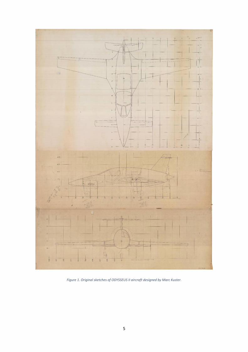
The 3D models developed throughout the study must comply with the

geometrical restrictions present in the plans developed by the client and

which can be seen in Figure 1.

For any other issue, CS23 and FAR23 standards are taken as reference, although

this aircraft is classified in the Experimental Catergory (Non Type Certified Aircraft).

1 Range based on the Lycoming IO-390 engine.

5

Figure 1. Original sketches of ODYSSEUS II aircraft designed by Marc Kuster.

State of the Art

6

1. STATE OF THE ART

1.1 EXPERIMENTAL AMATEUR-BUILT AIRCRAFT

Experimental amateur-built aviation, also known as homebuilts, is a growing

activity within the world of sports aviation. The basic idea is that the enthusiast builds his

own aircraft.

The most common forms of constructions are: Own Design, Plan Built or Kit Built

constructions. Restorations of old aircrafts also have a strong following in many countries

around the world.

The Homebuilder’s main aim is to enjoy the construction and finally flying his own

creation.

Although, a priori this type of undertaking would suggest an increased level of

danger, it soon becomes evident that through adherence to strict aeronautical

engineering practices, quality controls and legislations regulating these activities; those

potential dangers are reduced to exceptionally low levels.

The most substantial number of followers are in the United States, where tens of

thousands of people and many associations dedicate their effort and free time to this

wonderful pastime, with the Experimental Aircraft Association (EAA) having the highest

membership, country and worldwide. Other countries with large groups of homebuilders

are: Australia, New Zealand and South Africa.

Within Europe, there are countries with a strong aeronautical culture the likes of

France, Germany, the UK, Czech Republic and Slovenia.

France has the distinction of being the world’s first country to promote

“Homebuilding”, started in 1934.

State of the Art

7

In most other countries of Europe, there is a steady growth of experimental

aircraft construction with Spain being no exception.

Questions which are often asked in the general aviation circles are: “Why are

these types of aircraft becoming more and more popular?”.

According to the article available in reference [1], it often can be simply the

challenge. The immensely rewarding experience of having created such a project with

one’s own hand is emotionally important to many people.

Aviation is expensive and for many an aspiring aviator, the costs of a factory built,

certified aircraft are prohibitive. The expensive upkeep and maintenance costs are often

a deterrent too.

With homebuilts, the construction costs are essentially carried by the buildery.

Certified components often cost astronomical sums of money due to insurance

premiums. A large portion of these costs are not applicable in the homebuilt sector.

Uniqueness is another consideration. It is fair to say that no homebuilt is the same.

The freedom to choose paint, instrumentation, upholstery, in some cases engines and

much more, are all plus points for the individualist. The completion of such an

undertaking ends up being a reflection of the person who built such an aircraft.

In addition, the fact of having this freedom, allows the builder to use the latest

technological advances which are not always available on certified machines. The results

often translate into better performances and higher efficiencies.

Another interesting aspect of Homebuilding is the fact that a large inventory of

second hand components is available worldwide making acquisitions more cost effective.

Such components are not so easily available in the certified aircraft sector, due to

for example the “Time Ex” factor, meaning that such components may have reached the

end of its hourly or cycle life.

A final point on the subject of economics, the possibility of being able to carry out

the maintenance and some inspections, also saves substantial amounts of costs.

State of the Art

8

Homebuilding has some down sides. To build an aircraft is not for everyone and

the investment in large quantities of materials and tooling may cause some people to

think twice before undertaking such a venture. Also, for many folks, manual work is

foreign to them.

The essence of owning an experimental aircraft is meant for leisure activity. For

those who wish to use a homebuilt aircraft as a business tool, the current regulations

restrict such activities in many countries. Flying a homebuilt fore hire and reward, i.e.

commercial activity, is prohibited.

Experimental Aviation (the word “experimental” being somewhat a misnomer) is

a world that has brought aviation closer to many people who could not otherwise have

had access to flying.

In this thesis, the reader may find some of the analyses and procedures helpful to

build an experimental aircraft.

1.2 STRUCTURE CONSTRUCTION TECHNOLOGIES

When faced with any problems, mankind has for eons developed and evolved

methods and solutions to overcome them.

In the case of aircraft manufacturing, and specifically airframe manufacturing, the

development of fabrication methodologies has been tightly linked with aerodynamic and

materials advances.

In this section, a brief summary of the different types of existing structures, their

pros and cons, following the references [2], [3] and [4] is put forward.

1.2.1 Aircraft Loads

Before investigating the structural topic, the main loads an aircraft is subjected to

in flight are presented herein. Such loads are to a large extent the criteria used to decide

which structure will best apply.

State of the Art

9

During the flight of any aircraft, there are 3 types of loads to which the structure

of the aircraft must face:

Aerodynamic Loads: The aerodynamic loads are generated by the pressure

differences created on the aircraft during the flight. This pressure

differences are responsible for generating the forces of lift and drag, and

moments, causing bending and torsion in the wing among other elements.

Generally, these forces depend on the geometry of the aircraft, its weight

and the flight conditions.

Inertial Loads: Inertial loads are those forces and moments generated by

aircraft accelerations generally due to the variation of G forces during

flight.

Operational Loads: Are those loads that are given by the use of the plane,

such as those due to the pilot climbing the wing to enter the cabin.

As a general rule, the dimensioning of the structure is based on the first two types

of forces, focusing mainly on the aerodynamic loads.

With regards to the reaction of the structure to the aforementioned loads, there

are five main stresses appearing:

Tension: This type of stress appears when trying to separate an element

through the application of a traction effort in its axial component.

Compression: The compression is the stress opposite to the tension,

appearing this when an effort of crushing is applied on the longitudinal

axis of the component.

Torsion: This type of stress appears when a force or moment of twist is

applied on the element.

Shear: This type of stress appears when the material is opposed to a layer

of material sliding on its attached layer.

Bending: It appears when compression and traction efforts are combined.

It generates a curvature on the piece to which said efforts are applied.

State of the Art

10

During the flight of an airplane, all the above mentioned reactions are possible to

appear. The tension and compression are present on the wings due to the lift and drag

forces through their combined form, the bending. The torsion appears as a result of the

different moments in flight, whether they are aerodynamic or inertial. Union elements,

such as screws and pins, are subjected to high shear forces.

Figure 2 shows a diagram that shows the different types of stress that appear in a

plate type element, such as for example the skin of the wing or the fuselage.

Figure 2. Bending Stress Diagram. Extracted from [3]

1.2.2 Aircraft Structures

With the knowledge of the types of loads the structure of this aircraft is subjected

to, the author of the thesis has looked at the different types of structures available.

Each of these types has advantages and disadvantages, and are in some cases the

result of the evolution of a previous type of structure due to the application of the latest

technologies and materials.

Fuselage

The fuselage is the body of the plane. In it, not only are located the crew and the

passage, but also the space for storing different systems and joining the different

components which allow the aircraft to fly.

State of the Art

11

Historically, Truss-type fuselages

were the first to appear. At the beginning,

manufactured in wood and later in metal,

they constitute a framework based on the

union of rigid elements such as tubes or

struts resisting the different loads. Many

times, this type of structure is accompanied

by tensioners which contribute with an

extra resistance against tensile loads. These

type of structures are complex to design, have a fairly good weight resistance ratio,

although the number of elements is high and there is a sensitivity to buckling present.

Trust construction is still used today on some occasions, but is somewhat a thing of the

past.

The next type of structure is the

semi-monocoque. This type of structure

combines frames and stringers with

structural skin. While the first elements

are responsible for resisting the various

loads and being the support for the skin,

the skin is responsible for providing

structural stiffness, keeping the different

elements together. In turn, the skin also

provides the aerodynamic finish

necessary to reduce aerodynamic drag.

This type of structures present a lower complexity when it comes to being designed and

a better behavior against buckling with a smaller number of pieces. The lightness of semi-

monocoque is similar to that of the truss structure.

Figure 3. Truss-Type Structure. Extracted from [3]

Figure 4. Semi-monocoque Structure. Extracted from [3]

State of the Art

12

A variant of the semi-

monocoque structures.

In them the stringers and

longerons are eliminated thanks to a

better design and resistance of the

skins. In these structures, the skin takes

on a larger structural role since it is

responsible for supporting the

different types of loads.

As a result, the application of

this type of structures produces lighter airframes than semi-monocoque constructions.

The down side is a slightly reduced resistance against buckling.

Wings and Empennage

Wings and tail surfaces are the components of an aircraft subjected to the highest

efforts and stresses, as they are responsible for generating the lift which counteracts the

weight of such a machine. The unwelcomed by-product of these efforts and stresses is

called Drag.

It is interesting to note that the type of wing structures of has not changed much

over time. The same components are still used today as those produced more than 50

years ago. A testimony to the ingenuity of the designers of times go by.

The technological advances lie in the use of new materials and the number of

elements which form the structure of the wing. A good example of such improvements is

the number of wing ribs a sports plane requires, often less than ten per half wing,

compared to up to thirty some 50 years ago.

Flying surfaces, whether wings or tails, are composed of three main components:

the spars, the ribs and the skin.

Figure 5. Monocoque Structure. Extracted from [3]

State of the Art

13

Spars are the main structural components of a wing. They are in charge of

sustaining bending and torsion efforts. Generally, and depending on the type of aircraft,

the number of spars is usually 2, sometimes 3.

Some of the newer models of ultralight aircraft contain only 1 spar per half wing,

thanks to the advances made in terms of composite elements.

Ribs are the components responsible for the shape of the aerodynamic profile of

a wing. They are also responsible for transmitting the aerodynamic loads towards the

beam.

The number of ribs in a wing depends on the type of skin of a wing, the greater

the resistance to buckling of the skin, the fewer ribs needed.

The third and last component is the skin, which is responsible for producing the

aerodynamic finish required for flight efficiency. The skin, as an integral part of the

structure is used to reinforce the resistance against wing twist and forms a type of torsion

box together with the two spars.

Figure 6. Typical Wing Structure. Extracted from [3]

State of the Art

14

1.3 MATERIALS IN SPORT AVIATION

Relating to the previous section, brief comparison of the different materials often

used when manufacturing an aircraft and in this case an experimental one, is herewith

presented.

1.3.1 Wood

At the beginning of aviation, only wood was used in the structural construction of

the aircraft. And for the most pioneering, wood had to be natural.

The advantages offered by this material is the availability, the low cost, the little

requirement of specialized tools and that it is easy to work given the few construction

skills.

Figure 7. Typical Wood Sections. Extracted from [3]

1.3.2 Aluminum Alloys

Relatively early in the history of aviation, aluminium constructions started to

appear. Different alloys were tried.

The advantages of aluminium alloys are: a good strength to weight ration as

proven through many laboratory tests, a relatively good resistance to corrosion, as well

as a good resistance to temperature variations.

The price of aluminum alloys, compared to composite materials, is lower. In

addition, the handling and machining of aluminium is simple and strait forward. Sheet

metal work experience is required to obtain suitable forms.

State of the Art

15

Also, of interest is the fact that aluminium is an isotropic material. It offers a high

versatility in many applications, regardless of grain orientation, which is not the case with

steel, for example.

Finally, the components are much easier to evaluate compared to other

materials, so the maintenance cost of the aircraft is lower. Is a great material for home-

builders.

A notable and substantial weakness of aluminum is the fact that it does not have

a defined fatigue limit. This means that in the case of dynamic loads, a component may

fail with low loads, if the number of cycles is high enough.

In addition, aluminium, when subjected to fatigue has a much lower tensile

strength compared to its normal maximum resistance to the traction. This consideration

implies that components have to be produced with a larger quantity of metal in order to

overcome this problem. And more material equals more weight. It also implies that the

total weight is greater than a structure that only faces static charges.

Another problem with aluminium is corrosion. Several types of corrosion rear

their ugly heads. Inter granular corrosion occurs in aluminium alloys especially 2024T3,

which has copper as its main alloying component, when subjected to water condensation

and or high atmospheric humidity contents causing aluminium oxide, a white powdery

substance.

Stress corrosion forms fissures between in the homogeneity of the aluminum

degrading and weakening the area until rupture in some cases. The causes of stress

corrosion are vibration and excessive tension, compression, torsion, shear and bending

loads.

Finally, aluminium has a great predisposition to galvanic corrosion. This occurs

when two metals with different electrical properties come into contact. Due to the

difference in electric potential, an electrical current is generated between the two metals

causing said corrosion.

State of the Art

16

Figure 8. Typical Metal Wing Spars. Extracted from [3]

1.3.3 Composite Materials

The combination of two or more compounds with completely different properties

in order to form a new material with remarkably better features, offers the opportunity

to manufacture components with greater resistance and lower weight. Lighter, faster

and more resistant aircraft construction results in better performance and lower

fuel/energy consumption.

Thus, composite materials stand out for their high strength, light weight,

flexibility, and the ease of building complex compound curves, which are difficult to

produce with aluminum. They also have a high dielectric strength, good dimensional

stability and no corrosion issues.

Unfortunately there are disadvantages with composites as well. Toxicity of the

resins, some sensitivity to impacts, limited resin and catalyst storage times, potential

mixing ratio issues and ambient working temperatures are a few.

A high degree of vigilance is required when working especially with epoxy resins,

all of it adding to the final price tag.

As with all materials, composite constructions required some specific protection

from the elements. To minimize heat absorption on surfaces exposed to the sun, it is

recommended to use light colors, the lighter the better. White being the least heat

absorbent.

Lightning strikes can cause serious damages to structures and auxiliary

components in a composite aircraft and it is of the utmost importance to channel these

very high electric charges in a safe manner.

State of the Art

17

Aluminum aircrafts are essentially Faraday cages and therefor mostly impervious

to lightening, whereas composites aircrafts are not.

Aluminum is still the predominant material with experimental aircrafts, but

composites are slowly catching up, despite the more complex manufacturing processes

and associated costs.

The legendary aircraft engineer and designer Burt Rutan set the pace of

composite aircraft constructions as early as the 1970’s.

Thesis and Design Methodologies

18

2. THESIS AND DESIGN METHODOLOGIES

As mentioned in previous sections, the objective of the Project is to analyze the

aerodynamics of the ODYSSEUS II aircraft and use the results to design a structure of

composite materials, which will then be briefly analyzed. This type of Project is included

in the preliminary design phase.

For the benefit of the reader, a prior knowledge is helpful to better understand

the context of thesis. To do so, the Standard Methodology of aircraft design is explained

below. For more information, the reader can consult references [2], [4], [7] and [8].

2.1 DESIGN PHASES

In engineering, the development of a product is not a trivial procedure, but a

drawn out and detailed process, often feedback-type and only complete when the

objectives and criteria of service meet all the requirements imposed.

In the aeronautical sector, this design process is somewhat more complex due to

the high demands imposed on an aircraft and the various tests and evaluations to which

the design must be submitted.

As a general rule, the steps one must follow in order to design and build an aircraft

are:

Thesis and Design Methodologies

19

1. Requirements Definition: In this first stage the designer and the client meet to

define the different requirements that the plane must fulfil. In this step it is

also important to record the type of certification you want to obtain.

2. Conceptual Design: The second step is to brainstorm and market research to

have one or several positions with which to solve the problem raised in the

requirements stage.

3. Preliminary Design: This stage is one of the most extensive of the process,

since it is about defining, studying and carrying out the first calculations and

simulations based on the design or closed designs in the conceptual phase.

Within the preliminary design, it is crucial to study the aerodynamics, the flight

mechanics, the structures and the stability of the aircraft.

4. Detail Design: Once the simulations and preliminary calculations indicate that

the design meets the requirements set, each of the aircraft’s components is

designed and tested and the necessary documentation is generated to

manufacture it.

5. Flight test: With the first prototype built, different flight tests are carried out

to verify the calculations made.

6. Critical Design Review: This stage of the design process is critical, since it

evaluates the results obtained and redesigns those components that may

pose some type of problem for the proper functioning of the aircraft.

7. Certification: With the closed, tested and verified design, the certification of

the aircraft is carried out.

The afore mentioned points are not a linear process, but a recursive process

where the aim is to optimize the concept initiated in the conceptual design phase, until

obtaining the best possible solution.

Thesis and Design Methodologies

20

2.2 THESIS METHODOLOGIES

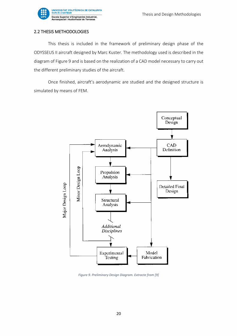
This thesis is included in the framework of preliminary design phase of the

ODYSSEUS II aircraft designed by Marc Kuster. The methodology used is described in the

diagram of Figure 9 and is based on the realization of a CAD model necessary to carry out

the different preliminary studies of the aircraft.

Once finished, aircraft’s aerodynamic are studied and the designed structure is

simulated by means of FEM.

Figure 9. Preliminary Design Diagram. Extracte from [9]

Cad Models

21

3. CAD MODELS

In order to carry out these studies, several characteristic models of the aircraft

are required in order to interact with different specific software within each of the areas

subject to study.

In this way, the author of the project has developed three different models

meeting the different needs and requirements to carry out studies concerning the

aerodynamics, the structural calculation and the visualization of the entire product.

These models have been developed through the use of CATIA V5 R2017. Catia is

a software of parametric design widely used in the engineering industry and especially

used for the aeronautical sector.

This software offers a great variety of modules and complements that allow to

carry out specific tasks according to the work sector of the person who is in charge the

design.

As it is indicated on its website (reference [5]),

CATIA, which is based on the 3DEXPERIENCE platform of Dassault Systèmes, offers the following:

Social design environment based on a unique source of authenticity, accessed through powerful 3D

panels that drive business intelligence, simultaneous real-time design and collaboration of all

stakeholders, including mobile workers.

3DEXPERIENCE offers an intuitive experience with top-level 3D modeling and simulation

functionalities that optimize the efficiency of all experienced and sporadic users.

It is an inclusive product development platform, which is easy to integrate with existing processes

and tools. This allows several disciplines to take advantage of effective and integrated specialized

applications in all phases of the product development process.

The author of the thesis has decided to use this software due to the experience

he has in the use of this tool, since he has not only used this program for personal and

academic projects but also is a frequent tool in his work environment.

Cad Models

22

The recurring modules to carry out the project shown in this document are:

Part Design,

Assembly Design,

Generative Shape Design

Drafting.

These modules, frequently in the aeronautical sector, have a specific and unique

function that, by combining them in an adequate way, are capable of realizing anything

that one can imagine.

The module of Part Design is the most basic of CATIA. In it, the designs of the

different pieces and components is used to carry out the design of different sections such

as fuselage frame, wing ribs, etc.

The Assembly Design module is used to join the different parts created and that

make up an assembly or set of parts with a purpose. This module also allows evaluating

design features such as assembly weight, center of gravity, inertia, etc.

This is very useful when making predictions and using these parameters to carry

out simulations and calculations. With the Assembly Design module, it is not only possible

to assemble parts, but it is also possible to compose assemblies with bases to sub-

assemblies. A good example of this module is the subsequent assembly of wings, canard,

fuselage and tail which then become the entire aircraft.

The GSD module is a tool requiring advanced knowledge of the program. This

module is used to design the surfaces and any element, usually finished components, but

with “visible” internal parts.

In the aeronautical and composite materials sector, it is an essential module since

its power is used to transform into reality the different aerodynamic profiles and

characteristic shapes of an aircraft. In addition, in the field of composite materials, this

module is used to carry out the Shell type models (see section 5.3) used in the different

calculation and simulation software.

Finally, the Drafting module is used to generate drawings, both of the components

and of the final assembly.

Cad Models

23

3.1 AERODYNAMIC MODEL

The aerodynamic model is used to carry out the various simulations using

Computational Fluid Dynamics.

This model traces the exterior geometry of the airplane and simplifying those

elements of small size which may disturb the continuity of the surface and compound

errors in the mesh and, therefore, in the final calculation of the aerodynamic loads. Thus,

elements such as holes, antennas and complex geometries have been removed or

simplified to develop this model.

Figure 10. CAD Model develope in order to perform CFD simulations

As seen in Figure 7, the aerodynamic model has all lines smoothed out between

the different elements making up the aircraft. In addition, this model is a faithful

reproduction of the original design seen in Figure 1, except for the winglets added by the

author of the thesis, which have being acknowledged and accepted by the designer.

These winglets have been inserted in order to improve the aerodynamic characteristics

of the airplane.

The model is made in 1:1 scale and has been exported in .stp format to carry out

the meshing in any of the different software existing in the market.

Cad Models

24

3.2 STRUCTURAL MODEL

The structural model can be very different depending on the type of structure of

the aircraft and the type of analysis that is needed to perform it. Concerning this thesis,

the complete structure of ODYSSEUS II is based on a monocoque structure made entirely

of composite materials, combining carbon fiber, Kevlar and fiberglass. This particular

structure makes this model necessary in order to calculate the structural behavior

required of a Shell type. The study of the structure proposed for the ODYSSEUS II is carried

out through the evaluation of the macro-scale material or component scale. This means

that the strength of the material is evaluated according to the type of composite material

layerings.

The shell type models are based on the creation of the outer or inner surface of

the component manufactured from laminar materials (such as composites). They are

used as a reference in the calculation software, which determines the layers to be

evaluated. Based on said surface, section 5.3 explains more about this type of analysis.

In this case study, the model of the complete structure of the aircraft has been

developed. However, only wing and tail structural models have been used to perform the

analysis. The particularity of this type of model lies in the use of the surfaces as a

reference of the real structural elements, without taking into account the real thickness

of the components.

As shown in Figures 11 and 12 the level of sizes is much higher than the

aerodynamic model. Furthermore, it can be seen that the design of components is based

on surfaces and not on solids, as mentioned above. In the two proposed models, details

such as fuel tanks and or ailerons can be noted. These elements are not taken into

account during the structural analysis, as these are focused on in the behavior of the main

structures of the assemblies.

Cad Models

25

Figure 11. Wing Shell Model

Figure 12. Tail Shell Model

Cad Models

26

3.3 CONCEPTUAL MODEL

The last model that has been developed within the framework of this thesis is the

conceptual model. This last model is the most detailed since the different parts and

components of the aircraft have been modeled in greater detail to obtain the first

estimates of the dimensioning of the parts, as well as to calculate the total weight of the

structural and the center of gravity.

In turn, this model helps to have a clearer vision of what the aircraft is like and

allows to evaluate factors that are not as relevant as the aerodynamics of the aircraft or

its structure, but that take on some importance when manufacturing the aircraft as they

can be the positioning of the different systems, the ergonomics and comfort of the

passengers, the accesses to carry out the maintenance, etc.

Below is a list of renders created by the KEYSHOT 6 program based on the

conceptual model designed in CATIA V5.

As mentioned in section 3.2, the design of the ODYSSEUS II structure is based on

a structure of monocoque type where both the interior structure and the skin are used

to support the different structural loads. In this way it has been defined that the base

material of the internal structure is the carbon fiber, either in combination with foam to

generate panels or substructures type sandwich.

Figure 13 shows a general view of the exterior of the aircraft, consisting mainly of

glass fiber with the different carbon fiber control surfaces. The reality is, that the skin of

the fuselage is made of glass fiber because the level of load that it must withstand is very

inferior to the one of the wings or other elements.

With regard to wings, tail and canard, the skin is composed of a stack that

combines both the glass fiber and carbon fiber, being the outer layer made of glass fiber.

Cad Models

27

Figure 13. ODYSSEUS II

With regards to the internal structure of the ODYSSEUS II, it is necessary to

differentiate the various elements making up the complete structure.

In the airframe of the fuselage, it can be noted how the different bulkheads and

formers uniformly distribute the loads and are responsible for providing structural

rigidity to the skin, this by transmitting said loads to both the upper and lower longitudinal

reinforcements.

The lower reinforcements also form a structural core, which is responsible for

supporting the floor of the cabin, withstand the impacts of the landing gear and to

dampen the efforts and stresses transmitted from the wing to the wing box.

Cad Models

28

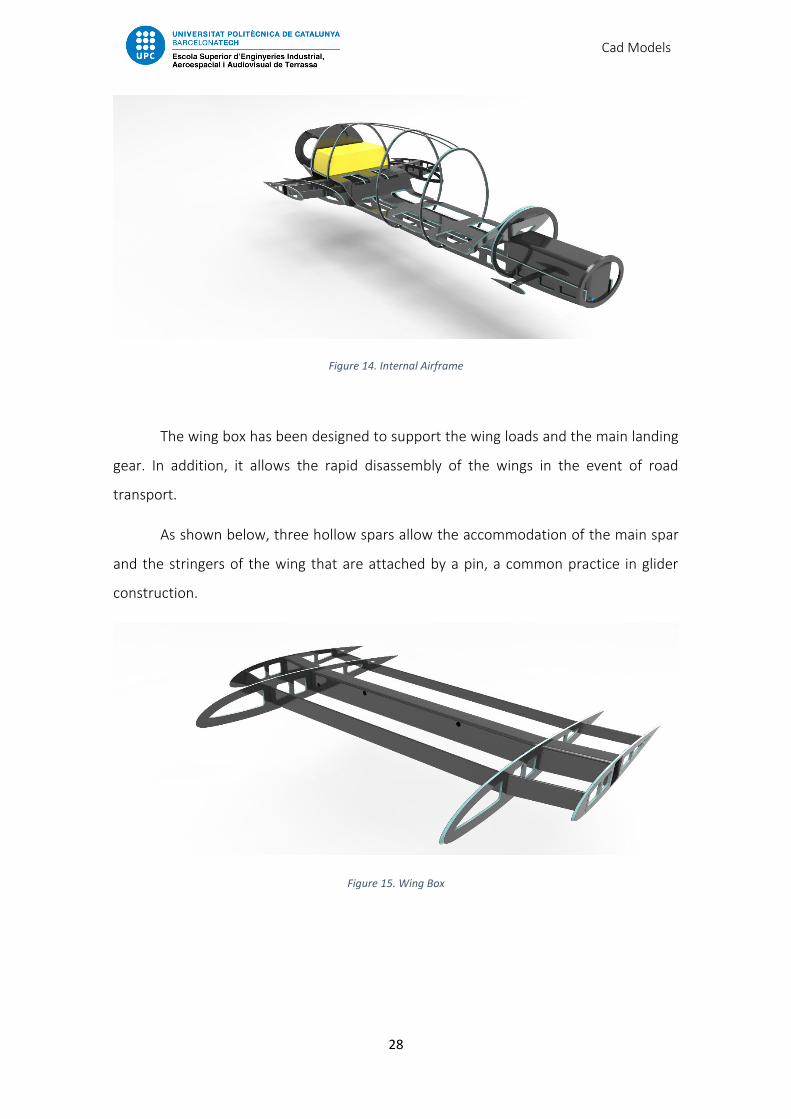
Figure 14. Internal Airframe

The wing box has been designed to support the wing loads and the main landing

gear. In addition, it allows the rapid disassembly of the wings in the event of road

transport.

As shown below, three hollow spars allow the accommodation of the main spar

and the stringers of the wing that are attached by a pin, a common practice in glider

construction.

Figure 15. Wing Box

Cad Models

29

Figure 16. Glider Wing Attaching System. Extracted from [6]

The structure of the wing is based on a central beam/main spar located around

40% of the chord of the wing.

The main spar is the principal load carrier and also responsible for supporting the

bending stresses together with the help of two secondary spars. These secondary spars

close up the torsion box, together with the skin of the upper and the lower wing profile.

This concept is responsible for minimizing torsional stresses. The hinges of the ailerons

and the simple flap mechanism are mounted on the rear spar.

Finally, winglets, ailerons and flaps are based on a core foam construction,

reinforced by a spar (in the case of aileron and flap tube) and covered by a carbon fiber

skin. This mode of construction widely used in the field of amateur aviation allows one to

obtain light structures with high resistance, both to the aerodynamic loads and against

impact.

The few ribs present on the ODYSEUS II wings are used as support to the skin,

avoiding any deformation of the leading edges due to compressive loads.

Finally, the wing has two integrated fuel tanks that are shown in yellow in the

Figure 17.

Cad Models

30

Figure 17. Wing Structure

The philosophy used in the design of the tail is conceptually identical to the rest

of the structure. Therefore, an internal structure based on carbon ribs with foam core,

form the resistant center of the tail. In turn, the carbon fiber skin provides extra

resistance against torsional loads.

As shown in Figure 18, the horizontal empennage is composed entirely of a foam

core reinforced with a front tubular spar, a rear spar and two ribs on each side. This type

of empennage, used as the elevator is a full flying wing and the most important element

in the maneuver of an aircraft in pitch axis.

Cad Models

31

Figure 18. Tail Structure

The tricycle-type landing gear is fully integrated into the fuselage structure and

wing box of the ODYSSEUS II. In this way it is possible to disassemble the wings to carry

out any repair, modification or transport.

This is an important feature, in that the fuselage is fully supported on the

undercarriage assembly, even with the wings removed.

As can be seen, the main landing gear transmits the loads towards the central

beam of the wing box, while the nose gear rests directly on the longitudinal

reinforcements of the fuselage.

Cad Models

32

Figure 19. Landing Gear

The design of the exterior and interior of the airplane has been carried out based

on the final appearance of the ODYSSEUS II, with the intention that the designer, Marc

Kuster, has a feeling of what the airplane could be like and assess the need for changes

or modifications.

The choice of colors has not been arbitrary. Through the broken white

background, reinforced with a garnet tonality, the thesis author wanted to transmit a

classic view of aviation.

In turn, the light interior, based on cream tones, aims to create a bright and

spacious atmosphere.

Cad Models

33

Figure 20. ODYSSEUS II Exterior

Figure 21. ODYSSEUS II Interior

Cad Models

34

Finally, the control panel combines analogue instrumentation with the most

modern of the integrated equipment, the Garmin 1000 screen.

As seen in Figure 22, in front of the pilot are the plane's governing instruments,

such as the artificial horizon, the turn coordinator, the speed indicator and the vertical

speed indicator.

In front of the co-pilot, there are instrumentation related to the condition of the

aircraft with indicators such as fuel level, engine temperatures or manifold pressure.

Figure 22. ODYSSEUS II panel

Aerodynamic Studies

35

4. AERODYNAMIC STUDIES

This section is aimed at evaluating the aerodynamic design of ODYSSEYS II aircraft.

The goal of this study is to determine initially if this aircraft design is viable from an

aerodynamics’ point of view, followed by the studies of parameters such as lift, drag and

efficiency, as well as focus on stability.

The second objective of this study is to obtain the distribution of forces that such

aircraft will experience under multiple flight conditions, for the purpose of structural

calculations. See section 5.1 of this document.

During the evaluation, the behaviour of the aircraft is assessed using two different

methodologies.

In the first instance, the potential theory is being applied to get an initial

approximation of the aircraft’s behaviour using the open source software “XFLR5”.

The potential theory provides relatively good results in terms of lift and moment

predictions. However, being a theory of potential flow, friction drag is not taken into

consideration and therefore produces somewhat erroneous results regarding drag

coefficients.

To carry out a more exhaustive evaluation of this project, “CFD” technology is

applied to calculate the loads with greater precision. The boundary layer viscosity

produces a drag coefficient that is taken into consideration with CFD.

As a result, one obtains a higher degree of accuracy and certainty that these

values are closer to reality.

The potential theory is very fast whereas the CFD methodology is more time

consuming.

Aerodynamic Studies

36

4.1 STUDIES METHODOLOGY

Although the overall methodology of the project has been based on loop from the

aerodynamic and structural design (as presented in section 19), the specific methodology

used during the design or aerodynamic study has been more pyramidal. The author of

the project, departed from the requirements demanded by Mr. Kuster and the various

conversations that were held, to determine the aerodynamic design in question. In turn,

through the original planes of the aircraft it was possible to extract what main

characteristics the Canard had to fulfil.

Although the overall methodology of the project is based on the loop principle for

the aerodynamic and structural side of the design (as presented in section 2), the specific

methodology used during the design and aerodynamic study is more pyramidal.

The author of this thesis started out from discussions and original plans submitted

by Mr. Kuster. Using these plans, it was possible to determine the aerodynamic

characteristics of this design.

Once, the exterior geometry of the front wing was determined, the modeling of

the entire aircraft was carried out in 3D (See section 3), including the necessary software

to perform all relevant calculations.

Multiple iterations have been carried out, first by means of the XFLR5 program

and later with the CFD program, providing the answer to the question of whether this

aircraft would fly or not.

Aerodynamic Studies

37

4.2 THREE SURFACE AIRCRAFT PARTICULARITIES

Before going deeper into the analyses carried out, it should be mentioned the

peculiarity of the airplane being studied. As the reader has already been able to observe,

the plane that is being evaluated is a three surface type and there are certain

considerations that must be taken into account when designing these kinds of aircraft.

That is why, the author of the project has thought it appropriate to expose in a generic

way the most relevant characteristics of a plane like this and that are a summary of what

the reader can find in the bibliography [10], [11]

Like any existing object, the canard has certain advantages and disadvantages if it

is compared to a conventional plane and varies according to the functionality or the

ultimate goal of the design that is intended to be built. From the aerodynamics’ point of

view, a front wing set up has several disadvantages.

One of the first things to consider when designing this kind of aircraft is that the

horizontal control surface is placed in front of the wing. This makes the lift of the front

wing itself causes a positive pitching moment that destabilizes the plane. This factor

means that to be able to stabilize the plane, statically and dynamically, and controllable,

the CG must move forward compared to a conventional airplane with similar

characteristics (see Figure 23). This overtaking of the CG often conflicts with the

positioning of the engine, since this is usually located in the rear of the aircraft, thus

expanding the destabilizing moment. The difficulty of the designer, therefore, is to be

able to maintain a slope of the negative 𝐶𝑚𝛼 curve with a value of 𝐶𝑚0 greater than 0.

Moreover, the position of the canard in front of the main wing makes the airflow

that reaches the wing disturbed. This fact causes that the generated lift in those sections

bathed in less clean air is produced less efficiently, thus reducing the efficiency of the

whole machine and, therefore, increasing fuel consumption.

In turn, such positioning can also cause problems of non-recoverable or super-

lost losses. The super lost is an aerodynamic event that occurs when being on the edge

of the loss the flow detached from an aerodynamic element (canard) causes the flow of

another element (wing) to be coupled, avoiding the possibility that the pilot can regain

control of the aircraft.

Aerodynamic Studies

38

Despite the aforementioned disadvantages, the three surface airplane also

presents some advantage from the aerodynamics’ point of view. Being the canard a

supporting surface, this is generating a lift force that helps the wing when lifting the load.

It has been calculated that the distribution of forces in a configuration like the one studied

can be around 80/85% for the front wing and 20/25% for the canard. This fact helps to

lighten the structure of the wing and helps the correct positioning of the CG.

Generally, due to the distribution of combined forces, the distribution of forces

around the wing ends up having a resemblance to an elliptical distribution, which is the

most efficient of the distributions.

Beyond the aerodynamic design, a canard has advantages such as a compact

design or greater visibility due to the tractor engine configuration. Thus, the decision to

choose what type of configuration is more appropriate resides in the designer.

Figure 23. CG positioning comparison between a conventional aircraft and a canard. Extracted from [1].

Aerodynamic Studies

39

4.3 AIRFOIL SELECTION

The envisaged wing profile chosen for the main wing and strakes is a NACA 63

series and a NACA 0010 series for the vertical fin/rudder assembly.

Burt Rutan used Eppler laminar wing profiles in his early designs of canards. These

profiles provided good lift and stability under normal flying conditions. Shortcomings

were subsequently discovered in rainy conditions, with to water molecules disturbing the

laminar air flow and causing difficulties in pitch control at lower speeds.

For this project, the designer has chosen a John Roncz profile for the canard wing,

which has proven highly successful in these designs.

Below is a summary table with the profiles used and their main characteristics.

Airfoil Characteristics

Parameter Symbol NACA 631-412 NACA 2414 NACA 0010

Maximum Lift Coefficient 𝐶𝑙𝑚𝑎𝑥 1.62 1.89 1.09

Cruise Lift Coefficient 𝐶𝑙𝑐 0.80 0.70 0.44

Parasite Drag Coefficient 𝐶𝑑𝑜 0.0053 0.0056 0.0045

Zero Lift Angle of Attack 𝛼𝑜 -3.00 -2.20 0.00

Stall Angle of Attack 𝛼𝑠 19.00 19.00 10.00

Cruise Angle of Attack 𝛼𝑐 4.00 4.00 4.00

Zero Lift Moment Coefficient 𝐶𝑚𝑜 -0.08 -0.05 0.00

Maximum efficiency (𝐶𝑙/𝐶𝑑)𝑚𝑎𝑥 119 132 113

Table 1. Airfoil Characteristics. All the parameters have been calculated for a Reynolds Number of 7.000.000 (which is the Re of the cruise speed).

Aerodynamic Studies

40

4.4 AIRCRAFT AERODYNAMICS’ PRELIMINARY EVALUATION

4.4.1 Modelling

As mentioned above, the preliminary aerodynamic study has been carried via the

XFLR5 program. Following the different analyzes carried out, some results are available

below.

The first step in order to be able to evaluate how the aircraft will behave, is to

transfer the geometry 2D to the calculation software. Said software, apart from

generating the aircraft’s geometry, lets one calculate the main characteristics and allows

adjustments according to requirements of the designer.

The following program captures show the 3D geometries obtained from the

original plans.

On noticeable feature in the original aerodynamic design presents a wing surface

generated from the interpolation between the wing tip profile and the root profile.

This design methodology is widely used in the aeronautical sector, both at the

amateur and commercial levels, since it allows obtaining wings with combined

characteristics of the different profiles used.

It allows one to find solutions or mitigating various problems arising when using

unconventional configurations such as a canard design. The intentionality of combining a

profile with a greater lift at the tip and a more moderate profile at the root, creates an

aerodynamic torsion that allows displacement of the stall entry towards the root, making

the aircraft controllable throughout the entire flight envelop.

Another beneficial facet during wing design is the use of winglets. These help

reduce wing tip vortices, improving aerodynamic efficiency and reducing energy

consumption.

The main wing has a dihedral of 1.5 degree and a wing twist (washout) of 2 degrees

throughout the entire span with the dihedral serving to improve lateral stability and

washout improving stall management.

Aerodynamic Studies

41

Generally, the designer seeks the best efficiency at cruising speeds and attitudes.

Thus, as it is later observed, the combination of a 2 degrees incidence with an angle of

attack of 4 degrees allows the aircraft to fly at maximum efficiency during the cruise stage.

Finally, the wing at root level has a short span section with a substantial chord

increase. They are called “Strakes”. This chord increase favors a lift improvement which

counteracts to a degree the adverse effects of air flow disturbance produced by the

canard.

Figure 24. Wing Design. Capture from XFLR5

Regarding the canard, it can be seen how the design is rectangular and presents

a certain elevation at the tip. In turn, the design presents an anhedral that aims to reduce

lateral stability in this area to provide greater manoeuvrability to the aircraft.

Figure 25. Canard Design. Capture from XFLR5

Aerodynamic Studies

42

Of note is the fact that this concept allows for a reduction of the stall onset to

between 10 and 11 𝐾𝑡𝑠, which in turn translate into a reduced approach and landing speed

when compared to a pure canard.

In order to guarantee lateral control of the aircraft, it is necessary to have a vertical

surface that generates the required forces. Generally, in pure canard designs, the vertical

fins are mounted at each tip of the main wing also providing, to a degree, a form of speed

brakes, (see Burt Rutan designs, Varyeze and Longeze).

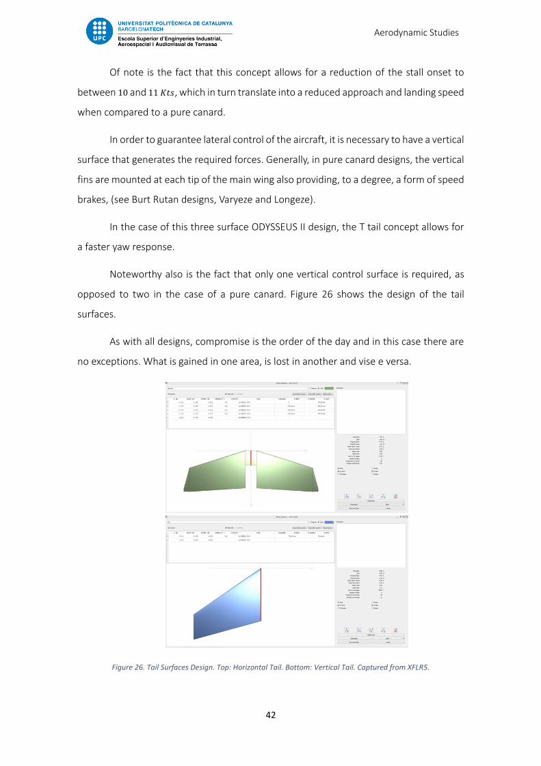
In the case of this three surface ODYSSEUS II design, the T tail concept allows for

a faster yaw response.

Noteworthy also is the fact that only one vertical control surface is required, as

opposed to two in the case of a pure canard. Figure 26 shows the design of the tail

surfaces.

As with all designs, compromise is the order of the day and in this case there are

no exceptions. What is gained in one area, is lost in another and vise e versa.

Figure 26. Tail Surfaces Design. Top: Horizontal Tail. Bottom: Vertical Tail. Captured from XFLR5.

Aerodynamic Studies

43

Finally, the modelling of the fuselage surface has been carried out. For purposes

of calculation, the XFLR5 does not take into account that body, so the results are always

better than experimentally can be verified. In Figure 27, a simulation completed in XFLR5

can be observed, the flight conditions of which are 120 𝑘𝑡𝑠, an attack angle of 0 𝑑𝑒𝑔. And

a flight level at sea level. In green, the distribution of the lift on the three supporting

surfaces is observed and in purple the drag induced

Figure 27. Full Aircraft Designed in XFLR5.

4.4.2 XFLR5 Analysis

For the purpose of analyzing the behavior of the aircraft in realistic flight

situations, a series of analyzes have been carried out in combination with the structural

design.

The flight conditions which have been evaluated with the results shown below,

have been those the author of the project considered most essential.

VLM2 (Vortex Lattice Method 2 is the program of choice and recommended in the

XFLR5 manual [4]. It is the most contrasting and most reliable. With this program, four

iterations have been carried.

With a maximum all up weight of 1170 kg, four extreme configurations have been

analyzed for different angles of attack, to verify the aircraft stability at any of these

parameters. These are:

Aerodynamic Studies

44

Aircraft loaded with pilot plus 3 passengers and maximum fuel.

Aircraft loaded with only pilot and maximum fuel.

Aircraft loaded with pilot plus 3 passengers and no fuel.

Aircraft loaded with only the pilot and no fuel.

The intentions of these analyzes is to assess any potential weak points of the

canard, in respect of longitudinal/pitch stability.

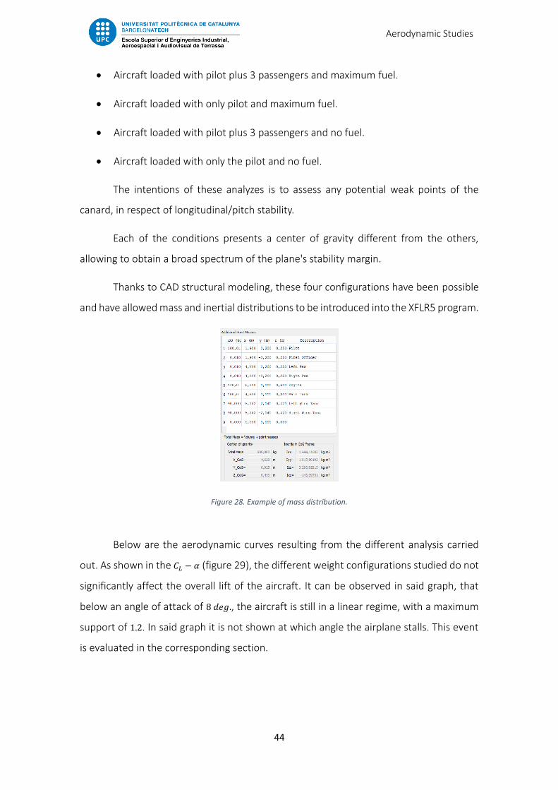
Each of the conditions presents a center of gravity different from the others,

allowing to obtain a broad spectrum of the plane's stability margin.

Thanks to CAD structural modeling, these four configurations have been possible

and have allowed mass and inertial distributions to be introduced into the XFLR5 program.

Figure 28. Example of mass distribution.

Below are the aerodynamic curves resulting from the different analysis carried

out. As shown in the 𝐶𝐿 − 𝛼 (figure 29), the different weight configurations studied do not

significantly affect the overall lift of the aircraft. It can be observed in said graph, that

below an angle of attack of 8 𝑑𝑒𝑔., the aircraft is still in a linear regime, with a maximum

support of 1.2. In said graph it is not shown at which angle the airplane stalls. This event

is evaluated in the corresponding section.

Aerodynamic Studies

45

Figure 29. 𝐶𝐿 − 𝛼 Curve. Extracted from XFLR5

In the polar curve (figure 30), it can be seen that, as in the first curve, the values

obtained for the different configurations do not differ much. In turn, it can be mentioned

that said polar curve is not very relevant, since as mentioned previously the viscous drag

has not been taken into account. So that the reader can have a sense of how wrong one

is, it must be said that the Cessna 172 has a parasite drag (minimum drag on the polar

curve) of approximately 0.02. Fixing us on the obtained graph, it can be seen how the

canard that is being designed presents a parasite drag 0.01.

Figure 30. Polar Curve. Extracted from XFLR5.

Aerodynamic Studies

46

Looking at the aerodynamic efficiency curve, it can be seen how it increases as the

aircraft weight goes up.

This is due to the increase in lift required to compensate for the increase in total

weight, when the aircraft flies in a balanced manner. Such a rise is much higher than the

increase in aerodynamic drag.

From this graph, one can conclude that the aircraft must fly trimmed with an angle

of 2.5 𝑑𝑒𝑔. for maximum flight efficiency.

This information helps when designing the wing, since the incidence (or rigger’s

angle) can be varied in order to control the angle at which the aircraft flies in a level

attitude.

Figure 31. Aerodynamic Efficiency Curve. Extracted from XFLR5.

The following graph is one of the most important at the level of study that can be

obtained from the XFLR5. This graph details the pitching moment of the airplane and,

therefore, it can be studied if it is statically stable or not. According to Torenbeek [13], a

good criterion of stability when carrying out preliminary studies and designs of aircraft is

that the airplane must have positive 𝐶𝑚0 and a slope between −0.005 𝑑𝑒𝑔.−1 and

−0.030 𝑑𝑒𝑔.−1.

Aerodynamic Studies

47

These limits are shown in the graph as two discontinuous red and cyan lines. As

can be seen, the canard designed by Mr. Kuster meets both criteria under any of the cases

provided as long as the aircraft is trimmed correctly. In table 2, it is possible to observe

the angle of trim of the elevator and the canard that are needed so that the airplane is

statically stable under the extreme conditions proposed.

As these angles are not excessive and are easily obtainable by means of a good

trim system, it can be concluded that the canard is statically stable.

Figure 32. 𝐶𝑚 − 𝛼 Curve. Extracted from XFLR5.

Moment Coefficient and Trimming Angle

Configuration 𝑪𝒎𝟎 𝒅𝑪𝒎

𝒅𝜶

Elevator Trimming

Angle

Canard Trimming

Angle

Full Passenger / Full Fuel 0.037 -0.017 -2.0 2.0

Only Pilot / Full Fuel 0.013 -0.006 -1.1 1.1

Full Passenger / Empty Fuel 0.055 -0.026 -2.8 2.8

Only Pilot / Empty Fuel 0.019 -0.009 -1.4 1.4

Table 2. Moment Coefficient and Trimming Angles.

Another very important graph is the one shown in figure 33.

Aerodynamic Studies

48

This shows the lift coefficient needed for the aircraft to fly at a given level and a

specific speed. This graph allows one to assess whether the aerodynamic design meets or

not the requirements for the speeds proposed in requirements section of this document.

As can be seen, the minimum flight speed, that is, the stall speed of the aircraft,

is below 45 𝐾𝑡𝑠. This is a clear indication that the design meets the initial requirements,

as it was required that the entry speed in lost with clean configuration, ie, without flaps,

and for any load condition should be below 52 𝑘𝑡𝑠.

Figure 33. 𝐶𝐿 versus speed curve. Extracted from XFLR5.

4.5 COMPUTATIONAL FLUID DYNAMICS

In this section the detailed aerodynamic study of the canard is presented. To do

this, the CFD methodology has been used through the CFX application of the commercial

software Ansys 17.

The analyses carried out have been based on numerical simulations of the aircraft

for ranging stall speed (50 𝐾𝑡𝑠) to never exceed speed (250 𝐾𝑡𝑠). The angle of attack of the

aircraft has been varied from -10 𝑑𝑒𝑔. to 10 𝑑𝑒𝑔. in order to obtain enough points to

represent the characteristic curves of the aircraft.

Aerodynamic Studies

49

The CFX module has been configured to use discrete pressure-based solver

(widely used for incompressible flow problems). For the discretization of the flow, a

second-order upwind scheme has been used, while for the turbulence simulation

“Turbulent Kinetic Energy” first-order scheme has been applied.

As convergence criterion RMS, 1𝑒−4 has been designated. The purpose of the

configuration of the software is to obtain decent results, but in a fast way due to because

these are first iterations of the design.

For boundary conditions a cubic space has been recreated which each side

measures 4 times the span of the plane. This cube is in undisturbed conditions with a

velocity of 0 𝐾𝑡𝑠, a pressure of 1 𝑎𝑡𝑚 and a density of 1,225 𝑘𝑔/𝑚3, pretending to simulate

the conditions at sea level. At the inlet wall, the applied velocity corresponds to which

the plane is flying.

The modelling of the surface has been carried using CATIA V5. The external

surface of the airplane has been simplified, avoiding elements such as windows,

propellers or antennas as shown in Figure 34. Subsequently, it has been meshed by the

Mesh module of Ansys 17, with refined mesh parameters.

Figure 34. Left: CATIA V5 Model. Right: Ansys 17 Mesh

The Ansys CFX module allows obtaining the aerodynamic forces that affect the

aircraft in the XYZ directions.

Aerodynamic Studies

50

However, to be able to extract the characteristic curves, a post-process has been

carried out in Excel, with which the drag forces and drag coefficients as well as

aerodynamic coefficients have been calculated.

The following table shows the values used to carry out these calculations,

including the equations used.

𝐿 = 𝐹𝑧 · cos(𝛼) − 𝐹𝑥 · sin(𝛼) (1)

𝐷 = 𝐹𝑧 · sin(𝛼) + 𝐹𝑥 · cos (𝛼) (2)

Canard CFD Parameter

Parameter Symbol Value

MTOW 𝑀𝑇𝑂𝑊 1170 kg

Wing Surface 𝑆𝑤 10.01 m2

Wingspan 𝐵𝑤 10.50 m

Mean Aerodynamic Chord 𝑀𝐴𝐶𝑤 1.21 m

Table 3. Canard CFD Parameter. Extracted from XFLR5

The obtained results are showed next. In the 𝐶𝐿 − 𝛼 curve it can be seen how the

obtained lift values are similar to those obtained in the XFLR5.

Although it is true that the values are slightly lower than those of XFLR5, these

results can be considered favorable, therefore providing a satisfactory first estimate of the

aircraft's behavior.

Using the CFD program, some divergences in values show up, due to the fuselage.

For obvious reasons the airflow disruptions created, affect the angle of maximum

lift coefficient. With the potential theory, the coefficient lift value is 1.2 to 8 𝑑𝑒𝑔.. For the

calculation in the CFD program, the value obtained is 10 𝑑𝑒𝑔.

Focusing on the polar, it can be observed as now, the viscous drag has been taken

into account by raising the parasite drag coefficient (parameter used as a reference) from

0.01 to 0.05. This increase of the drag causes a decrease in the aerodynamic efficiency as

shown in figure 37.

Aerodynamic Studies

51

According to the results of the Ansys 17, the maximum efficiency of the airplane

is approximately 9 and it is placed around 4 𝑑𝑒𝑔.. Although it is not a very high efficiency

value, it is a value that falls within normal limits for this type of aircraft, especially

considering that it is a canard whose disadvantage is the lower efficiency compared to a

conventional aircraft.

Figure 35. CFD Aerodynamic Coefficients

0,00

0,05

0,10

0,15

0,20

0,25

0,30

-0,80

-0,70

-0,60

-0,50

-0,40

-0,30

-0,20

-0,10

0,00

0,10

0,20

0,30

0,40

0,50

0,60

0,70

0,80

0,90

1,00

1,10

1,20

1,30

-11 -10 -9 -8 -7 -6 -5 -4 -3 -2 -1 0 1 2 3 4 5 6 7 8 9 10 11D

rag

Co

effi

cien

t

Lift

Co

effi

cien

t

Angle Of Attack [deg]

CL @ 50 KEAS CL @ 100 KEAS CL @ 150 KEAS CL @ 200 KEAS

CL @ 250 KEAS CD @ 50 KEAS CD @ 100 KEAS CD @ 150 KEAS

CD @ 200 KEAS CD @ 250 KEAS

Aerodynamic Studies

52

Figure 36. CFD Polar Curve.

Another of the studies that is possible to realize thanks to the CFD analysis is the

one that compares the drag with the speed and the angle of attack.

-0,80-0,70-0,60-0,50-0,40-0,30-0,20-0,100,000,100,200,300,400,500,600,700,800,901,001,101,201,30

0,00 0,02 0,04 0,06 0,08 0,10 0,12 0,14 0,16 0,18 0,20 0,22 0,24 0,26

CL

CD

CL @ 50 KEAS CL @ 100 KEAS CL @ 150 KEAS

CL @ 200 KEAS CL @ 250 KEAS

-7-6-5-4-3-2-10123

456789

10

-12 -10 -8 -6 -4 -2 0 2 4 6 8 10 12

CL/

CD

AoA [deg]

CL/CD @ 50 KEAS CL/CD @ 100 KEAS CL/CD @ 150 KEAS

CL/CD @ 200 KEAS CL/CD @ 250 KEAS

Figure 37. CFD Aerodynamic Efficiency

Aerodynamic Studies

53

Using the graph in figure 38, it is possible to cross-link the thrust curve of the

engine to assess whether the aircraft is capable of flying with the chosen engine and in

the indicated flight conditions.

As the propulsive study is outside the scope of the project, a fictitious propulsion

curve has been provided to illustrate what the study process would look like. However,

the drag values presented are those calculated during the CFD analysis performed.

Figure 38. CFD Drag vs Speed

Finally, a qualitative study of the stall behavior of the aircraft has been carried out.

This study is very important since the occurrence of the stall onset is key to ensuring that

the aircraft is safe and controllable in such an event.

0,00

2000,00

4000,00

6000,00

8000,00

10000,00

12000,00

14000,00

16000,00

18000,00

20000,00

22000,00

24000,00

0,00 25,00 50,00 75,00 100,00 125,00 150,00 175,00 200,00 225,00 250,00 275,00

Dra

g [N

]

Speed [KEAS]

- 10 deg. - 4 deg. 0 deg 4 deg. 10 deg. Fictional Engine Thrust

Ava

ilab

le T

hru

st

Max. Speed Under This Conditions

Aerodynamic Studies

54

In order for an aircraft to have a stall as controllable as possible, such stall has to

start at the wing root and progressively move toward the wing tip. As mentioned earlier,

the main wing never reaches a stall situation. The canard is the wing surface that will let

go, so to speak.

Abrupt stalls are never a comfortable occurrence whether to a novice,

experienced and or even seasoned pilot. There are ways of softening such stall behaviors.

One of them, mentioned earlier, is the use of “Washout”.

The negative aspect of washout is a certain amount of lift loss at wing tip level.

This happens due to the root chord line having a higher value compared to the chord line

of the wing tip. But the positive side of it is a more gradual stall moving from root to tip.

The norm for washout is between 2 and 3 degrees.I t follows that with this scenario

the wing tip flies at 2 to 3 degrees less angle of attack. Hence, the loss of aerodynamic

efficiency of the surface in question.

In this project, the designer has chosen a 2 degree washout, which is ample to

insure total safety against a potential wing stall. Since in this particular design, the only

wing surface allowed to stall is the canard, a milder stall behaviour can also be welcomed.

All the above information confirms that this aerodynamic design is valid and is a

solid base for envisaging the construction of such a craft.

There are no adverse circumstances throughout this projected flight envelop that

can affect the controllability in any negative manner.

On a side note, there is an interesting aspect of the canard concept, in as such that

the airflow disturbance caused by the canard affects the main win at root level.

This causes the air flow at the leading edge of the main wing to be turbulent which

favors the subsequent detachment of the boundary layer on said main wing.

Aerodynamic Studies

55

Figure 39. Stall Studies

4 deg.

10 deg.

15 deg.

20 deg.

Structural Studies

56

5. STRUCTURAL STUDIES

In this section the various studies and calculations that have been carried out in

order to obtain a first pre-dimensioning of the structure of the aircraft, and an

assessment of the most critical parts under the most extreme conditions are exposed.

The methodology that has been used to carry out these analyzes has been based

on the methodology used in the final degree thesis of the author of this study (see

reference [15]), and which is explained below.

The steps to follow to pre-sizing the structure are 4:

1. Study of the loads in the most extreme situations. This step consists of

calculating the aerodynamic loads to which the aircraft must face based on its

flight envelope. For this, said envelope is previously calculated.

2. Analytical pre-sizing. Through different Matlab codes developed in the

framework of the previous thesis, and improved for the development of this

thesis, several analytical calculations are carried out to obtain the main

parameters of the structure.

3. Modeling and analysis in Finite elements. This section consists of analyzing the

previously developed 3D model. Depending on the degree of detail of the

study, the values will be closer to the real behavior of the structure tested.

4. Redesign those elements that show unfavorable results compared to the tests

carried out.

The calculations developed in this section have been linked to the aerodynamic

studies of the previous sections, as mentioned in the exposition of the thesis

methodology.

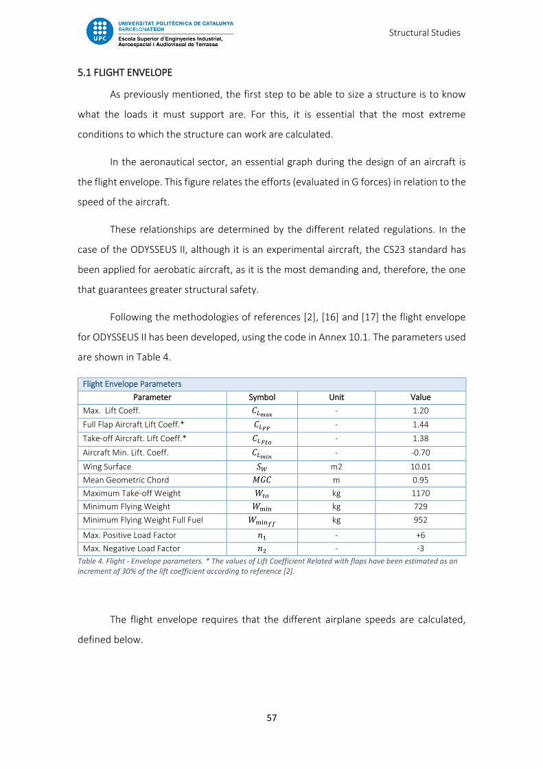
Structural Studies

57

5.1 FLIGHT ENVELOPE

As previously mentioned, the first step to be able to size a structure is to know

what the loads it must support are. For this, it is essential that the most extreme

conditions to which the structure can work are calculated.

In the aeronautical sector, an essential graph during the design of an aircraft is

the flight envelope. This figure relates the efforts (evaluated in G forces) in relation to the

speed of the aircraft.

These relationships are determined by the different related regulations. In the

case of the ODYSSEUS II, although it is an experimental aircraft, the CS23 standard has

been applied for aerobatic aircraft, as it is the most demanding and, therefore, the one

that guarantees greater structural safety.

Following the methodologies of references [2], [16] and [17] the flight envelope

for ODYSSEUS II has been developed, using the code in Annex 10.1. The parameters used

are shown in Table 4.

Flight Envelope Parameters

Parameter Symbol Unit Value

Max. Lift Coeff. 𝐶𝐿max - 1.20

Full Flap Aircraft Lift Coeff.* 𝐶𝐿𝐹𝐹 - 1.44

Take-off Aircraft. Lift Coeff.* 𝐶𝐿𝐹𝑡𝑜 - 1.38

Aircraft Min. Lift. Coeff. 𝐶𝐿𝑚𝑖𝑛 - -0.70

Wing Surface 𝑆𝑊 m2 10.01

Mean Geometric Chord 𝑀𝐺𝐶 m 0.95

Maximum Take-off Weight 𝑊𝑡𝑜 kg 1170

Minimum Flying Weight 𝑊min kg 729

Minimum Flying Weight Full Fuel 𝑊min𝑓𝑓 kg 952

Max. Positive Load Factor 𝑛1 - +6

Max. Negative Load Factor 𝑛2 - -3

Table 4. Flight - Envelope parameters. * The values of Lift Coefficient Related with flaps have been estimated as an increment of 30% of the lift coefficient according to reference [2].

The flight envelope requires that the different airplane speeds are calculated,

defined below.

Structural Studies

58

Maximum Speed in Level Flight

It is considered the maximum speed defined in the requirements,

𝑉𝐻 = 220 𝐾𝐸𝐴𝑆

Stall Speeds

It are considered four stall speeds for the four principal flight configurations of the

aircraft. This speeds must be proved in flight as the requirement 4.4.1 of the reference

[17] dictate,

Flaps retracted (cruise configuration)

𝑉𝑠 = √2𝑊𝑡𝑜 · 𝑔

𝜌𝑜𝐶𝐿𝑚𝑎𝑥𝑆𝑤

(3)

Flaps full extended (landing configuration)

𝑉𝑠𝑜 = √2𝑊𝑡𝑜 · 𝑔

𝜌𝑜𝐶𝐿𝑚𝑎𝑥𝐹𝐹𝑆𝑤

(4)

Flaps partial extended (Take-off configuration)

𝑉𝑠1 = √2𝑊𝑡𝑜 · 𝑔

𝜌𝑜𝐶𝐿𝑚𝑎𝑥𝐹𝑡𝑜𝑆𝑤

(5)

Flaps retracted (Inverted cruise configuration)

𝑉𝑠2 = √2𝑊𝑡𝑜 · 𝑔

𝜌𝑜|𝐶𝐿𝑚𝑖𝑛|𝑆𝑤

(6)

Structural Studies

59

Design Manoeuvring Speeds

The next speed to define is the design manoeuvring speed. According to

requirement 5.2.4.1 [17] which is defined by the expression 7,

𝑉𝐴 = 𝑉𝑆√𝑛1 (7)

Flap Maximum Operating Speed

The flap maximum operating speed must be equal to or greater than the highest

speed defined by the expressions 23 and 24 according to 5.2.4.2 [17],

𝑉max 𝐹 = 1.4𝑉𝑆 (8)

𝑉max 𝐹 = 2𝑉𝑆𝑂 (9)

Flap Maximum Extended Speed

It is chosen the flap maximum extended speed the same as the flap maximum

operating speed.

Design Cruise Speed

According to requirement 5.2.4.3 [17], the cruising speed must be chosen within

the limits established by the equation 10 and 11,

𝑉𝐶𝑚𝑖𝑛 = 4.77√𝑊𝑡𝑜 · 𝑔

𝑆

(10)

𝑉𝐶𝑚𝑎𝑥 = 0.9𝑉𝐻 (11)

Design Dive Speed

According to requirement 5.2.4.4 [31] the minimum dive speed must be,

𝑉𝐷 = 1.4𝑉𝑐𝑚𝑖𝑛 (12)

Structural Studies

60

Never Exceed Speed

This speed should be equal to or greater than 1.1 cruise speed, and must be equal

to or less than 0.9 dive speed.

Once the different speeds of the aircraft are calculated, the gust loads are

computed. For this, the calculation method proposed in appendices of [15] is used. The

appendix also states that for cruise speed a gust of 15 m/s should be considered, whereas

a 7.5 m/s gust must be considered for dive and flaps extended flights.

Thus, using the expression 13, the loads produced by the gust are evaluated for

different weights of the aircraft (maximum weight, minimum flying weight and minimum

flying weight with full fuel). Then, the maximum gust load factors are drawn in the flight

envelope.

𝑛3/4 = 1 ±

12 𝜌𝑜𝑘𝑔𝑉𝑎𝑈𝑑𝑒

𝑊𝑆

(13)

Where 𝑎 = (𝑑𝐶𝐿

𝑑𝛼) = 4.97

𝑟𝑎𝑑

𝑠 , 𝑘𝑔 = 0.88 ·

𝜇𝑔

5.3+𝜇𝑔 and 𝜇𝑔 =

2𝑊

𝜌𝑜𝑀𝐺𝐶𝑎𝑆𝑤

In Figure 40, the flight envelope of ODYSSEUS II calculated by the code of Annex

10.1 is observed.

The values obtained show how the most extreme situations consist of the upper

and lower limits of the maneuvering curve. This is because by requiring that the load

factor values be + 6 / -3.

On the other hand, it can be seen how the most extreme value of all is that in

which the plane flies at maximum speed with the maximum G positive. This point is the

one that will be used to analyze the structure of the aircraft

Structural Studies

61

Figure 40. ODYSSEUS II Flight Envelope

5.2 STRUCTURE PRE-SIZING

The process that is exposed below is extracted from the reference [15], which

corresponds to the thesis of the degree of the author of the project.

Said that, the analysis carried out below are considering a level flight with

symmetric loads under different Gs conditions.

To carry out a first estimation of the structural design in order to calculate the

different thicknesses necessary for the structure to resist, the assumptions of the

reference [2] are used. In it, the wing is idealized as a D composed of a skin, two caps and

a shear web. The first is responsible for supporting the torque moment, the caps of the

beam are in charge of the bending moment and shear web holds the shear efforts, as

shown in figures 41 and 42.

Structural Studies

62

Figure 41. Wing Section idealization. Extracted from [2]

Figure 42. Loads in the idealized wing. Extracted from [2]

The thickness of the skin is calculated by following the procedure described

below. For this, it is considered that entire torque is fully supported by the skin, and is

calculated by the expression 29.

𝑇 =1

2𝜌𝑉𝐷

2𝑆𝑤

2· 𝑀𝐺𝐶 · |𝐶𝑚 |

(14)

From the expression of the shear stress in the root can be extracted the thickness

of the skin as,

𝑡𝑠𝑘𝑖𝑛 =|𝑇|

2𝐴𝑐𝑒𝑙𝑙𝜏𝑚𝑎𝑥

(15)

Structural Studies

63

The area of the idealized cell is defined as,

𝐴𝑐𝑒𝑙𝑙 =4𝐶𝑐𝑒𝑙𝑙ℎ/3

3

(16)

Where 𝐶𝑐𝑒𝑙𝑙 is the root chord minus the flap and ℎ is the airfoil thickness.

Finally, the maximum shear stress is defined as the maximum tensile strength of

the material divided by the shear strength of 1.5 indicated by the CS-LSA snd CS-23

standards.

𝜏𝑚𝑎𝑥 =𝜏𝑔𝑙𝑎𝑠𝑠𝑓𝑖𝑏𝑒𝑟

𝐹𝑆 (17)

The calculation of the shear web thickness is performed considering that the shear

stress is reacted entirely by this and that the maximum requirement is in the root. Thus,

the shear effort is defined as,

𝑉 =1

2𝑛𝑚𝑎𝑥𝑊

(18)

The shear web thickness can be obtained from the expression of the shear stress.

𝑡𝑤𝑒𝑏 =3

4

𝑛𝑚𝑎𝑥𝑊

ℎ𝜏𝑚𝑎𝑥

(19)

As before, the maximum shear stress is defined as,

𝜏𝑚𝑎𝑥 =𝜏𝑐𝑎𝑟𝑏𝑜𝑛

𝐹𝑆 (20)

The procedure of obtaining these expressions is described in reference [2].

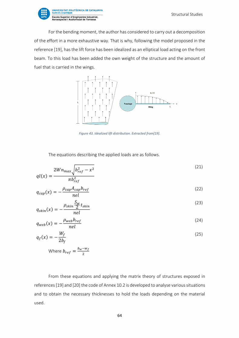
Structural Studies

64

For the bending moment, the author has considered to carry out a decomposition

of the effort in a more exhaustive way. That is why, following the model proposed in the

reference [19], has the lift force has been idealized as an elliptical load acting on the front

beam. To this load has been added the own weight of the structure and the amount of

fuel that is carried in the wings.

Figure 43. Idealized lift distribution. Extracted from[19].

The equations describing the applied loads are as follows.

𝑞𝑙(𝑥) =

2𝑊𝑛𝑚𝑎𝑥√𝑏𝑟𝑒𝑓2 − 𝑥2

𝜋𝑏𝑟𝑒𝑓2

(21)

𝑞𝑐𝑎𝑝(𝑥) = −𝜌𝑐𝑎𝑝𝐴𝑐𝑎𝑝𝑏𝑟𝑒𝑓

𝑛𝑒𝑙

(22)

𝑞𝑠𝑘𝑖𝑛(𝑥) = −𝜌𝑠𝑘𝑖𝑛

𝑆𝑤

2 𝑡𝑠𝑘𝑖𝑛

𝑛𝑒𝑙

(23)

𝑞𝑤𝑒𝑏(𝑥) = −𝜌𝑤𝑒𝑏𝑏𝑟𝑒𝑓

𝑛𝑒𝑙

(24)

𝑞𝑓(𝑥) = −𝑊𝑓

2𝑏𝑓

(25)

Where 𝑏𝑟𝑒𝑓 =𝑏𝑤−𝑤𝑓

2

From these equations and applying the matrix theory of structures exposed in

references [19] and [20] the code of Annex 10.2 is developed to analyse various situations

and to obtain the necessary thicknesses to hold the loads depending on the material

used.

Structural Studies

65

5.2.1 Main Wing Sizing

To pre-size the structural elements of the main wing, the data chosen in the

following table have been used.

It has been considered that the main wing generates a lift of 75% of the overall lift

of the aircraft. In turn, the structure has been analysed without counting the weight of

the fuel in the wings, as this is an element that helps reduce the load to which the

structure is subject.

Main Wing Pre-sizing Parameters

Parameter Symbol Unit Value

Max. Take-off Weight 𝑀𝑇𝑂𝑊 kg 877.5

Mean Geometric Chord 𝑀𝐺𝐶 m 0.95

Wing Surface 𝑆𝑊 m2 10.50

Airfoil Thickness 𝑡𝑎𝑖𝑟𝑓 % 12

Wingspan 𝐵𝑤 m 10.01

Reference Moment Coefficient 𝐶𝑚𝑟𝑒𝑓 - -0.186

Security Factor 𝐹𝑆 - 3

Wide Spar Cap 𝑤𝑐𝑎𝑝 m 0.12

Estimated Cap Thickness 𝑡𝑐𝑎𝑝 m 0.02

Load Factor 𝑛 - 6

Table 5. Main Wing Pre-sizing Parameters.

The characteristics of the material used have been obtained from the reference

[2]. The homogenized properties of an epoxy-based composite material and

reinforcements in carbon fiber, and another with epoxy base and fiberglass

reinforcements have been used.

The properties of both materials are shown in the following table.

Materials’ Mechanical Properties

Parameter Symbol Units Carbon Fibre + Epoxy Glass Fibre + Epoxy

Density 𝜌 kg/m3 1590 1770

Young Modulus 𝐸 GPa 67.6 24.8

Ultimate Yield Tensile 𝜎𝑢𝑙𝑡 MPa 835 320

Ultimate Shear Tensile 𝜏𝑢𝑙𝑡 MPa 97 99

Table 6. Materials' Mechanical Properties

The results obtained after carrying out the necessary calculations are shown in

the following table.

Structural Studies

66

In the first place, the minimum skin value necessary to support the load values for

the most extreme flight conditions of the flight envelope calculated in section 5.1 has

been obtained.

In turn, the table also shows the maximum displacement of the wing tip.

Main Wing Sizing Results

Parameter Skin Thickness [mm] Shear Web Thickness

[mm]

Tip Vertical Displacement

[mm]

Speed: 250 Kts

n: +6 G 2.96 10.30 578

Speed: 250 Kts

n: -3 G 2.96 5.15 -289

Speed: 70 Kts

n: +1.5 G 0.22 2.57 129

Speed: 100 Kts

n: -1 G 0.44 1.71 87

Table 7. Main Wing Sizing Results.

As can be seen, the most extreme case and that requires higher thicknesses is the

one made at 250 𝑘𝑡𝑠 and with a load factor of +6. These conditions are those used to size

the structure, with the values obtained, and are the boundary conditions that will be used

during the FEM analyzes.

The following figure shows the different distribution of loads and the response of

the structure obtained after the analysis of 250 𝑘𝑡𝑠 and +6 𝐺.

Structural Studies

67

Figure 44. Main Wing Pre-sizing Results.

5.2.2 Front Wing Sizing & Tail Sizing

The same process that has previously been carried out to size the main

malfunction is then applied to size the front wing and tail. The materials used, as well as

the wing structure, are the same.

Following tables collect the results of the front wing and tail. It is thus observed

that the most critical conditions remain the same as before.

Structural Studies

68

Front Wing Pre-sizing Parameters

Parameter Symbol Unit Value

Max. Take-off Weight (15%) 𝑀𝑇𝑂𝑊 kg 175.5

Mean Geometric Chord 𝑀𝐺𝐶 m 0.35

Wing Surface 𝑆𝑊 m2 1.53

Airfoil Thickness 𝑡𝑎𝑖𝑟𝑓 % 14

Wingspan 𝐵𝑤 m 4.40

Reference Moment Coefficient 𝐶𝑚𝑟𝑒𝑓 - -0.40

Security Factor 𝐹𝑆 - 3

Wide Spar Cap 𝑤𝑐𝑎𝑝 m 0.03

Estimated Cap Thickness 𝑡𝑐𝑎𝑝 m 0.02

Load Factor 𝑛 - 6

Table 8. Front Wing Pre-sizing Parameters.

Front Wing Sizing Results

Parameter Skin Thickness [mm] Shear Web Thickness

[mm]

Tip Vertical Displacement

[mm]

Speed: 250 Kts

n: +6 G 2.26 4.79 80

Speed: 250 Kts

n: -3 G 2.26 2.40 -40

Speed: 70 Kts

n: +1.5 G 0.17 1.19 15

Speed: 100 Kts

n: -1 G 0.33 0.79 -10

Table 9. Front Wing Sizing Results.

Tail Wing Pre-sizing Parameters

Parameter Symbol Unit Value

Max. Take-off Weight (10%) 𝑀𝑇𝑂𝑊 kg 117

Mean Geometric Chord 𝑀𝐺𝐶 m 0.50

Wing Surface 𝑆𝑊 m2 5.30

Airfoil Thickness 𝑡𝑎𝑖𝑟𝑓 % 8

Wingspan 𝐵𝑤 m 2.40

Reference Moment Coefficient 𝐶𝑚𝑟𝑒𝑓 - -0.01

Security Factor 𝐹𝑆 - 3

Wide Spar Cap 𝑤𝑐𝑎𝑝 m 0.045

Estimated Cap Thickness 𝑡𝑐𝑎𝑝 m 0.02

Load Factor 𝑛 - 6

Table 10. Tail Pre-sizing Parameters.

Structural Studies

69

Front Wing Sizing Results

Parameter Skin Thickness [mm] Shear Web Thickness

[mm]

Tip Vertical Displacement

[mm]

Speed: 250 Kts

n: +6 G 0.24 3.91 13

Speed: 250 Kts

n: -3 G 0.24 1.95 -7

Speed: 70 Kts

n: +1.5 G 0.018 0.98 3

Speed: 100 Kts

n: -1 G 0.04 0.65 -2

Table 11. Front Wing Sizing Results.

Structural Studies

70

5.3 FINITE ELEMENT ANALYSIS

Composite materials are non-isotropic materials that have different behaviors

depending on the orientation of the fibers and applied loads.

When simulating a composite material, different types of studies can be carried

out depending on the purpose and the object of study of the same, and depending on

the scale at which you are working.

As shown in Figure 45, there are three types of studios in finite elements on

composite materials.

Figure 45. Composite Analysis Scales. Extracted from [19].

In essence, there is the so-called unit cell, which consists in evaluating the

behavior of a single reinforcing fiber inside a cubic cell of resin. This type of studies is

carried out when parameterizing the behavior of the compound at a micro scale, studying

how it reacts against the different types of loads.

When several unit cells are joined, the study scale can be raised to the level known

as the laminate scale. In this type of studies it is intended to find homogenized properties

of the study material in order to be able to apply these properties to a structure, being

able to analyze their real behavior.

As the computational cost of performing simulations in composite materials is

very high, in order to carry out the studies in this thesis, the analysis performed are based

in structural scale.

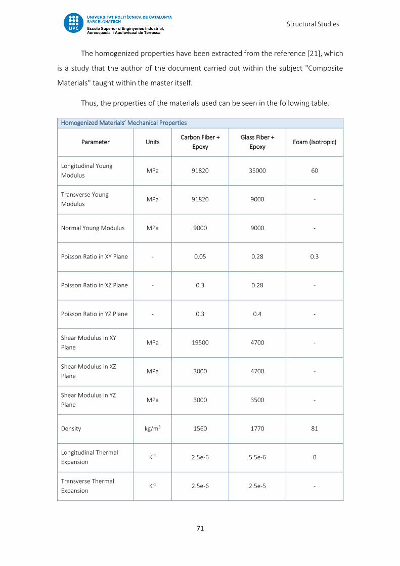
Structural Studies

71

The homogenized properties have been extracted from the reference [21], which

is a study that the author of the document carried out within the subject "Composite

Materials" taught within the master itself.

Thus, the properties of the materials used can be seen in the following table.

Homogenized Materials’ Mechanical Properties

Parameter Units Carbon Fiber +

Epoxy

Glass Fiber +

Epoxy Foam (Isotropic)

Longitudinal Young

Modulus MPa 91820 35000 60

Transverse Young

Modulus MPa 91820 9000 -

Normal Young Modulus MPa 9000 9000 -

Poisson Ratio in XY Plane - 0.05 0.28 0.3

Poisson Ratio in XZ Plane - 0.3 0.28 -

Poisson Ratio in YZ Plane - 0.3 0.4 -

Shear Modulus in XY

Plane MPa 19500 4700 -

Shear Modulus in XZ

Plane MPa 3000 4700 -

Shear Modulus in YZ

Plane MPa 3000 3500 -

Density kg/m3 1560 1770 81

Longitudinal Thermal

Expansion K-1 2.5e-6 5.5e-6 0

Transverse Thermal

Expansion K-1 2.5e-6 2.5e-5 -

Structural Studies

72

Normal Thermal

Expansion K-1 1.0e-5 2.5e-5 -

Longitudinal Tensile

Stress MPa 829 780 60

Longitudinal

Compressive Stress MPa -439 -480 -

Transverse Tensile Stress MPa 829 31 -

Transverse Compressive

Stress MPa -829 -100 -

Shear Stress Limit in XY

Plane MPa 120 60 -

Shear Stress Limit in XZ

Plane MPa 50 60 -

Shear Stress Limit in YZ

Plane MPa 50 35 -

Table 12 Homogenized Material's Mechanical Properties.

5.3.1 Main Wing Analysis

By means of the Generative Structural Analysis module of CATIA V5 and the shell

model developed in section 3.2, analyses of the wing under static load has been carried

out in the most extreme conditions calculated previously.

Static load analysis is one of the most demanding because the structure is

subjected to a load much higher than the one that can really undergo during the flight.

This first analysis is used to evaluate the conceptual design of the structure and

thus have more or less accurate data to work with in order to optimize the structure and

be able to carry out the detailed design of the aircraft.

The mesh that has been carried out meets high computational requirements,

since a 20 𝑚𝑚 mesh with a 1 𝑚𝑚 sag has been calculated. The computational requirement

is high because the size of the structure is very large compared to the size of the cell,

which means that the number of operations to be performed is of the order of millions.

Structural Studies

73

Figure 46. Main Wing Mesh.

As an anchoring point for the first analysis, a restriction of 6 degrees of freedom

has been chosen for the spar and the stringers that protrude from the structure of the

wing. This pretends to simulate the union of the wing with the fuselage.

On the other hand, a load has been distributed uniformly in the area marked in

orange in Figure 47. This load is equivalent to 75% of the total lift obtained by flying at

250 𝑘𝑡𝑠 and 6 𝐺.

In turn, a load has been applied along the X-axis that simulates the drag in these

conditions. This drag has been calculated using the polar curve calculated in the

aerodynamics section,

𝐿 = 25825 𝑁 (26)

𝐷 = 3705 𝑁 (27)

Structural Studies

74

Figure 47. Wing Boundary Conditions.

As shown in figures 48, 49 and 50 the results obtained indicate that the wing bears

the extreme conditions that have been imposed.

On the one hand, it can be observed how the maximum Von Misses Stress

obtained is 500 𝑀𝑃𝑎 and it is placed on the central spar below the first rib. This point

where the tensions are concentrated, has a calculated safety factor of 1.65, higher than

the minimum required by the 1.5 standard.

On the other hand it can be seen that the vertical displacement of the tip is

148 𝑚𝑚, much lower than that calculated in the pre-sizing phase.

Finally, it can be observed how there is tension concentration on the skin at those

points where it joins with the ribs.

For a more detailed design of the structure, the author of the study proposes that

the thickness of the skin be increased at said points to provide greater structural strength

to the whole.

Structural Studies

75

Figure 48. Von Misses Stress over skin.

Figure 49. Von Misses Stress over the internal structure.

Figure 50. Wing Displacements.

Structural Studies

76

5.3.2 Tail Analysis

The analysis of the tail has been carried out maintaining the same characteristics

as in the previous analysis, both mesh and loading conditions.

For the case in question, a load has been distributed on the external surface of

the tail, generating a torque around the X-axis. That is, for the right half-shell a positive

lift has been produced with a value equivalent to the lift at 250 𝑘𝑡𝑠. and 6 𝐺, and for the

left side a negative lift with the same value. In addition, the drag has been added.

𝐿 = ± 3443 𝑁 (28)

𝐷 = 1324 𝑁 (29)

Figure 51. Tail Mesh and Boundary Conditions.

The results observed in Figure 52 show that there are two critical points of the

structure, which are the joint of the tail and the arrow change in the front tube.

In these two points the value of the Von Misses voltage is 694 𝑀𝑃𝑎, which equals

a safety factor of 1.21. This value of the safety factor is lower than the 1.50 required by

the regulations, so the design of the structure should be revised in future iterations.

A proposal to solve this problem would be to add more layers of fiber in those

points or replace the tube with one with a wider thickness.

Structural Studies

77

Figure 52. Von Misses Stress over Tail.

Performance Studies

78

6. PERFORMANCE STUDIES

6.1 WEIGHT AND BALANCE

In the following section the estimation of the overall weight of the structure is

exposed and a preliminary study is carried out to obtain the CG - Envelope chart. To

perform these actions, the estimates and procedures shown in reference [2] and [22]

have been followed.

The first step to determine the weight of the aircraft and calculate its CG is to

define a coordinate system that is used to reference the position of the different

components. In Figure 53, said reference system is shown.

As can be seen, the origin of coordinates is located in the nose of the plane. The

X-axis takes the direction from nose to tail, the Y-axis follows the direction of the wing of

the plane with positive direction towards the right point and the Z-axis takes the vertical

direction.

The chosen coordinate system has these characteristics since it is the reference

system used by the XFLR5 program and that has been transferred to CATIA V5. In this

way, and with a common reference system, the design process is facilitated when

carrying out the different iterations.

Figure 53. Aircraft Reference System

Z

X

Performance Studies

79

6.1.1 Weight Estimation

The estimation of the global weight of the aircraft has been carried out through a

combination between the estimation of the components designed in CAD and the two

semi-analytical estimation methodologies developed by the engineers D. P. Raymer and

L.M. Nicolai, which are applied in those components that have not been designed.

In those components in which the approximations of D. P. Raymer and L. M.

Nicolai are notably different, it has been decided to use an arithmetic mean to obtain the

weight estimation.

The following table shows the input data that has been used to carry out the

calculations of the weights of the non-designed components.

Weight Estimation Inputs

Parameter Symbol International System Imperial System

Total Fuel Quantity Qtot 280 L 74 gal

Fuel Quantity in Integral Fuel Tanks Qint 280 L 74 gal

Number of Tanks Ntank 3 3

Number of Engines Neng 1 1

Number of Occupants Nocc 4 4

Number of Crew Ncrew 2 2

Length of Fuselage Structure LFS 6847 mm 22.5 ft

Length of the Main Landing Gear Sturt Lm 790 mm 31 in

Wingspan BW 10500 mm 34.5 ft

Ultimate Load Factor nl 6 6

Maximum Take-off Weight Wo 1170 kg 2579 lb

Weight of unmounted avionics WAV 5 kg 11 lb

Weight of the Engine Weng 140 kg 257 lb

Mach Number M 0.258 0.258

Dynamic Pressure qh 4636 Pa 97 lb/ft2

Table 13. Weight Estimation Inputs

Performance Studies

80

The estimates of the components not designed in CATIA V5 are shown below.

Landing Gear

Raymer 𝑊𝑀𝐿𝐺 = 0.095(𝑛𝑙𝑊𝑜)0.768 (

𝐿𝑚

12)

0.409

= 231 𝑙𝑏 = 105 𝑘𝑔 (30)

Nicolai 𝑊𝑀𝐿𝐺 = 0.054(𝑛𝑙𝑊𝑜)0.684 (

𝐿𝑚

12)

0.601

= 70 𝑙𝑏 = 32 𝑘𝑔 (31)

Average 𝑊𝑀𝐿𝐺 = 68.5 𝑘𝑔

Fuel system

Raymer 𝑊𝐹𝑆 = 2.49𝑄𝑡𝑜𝑡

0.726 (𝑄𝑡𝑜𝑡

𝑄𝑡𝑜𝑡 + 𝑄𝑖𝑛𝑡)

0.363

𝑁𝑡𝑎𝑛𝑘0.242𝑁𝑒𝑛𝑔

0.157

= 57.5 𝑙𝑏 = 26 𝑘𝑔

(32)

Nicolai 𝑊𝐹𝑆 = 2.49 [𝑄𝑡𝑜𝑡

0.6 (𝑄𝑡𝑜𝑡

𝑄𝑡𝑜𝑡 + 𝑄𝑖𝑛𝑡)

0.3

𝑁𝑡𝑎𝑛𝑘0.2 𝑁𝑒𝑛𝑔

0.13]

1.21

=

= 57.5 𝑙𝑏 = 26 𝑘𝑔

(33)

Average 𝑊𝐹𝑆 = 26 𝑘𝑔

Control system

Raymer 𝑊𝐶𝑇𝑅𝐿 = 0.053𝐿𝐹𝑆1.536𝐵𝑊

0.371(𝑛𝑙𝑊𝑜 · 10−4)0.8 = 33 𝑙𝑏 = 15 𝑘𝑔 (34)

Nicolai 𝑊𝐶𝑇𝑅𝐿 = 1.066𝑊𝑜0.626 = 66 𝑘𝑔 (35)

Average 𝑊𝐶𝑇𝑅𝐿 = 40.5 𝑘𝑔

Mounted avionics

Raymer 𝑊𝐴𝑉 = 2.117𝑊𝑈𝐴𝑉0.933 = 20 𝑙𝑏 = 9 𝑘𝑔 (36)

Nicolai 𝑊𝐴𝑉 = 2.117𝑊𝑈𝐴𝑉0.933 = 20 𝑙𝑏 = 9 𝑘𝑔 (37)

Average 𝑊𝐴𝑉 = 9 𝑘𝑔

Performance Studies

81

Electrical system

Raymer 𝑊𝐸𝐿 = 12.57(𝑊𝐹𝑆 + 𝑊𝐴𝑉)0.51 = 115.5 𝑙𝑏 = 52 𝑘𝑔 (38)

Nicolai 𝑊𝐸𝐿 = 12.57(𝑊𝐹𝑆 + 𝑊𝐴𝑉)0.51 = 115.5 𝑙𝑏 = 52 𝑘𝑔 (39)

Average 𝑊𝐸𝐿 = 52 𝑘𝑔

Hydraulic system

Raymer 𝑊𝐻𝑌𝐷 = 0.001𝑊𝑜 = 2.6 𝑙𝑏 = 1 𝑘𝑔 (40)

Nicolai 𝑊𝐻𝑌𝐷 = 0.001𝑊𝑜 = 2.6 𝑙𝑏 = 1 𝑘𝑔 (41)

Average 𝑊𝐻𝑌𝐷 = 1𝑘𝑔

Furnishings

Raymer 𝑊𝐹 = 0.0582𝑊𝑜 − 65 = 85 𝑙𝑏 = 39.5 𝑘𝑔 (42)

Nicolai 𝑊𝐹 = 34.5𝑁𝑐𝑟𝑒𝑤𝑞ℎ0.25 = 216 𝑙𝑏 = 98 𝑘𝑔 (43)

Average 𝑊𝐹 = 69 𝑘𝑔

The table below shows the empty weight of the airplane taking into account the

previously calculated estimates and the values obtained from the CAD design.

Component Weight [kg ] Xcg

[mm]

Ycg

[mm]

Zcg

[mm] Determined by

Main Wing 112 5455 0 434 CAD

Canard 10 1591 0 112 CAD

Tail and Fuselage 118 4264 0 428 CAD

Landing Gear 68.5 2764 0 205 Estimation & CAD

Engine 140 6200 0 600 Technical Sheets

Fuel System 26 5243 0 420 Estimation & CAD

Control System 40.5 5243 0 420 Estimation & CAD

Mounted Avionics 9 2409 0 775 Estimation & CAD

Electrical System 52 2417 0 600 Estimation & CAD

Hydraulic System 1 2764 0 205 Estimation & CAD

Furnishings 69 3690 0 460 Estimation & CAD

Empty Aircraft 646 4492 0 463 Estimation

Table 14. Aircraft weights and centers of gravity. All the CG positions have been obtained from the CAD representation.

Performance Studies

82

6.1.2 CG - Envelope

The CG - Envelope chart provides key information for the pilot when loading and

distributing the weight, both passage and fuel.

For this reason, the author of the project considered it appropriate to calculate

this envelope and whether to perform a first iteration of the calculation of static and

dynamic stability, which are merely a reflection of the behavior and maneuverability of

the aircraft.

The calculation of the flight envelope is made following the steps established in

the EASA form of reference [23]. Although this form is designated for aircraft under the

CS-LSA category, the procedure is valid for aircraft that are certified under CS-23.

6.1.3 Loading Cases

The following table shows the different components that confer the airplane,

including weight and fuel. These components are used to calculate the aircraft's center

of gravity for different flight configurations and obtain the limit curve.

Weight Items

Item Includes Weight [kg] Xcg [mm] Determined by

Empty aircraft

(WEW)

equipment and all

necessary fluids

(oil, coolant)

except fuel

673 4492 Estimation

Fuel unusable fuel min 11 max 224 5243 Regulations

Pilot min 55 max 100 3065 Regulations

Co-Pilot min 0 max 100 3065 Regulations

Left Passenger min 0 max 100 4310 Regulation

Right Passenger min 0 max 100 4310 Regulations

Table 15. Aircraft Weight Items. It is used the table format of reference

The first step is to calculate the basic empty weight of the plane. This weight

represents the empty weight of the aircraft next to the unusable fuel. This fraction of the

fuel is usually between 5 and 10% of the total fuel of the aircraft [23].

Performance Studies

83

It has been estimated, then, that the basic empty weight of the ODYSSEUS II that

is being studied is of,

𝑊𝐵𝐸𝑊 = 684 𝑘𝑔 (44)

The maximum empty weight is defined as the weight of the empty plane loaded

with an 86 𝑘𝑔 pilot and with enough fuel to fly at a maximum speed of 𝑉ℎ for one hour.

Taking into account the fuel consumption of the engine according to the

manufacturer is approximately 42 𝐿 / ℎ, it is therefore considered that the fuel

consumption needed to fly for one hour is 42 𝐿 or 34 𝑘𝑔. Thus, the maximum empty

weight is of,

𝑊𝑀𝐸𝑊 = 𝑊𝐵𝐸𝑊 + 𝑊𝑝𝑖𝑙𝑜𝑡 + 𝑊min𝐹 = 684 + 86 + 34 = 804 𝑘𝑔 (45)

The minimum flying weight is that which simulates the weight of the airplane

under the maximum load factor entering in a burst and taking into account that the pilot

weights 55 𝑘𝑔.

𝑊𝑚𝑖𝑛𝐹𝐹 = 𝑊𝐵𝐸𝑊 + 𝑊𝑚𝑖𝑛𝑝𝑖𝑙𝑜𝑡 = 684 + 55 = 739 𝑘𝑔 (46)

The maximum weight of zero wing fuel weight is that which takes into account

the empty basic weight plus the weight of the pilot and passengers, as well as unused

fuel.

𝑊𝑀𝑍𝐹 = 𝑊𝐵𝐸𝑊 + 𝑊𝑚𝑎𝑥𝑝𝑖𝑙𝑜𝑡 + 𝑊𝑚𝑎𝑥𝑝𝑎𝑥 = 684 + 200 + 200 = 1084 𝑘𝑔 (47)

The maximum takeoff weight of the aircraft determined by customer

requirements is,

𝑊𝑀𝑇𝑂𝑊 = 1170 𝑘𝑔 (48)

Performance Studies

84

The following table shows the different weights of the airplane that make up

different combinations of situations and their respective centers of gravity calculated

from the equation 48.

As can be seen, the positions fwd and aft of the maximum calculation take of

weight are those calculated by XFLR5 in the static stability section (Figure 32).

Aircraft Weights

Includes Centre of gravity Requirement

Basic Empty

weight 𝑊𝐵𝐸𝑊

all necessary fluids

(oil, coolant) and

unusable fuel

684 kg 5041 mm 4.2.3 (AST)

Minimum flying

weight 𝑊𝑚𝑖𝑛

min pilot and

unusable fuel 729 kg 4894 mm 4.2.2 (AST)

Minimum flying

weight with full

fuel

𝑊𝑚𝑖𝑛𝐹𝐹 min pilot and full

fuel 952 kg 4972 mm

Load

calculation

(EAS)

Maximum zero

wing-fuel weight 𝑊𝑍𝑊𝐹

full useful load of

𝑊𝑙𝑜𝑎𝑑 1084 kg 4542 mm 5.2.1.3 (AST)

Maximum take-

off weight 𝑊𝑀𝑇𝑂𝑊

combination of fuel

and passenger load 1170 kg

fwd

4400 mm

aft

4700 mm CS-LSA.5

Table 16. Loading Cases. Ref. [23]

𝑋𝑐𝑔 =∑ 𝑊𝑖 · 𝑋𝑐𝑔𝑖

∑ 𝑊𝑖

(49)

Performance Studies

85

6.1.4 Center of gravity locations

The CG of the aircraft is determined following the methodology described in the

reference [23] and takes into account the results obtained in section 4.4.2 (Static stability

study).These limits are,

Most forward 4300 𝑚𝑚

Most aft 4700 𝑚𝑚

The limited conditions that are studied below have been calculated based on the

weight predictions in section 6.1.3 and the estimation of the position of the center of

gravity obtained by the CAD design and the equation 49.

These conditions take into account different stages of the use of the airplane,

since they take into account the airplane in flight and the operations on the ground.

As can be seen in graph 54, which represents the flight envelope, all the calculated

combinations are located within the theoretical envelope. Except one.

Those situations in which the load of the plane is located inside the envelope, are

safe situations, because the plane is stable within the limits explained during the

aerodynamic analysis.

In the event of an aircraft’s CG being too far forward, the maneuverability is

compromised in the sense that a higher approach speed is required. With an excessive

aft CG, it becomes an outright dangerous aircraft, since any low speed flight becomes

most of the time unrecoverable. A guaranteed accident.

However, and as a comment for future studies, this point should be thoroughly

reviewed and calculated in more detail if the plane is stable under such conditions.

Performance Studies

86

Condition Pilots [kg] Fuel [kg] Passengers [kg] Aircraft weight

[kg] Aircraft CG [mm]

CG envelope limits for

flight

𝑊𝑀𝑇𝑂𝑊,𝑎𝑓𝑡 73 Max 224 Max 200 1170 4830

𝑊𝑀𝑇𝑂𝑊,𝑓𝑤𝑑 Max 200 111 Max 200 1170 4328

𝑊𝑚𝑖𝑛,𝑎𝑓𝑡 Min 55 Min 11 Min 0 729 4436

𝑊𝑚𝑖𝑛,𝑓𝑤𝑑 Min 55 Min 11 Min 0 729 4436

Loading conditions in

flight

𝑊𝑚𝑖𝑛𝐹𝐹 Min 55 Max 224 Min 0 952 4572

𝑊𝑍𝑊𝐹,𝑎𝑓𝑡 Max 200 Min 11 Max 200 1074 4227

𝑊𝑍𝑊𝐹,𝑓𝑤𝑑 Max 200 Min 11 Min 0 874 4208

𝑊𝑚𝑖𝑛𝐹𝐹𝑏𝑎𝑔 Min 55 Max 224 Max 200 1142 4564

Loading conditions on

ground

𝑊𝐵𝐸𝑊 0 Min 11 0 0 674 4548

𝑊 𝑎𝑓𝑡𝑚𝑎𝑥 0 Min 11 Max 200 874 4493

Table 17. Loading Cases on center of gravity envelope for standard configuration. Ref. [18].

Figure 54. CG-Envelope

550

650

750

850

950

1050

1150

1250

4100 4150 4200 4250 4300 4350 4400 4450 4500 4550 4600 4650 4700 4750

Wei

ght

[kg]

CG Position [mm]

Flight Conditions Flight Envelope Baggage Loading Theorical Envelope

Performance Studies

87

6.2 RANGE ESTIMATION

The range has been estimated through the code of the Annex 10.3 that applies

the Breguet equation, using the methodologies established in the references [2] and [24].

This code was developed by the author of the thesis in the framework of his final degree

thesis.

𝑅𝑎𝑛𝑔𝑒 =𝑉

𝑔·

𝐿

𝐷·

1

𝑆𝐹𝐶· 𝜂𝑝 · ln (

𝑊𝑖𝑛

𝑊𝑓)

(50)

Where 𝑆𝐹𝐶 is defined as the mass flow rate of fuel per unit of thrust in (𝐾𝑔/𝑠/𝑁),

and 𝜂𝑝 is the propeller efficiency.

The calculations have been done using the nominated cruise speed (170 𝑘𝑡𝑠) seen

in the requirements of the thesis.

Other considerations for this estimation is that the total fuel reserve is a 10% of

the total fuel that can carry the airplane, which is translated in 25 𝑘𝑔,

The specific fuel consumption is calculated from the cruise power (around 60% of

the total engine power), and for conservative reasons the propeller efficiency is around

40%.

𝑇𝑐𝑟𝑢𝑖𝑠𝑒 =𝑃𝑐𝑟𝑢𝑖𝑠𝑒

𝑉𝑐𝑟𝑢𝑖𝑠𝑒

(51)

𝑆𝐹𝐶𝑐𝑟𝑢𝑖𝑠𝑒 =𝐹𝐶𝑐𝑟𝑢𝑖𝑠𝑒

𝑇𝑐𝑟𝑢𝑖𝑠𝑒

(52)

Figure 55 shows the payload rage diagram calculated for the ODYSSEUS II plane.

As it is observed, the maximum payload weight that the airplane could carry, counting

passage and equipage, is of 262 𝑘𝑔.

With the airplane fully loaded, it is possible to fly 2200 𝑘𝑚 (red circle in Figure 56).

As the payload weight decreases it is possible to increase the range up to 2750 𝑘𝑚 (blue

circle).

Performance Studies

88

The results of this analysis meet the requirement of having a range of 6.5 hours,

without counting the reserve fuel. 6.5 hours at a speed of 170 𝑘𝑡𝑠 make a range of 2047 𝑘𝑚.

Thus, the plane meets the requirements of the designer.

Figure 55. Payload-Range Diagram

Figure 56. ODYSSEUS II Range over Europe

Conclusions

89

7. CONCLUSIONS

7.1 AERODYNAMIC CONCLUSIONS

In the field of aerodynamics it has been seen that the solution designed by Marc

Kuster is viable and safe. Its commitment to a three-surface aircraft design allows the

behavior of the ODYSSEUS II to be secure and maneuverable.

One of the strengths of this design is the low stall speed thanks to the extra lift

achieved with the use of a canard.

Despite some difficulty in finding the CG range to ensure stability, it is noteworthy

that the ODYSSEUS II is within normal stability limits.

After studying the design in more details, it can be concluded that the ODYSSEUS

II drag is a little higher than that of a conventional airplane with similar characteristics.

This factor, caused by the added surface of the elevator wing, also affects the aircraft's

aerodynamic efficiency, which, as seen in the theoretical exposé, is usually less than that

of a similar aircraft.

Therefore, in view of the studies carried out and in the absence of studying more

carefully the design of flaps and control surfaces, the author of this thesis states that the

aerodynamic design meets the requirements proposed by the designer and current

regulation

7.2 STRUCTURAL CONCLUSIONS

After studying the different existing structural options, a monocoque structure

design is proposed for ODYSSEUS II.

The analysis of this structure shows that both wings and tail structure are safe

within the most extreme conditions of the flight envelope limits as well as complying with

all regulations.

Conclusions

90

Apart from these results, it must be noted that tail structure should be redesigned

as the safety factor does not meet the 1.5 safety factor for conformance.

As a result, the author concludes that it is necessary to carry out more analyzes

on the entire structure of the aircraft, before starting with the detailed designs.

However, the results in general, including the aerodynamics, are good enough to

continue with the project proposed by the designer.

7.3 PERFORMANCE CONCLUSIONS

In the performance section, the CG centering of the aircraft and the range have

been evaluated. It has been seen that the aircraft is well centered in all cases imposed by

the standards, except for one.

Given this, and based on the future structural changes that must be made, the

centering of the aircraft must be recalculated to confirm that all the planned points meet

the requirements.

The calculations are promising and validate the continuation with this design.

Finally, regarding the range, it has been seen that using the engine proposed by

the designer and the data calculated in the different sections of the thesis, the maximum

range of the aircraft meets the minimum requested by Mr. Kuster.

In conversations with the designer, the possibility of replacing the combustion

engine with an electric motor of similar characteristics appeared. An option that, in the

eyes of the thesis author, is entirely valid. This substitution will imply recalculating the

range to make sure that the requirement continues to be met.

Conclusions

91

7.4 THESIS CONCLUSIONS

As conclusions of the thesis, on a personal basis, the author of the project is

strongly satisfied with the results, since he has been able to carry out the study of an

aircraft in the design phase, and which is intended to be built.

On the other hand, the author has been able to carry out a consultant / engineer

role that serves a client with a need. This has been a pleasant experience which I would

not hesitate to repeat.

7.5 FURTHER WORK

As future short-term works, the author of this thesis believes that it is necessary

to conduct more studies on the aerodynamic design, as well as more detailed analysis on

specific elements such as flaps, control surfaces and winglets.

The process of these further studies can be performed in the same manner as

those presented in this thesis.

With respect to the structural field, the author proposes more exhaustive studies

to be carried out such components as the landing gear, the fuselage and canard.

At the same time, a full study of aerolasticity would be convenient, in order to

provide greater design security before the start of construction.

In the long term, the author proposes the fabrication of sample specimens of the

materials intended to be used, including laboratory testings.

Finally, the ODYSSEUS II will be required to pass several non-destructive tests to

prove its safety and reliability.

As for the study of performance, further factors should be studied, such as

maximum speed, landing and take-off distances, climb speed and other maneuvers.

References

92

8. REFERENCES

[1] EAA. Experimental Amateur-Built Aircraft Sourcebook. EAA. 2018 [Online]

https://www.eaa.org/~/media/files/eaa/homebuilders/EAA_ExpAmatuerBuildSo

urcebook

[2] Gudmunsson S. General Aviation Aircraft Design: Applied Methods and

Procedures. First Edition. Elsevier. 2014

[3] FAA. Aviation Maintenance Technician Handbook-Airframe, Volume 1. FAA. 2018

[Online]

https://www.faa.gov/regulations_policies/handbooks_manuals/aircraft/media/a

mt_airFrame_hb_vol_1.pdf

[4] Raymer D. Aircraft Design: A conceptual Approach. AIAA. Fifth Edition 2012

[5] Dassault Systemes. CATIA V5. 3DS. 2019. [Online]

https://www.3ds.com/es/productos-y-servicios/catia/

[6] Horne Thomas A. Stemme S10-VT: Powersailing. AOPA. 2014. [Online]

https://www.aopa.org/news-and-media/all-

news/2014/november/pilot/f_stemme

[7] Domun Y. Aircraft Design Process Overview. Engineeringclicks. 2016 [Online]

https://www.engineeringclicks.com/aircraft-design-process/

[8] Amadori K. On Aircraft Conceptual Design. Linköping University. 2008.

[9] Reed J. A. Improving the aircraft design process using Web-based modeling and

simulation. ACM Trans. Model. Comput. Simul. 2000

[10] Gudmunsson S. APP2: Design of Canard Aircraft. Elsevier. 2014

[11] Anon. Canard Efficiency Myths. Apollo Canard. 2012 [Online]

http://www.apollocanard.com/4_canard%20myths.htm

[12] Airfoiltools. 2019 [Online] http://airfoiltools.com/

[13] Torenbeek E. Synthesis of subsonic airplane design. Delf University. 1976.

References

93

[14] XFLR5. XFLR5 Documentation. XFLR5. 2019 [Online]

http://www.xflr5.com/xflr5.htm

[15] Campos D. Project of a new LSA semi-aerobatic airplane. ESEIAAT. 2017

[16] Sadrey M. Aircraft Performance Analysis. 2009

[17] EASA. CS23 Amendment 3. EASA

[18] Hernández J. Mechanics of unidirectional ply. ESEIAAT. 2018

[19] Doherty D. Analytical Modeling of Aircraft Wing Loads Using MATLAB and

Symbolic Math Toolbox. Mathworks. 2009. [Online].

https://es.mathworks.com/company/newsletters/articles/analytical-modeling-

of-aircraft-wing-loads-using-matlab-and-symbolic-math-toolbox.html

[20] Gil L. Estructures Aeroespacials. UPC. 2016.

[21] Campos. D. Assignment 3: Laminated composite plate. ESEIAAT. 2018

[22] Shpati. G. Aircraft CG Envelopes. 2011 [Online]

http://www.sawe.ca/download/tech2011/Aircraft%20CG%20Envelopes.pdf

[23] EASA. ABCD-FE-01-00 Flight Envelope-v1 08.03.16. EASA

[24] Anon. Aircraft Performance and Flight Mechanics. Clarkson University

[25] Anon. Operation Reference Manual IO-390 Series. Lycoming. 2018

Budget

94

9. BUDGET

The following is the budget of the study carried out in the framework of the thesis

of the end of the master. This budget has been calculated in a detailed manner, as can

be seen in the tables.

Hiring Fees

Concept Responsibility Hours €/hour Total €

Project Management Coordinator 38 70 2.660 €

Project Development Developer 227 40 9.080 €

Software and Licencies - - - 1.164 €

Total 12.904 €

Table 18. Hiring Fees.

Study Development Detail

Department Task Hours Total Hours Total €

Management Requirements Study 4 38 2.660 €

Scheduling 4

Coordination 10

Reporting 20

Aerodynamics Information Research 15 110 4.400 €

Modelling 20

XFLR5 Analysis 25

CFD Analysis 50

Structures Information Research 15 100 4.000 €

CAD Design 50

Structural Pre-sizing 15

Structural Analysis 20

Performances Information Research 5 17 680 €

CG-Envelope 8

Range Study 4

Subtotal 11.740 €

Table 19. Study Development Details

Software and Licences

Software Licence Price €

CATIA V5 R2017 Student 100

Ansys R17 Student 0

XFLR5 Open Source 0

Keyshot 6 HD Version 995

Matlab Student Student 69

Subtotal 1.164 €

Table 20. Software and Licences

Annexes

10. ANNEXES

10.1 FLIGHT ENVELOPE CODE

%% FLIGHT ENVELOPE clear all; clc;

% AIRCRAFT PARAMETERS MTOM = 1170; g = 9.81; MTOW = g * MTOM; Sw = 10; MGC = 1.23; nmax = 6; nmin = -3; nmaxf = 2; nminf = 0;

% Coefficients CLmax = 1.2; Clmax = 1.9; Clff = 2.25; Clto = 2.05; CLmin = -0.7; red = CLmax/Clmax; CLff = red * Clff; CLto = red * Clto; a = 4.97;

% FLIGTH CONDITIONS rho = 1.225;

% SPEEDS [KEAS] % Maximum Speed Vh = 250;

% Stall Speeds Vs = sqrt(2 * MTOW/(rho * CLmax * Sw))/0.5144; Vso = sqrt(2 * MTOW/(rho * CLff * Sw))/0.5144; Vs1 = sqrt(2 * MTOW/(rho * CLto * Sw))/0.5144; Vs2 = sqrt(2 * MTOW/(rho * abs(CLmin) * Sw))/0.5144;

% Design Manoeuvring Speed Va = Vs * sqrt(nmax); Vaneg = Vs2 * sqrt(abs(nmin)); Vaf = Vso * sqrt(nmaxf);

% Flaps Speeds Vf = 120; Vff = Vf;

% Cruise, Dive and Never Exceed Speeds Vc = 170;

Annexes

Vd = 250;

Vne = 250;

% GUST n3c = zeros(100,1); n3d = zeros(100,1); n4c = zeros(100,1); n4d = zeros(100,1);

Udec = 15; Uded = 7.5;

Vudec = linspace (0,Vc); Vuded = linspace (0,Vd);

mug = 2 * MTOW/(rho * MGC * a * Sw); kg = 0.88 * mug/(5.3 + mug);

for i = 1:100 n3c(i) = 1 + 0.5 * rho * kg * Vudec(i) * a * Udec/(MTOW/Sw)

* 0.5144; n3d(i) = 1 + 0.5 * rho * kg * Vuded(i) * a * Uded/(MTOW/Sw)

* 0.5144; n4c(i) = 1 - 0.5 * rho * kg * Vudec(i) * a * Udec/(MTOW/Sw)

* 0.5144; n4d(i) = 1 - 0.5 * rho * kg * Vuded(i) * a * Uded/(MTOW/Sw)

* 0.5144; end

% PLOT seg1 = [Va Vd]; seg2 = [Vd,Vd]; seg3 = [Vaneg Vd]; seg4 = [Vs2 Vs2]; seg5 = [Vs Vs]; seg6 = [Vaf Vff]; seg7 = [Vso Vff]; seg8 = [Vso Vso]; seg9 = [Vff Vff];

% Stall lines V = linspace(Vs,Va); Vneg = linspace(Vs2,Vaneg); Vf = linspace(Vso,Vaf); n = zeros(100,1); nneg = zeros(100,1); nf = zeros(100,1);

for i = 1:100 n(i) = 0.5 * rho * V(i)^2 * Sw * CLmax/MTOW * 0.5144^2; nneg(i) = 0.5 * rho * Vneg(i)^2 * Sw * CLmin/MTOW *

0.5144^2; nf(i) = 0.5 * rho * Vf(i)^2 * Sw * CLff/MTOW * 0.5144^2; end

plot(seg1,[nmax nmax],'-k',...

Annexes

seg6,[nmaxf nmaxf],'-r',... Vudec,n3c, '--b',... seg2,[nmax nmin],'-k',...

seg3,[nmin nmin],'-k',...

seg4,[0 -1], '-k',... seg5,[0 1],'-k',... V,n,'-k',... Vneg,nneg,'-k',... seg7,[0 0],'-r',... Vf,nf,'-r',... seg8,[0 1],'-r',... seg9,[0 nmaxf],'-r',... Vuded,n3d,'--b',... [Vc Vd], [n3c(100) n3d(100)],'--b',... Vudec,n4c,'--b',... Vuded,n4d,'--b',... [Vc Vd],[n4c(100) n4d(100)],'--b');

xlabel('Aispeed [KEAS]') ylabel('Load Factor') ylim([-5 7]) xlim([0 260])

legend('Manoeuvre Diagram', 'Flap Manoeuvre Diagram', 'Gust

Diagram') grid on; grid minor;

Annexes

10.2 STRUCTURE PRE-SIZING

%% WING STRUCTURE PRE-DESIGN clc; clear all; close all; % AIRCRAFT DATA % MTOW: Maximum take-off weight [kg] % MF: Fuel Mass [kg] % Sw: Wing Surface [m^2] % Cmgc: Mean Geometric Chord [m] % t_c: Airfoil thickness [mm] % b: Wingspan [m] % bf: Fuel span [m] % Cmref: Reference moment coefficient % FS: Security factor

% Wing Spar MTOW = 1170*0.10; % Kg MF = 0; % kg Sw = 5.30; % m^2 Cmgc = 0.50; % m t_c = 0.08; b = 2.40; % m bf = 1.85; % m Cmref = -0.01; FS = 3; Sref = Sw/2; % m bref = b/2; % m

% % Canard Spar % MTOW = 15; % Kg % MF = 0; % kg % Sw = 1; % m^2 % Cmgc = 0.47; % m % t_c = 0.11; % b = 3.8; % m % bf = 0; % m % Cmref = -0.4; % FS = 1.5; % Sref = Sw/2; % m % bref = 1.7; % m % % FLIGHT CONDITIONS % nmax: Flight Gs % rho: Air density [kg/m^3] % V: Speed [m/s] % g: Gravity [kg/m^3]

nmax = 6; rho = 1.225; % kg/m^3 V = 130; % m/s g = 9.81; % m/s^2

% MATERIALS PROPERTIES % Carbon Fiber + Epoxy % rhoc: density of carbon fiber [kg/m^3] % sigmac: Ultimate Yield Tensile of carbon fiber [Pa] % Ec: Young Modulus of carbon fiber [Pa]

Annexes

% tauc: Ultimate Shear Tensile of carbon fiber [Pa]

rhoc = 1590; % kg/m^3 sigmac = 835e6; % Pa Ec = 67.6e9; % Pa tauc = 97e6; % Pa

% Glass Fiber + Epoxy % rhog: density of glass fiber [kg/m^3] % sigmag: Ultimate Yield Tensile of glass fiber [Pa] % Eg: Young Modulus of glass fiber [Pa] % taug: Ultimate Shear Tensile of glass fiber [Pa]

rhog = 1770; % kg/m^3 sigmag = 320e6; % Pa Eg = 24.8e9; % Pa taug = 99e6; % Pa

% THICKNESS OF THE SKIN % Skin Parameters E_skin = Eg; rho_skin = rhog; tau_skin = taug/FS;

% Torsion Load at Root Tor = 0.5 * rho * V^2 * Cmgc * Sref * Cmref;

% Cell Characteristics Ccell = 0.65 * Cmgc; h = Cmgc * t_c; Acell = 2/3 * Ccell * h;

% Skin Thickness Computatuon t_skin = abs(Tor)/(2 * Acell * tau_skin);

disp('Skin Thickness [mm]'); disp(t_skin * 1000);

% THICKNESS OF SHEAR WEB % Web Parameters rho_web = rhog; tau_web = taug/FS;

% Shear Load at Root V = nmax * MTOW * g/2; t_web = 3/4 * nmax * g * MTOW/h/tau_web;

disp('Shear Web Thickness [mm]') disp(t_web * 1000);

% THICKNESS OF THE WING SPAR CAPS % Caps Parameters w_cap = 0.12; h_cap = Cmgc * t_c - 2 * t_skin; t_cap = 0.015;

Annexes

A_cap = t_cap * w_cap * 2; rho_cap = rhoc; E_cap = Ec; I_cap = w_cap * h_cap^3/12 - w_cap * (h_cap - 2 *

t_cap)^3/12;

% ANALISYS PROPERTIES nel = 100; % GEOMETRY % nd: problem dimensions % nel: total bars % n: total number of nodes % ngle: elements degrees of freedom % ngl: total degrees of freedom % nnod: number of nodes in bar

% x: node coordenades % T: connectivity table nd = 1; n = nel + 1 ; ngle = 2; ngl = n * ngle ; nnod = 2;

% Computation of X x = zeros(1,n);

for i = 2:n x(i) = bref/nel * (i - 1); end

% Computation of T and xfq T = zeros(2,nel);

for i = 1:nel T(1,i) = i; T(2,i) = i + 1; end

% DISTRIBUTED AND PUNTUAL LOADS Q = zeros(n,1); qf = zeros (n,1); q_cap = zeros (n,1); q_skin = zeros (n,1); q_web = zeros (n,1);

% Estimated Loads for i = 1:n ql = 2 * MTOW * g * nmax * sqrt(bref^2 - x(i)^2)/(pi

* bref^2); q_cap(i) = -rho_cap * A_cap * bref/nel; q_skin(i) = -2 * rho_skin * Sref * t_skin/nel; q_web(i) = -rho_web * bref/nel;

if x(i) >= 0.35 && x(i) <= bf + 0.35

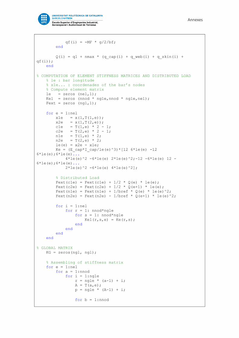
Annexes

qf(i) = -MF * g/2/bf; end

Q(i) = ql + nmax * (q_cap(i) + q_web(i) + q_skin(i) +

qf(i)); end

% COMPUTATION OF ELEMENT STIFFNESS MATRICES AND DISTRIBUTED LOAD % le : bar longitude % x1e... : coordenades of the bar’s nodes % Compute element matrix le = zeros (nel,1); Kel = zeros (nnod * ngle,nnod * ngle,nel); Fext = zeros (ngl,1);

for e = 1:nel x1e = x(1,T(1,e)); x2e = x(1,T(2,e)); c1e = T(1,e) * 2 - 1; c2e = T(2,e) * 2 - 1; n1e = T(1,e) * 2; n2e = T(2,e) * 2; le(e) = x2e - x1e; Ke = (E_cap*I_cap/le(e)^3)*[12 6*le(e) -12

6*le(e);6*le(e)... 4*le(e)^2 -6*le(e) 2*le(e)^2;-12 -6*le(e) 12 -

6*le(e);6*le(e)... 2*le(e)^2 -6*le(e) 4*le(e)^2];

% Distributed Load Fext(c1e) = Fext(c1e) + 1/2 * Q(e) * le(e); Fext(c2e) = Fext(c2e) + 1/2 * Q(e+1) * le(e); Fext(n1e) = Fext(n1e) + 1/bref * Q(e) * le(e)^2; Fext(n2e) = Fext(n2e) - 1/bref * Q(e+1) * le(e)^2;

for i = 1:nel for r = 1: nnod*ngle for s = 1: nnod*ngle Kel(r,s,e) = Ke(r,s); end end end end

% GLOBAL MATRIX KG = zeros(ngl, ngl);

% Assembling of stiffness matrix for e = 1:nel for a = 1:nnod for i = 1:ngle r = ngle * (a-1) + i; A = T(a,e); p = ngle * (A-1) + i;

for b = 1:nnod

Annexes

for j = 1: ngle s = ngle * (b-1) + j; B = T(b,e); q = ngle * (B-1) + j;

KG(p,q) = KG(p,q) + Kel(r,s,e); end end end end

end

% Free Nodes vl = zeros(1,ngl-2);

for i = 2:ngl-2 vl(1) = 3; vl(i) = vl(i-1) + 1; end

% Restricted Nodes vr = [1 2]; Kll = KG(vl,vl); Klr = KG(vl,vr); Krl = KG(vr,vl); Krr = KG(vr,vr);

% Reduce global system ul(vl) = Kll\Fext(vl);

% REACTIONS r(vr) = Krl * ul(vl)' - Fext(vr); R = zeros(ngl,1);

for i = 1:2 R(i) = r(i); end

displ = reshape (ul,ngle,n);

F = Fext + R; B = zeros (n,2); l = zeros(n,1);

for i = 1:n l(i) = (i-1) * bref/nel; stop = 0; for j = 1:n if x(j) > l(i) && stop ==0 n0 = j; stop = 1; end end for k = n0:n

Annexes

s = 2 * k-1;

m = 2 * k;

B(i,1) = B(i,1) + F(s); B(i,2) = B(i,2) + F(m) - F(s) * (l(i) - x(k)); end end

% RESULTS disp('Tip Vertical displacement [m]') disp (displ(1,n));

% PLOTS viga = zeros(1,n); figure (1) h = area (x+0.35,Q); h.FaceColor = 'g'; bl = h.BaseLine; bl.LineWidth = 5; xlim([0 bref+0.35]); xlabel('x[m]') ylabel('Q[N]') title('Loads Diagram')

figure (2) h = area (x+0.35,B(:,1)); h.FaceColor = 'c'; bl = h.BaseLine; bl.LineWidth = 5; xlim([0 bref+0.35]); xlabel('x [m]') ylabel('S [N]') title('Shear Diagram')

figure(3) plot(x,viga,'k','LineWidth',8); h = area (x+0.35,B(:,2)); h.FaceColor = 'm'; bl = h.BaseLine; bl.LineWidth = 5; xlim([0 bref+0.35]); xlabel('x[m]') ylabel('M[Nm]') title('Moment Diagram')

figure(4) xd = linspace(0,bref+0.35,n); DISP = plot(x+0.35,displ(1,:)); hold on; BEAM = plot(xd,viga,'k'); set(BEAM,'LineWidth',5); xlabel('x[m]') ylabel('v[m]') xlim([0 bref+0.35]); title('Displacements')

Annexes

10.3 PAYLOAD RANGE

%% PAYLOAD-RANGE DIAGRAM clear all; clc; close all;

% AIRCRAFT PARAMETERS % Cruise Conditions Vc = 170; % KTS V = Vc * 0.5144; % m/s Dc = 3500; % N g = 9.81; % m/s^2

% Weights MTOW = 1170; % kg MZFW = 946; % kg OEW = 684; % kg MFW = 224; % kg RF = 25; % kg minPL = 55; % kg

% Engine Parameters FC = 42; % L/h FC = 0.8 * FC/3600 ; % kg/s P = 156000 * 0.6; % W T = P/V; % N SFC = FC/T; % kg/s/N rhop = 0.4;

% POINT 1: MAX PAYLOAD-MIN FUEL MPL = MZFW - OEW; R = 0;

% POINT 2: MAX PAYLOAD-MTOW FW1 = MTOW - OEW - MPL - RF; LW1 = MTOW - FW1; E1 = ((MTOW+LW1)/2) * g/Dc; R1 = (V/SFC) * rhop * E1 * log(MTOW/LW1);

% POINT 3: MAX FUEL-MTOW PL2 = MTOW - MFW - OEW; LW2 = MTOW - MFW + RF; E2 = ((MTOW + LW2)/2) * g/Dc; R2 = (V/SFC) * rhop * E2 * log(MTOW/LW2);

% POINT 3: MAX FUEL-MinPL PL3 = minPL; TOW = OEW + MFW + PL3; LW3 = TOW - MFW + RF; E3 = ((MTOW + LW2)/2) * g/Dc; R3 = (V/SFC) * rhop * E3 * log(TOW/LW3);

Range = [R R1 R2 R3]/1000; PL = [MPL MPL PL2 PL3];

plot(Range(1),PL(1),'o',Range(2),PL(2),'o',Range(3),PL(3),'o',...

Annexes

Range(4),PL(4),'o',Range,PL);

grid on;

xlabel ('Range [km]'); ylabel ('Payload Weight [kg]');

legend('Max. Payload-Min. Fuel', 'Max. Payload-MTOW','Max. Fuel-

MTOW',... 'Max Fuel-Min. Flying Weight');

Annexes