2021 - Census and Statistics Department

2021

Census and Statistics Department

Hong Kong Special Administrative Region

Living with Statistics

2021 Edition

Enquiries about this teaching kit can be directed to :

General Statistics Section (1) Census and Statistics Department

Address : 21/F, Wanchai Tower, 12 Harbour Road, Wan Chai, Hong Kong. Tel. : (852) 2582 5054 Fax : (852) 2119 0161

E-mail : [email protected]

Website of the Census and Statistics Department www.censtatd.gov.hk

Published in September 2021

This teaching kit is available in download version only

i

Page

Introduction ii

Part I Official statistics

Chapter 1 Population size and growth 3 – 26

Chapter 2 Population structure 27 – 50

Chapter 3 Impact of changes in population and its structure on society

51 – 70

Chapter 4 Other official statistics 71 – 100

Part II Survey methods and basic statistical concepts

Chapter 5 Survey methods 103 – 118

Chapter 6 Uses and misuses of statistics 119 – 142

Chapter 7 Rate, ratio, proportion and percentage 143 – 150

Chapter 8 Measures of central tendency 151 – 164

Chapter 9 Measures of dispersion 165 – 174

Solutions to exercises 175 – 188

Enquiries on Statistical Data 189

ii

As part of the programme for promoting statistical literacy, the Census and Statistics Department (C&SD) releases annually the teaching kit entitled “Living with Statistics”. The teaching kit aims mainly at providing secondary school teachers and students with a convenient means of accessing reference materials on commonly used statistical methods and official statistics in Hong Kong. It also touches upon statistical methods as well as possible pitfalls that should be avoided in applying statistics.

With a better understanding of official statistics and proper statistical methods, students will be able to enhance their awareness and appreciation of statistical information in interpreting the social and economic situations of our society in an objective and effective manner.

The following symbols are used throughout the teaching kit :

# Provisional figures

@ Figures are subject to revision later on

[This page is intentionally left blank]

Introduction

Population estimates are widely used by the Government for planning and policy

formulation. The private sector and the academia also use population estimates for

business or research purposes.

Births, deaths and net movements(1) are the three factors that affect population

growth. This chapter describes how the size of a population and its change can be

measured. Various statistical indicators of their trends are also introduced.

Finally, a few general characteristics of population growth are outlined in relation to

these determining factors.

Concepts of compiling population estimates

Basically, there are two enumeration concepts to count the population of a

country / territory, namely the “de jure” concept and the “de facto” concept.

Under the “de jure” concept, all persons who usually live in a country / territory at a

particular reference time-point (usually taken as the middle of a year) will be counted

as the population of the country / territory.

Under the “de facto” concept, the population includes all persons who are in the

country / territory at the reference time-point. This method is equivalent to taking a

“snapshot” of the population at a reference time-point.

In practice, the two concepts can be used in conjunction.

Previous method of compiling population estimates in Hong Kong

The “extended de facto” method was used for compiling the series of population

estimates for Hong Kong up to 1995. Under the “extended de facto” approach, the

Hong Kong population covers all persons who are physically in Hong Kong at the

reference time-point, including Hong Kong Permanent Residents and Hong Kong

Non-permanent Residents as well as visitors. “Extended” relates to the fact that for

a Hong Kong Permanent Resident, he / she will still be counted as part of the

Note :

(1) In the case of Hong Kong, movements of people from Hong Kong to overseas countries, the

mainland of China (the Mainland) or Macao for living, studying or working, and vice versa, are

all regarded as movements.

3

Hong Kong population if, at the reference time-point, he / she is not in Hong Kong

but is temporarily in the mainland of China (the Mainland) or Macao.

The application of the “extended” compilation method in the past was intended to

avoid fluctuations in the population estimates around major public holidays when

there were enormous temporary movements of people between Hong Kong and the

Mainland / Macao.

Current method of compiling population estimates in Hong Kong

As from August 2000, the “resident population” method has been adopted in

compiling the population estimates in Hong Kong in view of the changing residency

and mobility patterns of Hong Kong people. Population figures have been

compiled with the new method to 1996 retrospectively.

“Resident population” is a relatively clear-cut concept according to international

statistical standards. However, the practical definitions adopted vary from place to

place, as the residency and mobility patterns unique to each place need to be given

adequate consideration. International statistical organisations have particularly

pointed out that, owing to business and social developments, the mobility of

residents of certain countries / territories is rather high. In handling the population

statistics of these countries / territories, the authorities concerned should consider the

situation in depth. In the case of Hong Kong, studies have shown that the “resident

population” of Hong Kong (which is referred to as the “Hong Kong Resident

Population”) should be defined to include “Usual Residents” and “Mobile

Residents”.

“Usual Residents” include two categories of people : (1) Hong Kong Permanent

Residents who have stayed in Hong Kong for at least three months during the six

months before the reference time-point, or for at least three months during the six

months after the reference time-point, regardless of whether they are in Hong Kong

or not at the reference time-point; and (2) Hong Kong Non-permanent Residents who

are in Hong Kong at the reference time-point.

Hong Kong Non-permanent Residents (such as foreign domestic helpers and persons

of Chinese or foreign nationalities entering Hong Kong for work or study) are

grouped under “Usual Residents”. This is because for the duration that they hold

the status of “Non-permanent Resident”, they can be expected to be usually staying

in Hong Kong.

For those Hong Kong Permanent Residents who are not “Usual Residents”, they are

classified as “Mobile Residents” if they have stayed in Hong Kong for at least one

month but less than three months during the six months before the reference

time-point, or for at least one month but less than three months during the six months

after the reference time-point, regardless of whether they are in Hong Kong or not at

the reference time-point.

4

The amount of time of stay in Hong Kong of “Mobile Residents” (such as persons

who usually work or study outside Hong Kong but occasionally return to Hong

Kong) is less than that of “Usual Residents”. Nevertheless, the “Mobile Residents”

have a close link with Hong Kong and most probably they have a regular residence

in Hong Kong and utilise much of Hong Kong’s facilities and services. In this

regard, they should be considered as part of the Hong Kong population.

Under the “resident population” approach, visitors are not included in the Hong

Kong population.

For details of the compilation methodology of population estimates, please see the

feature article “Compiling Population Estimates of Hong Kong” published in the

February 2002 issue of Hong Kong Monthly Digest of Statistics released by the

Census and Statistics Department (C&SD).

Population data system

To furnish data users with the latest information on the position of the Hong Kong

population, it is the standing practice of C&SD to update and release the population

estimates every half-year. The updated estimates relate to the mid-year and

year-end positions.

In Hong Kong, the compilation of population estimates is supported by a

comprehensive population data system. The main component of the system is the

population censuses and by-censuses which provide benchmarking population data,

as well as the prime sources of data for small geographical areas and population

sub-groups. Apart from population censuses and by-censuses, the population data

system also covers sample surveys as well as statistical data compiled based on

administrative systems such as birth, death and passenger movement records.

Taking all information together, they provide a population statistical database for

compiling various types of population figures.

Population censuses and by-censuses taken in Hong Kong

It is an established practice in Hong Kong to conduct a population census every

ten years and a population by-census in the middle of the intercensal period.

Population censuses were conducted in 1961, 1971, 1981, 1991, 2001, 2011 and 2021

and population by-censuses in 1966, 1976, 1986, 1996, 2006 and 2016.

The aim of conducting population censuses / by-censuses is to obtain up-to-date

benchmark information on the socio-economic characteristics of the population and

its geographical distribution. They provide benchmark data for studying the

direction and trend of population changes. The data are key inputs for compiling

projections concerning population, household, labour force and employment.

5

https://www.censtatd.gov.hk/en/EIndexbySubject.html?pcode=FA100123&scode=150

Population censuses / by-censuses differ from other general sample surveys of

households in their sizable scale, which enable them to provide statistics of high

precision, even for population sub-groups and small geographical areas. Such

information is vital to the Government for planning and policy formulation and

important to the private sector for business and research purposes.

For both the 1961 and 1971 Population Censuses, all persons in the population were

counted and enquired of their socio-economic characteristics. In the 1981, 1991,

2001, 2011 and 2021 Population Censuses, there was a complete headcount of all

persons by age and sex while the detailed characteristics of households and persons

were collected from a large sample. Through the use of appropriate computation

methods, statistics on the size and characteristics of the population can be compiled

by combining the data from the simple enumeration and the detailed enquiry.

A by-census differs from a census in not having a complete headcount of the

population but simply focusing enquiry on the detailed characteristics of a large

sample of the population. The size and characteristics of the entire population are

inferred from the sample results in accordance with appropriate statistical theory.

The 2021 Population Census

In the 2021 Population Census (21C), about nine-tenths of the households in Hong

Kong were subject to simple enumeration to provide basic demographic information

using a “Short Form” questionnaire, and the remaining one-tenth of the households

were subject to more detailed enquiry on a broad range of demographic and

socio-economic characteristics using a “Long Form” questionnaire.

The 21C covers the Hong Kong Resident Population under the “resident population”

approach. The “resident population” approach has been adopted to compile the

population estimates of Hong Kong since August 2000, so as to take into account the

changing residency and mobility patterns of the Hong Kong population (see also the

previous section on the “resident population” method).

6

A multi-modal data collection approach was adopted in the 21C. Under this

approach, data were collected through different means including online

questionnaires, telephone interviews and postal returns with pre-paid envelopes (for

“Short Form” only). Census officers from C&SD then conducted face-to-face

interviews with households that had not submitted their questionnaires and used

mobile tablets to record information of the households at the later stage of the data

collection period.

Computer-assisted Telephone Interviewing

A poster on how to verify the identity of census officers of

the 2021 Population Census

7

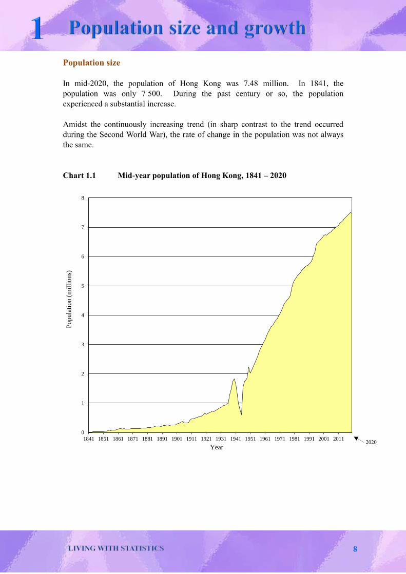
Population size

In mid-2020, the population of Hong Kong was 7.48 million. In 1841, the

population was only 7 500. During the past century or so, the population

experienced a substantial increase.

Amidst the continuously increasing trend (in sharp contrast to the trend occurred

during the Second World War), the rate of change in the population was not always

the same.

Chart 1.1 Mid-year population of Hong Kong, 1841 – 2020

0

1

2

3

4

5

6

7

8

1841 1851 1861 1871 1881 1891 1901 1911 1921 1931 1941 1951 1961 1971 1981 1991 2001 2011

Po

pula

tio

n (

mil

lio

ns)

Year

2020

8

Growth rate of the population

To measure the speed of population change, the growth rate can be calculated by

dividing the increase in population during a period by the population size at the

beginning of that period.

Thus, given that the population decreased from 7 507 400 at mid-2019 to 7 481 800

at mid-2020, the population grew at a rate of

7 481 800 – 7 507 400

7 507 400 × 100% = -0.3%^

during the period from mid-2019 to mid-2020.

If the population increased in the period, the growth rate would have been a positive

number.

Compound average growth rate of the population

For a span of time over a number of years, it is a common practice to measure the

average annual growth rate on a compound basis.

The population was 7 481 800 at mid-2020 and 7 291 300 at mid-2015

(i.e. five years ago). If the unknown compound average growth rate is r%

per annum during the 5-year period from mid-2015 to mid-2020, then

[Population

at mid-2020 ] = [

Population

at mid-2015 ] × ( 1 +

r

100 )

5

or 7 481 800 = 7 291 300 × ( 1 + r

100 )

5

Hence r = (√7 481 800

7 291 300

5

– 1) × 100 = 0.5 ^

That is, the compound average growth rate of the population was 0.5%^ per annum

during the 5-year period from mid-2015 to mid-2020.

9

Three factors affecting population growth

There are three factors affecting the population growth, namely births, deaths and net

movements.

At different times, some factors may have greater effects than the others. To study

their contributions to population growth, it is useful to express the change in

population size in terms of its components :

P1 – P0 = (B – D) + (E – L)

where P1 = population at end of the period

P0 = population at beginning of the period

B = live births during the period

D = deaths during the period

(B – D) = natural change during the period

E = number of entrants during the period

L = number of leavers during the period

(E – L) = net movement during the period

10

Chart 1.2 Annual change in population of Hong Kong,

mid-1961 to mid-2020(2)

Note :

(2) Population figures from 1996 onwards are compiled based on the “resident population” method

and are broadly comparable with figures for 1995 and before. Notwithstanding this, the

population figure for 1996 compiled based on the old method (i.e. 6 311 000) has been used in

calculating the population growth and net movement from 1995 to 1996.

(a) Annual change in population size

[= (b) Natural change + (c) Net movement]

(c) Net movement

(b) Natural change

2020

-50

0

50

100

150

200

250

300

1961 1966 1971 1976 1981 1986 1991 1996 2001 2006 2011 2016

Pop

ula

tion

(th

ou

san

ds)

Year

Population growth

2020

0

50

100

150

200

250

300

1961 1966 1971 1976 1981 1986 1991 1996 2001 2006 2011 2016

Pop

ula

tion

(th

ou

san

ds)

Year

Live births

Deaths

Natural change

-50

0

50

100

150

200

250

300

1961 1966 1971 1976 1981 1986 1991 1996 2001 2006 2011 2016

Pop

ula

tion

(th

ou

san

ds)

Year

Excess of entrants over leavers

Excess of leavers over entrants

2020

2

0

1

9 2

0

1

9

2

0

1

9

11

Stock-flow relationship

To understand the equation shown in the above section, take the size of population at

a point of time as a pool of water (i.e. the population “stock”), its level being raised

by adding water from the tap (i.e. inflows of births and entrants) and lowered by

draining water away through the plughole (i.e. outflows of deaths and leavers).

Thus, the population size measures the stock at a particular point of time, whereas

changes in all the components, or “flows”, contribute to changes in the stock size

during an interval of time.

Crude birth rate

The childbearing trend in the population is measured by the birth rate, which is

expressed in terms of number of births per 1 000 population.

The crude birth rate is calculated by dividing the number of known “live births(3)”

born in a calendar year by the average population size during the calendar year.

Usually the mid-year population is taken as the average population size.

Thus, in 2020, with 43 000 live births and a mid-year population of 7 481 800, the

crude birth rate is equal to

(43 000

7 481 800 × 1 000) = 5.8^

or 5.8^ per 1 000 population.

Note :

(3) Live births are defined as babies born with evidence of life, such as respiration, movement of

voluntary muscles or heartbeat after complete expulsion or extraction.

12

Chart 1.3 Crude birth rate, 1961 – 2020

General fertility rate

Sometimes, the crude birth rate does not reflect correctly the birth trend. For

instance, an inflow of male immigrants increases the population size, leading to a

lowered birth rate, but the birth trend may not have changed actually.

This pitfall can be avoided by using the general fertility rate, which relates the

number of births to the number of women of childbearing age (i.e. those aged 15 to

49) in the population. The rate is usually expressed in terms of number of births per

1 000 females of childbearing age.

There is a special issue for Hong Kong. There are a large number of female foreign

domestic helpers working in Hong Kong, yet the great majority of whom will not

give birth to children here. To better reflect the fertility situation in Hong Kong,

female foreign domestic helpers are excluded from the number of women of

childbearing age in computing the general fertility rate.

0

5

10

15

20

25

30

35

40

1961 1966 1971 1976 1981 1986 1991 1996 2001 2006 2011 2016

Bir

ths

per

1 0

00

po

pula

tio

n

Year

2020

13

2

0

2

0

Chart 1.4 General fertility rate and crude birth rate, 1961 – 2020

Decline in birth trend

Since the 1970’s, the birth rate in Hong Kong has been falling rapidly. This is

mainly because of late marriage. The median age of women who got married for

the first time(4) was 22.9 in 1971, while that in 2020 was 30.4.

Over the same period, there is also a significant increase in the prevalence of

spinsterhood. In 1971, the percentage of never married women in the age group

40-44 was 3%. In 2016, this percentage reached 16%.

Furthermore, people tend to have children later after marriage and have fewer

children than before. Among all the births recorded in 2020, 89.3% were the first

or second births to their mothers as compared with 83.5% in 1990.

Correspondingly, the average size of domestic households dropped from 3.6 persons

per household in 1990 to 2.8 in 2020, indicating a tendency towards the formation of

smaller households.

Note :

(4) Median age at first marriage is an indicator of the average age of persons at their first marriage

such that 50% of these persons are above this age while the other 50% are below it.

0

20

40

60

80

100

120

140

160

180

1961 1966 1971 1976 1981 1986 1991 1996 2001 2006 2011 2016

Bir

ths

per

1 0

00

rel

ated

po

pula

tio

n

.

Year

General fertility rate

(per 1 000 females of childbearing age, excluding

female foreign domestic helpers)

Crude birth rate (per 1 000 population)

2020

14

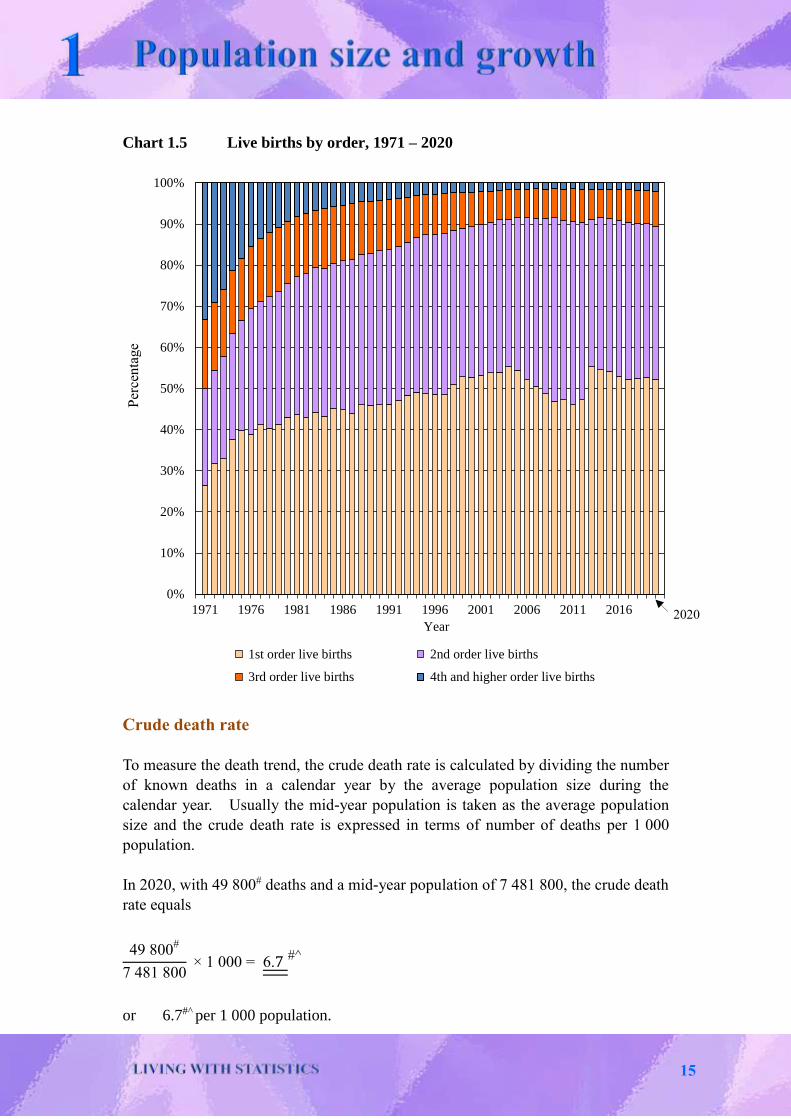
Chart 1.5 Live births by order, 1971 – 2020

Crude death rate

To measure the death trend, the crude death rate is calculated by dividing the number

of known deaths in a calendar year by the average population size during the

calendar year. Usually the mid-year population is taken as the average population

size and the crude death rate is expressed in terms of number of deaths per 1 000

population.

In 2020, with 49 800# deaths and a mid-year population of 7 481 800, the crude death

rate equals

49 800#

7 481 800 × 1 000 = 6.7

#^

or 6.7#^ per 1 000 population.

Per

cen

tage

2020

0%

10%

20%

30%

40%

50%

60%

70%

80%

90%

100%

1971 1976 1981 1986 1991 1996 2001 2006 2011 2016

Year

1st order live births 2nd order live births

3rd order live births 4th and higher order live births

15

Chart 1.6 Crude birth rate and crude death rate, 1961 – 2020

Rate of natural change

The excess of known live births over known deaths occurring in a year is called the

natural change in population.

The rate of natural change is given as the excess of known live births over known

deaths occurring in a year per 1 000 mid-year population of that year. This

indicator shows that the rate at which the population growth is due to vital events

(viz. births and deaths) only. The gain or loss in population due to net movement is

not taken into account.

During the year 2020, there were 43 000 known live births and 49 800# known deaths.

With a mid-year population of 7 481 800, the rate of natural change during the year

equals

(43 000 – 49 800

#

7 481 800× 1 000) = -0.9 #^

or -0.9#^ per 1 000 population.

Crude birth rate

0

5

10

15

20

25

30

35

40

1961 1966 1971 1976 1981 1986 1991 1996 2001 2006 2011 2016

Bir

ths

/ D

eath

s p

er 1

00

0 p

op

ula

tio

n

.

Year

Rate of natural change

Crude death rate

2020#

16

Alternatively, the rate of natural change may be computed by the difference between

the crude birth rate and the crude death rate. For the above example, the rate of

natural change may also be calculated as crude birth rate for 2020 minus crude death

rate for 2020 (i.e. 5.8^ – 6.7#^ = -0.9 #^) or -0.9#^ per 1 000 population (see Chart 1.6).

Effect of age structure on birth and death rates

For a population with more women at childbearing age, the crude birth rate will

normally be higher. For a population with more old people, the crude death rate can

be expected to be higher. It is therefore necessary to study the age composition of a

population before definitive statements can be made about its birth and death trends.

More in-depth studies of the population will adopt appropriate methods to isolate the

age composition effects such that the birth and death trends at different points of time

or among different countries can be meaningfully compared.

Expectation of life at birth

The crude death rate for the population of Hong Kong has been greatly reduced since

the 1950’s, which fell from 10.2 per 1 000 population in 1951 to 5.0 per 1 000

population in 1971. The rate has remained rather stable since then. It has to be

noted, however, that at a time when the population of old persons is increasing, a

stable crude death rate actually suggests an overall improvement in the death trend.

A lower death trend would mean that people can expect a longer life. Thus, the

death trend may also be measured by the “expectation of life at birth”. This

indicates how long a child born in a year, say 2020, would expect to live, assuming

that upon reaching various ages in his / her life, he / she would be subject to the same

death risks as those faced by people of the respective ages in 2020.

The expectation of life at birth in 2020 was 82.7# years for males and 88.1# years for

females, representing a substantial increase of 8.1# years for males and 7.9# years for

females since 1990.

17

Chart 1.7 Expectation of life at birth, 1971 – 2020

0

20

40

60

80

100

1971 1976 1981 1986 1991 1996 2001 2006 2011 2016

Exp

ecta

tio

n o

f li

fe a

t b

irth

(Y

ears

) .

Year

Male Female

2020#

18

Infant mortality rate

The decline in death rate in the past 49 years was partly due to improvements in birth

care and child health, which reduced deaths of infants. The relevant indicator to

study the phenomenon is the infant mortality rate, which is obtained by dividing the

number of deaths of infants aged under one year by the total number of live births.

The rate is usually expressed in terms of deaths per 1 000 live births.

Chart 1.8 Infant mortality rate, 1971 – 2020

2020 0

2

4

6

8

10

12

14

16

18

20

1971 1976 1981 1986 1991 1996 2001 2006 2011 2016

Dea

ths

of

infa

nts

per

1 0

00

liv

e b

irth

s

Year

2

0

1

9

#

#

19

0

1

2

3

4

5

6

1971 1976 1981 1986 1991 1996 2001 2006 2011 2016

Num

ber

per

1 0

00

po

pula

tio

n

.

Year

Hospital beds (6)

Registered nurses (General) (7)

Doctors (8)

2020 #

Better medical and health services

The general decline in death trend can also be associated with better medical and

health services. Besides, people are having more knowledge about health and are

more health conscious now.

Chart 1.9 Rate of hospital beds and selected types of registered healthcare

professionals, 1971 – 2020(5)

Notes :

(5) Figures are as at end of the year.

(6) Figures include all hospital beds in Hospital Authority hospitals, private hospitals, nursing

homes and correctional institutions, which follow the coverage of the Hospitals, Nursing Homes

and Maternity Homes Registration Ordinance, Cap. 165, Laws of Hong Kong. Prior to 2019,

the number of private hospital beds included inpatient beds only. Starting from 2019, the total

number of private hospital beds included both inpatient beds and day beds.

(7) The drop in 2005 was due to the removal of names of more than 6 000 registered nurses

(General) from the register / roll in accordance with Section 7(3)(e) and Section 13(3)(e) of the

Nurses Registration Ordinance, Cap. 164, Laws of Hong Kong.

(8) Figures refer to doctors with full registration on the local and overseas lists.

20

Movement of population

A substantial part of the Hong Kong population are entrants from the Mainland. Nevertheless the locally born population remains the largest group. This can be seen by comparing the proportion of the population by their place of birth.

Chart 1.10 Distribution of population by place of birth, 1996, 2006 and 2016(9)

Note :

(9) Statistics shown in the charts above refer to information collected via population by-censuses.Areas of the pie charts are proportional to the population sizes in the corresponding years.

21

Demographic transition model as a general pattern of population growth The demographic transition model describes changes in birth and death rates as a population passes from a traditional society to an urbanised and industrialised one. Generally, birth and death rates are high in traditional societies and low in modern societies. According to different rates of birth and death, changes in population are thought to occur in four stages: (1) high birth and death rates; (2) high birth rate and declining death rate; (3) declining birth and death rates; and (4) low birth and death rates. Chart 1.11 Demographic transition model

22

As the population grows naturally by excess of births over deaths, it would increase

at varying speeds in these different stages. This, of course, assumes that flows of

movement are not significant. Otherwise, rather different pictures can emerge.

Further information

The above contents present only part of the information produced by C&SD on the

topics concerned. For further information regarding the topics discussed in this

chapter (e.g. latest statistics, statistical reports, concepts and methods), please visit

the following sections of the C&SD website :

Population estimates

Population censuses and by-censuses

Demographics

Health

Note :

^ Growth rates of the population, crude birth rate, crude death rate and rate of natural change are

calculated based on unrounded population figures.

Interactive quiz

You may test the knowledge you have learnt in this Chapter by trying this

interactive quiz. Answers to the questions can be found in the relevant

paragraphs of this Chapter.

23

https://www.censtatd.gov.hk/en/scode150.html


https://www.censtatd.gov.hk/en/page_8000.html#menu_action25




http://www.censtatd.gov.hk/hkstat/sub/so380.jsp

https://www.censtatd.gov.hk/en/living_with_statistics/2021/chapter1/index.html

Exercise

Growth patterns of different countries

Births, deaths and net movements are the three factors affecting population growth.

Annual growth rates, rates of natural change, crude birth rates and crude death rates

are useful indicators of the growth pattern.

Readers may try to calculate these rates from the table below where data on

population size, births and deaths are given for different countries.

The aim of this exercise is to enable readers to get familiarised with the fundamental

concepts in population growth.

Generally speaking, the rate of natural change may be taken as the difference

between the crude birth rate and the crude death rate.

To further test one’s understanding of the demographic transition model as a general

pattern of population growth, the second part of this exercise is to classify those

countries into different transitional stages based on the birth and death rates

computed in the first part. There are no universal rules to classify such rates as high

or low. However, as a practical guide, a crude birth rate of 25 per 1 000 population

or above may be regarded as high; and a crude death rate of 15 per 1 000 population

or above can be considered as high.

(1) From the data given below, complete the table.

(Figures are given in thousands; rates are expressed in “per 1 000 population”.)

Country

Mid-year

population

at year T

No. of births

in year T

No. of deaths

in year T

Crude birth

rate

Crude death

rate

Rate of

natural

change

Country A 29 863 1 322 525

Country B 15 941 723 332

Country C 20 155 249 132

Country D 32 268 332 226

Country E 9 749 433 181

Country F 1 315 844 17 558 8 795

Country G 74 033 1 860 421

Country H 1 517 51 17

Country I 82 689 702 853

Country J 10 098 96 132

24

(2) From the rates obtained in part (1), classify the countries into various stages of the

demographic transition model.

Stage (1)

(High birth and death rates)

Stage (4)

(Low birth and death rates)

25

400 300 200 100 0 100 200 300 400

0-4

5-9

10-14

15-19

20-24

25-29

30-34

35-39

40-44

45-49

50-54

55-59

60-64

65-69

70-74

75-79

80-84

85+

Number (thousands)

AgeMale Female

Introduction

Individuals differ in terms of their sex, age, employment, and so on. A population,

made up of individuals, is characterised by the distribution of individuals in regard to

these features. This chapter introduces various measures for describing population

characteristics and their changes over time.

Population pyramid

The age-sex distribution of a population is most clearly presented in the graphical

form of a “population pyramid”. The pyramid can be scaled in either population

numbers or percentages. The percentage distribution is more appropriate for

comparison of two or more populations.

Chart 2.1 Population of Hong Kong by age and sex, mid-2020

Number (thousands)

Number (thousands)

Percentage

6 5 4 3 2 1 0 1 2 3 4 5 6

0-4

5-9

10-14

15-19

20-24

25-29

30-34

35-39

40-44

45-49

50-54

55-59

60-64

65-69

70-74

75-79

80-84

85+

Percentage

Male Female

27

1 0 1

2016-20

2011-15

2006-10

2001-05

1996-00

1991-95

1986-90

1981-85

1976-80

1971-75

1966-70

1961-65

1956-60

1951-55

1946-50

1941-45

1936-40

1935 and before

Year of Birth

6 5 4 3 2 1 0 1 2 3 4 5 6

0-4

5-9

10-14

15-19

20-24

25-29

30-34

35-39

40-44

45-49

50-54

55-59

60-64

65-69

70-74

75-79

80-84

85+

Percentage

AgeMale Female

The age-sex distribution reflects the combined effects of the past and recent trends in

births, deaths and net movements. It is a rather persistent feature, and will not

change drastically in a short span of time. Irregularities, like age or sex groups of

exceptional size, reflect unusual numbers of births, deaths or net movements at some

points of time in the past. Normally, births and net movements have larger impacts

on the age-sex distribution than deaths.

Chart 2.2 Age-sex distribution of Hong Kong population, mid-2020

Shape of population pyramid in relation to the growth pattern of a

population

In a growing population with high birth rates, the numbers of people in younger age

groups are larger and the age structure would take on the shape of a typical pyramid.

If death rates are also high, the pyramid, which has a broad base, would narrow

rapidly towards the top. Conversely, as the birth trend declines and the death trend

improves, the pyramid would have a relatively narrow base and a middle section of

nearly the same width; it does not begin to converge to the vertex until after very old

age groups.

28

Chart 2.3 Population pyramids (in percentage) of selected countries, 2020

Source : Population Pyramid.net

The shape of a population pyramid is thus closely related to the growth pattern of a

population. Countries in different transitional stages may take on varying shapes of

the population pyramid for their age-sex structures. For instance, the pyramid for

Pakistan (2020) has a very broad base that narrows upwards very rapidly. It has

almost a triangular shape. It results from a very high crude birth rate of 27.4 per

1 000 population(1) and relatively low expectation of life at birth, 66.5 years(1) for

males and 68.5 years(1) for females.

10 8 6 4 2 0 2 4 6 8 10

0-4

5-9

10-14

15-19

20-24

25-29

30-34

35-39

40-44

45-49

50-54

55-59

60-64

65-69

70-74

75-79

80-84

85+

Percentage

Pakistan

Male FemaleAge

10 8 6 4 2 0 2 4 6 8 10

0-4

5-9

10-14

15-19

20-24

25-29

30-34

35-39

40-44

45-49

50-54

55-59

60-64

65-69

70-74

75-79

80-84

85+

Percentage

Mexico

Male FemaleAge

10 8 6 4 2 0 2 4 6 8 10

0-4

5-9

10-14

15-19

20-24

25-29

30-34

35-39

40-44

45-49

50-54

55-59

60-64

65-69

70-74

75-79

80-84

85+

Percentage

Sri Lanka

Male FemaleAge

10 8 6 4 2 0 2 4 6 8 10

0-4

5-9

10-14

15-19

20-24

25-29

30-34

35-39

40-44

45-49

50-54

55-59

60-64

65-69

70-74

75-79

80-84

85+

Percentage

Switzerland

Male FemaleAge

29

In contrast, the pyramid for Switzerland (2020) has a much narrower base, a little bit

wider middle section and a slowly converging tip. The shape is almost

semi-elliptical. It illustrates the effects of a low crude birth rate of 10.2 per 1 000

population(1) and high expectation of life at birth, 82.0 years(1) for males and 85.7

years(1) for females.

The pyramids for Mexico (2020) and Sri Lanka (2020) illustrate configurations

intermediate between those for Pakistan and Switzerland; their crude birth rates were

17.0 and 15.3 per 1 000 population(1) respectively and their respective expectations of

life at birth were 75.1 and 73.8 years(1) for males and 77.9 and 80.4 years(1) for

females.

Expectation of life at birth is preferred to crude death rate as an indicator of death

trend here because the crude death rates for the four countries are found highly

distorted by the different age structures of their populations.

Apart from the natural effect of births and deaths, it should be noted that these four

pyramids are affected by other irregular variations and therefore may deviate from

the theoretical triangular and semi-elliptical shapes that the demographic transition

model prescribes.

Besides the detailed description of age-sex structure provided by the population

pyramid, the age-sex distribution of a population can also be given by other summary

measures.

Sex ratio

To compare the relative size of the male group and female group in the population,

the sex ratio is calculated. The ratio is obtained by dividing the number of males in

the population by the number of females. The sex ratio is usually expressed as the

number of males per 1 000 females.

At mid-2020, there were 3 416 300 males and 4 065 500 females in Hong Kong.

Thus the sex ratio was

3 416 300

4 065 500 × 1 000 = 840

or 840 males per 1 000 females. Note :

(1) Source–World Data Atlas

30

0

200

400

600

800

1 000

1 200

1961 1966 1971 1976 1981 1986 1991 1996 2001 2006 2011 2016

Mal

es p

er 1

00

0 f

emal

es

Year

All ages

Aged 65 and over

Sex ratio by age group

Sex ratio may also be calculated separately for various age groups. For instance,

the sex ratio at birth compares the number of male births to female births. Usually,

as a biological norm, slightly more male babies are born than female babies.

Sex ratio (number of males per 1 000 females)

Age group Mid-2010 Mid-2015 Mid-2020

0-14 1 072 1 070 1 055

15-19 1 061 1 062 1 049

20-24 949 984 1 004

25-29 756 786 873

30-34 707 678 717

35-39 719 674 643

40-44 758 706 659

45-49 859 760 711

50-54 968 865 765

55-59 985 972 878

60-64 1 007 976 978

65 and over 872 875 881

All ages 883 857 840

Chart 2.4 Sex ratio of Hong Kong population by age group,

mid-1961 to mid-2020

2020

31

As revealed by the above chart, the sex ratio for the older ages was on the rise over

the years. This reflects a greater improvement in the death trend for males than for

females in recent years.

Increasing proportion of females in Hong Kong population

In Hong Kong, the proportion of females in the total Hong Kong population

increased continuously in the past 10 years. The sex ratio of the population

remained below parity and was consistently on a decreasing trend. The ratio

dropped from 883 in mid-2010 to 840 in mid-2020.

The increase in the proportion of females in the population was brought about by

three major factors.

Effect of foreign domestic helpers

Firstly, there was a significant number of foreign domestic helpers in Hong Kong,

who were mostly young and middle-aged females. Owing to this factor, the number

of females in the age group of 20-39 was relatively large, with the corresponding sex

ratio at mid-2020 being 777 males per 1 000 females.

Sex ratio (number of males per 1 000 females)


0-19 1 068 1 068 1 054

20-39 770 761 777

40-64 901 847 794

65 and over 872 875 881

All ages 883 857 840

After excluding foreign domestic helpers, the sex ratio for the age group of 20-39 at

mid-2020 rose to 940. The sex ratio for the entire population was 913.

Sex ratio excluding foreign domestic helpers

(number of males per 1 000 females)


0-19 1 068 1 069 1 054

20-39 928 934 940

40-64 946 900 859

65 and over 872 875 882

All ages 952 932 913

32

0

4

8

12

16

20

24

28

32

36

40

44

48

1961 1966 1971 1976 1981 1986 1991 1996 2001 2006 2011 2016

Age

Year

Median Age

Mean Age

2020

Effect of one-way permit holders from the Mainland

The second factor contributing to the increasing proportion of females in the

population was that a large proportion of the one-way permit holders from the

Mainland were women who came to Hong Kong to join their husbands. In 2020,

there were 10 134 one-way permit holders from the Mainland and about 58% of

these new entrants were females.

Effect of higher expectation of life for females

The third factor is that females generally live longer than males. The expectation of

life at birth of females was 88.1# years while that for males was only 82.7# years in

2020.

Mean and median ages

To describe the age structure of a population, its average age can be used. A simple

average, or the “mean”, can be obtained by dividing the sum of ages of the total

population by the population size. Alternatively, a measure is provided by the

“median” age of the population. Median age of the population is an indicator of the

average age of the population such that 50% of the total population are above this

age while the other 50% are below it.

Chart 2.5 Mean and median ages of Hong Kong population,


33

“Median” is normally a better measure of its average value in a set of data if there are

extreme values, since the “mean” will be much affected by those extreme values. In

the case of age, the general experience is that the median age is considered more

preferable.

“Young” and “old” populations

A population may be described as “young” or “old”.

A population may be considered as “ageing” when its median age is on the rise.

Dependency ratios

It is interesting and useful to divide the population into three groups by age, namely

the young (i.e. those aged 0 to 14), those in the working age (i.e. aged 15 to 64) and

the elderly (i.e. aged 65 and over) and study their relative sizes.

The overall dependency ratio is computed by dividing the number of the young and

the elderly in the population by those in the working age. The components of this

measure may be calculated separately as the “child dependency ratio” and “elderly

dependency ratio”.

Given the following population data for Hong Kong in mid-2020, the various

dependency ratios are computed accordingly:

Age group Population at mid-2020

0-14 869 300

15-64 5 240 700

65 and over 1 371 800

Child dependency ratio

= 869 300

5 240 700 × 1 000 = 166

or 166 persons aged under 15 per 1 000 population of working age.

34

Elderly dependency ratio

= 1 371 800

5 240 700 × 1 000 = 262

or 262 persons aged 65 and over per 1 000 population of working age.

Overall dependency ratio

= 869 300 + 1 371 800

5 240 700 × 1 000 = 428

or 428 persons aged under 15 or aged 65 and over per 1 000 population of

working age.

Chart 2.6 Dependency ratios of Hong Kong population,


2020

0

200

400

600

800

1 000

1961 1966 1971 1976 1981 1986 1991 1996 2001 2006 2011 2016

Num

ber

of

dep

end

ents

per

1 0

00

po

pula

tio

n o

f

wo

rkin

g a

ge

Year

Overall dependency ratio

Child dependency ratio

Elderly dependency ratio

35

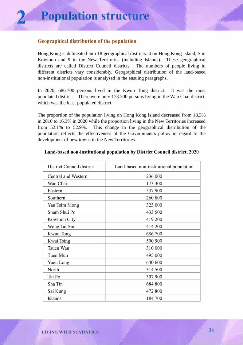
Geographical distribution of the population

Hong Kong is delineated into 18 geographical districts: 4 on Hong Kong Island; 5 in

Kowloon and 9 in the New Territories (including Islands). These geographical

districts are called District Council districts. The numbers of people living in

different districts vary considerably. Geographical distribution of the land-based

non-institutional population is analysed in the ensuing paragraphs.

In 2020, 686 700 persons lived in the Kwun Tong district. It was the most

populated district. There were only 173 300 persons living in the Wan Chai district,

which was the least populated district.

The proportion of the population living on Hong Kong Island decreased from 18.3%

in 2010 to 16.3% in 2020 while the proportion living in the New Territories increased

from 52.1% to 52.9%. This change in the geographical distribution of the

population reflects the effectiveness of the Government’s policy in regard to the

development of new towns in the New Territories.

Land-based non-institutional population by District Council district, 2020

District Council district Land-based non-institutional population

Central and Western 236 000

Wan Chai 173 300

Eastern 537 900

Southern 260 800

Yau Tsim Mong 323 000

Sham Shui Po 433 500

Kowloon City 419 200

Wong Tai Sin 414 200

Kwun Tong 686 700

Kwai Tsing 500 900

Tsuen Wan 310 000

Tuen Mun 495 000

Yuen Long 640 600

North 314 500

Tai Po 307 900

Sha Tin 684 800

Sai Kung 472 800

Islands 184 700

36

Employment structure of the population

“Economically active” persons are those aged 15 and over who are either working or

seeking jobs. These people make up the “labour force”. Children at school, the

retired and home-makers are economically inactive persons.

The labour force of Hong Kong increased from 3.63 million in 2010 to 3.98 million

in 2018, and then decreased gradually to 3.89 million in 2020.

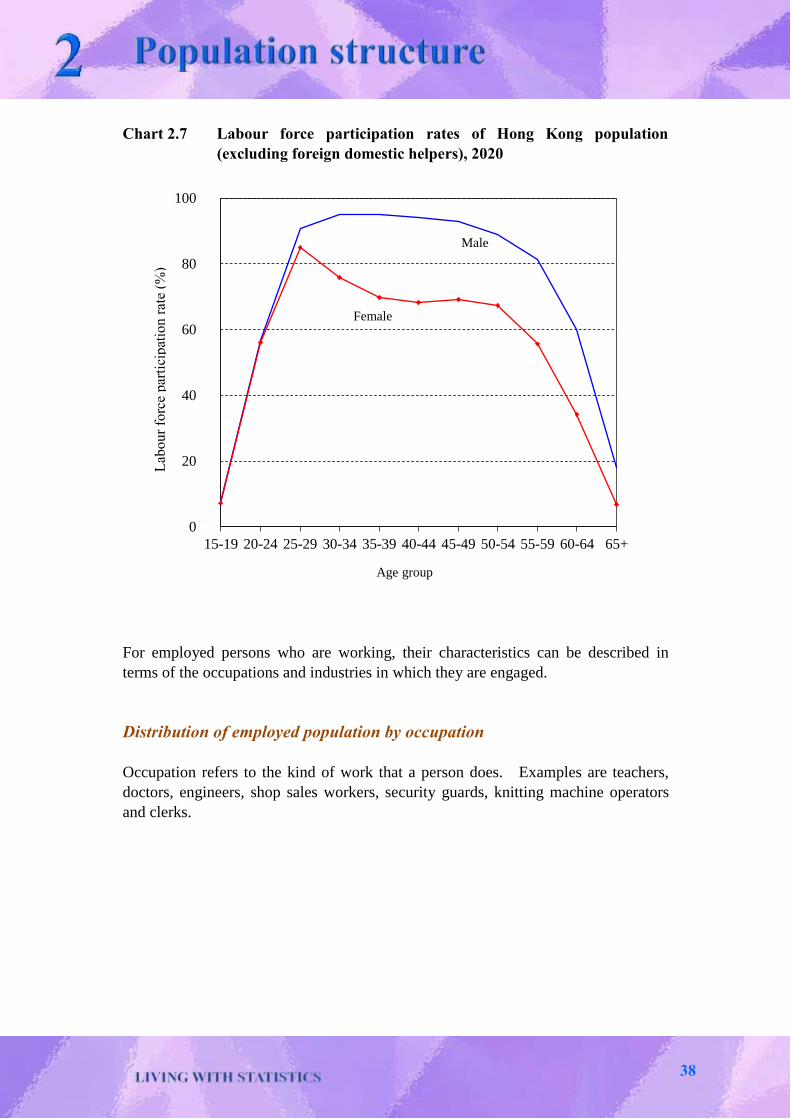
“Labour force participation rates” are used to measure the proportion of

economically active persons in the population aged 15 and over. These rates are

usually calculated separately for males and females in different age groups. Since

more women tend to concentrate on household duties, their labour force participation

rates are generally lower than those for males. The age specific labour force

participation rates for males are highest at their prime working ages (i.e. 25 to 49)

while the rates for females reach the peak at the age group 25-29 and decline

gradually in the older age groups.

The labour force participation rates in the age groups 15-19 and 65 and over for both

sexes in 2020 were substantially lower than those in other age groups, as most

members of the former group were still at school while a fair proportion of those in

the latter group were retired people.

The characteristics of foreign domestic helpers differ from those of the entire

population, particularly in their labour force participation rates. Because of this, the

age-sex specific labour force participation rates presented in Chart 2.7 have excluded

foreign domestic helpers in order to better reflect the profile of the local population.

Information on the labour force, employment,

unemployment and underemployment is

collected through the General Household

Survey.

37

0%

20%

40%

60%

80%

100%

15-19 20-24 25-29 30-34 35-39 40-44 45-49 50-54 55-59 60-64 65+

Age group

Female

Male

Chart 2.7 Labour force participation rates of Hong Kong population

(excluding foreign domestic helpers), 2020

For employed persons who are working, their characteristics can be described in

terms of the occupations and industries in which they are engaged.

Distribution of employed population by occupation

Occupation refers to the kind of work that a person does. Examples are teachers,

doctors, engineers, shop sales workers, security guards, knitting machine operators

and clerks.

Lab

our

forc

e par

tici

pat

ion

rat

e (%

)

38

Chart 2.8 Distribution of employed population by occupation(2),

2010 – 2020

(a) Based on International Standard Classification of Occupations 1988 (ISCO-88)

(b) Based on International Standard Classification of Occupations 2008 (ISCO-08)

Note :

(2) Statistics for 2010 are compiled based on ISCO-88. Statistics for 2011 and onwards are

compiled based on ISCO-08. Hence, figures for 2011 and onwards are not directly comparable

to the figures for 2010.

Per

centa

ge

0%

20%

40%

60%

80%

100%

2011 2012 2013 2014 2015 2016 2017 2018 2019 2020

Year

Others (including elementary

occupations)

Plant and machine operators and

assemblers

Craft and related workers

Service and sales workers

Clerical support workers

Associate professionals

Professionals

Managers and administrators

0%

20%

40%

60%

80%

100%

2010

Year

Others (including elementary

occupations)

Plant and machine operators and

assemblers

Craft and related workers

Service workers and shop sales

workers

Clerks

Associate professionals

Professionals

Managers and administrators

Per

centa

ge

39

Distribution of employed population by industry sector

Industry, on the other hand, refers to the kind of activity carried out by the

establishment or enterprise in which a person works. Examples of some

establishments are schools, hospitals, shops, construction firms and factories.

Examples of “industries” are business services sector, retail sector, construction

sector, transportation sector and manufacturing sector.

The economic characteristics of a population reflect the stage of the society’s

economic development. In general, the labour force tends to shift away from

agriculture to manufacturing industries, and then to services industries.

In Hong Kong, the economic characteristics of the population follow this general

pattern in economic development. Over these years, the services sector in Hong

Kong has been gaining increasing prominence.

Being the industry sector with the largest share of employment, the services sector as

a whole engaged 3.2 million@ persons in 2020, accounting for 88.9%@ of the overall

employment. The corresponding figures for 2015 were 3.3 million persons and

88.4%.

40

Chart 2.9 Distribution of employed population by industry(3), 2010 – 2020

Based on Hong Kong Standard Industrial Classification (HSIC)

Notes :

(3) Figures are compiled based on Hong Kong Standard Industrial Classification Version 2.0.

(4) Accommodation services cover hotels, guesthouses, boarding houses and other establishments

providing short term accommodation.

(5) The retail, accommodation and food services industries as a whole is generally referred to as the

consumption- and tourism-related segment.

Per

centa

ge

0%

20%

40%

60%

80%

100%

2010 2011 2012 2013 2014 2015 2016 2017 2018 2019 2020

Year

Other industries

Public administration, social and

personal services

Financing, insurance, real estate,

professional and business services

Transportation, storage, postal and

courier services, information and

communications

Retail, accommodation (4)

and food

services (5)

Import / export trade and wholesale

Construction

Manufacturing

41

Further information



chapter (e.g. latest statistics, statistical reports, concepts and methods), please visit

the following sections of the C&SD website :



Demographics

Labour force, employment and unemployment

Interactive quiz




42










Exercise

Age-sex structure of the 18 districts

Population pyramid is a useful tool to depict the age-sex structure of a population.

This exercise demonstrates how to present age-sex data by means of population

pyramids. It further shows how age-sex structure differs in different districts of

Hong Kong, which has implications for the requirement for social services and

facilities in these districts.

(1) With reference to the age-sex data obtained from the 16BC for the 18 districts

shown on pages 44 to 46, please prepare a population pyramid for each of

these districts on graph papers according to the formats given on pages 47 to

49.

(2) Please rank the 18 districts according to their ageing extent, by referring to the

median age of the district populations.

District Council

district Median age

Ranking for ageing extent (Note)

(“1” for the most aged district)

Central and Western 43.8

Wan Chai 44.9

Eastern 43.8

Southern 43.9

Yau Tsim Mong 43.2

Sham Shui Po 42.9

Kowloon City 43.1

Wong Tai Sin 44.6

Kwun Tong 43.8

Kwai Tsing 43.5

Tsuen Wan 43.2

Tuen Mun 43.7

Yuen Long 42.1

North 42.7

Tai Po 43.6

Sha Tin 44.2

Sai Kung 42.8

Islands 42.4

Note : Where there are ties in rank, the tied observations are assigned the mean of the ranks

which they jointly occupy.

43

(3) With reference to the statistics shown on pages 44 to 46, please analyse how

various districts may differ in their requirements for public services and

facilities.

Percentage distribution of population by age and sex, June 2016 Central and Western Wan Chai Eastern

Age group Male Female Total Male Female Total Male Female Total

0-4 1.6 1.5 3.1 1.5 1.5 3.0 2.0 1.9 3.9

5-9 1.7 1.7 3.5 1.8 1.7 3.6 2.0 1.8 3.8

10-14 1.6 1.5 3.1 1.6 1.5 3.1 1.6 1.6 3.3

15-19 2.3 2.1 4.4 1.9 1.9 3.8 2.3 2.2 4.4

20-24 3.2 3.4 6.6 2.2 2.5 4.7 2.8 2.9 5.7

25-29 3.4 4.2 7.6 3.0 4.5 7.6 2.9 3.9 6.8

30-34 3.1 4.9 8.0 3.1 5.5 8.6 3.2 4.9 8.0

35-39 2.9 4.9 7.7 2.8 5.2 8.1 3.1 5.0 8.1

40-44 3.0 4.7 7.7 3.0 4.7 7.7 3.2 4.6 7.7

45-49 3.0 4.8 7.8 3.0 4.9 7.9 3.1 4.5 7.6

50-54 4.0 5.4 9.4 4.3 5.5 9.7 4.0 5.0 8.9

55-59 4.3 4.4 8.7 4.3 4.5 8.9 4.2 4.3 8.5

60-64 3.2 3.2 6.4 3.3 3.5 6.8 3.2 3.4 6.6

65-69 2.6 2.8 5.4 2.6 2.6 5.2 2.8 2.9 5.8

70-74 1.3 1.5 2.8 1.5 1.5 3.0 1.5 1.4 2.9

75-79 1.4 1.4 2.8 1.3 1.5 2.8 1.4 1.5 2.8

80-84 1.0 1.2 2.2 1.1 1.4 2.5 1.0 1.4 2.4

85+ 0.9 1.7 2.7 1.0 1.9 2.9 0.9 1.8 2.7

All ages 44.7 55.3 100.0 43.6 56.4 100.0 45.0 55.0 100.0

Median age 43.8 44.9 43.8

Southern Yau Tsim Mong Sham Shui Po


0-4 2.2 1.8 4.0 2.1 1.8 3.8 2.2 2.1 4.2

5-9 2.0 1.9 3.9 1.8 2.0 3.8 2.2 1.9 4.1

10-14 1.8 1.6 3.4 1.7 1.6 3.3 1.7 1.7 3.4

15-19 2.3 2.1 4.3 2.4 2.1 4.5 2.3 2.2 4.5

20-24 2.6 2.7 5.3 3.1 3.5 6.6 2.9 3.1 6.0

25-29 2.7 3.8 6.4 3.5 4.3 7.7 3.1 4.0 7.1

30-34 3.0 4.9 7.9 3.1 4.8 7.9 3.4 4.8 8.2

35-39 3.0 5.2 8.2 2.9 4.6 7.5 3.2 4.7 7.9

40-44 3.4 4.7 8.1 3.0 4.5 7.6 3.3 4.5 7.9

45-49 3.2 4.5 7.7 3.0 4.5 7.6 3.3 4.5 7.8

50-54 4.1 4.8 8.9 4.2 5.1 9.3 3.9 4.6 8.5

55-59 4.0 4.3 8.3 4.3 4.4 8.6 4.0 4.1 8.2

60-64 3.3 3.4 6.8 3.6 3.2 6.8 3.2 3.2 6.4

65-69 2.7 2.7 5.4 2.9 2.5 5.5 2.6 2.5 5.1

70-74 1.5 1.4 3.0 1.4 1.2 2.7 1.5 1.4 2.9

75-79 1.3 1.6 2.9 1.2 1.3 2.5 1.4 1.4 2.8

80-84 0.9 1.3 2.3 1.0 1.2 2.2 1.1 1.3 2.4

85+ 0.9 2.1 3.0 0.8 1.5 2.3 0.9 1.8 2.7

All ages 45.1 54.9 100.0 46.0 54.0 100.0 46.4 53.6 100.0

Median age 43.9 43.2 42.9

44

Percentage distribution of population by age and sex, June 2016 (cont’d)

Kowloon City Wong Tai Sin Kwun Tong


0-4 2.1 2.0 4.1 1.7 1.7 3.4 2.0 1.8 3.8

5-9 2.2 2.0 4.2 2.1 1.9 3.9 2.1 1.9 4.0

10-14 1.7 1.6 3.3 1.8 1.7 3.5 1.9 1.8 3.7

15-19 2.2 2.2 4.4 2.5 2.3 4.8 2.4 2.2 4.6

20-24 3.2 3.1 6.3 3.2 3.2 6.4 3.0 3.0 6.1

25-29 3.3 4.1 7.4 3.0 3.6 6.6 3.0 3.8 6.8

30-34 3.1 5.0 8.2 3.0 4.2 7.2 3.3 4.5 7.8

35-39 2.9 4.7 7.6 3.0 4.3 7.3 3.3 4.4 7.6

40-44 2.8 4.5 7.3 3.1 4.3 7.4 3.2 4.3 7.4

45-49 2.9 4.3 7.2 3.3 4.3 7.6 3.2 4.2 7.4

50-54 3.8 5.1 8.9 4.1 4.8 8.9 3.8 4.6 8.4

55-59 4.2 4.6 8.8 4.5 4.3 8.8 4.1 4.3 8.4

60-64 3.5 3.4 6.9 3.3 3.6 6.9 3.3 3.5 6.9

65-69 2.8 2.7 5.4 2.7 2.8 5.5 2.6 2.7 5.4

70-74 1.3 1.4 2.7 1.6 1.5 3.1 1.7 1.5 3.2

75-79 1.3 1.3 2.6 1.4 1.6 3.0 1.5 1.6 3.2

80-84 1.0 1.2 2.2 1.2 1.6 2.8 1.2 1.5 2.6

85+ 0.8 1.6 2.4 0.9 1.8 2.8 1.0 1.8 2.7

All ages 45.1 54.9 100.0 46.4 53.6 100.0 46.6 53.4 100.0

Median age 43.1 44.6 43.8

Kwai Tsing Tsuen Wan Tuen Mun


0-4 1.9 1.8 3.7 2.0 1.8 3.8 1.9 1.7 3.6

5-9 2.0 1.8 3.8 2.0 1.8 3.8 1.9 2.0 3.9

10-14 2.0 1.8 3.7 1.8 1.6 3.4 1.8 1.8 3.7

15-19 2.5 2.4 4.9 2.4 2.3 4.6 2.5 2.4 4.9

20-24 3.0 3.0 6.0 3.1 3.2 6.4 3.0 3.2 6.2

25-29 3.2 3.7 6.9 3.4 4.0 7.4 3.1 3.6 6.7

30-34 3.2 4.6 7.9 3.2 4.7 7.9 3.1 4.3 7.4

35-39 3.2 4.6 7.8 2.8 4.6 7.4 3.2 4.5 7.7

40-44 3.3 4.4 7.7 3.5 4.8 8.3 3.4 4.7 8.1

45-49 3.4 4.1 7.4 3.1 4.5 7.7 3.7 4.6 8.3

50-54 3.9 4.6 8.5 4.1 5.0 9.1 4.2 4.6 8.9

55-59 4.1 4.2 8.3 4.5 4.4 8.9 4.3 4.4 8.8

60-64 3.2 3.5 6.7 3.5 3.3 6.7 3.5 3.7 7.3

65-69 2.6 2.8 5.4 2.5 2.5 5.0 2.7 2.6 5.3

70-74 1.8 1.8 3.6 1.5 1.4 2.9 1.5 1.5 3.0

75-79 1.5 1.4 2.9 1.2 1.4 2.5 1.3 1.4 2.7

80-84 1.0 1.4 2.4 1.0 1.3 2.2 0.8 1.1 1.9

85+ 0.8 1.6 2.4 0.7 1.4 2.0 0.6 1.2 1.8

All ages 46.8 53.2 100.0 46.1 53.9 100.0 46.6 53.4 100.0

Median age 43.5 43.2 43.7

45

Percentage distribution of population by age and sex, June 2016 (cont’d)

Yuen Long North Tai Po


0-4 2.1 2.0 4.1 2.2 2.0 4.1 1.8 1.7 3.6

5-9 2.2 2.0 4.3 2.2 2.3 4.5 2.1 2.0 4.1

10-14 1.9 1.8 3.7 2.0 2.1 4.2 1.9 2.0 3.9

15-19 2.6 2.3 4.9 2.5 2.2 4.7 2.4 2.3 4.7

20-24 3.4 3.2 6.5 2.9 2.9 5.8 2.7 2.9 5.7

25-29 3.0 3.9 6.9 3.0 3.6 6.6 3.3 3.6 6.9

30-34 3.3 4.8 8.1 3.2 4.8 8.0 3.1 4.3 7.4

35-39 3.4 4.9 8.2 3.3 4.6 8.0 3.0 4.8 7.8

40-44 3.3 4.6 7.9 3.1 4.5 7.7 3.3 4.9 8.2

45-49 3.2 4.2 7.4 3.3 4.3 7.7 3.5 4.5 8.0

50-54 3.8 4.5 8.3 4.1 4.5 8.6 3.9 4.6 8.5

55-59 4.0 4.0 8.0 4.2 3.9 8.1 4.5 4.7 9.2

60-64 3.3 3.4 6.7 3.3 3.2 6.5 3.4 3.4 6.8

65-69 2.7 2.8 5.4 2.6 2.6 5.2 2.5 2.5 5.0

70-74 1.7 1.4 3.1 1.5 1.4 3.0 1.4 1.5 2.9

75-79 1.4 1.3 2.7 1.3 1.4 2.7 1.5 1.4 2.9

80-84 0.9 1.0 1.9 1.1 1.2 2.3 0.9 1.2 2.1

85+ 0.6 1.3 1.9 0.8 1.6 2.4 0.8 1.5 2.3

All ages 46.6 53.4 100.0 46.8 53.2 100.0 46.1 53.9 100.0

Median age 42.1 42.7 43.6

Sha Tin Sai Kung Islands


0-4 1.9 1.7 3.6 2.1 2.0 4.1 2.4 2.1 4.4

5-9 2.1 1.9 4.1 2.1 1.9 4.0 2.0 1.9 3.9

10-14 1.9 1.8 3.7 1.7 1.6 3.4 1.6 1.6 3.2

15-19 2.5 2.4 4.9 2.5 2.1 4.6 2.3 2.1 4.5

20-24 3.0 3.1 6.1 3.0 3.1 6.1 2.9 2.8 5.8

25-29 2.9 3.6 6.5 3.1 4.0 7.1 3.4 4.1 7.5

30-34 3.0 4.4 7.3 3.3 5.0 8.4 3.5 5.1 8.6

35-39 2.8 4.5 7.3 3.3 4.8 8.1 3.5 4.9 8.4

40-44 3.1 4.8 7.9 3.2 4.6 7.8 3.3 4.4 7.7

45-49 3.8 5.0 8.7 3.3 4.6 7.8 2.9 4.1 7.1

50-54 4.2 4.8 9.0 3.9 4.8 8.7 3.6 4.4 8.0

55-59 4.0 4.3 8.3 4.1 4.3 8.5 4.2 4.2 8.4

60-64 3.2 3.4 6.6 3.3 3.5 6.8 3.4 3.4 6.8

65-69 2.7 2.7 5.4 2.7 2.9 5.5 2.8 2.7 5.6

70-74 1.4 1.5 2.9 1.5 1.5 3.0 1.7 1.5 3.2

75-79 1.4 1.6 2.9 1.4 1.3 2.6 1.6 1.3 2.8

80-84 1.1 1.3 2.4 0.9 1.0 1.9 0.9 1.3 2.2

85+ 0.8 1.5 2.3 0.6 1.0 1.6 0.8 1.0 1.8

All ages 45.7 54.3 100.0 45.9 54.1 100.0 46.9 53.1 100.0

Median age 44.2 42.8 42.4

Note : Individual percentages may not add up to 100 due to rounding.

46

Age Group

0

Percentage2468 8642

Age Group

0

Percentage2468 8642

Age Group

0

Percentage2468 8642

Age Group

0

Percentage2468 8642

Age Group

0

Percentages2468 8642

Age Group

0

Percentage2468 8642

Central and Western Wan Chai

Eastern Southern

Yau Tsim Mong Sham Shui Po

47

Age Group

0

Percentage

2468 8642

Age Group

0

Percentage2468 8642

Age Group

0

Percentage

2468 8642

Age Group

0

Percentage2468 8642

Age Group

0

Percentage2468 8642

Age Group

0

Percentage2468 8642

Kowloon City Wong Tai Sin

Kwun Tong Kwai Tsing

Tsuen Wan Tuen Mun

48

Age Group

0

Percentage

2468 8642

Age Group

0

Percentage2468 8642

Age Group

0

Percentage2468 8642

Age Group

0

Percentage

2468 8642

Age Group

0

Percentage2468 8642

Age Group

0

Percentage2468 8642

Yuen Long North

Tai Po Sha Tin

Sai Kung Islands

49

Introduction

This chapter discusses the impact of changes in population and its structure on society.

It shows how statistical data can be used to identify the problems caused by population

growth. Population control and forward planning of service requirements are the

solutions to these problems. To carry out such work, population data of good quality

are required.

The current population of the world as at 2021 is estimated to be around 7.9 billion by

the United Nations Population Division, being mainly a result of an unprecedented

growth of population in the 20th century. This very large population size has caused

much concern about the availability of resources to meet the demand of all the people

for food, clothing, housing, education, medical services, etc.

The great burden from rapid population growth is likely to persist in the near future.

Latest population projections indicate that by 2100, the world population will increase

to 10.9 billion. In particular, population problems will be more serious in some

poorer areas or countries where populations grow faster than in more developed

regions.

51

Chart 3.1 Distribution of world population by major area,

1950, 2020 and 2100(1), (2)

Notes:

(1) Latin America includes Central America, South America and the Caribbean.

(2) Areas of the pie charts are proportional to the population sizes in the corresponding years.

Source: World Population Prospects : The Population Database, Population Division of the United

Nations Department of Economic and Social Affairs

Africa 39.4%

Europe 5.8%

Northern America 4.5%

Latin America 6.3%

Oceania 0.7%

Asia 43.4%

2100 (Projected)

1950

2020 Africa 17.2%

Europe 9.6%

Northern America 4.7%

Latin America 8.4%

Oceania 0.5%

Asia 59.5%

Africa 9.0%

Europe 21.7%

Latin America 6.7%

Oceania 0.5%

Asia 55.4% Northern America 6.8%

52

Impact of changes in population and its structure on Hong Kong

In Hong Kong, there are a number of concerns arising from the continuous growth of

population and changes in its structure.

Increasing population density

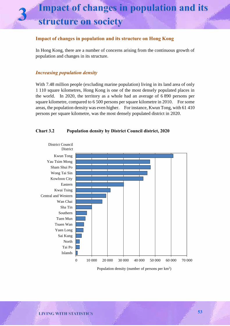
With 7.48 million people (excluding marine population) living in its land area of only

1 110 square kilometres, Hong Kong is one of the most densely populated places in

the world. In 2020, the territory as a whole had an average of 6 890 persons per

square kilometre, compared to 6 500 persons per square kilometre in 2010. For some

areas, the population density was even higher. For instance, Kwun Tong, with 61 410

persons per square kilometre, was the most densely populated district in 2020.

Chart 3.2 Population density by District Council district, 2020

0 10 000 20 000 30 000 40 000 50 000 60 000 70 000

Islands

Tai Po

North

Sai Kung

Yuen Long

Tsuen Wan

Tuen Mun

Southern

Sha Tin

Wan Chai

Central and Western

Kwai Tsing

Eastern

Kowloon City

Wong Tai Sin

Sham Shui Po

Yau Tsim Mong

Kwun Tong

Population density (number of persons per km2)

District Council

District

53

To reduce urban congestion and to meet the new housing needs of the growing

population, systematic and coordinated development of new towns began in the early

1970’s. Since then, there has been rapid development of new towns in the more

remote areas. At present, there are twelve new towns, namely Tuen Mun, Sha Tin,

Kwai Chung, Tai Po, Tsuen Wan, Fanling / Sheung Shui, Tsing Yi, Tseung Kwan O,

Ma On Shan, Yuen Long, Tin Shui Wai and North Lantau.

The development of new towns has led to a re-distribution of the population, from the

older urban areas on Hong Kong Island and in Kowloon to the new towns. According

to the results of the 16BC, people living in the new towns accounted for about 47% of

the Hong Kong land population in 2016, while the percentage was only 22% in 1976.

Traffic congestion

The large population of Hong Kong generates a huge volume of traffic which, coupled

with a lack of space, places a great strain on the internal transport systems.

To obtain an indication of the traffic volume, the number of motor vehicles can be

compared with the total length of roads. As at end-2020, there were 373 motor

vehicles per kilometre of road, compared with 293 as at end-2010. The increase was

mainly contributed by the increase in the number of private cars.

As in places all over the world, people of Hong Kong rely much on public transport

services in their daily living.

In 2020, public transport carried 3.3 billion passengers(3), as compared with 4.2 billion

in 2010. The drop in patronage in 2020 was mainly due to the COVID-19 pandemic

and implementation of the related anti-epidemic and social distancing measures.

As in past years, railways continue to be a major type of carrier among the various

public transport modes in Hong Kong. They comprise the Mass Transit Railway

(MTR) heavy rail systems (which include ten local lines, Intercity Through Train, the

Hong Kong Section of the Express Rail Link and the Airport Express Line), the Light

Rail and the Hongkong Tramways. In 2020, the daily patronage of railways was

3.6 million passenger journeys, as compared with 4.5 million in 2010. Over the same

period, the share of railways in total public transport journeys increased from 38.9%

in 2010 to 40.1% in 2020.

Note :

(3) The number of passengers cited in transport statistics actually refers to the number of passenger

journeys. Since a person may make more than one journey during a period of time, the figure is

usually larger than the number of people who have ever made journeys during the period.

54

Another important component of the public transport system in Hong Kong is

franchised buses. In 2020, they carried about 3.0 million passenger journeys or

34.0% of all public transport journeys a day. Ten years ago, the daily patronage was

3.8 million passenger journeys, or 32.5% of the total public transport journeys.

To ensure the smooth and efficient movement of people and goods, careful co-

ordination and management of the traffic and transport systems are needed. This

involves a programme to improve the road network, expansion of public transport

services and measures to achieve more economic use of the limited road capacity.

Chart 3.3 Passenger journeys by major mode of public transport,

2010 – 2020

Note :

(4) Railways comprise the MTR heavy rail systems (which include ten local lines, Intercity Through

Train, the Hong Kong Section of the Express Rail Link and the Airport Express Line), the Light

Rail and the Hong Kong Tramways.

0

300

600

900

1 200

1 500

1 800

2 100

2010 2011 2012 2013 2014 2015 2016 2017 2018 2019 2020

Num

ber

of

pas

senger

jo

urn

eys

(m

illi

ons)

.

Year

Franchised Buses

Railways(4)

Public light buses (red minibus and green minibus)

55

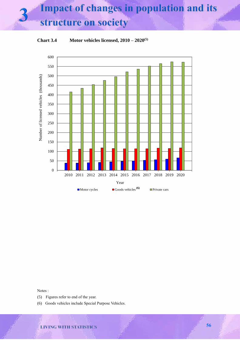
Chart 3.4 Motor vehicles licensed, 2010 – 2020(5)

Notes :

(5) Figures refer to end of the year.

(6) Goods vehicles include Special Purpose Vehicles.

0

50

100

150

200

250

300

350

400

450

500

550

600

2010 2011 2012 2013 2014 2015 2016 2017 2018 2019 2020

Num

ber

of

lice

nse

d v

ehic

les

(th

ousa

nd

s)

Year

Motor cycles Goods vehicles Private cars(6)(6)

56

Increasing demand for housing

As Hong Kong is scarce of land, the Government has to ensure that there is steady and

sufficient supply of serviced land for meeting the demand for housing brought about by

the continuous growth of the population. To achieve this, the Government needs to

develop strategic growth areas (including new and existing land for housing), renew

urban areas, redevelop old districts, reclaim more land, perform better town planning and

rezone agricultural and industrial land for housing development where appropriate.

During 2010 to 2020, around 321 000 residential flats were completed to meet the

housing needs of people in Hong Kong. As at end of September 2020, the total stock

of permanent living quarters in Hong Kong was 2 923 600.

Of the 2.65 million domestic households in 2020, 30.4% resided in public rental

housing, 14.9% in subsidised home ownership housing(7) and 53.9% in private

permanent housing(8). Only less than 1% of domestic households lived in temporary

housing.

Notes :

(7) Subsidised home ownership housing includes flats built under the Home Ownership Scheme,

Middle Income Housing Scheme, Private Sector Participation Scheme, Green Form Subsidised

Home Ownership Scheme, Buy or Rent Option Scheme and Mortgage Subsidy Scheme, and flats

sold under the Tenants Purchase Scheme of the Hong Kong Housing Authority. It also includes

flats built under the Flat for Sale Scheme, Sandwich Class Housing Scheme and Subsidised Sale

Flats Projects of the Hong Kong Housing Society; and flats in Urban Renewal Authority

Subsidised Sale Flats Scheme. Subsidised sale flats that can be traded in open market are

excluded.

(8) Figures include private housing blocks, flats built under the Urban Improvement Scheme of the

Hong Kong Housing Society, villas / bungalows / modern village houses, simple stone structures

/ traditional village houses and quarters in non-residential buildings. Subsidised sale flats that

can be traded in open market are also put under this category.

57

Chart 3.5 Distribution of domestic households by type of housing,

2010 – 2020

Increase in post-secondary education opportunities

Owing to the changes in the age structure of the population, the number of students

studying in primary education showed a decrease during 2010 to 2012 but has

rebounded since 2013. On the other hand, the number of students studying in

secondary education has decreased remarkably since 2012 due to the drop in the

number of students in the relevant age group. On post-secondary education, through

the development of the publicly-funded and self-financing sectors, about 50% of our

young people in the relevant age cohort in the 2020/21 academic year have access to

degree-level education, and nearly 80% of them now have access to post-secondary

education locally, taking into account sub-degree students.

Per

centa

ge

0%

10%

20%

30%

40%

50%

60%

70%

80%

90%

100%

2010 2011 2012 2013 2014 2015 2016 2017 2018 2019 2020

Year

Public rental housing Subsidised home ownership housing

Private permanent housing Temporary housing

58

0

100

200

300

400

500

600

2010 2011 2012 2013 2014 2015 2016 2017 2018 2019 2020

Num

ber

of

stud

ents

(th

ousa

nd

s).

Year

(11), (12)

Secondary

(11)Primary

(10)Pre-primary

(13)

Post-secondary

Chart 3.6 Student enrolment(9) by level of education, 2010 – 2020

Notes :

(9) Figures include both full-time and part-time students attending long programmes lasting for at

least one school / academic year. Figures do not include students attending tutorial, vocational

and adult education courses offered by schools below post-secondary education level. Figures

for secondary and post-secondary education for 2020 are provisional.

(10) Figures include nursery, lower and upper classes in kindergartens and kindergarten-cum-child

care centres registered under the Education Bureau, and special child care centres registered under

the Social Welfare Department.

(11) Figures include special schools.

(12) Figures include evening schools, craft level courses and Diploma Yi Jin programme. Prior to

the 2012/13 school year, secondary education covers Secondary 1 to Secondary 7. Upon

implementation of the New Senior Secondary Academic Structure, there are no subsidised

Secondary 7 places under local curriculum starting from the 2012/13 school year.

(13) Figures include universities and colleges offering post-secondary courses including

certificate / diploma, associate degree or equivalent and bachelor degree or above; and also non-

local registered or exempted courses leading to non-local higher academic qualifications and

operated jointly with non-local institutions.

59

Increasing elderly dependency ratio

The population of Hong Kong is ageing, as can be seen from the increase in the median

age of the population from 41.2 in 2010 to 45.0 in 2020. As a result, the elderly

dependency ratio increased from 175 per 1 000 population of working age in 2010 to

262 per 1 000 population of working age in 2020. It is common to consider the

elderly as dependent on those aged 15 to 64. The rise in the elderly dependency ratio

reflects that there is an increase in the demand for social services, in particular social

welfare and medical and health services.

Increasing demand for social welfare services

The percentage of population aged 65 and above has increased gradually, resulting in

the increasing demand for social welfare services. The total number of elderly

recipients (i.e. recipients aged 65 and above) of the Comprehensive Social Security

Assistance (CSSA) and Social Security Allowance (SSA) Schemes (excluding

Guangdong Scheme and Fujian Scheme) increased from 723 700 in end-2010 to

1 049 600 in end-2020. While the CSSA Scheme is designed to provide members of

the community who cannot support themselves financially with monetary assistance

to meet their basic and special needs, the SSA Scheme is to provide a monthly

allowance to members of the community to meet their special needs arising from old

age or disability.

The Government also provides a wide range of elderly and community services.

Community services include the operation of social centres for the elderly, district

elderly community centres, neighbourhood elderly centres, day care centres / units for

the elderly, enhanced home and community care services, and integrated home care

services, etc. which aim to enable the elderly to continue to stay in the community.

60

Chart 3.7 Number of elderly recipients of the Comprehensive Social

Security Assistance (CSSA) and Social Security Allowance (SSA)

Schemes (excluding Guangdong (GD) Scheme and Fujian (FJ)

Scheme) and percentage of population aged 65 and

above, 2010 – 2020(14)

Population projections

For the purpose of forward planning of service needs, the size, structure and

distribution of the population in future years have to be projected. A reliable

projection requires careful examination of past trends of fertility, mortality and

population movement to determine their possible changes in the future. The assumed

changes are then added onto the base population, which is derived from a population

census or by-census, year after year to obtain the projection results.

Note :

(14) Figures refer to December of the year.

0

4

8

12

16

20

0

300

600

900

1 200

1 500

2010 2011 2012 2013 2014 2015 2016 2017 2018 2019 2020

Year

Number of elderly recipients (i.e. recipients aged 65 and above) of CSSA

and SSA Schemes (excluding GD Scheme and FJ Scheme)

Percentage of population aged 65 and above

Num

ber

of

eld

erly

rec

ipie

nts

(th

ousa

nd

s)

Po

pula

tio

n a

ged

65

and

ab

ove

(%)

61

C&SD is responsible for compiling projections of the population of Hong Kong. The

main use of the population projections is to provide a common basis for government

programme planning in such areas as education, housing, transport, social services and

health services. The projection results are also widely applied in academic research

and business development and planning in the private sector. The latest set of

population projections was released in September 2020, with a 50-year projection

period from mid-2020 to mid-2069.

“Component method” for population projections

The “component method”, which is commonly used internationally, is adopted for

compiling the population projections. Under this method, the size and age-sex

structure of the projected population in each of the projection years are obtained by

applying different assumptions made on the fertility, mortality and population

movement conditions for the projection year to the population situation in the

preceding year. Therefore, in compiling the population projections, the population

situation in a base year will be used as the starting point. It is then brought forward

under separate projections of fertility, mortality and population movement, year after

year until the end of the projection period. While fertility, mortality and population

movement assumptions are formulated mainly on the basis of the past trends and recent

developments pertaining to the socio-economic conditions in Hong Kong, government

policies, if involved, are taken as that the existing policies would continue to apply

except for known policy changes.

Major projection results

In the 2019-based projections, the Hong Kong population is projected to increase at an

average annual rate of 0.4%, from 7.51 million in mid-2019 to the peak of 8.11 million

in mid-2041, and then decline to 7.35 million in mid-2069 (at an average annual rate

of decrease of 0.3%). The average annual growth rate over the 10-year period from

2019 to 2029 is projected to be 0.5%. Yet, with significant increase in the number of

deaths upon ageing of the population, the average annual rate of decline over the last

10 years of the projection period (i.e. from 2059 to 2069) is projected to be 0.5%.

A set of population projections compiled based on

the mid-2019 population estimate and a

corresponding set of domestic household

projections were released in September 2020.

62

Chart 3.8 Hong Kong population pyramid at selected years

600 500 400 300 200 100 0 100 200 300 400 500 600

0-4 5-910-1415-1920-2425-2930-3435-3940-4445-4950-5455-5960-6465-6970-7475-7980-84 85+

Number (thousands)

Mid-2020 (Actual)Male Female

600 500 400 300 200 100 0 100 200 300 400 500 600

0-4 5-910-1415-1920-2425-2930-3435-3940-4445-4950-5455-5960-6465-6970-7475-7980-84 85+

Number (thousands)

Mid-2029 (Projected)Male Female

600 500 400 300 200 100 0 100 200 300 400 500 600

0-4 5-910-1415-1920-2425-2930-3435-3940-4445-4950-5455-5960-6465-6970-7475-7980-84 85+

Number (thousands)


600 500 400 300 200 100 0 100 200 300 400 500 600

0-4 5-910-1415-1920-2425-2930-3435-3940-4445-4950-5455-5960-6465-6970-7475-7980-84 85+

Number (thousands)


600 500 400 300 200 100 0 100 200 300 400 500 600

0-4 5-910-1415-1920-2425-2930-3435-3940-4445-4950-5455-5960-6465-6970-7475-7980-84 85+

Number (thousands)


600 500 400 300 200 100 0 100 200 300 400 500 600

0-4 5-910-1415-1920-2425-2930-3435-3940-4445-4950-5455-5960-6465-6970-7475-7980-84 85+

Number (thousands)


63

Population on an ageing trend

Population ageing is expected to continue. With post-war baby boomers entering old

age, the number of elderly persons aged 65 and over is projected to nearly double in

the coming 20 years. Excluding foreign domestic helpers, the number of elderly

persons will increase from 1.32 million (18.4% of the total population) in 2019 by 1.20

million to 2.52 million (33.3%) in 2039. Compared with the growth of about 0.61

million in the last 20 years (from 1999 to 2019), the elderly population will increase

distinctly at a much faster pace in the future. It is also worth noting that the elderly

population will remain at over 2.5 million for at least 30 years. In 2069, the number

of elderly persons is projected to reach 2.58 million (38.4%). Meanwhile, due to the

persistently low fertility rate, the proportion of the population aged under 15 is

projected to decrease gradually from 12.2% in 2019 to 7.6% in 2069.

Chart 3.9 Hong Kong population by age group, 2009 – 2069

0

2

4

6

8

10

2009 2014 2019 2024 2029 2034 2039 2044 2049 2054 2059 2064 2069

Popula

tion (

mil

lions)

Year

Aged below 15 Aged 15 - 64 Aged 65 and over

Actual Projected

64

Decreasing sex ratio

Another noteworthy point is that the proportion of males in the population would keep

on decreasing. In 2019, the sex ratio (i.e. the number of males per 1 000 females) of

the population was 838. Owing to the continued entry of One-way Permit holders

(many being Hong Kong men’s wives in the Mainland) and foreign domestic helpers

(mostly being younger females) into Hong Kong in the coming years and the fact that

females in general live longer than males, the sex ratio is projected to fall noticeably

to 685 in 2069. Even with the effects of foreign domestic helpers excluded, the sex

ratio would still come down from the level of 910 in 2019 to 801 in 2069.

Chart 3.10 Proportion of male and female populations, 2009 – 2069

(including foreign domestic helpers)

0%

20%

40%

60%

80%

100%

2009 2014 2019 2024 2029 2034 2039 2044 2049 2054 2059 2064 2069

Per

centa

ge

Year Male Female

Actual Projected

65

Labour force projections

The size and the composition of the labour force within the population are important

determinants of economic development. Labour force projections of Hong Kong

compiled by C&SD provide information on the future labour supply in Hong Kong

and its age and sex distribution. Such information serves as useful reference for

policy planning and formulation. The latest set of labour force projections was

released in September 2020, covering the projection period from 2020 to 2069.

Methodology

In compiling the labour force projections for the period from 2020 to 2069, reference

has been made to the results of the 2019-based population projections and the latest

trends of the age-sex specific labour force participation rates. Foreign domestic

helpers are not included in the projected labour force participation rates and labour

force figures.

The labour force, synonymous with the economically active population, comprises the

employed population and the unemployed population. The labour force participation

rate refers to the proportion of the labour force in the population aged 15 and over. It

is a measure of the propensity of the persons of working age to be in the labour force.

In particular, the proportion of persons participating in the labour force in a particular

age-sex group is termed as the age-sex specific labour force participation rate for the

group.

In compiling the projected labour force, a set of projected labour force participation

rates for individual projection groups in the population for different years within the

projection period is first compiled with reference to the latest trends of the age-sex

specific labour force participation rates. The projected labour force participation rate

for each projection group is then multiplied to the projected population size of the

corresponding group to derive the projected labour force of the group in each of the

years over the projection period. Finally, the projected labour force of all groups in

the same year are summed up to give the projected total labour force for the year

concerned.

66

Major projection results

Projected labour force participation rates (excluding foreign domestic helpers)

The overall labour force participation rate is projected to decline steadily from 58.5%

in 2019 to 49.2% in 2069. Owing to the population ageing effect, the overall labour

force participation rate for both males and females are projected to decrease from

67.4% and 50.5% in 2019 to 57.6% and 42.6% in 2069 respectively.

Chart 3.11 Labour force participation rate (excluding foreign domestic

helpers) by sex, 2009 – 2069(15)

Note :

(15) Owing to the impact of the COVID-19 pandemic, the projection results, which are derived based

on long-term underlying trends of the population structure and its propensity to be in the labour

force, for the years from 2020 to 2023 are not shown.

20

30

40

50

60

70

80

90

2009 2014 2019 2024 2029 2034 2039 2044 2049 2054 2059 2064 2069

Lab

our

forc

e p

arti

cip

atio

n r

ate

(%)

Year

Actual Projected

Male

Both sexes

Female

0

67

Projected labour force (excluding foreign domestic helpers)

The total labour force is projected to decrease from 3.64 million in 2019 to 3.56 million

in 2031. It will then hover between 3.55 million and 3.56 million until 2037, before

decreasing to 2.98 million in 2069.

The labour force for males is projected to decrease gradually from 1.98 million in 2019

to 1.54 million in 2069. The labour force for females is projected to vary narrowly

between 1.66 million and 1.69 million in 2019 to 2042 and then decrease gradually to

1.44 million in 2069.

Chart 3.12 Labour force (excluding foreign domestic helpers),

2009 – 2069(16)

Note :

(16) Owing to the impact of the COVID-19 pandemic, the projection results, which are derived based

on long-term underlying trends of the population structure and its propensity to be in the labour

force, for the years from 2020 to 2023 are not shown.

0.0

0.5

1.0

1.5

2.0

2.5

3.0

3.5

4.0

2009 2014 2019 2024 2029 2034 2039 2044 2049 2054 2059 2064 2069

Lab

our

forc

e (m

illi

ons)

Male Female

Actual Projected

Year

68

Further information



chapter (e.g. latest statistics, statistical reports, concepts and methods), please visit the

following sections of the C&SD website :



Population and household projections

Demographics


Transport

Information and communications

Tourism

Housing and property

Education

Social welfare

Health

Interactive quiz




69
















http://www.censtatd.gov.hk/hkstat/sub/so370.jsp






Exercise

Identifying impact of changes in population and its structure on society

To arouse the public’s awareness of various population and social problems, readers

may try to identify such problems in the districts they live, in the whole territory of

Hong Kong, or in other countries.

For example, readers may consider the problem of traffic congestion in Hong Kong by

looking up statistics compiled by C&SD or other government departments (e.g.

Transport Department) in order to quantify the magnitude of traffic congestion in broad

terms, and to consider how the various problems can be solved. Examples of relevant

statistics include number of motor vehicles licensed, length of roads and number of

passengers using different kinds of public transport.

70

Introduction Official statistics are generally statistics compiled by the Government based on raw

data from such sources as administrative records, special returns and surveys.

Where surveys are conducted, there are often statistical legislations requiring the

target persons or companies to supply the required raw data.

C&SD is the central statistical office of Hong Kong. C&SD together with

statistical units established in various government bureaux and departments forms

the Government Statistical Service. Broadly speaking, most general-purpose

statistics come under the responsibility of C&SD. The statistical units in various

government bureaux and departments are responsible for specific-purpose statistics

(for dedicated use in their respective work areas) and provide necessary support in

the application of statistics.

In this knowledge-based era, more and more people are making use of statistics in

their work and daily lives. Official statistics play an important role in a wide range

of endeavours, including macro-economic analysis, day-to-day administration and

long term planning of the Government, decision-making of individuals and business

firms, and enhancing people’s understanding of the society and their participation in

discussions about social and economic policies.

Some of the more common economic and social statistics are introduced in the

following sections.

(A) Economic statistics

Economic statistics comprise, among others, the following areas : trade statistics,

national income statistics, balance of payments statistics, labour statistics, price

statistics and operating statistics of businesses.

Just as doctors need to use medical equipment when they make diagnoses, economic

analysts need to make reference to statistics in forming their views from theoretical

considerations. Economic statistics serve as measuring instruments which enable

the analysts to judge whether different economic sectors in the economy are in

harmony, whether the economy is stagnant or overheated, and whether economic

performance will improve or decline. Although different analysts may have

different views on economic prospects or on the role of the Government, there is no

doubt about the importance of good measuring instruments to them.

71

Apart from facilitating macro-economic analysis, economic statistics are also very

useful in business planning. Businessmen can make use of the statistics in deciding

what businesses to invest in, what products to produce, where to locate shops, at

what wages they should employ workers, and so on.

Trade statistics

Hong Kong is an externally oriented economy. Its economic performance is highly

related to the performance of the external sector. Hong Kong external trade

comprises trade in goods (i.e. merchandise trade) and trade in services.

Trade in goods covers movements of merchandise between Hong Kong and her

trading partners, by land, air, water and by post. It comprises imports and total

exports.

Trade in services includes exports and imports of services. Exports of services are

the sales of services to the rest of the world, whereas imports of services are the

purchases of services from the rest of the world.

(1) Merchandise trade

Merchandise trade statistics provide important indicators of the performance of

the external sector of the economy in respect of merchandise trade. They can

be analysed by the two components of external merchandise trade, namely total

exports and imports. In addition to aggregate statistics of trade in respect of

each of the components, detailed statistics are also available on Hong Kong’s

trade with different countries / territories and for different commodities.

Besides providing very useful information on the performance of an economy,

trade statistics can also be used by business firms in decision-making on such

areas as forecasting business prospects, measuring market shares, planning

investment and formulating marketing, production and development strategies.

As a free port, Hong Kong has minimal import and export licensing

requirements. Most products do not need licences to enter or leave Hong

Kong. Unlike many other economies, there is no import tariff in Hong Kong.

Yet, persons who import or export goods (except for exempted goods) are

required to submit import / export declarations to the Customs and Excise

Department within 14 days after the importation / exportation of goods. The

import / export declarations are subsequently forwarded to C&SD for further

processing and compilation of Hong Kong’s external merchandise trade

statistics. The import / export declaration is a typical example of special

returns for collecting raw data essentially used for trade statistics compilation.

72

Electronic submission of trade declarations has been made mandatory as from

April 2000. In 2020, around 18.7 million import / export declarations were

processed by C&SD.

The Hong Kong Special Administrative Region is a separate customs territory,

as stated in “The Basic Law of the Hong Kong Special Administrative Region

of the People’s Republic of China”. Import / export declaration is also

required of Hong Kong’s trade with the Mainland, and statistics relating to this

are included in Hong Kong’s external merchandise trade statistics.

In 2020, the value of Hong Kong’s total merchandise trade was $8,197.3

billion, lower than that in 2019 by 2.5%. Of this, $3,927.5 billion were

attributable to total exports and $4,269.8 billion to imports.

Between 2010 and 2020, the values of total exports and imports of goods

increased respectively at an average annual growth rate of 2.6% and 2.4%.

Total exports of goods comprise domestic exports and re-exports. Domestic

exports are the natural produce of Hong Kong or the products of a

manufacturing process in Hong Kong which has changed permanently and

substantially the shape, nature, form or utility of the basic materials used in

manufacture. Re-exports are products which have previously been imported

into Hong Kong and which are re-exported without having undergone in Hong

Kong a manufacturing process which has changed permanently and

substantially the shape, nature, form or utility of the basic materials used in the

manufacture. The values of exports are recorded on f.o.b. (free on board)

basis, i.e. on the basis of the value of the commodities when they leave the

customs boundary of Hong Kong.

In 2020, some 18.7 million import/export

declarations and 6.1 million cargo

manifests were processed by C&SD.

73

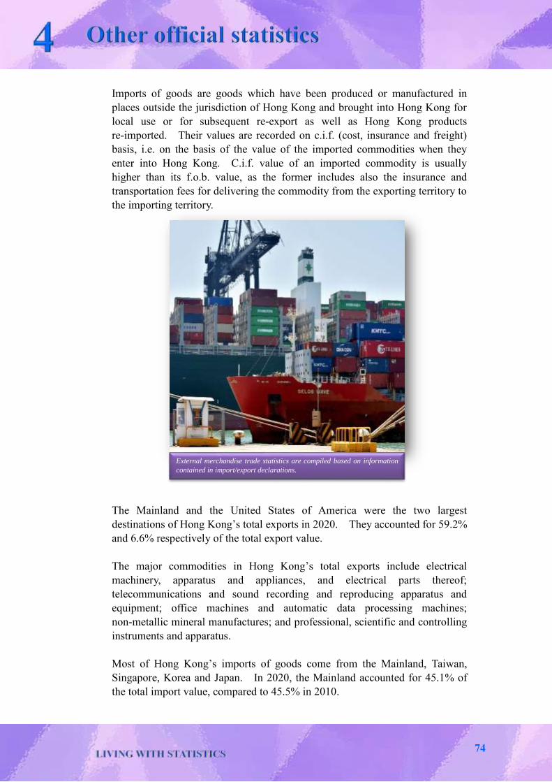
Imports of goods are goods which have been produced or manufactured in

places outside the jurisdiction of Hong Kong and brought into Hong Kong for

local use or for subsequent re-export as well as Hong Kong products

re-imported. Their values are recorded on c.i.f. (cost, insurance and freight)

basis, i.e. on the basis of the value of the imported commodities when they

enter into Hong Kong. C.i.f. value of an imported commodity is usually

higher than its f.o.b. value, as the former includes also the insurance and

transportation fees for delivering the commodity from the exporting territory to

the importing territory.

The Mainland and the United States of America were the two largest

destinations of Hong Kong’s total exports in 2020. They accounted for 59.2%

and 6.6% respectively of the total export value.

The major commodities in Hong Kong’s total exports include electrical

machinery, apparatus and appliances, and electrical parts thereof;

telecommunications and sound recording and reproducing apparatus and

equipment; office machines and automatic data processing machines;

non-metallic mineral manufactures; and professional, scientific and controlling

instruments and apparatus.

Most of Hong Kong’s imports of goods come from the Mainland, Taiwan,

Singapore, Korea and Japan. In 2020, the Mainland accounted for 45.1% of

the total import value, compared to 45.5% in 2010.

External merchandise trade statistics are compiled based on information

contained in import/export declarations.

74

0

500

1,000

1,500

2,000

2,500

3,000

3,500

4,000

4,500

5,000

2010 2011 2012 2013 2014 2015 2016 2017 2018 2019 2020

Tra

de

val

ue

(HK

$ b

illi

on)

Year

Imports

Total exports

Chart 4.1 Values of total exports and imports of goods, 2010 – 2020

(2) Trade in services

With the structural change in the Hong Kong economy, the importance of

service industries has been on the rise. Being an externally oriented economy,

Hong Kong is an important centre not only for trade in goods, but also for trade

in services (TIS). TIS in Hong Kong has been maintaining observable growth

in recent years.

Hong Kong’s TIS statistics can be traced back to the reference year of 1980.

Owing to data limitation, the classification of services at that time was only

based on major industries in which the Hong Kong businesses were engaged.

In response to the growing demand for detailed statistics on TIS, Hong Kong

has started releasing detailed TIS statistics by type of services and

country / territory on an annual basis since 2002, with the series dated back to

the reference year of 1995.

During the period from 2010 to 2019, the value of total exports of services rose

significantly, from $625.7 billion in 2010 to $798.9 billion in 2019, at an

average annual growth of 2.8%. Total value of imports of services also

increased, from $546.9 billion in 2010 to $634.2 billion in 2019, at an average

annual growth of 1.7%. However, both the values of total exports and

imports of services recorded declines in 2020 due to the impact of the

COVID-19 pandemic. In 2020, the two largest service components in exports

of services were transport and financial services (at $177.7 billion@ and $168.1

billion@ respectively), which also brought about a sizable surplus in the overall

TIS after netting out the total imports of services.

75

Analysing exports of services of Hong Kong by geographical breakdown(1) in

2019, the Mainland (37.7%) and the United States of America (14.9%) were

the major destinations, followed by the United Kingdom (8.9%), Japan (4.4%)

and Singapore (4.2%).

For imports of services(1) of Hong Kong, the Mainland (37.8%) and the United

States of America (11.0%) were also the major sources, followed by Japan

(8.2%), the United Kingdom (6.3%) and Singapore (4.4%).

Chart 4.2 Values of exports and imports of services of Hong Kong,

2010 – 2020

Note :

(1) Financial intermediation services indirectly measured (FISIM) have no geographical breakdowns. Hence, trade in services figures analysed by country / territory do not include figures in respect of FISIM.

0

100

200

300

400

500

600

700

800

900

1,000

2010 2011 2012 2013 2014 2015 2016 2017 2018 2019 2020

Val

ue

(H

K$

bil

lio

n)

Year

Exports of services

Imports of services

@

76

National income statistics

Gross Domestic Product (GDP) and Gross National Income (GNI) are core statistics

in National Accounts. They are both important economic indicators and are useful

for analysing the overall economic situation of an economy, with the former

particularly useful for reflecting the level of production, and the latter for aggregate

income of residents.

GDP is a measure of the total value of production of all resident producing units of

an economy in a specified period (typically a year or a quarter), before deducting the

consumption of fixed capital. By providing statistics on the production of various

sectors of the economy, GDP is more relevant for analyses related to production

activities in the economy, such as employment, productivity, industrial output,

investment in equipment and structure.

GDP of Hong Kong is compiled using both the “production approach” and the

“expenditure approach”. Under the production approach, GDP is an aggregate

measure of the total value of net output of all resident producing units. Net output

is measured by value added, which is defined as the value of gross output less the

value of intermediate consumption (that is the value of goods and services used up in

the course of production). Each producing unit works to “add value”. Summation

of the value added of all resident producing units gives an aggregate measure of the

total output of the economy which is free from double counting.

It is essential to apply the concept of value added in GDP compilation in order to

avoid double counting the value of production. Since various producing units are

indeed closely linked in the course of production, the goods or services produced by

a producing unit may be used as the intermediate consumption of another producing

unit. If the gross outputs of individual producing units are added up directly, the

values of certain goods and services will be counted more than once and the GDP so

derived will exaggerate the true value of production.

From another angle, goods and services produced will eventually be consumed by

final users which will be captured in the total expenditure on final demand for goods

and services. Thus, the expenditure approach can also be applied for the

compilation of GDP.

77

Under the expenditure approach, GDP is compiled as the total final expenditures on

goods and services (including private consumption expenditure(2), government

consumption expenditure, gross domestic fixed capital formation, changes in

inventories and exports of goods and services), less imports of goods and services.

The production and expenditure approaches represent how components within

GDP can be viewed from two different perspectives. In theory, there is only one

GDP figure. However, since the data sources and estimation methods adopted in

the compilation of GDP in different approaches are not the same, some statistical

discrepancies may exist between the GDP estimates compiled under the two different

approaches.

Conceptually, changes over time in GDP at current prices can be factored into two

components, reflecting (1) changes in the prices of goods and services produced or

purchased, and (2) changes in their volumes. In order to measure the volume

growth of GDP and its components, the effect of price changes has to be eliminated.

The year-on-year change in the volume measure of GDP gives a measure of the

“real” growth of an economy.

To compile the volume measures of GDP and its components, the annually

re-weighted chain linking approach is adopted. For a particular year, the volume

estimates of major components of GDP revalued at preceding year prices are first

derived by “deflating” the current price values of sub-components by the relevant

price indices (or in some cases by revaluing the current period quantities at preceding

year prices) at the most disaggregated levels. The volume estimate of GDP is then

obtained by aggregating the volume estimates of GDP major components revalued at

preceding year prices. With the effect of price changes eliminated, the volume

estimate reflects the real growth of GDP. The preceding-year weighted volume

measures of GDP and its components are chain linked to a selected reference year in

order to obtain a continuous time series of the chain volume measures of GDP and its

components.

Note :

(2) Private consumption expenditure (PCE) refers to the total value of final consumption

expenditure on goods and services by households and private non-profit institutions serving

households. It is a comprehensive measure of household overall spending on consumption

goods (purchased from various channels including the conventional retail outlets) and services

purchased locally or outside Hong Kong.

PCE is distinguished from retail sales statistics in that:

(i) retail sales statistics, primarily intended to measure the sales receipts of goods sold by local

retail establishments for gauging the short-term business performance of the local retail

sector, refer to consumer spending on goods purchased from local retail establishments but

do not cover those consumer spending on electricity, gas and water and on various services

(such as housing, transportation, education, medical and health care, recreation,

entertainment);

(ii) visitors' spending in Hong Kong is included in the retail sales figure but not in PCE; and

(iii) Hong Kong residents' consumption expenditure abroad is covered in PCE but such

spending outside Hong Kong is outside the coverage of retail sales statistics.

78

1,000

1,200

1,400

1,600

1,800

2,000

2,200

2,400

2,600

2,800

3,000

2010 2011 2012 2013 2014 2015 2016 2017 2018 2019 2020

Gro

ss D

om

esti

c P

rod

cut

(HK

$ b

illi

on)

Year

At current market prices

In chained (2019) dollars

0

Chart 4.3 Gross Domestic Product of Hong Kong, 2010 – 2020

Hong Kong’s GDP for 2020 at current market prices amounted to $2,688.5 billion,

about 1.5 times of the corresponding figure of $1,776.3 billion for 2010. GDP for

2020 in chained (2019) dollars was $2,671.6 billion, or 1.2 times of the

corresponding figure of $2,294.1 billion for 2010. This represented an average

annual growth rate of 1.5% in real terms between 2010 and 2020.

Apart from being a measure of the overall economic performance of an economy,

GDP is often used in international comparisons of state of economic well-being. In

the light of the variations in the scale of different economies, “per capita GDP” is a

more relevant indicator for comparing the economic well-being in different places.

Per capita GDP of an economy is obtained by dividing the total GDP in a year by the

population of that economy in the same year.

At current market prices, per capita GDP for Hong Kong increased from $252,887 in

2010 to $359,343 in 2020. This represented an average annual growth rate of 3.6%.

To eliminate the effect of price changes over the ten-year period, the average annual

growth rate of per capita GDP in real terms during the period can be referred to,

which was 0.9%.

0

79

GNI is another useful measure of economic performance. It measures the total

income earned by residents of an economy(3) from engaging in various economic

activities, irrespective of whether the economic activities are carried out within the

economic territory of the economy or outside. Therefore, GNI and related statistics

are particularly useful for analysing economic situations relating to income of

residents, investment, domestic demand and inflation.

GNI is obtained by adding to GDP the primary income earned by residents from

outside the economic territory and deducting primary income earned by

non-residents from within the economic territory. Primary income includes income

from direct investment, portfolio investment, other investment, reserve assets(4) and

compensation of employees. Similar to GDP, GNI can be compiled on the basis of

current market prices and in chained dollars.

Real Gross National Income (RGNI) measures the real purchasing power of the total

income earned by residents of an economy, taking into account the relative changes

in import and export prices. RGNI at preceding year prices is obtained by adding

the terms of trade adjustment and real net external primary income flows to GDP in

volume terms. The RGNI in chained dollars is calculated using the annually

re-weighted chain linking approach, in much the same way as the compilation of the

chain volume measures of GDP.

In Hong Kong, the first set of GNI statistics was produced in 1995 in respect of the

reference year of 1993.

GNI for 2020 at current market prices was $2,837.0 billion, or about 1.6 times of the

corresponding figure for 2010. RGNI for 2020 in chained (2019) dollars was

$2,815.9 billion, or about 1.2 times of the corresponding figure for 2010.

Notes :

(3) Residents of an economy include individuals and organisations. According to international

standards, for individuals, residents refer to those who normally stay in the economic territory of

the economy, irrespective of their nationality. If an individual has stayed in the economy for at

least 12 months or intends to do so, he / she is considered as normally staying in that economy.

For organisations, residents refer to those which ordinarily operate in the economic territory of

the economy. The economic territory is the geographic territory under the effective control of

the government of that economy. Conceptually, the residence status of individuals and

organisations depends on their centre of predominant economic interest.

(4) Please refer to the section on “Balance of Payments statistics” on page 81 for more details about

direct investment, portfolio investment, other investment and reserve assets.

80

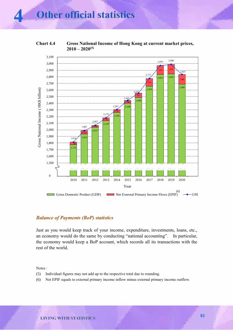
Chart 4.4 Gross National Income of Hong Kong at current market prices,

2010 – 2020(5)

Balance of Payments (BoP) statistics

Just as you would keep track of your income, expenditure, investments, loans, etc.,

an economy would do the same by conducting “national accounting”. In particular,

the economy would keep a BoP account, which records all its transactions with the

rest of the world.

Notes :

(5) Individual figures may not add up to the respective total due to rounding.

(6) Net EPIF equals to external primary income inflow minus external primary income outflow.

1,776

1,934

2,037

2,138

2,260

2,398

2,490

2,659

2,835 2,845

2,689

38

53

29

41

47

44

63

116

135 144

148

1,814

1,987

2,067

2,179

2,307

2,443

2,553

2,775

2,9702,988

2,837

1,300

1,400

1,500

1,600

1,700

1,800

1,900

2,000

2,100

2,200

2,300

2,400

2,500

2,600

2,700

2,800

2,900

3,000

3,100

2010 2011 2012 2013 2014 2015 2016 2017 2018 2019 2020

Gro

ss N

atio

nal

Inco

me

( H

K$

bil

lio

n)

Year

Gross Domestic Product (GDP) Net External Primary Income Flows (EPIF) GNI

0

，，

(6)

81

BoP is a statistical statement that systematically summarises, for a specific time

period (typically a year or a quarter), the economic transactions of an economy with

the rest of the world (i.e. between residents and non-residents). A BoP account

comprises two broad accounts : (a) the current account; and (b) the capital and

financial account.

The current account measures the flows of goods, services, primary income and

secondary income between residents and non-residents. Transactions recorded in

this account reflect the provision and acquisition of resources by an economy to and

from other economies.

The primary income account shows the amounts receivable and payable abroad in

return for providing / obtaining use of labour, financial resources or natural resources

to / from non-residents. Primary income mainly comprises compensation of

employees and investment income. Compensation of employees is the return for

the contribution of labour inputs to the production process. Investment income is

the return for providing financial resources; it consists of dividends, reinvested

earnings, interest, etc.

The secondary income account records current transfers between residents and

non-residents. Current transfers are transactions in which real or financial resources

that are likely to be consumed immediately or shortly are provided without the

receipt of equivalent economic values in return. Examples include workers’

remittances, donations, official assistance and pensions. Current transfers are

unilateral in nature and are offsetting entries in the BoP account for one-sided

transactions.

Within the capital and financial account, the capital account measures external

transactions in capital transfers, and the acquisition and disposal of non-produced,

non-financial assets (such as trademarks and brand names). Examples of capital

transfers include forgiveness of debts by creditors and cash transfers involving the

acquisition or disposal of fixed assets. The financial account records transactions in

financial assets and liabilities between residents and non-residents. It shows how an

economy’s external transactions are financed. Transactions in the financial account

are classified by function (i.e. the purpose of the investment) into direct investment,

portfolio investment, financial derivatives, other investment and reserve assets.

Direct investment refers to external investment in which an investor of an economy

acquires a lasting interest and a significant degree of influence or an effective voice

in the management of an enterprise located in another economy. For statistical

purpose, an effective voice is taken as being equivalent to a holding of 10% or more

of the voting power in an enterprise.

82

Portfolio investment refers to investment in non-resident equity securities and debt

securities (e.g. bonds and notes, money market instruments), other than that included

in direct investment or reserve assets. Compared with direct investors, portfolio

investors in equity securities and debt securities of non-resident enterprises have no

lasting interest or influence in the management of the enterprises concerned. A

holding of less than 10% of the voting power in an enterprise is regarded as portfolio

investment.

Financial derivatives are financial instruments that are linked to a specific financial

instrument, indicator or commodity, and through which specific financial risks can be

traded in financial markets in their own right. Financial derivatives include

option-type contracts (e.g. warrants and options) and forward-type contracts (e.g.

futures, interest rate swaps, currency swaps, forward rate agreements, forward

foreign exchange contracts).

Other investment refers to other financial claims on and liabilities to non-residents

that are not classified as direct investment, portfolio investment, financial derivatives

or reserve assets. Other investment includes non-marketable loans, currency and

deposits, trade credits and advances, and other assets / liabilities.

Reserve assets are external assets that are readily available to and controlled by the

monetary authority of an economy (for Hong Kong, the Hong Kong Monetary

Authority) for meeting BoP financing needs, for intervention in exchange markets to

regulate the currency exchange rate of that economy, and for other related purposes

(such as maintaining confidence in the currency and the economy, and serving as a

basis for foreign borrowing).

83

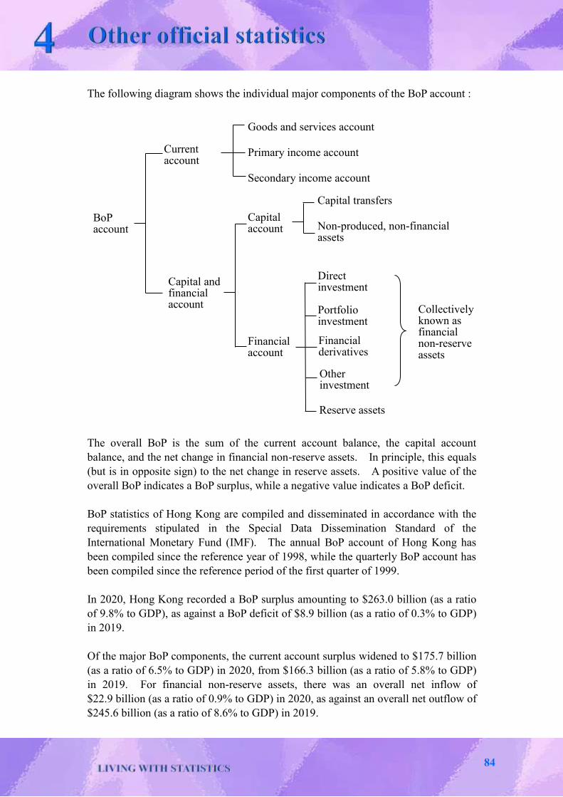
The following diagram shows the individual major components of the BoP account :

The overall BoP is the sum of the current account balance, the capital account

balance, and the net change in financial non-reserve assets. In principle, this equals

(but is in opposite sign) to the net change in reserve assets. A positive value of the

overall BoP indicates a BoP surplus, while a negative value indicates a BoP deficit.

BoP statistics of Hong Kong are compiled and disseminated in accordance with the

requirements stipulated in the Special Data Dissemination Standard of the

International Monetary Fund (IMF). The annual BoP account of Hong Kong has

been compiled since the reference year of 1998, while the quarterly BoP account has

been compiled since the reference period of the first quarter of 1999.

In 2020, Hong Kong recorded a BoP surplus amounting to $263.0 billion (as a ratio

of 9.8% to GDP), as against a BoP deficit of $8.9 billion (as a ratio of 0.3% to GDP)

in 2019.

Of the major BoP components, the current account surplus widened to $175.7 billion

(as a ratio of 6.5% to GDP) in 2020, from $166.3 billion (as a ratio of 5.8% to GDP)

in 2019. For financial non-reserve assets, there was an overall net inflow of

$22.9 billion (as a ratio of 0.9% to GDP) in 2020, as against an overall net outflow of

$245.6 billion (as a ratio of 8.6% to GDP) in 2019.

BoP account

Capital and financial account

Current account

Primary income account

Goods and services account

Secondary income account

Capital account

Capital transfers

Non-produced, non-financial assets

Financial account

Direct investment

Portfolio investment

Financial derivatives

Other investment

Reserve assets

Collectively known as financial non-reserve assets

84

Besides the BoP account, the International Investment Position (IIP) statement is also

an important component under the framework of BoP statistics.

While the BoP financial account measures transactions in external financial assets

and liabilities of an economy occurred during a period, IIP reflects the level of such

assets and liabilities at a particular time point. The former involves a flow concept,

while the latter refers to a stock concept. Transactions are economic flows during a

specific time period. On the other hand, stocks are positions in, or holdings of,

assets and liabilities at a particular time point. Transactions in assets and liabilities,

among other factors, will affect the stock of these assets and liabilities. In addition

to transactions, price changes and exchange rate variations as well as other

adjustments (e.g. reclassifications, unilateral cancellation of debts) also have an

impact on the value of the stock of an economy’s external financial assets and

liabilities when expressed in the local currency of the economy.

C&SD started to release annual IIP statistics for Hong Kong in mid-2002. Time

series on annual IIP statistics since the end of 2000 and quarterly IIP statistics since

the first quarter of 2010 are available.

At the end of 2020, Hong Kong’s external financial assets and liabilities amounted to

$48,767.7 billion and $32,077.3 billion respectively. After netting out the external

financial liabilities from the external financial assets, Hong Kong stood as a net

creditor, with net external financial assets amounting to $16,690.4 billion (equivalent

to 6.2 times of GDP).

BoP and IIP statistics provide an integrated framework for the analysis of an

economy’s external economic relationships. They are important for monetary and

financial monitoring and policy deliberations in both the domestic and international

contexts.

The world economy is becoming increasingly integrated through international trade

and investment flows. Globalisation of economic activities is a topic of concern to

both the government and private sector of an economy. BoP statistics provide a lot

of useful information required for the study of an economy’s external orientation.

Besides, previous international financial crises have aroused increased interest in the

analysis of IIP statistics, through which an economy’s external vulnerability can be

assessed. Analyses on the sizes of the external assets and liabilities by type of

investment, by financial instrument and by sector allow us to understand which

sector in the economy is most vulnerable.

85

Labour statistics

Labour statistics are very useful economic statistics regarding the labour force and

labour market of Hong Kong. They reflect the characteristics of the economically

active population and their economic activities. Since working is also an important

aspect of one’s life, labour statistics are considered as social statistics as well.

The labour force participation rate (LFPR) is obtained by expressing the size of the

labour force as a percentage of the population of working age, i.e. population aged 15

and over. This is a measure of the working age population’s propensity to be in the

labour force. The size of the labour force of Hong Kong in 2020 was 3.89 million

and the LFPR was 59.6%.

The unemployment rate, in particular, is one of the most important indicators

describing the labour market situation. It refers to the percentage of “unemployed

population” in the “labour force”. Because of economic downturn, the

unemployment rate reached the high level of 7.9% in 2003. The labour market

improved drastically towards the end of 2003 and this trend sustained thereafter.

Consequently, the unemployment rate dropped significantly to 3.5% in 2008.

Impacted by the outbreak of the global financial tsunami in late 2008, the

unemployment rate bounced back to 5.3% in 2009. Along with the gradual

recovery of the economy from the global recession in 2009, the labour market saw

notable improvement, with the unemployment rate gradually dropping from 4.3% in

2010 to 2.8% in 2018. However, owing to the elevated US-Mainland trade tensions

and the local social incidents, the unemployment rate increased slightly to 2.9% in

2019. In 2020, owing to the impact of the COVID-19 pandemic, the unemployment

rate increased sharply to 5.8%.

As the unemployment rate is subject to effects of seasonal variations (e.g. there are

generally more job-seeking graduates entering the labour market in late summer,

leading to a higher unemployment rate), short-term fluctuations, say between

adjacent months or quarters, in the unemployment rate do not necessarily signal an

actual change in the labour market conditions. Hence, when studying the

underlying trend of unemployment, it is common to use the seasonally adjusted

unemployment rate, which is obtained by using statistical methods that estimate and

remove the seasonal variations from the original figures.

The definition used for measuring unemployment follows closely that recommended

by the International Labour Organization (ILO). According to the definition, a

person aged 15 or over is classified as unemployed if he / she satisfies all of the three

following criteria :

(a) has not had a job and should not have performed any work for pay or profit

during the 7 days before enumeration;

86

(b) has been available for work during the 7 days before enumeration; and

(c) has sought work during the 30 days before enumeration.

However, if a person aged 15 or over fulfils conditions (a) and (b) above only and

he / she has not sought work during the 30 days before enumeration because he / she

believed that work was not available, he / she is still classified as unemployed, and is

regarded as a so-called “discouraged worker”.

It should be emphasised that “whether available for work” is an important condition

for defining unemployment. Those persons who are not available for work because

of one reason or another (e.g. being fully engaged in household duties) are not

classified as unemployed even though they are without work, as they do not fulfil

condition (b) of the above definition of unemployment, i.e. not available for work

during the 7 days before enumeration.

When looking at the unemployment figures, it should be noted that “unemployment”

is a state of affairs, which is not equivalent to the event of “losing a job”. For

persons who have been dismissed from their jobs or who have left their jobs for

certain reasons, but have managed to take up another job within a short period of

time, they may not be counted in the unemployed population by definition, even

though they have experienced the event of “losing a job” during the period.

Chart 4.5 Unemployment rate in Hong Kong, 2010 – 2020

0%

1%

2%

3%

4%

5%

6%

7%

8%

2010 2011 2012 2013 2014 2015 2016 2017 2018 2019 2020

Unem

plo

ym

ent

rate

Year

87

Statistics in respect of “underemployed persons” also provide another useful piece of

information about the labour force. The underemployed persons are defined as

those employed persons who have involuntarily worked less than 35 hours during the

7 days before enumeration and have sought additional work during the 30 days

before enumeration, or have not sought but have been available for additional work

during the 7 days before enumeration. Those employed persons who worked less

than 35 hours per week but have not been available for additional work and have not

sought additional work (e.g. full-time teachers in bi-sessional schools) are not

classified as underemployed.

Statistics on labour force, employment, unemployment and underemployment are

compiled by C&SD based on the data collected from a continuous General

Household Survey (GHS) conducted on households (and their members). The

sample size of the GHS in a three-month period is about 25 000 households and the

survey methodology adopted is in line with international standards and practices.

Apart from the aggregate figures mentioned above, a large amount of statistics

analysed by various groupings (e.g. industrial and occupational distributions of the

employed population) are also available from the GHS. These statistics are

provided to the government bureaux and departments concerned for reference and

are also published in the Quarterly Report on General Household Survey, which is

available to the public on the C&SD website.

Furthermore, statistics on employment (i.e. number of employees and vacancies in

different industries) and wage and payroll statistics are also compiled by C&SD.

They are commonly referred to by enterpreneurs and human resources management

personnel, since they provide information which is very useful for formulation of

personnel management strategies. For example, firms can compare their staffing

and vacancy situations with those of the industry taken as a whole or with those of

other industries. They can also compare wage levels of their employees with others

in the same industry. In addition, C&SD also compiles statistics on the level and

distribution of wages of all employees in Hong Kong, as well as their employment

and demographic characteristics. These statistics are essential inputs for analyses

related to the Statutory Minimum Wage. They are also useful for studies on

labour-related topics by the Government and the private sector. The relevant data

are collected from surveys conducted on business establishments.

88

Price statistics

The Consumer Price Index (CPI) is another widely quoted item of official statistics.

It is an important economic indicator which summarises changes over time in the

price levels of consumer goods and services generally purchased by households.

The year-on-year rate of change in the CPI is commonly used to reflect the inflation

or deflation affecting households. Specifically, it measures changes in the total cost

of a given basket of consumer goods and services representative of the purchases

made by households in a specified time period.

The CPI has been widely accepted and used as a reference for salary adjustment

purposes so as to maintain the purchasing power of employees in the face of

changing prices.

The prices of some consumer goods and services may be subject to seasonal

variations causing the CPI to rise or fall. Therefore, when studying changes in the

CPI, it is common to refer to year-on-year changes (e.g. comparing the CPI of a

month with that of the same month in the preceding year) so as to eliminate the

effects of seasonal factors. Another alternative is to use the deseasonalised CPI.

The latter is obtained by using statistical methods that estimate and remove the

seasonal variations from the original index.

Households in different expenditure ranges have different expenditure patterns.

Different series of CPIs are therefore compiled by C&SD to reflect the impact of

consumer price changes on households in different expenditure ranges. The CPI(A),

CPI(B) and CPI(C) are compiled based on the

expenditure patterns of households in the relatively

low, medium and relatively high expenditure ranges

respectively. The Composite CPI, which is compiled

based on the overall expenditure pattern of all these

households taken together, reflects the impact of

consumer price changes on the household sector as a

whole.

Two types of data are required for compiling the CPI,

namely price movements of consumer goods and

services and their expenditure weights. Given the

wide variety of consumer goods and services, it can be

imagined that a lot of price data must be collected for

the compilation of the CPI. Indeed, C&SD collects

over 40 000 price quotations each month from around

3 500 local retail outlets and service providers in Hong

Kong for the purpose of compiling the index. Price

quotations are also collected from online outlets (both

local and non-local) commonly patronised by

households in Hong Kong as supplementary data in CPI compilation.

An enumerator is using a mobile tablet to

collect retail prices of commodities for

compiling the Consumer Price Index.

89

As for the expenditure weights, they are derived from the results of the Household

Expenditure Survey (HES) which is conducted once every 5 years. As households

spend more on some items and less on the others, similar price movements in

different items may have different impacts on the households and effects on the

overall price change. Therefore, a weighting system which represents the relative

importance, in terms of expenditure, of individual items in the basket of consumer

goods and services bought by households is required for the compilation of the CPI.

The weight of each item represents the share of the item in the total expenditure of

households.

As driven by the increases in food prices and private housing rents, annual rates of

increase in the CPIs climbed up in 2011, and then stabilised during 2012 to 2014.

The increasing trend in the CPIs started to moderate from 2015, due to the continued

softening in international food and commodity prices as well as the strong US dollar.

Annual rates of increase in the CPIs moderated further in 2017 and picked up again

since 2018. However, the CPI registered a mild annual rate of increase in 2020

amid the COVID-19 pandemic.

In making reference to the CPI or its change over time, it should be noted that the

information thus conveyed reflects the collective experience of all households about

inflation / deflation and that it does not always correspond to the experience of

individual households. As each household has its own expenditure pattern and

prices of different goods and services increase or decrease at varying rates,

inflation / deflation does not affect all households to the same extent. If a

household spends a lot on goods and services with rapid price increases / decreases,

the household will feel greater impact of inflation / deflation.

Besides, people are generally psychologically more aware of isolated cases of drastic

price changes, especially those which affect them personally. Thus, one would tend

to notice and remember only those large price changes and do not realise that there

are other cases of moderate or small price changes. Even individual members of the

same household may feel different impacts of price changes. Therefore, while

personal experience may be subjective or biased, the CPI provides an objective

assessment of price changes affecting households generally.

Another point to note is that the CPI measures changes in the price level of consumer

goods and services purchased by households. If we buy more goods or consume

services of higher quality than before, then the increase in expenditure is not solely

caused by price increase.

90

Chart 4.6 Composite Consumer Price Index and its year-on-year rate of

change, 2010 – 2020(7), (8)

Operating statistics of businesses

Statistics from economic surveys conducted periodically by C&SD provide

information about business trend, cost structure and profit situation in various

economic sectors. Firms can make use of the statistics to compare their own

performance against the general situation within their specific sectors and adjust their

business strategies accordingly.

Other economic statistics

Shipping statistics are compiled by C&SD in collaboration with other parties.

Notes :

(7) The CPIs from October 2019 onwards are compiled based on expenditure weights obtained from the 2019/20 Household Expenditure Survey. The CPIs for earlier periods are compiled based on old weights and have been re-scaled to the new base period for linking with the new index series.

(8) From October 2020 onwards, the year-on-year rates of change are derived from the 2019/20-based CPIs. The year-on-year rates of change before October 2020 were derived using the index series in the base periods at that time (e.g. the 2014/15-based index series for compiling the rates of change during the period from October 2015 to September 2020), compared with the index a year earlier in the same base period.

0

20

40

60

80

100

120

0

2

4

6

8

10

12

20202019201820172016201520142013201220112010

Co

mp

osi

te C

PI

(Oct

20

19

–S

ep 2

02

0 =

10

0)

Yea

r-o

n-y

ear

rate

of

chan

ge

(%)

Year

Year-on-year rate of change

Composite CPI

91

(B) Social statistics

Social statistics broadly comprise the following areas : population statistics, poverty

statistics, education statistics, transport statistics, housing statistics, medical and

health statistics, social welfare statistics and crime statistics.

Population statistics

Population statistics have already been discussed in detail in Chapters 1 to 3. It

may be emphasised again here that population statistics, which depict the size,

growth and socio-economic characteristics of the Hong Kong population, are among

the most useful items of statistical information for government administrators.

They are of prime importance in the formulation and administration of government

policies in such areas as education, housing, transport, medical and health, and social

welfare services. For businesses, population statistics are useful in identifying

potential target markets more accurately and in supporting better investment

decision-making.

Poverty statistics

Setting a poverty line is useful for better understanding of Hong Kong’s poverty

situation and supporting the formulation of poverty alleviation policies.

Generally speaking, there are two mainstream approaches in deriving a poverty line

viz. “absolute poverty” and “relative poverty”. While the former defines those

individuals who cannot meet a level of “minimum subsistence” or “basic needs” as

“poor”, the latter refers “poor” as those whose living standards are below that of the

general public.

92

In the case of Hong Kong, the concept of “relative poverty” is adopted. Under this

approach, household income before policy intervention (purely theoretical

assumption) (9) (i.e. with the impact of taxation and cash transfers removed) is used as

the basis for a measurement yardstick and the main poverty line is set at 50% of

median household income in respect of each household size. As such, poor

households refer to the number of households with monthly household income less

than the poverty line while poor population refers to the number of persons in these

households. Poverty rate is the ratio of poor population to total population in

domestic households. To evaluate the effectiveness of poverty alleviation measures,

these poverty indicators based on household income before and after policy

intervention (recurrent cash) (10) would be compared.

Chart 4.7 Poverty lines by household size, 2009 – 2019

Notes :

(9) “Pre-intervention” (purely theoretical assumption) household income refers to the original household income without any policy intervention. It only includes households’ own employment earnings and other non-policy intervention cash income. This is a form of “simulated” household income which does not exist in reality and only represents a certain portion of the total disposable income. Setting a poverty line on such basis aims to reveal the most fundamental situation of a household, and to avoid any distortion of policy measures on the poverty line thresholds.

(10) “Post-intervention” (recurrent cash) household income is derived by deducting taxes payable and adding back all recurrent cash benefits (such as Comprehensive Social Security Assistance, Old Age Allowance, Old Age Living Allowance, Disability Allowance, Work Incentive Transport Subsidy and Working Family Allowance) from the original household income. The derived household income can more genuinely reflect the amount of monthly disposable cash available in the “pocket” of a household.

0

2,000

4,000

6,000

8,000

10,000

12,000

14,000

16,000

18,000

20,000

22,000

24,000

26,000

2009 2010 2011 2012 2013 2014 2015 2016 2017 2018 2019

6-person+

5-person

4-person

3-person

2-person

1-person

Mo

nth

ly h

ouse

ho

ld i

nco

me

(HK

$)

Year

93

As the poverty line is defined in a way relative to median household income by

household size, the poverty line for a particular household size group will be raised

along with an increase in the median household income in respect of that household

size group. The economy fell into recession in the second half of 2019. As labour

demand began to slacken, growth in employment earnings of the grassroots also

decelerated further in 2019. Against this background, the growth in median

household income moderated noticeably. The poverty line thresholds showed a

similar trend of decelerating increase in 2019. The poverty lines of 3-person

households to 5-person households registered the smallest increases in a decade

(ranging from 1.1% to 2.8%(11)). The poverty line of 2-person households remained

virtually unchanged, ending its continuous upward trend for nine years. The annual

changes of the poverty line thresholds of 1-person households and

6-person-and-above households were the exceptions, with the former rising markedly

by 12.5% to $4,500 in 2019 and the latter rebounding after a visible fall in the

preceding year.

In 2019, the local economy fell into recession and the labour market situation

deteriorated during the year. These, coupled with the continuous effect of structural

factors of population ageing and dwindling household size, contributed to a notable

worsening in the overall poverty situation. After recurrent cash intervention, the

overall number of poor households and the poor population in 2019 increased

notably to 474 000 (+39 200 or +9.0%) and 1 097 800 (+73 500 or +7.2%)

respectively, with the poverty rate up by 0.9 percentage point to 15.8%. Before

policy intervention (purely theoretical assumption), increases in some of the poverty

indicators would be even more pronounced, with the number of poor households, the

poor population and the poverty rate up to 648 500 (+35 700 or +5.8%), 1 490 700

(+84 200 or +6.0%) and 21.4% (+1.0 percentage point) respectively over the period.

Note :

(11) The annual changes in poverty line thresholds are calculated based on unrounded figures.

94

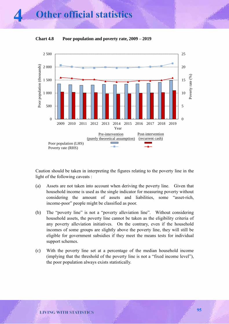
Chart 4.8 Poor population and poverty rate, 2009 – 2019

Caution should be taken in interpreting the figures relating to the poverty line in the

light of the following caveats :

(a) Assets are not taken into account when deriving the poverty line. Given that

household income is used as the single indicator for measuring poverty without

considering the amount of assets and liabilities, some “asset-rich,

income-poor” people might be classified as poor.

(b) The “poverty line” is not a “poverty alleviation line”. Without considering

household assets, the poverty line cannot be taken as the eligibility criteria of

any poverty alleviation initiatives. On the contrary, even if the household

incomes of some groups are slightly above the poverty line, they will still be

eligible for government subsidies if they meet the means tests for individual

support schemes.

(c) With the poverty line set at a percentage of the median household income

(implying that the threshold of the poverty line is not a “fixed income level”),

the poor population always exists statistically.

0

5

10

15

20

25

0

500

1 000

1 500

2 000

2 500

2009 2010 2011 2012 2013 2014 2015 2016 2017 2018 2019

Po

ver

ty r

ate

(%)

Po

or

po

pula

tio

n (

tho

usa

nd

s)

數列2 數列1

數列3 數列4

Year

Pre-intervention

(purely theoretical assumption)

Post-intervention

(recurrent cash)

Poor population (LHS)

Poverty rate (RHS)

95

Other social statistics

Education statistics, transport statistics, housing statistics, medical and health

statistics, social welfare statistics and crime statistics are basically compiled by the

respective government bureaux and departments to meet specific planning and

administrative needs. They are also useful to the Government as a whole in

formulating broad-range policies. Coordination is necessary to ensure that statistics

relating to different areas can be used together in a compatible way for planning

activities which cut across various facets of the society.

On education, there are three main areas of statistics, viz. pupils, teachers and school

place provision. The Education Bureau compiles a lot of statistics which are very

useful for formulating policies and planning facilities.

Regular public transport operating statistics and related statistics on transport are

compiled. These provide a basis for understanding the transport and traffic

situation of Hong Kong and for transport planning.

Housing statistics cover housing stock and housing production in both the public and

private sectors. They also relate to the situation in various housing estates. They

are very useful in reflecting the housing conditions of the people of Hong Kong and

are important references when planning for housing development is undertaken.

Medical and health statistics provide information about births, diseases, deaths,

health-related behaviours and health services. They facilitate a better understanding

of health status of people in Hong Kong and are useful to the Government for disease

surveillance and control, and formulation of health measures.

Social welfare statistics attempt to establish the number and characteristics of

individuals in the community who require assistance, in particular the aged, the

unemployed, the disabled, the orphaned or deserted children, the delinquent and

people in families with special problems. These statistics are useful in planning,

review and monitoring of the provision of social welfare services.

Crime statistics are compiled on the basis of crimes reported to the police, which

partially reflect the state of law and order in the society. Some crimes are not

reported and statistics on unreported crimes may be collected through the conduct of

a survey on crime victimisation periodically.

From a general data user’s perspective, social statistics provide an objective and

in-depth view of the respective facets of the society, as they can effectively reflect

developments and shortfalls in various areas of living conditions and provision of

social services.

96

Ways of obtaining official statistics

C&SD disseminates official statistics through different media, with emphasis on the

service principles of friendly access and prompt delivery.

For statistics of common interest, C&SD issues press releases to the media. The

schedule for issuing around 130 press releases of regular nature in each calendar year

is announced to the media in September of the preceding year. The schedule is also

available to the general public for reference on the C&SD website.

Statistics which should be of general public knowledge are also uploaded on the

C&SD website under the “Statistics” section.

C&SD also produces different types of statistical products. Members of the public

can download statistical publications and detailed statistical tables of C&SD free of

charge from the C&SD website.

To cater for the changing technological environment and service needs, continuous

efforts have been made in enhancing the contents and functionality of the C&SD

website with a view to further promoting better understanding and application of

statistics in the community. The department’s first Annual Open Data Plan was

announced on the C&SD website in December 2018. To support the government’s

Open Data Policy, statistical tables, datasets and press releases available on the

C&SD website have been listed on DATA.GOV.HK for free download and re-use by

the public for both commercial and non-commercial purposes. Moreover, statistical

datasets in machine readable format (XLS, CSV or XML) are available on the

website to provide the statistics currently published in PDF format in statistical

reports.

Proper understanding of the concepts and definitions of different kinds of statistics is

imperative for their correct interpretation and application. Apart from providing

statistical information to the public, C&SD is also prepared to give advice on the

interpretation and application of statistics so as to maximise their utilisation to users.

In case users require assistance or statistics more detailed than those contained in the

press releases and publications of C&SD, they are welcome to approach C&SD for

assistance by telephone, facsimile, letter, electronic mail or personal visit. A list of

telephone numbers, facsimile numbers, office addresses and e-mail addresses is

given at the C&SD website.

97

https://www.censtatd.gov.hk/en/press_release.html

https://www.censtatd.gov.hk/en/page_105.html


Further information

The above contents present only part of the economic and social statistics produced

by C&SD and various government bureaux and departments. For further

information regarding the official statistics covering various social and economic

aspects of Hong Kong (e.g. latest statistics, statistical reports, concepts and methods),

please visit the following sections of the C&SD website :


External trade

National accounts

Balance of Payments

Prices

Business prospects

The Four Key Industries and other selected industries

Energy

Housing and property

Public finance, money and market

Innovation and technology

Transport

Information and communications

Tourism

Education

Health

Social welfare

Law and order

Culture, entertainment and recreation

Environment, climate and geography

Interactive quiz




98



















https://www.censtatd.gov.hk/en/scode110.html#section1



















Exercise

Please give a in the appropriate box () for the correct answer.

1. The population of Hong Kong in mid-2020 was

5.75 million

6.50 million

7.48 million

7.24 million

2. Crude birth rate in Hong Kong

Year (Number of births per 1 000 population)

2011 13.5

2020 x

x =

7.6

5.8

9.3

9.8

3. If the crude death rate in a given year was 5.0 deaths per 1 000 population and

the crude birth rate was 7.2 births per 1 000 population, the rate of natural

change per 1 000 population in the period was

-2.4

2.2

-12.0

12.0

4. Most of the visitors visiting Hong Kong in 2020 came from

United States of America

Japan

The Mainland

Europe

99

5. The population in mid-2015 = a; and

the population in mid-2020 = b.

The compound average growth rate per annum of the population in this period

was

%10014

a

b

%1004

1

a

b

%10015

a

b

%1005

1

a

b

6. In 2020, the size of the labour force in Hong Kong was

3.82 million

3.88 million

3.95 million

3.89 million

7. Which category of persons is regarded as economically inactive?

Unpaid family workers

Employers

The unemployed

Full-time home-makers

8. Which of the following is not an approach in the compilation of the Gross

Domestic Product?

Expenditure approach

Production approach

Industrial approach

100

Introduction

Statistics on births, deaths and net movements used in making population projections

are compiled from birth and death registration records and immigration clearance

records. In addition, information on the latest size and age-sex structure of the

population and on various other aspects of persons in the population has to be

obtained. This can be achieved by conducting a population census or by-census.

Administrative records, such as the registration records mentioned above, and survey

results, such as those obtained through a population census / by-census, are the

typical sources of data from which statistics are compiled.

Administrative records provide an economical and accurate data source. However,

since they are primarily intended for certain specific purposes, they may not

completely meet the statistical requirements, unless special provision has been made

to cater for such requirements. Naturally, there are situations where meeting such

requirements would mean distorting the original purposes of the administrative

records too much. In such circumstances we would have to give up the idea of

generating the required statistics as a by-product of the administrative system, and

resort to other means of data collection.

Surveys are another important means of data collection whereby the objects of our

study are interviewed, observed or given questionnaires to fill in. If we design the

survey in such a way that all objects of study will be contacted, one way or another,

the survey is specifically referred to as a “census”. If only a sample of the objects

is taken for data collection later on, then the survey is more clearly described as a

“sample survey”. The language in this aspect is, however, a little loose sometimes.

When the word “survey” is used, quite often it is implied that only a sample is taken.

Census versus sample survey

When deciding whether a census or a sample survey should be carried out, a number

of factors should be considered. For studies in which the “population” (i.e. the

group of persons or other objects we wish to study) is large, a proper sample survey,

as compared to a census, is very useful for cutting down the resources required,

including money and manpower, and for reducing the overall burden imposed on the

persons / objects to be studied. Another benefit of carrying out a sample survey

instead of a census is that we can collect, summarise and analyse data more quickly

when the information is urgently needed.

103

On the other hand, a complete census can be considered if very accurate information

is required on small sub-divisions of the “population” under study, and when

comprehensive data on the “population” are needed for forming a benchmark to

support further statistical analyses, such as projections.

Population census and by-census

In a population census, basic information is collected from all persons in the

population of a country / territory while in a population by-census, only a large

sample of persons is covered. Usually a population census is conducted once every

ten years. A by-census may be conducted in between two censuses to update the

information obtained from the last census.

Because of its long history world-wide, and when there is not likely to be confusion,

“population census” is abbreviated as “census” for convenience. Thus, it should be

noted that there can actually be census of agriculture, census of industry and so on,

apart from population census.

Population censuses and by-censuses taken in Hong Kong

The history of population census in Hong Kong can be traced back to 1841. Earlier

censuses were simple, with headcounts taken only. The “1961 Census” was the

first population census in which detailed information was collected on a broad

spectrum of demographic, social and economic characteristics of the population.

Since then, it has become a well-established practice in Hong Kong to conduct

population censuses and by-censuses at regular intervals. Censuses were conducted

in 1961, 1971, 1981, 1991, 2001, 2011 and 2021. By-censuses were conducted in

1966, 1976, 1986, 1996, 2006 and 2016.

Details of the last population by-census are available in the section “The 2021

Population Census” in Chapter 1.

Objectives of conducting population censuses and by-censuses

In a dynamic city like Hong Kong, many changes in major characteristics of the

population occur in a relatively short span of time. Up-to-date and reliable

information on the size, composition and geographical distribution of the population

is necessary for forward planning by the Government. Moreover, as Hong Kong

develops into an international business centre, census and by-census data are widely

used in assessing market conditions and making investment plans. Such data will

also help researchers in studying important social issues.

104

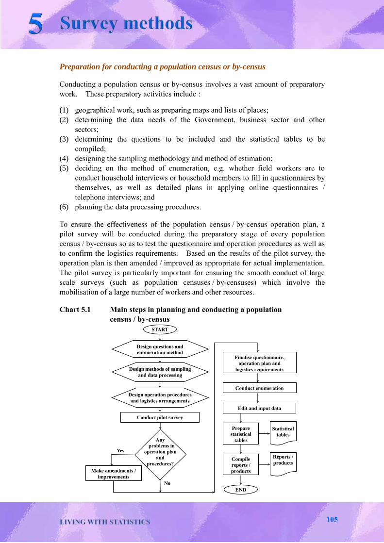
Preparation for conducting a population census or by-census

Conducting a population census or by-census involves a vast amount of preparatory

work. These preparatory activities include :

(1) geographical work, such as preparing maps and lists of places;

(2) determining the data needs of the Government, business sector and other

sectors;

(3) determining the questions to be included and the statistical tables to be

compiled;

(4) designing the sampling methodology and method of estimation;

(5) deciding on the method of enumeration, e.g. whether field workers are to

conduct household interviews or household members to fill in questionnaires by

themselves, as well as detailed plans in applying online questionnaires /

telephone interviews; and

(6) planning the data processing procedures.

To ensure the effectiveness of the population census / by-census operation plan, a

pilot survey will be conducted during the preparatory stage of every population

census / by-census so as to test the questionnaire and operation procedures as well as

to confirm the logistics requirements. Based on the results of the pilot survey, the

operation plan is then amended / improved as appropriate for actual implementation.

The pilot survey is particularly important for ensuring the smooth conduct of large

scale surveys (such as population censuses / by-censuses) which involve the

mobilisation of a large number of workers and other resources.

Chart 5.1 Main steps in planning and conducting a population

census / by-census

No

Yes

START

Conduct pilot survey

Any

problems in

operation plan

and

procedures?

Make amendments /

improvements

Finalise questionnaire,

operation plan and

logistics requirements

Conduct enumeration

Edit and input data

Prepare

statistical

tables

Compile

reports /

products

END

Reports /

products

Statistical

tables

Design operation procedures

and logistics arrangements

Design methods of sampling

and data processing

Design questions and

enumeration method

105

Census order

Furthermore, legislation is needed to provide a legal basis for conducting the

population census or by-census. Under the Census and Statistics Ordinance

(Chapter 316), C&SD is vested with the authority to conduct population census or

by-census. The legislation requires all persons to give particulars for themselves

and their dwelling places in the data collection process. It also lays down penalties

for those who refuse to do so. On the other hand, it contains strict provisions for

safeguarding the confidentiality of the information supplied by individual households

and persons, which assure that such information will only be used for compiling

statistics and will not be released to any parties, including other government

departments.

Public support for the population census / by-census

While there are legal provisions in relation to the conduct of population censuses and

by-censuses, it is important for the community to realise that the findings of the

census / by-census are crucial to the future planning of Hong Kong and that public

participation and cooperation are essential in making the operation successful.

In the 21C, a considerable number of students and teachers were recruited as

temporary field workers to undertake various tasks. They thus had a chance to

participate actively in this important project. Training on interviewing techniques

and other necessary skills was provided. Some school premises were used as field

centres for the field operation.

Processing of population census / by-census data

After raw data are collected from households and individuals in the population, they

must undergo a number of processes before statistical outputs can be produced.

The raw data are first edited to correct for inconsistent answers. They are then

converted into codes for input into the computer. Finally, various computations are

performed by the computer to produce statistical tables in appropriate formats.

Dissemination of population census and by-census results

Results of the more recent rounds of population census and by-census are published

in the forms of summary reports and detailed reports. Users can refer to them

easily and make use of the results for various purposes. In particular, data users can

use the free-of-charge online Interactive Data Dissemination System to build their

own statistical tables. Results of the 16BC are obtainable from the website of the

2016 Population By-census.

106

http://www.censtatd.gov.hk/about_us/census_and_statistics_ordinance/index.jsp

https://www.bycensus2016.gov.hk/en/bc-own_tbl.html

http://www.bycensus2016.gov.hk/en/index.html

http://www.bycensus2016.gov.hk/en/index.html

Other surveys

Apart from population censuses and by-censuses, C&SD and other government

bureaux and departments also carry out other surveys to collect various types of

social and economic data.

Examples of surveys carried out by C&SD are :

– General Household Survey

– Monthly Survey of Retail Sales

– Monthly Retail Price Survey

– Household Expenditure Survey

– Quarterly Survey of Employment and Vacancies

– Annual Earnings and Hours Survey

– Annual Survey of Economic Activities

Examples of surveys carried out by other government bureaux and departments are :

– Enrolment Survey (by Education Bureau)

– Traffic Census (by Transport Department)

– Health Manpower Survey (by Department of Health)

Important points to note in conducting surveys

In planning and conducting surveys, there are a number of major points which need

to be carefully considered :

(A) Overall planning

(1) The objectives of the survey should be clearly specified.

(2) The population covered by the survey should be clearly defined with

reference to the survey objectives. “Population”, in the context of a

survey, refers to the totality of objects under study. The objects may be

human being or otherwise.

(3) It should be ensured that respondents of the survey are able to provide the

information required.

(4) Adequate resources such as time, money and manpower should be

available for the survey.

(5) In conducting a survey, professional advice is often required and should

preferably be sought at an early stage to ensure that the various steps of a

survey are properly planned. This is because rectification is normally

very difficult after the survey is completed and its results are found to be

invalid.

107


(B) Design and selection of sample (in case a sample survey instead of a census is

to be conducted)

(1) Probability sampling methods should be used as far as practicable, instead

of non-probability sampling methods. In probability sampling methods,

every unit in the population has a known and non-zero probability of being

sampled. This allows researchers to draw inferences scientifically from

the sample results about the entire population. Examples of probability

sampling methods include simple random sampling, stratified random

sampling, systematic sampling and cluster sampling.

(2) Non-probability sampling methods such as haphazard sampling

(i.e. picking the sampling units as they come along or as convenient), quota

sampling (i.e. selecting sampling units according to some criteria, such as

50% being male and 50% being female, but the selection of units is at the

discretion of the interviewers) and self-initiated telephone / online polling

(i.e. interested individuals dial a telephone number / visit a website at their

own initiative to give views) should be avoided because such methods

normally induce biases to the survey results.

(3) The sample size depends on the characteristics of the population under

study, the choice of sampling method and the desired precision level of the

estimates. It can be worked out using established statistical methodology.

In general, a larger sample size is needed if estimates of higher precision

are required.

(4) Substitution of sampling units or respondents should not be done once they

have been selected according to a pre-set sampling method.

(C) Questionnaire design

(1) The questionnaire used for a survey should contain questions which are

relevant, precise, unambiguous, well-sequenced and appropriately phrased.

If the questions involve tapping of opinions, care should be taken to avoid

questions which may lead respondents towards the direction of a certain

answer or questions being loaded in favour of a particular response.

(2) Requiring respondents to provide an answer while they are unable to do so

or genuinely have no opinion will result in invalid answers. Answers like

“don’t know” or “no opinion” should be allowed in the questionnaire, as

appropriate.

(3) The questionnaire should not be too long.

(4) To ensure the effectiveness of the questionnaire, a pilot test of the

questionnaire should be conducted on potential respondents.

108

(D) Collection of raw data

(1) The mode of data collection, such as the use of personal interviews,

telephone interviews, online questionnaires or self-administered

questionnaires by mail, should be carefully selected by considering the

respondents’ willingness to cooperate, the degree of complexity of the

subject of enquiry and other relevant factors.

(2) Various arrangements related to fieldwork should be carefully planned in

order to ensure smooth and efficient operation. Fieldwork procedures

should be thoroughly tested before implementation.

(3) The interviewers should be carefully briefed on the concepts and

definitions of terms used in the survey and properly trained on the survey

procedures before they start working.

(4) Interviewers should ensure that respondents understand the questions.

Probing should be done where necessary. This, however, should not be

overdone, lest unnecessary influence will be exerted on respondents.

(5) Every effort should be made to minimise non-contact or refusal cases of

respondents because a low response rate may induce a serious bias in the

survey results. Adequate publicity of the survey, proper introduction of

the surveying organisation, clear identification of interviewers, and giving

advance notice to sampled respondents should help. Arrangements

should also be made to follow up on non-contact respondents and to

persuade uncooperative respondents to participate.

(6) The identity and information supplied by individual respondents should be

kept confidential. With such assurance, respondents would feel at ease

and would be more willing to provide individual or organisational

information and opinions. It should be emphasised that survey is a kind

of statistical work and not an investigation on individuals.

(E) Processing of raw data and compilation and analysis of statistics

(1) Raw data should be carefully and thoroughly checked before compilation

of statistics.

(2) Appropriate statistical methodology should be adopted in compiling and

analysing the data. In particular, in case a sample design has been used

where the probability of selection of every individual respondent is not

equal, it is necessary that proper weighting methods are applied to survey

results to give unbiased population estimates.

(3) Due deliberation should be made to decide on an appropriate sub-grouping

scheme in analysing survey results at disaggregate levels, taking into

account the precision of estimates derived from the sample.

109

(F) Dissemination of survey results

(1) It is a usual practice to publish the survey results if the subject of the

survey is related to a topic of public interest.

(2) The survey results should be presented in the form of aggregate statistics

so that information supplied by individual respondents would not be

disclosed.

(3) A comprehensive survey report should contain details about different

aspects of the survey, in particular details on population coverage, sample

design, sample size, sampling error, response rate and likely sources of

non-sampling error. Where appropriate, specimen of the questionnaire

should be attached.

(4) When the survey results are released to the media, sufficient details on the

survey methodology should be provided in addition to survey findings such

that the media may report both. Otherwise, members of the public will

have no basis to assess the reliability of the findings.

Assessing quality of survey results

There are many factors that will affect the quality of data obtained from a sample

survey. In assessing the data quality of a survey, at least the following issues

should be considered :

(1) Whether the sample of the survey is selected in accordance with a probability

sampling method;

(2) Whether the sample size is sufficiently large;

(3) Whether the questionnaire is well designed; and

(4) Whether the response rate of the survey is sufficiently high.

A well-designed and properly selected sample is crucial to the quality of results

derived from a survey. Nevertheless, some survey-takers may not appreciate the

need for conducting surveys scientifically. “Street-corner surveys” and

“self-initiated telephone / online polling” that we frequently come across are

examples of non-scientific surveys.

110

In “street-corner surveys”, interviewers pick on passers-by haphazardly. Even

though sometimes there are stipulations such as 50% of interviewees being male and

50% being female (such selection procedures are known as “quota sampling”), there

is still much discretion for the interviewers to pick the interviewees within such

stipulations. Thus, interviewees who seem to be more approachable will have a

much greater tendency to be selected generally. Moreover, out of convenience,

busy street corners are often chosen for interviewing and thus people who tend to

avoid busy spots will have little chance of being selected. Therefore, samples taken

through these surveys may not be representative of the target population.

Also, respondents of “self-initiated telephone / online polling” are not selected

through an objective method. Because of this, we can expect that people who tend

to be more concerned about the subject and have stronger views will be more willing

to call / go online while others may not. Obviously, data so obtained cannot be

taken for granted to represent the target population.

In a scientific survey, the sample should be selected from a well-defined population

by a probability sampling method. Only when probability sampling method is

employed, statistical inference based on the data obtained from the sample can be

appropriately made.

Apart from using a scientific sampling method, the size of the sample (i.e. the

number of selected respondents) of a survey should be sufficiently large. Otherwise,

the results of the survey may be subject to substantial error. One should also note

that sometimes even though the sample size may be large enough for estimating the

characteristics of the “population”, it may not be large enough for estimating the

characteristics of certain sub-groups. Consideration for providing estimates

pertaining to certain sub-groups should take into account the precision of the

corresponding estimates.

In surveys, data are very often collected by way of a questionnaire, though

sometimes by observations. Hence, the design of the questionnaire will affect

directly the quality of data to be collected. As an example, consider the question :

“Many people are against smoking. Do you smoke?” This is obviously a leading

question. In fear of counteracting the social norm, a respondent may have a

tendency of giving a negative response even though he / she is a habitual smoker.

The reliability of data obtained from such a question is dubious.

Last but not least, the response rate achieved in a survey is also an important

indicator that helps assess the quality of survey results. Response rate is the

percentage of selected respondents who are successfully interviewed. Low

response rate will introduce non-response bias to the data because the characteristics

of the non-respondents may often be quite different from those of respondents.

Therefore, the results of surveys with a low response rate are likely to be biased and

misleading.

111

References

Croxton, Frederick E., Applied General Statistics, Chapter 2, Prentice-Hall, 1975.

Ilersic, A.R. and Pluck, R.A., Statistics, Chapter XVI, HEL Ltd., 1979.

Moser, C.A. and Kalton, G., Survey Methods in Social Investigation, Chapter 2,

Heinemann Educational Books Ltd., 1979.

Hong Kong Statistical Society, A Practical Guide to Sample Surveys, 1992.

United Nations Statistics Division, Principles and Recommendations for Population

and Housing Censuses, Revision 3, 2017.

Interactive quiz




112

http://www.hkss.org.hk/

http://www.hkss.org.hk/images/book/Eng_sample_survey.pdf

https://unstats.un.org/unsd/publication/seriesM/Series_M67Rev3en.pdf





Exercise

Conducting surveys

Readers can design and conduct a survey by drawing reference to the following

illustrative example regarding the major procedures in conducting a school survey.

(1) Listing and sampling

There are several possible methods :

(i) A list of all students in the school is prepared and all students are to be

surveyed. This is a “census”.

(ii) The above list is prepared. By drawing lots, a pre-set number of

students is selected. (A more advanced treatment is to use “random”

numbers but lot-drawing can achieve the same purpose.) This is called

a “simple random sampling method”.

(iii) Another convenient yet scientific method is to prepare a list of all classes,

then randomly select a pre-set number of classes by lot-drawing, and

survey all students in the selected classes. This is called a “cluster

sampling method”.

Methods (ii) and (iii) above involve “random” selection, which should be

distinguished from arbitrary choice of students or classes. The students

selected from these methods would form a representative sample for the whole

school.

(2) Questionnaire design

The type of information to be collected has to be decided first. Subsequently

questions are designed to collect the required information. The information

usually includes basic data about the students, such as their age, sex and class.

The primary questions may focus on some of their characteristics or about

their opinions on certain aspects. A specimen questionnaire is provided

herewith for collecting information on students’ habit of surfing the Internet.

More items may be added if necessary.

113

(3) Data collection and editing

To collect the information, interviewers may interview respondents (i.e. the

selected students) or distribute the questionnaires for self-completion by the

respondents themselves. If the interviewing method is used, the interviewers

should be trained to conduct interviews properly, ensuring that the questions

are understood by respondents and complete answers are supplied. If

self-completion method is used, questionnaires normally have to be simple and

fully self-explanatory. The completed questionnaires are then edited

subsequently. If there are errors, they have to be rectified.

(4) Data processing and analysis

Data in the questionnaires are then processed, with the aid of the computer if

necessary. Statistical tables are produced. Graphs may also be prepared for

further discussion and analysis. Some simple statistical indicators may also

be calculated from the data collected.

Below are some other hints in organising the school survey :

(i) When setting the questionnaire, try to limit the number of questions to no more

than some 15 questions. Keep the questions concise yet precise. Avoid

using open-ended questions in a relatively simple survey.

(ii) Before carrying out the actual school survey, try to test the questionnaire with

some potential respondents to see whether it is clear and easy to understand,

and whether the respondents are able to provide the information.

(iii) It is necessary to make sure that every selected student has completed one and

only one questionnaire. Omissions and duplications should be rectified.

(iv) It is necessary to instill in the interviewers a sense of respect for private

information. They should be aware of the need to avoid revealing to any

unauthorised person the information with regard to individual persons obtained

in the interviews. (A small ceremony may be held for interviewers to take an

oath on this obligation. This may also boost respondents’ confidence in

giving true information).

(v) To process the data, workers can work in groups for data coding, editing,

counting, computing, etc. Editing is a process to correct inconsistencies and

to eliminate omissions found in answers in the completed questionnaires.

114

(vi) There are many ways to present the findings. For example, obtain simple

frequency count of each variable and present the frequency distributions in the

form of bar graphs, line graphs or pie charts.

(vii) To find out relationship among different variables, it may be interesting to

cross-tabulate some of them as follows :

number of students by type of housing by monthly household income;

number of students by type of housing by type of equipment used to surf

the Internet;

number of students by type of housing by number of hours spent on

surfing the Internet; and

number of students by age by purpose for surfing the Internet.

Points to note

The “population” in the school survey (whether a census of the students or a sample

survey of them) comprises all students of the school in question. The findings are

applicable to students of the school (if the survey is conducted properly). One

should be careful not to generalise the findings to, say, students of the district where

the school is situated or even to all students of Hong Kong. If we do wish to find

out facts about all students of Hong Kong, the design of the survey will have to be

more complex and the scale of the operation will be much bigger.

115

Survey questionnaire

Serial No.：________

Please put a “” in the appropriate answers.

(1) Age：_______________ (in complete years)

(2) Sex： 1 □ Male 2 □ Female

(3) Number of household members (including yourself)：_________________

(4) Type of housing

1 □ Public rental housing

2 □ Subsidised home ownership housing

3 □ Private housing

(5) Monthly household income

1 □ Less than $10,000

2 □ $10,000 - $19,999

3 □ $20,000 - $29,999

4 □ $30,000 - $39,999

5 □ $40,000 - $49,999

6 □ $50,000 or more

(6) What is your major purpose(s) for surfing the Internet?

(You may choose more than one option.)

1 □ Communication with others (e.g. sending/receiving messages/e-mails)

2 □ Online entertainment (e.g. playing Internet games, watching videos/movies)

3 □ Online shopping

4 □ Surfing social media

5 □ Searching for information

6 □ Others ( please specify: ________________________ )

(7) How much time did you totally spend in surfing the Internet last week?

1 □ Less than 10 hours

2 □ 10 to less than 20 hours



5 □ 40 hours or more

116

(8) How often did you use the Internet to search for information for your study last week?

1 □ Less than 5 times

2 □ 5 to less than 10 times

3 □ 10 to less than 15 times

4 □ 15 times or more

(9) What kind(s) of equipment do you usually use to surf the Internet?


1 □ Smartphone

2 □ Notepad / tablet

3 □ Notebook / desktop computer


(10) Which of the following web browsers do you prefer to use for surfing the Internet?


1 □ Internet Explorer / Microsoft Edge

2 □ Google Chrome

3 □ Firefox

4 □ Safari


117

Introduction

“Statistics” has two meanings: first, as information in quantitative form relating to an

aggregate group, i.e. the numbers themselves; second, as the subject in science dealing

with such information, i.e. the principles and methods which have been developed for

handling data. Information pertaining to an individual element – be it a person, firm

or other subject of interest – is, on its own, normally not referred to as “statistics”. In

the context of statistical work, such information is called raw data, which become

statistics only after going through some compilation or processing steps such as

summation or calculation of average. Hence, the two aspects of statistics, as

information and methodology, have interlocking relationships.

Statistics, as a subject in science, plays an increasingly important role on various fronts.

It is widely used in business, education, science, engineering, and economic and social

research. It also serves as a useful tool to facilitate better understanding of the society

and discussion of socio-economic issues in a scientific manner.

Although statistics are useful, it is important to use them properly. Statistical data

have to be of reasonably good quality before they are put into use and this relies on

proper methods of data collection and compilation. When interpreting and analysing

statistics, appropriate techniques should be applied, or else wrong conclusions may be

arrived at.

Uses of statistics

(1) Description of situations

People are often looking for relevant information in a form which can help them

understand the situations at work or in their daily lives. For example, a

headmaster observes that students of the S1 class seem to be taller than the

students of the S1 class five years ago (this is a piece of qualitative information

as it represents the perception of a phenomenon).

To ascertain this, information on the height of each student in the S1 class and

similar information of students in the S1 class five years ago are studied.

However, there are hundreds of students and going over the records alone may

only give an impression of the students’ height in general, leading to merely a

broad confirmation of the headmaster’s impression.

119

The most common way to tackle this kind of situation is to calculate the “mean”

height for each of the two groups. The summarisation of individual students’

data to an aggregate form, i.e. “statistics”, is a more precise, quantitative

description of the situation.

(2) Comparison

Comparison is to assess whether two or more groups of items have different

properties, e.g. comparison between districts, countries, or different points of time.

In the above example of students’ height, the headmaster can compare the average

height of each of the two groups of students and then identify which group of

students are on the whole actually taller, and by how much.

(3) Detection of relationship

Examples include detection of relationship between smoking and having lung

cancer, and the relationship between income and expenditure.

(4) Evaluation

An example is the evaluation of the effectiveness of certain action programmes,

such as the “Water Conservation Campaign”.

(5) Prediction

An example is the prediction about the future based on existing trends and

knowledge of relevant developments, such as sales forecast and population

projections.

(6) Support for policy formulation

An example is to make reference to data on current and future road traffic

obtained in a study to decide whether a highway should be constructed.

(7) Operational and process control

An example is to use statistics for application in the quality control process of

manufactured goods.

120

Social statistics

Social statistics are concerned with such subjects as the social environment,

demographic characteristics of people, their activities and their opinions and attitudes.

Some important social statistics are :

(1) Demographic characteristics - population size

- population composition

- births

- deaths

- net movements

- marriages

Chart 6.1 Population of Hong Kong by age and sex, mid-2020

400 300 200 100 0 100 200 300 400

0-4

5-9

10-14

15-19

20-24

25-29

30-34

35-39

40-44

45-49

50-54

55-59

60-64

65-69

70-74

75-79

80-84

85+

Number (thousands)

AgeMale Female

6 5 4 3 2 1 0 1 2 3 4 5 6

0-4

5-9

10-14

15-19

20-24

25-29

30-34

35-39

40-44

45-49

50-54

55-59

60-64

65-69

70-74

75-79

80-84

85+

Percentage

年齡Male Female

121

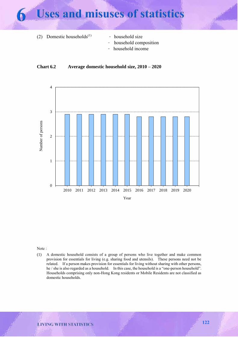
(2) Domestic households(1) - household size

- household composition - household income

Chart 6.2 Average domestic household size, 2010 – 2020

Note :

(1) A domestic household consists of a group of persons who live together and make common

provision for essentials for living (e.g. sharing food and utensils). These persons need not be

related. If a person makes provision for essentials for living without sharing with other persons,

he / she is also regarded as a household. In this case, the household is a “one-person household”.

Households comprising only non-Hong Kong residents or Mobile Residents are not classified as

domestic households.

0

1

2

3

4

2010 2011 2012 2013 2014 2015 2016 2017 2018 2019 2020

Num

ber

of

per

sons

Year

122

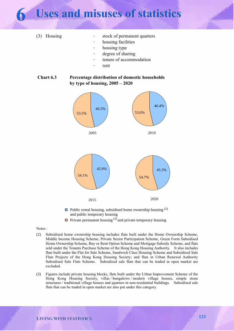
45.9%

54.1%

2015

46.5%

53.5%

2005

46.4%

53.6%

2010

45.3%

54.7%

2020

(3) Housing - stock of permanent quarters

- housing facilities

- housing type

- degree of sharing

- tenure of accommodation

- rent

Chart 6.3 Percentage distribution of domestic households

by type of housing, 2005 – 2020

Notes :

(2) Subsidised home ownership housing includes flats built under the Home Ownership Scheme,

Middle Income Housing Scheme, Private Sector Participation Scheme, Green Form Subsidised

Home Ownership Scheme, Buy or Rent Option Scheme and Mortgage Subsidy Scheme, and flats

sold under the Tenants Purchase Scheme of the Hong Kong Housing Authority. It also includes

flats built under the Flat for Sale Scheme, Sandwich Class Housing Scheme and Subsidised Sale

Flats Projects of the Hong Kong Housing Society; and flats in Urban Renewal Authority

Subsidised Sale Flats Scheme. Subsidised sale flats that can be traded in open market are

excluded.

(3) Figures include private housing blocks, flats built under the Urban Improvement Scheme of the Hong Kong Housing Society, villas / bungalows / modern village houses, simple stone structures / traditional village houses and quarters in non-residential buildings. Subsidised sale flats that can be traded in open market are also put under this category.

Public rental housing, subsidised home ownership housing

and public temporary housing

Private permanent housing and private temporary housing

(2)

(3)

123

(4) Education - educational attainment of population

- schools

- teachers

- student enrolment

Chart 6.4 Student enrolment(4) by level of education, 2010 – 2020

Notes :

(4) Figures include both full-time and part-time students attending long programmes lasting for at

least one school / academic year. Figures do not include students attending tutorial, vocational

and adult education courses offered by schools below post-secondary education level. Figures

for secondary and post-secondary education for 2020 are provisional.

(5) Figures include nursery, lower and upper classes in kindergartens and kindergarten-cum-child

care centres registered under the Education Bureau, and special child care centres registered under

the Social Welfare Department.

(6) Figures include special schools.

(7) Figures include evening schools, craft level courses and Diploma Yi Jin programme. Prior to

the 2012/13 school year, secondary education covers Secondary 1 to Secondary 7. Upon

implementation of the New Senior Secondary Academic Structure, there are no subsidised

Secondary 7 places under local curriculum starting from the 2012/13 school year.

(8) Figures include universities and colleges offering post-secondary courses including

certificate / diploma, associate degree or equivalent and bachelor degree or above; and also non-

local registered or exempted courses leading to non-local higher academic qualifications and

operated jointly with non-local institutions.

0

100

200

300

400

500

600

2010 2011 2012 2013 2014 2015 2016 2017 2018 2019 2020

Num

ber

of

stud

ents

(th

ousa

nd

s).

Year

(6), (7)Secondary

(6)Primary

(5)Pre-primary

(8)Post-secondary

124

(5) Employment - labour supply

- unemployment and underemployment

- distribution of employed persons by industry

- distribution of employed persons by occupation

- hours worked

- earnings from employment

Chart 6.5 Distribution of employed population by industry(9), 2010 – 2020

Notes :

(9) Figures are compiled based on Hong Kong Standard Industrial Classification Version 2.0.

(10) Accommodation services cover hotels, guesthouses, boarding houses and other establishments

providing short term accommodation.

(11) The retail, accommodation and food services industries as a whole is generally referred to as the

consumption- and tourism-related segment.

Per

centa

ge

0%

20%

40%

60%

80%

100%

2010 2011 2012 2013 2014 2015 2016 2017 2018 2019 2020

Year

Other industries

Public administration, social

and personal services

Financing, insurance, real

estate, professional and

business services

Transportation, storage,

postal and courier services,

information and

communications

Retail, accommodation (10)

and food services (11)

Import / export trade and

wholesale

Construction

Manufacturing

125

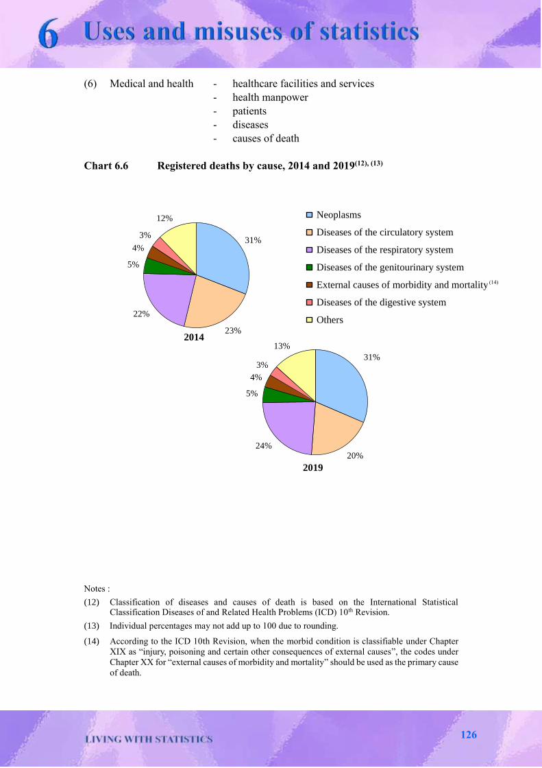
(6) Medical and health - healthcare facilities and services

- health manpower

- patients

- diseases

- causes of death

Chart 6.6 Registered deaths by cause, 2014 and 2019(12), (13)

Notes :

(12) Classification of diseases and causes of death is based on the International Statistical Classification Diseases of and Related Health Problems (ICD) 10th Revision.

(13) Individual percentages may not add up to 100 due to rounding.

(14) According to the ICD 10th Revision, when the morbid condition is classifiable under Chapter

XIX as “injury, poisoning and certain other consequences of external causes”, the codes under

Chapter XX for “external causes of morbidity and mortality” should be used as the primary cause

of death.

31%

23%

22%

5%

4%

3%

12%

2014

31%

20%24%

5%

4%

3%

13%

2019

Neoplasms

Diseases of the circulatory system

Diseases of the respiratory system

Diseases of the genitourinary system

External causes of morbidity and mortality*

Diseases of the digestive system

Others

(14)

126

(7) Social welfare - beneficiaries and benefits

- services for the elderly

- family and child welfare services

- services for young people

- rehabilitation and medical social services

- institutional services

(8) Law and order - crimes

- victims

- judicial services

- prisoners / inmates and correctional services

(9) Culture, entertainment and recreation

- cultural, entertainment and sports presentations

- recreational facilities

127

0

400

800

1,200

1,600

2,000

2,400

2,800

3,200

2010 2011 2012 2013 2014 2015 2016 2017 2018 2019 2020

Gro

ss D

om

esti

c P

rod

uct

(H

K$

bil

lio

n)

Year

Economic statistics

Economic statistics are statistics related to the structure and performance of an

economy and the operating characteristics of different industries. Some statistics can

be treated as either economic or social statistics under different analytical frameworks,

such as wages and employment.

Some important economic statistics are :

(1) National Income and Balance of Payments statistics

- Private consumption expenditure

- Gross Domestic Product

- Investment income

- Gross National Income

- Balance of Payments account

- International Investment Position

- External Debt

Chart 6.7 Gross Domestic Product of Hong Kong

(at current market prices), 2010 – 2020

128

0

500

1,000

1,500

2,000

2,500

3,000

3,500

4,000

4,500

5,000

2010 2011 2012 2013 2014 2015 2016 2017 2018 2019 2020

Tra

de

val

ue

(HK

$ b

illi

on)

Year

Imports

Total exports

(2) External trade - imports and exports of goods

- trade involving outward processing in the Mainland

- trade in services

- offshore trade in goods

Chart 6.8 Values of total exports(15) and imports(16) of goods, 2010 – 2020

Notes :

(15) “Total exports” comprise domestic exports and re-exports. Domestic exports are the natural

produce of Hong Kong or the products of a manufacturing process in Hong Kong which has

changed permanently and substantially the shape, nature, form or utility of the basic materials

used in manufacture. Re-exports are products which have previously been imported into Hong

Kong and which are re-exported without having undergone in Hong Kong a manufacturing

process which has changed permanently and substantially the shape, nature, form or utility of the

basic materials used in the manufacture.

(16) “Imports” are goods which have been produced or manufactured in places outside the jurisdiction

of Hong Kong and brought into Hong Kong for local use or for subsequent re-export, as well as

Hong Kong products re-imported.

129

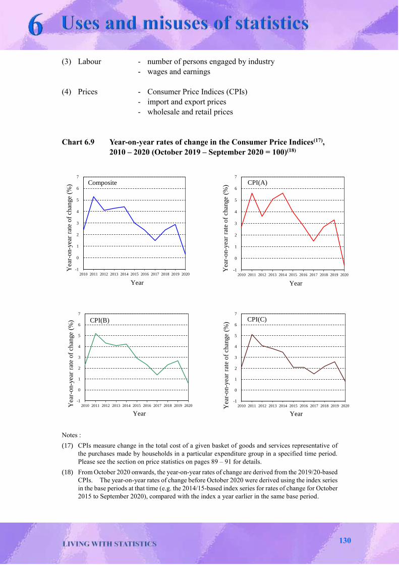
(3) Labour - number of persons engaged by industry

- wages and earnings

(4) Prices - Consumer Price Indices (CPIs)

- import and export prices

- wholesale and retail prices

Chart 6.9 Year-on-year rates of change in the Consumer Price Indices(17),

2010 – 2020 (October 2019 – September 2020 = 100)(18)

Notes :

(17) CPIs measure change in the total cost of a given basket of goods and services representative of

the purchases made by households in a particular expenditure group in a specified time period.

Please see the section on price statistics on pages 89 – 91 for details.

(18) From October 2020 onwards, the year-on-year rates of change are derived from the 2019/20-based

CPIs. The year-on-year rates of change before October 2020 were derived using the index series

in the base periods at that time (e.g. the 2014/15-based index series for rates of change for October

2015 to September 2020), compared with the index a year earlier in the same base period.

-1

0

1

2

3

4

5

6

7

2010 2011 2012 2013 2014 2015 2016 2017 2018 2019 2020

Yea

r-o

n-y

ear

rate

of

chan

ge

(%)

Year

Composite

-1

0

1

2

3

4

5

6

7

2010 2011 2012 2013 2014 2015 2016 2017 2018 2019 2020

Yea

r-o

n-y

ear

rate

of

chan

ge

(%)

Year

CPI(A)

-1

0

1

2

3

4

5

6

7

2010 2011 2012 2013 2014 2015 2016 2017 2018 2019 2020Yea

r-o

n-y

ear

rate

of

chan

ge

(%)

Year

CPI(B)

-1

0

1

2

3

4

5

6

7

2010 2011 2012 2013 2014 2015 2016 2017 2018 2019 2020Yea

r-o

n-y

ear

rate

of

chan

ge

(%)

Year

CPI(C)

130

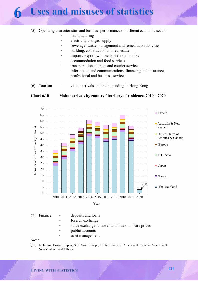
(5) Operating characteristics and business performance of different economic sectors

- manufacturing

- electricity and gas supply

- sewerage, waste management and remediation activities

- building, construction and real estate

- import / export, wholesale and retail trades

- accommodation and food services

- transportation, storage and courier services

- information and communications, financing and insurance,

professional and business services

(6) Tourism - visitor arrivals and their spending in Hong Kong

Chart 6.10 Visitor arrivals by country / territory of residence, 2010 – 2020

(7) Finance - deposits and loans

- foreign exchange

- stock exchange turnover and index of share prices

- public accounts

- asset management Note :

(19) Including Taiwan, Japan, S.E. Asia, Europe, United States of America & Canada, Australia &

New Zealand, and Others.

0

5

10

15

20

25

30

35

40

45

50

55

60

65

70

2010 2011 2012 2013 2014 2015 2016 2017 2018 2019 2020

Num

ber

of

vis

ito

r ar

rival

s (m

illi

ons)

Year

Others

Australia & New

Zealand

United States of

America & Canada

Europe

S.E. Asia

Japan

Taiwan

The Mainland(19)

131

Misuses of statistics

Nowadays, the society has become increasingly more scientific-minded. Arguments

without the support of relevant figures can hardly convince people. This shows how

important statistics are. However, if the data are not properly used, one will make a

blunder in trying to be smart. Not only will the arguments be refuted and queried,

decision-makers may also be misled to make the wrong decisions, which may cause

serious consequences.

To fully understand the proper ways of using statistics, one has to acquire the

knowledge through in-depth learning and accumulation of experience. The

following are some common mistakes that should be avoided.

Unknown reference periods of statistics

When making statements about comparisons of statistics over time, it is important to

specify the reference periods in question. A statement like “the number of students

has grown 30%” is not meaningful. It is necessary to specify that the growth has

taken place over a certain interval of time, be it 1 year, 5 years or 10 years, etc.

When describing the changes of a series of statistics over time, it is important to specify

the base period of comparison.

Example:

What is wrong with the following statements?

1. “CPI in July was 2.8% higher.”

2. “GDP last quarter declined by 0.5%.”

The base period of comparison should be stated clearly:

1. “The year-on-year growth rate of CPI in July was 2.8%.” or “CPI in July

this year was 2.8% higher than that in July last year.”

2. “The year-on-year growth rate of GDP in the last quarter was 3.5%, which

was lower by half a percentage point when compared with the 4.0% year-on-

year growth rate in the quarter earlier.”

132

Improper use of base of comparison

A restaurant claims in its advertisement that its prices will be cut by 100%. It is, of

course, clear that prices cannot be cut by 100%, lest the servings would now be given

away free of charge! In fact, what the restaurant does is that food formerly sold at

$60 per order will be sold at $30 after the price deduction. The restaurant has

calculated the 100% from ($60 – $30)/$30×100% by using the reduced price as the

base of comparison. This is incorrect. The proper way of calculation is to use the

original price as the base. Hence the reduction is only 50%,

i.e.($60 – $30)/$60×100%.

Improper averaging of percentages and ratios

When individual percentages and ratios are calculated on different bases, they should

not be added together directly to get the overall average.

Example :

Population figures(20) from 2016 Population By-census

It is incorrect to derive the overall sex ratio for Hong Kong by adding the individual

ratios for different areas and then dividing by 3. This would give a wrong value of

843 [i.e. (810+856+863)/3]. The true value of 852 should be calculated from the

total number of males and females [i.e. (3 374 702/3 960 682)×1 000] instead.

Note :

(20) Excluding the marine population.

Area Male Female Sex ratio

(No. of males per

1 000 females)

Hong Kong Island 561 106 692 311 810

Kowloon 1 033 979 1 207 368 856

New Territories 1 779 617 2 061 003 863

Overall 3 374 702 3 960 682 852

133

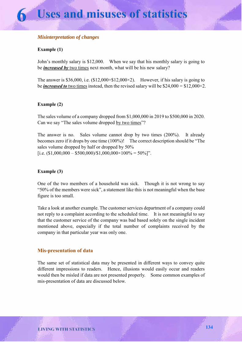
Misinterpretation of changes

Example (1)

John’s monthly salary is $12,000. When we say that his monthly salary is going to

be increased by two times next month, what will be his new salary?

The answer is $36,000, i.e. ($12,000+$12,000×2). However, if his salary is going to

be increased to two times instead, then the revised salary will be $24,000 = $12,000×2.

Example (2)

The sales volume of a company dropped from $1,000,000 in 2019 to $500,000 in 2020.

Can we say “The sales volume dropped by two times”?

The answer is no. Sales volume cannot drop by two times (200%). It already

becomes zero if it drops by one time (100%)! The correct description should be “The

sales volume dropped by half or dropped by 50%

[i.e. ($1,000,000 – $500,000)/$1,000,000×100% = 50%]”.

Example (3)

One of the two members of a household was sick. Though it is not wrong to say

“50% of the members were sick”, a statement like this is not meaningful when the base

figure is too small.

Take a look at another example. The customer services department of a company could

not reply to a complaint according to the scheduled time. It is not meaningful to say

that the customer service of the company was bad based solely on the single incident

mentioned above, especially if the total number of complaints received by the

company in that particular year was only one.

Mis-presentation of data

The same set of statistical data may be presented in different ways to convey quite

different impressions to readers. Hence, illusions would easily occur and readers

would then be misled if data are not presented properly. Some common examples of

mis-presentation of data are discussed below.

134

Illusion in interpreting absolute magnitude of figures

Simply comparing the absolute magnitude of figures but ignoring other relevant

factors may create illusion.

Example:

What is wrong with the following analysis?

“According to Table 1, City A had the least number of hospital beds among the three

cities.”

Table 1 City

No. of hospital beds

City A 34 000

City B 45 000

City C 83 000

By simply comparing the number of hospital beds as shown in the table, one may think

that the provision of hospital beds is most inadequate in City A among the three.

However, to avoid illusion created by the numbers, we should use the “rate” (i.e. the

ratio of number of beds to population) to compare the availability of hospital beds in

different cities (see Table 2).

Table 2

City No. of hospital beds per 1 000 population

City A 5.0

City B 1.8

City C 1.0

135

Illusion in interpreting small-based figures

Special care should be taken when interpreting figures in comparison of small base to

avoid arriving at the wrong conclusion.

Example:

Which government department best fulfills the requests of information enquirers?

Top five government departments that fulfill the requests of information enquirers

Rank Department Percentage of cases that the enquirers’

requests were fully entertained

(1) Department A 100%

(2) Department B 55.0%

(3) Department C 52.5%

(4) Department D 45.8%

(5) Department E 42.4%

How would you conclude if more information is given?

Top five government departments that fulfill the requests of information enquirers

Rank Department Total no.

of cases

No. of cases that the

enquirers’ requests

were fully

entertained

Percentage of cases that

the enquirers’ requests

were fully entertained

(1) Department A 1 1 100%

(2) Department B 20 11 55.0%

(3) Department C 40 21 52.5%

(4) Department D 48 22 45.8%

(5) Department E 33 14 42.4%

136

Charts using an improper vertical scale

It is essential that charts with an arithmetic scale should begin at the zero base line in

order to show the true picture. However, when the data to be presented graphically

are of very large values but with small variations, some people would tend to adopt a

larger scale and plot the chart from a larger initial point for easy observation and

comparison purposes. Watch out for this, as the true relationship between the data

for different time points is bound to be exaggerated and a distorted impression will be

conveyed. Differences between the data would appear greater, and the slopes

indicating the trends seem to be steeper (Chart 6.11(A)).

In order to convey a true picture of the relationship while still highlighting the

variations, a broken scale chart is often used (Chart 6.11(B)). It enables the data

variations to be observed easily but still reminds readers to watch out for the possible

distorted impression that may be conveyed by the chart.

Chart 6.11

(A) Charts not using the broken scale

Sales turnover of Company ABC, 2017 – 2020

(B) Charts using the broken scale

Sales turnover of Company ABC, 2017 – 2020

1,000

1,100

1,200

2017 2018 2019 2020

Year

HK$ million

800

900

1,000

1,100

1,200

2017 2018 2019 2020

Year

HK$ million

800

900

1,000

1,100

1,200

2016 2017

Year

HK$ million

1,000

1,100

1,200

2017 2018 2019 2020

Year

HK$ million

2017 2018 2019 2020

137

(v) Contracting vertical scale

(i) Original scale arrangement

(ii) Expanding vertical scale

(iv) Expanding horizontal scale

(iii) Contracting horizontal scale

Illusions caused by expanding / contracting the grid

Seemingly, expanding the vertical axis or contracting the horizontal axis of a chart may

exaggerate the changes in the trends as depicted in the chart. On the other hand,

changes in the trends will appear to be less vigorous than the actual situation if the

horizontal axis is expanded or the vertical scale is contracted to a large extent.

Chart 6.12 Changing the visual image : Contracting or expanding vertical

(amount) scale or horizontal (time) scale tends to change the

visual picture

138

0

20

40

60

80

100

120

140

1975 1980 1985 1990 1995 2000 2005 2010 2015 2020

HK$ million

Year

0

20

40

60

80

100

120

140

1975 1995 2014 2015 2016 2017 2018 2019 2020

HK$ million

Year

Illusions caused by skipping the grid

A familiar layout in reports and advertisements is seen in Chart 6.13(A). In order to

dramatise the story, a little trick is done with the horizontal (time) scale, so that the

period represented by each grid is different. It is not noticeable at a casual glance.

Chart 6.13(B) shows what the actual trend looks like when the correct grid spacing is

used for the respective years.

Chart 6.13

(A)

(B)

139

Illusions caused by 3-D charts

Chart 6.14

3-D charts may confuse the readers about the relative size of the portions.

(A)

2-D charts are clearer and should be used instead.

(B)

140

References


Ilersic, A.R. and Pluck, R.A., Statistics, Chapter XVII, XVIII and XIX, HFL Ltd., 1979.

Moroney, M.J., Facts from Figures, Penguin Books Ltd., 1965 (3rd edition).

Reichmann, W.J., Use and Abuse of Statistics, Penguin Books Ltd., 1964.

Interactive quiz




141


Exercise Misuse of base figure for comparison

1. Bank Y charges very high interest rates.

A man borrowed $100,000 from Bank Y for 15 days. He received only

$80,000 in cash. The remaining $20,000 was deducted as interest for the 15-

day period.

Bank Y claimed that the interest rate was 20%

(i.e. %100000,100$/000,20$ ) per 15 days. Is this correct?

2. The price of an article A was $100 in 2019 and $50 in 2020. This means that

the price of A in the period has decreased by

50%

100%

150%

200%

Mis-presentation of data

3. Which one of the following charts is visually distorted and should not be used?

Chart A

Chart B

Misuses of statistics in daily endeavours

4. Readers can collect materials from newspaper cuttings, articles in magazines

and commercials on television which may appear to involve misuses of statistics.

Readers may then examine various aspects of such examples and analyse

whether these are misuses of statistics. Subsequently, readers may make

suggestions on how the errors can be rectified, or how the presentation can be

improved.

800

900

1,000

1,100

1,200

2017 2018 2019 2020

Year

HK$ million

Chart B Chart A

1,000

1,100

1,200

2017 2018 2019 2020

Year

HK$ million

142

Introduction

Very often, a figure is not meaningful unless it is compared with another figure.

For instance, there may be 100 cinemas in a certain city. This may seem to be a

large figure. However, when compared with the city’s population (say, 10 million),

this represents 1 cinema to every 100 000 persons. On the other hand, suppose

there are only 10 cinemas in another city. The number may look small, but if the

population of the city is only 100 000, each cinema actually serves only 10 000

persons.

Let us look at another example. Suppose there is an increase of 1 000 participants

in a certain medical scheme. This may appear to be a remarkable increase.

However, if the scheme originally consists of 100 000 participants, the increase is

only 1%. On the contrary, an increase of 100 participants in a scheme originally

with 500 participants represents a substantial increase of 20%.

“Relative numbers”, which are derived by comparing two related figures(1), are

generally more useful than “absolute figures” for data analyses. Rate, ratio,

proportion and percentage are examples of some commonly used relative numbers.

Rate

“Rate” is obtained by expressing the measurement of something per unit of

something else. The quantities compared are not necessarily of the same kind and

hence rate often bears a unit. An example of rate is car speed, say 50 km per hour.

Another example is population density, which is calculated by dividing the size of

population in a district by the area of the district. The rate of 1 cinema per 100 000

persons mentioned above is also another example describing the degree of

availability of movie entertainment facilities.

In the compilation of “rates”, the choice of correct bases is very important, otherwise

the results would be misleading. For accurate comparison of “rates”, a base closely

related to the target figures to be measured should be used. For example, to calculate

the voting rate of a city, the total number of citizens having the right to vote as the base

is considered more appropriate than using the total number of citizens in the city as the

base. Note : (1) Comparisons are meaningful only when the base figures are not too small. Thus, it would not

be meaningful to make a statement that 25% of the members of a household are sick when 1 out of its 4 members falls ill.

143

With different rates compiled from smaller groups of a population, we often want to

get an overall picture for the whole population concerned. However, one should be

cautious that individual rates with different bases should not be added together for

getting the overall rate.

Ratio

“Ratio” is another way of expressing the relationship between figures. It is normally

derived by comparing quantities of the same kind and therefore unlike rate, it does not

bear a unit. Sometimes, the relationship is expressed as a ratio to one. For example,

the ratio between boys and girls in a class is 3 : 1. However, if it suits our purpose

better, we can express the relationship as a ratio to any other number (i.e. other

than 1). For the previous example, the ratio between boys and girls can also be

written as 30 : 10.

Proportion and percentage

“Proportion” and “percentage” are special types of ratio. “Proportion” relates a

“part” to the “whole”; while “percentage” is the case where the relationship between

figures is presented as a ratio to one hundred.

Some frequently used relative numbers

Crude death rate

The crude death rate for a given calendar year is obtained by dividing the number of

known deaths occurring in a community during that calendar year by the mid-year

population of that community, and expressing the result in terms of deaths per 1 000

population.

In 2020, the number of known deaths in Hong Kong was 49 800# and the mid-year

population was 7 481 800. The crude death rate for 2020 was therefore 6.7# per

1 000 population.

144

Age-sex specific death rate

Mortality varies significantly with age and sex. To study in greater depth the

pattern of mortality of people in different age groups and sex, the age-sex specific

death rates (or age-sex specific mortality rates) may be referred to. This rate is

expressed as the number of known deaths per 1 000 population in the same age group

and same sex. For example:

Age-sex specific

death rate for males

in the age group 60-64

=

Number of known deaths of

males in the age group 60-64

Number of males


1 000

Crude birth rate

Similar to crude death rate, crude birth rate is calculated by dividing the number of

known live births during a calendar year by the mid-year population for that year,

and expressing the result in terms of births per 1 000 population.

In 2020, the number of known live births in Hong Kong was 43 000 and the mid-year

population was 7 481 800. The crude birth rate for 2020 was therefore 5.8 per

1 000 population.

Unemployment rate

The unemployment rate is obtained by dividing the total number of unemployed

persons by the labour force in the community. The labour force or economically

active population refers to the land-based non-institutional population aged 15 and

over who satisfy the criteria for inclusion in the employed population or unemployed

population. The unemployment rate of Hong Kong was 5.8% in 2020.

Industrial accident rate in the manufacturing sector

The industrial accident rate in the manufacturing sector is expressed as the number of

reported casualties per 1 000 manufacturing workers. The structure of this relative

number, with the number of manufacturing workers as the base, highlights the fact

that the base figure should relate to the subject matter in question as much as possible.

(In this case, manufacturing workers are those “at risk” of industrial accidents and

the number of such workers is used as the base.) In 2020, the industrial accident

rate in the manufacturing sector in Hong Kong was 12.5 per 1 000 manufacturing

workers.

145

Crime rate

Crime rate is usually expressed as the number of cases of reported crime per 100 000

population. In 2020, the crime rate for Hong Kong was 845 per 100 000

population. Age specific prosecution rates

To study in greater depth the tendency of committing crimes by people in different

age groups, the age specific prosecution rates may be referred to. This rate is

usually expressed as the number of persons prosecuted per 100 000 population in the

same age group. For example:

Age specific

prosecution rate for

the age group 16-20

=

Number of persons


who are prosecuted

Number of persons


× 100 000

Sex ratio

The relationship of the number of males to the number of females in a population is

given by the sex ratio, which presents the number of males per 1 000 females.

As in mid-2020, there were 3 416 300 males and 4 065 500 females in Hong Kong.

Thus, the sex ratio was 840 males per 1 000 females. Proportion of domestic households residing in subsidised home ownership

housing

To relate the number of domestic households residing in subsidised home ownership

housing(2) to the total number of domestic households in Hong Kong, we can obtain

the proportion of domestic households residing in subsidised home ownership

housing.

The proportion of domestic households residing in subsidised home ownership housing

was 14.9% in 2020.

Note :

(2) Subsidised home ownership housing includes flats built under the Home Ownership Scheme, Middle Income Housing Scheme, Private Sector Participation Scheme, Green Form Subsidised Home Ownership Scheme, Buy or Rent Option Scheme and Mortgage Subsidy Scheme, and flats sold under the Tenants Purchase Scheme of the Hong Kong Housing Authority. It also includes flats built under the Flat for Sale Scheme, Sandwich Class Housing Scheme and Subsidised Sale Flats Projects of the Hong Kong Housing Society; and flats in Urban Renewal Authority Subsidised Sale Flats Scheme. Subsidised sale flats that can be traded in open market are excluded.

146

Percentage of population by age group

The percentage of population by age group is obtained by dividing the total number

of people in a particular age group by the total population size and then multiplying

by 100.

As in mid-2020, 11.6% of people in the Hong Kong population were aged under 15,

70.0% aged 15-64 and 18.3% aged 65 and over.

Proper use of relative numbers

Care must be taken when handling or interpreting relative numbers; otherwise we

may arrive at incorrect conclusions or mislead other people. The following are

two examples to illustrate this.

Example 1 Land-based non-institutional population by District Council

district, 2010 and 2020(3)

District Council district Land-based non-institutional population

2010 2020

No. % of total No. % of total

Central and Western 257 000 3.7 236 000 3.2

Wan Chai(4) 158 100 2.3 173 300 2.3

Eastern(4) 585 400 8.4 537 900 7.3

Southern 270 600 3.9 260 800 3.5

Yau Tsim Mong 302 800 4.4 323 000 4.4

Sham Shui Po 364 200 5.3 433 500 5.9

Kowloon City 364 200 5.3 419 200 5.7

Wong Tai Sin 414 700 6.0 414 200 5.6

Kwun Tong 606 200 8.7 686 700 9.3

Kwai Tsing 504 500 7.3 500 900 6.8

Tsuen Wan 290 300 4.2 310 000 4.2

Tuen Mun 485 600 7.0 495 000 6.7

Yuen Long 552 500 8.0 640 600 8.7

North 303 800 4.4 314 500 4.3

Tai Po 289 900 4.2 307 900 4.2

Sha Tin 616 600 8.9 684 800 9.3

Sai Kung 421 400 6.1 472 800 6.4

Islands 148 600 2.1 184 700 2.5

Total 6 936 200 100.0 7 395 900 100.0

Notes :

(3) There may be a slight discrepancy between the sum of individual items and the total due to rounding.

(4) The boundaries of the Wan Chai district and Eastern district having been adopted since 2016 are different from those adopted in 2015 and earlier years. Therefore, figures of the Wan Chai and Eastern districts for 2016 and thereafter are not strictly comparable with those for 2015 and earlier years in this table.

147

Comparing the percentage figures for 2010 and 2020, one may notice that the figures

for Central and Western, Eastern, Southern, Wong Tai Sin, Kwai Tsing, Tuen Mun

and North districts have decreased. For instance, the drops for Eastern and North

districts were 1.1 “percentage points(5)” and 0.1 “percentage point” respectively.

One may arrive at a wrong conclusion that these districts have become less populated.

In fact, a decrease in the share does not necessarily imply there is a decrease in the

actual number. Take the North district as an example. Despite a decrease of 0.1

percentage point in share, the number of land-based non-institutional population of

the North district actually increased by 10 700 persons, or 3.5% (i.e. (314 500 –

303 800) / 303 800 x 100%).

This situation can be attributed mainly to the increase in the total number of

land-based non-institutional population over the period. The percentage shares of

population in certain districts decreased relatively.

Merely mentioning the drop in the proportion of population, though correct, may not

create a right impression for the less statistically-minded people. Referring to both

the numbers and the proportions of population will enable the presentation of a more

complete and accurate picture.

Note :

(5) “Percentage point” refers to the absolute sum or difference between two rates or percentages, which is obtained by direct addition or subtraction of the figures concerned. As a matter of fact, an increase of x percentage points and an increase of x% are not the same. Suppose the passing rates of two different rounds of examination for a class of students were 80% and 84% respectively, the passing rate increased by 4 percentage points (84% – 80% = 4 percentage points). Alternatively we can also say that the passing rate recorded an increase of 5% (i.e. (84 – 80)/80×100%). However, the second way of presentation is generally not recommended.

148

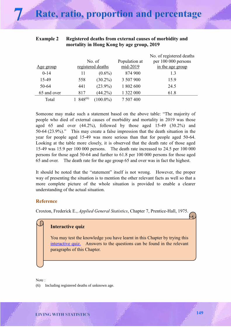
Example 2 Registered deaths from external causes of morbidity and

mortality in Hong Kong by age group, 2019

Age group

No. of

registered deaths

Population at

mid-2019

No. of registered deaths

per 100 000 persons

in the age group

0-14 11 (0.6%) 874 900 1.3

15-49 558 (30.2%) 3 507 900 15.9

50-64 441 (23.9%) 1 802 600 24.5

65 and over 817 (44.2%) 1 322 000 61.8

Total 1 848(6) (100.0%) 7 507 400 Someone may make such a statement based on the above table: “The majority of

people who died of external causes of morbidity and mortality in 2019 was those

aged 65 and over (44.2%), followed by those aged 15-49 (30.2%) and

50-64 (23.9%).” This may create a false impression that the death situation in the

year for people aged 15-49 was more serious than that for people aged 50-64.

Looking at the table more closely, it is observed that the death rate of those aged

15-49 was 15.9 per 100 000 persons. The death rate increased to 24.5 per 100 000

persons for those aged 50-64 and further to 61.8 per 100 000 persons for those aged

65 and over. The death rate for the age group 65 and over was in fact the highest.

It should be noted that the “statement” itself is not wrong. However, the proper

way of presenting the situation is to mention the other relevant facts as well so that a

more complete picture of the whole situation is provided to enable a clearer

understanding of the actual situation.

Reference


Note :

(6) Including registered deaths of unknown age.

Interactive quiz




149


Exercise

Calculating “rate”

Consider the following hypothetical example for studying the passing rate of an open

examination :

Broad area /

District Council district

Population

in 2020

No. of students

sitting for the

examination

in 2020

No. of students

passing the

examination

in 2020

Hong Kong

Island

Central and

Western 236 000 60 293 44 014

Wan Chai 173 300 41 110 28 366

Eastern 537 900 144 528 93 943

Southern 260 800 63 142 44 831

Kowloon

Yau Tsim

Mong 323 000 57 773 36 397

Wong Tai Sin 414 200 85 917 51 550

... ... ... ...

New

Territories

Sha Tin 684 800 138 281 76 055

Tai Po 307 900 156 552 60 494

... ... ... ...

Total 7 395 900 1 403 211 841 927

(i) Comment on the statement :

“The overall passing rate of the examination in 2020 was 11.4%,

i.e. ( 841 927 / 7 395 900 ) x 100 %.”

(ii) Calculate the passing rates for the 4 District Council districts on Hong Kong

Island and the overall passing rate for Hong Kong Island.

(iii) Suppose the number of students passing the examination in the Wan Chai

district in 2015 was 23 479. Can it be concluded that since there was an

increase in the number of students passing the examination (28 366) in 2020,

the academic results of students in the Wan Chai district had improved during

the period from 2015 to 2020?

150

Introduction

Given a set of data, it is often required to describe them in terms of a single value

around which the data are distributed. This value is a measure of “central

tendency”, indicating the central position of the given set of data.

There are different choices for the measurement of central tendency. The most

common ones are arithmetic mean (or briefly “the mean”), median and mode.

These measures of central tendency are applied in different situations depending on

the nature of data and the intended purpose.

Mean

The arithmetic mean of a set of data is defined as the sum of the values of the given

set of data divided by the number of data points.

N

XXXX

N

...21

where X is the mean;

N is the total number of data points; and

Xi is the value of the ith data point, for i = 1, 2, ..., N

Examples :

(1) The mean height of the students in a class is 1.52 m.

(2) The mean daily maximum air temperature for the year 2020 was 27.2oC.

(The method is to find out the maximum air temperature recorded for each of

the 366 days in the year 2020 and then calculate the arithmetic mean of the 366

data points.)

151

Median

The median of a set of data is the middle value of the given set of data when they are

arranged in order, either ascending or descending, of magnitude. In case there are

two middle values (i.e. when the data set has an even number of data points), then the

median is the arithmetic mean of these two middle values.

Examples :

(1) The median of the set of numbers ｛4, 6, 7, 9, 10｝ is 7.

(2) The median of the set of numbers ｛1, 3, 4, 4, 7, 9, 10, 11, 13, 14｝ is (7+9)/2,

i.e. 8.

(3) The median monthly household income of domestic households in Hong Kong

in 2020 was $27,000. In other words, 50% of the domestic households in

Hong Kong had a household income more than $27,000 per month in 2020

while the other 50% had less than $27,000 per month.

(4) The median age of men who married for the first time in Hong Kong in 2020

was 31.9.

Mode

The mode of a set of data is the value which occurs with the largest frequency,

i.e. the most common value in the given set of data. The mode may not exist, and

even if it does exist, it may not be unique.

Examples :

(1) The set of numbers ｛1, 3, 3, 5, 7, 8, 8, 8, 9, 10, 10, 11, 12｝ has a mode of 8.

(2) The set of numbers ｛2, 3, 4, 6, 8, 9｝ does not have any mode.

(3) The set of numbers ｛1, 3, 4, 4, 4, 6, 7, 7, 9, 9, 9, 10, 12｝ has two modes, 4

and 9.

(4) The modal household size in Hong Kong was 2 in 2020.

152

Grouped data

When presenting a large set of data, it is often useful to classify the data into

different classes and to find out the number of data points belonging to each class (i.e.

the class frequency). Data organised in this way are called grouped data whereas a

tabular arrangement of the data by class showing the corresponding class frequency

is called a frequency distribution or frequency table.

Example :

The weights (in kg) of individual students in a class are as follows :

61, 62, 63, 63, 63, 64, 64, 64, 64, 65, 65, 65, 66, 66, 66,

66, 66, 67, 67, 67, 67, 68, 68, 68, 69, 69, 69, 69, 70, 70

To help give a clear overall picture of the weights of the students, the above 30 data

points can be re-organised into several classes and a frequency distribution can be

constructed.

Step 1 Determine the largest and smallest values in the data set and find the range

(i.e. the difference between the largest and smallest values).

Smallest value = 61

Largest value = 70

Range = 9 (i.e. 70 − 61)

Step 2 Divide the range into a convenient number of classes having the same size

(i.e. same class interval(1)). The number of classes usually ranges from 5

to 20, depending on the values of the data.

Given that there are only 30 data points in the data set, it is not appropriate

to divide the range into a large number of classes (otherwise there will be

too few observations in each class). In this example, it is sensible to

divide the data set into 5 classes. The class intervals to be used are thus :

61-62;

63-64;

65-66;

67-68; and

69-70 Note :

(1) The smaller value of each class interval shown above is called the lower class limit and the

larger value the upper class limit. The mid-point of the class interval is known as the class

mark.

153

Step 3 Find the class frequency for each class and then construct the frequency

distribution.

Weight(2) (kg) Number of students

61-62 2

63-64 7

65-66 8

67-68 7

69-70 6

Total 30

Histogram

A histogram is a bar chart, with no space between the bars. It is commonly used for

presenting frequency distributions of grouped data with continuous class boundaries,

with class boundaries shown as points on the horizontal axis and the frequencies as

units on the vertical axis. The frequency in a class is proportional to the area of a

bar with the base as the class interval. (Please see Chart 8.1 below which is a

histogram for the grouped data of the example mentioned above.)

Chart 8.1 Histogram of the number of students

The population pyramid may be visualised as being formed from two horizontally

placed histograms, one being the age distribution of males and the other being the

age distribution of females.

Note :

(2) If the weights are rounded to the nearest kg, the class interval, say, 61 kg-62 kg, theoretically

includes all measurements from 60.5000…kg to 62.4999…kg. These two class limits,

indicated briefly by the exact numbers 60.5 kg and 62.5 kg, are called true class limits or class

boundaries.

0

2

4

6

8

10

61.5 63.5 65.5 67.5 69.5

Weight (kg)

No. of students

60.5 62.5 64.5 66.5 68.5 70.5

154

Cumulative frequency polygon

For some purposes, it is desirable to consider the total frequency of all values greater

than the lower class boundary of each class (i.e. the “more than” basis for counting

total frequency) or the total frequency of all values less than or equal to the upper

class boundary of each class (i.e. the “less than” basis for counting total frequency).

In such circumstances, it is necessary to construct the cumulative distribution (in

tabular form) or the cumulative frequency polygon (in graphical form).

To construct a cumulative frequency polygon, frequencies accumulated for each class

are plotted at the lower class limits when the “more than” basis is used. When the

“less than” basis is used, cumulated frequencies are plotted at the upper class limits.

Regardless of the basis used, the Y-axis should be drawn long enough to

accommodate the total frequency. The points, each representing the cumulative

frequency of a particular class, are then joined by a series of straight lines and the

S-curve so obtained may be extended to touch the X-axis by dropping a

perpendicular line from its highest point. The polygon so formed is a cumulative

frequency polygon. (Please see Chart 8.2 below which is a cumulative frequency

polygon for the grouped data of the example mentioned above.)

Chart 8.2 Cumulative frequency polygon of the number of students

The cumulative frequency polygon is particularly useful for interpolation.

However, it is important to note that the use of straight lines to connect the series of

known points is only an approximation to the frequency distribution of the items

within any given interval. Nevertheless, this approximation is considered to be

sufficiently accurate under most circumstances.

0

5

10

15

20

25

30

35

60.5 62.5 64.5 66.5 68.5 70.5

Num

ber

of

stud

ents

Weight (kg)

155

Mean of grouped data

The formula to be used to calculate the mean of a set of grouped data is as follows:

k

kk

fff

XfXfXfX

...

...

21

2211

where X is the mean;

Xi is the class mark (i.e. mid-point of the class interval) of the ith class,

for i = 1, 2, ..., k; and

fi is the frequency of the ith class, for i = 1, 2, ..., k

The mean thus obtained depends on the way the data are grouped and is only an

approximation. However, it reduces the burden of numerical calculation.

156

Finding the median of grouped data from histogram

Making use of the histogram, an approximation of the median of a set of grouped

data can be found.

Step 1 Construct the histogram for the data set (please see Chart 8.3 below).

Step 2 Identify the median class, i.e. the class which contains the “middle value”.

Step 3 Calculate the sum of frequencies of classes lower than the median class, ( f)l.

Step 4 Find f, using the expression f = N/2 – ( f)l

where N is the total frequency; and

( f)l is the sum of frequencies of classes lower than the median

class

Step 5 Construct a diagonal in the median class. The line should be drawn from

the lower left corner to the upper right corner (AB).

Step 6 At the height corresponding to “ f ” found in step 4, draw a horizontal line

(CD) to cut the median class. The line will intersect with the diagonal

(E).

Step 7 Drop a perpendicular line from this point of intersection (E) to the X-axis.

The point thus located on the X-axis (F) will give the value of the median.

Chart 8.3

median class

F 0

C

A

Median

x

Frequency

E D

B

f

157

Finding the median of grouped data from cumulative frequency polygon

Another graphical method of finding the median is to draw a cumulative frequency

polygon.

Step 1 Construct the cumulative frequency polygon for the data set (please see

Chart 8.4 below).

Step 2 At the cumulative frequency height N/2 (N is the number of data points),

draw a horizontal line until it touches the cumulative frequency polygon.

Step 3 Draw a perpendicular line from this point of intersection to the X-axis.

The point thus located on the X-axis (M) will give the value of the median.

Chart 8.4

Cumulative frequency

x 0

N/2

N

Median

M

158

Finding the mode of grouped data from histogram

A rough estimate of the mode can also be found with the use of the histogram.

Step 1 Construct a histogram for the data set (please see Chart 8.5 below).

Step 2 Identify the modal class, i.e. the class with the largest frequency.

Step 3 Draw 2 diagonals as shown in Chart 8.5 (AB and CD).

Step 4 Drop a vertical line from the point of intersection of these 2 diagonals (E)

to the X-axis. The point thus located on the X-axis (F) will give the value

of the mode.

Chart 8.5

B C

D

A

E

F

Mode

modal class

x

Frequency

159

Use of mean and median

The mean is the most widely used among all the measures of central tendency,

because it has a lot of desirable properties in statistical theories.

For an approximately symmetric set of data such as ｛13, 14, 15, 17, 18.5｝, the mean

15.5 gives the central location effectively.

The mean, however, is affected by the value of every item in the set of data, and the

presence of a few extremely large (or extremely small) items may result in a mean

which could be misleading. For example, for the data set｛1 000, 2 000, 3 000,

3 500, 4 500, 5 000, 30 000｝, the mean is 7 000 which is not a good measure of the

central tendency. However, the median, 3 500, is more satisfactory because the

existence of a few extreme values generally would not cause the median to fluctuate

much.

In daily life, the mean monthly household income is easily affected by extreme

values. Hence, the median is more suitable than the mean in measuring the central

tendency of household income. In 2020, the median monthly household income of

domestic households in Hong Kong was $27,000.

Supplementary notes - weighted mean

Sometimes, we associate the data (X1, X2, ..., Xk) with certain weighting factors or

weights (W1, W2, ..., Wk), depending on the significance or importance attached to the

individual data points. In this case,

k

kk

WWW

XWXWXWX

...

...

21

2211

The mean of a set of grouped data is in fact a mean of the class marks weighted by

the class frequencies.

Normally, the use of the weighted mean leads to a different conclusion from that

using the unweighted mean. In fact, the concept of weighted mean is commonly

used in daily life.

160

Example :

The following is a summary of the grade points of the final examination and the

mid-term test scored by two students A and B, with the final examination grades

weighted 3 times as much as the mid-term test grades :

Grade points Weights

A B

Final examination 82 90 3

Mid-term test 78 66 1

If the weights are disregarded,

the mean score of A 802

7882

, and

the mean score of B 782

6690

.

We would say that A did better than B.

On the other hand, if the weights are taken into consideration,

the weighted mean score of A 8113

178382

,

and

the weighted mean score of B 8413

166390

.

We would then say that B did better than A.

161

References


Spiegel, Murray R., Theory and Problems of Statistics, Chapter 3, Schaum

Publishing Co., 1961.

Interactive quiz




162


Exercise Calculating mean, median and mode

1. Consider a set of figures：

｛1, 9, 3, 7, 8, 12, 9｝

(i) What is the sum of these seven values?

(ii) What is the mean?

(iii) What is the median?

(iv) What is the mode?

(v) Is the median equal to the mean of the same seven values?

(vi) Are the mean and median the same when the set of figures is ｛1, 3, 7, 11,

13｝?

(vii) When the mean and median of a set of data are the same, what does this

suggest?

2. The mean of ｛10, 20, 30, 40, 50｝is

30

35

40

45

3. The mode of ｛3, 10, 14, 23, 29, 30, 31｝is

20

23

31

Mode does not exist in this set of figures

163

4. When half of the elements of a population are smaller than a value X and half

are greater than it, X is the

Mean

Median

Mode

5. Among mean, median and mode, which one is the most easily affected by

extreme values?

Mean

Median

Mode

164

Introduction

Information on the central tendency of a set of data alone is not sufficient to describe

its distribution. For instance, two groups of data may have the same mean, yet

having different degrees of spread among the data points. To have a better

knowledge of a set of data, it is necessary to measure the extent to which individual

values vary within the set, or equivalently, the extent to which individual values vary

around the mean.

The degree to which numerical data tend to spread around the mean value is called

the dispersion of the data. Various measures of dispersion are available. The

more common ones are range, mean deviation, variance and standard deviation.

Chart 9.1 Various degrees of variation

Small variation

Large variation

165

Range

The range of a set of numbers is the difference between the maximum and the

minimum values. This measure is greatly affected by extreme values. The

advantage of this measure is simplicity. The disadvantage is that it does not take

the intermediate values into account at all.

Chart 9.2 Range

The following two sets of data have the same range but different dispersions:

Mean deviation (Mean absolute deviation)

Mean deviation, also known as mean absolute deviation, is a measure summarising

how large the extent a data set deviates from its mean, irrespective of the direction of

spread of individual data points in the set. For a given set of numerical data, the

mean deviation is defined as the sum of the absolute deviations (i.e. the absolute

values of the deviations from the mean) of individual data points divided by the total

number of data points.

md = N

XXXXXX N 21

= N

XXN

i

i

1

Range of both sets of

data = 8 – 1 = 7

where md is the mean deviation;

X is the mean;

N is the total number of data points;

iX is the value of the ith data point, for i = 1, 2, …, N; and

XX i is the absolute value of the deviation from the mean of the ith data

point, for i = 1, 2, …, N

166

For example, considering a set of data ｛13, 3, 5, 1, 8｝ which has a mean of 6. By

subtracting the mean from each of the data points in the set, the deviations(1) from the

mean can be found, which are 7, -3, -1, -5 and 2 respectively.

The mean deviation of the set of data can then be computed by finding the simple

average of the absolute deviations:

6.35

25137

This tells that the data points within the given set lie on average 3.6 units from their

mean of 6.

From the above example, it can be seen that if we simply add up individual

deviations, a zero sum will be obtained despite the dispersion of the data points

around the mean. This is because the negative deviations will balance the positive

deviations. To avoid such problem, the absolute values of the deviations, or

absolute deviations, are used in the computation of the mean deviation. With the

negative signs of those negative deviations removed, only the “distances” but not the

“directions” in which individual data points spread away from the mean are indeed

considered.

Another point worth noting is that the sum of absolute deviations is highly sensitive

to the total number of data points in the given set of data. For two sets of data with

same degree of dispersion, the set which has more data points is bound to have a

greater sum of absolute deviations. To enable comparisons of data sets of different

sizes to be made, it is essential to discount the size effect by dividing the sum of

absolute deviations by the total number of data points.

Note :

(1) Some of the deviations derived are negative. This shows that the values of the data points concerned are smaller than the mean. Conversely, the deviations will be positive when the data points have a value larger than the mean.

167

Variance

The average of the squared deviations from the mean is called the variance.

2 =

N

XXXXXX N

22

2

2

1

=

N

XXN

i

i

2

1

where 2 is the variance;

X is the mean;



2XX i is the squared deviations from the mean of the ith data point,

for i = 1, 2, …, N

In our example above, the variance of the data set is 17.6

(i.e.

5

2)5(1)3(7 22222 ).

This is another way of measuring the size of the deviations irrespective of their signs,

since squares of positive and negative numbers are all positive.

168

Standard deviation

The variance measures the scatter of the data points from their mean, but it is

expressed in “squared units”. To return it to the original unit of measurement, one

takes the square root of the variance. This gives a measure known as standard

deviation.

=

N

XXXXXX N

22

2

2

1

=

N

XXN

i

i

2

1

where is the standard deviation;

X is the mean;



2XX i is the squared deviations from the mean of the ith data point,

for i = 1, 2, …, N

In our example above, the standard deviation of the data set is 4.2 (i.e. 6.17 ).

Both variance and standard deviation are commonly used measures of the spread of

data, as they can be used for other more sophisticated statistical calculations.

In general, for two sets of data with equal (or more or less similar) values of mean,

the set with a higher variance and standard deviation has a distribution with bigger

dispersion.

169

Application of some measures of dispersion

Example 1 : Standard scores ( Z )

XXZ i

The standard score is a transformation of raw scores for comparison purposes. It is

commonly used in examinations for assessing a student’s ranking among a group of

students.

Consider the marks in Mathematics and English of a class with ten students :

Scores

Student Mathematics English

(1) 95 60

(2) 90 50

(3) 80 55

(4) 87 69

(5) 79 61

(6) 55 68

(7) 70 70

(8) 97 59

(9) 75 71

(10) 55 72

Student (4) scores 87 in Mathematics and 69 in English. In order to understand this

student’s ranking among his / her fellow classmates, we can separately calculate

his / her standard scores in the two subjects.

Mathematics English

Class mean ( X ) 78.3 63.5

Class standard deviation ( ) 14.2 7.2

Student (4)’s standard score ( Z ) 2.14

3.7887

2.7

5.6369

= 0.61 = 0.76

Comparing his / her original score in each subject with the respective class mean

score, we may already observe that he / she is doing better than the average in both

subjects. If supplemented by the standard scores, we may further observe that

he / she stands relatively better in English (better than the mean score by 0.76

standard deviation) among his / her classmates than he / she does in regard to

Mathematics (only better than the mean score by 0.61 standard deviation).

170

Example 2 : Standard deviation as an indication of precision

Two balances, A and B, are used for measuring the weight of a piece of baggage of

about 100 kg, each for 20 times.

There may be the thinking that a balance should always give the same reading in

respect of the weight of the baggage no matter how many times weighing is done.

In fact, this is not the case in reality as illustrated by the experiment below :

Balance readings (kg)

Balance measurement Balance A Balance B

1 100.3 100.3

2 100.3 100.2

3 100.0 99.7

4 99.8 100.1

5 99.7 99.8

6 100.3 100.2

7 100.1 100.2

8 99.6 99.9

9 100.2 100.4

10 100.3 100.3

11 100.2 100.0

12 99.6 100.3

13 100.4 100.2

14 99.6 99.8

15 99.7 99.9

16 100.3 100.1

17 100.0 100.4

18 99.6 100.1

19 100.4 100.2

20 99.6 99.9

Mean 100.0 100.1

Standard deviation 0.3 0.2

Balance A gives a standard deviation of 0.3 kg while Balance B gives a standard

deviation of 0.2 kg. Which balance is more “precise”?

The answer is Balance B because its measurements have a smaller standard deviation.

(It should, however, be noted that we are actually not sure whether Balance B or

Balance A measures weight more accurately (i.e. we do not know whether the weight

of the baggage is actually closer to 100.0 kg or 100.1 kg).)

171

References A.S.C. Ehrenberg, A Primer in Data Reduction, Chapter 2, John Wiley & Sons Ltd., 1982. Croxton, Frederick E., Applied General Statistics, P. 189-198, Prentice-Hall, 1975. Spiegel, Murray R and Stephens, Larry J., Schaum's outline of Theory and Problems of Statistics, Chapter 4, Schaum Publishing Co., 2008. The English Universities Press Limited, Introduction to Management Statistics, 1967.

Interactive quiz

You may test the knowledge you have learnt in this Chapter by trying this interactive quiz. Answers to the questions can be found in the relevant paragraphs of this Chapter.

172

Exercise

Measures of dispersion

1. The mean deviation of ｛2, 5, 13, 28｝ is

0

8.5

12

34

Application of standard score

2. The following are the examination marks of a class of ten students.

Comparing their total standard scores, which student in the class would you

consider to have attained the best overall result?

Examination scores

Student English Chinese Mathematics

(1) 40 62 80

(2) 57 60 60

(3) 60 70 95

(4) 48 64 92

(5) 53 66 75

(6) 66 72 78

(7) 72 70 86

(8) 49 67 87

(9) 69 60 99

(10) 70 74 83

173

The student in the class who has attained the best overall result is .

Student Examination scores Standard examination scores

English Chinese Mathematics English Chinese Mathematics Total

(1) 40 62 80

(2) 57 60 60

(3) 60 70 95

(4) 48 64 92

(5) 53 66 75

(6) 66 72 78

(7) 72 70 86

(8) 49 67 87

(9) 69 60 99

(10) 70 74 83

Mean

Standard

deviation

174

Chapter 1 Population size and growth

(1) From the data given below, complete the table.(Figures given in thousands; rates expressed in “per 1 000 population”.)

Country Mid-year

population at year T

No. of births in year T

No. of deaths in

year T

Crude birth rate

Crude death rate

Rate of natural

increase

Country A 29 863 1 322 525 44.3 17.6 26.7

Country B 15 941 723 332 45.4 20.8 24.5

Country C 20 155 249 132 12.4 6.5 5.8

Country D 32 268 332 226 10.3 7.0 3.3

Country E 9 749 433 181 44.4 18.6 25.8

Country F 1 315 844 17 558 8 795 13.3 6.7 6.7

Country G 74 033 1 860 421 25.1 5.7 19.4

Country H 1 517 51 17 33.6 11.2 22.4

Country I 82 689 702 853 8.5 10.3 -1.8

Country J 10 098 96 132 9.5 13.1 -3.6

(2) From the rates obtained in part (1), classify the countries into various stagesof the demographic transition model.

Stage (1)

(High birth and death rates)

Stage (4)

(Low birth and death rates)

Country A Country C

Country B Country D

Country E Country F

Country I

Country J

175

Chapter 2 Population structure (1) Population pyramids (in percentage) of the 18 districts in Hong Kong,

June 2016

Central and Western

Wan Chai

Eastern

Southern

10 8 6 4 2 0 2 4 6 8 10

0 - 45 - 9

10 - 1415 - 1920 - 2425 - 2930 - 3435 - 3940 - 4445 - 4950 - 5455 - 5960 - 6465 - 6970 - 7475 - 7980 - 84

85+

Percentage

Male Female

Agegroup

10 8 6 4 2 0 2 4 6 8 10

0 - 45 - 9

10 - 1415 - 1920 - 2425 - 2930 - 3435 - 3940 - 4445 - 4950 - 5455 - 5960 - 6465 - 6970 - 7475 - 7980 - 84

85+

Percentage

Male Female

Age group

10 8 6 4 2 0 2 4 6 8 10

0 - 45 - 9

10 - 1415 - 1920 - 2425 - 2930 - 3435 - 3940 - 4445 - 4950 - 5455 - 5960 - 6465 - 6970 - 7475 - 7980 - 84

85+

Percentage

Male Female

Age group

10 8 6 4 2 0 2 4 6 8 10

0 - 45 - 9

10 - 1415 - 1920 - 2425 - 2930 - 3435 - 3940 - 4445 - 4950 - 5455 - 5960 - 6465 - 6970 - 7475 - 7980 - 84

85+

Percentage

Male Female

Age group

176

(1) Population pyramids (in percentage) of the 18 districts in Hong Kong,

June 2016 (cont’d)

Yau Tsim Mong

Sham Shui Po

Kowloon City

Wong Tai Sin

10 8 6 4 2 0 2 4 6 8 10

0 - 45 - 9

10 - 1415 - 1920 - 2425 - 2930 - 3435 - 3940 - 4445 - 4950 - 5455 - 5960 - 6465 - 6970 - 7475 - 7980 - 84

85+

Percentage

Male Female

Age group

10 8 6 4 2 0 2 4 6 8 10

0 - 45 - 9

10 - 1415 - 1920 - 2425 - 2930 - 3435 - 3940 - 4445 - 4950 - 5455 - 5960 - 6465 - 6970 - 7475 - 7980 - 84

85+

Percentage

Male Female

Age group

10 8 6 4 2 0 2 4 6 8 10

0 - 45 - 9

10 - 1415 - 1920 - 2425 - 2930 - 3435 - 3940 - 4445 - 4950 - 5455 - 5960 - 6465 - 6970 - 7475 - 7980 - 84

85+

Percentage

Male Female

Age group

10 8 6 4 2 0 2 4 6 8 10

0 - 45 - 9

10 - 1415 - 1920 - 2425 - 2930 - 3435 - 3940 - 4445 - 4950 - 5455 - 5960 - 6465 - 6970 - 7475 - 7980 - 84

85+

Percentage

Male Female

Age group

177



Kwun Tong

Kwai Tsing

Tsuen Wan

Tuen Mun

10 8 6 4 2 0 2 4 6 8 10

0 - 45 - 9

10 - 1415 - 1920 - 2425 - 2930 - 3435 - 3940 - 4445 - 4950 - 5455 - 5960 - 6465 - 6970 - 7475 - 7980 - 84

85+

Percentage

Male Female

Age group

10 8 6 4 2 0 2 4 6 8 10

0 - 45 - 9

10 - 1415 - 1920 - 2425 - 2930 - 3435 - 3940 - 4445 - 4950 - 5455 - 5960 - 6465 - 6970 - 7475 - 7980 - 84

85+

Percentage

Male Female

Age group

10 8 6 4 2 0 2 4 6 8 10

0 - 45 - 9

10 - 1415 - 1920 - 2425 - 2930 - 3435 - 3940 - 4445 - 4950 - 5455 - 5960 - 6465 - 6970 - 7475 - 7980 - 84

85+

Percentage

Male Female

Age group

10 8 6 4 2 0 2 4 6 8 10

0 - 45 - 9

10 - 1415 - 1920 - 2425 - 2930 - 3435 - 3940 - 4445 - 4950 - 5455 - 5960 - 6465 - 6970 - 7475 - 7980 - 84

85+

Percentage

Male Female

Age group

178



Yuen Long

North

Tai Po

Sha Tin

10 8 6 4 2 0 2 4 6 8 10

0 - 45 - 9

10 - 1415 - 1920 - 2425 - 2930 - 3435 - 3940 - 4445 - 4950 - 5455 - 5960 - 6465 - 6970 - 7475 - 7980 - 84

85+

Percentage

Male Female

Age group

10 8 6 4 2 0 2 4 6 8 10

0 - 45 - 9

10 - 1415 - 1920 - 2425 - 2930 - 3435 - 3940 - 4445 - 4950 - 5455 - 5960 - 6465 - 6970 - 7475 - 7980 - 84

85+

Percentage

Male Female

Age group

10 8 6 4 2 0 2 4 6 8 10

0 - 45 - 9

10 - 1415 - 1920 - 2425 - 2930 - 3435 - 3940 - 4445 - 4950 - 5455 - 5960 - 6465 - 6970 - 7475 - 7980 - 84

85+

Percentage

Male Female

Age group

10 8 6 4 2 0 2 4 6 8 10

0 - 45 - 9

10 - 1415 - 1920 - 2425 - 2930 - 3435 - 3940 - 4445 - 4950 - 5455 - 5960 - 6465 - 6970 - 7475 - 7980 - 84

85+

Percentage

Male Female

Age group

179



Sai Kung

Islands

10 8 6 4 2 0 2 4 6 8 10

0 - 45 - 9

10 - 1415 - 1920 - 2425 - 2930 - 3435 - 3940 - 4445 - 4950 - 5455 - 5960 - 6465 - 6970 - 7475 - 7980 - 84

85+

Percentage

Male Female

Age group

10 8 6 4 2 0 2 4 6 8 10

0 - 45 - 9

10 - 1415 - 1920 - 2425 - 2930 - 3435 - 3940 - 4445 - 4950 - 5455 - 5960 - 6465 - 6970 - 7475 - 7980 - 84

85+

Percentage

Male Female

Age group

180

(2) Rank the ageing extent of these districts by comparing their median ages.

District Council district

Median age Ranking for ageing extent (Note)

(“1” for the most aged district)

Central and Western 43.8 6

Wan Chai 44.9 1

Eastern 43.8 6

Southern 43.9 4

Yau Tsim Mong 43.2 11.5

Sham Shui Po 42.9 14

Kowloon City 43.1 13

Wong Tai Sin 44.6 2

Kwun Tong 43.8 6

Kwai Tsing 43.5 10

Tsuen Wan 43.2 11.5

Tuen Mun 43.7 8

Yuen Long 42.1 18

North 42.7 16

Tai Po 43.6 9

Sha Tin 44.2 3

Sai Kung 42.8 15

Islands 42.4 17

Note : Where there are ties in rank, the tied observations are assigned the mean of the ranks which they

jointly occupy.

181

Chapter 4 Other official statistics

1. The population of Hong Kong in mid-2020 was

5.75 million

6.50 million

7.48 million

7.24 million

2. Crude birth rate in Hong Kong

Year (Number of births per 1 000 population)

2011 13.5

2020 x

x =

7.6

5.8

9.3

9.8

3. If the crude death rate in a given year was 5.0 deaths per 1 000 population and

the crude birth rate was 7.2 births per 1 000 population, the rate of natural

increase per 1 000 population in the period was

-2.4

2.2

-12.0

12.0

4. Most of the visitors visiting Hong Kong in 2020 came from

United States of America

Japan

The Mainland

Europe

182

5. The population in mid-2015 = a; and

the population in mid-2020 = b.

The compound average growth rate per annum of the population in this period

was

%10014

a

b

%1004

1

a

b

%10015

a

b

%1005

1

a

b

6. In 2020 the size of the labour force in Hong Kong was

3.82 million

3.88 million

3.95 million

3.89 million

7. Which category of persons is regarded as economically inactive?

Unpaid family workers

Employers

The unemployed

Full-time home-makers

8. Which of the following is not an approach in the compilation of the Gross Domestic Product? Expenditure approach

Production approach

Industrial approach

183

Chapter 6 Uses and misuses of statistics 1. The man actually received $80,000 in cash from Bank Y and he had to repay

$100,000 on the 16th day. Therefore the interest rate should be

000,80$

000,20$ 100% = 25%

or 25% per 15 days.

2. The price of an article A was $100 in 2019 and $50 in 2020. This means that

the price of A in the period has decreased by

50%

100%

150%

200%

3. Which one of the following charts is visually distorted and should not be used?

Chart A

Chart B

2017 2018 2019 2020 2017 2018 2019 2020 1,000

1,100

1,200

Year

HK$ million

800

900

1,000

1,100

1,200

Year

HK$ million

Chart B Chart A

184

Chapter 7 Rate, ratio, proportion and percentage (i) 841 927 / 7 395 900 is just the proportion of the number of students passing the

examination to the total population, irrespective of whether they had taken the examination. The accurate measure of the overall passing rate is 841 927 / 1 403 211, i.e. only those students who had taken the examination should be counted in the base used for comparison.

(ii) The passing rates for the four districts on Hong Kong Island should be

Central and Western district = (44 014/60 293) 100% = 73% Wan Chai district = (28 366/41 110) 100% = 69% Eastern district = (93 943/144 528) 100% = 65% Southern district = (44 831/63 142) 100% = 71% The overall passing rate for Hong Kong Island should be

%68%100)142635281441104129360(

)83144943933662801444(

(iii) As the increase in the number of students passing the examination might be due to the fact that there were more students in the Wan Chai district sitting for the examination in 2020, the comparison for the two years should therefore be based on the passing rate for the district in the two respective years.

As we only have limited information (data for two years only, viz. 2015 and 2020), it is difficult for us to draw the conclusion that the academic results of students in the Wan Chai district had improved during the period from 2015 and 2020. Maybe, the results in years 2015 and 2020 are outliers in the data series.

185

Chapter 8 Measures of central tendency 1. Consider a set of figures：

｛1, 9, 3, 7, 8, 12, 9｝ (i) What is the sum of these seven values? [49] (ii) What is the mean? [7] Note： Mean = Sum of the figures ÷ Number of data points Sum of the figures = Mean × Number of data points (iii) What is the median? [8] (iv) What is the mode? [9] (v) Is the median equal to the mean of the same seven values? [No] (vi) Are the mean and median the same when the set of figures is

｛1, 3, 7, 11, 13｝? [Yes; Mean = Median = 7]

(vii) When the mean and median are the same, what does this suggest?

[When the set of data is symmetrical, the mean and median will be the same. However, having the same mean and median, the set of data is not necessarily symmetrical. For example, in the set of figures ｛1, 7, 9, 13, 15｝, although both the mean and median are equal (= 9), the set of data is not symmetrical.]

2. The mean of ｛10, 20, 30, 40, 50｝ is

30

35

40

45

3. The mode of ｛3, 10, 14, 23, 29, 30, 31｝ is

20

23

31

Mode does not exist in this set of figures

186

4. When half of the elements of a population are smaller than a value X and half

are greater than it, X is the

Mean

Median

Mode

5. Among mean, median and mode, which one is the most easily affected by

extreme values?

Mean

Median

Mode

187

Chapter 9 Measures of dispersion 1. The mean deviation of ｛2, 5, 13, 28｝ is

0

8.5

12

34

2.

Student Examination scores Standard examination scores

English Chinese Mathematics English Chinese Mathematics Total

(1) 40 62 80 -1.8 -1.0 -0.3 -3.1 (2) 57 60 60 -0.1 -1.4 -2.2 -3.7 (3) 60 70 95 0.2 0.7 1.1 2.0 (4) 48 64 92 -1.0 -0.5 0.8 -0.7 (5) 53 66 75 -0.5 -0.1 -0.8 -1.4 (6) 66 72 78 0.7 1.2 -0.5 1.4 (7) 72 70 86 1.3 0.7 0.2 2.3 (8) 49 67 87 -0.9 0.1 0.3 -0.5 (9) 69 60 99 1.0 -1.4 1.5 1.1

(10) 70 74 83 1.1 1.6 0.0 2.7

Mean 58.4 66.5 83.5 Standard deviation

10.3 4.7 10.6

The student in the class who has attained the best overall result is (10) . (Reason: Student (10) got the highest total standard score.)

188

The following are telephone numbers, fax numbers and e-mail addresses for

enquiries about various statistical data compiled by the Census and Statistics

Department. In case more detailed information is needed, enquiries will be referred

to the subject officers concerned.

Statistical Data Tel No. Fax No. E-mail Address

Merchandise trade statistics 2582 4915 2802 1101 [email protected]

Trade in services and offshore trade statistics

3903 7415 2121 8296 [email protected]

Shipping statistics 2582 2126 3101 9275 [email protected]

Consumer Price Indices 3903 7374 2577 6253 [email protected]

Household expenditure statistics 3903 7384 2127 4698 [email protected]

Labour force and unemployment statistics

2887 5508 2508 1501 [email protected]

Persons engaged and job vacancies in establishments statistics

2582 5076 2827 2296 [email protected]

Wage and labour earnings statistics

2887 5550 3579 2070 [email protected]

National income statistics

Gross Domestic Product by expenditure component

2582 5077 2157 9295 [email protected]

Gross Domestic Product by economic activity

3903 7005 3902 3045 [email protected]

Gross National Income 3903 7054 2116 0370 [email protected]

Balance of Payments statistics 3903 6981 2116 0278 [email protected]

Economic statistics by industry 3903 7267 2123 1053 [email protected]

Population statistics 3903 6943 2716 0231 [email protected]

Social statistics 2887 5508 2508 1501 [email protected]

Other statistics 2582 5073 2827 1708 [email protected]

Statistical publications 2582 3025 2827 1708 [email protected]

189

mailto:[email protected]


















2021 - Census and Statistics Department

Documents

Transcript of 2021 - Census and Statistics Department