2013 sav bs n20 pp 493 502 copy

Shock and Vibration 20 (2013) 493–502 493DOI 10.3233/SAV-120763IOS Press

Analysis of stationary random vibratingsystems using smooth decomposition

Sergio Bellizzia,∗ and Rubens SampaiobaLMA, CNRS, Aix-Marseille University, Marseille, FrancebDepartment of Mechanical Engineering, PUC-Rio, Rio de Janeiro, Brazil

Received 5 July 2012

Revised 4 November 2012

Accepted 9 November 2012

Abstract. A modified Karhunen-Loève Decomposition/Proper Orthogonal Decomposition method, named Smooth Decomposi-tion (SD) (also named smooth Karhunen-Loève decomposition), was recently introduced to analyze stationary random signal.It is based on a generalized eigenproblem defined from the covariance matrix of the random process and the covariance matrixof the associated time-derivative random process. The SD appears to be an interesting tool in terms of modal analysis. In thispaper, the SD will be described in case of stationary random processes and extended also to stationary random fields. The mainproperties will be discussed and illustrated on a randomly excited clamped-free beam.

Keywords: Karhunen-Loève decomposition, random vibration, random fields, modal analysis

1. Introduction

The Karhunen-Loève Decomposition (KLD) also known as Proper Orthogional Decomposition (POD) has beenextensively used as a tool for analyzing random processes and random fields. The KLD reveals some coherentstructures which have been advantageously used in different domains as, for example, the stochastic finite elementsmethod, the simulation of random fields, the dynamical analysis of nonlinear systems [9], and in the construction ofreduced order models [1,4,7].

Recently, a new multivariable data analysis method originally called Smooth Orthogonal Decomposition (SOD)has been proposed in [5]. The SOD can be viewed as a tool to extract structures from a maximization problemassociated to a scalar time series of measurement but subject to a minimization constraint acting on the associ-ated time derivative of the time series. The constraint ensures that the time variation of the component associatedto the structures is as small as possible. The SOD can be used to extract normal modes and natural frequenciesof multi-degree-of-freedom vibration systems. Free and forced sinusoidal responses have been considered in [5]and randomly excited systems have been analyzed in [6]. The Smooth Orthogonal Decomposition has been for-mulated in term of a smooth Karhunen-Loève decomposition to analyze time continuous random processes in [3].The decomposition was extended to the non-stationary case in [11]. The smooth Karhunen-Loève decomposition isobtained solving a generalized eigenproblem defined from the covariance matrix of the random field and the covari-ance matrix of its time derivative. These two matrices are output-only data dependent. In this paper, as in [11], thesmooth Karhunen-Loève decomposition will be renamed as Smooth Decomposition (SD) since it does not have theproperties of a Karhunen-Loève decomposition.

∗Corresponding author: Sergio Bellizzi, LMA, CNRS, UPR 7051, Centrale Marseille, Aix-Marseille University, F-13420 Marseille Cedex 20,France. E-mail: [email protected].

ISSN 1070-9622/13/$27.50 c© 2013 – IOS Press and the authors. All rights reserved

AUTH

OR

COPY

494 S. Bellizzi and R. Sampaio / Analysis of stationary random vibrating systems using smooth decomposition

This paper presents and discusses the SD for continuous processes in time and for continuous processes in spaceand time, classically named random fields. The techniques used so far to show the relation between the smoothmodes and the normal modes rely on the possibility to write both problems, the covariance definition of smoothmodes and the eigenvalue problem defining the normal modes, in matrix form and to reduce one form to the otherunder convenient hypothesis. This technique can be applied only because the number of degrees of freedom is finite.This technique cannot be used in the random-field case, that is, to write in a global form the covariance operatorand the eigenvalue problem for continuous systems. The resulting SD characteristics are discussed in the case ofvibrating clamped-free beam subjected to white-noise excitation, in terms of the normal modes. The results are alsocompared to results obtained from a KLD analysis.

2. Smooth orthogonal decomposition of a Rn-valued random process

Without loss of generality, we will assume that {U(t), t ∈ R} is a zero-mean random process and that RU andRU are symmetric positive definite.

2.1. Decomposition principle

The Smooth Decomposition (SD) of {U(t), t ∈ R} aims at obtaining the most characteristic constant vectors, orstructures, Γ in the sense that they maximize the ratio of the ensemble average of the inner product between U(t)and Γ and the inner product between U(t) and Γ

maxΓ∈Rn

E(< U(t),Γ) >2)

E(< U(t),Γ >2)(1)

where <,> denotes the inner product in Rn.

Due to the stationary property, the optimization problem Eq. (1) can be rewritten as

maxΓ∈Rn

ΓTRUΓ

ΓTRUΓ(2)

showing that the cost function depends on the covariance matrices of {U(t), t ∈ R} and {U(t), t ∈ R}. The vectorswhich yields local maximums are solutions of the following eigenproblem

RUΓk = σkRUΓk (3)

involving the covariance matrices RU and RU. Assuming that the matrices are positive define, it is easy to showthat the set of vectors Γk constitutes a basis which is RU and RU-orthogonal.

The SD of the random process {U(t), t ∈ R} is then defined for this basis as

U(t) =

n∑k=1

ξk(t)Γk (4)

where the scalar random processes, ξk(t), are given by

ξk(t) =ΓTkRUU(t)

ΓTkRUΓk

=ΓTk RUU(t)

ΓTk RUΓk

. (5)

Note that the scalar processes {ξk(t), t ∈ R} can be defined from either RU or RU, that is, they do not depend onwhich one of these two covariance matrices is used in the computation.

AUTH

OR

COPY

S. Bellizzi and R. Sampaio / Analysis of stationary random vibrating systems using smooth decomposition 495

The following notation is used: the eigenvalues σk are called the Smooth Values (SVs) (Σ = diag(σk)), theeigenvectorsΓk are called the Smooth Modes (SMs), and the scalar random processes {ξk(t)} are called the SmoothComponents (SCs). The following ordering σ1 � σ2 � . . . � σn will be used to sort the SMs.

The generalized eigenproblem Eq. (3) is a statistical version (for continuous-time random process), of the gener-alized eigenvalue problem introduced in [5] to characterize the SOD. This definition constitutes a major difference.In the definition Eq. (3) only the covariance matrices RU and RU are used, no other operator is necessary. The ideacomes from [3]. The results are, of course, similar to the ones presented in [5,6], but now, since one relies on thecovariance matrices, one has a powerful computation tool, not available before.

The objective function used to define the SD differs significantly from that used to define the classical Karhunen-Loève Decomposition [2]. Here the denominator of the objective function takes the covariance matrix of the time-derivative process {U(t), t ∈ R} into account. This term assures that, for each mode, the time variation of the SCassociated to the SM is as small as possible. This property justifies the term smooth used to name the decomposition.

2.2. Some properties of the SD

2.2.1. Properties of SV, SM, and SCAssuming that the matrices RU and RU are symmetric positive definite (which is generally the case), all the SVs

(eigenvalues) νk are strictly positive and the set of the SMs Γk constitutes a basis which is orthogonal with respectto both covariance matrices RU and RU. Note that the SM are unique up to a scaling constant.

The scalar processes {ξk(t), t ∈ R} are correlated and the following result holds

E(ξk(t)ξl(t)) =ΓTkRURURUΓl

ΓTk RUΓkΓT

l RUΓl=

ΓTk RURURUΓl

ΓTk RUΓkΓT

l RUΓl. (6)

The SD does not define an optimum basis in terms of energy as the KLD approach does [2]. So, properly speaking,the SD is not a Karhunen-Loève decomposition. The introduction of regularity has then its drawbacks.

2.2.2. Invariance with respect to linear transformationsSome parameters defining the SD are invariant with respect to linear transformation. Consider the random process

{V(t), t ∈ R} defined as a linear transformation of {U(t), t ∈ R} byV(t) = AU(t) (7)

where A is a square invertible matrix.Using the relationships RV = ARUAT and RV = ARUAT it can be shown that the SVs of {V(t), t ∈ R}

coincide with those of {U(t), t ∈ R} and the sets of the SMs satisfy the condition

Γk(V ) = A−TΓk(U) (8)

where Γk(U) (respectively Γk(V )) denotes a SM of {U(t), t ∈ R} (respectively, of {V(t), t ∈ R}). Finally,following Eq. (5), the SCs are invariant with respect to the linear change of variables if and only if AAT = I.

2.3. Mechanical interpretation of SD

The objective of this section is to find relationships between the parameters of the SD (SMs and SVs) and thenormal modes (in terms of mode shapes and resonance frequencies) of a linear system with n Degrees Of Freedom(DOF). Some relationships between the SMS and the mass matrix of the system will also be discussed. The equationof motion is written as

MU(t) +CU(t) +KU(t) = F(t) (9)

where {F(t), t ∈ R}, is a zero-mean white-noise random excitation (i.e., RF (τ) = E(F(t + τ)FT (t)) = SF δ(τ),where the intensity SF is a symmetric constant matrix). External excitation and damping terms have being consid-ered in such a way to work with well defined covariance matrices, RU and RU.

The Normal Modes (NMs) associated to Eq. (9) are defined by the eigenproblem KΦk = MΦkω2k with the

normalization conditions ΦTMΦ = I. Using the classical modal-displacement vector Q(t) defined by U(t) =ΦQ(t) the equation of motion Eq. (9) can be equivalently replaced by

Q(t) +ΘQ(t) +Ω2Q(t) = ΦTF(t) (10)

with Θ = ΦTCΦ.

AUTH

OR

COPY


2.3.1. SD and modal analysisWe will discuss here relationships between the SD of the steady-state (stationary) response of Eq. (9) and the

modal parameters (ω2i , Φi).

If the damping is proportional (i.e., ΦTCΦ = diag(2τiωi) is diagonal) and the matrix ΦTSFΦ is also diagonal(i.e., if the modal-excitation terms ΦT

i F(t) in Eq. (10) are uncorrelated) then, as established in [3], the covariancematrices RQ and RQ of the stationary responses {Q(t), t ∈ R} and {Q(t), t ∈ R} are diagonal. Hence the SMassociated to the process {Q(t), t ∈ R} are equal to the vector of the canonical basis of R

n and the SVs aregiven by the diagonal terms of the matrix R−1

QRQ which are given by (Ω2)−1. Now using the linear relation (see

Section 2.2.2), we can easily deduce that the SVs of {U(t), t ∈ R} coincide with the SVs of {Q(t), t ∈ R} and thatthe SMs of {U(t), t ∈ R} are given by Φ−T . This relationship is determined up to a multiplicative constant.

To summarize, the SD has the following nice properties

Φ = Γ−T and Ω2 = Σ−1, (11)

the mode shapes of the normal modes are obtained by inverting the transpose of the SM matrix and the resonancefrequencies are given by the inverse of the SVs (characteristic which is not easily to obtain from the KLD). This lastrelation justifies the ordering chosen to sort the SMs which is in line with ordering of the resonance frequencies.

It is interesting to note that, as indicated in [5], no assumption on the mass matrix M is needed to relate the NMsto the SMs whereas the KLMs coincide with the NMs only when the mass matrix is proportional to the identitymatrix (M = cI, where c is any positive real number)[2]. Moreover, if M = cI, then the SMs coincide with theKLMs, hence, they both, of course, coincide with the LNMs.

2.3.2. Influence of the mass inhomogeneity on the SMAn interesting property of the SM is its sensitivity to the mass-inhomogeneity. Combining the following two

equations, Γ = Φ−T and ΦTMΦ = I, the SM matrix reads as Γ = MΦ and in case of mass-inhomogeneity, thatis to say, when the mass matrix is diagonal i.e M = diag(D) where D = (d1, . . . , dn)

T then Γk = D.Φk where“.” denotes the element-by-element product. Each SM differs from a NM by a scaling vector factor given by themass-inhomogeneity.

3. Smooth decomposition of a random fields

The objective of this section is to extent the SD to continuous in time and space random processes {u(t, x),(t, x) ∈ R × Dx}. The covariance functions Ru(0, x, x

′) and Ru(τ, x, x′) will play the same role as the matrices

RU and RU in case of Rn-valued random processes considered in the previous section.

3.1. Definition and properties

Recalling the eigenproblem Eq. (3) used to define the SD in the Rn-valued case, the SD of a random field

{u(t, x), (t, x) ∈ R×Dx} can be defined as

u(t, x) =

+∞∑k=1

ζk(t)Γk(x) (12)

where the deterministic functions Γk solve the generalized eigenproblem∫Dx

Ru(0, x, x′)Γk(x

′)dx′ = νk

∫Dx

Ru(0, x, x′)Γk(x

′)dx′ (13)

and the scalar random processes, ζk(t) are given by

ζk(t) =

∫Dx

∫Dx

ΓTk (x)Ru(0, x, x

′)u(t, x′)dxdx′

ckk(14)

AUTH

OR

COPY


with

ckl =

∫Dx

∫Dx

ΓTk (x)Ru(0, x, x

′)Γl(x′)dxdx′. (15)

The eigenproblem Eq. (13) is a “space continuous” version of the generalized eigenvalue problem Eq. (3) tocharacterize the SD of a random process. The discussion on the existence and the properties of the solutions of thiseigenproblem is out of the scope of this paper. We will assume here that the covariance functions Ru(0, x, x

′) andRu(0, x, x

′) as such that the eigenproblem Eq. (13) admits a countable number of eigenvalues ν1 � ν2 � . . . �νk � . . ., and that the set of associated normalized eigenfunctions, (Γk)k�1, constitute a basis of L2(Dx,R

n).As in the discrete case (see Eq. (14)), the scalar processes {ζk(t), t ∈ R} can be defined from either Ru(0, x, x

′)or Ru0, x, x

′), that is, they do not depend on which one of this two covariance matrices is used.As classical, the following notations will be used: the eigenvalues νk are called the Smooth Values (SVs), the

eigenvector functions Γk are called the Smooth Modes (SMs), and the scalar random processes {ζk(t)} are calledthe Smooth Components (SCs).

The SD differs significantly from the POD used for example in [1,4]. The SD are characterized from the “space”covariance matrices Ru(0, x, x

′) and Ru0, x, x′) whereas POD are derived from snapshots.

Finally, the properties of the parameters of the SD as described in Sections 2.2.1 and 2.2.2 can be extentedto the random field case. All the SVs (eigenvalues) νk are strictly positive and the set of the functions Γk (theSMs) constitutes a basis which is orthogonal with respect to both covariance matrix functions Ru(0, x, x

′) andRu(0, x, x

′). Here also, the scalar processes {ζk(t), t ∈ R} are correlated. The SD does not satisfy the optimalityrelationship as KLD does [2]. Properly speaking, the SD is not a Karhunen-Loève decomposition. Finally, invariancewith respect to linear transformation can also be deduced.

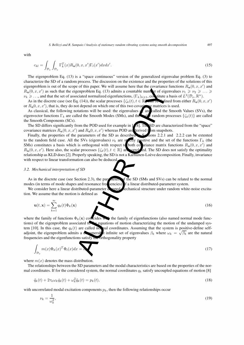
3.2. Mechanical interpretation of SD

As in the discrete case (see Section 2.3), the parameters of the SD (SMs and SVs) can be related to the normalmodes (in terms of mode shapes and resonance frequencies) of a linear distributed-parameter system.

We consider here a linear distributed-parameter damped mechanical structure under random white-noise excita-tion. We assume that the motion is defined as

u(t,x) =

∞∑k=1

qk(t)Φk(x) (16)

where the family of functions Φk(x) coincides with the family of eigenfunctions (also named normal mode func-tions) of the eigenproblem associated to the equations of motion characterizing the motion of the undamped sys-tem [10]. In this case, the qk(t) are called normal coordinates. Assuming that the system is positive-define self-adjoint, the eigenproblem admits a denumerable infinite set of eigenvalues βk where ωk =

√βk are the natural

frequencies and the eigenfunctions satisfy the orthogonality property∫Dx

m(x)Φk(x)TΦl(x)dx = δkl (17)

where m(x) denotes the mass distribution.The relationships between the SD parameters and the modal characteristics are based on the properties of the nor-

mal coordinates. If for the considered system, the normal coordinates qk satisfy uncoupled equations of motion [8]

qk(t) + 2τkωk qk(t) + ω2k qk(t) = pk(t), (18)

with uncorrelated modal excitation components pk, then the following relationships occur

νk =1

ω2k

, (19)

AUTH

OR

COPY


Γk(x) =m(x)Φk(x) (20)

showing that the SVs (νk) of {u(t, x), (t, x) ∈ R × Dx} are equal to the inverse of the square of the naturalfrequencies ωk of the system and that the SMs (Γk(x)) of {u(t, x), (t, x) ∈ R × Dx} are simply related to thenormal mode functions (Φk(x)) by the product with the mass distribution m(x).

Substituting Eq. (20) into Eq. (17) reduces to∫Dx

Γk(x)Φl(x)dx = δkl (21)

showing that the family of SMs are orthogonal to the family of the normal modes.The relations Eqs (19) and (21) are the space-continuous versions of the relations Eq. (11) obtained for discrete

mechanical systems. These relationships are only valid under proportional damping assumption and uncorrelatedmodal excitations.

4. Illustrative example

We consider a Euler-Bernoulli beam that is clamped at one end and free at the other. The model is the following

ρSu(t, x) + EIuIV (t, x) = δ(x− xf )f(t)

u(t, 0) = 0,uI(t, 0) = 0 (22)

uII(t, L) = 0,uIII(t, L) = 0

with the usual parameters: L the length, S the cross-section area, E the Young’s modulus of elasticity, I the momentof inertia, ρ the mass density. We also assume that a space-localized (at x = xf ) excitation force, f(t), is applied tothe beam where f(t) is a scalar random process with covariance function E(f(t+ τ)fT (t)) = Sfδ(τ) (Sf > 0).

Let (ωi,Φi) be the resonance frequencies and the modal functions associated to the unforced model Eq. (22). Thedisplacement of the beam is approximated in a truncated series form

u(t, x) =

p∑i=1

qi(t)Φi(x) (23)

where the dynamics of the modal components are given by the p equations of motion

qi(t) + 2τωiqi(t) + ω2i qi(t) = gi(t) (24)

obtained applying a classical Galerkin procedure to Eq. (22) using the basis (Φi)i�1. The modal excitation compo-nent gi is related to the physical excitation f by

gi(t) = Φi(xf )f(t).

Note that the modal excitation components are correlated (the cross power spectral density function between gi andgj is given by SfΦi(xf )Φj(xf ), for 1 � i, j � p) showing that the SD approach can not give the exact modalparameters. As classical, proportional damping has been added to take into account dissipation.

For a given p, the covariance function Ru(0, x, x′) was evaluated using the relation

Ru(0, x, x′) =

p∑i=1

p∑j=1

Φi(x)Φj(x′)E(qi(t)qj(t)) (25)

whereE(qi(t)qj(t)) denotes the covariance quantities associated to the stationary response of the p (for i = 1, . . . , p)coupled Eq. (24). The covariance matrix of Eq. (24) was obtained solving numerically the associated Lyapounovequation [2]. A similar approach was used to evaluate Ru(0, x, x

′).

AUTH

OR

COPY


Table 1Resonance frequencies estimated from SD

SDNs = 2

SDNs = 4

SDNs = 6

SDNs = 8

SDNs = 10

SDNs = 20

Exact

ω1 4.58 4.57 4.57 4.57 4.57 4.57 4.57ω2 28.95 28.71 28.65 28.64 28.64 28.64 28.64ω3 – 81.83 80.48 80.26 80.21 80.18 80.18ω4 – 160.58 159.57 157.83 157.33 157.13 157.13ω5 – – 270.37 263.34 260.86 259.80 259.75ω6 – – 399.39 400.28 392.37 388.13 388.01ω7 – – – 572.29 555.32 542.42 541.94ω8 – – – 746.80 757.23 722.53 721.52ω9 – – – – 988.56 929.23 926.75ω10 – – – – 1199.40 1162.90 1157.60

The SD method was then developed from a spatial sampling of the random field {u(t, x), (t, x) ∈ R× [0, L]}.Let xk = kΔx for k = 1, . . . , Ns with Δx = L/Ns and Ns > 1 the Ns sampling points. Starting from the

sample functions, Ru(0, xi, xj) and Ru(0, xi, xj), Eq. (13) can be written for x = xi given∫Dx

Ru(0, xi, x′)Γk(x

′)dx′ = νk

∫Dx

Ru(0, xi, x′)Γk(x

′)dx′. (26)

Next, applying the numerical trapezoidal quadrature method to approximate the two integrals gives

Ns∑j=1

αjRu(0, xi, xj)Γk(xj) = νNs

k

Ns∑j=1

αjRu(0, xi, xj)Γk(xj). (27)

where αj = 1 for 1 < j < Ns − 1 and αNs = 0.5.Finally, collecting for i = 1 to Ns the Ns Eq. (27), the sample functions, Γk(xj), written as a vectors ΓNs

k =[Γk(x1)Γk(x2) . . .Γk(xNs)]

T solves the eigenproblem

AΓNs

k = νNs

k BΓNs

k (28)

where A and B are two Ns ×Ns matrices which are easily obtained from Eq. (27).Solving the eigenproblem Eq. (28) gives access to the SMs and to the SVs. The relation Eq. (19) can be used

to approximate the resonance frequencies. The modal functions can be estimated using Eq. (21) which does notrequires any information on the system.

Using the numerical trapezoidal quadrature method to approximate the integrals, Eq. (21) reduces to

Ns∑j=1

αjΓk(xj)Ψl(xj) = δkl. (29)

Introducing the following notations

ΓNs

k = [α1Γk(x1)α2Γk(x2) . . . αNsΓk(xNs)]T (30)

ΓNs = [ΓNs1 ΓNs

2 . . . ΓNs

Ns] (31)

ΦNs

k = [Φk(x1)Φk(x2) . . .Φk(xNs)]T (32)

ΦNs = [ΦNs

1 ΦNs

2 . . .ΦNs

Ns] (33)

the N2s Eq. (29) can then be written in the matrix form

ΦNsΓNsT

= I (34)

AUTH

OR

COPY


Fig. 1. The modal functions (solid line) and the modal functions approximated from the SD approach with Ns = 2 (◦), Ns = 4 (�), Ns = 6(�), Ns = 8 (�), Ns = 10 (�) and Ns = 20 (∗).

where I denotes the Ns ×Ns identity matrix given the relation

ΦNs = ΓNs−T

(35)

which has been used to estimate from the SMs the modal functions at the sampling points.In Table 1, the exact first ten resonance frequencies of the clamped-free beam are compared with the associated

ones obtained using the SD approach (Eq. (19)). The parameter values used are: L = 0.6, EI = 1.4, ρS = 0.1620,τ = 0.005, xf = 0.05, Sf = 1 and p = 40. The SD approach has been developed for Ns = 2, 4, 6, 8, 10 and 20sampling points. For Ns = 2, the estimation of the first two resonance frequencies are not so bad. The accuracyincreases quickly with Ns. For Ns = 10, the first five frequencies are well estimated. Twenty points are needed toestimate satisfactorily the first ten frequencies.

In Fig. 1, the exact first ten modal functions of the clamped-free beam are compared with the associated onesobtained using the SD approach (Eq. (35)) with Ns = 2, 4, 6, 8, 10 and 20 sampling points. With Ns = 2 whereonly two modes are accessible, the SD approach gives values for the first two modal functions at the sampling pointsvery closed to the exact one (see circle positions on the modes 1 and 2). The same comment is also valid for Ns = 4.For the other values of Ns (Ns = 6, 8 and 10) only the last accessible modal function is not correctly approximated.For Ns = 20, the results illustrate well the numerical convergence with respect of the parameter Ns.

AUTH

OR

COPY


Fig. 2. The modal functions (solid line) and the KLMs with Ns = 2 (◦), Ns = 4 (�), Ns = 6 (�), Ns = 8 (�), Ns = 10 (�) and Ns = 20 (∗).

Fig. 3. The modal functions (solid line), the KLMs with Ns = 20 (dotted-dashed line with ◦), the SMs with Ns = 20 (dotted line with ×) andthe modal functions approximated from the SD approach with Ns = 20 (dashed line with �).

In Fig. 2, the results obtained with the KLD approach using the same data are reported. When the number ofsampling points is small, the KLMs show significant differences from the modal functions. Even for Ns = 20, somedifferences are still present.

Finally, it is interesting to observe the SMs. They are plotted in Fig. 3 in case of Ns = 20. As expected, they arevery close to the modal functions but they show small spatial fluctuations.

AUTH

OR

COPY


5. Conclusion

This paper has presented the potential of the smooth decomposition in terms of output-only modal analysis toolwhen stationary random responses are considered. The properties of the smooth decomposition when it is appliedto a discrete linear mechanical system were recalled. The smooth decomposition was extended to the class of scalarstationary random processes indexed in time and space. It was shown that when the SD is applied to the stationaryresponse of a linear distributed-parameter damped mechanical structure under random white-noise excitation, thesame properties as in the discrete case hold. Under uncorrelated modal forcing terms, the SD gives access to reso-nance frequencies and modal functions. Simulations have shown that the SD approach can advantageously replacethe KLD approach in the context of the modal analysis or in terms of dynamical analysis. Important but not analysishere is the dependency of the SMs with respect to the mass distribution which could be a tool to study the integrityof a structure and monitoring its healthy.

Current works include the use of the SD to analysis nonlinear problem and the develpment of a SD-based reducedorder model.

Acknowledgment

The authors gratefully acknowledge the financial support of COFECUB, CAPES, Faperj, and CNPq.

References

[1] J.S.R. Anttonen, P.I. King and P.S. Beran, POM-based reduced-order model with deforming grids, Mathematical and Computer Modelling38 (2003), 41–62.

[2] S. Bellizzi and R. Sampaio, POMs analysis of randomly vibrating systems obtained from Karhunen-Loève expansion, Journal of Soundand Vibration 297 (2006), 774–793.

[3] S. Bellizzi and R. Sampaio, Smooth Karhunen-Loève decomposition to analyze random vibrating systems, Journal of Sound and Vibration325 (2009), 491–498.

[4] K. Carlberg and C. Farhat, A low-cost, goal-oriented compact proper orthogonal decomposition basis for model reduction of static systems,International Journal for Numerical methods in Engineering 86 (2011), 381–402.

[5] D. Chelidze and W. Zhou, Smooth orthogonal decomposition-based vibration mode identification, Journal of Sound and Vibration 292(2006), 461–473.

[6] U. Farooq and B.F. Feeny, Smooth orthogonal decomposition for modal analysis of randomly excited systems, Journal of Sound andVibration 316 (2008), 137–146.

[7] G. Kerschen, J.-C. Golinval, A. Vakakis and L. Bergman, The method of proper orthogonal decomposition for dynamical characterizationand order reduction of mechanical systems: an overview, Non-linear Dynamics, Special Issue on Reduced Order Models: Methods andApplications Applications 41 (2005), 147–169.

[8] Y.K. Lin, Probability Theory of Structural Dynamics, McGraw-Hill, Inc, 1967.[9] X. Ma, A.F. Vakakis and L. Bergman, Karhunen-Loève analysis and order reduction of the transient dynamics of linear coupled oscillators

with strongly nonlinear end attachments, Journal of Sound and Vibration 309 (2008), 569–587.[10] L. Meirovitch, Computational Method in Structural Dynamics, Sijthoff and Noordhoff International Publishers, 1980.[11] R. Sampaio and S. Bellizzi, Analysis of non-stationary random processes using smooth decomposition, Journal of Mechanics of Materials

and Structures 2011, (to appear). AUTH

OR

COPY

2013 sav bs n20 pp 493 502 copy

Documents

Transcript of 2013 sav bs n20 pp 493 502 copy