1661661.pdf - Hindawi.com

Research ArticleNumerical Treatment on Parabolic Singularly PerturbedDifferential Difference Equation via Fitted Operator Scheme

Dagnachew Mengstie Tefera , Awoke Andargie Tiruneh, and Getachew Adamu Derese

Department of Mathematics, Bahir Dar University, Ethiopia

Correspondence should be addressed to Dagnachew Mengstie Tefera; [email protected]

Received 8 July 2021; Revised 14 September 2021; Accepted 6 October 2021; Published 22 October 2021

Academic Editor: Yufeng Xu

Copyright © 2021 Dagnachew Mengstie Tefera et al. This is an open access article distributed under the Creative CommonsAttribution License, which permits unrestricted use, distribution, and reproduction in any medium, provided the original workis properly cited.

This paper proposes a new fitted operator strategy for solving singularly perturbed parabolic partial differential equation withdelay on the spatial variable. We decomposed the problem into three piecewise equations. The delay term in the equation isexpanded by Taylor series, the time variable is discretized by implicit Euler method, and the space variable is discretized bycentral difference methods. After developing the fitting operator method, we accelerate the order of convergence of the timedirection using Richardson extrapolation scheme and obtained Oðh2 + k2Þ uniform order of convergence. Finally, threeexamples are given to illustrate the effectiveness of the method. The result shows the proposed method is more accurate thansome of the methods that exist in the literature.

1. Introduction

The spatial delay parabolic singularly perturbed differentialequation is a differential equation in which the perturbationparameter multiply the highest order derivative, and it has atleast one retarded term on the spatial variable. Some mathe-matical problems can be treated as singularly perturbedproblems such as Navier–Stokes equations, atmospheric pol-lution, turbulent transport, groundwater flow and solutetransport, and Black–Scholes model, as presented in the sur-vey paper by Kadalbajoo and Gupta [1]. There are two prin-ciple approaches for solving singular perturbation problems:numerical approach and asymptotic approach by Sharmaet al. [2]. The numerical solution of the model problem ischallenging due to the existence of a boundary layer. Fur-thermore, when using the classical finite difference method,we are unable to achieve an accurate solution, and the sys-tem becomes unstable. To tackle this issue, we need to createa fitted method for uniform or nonuniform meshes. As aresult, ε-uniformly convergent numerical methods wereconstructed, with the order of convergence and error con-stant being independent of the perturbation parameter ε.For solving singular perturbation problems, some ε-uni-

form numerical schemes have been developed in theliterature.

Most of the scholars studied on time delayed singularlyperturbed problems. Mbroh et al. [3] proposed parameteruniform method for solving a time delay nonautonomoussingularly perturbed parabolic differential equation. Claveroand Gracia [4] studied singularly perturbed time-dependentproblem of reaction–diffusion type using Richardson extrap-olation technique. Woldaregay and Duressa [5] considered anumerical method for both small time delay and large timedelay singularly perturbed boundary value problem. Kumarand Kumari [6] show that the influence of a small delay onthe solution is extremely sensitive and that a small changein the delay can have a significant impact on the solution.Chakravarthy et al. [7] using the fitted technique, singularlyperturbed differential equations with large delays wereinvestigated.

Nowadays, a few scholars have examined numericalsolution for spatial delay singularly perturbed parabolic par-tial differential equations. Bansal and Sharma [8] numericalsolutions for a large delay reaction-diffusion problem hasbeen developed. Gupta et al. [9] examined spatial delay par-abolic singularly perturbed partial differential equations and

HindawiAbstract and Applied AnalysisVolume 2021, Article ID 1661661, 12 pageshttps://doi.org/10.1155/2021/1661661

https://orcid.org/0000-0001-5226-1083

https://creativecommons.org/licenses/by/4.0/

https://creativecommons.org/licenses/by/4.0/

https://doi.org/10.1155/2021/1661661

its solution using higher order fitted mesh method. Expo-nentially fitted operator method was developed to solvedifferential-difference singularly perturbed problem by Wol-daregay and Duressa [10]. Das and Natesan [11] presentedthe solution of delay singularly perturbed partial differentialequation using second-order convergent method. Singh andSrinivasan [12] developed Richardson extrapolation methodfor solving convection-diffusion equations with retardedterm. Chahravarthy and Kumar [13] presented adaptive gridmethod for solving singularly perturbed convection-diffusion problems with spatial delay. Bansal et al. [14]designed numerical scheme for solving general shift singu-larly perturbed parabolic convectional diffusion problems.

In this study, a singularly perturbed delayed partial dif-ferential equation with small spatial shift right boundarylayer problem is decomposed into three piecewise equationswhich are treated using fitted operator difference methods.To accelerate the order of accuracy in the time variable,the Richardson extrapolation method is applied. The orderof convergence of the present method is shown to be secondorder in both time and spatial variable, whereas the rate ofconvergence is two. Furthermore, the numerical results ofthe examples considered shows that the present methodhas better accuracy compared to some results that appearin the literature.

2. Statement of the Problem

Consider the parabolic singularly perturbed second-orderdifferential equation with small spatial delay, on the domain

Ω =D1 ×D2 = ð0, 1Þ × ð0, T� and Ω =Ωl ∪Ωb ∪Ωr , whereΩl = fðx, tÞ: − γ ≤ x ≤ 0 and 0 ≤ t ≤ Tg, Ωb = fðx, tÞ: 0 ≤ x ≤1 and 0 ≤ t ≤ Tg, and Ωr = fðx, tÞ: 1 ≤ x ≤ 1 + μ and 0 ≤ t ≤ Tg of the form:

ut − εuxx + A xð Þux + B xð Þu x, tð Þ + C xð Þu x − γ, tð Þ +D xð Þu x + μ, tð Þf= F x, tð Þ, x, tð Þ ∈Ω,

ð1Þ

with

u x, tð Þ = φl x, tð Þ, ∀ x, tð Þ ∈Ωl,

u x, 0ð Þ = φb xð Þ, x ∈ 0, 1½ �,u x, tð Þ = φr x, tð Þ, ∀ x, tð Þ ∈Ωr ,

8>><>>: ð2Þ

where 0 < ε≪ 1 and γ, μ denote the small delay parameters.The functions AðxÞ, BðxÞ, CðxÞ,DðxÞ, φlðx, tÞ, φbðxÞ, and φrðx, tÞ are supposed to be bounded and smooth functions on�Ω, that satisfy the conditions BðxÞ + CðxÞ +DðxÞ ≥ β > 0 onΩb = ½0, 1�. When γ = μ = 0, the above problem (1) reducedto singularly perturbed parabolic partial differential prob-lem. If AðxÞ ≥ α > 0, CðxÞ < 0 and DðxÞ < 0, ∀x ∈Ωb = ½0, 1�,then the solution has boundary layer on the right side, i.e.,at x = 1, where α, β are some constants.

Equation (1) together with initial boundary conditionEquation (2) can be rewrite as

Under the assumption that the data are uniformlycontinuous and also meet relevant compatibility condi-tions at the corner points ð0, 0Þ, ð1, 0Þ, ð−γ, 0Þ, andð1 + μ,

0Þ, it is possible to establish the uniqueness of a solutionto (1) [15]. The compatibility conditions are given asfollows:

Lεu x, tð Þ =ut − εuxx + A xð Þux + B xð Þu +D xð Þu x + μ, tð Þ = F x, tð Þ − C xð Þφl x − γ, tð Þ, if 0 < x ≤ γ, 0 < t ≤ T ,

ut − εuxx + A xð Þux + B xð Þu + C xð Þu x − γ, tð Þ +D xð Þu x + μ, tð Þ = F x, tð Þ, if γ < x < 1 − μ, 0 < t ≤ T ,

ut − εuxx + A xð Þux + B xð Þu + C xð Þu x − γ, tð Þ = F x, tð Þ −D xð Þφr x + μ, tð Þ, if 1 − μ ≤ x < 1, 0 < t ≤ T:

8>><>>: ð3Þ

φl 0, 0ð Þ = φb 0ð Þ,φr 1, 0ð Þ = φb 1ð Þ,

(

∂φl 0, 0ð Þ∂t

− ε∂2φb 0ð Þ∂x2

+ A 0ð Þ ∂φb 0ð Þ∂x

+ B 0ð Þφb 0ð Þ + C 0ð Þφl −γ, 0ð Þ +D 0ð Þφb μð Þ = F 0, 0ð Þ,

∂φr 1, 0ð Þ∂t

− ε∂2φb 1ð Þ∂x2

+ A 1ð Þ ∂φb 1ð Þ∂x

+ B 1ð Þφb 1ð Þ + C 1ð Þφb 1 − γð Þ +D 0ð Þφr 1 + μ, 0ð Þ = F 1, 0ð Þ:

8>>><>>>:

ð4Þ

2 Abstract and Applied Analysis

Using the above compatibility conditions, there exists aconstant M independent of the perturbation parameter ε∀ðx, tÞ ∈ �Ω; we have

∣u x, tð Þ − u x, 0ð Þ∣ = ∣u x, tð Þ − φb 0ð Þ∣ ≤Mt,

u x, tð Þ − u 0, tð Þj j = u x, tð Þ − φl 0, tð Þj j ≤M 1 − xð Þ,

(ð5Þ

for the proof of Equation (5) see [16].

Lemma 1 (Continuous Maximum Principle). Let the func-tion ψðx, tÞ ∈ C2,1ð�ΩÞ. If ψðx, tÞ ≥ 0, for all ðx, tÞ ∈ ∂Ω andLεψðx, tÞ ≥ 0, for all ðx, tÞ ∈Ω, then ψðx, tÞ ≥ 0, for all ðx, tÞ∈ �Ω.

Proof. Assume ðxy, tzÞ ∈ �Ω − ∂Ω such that ψðxy, tzÞ = minðx,tÞ∈ �Ω

ψðx, tÞ and suppose ψðxy , tzÞ < 0. This gives that ψtðxy, tzÞ= 0, ψxðxy, tzÞ = 0 and ψxxðxy, tzÞ ≥ 0.☐

Now, in order to show Lεψðx, tÞ ≤ 0, consider the follow-ing cases.

Case 1. 0 < xy ≤ γ and 0 ≤ tz ≤ T

Lεu xy, tz� �

= ut xy, tz� �

− εuxx xy, tz� �

+ A xy� �

ux xy, tz� �

+ B xy� �

u xy, tz� �

+D xy� �

u xy + μ, tz� �

= −εuxx xy, tz� �

+ B xy� �

u xy, tz� �

+D xy� �



+ B xy� �

+D xy� ��

u xy, tz� �

+D xy� �


− u xy, tz� ��

≤ 0:

ð6Þ

Case 2. 1 − μ < xy < 1 and 0 ≤ tz ≤ T

Lεu xy, tz� �

= ut xy, tz� �


+ A xy� �

ux xy, tz� �

+ B xy� �

u xy, tz� �

+ C xy� �

u xy − γ, tz� �


+ B xy� �

u xy, tz� �

+ C xy� �



+ B xy� �

+ C xy� ��

u xy, tz� �

+ C xy� �


− u xy, tz� ��

≤ 0:

ð7Þ

Case 3. γ < xy ≤ 1 − μ and 0 ≤ tz ≤ T

Lεu xy, tz� �

= ut xy, tz� �


+ A xy� �

ux xy, tz� �

+ B xy� �

u xy, tz� �

+ C xy� �


+D xy� �



+ B xy� �

u xy, tz� �

+ C xy� �


+D xy� �


≤ 0:ð8Þ

Since BðxyÞ + CðxyÞ +DðxyÞ ≥ α > 0 and using the aboveassumption, we have Lεψðx, tÞ ≤ 0 which contradicts ourassumption.

Thus, ψðxy , tzÞ ≥ 0 which leads to ψðx, tÞ ≥ 0∀ðx, yÞ ∈ �Ω.

Lemma 2. Let uðx, tÞ be the solution of the continuous prob-lem for Equations (1) and (2). Then, we get the bound

∣u x, tð Þ∣ ≤ ∥f ∥θ

+max ∣φl x, tð Þ∣,∣φb xð Þ∣,∣φr x, tð Þ ∣f g, ð9Þ

where BðxÞ ≥ θ > 0, ∀x ∈ ½0, 1�.

Proof. Let the barrier function ψ± and defined as

ψ± =∥f ∥θ

+max φl x, tð Þj j, φb xð Þj j, φr x, tð Þj j ± u x, tð Þf , ð10Þ

applying Lemma 1, and we get the above bound.☐

Lemma 3. The derivatives of the exact solution uðx, tÞ ofthe Equation (1) fulfill the following bound for v = 0, 1,and 2.

∂vu x, tð Þ∂tv

�� ≤M, ∀ x, tð Þ ∈ �Ω, ð11Þ

where M ∈ℝ is independent of ε.

Proof. The proof of this lemma can be found in [7].☐

Theorem 4. The analytical solution of Equation (1) satisfies

∣diu x, tð Þ

dxi∣ ≤ 1 + ε−i exp −

α 1 − xð Þε

� �� , 0 ≤ i ≤ 4: ð12Þ

Proof. The proof for the bounds of its derivatives is given in[4].☐

3. Numerical Method

In this section, we develop an exponentially fitted operatordifference method to solve Equation (1).

3.1. Time Discretization. A uniform mesh with a time stepof k is used to discretize the time domain ½0, T� as fol-lows:

t j = jk, for j = 0, 1, 2,⋯, n, ð13Þ

3Abstract and Applied Analysis

where k = T/n and in the interval ½0, T�, n is the numberof subintervals in the time direction.

We utilize the implicit Euler’s approach to approximatethe time derivative term of Equation (1), which results in asystem of boundary value problems.

uj+1 − uj

k− εuj+1

xx + A xð Þuj+1x + B xð Þuj+1 + C xð Þuj+1 x − γ, tð Þ

+D xð Þuj+1 x + μ, tð Þ = F x, tð Þ:ð14Þ

Using Equations (3) and (14), we have

where EðxÞ = BðxÞ + ð1/kÞ:3.2. Spatial Discretization. The spatial domain ½0, 1� is subdi-vided as follows using a uniform mesh with a step length of h:

xi = ih, for i = 0, 1, 2,⋯,m, ð16Þ

where h = 1/m and m is the number of subintervals in spatialdirection in the interval ½0, 1�. Using expansion of Taylor

series expansion, we have

uj+1 x + μð Þ = uj+1 xð Þ + μuj+1x +

μ2

2uj+1 xð Þ +O μ3

� �,

uj+1 x − γð Þ = uj+1 xð Þ − γuj+1x +

γ2

2uj+1 xð Þ +O γ3

� �:

8>><>>:

ð17Þ

Substituting Equation (17) into Equation (15) and rear-ranging gives

with the boundary conditions:

u 0, tð Þ = φl 0, tð Þ, ∀ x, tð Þ ∈Ωl,

u 1, tð Þ = φr 1, tð Þ, ∀ x, tð Þ ∈Ωr ,

(ð19Þ

and initial condition

u x, 0ð Þ = φb xð Þ, x ∈ 0, 1½ �, ð20Þ

where

p1 xð Þ = ε A xð Þ + μD xð Þð Þε − μ2/2ð ÞD xð Þ ,

p2 xð Þ = ε A xð Þ − γC xð Þ + μD xð Þð Þε − γ2/2ð ÞC xð Þ − μ2/2ð ÞD xð Þ ,

p3 xð Þ = ε A xð Þ − γC xð Þð Þε − γ2/2ð ÞC xð Þ ,

q1 xð Þ = ε D xð Þ + E xð Þð Þε − μ2/2ð ÞD xð Þ ,

q2 xð Þ = ε C xð Þ +D xð Þ + E xð Þð Þε − γ2/2ð ÞC xð Þ − μ2/2ð ÞD xð Þ ,

Lεuj+1 xð Þ =

−εuj+1xx + A xð Þuj+1

x + E xð Þuj+1 +D xð Þuj+1 x + μð Þ = F x, tð Þ − C xð Þφl x − γ, t j+1� �

+uj

k, if 0 < x ≤ γ, 0 < t ≤ T ,


x + E xð Þuj+1 + C xð Þuj+1 x − γð Þ +D xð Þuj+1 x + μð Þ = F x, tð Þ + uj

k, if γ < x < 1 − μ, 0 < t ≤ T ,


x + E xð Þuj+1 + C xð Þuj+1 x − γð Þ = F x, tð Þ −D xð Þφr x + μ, t j+1� �

+uj

k, if 1 − μ ≤ x ≤ 1, 0 < t ≤ T ,

8>>>>>>><>>>>>>>:

ð15Þ

Lεuj+1 xð Þ =−εuj+1

xx + p1 xð Þuj+1x + q1 xð Þuj+1 = g1 x, tð Þ, if 0 < x ≤ γ, 0 < t ≤ T ,

−εuj+1xx + p2 xð Þuj+1

x + q2 xð Þuj+1 = g2 x, tð Þ, if γ < x < 1 − μ, 0 < t ≤ T ,

−εuj+1xx + p3 xð Þuj+1

x + q3 xð Þuj+1 = g3 x, tð Þ, if 1 − μ ≤ x ≤ 1, 0 < t ≤ T ,

8>><>>: ð18Þ


q3 xð Þ = ε C xð Þ + E xð Þð Þε − γ2/2ð ÞC xð Þ ,

g1 x, tð Þ = ε F x, t j+1� �

− C xð Þφl x − γ, t j+1� �

+ uj/k� ��

ε − μ2/2ð ÞD xð Þ ,

g2 x, tð Þ = ε F x, t j+1� �

+ uj/k� ��

ε − γ2/2ð ÞC xð Þ − μ2/2ð ÞD xð Þ ,

g3 x, tð Þ = ε F x, t j+1� �

−D xð Þφr x + μ, t j+1� �

+ uj/k� ��

ε − γ2/2ð ÞC xð Þ :

ð21Þ

Applying central difference approximation for spatialvariable of Equation (18), we obtain

To obtain more accurate and ε-uniform solution forEquation (22), introducing fitting factor ðσÞ as follows:

To obtain the value of the fitting factor, multiply bothsides of the equations in (23) by h and evaluating limit ash⟶ 0.

limh⟶0

−σ1ρ

uj+1i−1 − 2uj+1

i + uj+1i+1 + lim

h⟶0p1 xið Þ u

j+1i+1 − uj+1

i−12

= 0,

ð24Þ

where ρ = h/ε.The solution of Equation (18) comes from the theory of

singular perturbation [16] given as

u x, tð Þ = u0 x, tð Þ + ae−pv 1ð Þ 1−xð Þ/εð Þ, v = 1, 2, 3, ð25Þ

where u0ðx, tÞ is outer solution.

This implies the approximate solution at ðxi, t jÞ is givenas:

limh⟶0

uji = uj

o 0ð Þ + ae −pv 1ð Þð Þ/εepv 1ð Þiρ: ð26Þ

Using Equation (26), we have

limh⟶0

uj+1i+1 − uj+1

i−1 = ae −pv 1ð Þð Þ/εepv 1ð Þiρ epv 1ð Þρ − e−pv 1ð Þρ� �

, ð27aÞ

and

limh⟶0

uj+1i−1 − 2uj+1

i + uj+1i+1 = ae −pv 1ð Þð Þ/εepv 1ð Þiρ epv 1ð Þρ − 2 + e−pv 1ð Þρ

� �:

ð27bÞ

−εuj+1i−1 − 2uj+1

i + uj+1i+1

h2+ p1 xið Þ u

j+1i+1 − uj+1

i−12h

+ q1 xið Þuj+1i = g1 xi, tð Þ, if 0 < x ≤ γ, 0 < t ≤ T ,

−εuj+1i−1 − 2uj+1

i + uj+1i+1

h2+ p2 xið Þ u

j+1i+1 − uj+1

i−12h

+ q2 xið Þuj+1i = g2 xi, tð Þ, if γ < x < 1 − μ, 0 < t ≤ T ,

−εuj+1i−1 − 2uj+1

i + uj+1i+1

h2+ p3 xið Þ u

j+1i+1 − uj+1

i−12h

+ q3 xið Þuj+1i = g3 xi, tð Þ, if 1 − μ ≤ x ≤ 1, 0 < t ≤ T:

8>>>>>>>>><>>>>>>>>>:

ð22Þ

−εσ1uj+1i−1 − 2uj+1

i + uj+1i+1

h2+ p1 xið Þ u

j+1i+1 − uj+1

i−12h

+ q1 xið Þuj+1i = g1 xi, tð Þ, for 0 < x ≤ γ, 0 < t ≤ T ,

−εσ2uj+1i−1 − 2uj+1

i + uj+1i+1

h2+ p2 xið Þ u

j+1i+1 − uj+1

i−12h

+ q2 xið Þuj+1i = g2 xi, tð Þ, for γ < x < 1 − μ, 0 < t ≤ T ,

−εσ3uj+1i−1 − 2uj+1

i + uj+1i+1

h2+ p3 xið Þ u

j+1i+1 − uj+1

i−12h

+ q3 xið Þuj+1i = g3 xi, tð Þ, for 1 − μ ≤ x ≤ 1, 0 < t ≤ T:

8>>>>>>>>><>>>>>>>>>:

ð23Þ


Thus, using Equation (24), (27a), and (27b), we get

σv =pv ið Þρ2

cothpv 1ð Þρ

2

, v = 1, 2, 3: ð28Þ

Substituting Equation (28) into Equation (23), we get thefollowing tri-diagonal system of equations that can be solvedusing Thomas algorithm.

Ej+1i,v u

j+1i−1 + Fj+1

i,v uj+1i +Gj+1

i,v uj+1i+1 =Hj+1

i,v , ð29Þ

for i = 1, 2,⋯,m − 1, j = 0, 1,⋯, n − 1 v = 1, 2, 3, where

Ej+1i,v =

−εσv

h2−pv xið Þ2h

Fj+1i,v =

2εσv

h2+ qv xið Þ,

Gj+1i,v =

−εσv

h2+pv xið Þ2h

Hj+1i,v = gv xi, tð Þ:

ð30Þ

Since qvðxiÞ is nonnegative, then the system of Equation(29) becomes diagonally dominant.

i:e: Fj+1i,v

�� > Ej+1i,v

�� + Gj+1i,v

�� : ð31Þ

Thus, the present method have convergent solution.

3.3. Convergence Analysis

Lemma 5 (Discrete Maximum Principle). Suppose that themesh function wj+1ðxiÞ satisfies wj+1ðx0Þ ≥ 0 and wj+1ðxmÞ≥ 0. If Lεwj+1ðxiÞ ≥ 0 for 1 ≤ i ≤m − 1, then wj+1ðxiÞ > 0, forall i, 0 ≤ i ≤m.

Proof. Let wj+1ðxyÞ = min1≤i≤m−1

wj+1ðxiÞ and suppose that wj+1ðxyÞ < 0, then

Lεwj+1 xy� �

= −εσv

wj+1 xy−1� �

− 2wj+1 xy� �

+wj+1 xy+1� �

h2

+ pv xy� �wj+1 xy+1

� �−wj+1 xy−1

� �2h

+ qvwj+1 xy� �

< 0,ð32Þ

which contradicts our assumption.☐

Thus, wj+1ðxiÞ > 0, for all i, 0 ≤ i ≤m:

Lemma 6 (Stability Estimate). The solution Uj+1i of the dis-

crete method satisfies the bound

U j+1i

�� ≤ θ−1 max LεU j+1i

�� +max φl 0, t j+1� �

, φr 1, t j+1� �� ,

ð33Þ

where qðxiÞ ≥ θ > 0.

Proof. Define the barrier function ψ±i,j+1 as

ψ±i,j+1 = θ−1 max ∣LεU j+1

i ∣ +max ∣φl 0, t j+1� �

, φr 1, t j+1� �

∣ ±U j+1i :

ð34Þ

In the barrier function at the boundary condition, weobtain

ψ±j+1 0ð Þ = θ−1 max ∣LεU j+1

i ∣ +max ∣φl 0, t j+1� �

, φr 1, t j+1� �

∣ ± φl 0, t j+1� �

≥ 0,

ψ±j+1 1ð Þ = θ−1 max ∣LεU j+1

i ∣ +max ∣φl 0, t j+1� �

, φr 1, t j+1� �

∣ ± φr 1, t j+1� �

≥ 0:

ð35Þ

The barrier function at spatial domain xi, 1 ≤ i ≤m − 1;we obtain

Lεψ±i,j+1 = Lε θ−1 max ∣ LεU j+1

i ∣+ max ∣ φl 0, t j+1� �

, φr 1, t j+1� �

∣h i

± LεU j+1i = qv xið Þ θ−1 max ∣ LεU j+1

i ∣h

+ max ∣ φl 0, t j+1� �

, φr 1, t j+1� �

∣�± LεU j+1

i ≥ 0:

ð36Þ

Using Lemma 5, we have that ψ±i,j+1 ≥ 0 for all ðxi, t j+1Þ

∈ �Ω. Thus, the required bound in Equation (33) is satisfied.

Consistency of the method: Consider the Taylor seriesexpansion of

uj+1i+1 = uj+1

i + huj+1x,i +

h2

2uj+1xx,i +

h3

3!uj+1xxx,i+⋯uj+1

i−1

= uj+1i − huj+1

x,i +h2

2uj+1xx,i −

h3

3!uj+1xxx,i+⋯uj

i

= uj+1i − kuj+1

t,i +k2

2uj+1tt,i −

k3

3!uj+1ttt,i+⋯:

ð37Þ


Using the above expansion of Equation (22) becomes

1k

uj+1i − uj+1

i − kuj+1t,i + k2

2uj+1tt,i −⋯

!" #

−ε

h2uj+1i + huj+1

x,i +h2

2uj+1xx,i +

h3

3!uj+1xxx,i+⋯

!"

− 2uj+1i + uj+1

i − huj+1x,i +

h2

2uj+1xx,i −

h3

3!uj+1xxx,i+⋯

!#

+A xið Þ2h

uj+1i + huj+1

x,i +h2

2uj+1xx,i +

h3

3!uj+1xxx,i+⋯

!"

− uj+1i − huj+1

x,i +h2

2uj+1xx,i −

h3

3!uj+1xxx,i+⋯

!#

+ B xið Þuj+1i + C xið Þu xi − γ, t j+1

� �+D xið Þu xi + μ, t j+1

� �− F xi, t j+1� �

:

ð38Þ

After simplifying the terms, the truncation errorbecomes

T:E: = uj+1i,t − εuj+1

xx,i + A xið Þuj+1x,i + B xið Þuj+1

i

+ C xið Þu xi − γ, t j+1� �

+D xið Þu xi + μ, t j+1� �

uj+1i

− F xi, t j+1� �

−k2uj+1tt,i −

εh2

12uj+1xxxx,i + A xið Þ h

2

6uj+1xxx,i,

ð39Þ

which gives

T:E: = −k2uj+1tt,i −

εh2

12uj+1xxxx,i + A xið Þ h

2

6uj+1xxx,i: ð40Þ

Thus, limðh,kÞ⟶ð0,0Þ

T:E: = 0, which shows that the present

method is consistent. Since the method is consistent and sta-ble, then using Lax equivalence theorem, the present methodis convergent.

Theorem 7. Let the exact solution and numerical solution ofEquation (1), respectively, are u and U . Then,

sup0<ε≤1

maxi,j

∣u xi, t j� �

−U ji ∣ ≤M h2 + k

� �: ð41Þ

Proof. For the proof, one can refer [17].☐

4. Richardson Extrapolation Approach

The Richardson extrapolation approach has been described,and it is designed to improve the accuracy of the computedsolutions in the basic scheme.

Let Dn2 ⊆D2n

2 , where D2n2 is the mesh obtained from

bisecting the step size k. Denote the numerical solutionobtained from D2n

2 by �UjðxÞ, we have

uj xð Þ −Uj xð Þ ≤ Ck + Rnj xð Þ, x, t j

� �∈D1 ×Dn

2 , ð42aÞ

uj xð Þ − �U j xð Þ ≤ Ck2

� �+ R2n

j xð Þ, x, t j� �

∈D1 ×D2n2 ,

ð42bÞ

where Rnj ðxÞ and R2n

j ðxÞ are the remainder terms of theerror. Now, subtracting the inequality (42b) from (42a) toobtain the extrapolation formula.

uj xð Þ −Uj xð Þ − 2 uj xð Þ − �Uj xð Þ� �

= Rnj xð Þ − R2n

j , ð43Þ

which gives that

Uextj xð Þ = 2�Uj xð Þ −U j xð Þ, ð44Þ

is an approximate solution [12].

Theorem 8. Let uðxi, t j+1Þ and Uexti,j+1 be the solution of prob-

lems in (1) and (44), respectively, then the proposed schemesatisfies the following error estimate

sup0<ε<1

maxxi ,t j+1

∣u xi, t j+1� �

−Uexti,j+1∣ ≤ C h2 + k2

� �: ð45Þ

Proof. Using the error for the temporal and spatial discreti-zation gives the required bound.☐

5. Numerical Examples

To determine the efficacy of the current scheme, we lookedat model problems that had been addressed in the literatureand had approximate solutions that could be compared.

We used the double-mesh principle to estimate the abso-lute maximum error of the current approach when the exactsolution for the given problem was unknown. We use thefollowing formula to approximate the absolute maximumerror at the selected mesh points:

Case 1. If the exact solution is known,

EM,Nε = max

xi ,t jð Þ∈Ωu xi, t j� �

− uext,ji

�� : ð46Þ

Case 2. If the exact solution is unknown,

EM,Nε = max

xi ,t jð Þ∈Ωuext,ji

� �M,N− uext,ji

� �2M,2N��

��: ð47Þ


We also evaluate the corresponding rate of convergence.

RM,N =log EM,N

ε − log E2M,2Nε

log 2: ð48Þ

Example 1. Let AðxÞ = ð2 − x2Þ, BðxÞ = ðx − 3Þ, CðxÞ = −2,DðxÞ = −1, Fðx, tÞ = 10t2e−txð1 − xÞ, where ðx, tÞ ∈ ð0, 1Þ × ð0,1�, and with initial boundary condition,

u x, tð Þ = 0, ∀ x, tð Þ ∈Ωl = x, tð Þ: − γ ≤ x ≤ 0, and 0 ≤ t ≤ 1f g,u x, tð Þ = 0, ∀ x, tð Þ ∈Ωr = x, tð Þ: 1 ≤ x ≤ 1 + μ, and 0 ≤ t ≤ 1f g,u x, tð Þ = 0, ∀ x, tð Þ ∈Ωb = x, tð Þ: 0 ≤ x ≤ 1, and 0 ≤ t ≤ 1f g:

ð49Þ

Example 2. Let AðxÞ = ð1 + x + x2Þ, BðxÞ = ð1 + x2Þ, CðxÞ =−ð0:25 + 0:5x2Þ, DðxÞ = −0:25, Fðx, tÞ = sin ðπxÞð1 − xÞ,where ðx, tÞ ∈ ð0, 1Þ × ð0, 1�, with initial and boundary con-dition,


ð50Þ

Example 3. Let AðxÞ = ð1 − x2/2Þ, BðxÞ = ðx + 6Þ, CðxÞ = −4,DðxÞ = −1, Fðx, tÞ = xð1 − xÞ, where ðx, tÞ ∈ ð0, 1Þ × ð0, 3�,with initial and boundary condition,


ð51Þ

6. Discussions and Results

We have presented the method for solving spatial delayedsingularly perturbed parabolic partial differential equation.The basic mathematical procedures are defining the modelproblem, decomposing into three equations, approximatingtime variable using implicit Euler’s method, approximatingthe delay term using Taylor series expansion of order two,approximating the spatial variable using the central differ-ence method, and finding fitting factor. Finally, apply Rich-ardson extrapolation method to accelerate the accuracy ofthe method.

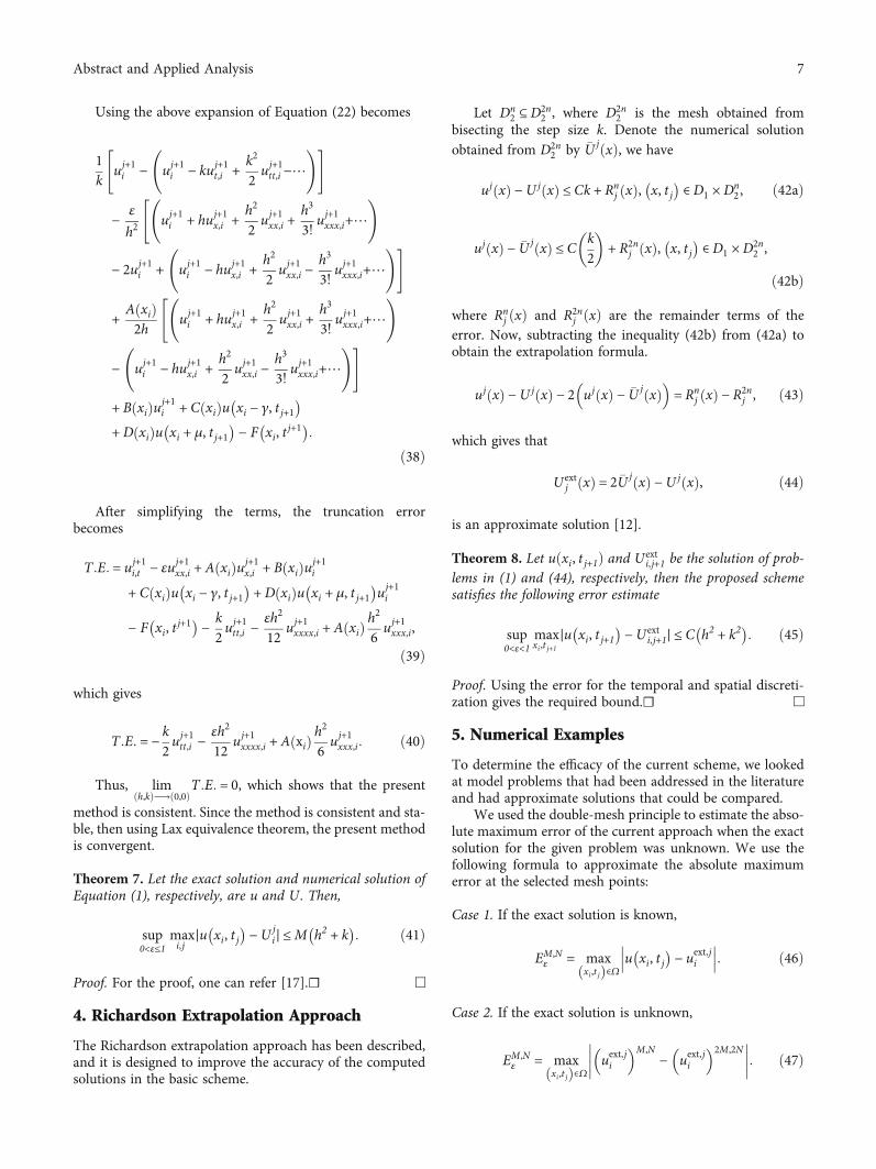
Three model examples are used to exemplify the perfor-mance of the proposed method. The maximum error andrate of convergence are shown in Tables 1–3 with differentvalues of ε, delay parameters, and mesh length. The physical

Table 1: Maximum absolute point-wise error and rate of convergence for Example 1 before and after Richardson extrapolation methodapplied, where γ = 0:5ε, μ = 0:6ε, and L ≥ 8.

ε↓ M,N ⟶ 32,32 64,64 128,128 256,256 512,512

Before

10−2 5.5909e-03 2.7792e-03 1.3847e-03 6.9081e-04 3.4501e-04

10−4 6.2590e-03 3.3063e-03 1.5449e-03 7.7016e-04 3.8448e-04

10−6 6.2656e-03 3.1096e-03 1.5465e-03 7.7096e-04 3.8488e-04

10−8 6.2657e-03 3.1096e-03 1.5465e-03 7.7097e-04 3.8488e-04

10−10 6.2657e-03 3.1096e-03 1.5465e-03 7.7097e-04 3.8488e-04

⋮ ⋮ ⋮ ⋮ ⋮ ⋮

10−L 6.2657e-03 3.1096e-03 1.5465e-03 7.7097e-04 3.8488e-04

Rate of convergence

10−L 1.0107 1.0077 1.0043 1.0022

After

10−2 1.8542e-04 5.5542e-05 1.5119e-05 3.9402e-06 1.0055e-06

10−4 2.2699e-04 6.6325e-05 1.7858e-05 4.6297e-06 1.1786e-06

10−6 2.2742e-04 6.6437e-05 1.7886e-05 4.6369e-06 1.1804e-06

10−8 2.2743e-04 6.6438e-05 1.7887e-05 4.6370e-06 1.1804e-06

10−10 2.2743e-04 6.6438e-05 1.7887e-05 4.6370e-06 1.1804e-06

⋮ ⋮ ⋮ ⋮ ⋮ ⋮

10−L 2.2743e-04 6.6438e-05 1.7887e-05 4.6370e-06 1.1804e-06

Rate of convergence

10−L 1.7753 1.8931 1.9476 1.9739


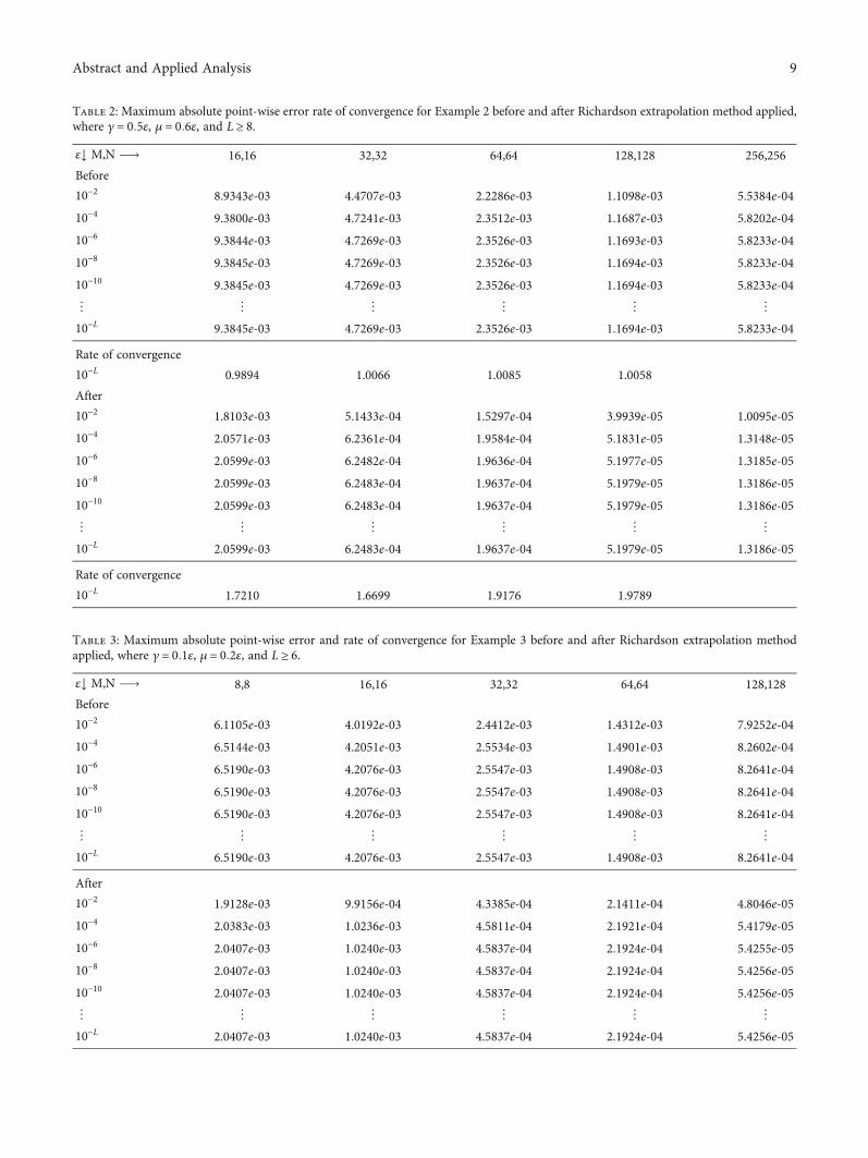
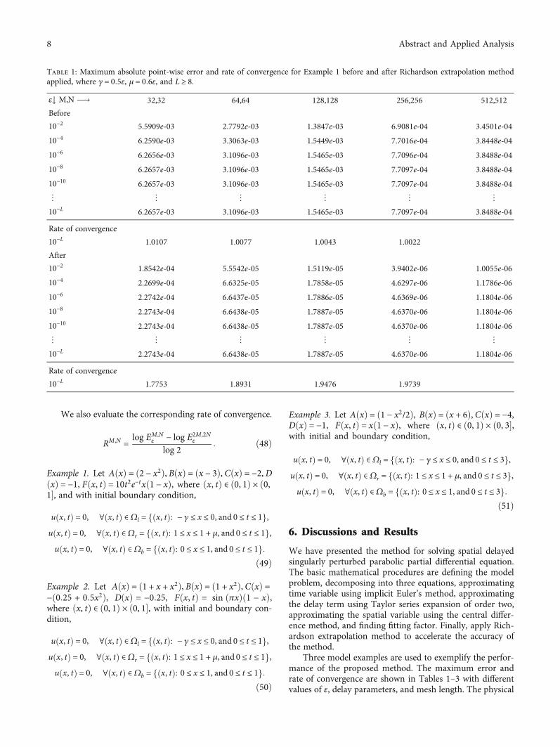
Table 2: Maximum absolute point-wise error rate of convergence for Example 2 before and after Richardson extrapolation method applied,where γ = 0:5ε, μ = 0:6ε, and L ≥ 8.

ε↓ M,N ⟶ 16,16 32,32 64,64 128,128 256,256

Before

10−2 8.9343e-03 4.4707e-03 2.2286e-03 1.1098e-03 5.5384e-04

10−4 9.3800e-03 4.7241e-03 2.3512e-03 1.1687e-03 5.8202e-04

10−6 9.3844e-03 4.7269e-03 2.3526e-03 1.1693e-03 5.8233e-04

10−8 9.3845e-03 4.7269e-03 2.3526e-03 1.1694e-03 5.8233e-04

10−10 9.3845e-03 4.7269e-03 2.3526e-03 1.1694e-03 5.8233e-04

⋮ ⋮ ⋮ ⋮ ⋮ ⋮

10−L 9.3845e-03 4.7269e-03 2.3526e-03 1.1694e-03 5.8233e-04

Rate of convergence

10−L 0.9894 1.0066 1.0085 1.0058

After

10−2 1.8103e-03 5.1433e-04 1.5297e-04 3.9939e-05 1.0095e-05

10−4 2.0571e-03 6.2361e-04 1.9584e-04 5.1831e-05 1.3148e-05

10−6 2.0599e-03 6.2482e-04 1.9636e-04 5.1977e-05 1.3185e-05

10−8 2.0599e-03 6.2483e-04 1.9637e-04 5.1979e-05 1.3186e-05

10−10 2.0599e-03 6.2483e-04 1.9637e-04 5.1979e-05 1.3186e-05

⋮ ⋮ ⋮ ⋮ ⋮ ⋮

10−L 2.0599e-03 6.2483e-04 1.9637e-04 5.1979e-05 1.3186e-05

Rate of convergence

10−L 1.7210 1.6699 1.9176 1.9789

Table 3: Maximum absolute point-wise error and rate of convergence for Example 3 before and after Richardson extrapolation methodapplied, where γ = 0:1ε, μ = 0:2ε, and L ≥ 6.

ε↓ M,N ⟶ 8,8 16,16 32,32 64,64 128,128

Before

10−2 6.1105e-03 4.0192e-03 2.4412e-03 1.4312e-03 7.9252e-04

10−4 6.5144e-03 4.2051e-03 2.5534e-03 1.4901e-03 8.2602e-04

10−6 6.5190e-03 4.2076e-03 2.5547e-03 1.4908e-03 8.2641e-04

10−8 6.5190e-03 4.2076e-03 2.5547e-03 1.4908e-03 8.2641e-04

10−10 6.5190e-03 4.2076e-03 2.5547e-03 1.4908e-03 8.2641e-04

⋮ ⋮ ⋮ ⋮ ⋮ ⋮

10−L 6.5190e-03 4.2076e-03 2.5547e-03 1.4908e-03 8.2641e-04

After

10−2 1.9128e-03 9.9156e-04 4.3385e-04 2.1411e-04 4.8046e-05

10−4 2.0383e-03 1.0236e-03 4.5811e-04 2.1921e-04 5.4179e-05

10−6 2.0407e-03 1.0240e-03 4.5837e-04 2.1924e-04 5.4255e-05

10−8 2.0407e-03 1.0240e-03 4.5837e-04 2.1924e-04 5.4256e-05

10−10 2.0407e-03 1.0240e-03 4.5837e-04 2.1924e-04 5.4256e-05

⋮ ⋮ ⋮ ⋮ ⋮ ⋮

10−L 2.0407e-03 1.0240e-03 4.5837e-04 2.1924e-04 5.4256e-05


0

0.2

0.4

0.6

0.8

1

00.2

0.40.6

0.81

0

0.2

0.4

0.6

0.8

X

t

Solu

tion

Figure 1: The physical behavior of the solutions for Example 1 at m = n = 32, ε = 10−2, γ = 0:5ε, and μ = 0:6ε.

0 0.1 0.2 0.3 0.4 0.5 0.6 0.7 0.8 0.9 10

0.1

0.2

0.3

0.4

0.5

0.6

0.7

x

u

t = 0.8t = 0.9t = 1

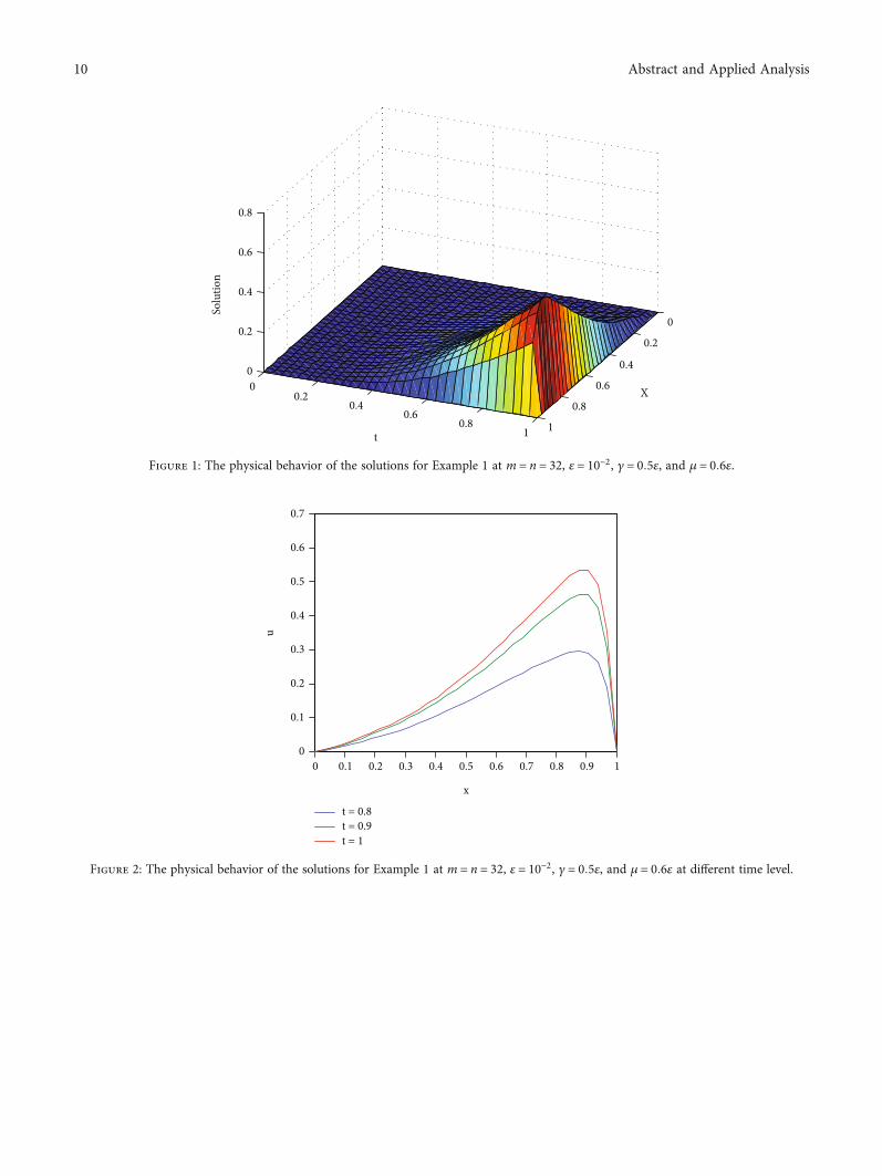
Figure 2: The physical behavior of the solutions for Example 1 at m = n = 32, ε = 10−2, γ = 0:5ε, and μ = 0:6ε at different time level.


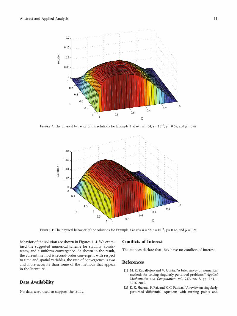
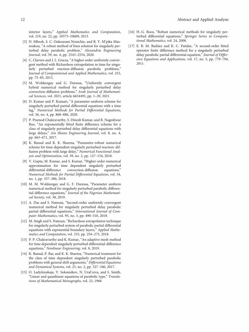
behavior of the solution are shown in Figures 1–4. We exam-ined the suggested numerical scheme for stability, consis-tency, and ε uniform convergence. As shown in the result,the current method is second-order convergent with respectto time and spatial variables, the rate of convergence is twoand more accurate than some of the methods that appearin the literature.

Data Availability

No data were used to support the study.

Conflicts of Interest

The authors declare that they have no conflicts of interest.

References

[1] M. K. Kadalbajoo and V. Gupta, “A brief survey on numericalmethods for solving singularly perturbed problems,” AppliedMathematics and Computation, vol. 217, no. 8, pp. 3641–3716, 2010.

[2] K. K. Sharma, P. Rai, and K. C. Patidar, “A review on singularlyperturbed differential equations with turning points and

00.20.4

0.60.81

0

0.2

0.4

0.6

0.8

1

0

0.05

0.1

0.15

0.2

X

t

Solu

tion

Figure 3: The physical behavior of the solutions for Example 2 at m = n = 64, ε = 10−2, γ = 0:5ε, and μ = 0:6ε.

00.2

0.40.6

0.81

00.5

11.5

22.5

3

0

0.02

0.04

0.06

0.08

X

t

Solu

tion

Figure 4: The physical behavior of the solutions for Example 3 at m = n = 32, ε = 10−2, γ = 0:1ε, and μ = 0:2ε:


interior layers,” Applied Mathematics and Computation,vol. 219, no. 22, pp. 10575–10609, 2013.

[3] N. Mbroh, S. C. Oukouomi Noutchie, and R. Y. M’pika Mas-soukou, “A robust method of lines solution for singularly per-turbed delay parabolic problem,” Alexandria EngineeringJournal, vol. 59, no. 4, pp. 2543–2554, 2020.

[4] C. Clavero and J. L. Gracia, “A higher order uniformly conver-gent method with Richardson extrapolation in time for singu-larly perturbed reaction-diffusion parabolic problems,”Journal of Computational and Applied Mathematics, vol. 252,pp. 75–85, 2013.

[5] M. Woldaregay and G. Duressa, “Uniformly convergenthybrid numerical method for singularly perturbed delayconvection-diffusion problems,” Arab Journal of Mathemati-cal Sciences, vol. 2021, article 6654495, pp. 1–20, 2021.

[6] D. Kumar and P. Kumari, “A parameter-uniform scheme forsingularly perturbed partial differential equations with a timelag,” Numerical Methods for Partial Differential Equations,vol. 36, no. 4, pp. 868–886, 2020.

[7] P. Pramod Chakravarthy, S. Dinesh Kumar, and R. NageshwarRao, “An exponentially fitted finite difference scheme for aclass of singularly perturbed delay differential equations withlarge delays,” Ain Shams Engineering Journal, vol. 8, no. 4,pp. 663–671, 2017.

[8] K. Bansal and K. K. Sharma, “Parameter-robust numericalscheme for time-dependent singularly perturbed reaction–dif-fusion problem with large delay,” Numerical Functional Anal-ysis and Optimization, vol. 39, no. 2, pp. 127–154, 2018.

[9] V. Gupta, M. Kumar, and S. Kumar, “Higher order numericalapproximation for time dependent singularly perturbeddifferential-difference convection-diffusion equations,”Numerical Methods for Partial Differential Equations, vol. 34,no. 1, pp. 357–380, 2018.

[10] M. M. Woldaregay and G. F. Duressa, “Parameter uniformnumerical method for singularly perturbed parabolic differen-tial difference equations,” Journal of the Nigerian Mathemati-cal Society, vol. 38, 2019.

[11] A. Das and S. Natesan, “Second-order uniformly convergentnumerical method for singularly perturbed delay parabolicpartial differential equations,” International Journal of Com-puter Mathematics, vol. 95, no. 3, pp. 490–510, 2018.

[12] M. Singh and S. Natesan, “Richardson extrapolation techniquefor singularly perturbed system of parabolic partial differentialequations with exponential boundary layers,” Applied Mathe-matics and Computation, vol. 333, pp. 254–275, 2018.

[13] P. P. Chakravarthy and K. Kumar, “An adaptive mesh methodfor time dependent singularly perturbed differential-differenceequations,” Nonlinear Engineering, vol. 8, 2019.

[14] K. Bansal, P. Rai, and K. K. Sharma, “Numerical treatment forthe class of time dependent singularly perturbed parabolicproblems with general shift arguments,” Differential Equationsand Dynamical Systems, vol. 25, no. 2, pp. 327–346, 2017.

[15] O. Ladyženskaja, V. Solonnikov, N. Ural’ceva, and S. Smith,“Linear and quasilinear equations of parabolic type,” Transla-tions of Mathematical Monographs, vol. 23, 1968.

[16] H.-G. Roos, “Robust numerical methods for singularly per-turbed differential equations,” Springer Series in Computa-tional Mathematics, vol. 24, 2008.

[17] E. B. M. Bashier and K. C. Patidar, “A second-order fittedoperator finite difference method for a singularly perturbeddelay parabolic partial differential equation,” Journal of Differ-ence Equations and Applications, vol. 17, no. 5, pp. 779–794,2011.


1661661.pdf - Hindawi.com

Documents

Transcript of 1661661.pdf - Hindawi.com