15EI403J- IMAGE PROCESSING

LAB MANUAL

Department of Electronics and

Instrumentation Engineering

Faculty of Engineering and Technology

Department of Electronics and Instrumentation Engineering

SRM IST, SRM Nagar Kattankulathur – 603203

Kancheepuram District

Tamil Nadu

2

CONTENTS

S.No. CONTENTS Page No.

1 Mark Assessment details 3

2 General Instructions for Laboratory classes 4

3 Syllabus 5

4 Introduction to the laboratory 6

5

List of Experiments

5.1 Display of gray scale images 9

5.2 Histogram Equalization 20

5.3 Design non-linear filtering 24

5.4 Determination of edge detection using operators 28

5.5 2-D DFT and DCT 34

5.6 Filtering in Frequency domain 40

5.7 Display of colour images 42

5.8 Conversion between colour spaces 50

5.9 DWT of images 53

5.10 Segmentation using watershed transform 56

3

1. MARK ASSESSMENT DETAILS

ALLOTMENT OF MARKS:

Internal assessment = 60 marks

Practical examination = 40 marks

----------------------

Total = 100 marks

----------------------

INTERNAL ASSESSMENT (60 MARKS)

Split up of internal marks

Record 5 marks

Model exam 10 marks

Quiz/Viva 5 marks

Experiments 40 marks

Total 60 marks

PRACTICAL EXAMINATION (40MARKS)

Split up of practical examination marks

Aim and

25 marks Procedure

Circuit 30 marks

Diagram

Tabulation 30 marks

Result 05 marks

Viva voce 10 marks

Total 100 marks

4

2. GENERAL INSTRUCTIONS FOR LABORATORY CLASSES

Enter the Lab with CLOSED TOE SHOES.

Students should wear lab coat.

The HAIR should be protected, let it not be loose.

TOOLS, APPARATUS and COMPONENT sets are to be returned before

leaving the lab.

HEADINGS and DETAILS should be neatly written

o Aim of the experiment

o Apparatus / Tools / Instruments

required

o Theory

o Procedure / Algorithm /

Program

o Model Calculations/ Design calculations

o Block Diagram / Flow charts/ Circuit diagram

o Tabulations/ Waveforms/ Graph

o Result / discussions.

Experiment number and date should be written in the appropriate place.

After completing the experiment, the answer to pre lab viva-voce questions should

be neatly written in the workbook.

Be REGULAR, SYSTEMATIC, PATIENT, AND STEADY.

5

3. SYLLABUS

15EI403J

Image Processing L T P C

2

0 2 3

Co-requisite: NIL

Prerequisite: 15EI301

Data Book /

Codes/Standards NIL

ELECTRONICS

Course Category P PROFESSIONAL ENGINEERING ENGINEERING

Course designed by Department of Electronics and Instrumentation Engineering

Approval 32nd

Academic Council Meeting held on 23rd

July, 2016

PURPOSE The purpose of this course is to introduce the basic concept and methodologies

for digital image processing INSTRUCTIONAL

OBJECTIVES

STUDENT OUTCOMES

At the end of the course, student will be able to 1. Study the image fundamentals, mathematical transforms

necessary for image processing

a b d k

2. About the various techniques of image enhancement, reconstruction, compression and segmentation a b h

3. . Know sampling and reconstruction procedures a b e 4.

Design image processing systems a

Session Description of experiments Contact C-D-

IOs

Reference hours I-O

1. Display of Gray scale Images. 3 I 1-4 1,2

2. Histogram Equalization. 3 C 1 1,2

3. Design of Non-linear Filtering. 3 D 1 1,3

4. Determination of Edge detection using Operators. 3 C,I 1,3,4 1

5. 2-D DFT and DCT. 3 C,D 1,3 1

6. Filtering in frequency domain. 3 C 3,4 1

7. Display of colour images. 3 D,I 3,4 1

8. Conversion between colour spaces. 3 I 3,4 1,3,4

9. DWT of images. 3 I 4 1,4,2

10. Segmentation using watershed transform. 3 I 4 1

Total contact hours 30

LEARNING RESOURCES

Sl.No TEXT BOOKS 1. Rafael.C,Gonzalez, Richard E Woods, “Digital Image Processing”,3rdEdition, Pearson India, 2013. 2. Jain A.K, “Fundamentals of Digital Image Processing”, 4

th Edition, Prentice hall of India, 2004.

REFERENCE BOOKS/OTHER READING MATERIAL

3. B.Chanda, D. DuttaMajumder, “Digital Image Processing and Analysis”, 2nd

Edition, Phi learning, 2011.

4. William K Pratt, “Digital Image Processing”, 4th

Edition, Wiley, 2012.

Assessment Method – Practical Component (Weightage 50%)

In- Assessment

Experiments

Record MCQ/Quiz/Viva Model

Total tool

Voce

examination

semester

Weightage

40%

5%

5%

10% 60%

End semester examination Weightage : 40%

6

4. INTRODUCTION

IMAGE PROCESSING LABORATORY COURSE FLOW:

This laboratory course completely deals with basics of image processing and their

experimental observations. Here the students are exposed to design the image processing

blocks and do image filtering, image enhancement, edge detection etc.

To start with this laboratory session, initially all students are trained to use the

LabVIEW software. Thorough understanding of LabVIEW software is mandatory for

proceeding with the course wear.

Instructions to the students are given in the start of this document which they are

advised to read before they start conducting experiments.

INSTRUCTIONS BEFORE STARTING THE EXPERIMENT

Study the theory and procedures, expected output before doing the experiment.

Get familiarize with the LabVIEW software

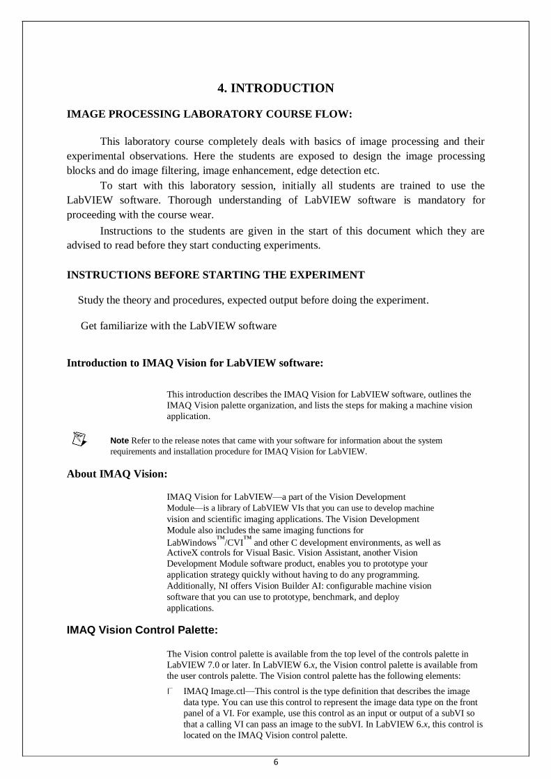
Introduction to IMAQ Vision for LabVIEW software:

This introduction describes the IMAQ Vision for LabVIEW software, outlines the

IMAQ Vision palette organization, and lists the steps for making a machine vision

application.

Note Refer to the release notes that came with your software for information about the system

requirements and installation procedure for IMAQ Vision for LabVIEW.

About IMAQ Vision:

IMAQ Vision for LabVIEW—a part of the Vision Development Module—is a library of LabVIEW VIs that you can use to develop machine vision and scientific imaging applications. The Vision Development Module also includes the same imaging functions for

LabWindows™/CVI™ and other C development environments, as well as ActiveX controls for Visual Basic. Vision Assistant, another Vision Development Module software product, enables you to prototype your application strategy quickly without having to do any programming. Additionally, NI offers Vision Builder AI: configurable machine vision software that you can use to prototype, benchmark, and deploy applications.

IMAQ Vision Control Palette:

The Vision control palette is available from the top level of the controls palette in

LabVIEW 7.0 or later. In LabVIEW 6.x, the Vision control palette is available from

the user controls palette. The Vision control palette has the following elements:

IMAQ Image.ctl—This control is the type definition that describes the image

data type. You can use this control to represent the image data type on the front

panel of a VI. For example, use this control as an input or output of a subVI so

that a calling VI can pass an image to the subVI. In LabVIEW 6.x, this control is

located on the IMAQ Vision control palette.

7

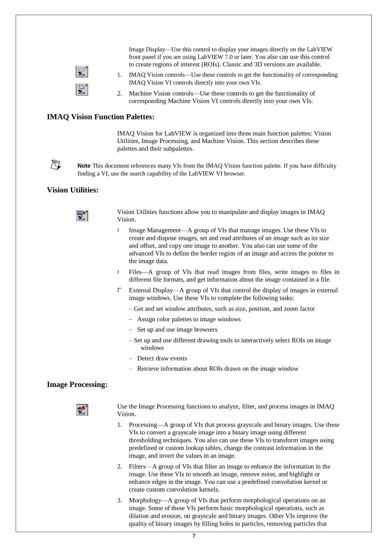
Image Display—Use this control to display your images directly on the LabVIEW

front panel if you are using LabVIEW 7.0 or later. You also can use this control

to create regions of interest (ROIs). Classic and 3D versions are available.

1. IMAQ Vision controls—Use these controls to get the functionality of corresponding

IMAQ Vision VI controls directly into your own VIs.

2. Machine Vision controls—Use these controls to get the functionality of

corresponding Machine Vision VI controls directly into your own VIs.

IMAQ Vision Function Palettes:

IMAQ Vision for LabVIEW is organized into three main function palettes: Vision

Utilities, Image Processing, and Machine Vision. This section describes these

palettes and their subpalettes.

Note This document references many VIs from the IMAQ Vision function palette. If you have difficulty

finding a VI, use the search capability of the LabVIEW VI browser.

Vision Utilities:

Vision Utilities functions allow you to manipulate and display images in IMAQ

Vision. Image Management—A group of VIs that manage images. Use these VIs to

create and dispose images, set and read attributes of an image such as its size

and offset, and copy one image to another. You also can use some of the

advanced VIs to define the border region of an image and access the pointer to

the image data.

Files—A group of VIs that read images from files, write images to files in

different file formats, and get information about the image contained in a file.

External Display—A group of VIs that control the display of images in external

image windows. Use these VIs to complete the following tasks:

– Get and set window attributes, such as size, position, and zoom factor

– Assign color palettes to image windows

– Set up and use image browsers

– Set up and use different drawing tools to interactively select ROIs on image

windows

– Detect draw events

– Retrieve information about ROIs drawn on the image window

Image Processing:

Use the Image Processing functions to analyze, filter, and process images in IMAQ

Vision. 1. Processing—A group of VIs that process grayscale and binary images. Use these

VIs to convert a grayscale image into a binary image using different

thresholding techniques. You also can use these VIs to transform images using

predefined or custom lookup tables, change the contrast information in the

image, and invert the values in an image.

2. Filters—A group of VIs that filter an image to enhance the information in the

image. Use these VIs to smooth an image, remove noise, and highlight or

enhance edges in the image. You can use a predefined convolution kernel or

create custom convolution kernels.

3. Morphology—A group of VIs that perform morphological operations on an

image. Some of these VIs perform basic morphological operations, such as

dilation and erosion, on grayscale and binary images. Other VIs improve the

quality of binary images by filling holes in particles, removing particles that

8

touch the image border, removing small particles, and removing unwanted

particles based on different shape characteristics of the particle. Another set of

VIs in this subpalette separate touching particles, find the skeleton of particles,

and detect circular particles.

4. Analysis—A group of VIs that analyze the content of grayscale and binary

images. Use these VIs to compute the histogram information and grayscale

statistics of an image, retrieve pixel information and statistics along any one-

dimensional profile in an image, and detect and measure particles in binary

images.

5. Color Processing—A group of VIs that analyze and process color images. Use

these VIs to compute the histogram of color images; apply lookup tables to

color images; change the brightness, contrast, and gamma information

associated with a color image; and threshold a color image. Some of these VIs

also compare the color information in different images or different regions in an

image using a color matching process.

Operators—A group of VIs that perform basic arithmetic and logical operations on images. Use some of these VIs to add, subtract, multiply, and divide an image with other images or constants. Use other VIs in this subpalette to apply logical

operations—such as AND/NAND, OR/NOR, XOR/XNOR—and make pixel comparisons between an image and other images or a constant. In addition, one VI

in this subpalette allows you to select regions in an image to process using a

masking operation.

Frequency Domain—A group of VIs that analyze and process images in the

frequency domain. Use these VIs to convert an image from the spatial domain to

the frequency domain using a two-dimensional Fast Fourier Transform (FFT)

and convert from the frequency domain to the spatial domain using the inverse

FFT. These VIs also extract the magnitude, phase, real, and imaginary planes of

the complex image. In addition, these VIs allow you to convert complex images

into complex 2D arrays and back. Also in this subpalette are VIs that perform

basic arithmetic operations—such as addition, subtraction, multiplication, and

division—between a complex image and other images or a constant. Lastly,

some of these VIs allow you to filter images in the frequency domain.

9

EXPERIMENT 1

DISPLAY OF GRAY SCALE IMAGES

1(a). Aim

To create a program to display grayscale image using read and write operation.

Apparatus Used

A PC with LabVIEW software Vision Toolbox

Theory

In photography and computing, a grayscale or greyscale digital image is an image in which the value

of each pixel is a single sample, that is, it carries only intensity information. Images of this sort, also

known as black-and-white, are composed exclusively of shades of gray, varying from black at the

weakest intensity to white at the strongest.

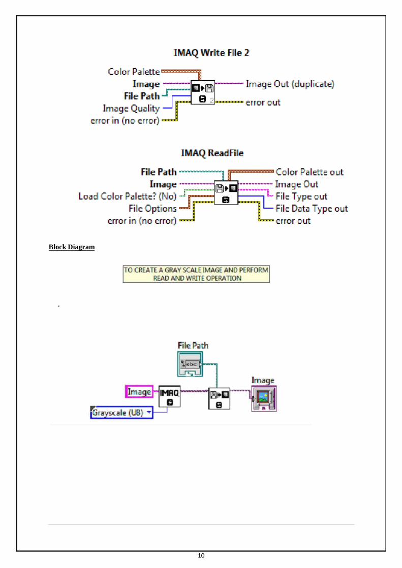
Procedure

1. Open LabVIEW from desktop. 2. Create a separate editor window and front panel. 3. Right click, select vision motion and choose IMAQ create and choose image type(specify U-

32) as grayscale. 4. Create control by choosing read image (IMAQ Read) and specifying the file path (from which

the image is to be acquired). 5. Similarly, create control for writing by choosing write image (IMAQ Write). 6. Create an indicator image for display to the front panel and join.

10

Block Diagram

11

Output

Result : Thus ,the program to display gray scale image using read and write operation was created.

12

1(b). Aim

To create a vision program to convert a 2D array into a grayscale image.

Apparatus Used

A PC with LabVIEW software Vision Toolbox

Theory

An array is a container object that holds a fixed number of values of a single type. The length of an

array is established when the array is created. After creation, its length is fixed.The Image block

displays the data in array as an image. Each element of array specifies the color for 1 pixel of the

image. The resulting image is an m-by-n grid of pixels where m is the number of columns and n is the

number of rows. The row and column indices of the elements determine the centers of the

corresponding pixels. The array values range from 0 to 255 to display the various shades of black.

Procedure

1. Open LabVIEW from desktop. 2. Create a separate editor window and front panel. 3. Right click in the window and set parameters as constant and the image type as grayscale. 4. In the editor window, through right click and the vision and motion category choose (by

searching for) ‘Array to Image’, set specifications as Image pixels-U8. 5. From the previous block, create an image display indicator. 6. Input values in Image Pixels present in front panel and check the Output.

13

Block Diagram

14

Output

Result : Thus ,the vision program to convert a 2D array into a gray scale image was created.

15

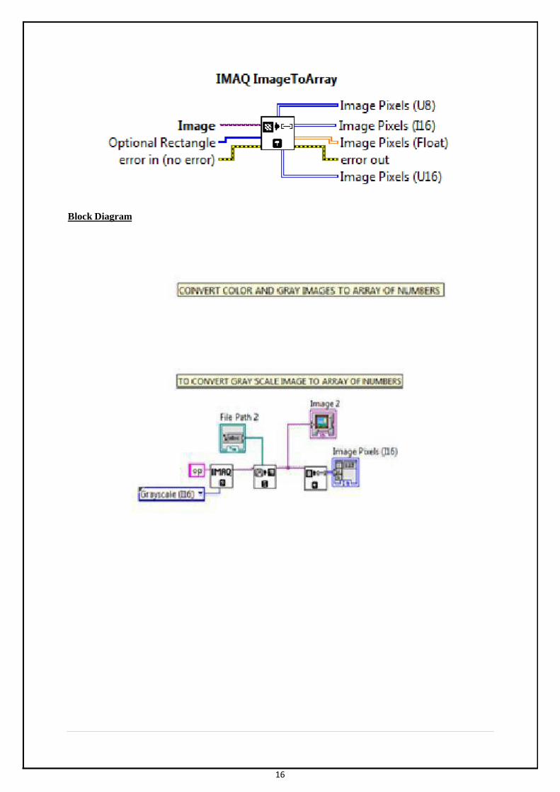
1(c). Aim

To create a vision program to convert gray images into an array of numbers.

Apparatus Used

A PC with LabVIEW software Vision Toolbox

Theory

A digital gray scale image is nothing more than data—numbers indicating variations of black and

white at a particular location on a grid of pixels. Most of the time, we view these pixels as miniature

rectangles sandwiched together on a computer screen. With a little creative thinking and some lower

level manipulation of pixels with code, however, we can display that information in a myriad of ways.

This tutorial is dedicated to breaking out of simple shape drawing in Processing and using images

(and their pixels) as the building blocks of Processing graphics.

Procedure

1. Open LabVIEW from desktop. 2. Create a separate editor window and front panel. 3. Right click, select vision and motion >> choose IMAQ create. Add a constant and image to it. 4. Add a file path and specify the path of the image (at the particular storage location) which is

to be processed. 5. Add a gray image to array block to obtain values into array. 6. Add an indicator at the end to check for the image pixels at the Output. 7. The Output will be obtained in the front panel in the image pixel indicator (set to U32).

16

Block Diagram

17

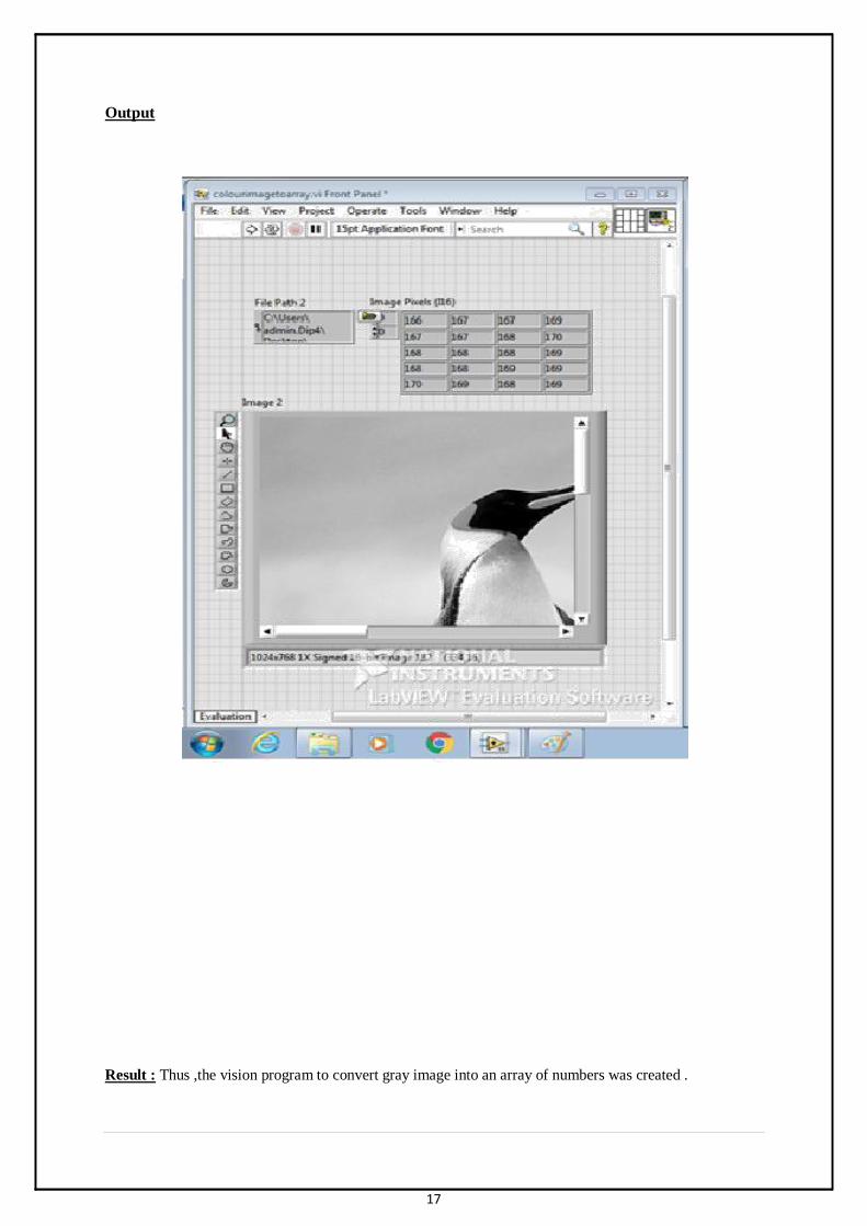
Output

Result : Thus ,the vision program to convert gray image into an array of numbers was created .

18

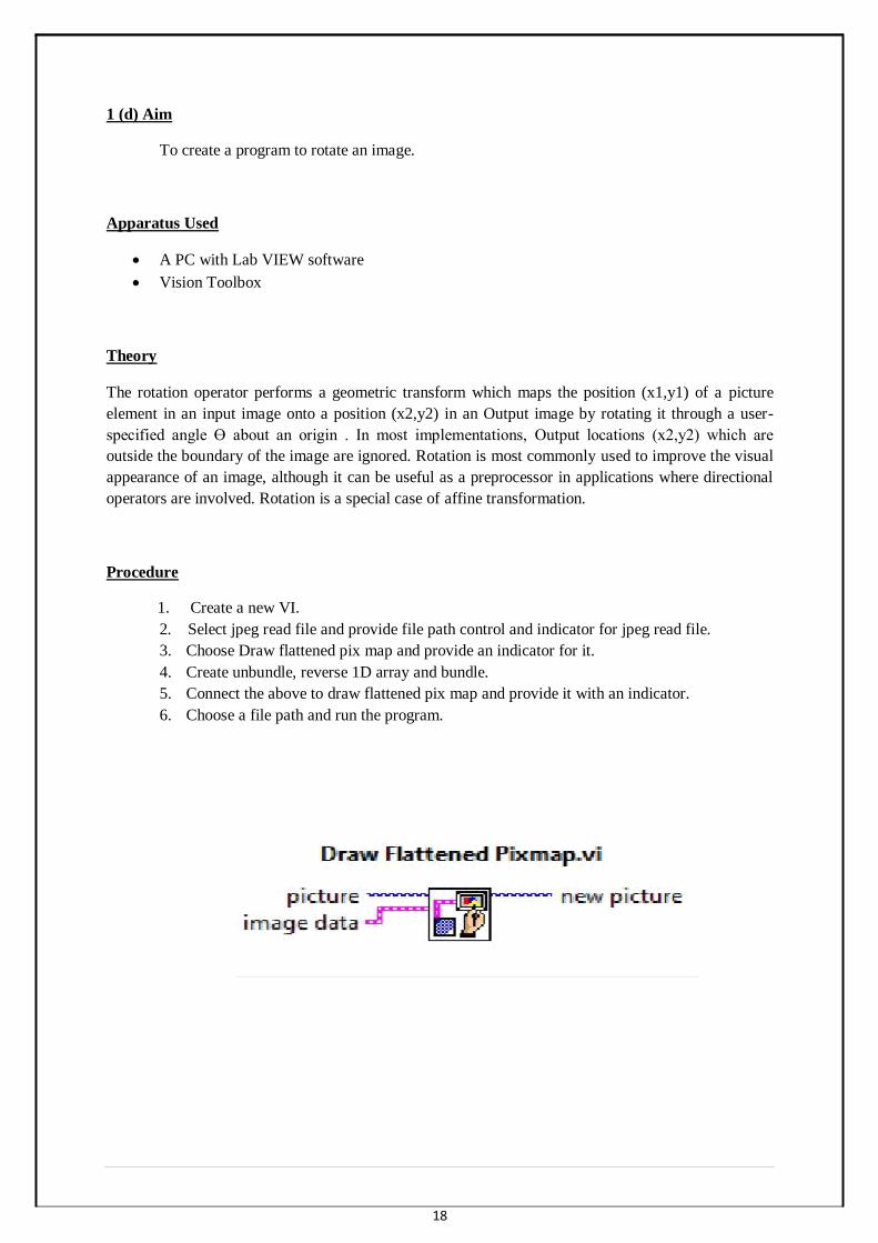
1 (d) Aim

To create a program to rotate an image.

Apparatus Used

A PC with Lab VIEW software Vision Toolbox

Theory

The rotation operator performs a geometric transform which maps the position (x1,y1) of a picture

element in an input image onto a position (x2,y2) in an Output image by rotating it through a user-

specified angle ϴ about an origin . In most implementations, Output locations (x2,y2) which are

outside the boundary of the image are ignored. Rotation is most commonly used to improve the visual

appearance of an image, although it can be useful as a preprocessor in applications where directional

operators are involved. Rotation is a special case of affine transformation.

Procedure

1. Create a new VI. 2. Select jpeg read file and provide file path control and indicator for jpeg read file.

3. Choose Draw flattened pix map and provide an indicator for it. 4. Create unbundle, reverse 1D array and bundle. 5. Connect the above to draw flattened pix map and provide it with an indicator. 6. Choose a file path and run the program.

19

Block Diagram

Output

Result: Thus, the program to rotate an image was created.

20

EXPERIMENT 2

HISTOGRAM EQUALIZATION

Aim

To create a vision program to find histogram value and display histograph of a grayscale and color

image.

Apparatus Used

A PC with LabVIEW software Vision Toolbox

Theory

An image histogram is a type of histogram that acts as a graphical representation of the tonal

distribution in a digital image. It plots the number of pixels for each tonal value. By looking at the

histogram for a specific image a viewer will be able to judge the entire tonal distribution at a glance.

The horizontal axis of the graph represents the tonal variations, while the vertical axis represents the

number of pixels in that particular tone. The left side of the horizontal axis represents the black and

dark areas, the middle represents medium grey and the right hand side represents light and pure white

areas. The vertical axis represents the size of the area that is captured in each one of these zones.

Procedure

1. Create a new VI. 2. Select Vision and Motion >> Vision Utilities >> Image Management >> IMAQ create. 3. Vision Utilities >> Files >> Read File. 4. Analyser >> Histogram and place it. 5. Analyser >>Histograph and place it. 6. Run the program.

21

Block Diagram

22

OUTPUT

Block Diagram

23

Output

Result : Thus ,the program to find histogram value and display histograph of a grayscale and colour

image was created.

24

EXPERIMENT 3

DESIGN OF NON-LINEAR FILTERING.

Aim

To create a vision program for Non-Linear Filtering technique using edge detection.

Apparatus Used

A PC with LabVIEW software Vision Toolbox

Theory

Edge detection includes a variety of mathematical methods that aim at identifying points in a digital

image at which the image brightness changes sharply or, more formally, has discontinuities. The

points at which image brightness changes sharply are typically organized into a set of curved line

segments termed edges. The same problem of finding discontinuities in 1D signals is known as step

detection and the problem of finding signal discontinuities over time is known as change detection.

Edge detection is a fundamental tool in image processing, machine vision and computer vision,

particularly in the areas of feature detection and feature extraction.

Procedure

1. Open LabVIEW software in desktop. 2. Create separate editor window and front panel. 3. Right click, select vision motion chooses IMAQ create. Add constant image type (grayscale

U8) to it. 4. Select file read and this is given to IMAQ edge detection. Give a constant for it. 5. Create an indicator for display and join it. 6. Give a file path and run the program.

25

Block Diagram

26

Output

Block Diagram

27

Output

Result:

Thus, the program for the non linear filtering for an image using edge detection was created.

28

EXPERIMENT 4

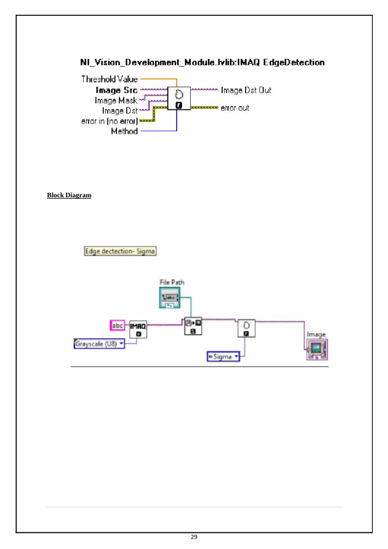
DETERMINATION OF EDGE DETECTION USING OPERATORS.

Aim

To create a vision program to determine the edge detection of an image using different operators.

Apparatus Used

A PC with LabVIEW software

Vision Toolbox

Theory

Edge detection includes a variety of mathematical methods that aim at identifying points in a digital

image at which the image brightness changes sharply or, more formally, has discontinuities. The

points at which image brightness changes sharply are typically organized into a set of curved line

segments termed edges. The same problem of finding discontinuities in 1D signals is known as step

detection and the problem of finding signal discontinuities over time is known as change detection.

Edge detection is a fundamental tool in image processing, machine vision and computer vision,

particularly in the areas of feature detection and feature extraction.

Procedure 1. Open LabVIEW software in desktop. 2. Create separate editor window and front panel. 3. Right click, select vision motion choose IMAQ create. Add constant image type (grayscale U8) to it. 4. Select file read and this is given to IMAQ edge detection. Give a constant for it. 5. Create an indicator for display and join it. 6. Give a file path and run the program.

29

Block Diagram

30

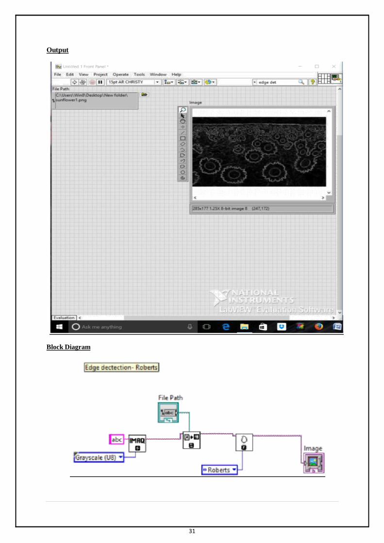
Output

Block Diagram

31

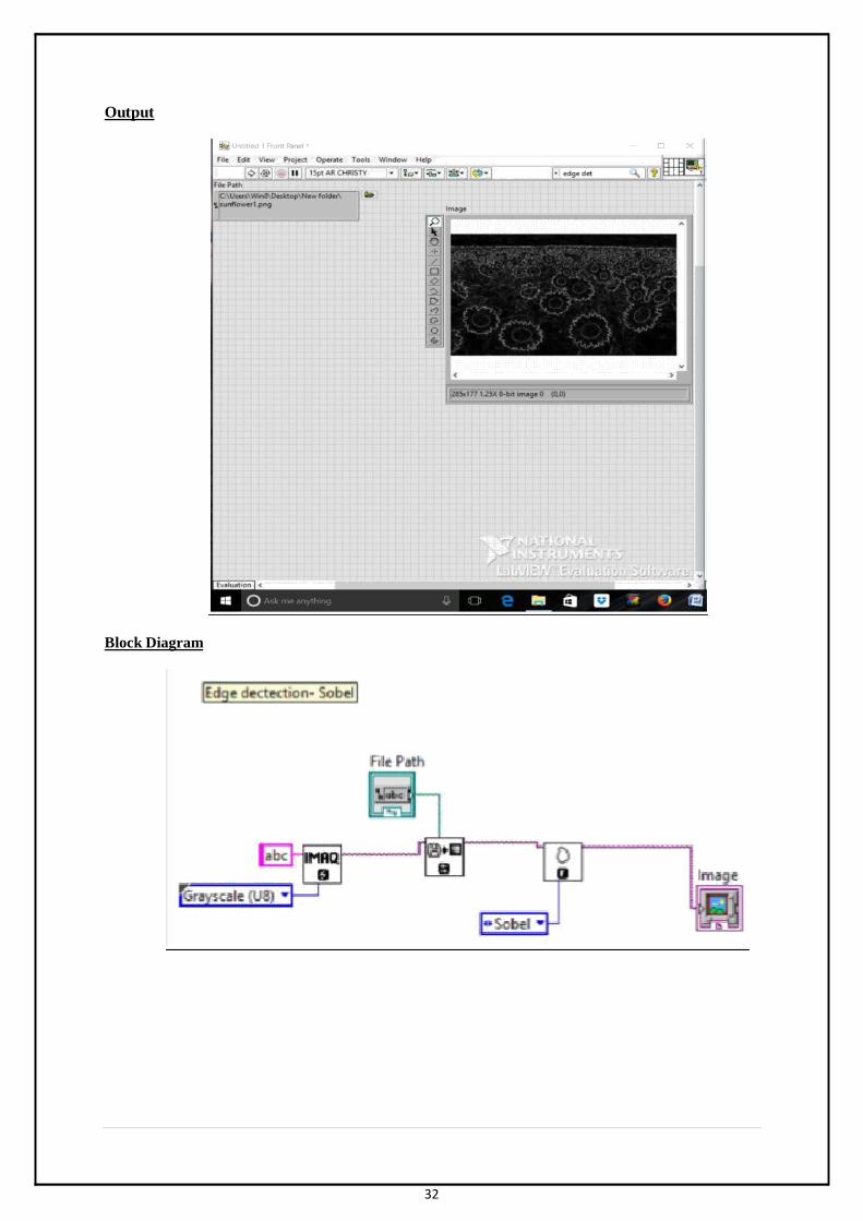
Output

Block Diagram

32

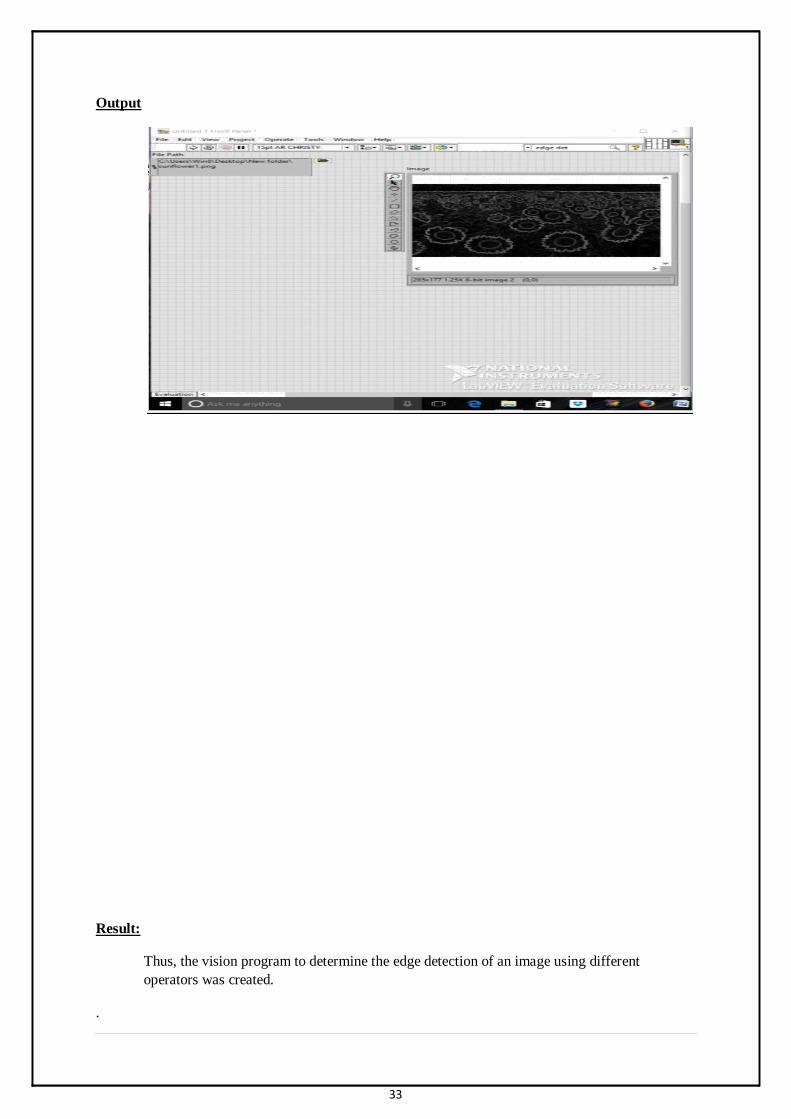
Output

Block Diagram

33

Output

Result:

Thus, the vision program to determine the edge detection of an image using different

operators was created.

.

34

Experiment 5

2-D DFT and DCT

5 (a) Aim:

To create a program to discretize an image using Fourier transformation.

Apparatus Used

A PC with LabVIEW software Vision Toolbox

Theory

The Fourier Transform is an important image processing tool which is used to decompose an image

into its sine and cosine components. The Output of the transformation represents the image in the

Fourier or frequency domain, while the input image is the spatial domain equivalent. In the Fourier

domain image, each point represents a particular frequency contained in the spatial domain image.

The Fourier Transform is used in a wide range of applications, such as image analysis, image

filtering, image reconstruction and image compression.

Procedure

1. Open LabVIEW software in desktop.

2. Create separate editor window and front panel.

3. Right click, select vision motion chooses IMAQ create. Add constant image type (grayscale

U8) to it.

4. Select file read and give a control.

5. Choose IMAQ FFT and give it to ab indicator (Image display), For IMAQ FFT give

IMAQ create (with image type as complex CSG ).

6. Choose Inverse FFT and to it give an indicator (image display). Also for inverse FFT give and \

IMAQ create with image type (grayscale U8).

7. Give a file path and run the program.

35

Block Diagram (Using vision Motion Tool)

36

Block Diagram (Using DSP Tool)

37

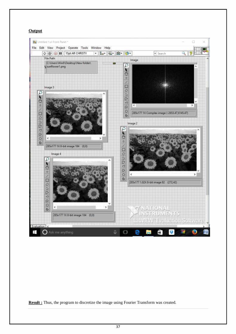
Output

Result : Thus, the program to discretize the image using Fourier Transform was created.

38

5(b) Aim

To create a program to perform Discrete cosine transform on an image.

Apparatus Used

A PC with LabVIEW software Vision Toolbox

Theory

A discrete cosine transform (DCT) expresses a finite sequence of data points in terms of a sum of

cosine functions oscillating at different frequencies. DCTs are important to numerous applications in

science and engineering, from lossy compression of audio (e.g. MP3) and images (e.g. JPEG) (where

small high-frequency components can be discarded), tospectral methods for the numerical solution of

partial differential equations. The use of cosine rather than sine functions is critical for compression,

since it turns out (as described below) that fewer cosine functions are needed to approximate a typical

signal, whereas for differential equations the cosines express a particular choice of boundary

conditions.

Procedure

1.Open LabVIEW software in desktop.

2.Create separate editor window and front panel.

3. Right click, select vision motion choose IMAQ create. Add constant image type (grayscale U8)

to it. Duplicate the blocks again.

4.Select file read and give a control.

5.Choose Image to array connect the same.

6. Select DCT block from signal processing and connect it to array to image block.

7.Create an indicator (image display).

8.Give an image file path and run the program.

39

Block Diagram

Output

Result : Thus ,The program to perform Discrete cosine transform on an image was created .

40

EXPERIMENT 6

FILTERING IN FREQUENCY DOMAIN

Aim

To create a program to eliminate the high frequency components of an image.

Apparatus Used

A PC with LabVIEW software Vision Toolbox

Theory

The most basic of filtering operations is called "low-pass". A low-pass filter, also called a "blurring"

or "smoothing" filter, averages out rapid changes in intensity. The simplest low-pass filter just

calculates the average of a pixel and all of its eight immediate neighbours. The result replaces the

original value of the pixel. The process is repeated for every pixel in the image.

Procedure

1. Open LabVIEW software in desktop.

2. Create separate editor window and front panel.

3. Right click, select vision motion chooses IMAQ create. Add constant image type (grayscale

U8) to it.

4. Select file read and give a control.

5. Choose IMAQ Low pass connect the same.

6. Create an indicator (image display).

7. Give an image file path and run the program.

41

Block Diagram

Output

Result : Thus ,the program to eliminate the high frequency components of an image was created.

42

EXPERIMENT 7

DISPLAY OF COLOUR IMAGES.

7 (a) Aim

To create a color image and perform read and write operation.

Apparatus Used

A PC with LabVIEW software

Vision Toolbox

Theory

A (digital) color image is a digital image that includes color information for each pixel. For visually

acceptable results, it is necessary (and almost sufficient) to provide three samples (color channels) for

each pixel, which are interpreted as coordinates in some color space. The RGB color space is

commonly used in computer displays, but other spaces such as YCbCr, HSV, and are often used in

other contexts. A color image has three values (or channels) per pixel and they measure the intensity

and chrominance of light. The actual information stored in the digital image data is the brightness

information in each spectral band.

Procedure

1. Open LabVIEW from desktop.

2. Create a separate editor window and front panel.

3. Go to file, right click and choose IMAQ. Create and choose image type as RGB (color image)

4. Create control by choosing read image (IMAQ Read) and specifying the file path (from which

the image is to be acquired).

5. Similarly, create control for writing by choosing write image (IMAQ Write).

6. Create an indicator image for display to the front panel and join.

43

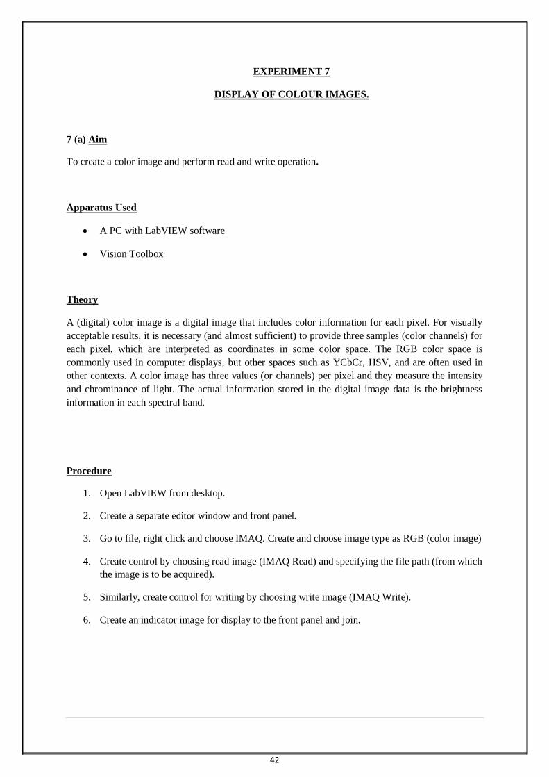
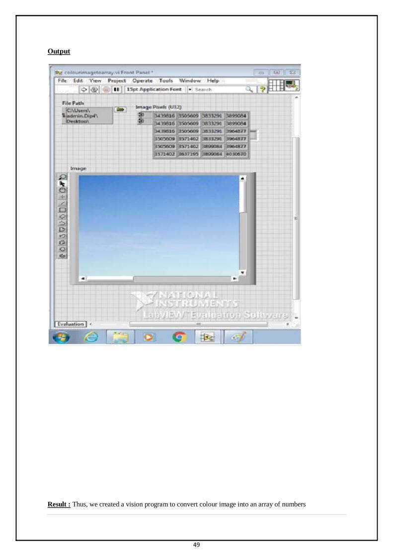
Block Diagram

44

Output

Result: Thus, the program to performed read and write operation on it a color image (RGB) was

created.

45

7 (b) Aim

To create a vision program to convert a 2D array into a color image.

Apparatus Used

A PC with LabVIEW software

Vision Toolbox

Theory

An array is a container object that holds a fixed number of values of a single type. The length of an

array is established when the array is created. After creation, its length is fixed. The Image block

displays the data in array as an image. Each element of array specifies the color for 1 pixel of the

image. The resulting image is an m-by-n grid of pixels where m is the number of columns and n is the

number of rows in C. The row and column indices of the elements determine the centers of the

corresponding pixels.

Procedure

1. Open LabVIEW from desktop.

2. Create a separate editor window and front panel.

3. Right click, select vision and motion, choose IMAQ create. Add a constant and control

image to it.

4. Create an array to colour image block (by adding it) and set image pixel (U32) as

it’s parameter.

5. Add an indicator image at the end to check the Output. Run the program.

6. Input values into the array and check the Output.

46

Block Diagram

47

Output

Result : Thus ,the program to convert a 2D array into a colour image using Vision tool was created.

48

7 (c) Aim

To create a vision program to convert colour images into an array of numbers.

Apparatus Used

A PC with Lab VIEW software Vision Toolbox

Theory

A digital image is nothing more than data—numbers indicating variations of red, green, and blue at a

particular location on a grid of pixels. Most of the time, we view these pixels as miniature rectangles

sandwiched together on a computer screen. With a little creative thinking and some lower level

manipulation of pixels with code, however, we can display that information in a myriad of ways. This

tutorial is dedicated to breaking out of simple shape drawing in Processing and using images (and

their pixels) as the building blocks of Processing graphics.

Procedure

1. Open LabVIEW from desktop. 2. Create a separate editor window and front panel. 3. Right click, select vision and motion >> choose IMAQ create. Add a constant and image to it. 4. Add a file path and specify the path of the image (at the particular storage location) which is

to be processed. 5. Add a colour image to array block to obtain values into array. 6. Add an indicator at the end to check for the image pixels at the Output. 7. The Output will be obtained in the front panel in the image pixel indicator (set to U32).

Block Diagram

49

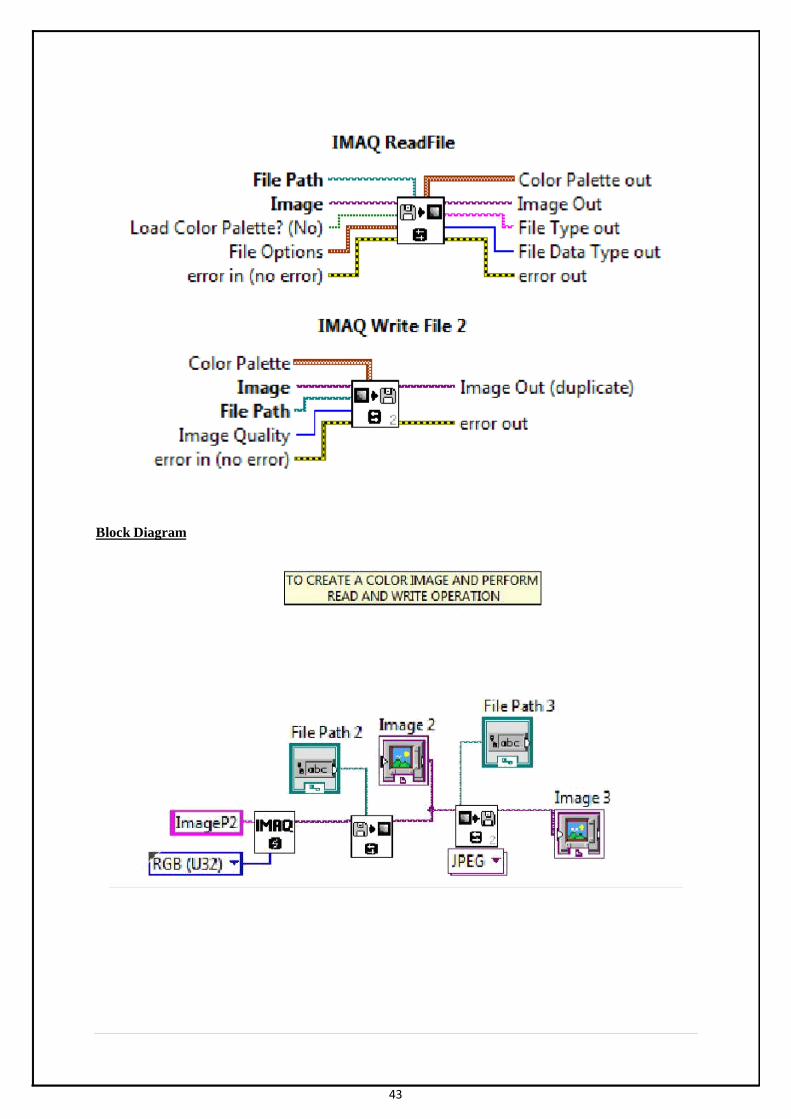
Output

Result : Thus, we created a vision program to convert colour image into an array of numbers

50

EXPERIMENT 8

CONVERSION BETWEEN COLOUR SPACES.

Aim:

To obtain the R, B, G colour values and resolved colour values from a colour box by choosing any

colour.

Apparatus Used

A PC with LabVIEW software Vision Toolbox

Theory

The RGB colour model is an additive colour model in which red, green and blue light are added

together in various ways to reproduce a broad array of colours. The name of the model comes from

the initials of the three additive primary colours, red, green and blue. The main purpose of the RGB

colour model is for the sensing, representation and display of images in electronic systems, such as

televisions and computers, though it has also been used in conventional photography. Before the

electronic age, the RGB colour model already had a solid theory behind it, based in human perception

of colours.

Procedure

1. Open LabVIEW from desktop. 2. Create a separate editor window and front panel. 3. Select Vision and Motion >> Vision Utilities >> Image Management >> IMAQ Create. 4. Select colour utilities >> Select RGB to colour and place it. 5. Give values for red, blue and green. 6. Select colour utilities >> Select colour to RGB. 7. Give values to colour box. 8. Run the program.

51

Block Diagram

52

Output

Result : Thus, we obtained the RGB colour values and resolved colour values from a colour

box by choosing any colour.

53

EXPERIMENT 9

DWT OF IMAGES

Aim

To create a program performs discrete wavelet transform on image.

Apparatus Used

A PC with LabVIEW software Vision Toolbox

Theory

A discrete wavelet transform (DWT) is any wavelet transform for which the wavelets are discretely

sampled. As with other wavelet transforms, a key advantage it has over Fourier transforms is temporal

resolution: it captures both frequency and location information (location in time).

Procedure

1.OpenLabVIEW software in desktop.

2.Create separate editor window and front panel.

3.Right click, select vision motion choose IMAQ create. Add constant image type (grayscale U8)

to it.

4.Select file read and give a control.

5.Choose IMAQ extract wavelet band and connect the same.

6.Choose 4 blocks of IMAQ create and place them. Select grayscale(SGL) as image type for all of

them and give name.

7.Choose 4 blocks of IMAQ array to image and place them. Connect them to image display.

8.Connect the Output of extract wavelet band to the four block of array to image.

9.Give an image file path and run the program.

54

Block Diagram

55

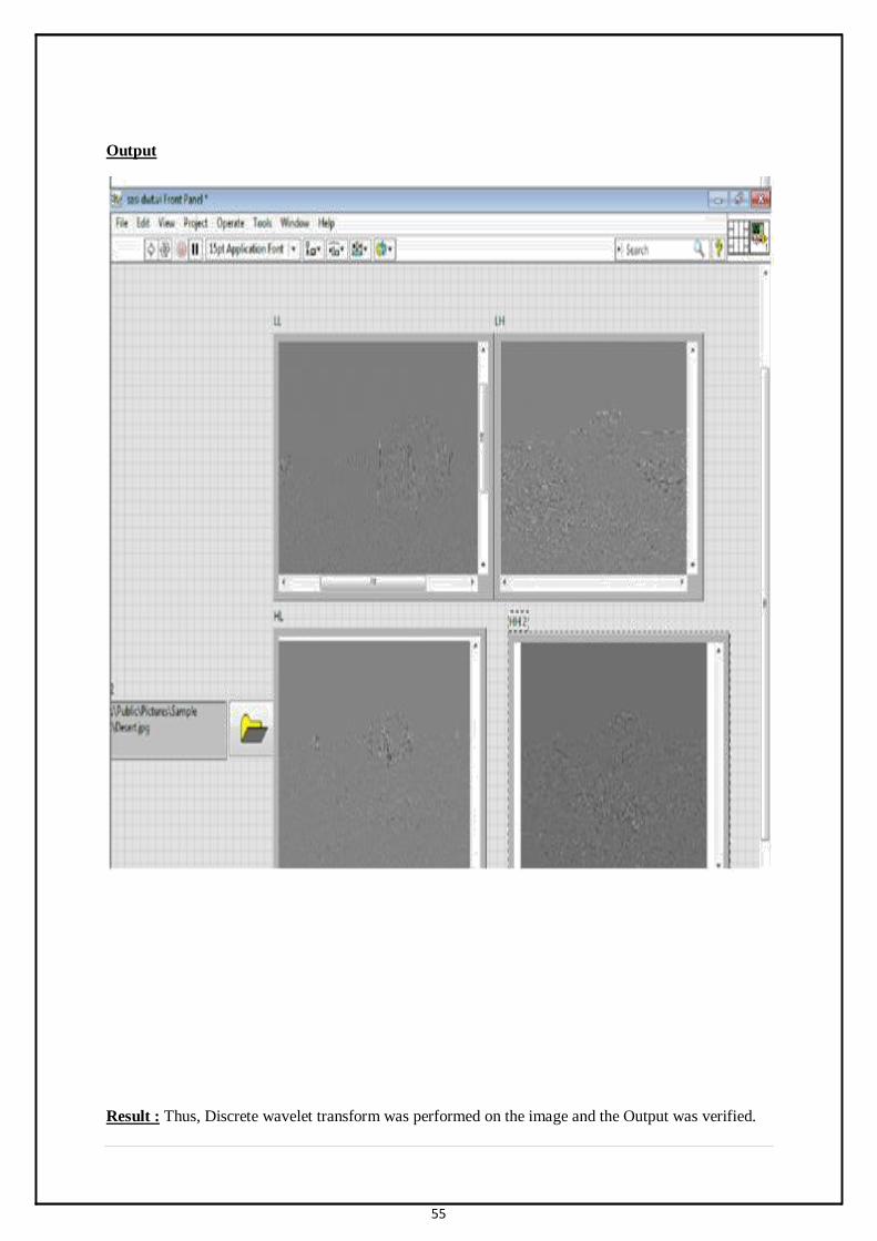
Output

Result : Thus, Discrete wavelet transform was performed on the image and the Output was verified.

56

EXPERIMENT 10

SEGMENTATION USING WATERSHED TRANSFORM

Aim

To create a program for segmentation of an image using watershed transforms.

Apparatus Used

A PC with LabVIEW software Vision Toolbox

Theory

In the study of image processing a watershed of a grayscale image is analogous to the notion of a

catchment basin of a height map. In short, a drop of water following the gradient of an image flows

along a path to finally reach a local minimum. Intuitively, the watershed of a relief corresponds to the

limits of the adjacent catchment basins of the drops of water. There are different technical definitions

of a watershed. In graphs, watershed lines may be defined on the nodes, on the edges, or hybrid lines

on both nodes and edges. Watersheds may also be defined in the continuous domain. There are also

many different algorithms to compute watersheds. Watershed algorithm is used in image processing

primarily for segmentation purposes.

Procedure

1. Open LabVIEW software in desktop.

2. Create separate editor window and front panel.

3. Right click, select vision motion chooses IMAQ create. Add constant image type (grayscale

U8) to it.

4. Select file read and give a control.

5. Choose IMAQ Watershed Transform connect the same.

6. Create an indicator (image display).

7. Give an image file path and run the program.

57

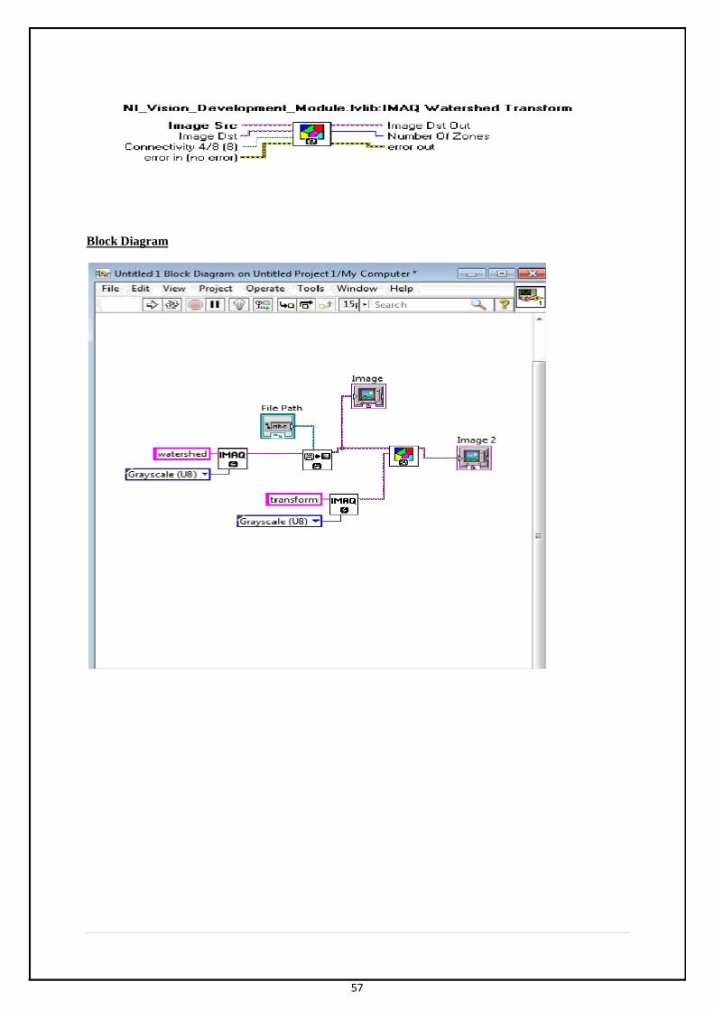
Block Diagram

58

Output

Result: Thus, watershed transformation was performed on the image and the Output was verified.