6 Composite Materials from Natural Resources: Recent Trends and Future Potentials
Upload
khangminh22Category
view
0download
0
Computer Science Journal of Moldova, vol.22, no.2(65), 2014
Recent trends in Medical Image Processing
Editorial (Preface) for a special issue of ComputerScience Journal of Moldova
Hariton Costin
It is said that images bear the greatest density of natural informa-tion of all ways of human communication, and biomedical images donot make any exception to this assertion, at least when dealing withmorphologic information. The recent rapid advances in medical imag-ing and automated image analysis will continue and allow us to makesignificant advances in our understanding of life and disease processes,and our ability to deliver quality healthcare.
Medical imaging and image processing domains mainly manage andprocess missing, ambiguous, inconsistent, complementary, contradic-tory, redundant and distorted data, and information has a strong struc-tural character. The processes of human and artificial understandingof any image involve the matching of features extracted from the imagewith pre-stored models. From the information technology point of viewthe production of a high-level symbolic model requires the representa-tion of knowledge about the objects to be modeled, their relationships,and how and when to use the information stored within the model.
In general, a distinction is made between (bio)medical imaging andimage processing technologies, even if between these fields of knowledgea strong interrelation may be established.
Biomedical imaging concentrates on the capture and display of im-ages for both diagnostic and therapeutic purposes, and modern imagingtechnology is 100% digital. Snapshots of in vivo physiology and physi-ological processes can be garnered through advanced sensors and com-puter technology. Biomedical imaging technologies utilize either x-rays
c©2014 by Hariton Costin
147

Hariton Costin
(CT scans), sound (ultrasound), magnetism (magnetic resonance imag-ing – MRI), radioactive pharmaceuticals (nuclear medicine: SPECT,PET) or light (endoscopy, OCT) to assess the current condition of anorgan or tissue and can monitor a patient over time for diagnostic andtreatment evaluation. From the information type point of view, med-ical imaging can be structural (or morphologic, e.g. CT, MRI, OCT)or functional (PET, SPECT).
Biomedical image processing is similar in concept to biomedical sig-nal processing in multiple dimensions (2D, 3D). It includes the enhance-ment, analysis and display of images captured via the above mentionedx-ray, ultrasound, MRI, nuclear medicine and optical imaging technolo-gies. Related procedures, like image reconstruction and modeling tech-niques allow quick processing of 2D signals to create 3D images. Imageprocessing software helps to automatically identify and analyze whatmight not be apparent to the human eye, even of an expert. Comput-erized algorithms can provide temporal and spatial analysis to detectpatterns and characteristics indicative of tumors and other ailments.Depending on the imaging technique and what diagnosis is being con-sidered, image processing and analysis can be used to determine, forinstance, the diameter, volume and vasculature of a tumor or organ,flow parameters of blood or other fluids and microscopic changes thathave yet to raise any otherwise discernible flags.
Nowadays some key components of clinical activity are image-guided therapy (IGT) and image-guided surgery (IGS), where localiza-tion, targeting, monitoring, and control are main issues. Specifically, inmedical imaging and medical image processing we have four key prob-lems: (1) Image Segmentation – dealing with (semi)automated meth-ods that lead to creating patient-specific models of relevant anatomyfrom images; (2) Image Registration – automated methods that alignmultiple data sets, eventually coming from different imaging modali-ties, with each other; (3) Visualization – the technological environmentin which image-guided procedures can be displayed; (4) Simulation –software that can be used to rehearse and plan procedures, evaluateaccess strategies, and simulate planned treatments.
In fact, all traditional and advanced techniques of image processing
148
Recent trends in Medical Image Processing. Preface
and computational vision, analysis and understanding may be usedto process medical images, in order to extract useful information fordiagnosis and treatment.
A special approach, including that of the editor of this journal issue,directs to the use of Artificial Intelligence (AI), which has proved toyield promising results in medical image processing and analysis. Thestructural character of information may successfully be approached byusing methods of AI such as Knowledge Based Systems, Expert Sys-tems, Decision Support Systems, Neural Networks, Fuzzy Logic andSystems, Neuro-Fuzzy Systems, Evolutionary and Genetic (or bio-inspired) Algorithms, Data Mining, Knowledge Discovery, SemanticNets, Symbolic Calculus for knowledge representation, etc. The datafusion methods successfully solve the aggregation of numerical and lin-guistic information, and are able to cope with ambiguous, uncertain,conflicting, complementary, imprecise and redundant information, likethat occurring in biomedical imaging domain, in order to provide amore accurate and less uncertain interpretation.
One of the main characteristic of the Medical Image Process-ing domain is its inter- and multidisciplinary nature. In fact, inthis field, methodologies of several fundamental and applicative sci-ences, such as Informatics, Mathematics, Physics, Statistics, Com-puter science, Medicine, Engineering, Psychology, Artificial Intelli-gence, (Bio)Mechanics are regularly used. Besides this characteristic,one of the main rationale that promotes the continuous effort beingmade in this area of human knowledge is the huge number of usefulapplications in the medical area, some of them being illustrated here-inafter.
This special issue of Computer Science Journal of Moldova containssix invited papers that illustrate new trends and outcomes in medicalimage processing. It gathers together prominent researches that alignto the state-of-the-art of Computational Vision and Medical Image Pro-cessing, contributing to the development of both these knowledge areas,and of medical research and clinical activity.
Probably is somehow justified that two of the invited articles dealwith retinal images processing. The first one, “Detection of Blood
149

Hariton Costin
Vessels in Retinal Fundus Images”, of Oloumi, Dhara, Rangayyan,and Mukhopadhyay approaches automatic detection of blood vesselsin retinal fundus images, in order to perform computer-aided diag-nosis of some pathologies of the eye such as diabetic retinopathy(DR), retinopathy of prematurity, and maculopathy. The vessels detec-tion techniques include a mix of multiscale and multifeature methods,like multiscale vesselness measures, Gabor filters, line operators, andmatched filters. An adaptive threshold selection method is crucial forprecise detection of retinal blood vessels. The accuracy of detection isimproved by an original postprocessing technique for removal of false-positive pixels around the optic nerve head. The results of detectionof blood vessels, evaluated in terms of the area under the receiver op-erating characteristic curve of up to 0.961, were obtained using the 20test images of the DRIVE database (which is considered as containinglow-resolution retinal images). These results have double meaning: onone hand they outperform other approaches of the chosen topic, andon the other hand they show that a single-scale Gabor filter is capableof detecting blood vessels with accuracy not much different from thebest value obtained by means of multifeature and multiscale methods.In this way the authors prove once again the famous Latin saying “nonmulta, sed multum”.
The second article, “Optic Disc Identification Methods for RetinalImages”, written by Rotaru, Bejinariu, Nita, Luca, and Lazar, pro-poses some original methods to identify and model the optic disc incolour retinal images, as well as the blood vessels network, to evaluatedifferent retina diseases such as diabetic macular edema, glaucoma, etc.The paper represents an extension of some early researches of the sameauthors, in which they heuristically apply certain traditional imageprocessing methods (low-pass filtering, Maximum Difference Method,texture analysis, voting algorithms, morphologic filtering, Otsu bina-rization) on 40 clinically validated retinal images of high resolution(2592×1728 pixels), 386 images of 720×576 resolution, and more than100 images from STARE database. The obtained results in terms ofaccuracy are comparable with the best outcomes in the literature, theproposed techniques are implemented as a Windows application writ-
150
Recent trends in Medical Image Processing. Preface
ten in C++ using Microsoft Visual Studio, and for image manipulationand some processing functions the OpenCV library was used.
The next invited article, “Characterization and Pattern Recogni-tion of Color Images of Dermatological Ulcers: a Pilot Study”, writ-ten by L.C. Pereyra, S.M. Pereira, Souza, Frade, Rangayyan, andAzevedo-Marques, approaches content-based image retrieval (CBIR)and computer-aided diagnosis (CAD) applied in dermatological ulcersdetection and analysis, which is a very difficult task of color imageprocessing and of tissue composition analysis, respectively. Unsuper-vised automatic segmentation was performed by using Gaussian mix-ture modeling, and its performance was assessed by computing the Jac-card coefficient between the automatically and manually segmented im-ages. A retrieval engine was implemented using the k-nearest-neighbormethod, and classification was made by means of a logistic regression.The performance of CBIR was measured in terms of precision of re-trieval, with average values of up to 0.617 obtained with the Chebyshevdistance, and the average value of correctly classified instances dividedby the total number of instances was 0.738. Results were obtained ona database containing 172 dermatologic images with high geometricand intensity resolution, obtained in a clinical environment and an-notated by an expert. Even if the obtained segmentation accuracyis not very high, from clinical and educational utility points of view“objective analysis of color images of skin ulcers using the proposedmethods might overcome some of the limitations of visual analysis andlead to the development of improved protocols for the treatment andmonitoring of chronic dermatological lesions.”
The last three articles are dedicated to some image processing topicsuseful in research and clinical practice, but which do not approach im-age segmentation or classification. They refer to image reconstruction,registration and human genome sequencing, respectively.
“A platform for Image Reconstruction in X-ray Imaging: Medi-cal Applications using CBCT and DTS algorithms”, by Kamarianakis,Buliev, Pallikarakis, presents the architecture of a software platformfor the purpose of testing and evaluation of reconstruction algorithmsin X-ray imaging. The main elements of the platform are classes, re-
151

Hariton Costin
lated together in a logical hierarchy. Real world objects can be de-fined and implemented as instances of corresponding classes. Differentimage processing routines (e.g. 3D transformations, loading, saving,filtering of images, etc.) have been incorporated in the software toolas class methods, too. The platform is viewed as a basic tool for fu-ture investigations of new reconstruction methods in combination withvarious scanning configurations. The current tests on ReconstructionTechniques Class Library (RTCL) and the Platform for Image Recon-struction in X-ray Imaging (PIRXI) prove the accuracy and flexibilityof this new approach for image reconstruction research and algorithmsimplementation.
Bejinariu, Costin, Rotaru, Luca, Nita, and Lazar authored the ar-ticle “Parallel Processing and Bio-inspired Computing for BiomedicalImage Registration”, that deals with image transformations aiming atoverlaying one or more image sources to a given model by maximiz-ing a similarity measure. Some bio-inspired metaheuristic optimiza-tion algorithms, such as Bacterial Foraging Optimization Algorithm(BFOA), Genetic Algorithms (GAs) and Clonal Selection Algorithm(CSA), are compared in terms of registration accuracy and executiontime for area-based and feature-based image registration. Normalizedcorrelation (NCC) and normalized mutual information (NMI) are usedas similarity measures. Implementation was made on many imagesfrom a publicly available database, mainly using MRI brain imageswith 256 × 256 pixels and 8 bits/pixels resolutions, without and with“salt & pepper” noise, respectively. In general, BFOA and GAs yieldedcomparable results in terms of registration accuracy, GAs performedabout three times faster than BFOA, and CSA is too slow for feature-based registration and also with lower registration precision. Even thefeature-based image registration performs faster, its use for multimodalimages is limited by the procedure’s capability to find common and sta-ble features in the images to be registered.
Last but not least, Voina, Pop, Vaida wrote the article “A NewAlgorithm for Localized Motif Detection in Long DNA Sequences”,that comes from bioinformatics research domain and approaches hu-man genome sequencing, i.e. the identification of the DNA segments
152

Recent trends in Medical Image Processing. Preface
that have a certain biological significance. The study presents a newalgorithm optimized for finding motifs in long DNA sequences andsome experiments done to evaluate the performance of the proposedalgorithm in comparison with other motifs finding algorithms are de-scribed. Some optimizations are introduced, that increase detectionaccuracy and lower the execution time. Thus, the proposed algorithmproved to have a clear advantage among other similar algorithms dueto the detection accuracy of the motifs in long DNA sequences, suchas those found in the human genome.
In conclusion we can say that the fundamental, engineering andlife sciences are all contributing to a remarkable synergy of efforts toachieve dynamic, quantitative (structural or functional) imaging of thebody using minimally invasive, non-invasive or even virtual methods.The structural and functional relationships between the cells, tissues,organs and organ systems of the body are being advanced by molecularimaging, and laboratory imaging techniques. With continuing evolu-tionary progress in biomedical imaging, visualization and analysis, wecan fully expect to benefit from new knowledge about life and diseaseprocesses, and from new and efficient methods of diagnosis therapy andprevention.
Iasi, 30-th of June, 2014 Prof. Hariton Costin
Brief biographyProf. dr. eng. Hariton Costin, B.Sc. in Electronics and
Telecommunications, Ph.D. in Applied Informatics, is full professor atthe University of Medicine and Pharmacy, Faculty of Medical Bioengi-neering, Iasi, Romania, (www.umfiasi.ro ; www.bioinginerie.ro). Also,he is senior researcher at the Romanian Academy – Iasi Branch, Insti-tute of Computer Science, within the Image Processing and ComputerVision Lab, (http://iit.academiaromana-is.ro/personal/h costin.html).Here his studies are in image processing and analysis by using ArtificialIntelligence methods and data fusion.
153
Hariton Costin
Competence areas include:medical electronics and in-strumentation, biosignal andimage processing and anal-ysis, artificial intelligence(soft-computing, bio-inspiredalgorithms, expert systems),hybrid systems, HCI (human-computer interfaces), assistivetechnologies, telemedicine/e-health.Scientific activity can be re-sumed by about 145 publishedpapers in peer-reviewed jour-nals and conference proceed-ings, 9 books, 4 book chaptersin foreign publishing houses, 3patents, 2 national awards.
Research activity: 54 research reports; technical manager (withinFP5/INES 2001-32316 project) for a telemedicine application (www.eu-roines.com; ,,Medcare” project); responsible for the first Romanian pi-lot telemedical centre in Iasi; director for 9 national funded projectsin bioengineering and (biomedical) image processing/analysis. He hasserved as the program committee member of various international con-ferences and reviewer for various international journals and conferences.Prof. Costin was invited as postdoc researcher at the University of Sci-ence and Technology of Lille (France, 2002, in medical imaging), theUniversity of Applied Sciences Jena (Germany, 2013) and had invitedtalks at international conferences. Prof. Costin is a member of theI.E.E.E./Engineering in Medicine & Biology Society (EMBS) and ofother 5 scientific societies.
154

Computer Science Journal of Moldova, vol.22, no.2(65), 2014
Detection of Blood Vessels in
Retinal Fundus Images∗
Invited Article
Faraz Oloumi, Ashis K. Dhara,Rangaraj M. Rangayyan@, Sudipta Mukhopadhyay
Abstract
Detection of blood vessels in retinal fundus images is an im-portant initial step in the development of systems for computer-aided diagnosis of pathologies of the eye. In this study, we per-form multifeature analysis for the detection of blood vessels inretinal fundus images. The vessel detection techniques imple-mented include multiscale vesselness measures, Gabor filters, lineoperators, and matched filters. The selection of an appropriatethreshold is crucial for accurate detection of retinal blood vessels.We evaluate an adaptive threshold selection method along withseveral others for this purpose. We also propose a postprocess-ing technique for removal of false-positive pixels around the opticnerve head. Values of the area under the receiver operating char-acteristic curve of up to 0.961 were obtained using the 20 testimages of the DRIVE database.
Keywords: Gabor filter, line operator, matched filter, mul-tiscale analysis, retinal fundus image, vessel detection, vesselnessmeasure.
c©2014 by Faraz Oloumi, Ashis K. Dhara, Rangaraj M. Rangayyan, and
Sudipta Mukhopadhyay∗This work was supported by grants from the Natural Sciences and Engineering
Research Council (NSERC) of Canada, the Shastri Indo-Canadian Institute, andthe Indian Institute of Technology Kharagpur, India. This article is a revised andexpanded version of the conference publication cited as Dhara et al. [1]. @Addressall correspondence to R. M. Rangayyan, [email protected]
155

F. Oloumi, A. Dhara, R. Rangayyan, S. Mukhopadhyay
1 Introduction
Retinal fundus images are used by ophthalmologists for the diagnosisof several disorders, such as diabetic retinopathy (DR), retinopathy ofprematurity, and maculopathy [2–4]. Detection of blood vessels is animportant initial step in the development of computer-aided diagnostic(CAD) systems and analysis of retinal fundus images. It is possible todetect other anatomical landmarks such as the optic nerve head (ONH)and the macula in the retina with respect to the vascular architecture.The location and certain characteristics of such landmarks can help inthe derivation of features for the detection of abnormalities. A varietyof methods have been proposed for the detection of blood vessels; someof these methods are reviewed in the following paragraphs.
Chaudhuri et al. [5] proposed an algorithm based on two-dimensional(2D) matched filters for vessel detection. Their method is based onthree assumptions: (i) the intensity profile of a vessel can be approx-imated by a Gaussian function, (ii) vessels can be approximated bypiecewise linear segments, and (iii) the width of vessels is relativelyconstant. Detection of blood vessels was performed by convolving thegiven image with the matched filter rotated in several orientations.The maximum filter response over all orientations was assigned to eachpixel.
Staal et al. [6] extracted the ridges in the images which roughlycoincide with the vessel centerlines. In the next step, image primitiveswere obtained by grouping image ridges into sets that model straight-line elements, which were used to partition the image by assigning eachpixel to the closest primitive set. Feature vectors were then computedfor every pixel using the characteristics of the partitions and their lineelements. The features were used for classification using a k-nearest-neighbor classifier. Staal et al. achieved an area under the receiveroperating operating characteristic (ROC) curve of Az = 0.9520 with20 images of the test set of the DRIVE database [7].
Soares et al. [8] applied complex Gabor filters for feature extractionand supervised classification for the detection of blood vessels in retinalfundus images. In this method, the magnitude outputs at several scales
156

Detection of Blood Vessels in Retinal Fundus Images
obtained from 2D complex Gabor filters were assigned to each pixel as afeature vector. Then, a Bayesian classifier was applied for classificationof the results into vessel or nonvessel pixels. Soares et al. reportedAz = 0.9614 for the 20 test images of the DRIVE database.
Blood vessels can be considered as dark elongated curvilinear struc-tures of different width and orientation on a brighter background. Sev-eral types of vesselness measures have been developed for the detectionof blood vessels based on the properties of the eigenvalues of the Hessianmatrix computed at each pixel. Because blood vessels are of varyingwidth, different scales are used to calculate the eigenvalues and themaximum response at each pixel over all scales is used for further ana-lysis. Frangi et al. [9] and Salem et al. [10] proposed different vesselnessmeasures to highlight vessel-like structures. Wu et al. [11] applied thevesselness measure of Frangi et al. to the 40 training and testing imagesof the DRIVE database and reported Az = 0.9485. Salem et al. [10]reported Az = 0.9450 using 20 images of the STARE database [12].
Lupascu et al. [13] performed multifeature analysis using previouslyproposed features [6,8,9,14,17], combined with new features that rep-resent information about the local intensity, the structure of vessels,spatial properties, and the geometry of the vessels at different scalesof length. They used a feature vector containing a total of 41 featuresobtained at different scales to train a classifier, which was then appliedto the test set. They reported Az = 0.9561 using the 20 test images ofthe DRIVE database.
Rangayyan et al. [15] performed multiscale analysis for the detec-tion of blood vessels using Gabor filters and classified pixels using mul-tilayer perceptron (MLP) neural networks and reported Az of 0.9597with the test set of the DRIVE database. Oloumi [16] used multi-scale Gabor filter magnitude responses, coherence, and the invertedgreen channel as features to train an MLP and achieved an Az valueof 0.9611 using the test set of the DRIVE database.
Other available methods in the literature that do not employ afiltering technique for the detection of the blood vessels include, but arenot limited to, segmentation using multiconcavity modeling [18]; fractalanalysis [19]; mathematical morphology and curvature evaluation [20];
157

F. Oloumi, A. Dhara, R. Rangayyan, S. Mukhopadhyay
and geometrical models and analysis of topological properties of theblood vessels [21].
In the present work, we perform vessel segmentation by multifea-ture analysis, using multiscale Gabor filters as proposed by Rangayyanet al. [15], multiscale vesselness measures as proposed by Frangi etal. [9] and Salem et al. [10], matched filters as proposed by Chaudhuriet al. [5], line operators [22], and a gamma-corrected version of theinverted green channel. Thresholding and binarization of the resultof vessel detection is a crucial step for further analysis of the char-acteristics of blood vessels such as thickness and tortuosity [23]; wepropose an adaptive thresholding technique by analyzing the intensityvalues of the boundary pixels of retinal blood vessels and compare theresults against several automated thresholding methods. Most of thereported methods for the detection of blood vessels cause false-positive(FP) pixels associated with the boundary of the ONH. We propose apostprocessing technique for removal of FP pixels around the ONH.
2 Database of Retinal Images
In this work, retinal fundus images from the DRIVE database wereused to assess the performance of the methods. The images of theDRIVE database [6, 7] were acquired during a screening program forDR in the Netherlands and show signs of mild DR. The images havea size 565× 584 pixels and a field of view (FOV) of 45◦. The DRIVEimages are considered to be low-resolution retinal images; the imageshave an approximate spatial resolution of 20 µm per pixel. The DRIVEdatabase consists of 40 images, which are labeled in two sets of 20images for training and testing. A manually segmented image (ground-truth) of the vasculature is available for each image in the DRIVEdatabase. Figure 1 shows the original color image 12 of the DRIVEdatabase and its ground-truth image.
158

Detection of Blood Vessels in Retinal Fundus Images
(a) (b)
Figure 1. (a) Original color image 12 of the DRIVE database.(b) Ground-truth of the image in part (a), as provided in the database.
3 Detection of Retinal Blood Vessels
In the present study, we review and implement several methods for thedetection of blood vessels and investigate their combined applicationfor multifeature analysis.
3.1 Vesselness Measures
Frangi et al. [9] defined a vesselness measure to detect pixels havingvessel-like structures based on the properties of the eigenvalues of theHessian matrix. A numerical estimate of the Hessian matrix, H, ateach pixel of the given image, L(x, y), is obtained as
H =
∂2L∂x2
∂2L∂x∂y
∂2L∂y∂x
∂2L∂y2
. (1)
The entries of H can be obtained at multiple scales by convolving the
159

F. Oloumi, A. Dhara, R. Rangayyan, S. Mukhopadhyay
image L(x, y) with the Gaussian kernel G(x, y; σ) of different scales σ,defined as
G(x, y; σ) =1
2πσ2exp
(−x2 + y2
2σ2
). (2)
The width of retinal blood vessels varies from 50 µm to 200 µmin retinal fundus images, which translates to the range of about 2 to10 pixels, given a spatial resolution of 20 µm for the DRIVE images.Gaussian kernels can be used to generate a suitable scale space with anamplitude range of σ related to the range of vessel width. Multiscalederivatives of the image L(x, y) can be obtained by linear convolution ofthe image with the scale-normalized derivatives of the Gaussian kernelas ∂2L
∂x2 = L(x, y) ∗ σ2Gxx = Lxx , ∂2L∂x∂y = ∂2L
∂y∂x = L(x, y) ∗ σ2Gxy =
Lxy = Lyx, and ∂2L∂y2 = L(x, y) ∗ σ2Gyy = Lyy. Here Gxx, Gxy, and Gyy
are the second derivatives of the Gaussian kernel G, and the symbol‘∗’ represents the 2D convolution operation.
The Hessian matrix is symmetrical with real eigenvalues. The signsand ratios of the eigenvalues can be used as signatures of a local struc-ture. Let λ1 and λ2 represent the eigenvalues of the Hessian matrix,with the condition |λ2| ≥ |λ1|. The larger eigenvalue, λ2, corresponds tothe maximum principal curvature at the location (x, y). A larger valueof λ2 compared to λ1 represents a vessel-like structure. The eigenvaluesand eigenvectors of the Hessian matrix can be computed by solving thefollowing equation:
∣∣∣∣Lxx − λ Lxy
Lyx Lyy − λ
∣∣∣∣ = 0, (3)
where λ represents the two eigenvalues λ1 and λ2. The eigenvalues λ1
and λ2 can be obtained as
λ1 =Lxx + Lyy − α
2, (4)
and
λ2 =Lxx + Lyy + α
2, (5)
160

Detection of Blood Vessels in Retinal Fundus Images
where α =√
(Lxx − Lyy)2 +4L2
xy. Based on the property of the eigen-values of the Hessian matrix, Frangi et al. [9] defined a vesselness mea-sure to highlight pixels belonging to vessel-like structures as
VF =
exp(− R2
β
2β2
)[1− exp
(− S2
2γ2
)]if λ1, λ2 < 0,
0 otherwise,(6)
where Rβ = λ1λ2
, S =√
λ12 + λ2
2 is the Frobenius norm of the Hessianmatrix, β = 0.5 (as used by Frangi et al. [9]), and γ is equal to one-halfof the maximum of all of the Frobenius norms computed for the wholeimage. The Frobenius norm is expected to be low in background areaswhere no vessels are present and the eigenvalues are low, because themagnitude of the derivatives of the intensities will be small. On theother hand, in regions with high contrast as compared to the back-ground, the Frobenius norm will become larger, because at least one ofthe eigenvalues will be large.
The vesselness measure proposed by Salem et al. [10] uses the eigen-values of the Hessian matrix to detect the orientation of blood vessels.Let ~e1 and ~e2 be the eigenvectors corresponding to the eigenvalues λ1
and λ2, respectively, and let θ1 and θ2 be the angles of the eigenvectorswith respect to the positive x-axis. The orientations of the eigenvec-tors corresponding to the larger and smaller eigenvalues for every fifthpixel are shown in Figure 2. It can be noted from Figure 2 that thevariation of the orientation of the eigenvectors corresponding to thesmaller eigenvalues is smaller inside the blood vessels as compared tothat outside the blood vessels. The eigenvectors corresponding to thesmaller eigenvalues are mainly oriented along the blood vessels; hence,the angle θ1 is used to analyze the orientation of blood vessels. Theorientation of the eigenvector ~e1 can be represented as
θ1 = arctan(− 2Lxy
Lyy − Lxx + α
). (7)
Detection of blood vessels can be accomplished by assuming that
161

F. Oloumi, A. Dhara, R. Rangayyan, S. Mukhopadhyay
(a) (b)
Figure 2. Orientation of the eigenvectors corresponding to (a) thelarger eigenvalue and (b) the smaller eigenvalue at each pixel for a partof a retinal fundus image with parts of blood vessels. Straight linescorresponding to the eigenvectors are shown for every fifth pixel. Thesize of the image is 50× 50 pixels.
the maximum value of λ2 (λmax) over several scales of σ is at the centerof the vessel. Salem et al. [10] defined a vesselness measure as
VS =λmax
θstd + 1, (8)
where θstd is the standard deviation (STD) of θ1 over all scales used forthe pixel under consideration. The larger the value of VS for a pixel,the higher the probability that the pixel belongs to a vessel.
In this work, the range of scales σ = [1, 6] with steps of 0.05 wasdetermined to be the most suitable range for the vesselness measuresof Frangi et al. and Salem et al. using the training set of the DRIVEdatabase, and was used for subsequent analysis. Note that the two ves-selness measures implemented in this work perform multiscale analysisby taking the maximum intensity value among all the available scalesof σ. The implementation of the method of Frangi et al. used in this
162

Detection of Blood Vessels in Retinal Fundus Images
work was provided by Dirk-Jan Kroon of University of Twente [36].Figure 3 shows the magnitude response images of the result of ap-
plying the vesselness measures of Frangi et al. and Salem et al. to theimage in Figure 1 (a).
(a) (b)
Figure 3. Magnitude response images of the result of filtering the imagein Figure 1 (a) obtained using (a) vesselness measure of Frangi et al.and (b) vesselness measure of Salem et al. Note that the result of themethod of Frangi et al. provides lower intensity values as compared tothe method of Salem et al. and the detected vessels may not be clearlyvisible in the result.
3.2 Gabor Filters
Rangayyan et al. [15] applied multiscale Gabor filters for the detectionof blood vessels by considering the fact that blood vessels are elongated,piecewise-linear, or curvilinear structures with a preferred orientation.Gabor filters are sinusoidally modulated Gaussian functions that aresuitable for the analysis of oriented structures because they provideoptimal localization in both the frequency and space domains. The realGabor filter kernel oriented at the angle θ = −π/2 can be represented
163
F. Oloumi, A. Dhara, R. Rangayyan, S. Mukhopadhyay
as [15]
g(x, y) =1
2πσxσyexp
[−1
2
(x2
σ2x
+y2
σ2y
)]cos(2πfox) . (9)
In this equation, the frequency of the modulating sinusoid is givenby fo, and σx and σy are the STD values in the x and y directions.For simplicity of design, a variable τ is used to represent the averagethickness of the vessels to be detected. The value of σx is defined basedon τ as σx = τ
2√
2 ln 2and σy = lσx, where l represents the elongation of
blood vessels. A bank of K Gabor filters may be obtained by rotatingthe main Gabor filter kernel given in Equation 9 over the range [−π/2,π/2]. For a given pixel, the maximum output value over all K filtersis saved as the Gabor magnitude response at that particular pixel; thecorresponding angle is saved as the Gabor angle response.
Values of τ = 8 pixels, l = 2.9, and K = 180 were determined toprovide the best single-scale results, as determined using the trainingset of the DRIVE database. Values of τ = 4, 8, and 12 were usedto perform multiscale and multifeature analysis as described in Sec-tion 3.5. Figure 4 shows the magnitude and angle responses of Gaborfilters with τ = 8 pixels, l = 2.9, and K = 180 as obtained for theimage in Figure 1 (a). It is seen that the magnitude response is highat pixels belonging to vessels and that the angle response agrees wellwith the angle of the vessel at the corresponding pixel.
3.3 Line Operators
Line operators were proposed by Dixon and Taylor [24] and used byZwiggelaar et al. [25] for the detection of linear structures in mammo-grams. The main line operator kernel detects horizontal lines. Assumethat N(x, y) is the average gray-level of M pixels along a horizontalline centered at (x, y). Next, assume that S(x, y) is the average gray-level of pixels in a square of width M pixels that is horizontally alignedand centered at (x, y). The main line operator kernel is defined asL(x, y) = N(x, y) − S(x, y). Detecting lines with various orientationsis achieved by rotating the main kernel. Let Lk(x, y) be the line opera-
164

Detection of Blood Vessels in Retinal Fundus Images
(a) (b)
Figure 4. (a) Gabor magnitude and (b) angle responses of the imagein Figure 1 (a). The Gabor angle information is shown for every fifthpixel over a portion of the original color image.
tor kernel rotated to the angles αk = −π/2+πk/K, k = 0, 1, ..., K−1.Given Wk(x, y) as the result of filtering the image, I(x, y), withLk(x, y), the orientation of the detected line is obtained as [22]
θ(x, y) = αkmax ,where kmax = arg{max[Wk(x, y)]}. (10)
The magnitude response of the result is obtained as Wkmax(x, y).The line operator does not provide a specific parameter for scaling;multiscale analysis is performed by applying the line operator to eachlevel of the Gaussian pyramid decomposition of the original image.
In the present work, values of M = 15 and K = 180 were de-termined to provide the best results for detection of vessels using thetraining set of the DRIVE database, and were employed for furtheranalysis. Figure 5 shows the magnitude response of line operators asapplied to the image in Figure 1 (a).
165

F. Oloumi, A. Dhara, R. Rangayyan, S. Mukhopadhyay
Figure 5. Magnitude response of line operators for the image in Fig-ure 1 (a), obtained using M = 15 and K = 180.
3.4 Matched Filters
The method of Chaudhuri et al. [5], as explained in Section 1, wasimplemented in the present work for the detection of blood vessels.The method assumes that blood vessels have a negative contrast withrespect to the background, so the Gaussian template will need to beinverted. The main kernel of the matched filter is expressed as
M(x, y) = − exp(−x2
/2σ2
), for − L/2 ≤ y ≤ L/2, (11)
where L represents the length of the vessel segment that is assumedto have a constant orientation and σ is the STD of the Gaussian. Themain kernel of the filter is oriented along the y-axis; in order to detectblood vessels at different orientations, the main kernel is rotated atmultiple angles.
In this work, detection of blood vessels using matched filters isperformed by taking the maximum filter response of a bank of K = 180filters over the range [−π/2, π/2] with L = 15 and σ = 1, as determined
166

Detection of Blood Vessels in Retinal Fundus Images
using the training set of the DRIVE database. Figure 6 representsthe magnitude response of matched filters obtained for the image inFigure 1 (a).
Figure 6. Magnitude response of matched filters obtained using L = 15,σ = 1, and K = 180 for the image in Figure 1 (a).
3.5 Multifeature Analysis
In the present work, various features are combined using pattern clas-sification methods [multilayer neural networks (MNN)] in order to dis-tinguish pixels belonging to blood vessels from the background. Thefeatures used are:
• the vesselness measure of Frangi et al. [9],
• the vesselness measure of Salem et al. [10],
• the magnitude response of line operators [22],
• the magnitude response of matched filters [5],
167

F. Oloumi, A. Dhara, R. Rangayyan, S. Mukhopadhyay
• the gamma-corrected [26] inverted green component, and
• the magnitude responses of Gabor filters for τ = {4, 8, 12} [15].
The inverted green (G) component of the RGB color space pro-vides high contrast for blood vessels. Therefore, a gamma-correctedversion [26] of the inverted G-component image is also used as a fea-ture in order to improve the result of classification of blood vessels.The value of gamma used for gamma correction in this work is 2.4,with the pixel values normalized to the range [0, 1].
All the MNNs used in this work for multifeature analysis containtwo hidden layers with 15 nodes per hidden layer. The number ofinput layer nodes is equal to the number of features being used andthe output layer always contains one node. A tangent sigmoid (tansig)function was used as the training function for each hidden layer and apure linear function was used at the output layer of the MNN. In eachcase, the MNN was trained using 10% of the available training data.
Sequential feedforward feature selection was used to determinewhich combination of the features listed above would provide the bestresults for multifeature analysis; the feature selection method selectedall eight available features.
3.6 Thresholding for Segmentation of Vessels
The histogram of the intensity values of the result of vessel detectionis not bimodal with a clear separation of the pixels belonging to bloodvessels from the background pixels. Considering the ground-truth dataprovided for the 20 training images of the DRIVE database within theirFOV, only 13% of an image is covered by vessel pixels. As a result,thresholding the gray-scale output images of vessel detection methodswith high accuracy is a rather difficult task. Several automated thresh-olding methods, including Otsu’s method [27], a moment-preservingthresholding method [28], the Ridler-Calvard thresholding method [31],the Rutherford-Appleton threshold selection (RATS) method [29], andan entropy-based thresholding method [30] are explored in this work.Additionally, it is possible to use a single fixed-value threshold for each
168

Detection of Blood Vessels in Retinal Fundus Images
single feature or the discriminant result of multifeature analysis, ob-tained as the value of the point on the ROC curve that is closest to thepoint [0, 1], with the ROC curve obtained by using the training set ofimages.
Considering that the majority of the pixels in a retinal image arebackground pixels and possess a low intensity value in the results ofvessel detection methods, it could be beneficial to select a binarizationthreshold by analyzing only the pixels that belong to the boundariesof the vessels. We propose an adaptive thresholding method in whichthe boundaries of blood vessels are detected using Gabor filters witha low value of τ = 3 pixels. The result is then thresholded at 0.2of the normalized intensity to obtain the boundaries of blood vessels.Morphological dilation is then applied to the binary image of the ves-sel boundaries using a disk-shaped structuring element of radius twopixels to identify the adjacent regions of boundaries of blood vessels.The histogram of the pixels (with 25 bins) in the selected regions wasobserved to have an abrupt change in the values for two adjacent bins.The two adjacent bins with the largest probabilities of values are iden-tified and their corresponding pixel intensity values are noted. Anadaptive threshold for each image is obtained as the average of theintensity values corresponding to the two identified bins.
The performance of the proposed and selected thresholding tech-niques was analyzed in terms of the sensitivity (SE), specificity (SP),and accuracy (Acc) of the segmentation of blood vessels with referenceto the ground-truth images provided in the DRIVE database.
3.7 Postprocessing for Removal of FP Pixels Around theONH
In the results obtained using various vessel detection techniques, theboundary and edges of the ONH are also detected since they representan abrupt change in intensity, i.e., an edge, which can lead to artifacts(FP pixels) when the gray-scale results are thresholded. In the presentwork, the FP pixels associated with the boundary of the ONH areidentified using an angular difference index (ADI), defined as [1]
169

F. Oloumi, A. Dhara, R. Rangayyan, S. Mukhopadhyay
ADI = cos[θ(i, j)− γ(i, j)
], (12)
where θ(i, j) is the Gabor angle response and γ(i, j) is the radial anglewith respect to the center of the ONH, as shown in Figures 7(a) and(b), respectively. The ranges of θ and γ are limited to [−π/2, π/2].The values of ADI are computed for each pixel within the annular re-gion limited by two circles of radii 0.75r and 2r, where r = 0.8 mmis the average radius of the ONH [16]. The center of the ONH wasautomatically detected using phase portrait analysis of the Gabor an-gle response [32]. The pixels for which ADI is less than 0.15, i.e., thedifference between the Gabor angle and the radial angle is greater than81◦, are removed from the output of the classifier, because they rep-resent artifacts related to the ONH. This step may cause the loss of afew pixels belonging to vessels.
(a) (b)
Figure 7. (a) Gabor angle response and (b) radial angle with respectto the center of the ONH for the selected annular region.
4 Results
In order to obtain each feature mentioned in Section 3.5, the luminancecomponent, Y , of the Y IQ color space, defined as
170
Detection of Blood Vessels in Retinal Fundus Images
Y = 0.299R + 0.587G + 0.114B, (13)
where R, G, and B represent the red, green, and blue color componentsin the RGB color space, respectively, was used as the input to the vesseldetection methods.
The performance of the proposed methods was tested with the setof 20 test images of the DRIVE database. The training set of 20 imageswas used to determine the best values for the parameters of the filters(Section 3), to perform the training of the MNNs (Section 3.5), and todetermine a suitable threshold for segmentation of vessels (Section 3.6).The ground-truth images of blood vessels were used as reference toperform ROC analysis.
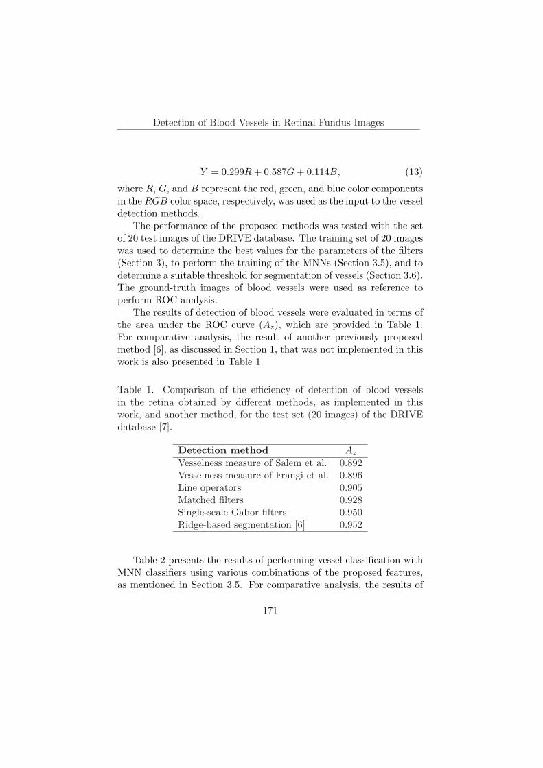
The results of detection of blood vessels were evaluated in terms ofthe area under the ROC curve (Az), which are provided in Table 1.For comparative analysis, the result of another previously proposedmethod [6], as discussed in Section 1, that was not implemented in thiswork is also presented in Table 1.
Table 1. Comparison of the efficiency of detection of blood vesselsin the retina obtained by different methods, as implemented in thiswork, and another method, for the test set (20 images) of the DRIVEdatabase [7].
Detection method Az
Vesselness measure of Salem et al. 0.892Vesselness measure of Frangi et al. 0.896Line operators 0.905Matched filters 0.928Single-scale Gabor filters 0.950Ridge-based segmentation [6] 0.952
Table 2 presents the results of performing vessel classification withMNN classifiers using various combinations of the proposed features,as mentioned in Section 3.5. For comparative analysis, the results of
171

F. Oloumi, A. Dhara, R. Rangayyan, S. Mukhopadhyay
the works of Soares et al. [8] and Lupascu et al. [13], who performedmultiscale and multifeature analysis, respectively, are also presented inTable 2 (see Section 1 for the details of the methods).
Table 2. Results of detection of blood vessels in terms of Az withthe test set (20 images) of the DRIVE database. For all cases, MNNclassifiers were used. Multiscale Gabor filters include the magnituderesponse images with scales of τ = {4, 8, 12} pixels. In order to keepthe table entries short, the following acronyms for different featuresare used: Gabor filters (GF), vesselness measure of Frangi et al. (VF),vesselness measure of Salem et al. (VS), gamma-corrected green com-ponent (GC), matched filters (MF), and line operators (LO).
Detection method Az
VF, VS, GC, MF, and LO 0.948Multiscale GF 0.960Multiscale GF and LO 0.960Multiscale GF and MF 0.960Multiscale GF and VS 0.960Multiscale GF and VF 0.960Multiscale GF, VF, and GC 0.961Multiscale GF, VF, VS, GC, MF, and LO 0.961Multiscale complex GF [8] 0.961Multifeature analysis (41 features) [13] 0.956
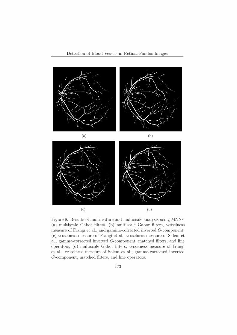
Figure 8 shows the result of multifeature and multiscale analysisfor the image in Figure 1 (a) using four of the combinations given inTable 2.
Table 3 provides the performance of the three methods of entropy-based [30] thresholing, adaptive thrsholding, and fixed-value thresh-olding. The methods of Otsu [27], moment-preserving thresholdingmethod [28], Ridler-Calvard thresholding method [31], and the RATSmethod [29] were also tested in this work; however, since they did notprovide better results than the three methods mentioned above, their
172
Detection of Blood Vessels in Retinal Fundus Images
(a) (b)
(c) (d)
Figure 8. Results of multifeature and multiscale analysis using MNNs:(a) multiscale Gabor filters, (b) multiscale Gabor filters, vesselnessmeasure of Frangi et al., and gamma-corrected inverted G-component,(c) vesselness measure of Frangi et al., vesselness measure of Salem etal., gamma-corrected inverted G-component, matched filters, and lineoperators, (d) multiscale Gabor filters, vesselness measure of Frangiet al., vesselness measure of Salem et al., gamma-corrected invertedG-component, matched filters, and line operators.
173
F. Oloumi, A. Dhara, R. Rangayyan, S. Mukhopadhyay
results are not presented in this table.
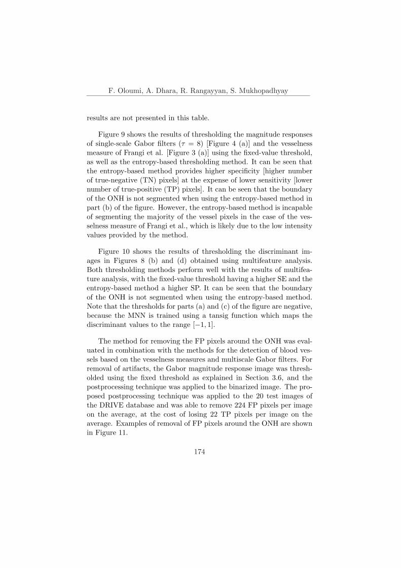
Figure 9 shows the results of thresholding the magnitude responsesof single-scale Gabor filters (τ = 8) [Figure 4 (a)] and the vesselnessmeasure of Frangi et al. [Figure 3 (a)] using the fixed-value threshold,as well as the entropy-based thresholding method. It can be seen thatthe entropy-based method provides higher specificity [higher numberof true-negative (TN) pixels] at the expense of lower sensitivity [lowernumber of true-positive (TP) pixels]. It can be seen that the boundaryof the ONH is not segmented when using the entropy-based method inpart (b) of the figure. However, the entropy-based method is incapableof segmenting the majority of the vessel pixels in the case of the ves-selness measure of Frangi et al., which is likely due to the low intensityvalues provided by the method.
Figure 10 shows the results of thresholding the discriminant im-ages in Figures 8 (b) and (d) obtained using multifeature analysis.Both thresholding methods perform well with the results of multifea-ture analysis, with the fixed-value threshold having a higher SE and theentropy-based method a higher SP. It can be seen that the boundaryof the ONH is not segmented when using the entropy-based method.Note that the thresholds for parts (a) and (c) of the figure are negative,because the MNN is trained using a tansig function which maps thediscriminant values to the range [−1, 1].
The method for removing the FP pixels around the ONH was eval-uated in combination with the methods for the detection of blood ves-sels based on the vesselness measures and multiscale Gabor filters. Forremoval of artifacts, the Gabor magnitude response image was thresh-olded using the fixed threshold as explained in Section 3.6, and thepostprocessing technique was applied to the binarized image. The pro-posed postprocessing technique was applied to the 20 test images ofthe DRIVE database and was able to remove 224 FP pixels per imageon the average, at the cost of losing 22 TP pixels per image on theaverage. Examples of removal of FP pixels around the ONH are shownin Figure 11.
174

Detection of Blood Vessels in Retinal Fundus ImagesTab
le3.
Per
form
ance
ofth
epr
opos
edad
apti
veth
resh
oldi
ngte
chni
que
com
pare
dw
ith
the
fixed
-va
lue
thre
shol
ding
met
hod
and
the
entr
opy-
base
dth
resh
old
sele
ctio
nm
etho
d.T
hefix
edth
resh
old
was
dete
rmin
edby
usin
gth
epo
int
onth
eR
OC
curv
ew
ith
the
shor
test
dist
ance
toth
epo
int
[0,1
]co
nsid
erin
gth
e20
trai
ning
imag
esof
the
DR
IVE
data
base
.T
hehi
ghes
tva
lues
ofSE
,SP
,an
dA
ccfo
rea
chth
resh
oldi
ngm
etho
dar
ehi
ghlig
hted
.In
orde
rto
keep
the
tabl
een
trie
ssh
ort,
the
follo
win
gac
rony
ms
for
diffe
rent
feat
ures
are
used
:si
ngle
-sca
leG
abor
filte
rs(S
GF),
mul
tisc
ale
Gab
orfil
ters
(MG
F),
vess
elne
ssm
easu
reof
Fran
giet
al.
(VF),
vess
elne
ssm
easu
reof
Sale
met
al.
(VS)
,ga
mm
a-co
rrec
ted
gree
nco
mpo
nent
(GC
),m
atch
edfil
ters
(MF),
and
line
oper
ator
s(L
O).
Fix
edEntr
opy
Adap
tive
Fea
ture
sSE
SPA
ccSE
SPA
ccSE
SPA
cc
VS
0.81
60.
886
0.87
70.
056
0.99
80.
875
0.86
30.
752
0.76
6V
F0.
810
0.89
80.
886
0.02
61.
000
0.87
30.
482
0.99
10.
925
LO
0.81
00.
839
0.83
50.
145
0.99
40.
883
0.55
60.
922
0.87
5M
F0.
832
0.87
90.
873
0.12
50.
999
0.88
50.
520
0.97
30.
913
SGF
0.85
70.
900
0.89
40.
269
0.99
80.
902
0.53
20.
966
0.91
0M
GF
0.87
60.
909
0.90
40.
821
0.94
40.
927
0.12
10.
988
0.87
6M
GF
and
LO
0.87
60.
912
0.90
70.
827
0.94
50.
929
0.15
00.
974
0.86
7M
GF
and
MF
0.87
60.
912
0.90
70.
821
0.94
60.
930
0.15
10.
983
0.87
5M
GF
and
VS
0.87
30.
914
0.90
90.
824
0.94
70.
931
0.13
80.
987
0.87
7M
GF
and
VF
0.87
20.
914
0.90
90.
818
0.94
90.
932
0.14
70.
964
0.85
9M
GF,V
F,an
dG
C0.
877
0.91
40.
909
0.82
90.
948
0.93
20.
134
0.99
30.
882
VF,V
S,G
C,M
F,an
dLO
0.85
30.
903
0.89
60.
806
0.94
40.
926
0.12
80.
990
0.87
8M
GF,V
F,V
S,G
C,M
F,an
dLO
0.87
60.
918
0.91
20.
856
0.93
40.
924
0.14
60.
983
0.87
4
175

F. Oloumi, A. Dhara, R. Rangayyan, S. Mukhopadhyay
(a) (b)
(c) (d)
Figure 9. Binarized versions of the image in Figure 4 (a) (single-scaleGabor filter) using: (a) the fixed-value threshold t = 0.0024 of the max-imum intensity value, with SE = 0.867, SP = 0.908, and Acc = 0.903;and (b) the entropy-based method (t = 0.196 of the normalized inten-sity value), with SE = 0.397, SP = 0.996, and Acc = 0.919. Binarizedversions of the image in Figure 3 (a) (vesselness measure of Frangi etal.) using: (c) the fixed-value threshold t = 3.22×10⁻⁸ of the maximumintensity value, with SE = 0.810, SP = 0.889, and Acc = 0.879; and(d) the entropy-based method (t = 0.290 of the normalized intensityvalue), with SE = 0.050, SP = 1.000, and Acc = 0.871.
176

Detection of Blood Vessels in Retinal Fundus Images
(a) (b)
(c) (d)
Figure 10. Binarized versions of the image in Figure 8 (b) using: (a) thefixed-value threshold t = −0.743 of the maximum intensity value, withSE = 0.893, SP = 0.909, and Acc = 0.907; and (b) the entropy-basedmethod (t = 0.263 of the normalized intensity value), with SE = 0.837,SP = 0.950, and Acc = 0.936. Binarized versions of the image inFigure 8 (d) using: (c) the fixed-value threshold t = −0.740 of themaximum intensity value, with SE = 0.895, SP = 0.909, and Acc =0.908; and (d) the entropy-based method (t = 0.302 of the normalizedintensity value), with SE = 0.870, SP = 0.933, and Acc = 0.925.
177

F. Oloumi, A. Dhara, R. Rangayyan, S. Mukhopadhyay
(a) (b)
Figure 11. Example of removal of ONH artifacts: (a) thresholded Ga-bor magnitude response image, and (b) the same region after the re-moval of ONH artifacts.
5 Discussion
As evident from the results in Table 1, even the use of a combination oflarge number of features (41) [13], does not lead to substantial increasein the value of Az. The large number of FP pixels caused by oversegmentation of small blood vessels seems to be the limiting factor inachieving higher Az values. The accuracy of detection of blood vesselscould be increased if thin, single-pixel-wide blood vessels are detectedaccurately. However, thin blood vessels may not be important in theanalysis of retinal vasculature as only changes in the major vessels havebeen observed to be clinically significant [23,33].
Based on the results obtained in this work, a single-scale Gaborfilter is capable of detecting blood vessels with accuracy (Az = 0.950)not substantially different from the highest Az value obtained with theresult of multifeature analysis in this work (Az = 0.961). It would beof interest to determine if the difference between the Az values givenabove is statistically significant.
Using a Lenovo Thinkpad T510, equipped with an Intel Core i7
178
Detection of Blood Vessels in Retinal Fundus Images
(Hyper-threaded-dual-core) 2.67-GHz processor, 4 MB of level 2 cache,8 GB of DDR3 RAM, running 64-bit Windows 7 Professional, andusing 64-bit Matlab software, the run time for single-scale Gabor filterswith K = 180, for a single color image from the DRIVE database isapproximately 13.5 seconds. The preprocessing step takes about 8.8seconds to execute.
Although the reduction of FP pixels is visible in the example shownin Figure 11, the result did not lead to a substantial increase in speci-ficity. This is mainly because the total number of FP pixels removed(224 pixels, on the average, per image) by the postprocessing step issmall compared to the total number of FP pixels (20, 038 pixels, on theaverage, per image) and the total number of TP pixels (24, 888 pixels,on the average, per image). Such a postprocessing step is most benefi-cial when applied to a skeleton of the vasculature in applications whereit is important to process only pixels that belong to vessels, such astracking the major branches of vessels [34] and measurement of vesselthickness [35].
The problem of segmentation of vessels via thresholding is crucialto applications that deal with measurement and analysis of the statis-tics of blood vessels. In this work, we have analyzed seven differentthresholding methods. Based on the results presented in Table 3, thethresholding method using a fixed value obtained using the ROC curvefor the training set of images provides the most consistent results interms of SE, SP, and accuracy. The entropy-based thresholding methodprovides a higher SP and similar SE in comparison to the fixed-valuemethod when applied to the results of multifeature analysis. However,the entropy-based method has low sensitivity when applied to singlefeatures. The proposed adaptive thresholding method does not per-form better than the other two methods. Depending on the desiredapplication, either the fixed-value method, the entropy-based method,or a combination of the two could be employed.
179

F. Oloumi, A. Dhara, R. Rangayyan, S. Mukhopadhyay
6 Conclusion
In this study, we have analyzed multiscale and multifeature methodsfor the detection of blood vessels in retinal fundus images, and achieveda maximum Az value of 0.961 using the 20 test images of the DRIVEdatabase. The results of the present study indicate that the state-of-the-art methods for the detection of blood vessels perform at high levelsof efficiency and that combining several features may not yield betterresults. The result of the fixed-value thresholding or the entropy-basedmethod could be helpful in analyzing the thickness and tortuosity ofblood vessels.
References
[1] A. K. Dhara, R. M. Rangayyan, F. Oloumi, S. Mukhopadhyay.“Methods for the detection of blood vessels in retinal fundus im-ages and reduction of false-positive pixels around the optic nervehead,” in Proc. 4th IEEE International Conference on E-Healthand Bioengineering - EHB 2013, Iasi, Romania, November 2013,pp. 1–6.
[2] N. Patton, T. M. Aslam, T. MacGillivray, I. J. Deary, B. Dhillon,R. H. Eikelboom, K. Yogesan, I. J. Constable. “Retinal image ana-lysis: Concepts, applications and potential,” Progress in Retinaland Eye Research, vol. 25, no. 1, pp. 99–127, 2006.
[3] American Academy of Pediatrics, American Association for Pedi-atric Ophthalmology and Strabismus, American Academy of Oph-thalmology, “Screening examination of premature infants for ret-inopathy of prematurity,” Pediatrics, vol. 108, pp. 809–811, 2001.
[4] R. van Leeuwen, U. Chakravarthy, J. R. Vingerling, C. Brussee,A. Hooghart, P. Mudler, P. de Jong. “Grading of age-related mac-ulopathy for epidemiological studies: Is digital imaging as goodas 35-mm film?,” Ophthalmology, vol. 110, no. 8, pp. 1540–1544,2003.
180
Detection of Blood Vessels in Retinal Fundus Images
[5] S. Chaudhuri, S. Chatterjee, N. Katz, M. Nelson, M. Goldbaum.“Detection of blood vessels in retinal images using two-dimensionalmatched filters,” IEEE Transactions on Medical Imaging, vol. 8,no. 3, pp. 263–269, 1989.
[6] J. Staal, M. D. Abramoff, M. Niemeijer, M. A. Viergever, B. vanGinneken. “Ridge-based vessel segmentation in color images ofthe retina,” IEEE Transactions on Medical Imaging, vol. 23, no.4, pp. 501–509, 2004.
[7] “DRIVE: Digital Retinal Images for Vessel Extraction,” www.isi.uu.nl/ Research/ Databases/ DRIVE/ , accessed December2013.
[8] J. V. B. Soares, J. J. G. Leandro, R. M. Cesar Jr., H. F. Je-linek, M. J. Cree. “Retinal vessel segmentation using the 2-DGabor wavelet and supervised classification,” IEEE Transactionson Medical Imaging, vol. 25, no. 9, pp. 1214–1222, 2006.
[9] A. F. Frangi, W. J. Niessen, K. L. Vincken, M. A. Viergever. “Mul-tiscale vessel enhancement filtering,” in Medical Image Comput-ing and Computer-Assisted Intervention - MICCAI98, vol. 1496 ofLecture Notes in Computer Science, pp. 130–137. Springer, Berlin,Germany, 1998.
[10] M. N. Salem, A. S. Salem, A. K. Nandi. “Segmentation of retinalblood vessels based on analysis of the Hessian matrix and clus-tering algorithm,” in 15th European Signal Processing Conference(EUSIPCO 2007), Poznan, Poland, September 2007, pp. 428–432.
[11] C.-H. Wu, G. Agam, P. Stanchev. “A hybrid filtering approach toretinal vessel segmentation,” in Biomedical Imaging: From Nanoto Macro, 4th IEEE International Symposium on, Arlington, VA,April 2007, pp. 604–607.
[12] “Structured Analysis of the Retina,” http:// www. parl. clemson.edu/ ahoover/ stare/ index. html, accessed December 2013.
181

F. Oloumi, A. Dhara, R. Rangayyan, S. Mukhopadhyay
[13] C. A. Lupascu, D. Tegolo, E. Trucco. “FABC: Retinal vessel seg-mentation using AdaBoost,” IEEE Transactions on InformationTechnology in Biomedicine, vol. 14, no. 5, pp. 1267–1274, Septem-ber 2010.
[14] M. Sofka, C. V. Stewart. “Retinal vessel centerline extraction usingmultiscale matched filters, confidence and edge measures,” IEEETransactions on Medical Imaging, vol. 25, no. 12, pp. 1531–1546,December 2006.
[15] R. M. Rangayyan, F. J. Ayres, Faraz Oloumi, Foad Oloumi,P. Eshghzadeh-Zanjani. “Detection of blood vessels in the retinawith multiscale Gabor filters,” Journal of Electronic Imaging, vol.17, pp. 023018:1–7, April-June 2008.
[16] F. Oloumi, R. M. Rangayyan, A. L. Ells. Digital Image Processingfor Ophthalmology: Detection and Modeling of the Retinal Vascu-lar Architecture, Morgan & Claypool, 2014, In press.
[17] T. Lindeberg. “Edge detection and ridge detection with automaticscale selection,” International Journal of Computer Vision, vol.30, no. 2, pp. 117–154, 1998.
[18] B. S. Y. Lam, Y. Gao, A.W.-C. Liew. “General retinal vessel seg-mentation using regularization-based multiconcavity modeling,”IEEE Transactions on Medical Imaging, vol. 29, no. 7, pp. 1369–1381, July 2010.
[19] T. Stosic, B. D. Stosic. “Multifractal analysis of human retinalvessels,” IEEE Transactions on Medical Imaging, vol. 25, no. 8,pp. 1101–1107, 2006.
[20] F. Zana, J. C. Klein. “Segmentation of vessel-like patterns us-ing mathematical morphology and curvature estimation,” IEEETransactions on Image Processing, vol. 10, no. 7, pp. 1010–1019,July 2001.
182

Detection of Blood Vessels in Retinal Fundus Images
[21] M. Foracchia, E. Grisan, A. Ruggeri. “Detection of optic disc inretinal images by means of a geometrical model of vessel struc-ture,” IEEE Transactions on Medical Imaging, vol. 23, no. 10, pp.1189–1195, 2004.
[22] F. J. Ayres, R. M. Rangayyan. “Design and performance analysisof oriented feature detectors,” Journal of Electronic Imaging, vol.16, no. 2, pp. 023007:1–12, 2007.
[23] C. M. Wilson, K. D. Cocker, M. J. Moseley, C. Paterson, S. T.Clay, W. E. Schulenburg, M. D. Mills, A. L. Ells, K. H. Parker,G. E. Quinn, A. R. Fielder, J. Ng. “Computerized analysis of reti-nal vessel width and tortuosity in premature infants,” InvestigativeOphthalmology and Visual Science, vol. 49, no. 1, pp. 3577–3585,2008.
[24] R. N. Dixon, C. J. Taylor. “Automated asbestos fibre counting,” inInstitute of Physics Conference Series, 1979, vol. 44, pp. 178–185.
[25] R. Zwiggelaar, S. M. Astley, C. R. M. Boggis, C. J. Taylor. “Linearstructures in mammographic images: detection and classification,”IEEE Transactions on Medical Imaging, vol. 23, no. 9, pp. 1077–1086, 2004.
[26] R. C. Gonzalez, R. E. Woods. Digital Image Processing, PrenticeHall, Upper Saddle River, NJ, 2nd edition, 2002.
[27] N. Otsu. “A threshold selection method from gray-level his-tograms,” IEEE Transactions on Systems, Man, and Cybernetics,vol. SMC-9, pp. 62–66, 1979.
[28] W.-H. Tsai. “Moment-preserving thresholding: A new approach,”Computer Vision, Graphics, and Image Processing, vol. 29, no. 3,pp. 377–393, 1985.
[29] J. Kittler, J. Illingworth, J. Foglein. “Threshold selection based ona simple image statistic,” Computer Vision, Graphics, and ImageProcessing, vol. 30, pp. 125–147, 1985.
183

F. Oloumi, A. Dhara, R. Rangayyan, S. Mukhopadhyay
[30] J. N. Kapur, P. K. Sahoo, A. K. C. Wong. “A new method for gray-level picture thresholding using the entropy of the histogram,”Computer Vision, Graphics, and Image Processing, vol. 29, pp.273–285, 1985.
[31] T. W. Ridler, S. Calvard. “Picture thresholding using an iterativeselection method,” IEEE Transactions on Systems, Man, andCybernetics, vol. 8, pp. 630–632, Aug 1978.
[32] R. M. Rangayyan, X. Zhu, F. J. Ayres, A. L. Ells. “Detection ofthe optic nerve head in fundus images of the retina with Gaborfilters and phase portrait analysis,” Journal of Digital Imaging,vol. 23, no. 4, pp. 438–453, August 2010.
[33] C. M. Wilson, K. Wong, J. Ng, K. D. Cocker, A. L. Ells, A. R.Fielder. “Digital image analysis in retinopathy of prematurity:A comparison of vessel selection methods,” Journal of AmericanAssociation for Pediatric Ophthalmology and Strabismus, vol. 16,no. 3, pp. 223 – 228, 2011.
[34] F. Oloumi, R. M. Rangayyan, A. L. Ells. “Tracking the major tem-poral arcade in retinal fundus images,” in Proc. IEEE Canada 27thAnnual Canadian Conference on Electrical and Computer Engi-neering (CCECE), Toronto, ON, Canada, May 2014.
[35] F. Oloumi, R. M. Rangayyan, A. L. Ells. “Measurement of ves-sel width in retinal fundus images of preterm infants with plusdisease,” in Proc. IEEE International Symposium on MedicalMeasurements and Applications (MeMeA), Lisbon, Portugal, May2014, In press.
[36] “Hessian based Frangi vesselness filter,” http:// www. mathworks.com/ matlabcentral/ fileexchange/ 24409- hessian- based- frangi-vesselness- filter.
184

Detection of Blood Vessels in Retinal Fundus Images
Faraz Oloumi, Ashis K. Dhara, Received June 5, 2014Rangaraj M. Rangayyan, and Sudipta Mukhopadhyay
Faraz Oloumi and Rangaraj M. Rangayyan∗
Department of Electrical and Computer Engineering,Schulich School of Engineering, University of Calgary,Calgary, Alberta, Canada T2N 1N4.Phone: +1 (403) 220− 6745E–mail: ∗[email protected]
Ashis K. Dhara and Sudipta MukhopadhyayDepartment of Electronics and Electrical Communication Engineering,Indian Institute of Technology,Kharagpur 721302, IndiaPhone: +91 3222 283568
185

Computer Science Journal of Moldova, vol.22, no.2(65), 2014
Optic Disc Identification Methods for Retinal
Images
Invited Article
Florin Rotaru, Silviu Ioan Bejinariu, Cristina Diana Nita,Ramona Luca, Camelia Lazar
Abstract
Presented are the methods proposed by authors to identifyand model the optic disc in colour retinal images. The first threeour approaches localized the optic disc in two steps: a) in thegreen component of RGB image the optic disc area is detectedbased on texture indicators and pixel intensity variance analysis;b) on the segmented area the optic disc edges are extracted andthe resulted boundary is approximated by a Hough transform.The last implemented method identifies the optic disc area byanalysis of blood vessels network extracted in the green channel ofthe original image. In the segmented area the optic disc edges areobtained by an iterative Canny algorithm and are approximatedby a circle Hough transform.
Keywords: optic disc, retinal images, vessel segmentation,Hough transform.
1 Introduction
Proposed in the last years, there is a huge literature on automaticanalysis of retinal images, the optic disc evaluation being part of thiswork. The recognition and assessment of optic disc in retinal imagesare important tasks to evaluate retina diseases as diabetic macularedema, glaucoma, etc. The uneven quality and diversity of the acquiredretinal images and the large variations between individuals made the
c©2014 by F. Rotaru, S.I. Bejinariu, C.D. Nita, R. Luca, C. Lazar
186

Optic Disc Identification Methods for Retinal Images . . .
automatic analysis a strongly context dependent task. Even so valuablemethods were proposed and the authors have reported their resultslately using public retinal images databases as DRIVE (40 images),DIARETDB1 (89 images) or STARE (402 images).
Part of the proposed techniques, called bottom-up methods, firstlocate the optic disc and then starting from that area track the retinalvessels and do the required measurements [1], [2], [3], [8]. There isanother approach of retinal image analysis that tracks the retinal ves-sels and gets the optic disc as the root of the vessels tree. The secondone is called top-down approach [4], [5], [7], [17]. Besides these twotrends, there are mixed approaches, independently detecting the opticdisc centre and retinal vessels, as the ones proposed in [15], [23]. Inthese ones the blood vessel network analysis is combined with othermethods to locate optic disc area.
A bottom-up technique is presented in [1]. The optic disc recog-nition and modelling were done in two steps. The first one locatesthe optic disc area using a voting procedure. There were implementedthree methods: the maximum difference method that computes themaximum difference between the maximum and minimum grey lev-els in working windows, the maximum variance method and frequencylow pass filter method. The green channel of the RGB input image wasused. The first method filters the image using a 21× 21 median filterand then for each pixel in the filtered image the difference between themaximum and minimum grey levels in a 21 × 21 window centred onthe current pixel is computed. The pixel with the maximum differenceis chosen optic disc centre candidate. Second method calculates thestatistical variance for every pixel of the green channel using a 71× 71window. Then, the blue channel image is binarized by Otsu technique.The pixel in the green channel with the maximum statistical varianceand having at least 10 white neighbours pixels in a 101× 101 area cen-tred on it but in the blue binarized channel is proposed as disc centre.The third voting method transforms the green channel from spatialdomain to frequency domain, by a Fourier transform. The magnitudeimage of the transform is filtered using a Gaussian low-pass filter andthe result image is transformed back to the spatial domain. The bright-
187

F. Rotaru, S.I. Bejinariu, C.D. Nita, R. Luca, C. Lazar
est pixel in result image is taken as the third optic disc centre candidate.Finally the voting procedure chooses the estimated disc centre from thethree candidates: 1) if all three candidates are close to their centre ofmass, the centre of mass is proposed as an approximate disc centre; 2)if only two from three candidates are close to the centre of mass of allthree points, the centre of mass of these two candidates is chosen; 3)if all candidates are far apart from their centre of mass, the candidateproposed by the second method is chosen, the most reliable consideredby the authors.
Part of this optic disc area segmentation was also implemented inour first system to process retinal images.
In the second step of the whole methodology proposed in [1] a 400×400 window is centred on the estimated disc centre, and extracted fromgreen and red channels of the original image. A morphological filter isemployed in [6] to erase the vessels in the new window and a Prewittedge detector is then applied. Then, by the same Otsu technique,the image is binarized. The result is cleaned by morphological erosionand finally a Hough transform is applied to get the final optic discboundary. The boundary with the best fitting from the two channelsis chosen. The authors report for 1200 retinal images a score of 100%for approximated localisation and a score of 86% for final optic disclocalisation.
Another bottom up approach to locate optic disc area was proposedin [8]. The method combines two algorithms: a pyramidal decomposi-tion using Haar wavelet transform and an optic disc contour detectionbased on Haussdorf distance. Areas, usually white patches that mightdisturb the right disc area detection are eliminated during the pyramidsynthesis. In the end, the low resolution level contains only the usefulinformation. Finally the disc is selected from ten optic disc candidates.
In [3] another automatic optic disc detection was proposed based onmajority voting for a set of optic disc detectors. There were employedfive methods to detect optic disc centre: pyramidal decomposition [8],edge detection [8], entropy filter [14], fuzzy model [5] and Hough trans-form [10]. Each of the five methods is applied on the whole workingimage. A circular template is fit on each pixel in the initial image to
188

Optic Disc Identification Methods for Retinal Images . . .
count the outputs of these algorithms that fall within the radius. Thecircle with the maximum number of optic disc detector outputs in itsradius is the chosen area to refine the optic disc detection. An improvedversion of the voting method was proposed in [2].
From the top down methods the one proposed in [4] detects theretinal vessels convergence using a voting-type algorithm named fuzzyconvergence. In another paper [5], in a first step there are identified thefour main vessels in the image. Then the four branches are modelledby two parabolas whose common vertex is identified as the optic disccentre.
Another top down approach is proposed in [17]. The blood vesselnetwork is segmented after a sequence of morphological operations:
a) the bright areas, associated with diabetic lesions, are removed ap-plying a morphological operator to detect regional minima pixelsand then the resulted image is reconstructed by dilation;
b) the result background image is enhanced by a morphological con-trast operation and then a Gaussian filter is applied;
c) the elongated low intensities regions, associated with vasculartree, are extracted with a top-hat by closing operator;
d) the maximum of openings are retained for a structuring elementof 80 pixels long segment and 24 orientations. These are the mainbranches of the vessels tree;
e) the vascular tree is then estimated by reconstruction by dilationusing the result image from step d) as marker image and theresult image from step c) as mask element;
f) the grey level image resulted in previous step is binarized usinga morphological operator to detect regional minima pixels as instep a). The result is complemented;
g) the skeleton of the vessel tree is obtained in the binary image bymorphological operation;
h) the useless short vessels branches are eliminated by a 20 steppruning operation.
189
F. Rotaru, S.I. Bejinariu, C.D. Nita, R. Luca, C. Lazar
In the resulted vessel tree image a point close to optic disc is calcu-lated: a) the holes of the vessel network are filled; b) the tree branchesare thinned; c) a recursive pruning operation is applied until no morereduction is possible, so only the main parabolic branch remains. Themass centre of the parabolic branch is considered the point closest tothe optic disc.
In [17] other optic disc detection methods taxonomy is proposed.There is identified a first group of methods, [7], [18 – 21], that local-izes the optic disc centre as the convergence point of the main bloodvessels. However, these methods can be assimilated to the top-downcategory. From the second category group identified in [17], M. Niemei-jer [23] uses a mixed algorithm combining the vessel network analysisand other segmentation method to locate optic disc area. The rest ofthe methods proposed in the second group of papers, [13], [22], [24 –28] can be assimilated to the bottom-up methods. For two of thesepapers, [27] and [28], the main purpose is the exudate detection, sothe optic disc detection and elimination are mandatory. While in [28]the optic disc area is identified using morphological operators, in [27],besides morphological filtering techniques, the watershed transforma-tion is used. Another approach [22] from the second group identifiesthe optic disc using specialized template matching and segmentationby a deformable contour model. In [25] a genetic algorithm is proposedto localize the optic disc boundary. In [26] the authors utilize texturedescriptors and a regression based method to find the most likely circlefitting the optic disc.
Most of the papers mentioned in the taxonomy proposed in [17]report very good results of detecting optic disc area for images fromDRIVE or DIARETDB1 database or both.
2 Optic disc area segmentation methods
To locate the optic disc area we started following a similar methodologyas the one proposed in [1]. In the first attempt tests have been done on720× 576 RGB retinal images [11], provided by our collaborators fromGrigore T. Popa University of Medicine and Pharmacy, Iasi, Romania
190
Optic Disc Identification Methods for Retinal Images . . .
(UMP). From the three methods of the voting procedure presentedin [1] we obtained good optic disc area localisation with a modifiedLow-Pass Filter Method and the Frequency Low Pass Filter Method.
The first method was implemented as in [1]. The green channel ofthe input image was transformed in frequency domain and on the imageof the magnitude of the FFT transform a Gaussian low-pass filter wasapplied:
H(u, v) = exp(−D2 (u, v)
2D20
), (1)
where D (u, v) is the Euclidean distance from point (u, v) to the originof frequency domain and D0 is the cutoff frequency, of 25 Hz. The resultwas transformed back to the spatial domain and the brightest pixel ofthe result image was chosen as an optic disc area centre candidate.
For the second voting procedure we tried the Maximum DifferenceMethod proposed in [1]. But good results were obtained with an ap-proach derived from this one. As in [1], a 21 × 21 median filter wasapplied on the green channel of the input image to eliminate isolatedpeaks. Then for each (i, j) pixel of the filtered green channel I(x, y) thedifference between the maximum grey value and minimum grey valueof the pixels inside a 21× 21 window centred on the current (i, j) pixelis calculated:
Diff(i, j) = ImaxW (i, j)− Imin
W (i, j). (2)
There are stored four pixels with the greatest values Diff(i, j). Then,starting from texture operators:
L5 =[
1 4 6 4 1],
E5 =[ −1 −2 0 2 1
],
S5 =[ −1 0 2 0 −1
],
(3)
where:L5 – mask to assess the grey level average;E5 – edge mask;S5 – corner mask,
191

F. Rotaru, S.I. Bejinariu, C.D. Nita, R. Luca, C. Lazar
the following masks, as in [8], are synthesized:
L5txE5 =
−1 −2 0 2 1−4 −8 0 8 4−6 −12 0 12 6−4 −8 0 8 4−1 −2 0 2 1
,
L5txS5 =
−1 0 2 0 1−4 0 8 0 4−6 0 12 0 6−4 0 8 0 4−1 0 2 0 1
,
E5txL5 =
−1 −4 −6 −4 −1−2 −8 −12 −8 −20 0 0 0 02 8 12 8 21 4 6 4 1
, (4)
S5txL5 =
−1 −4 −6 −4 −10 0 0 0 02 8 12 8 20 0 0 0 0−1 −4 −6 −4 −1
.
For each pixel of the filtered green channel I(x, y) the texture pa-rameter f(i, j) is computed:
f(i, j) = (5)√
(fL5txE5(i, j))2 + (fL5txS5(i, j))2 + (fE5txL5(i, j))2 + (fS5txL5(i, j))2.
The value f(i, j) is then normalized:
F (i, j) =f(i, j)− fmin
fmax − fmin, (6)
where fmax = max{f(i, j)}, fmin = min{f(i, j)}, 0 ≤ i ≤ H − 1,0 ≤ j ≤ W − 1, H is the image height and W is the image width.
192

Optic Disc Identification Methods for Retinal Images . . .
From the four pixels with the greatest values Diff(i, j) selected inthe first stage it is retained the one with the largest average of F (i, j)computed on the 21× 21 window centred on the processed pixel.
From our tests we concluded that on the retinal images of healthypatients or in the early stages of affection this second voting methodprovides a closer point to the real optic disc centre than the first one.However, on the retinal images strongly affected it fails. Finally, if thetwo methods to approximate the optic disc centre provide close centres,it is chosen the one computed by the second method. Otherwise thecentre computed by the first method is chosen. The results obtainedwith the two procedures are illustrated in Figure 1, where the littlecross is the point found out by maximum difference method and thebig cross is the point provided by the second algorithm.
In a second step, we tried to apply the same methodology on imagesof resolution 2592×1728 [12]. Good optic disc area localization resultswere obtained only with the Low-Pass Filter Method (1), the thirdmethod of the voting procedure in [1].
Results of detecting approximate optic centre position by two votingprocedures for low resolution image are illustrated by Figures 2.a and2.b. A result using Low-Pass Filter Method for high resolution imageis depicted in Figure 2.d.
The optic disc zone identification using the same voting procedureas in [12] failed for a third set of retinal images, of resolution 720×576,provided by our collaborators from a different acquisition system. Inthe new set, the green channel was not always consistent in term ofcontrast. For some images the red channel is more suited to locate theoptic disc area, for other ones the green channel is desirable.
The right channel selection was done using a square window scan-ning the whole red and green channels. The pixel intensity variance ofthe scanning window centre was computed. The window side lengthis the maximum expected circle diameter, estimated as a fraction ofimage width. The channel with the greatest maximum variance waschosen as working image to locate the optic disc area.
To identify the optic disc area in the selected image a new methodwas proposed [13]: the image was transformed in frequency domain
193

F. Rotaru, S.I. Bejinariu, C.D. Nita, R. Luca, C. Lazar
a) b)
c)
Figure 1. Results of detecting approximate optic centre position bytwo voting procedures. Point marked with little cross is provided bythe first method and the one indicated by large cross is computed bythe second voting algorithm. When the two points are far apart, as inthe c) image, the centre computed by the first method is chosen – [11].
194
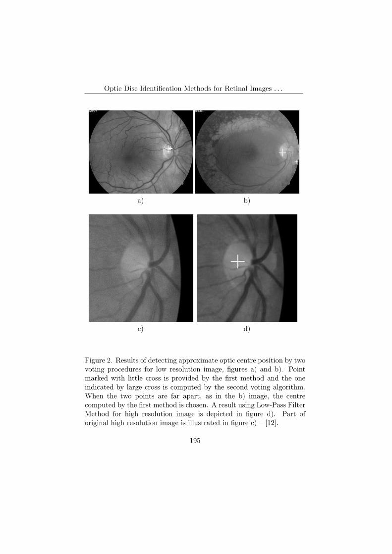
Optic Disc Identification Methods for Retinal Images . . .
a) b)
c) d)
Figure 2. Results of detecting approximate optic centre position by twovoting procedures for low resolution image, figures a) and b). Pointmarked with little cross is provided by the first method and the oneindicated by large cross is computed by the second voting algorithm.When the two points are far apart, as in the b) image, the centrecomputed by the first method is chosen. A result using Low-Pass FilterMethod for high resolution image is depicted in figure d). Part oforiginal high resolution image is illustrated in figure c) – [12].
195

F. Rotaru, S.I. Bejinariu, C.D. Nita, R. Luca, C. Lazar
and the magnitude result of the FFT transform was filtered by Gaus-sian low-pass filter (1). The filtered result was transformed back to thespatial domain. Using the histogram of the new image, noted I (i, j), abinarization threshold was computed. On each “bright” pixel (havinga grey value greater than the binarization threshold) a square win-dow of the same dimension as the one used in the channel selectionstep was centred. Then for every window centred in the “bright” pix-els, intensity pixel variance, noted V ar(i, j), was calculated. Also, forevery pixel I (i, j) a texture measure was computed, using the sametechnique, Modified Maximum Difference Method, presented at thebeginning of paragraph 2. A new image F (i, j), of normalized texturevalues, was created. Finally, the pixel O (m,n) of image I (i, j) withF (m,n) > F (i, j)
0≤i≤H−10≤j≤W−1
and V ar(m,n) > 0.7max (V ar(i, j)) was declared
as the centre of a window containing the optic disc.Results of the new identification optic disc area procedure are de-
picted in Figure 3. The original image is 3.a. The images I (i, j) andF (i, j) are illustrated by Figures 3.b and 3.c. Black pixels in Figure 3.care “dark” pixels of I (i, j) not considered as possible optic disc centrecandidates. The final result is depicted in Figure 3.d, where the crossindicates the centre of the working window in the selected channel.
Our previous methods to identify and model the optic disc pro-vided very good results on retinal images of patients in early stagesof ophthalmic pathologies as diabetic retinopathy or glaucoma. Testshave been made on three databases provided by our collaborators fromUMP, Iasi. We obtained good results also on images seriously affectedby ophthalmic pathologies [12], [13].
The method proposed in [13] was tested on more than 100 imagesfrom STARE database of an image selection based on optic disc visi-bility. The results were good on the majority of these images but onother ones the optic disc was not correctly localized. Another methodto segment the optic disc area was implemented based on the mainblood vessels convergence point identification in the green channel.
Based on a technique employed from [6], in a first step the vesseltree of the green channel was iteratively segmented. A line of 27 pixels
196

Optic Disc Identification Methods for Retinal Images . . .
a) b)
c) d)
Figure 3. Result of detecting approximate optic centre position. a)Original RGB image; b) Gaussian filtering result in frequency domainI(i, j); c) F (i, j) image, where black pixels are “dark” pixels of I(i, j);d) the cross indicates the working window centre – [13].
197

F. Rotaru, S.I. Bejinariu, C.D. Nita, R. Luca, C. Lazar
length and 1 pixel width was used as structuring element for an openingoperation applied on the green channel for 12 different orientations ofthe element:
IC = mini=1,...12
(γBi (I)) , (7)
where I is the input image, Bi is the structuring element and γBi (I) isthe result of the opening for orientation i of the structuring element.
Then, using IC as marker image and the green channel as maskimage a morphological reconstruction was performed:
IC = RI
(min
i=1,...12(γBi (I))
). (8)
An image containing only background (large homogenous areas) resultsfrom:
IB = maxi=1,...12
(γBi (I)) . (9)
Subtracting IB from IC an image containing only blood vessels is gen-erated:
IV = IC − IB. (10)
Then an Otsu binarization of the IV image is iteratively applied untilone of the vessel configurations is obtained: a) a vessel tree with a bigratio (number of white pixels)/(surrounding tree rectangle area) andwith surrounding tree rectangle area at least half of the input image;b) two big vessel branches as illustrated in Figure 4; c) a single largebranch with a low ratio (number of white pixels)/(surrounding treerectangle area) but with surrounding tree rectangle area at least halfof the input image.
For cases b) and c) the principal axis of the binarized vessels iscomputed. A search region is computed considering the distances toprincipal axis of the endpoints of the branches in two branch case orof the distances to principal axis of the parabola points in case c).
For configuration a) the search area was considered the minimumsurrounding rectangle. The search area for case b) is illustrated inFigure 5.
198

Optic Disc Identification Methods for Retinal Images . . .
a) b)
c) d)
Figure 4. Results of IV image binarization for two branch case. a) Ori-ginal image; b) first step binarization; c) second step binarization; d)final step binarization.
199

F. Rotaru, S.I. Bejinariu, C.D. Nita, R. Luca, C. Lazar
a) b)
c) d)
Figure 5. Search region for two branch case. a) original image; b) twofinal branches; c) search region in the working image; d) search regionin the green channel were the next step is to approximately find thedisc centre.
200
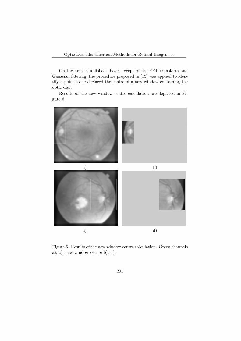
Optic Disc Identification Methods for Retinal Images . . .
On the area established above, except of the FFT transform andGaussian filtering, the procedure proposed in [13] was applied to iden-tify a point to be declared the centre of a new window containing theoptic disc.
Results of the new window centre calculation are depicted in Fi-gure 6.
a) b)
c) d)
Figure 6. Results of the new window centre calculation. Green channelsa), c); new window centre b), d).
201

F. Rotaru, S.I. Bejinariu, C.D. Nita, R. Luca, C. Lazar
3 Optic disc recognition
As in [1], [11], [12] and [13] the further work was done on a squarewindow centred on the optic centre candidate computed previously.The searching window side is a fraction of image height. The tests havebeen done on the green channel of the first two sets of retinal images(86 retinal images of 720 × 576 size and 40 images of 2592 × 1728resolutions), on chosen channel of the last set (300 of RGB retinalimages of 720 × 576 size) from our collaborators (UMP, Iasi) and on100 images from STARE database where the optic disc is visible.
Following the same technique employed in [6] in the establishedwindow I the blood vessels were eliminated (7).
Results of the vessels erasing operation are illustrated by Figure 7,for last set of retinal images received from our collaborators (UMP,Iasi).
a) b)
Figure 7. The result of vessels erasing. a) Selected channel b) Cleanedworking window – [13].
In order to perform a circle fitting the disc, edges have to be ex-tracted. This is done by applying on image IC an iterative Canny filterfollowed by binarisation. The same technique proposed in [12] and [13]
202

Optic Disc Identification Methods for Retinal Images . . .
was employed to do this:
1. Compute a binarization threshold using Otsu method, [9], onimage IC , without performing the binarization.
2. Choose a value close to Otsu threshold as a primary thresholdfor Canny filtering.
3. Perform Canny filtering.
4. If there are not enough white pixels (less than a predefined thresh-old) adapt the threshold for Canny filtering and resume processfrom step 3.
5. Compute rmin and rmax, the minimum and maximum values ofcircles radius, as fractions of the original image width.
6. For an interval [rmin, rmax] of circle radius compute a circle fittingby Hough transform applied on window pixels with grey levelclose to the window centre level.
7. Choose the centre radius with the best fitting score and bestdistribution of fitting points.
8. If the fitting score is not desirable or there are few points toperform the fitting, decrease the Canny threshold by a certainamount (constant in our implementation) and perform Cannyfiltering on IC and resume the process from step 6. Do this notmore than a predefined number of iterations.
9. If the detected circles have comparable fitting scores and fittingpoint distributions, choose the circle with the longest radius.
Canny filtering was done using the OpenCV function. Hough trans-form was performed by implementing our own method in order to getmore control on the distribution of the fitting points [12], [13]. Thedistance between the current fitted circle centre and the mass centreof the fitting points was used to evaluate the point distribution. In
203

F. Rotaru, S.I. Bejinariu, C.D. Nita, R. Luca, C. Lazar
this way some configurations can be rejected even they are generatedby an acceptable number of fitting points if the points are not equallydistributed around circle centre.
4 Results and conclusions
Tests have been done on two first sets of 86 RGB retinal images of720× 576 resolution and 40 images of 2592× 1728 resolution providedby our collaborators (UMP, Iasi). The method [13] to detect the opticdisc area worked well, with the same results as the one presented in[12]: the rough optic disc localization has been successful on both imagesets. The final circle fitting failed on two low resolution images stronglyaffected. Because the previous method [12] is faster we opted to keepit for the old sets and use the approach presented in [13] only for thelast set of 300 retinal images of 720 × 576 resolution. The optic disclocalization has been successful on 280 images of the last set. Thefinal circle fitting failed on 10 images of the 280 images previouslymentioned.
The last method based on vessel tree analysis was tested on theset of 300 RGB retinal images of 720× 576 size provided lately by ourcollaborators (UMP, Iasi) and on 100 images from STARE databasewhere the optic disc is visible. The new optic disc localization hasbeen successful on 282 images of the first set, a little bit better than theprevious method [13]. However, from 100 images chosen from STAREdatabase the method [13] failed to localize to optic disc area on 20images while the new method was successful on 90 STARE images.
Figure 8 illustrates some final circle localization results for imagesfrom the three sets from Grigore T. Popa University of Medicine andPharmacy Iasi and an image from STARE database.
The optic disk localization and modelling procedure was imple-mented and tested in an image processing framework developed byauthors. It is implemented as a Windows application, in C++ usingMicrosoft Visual Studio. For image manipulation and some processingfunctions, the OpenCV library is used.
204

Optic Disc Identification Methods for Retinal Images . . .
a) b)
c) d)
e) f)
205
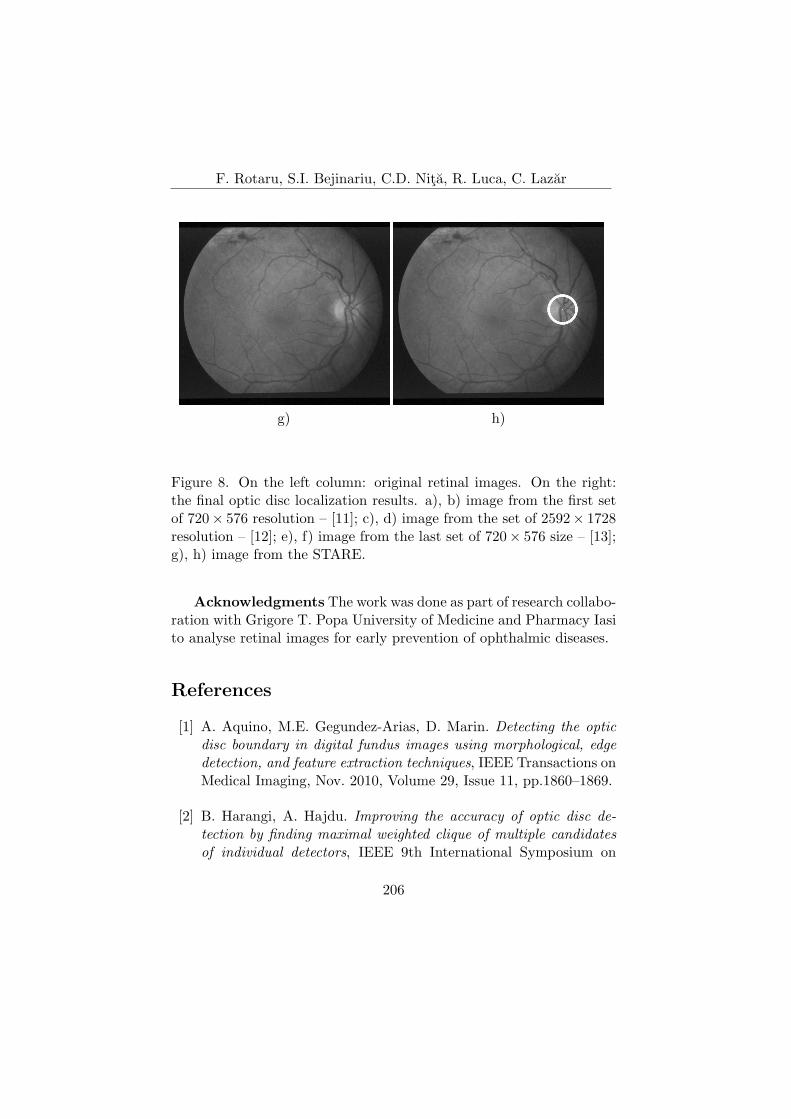
F. Rotaru, S.I. Bejinariu, C.D. Nita, R. Luca, C. Lazar
g) h)
Figure 8. On the left column: original retinal images. On the right:the final optic disc localization results. a), b) image from the first setof 720× 576 resolution – [11]; c), d) image from the set of 2592× 1728resolution – [12]; e), f) image from the last set of 720× 576 size – [13];g), h) image from the STARE.
Acknowledgments The work was done as part of research collabo-ration with Grigore T. Popa University of Medicine and Pharmacy Iasito analyse retinal images for early prevention of ophthalmic diseases.
References
[1] A. Aquino, M.E. Gegundez-Arias, D. Marin. Detecting the opticdisc boundary in digital fundus images using morphological, edgedetection, and feature extraction techniques, IEEE Transactions onMedical Imaging, Nov. 2010, Volume 29, Issue 11, pp.1860–1869.
[2] B. Harangi, A. Hajdu. Improving the accuracy of optic disc de-tection by finding maximal weighted clique of multiple candidatesof individual detectors, IEEE 9th International Symposium on
206
Optic Disc Identification Methods for Retinal Images . . .
Biomedical Imaging (ISBI2012), Barcelona, Spain, 2012, pp.602–605.
[3] B. Harangi, R.J. Qureshi, A. Csutak, T. Peto, A. Hajdu. Auto-matic detection of the optic disc using majority voting in a col-lection of optic disc detectors, IEEE 7th International Symposiumon Biomedical Imaging (ISBI 2010), Rotterdam, The Netherlands,2010, pp.1329–1332.
[4] H.Li, O. Chutatape. Automated feature extraction in color retinalimages by a model based approach, IEEE Transactions on Biomed-ical Engineering, Vol.51, No.2, February 2004.
[5] A. Hoover, M. Goldbaum. Locating the optic nerve in a retinalimage using the fuzzy convergence of the blood vessels, IEEE Trans.Med. Imag., vol. 22, no. 8, pp.951–958, Aug. 2003.
[6] C. Heneghan, J. Flynn, M. O’Keefe, M. Cahill. Characterization ofchanges in blood vessel width and tortuosity in retinopathy of pre-maturity using image analysis, Med. Image Anal., vol. 6, pp.407–429, 2002.
[7] M. Foracchia, E. Grisan, A. Ruggeri. Detection of optic disc inretinal images by means of a geometrical model of vessel structure,IEEE Trans. Med. Imag., vol. 23, no. 10, pp. 1189–1195, Oct. 2004.
[8] M. Lalonde, M. Beaulieu, L. Gagnon. Fast and robust optic diskdetection using pyramidal decomposition and Hausdorff-based tem-plate matching, IEEE Trans. Medical Imaging, Vol. 20, pp. 1193–1200, Nov. 2001.
[9] N. Otsu. A threshold selection method from gray-level histograms,IEEE Transactions on Systems, Man, and Cybernetics, Vol. 9, No.1, 1979, pp. 62–66.
[10] S. Ravishankar, A. Jain, A. Mittal. Automated feature extractionfor early detection of diabetic retinopathy in fundus images, CVPR– IEEE Conference on Computer Vision and Pattern Recognition,pp. 210–217, 2009.
207

F. Rotaru, S.I. Bejinariu, C.D. Nita, R. Luca, C. Lazar
[11] F. Rotaru, S. Bejinariu, C.D. Nita, M. Costin. Optic disc localiza-tion in retinal images, 5th IEEE International Workshop on SoftComputing Applications, 23-25 August, 2012, Szeged, Hungary,Soft Computing Applications – Advances in Intelligent Systemsand Computing Volume 195, 2013, Springer Verlag.
[12] F. Rotaru, S. Bejinariu, C.D. Nita, R. Luca. New optic disc local-ization method for retinal images, IEEE International Symposiumon Signal, Circuits and Systems, ISSCS 2013, 11-12 July 2013,Iasi, Romania.
[13] F. Rotaru, S. Bejinariu, C.D. Nita, R. Luca, C. Lazar. New opticdisc localization approach in retinal images, The 4th IEEE Inter-national Conference on E-Health and Bioengineering, EHB 2013,21-23 November 2013, Iasi, Romania.
[14] A. Sopharak, K. Thet Nwe, Y. Aye Moe, M. N. Dailey, B.Uyyanonvara. Automatic exudate detection with a naive Bayesclassifier, International Conference on Embedded Systems andIntelligent Technology, Grand Mercure Fortune Hotel, Bangkok,Thailand, pp.139–142, 2008.
[15] G.C. Manikis, V. Sakkalis, X. Zabulis, P. Karamaounas, A. Tri-antafyllow, S. Douma, Ch. Zamboulis, K. Marias. An ImageAnalysis Framework for the Early Assessment of HypertensiveRetinopathy Signs, Proceedings of the 3rd IEEE International Con-ference on E-Health and Bioengineering - EHB 2011, 24th-26thNovember, 2011, Iasi, Romania.
[16] Yanhui Guo. Computer-Aided Detection of Breast Cancer UsingUltrasound Images, PhD Thesis, Utah State University, 2010.
[17] D. Welfer, J. Scharcanski, C.M. Kitamura, M.M. DalPizzol. Seg-mentation of the optic disk in color eye fundus images using anadaptive, Comput Biol Med, vol. 40, no. 2, pp. 124–137, 2010.
208

Optic Disc Identification Methods for Retinal Images . . .
[18] K.W. Tobin, E. Chaum, V.P. Govindasamy, T.P. Karnowski. De-tection of anatomic structures in human retinal imagery, IEEETransactions on Medical Imaging 26 (12) (2007), pp.1729–1739.
[19] M. Park, J.S. Jin, S. Luo. Locating the optic disc in retinal images,Proceedings of the International Conference on Computer Graph-ics, Imaging, and Visualisation, IEEE, Sydney, Australia, 2006,pp.14–145.
[20] C. Sinthanayothin, J.F. Boyce, H.L. Cook, T.H. Williamson. Auto-mated localisation of the optic disc, fovea, and retinal blood vesselsfrom digital colour fundus images, British Journal of Ophthalmol-ogy 83 (1999), pp.902–910.
[21] A.A.-H.A.-R. Youssif, A.Z. Ghalwash, A.A.S.A.-R. Ghoneim. Op-tic disc detection from normalized digital fundus images by meansof a vessels’ direction matched filter, IEEE Transactions on Med-ical Imaging 27 (1) (2008) pp.11–18.
[22] J. Lowell, A. Hunter, D. Steel, A. Basu, R. Ryder, E. Fletcher, L.Kennedy. Optic nerve head segmentation, IEEE Transactions onMedical Imaging 23 (2) (2004), pp.256–264.
[23] M. Niemeijer, M.D. Abramoff, B.V. Ginneken. Segmentation ofthe optic disc macula and vascular arch in fundus photographs,IEEE Transactions on Medical Imaging 26 (2007), pp.116–127.
[24] A.D. Fleming, K.A. Goatman, S. Philip, J.A. Olson, P.F. Sharp.Automatic detection of retinal anatomy to assist diabetic retinopa-thy screening, Physics in Medicine and Biology 52 (2) (2007),pp.331–345.
[25] E.J. Carmona, M. Rincon, J. Garcıa-Feijoo, J.M.M.de-la Casa.Identification of the optic nerve head with genetic algorithms, Ar-tificial Intelligence in Medicine 43 (3) (2008), pp.243–259.
[26] C.A. Lupascu, D. Tegolo, L.D. Rosa. Automated detection of opticdisc location in retinal images, in: 21st IEEE International Sym-
209
F. Rotaru, S.I. Bejinariu, C.D. Nita, R. Luca, C. Lazar
posium on Computer-Based Medical Systems, IEEE, University ofJyvaskyla, Finland, 2008, pp. 17–22.
[27] T. Walter, J.-C. Klein, P. Massin, A. Erginay. A contributionof image processing to the diagnosis of diabetic retinopathy—detection of exudates in color fundus images of the human retina,IEEE Transactions on Medical Imaging, 21 (10) (2002), pp.1236–1243.
[28] A. Sopharak, B. Uyyanonvara, S. Barman, T.H. Williamson. Au-tomatic detection of diabetic retinopathy exudates from non-dilatedretinal images using mathematical morphology methods, Comput-erized Medical Imaging and Graphics, 32 (2008), pp.720–727.
Florin Rotaru, Silviu Ioan Bejinariu, Received June 2, 2014Cristina Diana Nita, Ramona Luca, Camelia Lazar
Institute of Computer Science, Romanian Academy,Iasi Branch, RomaniaE–mails: {florin.rotaru, silviu.bejinariu, cristina.nita, ramona.luca, camelia.lazar}@iit.academiaromana-is.ro
210
Computer Science Journal of Moldova, vol.22, no.2(65), 2014
Characterization and pattern recognition of
color images of dermatological ulcers:
a pilot study∗
Invited Article
Lucas C. Pereyra, Sılvio M. Pereira, Juliana P. Souza,Marco A. C. Frade, Rangaraj M. Rangayyan,
Paulo M. Azevedo-Marques
Abstract
We present color image processing methods for the charac-terization of images of dermatological lesions for the purpose ofcontent-based image retrieval (CBIR) and computer-aided diag-nosis. The intended application is to segment the images and per-form classification and analysis of the tissue composition of skinlesions or ulcers, in terms of granulation (red), fibrin (yellow),necrotic (black), callous (white), and mixed tissue composition.The images were analyzed and classified by an expert dermatolo-gist following the red-yellow-black-white model. Automatic seg-mentation was performed by means of clustering using Gaussianmixture modeling, and its performance was evaluated by derivingthe Jaccard coefficient between the automatically and manuallysegmented images. Statistical texture features were derived fromcooccurrence matrices of RGB, HSI, L∗a∗b∗, and L∗u∗v∗ colorcomponents. A retrieval engine was implemented using the k-nearest-neighbor classifier and the Euclidean, Manhattan, andChebyshev distance metrics. Classification was performed by
c©2014 by Lucas C. Pereyra, Sılvio M. Pereira, Juliana P. Souza, Marco
A. C. Frade, Rangaraj M. Rangayyan, Paulo M. Azevedo-Marques.∗This work was partially supported by The National Council for Scientific and
Technological Development (CNPq) — grants 472508/2010-5, 304225/2010-0, and573714/2008-8 (INCT/INCoD), and the Natural Sciences and Engineering ResearchCouncil of Canada.
211

Pereyra et al.
means of a metaclassifier using logistic regression. The aver-age Jaccard coefficient after the segmentation step between theautomatically and manually segmented images was 0.560, witha standard deviation of 0.220. The performance in CBIR wasmeasured in terms of precision of retrieval, with average valuesof up to 0.617 obtained with the Chebyshev distance. The meta-classifier yielded an average area under the receiver operatingcharacteristic curve of 0.772.
Keywords: Color image processing, color medical images,color texture, content-based image retrieval, computer-aided di-agnosis, image segmentation, dermatological ulcers, tissue com-position analysis.
1 Introduction
1.1 Computer-Aided Analysis of Medical Images
Recent developments in information and communication technologieshave led to the creation and use of huge archives of multimedia datain diverse application areas, such as medical imaging, remote sensing,entertainment, education, and online information services. Traditionaldatabase management systems were designed to organize alphanumericdata into interrelated collections so that information storage and re-trieval could be performed conveniently and efficiently. However, suchmethods are not well suited for the organization, management, andefficient use of multimedia information [1]. In many practical appli-cations, the retrieval of a specific image from a database of imagescould be an important task [2]. Several search engines are availablefor searching and retrieval of textual and pictorial information [2–5].However, general-purpose tools for searching and retrieval of data arenot suitable for specialized medical applications. For this reason, spe-cific methods and systems for the characterization, searching, and re-trieval of image-based data are being developed for particular medicalimaging applications [6, 7], such as mammography [8–11], chest andother radiographic imaging [12,13], dermatological lesions [14–17], andpathology [18].
212

Characterization of Dermatological Ulcers . . .
The traditional approach of indexing images using manual notes(textual annotation) is slow, labor-intensive, and expensive. In addi-tion, textual annotations cannot effectively encode all of the informa-tion available in a given image. Furthermore, image features based onhuge amounts of pixel data, complex concepts of application-specificpatterns, and domain-specific notions may not lend themselves to easyor efficient textual description. Thus, there is a need to develop ad-vanced methods of image processing, feature extraction, quantitativerepresentation, and pattern recognition for effective and efficient inde-xing and retrieval of images based on their content.
Content-based image retrieval (CBIR) refers to searching, selection,and retrieval of images from a database that are similar to a query im-age, using measures of information derived from the images themselves,rather than relying on the accompanying text or annotation [6,19]. Tofacilitate CBIR, the contents of the images need to be characterizedby quantitative features. The features of the query image may thenbe compared with the features of each image in the database, and im-ages having high similarity with respect to the computed features ofthe query image may be retrieved and displayed [19]. CBIR of medicalimages is a useful tool, and could provide physicians with assistance inthe form of a display of relevant past cases with proven pathology, alongwith the associated clinical, diagnostic, and other information [19].
The potential use of automated image categorization techniques toassist physicians in diagnosis led to intense research in the field of med-ical image processing classification [19–21]. This approach usually con-sists of mapping images into predefined classes and involves the stepsof representation (description of image content by feature extraction),adaptation (selection of the most representative subset of features toclassify information) and, generalization (the training and evaluationof a classifier) [19,21,22].
The same steps mentioned above may also be used to assist inclinical decision making and lead towards computer-aided diagnosis(CAD) [19,21,23]. The medical domain has specific requirements (highsensitivity and low false-negative as well as false-positive rates) anderrors in detection are extremely costly, making the development of a
213

Pereyra et al.
computerized scheme to aid diagnosis with broad application in clinicalpractice a challenge [19,20].
1.2 Analysis of Dermatological Ulcers
Ulcers on the lower limbs can be described as the irregular loss of theepidermis, also possibly involving the dermis and subcutaneous tissue.They affect approximately 1% of the population, causing considerablemorbidity [24]. This condition is usually ascribed to a deficiency inblood flow due to venous or arterial insufficiency, and can be causedby ailments such as diabetes mellitus, autoimmune diseases, and localinfections. The ulceration may be referred to as a wound, lesion, orulcer, and medical professionals in dermatology base the diagnosis ofskin lesions mainly on visual assessment of pathological regions andthe evaluation of macroscopic features. This fact indicates that correctdiagnosis is highly dependent on the observer’s experience and visualperception [16, 25]. Accurate wound assessment is a critical task inpatient care and important for the reduction of costs of care in hospi-tals. However, this task still relies on manual procedures and tediouspractices. Wound shape is measured with rulers and tracing paper, orrarely with alginate castings and serum injection.
Healing is a complex cascade of cellular events operating to recon-struct damaged tissues, and also an individual process that exhibitsconsiderable interpatient variability. As the different tissues may over-lap and be difficult to distinguish, wound assessment is not straightfor-ward. The lack of quantitative data affects the coordination of health-care staff and hinders clinical studies focused on healing. Digital ca-meras, though now widespread in clinical centers, are used mostly forbasic patient data recording and not image processing [17].
The appearance of a wound, lesion, or ulcer provides importantclues that can help with the diagnosis, determination of severity, andthe prognosis of healing [26, 27]. Chronic skin lesions, wounds, or ul-cers typically have a nonuniform mixture of red granulation, yellowfibrin (slough), and black necrotic scar tissue. Thus, a red-yellow-black (RYK) model is used by physicians in a descriptive manner[15, 17, 26–29]. In clinical assessment, the category of callous lesions,
214
Characterization of Dermatological Ulcers . . .
composed predominantly of white tissue, is also used. Therefore, anextended version of the RYK model, including white (RYKW) one,may be of interest. The quantification of texture and color distributionin lesions by image processing techniques could assist in the analysis ofthe dynamics of the pathological process, as well as of healing and res-ponse to treatment [17, 27, 29, 30]. Such quantitative analysis, in turn,can be used to design optimized and personalized treatment protocolsfor each patient.
In a clinical scenario, the possibility of retrieving images from anestablished database that are similar to the case on hand, based ondigital image processing techniques that characterize the color com-position of lesions, could facilitate understanding how dermatologicallesions are classified and assist in arriving at a diagnostic or therapeuticdecision. In this context, efficient systems for content-based indexingand retrieval [6, 27, 31], as well as methods to perform classification ofwounds based on the types of tissue present in the wound are usefuland could help health professionals assess lesions for any of the afore-mentioned purposes.
Celebi et al. [32] described a system to retrieve skin lesion imagesbased on shape similarity, using a database with 184 skin ulcerationimages in cases of melanoma. The agreement between computer as-sessment and human perception was indicated by values of up to 0.73,when similarity functions were optimized using a genetic algorithm.Dorileo et al. [14] proposed a CBIR system for images of dermatologiculcers. Features based on histogram and multispectral cooccurrencematrices were used for image retrieval. Performance was evaluatedbased on precision values with a database of 215 images. The best pre-cision result was 70% for mixed tissue composition images. Rahmanet al. [33] presented a CBIR system for dermatoscopic images. Imageprocessing, segmentation, feature extraction (color and texture), andsimilarity matching were performed on a database comprising 358 im-ages of pigmented skin lesions in three categories (benign, dysplasticnevi and, melanoma). The analysis of precision curves displayed theability of their system to retrieve visually similar lesions with an aver-age precision value of 60%.
215

Pereyra et al.
The variability and inhomogeneity of tissues makes color analysisfor tissue classification innefective if the methods are applied directlyon the pixels with simple thresholds on separate color components.Spatial continuity needs to be incorporated, which suggests that theclassification process should be guided by a segmentation step [34].Color histograms are commonly utilized as descriptors for statisticaldata analysis [35], and the use of hybrid tissue classes and limitingclassification to a reduced number of tissue types have also been re-ported, with an average accuracy of 88.7% using a k-nearest-neighbor(kNN) classifier [29].
In previous related work, we evaluated the performance of differentdistance metrics for CBIR of dermatological images [31]. A database of172 manually segmented images was used. CBIR using a kNN classi-fier and the Euclidean, Manhattan, Chebyshev, cosine, and correlationdistances was performed. The best results were obtained with the co-sine and correlation distances, with average precision of 75%. We alsoperformed automatic segmentation using methods of color clusteringand mathematical morphology [36]. The same database of 172 imageswas used. The average Jaccard coefficient between automatically andmanually segmented regions was 0.56, with a standard deviation of0.22.
The present work, which is an expanded and updated version ofrecent conference presentations [31, 36], focuses on quantitative as-sessment of color components in images of ulcers on the lower limbs.We present techniques to perform analysis of color components, tex-ture analysis, and automatic segmentation. Results are presentedand discussed in the context of CBIR and computer-aided diagnosisCAD [15–17,27,28,30,31,36].
2 Materials and Methods
2.1 Database of Images
A database consisting of 172 dermatologic images has been preparedto date, based on 63 consecutive medical examinations of outpatients
216

Characterization of Dermatological Ulcers . . .
at the University Medical Center at the Ribeirao Preto Medical Schoolof the University of Sao Paulo, Brazil. Approval was obtained fromthe Medical Center Ethics Committee for this research. Images wereobtained based on a specific protocol that was determined after initialtests [14]. All images were obtained with the same digital camera(Canon EOS 5D0, 2 Megapixels), a 50-mm macro lens, and a pola-rization filter; see Figure 1 for examples of images of various typesof ulcers. The typical size of the color images is 1747×1165 pixelswith 24 bits/pixel. The tissue composition of each lesion was classifiedindependently by an expert dermatologist (MACF), based on the colorcomposition, as granulation (red), fibrin (yellow), and mixed tissue.The 172 images in the database include 51 images of lesions predomi-nantly composed of granulation, 31 images of fibrin, three images ofcallous, three images of necrotic, and 84 images of mixed tissue. Thedermatologist also drew the boundaries of the lesions.
A blue cloth was used to create a background in a color not ex-pected within the ulcer or on the part of the body being imaged, ascan be seen in Figure 1, parts (c) and (d). Color patches and rulerswere included in the images (see Figure 1) to facilitate color normali-zation and calibration of the images. A suite of color image processingtechniques, pattern analysis, classification methods, and graphical userinterfaces (GUIs) is being developed to facilitate image analysis, CAD,and CBIR [14,27,28,31,37].
2.2 Automatic Segmentation of the Ulcer Region
A color clustering process using an expectation maximization (EM)procedure based on a multivariate Gaussian mixture model [37,38] wasapplied to each hue-saturation (HS) histogram [39]. The EM algorithmimplemented in the present work is an iterative method for findingmaximum-likelihood or maximum-a-posteriori (MAP) estimates of pa-rameters in statistical models. The EM iteration alternates betweenperforming an expectation (E) step, which creates a function for the ex-pectation of the log-likelihood evaluated using the current estimate forthe parameters, and a maximization (M) step, which computes param-
217

Pereyra et al.
Figure 1. Examples of images of various types of ulcers: (a) pre-dominantly granulation, (b) predominantly fibrin, (c) predominantlynecrotic tissue, and (d) mixed tissue composition.
eters maximizing the expected log-likelihood found in the E step. Theinitialization assumes that the whole set of values in the HS histogramcan be clustered into just one Gaussian distribution. This hypothesisis tested based on the values of the mean and standard deviation ofa sample of 1,000 values obtained randomly from the HS histogram,considering an estimation error of 0.0001%. If the hypothesis is nottrue, that is, if the Gaussian adjustment error for the sample is greaterthan the specified error, a new iteration is performed, assuming themixture of two Gaussians. The procedure is iterated until every pixelin the sample belongs to a cluster, or the number of iterations reachesa specified limit (100 cycles). The clustering procedure was developedusing the Waikato Environment for Knowledge Analysis (WEKA) [41].
218

Characterization of Dermatological Ulcers . . .
After color clustering, the set of clusters representing the tissue com-position of the ulcer was manually selected. A GUI was implementedusing the Java programming language and the NetBeans1 environmentto facilitate cluster selection. To fill any residual gap, a method basedon mathematic morphology and automatic delineation of the convexhull was implemented using ImageJ plugins and applied to determinethe final lesion area. The convex hull is defined as the smallest con-vex polygon that encompasses a set of points [42]. Figure 2 showsan example of an image of an ulcer and the corresponding result ofsegmentation.
Figure 2. Example of ulcer segmentation. The clustering process re-sulted in six clusters (e) to (j). (a) shows the original image, (b) thesegmentation mask generated by manual cluster selection followed byapplication of mathematic morphology operations, (c) is the partialsegmented area, and (d) is the final lesion area after automatic delin-eation of the convex hull.
1https://netbeans.org/. Accessed on 01/04/2014.
219

Pereyra et al.
2.3 Feature Extraction and Indexing of Images
Feature extraction was based on the automatically segmented regions.For each region representing a lesion, in addition to the basic RGB colorcomponents, six images were generated. According to the HSI repre-sentation, an image (I) was generated based on the hue (H) componentand another was generated based on the saturation (S) component [39]:
I = R+G+B3
,
S = 1−(
3(R+G+B)
)∗ a,
where a is the minimum of R, G, and B,
H = cos−1 (0.5∗(R−G)+(R−B))(((R−G)2+(R−B)(G−B))
0.5) .
The next color representations are based on the CIE XYZ colorspace. The conversion from RGB to XYZ is performed as follows [40]:
[R][G][B]
=[3.240479 − 1.537150 − 0.498535]
[−0.969256 1.875992 0.041556][0.055648 − 0.204043 1.057311]
∗[X][Y ][Z],
x = X(X+Y +Z) ,
y = Y(X+Y +Z) .
According to the L∗u∗v∗ color representation, an image was gener-ated based on the u∗ component and another was generated based onthe v∗ component:
220

Characterization of Dermatological Ulcers . . .
u′ = 2x(6y−x+1.5) ,
v′ = 4.5y(6y−x+1.5) ,
L∗
116(
YYn
) 13 − 16 if Y
Yn> 0.008856,
903.3(
YYn
)if Y
Yn≤ 0.008856,
u∗ = 13 (L∗)(u′ − u
′n
),
v∗ = 13 (L∗)(v′ − v
′n
).
Similarly, according to the L∗a∗b∗ color representation, an imagewas generated based on the a∗ component and another was generatedbased on the b∗ component:
L∗
116(
YYn
) 13 − 16 if Y
Yn> 0.008856,
903.3(
YYn
)if Y
Yn≤ 0.008856,
a∗ = 500 ∗ (f (X/Xn)− f (Y/Yn)),
b∗ = 200 ∗ (f (Y/Yn)− f (Z/Zn)),
where f (t) =
{t
13 if t ≤ 0.008856,
7.787 ∗ t + 16/116 if t ≤ 0.008856.
Values of the mean, standard deviation, skewness, and kurtosis werecomputed from the histogram of each of the R, G, B, H, S, u∗, v∗, a∗,
221

Pereyra et al.
and b∗ components. In addition, the five most discriminative featuresof the 14 texture features proposed by Haralick et al. [43] were de-rived from an averaged cooccurrence matrix (CoM) computed fromfour CoMs for a distance of one pixel at 0, 45, 90, and 135 degrees.The features are homogeneity, contrast, correlation, entropy, and lo-cal homogeneity, as suggested by Conners and Harlow [44], and werecomputed for each of the R, G, B, H, S, u∗, v∗, a∗, and b∗ compo-nents. Furthermore, the five texture features mentioned above werecomputed from multispectral or color cooccurrence matrices (CCMs),obtained from the RG, GB, BR, HS, u∗v∗, and a∗b∗ components, usingthe method proposed by Arvis et al. [45]. The method is an extension ofthe method of Haralick et al. [43], and was developed for application tocolor images to take into account the correlation existing between thecolor components, as shown in Figure 3. Thus, a total of 111 featureswere extracted from the R, G, B, H, S, u∗, v∗, a∗, and b∗ componentsto characterize and index each color image [27,31,36].
Figure 3. Color cooccurrence matrices (CCMs) obtained from theRGB, HS, u∗v∗, and a∗b∗ components
222

Characterization of Dermatological Ulcers . . .
2.4 CBIR Experiment
A retrieval engine was developed using the kNN classifier based on theEuclidean, Manhattan, and Chebyshev metrics between the featuresof the query image and those of each image in the database. Thedefinitions of the metrics are summarized in Table 1. The value of kwas varied from 1 to 7 in steps of 2.
Table 1. Distance metrics used in CBIR experiments. In the equations,x is the feature vector of size n of the query image, y the feature vectorof size n of an image being considered for retrieval, and dxy is thedistance between the two vectors.
Metric Name Formula
Euclidean dxy =√∑n
j=1 (xj − yj)2
Manhattan dxy =∑n
j=1 |xj − yj |Chebyshev dxy = maxn
j=1 {|xj − yj |}
For every value of k, all images in the database were used, one byone, as the query image. The mean value of the precision of retrievalwas computed for each retrieval experiment and for each distance ormetric. Precision values for the categories of necrotic and callous ulcerswere not computed due to the small numbers of samples available. Theprecision of retrieval was computed in each experiment as the ratio ofthe number of relevant images retrieved to the total number of im-ages retrieved. In computing precision, each retrieved image receiveda binary weight of unity or zero, representing a relevant image or not,respectively; the sum of such scores for all of the retrieved images wasthen divided by the total numbers of retrieved images. Ten-fold crossvalidation was the chosen validation method. An image was conside-red to be relevant when it belonged to the same class as the queryimage, according to the classification provided independently by theexpert dermatologist (MACF). It should be noted that, in a medicalapplication, a clinician would not be interested in the retrieval of alarge number of images or cases. A small number of highly relevant
223

Pereyra et al.
cases, such as 3 or 5 cases, retrieved from a large database along withthe related clinical reports, would serve the purpose of assisting in thediagnosis of the current query case. It would not be of interest toretrieve all relevant cases that exist in the database. Thus, in a clinicalapplication, precision would be, in general, more important than othermeasures of performance of CBIR, such as recall or area under theprecision-versus-recall curve.
2.5 Classification Experiment
Classification of images was performed by means of a metaclassifier forhandling multiclass datasets with two-class classifiers, as a proxy to themain classifier which it wraps to provide additional data preprocessingbefore actually training and/or testing of the wrapped classifier. Logis-tic regression was used as the wrapped classifier. In order to improvethe parameters of the estimates and reduce the prediction error, ridgeestimators are used to pool highly correlated covariates and reduceoverfitting and colinearity [46]. The classification experiment did notinclude the categories of necrotic and callous ulcers due to the smallnumber of samples available. Validation was also performed using ten-fold cross validation.
3 Results
3.1 Automatic Segmentation of the Ulcer Region
The Gaussian mixture modeling procedure applied to 172 images re-sulted in a clustering process with the number of clusters varying from3 to 9, before the manual selection step using the GUI. Processingtimes for the clustering process ranged from 3 to 5 minutes per image.After cluster selection, the evaluation of the segmentation step indi-cated an average Jaccard coefficient of 0.56 with a standard deviationof 0.22 between the lesion area obtained computationally and the samelesion region manually delineated by the dermatologist. The Jaccardcoefficient (J) is calculated by computing the ratio of the intersection
224

Characterization of Dermatological Ulcers . . .
to the union of the manually and computationally derived regions andhas a value range from zero to one, where zero means a total failureof the computational segmentation process and one indicates a per-fect segmentation, based on comparison with the manually segmentedregions:
J (A,B) = |A∩B||A∪B| .
3.2 Analysis of Tissue Composition and Classification ofUlcers
To compare the tissue composition within the lesion regions segmentedcomputationally and manually, a measurement approach was appliedbased on thresholding of HSI values [31,36,39]. White tissue componentwas defined as the number of pixels within the lesion with S ≤ 0.2and I ≥ 0.75 (independent of H and with the S and I componentsnormalized to the range 0 to 1); black tissue component was defined asthe number of pixels within the lesion with S ≤ 0.2 and I ≤ 0.2; redtissue component was defined as the number of pixels within the lesionwith S > 0.2 and −30◦ < H < 30◦ (independent of I); and yellowtissue component was defined as the number of pixels within the lesionwith S > 0.2 and 30◦ < H < 90◦. A low average root-mean-squarederror (RMSE) [36] of 4% with a standard deviation of 5% was obtainedbetween the RYKW tissue composition vectors of computationally andmanually segmented lesions.
Classification results with the metaclassifier using logistic regres-sion were analyzed in terms of correctly classified instances and theaverage area under the receiver operating characteristic curve (AUC).The ratio between the number of correctly classified instances and thetotal number of instances was 0.638, and the average AUC value was0.772. The processing time using all the images from the dataset wasless than 3 seconds.
225

Pereyra et al.
3.3 CBIR
Based on the retrieval experiments performed using different distancemeasures, precision values were calculated for each image class andan average precision value was derived. The Processing time was lessthan 1 second for all CBIR experiments. The most significant distanceregarding precision values was the Chebyshev distance. For k = 1,the average precision was 0.617 (as compared to 0.587 and 0.550 us-ing Manhattan and Euclidean distances, respectively), and for k = 3,the average precision was 0.609 (as compared to 0.566 and 0.538 us-ing Manhattan and Euclidean distances, respectively). The rates ofprecision for values of k = 5 and 7 were lower than those previouslymentioned, for all of the distances considered in this study. Tables 2and 3 display the confusion matrices for the kNN procedure with k = 1and 3 and using the Chebyshev distance, respectively.
Table 2. Confusion matrix for the CBIR experiment, using a kNNclassifier with k = 1 and the Chebyshev distance.
Red Yellow Mixed Retrieved for31 3 17 Red3 20 8 Yellow26 8 50 Mixed
Table 3. Confusion matrix for the CBIR experiment, using a kNNclassifier with k = 3 and the Chebyshev distance.
Red Yellow Mixed Retrieved for30 5 16 Red9 15 7 Yellow24 6 54 Mixed
226

Characterization of Dermatological Ulcers . . .
4 Discussion
Assessment of tissue composition provides crucial information to mon-itor the effects of treatment in patients with chronic ulcers. Quanti-tative measures can contribute to objective assessment of the healingprocess, and may be used for pattern recognition, CAD, and CBIR.Pattern recognition focuses on the classification of ulcers based on tis-sue composition to help enhance the diagnostic process and follow-upto treatment. CBIR is an approach to information retrieval and ismore commonly used for medical decision-making based on previousand proven cases. If the results of a CBIR query bring images withone or more types of tissue composition, the clinician will be able toanalyze them, determine which images are relevant, review the clinicalreports associated with the retrieved images, and decide on the diag-nostic classification of the image on hand. The clinician could also gainan understanding on why some of the retrieved images were classifiedinto certain categories, either by an expert dermatologist or by theCBIR process. In this manner, the CBIR system could assist in arriv-ing at a decision when the image on hand is at the boundaries betweendifferent categories. The concept of similarity is important because notwo images may be expected to be identical, even when belonging tothe same diagnostic category, and a perfect or exact match to a queryimage is unlikely. The use of vectors of quantitative parameters orfeatures to index images facilitates the application of simple distancemeasures to select images that are most similar to the query sample,that is, to evaluate the similarity between images. Classification andCBIR applications may share the same set of image processing proce-dures, such as preprocessing, image segmentation, feature extraction,and categorization [11,19,21].
In a previous work based on the same images of manual segmen-tation of the ulcers by an experienced dermatologist [27], we obtainedaverage AUC values of 0.820, and an average value of correctly classi-fied instances divided by the total number of instances of 0.738. Resultsusing automatic segmentation were observed to be poorer than thoseusing manually segmented images. Therefore, our efforts to perform
227

Pereyra et al.
automatic segmentation have yielded poorer results in terms of correctclassification, which indicates that further improvements are needed.Nonetheless, our results of classification using a metaclassifier (averageAUC value of 0.772) are encouraging.
Limitations of this work reside in the difficulty in applying the im-aging protocol in a consistent manner. The images were not acquiredin laboratory facilities, but in a clinical environment. In some cases,the patient’s mobility affected positioning and imaging of the ulcers.Such difficulties also affected the distance and orientation of the cam-era, the illumination of the ulcer and the composition of the image.Procedures for color correction and normalization of images [39] needto be incorporated.
Another difficulty related to the current database is the variationof the size and position of the ulcers. It was observed that the cluste-ring procedure tends to give better results when the ulcers are small,properly centered in the image, and without significant curvature. Insuch a situation, the number of Gaussians obtained by the clusteringprocedure was usually small, in the range of 3 to 5.
The segmentation results obtained in this pilot study have loweraccuracy than desired, but are encouraging. Although the results arenot very good in terms of the Jaccard coefficient, the small value ob-tained for the RMSE indicates that the estimation of tissue compositionwas not substantially affected by the limitations of the segmentationprocess. To improve the segmentation results, it would be desirableto include procedures for comparative analysis of an ulcer region withreference to the color characteristics of the surrounding normal skinof the patient. Further work is planned with a larger database of im-ages, especially for the callous and necrotic categories of lesions, andalso including longitudinal series of images of the same patients undertreatment.
Clinical interpretation of images of dermatological ulcers is com-monly based on visual analysis of the tissue composition as indicatedby their color characteristics. This, however, is a qualitative approachthat is affected by interobserver and intraobserver variability. Accurateestimation of the fractional composition of an ulcer in terms of tissue
228

Characterization of Dermatological Ulcers . . .
types, such as granulation and fibrin, is nearly impossible via visualanalysis. Quantitative evaluation of tissue composition provides keyinformation for monitoring the response to treatment of patients withchronic ulcers and can assist in the evaluation of the healing process.In the present study, we have proposed the potential use of methodsof digital image processing to achieve image segmentation focused onfacilitating the characterization of the tissue composition of skin ulcers.We believe that objective analysis of color images of skin ulcers usingthe proposed methods can overcome some of the limitations of visualanalysis and lead to the development of improved protocols for thetreatment and monitoring of chronic dermatological lesions. Such ad-vances, in turn, can assist in the design of optimized and personalizedtherapy for each patient.
References
[1] T. Chaira, A. K. Ray. Fuzzy measures for color image retrieval.Fuzzy Sets and Systems, 150:545–560, 2005.
[2] P. Welter, T. Deserno, B. Fischer, R. Gunther, C. Spreckelsen. To-wards case-based medical learning in radiological decision makingusing content-based image retrieval. BMC Medical Informatics andDecision Making. 11(1):68:1–16, 2011.
[3] J. Z. Wang, J. Li, G. Wiederhold. SIMPLIcity: Semantics-Sensitive Integrated Matching for Picture Libraries. IEEE Tran-sactions on Pattern Analysis and Machine Intelligence. 23(9):947–963, 2001.
[4] Q. Iqbal, J.K. Aggarwal. CIRES: A system for content-based re-trieval in digital image libraries. International Conference on Con-trol, Automation, Robotics and Vision (ICARCV), Singapore,1:205-210, December 2–5, 2002.
[5] J. Ruiz-del-Solar, P. Navarrete. FACERET: An interactive faceretrieval system based on self-organizing maps. In Image and Video
229

Pereyra et al.
Retrieval - Lecture Notes in Computer Science, Springer, Berlin,Germany, 45–64, 2002.
[6] H. Muller, N. Michoux, D. Bandon, A. Geissbuhler. A reviewof content-based image retrieval systems in medical applications:clinical benefits and future directions. International Journal ofMedical Informatics, 73:1–23, 2004.
[7] H. Muller, A. Rosset, J. Vallee, F. Terrier, A. Geissbuhler. A refer-ence data set for the evaluation of medical retrieval systems. Com-puterized Medical Imaging and Graphics. 28:295–305, 2004.
[8] I. El-Naqa, Y. Yang, N. P. Galatsanos, R. M. Nishikawa, M. N.Wernick. A similarity learning aprroach to content-based imageretrieval: application to digital mammography. IEEE Transactionson Medical Imaging. 23(10): 1233–1244, 2004.
[9] S. K. Kinoshita, P. M. Azevedo-Marques, R. R. Pereira Jr., J. AH. Rodrigues, R. M. Rangayyan. Content-based retrieval of mam-mograms using visual features related to breast density patterns.Journal of Digital Imaging. 20(2): 172–190, 2007.
[10] D. Tahmoush. CBIR for mammograms using medical image simi-larity. Medical Imaging 2010: Advanced PACS-based Imaging In-formatics and Therapeutic Applications. Edited by B. J. Liu, W.W. Boonn. Proceedings of the SPIE. 7628(1):76280A 1–9, 2010.
[11] H. Alto, R.M. Rangayyan, J. E. L. Desautels. Content-based re-trieval and analysis of mammographic masses. Journal of Elec-tronic Imaging. 14(2):023016:1–17, 2005.
[12] C. R. Shyu, C. E. Brodley, A.C. Kak, A. Kosaka, A. M. Aisen, L. S.Broderick. ASSERT: A physician-in-the-loop content-based imageretrieval system for HRCT image databases. Computer Vision andImage Understanding (Special Issue on Content-based Retrievalfrom Image Databases). 75(1/2): 111–132, 1999.
230

Characterization of Dermatological Ulcers . . .
[13] M. C. Oliveira, W. Cirne, P. M. Azevedo-Marques. Towards ap-plying content-based image retrieval in the clinical routine. FutureGeneration Computer Systems. 23:466–474, 2007.
[14] E. A. G. Dorileo, M. A. C. Frade, A. M. Roselino, R. M. Ran-gayyan, P. M. Azevedo-Marques. Color image processing andcontent-based image retrieval techniques for the analysis of der-matological lesions. In: Proc. 30th Annual International Confe-rence of the IEEE Engineering in Medicine and Biology Society,Vancouver, BC, Canada. pages 1230–1233, August, 2008.
[15] L. Ballerini, X. Li, R. B. Fisher, J. Rees. A query-by-examplecontent-based image retrieval system of non-melanoma skin le-sions. In: Proc. International Conference on Medical ImageComputing and Computer Assisted Intervention, London, UK,5853:31–38, September, 2009.
[16] H. H. W. J. Bosman, N. Petkov, M. Jonkman. Comparison of colorrepresentations for content-based image retrieval in dermatology.Skin Research and Technology. 16:1–5, 2009.
[17] H. Wannous, S. Treuillet, Y. Lucas. Robust tissue classificationfor reproducible wound assessment in telemedicine environments.Journal of Electronic Imaging. 19(2):023002, 2010.
[18] J. Z. Wang. Pathfinder: multiresolution region-based searching ofpathology images using IRM. In Proceedings of the AMIA Sympo-sium, Los Angeles, CA, pp. 883887, November 4–8, 2000.
[19] P. M. Azevedo-Marques, R.M. Rangayyan. Content-based Re-trieval of Medical Images: Landmarking, Indexing and, RelevanceFeedback. Synthesis Lectures on Biomedical Enginering. Lecture#48, Morgan & Claypool, 2013.
[20] M. Antoine, O. R. Zaiane, A. Coman. Application of data mi-ning techniques for medical image classification. Proceedings ofthe Second International Workshop on Multimedia Data Mining,MDM/KDD, 2001:94–101, San Francisco, CA, August 26, 2001.
231

Pereyra et al.
[21] R. M. Rangayyan. Biomedical Image Analysis, CRC Press, BocaRaton, FL, 2005.
[22] T. M. Lehman, M. O. Guld, T. Deselaers, D. Keysers, H. Schu-bert, K. Spitzer, H. Ney, B. B. Wein. Automatic categorization ofmedical images for content-based image retireval and data mining.Computerized Medical Imaging and Graphics. 29:143–155, 2005.
[23] K. Doi. Computer-aided diagnosis in medical images: Historicalreview, current status and future potential. Computerized MedicalImaging and Graphics. 31:198–211, 2007.
[24] M. J. Callam, C. V. Ruckley, D. R. Harper, J. J. Dale.Chronic ulceration of the leg: extent of the problem and provi-sion of care. British Medical Journal (Clinical Research Edition).290(6485):1855–1856, 1985.
[25] I. Maglogiannis, S. Pavlopoulos, D. Koutsouris. An integrated com-puter supported acquisition, and characterization system for pig-mented skin lesions in dermatological images. IEEE Transactionson Information Technology in Biomedicine. 9:86–98, March, 2005.
[26] H. Oduncu, A. Hoppe, M. Clarck, R. J. Williams, K. G. Harding.Analysis of skin wound images using digital color image processing:a preliminary communication. The International Journal of LowerExtremity Wounds. 3(3):151–156, 2004.
[27] S. M. Pereira, M. A. C. Frade, R. M. Rangayyan, P. M. Azevedo-Marques. Classification of color images of dermatological ulcers.IEEE Journal of Biomedical and Health Informatics. 17(1):136–142, 2013.
[28] E. A. G. Dorileo, M. A. C. Frade, R. M. Rangayyan, P. M.Azevedo-Marques. Segmentation and analysis of the tissue com-position of dermatological ulcers. Proceedings of the Symposiumof the IEEE Canadian Conference on Electrical and ComputerEngineering, 1:1–4, Calgary, AB, Canada, May, 2010.
232

Characterization of Dermatological Ulcers . . .
[29] H. Zheng, L. Bradley, D. Patterson, M. Galushka, J. Winder. Newprotocol for leg ulcer tissue classification from colour images. Pro-ceedings of the 26th Annual International Conference of the IEEEEngineering in Medicine and Biology Society, San Francisco, CA,1:13891392, September 1–4, 2004.
[30] A. S. Tarallo, A. Gonzaga, M. A. C. Frade. Artificial neural net-works applied to the segmentation and classification of digital im-ages of cutaneous ulcers. Proceedings of the IEEE 7th Interna-tional Conference on Bioinformatics and Bioengineering, 1:1–1,Boston, MA, October 14-17, 2007.
[31] S. M. Pereira, M. A. C. Frade, R. M. Rangayyan, P. M. Azevedo-Marques. Recuperao de imagens baseada em seu contedo: umaavaliao da performance de mtricas de distncia. Proc. XXIII Con-gresso Brasileiro em Engenharia Biomdica XXIII CBEB, Portode Galinhas, PE, Brasil, 1:1040-1044, October 2–5, 2012.
[32] M. E. Celebi, Y. A. Aslandogan. Content-based image retrievalincorporating models of human perception. Proceedings of the In-ternational Conference on Information Technology: InternationalConference on Coding and Computing, Las Vegas, NV, 2:241-245,April 5–7, 2004.
[33] M. M. Rahman, B. C. Desai, P. Bhattacharya. Image retrieval-based decision support system for dermatoscopic images. Procee-dings of the 19th IEEE Symposium on Computer-based MedicalSystems, Salt Lake City, UT, 285-290, 22–23 June, 2006.
[34] M. Celebi, Y. Aslandogan, P. Bergstresser, Unsupervised borderdetection of skin lesion images. Proceedings of the InternationalConference on Information Technology: International Conferenceon Coding and Computing, Las Vegas, NV, 2:123-128, April 4–6,2005.
[35] P. Plassmann, T. Jones. MAVIS: A non-invasive instrument tomeasure area and volume of wounds. Medical Engineering andPhysics, 20:332-338, 1998.
233

Pereyra et al.
[36] P. M. Azevedo-Marques, S. M. Pereira, M. A. C. Frade, R. M.Rangayyan. Segmentation of dermatological ulcers using cluste-ring of color components. In Proc. IEEE Canadian Conference onElectrical and Computer Engineering, Regina, SK, Canada, May5-8, 2013.
[37] P. Dempster, N. M Laird, D. B. Rubin. Maximum likelihood fromincomplete data via the EM algorithm. Journal of the Royal Sta-tistical Society. 39(1):1–38, 1977.
[38] F. Pernkopf, D. Bouchaffra. Genetic-based EM algorithm for learn-ing Gaussian mixture models. IEEE Transactions on PatternAnalysis and Machine Intelligence. 39(8):1344–1348, 2005.
[39] R. M. Rangayyan, B. Acha, C. Serrano, Color Image Processingwith Biomedical Applications. SPIE Press, Bellingham, WA, 2011.
[40] A. Ford, A. Roberts. Color Space Conversions. Technical report.Westminster University, London, 1998.
[41] S. R. Garner. WEKA: The Waikato Environment for KnowledgeAnalysis. In Proc. of the New Zealand Computer Science ResearchStudents’ Conference, Hamilton, New Zealand, 1:57-64, April 18–21, 1995.
[42] R. C. Gonzalez, R. E. Woods. Digital Image Processing, 221–248,Addison-Wesley, New York, NY, 1993.
[43] R. M. Haralick, K. Shanmugam, I. Dinstein. Textural features forimage classification. IEEE Transactions on Systems, Man, andCybernetics. 3:610–621, 1973.
[44] R. W. Conners, C. A. Harlow. A theoretical comparison of texturealgorithms. IEEE Transactions on Pattern Analysis and MachineIntelligence. 2:204–222, 1980.
[45] V. Arvis, C. Debain, M. Berducat, A. Benassi. Generalization ofthe cooccurrence matrix for colour images: application to colour
234

Characterization of Dermatological Ulcers . . .
texture classification. Image Analysis and Stereology, 23(1):63–72,2011.
[46] S. Le-Cessiet, J.C Van-Howelingen. Ridge estimators in logisticregression. Applied Statistics. 41(1):191–201, 1992.
Lucas C. Pereyra, Sılvio M. Pereira, Juliana P. Souza, Received May 19, 2014Marco A. C. Frade, Rangaraj M. Rangayyan,Paulo M. Azevedo-Marques
Lucas C. PereyraRibeirao Preto Medical School, University of Sao PauloAv. dos Bandeirantes 3900, Monte Alegre, 14049-900, Ribeirao Preto - SP, BrazilE–mail: [email protected]
Sılvio M. PereiraBioengineering Interunits Graduate Course, University of Sao PauloSao Carlos - SP, BrazilE–mail: [email protected]
Juliana P. SouzaRibeirao Preto Medical School, University of Sao PauloAv. dos Bandeirantes 3900, Monte Alegre, 14049-900, Ribeirao Preto - SP, BrazilE–mail: [email protected]
Marco A. C. FradeRibeirao Preto Medical School, University of Sao PauloAv. dos Bandeirantes 3900, Monte Alegre, 14049-900, Ribeirao Preto - SP, BrazilE–mail: [email protected]
Rangaraj M. RangayyanDepartment of Electrical and Computer Engineering, Schulich School of Engineer-ing, University of Calgary, Calgary, Alberta, T2N 1N4, CanadaE–mail: [email protected]
Paulo M. Azevedo-MarquesRibeirao Preto Medical School, University of Sao PauloAv. dos Bandeirantes 3900, Monte Alegre, 14049-900, Ribeirao Preto - SP, BrazilE–mail: [email protected]
235

Computer Science Journal of Moldova, vol.22, no.2(65), 2014
A platform for Image Reconstruction in X-ray
Imaging: Medical Applications using CBCT and
DTS algorithms
Invited Article
Zacharias Kamarianakis, Ivan Buliev, Nicolas Pallikarakis
AbstractThis paper presents the architecture of a software platform
implemented in C++, for the purpose of testing and evaluationof reconstruction algorithms in X-ray imaging. The fundamen-tal elements of the platform are classes, tightened together ina logical hierarchy. Real world objects as an X-ray source ora flat detector can be defined and implemented as instances ofcorresponding classes. Various operations (e.g. 3D transforma-tions, loading, saving, filtering of images, creation of planar orcurved objects of various dimensions) have been incorporated inthe software tool as class methods, as well. The user can easilyset up any arrangement of the imaging chain objects in 3D spaceand experiment with many different trajectories and configura-tions. Selected 3D volume reconstructions using simulated dataacquired in specific scanning trajectories are used as a demon-stration of the tool. The platform is considered as a basic toolfor future investigations of new reconstruction methods in com-bination with various scanning configurations.
Keywords: Computed Tomography, Digital Tomosynthesis,CBCT, image reconstruction, class library.
1 Introduction
Virtual instrumentation has become a valuable tool for testing or eval-uating different approaches, methods, and techniques in any researchfield. In the field of Medical Imaging this is especially valid for the
c©2014 by Z. Kamarianakis, I. Buliev, N. Pallikarakis
236

A platform for Image Reconstruction in X-ray Imaging . . .
radiography, nuclear imaging, computed tomography, etc., where dueto the hazardous nature of the radiation and the limited access to in-strumentation, organizing experiments is often difficult. There existsoftware packages [1-6], which can be used for simulation of X-ray im-ages. For producing series of realistic projections these packages usuallyassume known, well-studied scanning trajectories, and the developmentor testing of new approaches is usually related to a significant additionalprogramming work.
The idea to develop a dedicated library to be used in simulationsin the field of X-ray imaging originates in the past [7]. Since its earlierimplementation showed some drawbacks, the authors have started todevelop a new such library – RTCL: Reconstruction Techniques ClassLibrary [12] based on the experience acquired in the field of X-rayimaging algorithms and taking into account the much larger varietyof possible applications. During the creation of the library two mainapplication aspects were considered. Firstly, in many cases, knownimage reconstruction algorithms need to be applied over various pro-jection data. Therefore, the possibility for fast development of suchtype of applications has been targeted. Secondly, it would be valuableto possess a tool for convenient programming and testing of new re-construction techniques, using modified or completely new projectionacquisition trajectories, etc. and this has been the main driving forceto create the RTCL.
This paper describes the current structure of the RTCL library andthe way it can be used for developing software applications within thefield of the X-ray Computed Tomography (CT). The library is nowthe core component of an ambitious software application – the Plat-form for Image Reconstruction in X-ray Imaging (PIRXI). An initialversion of the platform has already been developed and is currentlyused in research projects of the team. The present paper also describeskey points in the development of PIRXI and the adopted approach ofdefining tasks, accessing projection data from different sources. Finally,the paper includes examples of reconstructed images with the help ofPIRXI, from simulated data used in medical imaging, after applyingCone-beam CT (CBCT) or Digital Tomosynthesis (DTS) reconstruc-tion algorithms.
237
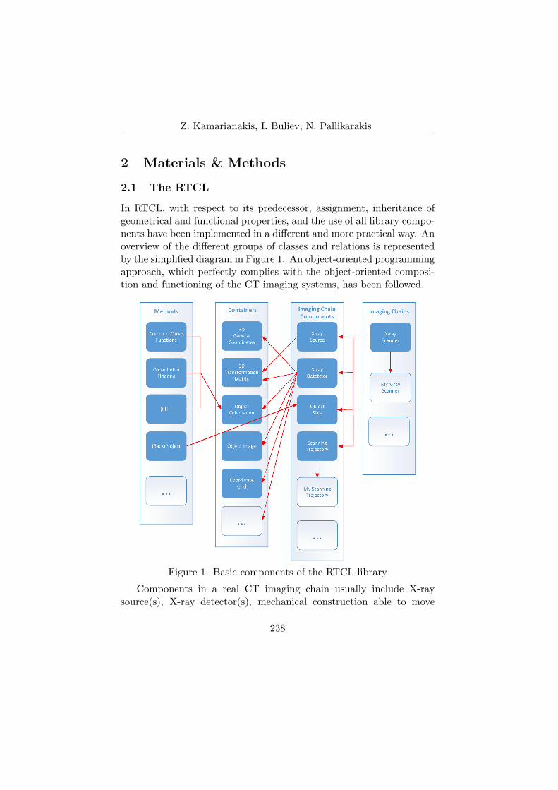
Z. Kamarianakis, I. Buliev, N. Pallikarakis
2 Materials & Methods
2.1 The RTCL
In RTCL, with respect to its predecessor, assignment, inheritance ofgeometrical and functional properties, and the use of all library compo-nents have been implemented in a different and more practical way. Anoverview of the different groups of classes and relations is representedby the simplified diagram in Figure 1. An object-oriented programmingapproach, which perfectly complies with the object-oriented composi-tion and functioning of the CT imaging systems, has been followed.
Figure 1. Basic components of the RTCL library
Components in a real CT imaging chain usually include X-raysource(s), X-ray detector(s), mechanical construction able to move
238

A platform for Image Reconstruction in X-ray Imaging . . .
the source-detector pair(s) along a specific trajectory, data processingunit(s), dedicated image reconstruction processor and object motion-correction techniques. RTCL provides the programmer with softwareequivalents of those components, allowing intuitively and easily to re-peat and simulate any imaging setup and eventually use the availableprojection images to reconstruct tomograms at arbitrary orientations.RTCL offers different types of classes, which combine content and in-herit properties in a hierarchical sequence. The Containers group com-prises classes for handling 2D/3D coordinates (of pixels, voxels, vectors,etc.) either locally on a surface (e.g. detector plane) or globally in the3D space. Grid classes carry analytical description of different sur-faces and contain arrays of the coordinates of their nodes. The lattercan belong to a flat surface, thus are equidistantly distributed overa plane, or they can belong to a curved (cylindrical, spherical) sur-face, therefore following a different description. Sets of Euler anglesdescribe the orientation of objects in space. Images are separate con-tainers for different types of image data. The Methods group of classesprovides mostly functions to facilitate handling and processing projec-tion or reconstruction data. It includes common 1D/2D functions (e.g.signal windows, filter kernels, filter responses), FFT/IFFT routines,convolution/filtering routines, for image processing in the frequencyand the spatial domain. Projection/backprojection routines are alsoimplemented in order to help in the validation or development of an-alytical reconstruction methods or in the production of experimentalprojection images. Specific classes form the Imaging Chain Compo-nents group. Detectors represent the variety of image sensors usedin the CT imaging, fluoroscopic or any other direct way of imaging.Within a 2D detector, pixels are uniquely identified by their indices orby their local or global coordinates. It is always possible to convertany type of coordinates to any other type, using the a priori informa-tion for the imaging system. Trajectory classes incorporate geometryand motion of different setups of source-detector pairs and simplifytheir positioning in space. Examples include circular isocentric trajec-tory, spiral/helical, partial isocentric along a limited arc, linear, etc.Slices are utilized in the representation of tomographic images or 3D
239

Z. Kamarianakis, I. Buliev, N. Pallikarakis
volumes, while the X-ray source class, for example, describes a pointsource in terms of its coordinates, focal spot size, energy, field distribu-tion, etc. The Imaging Chains group is intended to contain functionalaggregations (e.g. scanners, C-arms, etc.) of the above classes. Thelast two groups are considered quite open (from the user’s/developer’saspect) and any new development (e.g. trajectories, geometrical con-figurations) can be added.
Figure 2 helps to illustrate the example definition of a simple CArmscanner class. As it is shown, the class is defined initially by inher-iting most of the functionality from a ready abstract class, the Ba-seXrayScanner. This parent class contains abstract components like abase-source, a base-detector, a base-trajectory as well as virtual meth-ods (e.g the function that is expected to implement the relevant move-ment – moveTo(...)) that the children classes should override accord-ingly. The constructor of the derived CArm class is written in a forwardmanner, as it is shown on the right. The input arguments in the defi-nition of the constructor are already specific for the derived class e.g.the source to isocenter distance (SID), the source to detector distance(SDD), the number of nodes along the principal axes of the detectoras well as the size of its pixels. In the implementation, these argu-ments can be used to create and retrieve specific components, like anXrayPointSource, and a FlatXrayDetector, where the S and D denotepointers to abstract equivalents of these components.
The rotation of the gantry is translated into motion of the source-detector pair. The rules for that could be provided by the Circular Tra-jectory Class. With the help of an overloaded function (e.g moveTo(...)in Figure 2) the source-detector pair is instructed to move along a circu-lar arc synchronously, defined exactly by the Circular Trajectory Class.The backprojection operation is performed with the help of a univer-sal projector/backprojector function. The arguments of this functioninclude a Projection Set Description object, which fully describes theacquisition and geometrical setup of an imaging scenario and a Sliceobject on which the backprojection process will be performed. Thecompactness of the code proves the robust implementation of the ini-tial idea of RTCL.
240

A platform for Image Reconstruction in X-ray Imaging . . .
Fig
ure
2.C
-arm
devi
ceco
nfigu
rati
onan
dre
lati
ons
toth
eRT
CL
com
pone
nts.
On
the
left
,th
eac
quis
itio
nge
omet
ryin
limit
edar
ctr
ajec
tory
like
aC
-arm
issh
own.
On
the
righ
t,ba
sic
build
ing
bloc
ksth
atco
nsti
tute
the
cons
truc
tion
ofa
CA
rmob
ject
scan
ner
clas
s.T
heC
Arm
isde
rive
dfr
omit
spa
rent
,th
eB
aseX
rayS
cann
ercl
ass
241

Z. Kamarianakis, I. Buliev, N. Pallikarakis
2.2 Integrating RTCL into PIRXI
The idea of integrating the library into a multi-purpose applicationfor image reconstruction is a logical follow-up of the first medical andnon-medical (e.g in the area of NDT) imaging applications based on it.The library is now a core component of a larger software application:the Platform for Image Reconstruction in X-ray Imaging – PIRXI. Aninitial version of the platform has been already created and is currentlybeing used in the implementation of various image reconstruction tasksin the research activities of the team.
The GUI of PIRXI is developed in C/C++ and Qt. This allows agood portability of the code along different computing platforms andOSs. It has been tested on Windows and Ubuntu Linux.
It is a common situation when a researcher obtains CT projectiondata from external sources and spends significant amount of time tryingto convert them into an appropriate format of the application he/sheuses. PIRXI tries to deal with this problem and can provide a solutionto reconstruction tasks using a wide range of scanning geometries andprojection image formats. Based on the system of the .INI files andwith the help of a rich set of keys, a large number of projection filenaming, contents and data formats are transparently handled by theplatform and the projections can be loaded and further used.
A snapshot of the GUI of the PIRXI platform running under Win-dows is shown in Figure 3. The GUI currently allows the definition of awhole reconstruction job. The user can interactively describe such a re-construction task by providing information to the system (e.g. througha Dialogue), where he/she describes the general settings of the task.Common parameters include the description of the projection set (bymeans of data format, geometric acquisition settings, description ofthe detector’s pixel size and metrics, location of data and destinationof the processed files, etc.). The projection processing/preprocessing(e.g. filtering) follows, where again the task is easily performed throughbuttons on the GUI. Finally, the user can easily perform experimentsand gain an understanding of the loaded/processed available data bychoosing to reconstruct either central positioned slices or tomograms
242

A platform for Image Reconstruction in X-ray Imaging . . .
Fig
ure
3.A
snap
shot
ofth
eG
UI
ofP
IRX
Ipl
atfo
rm
243

Z. Kamarianakis, I. Buliev, N. Pallikarakis
of arbitrary orientation. Moreover, the possibility for a direct volumet-ric reconstruction is given. The image reconstruction method can bechosen from the already implemented ones through the GUI, where fur-ther options are provided in case the reconstruction algorithm demandsadditional input from the user (e.g. the arc in DTS or the projectionangle spacing used for reconstruction).
2.3 Examples of using PIRXI in medical applications
Selected reconstructed tomograms using simulated data acquired inspecific scanning trajectories are used as a demonstration of the tool.The use of simulated data is particularly useful in studying and ana-lyzing reconstruction algorithms in principle, since data are free fromdistortions and mechanical inaccuracies inherent to radiographic units.Noise-free monoenergetic projection images of three simulated phan-toms were acquired using an in-house developed tool, the XRAYImag-ingSimulator [2].
The first phantom is a modified (high contrast) version of the wellknown analytical Shepp-Logan phantom that approximates the humanhead and consists of 12 ellipsoids. The phantom was included in a cubicvolume of size 190x190x190 and voxel size 1.
The second phantom is a 3D voxelized model of a metallic cylin-drical implant (e.g. intramedullary tibial nail) used in interventionalprocedures in orthopedic surgery for the treatment of bone fractures.The implant consists of 8 screw holes at various locations and orien-tations, and is placed in three other cylinders that model a human leg(e.g. red bone marrow, bone and muscle). A detailed study on accuratelocalization of hole canals using CBCT, is presented in [9].
As a third example, a simulated 8cm complex uncompressed breastphantom [3] approximating the medium-sized breast was used. Themodel contains four clusters of microcalcifications (µCs) delivered intwo different groups. In two different layers of the phantom, twoclusters of 5µCs in one layer and two clusters of 6µCs, modeled asspheres/ellipsoids of calcium carbonate and of size 0.2 mm and 0.4 mm,are placed. The simulation parameters for image acquisition as well as
244

A platform for Image Reconstruction in X-ray Imaging . . .
the reconstruction settings used for all the phantoms are presented intable [1].
Table 1. Acquisition and reconstruction settings used along with thethree simulated phantoms
Phantoms
Parameter/Settings
Shepp-Logan Metallic im-plant
UncompressedBreast
Source-isocenterdistance (SID)
1000 mm 1000 mm 600 mm
Source-detectordistance (SDD)
1300 mm 1300 mm 665 mm
Number ofviews/Projections
360 121 25
Detector size 512x512 (pixels) 480x480 (pixels) 500x500 (pixels)
Pixel pitch 0.5mm 0.5mm 0.2 mm
Magnificationfactor
1.3 1.3 1.108
Reconstructionmatrix/slice size
190x190x190 370x370 500x500
Source/Detectortrajectory
Full 360o circulartrajectory, angu-lar step 1o
Circular isocen-tric rotation,121o limited arc,angular step 1o
Circular isocen-tric rotation, 48o
limited arc, an-gular step 2o
Reconstructionalgorithm
FDK FBP FBP & SAA
2.3.1 CBCT reconstruction using the FDK algorithm
For the case of Shepp-Logan phantom, 360 projections images, acquiredevery 1o step, were used for volumetric reconstruction using the FDKalgorithm [10]. The main advantage of cone beam algorithms is thereduction in data collection time. With a single source, ray integralsare measured through every point in the object, in the time it takes tomeasure a single slice in a conventional two-dimensional scanner. Theprojection data can be expressed as a function of the source angle and
245

Z. Kamarianakis, I. Buliev, N. Pallikarakis
the horizontal and vertical positions on the detector plane. The FDKalgorithm is an approximate formula and represents a generalization ofthe 2D fan-beam reconstruction formula to the 3D case. The volumereconstruction is based on initial filtering and subsequent length cor-rection weighting of the projection data followed by backprojecting asingle plane within the cone, for each elevation along the z-axis. Thefinal three-dimensional reconstruction is obtained by summing the con-tribution to the object from all tilted fan beams [8], which involves afinal weighting that accounts for this tilt during backprojection. TheFDK algorithm can be implemented with moderate computational re-quirements and delivers a satisfactory reconstruction quality for smallcone angles (e.g. up to 10o). The individual steps of this algorithm arealready implemented in the RTCL.
2.3.2 DTS reconstruction using Shift and Add & FilteredBackprojection algorithms
For the breast phantom and the metallic implant phantom, DTS imagereconstruction techniques were applied. DTS is a limited angle methodof image reconstruction, where projection images acquired at regularangular intervals, and during a single acquisition pass, are used for re-construction of planar sections [11]. In many applications (e.g. mam-mography) the source trajectory traces a limited circular arc, whilethe detector usually remains stable. In the current investigation, theacquisition geometry is isocentric. The acquisition geometry of isocen-tric Digital Tomosynthesis setup resembles that of the C-arm shown inFigure 2, but the angular range of the source-detector pair is usuallymuch smaller. Important parameters for this acquisition geometry areonce again the SID and SDD, as well as the acquisition range (denotedwith φ) and the angular step θ. With the parameter α in Figure 2, thefan-beam angle is indicated. In the present example, 25 images of anuncompressed simulated breast were acquired in the limited arc −24o
to 24o, with 2o step (Table 1). Tomograms were further reconstructedusing a simple backprojection technique (Shift and Add algorithm –SAA), similar to that of [11] and a Filtered Backprojection (FBP) al-
246

A platform for Image Reconstruction in X-ray Imaging . . .
gorithm. Both of these algorithms are implemented in RTCL. In bothcases, the purpose was to bring in focus the planes of interest (e.g. theµCs). The Simple Backprojection algorithm was utilized, as it requiresa straightforward implementation and minimal computational powerand processing time efforts. However, since this technique introducesadditional reconstruction artifacts (e.g. out-of-plane structures withhigh contrast tend to appear as low-contrast replicas in reconstructionplanes), the FBP algorithm was also applied in an attempt to recoverthe loss of contrast especially for the small structures (e.g. the µCs).For the case of metallic implant phantom, a larger acquisition arc of121o was used with step of 1o. In this case, only a FBP approach wasfollowed for the reconstruction.
3 Results
Figure 4 demonstrates the outcome of the FDK reconstruction of thefirst phantom. Using projection images of the modified Shepp-Loganphantom, central three orthogonal to each other reconstructed slices(axial, coronal, saggital) and a slice at a plane Z = −24 mm awayfrom the central plane, are presented.
Accordingly, below each reconstructed slice, line plot profiles (cor-responding positions are marked with a white solid line in each recon-struction), are presented as compared to the original (dashed line).
The visual inspection of the reconstructed images and especiallythe comparison of the selected line profiles (in the reconstructions ascompared to the original phantom) validate the correct implementationof the reconstruction algorithm using the RTCL.
In Figure 5, DTS reconstructions of a simulated uncompressedbreast are shown. In the upper row, a FBP algorithm implementedwith the help of the RTCL library is used for reconstruction, while inthe bottom row, results after applying a SAA approach in correspond-ing locations, are presented. In both reconstruction approaches theµCs were found to be in-focus in the planes at Z = −21mm below andZ = 9mm above the central plane, which is considered at the isocenter.In the right part of Figure 5 and from up to down, zoomed recon-
247

Z. Kamarianakis, I. Buliev, N. Pallikarakis
Figure
4.C
BC
Treconstruction
ofam
odifiedShepp-L
oganphantom
usingthe
FD
Kalgorithm
imple-
mented
inthe
RT
CL
library.From
leftto
right,lineprofiles
(with
solidlines)
inthe
reconstructionsat
x=
70,y
=95,
x=
105and
x=
96(for
thefar
rightslice)
atplane
z=−
24,ascom
paredto
theoriginal
(with
dashedline)
248

A platform for Image Reconstruction in X-ray Imaging . . .
structed regions of interest containing the features under investigationare presented, at Z = −21mm and Z = 9mm, after applying a FBPalgorithm and after using SAA, respectively. Both groups of largerµCs (4mm diameter) are well visualized in the reconstructed planes.Regarding the smaller in diameter µCs (2mm), 2 out of the group of5µCs from the plane at Z = −21mm and 1 out of the group of 6µCswere not observed at all in any of the reconstructed slices.
This is a common situation in Breast imaging tomography, sinceµCs with size smaller than 0.25mm are reported to have difficultiesin detection. Moreover, tomographic reconstruction further away fromthe central plane of the isocenter introduces additional artifacts thatoverlay in some cases the features under investigation.
Figure 5. DTS reconstruction of a simulated breast using an implemen-tation of a FBP reconstruction algorithm in RTCL (upper row) and acorresponding Shift and Add technique (bottom)
249

Z. Kamarianakis, I. Buliev, N. Pallikarakis
In Figure 6, DTS reconstructions of a simulated metallic implantare shown. Reconstructions were performed as previously with a FBPreconstruction algorithm using the RTCL library. 2D tomograms werereconstructed at “arbitrary” orientations by feeding the platform withEuler angles close to those that describe the phantom rotation aroundthe principal axes, but not with their exact values.
The results present reconstructed slices almost “parallel” to themain axis of the implant, providing useful information for further imageprocessing and analysis. The openings (e.g. hole canals) are in mostcases well visualized.
Figure 6. DTS reconstruction of a simulated metallic surgical implant
4 Conclusions
This paper describes the current structure of the RTCL library andthe way it can be used for developing software applications within thefield of the X-ray Computed Tomography (CT). The library is consid-ered as the core component of an integrated software application – thePlatform for Image Reconstruction in X-ray Imaging (PIRXI). Selectedreconstructed slices from simulated data used in medical imaging, af-ter applying CBCT or DTS reconstruction algorithms, were used fordemonstration purposes. The current tests of both RTCL and PIRXIprove the flexibility of the new approach to image reconstruction re-search and algorithms implementation. The tools aim to facilitateany experimentation, study and development/implementation of re-construction algorithms and scanning geometries and configurations inthe Computed Tomography field.
250
A platform for Image Reconstruction in X-ray Imaging . . .
References
[1] A.Gliere. Sindbad:From CAD model to synthetic radiographs(1998) Review of Progress in Quantitative NondestructiveEvaluation,17:387–394.
[2] D.Lazos, K.Bliznakova, Z.Kolitsi, N.Pallikarakis. (2003) An inte-grated research tool for X-ray imaging simulation, Comp. Meth. &Prog. in Biomed: 70:241–251.
[3] K.Bliznakova, R.Speller, J.Horrocks, P.Liaparinos, Z.Kollitsi,N.Pallikarakis. Experimental validation of a radiographic simula-tion code using breast phantom for X-ray imaging, vol 40:2 (2010),pp. 208–214.
[4] P.Duvauchelle, N.Freud, V.Kaftandjian, D.Babot. A computercode to simulate X-ray imaging techniques, Nuclear Instrumentsand Methods in Physics Research B 170, (2000), pp. 245–258.
[5] M.Winslow, X.G.Xu, B.Yazici. Development of a simulator forradiographic image optimization, Comp. Meth. & Prog. in Biomed,(2005) 78, pp. 179–190.
[6] D.Lazos, Z.Kolitsi, N.Pallikarakis. A software data generator forradiographic imaging investigations, IEEE T. Inf. Technol. B, 4(2000), pp. 76–79.
[7] Z.Kamarianakis, I.Buliev, N.Pallikarakis. CLCT: A C++ Libraryfor Computed Tomography applications, Proc. ESBME 2008, 6th
European Symposium on Biomedical Engineering, 19-21 June,Chania, Greece.
[8] A.C.Kak, M.Slaney. Principles of Computerized TomographicImaging, IEEE Press 1988.
[9] Z.Kamarianakis, I.Buliev, N.Pallikarakis. Robust identificationand localization of intramedullary nail holes for distal locking usingCBCT: A simulation study, Med. Eng. & Physics vol. 33(2011),pp. 479–489.
251

Z. Kamarianakis, I. Buliev, N. Pallikarakis
[10] L.A.Feldkamp, L.C.Davis, J.W.Kress. Practical cone-beam algo-rithm, J. Opt. Soc. Am. A. 1(6): 612–619, 1984.
[11] Z.Kolitsi, G.Panayiotakis, V.Anastassopoulos, A.Scodras,N.Pallikarakis. A multiple projection method for digital tomosyn-thesis, Med. Phys. 19(4), 1045–1050, 1992.
[12] Z.Kamarianakis, I.Buliev, N.Pallikarakis. A C++ platform for im-age reconstruction in X-ray imaging, 5th Panhellenic Conferenceon Biomedical Technologies, ELEVIT(2013), 4-6 April, Athens,Greece.
Zacharias Kamarianakis, Ivan Buliev, Received March 13, 2014Nicolas Pallikarakis
Zacharias KamarianakisUniversity of Patras, Dept. of Medical Physics26504 Rio, Patras, GreecePhone: (30) 2610 969109E–mail: [email protected]
Ivan Buliev,Studentska str.1, Technical University of Varna, Dept. of Electronics9010, Varna, BulgariaPhone: (359) 52 383 572E–mail: [email protected]
Nicolas PallikarakisUniversity of Patras, Dept. of Medical Physics26504 Rio, Patras, GreecePhone: (30) 2610 997702E–mail: [email protected]
252

Computer Science Journal of Moldova, vol.22, no.2(65), 2014
Parallel Processing and Bio-inspired
Computing for Biomedical Image Registration
Invited Article
Silviu Ioan Bejinariu, Hariton Costin, Florin Rotaru,Ramona Luca, Cristina Nita, Camelia Lazar
Abstract
Image Registration (IR) is an optimization problem comput-ing optimal parameters of a geometric transform used to overlayone or more source images to a given model by maximizing a simi-larity measure. In this paper the use of bio-inspired optimizationalgorithms in image registration is analyzed. Results obtainedby means of three different algorithms are compared: BacterialForaging Optimization Algorithm (BFOA), Genetic Algorithm(GA) and Clonal Selection Algorithm (CSA). Depending on theimages type, the registration may be: area based, which is slowbut more precise, and features based, which is faster. In this pa-per a feature based approach based on the Scale Invariant FeatureTransform (SIFT) is proposed. Finally, results obtained using se-quential and parallel implementations on multi-core systems forarea based and features based image registration are compared.
Keywords: image registration, clonal selection algorithm,bacterial foraging algorithm, genetic algorithm, parallel comput-ing.
1 Introduction
Image registration is the process of geometric overlaying or alignmentof two or more images of the same scene taken at different times, fromdifferent viewpoints, and/or by different sensors [1]. Image registration
c©2014 by Silviu Ioan Bejinariu, Hariton Costin, Florin Rotaru, Ramona
Luca, Cristina Nita, Camelia Lazar
253

S.I. Bejinariu, H. Costin, F. Rotaru, R. Luca, C. Nita, C. Lazar
(IR) is the first step in image fusion procedures, which combine relevantinformation from one or more images to create a single image with moreinformational content. Image registration and fusion methods are usedin remote sensing applications, geographic information systems, mul-tispectral image analysis, medical image analysis and other domains.Image fusion may be applied at pixel, feature or decision levels. In thefirst case, when pixel level image fusion have to be applied, the inputimages must be registered, because they may differ by the view angle,subject position and also some geometric distortions may be added bythe capture device.
There are two different approaches in IR: area (pixel intensity)based methods and feature-based methods [1]. The geometric trans-form that must be computed may be global (for the entire image) orlocal in case the images are locally deformed. The most frequentlyused transforms are the shape preserving mappings (rotation, transla-tion, scaling and the affine transform).
In this paper three different optimization methods are used for thegeometric transform parameters estimation: Bacterial Foraging Opti-mization Algorithm (BFOA), Genetic Algorithm (GA) and Clonal Se-lection Algorithm (CSA). The foraging model is suitable for optimiza-tion problems because animals search for nutrients and try to avoidnoxious substances in a way that maximize their energy intake perunit time spent foraging [2]. Computational methods can provide deci-sion models for optimal foraging. The Bacterial Foraging OptimizationAlgorithm (BFOA) proposed by Passino uses the Escherichia coli bac-teria model because it is the most understood microorganism [2], [3],[4]. BFOA is used in image processing to solve also other optimizationproblems: edge detection in combination with a probabilistic derivativetechnique [5]; fuzzy entropy based image segmentation [6]. A modifiedversion of BFOA used for multilevel thresholding segmentation wascompared to genetic algorithms and particle swarm optimization algo-rithm [7]. Image registration BFOA based methods were proposed in[8], [9] and [10] Parallel implementations of BFOA were proposed in [11]and [12]. Genetic Algorithms are search techniques that emulate evo-lutionary processes to solve optimization problems [13]. Like BFOA,
254
Parallel Processing and Bio-inspired Computing for . . .
GAs start with a population of individuals (points) in the problem do-main and use these points to approximate the optimal solution. Thedifference is that instead moving in the problem domain, GAs use therecombination of two or more parents to produce offspring [14]. GAsare often used in biomedical or remote sensing image registration [13].The Clonal Selection Algorithm (CSA) belongs to the field of ArtificialImmune Systems that include computational methods inspired by themechanisms of the biological immune system [15]. Like GAs, CSA mayuse binary solution coding and real coding. In [16] a real coded clonalselection algorithm is used in electromagnetic design optimization. Itis also suitable for high dimensional optimization problems. CSA iseffective, in terms of accuracy, capable of solving large-scale problems[17] and is comparable to other optimization algorithms. A perfor-mance comparison of CSA and GA is presented in [18] and conclusionis that each one has better performance depending on the function tooptimize.
The paper is organized as follows. In the second section the mea-sures used for area based and features based IR methods are described.In case of features based IR, a short description of SIFT transformand procedure to find the SIFT key points correspondences are alsoincluded. In the third section, the optimization algorithms – BFOA,GA and CSA – are shortly presented. In the fourth section the pro-posed parallel versions of BFOA and GA are presented. In the fifthsection the results obtained by applying the optimization proceduresfor biomedical image registration are shown in both sequential andparallel versions. The last section concludes the paper.
2 Image Registration
There are two different approaches in IR: area (pixel intensity) basedmethods and feature-based methods [1]. Almost all methods consist offour steps: feature detection, feature matching, transform estimationand image resampling. The feature detection step is specific to featurebased registration methods and distinctive and stable features (points,lines, contours, regions) have to be detected. Because the transform es-
255

S.I. Bejinariu, H. Costin, F. Rotaru, R. Luca, C. Nita, C. Lazar
timation is performed while looking for the correspondent features, thesecond and third steps are usually combined. In the image resamplingstep, different interpolation methods are used: the nearest neighborfunction, the bilinear and bicubic functions, quadratic splines, cubicand higher-order B-splines [1].
2.1 Area Based IR
In case of area based IR methods, to evaluate the similarity betweenimages the normalized correlation (NCC), the Fourier representationor normalized mutual information (NMI) are used. In this study, theMutual Information is used to evaluate the similarity in case of areabased registration.
Mutual information is a robust measure used in image registration[1], [10]. It evaluates the relative independence of two images and doesnot depend on the specific dynamic range or intensity scaling of theimages. High values of mutual information indicate high dependencebetween images. It is defined as
MI(A,B) = H(A) + H(B)−H(A,B), (1)
where H(.) is the image entropy and H(A,B) is the joint entropy of thetwo images. Because mutual information based registration methodsare sensitive to changes that occur in the distributions as a result ofdifference in overlapping regions, normalized mutual information canbe used:
NMI(A,B) =H(A) + H(B)
H(A,B). (2)
Registration of two images A and B requires maximization of mutualinformation, thus maximization of the entropies H(A) and H(B), andminimization of the joint entropy H(A,B).
Usually, optimization in image registration means to maximize sim-ilarity. If the optimization algorithm is oriented on cost function min-imization, then the value of (−1) ∗MI is used to evaluate the cost ofthe transform for a certain solution.
256
Parallel Processing and Bio-inspired Computing for . . .
2.2 Feature based IR
In case of feature based IR methods, spatial relations, invariant descrip-tors, relaxation methods and multiresolution transforms (pyramids andwavelets) are used. In this paper, the features based IR will use keypoints determined using the Scale Invariant Feature Transform (SIFT)[19], [20]. SIFT is used to select distinctive features, used in patternrecognition, localization, 3D mapping, tracking and image registration.It allows scale and rotation invariant features detection, with good re-sults for affine distortions. The SIFT algorithm has 4 distinctive stages:extrema detection in the scale space of the image, key points selectionand localization, key points orientation assignment and description gen-eration. The identified features have to be distinctive.
a. Scale-space extrema detection. Key point candidates selection isperformed by finding the extrema of the Difference of Gaussians (DOG)function computed as the difference of two scaled images separated bya multiplicative factor k.
D(x, y, σ) = L(x, y, kσ)− L(x, y, σ) == (G(x, y, kσ)−G(x, y, σ)) ∗ I(x, y), (3)
where L(x, y, σ) is the scale space of the image I(x, y) obtained by con-volving it with the Gaussian kernel G(x, y, σ). Extrema points dependon the frequency sampling in the scaled space and the initial value of σ.
b. Key points localization. Key points are selected from the moststable and accurately localized candidates. Key point candidates hav-ing low contrast or strong edge response in one direction only are re-moved. Because the candidates obtained in higher scales correspondto several pixels in the original image, for an exact localization is per-formed by computing the extrema points of the Taylor expansion upto quadratic terms of the scale space function D(x, y, σ) [19].
c. Orientation assignment. To make key point descriptions invari-ant to rotation, their orientations are computed using the orientationhistogram of local gradients of the closest smoothed image L(x, y, σ).
257

S.I. Bejinariu, H. Costin, F. Rotaru, R. Luca, C. Nita, C. Lazar
The gradient magnitude and orientation are computed using pixel dif-ferences:
m(x, y) =
=√
(L(x− 1, y)− L(x + 1, y))2 + (L(x, y − 1)− L(x, y + 1))2, (4)
θ(x, y) = arctgL(x, y + 1)− L(x, y − 1)L(x + 1, y)− L(x− 1, y)
. (5)
Each point is added to the histogram weighted by the gradient mag-nitude m(x, y) and by a circular Gaussian. To obtain a more accurateorientation, the dominant peaks in the histogram are interpolated withtheir neighbors.
d. Key point descriptor computing. The key point descriptor con-tains 128 = 4× 4 × 8 values obtained using 16 orientation histogramscomputed in a 4× 4 grid. Each histogram contains 8 orientation bins.The descriptor is computed in a support window of 16 × 16 pixelsaround the key point [19].
To evaluate the similarity between two images the key points cor-respondences have to be established. The Euclidian distances betweenSIFT descriptors of each key point from source image and those of themodel image are computed. By sorting the computed values for sourceimages key points, a match is established when the minimum computeddistance is less than a certain percentage from the second distance. Inour experiment a percent of 30% is used [20].
For IR, in the similarity evaluation step, the coordinates of the keypoints in the source image are transformed accordingly to the valuesof transform parameters and the sum of Euclidean distances betweenpositions of key points in the model and transformed source image isused as similarity value [12].
3 Bio-inspired computing in IR
In this paper three different bio-inspired optimization methods are usedin order to compute the optimal geometric transform that allows the
258

Parallel Processing and Bio-inspired Computing for . . .
source image to overlay the model image: Clonal Selection Algorithm,Bacterial Foraging Optimization Algorithm and Genetic Algorithm.
3.1 Clonal Selection Algorithm
The Clonal Selection Algorithm (CSA) belongs to the field of ArtificialImmune Systems which includes computational methods inspired bythe mechanisms of the biological immune system. A simplified descrip-tion of the immune system is an organ system intended to protect thehost organism from the threats posed to it from pathogens and toxicsubstances.
CSA is inspired by the Clonal Selection theory of acquired immu-nity. It is a population based stochastic method with binary representa-tion of variables [16] which may be used for multimodal optimization.In some cases, also real encoding of variables may be used to solvenumerical problems.
Clonal Selection Algorithm can be listed as follows [18]:
1. Randomly generate a set of solution candidates: antibodies.
2. Compute the affinity values of each candidate solutions.
3. While the minimum error criterion is not met
3.1 Sort the antibodies starting from the lowest affinity. Thelowest affinity means better matching between antibodyand antigen.
3.2 Clone the better matching antibodies more with somepredefined ratio.
3.3 Mutate the antibodies with some predefined ratio. Thisratio is obtained in a way that better matching clonesmutated less and weakly matching clones mutated muchmore in order to reach the optimal solution.
3.4 Compute affinity values of each antibody.
259

S.I. Bejinariu, H. Costin, F. Rotaru, R. Luca, C. Nita, C. Lazar
It starts with an initial set of adaptive units: the general immunecells. Each cell represents a possible solution of the problem and par-ticipates in a competitive selection process. The algorithm involves theselection of antibodies based on affinity against a pattern, computed bya cost function. Selected antibodies are cloned and resulted clones aresubject of hypermutation. The hypermutation is inverse proportionalto computed clone affinity. The resulted set competes with the alreadyexisting antibodies in the next generation of the evolution process. Thelow-affinity population members are replaced by new randomly gener-ated antibodies.
3.2 Bacterial Foraging Optimization Algorithm
The Bacterial Foraging Optimization Algorithm belongs to the fieldof Bacteria Optimization Algorithms and Swarm Optimization. Therehave been many extensions of the approach that attempt to hybridizethe algorithm with other Computational Intelligence algorithms andMetaheuristics such as Particle Swarm Optimization, Genetic Algo-rithm.
The bacterial foraging paradigm [2], [3], [4] is suitable as modelfor optimization algorithms because animals / bacteria behavior is tosearch for nutrients and avoid noxious substances to maximize theirenergy. BFOA is based on a colony of evolving bacteria which arereplicated if have a good strategy to find nutrients or die in the othercase. Each bacterium is characterized by its position and quantity ofaccumulated nutrients or healthy status.
In optimization problems, the possible solutions are encoded in thebacteria position and the movement of the colony members tends toapproximate the optimal solution. The final solution is specified bythe position in which a bacterium is in the best healthy state or thenutrients amount is the highest.
According to BFOA approach, the bacteria colony moves in then-dimensional space, where n is the optimization problem dimen-sion and the quantity of nutrients / healthy status is described bya cost function defined according to the optimization problem. Dur-
260

Parallel Processing and Bio-inspired Computing for . . .
ing its evolution, the bacteria colony proceeds through four foragingsteps: chemotaxis, swarming, reproduction and elimination-dispersal.In the following paragraphs, the colony consists of S individuals;P (j, k, l) = {θi(j, k, l), i = 1...S} is the position of colony members inthe jth chemotactic step, kth – reproduction step and lth – elimination-dispersal step; J(i, j, k, l) – the cost of the ith bacterium in positionθi(j, k, l).
Chemotaxis. In the chemotactic step, a bacterium can move intwo ways: tumble and swim. First, a tumble is executed in a randomdirection. The new position of the ith bacterium is:
θi(j + 1, k, l) = θi(j, k, l) + C(i)ϕ(i), (6)
where C(i) is the size of the chemotactic step and ϕ(i) is a unit lengthof randomly generated direction [4]. The movement continues in thesame direction while the value of the cost function decreases but notmore than a maximum number of steps.
Swarming. The bacteria tend to swarm together if they have thepossibility to signal to each other the presence of a favorable or poi-sonous environment (social behavior). The cell to cell attraction or re-jection is modeled by modifying the value of the cost function J(i, j, k, l)by a value that depends on the status of all the other bacteria in thecolony.
Reproduction. After a number of chemotactic steps, all bacteriaaccumulate a quantity of nutrients that is usually expressed as the costfunction computed in the current position. Those which accumulateda greater quantity of nutrients are in a healthier state and split intotwo bacteria. Those which accumulated a smaller amount of nutrientsdie. In BFOA, to keep constant the size of the colony, the number ofbacteria which split is equal to the number of bacteria which die. Thenew bacteria are created without mutation in the same position as theparent bacteria [4].
Elimination and Dispersal. After a number of reproduction steps,with a specified probability Ped, some bacteria are removed from colony
261

S.I. Bejinariu, H. Costin, F. Rotaru, R. Luca, C. Nita, C. Lazar
(elimination) regardless their healthy state and new bacteria are cre-ated in random positions (dispersal) [4].
The optimization algorithm starts with a colony of S bacteria placedin randomly generated positions. The evolutionary process consists ofNed elimination-dispersal steps, each of these consists of Nre reproduc-tion steps and each reproduction step consists of NC chemotactic steps.In each chemotactic step a bacterium may do at most NS swarmingsteps while the cost function value decreases.
Bacterial Foraging Optimization Algorithm can be listed as follows:
Initialize bacteria colonyfor l = 1 to Ned (elimination dispersal loop)
for k = 1 to Nre (reproduction loop)for j = 1 to NC (chemotaxis loop)
for i = 1 to S (each bacterium)perform tumble and change bacteria position to θi(j+1, k, l)compute cost function in new positionm = 0while cost function value decreases and m < NS
perform swarm and change bacteria positioncompute cost function in new position
end whileend for
end forend for
end for
The position in which a bacterium reaches the lowest value of thecost function (greatest healthy status) is the solution of the optimiza-tion problem. In case of image registration, the size of the search spaceis equal to the number of parameters of the geometric transform.
262

Parallel Processing and Bio-inspired Computing for . . .
3.3 Genetic Algorithms
Genetic Algorithm is an adaptive strategy used for global optimizationproblems. Inspired by population genetics, GA is based on a set ofindividuals in which the possible solutions of the problem are encodedas chromosome strings. The general structure of GAs is: (a) selectionof the appropriate encoding method and fitness function, (b) genera-tion of a random initial population and (c) the evolution loop of thealgorithm: fitness function evaluations, application of genetic operatorsand creation of the new generation. After a number a generations, thepopulation is expected to contain chromosomes that approximate theglobal maximum value of the fitness function. In each generation chro-mosomes with best fitness values are retained and generate offspringthat replaces chromosomes with the lowest values of the fitness func-tion. Genetic operators used for new generation creation are: selection,crossover and mutation.
1. Randomly generate a set of individuals.
2. Compute fitness for all individuals.
3. While the stop criterion and maximum generation number arenot met(Evolution loop)
3.1 Apply reproduction3.2 Mutation3.3 Crossover.
In [13] it is proposed an IR procedure using the string encoding ofchromosomes. The parameters of the geometric transform are encodedas bit fields in a 32 bit value. In the procedure described below, the realencoding is used and each chromosome is characterized by a numberof real values equal to the number of geometric transform parameters.Discrete, average and simplex crossover operators are used dependingon user defined probabilities (pd, pa and ps).
263

S.I. Bejinariu, H. Costin, F. Rotaru, R. Luca, C. Nita, C. Lazar
4 Parallel approach for bio-inspired IR
Analyzing the optimization procedures execution, it must be noticedthat most of the processing time is spent in the cost function evalua-tions. In case of BFOA based registration, about 99% of the executiontime is spent in the cost evaluation function and more detailed, about83% for mutual information computing and 16% of total time is spentin when the geometric transform is applied to source image. The same,in case of GA optimization: 96% of the execution time is spent in thecost evaluation (81% to compute mutual information and 15% to ap-ply the geometric transform). Because both BFOA and GA procedureswere executed using the sequential implementation, only about 25% ofthe computing power is used in case of a Core i5 processor.
To optimize the IR procedure parallel implementations based onthe computing power of multi-core processors were proposed in [12].
A closer look at BFOA reveals that it contains 4 nested loops:elimination/dispersal, reproduction and chemotaxis for each bacteriumin the colony. The body of the inner loop is executed Ned×Nre×NC×Stimes, which may be a fairly large number. In fact, the cost functionevaluation is performed more than two times this number due to thefact that each bacterium may perform more swim steps in a singlechemotactic step. While the calculations performed for each individualbacterium in the inner loop are independent, the bacteria colony mayperform the chemotactic steps simultaneously.
In case of GA optimization, the cost function evaluation is calledfrom two different places. First, it is called from the main evolutionloop of the algorithm (about 41% of execution time) only for the newcreated chromosomes evaluation, and second, in the simplex crossoverfunction (about 53% of execution time). In the first case, the costfunction is called for all not already evaluated chromosomes, so thistask is easily parallelized. In case of simplex crossover that involvesmore than one chromosome, the crossover function will be executed inparallel for each group of chromosomes [12].
The IR procedure that uses the Clonal Selection Algorithm wasnot parallelized because there are few tasks completely independent,
264

Parallel Processing and Bio-inspired Computing for . . .
suitable for parallel execution.The parallel implementation was evaluated on an Intel Core i5 3.10
GHz processor and is detailed in the next section.
5 Experiments
In this section a comparison of results obtained using image registra-tion procedures based on Bacterial Foraging Optimization Algorithm,Clonal Selection Algorithm and Genetic Algorithm is presented. Theoptimization procedures were applied for area based registration andfeatures based registration. In the second case the SIFT features areused.
The image registration procedure was tested on a large set of DI-COM medical images from a database available at http://www.osirix-viewer.com/datasets/ [21]. Below, only the results obtained using theBrainix image as model are described. It is a gray level image (8 bitsper pixel) and size 256× 256 pixels. Brainix is a MR image of a braintumor.
The image registration procedure was applied also to the imageafter it was modified by adding “salt & pepper” noise.
Figure 1. Original image BRAINIX (from [21])
265

S.I. Bejinariu, H. Costin, F. Rotaru, R. Luca, C. Nita, C. Lazar
The source images were obtained by applying a rotation (angleθ = 10◦) against the rotation center (cx = −20 and cy = 20) followedby an isotropic scaling (scale = 1.2). While the transform is definedby 4 parameters, the search space in the optimization problem is R4.The actual value of the transform matrix is
T =
=
α β (1− α) cx − β cy
−β α β cx + (1− α) cy
0 0 1
=
1.1818 0.2084 −0.5322−0.2084 1.1818 −7.80290 0 1
, (7)
where α = scale · cos θ and β = scale · sin θ.The inverse transform matrix is
T−1 =
0.8207 −1.1447 −0.69241.1447 0.8207 6.48070 0 1
that corresponds to an affine transform with the following parameters:θ′ = −10◦, c′x = −20, c′y = 20 and scale′ = 0.8333.
To evaluate the similarity between model image and registeredsource image, the normalized mutual information is used.
The BFO parameters values used in the experiment are: bacteriacolony size S = 400; number of chemotactic steps Nc = 20; maximumnumber of swim steps Ns = 10; number of reproduction steps Nre =16; number of elimination / dispersal steps Ned = 2; probability ofdispersal Ped = 0.25; length of the move step Ci = 0.005.
In case of GA optimization, the real encoding is used, and eachchromosome is characterized by four real values representing the num-ber of geometric transform parameters. Discrete, average and sim-plex crossover operators are used depending on user defined probabil-ities (pd, pa and ps). The GA parameters are: number of generationsnGen = 500 and number of chromosomes nCr = 1500. The crossoverprobabilities are: pd = 0.05, pa = 0.15 and ps = 0.2.
Two different source images were used. The first one was obtainedby applying the transform described above to the model image. The
266

Parallel Processing and Bio-inspired Computing for . . .
second source image was obtained from the first one by applying “salt& pepper” noise. The signal-to-noise ratio in these images is about−1 dB.
In Figure 2, source images and some samples of registered imagesare presented.
In Tables 1 and 2 the results of both sequential and parallel areabased registration are presented. The column ‘# cost eval’ shows thetotal number of cost function evaluations; the column ‘best cost eval’shows the cost function evaluation in which the best value was obtained;column ‘ex MI’ (expected MI) shows the expected cost value obtainedby measuring the similarity between model image and the source imageafter the computed inverse transform was applied; column ‘c MI’ (com-puted MI) shows the cost value obtained by measuring the similaritybetween model image and source image after the approximated inversetransform was applied. In both tables 1 and 2, ‘Brainix’ denotes thesource image and ‘Brainix+SP’ denotes the source image altered byadding the “salt & pepper” noise.
Table 1. Results of area based image registration, sequential version
Mode Image Opt. Time(sec)
# costeval
bestcosteval
ex MI c MI
Seq Brainix BFOA 811.3 591686 469054 1.3218 1.3202GA 135.8 99148 63176 1.3218 1.3215
Brainix+SP
BFOA 820.9 563561 546678 1.1394 1.1382
GA 140.2 95371 60.348 1.1402 1.1387Paral-lel
Brainix BFOA 253.4 595365 249742 1.3218 1.3177
GA 46.6 98894 79889 1.3218 1.3191Brainix+SP
BFOA 254.9 566433 269008 1.1398 1.1390
GA 47.4 95042 86093 1.1398 1.1388
267
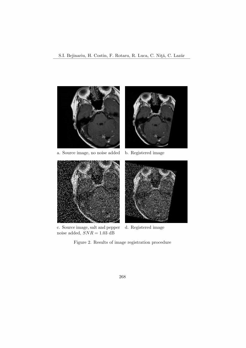
S.I. Bejinariu, H. Costin, F. Rotaru, R. Luca, C. Nita, C. Lazar
a. Source image, no noise added b. Registered image
c. Source image, salt and peppernoise added, SNR = 1.03 dB
d. Registered image
Figure 2. Results of image registration procedure
268
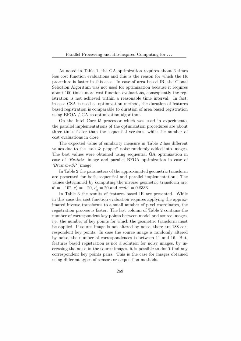
Parallel Processing and Bio-inspired Computing for . . .
As noted in Table 1, the GA optimization requires about 6 timesless cost function evaluations and this is the reason for which the IRprocedure is faster in this case. In case of area based IR, the ClonalSelection Algorithm was not used for optimization because it requiresabout 100 times more cost function evaluations, consequently the reg-istration is not achieved within a reasonable time interval. In fact,in case CSA is used as optimization method, the duration of featuresbased registration is comparable to duration of area based registrationusing BFOA / GA as optimization algorithm.
On the Intel Core i5 processor which was used in experiments,the parallel implementations of the optimization procedures are aboutthree times faster than the sequential versions, while the number ofcost evaluations in close.
The expected value of similarity measure in Table 2 has differentvalues due to the “salt & pepper” noise randomly added into images.The best values were obtained using sequential GA optimization incase of ‘Brainix’ image and parallel BFOA optimization in case of‘Brainix+SP’ image.
In Table 2 the parameters of the approximated geometric transformare presented for both sequential and parallel implementation. Thevalues determined by computing the inverse geometric transform are:θ′ = −10◦, c′x = −20, c′y = 20 and scale′ = 0.8333.
In Table 3 the results of features based IR are presented. Whilein this case the cost function evaluation requires applying the approx-imated inverse transforms to a small number of pixel coordinates, theregistration process is faster. The last column of Table 2 contains thenumber of correspondent key points between model and source images,i.e. the number of key points for which the geometric transform mustbe applied. If source image is not altered by noise, there are 188 cor-respondent key points. In case the source image is randomly alteredby noise, the number of correspondences is between 11 and 16. But,features based registration is not a solution for noisy images, by in-creasing the noise in the source images, it is possible to don’t find anycorrespondent key points pairs. This is the case for images obtainedusing different types of sensors or acquisition methods.
269

S.I. Bejinariu, H. Costin, F. Rotaru, R. Luca, C. Nita, C. Lazar
Table 2. Parameters of inverse affine transform computed using areabased registration
Mode Image Opt. c′x c′y θ′ scale′
Seq Brainix BFOA -19.69 20.17 -10.02 0.83GA -20.10 20.12 -9.99 0.83
Brainix+SP BFOA -20.40 18.79 -9.98 0.83GA -19.12 19.35 -10.07 0.83
Parallel Brainix BFOA -20.16 19.90 -9.98 0.83GA -20.26 20.30 -9.98 0.83
Brainix+SP BFOA -19.85 19.41 -9.99 0.83GA -19.10 20.13 -10.06 0.83
In Table 4 the values of the approximated transform parametersare presented. It must be noticed that in two cases the results are notso near to expected values: when the noisy image ‘Bainix+SP’ is usedas source and in case CSA is used as optimization method.
The charts presented in Figure 4 show compare the sequential andparallel execution time for all the experiments presented before. It isobvious that for long tasks, as area based IR, the gain obtained byusing the parallel versions is greater. For short tasks, as features basedIR, the speedup is lower. This happens because the processing timebecomes comparable to that of the synchronization tasks required bythe parallel implementation and also because shorter time intervals areaffected by all other processes and events that occur in the operatingsystem. The results obtained in case of CSA optimization are notincluded in charts because in this case the duration was too long.
In Figure 4, the parallelization evaluation is presented. The mostcommon evaluation of parallel algorithms is performed using the par-allel efficiency E = ts
tp×n , where ts is the time used by the sequentialversion of the algorithm, tp is the processing time for the parallel ver-sion and n is the number of used processors. As it was already said,better efficiency (> 74%) is obtained for area based IR parallelization
270

Parallel Processing and Bio-inspired Computing for . . .
a.A
rea
base
dIR
ofB
rain
ixim
age
b.A
rea
base
dIR
ofB
rain
ix+
SPim
age
c.Fe
atur
esba
sed
IRof
Bra
inix
imag
ed.
Feat
ures
base
dIR
ofB
rain
ix+
SPim
age
Fig
ure
3.P
roce
ssin
gti
me
for
diffe
rent
IRap
proa
ches
271

S.I. Bejinariu, H. Costin, F. Rotaru, R. Luca, C. Nita, C. Lazar
Table 3. Results of features based image registration, sequential version
Mode Image Opt. Time(sec)
# costeval
bestcosteval
ex MI c MI key-points
Seq Brainix BFOA 1.9 660726 391414 1.3218 1.3145 188GA 2.4 118359 17701 1.3218 1.3173 188CSA 353.3 73240500 - 1.3218 1.2948 188
Brainix BFOA 0.7 662137 378711 1.1400 1.1365 15+SP GA 2.2 111775 40274 1.1405 1.1240 11
CSA 191.5 65687973 - 1.1392 1.1187 12Paral-lel
Brainix BFOA 0.9 658684 636958 1.3218 1.3171 188
GA 2.2 115568 39971 1.3218 1.3168 188CSA 139.9 71315426 - 1.3218 1.2916 188
Brainix BFOA 0.6 640345 528443 1.1398 1.1234 12+SP GA 2.1 104900 26898 1.1389 1.1174 16
CSA 102.9 70095946 - 1.1405 1.1305 11
which has a longer execution time. In case of CSA optimization usedfor features based IR, the efficiency is between 47% and 68% whichmay lead to the conclusion that the procedure was not completely par-allelized. In all other cases (BFOA and GA for features based IR), thelower parallelization efficiency is not relevant, while the execution timeis too short.
The image registration procedures were implemented and tested inan image processing framework developed by authors of this paper. Itis implemented in C++ as a Windows application and uses OpenCVlibrary [22] for images manipulation and the parallel programming sup-port available in Microsoft Visual Studio 2010 [23].
6 Conclusions
This paper is focused on the use of some bio-inspired optimizationmethods for medical images registration. Three different approaches
272

Parallel Processing and Bio-inspired Computing for . . .
Table 4. Parameters of inverse affine transform computed using fea-tures based registration
Mode Image Opt. c′x c′y θ′ scale′
Seq Brainix BFOA -20.85 20.14 -9.93 0.83GA -19.81 20.10 -9.99 0.83CSA -20.35 19.15 -9.97 0.83
Brainix+SP BFOA -20.01 20.20 -9.97 0.83GA -22.48 19.33 -9.96 0.84CSA -17.99 16.93 -10.22 0.84
Parallel Brainix BFOA -19.88 19.54 -9.99 0.83GA -19.82 20.01 -9.99 0.83CSA -17.33 20.11 -10.16 0.83
Brainix+SP BFOA -25.43 21.66 -9.45 0.83GA -11.73 19.72 -10.77 0.83CSA -20.31 20.64 -9.85 0.83
are presented: Bacterial foraging optimization algorithm, genetic algo-rithm and clonal selection algorithm. Since image registration may bea time consuming task, different optimization strategies were applied:the use of scale invariant features transform key points and full usageof computing power of multi-core processors. The obtained results maybe summarized as follows:
• BFOA and GA allow to obtain comparable results in terms ofregistration precision;
• GAs perform faster the image registration about three timesfaster than BFOA;
• CSA is too slow for features based registration (comparable toarea based IR combined with BFOA and GA) and also with lowerprecision, provided that algorithm’s parameters were not enoughtuned;
273
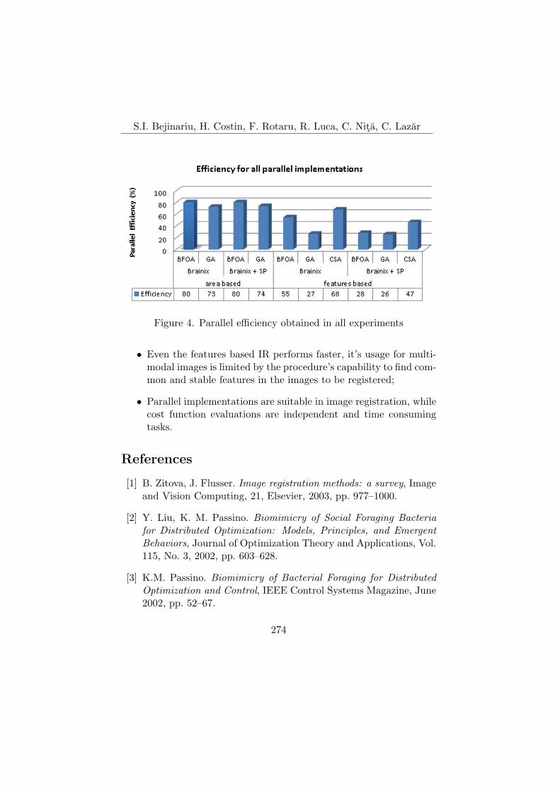
S.I. Bejinariu, H. Costin, F. Rotaru, R. Luca, C. Nita, C. Lazar
Figure 4. Parallel efficiency obtained in all experiments
• Even the features based IR performs faster, it’s usage for multi-modal images is limited by the procedure’s capability to find com-mon and stable features in the images to be registered;
• Parallel implementations are suitable in image registration, whilecost function evaluations are independent and time consumingtasks.
References
[1] B. Zitova, J. Flusser. Image registration methods: a survey, Imageand Vision Computing, 21, Elsevier, 2003, pp. 977–1000.
[2] Y. Liu, K. M. Passino. Biomimicry of Social Foraging Bacteriafor Distributed Optimization: Models, Principles, and EmergentBehaviors, Journal of Optimization Theory and Applications, Vol.115, No. 3, 2002, pp. 603–628.
[3] K.M. Passino. Biomimicry of Bacterial Foraging for DistributedOptimization and Control, IEEE Control Systems Magazine, June2002, pp. 52–67.
274
Parallel Processing and Bio-inspired Computing for . . .
[4] K.M. Passino. Biomimicry for Optimization, Control, and Au-tomation, Chapter 18: Cooperative Foraging and Search, SpringerVerlag, 2005.
[5] O. P. Verma, M. Hanmandlu, P. Kumar, S. Chhabra, A. Jindal.A novel bacterial foraging technique for edge detection, PatternRecognition Letters, 32, Elsevier, 2011, pp. 1187–1196.
[6] N. Sanyal, A. Chatterjee, S. Munshi. An adaptive bacterial forag-ing algorithm for fuzzy entropy based image segmentation, ExpertSystems with Applications, 38, Elsevier, 2011, pp. 15489–15498.
[7] P.D. Sathya, R. Kayalvizhi. Modified bacterial foraging algorithmbased multilevel thresholding for image segmentation, EngineeringApplications of Artificial Intelligence, 24, Elsevier, 2011, pp. 595–615.
[8] Z. Yudong, W. Lenan. Multi-resolution rigid image registrationusing bacterial multiple colony chemotaxis, 5th International Con-ference on Visual Information Engineering, 2008, VIE 2008, pp.528–532.
[9] H. Costin, C. Rotariu. PET and CT images registration by meansof soft computing and information fusion, Proceedings of the 1stWSEAS international conference on Biomedical electronics andbiomedical informatics, 2008, pp. 150–161.
[10] H. Costin, S. Bejinariu. Medical Image Registration by means of aBio-Inspired Optimization Strategy, Computer Science Journal ofMoldova, vol. 20, Nr. 2 (59), 2012, pp. 178–202.
[11] H. Costin, S. Bejinariu. Medical Signal Processing by Means ofImmune Algorithms, 4th IEEE International Conference E-Healthand Bioengineering – ”EHB 2013”, Iasi, Romania, 21-23 Nov.2013.
[12] S. Bejinariu. Image Registration using Bacterial Foraging Opti-mization Algorithm on Multi-core Processors, Electrical and Elec-
275

S.I. Bejinariu, H. Costin, F. Rotaru, R. Luca, C. Nita, C. Lazar
tronics Engineering (ISEEE), 2013 4th International Symposiumon, October, 11-13, 2013. Galati, Romania.
[13] R. Singhai, J. Singhai. Registration of Satellite Imagery using Ge-netic Algorithm, Proc of the World Congress on Engineering, WCE2012, London, UK, Vol II.
[14] S. Tsutsui, M. Yamamura, T. Higuchi. Multi-parent Recombina-tion with Simplex Crossover in Real Coded Genetic Algorithms,Proc. of the Genetic and Evolutionary Computation Conference,pp. 657–664. Orlando, Florida, USA, 2000.
[15] J.Brownlee. Clever Algorithms. Nature-Inspired ProgrammingRecipes, lulu.com; 1st edition, 2012.
[16] F.Campelo, F.G. Guimaraes, H.Igarashi, J.A. Ramırez. A ClonalSelection Algorithm for Optimization in Electromagnetics, IEEETransactions on Magnetics, Vol. 41, no. 5, 2005, pp.1736–1739.
[17] M. Pavone, G. Narzisi, G. Nicosia. Clonal selection: an immuno-logical algorithm for global optimization over continuous spaces,Journal of Global Optimization, Springer Science+Business Me-dia, LLC. 2011.
[18] E.D. Ulker, S. Ulker. Comparison Study for Clonal Selection Algo-rithm and Genetic Algorithm, International Journal of ComputerScience & Information Technology (IJCSIT) Vol 4, No 4, 2012.
[19] D. Lowe. Distinctive Image Features from Scale-Invariant Key-points, International Journal of Computer Vision, 60(2), 2004, pp.91–110.
[20] S. Bejinariu, M.Costin, A. Ciobanu, S. Cojocaru. SimilaritiesIdentification in Logo Images, Proceedings IIS 2013, InternationalWorkshop on Intelligent Information Systems, Chisinau, Republicof Moldova, 2013, pp. 53–59.
[21] DICOM sample image sets, http://www.osirix-viewer.com/datasets/, last accessed on 1.06.2014.
276

Parallel Processing and Bio-inspired Computing for . . .
[22] G. Bradski, A. Kaehler. Learning OpenCV. Computer Vision withthe OpenCV Library, O’Reilly Media, Inc., 2008.
[23] C. Campbell, A. Miller. Parallel programming with Microsoft Vi-sual C++, Microsoft Corporation, 2012.
Silviu Ioan Bejinariu, Hariton Costin, Florin Rotaru, Received June 2, 2014Ramona Luca, Cristina Nita, Camelia Lazar
Institute of Computer Science, Romanian Academy,Iasi Branch, RomaniaE–mails: {silviu.bejinariu, hariton.costin, florin.rotaru, ramona.luca, cristina.nita,camelia.lazar}@iit.academiaromana-is.ro
277
Computer Science Journal of Moldova, vol.22, no.2(65), 2014
A New Algorithm for Localized Motif Detection
in Long DNA Sequences
Invited Article
Alin G. Voina, Petre G. Pop, Mircea F. Vaida
Abstract
The evolution in genome sequencing has known a spectacu-lar growth during the last decade. One of the main challengesfor the researchers is to understand the evolution of the genomeand in particular to identify the DNA segments that have a bi-ological significance. In this study we present a new algorithm– ADMSL – optimized for finding motifs in long DNA sequencesand we emphasize some experiments done in order to evaluatethe performance of the proposed algorithm in comparison withother motifs finding algorithms.
Index Terms: motifs search algorithms, motifs identifica-tion, transcriptions factor binding site, biological data analysis.
1 Introduction
The identification of novel cis-regulatory motifs in DNA sequences ex-perienced a spectacular development in the recent years. As a conse-quence, an important number of algorithms have been developed withthe scope to detect transcriptional regulatory elements from genes thatbelong to a specific genome [1].
The main scope of these algorithms is to identify the transcriptionalregions and to find the motifs which are repeating most because thoseare good candidates for functional elements in genome. Phylogeneticfootprinting is a particular method that is used to identify transcriptionfactor binding sites in a set of orthologous noncoding DNA sequences.
c©2014 by Alin G. Voina, Petre G. Pop, Mircea F. Vaida
278

A New Algorithm for Localized Motif Detection in . . .
The algorithms elaborated so far are capable of analyzing multiple DNAsequences and some of them can perform also over an entire gene.The process of regulating gene expression is an important challenge inmolecular biology. The main task in this challenge is to identify theDNA binding sites for transcription factors. Computational methodshave a special place in researcher’s studies as are expected to offer themost promising results.
The problem of motifs detection can be formulated as: having agroup of S sequences, search for a pattern M of length l which is spreadmore often. If the pattern M of length l is present in each sequencefrom the group of S sequences, then by enumerating the l letters ofthe pattern we obtain the regulatory element. The mutations of thenucleotides can affect the identification of transcription factor bindingsites from a set of DNA sequences.
The identification of sequence motifs is an important step for under-standing the process behind gene expression. A DNA motif is a short,well conserved pattern that usually has a biological significance [2].Some of the motifs are included in complex RNA processes like tran-scription termination, mRNA processing, ribosome binding [3]. Thelength of the motif can vary from five base pairs (bp) to twenty (bp)and can be identified within the same gene or in different genes. Motifscan be classified based on their length but can be split also in palin-dromic motifs and gapped (space dyad) motifs [4]. We classify a motifas palindromic if its complementary read backwards is identical withthe motif itself (e.g. ‘AGAGCGCTCT’ is a palindromic motif). Spacedyed (gapped) motifs are usually formed from two sites of relativelyshort length, well conserved and usually separated by a spacer. Thegap is usually located in the middle of the motif due to the fact thattranscription factor (TF) usually binds as a dimer. The length of thesites where TF binds to the DNA varies from three to five bp whichare usually well conserved.
In the past, binding sites determination was performed with gel-shift and footprinting methods or reported construct assays [3].
In the recent years, for determining motifs in a sequence or a set ofsequences, computational methods are used increasingly more.
279

Alin G. Voina, Petre G. Pop, Mircea F. Vaida
The development of DNA motifs search algorithms was materializedinto more than seventy elaborated methods for motifs identification.A good part of these methods are based on phylogenetic footprintingand/or probabilistic models.
The algorithms dealing with motifs identification can be organizedinto three main groups:
• algorithms that use promoter sequences from co-regulated genesof a single genome;
• algorithms that use phylogenetic footprinting;
• a combination of the above algorithms.
In this study we present a new algorithm (ADMSL) for motifs iden-tification in long DNA sequences and we compare the results with theones obtained with six popular tools: MEME, Weeder, AlignACE,YMF, Scope and Improbizer which are presented in the table below(Table 1).
2 Motifs localization in long sequences
The detection of motifs in case of long-range regulatory sequences be-came a requirement in ChIP experiments [5] – especially when search-ing for vertebrate promoters. If we refer to long DNA sequences, somerecent studies [6] [7], reported that stochastic patterns may behave asreal motifs. This can lead to false positive motifs which can eclipsethe motifs identified as real. The length of the analyzed DNA sequencehas a large influence over memory and time requirements for algorithmsthat search for motifs.
The binding sites are specifically bound by one or more DNA-binding proteins and are usually localized in specific positions [5]. Mostof the Transcription Factor Binding Sites-TFBS are positioned relativeto TSS to allow the transcription factors to anchor at specific positionswith respect to each other and the TSS [8]. For this particular situ-ation, the detection of the motif can be performed by searching into
280

A New Algorithm for Localized Motif Detection in . . .
Table 1. Analyzed Tools-Operation Principles
Analyzedtool
Principle offunctionality
Observations
AlignAce It uses an iter-ative maskingprocedure to-gether withGibbs sampling.
The detection of motifs is accom-plished using an iterative maskingprocedure [6].
MEME Uses statisti-cal modelingtechniques.
Motif detection consists in per-forming expectation maximiza-tion from starting points derivedfrom each subsequence occurringin the input dataset [15].
Improbizer Uses Expectac-tion Maximiza-tion.
In particular, Improbizer is us-ing a variation of the expec-tation maximization (EM) algo-rithm [16].
Weeder Consensus-basedmethod.
It has options for “post-processing” i.e. analysis oflocation and significance of themotifs [17].
YMF Finds motifswith the great-est z-score.
Identifies candidates for bindingsites by searching for statisticallyover-represented motifs.
SCOPE Uses three pro-grams behindthe scenes toidentify differentkind of motifs.
Utilizes three algorithms toidentify sequence motifs: BEAM-finds non degenerate motifs,PRISM-finds degenerate motifsand SPACER – finds bipartitemotifs [18].
281

Alin G. Voina, Petre G. Pop, Mircea F. Vaida
an appropriate interval after the sequence is aligned relative to an an-chor point. In this way, the regions that are not containing any motifare removed and the probability of reporting false positive motifs isdecreased.
One solution would be to divide the long sequences into short over-lapping sequences of the same length and to analyze each subsequencewith a motif finding algorithm. But this approach can lead us intoseveral problems:
• in most of the situations we have no prior information regardingthe regulatory region where motifs may be localized;
• it is a big challenge to localize the motifs which are most signif-icant for the whole DNA sequence when a considerable numberof motifs were reported over a range of intervals;
• the length of the subsequences has a big influence over the motifidentification process – in case of a short length the motif maynot be visible and in case of a long length, the motif may beeclipsed;
• the analyzed sequence must be divided automatically; otherwiseit will take considerable time and also may be predisposed toerrors.
In the proposed algorithm of this research, we’ve taken the decisionto not use subsequences of the original DNA sequence and to make theanalysis over the entire sequence as we get it from genome repositories.
The problem of motif detection is well defined in the literature.One of the most common definitions is the one described in [9]. So, themain task is to determine all the instances of the pattern M of lengthl with d substitutions that occur into the set of analyzed sequences.The pattern M is known as a motif and each instance of the motif Mrepresents a binding site.
Positional weight matrix (PWM) is another representation that canbe used for motif detection, especially for the motifs that have particu-lar instances localized over DNA sequences. For initial motif detection,
282

A New Algorithm for Localized Motif Detection in . . .
the consensus representation (l, d) proved to be more efficient, in par-ticular for the motifs which are not having a consistent instance acrossthe sequences [9].
The definition of motif referenced above is taking into considerationthe fact that instances of a motif can be distributed over the entiresequence which is true, in particular for short sequences. For longsequences it is considered that most of the motif instances are foundinto a specific interval, relative to an anchor point (Figure 1).
Figure 1. Motifs detection of pattern (6,1) into a set of N sequences,each one of length L. The random pattern TTTAAA hides the realmotif TTGACA
The problem of motif detection, in fact, is a variation of the abovedefinition:
• for a set of S sequences S = S1, S2, . . . , SN , each of length L,we have to find all instances of pattern M of length l across theinterval (p1, p2) of the sequences S;
• known values: S – the set of sequences, l – length of the pattern,d – maximum number of substitutions.
3 ADMSL – Algorithm description
The scope of the ADMSL algorithm is to identify candidate motifs fromdifferent intervals of the analyzed sequence and to report the ones which
283

Alin G. Voina, Petre G. Pop, Mircea F. Vaida
have the best score. An exhaustive enumeration strategy will requirethe computation of the score functions for 4l patterns from all possibleintervals of the sequences which gets to an increased complexity. Oneof the goals of the ADMSL algorithm is to process faster long datasequences.
In order to make judgments if a candidate pattern is a motif ornot we’ve used several score functions. The motifs are expected to bedistinct from the general nucleotide composition of the regulatory se-quences – known as background – since the transcription factors candistinguish them from other neighborhood nucleotide patterns. Onescore function that we’ve used in order to measure the difference be-tween the motif M and the background model B is the relative entropyscore [10] [11] measured as Kullback-Leibler divergence:
D norm(M‖B) =1
l ln 4
L∑
i=1
∑
b
fb,i ln(fb,i)− 1ln 4
∑
b
fb ln pb , (1)
where
fb =1l
L∑
i=1
fb,i. (2)
fb,i – represents the average frequency of occurrence on each nucleotideb ∈ {A,C, G, T} at each position i = 1, 2, ..., l. To measure the statisti-cal deviation between the observed and expected occurrences of a motifwe’ve used the Z-score function [12]:
Z − score =( n
NL)− e
δ, (3)
where n is the number of observed instances, N – is the total number ofinput sequences, L – is the average length of input sequence, e – is theprobability to generate a motif instance according to the backgroundmodel and δ – represents the standard deviation.
In order to make decisions regarding the distribution and localiza-tion of motifs into a certain interval (p1, p2) we’ve used the followingscore function defined by the mathematical definition from relation (4):
284
A New Algorithm for Localized Motif Detection in . . .
D(p‖p0) = p ln(p
p0) + (1− p ln(
1− p
1− p0), (4)
where p – represents the observed proportion of the motifs that is foundin (p1, p2) interval, (1− p) – the observed proportion of the motifs thatlies outside of (p1, p2); p0 and 1−p0 are the proportions that correspondto uniform distribution.
The combined score function may be calculated as a sum of theabove scoring functions (Hamming measure) or as an Euclidean mea-sure – root mean square of the above score functions.
The algorithm contains several optimizations which are presentedin the next paragraphs.
One of the optimizations that we’ve done is to create a position dic-tionary. The main role of the dictionary is to optimize the computationof the number of candidate pattern instances from a specific positioninterval of the sequence. The dictionary is formed from all unique char-acter arrays, with the length l, identified in input sequences. One ofthe particularities of the dictionary is the fact that the patterns whichoverlap are excluded: e.g. if the array ‘ACACACAC’ is found in eachinput sequence and we are interested to find just the patterns of 4 nu-cleotides length, then into the dictionary we’ll have just two instancesfor the pattern ‘ACAC’ instead of three. Another particularity of theproposed dictionary is the fact that the patterns which are having aHamming distance d or lower than d are interconnected. This inter-connection allows a fast enumeration of all instances for each patternof a specific length.
Another optimization that we’ve used in the algorithm is to ac-celerate the calculation of the score functions that we’ve used. Scorefunctions calculations for each candidate pattern in all positions inter-vals (p1, p2,), where 0 ≤ p1 ≤ p2 ≤ L, will be ideal. In the currentalgorithm implementation we’ve taken into consideration the intervals(p1, p2,); p1 < p2, p1, p2 ∈ {0, i, 2i, 3i, . . . , L}, where i represents thestep size of the search. The score functions are being determined in-dividually for each position interval. The score for a long interval canbe directly determined from the scores of the shorter intervals from
285
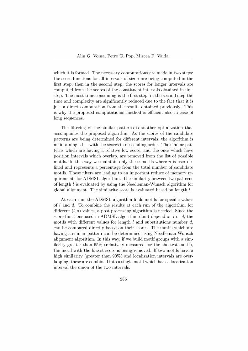
Alin G. Voina, Petre G. Pop, Mircea F. Vaida
which it is formed. The necessary computations are made in two steps:the score functions for all intervals of size i are being computed in thefirst step, then in the second step, the scores for longer intervals arecomputed from the scores of the constituent intervals obtained in firststep. The most time consuming is the first step; in the second step thetime and complexity are significantly reduced due to the fact that it isjust a direct computation from the results obtained previously. Thisis why the proposed computational method is efficient also in case oflong sequences.
The filtering of the similar patterns is another optimization thataccompanies the proposed algorithm. As the scores of the candidatepatterns are being determined for different intervals, the algorithm ismaintaining a list with the scores in descending order. The similar pat-terns which are having a relative low score, and the ones which haveposition intervals which overlap, are removed from the list of possiblemotifs. In this way we maintain only the n motifs where n is user de-fined and represents a percentage from the total number of candidatemotifs. These filters are leading to an important reduce of memory re-quirements for ADMSL algorithm. The similarity between two patternsof length l is evaluated by using the Needleman-Wunsch algorithm forglobal alignment. The similarity score is evaluated based on length l.
At each run, the ADMSL algorithm finds motifs for specific valuesof l and d. To combine the results at each run of the algorithm, fordifferent (l, d) values, a post processing algorithm is needed. Since thescore functions used in ADMSL algorithm don’t depend on l or d, themotifs with different values for length l and substitutions number d,can be compared directly based on their scores. The motifs which arehaving a similar pattern can be determined using Needleman-Wunschalignment algorithm. In this way, if we build motif groups with a sim-ilarity greater than 65% (relatively measured for the shortest motif),the motif with the lowest score is being removed. If two motifs have ahigh similarity (greater than 90%) and localization intervals are over-lapping, these are combined into a single motif which has as localizationinterval the union of the two intervals.
286

A New Algorithm for Localized Motif Detection in . . .
4 Experiments and Results
The first test that we’ve done with the scope to get an overview of theADMSL algorithm was by generating with [13] a dataset which contains50 DNA sequences, each of them of 3000 nucleotides length. Randomly,we’ve inserted the motif GCATG (5,1) in 75% of the sequences at dif-ferent positions. The obtained sequences were analyzed using ADMSLconfigured to search for motifs of length l = 5 and a maximum of d = 1substitutions. The motif instances have been determined by ADMSLalgorithm as localized in [900, 1500] interval.
From the analysis of other researchers [7] [14], the motif (5,1) is asubtle motif and is almost impossible to detect through a sequence of3000 nucleotides because there actually are like a few thousands possi-ble random motifs. The first ten motifs detected by ADMSL (togetherwith the afferent scores) are presented in Table 2.
Table 2. The first 10 motifs reported by ADMSL algorithm whenrunning over a dataset of 50 DNA sequences of 3000 nucleotides each
Pattern Interval SER SSR SIS ScoreGCATG [900, 950] 0.469 0.345 0.432 1.246CGCGA [400, 450] 0.471 0.325 0.423 1.219GTCGA [900, 950] 0.424 0.342 0.359 1.125ATCGT [1200, 1250] 0.425 0.297 0.398 1.12CTTCG [2100, 2150] 0.378 0.432 0.295 1.105TACGC [2850, 2900] 0.421 0.305 0.292 1.018CCGAT [2650, 2700] 0.397 0.297 0.291 0.985TACCG [1800, 1850] 0.345 0.348 0.287 0.98CGTCG [900, 950] 0.451 0.276 0.251 0.978CGATC [950, 1000] 0.411 0.324 0.237 0.972
The pattern (5,1) was correctly identified as the most prominentmotif and the localization interval was detected with accuracy.
This first test was performed to get an overview of the ADMSL
287

Alin G. Voina, Petre G. Pop, Mircea F. Vaida
performance before getting to more representative tests.In the next paragraphs we’ll present the ADMSL performance in
case of short sequences, long sequences and real sequences.
4.1 Short DNA sequences
The tests performed on short DNA sequences have the role to evalu-ate the detection accuracy of ADMSL algorithm and to emphasize therobustness of the algorithm. Each set of sequences was having N se-quences of nucleotides, each of them with a length L < 1000, randomlygenerated using [13]. All of the sequences were artificially implantedwith a motif M which has the characteristics l = 6 and d = 1 along ofa randomly position interval (p1, p2). We have generated 10 datasetsby varying the number of sequences N and the length of the sequenceL. The parameters and their values are presented in Table 3.
Table 3. The value of the parameters used in performance analysis overshort DNA sequences
Parameter N L l d
Value 10..50 200-1000 6 1
In Figure 2 it is presented the detection accuracy of the ADMSLalgorithm in case of short DNA sequences (randomly generated) im-planted with motif M =′ CGATGC ′.
The ADMSL algorithm was configured to report the first 50 possiblemotifs for each DNA sequence. From the reported motifs, we’ve chosenthe motif most closely of the implanted motif M and we had retained –based on the score – the position occupied in the list of reported motifs.
The motifs reported in this case are presented in Table 4.From Figure 2 we can observe that the detection accuracy is de-
creasing while the length of the sequence is increasing but the averagedetection accuracy value was around 83.6%. So, we can observe thatthe detection accuracy of the ADMSL algorithm is relatively high. Thisis because the ADMSL algorithm is not dependent upon the length of
288
A New Algorithm for Localized Motif Detection in . . .
Figure 2. ADMSL detection accuracy in case of short DNA sequencesrandomly generated
Table 4. Detected motifs by ADMSL algorithm in case of short DNAsequences. Detection accuracy for the considered dataset
DNA Se-quence
Motif Position (in the list of 50motifs reported)
Detectionaccuracy
N10L200 GCATGC 3 97%N10L300 GCATGC 39 62%N20L400 TCATGC 4 97%N20L500 ATGCTT 39 62%N30L600 CATGCG 27 74%N30L700 GCATGC 5 97%N40L800 GTGCTA 24 77%N50L800 CATGTA 16 85%N50L900 CCATGC 15 86%N50L1000 ATGCGT 2 99%
289

Alin G. Voina, Petre G. Pop, Mircea F. Vaida
the sequence but rather of the motif localization interval. The localizedsearch reduces the number of concurrent random patterns and increasesthe possibility of comparing motifs.
4.2 Long DNA sequences
The analysis of detection accuracy in case of ADMSL algorithm forlong sequences was performed using data sequences as it follows:
• we’ve generated using [13] ten data sets of 30 random sequencesby varying the length of the sequences from 1000 to 6000 of basepairs;
• in each data set we’ve randomly inserted, in the interval position[200-800], the motif CATGCT.
The ADMSL algorithm was executed directly on the sequences pre-viously obtained, with a maximum length of the interval set to 500nucleotides. We must specify that the fragmentation of the analyzedsequences was not needed (even if their length hit almost 180000 nu-cleotides), because the ADMSL algorithm automatically determinesthe localization interval of the motif.
In case of other motif detection algorithms (like MEME, Weeder)there is necessary a fragmentation of the long sequences and to maintainthe accuracy, these fragments need to have an overlapping rate of about50%.
Each run of the ADMSL algorithm was performed using the pa-rameters specified in Table 5.
Table 5. The value of the parameters used in performance analysis overlong DNA sequences
Parameter N L l dValue 30 1000-6000 6 1
290

A New Algorithm for Localized Motif Detection in . . .
The detection accuracy of the randomly implanted motif, in caseof the long sequences is presented in Figure 3. The detection accuracywas evaluated as the detection sensitivity based on the combined scorefunction of the reported motif.
Figure 3. ADMSL detection accuracy in case of long DNA sequencesrandomly generated
As we can observe, the detection accuracy is maintained over 60%also in case of the long sequences. It is interesting to observe thefluctuation of the accuracy detection once the length of the analyzedsequences grows – we can notice that the accuracy value is increasingand decreasing randomly for the sequences that have a length between200 and 4500 nucleotides. These fluctuations appeared due to the factthat we had randomly inserted the implanted motif and also becausethe analyzed sequences were randomly generated.
The motifs detected by ADMSL algorithm, as being the most closestto the implanted motif, are presented in Table 6.
In Table 6, we can observe that motifs similar to the implantedmotif were detected and reported in localization intervals where the in-
291

Alin G. Voina, Petre G. Pop, Mircea F. Vaida
Table 6. Detected motifs by ADMSL algorithm in case of short DNAsequences. Localization interval
DNA Se-quence
Motif Position (in the list of50 motifs reported)
Localizationinterval
N30L1000 CATGCG 2 [300,550]N30L1500 GCATGC 9 [250,300]N30L2000 CATGCG 10 [250,600]N30L2500 CATGCT 48 [450,500]N30L3000 ATGCTC 34 [1050,1100]N30L3500 ATGCTG 22 [2700,2750]N30L4000 GCATGC 33 [1550,1600]N30L4500 ACATGC 44 [300,350]N30L5000 GCATGC 3 [400,450]N30L6000 CATGCA 1 [250,350]
sertion of the random motif did not occurred – the motif was implantedonly in the positions interval [200, 800]. Those reported motifs havebeen detected as valid motifs because they were present in the initialsequences, randomly generated.
4.3 Real DNA sequences
Motifs detection in long regulatory sequences it is an actual require-ment especially in ChIP experiments for determining the promoters forvertebrates [5]. Some recent studies [7] [14] are highlighting that ran-dom patterns from DNA sequences may become remarkable as if thereal motifs. In this specific case, the algorithms used for motif detec-tion are returning false positives hiding the real motif. For most of thealgorithms, the necessary resources – memory requirements and execu-tion time – are proportionally increasing with the size of the analyzedsequence.
In the literature, it is known the fact that the motif instances are
292

A New Algorithm for Localized Motif Detection in . . .
found to be localized at specific positions, relatively to a reference po-sition (anchor point) [5]. Most of the transcriptions factors are beinglocalized relatively to a transcription start site to allow the transcrip-tion factors to be localized in specific positions. In these conditions,the motif detection can be done by searching into a specific intervalafter the alignment of the sequences relatively to the anchor point.
The localization of motifs has an important advantage by remov-ing the regions which are not containing motifs and by decreasing thepossibility of returning false positives.
One possibility is to divide the DNA sequences into short overlap-ping subsequences of the same size. Some problems may occur:
• in most of the cases we don’t have prior information regardingthe regions where the motifs are distributed;
• in case of a big number of reported motifs in a range of intervalsit is really a challenge to identify and extract those motifs whichhave the greatest importance for the analyzed sequence;
• depending on the chosen length for the sequences the motifs mightnot be so obvious if the length is short and might be poorlydemarcated if the length is too big;
• the division of the analyzed sequence in subsequences must bedone automatically otherwise it will require time and it will bemore susceptible to errors.
In the performance evaluation for real data sequences, to not disad-vantage any of the algorithms, we’ve chosen to not split the sequenceinto subsequences. The analysis was performed on the entire sequencein order to make judgments regarding performance directly over longDNA sequences as we found them in genomic repositories.
A big challenge in this research was to choose the right datasetswith the scope to not favor or disfavor any of the algorithms thatwe’ve used in comparison with ADMSL. Tompa [12] presents a fewsolutions for DNA datasets selection but each of them have severaldrawbacks. In order to pass these drawbacks we’ve used transcription
293
Alin G. Voina, Petre G. Pop, Mircea F. Vaida
factors reported as real in TRANSFAC repository. From the biologicaldatabase previously mentioned, we had chosen only the transcriptionfactors which were having also a consensus sequence defined.
We’ve executed tests on different sequences corresponding to thefollowing species: Saccaromyches Cerevisiae, Drosophila Melanogasterand Homo Sapiens. All the algorithms used in this assessment(ADMSL, MEME, AlignAce, YMF, Improbizer, Weeder and SCOPE)have been configured to detect motifs that have a length in the rangeof six to ten nucleotides. In this performance evaluation we took intoaccount the first ten motifs detected by each of the analyzed algorithm.In order to obtain an overview of each algorithm we’ve run the appli-cations/algorithms over each dataset. Besides the proposed algorithm– ADMSL – all others have been used without modifying the sourcecode of the applications and the evaluations were performed over theirofficial web sites or by running the application locally.
In the next figures we present the detection accuracy of the consid-ered algorithms.
If we consider the Drosophila Melanogaster dataset (Figure 4), a bigmajority of the reported motifs had a length between 3bp (Improbizer)and 10bp (MEME, YMF).
Most of the motifs reported had a corresponding real transcriptionfactor in TRANSFAC database (the motifs reported by Improbizerwere not found in TRANSFAC database – that’s why the accuracy is setto 0). From the performance point of view we can confirm that ADMSLhad reported the most motifs for which we had found a correspondingtranscription factor in TRANSFAC database. Also, we’ve noticed thatYMF and SCOPE had good performances.
For Homo Sapiens dataset (Figure 5) we’ve used sequences withmore than 36000 nucleotides. We’ve observed that the algorithm hadreported motifs that we had found as transcription factors in biologicaldatabase (TRANSFAC). Over 90% of the motifs reported by ADMSLwere identified as real transcription factors in TRANSFAC genomerepository. Once the length of the analyzed sequence had increased,the number of false positives had also increased.
Also in case of Saccaromyches Cerevisiae dataset (Figure 6) the
294

A New Algorithm for Localized Motif Detection in . . .
Figure 4. Detection accuracy for Drosophila Melanogaster dataset
ADMSL algorithm had proved to be more accurate than the otheranalyzed algorithms. MEME and YMF had accuracy close to ADMSLalgorithm.
5 Conclusions
The main purpose of this research was to design and develop a newalgorithm for detecting DNA motifs especially in long sequences wherethe performance of existing applications is relatively poor. The algo-rithm proposes an innovative way for detection and localization of DNAmotifs by combining multiple score functions to evaluate the existenceof a motif.
ADMSL had been optimized to fast process long DNA sequences.The results obtained on synthetic or real data confirmed us that
295

Alin G. Voina, Petre G. Pop, Mircea F. Vaida
Figure 5. Detection accuracy in case of Homo Sapiens dataset
ADMSL has a definite advantage beside other algorithms due to thedetection accuracy of the motifs in long DNA sequences.
In the recent years, considerable efforts were made in elaboratingcomputational methods and more and more species have a completeDNA sequence. Nevertheless, the identification of the elements thatare part of the cis-regulatory process continues to be an importantchallenge for scientists.
At the beginnings, the algorithms focused on motifs searching werecombining the phylogenetic data with co-regulated genes in order tofind regulatory motifs. In the present, most of the algorithms are ori-ented to computational methods and researchers are designing newapproaches to better identify the motifs from the analyzed DNA se-quences.
Due to the big number of algorithms and multitude of the methodsdesigned for motif identification, for a user, it will be helpful a set of
296

A New Algorithm for Localized Motif Detection in . . .
Figure 6. Detection accuracy in case of Saccaromyches Cerevisiaedataset
instructions for choosing the best algorithm/method before starting theanalysis of the DNA sequence.
One of the drawbacks when providing instructions for deciding toa method or another is the number of settings and parameters whichneed to be chosen for each algorithm. The main advantage of ADMSLalgorithm is the fact that the DNA sequences, even if they have aconsiderable length, don’t need to be divided in order to obtain motiflocalization information. Another plus of ADMSL algorithm is thefact that needs just a few parameters (e.g. length of the search motif,allowed substitutions, size of interval search) which have also defaultvalues set in the application that runs ADMSL algorithm. In this waya user can obtain a first set of results with a minimum effort.
Performance evaluation of a motif search algorithm by comparingwith other algorithms is especially problematic. This is because we
297

Alin G. Voina, Petre G. Pop, Mircea F. Vaida
don’t have yet a complete understanding of the process that regulatesgene activity and expression. Also, there is no standardized modelagainst to evaluate the efficiency of an algorithm. In the tests donein this research we must consider the fact that in case of the otheralgorithms used in comparison with ADMSL, the parameters were setwith values to reflect as much as accurate the configurations done forADMSL algorithm. Because this was done through human interaction– it is susceptible to errors.
Most of the algorithms used in comparison to evaluate the per-formance of ADMSL algorithm, have good results in case of lowerorganisms, especially when they are set to report short motifs (of 6-8 nucleotides). The ADMSL algorithm, through the computed scorefunctions, highlights the motifs conservation through different species.The performances of ADMSL algorithm have proved to be much bet-ter especially for long DNA sequences like the ones that we’ve analyzedfrom human genome.
References
[1] Martin Tompa Mathieu Blanchette. Discovery of Regulatory Ele-ments by a Computational Method for Phylogenetic Footprinting,Genome Res, pp. 739–748, 2002.
[2] Patrik D’haeseleer. What are DNA motifs?, Nature Biotechnology,vol. 24, pp. 423–425, 2006.
[3] Hubbard TJ. Down TA, NestedMICA: sensitive inference of over-represented motifs in nucleic acid sequence, Nucleic Acids Res.,pp. 1445–53., 2005.
[4] Ho-Kwok Dai Modan K Das. A survey of DNA motif finding al-gorithms, BMC Bioinformatics, 2007.
[5] Ankush Mital, Wing-Kin Sung Vipin Narang. Localized Motif dis-covery in gene regulatory sequences, Bioinformatics, vol. 26, no. 9,2010.
298
A New Algorithm for Localized Motif Detection in . . .
[6] F.P. Roth, J. D. Hughes, P. W. Estep, G.M. Church. Finding DNARegulatory Motifs within Unaligned Non-Coding Sequences Clus-tered by Whole-Genome mRNA Quantitation, Nature Biotechnol-ogy, pp. 939–945, 1998.
[7] Martin Tompa Jeremy Buhler. Finding Motifs using Random Pro-jections, Journal of Computational Biology, vol. 9, no. 2, pp. 225–242, 2002.
[8] S.T. Smale, J.T. Kadonaga. The RNA polymerase II core pro-moter, Annu Rev Biochem, vol. 72, pp. 449–479, 2003.
[9] P.A. Pevzner, M.Yu. Borodovsky, A.A. Mironov. Linguistics ofnucleotide sequences, J Biomol Struct Dyn, vol. 6, pp. 1013–1026,1989.
[10] G. Thijs, M. Lescot, K. Marchal, S. Rombauts, B. De Moor,P. Rouze, Y. Moreau. A higher-order background model improvesthe detection of promoter regulatory elements by Gibbs sampling,Bioinformatics, pp. 1113–1122, 2001.
[11] Stormo G.D. DNA binding sites: representation and discovery,Bioinformatics, vol. 16, no. 23, 2000.
[12] Tompa M. An exact method for finding short motifs insequences,with application to the ribosome binding site problem, in Proceed-ings of the Seventh International Conference on Intelligent Systemson Molecular Biology, 1999, pp. 262–271.
[13] http://www.bioinformatics.org/sms2/random dna.html
[14] U. Keich, P.A. Pevzner. Finding motifs in the twilight zone, Bioin-fomratics, vol. 18(10), no. 1382–1390.
[15] Elkan C Bailey TL. Unsupervised learning of multiple motifs inbiopolymers using expectation, Machine Learning, pp. 51–80, 1995.
[16] W.Y. Ao, J. Gaudet, W.J. Kent, S. Muttumu, S.E. Mango. En-vironmentally Induced foregut remodelling by PHA-4/FoxA andDAF-12/NHR, Science 305, pp. 1743–1746, 2004.
299

Alin G. Voina, Petre G. Pop, Mircea F. Vaida
[17] G. Pavessi, P. Mereghetti, G. Mauri, G. Pesole. Weeder Web: dis-covery of transcription factor binding sites in a set of sequencesfrom co-regulated genes, Nucleic Acid Res. 32, pp. 199-203, 2003.
[18] Jonathan M. Carlson, Arijit Chakravarty, Charles E. DeZiel,Robert H. Gross. Scope: a web server for practical de novo motifdiscovery, Nucl. Acids Res, pp. 259–64, Jul 2007.
Alin G. Voina, Petre G. Pop, Mircea F. Vaida Received May 19, 2014
Technical University of Cluj-Napoca,Communications Department,26-28 George Baritiu St., Room 364400027 Cluj-Napoca, Romania,Tel: +40-264-401226, Fax: +40-264-597083E–mails: [email protected]
[email protected]@com.utcluj.ro
300
Copyright © 2022 FDOKUMEN