Brain Tumor Detection Through Image

Processing

by

Tahaziba Azmim 17301019

Azizul Hakim chy.Shumon 18301300

Maksud Alam 16201033

Saurav Ahmed Mishu 16201022

Nuhash Ahmed Chowdhury 16301037

A thesis submitted to the Department of Computer Science and Engineering in partial fulfillment of the requirements for the degree of

B.Sc. in Computer Science

Department of Computer Science and Engineering BRAC UNIVERSITY

January 2021

© 2021. Brac University All rights reserved.

Declaration

It is hereby declared that

1. The thesis submitted is my/our own original work while completing degree at Brac University.

2. The thesis does not contain material previously published or written by a

third party, except where this is appropriately cited through full and accurate referencing.

3. The thesis does not contain material which has been accepted, or submitted,

for any other degree or diploma at a university or other institution.

4. We have acknowledged all main sources of help.

Student’s Full Name & Signature:

Tahaziba Azmin Azizul Hakim chy.Shumon 17301019 18301300

Maksud Alam Saurav Ahmed Mishu 16201033 16201022

Nuhash Ahmed Chowdhury 16301037

i

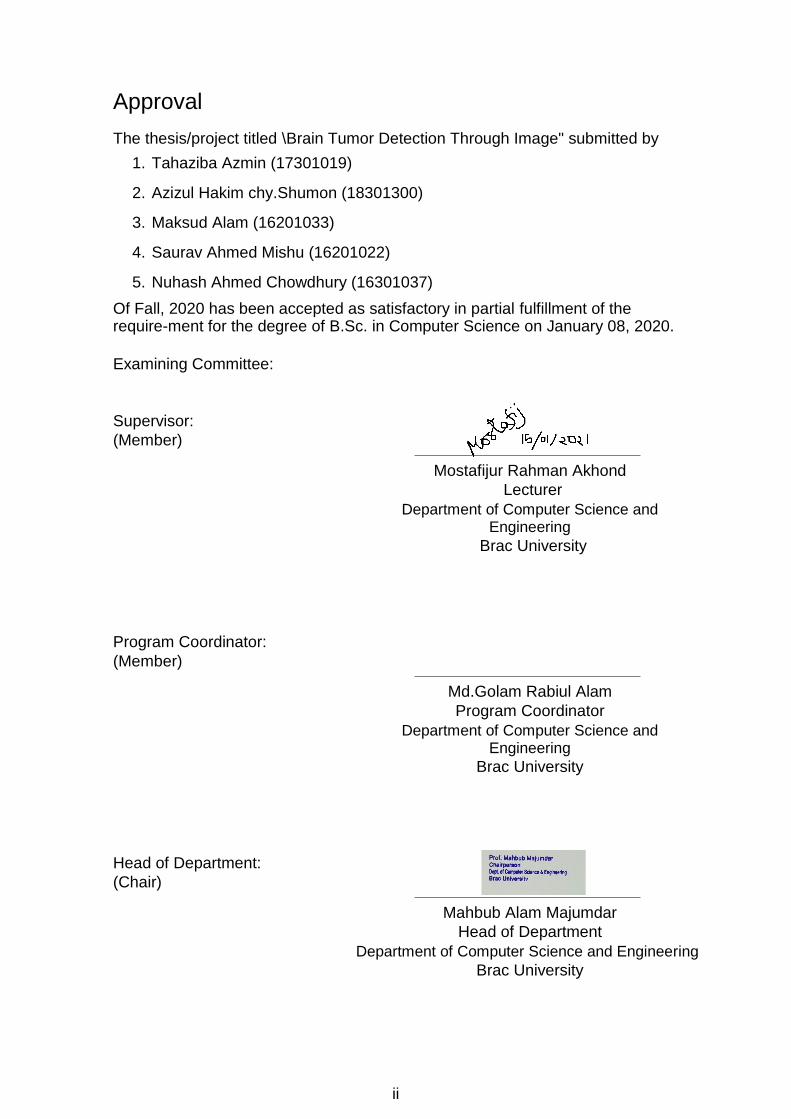
Approval

The thesis/project titled \Brain Tumor Detection Through Image" submitted by

1. Tahaziba Azmin (17301019)

2. Azizul Hakim chy.Shumon (18301300)

3. Maksud Alam (16201033)

4. Saurav Ahmed Mishu (16201022)

5. Nuhash Ahmed Chowdhury (16301037)

Of Fall, 2020 has been accepted as satisfactory in partial fulfillment of the require-ment for the degree of B.Sc. in Computer Science on January 08, 2020.

Examining Committee:

Supervisor: (Member)

Mostafijur Rahman Akhond Lecturer

Department of Computer Science and Engineering

Brac University

Program Coordinator: (Member)

Md.Golam Rabiul Alam Program Coordinator

Department of Computer Science and Engineering

Brac University

Head of Department: (Chair)

Mahbub Alam Majumdar Head of Department

Department of Computer Science and Engineering Brac University

ii

Abstract

Begin with image processing for technology to detect brain tumors. I.e.

(The identification of tumor/cancer cells from brain images is primarily

based on image recognition methods, since these images are complex

and human eyes are not ideal for interpreting the transformed cells

with several degrees of changes). There are different types of

instruments to help diagnose brain tumors, such as MRI scans, CT

scans, etc. The device that can detect any organ and brain problem is

MRI (Magnetic Resonance Imaging). Segmentation cell multiplication

is an important strategy for processing brain tumor images. The

segmentation or multiplication of cells will recognize the tumor along

with its neighboring compartments and nearby tissues, but it is difficult

enough to repair and shape the morphological changes caused by

the tumor. Even though there are a number of current works on the

subject. Many methods, such as template-based K means algorithm,

fuzzy logic algorithms, threshold segmentation, etc., have been used to

establish image processing, but the precision of the performance rate

is still not up to the mark. In our proposed methodology our main purpose is to get a more clear image form

MRI. We would try to use CNN algorithm which is more flexible and convenient. That will detect the position of the tumor automatically. This proposed methodology will be more efficient and faster to identify the tumor region and also it will be more effective and accurate for brain tumor detection and segmentation. Our main focus is on the methods used to identify brain tumors through image segmentation.

Keywords: Image Processing; Cell multiplication; Tumor detection ; Template- based K means algorithm; Fuzzy logic algorithms; Threshold segmentation; Machine learning; Statistical approach ,Deep neural network; algorithms; Deep learning; Precision, neural network

Acknowledgement

Firstly, all praise to the Great Allah for whom our thesis have been completed with-out any major interruption.

Secondly, to our advisor Mosta zur Rahman Akhond sir for his kind support and advice in our work. He helped us whenever we needed help.

And nally to our parents without their throughout sup-port it may not be possible. With their kind support and prayer we are now on the verge of our graduation.

iv

Table of Contents

Declaration i

Approval ii

Abstract iii

Acknowledgment iv

Table of Contents v

List of Figures vii

List of Tables 1

1 Introduction 2

2 Proposed Idea 5

2.1 U-net and Convolutional Neural Network . . . . . . . . . . . . . . . . 5

2.2 Convolutional Neural Network (CNN) . . . . . . . . . . . . . . . . . . 8

2.3 Reason behind choosing CNN: . . . . . . . . . . . . . . . . . . . . . . 9

3 Research Methodology 11

3.1 Research strategy . . . . . . . . . . . . . . . . . . . . . . . . . . . . . 11

3.2 Why machine learning . . . . . . . . . . . . . . . . . . . . . . . . . . 11

3.3 Research method { Qualitative versus Quantitative techniques . . . . 12

3.4 Table: Features of Qualitative and Quantitative Research . . . . . . . 12

3.5 Research approach . . . . . . . . . . . . . . . . . . . . . . . . . . . . 13

4 Literature Review 14

4.1 Causes of Tumor Development . . . . . . . . . . . . . . . . . . . . . . 14

4.2 Causes and Classi cation of Brain Tumor . . . . . . . . . . . . . . . . 14

4.3 Recurrent neural networks (RNN) . . . . . . . . . . . . . . . . . . . . 15

4.4 Deep Neural Networks (DNN) . . . . . . . . . . . . . . . . . . . . . 16

4.5 Image Segmentation and Technology used for Brain Tumor Detection 19

4.6 Papers Based on Brain Tumor Detection . . . . . . . . . . . . . . . . 19

5 Research objectives 25

v

6 DATA ANALYSIS 26

6.1 DATAANALYSIS ............................ 26

6.2 Comparison of di erent functions . . . . . . . . . . . . . . . . . . . . 27

7 Result 29

8 Conclusion and future work 35

Bibliography 36

Bibliography 37

vi

List of Figures

2.1 U-net Architecture. . . . . . . . . . . . . . . . . . . . . . . . . . . . . 6

2.2 Detailed U-net Architectur . . . . . . . . . . . . . . . . . . . . . . . . 7

2.3 CNN Methodology . . . . . . . . . . . . . . . . . . . . . . . . . . . . 9

4.1 Flowchart of the proposed TKFCM algorithm . . . . . . . . . . . . . 22

7.1 ReLU and ADAM(Attributes) . . . . . . . . . . . . . . . . . . . . . . 29

7.2 Sample test image . . . . . . . . . . . . . . . . . . . . . . . . . . . . . 30

7.3 Sample predicted image . . . . . . . . . . . . . . . . . . . . . . . . . 30

7.4 Maximum accuracy (01) . . . . . . . . . . . . . . . . . . . . . . . . . 30

7.5 Maximum accuracy (02) . . . . . . . . . . . . . . . . . . . . . . . . . 31

7.6 Loss . . . . . . . . . . . . . . . . . . . . . . . . . . . . . . . . . . . . 31

7.7 ACCURACY ............................... 32

7.8 Dice co-e cient . . . . . . . . . . . . . . . . . . . . . . . . . . . . . . 32

7.9 Validation Loss . . . . . . . . . . . . . . . . . . . . . . . . . . . . . . 33

7.10 Validation Accuracy . . . . . . . . . . . . . . . . . . . . . . . . . . . 33

7.11 Vallidation dice co-e cient . . . . . . . . . . . . . . . . . . . . . . . . 34

vii

List of Tables

6.1 Data Analysis Table(a) . . . . . . . . . . . . . . . . . . . . . . . . . 27

6.2 Data Analysis Table(b) . . . . . . . . . . . . . . . . . . . . . . . . . . 27

6.3 Data Analysis Table(c) . . . . . . . . . . . . . . . . . . . . . . . . . . 28

6.4 Data Analysis Table(d) . . . . . . . . . . . . . . . . . . . . . . . . . . 28

1

11

Chapter 1

Introduction

Computer plays a vast role in today’s world. In today’s world, we use

computers in various ways such as, for communication, for animation, for

making games, for doing various kinds of experiments, for running

algorithms and most uses for medical science. Image processing is mostly

used in medical science. Two kinds of image processing techniques are there.

Linear image processing is one, and optical image processing is another. Using

the machine, digital image processing methods aid in editing the images. So, by

using digital image processing we can improve biological sciences. For

example, many kinds of detection for instance, tumor detection, cancer

detecting. Moreover, by using digital image processing we can do

classification, testing and also can examine the critical parts of the human

body. In today’s medical science, brain tumor detection plays a conspicuous

role. Therefore, the brain is the most important part and the most complex

organ in the human body. It is the central organ of the human nervous

system. Emotions, memory, behavior, thought, etc. are controlled by the

brain as well as breathing and heart beating. The brain contains almost 50-

100 billion neurons. Moreover, with large numbers of cells, the brain is

manufactured though the damaged cells or the old cells die whenever the

new natural cells grow and then the new cells take their place into the old

one’s or damaged cells place but, sometimes the damaged cells or old cells

do not die and the new cells procreate when the body does not necessarily of

them. So, when the damaged cells do not die and grow of the new cells

which are useless for the body, then the extra cells build up with a mass

collection of tissues which is called a tumor. It is so chancy to treat the tumor

because of its spreading capability and location. Two general brain tumor

groups are there. Primary or Core brain tumors are one of them and

secondary brain tumors are another. Brain tissue is the starting point of The

Core brain tumor and they take place there, on the other hand, a most

common issue is secondary brain tumors where cancers grow somewhere

else in the part of the body and go to the brain, kidney, skin, etc. that leads to

cancer and can go to the brain. There might be cancer cells in some brain

tumors and some don’t contain it. One is benign brain tumors and another

one is malignant brain tumors. The benign brain tumors do not contain

cancer cells moreover they generate so slowly, can be removed and its too

rare to spread around the brain. On the other hand, malignant brain tumors

have cancer cells whose growth rate is so fast. The tumor can be grown

12

and spread so fast. In the beginning the tumors are going to look normal and

will grow slowly then in 2nd grade the cells look abnormal and now this time

the tumor can be spread to the nearby tissue. In the end, the tumor cells will

look like most abnormal and it will grow so fast and spread quickly.

It is a common disease nowadays. For this reason, the mortality rate among

adults and young people is increasing. In 2012, the age-specific incidence

and mortality rate (ASR) of brain cancer in developed countries were 5.9

and 4 in men, and 4.4 and 0.4 in women, respectively. These rates were 3.3

and 2.6 in men and 2.7 and 9.1 in women, respectively in developing

countries. (KHODAMORADI, GHONCHEH, PAKZAD, GANDOMANI, and

SALEHINIYA, 2017) An approximate 23,890 people (13,590 males and

10,300 females) will be treated with cancerous tumor of the brain. [2] The

probability of a person developing this type of tumor in their lifetime is less

than 1% . Of all main central nervous system (CNS) cancers, brain tumors

account for 85 percent to 90 percent. The tenth main cause of death for

men and women is brain cancer. It is projected that this year, 18,020

individuals (10,190 males and 7,830 females) will suffer from primary brain

and CNS cancers Imaging plays a significant role in medical research in

today's healthcare system. [1]. By the segmentation and partition of the

image, doctors can easily find out the exact problem. But it is quite hard to

do. There are some problems such as medical image management, image

data mining, bio-imaging, medical visualization augmented reality, and

neuroimaging to do imaging. At an early age, it was quite hard to detect the

tumor but today, it becomes easy to detect the tumor at the exact location

by using computers through digital image processing. By detection of brain

tumors, we can identify not only the affected part of the brain but also the

size, boundary, shape and position of the tumor. There are different kinds

of imaging technologies such as computed tomography (CT), magnetic

resonance image (MRI), etc. and these technologies are used for brain

imaging [3]. The physiology of the brain tumor can be tested by a CT scan

or MRI. MRI (magnetic resonance imaging) is a type of scan that uses

strong magnetic fields and radio waves to produce high- quality images of

the inside of the body and body parts such as the brain, bones, joints, heart,

blood vessels and internal organs. Through the high quality or resolution of

the image we can derive the corporal tidings and can easily apprehend the

abnormalities of tumors. Moreover, that technic can easily detect the

varieties in tissues and structure of the tissues. But, the main goal of our

tumor detection by image processing is going to solve by multiple machine

learning algorithms. Machine learning is an artificial intelligence technology

that allows algorithms the ability to learn and optimize from recreation

without being directly programmed in addition, it is the idea that a computer

program can learn and handle new information without human intrusion. In

comparison, machine learning focuses largely on the development of

computer programs that can view and then use data and learn about

themselves, allowing voluminous volumes of data to be studied. Machine

learning algorithms are, however, known as supervised or unsupervised.

Supervised machine learning algorithms can be applied where what has

been learned already in the past to new data using labeled examples to

predict future thoughts. On the other hand, when the information is not

13

classified or labeled then unsupervised machine learning algorithms are

being used. So, we will use machine learning for our image processing.

Suppose, training the machine to do something (here, image processing) by

providing a set of training data. Machine learning has features, loss

functionality and different methods which can be used to decide which will

provide improved analysis of images. It also relies on the type of processing

of images that we intend to do as certain loss functions perform better than

others due to their inherent properties for instance, there is a strong

probability that the cross-entropy logistic regression will work better in order

to have better image analysis than other loss function

14

Chapter 2

Proposed Idea

This section describes the process of brain tumor segmentation approach of our U- NET based Convolutional Neural Network in detail including CNN methodology, Algorithm, Reason behind using CNN, U-NET architecture.

2.1 U-net and Convolutional Neural Network

Brief description of U-net Architecture The UNET for Bio Medical Image

Segmentation was designed by Olaf Ronneberger et al. There are two

approaches to this architecture. The first direction is the contraction path,

(also known as the encoder) that is used in the image to catch the

backdrop. The encoder is just a conventional stack of max pooling and

layers of convolutional. The second direction is the symmetrical path that

extends (also known as decoder) that uses Convolutions transposed to

allow Accurate localisation. It is therefore a fully convolutional end-to-end

(FCN) network, for instance It just includes convolutionary layers and no

thick layer is used. This makes it to accept pictures of any dimension.

15

ILLUSTRATION OF U-NET ARCHITECTURE

Figure 2.1: U-net Architecture.

Fig-3.1 U-net architecture (Example for the lowest resolution of 32*32 pixels). Each blue box corresponds to a multi-channel feature map. On the top of the box, the number of channels is denoted. At the lower left edge of the box, the x-y size is given. White boxes represent copied feature maps. The arrows denote the distinct operation.

6

16

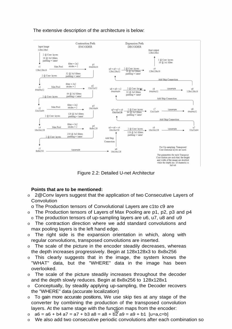
The extensive description of the architecture is below:

Figure 2.2: Detailed U-net Architectur

Points that are to be mentioned:

o 2@Conv layers suggest that the application of two Consecutive Layers of

Convolution

o The Production tensors of Convolutional Layers are c1to c9 are

o The Production tensors of Layers of Max Pooling are p1, p2, p3 and p4

o The production tensors of up-sampling layers are u6, u7, u8 and u9

o The contraction direction where we add standard convolutions and

max pooling layers is the left hand edge.

o The right side is the expansion orientation in which, along with

regular convolutions, transposed convolutions are inserted.

o The scale of the picture in the encoder steadily decreases, whereas

the depth increases progressively. Begin at 128x128x3 to 8x8x256

o This clearly suggests that in the image, the system knows the

"WHAT" data, but the "WHERE" data in the image has been

overlooked.

o The scale of the picture steadily increases throughout the decoder

and the depth slowly reduces. Begin at 8x8x256 to 128x128x1

o Conceptually, by steadily applying up-sampling, the Decoder recovers

the "WHERE" data (accurate localization)

o To gain more accurate positions, We use skip ties at any stage of the

converter by combining the production of the transposed convolution

layers. At the same stage with the function maps from the encoder:

o a6 = a6 + b4 a7 = a7 + b3 a8 = a8 + b2 a9 = a9 + b1 [u=a,c=b]

o We also add two consecutive periodic convolutions after each combination so

17

that the design can be trained to build a more accurate output.

o This is what brings a symmetrical U-shape to the architecture, so the term UNET

2.2 Convolutional Neural Network (CNN)

Convolutionary Neural Network: The Con-volutionary Neural Network is commonly

used in medical image processing. A Five-Layer Convolution Neural Network has

been introduced and implemented for tumor detection. Using the convolution layers

as the beginners layer, which is 64 * 64 * 3, an input form of the MRI images is

formed, converting all the images into a homogeneous dimension. After accu-

mulating all images in almost the same aspect, we created a convolutional kernel

that is convoluted with the input layer, implementing 32 convolutional filters of size 3

* 3 each with the help of 3 channel tensors. As an activation function, ReLU is used,

so that the output does not corroborate.

For the spatial data that our input map supports, we use MaxPooling2D for the model.

On a scale of 31*31*32, this convolutional layers layer exists. As the input images

are split into all spatial dimensions, the pool size is (2, 2), suggesting a tuple of two

integers that can be horizontally and vertically scaled down. Following the pooling

layer, a pooled features pattern is generated. Attening is one of the critical layers

after the pooling, as we have to transform the entire matrix reflecting the input

images into a single column vector, and it is crucial for extraction. It is then fed to the

Neural Network for calculation.

Two fully connected layers have been used and the dense layer was represented by

Dense-1 and Dense-2. The dense function is used in Keras for the application of the

Neural Network, and the vector acquired serves as an input for this layer. There are

128 nodes in the secretive layer. Since we held it as mild as possible because we

need to t our model because of the amount of dimension or nodes equal to the

computational resources, and 128 nodes provide much more important result for this

perspective. ReLU is used as the activation function in order to show better

convergence performance. After the first thick layer, the second fully-connected layer

has been used as a model's kernel layer.

[7]

8

18

Figure 2.3: CNN Methodology

Using Adam optimizer and binary cross-entropy as a loss function, we compiled the model and find the accuracy of detecting the tumor. An algorithm is depicted below where we evaluated the performance of the model.

Algorithm : Evaluation process of CNN model loadImage(); dataAugmentation(); splitData(); loadModel(); for each epoch in epochNumber do for each batch inbatchSize do y = model (features); loss = crossEntropy(y, y); optimization(loss); accuracy();

bestAccuracy = max(bestAcuuracy, accuracy); return

2.3 Reason behind choosing CNN:

Assume we have a standard neural feed-forward network, and as an input, giving it the word "neuron" and process the word character by character. "It has

already forgotten about "n," "e" and "u" by the time it hits the character "r,"

which makes it almost di cult for this form of neural network to determine which

character will come next. However, because of its internal memory, a recurrent

neural network is capable of recalling certain characters. This creates output,

copies it and loops it back into the network. Simply stated, recurrent neural

networks add the present to the recent past.

9

19

Therefore, two inputs are required for an RNN: the current and the recent past. This is important because the data sequence provides vital details on what is coming next, which is why other algorithms can not do things an RNN can.

The state of the art sequential data algorithm, Recurrent Neural Networks (RNN), is used by Apple’s Siri and Google’s voice scanIt as because it is the first algorithm that recalls its input due to an inherent memory, which makes it ideally suited for machine learning problems involving sequential data. It is one of the algorithms behind the scenes of the remarkable achievements seen in deep learning over the past couple of years.

10

20

Chapter 3

Research Methodology

As indicated on the top this portion of our research paper includes the research methodology of our thesis paper. We tried to outline the research strategy, the research method, the research approach, the methods of data collection, the se-lection of the sample, the research process, the type of data analysis, the ethical consideration and the research limitations of the project.

3.1 Research strategy The research conducted regarding this dissertation was an applied one, but not

new. There are quite a number of previous academic studies relating to tumor

detection using MRI and brain image processing. Our team has studied some of

the new techniques that have recently taken place, such as morphological

operations, threshold segmentation, K means, clustering of Fuzzy C means,

and U-net dependent networks. We would like to use the neural network

concept and deep learning methods in our proposal. The neural network is

trained to change the input weights of the neurons based on the weights of the

network, leading to output on example inputs. If the network accurately

classifies an image, the weights that contribute to the correct response are

increased, while other weights are reduced. The procedure allowed early neural

networks to learn in a manner that resembled the human nervous system's

actions superficially.

3.2 Why machine learning

First of all from our literature review, where we reviewed the existing methods

for brain image analysis and choose machine learning and deep learning as our

base for this project. A machine learning technique is deep learning at a very

simple level. To learn how to predict and classify data, it teaches a machine to

process inputs through layers. Observation can be in the form of picture, sound

or text. The motivation for deep learning is the way that knowledge is filtered by

the human brain. This technique is ideal for brain tumor detection as well as our

proposal. Though machine learning has been extensively used for brain image

analysis but still can be used for this project and produce the expected result.

11

21

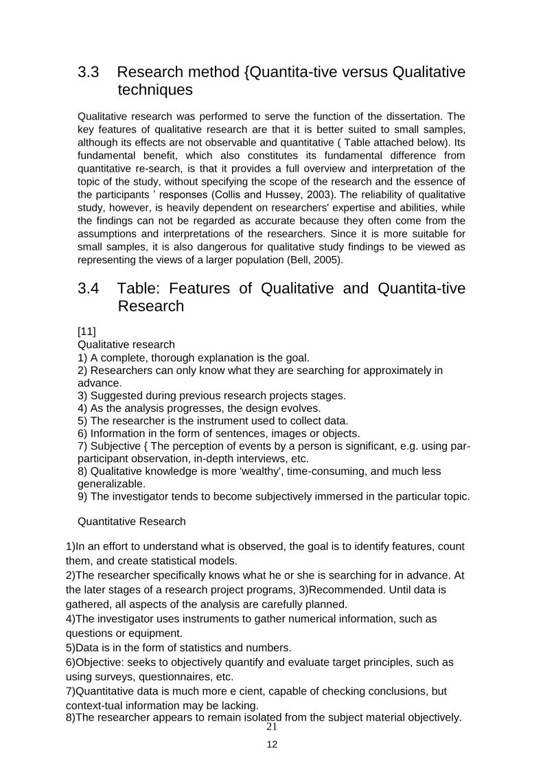
3.3 Research method {Quantita-tive versus Qualitative techniques

Qualitative research was performed to serve the function of the dissertation. The

key features of qualitative research are that it is better suited to small samples,

although its effects are not observable and quantitative ( Table attached below). Its

fundamental benefit, which also constitutes its fundamental difference from

quantitative re-search, is that it provides a full overview and interpretation of the

topic of the study, without specifying the scope of the research and the essence of

the participants ’ responses (Collis and Hussey, 2003). The reliability of qualitative

study, however, is heavily dependent on researchers' expertise and abilities, while

the findings can not be regarded as accurate because they often come from the

assumptions and interpretations of the researchers. Since it is more suitable for

small samples, it is also dangerous for qualitative study findings to be viewed as

representing the views of a larger population (Bell, 2005).

3.4 Table: Features of Qualitative and Quantita-tive Research

[11] Qualitative research 1) A complete, thorough explanation is the goal. 2) Researchers can only know what they are searching for approximately in advance. 3) Suggested during previous research projects stages. 4) As the analysis progresses, the design evolves. 5) The researcher is the instrument used to collect data. 6) Information in the form of sentences, images or objects. 7) Subjective { The perception of events by a person is significant, e.g. using par-participant observation, in-depth interviews, etc. 8) Qualitative knowledge is more 'wealthy', time-consuming, and much less generalizable. 9) The investigator tends to become subjectively immersed in the particular topic. Quantitative Research

1)In an effort to understand what is observed, the goal is to identify features, count

them, and create statistical models.

2)The researcher specifically knows what he or she is searching for in advance. At

the later stages of a research project programs, 3)Recommended. Until data is

gathered, all aspects of the analysis are carefully planned.

4)The investigator uses instruments to gather numerical information, such as

questions or equipment.

5)Data is in the form of statistics and numbers.

6)Objective: seeks to objectively quantify and evaluate target principles, such as

using surveys, questionnaires, etc.

7)Quantitative data is much more e cient, capable of checking conclusions, but

context-tual information may be lacking. 8)The researcher appears to remain isolated from the subject material objectively.

12

22

3.5 Research approach

The research methodology that was adopted was the inductive one for this analysis.

We start with concrete observations according to this method, which can be used to

generate generalized hypotheses and conclusions drawn from the study. The

explanation for the inductive method was to take account of the context in which

research is active, although it is also most suitable for small samples generating

qualitative data. The key drawback of the inductive approach, moreover, is that it

creates abstract hypotheses and assumptions based only on a limited number of

results, thereby questioning the accuracy of study findings (Denzin and Lincoln,

2005).

13

23

Chapter 4

Literature Review

4.1 Causes of Tumor Development

Tumors are generally known to occur when division and undue growth of cells forms an abnormal mass. Generally, body can control the growth and multiplication of cells but creation of new cells to replace older ones and perform new functions prevent death of cells for a healthier process rejuvenation. Therefore, this process of rejuvenation strikes a balance between growth and mortality of cells, which if disturbed may be responsible in the formation of a tumor. In addition, issues to a body’s immune system can be the cause for tumors as well! Tobacco for example is a leading cause for malignant tumors such as cancer.

The risk factors are[13]: • Benzene and other toxins and chemicals

• Excessive consumption of alcohol

• Environmental toxins like some toxic mushrooms and some kind of poison

that can grow on peanuts (a atoxins).

• Excessive sunlight exposure

• Genetic problems

• Obesity

• Viruses

• Radiation Exposure

4.2 Causes and Classification of Brain Tumor

The reason for most brain and spinal cord tumors is not completely perceived[12], and there are not many settled danger factors. In any case, scientists have discovered a portion of the progressions that happen in typical synapses that may lead them to shape brain tumors. There are three types of Tumor: 1)Benign 2)Pre malignant 3) Malignant[14]

24

Benign

Benign tumors are unusual growth which go beyond the parameters of normal cell growth. .They are not cancerous .They develop gradually, take after typical cells, and are not harmful .They grow only in one place and cannot spread or attack di erent parts of the body. They can anyway get unsafe on the o chance that they push on essential

organs. They only grow in one place and cannot spread or attack various parts of the body [15]. Benign tumors include skin moles, lipomas, liver adenomas as examples.

[16].

Pre malignant

The cells are still not cancerous, but they can become malignant in these tumors. i.e. the development of cancer properties .

Malignant

These tumors consist of embryonic, primitive or cell with little distinction. They grow in a fast, disorganized way that is harmful to the body. They can also invade surrounding tissues and become metastatic, triggering the growth of similar tumors in distant organs.

4.3 Recurrent neural networks (RNN)

Recurrent neural networks also know in its abbreviated form as RNN’s are neural networks with one or more layers of neurons or nodes especially one or more hidden layers therefore fall under the category of multilayer perceptrons or MLP’s[19] for short. Sk=f(Sk-1*Wrec+Xk*Wx) [20]

If Sk is the condition at k, Xk is an external input at k, Wrec and Wx are parameters like the weights of networks feeding forward. Note that the Recurrent neural network can be seen as a state model with a feedback loop. The state evolves over time as a result of the repeat relationship, with a one-times-step delay in feedback. This delayed feedback loop gives the memory of the model because it can remember information from time to time in the states.[21] Typically the final output of the network Yk is calculated from one or more Sk-i....Sk+j states in a certain phase k. [22]

Outputs in an RNN are based on previous input. Therefore it is able to accesses past input known as sequential data which is a series of data that can be used to create a pattern. Unlike the state machine the RNN is able to retain memory of past inputs known as sequential memory. To create a Neural Network that’s strong for Sequential data, we include an inside state to our feed forward neural network that gives us with internal memory or in nutshell, Recurrent Neural Network may be a generalization of a feed forward neural network that has inner memory. RNN executes the theoretical concept of sequential memory, that makes a difference by providing the past encounter and in this way permitting it to anticipate superior on successive information. RNN proves that each input has a recurring function, while the current input output depends on previous input. Simple RNN Cells follow this pattern: [21] Given the following data: input data: X weights: wx recursive weights: wRec Initialize initial hidden state to 0 For each state, one by one:

25

Update new hidden state as: (Input data * weights) + (Hidden state + recursive weights)

26

4.4 Deep Neural Networks (DNN)

Deep Neural Networks (DNN) are a type of Arti cial Neural Network (ANN) which specificity is to contain more than one covered up layer of neurons between the input layer and the yield layer. DNNs are made and trained to grant precise comes about for the particular purpose they were made for. In the event that you need to utilize a DNN for another purpose, you’ll better to be making another one and prepare it for that other reason. The preparing handle is called profound learning. Basically, data is to begin with encouraged to the input neurons. This data will at that point stream through differrant layers of neurons called hidden layers. Neurons in these hidden layers will send a high or low value to all the neurons within the following layer depending on the degree of signi cance (weight) of the connection between the primary said neurons and the ones within the previous layer. Finally the output neurons, values, from which we’ll choose the highest to represent the result given by our neural network. That’s for the forward pass. To train the DNN, the output values are compared to the expected value to calculate the total error, or total cost, of the neural network. We then back propagate the error back through the entire links of the network, with respect to the weights of those links. By doing so, we get the amount of error for which that weight participates towards the total cost. And therefore, how much we should make a change to that weight so that the output of our DNN gets closer to the expected output.

Algorithm for Forward Pass:-

6. Sigmoid Function: S(x) = 1 + =e x returns a value between 0 and 1 FUNCTION sigmoid(x) Return 1=(1 + exp x) END FUNCTION /* * */ PROCEDURE forwardPass() // HIDDEN LAYERS

FOR each hiddenLayers FOR each hiddenLayer’s neurons Set weightedSum to 0 FOR each neuron’s links Multiply link’s weight with associated previousLayer’s neuron’s value Add result to weightedSum END FOR Call sigmoid(weightedSum) Set neuron’s value to result END FOR END FOR // OUTPUT LAYER FOR each outputLayer’s neurons Set weightedSum to 0 FOR each neuron’s links

16

27

Multiply link’s weight with associated previousLayer’s neuron’s value Add result to weightedSum END FOR Call sigmoid(weightedSum) Set neuron’s value to result END FOR END PROCEDURE Algorithm for Total Error(Total cost of the Network):- 2) For E01 and E02 being the output errors of O1 and O2 respectively:- E01 =

(t1 O1)2; E02 = (t2 O2)2

• Total Error of network= E01+E02

• Equation for Process = n1=2(targetn Outputn)2 n=Number of Output Neurons PROCEDURE calculateTotalError() Set totalError to 0 FOR each outputLayer’s neurons

IF neuron EQUALS expected output neuron Set neuron’s expectedValue to 1 ELSE Set neuron’s expectedValue to 0 END IF // /! don’t forget the power of 2 Do (1 / 2) * (neuron’s expectedValue - neuron’s value)² Add result to totalError END FOR END PROCEDURE Combined Algorithm for Backpropogation and Hidden layers:- FUNCTION sigmoidDerivative(x) Return sigmoid(x) * (1 - sigmoid(x)) END FUNCTION /* * */ FUNCTION chainRuleOutput(neuron, link) Do neuron’s value - neuron’s expectedValue Set x to result Call sigmoidDerivative(neuron’s value) Set y to result Set z to previousLayer’s linkedNeuron’s value Save x and y in link Return x * y * z END FUNCTION /* * */ FUNCTION chainRuleHidden(layer, neuron, link) Set x to 0 FOR each nextLayer’s linkedNeuron’s links

17

28

Do linkedNeuron’s link’s x * linkedNeuron’s link’s y * linkedNeuron’s link’s weight Add result to x END FOR Call sigmoidDerivative(nextLayer’s linkedNeuron’s value) Set y to result Set z to previousLayer’s linkedNeuron’s value Save x and y in link Return x * y * z END FUNCTION /* * */ PROCEDURE updateWeights()

• HIDDEN LAYERS

FOR each hiddenLayers FOR each hiddenLayer’s neurons

FOR each neuron’s links

Set link’s weight to link’s newWeight END FOR END FOR END FOR • OUTPUT LAYER FOR each outputLayer’s neurons FOR each neuron’s links Set link’s weight to link’s newWeight END FOR END FOR END PROCEDURE /* * */ PROCEDURE backpropagation() Call calculateTotalError() // OUTPUT LAYER FOR each outputLayer’s neurons FOR each neuron’s links Call chainRuleOutput(neuron, link) Set gradient to result Do link’s weight - (learningRate * gradient)

• do not overwrite link’s weight (weight =/= newWeight) Set link’s newWeight to result END FOR END FOR • HIDDEN LAYERS FOR each hiddenLayers FOR each hiddenLayer’s neurons FOR each neuron’s links Call chainRuleHidden(layer, neuron, link)

18

29

Set gradient to result Do link’s weight - (learningRate * gradient)

• do not overwrite link’s weight (weight =/= newWeight) Set link’s newWeight to result END FOR END FOR END FOR Call updateWeights() END PROCEDURE

4.5 Image Segmentation and Technology used for Brain Tumor Detection

Image segmentation is the process where many mathematical algorithms are applied for segment-specific parts of the image. Nowadays this process is used in the medical sector for early diagnosis. Brain tumor image is one of the sectors of medical image analysis. Early diagnosis will increase the survival rate of patients. Brain tumor cells are abnormal cells that the brain produces in an uncontrolled way various kinds of brain tumors exist. But there are two types of brain tumors, one is benign and the other is malignant. In the past ten years, the number of brain tumor affected people has been increasing day by day, it has been reduced by early diagnosis. Researchers are now trying to make a new algorithm for detecting the brain tumor and segment the tumor cell which can help the doctor for making decisions. Researchers are using MRI images for brain tumor image analysis. Four standard MRI modalities for brain tumor diagnosis which are MRI weighted T1 (T1), MRI weighted T2 (T2), contrast weighted T1 and reversing fluid reduced. Although this can differ from device to device during the MR1 acquisition, about one hundred and fifty slices of 20 Images reflect 3D brain volumes. (Soltaninejad, Zhang, Lambrou, Allinson, and Ye, 2017)

4.6 Papers Based on Brain Tumor Detection

In the paper \A Noble Approach for Brain Tumor Detection Using MRI Images" describes

Based on modern technology, the most commonly used brain tumor detection

technology is MRI. Where wave used MRI from all over the body tissues to and out

the high-quality image. The smallest abnormality in the body can be identified by

MRI, which has the great ability to recognise the variations in tissue structure. It is

more suitable for tumor size detection than computed tomography. Thresholding,

which splits an image into two regions and forms a binary image for segmentation,

is a more flexible technique. It offers a better outcome since the threshold value

depends on the variance of the inner cluster. And the morphological operation is a

large image processing operation in which each pixel is modified based on the

value of another neighborhood pixel to process images based on shapes in this

operation. out On the binarized images, the morphological filter works and output

through operations like erosion and dilation. They used threshold segmentation

based on the morphological operation in this paper. Based on the morphological

19

30

operation, this two-approach greatly improves the threshold segmentation,

identification and extraction of the tumor region , They first retrieved the image from

the MRI database in their suggested technique and then submitted the image to be

pre-processing and enhancement. Where the noise and high-frequency device are

removed and the patient’s data are also removed. The median filter and histogram

equalization for image enhancement were used for pre-processing. Threshold

segmentation is achieved here by turning all pixels below the threshold to one and

all pixels above the threshold to one by taking the binary picture from gray-level

ones. And it defines and extracts relevant information in the case of morphological

operation by using the properties of the shape in the image using binary opening

and binary closing with the assistance of an equation. This morphological method

detects the tumor region in MRI brain images, and also detects the tumor image

alone and also the picture of the morphological operation. (2016 Abd Shuai)

In the paper \Brain Tumor MRI Images Detection and Segmentation Using Genetic Algorithm" describes

A naturally-inspired metaheuristic algorithm is the Genetic Algorithm (GA). Where each solution is represented as a chromosome, each chromosome is constructed from genes. They proposed automatically finding out the position and edge of the tumor in this paper. This analysis was carried out on real images. Due to poor image contrast and artifacts that result in missing or di use tissue borders, segmentation of MRI images is challenging. In order to detect MR brain images, this paper proposed a discrete wavelet-based Genetic Algorithm. First, the MR images are enhanced with discrete wavelet description in their proposed methodology and then the genetic algorithms are applied to detect the tumor pixels. It needs to go through four phases to execute genetic algorithms. The first step is the genotype, whereby the result of an image SI segmentation using k-means is regarded as an individual described by the class of each pixel. The second step is the initial population, where the genotype characterizes a set of individuals. It consists of a combination of the outcomes of segmentation. The third step is the function of fitness, which allows us to quantify an individual’s fitness to the environment by considering its genotype. There are two phases in the fitness function and these two phases run from the formation of the cluster until the chromosome is encoded. by the mean points of the respective cluster. They went through the two processes, which are a selection of people and mutation and cross-over of people, after completing all four phases, to go to the next implementation process, which is the termination criterion. We’ll get the final outcome after that. Their outcome demonstrates that their algorithm is flexible and simple. (2018, Joseph)

In the paper \Automatic Human Brain Tumor Detection in MRI Image Using Template-Based K Means and Improved Fuzzy C Means Clustering Algorithm" describes

This paper proposes a Template based K-means and modified Fuzzy C-means clustering algorithm also known as TKFCM to propose a model that identifies or detects brain tumor from MRI images. In this model, the template is selected based on the convolution between the intensity of the grey level in the small portion of the brain image and the image of the brain tumor. K-means algorithm accentuates the initial segmentation by the selection of the template. The paper calls the C means integration as a mathematical improvement to the K means model as its clustering method of identifying different features can add to important information that can help to identify the tumor in an MRI image better as opposed to just a single cluster centroid using a mean calculation of the data points in a K means model. The paper claims that the results for this model shows a better distinction between irregular and regular brain tissues. It also claims that the calculation for this model in identifying distinctions in brain tissues are faster than that of other models. The paper proposes that their TKFCM model has such high accuracy that even very tiny irregularities in Brain tissues! They also propose the algorithm to work more e effectively and accurately than other algorithms for noisy images. In clustering, K

31

implies clustering calculation, the most widely used brain tumor discovery strategies are the calculation of FCM clustering computations and the maximization of expectations (EM). Clustering is a process by which information is divided into certain bunches. In K-means clustering algorithm the calculation is not supervised, that raw data are isolated into k bunches where k could be a positive number. It is a very basic calculation of clusters, provides clusters and works well for multi dimension information. When the number of factors is huge, it works faster than different level clustering. The paper however admits to the poor performance of the algorithm to large datasets and yet proposes its higher execution time as opposed to Artificial Neural Network as a major advantage for their preference. The paper then describes how the K means model and algorithm utilizes the dataset into K pre-defined separate, non-overlapping subgroups (clusters), where only one group is part of each point. It attempts to keep the inter cluster data points as similar as possible and the clusters as distinct (far). It allots data points to a cluster, so that all data points belonging to that cluster are at a minimum amount of the squared distance between data points and the arithmetical mean of the cluster’s centroid. The less change in clusters, the more homogenous the data points are in the same cluster. The entire tumor detection methodology in the human brain has been introduced. It then describes how the C means algorithm is integrated by the model by feeding this pre-processed image which has gone through the K means model to the fuzzy C means algorithm which then separates the features using its multiple clusters groups on the single cluster group of the K means processed image. This is shown in Figure 1 below.

21

32

Figure 4.1: Flowchart of the proposed TKFCM algorithm

22

33

The images collected in the data set are most often so deprived of the quality that filters clamor and forms the image. The image obtained is converted into a two-dimensional gate in the pre-processing step and is converted in the RGB image to a gray image. A middle channel is used to kill the concussion in the picture. At that point, the image is upgraded by a balanced operation based on the histogram. The initial fragmentation using a format K-means (TK) is based on the premise that concentrates gray level and color mood where k = 8 is concentrated at that level. Once again, the tumor is sifted by the median filter. At that point, the tumor is identified and checked as a rugged line using the advanced FCM algorithm based on the Euclidean removal from the cluster center to each information point, which is essentially dependent on the different features. This may be critical if we are to get a grip on the significance of this modified and incorporated technique. The enhanced FCM is performed for 13 clusters on the basis of the gray level strength. The clustered images are then separated factoring the lowest grey level and differences color intensity. And therefore the paper proposes that TKFCM has a better precision than the other models! The results presented in the paper are as follows :-

• The sensitivity of the proposed TKFCM algorithm for human neoplasm

detection is 27.07 per cent, 4.75 per cent, 1.98 per cent, 2.03 per cent,

15.11 per cent and 17.89 per cent..

• The characteristics of the proposed TKFCM algorithm are 27.04%,

17.07%, 11.2%, 5.5%, 9.1% and 20.% above the normal threshold.

• The accuracy of the proposed TKFCM algorithm is 25.64%, 7.692%,

5.12%, 2.56%, 12.82% and 17.94% over the standard thresholding.

In the paper \Automatic Brain Tumor Detection and Segmentation Using U-Net Based Fully Convolutional Networks" describes

This paper proposes U-Net Based Fully Convolutional Networks for Brain tumor detection and segmentation. This paper begins by analyzing the different medical imaging methods for brain tumor segmentation from Ionizing radiation techniques to Magnetic resonance imaging (MRI). The paper then goes onto explain the inefficiency of manual segmentation for MRI imaging due to its time consuming and human error prone nature, which is why much faster and human error p less tech-nology powered algorithms have taken over. The paper then sets up high grade glioblastoma (HGG) and low grade gilomas (LGG) as the tumors that are going to be the major targets for identification using these U Net Based Fully CNN’s using the BRATS datasets. The paper then describes the challenges as contrasts generated during imaging by these various protocols create an image with all the physical complexities in the brain and thus provide valuable visual information that can eventually diagnose the tumor successfully. Usual MRI protocols use fluid-attenuated reverse retrieval, weighted T1 and T2 or FLAIR and gadolinium-enhanced T1 images. The segmented extent of the brain tumor can separate structures from other tissues of the brain and thus allow a more accurate classification of brain tumor types. Segmentation of longitudinal MRI scans can also accurately track the recurrence of brain tumors, both growth and shrinkage. But even in this case, operators have to manually delineate the method to allow space for mistakes and subjective decision-making which is what the paper wants to eliminate using its model. The paper then informs us of the supervised learning that the BRATS dataset will be put through as opposed to the unsupervised

learning because deep learning requires a hierarchy of increasingly complex features directly from the data. The fundamental idea behind a totally convolutionary network is that all its layers in other words are fully - connected layers. The paper then describes how fully connected layers use convolutional layers to classify each pixel in the image. The final output layer is thus identical in height and width to the picture, but the channel number corresponds to a class number. The final output

34

layer will be height x width x 15 classes if we classify each pixel as a class of fifteen. We can and the most likely class for every pixel with a soft max probability function. The proposed supervised learning approach was validated with both LGG and HGG patients’ data obtained. Our fully automatic method obtained promising results compared to manually defined ground truth. The results for delineating the full tumor regions and higher segmentation for central tumor areas were comparable to other state-of- the-art methods.

24

35

Chapter 5

Research objectives

According to the biological study, the tumor is also called as a neoplasm, which

implies abnormal expansion of tissue where the cell divides more then they

need[17]. Unregulated by the mechanism that controls cells. In this recent

technology we used magnetic resonance image (MRI) for detecting any kind of

brain tumor or abnormality in tissues. In our proposed methodology our main

purpose is to get a more clear image form MRI. We would try to use an

algorithm that is more flexible and convenient. That will detect the position of

the tumor automatically. This proposed methodology will be more efficient and

faster to identify the tumor region and also it will be more effective and accurate

for brain tumor detection and segmentation. Our main focus is on the

techniques used to identify brain tumors through image segmentation.

25

36

Chapter 6

DATA ANALYSIS

6.1 DATA ANALYSIS

Separate genomic subtypes of low-grade gliomas were identified in this

study and may theoretically be used to direct the care of patients is the

purpose of this research is to establish if there is a correlation between

low-grade glioma tumor genomics and patient results through tumor

heterogeneity quantitative measurements in magnetic resonance (MRI)

[4]. Preoperative MRI and genomic results were used in 110 clinicians

from 5 Genome of cancer Atlas facilities with inferior gliomas. To

analyze the imaging data, computer algorithms were applied and given

five quantitative tumor shape measurements in two dimensions. The

genomic results for the investigated patient cohort consisted of long

established genomic clusters, focused on IDH mutation and 1p/19q co-

deletion, cell proliferation, DNA methylation, DNA copy number and

expression of micro RNA. In the IDH wild type group and R2 RNA

Sequence cluster, cancers correlated with far worse outcomes usually

had stronger ASD that suggested a more abnormal shape. The images

collected from the archive of cancer and imaging. The image dataset

contains 110 pa- tients with a total of 4456 brain images where we

used 1056 images for test. Here we used 70% images for training and

30% images for testing. Each image contained an original size of 128

x 128 x 1 in pixels.[5]

37

6.2 Comparison of different functions

We tried to show the difference in our result when we use different

combination of Activation function and Optimizer function.

ReLU ReLU also known as rectified linear function of activation is a function of piecewise that provide the result directly if it is non negative otherwise it will provide output as zero.It overcomes the problem of vanishing gradient and give the opportunity to the model to learn faster and show good performance. Adam: Adam is known as algorithm for optimization that generally used in place of classical stochastic gradient descent process to update network cost iterative based by tranning data. ELU: ELU is known as Exponential Linear Unit is a function that appears to accumulate cost to zero faster and yield more detailed effects. RmsProp optimizer: RmsProp is known as optimizer that normalizes the gradients by using the severity of recent gradients. Over the root mean square gradients, we still establish a moving average from which we split the present gradient

Tables of Data Analysis

Table:01

Activation Optimizer

Epoch Loss Accuracy

Dice coefficient Val Val Val dice

function function Accuracy Loss accuracy coefficiet

ReLU Adam 1/30 -0.3195 0.9619 0.3209 -0.0131 0.1741 0.0127

ReLU Adam 2/30 -0.6365 0.9920 0.6368 -0.0155 0.3056 0.0150

ReLU Adam 3/30 -0.6747 0.9932 0.7050 -0.4079 0.9952 0.4094

ReLU Adam 4/30 -0.7441 0.9939 0.7438 -0.3829 0.9956 0.3857

ReLU Adam 5/30 -0.7720 0.9945 0.7725 -0.4561 0.9949 0.4648

Table 6.1: Data Analysis Table(a)

Table:02

Activation Optimizer

Epoch Loss Accuracy

Dice coefficient Val Val Val dice

function function Accuracy Loss accuracy coefficiet

Elu Adam 1/30 -0.1831 0.9040 0.1825 -0.0112 0.0315 0.0109

Elu Adam 2/30 -0.5218 0.9864 0.5206 -0.0139 .02285 0.0135

Elu Adam 3/30 -0.6697 0.9923 0.6690 -0.4213 0.9956 0.4252

Elu Adam 4/30 -0.6888 0.9987 0.6894 -0.4545 0.9948 0.4665

Elu Adam 5/30 -0.72.59 0.9935 0.7262 -0.4574 0.9952 0.4675

Table 6.2: Data Analysis Table(b)

27

38

Table:03

Activation Optimizer

Epoch Loss Accuracy

Dice coefficient Val Val Val dice

function function Accuracy Loss accuracy coefficient

ReLU RMSProp 1/30 -0.1325 0.9028 0.1332 -0.0114 0.9941 0.0112

ReLU RMSProp 2/30 -0.4936 0.9896 0.4932 -0.1867 0.9926 0.1817

ReLU RMSProp 3/30 -0.6624 0.9923 0.6622 -0.3157 0.9945 0.3349

ReLU RMSProp 4/30 -0.7224 0.9935 0.7227 -0.4678 0.9952 0.4842

ReLU RMSProp 5/30 -0.7577 0.9941 0.7581 -0.5223 0.9958 0.5362

Table 6.3: Data Analysis Table(c)

Table:04

Activation Optimizer

Epoch Loss Accuracy

Dice coefficient Val Val Val dice

function function Accuracy Loss accuracy coefficient

ELu RMSProp 1/30 -0.1719 0.9028 0.1735 -0.0114 0.0541 0.1387

ELu RMSProp 2/30 -0.4606 0.9848 0.4625 -0.1412 0.9755 0.1387

ELu RMSProp 3/30 -0.6492 0.9917 0.6480 -0.4126 0.9957 0.4195

ELu RMSProp 4/30 -0.6894 0.9927 0.6902 -0.3519 0.9942 0.3602

ELu RMSProp 5/30 -0.7238 0.9933 0.7234 -0.1520 0.9940 0.1697

Table 6.4: Data Analysis Table(d)

28

39

Chapter 7

Result

Convolutional neural network method has been used to analysis the performance

for the algorithm. Different kinds of activation functions and optimizer has been

used to nd the accuracy level. First of all, the combination of activation function ‘elu’

and optimizer ‘ADAM’ has shown 90.40%, 98.64%, 99.23%, 99.27%, 99.35%,

respectively. moreover, , the combination of activation function ‘elu’ and optimizer

‘RMSPROP’ has shown 90.28%, 98.48%, 99.17%, 99.27%, 99.33%, respectively.

Furthermore, , the combination of activation function ‘ReLU’ and optimizer ‘RM-

SPROP’ has shown 90.28%, 98.96%, 99.23%, 99.35%, 99.41%, respectively.

How-ever, the combination of activation function ‘ReLU’ and optimizer ‘ADAM’ has

shown 96.19%, 99.20%, 99.32%, 99.39%, 99.45%, respectively. From the

comparison, it is observed that the activation function ‘ReLU’ and the optimizer

‘ADAM’ performs better than others.

Figure 7.1: ReLU and ADAM(Attributes)

In the above figure, ReLU has been used for activation function and ADAM has been used for optimizer. By using this combination, we found the better accuracy.

29

40

Figure 7.2: Sample test image

Figure 7.3: Sample predicted image

Figure 7.4: Maximum accuracy (01)

30

41

From the above figure of accuracy level01, here it has been shown top ve epochs where the accuracy are 96.19%, 99.20%, 99.32%, 99.39%, 99.45%.

Figure 7.5: Maximum accuracy (02)

From the above figure of accuracy level02, here it has been shown the next epochs where the accuracy are 99.49%, 99.50%, 99.53%, 99.54%, 99.57% respectively.

Figure 7.6: Loss

31

42

Figure 7.7: ACCURACY

Figure 7.8: Dice co-e cient

32

43

Form the above figures 7.6,7.7 and 7.8 show the loss, accuracy and dice-coefficient values in every epochs on training time.

Figure 7.9: Validation Loss

Figure 7.10: Validation Accuracy

33

44

Figure 7.11: Vallidation dice co-efficient

In the above figures 7.9,7.10 and 7.11 shows the validation loss, validation accuracy and validation dice-coefficient in every epochs on testing time.

34

45

Chapter 8

Conclusion and future work

We plan to use a convolutional neural network which is a part of machine learning algorithm in image processing for the detection of brain tumors. This article is a draft of stu that we are going to deal with. We have explored all the recent common segmentation techniques in this paper that have shown good efficiency and accuracy and tried to reduce if not eliminate human delineation in such matters, thus eliminating human error. The paper describes the segmentation techniques and the algorithms such as template-based K means algorithm, fuzzy logic algorithm, convolutional neural network, FCM, TKFCM and TK means algorithm but we used convolutional neural network (CNN) for our work. We also briefly describe the methodology we will follow in the future for our thesis. Through our methodology and research objective we move forward. There are many fields to function or grow but we have chosen image processing because nowadays, the brain tumor is an important medical issue. Although there are lots of researchers behind the subject working in different ways, the rate of accuracy still leaves a lot to be desired. We want to improve this field so it can be useful for medical research in the future. In addition to the use of machine learning in medical imaging, Once the daily work owing at the clinic has sufficient high-impact software systems based on mathematics, computer science, physics and engineering, acceptance for other of those systems is good. We agree that medical attention may also be leveraged to enhance the computer attitude of physics researchers and practitioners in the general field. The move to a new predictive, preventive, personalized and participatory medical paradigm, P4 medicine, will likely accelerate access to biosensors and (edge) computing on wearable disease or lifestyle monitoring systems, plus a machine learning ecosystem and other innovations centered on computational medicine. Therefore, we want to increase the precision rate by using advanced machine learning techniques.

35

46

Bibliography

[1] Kasban, Hany and El-bendary, Mohsen and Salama, Dina. (2015). \A Compar-

ative Study of Medical Imaging Techniques". InternationalJournal of Informa-

tion Science and Intelligent System. 4. 37-58.J. Clerk Maxwell, A Treatise on

Electricity and Magnetism, 3rd ed., vol. 2. Oxford: Clarendon, 1892, pp.68{73

[2] Brain Tumor: Statistics, Cancer.Net Editorial Board, 11/2017 (Accessed on 17th January 2019)

[3] Kavitha Angamuthu Rajasekaran and Chellamuthu Chinna Gounder, Ad-

vanced Brain Tumour Segmentation from MRI Images, 2018.

[4] Mateusz Buda, AshirbaniSaha, Maciej A. Mazurowski "Association of genomic

subtypes of lower-grade gliomas with shape features automatically extracted

by a deep learning algorithm." Computers in Biology and Medicine, 2019.

[5] Maciej A. Mazurowski, Kal Clark, Nicholas M. Czarnek, Parisa Shamsesfand-

abadi, Katherine B. Peters, Ashirbani Saha "Radiogenomics of lower-grade

glioma: algorithmically-assessed tumor shape is associated with tumor

genomic subtypes and patient outcomes in a multi-institutional study with The

Cancer Genome Atlas data." Journal of Neuro-Oncology, 2017.

[6] Anam Mustaqeem, Ali Javed, Tehseen Fatima, \An E cient Brain Tumor De-

tection Algorithm Using Watershed and Thresholding Based Segmentation",

I.J. Image, Graphics and Signal Processing, 2012, 10, 34-39.

[7] Seetha, J and Selvakumar Raja, S. (2018). \Brain Tumor Classi cation Using Convolutional Neural Networks. Biomedical and Pharmacology Journal". 11. 1457-1461. 10.13005/bpj/1511.

[8] B. H. Menze, A. Jakab, S. Bauer, J. Kalpathy-Cramer, K. Farahani, J.

Kirby, et al. "The Multimodal Brain Tumor Image Segmentation Benchmark (BRATS)", IEEE Transactions on Medical Imaging 34(10), 1993-2024 (2015) DOI: 10.1109/TMI.2014.2377694

[9] S. Bakas, H. Akbari, A. Sotiras, M. Bilello, M. Rozycki, J.S. Kirby, et al.,

"Advancing The Cancer Genome Atlas glioma MRI collections with expert segmentation labels and radiomic features", Nature Scienti c Data, 4:170117 (2017) DOI: 10.1038/sdata.2017.117

[10] Adapted from: Miles and Huberman (1994, p. 40). Qualitative Data Analysis, available at http://wilderdom.com/research/QualitativeVersusQuantitativeResearch.html

36

47

[11] Dorsey JF, Salinas RD, Dang M, et al. Chapter 63: Cancer of the central nervous system. In: Niederhuber JE, Armitage JO, Doroshow JH, Kastan MB, Tepper JE, eds. Abelo ’s Clinical Oncology. 6th ed. Philadelphia, Pa: Elsevier; 2020.

[12] Michaud D, Batchelor T. Risk factors for brain tumors. UpToDate. 2020.

Ac-cessed at https://www.uptodate.com/contents/risk-factors-for-brain-tumors on February 7, 2020.

[13] National Cancer Institute Physician Data Query (PDQ). Adult

Central Nervous System Tumors Treatment. 2020. Accessed at www.cancer.gov/types/brain/hp/adult-brain-treatment-pdq on February 7, 2020.

[14] Tumor: MedlinePlus Medical Encyclopedia. Retrieved January 08, 2019, from https://medlineplus.gov/ency/article/001310.htm#: :text=In%20general%2C%20tumors%20oc

[15] Types of Tumors. Retrieved January 08,

2020, from https://sphweb.bumc.bu.edu/otlt/mph- modules/ph/ph709 cancer/PH709 Cancer9.html

[16] Brazier, Y. (2019, August 21). "What are the di erent types of tumor?" Re-trieved May 5, 2020, from

[17] NCI Dictionary of Cancer Terms. (2018). Retrieved January 8, 2020, from

https://www.cancer.gov/publications/dictionaries/cancer-terms/def/neoplasm

[18] Cambridge Dictionary. (2019, January 6). brain tumor de nition: an ab-normal growth of tissue in the brain or spinal canal that may be be-nign (= not likely to cause. . . . Learn more. Retrieved June 25, 2020, from https://dictionary.cambridge.org/dictionary/english/brain-tumor

[19] Hossain, T., Ashraf, M., Shishir, F., and Nasim, M. (December 19). Brain

Tumor Detection Using Convolutional Neural Network. Retrieved June, 2020, from

https://www.researchgate.net/publication/337768246 Brain Tumor Detection Using Convolutional Neural Network

[20] How to implement a simple RNN. (2019). Retrieved February 2020, from

https://peterroelants.github.io/posts/rnn-implementation-part01/

[21] RNN in pseudo-code. (2020, March 4). Retrieved May 2020, from

https://datascience.stackexchange.com/questions/69140/rnn-in-pseudo-

code?fbclid=IwAR0gyFpZ3hbN3b1qX9kSj4N6Zs0dT3JV4vQTvgTwqCOYiht1ppXzorCTyqU

[22] M.T., C. (2020, September 8). Deep Neural Net- work: Examples and pseudo-code. Retrieved 2020, from

https://calvinmt.com/slider/deep-neural-network/?fbclid=IwAR0-iLTz2lkc82mcMhyrXTwonLcFObYRkXeDYcDYZb1xfNHF2G3B94hVmW4

[23] Data collected from: -https://www.cancerimagingarchive.net/ -https://www.kaggle.com/mateuszbuda/lgg-mri-segmentation

37