14-1.pdf - Energy and Building Design

Lund University

Lund University, with eight faculties and a number of research centers and specialized institutes, is the largest establishment for research and higher education in Scandinavia. The main part of the University is situated in the small city of Lund which has about 112 000 inhabitants. A number of departments for research and education are, however, located in Malmö and Helsingborg. Lund University was founded in 1666 and has today a total staff of 6 000 employees and 47 000 students attending 280 degree programs and 2 300 subject courses offered by 63 departments.

Master Program in Energy-efficient and Environmental Building Design

This international program provides knowledge, skills and competencies within the area of energy-efficient and environmental building design in cold climates. The goal is to train highly skilled professionals, who will significantly contribute to and influence the design, building or renovation of energy-efficient buildings, taking into consideration the architecture and environment, the inhabitants’ behavior and needs, their health and comfort as well as the overall economy.

The degree project is the final part of the master program leading to a Master of Science (120 credits) in Energy-efficient and Environmental Buildings.

Examiner: Maria Wall

Supervisor: Marie-Claude Dubois

Secondary Supervisor: Jouri Kanters

Keywords: Solar lighting, Simulation, Daylight, Fiber optics, LEED, Illuminance, Glare.

Thesis: EEBD–14/01

Program Scripting & Evaluating Fiber Optic Daylighting Systems

2

Abstract

Keeping in mind the positive health- and emotional effects on hum an beings, using daylighting over electric lighting, this thesis demonstrates the use of an innovative daylighting technology, fiber optics.

The objective of using the fiber optic daylighting system is to transfer daylight from exterior to interior into rooms with small or no w indows. In this project, a simulation script was created for the SP4 fiber optic daylighting system from the company Parans Solar Lighting AB. The script was programmed in Grasshopper, using Rhinoceros as an interface and a detailed study guide completed. The environmental certification system Leadership in Energy and Environmental Design (LEED) was chosen as a guideline to meet certain credit points for the horizontal illuminance desired in a specific area.

The fiber optic daylighting system was installed in the laboratory of Lund University, Energy and Building Design. Real measurements were taken on a sunny day, for the reason that the system solely works with direct illuminance. A case study was then carried out to evaluate the accuracy and functionality of the script.

In a second phase, a parametric study was performed where the climate was varied. Four countries were selected using a solar map, with ratios of diffuse to direct irradiation. The choice of cities was influenced by where the company Parans has most of their clients. Additionally, one Daylight Autonomy simulation was completed.

Finally, a d etailed glare risk assessment was performed to evaluate the possible visual discomfort of the daylighting system.

The script created is useful to save time when planning the systems’ use and can be adjusted to different locations and room types. Furthermore, it could be used to help to optimize the installation and to estimate the optimum amount of cables used.


3

Acknowledgements

This thesis was formed as a p art of the Master Program in Energy-efficient and Environmental Building Design. We are especially grateful to our supervisor and daylighting expert Marie-Claude Dubois who showed interest, helped and supported us exceptionally throughout this work. She helped us keep a positive attitude during the development of the thesis project and encouraged us in every way she saw possible. We are profoundly thankful for our secondary supervisor Jouri Kanters, whose kind presence and excellence in Grasshopper computer programming technology came in good use when assisting us developing the fiber optic simulation script. We are grateful to Maria Wall for supporting us and providing important information during the study.

We thank Karl Richard Nilsson from Parans Solar Lighting AB for his countless support and provision of the project, and Maria Nordberg from White Architects for providing this project. Additionally, we are thankful for the financial support from Parans who made it possible for us to go on an unforgettable study visit to the United States to meet with two board members of the U.S. Green Building Council. We would like to thank Rob Hink, principal and senior vice president of the LEED faculty and Brian Lomel, principal and sustainability consultant for LEED, for taking time to interview with us. Furthermore, we would like to thank Campus Vänner for their funding.

We wish to acknowledge the help and support from Henrik Davidsson, Niko Gentile and Ricardo Bernardo. We thank our good friend and classmate Alejandro Pacheco Diéguez for his help and encouragement. We express great gratitude to everyone else at the department, who brightened our days with great support and interesting conversations. Special thanks to our partners, family and close friends for all their moral support, true interest and believing in us.

Finally, we are truly grateful to the Eliasson foundation for sponsoring the program of Energy-efficient and Environmental Building Design.


4

Table of Content Abstract ............................................................................................................. 2 Acknowledgements ........................................................................................... 3 Terminology ...................................................................................................... 7

Acronyms / Abbreviations 7 Terms and Definitions ....................................................................................... 8

Photometric Units 8 Luminous Flux 9 Illuminance 9 Luminance 9 Luminous Efficacy 10

Daylight Autonomy 10 RGB Values vs. Wavelengths 10 Transmittance vs. Transmissivity 10 Glare 11

Disability Glare 11 Discomfort Glare 11 Daylight Glare Probability 11 Daylight Glare Index 11

Window to Floor Ratio (WFR) 12 Daylight Factor 12 High Dynamic Range (HDR) Image 12

Structure and Short Summary of the Thesis .................................................... 13 1 Introduction ............................................................................................. 15

1.1 Background and Problem Motivation 16 1.1.1 Parans Lighting System 16 1.1.2 Environmental Certification Systems 18 1.1.3 Environmental Certification System LEED – Daylight Part 19 1.1.4 Simulation Programs Rhinoceros and Grasshopper 20 1.1.5 Problem Motivation 21

1.2 Overall aim and concrete and verifiable goals 21 1.3 Scope 22

2 Literature Review .................................................................................... 23 2.1 Studies about Daylighting Technologies 23 2.2 Studies about Benefits of Daylight (Health and Performance) 24 2.3 Earlier Studies about Energy Savings, using Fiber Optic Lighting Systems 24 2.4 Earlier Studies about Risk of Glare 25

3 Methodology / Model .............................................................................. 26 3.1 Fiber Optic Lighting System 26


5

3.2 Creating a new Simulation Script 30 3.2.1 Geometry in Grasshopper 30 3.2.2 Material Properties 31 3.2.3 Simulations in Grasshopper 32 3.2.4 Output in Rhinoceros 34

3.3 Case Study for Verification 34 3.3.1 Calculation of Surface Reflectances 36 3.3.2 Simulation Script 37

3.4 Parametric Study 38 3.4.1 Daylight Autonomy 40

3.5 Glare Assessment 40 3.5.1 Assessment of the Real Scene 41 3.5.2 Assessment of the Modelled Scene 43

4 Results ..................................................................................................... 44 4.1 Simulation Script 44 4.2 Measurements and validation 45

4.2.1 Weather Data 45 4.2.2 Real Measurements vs. Simulations 46

4.3 Parametric Study 47 4.3.1 Average Illuminance vs. Percentage of Illuminance between 300 and 3000 lux. 47 4.3.2 Optimum placement for San Francisco 48 4.3.3 Optimum placement for Copenhagen 49 4.3.4 Comparison of locations 50

4.4 Daylight Autonomy 51 4.5 Glare Assessment 51

4.5.1 Assessment of the Real Scene 51 4.5.2 Assessment of the Modelled Scene 54

4.6 Summary of Results 57 4.6.1 Simulation Script 57 4.6.2 Measurements and validation 57 4.6.3 Parametric Study 57 4.6.4 Daylight Autonomy 57 4.6.5 Glare Assessment 57

5 Discussion ............................................................................................... 58 5.1 Simulation Script 58 5.2 Measurements and validation 58 5.3 Parametric Study 59

5.3.1 Daylight Autonomy 59 5.4 Daylight 60 5.5 Glare Assessment 60

6 Conclusion ............................................................................................... 61


6

6.1 Limitations 62 6.1.1 Limitations of the Simulation Script 62 6.1.2 Limitations Related to Measurements and Validation 62 6.1.3 Limitations of glare study 63

6.2 Further Development and future work 63 References ....................................................................................................... 65 Appendix A: Calculation of Transmissivity .................................................... 69 Appendix B: User Guide ................................................................................. 70

Preliminary Work 70 Installations needed 70 How to open the project 70 Editing the Radiance Material File 70 Manipulation of the Weather Data 71 Turning a specific script on/off 80

Model ............................................................................................................... 82 Changing the Geometry of the Room 82 Important changes 82 Weather file and Material settings 83 Changing tube placement 85 Other changes 85 Cluster 86 Hour in the year 87 Start Simulation 87 Simulation Data Viewed 88 Excel file 89 Windows 92 Daylight Factor for windows 93

Appendix C: Perez Sky Model ........................................................................ 95


7

Terminology

Acronyms / Abbreviations

DA Daylight Autonomy

LEED Leadership in Energy & Environmental Design

lx Lux

lm Lumen

W Watt

RGB Red Green Blue Color Spectrum Model

WFR Window to Floor Ratio

IR Infrared

UV Ultraviolet

CRI Color Rendering Index

DGP Daylight Glare Probability

DGI Daylight Glare Index

HDR High Dynamic Range


8

Terms and Definitions

In the following sections, the different terms used in this project report are clarified. The definitions regarding light related units are shortly explained.

Photometric Units

Light, in the dimensions of the human world, can be considered as a flow of energy that the human eye can perceive through the visual system (Tregenza & Wilson, 2011).

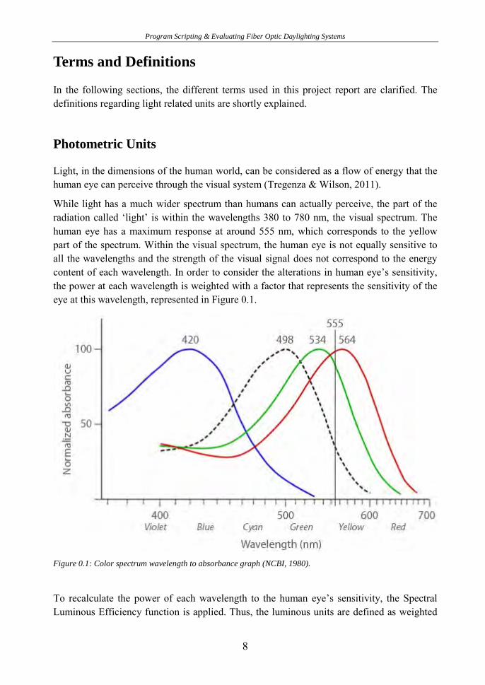
While light has a much wider spectrum than humans can actually perceive, the part of the radiation called ‘light’ is within the wavelengths 380 to 780 nm, the visual spectrum. The human eye has a maximum response at around 555 nm, which corresponds to the yellow part of the spectrum. Within the visual spectrum, the human eye is not equally sensitive to all the wavelengths and the strength of the visual signal does not correspond to the energy content of each wavelength. In order to consider the alterations in human eye’s sensitivity, the power at each wavelength is weighted with a factor that represents the sensitivity of the eye at this wavelength, represented in Figure 0.1.

Figure 0.1: Color spectrum wavelength to absorbance graph (NCBI, 1980).

To recalculate the power of each wavelength to the human eye’s sensitivity, the Spectral Luminous Efficiency function is applied. Thus, the luminous units are defined as weighted


9

sums of the radiometric spectral energy distribution, which take the varying sensitivity into account (Renström & Hallqvist, 2011).

Luminous Flux

The luminous flux defines the rate at which luminous energy is flowing out of a lamp or through a window (Tregenza & Wilson, 2011). Its unit is lumen [lm] and its radiometric equivalent is watt [W].

Illuminance

Illuminance, E, is defined as the quotient of the luminous flux [lm] over the area that is lit [m2]. The unit for illuminance is lux [lx] and one lux is equal to one lumen per square meter (Tregenza & Wilson, 2011). See equation 1.

𝐸 = 𝑑Ф𝑑𝐴

(1)

Where:

dφ: Luminous flux

dA: Area of the element

Luminance

In a given direction, the luminance, at a given point of a real or imaginary surface, is the quantity defined by the CIE (CIE, 1987) as:

𝐿 = 𝑑Ф𝑑𝐴×𝑐𝑜𝑠 𝜃×𝑑Ω

(2)

Where:

dФ: Luminous flux transmitted by an elementary beam shifting through the given point and propagating in the solid angle, dΩ, while containing a given direction.

dA: Area of a section of a beam containing a given point.

θ: Angle between the normal to the beam direction and section. Unit: cd/m2


10

Luminous Efficacy

Luminous efficacy expresses the ratio of the light output from a source to the total radiation emitted (Tregenza & Wilson, 2011), as:

𝜂 = 𝑙𝑚𝑊

(3)

Daylight Autonomy

Daylight Autonomy is defined as the percentage of the occupied times of the year, when a specified minimum illuminance level at a given point is reached by daylight alone. Unlike the Daylight Factor, the Daylight Autonomy calculation is performed for all hours and all skies, thus including overcast as well as all other sky conditions (Reinhart, 2014).

RGB Values vs. Wavelengths

The name of the color model RGB refers to the initials of the primary colors Red, Green and Blue. In this model, each of the three different colors corresponds to a range of wavelengths, with diverse peaks. Red peaks at wavelengths of 700 nm, green at 546.1 nm and blue at 435.8 nm. The last two wavelengths were chosen as they were easy to replicate, while the wavelength of 700 nm was chosen due to the fact that it is the peak of response of the human eye to the color red (Strajescu & Mihai, 2007).

When the RGB model is used for color representation, as for instance on a computer screen, the colors red, green and blue are combined in order to create the other colors.

In this study, the RGB model is applied to create new colored materials for the material database used for the simulation program Radiance.

Transmittance vs. Transmissivity

When adding a n ew material to the Radiance material database, used for Grasshopper, attention has to be paid between the terms transmittance and transmissivity. The glass material type requires the specification of a transmissivity value, which is defined as the amount of light which is not absorbed in a single pass through the device. Transmissivity does not account for any specular reflectance.

The transmissivity of a material can be calculated using a certain mathematical formula, as presented in Appendix A.


11

Compared to the transmissivity, the transmittance is the fraction of the incident radiation flux or the luminous flux, which completely penetrates a transparent material. It is normally specified having a normal incidence (Mischler, 2004-2011).

Glare

Disability Glare

Disability glare distorts vision without necessarily causing discomfort, which usually has the effect that the occupants react, by closing blinds, changing position, among other actions. Disability glare is thus not a significant problem in buildings considering that occupants normally take action to solve the problem (IES, 1993).

Discomfort Glare

Discomfort glare causes an uncomfortable sensation, nuisance or fatigue without necessarily disturbing the vision. This type of glare is generally due to large contrasts in the visual field which can be the origin of long term health effects such as fatigue and headaches. The occupant is not always aware of the sensation which is why discomfort glare in buildings is something that needs to be seriously considered (IES, 1993).

Daylight Glare Probability

Based on human reactions, the Daylight Glare Probability (DGP) represents the percentage of people likely to be disturbed by discomfort glare. To determine the DGP, a HDR photograph, rendering or CCD image is necessary (Kleindienst & Andersen, 2009). Different classes of glare probability can be reached starting from class A, which indicates a glare probability of less than 35%, and ending with class C, meaning that the glare probability is less than 45%. In all cases, the DGP is allowed to exceed the limit to a slightly higher percentage in 5% of the time (Mardaljevic, Andersen, Roy, & Christoffersen, 2012). More detailed information about the different classes and a table presenting the exact- and maximum percentages can be found further on in this study.

Daylight Glare Index

Among the different glare indices available, the Direct Glare Index (DGI), developed by R.G Hopkinson, considers discomfort glare caused by large glare sources. As it predicts little glare when the sun is visible, this index should only be applied when no direct sun will enter the rooms (Hopkinson, 1963). Reinhart and Jakubiec divide the DGI into four different


12

classifications, reaching from Imperceptible Glare to Intolerable Glare, which will be presented in this study (Jakubiec & Reinhart, 2010).

Window to Floor Ratio (WFR)

According to LEED, the window-to-floor ratio (WFR) includes the total area of the fenestration, divided by the total floor area of the room. The window area includes the frame, sash, and other non-glazed window components (LEED, 2014).

Daylight Factor

The Daylight Factor is defined as the ratio of the illuminance at a point on a given plane, due to the amount of light received directly or indirectly from a sky of a distribution (known or assumed), to the illuminance on a horizontal plane due to an unobstructed hemisphere of this sky. The impact of direct sunlight to the illuminance is excluded; however, dirt, glazing effects and other issues are included. It is essential that the room is lit solely by daylight and not in conjunction with lighting of interiors (CIE, 1987).

High Dynamic Range (HDR) Image

Image that stores information in a format that has a range of various orders of magnitude that may be photometrically correct. This makes it possible to make advance tone mapping or calibrated false color luminance images (Jaloxa, 2011).


13

Structure of the Thesis

The thesis is structured as follows:

Part 1: Introduction into the background and problem motivation. The objective of the necessity to install fiber optic daylighting systems is explained. The environmental certification system LEED is described briefly and as well as the simulation programs that were applied during the work on the thesis project.

Part 2: Connection of the topic of the thesis project to previous studies in form of a literature review. The studies performed in the project are related to the studies already carried out in the scientific world.

Part 3: Detailed description of the methodology. The four main steps taken during the development of the thesis project are explained:

• A simulation script is created, to allow the simulation of the fiber optic system. By applying the script to an available building model, the effect of the fiber optic daylighting system can be evaluated.

• A case study is performed in order to verify the functionality of the new simulation script. Measurements are completed inside a laboratory room and compared to results obtained from computer simulations.

• A parametric study is carried out to study the effect of the fiber optic system for different locations, room types and cable configurations. The LEED 2015 document is used as a guideline for the desired minimum level of daylight inside the chosen room.

• Finally, a g lare assessment is completed to evaluate possible risks of glare in the room used previously for the case study. Another test of the functionality of the simulation script is carried out by comparing the results obtained by taking HDR images and computer renderings, regarding glare.

Part 4: Presentation of the results obtained from each of the four steps taken.

Part 5: Critical discussion of the topics studied during the project, including a reflection of the development when creating the new simulation script and of both the process of the case and parametric study, together with the glare assessment.


14

Part 6: Conclusion of the project as a whole, considering all parts. The main aim of this part is the determination of the connection between the problem motivation, the background and the outcome of the project. Further development and future work regarding this subject is discussed.

Part 7: As a support for further use of the simulation script or studies about simulating fiber optic systems, a u ser guide is added to the project report and can be found in the Appendices, in addition to formulas used in this study.


15

1 Introduction

According to the most recent Intergovernmental Panel on Climate Change report, global warming poses a m oderate threat to current- and future sustainable development (IPCC, 2014). The building sector accounts for approximately 40% of the total primary energy use in the world and contributes for up t o 30% of global annual green house gas emissions (United Nations Environment Programme, 2009). Electricity uses 12% of the world’s primary energy, of which 19% arise from electric lighting. Currently, more than 33 billion lamps are in operation worldwide, consuming over 2 650 TWh of energy annually. The total consumption of electricity for lighting is larger than all electricity produced by hydro- or nuclear power plants in the world. The environmental impacts of electric lighting are caused by the use of energy, the production of materials and the disposal of equipment. Due to the versatile nature of both the production and consumption of electricity, the global consumption of electricity has been rising at a faster rate in comparison to the overall consumption of energy (Espoo, 2010 ).

Energy use for electric lighting can vary to a large extent in buildings of similar types and economy. The amount of input energy for electricity generation is significantly higher than the amount of electricity at its point of use, because of losses in the generation process of electric energy. A great proportion is however used by inefficient and outdated lighting technologies (International Energy Agency, 2006). Electric lighting in buildings is thus a major threat to the environment and with a more holistic view and focus on sustainability and energy efficiency, energy savings and reduction of environmental footprint can be improved significantly.

Humans have limited vision in darkness, which is why the common way to light building interiors is through windows or electric light sources. When access to daylight is restricted through windows, electric lighting is the usual choice. Daylight can however be brought in using energy efficient technologies, which does not only reduce energy use, it also has multiple positive effects on human beings. “Daylighting is the illumination of building interiors with sunlight or skylight and is known to affect visual performance, lighting quality, health, human performance, and energy efficiency” (NFRC, 2005). Studies have shown that using daylight over electric lighting improves the performance, subjective emotional status and the chronobiological system of humans (Govén, Laike, Raynham, & Sansal, 2011). It is therefore vital to assess daylighting conditions when renovating or designing new buildings for the working environment. Currently, several innovative daylighting technologies exist for buildings that transport external daylight into buildings.

Some light guiding systems that guide natural light into the core of a building, redirect both direct and diffuse daylight by reflection, refraction or deflection. These systems are generally fixed and thus unable to illuminate the core of deep plan buildings. To ensure so, light transport systems are needed, using the three components, collection, transportation and distribution. Nevertheless, light transportation systems are ordinarily dependent on


16

direct sunlight. The most commonly used channeling devices are prismatic or mirrored light pipes (MLPs), lens- and fiber optic systems. These systems collect and transmit daylight through buildings actively or passively. Passive systems are fixed with a specific angle and orientation to maximize light collection. Active systems have a tracking device that allows the system to continuously orientate the collector towards the sun (Nair, Ramamurthy, & Ganesan, 2013). In this thesis, the active fiber optic daylighting system that captures the direct rays of the sun is studied and evaluated with the help of an environmental certification system.

Several well established certification systems exist that give credit points for various categories, meeting goals regarding energy, environmental impact and ecological well-being. The US Green Building Council’s certification system LEED emphasizes, among other credit points, the necessity to reduce electric lighting, and reinforce occupants’ circadian rhythms by controlling natural daylight into buildings. LEED requires the evaluation of daylight through simulations or measurements to verify the quantity of daylight reached in an interior area (LEED, 2015).

In order to perform an evaluation of the fiber optic daylighting system, created by the solar lighting company Parans, a simulation script was developed. Creating such a script, makes it possible to obtain credit points in the LEED certification system during the design process. Previously, this was only possible by carrying out measurements after installing the system. In this study, real measurements were taken to validate the credibility of the simulation script and a d etailed parametric study performed for four cities that have particularly different average illuminance from the sun. In addition a detailed glare assessment was completed and analyzed. This was supported by research in class environments where children perform better in naturally daylit conditions, however worse when they sense glare (Lomel, 2014). Assumptions can be made that this could be valid for human beings in general.

By engaging in evaluating a building’s performance by an environmental certification system and using a technology that encourages sustainability, environmental responsibility and energy performance beyond prerequisite, one may motivate energy savings worldwide.

1.1 Background and Problem Motivation

1.1.1 Parans Lighting System

This study focuses on t he fiber optic daylighting system produced by the company Parans Solar Lighting. The company is located in Göteborg, and founded in 2002. Parans’ idea was to create a system that makes it possible to transport sunlight into rooms that have no access to sunlight, that is, rooms without windows. The system can also be used to increase the level of daylight in rooms with very small windows or deep rooms.


17

Different systems were invented by Parans during the last decade. The first system, SP1, was introduced in 2004. Recently, the company developed the fourth generation called SP4. Figure 1.1 shows the latest edition of how the SP4 system will look. The values and collector sizes considered in this project report are according to the newest system, SP4.

Figure 1.1: The latest edition of the SP4 system visualized.


18

Compared to the previous systems, the SP4 system will have a b etter transmission and a collector size that is according to the costumer’s need. The improved transmission is obtained through the use of glass fibers instead of plastic fibers, which were used by the first generations (Parans, 2014).

Listed below are additional advantages of the SP4 system compared to the previous systems, according to K.R. Nilsson from Parans:

• It has a l onger cable distance yet equal losses as the plastic fibers; 100 meters instead of 20 meters. Light can thus be brought down several floors or cables bent to reach a certain area.

• A color shift to the yellow to red area after 75 to 100 meters, instead of to the blue to green area after 20 to 25 meters, which is considered more comfortable according to most human beings.

• Lower price per lumen compared to the other systems.

• Every SP4 unit will be online, either over GPRS, 3G, 4G, Ethernet-cable or over WiFi. This way, Parans will continuously have surveillance on each unit and be able to remotely do support and maintenance for their customers.

• The SP4 system will include a G PS, compass and tilt-sensor, simplifying the installation. When fixating the system to the roof and turning the unit to a zero point, it will immediately know where it is and where the sun is using the GPS, compass and tilt-sensor.

Parans’ objective for indoor environmental quality, energy and atmosphere is to connect building occupants with the outdoors, reduce the use of electric lighting by introducing daylight into the space and reinforce circadian rhythms. Additionally, both the economic and environmental threats connected to the use of fossil fuel energy are reduced, by increasing the self-supply of renewable energy (Nilsson, 2014).

1.1.2 Environmental Certification Systems

In order to assess the energy efficiency of a specific building, the building owner or the person in charge of the building planification can choose between two different groups of certification systems, environmental certification systems or energy certification systems.

While the energy certification systems consider solely the energy performance of the assessed building, the environmental certification systems have a broader scope covering a range of environmental aspects in addition to the building’s overall impact on the environment. In this project, the environmental certification system, called LEED, is chosen as a guideline for the minimum amount of illuminance desired in different types of rooms.

If the building being assessed, reaches a high rating, several environmental, financial and health related benefits can be considered. The main two advantages are the increase of the


19

financial value of the building and the limitation of the ecological footprint. Due to the high rating, the external image of the building owner, or the company renting the building, is improved and a higher quality of indoor environment may be expected. Thus, the employee’s productivity may increase, more companies could get interested in renting space inside the building and may even agree to pay a higher rent. Another main advantage of owning or renting a building that reaches a high rating, is the lower energy use and thus, a lower overall cost. In some countries, when purchasing a certified building, banks may offer better mortgage conditions, lower interest rates and even tax reductions due to the improved long-term value of the building.

Among the numerous environmental certification systems, LEED and Breeam, founded in the USA and the UK, respectively, are the two most used systems in Scandinavia. While LEED and Breeam are applied for the certification of buildings worldwide, other systems are only used in certain countries, such as the Australian certification system Green Star. The environmental certification system Miljöbyggnad is the Swedish system and solely applied to Swedish buildings (Olsson & Heincke, 2012).

1.1.3 Environmental Certification System LEED – Daylight Part

LEED was developed by the U.S Green Building Council (USGBC). First launched in the USA in 2000, more than 32 000 building were certified by LEED, which makes it to one of the most widespread environmental certification systems in the world (Olsson & Heincke, 2012).

Within the certification system, several key areas of requirements are evaluated, one of them being daylight. Different amounts of credit points are attributed for each requirement fulfilled and finally after evaluating each key area, the number of credit points scored is recalculated into ratings on a scale. It is of high interest to fulfill as many requirements as possible, since certifying a building can be a challenging process. In this project, the possibilities of increasing a building’s overall credit point score, by installing a fiber optic system, is studied.

By installing a fiber optic system, credit points can be obtained from several areas. There are one to three credit points available for ‘Daylight and Views’, within the key area ‘Indoor Environmental Quality’. However, the credit points that can be obtained for the view need to be neglected due to the fact that the fiber optic system provides daylight but not a view out. Other credit points can be earned in the area of ‘Renewable Energy Production’, which gives up to three credit points, the key area of ‘Innovation’, which gives up to five credit points and the area ‘Optimize Energy Performance’, giving up to 20 credit points. Lastly, the area of ‘Thermal Comfort’ and the area of ‘Light pollution Reduction’ can give one credit point each if fulfilled. In this project the focus is on evaluating the fiber optic system by using the key area of ‘Indoor Environmental Quality’, which contains the credit points for ‘Daylight and Views’.


20

Three options are available to assess a room in relation to daylighting. The first option is the simulation of the spatial daylight autonomy and annual sunlight exposure, the second one is the simulation of illuminance and the third one consists of measurements, which can be performed after constructing the building. Due to technical issues explained further on in this study, this project focuses on the evaluation of daylight levels using Option 2, t he simulation of illuminance calculations.

By performing computer simulations, the daylight conditions inside the buildings can be evaluated. If a certain level of daylight illuminance is maintained, one or two credit points can be obtained for the criteria ‘Daylight and View’, Option 2, see Table 1.1. In this case, the average illuminance must be between 300 to 3000 lx on at least 75% of all measured points inside the room in order to obtain one credit point. An additional credit point is obtained when the illuminance of 300 to 3000 lx is reached on at least 90% of the measured points. The Daylight Autonomy in Option 1 i s used for the verification of the simulation script. The criteria itself will not be considered, rather the proposed illuminance levels and the idea of the credit point system in general (LEED, 2015).

Table 1.1: Points for daylit floor area: Illuminance calculation.

New Construction, Core & Shell, Schools, Retail, Data Centers, Warehouses & Distribution Centers, Hospitality

Option 1

sDA (for regularly occupied floor area) Points 55% 2

75% 3

Option 2

Percentage of regularly occupied floor area Points 75% 1

90% 2

1.1.4 Simulation Programs Rhinoceros and Grasshopper

The two main computer programs used in this study are Rhinoceros and Grasshopper. The main component used in Grasshopper is based on Radiance Lighting Simulation System.


21

Rhinoceros is a software produced by Mc Neil North America. It is mainly used for free-form modelling for both design and architecture purposes. A series of plug-ins are available, including the program Grasshopper (McNeil, 2014).

Grasshopper is a parametric modelling script that uses generative algorithms. It allows designers and architects to create form generators without requiring knowledge of programming or scripting (Davidson, 2014). Rhinoceros is used as the interface to Grasshopper.

Within Grasshopper, a component called ‘Diva Daylight’ provides the option to perform light and daylight simulations using Radiance. Radiance is a well-known set of programs, which can be used for the analysis and visualization of lighting conditions in buildings. The input files to Radiance specify the geometry, material, time, date and sky conditions. Radiance produces photometrically-correct renderings of arbitrary light environments, as well as numerical values, such as, illuminance, luminance and even glare indices (Mcneil & Fuller, 2013). Diva also uses the daylight coefficient and Perez sky model principles as developed earlier through the Daysim program, in order to perform climate-based daylight modeling (CBDM). The Perez sky model is explained briefly further on in this study.

1.1.5 Problem Motivation

As the Parans lighting system can positively contribute to fulfilling the requirements stated in LEED Daylight, it is of high interest to be able to simulate the impact the fiber optic lighting system has on a certain room or space inside a building at an early design phase.

In this study, a simulation script was created, with the aim to predict the daylighting output of the Parans lighting system. Using the simulation script simplifies design decisions when planning the installation of the Parans lighting system.

1.2 Overall aim and concrete and verifiable goals

The aim of the thesis project was to create a s imulation script, using the programs Rhinoceros, Grasshopper and Radiance. The script should be reliable and easy to use in order to be able to apply it to different types of rooms and buildings in different locations. The goal was to apply the LEED certification credit points to the outcome of the simulation script. A second goal was to perform full-scale measurements and assess the results, in order to evaluate the functionality of the script. A third goal was to analyze the daylighting conditions using varying amount of fiber optics in different countries. Finally, the risk for glare, when using the fiber optic lighting system, was assessed using HDR photography and Evalglare, which is a sp ecial program imbedded in the Radiance Lighting Simulation System.


22

1.3 Scope

The development of the simulation script is built on information received from Parans Solar Lighting AB as well as real measurements using the SP3 system. The study is limited by the technical expertise of the participants and possibility of performing deeper investigations. Additional restrictions are the amount and accuracy of the measurement tools and practical limitation due to weather during the measurement phase, since the system works with direct sunlight.

The script can be adjusted to fit other fiber optic daylighting systems to perform investigations.


23

2 Literature Review

The following section presents a summary about research on similar daylight guiding systems and earlier generations of the Parans systems, with the aim to identify useful previous knowledge and unexplored questions.

2.1 Studies about Daylighting Technologies

Han and Kim performed investigations regarding a f iber optic system’s photometric characteristics in 2009. Different lenses were compared in terms of spatial distribution of light on a work plane. According to the authors, electrical lighting uses at least 15% of the buildings’ total electricity consumption and is still increasing due to the desire of improving indoor comfort and productivity. Using a fiber optic daylighting system resulted in an energy-saving sustainable solution for building design. While the daylight levels increased, CO2 emissions decreased. The authors also found that the occupants’ satisfaction was improved since natural light was collected and distributed in an ideal condition inside the office space.

The previous study also showed that using a concave lens, the light spreads more widely than the semi-concave lens. Another finding was the independence between indoor- and outdoor illuminance, due to the fact that the system is solely using direct solar illuminance (Han & Kim, 2009).

According to studies by Carter and Marwaee, tubular daylight guidance systems, also known as light tubes, supported the improvement of the visual environment (Carter & Marwaee, 2009).

A study by J. Kim and G. Kim showed that by using optical daylighting systems, it is possible to deliver natural light and reduce the energy use in spaces inside a building where daylight is needed (Kim & Kim, 2009).

In 2012, Oh, et al. showed that for solar altitudes of less than 50°, fiber optic systems are more suitable than light tubes since it is easier to harvest daylight with the solar tracking dish concentrator system. Although the fiber optic system studied in the paper is provided with a collector in form of a solar tracking dish concentrator system, it is comparable to the Parans fiber optic system. Additionally, the uniformity on t he work plane is more stable when using fiber optic systems, instead of light tubes.

In order to evaluate the fiber optic system, the authors created simulation models by using a series of software programs including Radiance, Ecotect, Relux and Photopia. The programs were also used to determine an optimum installation of dimming systems to create a hybrid lighting system in accordance to humans’ preferences regarding light levels indoor (Oh, Chun, Riffat, Jeon, Dutton, & Han, 2012).


24

Later, in 2013, Han, et al. studied the functionality and applicability of a fiber optic daylighting system. The system included a dual-axis solar tracker and light guides in form of optical fiber cables. In contrast to the system studied in this project, the system also included a dish concentrator instead of a collector. In order to evaluate the effectiveness of the system, a v irtual luminaire of the daylighting system was modelled and simulated by using the software Photopia. The combination of sunlight gained by using the system and electric lighting was studied by applying a dimming control (Han, Riffat, Lim, & Oh, 2013).

2.2 Studies about Benefits of Daylight (Health and Performance)

A study performed in 1994 by Franta and Anstead showed that office workers’ well-being increases when working in a daylit office space. Several benefits, including increased productivity, better health, reduced absenteeism and thus financial savings can be expected when exposed to full spectrum daylighting. Due to these advantages, the requirement in many countries is to provide employees a working space within eight meters to a window (Franta, 1994).

An alternative to windows could be full-spectrum bright lights, which were studied by Luo in 1998. Similar to the effects of working close to a window, an improved productivity, decrease in accidents, an increase in mental performance and an increase in moral can be expected (Luo, 1998). On the other hand, Veitch and McColl published a literature review in 2001, where evidence showed no dramatic effects of fluorescent lamps on health or behavior of human beings (Veitch, 2001).

According to a study performed by the Heschong Mahone Group, the achievement of students under good daylighting conditions is 20% faster on math tests and 26% better on reading tests than students with the least access to daylight. This study also showed that their test scores were improved by 7-18% (Heschong Mahone Group, 1999).

In 2011, Govén et al., studied the effect of daylight on school children taking in to consideration their well-being, academic performance and subjective emotional status. According to these authors, all three aspects were positively affected by allowing children to study under daylight conditions (Govén, Laike, Raynham, & Sansal, 2011).

2.3 Earlier Studies about Energy Savings, using Fiber Optic Lighting Systems

In 2007 Wall and Hastings studied the energy saving potential by applying highly efficient systems, including heating plants, control systems, photovoltaic systems, solar thermal systems and lighting systems. In the paper it was shown, that a glare free, naturally lit room, has a positive impact on how the room is perceived. It is mentioned that even though dark parts inside the room are perceived negatively and sufficient daylight inside the room is


25

desired, it is essential to avoid the design of oversized windows due to heat losses during the winter and increased cooling need during summer (Hastings & Wall, 2007).

Studies carried out in 2013 by Lingfors and Volotinen showed that the lighting energy savings due to changing fluorescent lights by SP3 fiber optic cables would result in 19% for a study hall in North Sweden and 46% in Italy, where more annual sun hours are available. When considering an interior space with lights turned on 16 h a day, the savings would be 27% and 55% in North Sweden and Italy, respectively. Energy used to control the electric lighting inside the building and to operate the solar lighting system were included in these calculations (Lingfors & Volotinen, 2013).

In 2013, Lingfors found, that the Parans SP3 fiber optic system provides light with a color temperature of 5800 ± 300 K and a color rendering index (CRI) of 84.9 ± 0.5, which are very similar to the sun’s color temperature and CRI (Lingfors, 2013).

2.4 Earlier Studies about Risk of Glare

In 1992, Heerwagen, Loveland and Diamond investigated the impact of glare due to excessive daylighting levels. The affected office workers took several measures against the disturbing glare which affected the work performance negatively. While the motivation and work efficiency decreased, the dissatisfaction and fatigue increased. The conclusion of the research project was the necessity of a well-lit work place without exposing the office worker to excessive glare (Heerwagen, Loveland, & Diamond, 1992).

In 2011, Reinhart and Jakubiec studied the ability of various metrics to predict the occurrence of discomfort glare. Simulation results were compared for DGI, CIE Glare Index, Visual Comfort Probability, Unified Glare Rating and DGP, under 144 c lear sky conditions in three spaces. It was found that DGP yielded the most reasonable results (Reinhart & Jakubiec, 2011). Studies in 2003, by Dubois et al. showed that it is essential to prevent glare caused by light patches and excessive luminance values inside the room. It was shown that discomfort glare is especially caused by high contrasts between different luminance values. This could happen if the luminance values in the region around a certain window are much higher than the luminance values of the wall (Dubois, Grau, Traberg-Borup, & Johnsen, 2003).


26

3 Methodology / Model

A modelling method was developed in this thesis project, according to four stages:

1. Development of simulation script 2. Case study analysis to verify the function of the simulation script 3. Parametric studies using the new simulation script 4. Glare assessment

3.1 Fiber Optic Lighting System

Numerous benefits can be obtained, by replacing electric light with sufficient daylight inside a building. The productivity of employees can be increased significantly with daylight. In addition, it has been demonstrated that the health conditions are improved and thus less employees are absent due to illness and their overall comfort is increased (Walch, 2005). It should therefore be in the interest of the employer or owner of a building to provide the employees with access to sufficient daylight.

Due to increasingly urbanized cities, where the floor plans are typically deep and the windows shaded by other buildings, it becomes more and more common to use alternative systems to provide sufficient daylight into buildings and save energy (HD & TM, 2005). These techniques include for instance, light tubes or, a fiber optic daylighting system as studied in this thesis project.

The fiber optic daylighting system harvests sunlight and brings it into dark areas of buildings. Figure 1.1, above, shows how the new Parans fiber optic SP4 system looks like. Sunlight is captured by the collector, which is generally located on the roof of a building. The tilt sensor makes it possible for the collector to rotate in 360° and tilt up and down 180° as shown in Figure 3.1.

Figure 3.1: Fiber optic collector, top view (left) and right view (right).


27

The collector has a series of Fresnel lenses, see Figure 3.2. The Fresnel lens is a thin transparent material with prismatic circular indentations or a chain of prisms, generally applied for solar concentration and collection of thermal energy, utilizing daylight. Due to the lens’ limited acceptance angle, it needs a tracking system to orient with the sun and to find the position of the focal point of the lens (Nair, Ramamurthy, & Ganesan, 2013). Each lens focuses the sunlight into one fiber. The SP4 system makes it possible to add or remove sequences of lenses depending on how many cables are necessary to light up a certain part of a building.

Figure 3.2: Fresnel lens. (Nair, Ramamurthy, & Ganesan, 2013)

In the case of the SP4 system, four fibers are bundled up into one cable, shown in Figure 3.3. These cables exit the collector on the rear end in the middle, where the optical fibers inside the cables transfer the sunlight through the building structure into the indoor environment and illuminate the interior via Parans luminaires. The fiber end has a 57.6°angle, and luminaires can be added to each cable bundle, which allows spreading the light in wider or narrower angles depending on the application.

Figure 3.3: Fiber optic Cables.

Figure 3.4 shows a simple image to clarify how the fiber optic lighting system works.


28

Figure 3.4: Overview of the fiber optic solar lighting system.

Sunlight provides a full spectrum of light, which contains all colors. However, it also contains infrared (IR) and ultraviolet (UV) radiation, which is not visible to the human eye. All non-visible radiation is filtered out in the Parans Solar lighting system by using IR-UV mirrors at the top of the fiber and glass on top of the Fresnel lens filtering all UVB- and UVC radiation. This reduces the need for cooling the indoor environment and eliminates health risks associated with the UV radiation. Figure 3.5 shows the process from when the sun hits the collector until it is transmitted to the fiber.

Figure 3.5: The process from the sunlight to the fiber.


29

The radiation profiles for sunlight, glass fiber optics, an incandescent light bulb and a low energy lamp is shown in Figure 3.6. The shaded areas show the non-visible radiation. The glass fiber optics are visibly closest to the sunlight compared to the other light sources.

Figure 3.6: Radiation profiles for direct sunlight, glass fibre optics, an incandescent light bulb and a low energy lamp (Parans, 2014) (MLL, 2012).

The fiber optic system that captures the rays of the sun, allows dark parts of buildings to receive natural daylight. In order to visualize the effect of the system, without installing it on a real building, a simulation process must be developed. The following chapter introduces the script created to simulate the effect of the system (Parans, 2014).


30

3.2 Creating a new Simulation Script

Design and simulation programs were used in order to develop a new simulation script. While Grasshopper was mainly used to model the system and Radiance applied to simulate its effect, Rhinoceros was used to evaluate the simulation results by exporting images of the output, displayed on a grid. More detailed information about how to apply the simulation script can be found in the User Guide in Appendix B.

The simulation script requires a specific geometry as input, described in the following subchapter.

3.2.1 Geometry in Grasshopper

The geometry of a room was modelled in Grasshopper and can be edited by changing number sliders, according to the geometry needed for a specific case.

Due to simulation-time constraints, the model was not created as an exact replica of the actual system. Instead of modelling the collector in its exact appearance, the collector area was divided by the amount of cables in the relevant system. In the case of the SP4 system, each cable contains four fibers with four lenses each. As presented in Figure 3.7, a SP4 collector containing 84 lenses is divided into 21 pieces, each including four lenses, that is, one cable. Each of the 21 pieces of the collector is represented by a tube. Instead of modelling the entire building, the rooms need to be assessed individually. Each room has to be modelled and equipped with the tubes, representing the set of four fibers.

The modelled tubes can be rotated 360° and tilted up and down 180°, similar to the real SP4 collector.

Figure 3.7: Picture explaining process of the method


31

When modelling the simulation script, it was necessary that the tubes, which represent the collector, follow the sun like the collector of the real fiber optic system does. This was accomplished by using a special component in the Grasshopper script, which made the tubes interactive, following the normal of the imitated sun. This special script made it possible to make the tubes move once per hour of the year according to the sun position.

The script includes number sliders, which can be adjusted according to the specific need, in order to make it possible to optimize the position and amount of tubes for each location. The script allows having one to four rows of tubes with selectable amount of tubes per row.

Additionally, the room can also be lit by optional North facing windows. A separate script was created for simulating the effect of the windows. By changing the WFR (Window to Floor Ratio), the window size can be adjusted. The window size is rather small, the placement relatively low in the wall compared to real life cases and the windows are facing north, in order to ensure that the results of the simulations are not too optimistic.

Once the simulation script and the fiber optic system were created, materials had to be defined in order to imitate the real system.

3.2.2 Material Properties

The material properties of the system were adapted, since the simulation script is a simplified version of the real system. In the real system, losses occur in various parts of the system, between the collector and the luminaire. This was simplified in the model. While the modelled tubes have a reflectance of 100%, the losses that occur in the real system, are accounted for by adding a lens, which has a specific transmissivity, to the end of each tube. This transmissivity was chosen according to the losses that occur between the real collector and the real luminaire. In the real case, 68% of red light reaches the room after passing through the system, which is simulated by setting the transmissivity of red light to 68% in the simulation. The green and blue are 65% and 59%, respectively.

To ensure a correct light distribution at the end of the tube, a cone with an angle of 57.6° was added as a luminaire. This was necessary due to the fact that the real fiber end spreads the light in the same angle of 57.6°. Additionally, a diffusive glass was added to the luminaire. Thus, the light is spread evenly and the behavior of the light passing through the luminaire of the real system is replicated. While the cone was set to have a reflectance of 100%, to avoid any losses, the diffusive glass was set to have a transmissivity of 100% and a reflectance of 0%, avoiding unwanted reflection of the light in other directions than into the room.

Standard reflectance values were considered for the interior surfaces of the modeled room surrounding the fiber optic system, see Table 3.1. Furthermore, a standard transmissivity was chosen for the windows (SIS, 2003). The final transmissivities, including the lenses, the diffusive glass and the windows, are presented in Table 3.2. More detailed information


32

about the difference between transmittance and transmissivity can be seen in ‘Terms and Definitions’.

Table 3.1: Reflectance values of different components.

Component Reflectance [%]

Interior Walls 60 Floor 30

Ceiling 80 Tubes 100

Luminaires 100

Table 3.2: Transmissivity of different components.

Component Transmissivity RGB [%]

Windows 78/78/78 Lenses 68/65/59

Diffusive Glass 100/100/100

When all materials have been set accordingly, the model is ready for simulations.

3.2.3 Simulations in Grasshopper, using Radiance

The tubes in the simulation script change their position once every hour, as well as the sun position in the program, which makes it possible to run an hourly simulation over a year.

To save time when performing the simulations, a component called Counter is added to the script. Without the Counter, simulations would have to be performed manually every hour. In the case of the Daylight Autonomy, the Counter makes it possible to carry out a series of simulations (a series of hours during the year), excluding weekends and holidays.

After each simulation, the output needs to be exported to an Excel sheet. After gathering information from the simulation, the Excel sheet can be imported to Grasshopper again and results viewed in Rhinoceros.

If the room contains windows, a separate simulation has to be performed, using the appropriate script. This is due to the reason, that the window simulation considers a weather file including both the diffusive and direct part of the global illuminance, while the weather file in the simulation of the fiber optic system alone only includes direct illuminance. By dividing the simulation into these two parts, it is considered that windows allow both the


33

direct and diffuse illuminance to enter the room. After finishing the window simulation and exporting the results to the Excel sheet, the results obtained from the window simulation have to be added to the results from the simulation, generated for the fiber optics.

A similar method is used if simulations for zigzag rows are desired. Since the script only allows parallel lines of tubes, the rows needed for the luminaires, arranged in a zigzag need to be simulated separately. The results can then be added up in the Excel table to obtain a final result for the zigzag row.

In Radiance, the ray tracing process is controlled via rendering options. These rendering options consist of five different simulation settings that need to be adjusted to achieve a high accuracy, when performing daylight assessments. The optimum simulation settings, according to a specific size of tubes, were found by testing and adjusting the rendering settings until the simulation time was reasonable, while the output stable and accurate. When changing the radius of the tube, the amounts of fibers per cable changes and consequently new rendering settings have to be found to maintain accuracy.

Certain guidelines had to be followed when adjusting the simulation settings. These guidelines were found in Dubois’ Simulations with Radiance (Dubois, 2001). In order to obtain qualitative output with photometric accuracy from Radiance, it was necessary to configure the correct input parameters in the simulation settings. There are five underlined rendering settings presented below, which according to Shakespeare and Larson, all need to be carefully adjusted.

The ambient bounces determine the maximum number of diffuse bounces considered by the indirect calculation. Due to the small radius of the tubes, the ambient bounces had to be relatively high. If the ambient bounces are too low, the risk of losing light rays, while directing them through the tubes, would be too high.

Due to the fact that Radiance uses backwards ray tracing, it is essential to set the ambient divisions to a high value. The ambient divisions determine the accuracy of the sky model and thus influence the probability that the few rays that reach through the tubes detect the spot in the sky where the sun is located. Thus, it determines the number of different directions where rays are sent out from each sample hemisphere.

To minimize the error in the indirect irradiance interpolation, the ambient accuracy was set to 0.15 as recommended by Larson and Shakespeare.

It was also recommended to set the ambient supersamples to a quarter of the ambient divisions, to maintain precision when simulating. By increasing the ambient supersamples, the spatial density of the sampled points is increased and thus, an improved accuracy can be expected (Schorsch.com, 2011).


34

The ambient resolution corresponds to the scene size, cut off point at which interpolation begins and further hemispherical sampling ends, as well as it relates to the accuracy. In this case the ambient resolution is set to 15 (Larson & Shakespeare, 1998).

All simulations were carried out to evaluate the amount of daylight on desk level, at 76 cm from the floor, according to LEED (LEED, 2015).

Radiance uses the Perez sky models to reconstruct the sky distributions. The sky model is a way to recreate some of the random aspects of daylight and can be applied to any continuous sky brightness distribution model. It can be applied to any climate, as long as the appropriate climate file exists. The Perez sky model uses a stochastic generation of hourly global values, which is why re-running the same simulation may result in slightly different outputs each time. This is due to the models complex empirically fitted functions and coefficients that they include for irradiance and specific bins of clearness, which are presented in detail in Appendix C (Mardaljevic J. , 2010).

Another source for possible variances in the output, when re-simulating the same case several times, could be the Radiance simulation, which blends deterministic and stochastic ray-tracing methods to accomplish the optimum balance between simulation time and accuracy (Ward, 1994).

Once simulation settings are modified and output reached, the program Rhinoceros is used to visualize the output in form of a colored grid or numbers, displayed, where the grid points were set previously.

3.2.4 Output in Rhinoceros

While the program Grasshopper is mainly used for the modelling, Rhinoceros is used as an interface during the process of modelling where the model and output can be visualized. It can thus be verified whether the tubes work properly and if the geometry of the room is as intended.

Once the simulations are completed and all results are exported and saved in the Excel sheet, the output can be shown in Rhinoceros as a colored grid. This colored grid can also be exported from the Rhinoceros interface as an image for further use.

Even though accomplishing promising output from a newly created simulation script, verification is essential to substantiate its reliability.

3.3 Case Study for Verification

A case study was carried out in order to evaluate the functionality of the simulation script, by performing measurements in a full scale laboratory room. The SP4 system is still being developed and not on the market and thus the prior system SP3 was used to verify the


35

dependability of the simulation script. Additionally, all simulation settings were set according to the SP3 system.

The room chosen for the installation of the SP3 system was located in a laboratory building in Lund. The width of the room was 2.70 m and the length 4.20 m, which results in 11.34 m2.The room height, was 2.6 m and the windows were entirely covered to avoid any exterior light entering the room. The system was installed in the South-West orientated corner on the roof of the building.

Measurements of the interior surfaces’ reflectances were carried out. The detailed procedure is presented in the following subchapter.

Four illuminance meters were placed at four different positions inside the room, as shown in Figure 3.8. Measurements were taken continuously every third minute over one hour.

Two measurements were performed simultaneously on t he unobstructed roof of the laboratory building. The measurements were completed using an illuminance meter, with and without a shading ring. The first measurement recorded the illuminance normal to the sun, and the second one, the global horizontal illuminance and finally the diffuse illuminance for the previous cases were measured, using the shading ring. Due to the fact, that the re-running of several simulations with and without the shading ring did not show noticeable variation, assumptions can be made that the losses caused by the shading ring could be neglected.


36

Figure 3.8: Location of luminaires and lux-meters inside the room.

Every building has its characteristics and it is therefore crucial to capture every detail. Using a luminance meter, reflectances were measured as presented in the next subchapter.

3.3.1 Calculation of Surface Reflectances

In order to achieve a maximum accuracy when verifying the functionality of the simulation script, preliminary studies were carried out regarding the determination of the reflectances of the interior surfaces in the chosen laboratory room. Measuring the reflectances was a crucial step in order to set the same reflectances in the simulation model. The components measured include the ceiling, the floor, the three walls made of the same material and a fourth wall with an alternative material.

To perform the measurements, two measurement tools were needed: A reference reflectance circle, which had a reflectance of 95.3% and a luminance meter.


37

Two different measurements of each component were necessary to determine their surface reflectances. The measurement tool was set to measure luminance in cd/m2 in order to be able to measure the reflectance. The first necessary measurement was the luminance of the reference plate, placed on one of the surfaces. The following step was the measurement of the luminance of the same surface at the same spot, without the reflectance plate (Velds & Christoffersen, 2001).

Finally, the reflectance of the particular surface could be calculated by applying the formula in Equation 3.

𝑟 (%) = 𝐿0 ×𝑅𝑛𝐿𝑛

(4)

Where:

Ln = Luminance of the reference plate L0 = Luminance of the surface itself rn = Reflectance of the reference plate

The obtained reflectance values, as p resented in Table 3.3, were applied as grey reflectances, regarding their RGB values, to the model in Grasshopper and used for the simulations. The ‘grey reflectance’ determines that the reflectances have the same value for each of the spectral colors, RGB.

Table 3.3: Reflectance values of different components in the Case Study.

Component Reflectance [%]

Interior Walls 87 Floor 39

Ceiling 93

When all information and calculations were finalized, they were applied to the simulation script for verification.

3.3.2 Simulation Script

The second step of the case study was the performance of computer simulations of the same room as the one in the laboratory building, using the previously created simulation script. Therefore, the geometry settings of the room in Grasshopper, including the geometry and the surface reflectances, had to be adjusted according to the laboratory room in which the real measurements were taken.


38

To ensure that the results of both cases would be comparable, the chosen date, time during the day and weather conditions for the simulation were set to the same as the ones in the case of the real measurement. Thus, the right time during the year needed to be chosen in Grasshopper and the weather file had to be edited. Due to unavailability of an accurate weather file for Lund, the data for Copenhagen was used.

Another necessary measure taken was the adjustment of the parameters of the model in Grasshopper. The standard model contains the cable configurations for the SP4 system, which is why the parameters had to be changed to suit the SP3 system. These include the transmissivity of the lens and the radius of the tubes, representing the collector area.

Finally, after carrying out the real measurements and performing the simulations accordingly, the data was collected and evaluated.

After validating the use of the simulation script, the effects of the system was evaluated in different countries.

3.4 Parametric Study

A parametric study was carried out in order to show how different places in the world and placement of tubes would affect the output of the simulation.

To evaluate the effect of the fiber optic daylighting system in different parts of the world, a solar map was used to choose locations with diverse ratios between diffuse and direct irradiation. The solar map, shown in Figure 3.9 supported the decision of choosing four different locations, as well as Parans’ client base. The four locations correspond to climates with different levels of direct to diffuse irradiation ratios and are presented in the map. Thus, locations with the same color can relate to the results obtained from this parametric study.


39

Figure 3.9: Direct to Diffuse Solar Irradiation map of the world, presented as ratios (Velux Group, 2013).

Another purpose of the parametric study was to find out the location dependent amount of cables needed for different locations and the optimum placement inside a room, to obtain the LEED requirements.

In the following, the four different locations and two room types which were chosen for the study are presented:

• Types of rooms:

o Dark rectangular room without any windows

o Rectangular room with the same dimensions, including north orientated windows with a WFR, varying from 10% and 15% to 20%.

• Locations:

o Copenhagen

o Paris

o Washington

o San Francisco

For each location, different placement settings were chosen for the tubes, ranging from one to five meters, measured from the back wall. For each setting, simulations were carried out. Finally, the results obtained were presented in a graph and analyzed.

When certifying a building, using the LEED document, three different options for compliance are available, see Subchapter 1.1.3. As the simulation of the Daylight Autonomy, which is Option 1, in the LEED document, takes over a week to simulate,


40

Option 2 w as used for the parametric study instead. Option 2 a llows choosing one day within 15 days of March 21st and one day within 15 days of September 21st (LEED, 2015). During these two days, one simulation has to be performed for 09:00 a.m. and one for 15:00 p.m. An average day was chosen within this time range, ensuring that direct illuminance was available on the chosen day. Finally the average of the results of the four hours is calculated and presented as an exported image from Rhinoceros.

During the parametric study, the aim was to determine the amount of cables needed to fulfil the requirements stated in the LEED document. This is due to the fact that the results obtained from the simulation script present conservative results, due to the following reasons:

• Reflectances of envelope were lower than in most real cases.

• Windows were not set to optimum height in the wall.

• Transmittance of windows was underestimated.

• Hours in weather file chosen are not the ones with most solar illumination.

For further inquiries, Option 1, r epresented by the Daylight Autonomy, in the LEED document was completed.

3.4.1 Daylight Autonomy

The Daylight Autonomy calculation is highly time consuming, thus solely one Daylight Autonomy simulation was carried out. This method was selected with the aim to determine whether the results gained from a simulation of four chosen hours in spring and autumn, as used in LEED Option 2 and for the parametric study in Chapter 3.4, would be comparable. By simulating only four hours and creating an ‘assumed Daylight Autonomy’, time could be saved and the results could be used to assume the appropriate placement and cable configurations before running the annual Daylight Autonomy calculation. Evidently, this could merely be completed if the annual Daylight Autonomy relates to the results of the ‘assumed Daylight Autonomy’.

Finally, when the effect of the fiber optic system for different cities and suitable placement of the tubes were established, a detailed glare assessment was carried out.

3.5 Glare Assessment

A glare assessment was performed to evaluate visual discomfort created by the daylighting system. When the ratio between the task and immediate surroundings is too large, human beings can sense an optical discomfort due to excessive contrasts.


41

The glare assessment was divided in two steps; first, the real scene inside the laboratory room was captured, with a series of HDR photographs, which were used to create a false color image. The false color image supports the detection of glare inside the real room. Secondly, the real scene was modeled in Grasshopper in order to run rendering simulations and obtain false color images of the modeled scene. The resulting false color images of the model were compared to the ones of the real scene, to test the functionality and accuracy of the simulation script regarding false color renderings.

3.5.1 Assessment of the Real Scene

Various steps were taken to measure the luminous environment of a specific scene in the same room as used for the case study, as described in Chapter 3.3. Initially, several pictures were shot using a 17 m m wide angle lens in order to catch as much of the indoor environment as possible. Ideally, this would be performed using a fish eye lens to catch the illuminance hitting all areas of the room, however, due to the rather evenly spread light, the wide angle lens was accepted. The pictures were captured with a range of exposure values at the exact same position, using a tripod to keep the camera steady.

These pictures were used to produce HDR images which were then fed into the program, needed to create false color images showing luminance values using a scale of colors. The ratios of the color represented values were calculated to evaluate possible discomfort due to glare; these values are shown in Table 3.4.

Table 3.4: Ratios to calculate possible discomfort glare.

3:1 Task to immediate surroundings 5:1 Task to general surroundings 10:1 Task to remote surroundings 20:1 Light sources to large adjacent surface

The ratios, as mentioned in Table 3.4, are presented in Figure 3.10; visualizing the locations inside the room that are measured regarding the luminance and compared in order to obtain the ratios (IES, 1993).


42

Figure 3.10: Luminance measurements needed to calculate the possible glare indicating ratios. (IES, 1993)

The images were uploaded to the online imaging script Jaloxa, to produce one HDR image out of the five pictures taken of the scene (Jaloxa, 2011). A file for the specific camera model used needed to be uploaded simultaneously, in order to get accurate results. The HDR image was imported into Radiance Image Viewer, the Information Overlay set to False Color and Exposure increased to imitate the brightness experienced in reality, to obtain the false color image described above.

Using the Radiance Image Viewer, luminance values inside the room can be determined by clicking on the image. This way, the ratios can be calculated and the highest illuminance value inside the room can be determined. According to Jakubiec and Reinhart, the highest luminance within the visual field should not exceed 30 000 cd/m2 to avoid disability glare

(Jakubiec & Reinhart, 2014). In addition, the program Evalglare was applied to determine possible sources of glare in the room. The obtained HDR image was imported to Radiance and, with support of Evalglare, assessed regarding possible glare. An image was created, illustrating the parts inside the room with the highest risk of glare. Both the DGP and DGI were calculated using the same program by creating a .dat file, including the two indices, and are presented later on in this study. The values considered for the different levels of glare according to the DGP are presented in Table 3.5 (Mardaljevic, Andersen, Roy, & Christoffersen, 2012) and the different classifications of glare using the DGI are shown in Table 3.6 (Jakubiec & Reinhart, 2010).


43

Table 3.5: DGPs limits

Class A B C 95% DGPs limit ≤ 0.35 ≤ 0.40 ≤ 0.45 Mean DGPs (5%) < 38 < 42 < 53

Table 3.6: Classification of possible glare in form of DGI

DGI

Imperceptible Glare < 18 Perceptible Glare 18 - 24 Disturbing Glare 24 - 31 Intolerable Glare > 31

3.5.2 Assessment of the Modelled Scene

Unlike the procedure necessary to obtain a false color image of the real scene, the scripts in Grasshopper make it possible to create a false color image by connecting one of the various components Grasshopper provides to the existing simulation script. By running the simulation, several images were created; one of them was a false color image of the modeled scene. It is essential to ensure the adjustment of the right material settings in the scene and rather high rendering settings in order to create more accurate false color images.

As for the real scene, the resulting image was imported to the Radiance Image Viewer and evaluated regarding possible sources of glare caused by high ratios or exceedingly high luminance values.


44

4 Results

The results of the following are presented:

1. Development of a simulation script.

2. Comparison of a real life scene to a modelled case.

3. A parametric study to test the script in different parts of the world.

4. Glare assessment performed and analyzed.

4.1 Simulation Script

With the fiber optic characteristics in mind, a simulation script was created. As mentioned before, a detailed user guide is available in Appendix B. Figure 4.1 shows an example of how the model can be visualized.

Figure 4.1: Fiber optic lighting system created in Grasshopper.

Several adjustable functions can be altered in the functioning simulation tool, they are presented as follows:

• Geometry of model and placement of tubes

• Window sizes

• Location

• Time during the year

• Cable configurations

• Transmissivity and reflectances of materials

• Angle of luminaires

• Number of tubes and luminaires


45

Using these functions, the script allows assessment of daylighting conditions and glare, which is carried out in the following chapters.

4.2 Measurements and validation

A case s tudy was performed to verify the reliability of the simulation script. The process was divided into two steps. First, real measurements were taken inside a laboratory room at Lund University’s Energy and Building Design laboratory. Subsequently, the laboratory room was modelled and simulated using the simulation script in Grasshopper. In order to create the same daylighting conditions as in the real case, the illuminance values, obtained from the real measurements, were imported into the weather data in the simulation script.

4.2.1 Weather Data

The weather data was obtained by measuring the daylighting conditions parallel to the Parans collector and horizontally with and without a shading ring. The real measurements were performed under the conditions shown in Table 4.1 and thus also used for the simulation.

Table 4.1: Measured Values of Exterior Illuminance

Global Horizontal Illuminance 85431 lux Direct Normal Illuminance (normal to sun) 89938 lux Diffuse Horizontal Illuminance 21300 lux

The weather data was edited to include the measured values, in order to create virtually equivalent weather conditions, The User Guide in Appendix B shows in detail how this is accomplished.

The laboratory room was modelled and reflectance values as well as weather data measured in reality, put into the simulation process. In addition, comparing the lumen output from exterior to interior, the losses through the system were accounted for in the simulation. The exterior lumen output was found using measurements from Table 4.1 and the area of the collector. The lumen output from interior was found measuring the output from the fiber at a distance as close as possible to the fiber.


46

4.2.2 Real Measurements vs. Simulations

The simulation model was created as an exact replica of the real room, in order to achieve highest accuracy between the two rooms. The real room and the model are presented in Figure 4.2 and Figure 4.3, respectively.

Figure 4.2: Scene in laboratory room. Figure 4.3: Modelled scene for simulations.

The four points chosen for the measurements were set to the same placement for both the measured and simulated scenes. Due to the fact that the Perez sky model uses a stochastic generation of hourly global values, the model was run ten times to attain an average value for each point and maintain accuracy. In the graph in Figure 4.4, the results of the four measured and simulated points are presented.

Figure 4.4: Measured points vs. simulated points.

0

200

400

600

0 1 2 3 4

Illu

min

ance

/lx

Points

Measurements

Simulation


47

The results obtained from the case study clearly indicate, that the output from the simulation script is not far from the measured values. Comparing the two cases, the average discrepancy is ± 24% which can be considered good taking into account the error margins in each case. The errors in both the measurements and simulation were estimated to be ± 10% in total. The results from the Calibration Report of all measurement tools used, showed that on average the illuminance meters had an error margin of ± 2.22% and the luminance meters ± 4.3% in addition to a calibration accuracy of ± 3%. The overall error margin in measurements is due to measurement tools, non-instrumental uncertainties and human errors. The errors in the simulation were due to limitations stated further on in this study.

A parametric study was carried out to evaluate the fiber optic system in different countries.


The simulation script was applied to a selection of different cases in order to study the effect of the fiber optic system for different locations and rooms with different sizes of windows.

Firstly, the case of a certain room in San Francisco is chosen, to analyze the differences and similarities between the average illuminance and the percentage of illuminance between 300 and 3000 lux, which can both be obtained from the simulations in Radiance. For each placement of the tubes, both the average illuminance and the percentage of illuminance between 300 and 3000 lux are obtained and compared regarding possible dependencies.

Secondly, two extreme locations (Copenhagen and San Francisco) were studied further in terms of percentage of illuminance between 300 and 3000 lux. Both locations are presented with simulation outputs including five North facing windows, considering a 15% WFR. In all figures in this chapter, the circles represent the luminaires.

Finally, all four locations (Copenhagen, Paris, Washington and San Francisco) are compared graphically with varying WFR. In order to find the optimum placement and amount of the fiber optic cables for each of the various cases, the tubes in the model had to be added/removed and relocated, until the desired illuminance in the room was achieved.

4.3.1 Average Illuminance vs. Percentage of Illuminance between 300 and 3000 lux.

Ten different settings regarding the placement of the cables were chosen and applied to the case of a two row system, located in San Francisco. In this case, windows with a WFR of 15% were studied. After classifying the results according to their value, a graph was produced. Figure 4.5 shows the dependency between the placements of the fibers and the percentage of reached illuminance between 300 and 3000 lx. In the secondary y-axis, the average illuminance in lux is presented.


48

Figure 4.5: Illuminance depending on the placement of the fibers

The graph clearly shows that while the percentage of illuminance between 300 and 3000 lux increases linearly with placement of fibers, the average illuminance fluctuates. While the two y-axis present the Illuminance between 300 to 3000 lux, as well as the Average Illuminance, the x-axis indicates the placement of the fibers in meters. In the case of placing the first row five meters and the second row four meters from the back wall, the x-axis would indicate ‘4; 5’. The same procedure, as for the case presented for San Francisco, was applied to all cities , however not presented in detail in this thesis report.

4.3.2 Optimum placement for San Francisco

The LEED certification requires 75% of the floor area to be between 300 and 3000 lux to obtain one credit point (LEED, 2015). Figure 4.6 shows that 8 cables are needed in that case for San Francisco. The illuminance distribution in this case is reasonably even.

Figure 4.6: San Francisco, illuminance between 300 and 3000 lux with 8 cables and WFR of 15%.


49

The results indicated that 12 cables are necessary to obtain two credit points in the LEED certification system. Figure 4.7 shows that with 12 cables, 92% of the floor area reaches an illuminance between 300 and 3000 lx (LEED, 2015). The distribution is rather even; only the parts closer to the walls and corners are less lit. The circles in both figures represent the luminaires and the five windows are placed on the North wall.

Figure 4.7: San Francisco, illuminance between 300 and 3000 lux with 12 cables and WFR of 15%.

The following subchapter presents the results for Copenhagen.

4.3.3 Optimum placement for Copenhagen

The results indicate that 15 cables are needed in Copenhagen to fulfil the requirement for one credit point. By installing 15 cables, the illuminance level of 300 and 3000 lx on 78% of the floor area can be reached.

Figure 4.8: Copenhagen, illuminance between 300 and 3000 lux with 15 cables and WFR of 15%.


50

In order to obtain two credit points, 21 cables were necessary to maintain at least 90% illuminance level between 300 and 3000 lx on the floor area; see Figure 4.9.

Figure 4.9: Copenhagen, illuminance between 300 and 3000 lux with 21 cables and WFR of 15%.

4.3.4 Comparison of locations

With varying WFR, results from Copenhagen, Paris, Washington and San Francisco are compared and presented in Figure 4.10. The graph shows the amount of cables needed to fulfill the 90% illuminance level between 300 and 3000 lux.

Figure 4.10: Cables necessary to reach 90% illuminance between 300 and 3000 for four countries with varying WFR: 0%, 10%, 15% and 20% for each city.

0

10

20

30

40

50

Copenhagen Paris Washington San Francisco

Amou

nt o

f Cab

les

No windows

10%

15%

20%


51

The graph indicates that the colder the colors of the solar map from Chapter 3.4 are the more cables are needed. There is however, little difference between San Francisco and Washington in most cases. This could be due to comparable latitudes, which result in similar output on days with high solar illuminance. If a DA would be simulated for these two cities, different output may be expected, due to their different diffuse to direct illuminance ratio. Countries with similar latitudes as the cities presented in the graph in Figure 4.10 could use this parametric study as a guideline to estimate how many fiber optic cables are needed to install, depending on the window size of the room area.

4.4 Daylight Autonomy

To evaluate if the procedure, applied for Option 2 in LEED, and for the parametric study, could be used to predict the approximate result of the simulation of the Daylight Autonomy, one annual Daylight Autonomy simulation is performed. San Francisco is chosen as the location for the simulation, since it is the location where a majority of clients for fiber optic systems are situated.

In parallel, the same room with the same cable configuration, as used for the simulation of the annual Daylight Autonomy, was assessed, by simulating four hours during spring and autumn. The results obtained from the four hours were treated the same way as the results of the annual Daylight Autonomy. Thus, an ‘assumed Daylight Autonomy’, explained in Chapter 3.4.1, was created and the results of both the annual Daylight Autonomy and the ‘assumed Daylight Autonomy’ can be compared to each other.

The output obtained from the simulation of the annual Daylight Autonomy resulted in 22% DA, while a DA of 14% was obtained for the simulation of the ‘assumed Daylight Autonomy’. The DA of the annual Daylight Autonomy is thus slightly higher than the DA of the ‘assumed Daylight Autonomy’.

Due to time constraints, this study was only completed for the case of San Francisco.


The glare assessment, performed in the laboratory in Lund, yielded positive results. In the following subchapters, different steps of the process are presented.

4.5.1 Assessment of the Real Scene

An HDR image obtained from the online imaging software Jaloxa, was imported to the Radiance Image Viewer in order to evaluate possible risks of glare due to inadequate ratios between different elements inside the room. Values obtained for the various elements inside the room are presented in Figure 4.11.


52

Figure 4.11: HDR image, produced using Jaloxa’s online imaging script.

To ensure the absence of disability glare, the highest luminance value presented inside the room was retrieved by using a function in Radiance Image Viewer. The book, with a luminance of 121 cd/m2 is the element with the highest luminance value and does not exceed 30 000 cd/m2, the absence of disability glare is ensured.

Next, a false color image was produced with the Radiance Image Viewer and presented in Figure 4.12. The color scale, on the bar to the left side of the image, represents the luminance spread by the fibers on the surfaces in the scene. The book on the table in Figure 4.12 clearly indicates a risk of glare due to high contrast to the surroundings. Table 4.2 in the following subchapter, shows the ratios according to the HDR and false color image.

While the scale is set to a range of 0 to 95 cd/m2, to ensure that the luminance of all larger surfaces is evaluated, some of the luminance values in the image exceed the limit of 95 cd/m2, such as the book with 121 cd/m2.


53

Figure 4.12: False Color Image of the Scene in Lund’s Laboratory.

As predicted by Figure 4.12, the calculated contrast exceeding the recommended ratio is formed by the luminance divergence of the book and the immediate surroundings, the table. In order to verify the prediction of glare risk, an image was created using Radiance and the program Evalglare. Radiance requires a certain size in order to assess the glare in the HDR image, therefore, the original image was reduced and imported to Radiance. Figure 4.13 visualizes the surfaces that could possibly cause glare and thus visual disturbance, in this case, the book on the table.


54

Figure 4.13: Glare assessment created by Evalglare.

Performing the additional assessment of the room, using Evalglare, both the DGP and the DGI result in comparable low values. For the DGP a percentage of 0.4% is obtained. Thus, class A is reached regarding the probability of glare. The DGI, resulting in 2.0, indicates that the scene reaches the classification Imperceptible Glare, which is the best one among the DGI classifications and indicates that the glare is unnoticeable.

4.5.2 Assessment of the Modelled Scene

When comparing the images obtained from the real scene to the one of the modelled scene, created by using the simulation tool, it is demonstrated that the image obtained from the modelled scene is corresponding to the one of the real case; see Figure 4.14.

The ratios attained from the image of the real scene, coincide to the ones in the rendered image. A dissimilarity of 16% on average is visible for all luminance values.


55

Figure 4.14: Rendered image, produced by the simulation script.

As for the case of the real scene, the ratios calculated for the modelled scene are presented in Table 4.2.

Table 4.2: Ratios evaluating possibilities of glare.

Ratios

Elements in the room Real scene Modelled scene Book to desk 1:3.3 1:2.8 Book to wall 1:7.2 1:2.5 Book to laptop 1:5.9 1:7.4 Laptop to wall 1:1.2 2.9:1 Laptop to desk 1.8:1 2.6:1 Computer to desk 22.3:1 9.8:1 Computer to frame 18:1 3.3:1 Computer to keyboard 15.5:1 6:1 Computer to wall 10:1 11:1


56

The same applies to the false color images of the real scene and the modelled scene. In both cases, the book is the element with the highest luminance value, reaching higher than 95 cd/m2, while the surrounding components are showing considerable lower luminance values; see Figure 4.15. As both the ratios and the false color images appear the same as in the real case, no further evaluation using the program Evalglare was considered necessary.

Figure 4.15: False color image of the modelled scene, created in the simulation script.

To summarize this chapter briefly, a summary was prepared.


57

4.6 Summary of Results

A short summary of the results is presented below.

4.6.1 Simulation Script

A functioning script was created in order to simulate the use of fiber optic daylighting systems.

4.6.2 Measurements and validation

Simulations were performed using data from real measurements to verify the accuracy of the script, resulting in an average discrepancy of 24% between the measured- and the simulated values. Both the simulation and measured values have an error margin of ± 10% due to inaccuracy in measurement tools, non-instrumental uncertainties, human errors and errors regarding the simulations, stated in the limitations later on in this study.

4.6.3 Parametric Study

A parametric study was carried out to show the system’s performance in four countries, characterized by climates with different direct to diffuse solar irradiation. Calculation of tube quantity, that is the fiber amount, to reach two credit points in the LEED certification was shown. The importance of presenting results as percentage between 300 and 3000 instead of using the average illuminance for precision was demonstrated.

4.6.4 Daylight Autonomy

One annual Daylight Autonomy study was performed using Option 1 in LEED as a guideline and compared to Option 2, resulting in a 36% difference between the outputs.

4.6.5 Glare Assessment

A detailed glare assessment was carried out using and comparing both real- and rendered images. The analysis of the ratios of the luminance of a series of chosen, representative surfaces resulted in a correspondence within a 16% difference from one another. A risk of glare was detected from one source, however, declared unnoticeable using results from the Evalglare program. Following is a thorough discussion of the stated results.


58

5 Discussion

The following chapters present the reflection on the project.

5.1 Simulation Script

While the model of the simulation script appears very different compared to the real Parans solar lighting system, it f unctions in the same way. One of the most important aspects of the simulation script that made it possible to create realistic results, was the sun tracking system, which moves once an hour to ensure that the generated direct sunlight can always reach the tubes. Even though the tubes only move once an hour instead of 20 times a minute, as the real Parans lighting system does, the values obtained from the simulations are not far from the ones measured. This could be due to the fact that the real system has a focal point in the lens that needs to be hit by the direct sunlight or else the output perceived inside the room decreases significantly. Unlike the real system, the simulated tubes have the ability to receive the sunlight even when the tube is not perfectly aligned with the direct sun rays.

The simulation script presents a conservative scenario regarding its architectural layout and characteristics. The windows are relatively small and placed inefficiently in the center of the walls instead of placing them to their optimum height, that is, close to the ceiling. Additionally, the inner surface reflectances and window transmittance are low compared to a real case. Due to the worst case situation, the amount of cables needed for each location could be the maximum needed. It is possible that in cases with better initial situations and better architectural parameters, fewer cables would be needed than indicated in this project report. In fact, it could be assumed that companies that desire a h igher level of daylight inside their office space would first invest into improving the transmissivity of the windows and into increasing the reflectances of the interior surfaces before they install the Parans lighting system. Due to the above reasons, it can be assumed that light levels could be better in spaces that install the system, than seen using the simulation script.

5.2 Measurements and validation

When comparing the results obtained for the real measurements in the case study to the ones obtained with the simulations, the discrepancy is rather small. While two of the measured points gave lower illuminances compared to simulations, the other two points had higher illuminances than the simulated ones. This could be due to the fact that the tubes were modelled using a larger diameter than the one of the real luminaires and thus increased the diameter of the modelled luminaires, which resulted in a wider light cone on the floor area. Another reason for the dissimilarity could be that the SP3 fiber optic daylighting system that was used in the study was an older system which had been used several times before and some of the fibers malfunctioned.


59

The SP3 system was used to perform the case study and thus some alterations had to be made to the simulation script to fit the system, instead of using the new SP4 system, which is used for the simulations in the remaining parts of the project. Due to these alterations made in the simulation script, such as characteristics of the fiber and losses through the system, it can be assumed that the simulation script would lead to similar results if the SP4 system had been used. Thus the script can be used both for the SP3 and SP4 systems, if all settings are carefully adjusted.


When comparing the average illuminance to the percentage between 300 and 3000 lux, obtained from the simulations, as shown in Figure 4.5, it is clear that the average illuminance is high for both the worst and best case regarding the percentage between 300 and 3000 lux. Contrary to what was expected, the two graphs do not correlate to each other. This could be due to the fact that when the tubes are placed rather close to the windows, the window area reaches very high values. The reason could be that the illuminance created by the light shining through the windows overlaps with the illuminance caused by the tubes. Unlike the percentage between 300 and 3000 lux, which indicates a positive distribution of light inside the room, the cases showing a maximum average illuminance do not necessarily predict that an optimum light distribution is achieved in the room. Thus choosing the percentage between 300 and 3000 lux over the average illuminance is considered more accurate when assessing an optimum placement for the fiber optic tubes in this study. As the LEED document uses the compliance path based on the percentage of illuminances between 300 and 3000 lux as Option 2, a good light distribution is assured if at least one credit point is fulfilled. Reaching two credit points would result in an even better light distribution inside the room, which could have a positive impact on how the room is perceived. This could lead to a better atmosphere, regarding work productivity and health at the work place.

The parametric study is performed using the simulation script, which is assuming conservative parameters, as explained in Chapter 5.1. Additionally, the days chosen for the four hours during spring and autumn, within the 15 days of March 21st and September 21st, have an intermediate level of global and direct illuminance; which returns conservative results. If the script was used by a consultant, the best days within the 15 days, regarding illuminance values could be chosen.

5.3.1 Daylight Autonomy Comparing the outputs of the DA and the ‘assumed DA’, explained in Chapter 3.4.1, results diverge by 36%, due to the higher output for the DA. This is most probably due to the fact that the DA is calculated annually, and the ‘assumed DA’ only takes four hours per year into account, two hours in the spring and two hours in the autumn. Thus, when considering the


60

50% of the annual time, which result in the highest illuminance inside the room for the DA, more summer days would be chosen in the case of the DA. Due to including a high amount of summer days with high illuminance values into the assessment of the DA, the end result could be higher than the output of the calculation of only two hours in spring and two hours in autumn.

LEED gives up to three credit points for the DA, in comparison of the maximum two credit points that are given for Option 2. It is therefore recommendable to perform a DA, especially since DA results in overall better values. The DA can be illustrated in the same way as the four hours in Option 2.

5.4 Daylight

The installation and especially the purchase of the Parans fiber optic daylighting system are rather costly. However, in the long term, the initial cost might pay off considering both energy savings and an increase of productivity and health among employees. Although it is challenging to account for health and productivity related advantages in cost calculations, it is evident that these would have a very positive impact on the overall payback time.

Another main advantage of the fiber optic daylighting system is the fact that the CRI is very close to the one of the sunlight. Thus, installing the system could help companies, as food or fashion stores, to display and sell their products more easily.


The glare assessment performed for the case of the laboratory room predicted possible sources of glare; however, it confirmed that there is no perceptible glare risk, using the DGP and DGI. The lack of glare could be due to placement of the luminaires, creating an even distribution of light inside the room. Compared to conventional windows and skylights, one of the advantages of the fiber optic system is the freedom in placing the luminaires. Thus, the luminaires can be placed in a way that creates an optimum light distribution and glare therefore avoided.

While taking the photographs, used for creating the HDR image, the measurement of the luminance vertically from the eye of the photographer, was neglected. This value would be needed to evaluate the glare with a maximum accuracy. Due to the fact that the room was evenly lit and no da rk corners could be found in the area that was not included in the photographs, this measurement could be overlooked.


61

6 Conclusion As verified in this project, the Parans fiber optic daylighting system could be a suitable solution when desiring higher level of daylight in parts of buildings that have no, or limited, access to windows. By installing the system, the building owner does not only benefit from energy savings but can obtain a significant amount of credit points if deciding to certify the building using the LEED certification system. Additionally, participants can profit from numerous visual and health advantages.

Due to the variances in the amount of sun hours depending on the latitude, the system could be more suitable for locations such as San Francisco, where LEED credit points for daylighting can be fulfilled using reasonable amounts of cables. For locations with higher latitudes, a much higher amount of cables is needed, as demonstrated in this study and thus, a larger collector is necessary to reach the same level of illuminance during sun hours. This would lead to higher investment costs, while the benefits regarding health and productivity would be the same. At the same time, in locations with low direct to diffuse irradiation ratios, as Copenhagen, the energy savings potential decreases significantly due to the fact that less hours of direct illuminance require more usage of electric lighting.

The positive results regarding the case study verify the accuracy and functionality of the simulation script. Risks of glare due to the fiber optic system are relatively low, according to the output of the case study.

By comparing the results of a Daylight Autonomy to the results of an ‘assumed DA’ by simulating four representative hours during the year, the study shows that in the case of San Francisco, the simulation of four hours can be used as a first approach to predict the amount of cables before simulating an annual DA. This could save an enormous amount of time and could be worth performing since more credits can be obtained for the DA in LEED.

The simulation script generated is capable of performing a series of predictions, as for instance, the Daylight Autonomy, the average illuminance and even renderings and glare assessments. Additionally, the simulation script simplifies the process when planning the installation of a fiber optic daylighting system. The script should be fairly easy to understand with the help of the User Guide. It requires, however, some knowledge in daylighting and experience with computer programs.

Overall, a functional simulation script was created for the fiber optic daylighting system, supporting future project development.


62

6.1 Limitations

The following subchapters state the limitations in this thesis work.

6.1.1 Limitations of the Simulation Script

When creating a script, the real model is generated as detailed as possible, to an extent of the participants’ knowledge, in order to develop precise results. The following points show the limitations of the simulation process:

• The simulation script does not have the same appearance as the system in reality. The squared collector area is represented by a n umber of tubes in the simulation program. This is to avoid future technical complications and increased simulation time. Each tube represents four fibers with corresponding amount of lenses, therefore, one cable.

• Since the real cables are represented by tubes in the model, the radius of the modelled tube, reaching the luminaire, is larger than the radius of the cable in reality. The radius of the light cone, spread by the luminaire, is thus only as much larger as the surplus area of the luminaire in the modelled scene. For that reason, this was neglected.

• The tubes move once an hour in the simulation script, whereas in reality the collector moves twenty times per minute, which increases the amount of sunlight reaching the fibers behind the lenses of the collector.

• The simulation script includes a simple room which is in the shape of a rectangular box. If different room shapes are desired, the geometry needs to be updated in grasshopper, which requires technical skills with the program.

6.1.2 Limitations Related to Measurements and Validation

When measuring real life scenes, some errors may occur. Limitations of the measurements and validation are presented as follows:

• The SP4 fiber optic system is still being developed and thus the SP3 system was used for the measurements. The cable configurations in the simulation script were however adjusted to match the SP3 system.

• Errors due to possible mistakes when measuring the direct normal illuminance; non-instrumental uncertainty. The illuminance meter was not fixed, but hand held, and therefore the measurements could have had a slightly different angle, than the collector.


63

• The SP3 tracking system was manually controlled due to technical errors, regarding the sun tracker of the collector. Instead of following the sun for each hour during the day, it followed the sun for one day only and had to be reset every morning.

• The modeled room was not identical to the real case, including different furniture, slight different placement and electrical boxes in the real scene that could not be removed.

• Due to limited availability of the system and since the system works solely with direct sunlight, the measurements could only be completed within a week.

• Due to time constraints for the study, measurements could not be performed continuously over a longer period of time.

6.1.3 Limitations of glare study

The following presents the limitations of the glare study:

• To catch the illuminance hitting all areas of a surface, a fisheye lens would be ideal. The glare study was performed using a wide lens that captured the light rather evenly. In addition, the luminance should be measured vertically on the eye height of the photographer and used as input in the Evalglare program. This step was not performed and could thus be a sl ight source of error in the glare calculation. However, since the wide angle lens image catches a large part of the visual field, it was assumed that the calculation of adaptation luminance in Evalglare is relatively correct despite the missing eye illuminance measurement

• The assessment could not be performed in various weather conditions, due to the limited availability of the system and lack of days with direct sunlight.

With these limitations in mind, further development and future work is suggested below.

6.2 Further Development and future work

Further development and future work is described below:

• Development of the script, including fixing appearance of the model to replicate the real system which could lead to more precise results. This requires advanced programming skills.

• Longer term measurements and validation. • Conduct a glare study using a fisheye lens and vertical eye luminance.


64

• Measure flickering of the fiber optic daylighting system. • Develop a study on hybrid fiber optic systems that include both natural- and

electrical lighting. • Perform a life cycle cost calculation and analysis of the fiber optic lighting system

(pure and hybrid) and compare to other systems. • Compare the fiber optic system to other innovative daylighting technologies. • Energy calculations comparing conventional light sources to the fiber optic lighting

system. • Evaluation of other energy or environmental certification systems. • Development of a user friendly interface using the developed script as background. • Perform simulations with various weather conditions, by choosing different days

within the 15 days before and after March and September 21st, according to the LEED document.

Further studies on the fiber optic daylighting system could lead to awareness of the technology, its positive impacts on human beings and increased use and popularity in the future.


65

References

AMcneil, D. a. (2013). RADSITE. Retrieved April 14th, 2014, from http://www.radiance-online.org/

ASHRAE-IES Standard 90.1. (1980). Energy standard for buildings exept low-rise residential buildings. Atlanta: American Society of Heating, Refrigerating, Air-Conditioning Engineers Inc.

Carter, D., & Marwaee, M. (2009). User attitudes toward tubular daylight guidance systems. CIE. (1987). International Lighting Vocabulary. Vienna: CIE No. 17.4. Commission

Internationale de l'Éclairage. Davidson, S. (2014). Grasshopper - Algorithmic Modelling For Rhino. Retrieved April

10th, 2014, from http://www.grasshopper3d.com/ Dubois, M.-C. (2001). Impact of Shading Devices on Daylight Quality in Offices,

Simulations with Radiance. Lund: Lund University. Dubois, M.-C., Grau, K., Traberg-Borup, S., & Johnsen, K. (2003). Impact of three window

configurations on daylight conditions. Energy, U. D. (2012, July). Energy Efficiency and Renewable Energy. Retrieved April 2014,

from http://apps1.eere.energy.gov/buildings/energyplus/cfm/weather_data3.cfm/region=6_europe_wmo_region_6/country=FRA/cname=France

Espoo. (2010 ). Annex 45, Guideline for energy efficient electric lighting for buildings. Retrieved May 2014, from http://www.nachhaltigwirtschaften.at/iea_pdf/ecbcs_annex_45_guidebook_extended_summary.pdf

Franta, G. A. (1994). Daylighting Offers Great Opportunities. Govén, T., Laike, T., Raynham, P., & Sansal, E. (2011). Influence of ambient light on the

performance, mood, endocrine systems of school children. The 27th Session of CIE in Sun City, South Africa.

Grasshopper - Algorithmic Modelling For Rhino. (2014). Retrieved April 10th, 2014, from http://www.grasshopper3d.com/

Han, H. J., Riffat, S. B., Lim, S. H., & Oh, S. J. (2013). Fiber optic solar lighting: Functional competitiveness and potential.

Han, H., & Kim, T. (2009). Application of high-density daylight for indoor illumination. Hastings, R., & Wall, M. (2007). Sustainable solar housing. HD, C., & TM, C. (2005). Calculation of the vertical daylight factor on window facades in a

dense urban environment. Heerwagen, J., Loveland, J., & Diamond, R. (1992). Post Occupancy Evaluation of Energy

Edge Buildings. Heschong Mahone Group. (1999). Retrieved May 10th, 2014, from http://h-m-

g.com/projects/daylighting/publicity%20daylighting.htm


66

Hopkinson, R. (1963). Architectural Physics: Lighting. London: HMSO. IES, R. M. (1993). Lighting Handbook: Reference and Application, 8th edition. Illuminating

Engineering Society of North America (IESNA). International Energy Agency. (2006). Light's labour's lost. Retrieved May 2014, from

http://www.iea.org/publications/freepublications/publication/light2006.pdf IPCC. (2014). Climate Change 2014: Impacts, Adaption and Vulnerability. Stanford: IPCC. Jakubiec, A., & Reinhart, C. (2010, September). The Use of Glare Metrics in the Design of

Daylit Spaces: Recommendations for Practice. Retrieved May 13th, 2014, from http://www.gsd.harvard.edu/research/gsdsquare/Publications/2010RadianceWorkshop_GlareIndices.pdf

Jakubiec, J., & Reinhart, C. (2014). Assessing Disability Glare Potential Due to Reflections From New Constructions: A Cases Study Analysis and Recommendations for the Future. Cambridge: Annual meeting of the transportation research board.

Jaloxa. (2011, January). Retrieved April 2014, from http://www.jaloxa.eu/ Kim, J. T., & Kim, G. (2009). Overview and new developments in optical daylighting

systems for building a healthy indoor environment. Kleindienst, S. A., & Andersen, M. (2009). The Adaptation of Glare Probability to Dynamic

Meters in a Computational Setting. Larson, G., & Shakespeare, R. (1998). Rendering with Radiance. LEED. (2014). LEED User. Retrieved May 2014, from

http://www.leeduser.com/glossary/term/4936 LEED. (2015). New Construction and Major Renovations Rating System. USA: USGBC. Lingfors, D. (2013). Illumination properties and energy savings of a solar fiber optic

lighting system balanced by artificial lights. Lingfors, D., & Volotinen, T. (2013). Illumination performance and energy saving of a solar

fiber optic lighting system. Lomel, B. (2014, May 6). Sustainability Consultant at TLC Engineering for Architecture.

(T. A. Hartmann, Interviewer) Luo, C. e. (1998). To Capture the Sun and Sky. Mardaljevic, J. (2010). Sky Models for Lighting Simulations. Retrieved 2014, from

http://www.iesd.dmu.ac.uk/~jm/lib/exe/fetch.php?media=resources:mardaljevic_chap5.pdf

Mardaljevic, J., Andersen, M., Roy, N., & Christoffersen, J. (2012). Daylighting Metrics: Is there a relation between useful daylight illuminance and daylight glare probability?

Mcneil, A., & Fuller, D. (2013). RADSITE. Retrieved April 14th, 2014, from http://www.radiance-online.org/

McNeil, R. (2014). Mc Neil North America. Retrieved April 10th, 2014, from http://www.en.na.mcneel.com/

Mischler, G. (2004-2011). Lichtplanungssoftware für die Architektur. Retrieved April 10th, 2014, from http://www.schorsch.com/de/wissen/glossar/transmissionsgrad.html

MLL, V. S. (2012). Inspection report of the sunlight system Parans. Bartenbach LichtLabor.


67

Nair, M., Ramamurthy, K., & Ganesan, A. (2013, June 13). Lighting research and technology. Classification of indoor daylight enhancement systems.

Nave, R. (n.d.). Fresnel Lens. Retrieved 2014, from http://hyperphysics.phy-astr.gsu.edu/hbase/geoopt/fresnellens.html

NCBI. (1980, January). US National Library of Medicine . Retrieved May 2014, from http://www.ncbi.nlm.nih.gov/pmc/articles/PMC1279132/?page=5

NFRC. (2005, January). The facts about windows and daylighting. Retrieved April 2014, from http://c.ymcdn.com/sites/www.nfrccommunity.org/resource/resmgr/fact_sheets/windows_and_daylighting.pdf

Nilsson, K. R. (2014, May). Product Manager at Parans Solar Lighting AB. (T. A. Hartmann, Interviewer)

Oh, S. J., Chun, W., Riffat, S. B., Jeon, Y. I., Dutton, S., & Han, H. J. (2012). Computational analysis on the enhancement of daylight penetration into dimly lit spaces: Light tube vs. fiber optic dish concentrator.

Olsson, D., & Heincke, C. (2012). Simply Green. Gothenburg: Conny Nilsson, Swegon Air Academy.

Parans. (2014). PARANS. Retrieved April 10th, 2014, from http://www.parans.com/swe/ Rayfront 1.0 User Manual. (2011). (Schorsch) Retrieved March 28th, 2014, from

http://www.schorsch.com/en/software/rayfront/manual/dielectricdef.html Reinhart, C. (2014). Daysim - Advanced Daylight Simulation Software. Retrieved April 8th,

2014, from http://daysim.ning.com/page/keyword-daylight-autonomy Reinhart, C., & Jakubiec, J. (2011). The 'adaptive zone' - A concept for assessing discomfort

glare throughout daylit spaces. Cambridge MA: SAGE. Renström, M., & Hallqvist, R. (2011). Development of a Hybrid Luminaire for Parans Solar

Lighting. Göteborg, Sweden: Chalmers University of Technology. Sandia Corporation. (2013). PV Performance Modeling Collaborative. Retrieved May 2014,

from http://pvpmc.org/modeling-steps/incident-irradiance/plane-of-array-poa-irradiance/calculating-poa-irradiance/poa-sky-diffuse/perez-sky-diffuse-model/

Schorsch. (2011). Rayfront 1.0 User Manual. (Schorsch) Retrieved March 28th, 2014, from http://www.schorsch.com/en/software/rayfront/manual/dielectricdef.html

Schorsch. (2011). Rayfront 1.0 User Manual. Retrieved May 20th 2014, from http://www.schorsch.com/en/software/rayfront/manual/par_ambient.html

Shakespeare, G. W. (1998). The RADIANCE 4.1 Synthetic Imaging System. Retrieved April 2014, from http://radsite.lbl.gov/radiance/refer/ray.html#Materials

SIS. (2003). Svensk Standard . Stockholm: SIS. Strajescu, E., & Mihai, D. (2007). From Wavelength to RGB Filter. Tregenza, P., & Wilson, M. (2011). Daylighting. Abingdon, Oxon: Routledge. United Nations Environment Programme. (2009). Sustainable Buildings and Climate

Initiative. Retrieved May 2014, from http://www.unep.org/sbci/pdfs/sbci-bccsummary.pdf


68

Varkie, T. (2013, April). Convert Energy-Plus Weather files to EXCEL tables and charts. Retrieved April 2014, from http://lists.onebuilding.org/pipermail/bldg-sim-onebuilding.org/2013-April/015489.html

Veitch, S. L. (2001, August). Full-spectrum fuorescent lighting, a review of its effects on physiology and health. Ottawa: National Research Council of Canada.

Velds, M., & Christoffersen, J. (2001). Monitoring Procedures for the Assessment of Daylighting Performance of Buildings. IEA SHC Task 21/ ECBCS Annex 29.

Velux Group. (2013). Daylight and architecture, issue 19. Walch, J. M. (2005). The Effect of Sunlight on Postoperative Analgesic Medication Use: A

Prospective Study of Patients Undergoing Spinal Surgery. American Psychosomatic Society.

Ward, G. J. (1994). The RADIANCE Lighting Simulation and Rendering System. Retrieved May 20th 2014, from http://radsite.lbl.gov/radiance/papers/sg94.1/paper.html

Wilson, P. T. (2011). Daylighting. Abingdon, Oxon: Routledge.


69

Appendix A: Calculation of Transmissivity

Calculation of Transmissivity (Schorsch, 2011):

tn =(0.8402528435 + 0.0072522239 Tn2) − 0.9166530661

0.003626119 Tn

Where:

tn = Transmissivity Tn = Tansmittance


70

Appendix B: User Guide

The following section describes how to use the script, created to simulate the daylighting conditions for the fiber optic solar technology. Note that figure names will not be mentioned in the text and thus important to follow each image step by step with the User Guide’s information.

Preliminary Work

Installations needed

• Rhinoceros (licensed) • DIVA4Rhino • Grasshopper

o Firefly o TT Scriptbox

How to open the project

The script created in this study is necessary to perform simulations and provided if required. Open Rhinoceros and a file called Tube. In the command window, enter Grasshopper and press Enter. In Grasshopper, open a file called fiber optics, in order to start simulating the daylighting conditions in a certain room. The Grasshopper file contains six scripts, which are all necessary depending on each individual case. Right click to move around in the canvas and scroll to zoom.

Editing the Radiance Material File

The Material file is located in the Diva folder under the C: drive of the computer. Various materials can be added or edited in a text file.

The current material file consists of wall, floor and ceiling materials with RGB reflectance values. All materials are assumed to be perfectly smooth and perfectly diffuse.

Glass materials are defined with transmissivity values for each given color spectrum wavelength (Red, Green and Blue). “Transmissivity is the amount of light not absorbed in one traversal of the material. Transmittance -- the value usually measured -- is the total light transmitted through the pane including multiple reflections” (Shakespeare, 1998).

The Transmissivity equation can be found in Appendix A.


71

The luminaires have a Trans filter which assures that the sun-tracking system provides an even light distribution on the desired floor area. The filter consists of seven modules, for which all transmittance values were set to 100% and all Reflectance values to 0%.

If a material is edited or added, Rhinoceros and Grasshopper need to be restarted in order for the modifications to update.

Manipulation of the Weather Data

In DIVA, various weather files are already included. For additional weather files, one can download Energy Plus Weather data files from the U.S. Department of Energy (Energy, 2012).

All weather files need to be stored in the WeatherData folder which is located in the Diva folder on the C: drive of the computer. Due to the systems limitations, not working with overcast conditions, the weather data needs to be manipulated in order to solely use the direct irradiation when performing the simulations.

The following steps show how the manipulation of weather data is performed:

1) Open the Energy Plus Weather data (.epw) file in a text format. To do so, right click on the .epw file and choose edit.


72

2) Copy the entire content and paste it into a clean Excel sheet.

3) Delete the first 8 lines – these will be added again later.


73

4) Make the data fit into columns instead of a single cell.

Find the Data tab in the Excel sheet, highlight column A and press Text to Columns.

This conversion is shown in three steps:

Step I:


74

Step II:

Step III:


75

After pressing Finish in the third step above, the Excel sheet should look as follows:

5) Copy the content into an Excel template.

Download the Excel template from the following link:

<http://bepan.info/yahoo_site_admin/assets/docs/5_-_Singapore_-_EPW-Weather-Analysis_-_Short.105105124.xlsx> (Varkie, 2013)

http://bepan.info/yahoo_site_admin/assets/docs/5_-_Singapore_-_EPW-Weather-Analysis_-_Short.105105124.xlsx

http://bepan.info/yahoo_site_admin/assets/docs/5_-_Singapore_-_EPW-Weather-Analysis_-_Short.105105124.xlsx


76

Copy the content from step 4 into the template.

The template will clarify what each number stands for.

6) Manipulating data

Copy the sheet EPW-Original-SI to a new sheet, in this case called Manipulated. Make sure that it is not linked to changes.


77

In the Manipulated sheet, enter the following equations into the specific fields listed below:

In field R9:

=IF('EPW-Original-SI'!S9=0,0,'EPW-Original-SI'!R9)

Cover the field R9 and double click in the bottom right corner to copy the equation through the whole column or drag down. Apply the same method for the following fields, after putting in the equations.

In field S9:

=IF('EPW-Original-SI'!S9=0,0,'EPW-Original-SI'!S9)

In field T9:

=IF('EPW-Original-SI'!S9=0,0,'EPW-Original-SI'!T9)

These equations ensure that the diffusive horizontal illuminance is neglected.

7) Changing data back to an .epw file.

Copy all the data of the Manipulated sheet (from 9th row) and paste it to a notepad.


78

In order to remove the gaps and make the file operate correctly, start with copying one gap and then press Ctrl H.

Paste the gap into Find what and replace with a comma; finally press Replace All.


79

The final step is to copy the lines that were deleted in the beginning, from the original .epw file and paste it at the top of the new manipulated data.

The manipulated data is now ready to be saved.


80

Note that the Save as type needs to be set to All files and the file saved as a .epw under Weather Data in the Diva file on the C: drive of the computer.

In order for the modifications to take place, Rhinoceros and Grasshopper need to be restarted.

Turning a specific script on/off

There are six scripts on the canvas, where one script is to be enabled at a time in order to avoid disturbance between the scripts. There are two scripts for the windows and four for the fiber optics.


81

To enable or disable a script, simply cover the desired script until it is all selected, right click and press Enable or Disable.


82

Model

The simulation script for the fiber optic lighting system is shown in the script below.

The following chapters explain each colored part of the script.

Changing the Geometry of the Room

To change the geometry of the room, use the following number sliders.

Important changes

Special attention needs to be paid to set the location and time zone before starting each simulation. The amount of cables and the angle of the luminaire can be changed, which is evidently dependent on the location, placement of windows, etc.


83

Weather file and Material settings

All materials can be changed by clicking Material of each component. A list will appear with various materials and their reflectance values. Under the Settings tap in the Diva Daylight component the appropriate weather file can be selected.


84

Under the Simulation Parameter tab, the appropriate rendering settings are chosen. These settings are carefully selected for this specific project.


85

Changing tube placement

The arrangement of the tubes may be changed in order to get the preferred light distribution. Each number slider takes the distance from the South wall.

Other changes

If a room is divided into two spaces, a division wall can be turned on and moved in a certain place with the number slider Move Division Wall. When simulating Illuminance, Daylight Factor or Daylight Autonomy, according to the different options in the LEED document, the grid height is set to desk-level. This can be changed, along with the grid size. The amount of fibers in each cable can be calculated and changed with the radius of the tube. The height of the cone, representing the luminaire is changeable by the number slider


86

Height of Luminaire. The negative value is due to the downwards facing vector and may thus be neglected.

Cluster

The cluster contains the entire script of the model which is visualized by Rhinoceros. No changes need to be performed inside the cluster for the simulation.

To be able to visualize any of the components on the right side of the image below, simply right click and press preview.


87

Hour in the year

This part of the script determines the Month, Day of Year, Hour of Day and Day in Month. Four text files are provided that need to be saved in a certain folder of the computer and directed to in the orange panels.

Start Simulation

Choose the hours of the year to simulate and list them in the big yellow panel below. There is a small yellow panel above which needs to be filled in as well, depending on how many hours are simulated. Note that the first number, set to 0, will not be simulated, therefore one should make sure to add a number there. Start by double clicking excel export until a radiance file will pop up; close that file; do the same for the simulation. Next, double click the start counter, close the radiance file, double click Toggle, close the radiance file again and finally double click the Toggle again. Now the simulation has started, it is finished when the yellow panel on the right is 4 in this case, as it simulates 4 hours. Note that by double clicking the toggles, the False turns to True. When the simulation is running, all three toggles on the very left should be True. The toggle right above the yellow panel should be False, once the Radiance file finishes the first simulation. When all the desired simulations are finished, make sure that all toggles are set to False, except the toggle that has a cross over it, that one is never to be changed. That toggle represents the direction of the simulation, weather it goes from 0-4 or 4-0.


88

Simulation Data Viewed

In order to view the results on a grid in Rhinoceros, the simulation data needs to be exported into an Excel file first.

Save the Excel file provided in a certain folder in the computer and direct to the file in the bottom orange panel on the left side. The upper panel on the left side should contain the name of the sheet of that Excel file to view the output in Rhinoceros. The next chapter explains the Excel sheet in detail.

On the right side, the Tag component may be turned on, by right clicking and choosing preview. This will show the output numbers on each point of the grid in Rhinoceros. The size of the numbers can be changed with the number slider Tag Size.

All other components are fixed and do not need to be changed.


89

The following number sliders control the upper and lower lux limit for the color schema on the grid viewed in Rhinoceros.

Excel file

The first tab in the Excel file is where the lux values are exported from Grasshopper. In this case, there are 2 170 grid points exported.

The second tab calculates the average value of each grid point for the four hours in the year selected. Next to the column, in field C7, is an average lux value for the total average of all the points.


90

The third tab shows an output including a Window to Floor Ratio (WFR) of 15%. The first column contains the lux values for the simulation of the room provided with only windows for a certain location; the next chapter will demonstrate how to simulate the room with windows. The second column is the average output from the second tab. The third column, Sum-Pic, is the sum of the window values and the average values, that is, total illuminance on the grid. Column D shows the values between 300 and 3000 lux (calculated with an IF sentence), which according to LEED need to be 75% in order to achieve 1 point and 90% for 2 points (LEED, 2015). The percentage on the right side of the columns is the percentage between 300 to 3000 lux. Below is the average illuminance value for both the output for the hours in a year selected and the output for the room solely illuminated by windows with a certain WFR.


91

Finally, the last tab picture is where one copies the values to view the output in Rhinoceros. To visualize the output, including both the average illuminance values of each grid point (of the four hours selected) and the North windows with a 15% WFR, the Sum-Pic should be copied.


92

Note that this should only be one column, starting from field A1, not including a title.

Windows

The script for the windows is very similar to the script for the fiber optics, yet simpler. The grey boxes on the canvas are all very similar and thus do not need to be repeated.


93

The number sliders below control the Window to Wall Ratio and the Amount of Windows desired.

Daylight Factor for windows

The script to simulate the Daylight Factor for a room with windows instead of a fiber optic system, works the same as the script described above, however, the output exported is in percentage. Note that for the Daylight Factor, the Simulation Type is set to Daylight Factor instead of Illuminance. It is thus essential to use the specific Daylight Factor script for the simultion.


94

Unlike the previous simulations, the Daylight Factor can be obtained by simulating only one hour during the year. This hour should be selected within the hours when there is sun during the chosen day. When the simulation is finished, the result can be found in the Excel table. The result is presented as a percentage for each gridpoint. In order to obtain the Daylight Factor for the entire room, a simple calculation of the average percentage is necessary.


95

Appendix C: Perez Sky Model

The Perez sky model formula:

𝐸𝑑 = 𝐷𝐻𝐼 𝑥 (1 − 𝐹1)1 + 𝑐𝑜𝑠(𝜃𝑇)

2 + 𝐹1 𝑎𝑏 + 𝐹2𝑠𝑖𝑛(𝜃𝑇)

𝑎 = max(0°, cos(𝐴𝑂𝐼))

𝑏 = max (cos(85°) , cos (𝜃𝑧)

𝐹1 = 𝑚𝑎𝑥 0, (𝑓11 + 𝑓12∆+𝜋𝜃𝑧

180°𝑓13

𝐹2 = 𝑓21 + 𝑓22∆+𝜋𝜃𝑧

180°𝑓23

∆=𝐷𝐻𝐼 𝑥 𝐴𝑀𝑎

𝐸𝑎

Where:

DHI: Diffuse Horizontal Irradiance AOI: Angle of incidence between the sun and the plane of the array AMa: Absolute air mass Ea: Extraterrestrial radiation

F1: Circumsolar brightness F2: Horizon brightness

θT: Array tilt angle from the horizontal θZ: Solar zenith angle In the complex empirically fitted functions F1 and F2, the f coefficients are defined for specific bins of clearness, specified with ε:

𝜀 = 𝐷𝐻𝐼 + 𝐷𝑁𝐼

𝐷𝐻𝐼 + 𝜅𝜃𝑧3 1 + 𝜅𝜃𝑧3

𝜅 = 1.041 for angles in radiance 𝜅:= 5.535 x 10-6 for angles in degrees Where:

DNI: Direct normal irradiance 𝜅: Constant


96

Table C.1: Perez model coefficients for irradiance.

𝜺 𝐛𝐢𝐧 𝒇𝟏𝟏 𝒇𝟏𝟐 𝒇𝟏𝟑 𝒇𝟐𝟏 𝒇𝟐𝟐 𝒇𝟐𝟑 1 -0.008 0.588 -0.062 -0.06 0.072 -0.022 2 0.13 0.683 -0.151 -0.019 0.066 -0.029 3 0.33 0.487 -0.221 0.055 -0.064 -0.026 4 0.568 0.187 -0.295 0.109 -0.152 -0.014 5 0.873 -0.392 -0.362 0.226 -0.462 0.001 6 1.132 -1.237 -0.412 0.288 -0.823 0.056 7 1.06 -1.6 -.0359 0.264 -1.127 0.131 8 0.678 -0.327 -0.25 0.156 -1.377 0.251 Different versions of the f coefficients have been published. These numbers are according to Perez’ 3rd datasets for irradiance. Table C.2: Sky clearness bin.

𝜺 𝐛𝐢𝐧 Lower Bound Upper Bound 1 (Overcast) 1 1.065 2 1.065 1.230 3 1.230 1.500 4 1.500 1.950 5 1.950 2.800 6 2.800 4.500 7 4.500 6.200 8 (Clear) 6.200 - The information about the Perez sky model was obtained from PV Performance Modeling Collaborative (Sandia Corporation, 2013).

Dept of Architecture and Built Environment: Division of Energy and Building DesignDept of Building and Environmental Technology: Divisions of Building Physics and Building Services

14-1.pdf - Energy and Building Design

Documents

Transcript of 14-1.pdf - Energy and Building Design