Advanced Engineering Informatics 25 (2011) 341–354

Contents lists available at ScienceDirect

Advanced Engineering Informatics

journal homepage: www.elsevier .com/ locate/ae i

Mining building performance data for energy-efficient operation

Ammar Ahmed a,⇑, Nicholas E. Korres b, Joern Ploennigs c, Haithum Elhadi d, Karsten Menzel a

a IRUSE, Department of Civil and Environmental Engineering, University College Cork, Irelandb Environmental Research Institute, University College Cork, Irelandc Institute of Applied Computer Science, Dresden University of Technology, Germanyd Illinois Institute of Technology, Chicago, IL, USA

a r t i c l e i n f o

Article history:Received 18 March 2010Received in revised form 27 September 2010Accepted 11 October 2010Available online 3 November 2010

Keywords:Data miningIntelligent buildingDecision supportEnergy efficiencyOccupants’ thermal comfortIndoor daylight

1474-0346/$ - see front matter � 2010 Elsevier Ltd. Adoi:10.1016/j.aei.2010.10.002

⇑ Corresponding author. Tel.: +353 87 680 5005/215450/21 427 6648.

E-mail addresses: a.ahmed@student.ucc.ie, ammar

a b s t r a c t

This research investigates the impact of connecting building characteristics and designs with its perfor-mance by data mining techniques, hence the appropriateness of a room in relation to energy efficiency.Mining models are developed by the use of comparable analytical methods. Performance of predictionmodels is estimated by cross validation consisting of holding a fraction of observations out as a testset. The derived results show the high accuracy and reliability of these techniques in predictinglow-energy comfortable rooms. The results are extended to show the benefits of these techniques in opti-mizing a building’s four basic elements (structure, systems, services and management) and the interrela-tionships between them. These techniques extend and enhance, current methodologies, to simplifymodeling interior daylight and thermal comfort, to further assist building energy management deci-sion-making.

� 2010 Elsevier Ltd. All rights reserved.

1. Introduction

Climate conditions and buildings’ physical specifications have ahigh impact on energy consumption and carbon emissions inbuildings [1–4]. Increases in energy prices and the global goal ofmitigating CO2 emissions necessitate the development of Intelli-gent Buildings (IBs) that operate on an energy-efficient and userfriendly basis [5]. A holistic definition of IB is given by Caffery[6]: ‘as one that provides a productive and a cost-effective environ-ment through optimization of its four basic elements: structure, sys-tems, services, and management and the interrelationships betweenthem’.

By definition, an IB compromises between building perfor-mance indicators. This involves the measurement and assessmentalong with management of energy, lighting, thermal comfort, oper-ational processes and maintenance according to the interests ofbuildings’ owners, operators, and occupants [5,7]. One of the chal-lenges in attaining an IB is to optimize the trade-off betweenenergy consumption and occupants’ comfort [8–11].

Thermal comfort is a complex measurement depending, in thecase of the Predicted Mean Vote (PMV), upon temperature, humid-ity, air velocity, occupants’ clothing, etc. Complex sensing equip-ments for data gathering are required, which are not necessarily

ll rights reserved.

420 5453; fax: +353 21 420

725@yahoo.com (A. Ahmed).

available in all buildings’ rooms. Additionally, the thermal comfortassessment outcomes differ, depending on thermal standards andbuildings’ characteristics. This shows the inadequacy of these crite-ria and has attracted solutions to enhance them [12–16]. Moreover,achieving a comfortable environment, under current buildingenergy management practices, results in an increase in energy con-sumption [10,11]. This involves well-operated Hybrid HVAC (Heat-ing, Ventilating, and Air conditioning) systems that requiresophisticated building design features, which is not the case inall buildings [14,17,18].

Energy savings in artificial light of 50–80% are possible in officebuildings by utilizing natural light [19,20]. These savings areminimized by adjusting for occupants’ thermal comfort, as stronglyday-lit rooms might not be comfortable [10,11]. Additionally,locating such rooms require the determination of indoor daylightlevels. This involves complex calculations and the developmentof simulation models, such as the ubiquitous Daylight Factor (DF)method [21–23].

The IB concept utilizes advanced IT approaches e.g., data mining(DM), to ‘‘learn” from building performance data to generateactionable information [7,24,25]. This can be employed to createan improved decision support system (DSS) that provides anarrangement of computerized tools, to assist in optimizing theinterrelationships between energy management and occupants’comfort [6,24,26,27].

The purpose is to exploit DM to analyze buildings’ monitoringdata to estimate energy consumption [28–30]. This includes

342 A. Ahmed et al. / Advanced Engineering Informatics 25 (2011) 341–354

human-environment behavior in laboratory and simulation meth-ods [13,31,32], which lack the quantity and quality of real timedata. Unfortunately, most adaptive thermal approaches integratethe IB concepts poorly in their totality, e.g. balancing between en-ergy saving and buildings’ expensive features [12,15,16]. Efforts tomake use of building characteristics and climate conditions to as-sist those on energy management towards taking decisive advanceaction, with minimum cost, are rarely made. Given that advancedweather forecasting facilitates the prediction of the atmosphericstatus for relevant buildings [33–35], this data can also be utilizedin the analysis of building’s future performance by the employ-ment of DM [36–38].

This research implements mining techniques that are capable ofintegrating any thermal comfort standards and indoor daylightprocedures, to ‘‘learn” from the vast amount of building perfor-mance real sensed data [7,24,25,39]. The aim is to observe correla-tions between weather conditions, building characteristics andlow-energy comfortable rooms [36–38] in order to build modelsthat optimize occupants’ comfort, energy consumption and man-agement and the interrelationship between them.

Section 2 details the methodology, while Section 3 discusses acase study. Section 4 calibrates mining techniques. Section 5 pro-vides discussion and conclusion.

2. Methodology

This research develops classification models to estimate build-ing performance indicators i.e., thermal comfort and stronglyday-lit rooms, and consequently schedule rooms for usage. Classi-fication is used to predict the categorical label of a data instance ina dataset.

2.1. Design methodology for rooms scheduling

This methodology is based on training mining models toobserve correlations between buildings’ physical specificationsand weather conditions that indicate the behavior of low-energycomfortable rooms. The sequential steps of this methodology aredepicted in Fig. 1.

Low-energy comfortable rooms are classified as those wherethe optimal energy is required for providing heating and cooling,with possible saving in artificial light, by the utilization of daylight.

Scheduling classes are defined as ‘one’, ‘two’, or ‘three’. In class‘one’, energy saving in terms of artificial light can be achieved.

Fig. 1. Low-energy comfortable rooms’ identification methodology.

Where this is not possible, the next option, class ‘two’, in whichartificial light is needed but no extra energy needs to be consumedin the HVAC system, is chosen. Otherwise this model output choiceis class ‘three’ where a room needs artificial light and energy forthe HVAC system.

Definitions of scheduling labels are based on two features i.e.,occupants thermal comfort status and indoor daylight levels.PMV and DF methods were chosen, for the determination of theseperformance indicators, respectively, for the purpose ofillustration.

A room is assigned a thermal class from the PMV, which is de-fined in the ISO 7730, values according to the categorization in Ta-ble 1. The PMV was selected for this case study to address thecomplexity of thermal comfort evaluation. Nevertheless, otherthermal comfort measurements can be analyzed in the same way.

Illuminance levels are sorted as ‘enough’ if daylight in a room issufficient and ‘not enough’ if artificial light is needed. This classifi-cation depends on energy management preferences, e.g. indoordaylight levels greater than or equal to 500 LUX are assigned a‘enough’ label and otherwise ‘not enough’, as an indication ofwhether a room is strongly day-lit or not. Illuminance levels in aroom are calculated by multiplying outside daylight measurementby the lowest annual DF value. DF is defined as the ratio of naturalindoor illuminance ‘Ein’, at a given point, to available external illu-minance ‘Ext’ expressed as a percentage i.e., DF = Ein/Ext [40–42].

The DF method was chosen as a substitute for the lack of indoordaylight measurement. Other measurements can be analyzed inthe same way.

The summary from the statements mentioned above consider-ing the scheduling classes’ definitions is shown in Table 2.

A dataset consisting of rooms’ physical specifications, weatherconditions, PMV values and indoor illuminance levels is con-structed. A column representing the scheduling classes, as definedin Table 2, is added. Various mining modeling techniques areinvestigated in this dataset.

DM models, in general, consist of a set of cases or mathematicalrelationships. These relationships are created, using algorithms,based on an existing knowledge obtained by observing the influ-ences (characteristics) that indicate a specific behavior over a largeamount of dataset, where a solution to a problem is already known.This process is known as building a model, through which themodel is trained to ‘‘learn” from observations the logic for makingpredictions. The goal of DM is to utilize this past knowledge toautomatically predict a solution to new similar problems, with cer-tain confidence (probability), since the influences indicating thisbehavior are encapsulated in the model with sufficient generality.This process is known as scoring or applying a model.

In this case, the behavior is ‘schedule’ classes, which are definedin Table 2. Influences are building physical specifications that arelikely to have an effect on thermal comfort and indoor daylight lev-els along with weather conditions. Historical weather conditionsare used in the training process, while forecast data is used forapplying this model i.e., scheduling rooms for usage.

Table 1Definitions of comfort classes.

Comfort class Classification

Hot 3.5 > PMV P 2.5Warm 2.5 > PMV P 1.5Slightly warm 1.5 > PMV P 0.5Neutral 0.5 > PMV P �0.5Slightly cool �0.5 > PMV P �1.5Cool �1.5 > PMV P �2.5Cold �2.5 > PMV P �3.5Out of range Otherwise

Table 2Definitions of scheduling classes.

Thermal class Illuminance class Schedule Intention

Neutral, slightly cool, slightly warm, cool Enough One Neither artificial light nor heating or cooling is neededNeutral, slightly cool, slightly warm, cool Not enough Two Artificial light is needed, no heating or cooling is neededCold, warm Enough, not enough Three Both artificial light and heating or cooling is needed

A. Ahmed et al. / Advanced Engineering Informatics 25 (2011) 341–354 343

2.2. Mining methodology

A DM methodology called Cross Industry Standard Process forData Mining (CRISP-DM) is followed in this study [38,43,44]. Thesteps of this procedure are depicted in Fig. 2.

Problem definition focuses on understanding the project objec-tive and requirements. In the case of this project, as mentionedpreviously, the challenge is to optimize the trade-off betweenenergy consumption and occupants’ comfort i.e., identifying low-energy comfortable rooms. In Section 2.1 a preliminary plan isdescribed to resolve this issue.

Data processing involves data collection and preparations. Thedata source for this project is a building performance data. Fromexisting literature, there is no common methodology agreed upondata preparation [45]. In general, data processing supports integra-tion, cleansing and transformation of the data to assure highquality.

Model building and evaluation involve the selection and appli-cation of various modeling techniques and the adjustment ofparameters to optimal values (Fig. 2). Models are developed usingcomparable analytical techniques. Building performance data arestratified into samples sizes of 10,000 based on randomly distrib-uted data and a seed number of 12,345. Data are partitioned intotwo subsets of 60% and 40% for training and testing models, respec-tively. Top N and quantile binning strategies are applied to discret-ize categorical and numerical attributes respectively. Models aretuned towards a maximum average accuracy that creates a modelcapable of predicting all labels. Performance of prediction modelsi.e., model selection problem, is estimated by cross-validation onthe hold-out sample i.e., the test set.

Fig. 2. Data mining an

In the case of rooms scheduling, a dataset of size 1,245,315 re-cords is used for models building. This results in a dataset of size756,081 for training and cross-validation i.e., approximately 45partitions of size 10,000 (Fig. 2). For each partition the mean andstandard deviation are calculated. Each partition is used once totest the performance of the prediction model that is trained fromthe combined data of the remaining 44 partitions. These 45 inde-pendent estimations are optimized to a single model to make pre-diction on the hold-out sample. This sample has a size of 504,054records and was not included for cross-validation. Metrics of accu-racy derived from testing are less likely to be affected by data dis-crepancies and therefore better reflect the characteristics of themodel. This is because the data in the training set is randomly se-lected from the same data that is used for training.

Model deployment is the use of DM models for decision-makingprocesses. In our case, models are scored in weather forecast datato identify low-energy comfortable rooms.

2.3. Prediction models

In this study, three popular classification models namely NaïveByes, decision tree and support vector machine are built and com-pared to each other based on their performance prediction i.e., theprediction of thermal comfort, strongly day-lit and comfortablerooms. Two combinations of indoor predictors are used for the pre-diction of thermal comfort, i.e., eleven models in total.

Naïve Bayes is a probabilistic classifier based on Bayesian the-ory. It simplifies ‘‘learning” by assuming that the inputs are inde-pendent [46]. The basic idea of Bayes’ theorem is that theoutcome of a hypothesis or an event can be predicted based on

d cross-validation.

344 A. Ahmed et al. / Advanced Engineering Informatics 25 (2011) 341–354

some evidence that can be observed to predict an outcome of someevents. Also, typically, the more evidence that is collected, the bet-ter the classification accuracy. In the case of this research, build-ing’s monitoring sensors are recording observations of specifiedvariables over long time periods and short intervals on a daily basisi.e., 15 min.

Naïve Bayes looks at the historical data and calculates condi-tional probabilities for the target values by observing the fre-quency of attribute values and of combinations of attributevalues. As mentioned above, given A as characteristics and B asbehavior, Bayes theorem states that

ProbabilityðB given AÞ ¼ ProbabiltiyðA and BÞ=ProbabilityðAÞ

In the case of rooms scheduling, B represents low-energy comfort-able rooms whereas A is a complex combination of building physi-cal specifications and weather conditions. To calculate theprobability by which a strongly day-lit room can also be comfort-able, the algorithm must count the cases where A and B occur to-gether as a percentage of all cases (i.e., ‘‘Pairwise” occurrences)and divides this outcome by the number of cases where A occursas a percentage of all cases (i.e., ‘‘singleton” occurrences). If thesepercentages are very small, they probably do not contribute to theeffectiveness of the model. For optimal speed and accuracy, anyoccurrences below a certain threshold are ignored. In this study,thresholds values used for singleton and pairwise occurrences were0.

Thus, if a dataset with the same attributes (i.e., weather condi-tions and a building’s physical specifications) missing the ‘sche-dule’ value is provided, the model can predict its value with acertain confidence (probability). This is possible because the phys-ical specifications and the outside weather conditions indicatinglow-energy and comfortable rooms are encapsulated into the mod-el with sufficient generality.

The decision tree algorithm, like Naïve Bayes, is based on condi-tional probabilities. Unlike Naïve Bayes, decision trees extract pre-dictive information in the form of human-understandable rules. Arule is a conditional statement i.e., ‘‘if-then-else” expressions. Theyexplain the decisions that lead to the prediction and are easily usedwithin a database to identify a set of records. The decision treealgorithm performs internal optimization to decide which attri-butes to use at each branching split. At each split, a homogeneitymetric is used to determine the attribute values on each side ofthe binary branching that ensures the cases satisfying each split-ting criterion are predominantly of one target value.

SVM algorithm is based on statistical learning theory. SVM clas-sification uses the concept of decision planes that define decisionboundaries. A decision plane is one that separates between a setof objects having different class memberships. SVM finds the vec-tors (‘‘support vectors”) that define the separators giving the wid-est separation of classes.

2.4. Criteria for assessing models

Classification models are assessed based on their accuracy andreliability on the hold-out samples. Typically, confusion matrix,per-class and overall accuracy, cost, predictive confidence, liftand receiver-operating characteristic are calculated. Machinelearning methods e.g., decision trees, SVM and Naïve Bayes, in dif-ferent settings, are superior to their statistical equivalents, as theyare less restricted by assumptions and produce better predictionsresults [47–52].

In the case of rooms scheduling, class ‘one’ is used as a positiveclass, while class ‘two’ and ‘three’ are combined as one negativeclass i.e., others. For thermal estimation and strongly day-lit roomidentification, ‘neutral’ and ‘enough’ classes are used as preferredtarget values respectively.

Reliability assesses the effectiveness of a model on whether it‘‘learned” sufficiently from the training process and its ability togeneralize this knowledge in different datasets compared to aNaïve guess i.e., model predictive confidence. A mining model isreliable if it generates the same type of predictions, or finds thesame general kinds of patterns, regardless of the test data that isprovided. The predictive improvement of mining models over aNaïve guess is calculated using formula such as the one given in 1.

Predictive Confidence ¼max 1� error of modelerror of native model

� �� �;0

� �

Model accuracy is a measure of how well the model correlates anoutcome with attributes in the data that has been provided. It refersto the percentage of correct predictions made by the model whencompared with the actual classifications in the test data, whichare displayed in a confusion matrix. Accuracy is defined as the pro-portion of true results i.e. both true positives and true negatives, asshown on Eq. (1), where ‘Tp’ is the number of true positives, ‘Tp’ isthe number of true negatives, ‘Fp’ is the number of false positivesand ‘Fn’ is the number of true negatives. Per-class and overall accu-racy are assessed. Per-class accuracy, errors rates and cost, are alsopresented in the confusion matrix. A confusion matrix is an n-by-nmatrix, where n is the number of classes. Rows represent actualclassifications in data, while columns represent number of pre-dicted classifications by the model. Cost represents damage doneby a model in mislabeling one class as another. Low cost meansan efficient model. It is important to consider costs in addition toaccuracy when evaluating model quality.

Accuracy ¼ ðTpþ TnÞ=ðTpþ Fpþ Fnþ TnÞ ð1Þ

A receiver operating characteristic (ROC) curve is another measure-ment for comparing predicted and actual target values. ROC is a plotof true positive rate vs. false positive rate. The top left corner is theoptimal location on an ROC graph, indicating a high true positiverate and a low false positive rate. ROC provides an insight into thedecision-making ability of a model i.e., how likely is the model toaccurately predict the negative or the positive class. It is a usefulmetric for evaluating how a model behaves with different probabil-ity thresholds. The area under the ROC curve measures the discern-ing ability of a classification model. The larger the area is, the higherthe likelihood that an actual positive case will be assigned a higherprobability of being positive than an actual negative case.

ROC statistics include probability threshold, true negatives andpositives along with false negatives and positives rate. It also in-clude true and false fraction. Probability threshold is the minimumpredicted positive class probability resulting in a positive class pre-diction. Changes in the probability threshold affect predictionsmade by a model and consequently distribution of values in theconfusion matrix. ROC represents all possible combinations of val-ues in its confusion matrix and it is used for model bias. A cost ma-trix is a mechanism for influencing the decision making procedureof a model. It can cause the model to minimize costly misclassifi-cations. It can also cause the model to maximize beneficial accu-rate classifications. A cost matrix could be used to bias the modelto avoid costly errors. The cost matrix might also be used to biasthe model in favor of the correct classification. It is also used tospecify the relative importance of accuracy for different predic-tions. True negatives are the negative cases in the test data withpredicted probabilities strictly less than the probability threshold(correctly predicted). True positive are the positive cases in the testdata with predicted probabilities greater than or equal to the prob-ability threshold (correctly predicted). False negatives are the posi-tive cases in the test data with predicted probabilities strictly lessthan the probability threshold (incorrectly predicted). Falsepositives are the negative cases in the test data with predicted

A. Ahmed et al. / Advanced Engineering Informatics 25 (2011) 341–354 345

probabilities greater than or equal to the probability threshold(incorrectly predicted). True positive fraction is defined as (Truepositives/(true positives + false negatives)). False positive fraction isdefined as (False positives/(false positive + true negatives)).

Lift is another measure of classification models accuracy. Itmeasures the degree to which the predictions of a classificationmodel are better than randomly-generated predictions i.e., the per-centage of correct positive classifications made by the model to thepercentage of actual positive classifications in the test data. Liftprovides numerous statistics such as cumulative gain. Cumulativegain is the ratio of the cumulative number of positive targets to thetotal number of positive targets i.e., increase in profit that is asso-ciated with using the model. In this research, lift is calculated in 10quantiles containing the same number of records sizes. Buildingperformance data is divided equally into these quantiles. It isranked by class and then by probability, from highest to lowest.Thus, the highest concentration of positive predictions is in thetop quantiles.

2.5. Sensitivity analysis

In machine learning, sensitivity analysis is used for identifyingthe ‘‘cause-and-effect” relationship between the inputs and out-puts of a prediction model [53]. Sensitivity measures the impor-tance of predictor values based on the change in modelingperformance that occurs if a predictor value is not included inthe inputs. It assesses the assumption of the likelihood of usingan attribute as an input to a model.

In this study, air and radiant temperature along with humidityand CO2 measurement in a room, are ranked by impact on occu-pants’ thermal comfort, using an algorithm called minimumdescription length (MDL). MDL is an information theoretic modelselection principle. It assumes the simplest, most compact repre-sentation of data is the best and most probable explanation ofthe data. MDL considers each attribute as a simple predictive mod-el of the target class. These single predictor models are comparedand ranked based on compression in bits and penalizing modelcomplexity to avoid over-fit. The model selection problem, withMDL, is treated as a communication problem that has a sender, re-ceiver and transmitted data. The data to be transmitted is a modeland the sequence of target class values in the training data. Thisdata is transmitted in two parts. The first part (preamble) transmitsthe model, in which its parameters are target probabilities associ-ated with each value of the prediction. For a target with ‘j’ valuesand a predictor with ‘k’ values, for ‘ni’ rows where ‘i = 1, . . . ,k’ thereare ‘ci’ combination of things ‘j � 1’ taken ‘ni � 1’ at a time possibleconditional probabilities. The second part transmits the target val-ues using the model.

Table 3The ERI sensors’ data volumes.

Sensors Sampling period Total records

180 Wired 15 min 6,307,20080 Wireless 1 min 42,048,000

Total volume 48,355,200

3. Case study

The capabilities of building energy usage and management withDM, is demonstrated for the Environmental Research Institute(ERI) [54], Ireland, a building designed with multi-buildings func-tionality to serve as a full-scale test bed to develop an IB concept[5].

This work was conducted as part of the Information and Com-munication Technology for Sustainable and Optimized BuildingOperation (ITOBO) project [55]. The aim of this research focuseson the simplification of procedures used in determining a build-ing’s performance indicators by the utilization of buildings’ physi-cal specifications [56–59]. These are available and easily obtainedfrom a building information model (BIM), which is a holistic andintegrated description of building’s geometry and functional char-acteristics [60].

3.1. Implementation of ITOBO in the ERI

The ERI is a 4500 m2 south-facing, low-energy building withmany sustainable energy features such as solar panels, geothermalheat pumps and heat recovery systems, as well as air handlingunits (AHU). The building consists of 70 rooms with different pur-poses. These include seminar rooms as well as open and enclosedoffices. It also has a range of laboratories designed with high safetyfeatures to support different scientific research groups. These in-clude immunology, microbiology and genetics, marine biology,supercritical fluids and sedimentology as well as fresh water anal-ysis, ecotoxology, microfossils, atmospheric, analytical chemistryand an aquaculture technology space. It also accommodates cleanand controlled temperature rooms as well as chilled storage areas.

The ERI supports a building management system (BMS) consist-ing of wireless and wired sensors along with meters and actuators,with 13 different types of measurements, including indoorenvironment and outdoor weather conditions. Accordingly, thisresearch uses real sensed data from the building. The active sen-sors data stream volumes for the ERI per year, from all the devicesinstalled is shown in Table 3. The wireless sensors have relativelysmall reading intervals to acquire more data in short periods,which improves DM models’ quality.

The building was designed with an overall daylight factor of 5%.This will facilitate a room with enough natural light. The facadewas designed to balance the day-light with relevant solar gainand overheating. The design for labs and offices differ slightly.The glazing is coordinated with the overall offices layout. A solarcontrol glass is fitted at the desk level, with a transmission ratingof 20%, limiting glare to avoid full window blinds. Labs aredesigned to have a minimum of 150 LUX while benches have 500LUX.

ITOBO implements a web-based Energy Building InformationModel (eBIM), using the ERI, which integrates BMS and BIM withIT tools for the planning and maintenance of facility managementprocesses [61]. This involves the design of business intelligencesolutions, data aggregation algorithms and the development of aDSS.

A data warehouse (DW), implemented in Oracle 11g data baseengine, serves as a central repository for storing and processingthe building’ s performance data. This provides more ideal perfor-mance data relevant to energy efficient space usage and facilitatessuccessful DM analysis, which allows common fault detection anddiagnosis along with maintenance scheduling. It also facilitatesgenerating a building’s energy requirements and consumptionsestimation. The system was integrated in a way that allows theimport of information already specified in the BIM and exportsthe ideal performance to the DW [61,62]. Additionally, a processto integrate the HSG Hotel and Conference Center in Frankfurt,Germany and the CEE building in UCC, Ireland in the eBIM iscurrently underway.

3.2. Data processing

This section describes data collection, integration and process-ing along with the calculations of occupants’ thermal comfortand indoor daylight levels.

346 A. Ahmed et al. / Advanced Engineering Informatics 25 (2011) 341–354

3.2.1. Data sourcesThe data sources for this research are a collection of stored ERI

building performance data that are integrated into the eBIM (Sec-tion 3.1). This includes BIM and BMS of the ERI building. To have ahigh range of different input values hence, enhancement of DMmodels’ quality, data from 10 rooms with different specificationswere used. The physical specifications of these rooms were ob-tained from the BIM and are shown in Table 4.

3.2.2. Sensed data collectionTo identify rooms with low energy demands for future usage,

historical weather data were needed. These include temperature,humidity, light level, total and diffuse radiation, outlook, winddirection and speed. Such data have been collected from the BMSfor the period of 25 August 2006–30 January 2010 and contains1,260,135 records. These data were collected during the workinghours of the ERI, i.e. 7:30 am GMT until 10:00 pm on weekdaysand from 9:00 am to 7:00 pm on weekends. Data extracted fromthe ERI’s monitoring data sources was stored in a table with attri-butes including the buildings’ physical specification and outsideweather conditions, which will be referred to as ‘the influences’.

Three data sets were needed to determine the thermal and theindoor daylight values, and finally to build, test, and apply thescheduling model. Data used in the calculations of thermal stateand illuminance levels were collected during the period of 25August 2006–28 January 2010 and this comprises 1,260,135 re-cords. The data for building and testing the scheduling modelwas sampled during the period 25 August 2006–31 December

Table 4Rooms’ physical specifications.

Room attribute LG04 LG24 G07 G22 G24

Type Multi-purpose

Lab Lab Open space Ope

Elevation 0.0 0.0 3.0 3.0 3.0Orientation North South North South SoutWidth 5.85 8.65 11.6 18 12.1Length 5.3 5.0 5 5..3 5.3Area 31.01 43.25 58 95.4 64.1

Size 93.02 129.75 174 286.2 192Height 3.0 3 3 3 3Wall area including

windows17.55 25.95 43.5 54 45.9

Window surface 5.6 19 23 40.78 35.6Number of fixtures 4 6 6 12 12Obstruction type Concrete

slabConcretebeam

Concreteslab

Concretebeam

Conbeam

Obstruction width 1.1 0.5S 1.76 0.5S 0.58Obstruction length 5.65 12.0 2.85 12.0 12.0Obstruction depth 0.15 0.45 0.15 0.45 0.45Obstruction elevation 3.0 3.0 6.0 6.0 6.0Wall color White

matteWhite White

matteMulticolorViolet

MulGree

Ceiling color Whitematte

Whitematte

Whitematte

Whitematte

Whimat

Floor type and color Carpetgrey

PVC grey PVC grey Carpet grey Carp

Window type Doubleglazed

Doubleglazing

Doubleglazing

Doubleglazing

Douglaz

Glazing surface 6.15m2 8.9m2 12.95m2 28.49 25.3Frame and timber

shading area6.4 m2 10.1m 10.05m2 12.29 10.3

Frame thickness 0.01m 0.01m 0.01m 0.01 0.01Total wall area 54.33 62.9m2 85.3m2 99.395m2 68.1

Wall material external Concrete Concrete Concrete Concrete ConWall internal Dry walls Dry walls Dry walls Dry walls DryOccupancy average 4 3 9 14 13

Ventilation type Natural Natural Natural Natural Natu

2009 and contains 1,245,315 records. Data for applying this modelwas collected for the period 1 January 2010–28 January 2010 andcontains 14,820 records.

3.2.3. Data preparations and transformationThis section describes the removal of noise and outliers from

the dataset for building the models and filling the null-values.As a first step, outliers were detected and removed, as it was

found that the air temperature sensor in one room was brokenand delivered readings between �300 and �200 �C. Additionally,the null values in the database were filled, as described below.The reason for these null values was that the timestamps of thesensors were not synchronized and each sensor filled only itsown column. For example, when the air temperature sensor addsa value in the ’room temperature’ column some of the other mea-surement columns were left empty. In DM a complete record is re-quired for the analysis of correlations. Linear interpolations foreach column over the timestamp were employed for the fulfill-ment of this task. Assuming for example, that the air temperaturesensor in room G07 was recorded at 20.0 �C at 4:00 pm and 15 minlater 21.5 �C, whereas the humidity sensor adds its value at4:05 pm to the database. For this timestamp the temperature inG07 can be linearly interpolated to 20.5 �C. The interpolation wasimplemented using MATLAB for all continuous measurements inSection 3.2.2. This was accomplished by the resample function ofthe time series object in MATLAB using the measurements’ time-stamp as a time vector [63] resulting in the construction of a com-plete dataset that contains all the influences.

G30 103 106 121 128

n space Meeting Lab Enclosedoffice

Open space Seminar

30 6.0 6.0 3.0 6.0h South North North South South

6 8.725 12 18 10.255.3 5.1 5 5..3 5

3 31.8 44.52 60 95.4 51.25

.32 95.4 133.65 180 286.2 153.753.0 3 3 3 332.7 35.7 36 54 40.65

7 23.28 23 25.824 40.78 35.3254 6 8 14 8

crete Noobstruction

Noobstruction

Noobstruction

Noobstruction

Noobstruction

0.0 0.0 0.0 0.0 0.00.0 0.0 0.0 0.0 0.00.0 0.0 0.0 0.0 0.00.0 0.0 0.0 0.0 0.0

ticolorn

White White White MulticolorViolet

White

tete

Whitematte

Whitematte

Whitematte

Whitematte

White

et grey Carpet grey PVC grey PVC grey Carpet grey

bleing

Doubleglazing

Doubleglazing

Doubleglazing

Doubleglazing

Doubleglazing

7 20.625 6.4 12.94 25.37 27.52.655 16.88 12.884 10.3 7.825

0.01 0.01 0.01 0.01 0.013 34.2 69.475 76.1 68.13 55.875

crete Concrete Concrete Concrete Concrete Concretewalls Dry walls Dry walls Dry walls Dry walls Dry walls

5 3 3 16 10

ral Natural Natural Natural Natural Natural

Table 5Number of entries in each thermal class.

Comfort class No. in data Percentage in data

Hot 0 0Warm 0 0Slightly warm 13,384 2.52Neutral 32,5206 61.21Slightly cool 183,858 34.61Cool 8853 1.67Cold 2 0Out of range 0 0

A. Ahmed et al. / Advanced Engineering Informatics 25 (2011) 341–354 347

3.3. Thermal comfort state and strongly day-lit rooms prediction

The methodologies described in Sections 2.2, 2.3 and 2.4 werefollowed to develop two classification models, namely ‘thermal’and ’illuminance’, for the determination of occupants’ thermalcomfort states and strongly day-lit rooms, respectively. The follow-ing subsections detail the development of these models.

3.3.1. The thermal modelThe complexity that governs the calculations of occupants’ ther-

mal comfort, as explained below, was simplified.The classification was based on the PMV, which depends on the

air temperature, radiant temperature, relative humidity and airvelocity, as well as occupant’s clothing and activity level s. Thesemeasurements are available for four rooms in the ERI database.To compute the PMV, a constant air velocity of 0.1 m/s wasassumed, which is a representative mean value for naturally venti-lated offices [15], as in the case of the ERI. An activity level officeworks with 1.2 met was assumed. The clothing value was interpo-lated depending on the outside temperature between 1.0 m2 K/W(indoor winter clothing at 0 �C) and 0.5 m2K/W (summer clothingat 30 �C).

To develop classification models i.e., Naïve Bayes, decision treeand SVM, outside weather conditions and indoor measurementswere needed. Outside weather conditions included temperature,humidity, natural light level, total and diffuse radiation, winddirection and speed. The indoor measurements included air andradiant temperature, humidity and CO2 level. The data for buildingand testing this model was collected during the period 8 February2007–24 April 2009 and contained 933,235 records for four roomsin the ERI. Data for applying the model represented the period of13 October 2008–01 February 2009 and contained 890,921 re-cords. These data were collected during the working hours of theERI, i.e., 7:30 am GMT until 10:00 pm on weekdays and from9:00 am to 7:00 pm on weekends.

Models were developed by first computing the actual thermalclasses for the four rooms in the built dataset. These classes wereassigned from the PMV values according to the categorization inTable 1. Based on this data, two subsets of indoor record were usedto train classification models to predict the thermal classes usingtwo combinations of inputs. The first uses room air temperatureand the second uses all indoor measurement i.e., air and radianttemperature, humidity and CO2 level.

As the aim is to reduce the number of sensors and the fact thatthere are four rooms equipped with air and radiant temperature,humidity and CO2 level sensors, all 70 of the ERI rooms have onlyair temperature sensors, in this case, models that use air tempera-ture were used to estimate occupants’ thermal comfort.

3.3.2. The illuminance modelMining models that ease the complexity of simulation methods

were used to classify the amount of external light that passes upthrough the apertures of a building into its spaces, in order topredict strongly day-lit rooms.

Classification models i.e., decision tree, Naïve Bayes and SVMwere used to predict a room status as ‘enough’ if indoor daylightlevel is greater than or equal to 500LUX and ‘not enough’ other-wise, for offices. Illuminance levels greater than or equal to150LUX are classified as ’enough’ for labs and ‘not enough’ other-wise. These models use outside daylight level, total and diffuseradiation as inputs along with window surface areas, room width,length, height, area and volume beside elevation and orientation,as well as obstruction’s height, length and depth, in addition towall, ceiling and floor colors. This classification was based on theERI daylight design specifications (Section 3.1). The data for build-ing and testing models was collected for the period of 28 January

2007–1 October 2009 and contained 906,540 records. The datafor applying models represented the period of 2 October 2009–2February 2009 and contained 140,218 records. These data werecollected during the working hours of the ERI as the goal was to lo-cate strongly day-lit rooms during these times.

The development of these models was achieved by calculatingthe annual lowest DF for rooms used in developing the modelsusing ‘Ecotect’ from the Autodesk family [64]. Then, using the DFdefinition (Section 2), the actual indoor daylight levels were calcu-lated for all rooms in the built dataset using the outside light sen-sor’s measurement as shown below.

Indoor daylight level ¼ DFcalculated via Ecotect

�Measured outdoor light level

Finally, the calculated natural indoor illuminance values weretransformed into ‘enough’ and ‘not enough’, as explained above.Classification models were then trained in this dataset, to predictthese values, given the inputs as mentioned above.

3.4. Rooms scheduling

The following section demonstrates how predictions in low-en-ergy comfortable rooms were conducted i.e. an overview of build-ing, testing, and scoring classification mining models based onpredictions of strongly day-lit and comfortable rooms. This sectionalso details the calculation of the scheduling labels from the outputof the thermal and the illuminance models.

The technique followed was firstly, to determine the thermalclass and natural indoor daylight level in a room, using the thermaland illuminance models respectively (Sections 3.3). This wasachieved by scoring these models into the built data for developingthe scheduling model. Secondly, a new attribute was defined in thedatabase, termed ’schedule’, implementing the relationship be-tween the natural illuminance levels in a room and the comfortclasses as described in Section 2.1.

There were 166,923 records of class ‘enough’ or 31.42% of thecases in the dataset for building the scheduling model, while the‘not enough’ label had 364,380 records or 68.58% of total records.The resulting number of entries in each thermal class in the currentdataset is shown in Table 5.

Finally, a dataset consisting of the ‘schedule’, building’s physicalspecifications and outside weather conditions was used to trainclassification models to predict scheduling classes. Class ‘one’ indi-cated that, no artificial light is needed and the room is comfortable,in contrast to class ‘two’ which indicated the need for artificial lightwhile the room is comfortable. Class ‘three’ is the least desirablesince it indicates the poor illuminance level within a room hencethe need for artificial light along with adjusting regarding thermalcomfort i.e. energy to be consumed in the HVAC system.

To determine the occupants’ thermal comfort in each room, thethermal model was scored in a subset table of the influences,which contains the input to this model as described in Section3.3.1. The values of the predicted thermal class for each room were

Fig. 3. Sample dataset for building the scheduling model.

348 A. Ahmed et al. / Advanced Engineering Informatics 25 (2011) 341–354

added to the influences’ table. To determine the natural indoor illu-minance class of each room, another subset of the influences thatincludes the input to the models, as detailed in Section 3.3.2, wasused. The predicted illuminance classes were added to the influ-ences’ table.

To prepare the data for training the scheduling model, the pre-dicted thermal and illuminance classes were re-coded into theattribute named ’schedule’. This was done by implementing therelationship in Table 2 in the data for developing the schedulingmodel as shown in Fig. 3. Re-coding is a DM transformation activityto prepare data for mining. Re-coding in the data set was necessaryfor the conversion of the methodology declared in Section 2.1 intoa DM problem as explained in shown in Table 2.

To schedule rooms for usage, a classification model was needed.The data for training this model was obtained as a result from thelast step in Section 3.2.3 (Fig. 3). It consists of the attributes shownin Table 6. This dataset was supplied to the Oracle Data Miner(ODM) version 11.1 g [65] to train models.

Thus, in the development process models ‘‘learn” from thebuildings’ physical specifications and the outside weather mea-

Table 6Properties of predictors.

Attribute name Mining attribute type Attribute data type

Reading id Numerical NUMBERRoom Dime Categorical VARCHAR2Out temperature Numerical FLOATOut humidity Numerical FLOATWind speed Numerical FLOATWind direction Numerical FLOATRoom temperature Numerical FLOATRoom type Numerical VARCHAR2Room elevation Categorical NUMBERRoom orientation Categorical VARCHAR2Room length Numerical FLOATRoom width Numerical FLOATWall area including Numerical FLOATwindowsRoom area Numerical FLOATRoom size Numerical FLOATWindows area Numerical FLOATNumber of fixtures Numerical NUMBERWall color Categorical VARCHAR2Floor type and color Categorical VARCHAR2Glazing surface Numerical FLOATFrame and timber Numerical FLOATshading areaWall area Numerical FLOATOccupancy Numerical NUMBERObstruction type Categorical VARCHAR2Obstruction width Numerical FLOATObstruction length Numerical FLOATObstruction depth Numerical FLOATObstruction Categorical NUMBERelevationOutlook Categorical VARCHAR2Building floor Categorical VARCHAR2Schedule Categorical VARCKAR2

surements how to distinguish between ‘schedule’ labels. This thenenables models to predict the same classes when they are appliedto a different data set. The test metrics, which are detailed in thefollowing section, allow the evaluation of models’ quality alongwith the quality of the input.

4. Results

4.1. Thermal models

Prediction accuracy of thermal models i.e., Naïve Bayes, deci-sion tree and SVM, using air temperature as the only indoor predic-tor along with weather conditions, are shown in Table 7. Decisiontree produced 92% overall accuracy while Naïve Bayes and SVMregistered at 77% and 40%, respectively.

SVM created the highest true positive rate at 99% while NaïveBayes and decision tree demonstrated 97% and 93%, respectively.On the other hand decision tree registered the lowest false positiverate of 11%, followed by Naïve Bayes and SVM registering 44% and99%, respectively. Decision tree has the highest accuracy of 92% in

Average Mix Min Variance

9.76762 25.71 �5.67 26.4563981.4056 100.2 0.0 191.3943

1.991 15.05 0.0 3.531431.01 7.2 0.0 0.04559

21.056 28.36 0.0 3.350412

1.52 6 0.0 5.0253

4.6925 1.8 5.85 16.327512.1775 5.3 5.0 0.020392

16.2897 5.4 17.55 120.5495

24.26299 95.4 31.1 469.5353672.77814 286.2 93.02 4229.243111.49367 40.78 5.6 108.8986

8.00868 14 4.0 11.2058

17.4438 28.49 6.15 72.58549.97711 16.88 2.66 13.2686

16.41827 99.4 34.2 285.40838.0102 16 3 23.02800.4590.19353 1.76 0.0 0.32004.44505 12.0 0.0 27.42270.16439 0.45 0.0 0.03802.3991 6.0 0.0 6.8525

Table 7Accuracy of thermal models using only air temperature as an indoor predictor.

NaïveBayes

Decision tree SVM

Accuracy Averageaccuracy (%)

87.19 63.75 73.87

Overall accuracy(%)

76.56 92.19 40.43

Total cost 1439779.9 1004843.0289 222191

ROC statistics True positiverate%

97.21 92.98 99.72

False positiverate (%)

43.91 11.43 99.89

Averageaccuracy (%)

76.65 90.78 49.92

Overall accuracy(%)

91.33 92.22 82.52

Cost 160815 29013 65192Probabilitythreshold

0.103 0.564 0.175

Predictiveconfidence

84.63 54.68 67.33

Table 8Performance of Naïve Bayes based on two combinations of indoor predictors.

Indoorpredictors

Roomtemperature

Room and radianttemperature, CO2 andhumidity

Accuracy Averageaccuracy (%)

87.19 91.94

Overallaccuracy (%)

76.56 80.34

Total cost 1439779.9 903724.87

ROC statistics Truepositive rate(%)

97.21 97.22

Falsepositive rate(%)

43.90 34.02

Averageaccuracy (%)

76.65 81.60

Overallaccuracy (%)

91.33 92.75

Cost 160815 134,549Probabilitythreshold

0.103 0.017

Predictiveconfidence%

84.63 90.34

A. Ahmed et al. / Advanced Engineering Informatics 25 (2011) 341–354 349

identifying true and false positive cases, followed by Naïve Bayesand SVM i.e., 91% and 83%, respectively.

The highest rate of 85% in generalizing knowledge ‘‘learned”,i.e., reliability, was achieved when applying Naïve Bayes, followedby decision tree and SVM, with 67% and 55% predictive confidence.Based on the statistics in Table 7, Naïve Bayes is likely to have thehighest efficiency.

The accuracy and reliability of Naïve Bayes were improved to80% and 90% respectively, when using air and radiant temperaturealong with humidity and CO2 as indoor predictors (Table 8). Errorsproduced by Naïve Bayes, using indoor air temperature, are shownin Table 9. Out of 1,229,076 records of class ‘neutral’, the modelpredicted 98% correctly. The model performed well in predictingall thermal classes with low and high accuracy of 76% and 100%.

4.1.1. Sensitivity analysisIn addition to assessing the prediction accuracy for each model,

a sensitivity analysis was conducted to identify the relative impor-tance of predictors i.e., air and radiant temperature, humidity, CO2

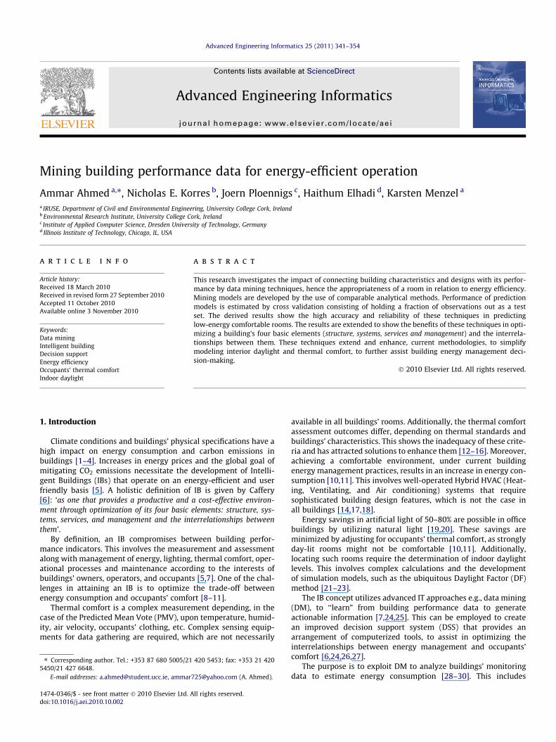
and weather conditions. This would evaluate the assumption ofusing a specific attribute as input to models. The attribute impor-tance analysis of MDL is shown in Fig. 4. A horizontal bar is createdto illustrate the relative sensitivity of variables. The y-axis listsvariables in the order of importance from top to bottom, whilethe x-axis shows the importance of each variable.

Considering indoor predictors that are involved in the calcula-tion of the PMV, room temperature is ranked first with approxi-mately importance of 0.44, on occupants’ thermal comfort.Radiant temperature was the next most important with signifi-

Table 9Errors produced by Naïve Bayes in mislabeling thermal classes.

Confusion matrix Cold Cool

Cold 122 2Cool 32 2,577Neutral 8 1,607Slightly cool 28 33,924Slightly warm 0 0Warm 0 0Total 190 38,090Correct (%) 64.21 6.71Cost 19577.25 295268

Model performance Total actual 132 3,072Correctly predicted (%) 92.42 84.47Cost 157912.38 284229

cance of 0.43. Room humidity and CO2 level demonstrated lessweight of 0.031 and 0.028, respectively.

4.2. Illuminance models

Decision tree showed high efficiency on predicting illuminancelabels i.e., over 99.9% overall accuracy and reliability, followed bySVM, which registered 99.9% and 99.7%. Naïve Bayes performedworst with 99.7% and 99.5% rates for the same metrics, respec-tively (Table 10).

Decision tree registered the highest true positive rate of 99.9%followed by SVM and Naïve Bayes with rates of 99.8% and 99.7%,respectively. The false positive rate of the three models is consid-erably low i.e., 0.004, 0.003 and 0.007 for decision tree, Naïve Bayesand SVM, respectively. Decision tree identified true and false posi-tive cases with 99.9% accuracy, while SVM and Naïve Bayes per-formed at 99.8% and 99.7% rates.

Decision tree correctly predicted both illuminance labels i.e.,‘enough’ and ‘not enough’, with accuracy higher than 99% with cost93 for the ‘enough’ label and 6 for the ‘not enough’ (Table 11).

4.3. Scheduling models

Using the original dataset, which consists of 1,245,315 records,Naïve Bayes showed 91% overall accuracy and 87% reliability. SVM

Neutral Slightly cool Slightly warm warm

0 8 0 00 438 0 01,209,661 253,763 125,173 617,698 188,345 556 01,717 29 19,841 70 0 0 21,229,076 442,583 145,570 1598.42 42.56 13.63 13.33

.53 284206.65 689781.15 150337.48 608.83

1,590,218 240,551 21,549 276.07 78.3 91.88 100

.94 444017.64 402903.81 150716.12 0

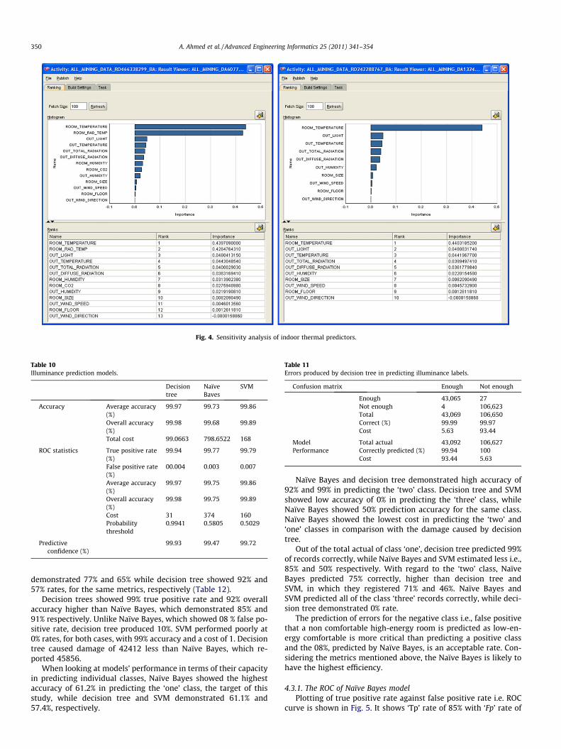
Fig. 4. Sensitivity analysis of indoor thermal predictors.

Table 10Illuminance prediction models.

Decisiontree

NaïveBaves

SVM

Accuracy Average accuracy(%)

99.97 99.73 99.86

Overall accuracy(%)

99.98 99.68 99.89

Total cost 99.0663 798.6522 168

ROC statistics True positive rate(%)

99.94 99.77 99.79

False positive rate(%)

00.004 0.003 0.007

Average accuracy(%)

99.97 99.75 99.86

Overall accuracy(%)

99.98 99.75 99.89

Cost 31 374 160Probabilitythreshold

0.9941 0.5805 0.5029

Predictiveconfidence (%)

99.93 99.47 99.72

Table 11Errors produced by decision tree in predicting illuminance labels.

Confusion matrix Enough Not enough

Enough 43,065 27Not enough 4 106,623Total 43,069 106,650Correct (%) 99.99 99.97Cost 5.63 93.44

Model Total actual 43,092 106,627Performance Correctly predicted (%) 99.94 100

Cost 93.44 5.63

350 A. Ahmed et al. / Advanced Engineering Informatics 25 (2011) 341–354

demonstrated 77% and 65% while decision tree showed 92% and57% rates, for the same metrics, respectively (Table 12).

Decision trees showed 99% true positive rate and 92% overallaccuracy higher than Naïve Bayes, which demonstrated 85% and91% respectively. Unlike Naïve Bayes, which showed 08 % false po-sitive rate, decision tree produced 10%. SVM performed poorly at0% rates, for both cases, with 99% accuracy and a cost of 1. Decisiontree caused damage of 42412 less than Naïve Bayes, which re-ported 45856.

When looking at models’ performance in terms of their capacityin predicting individual classes, Naïve Bayes showed the highestaccuracy of 61.2% in predicting the ‘one’ class, the target of thisstudy, while decision tree and SVM demonstrated 61.1% and57.4%, respectively.

Naïve Bayes and decision tree demonstrated high accuracy of92% and 99% in predicting the ‘two’ class. Decision tree and SVMshowed low accuracy of 0% in predicting the ‘three’ class, whileNaïve Bayes showed 50% prediction accuracy for the same class.Naïve Bayes showed the lowest cost in predicting the ‘two’ and‘one’ classes in comparison with the damage caused by decisiontree.

Out of the total actual of class ‘one’, decision tree predicted 99%of records correctly, while Naïve Bayes and SVM estimated less i.e.,85% and 50% respectively. With regard to the ‘two’ class, NaïveBayes predicted 75% correctly, higher than decision tree andSVM, in which they registered 71% and 46%. Naïve Bayes andSVM predicted all of the class ‘three’ records correctly, while deci-sion tree demonstrated 0% rate.

The prediction of errors for the negative class i.e., false positivethat a non comfortable high-energy room is predicted as low-en-ergy comfortable is more critical than predicting a positive classand the 08%, predicted by Naïve Bayes, is an acceptable rate. Con-sidering the metrics mentioned above, the Naïve Bayes is likely tohave the highest efficiency.

4.3.1. The ROC of Naïve Bayes modelPlotting of true positive rate against false positive rate i.e. ROC

curve is shown in Fig. 5. It shows ‘Tp’ rate of 85% with ‘Fp’ rate of

Table 12Prediction results for scheduling models validation with random data distribution.

Naïve Bayes Decision trees SVM

One Three Two One Three Two One Three Two

Confusion matrix One 56,447 0 10,072 66,215 0 304 32,921 2,456 21,551Three 0 1 0 0 0 1 0 1 0Two 35,818 1 109,856 42,108 0 103,567 24,464 28,113 66,979Total 92,265 2 119,928 108,323 0 103,872 57,385 34,700 88,530Correct (%) 61.18 50 91.60 61.13 0 99.71 57.37 0 75.66Cost 123,870.03 3.46 76,035.54 145,622.85 0 632,362.46 24,464 34,699 21,551

Model performance Total actual 66,519 1 145,675 66,519 1 145,675 66,519 1 145,675Correctly predicted (%) 84.86 100 75.41 99.54 0 71.09 49.49 100 45.98Cost 76,035.54 0 123,873.49 2,294.96 630,067.5 145,622.85 33,598 0 78.696

Model accuracy Average accuracy (%) 90.07 67.66 73.51Overall accuracy (%) 90.88 91.57 76.87Total cost 199909.0285 777985.3114 116424

ROC statistics True positive rate (%) 85.24 99.54 0False positive rate (%) 08.25 09.634 0Average accuracy (%) 88.5 94.95 50Overall accuracy (%) 90.90 91.58 99.99Cost 45856 42412 1Probability threshold 0.3057 0.5687 1

Predictive confidence (%) 86.76 56.88 64.68

A. Ahmed et al. / Advanced Engineering Informatics 25 (2011) 341–354 351

08%. This results in an average and overall accuracy of 89% and 91%respectively, with cost of 45,856 and probability threshold of 31%.The top left corner of the ROC graph is significantly high, indicatinga high true positive rate and a low false positive rate. The area un-der the curve is considerably large, indicating the high likelihood ofthe model that an actual positive case will be assigned a higherprobability of being positive than an actual negative case. This ispossible as the dataset has unbalanced target distribution. Thismodel can be biased in favor of positive cases by changing thethreshold. This depends on the acceptable false positive rate.

4.3.2. Lift of the Naïve Bayes modelThe ratio between the predicted positive results obtained using

the model and the actual values, is shown in Fig. 6. This metric issubjected to different interpretations depending on the miningproblem. The graph shows the positive cumulative cases in quantilesof 50,341 sizes, in which the predicted results were sorted by prob-ability, and the predicted positive values were counted and com-pared to the actual values. For example, in quantile number 3, thelift for the first 30% of the records is approximately 3 indicating thatat least twice the effectiveness is expected by not using the model.This indicates that over 77% of cumulative positive values are likelyto be found in the first three quantilies. In fact, 100% increase inpositive cases is likely to be achieved in over 80% of the records.

4.3.3. DeploymentThe Naïve Bayes was applied to weather data recorded in Janu-

ary 2010 consisting of 14,820 records. The cost matrix of modelperformance accuracy is shown in Table 13. The model correctlypredicted 75%, 86% and 100% of classes ‘one’, ‘two’ and ‘three’ with0 costs for the same label. The cost of mislabeling class ‘one’ as‘two’ or ‘three’ is 8. This is higher than mislabeling class ‘two’ as‘one’ or ‘three’, which are 3. The highest cost is 630,068, which isthe model produced in mislabeling class ‘three’.

4.3.3.1. ERI performance.The overall building performance regarding energy saving for

each room was analyzed to identify rooms, particularly those inclass ‘one’, for the years 2006–2009.

The building shows actual total of 31% for the ‘one’ class. Roomsin the south facade of the building show 20% class ‘one’ (no artifi-

cial light is needed and the room is comfortable) while the northfacade shows 12 %. This means that energy mangers should focustheir attention on using the rooms in the south facade, where thebuilding could operate under the status of energy-efficiently. Addi-tionally, rooms on the first floor show 13.2% class ‘one’, whereasthose on the ground floor show 13% and those on the undergroundfloor show 7%. Thus, the first floor of the south facade is the mostefficient location in the building. There is a conference room on thefirst floor of the south facade with 7% under class ‘one’ and 10 % un-der class ‘two’, while the meeting room on the ground floor shows0% under class ‘one’ and 17% under class ‘two’. Thus the seminarroom is more efficient than the meeting room, and therefore itshould be used more frequently. As the model uses the weatherconditions as input parameters and these vary between winterand summer, the energy saving was analyzed for the two main sea-sons. Summer starts on the first of May and ends on the first of Au-gust. The building shows 29% under class ‘one’ in winter and 40%for summer time, even though summer time is much less thanthe winter time (3 months). Possibly because the building showshigh comfortable class (no heating or cooling is needed) in thedatabase (Table 5) and the illuminance is higher in summer thanwinter (Ireland has mostly overcast sky in winter). Thus, if thebuilding hosts conferences, these should be scheduled for the sum-mer time.

5. Discussion and conclusion

Results show that, given sufficient data with proper variables,DM methods are capable of predicting building performance indi-cators i.e., occupants’ comfort, strongly day-lit rooms and conse-quently low-energy comfortable rooms with approximately 80%,99% and 90% accuracy, 90%, 99% and 86% reliability, in that order.

Among three prediction models used in this study, Naïve Bayesperformed better, in scheduling rooms for usage, followed by deci-sion tree and support vector machine. Decision tree, like NaïveBayes, demonstrated high accuracy. Unlike Naïve Bayes, decisiontree showed less reliability. Support vector machine performedvery poorly, in comparison with Naïve Bayes and decision tree. Thismerits further research to train decision tree models, as they showthe reasoning process in human-understandable rules. This can as-sist building design towards energy efficient operation. On the

Fig. 5. ROC curve of Naïve Bayes.

352 A. Ahmed et al. / Advanced Engineering Informatics 25 (2011) 341–354

other hand support vector machine are mathematical models thatdo not provide such features.

For more accurate and more robust outcomes in prediction, it isa common practice to use a combination of mining models. It is agood idea to use the three models together for the prediction oflow-energy comfortable rooms. This will support not only betterprediction results but also a forecasting system that is robust inits predictions. The same applies to thermal and illuminancemodels.

Decision tree, Naïve Bayes and support vector machine showedover 99% prediction rates, for the identification of strongly day-litrooms. Decision tree created the best results, followed by supportvector machine and Naïve Bayes. On the other hand, Naïve Bayesproduced the best results with approximately 87% prediction accu-racy in estimating occupants’ thermal comfort followed by supportvector machine and decision tree.

The success of data mining project relies exclusively on thequality and quantity of data representing the behavior under con-sideration. Even though this study used a huge amount of data,with a rich set of features, more building characteristics can be in-cluded to enhance models’ efficiency and performance. The sensi-tivity analysis provides insight about the importance of attributesand their impact on a specific behavior. This would facilitate exam-ining building characteristics that are likely to influence its perfor-mance indicators. This also supports testing different buildingdesign proposals in order to evaluate energy-efficiency. Historicalweather data, which can be easily obtained from any weather sta-

tion database relevant to the location, along with the proposed de-sign (physical specifications) can be loaded into the model toevaluate energy efficiency of the proposed design. Assessing theperformance of existing buildings, relevant renovation tasks, fa-cade designs and room layouts is considerably more efficient. Italso supports long planning of rooms’ usage.

Techniques presented in this paper are intended to integrateany thermal comfort standard and indoor daylight method, simpli-fying the procedures used in determining these performance indi-cators. This allows for optimizing a building’s four basic elementsand the interrelationships between them, providing building per-formance data and adopting advanced analytical techniques. Thisis achievable as mining models ‘‘learn” from building performancebehaviors regardless of how it was carried out. This adds power tothe models as the characteristics that indicate building perfor-mance indicators are integrated into models.

Models presented in this manuscript use the output of twoother models (thermal comfort and illuminance models), whichwere developed and assessed in the same way presented in this pa-per. One option to enhance its efficiency is to improve the qualityof these models. Another option is to calculate the occupants’ ther-mal comfort and the natural indoor illuminance in rooms manu-ally, however, complex calculations and equipment are requiredalong with simulation tools (i.e., time and money). This will ensurethat all input to the scheduling model are actual values, and henceincrease its quality. The efficiency of the model can also be in-creased by improving the quality of the built data. This can be

Fig. 6. Cumulative gains chart of Naïve Bayes.

Table 13Cost matrix of applying Naïve Bayes.

One Two Three

Cost matrix One 0 7.549 7.549Two 3.458 0 3.458Three 630067.5 630067.5 0

Actual 4,452 10,368 0Prediction 5893 8927 0Correctly predicted (%) 75.55 86.1 100

A. Ahmed et al. / Advanced Engineering Informatics 25 (2011) 341–354 353

achieved by synchronizing the sensors’ reading time, hence reduc-ing the number of null values in the data set. Consequently, therewill be no need to replace the outside sensors locations with anuninterested scheduling label. This issue has been raised with thesensors’ network research group in ITOBO.

The scheduling classes in Table 2 can be re-defined based on abuilding’s energy management preferences. The number of classescan be increased to give more options in choosing a room e.g. class‘one’ could be defined for the thermal comfort class ‘neutral’ andnatural illuminance label ‘enough’ that high comfort level is pro-vided. Also, the value of class ‘enough’ can be reduced e.g. if light-ing is not as critical as thermal. Additionally, training thescheduling model in a building that has a larger number of roomswith different specifications and used irregularly (e.g. a conferencecenter) will increase its quality in-so-far-as the model will havemore chance to ‘‘learn” from a wide range of inputs. For example,the ‘walls’ external and internal material’ has the same value, thus

the model does not ‘‘learn” sufficiently from these inputs. Conse-quently, the flexibility of the models is enhanced since Table 4and consequently Table 6 can be expanded to include more attri-butes that have different values, which is appropriate for industry.Adopting an international naming convention for the influences,such as industrial foundation class (IFC), will extend the applicabil-ity of the model.

The focus of this study is to predict building performance indi-cators using climate conditions and building characteristics. Eventhough it enhances the findings of previous studies, this study isnot meant to develop a new theory rather than it is meant to showthe capabilities of data mining as a means to assist improvingbuilding performance. An energy management system integratingthese models can be used as a decision aid to facilitate short-termand long-term building operational processes.

Potentials future research includes enhancing the performanceof models. This incorporates models bias with further cost andprobability threshold analysis. It also considers investigating deci-sion trees reliability in predicting scheduling labels. The automa-tion of loading weather forecast data into models andimplementing a graphical user interface, to ease its usability as adecision aid for energy management, is also considered.

Acknowledgement

Work in the Strategic Research Cluster ‘ITOBO’ is funded by Sci-ence Foundation Ireland (SFI) and additional contributions fromfive industry partners.

354 A. Ahmed et al. / Advanced Engineering Informatics 25 (2011) 341–354

The authors thank Gemma Langridge, Wellcome Trust SangerInstitute, UK, Dr. Angela McCann, ERI UCC, Michal Orteba, Brian Ca-hill, and Luke Allan, Civil Engineering UCC for their contribution tothis research.

References

[1] Amar A. Khudhair, Mohammed M. Farid, A review on energy conservation inbuilding applications with thermal storage by latent heat using phase changematerials, Energy Conversion and Management 45 (2) (2004) 263–275.

[2] D.J. Sailor, A.A. Pavlova, Air conditioning market saturation and long-termresponse of residential cooling energy demand to climate change, Energy 28(9) (2003) 941–951.

[3] H. Akbari, M. Pomerantz, H. Taha, Cool surfaces and shade trees to reduceenergy use and improve air quality in urban areas, Solar Energy 70 (3) (2001)295–310.

[4] Timothy J. Considine, The impacts of weather variations on energy demandand carbon emissions, Resource and Energy Economics 22 (4) (2000) 295–314.

[5] D.T. O’Sullivan, M.M. Keane, D. Kelliher, R.J. Hitchcock, Improving buildingoperation by tracking performance metrics throughout the building lifecycle(BLC), Energy and Building 36 (11) (2004) 1075–1090.

[6] R. Caffrey, The intelligent building, an ASHRAE opportunity, ASHRAE TechnicalData Bulletin 4 (1) (1985) 925–933.

[7] G. Augenbroe, C.S. Park, Quantification methods of technical buildingperformance, Building Research and In-formation 33 (2) (2005) 159–172.

[8] B.L. Capehar, W.C. Turner, W.J. Kennedy, Guide to Energy Management, TheFairmont Press, 2008.

[9] Bert Metz, IPCC Fourth Assessment Report on the mitigation of climate changefor researchers, students, and policymakers, 9780521880114, 2007.

[10] A. Nilson, R. Uppstrom, C. Hjalmarsson, Energy efficiency in office buildings:lessons from Swedish projects, Swedish Council for Building Research (1997).

[11] L. Weber, I. Keller, Stromverbrauch in burogebauden: gespart ohne zu wollen,ENET Bulletin SVE/VSE 18 (99) (1999) 19–23.

[12] R. Yao, B. Li, J. Liu, A theoretical adaptive model of thermal comfort – adaptivepredicted mean vote (a PMV), Building and Environment 44 (10) (2009) 2089–2096.

[13] F. Nicol, K. Parsons, Special issue on thermal comfort standards, Energy andBuildings 34 (6) (2002) 529–685.

[14] J.U. Pfafferott, S. Herkel, D.E. Kalz, A. Zeushner, Comparison of low-energyoffice buildings in summer using different thermal comfort criteria, Energyand Buildings 39 (7) (2007) 750–757.

[15] B. Moujalled, R. Cantin, G. Guarracin, Comparison of thermal comfortalgorithms in naturally ventilated office buildings, Energy and Buildings 40(12) (2008) 2215–2223.

[16] Fergus Nicol, Adaptive thermal comfort standards in the hot-humid tropics,Energy and Buildings 36 (7) (2004) 628–637.

[17] Marcuse Keane, Hidden depths, Building Service Journal (2005) 23–28.[18] Jens Pfafferott, Sebastian Herkel, Matthias Wambsganß, Design, monitoring

and evaluation of a low energy office building with passive cooling by nightventilation, Energy and Buildings 36 (5) (2004) 455–465.

[19] M. Bodart, A. De Herde, Global energy savings in offices buildings by the use ofdaylighting, Energy and Buildings 34 (15) (2002) 421–429.

[20] Danny W.H. Li, Joesph C. Lam, Evaluation of lighting performance in officebuildings with day light controls, Energy and Buildings 33 (2001) 793–803.

[21] C.F. Reinhart, S. Herkel, The simulation of annual daylight illuminancedistributions – a state-of-the-art comparison of six RADIANCE-basedmethods, Energy and Buildings 33 (2000) 683–697.

[22] Fakra Ali Hamada, Harry Boyer, Eddy Lafosse, Philippe Lauret, A new methodto calculate indoor natural lighting by improving Lumen models, in: ISESWorld Congress Solar Energy and Human Settlement, 2009, pp. 456–460.

[23] Jan de Boer, Modelling indoor illumination by complex fenestration systemsbased on bidirectional photometric data, Energy and Buildings 38 (7) (2006)849–868.

[24] N. Kasabov, Introduction: hybrid intelligent system adaptive systems,International Journal of Intelligent Systems 16 (13) (1998) 453–454.

[25] S. Sharples, V. Callaghan, G. Clarke, A multi-agent architecture for intelligentbuilding sensing and control, Sensor Review 19 (2) (1999) 135–140.

[26] P. Rob, C. Coronely, K. Crockett, Data Bases Systems: Design, Implementationand Management, Cengage Learning EMEA, 2008.

[27] David W. Cash et al., Knowledge systems for sustainable development, in: Natl.Acad. Sci., USA, 2003, pp. 100:8086-100:8091.

[28] G. Mihalakakou, M. Santamouris, A. Tsangrassoulis, On the energyconsumption in residential buildings, Energy and Buildings 34 (2002) 727–736.

[29] Bing Dong, Cheng Cao, Siew Eang Lee, Applying support vector machines topredict building energy consumption in tropical region, Energy and Buildings37 (2005) 545–553.

[30] S. Wu, D. Clements-Croom, Understanding the indoor environment throughmining sensory data – a case study, Energy and Buildings 39 (11) (2007) 1183–1191.

[31] C. Morbitzer, P. Strachan, C. Simpson, Data mining analysis of buildingsimulation performance data, Building Services Engineering Research andTechnology (2004) 253–267.

[32] Leen Peeters, Richard de Dear, Jan Hensen, William D’haeseleer, Thermalcomfort in residential buildings: comfort values and scales for building energysimulation, Applied Energy 86 (2009) 772–780.

[33] J.R. Dutton, Opportunities and priorities in a new era for weatherand climateservices, Bulletin of American Meteorology Society 83 (2002) 1303–1311.

[34] J. Michalakes et al., The weather research and forecast model: softwarearchitecture and performance, in: proceeding of the Eleventh ECMWFWorkshop on the Use of High Performance Computing in Meteorology,Meteorology Reading, UK, 2004.

[35] R. Saunders, M. Matricardi, B. Brunel, An improved fast radiative transfermodel for assimilation of satellite radiance observations, Quarterly Journal ofthe Royal Meteorological Society (1999) 1407–1425.

[36] Xingwen Wang, Joshua Zheuxe Huang, A cased-based data mining platform,in: A State of the Art Survey, Data mining: Theory, Methodology, Techniques,and Applications, Springer Science and Business, 2006, pp. 28–38.

[37] Jiawei Han, Micheline Kamber, Data Mining: Concepts and Techniques, 2nded., Morgan Kaufmann, 2006.

[38] Oracle, Oracle Data Mining Concepts, Oracle, 2008.[39] Karsten Menzel, Dirk Pesch, Brendan O’Flynn, Marcus Keane, Cian O’Mathuna,

Towards a wireless sensor platform for energy efficient building operation, in:12th International conference on Computing in Civil and Building Engineering,vol. 13, Beijing, China, 2008, pp. 381–386.

[40] S. Shekari, R. Golmohammadi, Evaluation of horizontal and verticalilluminance models against measured data in Iran, Applied SciencesResearch 4 (3) (2009) 158–166.

[41] The European Commission Directorate, Daylighting in Buildings, 1999.[42] Londonmet, 1998. <www.learn.londonmet.ac.uk>.[43] CRISP, CRoss Industry Standard Process for Data Mining, 2010. Online: <http://

www.crisp-dm.org/>.[44] C. Shearer, The CRISP-DM model: the new blueprint for data mining, Journal of

Data Warehousing 5 (2000) 13–22.[45] Zhi Li, Hong Ma, Yongbing Mei, A unifiying method for outlier and change

detection from data stream based on local ploynomial fitting, in: The Pacific-Asia Conference on Knowledge Discovery and DataMining (PAKDD), Nanjing,China, 2007, pp. 150–161.

[46] Jaoquin Abellan, Andres Cano, Andres R. Masegosa, Serafin Moral, A semi-naivebayes classifier with grouping of cases, in: 9th European Conference,ECSQARU, Hammamet, Tunisia, 2007, pp. 477–488.

[47] D. Delen, R. Sharda, P. Kumar, Movie forecaset guru: a web-based DSS forhollywood managers, Decision Support System 43 (4) (2007) 113–127.

[48] M.Y. Kiang, A comparative assessment of classification algorithms, DecisionSupport Systems 35 (2003) 441–454.

[49] X. Li, G.C. Nsofor, L. Song, A comparative analysis of predictive data miningtechniques, International Journal of Rapid Manufacturing 1 (2) (2009) 150–172.

[50] Dursen Delen, A comparative analysis of machine learning technques forstudent retention management, Decision Support System (2010), doi:10.1016/j.dss.2010.06.003.

[51] R. Sharda, D. Delen, Predicting box-office success of motion pictures withneural networks, Expert Systems with Applications 30 (2) (2006) 243–254.

[52] Microsoft, TechNet, 2010. Online: <http://technet.microsoft.com/en-us/library/ms174493.aspx>.

[53] G. Davis, Sensitivity analysis in neural net solutions, IEEE Transactions onSystems, Man and Cybernetics 19 (1989) 1078–1082.

[54] ERI, Environmental Research Institute, UCC, 2010. Online: <http://www.ucc.ie/en/eri/>.

[55] ITOBO, Information and Communication Technology for Sustainable andOptimised Building Operation, 2007. Online: <http://zuse.ucc.ie/itobo>.

[56] Ammar Ahmed, Joern Ploennigs, Y. Gao, Karsten Menzel, Analyze buildingperformance data for energy-efficient building operation, in: Managing IT inConstruction, CIB-W78, 2009.

[57] Ammar Ahmed, Brian Cahill, Karsten Menzel, A New Perspective inSupervising Building Performance, ECPPM, Cork, Ireland, 2010.

[58] Ammar Ahmed, Orteba Michel, Korres E. Nicholas, Elhadi Haithum, MenzelKarsten, Assessing the performance of naturally day-lit buildings using datamining, Advanced Engineering Informatics (2010).

[59] Joern Ploennigs, Ammar Ahmed, Paul Stack, Karsten Menzel, Model-basedEstimation of Rooms’ Energy Consumption in Building with Renewable EnergySources, ICCCBE, Nottingham, UK, 2010.

[60] Alain Zarli, Ework and Ebusiness in Architecture, Engineering andConstruction: Ecppm, CRC Press, 2008.

[61] Ammar Ahmed, Joern Ploennigs, Karsten Menzel, Brian Cahill, Multi-dimensional Building Performance Data Management for ContinuousCommissioning, Advance Engineering Informatics 24 (2) (2010) 466–475.

[62] G. Provan, J. Ploennigs, M. Boubekeur, A. Mady, A. Ahmed, Using buildinginformation model data for generating and updating diagnostic models, in: theTwelfth International Conference on Civil, Structural and EnvironmentalEngineering Computing, Stirlingshire, Scotland, 2009.

[63] Mathworks, The Mathworks, 2010. Online: <http://www.mathworks.com/access/helpdesk/help/techdoc/ref/resampletimeseries.html>.

[64] Autodesk, 2006. Online: <www.ecotect.com>.[65] Robert Haberstroh, Oracle Data Mining Tutorial for Oracle Data Mining 11g

Release 1, Oracle, 2008.