Efficient Mining of Frequent Closures with Precedence Links and Associated Generators

Efficient Mining of Frequent Closures with Precedence

Links and Associated Generators

Laszlo Szathmary, Petko Valtchev, Amedeo Napoli

To cite this version:

Laszlo Szathmary, Petko Valtchev, Amedeo Napoli. Efficient Mining of Frequent Closureswith Precedence Links and Associated Generators. [Research Report] RR-6657, 2008, pp.58.<inria-00322798v2>

HAL Id: inria-00322798

https://hal.inria.fr/inria-00322798v2

Submitted on 18 Sep 2008

HAL is a multi-disciplinary open accessarchive for the deposit and dissemination of sci-entific research documents, whether they are pub-lished or not. The documents may come fromteaching and research institutions in France orabroad, or from public or private research centers.

L’archive ouverte pluridisciplinaire HAL, estdestinee au depot et a la diffusion de documentsscientifiques de niveau recherche, publies ou non,emanant des etablissements d’enseignement et derecherche francais ou etrangers, des laboratoirespublics ou prives.

https://hal.archives-ouvertes.fr

https://hal.inria.fr/inria-00322798v2

appor t de r ech er ch e

ISS

N02

49-6

399

ISR

NIN

RIA

/RR

--66

57--

FR+E

NG

Thème SYM

INSTITUT NATIONAL DE RECHERCHE EN INFORMATIQUE ET EN AUTOMATIQUE

Efficient Mining of Frequent Closures withPrecedence Links and Associated Generators

Laszlo Szathmary — Petko Valtchev — Amedeo Napoli

N° 6657

May 2008

Centre de recherche INRIA Nancy – Grand EstLORIA, Technopôle de Nancy-Brabois, Campus scientifique,

615, rue du Jardin Botanique, BP 101, 54602 Villers-Lès-NancyTéléphone : +33 3 83 59 30 00 — Télécopie : +33 3 83 27 83 19

Efficient Mining of Frequent Closures withPrecedence Links and Associated Generators

Laszlo Szathmary∗†, Petko Valtchev† , Amedeo Napoli∗

Thème SYM — Systèmes symboliquesÉquipes-Projets Orpailleur

Rapport de recherche n° 6657 — May 2008 — 58 pages

Abstract: The effective construction of many association rule bases requirethe computation of frequent closures, generators, and precedence links betweenclosures. However, these tasks are rarely combined, and no scalable algorithmexists at present for their joint computation. We propose here a method thatsolves this challenging problem in two separated steps. First, we introducea new algorithm called Touch for finding frequent closed itemsets (FCIs) andtheir generators (FGs). Touch applies depth-first traversal, and experimen-tal results indicate that this algorithm is highly efficient and outperforms itslevelwise competitors. Second, we propose another algorithm called Snow forextracting efficiently the precedence from the output of Touch. To do so, weapply hypergraph theory. Snow is a generic algorithm that can be used withany FCI/FG-miner. The two algorithms, Touch and Snow, provide a completesolution for constructing iceberg lattices. Furthermore, due to their modulardesign, parts of the algorithms can also be used independently.

Key-words: algorithm, data mining, itemset search, association rule bases,closed itemsets, generators, concept lattice, iceberg lattice

[email protected], [email protected], [email protected]

∗ LORIA UMR 7503, B.P. 239, 54506 Vandœuvre-lès-Nancy Cedex, France† Dépt. d’Informatique UQAM, C.P. 8888, Succ. Centre-Ville, Montréal H3C 3P8, Canada

Une méthode efficace de recherche de motifsfréquents fermés et générateurs et de la relation

d’ordre entre fermésRésumé : En fouille de données, la construction effective de la plupart desbases de règles d’association nécessite le calcul des motifs fermés fréquents, desgénérateurs et des relations de subsomption entre motifs fermés, ce qui donned’ailleurs l’ordre du treillis des concepts sous-jacent. Ces trois tâches, qui sontentremêlés, sont pourtant rarement combinées et il n’existe aucun algorithmequi propose une telle combinaison qui soit efficace et qui passe à l’échelle. Nousproposons dans ce rapport une façon de résoudre ce problème important, quis’appuie sur deux étapes principales. D’abord, nous introduisons un nouvelalgorithme appelé Touch procède en profondeur, et qui recherche les motifsfermés fréquents (FCIs) et les motifs générateurs. Des résultats expérimen-taux montrent que l’algorithme Touch est très efficace et qu’il a de très bonnesperformances comparé à ses homologues qui procèdent par niveaux. Ensuite,nous proposons l’algorithme appelé Snow qui calcule la relation de subsomp-tion entre les motifs fermés produit par Touch, en faisant appel à la théoriedes hypergraphes. L’algorithme Snow est générique et peut être utilisé avecn’importe quel algorithme de recherche de FCIs/FGs. Les deux algorithmes,Touch et Snow, apportent l’ensemble des éléments nécessaires à la constructiondes treillis iceberg. En outre, la conception modulaire de ces algorithmes faitqu’ils peuvent être utilisés indépendamment les uns des autres.

Mots-clés : algorithmes pour la fouille de données, motifs fréquents, mo-tifs fermés, motifs générateurs, règles d’association, bases, treillis de concepts,treillis iceberg

Table of Contents

1 Frequent Itemsets and Formal Concept Analysis 1

1.1 Frequent Itemsets and Frequent Association Rules . . . . . . . . . . . . . . . . . 1

1.2 Formal Concept Analysis . . . . . . . . . . . . . . . . . . . . . . . . . . . . . . . . 2

1.3 Relation Between Data Mining and Formal Concept Analysis . . . . . . . . . . . 4

2 Frequent Itemset Search with Vertical Algorithms 5

3 The Touch Algorithm 9

3.1 Motivation and Contribution . . . . . . . . . . . . . . . . . . . . . . . . . . . . . 9

3.2 Main Features of Touch . . . . . . . . . . . . . . . . . . . . . . . . . . . . . . . . 10

3.2.1 Finding Frequent Closed Itemsets . . . . . . . . . . . . . . . . . . . . . . . 10

3.2.2 Finding Frequent Generators . . . . . . . . . . . . . . . . . . . . . . . . . 11

3.2.3 Associating Frequent Generators to Their Closures . . . . . . . . . . . . . 12

3.3 The Algorithm . . . . . . . . . . . . . . . . . . . . . . . . . . . . . . . . . . . . . 13

3.3.1 Pseudo Code . . . . . . . . . . . . . . . . . . . . . . . . . . . . . . . . . . 13

3.3.2 Running Example . . . . . . . . . . . . . . . . . . . . . . . . . . . . . . . 13

3.4 Experimental Results . . . . . . . . . . . . . . . . . . . . . . . . . . . . . . . . . . 13

3.5 Conclusion . . . . . . . . . . . . . . . . . . . . . . . . . . . . . . . . . . . . . . . . 15

4 The Snow and Snow-Touch Algorithms 17

4.1 Basic Concepts of Hypergraphs . . . . . . . . . . . . . . . . . . . . . . . . . . . . 17

4.2 Detailed Description of Snow . . . . . . . . . . . . . . . . . . . . . . . . . . . . . 19

4.2.1 The Snow-Touch Algorithm . . . . . . . . . . . . . . . . . . . . . . . . . . 21

4.2.2 Pseudo Code . . . . . . . . . . . . . . . . . . . . . . . . . . . . . . . . . . 21

4.3 Experimental Results . . . . . . . . . . . . . . . . . . . . . . . . . . . . . . . . . . 22

4.4 Conclusion . . . . . . . . . . . . . . . . . . . . . . . . . . . . . . . . . . . . . . . . 23

A Test Environment 27

Table of Contents

B Detailed Description of Vertical Algorithms 29

B.1 Eclat . . . . . . . . . . . . . . . . . . . . . . . . . . . . . . . . . . . . . . . . . . . 29

B.2 Charm . . . . . . . . . . . . . . . . . . . . . . . . . . . . . . . . . . . . . . . . . . 33

B.3 Talky-G . . . . . . . . . . . . . . . . . . . . . . . . . . . . . . . . . . . . . . . . . 37

C Horizontal and Vertical Data Layouts 45

D Efficient Support Count of 2-itemsets 47

E Computing the Transversal Hypergraph 49

Bibliography 55

Index 57

Chapter 1

Frequent Itemsets and Formal ConceptAnalysis

In this chapter, we present the basic concepts of (i) frequent itemset search, and (ii) formalconcept analysis. The chapter is organized as follows. Section 1.1 presents the basic conceptsrelated to frequent itemset search. Section 1.2 sums up the definitions and properties of formalconcept analysis (FCA). Section 1.3 points out the close relation between data mining and formalconcept analysis.

1.1 Frequent Itemsets and Frequent Association Rules

Frequent Itemsets. Below we use standard definitions of data mining. We consider a set ofobjects or transactions O = {o1, o2, . . . , om}, a set of attributes or items A = {a1, a2, . . . , an},and a relation R ⊆ O×A, where R(o, a) means that the object o has the attribute a. In formalconcept analysis [GW99] the triple (O,A,R) is called a formal context. A set of items is calledan itemset or a pattern. Each transaction has a unique identifier (tid), and a set of transactionsis called a tidset .1 The length of an itemset is the cardinality of the itemset, i.e. the numberof items included in the itemset. An itemset of length i is called an i-long itemset, or simplyan i-itemset2. An itemset P is said to be larger (resp. smaller) than Q if |P | > |Q| (resp.|P | < |Q|). We say that an itemset P ⊆ A is included in an object o ∈ O, if (o, p) ∈ R forall p ∈ P . Let f be the function that assigns to each itemset P ⊆ A the set of all objects thatinclude P : f(P ) = {o ∈ O | o includes P}. The set of objects including the itemset is also knownas the image of the itemset.3 The (absolute) support of an itemset P indicates how many objectsinclude the itemset, i.e. supp(P ) = |f(P )|. The support of an itemset P can also be defined inrelative value, which corresponds to the proportion of objects including P , with respect to thewhole population of objects. An itemset P is called frequent, if its support is not less than agiven minimum support (denoted by min_supp), i.e. supp(P ) ≥ min_supp.

Definition 1.1 (generator) An itemset G is called generator if it has no proper subset H(H ⊂ G) with the same support.

1For convenience, we will use separator-free set notations throughout the paper, e.g. AB stands for {A, B},13 stands for {1, 3}, etc.

2For instance, ABE is a 3-itemset.3For instance, in dataset D (Table 2.1), the image of AB is 23.

1

2 Chapter 1. Frequent Itemsets and Formal Concept Analysis

Definition 1.2 (closed itemset) An itemset X is called closed if it has no proper superset Y(X ⊂ Y ) with the same support.

The closure of an itemset X (denoted by γ(X)) is the largest superset of X with the samesupport. Naturally, if X = γ(X), then X is closed. The task of frequent (closed) itemset miningconsists of generating all (closed) itemsets with supports greater than or equal to a specifiedmin_supp.

Equivalence Classes. Two itemsets P,Q ⊆ A are said to be equivalent (P ∼= Q) iff theybelong to the same set of objects (i.e. γ(P ) = γ(Q)). From this definition it follows thatequivalent itemsets have the same support values. The set of itemsets that are equivalent to anitemset P (P ’s equivalence class) is denoted by [P ] = {Q ⊆ A | P ∼= Q}. Generators areminimal elements in their equivalence classes (w.r.t. set inclusion), i.e. a generator G ∈ [G] hasno proper subset in [G]. An equivalence class has at least one generator. Closed itemsets aremaximal elements in their equivalence classes (w.r.t. set inclusion), i.e. a closed itemset X ∈ [X]has no proper superset in [X]. An equivalence class has exactly one closed itemset, which meansthat closed itemsets are unique elements in their equivalence classes. If an equivalence class hasonly one element, then the equivalence class is called singleton. The only element of a singletonequivalence class is closed as well as generator.

Frequent Association Rules. An association rule is an expression of the form P1 → P2, whereP1 and P2 are arbitrary itemsets (P1, P2 ⊆ A), P1∩P2 = ∅ and P2 6= ∅. The left side, P1 is calledantecedent, the right side, P2 is called consequent. The support of an association rule r: P1 → P2

is defined as: supp(r) = supp(P1 ∪ P2). An association rule r is called frequent, if its support isnot less than a given minimum support (denoted by min_supp), i.e. supp(r) ≥ min_supp. Theconfidence of an association rule r: P1 → P2 is defined as the conditional probability that anobject includes P2, given that it includes P1: conf(r) = supp(P1∪P2)/supp(P1). An associationrule r is called confident, if its confidence is not less than a givenminimum confidence (denoted bymin_conf), i.e.conf(r) ≥ min_conf . An association rule r with conf(r) = 1.0 (i.e. 100%) is an exact as-sociation rule, otherwise it is an approximate association rule. A frequent association rule isvalid (their set is denoted by AR) if it is both frequent and confident, i.e. supp(r) ≥ min_suppand conf(r) ≥ min_conf . The problem of mining frequent association rules in a database Dconsists of finding all frequent valid rules in the database.

1.2 Formal Concept Analysis

We describe here the basic notions of FCA [GW99]. Formal concept analysis considers a tripleK = (O,A,R) called context, where O = {o1, o2, . . . , om} is a set of objects, A = {a1, a2, . . . , an}is a set of attributes, and the binary relation R(o, a) means that the object o has the attributea. Two operators, both denoted by ′, connect the power sets of objects 2O and attributes 2A asfollows:

′ : 2O → 2A, Z ′ = {o ∈ O | ∀a ∈ Z, R(o, a)}

The operator ′ is dually defined on attributes. The pair of ′ operators induces a Galois connectionbetween 2O and 2A. The composition operators ′′ are closure operators: they are idempotent,extensive, and monotonous.

1.2. Formal Concept Analysis 3

Figure 1.1: The complete concept lattice (left) and an iceberg concept lattice (right) of theformal context of Table 2.1.

A formal concept of the context K = (O,A,R) is a pair (X, Y) ⊆ O × A, where X′ = Y andY′ = X. X is called extent , and Y is called intent . A concept (X1, Y1) is a subconcept of a concept(X2, Y2) if X1 ⊆ X2 (or dually Y2 ⊆ Y1) and we write (X1, Y1) ≤ (X2, Y2). The concept whoseextent contains all the objects is called the top concept. The concept whose intent contains allthe attributes is called the bottom concept.

Definition 1.3 (concept lattice) The set B of all concepts of a formal context K togetherwith the partial order relation ≤ forms a lattice and is called the (complete) concept lattice of K.

A concept lattice can be visualized with a Hasse diagram. For instance, the concept latticeassociated to the formal context of Table 2.1 is shown in Figure 1.1 (left).

A concept is called frequent if its intent is frequent.

Definition 1.4 (iceberg lattice [STB+02]) The set of all frequent concepts of a context Ktogether with the partial order relation ≤ forms a so-called iceberg concept lattice of K.

Note that an iceberg lattice is an order filter of the complete concept lattice and in general onlya join semi-lattice. However, adding a bottom element makes it a lattice again. For instance, theiceberg lattice of the formal context of Table 2.1 by min_supp = 3 is shown in Figure 1.1 (right).

Let (Xj, Yj) be a subconcept of (Xi, Yi), i.e. (Xj, Yj) ≤ (Xi, Yi). If there is no concept (Xk, Yk)such that (Xj, Yj) ≤ (Xk, Yk) ≤ (Xi, Yi), then (Xi, Yi) is said to cover (Xj, Yj) from above (anddually, (Xj, Yj) is said to cover (Xi, Yi) from below). For instance, in Figure 1.1 the concept(123, A) covers the concept (12, ACDE) from above (and dually, (12, ACDE) covers (123, A)from below).

Definition 1.5 (upper cover) The upper cover of a concept C is a set of concepts where eachelement of the set covers C from above.

The lower cover of a concept is defined dually. For instance, in Figure 1.1 the upper cover of(12, ACDE) is {(123, A), (124, D)}, and the lower cover of (123, A) is {(23, AB), (12, ACDE)}.

4 Chapter 1. Frequent Itemsets and Formal Concept Analysis

In other words, the upper cover contains all the “direct parents”, and the lower cover contains allthe “direct children” of a concept.

When the upper cover (or dually, the lower cover) for each concept is discovered, we say thatthe order (or covering relation) is found among the concepts.

1.3 Relation Between Data Mining and Formal Concept Analysis

In this subsection we review the relation between data mining (DM) and formal concept analysis(FCA). The intents of a formal concept lattice are closed itemsets. The intents of an iceberglattice are frequent closed itemsets [STB+02]. For constructing the Hasse diagram of a conceptlattice, extents are not necessary, i.e. the order among concepts can be discovered based uponthe intents only.

Discovering the set of all intents in FCA is equivalent to the DM problem of finding all closeditemsets by min_supp = 0. Most DM algorithms only concentrate on itemsets, thus the ordermust be established in an additional step. When min_supp > 0, DM algorithms will extractfrequent closed itemsets. Finding the order among them results in an iceberg concept lattice.

As a summary, we can state that the general schema for using DM algorithms for buildingformal concept lattices (either complete or iceberg) consists of two main steps: (1) extracting(frequent) closed itemsets, and then (2) finding the order among them.

Chapter 2

Frequent Itemset Search with VerticalAlgorithms

In this chapter, we present the common parts of three vertical algorithms namely Eclat, Charm,and Talky-G. The detailed description of these algorithms can be found in Appendix B. Thischapter mainly relies on [ZPOL97], [Zak00], and [ZH02].

Overview of Vertical Algorithms

Eclat was the first successful algorithm proposed to generate all frequent itemsets in a depth-firstmanner. Charm is a modification of Eclat to explore frequent closed itemsets only. Talky-G isan adaptation of Eclat and Charm. Talky-G extracts frequent generators only. All three algo-rithms use a vertical layout of the database. In this way, the support of an itemset can be easilycomputed by a simple intersection operation.

Consider the following dataset D (Table 2.1) that we will use for our examples throughoutthe paper.

A B C D E1 x x x x2 x x x x x3 x x4 x5 x

Table 2.1: A sample dataset (D) for the examples.

Basic concepts. Here we would like to present the necessary notions specific to Eclat, Charm,and Talky-G, using the terminology of Zaki. Let I be a set of items, and D a database oftransactions, where each transaction has a unique identifier (tid) and contains a set of items.The set of all tids is denoted as T . A set of items is called an itemset, and a set of transactions iscalled a tidset. For convenience, we write an itemset {A,B,E} as ABE, and a tidset {2,3} as 23.For an itemset X, we denote its corresponding tidset as t(X), i.e. the set of all tids that containX as a subset. For a tidset Y , we denote its corresponding itemset as i(Y ), i.e. the set of items

5

6 Chapter 2. Frequent Itemset Search with Vertical Algorithms

Figure 2.1: IT-tree: Itemset-Tidset search tree of dataset D (Table 2.1).

common to all the tids in Y . Note that t(X) =⋂x∈X t(x), and i(Y ) =

⋂y∈Y i(y). For instance,

using our dataset D (Table 2.1), t(ABE) = t(A) ∩ t(B) ∩ t(E) = 1235 ∩ 1345 ∩ 1345 = 135 andi(23) = i(2)∩i(3) = AC∩ABCE = AC. The support of an itemset X is equal to the cardinalityof its tid-list, i.e. supp(X) = |t(X)|.

Lemma 2.1 Let X and Y be two itemsets. Then, X ⊆ Y ⇒ t(X) ⊇ t(Y ).

Proof. Follows from the definition of support. �

Itemset-tidset search tree and prefix-based equivalence classes. Let I be the set ofitems. Define a function p(X, k) = X[1 : k] as the k length prefix of X, and a prefix-basedequivalence relation θk on itemsets as follows: ∀X,Y ⊆ I, X ≡θk

Y ⇐⇒ p(X, k) = p(Y, k).That is, two itemsets are in the same k-class if they share a common k-length prefix.

Eclat (resp. Charm and Talky-G) performs a search for frequent itemsets (resp. frequentclosed itemsets and frequent generators) over a so-called IT-tree search space, as shown in Fig-ure 2.1. While most previous methods exploit only the itemset search space, Eclat, Charm,and Talky-G simultaneously explore both the itemset space and the transaction space. Eachnode in the IT-tree, called an IT-node, represented by an itemset-tidset pair, X × t(X), is infact a prefix-based equivalence class (or simply a prefix-based class). All the children of a givennode X belong to its prefix-based class, since they all share the same prefix X. We denote aprefix-based class as [P ] = {l1, l2, . . . ln}, where P is the parent node (the prefix), and each li isa single item, representing the node Pli × t(Pli). For example, the root of the tree correspondsto the class [ ] = {A,B,C,D,E}. The left-most child of the root consists of the class [A] of allitemsets containing A as the prefix. Each class member represents one child of the parent node.A class represents items that the prefix can be extended with to obtain a new frequent node.Clearly, no subtree of an infrequent prefix has to be examined. The power of the prefix-basedclass approach is that it breaks the original search space into independent sub-problems. Whenall direct children of a node X are known, one can treat it as a completely new problem; one canenumerate the itemsets under it and simply prefix them with the item X, and so on.

Lemma 2.1 states that if X is a subset of Y , then the cardinality of the tid-list of Y(i.e. its support) must be less than or equal to the cardinality of the tid-list of X. A practi-cal and important consequence of this lemma is that the cardinalities of intermediate tid-listsshrink as we descend in the IT-tree. This results in very fast intersection and support counting.

Vertical layout. It is necessary to access the dataset in order to determine the support of acollection of itemsets. Itemset mining algorithms work on binary tables, and such a database can

7

be represented by a binary two-dimensional matrix. There are two commonly used layout forthe implementation of such a matrix: horizontal and vertical data layout. Levelwise algorithmsuse horizontal layout. Eclat, Charm, and Talky-G use instead vertical layout, in which thedatabase consists of a set of items and their tid-lists. To count the support of an itemset Xusing the horizontal layout, we need one full database pass to test for every transaction T ifX ⊆ T . For a large collection of itemsets, this can be done at once using the trie data structure.The vertical layout has the advantage that the support of an itemset can be computed by asimple intersection operation. In [Zak00], it is shown that the support of any k-itemset can bedetermined by intersecting the tid-lists of any two of its (k − 1)-long subsets. A simple checkon the cardinality of the resulting tid-list tells us whether the new itemset is frequent or not. Itmeans that in the IT-tree, only the lexicographically first two subsets at the previous level arerequired to compute the support of an itemset at any level. One layout can be easily transformedto the other layout on-the-fly (see Appendix C for more details).

Other Optimizations

Element reordering. As pointed out in [Goe03] and [CG05], Eclat does not fully exploit themonotonocity property. It generates a candidate itemset based on only two of its subsets, thusthe number of candidate itemsets is much larger as compared to breadth-first approaches suchas Apriori. Eclat essentially generates candidate itemsets using only the join step of Apriori,since the itemsets necessary for the prune step are not available due to the depth-first search.A technique that is regularly used is to reorder the items in support ascending order, whichleads to the generation of less candidates. In Eclat, Charm, and Talky-G such reordering can beperformed on the children of a node N when all direct children of N are discovered. Experimentalevaluations show that item reordering results in significant performance gains in the case of allthree algorithms.

Support count of 2-itemsets. It is well known that many itemsets of length 2 turn out to beinfrequent. A naïve implementation for computing the frequent 2-itemsets requires n(n − 1)/2intersection operations, where n is the number of frequent 1-items. Considering that 1-itemshave the largest tid-lists (see Lemma 2.1), these operations are quite expensive. Here we presenta method that can be used not only for depth-first, but for breadth-first algorithms too, suchas Apriori. First, the database must be transformed in horizontal format (see Appendix C).Second, through a database pass on the horizontal layout, an upper-triangular 2D matrix is builtcontaining the support values of 2-itemsets [ZH02] (see Appendix D for a detailed descriptionand an example).

Diffsets for further optimizing memory usage. Recently, Zaki proposed a new approachto efficiently compute the support of an itemset using the vertical data layout [ZG03]. Insteadof storing the tidset of a k-itemset P in a node, the difference between the tidset of P and thetidset of the (k−1)-prefix of P is stored, denoted by the diffset of P . To compute the support ofP , we simply need to subtract the cardinality of the diffset from the support of its (k−1)-prefix.Support values can be stored in each node as an additional information. The diffset of an itemsetP ∪ {i, j}, given the two diffsets of its subsets P ∪ {i} and P ∪ {j}, with i < j, is computedas follows: diffset(P ∪ {i, j})← diffset(P ∪ {j}) \ diffset(P ∪ {i}). Diffsets also shrink as largeritemsets are found. Diffsets can be used together with the other optimizations presented above.This technique can significantly reduce the size of memory required to store intermediate results.Diffsets can be used for Eclat, Charm, and Talky-G resulting in dEclat, dCharm, and dTalky-G,

8 Chapter 2. Frequent Itemset Search with Vertical Algorithms

respectively. Note that we have not used diffsets in our implementations yet.4

Conclusion

In this chapter we presented the common parts of Eclat, Charm, and Talky-G. Detailed descrip-tion of Eclat can be found in Appendix B.1. Charm is presented in Appendix B.2. Talky-G isdetailed in Appendix B.3.

4We plan to investigate this technique as a future perspective.

Chapter 3

The Touch Algorithm

In this chapter, we introduce a very efficient new algorithm called Touch that can find frequentequivalence classes in a dataset. The chapter is organized as follows. First, we present themotivation and contribution of the algorithm. This is followed by the description of the threemain features of Touch. We then present the pseudo code of the algorithm and give a runningexample. Next, we provide experimental results for comparing the efficiency of Touch to someother algorithms. Finally, we draw conclusions.

3.1 Motivation and Contribution

Finding association rules is one of the most important tasks in data mining. Generating validassociation rules from frequent itemsets (FIs) often results in a huge number of rules, which limitstheir usefulness in real life applications. To solve this problem, different concise representations ofassociation rules have been proposed, e.g. generic basis [BTP+00b], informative basis [BTP+00b],minimal non-redundant association rules [BTP+00b], representative rules [Kry98], Duquennes-Guigues basis [GD86], Luxenburger basis [Lux91], proper basis [PBTL99a], structuralbasis [PBTL99a], etc. A very good comparative study of these bases can be found in [Kry02],where it is stated that a rule representation should be lossless (should enable derivation of allvalid rules), sound (should forbid derivation of rules that are not valid), and informative (shouldallow determination of rules parameters such as support and confidence).

In this present work, we are more interested in finding minimal non-redundant associationrules (MNR). Rules in this set have the following form: P → Q \ P , where P ⊂ Q and P isa generator and Q is a closed itemset. These rules are particularly interesting because of thefollowing reasons. First, this set of rules is lossless, sound, and informative. In [Kry02], it isshown that with the so-called cover operator, which is an inference mechanism, all valid rulescan be restored from these rules with their proper support and confidence values. Second, amongrules with the same support and same confidence, these rules contain the most information andthese rules can be the most useful in practice [Pas00].

The minimal non-redundant association rules were introduced in [BTP+00b]. In [BTP+00a],Bastide et al. presented the Pascal algorithm and claimed that MNR can be extracted withthis algorithm. However, to obtain MNR from the output of Pascal, one has to do a lot ofcomputing. First, from the form of MNR it can be seen that frequent closed itemsets mustalso be known. Second, frequent generators must be associated to their closures. Recently weproposed the algorithm Zart, an extension of Pascal, that gives a solution for these two extraneeds [SNK07]. With the output of Zart, one can easily construct the set ofMNR.

9

10 Chapter 3. The Touch Algorithm

Pascal is very efficient among levelwise frequent itemset mining algorithms. This is due toits pattern counting inference mechanism that can significantly reduce the number of expensivedatabase passes. In [SNK07] we showed that Zart, in spite of its additional features, is almostas efficient as Pascal. Furthermore, as it was argued in [Sza06], the idea introduced in Zart canbe generalized, and thus it can be applied to any frequent itemset mining algorithm.

However, Zart has a drawback too. It traverses the whole set of frequent itemsets in orderto filter generators and closed itemsets. It can be a serious waste in dense, highly correlateddatasets, in which the number of FCIs and the number of FGs is usually much less than thenumber of FIs. That is, if we only want the frequent equivalence classes with their minimal andmaximal elements (FGs and FCIs), it is no good enumerating the whole set of FIs.

Here we present an algorithm that gives an elegant solution for this problem. The algorithmTouch reduces the search space to frequent generators and frequent closed itemsets only. Then,we use a novel method for associating the frequent generators to their closures, thus the algorithmproduces exactly the same output as Zart. Experimental results show that our new method isvery efficient, especially on dense, highly correlated datasets.

3.2 Main Features of Touch

Touch has three main features, namely (1) extracting frequent closed itemsets, (2) extractingfrequent generators, and (3) associating frequent generators to their closures, i.e. identifyingfrequent equivalence classes.

3.2.1 Finding Frequent Closed Itemsets

This part of Touch relies on Charm. Charm is a vertical algorithm that can find FCIs veryefficiently in a database. Charm traverses the IT-tree in a depth-first manner in a pre-order way,from left-to-right. As detailed in Appendix B.2, Charm collects FCIs in the main memory in aspecial hash data structure. This data structure is taken over from Charm by Touch. That is,the hash structure containing all FCIs is one of the two inputs of Touch.

Charm builds this hash structure for filtering non-closed itemsets. When a new candidateIT-node is created (let us call it current node), Charm checks if a proper superset with thesame support is already stored in the hash. If yes, then the current node is not closed. Charmperforms this test the following way. First, it assigns a hash key to the current node. It takesthe sum of the tids in the tidset, and then it calculates the modulo of the sum with the size ofthe hash table. The resulting hash key gives a position in the hash table, where a list of closeditemsets is stored. Finally, Charm checks if this list includes a proper superset of the currentnode with the same support. For a running example, please consult Appendix B.2. The hashstructure of Charm has the following important property:

Property 3.1 If the hash key of an itemset is calculated as above (i.e. taking the sum of thetids in the tidset of the itemset, and calculating the modulo of the sum with the size of the hashtable), then itemsets with the same image are to be stored in the same slot of the hash table.

Example. Let us see the left part of Figure 3.1 (Charm) that depicts the hash structure ofFCIs extracted from dataset D (Table 2.1). For this example, the size of the hash table is set tofour. To demonstrate Property 3.1, let us investigate the itemsets ABCDE and BD (see alsoFigure B.2). The two itemsets are included in transaction 2 (see also Table 2.1). Charm findsABCDE first. Its hash key is 2, thus it is stored in the hash structure at position 2. Later,

3.2. Main Features of Touch 11

Figure 3.1: Hash tables for dataset D (Table 2.1) by min_supp = 1. Left: hash table of Charmcontaining all FCIs. Right: hash table of Talky-G containing all FGs.

in another branch of the IT-tree, Charm finds BD, whose hash key is also 2 by Property 3.1.Charm checks the list of itemsets at position 2 in the hash structure, but since the list alreadyincludes a proper superset of BD with the same support (ABCDE), BD is not inserted in thehash since it it not closed.

3.2.2 Finding Frequent Generators

This part of Touch relies on Talky-G. Talky-G is a vertical algorithm that can find FGs veryefficiently in a database. Talky-G traverses the IT-tree in a depth-first manner in a reverse pre-order way, from right-to-left. As detailed in Appendix B.3, this traversal has the advantage thatwhen an itemset X is found, all subsets of X are treated before X itself. Talky-G collects FGsin the main memory in a special hash data structure. This data structure is taken over fromTalky-G by Touch. That is, the hash structure containing all FGs is the second input of Touch.

Talky-G builds this hash structure for filtering non-generator itemsets. When a candidateIT-node is created (let us call it current node), Talky-G checks if a proper subset with the samesupport is already stored in the hash. If yes, then the current node is not generator. Talky-Gperforms this test the following way. First, it assigns a hash key to the current node. It takes thesum of the tids in the tidset, and then it calculates the modulo of the sum with the size of thehash table. The resulting hash key gives a position in the hash table, where a list of generatorsis stored. Finally, Talky-G checks if this list includes a proper subset of the current node withthe same support. For a running example, please consult Appendix B.3.

Since Talky-G calculates the hash key of an itemset exactly the same way as Charm does(see Section 3.2.1), Property 3.1 also holds for Talky-G. That it, itemsets having the same imageare to be stored in the same slot of the hash table.

Example. Let us see the right part of Figure 3.1 (Talky-G) that depicts the final state ofthe hash structure of FGs extracted from dataset D (Table 2.1). For this example, the size ofthe hash table is set to four. To demonstrate that Property 3.1 is also true for Talky-G, let usinvestigate the itemsets BD and ABD (see also Figure B.5). The two itemsets are includedin transaction 2 (see also Table 2.1). Talky-G finds BD first because of the reverse pre-orderstrategy. Its hash key is 2, thus it is stored in the hash structure at position 2. Later, in anotherbranch of the IT-tree, Talky-G finds ABD, whose hash key is also 2 by Property 3.1. Talky-Gchecks the list of itemsets at position 2 in the hash structure, but since the list already includesa proper subset of ABD with the same support (BD), ABD is not inserted in the hash since itit not generator.


Algorithm 1 (Touch):

Description: finds frequent equivalence classes

1) hashFCI ←(call Charm and get its hash data structure); // see Appendix B.22) hashFG←(call Talky-G and get its hash data structure); // see Appendix B.33) loop over the FCIs in hashFCI (c)4) {5) i←(index position of c);6) c.generators← ∅; // empty set7) loop over the list of FGs in hashFG at index i (g)8) {9) if (c.support = g.support) {10) if g is a subset of c, then11) c.generators← c.generators ∪ {g}; // g is a generator of c12) }13) }14) }

3.2.3 Associating Frequent Generators to Their Closures

In the previous two steps (Sections 3.2.1 and 3.2.2) we managed to extract FCIs and FGs. Thereis one more step to do namely associating frequent generators to their closures, i.e. identifyingthe equivalence classes. If we had two simple sets of FCIs and FGs, the following naïve methodcould be used for instance. Enumerate all FCIs, and find their FG subsets with the same support.Unfortunately, this approach is very expensive.

In our method, instead of simple sets, we take over FCIs and FGs in a special hash datastructure. The reason is that we use these hash structures for the association process. The ideais the following:

Property 3.2 If both Charm and Talky-G use the same size for the hash tables (i.e., samenumber of slots), and if both algorithms use the same image-based hashing method (i.e., sum oftids in the tidset modulo with the size of the hash table), then from Property 3.1 and from thedefinition of equivalence classes it follows that a frequent closed itemset and its generators are indifferent tables but they are at the same index position.

Example. Let us see Figure 3.1 that depicts the two inputs of Touch, i.e. the hash structureof Charm and the hash structure of Talky-G. Say we want to determine the generators of theclosed itemset ACDE. ACDE is stored at position 3 in the hash structure of Charm. ByProperty 3.2, its generators are stored in the list at position 3 in the other hash structure, i.e.in the hash structure of Talky-G. In this list, there are three itemsets that are subsets of ACDEand that have the same support values: E, C, and AD. It means that these three itemsets arethe generators of ACDE.

3.3. The Algorithm 13

FCI support associated FG(s)AB 2 AB

ABCDE 1 BE; BD; BCA 3 A

B 3 B

ACDE 2 E; C; ADD 3 D

Table 3.1: Output of Touch on dataset D by min_supp = 1.

3.3 The Algorithm

3.3.1 Pseudo Code

The pseudo code of Touch is given in Algorithm 1. Line 1 corresponds to Section 3.2.1. Line 2is explained in Section 3.2.2. The block between lines 3 and 14 is detailed in Section 3.2.3.

3.3.2 Running Example

Here we demonstrate the execution of Touch on dataset D with min_supp = 1 (20%). First,Charm and Talky-G are called on D with the given min_supp value. As a result, they returnFCIs and FGs in two hash structures, as shown in Figure 3.1. Then, Touch associates generatorsto their closures the following way. Processing AB. The frequent closed itemset AB has onesubset with the same support in the other hash structure at index 1 (AB). This means thatAB is a closed itemset and a generator at the same time, i.e. the equivalence class of AB hasone element only (singleton equivalence class). Processing ABCDE. The frequent closed itemsetABCDE has three generators: BE, BD, and BC. Etc. The output of Touch is shown inTable 3.1. Recall that due to the property of equivalence classes, the support of a generator isequal to the support of its closure.

3.4 Experimental Results

We evaluated Touch against Zart [SNK07] and A-Close [PBTL99b]. The algorithms were imple-mented in Java in the Coron data mining platform [SN05].5 The experiments were carried outon a bi-processor Intel Quad Core Xeon 2.33 GHz machine running under Ubuntu GNU/Linuxoperating system with 4 GB of RAM. For the experiments we have used the following datasets:T20I6D100K, C20D10K, and Mushrooms. The T20I6D100K6 is a sparse dataset, constructedaccording to the properties of market basket data that are typical weakly correlated data. TheC20D10K is a census dataset from the PUMS sample file, while the Mushrooms7 describesmushrooms characteristics. The last two are highly correlated datasets.

Table 3.2 contains detailed information about the execution of Touch. The first three columnscorrespond to the three main steps of Touch namely (1) getting FCIs using Charm, (2) gettingFGs using Talky-G, and (3) associating FGs to their closures. Column 4 indicates the totalexecution time of the algorithm including input and output. In the sparse dataset T20I6D100K,almost all frequent itemsets are closed and generators at the same time. It means that most

5http://coron.loria.fr6http://www.almaden.ibm.com/software/quest/Resources/7http://kdd.ics.uci.edu/


execution time (sec.)min_supp get FCIs get FGs associate total time # FCIs # FGs (# FIs) #FCIs

#FIs#FGs#FIs

(Charm) (Talky-G) FCIs and FGs (with I/O)T20I6D100K

1% 19.07 2.16 0.03 22.76 1,534 1,534 1,534 100.00% 100.00%0.75% 24.06 2.65 0.05 28.32 4,710 4,710 4,710 100.00% 100.00%0.5% 35.21 5.01 0.14 42.45 26,208 26,305 26,836 97.66% 98.02%0.25% 94.59 20.71 0.50 121.60 149,217 149,447 155,163 96.17% 96.32%

C20D10K30% 0.20 0.29 0.02 1.06 951 967 5,319 17.88% 18.18%20% 0.34 0.41 0.03 1.42 2,519 2,671 20,239 12.45% 13.20%10% 0.71 0.70 0.07 2.27 8,777 9,331 89,883 9.76% 10.38%5% 1.13 1.06 0.11 3.37 21,213 23,051 352,611 6.02% 6.54%

Mushrooms30% 0.12 0.21 0.02 0.82 425 544 2,587 16.43% 21.03%20% 0.19 0.27 0.02 0.98 1,169 1,704 53,337 2.19% 3.19%10% 0.43 0.46 0.04 1.57 4,850 7,585 600,817 0.81% 1.26%5% 0.80 0.81 0.08 2.53 12,789 21,391 4,137,547 0.31% 0.52%

Table 3.2: Detailed execution times of Touch and other statistics (number of FCIs, number ofFGs, number of FIs, proportion of the number of FCIs to the number of FIs, proportion of thenumber of FGs to the number of FIs). Note that the number of FIs is shown for comparativereasons only. Touch does not need to extract all FIs.

equivalence classes are singletons. It is known that Charm is less efficient on sparse datasets. Thereason is that Charm performs four tests on each candidate for reducing the IT-tree. However,in sparse datasets the number of FCIs is almost equivalent to the number of FIs, thus the searchspace cannot be reduced significantly. Consequently, the four tests give some overhead to thealgorithm. Talky-G is also less efficient on sparse datasets, but still much faster than Charm.It can be due to the less number of tests on a candidate. In dense, highly correlated datasets(C20D10K and Mushrooms), both Charm and Talky-G are very efficient, even at low minimumsupport values. Since the number of FCIs and FGs is much less than the number of FIs, thetwo algorithms can take advantage of exploring a much smaller search space. The associationof FCIs and FGs is done extremely efficiently in all cases. That is, the association step givesabsolutely no overhead to Touch.

Table 3.3 contains the experimental evaluation of Touch against Zart and A-Close. All timesreported are real, wall clock times as obtained from the Unix time command between input andoutput. We have chosen Zart and A-Close because they represent two efficient algorithms thatproduce exactly the same output as Touch. Zart and A-Close are both levelwise algorithms. Zartis an extension of Pascal, i.e. first it finds all FIs, then it filters FCIs, and finally the algorithmassociates FGs to their closures. A-Close reduces the search space to FGs only, then it calculatesthe closure for each generator. Both algorithms have advantages and disadvantages. Zart, due toits pattern counting inference, can enumerate FIs very efficiently. As shown in [SNK07], the extracomputations of Zart give no significant overhead to the algorithm. Thus, when the number ofFIs is not too high, Zart proves to be quite efficient. A-Close, on the other hand, requires muchless memory since it reduces the search space to FGs only. This reduction of the memory usageis more spectacular in the case of dense, highly correlated datasets. However, the way A-Closecomputes the closures of generators is very expensive because of the huge number of intersectionoperations. Thus, in spite of reducing the search space, A-Close is less efficient than Zart inmost cases. Touch, just like A-Close, reduces the search space to the strict minimum, i.e. it onlyextracts what it really needs namely the set of FCIs and the set of FGs. Then, Touch associates

3.5. Conclusion 15

execution time (sec.)min_supp Touch Zart A-Close

T20I6D100K1% 22.76 7.33 31.25

0.75% 28.32 14.96 39.490.5% 42.45 45.52 100.600.25% 121.60 159.78 285.41

C20D10K30% 1.06 8.17 15.7820% 1.42 15.84 29.8810% 2.27 36.66 59.415% 3.37 75.28 94.18

Mushrooms30% 0.82 3.65 7.1720% 0.98 10.69 15.2810% 1.57 75.36 36.835% 2.53 641.54 63.37

Table 3.3: Response times of Touch, compared to Zart and A-Close.

the two sets in a very efficient way. Since Touch is based on Charm and Talky-G, the algorithmis very efficient on dense, highly correlated datasets. We must admit however that levelwisealgorithms like Zart are sometimes more suitable for sparse datasets.

3.5 Conclusion

In this chapter we presented a new algorithm called Touch for exploring the frequent equivalenceclasses in a dataset. The algorithm has three main features namely (1) extraction of FCIs,(2) extraction of FGs, and (3) association of FGs to their closures. The algorithm is verycompetitive because each one of the three steps is solved in a very efficient way. First, FCIsare extracted with Charm, and Charm is considered to be one of the most efficient FCI-miningalgorithms. Second, for the extraction of FGs we propose a new algorithm called Talky-G. Talky-G concentrates on FGs only in the search space. Third, we found a very efficient solution forassociating FCIs and FGs together that gives no overhead at all to the algorithm. That is, theassociation can be done in almost no time. Moreover, the memory footprint of Touch is lowsince, unlike Zart for instance, the algorithm does not need to extract all frequent itemsets.Experimental results prove the interest of Touch, especially on dense, highly correlated datasets.

To sum up, Touch is a very efficient new algorithm that has two original parts: (1) thealgorithm Talky-G for finding FGs in a depth-first manner with a reverse pre-order traversal,and (2) the association of FCIs and FGs for identifying frequent equivalence classes.

Chapter 4

The Snow and Snow-Touch Algorithms

In this chapter, we present the Snow and Snow-Touch algorithms. Snow can find order amongconcepts in a formal lattice, and Snow-Touch is a combination of two algorithms namely Snowand Touch. The chapter is organized as follows. Section 4.1 presents the basic concepts ofhypergraphs. This short overview of hypergraph theory is necessary for understanding the Snowalgorithm that is detailed in Section 4.2. Section 4.2 also includes the pseudo code of Snow andSnow-Touch. Experimental results of the two algorithms are provided in Section 4.3. Finally, wedraw conclusions in Section 4.4.

4.1 Basic Concepts of Hypergraphs

In this subsection we mainly rely on [EG95]. Hypergraph theory [Ber89] is an important field ofdiscrete mathematics with many relevant applications in applied computer science. A hypergraphis a generalization of a graph, where edges can connect arbitrary number of vertices. Formally:

Definition 4.1 (hypergraph) A hypergraph is a pair (V ,E) of a finite set V = {v1, v2, . . . , vn}and a family E of subsets of V . The elements of V are called vertices, the elements of E edges.

Note that some authors, e.g. [Ber89], state that the edge-set as well as each edge must be non-empty and that the union of all edges results in the vertex set.

Definition 4.2 (partial hypergraph) Let H = {E1, E2, . . . , Em} be a hypergraph. The partialhypergraph Hi of H (i = 1, . . . , n) is the hypergraph that contains the first i edges of H, i.e.Hi = {E1, . . . , Ei}.

A hypergraph is simple if none of its edges is contained in any other of its edges. Formally:

Definition 4.3 (simple hypergraph) A hypergraph is called simple if it satisfies ∀Ei, Ej ∈ E :Ei ⊆ Ej ⇒ i = j.

Example. The hypergraph H in Figure 4.1 is not simple because the edge {a} is contained inthe edge {a, c, d}.

Definition 4.4 Let H = (V, E) be a hypergraph. Then min(H) denotes the set of minimal edgesof H w.r.t. set inclusion, i.e. min(H) = {E ∈ E | @E′ ∈ E : E′ ⊂ E}, and max(H) denotes theset of maximal edges of H w.r.t. set inclusion, i.e. max(H) = {E ∈ E | @E′ ∈ E : E′ ⊃ E}.

17

18 Chapter 4. The Snow and Snow-Touch Algorithms

Figure 4.1: A sample hypergraph H, where V = {a, b, c, d} and E = {{a}, {b, c}, {a, c, d}}.

Clearly, for any hypergraph H, min(H) and max(H) are simple hypergraphs. Moreover, everypartial hypergraph of a simple hypergraph is simple, too.

Example. In the case of hypergraph H in Figure 4.1, min(H) = {{a}, {b, c}} and max(H) ={{b, c}, {a, c, d}}.

The problem that is of high interest for us concerns hypergraph transversals. A transversal of ahypergraph H is a subset of the vertex set of H which intersects each edge of H. A transversalis minimal if it does not contain any transversal as proper subset. Formally:

Definition 4.5 (transversal) Let H = (V, E) be a hypergraph. A set T ⊆ V is called atransversal of H if it meets all edges of H, i.e. ∀E ∈ E : T ∩ E 6= ∅. A transversal T iscalled minimal if no proper subset T ′ of T is a transversal.

Note that Pfaltz and Jamison call transversal (resp. minimal transversal) as blocker (resp.minimal blocker) in [PJ01]. Outside hypergraph theory, a transversal is usually called a hittingset.

Example. The hypergraph H in Figure 4.1 has two minimal transversals: {a, b} and {a, c}.For instance, the sets {a, b, c} and {a, c, d} are transversals but they are not minimal.

Definition 4.6 (transversal hypergraph) The family of all minimal transversals of H con-stitutes a simple hypergraph on V called the transversal hypergraph of H, which is denoted byTr(H).

Example. Considering the hypergraph H in Figure 4.1, Tr(H) = {{a, b}, {a, c}}. See Ap-pendix E for an algorithm and further examples.

The following propositions capture important relations between a hypergraph and its transversalhypergraph (for proofs see [Ber89]).

Proposition 4.1 Let H = (V, E) be a hypergraph. Then Tr(H) is a simple hypergraph, andTr(H) = Tr(min(H)).

Proposition 4.2 Let G and H be two simple hypergraphs. Then G = Tr(H) if and only ifH = Tr(G).

Corollary 4.1 Let G and H be two simple hypergraphs. Then Tr(G) = Tr(H) iff G = H.

4.2. Detailed Description of Snow 19

Corollary 4.2 (duality property) Let H be a simple hypergraph. Then Tr(Tr(H)) = H.

Corollary 4.2 states that calculating the transversal hypergraphH′ of a simple hypergraphH, andcalculating once again the transversal hypergraph H′′ of H′, we get back the original hypergraphH, i.e. H′′ = H.

Example. Consider the hypergraph H in Figure 4.1. Since H is not simple, let G = min(H) ={{a}, {b, c}}. Then,

G′ = Tr(G) = Tr({{a}, {b, c}}) = {{a, b}, {a, c}}

G′′ = Tr(G′) = Tr({{a, b}, {a, c}}) = {{a}, {b, c}} .

That is, G′′ = G. �

4.2 Detailed Description of Snow

The goal of the Snow algorithm is to find order among concepts, i.e. provided a set of concepts,construct the corresponding concept lattice. As shown in Section 1.3, the order is uniquelydetermined by the set of concept intents. In a concept, in addition to its intent, we also need itsassociated generators (see Def. 1.1). It is important to note that Snow does not require conceptextents. To give an overview of the algorithm, Snow performs the following operations. As input,it takes a set of concepts, where a concept contains the intent and its generators. As output,Snow provides a concept lattice, i.e. it finds the order among concepts.

For the examples of Snow we will use the concept lattice depicted in Figure 4.2. In a concept,the following details are provided: intent, support of the intent (in parentheses), and below thelist of generators of the intent (separated by hashmarks). For instance, the bottom concept’sintent is ABCDE, and it has three generators namely BC, BD, and BE. Since they belong tothe same equivalence class, the support of all these four itemsets is the same, which is 1 in thisexample.

Now, let us see the theoretical background of Snow.

Definition 4.7 (face [Pfa02]) Let C1 and C2 be two concepts where C2 covers C1 from above.The difference between the intents of C1 and C2 is called a face of C1.

A concept has as many faces as the number of concepts in its upper cover.

Example. Let us consider the bottom concept in Figure 4.2. This concept has two faces:F1 = ABCDE \AB = CDE, and F2 = ABCDE \ACDE = B.

A basic property of the generators of a closed itemset X states that they are the minimalblockers of the family of faces associated to X [Pfa02]:

Theorem 4.1 Assume a closed itemset X and let F = {F1, F2, . . . , Fk} be its family of asso-ciated faces. Then a set Z ⊆ X is a minimal generator of X iff X is a minimal blocker ofF .

As indicated in Section 4.1, a minimal blocker of a family of sets is an identical notion to aminimal transversal of a hypergraph. This trivially follows from the fact that each hypergraph(V ,E) is nothing else than a family of sets drawn from ℘(V ). Now following Theorem 4.1,


Figure 4.2: Concept lattice of the context of Table 2.1. Concepts are labeled with their generators.

we conclude that given a closed itemset X, the associated generators compose the transversalhypergraph of its family of faces F seen as the hypergraph (X,F).

Next, further to the basic property of a transversal hypergraph, we conclude that (X,F)is necessarily simple. In order to apply Proposition 4.2, we must also show that the familyof generators associated to a closed itemset, say G, forms a simple hypergraph. Yet this holdstrivially due to the definition of generators. We can therefore advance that both families representtwo mutually corresponding hypergraphs.

Property 4.1 Let X be a closure and let G and F be the family of its generators and the family ofits faces, respectively. Then, for the underlying hypergraphs it holds that (a) Tr(X,G) = (X,F)and (b) Tr(X,F) = (X,G).

The Snow algorithm is based on part (a) of Property 4.1, which says that computing allthe minimal transversals of the generators of a concept, one obtains the family of faces of theconcept. By taking the difference between the concept intent and its family of faces, we get theintents of the concepts in the upper cover. This is the principal idea of Snow.

Example 4.1 Let us consider the bottom concept in Figure 4.2 whose intent is ABCDE. First,we compute the transversal hypergraph of its generators: Tr({BC,BD,BE}) = {CDE,B}. Thismeans that the bottom concept has two faces namely F1 = CDE and F2 = B. The number of facesindicates that the bottom concept is covered by two concepts C1 and C2 from above. By Def. 4.7,intent(C1) = ABCDE \ CDE = AB, and intent(C2) = ABCDE \B = ACDE. Applying thisprocedure for all concepts, the order relation among concepts can easily be discovered. �

Note that part (b) of Property 4.1 can be applied to determine the generators of concepts ina concept lattice (that is, order is known this time). First, the family of faces F of a concept Cmust be computed by using Def. 4.7. Then, calculating all the minimal transversals of F resultsin the family of generators of C.

4.2. Detailed Description of Snow 21

4.2.1 The Snow-Touch Algorithm

By Snow we refer to the algorithm that finds the order among concepts, i.e. the input is a set ofconcepts8 and the output is a concept lattice (either complete or iceberg). By Snow-Touch werefer to our complete solution as described in this paper. In addition to Snow, Snow-Touch alsoincludes the call of Touch for extracting the set of concepts, i.e. the input of Snow-Touch is acontext and a minimum support value, and the output is a concept lattice (either complete oriceberg).

4.2.2 Pseudo Code

The pseudo code of Snow (lines 3–12) and Snow-Touch (lines 1–12) is given in Algorithm 2.

Algorithm 2 (Snow and Snow-Touch):

Description (Snow): build a concept lattice from a set of concepts (lines 3–12)Description (Snow-Touch): build a concept lattice from a context (lines 1–12)

1) setOfItemsets← getItemsets(context, min_supp); // only for Snow-Touch2) setOfConcepts← convertToConcepts(setOfItemsets); // only for Snow-Touch3) identifyOrCreateTopConcept(setOfConcepts); // Snow starts here4) loop over the elements of setOfConcepts (c) // find the upper cover for each concept5) {6) setOfFaces← getMinTransversals(c.generators);7) intentsInUpperCover ← getIntentsInUpperCover(c.intent, setOfFaces);8) upperCover ← getCorrespondingConcepts(intentsInUpperCover);9) loop over the concepts in upperCover (p) {10) createLink(c, p);11) }12) }

getItemsets function: this method calls an itemset mining algorithm that returns (frequent)closed itemsets and their associated generators. In our implementation we used the Touchalgorithm for this purpose (see Chapter 3 for more details). Table 3.1 depicts a sample outputof Touch. This function is specific for Snow-Touch.

convertToConcepts function: this method converts the set of itemsets obtained from Touchto a set of concepts. A sample output of Touch is shown in Table 3.1. A concept is an object withthe following properties: intent, support, list of generators, list of references to concepts in theupper cover, list of references to concepts in the lower cover. The lists of references are initial-ized empty; the other properties are provided by Touch. This function is specific for Snow-Touch.

identifyOrCreateTopConcept procedure: this method tries to identify the top concept in theset of concepts. If it fails to find it, then it creates the top concept. The top concept is somewhatspecial, that is why it requires special attention. By definition, the intent of the top concept is theitemset that is present in all the objects of the input dataset, i.e. whose support is 100%. If thereis no full column in the input context, then this itemset is the empty set, because by definitionits support is 100%. The empty set is always a generator. If the input context has a closed

8Recall that concept intents are labeled by their generators.


itemset X (different from the empty set) with support 100%, then X is the closure of the emptyset; otherwise the empty set is a closed itemset. If the closure of the empty set is itself (like thisis the case in Figure 4.2), then it is considered to be a trivial case, thus data mining algorithmsoften omit the empty set in their output (like Touch for instance in Table 3.1). However, thetop concept is important in the case of concept lattices, thus the identifyOrCreateTopConceptprocedure performs the following task. It enumerates the concepts looking for a concept whosesupport is 100%. If it does not find such a concept, then it creates a concept whose intent andgenerator is the empty set. The support value of this newly created concept is set to 100% (seeFigure 4.2 for an example).

getMinTransversals function: this method computes the transversal hypergraph of a givenhypergraph. More precisely, given the family of generators of a concept c, the function returns thefamily of faces of c (by Property 4.1). For a detailed description of this function, see Algorithm 9in Appendix E.

getIntentsInUpperCover function: this method calculates the differences between the intentof the current concept c and the family of faces of c (by Def. 4.7). The function returns a set ofitemsets that are the intents of the concepts that form the upper cover of c.

getCorrespondingConcepts function: this method gets a set of intents as input, and itreturns their concept objects. This correspondence can be easily done with a hash table whereintents are keys and concept objects are values.

createLink procedure: this method links together the current concept and its upper cover.Links are established with references in both directions.

For a running example, see Example 4.1.

4.3 Experimental Results

Experiments were carried out on three different databases, namely T20I6D100K, C20D10K andMushrooms. Detailed description of these datasets and the test environment can be found inAppendix A. It must be noted that T20I6D100K is a sparse, weakly correlated dataset imitatingmarket basket data, while the other two datasets are dense and highly correlated.

Response time of Snow. The first two columns of Table 4.1 contain the following information:(1) number of concepts, and (2) execution time of Snow for finding the order among the concepts.Recall that the execution time of Snow does not include the extraction of concepts, i.e. wesuppose that the set of concepts is already given.

As can be seen, Snow is able to discover the order very efficiently in sparse as well as in densedatasets. That is, the efficiency of Snow is independent of the density of the input dataset.This is due to the following reason. Looking at Algorithm 2, we can see that Snow only has oneexpensive step namely the computation of all minimal transversals of a given hypergraph (line 6).As seen before, Snow considers the family of generators of a concept as a hypergraph. Thus,the response time of Snow mainly depends on how efficiently it can compute the transversalhypergraphs. In Appendix E, we presented an optimized version of Berge’s original algorithmcalled BergeOpt. BergeOpt is very efficient when the input hypergraph does not contain toomany edges. Figure 4.3, 4.4, and 4.5 indicate the distribution of hypergraph sizes in the threedifferent datasets.9 These figures show that most hypergraphs only have 1 edge, which is a trivial

9For instance, the dataset T20I6D100K by min_supp = 0.25% contains 149,019 1-edged hypergraphs, 1712-edged hypergraphs, 25 3-edged hypergraphs, 0 4-edged hypergraphs, 1 5-edged hypergraph, and 1 6-edged

4.4. Conclusion 23

min_supp # concepts Snow total time(including top) (finding order) (Snow-Touch with I/O)

T20I6D100K1% 1,535 0.04 22.80

0.75% 4,711 0.11 29.020.5% 26,209 0.36 44.750.25% 149,218 3.24 137.06

C20D10K30% 951 0.03 1.2220% 2,519 0.07 1.6710% 8,777 0.29 3.075% 21,213 0.54 4.93

Mushrooms30% 425 0.02 0.8720% 1,169 0.05 1.1710% 4,850 0.17 1.155% 12,789 0.47 2.26

Table 4.1: Response times of Snow and Snow-Touch.

case for BergeOpt, and large hypergraphs are rare. As a consequence, BergeOpt, and thus Snowcan work very efficiently. Note that we obtained similar hypergraph-size distributions on twofurther datasets namely T25I10D10K and C73D10K.

Response time of Snow-Touch. The last column of Table 4.1 contains the execution timeof the Snow-Touch algorithm. These response times include the following operations: readingthe input dataset; extracting the set of concepts with Touch; finding order among concepts withSnow ; writing the description of the lattice in a file.

Table 4.1 shows that the efficiency of Snow is similar on both sparse and dense datasets. Asseen in Chapter 3, Touch is very efficient on dense, highly correlated datasets, and performs wellon sparse datasets too. From this it follows that Snow-Touch represents a very efficient solution,especially on dense datasets.

4.4 Conclusion

In this paper, we presented a complete and efficient solution for constructing a concept latticefrom a given context. With our approach, one can build not only complete, but iceberg latticestoo. In addition to most lattice-building algorithms, our method labels concept intents withtheir generators, thus the resulting concept lattice can easily be used to generate interestingassociation rules for instance.

Our combined and complete algorithm Snow-Touch is a combination of two algorithmsnamely Snow and Touch. Touch is a new algorithm that extracts frequent equivalence classes,i.e. frequent closed itemsets and their associated generators. This way Touch provides theconcepts of the corresponding formal lattice. The second algorithm, Snow, can find the order

hypergraph.


among the previously found concepts using hypergraph theory. Experimental results show thatthe combination of the two algorithms gives a very efficient solution.

4.4. Conclusion 25

Figure 4.3: Distribution of hypergraph sizes for T20I6D100K.

Figure 4.4: Distribution of hypergraph sizes for C20D10K.

Figure 4.5: Distribution of hypergraph sizes for Mushrooms.

Appendix A

Test Environment

Test Platform

All the experiments in this paper were carried out on the same bi-processor Intel Quad CoreXeon 2.33 GHz machine running under Ubuntu GNU/Linux operating system with 4 GB ofRAM. All the experiments were carried out with the Coron system, which is a domain andplatform independent, multi-purposed data mining toolkit implemented entirely in Java.10 Alltimes reported are real, wall clock times, as obtained from the Unix time command betweeninput and output. Time values are given in seconds.

Test Databases

For testing and comparing the algorithms, we chose several publicly available real and syntheticdatabases to work with. Table A.1 shows the characteristics of these datasets, i.e. the name andsize of the database, the number of transactions, the number of different attributes, the averagetransaction length, and the largest attribute in each database.

database database # of transactions # of attributes # of attributes largest attributename size (bytes) in average

T20I6D100K 7,833,397 100,000 893 20 1,000T25I10D10K 970,890 10,000 929 25 1,000C20D10K 800,020 10,000 192 20 385C73D10K 3,205,889 10,000 1,592 73 2,177

Mushrooms 603,513 8,416 119 23 128

Table A.1: Database characteristics.

The T20I6D100K and T25I10D10K11 are sparse datasets, constructed according to the propertiesof market basket data that are typically sparse, weakly correlated data. The number of frequentitemsets is small, and nearly all the FIs are closed. The C20D10K and C73D10K are censusdatasets from the PUMS sample file, while the Mushrooms12 describes the characteristics ofvarious species of mushrooms. The latter three are dense, highly correlated datasets. Weaklycorrelated data, such as synthetic data, constitute easy cases for the algorithms that extractfrequent itemsets, since few itemsets are frequent. On the contrary, correlated data constitute

10http://coron.loria.fr11http://www.almaden.ibm.com/software/quest/Resources/12http://kdd.ics.uci.edu/

27

28 Appendix A. Test Environment

far more difficult cases for the extraction due to the large number of frequent itemsets. Suchdata are typical of real-life datasets.

Appendix B

Detailed Description of VerticalAlgorithms

B.1 Eclat

This appendix is based on Chapter 2, where we presented Eclat [ZPOL97, Zak00] in a generalway. As seen, Eclat is a vertical algorithm that traverses a so-called itemset-tidset search tree(IT-tree) in a depth-first manner in a pre-order way, from left-to-right. The IT search tree ofdataset D (Table 2.1) is depicted in Figure 2.1. The goal of Eclat is to find all frequent itemsetsin this search tree. Eclat processes the input dataset in a vertical way, i.e. it associates to eachattribute its tidset pair. Here we present the algorithm in detail through an example.

The Algorithm

Eclat uses a special data structure for storing frequent itemsets called IT-search tree. Thisstructure is composed of IT-nodes. An IT-node is an itemset-tidset pair, where an itemset is aset of items, and a tidset is a set of transaction identifiers. That is, an IT-node shows us whichtransactions (or objects) include the given itemset.

Pseudo code. The main block of the algorithm13 is given in Algorithm 3. First, the IT-treeis initialized, which includes the following steps: the root node, representing the empty set, iscreated. By definition, the support of the empty set is equal to the number of transactions inthe dataset (100%). Eclat transforms the layout of the dataset in vertical format, and insertsunder the root node all frequent attributes. After this the dataset itself can be deleted from themain memory since it is not needed anymore. Then we call the extend procedure recursively foreach child of the root. At the end, all frequent itemsets are discovered in the IT-tree.

addChild procedure: this method inserts an IT-node under the current node.save procedure: this procedure has an IT-node as its parameter. This is the method that is

responsible for processing the itemset. It can be implemented in different ways, e.g. by simplyprinting the itemset and its support value to the standard output, or by saving the itemset in afile, in a database, etc.

delete procedure: this method deletes a node from the IT-tree, i.e. it removes the referenceon the node from its parent, and frees the memory that is occupied by the node.

13Note that the main block of Charm is exactly the same.

29

30 Appendix B. Detailed Description of Vertical Algorithms

getCandidate function: this function has two nodes as its parameters (curr and other).The function creates a new candidate node, i.e. it takes the union of the itemsets of the twonodes, and it calculates the intersection of the tidsets of the two nodes. If the support of thecandidate is less than the minimum support, it returns “null”, otherwise it returns the candidateas an IT-node. In Chapter 2 we presented an optimization method for the support count of2-itemsets. This technique can be used here: if the itemset part of curr and other consists of oneattribute only, then the union of their itemsets is a 2-itemset. In this case, instead of taking theintersection of their tidsets, we consult the upper-triangular matrix to get its support. Naturally,this matrix had been built before in the initialization phase.

sortChildren procedure: this procedure gets an IT-node as parameter. The method sortsthe children of the given node in ascending order by their support values. This step is highlyrecommended since it results in a much less number of non-frequent candidates (see also Chap-ter 2).

B.1. Eclat 31

Algorithm 3 (main block of Eclat & Charm):

1) root.itemset← ∅; // root is an IT-node whose itemset is empty2) root.tidset← {all transaction IDs}; // the empty set is present in every transaction3) root.support← |O|; // where |O| is the total number of objects in the input dataset4) root.parent← null; // the root has no parent node5) loop over the vertical representation of the dataset (attr) {6) if (attr.supp ≥ min_supp) then root.addChild(attr);7) }8) delete the vertical representation of the dataset; // free memory, not needed anymore9) sortChildren(root); // optimization, results in a less number of non-frequent candidates10)11) while root has children12) {13) child← (first child of root);14) extend(child);15) save(child); // process the itemset16) delete(child); // free memory, not needed anymore17) }

Algorithm 4 (“extend” procedure of Eclat):

Method: extend an IT-node recursively (discover FIs in its subtree)Input: curr – an IT-node whose subtree is to be discovered

1) loop over the “brothers” (other children of its parent) of curr (other)2) {3) candidate← getCandidate(curr, other);4) if (candidate 6= null) then curr.addChild(candidate);5) }6)7) sortChildren(curr); // optimization, results in a less number of non-frequent candidates8)9) while curr has children10) {11) child← (first child of curr);12) extend(child);13) save(child); // process the itemset14) delete(child); // free memory, not needed anymore15) }


Running example. The execution of Eclat on dataset D (Table 2.1) with min_supp = 2(40%) is illustrated in Figure B.1. The execution order is indicated on the left side of thenodes in circles. For the sake of easier understanding, the element reordering optimization is notapplied.

Figure B.1: Execution of Eclat on dataset D (Table 2.1) with min_supp = 2 (40%).

The algorithm first initializes the IT-tree with the root node, which is the smallest itemset,the empty set, that is present in each transaction, thus its support is 100%. Using the verticalrepresentation of the dataset, frequent attributes with their tidsets are added directly under theroot. The children of the root node are extended recursively one by one in a pre-order way, fromleft-to-right. Let us see the prefix-based equivalence class of attribute A. This class includesall frequent itemsets that have A as their prefix. 2-long supersets of A are formed by using the“brother” nodes of A (nodes that are children of the parent of A, i.e. B, C, D, and E). AsAB, AC, AD, and AE are all frequent itemsets, they are added under A. The extend procedureis now called recursively on AB. It turns out that none of its 3-long supersets are frequent,thus ABC, ABD, and ABE are discarded. Then, extend is called on AC. Its 3-long supersetsare frequent, thus they are added in the IT-tree. Extending ACD results in another frequentitemset, ACDE. Finally, extend is called on AD and ADE is added in the IT-tree. With this,the subtree of A is completely discovered. After processing the nodes, this subtree can be deletedfrom main memory. Extension of nodes continues with B, etc. When the algorithm stops, allfrequent itemsets are discovered.

Conclusion

We presented here the frequent itemset mining algorithm Eclat that is based on a differentapproach. Eclat is not a levelwise, but a depth-first, vertical algorithm. As such, it makesonly one database scan. Eclat requires no complicated data structures, like trie, and it usessimple intersection operations to generate candidate itemsets (candidate generation and supportcounting happen in a single step). Apriori has been followed by lots of optimizations, extensions.The same is true for Eclat. Experimental results show that Eclat outperforms levelwise, frequentitemset mining algorithms. It also means that Eclat can be used on such datasets that otherlevelwise algorithms cannot simply handle.

B.2. Charm 33

B.2 Charm

This appendix is based on Chapter 2, where we presented the common parts of Eclat andCharm [ZH02]. Eclat was designed to find all frequent itemsets in a dataset. Charm is amodification of Eclat, allowing one to find frequent closed itemsets only. Since Charm is basedon Eclat, reading Appendix B.1 is highly recommended for an easier understanding. Charm is avertical algorithm that traverses the itemset-tidset search tree (IT-tree) in a depth-first mannerin a pre-order way, from left-to-right. The IT search tree of dataset D (Table 2.1) is depictedin Figure 2.1. The goal of Charm is to find frequent closed itemsets only in this search tree.Charm, just like Eclat, processes the input dataset in a vertical way, i.e. it associates to eachattribute its tidset pair. Here we present the algorithm in detail. This subsection mainly relieson [ZH02], where the proof of Theorem B.2 can also be found.

Basic Properties of Itemset-Tidset Pairs

There are four basic properties of IT-pairs that Charm exploits for efficient exploration of closeditemsets. Assume that we are currently processing a node P ×t(P ), where [P ] = {l1, l2, . . . , ln} isthe prefix class. Let Xi denote the itemset Pli, then each member of [P ] is an IT-pair Xi×t(Xi).

Theorem B.2 Let Xi×t(Xi) and Xj×t(Xj) be any two members of a class [P ], with Xi ≤f Xj,where f is a total order (e.g. lexicographic or support-based). The following four properties hold:

1. If t(Xi) = t(Xj), then γ(Xi) = γ(Xj) = γ(Xi ∪Xj)

2. If t(Xi) ⊂ t(Xj), then γ(Xi) 6= γ(Xj), but γ(Xi) = γ(Xi ∪Xj)

3. If t(Xi) ⊃ t(Xj), then γ(Xi) 6= γ(Xj), but γ(Xj) = γ(Xi ∪Xj)

4. If t(Xi) 6= t(Xj), then γ(Xi) 6= γ(Xj) 6= γ(Xi ∪Xj)

The Algorithm

Pseudo code. The main block of the algorithm is exactly the same as the main block of Eclat(see Algorithm 3), thus we do not repeat it here. The difference is in the extend procedure (Al-gorithm 5). While Eclat finds all frequent itemsets in the subtree of a node, Charm concentrateson frequent closed itemsets only.

The initialization phase is equivalent to Eclat ’s: first the root node is created that representsthe empty set. By definition, the empty set is included in every transaction, thus its support isequal to the number of transactions in the dataset (100%). Charm transforms the layout of thedataset in vertical format, and inserts under the root node all frequent attributes. After this,the dataset itself can be deleted from main memory since it is not needed anymore. Then theextend procedure is called recursively for each child of the root. At the end, all frequent closeditemsets are discovered in the IT-tree.

The following methods are equivalent to the methods of Eclat with the same name: addChild,delete, getCandidate, sortChildren. Their description can be found in Appendix B.1.

replaceInSubtree procedure: it has two parameters, an IT-node (curr), and an itemset X(the itemset part of another node). The method is the following: let Y be the union of X andthe itemset part of curr. Then, traverse recursively the subtree of curr, and replace everywherethe itemset of curr (as a sub-itemset) with Y .

save procedure: this procedure is a bit different from the procedure described in Eclat. First,it must be checked whether the current itemset is closed or not. It can be done by testing if a


proper superset of the current node with the same support was found before. If yes, then thecurrent node is not closed. If the test is negative, i.e. the current itemset is closed, we canprocess the itemset as we want (print it to the standard output, save it in a database, etc.).

Algorithm 5 (“extend” procedure of Charm):

Method: extend an IT-node recursively (discover FCIs in its subtree)Input: curr – an IT-node whose subtree is to be discovered

1) loop over the “brothers” (other children of its parent) of curr (other)2) {3) if (curr.tidset = other.tidset) { // Property 1 of Theorem B.24) replaceInSubtree(curr, other.itemset);5) delete(other);6) }7) else if (curr.tidset ⊂ other.tidset) { // Property 2 of Theorem B.28) replaceInSubtree(curr, other.itemset);9) }10) else if (curr.tidset ⊃ other.tidset) { // Property 3 of Theorem B.211) candidate← getCandidate(curr, other);12) delete(other);13) if (candidate 6= null) then curr.addChild(candidate);14) }15) else { // if (curr.tidset 6= other.tidset) // Property 4 of Theorem B.216) candidate← getCandidate(curr, other);17) if (candidate 6= null) then curr.addChild(candidate);18) }19) }20)21) sortChildren(curr); // optimization, results in a less number of non-frequent candidates22)23) while curr has children24) {25) child← (first child of curr);26) extend(child);27) save(child); // process the itemset28) delete(child); // free memory, not needed anymore29) }

B.2. Charm 35

Running example. The execution of Charm on dataset D (Table 2.1) with min_supp = 1(20%) is illustrated in Figure B.2. The execution order is shown in circles. Numbers on the leftside indicate the step when the node is inserted in the IT-tree, while numbers on the right sidesignal when the node is removed. For instance, C is inserted at step 3, and it is removed from theIT-tree at step 7/b. For the sake of easier understanding, the element reordering optimization isnot applied.

Figure B.2: Execution of Charm on dataset D (Table 2.1) with min_supp = 1 (20%).

The algorithm first initializes the IT-tree with the root node, and adds all frequent attributesunder it. The children of the root node are extended recursively one by one in a pre-order way,from left-to-right. Extending A. The tidsets of A and B have no relation (Property 4), thusAB is generated and inserted under A (step 6). The tidset of A is a proper superset of thetidset of C (Property 3), thus the following tasks are executed: first, AC is inserted under A(step 7/a), and then C is removed from the IT-tree (step 7/b). Step 8 is similar to step 6, andstep 9 is like step 7. Now, extend is called on AB. By Property 4, ABC, ABD, and ABE areinserted under AB. The tidset of ABC is equivalent to the tidset of ABD (Property 1), thusin the subtree of node ABC the sub-itemset “ABC” is replaced by “ABCD” everywhere (step13/a). Since the subtree of node ABC consists of one node only, this replacement only concernsone node (ABC × 2 becomes ABCD × 2). After the replacement, the node ABD is removed(step 13/b). The following three steps (steps 14, 15, and 16) are similar to step 13. With step16 the subtree of A is completely discovered, i.e. all frequent closed itemsets are found in thissubtree. Extending B. After applying Property 4, we get the itemset BD (remember, node Cwas removed in step 7). With BD there is a “problem”: although it is frequent, this itemset isnot closed because we already found a proper superset of it with the same support (ABCDE),thus BD is not added to the IT-tree. Extending D. Since this node has no “brother” nodes (nodeE was removed in step 9), the algorithm stops. At this point, all frequent closed itemsets arediscovered.

Fast Subsumption Checking

Let Xi and Xj be two itemsets. We say that Xi subsumes Xj (or Xj is subsumed by Xi), iffXj ⊂ Xi and supp(Xi) = supp(Xj). Recall that in the save procedure, before adding an itemsetX to the set of closed itemsets, Charm checks if X is subsumed by a previously found closeditemset. In other words, Charm can find itemsets that are actually not closed. It might seem to


be a problem, but Zaki managed to find a very efficient way to filter these non-closed itemsets.Zaki proposes a hash structure for storing FCIs in order to perform fast subsumption checking.

It also means that Charm stores the found frequent closed itemsets in the main memory. Theidea is the following. Charm computes a hash function on the tidset and stores in the hash tablea closed set with its support value. Let h(Xi) denote the hash function on the tidset of Xi. Thishash function has one important criteria: it must return the same value for itemsets that areincluded by the same set of objects. Several hash functions could be possible, but Charm uses thesum of the tids in the tidset (note that this is not the same as support, which is the cardinality ofthe tidset). Itemsets having the same hash value are stored in a list at the same position of thehash. Before adding X to the set of closed itemsets, we retrieve from the hash table all entrieswith the hash key h(X). For each element C in this list, check if supp(X) = supp(C). If yes,check if X ⊂ C. If yes, then X is subsumed by C, and we do not register X in the hash table.

Figure B.3: Hash table for the IT-tree in Figure B.2.

Example. Let us see Figure B.3 that depicts the hash structure of the IT-tree in Figure B.2.For this example, the size of the hash table is set to four.14 At each position of the hash tablethere are pointers to lists. In each list we can find itemsets that have the same hash key. Inthe running example we saw that BD is not closed. Using the hash table it can be determinedthe following way. First, compute the sum of the tids in its tidset (its tidset has one elementonly, so the sum is 2); then modulo this sum by the size of the hash table to get its hash value:2 mod 4 = 2. Traverse the list of the hash table at position 2. We find that ABCDE has thesame support value as BD, thus check if BD is a proper subset of ABCDE. As the answer ispositive, it means that BD is not closed.

Experimental Results

Experimental results of Charm are reported in Chapter 3 together with the Touch algorithm.

14In our implementation, we set the size of the hash table to 100,000.

B.3. Talky-G 37

B.3 Talky-G

This appendix is based on Chapter 2, where we presented the common parts of vertical algo-rithms. Talky-G is an adaptation of Eclat and Charm, allowing one to find frequent generatorsonly. Talky-G is a vertical algorithm that traverses the itemset-tidset search tree (IT-tree) in adepth-first manner, in a reverse pre-order way. The IT search tree of dataset D (Table 2.1) isdepicted in Figure 2.1. The goal of Talky-G is to find frequent generators only in this searchtree. Talky-G, just like Eclat, processes the input dataset in a vertical way, i.e. it associates toeach attribute its tidset pair. Here we present the algorithm in detail.

Reverse Pre-Order Traversal

While Eclat traverses the IT-tree in a pre-order way, Talky-G uses a so-called reverse pre-ordertraversal. In [CG05], Calders and Goethals made the following important observation. Let X bethe itemset of a node in the IT-tree. The nodes of the subsets of X are either on the path fromthe root node to the node of X, or are in a branch that comes after X, never in a branch thatcomes before the branch of X. Hence, the traversal can be changed as follows: the same tree isprocessed, still in a depth-first manner, but from right-to-left. This order is called reverse pre-order. As pointed out in [CG05], using reverse pre-order traversal, all subsets of X are handledbefore X itself. Though no name was given in [CG05] to this modified version of Eclat, we willrefer to this algorithm as Talky. That is, Talky is Eclat with reverse pre-order traversal. As wewill see, our algorithm Talky-G also uses the reverse pre-order strategy.

The reverse pre-order traversal does not have any drawback on performance or memoryusage. Furthermore, all the optimization methods described in Chapter 2 can be combined withthe reverse pre-order traversal namely (1) element reordering, (2) support count of 2-itemsets,and (3) diffsets.

Example. See Figure B.4 for a comparison between the two traversals namely pre-order withEclat (left) and reverse pre-order with Talky (right). The order of traversal is indicated in circleson the left side of the nodes.

Basic Property of Generators

As defined in Def. 1.1, an itemset is called generator if it has no proper subset with the samesupport. Talky-G exploits the following property of generators in order to reduce the searchspace in the IT-tree:

Property B.2 If an itemset is not generator, then none of its supersets are generators [BTP+00a].

The Algorithm

Pseudo code. The main block of the algorithm is given in Algorithm 6. First, the IT-treeis initialized, which includes the following steps: the root node, representing the empty set, iscreated. By definition, the support of the empty set is equal to the number of transactions in thedataset (100%). Talky-G transforms the layout of the dataset in vertical format, and inserts underthe root node all frequent attributes. In addition to Eclat, Talky-G has to determine whetheran attribute is generator or not. If the support of an attribute is equal to the total number oftransactions in the database, then the attribute is not generator since it has a proper subset


Figure B.4: Left: pre-order traversal with Eclat. Right: reverse pre-order traversal with Talky.

(the empty set) with the same support. After the insertion of all frequent 1-long generators,the dataset itself can be deleted from the main memory since it is not needed anymore. Then,the extend procedure is called recursively for each child of the root in a reverse pre-order wayfrom right-to-left. While Eclat finds all frequent itemsets in the subtree of a node, Talky-Gconcentrates on frequent generators only. At the end, all frequent generators are discovered inthe IT-tree.

The following methods are equivalent to the methods of Eclat with the same name: addChild,sortChildren, and delete. The description of these methods can be found in Appendix B.1.

extend procedure: this method (see Algorithm 7) discovers all frequent generators in thesubtree of the current node. First, the procedure forms new generators with the “brother” nodesof the current node. Then, these generators are added below the current node and are extendedrecursively in a reverse pre-order way from right-to-left.

getNextGenerator function: this method (see Algorithm 8) is a bit different from thegetCandidate function of Eclat. The function has two nodes as input parameters. The functioneither returns a new frequent generator, or “null” if no frequent generator can be produced fromthe two input nodes. A candidate node is created by taking the union of the itemsets of thetwo input nodes, and by calculating the intersection of their tidsets. The input nodes are alsocalled as the parents of the candidate. Then, the candidate undergoes a series of tests. First, afrequency test is used to eliminate non-frequent itemsets. Second, the candidate is compared toits parents. If its tidset is equivalent to the tidset of one of its parents, then the candidate is notgenerator by Def. 1.1. If an itemset passed these two tests, it is still not sure that it is generator.As seen before, the reverse pre-order traversal guarantees that when an itemset is reached in theIT-tree, all its subsets are handled before. Talky-G collects frequent generators in a “list” too(see also the save procedure). The third test checks if the candidate has a proper subset withthe same support in this “list”. If yes, then the candidate is not generator by Def. 1.1. Thislast step might seem to be a very expensive step, but as we will see later, it can be done veryefficiently with a special hash data structure. If a candidate survives all the tests, then it is surethat the candidate is a frequent generator. If a candidate fails a test, then it is not added to theIT-tree, and thus none of its supersets are generated (see Prop. B.2). This way the search spaceis reduced to frequent generators only.

In Chapter 2 we presented an optimization method for the support count of 2-itemsets. Thistechnique can be used here: if the itemset parts of the parents of a candidate consist of oneattribute only, then the union of their itemsets is a 2-itemset. In this case, instead of taking theintersection of their tidsets, we consult the upper-triangular matrix to get its support. Naturally,this matrix had been built before in the initialization phase. For the sake of easier understanding,this optimization is not included in Algorithm 8.

B.3. Talky-G 39

Algorithm 6 (main block of Talky-G):

1) root.itemset← ∅; // root is an IT-node whose itemset is empty2) root.tidset← {all transaction IDs}; // the empty set is present in every transaction3) root.support← |O|; // where |O| is the total number of objects in the input dataset4) root.parent← null; // the root has no parent node5) loop over the vertical representation of the dataset (attr) {6) if ((attr.supp ≥ min_supp) and (attr.supp < |O|)) { // frequent and generator7) root.addChild(attr);8) }9) }10) delete the vertical representation of the dataset; // free memory, not needed anymore11) sortChildren(root); // optimization, results in a less number of non-frequent candidates12)13) loop over the children of root from right-to-left (child) {14) save(child); // process the itemset15) extend(child); // discover and then destroy the subtree below child

16) }17) delete the children of root; // only 1-long itemsets are left below the root18) delete root; // destroy the IT-tree

Algorithm 7 (“extend” procedure of Talky-G):

Method: extends an IT-node recursively (discovers FGs in its subtree)Input: curr – an IT-node whose subtree is to be discovered

1) loop over the “brothers” (other children of its parent) of curr from left-to-right (other) {2) generator ← getNextGenerator(curr, other);3) if (generator 6= null) then curr.addChild(generator);4) }5) sortChildren(curr); // optimization, results in a less number of non-frequent candidates6)7) loop over the children of curr from right-to-left (child) {8) save(child); // process the itemset9) extend(child); // discover and then destroy the subtree below child

10) }11) delete the children of curr; // free memory

save procedure: this method has an IT-node as its parameter representing a frequent gen-erator. The method has two tasks to perform. First, this is the method that is responsible forprocessing the itemset. It can be implemented in different ways, e.g. by simply printing theitemset and its support value to the standard output, or by saving the itemset in a file, in adatabase, etc. Second, the save procedure will also store the current frequent generator in a“list”. Due to the reverse pre-order traversal, it can be possible that later on in another branchof the IT-tree we will find a proper superset (call it X) of the current itemset with the samesupport. According to Def. 1.1, X is not generator, and thanks to the “list” X can be pruned.


Algorithm 8 (“getNextGenerator” function of Talky-G):

Method: create a new frequent generatorInput: two IT-nodes (curr and other)Output: a frequent generator or null

1) cand.tidset← curr.tidset ∩ other.tidset;2) if (cardinality(cand.tidset) < min_supp) { // test 13) return null; // not frequent4) }5) // else, if it is frequent6) if ((cand.tidset = curr.tidset) or (cand.tidset = other.tidset)) { // test 27) return null; // not generator (its supp. is equal to the supp. of one of its proper subset)8) }9) // else, if it is a potential generator10) cand.itemset← curr.itemset ∪ other.itemset;11) if (cand has a proper subset with the same support in the hash) { // test 312) return null; // not generator13) }14) // if cand passed all the tests then cand is a frequent generator15) return cand;

When the algorithm stops, all frequent generators are stored in the “list”. That is, Talky-G findsall frequent generators and nothing else.

Running example. The execution of Talky-G on dataset D (Table 2.1) with min_supp = 1(20%) is illustrated in Figure B.5. The execution order is indicated on the left side of the nodes incircles. For the sake of easier understanding, the element reordering optimization is not applied.

Figure B.5: Execution of Talky-G on dataset D (Table 2.1) with min_supp = 1 (20%).

The algorithm first initializes the IT-tree with the root node. Since there is no full columnin the input dataset, all attributes are generators, thus they are added under the root. Thechildren of the root node are extended recursively one by one from right-to-left. Node E has no“brother” nodes on its right side, thus it cannot be extended. Node D is extended with E, but

B.3. Talky-G 41

the resulting itemset DE is not generator since its support is equal to the support of its parentE. Node C is extended with D and E, but neither CD nor CE is generator because of theprevious reason. 2-long supersets of B are formed by using its “brother” nodes on its right side.When a new candidate is created, it is also tested if it has a previously found proper subset withthe same support. If the test is negative, then the candidate is added to the IT-tree and to the“list” of generators. Thus, the nodes BC, BD, and BE are added below B. Node BE cannotbe extended. The extensions of BD and BC produce no new generators. 2-long supersets of Aare added to the IT-tree. The candidates AC and AE are not generators because of C and E,respectively. The combination of AB and AD produces the candidate ABD, which represents aspecial case. Its support is different from its parents, but we already found a proper subset of itwith the same support (BD) in a previous branch. According to Def. 1.1, ABD is not generator,thus it is not added to the IT-tree. When the algorithm stops, all frequent generators (and onlyfrequent generators) are inserted in the IT-tree and in the “list” of generators.

Fast Subsumption Checking

Let Xi and Xj be two itemsets. We say that Xi subsumes Xj (or Xj is subsumed by Xi), iffXj ⊂ Xi and supp(Xi) = supp(Xj). Xi (resp. Xj) is also known as subsumer (resp. subsumee).By Def. 1.1, if an itemset subsumes another itemset, then the subsumer is not generator. Recallthat in the getNextGenerator function, when a new candidate itemset C is created, Talky-Gchecks if C subsumes a previously found generator. If the test is positive, then clearly C is notgenerator. This subsumption test might seem to be an expensive step, but we found a veryefficient way to filter these non-generator itemsets.

In Charm, Zaki proposed a hash structure for storing FCIs in order to perform fast subsump-tion checking. In Talky-G we adapted this hash structure for storing frequent generators. Ourmotivation is the same: we want to perform subsumption checks very efficiently. It also meansthat Talky-G, just like Charm, stores the found frequent generators in the main memory (seealso the save procedure). The idea is the following. Talky-G computes a hash function on thetidset and stores in the hash table a generator with its support value. Let h(Xi) denote thehash function on the tidset of Xi. This hash function has one important criteria: it must returnthe same value for itemsets that are included by the same set of objects. Several hash functionscould be possible, but Talky-G uses the sum of the tids in the tidset (note that this is not thesame as support, which is the cardinality of the tidset). Itemsets having the same hash valueare stored in a list at the same position of the hash. For the subsumption check of a candidateitemset C, we retrieve from the hash table all entries with the hash key h(C). For each elementG in this list, test if supp(C) = supp(G). If yes, test if C ⊃ G. If yes, then C subsumes G, i.e.C is not generator. If C subsumes no entries in the list, then C is generator, thus C is added tothe end of the list.

Example. Let us see Figure B.6 that depicts the hash structure of the IT-tree in Figure B.5.This hash table contains all frequent generators of dataset D. For this example, the size of thehash table is set to four.15 At each position of the hash table there are pointers to lists. In eachlist we can find itemsets that have the same hash key. In the running example we saw that ABDis not generator. Using the hash table it can be determined the following way. First, computethe sum of the tids in its tidset (its tidset has one element only, so the sum is 2); then modulothis sum by the size of the hash table to get its hash value: 2 mod 4 = 2. Traverse the list of

15In our implementation, we set the size of the hash table to 100,000.


Figure B.6: Hash table for the IT-tree in Figure B.5.

the hash table at position 2. The support of B differs from the support of ABD, thus we takethe next element of the list. We find that BE has the same support value as ABD, but ABD isnot a proper superset of BE, thus we continue. BD has the same support as ABD, and ABDis a proper superset of BD, thus ABD is not generator. At this point the traversal of the list isfinished.

Pre-Order Traversal

One might ask the question if it is possible to produce the same result with Eclat, i.e. with a pre-order traversal of the IT-tree. The answer is positive, but this approach has several drawbacks.16

First, in the case of pre-order traversal, all subsets of the current node are not yet available,i.e. it cannot be decided whether a candidate is a generator or not. However, this problemcan be solved the following way. Candidate generators that passed the first two tests in thegetNextGenerator function are added to the hash structure. In the hash such itemsets arestored that are likely to be generators, but their generator status is not yet sure. Hence, we callthem candidate generators. When a new candidate C is found, non-generators that are propersupersets of C with the same support are removed from the hash, and C is added to the endof the list. Note that the hash can contain several subsumers of C, thus all the entries in thecorresponding list must be compared to C. Furthermore, each potential generator C must beadded to the hash. The second drawback is that the search space is larger. This is due to the factthat the IT-tree can contain non-generators too. Third, the hash contains candidate generatorswhose generator status only becomes clear when the algorithm terminates. However, with thereverse pre-order strategy, all these drawbacks can be eliminated in Talky-G.

Experimental Results

Experimental results of Talky-G are reported in Chapter 3 together with the Touch algorithm.

Conclusion

Here we presented a new algorithm for extracting frequent generators from a dataset. Theproposed algorithm called Talky-G is a vertical, depth-first algorithm that traverses its IT-treein a reverse pre-order way. Talky-G has several advantages: (1) Due to the reversed traversal,it is guaranteed that when an itemset X is found, all its subsets are handled before X. Thisproperty allows us to quickly eliminate non-generators. (2) As non-generators are eliminated,only frequent generators are added to the IT-tree, i.e. the search space is reduced to the minimum.(3) At each time, the hash structure contains the already found frequent generators. Once an

16We refer to this algorithm as Eclat-G. That is, Eclat-G produces the same result as Talky-G by using anEclat-like traversal.

B.3. Talky-G 43

itemset G is added to the hash, it is sure that G is generator. When the algorithm terminates,all frequent generators are collected in the hash.

As a summary, we can say that Talky-G is a very efficient solution for finding the family offrequent generators.

Appendix C

Horizontal and Vertical Data Layouts

Most itemset mining algorithms use a horizontal database layout, such as the one shown inFigure C.1 (left), consisting of a list of transactions (or objects), where each transaction has anidentifier followed by a list of items that are included in that transaction. Some algorithms, likeEclat, Charm, or Talky-G, use a vertical database layout, such as the one shown in Figure C.1(right), consisting of a list of items (or attributes), where each item is associated with a listof transactions that include the given item. One layout can easily be converted into the otheron-the-fly, with very little cost. This process requires only a trivial amount of overhead.

Figure C.1: Horizontal and vertical layouts of dataset D (Table 2.1).

Horizontal to Vertical Database Transformation

For each transaction t, we read its item list. During the transformation process, we build anarray that is indexed by items of the database. We insert the ID of t in those positions of thearray that are indexed by the items present in the associated list of t.

Example. Consider the item list of transaction 1, shown in Figure C.1 (left). We read its firstitem, A, and insert 1 in the array indexed by item A. We repeat this process for all other itemsin the list and for all other transactions. Figure C.2 shows the transformation process step bystep.17

17In the figure, “tid” stands for “transaction ID”.

45

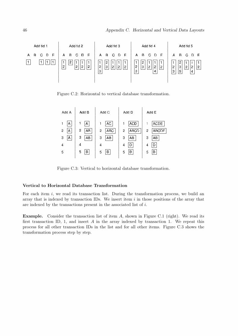
46 Appendix C. Horizontal and Vertical Data Layouts

Figure C.2: Horizontal to vertical database transformation.

Figure C.3: Vertical to horizontal database transformation.

Vertical to Horizontal Database Transformation

For each item i, we read its transaction list. During the transformation process, we build anarray that is indexed by transaction IDs. We insert item i in those positions of the array thatare indexed by the transactions present in the associated list of i.

Example. Consider the transaction list of item A, shown in Figure C.1 (right). We read itsfirst transaction ID, 1, and insert A in the array indexed by transaction 1. We repeat thisprocess for all other transaction IDs in the list and for all other items. Figure C.3 shows thetransformation process step by step.

Appendix D

Efficient Support Count of 2-itemsets

Here we present an optimization of the support count of 2-itemsets. This method was proposedby Zaki in [ZH02] for the Charm algorithm. However, this optimization can also be used withEclat and Talky-G, as well as with breadth-first algorithms, such as Apriori.

In the case of vertical algorithms (e.g. Eclat, Charm, Talky-G), this method significantlyreduces the number of intersection operations. The idea is that the support of 2-itemsets iscalculated and stored in a matrix. Then, an intersection operation is performed only if it surelyresults in a frequent itemset.

In the case of levelwise algorithms, with this method we can read the support from the matrixdirectly, and we do not need to use a trie for finding the subsets of each transacation in C2 (whereC2 contains the potentially frequent 2-itemsets). Note that this optimization only concerns thesupport count of 2-itemsets in C2. The support values of larger candidates are determined by atrie.

The Algorithm

The algorithm requires that the database be in horizontal format. In the case of vertical algo-rithms it means that first the database must be transformed (see Appendix C). If the databasehas n attributes, then an (n − 1) × (n − 1) upper triangular matrix is built, such as the oneshown in Figure D.1. This matrix will contain the support values of 2-itemsets, thus its entriesare initialized by 0. A row (transaction) of the database is decomposed into a list of 2-itemsets.For each element in this list, the value of its corresponding entry in the matrix is incrementedby 1. This process is repeated for each row of the database.

Figure D.1: Initialized upper triangular matrix for counting the support of 2-itemsets.

47

48 Appendix D. Efficient Support Count of 2-itemsets

Figure D.2: Support count of 2-itemsets of dataset D (Table 2.1) with an upper triangularmatrix.

Example. The first row of dataset D (Table 2.1) includes the itemset ACDE. This itemset isdecomposed into the following list of 2-itemsets: {AC, AD, AE, CD, CE, DE}. We read thefirst element of this list, AC, and increment its entry in the triangular matrix. We repeat thisprocess for all other itemsets in the list and for all other rows of the database. Figure D.2 showsthe process step by step.

Appendix E

Computing the Transversal Hypergraph

This appendix presents an optimized version of Berge’s algorithm [Ber89] for solving the transver-sal hypergraph problem (see Def. 4.6). Before presenting the algorithm, we show the correspon-dance between itemsets and hypergraphs, and we also review Berge’s algorithm.

Relation Between Itemsets and Hypergraphs

In this paper we present several itemset mining algorithms, e.g. Eclat, Charm, Talky-G, etc.These algorithms extract specific subsets of frequent itemsets from a given context. Here weshow that a family of itemsets can be treated as a hypergraph, and vice versa. As seen inDef. 4.1, a hypergraph H is a pair (V, E), where V is a finite set {v1, v2, . . . , vn} and E is a familyof subsets of V . The elements of V are called vertices, the elements of E edges. In Section 1.1we saw that a formal context is a triple (O,A,R), where O = {o1, o2, . . . , om} is a set of objects,A = {a1, a2, . . . , an} is a set of items, and R ⊆ O × A is a relation between O and A, whereR(o, a) means that the object o has the item a. A set of items is called an itemset.

The set A can be considered as a set of vertices V . An itemset corresponds to an edge E ∈ E .From this it follows that a set of itemsets can be considered as a family of edges E .

Example. Consider the hypergraph H in Figure 4.1, where V = {a, b, c, d} and E = {{a}, {b, c},{a, c, d}}. This hypergraph corresponds to the following set of itemsets: {{a}, {b, c}, {a, c, d}}.For convenience, we will use separator-free set notations, and we will indicate itemsets withcapital letters. That is, the hypergraph H can be considered as the following set of itemsets:{A,BC,ACD}. This holds in the other direction too, i.e. the hypergraph representation of thefamily of itemsets {A,BC,ACD} is depicted in Figure 4.1.

In the rest of the paper, we will treat a family of itemsets as a hypergraph and vice-versaif there is no danger of ambiguity. Thus for a set of itemsets {A,BC,ACD}, we write “thehypergraph {A,BC,ACD}”, etc.

The Algorithm of Berge

In this subsection we review the basic algorithm of Berge [Ber89], which is the most simple anddirect scheme for generating all minimal transversals of a hypergraph. First, let us see two usefuloperations on hypergraphs:

49

50 Appendix E. Computing the Transversal Hypergraph

Definition E.8 Let H = {E1, . . . , En} and G = {E ′1, . . . , E ′n′} be two hypergraphs. Then,

H ∪ G = {E1, . . . , En, E ′1, . . . , E ′n′}, and

H ∨ G = {Ei ∪ E ′j , i = 1, . . . , n, j = 1, . . . , n′}.

The first operation is the union of H and G, i.e. the hypergraph whose edges are the edges ofboth hypergraphs. The second operation is very similar to the Cartesian product, i.e. the unionof all possible pairs of edges, where one element of a pair is from the first hypergraph, and theother element is from the second hypergraph.

Proposition E.3 ([Ber89]) Let H and G be two simple hypergraphs. Then,

Tr(H ∪ G) = min(Tr(H) ∨ Tr(G)).

Let Hi = {E1, . . . , Ei}, i = 1, . . . , n be the partial hypergraph of the hypergraph H. Itholds that Hi = Hi−1 ∪ {Ei}, for all i = 2, . . . , n, where H1 = {E1} and Hn = H. Thus,Tr(Hi) = Tr(Hi−1 ∪ {Ei}), and by Prop. E.3,

Equation E.1Tr(Hi) = min(Tr(Hi−1) ∨ Tr({Ei}))

= min(Tr(Hi−1) ∨ {{v}, v ∈ Ei})

The algorithm of Berge is based on this equation. The algorithm computes all minimaltransversals of a given hypergraph H in two steps. First, it computes the minimal transversalsof the partial hypergraph Hi−1 and then it calculates the Cartesian product of the set Tr(Hi−1)by the ith edge Ei of H. Finally, non-minimal elements are removed. Thus, the algorithmstarts with the computation of Tr(H1), which is a trivial case (H1 has one edge only, E1, whoseminimal transversals are its vertices). Then, the algorithm adds one by one the rest of the edges,computing at each step the set of minimal transversals of the new partial hypergraph. Thealgorithm terminates when the last edge En is added. The algorithm of Berge outputs at the endall minimal transversals of the input hypergraph H [Ber89].

BergeOpt: An Optimized Version of Berge’s Algorithm

In the previous subsection we reviewed the algorithm of Berge, which implements the most simpleand direct approach for calculating the minimal transversals of a hypergraph. Here we presentan optimized version of Berge’s algorithm that we call BergeOpt.

In [LFFM+03], Le Floc’h et al. presented an algorithm called JEN whose goal is to efficientlyextract generators from a concept lattice for mining exact and approximate association rules.As part of JEN, the aforementioned authors presented a simple algorithm without a name forcalculating all the minimal transversals of a hypergraph. In the rest of this appendix we presentthis algorithm in an extended and completed way. In addition to [LFFM+03], (i) we showthat this algorithm is actually an optimization of Berge’s original algorithm (hence the nameBergeOpt), and (ii) we provide a proposition (see Prop. E.4) and its proof.

51

Optimization idea. One drawback of Berge’s algorithm is that after calculating the Cartesianproduct of the set Tr(Hi−1) by the ith edge Ei of H (see Equation E.1), it stores the resultingelements together in the same set, i.e. it has no information whether an element is minimal ornot. As a consequence, the filtering of non-minimal elements can be quite expensive when theresulting set has a large number of elements because the algorithm must test the minimality ofall elements, including also such elements that are actually minimal.

Our optimization is based on the idea to separate minimal and potentially minimal transver-sals in two different lists L1 and L2, respectively. This way, our optimized algorithm only hasto check the minimality of the potentially minimal elements in L2. As a result, the number ofexpensive subset checks can be reduced.

The BergeOpt algorithm exploits the following proposition:

Proposition E.4 In the BergeOpt algorithm, the potentially minimal transversals stored in thelist L2 form a simple hypergraph, i.e. L2 has no two elements ei and ej such that ei ⊆ ej.

Proof. Assume X,Y ⊆ V are two distinct subsets in Tr(Hi−1)− Tr(Hi), i.e., they are minimaltransversals ofHi−1 that lost this status in the i-th partial hypergraph. Assume also that X∪{a}and Y ∪ {b} are two candidates for Tr(Hi) produced by the algorithm (i.e., {a, b} ⊆ Ei wherebya 6∈ X and b 6∈ Y ).

Notice that any element of the L2 list will have the form X ∪ {a} for some X and a.Now, without loss of generality we can hypothesize X∪{a} ⊆ Y ∪{b}, and show this leads to

a contradiction. First, notice that a 66= b, otherwise we would have X ⊆ Y hence a contradictionwith the minimal transversal status. Next, we deduce that Y = X∪ Y where X = X−{b} henceX = X ∪ {b}. Yet this means that b ∈ X ∩ Ei which contradicts X 6∈ Tr(Hi). �

Pseudo code. The pseudo code of the algorithm is given in Algorithm 9. LetHi = {E1, . . . , Ei},i = 1, . . . , n be the partial hypergraph of the hypergraph H. It holds that Hi = Hi−1 ∪ {Ei},for all i = 2, . . . , n, where H1 = {E1} and Hn = H. Let MT Hi denote the set of all minimaltransversals of the partial hypergraph Hi.

As input, we have a set of itemsets that we treat as a hypergraph. The goal is to compute allthe minimal transversals of this hypergraph. The algorithm performs this task in an incrementalway. First, the algorithm takes the first itemset E1 of the input and it calculates its minimaltransversals. This is a trivial case; we only have to decompose the itemset into its 1-long subsets.For instance, the itemset ABC has three minimal transversals namely A, B, and C. Then, thealgorithm takes the next itemset Ei of the input and it updates the list of minimal transversalsMT Hi−1 if necessary. This is done the following way. Each minimal transversal m found so far,i.e. each element ofMT Hi−1 , is tested if it has a common part with the current itemset Ei. Ifit has, then m is a minimal transversal of Hi too, thus m is added to the list L1. In the listL1 we collect those itemsets that are minimal transversals of the partial hypergraph processedso far, including the current itemset Ei too. Prop. 4.1 guarantees that L1 has no two elementse1 and e2 such that e1 ⊆ e2. If the test was negative, i.e. m has no common part with thecurrent itemset Ei, then it means that m is not a transversal of Ei, thus m must be extended tohave an intersection with Ei (in other words, m is a transversal of Hi−1, but not a transversalof Hi). This can be done by decomposing Ei, and generating the one-size larger supersets of musing the 1-long subsets of Ei (Cartesian product of m with the vertices of Ei). For instance, ifEi = BCH, and the minimal transversal to be updated is AD, then the following potentiallyminimal transversals are generated: ABD, ACD, and ADH. We call these itemsets “potentially


minimal transversals”, because with this extension it is guaranteed that they became transversalsof Hi, but it is not sure that they are minimal, thus they are put in another list L2. It can bepossible that they have subsets among the minimal transversals in L1. When all elements ofMT Hi−1 are tested against the current itemset Ei, the lists L1 and L2 are filled. At this point,there are three possibilities (lines 20–23 of Algorithm 9): (1) L1 is non-empty and L2 is empty,or (2) L1 is empty and L2 is non-empty, or (3) both L1 and L2 are non-empty. In the first case,L1 contains all the minimal transversals of Hi. By Prop. 4.1, L1 is a simple hypergraph. In thesecond case, L2 contains all the minimal transversals of Hi. Since L1 is empty, all elements in L2

are minimal. Moreover, from Prop. E.4 it follows that L2 is a simple hypergraph. In the thirdcase, the list L2 must be cleaned first, i.e. if an element e1 in L1 is a subset of an element e2 inL2, then e2 must be removed because e2 is not minimal. Prop. E.4 guarantees that the elementsof L2 are not comparable w.r.t. set inclusion. Then, taking the union of the lists L1 and L2, wehave all the minimal transversals of Hi.

The algorithm continues by taking the next itemset of the input set (next current itemset)and it updates again the list of minimal transversals. The algorithm terminates when all elementsof the input set are processed. At this point, the algorithm collected all the minimal transversalsof the input set, i.e. it calculated the transversal hypergraph of the input hypergraph.

cleanSupersets procedure: this method removes non-minimal transversals from the list L2,i.e. itemsets that have subsets in L1. The procedure works as follows. It enumerates all elementsof L2. If the current element e2 in L2 has a subset in L1, then e2 is removed from L2. When theprocedure terminates, L2 only contains minimal transversals.

Running example. Consider the following hypergraph H = {ACD,ACH,BCD,DF, FH}.Let Ei denote the ith element (edge) of the hypergraph, i.e. E1 = ACD, E2 = ACH, . . . , E5 = FH.Let Hi denote the partial hypergraph that contains the first i elements of H, i.e. H1 = {ACD},H2 = {ACD,ACH}, . . . , H5 = {ACD,ACH,BCD,DF,FH} = H. The notation MT Hi

denotes the set of all minimal transversals of the partial hypergraph Hi.The execution of the algorithm is depicted in Table E.1. First, the algorithm takes E1

(ACD) and computes its minimal transversals that are A, C, and D. The algorithm continueswith processing E2 (ACH). Each time when a new element of H is handled, the already foundminimal transversals are tested. The itemsets A and C have common parts with E2, thus they areminimal transversals of ACH, so they are added to the list L1. However, D has no common partwith E2, which means that D is a minimal transversal of H1, but not a transversal of H2. In orderto make D a transversal of H2, D is extended with the 1-long subsets of ACH, thus the followingcandidates are generated: AD, CD, and DH. These three itemsets are put in the list L2. Then,the algorithm removes itemsets from L2 that have subsets in L1 since they are not minimaltransversals (AD and CD). The union of L1 and L2, which is stored in the listMT H2 , gives allthe minimal transversals of H2. The same steps are repeated with the other elements of H (E3,E4, and E5). When the algorithm terminates, all minimal transversals of the hypergraph H arediscovered. In this example, the transversal hypergraph ofH is Tr(H) = {DH,CF,ABF,ADF}.

Conclusion. In this appendix we presented an optimization of Berge’s original algorithm [Ber89]called BergeOpt that can significantly reduce the number of expensive inclusion tests. SinceBerge’s algorithm several other, more efficient algorithms have been introduced. As pointed outin [KS05] for instance, the simple method of Berge needs exponential many steps to produce thewhole output. It generates the first minimal transversal near the end of the procedure and itshigh memory requirements make it suitable only for small problem cases. However, as we pointed

53

Algorithm 9 (“getMinTransversals” function):

Description: BergeOpt algorithm (computing all minimal transversals of a hypergraph)Input: a hypergraph (H)Output: all minimal transversals of H (MT )

1) MT ← ∅; // initialisation; no minimal transversals are found yet2) loop over the elements of H (Ei) // an element of H is an edge (an itemset)3) {4) if (Ei is the first element of H) {5) MT ← {vertices of Ei}; // decomposition (1-itemsets of Ei)6) }7) else8) {9) L1 ← ∅; L2 ← ∅; // two empty lists

10) loop over the elements ofMT (m)11) {12) if (m ∩ Ei 6= ∅) { // m has a common vertex with Ei13) L1 ← L1 ∪m; // m is a minimal transversal of Ei14) }15) else {16) S ← {one-size larger supersets of m using the vertices of Ei};17) L2 ← L2 ∪ S;18) }19) }20) if (L1 6= ∅ and L2 6= ∅) {21) cleanSupersets(L1, L2); // removing non-minimal transversals from L2

22) }23) MT ← L1 ∪ L2;24) }25) }26)27) returnMT ;

out in the Snow algorithm in Section 4.2, our hypergraphs are usually very small, thus we didnot have to face these efficiency problems. Experimental results show that BergeOpt provides avery efficient solution for the problem instance that we had to deal with in the Snow algorithm.


E1 = ACD MT H1 = {A,C,D}E2 = ACH L1 = {A,C}

L2 = {AD,CD,DH}MT H2 = {A,C,DH}

E3 = BCD L1 = {C,DH}L2 = {AB,AC,AD}MT H3 = {C,DH,AB,AD}

E4 = DF L1 = {DH,AD}L2 = {CD,CF,ABD,ABF}MT H4 = {DH,AD,CD,CF,ABF}

E5 = FH L1 = {DH,CF,ABF}L2 = {ADF,ADH,CDF ,CDH}MT H5 = {DH,CF,ABF,ADF} =MT H = Tr(H)

Table E.1: Incremental computation of the transversal hypergraph of H = {ACD, ACH, BCD,DF , FH} with the BergeOpt algorithm.

Bibliography

[Ber89] C. Berge. Hypergraphs: Combinatorics of Finite Sets. North Holland, Amsterdam,1989.

[BTP+00a] Y. Bastide, R. Taouil, N. Pasquier, G. Stumme, and L. Lakhal. Mining frequentpatterns with counting inference. SIGKDD Explor. Newsl., 2(2):66–75, 2000.

[BTP+00b] Y. Bastide, R. Taouil, N. Pasquier, G. Stumme, and L. Lakhal. Mining MinimalNon-Redundant Association Rules Using Frequent Closed Itemsets. In J. Lloyd etal., editor, Proc. of the Computational Logic (CL ’00), volume 1861 of LNAI, pages972–986. Springer, 2000.

[CG05] T. Calders and B. Goethals. Depth-first non-derivable itemset mining. In Proc. ofthe SIAM Intl. Conf. on Data Mining (SDM ’05), Newport Beach, USA, Apr 2005.

[EG95] T. Eiter and G. Gottlob. Identifying the Minimal Transversals of a Hypergraph andRelated Problems. SIAM Journal on Computing, 24(6):1278–1304, 1995.

[GD86] J. L. Guigues and V. Duquenne. Familles minimales d’implications informativesrésultant d’un tableau de données binaires. Mathématiques et Sciences Humaines,95:5–18, 1986.

[Goe03] B. Goethals. Survey on Frequent Pattern Mining. Manuscript, 2003.

[GW99] B. Ganter and R. Wille. Formal concept analysis: mathematical foundations.Springer, Berlin/Heidelberg, 1999.

[Kry98] M. Kryszkiewicz. Representative Association Rules. In Proc. of the 2nd Pacific-Asia Conf. on Research and Development in Knowledge Discovery and Data Mining(PAKDD ’98), pages 198–209, London, UK, 1998. Springer-Verlag.

[Kry02] M. Kryszkiewicz. Concise Representations of Association Rules. In Proc. of the ESFExploratory Workshop on Pattern Detection and Discovery, pages 92–109, 2002.

[KS05] D. J. Kavvadias and E. C. Stavropoulos. An Efficient Algorithm for the TransversalHypergraph Generation. Journal of Graph Algorithms and Applications, 9(2):239–264, 2005.

[LFFM+03] A. Le Floc’h, C. Fisette, R. Missaoui, P. Valtchev, and R. Godin. JEN : unalgorithme efficace de construction de générateurs pour l’identification des rè-gles d’association. Numéro spécial de la revue des Nouvelles Technologies del’Information, 1(1):135–146, 2003.

55

56 Bibliography

[Lux91] M. Luxenburger. Implications partielles dans un contexte. Mathématiques, Infor-matique et Sciences Humaines, 113:35–55, 1991.

[Pas00] N. Pasquier. Mining association rules using formal concept analysis. In Proc. of the8th Intl. Conf. on Conceptual Structures (ICCS ’00), pages 259–264. Shaker-Verlag,Aug 2000.

[PBTL99a] N. Pasquier, Y. Bastide, R. Taouil, and L. Lakhal. Closed set based discoveryof small covers for association rules. In Proc. 15emes Journees Bases de DonneesAvancees (BDA), pages 361–381, 1999.

[PBTL99b] N. Pasquier, Y. Bastide, R. Taouil, and L. Lakhal. Discovering frequent closeditemsets for association rules. Lecture Notes in Computer Science, 1540:398–416,1999.

[Pfa02] J. L. Pfaltz. Incremental Transformation of Lattices: A Key to Effective KnowledgeDiscovery. In Proc. of the First Intl. Conf. on Graph Transformation (ICGT ’02),pages 351–362, Barcelona, Spain, Oct 2002.

[PJ01] J. L. Pfaltz and R. E. Jamison. Closure Systems and their Structure. InformationSciences, 139(3–4):275–286, 2001.

[SN05] L. Szathmary and A. Napoli. CORON: A Framework for Levelwise Itemset MiningAlgorithms. In B. Ganter, R. Godin, and E. Mephu Nguifo, editors, SupplementaryProc. of the 3rd Intl. Conf. on Formal Concept Analysis (ICFCA ’05), Lens, France,pages 110–113, Feb 2005.

[SNK07] L. Szathmary, A. Napoli, and S. O. Kuznetsov. ZART: A Multifunctional ItemsetMining Algorithm. In Proc. of the 5th Intl. Conf. on Concept Lattices and TheirApplications (CLA ’07), pages 26–37, Montpellier, France, Oct 2007.

[STB+02] G. Stumme, R. Taouil, Y. Bastide, N. Pasquier, and L. Lakhal. Computing IcebergConcept Lattices with TITANIC. Data and Knowledge Engineering, 42(2):189–222,2002.

[Sza06] L. Szathmary. Symbolic Data Mining Methods with the Coron Platform. PhD Thesisin Computer Science, University Henri Poincaré – Nancy 1, France, Nov 2006.

[Zak00] M. J. Zaki. Scalable Algorithms for Association Mining. IEEE Transactions onKnowledge and Data Engineering, 12(3):372–390, 2000.

[ZG03] M. J. Zaki and K. Gouda. Fast vertical mining using diffsets. In Proc. of the 9thACM SIGKDD Intl. Conf. on Knowledge discovery and data mining (KDD ’03),pages 326–335, New York, NY, USA, 2003. ACM Press.

[ZH02] M. J. Zaki and C.-J. Hsiao. CHARM: An Efficient Algorithm for Closed ItemsetMining. In SIAM Intl. Conf. on Data Mining (SDM’ 02), pages 33–43, Apr 2002.

[ZPOL97] M. J. Zaki, S. Parthasarathy, M. Ogihara, and W. Li. New Algorithms for Fast Dis-covery of Association Rules. In Proc. of the 3rd Intl. Conf. on Knowledge Discoveryin Databases, pages 283–286, August 1997.

Index

A-Close, 13associating FCIs and FGs, 12association rule, 2association rule bases, 9

Berge’s algorithm, 49BergeOpt, 50blocker, 18

Charm, 5, 10, 33closed itemset, 1closure, 2concept lattice, 3confidence, 2context, 1covering relation, see order

data mining, 1, 4dCharm, 8dEclat, 8diffset, 7dTalky-G, 8duality property of hypergraphs, 19

Eclat, 5, 29Eclat-G, 42element reordering, 7equivalence class, 2example dataset, 5extent, 3

face, 19formal concept analysis, 2, 4

Galois connection, 2generator, 1

Hasse diagram, 3hitting set, see transversalhorizontal layout, 7, 45hypergraph, 17

iceberg lattice, 3image, 1intent, 3IT-tree, 6itemset, 1itemset-tidset search tree, see IT-tree

lower cover, 4

minimal blocker, 18minimal non-redundant association rules, 9minimal transversal, 18minimum confidence, 2minimum support, 1

order, 4

partial hypergraph, 17Pascal, 9pre-order traversal, 37prefix-based equivalence class, 6

reverse pre-order traversal, 37

sample dataset, see example datasetsimple hypergraph, 17singleton equivalence class, 2Snow, 17Snow-Touch, 17subsumption checking, 35, 41support, 1support count of 2-itemsets, 7, 47

Talky, 37Talky-G, 5, 11, 37test environment, 27tidset, 1Touch, 9transversal, 18transversal hypergraph, 18transversal hypergraph problem, 49

57

58 Index

upper cover, 3

vertical layout, 6, 45

Zart, 9, 13

Centre de recherche INRIA Nancy – Grand EstLORIA, Technopôle de Nancy-Brabois - Campus scientifique

615, rue du Jardin Botanique - BP 101 - 54602 Villers-lès-Nancy Cedex (France)

Centre de recherche INRIA Bordeaux – Sud Ouest : Domaine Universitaire - 351, cours de la Libération - 33405 Talence CedexCentre de recherche INRIA Grenoble – Rhône-Alpes : 655, avenue de l’Europe - 38334 Montbonnot Saint-Ismier

Centre de recherche INRIA Lille – Nord Europe : Parc Scientifique de la Haute Borne - 40, avenue Halley - 59650 Villeneuve d’AscqCentre de recherche INRIA Paris – Rocquencourt : Domaine de Voluceau - Rocquencourt - BP 105 - 78153 Le Chesnay CedexCentre de recherche INRIA Rennes – Bretagne Atlantique : IRISA, Campus universitaire de Beaulieu - 35042 Rennes Cedex

Centre de recherche INRIA Saclay – Île-de-France : Parc Orsay Université - ZAC des Vignes : 4, rue Jacques Monod - 91893 Orsay CedexCentre de recherche INRIA Sophia Antipolis – Méditerranée : 2004, route des Lucioles - BP 93 - 06902 Sophia Antipolis Cedex

ÉditeurINRIA - Domaine de Voluceau - Rocquencourt, BP 105 - 78153 Le Chesnay Cedex (France)

http://www.inria.frISSN 0249-6399

Efficient Mining of Frequent Closures with Precedence Links and Associated Generators

Documents

Transcript of Efficient Mining of Frequent Closures with Precedence Links and Associated Generators