Mining frequent closed graphs on evolving data streams
9
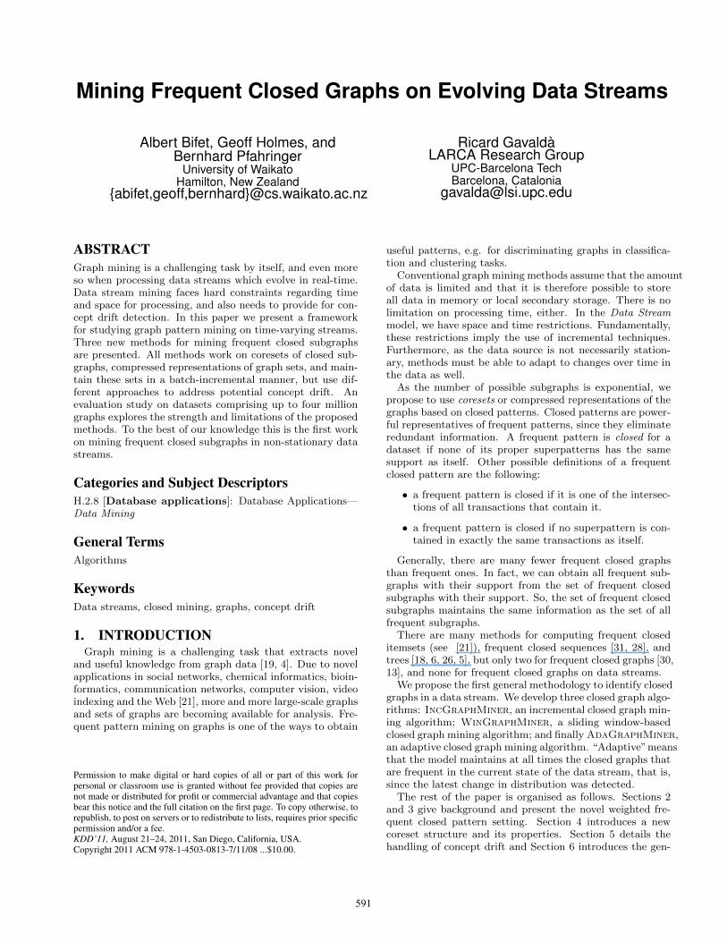
Mining Frequent Closed Graphs on Evolving Data Streams Albert Bifet, Geoff Holmes, and Bernhard Pfahringer University of Waikato Hamilton, New Zealand {abifet,geoff,bernhard}@cs.waikato.ac.nz Ricard Gavaldà LARCA Research Group UPC-Barcelona Tech Barcelona, Catalonia [email protected] ABSTRACT Graph mining is a challenging task by itself, and even more so when processing data streams which evolve in real-time. Data stream mining faces hard constraints regarding time and space for processing, and also needs to provide for con- cept drift detection. In this paper we present a framework for studying graph pattern mining on time-varying streams. Three new methods for mining frequent closed subgraphs are presented. All methods work on coresets of closed sub- graphs, compressed representations of graph sets, and main- tain these sets in a batch-incremental manner, but use dif- ferent approaches to address potential concept drift. An evaluation study on datasets comprising up to four million graphs explores the strength and limitations of the proposed methods. To the best of our knowledge this is the first work on mining frequent closed subgraphs in non-stationary data streams. Categories and Subject Descriptors H.2.8 [Database applications]: Database Applications— Data Mining General Terms Algorithms Keywords Data streams, closed mining, graphs, concept drift 1. INTRODUCTION Graph mining is a challenging task that extracts novel and useful knowledge from graph data [19, 4]. Due to novel applications in social networks, chemical informatics, bioin- formatics, communication networks, computer vision, video indexing and the Web [21], more and more large-scale graphs and sets of graphs are becoming available for analysis. Fre- quent pattern mining on graphs is one of the ways to obtain Permission to make digital or hard copies of all or part of this work for personal or classroom use is granted without fee provided that copies are not made or distributed for profit or commercial advantage and that copies bear this notice and the full citation on the first page. To copy otherwise, to republish, to post on servers or to redistribute to lists, requires prior specific permission and/or a fee. KDD’11, August 21–24, 2011, San Diego, California, USA. Copyright 2011 ACM 978-1-4503-0813-7/11/08 ...$10.00. useful patterns, e.g. for discriminating graphs in classifica- tion and clustering tasks. Conventional graph mining methods assume that the amount of data is limited and that it is therefore possible to store all data in memory or local secondary storage. There is no limitation on processing time, either. In the Data Stream model, we have space and time restrictions. Fundamentally, these restrictions imply the use of incremental techniques. Furthermore, as the data source is not necessarily station- ary, methods must be able to adapt to changes over time in the data as well. As the number of possible subgraphs is exponential, we propose to use coresets or compressed representations of the graphs based on closed patterns. Closed patterns are power- ful representatives of frequent patterns, since they eliminate redundant information. A frequent pattern is closed for a dataset if none of its proper superpatterns has the same support as itself. Other possible definitions of a frequent closed pattern are the following: • a frequent pattern is closed if it is one of the intersec- tions of all transactions that contain it. • a frequent pattern is closed if no superpattern is con- tained in exactly the same transactions as itself. Generally, there are many fewer frequent closed graphs than frequent ones. In fact, we can obtain all frequent sub- graphs with their support from the set of frequent closed subgraphs with their support. So, the set of frequent closed subgraphs maintains the same information as the set of all frequent subgraphs. There are many methods for computing frequent closed itemsets (see [21]), frequent closed sequences [31, 28], and trees [18, 6, 26, 5], but only two for frequent closed graphs [30, 13], and none for frequent closed graphs on data streams. We propose the first general methodology to identify closed graphs in a data stream. We develop three closed graph algo- rithms: IncGraphMiner, an incremental closed graph min- ing algorithm; WinGraphMiner, a sliding window-based closed graph mining algorithm; and finally AdaGraphMiner, an adaptive closed graph mining algorithm. “Adaptive”means that the model maintains at all times the closed graphs that are frequent in the current state of the data stream, that is, since the latest change in distribution was detected. The rest of the paper is organised as follows. Sections 2 and 3 give background and present the novel weighted fre- quent closed pattern setting. Section 4 introduces a new coreset structure and its properties. Section 5 details the handling of concept drift and Section 6 introduces the gen- 591
Transcript of Mining frequent closed graphs on evolving data streams
Mining Frequent Closed Graphs on Evolving Data Streams
Albert Bifet, Geoff Holmes, andBernhard Pfahringer
University of WaikatoHamilton, New Zealand
{abifet,geoff,bernhard}@cs.waikato.ac.nz
Ricard GavaldàLARCA Research Group
UPC-Barcelona TechBarcelona, Catalonia
ABSTRACTGraph mining is a challenging task by itself, and even moreso when processing data streams which evolve in real-time.Data stream mining faces hard constraints regarding timeand space for processing, and also needs to provide for con-cept drift detection. In this paper we present a frameworkfor studying graph pattern mining on time-varying streams.Three new methods for mining frequent closed subgraphsare presented. All methods work on coresets of closed sub-graphs, compressed representations of graph sets, and main-tain these sets in a batch-incremental manner, but use dif-ferent approaches to address potential concept drift. Anevaluation study on datasets comprising up to four milliongraphs explores the strength and limitations of the proposedmethods. To the best of our knowledge this is the first workon mining frequent closed subgraphs in non-stationary datastreams.
Categories and Subject DescriptorsH.2.8 [Database applications]: Database Applications—Data Mining
General TermsAlgorithms
KeywordsData streams, closed mining, graphs, concept drift
1. INTRODUCTIONGraph mining is a challenging task that extracts novel
and useful knowledge from graph data [19, 4]. Due to novelapplications in social networks, chemical informatics, bioin-formatics, communication networks, computer vision, videoindexing and the Web [21], more and more large-scale graphsand sets of graphs are becoming available for analysis. Fre-quent pattern mining on graphs is one of the ways to obtain
Permission to make digital or hard copies of all or part of this work forpersonal or classroom use is granted without fee provided that copies arenot made or distributed for profit or commercial advantage and that copiesbear this notice and the full citation on the first page. To copy otherwise, torepublish, to post on servers or to redistribute to lists, requires prior specificpermission and/or a fee.KDD’11, August 21–24, 2011, San Diego, California, USA.Copyright 2011 ACM 978-1-4503-0813-7/11/08 ...$10.00.
useful patterns, e.g. for discriminating graphs in classifica-tion and clustering tasks.
Conventional graph mining methods assume that the amountof data is limited and that it is therefore possible to storeall data in memory or local secondary storage. There is nolimitation on processing time, either. In the Data Streammodel, we have space and time restrictions. Fundamentally,these restrictions imply the use of incremental techniques.Furthermore, as the data source is not necessarily station-ary, methods must be able to adapt to changes over time inthe data as well.
As the number of possible subgraphs is exponential, wepropose to use coresets or compressed representations of thegraphs based on closed patterns. Closed patterns are power-ful representatives of frequent patterns, since they eliminateredundant information. A frequent pattern is closed for adataset if none of its proper superpatterns has the samesupport as itself. Other possible definitions of a frequentclosed pattern are the following:
• a frequent pattern is closed if it is one of the intersec-tions of all transactions that contain it.
• a frequent pattern is closed if no superpattern is con-tained in exactly the same transactions as itself.
Generally, there are many fewer frequent closed graphsthan frequent ones. In fact, we can obtain all frequent sub-graphs with their support from the set of frequent closedsubgraphs with their support. So, the set of frequent closedsubgraphs maintains the same information as the set of allfrequent subgraphs.
There are many methods for computing frequent closeditemsets (see [21]), frequent closed sequences [31, 28], andtrees [18, 6, 26, 5], but only two for frequent closed graphs [30,13], and none for frequent closed graphs on data streams.
We propose the first general methodology to identify closedgraphs in a data stream. We develop three closed graph algo-rithms: IncGraphMiner, an incremental closed graph min-ing algorithm; WinGraphMiner, a sliding window-basedclosed graph mining algorithm; and finally AdaGraphMiner,an adaptive closed graph mining algorithm. “Adaptive”meansthat the model maintains at all times the closed graphs thatare frequent in the current state of the data stream, that is,since the latest change in distribution was detected.
The rest of the paper is organised as follows. Sections 2and 3 give background and present the novel weighted fre-quent closed pattern setting. Section 4 introduces a newcoreset structure and its properties. Section 5 details thehandling of concept drift and Section 6 introduces the gen-
591

eral mining framework. Experimental results are given inSection 7, and conclusions are drawn in Section 8.
1.1 Related WorkThere is a large body of work on itemset mining from
data streams; see the survey [23] and the references therein.We can divide these data stream methods into two differ-ent classes depending on whether they use a landmark win-dow, containing all the examples seen so far, or a slidingwindow. Only a small fraction of these methods deal withfrequent closed mining. Moment [17], CFI-Stream [24] andIncMine [22] are state-of-the-art algorithms for mining fre-quent closed itemsets over a sliding window. CFI-Streamstores only closed itemsets in memory, but maintains allclosed itemsets as it does not apply a minimum supportthreshold, with the corresponding memory penalty. Momentstores much more information besides the current frequentclosed itemsets, but it has a minimum support thresholdto reduce the number of patterns found. IncMine proposesa notion of semi-FCIs that increases the minimum supportthreshold for an itemset as it is retained longer in the win-dow.
For trees, the work in [8] shows a general methodologyto identify closed patterns in a data stream, using GaloisLattice Theory. This approach is based on an efficient rep-resentation of trees and a low complexity notion of relaxedclosed trees, and presents an online strategy and an adap-tive sliding window technique for dealing with changes overtime. The approach is different to the one presented in thispaper, as it does not use coresets, or weighted frequent min-ing techniques.
In terms of graphs, two main algorithms exist for miningfrequent closed graphs:
• CloseGraph [30]: based on gSpan [29], a miner forfinding frequent subgraphs, based on depth-first search(DFS)
• MoSS [13]: an extension to MoFa [11] based on breadth-first search (BFS).
Aggarwal et al. [3] present a mining methodology to findfrequent and dense patterns in graph streams. Their no-tion of density is based both on node-occurrence and edgedensity, and they present an approach based on finding anapproximation of the exact method with the use of a min-hash approach.
To the best of our knowledge the work presented here isthe first work dealing with mining frequent closed graphs instreaming data that evolve with time.
2. PRELIMINARIESWe are interested in (possibly infinite) sets of graphs, en-
dowed with a partial order relation � among these graphs.The set of all graphs will be denoted by G, but actuallyall our developments will proceed in some finite subset of Gwhich will act as our universe of discourse.
Given two graphs g and g′, we say that g is a subgraph ofg′, or g′ is a super-graph of g, if g � g′. Two graphs g, g′
are said to be comparable if g � g′ or g′ � g. Otherwise,they are incomparable. Also we write g ≺ g′ if g is a propersubgraph of g′ (that is, g � g′ and g 6= g′).
The input to our data mining process is a dataset D ofweighted transactions, where each transaction s ∈ D consists
Transaction Id Graph Weight
1
C C S N
O
O 1
2
C C S N
O
C 1
3
C S N
O
C 1
4 C C S N
N
1
5 C S N
N
1
6 C S O
N
1
Table 1: Example of graph weighted transactiondataset.
of a transaction identifier tid, and a graph. The dataset is afinite set in the standard setting, and a potentially infinitesequence in the data stream setting. Tids are supposed torun sequentially from 1 to the size of D.
Following standard usage, we say that a transaction s sup-ports a graph g if g is a subgraph of the graph in transactions. The number of transactions in the dataset D that supportg is called the support of the graph g. A subgraph g is calledfrequent if its support is greater than or equal to a giventhreshold min sup. The frequent subgraph mining problemis to find all frequent subgraphs in a given dataset. Anysubgraph of a frequent graph is also frequent and, therefore,any supergraph of a infrequent graph is also infrequent (theantimonotonicity property).
We define a graph g to be closed (implicitly, w.r.t. to D)if none of its proper supergraphs has the same support as ghas in D.
In this paper we focus our examples and experiments onmolecular graphs, but our approach is general enough to beapplied to any type of graph.
3. FREQUENT CLOSED WEIGHTEDGRAPH MINING
In this section we introduce an extension to the frequentclosed graph mining problem which enables the use of com-pressed graph representations in our adaptive methods: thefrequent weighted closed graph mining problem. This prob-lem differs from standard frequent closed graph mining inthat each input graph has a weight, and this weight is usedto compute its weighted support.
The input into the data mining process is a dataset D ofweighted transactions, where each transaction s ∈ D consistsof a transaction identifier, tid, a graph, and a weight value.
592

Graph Relative Support Support
N -2 6
C S -3 6
C C S N 3 3
C S N
O
3 3
C S
N
3 3
C S O 1 4
C S N -1 5
Table 2: Example of a coreset with minimum sup-port 50% and δ = 0 for the transaction dataset ofTable 1.
Table 1 shows an example of a weighted dataset with sixmolecule graphs [11].
The sum of the weights of transactions in the dataset Dthat supports g is called the weighted support of the graphg. For brevity, weighted support will be abbreviated to justsupport. A subgraph g is called frequent if its weighted sup-port is greater than or equal to a given threshold min sup.
We define a graph g to be closed if none of its proper su-pergraphs has the same weighted support as it has. A graphg is maximal if none of its proper supergraphs is frequent.All maximal graphs are closed but not necessarily otherwise.We define a graph g to be δ-tolerance closed [16, 25] if noneof its proper frequent supergraphs has a weighted supportlarger than or equal to (1 − δ) · support(g). Note that amaximal graph is a 1-tolerance closed graph, and a closedgraph is a 0-tolerance closed graph. Note that, from [8] wehave the following propositions:
Proposition 1. Adding a transaction with pattern g toa dataset of patterns D where g is closed does not modify thenumber of closed patterns for D.
Proposition 2. Deleting a pattern transaction that is re-peated in a dataset of patterns D does not modify the numberof closed patterns for D.
Using these propositions we can observe that when addingto or removing from the weights of transactions, we are notmodifying the number of closed patterns provided they re-main frequent.
4. CORESETS OF CLOSED GRAPHSA coreset [2] of a set P with respect to some problem is
a small subset that approximates the original set P , in thesense that solving the problem for the coreset provides anapproximate solution for the problem on the original set P .This notion was introduced in computational geometry todenote a small subset of points that can be used to obtainapproximate solutions with theoretical guarantees.
For example, for clustering [1], a coreset for a set is a smallset, such that for any set of cluster centers the clustering costof the coreset is an approximation for the clustering cost ofthe original set with small relative error.
Graph Relative Support Support
C C S N 3 3
C S N
O
3 3
C S
N
3 3
Table 3: Example of a coreset with minimum sup-port 50% and δ = 1 for the graph dataset of Table 1.
The main advantage of coresets is that we can apply anyfast approximation algorithm on the usually much smallercoreset to compute an approximate solution for the originalset more efficiently.
Here we use the set of frequent closed subgraphs as asmaller subset of the frequent subgraphs maintaining thesame information but using less space. We define the rel-ative support of a closed graph as the support of a graphminus the relative support of its closed supergraphs. Wedefine the relative support in this way to exploit the factthat the sum of the closed supergraphs’ relative supports ofa graph is equal to its own support.
We define a (s, δ)-coreset for the problem of computingclosed graphs as a weighted multiset of frequent δ-toleranceclosed graphs with minimum support s using their relativesupport as a weight. Table 2 shows a (50%,0)-coreset for thedataset in Table 1 and Table 3 shows a (50%,1)-coreset forthe same dataset.
Note that given a graph dataset D, its (s, 0)-coreset is theset of frequent closed graphs, and its (s, 1)-coreset containsthe frequent maximal graphs. As the set of maximal graphsis contained in the set of closed graphs for a minimum sup-port s, the set of graphs in the (s, 1)-coreset is also a subsetof the graphs in the (s, 0)-coreset. For example, the set ofgraphs in the (50%,1)-coreset of Table 3 is a subset of thegraphs in the (50%,0)-coreset of Table 2.
For two minimum supports sL and sH where sL < sH , theset of graphs in its (sH , δ)-coreset is a subset of the graphsin the (sL, δ)-coreset.
A coreset is a “compressed representation” of the originaldataset. This compression is two-dimensional:
• Minimum support excludes infrequent graphs
• δ-tolerance excludes supergraphs with very similar sup-port
In this paper we focus only on (s, 0)-coresets, i.e., frequentclosed graphs, as they are the only coresets that can guar-antee the recovery of all frequent and frequent closed graphswith minimum support s. To show that this (s, 0)-coresetoutputs all the frequent subgraphs with minimum supports, we need the following proposition.
Proposition 3. Let D1 and D2 be two datasets of graphs.Let C1 and C2 be the (s, 0)-coresets of closed graphs for D1and D2. The set of closed graphs of C1 ∪ C2 is exactly theset of closed graphs of D1 ∪ D2.
First, we note that the support of a graph in C1 and C2is the same support of a graph in D1 and D2, due to the
593

fact that the support of a graph in C1 and C2 is the sumof all relative supports. As the support of a closed graph inD1 and D2 is the same support as in C1 and C2, we canobtain from them the same closed subgraphs, using relativesupport instead of support.
Proposition 4. Let D1 and D2 be two datasets of graphs.Let C1 and C2 be the (s, 0)-coresets of closed graphs for D1and D2. The set of frequent graphs of C1∪C2 is exactly theset of frequent graphs of D1 ∪ D2.
To show that we can also obtain the frequent ones, wesee that the frequent non-closed graphs have the support oftheir closure, so we obtain the same frequent graphs.
Proposition 5. Let D1, D2 and D be three datasets ofgraphs with D = D1 ∪ D2. Let C1, C2 and C be the (s, 0)-coresets of closed graphs for D1,D2 and D. The set of fre-quent graphs for C1 = C\C2 = C ∪C2 obtained using rela-tive support for C1 and negative relative support for C2, isexactly the set of frequent graphs for D1 = D\D2.
As the support of a graph in C1 is the support of thegraph in C minus its support in C2, we can obtain theclosed graphs in C1 by adding the closed graphs in C2, withnegated relative support, to C.
In general terms, using (s, 0)-coresets we can obtain allfrequent, closed and maximal graphs with minimum sup-port s without losing any information. Using (s, δ)-coresetswe get more compact representations of the original dataset,and we can still obtain the maximal graphs, but we cannotcompletely recover all frequent closed graphs of minimumsupport s.
5. ESTIMATING FREQUENCIESADAPTIVELY
To deal with concept drift, our methods have to be ableto adapt to changes in the input distribution. Keeping asliding window of recent elements is an option, however, ithas the cost of maintaining it in memory. In this paper, wepropose to use ADWIN to estimate frequencies of graphs withtheoretical guarantees.ADWIN (ADaptive sliding WINdow) [7] is a change detector
and estimation algorithm. It solves, in a well-specified way,the problem of tracking the average of a stream of bits orreal-valued numbers. ADWIN keeps a variable-length windowof recently seen items, with the property that the windowhas the maximal length statistically consistent with the hy-pothesis “there has been no change in the average value in-side the window”.
More precisely, an older fragment of the window is droppedif and only if there is enough evidence that its average valuediffers from that of the rest of the window. This has twoconsequences: one, change is reliably detected whenever thewindow shrinks; and two, at any time the average over theexisting window can be used as a reliable estimate of the cur-rent average in the stream (barring a very small or recentchange that is not yet statistically significant).
The inputs to ADWIN are a confidence value δ ∈ (0, 1) anda (possibly infinite) sequence of real values x1, x2, x3, . . . ,xt, . . . The value of xt is available only at time t. Each xt isgenerated according to some distribution Dt, independentlyfor every t. We denote with µt the expected value of xt when
it is drawn according to Dt. We assume that xt is alwaysin [0, 1]; rescaling deals with cases where a ≤ xt ≤ b. Nofurther assumption is being made about the distribution Dt;in particular, µt is unknown for all t.ADWIN is parameter- and assumption-free in the sense that
it automatically detects and adapts to the current rate ofchange. Its only parameter is a confidence bound δ, indicat-ing how confident we want to be in the algorithm’s output,inherent to all algorithms dealing with random processes.
It is important to note that ADWIN does not maintain thewindow explicitly, but compresses it using a variant of theexponential histogram technique [20]. This means that itkeeps a window of length W using only O(logW ) mem-ory and O(logW ) processing time per item, rather than theO(W ) one expects from a naıve implementation.
The main technical result in [7] about the performance ofADWIN is the following theorem, that provides bounds on therate of false positives and false negatives:
Theorem 1. With εcut defined as
εcut =
√1
2m· ln 4|W |
δ
where for some partition of W in two parts W0W1 (whereW1 contains the most recent items), and m is the harmonicmean of |W0| and |W1|, at every time step we have:
1. (False positive rate bound). If µt has remained con-stant within W , the probability that ADWIN shrinks thewindow at this step is at most δ.
2. (False negative rate bound). Suppose that for somepartition of W in two parts W0W1 we have |µW0 −µW1 | > 2εcut. Then with probability 1−δ ADWIN shrinksW to W1, or shorter.
6. FREQUENT GRAPH MINING ON DATASTREAMS
In this section we present new graph mining methods fordata streams using the results discussed in previous sec-tions. We start by reviewing non-incremental basic methods,and then present the incremental miner IncGraphMiner,the sliding-window based miner WinGraphMiner, and theadaptive miner AdaGraphMiner.
6.1 Non-Incremental Graph Mining[29, 30] presents two algorithms for computing frequent
and closed graphs from a dataset of graphs, in a non in-cremental way. They represent the potential subgraphs tobe checked for, being frequent and closed on the dataset, insuch a way that extending them by one single node, in allpossible ways, corresponds to a clear and simple operationon the representation. The completeness of the procedureis assured, that is, all graphs can be obtained in this way.This allows them to avoid extending graphs that have al-ready been found to be infrequent.
The pseudocode of CloseGraph is presented in Figure 1.Note that the first line of the algorithm is a canonical rep-resentative check. Such checks are used frequently in treeand graph mining. The use of the right-most extension ap-proach in CloseGraph, based on depth-first search, guar-antees that all possible graphs are reached, but reduces thegeneration of duplicate graphs. CloseGraph selects the
594

minimum DFS code based on a DFS lexicographical orderas the canonical representative.
In MoSS [12], Borgelt et al. present a different methodto perform frequent closed graph mining using breadth-firstsearch instead of using the right-most extension approach.
CloseGraph(g,D,min sup, S)
Input: A graph g, a graph dataset D, min sup.Output: The frequent graph set S.
1 if g 6= Canonical Representative(g)2 then return S3 isClosed← true4 C ← ∅5 for each g′ that is a one step right-most
extension of g6 do if support(g′) ≥ min sup7 then insert g′ into C8 if support(g′) = support(g)9 then isClosed← false
10 if isClosed = true11 then insert g into S12 for each g′ in C13 do S ← CloseGraph(g′, D,min sup, S)14 return S
Figure 1: The CloseGraph algorithm
IncGraphMiner(D,min sup)
Input: A graph dataset D, and min sup.Output: The frequent graph set G.
1 G← ∅2 for every batch bt of graphs in D3 do C ← Coreset(bt,min sup)4 G← Coreset(G ∪ C,min sup)5 return G
Coreset(bt,min sup)
Input: A graph dataset bt, and min sup.Output: The coreset C.
1 C ← CloseGraph(bt,min sup)2 C ← Compute Relative Support(C)3 return C
Figure 2: The IncGraphMiner algorithm
6.2 Incremental MiningThe incremental setting is different. Suppose that the
data arrives in batches of graphs. We consider every batch ofgraphs bt as a small finite dataset Db of transactions, whereeach transaction s ∈ Db consists of a transaction identifier,tid, a graph and a weight value. We maintain a set of graphsG and we update this set every time a new batch of graphsDb arrives. We compute the coreset of the batch bt, andthen we use it to update the graph set G.
Note that using this methodology we can transform non-incremental methods into incremental ones by extendingthem to use weights and coresets of graphs. Figure 2 showsthe pseudocode of IncGraphMiner.
WinGraphMiner(D,W,min sup)
Input: A graph dataset D, a size window W and min sup.Output: The frequent graph set G.
1 G← ∅2 for every batch bt of graphs in D3 do C ← Coreset(bt,min sup)4 Store C in sliding window5 if sliding window is full6 then R← Oldest C stored in sliding window,
negate all support values7 else R← ∅8 G← Coreset(G ∪ C ∪R,min sup)9 return G
Figure 3: The WinGraphMiner algorithm
6.3 Erroneous omission or inclusion boundsWhen working on batches of graphs at a time, there is a
possibility that the current batch does not contain enoughoccurrences of a frequent pattern, and it might also containmore than min sup occurrences of an otherwise infrequentpattern. The probabilities for these two types of errors, er-roneous omission or inclusion, can be bounded in the follow-ing way. Given a fixed batch size n, every min sup valueis equivalent to a probability p of finding a specific patternin any given graph. Then, if the global true probability forsome pattern is p+ ∆, and if we approximate the binomialdistribution with the normal distribution N(n ∗ (p+ ∆), n ∗(p+ ∆) ∗ (1− p−∆), the following bound can be derived:
pdiscard(∆, n) ≤ 1√2π·∫ −2∆
√n
−∞e−
t2
2 dt (1)
If ∆ = 0, then half of the patterns will be missed, butreasonably small values for ∆ will already result in accept-able probabilities: if n = 10000, then ∆ = 0.01 results in lessthan 5% erroneous omissions or inclusions, and for ∆ = 0.02this percentage is already very close to zero.
This type of argument is a heuristic that can be madeformal (at the expense of worse figures) by the use of rigorousHoeffding bounds, which underlie e.g. the ADWIN algorithm.
6.4 Mining with a Sliding WindowWe present WinGraphMiner as a learner that maintains
a sliding window. Its main important parameter is the sizeof the window W . The difference to IncGraphMiner liesin the management of the items in the sliding window. Weupdate the recent frequent closed graphs, using the coresetsof the new batches that arrive. When the window is full, wedelete the oldest batch on the sliding window using negativerelative support (Proposition 5).
Figure 3 shows the pseudocode of WinGraphMiner. Whena new batch bt arrives, the method performs as IncGraph-Miner, while the sliding window is not full. Once the win-
595

dow is full, the oldest coreset C is removed. The new coresetfor G is computed in one step from the coresets of G and bt,and C with negated relative support.
AdaGraphMiner(D,Mode,min sup)
Input: A graph dataset D, mode Mode and min sup.Output: The frequent graph set G.
1 G← ∅2 Init ADWIN
3 for every batch bt of graphs in D4 do C ← Coreset(bt,min sup)5 R← ∅6 if Mode is Sliding Window7 then Store C in sliding window8 if ADWIN detected change9 then R← Batches to remove
in sliding windowwith negative support
10 G← Coreset(G ∪ C ∪R,min sup)11 if Mode is Sliding Window12 then Insert # closed graphs into ADWIN
13 else for every g in G update g’s ADWIN
14 return G
Figure 4: The AdaGraphMiner algorithm
6.5 Adaptive MiningFinally, we present AdaGraphMiner, an extension to
the previous methods that is able to adapt to changes onthe stream, maintaining only the currently frequent closedgraphs.
We present two versions of this method. One uses anadaptive sliding window to maintain the batches of graphs.The other uses a separate ADWIN instance for managing thesupport of every single frequent closed subgraph.
Figure 4 shows the pseudocode of AdaGraphMiner, wherethe Sliding Window test distinguishes between the two meth-ods.
Assume a scenario where at each time t the t-th elementof the stream is a graph taken independently from a distri-bution Dt over a fixed universe G of graphs. Then, changesin the Dt’s over time t are modelling the evolution in thestream. In particular, we say that “the stream is stationarybetween times t1 and t2” (for t1 < t2) if
Dt1 = Dt1+1 = · · · = Dt2−1 = · · · = Dt2.
For a graph g, let ft(g) be the probability of g under distri-
bution Dt, and ft(g) the observed probability of g at timet (the number of times g has appeared in the window at
time t divided by the length of the window). Since ft(g) isour estimate of the current support of t, we would like itto be close enough to ft(g) to reliably decide whether g isfrequent.
We can prove the following theorem:
Theorem 2. Suppose the ADWIN’s in Algorithm AdaGraph-Miner are initialized with parameter δ. For every time stept1, t2 such that t1 < t2, if the stream is stationary between
t1 and t2, then for every g ∈ G we have with probability atleast 1− 2δ
|ft2(g)− ft2(g)| ≤√
1
t2− t1 ln4W
δ
That is, if the stream remains stationary for T steps, theestimates of graph frequencies tend to the their value ata rate of roughly O(1/
√T ), which tends to 0 as T → ∞.
Observe that this is the best convergence rate obtainableby sampling even on a totally stationary stream. That is,the algorithm is able to effectively forget previous history,and converge at an optimal rate on stationary periods. Notethat, if instead of ADWIN, we keep a simple sliding windowof fixed size W the approximation will not tend to zero,but remain at about 1/
√W . The dependence on ln(W ) in
the theorem is to a large extent an artifact of the proof ofADWIN’s guarantees, and in practice, slightly increasing theleading constant in the bound suffices for accurate results.
Proof. (Note: this proof uses both the definition of theADWIN algorithm as well as Theorem 1 stating false positiveand false negative ratios; see [7]).
Fix t1 < t2. We will show the following statement: Forevery fixed graph g ∈ G, with probability at least 1− 2δ wehave
|ft2(g)− ft2(g)| ≤√
1
t2− t1 ln4W
δ. (2)
Now also fix a graph g ∈ G. If g is not present in the setG kept by the algorithm, then ft2(g) = 0 and an applicationof the Hoeffding bound shows that (2) holds for g. Other-wise, g is in the set G, so it has an associated instance ofADWIN, A. Say that, at time t2, A keeps a window of sizeW . Because the stream is stationary between t1 and t2, byTheorem 1, part (1), we know that W ≥ t2−t1 (i.e., the ele-ment gathered at t1 has not been cut out from A’s window)with probability at least 1− δ.
Let t0 be the oldest element present in the window, so thatt0 = t2 −W ≤ t1. Now let µ0 (resp., µ1) be the observedfrequence of g in the window [t0..t1−1] (resp., in the window[t1..t2]); observe that E[µ1] = ft2(g). Observe also that bythe definition of ADWIN, if the interval [t0..t1−1] has not beencut out from the window, we must have |µ0 − µ1| ≤ εcut,where
εcut =
√1
2
(1
t2− t1 +1
t1− t0
)ln
4W
δ.
The estimate produced by A at time t2 is the average ofthe elements in the window of length W , which is
ft2(g) = µ1 ·t2− t1W
+ µ0 ·t1− t0W
= µ1 ·t2− t1W
+ (µ1 ± εcut) ·t1− t0W
= µ1 ± εcut ·t1− t0W
.
Now using W = t2− t0 and some simple algebra one can see
εcut ·t1− t0W
≤
√t1− t0
2(t2− t1)(t2− t0)ln
4W
δ
≤
√1
2(t2− t1)ln
4W
δ.
596
Memory NCI Dataset
0100020003000400050006000700080009000
10.0
00
30.0
00
50.0
00
70.0
00
90.0
00
110.
000
130.
000
150.
000
170.
000
190.
000
210.
000
230.
000
250.
000
Instances
Me
ga
by
tes
IncGraphMiner IncGraphMiner-C MoSS closeGraph
Time NCI Dataset
0
20
40
60
80
100
120
10.0
00
30.0
00
50.0
00
70.0
00
90.0
00
110.
000
130.
000
150.
000
170.
000
190.
000
210.
000
230.
000
250.
000
Instances
Se
co
nd
s
IncGraphMiner IncGraphMiner-C MoSS closeGraph
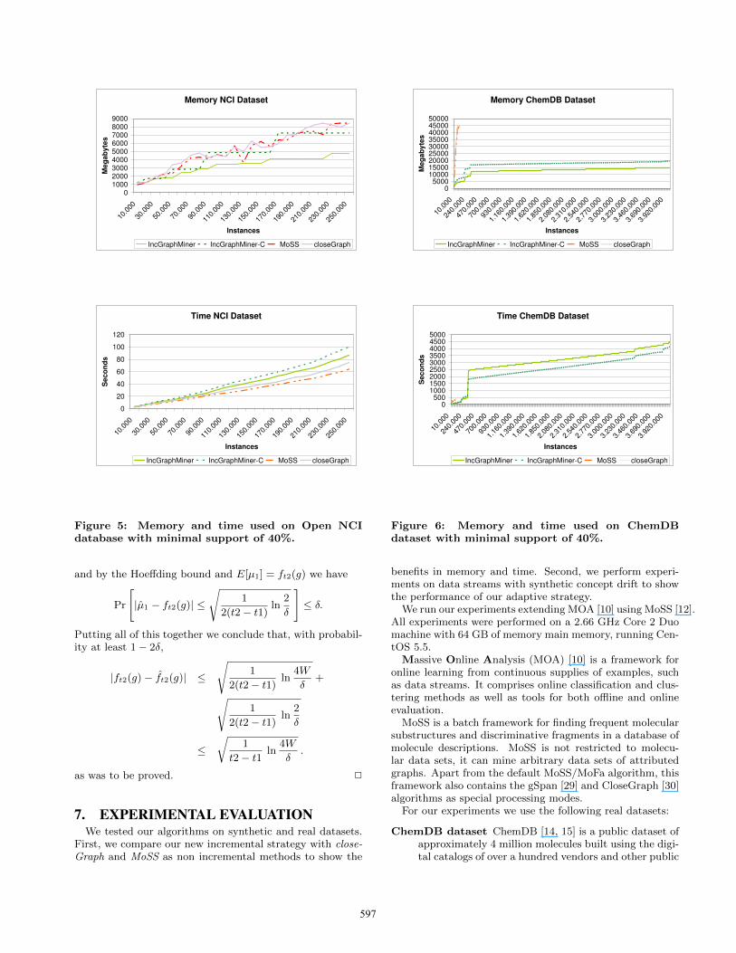
Figure 5: Memory and time used on Open NCIdatabase with minimal support of 40%.
and by the Hoeffding bound and E[µ1] = ft2(g) we have
Pr
[|µ1 − ft2(g)| ≤
√1
2(t2− t1)ln
2
δ
]≤ δ.
Putting all of this together we conclude that, with probabil-ity at least 1− 2δ,
|ft2(g)− ft2(g)| ≤
√1
2(t2− t1)ln
4W
δ+√
1
2(t2− t1)ln
2
δ
≤√
1
t2− t1 ln4W
δ.
as was to be proved. 2
7. EXPERIMENTAL EVALUATIONWe tested our algorithms on synthetic and real datasets.
First, we compare our new incremental strategy with close-Graph and MoSS as non incremental methods to show the
Memory ChemDB Dataset
05000
100001500020000250003000035000400004500050000
10.0
00
240.
000
470.
000
700.
000
930.
000
1.16
0.00
0
1.39
0.00
0
1.62
0.00
0
1.85
0.00
0
2.08
0.00
0
2.31
0.00
0
2.54
0.00
0
2.77
0.00
0
3.00
0.00
0
3.23
0.00
0
3.46
0.00
0
3.69
0.00
0
3.92
0.00
0
Instances
Me
ga
by
tes
IncGraphMiner IncGraphMiner-C MoSS closeGraph
Time ChemDB Dataset
0500
100015002000250030003500400045005000
10.0
00
240.
000
470.
000
700.
000
930.
000
1.16
0.00
0
1.39
0.00
0
1.62
0.00
0
1.85
0.00
0
2.08
0.00
0
2.31
0.00
0
2.54
0.00
0
2.77
0.00
0
3.00
0.00
0
3.23
0.00
0
3.46
0.00
0
3.69
0.00
0
3.92
0.00
0
Instances
Se
co
nd
s
IncGraphMiner IncGraphMiner-C MoSS closeGraph
Figure 6: Memory and time used on ChemDBdataset with minimal support of 40%.
benefits in memory and time. Second, we perform experi-ments on data streams with synthetic concept drift to showthe performance of our adaptive strategy.
We run our experiments extending MOA [10] using MoSS [12].All experiments were performed on a 2.66 GHz Core 2 Duomachine with 64 GB of memory main memory, running Cen-tOS 5.5.
Massive Online Analysis (MOA) [10] is a framework foronline learning from continuous supplies of examples, suchas data streams. It comprises online classification and clus-tering methods as well as tools for both offline and onlineevaluation.
MoSS is a batch framework for finding frequent molecularsubstructures and discriminative fragments in a database ofmolecule descriptions. MoSS is not restricted to molecu-lar data sets, it can mine arbitrary data sets of attributedgraphs. Apart from the default MoSS/MoFa algorithm, thisframework also contains the gSpan [29] and CloseGraph [30]algorithms as special processing modes.
For our experiments we use the following real datasets:
ChemDB dataset ChemDB [14, 15] is a public dataset ofapproximately 4 million molecules built using the digi-tal catalogs of over a hundred vendors and other public
597

Figure 7: Number of graphs in (40%, δ) for NCI.
sources. It is annotated with information derived fromthese sources as well as from computational methods,such as predicted solubility and 3D structure. It sup-ports multiple molecular formats and is periodicallyupdated, automatically whenever possible. It is main-tained by the Institute for Genomics and Bioinformat-ics at the University of California, Irvine.
Open NCI Database The open National Cancer Institute(NCI) dataset [27] consists of approximately 250,000structures. It is based on a large NCI database, builtusing samples from organic synthesis submitted to NCIfor testing. While about half of the NCI database isnot accessible, the other half of the structural data isfree of any disclosure and usage restrictions and there-fore termed “open”. This data is public domain andoften referred to as the “Open NCI Database”.
First, we compare the runtime and memory usage of theincremental method IncGraphMiner to the non-incrementalones. As all methods are implemented in Java, the memoryshown is the memory allocated by the Java Virtual Machine.
The results of our experiments using batches of 10, 000instances, minimum support of 40%, δ = 0, and 50 Giga-bytes of maximum memory are shown in Figures 5 and 6.We test two incremental methods, IncGraphMiner basedon MoSS, and IncGraphMiner-C based on closeGraph asbatch learners. For the Open NCI database, which is thesmaller dataset, we see that our new incremental methodsneed more time but less memory. However, for the largerChemDB dataset, the non-incremental methods can onlyprocess about 110,000 instances before running out of mem-ory (50 Gigabytes). Surprisingly, the incremental methodsalso outperform the non-incremental ones both in terms ofruntime and memory usage for smaller subsets of ChemDB.Note that in Figure 6 there is a sudden bump in time used,since the graphs in this part of the stream are much larger.
Figure 7 shows the size of the coreset (40%, δ) on the OpenNCI database. For δ = 0 there are 649 frequent closedgraphs, and for δ = 1 there are 140 frequent maximal graphs.
The next experiment shows how the new methods are ableto adapt to changes in the distribution of graphs in an evolv-ing stream scenario. Figure 8 shows the number of closed
0
10
20
30
40
50
60
10.0
00
60.0
00
110.
000
160.
000
210.
000
260.
000
310.
000
360.
000
410.
000
460.
000
510.
000
560.
000
610.
000
660.
000
710.
000
760.
000
810.
000
860.
000
910.
000
960.
000
Instances
Nu
mb
er
of
Clo
se
d G
rap
hs
ADAGRAPHMINER ADAGRAPHMINER-Window IncGraphMiner
Figure 8: Number of frequent closed graphs on OpenNCI database with minimal support of 40% withartificial concept drift.
graphs detected using the incremental method IncGraph-Miner, and the two adaptive methods. AdaGraphMiner-Window uses a sliding window monitored only by one ADWIN
instance, and AdaGraphMiner uses one ADWIN instancefor each graph to monitor its support. In this experiment,the data stream exhibits artificial concept drift, as it isa concatenation of parts of two different streams. One isthe Open NCI database and the other is an artificial datastream with exactly 15 frequent closed graphs generated ar-tificially. Concept drift occurs three times, after 250,000,500,000, and 750,000 examples, respectively. We follow themethodology in [9] to combine two data streams into one inorder to create artificial drift. We observe that the incre-mental method is the slowest to adapt, as it does not haveany forgetting mechanism. Comparing the adaptive ones,we see that AdaGraphMiner-Window, which only main-tains one global ADWIN instance for change detection, showsa slower response to concept change. AdaGraphMiner,on the hand, can detect and respond to change faster, as itmaintains a separate ADWIN instance for each graph.
8. CONCLUSIONSWe have presented the first efficient algorithms for mining
frequent closed graphs on evolving data streams.If the distribution of the graph dataset is stationary, the
best method to use is IncGraphMiner, as no past transac-tions need to be forgotten. If the distribution evolves, then asliding window method is more appropriate. If the right sizeof the sliding window is known in advance, then WinGraph-Mineris the method of choice, otherwise AdaGraphMineris the preferred option.
Future work will analyze the impact of the size of batchesand apply these new adaptive frequent mining techniquesto discriminative graph feature generation for classificationand clustering. Another ambitious direction for future workwould be going beyond batch-incremental methods of graphmining, to develop methods that are fully instance-incremental.It is currently unclear how this could be done efficiently.
598
9. ACKNOWLEDGMENTSUPC research is partially supported by the Spanish Min-
istry of Science and Technology TIN-2008-06582-C03-01(SESAAME), by the Generalitat de Catalunya 2009-SGR-1428 (LARCA), and by the EU PASCAL2 Network of Ex-cellence (FP7-ICT-216886).
The authors would like to thank Christian Borgelt formaking his MoSS graph software available and for helpfuldiscussions.
10. REFERENCES[1] M. R. Ackermann, C. Lammersen, M. Martens,
C. Raupach, C. Sohler, and K. Swierkot.StreamKM++: A Clustering Algorithm for DataStreams. In Proceedings of the Workshop on AlgorithmEngineering and Experiments (ALENEX ’10), 2010.
[2] P. K. Agarwal, S. Har-Peled, and K. Varadarajan.Geometric approximation via coresets. In J. E.Goodman, J. Pach, and E. Welzl, editors,Combinatorial and computational geometry, pages1–30. Cambridge University Press., 2005.
[3] C. C. Aggarwal, Y. Li, P. S. Yu, and R. Jin. On densepattern mining in graph streams. PVLDB,3(1):975–984, 2010.
[4] C. C. Aggarwal and H. Wang. Managing and MiningGraph Data. Springer Publishing Company,Incorporated, 1st edition, 2010.
[5] H. Arimura and T. Uno. An output-polynomial timealgorithm for mining frequent closed attribute trees.In ILP, pages 1–19, 2005.
[6] J. L. Balcazar, A. Bifet, and A. Lozano. Miningfrequent closed rooted trees. Machine Learning,78(1-2):1–33, 2010.
[7] A. Bifet and R. Gavalda. Learning from time-changingdata with adaptive windowing. In SIAM InternationalConference on Data Mining, 2007.
[8] A. Bifet and R. Gavalda. Mining adaptively frequentclosed unlabeled rooted trees in data streams. In 14thACM SIGKDD, pages 34–42, 2008.
[9] A. Bifet, G. Holmes, B. Pfahringer, R. Kirkby, andR. Gavalda. New ensemble methods for evolving datastreams. In 15th ACM SIGKDD, pages 139–148, 2009.
[10] A. Bifet, G. Holmes, B. Pfahringer, P. Kranen,H. Kremer, T. Jansen, and T. Seidl. MOA: MassiveOnline Analysis, a Framework for StreamClassification and Clustering. Journal of MachineLearning Research - Proceedings Track, 11:44–50, 2010.
[11] C. Borgelt and M. R. Berthold. Mining molecularfragments: Finding relevant substructures ofmolecules. In ICDM ’02, pages 51–, Washington, DC,USA, 2002. IEEE Computer Society.
[12] C. Borgelt, T. Meinl, and M. Berthold. Moss: aprogram for molecular substructure mining. In OSDM’05, pages 6–15, New York, NY, USA, 2005. ACM.
[13] C. Borgelt, T. Meinl, and M. R. Berthold. Advancedpruning strategies to speed up mining closedmolecular fragments. In IEEE Conf. on Systems, Manand Cybernetics (SMC 2004). IEEE Press, 2004.
[14] J. Chen, S. J. J. Swamidass, Y. Dou, J. Bruand, andP. Baldi. ChemDB: a public database of smallmolecules and related chemoinformatics resources.Bioinformatics, September 2005.
[15] J. H. Chen, E. Linstead, S. J. Swamidass, D. Wang,and P. Baldi. ChemDB update full-text search andvirtual chemical space. Bioinformatics,23(17):2348–2351, September 2007.
[16] J. Cheng, Y. Ke, W. Ng, and A. Lu. Fg-index: towardsverification-free query processing on graph databases.In SIGMOD Conference, pages 857–872, 2007.
[17] Y. Chi, H. Wang, P. S. Yu, and R. R. Muntz.Moment: Maintaining closed frequent itemsets over astream sliding window. In Proceedings of the 2004IEEE International Conference on Data Mining(ICDM’04), November 2004.
[18] Y. Chi, Y. Xia, Y. Yang, and R. Muntz. Mining closedand maximal frequent subtrees from databases oflabeled rooted trees. Fundamenta Informaticae,XXI:1001–1038, 2001.
[19] D. J. Cook and L. B. Holder. Mining Graph Data.Wiley-Interscience, 2006.
[20] M. Datar, A. Gionis, P. Indyk, and R. Motwani.Maintaining stream statistics over sliding windows.SIAM Journal on Computing, 14(1):27–45, 2002.
[21] J. Han, H. Cheng, D. Xin, and X. Yan. Frequentpattern mining: current status and future directions.Data Mining and Knowledge Discovery, 15:55–86,2007.
[22] Y. K. James Cheng and W. Ng. Maintaining frequentclosed itemsets over a sliding window. Journal ofIntelligent Information Systems, 2007.
[23] Y. K. James Cheng and W. Ng. A survey onalgorithms for mining frequent itemsets over datastreams. Knowledge and Information Systems, 2007.
[24] N. Jiang and L. Gruenwald. Cfi-stream: mining closedfrequent itemsets in data streams. In KDD ’06, pages592–597, New York, NY, USA, 2006. ACM.
[25] I. Takigawa and H. Mamitsuka. Efficiently miningδ-tolerance closed frequent subgraphs. MachineLearning, 82(2):95–121, 2011.
[26] A. Termier, M.-C. Rousset, M. Sebag, K. Ohara,T. Washio, and H. Motoda. DryadeParent, an efficientand robust closed attribute tree mining algorithm.IEEE Trans. Knowl. Data Eng., 20(3):300–320, 2008.
[27] J. H. Voigt, B. Bienfait, S. Wang, and M. C. Nicklaus.Comparison of the nci open database with seven largechemical structural databases. Journal of ChemicalInformation and Computer Sciences, 41(3):702–712,2001.
[28] J. Wang and J. Han. Bide: Efficient mining offrequent closed sequences. In ICDE, pages 79–90.IEEE Computer Society, 2004.
[29] X. Yan and J. Han. gSpan: Graph-based substructurepattern mining. In ICDM ’02, page 721, Washington,DC, USA, 2002. IEEE Computer Society.
[30] X. Yan and J. Han. CloseGraph: mining closedfrequent graph patterns. In KDD ’03, pages 286–295,2003.
[31] X. Yan, J. Han, and R. Afshar. Clospan: Miningclosed sequential patterns in large databases. In SDM,2003.
599