Plan3D: Viewpoint and Trajectory Optimization for Aerial Multi ...
Upload
independentCategory
view
5download
0
(IJACSA) International Journal of Advanced Computer Science and Applications, Vol. 4, No. 3, 2013
165 | P a g e www.ijacsa.thesai.org
A New Viewpoint for Mining Frequent Patterns
Thanh-Trung Nguyen
Department of Computer Science
University of Information Technology,
Vietnam National University HCM City
Ho Chi Minh City, Vietnam
Phi-Khu Nguyen
Department of Computer Science
University of Information Technology,
Vietnam National University HCM City
Ho Chi Minh City, Vietnam
Abstract—According to the traditional viewpoint of Data
mining, transactions are accumulated over a long period of time
(in years) in order to find out the frequent patterns associated
with a given threshold of support, and then they are applied to
practice of business as important experience for the next business
processes. From the point of view, many algorithms have been
proposed to exploit frequent patterns. However, the huge number
of transactions accumulated for a long time and having to handle
all the transactions at once are still challenges for the existing
algorithms. In addition, today, new characteristics of the business
market and the regular changes of business database with too
large frequency of added-deleted-altered operations are
demanding a new algorithm mining frequent patterns to meet the
above challenges. This article proposes a new perspective in the
field of mining frequent patterns: accumulating frequent patterns
along with a mathematical model and algorithms to solve existing challenges.
Keywords—accumulating frequent patterns; data mining;
frequent pattern; horizontal parallelization; representative set;
vertical parallelization
I. INTRODUCTION
Frequent pattern mining is a basic problem in data mining and knowledge discovery. Frequent patterns are set of items which occur in dataset more than user specified number of times. Identifying frequent patterns will play an essential role in mining associations, correlations, and many other interesting relationships among data (Prakash et. al. 2011). Recently, frequent pattern has been studied and applied into many areas such as: text categorization (Yuan et. al. 2013), text mining (Kim et. al. 2012), social network (Nancy and Ramani 2012), frequent subgraph (Wang and Ramon 2012) … Various techniques have been proposed to improve the performance of frequent pattern mining algorithms. In general, methods of finding frequent patterns may fall into 3 main categories: Candidate Generation Methods, Without Candidate Generation Methods and Parallel Methods.
The common rule of Candidate Generation Methods is probing dataset many times to generate good candidates which can be used as frequent patterns of dataset. Apriori algorithm, proposed by Agrawal and Srikant in 1995 (Prasad and Ramakrishna 2011), is a typical technique in this approach. Recently, many researches focus on Apriori and improve this algorithm to reduce the complexity and increase the efficiency of finding frequent patterns. Partitioning technique (Prasad and Ramakrishna 2011), pattern based algorithms and incremental Apriori based algorithms (Sharma and Garg 2011) can be
viewed as the Candidate Generation Methods. Many improvements of Apriori were presented. An efficient improved Apriori algorithm for mining association rules using Logical Table based approach was proposed (Malpani and Pal 2012). Another group focuses on map/reduce design and implementation of Apriori algorithm for structured data analysis (Koundinya et. al. 2012) while some researchers proposed an improved algorithm for mining frequent patterns in large datasets using transposition of the database with minor modification of the Apriori-like algorithm (Gunaseelan and Uma 2012). The custom-built Apriori algorithm (Rawat and Rajamani 2010), and the modified Apriori algorithm (Raghunathan and Murugesan 2010) were introduced but the time consuming has been still a big obstacle. Reduced Candidate Set (RCS) is an algorithm which is more efficiency than original Apriori algorithm (Bahel and Dule 2010). Record Filter Approach is a method which takes less time than Apriori (Goswami et. al. 2010). In addition, Sumathi et. al. 2012 also proposed the algorithm taking vertical tidset representation of the database and removes all the non-maximal frequent item-sets to get exact set of Maximal Frequent Itemset directly. Besides, a method was introduced by Utmal et. al. 2012. This method firstly finds frequent 1_itemset and then uses the heap tree to sort frequent patterns generated, and so repeatedly. Although Apriori and its developments are proved the effectiveness, many scientists still focus on the other heuristic algorithms and try to find better algorithms. Genetic algorithms (Prakash et. al. 2011), Dynamic Function (Joshi et. al. 2010) and depth-first search were studied and applied successfully in reality. Besides, a study presented a new technique using a classifier which can predict the fastest ARM (Association Rule Mining) algorithm with a high degree of accuracy (Sadat et. al. 2011). Another approach was also based on Apriori algorithm but provides better reduction in time because of the prior separation in the data (Khare and Gupta 2012).
Apriori and Apriori-like algorithms sometimes create large number of candidate sets. It is hard to pass the database and compare the candidates. Without Candidate Generation is another approach which determines complete set of frequent item sets without candidate generation, based on divide and conquer technique. Interesting patterns, Constraint-based mining are typical methods which were all introduced recently (Prasad and Ramakrishna 2011). FP-Tree, FP-Growth and their developments (Aggarwal et. al. 2009) – (Kiran and Reddy 2011) – (Deypir and Sadreddini 2011) – (Xiaoyun et. al. 2009) – (Duraiswamy and Jayanthi 2011) introduced a prefix tree structure which can be used to find out frequent patterns in

(IJACSA) International Journal of Advanced Computer Science and Applications, Vol. 4, No. 3, 2013
166 | P a g e www.ijacsa.thesai.org
datasets. In other hand, researchers studied a transaction reduction technique with FP-tree based bottom up approach for mining cross-level pattern (Jayanthi and Duraiswamy 2012), and construction of FP-tree using Huffman Coding (Patro et. al. 2012). H-mine is a pattern mining algorithm which is used to discover features of products from reviews (Prasad and Ramakrishna 2011) – (Ghorashi et. al. 2012). Besides that, a novel tree structure called FPU-tree was proposed which is efficient than available trees for storing data streams (Baskar et. al. 2012). Another study tried to find improved association to show that which item set is most acceptable association with others (Saxena and Satsangi 2012). Q-FP tree was introduced as a way to mine data streams for association rule mining (Sharma and Jain 2012).
Applying parallel technique to solve high complexity problems is an interesting field. In recent years, several parallel, distributed extensions of serial algorithms for frequent pattern discovery have been proposed. A study presented a distributed, parallel algorithm, which makes feasible the application of SPADA to large data sets (Appice et. al. 2011) while another group introduced HPFP-Miner algorithm, based on FP-Tree algorithm, to integrate parallelism into finding the frequent patterns (Xiaoyun et. al. 2009).
A method for finding the frequent occurrence patterns and the frequent occurrence time-series change patterns from the observational data of the weather-monitor satellite applied successfully parallel method to solve the problem of calculation cost (Niimi et. al. 2010). PFunc, a novel task parallel library whose customizable task scheduling and task priorities facilitated the implementation of clustered scheduling policy, was presented and proved its efficiency (Kambadur et. al. 2012). Another method is partitioning for finding frequent pattern from huge database. It is based on key based division for finding the local frequent pattern (LFP). After finding the partition frequent pattern from the subdivided local database, it then find the global frequent pattern from the local database and perform the pruning from the whole database (Gupta and Satsangi 2012).
Fuzzy frequent pattern mining has been also a new approach recently (Picado-Muiño et. al. 2012).
Although there are significant improvement in finding frequent patterns recently, working with the varying database is still a big challenge. Especially, it need not scan again the whole database whenever having need of adding a new element or deleting/modifying an element. Besides, a number of algorithms are effective, but their basis of mathematics and way of installation are complex. In addition, it is the limit of computer memory. Hence, combining how to store the data mining context most effectively with costing the memory least and how to store frequent patterns is also not a small challenge. Finally, ability of dividing data into several parts for parallel processing is also concerned.
Furthermore, characteristics of the medium and small market also produce challenges need to be solved:
Most enterprises have medium and small scale, such as: interior decoration, catering business, computer training, foreign language traning, motor business, and
so on. The number of categories of goods which they trade in is about 200 to 1000. Cases up to 1000 items, it is usually the supermarkets with diverse categories such as food, appliances, makeup, homemaker, …
The purchasing invoices have the same general principle is that the number of categories sold is about 20 (the invoice form is in accordance with the government)
The fact that the laws indicating a shopping tendency of the market in the best way are drawn from the number of invoices having accumulated time from 6 months to 1 year before. Because the current market needs and design, utility, function of goods change rapidly and continuously, so it can not use the laws of the previous years to apply to the current time.
Market trends in different areas are different.
Businesses need to regularly change the minimum support threshold in order to find acceptable laws based on the number of buyers.
Due to the specific management of enterprises, the operations such as adding, deleting, editing frequently impact on database.
The need of accumulating the results immediately after each operation on the invoice to be able to refer to the laws at any time.
In this article, a mathematical space will be introduced with some new related concepts and propositions to design new algorithms which are expected to solve remain issues in finding frequent patterns.
II. MATHEMATICAL MODEL
Definition 1: Given 2 bit chains with the same length: a = a1a2…am, b = b1b2…bm. a is said to cover b or b is covered by a
– denoted a b – if pos(b) pos(a) where pos(s) = {i si = 1}
Definition 2:
+ Let u be a bit chain, k is a non-negative integer, we say [u; k] is a pattern.
+ Let S be the set of size-m bit chains (chains with the length of m), u is a size-m bit chain. If there are k chains in S cover u, we say: u is a form of S with frequency k; and [u; k] is
a pattern of S – denoted [u; k]S
For instance: S = {1110, 0111, 0110, 0010, 0101} and u =
0110. We say u is a form with frequency 2 in S, so [0110; 2]S
+ A pattern [u; k] of S is called maximal pattern – denoted
[u; k]maxS – if and only if it doesn’t exist k’ such that [u;
k’]maxS and k’ > k. With the above instance, [0110; 3]maxS
Definition 3: P is representative set of S when P = {[u;
p]maxS ∄[v; q]maxS : (v u and q > p)}. Each element in P is called a representative pattern of S
Proposition 1: Let S be a set of size-m bit chains with representative set P, then two arbitrary elements in P do not coincide with each other.
(IJACSA) International Journal of Advanced Computer Science and Applications, Vol. 4, No. 3, 2013
167 | P a g e www.ijacsa.thesai.org
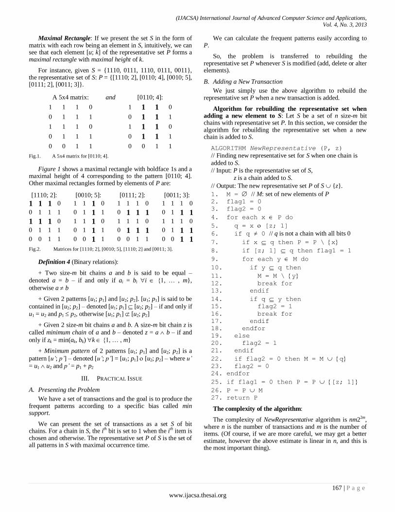
Maximal Rectangle: If we present the set S in the form of matrix with each row being an element in S, intuitively, we can see that each element [u; k] of the representative set P forms a maximal rectangle with maximal height of k.
For instance, given S = {1110, 0111, 1110, 0111, 0011}, the representative set of S: P = {[1110; 2], [0110; 4], [0010; 5], [0111; 2], [0011; 3]}.
A 5x4 matrix: and [0110; 4]:
1 1 1 0 1 1 1 0
0 1 1 1 0 1 1 1
1 1 1 0 1 1 1 0
0 1 1 1 0 1 1 1
0 0 1 1 0 0 1 1
Fig.1. A 5x4 matrix for [0110; 4].
Figure 1 shows a maximal rectangle with boldface 1s and a maximal height of 4 corresponding to the pattern [0110; 4]. Other maximal rectangles formed by elements of P are:
[1110; 2]: [0010; 5]: [0111; 2]: [0011; 3]:
1 1 1 0 1 1 1 0 1 1 1 0 1 1 1 0
0 1 1 1 0 1 1 1 0 1 1 1 0 1 1 1
1 1 1 0 1 1 1 0 1 1 1 0 1 1 1 0
0 1 1 1 0 1 1 1 0 1 1 1 0 1 1 1 0 0 1 1 0 0 1 1 0 0 1 1 0 0 1 1
Fig.2. Matrices for [1110; 2], [0010; 5], [1110; 2] and [0011; 3].
Definition 4 (Binary relations):
+ Two size-m bit chains a and b is said to be equal –
denoted a = b – if and only if ai = bi i {1, … , m},
otherwise a b
+ Given 2 patterns [u1; p1] and [u2; p2]. [u1; p1] is said to be
contained in [u2; p2] – denoted [u1; p1] [u2; p2] – if and only if
u1 = u2 and p1 p2, otherwise [u1; p1] [u2; p2]
+ Given 2 size-m bit chains a and b. A size-m bit chain z is
called minimum chain of a and b – denoted z = a b – if and
only if zk = min(ak, bk) k {1, … , m}
+ Minimum pattern of 2 patterns [u1; p1] and [u2; p2] is a
pattern [u’; p’] – denoted [u’; p’] = [u1; p1] [u2; p2] – where u’
= u1 u2 and p’ = p1 + p2
III. PRACTICAL ISSUE
A. Presenting the Problem
We have a set of transactions and the goal is to produce the frequent patterns according to a specific bias called min support.
We can present the set of transactions as a set S of bit chains. For a chain in S, the ith bit is set to 1 when the ith item is chosen and otherwise. The representative set P of S is the set of all patterns in S with maximal occurrence time.
We can calculate the frequent patterns easily according to P.
So, the problem is transferred to rebuilding the representative set P whenever S is modified (add, delete or alter elements).
B. Adding a New Transaction
We just simply use the above algorithm to rebuild the representative set P when a new transaction is added.
Algorithm for rebuilding the representative set when adding a new element to S: Let S be a set of n size-m bit chains with representative set P. In this section, we consider the algorithm for rebuilding the representative set when a new chain is added to S.
ALGORITHM NewRepresentative (P, z)
// Finding new representative set for S when one chain is
added to S.
// Input: P is the representative set of S,
z is a chain added to S.
// Output: The new representative set P of S {z}.
1. M = // M: set of new elements of P 2. flag1 = 0
3. flag2 = 0
4. for each x P do
5. q = x [z; 1]
6. if q ≠ 0 // q is not a chain with all bits 0
7. if x q then P = P \ x
8. if [z; 1] q then flag1 = 1
9. for each y M do
10. if y q then
11. M = M \ y
12. break for
13. endif
14. if q y then 15. flag2 = 1
16. break for
17. endif
18. endfor
19. else
20. flag2 = 1
21. endif
22. if flag2 = 0 then M = M q 23. flag2 = 0
24. endfor
25. if flag1 = 0 then P = P [z; 1]
26. P = P M 27. return P
The complexity of the algorithm:
The complexity of NewRepresentative algorithm is nm22m, where n is the number of transactions and m is the number of items. (Of course, if we are more careful, we may get a better estimate, however the above estimate is linear in n, and this is the most important thing).

(IJACSA) International Journal of Advanced Computer Science and Applications, Vol. 4, No. 3, 2013
168 | P a g e www.ijacsa.thesai.org
Proof: Let P be the representative set before adding z, and let Q the new representative set after adding z. Let |P| be the cardinal of P (i.e. the number of elements of P).
The key observation is that |P| ≤ 2m. This is because we can not have two elements [z; p] and [z'; p'] in P such that z = z' and p ≠ p'. Therefore, the number of elements of P will always less than or equal to the number of chains of m bits, the latter is 2m.
Fixed an x in P.
In line 5, the complexity will be m.
In line 7, the complexity will be m again.
In line 8, the complexity is m again.
In lines 9-13, the cardinal |M| is at most |P|, since from the definition of M on line 22 the worst case is when we add every
thing of the form q = x [z; 1] into M, here x runs all over P, and in this case |M| = |P|. Hence the complexity of these lines 9-13 is less than or equal to |P|.
Lines 18-24 the complexity is at most m.
Hence when we let x vary in P (but fix a transaction z), we see that the total complexity for lines 5-24 is about m|P|2 ≤ m22m.
If we vary the transactions z (whose number is n), we see that the complexity for the whole algorithm is nm22m.
Theorem 1:
Let S be a set of size-m bit chains and P be representative
set of S. For [u; p], [v; q] P and z S, let [u; p] [z; 1] = [t;
p+1], [v; q] [z; 1] = [d; q+1]. Only one of the following cases must be satisfied:
i. [u; p] [t; p+1] and [u; p] [d; q+1], t = d
ii. [u; p] [t; p+1] and [u; p] [d; q+1], t ≠ d
iii. [u; p] [t; p+1] and [u; p] [d; q+1].
Proof: From Proposition 1, obviously u ≠ v. The theorem is proved if the following claim is true: Let
(a): u = t , u = d , and t = d;
(b): u = t , u ≠ d , and t ≠ d;
(c): u ≠ t and u ≠ d,
only one of the above statements is correct.
By the method of induction on the number m of entries of chain, in the first step, we show that the claim is correct if u and v differ at only one kth entry.
Without loss of generality, we assume that uk = 0 and vk = 1. The following cases must be true:
- Case 1: zk = 0; Then min(uk, zk) = min(vk, zk) = 0, hence
t = u z = (u1, u2, ... , 0, ... , um) (z1, z2, ... , 0, ... , zm) = (x1, x2, ... , 0, ... , xm), xi = min(ui, zi), for i = 1, … , m, i ≠ k;
d = v z = (v1, v2, … , 1, … , vm) (z1, z2, … , 0, … , zm) = (y1, y2, … , 0, … , ym), yi = min(vi, zi), for i = 1, ... , m, i ≠ k.
From the assumption ui = vi when i ≠ k thus xi = yi, so t = d. Hence, if u = t then u = d and (a) is correct. On the other hand, if u ≠ t then u ≠ d, therefore (c) is correct.
- Case 2: zk = 1; We have min(uk, zk) = 0, min(vk, zk) = 1 and
t = u z = (u1, u2, … , 0, … , um) (z1, z2, … , 1, … , zm) = (x1, x2, … , 0, … , xm), xi = min(ui, zi), for i = 1, … , m, i ≠ k;
d = v z = (v1, v2, ... , 1, … , vm) (z1, z2, … , 1, … , zm) = (y1, y2, … , 1, … , ym), yi = min(vi, zi), for i = 1, … , m, i ≠ k.
So, t ≠ d. If u = t then u ≠ d, thus the statement (b) is correct.
In summary, the above claim is true for any u and v of S that differ only at one entry.
By induction in the second step, it is assumed that the claim is true if u and v differ at r entries, and only one of the three statements (a), (b) or (c) is true.
Without loss of generality, we assume that the first r entries of u and v are different, and they differ at (r + 1)-th entries. Applying the same method in the first step where r = 1 to this instance, it is obtained
True statements when u ≠ v, and
their first r entries
are different:
True statements when u ≠ v, and
their first r + 1
entries are
different:
True statements when combining
the two
possibilities:
(a) (a) (a)
(a) (b) (b)
(a) (c) (c)
(b) (a) (b)
(b) (b) (b)
(b) (c) (c)
(c) (a) (c)
(c) (b) (c)
(c) (c) (c)
Fig.3. Cases in comparison.
Therefore, if u and v are different at r + 1 entries, only one of the (a), (b), (c) statements is correct. The above claim is true, and Theorem 1 is proved.
Theorem 2:
Let S be a set of n size-m bit chains. The representative set of S is determined by applying NewRepresentative algorithm to each of n elements of S in turn.
Proof: We prove the theorem by induction on the number n of elements of S.
Firstly, when applying the above algorithm to the set S of only one element, this element is added into P and then P with that only element is the representative set of S. Thus, theorem 2 is proved in the case of n = 1.
Next, assume that whenever S has n elements, the above algorithm can be applied to S to obtain a representative set P0.
(IJACSA) International Journal of Advanced Computer Science and Applications, Vol. 4, No. 3, 2013
169 | P a g e www.ijacsa.thesai.org
Now we prove that when S has n + 1 elements then the above algorithm can be applied to yield a representative P for S. We assume that S is the union of a set S0 of n elements and an element z, and that we already had a representative set P0 for S0. Each element of P0 allows forming a maximal rectangle from S0, and we call p the number of elements of P0.
The fifth statement in the NewRepresentative algorithm
shows that the operator can be applied to z and p elements of P0 to produce p new elements belonging to P. This means z “scans” all elements in the set P0 to find out new rectangle forms when adding z into S0. Consequently, three groups of 2p + 1 elements in total are created from the sets P0, P, and z.
To remove redundant rectangles, we have to check whether each element of P0 is contained by elements of P or not, whether elements of P contain other one another, and whether z is contained by an element in P.
Let x be an element of P0 and consider the form x [z; 1]. There are two cases: if the form of z covers the one of x then x is a new form; or if the form of x covers the one of z then z is a new form. In either case, the frequency of the new form is always one unit greater than frequency of the original.
According to Theorem 1, with x P0, if some pattern w contains x then w must be a new element which belongs to P,
and that new element is q = x [z; 1]. To check whether x is contained by elements belonging to P, we need only to check that whether x is contained by q or not. If x is contained by q, it must be removed from the representative set (line 7).
In summary, first, the algorithm checks whether elements belonging to P0 is contained by elements belonging to P. Then, the algorithm checks whether elements of P contain one another (from line 9 to line 18), and whether [z; 1] is contained by elements belonging to P or not (line 8).
Finally, the above NewRepresentative algorithm can be used to find new representative set when adding new elements to S.
C. Deleting a Transaction
Definition 5: Let S be a set of bit chains and P received by applying the algorithm NewRepresentative to S be the
representative set of S. Given [p; k] P, and s1, s2, … , sr S
are r (r k) chains participating in taking shape p, i.e., these chains participate in creating a rectangle with the form p in S, denoted p_crd: s1, s2, … , sr, otherwise, p_crd: !s1, !s2, … , !sr
For example, with Figure 1, the chains 1110 and 0111 are 2 in 4 chains participating in creating [0110; 4]. Let s1 = 1110, s2 = 0111 and p = 0110, we have p_crd = s1, s2. Besides, the chain s3 = 0011 does not participate in creating [0110; 4], so p_crd = !s3
Theorem 3:
Let S be a set of bit chains and P received by applying the algorithm NewRepresentative to S be the representative set of
S. With an arbitrary s S, we have:
[p; k] P p_crd: s, s p and [p’; k’] P p’_crd: !s, s ! p’
Proof: Suppose to the contradiction that Theorem 3 is wrong. It has 2 cases:
(1) [p; k] P p_crd: s, s ! p or
(2) [p’; k’] P p’_crd: !s, s p’
With (1), we have s ! p. According to the algorithm NewRepresentative, s can not participate in creating p, p_crd: !s, hence (1) is wrong.
With (2), we have s p’. According to the algorithm NewRepresentative, s have to participate in creating p’, p’_crd: s, hence (2) is wrong.
To sum up, Theorem 3 is right.
When having Theorem 3, modifying the representative set after a transaction was deleted is rather simple. We just use the chain/transaction deleted to scan all elements of the representative set and reduce their frequency by 1 unit if they are covered by this chain. The example for this situation will be showed in the section III.E Now the algorithm NewRepresentative_Delete are generated:
ALGORITHM NewRepresentative_Delete (P,
z)
// Finding new representative for S when one chain is
removed from S. // Input: P is the representative set of S,
z is a chain removed from S.
// Output: The new representative set P of S \ {z}
1. For each x P do
2. if z x.Form then
3. x.Frequency x.Frequency – 1
4. if x.Frequency = 0 then P P \
{x}
5. endif
6. endfor
D. Altering a Transaction
The operation of altering a transaction is equivalent to deleting that transaction and adding new transaction with the changed content.
E. Example
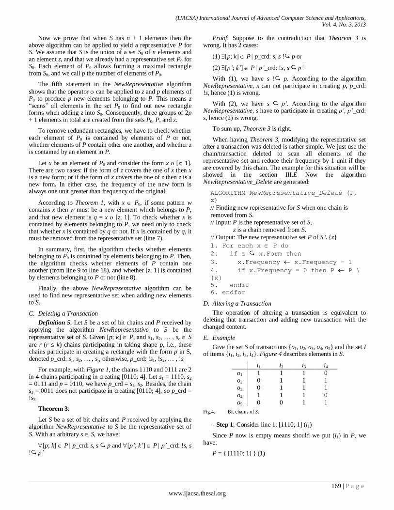
Give the set S of transactions {o1, o2, o3, o4, o5} and the set I of items {i1, i2, i3, i4}. Figure 4 describes elements in S.
i1 i2 i3 i4
o1 1 1 1 0
o2 0 1 1 1 o3 0 1 1 1
o4 1 1 1 0
o5 0 0 1 1
Fig.4. Bit chains of S.
- Step 1: Consider line 1: [1110; 1] (l1)
Since P now is empty means should we put (l1) in P, we have:
P = { [1110; 1] } (1)
(IJACSA) International Journal of Advanced Computer Science and Applications, Vol. 4, No. 3, 2013
170 | P a g e www.ijacsa.thesai.org
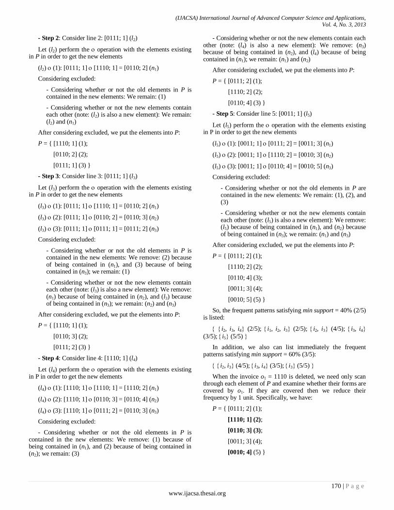
- Step 2: Consider line 2: [0111; 1] (l2)
Let (l2) perform the operation with the elements existing in P in order to get the new elements
(l2) (1): [0111; 1] [1110; 1] = [0110; 2] (n1)
Considering excluded:
- Considering whether or not the old elements in P is contained in the new elements: We remain: (1)
- Considering whether or not the new elements contain each other (note: (l2) is also a new element): We remain: (l2) and (n1)
After considering excluded, we put the elements into P:
P = { [1110; 1] (1);
[0110; 2] (2);
[0111; 1] (3) }
- Step 3: Consider line 3: [0111; 1] (l3)
Let (l3) perform the operation with the elements existing in P in order to get the new elements
(l3) (1): [0111; 1] [1110; 1] = [0110; 2] (n1)
(l3) (2): [0111; 1] [0110; 2] = [0110; 3] (n2)
(l3) (3): [0111; 1] [0111; 1] = [0111; 2] (n3)
Considering excluded:
- Considering whether or not the old elements in P is contained in the new elements: We remove: (2) because of being contained in (n1), and (3) because of being contained in (n3); we remain: (1)
- Considering whether or not the new elements contain each other (note: (l3) is also a new element): We remove: (n1) because of being contained in (n2), and (l3) because of being contained in (n3); we remain: (n2) and (n3)
After considering excluded, we put the elements into P:
P = { [1110; 1] (1);
[0110; 3] (2);
[0111; 2] (3) }
- Step 4: Consider line 4: [1110; 1] (l4)
Let (l4) perform the operation with the elements existing in P in order to get the new elements
(l4) (1): [1110; 1] [1110; 1] = [1110; 2] (n1)
(l4) (2): [1110; 1] [0110; 3] = [0110; 4] (n2)
(l4) (3): [1110; 1] [0111; 2] = [0110; 3] (n3)
Considering excluded:
- Considering whether or not the old elements in P is contained in the new elements: We remove: (1) because of being contained in (n1), and (2) because of being contained in (n2); we remain: (3)
- Considering whether or not the new elements contain each other (note: (l4) is also a new element): We remove: (n3) because of being contained in (n2), and (l4) because of being contained in (n1); we remain: (n1) and (n2)
After considering excluded, we put the elements into P:
P = { [0111; 2] (1);
[1110; 2] (2);
[0110; 4] (3) }
- Step 5: Consider line 5: [0011; 1] (l5)
Let (l5) perform the operation with the elements existing in P in order to get the new elements
(l5) (1): [0011; 1] [0111; 2] = [0011; 3] (n1)
(l5) (2): [0011; 1] [1110; 2] = [0010; 3] (n2)
(l5) (3): [0011; 1] [0110; 4] = [0010; 5] (n3)
Considering excluded:
- Considering whether or not the old elements in P are contained in the new elements: We remain: (1), (2), and (3)
- Considering whether or not the new elements contain each other (note: (l5) is also a new element): We remove: (l5) because of being contained in (n1), and (n2) because of being contained in (n3); we remain: (n1) and (n3)
After considering excluded, we put the elements into P:
P = { [0111; 2] (1);
[1110; 2] (2);
[0110; 4] (3);
[0011; 3] (4);
[0010; 5] (5) }
So, the frequent patterns satisfying min support = 40% (2/5) is listed:
i2, i3, i4 (2/5); i1, i2, i3 (2/5); i2, i3 (4/5); i3, i4
(3/5); i5 (5/5)
In addition, we also can list immediately the frequent patterns satisfying min support = 60% (3/5):
i2, i3 (4/5); i3, i4 (3/5); i3 (5/5)
When the invoice o1 = 1110 is deleted, we need only scan through each element of P and examine whether their forms are covered by o1. If they are covered then we reduce their frequency by 1 unit. Specifically, we have:
P = { [0111; 2] (1);
[1110; 1] (2);
[0110; 3] (3);
[0011; 3] (4);
[0010; 4] (5) }

(IJACSA) International Journal of Advanced Computer Science and Applications, Vol. 4, No. 3, 2013
171 | P a g e www.ijacsa.thesai.org
To increase the speed of computation, we can realize intuitively that grouping the chains/transactions in the period of preprocessing data, before running the algorithms is a good idea.
Form Frequency
1110 2 0111 2
0011 1
Fig.5. The result after grouping the bit chains of S.
IV. EXPERIMENTATION 1
The experiments of NewRepresentative algorithm are conducted on a machine with Intel(R) Core(TM) i3-2100 CPU @ 3.10GHz (4 CPUs), ~3.1GHz and 4096MB main memory installed. The operating system is Windows 7 Ultimate 64-bit (6.1, Build 7601) Service Pack 1. Programming language is C#.NET.
The proposed algorithm is tested on two datasets: the Retail data taken from a small and medium enterprise in reality and the T10I4D100K data taken from http://fimi.ua.ac.be/data/ website. First 10,000 transactions of T10I4D100K is run and compared with 12,189 transactions of Retail data.
Datasets No. of
transactions
The
maximum
number of
items
which
customer
can
purchase
The
maximum
number
of items
in the
dataset
Running
time
(second)
No. of
frequent
patterns
Retail 12,189 8 38 0.900051
5 44
T10I4D1
00K 10,000 26 1,000
702.1381
6 139,491
Fig.6. The experimental results when running proposed algorithm on 2
datasets.
Figure 6 shows the experimental results. The running time and the number of frequent patterns of T10I4D100K are absolutely larger than Retail. The result shows that the number of frequent patterns in reality of a store or an enterprise is often small. T10I4D100K is generated using the generator from the IBM Almaden Quest research group so that the transactions fluctuate much and the number of frequent patterns increases sharply when adding a new transaction.
The fast increase of number of frequent patterns leads to a big issue in computation: overflow. Although the large and the fast growth of frequent patterns, it is easy to prove that the maximum number of frequent pattern cannot be larger than a specified value. For example, if M is the maximum number of items in a store and N is the maximum number of items which a customer can purchase. The number of frequent patterns in
the store is always not larger than N
MMM CCC ...21. It
means the number of frequent patterns may increase fast but it is not big enough to make the system to be crashed.
To reduce the running time of the algorithm, parallelization is one of good ways. Parallelization was applied to find frequent patterns from huge database in the past (Gupta and Satsangi 2012). The large amount of frequent patterns is a reason makes us apply parallelization method to the NewRepresentative algorithm.
One of the big issues when developing an algorithm in parallel systems is the complexity of algorithms. Some algorithms can not divide into small part to run simultaneously in separate sites or machines. Fortunately, the NewRepresentative algorithm can be expanded for parallel systems easily. The following section introduces two ways to parallelize the algorithm: Horizontal Parallelization and Vertical Parallelization. The parallelization methods share the resource of machines and reduce the running time. It’s one of the efficient ways to increase the speed of algorithms having high executing complexity.
V. THE PRINCIPLES OF PARALLEL COMPUTING
Parallel computing is a form of computation in which many calculations are carried out simultaneously operating on the principle that large problems can often be divided into smaller ones, which are then solved concurrently.
The parallel system of the NewRepresentative algorithm has the following structure:
At first, the fragmentation will be implemented. The whole data will be divided into small and equal fragments. In Horizontal Parallelization, the transactions in data will be divided while the items are the information which will be divided in Vertical Parallelization. After the data is fragmented properly, all fragments must be allocated in various sites of network. A master site has responsibility for fragmenting data, allocating fragments to sites and merging the results from site into the final result. Sites will run the NewRepresentative algorithm with the fragments which are assigned to them simultaneously and finally, send the results into the master site for merging.
VI. HORIZONTAL PARALLELIZATION
Consider a set of n transactions S. If there are k machine located in k separate sites. Horizontal Parallelization (HP) will divide the set S into k equal fragments and allocate those fragments to k sites. The NewRepresentative algorithm is applied on n/k transactions in each site. After running algorithm, every site has its own representative set. All representative sets are sent back to master site for merging.
Merging representative sets from sites in mater site is similar to find representative set when adding new transactions into dataset.
ALGORITHM HorizontalMerge(PM, PS)
//Input: PM: representative set of master site.
PS: the set of representative sets from other sites. //Output: The new representative set of horizontal
parallelization.
1. for each P PS do

(IJACSA) International Journal of Advanced Computer Science and Applications, Vol. 4, No. 3, 2013
172 | P a g e www.ijacsa.thesai.org
2. for each z P do 3. PM = NewRepresentative(PM, z);
4. end for;
5. end for;
6. return PM;
Theorem 4:
Horizontal Parallelization method returns the representative set.
Proof: We prove by induction on k.
If k = 1, then the HP method is the NewRepresentative method, hence returns the representative set.
If k = 2, then let the two sites be S1 and S2, and let (u1, p1), … , (um, pm) be the representative set for S1, and let (v1, q1), … , (vn, qn) be the representative set for S2. We need to show that the HP algorithm will give us the representative for the union
of S1 and S2 (S1 S2). Let (w, r) be a representative element for
S1 S2. We denote by (w1, r1) the restriction of (w, r) to S1, that is w1 = w and r1 = the number of when w appears in S1. Similarly we define (w2, r2). Then by definition we must have r1 + r2 = r. Also, there must be one of the representative elements in S1, called (u1, p1), so that u1 w and p1 = r1. In fact, by definition of representative elements, there must be
such a (u1, p1) for which u1 w and p1 r1. We also have a (v1,
q1) in S2 with v1 w and q1 r2. Now we must have p1 = r1 and q1 = r2 because otherwise w will appear p1 + q1 > r1 + r2 = r
times in S1 S2. Now when we apply the HP algorithm then
we will see at least one element (w’, r) where w’ = u1 v1, and in particular w’ must cover w. Then w’ must be in fact w, otherwise, we have an element (w’, r) with w’ w but the frequency of w’ is strictly larger than of w, and hence (w, r) cannot be a representative element. Then we see that (w, r) is produced when using the HP algorithm as wanted.
Assume that we proved the correctness of the HP algorithm for k sites. We now prove the correctness of the HP algorithm for k + 1 sites. We denote these sites by S1, S2, … , Sk, Sk+1. By the induction assumption, we can find the representative set for k sites S1, S2, … , Sk using the HP algorithm. Denote by
k
i
iSS1
. Now apply the case of two sites which we proved
above to the two sites S and Sk+1, we have that the HP
algorithm produces the representative set for S Sk+1, that is we have the representative set for the union of the k + 1 sites S1, … , Sk, Sk+1. Therefore we completed the proof of Theorem 4.
VII. VERTICAL PARALLELIZATION
Vertical Parallelization is more complex than Horizontal Parallelization. While Horizontal Parallelization focuses on transactions, Vertical Parallelization focuses on items. Vertical Parallelization (VP) divides the dataset into fragments based on items. Each fragment contains a subset of items. Fragments are allocated into separate sites. In each sites, they run NewRepresentative algorithm to find out representative sets. The representative sets will be sent back to the master site and will be merged to find the final representative set.
Vertical merging is based on merged-bit operation and vertical merging operation.
Definition 6 (merged-bit operation ⊍): merged-bit operation is a dyadic operation in bit-chain space (a1a2 … an)
⊍ (b1b2 … bm) = (a1a2 … anb1b2 … bm).
Definition 7 (vertical merging operation ⇼): Vertical merging operation is a dyadic operation between two representative patterns from two different vertical fragments:
[(a1a2 … an), p, {o1, o2, … , op}] ⇼ [(b1b2 … bm), q, {o1, o2, …, oq}] = [vmChain, vmFreq, vmObject];
vmChain = (a1a2 … an) ⊍ (b1b2 … bm) = (a1a2 … anb1b2 … bm)
vmObject = {o1, o2 , … , op} {o1, o2 , … , oq} = {o1, o2, … , ok}
vmFreq = k
At the master site, representative sets of other sites will be merged into representative set of master site. The below algorithm is run to find out the final representative set.
ALGORITHM VerticalMerge(PM, PS)
//Input: PM: representative set of master site.
PS: the set of representative sets from other sites. //Output: The new representative set of vertical
parallelization.
1. for each P PS do
2. for each m PM do 3. flag = 0;
4. M = // M: set of used elements in P
5. for each z P do
6. q = m ⇼ z;
7. if frequency of q ≠ 0 then
8. flag = 1; // mark m as used element
9. M = M q; // mark q as used
element
10. PM = PM q;
11. end if;
12. end for;
13. if flag = 1 then
14. PM = PM {m}
15. end if;
16. PM = PM (P \ M); 17. end for;
18. end for;
19. return PM;
Theorem 5:
Vertical Parallelization method returns the representative set.
Proof: We prove by induction on k.
If k = 1, this is the NewRepresentative algorithm, hence gives the representative set.
If k = 2, we let S1 and S2 be the two sites, and let S be the union. Let R = ({i1, … , in}, k, {o1, … , ok}) = (I, k, O) be a

(IJACSA) International Journal of Advanced Computer Science and Applications, Vol. 4, No. 3, 2013
173 | P a g e www.ijacsa.thesai.org
representative element for S. Let R1 be the restriction of R to S1, that is R1 = (I1, p1, O1), where I1 is the intersection of {i1, … , in} with the set of items in S1, O1 is the set of transactions in R1 containing all items in I1. We define similarly R2 = (I2, p2, O2)
the restriction of R to S2. Note that if I1 = then p1 = 0,
otherwise p1 must be positive (p1 > 0). Similarly, if I2 = then p2 = 0, otherwise p2 must be positive (p1 > 0). We use the
convention that if I1 = then O1 = O, and if I2 = then O2 = O. Remark that at least one of I1 or I2 is non-empty. Now by definition, there must be a representative element Q1 = (I1’, p1’,
O1’) in S1 with I1 I1’, O1 O1’, and p1’ >= p1. Similarly, we
have a representative element Q2 = (I2’, p2’, O2’) in S2 with I2
I2’, O2 O2’, and p2’ >= p2. When we do the vertical merging operation of Q1 and Q2, then we must obtain I. Otherwise, we
obtain an element R’ = (I’, k’, O’) where I I’, O O’, and k’ >= k, and at least one of these is strict. This is a contradiction to the assumption that R is a representative element of S. Now that we proved the correctness of the algorithm for k = 1 and k = 2. Then, assume that we proved the correctness of the VP algorithm for k sites. We now prove the correctness of the VP algorithm for k + 1 sites. We denote these sites by S1, S2, … , Sk, Sk+1. By the induction assumption, we can find the representative set for k sites S1, S2, … , Sk using the VP
algorithm. Denote by k
i
iSS1
. Now apply the case of two
sites which we proved above to the two sites S and Sk+1, we have that the VP algorithm produces the representative set for S
Sk+1, that is we have the representative set for the union of the k + 1 sites S1, … , Sk, Sk+1. Therefore we completed the proof of Theorem 5.
Example: Give the set S of transactions {o1, o2, o3, o4, o5, o6, o7} and the set I of items {i1, i2, i3}.
i1 i2 i3
o1 0 0 1
o2 0 1 0
o3 0 1 1
o4 1 0 0
o5 1 0 1
o6 1 1 0
o7 1 1 1
Fig.7. Bit-chains of S.
Divide the items into two segments: {i1} and {i2, i3}.
i1
o1 0
o2 0
o3 0
o4 1
o5 1
o6 1
o7 1 Fig.8. The first segment.
i2 i3
o1 0 1
o2 1 0
o3 1 1
o4 0 0
o5 0 1
o6 1 0
o7 1 1
Fig.9. The second segment.
Allocate two segments in two separate sites and run NewRepresentative algorithm on those fragments simultaneously.
It is easy to get the representative sets from two sites:
The site has {i1} fragment: }{ 1i
P ={[(1); 4; {o4, o5, o6, o7}]}
The site has {i2, i3} fragment: },{ 32 iiP ={[(01); 4; {o1, o3, o5,
o7}], [(10); 4; {o2, o3, o6, o7}], [(11); 2; {o3, o7}]}
Merge both of them:
[(1); 4; {o4, o5, o6, o7}] ⇼ [(01); 4; {o1, o3, o5, o7}] = [(101); 2; {o5, o7}]
[(1); 4; {o4, o5, o6, o7}] ⇼ [(10); 4; {o2, o3, o6, o7}] = [(110); 2; {o6, o7}]
[(1); 4; {o4, o5, o6, o7}] ⇼ [(11); 2; {o3, o7}] = [(111); 1; {o7}]
The full representative set P is:
P = {[(100); 4; {o4, o5, o6, o7}],
[(001); 4; {o1, o3, o5, o7}],
[(010); 4; {o2, o3, o6, o7}],
[(011); 2; {o3, o7}],
[(101); 2; {o5, o7}],
[(110); 2; {o6, o7}],
[(111); 1; {o7}]}
VIII. EXPERIMENTATION 2
The experiments of Vertical Parallelization Method are conducted on machines which has similar configuration: Intel(R) Core(TM) i3-2100 CPU @ 3.10GHz (4 CPUs), ~3.1GHz and 4096MB main memory installed. The operating system is Windows 7 Ultimate 64-bit (6.1, Build 7601) Service Pack 1. Programming language is C#.NET.
The proposed methods are tested on T10I4D100K dataset taken from http://fimi.ua.ac.be/data/ website. First 10,000 transactions of T10I4D100K are run and compared with the result when running without parallelization.
(IJACSA) International Journal of Advanced Computer Science and Applications, Vol. 4, No. 3, 2013
174 | P a g e www.ijacsa.thesai.org
Dataset No. of
transactions
The
maximum
No. of
items
which
customer
can
purchase
The
maximum
No. of
items in
the
dataset
Running
time
(second)
No. of
frequent
patterns
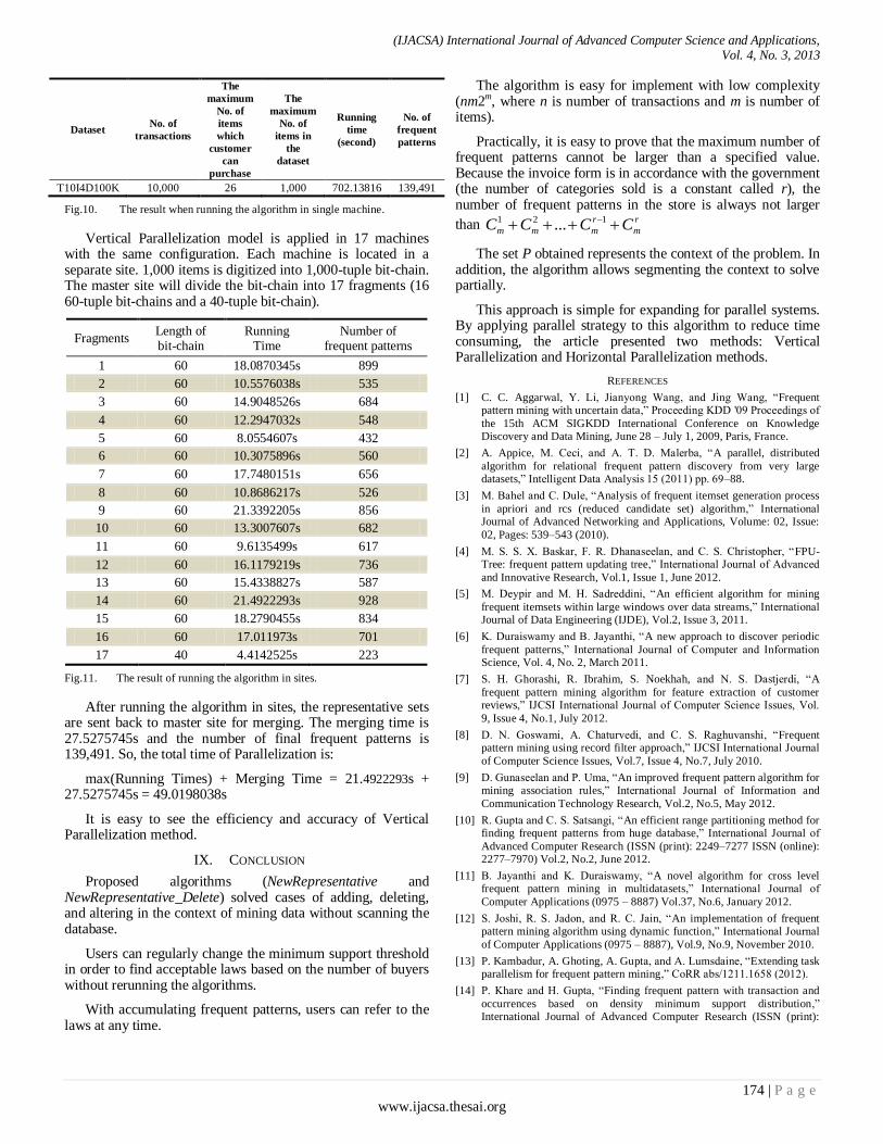
T10I4D100K 10,000 26 1,000 702.13816 139,491
Fig.10. The result when running the algorithm in single machine.
Vertical Parallelization model is applied in 17 machines with the same configuration. Each machine is located in a separate site. 1,000 items is digitized into 1,000-tuple bit-chain. The master site will divide the bit-chain into 17 fragments (16 60-tuple bit-chains and a 40-tuple bit-chain).
Fragments Length of bit-chain
Running Time
Number of frequent patterns
1 60 18.0870345s 899
2 60 10.5576038s 535
3 60 14.9048526s 684
4 60 12.2947032s 548
5 60 8.0554607s 432
6 60 10.3075896s 560
7 60 17.7480151s 656
8 60 10.8686217s 526
9 60 21.3392205s 856
10 60 13.3007607s 682
11 60 9.6135499s 617
12 60 16.1179219s 736
13 60 15.4338827s 587
14 60 21.4922293s 928
15 60 18.2790455s 834
16 60 17.011973s 701
17 40 4.4142525s 223
Fig.11. The result of running the algorithm in sites.
After running the algorithm in sites, the representative sets are sent back to master site for merging. The merging time is 27.5275745s and the number of final frequent patterns is 139,491. So, the total time of Parallelization is:
max(Running Times) + Merging Time = 21.4922293s + 27.5275745s = 49.0198038s
It is easy to see the efficiency and accuracy of Vertical Parallelization method.
IX. CONCLUSION
Proposed algorithms (NewRepresentative and NewRepresentative_Delete) solved cases of adding, deleting, and altering in the context of mining data without scanning the database.
Users can regularly change the minimum support threshold in order to find acceptable laws based on the number of buyers without rerunning the algorithms.
With accumulating frequent patterns, users can refer to the laws at any time.
The algorithm is easy for implement with low complexity (nm2m, where n is number of transactions and m is number of items).
Practically, it is easy to prove that the maximum number of frequent patterns cannot be larger than a specified value. Because the invoice form is in accordance with the government (the number of categories sold is a constant called r), the number of frequent patterns in the store is always not larger
than r
m
r
mmm CCCC 121 ...
The set P obtained represents the context of the problem. In addition, the algorithm allows segmenting the context to solve partially.
This approach is simple for expanding for parallel systems. By applying parallel strategy to this algorithm to reduce time consuming, the article presented two methods: Vertical Parallelization and Horizontal Parallelization methods.
REFERENCES
[1] C. C. Aggarwal, Y. Li, Jianyong Wang, and Jing Wang, “Frequent pattern mining with uncertain data,” Proceeding KDD '09 Proceedings of
the 15th ACM SIGKDD International Conference on Knowledge Discovery and Data Mining, June 28 – July 1, 2009, Paris, France.
[2] A. Appice, M. Ceci, and A. T. D. Malerba, “A parallel, distributed
algorithm for relational frequent pattern discovery from very large datasets,” Intelligent Data Analysis 15 (2011) pp. 69–88.
[3] M. Bahel and C. Dule, “Analysis of frequent itemset generation process
in apriori and rcs (reduced candidate set) algorithm,” International Journal of Advanced Networking and Applications, Volume: 02, Issue:
02, Pages: 539–543 (2010).
[4] M. S. S. X. Baskar, F. R. Dhanaseelan, and C. S. Christopher, “FPU-Tree: frequent pattern updating tree,” International Journal of Advanced
and Innovative Research, Vol.1, Issue 1, June 2012.
[5] M. Deypir and M. H. Sadreddini, “An efficient algorithm for mining
frequent itemsets within large windows over data streams,” International Journal of Data Engineering (IJDE), Vol.2, Issue 3, 2011.
[6] K. Duraiswamy and B. Jayanthi, “A new approach to discover periodic
frequent patterns,” International Journal of Computer and Information Science, Vol. 4, No. 2, March 2011.
[7] S. H. Ghorashi, R. Ibrahim, S. Noekhah, and N. S. Dastjerdi, “A
frequent pattern mining algorithm for feature extraction of customer reviews,” IJCSI International Journal of Computer Science Issues, Vol.
9, Issue 4, No.1, July 2012.
[8] D. N. Goswami, A. Chaturvedi, and C. S. Raghuvanshi, “Frequent pattern mining using record filter approach,” IJCSI International Journal
of Computer Science Issues, Vol.7, Issue 4, No.7, July 2010.
[9] D. Gunaseelan and P. Uma, “An improved frequent pattern algorithm for mining association rules,” International Journal of Information and
Communication Technology Research, Vol.2, No.5, May 2012.
[10] R. Gupta and C. S. Satsangi, “An efficient range partitioning method for finding frequent patterns from huge database,” International Journal of
Advanced Computer Research (ISSN (print): 2249–7277 ISSN (online): 2277–7970) Vol.2, No.2, June 2012.
[11] B. Jayanthi and K. Duraiswamy, “A novel algorithm for cross level frequent pattern mining in multidatasets,” International Journal of
Computer Applications (0975 – 8887) Vol.37, No.6, January 2012.
[12] S. Joshi, R. S. Jadon, and R. C. Jain, “An implementation of frequent pattern mining algorithm using dynamic function,” International Journal
of Computer Applications (0975 – 8887), Vol.9, No.9, November 2010.
[13] P. Kambadur, A. Ghoting, A. Gupta, and A. Lumsdaine, “Extending task parallelism for frequent pattern mining,” CoRR abs/1211.1658 (2012).
[14] P. Khare and H. Gupta, “Finding frequent pattern with transaction and
occurrences based on density minimum support distribution,” International Journal of Advanced Computer Research (ISSN (print):
(IJACSA) International Journal of Advanced Computer Science and Applications, Vol. 4, No. 3, 2013
175 | P a g e www.ijacsa.thesai.org
2249–7277 ISSN (online): 2277–7970) Vol.2, No.3, Issue 5, September
2012.
[15] H. D. Kim, D. H. Park, and Y. L. C. X. Zhai, “Enriching text
representation with frequent pattern mining for probabilistic topic modeling,” ASIST 2012, October 26–31, 2012, Baltimore, MD, USA.
[16] R. U. Kiran and P. K. Reddy, “Novel techniques to reduce search space
in multiple minimum supports-based frequent pattern mining algorithms,” Proceeding EDBT/ICDT '11 Proceedings of the 14th
International Conference on Extending Database Technology, March 22–24, 2011, Uppsala, Sweden.
[17] A. K. Koundinya, N. K. Srinath, K. A. K. Sharma, K. Kumar, M. N.
Madhu, and K. U. Shanbag, “Map/Reduce design and implementation of apriori algorithm for handling voluminous data-sets,” Advanced
Computing: An International Journal (ACIJ), Vol.3, No.6, November 2012.
[18] K. Malpani and P. R. Pal, “An efficient algorithms for generating
frequent pattern using logical table with AND, OR operation,” International Journal of Engineering Research & Technology (IJERT)
Vol.1, Issue 5, July – 2012.
[19] P. Nancy and R. G. Ramani, “Frequent pattern mining in social network data (facebook application data),” European Journal of Scientific
Research, ISSN 1450–216X Vol.79 No.4 (2012), pp.531–540, © EuroJournals Publishing, Inc. 2012.
[20] A. Niimi, T. Yamaguchi, and O. Konishi, “Parallel computing method of
extraction of frequent occurrence pattern of sea surface temperature from satellite data,” The Fifteenth International Symposium on Artificial Life
Robotics 2010 (AROB 15th '10). B-Con Plaza, Beppu, Oita, Japan, February 4–6, 2010.
[21] S. N. Patro, S. Mishra, P. Khuntia, and C. Bhagabati, “Construction of FP tree using huffman coding,” IJCSI International Journal of Computer
Science Issues, Vol.9, Issue 3, No.2, May 2012.
[22] D. Picado-Muiño, I. C. León, and C. Borgelt, “Fuzzy frequent pattern mining in spike trains,” IDA 2012: 289–300.
[23] R. V. Prakash, Govardhan, and S. S. V. N. Sarma, “Mining frequent
itemsets from large data sets using genetic algorithms,” IJCA Special Issue on “Artificial Intelligence Techniques – Novel Approaches &
Practical Applications” AIT, 2011.
[24] K. S. N. Prasad and S. Ramakrishna, “Frequent pattern mining and current state of the art,” International Journal of Computer Applications
(0975 – 8887), Vol. 26, No.7, July 2011.
[25] A. Raghunathan and K. Murugesan, “Optimized frequent pattern mining
for classified data sets,” ©2010 International Journal of Computer Applications (0975 – 8887), Vol.1, No.27.
[26] S. S. Rawat and L. Rajamani, “Discovering potential user browsing behaviors using custom-built apriori algorithm,” International Journal of
Computer Science & Information Technology (IJCSIT) Vol.2, No.4, August 2010.
[27] M. H. Sadat, H. W. Samuel, S. Patel, and O. R. Zaïane, “Fastest
association rule mining algorithm predictor (FARM-AP),” Proceeding C3S2E '11 Proceedings of the Fourth International Conference on
Computer Science and Software Engineering, 2011.
[28] K. Saxena and C. S. Satsangi, “A non candidate subset-superset dynamic minimum support approach for sequential pattern mining,” International
Journal of Advanced Computer Research (ISSN (print): 2249–7277 ISSN (online): 2277–7970) Vol.2, No.4, Issue 6, December 2012.
[29] H. Sharma and D. Garg, “Comparative analysis of various approaches
used in frequent pattern mining,” International Journal of Advanced Computer Science and Applications, Special Issue on Artificial
Intelligence IJACSA pp. 141–147 August 2011.
[30] Y. Sharma and R. C. Jain, “Analysis and implementation of FP & Q-FP tree with minimum CPU utilization in association rule mining,”
International Journal of Computing, Communications and Networking, Vol.1, No.1, July – August 2012.
[31] K. Sumathi, S. Kannan, and K. Nagarajan, “A new MFI mining
algorithm with effective pruning mechanisms,” International Journal of Computer Applications (0975 – 8887) Vol.41, No.6, March 2012.
[32] M. Utmal, S. Chourasia, and R. Vishwakarma, “A novel approach for finding frequent item sets done by comparison based technique,”
International Journal of Computer Applications (0975 – 8887) Vol.44, No.9, April 2012.
[33] C. Xiaoyun, H. Yanshan, C. Pengfei, M. Shengfa, S. Weiguo, and Y.
Min, “HPFP-Miner: a novel parallel frequent itemset mining algorithm,” Natural Computation, 2009. ICNC '09. Fifth International Conference on
14–16 Aug. 2009.
[34] M. Yuan, Y. X. Ouyang, and Z. Xiong, “A text categorization method using extended vector space model by frequent term sets,” Journal of
Information Science and Engineering 29, 99–114 (2013).
[35] Y. Wang and J. Ramon, “An efficiently computable support measure for frequent subgraph pattern mining,” – ECML/PKDD (1) 2012: 362–377.
Copyright © 2022 FDOKUMEN