Interpreting populationpharmacokinetic-pharmacodynamic analyses –a clinical viewpointStephen B. Duffull,1 Daniel F. B. Wright1 & Helen R. Winter1,2

1School of Pharmacy, University of Otago, PO Box 56, Dunedin 9054, New Zealand and 2Global

Alliance for TB Drug Development, New York 10005, USA

CorrespondenceProfessor Stephen Duffull, School ofPharmacy, University of Otago, PO Box 56,Dunedin 9054, New Zealand.Tel.: + 64 3 479 5044Fax: + 64 3 479 7034E-mail: stephen.duffull@otago.ac.nz----------------------------------------------------------------------

Keywordspharmacodynamics, pharmacokinetics,pharmacometrics, population analyses,statistical models----------------------------------------------------------------------

Received12 October 2010

Accepted23 December 2010

Accepted Article23 December 2010

The population analysis approach is an important tool for clinical pharmacology in aiding the dose individualization of medicines.However, due to their statistical complexity the clinical utility of population analyses is often overlooked. One of the key reasons toconduct a population analysis is to investigate the potential benefits of individualization of drug dosing based on patientcharacteristics (termed covariate identification). The purpose of this review is to provide a tool to interpret and extract information frompublications that describe population analysis. The target audience is those readers who are aware of population analyses but have notconducted the technical aspects of an analysis themselves. Initially we introduce the general framework of population analysis andwork through a simple example with visual plots. We then follow-up with specific details on how to interpret population analyses forthe purpose of identifying covariates and how to interpret their likely importance for dose individualization.

Introduction

The primary purpose of population pharmacokinetic (PK)and pharmacokinetic-pharmacodynamic (PKPD) analysisis to individualize drug choice and dosing regimen. In thisperspective we consider that dose ranging and dose selec-tion in pre-marketing clinical trials as well as culmination ofknowledge to develop a product label are all versions ofdose individualization which are not conceptually differ-ent from that faced in the clinic. Dose individualization inthis setting is therefore an overarching term that accountsfor both how dosing requirements vary across individualsas well as an understanding of sources of variability in doserequirements.

Dose individualization is achieved by understandingthe onset, magnitude and duration of drug effects thatresult from a given dose and dosing regimen and howthese effects vary over the target population. Readers arereferred to our companion review [1] for an introductorydiscussion on PKPD models.

The population approach we see today arose from thedevelopment of the conceptual framework of populationanalysis in 1972 to 1977 [2, 3]. From 1977 there was a trickleof papers over the next 10 years, until 1985 where therewas an exponential growth in publications.The applicationof population analysis methods to therapeutic problems

has led to on-going methodological and software devel-opment which in turn has resulted in further and morecomplex applications.

The first population analysis software applicationNONMEM (NONlinear Mixed Effects Modeling [4–6]) stillaccounts for the majority of the literature (Table 1).Readers are referred to other papers that describe thehistory of software development for population analysis[e.g. 7, 8].

The discipline of population analysis shares a commonhistory with clinical pharmacology and, importantly,the same fundamental aim. Yet, the results of populationanalyses are often viewed with scepticism by those not inthe field, particularly by practising clinicians [9]. This maybe attributed to a perceived lack of relevance to clinicalpractice, the inaccessible nature of the methodologyand the use of complex equations and statistical jargon inpublished papers. As a result the clinical utility of modelsthat are developed in the population analysis setting isdiminished.

Aim

There are many general reviews [e.g. 7, 9–15] and introduc-tory articles [e.g.16,17] on population analyses and it is not

British Journal of ClinicalPharmacology

DOI:10.1111/j.1365-2125.2010.03891.x

Br J Clin Pharmacol / 71:6 / 807–814 / 807© 2011 The AuthorsBritish Journal of Clinical Pharmacology © 2011 The British Pharmacological Society

the intention of this article to emulate those works. Thepurpose of this review is to provide a tool to interpret andextract information from population PKPD analysis publi-cations. This review is aimed at those readers who haveheard about population analyses but have not conductedthe technical aspects of an analysis themselves.

What is a population analysis?

In this review, we use the term population analysis (alsotermed repeated measures modelling, nonlinear mixedeffects modelling and nonlinear hierarchical modelling) torefer to a set of statistical techniques that can be used tolearn about the average response in a population as well asthe variability in response that arises from differentsources.We use the term response to refer to any biomarkeror event that might be measured clinically. Readers arereferred to Pillai [7] for a detailed overview of populationanalysis.The approach has also been reviewed recently in amodel based drug development setting [18] and in rela-tion to modelling vs. non-modelling techniques from a sta-tistical stand point [19].

Population analysis is the application of a model todescribe data that arise from more than one individual.The process does not require that each study individualprovides sufficient data to characterize completely theirown PK or PKPD profile. Population analysis methods allowborrowing of information between individuals to fill ingaps in the PK and PD profiles. In doing so the methodallows the use of sparse sampling study designs. The influ-ence of patient characteristics (such as renal function) onthe PK or PKPD profile can be quantified from the data setas well as any remaining unexplained variability betweenpatients.

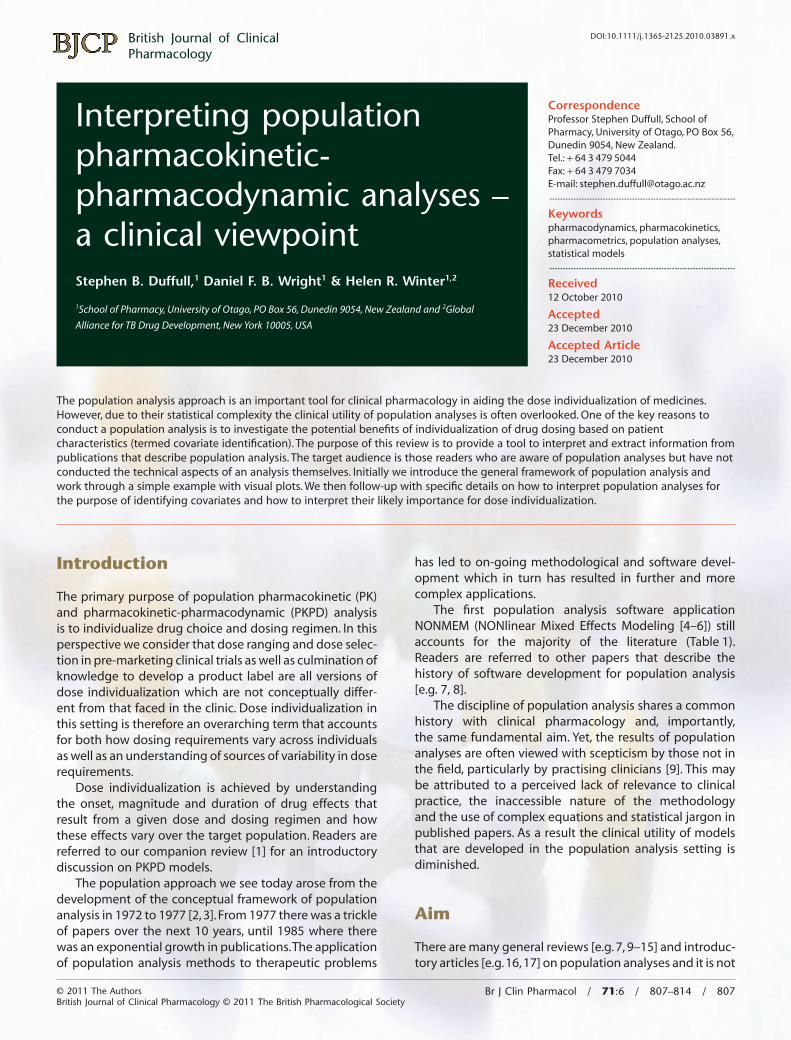
For the purposes of this review, we constructed a PKmodel for a gentamicin-like drug that incorporates thecentral elements relevant to a population analysis. Thisdrug displays one compartment model characteristicswith a volume of distribution (20 l) and clearance (4 l h–1)and the dose is administered by intravenous bolus. Weused this PK model to simulate plasma concentration–timedata for 30 patients who received a single intravenousbolus dose of 420 mg (6 mg kg–1 for a 70 kg individual),where each patient provided seven blood samples at times0.25, 0.5, 1, 2, 4, 8 and 12 h following dosing (Figure 1).A population analysis was then conducted on the simula-tion ‘dataset’.

A population model for our data will consist of threeelements: (1) A model for the typical response – this is theresponse for a typical (average) patient, (2) a model forheterogeneity and (3) a model for uncertainty.

1. A model for the typical responseThis is sometimes also called a structural model. For phar-macokinetics this would be a compartmental model thatdescribes the plasma drug concentration over time (seeFigure 2A).

The pharmacokinetic model that describes ourgentamicin-like drug at a specific time (t) is:

y tV V

t( ) = −( )dose CLexp . (1)

where CL is clearance and V is volume of distribution whichwill be estimated as a part of the modelling process.

2. A model for heterogeneityWe use the term heterogeneity in population analysis todescribe the variability between individuals. This is alsotermed between subject variability (BSV) or interindividual

Table 1Population analysis software

Software*Number ofpublications†

First year indexed onMEDLINE and EMBASE

NONMEM 2456 1980NPEM (NonParametric

Expectation Maximization)or NPAG (NonParametricAdaptive Grid)

139 1991

PPharm 4 1996WinBUGS or related 27 1998‡

Monolix 30 2007MCPEM (Monte Carlo

Parametric ExpectationMaximization)

4 2007

*Phoenix NLME has been recently released but no publications yet cite use of thissoftware. †Only about half of publications on MEDLINE or EMBASE mention thesoftware in the title or abstract. ‡The first use appears to relate to a nonlinearhierarchical modelling application in SAS.

30

25

20

0 2 4 6

Time (h)

Co

ncen

trat

ion

(mg

L–1

)

8 10 12

15

10

5

0

Figure 1Observed concentration–time data for 30 individuals

S. B. Duffull et al.

808 / 71:6 / Br J Clin Pharmacol

variability (IIV). This involves two distinct models. Firstly, amodel is developed to describe predictable reasons whyindividuals are different and secondly a model is devel-oped to quantify the remaining source of random variabil-ity when we have exhausted our ideas of why individualsare different from one another. The latter model is a statis-tical model for random variability.

We quantify both predictable and unpredictable vari-ability in a population to characterize not only the typicalresponse of the population, but also to predict the likelyrange of responses that may occur. In the case of our PKexample we now see the range of model predictions inFigure 2B encompass the observed plasma concentrationdata of our PK example.

If we consider our pharmacokinetic example (Equa-tion 1), we now end up with two equations with Equation 3directly substituted into Equation 2:

yV V

tii

i

i

i

= −( )dose CLexp (2)

CL CL CLNR CRi ife ci= + × + (3)

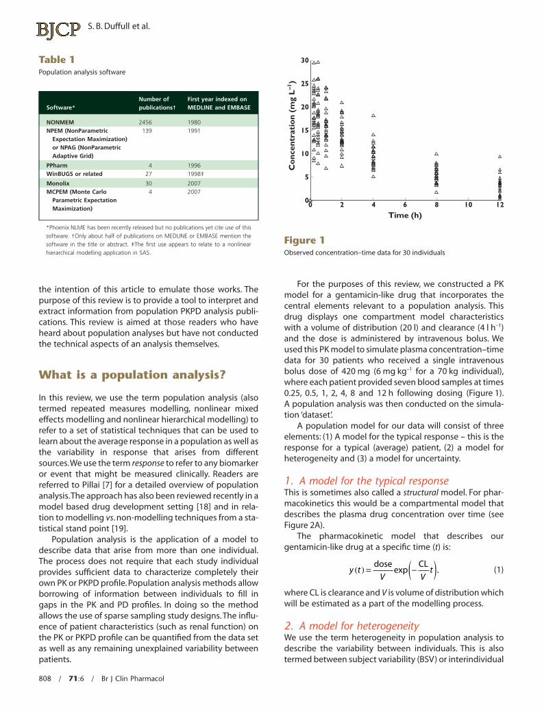
We use CLCR as an abbreviation for creatinine clearance andCLNR as an abbreviation for non-renal clearance. Note thatEquation 3 has the same form as simple linear regression(see Figure 3). Here we show a model for renal clearancefe i× CLCR , where fe = fraction of unchanged drug elimi-nated by the kidneys (i.e. the slope), and non-renal clear-ance (i.e. the intercept). We see that CL for the ith individualis dependent on this individual’s CLCR and non-renal clear-ance.However, including these processes into Equation 3 isstill insufficient to describe completely the variability in CLand hence there is some remaining (residual) variabilitywhich we attribute to random variability between patients(the scatter around the regression line in Figure 3). Theterm ci is the difference of patient i from the mean patientwith this level of renal function and the variance of c overall individuals is the between-subject-variance. We couldassume that c is normally distributed, but as shown inFigure 4A this would result in implausible (negative orzero) values of CL. In this particular case,we would considerthat c assumes a log-normal distribution which results inno zero or negative values of CL (Figure 4B). A log normaldistribution is one in which the natural logarithm transfor-mation of the variable c is normally distributed. The actual

30

A

B

20

25

15

10

5

00 2 4 6

Time (h)

Co

ncen

trat

ion

(mg

L–1

)

8 10 12

35

20

30

15

10

5

00 2 4 6

Time (h)

Co

ncen

trat

ion

(mg

L–1

)

8 10 12

25

Figure 2(A) The observed concentration–time data overlaid with the median pre-dicted concentration from the PK model. (B) Observed concentration–time data overlaid with the median and 2.5th and 97.5th percentiles of thepredicted concentrations from the PK model

160

140

120

100

80

60

40

20

00 20 40 60

Creatinine clearance (mL min–1)

Cle

aran

ce (

mL

min

–1)

80 100 120

Figure 3Individual estimates of systemic drug CL vs. creatinine clearance. The lineis the regression line and the intercept represents non-renal clearanceand the slope represents the fraction of drug cleared unchanged by thekidneys. The vertical difference of any individual from the regression linerepresents the difference of that individual from the population averageand is given by c (Equation 3)

Interpretation of population analyses for clinicians

Br J Clin Pharmacol / 71:6 / 809

value for the difference of any given patient from theaverage patient is then obtained by exponentiating thevalue of c.

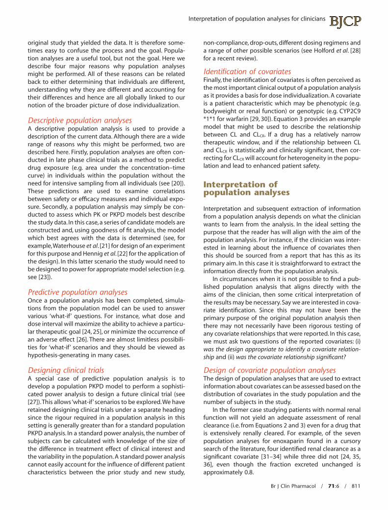
We can now show what the predictive plots would looklike if we found that CLCR described 50% of the between-subject variability (heterogeneity) in CL and the remaining50% of the variability is unexplained (assumed to berandom). When we account for CLCR in the model, we findthat the range of model predictions for plasma concentra-tion over time for the 2.5th and 97.5th percentiles of thepopulation is now reduced (Figure 5).

3. A model for uncertainty.This is a statistical model that describes why our modelsfrom Equations 1 and 2 do not match our observations

exactly. Uncertainty is also called residual error. It isassumed that uncertainty arises from (at least) foursources: (i) process error – where the dose or timing of doseor timing of blood samples are not conducted at the timesthat they are recorded, (ii) measurement error – where theresponse (e.g. concentration) is not measured exactly dueto assay error, (iii) model misspecification – where themodels we propose in Equations 1–3 are in reality toosimple and (iv) moment to moment variability within apatient.

The final component to add to our analysis mustaccount for the uncertainty in our model predictions. It isusual, but not essential, to assume that the uncertainty isentirely random and due to error. We can add this into ourmodel by introducing the term eij [for error], which is theerror for the jth observation for the ith individual. We showthis for our PK model by

yV V

t eiji

i

i

iij ij= −( ) +

dose CLexp (4)

This error represents the (residual) difference of themodel prediction from the data. In the pharmacokineticexample it is usual (but not essential) to consider e to benormally distributed.

Why are population PKPDanalyses performed?

To anyone who has performed a population analysis theprocess is almost as involved and convoluted as the

0.2A

B

0.18

0.16

0.14

0.12

0.1

0.08

0.06

0.04

0.02

0–2 2 4

Clearance (L h–1)

6 8 100

Den

sity

0.35

0.3

0.25

0.2

0.15

0.1

0.05

0–2 2 4

Clearance (L h–1)

6 8 100

Den

sity

Figure 4The distribution of values of CL in the population. (A) Allows the distribu-tion to be normal. The verticle line at 0 indicates the lower bound ofbiologically acceptable values. Here 2.3% of the predicted values of CL areunrealistic. (B) Allows the distribution to be lognormal. Negative (or zero)values of predicted CL are not allowed

35

30

25

20

Co

ncen

tria

tio

n (m

g L

–1)

15

10

5

00 2 4 6

Time (h)8 10 12

Figure 5Predicted concentrations from the PK model that does not include thecovariate CLCR (solid line). Predicted concentrations from a PK model thatincludes the covariate CLCR as a covariate on CL (dashed lines). Includingthe covariate CLCR in the model reduces the unexplained variability inthe model predictions and hence improves the reliability of the modelpredictions

S. B. Duffull et al.

810 / 71:6 / Br J Clin Pharmacol

original study that yielded the data. It is therefore some-times easy to confuse the process and the goal. Popula-tion analyses are a useful tool, but not the goal. Here wedescribe four major reasons why population analysesmight be performed. All of these reasons can be relatedback to either determining that individuals are different,understanding why they are different and accounting fortheir differences and hence are all globally linked to ournotion of the broader picture of dose individualization.

Descriptive population analysesA descriptive population analysis is used to provide adescription of the current data. Although there are a widerange of reasons why this might be performed, two aredescribed here. Firstly, population analyses are often con-ducted in late phase clinical trials as a method to predictdrug exposure (e.g. area under the concentration–timecurve) in individuals within the population without theneed for intensive sampling from all individuals (see [20]).These predictions are used to examine correlationsbetween safety or efficacy measures and individual expo-sure. Secondly, a population analysis may simply be con-ducted to assess which PK or PKPD models best describethe study data. In this case, a series of candidate models areconstructed and, using goodness of fit analysis, the modelwhich best agrees with the data is determined (see, forexample,Waterhouse et al. [21] for design of an experimentfor this purpose and Hennig et al. [22] for the application ofthe design). In this latter scenario the study would need tobe designed to power for appropriate model selection (e.g.see [23]).

Predictive population analysesOnce a population analysis has been completed, simula-tions from the population model can be used to answervarious ‘what-if’ questions. For instance, what dose anddose interval will maximize the ability to achieve a particu-lar therapeutic goal [24, 25], or minimize the occurrence ofan adverse effect [26]. There are almost limitless possibili-ties for ‘what-if’ scenarios and they should be viewed ashypothesis-generating in many cases.

Designing clinical trialsA special case of predictive population analysis is todevelop a population PKPD model to perform a sophisti-cated power analysis to design a future clinical trial (see[27]).This allows ‘what-if’ scenarios to be explored.We haveretained designing clinical trials under a separate headingsince the rigour required in a population analysis in thissetting is generally greater than for a standard populationPKPD analysis. In a standard power analysis, the number ofsubjects can be calculated with knowledge of the size ofthe difference in treatment effect of clinical interest andthe variability in the population. A standard power analysiscannot easily account for the influence of different patientcharacteristics between the prior study and new study,

non-compliance, drop-outs, different dosing regimens anda range of other possible scenarios (see Holford et al. [28]for a recent review).

Identification of covariatesFinally, the identification of covariates is often perceived asthe most important clinical output of a population analysisas it provides a basis for dose individualization. A covariateis a patient characteristic which may be phenotypic (e.g.bodyweight or renal function) or genotypic (e.g. CYP2C9*1*1 for warfarin [29, 30]). Equation 3 provides an examplemodel that might be used to describe the relationshipbetween CL and CLCR. If a drug has a relatively narrowtherapeutic window, and if the relationship between CLand CLCR is statistically and clinically significant, then cor-recting for CLCR will account for heterogeneity in the popu-lation and lead to enhanced patient safety.

Interpretation ofpopulation analyses

Interpretation and subsequent extraction of informationfrom a population analysis depends on what the clinicianwants to learn from the analysis. In the ideal setting thepurpose that the reader has will align with the aim of thepopulation analysis. For instance, if the clinician was inter-ested in learning about the influence of covariates thenthis should be sourced from a report that has this as itsprimary aim. In this case it is straightforward to extract theinformation directly from the population analysis.

In circumstances when it is not possible to find a pub-lished population analysis that aligns directly with theaims of the clinician, then some critical interpretation ofthe results may be necessary.Say we are interested in cova-riate identification. Since this may not have been theprimary purpose of the original population analysis thenthere may not necessarily have been rigorous testing ofany covariate relationships that were reported. In this case,we must ask two questions of the reported covariates: (i)was the design appropriate to identify a covariate relation-ship and (ii) was the covariate relationship significant?

Design of covariate population analysesThe design of population analyses that are used to extractinformation about covariates can be assessed based on thedistribution of covariates in the study population and thenumber of subjects in the study.

In the former case studying patients with normal renalfunction will not yield an adequate assessment of renalclearance (i.e. from Equations 2 and 3) even for a drug thatis extensively renally cleared. For example, of the sevenpopulation analyses for enoxaparin found in a cursorysearch of the literature, four identified renal clearance as asignificant covariate [31–34] while three did not [24, 35,36], even though the fraction excreted unchanged isapproximately 0.8.

Interpretation of population analyses for clinicians

Br J Clin Pharmacol / 71:6 / 811

In the latter case, if there are too few patients in thestudy (low power) then the analysis will not be able toidentify correctly covariate relationships due to randomnoise. Hence, low power studies are more likely to findspurious and exaggerated effects. In this regard it is recom-mended that a minimum of 50 to 100 patients are requiredto provide accurate estimates of covariate effects in apopulation analysis setting (readers are referred to Ribbing& Jonsson [37] for a detailed evaluation).

Significance of covariate relationshipsFor a given population analysis, not all covariates inc-luded in the final population model are necessarily sig-nificant and not all significant covariates are includedin the final population model. This potentially confusingsituation requires a means of understanding the signi-ficance of any reported covariates. Generally, this canbe accomplished by assessing; biological plausibility,clinical significance, statistical significance and a reduc-tion in unexplained between subject variability. It shouldbe noted that the acceptance of a covariate under anyone of these criteria does not automatically indicate thatthe other criteria will also be considered to be true.For instance, it is possible for a covariate to be statisticallysignificant but not clinically significant nor biologicallyplausible.

Biological plausibility requires that the covariate makes(bio)logical sense, for example CL increases rather thandecreases with increasing weight.

Clinical significance implies that the dosing regimenwould be modified in accordance with the covariate. Forexample if only 20% of a drug is eliminated renally, thenalthough creatinine clearance may be included in themodel as a statistically significant covariate, it is unlikelythat the difference in CL would be significant over a typicalrange of renal function values and hence this covariatewould not be clinically significant.

Statistical significance can be assessed by either globalor local tests. Global tests are commonly used and describethe overall fit of the model to the data.When covariates areadded to the model then it is expected that the modelshould provide a better fit to the data. If using NONMEMthis is usually assessed by the difference in successiveobjective function values between the model with thecovariate and without the covariate1. A reduction in theobjective function by more than 3.84 units (for one addedcovariate) represents a statistically significant improve-ment in model fit (P < 0.05). Local tests are aimed at deter-mining the significance of the parameter that describesthe covariate relationship. In Equation 3 this is the param-eter fe and we would assess its significance by determining

whether the confidence interval for fe includes the nullvalue, in this case 0. Confidence intervals can be calculated(asymptotically) using standard methods 95% CI(fe) = fe �1.96 ¥ SE(fe) where the population analysis report shouldprovide the standard error estimate of fe. It should benoted that global tests and local tests do not always agree,in which case (generally) global tests are preferred.

A reduction in unexplained variability implies thatdosing based on the covariate value (e.g. dosing based onweight or creatinine clearance) will improve the predict-ability of the drug effect.To determine a reduction in unex-plained variability you need to have access to the varianceestimates for the base model and also the full covariatemodel. The base model is the best model without covari-ates and the full covariate model is the (best) final modelonce all covariates have been added into the base model.Unexplained variability between subjects is provided bythe remaining between subject variance (based onNONMEM convention we use the symbol W for this vari-ance). The difference in the estimated variance of themodel parameter in the population (e.g. between subjectvariance of CL) between the full covariate model and basemodel provides the potential size of benefit. The relativereduction in variance (W) is therefore,

Relative reduction in unexplained variability base full

=−Ω Ω

ΩΩbase(5)

Note, if the population analysis reports the %CV(percent coefficient of variation) as the measure ofbetween subject variability then the variance can beapproximated by W ª (CV%/100)2. It is desirable to see alarge reduction in the variance (30–50% or more) but this isrelatively uncommon and sometimes a modest reductionby 5–10% is reasonable. It is worth noting that not allimportant and statistically and clinically significant covari-ates result in a reduction in the unexplained variability.Nevertheless this is a useful guide.

As an example, in the paper by Green & Duffull [24],the aim of this population analysis was to recommendan appropriate individualized dosing regimen forobese patients based on identification of a covariate (leanbodyweight) to predict CL. Here the authors state thatlean bodyweight was a significant covariate for CL andtotal bodyweight for V. The base model is given in table 2of their text and the full covariate model in table 3 of theirtext. This was reported as statistically significant using theglobal goodness of fit measure (the objective functionvalue of NONMEM). We see a significant reduction in theunexplained variability between patients of approximately30%. Clinical relevance was evaluated by simulating differ-ent dosing regimens with and without the covariate ofinterest and showed the potential clinical utility of dosingbased on lean bodyweight as it reduced the probability ofexcessive concentrations by up to 50%.

1The objective function of NONMEM is proportional to the sum ofsquared differences of the observations from the model prediction.Smaller values represent a better fit. The value can be negative in whichcase larger negative numbers represent a better fit than smaller negativenumbers.

S. B. Duffull et al.

812 / 71:6 / Br J Clin Pharmacol

Conclusions

In summary, population analysis is a powerful techniquethat can be used to understand the time course of drugeffects. Although these analyses can be statisticallycomplex their application is well-grounded in the prin-ciples of clinical pharmacology. These powerful methodsprovide a method to quantify how well a given dosingregimen will achieve a desirable target and how thisdosing regimen can best be modified to meet an indi-vidual patient’s needs.

Competing Interests

There are no competing interests to declare.Dan Wright was supported by a University of Otago Post-

graduate Scholarship.

REFERENCES

1 Wright DFB, Winter HR, Duffull SB. Understanding thetime course of pharmacological effect: a PKPD approach.Br J Clin Pharmacol 2011; 71: 815–23.

2 Sheiner LB, Rosenberg B, Melmon KL. Modelling of individualpharmacokinetics for computer-aided drug dosage. ComputBiomed Res 1972; 5: 411–59.

3 Sheiner LB, Rosenberg B, Marathe VV. Estimation ofpopulation characteristics of pharmacokinetic parametersfrom routine clinical data. J Pharmacokinet Biopharm 1977;5: 445–79.

4 Sheiner LB, Beal SL. Evaluation of methods for estimatingpopulation pharmacokinetic parameters II. Biexponentialmodel and experimental pharmacokinetic data. JPharmacokinet Biopharm 1981; 9: 635–51.

5 Sheiner LB, Beal SL. Evaluation of methods for estimatingpopulation pharmacokinetic parameters. III.Monoexponential model: routine clinical pharmacokineticdata. J Pharmacokinet Biopharm 1983; 11: 303–19.

6 Sheiner LB, Beal SL. Evaluation of methods for estimatingpopulation pharmacokinetic parameters. I. Michaelis-Mentenmodel: routine clinical pharmacokinetic data. JPharmacokinet Biopharm 1980; 8: 553–71.

7 Pillai G, Mentre F, Steimer J-L. Non-linear mixed effectsmodeling – from methodology and software developmentto driving implementation in drug development science.J Pharmacokinet Pharmacodyn 2005; 32: 161–83.

8 Aarons L. Software for population pharmacokinetics andpharmacodynamics. Clin Pharmacokinet 1999; 36: 255–64.

9 Minto C, Schnider T. Expanding clinical applications ofpopulation pharmacodynamic modelling. Br J ClinPharmacol 1998; 46: 321–33.

10 Bonate PL. Recommended reading in populationpharmacokinetic pharmacodynamics. AAPS J 2005; 7:E363–73.

11 Ette EI, Williams PJ. Population pharmacokinetics II:estimation methods. Ann Pharmacother 2004; 38: 1907–15.

12 Ette EI, Williams PJ. Population pharmacokinetics I:background, concepts, and models. Ann Pharmacother 2004;38: 1702–6.

13 Ette EI, Williams PJ, Lane JR. Population pharmacokinetics III:design, analysis, and application of populationpharmacokinetic studies. Ann Pharmacother 2004; 38:2136–44.

14 Al-Sallami HS, Pavan Kumar VV, Landersdorfer CB, Bulitta JB,Duffull SB. The time course of drug effects. Pharm Stat 2009;8: 176–85.

15 Csajka C, Verotta D. Pharmacokinetic-pharmacodynamicmodelling: history and perspectives. J PharmacokinetPharmacodyn 2006; 33: 227–79.

16 Schoemaker RC, Cohen AF. Estimating impossible curvesusing NONMEM. Br J Clin Pharmacol 1996; 42: 283–90.

17 Wade JR, Edholm M, Salmonson T. A guide for reporting theresults of population pharmacokinetic analyses: a Swedishperspective. AAPS Journal 2005; 7: 45.

18 Grasela TH, Dement CW, Kolterman OG, Fineman MS,Grasela DM, Honig P, Antal EJ, Bjornsson TD, Loh E.Pharmacometrics and the transition to model-baseddevelopment. Clin Pharmacol Ther 2007; 82: 137–42.

19 Senn S. Statisticians and pharmacokineticists: what they canstill learn from each other. Clin Pharmacol Ther 2010; 88:328–34.

20 Lalonde RL, Kowalski KG, Hutmacher MM, Ewy W, Nichols DJ,Milligan PA, Corrigan BW, Lockwood PA, Marshall SA,Benincosa LJ, Tensfeldt TG, Parivar K, Amantea M, Glue P,Koide H, Miller R. Model-based drug development. ClinPharmacol Ther 2007; 82: 21–32.

21 Waterhouse TH, Redmann S, Duffull SB, Eccleston JA. Optimaldesign for model discrimination and parameter estimationfor itraconazole population pharmacokinetics in cysticfibrosis patients. J Pharmacokinet Pharmacodyn 2005; 32:521–45.

22 Hennig S, Waterhouse TH, Bell SC, France M, Wainwright CE,Miller H, Charles BG, Duffull SB. A d-optimal designedpopulation pharmacokinetic study of oral itraconazole inadult cystic fibrosis patients. Br J Clin Pharmacol 2007; 63:438–50.

23 Roos JF, Kirkpatrick CM, Tett SE, McLachlan AJ, Duffull SB.Development of a sufficient design for estimation offluconazole pharmacokinetics in people with HIV infection.Br J Clin Pharmacol 2008; 66: 455–66.

24 Green B, Duffull SB. Development of a dosing strategy forenoxaparin in obese patients. Br J Clin Pharmacol 2003; 56:96–103.

25 Mandema JW, Stanski DR. Population pharmacodynamicmodel for ketorolac analgesia. Clin Pharmacol Ther 1996; 60:619–35.

Interpretation of population analyses for clinicians

Br J Clin Pharmacol / 71:6 / 813

26 Bouillon T, Meineke I, Port R, Hildebrandt R, Gunther K,Gundert-Remy U. Concentration-effect relationship of thepositive chronotropic and hypokalaemic effects of fenoterolin healthy women of childbearing age. Eur J Clin Pharmacol1996; 51: 153–60.

27 Jordan P, Goggin T, Pillai G, Steimer J-L, Fotteler B,Gieschke R. Modeling and simulation of clinical trials. In:Simulation for Designing Clinical Trials: Informa Healthcare.2002.

28 Holford N, Ma SC, Ploeger BA. Clinical trial simulation: areview. Clin Pharmacol Ther 2010; 88: 166–82.

29 Hamberg AK, Wadelius M, Lindh JD, Dahl ML, Padrini R,Deloukas P, Rane A, Jonsson EN. A pharmacometric modeldescribing the relationship between warfarin dose and INRresponse with respect to variations in CYP2C9, VKORC1, andage. Clin Pharmacol Ther 2010; 87: 727–34.

30 Yuen E, Gueorguieva I, Wise S, Soon D, Aarons L. Ethnicdifferences in the population pharmacokinetics andpharmacodynamics of warfarin. J PharmacokinetPharmacodyn 2010; 37: 3–24.

31 Feng Y, Green B, Duffull SB, Kane-Gill SL, Bobek MB, Bies RR.Development of a dosage strategy in patients receivingenoxaparin by continuous intravenous infusion usingmodelling and simulation. Br J Clin Pharmacol 2006; 62:165–76.

32 Green B, Greenwood M, Saltissi D, Westhuyzen J, Kluver L,Rowell J, Atherton J. Dosing strategy for enoxaparin inpatients with renal impairment presenting with acutecoronary syndromes. Br J Clin Pharmacol 2004; 59: 281–90.

33 Hulot J-S, Vantelon C, Urien S, Bouzamondo A, Mahe I,Ankri A, Montalescot G, Lechat P. Effect of renal function onthe pharmacokinetics of enoxaparin and consequences ondose adjustment. Ther Drug Monit 2004; 26: 305–10.

34 Berges A, Laporte S, Epinat M, Zufferey P, Alamartine E,Tranchand B, Decousus H, Mismetti P, Group PS. Anti-factorXa activity of enoxaparin administered at prophylacticdosage to patients over 75 years old. Br J Clin Pharmacol2007; 64: 428–38.

35 Kane-Gill SL, Feng Y, Bobek MB, Bies RR, Pruchnicki MC,Dasta JF. Administration of enoxaparin by continuousinfusion in a naturalistic setting: analysis of renal functionand safety. J Clin Pharm Ther 2005; 30: 207–13.

36 O’Brien SH, Lee H, Ritchey AK. Once-daily enoxaparin inpediatric thromboembolism: a dose finding andpharmacodynamics/pharmacokinetics study. J ThrombHaemost 2007; 5: 1985–7.

37 Ribbing J, Jonsson EN. Power, selection bias and predictiveperformance of the Population Pharmacokinetic CovariateModel. J Pharmacokinet Pharmacodyn 2004; 31: 109–34.

S. B. Duffull et al.

814 / 71:6 / Br J Clin Pharmacol