Modern pharmacokinetic-pharmacodynamic
276
Modern pharmacokinetic-pharmacodynamic techniques to study physiological mechanisms of pharmacokinetic drug-drug interactions and disposition of antibiotics and to assess clinical relevance Dissertation zur Erlangung des naturwissenschaftlichen Doktorgrades der Bayerischen Julius-Maximilians-Universität Würzburg vorgelegt von Cornelia Landersdorfer aus Eching bei Landshut Würzburg 2006
-
Upload
khangminh22 -
Category
Documents
-
view
1 -
download
0
Transcript of Modern pharmacokinetic-pharmacodynamic
Modern pharmacokinetic-pharmacodynamic techniques to study physiological mechanisms of pharmacokinetic drug-drug interactions and disposition of antibiotics and to assess clinical
relevance
Dissertation zur Erlangung des
naturwissenschaftlichen Doktorgrades
der Bayerischen Julius-Maximilians-Universität Würzburg
vorgelegt von
Cornelia Landersdorfer
aus Eching bei Landshut
Würzburg 2006
Eingereicht am: ……………………………………
Bei der Fakultät für Chemie und Pharmazie
1. Gutachter: ……………………………………….
2. Gutachter: ……………………………………….
der Dissertation
1. Prüfer: ……………………………………………
2. Prüfer: ……………………………………………
3. Prüfer: ……………………………………………
des Öffentlichen Promotionskolloquiums
Tag des Öffentlichen Promotionskolloquiums: ………………………
Doktorurkunde ausgehändigt am: ………………………

Page III
Für meine Familie

Page IV
Page V
Acknowledgement
The work for this thesis has been accomplished under the supervision
of Professor Dr Fritz Sörgel, Institute for Biomedical and Pharmaceutical
Research – IBMP in Nürnberg-Heroldsberg, and Professor Dr Ulrike
Holzgrabe, Department of Pharmaceutical Chemistry, University of Würzburg.
First and foremost, I greatly thank Professor Dr Sörgel for the
assignment of the scientific topic for this Ph.D. thesis, for his continuous
support, advice and guidance during this thesis and for making it possible for
me to work with the groups in Brisbane, Australia, and in Albany, NY, USA.
My warmest thank you goes to Professor Dr Holzgrabe for supporting
this Ph.D. work, for her time, for her help in organizational issues, and for
reading and constructive commenting on the text of this thesis.
I am very thankful to Dr Martina Kinzig-Schippers and the whole
laboratory team of the IBMP who did the analysis of the samples and helped
me with the analytical work of the moxifloxacin samples. I am very grateful to
all clinical study teams and all people otherwise involved in those studies,
without their work the data which were analyzed in this thesis would not exist.
My warmest thank you goes to Professor Dr George L Drusano,
Ordway Research Institute, Albany, New York, USA, for valuable guidance on
analysis and interpretation of the data and comments on draft manuscripts
that were the basis for this thesis.
My warmest thank you also goes to Dr Carl Kirkpatrick, University of
Queensland, Brisbane, Australia, for the opportunity of training at the
University of Queensland, for his support in analysis and interpretation of the
modeling results, for discussions on modeling questions and comments on
draft manuscripts.
I thank Jürgen Bulitta for his support in data analytical questions and
for proof reading this thesis. I am very happy to thank all my friends at the
IBMP, in GoldLab and at the Ordway Research Institute who made the time of
my Ph.D. work unforgettable.

Page VI

Page VII
Publications Full papers:
1. Sörgel F, Weissenbacher R, Kinzig-Schippers M, Hofmann A, Illauer M, Skott A,
Landersdorfer C: Acrylamide: increased concentrations in homemade food and first evidence of its variable absorption from food, variable metabolism and placental and breast milk transfer in humans. Chemotherapy 2002; 48:267-74.
2. Sörgel F, Landersdorfer C, Bulitta J: Zur Pharmakokinetik von Linezolid und Telithromycin: Zwei neue Antibiotika mit besonderen Eigenschaften. (Two new antibiotics with special qualities: the pharmacokinetics of linezolid and telithromycin.) Pharm Unserer Zeit 2004; 33:28-36.
3. Sörgel F, Landersdorfer C, Bulitta J, Keppler B: Vom Farbstoff zum Rezeptor: Paul Ehrlich und die Chemie. Nachrichten aus der Chemie 2004; 52:777-82.
4. Sörgel F, Landersdorfer C, Holzgrabe U: Welche Berufsbezeichnung wird Ehrlichs Wirken gerecht? Bemerkungen zu seinem 150. Geburtstag. Chemother J 2004; 13:157-65.
5. Krueger WA, Bulitta J, Kinzig-Schippers M, Landersdorfer C, Holzgrabe U, Naber KG, Drusano GL, Sorgel F. Evaluation by Monte Carlo Simulation of the Pharmacokinetics of Two Doses of Meropenem Administered Intermittently or as a Continuous Infusion in Healthy Volunteers. Antimicrob Agents Chemother 2005; 49:1881-9.
Congress presentations:
1. Landersdorfer C, Kinzig-Schippers M, Skott A, Gusinde J, Hennig FF, Sörgel F:
Determination of moxifloxacin in bone by HPLC-FLUO. Poster P K10, Annual meeting of the German Pharmaceutical Society (Deutsche Pharmazeutische Gesellschaft, DPhG); Würzburg, Germany; October 8 - 11, 2003.
2. Sörgel F, Bulitta J, Kinzig-Schippers M, Landersdorfer C, Tomalik-Scharte D, Jetter A, Fuhr U, Cascorbi I: Dosing of antiinfectives – “One size fits all” vs. individualized therapy. Poster P K18, Annual meeting of the German Pharmaceutical Society (Deutsche Pharmazeutische Gesellschaft, DPhG); Würzburg, Germany; October 8 - 11, 2003.
3. Landersdorfer C, Skott A, Kinzig-Schippers M, Holzgrabe U, Sörgel F: Determination of Moxifloxacin in Bone by HPLC-FLUO. Abstract no. 288, World Conference on Magic Bullets; Nürnberg, Germany; September 9 - 11, 2004.
4. Landersdorfer C, Holzgrabe U, Kinzig-Schippers M, Gusinde J, Hennig FF, Rodamer M, Skott A, Sörgel F: Concept of Internal Standard Used to Standardize Tissue Level Measurements and Allow Valid Comparison Between Agents. 44th Interscience Conference on Antimicrobial Agents and Chemotherapy; Washington, DC, USA; October 30 - November 2, 2004.
5. Landersdorfer C, Kirkpatrick C. M. J., Kinzig-Schippers M., Bulitta J., Holzgrabe U., Sörgel F: New Insights into the Most Commonly Studied Drug Interaction with Antibiotics: Pharmacokinetic Interaction between Ciprofloxacin, Gemifloxacin and Probenecid at Renal and Non-renal Sites. Abstract 882, 15th Annual Meeting of the Population Approach Group in Europe (PAGE); Brugge, Belgium; June 14 - 16, 2006.

Page VIII

Page IX
Table of contents
Page
Table of contents IX
List of figures XV
List of tables XVIII List of chemical structures XX
1 Introduction 1
1.1 Pharmacokinetics................................................................................ 1
1.1.1 Definition of pharmacokinetics ................................................ 1
1.1.2 Why are we studying pharmacokinetics? ................................ 1
1.2 Pharmacodynamics ............................................................................ 2
1.3 How is pharmacokinetics combined with pharmacodynamics?........... 3
1.3.1 Definition of pharmacokinetics-pharmacodynamics ................ 3
1.3.2 Advantages of pharmacokinetic-pharmacodynamic
models .................................................................................... 4
1.3.3 Clinical applications................................................................. 5
1.3.4 Applications for drug development .......................................... 6
1.4 Why are we studying antibiotics?........................................................ 9
1.4.1 Drug development................................................................... 9
1.4.2 Clinical situation – drug resistance.........................................10
1.5 Why are we studying healthy volunteers?..........................................11
1.6 Contributions by the author of this thesis ...........................................13
1.7 Aims and scopes................................................................................13
1.7.1 General aims and scopes ......................................................13
1.7.2 Dose linearity .........................................................................14
1.7.3 Pharmacokinetic drug-drug interactions.................................14
1.7.4 Bone penetration....................................................................15
2 General methods, procedures and modeling 17
2.1 Study participants ..............................................................................17
2.2 Study design and drug administration................................................17
2.3 Sample collection...............................................................................17
2.4 Sample preparation............................................................................18
2.4.1 Serum and plasma samples...................................................18

Page X
2.4.2 Urine samples ........................................................................18
2.4.3 Bone samples ........................................................................19
2.5 Determination of drug concentrations ................................................19
2.5.1 HPLC with UV or fluorescence detection ...............................19
2.5.2 LC-MS/MS .............................................................................22
2.6 Pharmacokinetic calculations.............................................................25
2.6.1 Non-compartmental analysis..................................................25
2.6.2 Compartmental modeling by the standard-two-stage
approach ................................................................................28
2.6.3 Population pharmacokinetics – nonlinear mixed effects
modeling ................................................................................31
2.6.4 Bayesian estimation ...............................................................34
2.6.5 Model discrimination ..............................................................35
2.7 Pharmacodynamic simulations ..........................................................37
2.7.1 Background............................................................................37
2.7.2 Monte Carlo simulation in the field of PKPD ..........................39
2.8 Statistical analysis..............................................................................42
2.8.1 Descriptive statistics – parametric and non-parametric
approach ................................................................................42
2.8.2 Analysis of variance (ANOVA) ...............................................44
3 Assessment of dose linearity, the extent of saturable drug elimination and its predicted clinical significance 46
3.1 Background on dose linearity and saturable elimination ....................46
3.2 Population pharmacokinetics at two dose levels and
pharmacodynamic profiling of flucloxacillin ........................................50
3.2.1 Chemical structure of flucloxacillin .........................................50
3.2.2 Indications and dosing of flucloxacillin ...................................50
3.2.3 Methods .................................................................................51
3.2.4 Results ...................................................................................53
3.2.5 Discussion..............................................................................59
3.3 Saturable elimination of piperacillin and its impact on the
pharmacodynamic profile ...................................................................63
3.3.1 Chemical structure of piperacillin ...........................................63
3.3.2 Background on dose linearity of piperacillin ...........................63

Page XI
3.3.3 Methods .................................................................................64
3.3.4 Results ...................................................................................68
3.3.5 Discussion..............................................................................77
3.4 Saturable versus non-saturable elimination .......................................82
3.4.1 Advantages of population pharmacokinetics for this
type of analysis ......................................................................82
3.4.2 Assessment of pharmacodynamic profiles via Monte
Carlo simulation .....................................................................83
3.4.3 When is saturable elimination important? ..............................84
4 Pharmacokinetic drug-drug interactions of antibiotics and their pharmacodynamic impact 86
4.1 Background on pharmacokinetic drug-drug interactions
involving transporters .........................................................................86
4.1.1 Drug transport and mechanisms of interaction at
transporters ............................................................................86
4.1.2 Literature data on interactions with probenecid......................92
4.2 Competitive inhibition of renal tubular secretion of gemifloxacin
by probenecid ....................................................................................93
4.2.1 Chemical structure of gemifloxacin ........................................93
4.2.2 Specific background on gemifloxacin .....................................93
4.2.3 Methods .................................................................................94
4.2.4 Results ...................................................................................98
4.2.5 Discussion............................................................................102
4.3 Competitive inhibition of renal tubular secretion of ciprofloxacin
and its metabolite by probenecid .....................................................105
4.3.1 Chemical structure of ciprofloxacin ......................................105
4.3.2 Specific background on ciprofloxacin ...................................105
4.3.3 Methods ...............................................................................106
4.3.4 Results .................................................................................110
4.3.5 Discussion............................................................................118
4.4 Competitive inhibition of flucloxacillin renal tubular secretion by
piperacillin ........................................................................................122
4.4.1 Specific background on flucloxacillin, piperacillin and
their use in combination .......................................................122

Page XII
4.4.2 Methods ...............................................................................123
4.4.3 Results .................................................................................125
4.4.4 Discussion............................................................................133
4.5 Resume on pharmacokinetic drug-drug interactions and their
possible clinical benefits...................................................................137
4.5.1 New insight into the mechanisms of interaction ...................137
4.5.2 Critical importance of modeling the full time course of
drug-drug interactions ..........................................................138
4.5.3 Pharmacokinetic interaction and improved
pharmacodynamic profile versus increased toxicity .............139
5 Penetration of antibiotics into bone 143
5.1 Overview of bone penetration studies from literature.......................143
5.1.1 Introduction ..........................................................................143
5.1.2 Methods for sample preparation and drug
determination .......................................................................145
5.1.3 Pharmacokinetic / pharmacodynamic methods....................149
5.1.4 Reporting .............................................................................151
5.1.5 Patient groups and study design ..........................................154
5.1.6 Limitations............................................................................155
5.1.7 PKPD for bone penetration studies & future
perspectives.........................................................................156
5.1.8 New analytical techniques....................................................157
5.1.9 Antibiotic concentrations in bone..........................................157
5.1.9.1 Quinolones ...............................................................159
5.1.9.2 Macrolides................................................................161
5.1.9.3 Telithromycin............................................................162
5.1.9.4 Clindamycin..............................................................163
5.1.9.5 Rifampicin ................................................................163
5.1.9.6 Linezolid ...................................................................164
5.1.9.7 Glycopeptides ..........................................................165
5.1.9.8 Penicillins and beta-lactamase inhibitors..................167
5.1.9.9 Cephalosporins ........................................................169
5.1.9.10 Aminoglycosides..................................................171
5.1.10 Conclusions..........................................................................172

Page XIII
5.2 Penetration of moxifloxacin into bone evaluated by Monte
Carlo simulation ...............................................................................174
5.2.1 Chemical structure of moxifloxacin.......................................174
5.2.2 Use of quinolones in treatment and prophylaxis of bone
infections..............................................................................174
5.2.3 Methods ...............................................................................175
5.2.4 Results .................................................................................180
5.2.5 Discussion............................................................................185
5.3 Penetration of amoxicillin and clavulanic acid into bone ..................189
5.3.1 Chemical structures of amoxicillin and clavulanic acid.........189
5.3.2 Perioperative prophylaxis in orthopedic surgery...................189
5.3.3 Methods ...............................................................................190
5.3.4 Results .................................................................................194
5.3.5 Discussion............................................................................200
5.4 Critical view on assessment of bone penetration studies and
future perspectives...........................................................................206
5.4.1 Advantages of population pharmacokinetics and Monte
Carlo simulations for bone penetration studies ....................206
5.4.2 Strengths and limitations of our bone penetration
studies..................................................................................207
5.4.3 Application of optimal sampling times ..................................209
5.4.4 Importance of clinical trial design for future studies..............210
6 Strengths, weaknesses, and alternative approaches 211
6.1 Assessment of dose linearity and saturable elimination...................211
6.1.1 Alternative approaches ........................................................211
6.1.2 Strengths and weaknesses of our dose linearity
assessment ..........................................................................214
6.2 Pharmacokinetic drug-drug interaction studies ................................215
6.2.1 Alternative approaches ........................................................215
6.2.2 Strengths and weaknesses of our drug-drug interaction
studies..................................................................................216
6.3 Bone penetration of antibiotics.........................................................217
7 Summary 219
8 Zusammenfassung 222

Page XIV
9 List of abbreviations 226
10 References 230

Page XV
List of figures
Figure 1.1-1 Dose – concentration – effect relationship .............................. 2 Figure 2.5-1 Block diagram of a HPLC system...........................................21 Figure 2.5-2 Electrospray ionization ...........................................................23 Figure 2.5-3 APCI ionization by a heated nebulizer source........................24 Figure 2.5-4 Chemical ionization reactions ................................................24 Figure 2.5-5 Tandem mass spectrometer ..................................................25 Figure 2.6-1 Determination of terminal half-life by NCA .............................26 Figure 2.6-2 Determination of AUC by linear interpolation between
measured concentrations.......................................................27 Figure 2.6-3 Standard-two-stage modeling of a plasma
concentration time profile .......................................................28 Figure 2.6-4 Three compartment model with zero-order input of an
intravenous infusion ...............................................................29 Figure 2.6-5 Illustration of the simplex algorithm for two parameters .........31 Figure 2.6-6 Visual predictive check...........................................................36 Figure 2.7-1 Derivation of time above MIC.................................................38 Figure 2.7-2 PTA vs. MIC profile and derivation of the PKPD
breakpoint ..............................................................................40 Figure 2.7-3 Calculation of the PTA expectation value based on the
PTA vs. MIC profile and the expected MIC distribution ..........41 Figure 2.8-1 Log-normal distribution of clearances without and with
interaction ..............................................................................43 Figure 2.8-2 Histograms including estimated log-normal distributions .......43 Figure 2.8-3 Scheme of an interaction study at two dose levels.................45 Figure 2.8-4 Individual clearances with and without interaction..................45 Figure 3.2-1 Average ± SD profiles of flucloxacillin in healthy
volunteers after a 5min infusion of 500 mg or 1000 mg flucloxacillin ............................................................................54
Figure 3.2-2 Visual predictive check for plasma concentrations and amounts excreted unchanged in urine ...................................57
Figure 3.2-3 Probabilities of target attainment for different dosage regimens and PKPD targets of flucloxacillin at a daily dose of 6g flucloxacillin ..........................................................58
Figure 3.3-1 Average ± SD profiles of piperacillin in healthy volunteers after 5min infusions of 1500 mg or 3000 mg piperacillin ..............................................................................68
Figure 3.3-2 Renal and nonrenal clearance from non-compartmental analysis after administration of 1500 mg or 3000 mg piperacillin to healthy volunteers ............................................70

Page XVI
Figure 3.3-3 Renal, nonrenal, and total body clearance at various plasma concentrations of piperacillin for model 3 (see Table 3.3-2)............................................................................72
Figure 3.3-4 Visual predictive check for plasma concentrations and amounts excreted unchanged in urine for model 3 (see Table 3.3-2)............................................................................73
Figure 3.3-5 Probabilities of target attainment for the four different population PK models and different dosage regimens of piperacillin (PKPD target: fT>MIC ≥ 50%).................................75
Figure 4.1-1 Michaelis Menten reaction scheme without inhibition.............87 Figure 4.1-2 Competitive inhibition .............................................................88 Figure 4.1-3 Uncompetitive inhibition .........................................................89 Figure 4.1-4 Mixed inhibition ......................................................................90 Figure 4.1-5 Noncompetitive inhibition .......................................................91 Figure 4.2-1 Gemifloxacin and probenecid plasma concentrations
and amounts in urine (average ± standard deviation) ............98 Figure 4.2-2 Visual predictive check for plasma concentrations of
gemifloxacin with or without probenecid for model 1 (see Table 4.2-1)..................................................................101
Figure 4.3-1 Ciprofloxacin, its metabolite M1 and probenecid plasma concentrations and amounts in urine (average ± standard deviation)...............................................................111
Figure 4.3-2 Renal clearances of ciprofloxacin (CIP) and M1 with or without probenecid (PRO) determined via NCA...................113
Figure 4.3-3 Compartmental model for CIP, M1, and PRO ......................114 Figure 4.4-1 Median [P25%-P75%] profiles of flucloxacillin in healthy
volunteers after a 5min infusion of 0.5g and 1g flucloxacillin with or without piperacillin ................................126
Figure 4.4-2 Renal and nonrenal clearance of flucloxacillin with or without piperacillin................................................................128
Figure 4.4-3 Median renal clearances of piperacillin and flucloxacillin from non-compartmental analysis ........................................129
Figure 4.4-4 Visual predictive check for plasma concentrations and amounts excreted unchanged in urine of flucloxacillin for model 1 (see Table 4.4-1) ...............................................131
Figure 4.5-1 Predicted unbound plasma concentration time curves after an oral dose of 320 mg gemifloxacin once daily at steady-state with or without 500 mg probenecid twice daily......................................................................................140
Figure 4.5-2 Unbound AUCs and peak concentrations after an oral dose of 320 mg gemifloxacin (GEM) once daily at

Page XVII
steady-state with or without 500 mg probenecid (PRO) twice daily ............................................................................141
Figure 4.5-3 Probability of target attainment for a 10,000 subject MCS for the PKPD target fAUC/MIC ≥ 30 after an oral dose of 320 mg gemifloxacin once daily at steady-state with or without 500 mg probenecid twice daily .....................141
Figure 5.1-1 Composition of cortical bone................................................144 Figure 5.1-2 Bone / serum or bone / plasma concentration ratios for
the different groups of antibiotics .........................................158 Figure 5.2-1 Concentrations in serum and bone of subjects
undergoing hip replacement surgery after a single oral dose of 400 mg moxifloxacin................................................181
Figure 5.2-2 Penetration of moxifloxacin into cortical and cancellous bone, determined by the ratio of AUCs in bone to serum at steady-state...........................................................182
Figure 5.2-3 Visual predictive check for serum and bone concentrations after 400 mg oral moxifloxacin .....................183
Figure 5.2-4 Probabilities of target attainment for serum, cortical and cancellous bone after 400 mg oral moxifloxacin ..................185
Figure 5.3-1 Concentrations in serum and bone of subjects undergoing hip replacement surgery after a single intravenous dose of 2000 mg amoxicillin and 200 mg clavulanic acid......................................................................195
Figure 5.3-2 Concentration ratios of amoxicillin versus clavulanic acid ......................................................................................196
Figure 5.3-3 AUC ratios between bone and serum at steady-state. The plots show the median, interquartile range, and 10-90% percentiles....................................................................197
Figure 5.3-4 Visual predictive check after 2000 mg amoxicillin and 200 mg clavulanic acid (30min iv infusion)...........................198
Figure 5.3-5 Probabilities of target attainment for serum, cortical and cancellous bone after 2000 mg amoxicillin (and 200 mg clavulanic acid) as 30min infusion at steady-state. ..............199
Figure 6.1-1 Average ± SD AUCs of a simulated data example for assessment of dose linearity ................................................211
Page XVIII
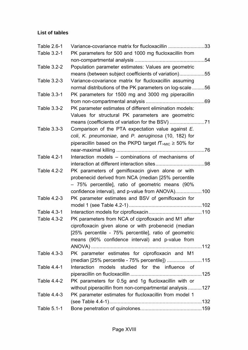
List of tables
Table 2.6-1 Variance-covariance matrix for flucloxacillin ..........................33 Table 3.2-1 PK parameters for 500 and 1000 mg flucloxacillin from
non-compartmental analysis ..................................................54 Table 3.2-2 Population parameter estimates: Values are geometric
means (between subject coefficients of variation)..................55 Table 3.2-3 Variance-covariance matrix for flucloxacillin assuming
normal distributions of the PK parameters on log-scale .........56 Table 3.3-1 PK parameters for 1500 mg and 3000 mg piperacillin
from non-compartmental analysis ..........................................69 Table 3.3-2 PK parameter estimates of different elimination models:
Values for structural PK parameters are geometric means (coefficients of variation for the BSV) .........................71
Table 3.3-3 Comparison of the PTA expectation value against E. coli, K. pneumoniae, and P. aeruginosa (10, 182) for piperacillin based on the PKPD target fT>MIC ≥ 50% for near-maximal killing ...............................................................76
Table 4.2-1 Interaction models – combinations of mechanisms of interaction at different interaction sites...................................98
Table 4.2-2 PK parameters of gemifloxacin given alone or with probenecid derived from NCA (median [25% percentile – 75% percentile], ratio of geometric means (90% confidence interval), and p-value from ANOVA)...................100
Table 4.2-3 PK parameter estimates and BSV of gemifloxacin for model 1 (see Table 4.2-1) ....................................................102
Table 4.3-1 Interaction models for ciprofloxacin......................................110 Table 4.3-2 PK parameters from NCA of ciprofloxacin and M1 after
ciprofloxacin given alone or with probenecid (median [25% percentile - 75% percentile], ratio of geometric means (90% confidence interval) and p-value from ANOVA) ...............................................................................112
Table 4.3-3 PK parameter estimates for ciprofloxacin and M1 (median [25% percentile - 75% percentile]) .........................115
Table 4.4-1 Interaction models studied for the influence of piperacillin on flucloxacillin ...................................................125
Table 4.4-2 PK parameters for 0.5g and 1g flucloxacillin with or without piperacillin from non-compartmental analysis ..........127
Table 4.4-3 PK parameter estimates for flucloxacillin from model 1 (see Table 4.4-1)..................................................................132
Table 5.1-1 Bone penetration of quinolones............................................159
Page XIX
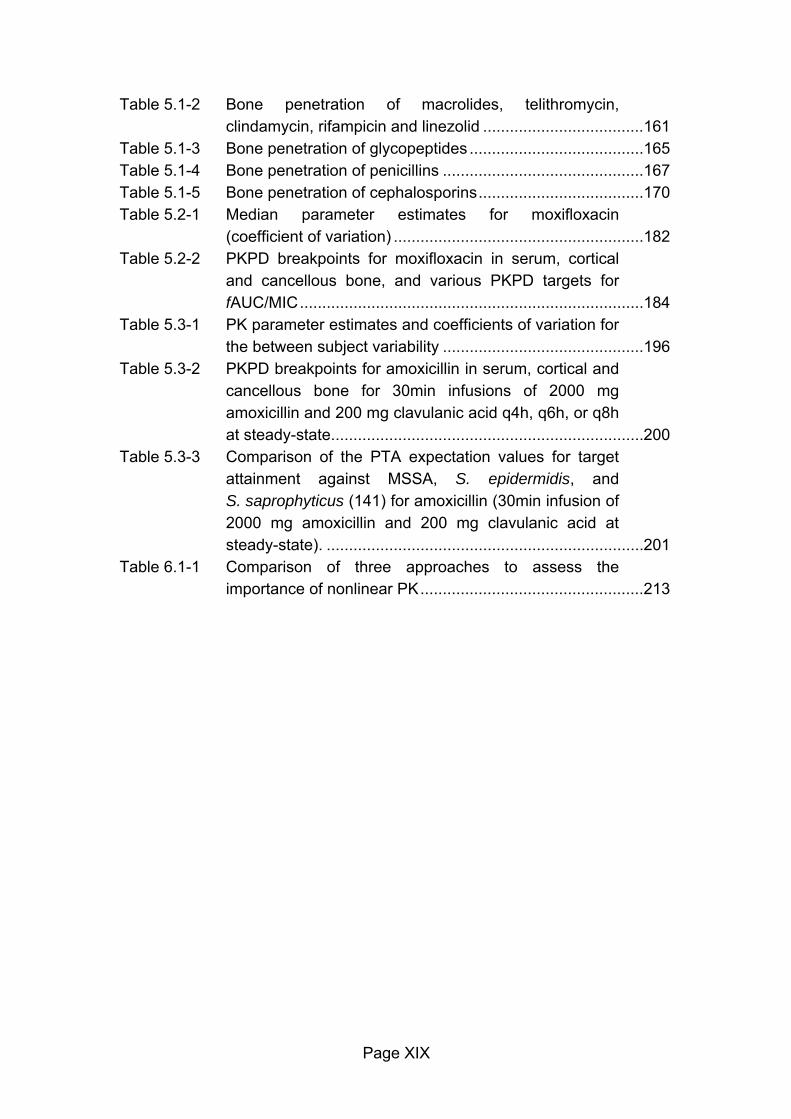
Table 5.1-2 Bone penetration of macrolides, telithromycin, clindamycin, rifampicin and linezolid ....................................161
Table 5.1-3 Bone penetration of glycopeptides .......................................165 Table 5.1-4 Bone penetration of penicillins .............................................167 Table 5.1-5 Bone penetration of cephalosporins.....................................170 Table 5.2-1 Median parameter estimates for moxifloxacin
(coefficient of variation) ........................................................182 Table 5.2-2 PKPD breakpoints for moxifloxacin in serum, cortical
and cancellous bone, and various PKPD targets for fAUC/MIC.............................................................................184
Table 5.3-1 PK parameter estimates and coefficients of variation for the between subject variability .............................................196
Table 5.3-2 PKPD breakpoints for amoxicillin in serum, cortical and cancellous bone for 30min infusions of 2000 mg amoxicillin and 200 mg clavulanic acid q4h, q6h, or q8h at steady-state......................................................................200
Table 5.3-3 Comparison of the PTA expectation values for target attainment against MSSA, S. epidermidis, and S. saprophyticus (141) for amoxicillin (30min infusion of 2000 mg amoxicillin and 200 mg clavulanic acid at steady-state). .......................................................................201
Table 6.1-1 Comparison of three approaches to assess the importance of nonlinear PK..................................................213
Page XX
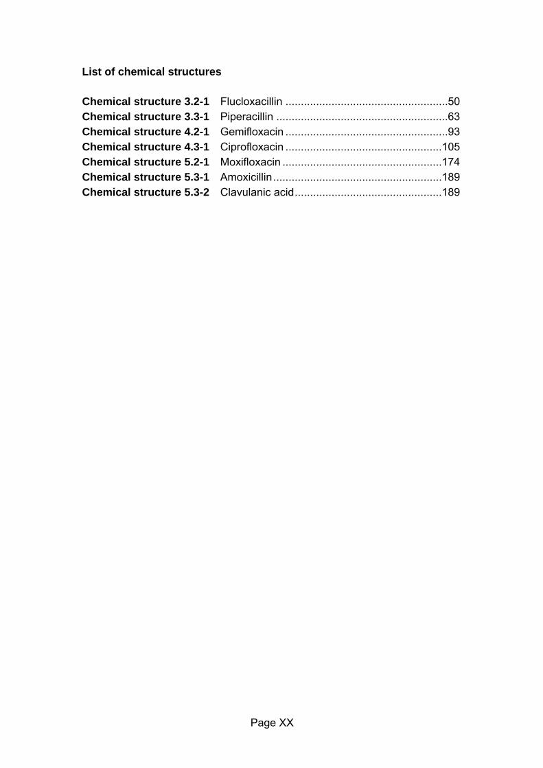
List of chemical structures
Chemical structure 3.2-1 Flucloxacillin .....................................................50 Chemical structure 3.3-1 Piperacillin ........................................................63 Chemical structure 4.2-1 Gemifloxacin .....................................................93 Chemical structure 4.3-1 Ciprofloxacin ...................................................105 Chemical structure 5.2-1 Moxifloxacin ....................................................174 Chemical structure 5.3-1 Amoxicillin.......................................................189 Chemical structure 5.3-2 Clavulanic acid................................................189
Pharmacokinetics & pharmacodynamics Introduction Definitions, applications, and objectives
Page 1
1 Introduction
1.1 Pharmacokinetics
1.1.1 Definition of pharmacokinetics
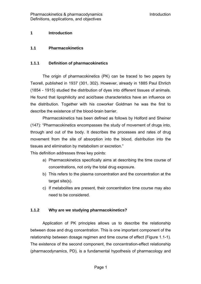
The origin of pharmacokinetics (PK) can be traced to two papers by
Teorell, published in 1937 (301, 302). However, already in 1885 Paul Ehrlich
(1854 - 1915) studied the distribution of dyes into different tissues of animals.
He found that lipophilicity and acid/base characteristics have an influence on
the distribution. Together with his coworker Goldman he was the first to
describe the existence of the blood-brain barrier.
Pharmacokinetics has been defined as follows by Holford and Sheiner
(147): “Pharmacokinetics encompasses the study of movement of drugs into,
through and out of the body. It describes the processes and rates of drug
movement from the site of absorption into the blood, distribution into the
tissues and elimination by metabolism or excretion.”
This definition addresses three key points:
a) Pharmacokinetics specifically aims at describing the time course of
concentrations, not only the total drug exposure.
b) This refers to the plasma concentration and the concentration at the
target site(s).
c) If metabolites are present, their concentration time course may also
need to be considered.
1.1.2 Why are we studying pharmacokinetics?
Application of PK principles allows us to describe the relationship
between dose and drug concentration. This is one important component of the
relationship between dosage regimen and time course of effect (Figure 1.1-1).
The existence of the second component, the concentration-effect relationship
(pharmacodynamics, PD), is a fundamental hypothesis of pharmacology and

Pharmacokinetics & pharmacodynamics Introduction Definitions, applications, and objectives
Page 2
Concentration Effect Dose PK PD
has been documented for many drugs (149). Therefore, by predicting the time
course of drug concentrations we have made one important step towards
predicting the time course of drug effect.
Figure 1.1-1 Dose – concentration – effect relationship
If the same dosage regimen of a drug is given to different patients,
there is true between subject variability (BSV) in the observed drug
concentrations. For cytotoxic drugs, the total exposure of two patients may
differ by a factor of two to ten at the same dose (311). After oral administration
of 50 mg etoposide to seven patients, the coefficient of variation for total drug
exposure was 58% (136). Assuming a log-normal distribution of drug
exposure, this corresponds to a ratio of about 10 for the 95th percentile of the
distribution of exposures divided by the 5th percentile (chapter 2.8.1).
A reason for high BSV may be that patients differ in their ability to
absorb or eliminate a drug. By including the variability of the PK parameters
into a PK model, one can predict drug effect more precisely and optimize
dosage regimens for the patient population. This provides a basis for choosing
dosage regimens at initiation of therapy, i.e. when no PK information about
the patient is available. In addition to the PK model, knowledge about the
concentration-effect relationship (see below) is necessary to optimize dosage
regimens. If the concentration-effect relationship is known, the PK model
alone can be used to make predictions about drug effect (147).
1.2 Pharmacodynamics
Pharmacodynamics (PD) is “the study of the biochemical and
physiological effects of drugs and the mechanisms of their actions” (89). It
describes the relationship between concentration and drug effect. The
Pharmacokinetics & pharmacodynamics Introduction Definitions, applications, and objectives
Page 3
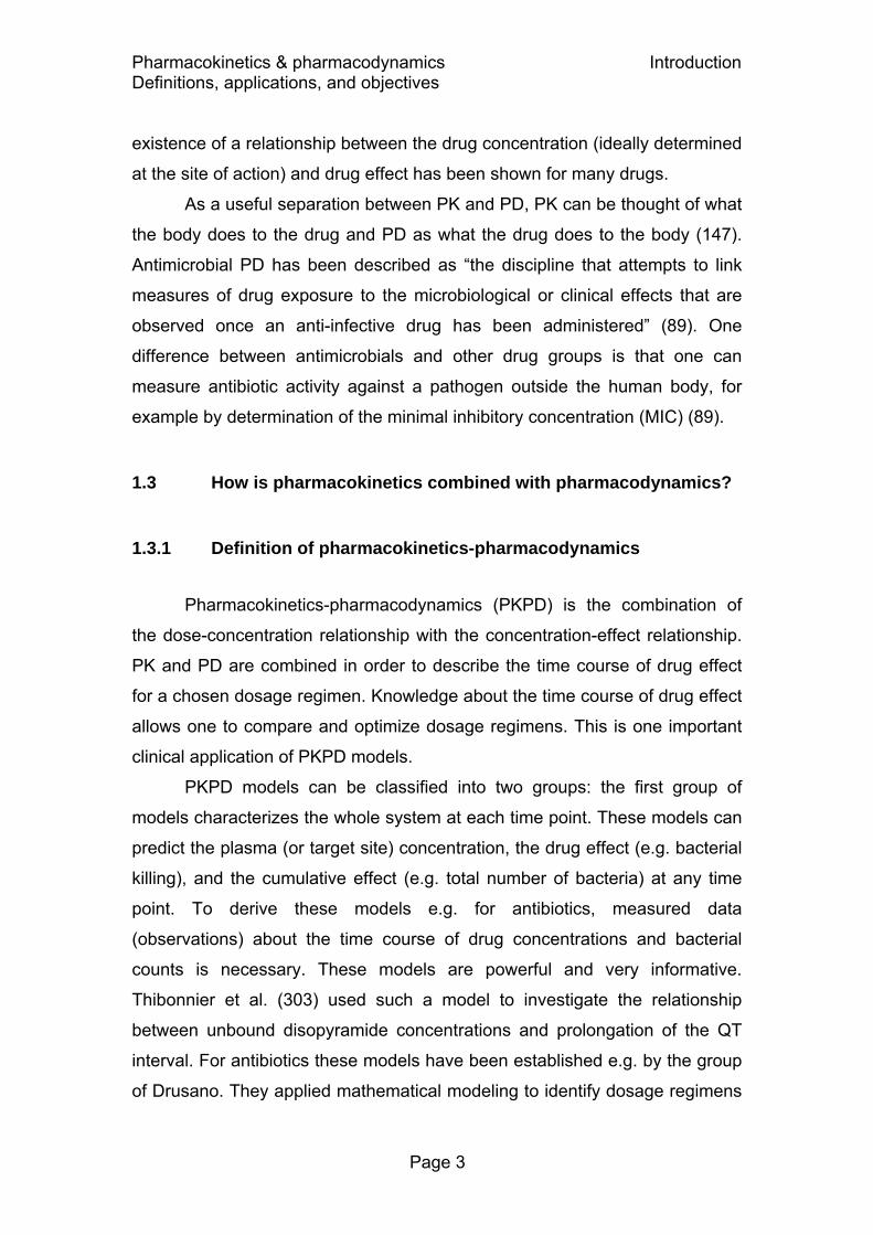
existence of a relationship between the drug concentration (ideally determined
at the site of action) and drug effect has been shown for many drugs.
As a useful separation between PK and PD, PK can be thought of what
the body does to the drug and PD as what the drug does to the body (147).
Antimicrobial PD has been described as “the discipline that attempts to link
measures of drug exposure to the microbiological or clinical effects that are
observed once an anti-infective drug has been administered” (89). One
difference between antimicrobials and other drug groups is that one can
measure antibiotic activity against a pathogen outside the human body, for
example by determination of the minimal inhibitory concentration (MIC) (89).
1.3 How is pharmacokinetics combined with pharmacodynamics?
1.3.1 Definition of pharmacokinetics-pharmacodynamics
Pharmacokinetics-pharmacodynamics (PKPD) is the combination of
the dose-concentration relationship with the concentration-effect relationship.
PK and PD are combined in order to describe the time course of drug effect
for a chosen dosage regimen. Knowledge about the time course of drug effect
allows one to compare and optimize dosage regimens. This is one important
clinical application of PKPD models.
PKPD models can be classified into two groups: the first group of
models characterizes the whole system at each time point. These models can
predict the plasma (or target site) concentration, the drug effect (e.g. bacterial
killing), and the cumulative effect (e.g. total number of bacteria) at any time
point. To derive these models e.g. for antibiotics, measured data
(observations) about the time course of drug concentrations and bacterial
counts is necessary. These models are powerful and very informative.
Thibonnier et al. (303) used such a model to investigate the relationship
between unbound disopyramide concentrations and prolongation of the QT
interval. For antibiotics these models have been established e.g. by the group
of Drusano. They applied mathematical modeling to identify dosage regimens

Pharmacokinetics & pharmacodynamics Introduction Definitions, applications, and objectives
Page 4
that suppress emergence of resistance during antibiotic therapy with
levofloxacin (166) or moxifloxacin (133).
The second group of models uses a surrogate target to predict the
treatment outcome. An example for this type of models is a study by Drusano
et al. (93) on rational dose selection for clinical trials with evernimicin. For
antibiotics the outcome is often microbiological or clinical success. Surrogate
targets for successful outcome of antibiotic treatment have been developed by
Craig et al. (67) and others. Those simplified models assume that achieving a
surrogate target is equivalent to microbiological or clinical success. Therefore,
it is not necessary to investigate the full time course of drug effect. Those
models can be implemented more easily and no data on the PD effect is
required once a surrogate target has been established and validated and is
applicable to the patient population of interest. By use of a surrogate target,
prior knowledge about the drug or drug group is incorporated into the model.
1.3.2 Advantages of pharmacokinetic-pharmacodynamic models
PK models alone cannot predict the time course or magnitude of drug
effect (148), since they do not account for the concentration-effect relationship
(PD model). Combination of PK and PD models allows one to describe the full
time course of the interaction between the drug and the body. For
antibacterials, such a PKPD model can describe the growth and killing of
bacteria over time dependent on the drug concentration-time course.
Understanding the time course of drug effect is important to optimize the
clinical benefit (148).
A PKPD model can be extremely helpful, if there is a delay between the
dose and the observed response. Such a delay can be caused by PK, PD or
by both. Once a PKPD model is established, the predicted time course of
response can be compared to the observed response in a patient. Comparing
the predicted and observed response may be very helpful to guide future
decisions on the dosage regimen. Vinks et al. presented a clinical application
of modeling the time course of bacterial growth and killing for aminoglycoside
therapy in dialysis patients at the Interscience Conference on Antimicrobial

Pharmacokinetics & pharmacodynamics Introduction Definitions, applications, and objectives
Page 5
Agents and Chemotherapy (ICAAC) 2005. It was shown that understanding
the time course of bacterial killing may greatly support selection of future
dosage regimens.
1.3.3 Clinical applications
Application of PKPD models can be used to improve treatment
success. Two different strategies to optimize drug-related response are
therapeutic drug monitoring (TDM) and target concentration intervention (TCI).
TDM aims at adjusting plasma drug concentrations of patients within a target
range of plasma concentrations (therapeutic window). This range is usually
derived from observation of therapeutic and adverse effects in small groups of
patients (36). Different drug effects in patients that receive the same dose can
arise from both PK and PD variability. TDM seeks to reduce the PK variability
by adjusting drug concentrations to a target range.
TDM uses the same target range for each patient and assumes that all
patients have the same therapeutic window. However, the concentration-
effect relationship might not be the same for all patients and PD variability is
not reduced by TDM. TDM has its greatest benefit, if there is only a small
range between effective and toxic concentrations, and if there is large
variability in drug concentrations between patients. If there is no readily
available measure of drug effect, like for example blood pressure (36), the
safe and effective use of a drug might require TDM. Gentamicin and
theophylline are monitored by TDM, as both are drugs with a narrow
therapeutic window and serious adverse effects (36, 323). In a meta-analysis
of 52 studies, Kim et al. (174) applied Bayes theorem to investigate the
incidence of aminoglycoside-associated nephrotoxicity related to once daily
dosing, multiple daily dosing, and individualized PK monitoring. Individualized
PK monitoring used patient specific PK parameters for designing dosage
regimens that are likely to achieve the desired peak and trough
concentrations. This approach resulted in lower probabilities for nephrotoxicity
(incidence rate: 10 to 11%) than once daily (12 to 13%) and multiple daily
dosing (13 to 14%) by use of nomograms.

Pharmacokinetics & pharmacodynamics Introduction Definitions, applications, and objectives
Page 6
The target serum concentration range for TDM of theophylline is 10 to
20 mg/L (36, 323). In a randomized double-blind study in patients on
intravenous theophylline the target concentrations 10 and 20 mg/L were
compared. There was no difference in treatment success between the two
groups, but significantly more toxicity in the 20 mg/L group (144).
A target range introduces variability, as practitioners might aim for any
concentration within this range and drug effect changes continuously
throughout the concentration range. Therefore, a target concentration strategy
has been proposed (146). TCI seeks to select the best dose to achieve the
desired therapeutic effect. TCI aims at a drug effect in the individual patient
and not at a concentration range that is the same for the whole population.
Concentration measurements are used to determine the individual PK
parameters in order to optimize future dosage regimens (146). Patient and
disease specific factors like body weight or creatinine clearance can be
included in the calculations to individualize PK parameters. That way, PK and
PD concepts are combined with information about the individual patient and
disease in TCI (146).
1.3.4 Applications for drug development
There are numerous applications of PKPD models in drug development.
Some examples are:
1) Selection of optimal dosage regimens to be studied in future clinical
trials,
2) decision about continuation or abandonment of clinical drug
development,
3) optimal design of clinical trials, including the number of subjects and
number of samples per subject, and
4) visualization and application of already available knowledge (data).
Selection of optimal dosage regimens for clinical studies is extremely
important as, according to a report from the US Food and Drug Administration
(FDA) from 2003, almost 50% of phase III trials do not succeed, often due to
Pharmacokinetics & pharmacodynamics Introduction Definitions, applications, and objectives
Page 7
poor dose selection. Therefore the FDA requests sponsors to present
exposure-response analyses to support dose selection for further clinical trials
(190). Pre-clinical data from e.g. in vitro or animal studies can be used in
PKPD models to select optimal dosage regimens for clinical studies.
Oritavancin is a new glycopeptide antibiotic and an example for the
application of PKPD models during clinical development. Bhavnani et al. (33)
studied the relationship between oritavancin exposure and microbiological and
clinical outcome in 55 patients with Staphylococcus aureus bacteremia to
select optimal dosage regimens for future clinical trials. It was established that
the time that the free drug concentration remains above the minimum
inhibitory concentration (fT>MIC) correlated with microbiological as well as with
clinical success (see also chapter 2.7.1). A percentage of the fT>MIC of 22% of
the dosing interval resulted in a probability of 93% for microbiological and of
87% for clinical success. Rational dose selection by use of such a PKPD
model allows one to optimize the information which will be gained from future
clinical studies.
Another example for optimization of dosage regimens is a study by
Gumbo et al. (133). They used an in vitro infection model, human PK data,
and PKPD modeling to identify a moxifloxacin dose that is likely to achieve a
successful microbiological outcome and suppress resistance of
Mycobacterium tuberculosis against moxifloxacin. They intended to provide
optimal dosage regimens for future clinical trials on the use of moxifloxacin
against tuberculosis. A ratio of the area under the non-protein bound
concentration vs. time curve to the MIC of the pathogen of 53 (fAUC/MIC=53)
was associated with complete suppression of the drug resistant mutants. A
dose of 800 mg per day is likely to achieve excellent microbial kill and
supression of resistant mutants. Predictions about emergence of resistance,
or about which PKPD target is associated with effectiveness or resistance
could not have been made without PKPD modeling.
There may be situations where PKPD modeling suggests to stop
further development of a drug. As the PD of antibiotics can be measured in
vitro, phase I PK data and in vitro activity data can be combined to predict the
probability of efficacious treatment for antibiotics in future clinical trials.

Pharmacokinetics & pharmacodynamics Introduction Definitions, applications, and objectives
Page 8
Drusano et al. (93) performed the first such analysis in the field of anti-
infectives. They combined pre-clinical microbiological and animal model data
with PK data from early phase I studies to identify efficacious dosage
regimens for evernimicin. A low probability of successful treatment was
predicted even for the optimized dosage regimens of evernimicin. For a dose
of 9 mg/kg the probability of attaining 90% of the maximum effect was 98% for
Streptococcus pneumoniae, but only 51% for S. aureus and 75% for
Enterococcus ssp. Those predictions were confirmed by phase II/III clinical
trials. In these trials no sufficient advantage of evernimicin over approved
antibiotics could be shown for treatment of infections by vancomycin
susceptible and resistant gram-positive bacteria. Subsequently, evernimicin
did not reach the market. This is one example that shows, how PKPD
modeling could save millions of dollars spent on phase II/III clinical trials.
Once the decision has been taken to continue clinical development, it is
a formidable task to optimize the design of clinical trials. There is a
tremendous amount of resources and time involved in the performance and
analysis of phase II/III clinical trials. Therefore, it would be very valuable to
increase the chance of success for those clinical trials. By optimization of the
design with PKPD models, future clinical studies can be made considerably
more cost-effective (95, 267).
A possible application of all PKPD models is their ability to visualize
knowledge which has already been gained in past experiments. It is often
difficult to visualize and interpret the results of clinical studies with a large
number of dosage regimens, compliant and non-compliant patients, disease
progression, and patients with unstable clinical conditions (e.g. changing renal
function in ICU patients). In those situations PKPD models are probably the
only possibility to visualize the results of the clinical trials and to use the past
experience for designing new trials and dosage regimens.

Pharmacokinetics & pharmacodynamics Introduction Definitions, applications, and objectives
Page 9
1.4 Why are we studying antibiotics?
1.4.1 Drug development
Drug development is a complicated and cost-intensive process. As only
a very small percentage of drugs that are investigated eventually reaches the
market, drug development carries a high risk for the pharmaceutical industry.
The average total costs for development of a new drug have been reported as
802 million US dollars (year 2000) (84). About 80% of all drugs entering phase
I are not approved for marketing.
For treatment of infections with antibiotics usually only a relatively short
duration of therapy is required. This reduces drug development costs for
antibiotics. However, unlike other drug groups, e.g. cardiovascular drugs or
antidiabetics, antibiotics are rarely given as chronic medication. Therefore,
more patients need to be treated with an antibiotic in order to regain the high
investments in drug development. Maybe due to some of these difficulties,
currently relatively few new antibiotics seem to be developed.
As has been reported at the ICAAC in December 2005, there are at the
moment three antibiotics against gram-negative pathogens in phase II or III of
clinical development: ceftobiprole, a cephalosporin with activity against
methicillin-resistant S. aureus (MRSA), doripenem, a new carbapenem, and
garenoxacin, a Des-(F6)-quinolone (46). Tigecycline, a glycylcyline, is already
marketed in the US and waiting for final approval in the European Union (46,
343). It has been difficult to find new antibiotics that work by a completely
different mechanism of action and that have no cross-resistance (90).
Therefore it is even more important to optimize therapy with the available
antibiotics.
Pharmacokinetics & pharmacodynamics Introduction Definitions, applications, and objectives
Page 10
1.4.2 Clinical situation – drug resistance
While fewer new antibiotics are being developed, drug resistance
among pathogens is increasing in the hospital setting as well as in the
community (47). According to data from 300 microbiological laboratories
throughout the United States, resistance rates of S. aureus have increased
continuously since 1998. In March 2005, 50-60% of S. aureus isolates from
inpatients and outpatients were methicillin-resistant (MRSA). About 60% of
MRSA from inpatients and 40% from outpatients were resistant to more than
three non-beta-lactam antibiotics (298). Methicillin resistance in S. aureus
bacteremia results in significantly longer hospitalization times and higher
hospital charges than methicillin-susceptible S. aureus bacteremia (65).
At the ECCMID in April 2006, data from the European Antimicrobial
Resistance Surveillance System (EARSS), i.e. data from laboratories that
serve more than 30% of the European population, have been presented (314).
Fluoroquinolone resistance in Escherichia coli continues to increase in most
European countries. Rates of MRSA are rising in Northern and Central
Europe. Recently, in Germany, France and Ireland, the rate of vancomycin
resistant Enterococcus faecium has increased significantly.
PKPD models are helpful for the choice of the most suitable drug,
selection of optimal dosage regimens, reduction of toxicity and prevention of
resistance, among other purposes. By application of PKPD modeling, the
probability for successful microbiological or clinical outcome can be predicted
for each drug and pathogen. The highest MIC for which a PKPD target is
attained with a probability of at least 90% is often defined as the PKPD
breakpoint. There is a high probability of successful treatment, if the individual
MIC of the infecting pathogen is lower than the PKPD breakpoint. To prevent
further emergence of resistance, antibiotics that are the treatment of choice
against nosocomial infections or in intensive care units should not be used for
less severe infections, if there is an alternative antibiotic with a sufficiently
high PKPD breakpoint. In the case of severe infections by problematic
pathogens like Pseudomonas aeruginosa, PKPD models for combinations of
two or more drugs may guide therapy, as they can predict up to which MIC of
Pharmacokinetics & pharmacodynamics Introduction Definitions, applications, and objectives
Page 11
a pathogen the dosage regimen will be successful. Hope et al. (151) applied
PKPD models to investigate and optimize antifungal combination therapy.
Combination chemotherapy is sometimes applied to increase the chance of
drug susceptibility in empiric therapy and to maximize effectiveness.
After choosing the most promising drug, optimal dosage regimens for
the antibiotic should be selected to further increase the PKPD breakpoint. This
applies to both, empirical treatment and individualized dosage regimens.
Other treatment outcomes to be optimized by PKPD models are reduction of
toxicity (261) and prevention of selection of resistant mutants (chapter 1.3.4).
1.5 Why are we studying healthy volunteers?
Our dose linearity and drug interaction studies were performed in
healthy volunteers as the variability in healthy volunteers is usually much
lower (e.g. 2-10 times lower variance) than in ill patients. Healthy volunteer
studies have the advantage that e.g. food and fluid intake, clinical procedures,
and drug administration are highly standardized and supervised or performed
by professional investigators. Those standardized trial designs are difficult to
perform in parallel to routine clinical practice. In a crossover study, subjects
act as their own controls and therefore, BSV, a considerable component of the
total variability, is removed from the comparison. However, it is not feasible to
perform crossover studies in patients who need antibiotic treatment against an
acute infection. Also, in healthy volunteer studies, there is no bias from an
impaired renal function or from intake of co-medication, whereas both is often
the case in hospitalized patients.
If frequent blood samples are collected, more information can be
gained about the pathways of elimination and about the mechanisms of PK
drug-drug interactions. This is especially true for complex PK models, to which
population PK sometimes cannot be applied due to exhaustive computation
time. It is not practical to obtain more than ten blood samples per day from a
patient and the same total blood loss might be more critical for an ill patient
than for a healthy volunteer.
Pharmacokinetics & pharmacodynamics Introduction Definitions, applications, and objectives
Page 12
For exploring mechanisms of PK interactions or elimination, as in the
dose linearity and interaction studies described in this thesis, it is
advantageous to study healthy volunteers. However, if dosage regimens are
developed from a healthy volunteer study, it needs to be considered that ill
patients might differ in their PK from healthy volunteers. We used PK data
from healthy volunteers to calculate the probabilities of attaining a PKPD
target (PTA) which is associated with successful clinical outcome (for details
see chapter 2.7). Compared to healthy volunteers, patients often have lower
clearances and larger volumes of distribution, which result in higher average
plasma concentrations and longer elimination half-lives. Both these alterations
for the PK in patients increase the PTA. Thus, our estimates for the PTA in
healthy volunteers are conservative (i.e. low) estimates for the PTA in
patients. Lodise et al. (194) compared data from healthy volunteers to
hospitalized patients after administration of piperacillin / tazobactam, and
report an approximately 27% lower total body clearance and a higher volume
of distribution of piperacillin at steady-state for patients. Consequently they
found lower PTAs for healthy volunteers than for patients.
We studied bone concentrations of antibiotics in patients undergoing
hip replacement due to arthrosis. Knowledge about antibiotic concentrations in
bone is useful for prophylaxis in orthopedic surgery and for treatment of
osteomyelitis. Samples from volunteers undergoing joint replacement have
the advantage that there are no pathological changes to the bone tissue. In
patients suffering from bone infections the tissue is usually changed due to
inflammation, existence of pus, or sequesters. Therefore the variability of
bone concentrations in joint replacement patients is probably lower than in
osteomyelitis patients. After the methodology of bone sample preparation and
drug analysis has been optimized in joint replacement patients, further studies
in osteomyelitis patients are required to investigate the influence of disease
state on bone penetration of antibiotics. We chose hip replacement patients
with arthrosis for our investigations on antibiotic bone penetration.

Pharmacokinetics & pharmacodynamics Introduction Definitions, applications, and objectives
Page 13
1.6 Contributions by the author of this thesis
The clinical and bio-analytical parts of the dose linearity and drug-drug
interaction studies described in this thesis were conducted by the group of
Professor Dr. Fritz Sörgel, head of the Institute for Biomedical and
Pharmaceutical Research – IBMP, before the start of this Ph.D. work. The
author contributed to the clinical and bio-analytical work related to the
moxifloxacin bone penetration study. The PKPD data analyses, simulations
and literature searches were conducted by the author. The reporting of the
results including all PKPD data analyses, introductions and discussions, but
not the details of the bio-analytical section of the respective projects, was
done by the author of this thesis.
1.7 Aims and scopes
1.7.1 General aims and scopes
The overall aim of this thesis was to study the pharmacokinetic and
pharmacodynamic aspects of saturable elimination, drug-drug interactions
and bone penetration of antibiotics by applying population PKPD techniques.
Our general aim was to optimize antibiotic dosage regimens by application of
PKPD modeling and Monte Carlo simulation (MCS). We combined the known
pharmacology of the respective group of antibiotics with the PK properties and
the bacterial susceptibility data to predict the probability for successful
therapy. Our population PKPD models specifically account for the true
between subject variability. This carries great advantages compared to
standard non-compartmental analysis (NCA) especially for MCS. If the
variability and correlation of PK parameters is known for a patient population,
the pharmacological response and probability for successful therapy can be
predicted by a population PKPD model in a MCS. The objectives of our
individual studies are described in chapters 1.7.2 to 1.7.4. The individual

Pharmacokinetics & pharmacodynamics Introduction Definitions, applications, and objectives
Page 14
studies and study drugs are described monographically in the respective
chapters of this thesis. PKPD modeling was expected to be advantageous for
our study objectives compared to solely performing NCA and it was expected
that different modeling approaches and programs would be necessary to deal
with different problems.
1.7.2 Dose linearity
We studied the effect of a possible saturable elimination on the choice
of optimized dosage regimens for piperacillin and flucloxacillin. Our first
objective was to compare the PK at two dose levels for both drugs. We
studied the extent of a possible saturation in the renal and nonrenal
elimination at therapeutic concentrations. Our second objective was to study
dosage regimens with an optimized PKPD profile. Our third objective was to
estimate the influence of saturable elimination on the PKPD profile. This
allowed us to estimate the clinical relevance of the saturation of elimination at
therapeutic doses.
Saturable elimination of piperacillin has been discussed in literature for
more than two decades, but so far no final conclusion has been drawn.
Controversial results have been reported about the existence of nonlinear
piperacillin PK at therapeutic concentrations. As a few newer studies indicate
that saturable elimination of piperacillin may exist, it was expected to find
saturable elimination. For flucloxacillin there was no indication for nonlinearity
of PK in literature, but no population PK analysis has been published yet.
1.7.3 Pharmacokinetic drug-drug interactions
We assessed the extent, site, time course and possible mechanisms of
PK drug-drug interactions in vivo and studied the possible therapeutic benefit
of inhibiting the clearance of one drug by an inhibitor. The first objective of our
interaction studies was to investigate the extent of change in drug exposure
that is caused by PK drug-drug interactions between two quinolones and
probenecid, and between two beta-lactams. The second objective was to
Pharmacokinetics & pharmacodynamics Introduction Definitions, applications, and objectives
Page 15
describe the time course and plausible mechanisms for the interactions at
possible sites of interaction by developing full mechanistic interaction models.
We were especially interested in the influence of probenecid on the formation
and elimination of ciprofloxacin’s 2-aminoethylamino-metabolite (M1). Such
full mechanistic interaction models have the power to predict the time course
of a PK interaction for other dosage regimens of interest. This allows one to
predict the potential clinical impact of such a PK drug-drug interaction. It was
expected that drug-drug interactions exist between the two beta-lactams
investigated and between the two quinolones and probenecid due to their
common and saturable pathways of elimination.
1.7.4 Bone penetration
The extent and time course of antibiotic bone penetration is important
to assure antibiotic effectiveness in prophylaxis and treatment of bone
infections. However, advanced techniques of PK analysis have not yet been
applied to bone penetration data for antibiotics. After a literature review on
antibiotic bone penetration, we applied population PKPD models to describe
the time course of bone and serum concentrations and to optimize antibiotic
dosage regimens for treatment of bone infections.
The primary objective of our overview of bone penetration studies from
literature was to compare the different methods that have been used to
assess bone penetration. The need of standardized methods for drug analysis
in bone, PK evaluation of bone penetration studies, and reporting of their
results is discussed. A short overview of the results from bone penetration
studies is given.
The first objective of the bone penetration studies was to determine
antibiotic concentrations in cancellous and cortical bone in a controlled study
in subjects undergoing hip replacement surgery. As our second objective, we
intended to develop a PK model to describe the time course of antibiotic
concentrations in bone as well as the exposure of these drugs in bone relative
to serum. Our third objective was to assess the PKPD profile in serum,
cortical, and cancellous bone. Reports from literature, that were evaluated for

Pharmacokinetics & pharmacodynamics Introduction Definitions, applications, and objectives
Page 16
the overview of antibiotic bone penetration, show that quinolone antibiotics
often achieve higher bone penetration than beta-lactams. Therefore, a
moderate to high extent of penetration of moxifloxacin into bone and a lower
extent of penetration of amoxicillin and clavulanic acid were expected.

General methods, procedures & modeling Materials & methods
Page 17
2 General methods, procedures and modeling
2.1 Study participants
Ten to twenty-four Caucasian subjects (females and males),
participated in each PK study. Prior to entry into the study, all subjects were
given a physical examination, electrocardiography and laboratory tests,
including analysis of urine samples for various laboratory values (urinalysis),
and screening for drugs of abuse. During the drug administration periods, the
volunteers were encouraged to report any discomfort or adverse reactions,
and were closely observed by physicians. Each day of the study the subjects
were asked to complete a questionnaire on their health status. All studies
were approved by the local ethics committees, and all subjects gave their
written informed consent prior to entering the respective study.
2.2 Study design and drug administration
The interaction and dose linearity studies were randomized controlled
crossover studies. Food and fluid intake were strictly standardized. Treatment
periods were separated by a washout period of at least four to seven days,
depending on the half-life of the study drugs. Subjects were requested to
abstain from alcohol and caffeine containing products during the study
periods. The bone penetration studies were not randomized as only one
treatment was studied, and this treatment was the same for all subjects.
2.3 Sample collection
All blood samples were drawn from a forearm vein via an intravenous
catheter contralateral to the one used for drug administration. In each of the
dose linearity and interaction studies 13, 19 or 23 blood samples were drawn
from each subject up to 24 or 48h after administration plus one sample
immediately before administration. Urine was collected from the time of

General methods, procedures & modeling Materials & methods
Page 18
administration until 24, 72 or 96h after administration, divided into nine, ten or
eleven sampling intervals.
In the bone penetration studies, blood samples were collected pre-dose
and at the time of femoral bone resection. Hip replacement involved resection
of the femoral head, or both femoral head and femoral neck, prior to
implantation of the prosthetic hip joint. Bone samples consisted of femoral
head or femoral head and femoral neck. Blood and bone samples for drug
analysis were collected 2 to 7h after oral administration of moxifloxacin and 0
to 1.1h after the end of the amoxicillin / clavulanic acid infusion. Bone samples
were immediately frozen on dry ice and stored at -70°C until analysis.
2.4 Sample preparation
2.4.1 Serum and plasma samples
When serum was obtained, blood samples were allowed to clot before
centrifugation. After centrifugation serum or plasma samples were
immediately frozen and stored at -20°C (gemifloxacin and ciprofloxacin) or at
-70°C (moxifloxacin and beta-lactams) until analysis. All quinolones and
probenecid were protected from sunlight throughout sample preparation and
analysis to prevent degradation of the study drugs from daylight exposure.
Blood samples containing beta-lactams were cooled in an ice-water bath
before centrifugation at 4°C to prevent degradation at room temperature.
Spiked quality controls (SQC) in human plasma or serum were prepared for
control of inter-assay variation. Defined volumes of the stock solution or of an
SQC of higher concentration were added to defined volumes of tested drug-
free plasma or serum samples.
2.4.2 Urine samples
Urine samples containing beta-lactams were stored at 4°C during the
collection period. The amount and pH of the urine were measured. After

General methods, procedures & modeling Materials & methods
Page 19
shaking the samples, aliquots were taken, immediately frozen and stored at
-20°C (gemifloxacin and ciprofloxacin) or -70°C (moxifloxacin and beta-
lactams) until analysis. SQCs in human urine were prepared by adding
defined volumes of the stock solution or of an SQC of higher concentration to
defined volumes of tested drug-free urine samples.
2.4.3 Bone samples
Bone specimens consisting of femoral head and femoral neck, were
separated into femoral head and femoral neck. Then the samples were
separated into cortical and cancellous tissue. Adhering blood was removed
from the samples that were then pulverized under liquid nitrogen by a
cryogenic mill (Freezer/Mill®). All moxifloxacin samples were protected from
sunlight during sample handling and analysis. For analysis of bone samples,
calibration standards and SQCs were prepared by adding appropriate
amounts of standard solutions to bone tissue that was shown to be free of the
study drug.
2.5 Determination of drug concentrations
The general principles of the methods used for drug determination are
described here. Assay details are included in the respective methods sections
of chapters 3 to 5.
2.5.1 HPLC with UV or fluorescence detection
High performance liquid chromatography (HPLC) is a frequently used
method for bioanalytical determination of drug concentrations. The drug to be
analyzed is chromatographically separated from the other components of the
sample and then quantified. Chromatography is a physical method of
separation. The components partition between a mobile and a stationary
phase. In HPLC the sample to be analyzed is dissolved in a solvent and then
transported with the mobile phase under high pressure over the stationary

General methods, procedures & modeling Materials & methods
Page 20
phase. The solutes are separated due to differences in their affinity to the two
phases. In normal phase HPLC, the stationary phase is more polar than the
mobile phase, however reversed phase HPLC is more common in bioanalysis
of antibiotics. In reversed phase HPLC the mobile phase is more polar than
the stationary phase, and polar substances are eluted faster than nonpolar
substances, as polar substances have less affinity to the stationary phase.
Thus, reversed phase HPLC is most useful for nonpolar drugs or compounds
with low polarity at the chosen pH.
The mobile phase is usually a mixture of different solvents. In isocratic
elution the mixture is the same during the whole analysis. If the use of a single
mobile phase composition does not result in adequate separation of all
compounds, often gradient elution is advantageous. In gradient elution the
composition of the mobile phase changes in a pre-defined way during the
analysis of each sample to improve the resolution or shorten retention times.
This change can be continuous or stepwise. In gradient elution the strength of
the mobile phase to elute the analyte is increased during the analysis. In
reversed phase HPLC this means that the mobile phase becomes less polar.
Therefore the retention times of compounds with very high affinity to the
stationary phase are shortened and sharper peaks for those compounds are
obtained. In reversed phase HPLC the mobile phase is often a mixture
containing water, buffers, methanol, acetonitrile or tetrahydrofuran.
The stationary phase consists of small particles, that produce a bed
with a very high flow impedance. Consequently, very high pressures are
necessary to force the mobile phase through the column. In reversed phase
HPLC the stationary phase consists of silica gel with hydrocarbon chains that
are bound to the surface. The polarity of the stationary phase depends on the
length of the hydrocarbon chains. Common stationary phases contain C8 or
C18 chains.
A HPLC system consists of one or more pumps, an injection system, a
column, a detector, and a computer (Figure 2.5-1). The pump pushes the
mobile phase through the system with a constant or changing flow rate. The
injector transports the sample into the mobile phase. The column is a
stainless steel tube that contains the stationary phase.

General methods, procedures & modeling Materials & methods
Page 21
Figure 2.5-1 Block diagram of a HPLC system
adapted from reference (326)
The detector detects the compounds as they elute from the column by
measuring response changes between the mobile phase alone and the mobile
phase containing the sample. The electrical response from the detector is
recorded and sent to a data system. A peak on the chromatogram is
observed.
The most appropriate method of detection depends on the properties of
the drug to be quantified. Besides mass spectrometers, ultraviolet (UV)
detectors and fluorescence detectors are two of the most common detectors.
A UV detector measures the ability of a sample to absorb light at one or
several wavelengths. As many compounds contain conjugated π-electron
systems that can act as chromophores and absorb UV light, this detector is
widely applied. The solvents that make up the mobile phase should not
absorb UV light at the same wavelengths as the analyte. The Beer-Lambert
law describes the relationship between the intensity of the transmitted light
and the concentration of the analyte in the solution.
Fluorescence detectors measure the ability of a compound to absorb
and then re-emit light at certain wavelengths. The excitation source passes
through the flow-cell to a photodetector while a monochromator selects the
emission wavelengths. The fluorescence detector is generally more sensitive
than UV detectors, because the excitation as well as the emission wavelength
Detector Integrator
Pump
Injector Autosampler
Solvent
HPLC column Data
Waste
General methods, procedures & modeling Materials & methods
Page 22
is specified. The emission light beam is detected in a 90° angle to the
excitation beam that goes through the sample. Therefore diffused light from
the excitation beam that might interfere with the detection is minimized. The
selected emission wavelength strikes a photomultiplier that measures the
intensity of the emission beam as a function of time. If the analyte exhibits
fluorescence, a fluorescence detector is usually a good choice as this is both
a specific and sensitive method.
For quantification of the analyte in the sample, the peaks in the
chromatogram are evaluated by different methods. Two common methods are
determination of the peak height or the peak area of the analytes. An internal
standard is used to account for variations e.g. during sample preparation or
due to inaccuracy in injection volume. The internal standard is added to each
sample in a known concentration. The peak height or peak area of the analyte
is then compared to the respective value of the internal standard. By this
method the concentration ratio between the analyte and the internal standard,
and finally the concentration of the analyte in the sample may be calculated.
2.5.2 LC-MS/MS
LC-MS is the combination of liquid chromatography (HPLC) with mass
spectrometry (MS). A mass spectrometer separates ions in the gas phase
according to their mass to charge ratio (m/z). The resulting mass spectrum is
a plot of the relative intensity vs. m/z. In LC-MS/MS, HPLC is combined with
two consecutive MS experiments by coupling multiple analyzers.
HPLC removes interferences that would influence ionization. Then an
interface eliminates the solvent and generates gas phase ions that are
transferred into the mass spectrometer. The two most common methods for
ionization are electrospray ionization (ESI) and atmospheric pressure
chemical ionization (APCI). With both techniques ionization takes place at
atmospheric pressure.
The electrospray probe consists of a metallic capillary to which a
voltage is applied. Due to the difference in potential a spray is generated at
the tip of the capillary <1> (see number <1> in Figure 2.5-2). A heated
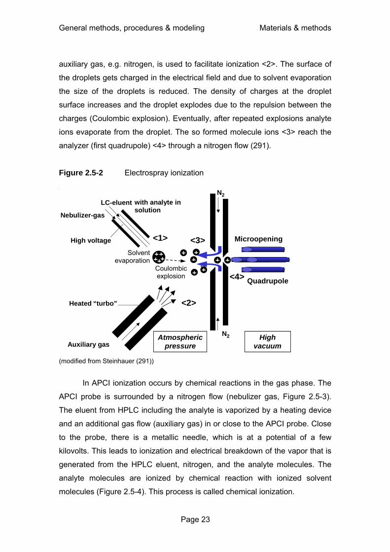
General methods, procedures & modeling Materials & methods
Page 23
auxiliary gas, e.g. nitrogen, is used to facilitate ionization <2>. The surface of
the droplets gets charged in the electrical field and due to solvent evaporation
the size of the droplets is reduced. The density of charges at the droplet
surface increases and the droplet explodes due to the repulsion between the
charges (Coulombic explosion). Eventually, after repeated explosions analyte
ions evaporate from the droplet. The so formed molecule ions <3> reach the
analyzer (first quadrupole) <4> through a nitrogen flow (291).
Figure 2.5-2 Electrospray ionization
+
Heated “turbo”
High voltage
LC- eluent with analyte in solution
Nebulizer -gas
Auxiliary gas N2
N2
Atmospheric pressure
High vacuum
Microopening
Quadrupole +
++
+
+
<1>
<2>
<3>
<4>
+ +++ +++
Coulombic explosion
Solventevaporation
(modified from Steinhauer (291))
In APCI ionization occurs by chemical reactions in the gas phase. The
APCI probe is surrounded by a nitrogen flow (nebulizer gas, Figure 2.5-3).
The eluent from HPLC including the analyte is vaporized by a heating device
and an additional gas flow (auxiliary gas) in or close to the APCI probe. Close
to the probe, there is a metallic needle, which is at a potential of a few
kilovolts. This leads to ionization and electrical breakdown of the vapor that is
generated from the HPLC eluent, nitrogen, and the analyte molecules. The
analyte molecules are ionized by chemical reaction with ionized solvent
molecules (Figure 2.5-4). This process is called chemical ionization.
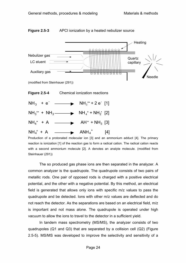
General methods, procedures & modeling Materials & methods
Page 24
Figure 2.5-3 APCI ionization by a heated nebulizer source
LC eluent
Nebulizer gas
Auxiliary gas
Heating
Needle
Quartz capillary
(modified from Steinhauer (291))
Figure 2.5-4 Chemical ionization reactions
NH 3 + e - NH3+• + 2 e- [1]
NH 3 +• + NH 3 NH 4+ + NH2• [2]
NH 4 + + A AH + + NH 3 [3]
NH 4 + + A ANH 4+ [4]
Production of a protonated molecular ion [3] and an ammonium adduct [4]. The primary
reaction is ionization [1] of the reaction gas to form a radical cation. The radical cation reacts
with a second ammonium molecule [2]. A denotes an analyte molecule. (modified from
Steinhauer (291))
The so produced gas phase ions are then separated in the analyzer. A
common analyzer is the quadrupole. The quadrupole consists of two pairs of
metallic rods. One pair of opposed rods is charged with a positive electrical
potential, and the other with a negative potential. By this method, an electrical
field is generated that allows only ions with specific m/z values to pass the
quadrupole and be detected. Ions with other m/z values are deflected and do
not reach the detector. As the separations are based on an electrical field, m/z
is important and not mass alone. The quadrupole is operated under high
vacuum to allow the ions to travel to the detector in a sufficient yield.
In tandem mass spectrometry (MS/MS), the analyzer consists of two
quadrupoles (Q1 and Q3) that are separated by a collision cell (Q2) (Figure
2.5-5). MS/MS was developed to improve the selectivity and sensitivity of a

General methods, procedures & modeling Materials & methods
Page 25
single quadrupole. The ions may be focussed by a quadrupole Q0. A
precursor ion is selected by the quadrupole Q1 according to the m/z of the
precursor. The precursor ion is then fragmented in the collision cell (Q2) by
acceleration in the presence of an inert collision gas, e.g. argon or helium.
The collision cell might also consist of a quadrupole. The resulting fragments
are then analyzed by the quadrupole Q3 based on the m/z of the fragment
ion.
Figure 2.5-5 Tandem mass spectrometer
Ar
Q1 Q2 Q3 Detector
Collision cell
Q0
Ions
(modified from Steinhauer (291)) After separation of the ions in the analyzer they are detected by the
detector. In quadrupole instruments electron multipliers are widely used as
detectors. The negative or positive ions are converted into electrons by a
conversion dynode. The resulting electrons are amplified by subsequent
dynodes. The dynodes are acceleration electrodes that accelerate the
electrons to speeds which allow them to generate more than one new electron
when hitting the next dynode.
2.6 Pharmacokinetic calculations
2.6.1 Non-compartmental analysis
Non-compartmental analysis (NCA) is a standard technique of PK
analysis. NCA is easier to apply and relies on fewer assumptions than
compartmental modeling (chapter 2.6.2). Standard NCA assumes linear PK,
i.e. all transport processes are assumed to follow first-order kinetics (113).
NCA does not provide a mechanistic description e.g. of saturable elimination.
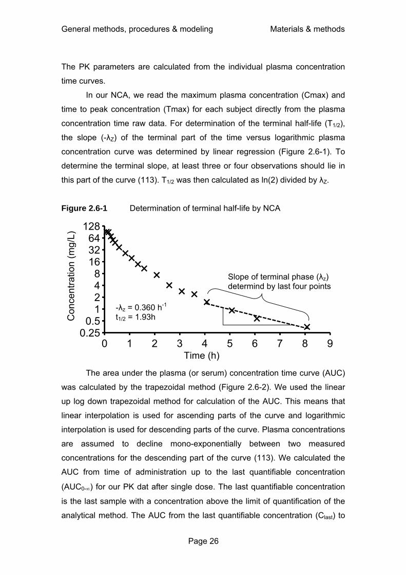
General methods, procedures & modeling Materials & methods
Page 26
The PK parameters are calculated from the individual plasma concentration
time curves.
In our NCA, we read the maximum plasma concentration (Cmax) and
time to peak concentration (Tmax) for each subject directly from the plasma
concentration time raw data. For determination of the terminal half-life (T1/2),
the slope (-λZ) of the terminal part of the time versus logarithmic plasma
concentration curve was determined by linear regression (Figure 2.6-1). To
determine the terminal slope, at least three or four observations should lie in
this part of the curve (113). T1/2 was then calculated as ln(2) divided by λZ.
Figure 2.6-1 Determination of terminal half-life by NCA
The area under the plasma (or serum) concentration time curve (AUC)
was calculated by the trapezoidal method (Figure 2.6-2). We used the linear
up log down trapezoidal method for calculation of the AUC. This means that
linear interpolation is used for ascending parts of the curve and logarithmic
interpolation is used for descending parts of the curve. Plasma concentrations
are assumed to decline mono-exponentially between two measured
concentrations for the descending part of the curve (113). We calculated the
AUC from time of administration up to the last quantifiable concentration
(AUC0-∞) for our PK dat after single dose. The last quantifiable concentration
is the last sample with a concentration above the limit of quantification of the
analytical method. The AUC from the last quantifiable concentration (Clast) to
0.250.5
1248
163264
128
0 1 2 3 4 5 6 7 8 9
Con
cent
ratio
n (m
g/L)
Time (h)
Slope of terminal phase (λz) determind by last four points
-λz = 0.360 h-1
t1/2 = 1.93h

General methods, procedures & modeling Materials & methods
Page 27
time infinity was extrapolated based on the terminal half-life by the formula
Clast/λZ. The AUC from time of administration up to time infinity was calculated
as AUC0-∞ = AUC0-last + Clast/λZ.
Figure 2.6-2 Determination of AUC by linear interpolation between measured concentrations
0
20
40
60
80
100
0 1 2 3 4 Total body clearance (CLT) was determined by dividing the
administered dose by the AUC0-∞ in plasma. For calculation of renal clearance
(CLR), cumulative renal excretion until the time of the last urine sample was
divided by the AUC for the respective time interval in plasma. Nonrenal
clearance (CLNR) was calculated as the difference between CLT and CLR:
CLNR = CLT - CLR.
The area under the product of the concentration and time versus time
curve is called the area under the first moment concentration time curve
(AUMC). AUC is the area under the zero moment curve. Mean residence time
(MRT) is the time that a drug molecule stays in the body, excluding the
gastrointestinal tract. MRT is calculated as the ratio of AUMC divided by AUC
(113). After intravenous dosing, volume of distribution at steady-state (Vss)
was calculated as MRT · CLT. The fraction excreted unchanged in urine (Ae)
was calculated by dividing the cumulative amount excreted in urine by the
Time (h)
Con
cent
ratio
n (m
g/L)
AUC0.6-0.8h=(0.8h - 0.6h) · (C0.6h + C0.8h) / 2
AUC4h-∞= C4h / λz Clast
Cmax
Tmax

General methods, procedures & modeling Materials & methods
Page 28
dose. We used WinNonlinTM Professional (version 4.0.1, Pharsight Corp.,
Mountain View, CA, USA) for NCA.
2.6.2 Compartmental modeling by the standard-two-stage approach
The standard-two-stage approach (STS) is frequently used for data
analysis from PK studies (Figure 2.6-3). In the first step the PK parameters
are estimated by compartmental modeling for each subject individually. For a
PK model with five structural PK parameters, STS requires at least six data
points (observations) to estimate those five parameters. Therefore, STS is
best applied for rich datasets i.e. studies with frequent observations from each
subject. In the second step the distribution of the individual PK parameters is
calculated by descriptive statistics (83). It is usually assumed that each
subject contributes an equal amount of information, or equivalently that the
respective PK parameter (e.g. clearance) is estimated with the same precision
in each subject. As the number (and timing) of observations determines the
precision, it is desirable that about the same number of samples is collected
from each subject.
Figure 2.6-3 Standard-two-stage modeling of a plasma concentration time profile
Con
cent
ratio
n (m
g/L)
Time (h)
0
20
40
60
80
100
0 1 2 3 4 5 6 7

General methods, procedures & modeling Materials & methods
Page 29
In compartmental models the body is represented as a system of
compartments. It is assumed that the rate of change of drug concentration is
the same within one compartment, i.e. distribution within one compartment is
instantaneous. Therefore, a one compartment model assumes that, if drug
concentration in plasma increases by 20% during a certain period of time,
concentrations in all other tissues and fluids of the body also increase by 20%
during this time period. However, after entering the systemic circulation most
drugs require some time to distribute throughout the body. Highly perfused
organs like the liver or kidneys are often in a rapid equilibrium with the blood.
Generally, together with the blood, those readily accessible tissues are
referred to as the central compartment (120).
In a two compartment model the second compartment is called the
peripheral compartment which has a slower equilibrium with the blood. This
compartment often represents less perfused tissues like muscle or fat.
Besides the perfusion rate, the physico-chemical characteristics (e.g. the
lipophilicity and pKa values) of the drug influence the time to reach
equilibrium. Three compartment models (Figure 2.6-4) comprise a central, a
shallow peripheral (fast equilibration) and a deep peripheral (slow
equilibration) compartment.
Figure 2.6-4 Three compartment model with zero-order input of an intravenous infusion
CLicshallow: intercompartmental clearance between the central and the shallow peripheral compartment, CLicdeep: intercompartmental clearance between the central and the deep peripheral compartment, TK0: duration of zero order input.
UrineCentral
compartment Volume V1
Shallow peripheral
compartment Volume V2
Deep peripheral
compartment Volume V3
CLR
CLNR
Zero-order inputTK0
Clicshallow Clicdeep
Zero-order process
First-order process
UrineCentral
compartment Volume V1
Shallow peripheral
compartment Volume V2
Deep peripheral
compartment Volume V3
CLR
CLNR
Zero-order inputTK0
Clicshallow Clicdeep
UrineCentral
compartment Volume V1
Shallow peripheral
compartment Volume V2
Deep peripheral
compartment Volume V3
CLR
CLNR
Zero-order inputTK0
Clicshallow Clicdeep
Zero-order process
First-order process
Zero-order process
First-order process
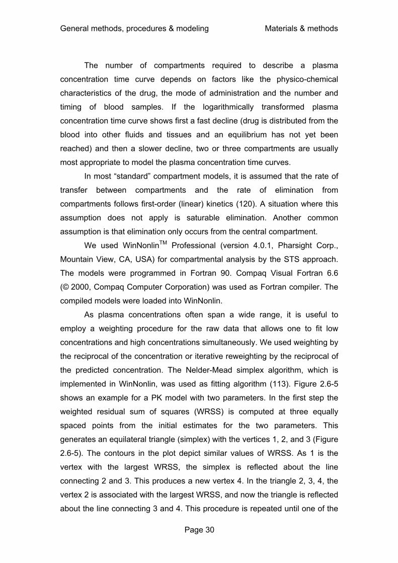
General methods, procedures & modeling Materials & methods
Page 30
The number of compartments required to describe a plasma
concentration time curve depends on factors like the physico-chemical
characteristics of the drug, the mode of administration and the number and
timing of blood samples. If the logarithmically transformed plasma
concentration time curve shows first a fast decline (drug is distributed from the
blood into other fluids and tissues and an equilibrium has not yet been
reached) and then a slower decline, two or three compartments are usually
most appropriate to model the plasma concentration time curves.
In most “standard” compartment models, it is assumed that the rate of
transfer between compartments and the rate of elimination from
compartments follows first-order (linear) kinetics (120). A situation where this
assumption does not apply is saturable elimination. Another common
assumption is that elimination only occurs from the central compartment.
We used WinNonlinTM Professional (version 4.0.1, Pharsight Corp.,
Mountain View, CA, USA) for compartmental analysis by the STS approach.
The models were programmed in Fortran 90. Compaq Visual Fortran 6.6
(© 2000, Compaq Computer Corporation) was used as Fortran compiler. The
compiled models were loaded into WinNonlin.
As plasma concentrations often span a wide range, it is useful to
employ a weighting procedure for the raw data that allows one to fit low
concentrations and high concentrations simultaneously. We used weighting by
the reciprocal of the concentration or iterative reweighting by the reciprocal of
the predicted concentration. The Nelder-Mead simplex algorithm, which is
implemented in WinNonlin, was used as fitting algorithm (113). Figure 2.6-5
shows an example for a PK model with two parameters. In the first step the
weighted residual sum of squares (WRSS) is computed at three equally
spaced points from the initial estimates for the two parameters. This
generates an equilateral triangle (simplex) with the vertices 1, 2, and 3 (Figure
2.6-5). The contours in the plot depict similar values of WRSS. As 1 is the
vertex with the largest WRSS, the simplex is reflected about the line
connecting 2 and 3. This produces a new vertex 4. In the triangle 2, 3, 4, the
vertex 2 is associated with the largest WRSS, and now the triangle is reflected
about the line connecting 3 and 4. This procedure is repeated until one of the
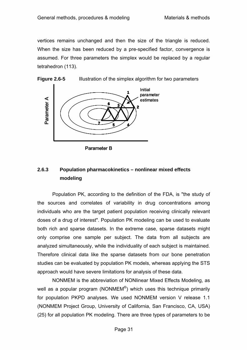
General methods, procedures & modeling Materials & methods
Page 31
vertices remains unchanged and then the size of the triangle is reduced.
When the size has been reduced by a pre-specified factor, convergence is
assumed. For three parameters the simplex would be replaced by a regular
tetrahedron (113). Figure 2.6-5 Illustration of the simplex algorithm for two parameters
2.6.3 Population pharmacokinetics – nonlinear mixed effects modeling
Population PK, according to the definition of the FDA, is "the study of
the sources and correlates of variability in drug concentrations among
individuals who are the target patient population receiving clinically relevant
doses of a drug of interest". Population PK modeling can be used to evaluate
both rich and sparse datasets. In the extreme case, sparse datasets might
only comprise one sample per subject. The data from all subjects are
analyzed simultaneously, while the individuality of each subject is maintained.
Therefore clinical data like the sparse datasets from our bone penetration
studies can be evaluated by population PK models, whereas applying the STS
approach would have severe limitations for analysis of these data.
NONMEM is the abbreviation of NONlinear Mixed Effects Modeling, as
well as a popular program (NONMEM®) which uses this technique primarily
for population PKPD analyses. We used NONMEM version V release 1.1
(NONMEM Project Group, University of California, San Francisco, CA, USA)
(25) for all population PK modeling. There are three types of parameters to be
1
23
45
6
7
Parameter B
Par
amet
er A
Initial parameter estimates
1
23
45
6
7
Parameter B
Par
amet
er A
1
23
45
6
7
1
23
45
6
7
1
23
45
6
7
1
23
45
6
7
1
23
45
6
7
1
23
45
6
7
Parameter B
Par
amet
er A
Initial parameter estimates

General methods, procedures & modeling Materials & methods
Page 32
estimated for our population PK models: 1) structural PK parameters (= fixed
effect), 2) parameters for the BSV model (= random effect), and 3) parameters
for the residual error model (= random effect). As both fixed and random
effects are simultaneously estimated, these models are called mixed effects
models. NONMEM uses a maximum likelihood approach. Maximum likelihood
estimation searches for the model parameters which optimize the probability
(likelihood) of the model given the observed data (e.g. plasma
concentrations). The estimation in NONMEM seeks to maximize the likelihood
or equivalently to minimize NONMEM’s objective function which is -2 times
the log-likelihood. The model with the lowest objective function is regarded to
give the best model fit. Technically, NONMEM approximates the likelihood to
accelerate computation time. We used the FOCE approximation method with
the INTERACTION option for all population PK modelling as implemented in
NONMEM. NONMEM’s optimization algorithm involves calculation of the
gradient for each model parameter. During the optimization these gradients
become smaller until convergence is reached. Importantly, we are not aware
of any general method to assure that the minimum found by NONMEM is a
global minimum and not a local minimum. However, it is possible to assure,
whether the model yields an adequate model fit and useful predictions (see
Figure 2.6-6).
Fixed effects comprise the population PK parameters, e.g. clearance,
and the parameters which describe the influence of covariates (like weight or
creatinine clearance) on the population PK parameters. The common
characteristic of a fixed effect is that this part of the model does not contain a
random component. Random effects comprise the random BSV in the PK
parameters and the random residual error. The residual error includes within
subject variability and measurement error.
Covariates are included into the model to decrease the unexplained
BSV. The fraction of the BSV that is explained by a covariate is called the
predictable component of the BSV. Usually more than 50 subjects are
required to study the influence of covariates on PK parameters. As our studies
had a small sample size and most studies were in healthy volunteers, we did
not include covariates into our population PK models.

General methods, procedures & modeling Materials & methods
Page 33
A population PK model directly estimates the variability in the PK
parameters within the whole study population, while fitting the concentration
time curves of all subjects simultaneously. The variability in the concentration
time curves is described by variability in the PK parameters. Table 2.6-1
shows an example of a variance-covariance matrix from the study on dose
linearity of flucloxacillin (see chapter 3.2) assuming a log-normal distribution.
Table 2.6-1 Variance-covariance matrix for flucloxacillin
CLR CLNR V1 V2 V3 CLR 0.0343 CLNR 0.0124 0.112 V1 0.00488 0.00551 0.0282 V2 0.0415 0.0641 0.00168 0.138 V3 0.0172 0.00804 0.0175 0.0351 0.023
The diagonal elements denote the variance of the respective
parameters (Var), i.e. 0.0343 for renal and 0.112 for nonrenal clearance. The
square root of the variance is an approximation to the apparent coefficient of
variation of a normal distribution on log-scale, i.e. 19% for renal and 33% for
nonrenal clearance. We report BSV as apparent between subject coefficient
of variation in the results of our population PK analyses. It is often
advantageous to consider the pairwise variability (covariance) of PK
parameters. The covariance (Cov) is described by the off-diagonal elements
of the variance-covariance matrix. The covariance between renal and
nonrenal clearance is 0.0124 in this example. The coefficient of correlation (r)
between two parameters P1 and P2 may be calculated as follows:
( ) ( )( )2PVar)1P(Var
2P,1PCov2P,1Pr⋅
=
Formula 2.6-1
In this example the coefficient of correlation between renal and
nonrenal clearance is 0.20.
By considering both average PK parameters and their variability, a
population PK model can predict the expected range of concentration time
profiles for the study population. This is done by simulating a large number

General methods, procedures & modeling Materials & methods
Page 34
(e.g. 1,000 to 10,000) of concentration time curves. The resulting large
number of profiles can be used for PKPD calculations to predict
microbiological or clinical success within the target population. This method
assumes that the subjects from the original study are representative for the
population of interest with regard to their PK.
2.6.4 Bayesian estimation
Sometimes the information contained in the observed concentrations
from a new study is too sparse to estimate a full population PK model. In
those situations Bayesian methods allow one to combine prior information
with the information from the new study. In our case, prior information about
PK parameters and their BSV was used to define a PK model. We assumed
that the patients for whom those PK parameters (=prior information) were
determined, were comparable to the patients of our new study.
The individual PK parameters of the patients from the new study are
estimated by “balancing” the prior information and the information contained in
the new dataset. The prior information becomes increasingly unimportant, the
more new information becomes available. This process of estimating the
individual PK parameters from the new study is called maximum a posteriori
probability (MAP) Bayesian estimation. By combining the prior information
with new data, this method yields the most likely (“maximum probability”)
individual PK parameters (“posterior” parameters) for the subjects of the new
study.
The assumption that the patients used to derive the prior information
and the patients from the new study come from the same population (or are at
least comparable) may be critical. Although this assumption might not be
perfectly valid, MAP-Bayesian estimation is a powerful tool to estimate the
individual PK parameters in case of very sparse data. We used MAP-
Bayesian estimation as implemented in ADAPT II (74), which is comparable to
the STS approach, since the PK parameters are estimated for each subject
individually. However, MAP-Bayesian estimation is applicable to sparse
datasets, to which the STS method cannot be applied.

General methods, procedures & modeling Materials & methods
Page 35
2.6.5 Model discrimination
Model discrimination aims at finding out which of the studied models
has the “best” performance according to the following two criteria: 1) How well
does the model fit the raw data? 2) how well do the simulated concentrations
mirror the average and variability of the observed concentrations, if one
simulates from the model? While the first criterion evaluates the model fit, the
second criterion studies the predictive performance of the PK model. The
second criterion is especially important for a model which is to be used in
MCS.
For the STS approach, we used the following criteria for model
discrimination: 1) visual inspection of the individual observed and predicted
plasma and urine concentration time curves, 2) visual comparison of the
patterns of residuals, 3) intra subject comparison of Akaike information criteria
(AIC) between competing models, and 4) the number of subjects who had the
best (i.e. lowest) AIC for each model. The AIC is a measure of goodness of fit
and is calculated as follows:
( ) P2WRSSlogN AIC +⋅= Formula 2.6-2
The AIC considers both the model fit (sum of squared residuals) and
the number of parameters of the model. N is the number of observations.
WRSS is the weighted residual sum of squares, an estimate of the variance of
the residuals. P is the number of parameters in the model. When comparing
several models for the same dataset, the model associated with the smallest
AIC value is regarded as the “best” model. If model A has a 2 point lower AIC
than model B, there is a 73% probability that model A is better and a 27%
chance that model B is better. As two times the value of P is added for
calculation of the AIC, from two models that fit the data equally well (same
WSSR) the model with the lower number of parameters (i.e. the simpler
model) is preferred. Because the weighted residuals are used for the AIC,
only AIC values for models estimated by the same weighting scheme can be
compared.

General methods, procedures & modeling Materials & methods
Page 36
In our population PK analyses, we discriminated competing models by
NONMEM’s objective function and residual plots. As for the AIC, the absolute
number of the objective function is not meaningful. Only the difference in
NONMEM’s objective function between two or more competing models is
informative. The model with the smallest objective function for the smallest
number of PK parameters is regarded to give the best fit to the data. If two
models had an insignificant difference in the objective function, we selected
the simpler model. In NONMEM, the objective function is -2 times the log of
the likelihood (plus a constant).
In addition to the criteria described above which all assess the
goodness of model fit, we evaluated the predictive performance of our models
from STS and population PK analysis via visual predictive checks. We
simulated the plasma, serum, urine, or bone concentration time profiles for
4,000 to 10,000 virtual subjects for each competing model. From those
simulated concentration time curves we calculated the median and e.g. the
nonparametric 80% prediction interval (10% to 90% percentile) of the
predicted concentration time profiles. These prediction interval lines were then
over-layed on the original raw data. If the model described the data correctly,
then 20% of the observed data points should fall outside the 80% prediction
interval at each time point (Figure 2.6-6).
Figure 2.6-6 Visual predictive check
0
2
4
6
8
10
12
0 1 2 3 4 5 6 7 8 9 10Time after administration (h)
P10% percentile
P25% percentile
P50% percentile
P75% percentile
P90% percentile
Raw data

General methods, procedures & modeling Materials & methods
Page 37
We compared the median predicted concentrations and the 80%
prediction interval with the raw data and assessed visually, whether the
median and the 80% prediction interval mirrored the central tendency and the
variability of the raw data for the respective model adequately.
2.7 Pharmacodynamic simulations
2.7.1 Background
PD simulations are used to determine the probability of successful
microbiological or clinical outcome for a specific antimicrobial dosage
regimen. The microbiological outcome of antimicrobial treatment is related to
the ability of an antibiotic to kill the pathogens causing the infection or to
inhibit their growth. Besides the “right” choice of antibiotic, a sufficient
exposure to the antimicrobial is necessary for successful microbiological
outcome. As protein binding was shown to have an adverse impact on
microbiological activity of antibiotics (35, 223), only free (non-protein bound)
drug is considered microbiologically active (89).
In the late 1940s and 1950s Eagle et al. (98) first showed in a mouse
thigh infection model that not only the total exposure but also the shape of the
concentration time curve is important for successful outcome. Their work was
continued and further substantiated by Craig and coworkers (319) in the
1980s and thereafter. They found that beta-lactams exhibit relatively
concentration-independent rates of killing. The rate of killing for beta-lactams
reaches its maximum very quickly as their concentration increases from 1
times the MIC to 4-6 times the MIC of the infecting pathogen. The time that
the non-protein bound plasma concentration remains above the MIC for the
pathogen (fT>MIC) is established as the PKPD index (228) that best predicts
microbiological outcome for beta-lactams. The time above MIC should be
reported as the cumulative percentage of a 24h period that the drug
concentration exceeds the MIC at steady-state conditions (228).

General methods, procedures & modeling Materials & methods
Page 38
Craig et al. (67) found in a mouse infection model for penicillins that the
concentration of free drug has to exceed the MIC for about 30% of the dosing
interval to achieve bacteriostasis, and for about 50% of the dosing interval to
achieve the near-maximal bactericidal effect (89). Therefore fT>MIC ≥ 50% is
called the PKPD target for near-maximal bactericidal activity of penicillins.
Attainment of the PKPD target is often used as a surrogate endpoint for
successful clinical outcome. The choice of the PKPD target depends, among
other factors, on the status of the patient’s immune system and on the
seriousness of the infection (67). Treatment of a minor infection might require
only bacteriostatic activity of the antibiotic, as the infection can then be
eliminated by the patient’s immune system. For treatment of severe infections
in immuno-compromised patients, near-maximal bacterial killing should be
achieved (89). Slow-growing bacteria in infection sites that require the use of
antibiotics with bactericidal activity for efficacious treatment, such as
osteomyelitis or endocarditis, may need higher PKPD targets compared to
acute respiratory infections (67). Figure 2.7-1 shows how fT>MIC is derived
from a plasma concentration time profile.
Figure 2.7-1 Derivation of time above MIC
0
20
40
60
80
100
0 0.5 1 1.5 2 2.5 3 3.5 4
for MIC = 20 mg/L fT>MIC = 25% of a 4h dosing interval
for MIC = 10 mg/L fT>MIC = 45%, bacteriostasis target achieved
for MIC = 5 mg/L, fT>MIC = 63%, near maximal kill target achieved
Time (h)
Con
cent
ratio
n (m
g/L)

General methods, procedures & modeling Materials & methods
Page 39
For quinolones the rates of killing are concentration-dependent over a
wide range of concentrations. The ratio of the free area under the
concentration-time curve over 24h to the MIC (fAUC/MIC) best predicts the
microbiological effect of quinolones (89).
2.7.2 Monte Carlo simulation in the field of PKPD
Monte Carlo simulation (MCS) was originally called “statistical
sampling”. MCS is a stochastic simulation method that uses random numbers
to simulate data. Therefore, the exact result of a single experiment cannot be
predicted. This differentiates MCS from deterministic simulations. In
deterministic simulations, one specific input will always give the same result
and therefore the simulations are fully predictable. The name Monte Carlo
simulation refers to the famous casino and was chosen because of the
randomness and repetitions involved in the simulations. MCS has been used
for very different purposes like studying the properties of the neutron in 1930,
or the development of the hydrogen bomb in the 1950s. The first use of MCS
for selection of antibiotic doses and setting susceptibility breakpoints was
presented in 1998 by Drusano et al. (89). They showed that MCS is a
valuable tool in rational dose selection for phase II/III clinical trials (93)
(chapter 1.3.4).
Although MCS cannot predict the concentration time profile for a new
subject, it can predict the expected range of concentration time profiles for a
population of individuals for a chosen dosage regimen. Based on this
expected range of profiles, the probability of attaining a PKPD target for a
dosage regimen of interest can be predicted. This PTA depends on the
antibiotic concentrations in the patient population and on the susceptibility of
the infecting pathogen. There is variability in the concentration time profiles
between patients and in the bacterial susceptibility to an antibiotic (described
by the MIC).
To describe the distribution of expected antibiotic concentrations for a
chosen dosage regimen, the concentration time profiles for a large number of
virtual subjects (e.g. 10,000) are simulated. Simulating 10,000 subjects
General methods, procedures & modeling Materials & methods
Page 40
provides a robust prediction for the PTA. Those simulations are based on a
population PK model which must have adequate predictive performance to
yield unbiased estimates for the PTA.
The PKPD targets for antibiotics are based on the MIC of the
pathogens. Therefore, the PTA is predicted for a range of MICs. The PKPD
indices (e.g. fT>MIC for beta-lactams or fAUC/MIC for quinolones) are then
calculated for the 10,000 subjects at each MIC within this range. The values of
the PKPD indices are compared to the PKPD target (e.g. fT>MIC at least 50%
of dosing interval) for all 10,000 simulated subjects at each MIC. The PTA at
each MIC is then derived by calculating the fraction of subjects who attained
the target at each MIC.
The highest MIC for which the target is attained by at least 90% of the
simulated subjects is often defined as the PKPD breakpoint (Figure 2.7-2).
Figure 2.7-2 PTA vs. MIC profile and derivation of the PKPD breakpoint
This definition is also used in this thesis. Therefore the PKPD
breakpoint is the highest MIC, for which the probability of successful treatment
with the chosen dosage regimen is ≥90%. If a patient is infected by pathogens
with an MIC higher than the PKPD breakpoint, another dosage regimen
should be chosen. Importantly, the PKPD breakpoint is determined in a
different way compared to the susceptibility breakpoints which are set by
national organizations like the DIN (Deutsches Institut für Normung), the CLSI
(Clinical and Laboratory Standards Institute), and the BSAC (British Society
0%10%20%30%40%50%60%70%80%90%
100%
2 4 8 16 32 64646464MIC (mg/L)
PTA = 90%
PKPD breakpoint 16 mg/L

General methods, procedures & modeling Materials & methods
Page 41
for Antimicrobial Chemotherapy). Consequently, the PKPD breakpoint and the
susceptibility breakpoints set by those organizations may differ by more than a
factor of 4.
To put the PTAs into clinical perspective, the PTA expectation value
(also called cumulative fraction of response (228)) is calculated. The PTA
expectation value is an estimate of the proportion of the population that will
achieve the PKPD target, for a specific drug dose and a specific population of
microorganisms. MIC distributions of pathogens of clinical interest can be
obtained from published studies where large numbers of isolates were
collected and their MICs determined. Alternatively the MIC distribution of a
local hospital can be used. The PTA expectation value is calculated by
multiplying the PTA at each MIC by the fraction of the population of
microorganisms at each MIC (Figure 2.7-3). Ideally, a PK model which has
been determined in the patient population of interest is combined with the MIC
distribution typically observed in those patients at a local hospital. The PTA
expectation value can then be used to predict the probability of microbiological
or clinical success in this local hospital.
Figure 2.7-3 Calculation of the PTA expectation value based on the PTA vs. MIC profile and the expected MIC distribution
0%10%20%30%40%50%60%70%80%90%
100%
0.5 1 2 4 8 16 32MIC (mg/L)
20%25% 25%
18%8% 4%
PTA = 100%PTA = 93%
0%10%20%30%40%50%60%70%80%90%
100%
0.5 1 2 4 8 16 32MIC (mg/L)
20%25% 25%
18%8% 4%
PTA = 100%PTA = 93%
PTA = 0%
PTA = 100%
PTA = 93%
PTA expectation value = 1·0.2 + 1·0.25 + 1·0.25 + 1·0.18 + 0.93·0.08 + 0·0.04 = 0.954

General methods, procedures & modeling Materials & methods
Page 42
2.8 Statistical analysis
2.8.1 Descriptive statistics – parametric and non-parametric approach
The aim of descriptive statistics is to summarize the central tendency
and variability for a set of data. If the distribution of values (roughly) follows a
normal distribution, the data can be adequately described by the arithmetic
mean and standard deviation (122). This approach is called parametric
statistics, as it assumes that the data follow a normal distribution.
If the distribution of data deviates notably from a normal distribution,
the arithmetic mean and standard deviation are not appropriate to describe
the central tendency and variability. PK parameters like clearance, volume of
distribution, and half-life often tend to follow a log-normal distribution, i.e. a
normal distribution can be achieved by taking the logarithm of each value and
calculating the average and standard deviation on log-scale. In case of a log-
normal distribution, the geometric mean and the coefficient of variation (CV)
are appropriate statistics to describe the central tendency and variability of the
data (Figure 2.8-1, Figure 2.8-2).
If there is insufficient prior knowledge on the form of a distribution, the
most reasonable way to describe a distribution is by the median and
representative percentiles. Percentiles are calculated by sorting the list of
values. The median is the 50% percentile. Half of the data fall below and half
of the data fall above the median. Describing a distribution by the median and
e.g. the 10% and 90% percentile (P10 and P90) is a non-parametric
approach, as no specific distribution is assumed (Figure 2.8-1). The median is
very insensitive towards outliers, whereas the arithmetic mean is sensitive to
outliers with high values and the geometric mean is sensitive to outliers with
low values. As it is difficult to identify an outlier for a small dataset of e.g. 20
samples, the non-parametric approach is a reasonable way to summarize the
PK parameters for a study with a small sample size.

General methods, procedures & modeling Materials & methods
Page 43
Figure 2.8-1 Log-normal distribution of clearances without and with interaction
Figure 2.8-2 Histograms including estimated log-normal distributions
Freq
uenc
y
0.0 0.4 0.8 1.2 1.6 2.0 2.4 2.80
2
4
6
8
10
12
Without interaction
0.0 0.5 1.0 1.5 2.0 2.5 3.00
4
8
12
16
20
24
28
With interaction
Freq
uenc
y To
tal b
ody
clea
ranc
e (L
/h)
0
1
2
3
Without interaction
With interaction
Geometric mean 0.883 0.727
CV 48% 67% P10 0.516 0.418 Median 0.872 0.669 P90 1.524 1.604 Without interaction With interaction

General methods, procedures & modeling Materials & methods
Page 44
2.8.2 Analysis of variance (ANOVA)
ANOVA is a parametric method which allows one to test for significant
differences between means of two (or more) groups of data. ANOVA is based
on the average and standard deviation. It assumes that the samples are
randomly drawn from normally distributed populations with the same standard
deviations (homoscedasticity). The null hypothesis is that the differences
between the means are simply due to random variability of data which all arise
from the same population. If the differences between the means are larger
than would be expected due to population variability, the null hypothesis is
rejected. We used an α-level of significance of 0.05.
If the populations are normally distributed, parametric methods
generally are more likely (i.e. have a higher power) to detect a real difference
than non-parametric methods (122). PK parameters in a population are
usually assumed to follow a log-normal distribution rather than a normal
distribution. It has been recommended by Cawello (56) to use a log-normal
distribution for AUC, clearance, peak concentration, terminal half-life, and
volume of distribution. This assumption is often reasonable, however, there is
no mathematical proof for this assumption. According to FDA guidelines AUC
and Cmax in bioequivalence studies are assumed to follow a log-normal
distribution and should be tested on log-scale (2).
We used ANOVA on log-scale to test for differences between
treatments in our dose linearity and drug-drug interaction studies. We tested
the non-compartmental parameter estimates for our study drugs for
differences between treatments (e.g. low versus high dose for assessment of
dose linearity, or with versus without concomitant administration of another
drug for the interaction studies). We used WinNonlinTM Professional for
descriptive statistics, ANOVA, and equivalence statistics.
Figure 2.8-3 shows the scheme of an interaction study at two dose
levels, like the study described in chapter 4.4 of this thesis. Two factors, dose
level and presence or absence of an interacting agent, have to be taken into
account in the ANOVA.

General methods, procedures & modeling Materials & methods
Page 45
Figure 2.8-3 Scheme of an interaction study at two dose levels
Figure 2.8-4 shows some individual clearances from the distributions of
Figure 2.8-1 and Figure 2.8-2, and how the individual values change in the
presence of an interacting agent.
Figure 2.8-4 Individual clearances with and without interaction
0.0
0.5
1.0
1.5
Without interaction With interaction
Tota
l bod
y cl
eara
nce
(L/h
)
Factor 1: Dose
Factor 2: Interaction
Dose 1000mg Dose 500mg
No interaction No interaction Interaction Interaction
Background Dose linearity & saturable elimination
Page 46
3 Assessment of dose linearity, the extent of saturable drug elimination and its predicted clinical significance
3.1 Background on dose linearity and saturable elimination
Plasma drug concentrations increase linearly with dose, if all transport
processes follow first-order kinetics. This is called dose-independent or linear
PK and is a reasonable assumption for many drugs within their therapeutic
range. However some drugs exhibit nonlinear, i.e. time- or concentration-
dependent PK. When the same dose of a drug results in different
concentrations when given at different times, or concentrations after repeated
dosing cannot be predicted from single dose data, time-dependent PK might
be the reason. A drug that exhibits time-dependent PK is carbamazepine. Due
to autoinduction of metabolizing enzymes, carbamazepine clearance
increases with time on repetitive oral administration. Other reasons for time-
dependent PK may be diurnal variations in urine pH, gastrointestinal
physiology or cardiac output (262). For drugs with concentration-dependent
PK, the PK parameters change with dose. Concentration dependence in PK
parameters may arise from saturation of drug absorption or first-pass
metabolism, which results in decreased or increased bioavailability,
respectively. Saturation of active renal secretion or reabsorption causes a
change in renal clearance, and capacity-limited biotransformation decreases
nonrenal clearance with increasing dose (201, 262). Generally, processes are
saturable when enzymes or transporters are involved. Concentration-
dependent PK is often called dose-dependent PK. Dose-dependent PK might
be the preferable term if the drug absorption is saturable. However, saturation
of drug transport or metabolism depends on the drug concentration at the
transporter or enzyme. Therefore we use the term concentration dependence.
Saturable elimination may be caused by capacity-limited drug transport
like renal tubular secretion, or capacity-limited metabolism in the liver. These
capacity-limited (saturable) processes can be described by the Michaelis
Menten equation:
Background Dose linearity & saturable elimination
Page 47
[ ][ ]CK
CVmax vm +
⋅= Formula 3.1-1
where v is the rate of drug elimination, Vmax is the maximum rate of
elimination, [C] the drug concentration and Km the drug concentration
associated with a half maximal rate (VmaxR/2) of elimination. Most commonly
[C] denotes the drug concentration in plasma (or serum).
As the rate of elimination (v) is given by CL · [C], clearance as a
function of [C] is calculated as follows:
[ ]CKVmax CLm +
= Formula 3.1-2
If drug concentrations are much lower than the value of Km, clearance
is approximately:
mKVmax CL ≅ Formula 3.1-3
and the elimination can be described by first-order kinetics, because
Vmax and Km are constants. This situation is often called pseudo-linear or
pseudo-first-order kinetics.
Saturation of elimination becomes apparent when drug concentrations
are close to or higher than the value of Km. Clearance decreases as drug
concentration increases. At very high concentrations relative to Km the rate of
elimination approaches Vmax. Once Vmax is reached, elimination resembles
zero-order kinetics, i.e. a constant amount of drug is eliminated per time unit.
In contrast, first-order kinetics means that clearance remains constant and a
constant proportion of drug is eliminated per time unit.
If a drug is only eliminated by a saturable process and if the dose rate
exceeds the maximal rate of elimination (Vmax), this drug could accumulate
indefinitely. However, virtually all drugs are likely to have a parallel first-order
(linear) pathway and are not eliminated by saturable pathways alone (201).
Ethanol and phenytoin are extreme examples for saturable elimination as they
Background Dose linearity & saturable elimination
Page 48
are almost exclusively eliminated by saturable pathways (262), whereas
theophylline and salicylate are examples for parallel saturable and linear
elimination (201). By a first-order pathway, a constant proportion of drug is
eliminated per time unit, independent of the concentration. The amount of
drug eliminated by this pathway increases linearly with concentration (dose).
The amount of drug eliminated by a saturable pathway cannot increase once
essentially complete saturation is reached. Therefore, if a drug is eliminated in
parallel by a first-order and a saturable pathway, the contribution of the first-
order pathway relative to the saturable pathway increases with drug
concentration. At very high drug concentrations most of the drug elimination
occurs via the first-order pathway, even if this pathway is only responsible for
a small percentage of the clearance that is seen at low concentrations (201).
Capacity-limited metabolism is a possible reason for saturable
elimination. Enzymatic reactions are generally capacity-limited as there is only
a finite number of enzymes present in the body. However, only very few drugs
reach high enough concentrations in the body to exceed the capacity of the
metabolizing enzymes. One example is ethanol that is metabolized by two
isoenzymes of alcohol dehydrogenase and a microsomal ethanol-oxidizing
system. Those enzymes have different Km values. A “pooled” Km has been
derived. The concentrations achieved after one or more alcoholic beverages
are well above this pooled Km value for ethanol (about 0.08 g/L) (201). This
means that the elimination of ethanol is saturated and the rate of elimination
approaches Vmax already at those concentrations. Therefore, zero-order
kinetics are often applied to describe ethanol elimination. However, Holford
(145) points out the limitations of applying a zero-order model to ethanol
elimination and concludes that elimination of ethanol can be described by a
model with capacity-limited elimination.
Another example for saturable metabolism is phenytoin. The
therapeutic range of phenytoin is usually given as 10 to 20 mg/L, but due to
saturable elimination the difference between doses that result in a
subtherapeutic effect and doses that cause toxicity is very small (262). An
additional difficulty is the high variability in Km between patients (201).

Background Dose linearity & saturable elimination
Page 49
Therefore, therapeutic drug monitoring is used for phenytoin (323) (chapter
1.3.3).
Saturable elimination may also be due to saturation of renal
elimination. Renal clearance is the sum of glomerular filtration, tubular
secretion and tubular reabsorption. Filtration is a passive process,
reabsorption can be passive or active, and tubular secretion is an active
saturable process. Saturation of active tubular reabsorption might result in
concentration-dependent renal elimination. Saturation in reabsorption causes
an increase in renal clearance of ascorbic acid at very high doses. Therefore,
and because of saturable absorption, plasma concentrations of ascorbic acid
do not change greatly even if the dose is much increased (262). A different
mechanism causes nonlinear elimination of salicylate. Salicylate decreases
urinary pH and shows pH-dependent tubular reabsorption, therefore renal
clearance decreases at higher doses. However, because of the small
contribution of renal clearance to total salicylate clearance this mechanism
has little influence on plasma concentrations (201).
Active secretion of anions and cations is mediated by a wide variety of
transporters located in the renal tubules. However active renal secretion does
not occur as the only pathway by which a drug is eliminated, as glomerular
filtration is always present if a drug is excreted by the kidneys. Therefore,
saturation of active renal secretion is not likely to result in accumulation of a
drug to an extent as it might happen with ethanol or phenytoin. Nonlinear
kinetics due to saturation of renal secretion has been reported for several
acylureido-penicillins (azlocillin (27), mezlocillin (29, 106, 212), piperacillin
(304, 317)) and dicloxacillin (234, 262).
There are contradictory reports about the existence of saturable
elimination of piperacillin at therapeutic concentrations. We are not aware of a
study using population PK to explore dose linearity of flucloxacillin, which is
also eliminated by active renal secretion. Therefore we investigated if
saturation of elimination becomes apparent at therapeutic concentrations. We
intended to compare various dosage regimens via MCS, and for this
knowledge about a possibly existing saturable elimination of the study drugs is
important.

Dose linearity of flucloxacillin Dose linearity & saturable elimination
Page 50
3.2 Population pharmacokinetics at two dose levels and pharmacodynamic profiling of flucloxacillin
3.2.1 Chemical structure of flucloxacillin
HN
NO
S
OO
Na
O
ON
F
ClH
Chemical structure 3.2-1 Flucloxacillin
3.2.2 Indications and dosing of flucloxacillin
Flucloxacillin is an isoxazolyl penicillin and is active against many gram
positive bacteria, including penicillinase producing staphylococci and
streptococci, but not against MRSA (123). In the United Kingdom flucloxacillin
remains the predominantly prescribed anti-staphylococcal oral antibiotic (263).
It is typically used for skin, soft tissue, and respiratory tract infections. For
serious infections like endocarditis or osteomyelitis caused by MSSA it is
administered intravenously as slow injection, short-term infusion, or
continuous infusion. In a randomized comparison trial with flucloxacillin at a
dose of 1g every 6h (1g q6h) and teicoplanin (6mg/kg q12h for three doses,
then the same dose given once daily) in the treatment of burn wound
infections due to gram positive pathogens, no significant differences in clinical
and microbiological success rates between flucloxacillin and teicoplanin were
found (289). Resistance against glycopeptides is increasing and restricting
glycopeptide use has been reported to be helpful in controlling vancomycin-
resistant enterococci (40, 125). Therefore it might be preferable to use
alternatives like flucloxacillin against MSSA, if the alternative grants a
sufficient probability for successful clinical outcome. In addition, flucloxacillin
(C19H16ClFN3NaO5S, Mol. Wt.: 475.85)

Dose linearity of flucloxacillin Dose linearity & saturable elimination
Page 51
has been suggested to show more rapid killing of MSSA than vancomycin in
vitro and in vivo, and usually flucloxacillin levels do not need to be monitored
(185).
Attainment of the PKPD targets fT>MIC ≥ 50% is often used as a
surrogate endpoint for successful clinical outcome (67, 89) (chapter 2.7.1).
For drugs with short half-lives like beta-lactams, prolonged and continuous
infusion have been shown to achieve longer fT>MIC than short-term infusions at
the same daily dose (69). Consequently, Drusano (90) proposed prolonged
infusions for carbapenems to optimize their PTA. Prolonged or continuous
infusions may require lower daily doses compared to intermittent treatment,
while achieving the same PTA as high dose intermittent treatment.
Conditions like endocarditis and osteomyelitis usually require
prolonged high dose treatment. Continuous infusion treatment can be
managed at patients’ homes better than frequent intermittent infusions (q6h or
q4h) and has been reported to be efficacious for completion of treatment
against serious staphylococcal infections as home-based treatment (153,
185). However the optimal doses for continuous and prolonged infusion of
flucloxacillin have not yet been determined by population PK and MCS. In
absence of these data, some authors report that they administered the same
daily doses via continuous infusion as for intermittent treatment (153, 185).
We used population PK and MCS to investigate differences in the PTA
between intermittent and continuous infusions. For this task it is important to
know, whether clearance changes with plasma concentration at therapeutic
concentrations. Therefore, our second objective was to compare the PK of
flucloxacillin at two different dose levels.
3.2.3 Methods
Study design and drug administration: Ten healthy subjects (five
males and five females) participated in the study. In each of the two study
periods each subject received a single dose of 500 mg or 1000 mg
flucloxacillin as a 5min intravenous infusion.

Dose linearity of flucloxacillin Dose linearity & saturable elimination
Page 52
Sampling Schedule: Blood samples were drawn immediately before
start of infusion, at the end of infusion as well as at 5, 10, 15, 20, 25, 45, 60,
75, 90 minutes and 2, 2.5, 3, 3.5, 4, 5, 6, 8, and 24h after the end of the
infusion. Urine samples were collected immediately before start of the
infusion, from start of the infusion until 1h after end of infusion and in the
following time intervals: 1 to 2, 2 to 3, 3 to 4, 4 to 5, 5 to 6, 6 to 8, 8 to 12, 12
to 24h after the end of the infusion.
Determination of Plasma and Urine Concentrations: For
determination of flucloxacillin in plasma 100µL of the sample were
deproteinized with 200µL acetonitrile containing the internal standard. After
mixing and centrifugation at 15,000 rounds/min 40µL were injected onto the
HPLC-system. For determination of flucloxacillin in urine 20µL of the sample
were diluted with 180µL water. After mixing 40µL were injected onto the
HPLC-system. Flucloxacillin was determined using a reversed phase column,
potassium dihydrogen phosphate (pH 6.2) / acetonitrile mobile phase with a
flow of 2 mL/min. Flucloxacillin and the internal standard were detected at
220nm. The plasma and urine samples were measured against a plasma or
urine calibration row. The calibration row in plasma (urine) was prepared by a
10:1 dilution of a tested drug-free plasma (urine) with a stock solution to
obtain the highest calibration level. The other calibration levels were obtained
by 1:1 dilution of the highest calibration level or a level of higher concentration
with drug-free plasma (urine).
No interferences were observed in plasma or urine for flucloxacillin or
the internal standard. Calibration was performed by linear regression. The
linearity of flucloxacillin calibration curves in plasma and urine was shown
between 0.500 - 250 mg/L and 5.00 - 400 mg/L, respectively. The
quantification limits were identical with the lowest calibration levels. The inter-
day precision and the analytical recovery of the spiked quality control
standards of flucloxacillin in human plasma (urine) ranged from 4.1 to 7.7%
(3.3 to 5.1%) and from 84.9 to 106.0% (100.0 to 103.0%), respectively.
Pharmacokinetics Non-compartmental analysis: NCA was performed for both dose
levels according to the methods described above.
Dose linearity of flucloxacillin Dose linearity & saturable elimination
Page 53
Population PK analysis: We tested two and three compartment
disposition models. The drug input was modeled as a zero order process with
a fixed duration of 5 min.
Individual PK model: We estimated the BSV for all parameters except
duration of zero order input and intercompartmental clearances. We assumed
a log-normal distribution for the PK parameters and used a full variance-
covariance matrix to describe the variability of the PK parameters as well as
their pairwise correlations. BSV was estimated as variance but we report the
square root of the estimate. We have expressed these values as a percentage
because this quantity is an apparent coefficient of variation of a log-normal
distribution (chapter 2.6.3).
Observation model: We described the residual unidentified variability
by a combined additive and proportional error model for plasma
concentrations and amounts excreted in urine.
Monte Carlo simulation: We used a non-protein bound plasma
concentration above the MIC (fT>MIC) for at least 30% or 50% of the dosing
interval as PKPD targets for flucloxacillin. We calculated the PTA within the
MIC range from 0.0625 to 2 mg/L and used a protein binding of 96% for
flucloxacillin (28, 30). Three dosage regimens at a daily dose of 6g were
compared: 1) continuous infusion, 2) prolonged (4h) infusion of 2g q8h and 3)
short-term (0.5h) infusion of 1.5g q6h. We simulated 10,000 virtual subjects
for each of these three dosage regimens at steady-state in absence of
residual error. We derived the PTA, the PKPD breakpoint, and the PTA
expectation value for each of the two targets.
3.2.4 Results
Demographics: All 10 subjects completed the study. The median
[range] weight was 71 [52-83] kg, height was 178 [165-190] cm and age was
25 [23-34] years.
Non-compartmental analysis: Plasma concentrations and amounts in
urine of flucloxacillin after infusion of 500 mg and 1000 mg are shown in
Figure 3.2-1.

Dose linearity of flucloxacillin Dose linearity & saturable elimination
Page 54
Figure 3.2-1 Average ± SD profiles of flucloxacillin in healthy volunteers after a 5min infusion of 500 mg or 1000 mg flucloxacillin
Table 3.2-1 shows the results of the NCA. Peak concentrations and
AUCs were dose linear. All other PK parameters were very similar at both
dose levels.
Table 3.2-1 PK parameters for 500 and 1000 mg flucloxacillin from non-compartmental analysis
Geometric mean (%coefficient of variation)
500 mg 1000 mg
Point estimate (90% confidence interval) 1000 mg / 500 mg
p-value from
ANOVA
Total body clearance (L/h) 8.16 (21%) 8.18 (20%) 100 [94-107] 0.94
Renal clearance (L/h) 5.37 (22%) 5.29 (22%) 99 [90-108] 0.77
Nonrenal clearance (L/h) 2.72 (30%) 2.79 (33%) 103 [88-119] 0.77 Fraction excreted unchanged in urine 0.66 (10%) 0.65 (12%) 98 [93-104] 0.62
Volume of distribution at steady-state (L) 9.63 (15%) 9.97 (17%) 104 [96-112] 0.44
Peak plasma concentration (mg/L) 86.8 (13%) 167 (16%) 192 [175-211] < 0.01
Terminal half-life (h) 1.40 (26%) 1.62 (25%) 116 [87-153] 0.36
Mean residence time (h) 1.18 (19%) 1.22 (14%) 103 [97-110] 0.36
0.1
1.0
10.0
100.0
1000.0
0 1 2 3 4 5 6 7 8 9Plasm
a con
centr
ation
(mg/L
)
1000 mg500 mg
Plasma concentrations
Time after start of infusion (h)
0
200
400
600
800
0 5 10 15 20 25
Amou
nt in
urin
e (m
g)
1000 mg500 mg
Cumulative amounts excreted unchanged in urine
Time after start of infusion (h)
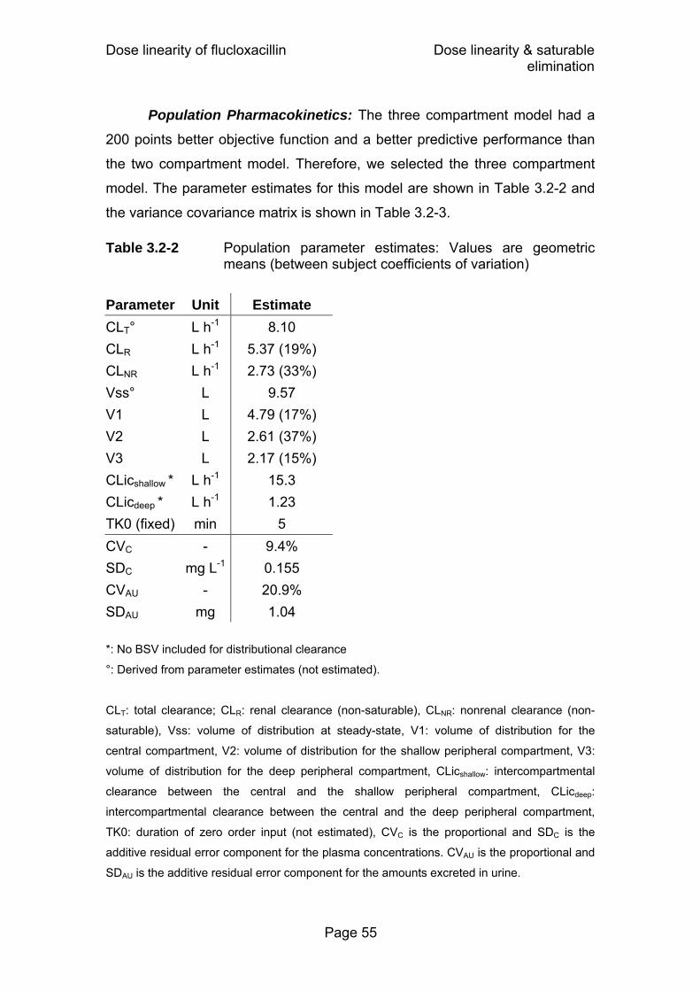
Dose linearity of flucloxacillin Dose linearity & saturable elimination
Page 55
Population Pharmacokinetics: The three compartment model had a
200 points better objective function and a better predictive performance than
the two compartment model. Therefore, we selected the three compartment
model. The parameter estimates for this model are shown in Table 3.2-2 and
the variance covariance matrix is shown in Table 3.2-3.
Table 3.2-2 Population parameter estimates: Values are geometric means (between subject coefficients of variation)
Parameter Unit Estimate CLT° L h-1 8.10 CLR L h-1 5.37 (19%) CLNR L h-1 2.73 (33%) Vss° L 9.57 V1 L 4.79 (17%) V2 L 2.61 (37%) V3 L 2.17 (15%) CLicshallow * L h-1 15.3 CLicdeep * L h-1 1.23 TK0 (fixed) min 5 CVC - 9.4% SDC mg L-1 0.155 CVAU - 20.9% SDAU mg 1.04
*: No BSV included for distributional clearance
°: Derived from parameter estimates (not estimated).
CLT: total clearance; CLR: renal clearance (non-saturable), CLNR: nonrenal clearance (non-
saturable), Vss: volume of distribution at steady-state, V1: volume of distribution for the
central compartment, V2: volume of distribution for the shallow peripheral compartment, V3:
volume of distribution for the deep peripheral compartment, CLicshallow: intercompartmental
clearance between the central and the shallow peripheral compartment, CLicdeep:
intercompartmental clearance between the central and the deep peripheral compartment,
TK0: duration of zero order input (not estimated), CVC is the proportional and SDC is the
additive residual error component for the plasma concentrations. CVAU is the proportional and
SDAU is the additive residual error component for the amounts excreted in urine.

Dose linearity of flucloxacillin Dose linearity & saturable elimination
Page 56
Table 3.2-3 Variance-covariance matrix for flucloxacillin assuming
normal distributions of the PK parameters on log-scale
CLR CLNR V1 V2 V3 CLR 0.0343 CLNR 0.0124 0.112 V1 0.00488 0.00551 0.0282 V2 0.0415 0.0641 0.00168 0.138 V3 0.0172 0.00804 0.0175 0.0351 0.023
See Table 3.2-2 for parameter explanation and chapters 3.2.3 and 2.6.3 for details.
Figure 3.2-2 shows the visual predictive checks for this model. There
was no indication that clearance decreased with the increase in dose from
500 mg to 1000 mg. The distribution of subjects with lower/higher individual
estimates for the 500 mg dose than for the 1000 mg dose was 5/5 for total
clearance, 5/5 for renal clearance, and 5/5 for nonrenal clearance. Thus, there
was no trend of any saturation of clearance at these dose levels.

Dose linearity of flucloxacillin Dose linearity & saturable elimination
Page 57
Figure 3.2-2 Visual predictive check for plasma concentrations and
amounts excreted unchanged in urine
Dose: 500 mg
Plasma concentrations (0-8h)
0.1250.250.5
1248
163264
128128128
0 1 2 3 4 5 6 7 8
Time after administration (h)
10 % percentile
25 % percentile
50 % percentile
75 % percentile
90 % percentile
Raw data
Dose: 1000 mg
Plasma concentrations (0-8h)
0.250.5
1248
163264
128256
0 1 2 3 4 5 6 7 8
Time after administration (h)
10 % percentile
25 % percentile
50 % percentile
75 % percentile
90 % percentile
Raw data
Plasma concentrations (0-1.75h)
Plasma concentrations (0-1.75h)
Amounts excreted unchanged in urine
0
50
100
150
200
250
300
0 1 2 3 4 5 6
Time after administration (h)
10 % percentile25 % percentile50 % percentile
75 % percentile90 % percentileRaw data
Amounts excreted unchanged in urine
0
100
200
300
400
500
600
0 1 2 3 4 5 6
Time after administration (h)
10 % percentile25 % percentile50 % percentile
75 % percentile90 % percentileRaw data
The plots show the raw data, the 80% prediction interval [10 - 90% percentile] and the
interquartile range [25 - 75% percentile]. Ideally, 50% of the raw data points should fall inside
the interquartile range at each time point and 80% of the raw data should fall inside the 80%
prediction interval.

Dose linearity of flucloxacillin Dose linearity & saturable elimination
Page 58
Monte Carlo simulations: We compared the PTA vs. MIC profiles for
three dosage regimens with a daily dose of 6g at two PKPD targets (Figure
3.2-3). For the target of fT>MIC ≥ 50% for near-maximal bactericidal activity of
penicillins, continuous infusion and prolonged infusion (4h) showed virtually
identical PTAs and short-term infusion (0.5h) had lower PTAs. The PKPD
breakpoint for near-maximal bactericidal activity was 0.75 to 1 mg/L (PTA
86% at 1 mg/L) for continuous infusion as well as prolonged infusion, and 0.25
to 0.375 mg/L (PTA 79% at 0.375 mg/L) for short-term infusion.
At the target for bacteriostasis (fT>MIC ≥ 30%), prolonged infusion
reached the highest PTAs. Continuous infusion and short-term infusion had
very similar PTAs (Figure 3.2-3). The breakpoints were 1.5 to 2 mg/L for
prolonged infusion, 0.75 to 1 mg/L (PTA 86% at 1 mg/L) for continuous
infusion, and 0.75 to 1 mg/L (PTA 83% at 1 mg/L) for short-term infusion.
Figure 3.2-3 Probabilities of target attainment for different dosage regimens and PKPD targets of flucloxacillin at a daily dose of 6g flucloxacillin
Target: fT>MIC ≥ 30%
0%10%20%30%40%50%60%70%80%90%
100%
0.125 0.25 0.5 1 2 4MIC (mg/L)
Target: fT>MIC ≥ 50%
0%10%20%30%40%50%60%70%80%90%
100%
0.125 0.25 0.5 1 2 4MIC (mg/L)
continuous infusion of 6g / day
2g q8h as 4h infusions
1.5g q6h as 0.5h infusions

Dose linearity of flucloxacillin Dose linearity & saturable elimination
Page 59
3.2.5 Discussion
We compared the PK of flucloxacillin at two dose levels in a crossover
study with healthy volunteers. For studying dosage regimens via MCS at
various doses, other modes of administration, or both, it is important to know,
whether the clearance changes with plasma concentration at therapeutic
concentrations. Different dose levels often help to estimate the concentration
dependence of clearance. Frequent plasma and urine samples were collected
and highly specific, precise and sensitive bioanalytical methods were applied.
We used population PK to fit plasma and urine data simultaneously.
Our NCA showed no differences in clearance and volume of
distribution between the low and the high dose (Table 3.2-1). A three
compartment population PK model with linear renal and nonrenal elimination
had excellent predictive performance and there was no indication for a
decrease in total, renal, or nonrenal clearance with the increase in dose from
500 mg to 1000 mg. Therefore, we used this model estimated from plasma
and urine data at both dose levels for MCS to compare the PTA vs. MIC
profiles for the three dosage regimens (Figure 3.2-3). The target in our MCS
was based on non-protein bound plasma concentrations. A range of 94.6 to
96.2% for the plasma protein binding of flucloxacillin has been reported (28,
32, 258). This corresponds to a rather wide range for the non-protein bound
fraction of 3.8 to 5.4%, which is a difference of 42% (5.4 vs. 3.8%) for the non-
protein bound concentrations. To account for this situation, we chose a
relatively high protein binding of 96%, which has also been reported by
Bergan (28), as this choice results in conservative (i.e. low) non-protein bound
plasma concentrations.
Our MCS with the bacteriostasis target (fT>MIC ≥ 30%) showed that
prolonged infusion had higher PTAs than continuous infusion and short-term
infusion. The PKPD breakpoints were 1.5 mg/L for prolonged infusion and
0.75 mg/L for continuous infusion and short-term infusion. For the target near-
maximal killing (fT>MIC ≥ 50%), prolonged infusion and continuous infusion
both had a 3 times higher PKPD breakpoint than short-term infusion at the

Dose linearity of flucloxacillin Dose linearity & saturable elimination
Page 60
same daily dose of 6g. The PKPD breakpoints were 0.75 mg/L for prolonged
infusion and continuous infusion, and 0.25 mg/L for short-term infusion. Thus,
prolonged infusion achieved PTAs that were higher than or similar to the
PTAs of the other two dosage regimens for both targets.
The different ranking of the three dosage regimens for the two targets
can be explained as follows: The breakpoint for continuous infusion at steady-
state is independent of the chosen target, as for any one patient fT>MIC can
only be 0% or 100%. The profile for short-term infusions shows a rather
pronounced peak without a plateau and the profile for prolonged infusion
shows a flat peak with a rather broad plateau. Subsequently, short-term
infusions reach very high concentrations for a short period of time and
prolonged infusions reach only moderately high concentrations, but these for
a longer period of time. We determined for flucloxacillin that short-term (0.5h)
infusions had the highest PTAs for targets up to fT>MIC ≥ 20%, prolonged (4h)
infusions performed best for targets between 20% and 50%, and continuous
infusion had the highest PTAs for longer targets (55% and above). Continuous
infusion was superior to short-term infusions for targets of 30% and above.
To put these results into clinical perspective, the PKPD breakpoints
need to be compared to the MICs encountered in clinical practice. MIC90
values of MSSA for flucloxacillin are usually reported to be ≤ 0.5 mg/L (153,
224, 229, 289). For an MIC of 0.5 mg/L, continuous infusion and prolonged
infusion of 6g / day have a PTA of more than 99%, whereas short-term
infusion of 6g / day reaches a PTA of only 46% based on the target for near-
maximal killing. As flucloxacillin is also available for oral treatment,
intravenous dosing is more relevant for patients with serious infections, where
attainment of the target for near-maximal bactericidal activity of the antibiotic
might be required (89) (chapter 2.7.1).
We could show that the PK of flucloxacillin was linear within our studied
dose range. Therefore, doubling the dose means that also the breakpoint will
double. As the PKPD breakpoint of the short-term infusion q6h of 6g / day was
0.25 mg/L, about 12g / day would be required to reach a breakpoint of
0.5 mg/L for near-maximal killing for short-term infusions. However, 4g / day
Dose linearity of flucloxacillin Dose linearity & saturable elimination
Page 61
as continuous or prolonged infusion would be sufficient to reach a breakpoint
of 0.5 mg/L.
The MIC90 of flucloxacillin is typically ≤ 0.5 mg/L for MSSA. Even
without data on an MIC distribution for flucloxacillin against MSSA, it is still
possible to calculate the PTA expectation value for an MIC90 of 0.5 mg/L. The
PTA vs. MIC profile for continuous or prolonged infusion of 4g / day with a
PKPD breakpoint of 0.5 mg/L for near-maximal killing can be roughly
simplified to assuming a PTA of 100% for all MICs ≤ 0.5 mg/L and a PTA of
0% for all MICs above 0.5 mg/L. For an MIC90 of 0.5 mg/L, 90% of the
patients (PTA=100% for MICs ≤ 0.5 mg/L) will achieve the target
(corresponding to the 90th percentile of the MIC distribution) and 10% of the
patients (PTA=0% for MICs > 0.5 mg/L) will not achieve the target. Therefore,
the PTA expectation value will be at least 90% for prolonged or continuous
infusion of 4g / day and an MIC90 of 0.5 mg/L. As described above, a dose of
12g / day given as short-term infusions would be required to reach a PKPD
breakpoint of 0.5 mg/L and a PTA expectation value of about 90% for an
MIC90 of 0.5 mg/L. This means that a 66% lower daily dose (4g vs. 12g) is
sufficient for continuous or prolonged infusion compared to short-term infusion
in order to reach the same PTA expectation value for successful clinical
outcome.
Besides a cost reduction for drug acquisition secondary to the dose
reduction for prolonged or continuous infusion, a lower risk for adverse events
of flucloxacillin is probably a major advantage of prolonged and continuous
infusion. Cholestatic jaundice and hepatitis rarely occur in relation with
flucloxacillin intake, risk factors being patients’ age, preexisting hepatic
impairment, and long term use (> 14 days, (1)). In a population based case
control study, de Abajo et al. (76) identified a dose dependency for these
adverse effects. It remains to be determined whether high peak
concentrations, total exposure, or trough concentrations contribute to the
frequency of adverse events for flucloxacillin. However, prolonged and
continuous infusion allow a significant dose reduction and avoid high peak
concentrations while achieving the same PTAs as short-term infusion.

Dose linearity of flucloxacillin Dose linearity & saturable elimination
Page 62
Whether prolonged or continuous infusion would be preferred depends
on the clinical situation of the patient. Continuous infusion of flucloxacillin may
be used for home treatment of MSSA infections that require high dose
intravenous treatment over prolonged time periods. This procedure has been
shown safe, convenient and effective for the follow up treatment of serious
staphylococcal infections (e.g. sepsis, endocarditis, osteomyelitis) and
cellulitis. Sufficient stability of flucloxacillin solutions at room temperature has
also been reported (203). However in the hospital setting and with patients
receiving multiple intravenous drugs, one of the major drawbacks of
continuous infusion is the need for an additional infusion line to prevent
incompatibilities with other drugs, and the resulting increase of the risk for line
infections (195).
In conclusion, we found that the PK of flucloxacillin is linear for the
doses of 500 and 1000 mg administered as 5min intravenous infusions. For
near-maximal killing (target: fT>MIC ≥ 50%) flucloxacillin showed robust (≥90%)
PTAs up to MICs of 0.75 to 1 mg/L (PTA 86% at 1 mg/L) for prolonged
infusions or continuous infusion of 6g / day. Short-term infusions of 6g / day
had a lower breakpoint of 0.25 to 0.375 mg/L (PTA 79% at 0.375 mg/L). For
MIC90’s of 0.5 mg/L which are typically found for flucloxacillin against MSSA,
prolonged and continuous infusion at a dose of 4g / day had a PTA
expectation value of at least 90%. To achieve the same PTA expectation
value, a dose of 12g / day would be required as short-term infusions. This
dose reduction from 12g / day for short-term infusion to 4g / day for prolonged
infusion and continuous infusion might be a considerable advantage in terms
of the risk for adverse events and drug acquisition costs. Future comparative
clinical trials are warranted to show whether prolonged and continuous
infusion of flucloxacillin at lower dose levels achieve similar or better clinical
success rates than short-term infusion.

Saturable elimination of piperacillin Dose linearity & saturable elimination
Page 63
3.3 Saturable elimination of piperacillin and its impact on the pharmacodynamic profile
3.3.1 Chemical structure of piperacillin
NN
OO
O
NH
HN
O
NO
S
OO Na
Chemical structure 3.3-1 Piperacillin
3.3.2 Background on dose linearity of piperacillin
Piperacillin in combination with the betalactamase inhibitor tazobactam
is one of the most frequently used intravenous antibiotic choices. It has good
bactericidal activity against gram-positive microorganisms and P. aeruginosa
(308) and is frequently used in the empirical treatment of hospital acquired
infections. It has sufficient stability at room temperature which makes it
attractive for prolonged or continuous infusion.
During piperacillin’s use for more than two decades there have been
many attempts to determine the extent of saturation for the elimination of
piperacillin. Tjandramaga et al. (304) and Bergan and Williams (31) reported a
decrease in clearance with increasing doses of piperacillin. These results are
supported by two recent studies that used population PK analysis and found
that a model with saturable elimination fits the data better than a model with
only first order elimination (194, 317). However there is no final agreement on
the extent of saturation of piperacillin elimination. The existence of a clinically
significant saturable elimination pathway may have consequences for the
choice of the optimal dosage regimen. This becomes especially important
(C23H26N5NaO7S, Mol. Wt.: 539.54)
Saturable elimination of piperacillin Dose linearity & saturable elimination
Page 64
when different doses and schedules or other modes of administration are
studied by MCS and when short-term versus continuous infusions are
compared (317).
Additionally there is conflicting data about whether the saturation arises
from the renal or the nonrenal elimination or both. Piperacillin is excreted by
the kidneys in parallel by glomerular filtration (a first order non-saturable
process) and active tubular secretion (a capacity-limited process). Batra et al.
(23) find a decreased renal clearance at higher doses. Tjandramaga et al.
(304) observe a decrease in renal clearance and an even more marked
decrease in nonrenal clearance at higher doses, whereas Bergan and
Williams (31) report a decreased nonrenal clearance and no changes in renal
clearance at higher doses. As both of the latter two studies find increasing
fractions excreted unchanged in urine at higher doses, nonrenal clearance
decreased more than renal clearance with increasing doses. A higher fraction
excreted unchanged in urine at steady-state than after single dose has also
been reported (284). Additionally probenecid, a well known inhibitor of various
active transport processes in the body, has been shown to decrease not only
the renal but also the nonrenal elimination of piperacillin (304). These findings
suggest a saturation in both renal and nonrenal elimination of piperacillin, with
the nonrenal pathway perhaps even more saturable than the renal one.
Our primary objective was to explore the PK of piperacillin based on
data from a crossover study at two dose levels in healthy volunteers. We
applied population PK to study the extent of saturation in the renal and
nonrenal elimination of piperacillin at therapeutic concentrations. Our
secondary objective was to study the influence of saturable elimination on the
PKPD characteristics of piperacillin via MCS and to estimate the clinical
relevance of the saturation of piperacillin elimination at therapeutic doses.
3.3.3 Methods
Study design and drug administration: Ten healthy subjects (five
males and five females) participated in the study. In each of the two study

Saturable elimination of piperacillin Dose linearity & saturable elimination
Page 65
periods each subject received a single dose of 1500 mg or 3000 mg
piperacillin as a 5min intravenous infusion.
Sampling Schedule: Blood samples were drawn immediately before
start of infusion, at the end of infusion as well as at 5, 10, 15, 20, 25, 45, 60,
75, 90min and 2, 2.5, 3, 3.5, 4, 5, 6, 8, and 24h after the end of the infusion.
Urine samples were collected immediately before start of the infusion, from
start of the infusion until 1h after end of infusion and in the following time
intervals: 1 to 2, 2 to 3, 3 to 4, 4 to 5, 5 to 6, 6 to 8, 8 to 12, 12 to 24h after the
end of the infusion.
Determination of Plasma and Urine Concentrations: Piperacillin
concentrations in plasma and urine were determined by HPLC. For
determination of piperacillin in plasma 100µL of the sample were
deproteinized with 200µL acetonitrile containing the internal standard. After
mixing and centrifugation at 15,000 rpm 40µL were injected onto the HPLC
system. For determination of piperacillin in urine 20µL of the sample were
diluted with 180µL water. After mixing 40µL were injected onto the HPLC
system. Piperacillin was determined using a reversed phase column,
potassium dihydrogen phosphate (pH 6.2) / acetonitrile mobile phase at a flow
of 2 mL/min. Piperacillin and the internal standard were detected at 220nm.
The calibration rows in plasma and urine were prepared as described
in chapter 3.2.3 for flucloxacillin. No interferences were observed in plasma
and urine for piperacillin or the internal standard. Calibration was performed
by linear regression. The linearity of piperacillin calibration curves in plasma
and urine was demonstrated between 0.200 - 150 mg/L and 1.00 - 1000 mg/L,
respectively. The quantification limits were identical with the lowest calibration
levels. The inter-day precision and the analytical recovery of the spiked quality
control standards of piperacillin in human plasma (urine) ranged from 3.5 to
9.2% (3.0 to 5.5%) and from 95.0 to 106.9% (92.0 to 97.9%), respectively.
Pharmacokinetics Non-compartmental analysis: NCA was performed for the data at
both dose levels according to the methods described above.

Saturable elimination of piperacillin Dose linearity & saturable elimination
Page 66
Population PK analysis: We tested one, two, and three compartment
disposition models. The drug input was modeled as a zero order process with
a fixed duration of 5min.
Clearance: We assumed a nonrenal (CLNR) and a renal (CLR)
component of clearance. We estimated the renal clearance based on the
amount of piperacillin excreted unchanged into urine. According to prior
population PK models and data on piperacillin (31, 194, 304, 317), we studied
four different elimination models for piperacillin, as shown below. The
respective formulas for total clearance (CLT) are:
Model 1: NRRT CLCL CL += Formula 3.3-1
Model 2: NRmR
RT CL
CKVmax CL +
+= Formula 3.3-2
Model 3: NRmR
RRT CL
CKVmaxCL CL +
++= Formula 3.3-3
Model 4: CK
maxVCK
VmaxCL CLmNR
NR
mR
RRT +
++
+= Formula 3.3-4
In these formulas, C is the concentration of piperacillin in the central
compartment, VmaxR and VmaxNR are the maximum rates of elimination for
the mixed order renal and nonrenal elimination, and KmR and KmNR are the
Michaelis Menten constants for the mixed order renal and nonrenal
elimination, respectively. Model 1 assumes that renal and nonrenal clearance
are non-saturable. Model 2 assumes that renal clearance is saturable and
nonrenal clearance is non-saturable. Model 3 assumes that renal clearance
has a saturable and a non-saturable component and nonrenal clearance is
non-saturable. Model 4 assumes that renal clearance has a saturable and a
non-saturable component and nonrenal clearance is saturable.
Between subject variability model: We estimated the BSV for all
parameters except duration of zero order input and intercompartmental
Saturable elimination of piperacillin Dose linearity & saturable elimination
Page 67
clearances. An exponential parameter variability model and a full variance-
covariance matrix was used.
Observation model: We described the residual unidentified variability
by a combined additive and proportional error model for plasma
concentrations and amounts excreted in urine.
Monte Carlo simulation: We used fT>MIC ≥ 50% as PKPD target for
near-maximal bactericidal activity of piperacillin (67, 89). We calculated the
PTA within the MIC range from 2 to 64 mg/L and used a protein binding of
30% for piperacillin (16, 283). Five dosage regimens were simulated: 1)
continuous infusion of 6g / day, 2) prolonged (4h) infusion of 3g q8h (daily
dose 9g), 3) continuous infusion of 18g / day, 4) short-term (30min) infusion of
6g q8h (daily dose 18g), and 5) short-term (30min) infusion of 3g q4h (daily
dose 18g). We simulated each of those five dosage regimens for all four
population PK models at steady-state in absence of residual error and used
2,000 subjects for each combination of population PK model and dosage
regimen. We calculated the PTA and the PKPD breakpoint.
In order to estimate the clinical relevance of the differences between
the four elimination models of piperacillin, we calculated the PTA expectation
value. We calculated the cumulative fraction of response (93, 228) of the five
dosage regimens against Klebsiella pneumoniae, E. coli, and P. aeruginosa
based on published MIC distributions (10, 182). Kuti et al. (182) determined
the MICs for 557 P. aeruginosa isolates by E-test® for piperacillin/tazobactam
at the Hartford Hospital. The E-test is a plastic strip with reference MIC
dilutions of an antibiotic, that is placed onto an inoculated agar plate. An
antibiotic gradient is formed beneath the strip and where the inhibition ellipse
intersects with the scale, the MIC can be read (14). Ambrose et al. (10) had
105 ESBL phenotype (NCCLS criteria) strains of E. coli and K. pneumoniae
from bloodstream isolates recovered during 2000 in the United States and
Canada (SENTRY Antimicrobial Surveillance Program, 2000).

Saturable elimination of piperacillin Dose linearity & saturable elimination
Page 68
3.3.4 Results
All 10 subjects completed the study. The average ± SD weight was
69.6 ± 9.7 kg, height was 177.5 ± 8.0 cm and age 25.7 ± 3.1 years. Plasma
concentrations and amounts in urine of piperacillin after infusion of 1500 mg
and 3000 mg are shown in Figure 3.3-1.
Figure 3.3-1 Average ± SD profiles of piperacillin in healthy volunteers after 5min infusions of 1500 mg or 3000 mg piperacillin
Panel A: Plasma concentrations
0
100
200
300
400
500
0 1 2 3 4 5 6 7 8 9Time after start of infusion (h)
Plasm
a con
centr
ation
(mg/L
)
1500 mg3000 mg
Panel B: Cumulative amounts excreted unchanged in urine
0
500
1000
1500
2000
0 5 10 15 20 25Time after start of infusion (h)
Amou
nt in
urin
e (m
g)
1500 mg3000 mg
Non-compartmental analysis: The results of the NCA are shown in
Table 3.3-1.
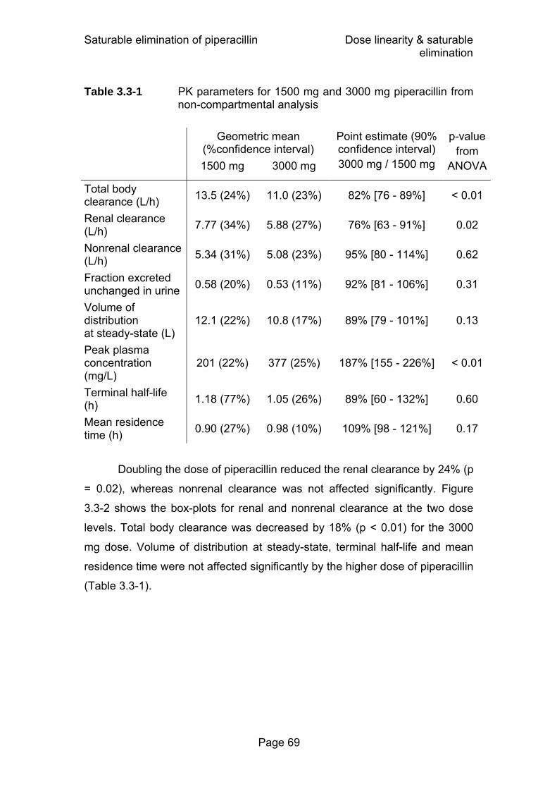
Saturable elimination of piperacillin Dose linearity & saturable elimination
Page 69
Table 3.3-1 PK parameters for 1500 mg and 3000 mg piperacillin from non-compartmental analysis
Geometric mean (%confidence interval)
1500 mg 3000 mg
Point estimate (90% confidence interval) 3000 mg / 1500 mg
p-valuefrom
ANOVA
Total body clearance (L/h) 13.5 (24%) 11.0 (23%) 82% [76 - 89%] < 0.01
Renal clearance (L/h) 7.77 (34%) 5.88 (27%) 76% [63 - 91%] 0.02
Nonrenal clearance (L/h) 5.34 (31%) 5.08 (23%) 95% [80 - 114%] 0.62
Fraction excreted unchanged in urine 0.58 (20%) 0.53 (11%) 92% [81 - 106%] 0.31
Volume of distribution at steady-state (L)
12.1 (22%) 10.8 (17%) 89% [79 - 101%] 0.13
Peak plasma concentration (mg/L)
201 (22%) 377 (25%) 187% [155 - 226%] < 0.01
Terminal half-life (h) 1.18 (77%) 1.05 (26%) 89% [60 - 132%] 0.60
Mean residence time (h) 0.90 (27%) 0.98 (10%) 109% [98 - 121%] 0.17
Doubling the dose of piperacillin reduced the renal clearance by 24% (p
= 0.02), whereas nonrenal clearance was not affected significantly. Figure
3.3-2 shows the box-plots for renal and nonrenal clearance at the two dose
levels. Total body clearance was decreased by 18% (p < 0.01) for the 3000
mg dose. Volume of distribution at steady-state, terminal half-life and mean
residence time were not affected significantly by the higher dose of piperacillin
(Table 3.3-1).

Saturable elimination of piperacillin Dose linearity & saturable elimination
Page 70
Figure 3.3-2 Renal and nonrenal clearance from non-compartmental
analysis after administration of 1500 mg or 3000 mg piperacillin to healthy volunteers
The markers represent the median, the boxes the 25% and 75% percentiles and the whiskers minimum and maximum
Population Pharmacokinetics: Three compartment models had an
approximately 130 points better objective function than two compartment
models, whereas the one compartment model had insufficient predictive
performance. Therefore, we selected models with three disposition
compartments. The parameter estimates for the four different elimination
models are shown in Table 3.3-2.
Panel A: Renal clearance Panel B: Nonrenal clearance
Panel B: Nonrenal clearance
CLnr 1500mg0123456789
clea
ranc
e (L
/h)
1500 mg 3000 mg Non
rena
l cle
aran
ce (L
/h)
Panel A: Renal clearance
1500 mg 3000 mgCLr 1500mg
02468
10121416
()
Ren
al c
lear
ance
(L/h
)

Saturable elimination of piperacillin Dose linearity & saturable elimination
Page 71
Table 3.3-2 PK parameter estimates of different elimination models:
Values for structural PK parameters are geometric means (coefficients of variation for the BSV)
Model 1 Model 2 Model 3 Model 4 Renal elimination First order Mixed order Parallel first order
& mixed order Parallel first order
& mixed order Nonrenal elimination
First order First order First order Mixed order
Parameter Unit Delta objective function
90.8 27.8 12.1 0
CLR L h-1 8.46 (39%) - 4.11 (38%) 4.94 (42%) VmaxR mg h-1 - 1990 (33%) 303 (33%) 138 (71%) KmR mg L-1 - 200 (66%) 46.8 (90%) 24.4 (111%) CLNR L h-1 3.40 (30%) 5.48 (18%) 5.52 (18%) - VmaxNR mg h-1 - - - 3100 (137%) KmNR mg L-1 - - - 419 (117%) Vss L 12.0 12.8 12.7 13.4 V1 L 6.42 (18%) 6.20 (18%) 6.30 (17%) 6.32 (21%) V2 L 3.63 (40%) 4.02 (48%) 3.64 (49%) 3.52 (44%) V3 L 1.92 (31%) 2.60 (16%) 2.73 (15%) 3.60 (7%) CLicshallow L h-1 14.0 18.3 15.7 16.3 CLicdeep L h-1 0.621 1.65 1.72 2.58 TK0 (fixed) min 5 5 5 5 CVC - 13.1% 12.8% 12.8% 12.4% SDC mg L-1 0.31 0.27 0.26 0.28 CVAU - 39.1% 25.6% 24.3% 22.4% SDAU mg 1.42 4.20 4.25 4.30
See Table 3.2-2 and chapter 3.3.3 for parameter explanation.
The objective function was 63 points better for the model with mixed
order renal elimination and first order nonrenal elimination (model 2) than for
the model with first order elimination for both pathways (model 1). Km for the
mixed order renal elimination (KmR) for model 2 was estimated to be 200 mg/L
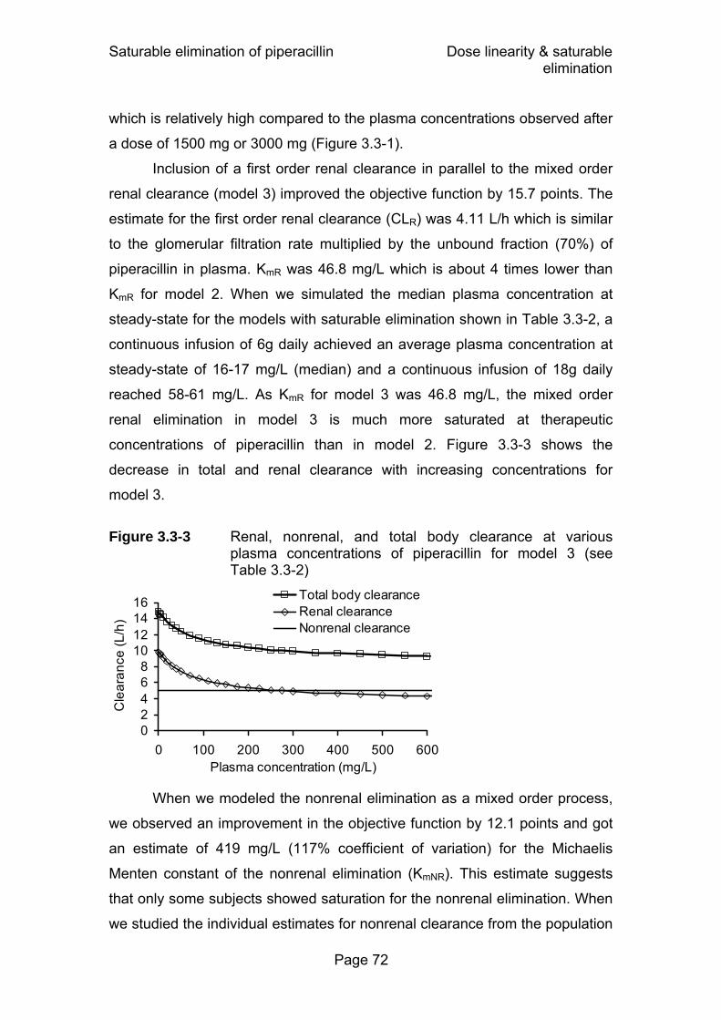
Saturable elimination of piperacillin Dose linearity & saturable elimination
Page 72
which is relatively high compared to the plasma concentrations observed after
a dose of 1500 mg or 3000 mg (Figure 3.3-1).
Inclusion of a first order renal clearance in parallel to the mixed order
renal clearance (model 3) improved the objective function by 15.7 points. The
estimate for the first order renal clearance (CLR) was 4.11 L/h which is similar
to the glomerular filtration rate multiplied by the unbound fraction (70%) of
piperacillin in plasma. KmR was 46.8 mg/L which is about 4 times lower than
KmR for model 2. When we simulated the median plasma concentration at
steady-state for the models with saturable elimination shown in Table 3.3-2, a
continuous infusion of 6g daily achieved an average plasma concentration at
steady-state of 16-17 mg/L (median) and a continuous infusion of 18g daily
reached 58-61 mg/L. As KmR for model 3 was 46.8 mg/L, the mixed order
renal elimination in model 3 is much more saturated at therapeutic
concentrations of piperacillin than in model 2. Figure 3.3-3 shows the
decrease in total and renal clearance with increasing concentrations for
model 3.
Figure 3.3-3 Renal, nonrenal, and total body clearance at various
plasma concentrations of piperacillin for model 3 (see Table 3.3-2)
When we modeled the nonrenal elimination as a mixed order process,
we observed an improvement in the objective function by 12.1 points and got
an estimate of 419 mg/L (117% coefficient of variation) for the Michaelis
Menten constant of the nonrenal elimination (KmNR). This estimate suggests
that only some subjects showed saturation for the nonrenal elimination. When
we studied the individual estimates for nonrenal clearance from the population
02468
10121416
0 100 200 300 400 500 600Plasma concentration (mg/L)
Cle
aran
ce (L
/h)
Total body clearanceRenal clearanceNonrenal clearance

Saturable elimination of piperacillin Dose linearity & saturable elimination
Page 73
PK analysis after 1500 mg and 3000 mg for model 3, we observed a nominal
value of 18% higher nonrenal clearances for the 1500 mg dose in six of the
ten subjects. Only one subject had a lower nonrenal clearance for the 1500
mg dose. The p-value for this comparison was 0.01 (paired two-sided t-test).
Figure 3.3-4 Visual predictive check for plasma concentrations and
amounts excreted unchanged in urine for model 3 (see Table 3.3-2)
Dose: 1500 mg
Plasma concentrations (0-8h)
0.1250.25
0.51248
163264
128256512
0 1 2 3 4 5 6 7 8
Time after administration (h)
10 % percentile25 % percentile50 % percentile
75 % percentile90 % percentileRaw data
Dose: 3000 mg
Plasma concentrations (0-8h)
0.1250.250.5
1248
163264
128256512
0 1 2 3 4 5 6 7 8
Time after administration (h)
10 % percentile25 % percentile50 % percentile
75 % percentile90 % percentileRaw data
Plasma concentrations (0-1.75h)
0
50
100
150
200
250
300
0 0.25 0.5 0.75 1 1.25 1.5 1.75
Time after administration (h)
10 % percentile25 % percentile50 % percentile
75 % percentile90 % percentileRaw data
Plasma concentrations (0-1.75h)
0
100
200
300
400
500
600
0 0.25 0.5 0.75 1 1.25 1.5 1.75
Time after administration (h)
10 % percentile25 % percentile50 % percentile
75 % percentile90 % percentileRaw data
Amounts excreted unchanged in urine
0
200
400
600
800
1000
0 0.5 1 1.5 2 2.5 3 3.5 4 4.5
Time after administration (h)
10 % percentile25 % percentile50 % percentile
75 % percentile90 % percentileRaw data
Amounts excreted unchanged in urine
0
200
400
600
800
1000
1200
1400
0 0.5 1 1.5 2 2.5 3 3.5 4 4.5
Time after administration (h)
10 % percentile25 % percentile50 % percentile
75 % percentile90 % percentileRaw data
ode ea e a & ea o e a e at o , , OG 3000
See chapter 2.6.5 and Figure 3.2-2 for explanation of the plots.
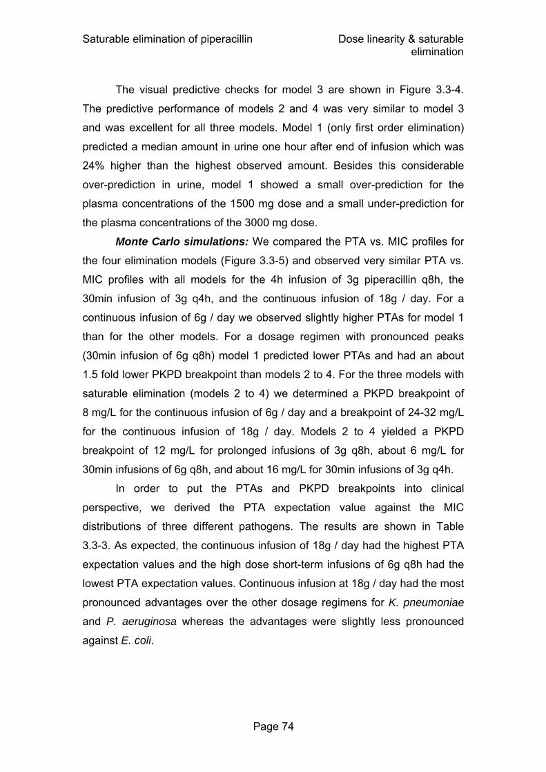
Saturable elimination of piperacillin Dose linearity & saturable elimination
Page 74
The visual predictive checks for model 3 are shown in Figure 3.3-4.
The predictive performance of models 2 and 4 was very similar to model 3
and was excellent for all three models. Model 1 (only first order elimination)
predicted a median amount in urine one hour after end of infusion which was
24% higher than the highest observed amount. Besides this considerable
over-prediction in urine, model 1 showed a small over-prediction for the
plasma concentrations of the 1500 mg dose and a small under-prediction for
the plasma concentrations of the 3000 mg dose.
Monte Carlo simulations: We compared the PTA vs. MIC profiles for
the four elimination models (Figure 3.3-5) and observed very similar PTA vs.
MIC profiles with all models for the 4h infusion of 3g piperacillin q8h, the
30min infusion of 3g q4h, and the continuous infusion of 18g / day. For a
continuous infusion of 6g / day we observed slightly higher PTAs for model 1
than for the other models. For a dosage regimen with pronounced peaks
(30min infusion of 6g q8h) model 1 predicted lower PTAs and had an about
1.5 fold lower PKPD breakpoint than models 2 to 4. For the three models with
saturable elimination (models 2 to 4) we determined a PKPD breakpoint of
8 mg/L for the continuous infusion of 6g / day and a breakpoint of 24-32 mg/L
for the continuous infusion of 18g / day. Models 2 to 4 yielded a PKPD
breakpoint of 12 mg/L for prolonged infusions of 3g q8h, about 6 mg/L for
30min infusions of 6g q8h, and about 16 mg/L for 30min infusions of 3g q4h.
In order to put the PTAs and PKPD breakpoints into clinical
perspective, we derived the PTA expectation value against the MIC
distributions of three different pathogens. The results are shown in Table
3.3-3. As expected, the continuous infusion of 18g / day had the highest PTA
expectation values and the high dose short-term infusions of 6g q8h had the
lowest PTA expectation values. Continuous infusion at 18g / day had the most
pronounced advantages over the other dosage regimens for K. pneumoniae
and P. aeruginosa whereas the advantages were slightly less pronounced
against E. coli.

Saturable elimination of piperacillin Dose linearity & saturable elimination
Page 75
Figure 3.3-5 Probabilities of target attainment for the four different
population PK models and different dosage regimens of piperacillin (PKPD target: fT>MIC ≥ 50%)
Continuous infusion of 6g/day
0%10%20%30%40%50%60%70%80%90%
100%
2 4 8 16 32 64646464
4h infusion of 3g q8h (9g/day)
0%10%20%30%40%50%60%70%80%90%
100%
2 4 8 16 32 64646464
Continuous infusion of 18g/day
0%10%20%30%40%50%60%70%80%90%
100%
2 4 8 16 32 64646464
30min infusion of 6g q8h (18g/day)
0%10%20%30%40%50%60%70%80%90%
100%
2 4 8 16 32 64646464
30min infusion of 3g q4h (18g/day)
0%10%20%30%40%50%60%70%80%90%
100%
2 4 8 16 32 64646464
TARGET 0.5, DOSE 18, NDD 6, DURATION 0.5
First order renal & first order nonrenal elimination (model 1) Mixed order renal & first order nonrenal elimination (model 2) Parallel first and mixed order renal & first order nonrenal elimination (model 3) Parallel first and mixed order renal & mixed order nonrenal elimination (model 4)
MIC (mg/L) MIC (mg/L)
MIC (mg/L) MIC (mg/L)
MIC (mg/L)
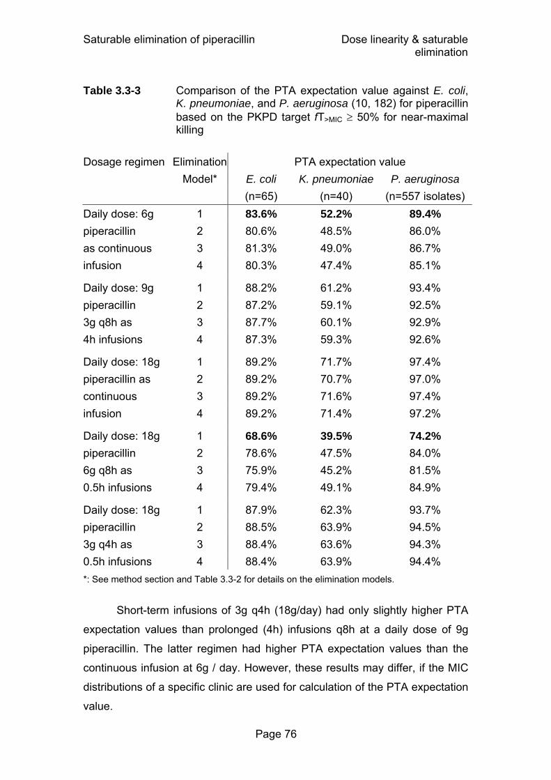
Saturable elimination of piperacillin Dose linearity & saturable elimination
Page 76
Table 3.3-3 Comparison of the PTA expectation value against E. coli, K. pneumoniae, and P. aeruginosa (10, 182) for piperacillin based on the PKPD target fT>MIC ≥ 50% for near-maximal killing
Dosage regimen Elimination PTA expectation value Model* E. coli K. pneumoniae P. aeruginosa (n=65) (n=40) (n=557 isolates) Daily dose: 6g 1 83.6% 52.2% 89.4% piperacillin 2 80.6% 48.5% 86.0% as continuous 3 81.3% 49.0% 86.7% infusion 4 80.3% 47.4% 85.1%
Daily dose: 9g 1 88.2% 61.2% 93.4% piperacillin 2 87.2% 59.1% 92.5% 3g q8h as 3 87.7% 60.1% 92.9% 4h infusions 4 87.3% 59.3% 92.6%
Daily dose: 18g 1 89.2% 71.7% 97.4% piperacillin as 2 89.2% 70.7% 97.0% continuous 3 89.2% 71.6% 97.4% infusion 4 89.2% 71.4% 97.2%
Daily dose: 18g 1 68.6% 39.5% 74.2% piperacillin 2 78.6% 47.5% 84.0% 6g q8h as 3 75.9% 45.2% 81.5% 0.5h infusions 4 79.4% 49.1% 84.9%
Daily dose: 18g 1 87.9% 62.3% 93.7% piperacillin 2 88.5% 63.9% 94.5% 3g q4h as 3 88.4% 63.6% 94.3% 0.5h infusions 4 88.4% 63.9% 94.4%
*: See method section and Table 3.3-2 for details on the elimination models.
Short-term infusions of 3g q4h (18g/day) had only slightly higher PTA
expectation values than prolonged (4h) infusions q8h at a daily dose of 9g
piperacillin. The latter regimen had higher PTA expectation values than the
continuous infusion at 6g / day. However, these results may differ, if the MIC
distributions of a specific clinic are used for calculation of the PTA expectation
value.
Saturable elimination of piperacillin Dose linearity & saturable elimination
Page 77
Comparing the results for the different elimination models, there were
very small differences between models 2 to 4 (see also Figure 3.3-5). Model 1
predicted 2-5% higher PTA expectation values for the 6g / day continuous
infusion and 6-11% lower PTA expectation values for the high dose
intermittent short-term infusions relative to models 2 to 4. For these two
dosage regimens the PTA expection values from model 1 are shown in bold in
Table 3.3-3. These differences may be smaller or larger depending on the
respective MIC distribution used for calculation of the PTA expectation value.
However, these deviations provide an estimate of what might be expected in
clinical practice.
3.3.5 Discussion
The most direct way to study the extent of saturation in the renal and
nonrenal elimination at therapeutic concentrations is to collect plasma and
urine samples in a well controlled healthy volunteer crossover study at
different dose levels (see also chapter 1.5). Different dose levels result in
different average plasma concentrations which often help to estimate the
saturable component of elimination. Studying both sides of the renal
elimination (i.e. plasma concentrations and amounts excreted in urine) further
supports the estimation of the parameters for renal elimination. Through a
highly standardized study design and bioanalysis, additional process noise is
minimized.
We had data from a well controlled crossover study with two different
dose levels that was performed in ten healthy volunteers. Frequent plasma
and urine samples were collected, and highly specific, precise and sensitive
bioanalytical methods were applied. We used population PK to fit plasma and
urine data at the two different dose levels simultaneously, and to estimate the
extent of saturation in the renal and nonrenal elimination of piperacillin at
therapeutic concentrations. Then we estimated the influence of saturable
elimination on the PKPD characteristics of piperacillin via MCS. We compared
the PTAs for different PK models with saturable and non-saturable elimination
and for various dosage regimens. From these PTAs, we derived the PKPD

Saturable elimination of piperacillin Dose linearity & saturable elimination
Page 78
breakpoints and the PTA expectation values against E. coli, K. pneumoniae,
and P. aeruginosa. This allowed us to estimate the clinical relevance of the
saturation of piperacillin elimination at therapeutic doses.
In clinical practice, piperacillin is given in combination with tazobactam
to prevent degradation of piperacillin by betalactamases, whereas in our study
piperacillin was given alone. It has been shown that the PK of piperacillin is
not affected by concomitant administration of tazobactam at dose ratios of 4:1
or 8:1 (283). However, if concomitant administration of tazobactam had an
effect on piperacillin elimination, this would result in a higher extent of
saturation of piperacillin elimination, as both drugs are secreted by the renal
tubules. Therefore, our PTAs are conservative estimates for the treatment
situation with piperacillin and tazobactam in combination.
We studied four elimination models for piperacillin (Table 3.3-2). Our
model with first order renal and first order nonrenal clearance (model 1) over-
predicted the amounts excreted in urine during the first sampling interval of
the high dose treatment considerably and showed a small bias in the
predicted plasma concentrations at both dose levels. This over-prediction and
bias were removed by adding a mixed order renal elimination term (model 3).
Model 3 is the physiologically most reasonable model for the renal elimination,
as it includes parallel first order and mixed order renal elimination. Model 3
had an excellent predictive performance (Figure 3.3-4) and its Michaelis
Menten constant (KmR) of the renal mixed order elimination was estimated to
be 46.8 mg/L. This is well in the range of plasma concentrations which are
reached after therapeutic doses of piperacillin. Together with the significant
decrease in renal clearance at the higher dose shown by NCA, this is
considerable evidence for the presence of a partly saturable renal elimination.
NCA did not show a significantly lower nonrenal clearance at the higher
dose level. Our population PK model with mixed order nonrenal elimination
had a slightly better objective function than the model with linear nonrenal
elimination, but there was no visible difference in predictive performance
between the two models. The geometric mean of the Michaelis Menten
constant for the nonrenal pathway (KmNR) was estimated to be 419 mg/L
(117% CV). For the majority of patients, the concentrations after continuous

Saturable elimination of piperacillin Dose linearity & saturable elimination
Page 79
infusion of therapeutic doses are far below this KmNR. Thus, the saturation of
nonrenal elimination is probably of less clinical relevance than the saturation
of the renal elimination. However, it should be noted that for four of the
20 profiles (two for each subject) KmNR was between 50 and 100 mg/L, and for
a further four profiles between 100 and 210 mg/L. Therefore, at clinically
relevant plasma concentrations the renal elimination showed a considerable
extent of saturation, but for the nonrenal pathway this extent is much smaller
and saturation becomes only apparent at higher concentrations and not for all
subjects.
Models 3 and 4 are the physiologically most reasonable models for the
elimination of piperacillin. Our data only showed a saturation of nonrenal
elimination for at most half of the subjects. The estimates for the first order
component of renal elimination were physiologically reasonable for models 3
and 4. More importantly, models 3 and 4 showed no clinically relevant
differences in the PKPD simulations. We selected model 3 as our final model,
because it had excellent predictive performance and is less complex than
model 4.
Overall, the saturation of piperacillin elimination at therapeutic
concentrations seems to be lower than has been reported e.g. for azlocillin
(27). This might be one reason why a saturation in piperacillin PK has not
been reported in some other studies that did not use different dose levels,
urinary excretion data, or a standardized crossover design in a homogenous
population. We tried to estimate the saturation of piperacillin elimination by
models 1 to 3 with 1) only plasma data from both dose levels, 2) urine and
plasma data from one dose level, or 3) only plasma data (no urine) from one
dose level. For cases 1) and 2) the estimated elimination parameters of
piperacillin were in agreement with the parameter estimates from the full
dataset. In case 3) the parameter estimates for the mixed-order elimination
ranged from underestimation by a factor of 22 to overestimation by a factor of
3.7 for Km, and from underestimation by a factor of 2.3 to overestimation by a
factor of 2.8 for Vmax, compared to the estimates based on plasma data at
both dose levels. Therefore, plasma data at two dose levels or plasma and
Saturable elimination of piperacillin Dose linearity & saturable elimination
Page 80
urine data at one dose level seem to be necessary to estimate Vmax and Km
of the mixed-order (renal) elimination of piperacillin.
A known saturation in elimination, as for mezlocillin (29, 106, 212), is
not always seen in real patients. Mangione et al. (212) performed a crossover
study in volunteers with various degrees of renal impairment at single doses
of 1g and 5g mezlocillin and found a significant saturation. In a crossover
study with acutely infected, traumatized patients with renal dysfunction, a fixed
daily dose of mezlocillin was given as large doses with long intervals or as
small frequent doses (91). The authors observed a similar net saturation and
similar clearances after both regimens at steady-state, probably due to
continuous saturation of the saturable elimination component of mezlocillin.
Thus the PK appeared pseudo-linear for this study design.
To put the saturation of elimination into clinical perspective we
compared the predicted PTA between the four different models by MCS. As
shown in Figure 3.3-5, the predicted PTA vs. MIC profiles did not differ much
between models which included mixed order elimination (models 2 to 4).
Model 1 predicted lower PTAs for the 30min infusion of 6g q8h relative to
models 2 to 4. This result was expected as saturation of the elimination was
not included in the linear model and becomes most apparent for dosage
regimens with (temporarily) high plasma concentrations. When compared to
models 2 to 4, model 1 predicted lower PTAs for MICs between 4 and 12
mg/L, and 6-11% lower PTA expectation values for the 30min infusions of 6g
q8h. On the contrary, model 1 predicted 2-5% higher PTA expectation values
for the 6g / day continuous infusion compared to models 2 to 4. At
permanently low concentrations relative to Km, the saturable models predict
higher clearances than the non-saturable model. Consequently the saturable
models predict lower plasma concentrations (and lower PTAs) for low dose
continuous infusion relative to the non-saturable model. If PK data on
continuous infusion of piperacillin at different dose levels become available,
these model predictions should be substantiated. The population PTAs of the
four studied models were very similar (± 2%) for the other three dosage
regimens (Table 3.3-3).
Saturable elimination of piperacillin Dose linearity & saturable elimination
Page 81
In conclusion, we found a saturable renal elimination of piperacillin and
a smaller degree of saturation for the nonrenal elimination. Our population PK
model with parallel mixed order and first order renal elimination and first order
nonrenal elimination had excellent predictive performance. At therapeutic
concentrations the renal elimination was significantly saturated, whereas the
degree of saturation for the nonrenal pathway was smaller and was only
observed in at most 50% of the subjects. A population PK model without
saturable elimination under-predicted the PTA expectation values for high
dose (6g piperacillin q8h) short-term infusions by 6-11% and over-predicted
the PTA expectation values for low dose continuous infusions (6g piperacillin
per day) by 2-5% compared to models with saturable elimination. As these
results depend on the choice of the MIC distribution, the differences may
become smaller or larger, if the MIC distributions from a local hospital are
used. However, probably more accurate estimates for the PTA expectation
value can be obtained by MCS with population PK models which include a
saturable elimination component for piperacillin.

Saturable vs. non-saturable elimination Dose linearity & saturable elimination
Page 82
3.4 Saturable versus non-saturable elimination
3.4.1 Advantages of population pharmacokinetics for this type of analysis
Population PK modeling is advantageous for detection of saturable
drug elimination. Jonsson et al. (163) showed that population PK modeling
can detect saturable elimination at an at least 4-fold lower dose level than
modeling by the STS approach. By the STS approach each subject’s data are
modeled individually (chapter 2.6.2) and a single subject’s data may not
contain enough information to find the most appropriate model. Different
models may be preferred for different subjects. Population PK modeling fits all
subjects’ data simultaneously and therefore the largest amount of information
can be drawn from the data (163) (chapter 2.6.3). Jonsson et al. (163)
simulated two PK studies with saturable elimination, each with only one dose
level. The difference between population PK and STS in the ability to detect a
saturable elimination might not be so pronounced, if two dose levels are
studied as in our piperacillin and flucloxacillin study. Our crossover design
with two dose levels in combination with a population PK analysis was a
powerful method to detect a saturable elimination and to quantify the extent
and sites of saturation. We could show for piperacillin that plasma data at two
dose levels or plasma and urine data at one dose level were necessary to
obtain reasonable estimates for Vmax and Km of the mixed-order elimination
of piperacillin. This might be due to the lesser extent of saturation of
piperacillin elimination at therapeutic doses compared to some other drugs
(chapter 3.1).
Besides studying saturable elimination, our objective was to compare
the probability for successful treatment between different dosage regimens by
MCS. The expected range of concentration time profiles in the population was
predicted in our MCS. For this, knowledge about the variability of the PK
parameters in the subject population is needed. Contrary to the STS
approach, population PK directly estimates this variability. Estimates for BSV
Saturable vs. non-saturable elimination Dose linearity & saturable elimination
Page 83
from the STS approach tend to be imprecise and biased towards higher
values (268), whereas the estimates from population PK have been shown to
be less biased and more precise.
3.4.2 Assessment of pharmacodynamic profiles via Monte Carlo simulation
The expected range of concentration time profiles for a population of
individuals can be predicted by MCS. Those simulations are based on a
population PK model and on a specific dosage regimen. Then the PTA at
each MIC is calculated. This allows one to calculate the PKPD breakpoint for
the specific drug and dosage regimen. The PKPD breakpoint is a valuable
information, as for MICs at or below the PKPD breakpoint the dosage regimen
is likely to result in successful outcome for the patient. MCS combines the
variability in PK and the expected variability in PD to predict the probability of
successful treatment.
For obtaining reliable conclusions by this method, ideally several
prerequisites should be met. The subjects in the PK study which is used to
build the population PK model should have similar PK to the patient
population for which the outcome is predicted. The MIC distributions used for
calculation of the PTA expectation value should reflect the susceptibility
situation at the local hospital.
The PKPD target should ideally have been established for the disease
and patients of interest. For instance for quinolones different targets for the
fAUC/MIC have been validated for different infections and depending on the
seriousness of the infection. The PKPD target should be chosen with regard
to the clinical situation of the patient population of interest. It needs to be
considered, how the applied PKPD target has been determined. Craig et al.
(67) first determined the PKPD indices and targets in animal models of
infection. During the last decade, several clinical studies have been performed
to study PKPD targets in ill patients in the clinic, e.g. for beta-lactams and
quinolones (11, 109, 251, 299). In clinical trials with patients with otitis media
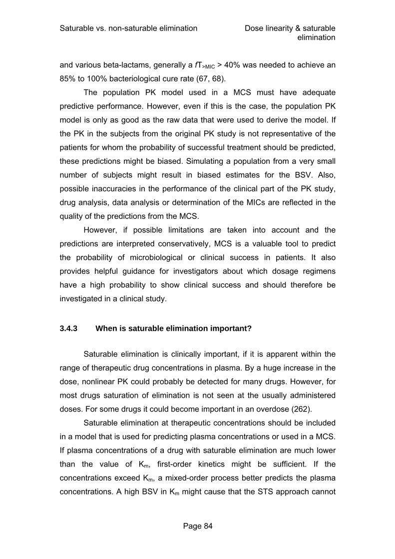
Saturable vs. non-saturable elimination Dose linearity & saturable elimination
Page 84
and various beta-lactams, generally a fT>MIC > 40% was needed to achieve an
85% to 100% bacteriological cure rate (67, 68).
The population PK model used in a MCS must have adequate
predictive performance. However, even if this is the case, the population PK
model is only as good as the raw data that were used to derive the model. If
the PK in the subjects from the original PK study is not representative of the
patients for whom the probability of successful treatment should be predicted,
these predictions might be biased. Simulating a population from a very small
number of subjects might result in biased estimates for the BSV. Also,
possible inaccuracies in the performance of the clinical part of the PK study,
drug analysis, data analysis or determination of the MICs are reflected in the
quality of the predictions from the MCS.
However, if possible limitations are taken into account and the
predictions are interpreted conservatively, MCS is a valuable tool to predict
the probability of microbiological or clinical success in patients. It also
provides helpful guidance for investigators about which dosage regimens
have a high probability to show clinical success and should therefore be
investigated in a clinical study.
3.4.3 When is saturable elimination important?
Saturable elimination is clinically important, if it is apparent within the
range of therapeutic drug concentrations in plasma. By a huge increase in the
dose, nonlinear PK could probably be detected for many drugs. However, for
most drugs saturation of elimination is not seen at the usually administered
doses. For some drugs it could become important in an overdose (262).
Saturable elimination at therapeutic concentrations should be included
in a model that is used for predicting plasma concentrations or used in a MCS.
If plasma concentrations of a drug with saturable elimination are much lower
than the value of Km, first-order kinetics might be sufficient. If the
concentrations exceed Km, a mixed-order process better predicts the plasma
concentrations. A high BSV in Km might cause that the STS approach cannot

Saturable vs. non-saturable elimination Dose linearity & saturable elimination
Page 85
detect a saturable elimination for all subjects. Population PK is more powerful
than STS in this situation (chapter 3.4.1).
Knowledge about an existing saturable elimination pathway is
important, when concentration time profiles are predicted for doses outside
the range of doses that were investigated in the PK study. A linear model
might be able to describe the elimination within a certain range of
concentrations. However, if this model is then used to predict the PK over a
wider range of concentrations, (e.g. for much higher or much lower doses),
the predictions may be biased. For example at higher doses, saturable
elimination becomes more important, and concentrations increase to a higher
extent than would be predicted by a linear (non-saturable) model. Inclusion of
a saturable elimination component may also be important, if different modes
of administration are compared (e.g. continuous and short-term infusion).
In dose escalation studies with drugs in clinical development, it is an
advantage if the data are evaluated by population PK modeling at each dose
level simultaneously. If nonlinear PK is present, the investigators can be more
cautious in increasing the dose and inappropriately high doses possibly
carrying an increased risk for toxicity can be avoided (163).
For dosage adjustment in patients it needs to be considered that the
time to reach steady-state increases with decreasing clearance (and therefore
increasing half-life). This is important e.g. for phenytoin, that is monitored by
TDM and where the time to reach steady-state can increase from several
days to two to three weeks at high dose rates. Higher than expected plasma
concentrations due to saturable elimination are clinically important, if
concentration-dependent side effects are likely to occur. Also, if other drugs
that share the same saturable elimination pathway are given in combination,
drug concentrations might increase more than expected.

Background Drug-drug interactions
Page 86
4 Pharmacokinetic drug-drug interactions of antibiotics and their pharmacodynamic impact
4.1 Background on pharmacokinetic drug-drug interactions involving transporters
4.1.1 Drug transport and mechanisms of interaction at transporters
Drug transport through membranes happens mostly by passive
diffusion, active transport or both. Passive diffusion occurs because of a
concentration gradient between both sides of the membrane and continues
until an equilibrium is reached. At equilibrium molecules still traverse the
membrane, but concentrations stay the same at both sides of the membrane.
No metabolic energy is needed for passive diffusion.
Active transport occurs through carrier proteins located in the
membranes. Transport proteins have been identified to be involved in
numerous processes in the body, e.g. renal tubular secretion, biliary secretion,
transport across the blood-brain barrier, gastro-intestinal absorption and
secretion. Contrary to passive diffusion, active transport can move drug
molecules against a concentration gradient, has a maximum rate of drug
transport, and can be inhibited by other substances or by metabolic inhibitors.
Active transport is a saturable (capacity-limited) process, and can be
described by the Michaelis Menten equation (see chapter 3.1 and Figure
4.1-1). The rate of transport increases less than linearly at concentrations
approaching or exceeding Km and at very high concentrations a maximum rate
of drug transport (Vmax) is reached asymptotically.
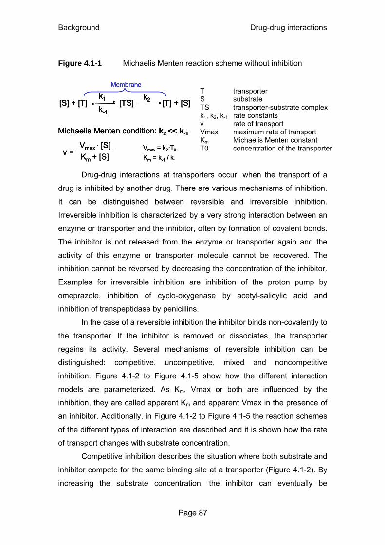
Background Drug-drug interactions
Page 87
Figure 4.1-1 Michaelis Menten reaction scheme without inhibition
T transporter S substrate TS transporter-substrate complex k1, k2, k-1 rate constants v rate of transport Vmax maximum rate of transport Km Michaelis Menten constant T0 concentration of the transporter
Drug-drug interactions at transporters occur, when the transport of a
drug is inhibited by another drug. There are various mechanisms of inhibition.
It can be distinguished between reversible and irreversible inhibition.
Irreversible inhibition is characterized by a very strong interaction between an
enzyme or transporter and the inhibitor, often by formation of covalent bonds.
The inhibitor is not released from the enzyme or transporter again and the
activity of this enzyme or transporter molecule cannot be recovered. The
inhibition cannot be reversed by decreasing the concentration of the inhibitor.
Examples for irreversible inhibition are inhibition of the proton pump by
omeprazole, inhibition of cyclo-oxygenase by acetyl-salicylic acid and
inhibition of transpeptidase by penicillins.
In the case of a reversible inhibition the inhibitor binds non-covalently to
the transporter. If the inhibitor is removed or dissociates, the transporter
regains its activity. Several mechanisms of reversible inhibition can be
distinguished: competitive, uncompetitive, mixed and noncompetitive
inhibition. Figure 4.1-2 to Figure 4.1-5 show how the different interaction
models are parameterized. As Km, Vmax or both are influenced by the
inhibition, they are called apparent Km and apparent Vmax in the presence of
an inhibitor. Additionally, in Figure 4.1-2 to Figure 4.1-5 the reaction schemes
of the different types of interaction are described and it is shown how the rate
of transport changes with substrate concentration.
Competitive inhibition describes the situation where both substrate and
inhibitor compete for the same binding site at a transporter (Figure 4.1-2). By
increasing the substrate concentration, the inhibitor can eventually be
[S] + [T] [T] + [S][TS] k1
k-1
k2
Michaelis Menten condition: k2 << k-1
v = Vmax · [S] Km + [S]
Vmax = k2·T0
Km = k-1 / k1
Membrane
[S] + [T] [T] + [S][TS] k1
k-1
k2
Michaelis Menten condition: k2 << k-1
v = Vmax · [S] Km + [S]
Vmax = k2·T0
Km = k-1 / k1
Membrane
[S] + [T] [T] + [S][TS] k1
k-1
k2
Michaelis Menten condition: k2 << k-1
v = Vmax · [S] Km + [S]
Vmax = k2·T0
Km = k-1 / k1
[S] + [T] [T] + [S][TS] k1
k-1
k2[S] + [T] [T] + [S][TS] k1
k-1
k2
Michaelis Menten condition: k2 << k-1
v = Vmax · [S] Km + [S]
Vmax = k2·T0
Km = k-1 / k1
Membrane Membrane

Background Drug-drug interactions
Page 88
displaced and Vmax can be reached at high substrate concentrations.
Therefore the extent of interaction decreases at high substrate concentrations,
i.e. above Km the difference in rate between the curves with and without
interaction decreases with increasing substrate concentrations. In competitive
inhibition the apparent Km is increased compared to the situation without an
inhibition, while Vmax is not changed. The competitive inhibition constant (Kic)
describes the affinity of the inhibitor to the transporter. A low Kic stands for a
high affinity of the inhibitor. The relative affinity of the substrate to the
transporter compared to the affinity of the inhibitor to the transporter is
calculated by the ratio of Kic / Km. A ratio greater than 1 means that the affinity
of the substrate is higher than that of the inhibitor. An example is ethanol, that
competitively inhibits the alcohol dehydrogenase and prevents production of
toxic metabolites after ethylene glycole poisoning. Sulfonamide antibiotics
compete with p-aminobenzoic acid and therefore inhibit production of
tetrahydrofolic acid in bacteria and multiplication of bacteria.
Figure 4.1-2 Competitive inhibition
0
0.25
0.5
0.75
1
0 200 400 600Substrate concentration (mg/L)
Rat
e (m
g/h)
Apparent Km
Apparent Vmax
[ ]⎟⎠⎞
⎜⎝⎛ +⋅
KicI1Km
Vmax
I inhibitor TI transporter-inhibitor complex Kic competitive inhibition constant
competitive inhibition
no inhibition
Km no inhibition (30 mg/L)
Km competitive (62 mg/L)
Vmax / 2 (no inhibition)
Rate of drug transport for a constant inhibitor concentration [I]
[T] + [S] [T] + [S] [TS] k1 k2
v = Vmax · [S] Km + [S]
[I]+
[TI]
k-1
[T] + [S] [T] + [S] [TS] k1 k2
v = Vmax · [S] Km + [S]
[I]+
[TI]
[T] + [S] [T] + [S] [TS] k1 k2
v = Vmax · [S] Km + [S] v = Vmax · [S] Km + [S]
[I]+
[TI]
k-1

Background Drug-drug interactions
Page 89
Uncompetitive inhibition means that the inhibitor only binds to the
transporter-substrate complex, i.e. after the substrate has bound to the
transporter (Figure 4.1-3). The uncompetitive inhibition constant (Kiu)
describes the affinity of the inhibitor to the transporter-substrate complex. Both
apparent Km and apparent Vmax are decreased by this inhibition. Contrary to
competitive inhibition, in uncompetitive inhibition the value of Vmax without
inhibition cannot be reached, even by greatly increasing the substrate
concentration. The extent of interaction is highest at high substrate
concentrations, i.e. the difference in rate between the curves with and without
interaction increases with increasing substrate concentrations (Figure 4.1-3).
The therapeutic effect of lithium in manic-depressive psychosis is caused by
uncompetitive inhibition of inositolmonophosphatase in the brain (200).
Memantine, an uncompetitive antagonist of the N-methyl-D-aspartate (NMDA)
receptor, is used for treatment of Alzheimer’s disease (102, 316). Despite
similar names, uncompetitive and noncompetitive inhibition (Figure 4.1-5) are
two different mechanisms of inhibition.
Figure 4.1-3 Uncompetitive inhibition
0
0.25
0.5
0.75
1
0 200 400 600
Substrate concentration (mg/L)
Rat
e (m
g/h)
Apparent Km
Apparent Vmax
[ ]Kiu
I1
Km
+ [ ]
KiuI1
Vmax
+
TSI transporter-substrate-inhibitor complex Kiu uncompetitive inhibition constant
uncompetitive inhibition
no inhibition
Vmax / 2 (no inhibition)
Km uncompetitive (16 mg/L)
Km no inhibition (30 mg/L)
Rate of drug transport for a constant inhibitor concentration [I]
v = Vmax · [S]Km + [S]
[T] + [S] [T] + [S] [TS] k1
k-1
k2+
[TSI]
[I]
v = Vmax · [S]Km + [S] v =
Vmax · [S]Km + [S]
[T] + [S] [T] + [S] [TS] k1
k-1
k2+
[TSI]
[I]
[T] + [S] [T] + [S] [TS] k1
k-1
k2+
[TSI]
[I]
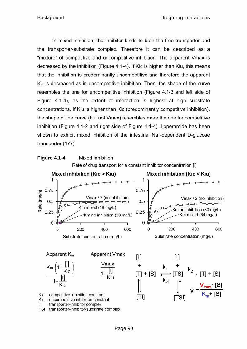
Background Drug-drug interactions
Page 90
In mixed inhibition, the inhibitor binds to both the free transporter and
the transporter-substrate complex. Therefore it can be described as a
“mixture” of competitive and uncompetitive inhibition. The apparent Vmax is
decreased by the inhibition (Figure 4.1-4). If Kic is higher than Kiu, this means
that the inhibition is predominantly uncompetitive and therefore the apparent
Km is decreased as in uncompetitive inhibition. Then, the shape of the curve
resembles the one for uncompetitive inhibition (Figure 4.1-3 and left side of
Figure 4.1-4), as the extent of interaction is highest at high substrate
concentrations. If Kiu is higher than Kic (predominantly competitive inhibition),
the shape of the curve (but not Vmax) resembles more the one for competitive
inhibition (Figure 4.1-2 and right side of Figure 4.1-4). Loperamide has been
shown to exhibit mixed inhibition of the intestinal Na+-dependent D-glucose
transporter (177).
Figure 4.1-4 Mixed inhibition
Mixed inhibition (Kic > Kiu)
0
0.25
0.5
0.75
1
0 200 400 600
Substrate concentration (mg/L)
Rat
e (m
g/h)
Mixed inhibition (Kic < Kiu)
0
0.25
0.5
0.75
1
0 200 400 600
Substrate concentration (mg/L)
Apparent Km
Apparent Vmax
[ ]
[ ]Kiu
I1
KicI1Km
+
⎟⎠⎞
⎜⎝⎛ +⋅
[ ]
KiuI1
Vmax
+
Kic competitive inhibition constant Kiu uncompetitive inhibition constant TI transporter-inhibitor complex TSI transporter-inhibitor-substrate complex
Km no inhibition (30 mg/L) Km mixed (64 mg/L)
Vmax / 2 (no inhibition)
Km mixed (18 mg/L)
Km no inhibition (30 mg/L)
Vmax / 2 (no inhibition)
Rate of drug transport for a constant inhibitor concentration [I]
[TI]
[T] + [S] [T] + [S] [TS] k1
k-1
k2
v = Vmax · [S]Km+ [S]
+ +
[TSI]
[I][I]
[TI]
[T] + [S] [T] + [S] [TS] k1
k-1
k2
v = Vmax · [S]Km+ [S] v =
Vmax · [S]Vmax · [S]Km+ [S]
+ +
[TSI]
[I][I]
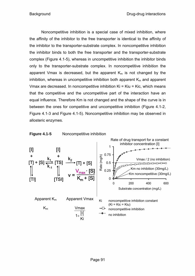
Background Drug-drug interactions
Page 91
Noncompetitive inhibition is a special case of mixed inhibition, where
the affinity of the inhibitor to the free transporter is identical to the affinity of
the inhibitor to the transporter-substrate complex. In noncompetitive inhibition
the inhibitor binds to both the free transporter and the transporter-substrate
complex (Figure 4.1-5), whereas in uncompetitive inhibition the inhibitor binds
only to the transporter-substrate complex. In noncompetitive inhibition the
apparent Vmax is decreased, but the apparent Km is not changed by the
inhibition, whereas in uncompetitive inhibition both apparent Km and apparent
Vmax are decreased. In noncompetitive inhibition Ki = Kiu = Kic, which means
that the competitive and the uncompetitive part of the interaction have an
equal influence. Therefore Km is not changed and the shape of the curve is in
between the ones for competitive and uncompetitive inhibition (Figure 4.1-2,
Figure 4.1-3 and Figure 4.1-5). Noncompetitive inhibition may be observed in
allosteric enzymes.
Figure 4.1-5 Noncompetitive inhibition
0
0.25
0.5
0.75
1
0 200 400 600
Substrate concentration (mg/L)
Rat
e (m
g/h)
Apparent Km
Apparent Vmax
Km [ ]KiI1
Vmax
+
Ki noncompetitive inhibition constant (Ki = Kic = Kiu)
noncompetitive inhibition
no inhibition
v = Vmax · [S] Km + [S]
[T] + [S] [TS] k-1
k2+
[TSI]
[I]
[T] + [S] +
[TI]
[I]
k1
v = Vmax · [S] Km + [S]
[T] + [S] [TS] k-1
k2+
[TSI]
[I]
[T] + [S] +
[TI]
[I]
k1
v = Vmax · [S] Km + [S] v =
Vmax · [S] Km + [S]
[T] + [S] [TS] k-1
k2+
[TSI]
[I]
[T] + [S] +
[TI]
[I]
k1
Km no inhibition (30mg/L) Km noncompetitive (30mg/L)
Vmax / 2 (no inhibition)
Rate of drug transport for a constant inhibitor concentration [I]
Background Drug-drug interactions
Page 92
4.1.2 Literature data on interactions with probenecid
A commonly studied drug-drug interaction with antibiotics is the
interaction with probenecid. This interaction has been studied for a long time
and for many quinolones and beta-lactams (123, 186, 304). Probenecid
interacts with both organic anion and organic cation transporters that are
involved in the active renal secretion of drug molecules. The extent of
interaction with probenecid may reach clinical significance for drugs which
display active tubular secretion (116, 233, 318). Probenecid is well
documented to decrease the renal secretion of many quinolones, e.g.
gatifloxacin (233), levofloxacin (105, 114), norfloxacin (271), fleroxacin (269),
and enoxacin (330), whereas moxifloxacin and sparfloxacin are not affected
by probenecid (270, 288).
In the vast majority of studies, the interaction with probenecid is studied
for the renal site. Less is known about the interaction of probenecid with drugs
at other sites in the body. Organic anion and organic cation transporters are
not only involved in the active renal secretion of drug molecules (121), but
have been found also at various other sites in the body (219, 272). Recently
probenecid was shown to affect active transport processes at the blood brain
barrier (61). The importance of drug transporters in hepatocytes has been
highlighted by Cummins et al. (71). Through an influence of probenecid on
drug transporters in the hepatocytes or enterocytes, changes in the nonrenal
elimination and metabolism of drugs seem likely. In humans, probenecid
decreases the renal excretion of paracetamol glucuronide by 79% (168) and
also increases the biotransformation of carbamazepine (173).
Recently it has been discussed that the shortage of oseltamivir might
be eased by concomitant administration of probenecid (53). By inhibition of
renal secretion, probenecid has been shown to increase the AUC of
oseltamivir’s active metabolite 2.5fold (140). However, to date no clinical trials
have been performed to investigate the effectiveness of lower oseltamivir
doses in combination with probenecid.
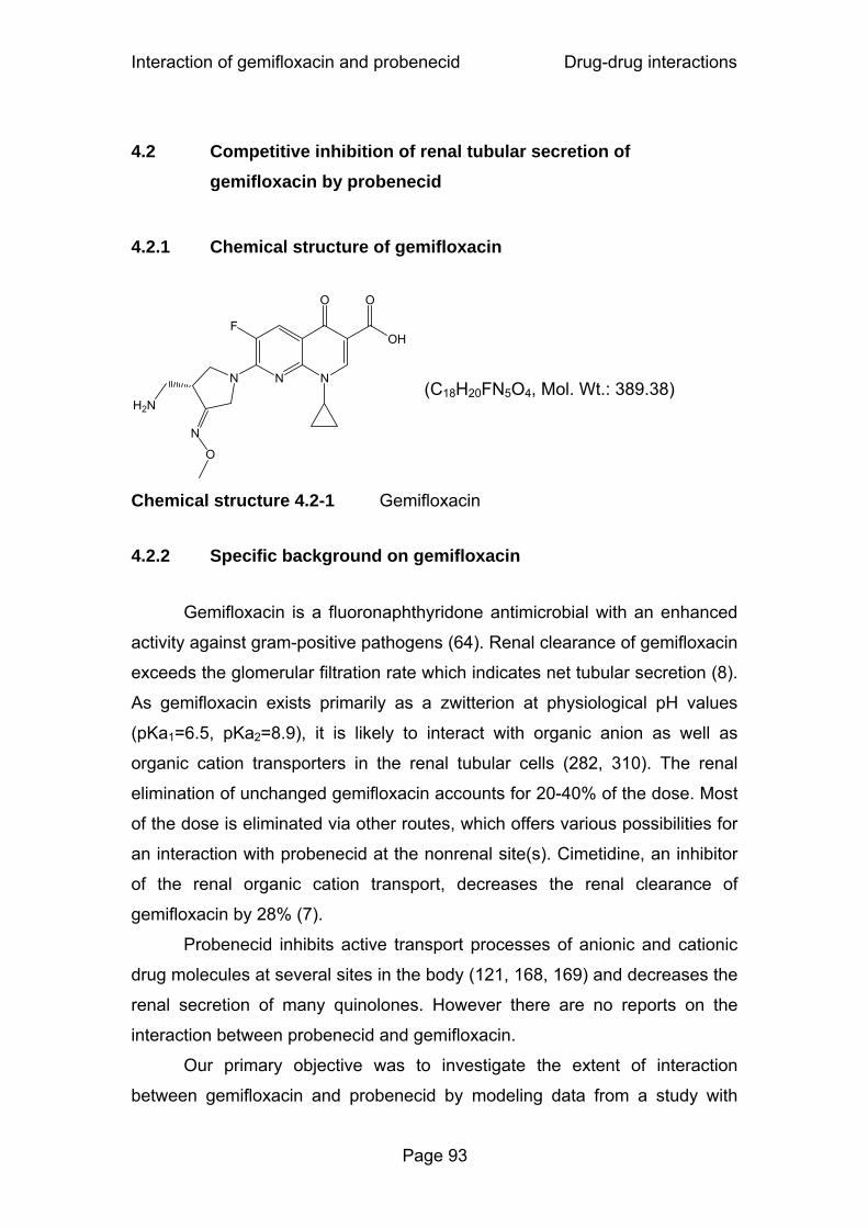
Interaction of gemifloxacin and probenecid Drug-drug interactions
Page 93
4.2 Competitive inhibition of renal tubular secretion of gemifloxacin by probenecid
4.2.1 Chemical structure of gemifloxacin
N N
O
OH
O
F
N
N
O
H2N
Chemical structure 4.2-1 Gemifloxacin
4.2.2 Specific background on gemifloxacin
Gemifloxacin is a fluoronaphthyridone antimicrobial with an enhanced
activity against gram-positive pathogens (64). Renal clearance of gemifloxacin
exceeds the glomerular filtration rate which indicates net tubular secretion (8).
As gemifloxacin exists primarily as a zwitterion at physiological pH values
(pKa1=6.5, pKa2=8.9), it is likely to interact with organic anion as well as
organic cation transporters in the renal tubular cells (282, 310). The renal
elimination of unchanged gemifloxacin accounts for 20-40% of the dose. Most
of the dose is eliminated via other routes, which offers various possibilities for
an interaction with probenecid at the nonrenal site(s). Cimetidine, an inhibitor
of the renal organic cation transport, decreases the renal clearance of
gemifloxacin by 28% (7).
Probenecid inhibits active transport processes of anionic and cationic
drug molecules at several sites in the body (121, 168, 169) and decreases the
renal secretion of many quinolones. However there are no reports on the
interaction between probenecid and gemifloxacin.
Our primary objective was to investigate the extent of interaction
between gemifloxacin and probenecid by modeling data from a study with
(C18H20FN5O4, Mol. Wt.: 389.38)

Interaction of gemifloxacin and probenecid Drug-drug interactions
Page 94
administration of multiple doses of probenecid. Our secondary objective was
to describe the time course and plausible mechanisms for the interaction
between gemifloxacin and probenecid at the renal and nonrenal sites by
compartmental modeling techniques.
4.2.3 Methods
Study design and drug administration: Seventeen healthy subjects
(nine males and eight females) participated in the study. Subjects fasted from
12h before until 3h after administration of gemifloxacin. In each of the two
study periods each subject received a single oral dose of 320 mg gemifloxacin
(Factive® 320 mg tablets) either alone or with 4.5g of probenecid (Probenecid
Weimer® 500 mg tablets) divided in eight oral doses. It was intended to study
the maximum extent of interaction between probenecid and gemifloxacin.
Therefore, relatively high doses of probenecid were administered throughout
the whole gemifloxacin plasma concentration time profile. Probenecid was
administered as follows: 1000 mg at 10h and 2h before gemifloxacin, followed
by 250 mg at 6h and 14h after, and 500 mg at 24h, 36h, 48h and 60h after the
dose of gemifloxacin.
Sampling Schedule: Blood samples were collected immediately
before the gemifloxacin dose and at 0.5, 1, 1.5, 2, 3, 4, 6, 8, 12, 16, 24, 36,
and 48h post-dose. Urine samples were collected before gemifloxacin
administration and in the following time intervals: 0 to 4, 4 to 8, 8 to 12, 12 to
16, 16 to 24, 24 to 30, 30 to 36, 36 to 48, 48 to 60 and 60 to 72h after
gemifloxacin dose.
Determination of Plasma and Urine Concentrations: For
determination of gemifloxacin concentrations, 50µL of each human plasma
sample were precipitated with 250µL acetonitrile containing the internal
standard. After thorough mixing, the samples were left to stand at room
temperature for approximately 10min, and were then centrifuged for
approximately 15min at 11,000 g. Of each human urine sample 50µL were
diluted by 400µL of mobile phase containing the internal standard. Of each so
prepared plasma and urine sample 10µL were chromatographed on a
Interaction of gemifloxacin and probenecid Drug-drug interactions
Page 95
reversed phase column by isocratic elution. The samples were analyzed by
LC-MS/MS with a selected reaction monitoring (SRM) method as follows:
Precursor → product ion for gemifloxacin m/z 390 → m/z 313 and internal
standard m/z 394 → m/z 313. Both analyses were in positive mode. Under
these conditions gemifloxacin and the internal standard were eluted after
approximately 1.1 minutes. Calibration was performed by weighted (1/y2)
linear regression.
For determination of probenecid concentrations, 100µL of each human
plasma sample were precipitated with 300µL acetonitrile containing the
internal standard. After thorough mixing the samples were centrifuged for
approximately 5 minutes at 3280 g. Of each sample 15µL were injected onto
the HPLC-MS/MS system. The samples were chromatographed on a reversed
phase column, eluted with an isocratic solvent and monitored by LC-MS/MS
with a SRM method as follows: Precursor → product ion for probenecid m/z
284 → m/z 240 and internal standard m/z 329 → m/z 205. Both analyses
were in negative mode. Under these conditions probenecid and the internal
standard were eluted after approximately 1.4 and 0.8 minutes, respectively.
Calibration was performed by weighted (1/x2) linear regression. The MacQuan
software (version 1.6, PE Sciex, Thornhill, Ontario, Canada, 1991 - 1998) was
used for evaluation of chromatograms.
Calibration standards in plasma and urine were prepared by adding the
appropriate volume of standard solution of gemifloxacin or probenecid or of
the higher concentrated calibration standard to drug-free human plasma or
urine. No interferences were observed in plasma and urine for gemifloxacin,
probenecid, or the internal standard. The linearity of the gemifloxacin
calibration curves in plasma and urine was determined between 0.0100 and
5.00 mg/L. The linearity of the probenecid calibration curves in plasma was
shown between 2.45 and 97.6 mg/L. The quantification limits were identical
with the lowest calibration levels. The inter-day precision and the analytical
recovery of the SQCs of gemifloxacin in human plasma (urine) ranged from
3.7 to 7.2% (5.7 to 7.7%) and from 100.9 to 101.4% (98.1 to 103.3%),
respectively. The inter-day precision and the analytical recovery of the SQCs
Interaction of gemifloxacin and probenecid Drug-drug interactions
Page 96
of probenecid in human plasma ranged from 5.1 to 5.8% and from 90.3 to
102.6%, respectively.
Pharmacokinetic Calculations: We applied NCA and compartmental
modeling methods to analyze the concentration-time data of gemifloxacin in
plasma and urine and of probenecid in plasma. We used NONMEM for visual
predictive checks (25).
Compartmental modeling:
Absorption and disposition of gemifloxacin: We tested one, two
and three compartment disposition models for gemifloxacin with first order
absorption and with or without lag-time for oral absorption. Identification of the
renal and nonrenal components of clearance was possible, because we had
both plasma and urine data. We used the following equation to describe the
renal clearance of gemifloxacin:
[ ]GKVmaxGFRf CLmR
RuR ++⋅= Formula 4.2-1
The first part (fu · GFR) describes the filtration clearance and the
second part of the equation describes the net tubular secretion. fu is the non-
protein bound fraction of gemifloxacin in plasma, GFR is the glomerular
filtration rate, VmaxR is the maximum rate of the mixed order renal elimination,
KmR is the gemifloxacin concentration associated with a half maximal rate
(VmaxR/2) for the mixed order renal elimination of gemifloxacin, and [G] is the
plasma concentration of gemifloxacin. The range of fu is between 0.3 and 0.4,
as a protein binding of 60 to 70% has been reported for gemifloxacin (15). All
subjects had normal renal function. Therefore, the renal filtration clearance of
gemifloxacin, fu · GFR, is about 2 L/h and accounts only for about 6% of the
total body clearance. Hence, we fixed the first order component of renal
clearance to 2 L/h in our models.
We described the nonrenal elimination of gemifloxacin as a first-order
process for the treatment with gemifloxacin alone. For models with a static
interaction for nonrenal clearance of gemifloxacin, we estimated first order
nonrenal clearance of gemifloxacin with (CLNR,with P) and without (CLNR,without P)
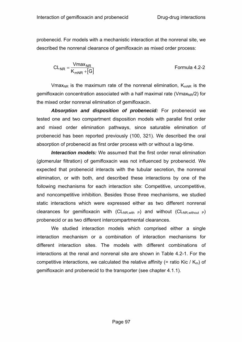
Interaction of gemifloxacin and probenecid Drug-drug interactions
Page 97
probenecid. For models with a mechanistic interaction at the nonrenal site, we
described the nonrenal clearance of gemifloxacin as mixed order process:
[ ]GKVmax CLmNR
NRNR +
= Formula 4.2-2
VmaxNR is the maximum rate of the nonrenal elimination, KmNR is the
gemifloxacin concentration associated with a half maximal rate (VmaxNR/2) for
the mixed order nonrenal elimination of gemifloxacin.
Absorption and disposition of probenecid: For probenecid we
tested one and two compartment disposition models with parallel first order
and mixed order elimination pathways, since saturable elimination of
probenecid has been reported previously (100, 321). We described the oral
absorption of probenecid as first order process with or without a lag-time.
Interaction models: We assumed that the first order renal elimination
(glomerular filtration) of gemifloxacin was not influenced by probenecid. We
expected that probenecid interacts with the tubular secretion, the nonrenal
elimination, or with both, and described these interactions by one of the
following mechanisms for each interaction site: Competitive, uncompetitive,
and noncompetitive inhibition. Besides those three mechanisms, we studied
static interactions which were expressed either as two different nonrenal
clearances for gemifloxacin with (CLNR,with P) and without (CLNR,without P)
probenecid or as two different intercompartmental clearances.
We studied interaction models which comprised either a single
interaction mechanism or a combination of interaction mechanisms for
different interaction sites. The models with different combinations of
interactions at the renal and nonrenal site are shown in Table 4.2-1. For the
competitive interactions, we calculated the relative affinity (= ratio Kic / Km) of
gemifloxacin and probenecid to the transporter (see chapter 4.1.1).

Interaction of gemifloxacin and probenecid Drug-drug interactions
Page 98
Table 4.2-1 Interaction models – combinations of mechanisms of interaction at different interaction sites
Model 1 2 3 4 5 6 Inhibition of renal tubular secretion C NC UC C NC C Inhibition of nonrenal clearance S S S C NC S Inhibition of distributional clearance None None None None None S Number of subjects for whom the model had the best AIC 8 2 1 - 5 1
C: Competitive inhibition (see Figure 4.1-2) NC: Noncompetitive inhibition (see Figure 4.1-5) UC: Uncompetitive inhibition (see Figure 4.1-3) S: Static inhibition (two different parameters for treatment with and without probenecid)
4.2.4 Results
All 17 subjects completed the study. The average ± SD weight was
69.1 ± 13 kg and height was 173 ± 10 cm. Plasma and urine concentrations of
gemifloxacin with and without probenecid and probenecid concentrations in
plasma are shown in Figure 4.2-1. Gemifloxacin concentrations in plasma
were slightly higher for the treatment with probenecid (Panel A). The amount
of gemifloxacin excreted in urine was reduced by probenecid (Panel B).
Figure 4.2-1 Gemifloxacin and probenecid plasma concentrations and amounts in urine (average ± standard deviation)
Panel A: Gemifloxacin concentrations in plasma with and without probenecid
Pla
sma
conc
entra
tion
(mg/
L)
0.0
0.2
0.4
0.6
0.8
1.0
1.2
1.4
1.6
1.8
0 6 12 18 24 30 36 42 48Time after gemifloxacin administration (h)
Gemifloxacin aloneGemifloxacin with probenecid

Interaction of gemifloxacin and probenecid Drug-drug interactions
Page 99
Panel B: Gemifloxacin amounts excreted in urine with and without probenecid
Panel C: Probenecid concentrations in plasma
Non-compartmental analysis: The results of the NCA are shown in
Table 4.2-2. Addition of probenecid to gemifloxacin reduced the median renal
clearance by 51% (p<0.01) and the median nonrenal clearance by 19%
(p<0.01). Therefore, total body clearance was decreased by 31% (p<0.01).
Although NCA indicated that the median volume of distribution at steady-state
(Vss) decreased from 367 to 315 L (p=0.06, Table 4.2-2), this is probably an
artifact from NCA and not a true decrease of Vss. We simulated the plasma
concentrations of gemifloxacin with and without probenecid with identical PK
parameters (including volume of distribution) for both profiles. We derived Vss
from both simulated profiles by NCA and observed an about 10% lower Vss
for the interaction profiles compared to when gemifloxacin was simulated
alone, although the true volume was identical in the simulation.
Cum
ulat
ive
amou
nt in
urin
e (m
g)
0
20
40
60
80
100
120
140
0 12 24 36 48 60 72Time after gemifloxacin administration (h)
Gemifloxacin aloneGemifloxacin with probenecid
Pla
sma
conc
entra
tion
(mg/
L)
0
20
40
60
80
100
120
140
160
0 6 12 18 24 30 36 42 48
Time after gemifloxacin administration (h)
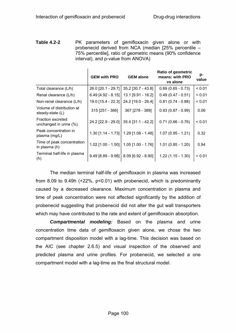
Interaction of gemifloxacin and probenecid Drug-drug interactions
Page 100
Table 4.2-2 PK parameters of gemifloxacin given alone or with
probenecid derived from NCA (median [25% percentile – 75% percentile], ratio of geometric means (90% confidence interval), and p-value from ANOVA)
GEM with PRO GEM aloneRatio of geometric means: with PRO
vs alone
p-value
Total clearance (L/h) 26.0 [20.1 - 29.7] 35.2 [30.7 - 43.8] 0.69 (0.65 - 0.73) < 0.01Renal clearance (L/h) 6.49 [4.92 - 8.15] 13.1 [9.91 - 16.2] 0.49 (0.47 - 0.51) < 0.01Non-renal clearance (L/h) 19.0 [15.4 - 22.3] 24.2 [19.0 - 26.4] 0.81 (0.74 - 0.88) < 0.01Volume of distribution at steady-state (L) 315 [251 - 366] 367 [278 - 389] 0.93 (0.87 - 0.99) 0.06
Fraction excreted unchanged in urine (%) 24.2 [22.9 - 29.0] 35.4 [31.1 - 42.2] 0.71 (0.66 - 0.76) < 0.01
Peak concentration in plasma (mg/L) 1.30 [1.14 - 1.73] 1.29 [1.08 - 1.48] 1.07 (0.95 - 1.21) 0.32
Time of peak concentration in plasma (h) 1.02 [1.00 - 1.50] 1.05 [1.00 - 1.76] 1.01 (0.85 - 1.20) 0.94
Terminal half-life in plasma (h) 9.49 [8.89 - 9.98] 8.09 [6.92 - 8.90] 1.22 (1.15 - 1.30) < 0.01
The median terminal half-life of gemifloxacin in plasma was increased
from 8.09 to 9.49h (+22%, p<0.01) with probenecid, which is predominantly
caused by a decreased clearance. Maximum concentration in plasma and
time of peak concentration were not affected significantly by the addition of
probenecid suggesting that probenecid did not alter the gut wall transporters
which may have contributed to the rate and extent of gemifloxacin absorption.
Compartmental modeling: Based on the plasma and urine
concentration time data of gemifloxacin given alone, we chose the two
compartment disposition model with a lag-time. This decision was based on
the AIC (see chapter 2.6.5) and visual inspection of the observed and
predicted plasma and urine profiles. For probenecid, we selected a one
compartment model with a lag-time as the final structural model.

Interaction of gemifloxacin and probenecid Drug-drug interactions
Page 101
Figure 4.2-2 Visual predictive check for plasma concentrations of gemifloxacin with or without probenecid for model 1 (see Table 4.2-1)
See chapter 2.6.5 and Figure 3.2-2 for explanation of the plots.
Gemifloxacin without probenecid
(logarithmic scale) Gemifloxacin with probenecid
(logarithmic scale)
Gemifloxacin without probenecid
(linear scale)
Gemifloxacin with probenecid
(linear scale)
The AIC and the visual predictive checks showed that model 1 had the
best predictive performance between the tested interaction models (Table
4.2-1 and Figure 4.2-2). This suggested a competitive inhibition of the renal
tubular secretion of gemifloxacin by probenecid as the most likely mechanism.
Table 4.2-3 lists the average PK parameters of gemifloxacin for model 1. The
average nonrenal clearance of gemifloxacin was significantly reduced from
25.2 to 21.0 L/h (reduction by 17%, p<0.01) with probenecid. Absorption lag-
time and absorption rate constant Ka were not affected by probenecid.
The affinity of gemifloxacin to the renal tubular transporter was 7.2 [5.8-
8.6] times (median [P25-P75]) higher than the affinity of probenecid. As shown
in Figure 4.2-1, probenecid reached about 150 times higher average plasma

Interaction of gemifloxacin and probenecid Drug-drug interactions
Page 102
concentrations than gemifloxacin and therefore inhibited the secretion of
gemifloxacin at the renal transporter to the extent shown in Table 4.2-2.
Table 4.2-3 PK parameter estimates and BSV of gemifloxacin for model 1 (see Table 4.2-1)
Parameter Unit Average (%coefficient of variation) for gemifloxacin
with probenecid without probenecid Ka h-1 0.897 (104%) 0.839 (62%) Tlag h 0.129 (104%) 0.223 (104%) CLNR L h-1 21.0 (23%)° 25.2 (26%)° KmR mg L-1 9.16 (20%) VmaxR mg h-1 113 (21%) CLR,Lin
L h-1 2#
Kic mg L-1 69.3 (26%) V1 L 89.5 (62%) V2 L 160 (31%) CLIC L h-1 39.8 (58%)
°: Significantly different (paired t-test: p<0.01). #: Fixed, not estimated.
Ka: Absorption rate constant, Tlag: Absorption lag-time, CLNR: Apparent nonrenal clearance,
KmR: Michaelis Menten constant of the mixed order renal elimination, VmaxR: Apparent
maximum rate of the mixed order renal elimination, CLR,Lin: First order renal clearance, Kic:
Competitive inhibition constant, V1: Apparent volume of distribution of central compartment,
V2: Apparent volume of distribution of peripheral compartment, CLIC: Apparent
intercompartmental clearance.
4.2.5 Discussion
We are not aware of any reports on the interaction between
gemifloxacin and probenecid. Therefore, our primary aim was to study the
extent of this interaction. Our secondary aim was to explore the time course,
mechanism, and site(s) of interaction. Frequent plasma and urine samples
were collected after administration of gemifloxacin alone and together with
probenecid, and gemifloxacin and probenecid were quantified. Our NCA
Interaction of gemifloxacin and probenecid Drug-drug interactions
Page 103
results for gemifloxacin alone were within the range of other studies (8, 117,
199). Probenecid significantly (p<0.01) decreased the median renal clearance
of gemifloxacin by 51%, the median nonrenal clearance by 19%, and the
median total clearance by 31% as determined by NCA. The peak
concentration was not significantly affected by probenecid. These findings
show that probenecid inhibited primarily the renal elimination of gemifloxacin.
However, also the nonrenal elimination was decreased.
The results from NCA provided an estimate for the maximum extent of
interaction between probenecid and gemifloxacin, since the probenecid doses
were rather high. We modeled the mechanistic interaction between
probenecid and gemifloxacin to further investigate the time course and
mechanism of the interaction between probenecid and gemifloxacin. We fitted
the plasma and urine profiles of gemifloxacin (with and without probenecid)
and of probenecid simultaneously, in order to derive the maximum amount of
information from the data. This method uses all data of an individual
simultaneously to derive the PK parameters of both drugs and to estimate the
time course of interaction.
Our compartmental modeling showed that model 1 (competitive
interaction at the renal site and static interaction at the nonrenal site) had the
best predictive performance of the tested models. It was the model with the
lowest AIC value in 8 of the 17 subjects, whereas the next best model (model
5) had the lowest AIC in 5 subjects (see Table 4.2-1 for performance of the
other models). The visual predictive check (Figure 4.2-2) showed that model 1
also had the best predictive performance and was able to capture both the
central tendency and the variability of the raw data. The highly sufficient
predictive performance further supported our estimates for the PK parameters
and their variability for the mechanistic interpretation.
We also found an interaction between gemifloxacin and probenecid for
the nonrenal elimination of gemifloxacin. However we could not identify a
specific mechanism for the nonrenal interaction, probably because the extent
of inhibition at the nonrenal site was much smaller than at the renal site. The
estimates for the intercompartmental clearance of gemifloxacin were very
similar with and without probenecid. Consequently, model 6 (Table 4.2-1) was

Interaction of gemifloxacin and probenecid Drug-drug interactions
Page 104
only preferred for one subject. Therefore our final model (model 1 in Table
4.2-1) had a competitive interaction at the renal site and a static interaction at
the nonrenal site. From the physiological point of view a competitive
mechanism seems the most reasonable as it describes the situation that
gemifloxacin and probenecid compete for the same active site of the renal
tubular transporter.
This interaction has not been studied before and we are not aware of
any reports where a mechanistic model for the interaction of quinolones and
probenecid in humans or animals has been developed. As most quinolones
are eliminated via tubular secretion, the competitive inhibition of renal tubular
secretion that we found for gemifloxacin with probenecid could also apply to
other quinolones.
In conclusion, we found that probenecid significantly decreased the
renal clearance of gemifloxacin from 13.1 to 6.49 L/h (medians) and the
nonrenal clearance from 24.2 to 19.0 L/h. Consequently, the total gemifloxacin
clearance was decreased by 31% (p<0.01). The absorption parameters,
volume of distribution and peak concentration of gemifloxacin were unaffected
by the interaction. Our data suggested a competitive inhibition of the renal
tubular secretion of gemifloxacin by probenecid. The median affinity to the
renal transporter was 7.2 times higher for gemifloxacin than for probenecid,
but probenecid inhibited the secretion of gemifloxacin because probenecid
reached about 150 times higher average plasma concentrations than
gemifloxacin. Future mechanistic studies for other quinolones are required to
further explore this mechanism of interaction.
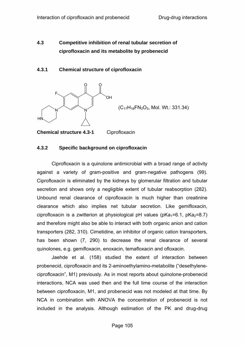
Interaction of ciprofloxacin and probenecid Drug-drug interactions
Page 105
4.3 Competitive inhibition of renal tubular secretion of ciprofloxacin and its metabolite by probenecid
4.3.1 Chemical structure of ciprofloxacin
N
O
OH
O
F
N
HN
Chemical structure 4.3-1 Ciprofloxacin
4.3.2 Specific background on ciprofloxacin
Ciprofloxacin is a quinolone antimicrobial with a broad range of activity
against a variety of gram-positive and gram-negative pathogens (99).
Ciprofloxacin is eliminated by the kidneys by glomerular filtration and tubular
secretion and shows only a negligible extent of tubular reabsorption (282).
Unbound renal clearance of ciprofloxacin is much higher than creatinine
clearance which also implies net tubular secretion. Like gemifloxacin,
ciprofloxacin is a zwitterion at physiological pH values (pKa1=6.1, pKa2=8.7)
and therefore might also be able to interact with both organic anion and cation
transporters (282, 310). Cimetidine, an inhibitor of organic cation transporters,
has been shown (7, 290) to decrease the renal clearance of several
quinolones, e.g. gemifloxacin, enoxacin, temafloxacin and ofloxacin.
Jaehde et al. (158) studied the extent of interaction between
probenecid, ciprofloxacin and its 2-aminoethylamino-metabolite (“desethylene-
ciprofloxacin”, M1) previously. As in most reports about quinolone-probenecid
interactions, NCA was used then and the full time course of the interaction
between ciprofloxacin, M1, and probenecid was not modeled at that time. By
NCA in combination with ANOVA the concentration of probenecid is not
included in the analysis. Although estimation of the PK and drug-drug
(C17H18FN3O3, Mol. Wt.: 331.34)
Interaction of ciprofloxacin and probenecid Drug-drug interactions
Page 106
interaction parameters is computationally intensive, modern computation
speeds and sophisticated software allow one to analyze those complex
systems.
Our first objective was to develop a model that adequately describes
the plasma concentrations and amounts in urine of ciprofloxacin and its
metabolite M1, including the formation of M1. As our second objective we
explored the possible influence of probenecid on renal clearance, nonrenal
clearance and distribution of both ciprofloxacin and M1, as well as on the
formation of M1. We intended to propose a possible mechanism for the
interaction between ciprofloxacin, M1 and probenecid at each site of
interaction. This full mechanistic interaction model can predict the time course
of a PK interaction for other dosage regimens of interest.
4.3.3 Methods
Study design and drug administration: Twelve healthy subjects (six
males and six females) participated in the study. The study was a
randomized, controlled, three-way crossover. The third treatment which is not
reported here was ciprofloxacin given together with charcoal. Subjects fasted
from 12h before until 6h after administration of ciprofloxacin. In each of the
two study periods reported here, each subject received a single dose of 200
mg ciprofloxacin (Ciprobay®) as 30min intravenous infusion either alone or
with 3g of probenecid (Benemid®) divided in five oral doses. Probenecid was
administered as follows: 500 mg at 10h and 1000 mg at 2h before the end of
the ciprofloxacin infusion, and 500 mg at 4h, 10h and 16h after the end of the
ciprofloxacin infusion.
Sampling schedule: Blood samples were taken before the start of the
ciprofloxacin infusion, 10 and 20min after the start of infusion, at the end of
infusion, and 5, 10, 20, 30, 45, 60, and 90min and 2, 3, 4, 5, 6, 8, 10, 12, 16,
24, 30, 36, and 48h after the end of infusion. Urine samples were collected
before ciprofloxacin administration and from start of the infusion to 2h after
end of infusion, as well as 2 to 4, 4 to 6, 6 to 8, 8 to 12, 12 to 16, 16 to 24, 24

Interaction of ciprofloxacin and probenecid Drug-drug interactions
Page 107
to 36, 36 to 48, 48 to 72, and 72 to 96h after the end of the ciprofloxacin
infusion.
Determination of plasma and urine concentrations: Ciprofloxacin
and M1 concentrations in plasma and urine were determined by reversed
phase HPLC as previously described (158). The assay was linear between
0.020 and 10 mg/L, with coefficients of correlation greater than 0.999. The
between-day precision of the assay evaluated by pooled biologically derived
plasma samples was found to be 2.6% (coefficient of variation) for
ciprofloxacin and 3.5% for M1 (average values of three different
concentrations). Probenecid concentrations in plasma were determined by
LC-MS/MS as described in chapter 4.2.3.
Pharmacokinetic calculations: We applied NCA and compartmental
modeling methods to analyze the concentration-time data of ciprofloxacin and
M1 in plasma and urine, and of probenecid in plasma.
Compartmental modeling: Initially we developed the compartment models for ciprofloxacin alone,
ciprofloxacin plus M1, and probenecid separately. Then we combined the
individual models to explore the interactions in the full model. We did not fix
any of the model parameters (except duration of infusion) while estimating the
full model. We modeled the plasma and urine profiles for ciprofloxacin with
and without probenecid, plasma and urine profiles for M1 with and without
probenecid, and plasma profiles for probenecid simultaneously.
Disposition of ciprofloxacin and M1: We tested two and three
compartment disposition models for ciprofloxacin. The input of ciprofloxacin
was modeled as a zero order process with a fixed duration of 30min. To
describe the disposition of M1 we tested one and two compartment models.
For ciprofloxacin, identification of the renal and nonrenal components
of clearance is possible, because both plasma concentrations and amounts in
urine were available. For M1 also plasma and urine data were available which
allows estimation of renal clearance for the metabolite. However the total
amount of the metabolite formed is unknown. If no further assumptions are
made, volume of distribution and nonrenal clearance of the metabolite are
therefore not mathematically identifiable simultaneously.

Interaction of ciprofloxacin and probenecid Drug-drug interactions
Page 108
In order to retain identifiability of all model parameters, e.g. one of the
following assumptions has to be made: 1) the metabolite is only eliminated
renally, 2) the volume of distribution for the metabolite is set to a pre-specified
value, e.g. to the estimated volume of distribution of ciprofloxacin, or 3) the
nonrenal clearance of the metabolite is set to a pre-specified value, e.g. to the
estimated nonrenal clearance of ciprofloxacin. More specifically, to “set” a
parameter to a pre-specified value meant in our analysis that the same
parameter was used for ciprofloxacin and M1 and that this one parameter was
optimized during the estimation process. We observed in the NCA that the
renal clearances of ciprofloxacin and M1 were very similar. Due to this and
other observations during model development we chose option 3) and
assumed that the nonrenal clearance of M1 was identical to the nonrenal
clearance of ciprofloxacin for each treatment.
We used the following equation to describe the renal clearance of
ciprofloxacin:
[ ]CKVmaxCL CL
CIPmR,
RlinR,CIPR, ++= Formula 4.3-1
CLR,lin is the first-order renal clearance (filtration clearance), and the
second part of the equation describes the net tubular secretion. VmaxR is the
maximum rate of the mixed-order renal elimination, KmR,CIP is the ciprofloxacin
concentration associated with a half maximal rate (VmaxR/2) for the mixed-
order renal elimination, and [C] is the plasma concentration of ciprofloxacin.
Since the NCA showed a significant reduction of renal clearance of M1
by probenecid, we assumed a parallel first-order and mixed-order renal
clearance for M1. This is the physiologically most reasonable way to describe
the renal elimination of M1. The M1 concentrations were about 1/10th to
1/200th the ciprofloxacin concentrations and, therefore, most likely far below
the KmR for the mixed-order renal elimination. Therefore, we used the same
parameter for the filtration clearance (CLR,lin) and VmaxR for the metabolite as
for ciprofloxacin and estimated KmR,M1 for the metabolite. This yields the
following equation for renal clearance of M1:
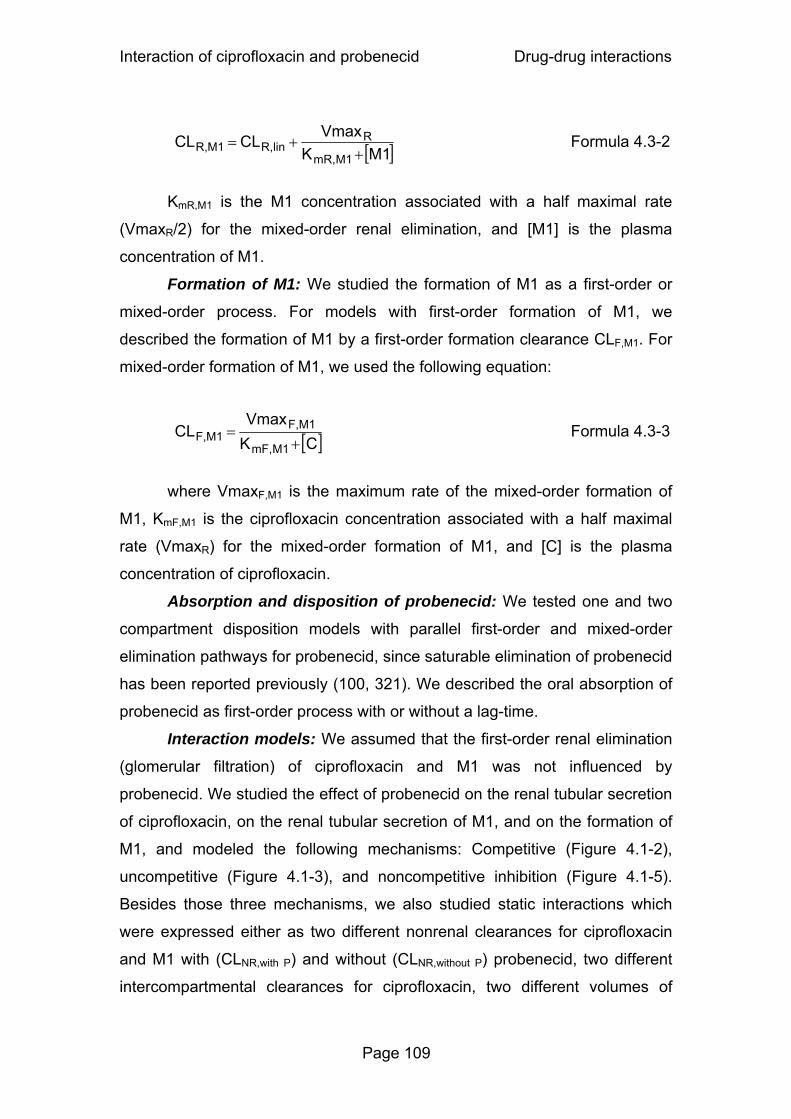
Interaction of ciprofloxacin and probenecid Drug-drug interactions
Page 109
[ ]M1KVmaxCL CL
M1mR,
RlinR,M1R, ++= Formula 4.3-2
KmR,M1 is the M1 concentration associated with a half maximal rate
(VmaxR/2) for the mixed-order renal elimination, and [M1] is the plasma
concentration of M1.
Formation of M1: We studied the formation of M1 as a first-order or
mixed-order process. For models with first-order formation of M1, we
described the formation of M1 by a first-order formation clearance CLF,M1. For
mixed-order formation of M1, we used the following equation:
[ ]CKVmax
CLM1mF,
M1F,M1F, +
= Formula 4.3-3
where VmaxF,M1 is the maximum rate of the mixed-order formation of
M1, KmF,M1 is the ciprofloxacin concentration associated with a half maximal
rate (VmaxR) for the mixed-order formation of M1, and [C] is the plasma
concentration of ciprofloxacin.
Absorption and disposition of probenecid: We tested one and two
compartment disposition models with parallel first-order and mixed-order
elimination pathways for probenecid, since saturable elimination of probenecid
has been reported previously (100, 321). We described the oral absorption of
probenecid as first-order process with or without a lag-time.
Interaction models: We assumed that the first-order renal elimination
(glomerular filtration) of ciprofloxacin and M1 was not influenced by
probenecid. We studied the effect of probenecid on the renal tubular secretion
of ciprofloxacin, on the renal tubular secretion of M1, and on the formation of
M1, and modeled the following mechanisms: Competitive (Figure 4.1-2),
uncompetitive (Figure 4.1-3), and noncompetitive inhibition (Figure 4.1-5).
Besides those three mechanisms, we also studied static interactions which
were expressed either as two different nonrenal clearances for ciprofloxacin
and M1 with (CLNR,with P) and without (CLNR,without P) probenecid, two different
intercompartmental clearances for ciprofloxacin, two different volumes of

Interaction of ciprofloxacin and probenecid Drug-drug interactions
Page 110
distribution for M1, two different first-order formation clearances of M1, or
different VmaxF,M1 and KmF,M1 for the formation of M1.
We studied interaction models which comprised either a single
interaction mechanism or a combination of interaction mechanisms for
different interaction sites. Table 4.3-1 shows the tested interaction models for
the disposition of ciprofloxacin. For the competitive interactions, we calculated
the relative affinity (= ratio Kic / Km) of ciprofloxacin, M1 and probenecid to the
transporter (chapter 4.1.1).
Table 4.3-1 Interaction models for ciprofloxacin
Model 1 2 3 4 Interaction in renal elimination C NC UC C Interaction in nonrenal elimination S S S S Interaction in distributional clearance None None None S Number of subjects for whom the model had the best AIC values 6 3 2 1
C: Competitive inhibition (see Figure 4.1-2) NC: Noncompetitive inhibition (see Figure 4.1-5) UC: Uncompetitive inhibition (see Figure 4.1-3) S: Static inhibition (two different parameters for treatment with and without probenecid).
4.3.4 Results
All 12 subjects completed the study. The average ± SD weight was
67.1 ± 12 kg, height was 175 ± 11 cm, and age was 28.5 ± 5.2 years. Plasma
and urine profiles of ciprofloxacin and M1 with and without probenecid and
probenecid concentrations in plasma are shown in Figure 4.3-1. Ciprofloxacin
had about 10 to 200 times higher concentrations than the metabolite.
Plasma concentrations of both ciprofloxacin and M1 were higher for the
treatment with probenecid. The amount of ciprofloxacin excreted in urine was
reduced by probenecid, whereas the amount of M1 excreted in urine was
increased by probenecid.
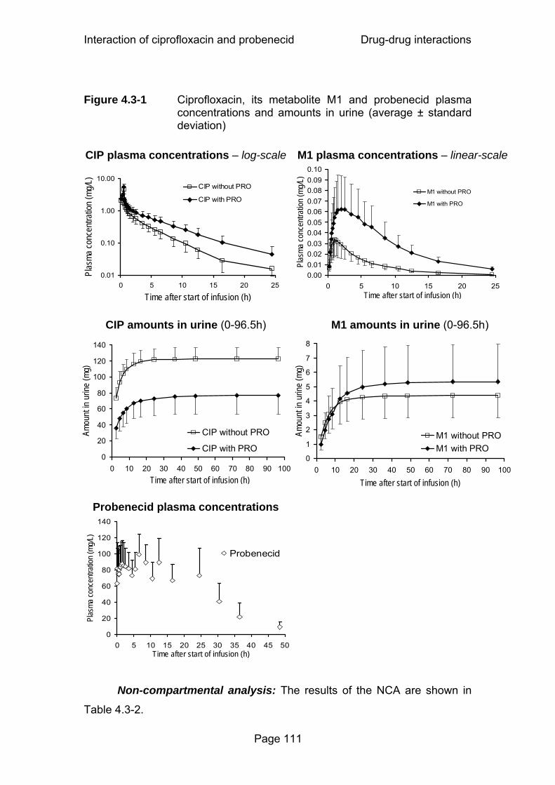
Interaction of ciprofloxacin and probenecid Drug-drug interactions
Page 111
Figure 4.3-1 Ciprofloxacin, its metabolite M1 and probenecid plasma
concentrations and amounts in urine (average ± standard deviation)
CIP plasma concentrations – log-scale
M1 plasma concentrations – linear-scale
CIP amounts in urine (0-96.5h)
M1 amounts in urine (0-96.5h)
Probenecid plasma concentrations
0
20
40
60
80
100
120
140
0 5 10 15 20 25 30 35 40 45 50Time after start of infusion (h)
Plas
ma co
ncen
tratio
n (m
g/L)
Probenecid
Non-compartmental analysis: The results of the NCA are shown in
Table 4.3-2.
0
20
40
60
80
100
120
140
0 10 20 30 40 50 60 70 80 90 100Time after start of infusion (h)
Amou
nt in
urin
e (m
g)
CIP without PRO
CIP with PRO0
1
2
3
4
5
6
7
8
0 10 20 30 40 50 60 70 80 90 100
Time after start of infusion (h)
Amou
nt in
urin
e (m
g)
M1 without PROM1 with PRO
0.01
0.10
1.00
10.00
0 5 10 15 20 25
Time after start of infusion (h)
Plas
ma co
ncen
tratio
n (m
g/L) CIP without PRO
CIP with PRO
0.000.010.020.030.040.050.060.070.080.090.10
0 5 10 15 20 25Time after start of infusion (h)
Plas
ma co
ncen
tratio
n (m
g/L)
M1 without PRO
M1 with PRO
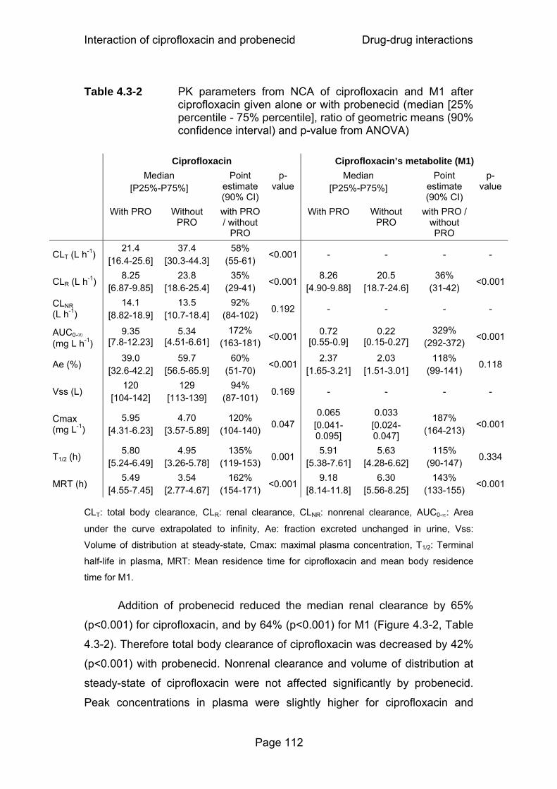
Interaction of ciprofloxacin and probenecid Drug-drug interactions
Page 112
Table 4.3-2 PK parameters from NCA of ciprofloxacin and M1 after ciprofloxacin given alone or with probenecid (median [25% percentile - 75% percentile], ratio of geometric means (90% confidence interval) and p-value from ANOVA)
Ciprofloxacin Ciprofloxacin’s metabolite (M1) Median
[P25%-P75%] Point
estimate (90% CI)
p-value
Median [P25%-P75%]
Point estimate (90% CI)
p-value
With PRO Without PRO
with PRO / without
PRO
With PRO Without PRO
with PRO / without PRO
CLT (L h-1) 21.4
[16.4-25.6] 37.4
[30.3-44.3] 58%
(55-61) <0.001 - - - -
CLR (L h-1) 8.25
[6.87-9.85] 23.8
[18.6-25.4] 35%
(29-41) <0.001
8.26 [4.90-9.88]
20.5 [18.7-24.6]
36% (31-42)
<0.001
CLNR (L h-1)
14.1 [8.82-18.9]
13.5 [10.7-18.4]
92% (84-102)
0.192 - - - -
AUC0-∞ (mg L h-1)
9.35 [7.8-12.23]
5.34 [4.51-6.61]
172% (163-181)
<0.001 0.72 [0.55-0.9]
0.22 [0.15-0.27]
329% (292-372)
<0.001
Ae (%) 39.0
[32.6-42.2] 59.7
[56.5-65.9] 60%
(51-70) <0.001
2.37 [1.65-3.21]
2.03 [1.51-3.01]
118% (99-141)
0.118
Vss (L) 120
[104-142] 129
[113-139] 94%
(87-101) 0.169 - - - -
Cmax (mg L-1)
5.95 [4.31-6.23]
4.70 [3.57-5.89]
120% (104-140)
0.047 0.065
[0.041-0.095]
0.033 [0.024-0.047]
187% (164-213)
<0.001
T1/2 (h) 5.80
[5.24-6.49] 4.95
[3.26-5.78] 135%
(119-153)0.001
5.91 [5.38-7.61]
5.63 [4.28-6.62]
115% (90-147)
0.334
MRT (h) 5.49
[4.55-7.45] 3.54
[2.77-4.67] 162%
(154-171)<0.001
9.18 [8.14-11.8]
6.30 [5.56-8.25]
143% (133-155)
<0.001
CLT: total body clearance, CLR: renal clearance, CLNR: nonrenal clearance, AUC0-∞: Area
under the curve extrapolated to infinity, Ae: fraction excreted unchanged in urine, Vss:
Volume of distribution at steady-state, Cmax: maximal plasma concentration, T1/2: Terminal
half-life in plasma, MRT: Mean residence time for ciprofloxacin and mean body residence
time for M1.
Addition of probenecid reduced the median renal clearance by 65%
(p<0.001) for ciprofloxacin, and by 64% (p<0.001) for M1 (Figure 4.3-2, Table
4.3-2). Therefore total body clearance of ciprofloxacin was decreased by 42%
(p<0.001) with probenecid. Nonrenal clearance and volume of distribution at
steady-state of ciprofloxacin were not affected significantly by probenecid.
Peak concentrations in plasma were slightly higher for ciprofloxacin and
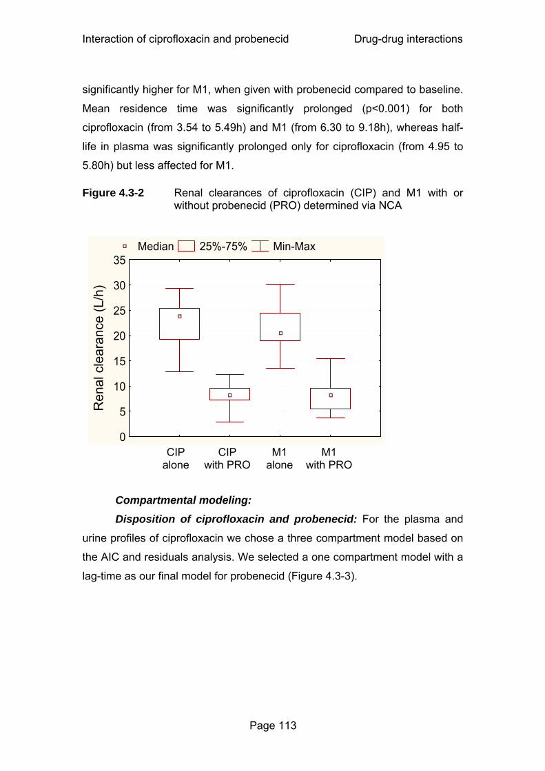
Interaction of ciprofloxacin and probenecid Drug-drug interactions
Page 113
significantly higher for M1, when given with probenecid compared to baseline.
Mean residence time was significantly prolonged (p<0.001) for both
ciprofloxacin (from 3.54 to 5.49h) and M1 (from 6.30 to 9.18h), whereas half-
life in plasma was significantly prolonged only for ciprofloxacin (from 4.95 to
5.80h) but less affected for M1.
Figure 4.3-2 Renal clearances of ciprofloxacin (CIP) and M1 with or without probenecid (PRO) determined via NCA
Compartmental modeling: Disposition of ciprofloxacin and probenecid: For the plasma and
urine profiles of ciprofloxacin we chose a three compartment model based on
the AIC and residuals analysis. We selected a one compartment model with a
lag-time as our final model for probenecid (Figure 4.3-3).
CIP alone
CIP with PRO
M1 with PRO
M1 alone
Median 25%-75% Min-Max
0
5
10
15
20
25
30
35
Ren
al c
lear
ance
(L/h
)

Interaction of ciprofloxacin and probenecid Drug-drug interactions
Page 114
Figure 4.3-3 Compartmental model for CIP, M1, and PRO
Panel A: Treatment without probenecid
Panel B: Treatment with probenecid
Mixed-order process
First-order process
CIP Urine
CIP Central compartment
V1
CIP Shallow peripheral
compartment V2
CIP Deep peripheral
compartment V3
CLR,Lin
VmaxR KmR,CIP
M1 Central compartment
VM1
M1 Urine
CLR,Lin
CLNR,without P
CLNR,without P
VmaxF,M1,without P KmF,M1,without P
VmaxR KmR,M1
Clicshallow,CIP Clicdeep,CIP
Zero-orderinput
CIP Urine
CIP Central compartment
V1
CIP Shallow peripheral
compartment V2
Clicshallow,CIP
CIP Deep peripheral
compartment V3Clicdeep,CIP
CLR,Lin
VmaxR KmR,CIP
M1 Central compartment
VM1M1
UrineCLR,LinCLNR,with P
CLNR,with P
VmaxF,M1,with P KmF,M1,with P
VmaxR KmR,M1
Kic,CIP
Kic,M1
Probenecid Central
compartmentVmaxPRO KmPRO
CLLin,PRO
Zero-orderinput

Interaction of ciprofloxacin and probenecid Drug-drug interactions
Page 115
Interaction of ciprofloxacin and probenecid: Our models for
ciprofloxacin and probenecid (without M1 data) suggested a competitive
inhibition of renal tubular secretion of ciprofloxacin by probenecid as the most
likely mechanism. We selected this mechanism for the interaction at the renal
site. The estimates for nonrenal clearance of ciprofloxacin were only slightly
lower for the treatment with probenecid (Table 4.3-3). Therefore we did not
study a mechanistic model for an effect of probenecid on the nonrenal
clearance of ciprofloxacin. We included two different parameters for the
nonrenal clearance to account for the small reduction and for the variability in
nonrenal clearance between both study periods.
Table 4.3-3 PK parameter estimates for ciprofloxacin and M1 (median [25% percentile - 75% percentile])
(see also Figure 4.3-3)
Ciprofloxacin Ciprofloxacin’s metabolite (M1) Parameter Unit Median
[P25-P75] Parameter Unit Median
[P25-P75] Renal elimination Renal elimination
CLR,Lin# L h-1 5.04 [4.40-5.37] CLR,Lin
# L h-1 5.04 [4.40-5.37] KmR,CIP mg L-1 4.66 [2.74-7.58] KmR,M1 mg L-1 5.83 [3.98-9.82]
VmaxR# mg h-1 106 [65.0-183] VmaxR
# mg h-1 106 [65.0-183] Kic,CIP mg L-1 12.3 [5.76-22.6] Kic,M1 mg L-1 18.5 [9.23-31.0]
Kic,CIP/KmR,CIP* - 3.77 [1.71-6.18] Kic,M1 / KmR,M1* - 3.20 [2.10-4.58]
Nonrenal elimination
Nonrenal elimination CLNR,without P
# L h-1 12.6 [9.69-15.9] CLNR,without P# L h-1 12.6 [9.69-15.9]
CLNR,with P# L h-1 11.9 [8.48-13.0] CLNR,with P
# L h-1 11.9 [8.48-13.0]
Volume of distribution
Volume of distribution V1CIP L 11.1 [4.17-15.4] VM1 L 15.8 [12.3-28.5] V2CIP L 38.2 [28.5-59.9] V3CIP L 57.6 [44.1-67.7] Mixed order formation of M1
KmF,M1,without P mg L-1 0.608 [0.327-0.826]Intercompartmental clearance KmF,M1,with P mg L-1 0.481 [0.422-1.41]
CLicshallow,CIP L h-1 97.0 [65.6-151] VmaxF,M1,without P mg h-1 1.94 [1.29-2.70] CLicdeep,CIP L h-1 16.2 [8.10-20.5] VmaxF,M1,with P mg h-1 1.89 [1.34-3.45]

Interaction of ciprofloxacin and probenecid Drug-drug interactions
Page 116
#: Parameter assumed to be the same for ciprofloxacin and M1. Parameter was
simultaneously estimated for ciprofloxacin and M1.
*: Derived from estimated parameters (not estimated).
CLR,Lin: First-order renal clearance, KmR,CIP: Michaelis Menten constant of the mixed-order
renal elimination of ciprofloxacin, VmaxR: Maximum rate of the mixed-order renal elimination,
Kic,CIP: Competitive inhibition constant of the mixed-order renal elimination of ciprofloxacin,
CLNR,without P: First-order nonrenal clearance without probenecid, CLNR,with P: First-order
nonrenal clearance with probenecid, V1CIP: Volume of distribution of central compartment,
V2CIP: Volume of distribution of shallow peripheral compartment, V3CIP: Volume of distribution
of deep peripheral compartment, CLicshallow,CIP: Intercompartmental clearance between the
central and the shallow peripheral compartment, CLicdeep,CIP: Intercompartmental clearance
between the central and the deep peripheral compartment, Kic,CIP / KmR,CIP: Affinity of
ciprofloxacin to the transporter divided by affinity of probenecid to the transporter, KmR,M1:
Michaelis Menten constant of the mixed-order renal elimination of M1, Kic,M1: Competitive
inhibition constant of the mixed-order renal elimination of M1, VM1: Volume of distribution of
M1, KmF,M1,without P: Michaelis Menten constant of the mixed-order formation of M1 without
probenecid, KmF,M1,with P: Michaelis Menten constant of the mixed-order formation of M1 with
probenecid, VmaxF,M1,without P: Maximum rate of the mixed-order formation of M1 without
probenecid, VmaxF,M1,with P: Maximum rate of the mixed-order formation of M1 with probenecid,
Kic,M1 / KmR,M1: Affinity of M1 to the transporter divided by affinity of probenecid to the
transporter.
Disposition of M1: We observed in the NCA that ciprofloxacin and M1
had very similar terminal half-lives. The geometric mean of the ratio for
terminal half-life(M1) / terminal half-life(ciprofloxacin) was 1.18 (34%
coefficient of variation). In absence of data on the terminal half-life of M1 after
iv dosing, we assumed that the formation of the metabolite determined its
terminal half-life. The flip-flop situation for M1 seems reasonable due to the
very similar terminal half-lives of parent and metabolite. The plasma
concentration time curves of the metabolite showed no two-compartment
behavior which was in agreement with the formation of the metabolite being
the rate limiting step. Therefore, we selected a one-compartment model for
M1 (Figure 4.3-3).
Formation of M1: Based on the ciprofloxacin and M1 data for the
treatment without probenecid, a mixed-order process described the formation
of the metabolite better than or equally well as a first-order formation process.
Interaction of ciprofloxacin and probenecid Drug-drug interactions
Page 117
More importantly, the Michaelis Menten constant for the formation of the
metabolite was about 0.6 mg/L which was well within the range of the
ciprofloxacin plasma concentrations. Therefore, we selected a mixed-order
process for the formation of the metabolite which is also the physiologically
most reasonable choice. Our models showed that probenecid did not affect
the formation parameters of M1, since the parameters for the mixed-order
formation of M1, VmaxF,M1 and KmF,M1 (Table 4.3-3), were not significantly
affected by the addition of probenecid.
Interaction of M1 and probenecid: We tested various models to
describe the interaction between M1 and probenecid at the renal site. The AIC
and residuals analysis suggested a competitive inhibition of renal tubular
secretion as the most likely interaction mechanism between M1 and
probenecid at the renal site.
As described in the methods section, we assumed that M1 had the
same nonrenal clearance as ciprofloxacin (option 3), and the nonrenal
clearance of ciprofloxacin and the metabolite was estimated simultaneously.
When we made this assumption, the volume of distribution of the metabolite
was very similar for the treatment with and without probenecid. Therefore, we
used the same volume of distribution for M1 for both treatments in our final
model. When we assumed that the metabolite was only eliminated renally
(option 1), the volume of distribution of M1 was about 45% lower for the
treatment with probenecid relative to the treatment without probenecid, and
Vmax for the formation of M1 was reduced by about 40% under the influence
of probenecid. Especially the reduction of volume of distribution would be a
very unreasonable result, because the volume of distribution of ciprofloxacin
was unaffected by probenecid. Therefore, this was a strong indication that
assuming the same nonrenal clearance for ciprofloxacin and M1 (option 3)
was a more reasonable choice than assuming that nonrenal clearance is zero
for M1 (option 1).
Final model: Figure 4.3-3 shows the compartment structure of our final
model and Table 4.3-3 lists the estimates for the PK parameters of
ciprofloxacin and M1. Our final model included a competitive inhibition of the
renal elimination of both ciprofloxacin and M1 by probenecid and described

Interaction of ciprofloxacin and probenecid Drug-drug interactions
Page 118
the formation of the metabolite as a mixed-order process. For the competitive
interaction at the renal site the affinity of ciprofloxacin for the renal transporter
was 3.8 times (median) higher than the affinity of probenecid and the affinity
of M1 was 3.2 times higher than the affinity of probenecid (Table 4.3-3). As
shown in Figure 4.3-1, probenecid reached about 100 times higher average
plasma concentrations than ciprofloxacin and about 1600-2100 times higher
average plasma concentrations than M1. Therefore probenecid inhibited the
renal tubular secretion of ciprofloxacin and M1 at the renal transporter to the
extent shown in Table 4.3-2, although ciprofloxacin and M1 had higher
affinities to the transporter than probenecid.
4.3.5 Discussion
The interaction with probenecid has been studied for several
quinolones. However, little is known about the mechanism of interaction,
site(s) of interaction, and the relative affinity of probenecid and quinolones to
the involved transporter(s). To the best of our knowledge, no mechanistic
model for the interaction of quinolones and probenecid in humans or animals
has been published. We determined the PK parameters of ciprofloxacin and
M1 via NCA to support model development and modeled the plasma and
urine profiles of ciprofloxacin, M1, and probenecid simultaneously in order to
derive the maximum amount of information from our data.
We explored several mechanisms of interaction between ciprofloxacin
and probenecid (Table 4.3-1). We found that a competitive inhibition of the
renal tubular secretion of ciprofloxacin by probenecid had the best AIC values
for 6 of the 12 subjects (see model 1, Table 4.3-1), good AIC values in the
other 6 subjects, and gave the best fit to our data. The other mechanisms of
inhibition of renal tubular secretion were ranked less likely. Our models
showed that there was no effect of probenecid on drug distribution. Neither
the ciprofloxacin intercompartmental clearance nor the volume of distribution
were affected by probenecid. In the treatment with probenecid the nonrenal
clearance of ciprofloxacin was reduced only by 8% (Table 4.3-2) which would

Interaction of ciprofloxacin and probenecid Drug-drug interactions
Page 119
appear to indicate that there was only a small (if any) inhibition of probenecid
on the nonrenal clearance of ciprofloxacin.
As for ciprofloxacin, the time course of the renal interaction of M1 with
probenecid was adequately described by a competitive inhibition of the renal
tubular secretion by probenecid. Also from the physiological point of view, a
competitive interaction seems the most reasonable one, as it describes the
situation that ciprofloxacin and probenecid compete for the same active site of
a renal transporter and that M1 and probenecid compete for the same active
site of a renal transporter. Therefore, we chose a competitive renal interaction
between ciprofloxacin and probenecid, and between M1 and probenecid.
Our models suggested that the affinity of ciprofloxacin for the renal
transporter was 3.8 times (median) higher than the affinity of probenecid and
the affinity of M1 was 3.2 times (median) higher than of probenecid (Table
4.3-3). The ratios of the relative affinity of ciprofloxacin to the transporter and
of M1 to the transporter within the individual subjects were close to 1 (median
0.99). This suggests that ciprofloxacin and M1 are probably secreted by the
same renal tubular transporter(s). The knowledge about transport proteins
and their substrate specificity has increased considerably during the last
decade(s) (216). OAT1, an organic ion transporter, has been suggested as
possible candidate for the renal interaction between ciprofloxacin and
probenecid, as OAT1 is inhibited by probenecid (226). Cinoxacin inhibited the
uptake of p-aminohippuric acid by OAT1, whereas ofloxacin and norfloxacin
showed no interaction (159). Further studies are required to identify the
transporter(s) involved in the interaction between quinolones and probenecid.
We attempted to describe the formation of M1 by a first-order or a
mixed-order process. The Michaelis Menten constant for the formation of M1
(KmF,M1,without P, KmF,M1,with P Table 4.3-3) was estimated to be about
0.5-0.6 mg/L and was about 1/10th the peak concentrations of ciprofloxacin.
The ciprofloxacin concentrations were above 0.5 mg/L for about 3h when
ciprofloxacin was given alone and for about 6h for ciprofloxacin plus
probenecid. The plasma concentration profiles of M1 showed broad, plateau
like peaks for the interaction treatment which were probably caused by a
partial saturation of the formation of M1 at high ciprofloxacin concentrations.

Interaction of ciprofloxacin and probenecid Drug-drug interactions
Page 120
The model with first-order formation does not account for a saturation of
metabolism. Consequently, the model with first-order formation over-predicted
the peak concentrations of the metabolite, whereas the model with mixed-
order formation of M1 described the plasma and urine data of M1 for both
treatments very well.
In our final model, we allowed the parameters for the mixed-order
formation of M1 to vary between both treatments to account for variability
between both study periods. The estimates for KmF,M1,without P and KmF,M1,with P
as well as for VmaxF,M1,without P and VmaxF,M1,with P were similar (p>0.05) for
both treatments (Table 4.3-3). The ratio of Vmax/Km which represents the
formation clearance of M1 at low ciprofloxacin concentrations was 3.0 [0.72-
13.9] L/h for ciprofloxacin alone and 3.1 [0.75-9.0] L/h for ciprofloxacin with
probenecid (median [range]). Consequently, it was not surprising that models
with a competitive or noncompetitive inhibition of the formation of M1 by
probenecid were not supported by the data. Therefore, our models indicated
that probenecid did not influence the formation of M1.
Compartmental modeling explicitly studies the full time course of the
metabolite formation as well as the time course of the effect of probenecid on
the disposition of ciprofloxacin and M1. We combined all features of the PK
model in our final model which included the competitive inhibition of renal
tubular secretion of ciprofloxacin and M1 by probenecid as well as the
saturable formation of M1.
Our models showed that probenecid did not affect the
intercompartmental clearance of ciprofloxacin. Consequently, probenecid did
not alter the distribution of ciprofloxacin. Besides the ability of compartmental
modeling to draw those mechanistic conclusions on the interaction of
ciprofloxacin, M1, and probenecid, the most valuable advantage of
compartmental analysis over NCA is probably the ability of our final
compartmental model to predict the extent and time course of the interaction
for other dosage regimens.
In conclusion, our compartmental analysis showed that the profiles of
ciprofloxacin, M1 and probenecid in plasma and urine could be well described
by a competitive inhibition of the renal tubular secretion of ciprofloxacin and
Interaction of ciprofloxacin and probenecid Drug-drug interactions
Page 121
M1 by probenecid. The affinities to the renal transporter were similar for the
parent drug and metabolite, and were 3 to 4 times higher for ciprofloxacin and
M1 than for probenecid. Probenecid inhibited the secretion of ciprofloxacin
and M1, because plasma concentrations of probenecid were about 100 times
higher than for ciprofloxacin and about 1600 to 2100 times higher than for M1.
The formation of M1 was best described by a mixed-order process. The
formation of M1, nonrenal clearance and volume of distribution of ciprofloxacin
and M1, as well as the intercompartmental clearance of ciprofloxacin were not
affected by probenecid. Simultaneous modeling of plasma and urine data of
ciprofloxacin, M1, and probenecid was a powerful method to study the
interaction of ciprofloxacin and M1 with probenecid at various possible
interaction sites. Future studies for other quinolones are required to further
explore the mechanism of interaction for probenecid in vivo.
Interaction of flucloxacillin & piperacillin Drug-drug interactions
Page 122
4.4 Competitive inhibition of flucloxacillin renal tubular secretion by piperacillin
4.4.1 Specific background on flucloxacillin, piperacillin and their use in combination
In serious hospital related infections, multiple pathogens may be
involved and empirical treatment needs to be implemented as soon as
possible. In order to widen the spectrum of pathogenic organisms covered,
combination antibiotic treatment is frequently used. Betalactams are often
given together with an aminoglycoside because of their synergistic activity.
Combinations of betalactams are also frequently used, especially when there
is concern about nephrotoxicity with aminoglycosides (1, 115, 335). The
combination of piperacillin and moxalactam (latamoxef), a cephamycin
antibiotic, was as effective as moxalactam together with amikacin in the
treatment of febrile granulocytopenic cancer patients, while piperacillin and
moxalactam was associated with significantly less frequent nephrotoxicity
(77). However moxalactam, as other antibiotics containing a methyl-
thiotetrazole group, is associated with an increased risk of bleeding and
therefore not used therapeutically any more. Indeed a synergistic effect of
betalactam combinations against some P. aeruginosa isolates in vitro has
been shown recently (57).
The use of piperacillin / tazobactam and flucloxacillin in combination is
recommended by the British National Formulary for the treatment of
community or hospital acquired septicemia, if the presence of (flucloxacillin
susceptible) staphylococci is suspected (1). The combination of piperacillin
and flucloxacillin together with an aminoglycoside has been used successfully
for the treatment of infections in children with cancer (162, 206).
Like most betalactams, piperacillin and flucloxacillin are predominantly
eliminated renally (123, 342) by glomerular filtration and tubular secretion. As
tubular secretion is an active saturable process, interactions may occur if two
drugs using this elimination pathway are given concomitantly. This has been
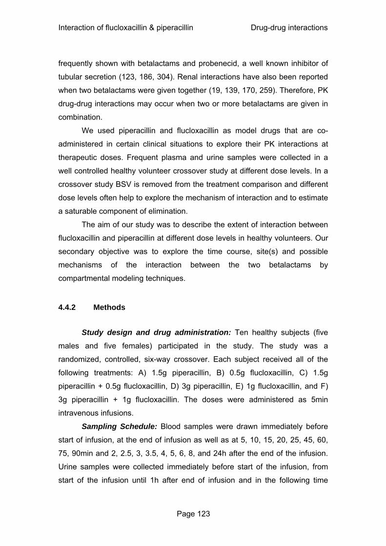
Interaction of flucloxacillin & piperacillin Drug-drug interactions
Page 123
frequently shown with betalactams and probenecid, a well known inhibitor of
tubular secretion (123, 186, 304). Renal interactions have also been reported
when two betalactams were given together (19, 139, 170, 259). Therefore, PK
drug-drug interactions may occur when two or more betalactams are given in
combination.
We used piperacillin and flucloxacillin as model drugs that are co-
administered in certain clinical situations to explore their PK interactions at
therapeutic doses. Frequent plasma and urine samples were collected in a
well controlled healthy volunteer crossover study at different dose levels. In a
crossover study BSV is removed from the treatment comparison and different
dose levels often help to explore the mechanism of interaction and to estimate
a saturable component of elimination.
The aim of our study was to describe the extent of interaction between
flucloxacillin and piperacillin at different dose levels in healthy volunteers. Our
secondary objective was to explore the time course, site(s) and possible
mechanisms of the interaction between the two betalactams by
compartmental modeling techniques.
4.4.2 Methods
Study design and drug administration: Ten healthy subjects (five
males and five females) participated in the study. The study was a
randomized, controlled, six-way crossover. Each subject received all of the
following treatments: A) 1.5g piperacillin, B) 0.5g flucloxacillin, C) 1.5g
piperacillin + 0.5g flucloxacillin, D) 3g piperacillin, E) 1g flucloxacillin, and F)
3g piperacillin + 1g flucloxacillin. The doses were administered as 5min
intravenous infusions.
Sampling Schedule: Blood samples were drawn immediately before
start of infusion, at the end of infusion as well as at 5, 10, 15, 20, 25, 45, 60,
75, 90min and 2, 2.5, 3, 3.5, 4, 5, 6, 8, and 24h after the end of the infusion.
Urine samples were collected immediately before start of the infusion, from
start of the infusion until 1h after end of infusion and in the following time

Interaction of flucloxacillin & piperacillin Drug-drug interactions
Page 124
intervals: 1 to 2, 2 to 3, 3 to 4, 4 to 5, 5 to 6, 6 to 8, 8 to 12, 12 to 24h after the
end of the infusion.
Determination of Plasma and Urine Concentrations: Plasma and
urine concentrations were determined as described above for flucloxacillin
(chapter 3.2.3) and piperacillin (chapter 3.3.3).
Pharmacokinetics Models: We modeled the profiles from the six different treatments
simultaneously. We tested one, two and three compartment disposition
models for both piperacillin and flucloxacillin. The drug input was modeled as
a zero order process with a duration of 5min. We could separate between
renal and nonrenal elimination, because the amounts of piperacillin and
flucloxacillin excreted in urine had been determined. We described renal
clearance as a parallel linear and mixed-order elimination process and used
the following equation for the renal clearances of piperacillin and flucloxacillin:
[ ]CKVmaxCL CLmR
RlinearR,R +
+= Formula 4.4-1
CLR,linear is the first order renal clearance, VmaxR is the maximum rate
of the mixed order renal elimination, KmR is the piperacillin or flucloxacillin
concentration associated with a half maximal rate (VmaxR/2) for the mixed
order renal elimination of the respective drug, and [C] is the plasma
concentration of piperacillin or flucloxacillin. As all subjects had normal renal
function and the non-protein bound fraction in plasma (fu) is reported as 6%
(28, 30) for flucloxacillin, the renal filtration clearance of flucloxacillin (fu · GFR)
is about 0.432 L/h, which only accounts for approximately 5% of total body
clearance. Therefore we fixed CLR,linear to 0.432 L/h for flucloxacillin.
For models without a mechanistic interaction for nonrenal clearance of
flucloxacillin, we described the nonrenal elimination as a first order process
with a nonrenal clearance (CLNR,FLU). For models with a mechanistic
interaction for nonrenal elimination we described the nonrenal clearance of
flucloxacillin as a mixed-order process:

Interaction of flucloxacillin & piperacillin Drug-drug interactions
Page 125
[ ]FKVmax
CLFLUmNR,
FLUNR,NR +
= Formula 4.4-2
VmaxNR,FLU is the maximum rate of the nonrenal elimination, KmNR,FLU is
the flucloxacillin concentration associated with a half maximal rate
(VmaxNR,FLU/2) for the mixed order nonrenal elimination of flucloxacillin and [F]
is the plasma concentration of flucloxacillin.
Interaction models: We assumed that the first order renal elimination
(glomerular filtration) of flucloxacillin was not influenced by piperacillin. We
tested the following four mechanistic interactions for the mixed order renal
elimination process: Competitive, uncompetitive, mixed and noncompetitive
inhibition. Besides those mechanistic interactions we also studied static
interactions. The static interactions were expressed as two different nonrenal
clearances for flucloxacillin with (CLNR,FLU with P) and without (CLNR,FLU without P)
piperacillin. The models with different combinations of interactions at the renal
and nonrenal sites are shown in Table 4.4-1. For the competitive interactions
we calculated the relative affinity (= ratio Km,FLU / Kic) of piperacillin and
flucloxacillin to the transporter for each subject (see chapter 4.1.1).
Table 4.4-1 Interaction models studied for the influence of piperacillin on flucloxacillin
Model 1 2 3 4 5 Interaction in renal elimination C UC M NC C Interaction in nonrenal elimination S S S S C
M: Mixed inhibition (see Figure 4.1-4) See Table 4.2-1 for explanation of the other abbreviations.
4.4.3 Results
All ten subjects (5 males and 5 females) completed the study. The
average ± SD weight was 75.6 ± 7.3kg for males and 63.6 ± 8.3kg for
females, height was 183.2 ± 5.0cm for males and 171.8 ± 6.1cm for females,
and age 26.8 ± 4.2 years for males and 24.6 ± 0.55 years for females. Plasma

Interaction of flucloxacillin & piperacillin Drug-drug interactions
Page 126
concentrations of flucloxacillin after infusion of 0.5g and 1g were considerably
higher with piperacillin compared to flucloxacillin given alone (Figure 4.4-1).
Flucloxacillin amounts excreted in urine during the first 2h after administration
were much lower with the interaction treatments compared to baseline.
Figure 4.4-1 Median [P25%-P75%] profiles of flucloxacillin in healthy volunteers after a 5min infusion of 0.5g and 1g flucloxacillin with or without piperacillin
Flucloxacillin dose: 0.5g
Plasma concentrations (0-6h)
0
25
50
75
100
0 1 2 3 4 5 6Time (h)
Flucloxacillin dose: 1g
Plasma concentrations (0-6h)
0
50
100
150
200
0 1 2 3 4 5 6Time (h)
Plasma concentrations (0-8h)
0.250.5
1248
163264
128128
0 1 2 3 4 5 6 7 8Time (h)
Plasma concentrations (0-8h)
0.250.5
1248
163264
128256
0 1 2 3 4 5 6 7 8Time (h)
Amounts excreted unchanged in urine
0
50
100
150
200
250
0 2 4 6 8 10Time (h)
Amounts excreted unchanged in urine
050
100150200250300350400450
0 2 4 6 8 10Time (h)
Flucloxacillin alone Flucloxacillin 0.5g with piperacillin 1.5g or Flucloxacillin 1g with piperacillin 3g y

Interaction of flucloxacillin & piperacillin Drug-drug interactions
Page 127
Non-compartmental analysis: The results of the NCA are shown in
Table 4.4-2.
Table 4.4-2 PK parameters for 0.5g and 1g flucloxacillin with or without piperacillin from non-compartmental analysis
Median (P25%-P75%)
Point estimate (90% CI)
* p-value
Median (P25%-P75%)
Point estimate (90% CI)
* p-value
Flucloxacillin 0.5g 0.5g 1g 1g
Piperacillin 1.5g -
with PIP / without
PIP 3g - with PIP /
without PIP
CLT (L/h) 5.04 [3.80-6.07]
7.82 [7.37-9.36]
59% (54-65%) < 0.01 3.79
[3.53-4.21]7.96
[6.81-9.57] 47%
(44-50%) < 0.01
CLR (L/h) 2.90 [2.20-3.46]
5.44 [4.63-6.27]
54% (46-64%) < 0.01 2.06
[1.88-2.35]5.47
[4.52-6.07] 37%
(34-41%) < 0.01
CLNR (L/h) 1.77 [1.53-2.60]
2.66 [2.18-3.44]
67% (56-80%) < 0.01 1.80
[1.64-1.99]2.79
[2.17-3.48] 65%
(55-76%) < 0.01
Ae (%) 56.7 [53.9-72.0]
68.6 [61.2-70.6]
92% (82-102%) 0.18 51.8
[50.8-58.5]64.0
[59.7-74.6] 80%
(73-87%) < 0.01
Vss (L) 7.14 [6.23-7.77]
9.52 [8.38-11.1]
72% (64-80%) < 0.01 6.56
[5.99-6.93]10.4
[8.89-11.6] 64%
(59-70%) < 0.01
Cmax (mg/L)
95.8 [82.0-101]
87.7 [79.1-93.0]
106% (94-120%) 0.40 183
[164-209] 173
[144-192] 109%
(99-120%) 0.13
T1/2 (h) 1.35 [1.18-1.45]
1.44 [1.31-1.75]
95% (74-121%) 0.70 1.24
[1.13-1.39]1.59
[1.32-1.84] 77%
(70-85%) < 0.01
MRT (h) 1.44 [1.33-1.56]
1.17 [1.06-1.41]
122% (115-130%) < 0.01 1.64
[1.47-1.79]1.18
[1.13-1.34] 136%
(129-144%) < 0.01
* p-value from ANOVA MRT: Mean residence time. For explanation of other parameters see Table 4.3-2.
Addition of the 3 times (on a mg basis) higher dose of piperacillin
reduced the renal clearance of flucloxacillin by 46% (from 5.44 to 2.90 L/h) for
the low dose and by 63% (from 5.47 to 2.06 L/h) for the high dose (p< 0.01).
Nonrenal clearance was reduced by 33% (from 2.66 to 1.77 L/h) for the low
and by 35% (from 2.79 to 1.80 L/h) for the high dose (p< 0.01). Figure 4.4-2
shows box-plots for renal and nonrenal clearance of flucloxacillin with and
without piperacillin.
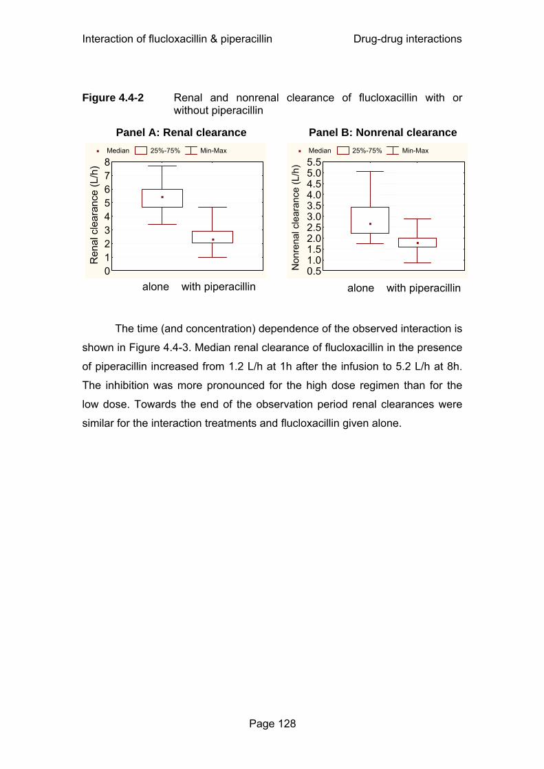
Interaction of flucloxacillin & piperacillin Drug-drug interactions
Page 128
Figure 4.4-2 Renal and nonrenal clearance of flucloxacillin with or
without piperacillin
The time (and concentration) dependence of the observed interaction is
shown in Figure 4.4-3. Median renal clearance of flucloxacillin in the presence
of piperacillin increased from 1.2 L/h at 1h after the infusion to 5.2 L/h at 8h.
The inhibition was more pronounced for the high dose regimen than for the
low dose. Towards the end of the observation period renal clearances were
similar for the interaction treatments and flucloxacillin given alone.
alone with piperacillin
Median 25%-75% Min-Max
012345678
Ren
al c
lear
ance
(L/h
)
Panel A: Renal clearance
alone with piperacillin
Median 25%-75% Min-Max
0.51.01.52.02.53.03.54.04.55.05.5
Non
rena
l cle
aran
ce (L
/h)
Panel B: Nonrenal clearance
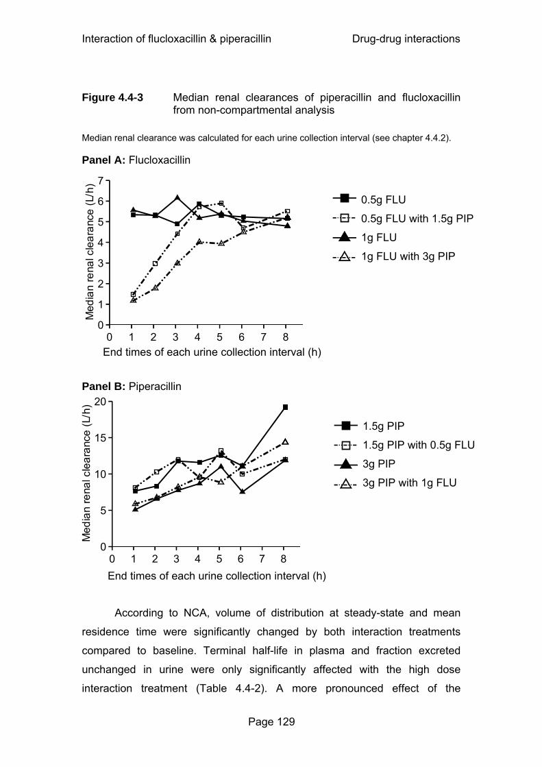
Interaction of flucloxacillin & piperacillin Drug-drug interactions
Page 129
Figure 4.4-3 Median renal clearances of piperacillin and flucloxacillin
from non-compartmental analysis
Median renal clearance was calculated for each urine collection interval (see chapter 4.4.2). Panel A: Flucloxacillin
Panel B: Piperacillin
According to NCA, volume of distribution at steady-state and mean
residence time were significantly changed by both interaction treatments
compared to baseline. Terminal half-life in plasma and fraction excreted
unchanged in urine were only significantly affected with the high dose
interaction treatment (Table 4.4-2). A more pronounced effect of the
0.5g FLU
0.5g FLU with 1.5g PIP
1g FLU
1g FLU with 3g PIP
0
1
2
3
4
5
6
7
0 1 2 3 4 5 6 7 8End times of each urine collection interval (h)
1.5g PIP
1.5g PIP with 0.5g FLU
3g PIP
3g PIP with 1g FLU
0
5
10
15
20
0 1 2 3 4 5 6 7 8End times of each urine collection interval (h)

Interaction of flucloxacillin & piperacillin Drug-drug interactions
Page 130
interaction was seen for all PK parameters at the higher dose level compared
to the lower dose. Maximum concentrations in plasma were not affected
significantly by the interaction.
PK parameters of piperacillin were very similar after the treatments with
and without flucloxacillin. No significant differences were seen, except for a
decrease in nonrenal clearance from 5.2 to 4.3 L/h (-23%, p<0.01) and an
increase from 0.53 to 0.60 (+15%, p=0.02) in the fraction excreted unchanged
in urine, when 3g piperacillin was given together with 1g flucloxacillin.
Models: For the plasma and urine concentration time data of both
piperacillin and flucloxacillin we chose a three compartment model based on
the AIC and visual inspection of the observed and predicted plasma and urine
concentration time curves.
The results from the AIC and the visual predictive checks showed that
models 1 and 4 (see Table 4.4-1) both had a highly sufficient predictive
performance. The visual predictive checks gave virtually identical results for
those two models. Model 3 achieved AIC values similar to models 1 and 4 but
was probably over-parameterized, and models 2 and 5 were ranked less likely
(median AIC at least 30 points higher, see also chapter 2.6.5). The visual
predictive checks of model 1 are shown in Figure 4.4-4 for the interaction
treatments. The visual predictive checks for the profiles of piperacillin and
flucloxacillin alone showed also a highly sufficient predictive performance for
model 1.

Interaction of flucloxacillin & piperacillin Drug-drug interactions
Page 131
Figure 4.4-4 Visual predictive check for plasma concentrations and amounts excreted unchanged in urine of flucloxacillin for model 1 (see Table 4.4-1)
FLU 0.5g with PIP 1.5g
Plasma concentrations (0-8h)
0.1250.250.5
1248
163264
128128128
0 1 2 3 4 5 6 7 8
Time after administration (h)
10 % percentile
25 % percentile
50 % percentile
75 % percentile
90 % percentile
Raw data
FLU 1g with PIP 3g
Plasma concentrations (0-8h)
0.250.5
1248
163264
128256256256
0 1 2 3 4 5 6 7 8
Time after administration (h)
10 % percentile
25 % percentile
50 % percentile
75 % percentile
90 % percentile
Raw data
Plasma concentrations (0-1.75h)
Plasma concentrations (0-1.75h)
Amounts excreted unchanged in urine
0
50
100
150
200
250
300
350
400
0 5 10 15 20
Time after administration (h)
10 % percentile25 % percentile50 % percentile
75 % percentile90 % percentileRaw data
Amounts excreted unchanged in urine
0
100
200
300
400
500
600
700
0 5 10 15 20 2
Time after administration (h)
10 % percentile
25 % percentile
50 % percentile
75 % percentile
90 % percentile
Raw data
See chapter 2.6.5 and Figure 3.2-2 for explanation of the plots.
Table 4.4-3 lists the median PK parameter estimates of flucloxacillin for
model 1. Piperacillin reduced the nonrenal clearance of flucloxacillin
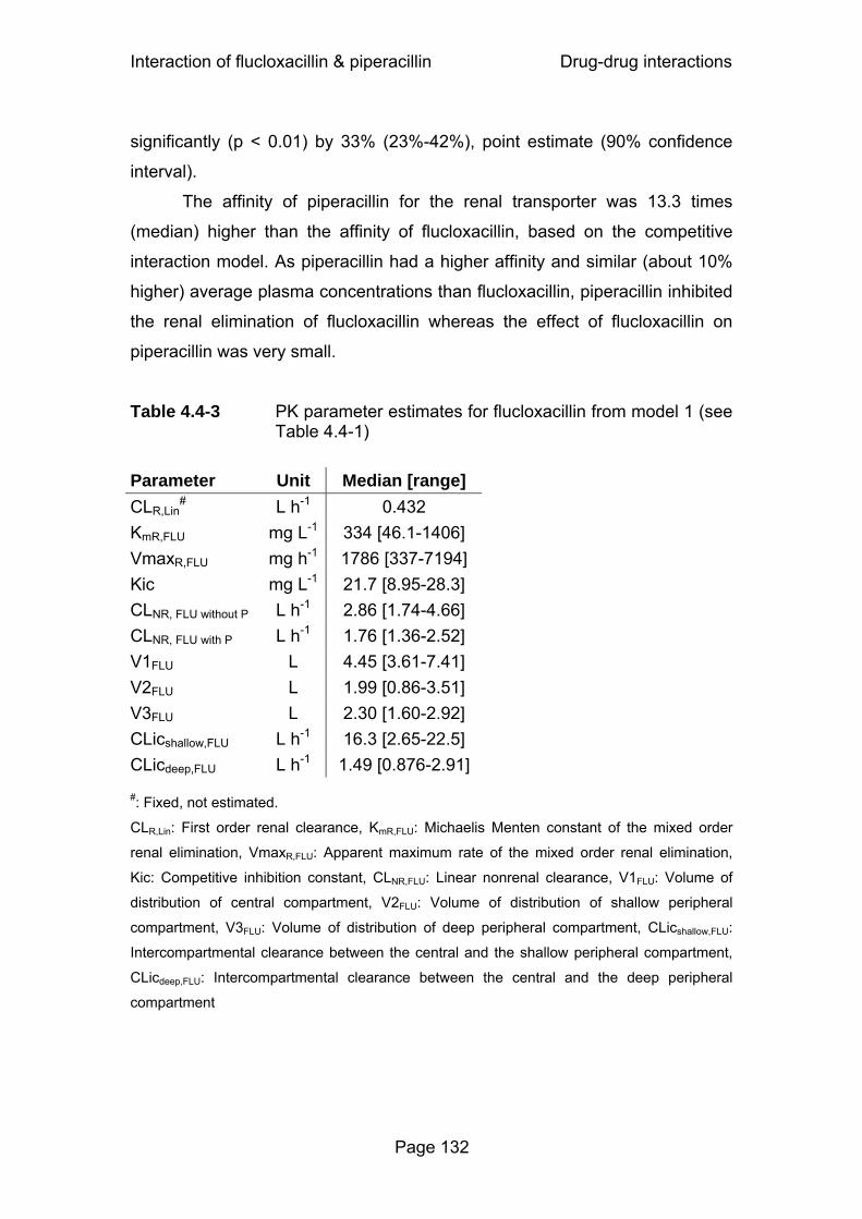
Interaction of flucloxacillin & piperacillin Drug-drug interactions
Page 132
significantly (p < 0.01) by 33% (23%-42%), point estimate (90% confidence
interval).
The affinity of piperacillin for the renal transporter was 13.3 times
(median) higher than the affinity of flucloxacillin, based on the competitive
interaction model. As piperacillin had a higher affinity and similar (about 10%
higher) average plasma concentrations than flucloxacillin, piperacillin inhibited
the renal elimination of flucloxacillin whereas the effect of flucloxacillin on
piperacillin was very small.
Table 4.4-3 PK parameter estimates for flucloxacillin from model 1 (see Table 4.4-1)
Parameter Unit Median [range] CLR,Lin
# L h-1 0.432 KmR,FLU mg L-1 334 [46.1-1406] VmaxR,FLU mg h-1 1786 [337-7194] Kic mg L-1 21.7 [8.95-28.3] CLNR, FLU without P L h-1 2.86 [1.74-4.66] CLNR, FLU with P L h-1 1.76 [1.36-2.52] V1FLU L 4.45 [3.61-7.41] V2FLU L 1.99 [0.86-3.51] V3FLU L 2.30 [1.60-2.92] CLicshallow,FLU L h-1 16.3 [2.65-22.5] CLicdeep,FLU L h-1 1.49 [0.876-2.91] #: Fixed, not estimated.
CLR,Lin: First order renal clearance, KmR,FLU: Michaelis Menten constant of the mixed order
renal elimination, VmaxR,FLU: Apparent maximum rate of the mixed order renal elimination,
Kic: Competitive inhibition constant, CLNR,FLU: Linear nonrenal clearance, V1FLU: Volume of
distribution of central compartment, V2FLU: Volume of distribution of shallow peripheral
compartment, V3FLU: Volume of distribution of deep peripheral compartment, CLicshallow,FLU:
Intercompartmental clearance between the central and the shallow peripheral compartment,
CLicdeep,FLU: Intercompartmental clearance between the central and the deep peripheral
compartment

Interaction of flucloxacillin & piperacillin Drug-drug interactions
Page 133
4.4.4 Discussion
Concomitant administration of multiple drugs carries the potential for
PK drug-drug interactions. This is especially true, when these drugs share the
same primary elimination pathway (216). Betalactams are organic anions and
excreted by the kidneys by glomerular filtration and active tubular secretion
(22, 27). Tubular secretion is a capacity-limited process. As betalactams are
similar to some extent in their chemical structure and physicochemical
properties, they may compete for the renal tubular secretion when given
concomitantly. PK interactions between betalactams, often involving
acylureidopenicillins like piperacillin, have been reported. Both azlocillin (170)
and mezlocillin (259) reduce the renal and nonrenal clearance of cefotaxime,
and mezlocillin also reduces the clearance of oxacillin (19). Piperacillin inhibits
the renal clearance of cefazolin and renal and nonrenal clearance of
cefoperazone in rabbits (139), as well as the total clearance of moxalactam
(latamoxef) (19). In addition to the interactions with other betalactams,
azlocillin reduces the renal and nonrenal clearance of ciprofloxacin (20).
These findings show that acylureidopenicillins have a high potential to
inhibit the elimination of other betalactams given concomitantly. We used
compartmental analysis to study the time course of the PK interaction
between piperacillin and flucloxacillin as model drugs at two dose levels and
tested various interaction models to explore possible mechanisms and site(s)
of the interaction. We had data from ten healthy volunteers in a six-way
crossover study. Although this is a small sample size, the design has distinct
advantages: In healthy volunteers the between occasion variability (BOV), i.e.
the variability in one subject between different study periods, of piperacillin for
clearance and volume of distribution at steady-state is small (<15%) (50) and
the subjects serve as their own controls (see also chapter 1.5). In our study
piperacillin was given without tazobactam. However, as tazobactam has been
reported not to affect the PK of piperacillin (283), a possible effect of
tazobactam on piperacillin PK is likely to be small.
Our NCA showed, that overall concomitant administration of piperacillin
significantly decreased the renal clearance of flucloxacillin from 5.44 to 2.29

Interaction of flucloxacillin & piperacillin Drug-drug interactions
Page 134
L/h (p<0.01) and the nonrenal clearance of flucloxacillin from 2.67 to 1.80 L/h
(p<0.01). Renal clearance of flucloxacillin became more similar between the
treatments with and without piperacillin towards the end of the observation
period when the piperacillin plasma concentrations were low (Figure 4.4-3).
For all PK parameters the extent of interaction was larger with the high dose
combination of piperacillin and flucloxacillin (Table 4.4-2). Although NCA
indicated a significant decrease of volume of distribution at steady-state for
flucloxacillin under the influence of piperacillin, we have shown by subsequent
simulations that this is probably an artifact from NCA. We simulated two
plasma concentration time profiles for flucloxacillin with and without
piperacillin as competitive inhibitor of renal tubular secretion. All flucloxacillin
PK parameters including volume of distribution were identical between both
treatments. However, as for the gemifloxacin study, NCA of the simulated
concentrations falsely indicated a decreased volume of distribution at steady-
state and during the terminal phase for the interaction treatment. Jungbluth
and Jusko showed that a decreased volume of distribution with increasing
doses of mezlocillin in rats was an artifact from NCA due to saturable
elimination of mezlocillin, as NCA assumes linear disposition (167).
Piperacillin PK parameters were not affected significantly by the low
dose interaction treatment (1.5g piperacillin + 0.5g flucloxacillin). For the high
dose interaction treatment (3g piperacillin + 1g flucloxacillin) nonrenal
clearance of piperacillin was reduced from 5.2 to 4.3 L/h (-23%, p<0.01), and
the fraction excreted unchanged in urine increased from 0.53 to 0.60 (+15%,
p=0.02), compared to 3g piperacillin alone. As nonrenal clearance only
accounted for about 40% of piperacillin elimination, the small decrease in
nonrenal clearance did not result in a significant decrease in total body
clearance. The increase in piperacillin renal clearance with decreasing plasma
concentrations (Figure 4.4-3), was independent of flucloxacillin and may be
attributed to saturable elimination of piperacillin (23, 31, 304). Therefore we
used a saturable elimination model for piperacillin and did not include an
influence of flucloxacillin on piperacillin PK.
We used compartmental modeling and tested several mechanistic
models (Table 4.4-1). Models 1, 3 and 4 showed similar values for the AIC,
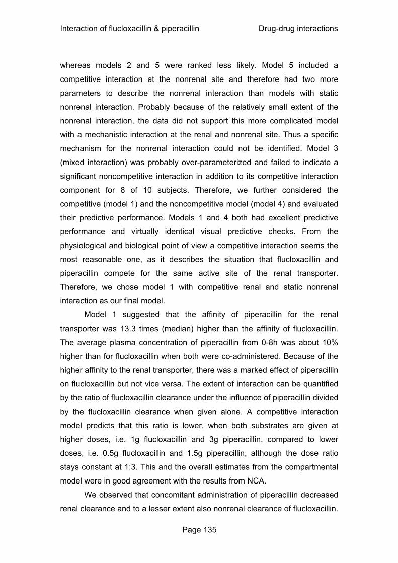
Interaction of flucloxacillin & piperacillin Drug-drug interactions
Page 135
whereas models 2 and 5 were ranked less likely. Model 5 included a
competitive interaction at the nonrenal site and therefore had two more
parameters to describe the nonrenal interaction than models with static
nonrenal interaction. Probably because of the relatively small extent of the
nonrenal interaction, the data did not support this more complicated model
with a mechanistic interaction at the renal and nonrenal site. Thus a specific
mechanism for the nonrenal interaction could not be identified. Model 3
(mixed interaction) was probably over-parameterized and failed to indicate a
significant noncompetitive interaction in addition to its competitive interaction
component for 8 of 10 subjects. Therefore, we further considered the
competitive (model 1) and the noncompetitive model (model 4) and evaluated
their predictive performance. Models 1 and 4 both had excellent predictive
performance and virtually identical visual predictive checks. From the
physiological and biological point of view a competitive interaction seems the
most reasonable one, as it describes the situation that flucloxacillin and
piperacillin compete for the same active site of the renal transporter.
Therefore, we chose model 1 with competitive renal and static nonrenal
interaction as our final model.
Model 1 suggested that the affinity of piperacillin for the renal
transporter was 13.3 times (median) higher than the affinity of flucloxacillin.
The average plasma concentration of piperacillin from 0-8h was about 10%
higher than for flucloxacillin when both were co-administered. Because of the
higher affinity to the renal transporter, there was a marked effect of piperacillin
on flucloxacillin but not vice versa. The extent of interaction can be quantified
by the ratio of flucloxacillin clearance under the influence of piperacillin divided
by the flucloxacillin clearance when given alone. A competitive interaction
model predicts that this ratio is lower, when both substrates are given at
higher doses, i.e. 1g flucloxacillin and 3g piperacillin, compared to lower
doses, i.e. 0.5g flucloxacillin and 1.5g piperacillin, although the dose ratio
stays constant at 1:3. This and the overall estimates from the compartmental
model were in good agreement with the results from NCA.
We observed that concomitant administration of piperacillin decreased
renal clearance and to a lesser extent also nonrenal clearance of flucloxacillin.

Interaction of flucloxacillin & piperacillin Drug-drug interactions
Page 136
Betalactams have been reported to be secreted by and also to inhibit various
members of the family of organic anion transporters (OAT) in the proximal
renal tubules (51, 159, 186). More specifically, Jariyawat et al. (159) tested 25
different antibiotics, among those 17 betalactams including piperacillin and
cloxacillin, which is structurally very similar to flucloxacillin. All of the tested
betalactams showed competitive inhibition of p-aminohippuric acid transport
by OAT 1 (159). These findings suggest that the site of the renal interaction of
piperacillin and flucloxacillin could be an OAT in the proximal renal tubules. As
OATs have been found in various organs of the body, including the liver (219,
272), a competitive interaction process could also be the reason for the
decreased nonrenal clearance of flucloxacillin when given with piperacillin.
Further studies would be needed to identify exactly which transporter(s) are
involved in this interaction.
In conclusion, compartmental modeling identified a competitive
inhibition of tubular secretion by piperacillin as the most likely mechanism of
the renal interaction. Piperacillin had a 13.3 times higher (median) affinity to
the renal transporter than flucloxacillin. The average plasma concentration of
piperacillin from 0-8h was about 10% higher than for flucloxacillin when both
were co-administered. Therefore piperacillin considerably inhibited the active
tubular secretion of flucloxacillin. Overall, piperacillin significantly decreased
the renal clearance of flucloxacillin from 5.44 to 2.29 L/h (p<0.01) and the
nonrenal clearance of flucloxacillin from 2.67 to 1.80 L/h (p<0.01). The extent
of the interaction was larger for the higher doses. The interaction reached
clinical significance, since the total clearance decreased from 7.96 to 4.00 L/h
(p<0.01) for flucloxacillin. Piperacillin PK was not affected by concomitant
flucloxacillin, except for a decrease in the nonrenal clearance from 5.2 to
4.3 L/h (p<0.01) with the high dose interaction treatment compared to
piperacillin alone. The inhibition of flucloxacillin clearance leads to a prolonged
time of non-protein bound concentrations above the MIC, which may be used
to improve effectiveness. As piperacillin has a higher affinity to the renal
transporter than flucloxacillin, it is the more likely drug to be used as inhibitor
in further studies which are required to show the clinical relevance of this or
other PK interactions between betalactams.
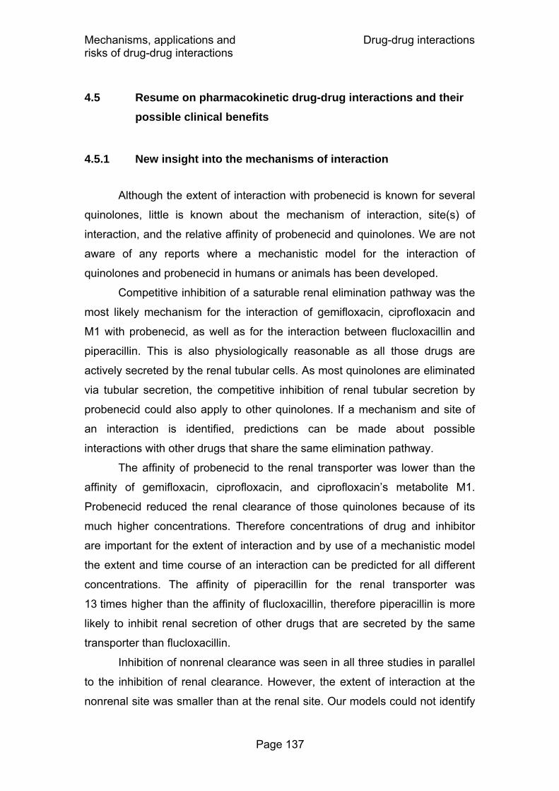
Mechanisms, applications and Drug-drug interactions risks of drug-drug interactions
Page 137
4.5 Resume on pharmacokinetic drug-drug interactions and their possible clinical benefits
4.5.1 New insight into the mechanisms of interaction
Although the extent of interaction with probenecid is known for several
quinolones, little is known about the mechanism of interaction, site(s) of
interaction, and the relative affinity of probenecid and quinolones. We are not
aware of any reports where a mechanistic model for the interaction of
quinolones and probenecid in humans or animals has been developed.
Competitive inhibition of a saturable renal elimination pathway was the
most likely mechanism for the interaction of gemifloxacin, ciprofloxacin and
M1 with probenecid, as well as for the interaction between flucloxacillin and
piperacillin. This is also physiologically reasonable as all those drugs are
actively secreted by the renal tubular cells. As most quinolones are eliminated
via tubular secretion, the competitive inhibition of renal tubular secretion by
probenecid could also apply to other quinolones. If a mechanism and site of
an interaction is identified, predictions can be made about possible
interactions with other drugs that share the same elimination pathway.
The affinity of probenecid to the renal transporter was lower than the
affinity of gemifloxacin, ciprofloxacin, and ciprofloxacin’s metabolite M1.
Probenecid reduced the renal clearance of those quinolones because of its
much higher concentrations. Therefore concentrations of drug and inhibitor
are important for the extent of interaction and by use of a mechanistic model
the extent and time course of an interaction can be predicted for all different
concentrations. The affinity of piperacillin for the renal transporter was
13 times higher than the affinity of flucloxacillin, therefore piperacillin is more
likely to inhibit renal secretion of other drugs that are secreted by the same
transporter than flucloxacillin.
Inhibition of nonrenal clearance was seen in all three studies in parallel
to the inhibition of renal clearance. However, the extent of interaction at the
nonrenal site was smaller than at the renal site. Our models could not identify

Mechanisms, applications and Drug-drug interactions risks of drug-drug interactions
Page 138
a mechanism for the interaction at the nonrenal site. Probably a higher extent
of interaction is needed to be able to identify a mechanism for the interaction
at the nonrenal site.
The interactions involve inhibition of transporters, but it is not possible
to identify these transporter(s) by PK studies in humans alone. Additional data
on the transporter itself are required. It might be possible that multiple
transporters are involved in this interaction, therefore the estimated values for
Km and Kic might represent pooled values and not apply to one specific
transporter. Findings from in vitro studies suggest that the site of the studied
renal interactions could be organic anion or organic cation transporters. These
transporters are located in the proximal renal tubules, but also in the liver
(219, 272) and in other parts of the body. Therefore, a competitive interaction
process like that at the renal site could also cause the decreased nonrenal
clearances. Despite the increasing knowledge on transport proteins, it would
be necessary to conduct further studies for an exact identification of the
transporter(s) involved in our studied interactions.
4.5.2 Critical importance of modeling the full time course of drug-drug interactions
NCA in combination with ANOVA statistics treats the presence or
absence of an inhibitor as a categorical variable, but the concentration of the
inhibitor is not included in the analysis. Therefore, NCA does not directly
account for the time and concentration dependence of an interaction.
Although NCA is an adequate method to explore the extent of the interaction
for the dose level used in the study, it cannot predict the extent of interaction
for other dosage regimens which might be relevant for clinical practice. It
would be very difficult – if at all possible – to draw a conclusion about the
influence of an inhibitor on the formation of a metabolite by use of NCA.
Furthermore, NCA is also not an adequate method to study a possible
influence of an interaction on the volume of distribution of a drug.
As has been seen e.g. with probenecid, the concentration, and not only
presence or absence, of an inhibitor is important for the extent and time

Mechanisms, applications and Drug-drug interactions risks of drug-drug interactions
Page 139
course of an interaction. The concentration of an inhibitor changes over time.
In our interaction models the concentrations of drug and inhibitor are included
to describe the interaction at each time point. The full time course of drug,
inhibitor, and metabolite (in the case of ciprofloxacin) in plasma and urine is
modeled simultaneously in order to derive the maximum amount of
information from the data.
Therefore, compartmental modeling is more powerful than NCA to
identify the site(s) of interaction, to propose a mechanism of interaction for
each site, to calculate relative affinities of the drugs to the transporter, and to
predict the time course of interaction for other dosage regimens via
simulations. Probably the most important advantage of a mechanistic
interaction model over NCA is the ability of an interaction model to predict the
extent and time course of interaction for other dosage regimens. This ability of
a mechanistic interaction model can be used in PD simulations to predict the
effect of an inhibitor on the probability of successful antiinfective treatment.
For PD simulations, generally a full population PK analysis would be preferred
to the STS approach. We used the STS approach to construct a population
PK model. We could show by visual predictive checks that our constructed
population PK models had highly sufficient predictive performance (see Figure
4.2-2 and Figure 4.4-4). Direct estimation of a population PK model e.g. with
NONMEM is superior to our STS approach. However investigating the
mechanisms of interaction by population PK modeling would not have been
feasible because of the tremendously long computation times of those
complex interaction models in NONMEM. As computation speed is increasing
this disadvantage of population PK modeling might become less important in
the future.
4.5.3 Pharmacokinetic interaction and improved pharmacodynamic profile versus increased toxicity
A mechanistic interaction model allows one to predict the extent and
time course of an interaction for other dosage regimens. Therefore we used
MCS with therapeutic doses of probenecid at steady-state in order to estimate
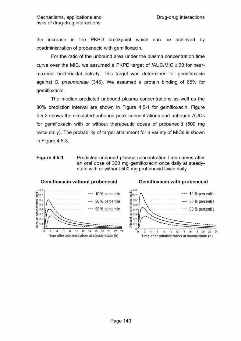
Mechanisms, applications and Drug-drug interactions risks of drug-drug interactions
Page 140
the increase in the PKPD breakpoint which can be achieved by
coadministration of probenecid with gemifloxacin.
For the ratio of the unbound area under the plasma concentration time
curve over the MIC, we assumed a PKPD target of fAUC/MIC ≥ 30 for near-
maximal bactericidal activity. This target was determined for gemifloxacin
against S. pneumoniae (346). We assumed a protein binding of 65% for
gemifloxacin.
The median predicted unbound plasma concentrations as well as the
80% prediction interval are shown in Figure 4.5-1 for gemifloxacin. Figure
4.5-2 shows the simulated unbound peak concentrations and unbound AUCs
for gemifloxacin with or without therapeutic doses of probenecid (500 mg
twice daily). The probability of target attainment for a variety of MICs is shown
in Figure 4.5-3.
Figure 4.5-1 Predicted unbound plasma concentration time curves after an oral dose of 320 mg gemifloxacin once daily at steady-state with or without 500 mg probenecid twice daily
Gemifloxacin without probenecid
0
0.1
0.2
0.3
0.4
0.5
0.6
0.7
0.8
0 2 4 6 8 10 12 14 16 18 20 22 24
Time after administration at steady-state (h)
10 % percentile50 % percentile90 % percentile
Gemifloxacin with probenecid
0
0.1
0.2
0.3
0.4
0.5
0.6
0.7
0.8
0 2 4 6 8 10 12 14 16 18 20 22 24
Time after administration at steady-state (h)
10 % percentile50 % percentile90 % percentile
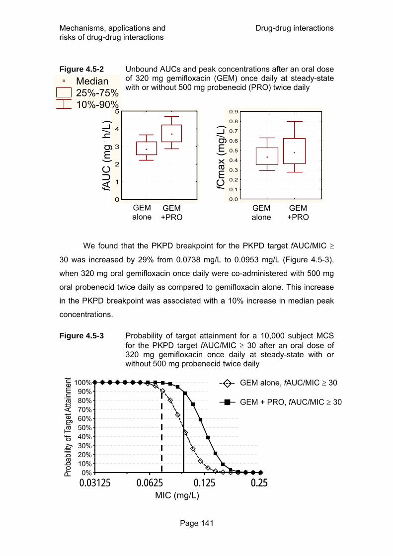
Mechanisms, applications and Drug-drug interactions risks of drug-drug interactions
Page 141
Figure 4.5-2 Unbound AUCs and peak concentrations after an oral dose of 320 mg gemifloxacin (GEM) once daily at steady-state with or without 500 mg probenecid (PRO) twice daily
We found that the PKPD breakpoint for the PKPD target fAUC/MIC ≥
30 was increased by 29% from 0.0738 mg/L to 0.0953 mg/L (Figure 4.5-3),
when 320 mg oral gemifloxacin once daily were co-administered with 500 mg
oral probenecid twice daily as compared to gemifloxacin alone. This increase
in the PKPD breakpoint was associated with a 10% increase in median peak
concentrations.
Figure 4.5-3 Probability of target attainment for a 10,000 subject MCS for the PKPD target fAUC/MIC ≥ 30 after an oral dose of 320 mg gemifloxacin once daily at steady-state with or without 500 mg probenecid twice daily
Median 25%-75% 10%-90%
GEM alone
GEM +PRO
0
1
2
3
4
5fA
UC
(mg ۟
h/L
)
GEM alone
GEM +PRO
0.0
0.1
0.2
0.3
0.4
0.5
0.6
0.7
0.8
0.9
fCm
ax (m
g/L)
0%10%20%30%40%50%60%70%80%90%
100%
0.03125 0.0625 0.125 0.250.25MIC (mg/L)
GEM alone, fAUC/MIC ≥ 30
GEM + PRO, fAUC/MIC ≥ 30
Mechanisms, applications and Drug-drug interactions risks of drug-drug interactions
Page 142
Considering only these results, the interaction with probenecid seems
to offer an appealing feature for optimization of the PD profile of gemifloxacin.
Coadministration of probenecid allows one to increase the extent of drug
exposure (AUC) with a negligible increase in peak concentrations. Peak
concentrations of sparfloxacin were shown to correlate well with cardiac
repolarization (QTc interval), whereas there was no correlation with AUC
(227).
However, this small increase in the PKPD breakpoint needs to be
viewed as opposed to the increased potential for side effects, when both
drugs are co-administered. The most common adverse effect of both
gemifloxacin and probenecid is rash. Thus, giving both drugs together would
probably increase the risk for this side effect. Furthermore, if probenecid
needs to be administered twice daily, one looses the advantage of once daily
dosing for gemifloxacin. Therefore, the relatively small extent of interaction at
clinical doses of probenecid does not counterbalance the increased risk for
side effects and the less convenient dosing schedule.
In conclusion, probenecid can be an option to improve the PKPD profile
of an antibiotic, as has been practiced with penicillin (323). PKPD modeling is
a good method to investigate these interactions and their potential clinical
benefit. However other factors, e.g. side effects, that might outweigh the
improvements in PD, need to be considered. The increased risk for side
effects with gemifloxacin and probenecid overrides the potential clinical
benefit in the PKPD breakpoint for this drug combination.
Literature data on antibiotics Bone penetration
Page 143
5 Penetration of antibiotics into bone
5.1 Overview of bone penetration studies from literature
5.1.1 Introduction
Despite great advances in antimicrobial chemotherapy, bone infections
remain difficult to diagnose and to treat. Chronic osteomyelitis requires
prolonged antibiotic treatment in addition to surgical debridement and has a
high recurrence rate even many years after the surgery (191). More
importantly, treatment failure may cause irreversible damage of the affected
bones. Since identification of the causative agent is often difficult, selection of
an adequate antimicrobial agent at the beginning of therapy is critical. The
overall number of infections has been predicted to increase because of the
large increase in reconstructive orthopedic procedures with prosthetic
materials. More than 1 million hip replacements are performed each year. It is
unlikely that any preventive measure will reduce the rate of infections below
0.5% (192). Also diabetes and vascular insufficiency as predisposing factors
for osteomyelitis are becoming more frequent. Consequently, appropriate
surgical prophylaxis and antimicrobial therapy are very important.
Rate and extent of penetration of an antimicrobial into bone determine
the therapeutic success, as does a high antibacterial activity of the chosen
drug against pathogens encountered in bone infections. As bone, excluding
bone marrow, is a less vascularised tissue compared e.g. to the lungs or skin,
it is particularly important to investigate the penetration of an antimicrobial
before starting a clinical trial on the effectiveness of antibacterial treatment in
osteomyelitis patients (94, 313). The composition of bone is very different
from other tissues, and it is difficult to predict whether agents showing good
penetration into other tissues will also achieve high concentrations in bone.
The two macroscopically different types of bone tissue are cortical and
cancellous bone. Cortical bone is a compact tissue composed of many
Haversian systems (osteons) that consist of concentrically arranged lamellae

Literature data on antibiotics Bone penetration
Page 144
(Figure 5.1-1). Cancellous bone consists of trabeculae that form the inner part
of the long bones. In general, bone tissue consists of an organic (30 - 35% of
total bone mass) and an inorganic (65 - 70%) fraction (66, 134, 232). Organic
matter consists mainly of collagen fibrils (ca. 90%), glycoproteins,
proteoglycans and extracellular fluid (134), and is arranged in lamellae in
cortical bone (Figure 5.1-1). The extracellular fluid in bone is believed to be of
similar composition as the interstitial fluid of other tissues (329) and water has
been reported to constitute 10% of total bone mass (232). Bone cells
(osteoblasts, osteocytes, and osteoclasts) represent only 1-2% of total bone
mass and are trapped within the organic matrix (66). The inorganic matrix
consists mainly of calcium phosphate as hydroxyapatite crystals that are
deposited inside the organic matrix. The inorganic and the organic matrix can
only be separated by chemical methods e.g. by destroying organic matter via
incubation of bone in peroxide solution (340) or by removing inorganic matter
with acids. These methods may be used to determine the fractions of organic
and inorganic matrix in a bone specimen.
Figure 5.1-1 Composition of cortical bone
However it does not seem possible to separate a bone sample into e.g.
extracellular fluid, collagen fibrils, bone cells, and hydroxyapatite, and to
determine drug concentrations in each of those components separately.
Therefore, the whole bone specimens are commonly homogenized for drug
Haversian canal with
blood vessels, nerve fibers
and interstitial fluid
Hav
ersi
an s
yste
m(o
steo
n)
osteocytes (bone cells) in lacunae (cavities)
Deposited between / in lamellae:hydroxyapatite (calcium phosphate)
canaliculi connecting the bone cells
lamellae (collagen, glycoproteins, proteoglycans, extracellular fluid)

Literature data on antibiotics Bone penetration
Page 145
analysis with chromatographic methods. Subsequently, total concentrations in
bone homogenate are obtained.
Blood vessels are located in Haversian and Volkmann canals that
vertically and horizontally traverse the bone matrix. In osteomyelitis, bacteria
are believed to spread through these canals and distribute in the interstitial
fluid (135). However S. aureus, the most frequently encountered pathogen in
osteomyelitis, additionally forms biofilms and adheres to bone matrix and
implants (192). S. aureus has been shown in in vitro studies to penetrate into
and survive in bone cells i.e. in osteoblasts (154, 161) which may be a reason
for relapses in chronic osteomyelitis (192).
Numerous studies have been conducted to determine antibiotic
concentrations in bone tissues. However a large variety of methods for
sample preparation, drug analysis, data analysis, and reporting of the results
has been employed. Therefore, the reported bone concentrations often differ
as much between studies with the same agent as between different drugs. To
determine bone concentrations reliably and to compare these concentrations
between antibiotics, standardization of methods is vital and an accurate and
precise determination of total concentrations in bone is the first prerequisite to
establish the PKPD profile of antibiotics in bone.
Boselli and Allaouchiche (42) reviewed the results from bone
penetration studies published between 1978 and 1998. Therefore the present
work summarizes the bone penetration studies before 1998 in brief and
addresses the studies between 1998 and end of 2005. This work focuses on
the methods of PK studies to assess bone penetration and on the
standardization of the drug analysis in bone, PK evaluation, and reporting of
the results.
5.1.2 Methods for sample preparation and drug determination
A large variety of techniques has been applied for sample preparation
and drug analysis in bone. The collection and preparation of the bone sample
at the clinical site and the drug extraction, analysis, and bioanalytical

Literature data on antibiotics Bone penetration
Page 146
validation in the laboratory are the most critical procedures of a bone
penetration study.
After resection of the bone sample, adhering blood, bone marrow or
soft tissues are often removed from the specimen by swabbing, scraping or
rinsing it. Bone samples often contain a high amount of blood in excess of the
intravascular portion due to intraoperative soaking of the sample with blood.
This can result in artificially high bone concentrations due to high antibiotic
concentrations in blood, if the excess blood is not removed (340). Separation
of cortical and cancellous bone is often reported. As cancellous bone contains
a higher proportion of extravascular fluid (135) and a lower percentage of
inorganic matter than cortical bone (328), drug disposition may differ between
the two types of bone tissue (292). Therefore it is important to specify whether
the analyzed specimens consist of cancellous or cortical bone or both.
For drug extraction sometimes the whole specimen (243, 322) or
smaller slices (187) are immersed in the extraction solution, or put onto the
agar surface for microbiological assay without homogenization (54). In most
studies one of various methods of homogenizing the bone specimens is used.
Bone samples are sliced into small pieces, or ground to a powder using a
mortar and pestle (80, 86, 129, 260, 333). Some authors use sand or
aluminum oxide (81, 208, 209) to facilitate the grinding process. Others use
liquid nitrogen (45, 181, 183, 306) to freeze the samples. Other devices being
used include various mills or mixers (3, 45, 78, 107, 108, 112, 176, 221, 324,
327, 331, 332), hammers (171), hydraulic presses (129) and metal plates
(171). Adsorption of the drug to the grinding devices or to sand and aluminum
oxide needs to be prospectively validated.
Recently, cryogenic laboratory mills which chill samples in liquid
nitrogen (-196°C) and pulverize the bone sample with a magnetically driven
impactor have been used for processing of bone samples (26, 111, 213, 218,
244, 254). Chilling in liquid nitrogen embrittles the tissue, so it can be
pulverized to a very fine powder. This can be used also for drugs prone to
thermal degradation, e.g. some beta-lactams, as considerable heat develops
due to the grinding if this process is not cooled. Petitjean et al. (246)
compared three grinding procedures for the extraction of rokitamycin from rat
Literature data on antibiotics Bone penetration
Page 147
bone. Pulverization of bone samples by a magnetic stirring bar in liquid
nitrogen gave a finer powder and a higher recovery during extraction than
slicing the bone tissue into small pieces or crushing it with pestle and mortar
(246). This would be expected, as creating a larger surface of the bone
powder facilitates extraction.
For drug extraction, usually the resulting pieces or powder are
immersed in buffer and left to stand (188) or put into a shaker, the latter being
more efficient for extraction. It is rarely reported if extraction equilibrium has
been reached (3), which could be tested e.g. by analyzing eluate from the
same samples after different extraction times. Sufficient drug stability under
the chosen extraction conditions is another requirement. The drug must be
stable until the extraction equilibrium has been reached. Otherwise drug
instability might result in artificially low bone concentrations. Some authors
discuss incomplete extraction as a possible reason for low concentrations
found in bone. Wittmann et al. (340) report that after 48h of shaking 72 to 75%
of the maximum extractable amount of ofloxacin was reached and therefore
they repeated the procedure 3 to 5 times with new buffer. Meissner et al.
(220) performed 3 elutions over 20h each to obtain a “complete” extraction. In
summary, the extraction of drug from bone powder is probably the most
critical part of a bone penetration study. Sufficient recovery during extraction,
drug instability, and adhesion of drug to bone powder and grinding devices all
need to be considered during assay development and prior to starting the
clinical study.
Calibration standards and quality control samples are most often
prepared in serum, plasma or buffer. Some more recent studies used blank
bone samples for preparation of calibration standards (26, 86, 107, 108, 111,
208, 209, 218, 253, 254). Among these studies that used blank bone powder
for preparation of calibration and quality control standards, only Djabarouti et
al. (86) report the use of an internal standard which they added to the
powdered bone sample before drug extraction.
Other studies used an internal standard which was added at various
stages of the extraction procedure, but did not report whether the calibration
standards were prepared in blank bone samples or reported that they used
Literature data on antibiotics Bone penetration
Page 148
serum or buffer for calibration standards. The internal standard has been
added to the bone samples either before homogenization (45, 320), or after
homogenization but before drug extraction (176, 327), or after drug extraction
(156, 171, 215, 331, 332).
Adherence of antibiotics to bone powder has been reported, e.g. by
Fong et al. (107, 108), who compared the solution phase concentrations of
ciprofloxacin and enoxacin in standards made up only with buffer to those
prepared with blank bone powder. Addition of the internal standard to the
ground bone powder before addition of the extraction solution would allow to
determine an upper limit for the recovery of drug during extraction from bone
powder. If the recovery of the internal standard in this experiment is low, the
drug concentrations in bone are likely to be biased towards lower
concentrations. Raymakers et al. (253, 254) prepared ceftazidime calibration
standards in presence or absence of bone powder as external standards.
They find a 10% bias toward lower concentrations in the reported
concentration secondary to the interaction of ceftazidime with bone powder.
Many of the more recent studies (45, 79, 86, 156, 171, 176, 215, 244,
320, 327, 331, 332) used an internal standard to improve the precision of the
measured bone concentrations, whereas many older studies lack an internal
standard. Using an internal standard can improve the accuracy and precision
of the steps after the extraction procedure. If the extraction procedure has a
low precision, uncertainty due to sample preparation and analysis could be
decreased by repeating the extraction and sample preparation procedure
several times for each bone sample. A low precision of the bone assay can
increase the BSV of the individual bone/serum concentration ratios. This will
especially be important, if there is only one bone sample per patient.
For determination of concentrations in the extraction fluid,
microbiological methods have been frequently used (3-5, 26, 44, 54, 78-81,
88, 111, 112, 126, 127, 132, 179, 188, 207-209, 221, 237, 249, 255, 260, 275,
281, 322, 324, 328, 331-333, 339, 344), especially in the older studies. Gas
chromatography with mass spectrometry has been applied for determination
of sulbactam (79, 324, 331, 332), fluorescence polarization immunoassay for
vancomycin (129, 213, 218, 322), and tobramycin has also been determined

Literature data on antibiotics Bone penetration
Page 149
by an immunofluorescence method (333). Recent studies most often used
HPLC with UV (86, 108, 156, 171, 176, 183, 196-198, 214, 215, 252-254, 257,
264) or fluorescence (107, 181, 217, 220, 244, 306, 320, 327, 340) detection.
Bottcher et al. (45) compared HPLC with fluorescence detection to a
microbiological assay for the determination of levofloxacin in several tissues,
including bone. They conclude that HPLC was superior to a microbiological
assay, although under optimized conditions the microbiological assay might
yield comparable results. Most recently, our group used LC-MS/MS for
analysis of antibiotics in bone (chapter 5.3.3).
Irrespective of the method chosen, the extraction procedures, the
method how and in which step the internal standard was added, and the
quality control data recovery, bias, and precision should be reported in detail
for bone penetration studies.
5.1.3 Pharmacokinetic / pharmacodynamic methods
In the vast majority of bone penetration studies, PK analysis is done by
calculating the concentration ratios between bone and serum. The nature of
bone penetration studies (e.g. in joint replacement surgery) often permits only
one bone sample per subject. However the concentration ratios between
tissue and serum change over time, unless an equilibrium has been reached
between the compartments. This phenomenon is known as system hysteresis,
and renders interpretation of the concentration ratios based on concentrations
from a single time point difficult, because this ratio depends on the sampling
time.
More recently, some authors used the naïve averaging approach and
NCA (181, 217) to derive AUC ratios between bone and serum. In these
studies, patients were divided into several groups and the bone
concentrations were averaged at about 5 different time points after dosing.
Other authors used naïve pooling and least square estimation to fit the
concentration time curves in bone (244, 328, 331, 340). However, both naïve
averaging and naïve pooling have been shown to be flawed (138, 157),
because these approaches ignore the BSV and are not recommended (268).

Literature data on antibiotics Bone penetration
Page 150
As both naïve approaches provide no measures for the BSV, they cannot be
used to predict the probability of successful treatment.
Bailer’s method has been developed (18, 235, 245, 247, 309) to obtain
confidence intervals for the AUC, if only sparse data are available. However,
this method does not provide estimates for the BSV. Subsequently, Bailer’s
method was extended to estimate variances (236), and non-parametric
bootstrap resampling techniques (39, 204, 205) have been developed to
obtain both confidence intervals and estimates for the BSV based on NCA.
Although those bootstrap techniques exist, they are rarely applied, possibly
due to a lack of available software as PK modeling tool.
Population PK models for analysis of sparse datasets have been
evaluated (41, 341) and applied in toxicokinetic (143) and tissue penetration
studies (94). Population PK considers the full time course of penetration and
allows one to calculate the extent of penetration by the ratio of AUCs in tissue
and serum and its BSV. Population PK is superior to NCA of tissue
penetration studies, because population PK can estimate the plasma and the
tissue concentration time course simultaneously. Even if only one tissue
(bone) sample per patient can be obtained, several blood samples from this
patient can help to improve the estimated rate and extent of tissue
penetration. It is a strength of the population PK approach that the full time
course of serum and bone concentrations is modeled simultaneously.
Drusano et al. (94) used stochastic optimal design theory to select sampling
times for modeling the penetration of levofloxacin into the prostate by
population PK. Such techniques are very valuable in sparse data situations.
For PD analysis, most authors (42) compare the concentrations in bone
and the MIC of commonly encountered pathogens in bone infections.
However, this approach ignores the time course of bone penetration as well
as its BSV. Jehl et al. (160) calculated the time above MIC for amoxicillin,
probably by the naïve averaging or naïve pooling approach. They extrapolated
the average bone concentration time curve by assuming a short half-life of 1h
for amoxicillin. Unlike the naïve averaging and naïve pooling approach,
population PK and MCS considers both the average antibiotic penetration to
the site of infection as well as its BSV.

Literature data on antibiotics Bone penetration
Page 151
MCS can be used to predict the PTA for a specific PKPD target, e.g.
fT>MIC ≥ 50% for near-maximal bactericidal activity of penicillins (67, 89) (see
also chapter 2.7.1). It is important to note that this target has been determined
for plasma concentrations, but has not yet been evaluated for bone
concentrations. Furthermore, there is no easily available measure for the
binding of antibiotics to proteins and other components in bone. It is likely that
the binding of drugs in bone will differ between drugs. Therefore, a PKPD
target in bone which is based on total bone concentrations will probably be
specific to each drug.
5.1.4 Reporting
Different methods have been used to express bone concentrations.
The numerical value for the concentration in bone will differ substantially, if the
amount of drug found in bone is related to total bone mass, to organic bone
mass, or to interstitial fluid in bone. It is therefore very important to describe in
detail, how the reported concentrations have been calculated.
Concentrations in bone are mostly reported as mg/kg total bone mass.
Some authors use an average bone density, e.g. 1.9 kg/L for both cortical and
cancellous bone (220), or 1.4 kg/L for cancellous and 1.9 kg/L for cortical
bone, and report bone concentrations as mg/L (43, 48). Djabarouti et al. (86)
report that 1g of bone (cortical or cancellous not specified) displaces 0.66 mL
of water, which would be equal to a bone density of 1.5 L/kg. If one assumes
a homogenous distribution of drug in bone and if the bone density is higher
than 1 kg/L, it is reasonable to compare the converted bone concentrations in
mg/L to serum concentrations. However, if bone concentrations are reported
in mg/L, the formula how the concentrations were calculated should be
described in detail, and the concentrations should be reported additionally in
mg/kg total bone mass, as has been done by Boselli et al. (43) and Breilh et
al. (48). With a bone density of more than 1 kg/L, concentration ratios (bone /
serum) based on mg/L are always higher than those based on mg/kg total
bone mass and the numerical values cannot be compared directly.
Literature data on antibiotics Bone penetration
Page 152
Some authors determined the organic fraction of bone by using
peroxide solution to dissolve it (3, 328, 340) (method not described in detail
(339)) and reported the total amount of drug they found in total bone divided
by the organic bone mass. The reason given is that the inorganic salts
represent no nutrient for bacteria and therefore would not need to be
considered in calculating antibiotic concentrations (340).
Furthermore, some authors dried bone samples (e.g. 1 cm³ of bone)
over silica gel before weighing. Subsequently, the reported concentrations (in
mg/kg) are probably related to dried and not to total bone mass (188). Other
authors determined the amount of interstitial fluid as the difference in bone
mass before and after freeze drying of the bone sample (221). Subsequently,
the amount of drug in total bone was related to the amount of interstitial fluid.
The resulting interstitial fluid concentrations in bone were on average about
5 times (range: 2 to 21 times) higher than the concentrations in total bone,
because the interstitial fluid comprised only about 20% (median) of total bone
mass on average.
The affinity of the antimicrobial towards hydroxyapatite as the main
constituent of the inorganic matter needs to be considered at least for some
drugs. No adsorption onto hydroxyapatite has been found for ticarcillin,
clavulanic acid (3) and other betalactams (339). Those drugs are assumed to
distribute only in the interstitial fluid in bone. The quinolones ofloxacin,
ciprofloxacin and pefloxacin have also been reported to bind to hydroxyapatite
and to be biologically active when re-extracted (340). The divalent cations
(e.g. calcium or magnesium) of the inorganic matrix are possible centers for
chelate complexes with quinolones. Fosfomycin has been shown to bind to
hydroxyapatite and antibacterial activity was still shown by hydroxyapatite
incubated in fosfomycin solution after 3 to 6 times of washing with normal
saline for 5min each time. The released fosfomycin has been shown to have
antimicrobial activity afterwards (24).
If one assumes that only unbound drug is microbiologically active (89),
relating the total concentration of antibiotics that bind to hydroxyapatite (e.g.
quinolones, fosfomycin or imipenem) to the organic bone mass or to the
Literature data on antibiotics Bone penetration
Page 153
amount of interstitial fluid (221) might overestimate the unbound bone
concentrations.
Some authors measure the hemoglobin concentration in the eluate
from the bone sample to quantify the total amount of blood in the bone
sample. The methods applied comprise HPLC (253), colorimetric assays (188,
255, 264), spectrophotometry (86, 107), a benzidine-superoxide method
(260), or determination of methemoglobin after oxidation (78). Irrespective of
the method used, the assay should be reported in detail. The formula for the
amount of drug in bone arising from contamination with an excess of blood
should be reported, e.g. if a red blood cell / plasma partition coefficient has
been used as reported by On et al. (244).
A so-called dextran method has also been used and is reported to yield
relatively comparable results to measuring hemoglobin for cortical, but not for
cancellous bone (249). As high molecular weight dextran does not leave the
blood vessels into the tissues, blood content of tissues has been determined
by quantification of dextran in tissue samples (249). The blood content of the
bone samples and plasma concentration of the drug is then used to calculate
the amount of drug in the blood of this bone sample and this amount is
subtracted from the amount determined in the bone sample. The rationale for
this correction procedure is that an excessive amount of blood might be
present in the bone sample after the surgery due to intra-operative soaking
(340). Contamination of bone samples with blood probably has the greatest
impact on the results for bone concentrations of drugs whose concentrations
in bone are much lower than in serum, e.g. many betalactams.
We propose that the concentrations in total bone (unit: mg/kg total
bone mass) should always be reported at least in parallel, since this helps to
compare the results from different authors and between different drug groups.
If concentrations e.g. in the organic bone mass or in the interstitial bone fluid
are calculated additionally, the method how these concentrations were
calculated should be described in detail.
Literature data on antibiotics Bone penetration
Page 154
5.1.5 Patient groups and study design
Most studies are conducted in patients undergoing joint replacement
surgery and antibiotic concentrations are determined in non-infected bone.
The majority of these studies are in hip replacement patients and some in
patients undergoing knee replacement. In knee replacement, a tourniquet is
applied to the leg to be operated on. The tourniquet decreases blood
circulation to the site of surgery (78, 184, 252) and therefore may affect the
rate of bone penetration and maybe also its extent. Usually the antibiotic is
administered about 1 to 2.5h before inflation of the tourniquet (78, 184, 252).
A small number of studies investigated antibiotic penetration in
osteomyelitis patients or patients (225, 253, 254) with impaired peripheral
circulation. In osteomyelitis, blood flow into bone may be increased because
of reactive hyperemia in the infected area. However presence of pus and
ischemic regions (sequester) may decrease blood circulation (155). Bacteria
that persist in sequesters are not easily accessible by antibiotics and are
probably the source of relapses in chronic osteomyelitis. Few studies have
been conducted in patients with osteomyelitis (172, 183, 221) or in parallel in
both patients with and without osteomyelitis (108, 129, 260). There is no clear
trend in literature, if concentrations in infected bone are higher, lower or
comparable to those in non-infected bone, since the data are sparse.
Fong et al. (107) conducted a study in both patients with or without
osteomyelitis, and found 30-100% higher ciprofloxacin concentrations in
infected bone samples than in non-infected bone samples, but the difference
was not statistically significant because of the small number of patients.
Wilson and Mader (334) found about 1.8 times higher vancomycin
concentrations in bone from rats with osteomyelitis than in non-infected rats.
Studies using samples from intact bone e.g. in hip replacement patients allow
one to better compare the obtained concentrations between studies and
between agents, whereas concentrations in osteomyelitic bone might depend
on the presence of e.g. hyperemia or sequesters (155). Still one has to note
that the distribution of drugs may differ between infected and non-infected

Literature data on antibiotics Bone penetration
Page 155
bone tissue and the penetration into infected bone needs to be studied in
more detail.
The timing of the tissue and blood sample is very important in tissue
penetration studies which allow only one tissue sample per patient. Since the
introduction of optimal design to PK studies (72, 73), great advances have
been made and this method has been extended to derive stochastic optimal
designs for estimation of population PK models (94-97, 128, 130, 238, 256,
300, 305, 325). An optimal design which accounts also for the BSV in PK
parameters allows one to estimate the population PK parameters (e.g. of a
bone penetration model) more precisely and permits to study a lower number
of patients. Therefore, stochastic optimal design techniques are very
appealing for bone penetration studies and are warranted also for ethical
reasons (see also chapters 5.4.3 and 5.4.4).
5.1.6 Limitations
When analyzing concentrations from bone specimens, one needs to
consider that the resulting concentrations are homogenate concentrations that
would be the unbound concentration in bone, if the antibiotic distributed
uniformly throughout the bone tissue and if the antibiotic was not bound to any
bone component. However, only free drug is microbiologically active (89) and
there is no easily available measure of free concentrations in bone. Also the
unbound fraction of a drug in bone could be different from the one in plasma.
As bone consists of many different materials, most notably inorganic matter
and organic tissue, neither antibiotics nor pathogens are expected to distribute
uniformly into these different compartments. This should be noted if the total
concentrations are compared to MICs. While antibiotics most likely do not
distribute into inorganic crystals in the bone, they may be bound on the
surface of the inorganic matrix. Exclusion from the volume of the inorganic
bone material increases the unbound antibiotic concentration, whereas
adsorption on the surface decreases the unbound antibiotic concentration. It is
currently unknown which of those two effects is more important for antibiotics.
Quinolones (340) and fosfomycin (24) have been shown to adsorb onto

Literature data on antibiotics Bone penetration
Page 156
hydroxyapatite, whereas it has been suggested for beta-lactams (3, 339) that
they distribute in extracellular fluid spaces and are not bound to the inorganic
matter in bone. Lunke et al. (202) report that the volume of distribution of
cefamandole was similar to the sum of the volumes of plasma space and
interstitial fluid in canine bone.
The site of the pathogens in bone is also not well known. Many studies
have been conducted which show that S. aureus is able to enter and survive
in bone cells (osteoblasts) (154, 161). S. aureus can also adhere to bone
matrix by expressing receptors for components of the bone matrix, e.g.
collagen (6). However, if total concentrations in bone homogenate are reliably
determined, they might be more predictive of therapeutic success than serum
concentrations. This will have to be evaluated in future clinical studies.
Development of analytical techniques to bring more insight into unbound drug
concentrations in bone is warranted.
5.1.7 PKPD for bone penetration studies & future perspectives
Although PK studies on bone penetration can provide valuable
information on the rate and extent of bone penetration, they cannot replace
large clinical effectiveness trials. However, it is important to investigate bone
penetration of an antimicrobial before starting a clinical trial, as in bone
infections relapses frequently occur and follow-up periods of at least one year
are needed to determine the clinical outcome.
If the time course of the bone concentration profile has been
determined and the treatment outcome e.g. for osteomyelitis patients has
been evaluated, the most appropriate PKPD target in bone for the studied
drug can be derived. This PKPD target links the drug exposure in bone to the
microbiological or clinical outcome of the patients. After identification of the
most appropriate measure of drug exposure (e.g. area under the curve in
bone, peak concentration in bone, or time of total bone concentration above
the MIC) and its associated target, optimal dosage regimens for treatment of
patients with bone infections can be derived. Clinical evaluation of those

Literature data on antibiotics Bone penetration
Page 157
optimal dosage regimens would be the ultimate goal to optimize the treatment
of patients with bone infections for a given drug.
5.1.8 New analytical techniques
Studies using microdialysis have been conducted for several tissues
(164, 347). Stolle et al. studied gentamicin concentrations in cortical (294) and
cancellous (293) bone of pigs, both by microdialysis and analysis of bone
specimens. They find similar AUCs in bone by use of microdialysis compared
to conventional analysis of resected bone specimens. However, they did not
homogenize their bone samples and used a microbiological assay for drug
determination. Recently, Stolle et al. (295) also used microdialysis for
determination of unbound linezolid bone concentrations in pigs. Microdialysis
seems to be an appealing technique to determine unbound drug
concentrations in interstitial fluid of bone.
Radiolabeled drug molecules have been used to investigate
concentrations of antibiotics in humans and in animal models of infection.
Fischman et al. studied the PK of [18F] trovafloxacin (103) and [18F] fleroxacin
(104) in bone of healthy volunteers by positron emission tomography (103).
This method yields total concentrations of drug per bone mass and does not
differentiate between intra- and extracellular drug. It allows multiple
measurements in the same subjects at different time points and may therefore
provide valuable information on the time course of total bone concentrations.
Cremieux et al. (70) investigated autoradiographic diffusion patterns of [14C]
sparfloxacin in experimental S. aureus joint prosthesis infection in rabbits.
5.1.9 Antibiotic concentrations in bone
If not indicated otherwise, the bone concentrations in the following
sections refer to concentrations in total bone homogenate (unit: mg/kg total
bone mass). If no value of bone density is given for bone concentrations
reported in mg/L, the authors of the respective studies did not specify a value
for bone density. Possibly they assumed a density of 1 kg/L for bone, and

Literature data on antibiotics Bone penetration
Page 158
then their results could be directly compared to other studies with values given
in mg/kg total bone mass. Times of sample collection are times after the start
of the infusion, if this could be derived from the publications. The doses were
given intravenously if not indicated otherwise. Concentration ratios in Figure
5.1-2 and Table 5.1-1 to Table 5.1-5 have been calculated as concentration in
bone (mg/kg) / concentration in serum or plasma (mg/L). A bone density of 1
kg/L was assumed, if not otherwise reported by the authors of the respective
publications. Each concentration ratio reported in Table 5.1-2 to Table 5.1-5
was based on at least 5 samples. Bone/serum or bone/plasma concentration
ratios from literature for the different groups of antibiotics are shown in Figure
5.1-1.
Figure 5.1-2 Bone / serum or bone / plasma concentration ratios for the different groups of antibiotics
Median 25%-75% Min-Max
penicillinscephalosporins
macrolidesquinolones
linezolidfosfomycin
glycopeptides5%7%9%
20%
40%
60%80%
100%
300%
500%
Media
n bon
e / se
rum
conc
entra
tion r
atio
Med
ian
bone
/ se
rum
or b
one
/ pla
sma
conc
entra
tion
ratio

Literature data on antibiotics Bone penetration
Page 159
5.1.9.1 Quinolones
Fluoroquinolones are established in the treatment of osteomyelitis
(193). In addition to their high concentrations in bone, their ability to penetrate
into cells may be advantageous in bone infections, as S. aureus has been
shown in in vitro studies to penetrate into and survive in bone cells (154, 161).
Binding to calcium in the inorganic bone matrix might be a reason for the high
total bone concentrations of quinolones compared to other antibiotics.
Numerous studies have been conducted to estimate quinolone concentrations
in bone (see Table 5.1-1).
Table 5.1-1 Bone penetration of quinolones
Antibiotic Range of time after last dose
Range of average bone / serum or bone / plasma
concentration ratios*
Method
Ofloxacin 0.5 - 12h 0.09 - 1.04a HPLC (220, 306, 307), bioassay (101)
Levofloxacin 0.7 - 2h 0.36 - 1.0 HPLC (257, 320) Ciprofloxacin 1 - 13h 0.27 - 1.2 HPLC (107, 189, 217) Ciprofloxacin (ischemic bone) 1h 0.16 - 0.31 HPLC (175)
Ciprofloxacin (osteomyelitis) 2 - 4.5h 0.42 HPLC (107)
Fleroxacin 2 - 24h 0.26 - 1.8 HPLC (250, 327), bioassay (225)
Fleroxacin (ischemic bone) 2h 0.28 bioassay (225)
a: Wittmann et al. (340) report concentration ratios of 0.17 to 0.48 related to organic bone
mass only. Assuming 35% for the organic fraction, ratios were 0.06 to 0.17 for total bone
mass.
*: Each concentration ratio was based on at least 4 samples.
The average concentration ratios bone / serum reported for
ciprofloxacin, ofloxacin and levofloxacin are most often between about 0.3 and
1. Concentration ratios tend to be higher at the end of the observation period
Literature data on antibiotics Bone penetration
Page 160
when plasma levels are lower. This would suggest a slow redistribution of
drug from bone to blood.
Two recent studies with levofloxacin (257, 320) have been conducted.
Rimmelé et al. (257) report average ± SD bone / plasma ratios of 1.0 ± 0.4 for
cortical and 0.5 ± 0.1 for cancellous bone in 12 elderly patients undergoing hip
replacement 40min to 2.0h after the infusion. Von Baum et al. (320) collected
6 cortical and 14 cancellous bone samples 1 to 2h after infusion of
levofloxacin. The average concentration ratios bone / serum were about 0.36
for cortical and 0.85 for cancellous bone. Therefore, bone / serum
concentration ratios were comparable in those two studies. However one
study showed concentrations in cortical bone being twice as high as in
cancellous bone (257) and the other study showed concentrations in
cancellous bone being twice as high as in cortical bone (320).
For ciprofloxacin, not only concentration ratios but also an AUC ratio
has been reported based on the naïve averaging approach. Massias et al.
(217) report an AUC ratio between cortical bone and serum of 0.63 after oral
doses of 500 mg twice daily at steady state in 21 patients. The AUCs were
calculated by the trapezoidal method based on data from 5 different time
points. Concentrations in bone were corrected for blood content. More
recently, Leone et al. (189) determined concentrations in 14 patients
undergoing brain tumor excision. Ciprofloxacin was infused 30min before skin
incision and the average ± SD concentrations ratios bone / serum were 0.44 ±
0.29 at opening of the skull bone and 0.97 ± 1.57 at closure. These results
support good average penetration of ciprofloxacin into bone, although there is
a large between patient variability.
For fleroxacin an average bone / plasma concentration ratio of 1.2 was
reported 2h to 24h after an oral dose of 400 mg (250, 327). Recently, Miglioli
et al. (225) studied fleroxacin concentrations in 13 patients undergoing
metatarsal amputation due to arterial occlusive disease about 2h after the
start of a 20min infusion of 400 mg fleroxacin. Average serum concentrations
were very similar to those reported previously (250, 327), but average bone /

Literature data on antibiotics Bone penetration
Page 161
serum concentration ratios were lower: 0.26 in non-ischemic and 0.28 in
ischemic bone tissues.
5.1.9.2 Macrolides
Studies on macrolide concentrations in bone have been performed
rarely and mostly before 1990, using microbiological assays. A wide range of
average concentration ratios between bone and plasma has been reported for
macrolides (Table 5.1-2).
Table 5.1-2 Bone penetration of macrolides, telithromycin, clindamycin, rifampicin and linezolid
Antibiotic Range of time after last dose
Range of average bone / serum or bone / plasma
concentration ratios
Method
Erythromycin 0.25 - 2h 0.18 - 0.28a Bioassay (54, 281) Roxithromycin 3 - 24h 0.4 - 1.2 Bioassay (81) Azithromycin 12h - 6.5 days 2.5 - 6.3 Bioassay (208, 209) Telithromycin 3.3 - 24h 1.5 - 2.6 HPLC (181) Clindamycin 1 -1.5 0.21 - 0.40b Bioassay (54, 239) Rifampicin 2 - 12h 0.20 - 0.46c,d Bioassay (62, 260) Rifampicin (osteomyelitis) 3.5 - 4.5h 0.57 Bioassay (260)
Linezolid 0.5 - 1.5h 0.40 - 0.51 HPLC (198, 252) Linezolid (osteomyelitis) 1h 0.23 HPLC (183) a: Detectable concentrations only in 3 of 7 cortical bone samples, whereas erythromycin
was detected in all 8 cancellous bone samples (281). b: Ratios of 0.45 (75) and 0.98 (42) were reported in reviews. c: Three (3) of 18 samples were not detectable. d: A ratio of 0.17 was reported in a review (42).
Erythromycin has been recommended for treatment of streptococcal
osteomyelitis (192). Low and variable concentrations in bone and
concentration ratios of about 0.2 have been reported for erythromycin (54,

Literature data on antibiotics Bone penetration
Page 162
281) in the 1970s. In one study, concentrations in cortical bone could only be
detected in 3 of the 7 tested samples (281), however recovery from cortical
bone was only 19 to 50%. Therefore, it is difficult to interpret the bone
penetration of erythromycin. In contrast, higher concentration ratios
(bone/plasma or bone/serum) of 0.4 to 1.2 have been reported for
roxithromycin (81) and flurithromycin (26). Those ratios changed over time
and the results were only presented in figures.
More recently, Malizia et al. performed two studies (208, 209) with very
similar results on the concentration of azithromycin in alveolar bone in 24 and
28 patients undergoing surgery for third-molar removal after administration of
500 mg once daily for three days. In the more recent study, 12h after the last
dose, average ± SD concentrations were 1.61 ± 0.22 mg/kg in bone and 0.37
± 0.05 mg/L in plasma, therefore concentrations in bone were on average
about 4.4 times as high as in plasma. Concentrations ratios at the other time
points were similar to those reported after 12h. Both studies report very similar
results and also the BSV was low in both studies. The authors used a
microbiological assay for drug analysis and prepared their calibration
standards in blank alveolar bone. In summary, macrolides seem to be a very
heterogeneous group concerning their PK in bone, with low penetration into
bone reported for erythromycin and very high bone penetration of
azithromycin as shown in Table 5.1-2.
5.1.9.3 Telithromycin
Recently, Kuehnel et al. (181) studied the penetration of telithromycin
into ethmoid bone in 29 patients undergoing sinus surgery after a single oral
dose. Patients were divided into groups based on sampling times at 3, 6, 9,
15, and 24h. Drug concentrations were determined by a HPLC assay with
fluorescence detection after pulverization of bone under liquid nitrogen with
mortar and pestle. In addition to concentration ratios (Table 5.1-2), the AUC
was calculated by naïve averaging and the trapezoidal method. The average
AUC was 4230 mg·h/L in plasma and 6730 mg·h/L in bone, which results in a

Literature data on antibiotics Bone penetration
Page 163
high average AUC ratio bone / plasma of about 1.6. However, the authors did
not report, which bone density they used for conversion of bone
concentrations from mg/kg to mg/L.
5.1.9.4 Clindamycin
Clindamycin is recommended for long-term oral therapy in bone
infections with susceptible pathogens (192) and is often cited as an antibiotic
with very good bone penetration (75, 192). Bone penetration studies have
mostly been conducted in the 1970s. Average bone / serum concentration
ratios of 0.21 (54) and 0.29 (42, 87) have been reported 1.5 to 2h after
300 mg clindamycin given orally or intravenously. Two other studies find
average bone / serum concentration ratios of 0.45 (75, 265) and 0.40 (SD
0.30) (239) (Table 5.1-2). However Boselli et al. (42) cite a more recent study
with concentration ratios between infected bone and serum of 0.98 after an
intravenous dose of 70 mg/kg. Mueller et al. (230) investigated concentrations
in bone from 13 patients undergoing oral or maxillofacial surgery after 600 mg
clindamycin as short infusion. Concentrations in bone between 0.5h and 8h
after the infusion ranged from about 0.2 mg/L to 3.4 mg/L. Average plasma
levels decreased from 12.8 mg/L immediately after the infusion to 1.4 mg/L
after 8h.
These different results for the bone / plasma concentration ratio of
clindamycin could be due to different analytical techniques applied or could
have been caused by active metabolites of clindamycin measured in bioassay
(75). Although it is difficult to draw a final conclusion, the average reported
bone / plasma concentration ratio of clindamycin ranges from 0.21 to 0.98.
5.1.9.5 Rifampicin
Rifampicin is used in combination with quinolones or beta-lactams for
staphylococcal bone infections (75, 192). Average bone / serum concentration
ratios of about 0.4 in cancellous bone and of 0.2 in cortical bone 3h after a
dose of 600 mg have been reported (62) (Table 5.1-2). Bone / serum

Literature data on antibiotics Bone penetration
Page 164
concentration ratios of 0.17 to 0.41 for cancellous and of 0.20 and below for
cortical bone were found in two other studies (42). Roth et al. (260)
administered a bolus dose of 300 mg followed by a 1h infusion of 300 mg
rifampicin and used a microbiological assay. The average bone / serum
concentration ratios were 0.46 (range: from below quantification limit up to
1.15) at 2 to 5h after the bolus dose in non-infected bone and 0.57 (range
0.15 to 0.89) at 3.5 to 4.5h in infected bone. These studies were performed in
the 1970 or 1980s and it should be noted that there was a substantial BSV.
5.1.9.6 Linezolid
Linezolid is a relatively new agent for treatment of MRSA infections and
clinical experience in osteomyelitis is limited (192). Kutscha-Lissberg et al.
(183) studied the concentrations in infected cancellous bone of 11 patients
with implant associated infections after a 30min infusion of 600 mg linezolid.
Average ± SD concentrations were 3.9 ± 2.0 mg/L in bone and 17.1 ±
5.1 mg/L in plasma. This results in an average bone / plasma ratio of about
0.23 (Table 5.1-2).
Lovering et al. (198) administered 600 mg linezolid as 20min infusion to
12 patients undergoing hip replacement. The average (95% confidence
interval) serum concentrations dropped from 19.2 (15.5 - 22.8) mg/L at 30min
after start of the infusion to 14.3 (11.3 - 17.2) mg/L after 50min and bone
concentrations were 9.1 (7.7 - 10.6) mg/L after 30min and 6.3 (3.9 - 8.6) mg/L
after 50 min. Those data suggest a rapid equilibration between serum and
bone. The concentration ratios bone / serum were 0.51 (0.43 - 0.75), average
(95% confidence interval) between 30 and 50min post start of infusion. The
BSV of those bone / plasma concentration ratios was low compared to the
results of older studies with other antibiotics.
Rana et al. (252) studied ten elderly patients undergoing knee
arthroplasty who were given 600 mg linezolid orally q12h for 48h before
surgery and 600 mg intravenously 1h before induction of anesthesia. Average
± SD concentrations 90min after the infusion were 8.49 ± 3.92 mg/kg in bone

Literature data on antibiotics Bone penetration
Page 165
and 23 ± 6.5 mg/L in serum. The concentration ratio bone / serum was 0.40 ±
0.24. All of these three studies (183, 198, 252) used HPLC with UV detection
to determine drug concentrations and report the reproducibility of the assay.
Recoveries of 95-110% from spiked bone samples (and other tissues) were
reported (183, 198). Results from these three studies (183, 198, 252) suggest
a lower penetration of linezolid into infected than into noninfected bone, that
could be due to an inflammation related decrease in blood supply to the
infected bone (183). Kutscha-Lissberg et al. (183) also considered a possible
bias secondary to sample preparation.
5.1.9.7 Glycopeptides
Vancomycin and teicoplanin are recommended for the treatment of
MRSA osteomyelitis (192). Widely varying average concentration ratios
between bone and serum have been reported for both glycopeptides (Table
5.1-3). For vancomycin, average bone / serum concentration ratios of about
0.5 - 0.6 (218) and 0.3 - 0.6 (213) have been reported for sternum. In hip
replacement patients average ± SD concentration ratios of 0.07 ± 0.07 were
reported in cortical and 0.132 ± 0.24 in cancellous bone (129). Only 3 of 6
bone samples from osteomyelitis patients had concentrations above the
quantification limit (129). These data show a substantial BSV of the
bone/serum concentration ratios.
Table 5.1-3 Bone penetration of glycopeptides
Antibiotic Range of time after last dose
Range of average bone / serum or bone / plasma
concentration ratios
Method
Vancomycin 0.7 - 6h 0.05 - 0.67 HPLC (176, 218), FPIA (129, 213), or bioassay (322)
Vancomycin (osteomyelitis) 1 - 7h 0.21 - 0.38 a FPIA (129)
Teicoplanin 0.5 - 3.2h 0.15 - 0.85 Bioassay (78, 237, 333) a: Concentrations not detectable in 3 of 6 samples, lower limit of detection not reported.
Literature data on antibiotics Bone penetration
Page 166
More recently two studies investigated concentrations in sternum of
patients undergoing coronary artery bypass surgery. Vuorisalo et al. (322)
report that the individual concentration ratios between bone and serum ranged
from 0.02 to 0.14 in ten patients. The average concentration ratios were about
0.05 and average concentrations in sternum were about 1.0 mg/L at about
42min after start of the infusion and 1.3 mg/L at about 254min after start of the
infusion.
Kitzes-Cohen et al. (176) found vancomycin concentrations in sternum
of 15 patients between 8.2 and 10.9 mg/kg at 2 to 4.5h after start of the
infusion. Average bone / serum concentration ratios of 0.30 to 0.60 were
reported, with the ratio increasing with time. Thus, Kitzes-Cohen et al. found
8-10 times higher concentrations in sternum and much higher bone / serum
concentration ratios than Vuorisalo et al., although both administered a similar
dose. Vuorisalo et al. used fluorescence polarization immunoassay, did not
homogenize the bone samples before extraction, and started to collect bone
samples during the infusion of vancomycin, whereas Kitzes-Cohen et al. used
HPLC and extraction of homogenized bone samples. Data from two previous
studies (213, 218) are in agreement with those higher ratios from Kitzes-
Cohen et al. (176).
For teicoplanin, the average bone / serum concentration ratio increased
from about 0.15 at about 45min to 0.30 at about 80min after an intravenous
dose of 10 mg/kg (237) in one study, and was 0.20 (78) at about 3h after a
5min infusion of 800 mg in another study. A higher value for the median bone
/ serum concentration ratio of 0.65 was found at about 30min to 3h after a
400 mg iv injection (average ratio at 3h about 0.85) (333). Recently, Lazzarini
et al. (184) performed a study with 800 mg teicoplanin administered as 10min
infusion to five patients with total knee replacement. Serum levels were not
determined. Average teicoplanin concentrations in bone were reported
between 1.72 and 2.36 mg/L at 3h to about 5h after start of the infusion.
Assuming that Lazzarini et al. used a density of 1 kg/L for bone, their results
are similar to the concentrations in bone reported by de Lalla et al. (78) about
3h after the infusion. These studies with teicoplanin (78, 237, 333) used

Literature data on antibiotics Bone penetration
Page 167
microbiological assays. In a study using a cryogenic mill and HPLC with UV
detection, teicoplanin could only be detected in sternal bone of 3 out of 23
patients (limit of quantification / detection not reported) (214), despite average
concentrations of 9 to 32 mg/L in serum and high concentrations in other
cardiac tissues.
5.1.9.8 Penicillins and beta-lactamase inhibitors
Ampicillin in combination with sulbactam or amoxicillin with clavulanic
acid are used in mixed (aerobic and anaerobic pathogens) bone infections
(191, 192). An overview of the expected bone / serum concentration ratios for
penicillins is shown in Table 5.1-4.
Table 5.1-4 Bone penetration of penicillins
Antibiotic / beta-lactamase inhibitor
Range of time after last dose
Range of average bone / serum or bone / plasma
concentration ratios
Method
Amoxicillin 0.5 - 8h 0.03 - 0.44 HPLC (160), bioassay (132, 328)
Clavulanic acid 0.5 - 6h 0.01 - 0.09a Bioassay (132, 328) Ampicillin 0.25 - 4h 0.11 - 0.71 Bioassay (79, 324, 331)
Sulbactam 0.25 - 4h 0.17 - 0.71 Gas chromatography (79, 324, 331)
Piperacillin 1 - 1.5h 0.18 - 0.3 HPLC (44, 156) Tazobactam 1 - 1.5h 0.22 - 0.3 HPLC (44, 156)
Flucloxacillin 0.3 - 3h 0.12 - 1.2b HPLC (333), bioassay (312), method not reported (178)
a: Other authors find substantially higher values. b: A ratio of 0.16 was reported in a review (180).
For ampicillin in combination with sulbactam average bone / serum
concentration ratios of 0.11 to 0.20 were found 15min to 1h after the dose. For
sulbactam average ratios were between 0.17 and 0.58 and were therefore
higher than the values for ampicillin in both studies (324, 331).

Literature data on antibiotics Bone penetration
Page 168
More recently, Dehne et al. (79) found a higher penetration of both
drugs. Average bone / serum concentration ratios of ampicillin were about
0.44, 0.52, 0.56 and 0.71 after 1, 2, 3, and 4h, respectively. The respective
ratios for sulbactam were similar to those for ampicillin: 0.58, 0.62, 0.50, and
0.71. The high ratios compared to previous studies (324, 331), probably arise
from the lower serum concentrations of ampicillin and sulbactam reported by
Dehne et al. In their study, Dehne et al. performed intra-operative blood
saving with washing of the drained blood before reinfusion into the patient.
The authors mention that this technique may increase drug elimination (79).
This might contribute to the lower serum concentrations and higher bone /
serum concentration ratios reported by Dehne et al. compared to other
authors. Dehne et al. (79) applied the same blood saving technique while
studying the bone penetration of cefuroxime, cefotiam and cefamandole
(chapter 5.1.9.9).
For amoxicillin and clavulanic acid Grimer et al. (132) report at least
10 times lower concentrations in bone than in serum about 30min after the
dose. Related to total bone mass, Weismeier et al. (328) found average
concentration ratios in bone / serum of about 8 to 18% during the first 4h after
the dose for amoxicillin, and of 4 to 8% for clavulanic acid. When related to
total bone mass, the concentrations of clavulanic acid in bone reported by
Adam et al. (3) are approximately 20 to 30 times higher than the
concentrations reported by Grimer et al. (132) and Weismeier et al. (328) after
the same dose. However, the authors did not provide a possible explanation
for this observation. More recently, Jehl et al. (160) reported average bone /
serum concentration ratios of 0.09 to 0.44 between 1.5h and 8h after the last
dose of amoxicillin. The time above MIC for amoxicillin was probably
determined by the naïve averaging approach. For an MIC of 1 mg/L bone
concentrations were above the MIC for 50% of the dosing interval with the 1g
dose of amoxicillin twice daily, and for 37.5% of the dosing interval with the
500 mg dose three times daily. Bone penetration of amoxicillin / clavulanic
acid will be discussed in more detail in chapter 5.3.5
For piperacillin / tazobactam two studies by different authors used the
same methods for sample preparation and drug determination and report
Literature data on antibiotics Bone penetration
Page 169
consistent results. Incavo et al. (156) report average concentration ratios of
0.18 in cortical and 0.23 in cancellous bone for piperacillin 1h after an infusion
of 3g piperacillin and 375 mg tazobactam. For tazobactam the ratios were
0.22 in cortical and 0.26 in cancellous bone. Boselli et al. (44) studied 12
patients undergoing hip replacement surgery 1.5h after start of a 30min
infusion of 4g piperacillin and 0.5g tazobactam. The average bone / plasma
concentration ratios were 0.2 for piperacillin and 0.3 for tazobactam in cortical
bone, and 0.3 for both drugs in cancellous bone. Both studies report
piperacillin concentration / tazobactam concentration ratios of about 8 in
cortical bone and of 9 in cancellous bone. In summary most studies with
penicillins and beta-lactamase inhibitors report average bone / serum ratios
between 0.1 and 0.3.
5.1.9.9 Cephalosporins
Cephalosporins are used in the treatment of bone infections, especially
as alternative to penicillins in S. aureus infections (192). The range of reported
bone / serum concentrations ratios is shown in Table 5.1-5.
Concentrations of ceftriaxone and cefamandole in bone have recently
been studied by Lovering et al. (197). Average (95% confidence interval)
ceftriaxone concentration ratios between bone and blood were 0.16 (0.12 -
0.19) at 10 to 30min after the dose (0.11 at 10 min, 0.17 at 30 min) and 0.14
(0.073 - 0.21) at 8h after the dose. For cefamandole the average ratio was
0.18 (0.16 - 0.21) at 10 to 30 min. Cefamandole has an about 10 times shorter
half-life than ceftriaxone (0.8h vs. 8h) (197). Cefamandole concentrations in
bone were not detectable (< 0.2 mg/L) at 8h, this indicates a fast equilibrium
between bone and blood. Average bone / blood concentration ratios at 10 and
20min were very similar for both drugs, despite the higher (95%) protein
binding of ceftriaxone compared to cefamandole (70%). In a previous study,
Martin et al. (215) found ceftriaxone concentrations in bone that were lower by
a factor of 2 to 3 at 1.5h after the same dose. However, they did not report
plasma levels.
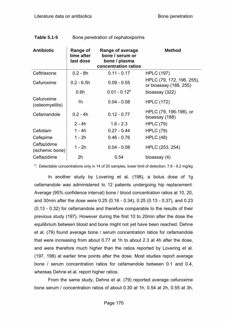
Literature data on antibiotics Bone penetration
Page 170
Table 5.1-5 Bone penetration of cephalosporins
Antibiotic Range of time after last dose
Range of average bone / serum or bone / plasma
concentration ratios
Method
Ceftriaxone 0.2 - 8h 0.11 - 0.17 HPLC (197)
Cefuroxime 0.2 - 6.5h 0.09 - 0.55 HPLC (79, 172, 196, 255), or bioassay (188, 255)
0.6h 0.01 - 0.12a bioassay (322) Cefuroxime (osteomyelitis) 1h 0.04 - 0.08 HPLC (172)
Cefamandole 0.2 - 4h 0.12 - 0.77 HPLC (79, 196-198), or bioassay (188)
2 - 4h 1.6 - 2.3 HPLC (79) Cefotiam 1 - 4h 0.27 - 0.44 HPLC (79) Cefepime 1 - 2h 0.46 - 0.76 HPLC (48) Ceftazidime (ischemic bone) 1 - 2h 0.04 - 0.08 HPLC (253, 254)
Ceftazidime 2h 0.54 bioassay (4) a: Detectable concentrations only in 14 of 20 samples, lower limit of detection: 7.6 - 9.2 mg/kg
In another study by Lovering et al. (198), a bolus dose of 1g
cefamandole was administered to 12 patients undergoing hip replacement.
Average (95% confidence interval) bone / blood concentration ratios at 10, 20,
and 30min after the dose were 0.25 (0.16 - 0.34), 0.25 (0.13 - 0.37), and 0.23
(0.13 - 0.32) for cefamandole and therefore comparable to the results of their
previous study (197). However during the first 10 to 20min after the dose the
equilibrium between blood and bone might not yet have been reached. Dehne
et al. (79) found average bone / serum concentration ratios for cefamandole
that were increasing from about 0.77 at 1h to about 2.3 at 4h after the dose,
and were therefore much higher than the ratios reported by Lovering et al.
(197, 198) at earlier time points after the dose. Most studies report average
bone / serum concentration ratios for cefamandole between 0.1 and 0.4,
whereas Dehne et al. report higher ratios.
From the same study, Dehne et al. (79) reported average cefuroxime
bone serum / concentration ratios of about 0.30 at 1h, 0.54 at 2h, 0.55 at 3h,

Literature data on antibiotics Bone penetration
Page 171
and 0.38 at 4h after the end of the infusion. Vuorisalo et al. (322) could detect
cefuroxime at an average of 36min after the dose in 14 of 20 sternal bone
samples, and bone / serum concentration ratios were between 0.01 and 0.12.
At about 4h after the infusion, cefuroxime could not be detected in any of 20
samples, however the detection limit of 7.6 to 9.2 mg/kg for the bioassay was
high. For cefotiam Dehne et al. (79) report average bone / serum
concentration ratios of about 0.27 at 1h, 0.30 at 2h, 0.44 at 3h, and 0.38 at 4h.
The ratios are similar to those reported for cefuroxime and to many of the
results for cefamandole.
Raymakers et al. (253) investigated ceftazidime concentrations in
ischemic bone of 16 patients undergoing lower limb amputation. Median bone
/ plasma concentration ratios at 1h to 1.5h after the dose ranged from 0.04 to
0.08 in the forefoot, midfoot, and tibial bone. These results are similar to a
previous study, that was conducted by the same group, and in a similar
patient collective (254). Because of poor circulation in ischemic tissue, high
concentration ratios would not have been expected.
Recently, Breilh et al. (48) investigated the bone concentrations of
cefepime in 10 patients. At 1 to 2h after the start of the infusion, average ± SD
bone / serum concentration ratios were 0.87 ± 0.37 for cortical and 1.06 ±
0.23 for cancellous bone. The ratios were calculated with bone concentrations
in mg/L, and a density of 1.9 kg/L for cortical and 1.4 kg/L for cancellous bone.
Therefore, concentration ratios were about 0.46 in cortical and 0.76 in
cancellous bone, based on bone concentrations expressed as mg/kg total
bone mass. These ratios for cefepime, especially in cancellous bone, are
higher than most results reported for other beta-lactams. In summary, most
studies report bone / serum concentration ratios between 0.1 and 0.5 for
cephalosporins. The ratios tend to be slightly higher than for most penicillins.
5.1.9.10 Aminoglycosides
There are few reports on aminoglycoside concentrations in human
bone after systemic administration and most studies were published some

Literature data on antibiotics Bone penetration
Page 172
decades ago. This renders interpretation of the penetration of
aminoglycosides into bone difficult. For gentamicin, bone / serum
concentration ratios at 1h to 12h after intramuscular administration of 1 mg/kg
range between 0.057 and 0.75 (42). Smilack et al. (277) found detectable
concentrations in bone only in 1 of 4 patients at 1h after an intramuscular
dose of 1.7 mg/kg, and report a high limit of detection of 2.1 mg/kg dry weight
of bone. For tobramycin, the average bone / serum concentration ratio is 0.13
at 0.3h (333) and 0.091 at 14.3h (42) after the dose.
Recently, Boselli et al. (43) investigated concentrations of isepamicin in
bone 1 to 2h after the dose in 12 patients. They report bone / plasma
concentration ratios of 0.31 in cortical and 0.28 in cancellous bone. These
ratios are based on bone concentrations in mg/L assuming a density of 1.9
kg/L for cortical and 1.4 kg/L for cancellous bone. Based on bone
concentrations in mg/kg, the average ratios are 0.16 for cortical and 0.20 for
cancellous bone.
Gentamicin is often used in beads, bone cement etc. for local treatment
or prophylaxis of bone infections. However local delivery of antibiotics to bone
is beyond the scope of this overview.
5.1.10 Conclusions
In summary, most of the studies find a substantial BSV in the observed
bone concentrations. There is also a considerable variability of the average
bone / serum concentration ratio between different studies on the same drug,
and between drugs within the same group of antibiotics. However, there are
some trends for the comparison of antibiotic groups. Most studies on
quinolones report high average bone / serum concentration ratios between 0.3
and about 1. Linezolid shows average bone / serum concentration ratios of
0.2 to 0.5. For macrolides and clindamycin, a large range of bone / serum
concentrations has been reported. Two recent studies showed that on
average azithromycin achieves higher concentrations in bone than in serum.
For glycopeptides very different results have been reported with the majority
of studies finding average bone / serum concentration ratios of 0.2 to 0.4.

Literature data on antibiotics Bone penetration
Page 173
Beta-lactams usually achieve average bone / serum concentration ratios of
less than 0.5 and most studies with penicillins report ratios between 0.1 and
0.3. For cephalosporins most studies report average bone / serum
concentration ratios between 0.1 and 0.5, whereas higher values have also
been reported. Average bone serum concentration ratios reported for
aminoglycosides are mostly between 0.05 and 0.2.
These trends among the antibiotic groups are caused by the
physicochemical characteristics of the different drug groups. For the passage
through the capillary walls into bone, molecular size, protein binding,
lipophilicity and acid / base characteristics are probably important
determinants (155). Binding to calcium in bone, as has been reported for
quinolones, or binding of fosfomycin to hydroxyapatite might also influence
bone concentrations of an antibiotic. Beta-lactams have been suggested to
distribute mainly in the interstitial fluid space in bone (202).
There is no prospectively evaluated PKPD target for treatment of bone
infections based on bone or serum concentrations. The PKPD target for
treatment of bone infections should be evaluated in future clinical trials. Those
studies should emphasize the validation, standardization, and reporting of the
analytical assay. Serum or plasma concentrations are probably a useful
surrogate measure for antibiotic effectiveness in bone, since some studies on
antibiotics suggest a fast rate of equilibration between bone and serum. The
PKPD targets based on serum concentrations are likely to be drug specific
due to the differences in the extent of bone penetration between various
antibiotics. Optimal design theory, population PK, and MCS are the methods
of choice to evaluate the average rate and extent of bone penetration as well
as the BSV.
Future studies are warranted to determine the influence of
osteomyelitis or ischemia on antibiotic concentrations in bone. There is also
very little data on the variability of bone penetration in different bone types.
Ideally, optimal dosage regimens should account for the disease state and
site of bone infection.
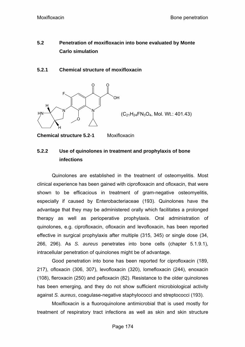
Moxifloxacin Bone penetration
Page 174
5.2 Penetration of moxifloxacin into bone evaluated by Monte Carlo simulation
5.2.1 Chemical structure of moxifloxacin
N
O
OH
O
F
N
OHN
H
H
Chemical structure 5.2-1 Moxifloxacin
5.2.2 Use of quinolones in treatment and prophylaxis of bone infections
Quinolones are established in the treatment of osteomyelitis. Most
clinical experience has been gained with ciprofloxacin and ofloxacin, that were
shown to be efficacious in treatment of gram-negative osteomyelitis,
especially if caused by Enterobacteriaceae (193). Quinolones have the
advantage that they may be administered orally which facilitates a prolonged
therapy as well as perioperative prophylaxis. Oral administration of
quinolones, e.g. ciprofloxacin, ofloxacin and levofloxacin, has been reported
effective in surgical prophylaxis after multiple (315, 345) or single dose (34,
266, 296). As S. aureus penetrates into bone cells (chapter 5.1.9.1),
intracellular penetration of quinolones might be of advantage.
Good penetration into bone has been reported for ciprofloxacin (189,
217), ofloxacin (306, 307), levofloxacin (320), lomefloxacin (244), enoxacin
(108), fleroxacin (250) and pefloxacin (82). Resistance to the older quinolones
has been emerging, and they do not show sufficient microbiological activity
against S. aureus, coagulase-negative staphylococci and streptococci (193).
Moxifloxacin is a fluoroquinolone antimicrobial that is used mostly for
treatment of respiratory tract infections as well as skin and skin structure
(C21H24FN3O4, Mol. Wt.: 401.43)

Moxifloxacin Bone penetration
Page 175
infections. It has a wider spectrum and improved activity against gram-positive
and anaerobic pathogens frequently found as causative agents in
osteomyelitis (193), while retaining potency and broad spectrum coverage
against gram-negative pathogens comparable to the earlier quinolones (37).
Moxifloxacin has lower MICs than levofloxacin, ciprofloxacin, ofloxacin, and
norfloxacin (313) for S. aureus, which is the most common pathogen in
osteomyelitis. Moxifloxacin achieves high concentrations in many tissues and
body fluids, e.g. gastrointestinal tissues (336), lung tissues and bronchial
secretions (49, 55, 274, 280), sinus tissues (85, 118), subcutaneous tissues
(165), skin blister fluid and saliva (231). However, bone penetration in humans
has not been reported for moxifloxacin and we are not aware of any reports
about PKPD modeling of quinolones in bone in humans or animals.
As described in chapter 5.1.3, reporting only bone / serum
concentration ratios makes interpretation of bone penetration difficult.
Modeling the full serum and bone concentration time course allows one to
evaluate the penetration of antimicrobials into bone and to study the PD
profile in bone. Therefore the first objective of our study was to determine
moxifloxacin concentrations after oral administration in cortical and cancellous
bone in a controlled study in subjects undergoing hip replacement surgery. As
our second objective we intended to develop a PK model to describe the time
course of moxifloxacin concentrations in bone and serum. Our third objective
was to calculate the PTA for serum, cortical and cancellous bone based on
PKPD targets for successful microbiological and clinical outcome.
5.2.3 Methods
Study participants: Our study comprised twenty-four patients
(10 males, 14 females) who were scheduled to undergo total hip replacement.
Their average ± SD weight was 76.8 ± 13.4 kg, height was 168.3 ± 9.9 cm
and age was 63 ± 15 years.
Study design and drug administration: Each patient received a
single oral dose of 400 mg moxifloxacin (Avalox®, BayerVital, Germany) 2 to
7h before surgery. Before surgery, 20 patients received amoxicillin / clavulanic

Moxifloxacin Bone penetration
Page 176
acid, three patients received levofloxacin, and one patient received
clindamycin, as intravenous infusion. Since there were no data on the bone
penetration of moxifloxacin prior to this study, those standard treatments for
perioperative prophylaxis were given in parallel to moxifloxacin to assure
antibacterial prophylaxis by an established treatment option.
Determination of Serum and Bone Concentrations: Serum and
bone samples were obtained as described in chapter 2.3. For determination of
moxifloxacin in plasma, 100µL of each sample were precipitated by adding
25µL of acetonitrile / perchloric acid containing the internal standard. After
thorough mixing the samples were centrifuged and 20µL of the clear
supernatant were analyzed by reversed-phase HPLC. For analysis of bone
samples, an aliquot of the bone powder was shaken with 6 times the amount
of buffer for 24h. After centrifugation, 100µL of the aqueous supernatant were
deproteinized by addition of 25µL of acetonitrile / perchloric acid containing
the internal standard. After thorough mixing and centrifugation, 20µL of the
aqueous supernatant were analyzed by HPLC.
The HPLC system consisted of a LaChrom L-7100 (E. Merck,
Darmstadt, Germany) pump, an autosampler (Autosampler L-7250, E. Merck,
Germany), an analytical reversed phase chomatographic column, and a
fluorescence detector (Jasco FP-920 Intelligent Fluoreszenz Detektor, Jasco,
Gross-Umstadt, Germany). The excitation wavelength was 296nm and the
emission wavelength 504nm. The mobile phase was a mixture of citric acid
solution, ammonium perchlorate, and acetonitrile. Moxifloxacin and the
internal standard were eluted by gradient elution after 4.4 and 3.1min,
respectively. For evaluation of the calibration standards a weighted linear
regression (1/y2) was performed with theoretical concentrations of calibration
standards and measured peak height ratios (peak height moxifloxacin / peak
height internal standard).
No interferences were observed in serum and bone for moxifloxacin
and the internal standard. The linearity of the moxifloxacin calibration curves
was demonstrated from 0.0100 to 5.00 mg/L in serum, and from 0.009 to
4.76 mg/L in bone homogenate. The inter-day precision and accuracy of the
spiked quality control standards of moxifloxacin in human serum ranged from

Moxifloxacin Bone penetration
Page 177
1.8 to 5.9% and from 95.1 to 103.8%, respectively. The inter-day precision
and accuracy of the spiked quality control standards of moxifloxacin in cortical
(cancellous) bone homogenate ranged from 3.7 to 9.2% (0.4 to 0.7%) and
from 94.7 to 97.6% (92.6 to 101.7%), respectively.
Pharmacokinetics PK analysis: We used a model with four disposition compartments and
a first-order absorption. The predictive performance of our final model was
tested via visual predictive checks and standard diagnostic plots were used.
Structural model: We had observations for moxifloxacin
concentrations in serum, cortical bone, and cancellous bone. We used a two
compartment disposition model for moxifloxacin in serum and in the peripheral
compartment plus one peripheral compartment for each bone matrix. The
differential equations for the model are as follows:
( ) ( )1Xka- dt
1dX⋅= Formula 5.2-1
( ) ( ) ( )
( ) ( ) ( )5Xk4Xk3XV
CLic
2XkkV
CLicCL1Xka dt
2dX
5242Peripheral
2524Serum
⋅+⋅+⋅+
⋅⎥⎦
⎤⎢⎣
⎡++
+−⋅=
Formula 5.2-2
( ) ( ) ( )3XV
CLic2XVCLic
dt3dX
PeripheralSerum⋅−⋅= Formula 5.2-3
( ) ( ) ( )4Xk2Xk dt
4dX4224 ⋅−⋅= Formula 5.2-4
( ) ( ) ( )5Xk2Xk dt
5dX5225 ⋅−⋅= Formula 5.2-5
Compartment 1 is the gut compartment, compartment 2 is the serum
compartment and compartment 3 the peripheral compartment. Compartment
4 is the compartment for cortical bone, and compartment 5 is the
compartment for cancellous bone. X(1), X(2), X(3), X(4) and X(5) denote the
amounts of drug in the respective compartment. CL is the apparent total

Moxifloxacin Bone penetration
Page 178
clearance from the central compartment, ka is the absorption rate constant,
CLic is the apparent intercompartmental clearance between the serum and
peripheral compartment, and k24, k42, k25, k52 are first order
intercompartmental transfer rate constants. VSerum and VPeripheral are the
apparent volumes of distribution of the respective compartment. For all
apparent clearance and apparent volume terms the extent of absorption term
(1/F) is left out for simplicity.
We included scale terms for the concentrations in cortical and
cancellous bone that describe the equilibrium concentration ratio between
cortical bone and serum (Fcortical) and between cancellous bone and serum
(Fcancellous). An Fcortical equal to 1 means that concentrations after a continuous
infusion at steady-state are the same in bone and serum, an Fcortical smaller
(greater) than 1 means that these concentrations are lower (higher) in bone
than in serum.
PK modeling: We had sparse serum concentration time data between
2 and 7h post oral administration. As the moxifloxacin half-life is about 12h,
these data did not allow us to estimate all PK parameters for a two
compartment model. Therefore, we used MAP-Bayesian estimation based on
the disposition parameters of Simon et al. (274) and derived the average
clearance and its standard deviation from published studies (274, 285-287,
337). Based on those disposition parameters and their standard deviation, we
estimated a typical half-life of absorption from our serum data via population
PK in NONMEM V (25).
We had no prior information on the rate or extent of bone penetration of
moxifloxacin. The raw data and initial modeling showed that the equilibrium
between serum and bone was virtually achieved 2h after dosing, indicating
that the rate of equilibration (k42 and k52) was fast. Therefore we could not
estimate k42 and k52 and fixed those values to an equilibration half-life of
15min. We assured the plausibility of this choice via visual predictive checks.
The disposition parameters of moxifloxacin as described above have
been determined in absence of a bone compartment. As we used MAP-
Bayesian estimation (see below), we had to keep the amount of moxifloxacin
in the bone compartments minimal so that the serum PK was not affected by

Moxifloxacin Bone penetration
Page 179
the presence of the bone compartments. This can be achieved by choosing a
small volume for the bone compartment or equivalently a small value for the
rate constants k24 and k25. Therefore, we chose a volume of distribution of
0.5L each for the cortical and cancellous bone compartments which is
equivalent to fixing k24 and k25 to 0.022 h-1 in our model.
MAP-Bayesian estimation: We estimated the individual PK
parameters by MAP-Bayesian estimation as implemented in ADAPT II (74).
We used informative priors with prior means and standard deviations and a
log-normal distribution to estimate the individual disposition parameters. In
absence of prior information on the bone penetration, we used non-
informative priors (uniform distribution) to estimate Fcortical and Fcancellous in the
MAP-Bayesian step. We described the residual unidentified variability by a
proportional error model for the serum and bone concentrations.
Reverse engineering method for PKPD targets: The ratio of the free
(non-protein bound) area under the plasma concentration time curve and MIC
(fAUC/MIC) has been shown to be predictive for the microbiological and
clinical outcome for fluoroquinolones (67, 92, 240). However, there is no
PKPD target for moxifloxacin in osteomyelitis patients in serum or for
quinolones in bone. Therefore, we used a reverse engineering method (38) to
propose a PKPD target for moxifloxacin in serum and bone based on studies
in osteomyelitis patients.
The reverse engineering method uses the success rate from clinical
studies in osteomyelitis patients, the expected AUCs after the doses given in
these studies, and published MIC distributions from the relevant time period to
derive the most likely target. The target which best predicts the observed
clinical success rate is derived via MCS in an iterative process.
We used published data from four studies (119, 131, 150, 242) on the
clinical or microbiological outcome of osteomyelitis caused by S. aureus in
patients who obtained ciprofloxacin orally at 500 mg or 750 mg every 12h. We
derived their expected AUCs based on published PK data for ciprofloxacin
(12, 348) or based on the AUCs reported by the authors (242). We assumed a
log-normal distribution for clearance and used a 25% protein binding for
ciprofloxacin to simulate the expected fAUCs for 5,000 virtual subjects for
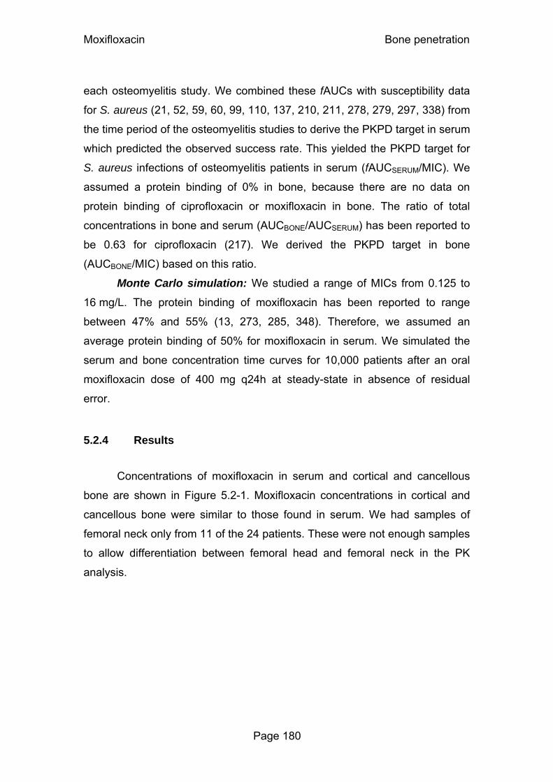
Moxifloxacin Bone penetration
Page 180
each osteomyelitis study. We combined these fAUCs with susceptibility data
for S. aureus (21, 52, 59, 60, 99, 110, 137, 210, 211, 278, 279, 297, 338) from
the time period of the osteomyelitis studies to derive the PKPD target in serum
which predicted the observed success rate. This yielded the PKPD target for
S. aureus infections of osteomyelitis patients in serum (fAUCSERUM/MIC). We
assumed a protein binding of 0% in bone, because there are no data on
protein binding of ciprofloxacin or moxifloxacin in bone. The ratio of total
concentrations in bone and serum (AUCBONE/AUCSERUM) has been reported to
be 0.63 for ciprofloxacin (217). We derived the PKPD target in bone
(AUCBONE/MIC) based on this ratio.
Monte Carlo simulation: We studied a range of MICs from 0.125 to
16 mg/L. The protein binding of moxifloxacin has been reported to range
between 47% and 55% (13, 273, 285, 348). Therefore, we assumed an
average protein binding of 50% for moxifloxacin in serum. We simulated the
serum and bone concentration time curves for 10,000 patients after an oral
moxifloxacin dose of 400 mg q24h at steady-state in absence of residual
error.
5.2.4 Results
Concentrations of moxifloxacin in serum and cortical and cancellous
bone are shown in Figure 5.2-1. Moxifloxacin concentrations in cortical and
cancellous bone were similar to those found in serum. We had samples of
femoral neck only from 11 of the 24 patients. These were not enough samples
to allow differentiation between femoral head and femoral neck in the PK
analysis.

Moxifloxacin Bone penetration
Page 181
Figure 5.2-1 Concentrations in serum and bone of subjects undergoing hip replacement surgery after a single oral dose of 400 mg moxifloxacin.
PK analysis: We estimated an absorption half-life of 26min. Table
5.2-1 shows our final parameter estimates from the MAP-Bayesian estimation.
Figure 5.2-2 shows the extent of moxifloxacin penetration into cortical
and cancellous bone, and its BSV, calculated from the ratios of AUCcortical /
AUCserum and AUCcancellous / AUCserum of 10,000 subjects that we simulated at
steady-state. The median AUC ratio [10% - 90% percentile] was 80% [51% -
126%] for cortical bone and 78% [42% - 144%] for cancellous bone.
Serum Cortical bone
0
1
2
3
4
5
0 1 2 3 4 5 6 7
Time after administration (h)
Conc
entra
tion
(mg/
L)
0
1
2
3
4
5
6
0 1 2 3 4 5 6 7
Time after administration (h)Co
ncen
tratio
n (µ
g/g) Femoral head
Femoral neck
0
1
2
3
4
5
6
7
0 1 2 3 4 5 6 7
Time after administration (h)
Conc
entra
tion
(µg/
g)
Femoral headFemoral neck
Cancellous bone
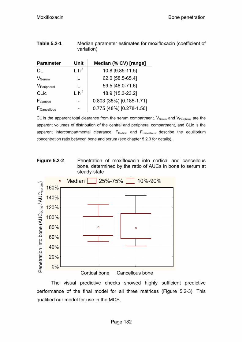
Moxifloxacin Bone penetration
Page 182
Table 5.2-1 Median parameter estimates for moxifloxacin (coefficient of
variation)
Parameter Unit Median (% CV) [range] CL L h-1 10.8 [9.85-11.5] VSerum L 62.0 [58.5-65.4] VPeripheral L 59.5 [48.0-71.6]
CLic L h-1 18.9 [15.3-23.2]
FCortical - 0.803 (35%) [0.185-1.71]
FCancellous - 0.775 (48%) [0.278-1.56] CL is the apparent total clearance from the serum compartment. VSerum and VPeripheral are the
apparent volumes of distribution of the central and peripheral compartment, and CLic is the
apparent intercompartmental clearance. FCortical and FCancellous describe the equilibrium
concentration ratio between bone and serum (see chapter 5.2.3 for details).
Figure 5.2-2 Penetration of moxifloxacin into cortical and cancellous
bone, determined by the ratio of AUCs in bone to serum at steady-state
The visual predictive checks showed highly sufficient predictive
performance of the final model for all three matrices (Figure 5.2-3). This
qualified our model for use in the MCS.
Cortical bone Cancellous bone Pen
etra
tion
into
bon
e (A
UC
bone
/AU
Cse
rum) Median 25%-75% 10%-90%
0%
20%
40%
60%
80%
100%
120%
140%
160%

Moxifloxacin Bone penetration
Page 183
Figure 5.2-3 Visual predictive check for serum and bone concentrations after 400 mg oral moxifloxacin
Serum
Cortical bone
Cancellous bone
The plots show the raw data, the 90% prediction interval [5 - 95% percentile] and the
interquartile range [25 - 75% percentile]. Ideally, 50% of the raw data points should fall inside
the interquartile range at each time point and 90% of the raw data should fall inside the 90%
prediction interval.
Reverse engineering method for PKPD targets: We used data from
published clinical studies with ciprofloxacin in osteomyelitis patients and
assumed a protein binding of 25% for ciprofloxacin and of 50% for
moxifloxacin in serum. The resulting PKPD targets for successful clinical or
microbiological outcome were fAUCSERUM/MIC ≥ 15 (119), fAUCSERUM/MIC
≥ 36 (242), fAUCSERUM/MIC ≥ 43 (150), and fAUCSERUM/MIC ≥ 66 (131). The
respective targets for total bone concentrations were AUCBONE/MIC ≥ 13
(119), AUCBONE/MIC ≥ 30 (242), AUCBONE/MIC ≥ 36 (150), and AUCBONE/MIC
≥ 55 (131). As the targets calculated from the studies by Nix et al. (242) and
Con
cent
ratio
n (m
g/L)
0
1
2
3
4
5
6
0 1 2 3 4 5 6 7
Time (h)
P25% percentileP5% percentileP50% percentile
P75% percentileP95% percentileRaw data
Con
cent
ratio
n (m
g/kg
)
01234567
0 1 2 3 4 5 6 7
Time (h)
P25% percentileP5% percentileP50% percentile
P75% percentileP95% percentileRaw data
0
1
2
3
4
5
6
0 1 2 3 4 5 6 7
Time (h)
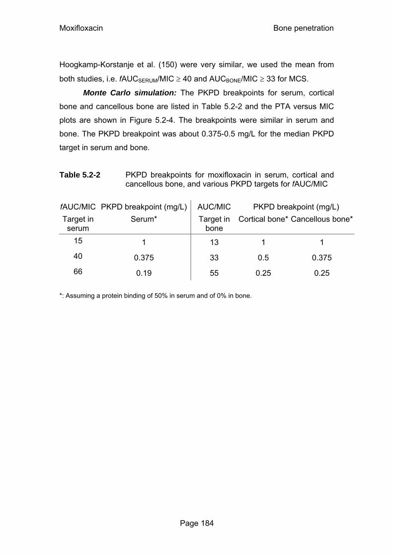
Moxifloxacin Bone penetration
Page 184
Hoogkamp-Korstanje et al. (150) were very similar, we used the mean from
both studies, i.e. fAUCSERUM/MIC ≥ 40 and AUCBONE/MIC ≥ 33 for MCS.
Monte Carlo simulation: The PKPD breakpoints for serum, cortical
bone and cancellous bone are listed in Table 5.2-2 and the PTA versus MIC
plots are shown in Figure 5.2-4. The breakpoints were similar in serum and
bone. The PKPD breakpoint was about 0.375-0.5 mg/L for the median PKPD
target in serum and bone.
Table 5.2-2 PKPD breakpoints for moxifloxacin in serum, cortical and cancellous bone, and various PKPD targets for fAUC/MIC
fAUC/MIC PKPD breakpoint (mg/L) AUC/MIC PKPD breakpoint (mg/L) Target in
serum Serum* Target in
bone Cortical bone* Cancellous bone*
15 1 13 1 1
40 0.375 33 0.5 0.375
66 0.19 55 0.25 0.25
*: Assuming a protein binding of 50% in serum and of 0% in bone.

Moxifloxacin Bone penetration
Page 185
Figure 5.2-4 Probabilities of target attainment for serum, cortical and cancellous bone after 400 mg oral moxifloxacin
Serum
0%10%20%30%40%50%60%70%80%90%
100%
0.125 0.25 0.5 1 2 4 8MIC (mg/L)
Cortical bone
0%10%20%30%40%50%60%70%80%90%
100%
0.125 0.25 0.5 1 2 4 8MIC (mg/L)
fAUC/MIC Serum
AUC/MIC Bone
Target calculated from
15 13 Gentry et al. (119)1
40 33
Nix et al. (242)2 and Hoogkamp-Korstanje (150)1
66 55 Greenberg et al. (131)1
Cancellous bone
0%10%20%30%40%50%60%70%80%90%
100%
0.125 0.25 0.5 1 2 4 8MIC (mg/L)
1 Targets for successful clinical outcome in osteomyelitis patients
2 Target for bacterial eradication in osteomyelitis patients
5.2.5 Discussion
Bone is not as highly vascularised as for example the lungs or skin.
Therefore it is important to investigate the time course and extent of bone
penetration of an antimicrobial before starting a clinical effectiveness trial (94,
313). Knowledge about how fast effective levels in bone are achieved may be
critical for the timing of perioperative prophylaxis and surgery. For selecting
the maintenance dose in treating bone infections, the AUC ratio (AUC in bone
/ AUC in serum) is the most informative measure for the extent of bone
penetration.
Moxifloxacin Bone penetration
Page 186
Therefore we studied the penetration of moxifloxacin into cortical and
cancellous bone in patients undergoing surgery for hip replacement and used
PK modeling and MCS for data analysis. We intended to study, if moxifloxacin
shows a sufficient extent of bone penetration to be used in perioperative
prophylaxis or treatment of bone infections. Furthermore we intended to study
the rate of bone penetration in order to determine the optimal time for initiation
of surgical prophylaxis. In absence of an established PKPD target for
moxifloxacin in bone infections, we used a reverse engineering method to
propose a necessary fAUCSERUM/MIC and AUCBONE/MIC for clinical or
microbiological success. For this method we used published MIC distributions
of S. aureus for ciprofloxacin and data on the effectiveness of ciprofloxacin in
osteomyelitis patients with S. aureus infection.
Our data showed high concentrations of moxifloxacin in both cortical
and cancellous bone tissues in subjects undergoing hip replacement surgery
(Figure 5.2-1). Moxifloxacin showed similar AUCs in bone and serum (Figure
5.2-2). Measures for the central tendency and BSV of the ratios AUCBONE /
AUCSERUM (median penetration [10% - 90% percentile]) were 80% [51% -
126%] for cortical bone and 78% [42% - 144%] for cancellous bone. We
studied the concentrations of moxifloxacin in bone and serum between 2 and
7h post the oral dose of moxifloxacin. The average concentration ratios
between serum and bone showed no obvious change with time during our
observation period. The raw data and initial modeling showed that the bone
penetration observed in our study was faster than expected, and equilibrium
between serum and bone was virtually achieved 2h after dosing. Therefore,
the bone and the serum compartment were in pseudo-equilibrium during our
observation period (from 2 to 7h post dose) and the bone concentrations
declined in parallel (on log-scale) to the serum concentration. As absorption of
moxifloxacin and bone penetration were fast, antibacterial prophylaxis should
be achieved within 2h in both cortical and cancellous bone after an oral dose
of moxifloxacin.
Secondary to the high extent of bone penetration for moxifloxacin, MCS
showed robust (≥90%) PTAs for MICs up to 0.375 mg/L in serum and in
cancellous bone, and up to 0.5 mg/L in cortical bone, for the targets

Moxifloxacin Bone penetration
Page 187
fAUCSERUM/MIC ≥ 40 and AUCBONE/MIC ≥ 33 (Table 5.2-2). This PKPD target
seems the most reasonable one, as it was the average reverse engineered
target of two studies investigating clinical and microbiological outcome. In one
of these two studies PK parameters were reported for several subjects and
could be used for calculation of the AUCs. The resulting targets from this
study (fAUCSERUM/MIC ≥ 40 and AUCBONE/MIC ≥ 33) fall between the targets
calculated from the other two studies (Table 5.2-2).
The calculated breakpoints were similar, or even slightly higher in bone
than in serum, although concentrations were slightly lower and more variable
in bone than in serum. However, it should be noted that we used a protein
binding of 50% for moxifloxacin in serum and assumed no protein binding in
bone, because of the absence of reports on moxifloxacin (and ciprofloxacin)
protein binding in bone. If 50% of moxifloxacin was bound to protein, or e.g. to
Ca2+, in bone, the PKPD breakpoints in bone would be half as high as shown
in Table 5.2-2. Assuming a (protein) binding of 50% in bone, breakpoints
would still be 0.125 mg/L (or above) in both cortical and cancellous bone for
all calculated targets.
An MIC90 of 0.125 mg/L has been reported for moxifloxacin against
S. aureus (313). If one simplifies the PTA vs. MIC profile by assuming a PTA
of 100% for all MICs ≤0.125 mg/L and a PTA of 0% for all MICs ≥0.25 mg/L, it
is possible to calculate that the overall probability of target attainment will be
≥90% for moxifloxacin against S. aureus based on an MIC90 of 0.125 mg/L.
Therefore, a high (≥90%) probability for successful clinical and microbiological
outcome would be predicted for S. aureus infections up to a target
AUCBONE/MIC ≥ 55 and a protein binding in bone of 50%.
In conclusion, we found a good penetration of moxifloxacin into bone.
Based on AUC ratios, the median penetration [10% - 90% percentile for BSV]
was 80% [51% - 126%] for cortical bone and 78% [42% - 144%] for
cancellous bone. We found a fast equilibrium half-life (< 60 min) between
serum and cortical bone as well as between serum and cancellous bone. As
the absorption of moxifloxacin was also fast, administering moxifloxacin 2h
before surgery would result in effective concentrations during surgery. The

Moxifloxacin Bone penetration
Page 188
PKPD breakpoint for moxifloxacin was 0.375 mg/L in serum and cancellous
bone, and 0.5 in cortical bone, based on the target AUCBONE/MIC ≥ 33
(fAUCSERUM/MIC ≥ 40) for successful microbiological outcome and assuming a
protein binding of 50% for moxifloxacin in serum and 0% in bone. As the
MIC90 of moxifloxacin is often reported to be 0.125 mg/L against S. aureus,
moxifloxacin was predicted to have a high probability (≥90%) for successful
microbiological outcome. This provides the required basis for a larger study on
the clinical effectiveness of moxifloxacin against bone infections.
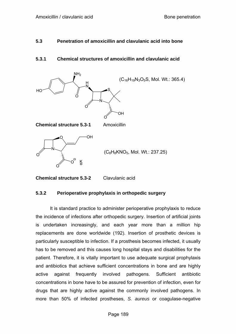
Amoxicillin / clavulanic acid Bone penetration
Page 189
5.3 Penetration of amoxicillin and clavulanic acid into bone
5.3.1 Chemical structures of amoxicillin and clavulanic acid
HN
NO
S
OOH
O
NH2
HO
Chemical structure 5.3-1 Amoxicillin
NO
O
OO
OH
K
Chemical structure 5.3-2 Clavulanic acid
5.3.2 Perioperative prophylaxis in orthopedic surgery
It is standard practice to administer perioperative prophylaxis to reduce
the incidence of infections after orthopedic surgery. Insertion of artificial joints
is undertaken increasingly, and each year more than a million hip
replacements are done worldwide (192). Insertion of prosthetic devices is
particularly susceptible to infection. If a prosthesis becomes infected, it usually
has to be removed and this causes long hospital stays and disabilities for the
patient. Therefore, it is vitally important to use adequate surgical prophylaxis
and antibiotics that achieve sufficient concentrations in bone and are highly
active against frequently involved pathogens. Sufficient antibiotic
concentrations in bone have to be assured for prevention of infection, even for
drugs that are highly active against the commonly involved pathogens. In
more than 50% of infected prostheses, S. aureus or coagulase-negative
(C16H19N3O5S, Mol. Wt.: 365.4)
(C8H8KNO5, Mol. Wt.: 237.25)

Amoxicillin / clavulanic acid Bone penetration
Page 190
staphylococci, e.g. S. epidermidis or S. saprophyticus, are the causative
pathogens (192).
Amoxicillin in combination with clavulanic acid is one of the most
frequently used antibiotics worldwide. It has a broad spectrum of activity
against gram-positive and gram-negative pathogens and is used for treatment
of respiratory tract infections, skin and skin structure infections, bone and joint
infections (often in combination with other antibiotics), and for perioperative
prophylaxis. Although amoxicillin / clavulanic acid shows good activity against
the pathogens commonly encountered in prosthesis-related bone infections
(MIC90s: 1 mg/L for methicillin-susceptible S. aureus, 8 mg/L for
S. epidermidis, and 0.5 mg/L for S. saprophyticus (141)), its PK profile in bone
(except bone / serum concentration ratios) and the PKPD breakpoints in bone
have not been determined. To the best of our knowledge there are no reports
about PKPD models in humans or animals for beta-lactam penetration into
bone. Therefore, we studied the rate and extent of penetration of amoxicillin /
clavulanic acid into cortical and cancellous bone in patients undergoing
surgery for hip replacement
The first objective of our study was to determine amoxicillin and
clavulanic acid concentrations in cancellous and cortical bone in a controlled
study in subjects undergoing hip replacement surgery. As our second
objective we intended to develop a PK model to describe the time course of
amoxicillin and clavulanic acid concentrations in bone as well as the exposure
(AUC ratios) of these drugs in bone relative to serum. Our third objective was
to calculate the probability to attain the PKPD targets for bacteriostasis and
near-maximal bacterial killing (67, 89) in serum, cortical and cancellous bone.
We derived the PKPD breakpoints and calculated the PTA expectation values
for target attainment against S. aureus, S. epidermidis, and S. saprophyticus
based on published MIC distributions.
5.3.3 Methods
Study design and drug administration: Twenty patients (9 males,
11 females) who were scheduled to undergo total hip replacement

Amoxicillin / clavulanic acid Bone penetration
Page 191
participated in the study. Their average ± SD weight was 78 ± 12 kg, height
was 169 ± 9 cm and age was 63 ± 16 years. Each patient received a single
dose of 2000 mg amoxicillin in combination with 200 mg clavulanic acid
(Augmentan®) as intravenous short-term infusion at the induction of
anesthesia.
Determination of Serum and Bone Concentrations: Serum and
bone samples were obtained as described in chapter 2.3. For determination of
amoxicillin and clavulanic acid in plasma, 50µL of ammonium acetate buffer
containing the internal standard were added to 100µL of each sample. The
samples were deproteinized by addition of 300µL acetonitrile. After thorough
mixing, the samples were centrifuged and 50µL of the clear supernatant were
analyzed by LC-MS/MS. For analysis of bone samples, an aliquot of the bone
powder was shaken with 6 times the amount of buffer for 4h. After
centrifugation, 50µL of buffer containing the internal standard were added to
50µL of the aqueous supernatant. After addition of 175µL acetonitrile, the
samples were thoroughly mixed and centrifuged. The clear supernatant was
diluted by twice the amount of buffer.
For determination of amoxicillin, 50µL of each sample were
chromatographed on a reversed-phase column (Ultracarb 5 ODS 30) and
eluted by an isocratic solvent system consisting of 0.001 M ammonium
acetate buffer and acetonitrile (90/10, v/v). The samples were monitored by
LC-MS/MS with a SRM method as follows: Precursor → product ion for
amoxicillin m/z 366 → m/z 208 and internal standard m/z 350 → m/z 160.
Both analyses were in positive mode. Under these conditions amoxicillin and
the internal standard were eluted after approximately 0.8 min.
For determination of clavulanic acid, 25µL of each sample were
chromatographed on a reversed-phase column (Nucleosil 100 Amino) and
eluted by an isocratic solvent system consisting of 0.01 M ammonium acetate
buffer and acetonitrile (40/60, v/v). The samples were monitored by LC-
MS/MS with a SRM method as follows: Precursor → product ion for clavulanic
acid m/z 198 → m/z 108 and internal standard m/z 232 → m/z 140. Both
analyses were in negative mode. Under these conditions clavulanic acid and

Amoxicillin / clavulanic acid Bone penetration
Page 192
the internal standard were eluted after approximately 2min. The MacQuan
software was used for evaluation of chromatograms. The precision and
accuracy of the SQCs for amoxicillin (clavulanic acid) in serum ranged from
1.8 to 10% (0.8 to 4.8%) and from 97.3 to 107.8% (96.0 to 100.5%),
respectively. The precision and accuracy of the SQCs for amoxicillin
(clavulanic acid) in bone homogenate ranged from 5.8 to 8.1% (5.0 to 7.8%)
and from 97.2 to 99.5% (91.7 to 100.0%), respectively.
Pharmacokinetics Population PK analysis: We used a model with two compartments for
amoxicillin and one compartment for clavulanic acid to describe the serum
concentrations. We added a bone compartment to describe the bone
penetration and used a time constrained zero-order input. The predictive
performance of our final model was tested via visual predictive checks.
Structural model: We had observations for amoxicillin and clavulanic
acid concentrations in serum, cortical bone, and cancellous bone. The
differential equations for amoxicillin were as follows:
( ) ( )
( ) ( )3XV
CLic2XV
CLic
1XV
CLicCLicCLrateinput dt
1dX
Bone
Bone
Peripheral
Central
Bone
⋅+⋅+
⋅⎥⎦
⎤⎢⎣
⎡ ++−=
Formula 5.3-1
( ) ( ) ( )2XV
CLic1XVCLic
dt2dX
PeripheralCentral⋅−⋅= Formula 5.3-2
( ) ( ) ( )3XV
CLic1XV
CLic dt
3dXBone
Bone
Bone
Bone ⋅−⋅= Formula 5.3-3
Compartment 1 is the central compartment. Compartment 2 is the
peripheral compartment. Compartment 3 is the bone compartment. X(1), X(2)
and X(3) denote the amounts of drug in the respective compartment. CL is the
total clearance from the central compartment, CLic is the intercompartmental
clearance between the central and peripheral compartment, and CLicBone the
intercompartmental clearance between the central and the bone
compartment. VCentral, VPeripheral and VBone are the volumes of distribution of the

Amoxicillin / clavulanic acid Bone penetration
Page 193
respective compartment. The differential equations for clavulanic acid can be
obtained from the above equations by setting CLic to zero. The raw data and
initial models showed that the rates of equilibration between serum and
cortical as well as between serum and cancellous bone were very similar.
Therefore we used only one bone compartment.
We included scale terms for the concentrations in cortical and
cancellous bone that describe the equilibrium concentration ratio between
cancellous bone and serum (Fcancellous) and between cortical bone and serum
(Fcortical). Fcortical equal to 1 means that the concentrations at steady-state after
a continuous infusion are the same in cortical bone and serum, Fcortical smaller
(greater) than 1 means that these concentrations are lower (higher) in cortical
bone than in serum.
We had sparse serum concentration time data between 0 and 1.1h
post end of infusion. Therefore, these data did not allow us to estimate all PK
parameters of the population PK model. We derived the average disposition
parameters for the serum concentration profiles and their variability from
published studies (9, 17, 142, 152, 241, 248). As those studies were
conducted in healthy volunteers, we used the amoxicillin clearance reported
by Sjovall et al. (276) for elderly subjects. This was in agreement with the age-
related decrease in renal function predicted by the Cockcroft and Gault
formula (63) based on the clearance from the other studies. For clavulanic
acid we accounted for the age-related decrease in renal function according to
the Cockcroft and Gault formula.
The disposition parameters of amoxicillin and clavulanic acid from
literature have been determined in absence of a bone compartment.
Therefore, we had to keep the amount of amoxicillin and clavulanic acid in the
bone compartment of our model minimal so that the serum PK was not
affected by the presence of the bone compartment. This can be achieved by
choosing a small volume VBone for the bone compartment.
Between subject variability and observation model: We estimated
the BSV for Fcortical and Fcancellous. The residual unidentified variability was
described by a proportional error model for serum and bone concentrations.

Amoxicillin / clavulanic acid Bone penetration
Page 194
Extent of drug exposure in bone: We determined the extent of drug
exposure in bone for amoxicillin and clavulanic acid by simulating the AUCs in
serum, cortical and cancellous bone. We simulated 10,000 virtual subjects at
steady-state and calculated the individual ratios of AUC in bone / serum as
well as their BSV.
Monte Carlo simulation: We used fT>MIC for at least 30% or 50% of
the dosing interval as PKPD targets for amoxicillin. We studied a range of
MICs from 0.25 to 64 mg/L and used a protein binding of 18% for amoxicillin
(124). In absence of data on protein binding in bone, a protein binding of 18%
in bone was assumed. We studied a 30min infusion of 2000 mg amoxicillin
q4h, q6h, or q8h at steady-state and simulated 10,000 virtual subjects in
absence of residual error. The PTAs and the PKPD breakpoints were derived
from those simulated profiles. We calculated the PTA expectation value based
on published MIC distributions. These comprised susceptibility data on MSSA,
S. epidermidis, and S. saprophyticus from North America (141).
5.3.4 Results
The concentrations of amoxicillin and clavulanic acid in serum, cortical
and cancellous bone are shown in Figure 5.3-1. Samples of femoral neck
were available only from 8 patients. These were not enough samples to
account for differences between femoral head and femoral neck in the PK
model.
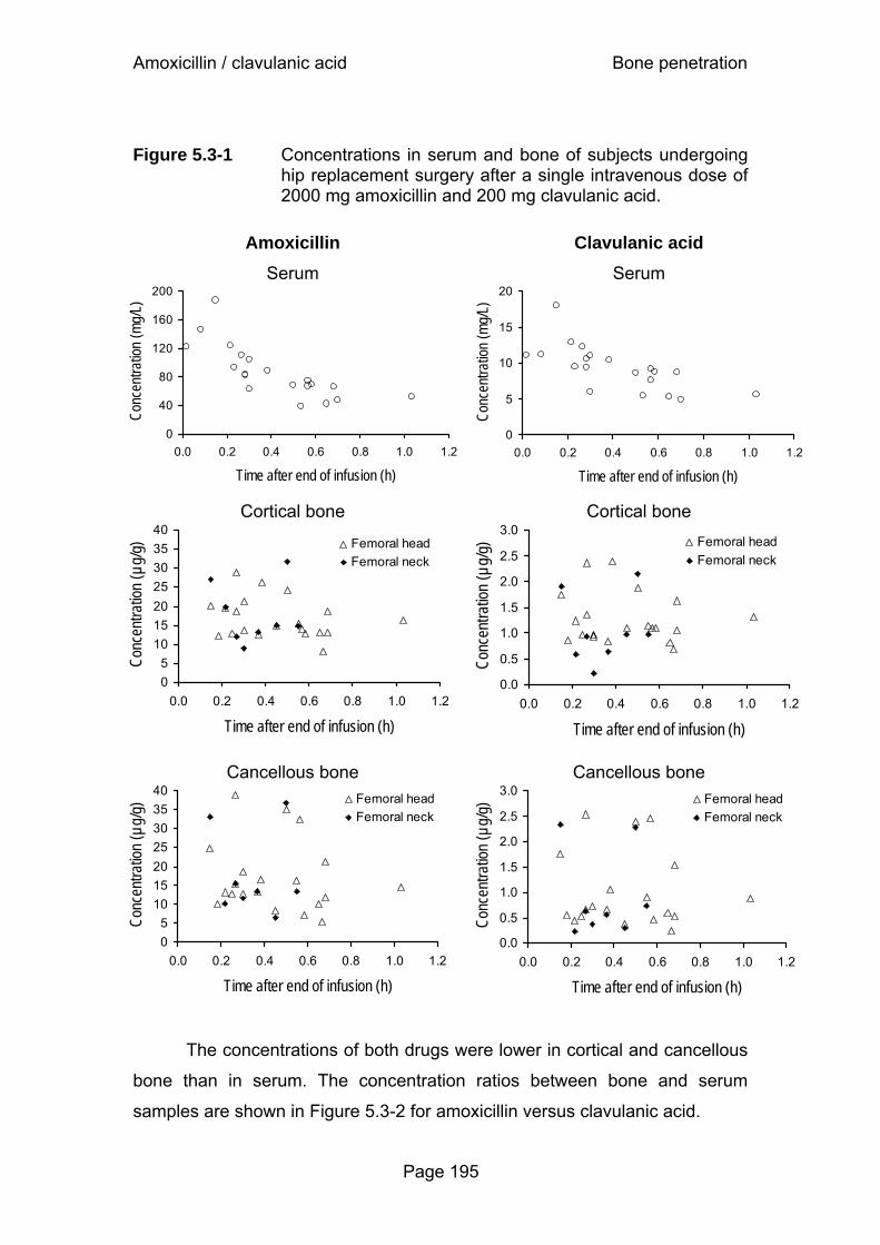
Amoxicillin / clavulanic acid Bone penetration
Page 195
Figure 5.3-1 Concentrations in serum and bone of subjects undergoing hip replacement surgery after a single intravenous dose of 2000 mg amoxicillin and 200 mg clavulanic acid.
Amoxicillin
Serum
0
40
80
120
160
200
0.0 0.2 0.4 0.6 0.8 1.0 1.2
Time after end of infusion (h)
Conc
entra
tion
(mg/
L)
Clavulanic acid
Serum
0
5
10
15
20
0.0 0.2 0.4 0.6 0.8 1.0 1.2
Time after end of infusion (h)Co
ncen
tratio
n (m
g/L)
Cortical bone
05
10152025303540
0.0 0.2 0.4 0.6 0.8 1.0 1.2
Time after end of infusion (h)
Conc
entra
tion
(µg/
g) Femoral headFemoral neck
Cortical bone
0.0
0.5
1.0
1.5
2.0
2.5
3.0
0.0 0.2 0.4 0.6 0.8 1.0 1.2
Time after end of infusion (h)
Conc
entra
tion
(µg/
g) Femoral headFemoral neck
Cancellous bone
05
10152025303540
0.0 0.2 0.4 0.6 0.8 1.0 1.2
Time after end of infusion (h)
Conc
entra
tion
(µg/
g)
Femoral headFemoral neck
Cancellous bone
0.0
0.5
1.0
1.5
2.0
2.5
3.0
0.0 0.2 0.4 0.6 0.8 1.0 1.2
Time after end of infusion (h)
Conc
entra
tion
(µg/
g)
Femoral headFemoral neck
The concentrations of both drugs were lower in cortical and cancellous
bone than in serum. The concentration ratios between bone and serum
samples are shown in Figure 5.3-2 for amoxicillin versus clavulanic acid.

Amoxicillin / clavulanic acid Bone penetration
Page 196
Figure 5.3-2 Concentration ratios of amoxicillin versus clavulanic acid
Cortical bone
y = 1.54x R 2 = 0.81
0.0 0.1 0.2 0.3 0.4 0.5
0.0 0.1 0.2
Cancellous bone
y = 1.85xR2 = 0.90
0.00.10.20.30.40.50.60.7
0.0 0.1 0.2 0.3
Population Pharmacokinetics: The final parameter estimates of the
population PK model and their between subject coefficients of variation are
shown in Table 5.3-1.
Table 5.3-1 PK parameter estimates and coefficients of variation for the
between subject variability
Parameter Unit Estimate (%CV) Amoxicillin Clavulanic acidCL L h-1 12.4 (19%) 11.0 (6.2%) VCentral L 11.3 (12%) 16.7 (25%) VPeripheral L 6.17 (3.7%) CLic L h-1 11.1 (19%) T1/2,Equilibration min 11.8 14.0 FCortical 0.199 (11%) 0.156 (17%) FCancellous 0.192 (39%) 0.119 (57%)
CL is the total clearance from the central compartment. VCentral is the volume of distribution of
the central compartment and VPeripheral the volume of distribution of the peripheral
compartment. CLic is the intercompartmental clearance between the central and the
peripheral compartment. T1/2,Equilibration is the half-life of equilibration between serum and bone.
FCortical and FCancellous describe the equilibrium concentration ratio between bone and serum
(see chapter 5.3.3 for details).
Am
oxic
illin
conc
entra
tion
ra
tio b
one
/ser
um
Clavulanic acid concentration ratio bone /serum
Am
oxic
illin
conc
entra
tion
ra
tio b
one
/ser
um
Clavulanic acid concentration ratio bone /serum

Amoxicillin / clavulanic acid Bone penetration
Page 197
Figure 5.3-3 shows the extent of amoxicillin and clavulanic acid
penetration into cortical and cancellous bone, and its BSV, calculated from the
ratios of AUCcortical / AUCserum and AUCcancellous / AUCserum at steady-state for
10,000 virtual subjects. The median AUC ratio of amoxicillin [10% - 90%
percentile for the BSV] was 20% [16% - 25%] for cortical bone and 18% [11%
- 29%] for cancellous bone. The median AUC ratio of clavulanic acid [10% -
90% percentile for the BSV] was 15% [11% - 21%] for cortical bone and 10%
[5.1% - 21%] for cancellous bone. Therefore, for both drugs the AUC ratio for
cancellous bone was more variable and (slightly) lower than for cortical bone.
The AUC ratios were lower for clavulanic acid than for amoxicillin.
Figure 5.3-3 AUC ratios between bone and serum at steady-state. The plots show the median, interquartile range, and 10-90% percentiles.
The rate of equilibration between serum and bone was fast for both
drugs. The estimate for the equilibration half-life was about 12min for
amoxicillin and 14min for clavulanic acid. The visual predictive checks showed
a highly sufficient predictive performance of the final model for both drugs
(Figure 5.3-4). This qualified our model for use in the MCS.
Cortical bone Cancellous bone
AUC
bone
/AU
Cse
rum
Amoxicillin Median 25%-75% 10%-90%
0%
5%
10%
15%
20%
25%
30%
AUC
bone
/AU
Cse
rum
Cortical bone Cancellous bone
Median 25%-75% 10%-90%
0%
5%
10%
15%
20%
Clavulanic acid
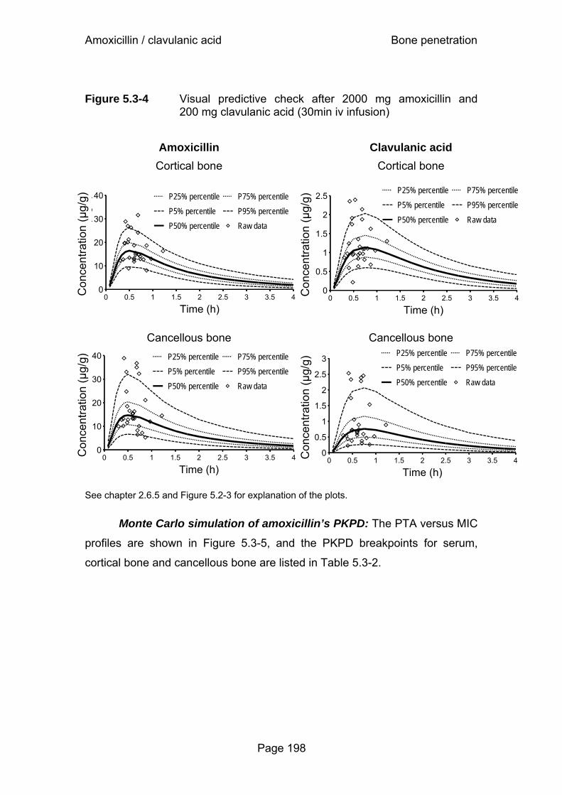
Amoxicillin / clavulanic acid Bone penetration
Page 198
Figure 5.3-4 Visual predictive check after 2000 mg amoxicillin and 200 mg clavulanic acid (30min iv infusion)
Amoxicillin Clavulanic acid Cortical bone
Cortical bone
Cancellous bone
Cancellous bone
See chapter 2.6.5 and Figure 5.2-3 for explanation of the plots.
Monte Carlo simulation of amoxicillin’s PKPD: The PTA versus MIC
profiles are shown in Figure 5.3-5, and the PKPD breakpoints for serum,
cortical bone and cancellous bone are listed in Table 5.3-2.
Con
cent
ratio
n (µ
g/g)
0
0.5
1
1.5
2
2.5
3
0 0.5 1 1.5 2 2.5 3 3.5 4
Time (h)
P25% percentileP5% percentileP50% percentile
P75% percentileP95% percentileRaw data
Con
cent
ratio
n (µ
g/g)
0
10
20
30
40
0 0.5 1 1.5 2 2.5 3 3.5 4
Time (h)
P25% percentileP5% percentileP50% percentile
P75% percentileP95% percentileRaw data
Con
cent
ratio
n (µ
g/g)
0
0.5
1
1.5
2
2.5
0 0.5 1 1.5 2 2.5 3 3.5 4
Time (h)
P25% percentileP5% percentileP50% percentile
P75% percentileP95% percentileRaw data
Con
cent
ratio
n (µ
g/g)
0
10
20
30
40
0 0.5 1 1.5 2 2.5 3 3.5 4
Time (h)
P25% percentileP5% percentileP50% percentile
P75% percentileP95% percentileRaw data

Amoxicillin / clavulanic acid Bone penetration
Page 199
Figure 5.3-5 Probabilities of target attainment for serum, cortical and cancellous bone after 2000 mg amoxicillin (and 200 mg clavulanic acid) as 30min infusion at steady-state.
Target fT>MIC ≥ 30% Target fT>MIC ≥ 50%
Dosing interval 4h
0%10%20%30%40%50%60%70%80%90%
100%
0.25 0.5 1 2 4 8 16 32 64MIC (mg/L)
Dosing interval 4h
0%10%20%30%40%50%60%70%80%90%
100%
0.25 0.5 1 2 4 8 16 32 64MIC (mg/L)
Dosing interval 6h
0%10%20%30%40%50%60%70%80%90%
100%
0.25 0.5 1 2 4 8 16 32 64MIC (mg/L)
Dosing interval 6h
0%10%20%30%40%50%60%70%80%90%
100%
0.25 0.5 1 2 4 8 16 32 64MIC (mg/L)
Dosing interval 8h
0%10%20%30%40%50%60%70%80%90%
100%
0.25 0.5 1 2 4 8 16 32 64MIC (mg/L)
Dosing interval 8h
0%10%20%30%40%50%60%70%80%90%
100%
0.25 0.5 1 2 4 8 16 32 64MIC (mg/L)
Cancellous bone
Cortical bone
Serum

Amoxicillin / clavulanic acid Bone penetration
Page 200
Table 5.3-2 PKPD breakpoints for amoxicillin in serum, cortical and cancellous bone for 30min infusions of 2000 mg amoxicillin and 200 mg clavulanic acid q4h, q6h, or q8h at steady-state.
PKPD breakpoint Target fT>MIC
Dosing interval Serum
(mg/L) Cortical bone
(µg/g) Cancellous bone
(µg/g) 30% 4h 24 6 4 30% 6h 16 3 2 30% 8h 8 2 1.5 50% 4h 12 3 2 50% 6h 6 1.5 1 50% 8h 3 0.75 0.5
The breakpoints were about 4 times higher in serum than in cortical
bone, and about 6 times higher in serum than in cancellous bone. The PTA
expectation values for the MIC distributions of three different pathogens are
shown in Table 5.3-3. With dosing intervals of 4h or 6h, PTA expectation
values above 90% were achieved against MSSA and S. saprophyticus in
serum, cortical and cancellous bone, based on the target fT>MIC ≥ 50% for
near-maximal killing. For S. epidermidis, a dosing interval of 4h was required
to reach PTA expectation values above 80% in bone.
5.3.5 Discussion
There is a wide variability of the reported bone concentrations for
amoxicillin and clavulanic acid in literature. One possible reason could be that
the determination of concentrations in bone is methodologically more complex
than in serum. Another reason might be that most bone penetration studies in
the past used microbiological assays. In the study described here a highly
standardized LC-MS/MS method was used. More specifically, we used
pulverization under liquid nitrogen by a cryogenic mill, as a very efficient
method for sample preparation that allows reproducible extraction of
amoxicillin and clavulanic acid from the resulting bone powder. A rapid and

Amoxicillin / clavulanic acid Bone penetration
Page 201
efficient extraction of an unstable drug like clavulanic acid may be critical for
studying its bone penetration. The degree of extraction was tested over time
to ensure reproducible results. Amoxicillin and clavulanic acid remained stable
during the 4h extraction period.
Table 5.3-3 Comparison of the PTA expectation values for target attainment against MSSA, S. epidermidis, and S. saprophyticus (141) for amoxicillin (30min infusion of 2000 mg amoxicillin and 200 mg clavulanic acid at steady-state).
MSSA S. epidermidis S. saprophyticus Target fT>MIC
Dosing interval (n=196 isolates) (n=119) (n=75)
Serum 30% 4h 99.5% 99.7% 100% 30% 6h 97.2% 98.0% 100% 30% 8h 96.4% 96.8% 100%
Cortical bone 30% 4h 95.7% 93.4% 99.5% 30% 6h 95.3% 87.7% 98.8% 30% 8h 94.8% 80.9% 98.7%
Cancellous bone 30% 4h 95.6% 91.5% 99.3% 30% 6h 95.1% 85.1% 98.9% 30% 8h 94.2% 77.9% 98.7%
Serum 50% 4h 97.2% 97.9% 100% 50% 6h 96.0% 95.1% 99.8% 50% 8h 95.3% 89.4% 99.2%
Cortical bone 50% 4h 95.3% 87.2% 98.9% 50% 6h 93.6% 72.9% 98.6% 50% 8h 86.5% 60.3% 96.1%
Cancellous bone 50% 4h 95.1% 84.4% 98.9% 50% 6h 92.0% 70.4% 98.1% 50% 8h 81.8% 57.7% 93.2%

Amoxicillin / clavulanic acid Bone penetration
Page 202
Some authors studied the bone penetration of amoxicillin and
clavulanic acid. Grimer et al. (132) report average concentrations of 3.6 mg/L
amoxicillin and 0.54 mg/L clavulanic acid in bone about 30min after
intravenous injection of 1000 mg amoxicillin and 200 mg clavulanic acid q6h
at steady-state (on day 2). They found at least 10 times lower concentrations
in bone than in serum, and amoxicillin and clavulanic acid did not accumulate
after multiple administration (132). Weismeier et al. (328) administered
2000 mg amoxicillin and 200 mg clavulanic acid by intravenous infusion. They
determined the concentration in the organic bone mass which accounted for
about 30 to 40% of total bone mass in their samples. They found slightly
higher concentrations in cortical than in cancellous bone. Related to total
bone, their average amoxicillin concentrations were about 8 mg/kg during the
first 2h, and about 2.5 mg/kg between 2 and 4h after the dose, average
clavulanic acid concentrations were about 0.7 to 0.8 mg/kg during the first 2h,
and about 0.3 mg/kg between 2 and 4h after the dose. Average concentration
ratios in total bone / serum were about 8 to 14% during the first 2h, and 15 to
18% between 2 and 4h after the dose for amoxicillin, and 4 to 8% during the
first 2h, and 6 to 7% between 2 and 4h after the dose for clavulanic acid (328)
related to total bone mass.
More recently, Jehl et al. (160) investigated concentrations of
amoxicillin and clavulanic acid in 63 patients after multiple oral administration
of amoxicillin / clavulanic acid (1g / 125 mg twice daily or 500 mg / 125 mg
three times daily). Between 1.5h and 8h after the last dose, bone / serum
concentration ratios of amoxicillin ranged between 0.09 and 0.44. Jehl et al.
(160) determined the time above MIC for amoxicillin, probably by using the
naïve averaging approach. For an MIC of 1 mg/L bone concentrations were
above the MIC for 50% of the dosing interval with the 1g dose of amoxicillin
twice daily, and for 37.5% of the dosing interval with the 500 mg dose three
times daily. However, this approach neglects the BSV and therefore does not
allow to determine a PKPD breakpoint.
Adam et al. (3) find 9.8 mg/kg clavulanic acid in cortical bone and
15 mg/kg in cancellous bone, between 0.5 and 1h after the end of a 20min
infusion of 200 mg clavulanic acid. Grimer et al (132), Weismeier et al. (328),

Amoxicillin / clavulanic acid Bone penetration
Page 203
and Adam et al. (3) used microbiological assays for determination of drug
concentrations. Dose-normalized amoxicillin and clavulanic acid
concentrations in bone found by Grimer et al. (132) and Weismeier et al. (328)
are approximately 2 to 3 times lower than the concentrations in our study,
whereas Adam et al. (3) report approximately 10 times higher concentrations
of clavulanic acid compared to our study (Figure 5.3-1). This pronounced (20
to 30-fold) difference for clavulanic acid underlines the need for standardized
methods for sample preparation, drug analysis and PK analysis.
We found lower concentrations for amoxicillin and clavulanic acid in
both cortical and cancellous bone compared to serum. Similar concentrations
were found in femoral head and femoral neck (Figure 5.3-1). As we had only
concentrations in femoral neck for eight patients, our final model did not
differentiate between femoral head and femoral neck. Concentrations of
amoxicillin and clavulanic acid showed a high correlation in cortical (r=0.90,
from raw data) as well as in cancellous bone (r=0.95 from raw data, see also
Figure 5.3-2). This suggests that both drugs were stable, and sample
preparation and drug analysis were precise and reproducible.
Our concentrations in cortical and cancellous bone were also
correlated for both drugs (r=0.76 for amoxicillin, r=0.75 for clavulanic acid).
This correlation was in agreement with the results from Weismeier et al. (328)
and indicated that the rate of equilibrium between cortical bone and serum
was probably similar to that between cancellous bone and serum. When we
estimated different equilibration half-lives for these two processes, we
obtained very similar estimates for both half-lives. Consequently, we assumed
both equilibration half-lives to be the same in our final model. Although bone is
not one of the most highly vascularised tissues, we observed short
equilibration half-lives between bone and serum of about 12min for amoxicillin
and of 14min for clavulanic acid (Table 5.3-1 and Figure 5.3-4). Therefore, the
peak concentration in bone will be reached within less than 45min post end of
a 30min infusion for most subjects. As the concentrations are decreasing in
serum and bone after the end of a short-term infusion, these fast equilibration
half-lives would suggest from a PK point of view that the surgery should start
within the first 30min post end of a 30min infusion. However, clinical

Amoxicillin / clavulanic acid Bone penetration
Page 204
effectiveness studies of amoxicillin/clavulanic acid are warranted to support
this suggestion and the PKPD target for surgical prophylaxis needs to be
determined.
The AUC in bone was lower than in serum for both drugs. We found
median (90% prediction interval for the BSV) ratios for AUC(bone) /
AUC(serum) of 20% [16% - 25%] for cortical bone and 18% [11% - 29%] for
cancellous bone for amoxicillin and of 15% [11% - 21%] for cortical bone and
10% [5.1% - 21%] for cancellous bone for clavulanic acid. Therefore, the
AUCs of amoxicillin in bone were on average about 5 to 6 times lower than in
serum and the AUCs of clavulanic acid in bone were on average about 6 to 10
times lower than in serum. For both drugs the AUC ratio for cancellous bone
was (slightly) lower than for cortical bone. This is in agreement to the data
from Weismeier et al. (328). The BSV of bone penetration was substantially
larger for cancellous bone than for cortical bone (see also variability for FCortical
and FCancellous in Table 5.3-1) for both drugs.
We used our final population PK model to calculate the PTA vs. MIC
profiles and the PKPD breakpoints for amoxicillin in bone and serum for three
different dosing intervals. For a 4h dosing interval, amoxicillin achieved robust
(≥90%) PTAs in serum for MICs ≤24 mg/L for the bacteriostasis target (fT>MIC
≥ 30%) and for MICs ≤12 mg/L for the near-maximal killing target (fT>MIC ≥
50%). The corresponding PKPD breakpoints in cortical and cancellous bone
for amoxicillin were 4-6 mg/L for the bacteriostasis target and 2-3 mg/L for the
near-maximal killing target (Table 5.3-2).
In order to put these PTAs into clinical perspective, we calculated the
PTA expectation values based on published MIC distributions for MSSA,
S. epidermidis, and S. saprophyticus which are frequently involved in
prosthesis related bone infections. Amoxicillin achieved excellent (>90%) PTA
expectation values against MSSA and S. saprophyticus for both targets in
bone and in serum for 30min infusions of 2000 mg / 200 mg amoxicillin /
clavulanic acid q4h and q6h (Table 5.3-3). As the S. epidermidis isolates were
less susceptible to amoxicillin / clavulanic acid, the PTA expectation values
were slightly lower for this pathogen. If 2000 mg / 200 mg amoxicillin /

Amoxicillin / clavulanic acid Bone penetration
Page 205
clavulanic acid were dosed q4h, the PTA expectation values were above or
equal to 90% for the bacteriostasis target and above 80% for the near-
maximal killing target for S. epidermidis. The susceptibility patterns of each
local hospital should be used to decide, whether amoxicillin / clavulanic acid
will be a promising choice for treatment of bone infections.
In conclusion, we found ratios for AUC(bone) / AUC(serum) of 20%
[16% - 25%] for cortical bone and 18% [11% - 29%] for cancellous bone for
amoxicillin and of 15% [11% - 21%] for cortical bone and 10% [5.1% - 21%]
for cancellous bone for clavulanic acid (median [90% prediction interval for the
BSV]). Equilibration between serum and bone was rapid with a half-life of
about 12min for amoxicillin and 14min for clavulanic acid. From a PK point of
view, this suggests that the surgery should start within the first 30min post end
of a 30min infusion. Assuming a 4h dosing interval, amoxicillin achieved
robust (≥90%) PTAs for MICs ≤12 mg/L in serum and 2-3 mg/L in cortical and
cancellous bone for the near-maximal killing target (fT>MIC ≥ 50%). Amoxicillin
achieved excellent (>90%) PTA expectation values against MSSA and
S. saprophyticus for both targets in bone and in serum for 30min infusions of
2000 mg / 200 mg amoxicillin / clavulanic acid q4h and q6h. Slightly lower
PTA expectation values were found for S. epidermidis. Clinical studies are
warranted to evaluate these results for amoxicillin / clavulanic acid in
treatment and surgical prophylaxis.

Assessment of bone penetration Bone penetration
Page 206
5.4 Critical view on assessment of bone penetration studies and future perspectives
5.4.1 Advantages of population pharmacokinetics and Monte Carlo simulations for bone penetration studies
Modeling the full serum and bone concentration time course is required
to describe the rate and extent of drug penetration into bone and to study the
PD profile in bone. For experimental reasons, only sparse concentration data
can be obtained in bone penetration studies (usually one bone sample per
patient). Therefore population PK modeling is needed to analyze these sparse
datasets. By the STS approach it is mathematically not possible to model
sparse data. The naïve averaging approach (chapter 5.1.3) has severe
methodological shortcomings, as it ignores the BSV. Population PK modeling
considers the full time course of penetration and allows one to calculate the
extent of penetration by the ratio of AUCs in tissue and serum. As the
concentration ratios between tissue and serum change over time, an AUC
ratio is a better measure for the extent of penetration than concentration
ratios. Comparing concentration ratios between studies is difficult due to the
different sampling times and different dosage regimens. A comparison
between studies is much more useful, if AUC ratios are reported. To obtain
reliable estimates for these ratios, population PK analysis is a powerful
approach.
Especially for sites of infections that may not be in a rapid equilibrium
with the blood stream, it is important to predict the probability of successful
outcome based on concentrations at the site of infection. Serum
concentrations might not be such a good surrogate marker in this case. Based
on a population PK model, MCS may be used to estimate PTAs for the
desired PD endpoint (e.g. successful microbiological outcome) in bone as well
as in serum. Evaluation of a PKPD target in bone would probably allow one to
obtain more reliable predictions for outcome of bone infections, than by use of

Assessment of bone penetration Bone penetration
Page 207
a PKPD target established in serum. However our bone penetration studies
showed that the equilibration between bone and serum had a half-life of
< 30min for amoxicillin, clavulanic acid, and moxifloxacin.
Appropriate PKPD targets in bone may be derived in studies where
both, the time course of the bone concentration profiles and the treatment
outcome, are determined, e.g. in osteomyelitis patients. Based on such a
validated target in osteomyelitis patients, optimal dosage regimens for
treatment of these patients with bone infections can be derived. Future studies
will have to show if a PKPD target in bone better predicts the outcome than a
PKPD target in serum.
5.4.2 Strengths and limitations of our bone penetration studies
Quantification of a drug in bone requires more extensive procedures
than in serum. Therefore the use of a standardized and validated analytical
method is very important to obtain reliable estimates of antimicrobial bone
penetration. In our studies pulverization of the bone samples under liquid
nitrogen by a cryogenic mill was used to ensure efficient and reproducible
extraction of the study drugs. The degree of extraction over time was
monitored and the stability of the study drugs during the extraction was tested.
Moxifloxacin, amoxicillin and clavulanic acid remained stable during the
extraction period. For studying the bone penetration of an unstable drug like
clavulanic acid, a rapid and efficient extraction is probably critical. Contrary to
many studies in literature, our spiked quality controls were prepared with bone
tissue. We assured that those bone tissue samples were free of the study
drug.
A highly precise and reproducible analytical method (including sample
preparation) needs special attention for datasets which contain only one
sample per patient for experimental reasons. The total variability of the
observed bone concentrations is determined by two components: 1) between
subject variability and 2) residual unexplained variability (primarily) due to
analytical imprecision (besides other factors). Those two types of variability
Assessment of bone penetration Bone penetration
Page 208
cannot be separated mathematically, if there is only one sample per patient
for the bone matrix.
There are two extreme cases: a) If there was no (or only negligible)
analytical imprecision, all the observed variability would represent BSV. b) If
the assay or sample preparation was very imprecise and if BSV was relatively
small, almost all of the observed variability in bone concentrations would be
due to analytical error. In real life, the results fall between those two extremes
and the data analyst has to pre-specify a realistic estimate for the analytical
precision in bone. It is possible to suggest a value and justify the chosen pre-
specified value for the residual variability e.g. via visual predictive checks, but
there is no proof for such a choice to be optimal.
If one is only interested in the average bone concentrations, a precise
analytical assay is important, but not vital. However, if one wishes to apply
Monte Carlo techniques and explicitely accounts for the BSV in those
simulations, obtaining a realistic (unbiased) estimate for the BSV is vitally
important.
As described above, a population PK model estimates the BSV of bone
penetration and accounts for the full time course of penetration. Thus,
population PK allows one to calculate the extent and time course of tissue
penetration. Unlike the naïve averaging approach, population PK and MCS
consider both the average antibiotic penetration into bone as well as its BSV.
Therefore, we used population PK and MCS to determine the variability of
bone penetration and to predict the PTAs and PTA expectation values for the
desired targets in serum and bone. The PTA expectation value is especially
helpful, since it can be used to predict the probability of successful treatment
in a local hospital. We are not aware of any reports about PKPD modeling of
quinolones or beta-lactams in bone in humans or animals.
One limitation of our study is that we had only sparse serum and bone
concentration time data between 2 and 7h post oral administration for
moxifloxacin and between 0 and 1.1h post end of infusion for amoxicillin /
clavulanic acid. We did not apply optimal sampling time theory to assign
sampling times or sampling time windows for our bone penetration studies.
Our bone penetration datasets did not allow us to estimate the PK parameters

Assessment of bone penetration Bone penetration
Page 209
of a full population PK model. Consequently, we used MAP-Bayesian
estimation of the individual PK parameters by including prior information from
literature for moxifloxacin. In the case of very sparse data, MAP-Bayesian
estimation is a powerful method to estimate the individual PK parameters. For
amoxicillin / clavulanic acid we derived the average disposition parameters
and their variability from published studies and used these in our population
PK model.
5.4.3 Application of optimal sampling times
Generally, in patients undergoing joint replacement, only one bone
sample can be obtained per subject, which yields very sparse bone
penetration data. If not all samples are collected within a narrow time window,
but are spread throughout the whole concentration time course, usually more
information can be gained about the distribution into and about the
redistribution out of the bone tissue.
It is important to take those precious bone samples at the most
informative time points. Informative refers to the ability to estimate the rate
and extent of bone penetration most precisely. Optimal sampling time theory
has been introduced in PK more than two decades ago by D’Argenio (73). In
bone penetration studies, one wishes to estimate the rate and extent of bone
penetration as well as their between patient variability, i.e. the full range of
observed bone penetration time curves.
While the optimal sampling time algorithm introduced by D’Argenio
originally aimed at providing optimal sampling times for one individual patient,
this theory has been extended to optimal sampling times for a population of
patients. Optimal sampling times for a population aim at estimating the
parameters of a population PK model for bone penetration most precisely (58,
94-96, 128, 130, 222, 238, 256, 300). Thus, the best estimates for the
average rate and extent of penetration as well as their variability should be
achieved. Optimal sampling times for a population of patients usually
comprise optimal sampling time windows. Those time windows could e.g.
state that from eight patients the bone sample has to be taken between 10

Assessment of bone penetration Bone penetration
Page 210
and 30min post end of infusion, from eight patients between 1 and 2h, and
from eight patients between 5 and 7h post end of infusion. A detailed
description of optimal sampling time is beyond the scope of this thesis.
However, it should be pointed out that the application of this theory may
greatly improve the precision of the results and conclusions that are drawn
from such studies.
5.4.4 Importance of clinical trial design for future studies
As outlined above, clinical trial design may be very valuable especially
for studies where only sparse data can be collected. Optimal trial design
allows one to choose optimal sampling time windows, so that the optimal
information can be gained from a limited number of samples. Ideally, optimal
design theory should be applied while planning a clinical study. Its application
may reveal that the number of patients originally planned is not sufficient to
draw the desired conclusions with an adequate precision. This underlines that
population PK is not only an option for data evaluation after conclusion of the
analytical part of a study, rather than that data collection, bio-analysis, and
data analysis are often very amalgamated.
Optimal trial design aims at estimating the population PK parameters
with at least a pre-specified precision. This yields more reliable predictions for
the PTA in subsequent PD simulations. Application of clinical trial design with
optimal sampling time windows may also allow one to study less patients and
might therefore be advantageous also for ethical reasons.
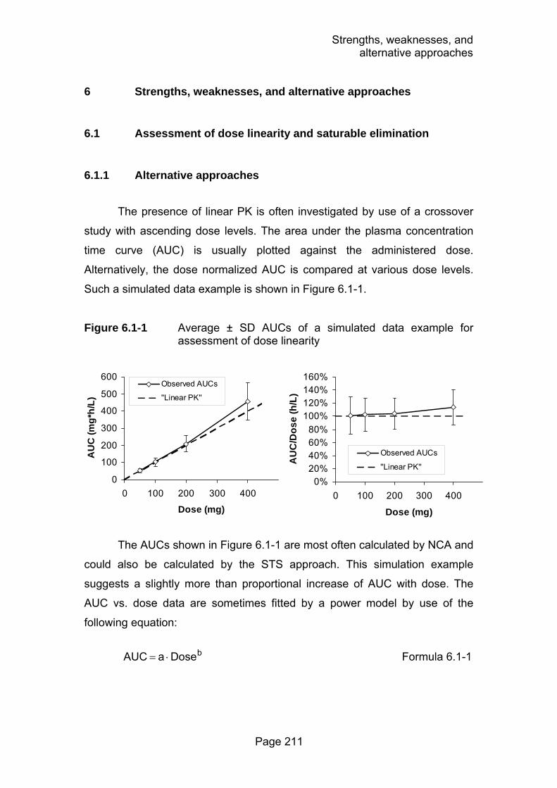
Strengths, weaknesses, and alternative approaches
Page 211
6 Strengths, weaknesses, and alternative approaches
6.1 Assessment of dose linearity and saturable elimination
6.1.1 Alternative approaches
The presence of linear PK is often investigated by use of a crossover
study with ascending dose levels. The area under the plasma concentration
time curve (AUC) is usually plotted against the administered dose.
Alternatively, the dose normalized AUC is compared at various dose levels.
Such a simulated data example is shown in Figure 6.1-1.
Figure 6.1-1 Average ± SD AUCs of a simulated data example for assessment of dose linearity
The AUCs shown in Figure 6.1-1 are most often calculated by NCA and
could also be calculated by the STS approach. This simulation example
suggests a slightly more than proportional increase of AUC with dose. The
AUC vs. dose data are sometimes fitted by a power model by use of the
following equation:
bDose a AUC ⋅= Formula 6.1-1
0
100
200
300
400
500
600
0 100 200 300 400
Dose (mg)
AU
C (m
g*h/
L)
Observed AUCs
''Linear PK''
0%20%40%60%80%
100%120%140%160%
0 100 200 300 400
Dose (mg)
AU
C/D
ose
(h/L
)
Observed AUCs
''Linear PK''

Strengths, weaknesses, and alternative approaches
Page 212
This equation converges to a simple linear relationship between AUC
and dose, if the exponent “b” is 1.0. Conversely, if “b” is significantly different
from 1.0, the nonlinearity is concluded to be statistically significant.
At this point, there are several possibly important questions:
1.) Is the deviation from dose linearity statistically significant?
2.) What is the extent of saturation at the studied dose levels?
3.) Is the nonlinearity only observed in some patients (e.g. patients with
“special” demographic characteristics)?
4.) Is the deviation from dose linearity clinically significant?
5.) What are possible mechanisms of the nonlinearity?
6.) Which extent of saturation would be expected at doses that are higher or
lower than the studied doses (extrapolation)?
There are three different data analytical methods which are commonly applied
to answer some or all of those questions:
a) Assessment of PK parameters by NCA and comparison of AUCs by
ANOVA statistics to test for statistical significance between dose levels.
Additionally, equivalence statistics are often applied to assess the extent
of nonlinearity.
b) Assessment of PK parameters by NCA and use of the power model (as
shown above) to describe the AUC vs. dose relationship.
c) Population PK analysis of the plasma concentration time raw data.
Those three methods differ in their ability to answer the above
mentioned questions and are compared in Table 6.1-1. As shown in this table,
population PK in combination with MCS is the most powerful approach to
study linear vs. nonlinear PK. The only drawback of this method is the time it
takes to prepare the raw data and the computation time to run the analysis.
Probably the most important advantage of population PK analysis compared
to the other two methods is the ability of population PK to predict the clinical
significance by use of a PKPD model and MCS.
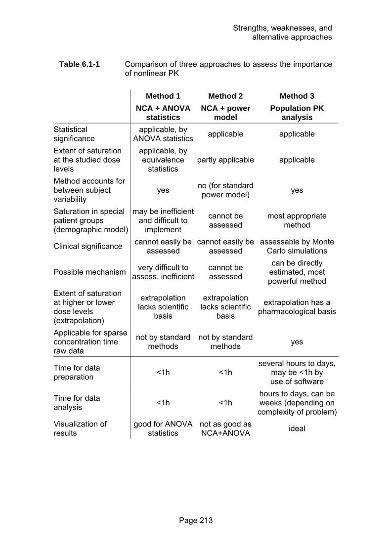
Strengths, weaknesses, and alternative approaches
Page 213
Table 6.1-1 Comparison of three approaches to assess the importance of nonlinear PK
Method 1 Method 2 Method 3 NCA + ANOVA
statistics NCA + power
model Population PK
analysis Statistical significance
applicable, by ANOVA statistics applicable applicable
Extent of saturation at the studied dose levels
applicable, by equivalence
statistics partly applicable applicable
Method accounts for between subject variability
yes no (for standard power model) yes
Saturation in special patient groups (demographic model)
may be inefficient and difficult to
implement
cannot be assessed
most appropriate method
Clinical significance cannot easily be assessed
cannot easily be assessed
assessable by Monte Carlo simulations
Possible mechanism very difficult to assess, inefficient
cannot be assessed
can be directly estimated, most powerful method
Extent of saturation at higher or lower dose levels (extrapolation)
extrapolation lacks scientific
basis
extrapolation lacks scientific
basis
extrapolation has a pharmacological basis
Applicable for sparse concentration time raw data
not by standard methods
not by standard methods yes
Time for data preparation <1h <1h
several hours to days, may be <1h by use of software
Time for data analysis <1h <1h
hours to days, can be weeks (depending on complexity of problem)
Visualization of results
good for ANOVA statistics
not as good as NCA+ANOVA ideal
Strengths, weaknesses, and alternative approaches
Page 214
6.1.2 Strengths and weaknesses of our dose linearity assessment
Strengths: We used NCA in combination with ANOVA statistics
(method 1, Table 6.1-1) and population PK (method 3) to analyze the
flucloxacillin and piperacillin dose linearity studies. The comparison of PK
parameters at two dose levels by ANOVA directly assesses the statistical
significance of the nonlinearity in PK (Table 3.2-1 and Table 3.3-1). The
equivalence statistics (also shown in those two tables) provided a measure for
the extent of nonlinearity at the studied dose levels.
We used population PK analysis and MCS as a powerful technique to
suggest the sites and possible mechanisms of the saturable elimination of
piperacillin. Additionally, we studied the possible clinical significance of the
saturable elimination of piperacillin. We assessed the influence of saturable
elimination for various dosage regimens at daily piperacillin doses between 6
and 18g (per 70kg body weight). To the best of our knowledge, this is the first
analysis of data from a crossover study for piperacillin by population PK. We
had frequent plasma and urine samples at both dose levels and we could
show that this supported the estimation of the saturable renal elimination
pathway. Our data were analyzed by validated HPLC methods which are often
superior to bioassays.
Weaknesses: There are some weaknesses of our flucloxacillin and
piperacillin studies: 1) The sample size of n=10 healthy volunteers was rather
small. Therefore, it was not feasible to study the influence of covariates (e.g.
demographic characteristics) on the PK. 2) Our studies were in healthy
volunteers and not in ill patients. Studying healthy volunteers is probably
advantageous to assess e.g. the mechanisms of renal elimination, because
the BSV in healthy volunteers is often substantially lower than in patients (see
chapter 1.5). However, the PK data used in a MCS should ideally arise from
the patient population of interest and not from healthy volunteers. Therefore,
the PTAs predicted by our simulations are probably conservative estimates for
ill patients. Although those limitations exist, their influence on our conclusions
on the dose linearity is probably limited to small.

Strengths, weaknesses, and alternative approaches
Page 215
6.2 Pharmacokinetic drug-drug interaction studies
6.2.1 Alternative approaches
We assessed the extent of the PK drug-drug interactions by NCA in
combination with ANOVA statistics and tested for significance and
equivalence (Table 4.2-2, Table 4.3-2, and Table 4.4-2). This method
adequately quantifies the extent of the drug-drug interation at the studied dose
levels and for the studied dosage regimens.
Additionally, we used the STS approach to construct a mechanistic
population PK model. This approach is inferior to directly estimating a
population PK model (e.g. with NONMEM). However, there is a substantial
difference in computation time between the STS method and population PK
for analysis of drug-drug interaction studies. While even our most complex
models took less than 2h on a laptop PC with the STS method in WinNonlin,
estimating a population PK model would require several days to weeks on the
fastest available personal computer at this time. For model development and
comparison, estimation of at least 10 to 20 of those population PK models
would have been required. Therefore, use of population PK for our drug-drug
interaction studies was not feasible.
Studies on a mechanistic model for the drug-drug interaction in vivo are
rare in the PK literature and the STS approach is commonly applied for
mechanistic models. The presence or absence of an interacting drug can be
treated as a covariate within a population PK analysis. This approach is often
chosen in population PK analyses of clinical trials in patients who received
other medication. Those clinical trials usually do not aim at studying the
mechanism of drug-drug interactions. This approach can quantify the extent of
interaction at the studied dose levels, but, in contrary to a mechanistic model,
it is usually not possible to draw conclusions about the mechanism and site of
the drug-drug interaction. As we were interested in the mechanism of the PK
drug-drug interaction, we did not select this approach.
Strengths, weaknesses, and alternative approaches
Page 216
6.2.2 Strengths and weaknesses of our drug-drug interaction studies
Strengths: The use of STS to construct a population PK model
allowed us to study a large number of mechanistic interaction models. We
were especially able to study various combinations of sites and mechanisms
of interaction. We could show that our population PK models constructed by
the STS approach had adequate predictive performance (Figure 4.2-2 and
Figure 4.4-4) which supported our selected approach and conclusions.
We studied the full time course of interaction with our interaction
models (Table 4.2-3, Table 4.3-3, and Table 4.4-3) and tried to gain the
maximum possible information from our data. Studying the full time course of
interaction by a mechanistic model is superior to NCA, because NCA ignores
the time course of interaction. Therefore, the use of NCA to draw conclusions
about the mechanism of interaction is an inefficient and to some extent
“wasteful” use of data and resources.
The strengths of the STS approach became especially apparent for the
analysis of the ciprofloxacin metabolite data. We were interested in a possible
effect of probenecid on the formation and elimination of the metabolite. We
could develop a full mechanistic model which explained the full time course of
the ciprofloxacin and metabolite data in plasma and urine with or without
probenecid. This would not have been possible by NCA.
We used our PK parameter estimates from the STS approach to
construct population PK models and to assess the clinical significance of the
drug-drug interactions for clinically relevant dosage regimens for gemifloxacin
(Figure 4.5-1 to Figure 4.5-3). Those simulations were helpful to balance the
possible clinical benefit with the increased risk for toxicity when gemifloxacin
and probenecid would be co-administered.
Weaknesses: The sample size in our interaction studies was small
(less than 20 subjects per study), although we had data from crossover
studies which allowed us to make intra-individual comparisons.
One limination of our interaction studies with probenecid is that the
sampling times were not optimized to characterize the PK of probenecid.

Strengths, weaknesses, and alternative approaches
Page 217
Therefore, the uncertainty of our PK parameters for probenecid is probably
larger than the uncertainty for the PK parameters of the antibiotics in those
studies. However, the aim of the PK model for probenecid in these studies
was to adequately describe the probenecid concentrations, as they were
included in the interaction models, and not to estimate the PK parameters of
probenecid most accurately. We could show that our PK models adequately
described and predicted the concentrations of probenecid.
We had to make several assumptions for the analysis of the
ciprofloxacin-probenecid dataset which were beyond the standard
assumptions. Although we could not prove those assumptions to be correct,
our results suggested that those were adequate and the best available option.
(see chapter 4.3.4)
6.3 Bone penetration of antibiotics
Alternative approaches for the assessment of bone penetrations have
been described in detail in chapter 5.1. The strengths and weaknesses of our
bone penetration studies are summarized in brief here.
Strengths: The main strengths of our bone penetration studies were
the highly standardized analysis of the bone samples and the data analysis by
population PK and MCS. From a data analytical perspective, there was no
viable alternative to population PK for our extremely sparse bone penetration
datasets.
Weaknesses: As a common weakness of almost all bone penetration
studies, the sample size of our bone penetration studies was small. As
described in chapter 5.4, the sampling times of the bone samples were not
optimized to estimate the population PK parameters most precisely. As
discussed above, there is no prospectively determined and validated PKPD
target for bone infections. Therefore, the results of our MCS for bone should
be interpreted conservatively. Although those limitations exist, we could
outline a perspective for the design and analysis of future bone penetration
studies. Future studies about the effect of disease state on the rate and extent
of bone penetration will be very valuable. Optimal clinical trial design is
Strengths, weaknesses, and alternative approaches
Page 218
probably very important for those trials, not only for ethical reasons.
Additionally, studies are required on the PKPD target for bone infections.
Conclusions
Page 219
7 Summary
There are numerous areas of application for which PKPD models are a
valuable tool. We studied dose linearity, bone penetration and drug-drug
interactions of antibiotics by PKPD modeling.
Knowledge about possible saturation of elimination pathways at
therapeutic concentrations is important for studying the probability of
successful treatment of dosage regimens via MCS at various doses, other
modes of administration, or both. We studied the dose linearity of flucloxacillin
and piperacillin. For data analysis of the dose linearity studies, population PK
modeling and MCS was used. Population PK has been reported to detect
saturable elimination at lower doses, and to estimate BSV more precisely than
the STS approach. The variability in PK and the expected variability in PD are
combined in a MCS to predict the probability of successful treatment.
Flucloxacillin showed no saturation of elimination at the studied doses
of 500 mg and 1000 mg. Comparison of various dosage regimens showed,
that only one third of the daily dose is needed with prolonged or continuous
infusion to achieve the same probability of successful treatment as short-term
infusions at the full dose. For serious infections with sensitive staphylococci
that are treated with intravenous flucloxacillin, prolonged infusion and
continuous infusion are an appealing treatment option.
Contrary to flucloxacillin, renal elimination and to a lesser extent also
nonrenal elimination of piperacillin were saturable at therapeutic
concentrations. Renal clearance decreased by 24% (p = 0.02) after a dose of
3000 mg piperacillin compared to the 1500 mg dose. A model without
saturable elimination predicted PTA expectation values that were 6 to 11%
lower for high dose short-term infusions and 2 to 5% higher for low dose
continuous infusions, compared to models with saturable elimination. These
differences depend on the MIC distributions of the local hospital. However,
more accurate estimates for the PTA expectation value can be obtained by
including an existent saturable elimination pathway into the PK model.
Developing a mechanistic model of an interaction allows one to predict
the extent of the interaction for other doses of drug and inhibitor. We studied

Conclusions
Page 220
the interactions between gemifloxacin and probenecid, between ciprofloxacin,
its metabolite M1 and probenecid, and between flucloxacillin and piperacillin.
Mechanistic models for drug-drug interactions were developed by the STS
approach. This approach directly accounts for the concentration dependence
of an interaction and describes the full time course of an interaction.
Probenecid significantly inhibited the renal elimination of gemifloxacin,
ciprofloxacin and ciprofloxacin’s metabolite M1, and slightly decreased
nonrenal clearance of gemifloxacin. Piperacillin significantly decreased renal
and nonrenal clearance of flucloxacillin, but hardly vice versa. For all three
interactions competitive inhibition of a capacity-limited renal elimination
pathway was identified as the most likely mechanism. As those drugs are all
actively secreted in the renal tubules, competitive interaction is physiologically
reasonable. Probenecid had a lower affinity to the renal transporter than
gemifloxacin, ciprofloxacin and M1. Due to its substantially higher
concentrations, probenecid inhibited the elimination of the quinolones. The
affinity of piperacillin for the renal transporter was 13 times higher compared
to flucloxacillin. Piperacillin PK was only slightly affected by flucloxacillin. PK
interactions with piperacillin are likely to occur also with other betalactam
combinations. PK interactions may be useful to improve the PD profile of an
antibiotic, however possibly increased risks for side effects (e.g. risk of rash
for gemifloxacin and probenecid) have to be considered.
Bone infections are difficult to treat. To ensure appropriate surgical
prophylaxis and antimicrobial treatment, knowledge about the rate and extent
of antibiotic bone penetration is valuable. Very different methods for sample
preparation, drug analysis, data analysis and reporting have been applied in
literature. The reported bone / serum concentration ratios differ widely
between studies, even for the same drug. Average concentration ratios are
usually between 0.1 and 0.4 for betalactams and glycopeptides, between 0.3
and 1.2 for quinolones, macrolides and linezolid, and even higher for
azithromycin. Standardization of methods is critical to be able to compare the
results from different studies. Population PK modeling and MCS should be
employed to predict penetration into bone and to investigate the PKPD
characteristics of antibiotics in bone.

Conclusions
Page 221
The bone penetration of moxifloxacin, amoxicillin and clavulanic acid
was studied in patients undergoing hip replacement surgery. The bone
penetration studies were evaluated by population PK, MAP-Bayesian
estimation and MCS. For evaluation of the PD profile of an antibiotic by MCS,
a population PK model is the best method, as it directly considers between
subject variability.
Moxifloxacin showed a high penetration into bone with a median AUC
ratio bone / serum of 80% for cortical and 78% for cancellous bone, while
amoxicillin and clavulanic acid had an about 5-10 times lower median AUC in
bone than in serum. All three studied antibiotics showed a fast equilibrium
between serum and bone with an average equilibration half-life of less than
about 30min. Amoxicillin achieved PTA expectation values of ≥95% in bone
and serum against S. aureus (methicillin-susceptible) and S. saprophyticus,
two pathogens commonly encountered in bone infections. Moxifloxacin
showed favorable PTAs compared to the MIC90 of S. aureus.
Future clinical trials are warranted to assess the effectiveness of
amoxicillin / clavulanic acid and moxifloxacin in bone infections and surgical
prophylaxis, and to evaluate possible PKPD targets in bone or serum for
these infections.
Overall, modeling and simulation techniques were applied to various
aspects of clinical studies for antibiotics within this thesis. The advantages of
population PK and MCS compared to standard NCA have been highlighted
based on practical problems. Probably one of the most important advantages
of population PK and MCS is their ability to incorporate additional
pharmacological data (e.g. PKPD targets) into the analysis. This greatly
supports assessment of the clinical relevance and emphasizes the power of
population PK and MCS to analyse data and visualize the results while
accounting for the true between patient variability. Such techniques should be
applied more frequently in the future to support drug development and therapy
at various stages.
Zusammenfassung
Page 222
8 Zusammenfassung
Es gibt viele Anwendungsgebiete für die PKPD-Modelle wertvoll sind.
In der vorliegenden Arbeit wurden Studien zu Dosislinearität,
Knochenpenetration und Arzneistoffinteraktionen von Antibiotika mit Hilfe von
PKPD-Modellen ausgewertet.
Um die Wahrscheinlichkeit einer erfolgreichen Therapie durch
Dosierungsregime mit verschiedenen Dosen, Verabreichungsmethoden oder
beidem zu studieren, ist es nötig, Kenntnisse über möglicherweise
vorhandene, bei therapeutischen Konzentrationen sättigbare Eliminations-
wege zu haben. Flucloxacillin und Piperacillin wurden auf ihre Dosislinearität
untersucht. Zur Datenanalyse der Dosislinearitätsstudien wurden
PopulationsPK-Modelle und MCS verwendet. Mit Hilfe von PopulationsPK
kann eine sättigbare Elimination schon bei geringeren Dosen erkannt werden,
und die Variabilität zwischen den Probanden kann genauer abgeschätzt
werden als mit der STS-Methode. In einer MCS wird die Variabilität in der PK
mit der erwarteten Variabilität in der PD kombiniert, um die Wahrscheinlichkeit
einer erfolgreichen Behandlung vorherzusagen.
Flucloxacillin zeigte bei 500 mg und 1000 mg keine Sättigung der
Elimination. Ein Vergleich verschiedener Dosierungsregime zeigte, dass bei
mehrstündiger oder kontinuierlicher Infusion im Vergleich zur Kurzzeitinfusion
nur ein Drittel der Dosis benötigt wird, um die gleiche Wahrscheinlichkeit für
eine erfolgreiche Behandlung zu erreichen. Für die Behandlung von schweren
Infektionen durch empfindliche Staphylokokken ist mehrstündige oder
kontinuierliche Infusion eine attraktive Möglichkeit.
Im Gegensatz zu Flucloxacillin war die renale, und in einem geringeren
Ausmaß auch die nicht-renale Elimination von Piperacillin bei therapeutischen
Dosen sättigbar. Die renale Clearance war nach der 3000 mg Dosis um 24%
(p = 0.02) verringert im Vergleich zur 1500 mg Dosis. Ein Modell ohne
sättigbare Elimination sagte für hochdosierte Kurzzeitinfusionen 6 bis 11%
niedrigere, und für niedrig dosierte kontinuierliche Infusion 2 bis 5% höhere
Erwartungswerte für die Erfolgswahrscheinlichkeit voraus, als Modelle mit
sättigbarer Elimination. Diese Unterschiede hängen von den minimalen

Zusammenfassung
Page 223
Hemmkonzentrationen der Pathogene im jeweiligen Krankenhaus ab. Durch
die Berücksichtigung eines vorhandenen sättigbaren Eliminationsweges im
Modell kann der Erwartungswert für die Erfolgswahrscheinlichkeit genauer
abgeschätzt werden.
Die Entwicklung eines mechanistischen Interaktionsmodells ermöglicht
es, das Ausmaß einer Interaktion für andere als die hier eingesetzten Dosen
von Arzneistoff und Inhibitor vorherzusagen. In der vorliegenden Arbeit
wurden die Interaktionen zwischen Gemifloxacin und Probenecid, sowie
zwischen Ciprofloxacin, dessen Metaboliten M1 und Probenecid, und
zwischen Flucloxacillin und Piperacillin untersucht. Die mechanistischen
Interaktionsmodelle wurden mit Hilfe der STS-Methode entwickelt. Diese
Methode bezieht die Konzentrationsabhängigkeit einer Interaktion direkt mit
ein und beschreibt den vollständigen zeitlichen Verlauf der Interaktion.
Probenecid hemmte die renale Elimination von Gemifloxacin,
Ciprofloxacin und M1 signifikant und verringerte leicht die nicht-renale
Clearance von Gemifloxacin. Piperacillin verminderte die renale und nicht-
renale Clearance von Flucloxacillin signifikant. Für alle drei Interaktionen
wurde eine kompetitive Inhibition eines sättigbaren renalen Eliminationsweges
als wahrscheinlichster Mechanismus identifiziert. Da alle untersuchten
Arzneistoffe aktiver renaler Sekretion unterliegen, ist eine kompetitive
Interaktion auch physiologisch sinnvoll. Die Affinität von Probenecid zum
renalen Transporter war niedriger als diejenige von Gemifloxacin,
Ciprofloxacin und M1. Trotzdem wurde die Elimination der Chinolone durch
Probenecid gehemmt, da Probenecid wesentlich höhere Konzentrationen
erreichte. Die Affinität von Piperacillin zum renalen Transporter war 13 Mal
höher als diejenige von Flucloxacillin. Die PK von Piperacillin wurde durch
Flucloxacillin nur leicht beeinflusst. Es ist wahrscheinlich, dass Piperacillin
auch mit anderen Betalaktamen PK-Interaktionen eingeht. PK-Interaktionen
können zur Verbesserung des PD-Profils eines Antibiotikums genutzt werden,
allerdings muss dabei auch das möglicherweise erhöhte Nebenwirkungsrisiko
(z.B. Hautausschlag bei Probenecid und Gemifloxacin) bedacht werden.
Knocheninfektionen sind schwierig zu behandeln. Zur Gewährleistung
einer geeigneten chirurgischen Prophylaxe und antibiotischen Therapie sind
Zusammenfassung
Page 224
Kenntnisse über Geschwindigkeit und Ausmaß der Knochenpenetration von
Antibiotika sehr wertvoll. In publizierten Studien wurden sehr unterschiedliche
Methoden der Probenvorbereitung, Arzneistoffanalyse, Datenauswertung und
Berichterstattung verwendet. Die berichteten Konzentrationsquotienten
zwischen Knochen und Serum unterscheiden sich stark zwischen den
Studien, sogar innerhalb eines Arzneistoffes. Bei Betalaktamen und
Glykopeptiden liegen die mittleren Konzentrationsquotienten meist zwischen
0.1 und 0.4, bei Chinolonen, Makroliden und Linezolid zwischen 0.3 und 1.2,
und bei Azithromycin noch höher. Eine Standardisierung der Methoden ist
sehr wichtig, um einen Vergleich der Ergebnisse verschiedener Studien zu
ermöglichen. PopulationsPK-Modelle und MCS sollten angewandt werden,
um die Knochenpenetration vorherzusagen und PKPD-Eigenschaften von
Antibiotika zu untersuchen.
Die Knochenpenetration von Moxifloxacin, Amoxicillin und
Clavulansäure wurde an Patienten mit Hüftersatzoperationen untersucht. Die
Knochenpenetrationsstudien wurden mit PopulationsPK, Bayes-Methoden
und MCS ausgewertet. Für die Untersuchung der PD-Eigenschaften eines
Antibiotikums durch MCS ist ein PopulationsPK-Modell die beste Methode, da
es die Variabilität zwischen den Probanden direkt berücksichtigt.
Moxifloxacin zeigte eine hohe Penetration in den Knochen mit einem
AUC-Quotienten von 0.8 (Median) zwischen Knochen und Serum. Die AUC
von Amoxicillin und Clavulansäure im Knochen war dagegen im Median ca. 5-
10 mal niedriger als im Serum. Alle drei untersuchten Antibiotika zeigten eine
schnelle Gleichgewichtseinstellung zwischen Serum und Knochen (mittlere
Halbwertszeit der Äquilibrierung kleiner als ca. 30min). Sowohl im Serum als
auch im Knochen erreichte Amoxicillin Erwartungswerte von ≥95% für die
Erfolgswahrscheinlichkeit gegen S. aureus (methicillin-empfindlich) und S.
saprophyticus, zwei häufige Auslöser von Knocheninfektionen. Moxifloxacin
zeigte vorteilhafte Erfolgswahrscheinlichkeiten im Vergleich mit der MHK90
von S. aureus. Zukünftige klinische Studien werden benötigt, um die
Wirksamkeit von Amoxicillin / Clavulansäure und Moxifloxacin in der Therapie
und Prophylaxe von Knocheninfektionen zu untersuchen, und mögliche
PKPD-Zielwerte für diese Infektionen in Knochen oder Serum zu evaluieren.
Zusammenfassung
Page 225
Diese Arbeit zeigt verschiedene Aspekte für Anwendungen von
Modellierung und Simulationen am Bespiel ausgewählter Antibiotika. Die
Vorteile von PopulationsPK und MCS im Vergleich zu Standard NCA wurden
an praktischen Beispielen aufgezeigt. Einer der wahrscheinlich wichtigsten
Vorteile von PopulationsPK und MCS ist deren Fähigkeit, zusätzliche
pharmakologische Daten (z.B. PKPD-Zielwerte) in die Analyse mit
einzubeziehen. Dies unterstützt die Abschätzung der klinischen Relevanz
sehr und betont die Vorteile von PopulationsPK und MCS bei der
Datenanalyse und Visualisierung von Ergebnissen, während gleichzeitig die
wahre Variabilität zwischen Patienten berücksichtigt wird. Diese Technik sollte
in der Zukunft häufiger angewendet werden, um die Entwicklung neuer
Substanzen und die Arzneistofftherapie an verschiedensten Stellen zu
unterstützen.
List of abbreviations
Page 226
9 List of abbreviations
Ae amount excreted unchanged in urine (expressed as fraction of administered dose)
AIC Akaike information criterion ANOVA analysis of variance APCI atmospheric pressure chemical ionization AUC area under the curve AUC0-last AUC from time of administration up to the last quantifiable
concentration AUC0-∞ AUC from time of administration up to time infinity AUMC area under the first moment concentration time curve BSAC British Society for Antimicrobial Chemotherapy BSV between subject variability Clast last quantifiable concentration CIP ciprofloxacin CLF,M1 formation clearance of the metabolite M1 CLic intercompartmental clearance CLicdeep intercompartmental clearance between the central and the
deep peripheral compartment CLicshallow intercompartmental clearance between the central and the
shallow peripheral compartment CLR renal clearance CLNR nonrenal clearance CLSI Clinical and Laboratory Standards Institute (formerly NCCLS)CLT total body clearance Cmax maximum observed plasma concentration CV coefficient of variation DIN Deutsches Institut für Normung E. coli Escherichia coli EARSS European Antimicrobial Resistance Surveillance System ECCMID European Congress of Clinical Microbiology and Infectious
Diseases ESBL extended-spectrum beta-lactamase ESI electrospray ionization fAUC/MIC ratio of the free area under the concentration time curve over
24h to the MIC

List of abbreviations
Page 227
Fcancellous describes the equilibrium concentration ratio between cancellous bone and serum
Fcortical describes the equilibrium concentration ratio between cortical bone and serum
FDA US Food and Drug Administration fT>MIC time that the non-protein bound plasma concentration
remains above the MIC of a pathogen fu non-protein bound fraction of drug in plasma GEM gemifloxacin GFR glomerular filtration rate HPLC high performance liquid chromatography ICAAC Interscience Conference on Antimicrobial Agents and
Chemotherapy iv intravenous K. pneumoniae Klebsiella pneumoniae Ka absorption rate constant Ki noncompetitive inhibition constant Kic competitive inhibition constant Kiu uncompetitive inhibition constant Km Michaelis Menten constant, drug concentration associated
with a half maximal rate of the mixed order process KmF,M1 Michaelis Menten constant of the mixed order formation of
the metabolite M1 LC-MS/MS liquid chromatography with tandem mass spectrometry ln natural logarithm log logarithm M1 2-aminoethylamino-metabolite of ciprofloxacin MAP maximum a posteriori probability MCS Monte Carlo simulation MIC minimum inhibitory concentration Mol. Wt. molecular weight MRSA methicillin-resistant Staphylococcus aureus MRT mean residence time MSSA methicillin-susceptible Staphylococcus aureus m/z mass to charge ratio NCA non-compartmental analysis NCCLS National Committee for Clinical Laboratory Standards
(now CLSI) NONMEM nonlinear mixed effects modeling

List of abbreviations
Page 228
OAT organic anion transporter P10 10% percentile P90 90% percentile P. aeruginosa Pseudomonas aeruginosa PD pharmacodynamics or pharmacodynamic PK pharmacokinetics or pharmacokinetic PKPD pharmacokinetics-pharmacodynamics PRO probenecid PTA probability of target attainment q quaque, every q4h every 4 hours q8h every 8 hours S. aureus Staphylococcus aureus S. epidermidis Staphylococcus epidermidis S. pneumoniae Streptococcus pneumoniae S. saprophyticus Staphylococcus saprophyticus
SD standard deviation SENTRY a global antimicrobial surveillance program SQC spiked quality control SRM selected reaction monitoring STS standard-two-stage T1/2 half-life T1/2,Equilibration half-life of equilibration between serum and bone TCI target concentration intervention TDM therapeutic drug monitoring TI transporter-inhibitor complex Tlag absorption lag-time Tmax time to peak concentration TS transporter-substrate complex TSI transporter-substrate-inhibitor complex US United States UV ultraviolet V1 volume of distribution for the central compartment V2 volume of distribution for the shallow peripheral compartmentV3 volume of distribution for the deep peripheral compartment

List of abbreviations
Page 229
Vmax maximum rate of a mixed order process VmaxF,M1 maximum rate of the mixed order formation of the metabolite
M1 Vss volume of distribution at steady-state WRSS weighted residual sum of squares λz terminal slope of the time vs. logarithmic concentration curve,
λz is defined as the absolute value of this slope and therefore positive

References
Page 230
10 References
1. 2005. British National Formulary 49. British Medical Association and Royal Pharmaceutical Society of Great Britain.
2. 2001. Guidance for Industry: Statistical Approaches to Establishing Bioequivalence. Center for Drug Evaluation and Research (CDER). U.S. Department of Health and Human Services. Food and Drug Administration.
3. Adam, D., H. D. Heilmann, and K. Weismeier. 1987. Concentrations of ticarcillin and clavulanic acid in human bone after prophylactic administration of 5.2 g of timentin. Antimicrob Agents Chemother 31:935-9.
4. Adam, D., B. Reichart, and K. J. Williams. 1983. Penetration of ceftazidime into human tissue in patients undergoing cardiac surgery. J Antimicrob Chemother 12 Suppl A:269-73.
5. Adam, D., K. Weismeier, F. Sorgel, and J. Zurcher. 1989. [Enoxacin concentration in bone tissue]. Infection 17 Suppl 1:S25-6.
6. Ahmed, S., S. Meghji, R. J. Williams, B. Henderson, J. H. Brock, and S. P. Nair. 2001. Staphylococcus aureus fibronectin binding proteins are essential for internalization by osteoblasts but do not account for differences in intracellular levels of bacteria. Infect Immun 69:2872-7.
7. Allen, A., Bird, N., Dixon, R., Hickmott, F., Pay, V., Smith, A., Stahl, M. 2001. Effect of Cimetidine on the Pharmacokinetics of Oral Gemifloxacin in Healthy Volunteers. Clin Drug Invest 21:519-526.
8. Allen, A., E. Bygate, S. Oliver, M. Johnson, C. Ward, A. J. Cheon, Y. S. Choo, and I. C. Kim. 2000. Pharmacokinetics and tolerability of gemifloxacin (SB-265805) after administration of single oral doses to healthy volunteers. Antimicrob Agents Chemother 44:1604-8.
9. Allen, G. D., P. E. Coates, and B. E. Davies. 1988. On the absorption of clavulanic acid. Biopharm Drug Dispos 9:127-36.
10. Ambrose, P. G., S. M. Bhavnani, and R. N. Jones. 2003. Pharmacokinetics-pharmacodynamics of cefepime and piperacillin-tazobactam against Escherichia coli and Klebsiella pneumoniae strains producing extended-spectrum beta-lactamases: report from the ARREST program. Antimicrob Agents Chemother 47:1643-6.
11. Ambrose, P. G., D. M. Grasela, T. H. Grasela, J. Passarell, H. B. Mayer, and P. F. Pierce. 2001. Pharmacodynamics of fluoroquinolones against Streptococcus pneumoniae in patients with community-acquired respiratory tract infections. Antimicrob Agents Chemother 45:2793-7.
12. Aminimanizani, A., P. Beringer, and R. Jelliffe. 2001. Comparative pharmacokinetics and pharmacodynamics of the newer fluoroquinolone antibacterials. Clin Pharmacokinet 40:169-87.
13. Andersson, M. I., and A. P. MacGowan. 2003. Development of the quinolones. J Antimicrob Chemother 51 Suppl 1:1-11.
14. Anonymous. 1998. E-Test Product information AB BIODISK.
References
Page 231
15. Anonymous. FACTIVE Investigator Brochure. Fourth edition. 16 January 1999.
16. Anonymous. Revised 5 April 1999. Piperacillin sodium and tazobactam sodium (Zosyn) product information. Lederle Laboratories, Pearl River, N.Y.
17. Arancibia, A., J. Guttmann, G. Gonzalez, and C. Gonzalez. 1980. Absorption and disposition kinetics of amoxicillin in normal human subjects. Antimicrob Agents Chemother 17:199-202.
18. Bailer, A. J. 1988. Testing for the equality of area under the curves when using destructive measurement techniques. J Pharmacokinet Biopharm 16:303-9.
19. Barriere, S. L. 1986. Therapeutic considerations in using combinations of newer beta-lactam antibiotics. Clin Pharm 5:24-33.
20. Barriere, S. L., D. H. Catlin, P. L. Orlando, A. Noe, and R. W. Frost. 1990. Alteration in the pharmacokinetic disposition of ciprofloxacin by simultaneous administration of azlocillin. Antimicrob Agents Chemother 34:823-6.
21. Barry, A. L., R. N. Jones, C. Thornsberry, L. W. Ayers, E. H. Gerlach, and H. M. Sommers. 1984. Antibacterial activities of ciprofloxacin, norfloxacin, oxolinic acid, cinoxacin, and nalidixic acid. Antimicrob Agents Chemother 25:633-7.
22. Barza, M., and L. Weinstein. 1976. Pharmacokinetics of the penicillins in man. Clin Pharmacokinet 1:297-308.
23. Batra, V. K., J. A. Morrison, K. C. Lasseter, and V. A. Joy. 1979. Piperacillin kinetics. Clin Pharmacol Ther 26:41-53.
24. Bauernfeind, A., and D. H. Wittmann. 1982. Presented at the International Symposium: Fosfomycin - ein neuartiges Antibiotikum, Salzburg.
25. Beal, S. L., A. J. Boeckmann, L. B. Sheiner, and NONMEM Project Group. 1999. NONMEM Users Guides, Version 5 ed. University of California at San Francisco, San Francisco.
26. Benoni, G., L. Cuzzolin, R. Leone, U. Consolo, G. Ferronato, C. Bertrand, V. Puchetti, and M. E. Fracasso. 1988. Pharmacokinetics and human tissue penetration of flurithromycin. Antimicrob Agents Chemother 32:1875-8.
27. Bergan, T. 1981. Overview of acylureidopenicillin pharmacokinetics. Scand J Infect Dis Suppl 29:33-48.
28. Bergan, T. 1978. Penicillins. Antibiot Chemother 25:1-122. 29. Bergan, T. 1978. Pharmacokinetics of mezlocillin in healthy volunteers.
Antimicrob Agents Chemother 14:801-6. 30. Bergan, T., A. Engeset, W. Olszewski, N. Ostby, and R. Solberg.
1986. Extravascular penetration of highly protein-bound flucloxacillin. Antimicrob Agents Chemother 30:729-32.
31. Bergan, T., and J. D. Williams. 1982. Dose dependence of piperacillin pharmacokinetics. Chemotherapy 28:153-9.
32. Bergeron, M. G., J. L. Brusch, M. Barza, and L. Weinstein. 1976. Bactericidal activity and pharmacology of flucloxacillin. Am J Med Sci 271:13-20.
References
Page 232
33. Bhavnani, S. M., J. A. Passarell, J. S. Owen, J. S. Loutit, S. B. Porter, and P. G. Ambrose. 2006. Pharmacokinetic-Pharmacodynamic Relationships Describing the Efficacy of Oritavancin in Patients with Staphylococcus aureus Bacteremia. Antimicrob Agents Chemother 50:994-1000.
34. Bijl, W., and R. A. Janknegt. 1993. Single-dose versus 3-day prophylaxis with ciprofloxacin in transurethral surgery. A clinical trial. Urol Int 51:73-8.
35. Bilello, J. A., P. A. Bilello, K. Stellrecht, J. Leonard, D. W. Norbeck, D. J. Kempf, T. Robins, and G. L. Drusano. 1996. Human serum alpha 1 acid glycoprotein reduces uptake, intracellular concentration, and antiviral activity of A-80987, an inhibitor of the human immunodeficiency virus type 1 protease. Antimicrob Agents Chemother 40:1491-7.
36. Birkett, D. J. 1998. Pharmacokinetics Made Easy. The McGraw-Hill Companies, Inc.
37. Blondeau, J. M. 1999. A review of the comparative in-vitro activities of 12 antimicrobial agents, with a focus on five new respiratory quinolones'. J Antimicrob Chemother 43 Suppl B:1-11.
38. Blumer, J. L., M. D. Reed, E. L. Kaplan, and G. L. Drusano. 2005. Explaining the poor bacteriologic eradication rate of single-dose ceftriaxone in group a streptococcal tonsillopharyngitis: a reverse engineering solution using pharmacodynamic modeling. Pediatrics 116:927-32.
39. Bonate, P. L. 1998. Coverage and precision of confidence intervals for area under the curve using parametric and non-parametric methods in a toxicokinetic experimental design. Pharm Res 15:405-10.
40. Bonten, M. J., S. Slaughter, A. W. Ambergen, M. K. Hayden, J. van Voorhis, C. Nathan, and R. A. Weinstein. 1998. The role of "colonization pressure" in the spread of vancomycin-resistant enterococci: an important infection control variable. Arch Intern Med 158:1127-32.
41. Booth, B. P., and J. V. Gobburu. 2003. Considerations in analyzing single-trough concentrations using mixed-effects modeling. J Clin Pharmacol 43:1307-15.
42. Boselli, E., and B. Allaouchiche. 1999. [Diffusion in bone tissue of antibiotics]. Presse Med 28:2265-76.
43. Boselli, E., D. Breilh, J. C. Bel, R. Debon, M. C. Saux, D. Chassard, and B. Allaouchiche. 2002. Diffusion of isepamicin into cancellous and cortical bone tissue. J Chemother 14:361-5.
44. Boselli, E., D. Breilh, L. Biot, J. C. Bel, M. C. Saux, and B. Allaouchiche. 2001. Penetration of Piperacillin/Tazobactam into Cancellous and Cortical Bone Tissue. Current Therapeutic Research 62:538-545.
45. Bottcher, S., H. von Baum, T. Hoppe-Tichy, C. Benz, and H. G. Sonntag. 2001. An HPLC assay and a microbiological assay to determine levofloxacin in soft tissue, bone, bile and serum. J Pharm Biomed Anal 25:197-203.

References
Page 233
46. Bradford, P. A. 2005. Presented at the 45th Interscience Conference on Antimicrobial Agents and Chemotherapy (ICAAC), Washington, D.C., USA.
47. Bradley, J. S., M. N. Dudley, and G. L. Drusano. 2003. Predicting efficacy of antiinfectives with pharmacodynamics and Monte Carlo simulation. Pediatr Infect Dis J 22:982-92; quiz 993-5.
48. Breilh, D., E. Boselli, J. C. Bel, D. Chassard, M. C. Saux, and B. Allaouchiche. 2003. Diffusion of cefepime into cancellous and cortical bone tissue. J Chemother 15:134-8.
49. Breilh, D., J. Jougon, S. Djabarouti, J. B. Gordien, F. Xuereb, J. F. Velly, P. Arvis, V. Landreau, and M. C. Saux. 2003. Diffusion of oral and intravenous 400 mg once-daily moxifloxacin into lung tissue at pharmacokinetic steady-state. J Chemother 15:558-62.
50. Bulitta, J., M. Kinzig-Schippers, U. Holzgrabe, F. Sörgel, and N. H. G. Holford. 2005. Replicate Design to Study the Population Pharmacokinetics (PopPK) of Piperacillin (PIP). Description of Saturable Elimination (EL) and Application to the Design of Optimal Dosage Regimens, Interscience Conference on Antimicrobial Agents and Chemotherapy, Washington, DC, USA.
51. Burckhardt, B. C., and G. Burckhardt. 2003. Transport of organic anions across the basolateral membrane of proximal tubule cells. Rev Physiol Biochem Pharmacol 146:95-158.
52. Bustamante, C. I., G. L. Drusano, R. C. Wharton, and J. C. Wade. 1987. Synergism of the combinations of imipenem plus ciprofloxacin and imipenem plus amikacin against Pseudomonas aeruginosa and other bacterial pathogens. Antimicrob Agents Chemother 31:632-4.
53. Butler, D. 2005. Wartime tactic doubles power of scarce bird-flu drug. Nature 438:6.
54. Bystedt, H., D. A. A, K. Dornbusch, and C. E. Nord. 1978. Concentrations of azidocillin, erythromycin, doxycycline and clindamycin in human mandibular bone. Int J Oral Surg 7:442-9.
55. Capitano, B., H. M. Mattoes, E. Shore, A. O'Brien, S. Braman, C. Sutherland, and D. P. Nicolau. 2004. Steady-state intrapulmonary concentrations of moxifloxacin, levofloxacin, and azithromycin in older adults. Chest 125:965-73.
56. Cawello, W. 1998. Parameter zur modellunabhängigen Pharmakokinetik - Standardisierung von Planung, Auswertung und Berichterstattung. Shaker, Aachen, Germany.
57. Chen, Y. H., C. F. Peng, P. L. Lu, J. J. Tsai, and T. P. Chen. 2004. In vitro activities of antibiotic combinations against clincal isolates of Pseudomonas aeruginosa. Kaohsiung J Med Sci 20:261-7.
58. Chenel, M., K. Ogungbenro, V. Duval, C. Laveille, R. Jochemsen, and L. Aarons. 2005. Optimal blood sampling time windows for parameter estimation using a population approach: design of a phase II clinical trial. J Pharmacokinet Pharmacodyn 32:737-56.
59. Chin, N. X., D. C. Brittain, and H. C. Neu. 1986. In vitro activity of Ro 23-6240, a new fluorinated 4-quinolone. Antimicrob Agents Chemother 29:675-80.

References
Page 234
60. Chin, N. X., and H. C. Neu. 1984. Ciprofloxacin, a quinolone carboxylic acid compound active against aerobic and anaerobic bacteria. Antimicrob Agents Chemother 25:319-26.
61. Clinckers, R., I. Smolders, A. Meurs, G. Ebinger, and Y. Michotte. 2005. Quantitative in vivo microdialysis study on the influence of multidrug transporters on the blood-brain barrier passage of oxcarbazepine: concomitant use of hippocampal monoamines as pharmacodynamic markers for the anticonvulsant activity. J Pharmacol Exp Ther.
62. Cluzel, R. A., R. Lopitaux, J. Sirot, and S. Rampon. 1984. Rifampicin in the treatment of osteoarticular infections due to staphylococci. J Antimicrob Chemother 13 Suppl C:23-9.
63. Cockcroft, D. W., and M. H. Gault. 1976. Prediction of creatinine clearance from serum creatinine. Nephron 16:31-41.
64. Cormican, M. G., and R. N. Jones. 1997. Antimicrobial activity and spectrum of LB20304, a novel fluoronaphthyridone. Antimicrob Agents Chemother 41:204-11.
65. Cosgrove, S. E., Y. Qi, K. S. Kaye, S. Harbarth, A. W. Karchmer, and Y. Carmeli. 2005. The impact of methicillin resistance in Staphylococcus aureus bacteremia on patient outcomes: mortality, length of stay, and hospital charges. Infect Control Hosp Epidemiol 26:166-74.
66. Cotran, R. S., V. Kumar, T. Collins, and S. L. Robbins. 1994. Robbins Pathological Basis of Disease, Philadelphia.
67. Craig, W. A. 1998. Pharmacokinetic/pharmacodynamic parameters: rationale for antibacterial dosing of mice and men. Clin Infect Dis 26:1-10; quiz 11-2.
68. Craig, W. A., and D. Andes. 1996. Pharmacokinetics and pharmacodynamics of antibiotics in otitis media. Pediatr Infect Dis J 15:255-9.
69. Craig, W. A., and S. C. Ebert. 1992. Continuous infusion of beta-lactam antibiotics. Antimicrob Agents Chemother 36:2577-83.
70. Cremieux, A. C., A. S. Mghir, R. Bleton, M. Manteau, N. Belmatoug, L. Massias, L. Garry, N. Sales, B. Maziere, and C. Carbon. 1996. Efficacy of sparfloxacin and autoradiographic diffusion pattern of [14C]Sparfloxacin in experimental Staphylococcus aureus joint prosthesis infection. Antimicrob Agents Chemother 40:2111-6.
71. Cummins, C. L., C. Y. Wu, and L. Z. Benet. 2002. Sex-related differences in the clearance of cytochrome P450 3A4 substrates may be caused by P-glycoprotein. Clin Pharmacol Ther 72:474-89.
72. D'Argenio, D. Z. 1990. Incorporating prior parameter uncertainty in the design of sampling schedules for pharmacokinetic parameter estimation experiments. Math Biosci 99:105-18.
73. D'Argenio, D. Z. 1981. Optimal sampling times for pharmacokinetic experiments. J Pharmacokinet Biopharm 9:739-56.
74. D'Argenio, D. Z., and A. Schumitzky. 1997. ADAPTII User's Guide: Pharmacokinetic/Pharmacodynamic Systems Analysis Software. Biomedical Simulations Resource, Los Angeles.

References
Page 235
75. Darley, E. S., and A. P. MacGowan. 2004. Antibiotic treatment of gram-positive bone and joint infections. J Antimicrob Chemother 53:928-35.
76. de Abajo, F. J., D. Montero, M. Madurga, and L. A. Garcia Rodriguez. 2004. Acute and clinically relevant drug-induced liver injury: a population based case-control study. Br J Clin Pharmacol 58:71-80.
77. De Jongh, C. A., J. H. Joshi, B. W. Thompson, K. A. Newman, R. S. Finley, M. R. Moody, P. C. Salvatore, J. H. Tenney, G. L. Drusano, and S. C. Schimpff. 1986. A double beta-lactam combination versus an aminoglycoside-containing regimen as empiric antibiotic therapy for febrile granulocytopenic cancer patients. Am J Med 80:101-11.
78. de Lalla, F., A. Novelli, G. Pellizzer, F. Milocchi, R. Viola, A. Rigon, C. Stecca, V. Dal Pizzol, S. Fallani, and P. Periti. 1993. Regional and systemic prophylaxis with teicoplanin in monolateral and bilateral total knee replacement procedures: study of pharmacokinetics and tissue penetration. Antimicrob Agents Chemother 37:2693-8.
79. Dehne, M. G., J. Muhling, A. Sablotzki, H. Nopens, and G. Hempelmann. 2001. Pharmacokinetics of antibiotic prophylaxis in major orthopedic surgery and blood-saving techniques. Orthopedics 24:665-9.
80. del Piano, M., R. Nicosia, R. Sessa, G. Grippaudo, R. Lolli, and B. Monaco. 1988. Study on tissue concentrations of antibiotics: bacampicillin in gingiva and maxillary bones. Chemotherapy 34:13-7.
81. Del Tacca, M., R. Danesi, N. Bernardini, M. Ducci, I. Zolfino, S. Senesi, E. Panattoni, M. Gabriele, M. Marcucci, A. Lazzarini, and et al. 1990. Roxithromycin penetration into gingiva and alveolar bone of odontoiatric patients. Chemotherapy 36:332-6.
82. Dellamonica, P., E. Bernard, H. Etesse, and R. Garraffo. 1986. The diffusion of pefloxacin into bone and the treatment of osteomyelitis. J Antimicrob Chemother 17 Suppl B:93-102.
83. Derendorf, H., T. Gramatté, and H. G. Schäfer. 2002. Pharmakokinetik. Einführung in die Theorie und Relevanz für die Arzneimitteltherapie, 2nd ed. Wissenschaftliche Verlagsgesellschaft mbH, Stuttgart.
84. DiMasi, J. A., R. W. Hansen, and H. G. Grabowski. 2003. The price of innovation: new estimates of drug development costs. J Health Econ 22:151-85.
85. Dinis, P. B., M. C. Monteiro, M. L. Martins, N. Silva, and J. G. Morais. 2004. Sinus tissue concentration of moxifloxacin after a single oral dose. Ann Otol Rhinol Laryngol 113:142-6.
86. Djabarouti, S., E. Boselli, B. Allaouchiche, B. Ba, A. T. Nguyen, J. B. Gordien, J. M. Bernadou, M. C. Saux, and D. Breilh. 2004. Determination of levofloxacin in plasma, bronchoalveolar lavage and bone tissues by high-performance liquid chromatography with ultraviolet detection using a fully automated extraction method. J Chromatogr B Analyt Technol Biomed Life Sci 799:165-72.
References
Page 236
87. Dornbusch, K., A. Carlstrom, H. Hugo, and A. Lidstrom. 1977. Antibacterial activity of clindamycin and lincomycin in human bone. J Antimicrob Chemother 3:153-60.
88. Dounis, E., S. Tsourvakas, L. Kalivas, and H. Giamacellou. 1995. Effect of time interval on tissue concentrations of cephalosporins after tourniquet inflation. Highest levels achieved by administration 20 minutes before inflation. Acta Orthop Scand 66:158-60.
89. Drusano, G. L. 2004. Antimicrobial pharmacodynamics: critical interactions of 'bug and drug'. Nat Rev Microbiol 2:289-300.
90. Drusano, G. L. 2003. Prevention of resistance: a goal for dose selection for antimicrobial agents. Clin Infect Dis 36:S42-50.
91. Drusano, G. L., A. Forrest, D. Fiore, F. Auger, and E. S. Caplan. 1984. Effect of saturable clearance during high-dose mezlocillin therapy. Antimicrob Agents Chemother 26:686-8.
92. Drusano, G. L., S. L. Preston, C. Fowler, M. Corrado, B. Weisinger, and J. Kahn. 2004. Relationship between fluoroquinolone area under the curve: minimum inhibitory concentration ratio and the probability of eradication of the infecting pathogen, in patients with nosocomial pneumonia. J Infect Dis 189:1590-7.
93. Drusano, G. L., S. L. Preston, C. Hardalo, R. Hare, C. Banfield, D. Andes, O. Vesga, and W. A. Craig. 2001. Use of preclinical data for selection of a phase II/III dose for evernimicin and identification of a preclinical MIC breakpoint. Antimicrob Agents Chemother 45:13-22.
94. Drusano, G. L., S. L. Preston, M. Van Guilder, D. North, M. Gombert, M. Oefelein, L. Boccumini, B. Weisinger, M. Corrado, and J. Kahn. 2000. A population pharmacokinetic analysis of the penetration of the prostate by levofloxacin. Antimicrob Agents Chemother 44:2046-51.
95. Duffull, S., T. Waterhouse, and J. Eccleston. 2005. Some considerations on the design of population pharmacokinetic studies. J Pharmacokinet Pharmacodyn 32:441-57.
96. Duffull, S. B., F. Mentre, and L. Aarons. 2001. Optimal design of a population pharmacodynamic experiment for ivabradine. Pharm Res 18:83-9.
97. Duffull, S. B., S. Retout, and F. Mentre. 2002. The use of simulated annealing for finding optimal population designs. Comput Methods Programs Biomed 69:25-35.
98. Eagle, H., R. Fleischman, and M. Levy. 1953. "Continuous" vs. "discontinuous" therapy with penicillin; the effect of the interval between injections on therapeutic efficacy. N Engl J Med 248:481-8.
99. Eliopoulos, G. M., A. Gardella, and R. C. Moellering, Jr. 1984. In vitro activity of ciprofloxacin, a new carboxyquinoline antimicrobial agent. Antimicrob Agents Chemother 25:331-5.
100. Emanuelsson, B. M., B. Beermann, and L. K. Paalzow. 1987. Non-linear elimination and protein binding of probenecid. Eur J Clin Pharmacol 32:395-401.
101. Etesse-Carsenti, H., F. Giaume, A. Barbarin, C. Argenson, V. Mondain, M. F. Masseyeff, E. Bernard, and P. Dellamonica. 1990. Presented at the Third Symposium on New Quinolones, Vancouver.

References
Page 237
102. Fauroux, C. M., and S. Freeman. 1999. Inhibitors of inositol monophosphatase. J Enzyme Inhib 14:97-108.
103. Fischman, A. J., J. W. Babich, A. A. Bonab, N. M. Alpert, J. Vincent, R. J. Callahan, J. A. Correia, and R. H. Rubin. 1998. Pharmacokinetics of [18F]trovafloxacin in healthy human subjects studied with positron emission tomography. Antimicrob Agents Chemother 42:2048-54.
104. Fischman, A. J., E. Livni, J. Babich, N. M. Alpert, Y. Y. Liu, E. Thom, R. Cleeland, B. L. Prosser, J. A. Correia, H. W. Strauss, and et al. 1993. Pharmacokinetics of [18F]fleroxacin in healthy human subjects studied by using positron emission tomography. Antimicrob Agents Chemother 37:2144-52.
105. Fish, D. N., and A. T. Chow. 1997. The clinical pharmacokinetics of levofloxacin. Clin Pharmacokinet 32:101-19.
106. Flaherty, J. F., S. L. Barriere, J. Mordenti, and J. G. Gambertoglio. 1987. Effect of dose on pharmacokinetics and serum bactericidal activity of mezlocillin. Antimicrob Agents Chemother 31:895-8.
107. Fong, I. W., W. H. Ledbetter, A. C. Vandenbroucke, M. Simbul, and V. Rahm. 1986. Ciprofloxacin concentrations in bone and muscle after oral dosing. Antimicrob Agents Chemother 29:405-8.
108. Fong, I. W., B. R. Rittenhouse, M. Simbul, and A. C. Vandenbroucke. 1988. Bone penetration of enoxacin in patients with and without osteomyelitis. Antimicrob Agents Chemother 32:834-7.
109. Forrest, A., S. Chodosh, M. A. Amantea, D. A. Collins, and J. J. Schentag. 1997. Pharmacokinetics and pharmacodynamics of oral grepafloxacin in patients with acute bacterial exacerbations of chronic bronchitis. J Antimicrob Chemother 40 Suppl A:45-57.
110. Foster, J. K., J. R. Lentino, R. Strodtman, and C. DiVincenzo. 1986. Comparison of in vitro activity of quinolone antibiotics and vancomycin against gentamicin- and methicillin-resistant Staphylococcus aureus by time-kill kinetic studies. Antimicrob Agents Chemother 30:823-7.
111. Fracasso, M. E., V. Consolo, G. Ferronato, R. Leone, L. Cuzzolin, and G. Benoni. 1989. Aztreonam penetration of bone and soft tissue, after i.v. infusion and bolus injection. J Antimicrob Chemother 23:465-7.
112. Fraschini, F., F. Scaglione, M. Falchi, P. Manzoni, S. D'Orsi, S. Badile, and M. Pignanelli. 1989. Miokamycin penetration into oral cavity tissues and crevicular fluid. Int J Clin Pharmacol Res 9:293-6.
113. Gabrielsson, J., and D. Weiner. 2001. Pharmacokinetic and Pharmacodynamic Data Analysis, Concepts and Applications, 3rd ed. Swedish Pharmaceutical Press, Stockholm, Sweden.
114. Gaitonde, M., Mendes, P., House, E. S. A., Lehr, K.H. 1995. The Effects of Cimetidine and Probenecid on the Pharmacokinetics of Levofloxacin, Interscience Conference on Antimicrobial Agents and Chemotherapy, San Francisco.
115. Gambertoglio, J. G., S. L. Barriere, E. T. Lin, and J. E. Conte, Jr. 1983. Amdinocillin pharmacokinetics. Simultaneous administration with cephalothin and cerebrospinal fluid penetration. Am J Med 75:54-9.
References
Page 238
116. Garton, A. M., R. P. Rennie, J. Gilpin, M. Marrelli, and S. D. Shafran. 1997. Comparison of dose doubling with probenecid for sustaining serum cefuroxime levels. J Antimicrob Chemother 40:903-6.
117. Gee, T., J. M. Andrews, J. P. Ashby, G. Marshall, and R. Wise. 2001. Pharmacokinetics and tissue penetration of gemifloxacin following a single oral dose. J Antimicrob Chemother 47:431-4.
118. Gehanno, P., S. Darantiere, C. Dubreuil, J. C. Chobaut, S. Bobin, J. C. Pages, G. Renou, F. Bobin, P. Arvis, and H. Stass. 2002. A prospective, multicentre study of moxifloxacin concentrations in the sinus mucosa tissue of patients undergoing elective surgery of the sinus. J Antimicrob Chemother 49:821-6.
119. Gentry, L. O., and G. G. Rodriguez. 1990. Oral ciprofloxacin compared with parenteral antibiotics in the treatment of osteomyelitis. Antimicrob Agents Chemother 34:40-3.
120. Gibaldi, M., and D. Perrier. 1982. Pharmacokinetics. Marcel Dekker, Inc., New York, USA.
121. Gisclon, L. G., R. A. Boyd, R. L. Williams, and K. M. Giacomini. 1989. The effect of probenecid on the renal elimination of cimetidine. Clin Pharmacol Ther 45:444-52.
122. Glantz, S. A. 1996. Primer of Biostatistics, fourth ed. McGraw-Hill. 123. GlaxoSmithKline. 2005. Flucloxacillin product information (Floxapen),
Uxbridge, Middlesex, UK. 124. Goodman Gilman, A. 1996. Goodman & Gilman's: The
pharmacological basis of therapeutics, 9th ed. McGraw-Hill, New York. 125. Gould, I. M. 1999. A review of the role of antibiotic policies in the
control of antibiotic resistance. J Antimicrob Chemother 43:459-65. 126. Gradl, W., and D. Adam. 1985. Apalcillinpharmakokinetik in
verschiedenen Geweben einschließlich des Knochens bei Patienten mit Totalendoprothese-Operation. FAC Fortschritte der antimikrobiellen und antineoplastischen Chemotherapie 4-7:1729-1736.
127. Gradl, W., and D. Adam. 1988. Gewebekonzentrationen von Mezlocillin und Oxacillin bei Hüftprothesen-Implantationen. ZAC Zeitschrift für antimikrobielle antineoplastische Chemotherapie 6:107-112.
128. Graham, G., I. Gueorguieva, and K. Dickens. 2005. A program for the optimum design of pharmacokinetic, pharmacodynamic, drug metabolism and drug-drug interaction models. Comput Methods Programs Biomed 78:237-49.
129. Graziani, A. L., L. A. Lawson, G. A. Gibson, M. A. Steinberg, and R. R. MacGregor. 1988. Vancomycin concentrations in infected and noninfected human bone. Antimicrob Agents Chemother 32:1320-2.
130. Green, B., and S. B. Duffull. 2003. Prospective evaluation of a D-optimal designed population pharmacokinetic study. J Pharmacokinet Pharmacodyn 30:145-61.
131. Greenberg, R. N., D. J. Kennedy, P. M. Reilly, K. L. Luppen, W. J. Weinandt, M. R. Bollinger, F. Aguirre, F. Kodesch, and A. M. Saeed. 1987. Treatment of bone, joint, and soft-tissue infections with oral ciprofloxacin. Antimicrob Agents Chemother 31:151-5.

References
Page 239
132. Grimer, R. J., M. R. Karpinski, J. M. Andrews, and R. Wise. 1986. Penetration of amoxycillin and clavulanic acid into bone. Chemotherapy 32:185-91.
133. Gumbo, T., A. Louie, M. R. Deziel, L. M. Parsons, M. Salfinger, and G. L. Drusano. 2004. Selection of a moxifloxacin dose that suppresses drug resistance in Mycobacterium tuberculosis, by use of an in vitro pharmacodynamic infection model and mathematical modeling. J Infect Dis 190:1642-51.
134. Guyton, A. C., and J. E. Hall. 1996. Textbook of Medical Physiology, 9 ed. Saunders.
135. Haag, R., R. Hölzlberger, E. Rienhoff, F. Bartels, and A. Meissner. 1989. Experimentelle Untersuchungen und Überlegungen zur Verteilung und zur verzögerten Freisetzung von Fosfomycin aus Knochengewebe. ZAC Zeitschrift für antimikrobielle antineoplastische Chemotherapie 7:3-10.
136. Hande, K., M. Messenger, J. Wagner, M. Krozely, and S. Kaul. 1999. Inter- and intrapatient variability in etoposide kinetics with oral and intravenous drug administration. Clin Cancer Res 5:2742-7.
137. Hardy, D. J., R. N. Swanson, D. M. Hensey, N. R. Ramer, R. R. Bower, C. W. Hanson, D. T. Chu, and P. B. Fernandes. 1987. Comparative antibacterial activities of temafloxacin hydrochloride (A-62254) and two reference fluoroquinolones. Antimicrob Agents Chemother 31:1768-74.
138. Hashimoto, Y., J. Ozaki, T. Koue, A. Odani, M. Yasuhara, and R. Hori. 1994. Simulation for the analysis of distorted pharmacodynamic data. Pharm Res 11:545-8.
139. Hayashi, T., Y. Watanabe, K. Kumano, R. Kitayama, T. Yasuda, I. Saikawa, K. Totsuka, T. Kumada, and K. Shimizu. 1986. Pharmacokinetic studies on the concomitant administration of piperacillin and cefazolin, and piperacillin and cefoperazone in rabbits. J Antibiot (Tokyo) 39:699-712.
140. Hill, G., T. Cihlar, C. Oo, E. S. Ho, K. Prior, H. Wiltshire, J. Barrett, B. Liu, and P. Ward. 2002. The anti-influenza drug oseltamivir exhibits low potential to induce pharmacokinetic drug interactions via renal secretion-correlation of in vivo and in vitro studies. Drug Metab Dispos 30:13-9.
141. Hoban, D. J., S. K. Bouchillon, J. L. Johnson, G. G. Zhanel, D. L. Butler, K. A. Saunders, L. A. Miller, and J. A. Poupard. 2003. Comparative in vitro potency of amoxycillin-clavulanic acid and four oral agents against recent North American clinical isolates from a global surveillance study. Int J Antimicrob Agents 21:425-33.
142. Hoffken, G., H. Tetzel, P. Koeppe, and H. Lode. 1985. Pharmacokinetics and serum bactericidal activity of ticarcillin and clavulanic acid. J Antimicrob Chemother 16:763-71.
143. Holder, D. J., F. Hsuan, R. Dixit, and K. Soper. 1999. A method for estimating and testing area under the curve in serial sacrifice, batch, and complete data designs. J Biopharm Stat 9:451-64.
144. Holford, N., P. Black, R. Couch, J. Kennedy, and R. Briant. 1993. Theophylline target concentration in severe airways obstruction - 10 or

References
Page 240
20 mg/L? A randomised concentration-controlled trial. Clin Pharmacokinet 25:495-505.
145. Holford, N. H. 1987. Clinical pharmacokinetics of ethanol. Clin Pharmacokinet 13:273-92.
146. Holford, N. H. 2001. Target concentration intervention: beyond Y2K. Br J Clin Pharmacol 52 Suppl 1:55S-59S.
147. Holford, N. H., and L. B. Sheiner. 1982. Kinetics of pharmacologic response. Pharmacol Ther 16:143-66.
148. Holford, N. H., and L. B. Sheiner. 1981. Understanding the dose-effect relationship: clinical application of pharmacokinetic-pharmacodynamic models. Clin Pharmacokinet 6:429-53.
149. Holford, N. H. G. 2003. Pharmacokinetics & Pharmacodynamics: Rational Dosing & the Time Course of Drug Action. In B. G. Katzung (ed.), Basic & Clinical Pharmacology, ninth ed. McGraw-Hill.
150. Hoogkamp-Korstanje, J. A. 1987. Treatment of chronic postsurgical osteomyelitis with ciprofloxacin. Pharm Weekbl Sci 9 Suppl:S90-2.
151. Hope, W. W., P. A. Warn, A. Sharp, P. Reed, B. Keevil, A. Louie, D. W. Denning, and G. L. Drusano. 2005. Surface response modeling to examine the combination of amphotericin B deoxycholate and 5-fluorocytosine for treatment of invasive candidiasis. J Infect Dis 192:673-80.
152. Horber, F. F., F. J. Frey, C. Descoeudres, A. T. Murray, and F. C. Reubi. 1986. Differential effect of impaired renal function on the kinetics of clavulanic acid and amoxicillin. Antimicrob Agents Chemother 29:614-9.
153. Howden, B. P., and M. J. Richards. 2001. The efficacy of continuous infusion flucloxacillin in home therapy for serious staphylococcal infections and cellulitis. J Antimicrob Chemother 48:311-4.
154. Hudson, M. C., W. K. Ramp, N. C. Nicholson, A. S. Williams, and M. T. Nousiainen. 1995. Internalization of Staphylococcus aureus by cultured osteoblasts. Microb Pathog 19:409-19.
155. Hughes, S. P., and F. M. Anderson. 1985. Penetration of antibiotics into bone. J Antimicrob Chemother 15:517-9.
156. Incavo, S. J., P. J. Ronchetti, J. H. Choi, H. Wu, M. Kinzig, and F. Sorgel. 1994. Penetration of piperacillin-tazobactam into cancellous and cortical bone tissues. Antimicrob Agents Chemother 38:905-7.
157. Jacquez, J. A. 1996. Parameter identifiability is required in pooled data methods. J Pharmacokinet Biopharm 24:301-5.
158. Jaehde, U., F. Sorgel, A. Reiter, G. Sigl, K. G. Naber, and W. Schunack. 1995. Effect of probenecid on the distribution and elimination of ciprofloxacin in humans. Clin Pharmacol Ther 58:532-41.
159. Jariyawat, S., T. Sekine, M. Takeda, N. Apiwattanakul, Y. Kanai, S. Sophasan, and H. Endou. 1999. The interaction and transport of beta-lactam antibiotics with the cloned rat renal organic anion transporter 1. J Pharmacol Exp Ther 290:672-7.
160. Jehl, F., J. M. Klossek, R. Peynegre, E. Serrano, L. Castillo, S. Bobin, D. Desprez, C. Renault, V. Neel, E. Rouffiac, and C. Borie. 2002. [Sinusal penetration of amoxicillin-clavulanic acid. Formulation 1
References
Page 241
g./125 mg., twice daily versus formulation 500 mg./125 mg., three times daily]. Presse Med 31:1596-603.
161. Jevon, M., C. Guo, B. Ma, N. Mordan, S. P. Nair, M. Harris, B. Henderson, G. Bentley, and S. Meghji. 1999. Mechanisms of internalization of Staphylococcus aureus by cultured human osteoblasts. Infect Immun 67:2677-81.
162. Jones, P. D., R. L. Henry, J. Stuart, and L. Francis. 1998. Suspected infection in children with cancer. J Qual Clin Pract 18:275-84.
163. Jonsson, E. N., J. R. Wade, and M. O. Karlsson. 2000. Nonlinearity detection: advantages of nonlinear mixed-effects modeling. AAPS PharmSci 2:E32.
164. Joukhadar, C., and M. Muller. 2005. Microdialysis: current applications in clinical pharmacokinetic studies and its potential role in the future. Clin Pharmacokinet 44:895-913.
165. Joukhadar, C., H. Stass, U. Muller-Zellenberg, E. Lackner, F. Kovar, E. Minar, and M. Muller. 2003. Penetration of moxifloxacin into healthy and inflamed subcutaneous adipose tissues in humans. Antimicrob Agents Chemother 47:3099-103.
166. Jumbe, N., A. Louie, R. Leary, W. Liu, M. R. Deziel, V. H. Tam, R. Bachhawat, C. Freeman, J. B. Kahn, K. Bush, M. N. Dudley, M. H. Miller, and G. L. Drusano. 2003. Application of a mathematical model to prevent in vivo amplification of antibiotic-resistant bacterial populations during therapy. J Clin Invest 112:275-85.
167. Jungbluth, G. L., and W. J. Jusko. 1989. Dose-dependent pharmacokinetics of mezlocillin in rats. Antimicrob Agents Chemother 33:839-43.
168. Kamali, F. 1993. The effect of probenecid on paracetamol metabolism and pharmacokinetics. Eur J Clin Pharmacol 45:551-3.
169. Kamali, F., and M. D. Rawlins. 1992. Influence of probenecid and paracetamol (acetaminophen) on zidovudine glucuronidation in human liver in vitro. Biopharm Drug Dispos 13:403-9.
170. Kampf, D., K. Borner, M. Moller, and M. Kessel. 1984. Kinetic interactions between azlocillin, cefotaxime, and cefotaxime metabolites in normal and impaired renal function. Clin Pharmacol Ther 35:214-20.
171. Kaukonen, J. P., P. Tuomainen, J. Makijarvi, R. Mokka, and P. T. Mannisto. 1995. Intravenous cefuroxime prophylaxis. Tissue levels after one 3-gram dose in 40 cases of hip fracture. Acta Orthop Scand 66:14-6.
172. Ketterl, R., and W. Wittwer. 1993. [Possibilities for the use of the basic cephalosporin cefuroxime in bone surgery. Tissue levels, effectiveness and tolerance]. Infection 21 Suppl 1:S21-7.
173. Kim, K. A., S. O. Oh, P. W. Park, and J. Y. Park. 2005. Effect of probenecid on the pharmacokinetics of carbamazepine in healthy subjects. Eur J Clin Pharmacol.
174. Kim, M. J., J. S. Bertino, Jr., T. A. Erb, P. L. Jenkins, and A. N. Nafziger. 2004. Application of Bayes theorem to aminoglycoside-associated nephrotoxicity: comparison of extended-interval dosing, individualized pharmacokinetic monitoring, and multiple-daily dosing. J Clin Pharmacol 44:696-707.

References
Page 242
175. Kitzes-Cohen, R., M. Erde, E. Sharvit, A. Gilboa, A. Laor, and I. Shweppy. 1990. Presented at the Third Symposium on New Quinolones, Vancouver.
176. Kitzes-Cohen, R., D. Farin, G. Piva, S. Ivry, R. Sharony, R. Amar, and G. Uretzky. 2000. Pharmacokinetics of vancomycin administered as prophylaxis before cardiac surgery. Ther Drug Monit 22:661-7.
177. Klaren, P. H., A. N. Giesberts, J. Chapman, S. J. White, C. J. Taylor, P. T. Hardcastle, and J. Hardcastle. 2000. Effect of loperamide on Na+/D-glucose cotransporter activity in mouse small intestine. J Pharm Pharmacol 52:679-86.
178. Kondell, P. A., C. E. Nord, and A. Nordenram. 1982. Concentrations of cloxacillin, dicloxacillin and flucloxacillin in dental alveolar serum and mandibular bone. Int J Oral Surg 11:40-3.
179. Kosmidis, J., C. Stathakis, K. Mantopoulos, T. Pouriezi, B. Papathanassiou, and G. K. Daikos. 1980. Clinical pharmacology of cefotaxime including penetration into bile, sputum, bone and cerebrospinal fluid. J Antimicrob Chemother 6 Suppl A:147-51.
180. Kropec, A., and F. D. Daschner. 1991. Penetration into tissues of various drugs active against gram-positive bacteria. J Antimicrob Chemother 27 Suppl B:9-15.
181. Kuehnel, T. S., C. Schurr, K. Lotter, and F. Kees. 2005. Penetration of telithromycin into the nasal mucosa and ethmoid bone of patients undergoing rhinosurgery for chronic sinusitis. J Antimicrob Chemother 55:591-4.
182. Kuti, J. L., C. H. Nightingale, R. Quintiliani, and D. P. Nicolau. 2002. Pharmacodynamic profiling of continuously infused piperacillin/tazobactam against Pseudomonas aeruginosa using Monte Carlo analysis. Diagn Microbiol Infect Dis 44:51-7.
183. Kutscha-Lissberg, F., U. Hebler, G. Muhr, and M. Koller. 2003. Linezolid penetration into bone and joint tissues infected with methicillin-resistant staphylococci. Antimicrob Agents Chemother 47:3964-6.
184. Lazzarini, L., A. Novelli, N. Marzano, L. Timillero, S. Fallani, R. Viola, and F. de Lalla. 2003. Regional and systemic prophylaxis with teicoplanin in total knee arthroplasty: a tissue penetration study. J Arthroplasty 18:342-6.
185. Leder, K., J. D. Turnidge, T. M. Korman, and M. L. Grayson. 1999. The clinical efficacy of continuous-infusion flucloxacillin in serious staphylococcal sepsis. J Antimicrob Chemother 43:113-8.
186. Lee, W., and R. B. Kim. 2004. Transporters and renal drug elimination. Annu Rev Pharmacol Toxicol 44:137-66.
187. Leigh, D. A. 1989. Determination of serum and bone concentrations of cephradine and cefuroxime by HPLC in patients undergoing hip and knee joint replacement surgery. J Antimicrob Chemother 23:877-83.
188. Leigh, D. A., J. Marriner, D. Nisbet, H. D. Powell, J. C. Church, and K. Wise. 1982. Bone concentrations of cefuroxime and cefamandole in the femoral head in 96 patients undergoing total hip replacement surgery. J Antimicrob Chemother 9:303-11.

References
Page 243
189. Leone, M., E. Sampol-Manos, D. Santelli, S. Grabowski, B. Alliez, A. Durand, B. Lacarelle, and C. Martin. 2002. Brain tissue penetration of ciprofloxacin following a single intravenous dose. J Antimicrob Chemother 50:607-9.
190. Lesko, L. 2003, posting date. Proposal for end-of-phase 2A (EOP2A) meetings, FDA Advisory Committee for Pharmaceutical Science, Clinical Pharmacology Subcommittee. [Online.]
191. Lew, D. P., and F. A. Waldvogel. 1997. Osteomyelitis. N Engl J Med 336:999-1007.
192. Lew, D. P., and F. A. Waldvogel. 2004. Osteomyelitis. Lancet 364:369-79.
193. Lew, D. P., and F. A. Waldvogel. 1999. Use of quinolones in osteomyelitis and infected orthopaedic prosthesis. Drugs 58 Suppl 2:85-91.
194. Lodise, T. P., Jr., B. Lomaestro, K. A. Rodvold, L. H. Danziger, and G. L. Drusano. 2004. Pharmacodynamic profiling of piperacillin in the presence of tazobactam in patients through the use of population pharmacokinetic models and Monte Carlo simulation. Antimicrob Agents Chemother 48:4718-24.
195. Lomaestro, B. M., and G. L. Drusano. 2005. Pharmacodynamic evaluation of extending the administration time of meropenem using a Monte Carlo simulation. Antimicrob Agents Chemother 49:461-3.
196. Lovering, A. M., J. Perez, K. E. Bowker, D. S. Reeves, A. P. MacGowan, and G. Bannister. 1997. A comparison of the penetration of cefuroxime and cephamandole into bone, fat and haematoma fluid in patients undergoing total hip replacement. J Antimicrob Chemother 40:99-104.
197. Lovering, A. M., T. R. Walsh, G. C. Bannister, and A. P. MacGowan. 2001. The penetration of ceftriaxone and cefamandole into bone, fat and haematoma and relevance of serum protein binding to their penetration into bone. J Antimicrob Chemother 47:483-6.
198. Lovering, A. M., J. Zhang, G. C. Bannister, B. J. Lankester, J. H. Brown, G. Narendra, and A. P. MacGowan. 2002. Penetration of linezolid into bone, fat, muscle and haematoma of patients undergoing routine hip replacement. J Antimicrob Chemother 50:73-7.
199. Lowe, M. N., and H. M. Lamb. 2000. Gemifloxacin. Drugs 59:1137-47; discussion 1148.
200. Lubrich, B., and D. van Calker. 1999. Inhibition of the high affinity myo-inositol transport system: a common mechanism of action of antibipolar drugs? Neuropsychopharmacology 21:519-29.
201. Ludden, T. M. 1991. Nonlinear pharmacokinetics: clinical Implications. Clin Pharmacokinet 20:429-46.
202. Lunke, R. J., R. H. Fitzgerald, Jr., and J. A. Washington, 2nd. 1981. Pharmacokinetics of cefamandole in osseous tissue. Antimicrob Agents Chemother 19:851-8.
203. Lynn, B. 2002. Recent work on parenteral penicillins. Journal of Hospital Pharmacy 29:183-194.
204. Mager, H., and G. Goller. 1995. Analysis of pseudo-profiles in organ pharmacokinetics and toxicokinetics. Stat Med 14:1009-24.
References
Page 244
205. Mager, H., and G. Goller. 1998. Resampling methods in sparse sampling situations in preclinical pharmacokinetic studies. J Pharm Sci 87:372-8.
206. Mahmood, S., T. Revesz, and C. Mpofu. 1996. Febrile episodes in children with cancer in the United Arab Emirates. Pediatr Hematol Oncol 13:135-42.
207. Makiyama, T., and T. Asai. 1988. Study on transfer of cefotaxime into bone tissue. Drugs 35 Suppl 2:88-92.
208. Malizia, T., G. Batoni, E. Ghelardi, F. Baschiera, F. Graziani, C. Blandizzi, M. Gabriele, M. Campa, M. Del Tacca, and S. Senesi. 2001. Interaction between piroxicam and azithromycin during distribution to human periodontal tissues. J Periodontol 72:1151-6.
209. Malizia, T., M. R. Tejada, E. Ghelardi, S. Senesi, M. Gabriele, M. R. Giuca, C. Blandizzi, R. Danesi, M. Campa, and M. Del Tacca. 1997. Periodontal tissue disposition of azithromycin. J Periodontol 68:1206-9.
210. Mandell, W., and H. C. Neu. 1986. In vitro activity of CI-934, a new quinolone, compared with that of other quinolones and other antimicrobial agents. Antimicrob Agents Chemother 29:852-7.
211. Manek, N., J. M. Andrews, and R. Wise. 1986. In vitro activity of Ro 23-6240, a new difluoroquinolone derivative, compared with that of other antimicrobial agents. Antimicrob Agents Chemother 30:330-2.
212. Mangione, A., F. D. Boudinot, R. M. Schultz, and W. J. Jusko. 1982. Dose-dependent pharmacokinetics of mezlocillin in relation to renal impairment. Antimicrob Agents Chemother 21:428-35.
213. Martin, C., M. Alaya, M. N. Mallet, X. Viviand, K. Ennabli, R. Said, and P. De Micco. 1994. Penetration of vancomycin into mediastinal and cardiac tissues in humans. Antimicrob Agents Chemother 38:396-9.
214. Martin, C., P. Bourget, M. Alaya, A. Sertin, C. Atlani, K. Ennabli, and R. Said. 1997. Teicoplanin in cardiac surgery: intraoperative pharmacokinetics and concentrations in cardiac and mediastinal tissues. Antimicrob Agents Chemother 41:1150-5.
215. Martin, C., X. Viviand, M. Alaya, F. Lokiec, K. Ennabli, R. Said, and M. Pecking. 1996. Penetration of ceftriaxone (1 or 2 grams intravenously) into mediastinal and cardiac tissues in humans. Antimicrob Agents Chemother 40:812-5.
216. Masereeuw, R., and F. G. Russel. 2001. Mechanisms and clinical implications of renal drug excretion. Drug Metab Rev 33:299-351.
217. Massias, L., P. Buffe, B. Cohen, Y. Cudennec, P. Gehanno, O. Sterkers, and R. Farinotti. 1994. Study of the distribution of oral ciprofloxacin into the mucosa of the middle ear and the cortical bone of the mastoid process. Chemotherapy 40 Suppl 1:3-7.
218. Massias, L., C. Dubois, P. de Lentdecker, O. Brodaty, M. Fischler, and R. Farinotti. 1992. Penetration of vancomycin in uninfected sternal bone. Antimicrob Agents Chemother 36:2539-41.
219. Meier, P. J., U. Eckhardt, A. Schroeder, B. Hagenbuch, and B. Stieger. 1997. Substrate specificity of sinusoidal bile acid and organic anion uptake systems in rat and human liver. Hepatology 26:1667-77.

References
Page 245
220. Meissner, A., K. Borner, and P. Koeppe. 1990. Concentrations of ofloxacin in human bone and in cartilage. J Antimicrob Chemother 26 Suppl D:69-74.
221. Meissner, A., R. Haag, and R. Rahmanzadeh. 1989. Adjuvant fosfomycin medication in chronic osteomyelitis. Infection 17:146-51.
222. Mentre, F., C. Dubruc, and J. P. Thenot. 2001. Population pharmacokinetic analysis and optimization of the experimental design for mizolastine solution in children. J Pharmacokinet Pharmacodyn 28:299-319.
223. Merrikin, D. J., J. Briant, and G. N. Rolinson. 1983. Effect of protein binding on antibiotic activity in vivo. J Antimicrob Chemother 11:233-8.
224. Meyer, B., S. Ahmed el Gendy, G. Delle Karth, G. J. Locker, G. Heinz, W. Jaeger, and F. Thalhammer. 2003. How to calculate clearance of highly protein-bound drugs during continuous venovenous hemofiltration demonstrated with flucloxacillin. Kidney Blood Press Res 26:135-40.
225. Miglioli, P. A., R. Kafka, H. Bonatti, G. Fraedrich, F. Allerberger, and U. Schoeffel. 2001. Fleroxacin uptake in ischaemic limb tissue. Acta Microbiol Immunol Hung 48:11-5.
226. Mizuno, N., T. Niwa, Y. Yotsumoto, and Y. Sugiyama. 2003. Impact of drug transporter studies on drug discovery and development. Pharmacol Rev 55:425-61.
227. Morganroth, J., G. H. Talbot, M. B. Dorr, R. D. Johnson, W. Geary, and D. Magner. 1999. Effect of single ascending, supratherapeutic doses of sparfloxacin on cardiac repolarization (QTc interval). Clin Ther 21:818-28.
228. Mouton, J. W., M. N. Dudley, O. Cars, H. Derendorf, and G. L. Drusano. 2005. Standardization of pharmacokinetic/pharmacodynamic (PK/PD) terminology for anti-infective drugs: an update. J Antimicrob Chemother.
229. Mouton, J. W., H. P. Endtz, J. G. den Hollander, N. van den Braak, and H. A. Verbrugh. 1997. In-vitro activity of quinupristin/dalfopristin compared with other widely used antibiotics against strains isolated from patients with endocarditis. J Antimicrob Chemother 39 Suppl A:75-80.
230. Mueller, S. C., K. O. Henkel, J. Neumann, E. M. Hehl, K. K. Gundlach, and B. Drewelow. 1999. Perioperative antibiotic prophylaxis in maxillofacial surgery: penetration of clindamycin into various tissues. J Craniomaxillofac Surg 27:172-6.
231. Muller, M., H. Stass, M. Brunner, J. G. Moller, E. Lackner, and H. G. Eichler. 1999. Penetration of moxifloxacin into peripheral compartments in humans. Antimicrob Agents Chemother 43:2345-9.
232. Mutschler, E., G. Thews, and P. Vaupel. 1999. Anatomie, Physiologie, Pathophysiologie des Menschen, 5 ed. Wissenschafliche Verlagsgesellschaft mbH Stuttgart.
233. Nakashima, M., T. Uematsu, K. Kosuge, H. Kusajima, T. Ooie, Y. Masuda, R. Ishida, and H. Uchida. 1995. Single- and multiple-dose pharmacokinetics of AM-1155, a new 6-fluoro-8-methoxy quinolone, in humans. Antimicrob Agents Chemother 39:2635-40.

References
Page 246
234. Nauta, E. H., and H. Mattie. 1976. Dicloxacillin and cloxacillin: pharmacokinetics in healthy and hemodialysis subjects. Clin Pharmacol Ther 20:98-108.
235. Nedelman, J. R., and E. Gibiansky. 1996. The variance of a better AUC estimator for sparse, destructive sampling in toxicokinetics. J Pharm Sci 85:884-6.
236. Nedelman, J. R., E. Gibiansky, and D. T. Lau. 1995. Applying Bailer's method for AUC confidence intervals to sparse sampling. Pharm Res 12:124-8.
237. Nehrer, S., F. Thalhammer, E. Schwameis, S. Breyer, and R. Kotz. 1998. Teicoplanin in the prevention of infection in total hip replacement. Arch Orthop Trauma Surg 118:32-6.
238. Nestorov, I., G. Graham, S. Duffull, L. Aarons, E. Fuseau, and P. Coates. 2001. Modeling and stimulation for clinical trial design involving a categorical response: a phase II case study with naratriptan. Pharm Res 18:1210-9.
239. Nicholas, P., B. R. Meyers, R. N. Levy, and S. Z. Hirschman. 1975. Concentration of clindamycin in human bone. Antimicrob Agents Chemother 8:220-1.
240. Nicolau, D. P. 2003. Optimizing outcomes with antimicrobial therapy through pharmacodynamic profiling. J Infect Chemother 9:292-6.
241. Nilsson-Ehle, I., H. Fellner, S. A. Hedstrom, P. Nilsson-Ehle, and J. Sjovall. 1985. Pharmacokinetics of clavulanic acid, given in combination with amoxycillin, in volunteers. J Antimicrob Chemother 16:491-8.
242. Nix, D. E., T. J. Cumbo, P. Kuritzky, J. M. DeVito, and J. J. Schentag. 1987. Oral ciprofloxacin in the treatment of serious soft tissue and bone infections. Efficacy, safety, and pharmacokinetics. Am J Med 82:146-53.
243. Nungu, K. S., S. Larsson, L. Wallinder, and S. Holm. 1995. Bone and wound fluid concentrations of cephalosporins. Oral cefadroxil and parenteral cefuroxime compared in 52 patients with a trochanteric fracture. Acta Orthop Scand 66:161-5.
244. On, A., C. H. Nightingale, R. Quintiliani, K. R. Sweeney, H. S. Pasternak, and E. G. Maderazo. 1992. Lomefloxacin concentrations in bone after a single oral dose. Am J Med 92:15S-17S.
245. Pai, S. M., J. R. Nedelman, G. Hajian, E. Gibiansky, and V. K. Batra. 1996. Performance of Bailer's method for AUC confidence intervals from sparse non-normally distributed drug concentrations in toxicokinetic studies. Pharm Res 13:1280-2.
246. Petitjean, O., M. Tod, and K. Louchahi. 1995. Influence of methodological aspects on tissue drug concentration estimation. J Pharm Biomed Anal 13:817-22.
247. Piegorsch, W. W., and A. J. Bailer. 1989. Optimal design allocations for estimating area under curves for studies employing destructive sampling. J Pharmacokinet Biopharm 17:493-507.
248. Piotrovskij, V. K., G. Paintaud, G. Alvan, and T. Trnovec. 1994. Modeling of the saturable time-constrained amoxicillin absorption in humans. Pharm Res 11:1346-51.
References
Page 247
249. Plaue, R., O. Müller, K. Fabricius, and B. Oellers. 1980. Untersuchungen über die Diffusionsrate von Fosfomycin in verschiedene menschliche Gewebe. Therapiewoche 30:8329-8333.
250. Portmann, R., and E. Weidekamm. 1992. Penetration of fleroxacin into human and animal tissues. Chemotherapy 38:145-9.
251. Preston, S. L., G. L. Drusano, A. L. Berman, C. L. Fowler, A. T. Chow, B. Dornseif, V. Reichl, J. Natarajan, and M. Corrado. 1998. Pharmacodynamics of levofloxacin: a new paradigm for early clinical trials. Jama 279:125-9.
252. Rana, B., I. Butcher, P. Grigoris, C. Murnaghan, R. A. Seaton, and C. M. Tobin. 2002. Linezolid penetration into osteo-articular tissues. J Antimicrob Chemother 50:747-50.
253. Raymakers, J. T., A. J. Houben, J. J. van der Heyden, J. H. Tordoir, P. J. Kitslaar, and N. C. Schaper. 2001. The effect of diabetes and severe ischaemia on the penetration of ceftazidime into tissues of the limb. Diabet Med 18:229-34.
254. Raymakers, J. T., N. C. Schaper, J. J. van der Heyden, J. H. Tordoir, and P. J. Kitslaar. 1998. Penetration of ceftazidime into bone from severely ischaemic limbs. J Antimicrob Chemother 42:543-5.
255. Renneberg, J., O. M. Christensen, N. O. Thomsen, and C. Torholm. 1993. Cefuroxime concentrations in serum, joint fluid and bone in elderly patients undergoing arthroplasty after administration of cefuroxime axetil. J Antimicrob Chemother 32:751-5.
256. Retout, S., F. Mentre, and R. Bruno. 2002. Fisher information matrix for non-linear mixed-effects models: evaluation and application for optimal design of enoxaparin population pharmacokinetics. Stat Med 21:2623-39.
257. Rimmele, T., E. Boselli, D. Breilh, S. Djabarouti, J. C. Bel, R. Guyot, M. C. Saux, and B. Allaouchiche. 2004. Diffusion of levofloxacin into bone and synovial tissues. J Antimicrob Chemother 53:533-5.
258. Roder, B. L., N. Frimodt-Moller, F. Espersen, and S. N. Rasmussen. 1995. Dicloxacillin and flucloxacillin: pharmacokinetics, protein binding and serum bactericidal titers in healthy subjects after oral administration. Infection 23:107-12.
259. Rodondi, L. C., J. F. Flaherty, P. Schoenfeld, S. L. Barriere, and J. G. Gambertoglio. 1989. Influence of coadministration on the pharmacokinetics of mezlocillin and cefotaxime in healthy volunteers and in patients with renal failure. Clin Pharmacol Ther 45:527-34.
260. Roth, B. 1984. Penetration of parenterally administered rifampicin into bone tissue. Chemotherapy 30:358-65.
261. Rougier, F., D. Claude, M. Maurin, A. Sedoglavic, M. Ducher, S. Corvaisier, R. Jelliffe, and P. Maire. 2003. Aminoglycoside nephrotoxicity: modeling, simulation, and control. Antimicrob Agents Chemother 47:1010-6.
262. Rowland, M., and T. N. Tozer. 1995. Clinical Pharmacokinetics: concepts and applications. Lippincott Williams & Wilkins, Philadelphia, PA, USA.
263. Russmann, S., J. A. Kaye, S. S. Jick, and H. Jick. 2005. Risk of cholestatic liver disease associated with flucloxacillin and flucloxacillin

References
Page 248
prescribing habits in the UK: cohort study using data from the UK General Practice Research Database. Br J Clin Pharmacol 60:76-82.
264. Scaglione, F., G. De Martini, L. Peretto, R. Ghezzi, M. Baratelli, M. M. Arcidiacono, and F. Fraschini. 1997. Pharmacokinetic study of cefodizime and ceftriaxone in sera and bones of patients undergoing hip arthroplasty. Antimicrob Agents Chemother 41:2292-4.
265. Schurman, D. J., B. L. Johnson, Jr., G. Finerman, and H. C. Amstutz. 1975. Antibiotic bone penetration. Concentrations of methicillin and clindamycin phosphate in human bone taken during total hip replacement. Clin Orthop Relat Res:142-6.
266. Schwarz, M., R. Isenmann, J. Thomsen, W. Gaus, and H. G. Beger. 2001. Efficacy of oral ofloxacin for single-dose perioperative prophylaxis in general surgery--a controlled randomized clinical study. Langenbecks Arch Surg 386:397-401.
267. Sheiner, L. B. 1997. Learning versus confirming in clinical drug development. Clin Pharmacol Ther 61:275-91.
268. Sheiner, L. B. 1984. The population approach to pharmacokinetic data analysis: rationale and standard data analysis methods. Drug Metab Rev 15:153-71.
269. Shiba, K., A. Saito, J. Shimada, S. Hori, M. Kaji, T. Miyahara, H. Kusajima, S. Kaneko, S. Saito, T. Ooie, and et al. 1990. Renal handling of fleroxacin in rabbits, dogs, and humans. Antimicrob Agents Chemother 34:58-64.
270. Shimada, J., T. Nogita, and Y. Ishibashi. 1993. Clinical pharmacokinetics of sparfloxacin. Clin Pharmacokinet 25:358-69.
271. Shimada, J., T. Yamaji, Y. Ueda, H. Uchida, H. Kusajima, and T. Irikura. 1983. Mechanism of renal excretion of AM-715, a new quinolonecarboxylic acid derivative, in rabbits, dogs, and humans. Antimicrob Agents Chemother 23:1-7.
272. Shitara, Y., H. Sato, and Y. Sugiyama. 2005. Evaluation of drug-drug interaction in the hepatobiliary and renal transport of drugs. Annu Rev Pharmacol Toxicol 45:689-723.
273. Siefert, H. M., A. Domdey-Bette, K. Henninger, F. Hucke, C. Kohlsdorfer, and H. H. Stass. 1999. Pharmacokinetics of the 8-methoxyquinolone, moxifloxacin: a comparison in humans and other mammalian species. J Antimicrob Chemother 43 Suppl B:69-76.
274. Simon, N., E. Sampol, J. Albanese, C. Martin, P. Arvis, S. Urien, B. Lacarelle, and B. Bruguerolle. 2003. Population pharmacokinetics of moxifloxacin in plasma and bronchial secretions in patients with severe bronchopneumonia. Clin Pharmacol Ther 74:353-63.
275. Sirot, J., R. Lopitaux, C. Dumont, S. Rampon, and R. Cluzel. 1983. [Diffusion of fosfomycin into bone tissue in man]. Pathol Biol (Paris) 31:522-4.
276. Sjovall, J., G. Alvan, and B. Huitfeldt. 1986. Intra- and inter-individual variation in pharmacokinetics of intravenously infused amoxycillin and ampicillin to elderly volunteers. Br J Clin Pharmacol 21:171-81.
277. Smilack, J. D., W. H. Flittie, and T. W. Williams, Jr. 1976. Bone concentrations of antimicrobial agents after parenteral administration. Antimicrob Agents Chemother 9:169-71.

References
Page 249
278. Smith, S. M. 1986. In vitro comparison of A-56619, A-56620, amifloxacin, ciprofloxacin, enoxacin, norfloxacin, and ofloxacin against methicillin-resistant Staphylococcus aureus. Antimicrob Agents Chemother 29:325-6.
279. Smith, S. M., and R. H. Eng. 1985. Activity of ciprofloxacin against methicillin-resistant Staphylococcus aureus. Antimicrob Agents Chemother 27:688-91.
280. Soman, A., D. Honeybourne, J. Andrews, G. Jevons, and R. Wise. 1999. Concentrations of moxifloxacin in serum and pulmonary compartments following a single 400 mg oral dose in patients undergoing fibre-optic bronchoscopy. J Antimicrob Chemother 44:835-8.
281. Sorensen, T. S., H. Colding, E. Schroeder, and V. T. Rosdahl. 1978. The penetration of cefazolin, erythromycin and methicillin into human bone tissue. Acta Orthop Scand 49:549-53.
282. Sorgel, F., J. Bulitta, and M. Kinzig-Schippers. 2001. [How well do gyrase inhibitors work? The pharmacokinetics of quinolones]. Pharm Unserer Zeit 30:418-27.
283. Sorgel, F., and M. Kinzig. 1993. The chemistry, pharmacokinetics and tissue distribution of piperacillin/tazobactam. J Antimicrob Chemother 31 Suppl A:39-60.
284. Sorgel, F., and M. Kinzig. 1994. Pharmacokinetic characteristics of piperacillin/tazobactam. Intensive Care Med 20 Suppl 3:S14-20.
285. Stass, H., A. Dalhoff, D. Kubitza, and U. Schuhly. 1998. Pharmacokinetics, safety, and tolerability of ascending single doses of moxifloxacin, a new 8-methoxy quinolone, administered to healthy subjects. Antimicrob Agents Chemother 42:2060-5.
286. Stass, H., and D. Kubitza. 1999. Pharmacokinetics and elimination of moxifloxacin after oral and intravenous administration in man. J Antimicrob Chemother 43 Suppl B:83-90.
287. Stass, H., D. Kubitza, A. Halabi, and H. Delesen. 2002. Pharmacokinetics of moxifloxacin, a novel 8-methoxy-quinolone, in patients with renal dysfunction. Br J Clin Pharmacol 53:232-7.
288. Stass, H., and R. Sachse. 2001. Effect of probenecid on the kinetics of a single oral 400mg dose of moxifloxacin in healthy male volunteers. Clin Pharmacokinet 40 Suppl 1:71-6.
289. Steer, J. A., R. P. Papini, A. P. Wilson, D. A. McGrouther, and N. Parkhouse. 1997. Teicoplanin versus flucloxacillin in the treatment of infection following burns. J Antimicrob Chemother 39:383-92.
290. Stein, G. E. 1991. Drug interactions with fluoroquinolones. Am J Med 91:81S-86S.
291. Steinhauer, S. 2002. Erhebung pharmakokinetischer Daten von Cisaprid, SC-72393, Haloperidol, Linezolid, Methotrexat und Ketoprofen nach Methodenentwicklung und Validierung durch LC-MS/MS Detektion. Ph.D. thesis, University of Würzburg.
292. Stepensky, D., L. Kleinberg, and A. Hoffman. 2003. Bone as an effect compartment: models for uptake and release of drugs. Clin Pharmacokinet 42:863-81.

References
Page 250
293. Stolle, L. B., M. Arpi, P. Holmberg-Jorgensen, P. Riegels-Nielsen, and J. Keller. 2004. Application of microdialysis to cancellous bone tissue for measurement of gentamicin levels. J Antimicrob Chemother 54:263-5.
294. Stolle, L. B., M. Arpi, P. H. Jorgensen, P. Riegels-Nielsen, and J. Keller. 2003. In situ gentamicin concentrations in cortical bone: an experimental study using microdialysis in bone. Acta Orthop Scand 74:611-6.
295. Stolle, L. B., N. Plock, C. Joukhadar, M. Arpi, K. J. Emmertsen, C. Buerger, P. Riegels-Nielsen, and C. Kloft. 2005. Presented at the 45th Interscience Conference on Antimicrobial Agents and Chemotherapy, Washington, DC, USA, December 16 - 19, 2005.
296. Stranne, J., G. Aus, C. Hansson, P. Lodding, E. Pileblad, and J. Hugosson. 2004. Single-dose orally administered quinolone appears to be sufficient antibiotic prophylaxis for radical retropubic prostatectomy. Scand J Urol Nephrol 38:143-7.
297. Stratton, C. W., C. Liu, and L. S. Weeks. 1987. Activity of LY146032 compared with that of methicillin, cefazolin, cefamandole, cefuroxime, ciprofloxacin, and vancomycin against staphylococci as determined by kill-kinetic studies. Antimicrob Agents Chemother 31:1210-5.
298. Styers, D., D. J. Sheehan, P. Hogan, and D. F. Sahm. 2006. Laboratory-Based Surveillance of Current Antimicrobial Patterns and Trends Among Staphylococcus aureus: 2005 Status in the United States. Ann Clin Microbiol Antimicrob 5:2.
299. Tam, V. H., P. S. McKinnon, R. L. Akins, M. J. Rybak, and G. L. Drusano. 2002. Pharmacodynamics of cefepime in patients with Gram-negative infections. J Antimicrob Chemother 50:425-8.
300. Tam, V. H., S. L. Preston, and G. L. Drusano. 2003. Optimal sampling schedule design for populations of patients. Antimicrob Agents Chemother 47:2888-91.
301. Teorell, T. 1937. Kinetics of distribution of substances administered to the body. I: The extravascular modes of administration. Arch Intern Pharmacodyn 57:205-225.
302. Teorell, T. 1937. Kinetics of distribution of substances administered to the body. II: The intravascular mode of administration. Arch Intern Pharmacodyn 57:226-240.
303. Thibonnier, M., N. H. Holford, R. A. Upton, C. D. Blume, and R. L. Williams. 1984. Pharmacokinetic-pharmacodynamic analysis of unbound disopyramide directly measured in serial plasma samples in man. J Pharmacokinet Biopharm 12:559-73.
304. Tjandramaga, T. B., A. Mullie, R. Verbesselt, P. J. De Schepper, and L. Verbist. 1978. Piperacillin: human pharmacokinetics after intravenous and intramuscular administration. Antimicrob Agents Chemother 14:829-37.
305. Tod, M., F. Mentre, Y. Merle, and A. Mallet. 1998. Robust optimal design for the estimation of hyperparameters in population pharmacokinetics. J Pharmacokinet Biopharm 26:689-716.
306. Tolsdorff, P. 1993. Penetration of ofloxacin into nasal tissues. Infection 21:66-70.

References
Page 251
307. Tolsdorff, P. 1993. Tissue and serum concentrations of ofloxacin in the ear region following a single daily oral dose of 400 mg. Infection 21:63-5.
308. Touw, D. J. 1998. Clinical pharmacokinetics of antimicrobial drugs in cystic fibrosis. Pharm World Sci 20:149-60.
309. Tse, F. L., and J. R. Nedelman. 1996. Serial versus sparse sampling in toxicokinetic studies. Pharm Res 13:1105-8.
310. Ullrich, K. J., G. Rumrich, C. David, and G. Fritzsch. 1993. Bisubstrates: substances that interact with both, renal contraluminal organic anion and organic cation transport systems. II. Zwitterionic substrates: dipeptides, cephalosporins, quinolone-carboxylate gyrase inhibitors and phosphamide thiazine carboxylates; nonionizable substrates: steroid hormones and cyclophosphamides. Pflugers Arch 425:300-12.
311. Undevia, S. D., G. Gomez-Abuin, and M. J. Ratain. 2005. Pharmacokinetic variability of anticancer agents. Nat Rev Cancer 5:447-58.
312. Unsworth, P. F., F. W. Heatley, and I. Phillips. 1978. Flucloxacillin in bone. J Clin Pathol 31:705-11.
313. Van Bambeke, F., J. M. Michot, J. Van Eldere, and P. M. Tulkens. 2005. Quinolones in 2005: an update. Clin Microbiol Infect 11:256-80.
314. van de Sande-Bruinsma, N. 2006. Presented at the 16th European Congress of Clinical Microbiology and Infectious Diseases (ECCMID), Nice, France.
315. van de Wetering, M. D., M. A. de Witte, L. C. Kremer, M. Offringa, R. J. Scholten, and H. N. Caron. 2005. Efficacy of oral prophylactic antibiotics in neutropenic afebrile oncology patients: a systematic review of randomised controlled trials. Eur J Cancer 41:1372-82.
316. van Dyck, C. H. 2004. Understanding the latest advances in pharmacologic interventions for Alzheimer's disease. CNS Spectr 9:24-8.
317. Vinks, A. A., J. G. Den Hollander, S. E. Overbeek, R. W. Jelliffe, and J. W. Mouton. 2003. Population pharmacokinetic analysis of nonlinear behavior of piperacillin during intermittent or continuous infusion in patients with cystic fibrosis. Antimicrob Agents Chemother 47:541-7.
318. Vlasses, P. H., A. M. Holbrook, J. J. Schrogie, J. D. Rogers, R. K. Ferguson, and W. B. Abrams. 1980. Effect of orally administered probenecid on the pharmacokinetics of cefoxitin. Antimicrob Agents Chemother 17:847-55.
319. Vogelman, B., S. Gudmundsson, J. Leggett, J. Turnidge, S. Ebert, and W. A. Craig. 1988. Correlation of antimicrobial pharmacokinetic parameters with therapeutic efficacy in an animal model. J Infect Dis 158:831-47.
320. von Baum, H., S. Bottcher, R. Abel, H. J. Gerner, and H. G. Sonntag. 2001. Tissue and serum concentrations of levofloxacin in orthopaedic patients. Int J Antimicrob Agents 18:335-40.
References
Page 252
321. Vree, T. B., E. W. Van Ewijk-Beneken Kolmer, E. W. Wuis, and Y. A. Hekster. 1992. Capacity-limited renal glucuronidation of probenecid by humans. A pilot Vmax-finding study. Pharm Weekbl Sci 14:325-31.
322. Vuorisalo, S., R. Pokela, J. Satta, and H. Syrjala. 2000. Internal Mammary Artery Harvesting and Antibiotic Concentrations in Sternal Bone During Coronary Artery Bypass. Int J Angiol 9:78-81.
323. Walker, R., and C. Edwards. 2000. Clinical Pharmacy and Therapeutics, second ed. Churchill Livingstone.
324. Warnke, J. P., A. Wildfeuer, G. Eibel, G. Pfaff, and A. Klammer. 1998. Pharmacokinetics of ampicillin/sulbactam in patients undergoing spinal microneurosurgical procedures. Int J Clin Pharmacol Ther 36:253-7.
325. Waterhouse, T. H., S. Redmann, S. B. Duffull, and J. A. Eccleston. 2005. Optimal Design for Model Discrimination and Parameter Estimation for Itraconazole Population Pharmacokinetics in Cystic Fibrosis Patients. J Pharmacokinet Pharmacodyn.
326. Waters 2006, posting date. HPLC primer. [Online.] 327. Weidekamm, E., and R. Portmann. 1993. Penetration of fleroxacin
into body tissues and fluids. Am J Med 94:75S-80S. 328. Weismeier, K., D. Adam, H. D. Heilmann, and P. Koeppe. 1989.
Penetration of amoxycillin/clavulanate into human bone. J Antimicrob Chemother 24 Suppl B:93-100.
329. West, J. B. (ed.). 1985. Best & Taylor's Physiological Basis of Medical Practice, 10 ed. Williams & Wilkins, Baltimore, MD.
330. Wijnands, W. J., T. B. Vree, A. M. Baars, and C. L. van Herwaarden. 1988. Pharmacokinetics of enoxacin and its penetration into bronchial secretions and lung tissue. J Antimicrob Chemother 21 Suppl B:67-77.
331. Wildfeuer, A., J. Mallwitz, H. Gotthardt, E. Hille, H. Gruber, G. Dahmen, G. Pfaff, and C. Gobel. 1997. Pharmacokinetics of ampicillin, sulbactam and cefotiam in patients undergoing orthopedic surgery. Infection 25:258-62.
332. Wildfeuer, A., V. Muller, M. Springsklee, and H. G. Sonntag. 1991. Pharmacokinetics of ampicillin and sulbactam in patients undergoing heart surgery. Antimicrob Agents Chemother 35:1772-6.
333. Wilson, A. P., B. Taylor, T. Treasure, R. N. Gruneberg, K. Patton, D. Felmingham, and M. F. Sturridge. 1988. Antibiotic prophylaxis in cardiac surgery: serum and tissue levels of teicoplanin, flucloxacillin and tobramycin. J Antimicrob Chemother 21:201-12.
334. Wilson, K. J., and J. T. Mader. 1984. Concentrations of vancomycin in bone and serum of normal rabbits and those with osteomyelitis. Antimicrob Agents Chemother 25:140-1.
335. Winston, D. J., W. G. Ho, R. E. Champlin, R. P. Gale, and R. W. Busuttil. 1986. Ureidopenicillins, aztreonam, and thienamycin: efficacy as single-drug therapy of severe infections and potential as components of combined therapy. J Antimicrob Chemother 17 Suppl A:55-66.
336. Wirtz, M., J. Kleeff, S. Swoboda, I. Halaceli, H. K. Geiss, T. Hoppe-Tichy, M. W. Buchler, and H. Friess. 2004. Moxifloxacin penetration into human gastrointestinal tissues. J Antimicrob Chemother 53:875-7.
References
Page 253
337. Wise, R., J. M. Andrews, G. Marshall, and G. Hartman. 1999. Pharmacokinetics and inflammatory-fluid penetration of moxifloxacin following oral or intravenous administration. Antimicrob Agents Chemother 43:1508-10.
338. Wise, R., C. Cross, and J. M. Andrews. 1984. In vitro activity of CGP 31523A, a broad-spectrum cephalosporin, in comparison with those of other agents. Antimicrob Agents Chemother 26:876-80.
339. Wittmann, D. H. 1980. Chemotherapeutic Principles of Difficult-to-Treat Infections in Surgery: II. Bone and Joint Infections. Infection 8:330-333.
340. Wittmann, D. H., and E. Kotthaus. 1986. Further methodological improvement in antibiotic bone concentration measurements: penetration of ofloxacin into bone and cartilage. Infection 14 Suppl 4:S270-3.
341. Wright, P. M., and D. M. Fisher. 1998. Can bioavailability of low-variance drugs be estimated with an unpaired, sparse sampling design? Clin Pharmacol Ther 63:437-43.
342. Wyeth. 2005. Piperacillin / tazobactam product information (Tazocin), Maidenhead, Berks, UK.
343. Wyeth 2006, posting date. Tygacil receives positive opinion from European Regulatory Authority. [Online.]
344. Wysocki, S. 1976. Gewebespiegel verschiedener Antibiotika beim Menschen. Infection 4:S115-S119.
345. Yoda, T., E. Sakai, K. Harada, M. Mori, I. Sakamoto, and S. Enomoto. 2000. A randomized prospective study of oral versus intravenous antibiotic prophylaxis against postoperative infection after sagittal split ramus osteotomy of the mandible. Chemotherapy 46:438-44.
346. Yoo, B. K., D. M. Triller, C. S. Yong, and T. P. Lodise. 2004. Gemifloxacin: a new fluoroquinolone approved for treatment of respiratory infections. Ann Pharmacother 38:1226-35.
347. Zeitlinger, M., M. Muller, and C. Joukhadar. 2005. Lung microdialysis--a powerful tool for the determination of exogenous and endogenous compounds in the lower respiratory tract (mini-review). Aaps J 7:E600-8.
348. Zhanel, G. G., K. Ennis, L. Vercaigne, A. Walkty, A. S. Gin, J. Embil, H. Smith, and D. J. Hoban. 2002. A critical review of the fluoroquinolones: focus on respiratory infections. Drugs 62:13-59.

Page 254
Page 255
Curriculum Vitae
Name Cornelia Barbara Landersdorfer Date of birth June 22, 1977 Place of birth Landshut, Germany Nationality German Marital status: Unmarried
Studies: July 2005 to January 2006
Internship in population pharmacokinetic data analysis and simulations at the Ordway Research Institute, Albany, NY, USA, supervisor: Professor Dr George Drusano
February 2005 to May 2005
Internship in modeling and simulations of pharmacokinetic and pharmacodynamic data at the University of Queensland, Brisbane, Australia, supervisor: Dr Carl Kirkpatrick
Since August 2002
Ph.D. student at the Institute for Biomedical and Pharmaceutical Research (IBMP) in Nürnberg-Heroldsberg, Germany, supervisor: Professor Dr Fritz Sörgel, and the Department of Pharmaceutical Chemistry, University of Würzburg, Germany, supervisor: Professor Dr Ulrike Holzgrabe
July 2002 Registration as a pharmacist
November 2001 to April 2002
Pre-registration training at a retail pharmacy, Munich, Germany
April to October 2001
Pre-registration training at Charing Cross Hospital, London, UK
August to October 1999
Practical training at the Centro de Investigación Biomedico del Occidente, Guadalajara, Mexico
1996 - 2001 Studies in pharmacy at the University of Regensburg, Germany
1987 - 1996 Gymnasium Seligenthal, Landshut, Bavaria, Germany
1983 - 1987 Primary School, Eching, Bavaria, Germany