13Capdeville-GJI

Geophysical Journal InternationalGeophys. J. Int. (2013) doi: 10.1093/gji/ggt102

GJI

Sei

smol

ogy

Residual homogenization for seismic forward and inverse problemsin layered media

Yann Capdeville,1 Eleonore Stutzmann,2 Nian Wang2 and Jean-Paul Montagner2

1Laboratoire de Planetologie et Geodynamique de Nantes, CNRS, Universite de Nantes, UMR-6112, France. E-mail: [email protected] de Sismologie, Institut de Physique du Globe de Paris, CNRS, UMR-7154, France

Accepted 2013 March 14. Received 2013 March 4; in original form 2013 January 29

S U M M A R YAn elastic wavefield propagating in an inhomogeneous elastic medium is only sensitive in aneffective way to inhomogeneities much smaller than its minimum wavelength. The correspond-ing effective medium, or homogenized medium, can be computed thanks to the non-periodichomogenization technique. In the seismic imaging context, limiting ourselves to layered me-dia, we numerically show that a tomographic elastic model which results of the inversion oflimited frequency band seismic data is an homogenized model. Moreover, we show that thishomogenized model is the same as the model that can be computed with the non-periodichomogenization technique. We first introduce the notion of residual homogenization, whichis computing the effective properties of the difference between a reference model and a ‘real’model. This is necessary because most imaging technique parametrizations use a referencemodel that often contains small scales, such as elastic discontinuities. We then use a full-waveform inversion method to numerically show that the result of the inversion is indeedthe homogenized residual model. The full-waveform inversion method used here has beenspecifically developed for that purpose. It is based on the iterative Gauss–Newton least-squarenon-linear optimization technique, using full normal mode coupling to compute the partialHessian and gradient. The parametrization has been designed according to the residual ho-mogenized parameters allowing to build a real multiscale inversion with progressive frequencyband enrichment along the Gauss–Newton iterations.

Key words: Numerical solutions; Inverse theory; Seismic tomography; Computational seis-mology; Theoretical Seismology; Wave propagation.

1 I N T RO D U C T I O N

Since Backus (1962)’s work, it is well known that elastic wavesof a given minimum wavelength λmin propagating in the Earth aresensitive to inhomogeneities of scale much smaller than λmin onlyin an effective way. For a given fine-scale layered medium, far awayfrom the free surface and from the source, Backus (1962) showedhow to compute the corresponding effective medium. Backus’s re-sult can be extended to more general cases thanks to the two-scalehomogenization technique for non-periodic media (Capdeville &Marigo 2007; Capdeville et al. 2010a,b; Guillot et al. 2010), andit is now possible, for a given general elastic 2-D or 3-D mediumand a given minimum wavelength, to compute the corresponding2-D or 3-D effective (or homogenized) medium for a given λmin.To solve the seismic forward problem of the elastic wave equation,the knowledge of the effective model is an important advantage.Indeed, the homogenized model is smooth and does not containany elastic discontinuity, which releases drastically the meshingconstraint and reduces the computational cost (Capdeville et al.

2010b). For the inverse problem, homogenization allows to mix re-sults obtained at different scales (Fichtner et al. 2013). An intuitiveinterpretation of the homogenization results is that the effectivemedium computed according to λmin is the medium ‘seen’ by thewavefield of minimum wavelength λmin. This interpretation has po-tentially important consequences for the seismic imaging inverseproblems. Indeed, it is not possible, using seismic records only, tohave better information about the elastic model than what is ‘seen’by the wavefield. As a consequence, a seismic inversion like a full-waveform tomographic method, can retrieve at best an effectivemedium but has no access to smaller scales. Moreover, this effec-tive medium can be computed with the direct homogenization tech-nique from the fine scale model. If it is difficult to mathematicallyprove this conjecture, it is possible to numerically show it is in-deed true. The main objective of the present work is to numericallyshow that, knowing a fine scale model, computing the homoge-nized medium gives the same result as inverting synthetic seismicdata (computed in the fine scale model) for the same minimumwavelength.

C©The Authors 2013. Published by Oxford University Press on behalf of The Royal Astronomical Society. 1

Geophysical Journal International Advance Access published April 10, 2013

at Universidade Federal do R

io Grande do N

orte on April 16, 2013

http://gji.oxfordjournals.org/D

ownloaded from

http://gji.oxfordjournals.org/

2 Y. Capdeville et al.

As a first step towards proving that an inverted elastic model ob-tained from a tomographic method is indeed an homogenized modelin the general case, we limit ourselves in this paper to the layeredmedia case. We work at the global Earth scale, that is we considerspherically symmetric earth models, knowing that our results willbe also valid for layered medium. The spherically symmetric casehas many advantages: the direct homogenization is quite simple andthe full-waveform inverse problem can be solved efficiently with alimited amount of computing resources. Working with sphericallysymmetric global earth models is also relevant to many currenttomography techniques used in global seismology. Indeed, manysource–receiver ‘path average’ inversion methods are based on theassumption that an average 1-D model can be used between eachsource–receiver pair. For such methods, typical measurements aredispersion curves of surface wave fundamental and higher modes,traveltimes of long-period body waves and eigenfrequencies (e.g.Cara et al. 1980; Nakanishi & Anderson 1982; Cara & Leveque1987; Montagner & Tanimoto 1990; Nolet 1990; Stutzmann & Mon-tagner 1993; Trampert & Woodhouse 1995; Ekstrom et al. 1997;van Heijst & Woodhouse 1997; Yoshizawa & Kennett 2002; Beu-cler et al. 2003; Lebedev & van der Hilst 2008). More sophisticatedmethods, at global and exploration geophysics scales, based on 2-Dor 3-D kernels and full-waveform methods (e.g. Li & Romanow-icz 1996; Pratt et al. 1998; Montelli et al. 2004; Capdeville et al.2005; Tromp et al. 2005; Fichtner et al. 2009; Virieux & Operto2009; Lekic & Romanowicz 2011) are more and more taking oversimple path average methods. Nevertheless, path average methodsstill have an important future thanks to tomographic methods basedon noise cross-correlation measurements (e.g. Shapiro et al. 2005;Nishida et al. 2009; Schimmel et al. 2011). This is mainly due tothe fact that the noise cross-correlation waveforms are difficult touse because the Earth’s noise source distribution is not perfect andpoorly known (Cupillard 2008). For all the classical ‘path average’tomographic methods, a reference model is necessary and quite im-portant to design the radial parametrization. What is inverted foris the difference, or residual, between the real earth model and thereference model. Therefore, the inversion is expected to retrieve atbest what the wavefield ‘sees’ of the difference between the realearth and the reference model. This leads us to introduce the newconcept of residual homogenization, that is the homogenization ofthe difference between two models. We first introduce this new con-cept for the forward homogenization problem case, and then weintroduce it for a full-waveform inverse problem.

The paper is organized as follows: in Section 2, the forwardmethod designed to build a residual homogenized model for a givenreference model is introduced and tested. In Section 3, the full-waveform inversion is introduced. The inversion is tested for twomodels that include small-scale inhomogeneities and the resultinginverted models are compared with the homogenized model in thesame frequency band, showing that they are the same up to a givenaccuracy. In Section 4 are shown the residual homogenization effectson a gallery of earth models.

2 R E D I S UA L H O M O G E N I Z AT I O N F O RT H E F O RWA R D P RO B L E M I N L AY E R E DM E D I A

2.1 Equations for elastic waves in layered media

In this section, we first recall the first-order system formulation ofthe elastic wave equations as it is classically done for the normalmode theory. When gravity and anelasticity are not taken into ac-

count, the wave equation in an elastic domain � of boundary ∂�

can be written as

ρu − ∇ · σ = f , (1)

σ = c : ε(u), (2)

where ρ is the density, u the displacement field, u the accelerationfield, σ the stress tensor, f the source force, c the fourth-orderelastic tensor, ‘:’ the double indices contraction (σ ij = ∑

klcijklεkl)and ε(u) = 1

2 (∇u + T ∇u) the strain tensor with T the transposeoperator. We impose a free surface boundary condition on ∂�,σ · n = 0, where n is the normal vector to ∂�. We assume that fdepends upon both time and space but we assume that the densityand elastic properties are not time-dependent.

In this paper, similarly to Capdeville & Marigo (2007), we limitour work to layered media, in other words to 1-D media. All theexamples and validation tests presented in this paper are performedin spherically symmetric global earth models of radius r�. We there-fore use a spherical coordinates system r = (r, θ, φ) where r is theradius, θ the colatitude and φ the longitude. This is absolutely nota limitation and all results presented here can be applied withoutmodification to Cartesian or cylindrical coordinate systems for othertypes of layered models. In spherically symmetric layered media,we have c(r) = c(r ) and ρ(r) = ρ(r ).

In such a framework, the classical wave equation can be rewrittenas a first-order system of equations. To do so, the solution to (1) and(2) with free surface conditions is often sought in the frequency andthe spectral domains for the horizontal directions (e.g. Takeuchi &Saito 1972). In spherically symmetric models, we use

u(r, ω) =[U m

l (r, ω)er + V ml (r, ω)∇1 − W m

l (r, ω)(er × ∇1)]

Y ml (θ, φ),

(3)

where (er , eθ , eφ) is the spherical coordinate unit vector set, ∇1 isthe gradient operator on the unit sphere, Y m

l the spherical harmonicof angular order l and azimuthal order m (e.g. Dahlen & Tromp

1998).√

l(l+1)

r can be seen as the horizontal wavenumber. The radialtraction T = σ .er can also be written under the form

T(r, ω) =[T m

Ul(r, ω)er + T m

Vl(r, ω)∇1 − T m

Wl(r, ω)(er × ∇1)

]Y m

l (θ, φ).

(4)

Using (3) and (4) into (1) and (2), we obtain, in the frequencydomain, for each l, two independent systems of equations, one for(Ul , TUl , Vl , TVl ) (spheroidal case) and one for (Wl , TWl ) (toroidalcase), independent of m, that can be rewritten as a first-order systemof equations

∂qY l

∂r(r, ω) = q Al (r, ω) qY l (r, ω) , (5)

where q can take two values, s for the spheroidal problem, t for thetoroidal problem. We have

sY l = T (rUl , rTUl , rγl Vl , rγl TVl ) (6)

for the spheroidal case and

tY l = T (r Wl , rTWl ) (7)

for the toroidal case, with γl = √l(l + 1). Expressions for q Al ma-trices can, for example, be found in Takeuchi & Saito (1972), Aki& Richards (1980) or in Appendix A. They depend only on the


io Grande do N



ownloaded from


Residual homogenization and inversion 3

radius, on a non-linear combination of the five elastic parameters A,C, F, L, N and on the density. These elastic parameters, necessary todescribe a vertical transversely isotropic (VTI) media, can be linkedto the wave speeds in the medium by

Vpv =√

C/ρ for vertically travelling P waves,

Vsv =√

L/ρ for vertically polarized S waves,

Vph =√

A/ρ for horizontally travelling P waves,

Vsh =√

N/ρ for horizontally polarized S waves (8)

and to

η = F

A − 2L. (9)

In the isotropic case, we have A = C = λ + 2μ, L = N = μ andη = 1, where λ and μ are the Lame elastic coefficients. From theform of the matrices q Al given in Appendix A, it can be seen thatthe problem linearly depends upon the following six parameters:

p1(r ) = ρ(r ), (10)

p2(r ) = 1

C(r ), (11)

p3(r ) = 1

L(r ), (12)

p4(r ) =(

A − F2

C

)(r ), (13)

p5(r ) = F

C(r ), (14)

p6(r ) = N (r ), (15)

which define the parameter vector p(r ). The six components of p(r )are the same as the one found by Backus (1962) considering layeredmedia and long waves. For that reason, pi are here called the Backusparameters. As it can be seen from eqs (10)–(15), parameters pi non-linearly depend upon the A, C, F, L and N elastic parameters andon the density ρ. The vector p fully defines the earth model and theoperators q Al and vice versa.

The solutions to (5) must be regular at r = 0 and the free surfaceboundary conditions impose that radial traction must vanish for r =r�. We therefore have T((r�, θ, φ), ω) = 0, which can be written as(see eqs 6 and 7)

[sY l (r�, ω)]2 = [sY l (r�, ω)]4 = [tY l (r�, ω)]2 = 0 , (16)

where [.]i is the ith component of a vector. In the following, weomit indices t and s if expressions are the same for spheroidal andtoroidal problems. The l index is also omitted in most of the expres-sions. Before applying boundary conditions, eq. (5) has four inde-pendent solutions for the spheroidal case and two for the toroidalcase. Only two solutions are regular at the centre of the Earth forthe spheroidal case and one for the toroidal case. The free surfaceboundary condition can only be met for a discrete set of eigenfre-quencies, {nωl , n ∈ N} where n is the radial order. For the toroidalcase, an eigenfrequency is found when the traction at the surfacevanishes and, for the spheroidal case, when the determinant of thetraction component of the two remaining solutions at the surfacevanishes. Finding all the eigenfrequencies to build a normal modecatalogue of a given spherically symmetric earth model requires anumerical scheme. The difficult part is to find all the eigenfrequen-cies without losing any of them, but once this is done, the normal

mode catalogue can, for example, be used to compute synthetic seis-mograms (see Dahlen & Tromp 1998 for a review). At this stage,we already have all the necessary ingredients to address our subjectand there is no need to describe in more details the classical nor-mal mode method theory to solve the wave equation in sphericallysymmetric earth models.

2.2 Non-periodic homogenization for the wave equationin layered media: summary of previous results

In this section, we summarize the results obtained by Capdeville& Marigo (2007) and Capdeville et al. (2010a) about non-periodichomogenization in layered media. For a given layered medium, thisasymptotic method allows to compute the corresponding effectivemedium and correctors for a given minimum wavelength.

We first define a small parameter

ε0 = λ0

λmin, (17)

where λ0 is a characteristic size for which inhomogeneities smallerthat λ0 are considered as microscopic and for which only effectiveproperties are relevant to the wave equation, λmin is the minimumwavelength of the wavefield. The λ0 value is user-defined and allowsto define a lowpass filter operator such that, for any function of g(r),the function

gε0∗(r ) ≡ F ε0 (g) (r ) (18)

does not contain any variation faster than λ0. The lowpass filter F ε0

can be defined from the Fourier orthogonal basis (see AppendixB) as we have done in our previous works (Capdeville & Marigo2007; Capdeville et al. 2010a,b; Guillot et al. 2010). Nevertheless,other orthogonal bases can be used if they are more adapted tostrong and slow velocity changes with depth in the Earth, inducinga strong change in the minimum wavelength from the bottom tothe top of the earth model. A well-chosen basis allows to obtain aroughly constant ε0 everywhere despite the fact that λmin changeswith depth. See Appendix B for more details. We then introduce themicroscopic space variable

y = r

ε0, (19)

where y is defined only on a limited segment [0, λmin] and allquantities depending on y are extended to R by periodicity. Theprinciple of the homogenization procedure is to expand the solutionY as a power series of ε0

Y(r ) = Yε0,0 (r, y) + ε0Yε0,1 (r, y) + ε20Yε0,2 (r, y) + ... (20)

When ε0 → 0, any change in y induces a very small change in r. Thisleads to the separation of scales: y and r are treated as independentvariables. Each term of the series Yε0,i depends upon the two spacevariables r and y (see Capdeville & Marigo 2007 and Capdevilleet al. 2010a for details). The Yε0,i coefficients of the series aresolutions of a coupled series of equations (Capdeville & Marigo2007) that must be solved one by one.

∂Y∂r

ε0,i

+ ∂Y∂y

ε0,i+1

= Sε0Yε0,i (21)

with similar boundary conditions like (16), and where, in the non-periodic case, Sε0 (r, y) is built as follows:

Sε0 (r, y) = F ε0 (A) (r ) + (I − F ε0 ) (A) (ε0 y) , (22)

where A is defined in eq. (5) and I is the identity operator. The lastequation can be understood as follows: any smooth variation of A,


io Grande do N



ownloaded from



and therefore, any smooth variation of the parameter pi, is assignedto the slow (r) variable and any fast variation of A is assigned to thefast variable (y).

Solving the series of eq. (21), it is first shown that

Y0 = ⟨Y0⟩, (23)

where the cell average, 〈g〉 for any function g(r, y), is defined as

〈g〉 (r ) ≡ 1

λmin

∫ λmin

0g(r, y)dy . (24)

This implies that Y0 does not depend upon the fast variable y. This isan important and intuitive result showing that, to the leading order,the solution to the wave equation is only affected in an average wayby inhomogeneities much smaller than the minimum wavelength.Then, it is shown that Y0, which is the effective solution, is solutionof the effective equation

∂Y0

∂r(r ) = Aε0∗(r ) Y0(r ), (25)

where the effective operator Aε0∗ is simply a lowpass filtered versionof A

Aε0∗ = 〈Sε0 〉 = F ε0 (A) (r ). (26)

Still solving the series of eq. (21), it is then obtained, to the firstorder

Y(r ) = Yε0,0

(I + ε0Xε0

(r,

r

ε0

))+ O

(ε2

0

), (27)

where Xε0 is the non-periodic corrector, solution of ∂Xε0

∂y (y) =Sε0 (r, y) − 〈Sε0 (r, y)〉 with periodic boundary conditions. Xε0 canbe seen as the site effect: it is a local correction to the receiver.Finally, let us mention that, to the order first and second order ofthe asymptotic expansion (20), the boundary conditions are affectedby the first- and second-order correctors (see Capdeville & Marigo2007, 2008, for details). The new boundary condition is of typeDirichlet–Neumann

T(r�, θ, φ) = D(u(r�, θ, φ)), (28)

where T is the normal traction to the Earth surface, u(r∂�, θ, φ))the displacement at the Earth surface and where the operator Ddepends on mainly five parameters related to integrals of non-linearcombination of the elastic properties in the near surface. With goodchoices on the way is built the effective parameters near the freesurface, the number of independent parameters controlling D canbe reduced from five to two (Capdeville & Marigo 2007, 2008).

The effective form (26) and the fact that the Aε0∗ matrices linearlydepend on the pi parameters (see eqs A1 and A2) imply that theeffective parameters pε0∗

i are

pε0∗i (r ) = F ε0 (pi ) (r ). (29)

The effective density and elastic parameters ρε0∗,Aε0∗, Cε0∗ F ε0∗, Lε0∗ and N ε0∗ are then deduced from thefollowing relations:

ρε0∗ = F ε0 (ρ) , (30)

1

Cε0∗ = F ε0

(1

C

), (31)

1

Lε0∗ = F ε0

(1

L

), (32)

Aε0∗ − (F ε0∗)2

Cε0∗ = F ε0

(A − F2

C

), (33)

F ε0∗

Cε0∗ = F ε0

(F

C

), (34)

N ε0∗ = F ε0 (N ) , (35)

which is the classical Backus (1962)’s result. A well-known con-sequence the above equations is that the effective medium is oftenanisotropic, even if the original medium is isotropic. Once the effec-tive density and elastic parameters defined, one can easily deducethe effective velocities V ε0∗

ph , V ε0∗pv , V ε0∗

sh , V ε0∗sv as well as ηε0∗.

The above development gives accurate results, the convergence isin ε2

0, and for a small enough ε0, the synthetic waveforms computedin the original medium and the effective one are the same up tothe wanted precision. Refer to Capdeville & Marigo (2007) for testexamples.

2.3 Non-periodic residual homogenization for the waveequation in layered media

In seismology, the inversion is often carried out with respect toa reference model. This reference model can contain small scalessuch as, for example, the PREM model (Dziewonski & Anderson1981) which presents many elastic discontinuities. In the previoussection, we have summarized an absolute homogenization for whichno small scale is left in the effective medium. To account for thepresence of a reference model, we describe here a modified ho-mogenization, carried out with respect to a reference model, whichwe refer to as the residual homogenization. To do so, we assumethat we have a reference earth model, defined by its density andelastic properties: (ρref , Aref , Cref , Fref , L ref , Nref ), allowing to de-fine the operators Aref based on (A1) and (A2). We do not makeany particular assumption on the reference model and, for example,this model can be discontinuous. We now define the operator Sε0

(eq. 22) as

Sε0 (r, y) = Aref (r )+F ε0 (A−Aref ) (r )+(I − F ε0 ) (A − Aref ) (ε0 y) .

(36)

With this construction, all the results of Section 2.2 are still validand we can find the effective operator, the receivers and sourcescorrectors as well as the boundary conditions. For the effectiveproperties, this new construction leads to

pε0∗(r ) = pref (r ) + F ε0 (p − pref ) (r ) , (37)

and therefore

ρε0∗ = ρref + F ε0 (ρ − ρref ) , (38)

1

Cε0∗ = 1

Cref+ F ε0

(1

C− 1

Cref

), (39)

1

Lε0∗ = 1

L ref+ F ε0

(1

L− 1

L ref

), (40)

Aε0∗ − (F ε0,∗)2

Cε0∗ = Aref − F2ref

Cref+ F ε0

(A − Aref − F2

C+ F2

ref

Cref

),

(41)

F ε0∗

Cε0∗ = Fref

Cref+ F ε0

(F

C− Fref

Cref

), (42)


io Grande do N



ownloaded from



N ε0∗ = Nref + F ε0 (N − Nref ) . (43)

A consequence of such a construction is that the discontinuities andany other variations present in the reference model are still presentin the effective medium. Only the residual between the real mediumand the reference medium is homogenized and therefore smooth. Inthe following, we refer to

δp(r ) ≡ p(r ) − pref (r ) (44)

as the Backus residual with respect to the reference model pref . Withsuch a definition, (37) can be rewritten

pε0∗(r ) = pref (r ) + F ε0 (δp) (r ) . (45)

Note that (45) falls back to the classical result (29) if pref (r ) ischosen constant with r.

2.4 Residual homogenization examples

In this section, we present two validation examples of this procedure.More tests showing interesting effects of the residual homogeniza-tion are shown in Section 4. Our reference model will always be thePREM model. Two models are used:

• TEST1 model, with strong inhomogeneities relative to the ref-erence model near the 220 km depth discontinuity (see Fig. 1,left-hand plot);

• TEST2 model, with the Moho discontinuity located at differentdepth from the reference model (see Fig. 1, right-hand plot).

Fig. 2 shows the δp3(r) residual parameter, for the TEST1 model,as a function of the Earth radius (black line) and F ε0 (δp3) (r ) (redline) for ε0 = 0.5 and λmin = 80 km (with such parameters, themaximum frequency for synthetic seismograms with good accu-racy would be of 1/40 Hz). It can be seen that for the residualparameter, the homogenization is trivial and involves only a linearlowpass filtering operation. Once the effective Backus residuals areobtained, using (39)–(43) and (8), the effective velocities and η∗parameters can easily be obtained. They are plotted in Fig. 3 forthe TEST1 model and in Fig. 4 for the TEST2 model. More ex-amples of the effects of the residual homogenization are shown inSection 4. Finally, Figs 5 and 6 show examples of traces computedin the residual effective model, for the TEST1 and TEST2 models,respectively, and compared with the reference solution (computed

Figure 2. δp3(r ) = [p − pref ]3(r ) for the model TEST1 (black line), PREM

as a reference model and Fε0 (δp3) (r ) for the same model and ε0 = 0.5 (redline).

in the target models TEST1 and TEST2, not to be confused with thesolutions obtained in reference model) and the solution obtained inthe PREM model (the reference model). In both cases, the referenceand homogenized traces show an excellent agreement.

In this paper, we do not study the convergence with ε0, but theresult would be the same as the one shown in Capdeville & Marigo(2007, 2008), that is a convergence in ε2

0 of the effective solutiontowards the reference solution.

3 F U L L - WAV E F O R M I N V E R S I O N

In this section, our objective is to numerically show that the ef-fective medium obtained by residual homogenization (or classicalhomogenization) and the one obtained from a seismic inverse prob-lem are the same. For this purpose and to make sure to use as muchas possible information from the seismic traces, we introduce afull-waveform inversion method. We could have used other inver-sion methods, such as phase velocity inversion. Nevertheless, it isdifficult with such methods to invert for the five elastic parametersplus density, which would have made our demonstration less ob-vious. The full-waveform inversion scheme developed here is not

Figure 1. TEST1 (left-hand plot) and TEST2 (right-hand plot) velocities and densities plotted with solid black lines as a function of the radius for the lastkilometres close to the free surface. In red are plotted the velocities and density of an isotropic version of the PREM model for comparison.


io Grande do N



ownloaded from



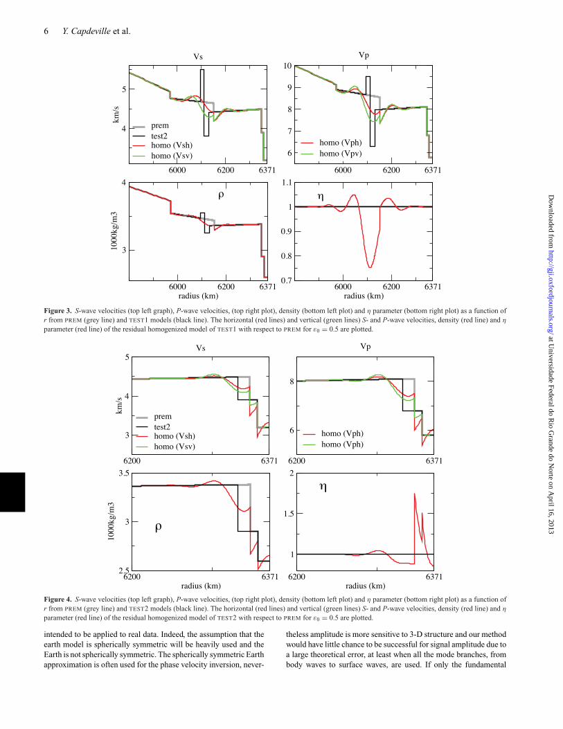
Figure 3. S-wave velocities (top left graph), P-wave velocities, (top right plot), density (bottom left plot) and η parameter (bottom right plot) as a function ofr from PREM (grey line) and TEST1 models (black line). The horizontal (red lines) and vertical (green lines) S- and P-wave velocities, density (red line) and η

parameter (red line) of the residual homogenized model of TEST1 with respect to PREM for ε0 = 0.5 are plotted.

Figure 4. S-wave velocities (top left graph), P-wave velocities, (top right plot), density (bottom left plot) and η parameter (bottom right plot) as a function ofr from PREM (grey line) and TEST2 models (black line). The horizontal (red lines) and vertical (green lines) S- and P-wave velocities, density (red line) and η

parameter (red line) of the residual homogenized model of TEST2 with respect to PREM for ε0 = 0.5 are plotted.

intended to be applied to real data. Indeed, the assumption that theearth model is spherically symmetric will be heavily used and theEarth is not spherically symmetric. The spherically symmetric Earthapproximation is often used for the phase velocity inversion, never-

theless amplitude is more sensitive to 3-D structure and our methodwould have little chance to be successful for signal amplitude due toa large theoretical error, at least when all the mode branches, frombody waves to surface waves, are used. If only the fundamental


io Grande do N



ownloaded from



Figure 5. Vertical (top plot) and transverse (bottom plot) component seis-mograms for a 110 km depth source and an epicentral distance of 130◦computed in PREM (green line), in TEST2 model (red line) and in the resid-ual homogenized TEST1 model with respect to PREM for ε0 = 0.5 andwith the order 2 boundary condition (dashed black line). The source has amaximum frequency of 1/40 Hz.

Figure 6. Vertical (top plot) and transverse (bottom plot) component seis-mograms for a 110 km depth source and an epicentral distance of 130◦computed in PREM (green line), in TEST2 model (red line) and in the resid-ual homogenized TEST2 model with respect to PREM for ε0 = 0.25 andwith the order 2 boundary condition (dashed black line). The source has amaximum frequency of 1/40 Hz.

mode and a few harmonics are used, a real data application of thepresent method could be attempted.

Let g be the forward modelling function that allows us to modelthe waveforms data (d) for a given set of model parameters (m):d = g(m). The inverse problem has to minimize the classical costfunction �

�(m) = T [g(m) − d]C−1d [g(m) − d] + T (m − m0)C−1

p (m − m0) ,

(46)

where m0 is the a priori value of the model parameters (the startingmodel), Cd and Cp are the covariance matrices of data and modelparameters, respectively. If g is a non-linear function, the minimum,or the closest local minimum to the starting model, of the costfunction � can be found using the Gauss–Newton method iterativeprocess (Tarantola & Valette 1982). Given mi the inverted model atiteration i, we can obtain model at the iteration i + 1 as

mi+1 = mi + ( TGi C−1d Gi + C−1

p

)−1

× [ TGi C−1d (d − g(mi )) − C−1

p (mi − m0)]

, (47)

where Gi is the partial derivative matrix

Gi =[

∂g(m)

∂m

]m=mi

. (48)

In our case, the earth models are spherically symmetric, which al-lows to use efficiently the classical normal mode summation methodto build g with no specific approximation except the summationtruncation, as well as the partial derivative matrix at each iterationGi with normal mode coupling, still with no specific approximation(see Appendix C).

To perform our exercise, we make some particular choices. First,if the covariance matrices Cd and Cp have an important meaningfor linear inversions, this is less obvious for significantly non-linearcases such as the one considered here. We set C−1

p = 0, whichimplies that the final model m∞ can be as far as necessary fromthe starting model m0. Nevertheless, to avoid issues with the smalleigenvalues of t Gi C−1

d Gi , we add to it a damping diagonal matrix λi .λi is allowed to vary during the inversion and the damping is smallerand smaller with the increasing number of iterations. Furthermore,as it is often done for many seismic inversion methods (e.g. Bunkset al. 1995; Pratt 1999; Virieux & Operto 2009), to avoid to falltoo quickly in a local minimum, the frequency band of the datachanges with the iterations, starting with the low frequencies onlyand then increasing the frequency band little by little. This practicecan be seen as a trick to avoid local minimum but, in our case, thisoperation has a special meaning that will be discussed in Section 5.To change the frequency band depending on the iteration number,we introduce a band limited data set

di ≡ d ∗ wi , (49)

where wi is a lowpass filter selecting the wanted frequency band foriteration i and ∗ the temporal convolution. As the frequency banddepends upon the iteration number, the function g also depends uponi (gi (mi ) ≡ g(mi ) ∗ wi ). To avoid the classical problem of relativeamplitude between surface waves and body waves, the data arenormalized by the inverse of its envelope plus a constant quantity.The data used at iteration number i can be written as

di = di

e(di ) + c, (50)

where e(·) denotes the envelope and c is a small value designedto avoid divisions by zero. This operation balances the amplitudeand gives approximately the same weight to all seismic phases ofthe seismogram, as it can be seen on the example given in Fig. 7.From a notation point of view, it is convenient to hide this datanormalization in the matrix Cd, where, the envelope depending onthe lowpass filter wi, now also depends on i. This can be done asfollows:

Cid = T (e(di ) + c)−1Cd(e(di ) + c)−1. (51)


io Grande do N



ownloaded from



Figure 7. Example of the effect of the envelope normalization (50) on avertical-component seismogram. In the top graph, is plotted the originalseismogram and on the bottom graph is plotted the same seismogram afternormalization.

Note that this operation is of minor importance for a synthetic test,even though if it helps the convergence when artificial noise is addedto the data. Let us mention that this normalization does not implythat the inversion scheme inverts for signal instantaneous phaseinstead of the full waveform. Indeed, the same normalization bythe data envelope is also applied to the forward modelling operatorgi and to the partial derivative matrix Gi which implies that nopartial derivative of the synthetic envelope are used. Again, thisnormalization plays a role only if noise or forward modelling errorsare involved.

According to the above choices, eq. (47) can now be rewrittenas

mi+1 = mi +(

TGi Cid−1

Gi + λi)−1 [

TGi Cid−1 (

di − gi(mi))]

.

(52)

We now need to define the set of parameters mi . Classically, themodel parameters are either velocities or slowness parametrizedwith spline functions or dicrete layers versus depth. When layersare involved a vertical correlation length is introduced to reduce thenumber of independent parameters. The upper-mantle structure isdominantly recovered from the surface wave data which enable toresolve only S-wave velocity. When Rayleigh and Love wave dataare simultaneously inverted, S-wave velocity radial anisotropy, cor-responding to a VTI medium, can also be recovered. Dziewonski &Anderson (1981) describe this 1-D earth model with the A, C, F, L,and N elastic parameters plus the density as a function of the radius.Because the model is overparametrized, correlations between pa-rameters is further introduced (e.g. Montagner & Anderson 1989;Sebai et al. 2006; Ekstrom 2011; Debayle & Ricard 2012). Here,we invert for δp(r ), the Backus residual vector with respect to areference model (see eq. 44). For the radial discretization, we usethe Lagrange polynomial interpolation associated with the Gauss–

Figure 8. Example of Lagrange polynomial basis associated with theGauss–Lobatto–Legendre points for degree 40. Each polynomial is plot-ted in grey line, except the one associated with r10 (h40

10(r ), red line) and theone associated with r40 (h40

40(r ), green line).

Lobatto–Legendre (GLL) points spread in the inversion depth range(see Fig. 8 for an example). For a polynomial degree N, the full de-scription of the model is given by the value of each parameters atthe N + 1 GLL depths.

mi = (δpi

1(r0), δpi2(r0), . . ., δpi

6(r0), δpi1(r1), . . ., δpi

j (rk) ,

. . ., δpi6(rN )

),

(53)

where δpij (rk) is the residual Backus parameter number j at iteration

i and for the GLL radius rk. If

hNk (r ) ≡

∏i=0,N

i �=k

r − ri

rk − ri(54)

is the Lagrange polynomial associated with the GLL point rk, thenthe interpolation formula for the Backus residual parameters is

δpi (r ) =N∑

k=0

δpi (rk)hNk (r ) . (55)

The Lagrange polynomial expansion used to radially expand theparameters δpi (r ) forces the continuity and the smoothness of theseparameters in the depth range of the inversion. Given that the ref-erence model can contain discontinuities or scale smaller than theones than can accurately be expanded on the Lagrange polynomialbasis, constraining the residuals to be smooth is a strong assump-tion, which can be wrong for most parametrizations. Nevertheless,for the Backus residual parameters, this assumption is valid shownby eq. (45) (see Fig. 2 for an example). For other parametriza-tions than the Backus residuals, for example velocity residuals, thissmoothness assumption is not valid. Indeed, the relation betweenthe Backus residuals and most of the commonly used quantities,such as velocities, slowness, etc. are non-linear. As a consequence,if the reference model is discontinuous (or with any king of fastvariations), any other residual parameters than the Backus residu-als are also discontinuous (see Fig. 9 for the Vs residuals for theTEST1 model example). There is therefore a clear advantage to usethe Backus residuals as parameters for the inversion: it allows tocorrectly assume the smoothness of the inversion parameters with


io Grande do N



ownloaded from



Figure 9. Vsh and Vsv residuals with respect to PREM from the TEST1homogenized model (see Fig. 3). These residuals are discontinuous at thePREM 220 km depth discontinuity.

depth and through the discontinuities of the reference model. Fi-nally, let us mention that to be fully complete, we have to invert forthe boundary term parameters mentioned eq. (28). In practice, weindeed have the possibility to invert for the boundary term parame-ters, but as shown by Capdeville & Marigo (2008), there is a strongtrade-off between the boundary parameters and the elastic modelvalues at the free surface. For the comparison between inverted andhomogenized models we intent to make here, this trade-off can bea problem. To limit this problem, we make the choice to force theboundary parameters to be small and we have made sure that, forall the presented examples, the effect of the boundary term is small.Nevertheless, to study very shallow inhomogeneities, one shouldkeep in mind to account for this trade-off.

Before starting the inversion, to have an idea on how many param-eters, among the six Backus residuals, can be inverted as a functionof depth, we analyse the eigenvalues of the G0 matrix computedin the reference model (here PREM) as a function of depth for aLagrange polynomial degree N = 40, in the [5000–6371 km] depthrange and for a minimum period of 33 s. To do so, we build asmaller G0 matrix by keeping only the lines and columns corre-sponding to a single h40

i (r ). This leads to a 6 × 6 matrix for eachGLL depth ri, for which we can compute the eigenvalues and plotthem as a function of ri (see Fig. 10). This test does not give anyinformation on the depth resolution, but it helps to identify poten-tial trade-offs between the Backus residual parameters for a givendepth. Because the problem is non-linear and because each depthshould not be considered independently, this analysis can only beconsidered as indicative. In Fig. 10, we can guess how many pa-rameters can be inverted per depth. Of course, the actual numberof parameter that can indeed be inverted depends upon the noiselevel. In Fig. 10, two horizontal grey lines, corresponding to twoexamples of noise level, have been plotted. The dashed grey linecorresponds to a low noise level and the solid grey line represents ahigher noise level corresponding to a more realistic case. In Fig. 10,the actual vertical positions of the two grey lines is just indicativeas a precise assessment of the noise level with respect to the eigen-values is not possible for our non-linear global case. For the lownoise level, it can be seen that below 5200 km and above 6350 kmdepth, we cannot retrieve the six parameters but in the range 5200–6350 km we have a good chance to retrieve the six parameters. Fora real data inversion, the noise level may be much higher (corre-sponding, e.g. to the solid grey line in Fig. 10) and in such a case

Figure 10. Square root of the eigenvalues of submatrices of TG0C0d−1

G0

obtained by keeping only the lines and columns corresponding to a singlehN

i (r ), plotted as a function of ri and normalized by the radius integral ofhN

i (r ). The reference model is PREM, N = 40 and a minimum period of 33 sare used. Each black line corresponds to one of the six eigenvalue as functionof depth. The two grey lines correspond to two noise level examples.

there is a little chance to retrieve the six parameters at any depth.For our synthetic tests, TEST1 model has been designed such thatinformation to be retrieved is in the range [5800–6300 km]. There-fore, we can hope to access the six Backus residual parameters.For TEST2, the inhomogeneities are concentrated in the shallow[6300–6371 km] depth range and therefore we do not expect to re-trieve all of the six Backus residual parameters, even for a low noiselevel.

To perform our synthetic tests, we first use the TEST1 model asa target model which means that the ‘data’ used for our inversionscheme described above are computed in the TEST1 earth model.We use a single three-component station and two earthquakes at thesame surface location but for two different depths (10 and 700 km)corresponding to an epicentral distance of 132◦. The data periodband is [1000–33 s] and the Lagrange polynomial degree is N =40 in the [5000–6371 km] depth range. To avoid to commit aninversion crime, we add some random noise to the synthetic datato be inverted. The noise has the same frequency band as the dataand is such that its standard deviation is 3 per cent of the standarddeviation of the data. Such a noise is probably weak compared to areal case (it approximately corresponds to the low noise level hor-izontal dashed line shown in Fig. 10), but is large enough to avoidto use the forward modelling method error as an information and tocommit an inversion crime. Moreover, local correctors at the sourceand receiver locations (see eq. 27) are not inverted for. This inducesa few per cents theoretical error (mainly on amplitude) which alsohelps to prevent for an inversion crime. We intent to invert thesefull waveforms starting from the PREM model and with PREM asa reference model (the pref model is therefore PREM and m0 = 0).To have an idea of the robustness of the inversion results, we per-form eight inversions with each time a different realization of the3 per cent random noise added to the data. The raw results of theinversion are given in Fig. 11. The agreement between the inversionoutputs (black lines in Fig. 11) and the TEST1 target model (redlines in Fig. 11) is not obvious. Nevertheless, computing a syntheticdata in one of the inverted model for a receiver that has not beenused for the inversion and comparing it with a reference syntheticseismogram computed in the TEST1 target model shows a very good


io Grande do N



ownloaded from



Figure 11. Raw results of the inversion. In grey, is plotted the reference model (PREM), in red the target model (TEST1) and in black the eight inversion resultsfor eight different realizations of the 3 per cent random noise added to the data.

fit, as it can be seen in Fig. 12. So, even if the Fig. 11 comparison isnot impressive, the inverted models are definitely not non-sense andare able to model accurately data in the [1000–33 s] frequency band,even for data that have not been used for the inversion. To performa better comparison, we use the fact that, for spherically symmetricmedia, the important quantities are the Backus residual parametersin the spectral domain (see Appendix B for the radial spectral do-main definition). Indeed, we have seen that the effective Backusresidual parameters are obtained by lowpass filtering the residualparameters for the direct upscaling. The lowpass filtering being asimple product in the spectral domain (see Appendix B), a bettercomparison between the target and inverted models can be donein the spectral domain. The spectral domain comparison is donein Fig. 13. This time the agreement between the inversion results(black lines in Fig. 13) and the target model (red line in Fig. 13) isthis time more obvious. As expected, the inversions give the correctanswer up to an error bar that could be computed, but only for lowwavenumbers. Indeed, below a wavenumber that depends upon theconsidered residual Backus parameter δpi, the inverted and targetmodels are in very good agreement, but above this number, theyquickly diverge. On the conservative side, in Fig. 13, all parametersroughly agree for wavenumbers n � 70, which corresponds to aperiod higher than 17 s, that is about half of the lowest period ofthe inversion band. This means that the inversion is effective up toa resolution of roughly λmin/2 where λmin is the minimum wave-length associated with the minimum period of the data used for theinversion. This is corresponding to the commonly admitted reso-lution power for most inversion methods. It can be seen that someparameters are very well recovered, but some, like the density (δp1)

Figure 12. Seismograms computed in the output model of the inversion fora station that has not been used for the inversion (red line) to be comparedwith the data computed in the target model (black line) and in the startingmodel (green line). The epicentral distance is 137◦.


io Grande do N



ownloaded from



Figure 13. Raw results of the inversion for the TEST1 model in the spectral domain. In red is plotted the target model (TEST1) and in black the eight inversionresults for eight different realizations of the 3 per cent random noise. For each plot, the PREM reference model would be the horizontal 0 line (not represented).To give a more physical idea of the horizontal axis values, modes n = 25, 50, 100 and 200 have a period of, respectively, 47, 24, 12 and 6 s, which, for a wavespeed of 4 km s−1, would respectively correspond to a wavelength of 186, 95, 48 and 24 km. δp1 parameter is related to ρ, δp2 to 1/C, δp3 to 1/L, δp4 to A −F2/C, δp5 to F/C and δp6 to N. See eqs (10)–(15) and (44) for the definition of the δpi residuals.

are retrieved with less accuracy: the results of different inversionsare scattered. Nevertheless, the different results gather around thetarget model spectrum which indicates that, despite a non-negligibleerror bar, the inversion is able to find all the six Backus residualparameters, including the correct density. To compare the modelsin the space domain, we conclude that the Backus residual spec-tral expansion of the inverted models need to be muted to zero forwavenumber beyond the resolution power of the inversion, and wetherefore need to compare the inverted results with the target modelhomogenized to the same resolution. To do so, we homogenize thetarget and inverted models up to n = 70 and the obtained resultsare plotted in Fig. 14. The match between the target model and theinverted models is this time very good, and we can conclude thatthey are the same up to a small error, which numerically shows thatthe inverted model is indeed the homogenized model.

An interesting observation can be made plotting the inverted pa-rameter δp3 in the spectral domain for different iterations of theinversion (see Fig. 15). As mentioned previously (see eq. 49), thefrequency content of the data increase with the increasing iteration

number, and consequently, the resolution of the inversion resultsis also expected to increase with the increasing iteration number.It is indeed what is seen in Fig. 15. However, the most interestingobservation that can be made from Fig. 15 is that, once inverted, theobtained low wavenumbers almost do not change while adding newfrequencies. With a more sophisticated spatial parametrization, itwould therefore be possible to invert only a new wavenumber rangefor each new frequency band added to the inversion while keepingunchanged the lower wavenumber obtained from previous itera-tions. Such an observation is only possible for the Backus residualparametrization, and, with such a parametrization the inversion ismultiscale in the sense that adding frequencies to that data does notmodify low wavenumber of the inverted models.

We conduct the same experiment for the TEST2 model. From theeigenvalue analysis shown in Fig. 10, three of the six eigenvaluesare going to zero at the free surface. Knowing that the inhomo-geneities of TEST2 model are focused in the crust, that is, closeto the free surface for the considered wavelengths, we expect thatit will not be possible to retrieve all of the six Backus residual


io Grande do N



ownloaded from



Figure 14. Upscaled results of the TEST1 inversion. In grey, is plotted the reference model (PREM), in red the target model (TEST1) and in black the eightinversion results for eight different realizations of the 3 per cent random noise.

Figure 15. Inversion results for the TEST1 model, for δp3 in the spectral domain for three different increasing iteration numbers of the inversion (and thereforethree different increasing maximum frequencies of the data frequency band).

parameters. In Fig. 16 are plotted the results of the inversions, inthe spectral domain (left-side six plots) and in the space domain,but homogenized down to n = 70 (right-side six plots). As ex-pected, the results accuracy is not as good as for the TEST1 case.Indeed, the different inversions are far more scattered for param-eters δp4, δp5 and δp6 than for the TEST1 inversions. Moreover,the δp2 amplitude is way to low and we can consider that δp2

is not retrieved at all. Nevertheless, comparing the target and in-verted models in the space domain as it has been done for TEST1

(Fig. 16, right-side six plots), the quality of the results is acceptable(the eight solutions gather around the true value), except for Vpv

and η. The TEST2 numerical experience shows that, once again,the inversions retrieve the homogenized model, even if no specifictreatment has been done to take into account the specific pattern ofthe shallow inhomogeneities. To improve a shallow inversion, oneshould take into account the strong trade-off between the shallowinhomogeneities (within roughly λmin/4 distance to the free sur-face) and the homogenized Dirichlet–Neumann boundary condition


io Grande do N



ownloaded from



Figure 16. TEST2 inversion results. Left-side six plots: raw results of the inversion in the spectral domain (see eqs 10–15 and 44 for the definition of the δpi

residuals). In red is plotted the target model (TEST2) and in black the eight inversion results for eight different realizations of the 3 per cent random noise. δp1

parameter is related to ρ, δp2 to 1/C, δp3 to 1/L, δp4 to A − F2/C, δp5 to F/C and δp6 to N. See eqs (10)–(15) and (44) for the definition of the δpi residuals.Right-side six plots: upscaled results of the inversion. In grey, is plotted the reference model (PREM), in red the target model (TEST2) and in black the eightinversion results for eight different realizations of the 3 per cent random noise.

coefficients (Capdeville & Marigo 2008). A potential solution to thefact that only three parameters can be inverted for at the free sur-face, would be to invert for the two significant parameters of theDirichlet–Neumann boundary condition and for the density whileforcing the Backus residuals parameters at the free surface to zero.This would stabilize the inversion but would make the inversioninterpretation difficult. We discuss further the interpretation issuein the conclusion section.

4 R E S I D UA L U P S C A L I N G G A L L E RY

We have numerically shown in synthetic examples, that the effec-tive medium and the inverted medium are at best the same, thatis the inverted medium cannot be more accurate than the effectivemedium. We can therefore directly use the homogenization upscal-ing tool to infer what would be retrieved at best by an inversionwithout actually running the inversion. As an example, we showin Fig. 17 some potential effects of mislocated crust interface onthe interpretation of inversion. The homogenized S-wave speed isplotted for six different target models (red line). Each target modelhas a low- or fast-velocity zone located around 100 km depth. Theresidual homogenization is performed with respect to PREM (greyline) in the same conditions as for the previous section (for a periodcut-off of 33 s) and the resulting two homogenized wave speedsare shown (green: Vsv; blue: Vsh). We have chosen to show only Vs

results to avoid any problems that could arise from the fact that areal inversion would have difficulties to recover all the parametersat the free surface (see TEST2 inversion test in the previous section).For each plotted case, the reference crust is mislocated, that is thetarget model crust is not the one of the reference model. For case(a) (Fig. 17 a), the crust interfaces mislocation does not changethe apparent location of the 100 km depth low-velocity zone, but

creates an apparent high-velocity zone just below the Moho. Forcase (b), the localized low-velocity zone disappears and for case(c), we can even see a small-amplitude fast-velocity zone insteadof a slow-velocity anomaly. Case (d) would be difficult to interpret:depending on which S-wave speed we are looking at, we can havea different interpretation. Finally, interpretation of cases (e) and(f) would be similar as the one of, respectively, cases (b) and (c).To conclude, the message of this test is that, even if an inversiongives a good result, the interpretation of this result can be non-trivial and misleading. Finally, let us mention that the similar issueof a wrong a priori crustal model have been studied by Bozdag &Trampert (2007) and Ferreira et al. (2010) and the uses of appar-ent anisotropic crustal models to improve numerical efficiency hasbeen studied by Fichtner & Igel (2008) and Lekic & Romanowicz(2011).

5 D I S C U S S I O N A N D C O N C LU S I O N S

In this paper, we have first shown, in the non-periodic determinis-tic layered medium or spherically symmetric case, how to performresidual homogenization. This homogenization with respect to a ref-erence model allows to perform more sophisticated operations thanthe classical homogenization. For example, it allows to homogenizeonly some interfaces of a discontinuous medium while keeping theother intact. Moreover, it allows to model what would produce aninversion relative to a non-homogeneous reference model. As usual,the residual homogenized model is anisotropic even if the fine scalemodel is isotropic. What is new and maybe puzzling is that the ef-fective media now still have fine scale features like discontinuitiesand this is the case if the reference model contains fine scales. Thetests performed for the forward problem show very a good accuracy.Note that, if we do not consider anelasticity for the homogenization


io Grande do N



ownloaded from



Figure 17. Grey: PREM (reference model), red: target model; green and blue: residual homogenized model (green: Vsv; blue: Vsh).

process in this paper, there is a no limitation to account for attenu-ation when solving the wave equation for the order 0 homogenizedsolution (the effective wave equation). If the attenuation model con-tains small scales, it can be upscaled the same way as for the elasticpart. Nevertheless, we have not studied that aspect yet and a simplelowpass filtering of the attenuation model might be good enoughfor a start.

Then, using a full-waveform inversion method, we have numer-ically shown that an earth model resulting from an inversion is anhomogenized model. Note that this result can be extended to anyother inversion method based on frequency band limited data suchas phase velocity inversion in the sense that such methods cannotrecover more than an homogenized model (but it can recover less,because of an incomplete data coverage for example).

From the inversion perspective, this work raises some importantissues. One point is that it helps to understand more clearly thenecessity to increase little by little the frequency content of the dataalong the increasing iteration number of the non-linear least-squareinversion algorithm, to avoid local minimum of the misfit functions.Indeed, the homogenization (or residual homogenization) principleshows that the elastic model ‘seen’ by the wavefield changes de-pending on the frequency cut-off applied to the seismic traces. Thelower the frequency cut-off is, the smoother is the effective model.As an inversion can only recover what is ‘seen’ by the wavefield,

it implies that the target model depends upon the frequency. Inother words, we can control the target model by tuning the cut-off frequency applied to the data. Knowing that for many cases,the reference models are good for very low frequencies, we canmost of the time find a low enough frequency such that the targetmodel is close enough to the reference model so that a linearizedinversion scheme, such as the Gauss–Newton scheme, can easilyconverge without falling into a local minimum. So does it make theinversion result unique? So far not yet, mainly because of the freesurface (there is a strong trade-off between the Dirichlet–Neumannboundary condition parameters mentioned in Section 2.2 and theshallow Backus residual parameters). However, it definitely reducesthe non-uniqueness especially for deep inversion and for excellentdata coverage.

An other result is that, from the technical point of view, we haveshown that using a parametrization based on the Backus residual, theinversion is mutliscale: inverting more and more higher frequencydata enlarges more and more the wavenumber spectrum of the in-verted model without changing the low wavenumbers obtained fromsmaller data frequency band. This is not the case using a classicalparametrization, such as velocity residuals.

The next important point is the interpretation of the results. Aswe have seen, the inversion can only retrieve at best an homogenizedmodel and this can be a problem for the interpretation of the results.


io Grande do N



ownloaded from



Indeed, the delocalization effect of the homogenization can lead tonon-trivial and misleading effects that can make the interpretationdifficult. Actually, the interpretation of the results in term of geolog-ical structures (discontinuities in our layered case) would require aseparate inverse problem, allowing to include a priori informations.This inverse problem can be seen as a dehomogenization problem:for a given smooth tomographic model obtained with a long-periodwaveform inverse problem, what are the possible fine scale modelsfitting with some given a priori informations which, once homoge-nized, are the same as this smooth tomographic model? The problemhas a high probability to be highly non-unique and one can guessthat we will need to rely on Monte Carlo type of inversion methods(e.g. Bodin et al. 2012a,b). This dehomogenization inverse problemis important as it addresses the main target of seismic inversions:obtaining information of the underground properties.

This work and conclusions need to be extended to higher dimen-sion problems (the now popular and challenging 2-D and 3-D full-waveform inversions developed by, e.g. Pratt et al. 1998; Capdevilleet al. 2005; Tromp et al. 2005; Fichtner et al. 2009; Virieux & Op-erto 2009; Lekic & Romanowicz 2011, and many others) and it willbe the purpose of future works.

A C K N OW L E D G E M E N T S

The authors would like to thank Andreas Fichtner for his posi-tive review. This work was funded by the ANR blanche ‘meme’grant (ANR-10-BLAN-613 MEME) and the European ITN QUEST.Computations were performed on the CCIPL computer ‘Erdre’.

R E F E R E N C E S

Aki, K. & Richards, P., 1980. Quantitative Seismology: Theory and Methods,Freeman, San Francisco.

Backus, G., 1962. Long-wave elastic anisotropy produced by horizontallayering, J. geophys. Res., 67(11), 4427–4440.

Beucler, E., Stutzmann, E. & Montagner, J.-P., 2003. Surface-wave highermode phase velocity measurements, using a roller coaster type algorithm,J. geophys. Res., 155(1), 289–307.

Bodin, T., Capdeville, Y. & Romanowicz, B.A., 2012a. The inverse homoge-nization: incorporating discontinuities in smooth full waveform inversionmodels, Abstract S31C-02 presented at 2012 Fall Meeting AGU, 3–7 Dec,San Francisco, Calif.

Bodin, T., Sambridge, M., Tkalcic, H., Arroucau, P., Gallagher, K. &Rawlinson, N., 2012b. Transdimensional inversion of receiver func-tions and surface wave dispersion, J. geophys. Res., 117, B02301,doi:10.1029/2011JB008560.

Bozdag, E. & Trampert, J., 2007. On crustal corrections in surface wavetomography, Geophys. J. Int., 172(3), 1066–1082.

Bunks, C., Saleck, F., Zaleski, S. & Chavent, G., 1995. Multiscale seismicwaveform inversion, Geophysics, 60(5), 1457–1473.

Capdeville, Y., 2005. An efficient Born normal mode method to computesensitivity kernels and synthetic seismograms in the Earth, Geophys. J.Int., 163, 639–554.

Capdeville, Y. & Marigo, J.J., 2007. Second order homogenization of theelastic wave equation for non-periodic layered media, Geophys. J. Int.,170, 823–838.

Capdeville, Y. & Marigo, J.J., 2008. Shallow layer correction for spectralelement like methods, Geophys. J. Int., 172, 1135–1150.

Capdeville, Y., Stutzmann, E. & Montagner, J.P., 2000. Effect of a plume onlong period surface waves computed with normal modes coupling, Phys.Earth planet. Inter., 119, 57–74.

Capdeville, Y., Gung, Y. & Romanowicz, B., 2005. Towards global earthtomography using the spectral element method: a technique based onsource stacking, Geophys. J. Int., 162, 541–554.

Capdeville, Y., Guillot, L. & Marigo, J.J., 2010a. 1-D non periodic homog-enization for the wave equation, Geophys. J. Int., 181, 897–910.

Capdeville, Y., Guillot, L. & Marigo, J.J., 2010b. 2D nonperiodic homoge-nization to upscale elastic media for P-SV waves, Geophys. J. Int., 182,903–922.

Cara, M. & Leveque, J., 1987. Waveform inversion using secondary observ-ables, Geophys. Res. Lett., 14(10), 1046–1049.

Cara, M., Nolet, G. & Nercessian, A., 1980. New inferences from highermode data in western Europe and northern Eurasia, Geophys. J. R. astr.Soc., 61(3), 459–478.

Cupillard, P., 2008. Simulation par la methode des elements spectraux desformes d‘onde obtenues par correlation de bruit sismique, PhD thesis,Universite Paris 7 - Denis Diderot, Institut de Physique du Globe deParis.

Dahlen, F.A. & Tromp, J., 1998. Theoretical Global Seismology, PrincetonUniversity Press, NJ.

Debayle, E. & Ricard, Y., 2012. A global shear velocity model of the up-per mantle from fundamental and higher Rayleigh mode measurements,J. geophys. Res., 117, B10308, doi:10.1029/2012JB009288.

Dziewonski, A.M. & Anderson, D.L., 1981. Preliminary reference Earthmodel, Phys. Earth planet. Inter., 25, 297–356.

Ekstrom, G., 2011. A global model of Love and Rayleigh surface wavedispersion and anisotropy, 25–250 s, Geophys. J. Int., 187, 1668–1686.

Ekstrom, G., Tromp, J. & Larson, E., 1997. Measurements and global modelsof surface wave propagation, J. geophys. Res., 102, 8137–8157.

Ferreira, A., Woodhouse, J., Visser, K. & Trampert, J., 2010. On the robust-ness of global radially anisotropic surface wave tomography, J. geophys.Res., 115(B4), B04313, doi:10.1029/2009JB006716.

Fichtner, A. & Igel, H., 2008. Efficient numerical surface wave propagationthrough the optimization of discrete crustal models—a technique basedon non-linear dispersion curve matching (DCM), Geophys. J. Int., 173(2),519–533.

Fichtner, A., Kennett, B.L.N., Igel, H. & Bunge, H.P., 2009. Full waveformtomography for upper-mantle structure in the Australasian region usingadjoint methods, Geophys. J. Int., 179, 1703–1725.

Fichtner, A., Trampert, J., Cupillard, P., Saygin, E., Taymaz, T., Capdeville,Y. & Villasenor, A., 2013. Multi-scale full waveform inversion, Geophys.J. Int., 10.1093/gji/ggt118.

Guillot, L., Capdeville, Y. & Marigo, J.J., 2010. 2-D non periodic ho-mogenization for the SH wave equation, Geophys. J. Int., 182, 1438–1454.

Lebedev, S. & van der Hilst, R., 2008. Global upper-mantle tomographywith the automated multimode inversion of surface and S-wave forms,Geophys. J. Int., 173(2), 505–518.

Lekic, V. & Romanowicz, B., 2011. Inferring upper-mantle structure by fullwaveform tomography with the spectral element method, Geophys. J. Int.,185(2), 799–831.

Li, X.B. & Romanowicz, B., 1996. Global mantle shear velocity modeldeveloped using nonlinear asymptotic coupling theory, J. geophys. Res.,101, 11 245–22 271.

Li, X.D. & Tanimoto, T., 1993. Waveforms of long–period body waves inslightly aspherical Earth model, Geophys. J. Int., 112, 92–102.

Lognonne, P. & Romanowicz, B., 1990. Modelling of coupled normal modesof the Earth: the spectral method, Geophys. J. Int., 102, 365–395.

Montagner, J. & Anderson, D., 1989. Constrained reference mantle model,Phys. Earth planet. Inter., 58(2), 205–227.

Montagner, J. & Tanimoto, T., 1990. Global anisotropy in the upper mantleinferred from the regionalization of phase velocities, J. geophys. Res.,95(B4), 4797–4819.

Montelli, R., Nolet, G., Dahlen, F., Masters, G., Engdahl, E. & Hung, S.,2004. Finite-frequency tomography reveals a variety of mantle plumes,Science, 303, 338–343.

Nakanishi, I. & Anderson, D., 1982. Worldwide distribution of group ve-locity of mantle Rayleigh waves as determined by spherical harmonicinversion, Bull. seism. Soc. Am., 72(4), 1185–1194.

Nishida, K., Montagner, J. & Kawakatsu, H., 2009. Global surface wavetomography using seismic hum, Science, 326(5949), 112–112.

Nolet, G., 1990. Partitioned waveform inversion and two-dimensional struc-ture under the network of autonomously recording seismographs, J. geo-phys. Res., 95(B6), 8499–8512.


io Grande do N



ownloaded from



Pratt, R., 1999. Seismic waveform inversion in the frequency domain, part1: theory and verification in a physical scale model, Geophysics, 64(3),888–901.

Pratt, R., Shin, C. & Hicks, G., 1998. Gauss-Newton and full Newton meth-ods in frequency domain seismic waveform inversion, Geophys. J. Int.,133, 341–362.

Romanowicz, B., Gung, M.P.Y. & Capdeville, Y., 2008. On the computationof long period seismograms in a 3-D Earth using normal mode basedapproximations, Geophys. J. Int., 175, 520–536.

Schimmel, M., Stutzmann, E. & Gallart, J., 2011. Using instantaneous phasecoherence for signal extraction from ambient noise data at a local to aglobal scale, Geophys. J. Int., 184(1), 494–506.

Sebai, A., Stutzmann, E., Montagner, J., Sicilia, D. & Beucler, E., 2006.Anisotropic structure of the African upper mantle from Rayleigh andLove wave tomography, Phys. Earth planet. Inter., 155(1), 48–62.

Shapiro, N., Campillo, M., Stehly, L. & Ritzwoller, M., 2005. High resolu-tion surface wave tomography from ambient seismic noise, Science, 307,1615–1618.

Stutzmann, E. & Montagner, J.-P., 1993. An inverse technique for retrievinghigher mode phase velocity and mantle structure, Geophys. J. Int., 113(3),669–683.

Takeuchi, H. & Saito, M., 1972. Seismic surface waves, Methods Comput.Phys., 11, 217–295.

Tanimoto, T., 1984. A simple derivation of the formula to calculate syn-thetic long period seismograms in heterogeneous earth by normal modesummation, Geophys. J. R. astr. Soc., 77, 275–278.

Tanimoto, T., 1986. Free oscillations of a slightly anisotopic earth, Geophys.J. R. astr. Soc., 87, 493–517.

Tarantola, A. & Valette, B., 1982. Generalized nonlinear inverse problemssolved using the least squares criterion, Rev. Geophys., 20, 219–232.

Trampert, J. & Woodhouse, J., 1995. Global phase velocity maps of Loveand Rayleigh waves between 40 and 150 seconds, Geophys. J. Int., 122(2),675–690.

Tromp, J., Tape, C. & Liu, Q., 2005. Seismic tomography, adjoint methods,time reversal and banana-doughnut kernels, Geophys. J. Int., 160, 195–216.

van Heijst, H. & Woodhouse, J., 1997. Measuring surface-wave overtonephase velocities using a mode-branch stripping technique, Geophys. J.Int., 131, 209–230.

Virieux, J. & Operto, S., 2009. An overview of full waveform inversion inexploration geophysics, Geophysics, 75(6), WCC127–WCC152.

Woodhouse, J. & Dahlen, F., 1978. The effect of a general aspherical pertur-bation on the free oscillations of the Earth, Geophys. J. R. astr. Soc., 53,335–354.

Woodhouse, J.H. & Girnius, T.P., 1982. Surface waves and free oscillationsin a regionalized earth model, Geophys. J. R. astr. Soc., 78, 641–660.

Yoshizawa, K. & Kennett, B., 2002. Non-linear waveform inversion forsurface waves with a neighbourhood algorithm application to multimodedispersion measurements, Geophys. J. Int., 149(1), 118–133.

A P P E N D I X A : A M AT R I C E S I NS P H E R I C A L LY L AY E R E D E A RT H

For the spheroidal case, we have

sAεl (r, ω) =

⎛⎜⎜⎜⎜⎝

d/r 1/C el/r 0

−ρω2 + a −d/r −aγl/2 γl/r

−γl/r 0 2/r 1/L

aγl/2 −el/r −ρω2 + bl −2/r

⎞⎟⎟⎟⎟⎠

(A1)

with

a = 4r2

(A − F2

C − N)

, bl = γ 2l

r2

(A − F2

C

)− 2N

r2 ,

d = 1 − 2FC , el = γl

FC .

In the toroidal case, we have

t Aεl (r, ω) =

(2/r 1/L

−ρω2 + �l N/r 2 −2/r

)(A2)

with �l = (l − 1)(l + 2).From these expressions, one can see that the averaged quantities

required to compute 〈S〉 are the Backus pi parameters, that is 〈 1C 〉,

〈 1L 〉, 〈A − F2

C 〉, 〈 FC 〉 and 〈N〉 which is different from the average of

the A, C, F, L, N elastic parameters. This is the same result as thatobtained by Backus (1962).

A P P E N D I X B : S PAT I A L F I LT E R I N GA N D S P E C T R A L D O M A I N

In this appendix, we define more precisely the lowpass filter operatorF ε0 (·) used along the paper. We define B = {un(r ), n ∈ Z} a setof orthogonal functions that can be considered as a basis for anyproperties of the Earth on the radius segment R = [ra, r�]. ra is aradius corresponding to a depth below which the waveform are notsignificantly sensitive to the elastic properties of the earth model.Let g(r) be a function of r on R [g can for example be any of theBackus residual parameters δpi(r)], B being an orthonormal basisfor such a function, we can write

g(r ) =∑

n

gnun(r ) , (B1)

where

gn =∫

Rg(r )u�

n(r ) dr , (B2)

where � is the complex conjugate. The gn coefficients constitute theradial spectral representation of g. Note that dr in (B2) might bereplaced by rdr to account for the sphericity, but it is of little effectknowing that the considered depth range is small with respect tor�. For a given λmin and for some Basis B (typically Fourier basis),we can precisely link an ε0 to an n0 such that un0 oscillate withcharacteristic wavelength of value λ0. In that case, we simply have

F ε0 (g) (r ) =∑

n,|n|≤n0

gnun(r ) . (B3)

In practice, such a brutal cut-off is not a good idea because itdelocalizes to much the properties. To avoid this drawback, we usea smoother transition to zero in the spectral model introducing acosine taper

wn1,n2 (n) =

⎧⎪⎪⎨⎪⎪⎩

1 for |n| ≤ n1,

12

(1 + cos

(π

|n|−n1n2−n1

))for |n| ∈ ]n1, n2],

0 for |n| ≥ n2,

(B4)

where n1 and n2 are two values close to n0. We use

F ε0 (g) (r ) =∑

n

gnun(r )wn1,n2 (n) . (B5)

A natural basis B is the Fourier basis. In such case, we use

un(r ) = cos

(nπ

r� − r

r� − ra

). (B6)

Note the fact that we use cosine Fourier basis instead of the classicalcomplex exponential basis is due to the fact that we extend the gfunction for r > r� by the symmetric of g with respect to r�. For


io Grande do N



ownloaded from



Figure B1. Example Fourier wavelet wn1,n2 (r ) (left-hand plot) and the corresponding wn1,n2 (k) where k = n/(r� − ra) for a n0/(r� − ra) � 1 km−1.

Figure B2. Left-hand plot: two examples of normal wavelet wn1,n2,r0 (see eq. B10) for two values of r0, 6000 km (solid line) and 5000 km (dashed line), forn1 =77 and n2 = 170 and for a normal basis computed in a smooth version of PREM. It can be seen that for the same wavenumber cut-off, the wavelet is widerat depth. The wavelet is also slightly asymmetric. In the right plot is shown the filtering operator wn1,n2 (n) as a function of n (bottom axis) and as a function ofthe corresponding eigenfrequency value (top axis).

such symmetric functions, a cosine expansion is enough. For theFourier case, we can compute the space domain wavelet

wn1,n2 (r ) =∑

n

un(r )wn1,n2 (n) , (B7)

and in such a case, the filtering operator can be written as

F ε0 (g) (r ) = g ∗ wn1,n2 (r ) , (B8)

where ∗ is here the spatial convolution. An example of waveletwn1,n2 is given in Fig. B1.

For many media, like all realistic spherically symmetric globalearth models, the minimum wavelength strongly varies with depth.This is due to the increase of the average wave speed with depth.From the homogenization point of view, we can always choose thesmallest minimum wavelength to measure ε0, but this is not opti-mum. To account for the strong change of minimum wavelengthwith depth, we can choose a different set of function B than theFourier basis. Remembering that the Fourier functions are solutionsof the wave equation in a homogeneous medium, we can use solu-tions of the radial wave equations solved in a very smooth version ofthe actual earth model as the orthogonal function un. We thereforeuse

un(r ) = rU0(r, nω0) , (B9)

where the U0 is the radial eigenfunction defined in eq. (6), nω0 theinfrequency of radial order n computed for l = 0 and in a smoothearth model roughly reproducing the variation of the S-wave speed.The smooth model does not need to be precisely defined and any

smooth model roughly reproducing the wavelength changes withdepth is acceptable. In such a case, the action of the filter F ε0 (.)cannot be computed as a convolution like for the Fourier case,nevertheless, we can plot the space representation of the waveletwn1,n2 for different depth. To do so, we compute

wn1,n2,r0 (r ) =∑

n

un(r )wn1,n2 (n) dr0,n , (B10)

where

dr0,n =∫

Rδ(r − r0)un(r ) dr . (B11)

Two examples of such wavelets are plotted in Fig. B2. We refer tothis way of performing the lowpass filtering as the ‘normal modefiltering’.

A P P E N D I X C : PA RT I A L D E R I VAT I V EC O M P U TAT I O N W I T H N O R M A L M O D E S

For spherically symmetric earth models, the partial derivatives forthe displacement solution to the wave equation with respect to theEarth’s elastic and density can be efficiently computed from theEarth normal mode method (this subject has been addressed bymany authors, e.g. Woodhouse & Dahlen 1978; Tanimoto 1984;Lognonne & Romanowicz 1990; Capdeville et al. 2000; Romanow-icz et al. 2008). This appendix is specifically based on Capdeville(2005) and we keep the same notations. Considering only a pertur-bation of the anelastic tensor δc, the displacement perturbation can


io Grande do N



ownloaded from



be rewritten (see Capdeville 2005) as

δu(rr , ω) · v =∫

V

[∑K

ε�K (r)RK

(ω2k − ω2)

]: δc(rd )

:

[∑K

εK (r)SK

iω(ω2k − ω2)

]drd , (C1)

where K = (q, n, l, m), mode uK (r) = u(r, ωK ), ωK is the eigenfre-quency number K, εK the deformation tensor corresponding to themode uK , RK = uK (rr ) · v is the receiver term for component v,SK = (uK , f ) the source term. In the following, generalized spher-ical harmonics expansion will be used to simplify expressions. Todo so, it is useful to use the contravariant canonical component ofδc

δ�αβγη =∑i jkl

C�αi C

�β j C

�γ kC�

ηlδci jkl , (C2)

as well as for the deformation tensor associated with mode uK

εαβ

K (r) =∑

i j

C�αi C

�β jεK ,i j (r), (C3)

where C is

(Ciα) =

⎛⎜⎜⎝

0 1 0

1√2

0 −1√2

i√2

0 −i√2

⎞⎟⎟⎠. (C4)

The generalized spherical harmonic expansions of RK, SK and εαβ

K

are well known.

RK (rr ) =∑

α=−1,1

Rαk (rr )Y αm

l (θr , φr ) , (C5)

SK (rs) =∑

α=−2,2

Sαk (rs)Y

αml

�(θs, φs) , (C6)

εαβ

K (rd ) = Eαβ

k (rd )Y α+β ml (θd , φd ), (C7)

where Y αml is the generalized spherical harmonics and k = (q, n, l).

The expression of Rαk and Sα

k can be found in Woodhouse & Girnius(1982) and Eαβ

k in Tanimoto (1986). Eq. (C1) can be rewritten as

δu(rr , ω) · v =∑

kk′mm′ηη′Rη

k Y ηml (r1r )Ca

kk′mm′ Sη′k′ Y

η′ml ′

�

(r1s), (C8)

where k′ = (q′, n′, l′), r1s = (θs, φs), r1r = (θr , φr ).

Cakk′mm′ =

∫ r�

0

∫S1

∑αβγ ηικ

Eαβ

k

�(r )δ�αβγη(r )E ικ

k′ (r )Y α+β ml

×(r1)Y ι+κ m′l ′

�(r1)r 2 dr dr1, (C9)

where the integral over the Earth sphere V has been decomposedinto an integration over the radius from 0 to the Earth radius (r�)

and an integration over the unit sphere surface (S1) and wherer1 = (θ, φ). Using the orthogonality of the generalized sphericalharmonics, we have∫

S1Y α+β m

l (r1)Y ι+κ m′l ′

�(r1)dr1 = δll ′ δmm′ δ(α+β)(ι+κ) . (C10)

Using the fact that no coupling occurs between spheroidal andtoroidal modes due to spherically symmetric inhomogeneities and(C10), eq. (C9) reduces to

Cakk′mm′ = Cqnn′lδll ′δmm′δqq ′ , (C11)

where

Cqnn′l =∑

αβγ ηικα+β=ι+κ

α+β+γ+η=0

∫ r�

0Eαβ

qnl

�(r )δ�αβγη(r )E ικ

qn′l (r )eγ ιeηκr 2dr,

(C12)

where eαβ =∑iCiαCiβ . Using the summation property for the gen-eralized spherical harmonics (Li & Tanimoto 1993; Capdeville et al.2000), we have

m=l∑m=−l

Y η′ml

�

(θs, φs)Y ηml (θr , φr ) = eiη′γsr Pηη′

l (cos(βsr ))eiηξsr , (C13)

where Pηη′l are the generalized Legendre functions. If the index s is

related to the ‘source’ location and r to the ‘receiver’ one, then theangle −ξ sr is the backazimuth at the receiver, π − γ sr the azimuthat the source and βsr is the angular epicentral distance.

Eq. (C1) can finally be rewritten as

δu(rr , ω) · v =∑qnn′l

RSqnn′lCqnn′l gqnl (ω) fqn′l (ω) , (C14)

where

RSqnn′l =∑ηη′

Rη

qml Sη′qn′le

iη′γsr Pηη′l (cos(βsr ))eiηξsr , (C15)

gqnl (ω) = 1

ω2nl − ω2

(C16)

and

fqnl (ω) = 1

iω(ω2

nl − ω2) . (C17)

Going back from the frequency domain to the time domain can bedone analytically using the residue theorem or with a fast Fouriertransform. It can be seen from the final expression (C14) that thecomputation only involves coupling along the radial order n, whichreduces drastically the amount of computation compared to theclassical mode coupling due to a 3-D inhomogeneities. From (C14),for a given earth model and a given parametrization (leading to aset of δ�), the partial derivative matrix Gi can easily be built.


io Grande do N



ownloaded from


13Capdeville-GJI

Documents

Transcript of 13Capdeville-GJI