1. Develop a program to obtain bus admittance matrix Y‐bus ...

WWW.VIDYARTHIPLUS.COM

ANNA UNIVERSITY: CHENNAI -600 025

B.E/B.TECH DEGREE EXAMINATIONS NOV/DEC 2015

(B.E. ELECTRICAL AND ELECTRONICS ENGINEERING)

SEVENTH SEMESTER

REGULATIONS : R-2008

EE2404- Power System Simulation Laboratory

Time 3 Hours Max: 100 Marks

1. Develop a program to obtain bus admittance matrix Y‐bus of the given power

system. Use any suitable assumptions

G1 G2

T1 T2

1 2

0.1+0.3j 0.15+0.5j

0.02j

0.2+0.6j

0.028j 0.0125j

3

Line Starting Ending Series Line Number Bus Bus Line Changing

Impedance Admittance

1 1 2 0.1+0.3j 0.02j 2 2 3 0.15+0.5j 0.0125j 3 3 1 0.2+0.6j 0.028j

Figure 1 Table 1


2. An isolated power station has the following parameters Turbine time constant, τT = 0.5sec, Governor time constant, τg = 0.2sec Generator inertia constant, H = 5sec. Governor speed regulation = R per unit

The load varies by 0.8 percent for a 1 percent change in frequency, i.e, D =

0.8 Find the load frequency dynamics of the system

3. Perform load flow analysis by Newton raphson method. Use any suitable assumptions

Line Starting Bus Voltage Magnitude Angle Real power Reactive power No.

1 1 1.04 0 0 0 2 2 1 10.69 0 0 3 3 1.05 20 0 0

Table 4.1

G1 G2

T1 T2

G1

G1 G1

Line Starting Ending Series Line Line

Changing

No. Bus Bus Impedance

Admittance

1 1 2 0.2+0.6j 0.05j

2 2 3 0.25+0.0125j 0.035j

3 3 1 0.02+0.28j 0.015j

Figure 4 Table 4.2


4. Develop a program to carry out simulation of a symmetrical three phase short circuit

on a given power system. Use any suitable assumptions

1

1

3

Line Starting

Ending Line

2

G1 3 No. Bus Bus Changing

G1

Admittance

2

G1

1 1

2

0.05j

G2 2 1 2 0.05j

3 1 3 0.1j

4

4 2 3 0.06j

Figure 5

Table 5.1

Transformer Data Transient

Generator Data

Gradient Reactance

Reactance

G1

0.25j

T1 0.10j

G2

0.20j

T2 0.08j

Table 5.2

Table 5.3

5. The fuel cost functions for three thermal plants in $/h are given by

C1 = 500 + 5.3 P1 + 0.004 P12 ; P1 in MW

C2 = 400 + 5.5 P2 + 0.006 P22 ; P2 in MW

C3 = 200 +5.8 P3 + 0.009 P32 ; P3 in MW

The total load , P D is 800MW.Neglecting line losses and generator limits, find the optimal dispatch and the total cost in $/h by analytical method. Verify the result using MATLAB program

6. Develop a program to obtain bus impedance matrix Z-bus of the given power system. Use

any suitable assumptions


Figure 7

Line Starting Ending Series Line Line

Changing

No. Bus Bus Impedance

Admittance

1 1 2 0.1+0.4j 0.15j

2 2 3 0.15+0.6j 0.02j

3 2 4 0.18+0.55j 0.018j

4 3 4 0.1+0.35j 0.012j

5 4 1 0.25+0.7j 0.03j

Table 7

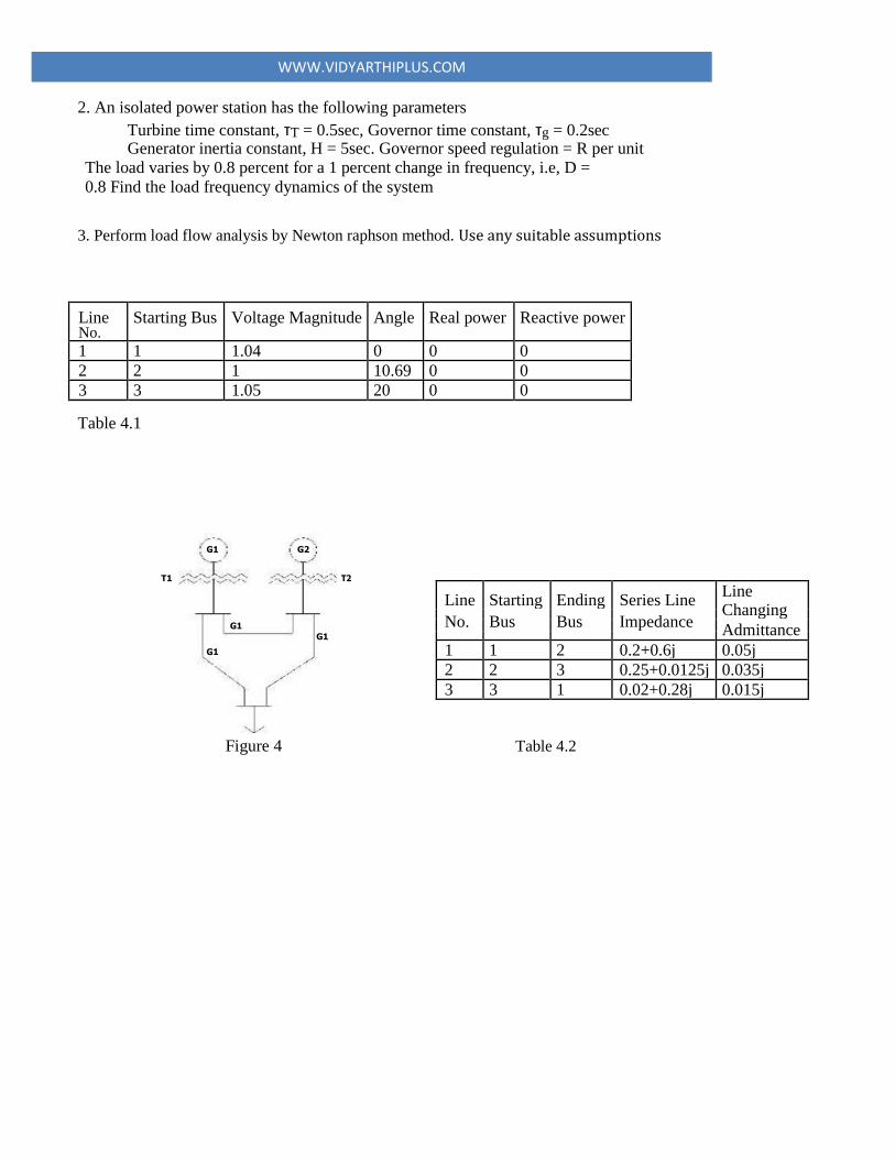
7.Develop a program to compute bus admittance matrix for the given power system

network. Also verify the obtained results with calculated values. Use any suitable

assumptions

Figure 8 LINE DATA:

Line Impedance Charging Admittance

Bus code

1 – 2 0.2 + j 0.8 j 0.02

2 – 3 0.3 + j 0.9 j0.03

2 – 4 0.25 + j 1.0 j 0.04

3 – 4 0.2 + j 0.8

j0.02


1 – 3 0.1 + j 0.4 j0.01


network. Line admittance values are shown in the figure. Also verify the obtained

results with calculated values. Use any suitable assumptions

Figure 9

9.Develop a program to compute bus impedance matrix for the given power system

network shown in figure 10. Use any suitable assumptions

Generator reactance : 0.2 p.u & 0.25 p.u for G1 and G2 respectively. Transformer leakage reactance: 0.08 p.u & 0.1 p.u for T1 and T2 respectively.


Figure 10


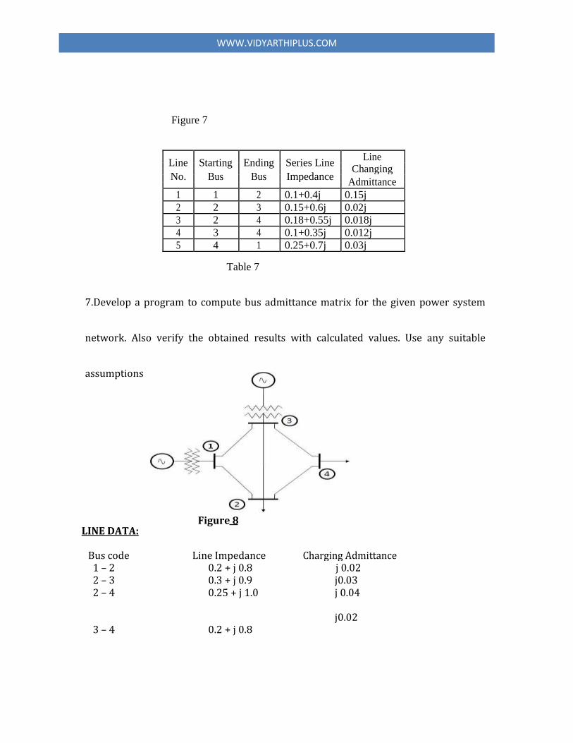
10.Develop a program to compute bus imp edance matrix for the given p ower system

network. Line imped ance values and transient reactance of generator & transformer

are in p.u is shown in the figure. 11. Use any suitable assumptions

Figure 11

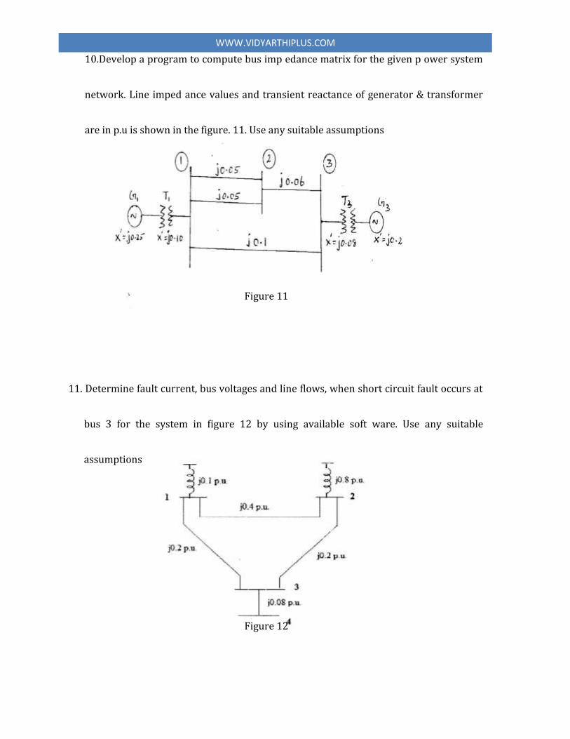
11. Determine fault current, bus voltages and line flows, when short circuit fault occurs at

bus 3 for the system in figure 12 by using available soft ware. Use any suitable

assumptions

Figure 12


12.A power system consists of two, 100 MW units, whose input cost data are represented by

the following equations:

F1 = 0.05 P12 + 20 P1 + 800 Rs/hr.

F2= 0.06 P22 + 15 P2 + 1000 Rs/hr. If the total received power P = 150 MW. What would be the division of load between the

units for the most economic operation? Assume the initial Lambda value. Also verify the

obtained result with calculated value.

13. The fuel cost of two units are given by

F1 = 0.1 P12 + 20 P1 + 1.5 Rs/hr.

F2= 0.1 P22 + 30 P2 + 1.9 Rs/hr.

If the total demand on the generation is 200 MW, find the economic load scheduling of

the two units. Assume the initial Lambda value. Also verify the obtained result with the

calculated value.


F1 = 0.04 P12 + 16 P1 + 2.8 Rs/hr.

F2= 0.04 P22 + 12 P2 + 4.6 Rs/hr.

The B mn matrix is given by

0.01 ‐0.005

‐0.005 0.024

Determine the economic schedule for the incremental cost of received power of Rs

20 / MWhr. Also find a) Total generation b) Transmission losses and c) Demand. Verify

the obtained result with calculated value.


15. Considering the two area system, find the new steady state frequency and change in tie

line flow for a load change of area two by 100 MW. Area one is operating with the spinning

reserves of 1000 MW. Area two is operating with the spinning reserves of 1000 MW.

Assume following data for the system.

Capacity of area 1, Pr1 = 1000 MW

Capacity of area 2, Pr2 = 2000 MW

Nominal load of area 1, PD1 = 500 MW

Nominal load of area 2, PD2 = 1500 MW

Regulation of area 1, R1 = 5%

Regulation of area 2 R2 = 4%

Nominal frequency Fo = 50 Hz

For both areas, each percent change in frequency causes 1% change in load. Also

verify the obtained result with calculated value.

16. For an isolated single area consider the following data:

Total rated area capacity Pr = 3000 MW

Normal operating load Pd = 2000 MW

Inertia constant H = 5 Secs

Regulation R = 2.5 Hz / p.u.M.W

Normal frequency F = 50 Hz Assume that the load frequency characteristic is linear meaning that the load will

increase 1 % for 1 % frequency increase. Find 1) Gain & Time constant of power system

and 2) Change in frequency under static condition. Also verify the obtained result with

calculated value.


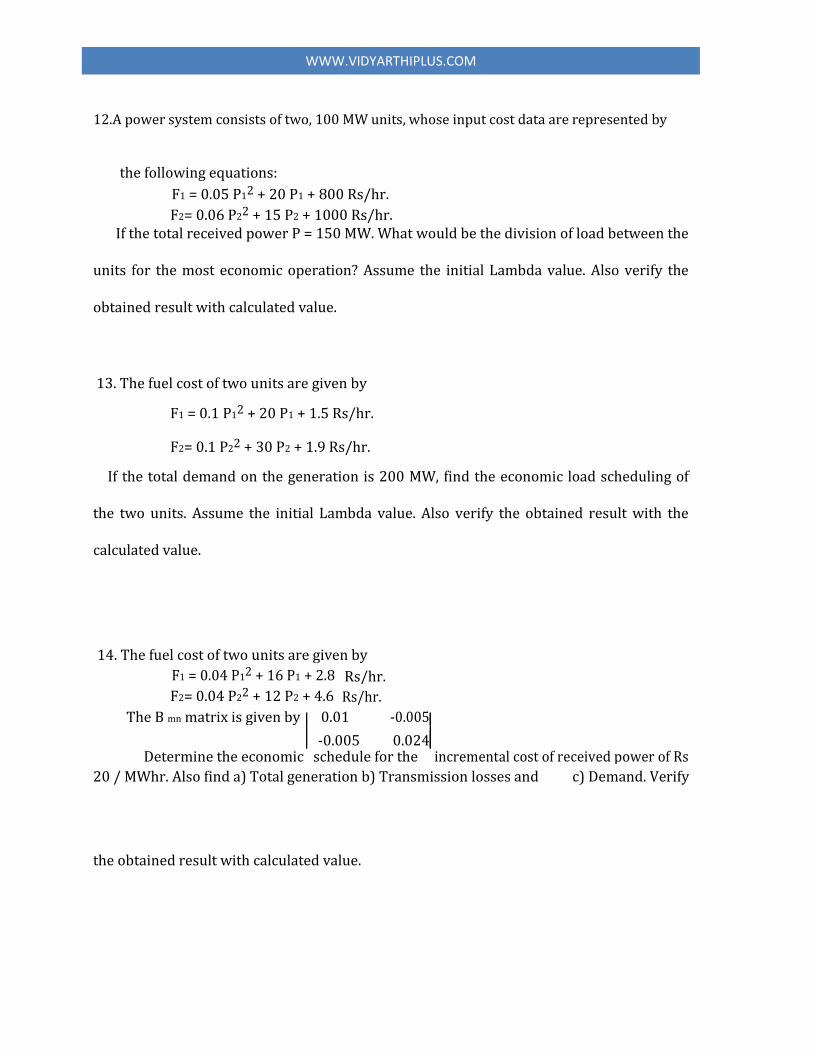
17.Develop a program to carryout load flow analysis of the given power system

network shown in figure 19 by using Gauss – Seidel method. Use any suitable

assumptions

Figure 19

BUS SPECIFICATIONS:

BUS V GENERATION LOAD

Q MIN Q MAX

BUS specified (p.u) (p.u)

NO (p.u) (p.u)

SLACK (p.u)

P

Q P Q

1 1.06 ‐ ‐

‐ ‐ ‐ ‐

2 P‐V 1.00 0.6 ‐ 0.0 0.1 ‐1.0 1.5

3 P‐Q ‐ ‐ ‐ 0.45 0.15 ‐ ‐

4 P‐Q ‐ ‐ ‐ ‐0.40 0.05 ‐ ‐

5 P‐Q ‐ ‐ ‐ 0.6 0.1 ‐ ‐

LINE DATA: LINE

SB EB SERIES HALF LINE CHARGING

NO IMPEDANCE(p.u) ADMITTANCE(p.u)

1 1 2 0.02 + j 0.06 j 0.03

2 1 3 0.08 + j 0.24 j 0.025

3 2 3 0.06 + j 0.18 j 0.02

4 2 3 0.02 + j 0.08 j 0.02

5 2 5 0.04 + j 0.12 j 0.015

6 3 4 0.01 + j 0.03 j 0.01

7 4 5 0.08 + j 0.24 j 0.035


18.a) Write the program in transient stability analysis of Single‐Machine Infinite Bus

System by using available software. b) For a two bus explain the procedure of forming Z bus by bus building algorithm.


network shown in figure 22 Also verify the obtained results with calculated values. Use

any suitable assumptions

Figure 22

LINE DATA:

Line Impedance Charging Admittance

Bus code

1 – 2 0.2 + j 0.8 j 0.02

2 – 3 0.3 + j 0.9 j0.03

2 – 4 0.25 + j 1.0 j 0.04

3 – 4 0.2 + j 0.8 j0.02

1 – 3 0.1 + j 0.4 j0.01



network. Line admittance values are shown in the figure. Also verify the obtained

results with calculated values. Use any suitable assumptions

Figure 23

21Develop a program to compute bus impedance matrix for the given power system

network shown in figure 24. Use any suitable assumptions

Generator reactance : 0.2 p.u & 0.25 p.u for G1 and G2 respectively. Transformer leakage reactance: 0.08 p.u & 0.1 p.u for T1 and T2 respectively.

Figure 24


22.Develop a program to compute bus impedance matrix for the given power system

network. Line impedance values and transient reactance of generator & transformer

are in p.u is shown in the figure 25. Use any suitable assumptions

Figure 25

22.(a)Write the program in transient stability analysis of Single‐Machine Infinite Bus

System by using available software.

(b)A single phase overhead transmission line delivers 1100 kW at 11 kV at 0.8 P.F.

lagging. The total resistance and inductive reactance of the line are 8 ohm and 16 ohm

respectively. Determine a) Receiving end current. b) Sending end voltage. c) Sending

end power. d) Transmission efficiency and E) Percentage regulation.


23.A power system consists of two, 100 MW units, whose input cost data are

represented by the following equations:

F1 = 0.05 P12 + 20 P1 + 800 Rs/hr.

F2= 0.06 P22 + 15 P2 + 1000 Rs/hr. If the total received power P = 150 MW. What would be the division of load between the

units for the most economic operation? Assume the initial Lambda value. Also verify the

obtained result with calculated value.

24.. The fuel cost of two units are given by

F1 = 0.1 P12 + 20 P1 + 1.5 Rs/hr.

F2= 0.1 P22 + 30 P2 + 1.9 Rs/hr.

If the total demand on the generation is 200 MW, find the economic load scheduling of

the two units. Assume the initial Lambda value. Also verify the obtained result with the

calculated value.


F1 = 0.04 P12 + 16 P1 + 2.8 Rs/hr.

F2= 0.04 P22 + 12 P2 + 4.6 Rs/hr.

The B mn matrix is given by

0.01 ‐0.005

‐0.005 0.024

Determine the economic schedule for the incremental cost of received power of Rs

20 / MWhr. Also find a) Total generation b) Transmission losses and c) Demand. Verify

the obtained result with calculated value.


26. Determine the Zbus matrix for the given system shown in figure 31 using available software

Figure 31

Buses : 6, numbered serially from 1 to 6 Lines : 5, numbered serially from L1 to L5 Base MVA : 100

Transmission Line Data: Half Line

Rating

Line ID No Send Bus Receive Resistance Reactance charging

No Bus No p.u p.u Suscept. MVA

P.u

1 1 6 0.123 0.518 0.0 55

2 1 4 0.080 0.370 0.0 65

3 4 6 0.087 0.407 0.0 30

4 5 2 0.282 0.640 0.0 55

5 2 3 0.723 1.050 0.0 40

Table 31


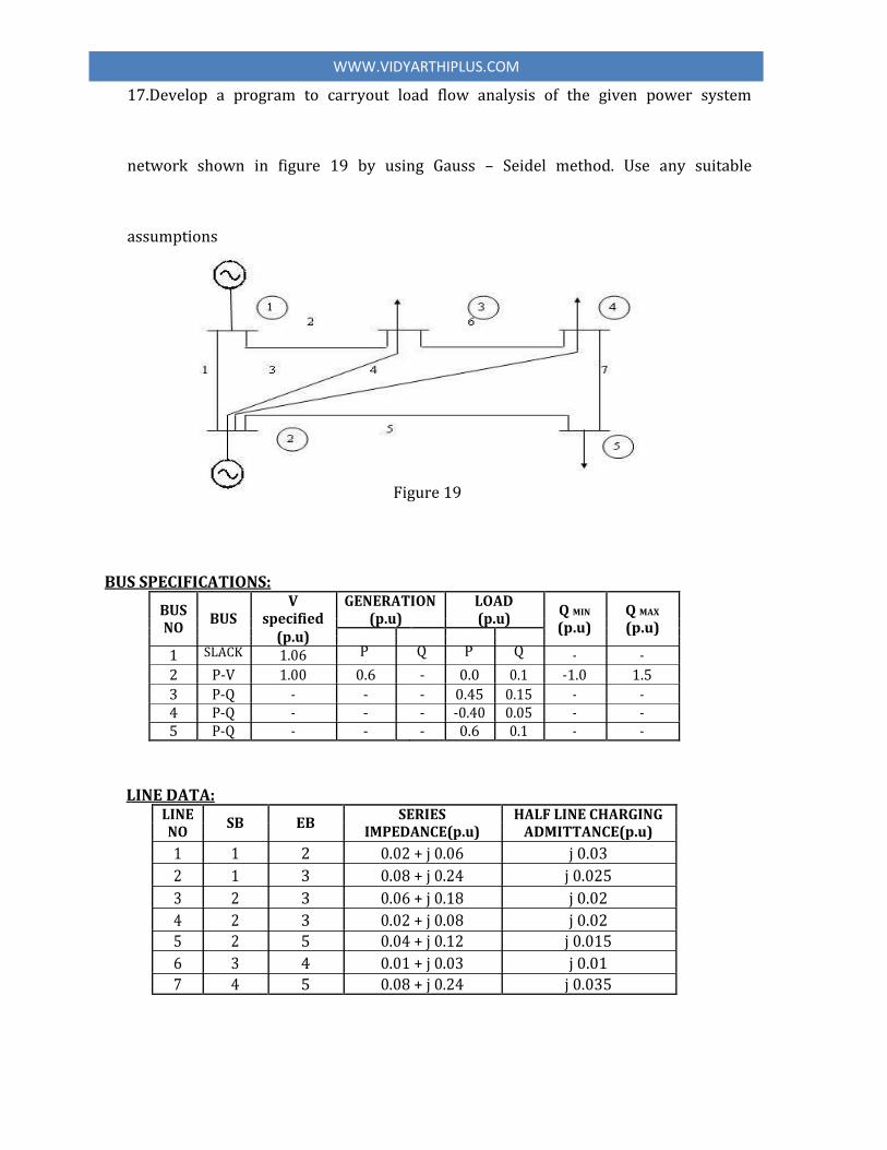
27.Conduct fault analysis on two alternative configurations of the 4 - bus system given in Figure

32 below. Determine the fault current and MVA at faulted bus 4, post fault bus voltages, fault

current distribution in different elements of the network. Also draw a single line diagram

showing above results. For a given system of figure 32, following are the fault conditions.

(i) Three phase to ground fault (ii) Line to ground fault (iii) Line to line fault

(iv) Double line to ground fault.

Fig:32 Four bus system

G1, G2 : 100MVA, 20KV, X+ = X

- = Xd’’ = 20%; X

0 = 4%; Xn =

5% T1, T2 : 100MVA, 20KV/345KV; X leak = 8%

L1, L2 : X+ = X

- = 15%; X

0 = 50% on a base of 100MVA

The first configuration, case (a), comprises star-star transformer and the second

configuration, case (b), comprises star-delta transformers.

28. Determine the Ybus matrix for the given system in figure 34 using available software.

Figure 34

Buses : 6, numbered serially from 1 to 6

Lines : 5, numbered serially from L1 to L5

Base MVA : 100


Transmission Line Data:

Half Line Rating



P.u

1 1 6 0.123 0.518 0.0 55

2 1 4 0.080 0.370 0.0 65

3 4 6 0.087 0.407 0.0 30

4 5 2 0.282 0.640 0.0 55

5 2 3 0.723 1.050 0.0 40

Table 34.1


Half Line Rating



P.u

1 1 6 0.123 0.518 0.0 55

2 1 4 0.080 0.370 0.0 65

3 4 6 0.087 0.407 0.0 30

4 5 2 0.282 0.640 0.0 55

5 2 3 0.723 1.050 0.0 40

Table 34.2

29. Simulate the load frequency dynamics of a single area power system whose data are given

below: Rated capacity of the area = 2000MW Normal operating load = 1000MW Nominal frequency = 50 Hz Inertia constant of the area = 5.0 s Speed regulation(governor droop) of all regulating generators = 4 percent Governor time constant = 0.08 s

Turbine time constant = 0.3 s

Assume linear load-frequency characteristics which mean the connected system load increases by one percent if the system frequency increases by one percent. The area has a governor control but not a load-frequency controller. The area is subjected to a load increase of


20 MW. Plot the time response of frequency deviation ∆f in Hz and change in turbine power

∆PT in p.u MW upto 20 sec. What is value of the peak overshoot in ∆f?

(ii) Simulate the load frequency dynamics of a two area power system. Both the area are identical and has the system parameters givem in (i). Assume that the tie-line has a capacity of Pmax 1-2 = 200MW and is operating at a power angle of (δ 1

0 – δ2

0) = 30

°. Assume that

both the areas do not have load-frequency controller. Area 2 is subjected to a load increase of 20 MW. Plot the time responses, ∆f1(t), ∆f2(t), ∆PT1(t), ∆PT2(t) and ∆P12(t).

Comment on the peak overshoot of ∆f1 and ∆f2.

30.Simulate and run the NRLF program for the system in figure 36 with a convergence

for p and q for power tolerance of 0.001p.u. and no of iteration is 10. Determine the

following values,

(i) Total active power generation in MW and total active power load in MW (ii) Total reactive power generation in MVAR and total reactive power in load (iii) Total system active power loss as a percentage of generator (iv) Line flows and bus voltage.

Single -line Diagram

Figure 36

Data for the system Buses : 6, numbered serially from 1 to 6 Lines : 5, numbered serially from L1 to L5 Transformer : 2, numbered serially from T1 to T2 Shunt Load : 2, numbered serially from S1 to S2 Base MVA : 100 Bus Data – P V Buses ( 1 slack bus; remaining P-V buses)


Bus ID Generation, MW Demand Gen.Limit, MVAR Scheduled

No.

Volt (p.u)

Schedule

Max

Min

MW

MVAR Max

Min

1 ? 200 40 0.0 0.0 100.0 -50.0 1.02

2 80.0 100 20 0.0 0.0 50.0 -25.0 1.02

Bus Data – PQ Buses

Bus ID Demand Volt. Mag.

No MW MVAR Assumed (p.u)

3 10.0 5.0 1.0

4 57.7 30.0 1.0

5 20.0 15.0 1.0

6 25.0 15.0 1.0


Half Line

Line ID No Send Bus Receive Resistance Reactance charging Rating


P.u

1 1 3 0.01 0.030 0.000 60.0

2 1 5 0.05 0.180 0.005 40.0

3 2 4 0.03 0.080 0.005 60.0

4 3 4 0.02 0.035 0.0 60.0

5 3 5 0.04 0.150 0.0 40.0

Transformer Data:

Transformer Send Receive Resistance Reactance Tap Ratio

Rating

ID No Bus(*) No Bus No p.u p.u MVA

1 2 6 0.0 0.06 1.02 60.0

2 5 6 0.0 0.08 1.01 60.0

(*) Note: The sending end bus of a transformer should be the tap side

Shunt Element Data:

Shunt ID No

Bus ID No Rated Capacity

MVAR (*)

1 4 0.5

2 6 0.5

(*) Note: Sign for capacitor : +ve

Sign for inductor : -ve

Internal Examiner External Examiner


Allotment of marks:

Aim/Procedure/ Program/ Simulation Results Viva Total

Algorithm voce

25 25 20 20 10 100

1. Develop a program to obtain bus admittance matrix Y‐bus ...

Documents

Transcript of 1. Develop a program to obtain bus admittance matrix Y‐bus ...