01 mich Slide 8 rpk22
36
Intertemporal Macroeconomics Lecture 8 Government Spending and Taxes Pontus Rendahl [email protected] University of Cambridge Michaelmas, 2013
Transcript of 01 mich Slide 8 rpk22

Intertemporal MacroeconomicsLecture 8
Government Spending and Taxes
Pontus [email protected]
University of Cambridge
Michaelmas, 2013

Outline
Budget DeficitsA Ricardian Thought ExperimentAre Keynesians Ricardian?Are Neoclassicals Ricardian?Ricardian Equivalence
Distortionary TaxesOn Labour IncomeOn Investments
Summary
Next topic

Budget Deficits
I Newspapers would say that deficits are bad as thegovernment is a large borrower which implies r ↑.
I → Crowds out investments.I ⇒ lower growth.
I Is this true?
I Let’s study government deficits without changing G .
A Ricardian (Thought) Experiment
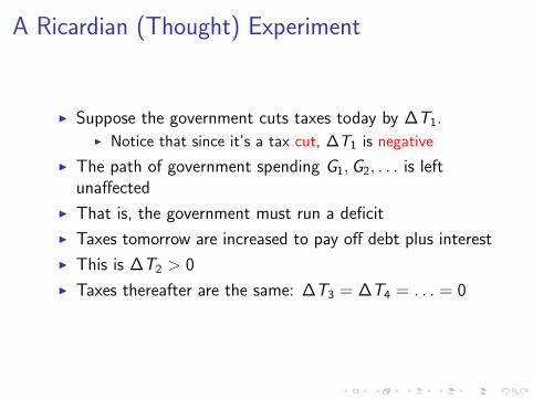
I Suppose the government cuts taxes today by ∆T1.I Notice that since it’s a tax cut, ∆T1 is negative
I The path of government spending G1,G2, . . . is leftunaffected
I That is, the government must run a deficit
I Taxes tomorrow are increased to pay off debt plus interest
I This is ∆T2 > 0
I Taxes thereafter are the same: ∆T3 = ∆T4 = . . . = 0
Budget Constraint
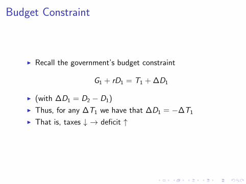
I Recall the government’s budget constraint
G1 + rD1 = T1 + ∆D1
I (with ∆D1 = D2 − D1)
I Thus, for any ∆T1 we have that ∆D1 = −∆T1
I That is, taxes ↓ → deficit ↑
Budget Constraint cont’d
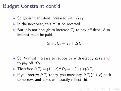
I So government debt increased with ∆T1.
I In the next year, this must be reversed.
I But it is not enough to increase T2 to pay off debt. Alsointerest must be paid.
G2 + rD2 = T2 + ∆D2
I So T2 must increase to reduce D2 with exactly ∆T1 andto pay off rD2.
I Therefore ∆T2 = (1 + r)∆D1 = −(1 + r)∆T1.
I If you borrow ∆T1 today, you must pay ∆T1(1 + r) backtomorrow, and taxes will exactly reflect this!
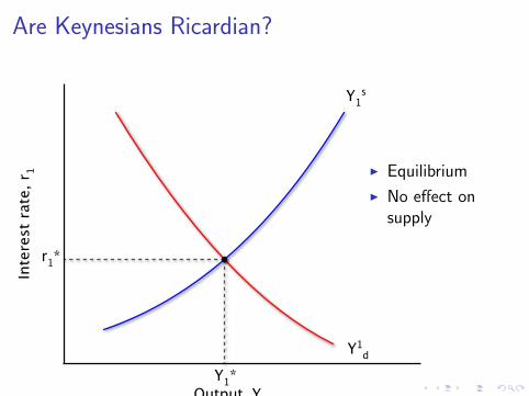
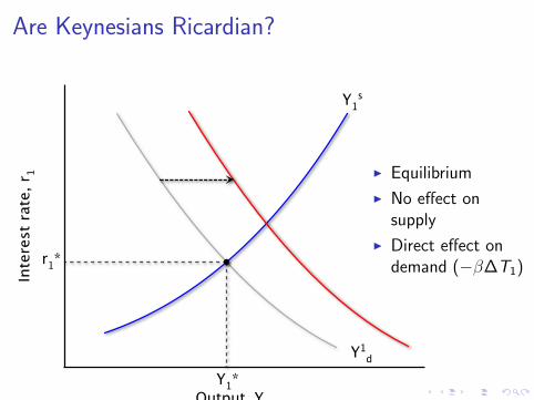
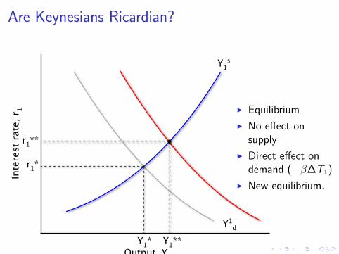
Are Keynesians Ricardian?
Output, Y1
Inte
rest
rat
e, r
1
Y1*
r1*
Y1s
Y1d
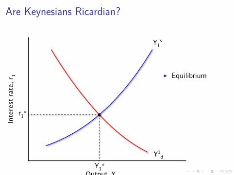
I Equilibrium
I No effect onsupply
I Direct effect ondemand (−β∆T1)
I New equilibrium.
Are Keynesians Ricardian?
Output, Y1
Inte
rest
rat
e, r
1
Y1*
r1*
Y1s
Y1d
I Equilibrium
I No effect onsupply
I Direct effect ondemand (−β∆T1)
I New equilibrium.
Are Keynesians Ricardian?
Output, Y1
Inte
rest
rat
e, r
1
Y1*
r1*
Y1s
Y1d
I Equilibrium
I No effect onsupply
I Direct effect ondemand (−β∆T1)
I New equilibrium.
Are Keynesians Ricardian?
Output, Y1
Inte
rest
rat
e, r
1
Y1*
r1*
Y1s
Y1d
r1**
Y1**
I Equilibrium
I No effect onsupply
I Direct effect ondemand (−β∆T1)
I New equilibrium.

Are Keynesians Ricardian?
I By financing G through debt instead of taxes, individual’scurrent disposable income goes up
I In a Keynesian world this increases consumption demand,increasing output.
I However, as r goes up as well, investments must fall
I ⇒ lower growth in the future
Are Neoclassical Ricardian?
I In a famous article titled “Are Government Bonds NetWealth?”, Barro (1974) showed that Neoclassicalconsumers don’t act like this.
I Recall that private consumption only responds topermanent income changes and not temporary.
I While taxes will fall today, they will increase tomorrow,potentially leaving permanent income unchanged.

Are Neoclassicals Ricardian?
Consumption in period 1
Con
sum
ptio
n in
per
iod
2
C2*
C1*Y1
Y2
-T1
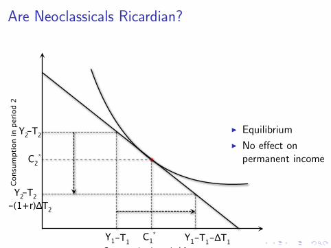
-T2I Equilibrium
I No effect onpermanent income
Are Neoclassicals Ricardian?
Consumption in period 1
Con
sum
ptio
n in
per
iod
2
C2*
C1*Y1
Y2
-T1
-T2
-T1Y1 -ΔT1
Y2-T2-(1+r)ΔT2
I Equilibrium
I No effect onpermanent income

Are Neoclassicals Ricardian?
I Look at the individuals’ present value income
Y1 − T1 +Y2 − T2
1 + r
I So any ∆T1 with ∆T2 = −∆T1(1 + r) will leave presentvalue income unchanged.
I No effect on consumption.
Are Neoclassicals Ricardian?
Output, Y1
Inte
rest
rat
e, r
1
Y1*
r1*
Y1s
Y1d
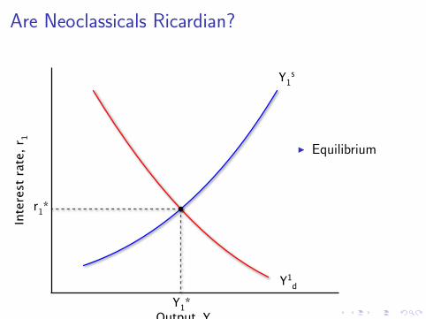
I Equilibrium
I No effect onsupply
I No effect ondemand.
Are Neoclassicals Ricardian?
Output, Y1
Inte
rest
rat
e, r
1
Y1*
r1*
Y1s
Y1d
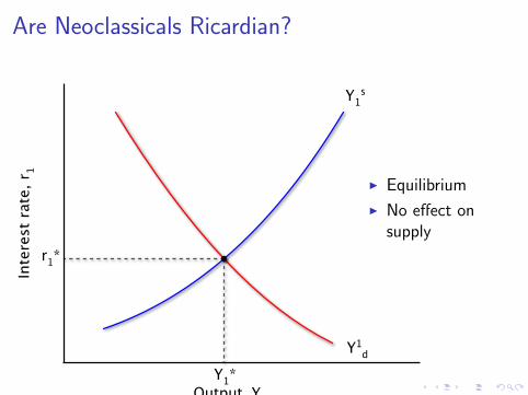
I Equilibrium
I No effect onsupply
I No effect ondemand.

Are Neoclassicals Ricardian?
Output, Y1
Inte
rest
rat
e, r
1
Y1*
r1*
Y1s
Y1d
I Equilibrium
I No effect onsupply
I No effect ondemand.

Ricardian Equivalence
I Debt Neutrality Theorem:
I If consumers choose consumption intertemporally, andgiven a certain level of G , a decline in lump-sum taxestoday financed by (a deficit and) an increase in taxestomorrow, has no real effects on the economy.
I Timing of taxes do not matterI Only the level of G is importantI Government bonds are not net wealth
Ricardian Equivalence
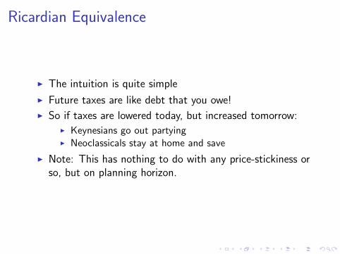
I The intuition is quite simple
I Future taxes are like debt that you owe!
I So if taxes are lowered today, but increased tomorrow:I Keynesians go out partyingI Neoclassicals stay at home and save
I Note: This has nothing to do with any price-stickiness orso, but on planning horizon.
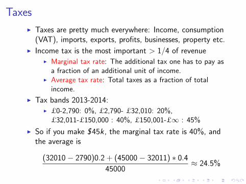
Taxes
I Taxes are pretty much everywhere: Income, consumption(VAT), imports, exports, profits, businesses, property etc.
I Income tax is the most important > 1/4 of revenueI Marginal tax rate: The additional tax one has to pay as
a fraction of an additional unit of income.I Average tax rate: Total taxes as a fraction of total
income.
I Tax bands 2013-2014:I £0-2,790: 0%, £2,790- £32,010: 20%,
£32,011-£150,000 : 40%, £150,001-£∞ : 45%
I So if you make $45k , the marginal tax rate is 40%, andthe average is
(32010− 2790)0.2 + (45000− 32011) ∗ 0.4
45000≈ 24.5%

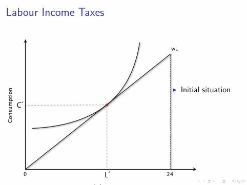
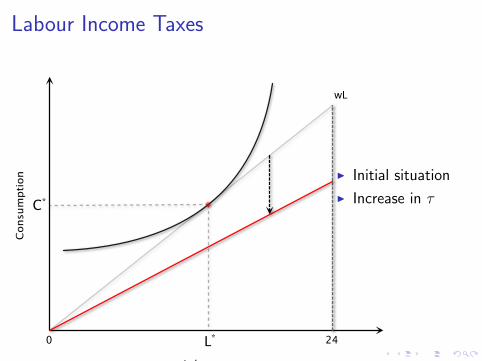
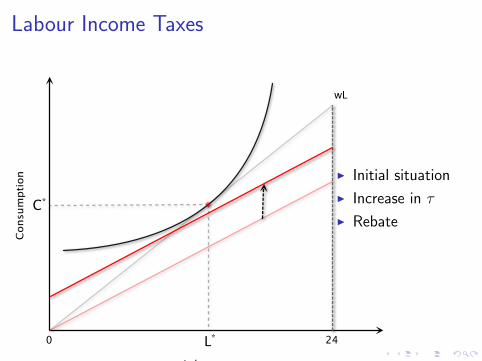
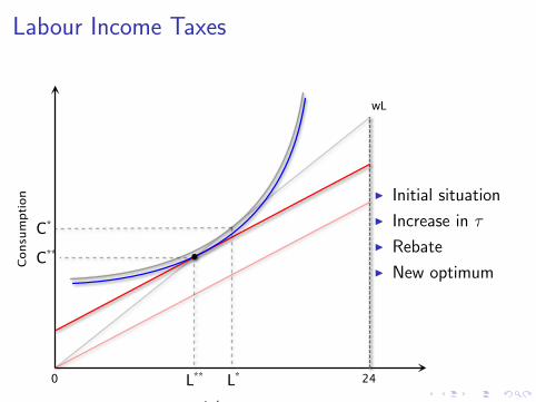
Labour Income Taxes
I Consider the static model
C = w(1− τ)L + b
I To isolate the effect of distortions, consider an increase inτ (from zero) which is rebated back to the consumersthrough an increase in b (from zero) in a lump-sum way.
I b must then equal wτL.
I Therefore, b will depend on L, but this is not internalizedby the consumers (as otherwise it wouldn’t be lump-sum).
Labour Income Taxes
0 24
Labour
Con
sum
ptio
n
L*
C*
wL
I Initial situation
I Increase in τ
I Rebate
I New optimum
Labour Income Taxes
0 24
Labour
Con
sum
ptio
n
L*
C*
wL
I Initial situation
I Increase in τ
I Rebate
I New optimum
Labour Income Taxes
0 24
Labour
Con
sum
ptio
n
L*
C*
wL
I Initial situation
I Increase in τ
I Rebate
I New optimum

Labour Income Taxes
0 24
Labour
Con
sum
ptio
n
L*
C*
wL
I Initial situation
I Increase in τ
I Rebate
I New optimum
Labour Income Taxes
0 24
Labour
Con
sum
ptio
n
L*
C*
wL
L**
C**
I Initial situation
I Increase in τ
I Rebate
I New optimum
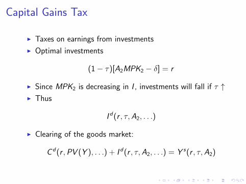
Capital Gains Tax
I Taxes on earnings from investments
I Optimal investments
(1− τ)[A2MPK2 − δ] = r
I Since MPK2 is decreasing in I , investments will fall if τ ↑I Thus
I d(r , τ,A2, . . .)
I Clearing of the goods market:
C d(r ,PV (Y ), . . .) + I d(r , τ,A2, . . .) = Y s(r , τ,A2)
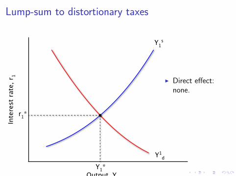
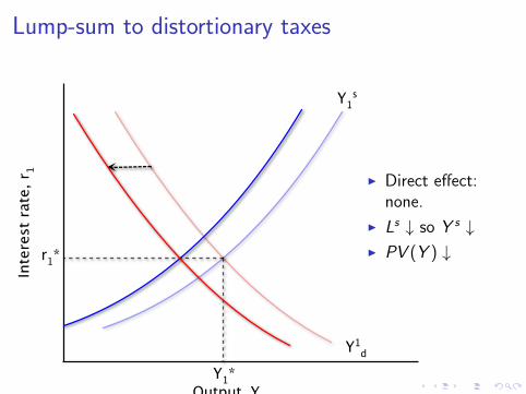
Lump-sum to distortionary taxes
Output, Y1
Inte
rest
rat
e, r
1
Y1*
r1*
Y1s
Y1d
I Direct effect:none.
I Ls ↓ so Y s ↓I PV (Y ) ↓I I ↓
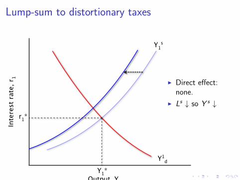
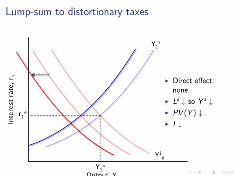
Lump-sum to distortionary taxes
Output, Y1
Inte
rest
rat
e, r
1
Y1*
r1*
Y1s
Y1d
I Direct effect:none.
I Ls ↓ so Y s ↓
I PV (Y ) ↓I I ↓
Lump-sum to distortionary taxes
Output, Y1
Inte
rest
rat
e, r
1
Y1*
r1*
Y1s
Y1d
I Direct effect:none.
I Ls ↓ so Y s ↓I PV (Y ) ↓
I I ↓
Lump-sum to distortionary taxes
Output, Y1
Inte
rest
rat
e, r
1
Y1*
r1*
Y1s
Y1d
I Direct effect:none.
I Ls ↓ so Y s ↓I PV (Y ) ↓I I ↓
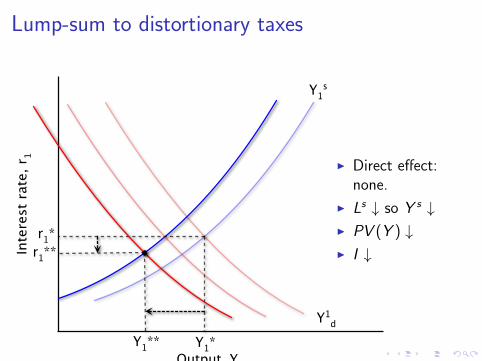
Lump-sum to distortionary taxes
Output, Y1
Inte
rest
rat
e, r
1
Y1*
r1*
Y1s
Y1d
Y1**
r1**
I Direct effect:none.
I Ls ↓ so Y s ↓I PV (Y ) ↓I I ↓

Lump-sum to distortionary taxes
I Total effects:I Y ↓I r ↓I I ↓I C , ?
Summary
I Budget Deficits
I Ricardian Equivalence
I Effect of distortionary taxes onI Consumption/leisure choiceI InvestmentsI Equilibrium in goods market

Next Topic
Unemployment and Labour Markets