- - - - - - Dépôt Institutionnel de l'Université libre de Bruxelles ...
265
- - - - - - Dépôt Institutionnel de l’Université libre de Bruxelles / Université libre de Bruxelles Institutional Repository Thèse de doctorat/ PhD Thesis Citation APA: Grosfils, V. (2009). Modelling and parametric estimation of simulated moving bed chromatographic processes (SMB) (Unpublished doctoral dissertation). Université libre de Bruxelles, Faculté des sciences appliquées – Chimie, Bruxelles. Disponible à / Available at permalink : https://dipot.ulb.ac.be/dspace/bitstream/2013/210313/4/0cd2c745-77d4-4adc-9800-4c61547574c4.txt (English version below) Cette thèse de doctorat a été numérisée par l’Université libre de Bruxelles. L’auteur qui s’opposerait à sa mise en ligne dans DI-fusion est invité à prendre contact avec l’Université ([email protected]). Dans le cas où une version électronique native de la thèse existe, l’Université ne peut garantir que la présente version numérisée soit identique à la version électronique native, ni qu’elle soit la version officielle définitive de la thèse. DI-fusion, le Dépôt Institutionnel de l’Université libre de Bruxelles, recueille la production scientifique de l’Université, mise à disposition en libre accès autant que possible. Les oeuvres accessibles dans DI-fusion sont protégées par la législation belge relative aux droits d'auteur et aux droits voisins. Toute personne peut, sans avoir à demander l’autorisation de l’auteur ou de l’ayant-droit, à des fins d’usage privé ou à des fins d’illustration de l’enseignement ou de recherche scientifique, dans la mesure justifiée par le but non lucratif poursuivi, lire, télécharger ou reproduire sur papier ou sur tout autre support, les articles ou des fragments d’autres oeuvres, disponibles dans DI-fusion, pour autant que : Le nom des auteurs, le titre et la référence bibliographique complète soient cités; L’identifiant unique attribué aux métadonnées dans DI-fusion (permalink) soit indiqué; Le contenu ne soit pas modifié. L’oeuvre ne peut être stockée dans une autre base de données dans le but d’y donner accès ; l’identifiant unique (permalink) indiqué ci-dessus doit toujours être utilisé pour donner accès à l’oeuvre. Toute autre utilisation non mentionnée ci-dessus nécessite l’autorisation de l’auteur de l’oeuvre ou de l’ayant droit. ------------------------------------------------------ English Version ------------------------------------------------------------------- This Ph.D. thesis has been digitized by Université libre de Bruxelles. The author who would disagree on its online availability in DI-fusion is invited to contact the University ([email protected]). If a native electronic version of the thesis exists, the University can guarantee neither that the present digitized version is identical to the native electronic version, nor that it is the definitive official version of the thesis. DI-fusion is the Institutional Repository of Université libre de Bruxelles; it collects the research output of the University, available on open access as much as possible. The works included in DI-fusion are protected by the Belgian legislation relating to authors’ rights and neighbouring rights. Any user may, without prior permission from the authors or copyright owners, for private usage or for educational or scientific research purposes, to the extent justified by the non-profit activity, read, download or reproduce on paper or on any other media, the articles or fragments of other works, available in DI-fusion, provided: The authors, title and full bibliographic details are credited in any copy; The unique identifier (permalink) for the original metadata page in DI-fusion is indicated; The content is not changed in any way. It is not permitted to store the work in another database in order to provide access to it; the unique identifier (permalink) indicated above must always be used to provide access to the work. Any other use not mentioned above requires the authors’ or copyright owners’ permission.
-
Upload
khangminh22 -
Category
Documents
-
view
0 -
download
0
Transcript of - - - - - - Dépôt Institutionnel de l'Université libre de Bruxelles ...

-
-
-
-
-
-
Dépôt Institutionnel de l’Université libre de Bruxelles /
Université libre de Bruxelles Institutional Repository
Thèse de doctorat/ PhD Thesis
Citation APA:
Grosfils, V. (2009). Modelling and parametric estimation of simulated moving bed chromatographic processes (SMB) (Unpublished doctoral dissertation).
Université libre de Bruxelles, Faculté des sciences appliquées – Chimie, Bruxelles. Disponible à / Available at permalink : https://dipot.ulb.ac.be/dspace/bitstream/2013/210313/4/0cd2c745-77d4-4adc-9800-4c61547574c4.txt
(English version below)
Cette thèse de doctorat a été numérisée par l’Université libre de Bruxelles. L’auteur qui s’opposerait à sa mise en ligne dans DI-fusion est invité à
prendre contact avec l’Université ([email protected]).
Dans le cas où une version électronique native de la thèse existe, l’Université ne peut garantir que la présente version numérisée soit
identique à la version électronique native, ni qu’elle soit la version officielle définitive de la thèse.
DI-fusion, le Dépôt Institutionnel de l’Université libre de Bruxelles, recueille la production scientifique de l’Université, mise à disposition en libre
accès autant que possible. Les œuvres accessibles dans DI-fusion sont protégées par la législation belge relative aux droits d'auteur et aux droits
voisins. Toute personne peut, sans avoir à demander l’autorisation de l’auteur ou de l’ayant-droit, à des fins d’usage privé ou à des fins
d’illustration de l’enseignement ou de recherche scientifique, dans la mesure justifiée par le but non lucratif poursuivi, lire, télécharger ou
reproduire sur papier ou sur tout autre support, les articles ou des fragments d’autres œuvres, disponibles dans DI-fusion, pour autant que :
Le nom des auteurs, le titre et la référence bibliographique complète soient cités;
L’identifiant unique attribué aux métadonnées dans DI-fusion (permalink) soit indiqué;
Le contenu ne soit pas modifié.
L’œuvre ne peut être stockée dans une autre base de données dans le but d’y donner accès ; l’identifiant unique (permalink) indiqué ci-dessus doit
toujours être utilisé pour donner accès à l’œuvre. Toute autre utilisation non mentionnée ci-dessus nécessite l’autorisation de l’auteur de l’œuvre ou
de l’ayant droit.
------------------------------------------------------ English Version ------------------------------------------------------------------- This Ph.D. thesis has been digitized by Université libre de Bruxelles. The author who would disagree on its online availability in DI-fusion is
invited to contact the University ([email protected]).
If a native electronic version of the thesis exists, the University can guarantee neither that the present digitized version is identical to the
native electronic version, nor that it is the definitive official version of the thesis.
DI-fusion is the Institutional Repository of Université libre de Bruxelles; it collects the research output of the University, available on open access
as much as possible. The works included in DI-fusion are protected by the Belgian legislation relating to authors’ rights and neighbouring rights.
Any user may, without prior permission from the authors or copyright owners, for private usage or for educational or scientific research purposes,
to the extent justified by the non-profit activity, read, download or reproduce on paper or on any other media, the articles or fragments of other
works, available in DI-fusion, provided:
The authors, title and full bibliographic details are credited in any copy;
The unique identifier (permalink) for the original metadata page in DI-fusion is indicated;
The content is not changed in any way.
It is not permitted to store the work in another database in order to provide access to it; the unique identifier (permalink) indicated above must
always be used to provide access to the work. Any other use not mentioned above requires the authors’ or copyright owners’ permission.

D 03656 JXELLES, UNIVERSITÉ D’EUROPE
Modelling and parametric estimation of simulated moving bed
chromatographie processes (SMB)
Thèse présentée en vue de l'obtention du grade de docteur en sciences appliquées par
VALERIE GROSFILS
Université Libre de Bruxelles
003433131Promoteur : Prof. M. Kinnaert Co-promoteur : Prof. A. Vande Wouwer avril 2009

ULB UNIVERSITE LIBRE DE BRUXELLES
Modelling and parametric estimation of simulated moving bed chromatographie
processes (SMB)
Thèse présentée en vue de l’obtention du grade de docteur en sciences appliquées par
Valérie Grosfils
Promoteur : Prof. M. KinnaertCo-promoteur : Prof A. Vande Wouwer avril 2009
2d édition

AUTORISEEConsultation (biffez la mention inutile)
INTERmTÉr
Signature :

ACKNOWLEDGEMENTS
This thesis is the resuit of a seven-year work. The first four years were financially supported by the Walloon Région within the ffamework of the MOVIDA project. I spent the last years as teaching assistant. I would like to thank ail the people who helped me to complété my work.
First of ail, my greatest thanks are due to my promoter, Professor Michel Kinnaert, who initiated me in research. He always found time in his full time table to guide me with relevant ideas and advices.
Many thanks are due to my co-promoter, Professor Alain Vande Wouwer for his interest in my work and the idea of new directions he proposed.
I would like to express my gratitude to Professor Raymond Hanus for his interesting suggestions conceming my work and for allowing me to continue my thesis as a teaching assistant.
My great thanks are also for Professor Véronique Halloin for her pertinent comments during the board for the thesis follow-up.
Moreover, I gratefially acknowledge Professor Achim Kienle and his coworkers of the Max Planck Institute of Magdeburg, especially Henning Schramm, for their contributions to the experimental work.
I also would like to acknowledge Professor Philippe Bogaerts and Professor Jean- Pierre Corriou for their participation in the thesis jury.
I would like to express my gratitude to the Fondation Van Buuren for its Financial support which helps me after the end of the MOVIDA project and before my nomination as teaching assistant.
I would like to thank Michel Hamende, Emile Cavoy, Sophie Vanlaethem and their co-workers of UCB Pharma for their interest in this work.

Many thanks to
ail the people who joined the prqject Movida, especially Caroline Levrie.
my department colleagues, especially, Andrée Delhaye, Pascale Lathouwers, Laurent Catoire, Serge Torfs, Lhoussain El Bahir, Joseph Yame, Xavier Hulhoven, Thomas Delwiche, Angelo Buttafuoco, Jonathan Verspecht, Manuel Ricardo Galvez Carrillo, Cristina Rétamai, Laurent Rakoto, Samuel Vagman, Valérie Decoux, and Mohamed El Aydam, for their kindness and the good atmosphère they contributed to install in the lab.
Antoni Severino and Guy De Weireld, ffom the FPMs, for their nice collaboration
Spécial thanks to my friends and my wonderful family for their love and their encouraging support.
David, Lucie, Simon, my little sunshine’s, thank you for your patience and your unconditional love.

Contents
CONTENTS
CHAPTER 1 : INTRODUCTION.....................................................................I
PART 1: GENERAL CONCEPTSCHAPTER 2 : AN INTRODUCTION TO CHROMATOGRAPHY AND SMB PROCESSES...................................................................................................... 7
2.1. Introduction 72.2. BATCH CHROMATOGRAPHY 72.3. SMB PROCESS: GENERAL INTRODUCTION 9
2.3.1. Description........................................................................................... 92.3.2. Operating parameters.......................................................................... 13
2.4. Description of the studied SMB plant 142.5. Modifications of the SMB process 16
CHAPTER 3 : MODELLING OF CHROMATOGRAPHIC PROCESSES . 17
3.1. Introduction 173.2. Equilibrium isotherm 173.3. MODELLING of a COLUMN and introduction TO THE WAVE THEORY 19
3.3.1. Column mode!...................................................................................... 193.3.2. Wave theory.......................................................................................... 25
3.4. MODELLING OF SMB PROCESSES 303.4.1. Counter-current movement.................................................................. 303.4.2. Connections between columns in a SMB process................................ 343.4.3. Column model in a SMB process.........................................................38
3.5. Model parameters and operating conditions 403.6. NUMERICAL SIMULATION 44
3.6.1. Introduction.......................................................................................... 443.6.2. Approximation of the spatial dérivatives..............................................443.6.3. Numerical Intégration.......................................................................... 46
3.7. Conclusions OF CHAPTER 3 47Appendix 3.1 ExplanATiON of the shape of the SMB profiles 48Appendix 3.2 Equations of a SMB model with 8 columns 55Appendix 3.3 Triangle theory with Langmuir isotherms 63Appendix 3.4 approximations of saptial dérivatives at the extremities
65Appendix 3.5 Simulation Parameters 67

Contents
PART 2: CONTRIBUTIONS TO THE MODELLING OF SMBPROCESSES
CHAPTER 4 : A SIMPLIFIED MODELLING APPROACH TO SMB PROCESSES......................................................................................................71
4.1. Introduction 714.2. PRINCIPLE OF THE TRANSLATED TMB MODEL 724.3. Assomptions 734.4. Wave velocity 734.5. Translation 744.6. Time delay and smoothing of the concentration curves 774.7. Results, limitations and discussions 804.8. Conclusion 87APPENDIX4.1.: Parameters and Operating conditions 88
CHAPTER 5 : EXTRA-COLUMN DEAD VOLUME MODELLING.......... 89
5.1. Introduction 895.2. General équation of mass balance in the dead volume 915.3. Dead volume in the circulating loop 915.4. Dead volume of the input and output lines 925.5. Boundary conditions 935.6. MEASUREMENT EQUATIONS 935.7. NUMERICAL SIMULATION 945.8. Validation with experimental profiles 945.9. Conclusions 100
PART 3: CONTRIBUTIONS TO PARAMETER ESTIMATIONIN SMB PROCESSES
CHAPTER 6 : INTRODUCTION TO DIRECT AND INVERSE METHODS ............................................................................................................................. 105
6.1. Introduction 1056.2. MODELLING AND UNK.NOWN PARAMETERS 107
6.2.1. SMB modelling......................................................................................1086.2.2. Batch Model..........................................................................................116
6.3. Direct Methods 1196.3.1. Dead volume.........................................................................................1196.3.2. Porosity................................................................................................. 1196.3.3. Isotherm parameters.............................................................................1206.3.4. Diffusion coefficient of the ED model.................................................. 1216.3.5. Diffusion coefficient of the LDF model and mass transfer coefficients ofthe LDF model and of the kinetic model.......................................................121

Contents
63.6. Calibration coefficients........................................................................1226.4. Inverse method or identification - general principles 122
6.4.1. Notations...............................................................................................1236.4.2. Optimization criterion...........................................................................1246.4.3. Parameter constraints...........................................................................1246.4.4. Numerical Optimization Methods........................................................ 1256.4.5. Identifiability and experiment design................................................... 1256.4.6. Confidence interval...............................................................................1276.4.7. Confidence envelope.............................................................................139
Appendix 6.1 Least square estimator without error on C 144Appendix 6.2 Calculation of first and second order dérivatives ofTHE COST FONCTION 146Appendix 6.3 Detailed calculation of the expectation 148
CHAPTER 7 : A SYSTEMATIC APPROACH TO SMB PROCESSESMODEL IDENTIFICATION FROM BATCH EXPERIMENTS....................151
7.1. Introduction 1517.2. PROBLEM STATEMENT and identification APPROACH 152
7.2.1. Batch experiments and définition of data sets......................................1527.2.2. Identification procedure........................................................................1537.2.3. Parameter constraints...........................................................................1547.2.4. Costfiunction.........................................................................................1547.2.5. Initial estimâtes.....................................................................................155
7.3. Experiment design and identifiability 1567.3.1. Génération of the fictitious data............................................................1567.3.2. Sensitivity analysis................................................................................1567.3.3. Local identifiability study from fictitious measurements......................171
7.4. Basin of attraction for error-free data 1717.5. Basin of attraction for noisy data 177
7.5.1. Basin of attraction.................................................................................1777.5.2. Confidence Interval...............................................................................1807.5.3. Confidence envelope.............................................................................182
7.6. Conclusion 1857.7. SUMMARY OF THE IDENTIFICATION PROCEDURE 186
Model.............................................................................................................. 186Identified parameters......................................................................................186Data................................................................................................................ 186Cost function...................................................................................................186Optimization algorithm...................................................................................187Identification procedure..................................................................................187
Appendix 7.1 Fictitious measurements 188Appendix 7.2 Results of the sensitivity analysis 195

Contents
CHAPTER 8 : VALIDATION WITH EXPERIMENTAL DATA.................203
8.1. Introduction 2038.2. The studœd séparation 2038.3. Statement of the identification problem 2058.4. First estimation of model parameters 2068.5. Batch identification 210
8.5.1. Results, validation, comparison..........................................................2108.5.2. Confidence interval............................................................................. 2178.5.3. Conclusions..........................................................................................218
8.6. Validation with SMB experiments 2198.7. Confidence envelope 2248.8. Remark; identification from SMB experiments 2288.9. Conclusions 228APPENDIX8.1 DEAD VOLUMES 230Appendix8.2 Covariance matrix 233Appendix 8.3 Model parameters and simulation parameters 234
CHAPTER 9 : CONCLUSIONS..................................................................... 237
BIBLIOGRAPHY 243

Notation
NOTATION
A: less retained componentB: more retained componentbj : isotherm parameter : ratio of the rate constants of adsorption and
desorption for component i c : concentration in the liquid phaseCp:: injected concentrationCs^ : injected concentration of data set S f
: weighting factor used in cost fonction Jd;C,=max(ys™^(t))/max(y^^(t))
d: index corresponding to dead volume VdD : Gram déterminantDapp : apparent diffusion coefficient (ED model)D(j; diffusion coefficient in a dead volumeDl: diffusion coefficient (LDF and general rate model)ge: sensitivity w.r.t. 0H: Henry coefficienth: height équivalent to a theoretical platei : component A, BJ: zoneJ; cost fonctionJcr “classical” cost fonction (Eq. 7-1)Jini cost fonction defined by (Eq. 7-2)Jmin- smallest cost fonction obtained with the multi start strategy: min
r
with r= 1, 2"kj! mass transfer coefficient of component i (kinetic model)kj^'': relative mass transfer coefficient of component i (kinetic model):
ki"'-ki/v„kp il mass transfer coefficient of component i (LDF model)L: column lengthm: column numbermg: number of the column placed before detector ôM ( : number of measurements in data set

Notation
Mt:
n:Hp:Hs:N;Ni:Ni:Ne:Nd:NG:Np:N,:Ptrans-
Ptmb:
PR:Q:
Qj:Qm
Qr:Qe:Qf:Qd
q :q"*’:^s■R,:
S:S,
ç‘-'max*
to:^Din*to:tp-
t,rtROi:ts:u:
number of parameters number of data sets used in identification number of switching periods already perfoimed number of componentsthe number of theoretical plates of component i the number of theoretical plates of component i number of columnsnumber of grid points in a dead volume number of grid points per columnnumber of positions in the SMB plant (defined in section 5.1) zone numberposition of a concentration in the translated TMB profile position of a concentration in the TMB profile productivity flow ratej = I,.., IV, flow rate in zone j m = 1,Ne, flow rate in column m raffmate flow rate extract flow rate feed flow rate desorbent flow rate countercurrent solid flow rate Covariance matrix of Çgconcentration in the solid phase adsorbed equilibrium concentration column saturation capacity (isotherm parameter) weighting factor in cost fimetion J|„:
= max(ln(y^^^ (t))) / max(ln(y^“(t)))t ^max (column géométrie cross-sectional area f = l,...,np : data set i ;
data set used in identification with c, : > c<-, : ( f = l,...,nn ), timetime delaytime delay of the injection due to dead volume before the unit the column dead time injection durationa constant characterizing the rise time of the puise the rétention time of component i at analytical concentration the time elapsed since the last switch inlet concentration profile

Notation
UV(i): UV1,UV2^ v:Vcc •vs:V:Vd:Vdin:Vcol,b.
d,m
Vcol,af. d,m
w port,b.''d,pw port.af.* d»pV •’ inj‘w:W:Wi.,/2
yz:
calibration coefficient of component i, UV3, UV4: refers to one of the 4 UV detectors of the MPI plant fluid velocityfluid velocity in the TMB model solid velocity column volume dead volumedead volume before the SMB unitdead volume located before column m (moving)dead volume located after column m (moving)dead volume located before a column at position p (fixed)dead volume located after a column at position p (fixed)injected volume (in batch experiments)weigthing factor in cost fimctionadsorbent weightthe width halfway up the peak for component i. model output measurement vector axial coordinate
Greek alphabet
ô : refers to the ô"' UV detectorAt : switching periode: porosityr: time span of experiment0: parameter vector0 . estimated parameter vector
0*; transformed parameter vector
6 : estimation error on 0 : 0 = 0 - 0,^0f; parameter vector of one of the fictitious cases defined in Table A.7.1â parameter value corresponding to (with the cost fonction Jd)'^min •A in parameter value corresponding to Jmin (with the cost fonction J|n)'^min
0,r: “true” value of 00sup> Qinr bound for parameter 0 (eonstraints)Ç, : vector containing a-priori known parameters (and not identified) (batch)
C = e Vdj^ Vi„j cp,A CP3 UVs(A) UVs(B)f'=[Ç^e
Ce(^) Estimation error on Çe : Çe(k) = te(k)~Ce , (*^)
Ce : part of vector C which may be corrupted by some errors;

Notation
Cp,A,^ U\è(A) U\{B) y„jf
Cev Cev=ke(l); ••■; CeCMj)]
part of vector Ç known without error; = [Vj.^ e]^
t-SMB. vector containing a-priori known parameters (and not identified)■ (SMB with UV detector S)
ÇgSMB =
[Qi Qii Qui Qiv - ^nc cpB UVô(A) uVsCb]^
Conventions for the vector oyerations
V = [V(1); V(M-p)] : vector of dimension MjX 1;V(k): k'*’ élément of vector VV(i:j): vector composed of éléments of vector V:
V(i:j) = [V(i); V(i + 1), ...;V(j-l) , V(j)]

Chapter 1 : Introduction 1
CHAPTER 1 : Introduction
Chromatographie séparation processes are based on the differential adsorption of the components of a mixture. In the conventional batch liquid chromatography, the séparation is achieved by injecting a puise of the soluté mixture. The components move with different velocities through the column in fonction of their affmity for the solid phase. Hence, as the low retained component exits the column earlier than the more retained one, the séparation is achieved. The simulated moving bed (SMB) process is a séparation process made of a sériés of chromatographie columns in which a counter-current movement of the liquid and solid phases is allowed by periodically switching the inlet and outlet valves in the direction of the liquid flow. This counter-current configuration offers significant advantages like the increase of the productivity and a decrease of the solvent consomption.
This process has been used for large scale production in the petrochemical and sugar industry since the 1950s. Since the 1990’s, the interest of the fine Chemical, pharmaceutical and biotechnical industries for the SMB process has grown. This attractive technology is now used to separate chiral molécules, amino-acids, enzymes, and sugars, to purify proteins or to produce insulin. In these fields, the SMB process is viewed as a powerful purification process which offers high yield and high purity at reasonable production rate even for difficult séparations. SMB plants are exploited at ail production scales from laboratory, with small columns with a diameter of a few millimeters for séparation of some grams per day, to production plants, with columns of one meter diameter for purification of hundreds of tons per year.
However, on the one hand, the transfer of the SMB technology to the séparation of fine Chemicals is not immédiate. Indeed, the conditions (characteristics of the phases, interactions, etc.) are very different. Moreover, product purity is also subject

2 Chapter 1 :Introduction
to tight constraints imposed by the pharmaceutical and food regulatory organisations. On the other hand, the optimal operating conditions, which, by définition, are achieved if the required purities are obtained with the highest possible productivity and the smallest possible solvent consumption, are not easy to détermine. Most of the methods use a process model and are, thus, subject to modelling errors. Besides, the optimal conditions of the SMB operations are not robust to the changes of température, of the feed composition, or of the feed flow rate. Hence, most of the SMB units work at robust but suboptimal conditions. In this way, they satisfy to the spécifications most of the time despite the disturbances. Indeed, in general, there is no closed loop control. Hence, the main issues are the sélection of optimal operating conditions and process control to achieve disturbance rejection, problems which require the development of a model of the process. The aim of this work is the study and the development of SMB process models and the estimation of model parameters.
The SMB models consist of mass balance équations in the liquid and in solid phases for the components to separate. Several SMB process models hâve been developed in the literature. They essentially differ in the description of mass transfer résistance and diffusion and in the représentation of the counter-current movement of the solid phase. The first task of this work is the analysis of the existing models to compare their ability to reproduce SMB concentration profiles and their complexity in terms of the number of parameters to estimate.
In general, large discrepancies are observed between the experimental profiles and the simulated ones. Two weaknesses are mentioned to explain this problem. First, the model parameters are often roughly estimated from few experiments or modified heuristically to minimize the différence between both profiles. Secondly, the introduction of the dead volumes in the SMB models is not often considered. Hence, there is obviously a need for a systematic estimation procedure of the parameters of SMB process models and for an effective modelling of the dead volumes.
Besides, models with a low computational load, easy to use in optimization, monitoring and control, do not show the cyclic behaviour of the process.
Hence, based on the results of this preliminary study, the rest of the work aims at finding solutions to the weak points of the existing models.
Two kinds of models, missing until now, are developed:a simplified model showing the cyclic behaviour of the process for use in optimization, monitoring and control, tasks which require a model with a low computational load as they are performed on-line, a very précisé model of the plant, including the dead volumes, to reproduce with details the working of the SMB. This kind of model should be usefül for example, to understand with details the influence of each disturbance on the process. Such a model may also be used to generate fictitious data to develop and test the methods to optimize, control and monitor the SMB processes.

Chapter 1 : Introduction 3
Moreover, a systematic estimation procedure of the parameters of a SMB process model is needed. Typically, in the literature, ail these parameters are determined from batch experiments, performed on analytical columns or on SMB columns. Most of the methods described in the literature suffer ffom a number of drawbacks (assumptions not verified, large amount of products needed, etc) and the results of the use of parameters estimated from batch experiments in SMB models are, in general, not conclusive. Besides, no systematic method for the estimation of the errors on the estimated parameters is reported. The aim of the third part of the work is to develop an identification method for determining, with good accuracy, from batch experiments, the isotherm parameters as well as the mass transfer coefficients and/or the diffusion coefficients for use in a SMB model. Distinctive features of the présent study are the following;- The chromatographie model is chosen within a class of three classical models
thanks to a systematic comparison of the identifiability and of the computational load of the three model types.
- Parameter identifiability is thoroughly investigated, including parameter sensitivity, experiment design and the influence of local minima on the optimization problem.
- Confidence intervals are provided for each of the estimated parameters and confidence envelopes are computed for the simulated elution peaks.
The developed approach will be validated with experimental data.
In order to présent the above described thèmes, this work is divided into three parts. The 1®’ part is a review of the literature conceming the chromatography, the SMB process and its modelling. The second part présents new modelling approaches: a simplified model and the modelling of the extra dead-volumes. Finally, the third part is dedicated to parameter estimation.
In particular, the first section begins with Chapter 2 which gives an introduction to the concept of chromatography and a description of the SMB process in general, and of the experimental plant in particular. Then, Chapter 3 provides a review of the literature on the modelling of chromatographie columns and SMB processes. A short introduction to the optimization of the operating conditions is also included. Besides an introduction to the methods used for numerical simulation of SMB models is presented.
The second part of the work is devoted to the présentation of our contributions in the modelling of SMB processes. Chapter 4 présents a simplified modelling approach, whereas Chapter 5 proposes a new strategy to model the dead volumes in a SMB process.
Finally, the third part of this thesis is dedicated to the development of the parameter estimation procedure. Chapter 6 gives some theoretical backgrounds about the direct and inverse method used in the following chapters. Chapter 7 présents the development of the identification procedure and the vérification of its effectiveness on fictitious data generated from a batch model with known parameters. Finally, the

4 Chapter 1 rintroduction
validation on SMB measurements is presented in Chapter 8.

PART I:
GENERAL CONCEPTS


Chapter 2 : An introduction to chromatography and SMB processes 7
CHAPTER 2 :An introduction to chromatography and SMB processes
2.1. Introduction
Chromatographie séparation is based on the differential adsorption of the components of a mixture on an adsorbent. In the case of liquid chromatography considered in this work, the components to separate are in the liquid mobile phase and the adsorbent is a packed bed of solid particles. Originally, chromatography is a discontinuons process (batch). However, several continuons processes like the SMB process hâve been developed. In this chapter, the principles of the batch chromatographie process and of the SMB process are ftrst introduced. Then the SMB unit of the Max Planck Institute of Magdeburg, where experiments were performed, is described.
Note that, in this study, only binary mixtures are considered. The more retained component will be labelled B and the less retained component A.
2.2. Batch chromatography
Batch chromatography is performed on a column filled with porous solid. Figure 2-1 shows a chromatographie column at 6 stages of the séparation process. A small volume of the mixture with components A and B to separate is introduced at time t = 0. The component A (in blue) has less affinity for the solid phase and migrâtes faster. The component B (in pink) is more adsorbed by the stationary phase and is withdrawn at the end of the column aller component A. In Figure 2-2, the évolution of the concentration peaks along the column is given.

8 Chapter 2 : An introduction to chromatography and SMB processes
trts
Figure 2-1: Schematic représentation of a batch chromatographie séparation
Figure 2-2: Concentration profiles in a batch chromatographie column at time t|, t2 and t4 defined in Figure 2-1; simulation parameters given in Appendix 3.4
This batch process is relatively simple to implement and to use. However it suffers from the following drawbacks: high solvent consumption, large dilution of products and low productivity. Continuons counter-current chromatographie processes, as illustrated in Figure 2-3, should alleviate these problems. They especially increase the exchange capabilities.
However, a real counter-current movement is difficult to réalisé in practice. Hence, simulated moving bed chromatographie processes (SMB), where there is no real solid movement but a simulated counter-current, hâve been developed. The process is described in details in the following section.

Chapter 2 : An introduction to chromatography and SMB processes 9
Fluid phase
A + B (Feed)
l
B A
H-Solidphase
Figure 2-3: Schematic représentation of a real counter-current chromatographie column (Lehoucq, 1999)
2.3. SMB process: general introduction
2.3.1. DescriptionThis process is constituted of chromatographie columns connected in sériés. The counter-current movement is usually achieved by periodically switching the inlet and outlet ports in the direction of the liquid flow, as shown in Figure 2-4. Note that, in some small-scale processes, the input and output ports are fixed and the counter- current movement is obtained by rotating the columns in the counter-current direction of the fluid flow (Figure 2-5). In both cases, during the operation, the columns successively occupy different relative positions with respect to the position of the input and output ports. The rôle of each input and output port is explained in the next paragraph.
The SMB processes considered in this study are constituted of 4 zones delimited by the inlet and outlet ports. To understand the rôle of each zone, an équivalent counter- current représentation of a SMB process for the séparation of components A and B is given in Figure 2-6. The mixture to separate is fed between zone II and III. The raffmate which mostly consists of the less adsorbed component is withdrawn between zone III and IV, and the extract which mostly contains the more retained component is obtained between zone I and II. Afler being regenerated in section IV, the liquid phase is recycled to section I together with ffesh solvent which is introduced between zone I and IV. This solvent is called desorbent because it helps to regenerate the solid phase.
Note that, in the following, the start-up of the plant coïncides with the beginning of the injection of a continuons feed flow in the process filled with solvent.

10 Chapter 2 : An introduction to chromatography and SMB processes
Figure 2-4: Schematic view of the simulated moving bed chromatographie process with switching of the inlet and outlet ports (Lehoucq, 1999)
Figure 2-5: Schematic view of the simulated moving bedchromatographie process using a rotative valve (column rotation)

Chapter 2 : An introduction to chromatography and SMB processes 11
D esorbent D 1 E X trac t E
R
Figure 2-6: Equivalent counter-current représentation of a SMB process for the séparation of components A and B (Haag et al., 2001)
In zone 111, just aller the feed injection, component B is preferentially adsorbed. The solid entering in this zone contains a small amount of component A which is desorbed. At the end of zone 111, the liquid consists essentially of component A which is partially withdrawn as raffinate. The solid entering zone IV has been regenerated in zone I. Hence component A and the small amount of B are adsorbed. The solid at the beginning of zone I mostly contains component B. In contact with the regenerated fluid coming from zone IV, B is desorbed and withdrawn as extract at the end of zone I. The solid entering zone II has been in contact with the feed and contains both components. Given their affinity for the solid phase, component A is desorbed and component B is adsorbed. In summary, in zone II and III, the séparation is performed. In zone I, the adsorbent is regenerated and zone IV regenerates the solvent.
Because of the periodical switching of the ports, the SMB process is a periodic process. Figure 2-7 gives spatial concentration profiles. By convention, these profiles are represented with the desorbent input at the origin of the spatial axis. Profiles are here given at steady State just after the switch, at 50% of a switching period, just before the next switch and just after the next switching. The concentration profiles move along the z-axis in fiinction of the time elapsed since the last switch. At each switching time, the profiles jump back one column behind. As seen in Figure 2-9 (a) and (b), the extract and raffinate concentrations are periodical signais. This period is equal to the switching period.
The following section is dedicated to the définition of the operating conditions.

12 Chapter 2 : An introduction to chromatography and SMB processes
Figure 2-7: SMB spatial concentration profiles with t, the time elapsed since thestart-up of the plant, N, an integer, At, the switching period, and S, a period oftime with 5 « At;___component B,___component A; simulation parametersgiven in Appendix 3.4.

Chapter 2 : An introduction to chromatography and SMB processes 13
time (s)
Figure 2-9: a) extract concentration profile in fonction of time
time (s)
Figure 2-9: b) raffinate concentration profile in fonction of time
2.3.2.0perating parameters
Besides the process characteristics like the column length, the column diameter, the number of columns per région, the bed particle size and distribution, the working conditions are defined by the choice of the switching time, the feed concentration, and 4 of the 8 flow rates. There are 4 internai flow rates (one per zone), Qj, j = I,..., IV , and 4 external flow rates (the feed flow rate, Qf, the raffinate flow rate, Qr, the extract flow rate, Qe, and the desorbent flow rate, Qd). In a classic SMB process, ail these flow rates are constant during the operation. They are linked by the mass balance équations:
Od +Qf = Qe +Qr
Oi =Oiv +Od
Qii=Qi“Qe 2-1
Qui ~ Qii + Qf
Qiv ~ Qm “ Qr
The operating conditions are usually determined in order to reduce solvent consomption;
increase the productivity, PR, which is defined as: pR = QfHl with cf, theW
feed concentration and W, the adsorbent weight; obtain the desired purities in the extract and in the rafflnate.

14 Chapter 2 : An introduction to chromatography and SMB processes
Note that constraints hâve to be taken into account like the maximum acceptable pressure drop and the solubility limits of the products.
A lot of methods hâve been developed in the literature to détermine the required operating conditions (Migliorini et ai, 1998 ; Klatt et al., 2002; Biressi et ai, 2000; Jupke et ai, 2002; Reste et a!., 2000 ; Azedo et ai, 1999; Pais et al., 1998“ ; Kleinert et ai, 2002; Schramm et al, 2003“; Abel et ai, 2004 and 2005; Garcia et ai 2006). One well-known method, the triangle theory (Mazzoti et ai, 1997) is presented in section 3.5.
2.4. Description of the studied SMB plant
Figure 2-10: Pictures of the préparative SMB unit (CSEP C912, Knauer, Berlin, Germany) located at the Max Pianck Institute of Magdeburg (Germany)
In this study, experiments were conducted in the Max-Planck-lnstitut Dynamik Komplexer Technisher Système in Magdeburg (Germany) on a préparative SMB unit (CSEP C912, Knauer, Berlin, Germany). Figure 2-10 shows pictures of the SMB plant and Figure 2-11 gives a schematic représentation of this unit. In this process, the counter-current movement of the solid and of the liquid phases is achieved by switching the columns, thanks to a multi-function valve. This valve consists of a rotor and a stator with 24 ports each. The ports are connected to each other by continuons channels. Hence, in Figure 2-11, ail the devices inside the inner circle move during the switching, whereas, the rest is fixed. Note that this SMB

Chapter 2 : An introduction to chromatography and SMB processes 15
plant is built for up to 12 columns but only 8 columns are introduced in the process used at MPI. Hence, as described in (Knauer, 2000), the ffee ports are connected by short capillaries and the valve switches altematively one and two times successively during a full cycle (which is equal to 8 switching periods).
The process is equipped with two inlet pumps, one on the feed flow (P4), and another on desorbent flow (P3). Two other pumps are located in the circulating stream (P 1 and P2).
Besides, this SMB process is also equipped with four UV detectors, two in the circulating stream (UV3 and UV4) (which move with the columns) and two on the product outlets (UVI and UV2).
Figure 2-11: Schematic représentation of the Knauer CSEP C912 unit (Max Planck Institute, Magdeburg, Germany) with 8 columns

16 Chapter 2 : An introduction to chromatography and SMB processes
2.5. Modifications of the SMB process
Note that several variants of the SMB process hâve been developed to improve the productivity. Some use a modulation of the feed concentration like the Modicon (Schramm et al, 2003*’ and 2003“^). Others use variable internai and extemal flow rates like the Powerfeed (Zhang et al., 2003) or variations in the feed flow rate (Zang et al., 2002). In the Varicol (Ludemann-Hombourger et al, 2000; Ludemann- Hombourger et al, 2002), asynchronous switching is performed. Asynchronous switching of the different ports may also be used to compensate dead volumes (Hotier et al, 1996). As this study focuses on the classical SMB process, these variants are not described in details here.

Chapter 3: Modelling of chromatographie processes 17
CHAPTER 3 :Modelling of chromatographie processes
3.1. Introduction
Chromatographie models consist of the mass balance équations of the components in the solid and liquid phases. In this section, the equilibrium isotherms which characterize the distribution of the soluté between both phases are first introduced. Then modelling of batch experiments is described. SMB modelling follows. The chapter ends with a description of the model parameters and a short introduction to the numerical simulation of these models.
3.2. Equilibrium isotherm
The adsorption isotherms characterize the equilibrium between the adsorbed concentration and the concentrations in the liquid phase at constant température.
At very low concentration, the adsorption is easy and one molécule has no influence on the other. The isotherms are then approximated by a linear function:
q,'‘^ = HiCi 3-1
where i = A, B, Hj and qj*"* are respectively the Henry coefficient and the adsorbed equilibrium concentration of component i. Cj is the concentration of component i in the fluid phase.
At higher concentration, as the capacity of the adsorbent is limited and many molécules are in compétition, the adsorption is more difficult. Hence, the isotherms

18 Chapter 3: Modelling of chromatographie processes
are non-linear and are a fonction of the concentrations of the two components in the liquid phase. Figure 3-1 shows an example of non-linear compétitive isotherms. Many multicomponent non-linear isotherm équations hâve been described (Quinones et al, 1998; Guiochon, 1994). As it will be explained in Chapter 8, the Langmuir isotherm has been chosen in this study. This widely used model relies on the assumption that the stationary phase is composed of a fixed number of adsorption sites of equal energy, one molécule being adsorbed per adsorption site until monolayer coverage is achieved. The isotherm équation for component i is the following:
9i eq _ qSibjCi1+ SbjCj
i=A,B
HjCj1+ IbiCj
i=A,B
3-2
qsi is the column saturation capacity of component i, b,, the ratio of the rate constants of adsorption and desorption and Hj, the Henry coefficient. Note that at
r \low concentration, the term
linear.
IbjCii=A,B
is negligible and the isotherms become
6
5- ✓ "
c (vol%)
Figure 3-1: Compétitive multi-components isotherms (c = Ca = Cb);__lessadsorbed component,__ more adsorbed component (Langmuir isotherms)

Chapter 3: Modelling of chromatographie processes 19
3.3. Modelling of a column and introduction to the wave theory
In this section, the modelling of a batch chromatographie column is presented and the wave theory is introduced. The latter is useful to understand a lot of phenomena in chromatography like the movement of the concentration profiles.
3.3.1. Column model
Hereafter several batch chromatographie models are presented. They differ in the assumptions used to build the mass balance équations (Guiochon et al., 1994; Guiochon, 2002). As the aim of this study is the modelling and the parameter estimation of SMB processes, the column models described here will be compared further, in section 3.4.3, when they will be introduced in a SMB model. The modelling of the injected concentration profile is also described.
The following assumptions are used to dérivé the model équations:The column is assumed to be radially homogeneous;Compressibility of the mobile phase is negligible;Isothermal operating conditions are considered;Only components A and B are adsorbed.
3.3.1.1. Equilibrium stage modelIn the equilibrium stage model, the bed éléments are represented by a cascade of N mixing éléments where equilibrium is achieved. Each element is called a theoretical plate.
-plate p-1
plate P
plate p+1
Figure 3-2: Theoretical plates, p"" plate

20 Chapter 3: Modelling of chromatographie processes
The differential mass balance équation in the bulk mobile phase States that the différence between the amount of component i that enters plate p and the amount of component i that exits plate p is equal to the amount accumulated in plate p.
The input flow of component i is: eSve?^*
The output flow of component i is given by: eSve?
de? dqPAnd the accumulation of component i is written: hS(e—!- + (l-e)----- )
dt dtwith
i = A,B;p=l,.., N;P thCj , the concentration in the liquid phase of component i in the p plate;
t, the time;V, the velocity of the fluid flow, e, the porosity;
h, the height équivalent to a theoretical plate (HETP): h = — ;N
L, the column length;S: the column géométrie cross-sectional area.
Hence, the following équations describe the mass balances of the p"’ plate in the fluid phase:
verp+l : ver +h(—------------ —)dt e dt
3-3
As equilibrium is achieved in plate p, the mass balance équation in the solid phase is described by:
with the adsorbed concentration of component i in equilibrium with
(CA,p>CB,p) •
At the origin, this model has been developed following an approach used in Chemical engineering which transforms the distributed parameter System into a System with mixing éléments in order to avoid the partial differential équation formalism. However, this model implies that the diffusion phenomenon is identical for both components which is not realistic (Dunnebier et al., 1998).

Chapter 3: Modelling of chromatographie processes 21
3.3.1.2. Linear Driving Force model (LDF)(Guiochon, 1994)In this model, a continuons flow of the liquid phase is taken into account. The axial dispersion is considered in the fluid phase and the intraparticle mass transfer rate is modelled by a linear driving force.
The dérivation of the LDF model is explained hereafter. The models described in the following sections hâve been built similarly.
The differential mass balance for component i in the bulk mobile phase States that the différence between the amount of component i that enters the slice of column with thickness Az during time At and the amount of component i which exits the slice is equal to the amount accumulated in the slice (Figure 3-3).
■>;e
Z z+Az
>
Z
Figure 3-3 : Chromatographie column m
3cThe input flow of component i is : eS(vC| -Dy —^)
3z
3cThe output flow is : eS(vCj - Dli —^)
3z
z,t3-5
3-6
The accumulation term of component i in the slice of volume SAz is:
SAz(E^!- + (I-E)^)^ ^ zmean.t
where qj is the concentration of component i in the solid phase and z, the axial coordinate. Dm is the axial dispersion coefficient for component i. S is the cross- section area.
If Az tends to zéro, the following équation is obtained:

22 Chapter 3: Modelling of chromatographie processes
3t e 3t dz^ 9z
The mass balance in the solid phase is written as:3qj0t =kF,i(qr-qi)
with kp.i, the mass transfer coefficient.
3-8
3-9
3.3.13. Equilibrium dispersive model (ED)(Guiochon, 1994)
In the equilibrium-dispersive model, the effects of mass transfer résistance and of diffusion are lumped in an apparent diffusion coefficient Dgpp. Hence, equilibrium is assumed between the solid and the fluid phase. The mass balance équation in the fluid phase is written as:
at e 3t dz3-10
where qj
and D^pp i2
Lv2N,
3-11
with hi, the length équivalent to a theoretical plate and Nj, the number of theoretical plates.
In the case of a linear isotherm, the following relation has been obtained between the apparent diffusion coefficient of the ED model and the diffusion and mass transfer coefficients of the LDF model:
Hj is the Henry coefficient (see Eq.3-1).According to (Guiochon, 1994), this model is correct if the mass transfer is only controlled by diffusion and if the mass transfer is very fast.

Chapter 3: Modelling of chromatographie processes 23
3.3.1.4. Kinetic model
Ail the non-ideal effects are lumped into a mass transfer coefficient.
^ + 3-133t e 9t 9z
^ = 3-14
kj, the lumped mass transfer coefficient, is a linear function of the fluid velocity. Hence, a relative mass transfer coefficient which is independent of the velocity isdefined as; kp' = kj / v.
3.3.1.5. General rate modelThis model takes ail the possible contributions to the mass transfer kinetics into account (Guiochon, 1994). As there are different ways to describe these effects, there are many versions of this model. In the SMB community, the axial diffusion, the mass transfer résistance and the pore diffusion are usually introduced in the équations. The solid phase is assumed to be constituted of porous, uniform and spherical particles with porosity £p and local equilibrium is considered within the pores. The concentration of component i in the liquid phase is the solution of the following mass balance équation:
9t= D
9^C;L,i
9z^-vj^-3^ ^ext
dz -ext
Inside the pores.3cp.
9t9q; i ^ 2 5cpj
9r" r 9r
3-15
3-16
9c p.i9r
= 0r=0
3-17
with r, the radial coordinate inside the pore, Eext, the extemal porosity, £p, the internai porosity of the particles, rp, the particle radius, k^xi, the extemal mass transfer coefficient. Dp, the diffusion coefficient inside the pores, Cp, the concentration in the stagnant fluid phase in the particle pores.
This is the most rigorous model (Guiochon, 2002). It is convenient for ail kinds of isotherms.

24 Chapter 3: Modelling of chromatographie processes
3.3.I.6. Idéal Model(Guiochon, 1994)The idéal model considers that the column has an infinité efficiency. It means that there is no axial dispersion and that the mass transfer between the mobile and the stationary phase is assumed to be instantaneous. The mass balance équation in the fluid phase is the following:
dC: l-e3q: 9C:dt E dt dz
3-18
with qj =q"‘’.
This model gives a first estimation of the concentration profiles but cannot accurately reproduce the elution peaks in case of low-efficiency columns. Indeed, in this case, the contributions of the mass transfer kinetics and axial dispersion become significant.
3.3.1.7. Modelling of the injectionIn this section, the inlet concentration profiles are described for several classical batch experiments.
Elution peakElution peaks resuit from the injection of a small volume of the solution containing the components to separate. The idéal shape of the inlet concentration profile should be a rectangle but dispersion phenomena affect significantly the profile. In this study, the inlet concentration profile of component i is described as follows:
if t<tpUi(t) = CFi(l-exp(-t/ttr))
, 3-19elseU i (t) = c F,i (1 - exp(-t /1 tr )) - C F,i (1 - exp(-(t -1 p ) /1))
with Cpj, the injected concentration of component i, t, the time, tp, the injection duration and t,r, a constant characterizing the rise time of the puise (Figure 3-4). Note that this injection profile is close to the one proposed in (Felinger et al., 2003) but it has less parameters.

Chapter 3; Modelling of chromatographie processes 25
f0.1
U(vol%)
0.05
0 0.5 1.5 2 2.5 3 3.5 4 4.5
time (s)
Figure 3-4: Shape of the inlet concentration profile u; simulation parameters given in Appendix 3.4.
Concentration stepOther batch experiments consist in the injection of abrupt step changes of different concentrations. The injected front should be abrupt but dispersion phenomena affect significantly the profile. Hence the inlet concentration profile of component i is described as follows
After this complété présentation of batch modelling, the wave theory which has been developed from batch models is presented. This theory notably helps to explain the movement of the peaks in the column.
3.3.2.Wave theory
The wave theory, presented in this section, has been built from the équation of the batch idéal model and helps to understand the behaviour of the concentration profiles in a chromatographie process. The wave theory is also used in Chapter 4 to build a new modelling approach.
Each elution peak resulting from the injection of a rectangular puise in a column initially free of soluté is constituted of two waves (Hellferich and Carr, 1993), one corresponding to the adsorption front, the other to the desorption front.
Ui(t) = cp,i (l-exp(-t/t,r)) 3-20

26 Chapter 3: Modelling of chromatographie processes
de de „ — + v, — = 0 dt " dz
with Vj, the concentration velocity equal to ;
3-21
_ V
”, l-e3q 3-22e de
In the case of idéal chromatography, the phases are in local equilibrium, hence, q can be expressed as a unique function of c and the partial dérivative becomes a total dérivative:
” , 1-edq 3-231 +----------e de
Hence v^, the velocity of concentration c, is a function of the slope of the isotherm at concentration c.
Therefore, in the case of an adsorption characterized by a linear isotherm, the velocity is not a function of the concentration. As shown in Figure 3-5 (a) and (b), the shape of the wave does not change during the displacement.
However, in the case of a non-linear isotherm, the slope of the isotherm decreases when the concentration increases. Hence, the velocity is higher for larger concentration. A front of the form represented in Figure 3-5 (d) is then spreading. Whereas, a front of the form shown in Figure 3-5 (c) tends to sharpen until it becomes a concentration discontinuity to avoid a physically impossible coexistence of different concentrations. It is called a shock. For non-linear isotherms, like the Langmuir isotherms, the final shock pattern is obtained rapidly. The velocity at which the shock moves is given by (Helfferich et al, 1993):
_ V
i + 3-24e Acj
where Aq; and Acj are the concentration différences between the downstream and upstream sides of the wave.
In conclusion, if the non-linearity increases, the symmetry of the elution peak decreases.

Chapter 3: Modelling of chromatographie processes 27
Figure 3-5: Illustration of the wave displacement in idéal chromatography: concentration profiles at two successive times t| and t2 (ti < t2)
In non-ideal chromatography, the non-idealities like the axial dispersion, the mass transfer résistance in the moving phase, the mass transfer résistance in the adsorbent, etc... modify the shape of the profiles. The effect is fronting or tailing depending on the dominant non-ideality considered.
From these explanations, the évolution of the shape of an elution peak along the column may be understood. For the inlet concentration profile described in Figure 3-6, Figure 3-7 shows an elution peak in the column at two successive times and Figure 3-8 shows the elution peak obtained at the end of the column in function of time.

28 Chapter 3: Modelling of chromatographie processes
i5r
Figure 3-6 : Inlet concentration profile; simulation parameters given in Appendix 3.4
Figure 3-7 : Elution peak at successive times t| and t2 (t] < t^); simulation parameters given in Appendix 3.4
1.5 <----------
Figure 3-8: Elution peak at the end of a chromatographie column; simulation parameters given in Appendix 3.4

Chapter 3: Modelling of chromatographie processes 29
For multicomponent Systems, Eq. (3-23) becomes:V
1-e dqj1-1- 3-25
e dc:
The adsorbed concentration of component i, qj, is a fonction of the concentrations ofdq,
ail the components in the fluid phase and is calculated as follows. ----- , the totaldCj
dérivative, is given bydq;___ _ j-^qj dc^dCj e=\dC( dCj
i = A,B 3-26
If equilibrium is assumed, 8qj /9c^ is easily computed by dérivation of the isotherm model. dc^/dcj is calculated using the cohérence principle (Helfferich and Withley, 1996). The latter implies that, at any point in the unit, ail the components présent in the same wave travel with the same velocity. Hence équation (3-25) implies that:
tlq A *iq B
dc ^ dc gor using (3-26)
I ^9a _ ^qs ^ ^qe ^‘'A9c, 9c B dCy^ 9c J 9c A deg
3-27
3-28
Reordering (3-28) and multiplying the resulting expression by dCy^ / dcg a second
order équation is obtained fordc,dc,
(Guiochon et al., 1994, pp. 250 & 256):
^qB 9c A
( dCA f 1 fdqR 5q.' CL O >
Idcg J ^dCg 3ca,Idcg J
^qA9c g
= 0 3-29
where the positive root is considered when the wave fronts of component A and B are both monotically increasing or decreasing (Guiochon et al., 1994, pp. 250 & 256). The négative root is used when one wave front is increasing and the other is decreasing.
The wave theory will be exploited in chapter 4 to develop a new modelling approach.

30 Chapter 3: Modelling of chromatographie processes
3.4. Modelling of SMB processes
The SMB process is constituted of a sériés of chromatographie columns. The continuous movement of the solid phase is simulated by a commutation of the inlet and outlet ports. Hence, the modelling of a SMB process may be divided into three parts. The first part is the représentation of the counter-current movement of the solid phase. The second part corresponds to the connections between the columns. The third one is the column modelling, for which the mass balance équations presented in the previous section are valid. These three parts are discussed in this section. Note that ail the model équations of a 8 columns -SMB process are given in Appendix 3.2.
3.4.1.Counter-current movement
Two modelling approaches are commonly applied to SMB processes (Ruthven and Ching, 1989). The first one is called TMB (true moving bed) and assumes an équivalent counter-current movement of the solid phase, like in an idéal counter- current process. The second, more rigorous approach, called SMB, considéra the System as an arrangement of static chromatographie columns and takes the discrète nature of the solid movement into account.
3.4.I.I. TMB model
As explained in the introduction, the TMB model assumes an équivalent counter- current movement of the solid phase. Hence, a term describing the solid movement is added in the mass balance équations. The TMB model is defined in each zone (cf section 2.3.1). For example, for the LDF model (3.3.1.2), the mass balance for each component i in the liquid phase in zone j can be expressed as:
l-e^qy----+------------- ’J.dt E dt ''“’j dz-
i_e 9qij
3zj2 e ' dzj3-30
j = I,...,IV, i = A,Bwhere Cj_j is the concentration of component i in the liquid phase in zone j, qjj, the corresponding concentration in the solid phase. Vecj represents the velocity of the liquid in zone j in the TMB model. Vj is the équivalent solid phase velocity and is given by Vj = L/At with L, the length of one column and At, the switching period. In order to get the équivalence between the SMB and the TMB models, Vjcj must fulfil the following expression
V • = V- — V ce,J ''j 3-31
Chapter 3: Modelling of chromatographie processes 31
where vj is the fluid velocity in zone j of the SMB process.
Zj is the axial coordinate in zone j and is defined as: Zj e [0,N2jL] where is
the number of column in zone j and L, the column length.
Moreover, the mass balance for component i in the solid phase is written as
3t= ky(q^]-qi,j) + Vs
^qydZ:
3-32
3.4.I.2. SMB model
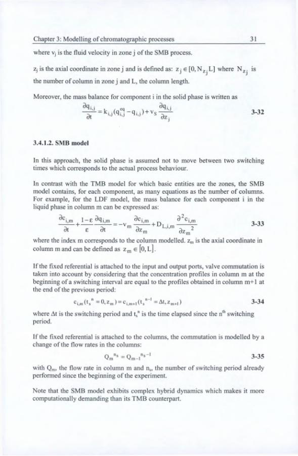
In this approach, the solid phase is assumed not to move between two switching times which corresponds to the actual process behaviour.
In contrast with the TMB model for which basic entities are the zones, the SMB model contains, for each component, as many équations as the number of columns. For example, for the LDF model, the mass balance for each component i in the liquid phase in column m can be expressed as:
de i,m
8t1-e 9qj,n
e 9t^Cj,ldZr,
- + D L,i,mdz‘
3-33
where the index m corresponds to the column modelled. z^ is the axial coordinate incolumn m and can be defined as z^ e [o, l] .
If the fixed referential is attached to the input and output ports, valve commutation is taken into account by considering that the concentration profiles in column m at the beginning of a switching interval are equal to the profiles obtained in column m+1 at the end of the previous period:
=0,z„) = c,_„„.,(t,,""' =At,z„„.,) 3-34
where At is the switching period and tj" is the time elapsed since the n"’ switching period.
If the fixed referential is attached to the columns, the commutation is modelled by a change of the flow rates in the columns:
Qm"* 3-35with Qm, the flow rate in column m and ns, the number of switching period already performed since the beginning of the experiment.
Note that the SMB model exhibits complex hybrid dynamics which makes it more computationally demanding than its TMB counterpart.

32 Chapter 3: Modelling of chromatographie processes
3.4.1.3, Comparison of SMB and TMB models
In this section, preliminary comparisons between the simulations of the TMB and SMB models are given. They are presented here even if ail the details about the modelling of a SMB process hâve not yet been given in order to compare these models directly after their présentation.
Figure 3-9 to Figure 3-12 compare the simulation results obtained with the TMB and SMB models for a SMB process with 8 columns.
In the literature, it is generally agreed that the TMB model represents the average behaviour of the SMB model and that the correspondence between TMB and SMB becomes better and better when the number of columns in the SMB unit increases (Pais et a/., 1998*’).
As seen in Figure 3-10 and Figure 3-11, the SMB model is able to reproduce the cyclic behaviour of the SMB process, contrary to the TMB model. However, the TMB model gives a good approximation of the spatial SMB profiles at 50% of the switching period (Figure 3-9). Nevertheless, it introduces modelling inaccuracies, particularly in the vicinity of the feed point. Around that point, the concentrations are higher than those predicted by the SMB model. This is due to the fact that the flow rates in the TMB model are always smaller than in the SMB model, leading to smaller dilution of the feed at the injection point. In Figure 3-12, the extract and raffmate concentration profiles produced with the TMB model give a better approximation of the average values of the SMB concentrations over a switching period than of the SMB concentrations sampled at 50% of the switching period. However, for simplicity, the concentrations obtained by the TMB model are often used as a first estimation of the SMB concentrations sampled at 50% of the switching period (Ruthven and Ching, 1989, Lim and Ching, 1996, Beste et al, 2000).
The main advantage of the TMB model is that it brings significant réduction of the computational complexity (Haag et al, 2001; Ruthven and Ching, 1989) and can be used for a first analysis in design, optimization and control (Kloppenburg and Gilles,1999).

Chapter 3; Modelling of chromatographie processes 33
Figure 3-9: Simulated steady-state concentration profiles. TMB model (__)and SMB model at 50% of the switching period (- -); simulation parameters given in Appendix 3.4
ioo 1000 ISOO 2000 2SOO 3000 MOO 4000 «WO 5000
time (s)
Figure 3-10: Simulated extract concentration in fonction of time; TMB model (__) and SMB model (...)
MO lôoo 1500 2000 2M0 3000 3500 «000 «500 5000time (s)
Figure 3-11: Simulated raffinate concentration in fonction of time; TMB model ( _ ) and SMB model (....)

34 Chapter 3; Modelling of chromatographie processes
0.25 r—
Figure 3-12 : (a) simulated extract concentration profile in function of time, (b) simulated raffinate concentration profile in function of time;TMB model ( ), SMB model, average value over a switching period (__);SMB model sampled at 50% of a switching period (— —);simulation parameters given in Appendix 3.4
3.4.2.Connections between colunins in a SMB processThis section is devoted to the modelling of the connections between the SMB columns. On the one hand, transitions between columns and mass balance équations at the input and output ports hâve to be considered; on the other hand, some models (Migliorini et al., 1999, Beste et al., 2000) include the dead volume introduced by the valves, the connecting tubes and the pumps placed between the columns.

Chapter 3: Modelling of chromatographie processes 35
3.4.2.1. Boundary conditions
TMB modelThe boundary conditions in the liquid phase are obtained by expressing simple mass balances for each component i ( i = A, B ) at the transition between two subséquent régions.
Between zone I and zone II (zone III and IV), a part of the flow rate is withdrawn as extract (raffinate). This operation does not modify the concentration. Hence, the concentration at the end of zone I (III) is equal to the concentration at the beginning of zone II (IV).
Fresh solvent is introduced between zone IV and zone I. This implies a dilution of both components.
The feed is injected between zones II and III. It modifies the concentration. The change of concentration is a function of the flow rate in zone II, the feed flow rate and the feed concentration.
Hence, the following boundary conditions are derived:'^cc,iCi,i(t,Z] =0) = Vcc,ivCi,rv(t,Z|V =Liv)
=L])''cc,lllCi,iii(t,ziii =0) = Vj.j.||Ciii(t,z,i =Lii) + vpUj(t)
Crv(t>ziv =0) = Cijii(t,Z|ii =Liij)where vp and Uj(t) are respectively the feed velocity and the inlet concentration profile of component 1. Indexes I to IV correspond to the zone number. L, to Liv are respectively the length of zones I to IV.
In the experiments considered in this study, the start-up of the plant coïncides with the beginning of the injection of a continuons feed flow in the process filled with solvent. The injected fi"ont should be abrupt but dispersion phenomena affect significantly the profile. Hence the inlet concentration profile is described as follows
Ui(t) = CF_i(l-exp(-t/t,r)) 3-37
with Cp j, the injected concentration of component i. t is the time and t,„ a constant characterizing the rise time of the puise.
The boundary conditions in the solid phase are the following:
qg(t,Zj =Lj) = qi_j+,(t,Zj+| =0) 3.38
j=I, ...,IV.

36 Chapter 3: Modelling of chromatographie processes
For the ED model and for the LDF model, the continuity of dispersion fluxes is assumed (Haag et al, 2001):
deD ____app,.,J 3^, = Dapp,i,j+l'
t,Zj=Lj dz j+i3-39
3-39 is used in place of the conventional Danckwerts boundary conditions assuming zero-dispersion conditions at the outlet of each section. Indeed, 3-39 is more consistent with the TMB model where each section is considered as a continuons bed with dispersion in the liquid phase (Haag et al, 2001).
SMB model
In the liquid phase, conditions similar to 3-36 can be used to define boundary conditions between columns placed at the end or at the beginning of a zone. Note that for this définition, the columns are numbered as column 1 is the first column of zone I and column N^, the last column of zone IV.
Limit between zone I and IV:ViCg(t,Z, =0)= VjvCi_N^(t,ZN^ =L)
Limit between zone I and II :^i,N]+l (L Zjvji+i — 0) — Cj f,(j (t, Zjvjj — L)
Limit between zone II and III:111 ^i,N]]+I (L ZN[]+1 “ ~(^> ^Nii ~ L)(0
Limit between zone III and IV:^i,Niii+l (LZj\J|ii.4.| — 0) — (L Znjii = L)
where N|, Nu, Nm and Niv give respectively the number of columns in zone I, II, III, or IV. Ne is the total number of columns in the process.
Boundary conditions between columns inside a zone are given by:
Ci,m (t, Zn, = 0) = Ci m-l (t, Zm_, = L) 3-41
Boundary conditions in the solid phase are:
~ ~ 9i,m+l ^m+1 ~ 3-42
For the ED model and for the LDF model, as proposed in (Haag et al, 2001), a simple advection équation at the outlet of each column is used:
dC;
dt
dC;i,mdz„
with i = A, B and m = l,...,N(-.
3-43

Chapter 3: Modelling of chromatographie processes 37
3A.2.2. The dead volumeIn a SMB process, the valves, the connecting tubes and the pumps placed between the columns introduce dead volumes.
Effective column length in a TMB modelAs there is a continuons flow of the solid phase in the TMB model, the dead volumes cannot be directly introduced. Hence, it is included in the column geometry; an effective column length and an effective porosity are calculated (Beste et al., 2000). The first is defined as the total volume of the process, Vj, including dead volumes, divided by the column cross-section area. S, and the number of columns N,.:
Leff - ^totalNcS
3-44
The effective porosity, Eefr, is either determined on the column surrounded by the dead volumes experimentally with the classical method described in section 6.3 or it is calculated as follows:
^effeVcNe+VdvVcN,+V,, 3-45
with V(., the column volume, Vjv, the dead volume.LcfT and Eefr are thus used in the TMB model équations in place of L and e.
Empty column in a SMB modelThe dead volume surrounding a column is modelled by one empty pre-column placed before the column (Beste et ai, 2000) or is divided in two parts, one placed before the column, the other after (Migliorini et ai, 1999). The dead volume switches with the column. Porosity is set to 1 and no adsorption takes place in this volume. The mass balance équation associated to a dead volume is the following (Migliorini étal., 1999):
9Cj,ddt
^Cj,. - + D i.d
‘•'a 2OZh3-46
with Vd, the velocity and Dd, the diffusion coefficient in the dead volume d and Zd, the axial coordinate in dead volume d.

38 Chapter 3: Modelling of chromatographie processes
3.4.3.Column mode! in a SMB process
In this section, the use of the different chromatographie models introduced in section3.3.1. to describe a SMB column is discussed. Note that, as équations of section 3.3.1 hâve been established for batch modelling, with a fixed solid phase, the terms describing the movement of the solid phase should be introduced for the TMB model as seen in section 3.4.1.1.
General rate modelThe general rate model is the most rigorous model (Dünnebier et al., 2000), convenient for ail types of isotherms (Klatt, et al., 2000). However, the computation load is high and the number of parameters is large which increases the difficulty to détermine them univocally.
Idéal modelFigure 3-13 shows the concentration profiles obtained at steady-state with the idéal SMB model with Langmuir isotherms. Appendix 3.1 explains how such a profile is physically obtained. The concentration fronts are sharper than experimental profiles (Figure 3-14). Some oscillations appear in the plateaus. These oscillations are generated by the switching phenomenon. They may be présent in a process with low diffusion. However, they do not appear in the profiles generated by the TMB model because of its continuons behaviour.
As the idéal model neglects the diffusion and the mass transfer résistance and produces very sharp concentration fronts, it usually gives only a rough approximation of SMB profiles (Dünnebier et ai, 1998 ; Guiochon, 2002). The sharp profiles also induce numerical problems and high computation load.
0.6----------------
Figure 3-13 : Idéal SMB model ; spatial concentration profiles at steady State;__component A;___component B; simulation parameters given in Appendix3.4

Chapter 3: Modelling of chromatographie processes 39
0 0.116 0.232 0.348 0.464 0.58 0.696 0.812 0.928 1.044 1.16 1.276 1.392
z(m)
Figure 3-14 : experimental concentration profiles ((Lehoucq, 1999,), fig V.12.e, P.V13)
Linear Driving Force model (LDF)This model has been widely used to model SMB processes (Dünnebier et al., 1998; Dünnebier et al., 2000; Beste et al., 2000; Pais, et al., 1998“; Ruthven et al.„ 1989; Pais et al., 1998*’; Lim et al., 1996). It is commonly said to be very efficient to reproduce concentration profiles. It could be used with ail kinds of isotherms (Pais et al., 1998“; Kloppenburg et ai, 1999). SMB concentration profiles simulated with a LDF SMB model are shown on Figure 3-15. The operating parameters are the same as in Figure 3-13 where the profiles simulated with an idéal model are plotted. The fronts of the LDF profiles are less sharp than those generated with the idéal model and their shape is doser to the shape of experimental profiles. Moreover, the oscillations in the plateau are less visible than in profiles simulated with the idéal model.
Equilibrinm dispersive modelThis model is also currently used to model SMB units (Dünnebier d a/., 1998; Klatt, et al, 2000; Klatt. et al, 2002; Guiochon, 2002; Strube et al, 1998; Zimmer et al, 1999). However, its use is much debated. In (Kaspereit et al, 2002 ; Küsters et al, 2000 ; Lehoucq, 1999), it has been used in the case of non-linear isotherms, but in other papers (Dünnebier et al, 1998; Klatt, et al, 2000; Strube et al, 1998 ; Zimmer et al, 1999), its use is recommended only with linear isotherms as Eq. 3-12, which relies the diffusion coefficient of the equilibrium dispersive model to the diffusion and mass transfer coefficients of the LDF model, is only valid for linear isotherms. A SMB profile simulated with an ED SMB model is shown on Figure 3-15. It is close to the profile simulated with the LDF model. Note that Eq. 3-12 has been used to déterminé the apparent diffusion coefficients to reproduce concentration profiles similar to those of the LDF model.

40 Chapter 3: Modelling of chromatographie processes
Kinetic modelThe use of the kinetic model in SMB modelling is rare. This model is only presented in (Dünnebier et ai, 2000). A SMB profile simulated with a kinetic SMB model is shown on Figure 3-15. It is close to the profiles simulated with the LDF and the equilibrium dispersive model.
Figure 3-15: Spatial concentration profiles at steady-state simulated with aSMB model; LDF column model (---- ); kinetic column model (...); ED columnmodel (__); simulation parameters given in Appendix 3.4
Comparison of the column models used in a SMB mode!It appears that the general rate model is generally assumed to be very efficient to reproduce the concentration profiles but has a large number of parameters and a large computational load, which are significant drawbacks for the parameter estimation step described in Part III. On the other hand, the idéal model which has less parameters, only gives a rough approximation of the profiles. The LDF, the ED and the kinetic models give similar profiles with a low number of parameters. Moreover, they are generally considered to be very efficient to model SMB profiles. Flence, these three models will be used in the following.
3.5. Model parameters and operating conditions
In batch and SMB models, the parameters may be divided into two categories:
geometrical parameters: the column length, the column diameter, thenumber of columns per section;physico-chemical parameters: diffusion coefficients, mass transfercoefficients, isotherm parameters.
The choice of the geometrical parameters is not discussed in this work.

Chapter 3: Modelling of chromatographie processes 41
The détermination of the physico-chemical parameters will be the object of the third part of this thesis.
Besides these parameters, the operating conditions are specified by the switching time and the flow rates.
As seen in 2.3.2, in a SMB process, the operating conditions must be carefiilly selected to obtain the desired purities, to reduce the solvent consumption and to increase the productivity. A very simple method to choose the operating conditions is based on the triangle theory (Mazzoti et al., 1997) which has been developed from the idéal TMB model. This method, usually considered as a reference, will be used in this study. It consists in setting the wave velocities in an idéal TMB model in order to achieve total séparation, by an appropriate choice of the flow in each zone. More specifically, for linear isotherms, the following constraints on the “relative flows”, mi to miv , hâve to be imposed:
m, >Hb m„ >H^
*^111 < Hg
where
m, =-Q.-Qs — 1-e Qii Qs l̂-e
IIIm 1 - eIII
Qiv Qsm,v =- l-e
and m,,, > m,|.
3-47
3-48
Qs is the countercurrent solid flow rate: Q§ = — (1 -e)S .
The latter condition is due to the introduction of the feed between zone II and zone III.The conditions on mi and miv ensure respectively the solid phase and the liquid phase régénération in order to avoid extract and raffinate pollution from the recycling. The conditions on mu and mm are independent of those on mj and miy. From the inequalities (3-47), the triangle “f’ of Figure 3-16 is built (Mazzoti et al, 1997):

42 Chapter 3: Modelling of chromatographie processes
Figure 3-16: Séparation zones defîned by the triangle theory (linear isotherm) (Lehoucq, 1999, fig. VI.l (Mazzoti étal., 1997))
In triangle “a”, the flow rate in zone II is too large, ail the feed is withdrawn in the raffinate.In triangle “b”, the flow rate in zone III is too low, ail the feed is withdrawn in the extract.
This theory has been extended to non-linear isotherms (Mazzoti et al., 1997) like the Langmuir isotherms, the modified Langmuir isotherms and bi-Langmuir isotherms. For Langmuir isotherms, the triangle is given in Figure 3-17. The équations used to build this triangle are given in Appendix 3.3.

Chapter 3: Modelling of chromatographie processes 43
Figure 3-17: Séparation zones defined by the triangle theory for Langmuir isotherms (Mazzoti et al., 1997)
In the complété séparation région, where extract and raffmate are pure, point O corresponds to maximum productivity (Mazzoti et ai, 1997). Indeed, the
productivity may be expressed as: PR = the adsorbent
weight and cp, the feed concentration. However, point O does not correspond to robust operating conditions. Indeed, the triangle is sensitive to modelling errors and experimental errors. Hence, it is advisable to use a point inside the triangle to defme the operating conditions.

44 Chapter 3: Modelling of chromatographie processes
3.6. Numerical simulation
3.6.1.Introduction
The models of chromatographie processes consist of partial differential équations. In this study, the model équations are solved numerically following the method of lines (Schiesser et al., 1991). First, the spatial operators are approximated using fmite différence schemes on a spatial grid. Then the resulting System of semi-discrete ODEs is integrated in time (Haag et al., 2001).
At the beginning of this work, four simulators were available:a simulator of a batch experiment with an equilibrium dispersive model, a SMB simulator built with a SMB LDF model; a SMB simulator built with a TMB LDF model; a SMB simulator built with a TMB ED model.
These programs hâve been developed in the works of (Lehoucq, 1999) and (Haag et al., 2001) and constitute the basis of the simulators developed in this study. They hâve notably been adapted to the kinetic models, to different isotherm équations, to SMB columns with different characteristics, and to the new modelling approaches developed in part II.
In the following, the approximation of the spatial operators is first presented, then, the intégration of the équations is discussed.
3.6.2.Approximation of the spatial dérivatives
Spatial dérivatives are approximated using a fourth-order fmite différence calculated on a spatial grid constituted of nodes distributed along the columns or along the zones.
In the TMB model, a non-uniform grid has been used in order to concentrate more nodes near the section boundaries where very steep concentration profiles form (Haag et al, 2001). However, for the SMB model structured in columns, a uniform grid has been chosen.
Two kinds of stencils are available.
On one hand, with the centred stencils, the spatial dérivative is estimated as:

Chapter 3: Modelling of chromatographie processes 45
------- == K._2 (ZQPg )c j (t, ZcPg_2 ) + K._1 (ZGPg )Cj (t,ZGPg_i )
+ K.(ZcPg )Cj(t,ZcPg ) + K|(ZGPg )Ci(t,ZGPg^| ) + K2(Zcpg )C;(t,ZGPg_^2 )
with d, the order of the dérivative, ZQPg , the position corresponding to grid point g,
g = 1,..., NG and NG, the number of grid point per column. K.2, K_i, K, K] and K2 are weighting coefficients depending on the grid chosen and on the order of the dérivative. They are determined with the algorithms proposed in (Fomberg, 1998).
These approximations are used when the direction of the individual component is not known like for the convection term of the TMB model (first-order spatial dérivatives) or for the diffusion terms (second order spatial dérivatives).
On the other hand, with non-centred stencil (with more points upwind), the spatial dérivative is calculated as follows:
^^Ci(t.ZGP )= K_3(zGPg )Ci(t,ZGPg_3 ) + K_2(ZGPg )Ci(t,ZGPg_2 ) + K_i(ZGPg )Cj(t,ZGPg_, )
+ Ki(zoPg )Ci(t,ZGPg ) + K](zGPg )Ci(t,ZGPg^, )
This stencil is used for the convection terms of the batch and SMB model in which the direction of the movement of each component is a priori known.
Note that the calculation of the spatial dérivatives at the extremities of the grid are given in Appendix 3.4.
Table 3-1 summarizes the number of points used in the approximation and the kind of stencil used.
A study has been performed to détermine the number of grid points which should be used for each model (Grosfils et ai, 2003“). When the number of nodes is small, the computational load is smaller but numerical oscillations may appear. The higher the non-linearity is or the smaller the diffusion is, the more grid points are necessary.Since, in this study, the fronts can be very abrupt in the concentration peaks seen in batch experiments (due to the use of higher product concentrations than in SMB operation) a large number of nodes is necessary. In this study, 100 grid points per columns are used in the SMB models. 100 to 200 grid points are defined in each section of the TMB model. In a batch model 2000 grid points are necessary.

46 Chapter 3: Modelling of chromatographie processes
Table 3-1: fînite différence to approximate spatial dérivatives
Model First-order dérivative second-order dérivativeBatch 5 points non centered 5 points centeredTMB 5 points centered 5 points centeredSMB 5 points non centered 5 points centered
3.6.3. Numerical Intégration
Two familles of solvers are used in this study: LSDODES (Hindmarsh, 1980) anddv
DDASSL (Petzold, 1982). The first solves problems of the form: — = f(t, y) whiledt
dyddassl solves problems like: g(t, y,—) = 0 .dt
Note that, as LSODES is not able to solve algebraic équations, the algebraic boundary conditions (3-36; 3-38; 3-39; 3-40; 3-41; 3-42) are transformed into “équivalent” ODEs. As an example, the first boundary condition in 3-36 becomes:
—^^(t,Zi = 0) = 'y{-Vç(.|Cj |(t,Z[ =0) + V(.j[vCi vi(t,z,v =L,v))
with gamma a parameter to adjust (équivalent to the inverse of a time constant). In the following, gamma has been taken as y = 10'^.Moreover, the use of DDASSL is necessary to solve the ED model because of its algebraic model équations (mass balance in the solid phase).
Both solvers use backward différentiation formulas and require the estimation of the matrix of partial dérivatives of the differential équations, the Jacobian matrix. For a
dfirst-order differential System, — = f(t,y), the Jacobian matrix is defined as — . It
dt 3yis approximated by numerical differencing. Moreover, both programs perform better if the Jacobian matrix is banded as the storage capacity is reduced and the algorithms are executed faster. In the batch case, the Jacobian matrix is really banded. However, in the TMB and SMB models, because of the recycling, the matrix is not banded, but sparse and has the following pattern;

Chapter 3: Modelling of chromatographie processes 47
where A and B are éléments corresponding to the recycling. However, the influence of the non-diagonal éléments of the Jacobian matrix on the concentration profiles has been studied (Grosfils et al, 2003“) and is negligible in the concentration range studied. Hence, to reduce the computational load, a banded Jacobian matrix is considered.
3.7. Conclusions of Chapter 3
In this chapter, the modelling of batch and SMB chromatographie processes has been described in details. Their models consist of the mass balance équations of the components in the solid and liquid phase. The different types of models differ by the description of the diffusion and mass transfer phenomena and by the représentation of the counter-current movement, in the case of the modelling of a SMB process. At this stage, three chromatographie models hâve been selected for SMB modelling: the linear driving force model, the equilibrium dispersive model and the kinetic model. They give similar profiles and hâve a low number of parameters.

48 Chapter 3: Modelling of chromatographie processes
Appendix 3.1 EXPLANATION OF THE SH APE OFTHE SMB PROFILES
In this appendix, the results of a study performed in (Zhong and Guiochon, 1996), (Zhong and Guiochon, 1997“) and (Zhong and Guiochon, 1997*’) are summarised. First the simulation results of a linear idéal SMB model are analysed at different instants of the cycle. It helps to understand the displacement of the concentration fronts in the process and, hence, the shape of the SMB profiles. The influences of the non-linearities are then observed by comparing profiles simulated ffom a LDF model with linear isotherms and ffom a LDF model with non-linear isotherms.
Explanations of the shape of the SMB profiles from the solution of an idéal modelThe analytical solution of the équations of an idéal linear model for a 4 column SMB process (with feed injection between columns 2 and 3) is calculated at the beginning and at the end of each switching period. The resulting profiles are plotted and discussed below.
First switching periodInitially the concentration of component A and B are equal to 0 in ail columns.
The profile obtained at the end of the first switching period is shown in Figure A. 3.1. The components travel in column 3. As the operating conditions hâve been chosen in order to avoid the pollution of the raffinate, component A enters in column 4 but not component B. The extract concentration is equal to 0.
The concentrations of component A and B in column 3 may be estimated at the end of this switching period. These concentrations, Ca' and Cb', are smaller than the feed concentration because of the dilution of the feed with the solvent coming from column 2.
Second switching periodAfter the switching, the profile is translated one column behind (Figure A. 3.2). It corresponds to initial conditions of this second switching period. The situation at the end of this switching period is shown in Figure A. 3.3.
Nothing happens in column 1. In column 2, both plateaus migrate. But thecomponent velocity is smaller than in column 3 during the previous switching periodas the flow rate in column 2 is smaller than the flow rate in column 3. Nevertheless,

Chapter 3: Modelling of chromatographie processes 49
component A leaves column 2 before the end of the period. The extract concentration is still null at the end of the switching period.
In column 3, the plateau of component A, of concentration Ca’, already présent at the beginning of the switching period migrate downstream. A second plateau of component A appears. It corresponds to the plateau coming ffom column 2 mixed with the feed. Its concentration, Ca^, is then larger than Ca'. At the end of the period, the plateau of component A has left column 2, then a new plateau of concentration appears at the beginning of column 3. Its concentration is equal to Ca' as, like in the first switching period, it is only generated by the input of feed.
At the beginning of the period, the concentration of component B in column 3 is Cb'. When the plateau coming from column 2 enters in column 3, a new plateau appears in column 3. Its concentration, Cb^, is higher than Cb'.
Third periodThe profiles obtained after the switching are shown in Figure A. 3.4. Now, component B is présent in column 1. Hence, the extract concentration is no more null.
The migration of the plateaus is easily deduced ffom the description of the two preceding switching periods. The profiles at the end of the switching period are shown in Figure A. 3.5.
Sixth periodThe same reasoning may be applied to the following periods. Hence, profiles after 6 switching are shown in Figure A. 3.6.
Steady-stateThe steady-state of a SMB process could only be reached in the asymptotic sense. In practice, the front of component A obtained in column 4 at the end of a switching period will never pass through its asymptotic limit. And, in the same way, the front of component B in column 2 calculated at the end of a switching period will never move behind its asymptotic limit. Hence, in column 3, only a fixed number of plateaus may hâve the time to form before switching. When this limit is achieved, the concentration of the highest plateau does not increase anymore. It stays constant or it oscillâtes between two different values as seen in Figure A. 3.7.
Note that equilibrium is not always obtained simultaneously in ail the régions. The raffinate usually reaches the steady-state after the extract.
Alt these phenomenon’s are due to the switching. The TMB profiles do not show theoscillations in the plateaus because of the continuous behaviour of this idealizedprocess.
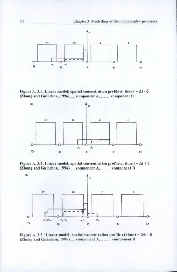
50 Chapter 3: Modelling of chromatographie processes
Figure A. 3.1: Linear model; spatial concentration profile at time t = At - 5 (Zhong and Guiochon, 1996)__component A,____ component B
D R F E D
Figure A. 3.2: Linear model; spatial concentration profile at time t = At + 5 (Zhong and Guiochon, 1996)__component A,____ component B
D R F E D
Figure A. 3.3 : Linear model; spatial concentration profile at time t = 2At - 5 (Zhong and Guiochon, 1996)__component A,____ component B

Chapter 3: Modelling of chromatographie processes 51
Figure A. 3.4: Linear model; spatial concentration profile at time t = 2At + ô (Zhong and Guiochon, 1996);__component A,____ component B
Figure A. 3.5: Linear model; spatial concentration profile at time t = 3At - S (Zhong and Guiochon, 1996);__component A,____ component B

52 Chapter 3: Modelling of chromatographie processes
Figure A. 3.6: Linear model; spatial concentration profile at time t = 6At - 6
(Zhong and Guiochon, 1996);__component A,_____ component B
R F E D
Figure A. 3.7 : Linear model; spatial concentration profile at time t > lOAt - 5 (Zhong and Guiochon, 1996);__component A,_____ component B
Influence of the diffusion and mass transfer coefficientsThe influences of the non-idealities hâve been studied with a LDF model (Zhong and Guiochon, 1997^'). The diffusion and the mass transfer résistance essentially influence the shape of the fronts and of the plateaus. Indeed, as seen in Figure A. 3.8, the fronts are less sharp in the profiles computed from a LDF model than in those obtained from an idéal model. Besides, the steps and the oscillations in the plateaus are less visible in concentration profiles simulated with a LDF model than in those simulated with an idéal model.

Chapter 3: Modelling of chromatographie processes 53
Coltune I Ceiunui U OolemA ill Colucnn tV
Figure A. 3.8: Concentration profile at steady State; simulated with an idéalmodel (... component B and__component A); simulated with a LDF model (.component B and — component A) (Zhong and Guiochon, 1997“)
Influence of the non-linearities
The study in (Zhong et Guiochon, 1997*’) has been realised on the basis a LDF model with a Langmuir isotherm for the operating conditions already used in the preceding section (LDF model with linear isotherm).
During the first periods, the plateaus of the less retained component are higher and migrate faster than in a linear LDF model. This is due to the well-known displacement effect. Indeed, because of the compétition between both components, the less retained component is displaced by the most retained component.
Moreover, as predicted by the wave theory, the highest concentrations migrate faster. Hence the adsorption fronts (column 3 and 4) are sharper and the desorption fronts (column 1 and 2) are more diffuse.
The steady-state is reached later than with the linear isotherm and the différence between the linear and the non-linear case increases with the number of switching periods. At steady-state oscillations in the plateaus are larger for the non-linear isotherms.
Figure A. 3.9 illustrâtes these conclusions at steady-state by comparing linear isotherms with non-linear isotherms.

54 Chapter 3: Modelling of chromatographie processes
1
a.8
04
0.2 ■
i0 ^
'V
tH) Toliimn I Cohimn I! Coliimn lU Column IV
Figure A. 3.9: Profiles in function of the position after 20 switches; (Zhong and Guiochon, 1997*’)Linear model in fis(a) and (b) :dotted line: component B; solid line: component ANon linear case:
Dashed line: component B; medium dashed line component A In Fig (a): bj = b2 = 0.1 In Fig (b): b) = b2 = 0.4
Long Dashed fines: component B; dotted dashed fines: component A In fig (a): bj = b2 = 0.2 In Fig (b): bi = b2 = 0.8

Chapter 3: Modelling of chromatographie processes 55
Appendix 3.2 EQUATIONS OF A SMB MODEL WITH 8 COLUMNS
In this appendix, the équations of a LDF model applied to a SMB process with 8columns (2 per zone) are given:
Initial conditions: Ca,i (0,Zi) =0 VziCb.i(0,z,)=0 Vz|Ca.2(0,Z2)=0 Vz2 Cb.2(0,Z2)=0 VZ2 Ca.3(0,Z3)=0 Vz3 Cb.3(0,Z3)=0 Vz3 Ca,4(0,Z4)=0 Vz4 Cb.4(0,Z4)=0 Vz4 Ca.5(0,Zs)=0 Vzs Cb,s(0,Z5)=0 Vzs Ca.6(0,Z6)=0 VZé Cb,6(0,Z6)=0 VZ6 Ca.7(0,Z7)=0 Vz7 Cb,7(0,Z7)=0 Vz7 Ca,8(0,Z8)=0 Vzg CB,8(0,Zg)=0 Vzg
Equations in column 1 :
3c A,1 de
dt-V, A,i 1-e
kp.A.I (<ÏA,I*'^ “<ÎA,i) + D^a_
di
3z| e^^ca,i
3zE
d^Cf3cb,I _ ^Cb,i 1-e, , eq ^ " ^B,l---------- :~kpB|(qB| ^-qB,i) + DL,B,r
dt
^qB,iat
az] e
= kpB,i(qB,i^^ ~qB,i)
azi

56 Chapter 3: Modelling of chromatographie processes
Boundarv conditions between column 1 and column 2
CA,2(t.Z2 =0) = CA,l(t,Z, =L)
‘^B,2(t.Z2 =0) = CB,l(t>Zl =L)3cA,i(t,zi =L) _ 3cA,i(t,z, =L)
9t “ 9^^
3cB,i(t,zi =L) _ 3cB,i(t,z, =L)
9t
Equations in column 2 :
^^A,2 1-e
9t
^<ÎA,2
:-V2
9t
^^B,29t
9qB,2
dz2 e
^kF,A,2(<ÎA,2*^ -qA,2)
^^B,2 1-e
*^F,A,2(1a,2*'’ “Qa,2) + Dl,a,2O^A.2
9z,2
:-V2
3t
9z2 e
= kF,B,2(qB,2^'’ -qB,2)
^ F,B,2 (qB,2*'' “ qB,2 ) + D l^,2^ ^B,2
9z,2
Boundarv conditions between column 2 and column 3 (extract output)
Ca,3(^>^3 =0) = Ca,2(1,Z2 =L)
‘^B,3(l>^3 - 0) = Cb,2(1>^2 =L) ^CA,2(t>Z2 =L) _ 9cA,2(t,Z2 =L)
9t “ ^2
^‘^B,2(l>^2 =L) 9cb_2(1>Z2 =L)
ât ^2

Chapter 3: Modelling of chromatographie processes 57
Equations in column 3 :
^ca,3 _ 3ca,3 1-e,3t
^qA,33t
^Cb,33t
9^8,3dt
= -V3 *^F,A,3(qA,3*'^ “qA,3) + ^L,A,33z3 e
= l^F,A,3(qA,3*'* ~qA,3)
^^^8,3 1-e
^^^A,3
-V39z3 e
• '^F,8,3(q8,3*'’
kF,B,3(qB,3 ^ “qB,3)"*'^L,A,39z,2
Boundarv conditions between column 3 and column 4
CA, 4(t,Z4 =0) = Ca,3(^Z3 =L)CB, 4(t>^4 = 0) = Cb 3(t,Z3 = L)
3cA,3(t>Z3 =L) 9cA,3(t,Z3=L)— = -V3-9t
3cB,3(t,Z3 =L)9t
:-V3
9z3
^Cb,3(^^3 = L) 9zi
Equations in column 4 :
9c A,4 _ ^Ca,4 1-e eq ^ ^^A,4~V4—--------------- kpA,4(qA,4 “qA,4) + DLA,49t
^qA,49t
9z4 e 9z^
-•^F,A,4(qA,4 ^ ~qA,4)
9c
9t
8,49t
8,4 _ ^Cb,4 1-e eq , . ^ ^^,4”''4^:;----------- —kp B,4(qB,4 ~qB,4 ) + Dp,A,49z4 e
■ ^F,B,4(qB,4*'’ ~qB,4)
dzA

58 Chapter 3; Modelling of chromatographie processes
Boundarv conditions between column 4 and column 5 (feed inpuO
V5CA,5(t.Z5 =0) = V4CA,4(t,Z4 =L) + VpUA(t) V5CB,s(t>Z5 =0) = V4CB,4(t,Z4 =L) + VFUB(t)
3cA,4(t,Z4 =L) 9cA4(t,Z4=L)
--------~ L) 9c34(t,Z4=L)
ai
Equations in column 5 :
^Ca,5 de a 5 1-e9t
^Qa.s9t
^^B,59t
^qB,59t
^-V5 9z5 e
l^F,A,5(qA,5^^ “^A.s)
^Cb,5 1-e
'^F,A,5 (qA,5^‘^
= -V59z5 e
kF,B,s(qB,5^^ ~qB,5)
1^F,B,5 (qfi,5eq
~qA,5) + DL,A,5d^CA,5
9z5^
9^Cb 5qB,5) + DL,A,5-------^
Boundarv conditions between column 5 and column 6
CA,6(t>Z6 =0) = CA,5(t,Z5 =L) ^B,60’^6 - 0) = Cq ^(t,Z^ = L)
9cA^(t^5 -L) _ 9ca,5(t,Z5 = L)
9t ^ 9z5
9cB,s(t,Z5 =L) 9cB5(t,Z5=L)
9^ 9^^

Chapter 3; Modelling of chromatographie processes 59
Equations in column 6
de A,6
dt
^9a,6
:-V6-3ca.6 1-t'A,6
9z6 e
eq
k F,A,6 (q A,6^^ “ q A,6 ) + Dl_a,6^^Ca,6
-•^F,A,6(qA,6 ^ ~qA,6)9t
^Cb,6 . 3cb,6 1-e, , ea ^
9t
^qB,6
:-V6
9t
9z6 E
= *^F,B,6(qB,6^^ ~qB,6)
•<^F,B,6(qB,6*'’ ~qB,6) + DL,A,6
Boundary conditions between column 6 and column 7 (raffînate output)
CA, 7(t,Z7 =0) = CA,6(t,Z6 =L)
CB, ?(t>z7 =0) = Ce,6(t,z6 =L)
3cA,6(t>Z6 =L) 9cA,6(t,Z6 =L)— = -V6-9t
3cB,6(t.Z6 =L)
9t■ = -V6
9z6
^<^B,6(^Z6 = L)
9za
Equations in column 7 :
^^A,7 1-e,3t
^qA,79t
= -V7- ^ F,A,7 (q A,7 - q A,7 ) + D l a,7dz-j E
= '^F,A,7(qA,7^'’ ~qA,7)
^^^A,7
0Z7^
^Cb,7 _ 5cbj 1-e . eq s^--------------- kpB,7(qB,7 ^ ~qB,7) + DL A,7 ------------Ot dZ-j e
^qB,7
dzn
dt ■ - F,B,7 (q B,7 “ q B,7 )

60 Chapter 3: Modelling of chromatographie processes
Boundarv conditions between column 7 and column 8
CA,8(t.Z8 =0) = CA,7(t,Z7 =L) ‘^B,8(t>^8 =0) = CB7(t,Z7 =L)
^‘'A,7(h^7 _ ^^A,7(t>Z7 =L)3t 3^^
3^B,7(t>^7 “ L) ^ 9cg 7(t,Z7 =L)
ât
Equations in column 8 :
3c A,8 3c
3t
^0a,8
-Vg A,8 1-ekF,A,8(OA,8^'' “<ÎA,8) + Dl,a,8
3t
3z8 e
*^F,A,s(0a,8^^ “0a,8)
3c0g dcQg 1-e
3t
^0b,83t
-Vg 1^F,B,8(‘1b,8*^ “<1b,8) + Dl,a,83z8 e
= 1^F,B,8(0b,8*^ ~‘îB,8)
Boundarv conditions between column 8 and column 1
9^^A,8
V|CA,i(t,z, =0) = vgCA,g(t,zg =L)
V|CB,i(t,Zi =0) = vgCB,g(t,zg =L)
3cA,g(t,zg =L) 3cA,g(t,Zg =L)
3t “ 3zg
^^B,g(t>zg = L) ^ 3cB,g(t,zg =L)
3t ^8

Chapter 3: Modelling of chromatographie processes 61
CommutationIf the fixed referential is attached to the input and output ports,
CA. lCts"® = 0,Zi) = CA,2(ts"®“' = At,Z2>
= 0,2]) = CB_2(ts"^ '
Ca,2(‘s"* = 0,Z2> = CA,3(ts"s-> = At,Z3)
= 0>Z2) = Cb 3(ts"s '=At,Z3)
Ca,3(‘s"* = 0,Z3> = CA,4(ts"*“' = At,Z4)
CB, 3(ts"" =0.Z3) = CB,4(ts"®“' =At,Z4)
CA,4(ts"^ =0,Z4) = CA,5(t3"s-l =At,Z5)
<=B,4(ts'’" = 0,Z4> = CB,5(ts"s-> = At,Z5)
CA,5(ts"^ = 0,Z5) = CA,6(ts"^“‘ = At,Z6)
‘^B,5(*s"® = 0’Z5) = CB_6(ts"® ’ =At,Z5)
CA, 6(ts"^ =0,Z6) = CA,7(ts"^"' =At,Z7)
CB, 6(ts"^ =0,Z6) = CB,7(ts"^“' =At,Z7)
= 0>Z7) = CA,8(ts"® ' = ^t,Zg)
Cb,7(‘s"* = 0,Z7) = CB,8(ts"*-' = At,Zg)
Ca.sOs"" =0,Zg) = CA,i(ts"s“' =At,Z,)
CB,g(ts"® =0>Z8) = CB,|(ts'’"''' =At,Z,)
Or, if the fixed referential is attached to the columns:
Qi-’s =Q8"s-1
Q2"s =Q,"S-1
Qj"s = Q2"s->
Q4"s = Qj"s->
Qs"s =Q4"s-1

62 Chapter 3: Modelling of chromatographie processes

Chapter 3: Modelling of chromatographie processes 63
Appendix 3.3 TRIANGLE THEORY WITHLANGMUIR ISOTHERMS
In this appendix, the équations defming the séparation zone in the triangle theory applied to the Langmuir isotherms (Mazzotti et al., 1997) are given.
The conditions for complété séparation are the following :
Hb =m™" <m, <oo
mil (™ii’™iii) ^ *^ii '^iii ™iii (fnio'^iii)
0 < mjy < m|Y (m|],m|i|)
= ^|ha + mm + bACAF(miii - mu)- ^[Ha + m,„ + bACAF(mi„ - m„)p -4HAm„, |
The conditions on mi and mjy are explicit and ensure respectively the solid phase and the liquid phase régénération in order to avoid extract and raffinate pollution from the recycling. The conditions on mu and mm are implicit and independent of those on m| and miy. They defme a triangle in the plane (mu, mm) shown in Figure A.3.9 whereStraight line « of » : (H g — (Oq (1 + b3Cgp))mi] +bgCgpCûQm jg = (Oq (H g — cûq )
Straight line « oa » :(H g -HA(l + bgCgp))m|| +bgCgpHySimjii = H^(Hg-HA)
Curve « rb » : m,,, = m+
Curve « ab » ; mm = mu
The intersection points between the straight lines are the following :
point a : (Ha, Ha) point b : (Hb, Hb) point f : (tüG, ojc)
)(Hb ~ h a ) + H aÜ)g (H b ~^f)1 Hb’ HaHb(Hb-(Of)
point r :

64 Chapter 3: Modelling of chromatographie processes
point O • f (OGk(HB-H^) + H^(H^-(OF)r'[ ' H^CHb-cOf)
with Cüt;>cûF>0, which are the roots of
(l + bAC^F +bBCBF)w “[HA(l+bBCBF) + Hg(l + bACAF)]®+HAHB =0
Figure A. 3. 9: Séparation zones defined by the triangle theory for Langmuir isotherms (Mazzoti et al., 1997)

Chapter 3: Modelling of chromatographie processes 65
Appendix3.4 APPROXIMATIONS OF SAPTIAL DERIVATIVES AT THE EXTREMITIES
centered stencil
3^Cj(t,ZQp| )
3z'■ K--2(^GPi )^i(t>2GPi ) + K^-|(^GPi )^i(t>ZGP2 )
+ K(ZgP| )Cj(t,Zopj ) + K|(ZgPj )Cj(t,ZQp_^ ) + K2(ZqPj )Cj(t,ZGP5 )
3'*Cj(t,ZGP2 )
3z‘- K_2 (Zg?2 )Ci(t,ZGPi ) + ^-i(^GP2 )^i(^>^GP2 )
+ K(Zgp2 )Cj (t,ZQP3 ) + K| (zgp2 )Ci(t,ZGP4 ) + K2(zqp2 )Cj (t, ZqPj )
3‘*Cj(t,Zcpj^j,_j )
3z^^-2 (^GP)s|G_i )^i ^GP]\ig_4 )
^ I (^GPimg_] )^i ^GP]4g_3 ) ^(^GPfjG—1 ^^^NG—2 ^
+ K ] (ZQPjyjG-i )^i ^GP]sjg—1 ^ ^2 (^GPfjG_| )^i (*•> ^GP^jq )
^‘^CjCt.ZGPfjf, )
3z'■ ^-2 (^GPng P’ ^GPng_4 )
^ ^-1 ^^GPjvjg P’ ^GPng_3 ) ^(^GP]\(g P’ ^GPnG-2 ^
+ K-i(zgPng )^i(t’^GPNG-l ) + ^2(ZgPng )‘^i(^^GPng )
Non-centered stencil :
^ Cj(t,ZQp^ )T"^---------= K.-3(ZgP] )Cj(t.ZGP| ) + K—2(2GP] )Ci(t,ZGP2 ) + K--|(ZgPi )Cj(t>ZG[^ )âz
+ ^(^GP| )Ci(t,ZQp^ ) + K.| (ZqP| )Cj(t,ZcP5 )
(t,ZQP2 )
dz^^-3(^GP2 )‘^i(^>^GP| ) + K.-2(2GP2 )^i(^>^GP2 )
+ K_|(zqp2 )Cj(t,ZGP3 ) + K(ZqP2 )Ci(t.ZGP4 ) + K](ZgP2 )Ci(t,ZGP5 )
3‘^Ci(t,ZQP3 )----------------------- = K_3 (Zqpj )Cj (t, ZqP| ) + K_2 (Zgpj )Cj (t, Zgp2 )
+ K^-i(zgP3 )Cj(t,ZGP3 ) + K(zgp3 )Cj(t,ZGP4) + K,(ZGP3 )Cj(t,ZGP5)

66 Chapter 3: Modelling of chromatographie processes
9^ ^GPnq )
dz'^^ -3 GPjvig i ^ GP]mg_4 ) + ^ -2 GP]mg i ^ GPng_3 )
^ ^-1 ^^GP]4g )^i (h ZgP]4q-2 ) ■*■ ^(^GP]4g ^GP^G-l ^
+ K^1 (^GPng )‘^i(t’^GPNG )

Chapter 3: Modelling of chromatographie processes 67
Appendix 3.5 SIMULATION PARAMETERS
Figure 2-2Ca,f= Cb,f = 0.1 vol% ; Vj„j = 2 ml, Q = 30 ml/min; e = 0.62; D = 0.0212 m; L = 0.1 m; Ha = 3.23; Hq = 4.7; Ica = 15 s''; ka = 15 s‘'
Figure 2-7: 2-8: 2-9
e = 0.83 ; Ca,f= Cb,f = 0.5 vol% ; Ni = 50 with i = A, B; Ha = 5.87 ; Hb = 8.52; 6a = 0.154 vol%-‘; be = 0.295 vol%''; At = 180s ; Q,v = 43.4 ml/min ; Qd = 20.0 ml/min ; Qii = 45.2 ml/min et Qf = 8 ml/min.
Figure 3-4
tp = 4 s, Ca,f “ Cb,f = 0.12 vol%, tp = 0.1
Figure 3-6; 3-7; 3-8
Cp = 12 vol%; tp = 4s; H = 7 ; b = 0.63, Q = 30 ml/min, L = 0.1 m ; D = 0.022 m ; e =0.6
Figures 3-9; 3-10; 3-11; 3.12e = 0.83 ; Ca,f = Cb,f = 0.5 vol% ; Ni = 50 with i = A, B; Ha = 5.87 ; Hb = 8.52; 6a = 0.154 vol% '; ba = 0.295 vol%''; At = 180s ; Qiv = 43.4 ml/min ; Qd = 20.0 ml/min ; Qii = 45.2 ml/min; Qf = 8 ml/min.
Figure 3-13e = 0.83 ; Ca,f = Cb,f = 0.5 vol% ; Ha = 5.87 ; Hb = 8.52; bA = 0.154 vol% '; ba = 0.295 vol%’’; At = 180s ; Qiv = 43.4 ml/min ; Qd = 20.0 ml/min ; Qu = 45.2 ml/min; Qf = 8 ml/min.
Figure 3-15 Kinetice = 0.83 ; Ca,f= Cb,f = 0.5 vol% ; kA'"' = 97.7 s’; ke^"' = 92.65 s'; Ha = 5.87 ; Hb = 8.52; bA = 0.154 vol%‘'; ba = 0.295 vol% '; At = 180s ; Q,v = 43.4 ml/min ; Qd = 20.0 ml/min ; Qu - 45.2 ml/min; Qf = 8 ml/min;
LDFe = 0.83 ; Ca,f= Cb,f = 0.5 vol% ; Du = 3.19®-6 m/s with i = A, B; kA"^'' = 198.3 s"' ;ke^"' = 185.3 s''; Ha = 5.87 ; Hb = 8.52; = 0.154 vol% '; ba = 0.295 vol%‘'; At =180s ; Qiv = 43.4 ml/min ; Qd = 20.0 ml/min ; Qn = 45.2 ml/min; Qf = 8 ml/min.

68 Chapter 3: Modelling of chromatographie processes
EDe = 0.83 ; Ca,f = Cb.f = 0.5 vol% ; N; = 50 with i = A, B; Ha = 5.87 ; Hb = 8.52; 6a =0.154 vol%''; 6b = 0.295 vol%''; At = 180s ; Qjv = 43.4 ml/min ; Qd = 20.0 ml/min ; Qii = 45.2 ml/min; Qf = 8 ml/min.

PART II:
CONTRIBUTIONS TO THE MODELLING OF SMB PROCESSES


Chapter 4 : A simplifiée! modelling approach to SMB processes 71
CHAPTER 4 :A Simplified modelling approach to SMB processes
4.1. Introduction
The second part of this work aims at improving SMB models. A first goal, which is pursued in the présent chapter, can be to dérivé a simplified, yet accurate enough, représentation of the SMB process. Another goal, which is discussed in Chapter 5, is to complété the description of the SMB taking into account of the presence of dead volumes.
The objective of this chapter is to build a model, for use in optimization, monitoring and control, which combines the advantages of TMB and SMB models without having their drawbacks. A model is thus sought with a similar computational efficiency as the TMB model, while reproducing the cyclic steady-state exhibited by the SMB model. To this end, different approaches hâve been studied.
The first approach (Grosfils et ai, 2003*’) considers a modification of the conventional TMB model, in which a periodic solid velocity (sinusoidal or puise velocity) is introduced. However, these models are not satisfactory. Indeed, on the one hand, a sinusoidal velocity is not able to reproduce the shape of the extract and raffinate concentration profile. On the other hand, a puise velocity induces numerical problems.
In the second approach (Grosfils et ai, 2007^), a periodic translation of the TMB of the internai concentration profiles computed numerically ffom a classical TMB is proposed. The translation vector is calculated based on the wave theory (section 3.3.2). Each point of the profile travels with its own velocity, fonction of its concentration and of the zone flow rate.

72 Chapter 4 : A simplifiée! modelling approach to SMB processes
The text is organised al follows. The principle of the translated TMB is described in details in section 4.2. The assumptions are presented in section 4.3. Section 4.4 is devoted to the présentation of the wave velocities used to translate the profile. The translation of the profile is explained in section 4.5. The introduction of the delay and the reproduction of the smoothing of the curves are described in section 4.6. Section 4.7 ends with the présentation of the results, the limitations and some discussions.
4.2. Principle of the translated TMB model
The idea behind the proposed solution is to translate the TMB profile along the z- axis during a switching period. This approach is based on the assumption that the TMB model gives an approximation of the SMB profiles at 50% of the switching period (see section 3.4.1.3.). Moreover, it exploits the fact that the temporal variations of the extract and raffinate concentrations during one switching period are due to the movement of the spatial concentration profiles through the columns in the direction of the fluid flow as shown in Figure 4-1. Hence, the translation vector is a function of the time elapsed since the last switch and of the velocity of the components in the SMB process. The latter is evaluated by application of the wave theory (section 3.3.2.) to the SMB process.
As the dynamics of the translated TMB model is not hybrid, it is expected that the computational load will be lower than with the SMB model. This will be confirmed by the simulation study reported in section 4.7.
0.6 H
Figure 4-1: Movement of the spatial concentration profiles during a switching period at steady state: dashed Unes: profiles at the beginning of a switching period, thick continuons Unes: profiles at 50 % of a switching period, thin continuons Unes: profiles at the end of a switching period

Chapter 4 : A simplified modelling approach to SMB processes 73
4.3. Assumptions
Column modelThe kinetic model is chosen for ils small computational load (a comparison of the computational expense of each model représentation is given in section 13.23.)
Column CharacteristicsIt is assumed that ail the columns hâve the same characteristics. Thus, the porosity, the mass transfer coefficients, the isotherm parameters and the hold up (and hence the time delay introduced later in section 4.6) are equal in ail columns.
In a real SMB process, the mass transfer coefficients are fonction of the zone flowrate. Hence, during the movement of the spatial concentration profiles through the columns, when a point of the profile leaves a zone for another, the corresponding mass transfer coefficients are modified. However, the translated TMB model is obtained by translating the profiles simulated with a classical TMB model which correspond to the SMB profiles at 50 % of a switching period. Hence, the mass transfer coefficients are assumed to be constant during a switching period for each point of the profile and equal to their value in the TMB model. The modification of the concentration waves due to the change of flowrates from one section to the next will only be taken into account in the translation vectors by considering that the spatial shift is a function of the zone velocity as it will be explained hereafter.
4.4. Wave velocity
As explained in section 3.3.2, according to the wave theory, the components move through the columns as nonlinear waves (Hellferich and Carr, 1993). As shown in Figure 4-2, a SMB profile is composed of desorption waves (labelled “D”) in zones 1 and II and adsorption waves (labelled “A”) in zones III and IV. In the case of Langmuir adsorption isotherms, the former are spreading, whereas the latter keep their constant pattern as already explained in section 3.3.2. (Hellferich and Carr, 1993). These properties influence the wave velocities. From the idéal chromatography theory (no diffusion, no mass transfer résistance), the following wave velocities are derived (Hellferich and Carr, 1993). For desorption waves, the velocity of component i in zone j, j = I, II, is given by:
Flowrate
D V ;
4-1

74 Chapter 4 : A simplifiée! modelling approach to SMB processes
wherede '.J
may be estimated as explained in section 3.3.2. Here, as both fronts are
increasing, the positive roots of Eq. 3-29 is used to calculate dq,,jde
In the case of adsorption waves which hâve a shock pattern (see section 3.3.2.), the velocity of component i in zone j, j = III, IV, is defined as:
i.J1 +------------- -
£ ACj j4-2
where A stands for the différence between the downstream and upstream sides of the wave. Hence, Aqjj/Acjj is calculated from the différence between the maximum and minimum values of the concentrations in the wave.
As the concentrations are unknown before the translation (cf the following section), ail the dérivatives are evaluated at an average concentration in zone j, computed ffom the classical TMB model at the considered time.
Figure 4-2: SMB profile; D : desorption wave; A : adsorption wave
4.5. Translation
For each defined position ptrans in zone j, the concentration of component translated TMB is calculated as follows:
translated TMB(Ptrans>0
TMB•O (Ptmb(*s)>0
in the
4-3
where Ptmb Os ) = Ptrans-^Os) 4-4

Chapter 4 : A simplified modelling approach to SMB processes 75
where ts is the time elapsed since the last switch, and t = nsAt + tg is the current time with ns, the number of switches already performed.
The translation vector tr is equal to 0 at 50% of the switching period in agreement with the assumption that the TMB model represents the SMB at 50% of the switching period. Moreover, to reproduce the movement along the z-axis (cf Figure 4-1), the translation direction of the TMB profile is pointing to the right (tr > 0) if ts is larger than At/2, and to left (tr < 0) when ts is smaller than At/2. The translation length is a ftinction of the time to or from the half of the current
switching period ( tgAt
2) (cf Figure 4-3) and of the velocity of the components in
the SMB process (Eq.4-1 or 4-2).
Figure 4-3: Evolution of the norm of the translation vector in function of ts
Hence, the translation is calculated as follows:
tr(ts) = sign f At^^'i i
Atts
l 2 j ^ 2
, At^4-5
with Vjj, obtained from Eq. 3-1 or 4-2 depending on the considered zone j.Notice however that (4-4) can only be used in (4-3) when both p,rans(ts) and piMB(ts) belong to the same zone (prMB(ts) is in zone j if Zj_| < Ptmb0s)< Zj where Zj is
the position corresponding to the end of zone j). If p,rans and pTMB(ts) belong to two different zones, the displacement of the component through the two neighbouring zones has to be evaluated with the appropriate velocities.
The following two possible cases are successively considered:1. Ptrans in zone j, pTMB(ts) in zone j-1 (Zj., > pjMB(ts)) ( Figure 4-4)2. ptrans in zone j, PTMs(ts) in zone j+1 (Zj < pTMB(ts))
1 ■ PiMB(ts) niust be calculated taking the displacements, with respect to the limit Zj.i, of component i in zone j-1 and zone j into account. As seen in Figure 4-4,

76 Chapter 4 : A simplified modelling approach to SMB processes
the new position is simply obtained by considering the appropriate velocities, i.e.,P _^
velocity Vy in zone j where component i spends a time ------— and'.J
velocity vy.i in zone j-1 where component i spends the remaining time At
t^onej-i = ts —2—*zone,j • Hence pTMB(ts) is calculated as follows (in zone j-1):
PtMb(^s) = Zj.i - Vj j^it^onej-l 4-6
The concentration of eomponent i in the translated TMB at position p,rans (in zone j) is then given by:
translatée! TMB(Ptrans > 0 — Cjj-i (Ptmb(^s)>^)i.J 4-7
2. Following the same line of thoughts, component i spends a time^ _P
tzonej in zone j, where it travels at velocity Vjj and a remaining time
t
as:
i.jAt
zonej+i =—— ts “ t^one.j 20"^ j+1 at veloclty Vy+j, so that piMB(ts) îs calculated
Ptmb(^s) ^i,j+l^zoneJ+l 4-8
The concentration of component i at position p,„„s in zone j is therefore given by:
Citranslatée!
(Ptrans > 0 “ Cj j+1 (PxMB(is)>0i.J 4-9
Figure 4-4: Schematic explanation of Eq. 4-8.

Chapter 4 : A simplified modelling approach to SMB processes 77
4.6. Time delay and smoothing of the concentration curves
In experimental data, a time delay between the occurrence of the switch and the beginning of the increase (decrease) of the extract (raffinate) concentration profiles may appear, as shown in Figure 4-5. Moreover, extract and raffinate concentration curves are usually smoother than predicted by the SMB model, i.e., the increase of the extract concentration and the decrease of the raffinate concentration at the switching time is usually less abrupt than predicted by the SMB model (cf Figure 4-5 and Figure 4-6). Both phenomena are physically due to hold-up and mixing éléments as described in (Strube and Schmidt-Traub, 1998) and (Beste et ai, 2000). Their introduction in the classical SMB or TMB models is not straightforward. However as explained hereafter, they are very easily reproduced with the translated TMB model by modifying équations (4-3) to (4-9) or by performing an additional translation of the profiles.
Figure 4-5: Experimental results: Ca in the raffinate at steady-state. Operating conditions described in Table A. 4.2

78 Chapter 4 : A simplified modelling approach to SMB processes
Time delay
Figure 4-6 : Ca in the rafflnate at steady State. __ SMB model,.... Translated TMB model with time delay and smoothing (parameters and operating conditions in Table A.4.1, case A, to = 10s, t, = 20s)
Figure 4-7: Evolution of the translation vector in function of ts; __without delay; — with delay
Time delayA time lag, to, is simply introduced by delaying the translation defmed by Eqs. 4-3to 4-9. The switching occurs now at At + t^. Figure 4-7 shows the évolution of thenorm of the translation vector taking the time delay into account. When ts is smallerthan the time delay, the translation corresponding to the preceding switching period

Chapter 4 : A simplifiée! modelling approach to SMB processes 79
is still performed. When ts is equal to to, the switching occurs in the translated TMB model and the translation corresponding to the current switch is then executed.In practice, this time lag is introduced by replacing in Eqs. 4-3 to 4-9 by ts* which is calculated as follows:
if
tg — At + tg — tjjelse 4-10
The effect is shown in Figure 4-6. It is assumed that the dead volume is the same for each column.
Smoothing of the concentration curvesDuring each switching period, the spatial concentration profiles move in the direction of the fluid flow (i.e. to the right). At each switching time, ail the inlet and outlet ports are switched in the direction of the liquid flow. This means that the concentration profiles obtained at the end of the switching period jump one column backward, causing rapid variations of the extract and raffmate concentrations.
In the SMB model, this is simulated with Eq. 3-34 or 3-35 which has immédiate effect. Hence, the increase of the extract concentration and the decrease of the raffmate concentration are quite sharp.
To reproduce qualitatively the smoothing of the extract and raffinate concentration curves observed experimentally, a progressive switch is introduced in the translated TMB model. This is performed by gradually translating, at each switching time, the concentration profiles obtained at the end of a switching period from the right to the left with a constant velocity. Only one parameter must be chosen: t„ the time necessary to switch. It could be equal to the duration of the increase (decrease) of the raffinate (extract) concentration curves due to the switch. This translation is thus performed Ifom ts = 0 until ts = t,.
Hence, two translations are successively applied;a. when 0 < tg ^ t,, the translation simulating a progressive switch;b. when ts > t„ the translation described in section 4.5.
Each step is successively detailed below.
a. For each defined position p„ans in zone j, the concentration of component i in the translated TMB is calculated as follows:
translated TMB/^ TMB/ tt/- \i (Ptrans.t) = Ci,j (PjMB Osl-t)

80 Chapter 4 : A simplified modelling approach to SMB processes
Equation (4-11) expresses the fact that the translation reproducing a progressive
switch, — tg, is applied to the profile obtained at the end of a switching period
which is calculated at Ptmb( ts = )• When ts is equal to t,, the length of thetranslation is equal to the column length, L. Ptmb( ^ = At ) is calculated as explained in section 4.5 and represents the translation performed to obtain the profile at tg = At.
In practice, a change of zone must be taken into account and the concentrations are calculated as follows (see section 4.5 and équations 4-3 to 4-9):
if 2j-i < Ptmb < Zj,_ translated TMB. T
(Ptrans’V ''i.j
else if Zj_i > Pj^b >_ translated TMB/
(Ptrans’^)
else Cj TMB (P,rans,t) = Ci,j„™®i
4-12TMB/
b. when ts > t„ the translation described in section 4.5 is applied. In order to take the delay introduced by the smoothing into account in équations 4-3 to 4-9, tg is replaced by tg calculated as follows:
if te > t,« 4-13
ts -tg-t,The results are shown in Figure 4-6.
4.7. Results, limitations and discussions
ResultsIn this section, simulation results obtained with the translated TMB model are compared with those obtained with the SMB model.
The parameters and operating conditions that hâve been used in the simulation study are given in Table A. 4.1. The results presented in Figure 4-8 and Figure 4-9 show that the raffinate and the extract signais of the translated TMB and SMB models are in good agreement. Particularly, in Figure 4-10, the displacement of the concentration profile along the z-axis during a switching period, as reproduced by the translated TMB model, is close to the prédiction of the SMB model. The translated TMB is also able to simulate the start-up of the process as shown in Figure 4-11 and Figure 4-12 and the change of process operating conditions as seen in Figure 4-13 and Figure 4-14.

Chapter 4 : A simplified modelling approach to SMB processes 81
Moreover, Table 4-1 shows the ratio of the simulation time of the translatée! TMB model as comparée! to the simulation time of the SMB model. The sampling period represents the time between two instants at which the simulated extract and raffinate concentrations are recorded. In almost ail cases, the simulation time of the translated TMB model is, at least, five times smaller than the one of the SMB model. In conclusion, the translated TMB model is able to reproduce the cyclic évolution of the SMB process, like the SMB model, with a highly reduced computational load.
Figure 4-8: Extract concentration at steady State:__SMB model,- - translated TMB model (Table A. 4.1, case A)
Figure 4-9: Raffinate concentration at steady-state:__SMB model,- - translated TMB model (Table A. 4.1, case A)

82 Chapter4 : A simplified modelling approach to SMB processes
Figure 4-10: Internai concentration profile In steady-state at 0%, 50% and
100% of the switching period: SMB model, “ “ translated TMB model(Table A. 4.1, case A)
Figure 4-11: Extract concentration at the start-up of the plant:
__ SMB model,___ translated TMB model (Table A. 4.1, case B)

cb(
voI%
) C
a(vo
I%)
Chapter 4 : A simplifiée! modelling approach to SMB processes 83
Igure 4-12: Raffinate concentration at the start-up of the plant:
SMB model,__ translatée! TMB model (Table A. 4.1, case B)
time (s) «10*
Figure 4-13: Extract concentration, change in the process operating conditions:
__ SMB model,___translated TMB model (Table A. 4.1, case B -¥ case A)

84 Chapter 4 : A simplified modelling approach to SMB processes
Figure 4-14: Rafflnate concentration, change in the process operating
conditions:__ SMB model,___ translated TMB model (Table A. 4.1, case B —>case A)
Table 4-1: the ratio r of the simulation time with the modifîed TMB model over the simulation time with the SMB model, for a 8 columns SMB process (Table A.4.1. case A)
Case Sampling period rA 1 s 0.17A 5 s 0.035B 1 s 0.17B 5 s 0.035C 1 s 0.84C 5 s 0.2
LimitationsAs the translated TMB model is based on the assumption that the TMB model is a good approximation of the SMB model at 50% of a switching period, the translated TMB model gives poor results when this assumption is not verified. This is especially the case when the diffusion in the process is low, i.e., when mass transfer coefficients are large. Indeed, in this case, the TMB model is not able to reproduce the oscillations originating from the thermodynamical nature of the SMB process as explained in (Zhong and Guiochon, 1997) and recalled in Appendix 3.1.
Moreover, the TMB model is not able to reproduce ail the effects due to thepresence of dead volume introduced by connecting tubes, pumps or detectors.Indeed, as it will be explained in chapter 5, a part of the dead volume switches ateach switching time and another part is fixed. This relative movement may, in some

Chapter 4 : A simpliFied modelling approach to SMB processes 85
conditions (like small flow rates), imply the appearance of bumps in the concentration profiles. However, the translated TMB model is only able to simulate the time delay effect and the smoothing of the concentration curves.
SMB process with a small number of cohimnsAs it is well known, the différences between SMB and TMB models become more significant when the number of columns decreases (Pais et ai, 1998). In our study, the quality of the simulations obtained with the modified TMB with a low number of columns can be improved by estimating the mass transfer coefficients of the TMB model in order to minimize the déviations between the internai concentration profiles generated by the TMB and SMB models. This can be written formally as:
2^,rel = arg mm
"posZ Z
=A,B p=l4-14
V ywith CsMB, the SMB concentration profile at 50% of the switching period at steady- state and Cjmb, the TMB concentration profile at steady-state. Opos is the number of positions considered on the z-axis. More details about this estimation technique are given in chapter 6.
With this approach, the results obtained with the translated TMB model are not significantly affected when the number of columns decreases as shown in Figure 4-15 and Figure 4-16. However, the computational load réduction is less significant since the simulation time of the SMB model with 4 columns is quite short. Even in this limiting situation. Table 4-1 shows that simulation times are however shorter with the translated TMB than with the SMB model.
Figure 4-15 : Extract concentration:__ SMB model,___ translated TMBwith identification of mass transfer coefficient
(k^' =39.1m~*,k3’ =62.62m“'), - - translated TMB model (Table A.4.1, case C)

86 Chapter 4 : A simplifiée! modelling approach to SMB processes
Figure 4-16: Raffinate concentration:__SMB model,______translatée! TMBwith identification of mass transfer coefficient
=39.1ni“',icB' =62.6m“'), --translated TMB model (Table A. 4.1,
case C)
RemarkNote that a somewhat similar idea bas been exploited to develop a parametric model for a State observer dedicated to a SMB process (Kleinert et ai, 2005). In particular, a wave front model, which describes the parts of the profiles with low concentration, is obtained by introducing a spatial shift into the analytical stationary solution of the TMB model with linear isotherms. Bach wave front is assumed to travel with a constant velocity during one switching period. The model parameters détermine the form, the position and the velocity of the wave fronts. If the parameters are interpreted as model State, a three-dimensional linear state-space model is obtained. The State is then estimated by a Luenberger observer given some measurements of each wave front concentration. Hence, the model proposed in (Kleinert et ai, 2005) has particularly been built for State observation and gives only the parts of the profile with small concentrations where linear adsorption occurs.
The Work reported here has been developed independently (Grosfils et ai, 2003^). The model introduced here is quite different as it is built by effecting a translation of the internai concentration profiles computed numerically from a classical TMB model with non-linear isotherms. The translation vector is calculated based on the wave theory (Hellferich and Carr, 1993). Each point of the profile travels with its own velocity, fonction of its concentration and of the zone flow rate. The results are also different as the whole profile and its cyclic évolution in fonction of time are reproduced here with a simulation time highly reduced in comparison with the SMB model. The model is also able to cope with a low number of columns (which is not the case for the modelling approach developed in (Kleinert et ai 2005)). Moreover, it reproduces the time delay and the smoothing of the extract and raffinate concentration curves observed experimentally.

Chapter 4 ; A simplified modelling approach to SMB processes 87
4.8. Conclusion
Simulated moving bed processes are usually represented by simplified models (so called TMB models), in which the solid movement is assumed to occur in a eontinuous way, or by more rigorous models (so called SMB models), in which the discrète nature of the solid movement is taken into account. Of course, the hybrid dynamics of the SMB models makes them more computationally demanding than their TMB counterparts. The main advantages of SMB models are that they are able to reproduce the cyclic steady State observed in real-life operation.
The contribution of this study is to propose a modified TMB model, which retains the original TMB model simplieity, and therefore its relatively modest computational load, but which also captures the essential features of the SMB cyclic steady State. This model is also able to reproduce the time delay and the smoothing of the extract and raffinate concentration curves observed experimentally.
The classical TMB model has already demonstrated its usefulness for optimising the operation of SMB processes (Kloppenburg and Gilles, 1999), based on the assumption that the TMB model represents well the average behaviour of the real process. It is expected that the proposed modified TMB model conveys more information on the process dynamics, and therefore has potentials (to be explored in future studies) for process optimization and control.

88 Chapter 4 : A simplifiée! modelling approach to SMB processes
APPENDIX 4.1.: PARAMETERS AND OPERATING CONDITIONS
Table A. 4.1: Parameters and process operating conditions for the séparation of two cycloketones using a preparative-scale SMB unit
Case A B CConfiguration 1-1-2-1 2-2-1-2 1 - 1 - 1 - 1Column length (m) 0.25 0.25 0.5Column diameter (m) 0.02 0.02 0.02Overall void fraction 0.83 0.83 0.83k^' (m-') 97.73 97.73 195.5kB^='(m-') 92.65 92.65 185.3Feed concentration (vol%) 0.5 0.5 0.5Ha 5.87 5.87 5.87Hb 8.52 8.52 8.52Ba (vo1%"‘) 0.154 0.154 0.154bB(vol%-') 0.295 0.295 0.295Switching time (s) 180 180 360Qu (ml/min) 45.2 43.96 45.2Qiv (ml/min) 43.4 44.72 43.4Qf (ml/min) 8 4.45 8Qd (ml/min) 20 15.4 20
Table A. 4.2 : experimental plant and process operating conditions of Figure 4-5: séparation of cyclopentanone and cycloheptanone with a mixture ofn-hexane and ethyl acetate as solvent
Configuration 2-2-2-2Column length (m) 0.25Column diameter (m) 0.02Feed concentration (vol%) 0.5Switching time (s) 180Qu (ml/min) 45.2Qiv (ml/min) 43.4Qf (ml/min) 8Qd (ml/min) 20

Chapter 5: Extra-column dead volume modelling 89
CHAPTER 5 :Extra-column dead volume modelling
5.1. Introduction
In this chapter, a précisé model of the plant is built. With such a model, fictitious measurements giving an accurate représentation of the working of the plant may be generated. This is useful for the development and the validation of methods to optimize, control and monitor the SMB processes.
In the literature, many comparisons hâve been performed between experimental concentration profiles and simulated profiles for SMB processes. In most of the reported results, discrepancies are observed between the experimental profiles and the simulated ones. Two critical points are mentioned. On the one hand, the parameters are often roughly estimated ffom few experiments (Strube et al., 98; Strube et al., 97; Pais et al., 97) or modified heuristically to minimize the différence between both profiles like in (Lehoucq et al., 2000) and (Haag et al, 2001). This problem is the subject of the third part of this work. On the other hand, the presence of the dead volumes influences significantly the concentration profiles (Beste et al., 2000; Strube et al., 1998, Antos et al. 2001). In the literature, dead volumes are usually taken into account in the détermination of the operating conditions by modifying équations of the triangle theory in some papers (Migliorini et al, 1999, Pedeferri et al, 1999, Abel et al, 2005, Katsuo et al, 2009) but the introduction of the dead volumes in the SMB models is seldom considered (Beste et al, 2000; Migliorini et al, 1999). Hence, there is obviously a need for an effective modelling of the dead volumes. The problem is the subject of the présent chapter.
In the studied installation (cf Figure 5-1), contrary to usual configurations where theinlet and outlet ports are switched, a multifunctional valve allows the rotation of thecolumns at each switching time. As pumps and detectors are introduced between thecolumns of this SMB process, it tums out that the extra-column dead volume can not

90 Chapter 5: Extra-column dead volume modelling
be neglected. In this chapter, the model developed in (Migliorini et al., 1999) is adapted to this kind of SMB: fixed and moving dead volumes are introduced to take into account the real configuration. The general mass balance équations in a dead volume are first given. Then, the définition and the relative movement of the dead volumes are described. Next, ail the modifications of the SMB models performed to introduce the dead volumes are presented. Finally, the model is validated with experimental data.
Note that the following conventions will be used:the columns are numbered; at the start-up column 1 follows the desorbent input; column 2 is the following in the direction of the fluid flow, and so on.a position is defined as a place dedicated to the columns in the unit; some are really occupied by a column, others by a capillary replacing the column.
Columns switch when the rotative valve switches whereas positions are fixed.
Figure 5-1: Schematic représentation of the Knauer CSEP C912 unit (Max Planck Institute, Magdeburg, Germany) with 8 columns

Chapter 5: Extra-column dead volume modelling 91
5.2. General équation of mass balance in the dead volume
As introduced in section 3.4.2.2, the mass balance équation in each dead volume d is calculated as foliows (Migliorini et al, 1999):
^Cj,d9t
9cj.ddzd
+ D(i 3^cj.d
W5-1
with vj, the velocity in the dead volume d, Dj, the diffusion coefficient in the dead volume d.
As most of the dead volumes consist of tubes where plug flow conditions may be considered, Dj is very small (= le-9 mVs).
5.3. Dead volume in the circulating loop
In (Migliorini et al, 1999), two dead volumes are attached to each column: one located before, another after. However, in the experimental plant of the Max Planck Institute of Magdeburg (Figure 5-1), a part of the dead volume is moving, the one associated to the detectors UV3 and UV4, and another part of the dead volume like , the one associated to the pumps is fixed. Hence, as seen in Figure 5-2, at the n"* switching period, the dead volume at position p where column m is located is divided into four parts, two moving, two fixed:
the dead volume which is located before column m andcorresponds to the connections between the valve and the column m or inside the valve; this dead volume switches with the column at each sampling time;the dead volume which is located after column m and correspondsto the connections between the column m and the valve or inside the valve; this dead volume switches with the column at each sampling time; the dead volume which is situated before column m andcorresponds to the pumps, P1 and P2, and connections ffom the inlet ports; this dead volume doesn’t move;the dead volume which is situated after column m and correspondsto the connections to the outlet ports or to the pumps P1 and P2; this dead volume doesn’t move;
Hence, if the fixed referential is associated to the columns, the switching of the dead volumes associated to the inlet and outlet ports, Vd p’’®"''’ and is modelled byconsidering that the concentration profiles in respectively dead volume, and
at the beginning of a switching interval are equal to the profiles obtained in

92 Chapter 5: Extra-column dead volume modelling
the dead volume and at position p-1 at the end of the previousperiod:
Ci,dp(ts"* = O.Zdp) = Cj,dp-i(ts"* ' = At,Zdp_|) 5-2
with Ci,dp, the concentration of component i in the dead volumes Vd.p'”"'*’ and V<j p'’°"’“'^
at position p. At is the switching period and tg"® is the time elapsed since the nj* switching.
Note that as explained in section 2.4. and illustrated on Figure 5-1, there are only 8 columns instead of 12 and the free ports are connected by short capillaries. In this case, if position p is not occupied by a column, and are directlyconnected and include the dead volume of the capillary.
Figure 5-2: Schematic représentation of the dead volume surrounding a column in the considered SMB unit
5.4. Dead volume of the input and output Unes
The dead volumes between the SMB plant and the UV detectors in the extract and raffmate output are fixed and their model équations follow équation 5-1.
The dead volume between the feed tank and the SMB unit is modelled by introducing a time delay in the modelling of the injection of the continuons feed flow. Hence, équation 3-37 describing the inlet concentration profile of component i becomes:

Chapter 5: Extra-column dead volume modelling 93
if t<tdinUi(t) = 0
else
Uj(t) = CF,i(l - exp(-(t -) / ttr))
5-3
where “^djn with Qp, the feed flow and , the dead volume before
the SMB unit. t,r characterizes the rise time of the step and has been chosen equal to 0.1 s. Cfj is the feed concentration of component i.
5.5. Boundary conditions
The boundary conditions in the liquid and the solid phase are obtained by expressing simple mass balances and simple advection équations for each component i ( i = A, B ) at the transition between two dead volumes or between a dead volume and a column. They hâve the same fomi as those given in (Haag et al., 2001) for transition between two columns (section 3.4.2.1).
5.6. Measurement équations
As explained in the présentation of the SMB facilities available at MPI in section 2.4., it appears that, in the considered concentration range, the UV signal is equal to the weighted sum of the concentrations of the two products. The measurement équations which will be given here model the UV detectors. The model validation is performed by comparing experimental concentration profiles with simulated ones.
The extract detector, UV 1, is fixed. The measurement équation is written:
y UVI (0 - C A,dE (T LdE > c F 1 ^ B,dE (f ^dE > ^ F 1 (®)
with Cj_dE, i = A, B , the concentration of component i in the dead volume between the SMB unit and the UV detector and Lje, the length of this dead volume. Cp is a 2X1 vector containing the feed concentration of component A and B. UV| = [UV| (A) UV] (B)] is a vector containing the calibration coefficients for detector UVl.

94 Chapter 5: Extra-column dead volume modelling
The raffinate detector, UV2, is also fixed. The measurement équation is written:
y UV2 (0 - c A,dR (t. L dR, c P )UV2 (A) + c B (JR (t, L jjR, c P )UV2 (B)
with Cj dR, i = A, B , the concentration of component i in the dead volume between the SMB unit and the UV detector on the raffinate line and L^r, the length of this dead volume. UV2 =[UV2(A) UV2(B)] is a vector containing the calibration coefficients for detector UV2.
The detectors UV3 and UV4 are placed in the circulating loop. UV3 (UV4) is located in the dead volume following the column II (VI) placed at position 2 (8) at the start-up of the experiments.
yuV3(0 - CA,d2(bL(juv3>^F)UV3 (A)d-0342 (b LdUV3 > )UV3 (B)
y UV4 (0 = c A,d6 (b L dUV4 > ^ F )UV4 ( A) -F C 345 (b L juV4. C F )UV4 (B)
with Ci,d2 (Ci.dd). the concentration of component i in the dead volume attached to column 2 (6), Lduv3 (Lduva), the position of the detector UV3 (UV4) in the dead volume of column 2 (6). UV3 (UV4) is a vector containing the calibration coefficients for detector UV3 (UV4).
5.7.Numerical simulation
Equations 5-1 are solved numerically with the équations of the column model using the method of fines (cf section 3.6). Ail the dead volumes in the circulating loop hâve the same number of grid points.
5.8. Validation with experimental profiles
In this section, the SMB model with the proposed dead volume models is validated with experimental data collected at the Max Planck Institute of Magdeburg. The model and the simulation operating conditions are given in appendix 5.1. Model and simulation parameters are summarised in the last Appendix of Chapter 8, Appendix8.3. The estimation of the model parameters is described in details in Part 3.
To illustrate the importance of a proper modelling of the dead volumes, Figure 5-3 to Figure 5-10 show the experimental profiles and the results of simulations for different approaches to introduce the dead volumes:
a) simulations performed with fixed and mobile dead volumes;b) simulations realised with ail the dead volumes set to zéro ;

Chapter 5: Extra-column dead volume modelling 95
c) simulations obtained with ail the dead volume attached to the columns, as considered usually;
d) simulations executed with ail the dead volume fixed.
The simulations hâve been performed with the model parameters (isotherm parameters and mass transfer coefficients) identified in Chapter 8. In the following figures, it appears that the best way to reproduce the amplitude of the concentration signais and the “bumps” in the concentration profiles is to consider that a part of the dead volume is moving and another is fixed during switching. Moreover, Figure 5-10 shows that the change of the amplitude of the extract peak in fonction of the position of the columns is aiso well reproduced with fixed and moving dead volume which is not the case with the other configurations. The remaining différences between the experiments and the simulation results obtained with fixed and mobile dead volume models, may be explained by errors in the parameters and operating conditions or small variations of parameters among the columns as it will be discussed in the part devoted to parameter estimation (section 8.6).
4500 4550 4600 4650 4700 4750 4800 4850 4900 4950 5000lime (s)
Figure 5-3: Case I (Table A. 5.1): UVl signal (extract);• experimental signal;__dead volume fixed and moving; - - ail thedead volume moving; dead volumes neglected;__all the deadvolume fixed

96 Chapter 5: Extra-column dead volume modelling
Figure 5-4: Case I (Table A. 5.1): UV2 signal (raffinate);• expérimentai signai;__dead volumes fixed and moving; - - ail thedead volume moving; dead volumes neglected;__ail the deadvolume fixed
time (s)
Figure 5-5: Case I (Table A. 5.1): UV3 signal; • experimental signal;__dead volumes fixed and moving; - - ail the dead volume moving;
dead volumes neglected;__ail the dead volume fixed

Chapter 5: Extra-column dead volume modelling 97
time (s)
Figure 5-6: Case III (Table A. 5.1): UVl signal (extract); •experimental signal; __dead volumes fixed and moving; - - ail thedead volume moving; dead volumes neglected; __ ail the deadvolume fixed
-0.053600 4000
Figure 5-7: Case III (Table A. 5.1): UV2 signal (raffinate);• experimental signal;__dead volumes fixed and moving; - - ail thedead volume moving; dead volumes neglected;__ail the deadvolume fixed

98 Chapter 5: Extra-column dead volume modelling
Figure 5-8: Case III (Table A. 5.1): UV3 signal; • experimental signal;__dead volumes fixed and moving; - - ail the dead volume moving;
dead volumes neglected;__ail the dead volume fixed
Figure 5-9: Case II (Table A. 5.1): UV3 signal; • experimental signal;__dead volumes fixed and moving; - - ail the dead volume moving;
dead volumes neglected; ail the dead volume fixed

Figure 5-10 : Case I (Table A. 5.1): UVl signal; • experimental signal;__dead volume fixed and moving;—ail the dead volume moving;___dead volumes neglected; ail the dead volume fixed
OvO
Chapter 5: Extra-colum
n dead volume m
odelling

100 Chapter 5: Extra-column dead volume modelling
5.9.Conclusions
In the studied SMB plant, the extra-dead volume introduced by the valves, the connecting tubes and the pumps is particularly large. Hence, its introduction in the SMB model turns out to be necessary. Like in other studies, dead volumes are described by convection - diffusion équations. However, a new approach to model the movement of the dead volumes is proposed here. The main idea is to introduce in the model the relative movement of the dead volumes which really happens in the process. Indeed, at each switching time, a part of the dead volume of the circulating îoop switches with the SMB columns whereas another part does not move. By comparing experimental SMB profiles with simulated profiles, the validation of this approach has been performed with success.

Chapter 5: Extra-column dead volume modelling 101
Appendix 5.1. Parameters and operating conditions
SMB experiments are performed on the unit described in section 2. The three operating conditions (case I, Il and III) are described in Table A. 5.1. The details about the séparation used and of the geometrical data of the unit are given in section 8.2. The estimation of the model parameters is described in details in Part 3.
Table A. 5.1: Operating conditions
Case I II IIIFeed concentration (vol%) 1.456 1.456 0.73Cp.A ~ Cp.BSwitching time (s) 150 130 150Qu (ml/min) 15.6 28.7 15.6Qiv (ml/min) 17.9 27 17.2Qf (ml/min) 10.6 8.4 10.6Qd (ml/min) 32.5 31.3 32.5


PART III:
CONTRIBUTION TO PARAMETER ESTIMATION IN SMB PROCESSES


Chapter 6: Introduction to direct and inverse methods 105
CHAPTER 6 :Introduction to direct and inverse methods
6.1. Introduction
As seen in Chapter 3, the SMB models consist of the mass balance équations of the components to separate in the solid and in the liquid phases. A first-principle SMB model usually includes the isothenn parameters, the column porosity, the diffusion and/or the mass transfer coefficients. Typically, ail these parameters are determined ffom batch experiments, performed on analytical columns or on SMB columns.
The aim of this third part is to develop a parameter estimation procedure dedicated to SMB models for binary mixtures, providing parameter estimâtes as well as associated confidence intervals. In view of the industrial constraints, this method must be fast, efficient and économie (both in terms of time and product consomption).
The column porosity, the mass transfer coefficients and the diffusion coefficients are generally obtained ffom simple methods requiring injection of peaks at the column inlet (Altenhôner et al., 1997). However, these methods are based on assumptions that are not verified in practice (e.g. idéal conditions) and they do not provide an estimation of the error on the estimated parameters.
The isotherm parameters are often determined by direct static or dynamic methods in a batch setup. Static methods use the information about the equilibrium States only and are time consuming. The dynamic methods use the response curves to different changes in the column inlet. Popular dynamic methods include the frontal analysis (FA), the elution by characteristic point (ECP), the frontal analysis by characteristic point (FACP) and the perturbation method (Seidel-Morgenstern, 2004). These methods are usually based on assumptions that are not verified in practice (e.g. idéal conditions). Some of them are not convenient for determining multicomponent isotherms (like ECP and FACP), are limited to a spécifie isotherm équation (e.g. methods based on the h-transform), or are slow and require significant

106 Chapter 6: Introduction to direct and inverse methods
amounts of products, like the frontal analysis. None of them gives an estimation of the error on the estimated parameters.
Another dynamic method for estimating the isotherm parameters is called model identification, inverse method, or peak fitting. The unknown parameters are determined by minimizing a measure of the déviation between the experimental profiles and the profiles simulated with the chromatographie model. Usually, elution peaks are used. In (Amell et al, 2005), an inverse method on plateaus is presented but it requires a large amount of products. Several isotherm models hâve been considered like, for example, the Langmuir isotherms (Felinger et al, 2003a, Zhang et al, 2001, Antos et al., 1999, Miyabe et al, 2000, James et al, 1999), the Tôth model (Felinger et al., 2003b), the Moreau isotherm (James et al, 1999), the Jovanovic - Freundlich model (Quinones and Guiochon, 1998), or neural networks (Gao and Engell, 2005). The model identification has already been applied in previous studies and has given relatively good results in batch experiments as compared to frontal analysis. However, only a few papers report on the use of the parameters identified from batch experiments in SMB models (Juza, 1999; Lehoucq et al, 2000, Ching et al, 2000), and some reported results are not conclusive (Juza, 1999, Ching et al, 2000).
In addition, several issues remain unaddressed in the reported studies. Most of the authors use an idéal model or an equilibrium dispersive model with numerical dispersion (Dose et al, 1991; James et al, 1999; Felinger et al, 2003b; Amell et al, 2005, Forssen et al, 2006). This implies that the diffusion phenomenon is identical for both components which is not realistic. Some methods are applied to one component Systems only (Dose et al, 1991, Cavazzini et al, 2003; Antos et al,2000) . Moreover, no systematic method for the estimation of the errors on the estimated parameters is reported. Indeed, often the error is only evaluated for some of the estimated parameters (Ching et al, 2000, Antos et al, 2000; Zhou et al, 2003; Quinones and Guiochon, 1996). Besides, the description of the method used for the error évaluation is only given in (Antos et al, 1999). The influence of the experimental errors on the estimated parameters has been studied in (Zhang et al,2001) and the problem of local minima has been mentioned in (James et al, 1999, Zhang et al, 2001, Quinones et al, 1998) but, to the author’s knowledge, no systematic identifiability study has been performed yet.
On the other hand, only a few studies report on model identification from SMB experiments. In (Zimmer et al, 1999), the parameters of a linear isotherm in an equilibrium-dispersive model are identified. In (Toumi and Engell, 2004), the Henry coefficients, the mass transfer résistances and the reaction constant of a reactive general rate model with hyperbolic isotherm are determined from batch experiments while the remaining isotherm parameters are estimated from SMB experiments. In both papers, certain parameters are not identified, e.g. the diffusion coefficient in (Zimmer et al, 1999) or the particle diffusion and particle porosity in (Toumi and Engell, 2004), and no confidence intervals on the estimated parameters are given.

Chapter 6: Introduction to direct and inverse methods 107
The aim of this third part is to develop an identification method for determining, with good accuracy the isotherm parameters as well as the mass transfer coefficients and/or the diffusion coefficients for use in a SMB model. To this end, elution peaks obtained by experiments on one SMB column are exploited.
Distinctive features of the présent study are the following:
The chromatographie model is chosen within a class of three classical models (equilibrium dispersive, kinetic and LDF models) thanks to a systematic comparison of the identifiability and of the computational load of the three model types.Parameter identifiability is thoroughly investigated, including parameter sensitivity, experiment design and the influence of local minima on the optimization problem.Confidence intervals are provided for each of the estimated parameters and confidence envelopes are computed for the simulated SMB profiles.
The présent chapter gives an introduction to some direct methods and to the inverse method. This will help to understand the development and the validation of our approach presented in chapters 7 and 8. First a révision of the model équations is presented in order to specify and to introduce the standard form of the model used in the System identification literature. Next, some classical direct methods used to détermine the initial estimâtes of the parameters are described. Finally the identification method is presented.
6.2.Modelling and unknown parameters
In the first part of this work, macroscopie models aimed at providing a satisfactory reconstruction of the elution peaks and SMB profiles hâve been selected, namely the equilibrium dispersive model, the LDF model, and the kinetic model. They hâve nearly the same complexity and they yield similar elution or SMB profiles. In chapter 7, these models will be compared to détermine which model is the best in terms of parameter identifiability and computational load. The importance of the latter criterion results from the fact that a large number of simulation runs has to be performed during the numerical optimization needed for parameter estimation.
In this section, these three SMB models are presented, as well as the conditions relative to a batch experiment on a SMB column.

108 Chapter 6: Introduction to direct and inverse methods
6.2.1. SMB modelling
As seen in section 3.4.1.3, to be able to reproduce SMB profiles in the best way, the SMB model (see section 3.4.1.2) is preferred to the TMB model (see section 3.4.1.1) which introduces some modelling errors. The LDF model (section 3.3.1.2.), the equilibrium-dispersive model (section 3.3.1.3.) and the kinetic model (section 3.3.1.4) are repeated hereafter for ease of reference. As seen in section 3.4, they include:
a column model with two isotherm équations; a model of the commutation;initial and boundary conditions including the models of the injection and the dead volumes between the columns;the measurement équations reproducing the measurements given by the available sensors.
Note that, to be general, the porosity is defmed in each column.
6.2.1.1. Column Model and isotherm équations
Linear driving force model (LDF)
The model équations of the m*'' chromatographie column of the SMB process are written as follows for the liquid phase:
dt Cm 3t -DLi,m9 Ci
dZr
m2
9Cj,m
9Zm6-1
with Cj.n,, the fluid concentration, qj ^,, the solid concentration, v^,, the fluid velocity. Cm, the porosity. t dénotés the time and z^, the axial coordinate. Index i, which stands for A or B refers to the species in the mixture to separate and index m to the column m. Dlj „ is the diffusion coefficient for component i. Vm is easily calculated
from v„, = with V, the column volume, and Qm, the flow rate. e„V
For the solid phase, the mass balance is given by:
9qi,mdt “■ F>iirn
eqqi.m ) 6-2
with kF,i,ni, the mass transfer coefficient, and qf^, the adsorbed equilibrium
concentration.
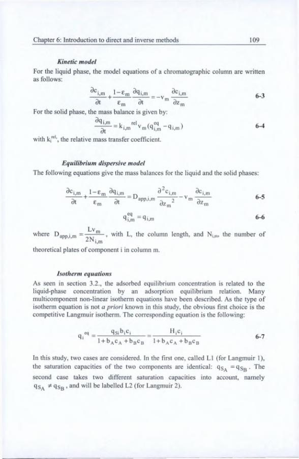
Chapter 6: Introduction to direct and inverse methods 109
Kinetic modelFor the liquid phase, the model équations of a chromatographie column are written as follows:
3c i,m
9tl-£m ^qj,n
6m 9t= -Vr
^Cj,i3z„
For the solid phase, the mass balance is given by:
, rel / eq9i,m)9t
with the relative mass transfer coefficient.
6-3
6-4
Equilibrium dispersive modelThe following équations give the mass balances for the liquid and the solid phases:
^^i,m 1-Em3t 9t "PP’"’"’
9Cj^
3z,2 ' '^m dZr
eq^i,m “li.m
6-5
6-6
where D^pp i n,Lv,
2Ni,-, with L, the column length, and Nj^,, the number of
theoretical plates of component i in column m.
Isotherm équationsAs seen in section 3.2., the adsorbed equilibrium concentration is related to the liquid-phase concentration by an adsorption equilibrium relation. Many multicomponent non-linear isotherm équations hâve been described. As the type of isotherm équation is not a priori known in this study, the obvions first choice is the compétitive Langmuir isotherm. The corresponding équation is the following:
g eq _ qSlbjCj H;C;
1 + b^CA+bgCB 1 + bACA+bgCB
In this study, two cases are considered. In the first one, called L1 (for Langmuir 1), the saturation capacities of the two components are identical: qg^ =9Sb-
second case takes two different saturation capacities into account, namely 9Sa 9Sb ’ labelled L2 (for Langmuir 2).

110 Chapter 6: Introduction to direct and inverse methods
6.2.1.2. CommutationAs the fixed referential is attached to the columns, the commutation is modelled by a change of the flow rate in the columns:
Qm"* = 6-8
with ns, the number of switching periods elapsed since the start-up and m = 1,...,N^ .
6.2.1.3. Initial and boundary conditions
Boundaty conditions and inlet concentration profile
Boundary conditions are given in section 3.4.2.1 and do not introduce any extra parameter except in the description of the inlet concentration profile. The latter takes the form:
if t<td._^ u,(t) = 0
else6-9
Uj (t) = cp,i(l - exp(-(t - tj.^ ) / t,r))
with Cp j, the injected concentration of component i. t is the time, t„, a constant
characterizing the rise time of the front, and tj.^ ^Qf Qf> f^^^
flow and Vh- , the dead volume before the SMB unit.°in ’
Initial conditions
The initial conditions are the following:
t^A.m (^î^m) ~ fi ^ [fi) L]? tU —1,...,N(^ CB.m(fi,Zn,) = fi Vz„, € [0, L]; m = l,...,Nc
Dead volumes
Modelling the dead volumes is the subject of Chapter 5. Four dead volumes (two fixed and two mobile) are associated to each column. The general équation is the following:
^Cj.dat -Vd
^Cj.dazd
+ Dd3^Cj,d 6-11
with Vd and Dd, respectively the velocity in the dead volume d, and the diffusion coefficient in the dead volume d.

Chapter 6: Introduction to direct and inverse methods 111
6.2.1.4. Measurement équationA measurement équation reproduces the information given by a sensor. As explained in the description of the SMB plant under study (see section 2.4.), the data are collected with four UV detectors. Each resulting UV signal is the weighted sum of the concentration of the two products (Grosfils, 2008). The measurement équation for UV detector ô, 5 = 1,...,4 , can be written:
y5^“^(t) = Ca,„5 (t, L)UVs(A) + Cg^^g (t, L)UV5(B) 6-12
where UVs(A) (UVg (B)) is the calibration coefficient of component A (B) for detector ô. m§ refers to the number of columns placed before the UV detector 5 at time t.
6.2.1.5. Unknown parameters
In équations (6-1) to (6-12), the model parameters are the porosity of each column,the fluid velocity in each column and in the dead volumes,the mass transfer coefficients, the diffusion coefficients or the numbers oftheoretical plates in each column;the isotherm parameters ;the UV calibration coefficients;the injected concentration, Cf,a and Cf.b;the dead volumes;the diffusion coefficient in the dead volumes, Dj.
The column geometry is a-priori exactly known and the columns and their packing are supposed to be identical. This implies that the porosity, the isotherm parameters, and the mass transfer coefficients, the diffusion coefficients or the numbers of theoretical plates are supposed to be the same in ail the columns. Small discrepancies between the columns may exist in practice, but this hypothesis is reasonable and is admitted in almost ail existing studies. Hence, the parameters will be estimated ffom one of the SMB columns.
In the following, the SMB parameters are divided into 2 categories.
Some parameters are assumed to be known or are easily determined with some experiments like
the calibration coefficients and the porosity that are easily measured ffom simple experiments (section 6.3.);the injected concentrations which are prepared analytically.

112 Chapter 6: Introduction to direct and inverse methods
the fluid velocities which are a function of the porosity and of the fluidflowrates: /(eS) , m = l.—.N^ , where the flowrate Qm is chosenby the user and imposed by the pumps,the dead volumes which are known process characteristics;the diffusion coefficients in the dead volumes which are assumed to be verysmall (= le-9 mVs) as plug flow conditions are considered in the deadvolumes (section 5.2).
The other parameters are unknown and the resulting parameter vectors are writtenfor each model in Table 6-1.
Table 6-1 : Parameter vector defmed for each modelmodel LDF kinetic EDIsotherm L1
Isotherm L2
kref Na‘A
krel Nb
B 0 = fisqs
bAt>A
_bB .
■ ^rel ■ NA A
ks"' Nb
Ha 0 = Ha
Hb Hb
bA bA
bB _ bB
Note that the known parameters are corrupted by some errors. Indeed, the précision of the pump is limited, the feed préparation and the experiments to détermine the porosity or the calibration coefficients can not be performed without error and, in practice, the columns are not identical. These errors will then be taken into account fiirther in the calculation of the confidence interval of the identified parameters (section 6.4.6) and of the confidence envelope (section 6.4.7). Moreover, in (Seidel- Morgenstern, 2004), it is demonstrated that if erroneous porosity is used in the détermination of the isotherm parameters from batch experiments, these parameters will not be correctly estimated but they will nevertheless be able to describe quite accurately the propagation of the elution fronts. Hence, in this study, the errors on these parameters will first be neglected during the identification of the unknown parameters from one SMB column.

Chapter 6: Introduction to direct and inverse methods 113
6.2.1.6. SMB Model in the standard form
In this section, the SMB models are rewritten in a standard form used in the literature on System identification that will be exploited in section 6.4.
As seen in section 3.6, équations (6-1), (6-2), (6-7), (6-8), (6-11), (or (6-3), (6-4), (6-7), (6-8), (6-11) or (6-5), (6-6), (6-7), (6-8), (6-11)) for input (6-9), and with adéquate initial and boundary conditions, are solved numerically following the method of lines. First, the spatial operators are approximated using fmite différence schemes on a spatial grid. Then the resulting System of semi-discrete ODEs is integrated in time.
Hence, aller approximation of the spatial dérivatives, équations (6-1), (6-2), (6-11) or (6-3), (6-4), (6-11) or (6-6), (6-5), (6-11) can be rewritten in a standard form used in the literature on System identification:
= f SMB(xSMB(() );0,(pSMB) g
with initial conditions : x(0) = Xo
The notations used in 6-13 are:- M: a mass matrix;
- a vector of which each component is a nonlinear fimction of the indicated arguments;
- u(t;cp) : a 2x1 vector containing the inlet concentration profiles of component A
and B at time t; as the shape of the injected profile is defined by Eq. (6-9), the only
parameters in u(t;cp) is Cp.
- 6: one of the n-dimensional vectors of unknown parameters given in Table 6-1.- 9®*^® : the vector containing the known quantities like the porosity, the feedflowrates, the dead volumes: rpSMB = [q^ Vd]’^
with Vd a vector containing ail the dead volumes;
- Xo, the known initial conditions (concentrations at each grid point within the columns before injection takes place, equal to zéro).
xSMB(t) is a vector containing the concentrations of components A and B in the liquid and in the solid phase calculated at each grid point. To simplify the présentation of the vector x®*^®(t), the dead volumes are first neglected hereafter. Then the following expression holds

114 Chapter 6: Introduction to direct and inverse methods
^SMB(t) =
SMB. .^Nc
6-14
where m = l,...,Nc, is a vector containing the concentrations ofcomponents A and B in the liquid and in the solid phase in column m, namely:
Xn,^'^®(t) =
'GPNG,n
SMB(t)
SMB(t)
6-15
^GPg,m^'^^(0 contains the concentrations in the liquid and in the solid phase for
the grid point g (g = 1,...,NG ) in column m ( m = l,.-,Nc ). NG is the total number of grid points per column and Ne, the number of columns. Thus one can write:
SMB.,_ ^GPg,m vt;
r SMB.. ^G>ZGPg,m
r SMB.Bm ^ ’ GPg,m
„ SMB.. ,vG^GPg^m
^ SMB.. ^^Bm * ’ GPg,m
))
) ’
)
2^GPg,m S [0,L] • 6-16
If the dead volumes are not neglected, to each dead volume, d, corresponds a vector containing the concentrations of components A and B in the liquid phase calculated at each grid point of the dead volume, g = l,...,N[), with Nq, the number of grid points in the dead volume :
„ SMB.^,_ Xd (t)-
V SMB.^, ^d] vG
where Xdg^'^®(t) =
„ SMB.. ,CAd (t.Zdp^)
r SMB. ,^=Bd (t’^d )
,g= 1, ...,Nd, Zh 6[0,Ld],
6-17
6-18
with L<j, the length of the dead volume.
Hence, for example, at start-up, when column 1 is placed at position 1, if the deadvolumes are not neglected and if the number of positions is equal to the number ofcolumns, as explained in section 5.3, the vector x®'^®(t) is the following:

Chapter 6: Introduction to direct and inverse methods 115
6-19
By an abuse of notation, one will use the expression x^’^^(t;0,(psp^3,Cp) to refer to the solution of (6-13) for the inlet concentration profile (6-9) and the specified parameters tpsMB and 9. Xo does not appear in this expression because it is always equal to zéro in the considered experiments.Hence, the corresponding solution of the measurement équation of the 5*, 5 = 1,...,4, UV detector is written in the standard from used in the literature of System identification:
where, for example, if the dead volumes are neglected:
The expression for this vector is explained as follows. As the measurements are performed at the end of the mg"' column, the detector ô gives the concentration of A and B in the liquid phase at the last grid point of the column mg. Hence, the first (4NGm g - 4) éléments of Ug are zéros They correspond to the length of the vector of
concentration of A and B in the liquid and solid phase (6-16) at a grid point (i.e. 4) multiplied by the number of grid points in each preceding column (i.e. NG), multiplied by the number of columns (mg), minus the length of the vector of concentration of A and B in the liquid and solid phase at the last grid point of the mg”’ column. The last (4NG(Nc -mg) + 2) éléments of vector Ug are zéros. They are
related to the concentrations of A and B in the liquid phase and in the solid phase at each of the NG grid points of the (Nc-mg) columns following column mg.
ygSMB (t; e, ÇgSMB ) = UgxS^^‘^(t; 0, tpSMB ^ cp) t > 0 6-20
Ug = 0 ... 0 UVg(A) UVg(B) 0 ........ 04NG(Nc-m5)+24NGtHj-4

116 Chapter 6: Introduction to direct and inverse methods
Otherwise, if the dead volumes are not neglected:
Uô = 0 ......... 0 UVg(A) UVgCB)4NGmg+P5-2
0 ........ 04NG(Nc-nig )+Rô+2
where Pg (Rg) is
the number of grid points corresponding to ail the dead volumes located before (after) detector 5 and is calculated by taking into account the detailed description of the measurement équations given in section 5.6.
Besides, vector in 6-20 is defmed as :
;gSMB=[(pSMB UVg(B)f
= [Qi Qii Qui Qiv Ei - Enc Vq cp,A cp,B UV6(A) UVgCB^
As discussed previously, Çg^*^® is assumed to be known. These parameters are in practice determined by some experiments or measurements and their estimated value
will be denoted •
6.2.2. Batch Model
The parameters are estimated ffom batch experiments performed on one SMB column. Hence, the batch models are repeated here and their standard forms used in the literature on System identification are deduced.
6.2.2.1. Column model and isotherm model
A batch model is described by a model of column (like column m in (6-1), (6-2)) and the isotherm équations. Possible batch models are thus given by équations (6-1 ), (6-2), (6-7), or (6-3), (6-4), (6-7) or (6-5), (6-6), (6-7). Note that, for simplicity, in the batch model, the column index, m, is no longer written as only one column is used.
6.2.2.2. Inlet concentration profile
As elution peaks are used (cf. section 3.3.1.7), the inlet concentration profile is a puise. Its équation is the following:

Chapter 6: Introduction to direct and inverse methods 117
ifUi(t) = 0
else if t<tp
U i (0 = c F,i (1 - exp(-(t -1 ) /1 tr )) 6-22
else
U i (t) = C F,i (1 - exp(-(t -1 d) /1 ,r )) - C F,i (1 - exp(-((t -1 dj„ ) -1 p ) /1 ,r ))
with cp,i, the injected concentration of component i, t, the time, tp, the injection duration, t,r, a constant characterizing the rise time of the puise and toin, a time delay associated to the dead volume located before the column, tn = Vj. / Q . Note that
ttr = Vjnj / Q with Vinj, the injected volume.
6.2.2.3. Measurement équation
Similarly as in (6-12), the measurement équation after a column is
For simplicity, as only one detector in the elution experiments is used, the index of the detector is not mentioned for the calibration factor.
6.2.2.4. Batch model in the standard form
Following the same idea as in the case of the SMB model (section 6.2.1.6.), the batch model may be written, after approximation of the spatial dérivatives, in the standard form used in the literature on System identification:
y(t) = c A (t, L)UV(A) + c B (t, L)UV(B) 6-23
Mx(t) = f(x(t),u(t;cF );6,(p)
with initial conditions : x(0) = Xo
6-24
withu(t;cF ) : the inlet concentration profile;
(p = [Q e
0 : the vector of unknown parameters (defined in Table 6-1);x(t): the liquid and solid concentrations at the grid points, namely:
XgP| (0x(t) = 6-25

118 Chapter 6: Introduction to direct and inverse methods
where XoPg (0 contains the concentrations in the liquid and in the solid phase for
the grid point g ( g = 1,...,NG ). NG is the total number of grid point per column.
^GPg(0-
CA(bZoPg)
CB(t,ZQpg)
<ÎA(bZGPg)
qBCb^Gpg )
^GPg ^ [0>L] 6-26
As in the SMB model, the solution of équation (6-24) for the inlet concentration profile 6-22 and for the specified parameters 0 and tp will be written: x(t;0,(p,cp) Hence, the corresponding solution of the measurement équation is given by:
y(t,0,Q = Ux(t;0,(p,Cp) t>0 6-27
where
Ç = [(p cp,A cp3 UV(A) UMB)F6 28
= [q e Vj„j Cp,A cp3 UV(A) UV(B)F
and U =4(NG-1)
UV(A) UV(B) 0 0 .
In the following, the parameter vector 0 is estimated. For the identification step, the parameter vector Ç is considered to be known. It is determined in practice by spécifie
experiments or measurements and will be labelled: Ç. Note that , the dead
volume, is assumed to be known without error as it is a known process
characteristic. The other éléments of Ç may be corrupted by some errors as seen in section 6.2.1.5. However, if the batch experiments are performed on one SMB column, the porosity is also supposed to be known without error as the error is compensated by the isotherm parameters (cf section 6.2.1.5). Hence, for the identification step, two vectors will be used in 7.5.2 and 7.5.3:
one containing parameters assumed to be known without error;
Cwe ~ >another with parameters which may be corrupted by some errors:
Çe=[Q Cp,A Cp,B UV(A) UV(B) Vi„j]'T.

Chapter 6: Introduction to direct and inverse methods 119
Hence, Ç =
Hence, Ç is function of parameters which define the process working mode (flow rate, injected concentration, injected volume) and Ç may differ from one batch experiment to another.
6.3. Direct MethodsThis section présents classical methods widely used to estimate the dead volumes, the column porosity, the isotherm parameters, the diffusion coefficients and the mass transfer coefficients. The détermination of the calibration coefficients of the UV detectors used in this study is also presented. Ail these methods will be used in chapter 7 and 8 to détermine the porosity, the UV calibration coefficients and the initial estimâtes of the parameters for the identification step.
6.3.1.Dead volumeA dead volume is determined by injecting a puise in the valves, the connecting tubes and detectors of which the volume must be measured. The rétention time of the peak, tR obtained at the end of the column is measured. This is the time elapsed between the injection of the puise and the observation of the maximum of the peak at the output. Then the dead volume, V^, is calculated as follows:
with Q, the flow rate.
Vd=QtR 6-29
6.3.2. PorosityThe bed porosity or the total void fraction can be easily estimated by injecting a puise of a non-retained component in the column (Altenhôner et al., 1997). The concentration at the end of the column is measured in function of time. From the peak obtained, a characteristic time, to, is measured. It corresponds either to the mean résidence time, estimated from the first moment of the peak or to the time instant corresponding to the peak maximum for symmetric peaks. The porosity is then calculated as follows:
c Qtp-Vd V
6-30
with V, the column volume, Q the flow rate and V<j the dead volume.
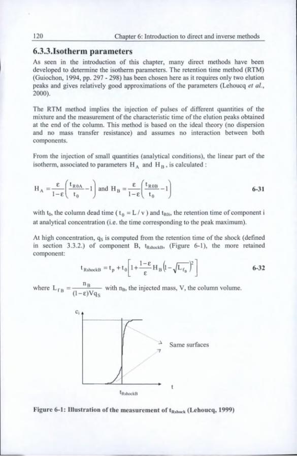
120 Chapter 6: Introduction to direct and inverse methods
6.3.3.Isotherm parametersAs seen in the introduction of this chapter, many direct methods hâve been developed to détermine the isotherm parameters. The rétention time method (RTM) (Guiochon, 1994, pp. 297 - 298) has been chosen here as it requires only two elution peaks and gives relatively good approximations of the parameters (Lehoucq et al, 2000).
The RTM method implies the injection of puises of different quantities of the mixture and the measurement of the characteristic time of the elution peaks obtained at the end of the column. This method is based on the idéal theory (no dispersion and no mass transfer résistance) and assumes no interaction between both components.
From the injection of small quantities (analytical conditions), the linear part of the isotherm, associated to parameters H and H g, is calculated :
H A_ £ ^
toand H g £ I J
1-el to .6-31
with to, the column dead time ( tg = L/ v ) and tROi. the rétention time of component i at analytical concentration (i.e. the time corresponding to the peak maximum).
At high concentration, qs is computed from the rétention time of the shock (defined in section 3.3.2.) of component B, tRshockB, (Figure 6-1), the more retained component;
t RshockB t P + 10 6-32
where Lfg = "b
(l-e)Vqswith ng, the injected mass, V, the column volume.
Same surfaces
t
Figure 6-1: Illustration of the measurement of tRshock (Lehoucq, 1999)

Chapter 6: Introduction to direct and inverse methods 121
6.3.4. Diffusion coefficient of the ED mode!As seen in 3.3.1.3, the apparent diffusion coefficient of component i, Dapp.i is given by
with Ni, the number of theoretical plates, L, the column length and v, the fluid velocity.
The number of theoretical plates may be estimated from elution peaks obtained in linear conditions where the shape of the peaks dépends only on the efificiency of the column (kinetic effect), and not on the isotherm non-linearity (thermodynamical effect).
The number of theoretical plates of component i is linked to the variance of a Gaussian peak of component i obtained in linear conditions (Guiochon et al, 1994):
26-34ROi
Niwith tR0i> the rétention time of component i (i.e. the time corresponding to the peak
maximum). Note that the peak width, Wi, is a ftmction of the variance: Wj = aCj with a, a constant, equal to 5.54 if the width halfway up the peak is considered. Hence the number of theoretical plates is estimated as follows:
fN; =5.54 ‘ROi
vW,i/2with Wi_|/2, the width halfway up the peak for component i.
6-35
6.3.5. Diffusion coefficient of the LDF mode! and mass transfer coefficients of the LDF model and of the kinetic model
Initial estimâtes of the mass transfer coefficients of the kinetic model, of the mass transfer coefficients and the diffusion coefficients of the LDF model are obtained from the following équation (cf section 3.3.1.3):
DLv
app,i Dt,i +l^Oi
6-36
with Djpp j the apparent diffusion coefficient of an equilibrium-dispersive model for
component i, Dli , the diffusion coefficient of a LDF model, N|, the number of

122 Chapter 6: Introduction to direct and inverse methods
theoretical plates (calculated with Eq. 6-35), kp.i, the mass transfer coefficient and
Equation 6-36 results ffom the relation, obtained in linear conditions, between the parameters of an equilibrium-dispersive model and of a LDF model (Guiochon et al.. 1994, p. 44).
For the kinetic model, the diffusion coefficient is set to zéro in (6-36). Flence, after an injection at low concentration to détermine Nj, i = A,B, the mass transfer coefficients are easily obtained from (6-36) (Mijabe et al, 2000).
For the LDF model, several injections at different liquid-phase velocities are required. Lv/Nj is plotted against v^. Dlj is then deduced ffom the intercept
between this curve and the ordinate axis, and k p ; ffom the slope.
6.3.6. Calibration coefficientsIn the experimental plant described in section 2.4., UV detectors are used to measure the experimental concentration profiles. However, they do not give the concentration of A and B separately. The UV signal is a fonction of the concentration of A and B.
Successive step changes of solutions of known concentration of component A and then of component B are successively injected through each UV detector. The measurement of the UV detector is recorded for each plateau. Then, the values of the UV signal recorded in each plateau are plotted against the injected concentrations to détermine the relationship between the concentration of component A and B and the UV signal. In this study, it tums out that the UV signal may be described by the weighted sum of the concentrations of both products (Grosfils, 2008). Hence, the calibration coefficients are the slope of the straight fines obtained when the UV signal is plotted against the injected concentrations.
6.4. Inverse method or identiHcation - general principles
The identification theory is introduced in this section. It is limited to the tools used to solve the considered problem. A more detailed overview is available in (Walter and Pronzato, 1997; Bogaerts, 1999, pp. 74 - 89; Hanus, 2007).
The unknown parameters are determined by minimizing a criterion which measures the déviation between the experimental profiles and the profiles simulated with the chromatographie model. In this section, some details and notations are first clarified. Then, the optimization criterion used is presented. The introduction of parameter constraints follows. The numerical optimization method used to fmd the parameters

Chapter 6: Introduction to direct and inverse methods 123
that minimize the cost function is then shortly presented. Afterwards, the problem of identifiability and experiment design is discussed. The chapter ends with the calculation of a confidence interval on each estimated parameter and of a confidence envelope for the simulated concentration profiles.
6.4.1. NotationsAs several experiments may be used to identify the parameters, some notations are introduced to define the experimental field.
The model identification uses Up experiments. M ^ is the number of measurements
of experiment 1,1 = l,...,np , and Mj is the total number of measurements used in
As introduced in 6.2.2.4, Ç is constituted of two kinds of parameters:
the parameters, , which are known without error and which are constant ffom one experiment to the other;the parameters, Çg , which may be corrupted by some errors and which are a function of the experiment, as the different experiments are performed with different process working modes defined in Hence, the notation, Çç(k), k = l,...,Mj, is introduced to refer to the value of Çe corresponding
to measurement point k. The vector = [Çe(0; —; CeC^x)] will also
be used further.
Parameters 6 are not a function of the measurement point.
The measurements and the corresponding output prédictions are also defined as vectors of dimension M-pxl :
npthe identification step, My = .
= [y?"UteO)) - yr(tf(Mf)]T
with £ = l,...,np , tf (i) < t^(i + l), and i = 0, 1, ..., Mf_j.
Similarly,
and

124 Chapter 6: Introduction to direct and inverse methods
yf(e.Çev(yMi+i:lMi).Cwe)-i=l i=l
t-\
i=l i=l i=l i=lwith t = l,...,np , tf (i) < t^(i + l), and i = 0, 1, M^_|.
6.4.2. Optimization criterionThe estimâtes of the parameters are determined by minimizing a cost fimction, which provides a measure of the différence between the experimental profile(s) and the corresponding simulated profile(s).
Several criteria hâve been developed in the literature (Walter and Pronzato, 1997; Bogaerts, 1999, pp. 74 - 89, Hanus, 2007). In this study, as there is no information about the measurement noise, a least square estimator has been chosen:
J(0,;ev-Çwe)= I (y"’“(k)-y(k,0,Çe(k),Cwe)] w(k) 6-37k=l
with y^^Ck), the k”’ measurement value, and y(k,0,Ç(,(k),Ç^^,ç), the corresponding
model output prédiction given by Eq. 6-27 with k =1....Mj. w(k) is a weightingfactor and Mt, the number of measurements.
The estimate of 0 is given by 0 = Argmin J(0,Ç^g ).
6.4.3. Parameter constraintsSeveral model parameters are subject to constraints of physical or numerical nature. Unconstrained algorithms are usually more efficient than constrained algorithms, whenever applicable (Haag, 2003). Hence, a solution is to apply a non-linear transformation to the parameters in order to transform the constrained optimization problem into an unconstrained one. Indeed, after the parameter transformation, the original bounded parameter range is mapped into an unbounded range. Hence if prior knowledge allows one to specify an interval within which the estimated value must lie, say 0 jpf (j) < 0(j) < 0 (j), to enforce these constraints, the following non-linear transformation is performed (Haag, 2003):
0*(j)=^ln|^^ with g(j): 2 l-g(j)
20(j)-0sup(j)-0inf(j)
0sup(j)-0inf (j)6-38

Chapter 6: Introduction to direct and inverse methods 125
with 0(j), the j*'’ parameter to identify, j = l,...,n , and 0* (j), the parameter which is actually determined by numerical optimization without constraint. After this
numerical optimization, the estimated parameter 0(j) is calculated from the
estimated 0 (j) with the inverse transformation;
00) = O.5(0,„p 0) + 9i„f 0) + (0SUP Ci) - 0i„f (i)) tanh(0* 0))) - 6-39
Note that, for simplicity, by an abuse of notation, y(t,0,Ç) is written y(t,0*,Ç) after parameter transformation.
6.4.4. Numerical Optimization MethodsThe optimization algorithms aim at flnding the value of 6 g which satisfles:
Cwe,Cey ^ ~ niin J(9, Cwe,Cev ^ ■ 6-406
This is a délicate task if J(0,Ç^g ) is a non convex fonction of 0 and has several
local minima. Several optimization algorithms hâve been developed in the literature. A good OverView may be found in (Hanus, 2007) and in (Walter and Pronzato, 1997).
In this study, a zero-order method has been chosen. Such a method uses the estimation of the cost fonction at different points (namely for different values of 0) and not the gradient of the cost fonction or the Hessian matrix like the well-known Newton method or the Levenberg-Marquartd method (Walter and Pronzato, 1997, pp. 141 - 182; Reklaitis et al., 1983). A zero-order method is generally more robust and often reaches the optimum optimorum (Hanus, 2007). Here, the direct search method called UOBYQA developed by Powell (2000) has been chosen. It takes into account the curvature of the cost function by interpolation with quadratic models. This algorithm is very efficient with cost functions requiring large numbers of computations for their évaluation. Indeed, it reduces the number of calculations of the cost function (Vander Berghen et al., 2005).
6.4.5. Identifiability and experiment designA critical point of the identification problem is the parameter identifiability. If identifiability is assured for the considered identification problem, it is possible to détermine in a univocal way the model parameters ffom the available measurements. Hence, it is important to plan the experiments to ensure the identifiability of the model parameters. In this section, the définition of the local identifiability of a model is first given and a numerical approach to test local identifiability is

126 Chapter 6: Introduction to direct and inverse methods
explained. Then, the sensitivity analysis that is helpfiil in the experiment design or to compare the identifiability of different models is presented.
Définition of the local identifiability of a model(Walter er a/., 1997, p. 21)
The following définition is formulated in an idealized ffamework where there is no modelling error, no noise and where the input and measurement time may be chosen at will. The parameters are said structurally locally identifiable from the available measurements if for almost any 0, there exists a neighbourhood V( 0 ) such that
if 0 E V(0) and y(t, 0, Ç) = y(t, 0,Q then 0 = 0.
Numerical approach to verify the local identifiability (Walter et a/., 1997, p.31)
Various algebraic methods hâve been developed to verify the identifiability of a model (Walter et al, 1997, pp. 22- 31). However, most of them are difficult to apply to a non-linear model for which there is no analytical solution. Hence, a numerical approach to verify the identifiability (at least locally) has been described in (Walter et al., 1997, p. 31). The following steps must be performed:
choose some nominal value 0q and generate some fictitious data with the model and this known parameter 0q.estimate 0 ffom the fictitious measurements with 0q, as initial estimate. If
the estimated parameter 0 fulfils 0 = 0q , the parameters are said structurally locally identifiable.
Sensitivity analysis
The sensitivity of measurement y(t,0) with respect to parameter 0(j) is defined as:
ge(i)(t,9,Q= . If the sensitivity is high, the measurementd0(j)
significantly when changes in 0(j) are perfonned.
varies
To détermine if the parameters 0(j), with j = l,.., n , are identifiable simultaneously
from the output y(t, 0, Q , the following matrix is built:
0(irjg0(i)(t,0,ç)"dt0
0(l)0(n) I ge(i)(t, 0, Ôg9(n)(t. Ôdt 0
0(n)0(l)yge(n)(t,0,Ôg0(i)(t,e,Ôdt0
0(n)^jg0(n)(t,e.Ô^dt
6-41

Chapter 6: Introduction to direct and inverse methods 127
where [0, T] is the time span of interest.It can be proven that if the déterminant of this matrix, the so-called Gram déterminant denoted D, does not vanish, the sensitivities are independent (Luenberger, 1969) and the parameters are identifiable simultaneously Irom output
Note that, this matrix is also called the Fisher information matrix. The éléments of its inverse correspond to a lower bound for the éléments of the parameter covariance matrix (Walter and Pronzato, 1997, p. 245 - 253).
Hence, models and experiments (Point et al, 1996; Vande Wouwer et al, 2000) that increase the Gram déterminant will be selected. This method is also called D- optimal design (Walter and Pronzato, 1997, p. 288).
6.4.6. Confidence intervalHereafter, the calculation of the confidence interval on 0 is presented. First, the asymptotic theory, which will be applied in this work, is described. Then, a brief summary of another method, the LSCR (Leave-out Sign dominant Corrélation Régions) approach, follows.
Note that, for the asymptotic theory, two options hâve been considered. At first, the error on the a-priori known parameter, Ç(k) has been neglected. Then, this error has
been introduced in the calculation of the confidence interval on 0.
To simplify the notation, the parameter = [Vj.^ e]^ , corresponding to
the part of Ç perfectly known and constant for ail the experiments will not be repeated in the development hereafter.
6.4.6.I. ASYMPTOTIC THEORY
Least square estimator without error on Ç
In this section, it is assumed that there is no error on parameter Çg(k),
V k = l,...,M-j- . Hence, V k = l,...,Mj, (*^) with Çg(k), the estimate
of parameter Çe(k)> and ^he true value of ^et 0 dénoté the
estimated value of the n-dimensional parameter vector obtained by minimization of
the cost (6-37). The detailed estimation of the confidence interval on 0 may be
found in (Hanus, 1997, pp. 125 - 127) and is reproduced in Appendix 6.1. Only the
assumptions and results are given hereafter.

128 Chapter 6; Introduction to direct and inverse methods
Consider the model équation (6-27). As the measurement y"’“(k) does not exactly verify the model équations, an error e(k) is introduced:
y™^(k) = y(k,e^,Ce„(k)) + e(k) k = l,...,MT 6-42
with 0,,., the “true” value of the parameter.
It is assumed that e(k) is zéro mean:
E(e(k)) = 0 Vks [1:Mt] 6-43
and white, namely,
E(e(k)e(k')) = Oeô(k-k')w“‘(k) 6-44
Hence, the weigthing factor w(k) is inversely proportional to the error variance so that the error terms with the smallest variance contribute more to the cost.
It can be demonstrated (Appendix 6.1 ) that, with function (6-37), the covariance
matrix of 9 may be estimated from:
Cov = Ê(èe^)=—!---- J(0,Ç, )P„ 6-45
whereMt
Pm, - X ge(k))ge''(k, 0, (k))w(k)k=l
And
ge(k,0,Ç. (k)):dy(k,9,^,_^(k))
39 e=9
6-46
6-47
Hence, the confidence interval at 99% on 0(j), the j"’ component of 9 ( j = l,...,n ),
is calculated as: 0(j) ± 3.^Cov(j,j) .
Least square estimator with error on Ç
In this section, the error on Ç is considered. The calculation of the covariance matrix follows the development presented in (Hanus, 1997, pp. 125 - 127) and
reminded (Appendix 6.1) but is, here, adapted to take the error on Ç into account.
Consider again the measurements y"'*(k)
y™*(k) = y(k,0,r,Çe.,(k)) + e(k) k =1,...,Mt 6-48

Chapter 6: Introduction to direct and inverse methods 129
with Çg ^ (k), the true value of the parameter Çg(k).
The confidence interval on 0 taking into account the error on the estimate of
Ce(k), Çe(I^) = Ce(k)-Çe„(k), k = l,...,Mx, will be calculated.
The following development is divided into 5 steps:Statement of the définitions and assumptions;Calculation of 0 from the optimality criterion;
Calculation of 00^ ;~ ~ 'T' ~ ~ 'T'
Calculation of the expectation of 00 , E(00 );
Estimation of the covariance of e(k) used in E(00 ).
Définitions and assumptions- The error is zero-mean:
E(e(k)) = 0 Vke [1:Mt]
- The error is white:
E(e(k)e(k'))=a2ô(k-k')w-‘(k)
- The estimation, Çg(k), is unbiased :
E(Ce(k))=0
- The covariance matrix of Çg (k) is denoted:
E(Çe(kKg(k')'T))=Q^e(k^k.)
- Sensitivities respectively to 0 and Çe(k) are defined as: dy(k,0,Çg(k))
ge(k,0,Çe(k)) = -
gÇe(k)(k>e.Çe(k))^
303y(k,0,Ce(k))
a^e(k)
6-49
6-50
6-51
6-52
6-53
6-54
Note that the error e(k) is defined in (6-48), with y™*(k), k = l,...,Mj, corresponding to measurements of elution peaks. Parameters Çg(k)> k = l,...,Mj, correspond to the flow rate, the calibration coefficients and the injected concentrations and volume which are respectively imposed by the pump, determined by simple experiments, prepared by the user (see section 6.2.1.5) and injected manually. Hence, the distribution of e(k) and of Çg(k) are uncorrelated:
E(Çg(k)e(k')'T))=0 Vk,k’=l,...,MT 6-55

130 Chapter 6: Introduction to direct and inverse methods
Calculation of 6The optimality conditions are written :
âjfeCev)90
0=e
Mt
= -2S (y™®(k)- k=l
y(k,e,Çe(k)))ge(k,e,Ce(k))w(k) = 0 6-56
If the estimation errors on 9, 0 = 0-9,^, and on Çç(k), k = l,...,My,
Çg(k) = Çg(k)-Çgjj.(k), are assumed to be small, higher order tenus of the Taylor
sériés development around (0tr,Ç etr neglected and y(k, 9, ^e(k)) may bewritten :
y(k,9,Çg(k))
= y(k, 0,r, Cetr(k)) + §0^ (k, 9,r, ^tr - (k)
6-57
It is assumed that in the neighbourhood of ( 0 = 0,^, Çg(k) = Cetr^k) )>
ge'^(k, 0, Çe(k)) = ge^(k, 0t„ Çetr(k)) and6 58
g (k, 0, Ce (k)) = gÇe(k)'" (k, e„, Cet,
Hence, in the neighbourhood of ( 0 = 0,,, Ce(k) = Cetr^k) )> the optimality condition
on 0 is obtained by introducing (6-57) and (6-58) in (6-56):
-2^ge(k,0„,Ce„(k))k=l
w(k)(y™^(k)-y(k,0„,Ce„(k))-ge''(k,6„,Ce,r(k))è-gç,(k)''(k,e,„Ce„(k))Ce(k))=O
6-59
Using the définition of the error (6-48), (6-59) becomes:
If ge(k,0t,, Ce„ (k))w(k)(e(k) - ge^(k, 0,„ Cet,(k))è - gÇg(k/(k, e,r. Çetr(k)Ke(k)) k=l= 0
6-60

Chapter 6: Introduction to direct and inverse methods 131
Mt
Defining P,^'^ = ^g0(k,0o.,i;etr(k))ge^(k,0tr.Çe,r(k))w(k), 6-61k=l
0 is then extracted from (6-60):
e = PM^^g6(k,0„,Çe„(k))w(k){e(k)-gç^(,/(k,0„,Ç„^(k))Ç,(k)) 6-62k=l
By taking the expectation of (6-62), and using (6-49) and (6-51), it is verified that the estimate of 0 is asymptotically correct:
E(9) = PM,Zg9(’^’®-^e,(k))w(k)(E(e(k))-gç^(,/(k,0„Ç,^(k))E(Ç,(k))] k=i
= 0
The product (00^) is now estimated.
Calculation of 00^ ;
=PMj^I^(e(k)-gUk)^(k,0,r,Ce,r(k))L(k)) ge(k,0,r>Ce,r(k))w(k)k'=l k=l
w(k')ge’'(k',0,„Ç,Jk'))(e(k')-gç^(k,''(k',0^,Ç,Jk'))Ç,(k'))lP^^
6-64
By reorganizing (6-64), the following expression is obtained:
ee^=PMT.[I I e(k)e(k')ge(k,e,„Ç,,^(k))w(k)w(k')ge^(k’,e,„Ce„(k'))]* k'=l k=l *
My My+P^^[Z Ige(k,0„,Ccr(k))w(k)
‘ k'=l k=l
(-gÇe(k/(k,e„,^,,^(k))4(k)e(k')-gç^,k/(k',e,„;e„(k’))^(k’)e(k))w(k’)ge^(k',9,„Ce„(k'))] Pm^
+ 'xge(k,0.r,Çe„(k))w(k)(gç^(k/(k,e,„^,,/k))^(k)Çe(k')'^gç,(k^(k'.e,r,Cc„(k’)))* k'=l k=l
w(k')ge’"(k',6„,Çe,,(k'))] P^,^
6-65

132 Chapter 6: Introduction to direct and inverse methods
Calculation of the expectation of 66^ . E(06^)
The expectation of (69 ) is calculated using (6-52) and (6-50):
00T)=P o^[l ge(k,e„,Ç„^(k))ge^k,e,„Çe,,(k))w(k)]PM^-* k=l
Mj Mj J.+ Pm^[I^ ge(k,0,r,;etr(k))w(k)gç^(k)^(k,0,r,Cetr(k))Q^=(k,k')
gÇe(k)(k',0U,Çetr(k'))w(k')ge'^(k',0,„Ce„(k'))]PM^Mj Mf
I ge(k,6,r.Çetr(*^))'^0^)' k'=l k=l
(gÇe(k)^(k,0,r,Çetr (k))E(C,(k)e(k')) + gç^(k/(k',0t„Ç,^^ (k'))E(Çe(k')e(k)))
g9'^(k',0,r,i;etr(k’))w(k')]P^^^
6-66
By exploiting the définition of (6-61) to evaluate the first line in (6-66) and by
notingthat E(Çg(k)e(k'))= E(Çg(k))E(e(k')) = 0 due to the independence of Çe(k) and e(k’) and to assumptions (6-49) and (6-51) one can rewrite (6-66) as:
E(èè")=P^,^Og^ +Mj M-r
'■m.iSI ge(k,0,r,ÇeJk))w(k)gç^(,/(k,e,,,Çg_^(k))k'=l k=l
Q^'(k,k')gç^(,.,(k',0,,,Çg,^(k-))w(k-)ge''(k',e„,Ce,r(k'))]PM,
6-67
Using approximation (6-58) yields:
Ê(èè^)=PM,^e +Mj Mj
PmJZZ g9(k,0,Çe(k))w(k)gç^„/(k,6,Çg(k))Q^'(k,k')
k'=l k=l
gç,(k')(k’,0,Çe(k’))w(k')ge^k’,0,Çg(k'))]P^^
6-68

Chapter 6: Introduction to direct and inverse methods 133
ivit
with =^ge(k,0,C,(k))ge’'(k,0,Ç,(k))w(k),k=I
(6-61).
obtained from (6-58) and
Estimation of the covariance of e(k~).In this case, may be estimated by adapting the calculation of performed
without considering an error on Ç (Hanus, 2007, p. 108). A Taylor sériés
development of the cost function J(0,Çe^) around 0,r“0 Ce (k) = Çe(k) >
k = l,...,M-j-, is performed :
J(0.r , Ce. J = J(6,r. Ce (D,-, Ce (Mt )) = J(0, Ce. ) "
1 ~T 3'j(0>Cev)
9J(0,Ce )
3J(9,Cey)
^ aCe(k)^k=l e.Çe,
Ce(k) + -0'^ "2 aeaeT
ao^
0
0.Çc,
0.Ç.,
k=l k'=l dCe(k)9Ce(k')‘ e.ç. é;5eaCe(krCe(k)
6,Çc.
6-69
where, by 6-37 :Mivi -J- ivi -J-
J(0,r > Cevtr) = Z (y""' ~ ®.r ’ Ce.r(k)))' w(k) = J] e(k)' w(k)k=l k = l
- - / \2 and J(0, Cev) = X iy- y(*^’ ^e(k))f w(k) = J] ê(k)' w(k)
k = l k=l
By définition of 0 which minimizes the cost function J(0,Cey)’
3J(6>Cey)3ûT . .
6-70
6-71
6-72V

134 Chapter 6: Introduction to direct and inverse methods
Ifd^y d^y
and are small, then the second order terms in 6-69
can be approximated using only the first order dérivatives of the model output w.r.t. 6 and (cf. Appendix 6.2). Indeed, the following approximations hold:
1 9'J(e,Çev)2 3930^
e-Çe
■Pmt = s ge(k,e,Çe(k))ge^(k,e,Çe(k))w(k) * k=l
6-73
1 a'J(e,Çev)2 3Çe(k)3;,(k-)^
e.Ce 6-74
= Z gç.(k)(k*,ê,Çe(k*))gç,(k'/(k*,ê,Ce(k*))w(k*)
k*=l
and
a"j(e,Cev)
303Ce(k)^e,Çe
Mj . . .= 2 S ge(k*,0,Çe(k*))gç,(k) (k*,0,Çe(k*))w(k*)
k*=i ®6-75
Hence, with équations (6-70) to (6-75), (6-69) gives :
fK A iVl I
J(0.r.Cev,r) = J(9>Cev)- Sk=l
0J(9,^ey)
aCeCk)"^ ê,Çe(k)Çe(k)
+ è^ S ge(k,0,Çe(k))ge'^(k,0,Ce(k))w(k)0k=l 6-76
Mj My My ~+ S I I Ce(k)^gÇe(k)(k*,e,Ce(k*))gç^(k') (k*,e,Çe(k*))w(k*)i;jk')
k=l k'=l k*=l
+ 20'^ge(k*,0,Çe(k*))gr (k/(k*,0,Ce(k*))w(k*)Çjk) k=lk*=l ®
or using approximations (6-58) and reorganizing (6-76),

Chapter 6: Introduction to direct and inverse methods 135
M Js
k=lV 2 ... ... 3J(0.Çev)2, e w(k)= Y e (k)w(k)- Y.
k=l k=l aCe(k)^Ce(k)
e,Çe(k)My
+ s g9^(k,0^,Cg^(k))00Tge(k,e^,;g,^(k))w(k)etr'k=l y y y
+ I X S gÇe(k)'^(k*,0,r,Ce.(k*)Ke(kKe(k’)'^gÇe(k')(k*,0.r,CeJk*))w(k*)k=l k'=I k*=lMy My
+ 2 1 s gç^(k/(k^0,,,Ç (k*)Kg(k)0'^■g6(k^0,,,Ç (k*))w(k*)k=lk«=l
6-77
The expected values of the ternis of (6-77) are then calculated. With Eq. (6-50), the following equality is obtained:
E[j(0.r.Cev„ )]= XE[e'(k)w(k)]=^a,' =k=l k=l
6-78
As calculated in Appendix 6.3, the expectation ofMt
Zk=l
9J(0,Çev)
5Çe(k)^Ce(k)
e,Çe(k)
IS
given by:
dJ(0,Çev)
k=l aÇe(k)'^Ce(k)
9,Çe(k)
Mj= S E
k=laj(0,Çev)
^e(k)9,Ce(k) y9Çe(k)'" ''>'36'*'/
e,^(k*))w(k*)
IVl 1 l»! 1 ^
2_s (k*, 0,r, Çe,r (k*))Q (k*. k)gç^(k)(k*, 0„, Ce„ (k*))w(k*)
6-79
2l' Ç ge'^(k*,0„,Çetr(k*))Efe(k)'^)gÇe(k)(k*>etr.Cek=l k*=l M J Mj
k=l k*=l
Finally, the expectations of the tree last terms of 6-77 are respectively:
E I ge^(k,e,„Çg^_.(k))00Tge(k,0,„Çg,^(k))w(k)V k=l .
= f ge'^(k,0t„Çg^^(k))E(00^)ge(k,0,r,Ce,r(k))w(k)
6-80

136 Chapter 6: Introduction to direct and inverse methods
My My My
^ k—1 k*—1 k*—1 J
My My My q-. ^t'= I I s gÇe(k) (k",0tr.Çe,r('^*))E(Ce(kKe(k’) )gÇe(k')(k*,0tr.Ce,,(k*))w(k*)
k=l k'=I k*=I My ^^y î^y
= gÇ,(k/(k*,0,r,Çe„(k*))Q^‘=(k,k')gç^(k.)(k*,0t„^g^(k*))w(k*)
6-81
f M-rgç.(k)^(k^0,^,Ce,/k*))Ç^(k)è^'ge(k^0„,Ç^_^(k*))w(k*)
^ k=I k*=i
M J M J
= 2EZ g;.(k/(k*,0,.,Çe,/k*))E(ç^(k)è^)ge(k*,0,„Ç^^(k*))w(k*)k=lk*=l
Introducing Eq. 6-78 to 6-82 in 6-77 gives, after simplifieation:
6-82
Mxae =Ef Mj
S ê2(k)w(k)U=1
My Mj „-2 S I g;,(k*) (k*,0,r,Çe,r(k*))Q^^ (k*,k)gç^(k)(k*,0t„(k*))w(k*)
k=l k*=l
+ ?ge''(k,e,r,Çe,r«)E(0è’^)ge(k,etr,Çe
Mj Mj My _ „+ S S I gÇe(k)^k^0,,,Ce.(k*))Q^e(k,k.)g (k*))w(k*)
k=l k'=l k*=l
6-83
2Introdueing 6-67 into 6-83, and using approximations 6-58, an estimation of is given by:

Chapter 6: Introduction to direct and inverse methods 137
=■ MjMt- S ge‘(k,0,Çe(k))PM^ge(k,0,Ce(k))
k=l
(J(ê,Cev)MX Mj T . ,
-2 1 I gÇ,(k*) (k*,0,Ce(k*))Q'="(k*,k)gç (k)(k*,0,Çe(k*))w(k*) k=l k*=l
Mj Mj Mj
+ r s I gÇe(k)‘(k*,e,r,Çe, (k*))Q^e(k,k')gç (k’)(k*,e„,Ce, (k*))w(k*)k=i k'=i k‘=i "
rp , , , Mj Mj- J ^ ge (k*, 0, Ce (k*))PMT [ ge (k, e, Ce (k))w(k)gç^(k) ‘ (k, 0, Ce(k))
Q'="(k,k')g;;^(k.)(k',0,Çe(k’))w(k-)g9'r(k',0,Ç,(k'))]P^^ge(k*,0,Çe(k*)))
6-84
with Pm^ =^ge(k,Ô,Ç,(k))g0’^(k,0,Ç^(k))w(k),k=l
(6-61).
obtained from (6-58) and
And an estimation of E(00^) is obtained:

138 Chapter 6; Introduction to direct and inverse methods
Cov=Ê(eF)=P^ --------------------------------------- !----------------------------------------
Mt- I ge^(k,e,Çe(k))PM^ge(k,e,Çe(k))k=l *
(J(ê,Çev)
-2 1 I gr (k*)^(k*,e,Ce(k*))Q^®(k*,k)gç (k)(k*,0,Ce(k*))w(k*)k=l k*=l ^ ®
Mj My Mj rj^+ Z Z I gç,(k)'(k*,e,r,Ce„(k*))
k=l k'=l k*=l
Q (k, k- )g (k*, e t,, ç g (k*)) w(k*)
+ Z ge^(k*,0,Ce(k*))PM^[I I ge(k,0,Ce(k))w(k)gç (k)^(k,0,i;e(k))k*=l k'=lk=l ®
Q^«(k,k')gç^(k.)(k',ê,Çe(k’))w(k')ge^(k',0,Çe(k'))]PMT-ge(k*,ê,te(k*)))
+ Pmx[^?j s, ge(k,0,Ce(k))w(k)gç^(k) (k,e,Ce(k))Q^nk,k')
gÇe(k')(k’.ê,Çe(k'))w(k')ge^(k’,è,Çe(k'))]PM^
6-85
Hence, the confidence interval at 99% on 0(j), the j"' component of 0 ( j = l,...,n ),
is calculated as: 0(j) ± 3^Cov(j, j) .
Note that in the whole above development, it is, implicitly, supposed that the number of samples, Mx, tends to infinity to correctly evaluate the expectations. This is the reason why another method evoked in the following section has been investigated.
6.4.6.2. LSCR METHODOnly a brief summary of this method is given here as it tums out to be difficult to be implemented in our case. A priori, results obtained with the previous theory may be unreliable as one will hâve only a finite number of data samples available. Hence, the LSCR approach (Leave-out Sign dominant Corrélation Régions) developed in (Campi and Weyer, 2005), which gives non-asymptotic confidence régions should be a good alternative. Assuming a noise symmetrically distributed around zéro, this method computes corrélation fiinctions for several parameter values and discards

Chapter 6: Introduction to direct and inverse methods 139
régions in the parameter space where too many functions are positive or négative. However, this method seems difficult to implement for a large number of parameters, as it is the case here. Indeed, the évaluation of the corrélation functions implies a huge number of simulations.
6.4.7.Confidence envelope
The introduction of the identified parameters in a model allows to simulate the behaviour of the proeess. However as there is an error on the estimated parameters, there is also an error on the results of the simulation. The aim of this section is to estimate the covariance of the simulation error in order to build a confidence envelope around the simulated concentration profiles. First, the calculation of the confidence envelope is presented for the elution profiles with parameters Ç, exactly known. This will be used in chapter 7 to verify the effectiveness of the proposed identification procedure. Secondly, the confidence envelope of the SMB concentration profiles will be estimated taking into account an error on parameters Ç
Confidence envelope for batch experiments without error on
In this section, it is assumed that there is no error on the estimate of parameters
true value of Çe(k)-Note that, to simplify the notation, the parameter corresponding to the part of Ç, perfectly known and constant for ail the experiments will not be repeated in the development hereafter.
Let y(k,6,Çgj^(k)) and y(k,0,^,Çg|j,(k)) dénoté respectively the solution of
équations 6-24, 6-27 with 9 = 0 and 0 = 0,^. The différence between these results is the simulation error, y(k), that one can write, for the k* data sample:
The covariance of the simulation error is calculated as follows (Bogaerts, 1999; pp.123-127).
The error on the estimation of y may be calculated using a Taylor sériés development (limited to the first order) around the true value 0,,:
6-86
y(k, 0, C„(k)) = y(k, 0„,Ç Jk)) + ge'^Ck, 0,„ Ç,,(k))0 6-87

140 Chapter 6: Introduction to direct and inverse methods
Hence, from 6-86 and 6-87, y(k) = g0^(k,0(r,Çjr(k))9 .Then, an estimate for the covariance of the simulation error can be computed as:
E(y(k)ÿ(k)'T) = ge'^(k, Çt,(k))E(0èT')g0(k, 0t„ Ç,,(k)) 6-88
with E(00 ) obtained in section 6.4.6.
It is assumed that in the neighbourhood of ( 0 = 0;^ ),
ge"" (k, 0, C„(k)) = ge^ (k, 0^, Ç Jk)) 6-89
Using 6-89, 6-87 becomes:
E(5(k)y(k)'r) = g0T(k,Ô,Çj^(k))E(00'^)g0(k,0,C,r(k)) 6-90
y SMBConfidence envelope for SMB experiments with error on Çg
In this section, the SMB model described in section 6.2.1.6 is considered, namely équations 6-13, 6-20. In the following, an error on the vector containing a-priori
known parameter, Çg^'^®(k), k = l,.., Mj (6-21), is taken into account. As
explained, since there is a différence between the estimated parameters, 0 and
k = l,..,Mj, and the true parameters, 0,r and there is a
simulation error between the results of the simulation, yg*™ (k,0,Çg®™ (k)),
obtained by introducing 0 and Çg™“(k) in équation (6-20) and the true values
yg^-« (k,0^,Çg „®^®(k)):
yg-» (k,e„,C8.tr""’®(k)) = yg-B(k,0,ÇgS^'B(k))-ÿg^«B (k)6-91
k = l,,..,MT
with yg^'^®(k), the simulation error.
The calculation of the eovariance of the simulation error is described hereafter. It
follows the same steps as the caleulation of the covariance without error on Çg^^^
but has been adapted, here, to the case of errors on Çg^*^^.
To simplify the notation, the indexes ô and SMB will not be written in the following.

Chapter 6: Introduction to direct and inverse methods 141
If the estimation errors on 6, 6 = 0-0„., and on Ç(k), Ç(k) = Ç(k)-Ç(j(k),
k = 1,, are assumed to be small, the Taylor sériés development around
(0tr,Ctr(k)) may be limited to the first order :
y(k,0,âk)) = y(k,0„,(;jk))
, ay(k,0,^(k))^00 0=0„,Ç(k)=Ç„(k)
0 +0y(k,0,;(k))^
0Ç(k)Ç(k)
0=0,„Ç(k)=Ç„(k)
6-92
which gives
y(k,0,Ç(k))
,.0y(k,0,C(k))^00
e=0tr,Ç(k)=Çtr,(k)0 +
9y(k,9,C(k))^0Ç(k)
Ç(k) 6-930=etr„Ç(k)=Çtr.(k)
Then, an estimate for the covariance of the simulation error is:
E(y(k)y(k)'^) =
0y(k,0,i;(k))^00
^ 0y(k,0,C(k)) 0C(k)
^ 0y(k,0,C(k))^00
^ 0y(k,0,;(k))'^ 0C(k)
E(èèT).9y(k,e,C(k))
0=0tr.Ç(k)=Çtr(k)T
00 0=0,r,Ç(k)=Ç,r(k)
0=0,r,Ç(k)=Çtr(k)0Ç(k) 0=0,r,Ç(k)=i;,r(k)
0=0,r,Ç(k)=Çtr(k)0Ç(k)
0=0,r.Ç(k)=Ç,r(k)00
0=0,r,Ç(k)=Çtr(k)
0=0,r,Ç(k)=Ç,r(k)
6-94

142 Chapter 6: Introduction to direct and inverse methods
Using E(ab)<VE(a^)E(b^) (Papoulis, 1965, p. 210),
ay(k,0,Ç(k))_ ay(k,0,C(k))a —------------------------------90
0 and b = -e=0tr,Ç(k)=Çtr(k) 9Ç(k)
with
e=0tr,C(k)=Çtr(k)the following inequality is obtained for the last two ternis of 6-94:
ay(k,0,C(k))30
0=0,r,Ç(k)=Çtr(k)
3y(k,0,Ç(k))'T
3C(k) 0=0,r,Ç(k)=Ctr(k)
3Ç(k)0=0tr,Ç(k)=Çtr(k)
E(Ç(k)èT)MSAÇ(M0=0,r,Ç(k)=Çtr(k)
<+2 |gy(ic,0,i;(k))^ 30
E(èèT>5y(k,0,Ç(k))
0=0tr,Ç(k)=Çtr(k)90 0=0tr,Ç(k)=Çtr(k)
|3y(k,0,C(k))'^ 3Ç(k)
0=0tr,Ç(k)=Çtr(k)3Ç(k) 0=0,r,Ç(k)=Çtr(k)
6-95
With 6-95, 6-94 may be written as:
E(ÿ(k)y(k)T)
gy(k,0,C(k))^30
3y(k,0,C(k))^
0=0tr,Ç(k)=Çtr(k)30 0=0tr,Ç(k)=Ç,r(k)
3C(k)E(Ç(k)Ç'^
0=0,r.Ç(k)=Çtr(k)3^k) 0=0,r,Ç(k)=Çtr(k)
+ 2 l^y(k,0,C(k))^ 30
0=0,r.Ç(k)=i;,r(k)
E(èè")MS:MM30 0=0tr,Ç(k)=Çtr(k)
|3y(k,0,C(k))'^ 3C(k)
0=0,r,Ç(k)=Ç,r(k)
E(Ç(k)Ç'T^ 9CÔÔ 0=0,r,i;(k)=Ç,r(k)
6-96

Chapter 6: Introduction to direct and inverse methods 143
It is assumed that in the neighbourhood of ( 0 = 0^, Çe(k) = Çetr(^) )’
gy(k.0,qk))90
. 9y(k,0,C(k))
0=e^,Ç(k)=U(it) 90 e=0,Ç(k)=Ç(k)
and^y(k,0,C(k))
9Ç(k)_ 9y(k,0,C(k))
0=0„,Ç(k)=Ç„(k) 3Ç(k) 0=0,Ç(k)=Ç(k)
6-97
6-98
^ ^ TpHence, an upper bound to E(y(k)y(k) ) may be estimated front ;
E(ÿ(k)y(k)'T)
|9y(k,0,C(k))^ 90
E(eèT).9y(k.e>C(k))
0=0,Ç(k)=Ç(k)90 0=0,Ç(k)=C(k)
l9y(k,0,i;(k)) 9C(k)
0=0,Ç(k)=Ç(k)9C(k)
v2 6-99
0=0,C(k)=Ç(k)
E(00^) is obtained as explained in section 6.4.6. E(Ç(k)Ç^(k)) is estimated from
the knowledge available on the process and experimental estimation error. The
upper (lower) bound of the confidence envelope at 68% is then obtained by adding
(substracting) the quantity (k) = (k)y (k)^ ] to
yf'"(k,0,Ç5^^^k)).

144 Chapter 6: Introduction to direct and inverse methods
Appendix 6.1 Least square estimator without error
on Ç
Details of the calculation of the covariance matrix on Ç (Hanus, 1997, pp. 125 - 127), introduced in section 6.4.6.1, are given in this appendix.
For cost fiinction 6-37, the optimality conditions are written as :
- 2^ (y™' (k) - y(k,ê, Ce,, (k))j ge(k, Ô, Ce,, (k))w(k) = 0k=l
where g0(k,ê,Ce„ (k)) =9y(k,e,Ce„(k))
30 e=è
A-6-1
If the estimation error on 9, 0 = 0-6,,., is assumed to be small, the Taylor sériés
development of y(k,0,Ce„(k)) around y(k,0,r,Ce„(k)) may be written :
y(k, 0, Ce„ (k)) = y(k, 6„, Ce„ (k)) + gg"' (k, 6,„ Ce„ (k))0 A-6-2
It is assumed that the higher order tenus can be neglected in A-6-2, and that in the
neighbourhood of 6 = 9,^,
ge^ (k,0,r,Çe„ (k)) - ge"" (k, 0, Ce,, (k)) ■ A-6-3
Hence, using A-6-2 and A-6-3 in A-6-1, in the neighbourhood of 6 = 0,,., the
optimality condition on 6 becomes :
30 8=6
= -2^(y--(k)- y(k,0„,Ce„ (k))-ge""(k,0„,Ce,, (k))0ie(k,,Ce,, (k))w(k)
k=l
= 0
A-6-4
Introducing the définition of the error (6-42) in (A-6-4), the following expression is obtained:

Chapter 6: Introduction to direct and inverse methods 145
90 0=é(e(k) - ge''(k,e„Ç,_^ (k))0^e(k,0,r,Çe„ (k))w(k) - 0
A-6-5
0 is obtained by reorganizing A-6-5 and lettingMt
Pm, =Xge(k,e^,Çe„(k))ge''(k,0,„i;,_^(k))w(k); A-6-6k=l
0 = Pm-t (k))w(k) A-6-7k=I
From this estimation of 0 , the covariance matrix, e(00^), is calculated. Indeed, (A-6-7) yields:
00'^ = P.M-r Mj
XXge(k,0tr.Çe„(k))w(k)e(k)e(k')w(k')ge^(k',0,r,Ce„(k))k'=l k=l
A-6-8
As it is assumed that the error, e, is white (see (6-44)), the covariance matrix of 0 is calculated as follows:
e(09")=Pmt ^g9(k,0^,Ce„(k))w(k)ae'g9''(k,0^,Çg_^(k))A=i
In order to be able to evaluate this expression ffom experimental data, the following approximation is introduced for as defined in A-6-6,
Mt
Pm't (k))ge''(k,0,Çe„ (k))w(k).k=l
Hence, the covariance matrix of 0 becomes:
§(00"^) =
As the variance of e, Og, may be estimated ffom (Hanus, 2007, p. 107):
ôe =1
Mj — nthe covariance matrix becomes:
7T^J(0>Ce„..)P,M-j- - nCov = E{00-^) = Mt
A-6-9
A-6-10
A-6-11

146 Chapter 6: Introduction to direct and inverse methods
Appendix 6.2 Calculation of first and second order dérivatives of the cost fonction
Following Eq. 6-37, the cost function is defined as:
J(0,Cev)= (y"’"*(k)-y(k,e,Ce(k))f w(k) A-6-12k=l
The first and second dérivatives are calculated as follows:ajce.c ) Mt-------^ = -2S (y'"=^(k)-y(k,0,Çe(k)))ge^(k,e,Çe(k))w(k) A-6-13
do k=l
3J(0, Çg ) Mj—--------^ = -2 Z (y"’"^(k*)-y(k*,0,i;g(k*)))gç (k) (k*,0,Ce(k*))w(k*)dCe(k)‘ k*=l
A-6-14
0 J(0>Çe„)
deaÇe(k)'= -2Z (y"’®*(k*)-y(k*,0,Çg(k*)))
k»=l
a^y(k*,0,Çg(k*))
d0dÇe(k)'rw(k*)
M J2 S ge (k*, 0, Çg (k*))gç^(k)'^ (k*, 0, Çg (k*))w(k)
k*=l
a^j(0,Çg ) ^” =-2£(y""*(k)-y(k,0,Çg(k)))
30" k=l
3^y(k,0,Cg(k))
3030'^w(k)
A-6-15
A-6-16
+ 2^ g 9 (k, 0, Ç g (k))g e"" (k, 0, Ç g (k))w(k)k=l
3J(0,Çg^) ^_^Mt (y mes d '.y(k*, 0, Ce (k*))
3Ce(k)3Çg(k')^ k*=l
Mj ~ 2:
3Çg(k)3Çg(k')
+ 2 J ^ gÇg(k') (k*, 0, Ce (k*))gÇg(k) (k, 0, Ce (k*))w(k)
A-6-17

Chapter 6: Introduction to direct and inverse methods 147
d^y d^y d^yIn Eq. A-6-15 to A-6-17, ------- ::r, -----------^ and ------^ are assumed to be small
dOdÇ,and, hence, the first term of each équation is neglected which gives:
9^J(0,Çev)= 2 1 ge(k*,0,Ç,(k*))gç^(k)'^(k*,0,Çe(k*))w(k*) A-6-18
a0a^e(k)‘ k*=i
a^j(0,Çg ) Mx ^------= 2 I ge(k, 0, Ce (k))ge^ (k, 0, Ce (k))w(k)
a0^ k=i A-6-19
aj(0,Ce ) X'' — = 2 X gç^(k)(k*,0,Ce(k*))gi;e(k') (k*,0,Ce(k*))w(k*)
aCe(k)aCe(k') k*=l
A-6-20

148 Chapter 6; Introduction to direct and inverse methods
Appendix 6.3 Detailed calculation of the expectation
The expectation ofMt
k=l
aj(0,Çev)
aÇe(k)^
aj(0,i;ev)\
Mt f-Vf
Ù aCe(k)" ê,ç.(k) k=i
^e(k)e.Çctk)
3J(0,Çev)
is calculated as follows :
9i;e(k)^Ce(k)
9,Ç.(k) ;
A-6-21
Let us first calculate
considered.
aj(0,Çev)Ce(k)
e,ç.(k), then the expectation will be
aj(0.Ce,)
aÇe(k)^ ê4(k)
Çe(k)
Mt
= X - (k*) - y(k*, ê, Ç,(k*)))gç^(k*, ê, (k*))w(k*)Ç,(k)k*=l
A-6-22
Using 6-57, the Taylor sériés development of y(k,0, Çç(k)) around (0tr,Çetr(k))>
and approximations 6-58, A-6-22 becomes:
aj(0^
aÇe(k)^ é.Çe(k)Çe(k)
Mt
= -2 J] (y (k*) - y(k*, e„, (k*)) - ge^ (k*, 9^, (k*))0k»=l
-gÇJk*/(k*,0,r,Cetr(k*))Ce(k*))gÇjk/(k*,0tr.Çe„(k*))w(k*)Ç^(k)
A-6-23
By using the définition of the error 6-48 and by reorganizing A-6-23 the following expression is obtained:

Chapter 6: Introduction to direct and inverse methods 149
3J(9,C )
aÇe(k)’0,U(k)
Çe(k) = -2^ e(k*)Çg(k)'^gç^(;<)(k*,0,,,Ç^_ (k*))w(k*) k*=lI
+ 2^ ge''(k^0,.,Ce,r(k*))èÇe(k)^gç,(k)(k^0,r,Çe,(k*))w(^^^ k*=l Mt
+ 2^ gçJk*^(k^e,,,;e,r(k*))l(k*)L''(k)gç^(k)(k^0.,,Çe,/k*))w(k*)k*=l
A-6-24
The expectation of A-6-24 is now calculated:r \
E
V
3J(9,Cey)
3Çe(k)^L(k)
ê,Çe(k)
Mt ~ T-2^1^ E(e(k*)Ce(kr)gÇ^(k)(k*,0,r,Ce.r(k*))w(k*)
M J+ 2 I
k*=lge'^(k*,0tr,Çe,r(k*))E(0Çe(k/)gÇe(k)(k*,e,r,Ce,r(k*))w(k*)
1 1 1 ’T' ~ _+ 2 I gç,(k*/(k*,0t„Çe„(k*))E(Çe(k*)Çe (k))gç,(k)(k*,0.r,Ce,r(k*))w(k*)
b*_1
A-6-25
According to 6-55, the first term of A-6-25 is null. Hence, with définition 6-52, A- 6-25 becomes:
(5J(0,Cev)
Çe(k)aÇe(k)'^
V ê,Çe(k) J
= 2ge'T(k*, 0J,, (k*))E(0Çe(k)^ )iç^(k)(k*,0„, Ce„ (k*))w(k*)k*=l M J
+ 2 I gÇe(k»)’^(k*,e,„Çe,r(k*))Q^^ (k*,k)gç^,k){k*,0„,Ç,,^(k*))w(k*)k*=l
A-6-26
Introducing A-6-26 into A-6-21 gives:

150 Chapter 6: Introduction to direct and inverse methods
aJ(0,Cev)
Vk=i aCe(k)^
Mj Mj
Çe(k)
e.ÇeO<)
Mt^ Z Ek=l
aj(0,i;ev)
V3Ce(k)^
Çe(k)0,Çe(k) y
= 2 s' I g0'^(k*,0„,Çetr(k*))E(0^(k)^)gÇjk)(k*,0,r.Ce„(k*))w(k*)k=l k*=l Mj Mjj tvi I -
+ 2 Z Z g;^(k*/(k*,0t„Ce,r(k*))Q^® (k*,k)gç^(k)(k*,0„,Çe,,(k"))w(k*)k=I k*=l
A-6-27

Chapter 7: A systematic approach to SMB processes modelidentification front batch experiments
151
CHAPTER 7 :A systematic approach to SMB processes model identification from batch experiments
7.1. Introduction
As already explained in the introduction of Chapter 6, the aim of this work is to develop an identification method for determining with good accuracy the parameters of a SMB model from elution peaks.
The distinctive features of the présent study are the following:
The chromatographie model is chosen within a class of three classical models (equilibrium dispersive, kinetic and LDF models) thanks to a systematic comparison of the identifiability and of the computational load of the three model types.Parameter identifiability is thoroughly investigated, including parameter sensitivity, experiment design and the influence of local minima on the optimization problem.Confidence intervals are provided for each of the estimated parameters and confidence envelopes are computed for the simulated elution peaks.
This chapter is dedicated to the development of the identification procedure and the vérification of its effectiveness on fictitious data generated from a batch model with known parameters (Grosfils et ai, 2007*’). Its validation on batch and SMB experiments is reported in chapter 8.

152 Chapter 7: A systematic approach to SMB processes modelidentification firom batch experiments
The text is organised as follows. The problem statement and the identification approach are presented in section 7.2. Section 7.3 is devoted to the identifiability study and section 7.4 to a study of the basin of attraction of the achieved minimum. In section 7.5, the confidence intervals and the simulation errors are calculated. A summary of the developed identification procedure is presented in section 7.7.
7.2. Problem statement and identification approach
As explained in chapter 6, the unknown parameters are determined by minimizing a measure of the déviation between the measured profiles and the profiles simulated with the chromatographie model. The batch model équations are given by Eq. (6-1), (6-2), (6-7), or (6-3), (6-4), (6-7) or (6-6), (6-5), (6-7) with the inlet concentration profile defined with (6-22) and measurement équation (6-23). Their solution is described in section 6.2.2. As explained in section 6.2.2.4, some parameters Çgy
and are determined with simple experiments and are assumed to be known. The parameters, 0, that are identified are given in Table 6-1.
In this section, the experiments are first described and the data sets are defined. The choice of the identification procedure is then discussed. The sélection of the parameters constraints and the description of the cost function follow.
7.2.1. Batch experiments and définition of data setsAs already explained in Chapter 6, elution peaks of binary mixtures of components called A and B are used. They are collected at the end of the chromatographie column aller injections of a small volume of a solution of components A and B at the top of the column. Here, the injected concentration of component A is always equal to the injected concentration of component B like in the case of enantiomer séparation.
For identification purpose, np different data sets S(, ( = l,...,np , will be considered,
each of them corresponding to a different injected concentration of A and B. The ( data set is obtained for the injected concentration Cp; = c^^ i, and contains
measurements. S„,ax will dénoté the data set associated to the largest injected concentration Cj^ | >Cj^j (i = l,...,np ), and Mj will stand for the total number of
"pmeasurements (Mt=^M^).
e=\Thus, the index is added to the variables to indicate that they correspond to data set S;.

Chapter 7; A systematic approach to SMB processes modelidentification from batch experiments
153
Letting y™* (t) dénoté the measured signal associated to the input concentrations
Cs^i > i = A,B , the set can be defined by
k = 0,1,...,M^-1, t^k<tf k+i|
where the injection is assumed to take place at time t = t^ q ■
TNote that e] . Hence, as it is assumed that the porosity of the column
does not change, parameter is not a function of the data set. Çç is constant for each data set but differs ffom one data set to another as the injected concentrations are not the same. Hence the vector, , is defined as:
Cy(t-\ ^ ^SMj+l:IMj
U=> j=> jwhere
Çe^=[Q %A Cs^,B UMA) UV(B) Vi„/, f = l,...,np.
7.2.2. Identification procedureThe identification procedure has been built based on the following physical well- known principles:1. The mass transfer coefficients and/or the diffusion coefficients hâve to be determined, in theory, at low concentration so that they are related directly to the column efficiency. In this way, one avoids including the non-linearity of the isotherms at high concentration (Guiochon et al., 1994).2. At very low concentration, the terms bjCj in the denominator of (6-7) are
negligible and Eq. 6-7 becomes: ^fisi^i^i =HjCj. Hence, parameters Hj maybe determined from peaks at low concentration whereas parameters bj must be estimated from peaks at high concentrations.
In brief, peaks at very low concentration (analytical conditions) are needed to détermine the diffusion or mass transfer eoefficients whereas peaks at high concentration are necessary to estimate the parameters bj.
Moreover, the estimation of the mass transfer coefficients and/or the diffusion coefficients and of the parameters Hj from one injeetion at very low concentration
may be biased if it is assumed that qj®‘* =qsibiCj =HjCj whereas the peaks are not perfectly symmetric and do not exaetly fulfil the linearity conditions.
In conclusion, it seems more advisable to estimate the parameters simultaneously from peaks at low and at high concentration. The optimal number of elution peaks and their eoncentration will be determined in the following.

154 Chapter 7: A systematic approach to SMB processes modelidentification front batch experiments
7.2.3. Parameter constraintsAs explained in section 6.4.3, parameter constraints are introduced in this study. The parameters are ail positive and an upper bound can be specified. The latter is justified by physical reasons, but also by numerical considérations. Indeed, for example, for very large values of the mass transfer coeffieients or of the diffusion coefficients, the équations become difficult to solve numerically. Moreover, the sensitivities to the diffusion parameters and mass transfer coefficients become small if these parameters are very large.
Parameter constraints are accounted for by transforming parameter 0 into 9 , by Eq. 6-38 and identifying 6*.
7.2.4. Cost functionThe cost function, which is minimized during this identification step, provides a measure of the différence between the experimental profile(s) and the corresponding profile(s) simulated with the équations given in seetion 6.2.2. (resulting in the solution given by 6-27). Two cost fonctions, which differ in the définition of the error, are considered here. The parameter identifiability using both cost fonctions will be compared in section 7.3.
Both cost fonctions follow the general form given by Eq. (6-37). The first cost fonction is defined as:
where is a constant that ensures that each data set has the same importance in the
cost fonction: C, = max(y™® (t, ))/max(y™*(t^ ^)). 9* is obtained by thek max » k ^ ’transformation of 0 with Eq. 6-38.
The error is given by Eq. 6-42 or Eq.6-48:
y™* (t f,k ) = y Sf (t e,k. 6tr ’ . C we,r ) )
with k = 0,1,...,Mf-1 and tfj^<tf^+|
with assumptions given by Eq. 6-43:E(e(tf,k)) = 0
and by Eq. 6-44
E(e(tf,k )e(t^_k’))= Oe8(k - k')Cf”^
The variance of the error is thus assumed to be constant for each data set.
The second cost fonction is defined as:

Chapter 7: A systematic approach to SMB processes modelidentification from batch experiments
155
Jln (6*. Cev . Ue ) = S T' R f (t ) " rs, (t ^,k. 6*, Ce,. ^ we ))f=l k=0 ‘
with rg"J“(t,k)-ln(y^®®(t,k)) and rg^ (t,,k ) = ln(ys, (tf,k).9*.Ce, >Cwe)
and R, = max(rs™® (t, ^ ))/ max(r™®k )) • Rf ^ constant that ensures that|j max • k ' ’each data set bas the same importance in the cost function;
For cost flinction 7-2, following 6-42, the définition of the error is:
(t^,k )=*S^ ^,k >®tr jj.’Cwe,f ))+^r(*?,k)
^*^(yf,k )) “ ltt(yg^ (t f,k ’ Ce, (J. > C wc(r ^ f,k )
with Eq. 6-43
E(er(ta)) = 0
and Eq. 6-44
E(e,(t,,,)er(t,,kO)=<S(k-k')R,
Hence, the variance of e, is assumed to be stationary for each data set and asf ITIAC , ^
erOf,k) = l"
relative sense.
'S, ’(tf,k)
ys, (ta > ®tr > Ce, (J. > C wejr ), the error is here considered in a
Note that, to avoid having an infinité cost function when using cost function 7-2, a
saturation of the values of yg^^®(t,_k) and of ys, (tf,k.0*.Ce, > Cwe) is performed :
^S, (^f.k)"^ ysat if ys,(ta.® >Ce,.Cwe)< ysat
ys, (tf,k)~ysat ys, (tf,k. ® > Ce, ’ Cwe) ~ ysat
where ysat >0.
7.2.5. Initial estimâtesThe initial estimate of 0, Gj^j,, is determined ffom classical methods based on the batch experiments already described in section 6.3.

156 Chapter 7: A systematic approach to SMB processes modelidentification from batch experiments
7.3. Experiment design and identiflabilityIn this section, parameter identiflability is thoroughly investigated. A sensitivity analysis is performed from case studies with known parameters and working conditions. This will help to design the experiments and to compare the three models (i.e. LDF, kinetic and ED model) and the two cost functions. First, the génération of the fictitious data is presented, then, the sensitivity analysis is described and finally, the local identiflability of the parameters is verified.
7.3.1. Génération of the fictitious data
As explained in the introduction, to study the identiflability of the three models and to perform experiment design, one will resort to case studies with known parameters, denoted 0f and Çv.r, and known working conditions. They correspond to realistic values of 0 and of the characteristics of associated experimental set-up (concentration range, column geometry, ...). Four case studies are considered and are described in Appendix 7.1.
The fictitious data generated with the corresponding model with these known parameters will be used instead of experimental data. In this way, one is able to
compare the estimated parameter 0 and the true one, 0,r = 0f, in the absence of modelling errors and measurement noise. The fictitious measurements are assumed to be recorded at fixed sampling time, T. Hence the set S, becomes:
= {ys, (kT, 0*f, ^), k = 0,1,..., M, -1}.
7.3.2.Sensitivity analysis
The tools for the sensitivity analysis, presented in section 6.4.5, allow one to détermine the number of elution peaks and the associated concentrations needed to identify the parameters with good accuracy. In this section, the calculation of the Gram déterminant with the specified cost functions and data sets is first explained. The experiment design is then performed. The comparison of the identiflability of the three models (kinetic, LDF and equilibrium dispersive) follows.
7.3.2.1. IntroductionFor each of the four cases described in details in Table A.7.1, the calculation of the Gram déterminant, introduced in section 6.4.5. will be computed with respect to the transformed parameters 0f’. The transformation (6-38) from 0f to 0f* accounts for

Chapter 7; A systematic approach to SMB processes modelidentification irom batch experiments
157
the constraints on the parameters. For each data set, the sensitivity flinctions are first computed at the end of the chromatographie column with the FORTRAN code DASSLSO (Maly and Petzold, 1996). This code solves numerically the original System ((6-1), (6-2), (6-7), or (6-3), (6-4), (6-7) or (6-6), (6-5), (6-7) with the input concentration profile (6-22) and the measurement équation (6-23)) and estimâtes the sensitivities by a finite différence. Then, the Gram matrix is built taking the number of elution peaks used for identification and the weighting, Cf or R^, used in the cost fimetion into account. The intégrais are evaluated using the rectangle rule, which reduces to a simple sum as the sampling period is constant.
Hence for the classical cost function (Eq. 7-1), élément (i,j) of déterminant 6-41 becomes:
1
Mj k=o ’e (i),Sf(kT,0f,Ç. )g
9 (j),S^
For the second cost function (Eq.7-2), the sensitivity of rg^ = ln(yg^ (kT,9*,^^f))
w.r.t. 0*(j) is:dviS(
30*0) ys.(kT,0*,Çf
Flence, element (i,j) of déterminant 6-41 becomes:
1 ^^f ®e*(i),S£ ’ ^f\ve (kT, 0f, ’^fwe ^
M T (=\ k=0 ys,(kT,0f,Cf^^^,Cf^^)^
7.3.2.2. Experiment designFor the four cases described in Table A.7.1., the impact of the number of peaks, np, and of the associated concentration is observed by calculating the Gram déterminant for different values of np and injected concentrations, Cj s^, f = l,...,np , i = A, B .
The results presented in the following hâve been obtained with the kinetic model but similar results hâve been observed for the other models (cf Appendix 7.2). The cost function Jd is first considered, then the analysis is performed for cost function J|n.
Cost function
Number of elution peaksFigure 7-1 gives the évolution of the Gram déterminant (in logarithmic scale) as a function of the maximum injected concentration, Cj > i = A, B . For each curvea different number of data sets and/or different values of the injected concentration are considered. The results are obtained for the parameters and the process characteristics corresponding to case 1 (Table A.l.) but similar trends hâve been observed for the three other cases (see Appendix 7.2.).

158 Chapter 7: A systematic approach to SMB processes modelidentification from batch experiments
The following combinations of data sets are considered in Figure 7-1 :one single data set S^ax corresponding to the injected concentration C A — Cd c I
two data sets: Smax and Si, the latter data set corresponding to an injected concentrationCi,si = 0.12 vol% or Cj,si = 2 vol%, i == A, B , which is lower than Cj i
three data sets: S^ax» Si and S2 with the injected concentrations Cj and
Ci S2 respectively equal to 0.12 vol% and 1 vol% or 0.12 vol% and 6
vol%.
^A.Smax “ CB.Smax (VOl%)
■5
-7 -
-9
-11
-13
ûO) -1 5O
-17 -
-19
-21 -
-23 -
-25 -
0X
OX
aX
□X
Figure 7-1: Illustration of the effect of the number of data sets on the Gram déterminant for case 1; cost fonction Jcl;
1 data set (Sn,ax)(*); two data sets: Cj,si =0.12 vol% (□);Ci,si = 2 vol% (x); 3 data sets: Cj_si =0.12 vol% and Cj,s2 = 1 vol% (0),Ci,si =0.12 vol% and Cj,s2 = 6 vol% (A)
From observations of the curves, one deduces that there is a significant increase of the Gram déterminant when two data sets are used instead of one. Adding a third data set at an intermediate injected concentration may increase or decrease log(D) when compared with the values obtained for two data sets. Therefore, it is advisable to Work with two elution peaks of concentration Cj gj and Cj §2 Cj g^ax )•

Chapter 7: A systematic approach to SM B processes modelidentification from batch experinients
159
Concentration of the elution peaksThe influence of the choice of the concentration of the two elution peaks used for model identification is studied here with the Gram déterminant. As seen on Figure 7-2 to Figure 7-5, at constant Cj,s2, the Gram déterminant, D, increases when Cj.si decreases. At constant Ci.si, the Gram déterminant increases if Ci,s2 increases. In conclusion, it is more advisable to work with two elution peaks, one with the smallest possible concentration and one with the highest possible concentration. This resuit can be intuitively justified as aiready discussed in section 7.2.2. Indeed,
at low concentration, the isotherm équation (6-7) becomes = H|Cj. The parameters H; détermine the rétention time of the peaks and the parameters, 0^, k| or N|, the shape of the peaks. However, at high concentration, the influence of parameters b| is high in the isotherm équation (6-7). Using data sets at low and high concentration thus provides sufficient excitation to estimate ail the parameters.
Note that Figure 7-2 to Figure 7-5 show that cases 1 and 3 will be easier to identify than cases 2 and 4 as their Gram déterminant is larger.
In practice, there are experimental limitations. Indeed, the concentration must be high enough to be détectable. The limit of solubility also has to be considered for the highest concentrations.
In accordance with these conclusions. Table A. 7.4 in the appendix gives the concentrations of the two data sets used for each case study in the following (except for Figure 7-13 and Figure 7-14).
C|.S2 (VOl%) 0 0
Figure 7-2 : case 1 : results of concentration changes of S| and S2 on the Gram déterminant; kinetic model; cost function Jd

160 Chapter 7: A systematic approach to SMB processes modelidentification front batch experiments
Figure 7-3 : case 2 : results of concentration changes of Si and Si on the Gram déterminant; kinetic model; cost fonction Jd
Figure 7-4 : case 3 : results of concentration changes of S| and S2 on the Gram déterminant; kinetic model; cost fonction Jd

Chapter 7: A systematic approach to SM B processes modelidentification front batch experinients
161
Figure 7-5 : case 4 : results of concentration changes of S| and S2 on the Grant déterminant; kinetic model; cost function
Cost function J|„A similar study bas been performed for cost function J|„ (Eq. 7-2). Note that ail the models and cases bave not been tested for this cost function. Indeed, the aiitt of this analysis is only to verify if the trends are the same as for cost function Jd.
Number of elution peaksFigure 7-6 gives the évolution of the Gram déterminant (in logarithmic scale) as a function of the maximum injected concentration, c, > i = A, B . For each curvea different number of data sets and/or different values of the injected concentration are considered. The results are obtained for the parameters and the process characteristics corresponding to case 1 (Table A.l.) with cost function Jin..
The following combinations of data sets are considered in Figure 7-6:one single data set Sn„K corresponding to the injected concentrationCas = Cr s \
two data sets: S^ax and S|, the latter data set corresponding to an injected concentrationCj.si = 0.12 vol%, i = A, B , which is lower than

162 Chapter 7; A systematic approach to SMB processes modelidentification from batch experiments
three data sets; S^ax, S, and S2 with the injected concentrations and
Cj 5^ respectively equal to 0.12 vol% and 1 vol% or 0.12 vol% and 6 vol%.
10
CA,Smax = CB.Smax (VOl%)
20 30 404
2
0
-2
m -4O-6
-8
-10
-12
□ □
OA
□ □
&
□
$
•P •
50 60
□O
70
Figure 7-6: Illustration of the effect of the number of data sets on the Gram déterminant for case 1; cost fonction Jj„
1 data set (Smax) (•); 2 data sets: Cj,si =0.12 vol% (n);3 data sets: Ci,si = 0.12 vol% and Ci,s2 = 1 vol% (0),Ci,si = 0.12 vol% and C|,s2 = 6 vol% (A)
From Figure 7-6, one deduces that there is a significant increase of the Gram déterminant when two data sets are used instead of one or three.
Therefore, as it is the case for cost fonction Jd, it is advisable to work with two elution peaks of concentration and (=
Concentration ofthe elution peaks
As seen on Figure 7-7 to Figure 7-10, at constant C|,s2, the Gram déterminant, D, increases when Ci,si decreases. At constant Cj.si, the Gram déterminant increases if Ci,s2 increases up to a certain value. Indeed, it appears that when the injected concentration, Ci,s2, becomes too high, the elution peaks are not separated at the end of the column and the Gram déterminant decreases. For example, for case 3, G is smaller for (Cjs, =10g/l;CjS2 =^00g/l ) than for (ciSj =10g/l;Ci^s2 =200g/l )

Chapter 7: A systematic approach to SMB processes modelidentification from batch experiments____________________
163
(cf. Figure 7-9). In Figure 7-12, it is shown that peaks at 300g/l are not separated at the end of the column in contrast to peaks at 200 g/l represented in Figure 7-11. Actually, the cost function J|„ seems more sensitive to the shape of the fronts as opposed to the cost function 3^ which is more sensitive to the top of the peaks. This will be verified in section 8.5. In conclusion, it is more advisable to work with two elution peaks, one with the smallest possible concentration and one with the highest possible concentration which gives sufficiently separated peaks.
Note that, as with the cost function Jd, Figure 7-7 to Figure 7-10 show that cases 1 and 3 will be easier to identify than cases 2 and 4 as their Gram déterminant is larger.
"5
i
3
2.5
2
1.5
1
0.5
0
-0.5
Figure 7-7 : case 1 : results of concentration changes of Si and S2 on the Gram déterminant; kinetic model; cost function J|„

164 Chapter 7: A systematic approach to SMB processes tnodelidentification from batch experiments
Figure 7-8 : case 2 : results of concentration changes of S] and S2 on the Gram déterminant; kinetic model; cost function J|„
Figure 7-9 : case 3 : results of concentration changes of S| and S2 on the Gram déterminant; kinetic model; cost function J|„

Ca.
Cb (
g/l)
Chapter 7: A systematic approach to SMB processes modelidentification from batch experiments
165
Figure 7-10 : case 4 : results of concentration changes of S| and S2 on the Gram déterminant; kinetic model; cost function J|„
Figure 7-11 : case 3 : elution peaks at 200 g/l; kinetic model
__component A;___component B

166 Chapter 7: A systematic approach to SMB processes modelidentification from batch experiments
time (s)
Figure 7-12 : case 3 : elution peaks at 300 g/l; kinetic model
__component A;___component B
7.3.2.3. Model ComparisonFigure 7-13 compares the Gram déterminant obtained with the three chromatographie models (LDF, kinetic and equilibrium dispersive) for case study 1 and cost function Jd. As concluded in the preceding section, two elution peaks are used for each identification, one with a small injected concentration and one with a high injected concentration. Log(D) is represented as a function of different couples of input concentrations (Cj.si, Cj,s2) given in the appendix in Table A. 7.5. Similar comparisons hâve been performed for the other three cases in Appendix 7.2 and for cost function J|„, in Figure 7-14. Note that the LDF model has not been tested for every case since, as expected, its Gram déterminant obtained in Figure 7-13 is smaller. Indeed, both parameters Dl,i and kj influence the band broadening of peak i at analytical concentration. Hence, this model is more difficult to identify than the others. Moreover, the Gram déterminant of the equilibrium dispersive (ED) model is in general slightly larger. However, in comparison with the différences obtained in the Gram déterminant when concentration variations are considered, the différences are small.

Chapter 7: A systematic approach to SMB processes modelidentification from batch experiments
167
A-
■25 ^
10 12 14 16 18
0
55 S
0
00 0
00
A
Figure 7-13: case 1: comparison of the Gram déterminant for the ED (□), LDF (A) and kinetic (0) models; cost function JdfAbscissa defined in Table A. 7.5)
3.5
3
2.5
2
g 1.5O)° 1
0.5
0
-0.5
-10 5 10 15 20
Figure 7-14: case 1: comparison of the Gram déterminant for the ED (□), kinetic (0) models; cost function J|n(Abscissa defined in Table A. 7.6)

168 Chapter 7: A systematic approach to SMB processes modelidentification from batch experiments
A comparison of the computational load associated to the kinetic and ED models is presented in Table 7-1 for the four cases of Table A.7.1 with concentrations given in the Appendix 7.1, in Table A. 7.4. The computational time of the kinetic model is considerably smaller at high concentration. As a large number of simulation runs hâve to be performed in the course of the numerical optimization needed for parameter estimation, the computational load for intégration of the model équations must be as small as possible. Hence, the kinetic model will be used in the following.
Table 7-1: Comparison of computational time of the kinetic and ED models
case Data set Kinetic (s) ED (s)
1 S, 7 7
S2 31 67
2 s, 11 15
S2 40 122
3 s, 19 21
S2 40 87
4 s, 18 19
S2 71 183
7.3.2.4 Other observationsAt the same concentrations, Ci,si and Cj,s2, the Gram déterminant may be significantly different for the different case studies. This is especially apparent when comparing Figure 7-2 and Figure 7-5. It is interesting to understand which other phenomena influence the identifiability. Hence, in this section, for the kinetic model with cost flinction Jd, the Gram déterminant of cases 1 to 4 has been calculated aller modifications in some of the parameters or in the configuration set-up of Table A.7.1.
In Figure 7-15, the effect on log(D) of changes in column length, in the mass transfer coefficients and in the time span T covered by the data set (see 6.4.2) are

Chapter 7: A systematic approach to SMB processes modelidentification from batch experiments
169
illustrated. From this figure, it can be concluded that the difficulty of the identification problem increases with
the column length,the magnitude of the mass transfer coefficients,the number of zero-concentration measurement points (measurement points for which CA(k,L) = Cb(1c,L) =0).
The effect of the selectivity, be/bA, on log(D) is investigated in Figure 7-16. It is observed that the identifiability increases when the selectivity grows. Finally, changes in the injected volume are considered in Figure 7-17. Identification is seen to be easier with a larger injected volume.
C|.S2 (vol%)
Figure 7-15: case 4 ; effect of the column length, the mass transfer coefficients and the time span on the Gram déterminant ; the other parameters and operating conditions are defined in Table A.7.1; C|,si = 0.1 vol%; kinetic model, cost fonction•L = lm;kA = 8.1 s'; kg = 5.69 s'';r= 1500 s;O L = 0.1m ;kA = 8.1 s '; ka = 5.69 s '; T = 1500 s;■ L = 0.1m ;kA = 3.19 s'';ka= 1.89 s ';T= 1500 s;AL = 0.1m;kA = 3.19s'';ka = 1.89 s''; T = 500 s

170 Chapter 7: A systematic approach to SMB processes modelidentification from batch experiments
Figure 7-16 : case 1, effect of selectivity. Parameters defined in Table A.7.1, except be/bA, Cj,si = 0.12 vol%, Ci,s2 = 12 vol%; kinetic model, cost function Jd
-3 22 n
-3 -
OO)O
-8 -
-13 -
-18
-23 -
-I-O
-H □ O□
-28
Ci,Sniax (VOl%) 7
+O□
-I-
o□
-I-
o
□
17 22
-,---------- +------ ,
O
□
Figure 7-17: case 1 (Table A.l.) : effect of the injected volume on the Gram déterminant, cost function
0 4 ml, csi = 0.12 vol%; □ 2 ml, Csi = 0.12 vol%; + 12 ml Csi = 0.12 vol%;
7.3.2.S. ConclusionsFrom the sensitivity analysis, the following conclusions may be drawn for the two cost functions, Jd and J|„ , and for the four cases studied:
It is advisable to use two data sets, one with the smallest possible concentration and one with the largest possible concentration. Note that, for cost function J|„, the peaks must be sufficiently separated.

Chapter 7: A systematic approach to SMB processes modelidentification from batch experiments
171
As the Gram déterminant of the LDF model is smaller than the Gram déterminant of the ED and of the kinetic model, the parameters of the LDF model are more difficult to identify.In general, the Gram déterminant of the ED model is slightly larger than the one of the kinetic model but the différence is small. Hence, the kinetic model will be used in the following as it is computationally more efficient than the ED model.When comparing different séparations and/or different chromatographie columns, one can notice that a small column length, small mass transfer coefficients, large selectivity and large injected volumes resuit in a large Gram déterminant.
7.3.3. Local identiflability study from fictitious measurements
As explained in section 6.4.5, for the four cases, fictitious measurements are generated with the kinetic model, the parameter vectors, 0f, given in Table A.7.1. and the injected concentrations given in Table A. 7.4. 0 is then estimated from these fictitious measurements with 0f as initial estimate. In every case described in the
appendix, 0 = 0j- is obtained. Hence, in ail these cases, the isotherm parameters together with the mass transfer coefficients are structurally locally identifiable.
7.4. Basin of attraction for error-free data
The basin of attraction of a minimizer is the set of ail values of the initial estimâtes from which the algorithm converges to this minimizer. As the cost fonction can hâve several local minima, it is useful to isolate them and to evaluate the extension of their respective basin of attraction, using a large range of initial parameter estimâtes - covering as much as possible the parameter space - for the optimization procedure.
In order to analyse the basin of attraction for the parameter 0f corresponding to the four cases of Table A.7.1, several identification runs are performed from fictitious measurements generated with 0f, with different initial estimâtes of the parameters. The procedure is described in details hereafter. Both cost fonctions, Jd and J|„, hâve been used to détermine how this choice affects the results.
1. Génération of fictitious measurementsFictitious measurements are generated using the kinetic model with parameter 0f for the process characteristics given in Table A.7.1.

172 Chapter 7: A systematic approach to SMB processes modelidentification from batch experiments
2. Calculation of the initial estimâtes
The initial estimâtes, , r = 1,.., 2" are obtained by parameter transformation with
Eq. 6-37 of the vertices of a hyper-parallelepiped centred around 0f of which the edge lengths, A0, are chosen at least as;
• 5% of the nominal value for the components of A0 associated to the parameters H,, i = A, B ;
• 10% of the nominal value for the components of A0 associated to the parameters bj, i = A,B ;
• 20% of the nominal value for the components of A0 associated to the parameters kj, i = A, B ;
These choices correspond to upper bounds on j = which is an
estimate of the error on the initial estimate 0i„|, computed with the methods indicated in section 6.3. The calculation of these bounds is described in (Grosfils, 2007'=).
3. Identification
2" identification runs are performed, each run corresponding to a different value of*r J,
the initial parameter vector 0g , r = 1,...,2 .
Each identification run yields an estimated parameter value denoted 0*'^, or after
transformation by équation (6-37), 0\ r = l,...,2". The associated value of the
minimum cost function will be denoted r = 1,...,2" . From these quantifies, the
standard déviation of 0"^, r = l,...,2", std(0), is deduced. Besides dénotés
minjG„ and 0,^j„ is the parameter value for which J^jn is reached.r
To characterise the r*'' minimum, two quantifies are observed: d"^ and Jb^ The first is
the vector of the relative distance from the corresponding estimated value, 0"^, to the
true parameter, 0f. The)* component is defined as d'^(j) = j(0'^(j)-0f(j))/0f(j)j,
j = l,...,n . represents a measure of the déviation between the measured elution peaks and the simulated peaks;
Jb'=Jm.„^/(MTmp) 7-5
with mp =max(yg^^^(kT,0f,Çf^g^^^,Çf^^)) and Mt, the number of
measurements used.

Chapter 7; A systematic approach to SMB processes modelidentification from batch experiments
173
When d'^(j) , j = l,...,n , are small and when V> is small as well, the corresponding
initial value 0o^ r = l,—,2", can be considered to belong to the basin of attraction of 0f. With the fictitious measurements studied here and with cost fiinction Jd, it can
be concluded that 0q^ belongs to the basin of attraction of 0f if
d^(j) < 0.01, V j = l,...,n andV<le-6 7-6
With cost fiinction J|„, Oo"^ belongs to the basin of attraction of 0f if
d^(j)<0.01, Vj = l,...,n andV<2e-4. 7-7
The bounds (7-6) and (7-7) hâve been set by visual inspection of the concentration profiles, noticing that when these constraints are fulfilled, the estimated profile and the profile corresponding to 0f almost coincide. nb, the number of initial values of the parameter vector belonging to the basin of attraction of 0f is also calculated. The initial values that yield estimated parameters for which conditions (7-6) or (7-7) are not fulfilled resuit in local minima.
In Table 7-2, Table 7-3, Table 7-6 and Table 7-7, the method is applied to cases 1 and 2 (isotherm Ll) respectively for cost fiinction Jd and Jin. Tables 7-4 to 7-9 give the results for cases 3 and 4 respectively for cost fonction Jd and J|„. Note that, in
these tables, the division operator in the expressions A0Bf and std( 0 )/0f, should be understood as component-wise division, md is defined as the maximum value of d' among the minima which satisfies the bound 7-6 or 7-7. nb/2" represents the number of success (nb) in comparison with the number of trials (2").
In general, std(0)/0f is larger for the mass transfer coefficients (0(1) and 0(2)).
Indeed, several values of k| give very similar concentration profiles. std( 0 )/0f is small for cases 1 and 3 and considerably larger for cases 2 and 4. For cases 1 and 3, ail the initial estimâtes belong to the basin of attraction of 0f. Case 2 shows local
minima but 0min = 0f and the existence of the basin of attraction is established. For case 4, the mass transfer coefficients are very difficult to identify as they are very large. Hence, the results obtained in Table 7-2 to Table 7-8 confirm the conclusions of the sensitivity analysis: cases 2 and 4 are more difficult to identify. Both cost ftinctions Jd and Jin give similar results. For cases 1, 2 and 3, the existence of a basin of attraction is established. However, the presence of local minima in case 2 indicates the need for a multi-start strategy. Such a strategy can efficiently alleviate the problem of local minima except in extreme cases like those of the parameter set4.

174 Chapter 7: A systematic approach to SMB processes modelidentification from batch experiments
Table 7-2: Study of the basin of attraction for case 1 (Ll); cost function J<.i;
0 = [kA kg qs bA
0f [3.19 1.89 15.4 0.21 0.422]‘
A0^f [0.2 0.2 0.1 0.1 0.1]
0inf [0 0 0 0 O]"^®sup [10 10 20 1 l]"^
std(0)/ef [0.0023 0.00076 0.0001 0.00012 0.00006]
0 min[3.19 1.89 15.4 0.21 0.422]"^
Jmin/^T 4.1e-10md [6.3e-3 8.4e-3 3.2e-4 4.78e-4 2.4e-4]'^
nb/2" 32/32
Table 7-3: Study of the basin of attraction for case 2 (Ll); cost function 3^;
0 = [kA kg qs bA bef
0f [3.2 2.4 26.55 0.216 0.325] ‘
AÔBf [0.2 0.2 0.1 0.1 0.1]^
0inf [0 0 0 0 0]”^^sup O O O H
1
std( 0 )/0f [0.07 0.09 0.006 0.0067 0.0059]^
0min[3.19 2.4 26.55 0.215 0.325]“^
1.6e-9md [0.0011 0.0061 0.0012 0.0056 0.0062]“^
nb/2" 6/32
Table 7-4: Study of the basin of attraction for case 3 (L2); cost function Je,.
[kA kg Ha Hb bA bgf
0f [3.75 2.52 0.8472 2.1 0.00052 0.0399]'
Aô^f [0.2 0.2 0.05 0.05 0.1 0.1]^0inf [0 0 0 0 0 0]^®sup [10 10 10 10 1 1]^
std( ê )/0f [2.5e-4 1.3e-3 4.6e-5 3.48e-4 2.6-4 3e-3]‘''
®min [3.75 2.52 0.847 2.1 0.0052 0.0399]'^
1.33^-8md [9.4e-4 7.9e-3 2.36e-4 1.4e-3 1.9e-3 2.2e-3]^
nb/2" 64/64

Chapter 7: A systematic approach to SMB processes modelidentification from batch experiments
175
Table 7-5: Study of the basin of attraction for case 4 (L2); cost function J,
0 = [kA ke Ha Hb bA bBf
0f [8.1 5.69 5.97 8.5 0.154 0.295]*
A0^f [0.2 0.25 0.05 0.05 0.1 O.!]"^0inf [0 0 0 0 0 0]^®sup O O O O H
1
std( 0 )/0f [0.27 0.28 0.075 0.053 0.18 0.25]^
®min[8.01 6.57 5.97 8.52 0.154 0.294]^
2.6"-7md
nb/2" 0
Table 7-6: Study of the basin of attraction for case 1 (Ll); cost function Ji
0 = [k k qçA B bA cr C
D
1
case 10f [3.19 1.89 15.4 0.21 0.422]'
[0.2 0.2 0.1 0.1 0.1]"^
0inf [0 0 0 0®sup [10 10 20 1 1]"^
std( 0 )/0f [0.003 0.00013 0.0002 0.0002 0.0002]'^
®min[3.189 1.9 15.399 0.21 0.422]’^
Jmin/MT 4.67e-8md [4.6e-3 9.6e-3 3e-4 4.7e-4 2.3e-4]'^
nb/2" 32/32
Table 7-7: Study of the basin of attraction for case 2 (Ll); cost function J|n;
0 = qs bA bef
Of [3.2 2.4 26.55 0.216 0.325] ‘
ABfif [0.2 0.2 0.1 0.1 0.1]^
Oinf [0 0 0 0 O]’^^sup [10 10 40 1 1]^
std( 0 )/0f [0.0094 0.087 0.0013 0.0014 0.0014]'^
A^min
[3.2 2.4 26.552 0.215 0.325]^
6.97e-7md [6e-3 le-3 2e-3 7e-3 2.5e-3]’^
nb/2" 22/32

176 Chapter 7: A systematic approach to SMB processes model identification ffom batch experiments
Table 7-8: Study of the basin of attraction for case 3 (L2); cost function J|n;
0-[kA k3 Ha Hb bA bef
0f [3.75 2.52 0.8472 2.1 0.00052 0.0399]'
[0.2 0.2 0.05 0.05 0.1 0.1]^0inf [0 0 0 0 0 0]^®sup [10 10 10 10 1 1]'^
std(ê)/0f [6e-4 1.4e-3 1.5e-5 2.7e-5 1.6e-4 7.8e-5]'^
0 [3.75 2.52 0.847 2.1 0.0052 0.0399]'^
1.72e-9md [8.26e-6 1.4e-4 0 2.5e-4 le-3 8e-3]
nb/2" 64/64
Table 7-9: Study of the basin of attraction for case 4 (L2); cost function J|„.
0-[kA kg Ha Hb bA bBf
0f [8.1 5.69 5.97 8.5 0.154 0.295] ‘
AÔBf [0.2 0.25 0.05 0.05 0.1 0.1]^0inf [0 0 0 0 0 0]^®sup O O O O H
std( ê )/0f [0.19 0.17 0.005 0.005 0.0082 0.0059]^
[8.04 5.7 5.97 8.52 0.154 0.295]^
1.03e-5md [8e-3 5e-3 8e-5 3.5e-5 6e-4 7e-4]^
nb/2" 2/64
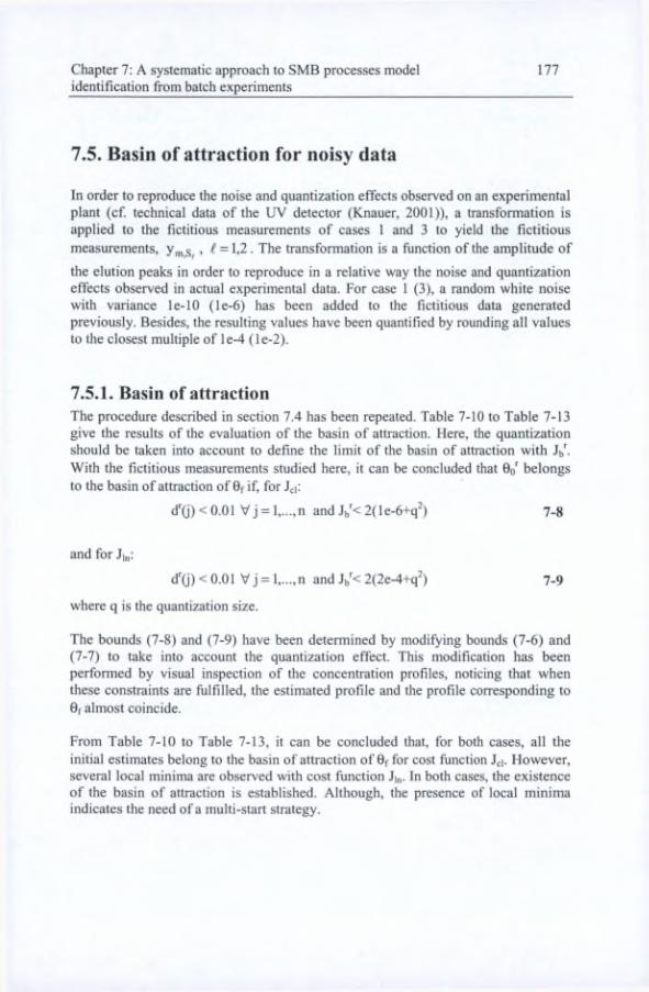
Chapter 7: A systematic approach to SMB processes modelidentification from batch experiments
177
7.5. Basin of attraction for noisy data
In order to reproduce the noise and quantization effects observed on an experimental plant (cf. technical data of the UV detector (Knauer, 2001)), a transformation is applied to the fictitious measurements of cases 1 and 3 to yield the fictitious measurements, y,„ g, > f = 1,2. The transformation is a function of the amplitude of
the elution peaks in order to reproduce in a relative way the noise and quantization effects observed in actual experimental data. For case 1 (3), a random white noise with variance le-10 (le-6) has been added to the fictitious data generated previously. Besides, the resulting values hâve been quantified by rounding ail values to the closest multiple of le-4 (le-2).
7.5.1. Basin of attractionThe procedure described in section 7.4 has been repeated. Table 7-10 to Table 7-13 give the results of the évaluation of the basin of attraction. Here, the quantization should be taken into account to define the limit of the basin of attraction with J(,^ With the fictitious measurements studied here, it can be concluded that Oq^ belongs to the basin of attraction of 0f if, for Jd:
d''G) < 0.01 V j = l,...,n and V< 2(le-6V) 7-8
and for J|n:
d'Ci) < 0.01 V j = l,...,n and V< 2(2e-4+q^) 7-9
where q is the quantization size.
The bounds (7-8) and (7-9) hâve been determined by modifying bounds (7-6) and (7-7) to take into account the quantization effect. This modification has been perfonned by visual inspection of the concentration profiles, noticing that when these constraints are fulfilled, the estimated profile and the profile corresponding to 0f almost coïncide.
From Table 7-10 to Table 7-13, it can be concluded that, for both cases, ail the initial estimâtes belong to the basin of attraction of 0f for cost function Jd. However, several local minima are observed with cost function J|n. In both cases, the existence of the basin of attraction is established. Although, the presence of local minima indicates the need of a multi-start strategy.

178 Chapter 7; A systematic approach to SMB processes modelidentification ffom batch experiments
Table 7-10: Study of the basin of attraction with noise and quantization, case 1 with gaussian noise (std = le-5) and quantization (q = le-4); cost function Jd;
0 = [kA kg qs bA bfif
9f [3.19 1.89 15.4 0.21 0.422]'
AÔBf [0.2 0.2 0.1 0.1 0.1]^
std( 0 )/0 [2.65e-3 1.94e-3 1.48e-4 2e-4 1.85e-4]'^
®min[3.188 1.9 15.399 0.21 0.422]^
1.12e-6
md [le-2 5.9e-3 7.5e-4 9.52e-4 7.1e-4]'^
nb/2" 32/32
Table 7-11: Study of the basin of attraction with noise and quantization for case 3 with Gaussian noise (std = le-3) and quantization (q = le-2) ; cost function 3^;
0 = [kA k3 Ha Hb bA ba]^
Of [3.75 2.52 0.8472 2.1 0.00052 0.0399]'
AOBf [0.2 0.2 0.05 0.05 0.1 0.1]’^
std( 0 )/0 [3.23e-4 1.29e-3 5.6e-8 3e-5 4e-8 3.5e-8]'^
®min [3.76 2.5 0.8471 2.1 0.0052 0.0399]"^
Jinin/^T 1.49e-4
md [3.8e-3 5.8e-3 1.18e-4 3.33e-4 9e-4 le-3]'^
nb/2" 64/64

Chapter 7: A systematic approach to SMB processes modelidentification from batch experiments
179
Table 7-12: Study of the basin of attraction with noise and quantization for case 1 with Gaussian noise (std = le-5) and quantization (q = le-4), cost fonction J|„.
e = bA bsŸ
0f [3.19 1.89 15.4 0.21 0.422] ‘
A&flf [0.2 0.2 0.1 0.1 0.1]^
std( è )/0 [0.1 0.03 0.006 0.006 0.006]^
®min[3.195 1.895 15.4 0.21 0.422]"^
2.3e-7
md [0.009 0.002 0.002 0.002 0.002]
nt/2" 10/32
Table 7-13: Study of the basin of attraction with noise and quantization for 3 with Gaussian noise (std = le-3) and quantization (q = le-2); cost fonction J]„;
0 = [kA ke Ha Hb bA bgf
Of [3.75 2.52 0.8472 2.1 0.00052 0.0399]'
A&Of [0.2 0.2 0.05 0.05 0.1 0.1]^
std( 0 )/0 [0.08 0.23 0.002 0.004 0.02 0.01]^
®min[3.76 2.5 0.8473 2.1 0.00519 0.03995]"^
1.94e-5
md [0.03 0.08 0.006 0.002 0.02 0.007 ]’'
nb/2" 10/64
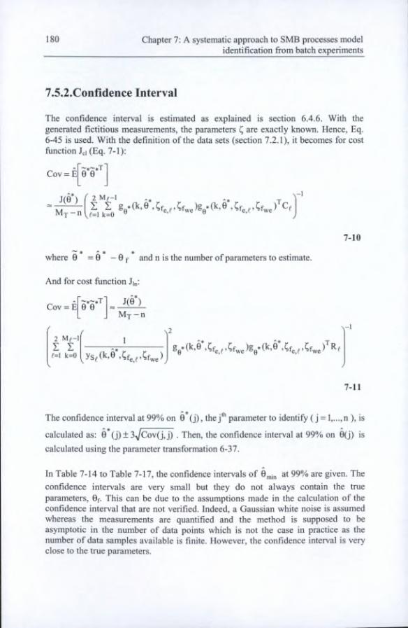
180 Chapter 7: A systematic approach to SMB processes modelidentification front batch experiments
7.5.2.Confîdence Interval
The confidence interval is estimated as explained is section 6.4.6. With the generated fictitious measurements, the parameters Ç, are exactly known. Hence, Eq. 6-45 is used. With the définition of the data sets (section 7.2.1), it becomes for cost function Jd (Eq. 7-1):
Cov = E 0 0
J(0)Mj -n
2 Mf-l
7-10
where 0 =0 - 0 f and n is the number of parameters to estimate.
And for cost function J|n:
J(0*)Cov = E
2 Mf-1I If=l k=0
V
0 0My — n
1
7-11
The confidence interval at 99% on Ô*(j), the j'*' parameter to identify ( j = l,...,n ), is
calculated as: 0*(j)±3.^Cov(j,j) . Then, the confidence interval at 99% on 0(j) is
calculated using the parameter transformation 6-37.
In Table 7-14 to Table 7-17, the confidence intervals of at 99% are given. The confidence intervals are very small but they do not always contain the true parameters, 0f. This can be due to the assumptions made in the calculation of the confidence interval that are not verified. Indeed, a Gaussian white noise is assumed whereas the measurements are quantified and the method is supposed to be asymptotic in the number of data points which is not the case in practice as the number of data samples available is finite. However, the confidence interval is very close to the true parameters.

Chapter 7: A systematic approach to SMB processes model 181identification from batch experiments
Table 7-14: case 1: confidence intervals; cost function
0f Confidence interval
kA(s-') 3.19 3.187 [3.183;3.19]Ms-') 1.9 1.9 [[1.8963;!.9037]
qs (vol%) 15.4 15.398 [15.393; 15.4]bA (vol%-') 0.21 0.21 [0.20993;0.21007]be (vol%-') 0.422 0.422 [0.42185;0.42215]
Table 7-15: case 3: confidence intervals; cost function Jd
0f 6minConfidence interval
kA(s-‘) 3.75 3.7592 [3.7537;3.7647]keCs-') 2.52 2.5233 [2.5258;2.5402]
Ha 0.8472 0.8471 [0.84702;0.84718]Hb 2.1 2.0995 [2.099;2.0998]
bA (g/l)-' 0.0052 0.0052 [0.005199;0.005208]bB(gd)-' 0.0399 0.0399 [0.3986;0.39942]
Table 7-16: case 1: confidence intervals; cost function Jjn
0f êm.nConfidence interval
kA (s-') 3.19 3.195 [3.1946;3.195]kB(s-') 1.9 1.895 [1.8947; 1.8952]
qs (vol%) 15.4 15.4 [15.3997;15.4003]bA (vol%-') 0.21 0.21 [0.2099;0.210004]bB (vol% ') 0.422 0.422 [0.42199;0.42201]
Table 7-17: case 3: confidence intervals; cost function J|„
0f 0minConfidence interval
kA(s-') 3.75 3.76 [3.72;3.768]kB(s') 2.52 2.5 [2.49;2.51]
Ha 0.8472 0.8473 [0.84716;0.84744]Hb 2.1 2.1 [2.099;2.1]
bA(g/l)-' 0.0052 0.00519 [0.005183;0.005196]bB (g/l)-' 0.0399 0.03995 [0.03994;0.03996]

182 Chapter 7: A systematic approach to SMB processes modelidentification from batch experiments
7.5.3. Confidence envelope
As explained in section 6.4.7, there is a différence between the estimated parameter,
0*, and the true parameter, 0*f. Hence, there is a simulation error between the
results of simulation, Ys^ ^ ). obtained by introducing 0 in Eq.
6-27 and the true values, yg^ (t,0f*,Çf^^^ ) :
ys, (kT, 0*, Ç) = Ys^ (kT, 0*f, ) + ys, (kT)
k = 0,l,...,M^ -1
with ÿs^ (t), the simulation error.
For data set ^ = l,np, this simulation error may be estimated from the estimated
covariance matrix of the simulation error (Eq. 6-88).
Figure 7-18 to Figure 7-20 represent the plot of the fictitious measurements,
the estimated, ys^(kT,0*,Cf^^^,Çf^^), and the
estimated confidence envelope, [ys^(kT,0*,Çfg_^,Çf^g)-ÿsf(kT),
ySf(kT,0*,Çfg^^,^f^^)-FySf(kT)], k = 0,..,M^-l, ^ = 1,2, for case 1 and cost
function Jd. Similar results hâve been obtained for case 3 and for cost flmction J|n as seen in Figure 7-20. The simulation error is very small. It contains the measurements or is very close to them. Hence, the effectiveness of the method is demonstrated.

Chapter 7: A systematic approach to SMB processes modelidentification from batch experiments
183
Figure 7-18: case 1, S2 with noise and quantization; cost function Jd,
fictitious measurements (kT,6f*,Çf^ 2 ’ ^ (•), the estimate,
ys2(kT,0*, 2’bounds of the estimated
confidence envelope, ys2(kT,0*,i;f^ 2’^fwe)-yS2 (^T)
ys2(kT,é*,Çf^2’^fwe)+ys2(kT)(_).
and

184 Chapter 7: A systematic approach to SMB processes modelidentification from batch experiments
xlO
Figure 7-19: case 1, Si, with noise and quantization; cost function Jei, fictitious
measurements, y,„ (•), the estimate,
ysi (kT,0*, ) (+), and the bounds of the estimated confidence
envelope, ys,(kT,0*,Çf^,,Çf^J-ÿs,(kT) and ys,(kT,0*,Cf^_,,Cf^^) + ysi(kT)
(_).

Chapter 7: A systematic approach to SMB processes modelidentification from batch experiments
185
xlO'^
time (s)
Figure 7-20: zoom on a part of the profile; case 1, cost function J|„, Sj, with noise and quantization; fictitious measurements,
ym,s, (•), the estimate, yg, )
(+), and the bounds of the estimated confidence envelope,
ys,(kT,0*,Çf^ ,,Çf^^)-ÿsj(kX) and ys,(kT,0*,Çf^ ,,Çf^^) + ys,(kT)
(_).
7.6.Conclusion
In this part of the study, the problem of identifying SMB model parameters from batch experiments is addressed. A numerical procedure is developed and evaluated on fictitious measurements generated from a model with known parameters. The method is based on the définition of a cost function and its minimization using an appropriate numerical procedure. The main contribution of this work is a careful identifiability study, including parameter sensitivity analysis, experiment design, the détection of local minima and the characterization of the basin of attraction associated to the known model parameters. Besides, confidence intervals for the estimated parameters are computed.
Thanks to the sensitivity analysis, the number of elution peaks and the associated concentration needed to identify the parameters with good accuracy are determined. Moreover, from a systematic comparison of the computational load and the identifiability of the parameters for kinetic, equilibrium dispersive and LDF models, it follows that a kinetic model yields an appropriate compromise between these criteria. Hence, it tums out that the most suitable identification procedure consists of the simultaneous identification of the isotherm parameters and the mass transfer coefficients of a kinetic model from two elution peaks, one at low concentration and

186 Chapter 7: A systematic approach to SMB processes modelidentification from batch experiments
a second at the highest possible concentration. From the study of the basin of attraction, the need for a multi-start optimization is exhibited in order to cope with the presence of local minima. The calculation of the confidence intervals and of the simulation error has also been tested. Two cost functions hâve been studied, one considering a relative error, J|„, another an absolute error, Jei. Both give similar results. The validation on experimental batch and SMB data is performed in chapter 8.
7.7.Summary of the identification procedure
Model- Kinetic model with Langmuir isotherm (Eq. (6-2),(6-3), (6-5))
Identified parameters- Mass transfer coefficients and isotherm parameters- Constraints on these parameters introduced with Eq. 6-37
Data- Elution experiments performed on one SMB column- 2 elution peaks necessary: one at the smallest possible concentration, one at the largest possible concentration
Cost function
Or
with y^®*, f = 1,2 , the measured UV signais, f = 1,2 , the simulated UV
signais, and M^, the number of measurements of the data set S^.
C, =max(ys7)/max(y™^).

Chapter 7: A systematic approach to SMB processes modelidentification from batch experiments
187
R, = max(ln(y^^(t)))/max(ln(y™^(t)))t ^ t '
Optimization algorithm- Algorithm for unconstrained optimization by quadratic approximation called UOBYQA (Powell, 2000).
Identification procedureMultistart procedure
1. Calculation of Oj^i, , a rough approximation of the parameters, ffom classical experimental methods applied directly to data sets S| and S2.2. Estimation of A0jnj,, an upper bound of the error on 0j„j,
3. Transformation of 0jj,j, and AOi^jt with (6-38) to obtain 0*init and A0jnj,*
4. Identification of r = l,...,2", from the different initial estimâtes:
0 0=0 init±A9 init, r = l,...,2 . The associated value of the minimum cost
fonction will be denoted r = 1,...,2" .5. Sélection of the identified parameter used in simulation:
©niin is the parameter value for which J^in is reached where = min Jj^jn,
r=3l,...,2".

188 Chapter 7: A systematic approach to SMB processes modelidentification from batch experiments
APPENDIX 7.1 FICTITIOUS MEASUREMENTS
This appendix provides some information about the fictitious measurements used in Chapter 7. Table A.7.1 gives the parameters and operating conditions used in the sensitivity analysis and in the génération of fictitious measurements. Note that the parameters kj™' of the kinetic model and Nj from the ED model verify the équation 6-36. Hence the profiles simulated with both models are similar.
Table A.7.1: case description (parameter and operating conditions) used for sensitivity analysis and fictitious measurements
Case 1 2 3 4Column length (m) 0.1 1 0.232 1Column diameter (m) 0.0212 0.02 0.048 0.02Injected volume (ml) 2 2 10 2Porosity 0.62 0.83 0.66 0.83kA (s'') (kinetic model) 3.19 3.2 3.75 8.1ke (s ') (kinetic model) 1.9 2.4 2.52 5.69Na 313 629 733 1599Nb 259 506 417 1200Dl,a mVs 1.8e-7 2.5e-7 4.2e-7 le-7Dl,b mVs 2.2e-7 3.1e-7 0.97e-7 0.94e-7kp.A (s'') (LDF model) 6.4 6.4 7.5 16.1kF,B(s'’)(LDF model) 3.8 4.8 5 11Isotherm El L1 L2 L2Ha 3.23 5.7 0.8472 5.97Hb 6.5 8.62 2.1 8.520Fa (vo1%‘' except case 3 in g/f') 0.21 0.215 0.0052 0.154bB(vol%'' except case 3 in g/f') 0.422 0.325 0.0399 0.295Selectivity (bs/bB) 2 1.51 7.67 1.91Flow rate (ml/min) 30 40 100 40UV(A) 0.256 0.35 0.1991 0.1991UV(B) 0.226 0.29 0.191 0.191Time span of each , T (s) 500 1500 500 1500
Sampling period, Ts (s) 1 1 1 1Mt 1000 3000 1000 3000

Chapter 7: A systematic approach to SMB processes modelidentification front batch experiments
189
In Table A. 7.2, the upper bounds on the parameters are defined. The lower bounds are equal to 0. Table A. 7.3 shows the saturation coefficient, ysa,, chosen to use the cost function J|n, To be consistent with the experimental study which will be performed later, they are taken equal to the standard déviation of the noise of the UV signal weighted by a factor to ensure that the relative effect is the same for ail case studies. Table A. 7.5 to Table A. 7.9 respectively give the concentrations used to plot Figure 7-13 and Figure A. 7.11 to Figure A. 7.13. Figure A. 7.1 gives the shape of the isotherms. It illustrâtes the non-linearity of these isotherms.
Table A. 7.2: Upper bounds on the identified parameters.
Case 1 2 3 4l^Asup (s ') (kinetic model) 10 10 10 10kssup (s ') (kinetic model) 10 10 10 10^Asup 2000 2000 2000 2000^Bsup 2000 2000 2000 2000^L.Asup ni /s le-5 le-5 le-5 le-5DuBsupIllVs le-5 le-5 le-5 le-5
kp,A sup (s'') (LDF model) 10 10 10 10kp.B sup(s'‘) (LDF model) 10 10 10 10QSsup 20 40 / /^Asup / / 10 10Hbsup / / 10 10bAsup (vol%'' except case 3 in g/f') 1 1 1 1bBsuD(vol%’’ except case 3 in g/f') 1 1 1 1
Table A. 7.3: Choice of the saturation coefficient used to avoid numerical problems with cost function J|„ (cf section 7.2.4)
Case_________________ 1_______________ 2_______________ 3_______________^ysai____________ le-3____________ 3e-4____________ OJ_____________ 3e-4
Table A. 7.4.: injected concentrations for fictitious measurements sets Sj and S2
Case 1 2 3 4
Ci.si (vol% except case 3 in g/l‘‘) 0.12 0.1 10 0.1
Ci.s2 (vol% except case 3 in g/1"') 12 10 100 10

190 Chapter 7: A systematic approach to SMB processes modelidentification from batch experiments
Table A. 7.5.: concentrations used in Figure 7-13
abscissa SI (vol%) S2 (vol%)1 1.20E-01 12 1.20E-01 33 1.20E-01 64 1.20E-01 85 1.20E-01 126 1.20E-01 207 1.20E-01 258 1.20E-01 409 1.20E-01 6010 2.00E+00 311 2.00E+00 612 2.00E+00 813 2.00E+00 1214 2.00E+00 1515 2.00E+00 2016 2.00E+00 2517 2.00E+00 4018 2.00E+00 60
Table A. 7.6: concentrations used in Figure 7-14
abscissa SI (vol%) S2(vol%)1 1.20E-01 12 1.20E-01 33 1.20E-01 64 1.20E-01 85 1.20E-01 126 1.20E-01 207 1.20E-01 258 1.20E-01 409 1.20E-01 6010 2.00E+00 311 2.00E+00 612 2.00E+00 813 2.00E+00 1214 2.00E+00 1515 2.00E+00 2016 2.00E+00 2517 2.00E+00 4018 2.00E+00 60

Chapter 7: A systematic approach to SM B processes modelidentification from batch experiments
191
Table A. 7.7: concentrations used in Figure A. 7.11
abscissa SI (vol%) S2 (vol%)
1 0.1 102 0.1 153 0.1 204 0.1 255 0.1 306 0.1 357 0.1 408 0.1 459 3 1010 3 1511 3 2012 3 2513 3 3014 3 3515 3 4016 3 4517 5 2018 5 2519 5 3020 5 3521 5 4022 5 4523 10 2024 10 2525 10 3026 10 3527 10 4028 10 45

192 Chapter 7: A systematic approach to SMB processes modelidentification from batch experiments
Table A. 7.8: concentrations used in Figure A. 7.12
abscissa SI (vol%) S2 (vol%)
1 0.1 52 0.1 103 0.1 204 0.1 305 0.1 506 0.1 1007 0.1 1508 1 59 1 1010 1 2011 1 3012 1 5013 1 10014 1 15015 1 20016 1 25017 1 30018 10 5019 10 10020 10 15021 10 20022 10 25023 10 30024 30 5025 30 10026 30 15027 30 20028 30 25029 30 300

Chapter 7: A systematic approach to SMB processes modelidentification from batch experiments
193
Table A. 7.9: concentrations used in Figure A. 7.13
abscissa SI (vol%) S2 (vol%)
1 0.1 12 0.1 33 0.1 54 0.1 105 0.1 156 0.1 207 0.1 258 0.1 309 0.1 4010 0.1 5011 0.1 6012 0.1 7013 2 7014 2 315 2 516 2 1017 2 1518 2 2019 2 2520 2 3021 2 4022 2 5023 2 60

194 Chapter 7; A systematic approach to SMB processes model
CA = CB
Figure A. 7.1 : Plane représentation (Ca = Cb) of the isotherms corresponding to the parameters in Table A.7.1

Chapter 7: A systematic approach to SMB processes modelidentification from batch experiments
195
APPENDIX 7.2 RESULTS OF THE SENSITIVITY ANALYSIS
In this appendix, complementary results are given for the sensitivity analysis with cost function Jd, performed in section 7.3.2.
Effect of the number of elution peaks
Figure A. 7.2 to Figure A. 7.5 give the évolution of the Gram déterminant (in logarithmic scale) as a function of the maximum injected concentration, Cj ,
i = A, B . For each curve a different number of data sets and/or different values of the injected concentration are considered. Figure A. 7.2 to Figure A. 7.4 show the results obtained with the kinetic model respectively for the parameters and the process characteristics corresponding to case 2, 3 or 4 (Table A.7.1.). Figure A. 7.5 shows the results obtained for case 1 and the equilibrium dispersive model.
*^A,Smax ~ ^B.Smax (VOl%)
0 10 20 30 40 50
-6 J ^ ^ ^ '
-11 -
'§ -16 -
ûa
O ^
ûK
û D
-21 5
-26
Figure A. 7.2: Illustration of the effect of the number of data sets on the Gram déterminant for case 2; kinetic model; cost function Jd
two data sets: Ci,si = 0.1 vol% (□);Cj,si = 10 vol% (x); 3 data sets: Ci_si = 0.1 vol% and Cj,s2 = 1 vol% (0),Ci,si = 10 vol% and Cj.s2 = 20 vol% (A)

196 Chapter 7: A systematic approach to SMB processes modelidentification ffom batch experiments
0 20 40 60 80 100 12010 i----------- '------------'----------- '----------- '----------- '----------- ^
0 -
QS -5 -
-10 -
-15 - □
140 160
A
Figure A. 7.3: Illustration of the effect of the number of data sets on the Gram déterminant for case 3; kinetic model; cost fonction
1 data set (•); two data sets: Ci,si = 0.1 vol% (□);3 data sets: Cj,si = 0.1 vol% and Cj,s2 = 5 vol% (0),Ci_si = 1 vol% and Cj_s2 = 5 vol% (A)
20 40 60 80-10 -
-15 -
-20 -
-25 □□
Q -30 ■O)O -35 -
•□
-40
-45 -
-50 -
-55 J
§ 9
Figure A. 7.4: Illustration of the effect of the number of data sets on the Gram déterminant for case 4; kinetic model; cost fonction
1 data set (•); two data sets: cj.si = 0.1 vol% (DijCi^si = 2 vol% (x)

Chapter 7: A systematic approach to SMB processes modelidentification from batch experiments
197
0-5
10
-10 -
-30 -
I-35 -
-40 -
15
X
20 25
"s
Figure A. 7.5: Illustration of the effect of the number of data sets on the Gram déterminant for case I; ED model, cost fonction
1 data set (S^ax) (•); two data sets: Ci,si = 0.12 vol% (□);ci,si = 2 vol% (x); 3 data sets: Ci.si =0.12 voI% and Cj,s2 = 1 vol% (0),Ci.si =0.12 vol% and Cj,s2 = 6 vol% (A)
Concentration of elution peaks
The Gram déterminant has been calculated here for the injection of two elution peaks with a different concentration. Figure A. 7.6 to Figure A. 7.9 give the results for the equilibrium-dispersive model respectively for case 1 to 4 of Table A.7.1. In Figure A. 7.10, the effect of the two injected concentrations is shown for case 1 of Table A.7.1 with the LDF model.

log(
D)
> lo
gP)
198 Chapter 7: A systematic approach to SMB processes modelidentification from batch experiments
ci,S2 (\ol%) 0 0 Ci.si (vol%)
. 7.6: Case 1 : results of concentration changes of SI and S2 on the Gram déterminant; ED model; cost function Jcl
Figure A. 7.7: case 2 : results of concentration changes of S| and S2 on the Gram déterminant; ED model; cost function

log(
D)
^ P
log(
D)
Chapter 7: A systematic approach to SMB processes modelidentification from batch experiments
199
. 7.8: case 3 : results of concentration changes of S| and S2 on the Gram déterminant; ED model; cost function Jd
Figure A. 7.9: Case 4 : results of concentration changes of S| and S2 on the Gram déterminant; ED model; cost function Jd

200 Chapter 7: A systematic approach to SMB processes modelidentification from batch experiments
- -r -
Figure A. 7.10: Case 1 : results of concentration changes of Si and S2 on the Gram déterminant; LDF model; cost function Jd
Model Comparison
Figure A. 7.11 to Figure A. 7.13 compare the Gram déterminant obtained with the kinetic and with the equilibrium dispersive model respectively for case 2 to 4 of Table A.7.1. Two elution peaks are used for each identification, one with a small injected concentration, one with a high injected concentration. Log(D) is represented as a function of different couples of input concentrations (Cj,si, Cj,s2) given in the appendix in Table A. 7.7 to Table A. 7.9.
Figure A. 7.11: Case 2: comparison of the Gram déterminant for the ED (□), and the kinetic (0) models, cost function

log(
D)
Chapter 7: A systematic approach to SMB processes modelidentification front batch experiments
201
Figure A. 7.12 : Case 3: comparison of the Gram déterminant for the ED (□), and the kinetic (0) models, cost function 3^
Figure A. 7.13: Case 4: comparison of the Gram déterminant for the ED (□), and the kinetic (0) models, cost function 3^

s-^'-ï- -^--;7,;."
r"' .
-i-, . "•
jf-‘
•V^ ’■ >’- tâs^t . ■ •r'tO- • r
■ _ —56^ *■. ‘i- "ïrr.il^..- *ihn •.,n?*-<jr ;
*-k*:i
■ V > ^ '“
-. “V•îV-V
J*'■; 5 :.:4
-ÎIC,
» ^ 11 ^
-,_ V,-^T•ï - -.,, •%•:=’ . ■■ ... 1• ■ ; ■ r ii -^ v|
■ -V .-■
, -fr
^ .!*iv
; - ' ^ --4'"^ - ='-^^’î'•■ ^ “ *c'^>. 6 .• ■_ .r ■ '-'
ir ■-■. . ■'•flSS-

Chapter 8: Validation with experimental data 203
CHAPTER 8 :Validation with experimental data
8.1. Introduction
The aim of this chapter is to validate on experimental data the systematic approach to SMB processes model identification from batch experiments developed in chapter 7. The first step is the parameter identification from batch experiments. The second step is the cross-validation with SMB experiments so as to assess whether the parameters identified from batch experiments may be used in a SMB model.
This chapter begins with a description of the séparation considered. Section 8.3 présents the statement of the identification problem for this case. Then, section 8.4
gives some information about the détermination of the parameters, Ç (like the porosity, the flow rate) and of the initial estimâtes of the parameters 0 that will be identified (mass transfer coefficients and isotherm parameters). Next, the identification is performed from batch experiments to estimate the mass transfer coefficients and isotherm parameters. Finally, the cross-validation on SMB experiments is realised.
8.2. The studied séparationThe studied SMB plant has been described in section 2.4. A schematic représentation of the plant is reminded in Figure 8-1. The considered séparation is a séparation studied by the Max Planck Institute of Magdeburg. It consists of the séparation of cyclopentanone and cyclohexanone on 8 columns with 21.2 mm internai diameter and 100mm length. The stationary phase is a silica gel (LiChroprep RP - 18, particle size 25 - 40 pm, Merck, Darmstadt) and the solvent is a water/methanol solution (70/30). The volumétrie mass of both components is equal to 0.95 g/ml. The cyclohexanone is the most adsorbed component and its molecular

204 Chapter 8: Validation with experimental data
weight is 98.15 g/mole. Hence, in the following, the cyclohexanone corresponds to component B and the cyclopentanone to component A.
To identify the parameters, the experiments are performed on a SMB column. Indeed, as seen in section 6.2.1.5, it is more advisable to work directly with experimental data recorded on the SMB columns and not on analytical columns to ensure that the porosity used in the estimation of the isotherm parameters is the same as the porosity of the SMB. As seen in section 6.2.1.5, it is assumed that ail the SMB columns hâve the same properties. Hence, only two columns hâve been selected (columns 2 and 6) and their estimated parameters will be compared.
Note that, according to a previous study (Grosfils et al, 2004), it appears that isotherms Ll, introduced in 6.2.1.1, are not appropriate to describe this séparation. Hence, only isotherms L2 hâve been considered.
A possible detector base-line drift is also considered by deducting to the measurements the mean of the detector signal calculated during a period during which there is no A and no B at the output.
Figure 8-1 : Schematic représentation of the studied SMB plant

Chapter 8: Validation with experimental data 205
8.3. Statement of the identification problemIn this section, the different steps of the identification procedure (see section 7.7) are reminded and completed with some information about their application in this case. For sake of easiness, ail the tables conceming the batch identification step (model parameters, experimental set-up characteristics, etc.) are grouped in section 8.4.8.
DataThe operating conditions and experimental set-up characteristics are described in Table 8-1. The number of samples per data set, , is given in Table 8-3.
To perform experiments, the column tested is placed, by rotation of the SMB multi- function valve, after pump P2 which is equipped with a manual injection valve. The UV detector which follows the column chosen is used (UV3 for column 2 and UV4 for column 6).
Two elution experiments are performed on each column, one with a small concentration and another with a high concentration. The injected concentrations are, here, prepared volumetrically by the user. The smallest concentration has been chosen high enough to be détectable and the highest concentration to be below the limit of solubility. Concentrations are given in Table 8-1. A calculation of the error due to the préparation of the samples is presented in (Grosfils, 2008).
Model- The kinetic model with Langmuir isotherm (Eq. (6-3), (6-4), (6-7)) is used.- The détermination of model parameters and (defined in sections
6.2.2.4 and 6.4.2), which are not identified, is explained in section 8.4. does not change from one experiment to the other:
However, as two data sets, which differ in the injected concentration, are used, the vector, Çg^ , is defined, for each column, as: Çg^ ^ (1 : M, ) = Çgl ^ and
Çg^m U\^(A) U\è(B) Vjnjf f = 1,2 . Index m is related
to the column number, m = 2 or 6 and S to the detector (ô = 3 if m = 2 and ô = 4 if m = 6).
Identified parameters- The mass transfer coefficients and isotherm parameters are identified on each
Çwe=[Vdi„ ef.
column: 0

206 Chapter 8; Validation with experimental data
- The constraints on these parameters, introduced with Eq. 6-37, are given in Table 8-3.
Cost functionCost functions 7-1 and 7-2 will be used and the obtained results will be compared. The weighting factors and the saturation value ysat are given in Table 8-3.
Optimization algorithmThe algorithm UOBYQA (Powell, 2000) is used.
IdentificationThe initial values of the parameter, 9o*^ r = 1,...,2", are obtained from the initial
estimâtes 0i„j, as explained in section 7.4. More details about this détermination are given in section 8.4. The identification results and the confidence intervals are given in section 8.5 and the validation on SMB experiments in section 8.6.
8.4. First estimation of model parameters
The détermination, on the experimental plant, of the parameters, Ç^^and
£ = 1,2, m = 2,6 and of the initial estimated of 0m, 0jm, m , is summarised in this
section. Note that an estimation of the error on performed as the
covariance matrix of will be necessary to calculate the confidence interval on
0 (see section 6.4.6). The obtained parameter values and the corresponding errors are summarised in section 8.4.8.
8.4.1. Flow rateThe flow rate is imposed to a pump by the user. Hence, the value of the flow rate is known. Moreover, according to the pump manual, the error is equal to 2% of the indicated flow rate.
8.4.2. PorosityThe porosity is measured as explained in section 6.3. Each column is placed after pump P2 equipped with a manual injection valve (see Figure 8-1). The rétention times of a non-retained component (thiourea) are measured. The detailed results of the experiments are given in (Grosfils, 2008) and the obtained porosities are given in

Chapter 8: Validation with experimental data 207
Table 8-1. The porosity of column 2 and 6 are not exactly the same. It shows that the packing is not exactly the same in both columns, it will be seen further how it influences the isotherm parameters. The calculation of the error on the experimental détermination of e is performed in (Grosfils, 2008). Note that as seen in 6.2.1.5, the error on the porosity will not be taken into account in batch as this error will be compensated in the identification of the isotherm parameters. Nevertheless, this error will be considered in the calculation of the confidence envelopes of the SMB concentration profiles as, in a SMB plant, the packing, its aging, and hence, the porosity, may differ from one column to the other.
8.4.3. Dead volumesDead volumes are due to connections, pumps and UV detectors. The values of some dead volumes hâve been transmitted by Knauer (see Table A. 8.1 in Appendix 8.1). Other dead volumes corresponding to changes to the original process performed by the Max Planck Institute are unknown and hâve been determined as explained in section 6.3. The results are given in Table A. 8.2.
8.4.4. Injected volumeThe injection is performed thanks to a manual injection valve. Its volume is 2 ml. However, it has been observed that the obtained peak is very sensitive to the way of the valve is used: velocity of the movement, duration in the open position, etc...
8.4.5. Injected concentrationsThe injected concentrations are given in Table 8-1. A calculation of the error due to the sample préparation is presented in (Grosfils, 2008); the resulting value is indicated in Table 8-4.
8.4.6. Calibration coefficientsTo détermine the calibration coefficients, the detectors are connected in sériés. Successive step changes of known concentrations of component A and then of component B are injected. The mean of each plateau is measured. Then the concentration is plotted against the measured UV value. It appears that the function is linear. The experimental results and the calculation of the error are given in (Grosfils, 2008). The calibration coefficients of the 4 detectors are given in Table A. 8.7 in Appendix 8.3.
8.4.7. Isotherm parameters and mass transfer coefficientsTo détermine the initial estimâtes of the isotherm parameters and the mass transfer coefficients as explained in section 6.3, several elution peaks at different

208 Chapter 8; Validation with experimental data
concentration hâve been recorded. The detailed experimental résulta are given in (Grosfils, 2008). The initial estimâtes obtained are given in Table 8-3. As experimental data are used, the values of AÔjni, /èmi, hâve been chosen superior to the minima used in section 7.4 and are given in Table 8-3. This choice should take the noise and the model error into account which do not exist with fictitious measurements.
8.4.8. SummaryTable 8-1 gives a summary of the séparation and experimental set-up characteristics.
The éléments of parameter vector Ç, estimated in the previous subsections, are
provided in Table 8-2. Table 8-3 shows the initial estimâtes of parameter, 9jj,j,, the chosen constraints and the relative edge length of the hyper-parallelepiped centred around used in the multi-start optimization procedure (cf. section 7.4). In
Table 8-4, the estimate of the error on Ç is indicated.
Table 8-1: Summary of the séparation and the experimental set-upcharacteristics
Column 2 Column 6
Q (ml/min) 30 30
£ 0.6 0.62
Vd.„ (ml) 10 10
(vol%) (with Cp,A = Cf.b) 0.12 0.12
Cg^ (vol%) with (cp.A = Cf,b) 6 12
Detector ô UV3 UV4
UV(A) 0.199 0.215
UV(B) 0.192 0.207
Vinj(ml) 2 2

Chapter 8: Validation with experimental data 209
Table 8-2 : Parameter Ç
-[Q ^F,A,^ U’S^CA) U\^(B) Xn/>U=[Vdi„ ef
Column 2 Column 6
te,[30 0.12 0.12 0.199 0.192 2] [30 0.12 0.12 0.215 0.207 2]
[30 6 6 0.199 0.192 2] [30 12 12 0.0.215 0.207 2]
twe[0.6 10] [0.62 10]
Table 8-3 : Batch identification conditions
0m = [k'Im HA.m bA,m bB,mrColumn 2 Column 6
0init[Î466 1015 3 6.96 0.24 0.56] [1194 801 3.24 7.5 0.26 0.61]
[0.3 0.3 0.1 0.1 0.3 0.3] [0.3 0.3 0.1 0.1 0.3 0.3]
êi„i.
6inf [0 0 0 0 0 0] [0 0 0 0 0 0]
^sup [4235 4235 10 10 1 1] [4375 4375 10 10 1 1]
Ysat le-3 le-3
C, 41.3 96.3
C2 1 1
R, 3. 3.2
R2 1 1
M| 316 398
M2 455 378

210 Chapter 8: Validation with experimental data
Table 8-4 : error on éléments of the parameter vector
Column 2 Column 6AQ/Q 0.02 0.02
Ae 0.013 0.013
Ac 0.0014 0.0014
AUV(A) Or AUV (B) 3e-3 3e-3
AV- -N- ■^ in/ ’ inj 0.01 0.01
8.5. Batch identification
Mass transfer coefficients and isotherm parameters are identified following the procedure summarised in section 8.3 with experimental conditions, model parameters and initial estimâtes given in Table 8-1 to Table 8-4.
Note that the following notations are introduced: 9min,m représenta the parameter
identified on column m, m = 2, 6, with the cost function Jd and the
parameter identified on column m, m = 2, 6, with the cost function J|n.
First, the résulta obtained with the two columns and two cost fonctions are compared and the validation with the experimental data is discussed. Then, the calculation of the confidence intervals is performed.
8.5.1.Results, validation, comparison
The résulta of the identification performed on the two columns of the SMB plant with the two cost fonctions Jd and Ji„ are shown in Table 8-5 to Table 8-8. For column 2, both cost fonctions Jd and J]„ give very similar résulta for parameters
^imin ^imin ’ * ~^ ’ whereas, parameters k/^*init are significantlydifferent. Moreover, from the comparison of the four tables (Table 8-5 to Table 8-8), it appears that the isotherm parameters identified on column 2 are very different from those obtained on column 6.
Figure 8-2 to Figure 8-5 show the experimental profiles as well as the peaks simulated with and with for both columns and both cost fiinctions. Note that data sets. Si and S2 used together for identification, are shown here separately for sake of clarity. These figures help to validate our identification approach. Note that the simulations are only compared with data that hâve been used for parameter

Chapter 8: Validation with experimental data 211
estimation. It should be interesting to validate the method with other experimental sets, but, unfortunately, data recorded at other process working modes are not usable because of a lack of reproducibility in the elution peaks recorded (probably due to injection problems). Nevertheless, the method will be validated with SMB experiments.
The correspondence between simulated and experimental curves is worse for column 6 than for column 2. This could be explained by the shape of the elution profile at 12 vol% (data set S2) for which the Langmuir isotherms might not be a good choice (cf Figure 8-5). However, results at 6 vol% are not available because of a large lack of reproducibility in the elution peaks recorded. Nevertheless, with smaller concentrations (Figure 8-2 to Figure 8-4), which are used in the SMB plant in this study, the Langmuir isotherm is able to reproduce the profiles with good accuracy.
For columns 2 and 6, the simulated profiles obtained with the parameters identified with Jji are different from those simulated with parameters estimated with Jjp. On the one hand, in general, the cost fonction J|„ gives profiles for which the bottom of the desorption fronts are close to the experimental profiles. This is especially clear in the blue ellipses added on Figure 8-2 to Figure 8-4. However, the top of the peaks is not well reproduced as seen in the red ellipses on the same figures. On the other hand, results obtained with cost fonction Jd provide peaks with a general shape (height and position) similar to the experimental ones, although the shape of the fronts obtained with cost fonction Ji„ is better. The good reproduction of the shape of the fronts may be a good advantage in SMB processes for control methods based on the position of the fronts. However, at this stage, it is difficult to conclude from batch experiments. Results must be compared in SMB mode.
Hence, the validation with parameters identified from column 6 is poor. Parameters identified with column 2 and the two cost fonctions, Jd and J|„, differ essentially in the mass transfer coefficients. This influences the form and the height of the elution peaks.
Table 8-5 : Batch identification results; column 2 cost fonction Jd
Ji„,/(M,+M2) = 1.2'-4;J™„/(M|+M2) = 2.81e-5
®initkA^^'(ni-') 1466 1546kB'*'(m-‘) 1015 1000.8Ha 3 3.05Hb 6.96 7.1bA (vol%)-' 0.24 0.215bB (vol%)'' 0.56 0.66

212 Chapter 8; Validation with experimental data
Table 8-6 : Batch identification results; column 2; cost function J]„Jm,/(M,+M2) =4.14; W(M,+M2) = 6.7e-2
®initA InÛ^min
kA^^' (m-') 1466 953.11015 720.1
Ha 3 3.075Hb 6.96 7.09bA (vol%)-' 0.24 0.21bB(vol%)' 0.56 0.65
Table 8-7 : Batcb identification results; column 6; cost function Jd
J^,„/(M,+M2) = 8e-3; J^,n/(M,+M2) = 6.7e-4
Qjnit____________^minkA"'(m‘) 1194 1707kB^^'Cm-’) 801 970Ha 3.24 3.25Hb 7.5 7.642bA (vol%)-‘ 0.26 0.174be (vol%y‘ 0.61 0.678
Table 8-8: Batch identification results; column 6, cost function J|„
Jini,/(Mi+M2) =7.8; W(M|+M2)= 1.15e-lA /'Inû û
kA^^' (m-') 1194 1225.8kB^^'Cm-') 801 713.5Ha 3.24 3.3Hb 7.5 7.67bA (vol%)-' 0.26 0.193ba (vol%y' 0.61 0.69

Figure 8-2 : Results of parameter estimation for column 2 with data set SI;
••• experimental profile; *** ys|(ti,k,6*min,Csi) 5+++ ysi(ti,k»6 min'",Csi) î
ySiOl,k>Q init,Çs[) , k = 0, M|-l•••
Chapter 8
; Validation with experim
ental data 213

Figure 8-3 : Results of parameter estimation for column 2 with data set S2;
••• experimental profile; *** '"'">^82^ ;-h-i- ys2(^2,k>® min .^82).
yS2(^2.k>® init,Cs2) , k = 0, M2-I• ••
214 C
hapter 8: Validation w
ith experimental data

Figure 8-4 : Results of parameter estimation for column 6 with data set SI;^ * In ^
••• experimental profile; *** ysj(ti,k>® r>iin! Cs]) ysi(tl,k>0 min -Cs]) i
ySiOl,k>® init>Cs| ) » k = 0, Mpl• ••
Chapter 8
: Validation with experim
ental data________________________________215

Figure 8-5 : Results of parameter estimation for column 6 with data set S2;
...experimental profile;*** ys2(t2,k>9*min,;s2) .+++ ys2(t2,k.6*min'",Çs2).
yS2(*2,k>6 init,Cs2) , k = 0,• ••
216 C
hapter 8: Validation w
ith experimental data

Chapter 8: Validation with experimental data 217
8.5.2.Confidence interval
The confidence intervals of the estimated parameters hâve been calculated following the two approaches proposed in section 6.4.6.1;
a) the error on the estimated parameter is neglected;
b) the error on the estimated parameter is taken into account.
Note that the column 6 is no more considered here as poor results hâve been obtained in validation in the previous section.
a) Confidence interval without error on parameter Çg^
It is assumed that the parameter Çg^ is perfectly known without error. Hence Eq.
6-45 is used. Confidence intervals at 99% are given in tables 8-9 and 8-10 for column 2 and the two cost functions and J|„. For both cost functions, the intervals are very small for parameters and Hb, and large for kA^^' and ke^''. However, the cost fonction Jd gives smaller confidence intervals for parameters bA and be than the cost fonction J|n. The confidence intervals obtained are probably under-estimated as the parameters Çg^ are not precisely known.
b) Confidence interval with error on parameter Çg^
The error on the parameter Çg^ is now taken into account which seems more
realistic (cf section 6.2.2.4). Eq. 6-85 is hence used. Details about the estimation ofr
Q’® are given in Appendix 8.2. Confidence intervals at 65% are given in tables 8-9 and 8-10. As expected, confidence intervals are larger than preceding. Note that they are larger for the cost fonction Jd than for the cost function J|n. However, the intervals seem to be overestimated. It is probably due the numerous assumptions performed to obtain Eq. 6-85 like
number of samples that tends to infinity assumptions on the errors 6-49,6-50 assumptions 6-58, etc...
Hence, the confidence intervals obtained without introducing the error on Çg^ are
probably under-estimated whereas the confidence intervals obtained with the error
on Çg^ are probably over-estimated. In both cases, the confidence intervals on
parameters Ha and Hb are small whereas the confidence intervals on parameters kA*^'' and kB"^'* are large. Hence, as already seen in Chapter 7, the latter are more difficult to estimate.

218 Chapter 8: Validation with experimental data
Table 8-9 : Confidence intervals; column 2 cost function Jd
Ꙅ Confidence
interval with known without
error (99%)
Confidence interval with
error on (65%)
kA^^' (m-‘) 1546 [1478;1613] [266; 3515]kB^'‘(m-') 1000.8 [944; 1076] [84 ;3473]Ha 3.05 [3.04;3.06] [2.8 ;3.27]Hb 7.1 [7.08;7.12] [6.4 ;7.7]bA (vol%)-‘ 0.215 [0.212;0.218] [0.13 ;0.32]be (vol%)-‘ 0.66 [0.65;0.67] [0.32 ;0.89]
Table 8-10 : Confidence intervals; cost function Ji„
In
9minConfidence Confidence
interval with Çy interval with
known without error onerror (99%) (65%)
kA^^‘ (m-') 953.1 [885;1025] [677 ;1296]kB"'(m-') 720.1 [665;771] [508 ;974]Ha 3.075 [3.05;3.09] [3 ;3.15]Hb 7.09 [7.06;7.13] [6.9 ;7.3]bA (vol%) ' 0.21 [0.19;0.23] [0.13 ;0.3]ba (vol%)'' 0.65 [0.61;0.68] [0.49 ;0.78]
8.5.3.ConclusionsIn conclusion, the validation with parameters identified from column 6 is poor. However, for column 2, both cost functions give nearly the same isotherm parameters but different mass transfer coefficients. Both results seem acceptable. Hence, the next step is the comparison of both sets of parameters in the SMB simulations in section 8.6.

Chapter 8: Validation with experimental data 219
8.6. Validation with SMB experiments
In this section, the parameters estimated from batch experiments are used to simulate the SMB process in order to verify the effectiveness of our approach.
On the one hand, SMB experiments hâve been performed on the unit described in section 2.3. for two operating conditions (case I and II) described in Table 8-11.
-SMBOn the other hand, simulations hâve been performed with parameter vector, Ç ,
ô, m
5 = 1,...,4 , m = 2,6 and 6min,m > corresponding to column 2 and 6. The model and simulation parameters are summarised in Appendix 8.3.
Results of simulation and experiments are, here, compared in order to verify if the parameters determined with batch experiments may be used in a SMB model. Note
that the following notation is used: corresponds to the
simulation of the signal of detector 5 obtained with the parameter identified on column m.
Note that, here, only two operating conditions are considered and ail the UV signais corresponding to these operating points are not shown. But similar results hâve been obtained for the other UV signais and for other operating conditions.
Table 8-11: Operating conditions
Case I 11
Ca.f = Cb,f (vo1%) 1.456 1.456
Switching time (s) 150 130
Qi] (ml/min) 15.6 28.7
Qiv (ml/min) 17.9 27
Qf (ml/min) 10.6 8.4
Qd (ml/min) 32.5 31.3

220 Chapter 8: Validation with experimental data
Figure 8-6 to Figure 8-10 show the comparisons between the measurements, the
signais simulated with the initial parameter roughly estimated, Oinj,, and with the parameters identified with J|„ or Jd, with column 2. In Figure 8-6, the extract signal (UVl) is given for case I. In Figure 8-7 and in Figure 8-9, the raffinate signal (UV2) is plotted respectively for case I and case II, and in Figure 8-10, the signal recorded with detector UV3 is represented for case II. Note that the experiments corresponding to case I hâve been reproduced two times in order to observe the reproducibility. Moreover, even if it has been shown in the previous section that the identification with column 6 gives poor results, some simulations performed with these parameters are given in Figure 8-11 in order to show the results obtained in SMB mode. Figure 8-8 shows the effect of a change of the flow rates on the simulated UV3 signal. From these figures, it can be concluded that:
- The parameters obtained with cost functions Jd and Jin give similar profiles. As the parameters differ essentially in the value of the mass transfer coefficients, it can be concluded that the latter hâve a low impact on the SMB concentration profiles studied here.
- As already observed in batch validation (in section 8.5), results obtained with the parameters of eolumn 6 are poor, especially at high concentration as seen in the pink circle added on Figure 8-11 in comparison with Figure 8-10.
- In ail the figures, the signais simulated with parameters of column 2 give a good approximation of the measurements. The worst parts of the simulation profile are the fronts of the raffinate signais. The différences between the experiments and the simulation results may be explained by different causes:
• Errors in the calibration coefficients or small variations of parameters among the columns.
• Experimental errors: as shown in Figure 8-6 to Figure 8-7, the reproducibility of the measurements is not perfect and some experimental errors due to inaccuracies in the flow rates or in the préparation of the solutions, are also to consider. For example, the largest différences observed in Figure 8-7 may be explained by a lack of précision of the flow rates of the SMB plant. Indeed, as seen in Figure 8-8, simulations with smaller internai flow rates (with output and input flows not changed) are doser to the experimental signal.
• Errors in the modelling of dead volumes where plug flow is assumed.• Errors in the values of the dead volume.• Error in the modelling of the permutation which is not abrupt in practice.
- Moreover, the signais simulated with are close to the one obtained with
Bjni,. Indeed, the concentrations obtained at the outputs are not very high and, as already observed, the initial parameters corresponding to the linear part of the isotherm and describing the behaviour at low concentration, and ,are
close the identified ones, and But a large improvement of theprofile is shown at higher concentration in the pink circle in Figure 8-10.

Chapter 8: Validation with experimental data 221
Figure 8-6 : case I; extract signal; experiments: ++-+ and •••; simulations:SMB/. A PSMB-,. 5
yi V,«init,2>Sl,2 )>— yiSMB
(t’0min,2'Cl,2SMB^
yi V'”min,2>oI,2 1’» In SMB,
Figure 8-7: case I; raffinate signal; experiments: and ••• ; simulations:SMB/j A
yi ti,Hinit,2>SMB/i A
y 2PSMBS2,2
* In(^’®min,2
P SMB s ^2,2

222 Chapter 8: Validation with experimental data
Figure 8-8 : case I; detector UV3 signal ; experiments: +++ and •••;
simulations:__y2*^^(t,6min,2.Ç2!2^) with flow rates in column 2 of
Table 8-12; y2*'^^(t,6min,2>Ç2!2^) with flow rates in column 3 of Table 8-12
Figure 8-9 : case II; raffinate signal; experiments: •••; simulations:
SMB,, A ?SMB. SMB.. û'" fSMBxSMByi (t-êiniu-ClT);.

Chapter 8: Validation with experimental data 223
Figure 8-10 : case II; detector UV3 signal; experiments: •••; simulations:
SMB/. û rsivuix. SMtJ/. û s— y-i (l»Winit,2>'=3.2 ------ y3 U'ymin,2'S3,2 )»-y3
iSMB SMB, -SMB-, ,.SMB û‘" pSMB. tl>«min,2>S3,2 > ■>
Figure 8-11: case II; detector UV3 signal; experiments: •••; simulations:
SMB/. A fSMB\. SMB/j A ?SMB\ SMB^, Ain ?SMB\ y3 2,S3,2 — y3 U-g, Ç,3 ^ )— y3 (l,Hmin,6>S3,6 >

224 Chapter 8: Validation with experimental data
Table 8-12 : Flowrates applied in Figure 8-8
: flow rates of case 1; 0*: modified flow rates)Q (ml/min) Q* (ml/min) AQ/Q (%)
Zone I 50.4 49.9 1
Zone II 15.6 15.1 3
Zone III 26.2 25.7 2.
Zone IV 17.9 17.4 2.3
8.7. Confidence envelope
In this section, the simulation error is calculated as explained in section 6.4.7 and already applied in section 7.5.3. However, here, contrary to section 7.5.3, an error on
the estimated parameter, , is introduced by using 6-99. Note that, in contrast with the study of chapter 7, here, as the measurements are “real” measurements, it is supposed that a “true” model exists to apply 6-99.
The confidence envelope has been calculated with two different approximations of
the covariance E(66 ) ;
a) with E(90 ) estimated without considering the error on the parameter ÇSMB
b) with E(00 ) estimated by taking the error on parameter Ç5 into account.
For sake of easiness, the covariance of case a is labelled Ea and these of case b, Eb.
Figure 8-12 and Figure 8-13 show the confidence envelopes of the UV3 signal simulated with the parameters identified with the cost fonction Jd built respectively with estimation Ea and with estimation Eb. On Figure 8-14, the confidence envelope calculated with approximation Eb is given for a UV3 signal obtained with cost fonction J|„ . Figure 8-15 compares the confidence envelopes calculated with Eb for a concentration profile simulated with parameters identified with the cost function Ji„ and for the cost function 3^.
Some conclusions may be drawn from these pictures:

Chapter 8: Validation with experimental data 225
as expected, the confidence envelopes obtained with Ea are smaller than those estimated by taking the error into account.the confidence envelopes obtained with the cost function Ji„ are in general smaller than those obtained with the cost functionthe experimental data are, in general, contained in the confidence envelope estimated with Eb but not with Eathe largest subset of the experimental data which is not contained in the confidence envelope corresponds to the raffmate fronts. As seen in section8.6, the latter are poorly simulated;the parts of the signal with a larger confidence envelope correspond to parts of the profiles where the reproducibility of the experiments is the worst.
Figure 8-12 : case I; detector UV3 signal; * and ... experiments;
__yf'^^(t.Ômin,2>Ç3,'2^) » bounds of the estimated confidence interval withthe cost function and Ea

226 Chapter 8; Validation with experimental data
Figure 8-13 : case I; detector UV3 signal; * and ... experiments;
__» bounds of the estimated confidence interval withthe cost function J^i and Eb
Figure 8-14 : case I; detector UV3 signal; * and ... experiments;
__0min,2 ’ Çf,'2’ bounds of the estimated confidence interval with
the cost function J|„ and Ea

Figure 8-15 : case I; detector UV3 signal; * and ... experiments;__ y3*^^(t,êmin ’ bounds of the estimated confidence interval with the costfunction J|„ and Eb;----- bounds of the estimated confidence interval with the cost fonction Jd andEb
Chapter 8
: Validation with experim
ental data 227

228 Chapter 8: Validation with experimental data
8.8. Remark: identification from SMB experiments
The parameter identification should be improved or performed directly from SMB experiments. A preliminary study has already been performed in (Grosfils et al., 2005). An identification procedure for determining the isotherm parameters as well as the mass transfer coefficients in a kinetic SMB model with compétitive Langmuir isotherms from SMB experiments has been proposed. The main contributions are a systematic identifiability study and the examination of the basin of attraction to déterminé the influence of local minima.
Both studies allow to- verify that the parameters are structurally identifiable,- détermine the measurements of which sensor are the most appropriate (i.e. the sensor in the circulating loop (UV3 or UV4));- set up an identification procedure (with multi-start strategy).
However, open issues are the choice of the operating conditions at which identification must be performed and the vérification of the effectiveness of the method on experimental data. Nevertheless, the priority is the complété validation of the proposed approach with batch experiments, as explained in the following section. Indeed, this method seems more convenient than the parameter estimation from SMB experiments. Actually, the SMB experiments take more time than batch experiments, and the simulations of a SMB plant are longer than batch simulations.
8.9. Conclusions
In conclusion, the parameters, estimated with good accuracy from one of chromatographie column of a SMB plant, may be used in a SMB model to reproduce the SMB profiles. Both cost functions used in batch, Jd and Jin, give similar results. The first is probably casier to use as it requires less mathematical operations but the second gives smaller confidence envelopes for the simulated SMB concentration profiles.
However, it should be interesting to test the approach on data at higher concentrations. Indeed, from the first results, the proposed method seems to bring significant improvements of the estimation of the parameters characterizing the non- linearity of the adsorption, which becomes important at high concentration.
Moreover, as the dead volumes significantly influence the form of the concentration profiles, the validation of the identification approach should also be performed with data less disturbed by dead volumes, for example, measurement recorded with larger flow rates or on SMB plants with smaller dead volumes.

Chapter 8; Validation with experimental data 229
Finally, some improvements of the simulations may probably be achieved with more précisé information about the dead volumes, the permutation and the flow rates.

230 Chapter 8: Validation with experimental data
Appendix 8.1 Dead volumes
The values of the dead volumes provided by Knauer are given in Table A. 8.1. Figure A. 8.1 shows a schematic représentation of the plant to understand terms used in Table A. 8.1 like “shortcut tubing”, “long and short connections”. In Table A. 8.2, the dead volumes measured on the experimental setup are shown. Note that in Appendix 8.3, Table A. 8.4 and Table A. 8.5 give the fixed and mobile dead volumes (defined in section 5.3) obtained from Table A. 8.1 and Table A. 8.2.
Table A. 8.1 : value of the dead volume given by Knauer in the SMB of the Max Planck Institute of Magdeburg
quantitylength(mm)
ID(mm) volume (ml)
total volume in each
zone (ml)
Zone 1eluent inlet tee to SMB valve 1 120 2.2 0.46shortcut tubing for SMB valve 3 205 2.2 2.34SMB valve to column inlet 2 445 2.2 3.38column outlet to SMB valve 2 243 2.2 1.85SMB valve to Zone2 pump 1 1040 1.6 2.09SMB valve short connections 0.39SMB valve long connections 0.29 10.79Zone 2pump head inlet and outlet 1 300 2.2 1.14piston stroke (250ml head) 1 9.4 9.525 0.67pump outlet to shut-off valve 1 310 2.2 1.18shut-off valve to SMB valve 1 1080 1.6 2.17shortcut tubing for SMB valve 3 205 2.2 2.34SMB valve to column inlet 2 445 2.2 3.38column outlet to SMB valve 2 243 2.2 1.85SMB valve to feed inlet tee 1 120 2.2 0.46SMB valve short connections 0.39SMB valve long connections 0.29 13.86Zone 3feed inlet tee to SMB valve 1 120 2.2 0.46shortcut tubing for SMB valve 3 205 2.2 2.34

Chapter 8: Validation with experimental data 231
SMB valve to column inlet 2 445 2.2 3.38column outlet to SMB valve 2 243 2.2 1.85SMB valve to Zone4 pump 1 1270 1.6 2.55SMB valve short connections 0.39SMB valve long connections 0.29 11.25Zone 4pump head inlet and outlet 1 300 2.2 1.14piston stroke (250ml head) 1 9.4 9.525 0.67pump outlet to shut-off valve 1 310 2.2 1.18shut-off valve to SMB valve 1 1200 1.6 2.41shortcut tubing for SMB valve 3 205 2.2 2.34SMB valve to column inlet 2 445 2.2 3.38column outlet to SMB valve 2 243 2.2 1.85SMB valve to eluent inlet tee 1 120 2.2 0.46SMB valve short connections 0.39SMB valve long connections 0.29 14.10
Total dead volume 50.00
Figure A. 8.1 : schematic représentation of the Knauer SM B process (Knauer)
“« shortcut tubing » ;__long connections ; _ short connections

232 Chapter 8; Validation with experimental data
Table A. 8.2. : Dead volumes determined experimentally
Dead volume (m^)Between P2 and UV lOe-6Connection between the SMB valve and the UV detector in the circulating loop
1.8 e-6
Dead volume of the UV detector 0.2 e-6Dead volume between the feed bottle and the feed pump P4
8.36 e-6

Chapter 8: Validation with experimental data 233
Appendix 8.2 Covariance matrix
Let one recall thatÇ. = and Ce (Mi+1 : Mj) = Cpt with’®v,m ^ ’ej m ’ey.m ^ ’®2,m
Cg ~[Q ^F,A,^ U\^(A) U\^(B) Vjnj]^ ^ = 1,2 . Index m is related to
the column number, m = 2 or 6 and 5 to the detector (ô = 3 if m = 2 and S = 4 if m = 6).
The covariance matrix (k, k')has been evaluated considering the different cases
of corrélation. Note that non-diagonal éléments of (k,k'), V k, k’ = 1, Mj,
are null as there is no cross-correlation between éléments of parameters Cey •
If k = k’, the covariance matrix has been evaluated from the estimated error on the parameters (Table 8-4): the diagonal contains the variance estimated from the square of the errordiag(Q^e(k k))
= [(AQ)2 (Acf,a,^)^ (Acp.b.^)^ (AUV5(A))2 (AUV5(B))2 (AVi^j)^]
If k and k’ correspond to two different experiments, it is considered that there is no corrélation between the error on the parameters as between two experiments the concentration has changed, and the UV calibration coefficients, the flow rate and the injected volume are never exactly the same. diag(Q^®(k,k')) = [0 0 0 0 0 0]
If k and k’ correspond to the same experiment, as the flow rate and the UV calibration coefficients may vary during the experiments, they are viewed as a white noise and the covariance matrix is obtained with: diag(Q^e(k,k')) = [o (Acf,a,,)^ (AcF,b,^)^ 0 0 (AVi„j)2]

234 Chapter 8: Validation with experimental data
Appendix 8.3 Model parameters and simulation parameters
In this appendix, ail the parameters necessary to perform the SMB simulations performed in this work are given. Table A. 8.3 give the physical characteristics of the process except the répartition of the dead volumes which are presented in Table A. 8.4 and in Table A. 8.5. The isotherm and mass transfer coefficients identified with both columns and cost function are reported in Table A. 8.6. Table A. 8.7 shows the calibration coefficients and Table A. 8.8 their position at start-up. Finally, the simulation parameters (number of grid points defined in 6.2.1.6) are provided in Table A. 8.9.
Table A. 8.3 : Physical characteristics
L(m) D(m) Ne Configuration £2 £6 VD.„(m3)
0.1 0.0212 8 2-2-2-2 0.6 0.62 8.35e-6
Table A. 8.4: Moving dead volume
column Vd.„^“'-Vm3) (m^)1 1.88'-6 1.07"-62 1.88"-6 3.07'-63 0.95'-6 0.145C64 1.88"-6 l.QT-65 1.88'-6 1.07"-66 0.95'-6 0.145'-67 1.88'-6 1.07"-68 1.88'-6 3.07^69 0.95^6 0.145^-610 1.88^-6 1.07^611 1.88C6 1.07^612 0.95^6 0.145'-6

Chapter 8: Validation with experimental data 235
Table A. 8.5: Fixed dead volume
Position (at start-up)
(m^)
1 0.655'-6 0.925"-62 0.195'-6 0.925"-63 0.195'-6 2.235'-64 5.35'-6 0.925'-65 0.195'-6 0.925'-66 0.195'-6 0.605^-67 0.655'-6 0.925^-68 0.195^-6 0.925^-69 0.195'-6 2.695'-610 5.595'-6 0.925"-611 0.195'-6 0.925"-612 0.195'-6 0.605'-6
Table A. 8.6 : Isotherm and mass transfer coefficients
Column 2; Jd Column 2; J|„ Column 6; Jd Column 6; J|„Ha 3.05 3.075 3.25 3.3Hb 7.1 7.09 7.642 7.67bA (vol%)'I
0.215 0.21 0.174 0.193
be (vol%)- 1
0.66 0.65 0.678 0.69
kA"'(m-') 1546 953.1 1707 1225.81000.8 720.1 970 713.5
Table A. 8.7 : Calibration factors of the UV detectors
UV(A) UV(B)Detector UVl 0.227 0.219Detector UV2 0.206 0.199Detector UV3 0.1991 0.1919Detector UV4 0.215 0.207
Table A. 8.8 : Starting position of UV detectors
PDetector UVl 3Detector UV2 9Detector UV3 2Detector UV4 7

236 Chapter 8: Validation with experimental data
Table A. 8.9 : simulation parameters
With NG : number of grid points per column, Nq, number of grid point per dead volumeNG 100Nd 50

Chapter 9: Conclusions 237
CHAPTER 9 : Conclusions
The classical SMB chromatography is an important séparation technique in the petrochemical industry and becomes more and more exploited in fine Chemical, pharmaceutical and biotechnical industries. Indeed, it can cope with the tight restrictions on product purity with a high productivity and a low solvent consomption. However, most of the SMB plants work at sub-optimal conditions notably in order to guarantee that the required purity is reached even in the presence of disturbances. This could be alleviated by a proper closed-loop control and a précisé computation of the optimal operating conditions. These tasks require an appropriate process model and the estimation of the model parameters. They constitute precisely the subject of this work.
First, a simplified modelling approach is developed for on-line applications that require a small computational load. Basically, in the literature, two modelling approaches exist to reproduce the counter-eurrent movement in the SMB process, i.e. True Moving Bed (TMB) and SMB models. Both approaches show advantages and drawbacks. The contribution of this study is to propose a modified TMB model, which retains the original TMB model simplicity, and therefore its relatively modest computational load, but which also captures the essential features of the SMB eyelic steady State. This model is also able to reproduce the time delay and the smoothing of the extract and raffinate concentration curves observed experimentally. However, the simplified model is not suitable for processes with low diffusion or with large dead volumes.
Secondly, a more detailed model is built to reproduce as best as possible the concentration profiles. As pumps and detectors are introduced between the columns of the experimental SMB process studied, it turns out that the extra-column dead volume influences significantly the concentration eurves and, therefore, can not be

238 Chapter 9: Conclusions
neglected. A new approach to model the dead volumes is proposed here. The main idea is to take the real relative movement of the dead volumes into account. Indeed, at each switching time, a part of the dead volume of the circulating loop switches with the SMB columns whereas another part does not move. This approach is validated with success with experimental data.
Finally, a systematic numerical procedure for determining the parameters of SMB models from batch experiments is presented and evaluated. First of ail, three classical models described in the literature hâve been selected (the LDF model, the kinetic model and the equilibrium-dispersive model). Ail of them give a good approximation of the SMB concentration profiles with a low number of parameters. Then, thanks to a sensitivity analysis, the number of elution peaks and the associated feed concentration needed to identify the parameters with good accuracy are determined for these models. Moreover, from a systematic comparison of the identifiability of the parameters of the three selected models, together with the évaluation of their computational load, it follows that the kinetic model yields an appropriate compromise between these criteria. Hence, it tums out that the most suitable identification procedure consists of the simultaneous identification of the isotherm parameters and the mass transfer coefficients of a kinetic model from two elution peaks, one at analytic concentration and a second at the highest possible concentration. The influence of local minima is also studied by identifying the parameters from fictitious measurements generated from a model with known parameters. Because of the presence of local minima, it turns out that a multi-start procedure is advisable. It consists in performing several identifications from different initial values of the parameters. Finally, good cross-validation results are obtained on SMB experiments.
However, many challenges remain in the modelling of SMB units and in the use of the proposed process models. Until now, the models and the identification procedure developed hâve only been tested at low concentration, with compétitive Langmuir isotherms, and with the configuration of the Knauer rotative valve. They should be validated at higher concentration, with other kinds of séparations and other plant configurations.
In conclusion, this work contributes to realize two kinds of simulations. On the one hand, thanks to the simplified model developed, the cyclic behaviour of the SMB process may be approximated with a low computational load for use in applications where a large number of simulation runs hâve to be performed in a short time. For example, such a model may be used in model prédictive control where the controller selects the new input in fonction of a prédiction generated by a model. Another application should be the monitoring of the process. Indeed, software sensors give an estimation of a State, which is not measured by hardware sensors, with the help of a model of the process. On the other hand, after identification of the parameters on batch experiments and with the introduction of the models of the dead volumes, the

Chapter 9: Conclusions 239
précisé forni of the concentration profiles may be reproduced and, hence, the précisé behaviour of the process. This kind of model may be used to produce fictitious data which could be exploited to build and validate methods for the optimization of the operating conditions, the supervision or the control of the process.


Bibliography 241
Bibliography
Abel S., G. Erdem, M. Mazzoti, M. Morari, M. Morbidelli, 2004, Optimizing control of simulated moving beds - linear isotherm, Journal of Chromatography A, 1033,229-239
Abel S., G. Erdem, M. Mazzoti, M. Morari, M. Morbidelli, 2005, Optimizing control of simulated moving beds - experimental implémentation. Journal of Chromatography A, 1092, 1-16
Altenhôner U., M. Meurer, J. Strube, H. Schmidt-Traub, 1997, Parameter estimation for the simulation of liquid chromatography. Journal of Chromatography A, 769, 59-69
Antos D., W. Piatkowski, K. Kaczmarski, 1999, Mathematical modelling of préparative liquid chromatography with binary mobile phase. Acta Chromatographica, 9, 5 - 24
Antos D., W. Piatkowski, K. Kaczmarski, 2000, Détermination of mobile phase effect on single-component adsorption isotherm by use of numerical estimation. Journal of Chromatography A, 874, 1 - 12
Antos D., A. Seidel-Morgenstern, 2001, Application of gradients in the simulated moving bed process, Chemical Engineering Science, 56, 6667 - 6682
Amell R., P. Forssén, T. Fomstedt, 2005, Accurate and rapid estimation of adsorption isotherms in liquid chromatography using the inverse method on plateaus, Journal of Chromatography A, 1099 (n°l-2), 167 - 174
Azedo D.C.S, A.E. Rodrigues, 1999, Design of a simulated moving bed in the presence of Mass-Transfer Résistances, AIChE Journal, 45 (N° 5), 956-966
Beste Y. A., Lisso M., Wozny G., Arlt W., 2000, Optimization of simulated moving bed plants with low efficient stationary phases: séparation of fructose and glucose. Journal of Chromatography A, 86, 169-188
Biressi G., O. Ludemann-Hombourger, M. Mazzotti, R. -M. Nicoud, M. Morbidelli, 2000, Design and optimisation of a simulated moving bed unit ; rôle of déviations from equilibrium theory. Journal of Chromatography A, 876, 3- 15

242 Bibliography
Bogaerts Ph., 1999, Ph. D. thesis, Contribution à la modélisation mathématique pour la simulation et l’observation des bioprocédés. Service d’automatique et d’analyse des systèmes, ULB
Campi M.C., E. Weyer, 2005, Guaranted non-asymptotic confidence régions in System identification, y^utomat/ca, 41, 1751 - 1764
Cavazzini A., A. Felinger, G. Guiochon, 2003, Comparison between adsorption isotherm détermination techniques and overloaded band profiles on four batches of monolithic columns, Jourwa/ of Chromatography A, 1012, 139 - 149
Ching C.B., W. Arlt, M. Lisso, G Wozny, 2000, Kinetic and Equilibrium Study of the Enantioseparation of the Fenoprofen in a Batch Setup, Industrial & engineering chemistry research., 39, 4365 - 4369
Dose E.V., S. Jacobson, G. Guiochon, 1991, Détermination of isotherms from chromatographie peak shapes, Analytical Chemistry, 63, 833 - 839
Dünnebier, I. Weirich and K-U Klatt, 1998, Computationnally efficient dynamic modelling and simulation of simulated moving bed chromatographie processes with linear isotherms, Chemical Engineering Science, 53 (n° 14), 2537 - 2546
Dünnebier G. and K-U Klatt, 2000, Modelling and simulation of nonlinear chromatic séparation processes : a comparision of different approaches, Chemical Engineering Science, 55, 373-380
Felinger A., A. Cavazzini, G. Guiochon, 2003“, Numerical détermination of the compétitive isotherm of enantiomers, Journal of Chromatography A, 986, 207-225
Felinger A., Zhou D., Guiochon G., 2003*’, Détermination of the single componenent and compétitive adsorption isotherms of the 1 -indanol enantiomers by the inverse method. Journal of Chromatography A, 1005, 35 - 49
B. Fomberg, 1998, Calculation of weights in fmite différence formulas. SIAM Rev. 40, pp. 685-691.
Forssén P., R. Amell, T. Fomstedt, 2006, An improved algorithm for solving inverse problems in liquid chromatography. Computers and Chemical Engineering, 30 (n° 9), 1381 - 1391
Gao W., S. Engell, 2005, Estimation of general nonlinear adsorption isotherms from chromatograms. Computers and Chemical Engineering, 29 (n° 10), 2242 - 2255
Garcia M.-S., E Balsa-Canto, A. Vande Wouwer, J.R. Banga, 2006, Dynamic optimization of a Simulated Moving Bed (SMB) chromatographie process. Industrial & engineering chemistry research, 45 (n° 26), 9033-9041

Bibliography 243
Grosfils V., C. Levrie, 2003“, Rapport Technique, Projet Movida, ULB, FPMs, FUCaM
Grosfils V., C. Levrie, M. Kinnaert, A. Vande Wouwer, 2003**, On a simplified modeling approach to SMB processes for use in optimization and control, Proceedings of Sysid 2003, WeM06-3, Rotterdam.
Grosfils V, 2004, Technical Report, A systematic approach to SMB processes model identification from batch experiments, ULB
Grosfils V., C. Levrie, M. Kinnaert, A. Vande Wouwer, 2005, A systematic approach to SMB process model identification from SMB process data, Proceedings of the “16th IFAC World Congress on Automatic Control”, TU-M19-TO/6, Prague, 6 pages
Grosfils V., C. Levrie, M. Kinnaert, A. Vande Wouwer, 2007“, On simplified modelling approaches to SMB Processes, Computers and Chemical Engineering, 31, 196-205
Grosfils V., C. Levrie, M. Kinnaert, A. Vande Wouwer, 200?\ A systematic approach to SMB process model identification from batch experiments, Chemical Engineering Science, 62, 3894 - 3908
Grosfils V, 2007“, Technical Report, Estimation of an upper bound of the error on the initial estimated, ULB
Grosfils V, 2008, Technical Report, Batch experiments at the Max Planck Institute of Magdeburg, ULB
Guiochon G., Golshan-Shirazi S., Katti A. M., 1994, Fundamentals of Préparative and Nonlinear Chromatography, Academie Press.
Guiochon G., 2002, Préparative liquid chromatography (review). Journal of Chromatography A, 965 129 - 161
Haag J., Vande Wouwer A., Lehoucq S., Saucez P., 2001, Modelling and simulation of a SMB chromatographie process designed for enantioseparation, Control Engineering Practice, 9, 921-928
Haag J., 2003, Dynamic modelling and State estimation of complex bioprocesses - theoretical issues and applications, FPMs, 2003
Hanus R., 2007, Automatique avancée I, Techniques d’identification et d'estimation, Lavoisier, Paris

244 Bibliography
Helfferich, F. G., Carr P. W., 1993, Review, Non-linear waves in chromatography, I. Waves, shoeks, and shapes, Journal of Chromatography, 629, 97 - 122
Helfferich, F. G., Whitley R. D., 1996, Non-linear waves in chromatography. II. Wave interférence and cohérence in multicomponent Systems, Journal of chromatography A, 734, 7-47
Hindmarsh Alan C, 1980, LSODE and LSODI, two new initial value ordinary differential équation sol vers, ACM-SIGNUM newsletter, 15 (n° 4), 10-11
Hotier G., R. G. Nicoud, 1996, Chromatographie simulated mobile bed séparation process with dead volume correction using period desynchronization, US Parent 5,578,215
James F., M. Sepulveda, F. Charton, I. Quinones, G. Guiochon, 1999, Détermination of binary compétitive equilibrium isotherms from the individual chromatographie band profiles, Chemical Engineering Science, 54, 1677 - 1696
Jupke A., A. Epping, H. Schmidt-Traub, 2002, Optimal design of batch and simulated moving bed chromatographie séparation processes, Journal of Chromatography A, 944 (n° 1-2) 93-117
Juza M., 1999, Development of an high-performance liquid chromatographie simulated moving bed séparation from an industrial perspective. Journal of Chromatography A, 865, 35 - 49
Kaspereit M., P. Jandera, M. Skavrada, A. Seidel-Morgenstern, 2002, Impact of adsorption isotherm parameters on the performance of enantioseparation using simulated moving bed chromatography. Journal of Chromatography A, 944, 249 - 262
Katsuo S., C. Langel, P. Schanen, M. Mazzotti, 2009, Extra-column dead volume in simulated moving bed séparations: Theory and experiments. Journal of Chromatography A, 1216, 1084 - 1093
Klatt K., F. Hanish, G. Dünnebier, S. Engell, 2000, Model-based optimization and control of chromatographie processes. Computers and Chemical Engineering, 24, 1119-1126.
Klatt K., F. Hanish, G. Dünnebier, 2002, Model-based control of a simulated moving bed chromatographie process for the séparation of fructose and glucose. Journal of Process Control, 12, 203 - 219.
Kleinert T., S. Peper, 2002, Operation point estimation for simulated moving bed processes, Spica 2002, Heidelberg, Germany

Bibliography 245
Kleinert T., Lunze J., 2005, Modelling and State observation of Simulated Moving Bed processes based on an explicit fiinctional wave form description, Mathematics and Computers in Simulation, 68, 235 - 270
Kloppenburg E., Gilles E. D., 1999, Automatic control of the simulated moving bed process for Cg aromatics séparation using asymptotically exact input/output- linearization, Journal of Process Control, 9, 41-50
Knauer, 2000, CSEP C9 Sériés, Simulated Moving Bed Chromatography Systems, V0499
Knauer, 2001, WellChrom, Spectro-Photometer K-2501, Spektralphotometer K- 2501, Handbuch / User Manual, V7584, 12/2001
Küsters E., C. Heuer, D. Wieckhusen, 2000, Purification of an ascomycin dérivative with simulated moving bed chromatography. A case study. Journal of Chromatography A, 874, 155 -165
Lehoucq S., Verheve D., Vande Wouwer A., Cavoy E., 2000, SMB Enantioseparation: Process Development, Modeling and Operating Conditions, AIChE Journa,l 46, 247-256
Lehoucq S., 1999, Ph. D. thesis, Etude du fonctionnement d'un lit mobile simulé (SMB) de laboratoire en vue de la séparation de mélanges racémiques — Mise au point du système, analyse des paramètres et choix des conditions opératoires. Faculté Polytechnique de Mons - service de chimie et biochimie appliquées, Belgique.
Lim, B-G, C.B. Ching, 1996, Modelling Studies on the transient and steady State behaviour of a simulated counter-current chormatograhpic System, Séparations Technology, 6, 29 - 41
Ludemann-Hombourger O., M. Bailly, 2000, The “Varicol” Process: A new multicolumn continuous chromatographie process, Séparation Science and technology, 35 (n° 12), 1829 - 1862
Ludemann-Hombourger O., G. Pigorini, R.M. Nicoud, D.S. Ross, G. Terfloth, 2002, Application of the varicol process to the séparation of the isomers of the SB - 553261 racemate. Journal of Chromatography A, 947 (n° 1), 59-68
Luenberger D. G., 1969, Optimization by vector space methods, John Wiley and sons, NY.
Maly T., L.R. Petzold, 1996, Numerical methods and software for sensitivity analysis of differential-algebraic Systems, Applied Numerical Mathematics, 20, 57 - 79

246 Bibliography
Mazzotti M., G. Storti, M. Mobidelli, 1997, Optimal operation of simulated moving bed units for nonlinear chromatographie séparations, Journal of Chromatography A, 769, 3-24
Migliorini C., Mazzoti M. and M. Morbidelli, 1998, Continuons chromatographie séparation through simulated moving beds under linear and nonlinear conditions. Journal of Chromatography A, 827, 161 — 173
Migliorini C., Mazzoti M. and M. Morbidelli, 1999, Simulated Moving-Bed Units with extra-Column Dead Volume, AIChE Journal, 45 (n° 7), 1411-1421
Miyabe K., Saad Khattabi, D.E. Cherrack, G. Guiochon, 2000, Study on the accuracy of the elution by characteristic point method for the détermination of single component isotherms. Journal of Chromatography A, 872, 1 -21
Pais L., J. M. Loureiro, A.E. Rodrigues, 1997, Modeling, simulation and operation of a simulated moving bed for continuons chromatographie séparation of 1,1 ’-bi-2-naphtol enantiomers. Journal of Chromatography A, 769, 25 - 35
Pais L.S., J M Loureiro, A. E. Rodrigues, 1998^, Séparation of chiral epoxide by simulated moving bed chromatography. Journal of Chromatography A, 827, 215- 233
Pais L.S., Loureiro J M, Rodrigues A. E., 1998^ Modeling Strategies for enantiomers séparation by SMB chromatography, AIChE Journal, 44 (n° 3), 561 — 569
Papoulis, A., Probability, Random Variables, and Stochastic Processes, McGraw-Hill, United States of America
Pedeferri M., G. Zenoni, M. Mazzotti, M. Morbidelli, 1999, Experimental analysis of chiral séparation through simulated moving bed chromatography, Chemical engineering science, 54, 3735 - 3748.
Petzold L.R., 1982, A Description of DASSL : A Dijferential/Algebraic System Solver, SAND82-8637, Sandia National Laboratories, Livermore, CA.
Point N., A. Vande Wouwer, M. Remy, 1996, Practical Issues in distributed parameter estimation: gradient computation and optimal experiment design, Control Engineering Practice, 4 (n° 11), 1553 - 1562.
Powell M.J.D., 2000, UOBYQA: unconstrained optimization by quadratic approximation. Report DAMTP 2000/NA 14
Quinones L, G. Guiochon, 1996, Application of different isotherm models to the description of single-component and compétitive adsorption data. Journal of chromatography A, 734, 83 - 96
Bibliography 247
Quinones 1., G. Guiochon, 1998, Extension of a Jovanovic-Freundlich isotherm model to multicomponent adsorption on heterogeneous surfaces, Journal of Chromatography A, 796, 15-40
Ruthven D. M. and C.B. Ching, 1989, Counter-current and simulated counter- current adsorption séparation processes, Chemical Engineering Science, 44 (n° 5), 1011-1038
Schiesser W.E., 1991, The Numerical Methods of Lines Intégration of Partial Differential Equations, Academie Press, San Diego,
Schramm H. S. Grüner, A. Kienle, 2003“, Optimal operation of simulated moving bed chromatographie processes by means of simple feedback control. Journal of Chromatography A, 1006 (n° 1-2), 3-13
Schramm H., Kienle A, Kaspereit M., Seidel-Morgenstern A., 2003*’, Improved operation of simulated moving bed processes through cyclic modulation of feed flow and feed concentration, Chemical Engineering Science, 58 (n° 23-24), 5217 - 5227
Schramm H., Kienle A, Kaspereit M., Seidel-Morgenstern A., 2003',Simulated moving bed process with cyclic modulation of the feed concentration. Journal of Chromatography A, 1006, 77-86
Seidel-Morgentsem A., 2004, Experimental détermination of single soluté and compétitive adsorption isotherms. Journal of Chromatography A, 1037, 255 - 272
Reklaitis G.V., A. Ravindran, KM Ragsdell; 1983, Engineering optimization methods and applications, Wiley Interscience, N. Y.
Ruthven D. M., Ching C.B., 1989, Counter-current and simulated counter- current adsorption séparation processes, Chemical Engineering Science, 44 (n° 5), 1011-1038
Schiesser, W.E. Partial Differential Equations, Lehigh University, USA.
Strube J., U. Altenhôner, M. Meurer, H. Schmidt-Traub, M. Schulte, 1997, Dynamic simulation of simulated moving-bed chromatographie processes for the optimization of chiral séparations. Journal of Chromatography A, 769, 81-92
Strube J., Schmidt-Traub H., 1998, Dynamic simulation of simulated moving- bed chromatographie processes. Computers Chemical Engineering, 22 (n° 9), 1309 - 1317
Toumi A., S. Engell, 2004, Optimization-based control of a reactive simulated moving bed process for glucose isomerization, Chemical Engineering Science, 59, 3777-3792

248 Bibliography
Vande Wouwer A., N. Point, S. Porteman, M. Remy, 2000, An approach to the sélection of optimal sensor locations in distributed parameter Systems, Journal of Process Control, 10, 291 - 300
Vanden Berghen F., H. Bersini, 2005, CONDOR, a new Parallel, Constrained extension of Powell’s UOBYQA algorithm. Experimental results and comparison with DFO algorithm, Journal of Computational and Applied Mathematics, 181, 157-175
Walter E. & L. Pronzato, 1997, Identification of parametric models firom experimental data, Springer, London
Zang Y. and P. C. Wankat, 2002, SMB operation strategy - Partial feed, Ind. Eng. Chem. Res., 41, 2504 - 2511
Zhang L., J. Selker, A. Qu, A. Velayudhan, 2001, Numerical estimation of multicomponent adsorption isotherms in préparative chromatography: implications of experimental error. Journal of Chromatography A, 934, 13 -29
Zhang Z., Mazzotti M. & Morbidelli M., 2003, Powerfeed operation of simulated moving bed units: changing flow-rates during the switching interval. Journal of Chromatography A, 1006 (n° 1-2), 87 - 99
Zhong G. & G. Guiochon, 1996, Analytical solution for the linear idéal model of simulated moving bed chromatography, Chemical Engineering Science, 51, 18, 4307-4319
Zhong G. & G. Guiochon, 1997“, Simulated moving bed chromatography. Effects of axial dispersion and mass transfer under linear conditions, Chemical Engineering Science, 52 (n° 18), 3117 - 3132
Zhong G. & G. Guiochon, 1997*’, Simulated moving bed chromatography. Comparison between the behaviors under linear and nonlinear conditions, Chemical Engineering Science, 52 (n°.23), 4403 - 4418
Zhou D., K. Kaczmarski, A. Cavazzini, X. Liu, G. Guiochon, 2003, Modeling of the séparation of two enantiomers using a microbore column, Journal of chromatography A, 1020, 199-217
Zimmer G, Dünnebier and K.U. Klatt, 1999, On-line parameter estimation and process monitoring of simulated moving bed chromatographie séparation processes, Proceedings of the European Control Conférence, Karlsruhe, Germany

- '*1 1^.05" ?cr
I
I
j L: .11. I iiiÉiiiÉyiiii4'iiii^É'afiiiî''ÿ


ULBUniversité libre de BruxellesAutomatique et analyse des systèmes50, Av. F.D. Roosevelt, 1050 Brussels, Belgium
Tel +32 2 650 26 75