- 208 -

C B

1* Patronalo mm, oiMvt, sifiti

A&STtACT

Thi» a rathar g«a«r*l eurvey of the properties of quantum cbroModynamic* ia tb« p*rtarbatlve approach «ad in the non-p«rturbativ* one of lattic« QCD.

I. - lilJOWCtlOI

Quantum chromodyuamic» la a th*ory of atrong Interaction» baaed oa local colour Invariance ^ . The colour la an internal quantum number which can ba cla*slfi«d according to the aymmmtry group Sü(3): th* locality meant the freedom of choosing Independently the colour at each point of tha apac«-tim«. Thia Invarlanca requirement needs the presence of fialda "trenamitting" the Information about the colour degrees of freedom at different pointa. They ara callad gluona. Tb* aituation ia rather similar to what happens In quantum electrodynamics : there, th* photons guarantee the freedom of choosing arbitrarily at each point of tb* apace-time th* phas* of the electron field*. This 1* realized by •ubetltuting for th* ordinary derivativ* In the fermlon'a Lagrangian, the covariant deriva­tive, daflnmd **:

e ^ u . - ' ^ t h ^ (l.i)

where a ia th* electric charge and la the Lorentr. covariant vector potential represent­ing the photon field in term* of which the electric <E) and magnetic (B) fields can be d*fln*d:

/ 0 U % E*

(1.2)

In QCD, th* covariant derivative read*:

3 ^ a t * ^ S ^ - ^ f 2 \ (1.3)

where g le th* atrong charge, X* b ar* th* generators of the SU(3) group (the Cell-Mann

- 209 -

aatrices for example) and A are eight íimtd» representing the gluon«. The indices (a,b) are colour iadicei »od, for quark* ', run froa one to three. Similarly to QED aa antlsya-aetric teaaor can b« defined:

The last tarm in Rq. (1.3) la peculiar to QCD: it repreaenta a self-interaction of the gluons. Differaotlf froa the photoae in OJEO, they carry a non-«ero charge and therefore must interact. Thia la a consequence of the fact that the aytmecry group under which a local invariance ie required, §0(3)» ia non-Abelian ', i.e., the commutator appearing in the secood Una of If. (1.3) la different froa zero. The gauge invariance in thia case la not just a shift of the field, like in QED

(x) - (1 .5 )

but alao a "rotation" in colour apace :

A/(*) - A>>r^ra^) -$[-0., ] (1.6)

where Q* are tha eat of eight independent ptoses that one can choose in SU(3) at each point

and (1.5), it f o l i o » » that while the QRD is Invariant under ( 1 . 4 ) , the F*v of QCD is of the epaca-tiae. The square bracket means, of course, the coenutator. Froa Eqa. (1.4) and (1.5), it f o l i o » » that wfci

covarlant, i.e., tranaforms like

1

The Lagranglan ia always invariant in both cases:

*>i that ao«* aleaantary notlona, like the concept of quark, are acquired.

- 210 -

4 (1.8)

4 - ^

la this last etf«, it 1« like forming che «quare of a vector which is invariant under the "•rotation*'* Ilk* in Eq, (1.7). By meen» of the covariant derivative defined in Eq. (1.3), on* for** th* part of the Lagrangian concerning the coupling of (anti)quarks to gluons

where #* i* a Di rac aplnor, "a" ia its colour index which runs from one to three [quarks transform a* th* fundamental representation of SU(3)].

from Che Lagrangian density on* can obtain the aquation* of motion »Aich go-ver» the claaaical limit of the th*orys

* m Ç * % " ° ( i . io)

in th* absence of quarks. The quantum f l u c t u a t i o n s around the classical l i m i t can be *)

calculated by me ana of a functional integral over the p o s s i b l e field c o n f i g u r a t i o n s ' of the types • -

- i S

j 1 J » • " >

»h«r* S it the action defined ** the four-dimenaional integral of the Lagraaglan densitys

$ S ^âkK c£(x) (1 .12)

Do not b* frightened by th* appearance of the i n t e g r a l i n Eq. (1.9) which oust remain

aystsrious to moat of you. âny long digression i n t o formal m a n i p u l a t i o n s is o u t s i d e the purpose of theft* lectures. It ia enough for you t o b e l i e v e that the whole quantum theory

can be derived from th*** integral*: In p a r t i c u l a r , the time-ordered Green f u n c t i o n ( a g a i n

a mysterious word ... of two gluon fields at different p o i n t s of the space-time i s given

fey

^"Functional" maana that on* is integrating over th§, poaaible functions A, (»), which can represent the fields at **ch point of tb* apace-time > ,

- 211 -

(1-13)

Tht» two-point Creen function 1« nothing but the "propagator" of the gluon field between the point "o* and "x" i it give a you the amplitude for « gluon with colour b, polarization v to propagate from the point *o" to the point **x" with colour a and polarisation u. In terns of Feynman diagraata it i* represented as in fig. 1.

0 X

Fig. 1 : A gluon propagating from the point o to the point x.

Unfortunately, w# are not able to perfora in the aoet general case the integrals like in Bqe. (I.11) or (1.13): the only feasible functional Integrals are the "Gaussian" ones when the action S la quadratic in the fields that we want to integrate. Actually, with the imaginary unit in the exponent, these integrals never look very "Gaussian"! to make then more "Gaussian-like" one baa to perform a "Wick rotation" from the real time (t) to an imaginary time (it). This brings an extra "i" into the exponent so that, when all these tricke are done, one obtains a "Euclidean" functional integral. Sow the metric la no longer Minkowski like but Euclldean-llke in four dimension*, i.e., the product of two Lorants vector* a ,b , in term* of their components, is:

a . l / * a * b 0 * cub*-*- 4 Z W *

instead of the wa«l

¿ytf * <xA » <v¿ l . 1 5 )

The "Buclidean* expression for Z is

(1 .16)

If S - jdkx[AÛA], i.e., la quadratic ia A, where 0 ia some operator acting on A, the inte­gral aaaumes a Oaussian fora. These integral* are feasible: in fact

- 212 -

_J 0 3 Ä , à- (1-18)

l á 3 Of course, the last t w o integrals are ordinary integrals. However, if we imagine the space-time diacretlaad, th* functional integral becomes

where â is th* value of the field in the point x, î making the product over all the *i .-. ; s . 1

point* of tb* integrals of the corresponding value* of the fields, one obtaina an estimate of tb* integral over all possible functions of the points. Gaussian functional Integrals b*com* than products of ordinary Gaussian integrals. They factorise in the product of independent integrals only la the case where the operator 0 in Eqs. <1.6)-(1.18) ia diag­onal (i.e., local). The simplest example of a Gaussian functional integral is given by the photon propagator. The Lagrangian density Is quadratic ln the photon field k^; according to Eq. (1.16), the photon propagator is just the inverse of t h e "coefficient* (actually it is an operator because it contains derivatives) of t h e quadratic term of F ^ . However, there is « complication: this inverse does not exist unless a gauge is fixed which removes the unphysical (or part of) degrees of polarization of t h e photon. Examples of t h e result­ing propagator are (in momentum sp*c«)t

\ V Oj) * ^ (1.20)

in a hêmmz-emmimt gaug* with ttis §«ag« fixing condition

(1.21)

and with X a parameter varying from one (Feynaan gauge) to aero (Landau gauge) and

in a non-covariant (light-lik*) gaug* with the gauge fixing condition:

(1.22)

(1.23)

In th* latter caaa, in order to implement the gaug* condition, one has to Introduce an auxiliary light-lite four vector which break* the Loreatx covariance of the propagator (it 1* Ilk* choosing a given r*f*r*oc« fram*). Notice that, ln th* latter case,

213 -

Tt,â f » U ^» O (1.24)

Th» propagator la fully "transverse"; it propagataa oaiy tha "physical" transverse degrees of freedom of the photon. For this reason, these gauges ere aomctiaes called "physical" gauge*. In the case of QED th» action S is purely quadratic in the photon fields: a theory Ilka that is said to be "free". In fact, if there were no electrons, QED with only photons would be a theory without interactlona: photon* propagate freely without doing anything. In th* case of QCD the action, due to the aoa-vaniahing commutator in Eq. (1.3), contains also cubic and «partie terms. The intégrala containing auch terms In the expo­nents cannot he done and on* need* method* of approximation. If g is sufficiently small, one can make: a series expansion in g of the cubic and quartic terns: this ia the per tur­ba tlve expansion:

- S -S(ciro) r

(1.25)

which can be translated, for the propagator, in the series of Feynman diagrams of Fig. 2.

92

~ * ~ ~ o ~ o —

Fig. 2 s Perturbative corrections to the gluon propagator.

Another method is the numerical evaluation of the functional Integral after having reduced th* •pace-tie* to a discrete set of points. This method 1* non-perturbativa b»caus« it keep* the suharaonie term* in the exponent : thia is the approach followed by lattice QCD.

The outline of th* lecturas 1* aa follows. Section 2 contains a discussion of the renormalisation and th* property of asymptotic freedom. Section 3 deals with the factori­sation theorem and with tha evolution equation* for partoo densities. Scaling violation» which are power-behavad, a* opposed to logarithmically-behaved, are discussed in Section 4, To the lattice approach are devoted the two last sections, 5 and 6.

- 214 -

2. - mmommmmimjm„mmnmte fkeepom Imagina a "laboratory" of a »i*e of - 0.1 Feral and, inside, the creation of a quark-

antiquark pair by a virtual photon having an invariant mass of the order of 10 OeV (and, therefore, by the uncertainty principle, a resolution of about 0 . 02 fa's). By applying the perturbative expansion, one obtains for the amplitude, which has then to be squared to get the rate for the process, the diagrams in Fig. 3. Among them, there are s one, like the ones in fig. 3b, whose value ia divergent, being proportional to:

Fig. 3a i Perturbativ* corrections to the a quark pair production from a photon.

Pig. 3b : Soma diagrams giving ris* - in the Feynaan gauge - to ultraviolet diver­gence».

(2.1)

This divergence cancels between the two diagrama ia fig. 3b, but at order gH one is left with a net divergence of tb* type (2.1) in the result. The ratio R for the rate of qq creatioa ovar, aay, tb* on* for u+u~ creation, takes the form

(2.2)

which, of eenrse, is not acceptable.

Th* divergence in if. ( 2 . 2 ) ia built up from the co-operative contribution of all energy scales entering th* integral in lq> (2.1). In fact, since the original Lagrangian

- 215 -

does not contain any intrinsic scale, the physics at distances of order 1/B feels the quant tat fluctuation* down to distance sero. A "brute force" remedy to the divergences is the introduction of an ultra-violet cut-off which represents the aaxltsum energy up to which one extend* the integral in Kq. (2.1). The value of R [gq. (2.2)] will now depend upon the choice of M i its presence can b* reabsorbed to any order of perturbation theory into m effective, cut-off d*p*Dd*nt, bar* coupling constant:

This might appear to be Just an aesthetical refinement (it is, up to now); however, the coupling S j ¿ J g e t Í 1 f * Mtlsfles the following equation (trivially true for the lowest order in perturbation theory):

BMC

The solution of this «quation, by naglectlng the 0(g 5) terne in the right-hand side, con­tains all th* terms in the «xp*nslon of Eq. (2.3) which are "leading" in the quantity gaift[lav/l]i in other words all the term* of the type g[g 2in[H w/E]] H where Rt is an arbi­trary integer. This approximation is called "leading log*. The solution of Eq. (2.4) look* like:

- . — ^ — r - M

where gg is *om* boundary valu* for g at M - K. The content of Eq. (2.5) «hows that the various energy scales which enter into the determination of the quantum corrections are locally coupled: th* variation of g ? " * c t i v a by an infinitesimal variation of the cut-off

effective around some value 1* governed by th* value of g^^^ at the gage value of the cut-off, i.e., at th* same *nergy *c«l«. The need for a cut-off is strictly related to the fact that m have been dealing up to now with a bare coupling constant and that we have been trying to describe the physics at a given energy E^ia terms of that at diatance «ero (or at distance i/M ).

The cut-off disappears from the results when we reparametrl*e (renormalixe) the theory In term* of a new coupling constant which Is normalised by some physical input at some enargy scale* *. This will lead us to th* replacement

- 216

% ínw) — - » â C H . . ) 6*ne rtnoxmoXii**- ( 2 , 6 )

where M r 4 t t i» tha «nergy «Câl« chosen tor normalising the new coupling constant. Hope­fully, I can aake «ore clear (or lea» obscure .,.) what I said by an explicit example. Let ua consider the quantity & of Eq. (2.2) and defines

TT Ko (2.7)

I* x p ia the m M § *rf _ _ _ _ _ - ' ^TT

and 1° = e 2 where e are the quark chargea and the BIM» runa over the quark species. Of course, having defined o R 2 S ( Q 2 )/% via Eq. (2.7), there are no predictions for R E X P ( Q ? ) which has been uaed as an input. However, one can now make cut-off Independent predictions for other processas or the same orte but at a different energy scale. In fact, consider the If. (2.2) at two different valúas of Q 2:

(2.8)

In ta raw of « ^ ( o j ) , R Q T reads:

lof i r i r ^

As promised, any cut-off dependence has dlaappearad at the expanse of buying a new energy •cale, th« (ra)normalitetlon acal* o j .

If « Ä 8 M(#)«*n Q 2 / oJ is of order 1, the series on the right-hand side of Eq. (2.10) convergaa vary slowly: however, all the powers of agEN(QÍ)*«HQ2/of can be resummed by solving the r «normalisation group «quation which relates a change of aflQ2) with a change of In Q 2

(2.9)

(2.10)

(2.U)

The function S[ ] «ppaaring in Eq. (2.11) 1* th* "beta function" of the theory: it can he calculated in perturbation theory and it* loweet order approximation

f M - - + O (^ ) (2.12)

allow* the r«*umm«tloa of all the leading logarithms of [a in O^/Qf ] N .

If w* ktt*w th* whole perturbatio* d«v*lop*ent, tb* result would not depend upon the choice of the normalisation «cale, provided one were to readjust the value of o^(Q 2) (the "running coupling constant") according to Eq. (2.11). The *«me physic* can be described with an expansion in terms of different renormalisation scales and running coupling con­stants . This freedom Implies that the parameters «(Oj2) and q 2 ar* redundant: for each choice of Q 2 there is * corresponding choice of « ( o J ) which leads to th* same physic*. This is depicted in Fig. * where th* curv«s in th* plane s(Q 2), Q 2 are curves of "constant physics". The parameters á|»â2,âj are th* ones characterising th* curves: the explicit form of a(Q 2) in term* Of A «od Q 2 In low«st order perturbation theory [Eq. (2.12)] ia:

<>((?) - - i - , (2.13)

By inverting Eq. (2.13), one gets:

which satisfies th* equation

In the equation above, the variation of Q 2 and the variation of a compensate each other, leaving A (th* r««l "parameter" of the theory) Invariant.

Fig. 4 : The behaviour of the running coupling constant a(Q 2) for various value* of A,

- -218 -

From Eq. (2.13) or Fig. 4, one can see the u n i q u e f e a t u r e o f n o n - Â b elían gauge

corresponding o (Q 2 ) ¿«crease» Differently from QED, the vacuu« fluctuations make the "effective charge" weaker at «maller distances. For example, asymptotically & tends to Rg , th* free qq production rate.

When we describe * given process characterized by a scale Q 2 (like Q 2 - 4E 2 for R), we have to choose which one la th« optimal scale entering in the running coupling constant; a(Q2), afQ 2/*] • . . T Different choices will actually Influence the result only at next-to-leading level, by altering th« eoeffieieat c In Eq. (2.10). It might be surprising for you that, after having said that different values of Q 2 and «(Q2) correspond to the same physics, I am now saying that this choice does actually alter a physical result. The point is that the above-mentioned invariance is « property of the entire perturbation series and not of an expansion truncated by human (and machine) limitations to a few terms. Different choices are always influencing terms which are formally of higher orders la the perturba-tive expansion: a "good" or "bad" choice ta then equivalent to "good" or "bad" guesses about the uncalculated term* of tha expansion. Stevenson ' has made a natural suggestion to guide the choice: his "principle of minimal sensitivity" states that the choice should be such aa to make the answer minimally sensitive to It. For example, one cart express the quantity of Eq. (2.2) in tarms of a[xQ 2] where x is a parameter to be "optimized". The optimisation critérium is to find a value of x for which the result has an extremua as a function of x. The reason for thia is staple; the whole perturbatlve expansion la totally Insensitive to th* choice: a good approximation is to make the truncated expansion locally i»«««aitiwt»

We have l**rnt that in ord«r to obtain finite predictions for the processes which can täte« place la our imaginary laboratory introduced at th* beginning of the section, we have to ranormallie the theory and relate a physical process at « given scale to a reference process at another (but not infinit«) energy scale. Only than does the ultra-violet cut­off dep«ndence, which was necessarily introduced during the Intermediate step* of the calculation, drop out. The perturbative expansion in terms of the running coupling con­stant having a* its argument th* *typlc*l* energy scale of the process (seen at quark-gluon l«v«l) convex*** better and better as the energy increases, thanks to the asymptotic freedom property of QCD.

Th* r«normalisation procedure sade the results Independent upon the ultra-violet cut­off: however, our imaginary laboratory possesses also a natural Infra-red cut-off,the box site. If we lacre*** it too much, we must follow the dynamics developing at larger and larger dlst*nc«* which ia governed by low momentum transfers and therefore by a strong coupling constant. We would then be faced with the non-perturbatlve properties of QCD which will be t*ekl«d with a different approach explained in the last two sections. If we want to rem«In in th* perturbative domain, we have to ask the question whether the predic­tion for a given process is s*nsitlvc or not to the infinite volume limit or, more pre­cisely » if such a limit is smooth or not. Consider a generic cross-section o, character­ised by aa *n*rgy scale Q «ni form the ilaensionless quantity:

theories (i with a non íf> 2 \ 4 « n r . r o

- 2 1 9 -

The last equality follows from the asymptotic freedom and shows that in this case, one obtains the "scaling limit* where a dimensiooless cross-section can only depend upon the ratio of tha external kinamatical Invariants of the process. In the case we are consider­ing we assumed only one invariant, Q 2 i there are no ratios which can be formed and the scaling limit ia just a constant [t • % as we have seen in Sq. (2.12)].

Sometimes the zero mass limit of the theory is singular: the dependence upon the laboratory sice becomes critical, as before was critical the dependence upon the ultra­violet cut-off. In the latter caaa, the renormalixatloa procedure got rid of the ultra­violet cut-off ; In the case of the ser© mass limit a new procedure, logically very similar to the renormalisation, must be introduced. It is called factorisation and it will be discussed in the next section.

3. - fàCTOlIZàlIOM

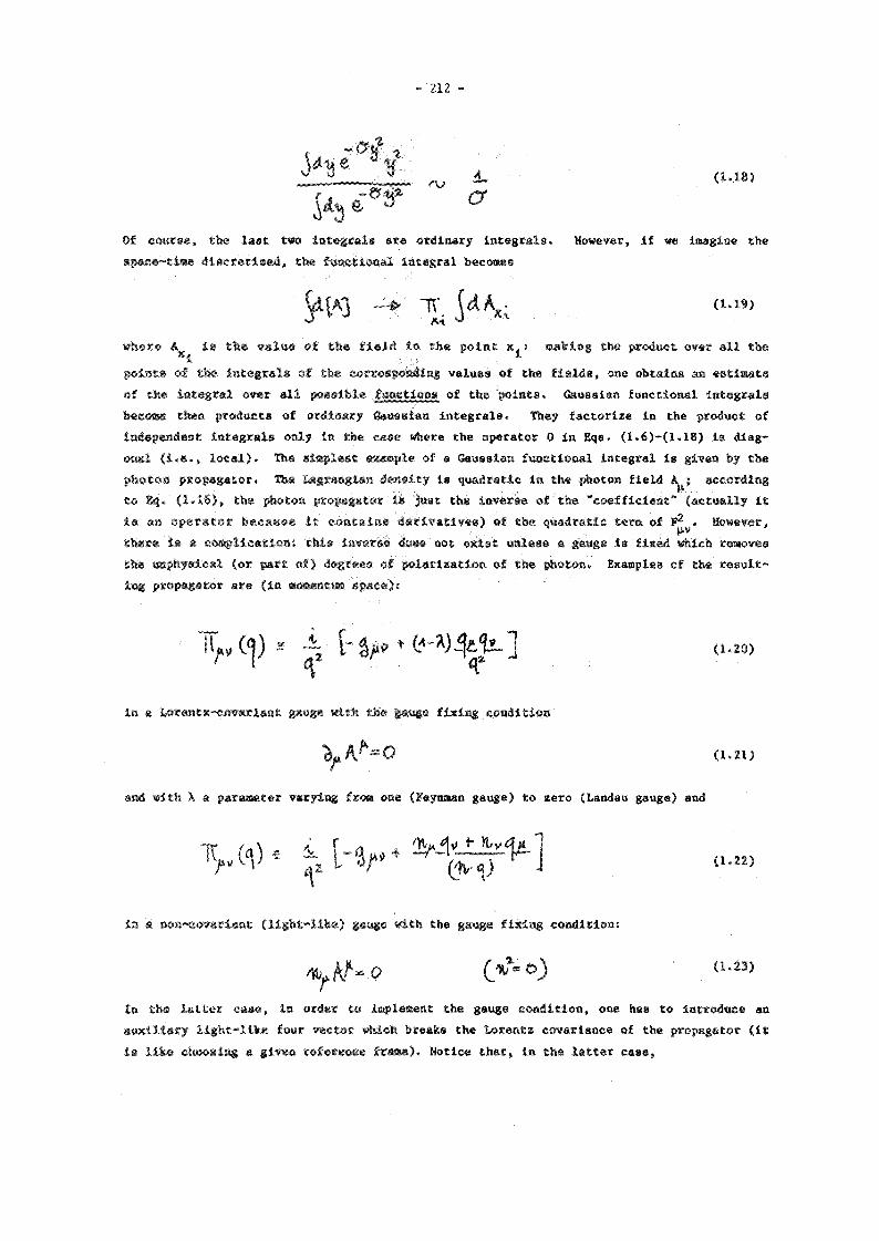
W* want to discuss a process where tha zero mass limit is singular and which therefore requires a "factorisation" procedure ^ . The simplest example is the deep inelastic scat­tering of a quark by a virtual space-like photon carrying a high momentum transfer. The corresponding lowest order Feynman diagram is given in Fig. 5a. The rate is obtained by

Fig. 5a : The lowest order amplitude for the photon-quark scattering.

which is • function o£ tb« dimeneionlees variable» obtained as ratio« of the possible energy «cele* of the processÎ Q, «^ (a set of quark, masses which represent the influence of the Inf r«-red cut-off : m^ ~ I / L J Q J] *nd the renormaliaatlon scale u. If the limit m^/Q 2 •* 0 is smooth (i.e., non singular), one gets

<¿r-t w w

by exploiting the freedom of choosing an arbitrary value for the renormalitation scale, we aet n 2 - Q 2 and obtain

taking tha square of thia amplitude or, *qulv*l*ntly, the Imaginary part (the daahed line) of the diagram In Fig. 5b. By projecting the photon'a polarieatioa by g ^ one obtain* for the race:

I^T/Aftj0 œ st^) (3.1) where x l q2/2p«q 1* the usual Bjorkan acallng variable i a terma of the qiuark momentum p (there are ao nucléons up to now)«

The calculation of the correction* of order a to the rate in Eq. (3.1) gives:

where

(3.2)

As anticipated, the limit • • 0 cannot be taken because of a logarithmic singularity.

The Identification of the diagrams responsible for the singularity among the ones providing the order a corrections is, in general, gauge dependent. By changing the gauge fixing condition, on* can shift th* appearance of a singularity from one diagram to another. However, som* mor* physical intuition can be gained by adopting a gauge where gluoo* propagate only the physical degrees of polarisations: it is the light-like gauge defined in Bq. (1.23) and leading to the transverse gluon propagator of Eq. (1.22). In this gauge th* amplitud* for th* «mission of a gluon collinear to « aassless fermion goes to ser o with the opening angle between the gluon and the fermion. Indeed, given that the gluon-fermion coupling conserve* the fermion's helicity, there is no way to emit a physical gluon (which carries helicity ±1) collin*ar to a measles**^ fermion and to conserve at the

*%ot«, that if the fermion is massive, kinematic* forbid* a totally colllnear amission.

221 -

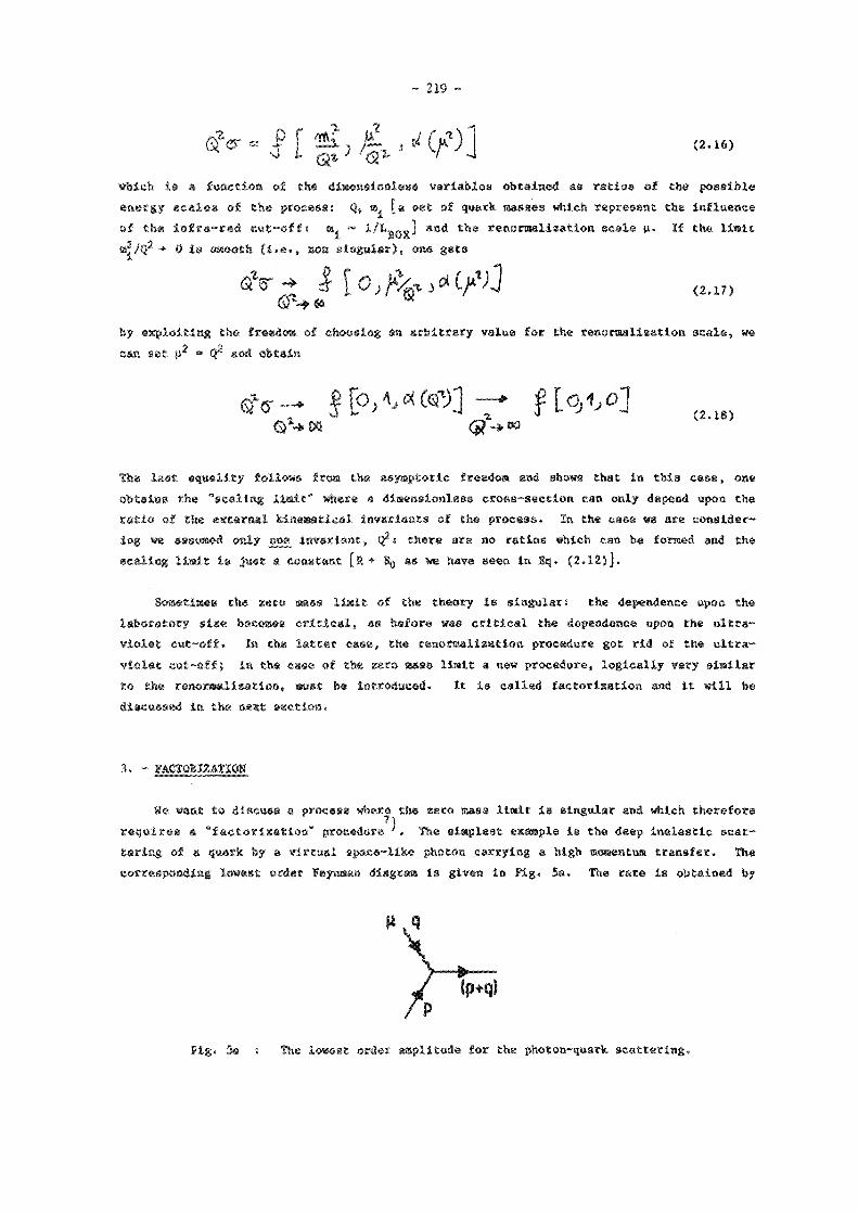
Mg* 6 î »slicitie* for a qmtk and a gluoa emitted collinearly.

I p 4

P > Flg. 7 : First order corrections to the diagram

of fig. 5b giving rise, in a non-co-variant gauge to the leading scaling violatlona.

Bmm time the angular momentum, along the direction of the momenta (aee Fig. 6). This leave* (at order ) only one cla*a of diagrama responsible for the logarithmic dependence in Eq. (3.2), th* ones of fig. 7. For thee* diagrams, when gluon are emitted collinearly, th* above-mentlonad euppression of tb* amplitude is not powerful enough to prevent a diver­gence for m • 0 arising from th* poles developing in the fermion propagators of Fig. 7 carrying ( P - A ) „ Physically, whan the quark, mass goes to tero, the gluons can be emitted collinearly allowing th* propagation of intermediate "on-ahell" quarks: the divergence is relatad to th* "lifeti*** of theae particle* which tenda to infinity when thay go on~*h*ll. In fact, an on-*ball particle can propagate indefinitely.

Kass singular!ti«* spoil th* possibility of getting rid of the infra-red cut-off (the quark mass or th* box sic*) in a painl*ss way. But, like the scales building up the ultra­violet divergence, also th* *infr*-r«d" acales are locally coupled: in other words, one can writ* an *qu*tion for an Infiniteeimel changa of scale which depends only upon the scalea nearby. Tb* aquation is:

á l a m l < H J (3.3)

if w* take P 0(y) 5 <5(l-y) and

we sa* that Rq. (3.3) can b« obtained by differentiating with respect to in a 2 the Sq. (3.2). Actually, up to the first order in perturbation theory one can replace F 0(y) with Kx.Q2/«2)« Th* resulting equation is an example of the "Altarelll-Parisl evolution equa­tion". Th* solution of th* equation, as waa the case for the solution of Eq. (2.11), contains arbitrarily high power of a s if the right-hand aida is of order a^, as is the caae for Kq. (3.3) with tha choice (3.4) for the "probability* P(s), one obtains the resum-mation to all orders in a of tsrm* [ a An Q 2/» 2] K; i.e., the "leading log" approximation for the Q 2 evolution of th* parton structure function F(x,Q 2/m 2).

- 222 -

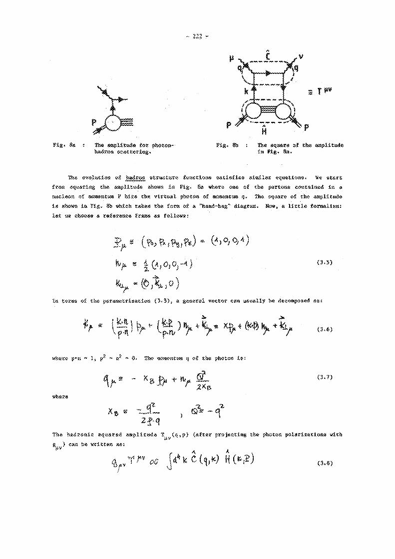
r i g . i* i Th« amplitud* for photoa-had ron »e»tt«rittg.

fig. 8% * The square of the in Fig. 8«.

jlitude

Th« evolution of |fdgOB atructur* functions satisfies similar equations. we start fro* squaring the amplitude shown in Fig. 8a where one of the partons contained in a nucleón of momentum P hit* tha virtual photon of momentum q. The square of the amplitude is shown in Fig. 8b which takes tha form of a "hand-bag" diagram. Now, a little formalism: let us chooee a référença frame as follows:

(3.5)

In terms of the parametrication (3.5), a general vector can usually be decomposed as:

where p«n - 1, p 2 » n 2 » 0. The momentum q of the photon is:

(3 . 7 )

2 % where

The hadronic squared amplitude * u v (l • P) (after projecting the photon polarisations with g^ v) can be written as:

(3-8)

- 223 -

where one integrate! over the four moeentum k of the quark which is struck by the photon .

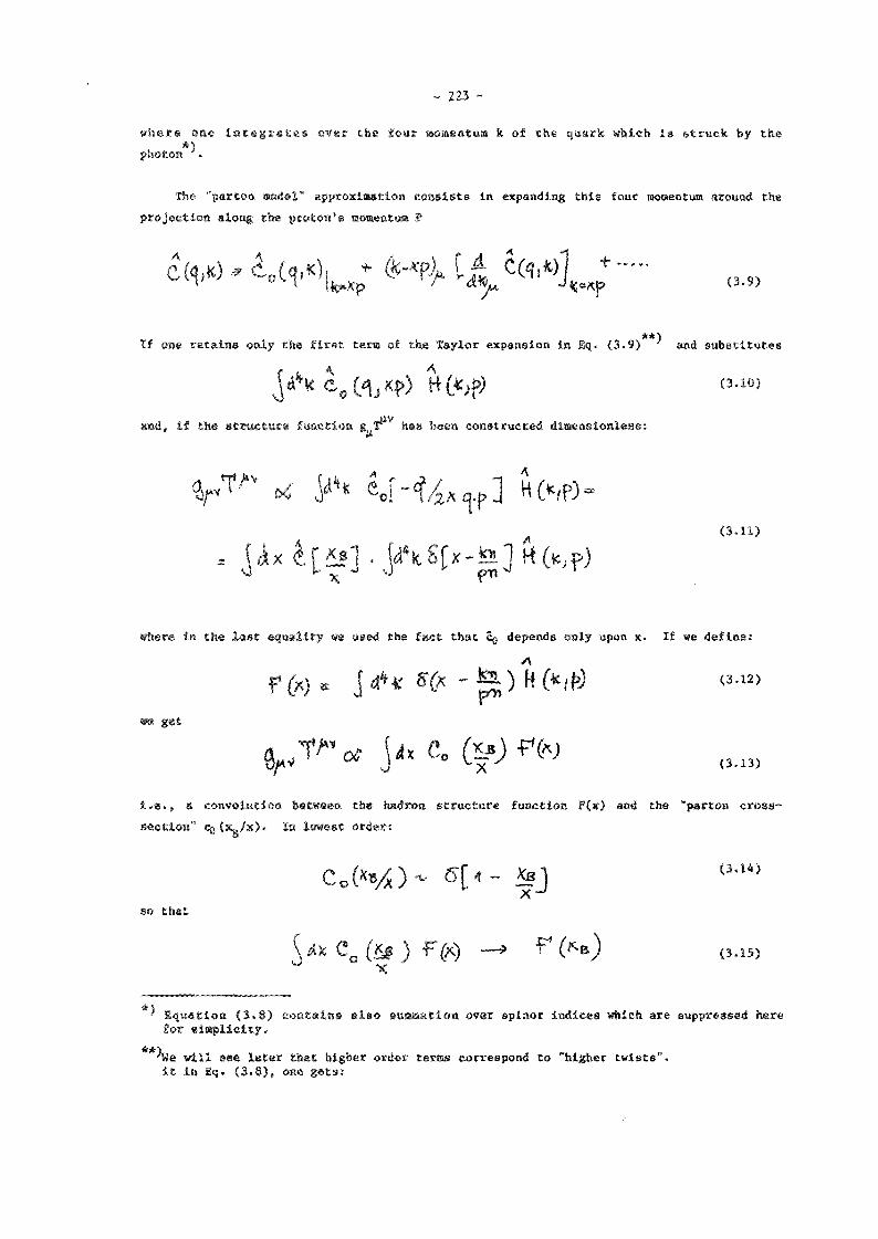
The "parton model" approximation consista in expanding this four momentum around the projection along the proton's momeaturn t

If one retains only the first term of the Taylor expansion in Eq. (3.9) ' and substitutes

and, if the structure function g T*iV has been constructed dlmensionless:

(3.11)

where In the last equality we used the fact that eg depends only upon x. If we define:

F ( * ) « ^(*ítí ( 3- 1 2 )

we get

(3.13)

i.e., a convolution between the hadron structure function F(x) and the "parton c r o s s -

sec t ion" CD ( XJ/X). In lowest order:

C 0 X B J (3.14)

so that

e o ( * * ) f > ) (sä«

*^ Equation (3.8) contains also summation over spiaor Indices which are suppressed here for simplicity.

**\ie will see later that higher order terms correspond to "higher twists", it in Eq. (3.8), one gets:

- 224 -

At order a we gets

Again we fiad * singular behaviour when m goes to zero. However, the relation between the structure functions at two different scales are cut-off (a) Independent

This fact, which at order a is just a consequence of the basic properties of the loga­rithm, is actually valid tö all orders in perturbation theory; by Introducing a set of parton densities normalised from the experiment at some reference momentos transfer Qj, and by expressing the prediction for any hard process in terms of these structure functions, the singular dependence upon the infra-red cut-off drop» out. The factorisation procedure is very similar to the reaormallsatlon technique where one gets rid of a cut-off (the ultra-violet on*) at the expeoae of introducing an extra scale u at which the coupling constant is normalised at aoms experimental input. The evolution equations for the hadron structure functions follow from Eq. (3 .17) and have the classical for»;

*1±!Ê^Ë A î ( . M P W C ) M . i e )

Actually, on* gats in general « »et of coupl*d equations for the quark and the gluon densities which contain th* probabilities P for a quark to go into a quark or a gluon and for the gluon to go into a quark or a gluon. The detailed form of these equations and the functional dependence of th* probabilities is given, for example, in Ref, 8). The terms of order a 2 in the probabilities P allow us to resus the next-to-leadlng logarithms, i.e., the terms of order «^(«^ia Q 2 ) * : their explicit form can depend upon the specific factorisa­tion procedure. The evolution equations can be extended to the "time-like" case, i.e., to the Q 2 variation of hadron fragmentation functions. The specification "time-like" refers to the positive invariant off-shell m*«* of the partons in the jet cascade*^.

Tor the time-like c«*«, *nd in particular for the evolution of gluon* into gluons, the order a 2 term* ia th* probability ar* very important when the fraction of momentum carried by the secondary gluon* gets v«ry «mall. Indeed, the order a term behaves like:

£ (A) A , C ^ £ (3.19) IS *

which, after p«rformlng the convolution integrals of the type in Eq. (3.18), gives

l a other words, th* "time-like" do«s not refer to the sign of Q 2: for the Drell-Yan muon pair production, for which th* dimuon m*ss is time-Ilk*, the parton off-shellness Is

- 225 -

The leading contribution of the second order term ia toe

4

(3.20)

region of small % ' la:

x a / ; 3 (3.21)

Me sa* that tha ratio of the second order term [Eq. (3.21)] to the first order one (3.20)] ist

(3.22)

Therefore, when « in 2 s is of order 1 (email values of * ) , the second (and higher) order corrections cannot b« neglected. One needs a specific reauauation of these "doubly loga­rithmic" terms % this has bean parformad. âs an application of these calculations, one predict tha Q 2 behaviour of the parton's (hadron's) multiplicity which takes the form

23)

The coefficients b and c ere tha result of the resuamatlon procedure: the determination of the overall normalisation is a problem which cannot ba solved with perturbation theory techniques. In Fig. 9 a numerical simulation of the parton branching sequence according to

16 "T

6 I ' > i 1 ' » « 10 20 30 40

CM, ENERGY (GeV!

Fig. f ; Bahaviour of tha hadron's multiplicity in e +«~ annihilation comparad with the prediction from lef. 10.

226 -

QCD is reported: th* fi&*l conversion into hadrone le «ade In a phénoménologies! way. The Q 2 dependence, which resalas essentially unaffected by the details of the hadronisatioo procedure, fits veil with the data taken froe e+e~ annihilation into hadrons.

Terms which are "doubly logarithmic" like In Eq. (3.22) occur in general when the radiated gluoas are soft. Indeed, besides the "mass singularities", due to the kinematics! configurations when the emitted radiation is colllnear, there are also potential "infra-red singularities" which cancel between the emiaslon of real gluons and the self-interactions with virtual gluons. If, by the kinematics, the real emissions are restricted to be soft, there is a mismatch between the real and virtual contributions leading to terms of the type

(3.24)

where Qf is the scale reatrlcted by the kinematics to be much lower than Q 2, the maximum allowed ooa. The example that I want to discusa Is the form of the transverse momentum (p^ ) distributions of W ' s and Z's produced at the collider. Of course, this also covers the transverse momentum distributions of lepton pairs Inclusively produced in hadron-hadron collisions. Let u« take the p^ differential cross-section suitably made diraensionless by multiplying It by ( Q 2 ) 2 :

dpi J

On the right-hand side of Eq. (3.25) there are the possible parameters upon which the cross-section depends : the transverse momentum p^, the W/Z mass Q, the total centre-of-mass energy squared s, the bare strong coupling constant, the bare parton densities q|» and finally the quark meas which Is kept finite to avoid mass singularities and the ultra­violet cut-off M which prevents the divergences arising from short wavelength fluctua­tions, after the renormalisation and factorisation procedure, the m., M scales dis-

**ataaaaaaaa*aas^^ ™—w———™— x uv appear in favour of a normalisation «cale u, taken for simplicity to be th* same for « the rano realisation and the factorisation. Tb*n Eq. (3.25) becomes:

(3.26)

(3.27)

When the variable» Q 2/* S t and 4p 2/8 S x 2 are kept fixed, one obtains a "scaling" behav­iour, modulo th* logarithmic correction* due to the Q 2 dependence of the running coupling

- 22? -

constant «ai parto» êeasities. ifcwever» if p|/Q2 i* vary ssail» the leading perturbatio term* look like:

SCîf) "-¿kf2fá ^"'i* w.m>

ao that the Integrated cro*a-aection: _

(T i f ) » ( " " ^ 5 " ^ (3-29)

goes like

"2- ~ jf*** ( + »**t-to-le*ding term*) (3.30)

The r*summ*tlon of th* l*ading term* in Eq. (3.30) to all orders of perturbation theory can be done by a "Block-Nordsiek" technique and gives:

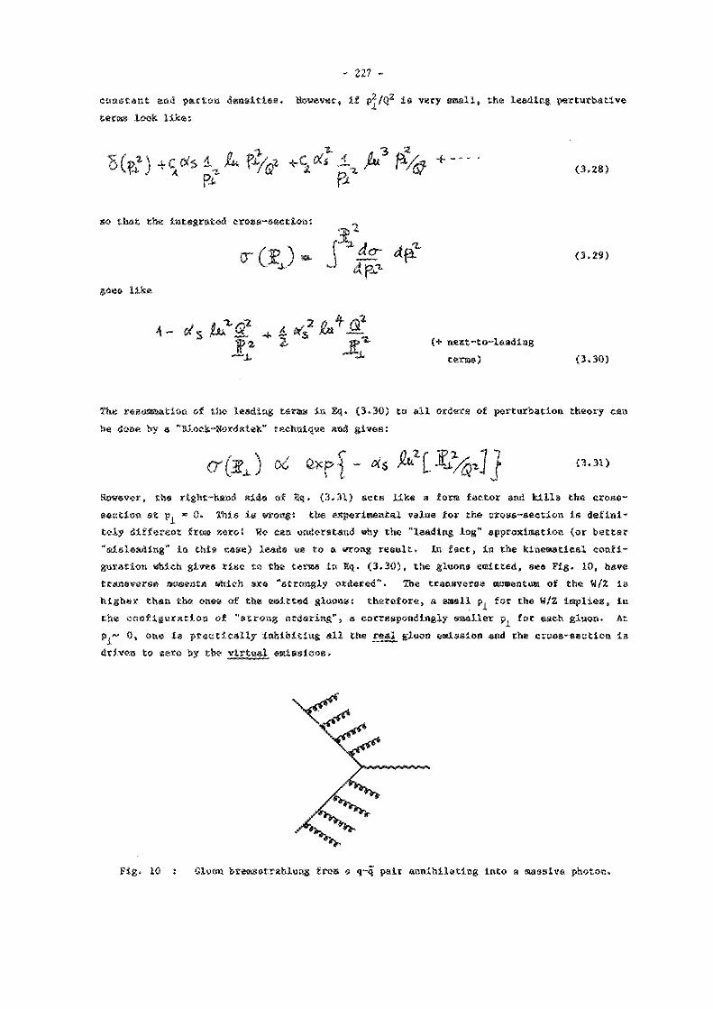
However, the right-hand aide of if. (3.31) acta like a form factor and kills the cross-section at p ¿ - 0. This is wrong: tb* experimental value for the cross-section is defini­tely different from e*roi Wa caa understand why the "leading log" approximation (or better "misleading" in this case) leads us to a wrong reault. In fact, ln the kinematical confi­guration which gives rise to th* terms in Eq. (3.30), the gluons emitted, see Fig. 10, have tranaverse momenta which are "strongly ordered". The transverse momentum of the W/Z is higher than the ones of th* *mltt«d gluon*: therefore, a small p i for the W/Z implies, in the configuration of "strong ordering", a correspondingly smaller p^ for each gluon. At p^~ 0, on* is practic*lly inhibiting all the real gluoo emission and the cross-section is driven to raro by the yirtttal emissions.

Fig. 10 : Gluon bremastrahlung from a q-q pair annihilating into a massive photon.

- 228 -

(3-33)

«hère "I, th* "impact p*ram*tar", is the two-dim*n*ion*l variable conjugate to "k^.

The utility of using th* r*pr**«nt*tion in the impact parameter space is that it allow* u* to r«#ttc« to a power aeries th* calculation of the «oft gluon «missions taking into account tb* coape»f»tl»« of their tr«o*v*rse momant«, on* of the terms being like the on* in Sq. (3.3*). The s«ri«s cmn thee be r«*umm*d very much like the on* in Kqs. (3.28)-(3.31) and th* final r**ult is ^:

where the r«*umm»d "soft" «missions are given by tha exponential and the function ïCîf »Q3»f> containa the contribution of "hard" gluons with p ~ 0 ( / 0 ? ). The details of the p^distributloB calculated according to Eq. ( 3 . 3 5 ) depend upon various parameters: their iaflaenee is shown in Figs. 11 ^. In particular, Fig. lia refers to two different choices of A and of gluon distributions and Fig, l i b shows the effects of using eeg(Qz) versus * (q|)« According to Eq. (3.35), all values of "o are Integrated out, in particular thoae corresponding to larg* distança physics which is not governed by perturbative QC0 (It

Th* possibility of defining auch a probability is related to the softness of the emitted gluons.

This approximation i» obviously bad, bacauaa at small p^ of tha W, many real gluon* can still b* emitted if there 1* a eengeaeation of their transverse momenta. A better resummetion technique which remedies tbl* problem can be conatructed. I will only give a few ¿«titile of this technique and discuss the result. Define by v(k. ) the probability for a singl* gittern «mission ' ; th* probability o (P^ ) for producing n gluons whose total tranaver** momentum sums up to P^ is given by:

ff* ÛPJ „ ja\ «%, - «X VGO - % ) 52 fc. - S . ]

The expression ia Kq. (3.32) is a convolution: It csn be more easily calculated by intro­ducing tb* Fourier tranaform of tb* probability v ( k ^ ) :

- 229 -

O 15

0 10

0 05

Fig , 11* Í Pr «diction» obtained from Ref. 12 using different perton d*n-• iti** for the W p x distribu­tion normalised to tb* t o t a l cross-section .

Û. IS

0.10 I I

0.05

0 15

0 10

0 05

- UA 1 - 52 evts - UA2 - 37 mU

fig. lib t Influence on th* prediction* Pig. 11c : Prediction* confront the experimental on th* prediction of th* ua« «(Q 2) or a ( q | ) . data.

- 230 -

larga)> This torcas the introduction oí a parameter "a" which is completely phenomena-logical; it rulas th« "freesing" of tha running coupling constant which is transformed according tot

<u<sV * — » ôC c^) * b ^ ^ T è f [ Î l 5 i X J (3.3«

For valúas of Q 2 below (aA 2), the coupling constant ceases to increase and flattens out. In api te of theae spurious parameters, when Q 2 (or s with Q2/s fixed) becoates large enough, the prediction becomes insensitive to the large distances: Indeed, the exponential in S<t« (3.35) acts like a form factor which kills the contributions coming froa large values of 1». Physically, this can he understood ss follows: the cross-section when the W's have a small p^ gets most of it* contributions from processes where many gluons are emitted with slasable p|* which compensât* each other. Therefore, the actual W production occurs most of the time whan the annihilating partons are very off-shell and interact with each other at small distances, fig. 11c containa the comparison of theoretical predictions with expe­rimental data: as one can see, it is not so bad.

Tha general picture for hard procassas is than the following. There are reactions which are free of meas singularities; i.e., for which the infinite volume limit is smooth: they can be expresamd as a aeries expansion in « 8(Q 2) of a function depending upon scaling variables. Instead, those processes which are affected by mass singularities need a "factorisation'* procedure which leads to the introduction of running parton densities and running fragmentation function* ^ f(Q*), D(Q 2). Sometimes, the kinematical configurations are such that they enhance the relevance of soft breaaatrahlungs: then the perturbative series contains double logs which aust be resuaaed with special techniques. "Asymptotically" simple mealing laws must hold.^ A nice check has been performed by the UAi collaboration on the high p^ jet cross-section » This process in general decomposes into a sum of many subprocasses which are convoluted with quark or/and gluon structure functiona. However, for a sufficiently large angular acceptance, i.e., when small angles are accaselble, the cross-section as a function of the jet energy fractions xl, x2

m & t h €

scattering angle cos6, takes a factorlsad fora:

*txc.¿x»tiec&e AOo&e (3.37)

where

3

*^We bava not discuss*d the eaae of fragmentation functions: it is conceptually the stuff as the structure functions.

- 231 -

T p — i — r _ _ T _ - T _ r

_ _ - l « _ _ J L _ _ _ J _ ^ ^ I L

0 0.1 0 2 0 3 0 4 0 5 0 6 0 ? 0.8 x

fig, 12 : The experimental combination of part on distributions G(x) + 4/9(Q(x) + Q"(x)) extracted fro* jat-jat data of UAl is compared with th« one «volved front low •n«rgy neutrino experiments CDHS (full line) «od CHASM (dashed line). The dashed area représenta the giuon'a contribution.

6 and Q being the gluoo and quark distributions respectively. The resulting F(x) can be successfully coeipared, as is done im Fig. 12, with the values for the same quantities extrapolated from the "low energy" data of fixed target neutrino experiments.

4. - KHjjt j y w COtlECTIOMS

Before the "asymptotic* regime where the scaling laws are affected by simple logarith­mic corrections is reached, one has to dael with violations which have a stronger energy dependence, dying as some inverse power of the typical scale of the hard process Q, i.e., like A 2/Q 2. They are often referred to as "higher twists" and can be divided into two classes:

i) inclusive, referring to 0(1/Q 2) corrections to inclusive hard processes;

ii) exclusive, referring for example to the behaviour of meson/baryon form factors, to the "prompt" resonance production at large transverse momentum in hadronic collisions or to the angular distribution of Drell-Yan lepton pairs close to the kinematic limit of the lepton's invariant mass.

The simplest "laboratory" to discuss the inclusive higher twists remains the deep inelastic scattering of hadroos against external electroweak currents. The following discussion is

- 232 -

rather technical, but necessary ' » Th* "lowest twist" approximation for the hadron «truc-ture function it expressed in Sq. (3.13) a* the convolution of a function referring to the "short-distance" interaction, denoted by c and one referring to the "long distance" physics, denoted by f. Th* physical picture of th* process in the leading twist approxima­tion is the following. One observes th* interference pattern of amplitudes for the inter­action with th* external current at points which are separated by a light-like distance. In order to *«• this, it is «nough to tak* th* Fourier transform of the quantity H(k,p) «ntaring the Eqs. (3.10)-(3.12);

, | C (4.1) « C * ) - C-) I*'] H(|J - ¿1* Hr|j <•.«

the integral over k can b* p«rform«d in tit* u«ual frame defined ia terms of the vectors n^, p^ (see Eqs. (3.5) and (3.6)]. In this frame, the four vector <n^ (remember that it defines the distance conjug«t* to th* mom*ntum k) is parametrised as :

so that

lam««8«rittg that

X

one obtains from th* integral over k 2 Í

(4.4)

(4.5)

(4-6)

and from the one over k :

Equation* (4.6) and (4.7) imply: T I 2 - 0» % - 0. Equation (4.2) then reads:

, y*«^ H O y ) (4.8)

where

- 233 -

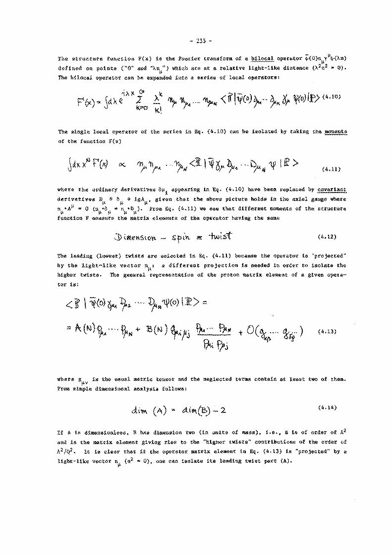
The structure function F(x) is the Fouri«r transform of a bilocal operator <¡<(0)n v ^ A n ) defined on pointa ("0" and "Xn^") which are at a relative light-like distance (X 2n 2 - 0). the bllocal operator can fea «xp«nd«d into a aeries of local operators;

The «Ingle local operator of the series in Eq. (4.10) can be isolated by taking the .moments of the function F(x)

(4.11)

where the ordinary derivatives du appearing In Eq. (4.10) have been replaced by coverlent derivativ«« D s ô +• igâ » given that the above picture hold* ia the axial gauge where n^»A - 0 í»p,*5p, " n^«D^). Fro* Eq. (4.11) we see that different moments of the structure function f measure the matrix elements of the operator having the same

^immum - S f n t t a "twist" < 4.u)

The leading (lowest) twists are s«l«ct*d ia Eq. (4.11) because the operator is "projected" by tha light-lik* vector n^ t a différant projection is needed in order to isolate the higher twists. The general representation of the proton matrix element of a given opera­tor is:

fa fa

where g^ v is the u*u*l m«trlc tensor and the neglected terms contain at least two of them. From simple dimensional analjais follows:

am ( A ) » - 2 C 4 - 1 4 )

If A is dlmensionlees, 1 has dimension two (in units of mass), i.e., B is of order of A 2

and is the matrix element giving rise to the "higher twists" contribution» of the order of A2lo. It Is clear that if tha operator matrix element In Eq. (4.13) is "projected" by a light-Ilk* vector n (n 2 - 0 ) , one can Isolate Its leading twist part (A).

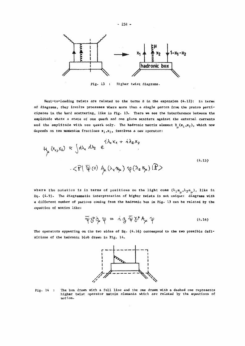
K*xt-to-l«*ding twist» « e related to the terms I in the expansion (4.13): in terms of diagram«, th*y involve processes where more than a single parton from the proton partl-cipatea in th« hard «catterlog, like in Fig. 13. There we see the Interference between the amplitude where a atata of one quark and one gluon scatters against the external currents and the amplitude with one quark Only. The hadronic matrix element H^ÍXj , x 2 ) , which now dep«nds on two mommntum fractions x¿ ,x 2, involvee a new operator:

(4.15)

where the notation is in t«rms of positions on the light cone (Xjn^.Xj«^)» lik« ln Bq. (*.»). The diagrammatic interpretation of higher twists is not unique: diagrama with a different numb«r of partons coming from the hadronic box ia fig. 13 can be related by the equation of motion like:

(4.16)

The operators appearing on the two sides of Bq. (4.16) correspond to the two possible defi­nitions of th* hadronic blob drawn In fig, 14.

fcs.

tig. 14 : Th* box drawn with a full H o * and th* on* drawn with a dashed on* represents higher twist operator matrix elements which are relatad by the aquations of motion,

- 235

The parametrliation of the structure function in terms of operators corresponding to different multipertoa densities (the genaraliration of the usual quark and gluon densities) depends upon the chosen operator basis: for a detailed (overdetailed?) description of all the technicelitiee, I suggest Ref. 13). Here I will only report the result for the longi­tudinal (F ) and the transverse (F ) structure function

The functions % and T 2 are related to multlparton densities: I will only report the explicit form of T|:

18)

where Is the covariant derivative on the transverse components only. In the limit of sero strong coupling constant, * 0^ and T| reduces to:

^ U k / a < ? ] r f t o ) ^ £ ^ > ) f f >

which measures the amount of "intrinsic k^" carried by the quarks. This is a well-known result In the naiv* parton model where the longitudinal structure function is proportional to tha parton's "intrinsic p Besides the teros of the order of A 2 / Q 2 , Eq. (4.17) contains also terms of order M 2 / Q 2 where M is the proton mass. I call these "kinematical higher twists": their normalitation is fixed in terms of the same function [ A ( x ) in Eq. (•.17)] which parametrises the leading^ twist behaviour. In Fig. 15 are reported the data for ff from the C H A R M collaboration ^ » and, superimposed, the QCD prediction including only the leading twist contribution, the sama and the "kinematical" higher twists, the latter and a phenomenologlcal parametrlsatlon of dynamical higher twists. The experimental tests of the contributions of Inclusive higher twists are difficult: one has to extract from the data an entirely new set of multlparton densities. If we think about the uncertainty by which the gluon distribution is known, we can imagine how poor the determination of further and more complicated parton distributions would be.

1 6 ) The tests of power law corrections seem more feasible for exclusive processes ' . The

simplest example is provided by th* electromagnetic meson form factor. In Fig. 16a is reported tb* simplest diagram wh«r* on* of th* quarks forming the meson is hit by the photon and it r*v«rs«* (lu a suitable frame) its momentum while the other acts aa a

- 236

f ig . 16« s

fig. 15 Î Th» longitudinal stroctur*, faaetioa from CHAIN data 1*' ia compared with the predic­tion b«»ai on 0 ( a ) calcula­tions CÄ«»h«««tt#i lln«). tb* oo« including M 2 ^ n / Q * correction* (fall IIa«) «ad th« O t t « tocisiittg « slmpl* p«ram«trltatiou of dynamical power correction* ( ' lin*).

A m*«on hit by • photon in th* *imple«t (and wrong) picture.

Fig. 16b : Lowest order contribution to the »««ott form factor.

»g, 17 t A* in Fig. 16b, specifying the positions where th* photon and the gluon interact with th« i d ) .

"spectator". Th* final «tat* would consist of a qq pair where th* fermion* get further and further sway from each other: it is very unlikely that they would turn out as a singla mason. In order to achiev* this, on* n««ds to pay th* price of exchanging a hard gluon like in Fig. 16b, which transmits to the "spectator" quark part of the momentum transfer of the photon. The corresponding diagram in th* configuration apace (Fig. 17) contains the positions where tb* photon ("0") hits the meson and where the gluon is emitted (^ ) and reabsorbed (* 2). In formulae, one has:

- 237 -

The expression ia Eq. (4.20) is «eng hj inspections in fact it containa a bilocal oper­ator matrix element

which la not gauge invariant. We need some operator made of gluon flaids which transports tha information about th* colour at point* *| and e 2> Such an operator ia th* following;

(4.22)

where th* lln* integral in Bq. (4.22) ia taken along a trajectory joining tha points ix and *2 • The form of the op«rator in Eq. (4.22) la easy to understand; for, remeaber - if you can - that th* operator which perform* the infinitesimal translation is 10^. Out of it one can form th* corraspondlng operator for a finite translation which reads

In fact

4(^a/á) - C ^ c f f ^ ) (4.24)

where * is a generic scalar field. (It works for ordinary functions.) At the beginning of th«s« lectures w* hav* learned that th* gauge invariance for the matter fields (i.e., for non-gauge fields) can be obtained aimply by replacing in the Lagrangian the ordinary deri­vative by the covariant on*:

^lA --* ^ 4 ^ fy^M- (4.25)

Therefore, wh*n on* n««d* th* "colour transporter" for a finite distance between two points, one has to exponentiate the "Inf initeeiaal" transporter IgA^ ovar a trajectory joining th* two points macroecoplcally separated. The operator matrix element in Bq. (4.21) is than replaced by:

< 0 | 1 f J ( f c ) (4.26)

The function "C" in Eq. (4.20) represents the "short-distance" kernal describing the absorption of th* photon and th* exchange of the hard gluon aa in Fig. 16b. In configuration apace, it ia proportional to the quark and the gluon propagator:

(4.27)

- 238 -

« i When q* •* », for the position vector s only the components on the light-cone survive and i i

th« four v«ctor t b«co«i«« proportion*! to the light-like vector n ; * • * »n . If we t*k* th* Fourier tr«n«form with r«sp«ct to the * variables of the operator in Eq. (4.26) m gets &

•here I h*v« specified th* flavour* of th* fermions appearing In Eq. (4.26). The variable* ,x 2, eonjugat* to th* light con* position* tj, s 2, ar* colllneer momentum fractions ln a

fm frame. Th* function • „(*!,x 2 ) then represents the pion wave function in th* same

Th* total answer is:

<T (P01J^) W f O > « C f c + t y f ; ( f ) ( 4 ' 2 9 )

where

sztr oís A X

with

with e , a, the electromagnetic quark charges. The variable x(y) is related to the u a variables xj,x 2 (y t,y 2) by:

„ H , . , , ( 4 . 3 0 )

The only unknowns in Eq. (4.29) are th* pion wave functions $*B which are related, as we have seen, to the Fourier transform of som* matrix elements of bilocal operators like

The** have the asm* form of the bilocal operators found in deep inelastic scattering, although th* matrix «l«m«nt Is different. The evolution with q 2 of these matrix elements,

- 239 -

Fig. 18 : Higher order correctivo» (leeding log in a noa-covariant gauge).

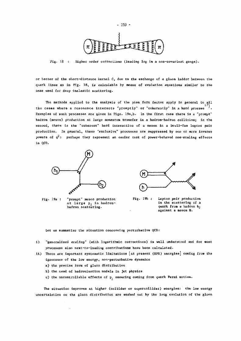
or better of tha short-distance kernel C, due to the exchange of a gluon ladder between the quark line* a* in rig. 18, 1« calculable by mean* of evolution equations similar to the one* ua*d for d**p in«la*tlc scattering.

The methods applied to the analysis of the pion for* factor apply in general to^ all th* casas whera a resonance interacts "promptly" or "coherently* ln a hard process ^ . Exaapla* of such process** *r« givan in Pig*. 19a,b. In the first case there is a "prompt" hadron (aeson) production at large momentum transfer in a hadron-hadron collision; in the second, there is th* "coh«r«nt" hard Interaction of a aeson in a Drell-ian lepton pair production. In general, th«s« "*xclusiv«" processes *re «uppreased by one or aore inverse powers of q 2 : perhape they represent an easier test of power-behaved non-scaling effects in QCD.

Fig. 19a : "prompt" mason production at large p x In hadron-hadron scattering.

Pig. 19b : Lepton pair production in the scattering of a quark from a hadron h^ against a meson M.

Let us summarise the situation concerning perturbative QCD:

i) "generalised *c«ling" (with logarithmic corrections) is well understood and for most processes also n*xt-to-leadlng contribution* have been calculated.

ii) Th«r* «re important systematic limitations [at present (SPS) energies] coming froa the ignorance of th* low energy, non-p*rturbative dynamics a) th* pr«cis* fora of gluon distribution b) the n**d of hadronisation aod«ls ia jet physics c) the uncontrollable affects of p^ smearing coming from quark Fermi motion.

The situation improves at higher (collider or supercollider) energies: the low energy uncertainties on th* gluon distribution are washed out by the long evolution of the gluon

240 -

distribution which is eventually determined by the low energy behaviour of quark distributions. Badrontzatton models will still affect events with only a few jets, but should not matter too much in the study of rare aultijet events . The effects of "intrinsic p^ smearing" sometimes become slider, like for small Z/W production at small

V ill) Tha general behaviour of Inclusiv« power law corrections is understood, but a system­

atic analysis is rather prohibitive, due to the complete ignorance of the new aulti-par ton distribution functions which parame triase these effects.

An interesting approach for «etlmating the long-distance behaviour of QCD and ln particular tb* valu** of various hadron matrix elements of quark/gluon operators is given by tb* "QCD sua rul**". A *hort dascrlptlon of them was part of ay lectures: however, the Präsentation prov«d to fee too technic*!, especially after the previous already technical sections. 1 then éeeiiei tô *uppr*s« this part in the written version of my lectures. The interested raadar can address h*r(hl*)s*lf to the original literature on the subject ^. I prefer to go directly to th* last subject of ay lectures: lattice QCD. Within this approach the only párasete» which are seeded to describe any QCD processes are the quark masses and A: modulo the uncertainties of any numerical approach, it is the beat candidate for the correct *v«luation of non-p«rturb«tiv* effects.

-Mmm=m

la ord«r to «stimmte the affecta of quantum fluctuatlona, we have said ln Section 1 that one haa in g«n*ral to perform exactly a non-GsttSsisti functional Integral. When one is facing aa integral that cannot b* don* analytically, on* can évaluât* it numerically by ••timatiag; its value on a finit* set of points. In the case of quantum field theories, this .mount, to ".creasing th. .peee-tlm. fey introducing an imaginary lattice whose nodes identify a finite set of co-ordinate* 1 .

If we want to «irnuiat* the behaviour of QCD on a finite region of space-time, it newts that we are calculating the properties of hadron* in a box. Th* question is: how big should it he to avoid finit* siie problem*t He know from nuclear physics that the energy shift for nucl*on* *qu**s*d in a regio» with a sise of about 2 Fermls is of 10+15 Me?. This mean* that on* can expect an effect of the order of two per cent on the nucléons' mass if the box sis* ( L § o x > is ~2 ferai. This is true for hadrons (Ilk* the aocieons) made of "light" quark* (!.«., up or down quark*). Bedron* mad* of heavier quarks (the strange on* will also tolerate smaller box sis**. Indeed, from the experimental data on total cross-•action* which can be uaed for estimating the hadrons* aise, one would deduce for the pion a dimension of about 1.5 Tarai, and for tha kaon of about 1 Fermi. To summarize, L ^ o x ~ 2 ferai and I ^ Q J ~ 1 Permi can be «attable values for hadrons made of light and strange quark* reepectlvely.

)Although, in this etlf, the contamination from other aultiparton subprocesses may be r e l e v a n t .

- 241 -

l a order to have • f l a t t e numb«r of degree* of freedom one has to introduce a finite résolution "»": th* l a t t i c e spac ing , low small should it h*? The answer to thia ques t ion

com** from p r a c t i c a l and t h e o r e t i c a l considerations. The practical ones are dictated by t h e limitation* of present computers c a p a b i l i t i e s . Indeed, the total number of degrees of freedom per nod* is vary high: t h e r e a t a (complex) variables - the fermions - which are defined on the nod*s

(5 . 1 )

wh*r* a 1* a colour index (• « 1-3 for quarks) and « is the ordinary Dirac Index running from on* to four ; this «afees in total 24 (real) variables per node. There are variables which are defined on th* link* a*socist*d to the gauge f i e l d s ;

\ ) m , (5.2)

where i and j are neighbouring points and A, S a re colour Indices. U Is a unitary 3x3 matrix, a total of § complex variables times the four possible directions; this makes 72 real ve r la

following real variables par node. Th* r e l a t i o n between the matrices U and the gauge field A* i s the

i.e., 0 is th* «xponentiel of the line integral of the gauge field A^ along the link asso­ciated with a given matrix. The action on the lattice i s written in terms of the variables D's. One starts from th* action on th* continuum:

(5.4)

where 3 A *

and ráscales the fields with th* coupling constants

then

^A. - A, «.»>

(5.6)

- 242 -

theo

Ott the lattice.

5. 2L i ^ A - )

(5.7)

(5.8)

where Che «us 1» performed over the plaquettes defined by a pair of directions ft, v and sn origin "n" aa in Fig. 20; the symbol 0 p denotes the trace of the product of the four links

n+v Fig, 20 î A plaquette on the lattice; the unit vectors, u, v are two generic directions.

around the plaquette. This product will involve the matrices Ü* or their Bermitian conju­gates Bjjj% depending on the relative orientation of the curve defining the plaquette and of the link. D^(n) deacribea a link from the point n to the point n4y, while u£(n) describes a link from n+û to the point n. One has:

The action on the lattice in terme of u£V can be written as follows!

(5.9)

5 » i ¿ Cüf-d)

The reduction of the action in Eq. (5.10) to the one of the continuum theory in the limit a • 0 can be understood aa follows. Remember that

% -V ( ^ á ^ ^ ^ / j ^ ^ K^-'^ÍS.li) If the matrices X* were commuting among themselves, one would form, by combining the four U's around a plaquette, the exponential of the curl of tha field A^ on a cloaed curve. The Stokes theorem then telle ua that this is equivalent to the flux of Ô^A^ - ô^â^ through a

surface bounded by the curve. Tha expansion in powers of " a " gives:

UjT * * + a a 1 - i ¿ j ' í - C5a2) The term quadratic in a vanishes when summed over u and v indices because of its (anti) symmetry properties: cae is left with

- 243 -

\)-± * i & é t % ^ * O (é) (5.13)

i.e., the continuum action once the correapondence /d Mx + S , .... t* i» made. Non-com-' plaquettes

muting X matrices (as is tha case for QCD) produce extra tenas which conspire to foro the complete expression for G^ v of Eq. (1.4). The reduction to the continuum action works to order a** î th* terms of order a 6 ar* irrelevant in the liait a • 0. In fact, different action* on the lattice may lead to th* same "continuum" limit. This is a non-trivial statemant In th* inte r*c ting theory s for the aoaeat, I Just mean that the naive limit a + 0 leads to th* Sam* action up to tsrm* of order a 6,

The practical consideration* about the mmllmm of "a" are related, as 1 already mentioned, to the present computers' capabilities. If for light hadrons one needs an overall sise of about 2 Fermi and one wants a resolution of 1 Feral, one needs 20 points p*r direction: this amount to about 30 megawords of (fast) memory, less without fermions or with some tricks on the storage of the unitary matrices. For strange hadrons with the same resolution but an overall site of about I Fermi, one can do it with 2 megawords. Present computer capabilities are closer to the 2 meg«word than to the 30 megaword case and

*) allow a reasonable estimate of the streng* hadrons' spectrum .

Of course, the answer "w* choos* "a" at our best" is not satisfactory. One must have a critérium for judging, from the results themselves, whether the value of a Is adequately small. Here come the theoretical considerations. The question Is: what guarantees that, for "a" small enough, th* physical rasults will not be affected?

You must realise that "a* acts aa an ultra-violet cut-off: wavelengths shorter than a, I.e. the high momenta, are cut off. The independence upon a of physical results is a consequence of the renomalleability of the continuum theory. According to this property, the lattice spacing a (i.e. the ultra-violet cut-off) and the bare coupling constant g are redundant parameters. The earn* physics is described by any of the pair of values of g and a which lies on a curve (the renorm*lle«tlon curve) parametrised by a single dlmensionfui parameter A. For any given valu* of A ( A - Ä ) , there is a curve like the one of Fig. 21;

9(-)

Fig. 21 : The behaviour of the bare coupling constant g(a) as a function of the lattice spacing a for a fixed value of A : A « I.

*Hilthtn some approximation which we w i l l discuss later.

- 244 -

if  is known and _lf the theory on the lattice behaves like the one on the continuo», by fixing g(a), one fixes «Ä, I.e., velue of a in physical units. The signature that the theory is behaving like the continuum theory, I.e., that physical results are only depen­dent on A and not oo « t is the scaling test. It can be obtained by studying the behaviour of a dimensionful quantity M (with the dimension of a mass, for example) as a function of the lattice coupling constant (remember that It is a bare coupling). On the lattice, actually from the computer output, one always obtains "dintenslooless" numbers, i.e., any dimensionful quantity M naturally comes in lattice spacing units: M • Ma. The curve In Fig. 21 is fereitattieei by tbm equation:

ö f ( a ) » — — — (5.14)

which can be inverted:

- e ^ ( s a s )

Therefore, for any dlmenslonful quantity ta units of a , one expects a definite scal ing

pattern ae a function of ß * 6/g2

r _ . x l (5.16)

where the constants f «ai C ere calculable perturbatively as well as the higher order 0(1/0) correctlOBS. when the scaling law defined by Eq. (5.16) ia at work, one can say that the lattice approximation is simulating well the continuum theory and that the influence of the cut-off in th* relations between physical quantities i s negligible.

The next question is: how êeee on* simulate the dynamics? One could think of solving a aet of coupl*d SchrtMiagar-like «quêtions to find the energy levels: this is by f a r too hard, given that tha Amount of lttd«p*nd*nt unknowns Is of the order of l#. The "natural" way is through the functional integral s after all, as I said at the beginning of this sactlon, th* lattic* approximation can he aeen as a way of performing numerically a dif­ficult integral. K*m«mber from Section I that the "propagator" of the gauge field can he expresseil «s • *ult*bl* average t

A S (A) % f€41 e * A. w Av <p)

- L 5 ( A ) (5.17)

On th* l a t t i c e , instead of th* f t e i á A^, ene uses the exponentiated form:

- 24S -

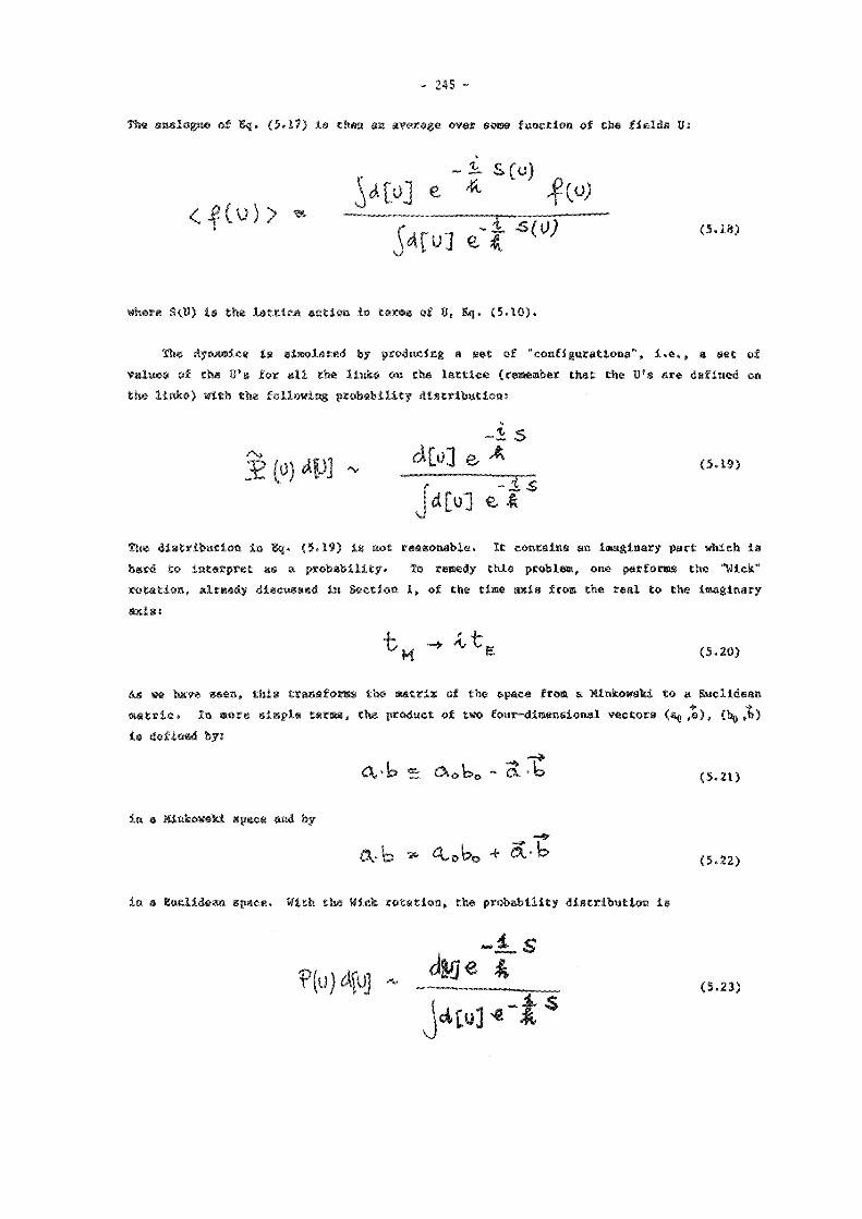
Tb* «n*logu* of Sq. (5.17) 1« then «n average over COM function of the fields Vi

-i. & ( u ) j f ( o ; < f ( u ) > - _____

(5.18)

where S(0) is the lattice action in ten* of U, Eq. (5.10).

The dynamics ia simulated by producing a set of "configurations", I.e., a set of value* of th* tJ's for «il th* link* on the lattice (remember th«t the U's are defined on the links) with th* following probability attributions

The distribution in Eq. (5.19) is not reasonable. It contains an imaginary part which 1* hard to Interpret as a probability. To remedy this problem, one perform* the "Wick" rotation, already discussed in Section 1, of the time axis from the real to the imaginary axis i

(5.20)

As we have seen, this transforms th* matrix of the space from a Minkowski to a Euclidean m«trlc. In mor* simple terms, th* product of two four-dimensional vectors (a ,a), (h9

is defined by:

-i S (5.19)

(5.21)

In • Minkowski apace and by

(5.22)

in a Euclidean specs. With the Wick rotation, the probability distribution is

(5.23)

- 246 -

i.e., th« imaginary unit in the exponent haa been compensated by the "i" appearing in the infinitesimal four-volume:

(5.24)

Th« value a of Che correlation function f (Ü) in Eq. (5.18) are obtained by averaging its value over the set of "equilibrium" configurationa collected.

(5.25)

A learned render can recognize (it is not dramatic if he does not) a strong similarity between Eq. (5.25) and the expression for the average taken on a statistical system la four dimensions: lattice QCD *pp**rs, from the point of view of statistical mechanics, as a theory defined on a four-dimmnelooal crystal.

The "equilibrium" conf Igurationa are produced most of the time by a Monte Carlo algorithm introduced by Metropolis ' ' . One:

i) starts from an arbitrary configuration (for example> randomly distributed); ii) looks at th* value of the field (call it • ) at any given point and tries to change it:

• • • «;

iii) calculates the variation of the action:

r 5 • 5 ( f ; - s (<()) <5-26>

then if S(s') < $#, one replaces the old value of # with the new value #«, if S(*') > S(»), on* accepts the new value with probability a~ 6 S.

The above procedure produces :

- 1> i f ) ~ H ^ l e

(5.27)

*%here are other methods which X will not discuss.

- 24? -

i.e., th* ratio of the probability W for going fron the value # to #* over the probability for tha opposite transition is said to respect the "detailed balance". Let us check Kq. (5.27) according to the tole» stated at the point iii) above: we can take, for example, S(i') < S#), Then

and Bq. (5.27) ia satisfied. The "detailed balance" law on the right-hand side of Bq. (5.28) is nothing but tha ratio of the equilibrium distributions:

- [ S O W - p ((j)9 e = — — —

given that:

_S(<d

(5.29)

(5.30)

The detailed balance rule leads "asymptotically", i.e., after many applications of the same algorlthe, to the equilibrium distribution f $). Indeed, let us calculate the variation of the probability distribution out of equilibrium

The minus sign in Eq. (5.31) comes from the fact that the "population" of the distribution for a certain value of # decreases if there Is a non-zero probability W(« * $ 1 ) to migrate out of that value. The equilibrium configuration is reached when the variation is zero: Sf - 0. This implies

248 -

which le true from 8qa. ( 3.27) «ai (3.29). To reach an equilibrium configuration, one needs in g entrai many iteration* ever the lattice. This procedure ia called "thermalisa-tiott" ly analogy with the approach to equilibrium of a statistical ayate» having a given temperatura.

I summa rix« what I have said so far aa follows. An overall lattice size of about 1

tat«! «eems appropriate for studying the dynamics of hadroas containing strange quarks. The value of the lattice spacing a can be judged as reasonably small when one can check the scaling law based on the renormsllrability of the theory. The dynamics is simulated by taking field averages over a set of "configurations" properly theraalised.

I will now give you some examples of what one can calculât* at present. The subject can b* divided into two main groupa; the "pure gauge" sector and the "fermion" sector, depending upon the inclualon or not of quarka. In the first sector, I will discuss the calculation of the string tension and of the "deconflning" temperature (we will see later *at that «aaah in the second, the calculation of the hadron spactr*, We start with the string tension ',

The general shape of the potential between two coloured quark charges in QCD is the one in Fig. 22. On* can identify two different regime* in its behaviour : at small distances, say below 0.2 Fermi, one has e "Coulomb" region where

V(V) A, £^ (5.33)

r while for r > 0.4 ferai, one expects the linearly rising confining shapes

Th* constant 1, which has the iimension of a mesa squared, is called ia Eq. (5.34) the string tension. In a simple model where a qq pair is bound by a string, K is tha string tension. How does one calculate the string tension? By the "Wilson loop". Consider a qq

(Fermi) - 0.2 f 0.5

fig. 12 » the q-q potentiel f(r) and its two regii and the confining (V(r) ~ Kr).

:s: the Coulomb-lik* (V(r) ~ a(r)/r)

2 4 9 -

p a i r at a distance <i. In quantum mechanics, the tine evolu t ion of such a system is governed by :

i El j - T * 1 1 (5.35)

where T is the t í a s , In the Euclidean space- t ime, one has

1 £ _ T - — (5.36)

In t he expression of E^~, i f one considers only very (infinitely) massive quarks, one gets only the potential part of the energy (the k i n e t i c one goes to «ero as I/o). If,

(5.37)

i.e., i f one i s In the confining regime of the potential, one g e t s ;

& —5» S « Ó ( 5 . 3 8 )

where A, see F ig . 23, i s the a rea spanned by the qq system during i t s time evolution. The s lope of the exponential i s the string tension. To define the c o r r e l a t i o n whose exponen­tial behaviour gives the s t r i n g tension, we have to answer the question: what i s the

effect of the giuon field along the quark (q) trajectory? I t performs a "colour rotation" on the quark fields : in the discussion about the form f ac to r s in Section 4 , we have seen t h a t such a rotation i a obtained by integrating the exponential of the gluon field along the quark trajectory:

- 1 S A x t y ( 5 . 3 9 )

The Wilson loop is defined ms the t r a c e of the product of the gluon matrices U along the

"world line" (or oore simply the trajectory in the space-t ime) of the q(q) as in Fig. 24. The expectation value of the Wilson loop W(U) for large values of T and d behaves like:

- k- ÍAR^á)

<~W(o)> -~ & < 5- A Û )

Fig . 23 : The area A spanned by a qq p a i r s i t t i n g a t a relative distance d as a function of the time T.

f i g . 24 A Wilson loop.

- 250 -

"area law" is a manifestation of confinement. The string tension is a diaensionful quantity. It can than be used for performing the "scaling" test. Of course, its value on tht computer output is a pure number, i.e., the string tension in lattice spacing unite

(call it Kjj rjTCE * t t 0 a E q ' i 5* 1 6? *** expect the scaling law:

MrTTlCg (5.41)

—c/S where f(ß) - e . There are two ways of performing the scaling teat: i) one plots K^j.jjjgg at a function of g and looks for the exponential behaviour for 8

large enough (remember a 2 - 1/A2 e"*^ •* 0 when ß • - ) ; ii) one plots the velue of [ ^ T T I C B ^ ' * * a f u r l c t l o n o f ß- When the scaling holds it

must he independent of p.

The reeulte for the latter test are given ia Pig. 25, For p < 6, there are big violations of the scaling law, while a reasonable agreement is obtained for ß _> 6. Notice that the function fCP> which has beea used is the one obtained by working to lowest order in per­turbation theory, i.e., by neglecting the higher order terms in Eq. (5.16). This scaling regime la called "asymptotic scaling".

100

80

60

40

20

5.2 5.4 i

5.6 .i 58 60 6.2

fig. 25 : The string tension In units of A 1 # t t l c e as a function of §,

- 251 -

From the "asymptotic" value of th« string tension in lattice spacing units that one cao. extract fro* Fig. 25, and fro* the knowledge of its value in physical units based on the angular momentum dependence of the qq resonance speetru», one obtains a first indica­tion of the value of the lattice spacing in physical units:

<X (. ~ ) 1/ . ± Fermi (5.42)

Another «xas.pl« of a physical quantity calculable in the pure gauge sector is the "deconfioing" temperature ' ; when warmed up by a huge amount (to a temperature of the order of 10 1 1 degrees 1 ), the hadrons are supposed to melt into a plasma of quarks and gluons. The questions that one can answer by a lattice calculation are: does the phase transition actually exist? If the answer is affirmative, at which temperature?

A theory at finite temperature can b* simulated on a lattice where one of four dimen­sions, say the time, is much smaller than the others. In the limit where the space dimen­sions go to Infinity, but the tine r «mains finite, the value of the temperature can be related to the time sit* by

~T[ M¿ = — ^ (5.43)

where K is the Boltemann constant. Finite temperature QCD is then studied on anisotropic lattice^ denoting by the number of points la the dimension 1:

The temperature in lattice spacing units is given by

(5.44)

(5.45) lATTICC ~ ' T t H f

Bow does on* identify the phase transition? One needs an "order parameter" which can tell you when the confinement no longer holds because the hadrons have melted into a plasma. This can be constructed as follow*. Preliminary, one has to know that the Wilson loop is not th* only quantity which can be used to determine the string tension. The Polyakov loop can also be used and it is defined a* the trace of the product of the links along a given direction through th* whole lattice. The gauge invariance is ensured by the periodicity of the boundary conditions which allow us to "close" the loop. In Fig. 26 one can see two

TIME

——i à

f— * i 1 r

i l 1 f

i i 1

/ \ 8 SPACE

Fig. 26 : Two Polyakov loops closed hy the periodic boundary conditions.

- 252 -

such loop* in tha time direction. Tb« points denoted by A(B) «re physically the same point do* to th* periodic boundary condition*. The correlations of the two loops as a function of tmeir s«p«r«tioa d decreases *st

(5.46)

wh*r« K^-(d) 1 * th* pot«ntl*l *nergy of * qq pair at a relative distance d. Imagine now that on* s«p*r«t«S tb* two Polyakov loops more and more up to the point where one of the two goes out of tb* lattic* volurn*, I.e., disappears. In this situation, for volumes large •nough, on* 1* measuring: 1 -(d * • ) , i.e., the energy of a free quark. Therefore, the

qq «xp*ct*tlon valu* of on* Polyakov loop, L, behaves likes

(5.47)

This i* tb* ord«r p*r«*Mit«r of tb* phasa transition: if there is confinement, E - (d - ») - - *od <L>-0; if there is the plasma without confinement, E -(«)< -(finite) and <L> 4 0,

n

Th* results obtained by various group* *o far indicate that:

i) the phase transition *xl«ts; ii) It ii of tb* first ord«r (i.e., with » latent heat of fusion); iii) the transition t«mf>er*Cur* is of «beat 250 MeV.

Th* transition t«mp«r«tur« c*n also he u**d for th* scaling tests, much in the aaste way as tb* string tension. The results «bout the valu* of $ where the scaling sets up are very much in *gr*«m«nt with the one* fron the «trlng tension.

He «re at tb* last subject of thi* section and of these lectures: the calculation of the hadron spectrum ^ * ' . The determination of the mess of a qq bound state goes a* follows: on* has to consider « bilocal correlation like:

(5.48) J à h < OWO + (o)> where 0(x) is in general a local** operator carrying the quantum number* of th* resonance that one wants to * t u d y . for th* pica, on* can choose:

(5.49)

By iaaerttag a complete «et of states ia Kq. (5.48) and by using the translation inva-rlanc«, on* gets:

*>It cao he «Isa «a "extended" an«, i.e., defined in terms of fields having "on average* th* peaitiaa x.

- 253 -

y\ <o(x) amy * 5 < om \%><^\o(®)> * - ^ & ' X ^ (5.50)

»her« p ii th* four moaentue of th* «täte n. By perforaing th* volume Integral in n

Eq. (5.50), on* obtain* a delta function which sets to aero the spatial coaponenta of the itua. Th* final expression for th* correlation is:

J* 3 * < om of(o)> _ > 2, e~ P°

= Z c „e *

where a are th* aasses of th* *tst«* coupled with the operator 0 and c are coefficients n n

positively defined.

for large values of the time, the correlation is dominated by the state having the lowest aass. To summarise, the recip* for calculating the hadron aasses is:

i) choose a (local or not) operator 0 with the required quantua numbers; ii) calculate the correlation /d 3x <0(x)0+(0)>; ill) make a fit to the tlae beheviour *s: ^ „ c

Be **** 0 1 more simply e "^CQ for large

times.

The correlation <0(x)0+(Q)> in terms of a functional integral which involves also the fermion fields reads

The action appearing in th* *xpon«nt now contains a part bilinear in the fermion fields coupl*d to gauge fields (U) through the matrix A(U). The functional Integration over the #(ï) fields can be performed (believe it) and gives

<Û(>)0+Co)> - 5^eSf"jàt A(o)[ (o,x)y5 a-Voj] ( s 5 3 )

^UeSiUJ-W A(u)]

- 254 -

Fig. 27« : The quark propagator in the pretence of « fixed external gluon field eoafigorafeioffl.

The inverse matrix á"10 + x) r«pre«ent» the propagator of a quark in the presence of a fixed "background" gauge field configuration, like in Fig. 27a. The figure 27b represents a typical diagram contributing to tha correction in Eq. (5.53). The wavy linee represent the gluons, the others are the fermions. The quantity [det_(U)] in Eq. (5.53) represents th» contribution of fermion loops. The calculations that I will discuss use the approxima­tion deta(U) • 1, i.e., without fermion loops. Two kinds of justifications can be given: one is Phänomenologie«! and relies on the «xperimental fact that the "Zweig rule" seems to work rather well. According to this rule, the amplitudes involving the creation of a qq pair are suppressed. The second is a theoretical explanation. In the limit where the number of colours N [ 3 for S0(3)] goes to infinity, each fermion loop gives a contribution which is suppressed by a factor 1/N with respect to the leading diagrams.

Bow one can calculate diagrams as complicated as the one in Fig. 27b, without feral on loops? First on* calculates the fermion propagator A - 1(U) for a fixed "configuration" of the Ü fields. This corresponds to a alegra» like the one in Fig. 27a: the crosses at the «od of th* gluon* m*«a that a giv*n field configuration has b«en fixed. Then one average* over th* set of equilibrium configurations that one has collected:

Ii Lfo A"V) A (U>i ) ] C5.54)

The expression in the square bracket above is the same appearing in square brackets on the numerator of Kq. (5.53). The functional integral has been "performed" by averaging over the configurations.

The numerical inversion of the matrix A(U) is the most cwoputer-time-consumlng part of the calculation given the large aise (of th* order of 200000 elements!) of the matrix. The method used is th* on* of CAUSS-SBID8L: on* solves an auxiliary equation

4 • A(U) q - ± (5.55)

where the matrix indices have been suppressed. The derivative (the dot) Is taken with respect to the "computer time": asymptotically, for t + », tha solution converges to G « 0, i.e., 0 - l/_(0). Bquation (5.55) Is solved iteratively.

Fig. 27b : A typical diagram contribu­ting to the correlation be­tween two operators 0 at relative distance x.

- 255 -

Hadroa spacer* ar« calculated for different values of the quark mass: s a a l l quark meaeae need large volume* ^. for «x*mpl«, * n« splitting between the various energy levels (reson*nce asases) contributing to th* «um in Eq. (5.51) reduce* when the quark Bass goes to aero and aake* It more difficult to disentangle the contribution of the lowest aass atate. A test of th* contribution du* to excited states is given by the quantity

L c ( t ) J

(5 .56)

where

C ( t ) * ^ 4 ? X < 0 ( K ) 0t(0)>

If only on* state dominâtes, c(t) ~ •

/tonstoYit" (5.57)

In r i g . 28 is shown the quantity a(t) for the pseudoscslar and for two values of the quark aass. Notice that the lower the quark mm Is, the slower is the approach to the regime a(t) - constant.

0 9 0 8

0 7 r 0 6

i i r T _ _ r

»q« 400 MtV

Fig. 28 I The value of a(t) for two different quark aasses as a function of th* time in lat­tice spacing units.

*q« 100 HtV

In fig, 29, I report the results obtained by our group on a 10 3*20 lattice, at ß - 6, wber* it bagina the scaling regie*. The hadron aaaa in lattice spacing units is reported as a function of the quark aass also in lattice spacing units. To determine the physical spectrua, one has two unknowns : th* quark mass and the lattice spacing in physical units. One therefore needs two inputs, plus an extra one for each new flavour and therefore each new quark mass value. By using and as inputs, I obtain:

a 4 * z q « v

- 256 -

I 1.1 0 2 "V*

Fig. 2f i The behaviour of varióos hadron aas sa a as a function of th« quark aass: •varything ia in lattice spacing units.

where the cap! tal letters refer to had roas and the others to quarks. A different fitting procedure cea be obtained by uaing aa inputs the masses of the hadrons containing a strange

(5.59)

quark. By using «nd the aaas of p««udoscalar made of strange quarks only, I get:

M - 4.65" C^cV

1 2 . 5 H«v

By adding the pion aass aa an input, 1 can fit also the spectrum of hadrons containing one atreng« and on» light quarkt

H| * O.fe €e¥

K<** 0, 3 C CV (5.60)

Hf * 4 , 1 CycV

I have the following comments on these resaltas

i) the baryons are rather too haavy. ii) loner quark aasses can be explored with larger lattices allowing ue to deterain« the

light hadroo spectrum without extrapolation».

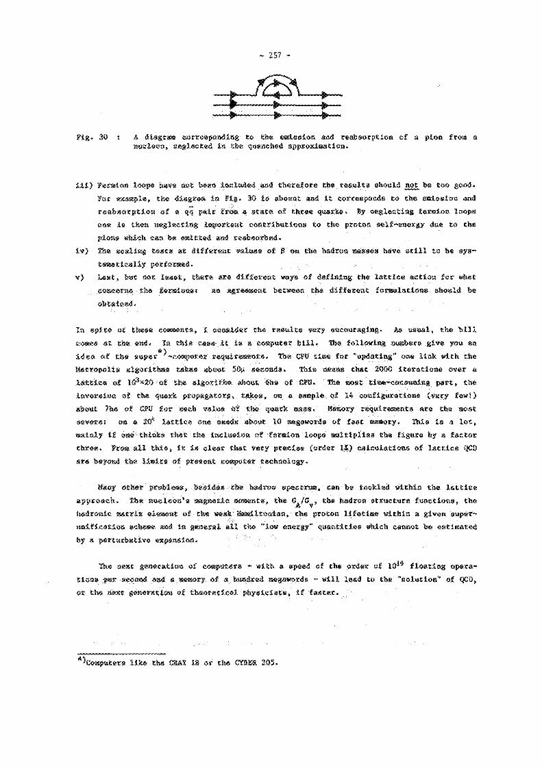
- 257 -

Fig. 30 s à di*graa corresponding to the emission and reabsorption of a pion from a nucleón, neglected in the quenched approximation.

Iii) Farmion loops bay* not b*«n included and therefore th* resulta should not be too good. For example, th* dl«gram in Fig. 30 i* absent and it corresponds to the emission and reabsorption of a qq p«ir from a state of three quark*. By n*gl*cting fermion loops on* is then n«gl*cting important contribution* to the proton «elf-energy du* to the pion* which c«n b« emitted and reabsorbed.

iv) Th* scaling t**ts «t different v«lu«s of p on th* hadron masse* have still to be sys­tematically p«rform*d.

v) Last, hot not least, there ere different ways of defining the lattice action, for what camerasthe fermion*: *n tgxmmat between the different formulations should be obtained.

In spit* of tb*s« comments, I coo*id«r th* results very encouraging. A* usual, the bill com** at the end. In this case it is a computer bill. The following numbers give you an idee of the super '-computer requirements. The CPU time for updating" one link with the Metropolis algorithm* takes about 5% seconds. This means that 2000 Iterations over a lattice of 103«20 of the algorithm about 6hs of CPU. The moat tlse-conaumlng part, the inversion of the quark propagators, takes, oa a sample of 14 configurations (very few! ) about 7h* of CPU for each value of the quark mass. Memory requirements are the most •*v«r*i on a 20* lattice one needs about 10 megawords of fast memory. This te a lot, mainly if one thinks that the Inclusion of fermion loops multiplies the figure by a factor three. Fro* all this, it is clear that very precise (order IX) calculations of lattice QCD are beyond th* limits of present computar technology.

Many oth«r problem*, t>«»ld«* the hadron spectrum, cm he tackled within the lattice approach. Th* ancleon's magnetic moments, the G^/C^, the hadron structure function*, the hadronic matrix élément of the weak Hsailtonlan, the proton lifetime within a given *up*r-uniflcation scheme «nd in general all the "low energy" quantities which cannot be estimated by a parturbative expansion.

The next generation of computers - with a speed of th* order of 10 1 0 floating opera­tions jer sacona aaJ e;«««ory of a hanéjraa megawords - will lead to the "solution" of QCD, or the east generation of tbeer«tical; physicists, if faster.

*>Comput«re l i k e th* CSAT IS or the C t l i l 205.

- 258 -

1) M. Gell-Hann, Acta Phya. Austriaca, Supp. IX (1972) 733; H. Fritzach and M. Cell-Mann, XVI International Conference on High Energy Physics, Batavia 1972, Vol. II, p. 135; S. Weinberg, Phys. te». Lett. 31 (1973) 494, Phya. Rev. D8 (1973) 4482.

2) See also the lecturea by C. Jarlskog at this school.

3) If you are Interested in the functional formulation of quantum field theories, see for example< J. Iliopouloa, J. Itsykeon and A. Kartin, Eev. of Modern Physics 47 (1975) 165.

4) B.C.G. Stueckelbarg and A. Petermen, Helv. Phys. Acta 26 (1953) 499; M. Gell-Mann and P. Low, Phya. Rev. 95 (1954) 1300.

5) G. *t Booft, unpublished (1972); H.D. Politter, Phys. Rev. Lett. 30 (1973) 1346; D.J. Croas and ?, WiLctek, Pays. Rev. Lett. 30 (1973) 1343.

6) P.M. Stavenaon, Phya. Bav. 023 (1981) 2916.

7) A.H. Mueller, Phya. Bav. 018 (1978) 3705; t.fU Ellis, H. Georgl, M. Mschacak, H.D. Politzer and G.G. Roas, Phys. Lett. 78B (1978) 281; Nucl. Phys. 8152 (1979) 285; D. Amati, R. Petronzio and G. Veneziano, Nucl. Phys. B140 (1978) 54; »146 (1978) 29.

8) G. Alteram, Phys. Rep. 81 (1982) 1.

9) W. Furmaneki and R. Petronilo, Phys. Lett. 97B (1980) 437.

10) A. Bassetto, M. CiafelOtti and G. Kercbcsini, Phys. Rep. 100 (1983) 201.

11) Yu.L. Dokehitzer, D.I. D'yakonov and S.I. Troyan, Phys. Lett. 78B (1978) 290; Phys. Rep. 58 (1980) 271; C. Pariai and ft. Petronzio, Nucl. Phys. 1154 (1979) 427; C. Corel. M. Greco «ad R. Srivastava, Nucl. Phys. B159 (1979) 451; J.C. Collins and D.E. Sopar, Sucl. Phys. B193 (1981) 381.

12) 6. Altarelli, R.K. Ellis, M. Greco and G. Martloelil, Sucl. Phys. B246 (1984) 12.

13) UAl Collaboration, Phys. Lett. 136B (1984) 294.

14) U.K. Ellis, W. Furmeoeki and S. Petronilo, Nucl. Phys. B212 (1983) 29.

15) CHARM Collaboration in M. Diamox, F. Ferroni and E. Longo, Nota Interna Ko. 851 Dipartiaento di Física, Univarsità di Koma, to appear ia Phys. Reports.

16) 6,1, Parrar and 0.1. Jackson, Phys. Rev. Lett. 43 (1976) 246; A.V. Rfremov and A.V. Radyushkln, D0BNA preprint 11983 (1978).

17) B.L. Berger and S.J. Brodsky, Phys. Rev. 024 (1981) 2428; J. Bagger and J.P. Gunion, Phys. Rev. 025 (1982) 2287.

18) T. Appelquist and H. Georgi, Phys. Rev. 08 (1973) 4000; A. Zee, Phys. Rev. OS (1973) 4038; V.A. Bovlkov at «1., Phys. Rev. Letter« 30 (1977) 626; Phys. Lett. 67B (1977) 409; M.A. Shifman, A.I. Vainstein and V.l. Zakharov, Sucl. Phys. B147 (1979) 385, 448, 519; K.B. Voloahin, fed. Fi*. 29 (1979) 1368; B.V. Shuryak, Mucl. Phys. B198 (1982) 83.

19) K.G. Wilson, Phys. Rev. D10 (1974) 2445; For a review, see; C. Sebbl, Lattice Gauge Theories and Monte Carlo Simulations, World Scientific (1983)

- 259

20) I» Metropolit, à. Roteabluth, M. Rotenbluth, A. Teller «ad E. Teller, Journ. of Che*, Phy«. 21 (19853) 1087.

21) Por t rte«iit review, «tt: A. Bttenfrttr «ad f. tUttnfrtt«, fSB preprint FSU-SCRI 85-2 (1985).

22) for a review, tees I, Sets, tea. Review of tkicleer Scioaee (1985).

23) H. Htaber and C. Periti, Phyt. lev, Lett. 47 (1981) 1792; E. Merineri, S* Paritl ma C. Xtbbl, Phy». Rev. Lett. 4? (1981) 1795; O.E. Weiegerten, Phyt. Utt. »109 (1982) 57; for e review, aee lef. 21).

24) 1 , Uppt, G. Ktrtlatlli, R. Petroaxio «ad P. Rtpuano, Phyt. Lett. 8126 (1983) 250.

25) C. P«ri«l, Phyt. Rtp. 103 (1984) 203.