CHAPTER 5
61
CHAPTER 5 CHAPTER 5 NON-LINIER OPTIMIZATION NON-LINIER OPTIMIZATION
-
Upload
tatyana-diaz -
Category
Documents
-
view
32 -
download
0
description
CHAPTER 5. NON-LINIER OPTIMIZATION. Problem estimisasi secara umum MaX (Min) f (X) s.t. X y F disebut objektif function. X disebut himpunan feasible. Himpunan feasible biasanya digambarkan dengan persamaan atau pertidaksamaan yang disebut kendala. - PowerPoint PPT Presentation
Transcript of CHAPTER 5

CHAPTER 5CHAPTER 5
NON-LINIER OPTIMIZATIONNON-LINIER OPTIMIZATION

5.1. Introduction5.1. IntroductionProblem estimisasi secara umumProblem estimisasi secara umum
MaX (Min) f (X)MaX (Min) f (X)
s.t. X s.t. X y y
F disebut objektif function.F disebut objektif function.
X disebut himpunan feasible.X disebut himpunan feasible.
Himpunan feasible biasanya digambarkan dengan Himpunan feasible biasanya digambarkan dengan persamaan atau pertidaksamaan yang disebut persamaan atau pertidaksamaan yang disebut kendala. kendala.
Contoh linier programming problem :Contoh linier programming problem :
MaX MaX ccttXXs.t. AX = bs.t. AX = b
X X ≥ 0≥ 0
X = {XX = {XRRnn| AX = b, X ≥0}| AX = b, X ≥0}
Jika tidak ada kendala maka X = RJika tidak ada kendala maka X = Rnn,,
dan problem ini disebut optimisasi tanpa kendaladan problem ini disebut optimisasi tanpa kendala

5.2. Global dan Local Optima5.2. Global dan Local Optima
f = D f = D R dimana D R dimana D R Rnn. . Fungsi f dikatakan memiliki Fungsi f dikatakan memiliki
global (absolute) maximum pada X* global (absolute) maximum pada X* D jhj f(X) D jhj f(X) ≤ f(X≤ f(X**) ) X X D. D.Titik X* disebut global maximizer (or maximizer) dari f Titik X* disebut global maximizer (or maximizer) dari f dan f(X*) disebut global maximum dari f dan dan f(X*) disebut global maximum dari f dan sebaliknya. sebaliknya.
Global minimum f(X) ≥ f (X*) Global minimum f(X) ≥ f (X*) X X D. D.Fungsi f dikatakan memiliki local (relative) maximum Fungsi f dikatakan memiliki local (relative) maximum pada X* pada X* D jhj terdapat neighborhood N (X*) seperti : D jhj terdapat neighborhood N (X*) seperti :
f(X) ≤ f(X*) f(X) ≤ f(X*) X X N (X*) N (X*) D. D.Titik X* disebut local maximizer dari f dan f(X*) disebut Titik X* disebut local maximizer dari f dan f(X*) disebut local maximum dari f.local maximum dari f.Dan sebaliknya adalah:Dan sebaliknya adalah:Fungsi local minimum X* Fungsi local minimum X* D jhj f(X) ≥ f(X*) D jhj f(X) ≥ f(X*) X X N(X*) N(X*) D D
5.2.1 Definisi 5.2.1 Definisi

XX11, X, X33, X, X55 adalah local maximum, X adalah local maximum, X55 global max global maxXX22, X, X44, X, X66 adalah local minimum, X adalah local minimum, X22 global min global min
5.2.2 Contoh Local dan Global Optimum5.2.2 Contoh Local dan Global Optimum
XX11 XX22 XX33 XX44 XX55 XX66
D
0
f(X)

(1)(1) Global max digunakan secara relatif to domain Global max digunakan secara relatif to domain D dari f yaitu global maximizer berarti global D dari f yaitu global maximizer berarti global maximizer to domainmaximizer to domain
(2)(2) Istilah optimum digunakan baik maximum Istilah optimum digunakan baik maximum maupun minimummaupun minimum
(3)(3) Suatu global maximizer (global minimizer) Suatu global maximizer (global minimizer) adalah local maximizer (local minimizer)adalah local maximizer (local minimizer)
(4)(4) Local maximum dapat lebih kecil dibanding Local maximum dapat lebih kecil dibanding local minimunlocal minimun
(5) (5) Suatu fungsi tidak memiliki baik maximizer Suatu fungsi tidak memiliki baik maximizer ataupun minimizer dalam domainnya. f(X) = X, ataupun minimizer dalam domainnya. f(X) = X, tidak memiliki max/min dalam interval (0,1)tidak memiliki max/min dalam interval (0,1)Catatan : Interval ini tidak tertutup meskipun Catatan : Interval ini tidak tertutup meskipun interval tertutup tetapi tidak memiliki batas interval tertutup tetapi tidak memiliki batas (bounded) (bounded)
5.2.3 Remark5.2.3 Remark
5.2.4 Theorema5.2.4 TheoremaSuatu fungsi continuous real-valued didefinisikan Suatu fungsi continuous real-valued didefinisikan atas suatu compact subset S dari atas suatu compact subset S dari RRnn memiliki memiliki maximizer & minimizer dalam S.maximizer & minimizer dalam S.

5.3 Necessary (or First-Order) 5.3 Necessary (or First-Order) ConditionCondition
untuk Local Optimumuntuk Local OptimumAndaikan f : D Andaikan f : D R, dimana D ≤ R R, dimana D ≤ Rnn, dan andaikan , dan andaikan turunan partial dari f turunan partial dari f X(S) pada suatu interior point X* X(S) pada suatu interior point X*
dari D X* adalah local optimizer dari f, maka f’(X) = 0. dari D X* adalah local optimizer dari f, maka f’(X) = 0. Proof :Proof :
5.3.1 Theorema5.3.1 Theorema
(1) Kasus satu variabel dari theorema 5.3.1(1) Kasus satu variabel dari theorema 5.3.1
(2)(2)Syarat bahwa turunan exist pada local optimizer Syarat bahwa turunan exist pada local optimizer adalah necessary dalam teorema 5.3.1 adalah necessary dalam teorema 5.3.1 contoh : contoh : f(X) = X f(X) = X2/3 2/3
f’(X) = 2/3Xf’(X) = 2/3X-1/3-1/3
5.3.2 Remark5.3.2 Remark
f(X)
f’(X*)=0
0 X* X
f(X) f’(X*)=0
0 X* X

Fungsi f memiliki local minimum pada X*=0 but Fungsi f memiliki local minimum pada X*=0 but f’(0)≠0. Contoh di atas tidak differentiable pada f’(0)≠0. Contoh di atas tidak differentiable pada X*=0 (ini berarti bukan sufficient).X*=0 (ini berarti bukan sufficient).
(3)(3) Syarat suatu X* adalah interior point dari Syarat suatu X* adalah interior point dari domainnya adalah necessary. Contoh andaikan domainnya adalah necessary. Contoh andaikan gambar 5.5 domain D adalah interval tertutup [0,1].gambar 5.5 domain D adalah interval tertutup [0,1].
Memenuhi local minimum pada X*=0 tetapi Memenuhi local minimum pada X*=0 tetapi f’(X*)f’(X*)0. 0. Note: X* tidak pada interior point dari D.Note: X* tidak pada interior point dari D.
X*
f(X)
X
Gambar 5.4
0 1X*
f’(X*)0
Gambar 5.5
f(X) = Xf(X) = X2/32/3
X
D

(4)(4) Kebalikan dari teorema 5.3.1 tidak benarKebalikan dari teorema 5.3.1 tidak benarContoh : f(X) = XContoh : f(X) = X33
f’(X) = 3Xf’(X) = 3X22
f’(0) = 0 tetapi f tidak memiliki local optimum pada f’(0) = 0 tetapi f tidak memiliki local optimum pada X*=0. X*=0.
Contoh tiga dimensi Contoh tiga dimensi f(Xf(X11,X,X22) = X) = X11
22 – X – X2222
Gambar 5.7 gradien f adalah Gambar 5.7 gradien f adalah
f’(Xf’(X11,X,X22) = ) =
Pada X*=[0,0]Pada X*=[0,0]tt, f(X*)=0 tetapi untuk titik dekat X* , f(X*)=0 tetapi untuk titik dekat X* pada sb Xpada sb X11–axis, f(X–axis, f(X11,X,X22)>0 dan titik dekat X* pada )>0 dan titik dekat X* pada sb Xsb X22 f(X f(X11,X,X22)<0.)<0.
2X1
-2X2
X
f(X)
f’(X)=X3
Gambar 5.6

Consekuensi X*=0 mendekati local maximizer dan Consekuensi X*=0 mendekati local maximizer dan local minimizer sehingga titik tersebut disebut local minimizer sehingga titik tersebut disebut saddle point.saddle point.
Gambar 5.7. Gambar 5.7. Saddle pointSaddle point
X1
X2
X3
Titik X* dimana f’(X*)=0 disebut stationary point f. Titik X* dimana f’(X*)=0 disebut stationary point f. stationary point dan bukan titik optimum disebut saddle stationary point dan bukan titik optimum disebut saddle point dari f.point dari f.Dalam pandang theorema 5.3.1 titik optimizer f pada Dalam pandang theorema 5.3.1 titik optimizer f pada domain D ditemukan.domain D ditemukan.(a) Stationary point (figure 5.7.1(a))(a) Stationary point (figure 5.7.1(a))(b) The boundary point (figure 5.7.1(b))(b) The boundary point (figure 5.7.1(b))(c) f’(X) tidak exist (figure 5.7.1(c))(c) f’(X) tidak exist (figure 5.7.1(c))
5.3.3 Definisi5.3.3 Definisi

a. f’(X*) = a. f’(X*) = 00
b. f’(X*) b. f’(X*) 00
c. f’(X*)=n tidak c. f’(X*)=n tidak diperolehdiperolehGambar Gambar
5.7.15.7.1Kemudian sufficient condition untuk suatu stationary Kemudian sufficient condition untuk suatu stationary point menjadi local optimizer ketika f setidaknya dapat point menjadi local optimizer ketika f setidaknya dapat di diferensialkan 2 kali secara continuous.di diferensialkan 2 kali secara continuous.
5.45.4 SufficientSufficient (Second-Order) Condition for(Second-Order) Condition for
Local Optima : The One-Variable CaseLocal Optima : The One-Variable Case5.4.1 Theorema5.4.1 TheoremaAndaikan D ≤ R . f : D Andaikan D ≤ R . f : D R memiliki continuous second- R memiliki continuous second-order derivative atas open interval I yang berisi X*. order derivative atas open interval I yang berisi X*. Andaikan f’(X*)=0.Andaikan f’(X*)=0.(i) Jika f”(X*) > 0, X* adalah local minimizer dari f(i) Jika f”(X*) > 0, X* adalah local minimizer dari f(ii) Jika f”(X*) < 0, X* adalah local maximizer dari f (ii) Jika f”(X*) < 0, X* adalah local maximizer dari f
X*X* X*X* X*X*
DD DDDD

5.4.2 Contoh5.4.2 Contoh
Let f : R Let f : R R R f(X) = 2Xf(X) = 2X33 – 3X – 3X22 – 12X + 1 – 12X + 1 f’(X) = 6Xf’(X) = 6X22 – 6X – 12 – 6X – 12 Setting f’(X) = 0 diperoleh X* = 2, X** = -1Setting f’(X) = 0 diperoleh X* = 2, X** = -1
f”(X) = 12 X – 6f”(X) = 12 X – 6f”(2) = 12(2) – 6 = 18 f”(2) = 12(2) – 6 = 18 f”(-1) = 12(-1) – 6 = -18 f”(-1) = 12(-1) – 6 = -18
Ini berarti bahwa X* = 2 adalah local maximizer dari f Ini berarti bahwa X* = 2 adalah local maximizer dari f X** = -1 adalah local minimizer dari f X** = -1 adalah local minimizer dari f
5.4.3 Remark5.4.3 Remark
Ketika f”(X*)=0, tidak ada kesimpulan yang dapat Ketika f”(X*)=0, tidak ada kesimpulan yang dapat dibuat. Kita gunakan theorema berikutnya untuk dibuat. Kita gunakan theorema berikutnya untuk menggeneralisasikan theorema 5.4.1menggeneralisasikan theorema 5.4.1
Proof :Proof :
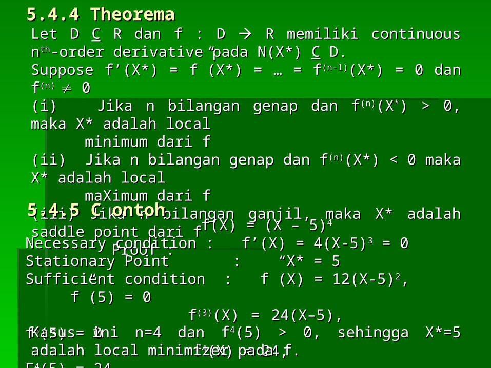
Let D Let D CC R dan f : D R dan f : D R memiliki continuous n R memiliki continuous nthth-order -order derivative pada N(X*) derivative pada N(X*) CC D. D.Suppose f’(X*) = f”(X*) = … = fSuppose f’(X*) = f”(X*) = … = f(n-1)(n-1)(X*) = 0 dan f(X*) = 0 dan f(n) (n) 0 0(i) Jika n bilangan genap dan f(i) Jika n bilangan genap dan f(n)(n)(X(X**) > 0, maka X* ) > 0, maka X* adalah local adalah local minimum dari fminimum dari f(ii) Jika n bilangan genap dan f(ii) Jika n bilangan genap dan f(n)(n)(X*) < 0 maka X* (X*) < 0 maka X* adalah local adalah local maXimum dari fmaXimum dari f(iii) Jika n bilangan ganjil, maka X* adalah saddle point (iii) Jika n bilangan ganjil, maka X* adalah saddle point dari fdari f Proof : Proof :
5.4.4 Theorema 5.4.4 Theorema
f(X) = (X – 5)f(X) = (X – 5)44
Necessary condition : f’(X) = 4(X-5)Necessary condition : f’(X) = 4(X-5)33 = 0 = 0 Stationary Point : X* = 5Stationary Point : X* = 5Sufficient condition : f”(X) = 12(X-5)Sufficient condition : f”(X) = 12(X-5)22, f”(5) = 0, f”(5) = 0
ff(3)(3)(X) = 24(X–5), f(X) = 24(X–5), f33(5) = 0 (5) = 0 ff44(X) = 24, F(X) = 24, F44(5) = 24(5) = 24
5.4.5 C ontoh5.4.5 C ontoh
Kasus ini n=4 dan fKasus ini n=4 dan f44(5) > 0, sehingga X*=5 adalah local (5) > 0, sehingga X*=5 adalah local minimizer pada f. minimizer pada f.
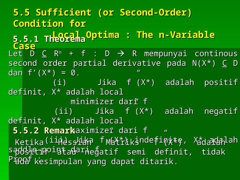
5.55.5 SufficientSufficient (or Second-Order) (or Second-Order) Condition forCondition for Local Optima : The n-Variable CaseLocal Optima : The n-Variable Case5.5.1 Theorema5.5.1 Theorema
Let D Let D CC R Rnn + f : D + f : D R mempunyai continous second R mempunyai continous second order partial derivative pada N(X*) order partial derivative pada N(X*) CC D dan f’(X*) = 0. D dan f’(X*) = 0.
(i) Jika f”(X*) adalah positif definit, X* adalah (i) Jika f”(X*) adalah positif definit, X* adalah locallocal
minimizer dari f minimizer dari f (ii) Jika f”(X*) adalah negatif definit, X* adalah (ii) Jika f”(X*) adalah negatif definit, X* adalah
locallocal maximizer dari f maximizer dari f (iii) Jika f”(X*) indefinite, X* adalah saddle-point (iii) Jika f”(X*) indefinite, X* adalah saddle-point
dari f dari f Proof :Proof :
5.5.2 Remark5.5.2 RemarkKetika Hessian Matriks f”(X*) adalah positif atau Ketika Hessian Matriks f”(X*) adalah positif atau negatif semi definit, tidak ada kesimpulan yang negatif semi definit, tidak ada kesimpulan yang dapat ditarik.dapat ditarik.

5.5.3 Contoh5.5.3 Contohf(X) = -Xf(X) = -X11
22 – 3X – 3X2222 – 2X – 2X33
22 + 2X + 2X11 – 12X – 12X22 + 8X + 8X33 – 5– 5
-2X-2X11 + 2 + 2 -6X-6X22 – – 12 12 -4X-4X33 + 8 + 8
f’(X) =f’(X) =Gradien dari Gradien dari f : f :
Setting f’(X) = 0, maka titik stationer Setting f’(X) = 0, maka titik stationer X* = [2 -2 2]X* = [2 -2 2]tt
Hessian matriks dari f pada X* adalah Hessian matriks dari f pada X* adalah
f”(X* ) = [f’’f”(X* ) = [f’’ijij(X*)] (X*)] ==
-2 0 0-2 0 0 0 -6 00 -6 0 0 0 -40 0 -4
Memiliki leading principle minor adalah Memiliki leading principle minor adalah |[-2]| = -2 < 0|[-2]| = -2 < 0
-2 0-2 0 0 -60 -6
= 12 > 0= 12 > 0

= -48 < 0= -48 < 0-2 0 0-2 0 0 0 -6 00 -6 0 0 0 -40 0 -4
Dari theorema 1.12.15 bahwa f”(X*) adalah negatif Dari theorema 1.12.15 bahwa f”(X*) adalah negatif definite. Alternatif, catatan bahwa f”(X*) adalah matriks definite. Alternatif, catatan bahwa f”(X*) adalah matriks diagonal, maka eigenvalue adalah elemen diagonal diagonal, maka eigenvalue adalah elemen diagonal (theorema 1.11.6). Sejak eigenvalue negatif maka f”(X*) (theorema 1.11.6). Sejak eigenvalue negatif maka f”(X*) adalah negatif definit (by Theorema 1.12.6). Sehingga adalah negatif definit (by Theorema 1.12.6). Sehingga X* adalah local maximizer dari f (by theorema 5.5.1).X* adalah local maximizer dari f (by theorema 5.5.1).
5.5.4 Contoh5.5.4 Contohf(X) = 4Xf(X) = 4X11
33 + X + X11XX22 – – 33//22XX1122 + ½X + ½X22
2 2 + 10+ 10Gradient dari f adalahGradient dari f adalah
f’(X) f’(X) = =
12X12X112 2 + X+ X22 – –
3X3X11
XX11+ X+ X22Setting f’(X) = 0 diperoleh titik stationer :Setting f’(X) = 0 diperoleh titik stationer :
X* = X* = 0000
, X** = , X** = 1/31/3-1/3-1/3

Hessian matriks dari f adalah Hessian matriks dari f adalah
f”(X) f”(X) ==
24X24X11-3 1-3 1 1 1 1 1
Pertimbangankan titik stationer X* maka Hessian matrix Pertimbangankan titik stationer X* maka Hessian matrix dari f pada X* adalah dari f pada X* adalah
f”(X*) f”(X*) ==
24(0)-3 24(0)-3 11 1 1 1 1
== -3 1-3 1 1 1 1 1
Matriks Real symmetric dimana eigenvalue adalahMatriks Real symmetric dimana eigenvalue adalah11 = 1 + 5 , = 1 + 5 , 22 = 1 – 5 = 1 – 5
Apabila Apabila 1 1 > 0 dan > 0 dan 22 < 0 sesuai teorema 1.12.6 bahwa < 0 sesuai teorema 1.12.6 bahwa f”(X*) adalah indefinite. Konsekuensinya, X* adalah f”(X*) adalah indefinite. Konsekuensinya, X* adalah saddle-point dari f by theorema 5.5.1saddle-point dari f by theorema 5.5.1
Hessian matrix pada X** adalahHessian matrix pada X** adalah
f”(X**) =f”(X**) = 24(1/3)-3 124(1/3)-3 1 1 1 1 1
== 5 15 11 1 1 1

Matriks Real symmetric dimana Leading Principal Minors Matriks Real symmetric dimana Leading Principal Minors (LPM) adalah(LPM) adalah
|[5]| = 5 > 0 , |[5]| = 5 > 0 , = 4 > 0 = 4 > 05 15 11 11 1
Theorema f”(X**) adalah positif definite. Alternatif, Theorema f”(X**) adalah positif definite. Alternatif, calculate eigenvalue dari f”(X**);calculate eigenvalue dari f”(X**); 11 = 3 + 5 = 3 + 5 , , 22 = 3 – 5 = 3 – 5 11>0 dan >0 dan 22>0, by theorem 1.12.6 f”(X**) adalah positif >0, by theorem 1.12.6 f”(X**) adalah positif definite. sehingga X** sebagai local minimizer dari f by definite. sehingga X** sebagai local minimizer dari f by theorem 5.5.1theorem 5.5.1 5.5.5 Contoh5.5.5 ContohLet f : RLet f : R22 R didefinisikan dengan R didefinisikan dengan
f(X) = Xf(X) = X1122 + X + X22
44
Gradient dari f adalahGradient dari f adalah
f’(X) = f’(X) =
Setting f’(X) = 0 , diperoleh stationary point Setting f’(X) = 0 , diperoleh stationary point X* = [ 0 0]X* = [ 0 0]tt
2X2X11
4X4X2233

Hessian matriks dari f adalahHessian matriks dari f adalah
f”(X) =f”(X) =
Pada X*, Hessian matriks dari f adalah Pada X*, Hessian matriks dari f adalah
f”(X*) =f”(X*) =
Eigenvalue adalah Eigenvalue adalah 11=2 dan =2 dan 22=0 sesuai theorema =0 sesuai theorema 1.12.6 that f”(X*) adalah positive semidefinite tetapi 1.12.6 that f”(X*) adalah positive semidefinite tetapi tidak positif definit sehingga tidak dapat diputuskan. tidak positif definit sehingga tidak dapat diputuskan.
2 02 00 0 12X12X22
22
2 02 00 00 0
5.5.6 Contoh5.5.6 Contoh Let f : RLet f : R22 R didefinisikan dengan R didefinisikan dengan
f(X) = Xf(X) = X1122 – X – X22
44
Gradient pada f adalahGradient pada f adalah
f’(X) = f’(X) = 2X2X11
- 4X- 4X2222

Setting f’(X) = 0 , diperoleh titik stasioner Setting f’(X) = 0 , diperoleh titik stasioner X* = [ 0 0]X* = [ 0 0]tt
Hessian matriks dari f adalahHessian matriks dari f adalah
f”(X) =f”(X) =
Pada X*, Hessian matriks dari f adalahPada X*, Hessian matriks dari f adalah
f”(X*) =f”(X*) =
Theorem 5.5.1 tidak dapat digunakan tetapi Theorem 5.5.1 tidak dapat digunakan tetapi f(X*)=0 dan untuk titik X mendekati X* pada Xf(X*)=0 dan untuk titik X mendekati X* pada X11––axis, f(X)=(Xaxis, f(X)=(X11))22 > 0 sedang untuk titik X mendekati > 0 sedang untuk titik X mendekati X* pada XX* pada X22–axis, (f(X)=-(X–axis, (f(X)=-(X22))44 < 0. Sehingga X* < 0. Sehingga X* adalah saddle-point dari f (lihat Danao, 244-247).adalah saddle-point dari f (lihat Danao, 244-247).
2 02 00 -0 -12X12X22
22
2 02 00 00 0

5.5.7 Contoh Profit Maximization5.5.7 Contoh Profit Maximizationq = output, R(q), C(q), q = output, R(q), C(q), (q). R dan C continuous second-(q). R dan C continuous second-order derivatives.order derivatives.
(q) = R(q) – C(q)(q) = R(q) – C(q)
’’(q*) = R’(q*) – C’(q*) = 0(q*) = R’(q*) – C’(q*) = 0R’(q*) = C’(q*) R’(q*) = C’(q*) optimal profit optimal profit R’(q*) < C’(q*) R’(q*) < C’(q*) q q RR’’(q(q**) > C) > C’’((q*) q*) q q
5.5.8 Contoh5.5.8 Contoh
The Method least Squares.The Method least Squares.Garis regresi :Garis regresi : Y = Y = 00 + + 11XXUntuk setiap iUntuk setiap i
ii = = YYii – ( – (00 + + 11XXii))
Untuk estimasi Untuk estimasi 00 dan dan 11 ((ii))22 = = (Y (Yii – – 00 – – 11XXii))22
n
i=1
n
i=1
adalah minimum. adalah minimum. disederhanakan sebagai disederhanakan sebagai ..
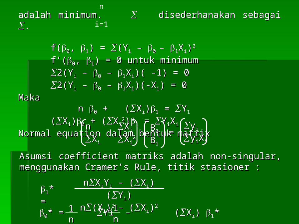
f(f(00, , 11) = ) = (Y(Yii – – 0 0 – – 11XXii))22
f’(f’(00, , 11) = 0 untuk minimum) = 0 untuk minimum2(Y2(Yii – – 00 – – 11XXii)( -1) = 0)( -1) = 02(Y2(Yii – – 00 – – 11XXii)(-X)(-Xii) = 0) = 0
Maka Maka n n 00 + ( + (XXii))11 = = YY11
((XXii))00 + ( + (XX1122))11 = = YYiiXXii
Normal equation dalam bentuk matrixNormal equation dalam bentuk matrixnn XXii
XXii XXii22
BB00
BB11
yyii
yyiiXXii==
Asumsi coefficient matriks adalah non-singular, Asumsi coefficient matriks adalah non-singular, menggunakan Cramer’s Rule, titik stasioner :menggunakan Cramer’s Rule, titik stasioner :
11* =* =nnXXiiYYii – ( – (XXii) () (YYii))
nn(X(Xii))2 2 – (– (XXii))22
00* = * = Yi – (Yi – (XXii) ) 11* * 11nn
11nn
n
i=1

to verify to verify * is a global minimizer dari f, dengan melihat * is a global minimizer dari f, dengan melihat Hessian matrix dari f : Hessian matrix dari f :
f”(f”(00, , 11) =) =22 2X2Xii
2X2Xii 2X2Xii22
2n2n 22XXii
22XXii 22XXii22==
LPM adalah LPM adalah ::
|[2n]| = |[2n]| = 2n>0 ;2n>0 ;
2n2n 22XXii
22XXii 2 2(X(Xii))22 = 4n= 4n(X(Xii))22 – 4( – 4(XXii))22
= 4[n= 4[n(X(Xii))22 – ( – (XXii))22]]= 4[(n-1)= 4[(n-1)(X(Xii))2 2 – – 2 X2 Xi i XXjj] >0 ] >0
Dari persamaan (5-2) Hessian matriks f”(Dari persamaan (5-2) Hessian matriks f”(00,,11) adalah ) adalah positive definite and so the stationary point positive definite and so the stationary point * minimizer * minimizer f.f.5.6 Optima of Concave and Convex 5.6 Optima of Concave and Convex
FunctionsFunctions
Let X,Y Let X,Y R Rnn, titik Z = , titik Z = X + (1–X + (1–)Y)YDimana 0 ≤ Dimana 0 ≤ ≤ 1 disebut convex combination dari X ≤ 1 disebut convex combination dari X dan Y dan Y
5.6.1 Definisi5.6.1 Definisi

Geometrically, the set of all convex combinations of X Geometrically, the set of all convex combinations of X and Y is the line segment joining X and Yand Y is the line segment joining X and Y
5.6.2 Remark5.6.2 Remark
A subset C of RA subset C of Rnn adalah convex jhj line segment adalah convex jhj line segment berhubungan dari titik dalam C berada dalam himpunan berhubungan dari titik dalam C berada dalam himpunan C. In symbols, C adalah convex jhj C. In symbols, C adalah convex jhj X,Y X,Y C, 0 ≤ C, 0 ≤ ≤ 1 ( ≤ 1 (X + (1- X + (1- )Y) )Y) C C
5.6.3 Definisi5.6.3 Definisi
1)1) Himpunan kosong (O) dan himpunan hanya satu Himpunan kosong (O) dan himpunan hanya satu elemen adalah convex setelemen adalah convex set
2) R2) Rnn adalah convex set adalah convex set
5.6.4 Remarks5.6.4 Remarks
y=1/X
ConvexSet
Strictly Convex Not Strictly Convex

Not ConveX
Set
3)3) The following sets are convex :The following sets are convex :(a) The closed half-spaces : (a) The closed half-spaces : HH+(+(P,P,) = {X ) = {X R Rnn| P| PttX X }}
HH--(P,(P,) = {X ) = {X R Rnn| P| PttX ≤ X ≤ }}(b) The hyperplane : (b) The hyperplane : H(PH(P,,) = {X ) = {X R Rnn | P | PttX = X = }}(c) The Non-negative orthant : (c) The Non-negative orthant : R Rnn
++ = {X= {XRRn n | X | X 0} 0}
(d) The positive orthant : (d) The positive orthant : R Rnn++++ = {X = {XRRnn|X>0}|X>0}
Interseksi dari convex set adalah convex.Interseksi dari convex set adalah convex.Proof :Proof :
5.6.5 Theorema5.6.5 Theorema
A subset C of RA subset C of Rnn adalah strictly convex jhj adalah strictly convex jhjX,Y X,Y C, X C, X Y, 0 < Y, 0 < < 1 [ < 1 [X + (1-X + (1-)Y] )Y] int int
(C)(C)
5.6.6 Definisi5.6.6 Definisi

An open convex set is strictly convex. A closed disk is An open convex set is strictly convex. A closed disk is strictly convex while a closed triangle is not. Intuitively, strictly convex while a closed triangle is not. Intuitively, a closed strictly convex set does not have a flat portion a closed strictly convex set does not have a flat portion on its boundary. on its boundary.
5.6.7 Remarks5.6.7 Remarks
A function f : C A function f : C R defined on a convex subset C of R R defined on a convex subset C of Rnn is is said to be concave on C if and only if said to be concave on C if and only if X,Y X,Y C, 0 ≤ C, 0 ≤ ≤ 1, f( ≤ 1, f(X+(1- X+(1- )Y) ≥ )Y) ≥ f(X)+(1- f(X)+(1- )f(Y))f(Y)
5.6.8 Definisi5.6.8 Definisi
f : C f : C R defined on a convex subset C of R R defined on a convex subset C of Rnn is said to be is said to be strictly concave on C if and only if strictly concave on C if and only if X,Y X,Y C, X ≠ Y, 0 < C, X ≠ Y, 0 < < 1, f( < 1, f(X+(1-X+(1-)Y) )Y) >> f(X)+(1- f(X)+(1- )f(Y))f(Y)
5.6.10 Definisi5.6.10 Definisi
f : C f : C R defined on a convex subset C of R R defined on a convex subset C of Rn n is said to be is said to be strictly convex on C if and only if strictly convex on C if and only if X,Y X,Y C, X ≠ y, 0 < C, X ≠ y, 0 < < 1, f( < 1, f(X+(1- X+(1- )Y) < )Y) < f(X)+(1-f(X)+(1-)f(Y))f(Y)
5.6.11 Definisi5.6.11 Definisi

A concave (convex) function is continuous in the interior A concave (convex) function is continuous in the interior of its domainof its domain
Concave functionConcave function
Convex functionConvex function
5.6.12 Theorema5.6.12 Theorema
f(X1)f(X2)
X1 (X1)+(1- )X2X2
f(X1)f(X2)
X1 X1+(1-)X2X2
f(X1)+(1-)f(X2)
f(X1+(1- )X2
f((X1)+(1- )X2)
f(X1)+(1- )f(X2)

Concave functionConcave function
Convex functionConvex function
Neither concave nor convex functionsNeither concave nor convex functionsFigure 5.11Figure 5.11
Y=ln(X)Y
XStrictly concavefunction
Y=1/X
Y
XStrictly convexfunction

f : C f : C R dimana C adalah convex subset of R R dimana C adalah convex subset of Rnn (i)(i) if f is concave on C then UCif f is concave on C then UCf(() = {X ) = {X C|f(X) ≥ C|f(X) ≥ }}
is convex for every is convex for every R R(ii)(ii)if f is convex on C then LCif f is convex on C then LCf(() = {X ) = {X C|f(X) ≤ C|f(X) ≤ }}
is convex for every is convex for every R R
5.6.13 Theorema5.6.13 Theorema
f : D f : D R adalah function defined on a subset D of R R adalah function defined on a subset D of Rnn. . - UC- UCf(() = {X ) = {X D| f(X) ≥ D| f(X) ≥ , , R} R}
disebut upper contour set of fdisebut upper contour set of f- - LCLCf(() ) = {X = {X D| f(X) D| f(X) ≤ ≤ , , R} R}
disebut lower contour set of fdisebut lower contour set of f- - CCf(() ) = {X = {X D| f(X) = D| f(X) = , , R} R}
disebut contour (or level) set of fdisebut contour (or level) set of f
5.6.14 Definisi5.6.14 Definisi
5.6.15 Remark5.6.15 Remark

5.6.16 Theorem5.6.16 Theorem
f : C f : C R adalah continuously differentiable on convex R adalah continuously differentiable on convex subset of Rsubset of Rnn
(i) f adalah concave on C if and only if (i) f adalah concave on C if and only if X,Y X,Y C, f(Y) - f(X) ≤ [f’(X)] C, f(Y) - f(X) ≤ [f’(X)] tt (Y-X) (Y-X)
(ii) f adalah convex on C if only if(ii) f adalah convex on C if only if X,Y X,Y C, f(Y) - f(X) ≥ [f’(X)] C, f(Y) - f(X) ≥ [f’(X)] tt (Y-X) (Y-X)
5.6.17 Theorem5.6.17 Theoremf : I f : I R adalah continuously differentiable on open R adalah continuously differentiable on open
interval Iinterval I
(i)(i) f adalah concave on I if only if f adalah concave on I if only if X,Y X,Y I, f(Y) - f(X) ≤ f’(X) (Y-X) I, f(Y) - f(X) ≤ f’(X) (Y-X)
(ii) f adalah convex on I if only if (ii) f adalah convex on I if only if X,Y X,Y I, f(Y) - f(X) ≥ f’(X) (Y-X) I, f(Y) - f(X) ≥ f’(X) (Y-X)

5.6.19 Theorem5.6.19 Theorem
f : C f : C R adalah continuously differentiable on open convex R adalah continuously differentiable on open convex subset C of Rsubset C of Rnn
(i)(i) f adalah strictly concave on C if only if f adalah strictly concave on C if only if X,Y X,Y C, X ≠ Y f(Y) - f(X) < [f’(X)] C, X ≠ Y f(Y) - f(X) < [f’(X)]tt (Y-X) (Y-X)
(ii) f adalah strictly convex on C if only if (ii) f adalah strictly convex on C if only if X,Y X,Y C, X ≠ Y f(Y) - f(X) C, X ≠ Y f(Y) - f(X) >> [f’(X)] [f’(X)]tt (Y-X) (Y-X)
5.6.20 Theorem5.6.20 Theoremf : C f : C R adalah twice continuously differentiable on R adalah twice continuously differentiable on
open open
concex subset C of Rconcex subset C of Rnn then then
(i)(i) f is concave on C jhj Hessian matrix f”(X) is negatif f is concave on C jhj Hessian matrix f”(X) is negatif
semidefinite on Csemidefinite on C
(ii)(ii) f is convex on C jhj Hessian matriX f”(X) is positive f is convex on C jhj Hessian matriX f”(X) is positive
semidefinite on Csemidefinite on C

f : I f : I R be twice continuously differentiable on an open R be twice continuously differentiable on an open
interval I interval I
X{Ci | if the hessian matriks f”(X) adalah negatif X{Ci | if the hessian matriks f”(X) adalah negatif
(i) f is concave on I jhj f”(X) (i) f is concave on I jhj f”(X) ≤ 0 on I≤ 0 on I
(ii) f is conveX on I jhj f”(X) ≥ 0 on I(ii) f is conveX on I jhj f”(X) ≥ 0 on I
5.6.21 Theorem5.6.21 Theorem
f have continuous second-order partial derivative on an f have continuous second-order partial derivative on an open convex subset C of Ropen convex subset C of Rnn
(i)(i) If Hessian matriks f”(X) is negative definite for every X If Hessian matriks f”(X) is negative definite for every X C, C, then f is strictly concave on Cthen f is strictly concave on C
(ii) If Hessian matriks f”(X) is positive definite for every X (ii) If Hessian matriks f”(X) is positive definite for every X C, C, then f is strictly convex on Cthen f is strictly convex on C
Proof : PolakProof : Polak
5.6.22 Theorem5.6.22 Theorem

f : R f : R R defined f (X) = X R defined f (X) = X44. . f is continuous second-order derivative on R. f is continuous second-order derivative on R. f is strictly convex on R. But f”(0) = 0 which is not f is strictly convex on R. But f”(0) = 0 which is not positive definite.positive definite.
5.6.23 Remark5.6.23 Remark
f : I f : I R adalah twice continuously differentiable R adalah twice continuously differentiable on an open interval Ion an open interval I(i) If f”(X) < 0 for every X (i) If f”(X) < 0 for every X I then f is strictly concave I then f is strictly concave on Ion I(ii) If f”(X) > 0 for every X (ii) If f”(X) > 0 for every X I then f is strictly convex I then f is strictly convex on Ion I
Sum and compositions of concave and convex Sum and compositions of concave and convex functionfunction
5.6.24 Theorema5.6.24 Theorema

f : C f : C R dan g : C R dan g : C R; dimana C is a convex subset R; dimana C is a convex subset on Ron Rnn
(i) If f dan g adalah strictly concave on C then (i) If f dan g adalah strictly concave on C then (a) f + g is strictly concave on C(a) f + g is strictly concave on C (b) (b) f is strictly concave for each f is strictly concave for each > 0 > 0 (c) (c) f is strictly convex for each f is strictly convex for each < 0 < 0(ii) If f dan g adalah strictly convex on C then (ii) If f dan g adalah strictly convex on C then (a) f + g is strictly convex on C(a) f + g is strictly convex on C (b) (b) f is strictly convex on C for each f is strictly convex on C for each > 0 > 0 (c) (c) f is strictly concave on C for each f is strictly concave on C for each < 0 < 0
5.6.25 Theorem5.6.25 Theorem
5.6.26 Theorem5.6.26 Theorem
f : C f : C R dan g : C R dan g : C R where C is a convex subset of R where C is a convex subset of RRnn
(i) If f dan g adalah concave on C then(i) If f dan g adalah concave on C then (a) f + g is concave on C(a) f + g is concave on C (b) (b) f is concave on C for each f is concave on C for each > 0 > 0 (c) (c) f is convex on C for each f is convex on C for each < 0 < 0(ii) If f dan g adalah convex on C then (ii) If f dan g adalah convex on C then (a) f + g is convex on C(a) f + g is convex on C (b) (b) f is convex on C for each f is convex on C for each > 0 > 0 (c) (c) f is concave on C for each f is concave on C for each < 0 < 0

Let : f : C Let : f : C R be defined on a convex subset C of R R be defined on a convex subset C of Rnn such that such that f(C) is convex. Let g : f(C) f(C) is convex. Let g : f(C) R be defined on f(C) R be defined on f(C)
(i) If f is strictly concave on C and g is strictly concave and (i) If f is strictly concave on C and g is strictly concave and increasing increasing
of f (C), then the composition of f and g is strictly concave of f (C), then the composition of f and g is strictly concave on C. on C.
(ii) If f is strictly convex on f(C), then the composition of f and g (ii) If f is strictly convex on f(C), then the composition of f and g isis
strictly convex on C.strictly convex on C.
5.6.28 Theorem5.6.28 Theorem
Let : f : C Let : f : C R be defined on a convex subset C of R R be defined on a convex subset C of Rnn such such that f(C) is convex. Let g : f(C) that f(C) is convex. Let g : f(C) R be defined on f(C) R be defined on f(C)
(i) If f is concave on C and g is concave and increasing of f (i) If f is concave on C and g is concave and increasing of f (C), (C),
then the composition of f and g is concave on C. then the composition of f and g is concave on C.
(ii) If f is convex on C and g is convex and increasing on f (ii) If f is convex on C and g is convex and increasing on f (C), (C),
then the composition of f and g is convex on C. then the composition of f and g is convex on C.
5.6.27 Theorem5.6.27 Theorem
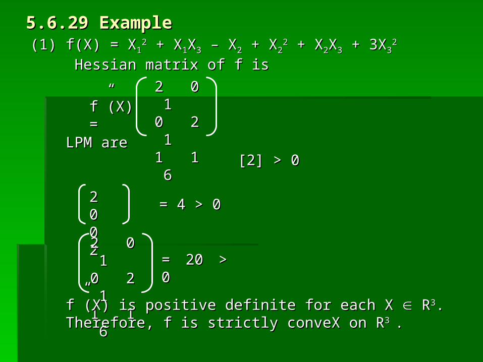
(1) f(X) = X(1) f(X) = X1122 + X + X11XX33 – X – X22 + X + X22
22 + X + X22XX33 + 3X + 3X3322
Hessian matrix of f is Hessian matrix of f is
5.6.29 Example5.6.29 Example
2 0 2 0 110 2 0 2 111 1 1 1 66
f”(X) =f”(X) =
LPM are LPM are [2] > 0[2] > 0
2 0 2 0 0 2 0 2
= 4 > 0= 4 > 0
2 0 2 0 110 2 0 2 111 1 1 1 66
= 20 > = 20 > 00
f”(X) is positive definite for each X f”(X) is positive definite for each X R R33. . Therefore, f is strictly conveX on RTherefore, f is strictly conveX on R3 3 ..

(2) Consider the production function f : R(2) Consider the production function f : R++++2 2 R R
f(L,K) = Lf(L,K) = L – K – K, 0<, 0<,,<1 , <1 , ++<1<1 The gradient of f is The gradient of f is
f’(L,K) f’(L,K) = =
LL-1-1 KK
LL K K -1 -1
The Hessian matrix of f is The Hessian matrix of f is
f”(L,K) f”(L,K) = =
((-1)L-1)L-2-2KK LL-1-1KK -1 -1
LL-1-1KK -1 -1 ((-1)L-1)LKK -2 -2
and its Leading Principal Minors areand its Leading Principal Minors are|[ |[ ((-1)L-1)L-2-2KK]| ]| = = ((-1)L-1)L-2-2KK < 0< 0
((-1)L-1)L-2-2K K LL-1-1K K -1 -1
LL-1-1KK -1 -1 ((-1)L-1)LKK -2 -2
= [= [((-1)(-1)(-1) -1) –– 2222]L]L22-2-2KK2 2 -2 -2
= = [1-( [1-(++)]L)]L22-2-2KK2 2 -2 -2 > 0> 0If follows that this function is strictly concave on the positive If follows that this function is strictly concave on the positive quadrant. quadrant.
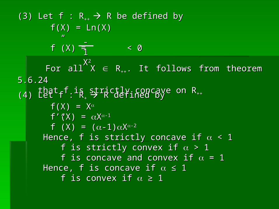
(3) Let f : R(3) Let f : R++++ R be defined by R be defined by
f(X) = Ln(X)f(X) = Ln(X)
f”(X) = < 0f”(X) = < 0
For all X For all X R R++++. It follows from theorem 5.6.24 . It follows from theorem 5.6.24 that f is strictly concave on Rthat f is strictly concave on R++ ++
-1-1XX22
(4) Let f : R(4) Let f : R++ R defined by R defined by
f(X) = Xf(X) = X
f’(X) = f’(X) = XX-1-1
f”(X) = (f”(X) = (-1)-1)XX-2-2
Hence, f is strictly concave if Hence, f is strictly concave if < 1 < 1 f is strictly convex if f is strictly convex if > 1 > 1 f is concave and convex if f is concave and convex if = 1 = 1
Hence, f is concave if Hence, f is concave if ≤ 1 ≤ 1 f is convex if f is convex if ≥ 1 ≥ 1

(5) Let f : R(5) Let f : R++++n n R defined by R defined by
f(X) = Cf(X) = CttX = X = CCiiXXii
then the function g : Rthen the function g : R++++nn R definey by R definey by
g(X) = ln (Cg(X) = ln (CttX) = ln (X) = ln ( C CiiXXii))
is concave on Ris concave on R++++nn, since f is concave and ln is a , since f is concave and ln is a
concave and incrasing function.concave and incrasing function.
n
i=1
n
i=1
(6) Let f : R(6) Let f : R++++2 2 R defined by R defined by
f(X) = f(X) = 1 1 ln (Xln (X11) + ) + 2 2 ln (Xln (X22) , ) , 11,,2 2 > 0> 0
claim that f is strictly concave on Rclaim that f is strictly concave on R++++2 2

(i)(i) Every local maximizer of a concave function is a Every local maximizer of a concave function is a global maximizerglobal maximizer
(ii)(ii)Every local minimizer of a convex function is a Every local minimizer of a convex function is a global minimizer global minimizer
Proof :Proof :
5.6.30 Theorem5.6.30 Theorem
(i)(i) A local maximizer of strictly concave function is A local maximizer of strictly concave function is unique unique
(ii)(ii)A local minimizer of strictly convex function is A local minimizer of strictly convex function is uniqueunique
5.6.31 Theorem5.6.31 Theorem
5.6.32 Example : Consider example 5.6.29(1)5.6.32 Example : Consider example 5.6.29(1) f(X) = Xf(X) = X11
22 + X + X11XX33 – X – X22 + X + X2222 + X + X22XX33 + 3X + 3X33
22
It was shown that f is strictly convex on RIt was shown that f is strictly convex on R33. The . The stationary point are obtained by setting f’(X) = 0, i.e.stationary point are obtained by setting f’(X) = 0, i.e.
2X2X11 + X + X33 = 0= 0 2X2X22 + X + X33 = 1= 1
2X2X11 + X + X2 2 + 6X+ 6X33 = 0= 0
Stationary point : X*Stationary point : X* = [= [11//2020, , 1111//2020, , 22//2020]]tt

Hessian matriks f’’(X*) is positive definite then theorem Hessian matriks f’’(X*) is positive definite then theorem 5.5.1, X*5.5.1, X* is a local minimizer of f. But f is strictly convex: is a local minimizer of f. But f is strictly convex: hence, X* is the unique global minimizer of f by theorem hence, X* is the unique global minimizer of f by theorem 5.6.30 and theorem 5.6.315.6.30 and theorem 5.6.31
5.6.33 Example5.6.33 ExampleThe Linier Programming Problem The Linier Programming Problem
min Co + Cmin Co + CttXXS.t. S.t. AX ≤ b , A is m x n , X AX ≤ b , A is m x n , X R Rnn
f is strictly conveX on Rf is strictly conveX on R33. The stationary point f’(X) = 0. The stationary point f’(X) = 0The objective function of the Linier Programming (LP) is The objective function of the Linier Programming (LP) is both concave and convex. The feasible regionboth concave and convex. The feasible region
X = {X X = {X R Rnn|AX ≤ b, X ≥ 0}|AX ≤ b, X ≥ 0}is convex since it is the intersection of convex set is convex since it is the intersection of convex set
X = H X = H R R++nn
Dimana Dimana H = {X H = {X R Rnn|AX ≤ b} and |AX ≤ b} and RR++
nn = {X = {X R Rnn|X ≥ 0}|X ≥ 0}Consequently, any optimal solution of the LP is a global Consequently, any optimal solution of the LP is a global optimal solution. Obviously, This is also true of the optimal solution. Obviously, This is also true of the maximization problem. maximization problem.

5.7.1 Definition5.7.1 DefinitionFunction f : C Function f : C R defined on convex subset C of R R defined on convex subset C of Rnn is is said to be quasiconcave on C if and only if said to be quasiconcave on C if and only if
5.7 The Optima of Quasiconcave and5.7 The Optima of Quasiconcave and
Quasiconvex FunctionQuasiconvex Function
5.7.2 Definition5.7.2 DefinitionFunction f : C Function f : C R defined on convex subset C of R R defined on convex subset C of Rnn is is said to be quasiconvex on C if and only ifsaid to be quasiconvex on C if and only if
Function f : C Function f : C R defined on convex subset C of R R defined on convex subset C of Rnn is said is said to be strictly quasiconcave on C if and only ifto be strictly quasiconcave on C if and only if
5.7.3 Definition5.7.3 Definition
5.7.4 Definition5.7.4 DefinitionFunction f : C Function f : C R defined on convex subset C of R R defined on convex subset C of Rnn is said is said to be strictly quasiconvex on C if and only ifto be strictly quasiconvex on C if and only if
5.7.8 Corollary5.7.8 Corollary(i)(i) Every concave function is quasiconcaveEvery concave function is quasiconcave(ii)(ii)Every convex function is quasiconvexEvery convex function is quasiconvex

A linear function is both quasiconcave and A linear function is both quasiconcave and quasiconvex.quasiconvex.
5.7.9 Corollary5.7.9 Corollary
5.7.12 Example5.7.12 Example
5.7.13 Theorem5.7.13 Theorem
5.7.11 Theorem5.7.11 Theorem
5.7.10 Theorem5.7.10 Theorem(i) A strictly concave function is strictly quasiconcave(i) A strictly concave function is strictly quasiconcave(ii) A strictly convex function is strictly quasiconvex.(ii) A strictly convex function is strictly quasiconvex.
Let : f : C Let : f : C R be continuous on a strictly convex subset C of R be continuous on a strictly convex subset C of RRnn. If is . If is strictly quasiconcave on C, then the upper contour strictly quasiconcave on C, then the upper contour set UCset UCff ( () is strictly convex for every ) is strictly convex for every R. R.
(i)(i) A differentiable function A differentiable function f : C f : C R defined on open convex R defined on open convex set C set C C C RRnn is quasiconcave on C if and only ifis quasiconcave on C if and only if
X,Y X,Y C, f(X) C, f(X) ≥≥ f(Y) [f’(Y)] f(Y) [f’(Y)] tt (X-Y) (X-Y) ≥ 0≥ 0(ii) A differentiable function (ii) A differentiable function f : C f : C R defined on open convex R defined on open convex
set C set C C C RRnn is quasiconvex on C if and only ifis quasiconvex on C if and only ifX,Y X,Y C, f(X) C, f(X) ≤≤ f(Y) [f’(Y)] f(Y) [f’(Y)] tt (X-Y) (X-Y) ≤≤ 0 0
The Normal Distribution FunctionThe Normal Distribution Function

5.8 Constrained 5.8 Constrained OptimizationOptimization The general form of the constrained optimization The general form of the constrained optimization problem may be expressed as follows :problem may be expressed as follows :
Max (Min) f (X)Max (Min) f (X)S.t. S.t. G Gk k (X) ≥ 0 , k = 1, 2, 3, …, m(X) ≥ 0 , k = 1, 2, 3, …, m
Where X Where X RRnn. The function f is objective function and the in-. The function f is objective function and the in-equalities called the constraints. A vector X satisfies the equalities called the constraints. A vector X satisfies the constraints called a feasible solution and the set of feasible constraints called a feasible solution and the set of feasible solutions is called feasible set or feasible region. A feasible solutions is called feasible set or feasible region. A feasible solution that maximizes (minimizes) the value of the objective solution that maximizes (minimizes) the value of the objective function on the feasible region is called maximizer (minimizer). function on the feasible region is called maximizer (minimizer). The term optimizer or optimal solution refers to either The term optimizer or optimal solution refers to either maximizer or minimizer.maximizer or minimizer. The distinction between a constrained optimization The distinction between a constrained optimization problem and an un-constrained problem can be seen fram the problem and an un-constrained problem can be seen fram the geometry of two-variable problem with a single equality geometry of two-variable problem with a single equality constraint.constraint.Suppose that the problem is :Suppose that the problem is :
Max f(XMax f(X11,X,X22))S.t.S.t. P P1 1 XX1 1 ++ PP2 2 XX2 2 = Y= Y
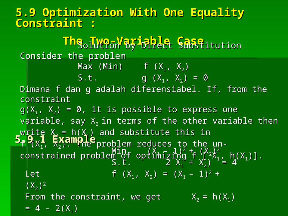
5.9 Optimization With One Equality 5.9 Optimization With One Equality Constraint :Constraint :
The Two-Variable CaseThe Two-Variable CaseSolution by Direct SubstitutionSolution by Direct SubstitutionConsider the problemConsider the problem
Max (Min) f (XMax (Min) f (X11, X, X22))S.t.S.t. g (X g (X11, X, X22) = 0) = 0
Dimana f dan g adalah diferensiabel. If, from the constraint Dimana f dan g adalah diferensiabel. If, from the constraint g(Xg(X11, X, X22) = 0, it is possible to express one variable, say X) = 0, it is possible to express one variable, say X2 2 in in terms of the other variable then write Xterms of the other variable then write X2 2 = h(X= h(X11) and ) and substitute this in substitute this in f (Xf (X11, X, X22). The problem reduces to the un-constrained ). The problem reduces to the un-constrained
problem of optimizing f problem of optimizing f [[ X X11, h(X, h(X11))]]. . 5.9.1 Example5.9.1 Example
Min (XMin (X1 1 – 1)– 1)2 2 + (X+ (X22))22
S.t.S.t. 2 X 2 X11 + X + X22) = 4) = 4LetLet f (Xf (X11, X, X22) = (X) = (X1 1 – 1)– 1)2 2 + (X+ (X22))22
From the constraint, we get XFrom the constraint, we get X2 2 = h(X= h(X11) = 4 - ) = 4 - 2(X2(X11))
XX11* = 9/5* = 9/5XX22* = 4 – 2(9/5) = 2/5* = 4 – 2(9/5) = 2/5
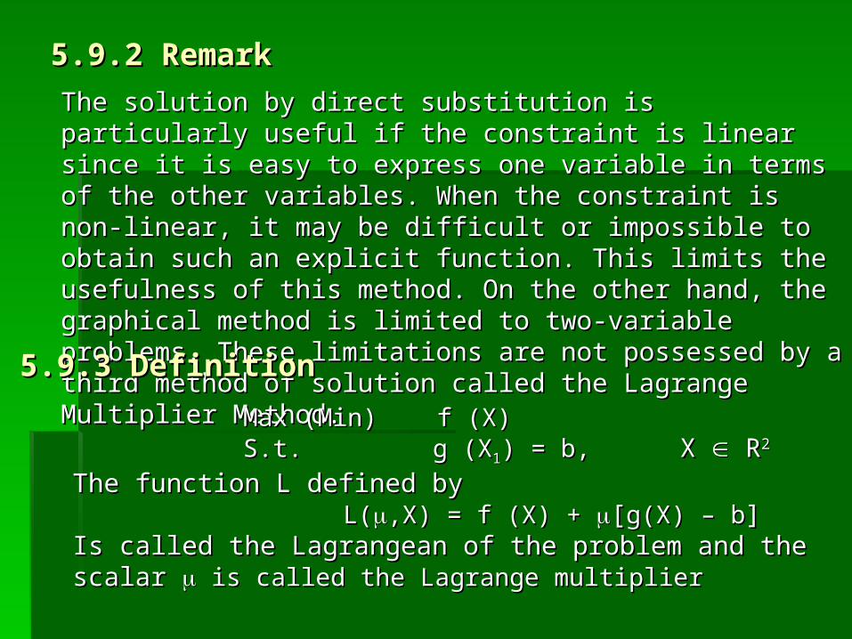
5.9.2 Remark5.9.2 Remark
The solution by direct substitution is particularly useful if The solution by direct substitution is particularly useful if the constraint is linear since it is easy to express one the constraint is linear since it is easy to express one variable in terms of the other variables. When the variable in terms of the other variables. When the constraint is non-linear, it may be difficult or impossible to constraint is non-linear, it may be difficult or impossible to obtain such an explicit function. This limits the usefulness obtain such an explicit function. This limits the usefulness of this method. On the other hand, the graphical method is of this method. On the other hand, the graphical method is limited to two-variable problems. These limitations are not limited to two-variable problems. These limitations are not possessed by a third method of solution called the possessed by a third method of solution called the Lagrange Multiplier Method.Lagrange Multiplier Method.5.9.3 Definition5.9.3 Definition
Max (Min) f (X)Max (Min) f (X)S.t.S.t. g (X g (X11) = b, ) = b, X X R R22
The function L defined byThe function L defined by L(L(,X) = f (X) + ,X) = f (X) + [[g(X) – bg(X) – b]]
Is called the Lagrangean of the problem and the scalar Is called the Lagrangean of the problem and the scalar is is called the Lagrange multipliercalled the Lagrange multiplier

5.9.4 Remark5.9.4 Remark
(1)(1) The Lagrangean is also written The Lagrangean is also written asas
L(L(,X) = f (X) – ,X) = f (X) – [[g(X) g(X) – b– b]]
(2) The Gradient of L is(2) The Gradient of L isLL’ (’ (,X) ,X) g (X) – b g (X) – b LL11’’ ((,X) ,X) ff11’’ (X)+ (X)+gg11’(X) ’(X)
LL22’ (’ (,X) ,X) ff22’’ (X)+ (X)+gg22’(X) ’(X) L’L’ ((,X) ,X) == ==
and the Hessian matrix of L isand the Hessian matrix of L is
LL’’ ’’ ((,X),X)
LL11’’’’ ((,X),X)
LL22’’ (’’ (,X),X)
LL11’’’’ ((,X),X)
LL1111’’’’ ((,X),X)
LL2121’’’’ ((,X),X)
LL22’’’’ ((,X),X)
LL1212’’’’ ((,X),X)
LL2222’’’’ ((,X),X)
L’’L’’ ((,X) ,X) ==
== 00
gg11’(X)’(X)
gg22’(X)’(X)
gg11’(X)’(X)
LL1111’’(’’(,X),X)
LL2121’’(’’(,X),X)
gg22’(X)’(X)
LL1212’’’’ ((,X),X)
LL2222’’ (’’ (,X),X)

5.9.5 Theorem5.9.5 Theorem
(Necessary or First-Order Condition) Given the problem(Necessary or First-Order Condition) Given the problemMax (Min) f (X)Max (Min) f (X)S.t.S.t. g (X) = b, g (X) = b, X X R R22
Where f and g have continuous partial derivatives. Let X* Where f and g have continuous partial derivatives. Let X* be an optimizer of f on the feasible set and suppose that be an optimizer of f on the feasible set and suppose that g’(X*) g’(X*) 0, j=1,2. Then there exists a scalar 0, j=1,2. Then there exists a scalar * such that* such that
L’(L’(*, X*) = 0*, X*) = 0Proof :Proof :
5.9.6 Theorem5.9.6 Theorem(Sufficient or Second-Order Condition) Given the (Sufficient or Second-Order Condition) Given the problemproblem
Max (Min) Max (Min) f (X)f (X)s.t. s.t. g(X) = b, X g(X) = b, X R R22
Where f and g have continuous second-order partial Where f and g have continuous second-order partial derivatives. Let X* and derivatives. Let X* and * satisfy L’(* satisfy L’(*,X*) = 0 and *,X*) = 0 and suppose that suppose that ggjj’’(X*) (X*) 0, j = 1, 2 0, j = 1, 2

(i) If |L”((i) If |L”(*,X*)| < 0 , Then X* is a local minimizer*,X*)| < 0 , Then X* is a local minimizer
(ii) If |L”((ii) If |L”(**,X,X**)| > 0 )| > 0 ,, Then X Then X** is a local maximizer is a local maximizer Proof :Proof :
For notational convenience, we will suppress the arguments of each For notational convenience, we will suppress the arguments of each function; e.g., gfunction; e.g., g11(X) will be written simply is g(X) will be written simply is g11’. From the constraint, ’. From the constraint, the total differential is gthe total differential is g11’dX’dX11+ g+ g11’ dX’ dX2 2 = 0, from which we get = 0, from which we get
gg11’’
gg22’’
LetLet Y = f(X Y = f(X11,X,X22))ThenThen dY = dY = ff11’dX’dX11+ f+ f22’dX’dX22
Hence,Hence, = f= f11’ + f’ + f22’ ’
ddXX
22
dXdX
11
= = ––
ddYY
dXdX11
ddXX22
dXdX11Subtituting ….Subtituting ….
We know that if < 0 at X*, then X* is a local maximizer. We know that if < 0 at X*, then X* is a local maximizer. Hence,Hence,
if the determinant |L’’(if the determinant |L’’(*,X*)| *,X*)| >> 0 , then X* is a local 0 , then X* is a local maximizer.maximizer.
dd22YY
dXdX1122

5.9.7 Example 5.9.7 Example
Min Min (X(X11 – 1) – 1)22 + (X + (X22))22
s.t. s.t. 2X2X11 + X + X22 = 4 = 4Lagrangean:Lagrangean: L( L(,X) ,X) = (X= (X11– 1)– 1)22 + (X + (X22))22 + + (2X(2X11 + X+ X22 – 4) – 4)F.O.C.F.O.C. L L
’’((,X) ,X) = 2X= 2X11 + X + X22 – 4 = 0 – 4 = 0 LL11’(’(,X),X)= 2(X= 2(X11– 1) + 2– 1) + 2 = 0 = 0 LL22’(’(,X) ,X) = 2X= 2X22 + + = 0 = 0XX11* = 9/5 , X* = 9/5 , X22* = 2/5 , * = 2/5 , * = – 4/5* = – 4/5 0 2 10 2 1
S.O.C. |L”(u*,X*)| = 2 2 0 = -10 < 0S.O.C. |L”(u*,X*)| = 2 2 0 = -10 < 0 1 0 21 0 2
By theorem 5.9.6 X* is local minimizer on feasible set. By theorem 5.9.6 X* is local minimizer on feasible set. Hessian matrix of the objective function is Hessian matrix of the objective function is
f”(X) = f”(X) =
Which is positive definite for every XWhich is positive definite for every XRR2 2 f is convex. The f is convex. The objective function is strictly convex. X* is the unique objective function is strictly convex. X* is the unique global minimizer.global minimizer.
2 02 00 20 2

5.9.8 Example 5.9.8 Example
MaxMax f(Xf(X11, X, X22) = X) = X11XX22
s.t. s.t. PP11XX11 + P + P22XX22 = Y , = Y , PP11,P,P22,Y > 0,Y > 0Lagrangean: L(u,X) Lagrangean: L(u,X) = X= X11XX22 + + (P(P11XX11 + P + P22XX22 – Y) – Y)F.O.C.F.O.C. L L’(’(,X) ,X) = P= P11XX11 + P + P22XX22 – Y = 0 – Y = 0
LL11’(’(,X) ,X) = X= X22 + + PP11 = 0 = 0 LL22’(’(,X) ,X) = X= X11 + + PP22 = 0 = 0
XX11* = Y/2P* = Y/2P11 , X , X22* = Y/2P* = Y/2P22 , , * = – Y/2P* = – Y/2P11PP22
0 P0 P11 P P22
S.O.C. |L”(u*,X*)| = PS.O.C. |L”(u*,X*)| = P11 0 1 = 2P 0 1 = 2P11PP22 > 0 > 0 PP22 1 0 1 0
By theorem 5.9.6 X* is a local maximizer on the feasible By theorem 5.9.6 X* is a local maximizer on the feasible set. X* the unique global maximizer on the feasible set. set. X* the unique global maximizer on the feasible set. They can not opposite signs since their objective They can not opposite signs since their objective function value would be negative which can not be function value would be negative which can not be optimal since optimal since
VOF (X*) = XVOF (X*) = X11*X*X22* = > 0* = > 0
X* is the unique global maximizer on the feasible set. X* is the unique global maximizer on the feasible set.
yy22
4P4P11PP22

5.10 Optimization With One Equality 5.10 Optimization With One Equality Constraint :Constraint : The n-Variable CaseThe n-Variable Case
Given the problemGiven the problemMax(min) Max(min) f(X) f(X) s.t. s.t. g(X) = b , X g(X) = b , X R Rnn
Lagrangean : Lagrangean : L(L(,X) = f(X) + ,X) = f(X) + [[(g(X) – b(g(X) – b]]
5.10.1 Definition5.10.1 Definition
1) The gradient of L is1) The gradient of L is5.10.2 Remark5.10.2 Remark
L’(L’(,X) =,X) =
LL’(’(,X),X)LL11’(’(,X),X) .. .. ..LLnn’(’(,X),X)
==
g(X) – b g(X) – b ff11’(X) + ’(X) + g’g’11(X)(X) .. .. .. ffnn’(X) + ’(X) + ggnn’(X)’(X)

2) Hessian matriz of L is 2) Hessian matriz of L is
L’’(L’’(,X) ,X) ==
0 g0 g11’(X) g’(X) g22’(X) … g’(X) … gnn’(X) ’(X) gg11’(X) L’(X) L1111”(”(,X) L,X) L1212”(”(,X) … ,X) … LL1n1n”(”(,X),X)gg22’(X) L’(X) L2121”(”(,X) L,X) L2222”(”(,X) … ,X) … LL2n2n”(”(,X),X) .. .. .. .. .. ..ggnn’’(X) L(X) Ln1n1””((,X) L,X) Ln2n2””((,X) … L,X) … Lnnnn””((,X),X)
Leading principal submatrices of order k of the Hessian Leading principal submatrices of order k of the Hessian matrix of L will be denoted by Lmatrix of L will be denoted by Lkk”(”(,X),X)
LL11’’ (’’ (,X) = ,X) = 00LL22” (” (,X) ,X) = =
0 g0 g11’(X) ’(X) gg11’(X) L ’(X) L
1111”(”(,X),X)
5.10.3 Notation5.10.3 Notation

0 g0 g11’(X) g’(X) g22’(X)’(X)gg11’(X) L’(X) L1111”(”(,X) L,X) L12 12 ”(”(,X),X)gg22’(X) L’(X) L2121””((,X) L,X) L2222”(”(,X),X)......etcetc
LL33”(”(,X) =,X) =
5.10.4 Theorem5.10.4 Theorem
(Necessary of First-Order Condition). given the problem(Necessary of First-Order Condition). given the problem
Max(min) Max(min) f(X)f(X)
s.t. s.t. g(X) = b , X g(X) = b , X R Rnn
Dimana f dan g have continuous FOC partial derivatives. Let Dimana f dan g have continuous FOC partial derivatives. Let X* be an optimizer over the feasible set such that g’j(X*) X* be an optimizer over the feasible set such that g’j(X*) 0, j= 1,2, …,n. Then there exists a scalar 0, j= 1,2, …,n. Then there exists a scalar * such that * such that
L’ (L’ (*,X*) = 0*,X*) = 0

(Sufficient or Second-Order Condition). Given the problem(Sufficient or Second-Order Condition). Given the problemMax (min) Max (min) f(X) f(X)
s.t. s.t. g(X) = b , X g(X) = b , X R Rnn
Where f and g have continuous second-order partial Where f and g have continuous second-order partial derivatives. Suppose that X* and derivatives. Suppose that X* and * satisfy FOC, i.e. * satisfy FOC, i.e. L’(L’(*,X*) = 0.*,X*) = 0.
(i)(i) If |LIf |L33”(”(*,X*)| < 0 , |L*,X*)| < 0 , |L44”(”(*,X*)| < 0, …, |L*,X*)| < 0, …, |Lnn”(”(*,X*)| < 0 , *,X*)| < 0 , then X* is a local minimizer of f on the feasible set.then X* is a local minimizer of f on the feasible set.
5.10.5 Theorem5.10.5 Theorem
(ii) If |L(ii) If |L33”(”(*,X*)| > 0 , |L*,X*)| > 0 , |L44”(”(*,X*)| < 0 ,*,X*)| < 0 ,
|L”|L”55((*,X*)| > 0, …, (-1)*,X*)| > 0, …, (-1)nn|L|Lnn”(”(*,X*)| > 0 , then X* is a *,X*)| > 0 , then X* is a locallocal
maximizer of f on the feasible set.maximizer of f on the feasible set.
Proof : Gue and Thomas (1968)Proof : Gue and Thomas (1968)

Max (min) Max (min) XX1122 + X + X11XX22 + 2X + 2X22
22 + X + X3322
s.t. s.t. XX11 – 3X – 3X22 – 4X – 4X33 = 16 = 16
Lagrangean :Lagrangean :
L(L(,X) = ,X) = XX1122 + X + X11XX22 + 2X + 2X22
22 + X + X3322 + + (X (X11 – 3X – 3X22 – 4X – 4X33 – 16) – 16)
First Order Condition :First Order Condition :
5.10.6 Example5.10.6 Example
L’ (L’ (,X) ,X) = =
XX11 –– 3X 3X22 –– 4X 4X33 –– 16 16
2X2X11 + X + X22 + + XX11 + 4X + 4X22 + 3 + 32X2X33 –– 4 4
00000000
= =
This system of equations yields the solutionThis system of equations yields the solutionXX11* = 4, X* = 4, X22* = – 4, X* = – 4, X33* = – 8, * = – 8, * = – 4* = – 4
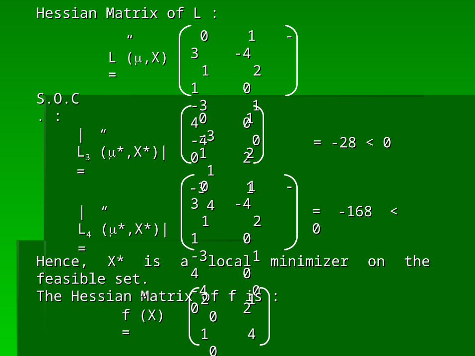
Hessian Matrix of L :Hessian Matrix of L :
L”(L”(,X) ,X) ==
0 1 -3 -40 1 -3 -4 1 2 1 01 2 1 0-3 1 4 0-3 1 4 0-4 0 0 2-4 0 0 2
S.O.C. S.O.C. ::
|L|L33”(”(*,X*)| *,X*)| ==
0 1 -30 1 -3 1 2 11 2 1-3 1 4-3 1 4
= -28 < 0= -28 < 0
|L|L44”(”(*,X*)| *,X*)| ==
0 1 -3 -40 1 -3 -4 1 2 1 01 2 1 0-3 1 4 0-3 1 4 0-4 0 0 2-4 0 0 2
= -168 < 0= -168 < 0
Hence, X* is a local minimizer on the feasible set.Hence, X* is a local minimizer on the feasible set.The Hessian Matrix of f is :The Hessian Matrix of f is :
f”(X) f”(X) ==
2 1 02 1 01 4 01 4 00 0 20 0 2

whose eigenvalues are :whose eigenvalues are :
11 = 2 , = 2 , 22 = 3 + 2 , = 3 + 2 , 33 = 3 – 2 = 3 – 2
Which are all positive. Hence, f”(X) is positive definite for Which are all positive. Hence, f”(X) is positive definite for
all X all X RR33..
That f is strictly convex on RThat f is strictly convex on R33. This implies X* is the unique . This implies X* is the unique
global minimizer of f on the feasible set.global minimizer of f on the feasible set.5.11 Optimization With Several 5.11 Optimization With Several Equality Equality Constraints : The n-Variable Constraints : The n-Variable CaseCase5.11.1 Definition5.11.1 DefinitionGiven The ProblemGiven The Problem
Max (min) f(X)Max (min) f(X) s.t. s.t. g gkk(X)(X) = b= bkk k = 1,2 …,m; m < n , X k = 1,2 …,m; m < n , X RRnn
The function L defined by The function L defined by L(L(,X) = f(X) + ,X) = f(X) + kk (g (gkk(X) (X) –– b bkk))
is called the Lagrangean of the problem. The variables is called the Lagrangean of the problem. The variables 11, , 22, …, , …, nn
are called the lagrange multipliers. are called the lagrange multipliers.
n
k=1
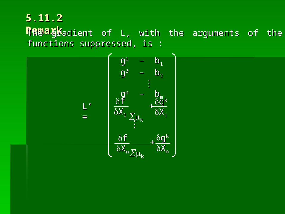
5.11.2 Remark5.11.2 Remark
The gradient of L, with the arguments of the functions The gradient of L, with the arguments of the functions suppressed, is :suppressed, is :
L’ =L’ =
gg11 – b – b11
gg22 – b – b22 .. .. ..ggnn – b – bmm
ffXX11
+ + kkggkk
XX11
ffXXnn
+ + kkggkk
XXnn
......

Note that the matrix L’’ has dimension (m+n) x Note that the matrix L’’ has dimension (m+n) x (m+n). (m+n). The Leading Principal Sub Matrix (LPSM) of order k The Leading Principal Sub Matrix (LPSM) of order k will be denoted by Lwill be denoted by Lkk”. ”.
L’ =L’ =LL1111” … L” … L1n1n”” . .. . . .. . . .. .
LLn1n1” … L” … Lnnnn””
0 … 0 … 00. .. .. .. .. .. .0 … 0 … 00
The Hessian Matrix of L is :The Hessian Matrix of L is :
ggmm
XXnn
ggmm
XX11
gg11
XX11
gg11
XXnn
ggmm
XX11
ggmm
XXnn
gg11
XXii
gg11
XXnn
……
……
……
……. . . . ..
. .
. .
..
. .
. .
..
. .
. .
..

5.11.3 Theorem5.11.3 Theorem(Necessary or F.O.C.). Given the problem (Necessary or F.O.C.). Given the problem Max (min) Max (min) f(X)f(X) s.t. s.t. ggkk(X) = b(X) = bkk , k = 1,2, …, m , k = 1,2, …, m
m < n , X m < n , X R Rnn Where f and gWhere f and gkk (k = 1,2, …,m) have continuous first-Order Partial (k = 1,2, …,m) have continuous first-Order Partial Derivatives. Let X* be an optimizer of f over the feasible set and Derivatives. Let X* be an optimizer of f over the feasible set and suppose that the Jacobian determinant suppose that the Jacobian determinant
gg11(X*)(X*) XX11
gg11(X*)(X*)XXnn
ggmm(X*)(X*)XX11
ggmm(X*)(X*)XXnn
… …
… …
. . . . . .
. . . . . . 00
Then there exist scalars Then there exist scalars kk* (k=1,2,…,m) such that * (k=1,2,…,m) such that
L’(L’(*, X*) = 0*, X*) = 0Proof : Panik (1976).Proof : Panik (1976).

5.11.4 Theorem5.11.4 Theorem
(Sufficient or S.O.C.). Given the problem(Sufficient or S.O.C.). Given the problem MaX (min) f (X)MaX (min) f (X) s.t. s.t. g gkk(X) = b(X) = bkk , k = 1,2, …,m , m < n , k = 1,2, …,m , m < n
X X R Rnn
Where f and gWhere f and gkk (k = 1,2,…,m) have continuous Second-Order (k = 1,2,…,m) have continuous Second-Order Partial Derivatives. Suppose X* and Partial Derivatives. Suppose X* and satisfy the F.O.C., i.e. satisfy the F.O.C., i.e.
L’ (L’ (*, X*) = 0*, X*) = 0
(i) If |L(i) If |L2m+12m+1”(”(*,X*)| , |L*,X*)| , |L2m+22m+2”(”(*,X*)| ,…, |L*,X*)| ,…, |Lm+nm+n”(”(*,X*)| *,X*)|
have the same sign as (-1)have the same sign as (-1)mm, then X* is a local minimizer of f, then X* is a local minimizer of f
on the feasible set.on the feasible set.
(ii) If |L(ii) If |L2m+12m+1”(”(*,X*)| , |L*,X*)| , |L2m+22m+2”(”(*,X*)| ,…, |L*,X*)| ,…, |Lm+nm+n”(”(*,X*)| *,X*)|
Alternate in sign with the sign of |LAlternate in sign with the sign of |L2m+12m+1((*,X*)| being that of *,X*)| being that of
(-1)(-1)m+1m+1 , then X* is a local maximizer of f on the feasible set. , then X* is a local maximizer of f on the feasible set.
Proof :Proof :