1

Pertemuan 07Variabel Acak Diskrit dan Kontinu

Matakuliah : I0284 - Statistika

Tahun : 2008

Versi : Revisi

2

Learning Outcomes

Pada akhir pertemuan ini, diharapkan mahasiswa

akan mampu :

• Mahasiswa akan dapat menghitung Peluang, nilai harapan, dan varians variabel acak diskrit dan kontinu.

3

Outline Materi

• Definisi variabel acak

• Distribusi probabilitas diskrit

• Distribusi probabilitas kontinu

• Nilai harapan dan varians

4

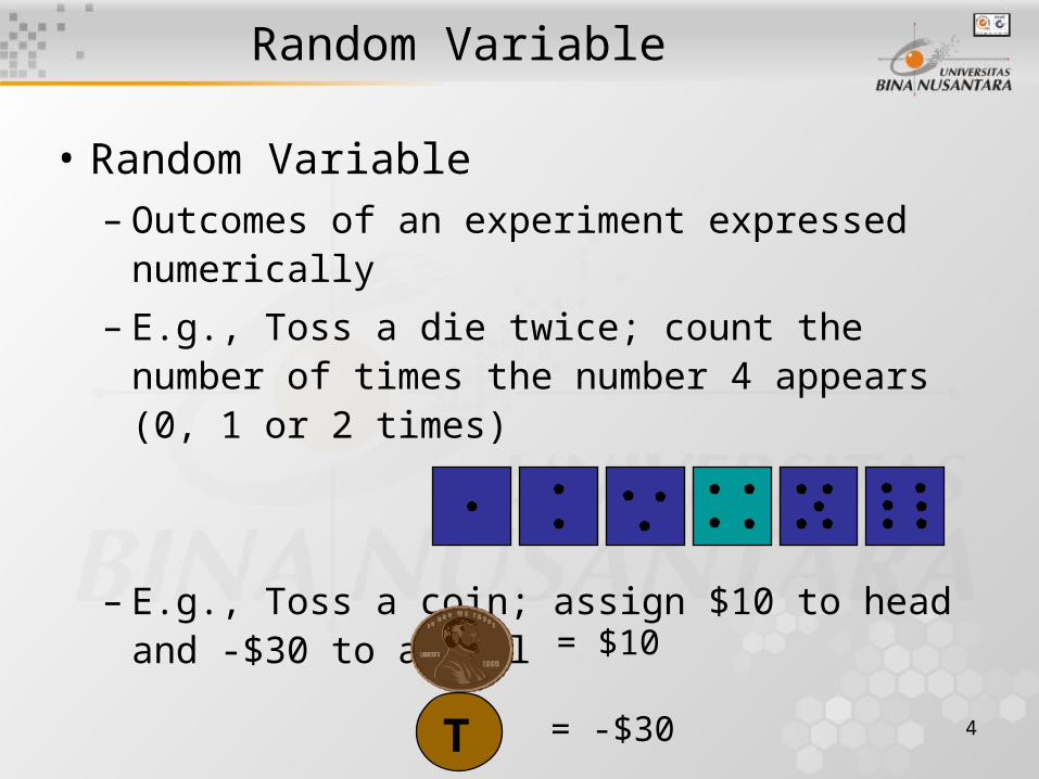
Random Variable

• Random Variable– Outcomes of an experiment expressed

numerically

– E.g., Toss a die twice; count the number of times the number 4 appears (0, 1 or 2 times)

– E.g., Toss a coin; assign $10 to head and -$30 to a tail = $10

T = -$30

5

Discrete Random Variable

• Discrete Random Variable– Obtained by counting (0, 1, 2, 3, etc.)

– Usually a finite number of different values

– E.g., Toss a coin 5 times; count the number of tails (0, 1, 2, 3, 4, or 5 times)

6

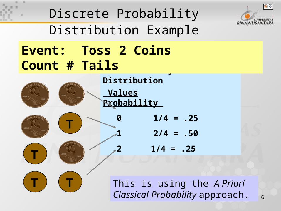
Probability Distribution

Values Probability

0 1/4 = .25

1 2/4 = .50

2 1/4 = .25

Discrete Probability Distribution Example

Event: Toss 2 Coins Count # Tails

T

T

T T This is using the A Priori Classical Probability approach.

7

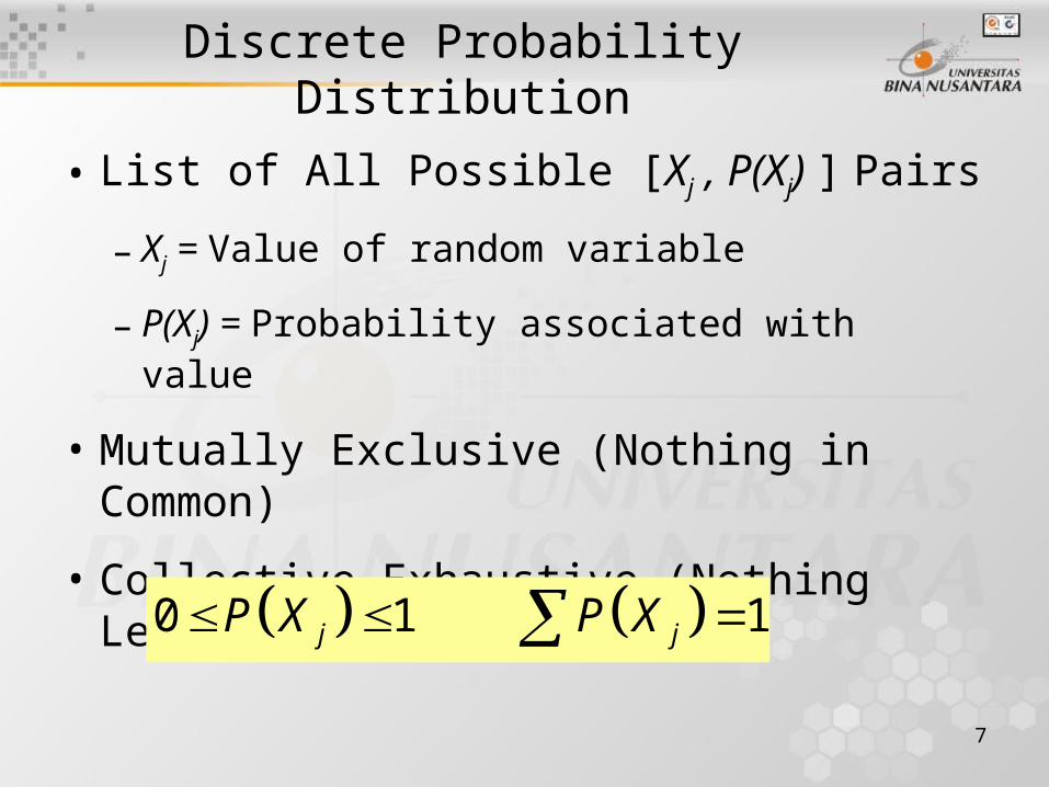
Discrete Probability Distribution

• List of All Possible [Xj , P(Xj) ] Pairs

– Xj = Value of random variable

– P(Xj) = Probability associated with value

• Mutually Exclusive (Nothing in Common)

• Collective Exhaustive (Nothing Left Out)

0 1 1j jP X P X

8

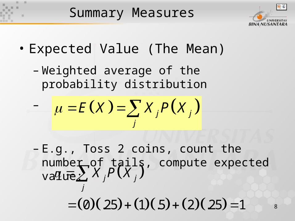
Summary Measures

• Expected Value (The Mean)

– Weighted average of the probability distribution

–

– E.g., Toss 2 coins, count the number of tails, compute expected value:

j jj

E X X P X

0 .25 1 .5 2 .25 1

j jj

X P X

9

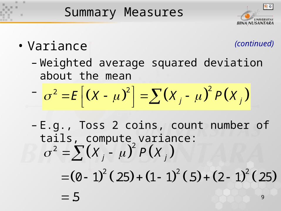
Summary Measures

• Variance– Weighted average squared deviation about the

mean–

– E.g., Toss 2 coins, count number of tails, compute variance:

(continued)

222j jE X X P X

22

2 2 2 0 1 .25 1 1 .5 2 1 .25

.5

j jX P X

10

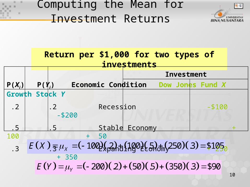
Computing the Mean for Investment Returns

Return per $1,000 for two types of investments

100 .2 100 .5 250 .3 $105XE X

200 .2 50 .5 350 .3 $90YE Y

P(Xi) P(Yi) Economic Condition Dow Jones Fund X Growth Stock Y

.2 .2 Recession -$100 -$200

.5 .5 Stable Economy + 100 + 50

.3 .3 Expanding Economy + 250 + 350

Investment

11

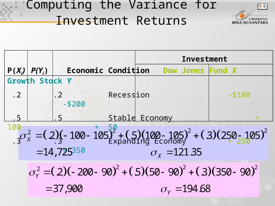
Computing the Variance for Investment Returns

2 2 22 .2 100 105 .5 100 105 .3 250 105

14,725 121.35X

X

2 2 22 .2 200 90 .5 50 90 .3 350 90

37,900 194.68Y

Y

P(Xi) P(Yi) Economic Condition Dow Jones Fund X Growth Stock Y

.2 .2 Recession -$100 -$200

.5 .5 Stable Economy + 100 + 50

.3 .3 Expanding Economy + 250 + 350

Investment

12

Continuous Random Variables

A random variable X is continuous if its set of possible values is an entire interval of numbers (If A < B, then any number x between A and B is possible).

13

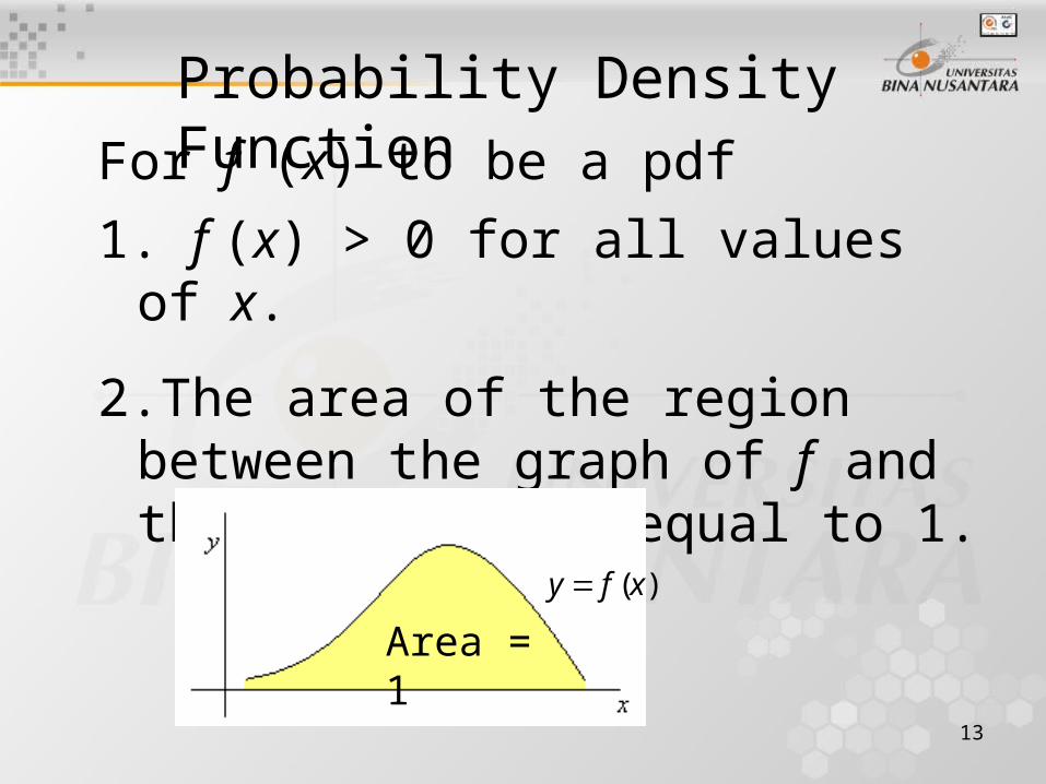
Probability Density Function

For f (x) to be a pdf

1. f (x) > 0 for all values of x.

2.The area of the region between the graph of f and the x – axis is equal to 1.

Area = 1

( )y f x

14

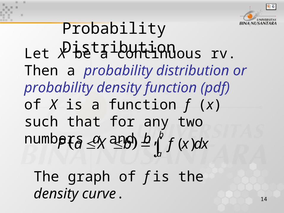
Probability Distribution

Let X be a continuous rv. Then a probability distribution or probability density function (pdf) of X is a function f (x) such that for any two numbers a and b,

( )b

aP a X b f x dx

The graph of f is the density curve.

15

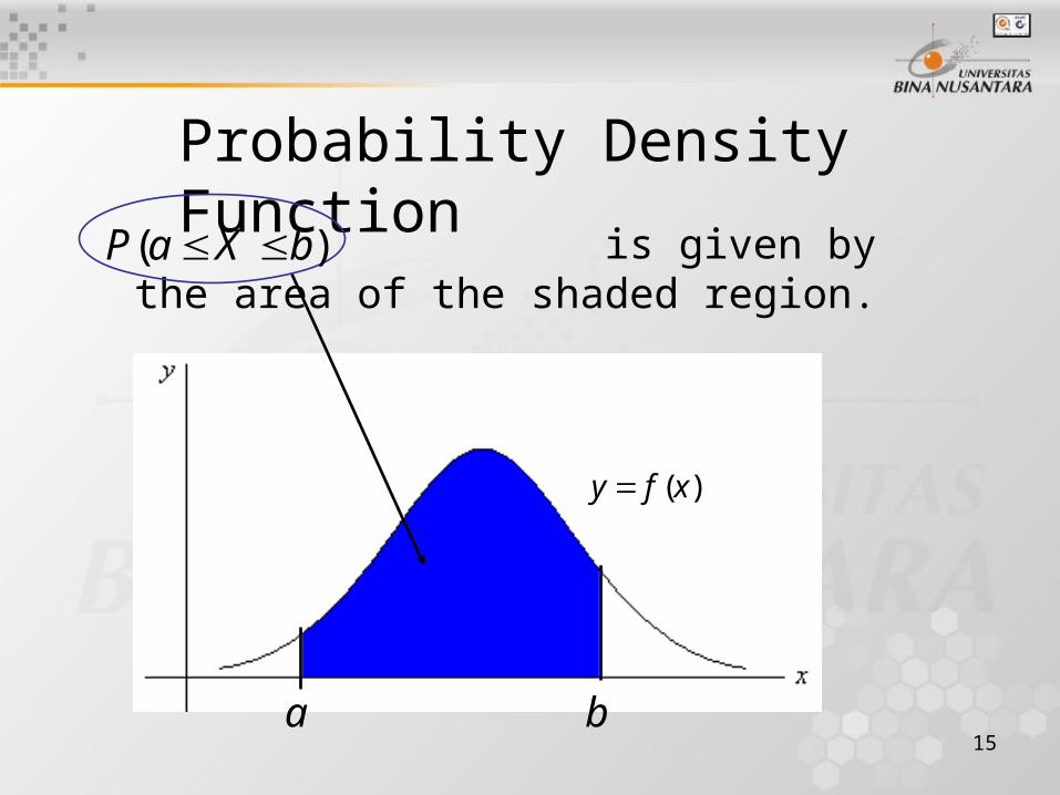
Probability Density Function

is given by the area of the shaded region.

( )y f x

ba

( )P a X b

16

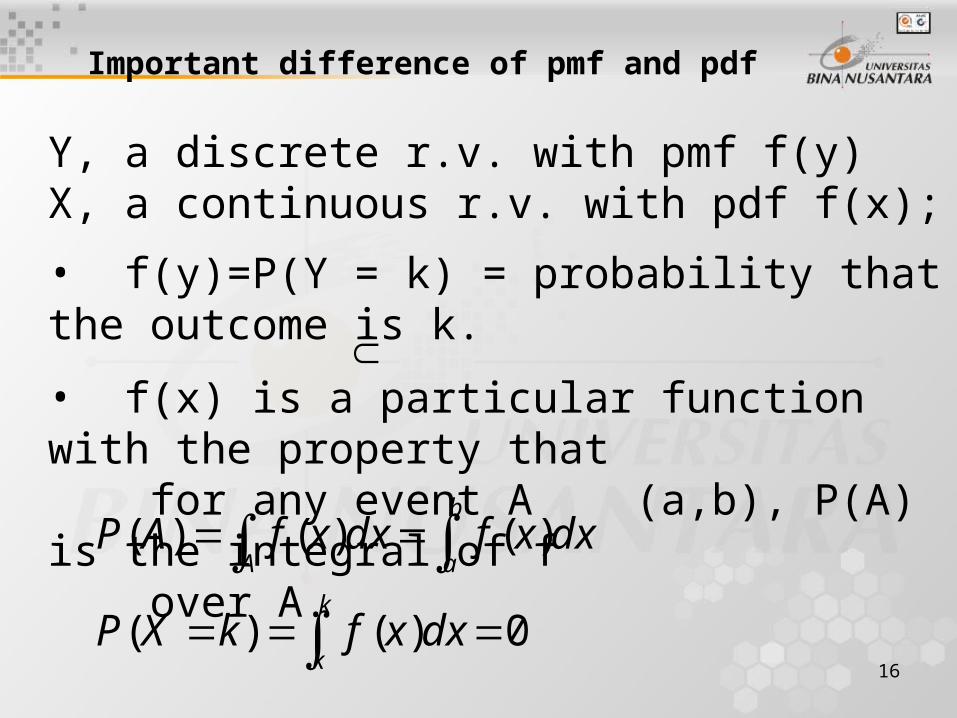
Important difference of pmf and pdf

k

k

b

aA

dxxfkXP

dxxfdxxfAP

0)()(

)()()(

Y, a discrete r.v. with pmf f(y)X, a continuous r.v. with pdf f(x);

• f(y)=P(Y = k) = probability that the outcome is k.

• f(x) is a particular function with the property that for any event A (a,b), P(A) is the integral of f over A.

17

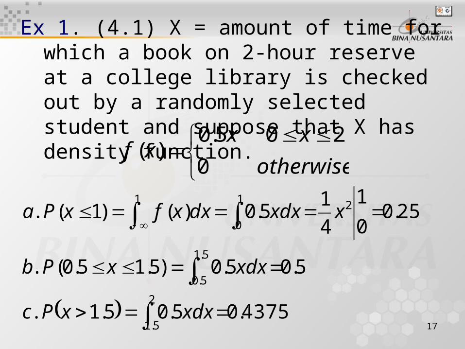
Ex 1. (4.1) X = amount of time for which a book on 2-hour reserve at a college library is checked out by a randomly selected student and suppose that X has density function.

otherwise

xxxf

0

205.0)(

4375.05.05.1.

5.05.0)5.15.0(.

25.00

1

4

15.0)()1(.

2

5.1

5.1

5.0

1 1

0

2

xdxxPc

xdxxPb

xxdxdxxfxPa

18

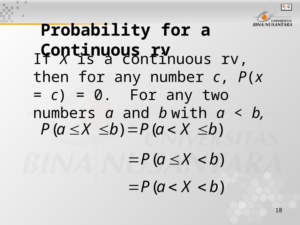
Probability for a Continuous rv

If X is a continuous rv, then for any number c, P(x = c) = 0. For any two numbers a and b with a < b,

( ) ( )P a X b P a X b

( )P a X b

( )P a X b

19

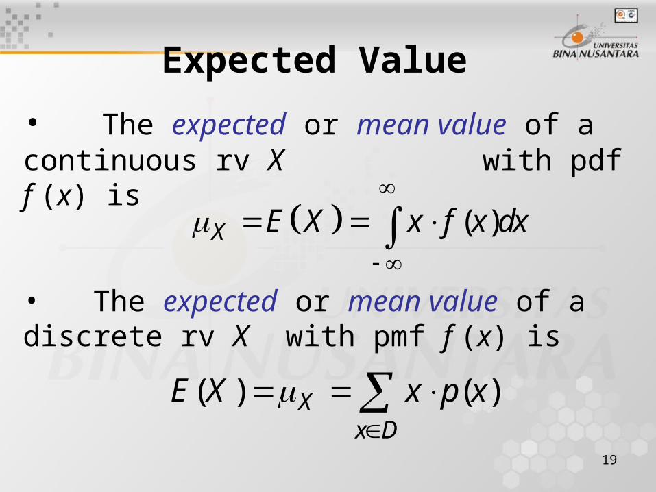
Expected Value

• The expected or mean value of a continuous rv X with pdf f (x) is

( )X E X x f x dx

( ) ( )Xx D

E X x p x

• The expected or mean value of a discrete rv X with pmf f (x) is

20

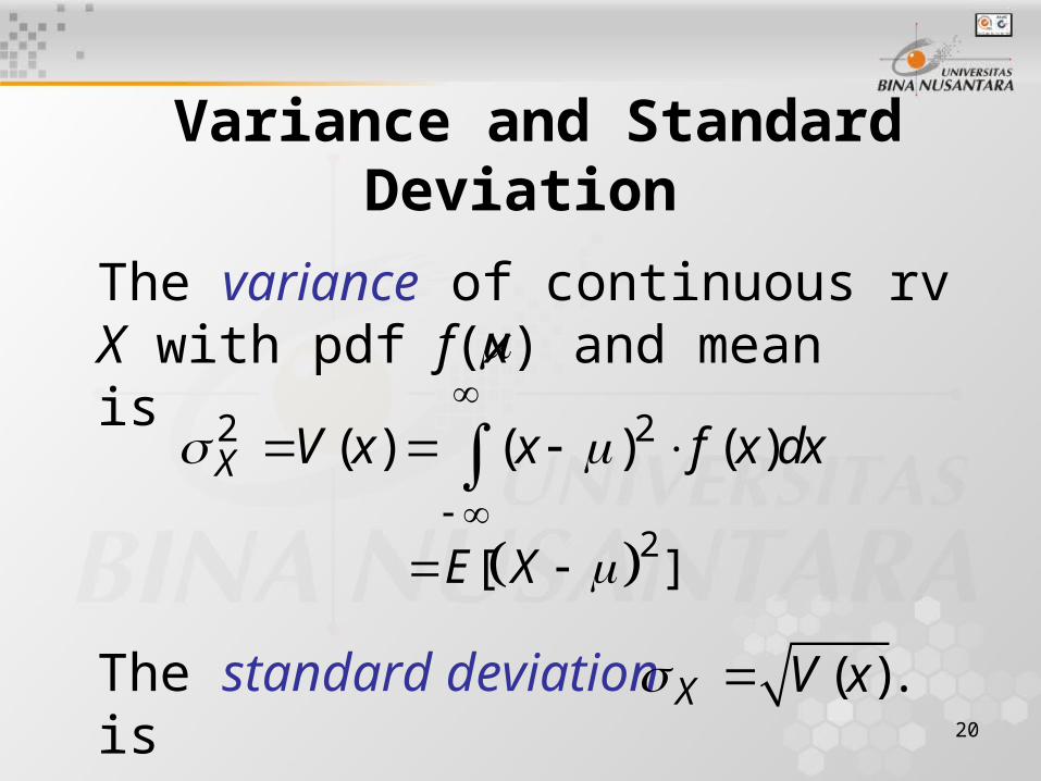
Variance and Standard Deviation

The variance of continuous rv X with pdf f(x) and mean is

2 2( ) ( ) ( )X V x x f x dx

2

[ ]E X

The standard deviation is

( ).X V x

21

Short-cut Formula for Variance

22( ) ( )V X E X E X

22

• Selamat Belajar Semoga Sukses.