Download - Retinal status analysis method based on feature extraction ...

Retinal status analysis method based on feature extraction and quantitative grading in OCT imagesDongmei Fu1* , Hejun Tong1, Shuang Zheng1, Ling Luo2, Fulin Gao2 and Jiri Minar3

BackgroundOptical coherence tomography (OCT) is an in vivo imaging technique that could rap-idly acquire high resolution cross-section images of biological tissues microstructure [1]. The most significant medical contribution of OCT is the ophthalmology area, as it could provide the retinal structure and functional images that no other noninvasive diagnosis

Abstract

Background: Optical coherence tomography (OCT) is widely used in ophthalmology for viewing the morphology of the retina, which is important for disease detection and assessing therapeutic effect. The diagnosis of retinal diseases is based primarily on the subjective analysis of OCT images by trained ophthalmologists. This paper describes an OCT images automatic analysis method for computer-aided disease diagnosis and it is a critical part of the eye fundus diagnosis.

Methods: This study analyzed 300 OCT images acquired by Optovue Avanti RTVue XR (Optovue Corp., Fremont, CA). Firstly, the normal retinal reference model based on retinal boundaries was presented. Subsequently, two kinds of quantitative methods based on geometric features and morphological features were proposed. This paper put forward a retinal abnormal grading decision-making method which was used in actual analysis and evaluation of multiple OCT images.

Results: This paper showed detailed analysis process by four retinal OCT images with different abnormal degrees. The final grading results verified that the analysis method can distinguish abnormal severity and lesion regions. This paper presented the simula-tion of the 150 test images, where the results of analysis of retinal status showed that the sensitivity was 0.94 and specificity was 0.92.The proposed method can speed up diagnostic process and objectively evaluate the retinal status.

Conclusions: This paper aims on studies of retinal status automatic analysis method based on feature extraction and quantitative grading in OCT images. The proposed method can obtain the parameters and the features that are associated with retinal morphology. Quantitative analysis and evaluation of these features are combined with reference model which can realize the target image abnormal judgment and provide a reference for disease diagnosis.

Keywords: Retinal OCT images, Image processing, Morphological characterization, Feature quantification, Grade evaluation

Open Access

© 2016 The Author(s). This article is distributed under the terms of the Creative Commons Attribution 4.0 International License (http://creativecommons.org/licenses/by/4.0/), which permits unrestricted use, distribution, and reproduction in any medium, provided you give appropriate credit to the original author(s) and the source, provide a link to the Creative Commons license, and indicate if changes were made. The Creative Commons Public Domain Dedication waiver (http://creativecommons.org/publicdo-main/zero/1.0/) applies to the data made available in this article, unless otherwise stated.

RESEARCH

Fu et al. BioMed Eng OnLine (2016) 15:87 DOI 10.1186/s12938-016-0206-x BioMedical Engineering

OnLine

*Correspondence: [email protected] 1 School of Automation and Electrical Engineering, University of Science and Technology Beijing, Xueyuan Road 30, Haidian District, Beijing, ChinaFull list of author information is available at the end of the article

http://orcid.org/0000-0002-9800-8603

http://creativecommons.org/licenses/by/4.0/

http://creativecommons.org/publicdomain/zero/1.0/

http://creativecommons.org/publicdomain/zero/1.0/

http://crossmark.crossref.org/dialog/?doi=10.1186/s12938-016-0206-x&domain=pdf

of 18Fu et al. BioMed Eng OnLine (2016) 15:87

method can perform. Several medical researchers used OCT to acquire retinal statistical characteristics and analyzed different kinds of fundus diseases, such as macular oedema caused by diabetic retinopathy [2], drusen and drusenoid pigment epithelium detach-ment caused by non-neovascular age-related macular degeneration [3], X-linked reti-noschisis [4], epiretinal membrane, macular hole, central serous chorioretinopathy [5] et al. In addition, there are researches on statistical analysis of normal retinal thickness [6].

Ophthalmologists diagnose the fundus diseases by analyzing the change of retinal fea-tures in OCT images; however, OCT instruments can produce large amounts of data in a short time, so it is difficult to analyze all data by manual method. In most cases, only a small number of selected images are analyzed, and this could cause the wasting of medi-cal resources. Furthermore, manual analysis results are very depending on ophthalmolo-gist’s personal experience and there is also lack of uniform quantization and evaluation standards. Therefore, rapid, accurate, objective detection and quantification of retinal features is the key of medical OCT images research and diagnosis of ophthalmic dis-eases, and this study has important theoretical significance and practical value.

In order to achieve the retinal features detection and quantification, computer image processing and analysis technologies have been widely applied in the field of medical OCT images. Quellec et al. [7] realized the automated identification of macular fluid-filled regions by analysis of retinal layer texture. Gregori et al. [8], Iwama et al. [9] and Chen et al. [10] utilized different methods to segment retinal drusen and made the dif-ferent levels quantification and evaluation. The upper studies are aimed at the known cases of illness, and extract the pathological areas in image. Liu et al. [11, 12] utilized retinal geometry, texture, shape features to identify the presence of normal macula and each of three types of macular pathologies, but without the analysis of pathologi-cal severity degree. Koprowski et al. [13] described a method for automatic analysis of selected choroidal diseases by features definition and quantification. By using the fea-ture data acquired from OCT, Koprowski et al. [14] also proposed an automatic method for the analysis of OCT images in assessing the severity degree of glaucoma. Xu et al. [15] segmented the nerve fiber layer and analyzed OCT data for glaucoma detection. These studies identified or classified the limited certain kinds of diseases according to the extracted pathologic features.

The upper studies are either for the extraction of pathological area in known cases of illness or for the features extraction and classification of limited certain kinds of diseases. In practical diagnostic process, the obtained retinal images are usually complex and the abnormal categories would not be limited within the scope of certain kinds of known cases. Furthermore, retinopathy is gradually evolved and the abnormal early detection and early diagnosis has great significance. Therefore, in order to realize computer auto-matic analysis of retinal status, it is also needed to rely on the ophthalmologists’ practical diagnosis process to deal with different situations in reality.

When ophthalmologists interpret retinal OCT images, they focus on the locations of the lesions occur (macular areas, internal limiting membrane, retinal pigment epithe-lium, nerve fiber layer, etc) and the feature morphologies (retinal thickness, overall shape change, boundary smoothness, boundary continuity, etc) that are conducive to abnormal judgment. And they compare the specific tissue structure morphology with the known


normal morphology. In the process of comparison, ophthalmologists do some extensive quantitatively analysis of the differences in morphology, such as retinal thickness (ratio) change, the morphological change of quantity, etc, and judge abnormal severity and lesion location. Finally ophthalmologists make the association between these morpho-logical differences and corresponding disease categories, and give the diagnosis decision.

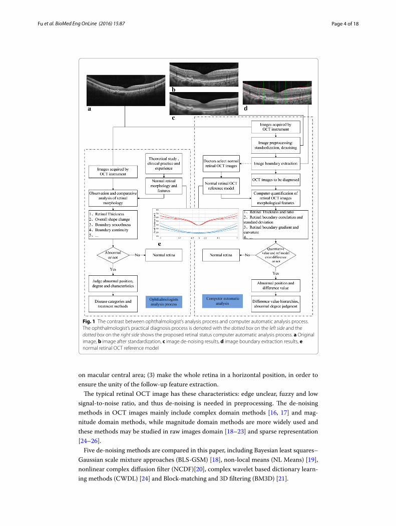
Based on the process of ophthalmologists’ observation and analysis on fundus retinal morphology in OCT images, this paper computerized the analysis and decision-making process, and put forward a retinal status automatic analysis method. The ophthalmolo-gists’ analysis process and the proposed retinal status automatic analysis process dia-gram are shown in Fig. 1. In this paper, a normal retinal reference model is constructed to analogy the normal tissue structures that ophthalmologists are familiar with. Image processing methods such as boundary extraction, morphological characterization and features quantification are used to express of the ophthalmologists’ diagnosis process. Finally, evaluation of the results are presented by the way of abnormal grading.

MaterialThis study analyzed 300 retinal OCT images, including 200 images judged as normal by ophthalmologists and the remaining 100 images with various abnormalities, such as drusen, macular epiretinal membrane, macular edema and macular hole, etc. These images are from 300 participants, aged from 18 to 78 years and they are acquired using Optovue Avanti RTVue XR (Optovue Corp., Fremont, CA) from the 306th Hospital of People’s Liberation Army, Department of ophthalmology. This study is supported by the National Natural Science Foundation of China. Image analysis was carried out in Matlab.

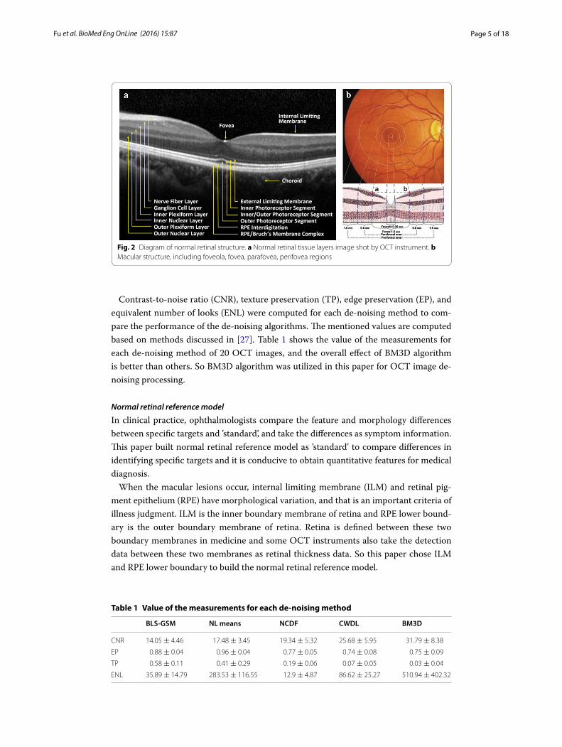
Retina is a transparent film layer located in the inner wall of eye. At present, the most advanced OCT instrument can distinguish 12 normal retinal tissue layers, as shown in Fig. 2a. In the posterior pole of the retina, there is a funnel-shaped depression pale, and that is the optical center of eye, known as the macular region, as shown in Fig. 2b. The structure and physiological activity of retina in this region are special, and it is easy to be affected by internal and external pathogenic factors. Therefore, this paper focuses on the morphological changes of retina in macular region. Retinal macula can be subdi-vided into three anatomical zones: (1) fovea, the center of macular region, and it is about 1.5 mm in diameter, that is, a optic disc diameter. The center of fovea is called foveola and it is about 0.35 mm in diameter. (2) parafovea, a circular ring area about 0.5 mm outside the fovea, and it contains ganglion cells, inner nuclear layer and outer plexi-form layer called Henle fiber. (3) perifovea, a circular ring area about 1.5 mm outside the parafovea.

MethodsImage preprocessing and normal retinal reference model

Image standardization and de‑noising

In the process of imaging, the OCT instrument auto focuses according to the size of the targets’ shape, changes the axial resolution of the image, and the retina appears with dif-ferent degree of tilt in the image. So first of all, OCT images should be standardized. The aims of image standardization are: (1) unify the image size and axial resolution; (2) focus


on macular central area; (3) make the whole retina in a horizontal position, in order to ensure the unity of the follow-up feature extraction.

The typical retinal OCT image has these characteristics: edge unclear, fuzzy and low signal-to-noise ratio, and thus de-noising is needed in preprocessing. The de-noising methods in OCT images mainly include complex domain methods [16, 17] and mag-nitude domain methods, while magnitude domain methods are more widely used and these methods may be studied in raw images domain [18–23] and sparse representation [24–26].

Five de-noising methods are compared in this paper, including Bayesian least squares–Gaussian scale mixture approaches (BLS-GSM) [18], non-local means (NL Means) [19], nonlinear complex diffusion filter (NCDF)[20], complex wavelet based dictionary learn-ing methods (CWDL) [24] and Block-matching and 3D filtering (BM3D) [21].

Fig. 1 The contrast between ophthalmologist’s analysis process and computer automatic analysis process. The ophthalmologist’s practical diagnosis process is denoted with the dotted box on the left side and the dotted box on the right side shows the proposed retinal status computer automatic analysis process. a Original image, b image after standardization, c image de-noising results, d image boundary extraction results, e normal retinal OCT reference model


Contrast-to-noise ratio (CNR), texture preservation (TP), edge preservation (EP), and equivalent number of looks (ENL) were computed for each de-noising method to com-pare the performance of the de-noising algorithms. The mentioned values are computed based on methods discussed in [27]. Table 1 shows the value of the measurements for each de-noising method of 20 OCT images, and the overall effect of BM3D algorithm is better than others. So BM3D algorithm was utilized in this paper for OCT image de-noising processing.

Normal retinal reference model

In clinical practice, ophthalmologists compare the feature and morphology differences between specific targets and ’standard’, and take the differences as symptom information. This paper built normal retinal reference model as ’standard’ to compare differences in identifying specific targets and it is conducive to obtain quantitative features for medical diagnosis.

When the macular lesions occur, internal limiting membrane (ILM) and retinal pig-ment epithelium (RPE) have morphological variation, and that is an important criteria of illness judgment. ILM is the inner boundary membrane of retina and RPE lower bound-ary is the outer boundary membrane of retina. Retina is defined between these two boundary membranes in medicine and some OCT instruments also take the detection data between these two membranes as retinal thickness data. So this paper chose ILM and RPE lower boundary to build the normal retinal reference model.

Fig. 2 Diagram of normal retinal structure. a Normal retinal tissue layers image shot by OCT instrument. b Macular structure, including foveola, fovea, parafovea, perifovea regions

Table 1 Value of the measurements for each de-noising method

BLS-GSM NL means NCDF CWDL BM3D

CNR 14.05 ± 4.46 17.48 ± 3.45 19.34 ± 5.32 25.68 ± 5.95 31.79 ± 8.38

EP 0.88 ± 0.04 0.96 ± 0.04 0.77 ± 0.05 0.74 ± 0.08 0.75 ± 0.09

TP 0.58 ± 0.11 0.41 ± 0.29 0.19 ± 0.06 0.07 ± 0.05 0.03 ± 0.04

ENL 35.89 ± 14.79 283.53 ± 116.55 12.9 ± 4.87 86.62 ± 25.27 510.94 ± 402.32


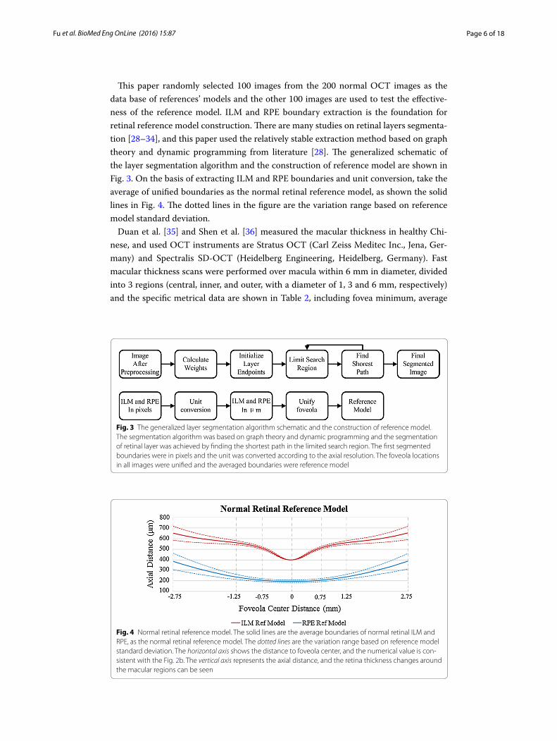
This paper randomly selected 100 images from the 200 normal OCT images as the data base of references’ models and the other 100 images are used to test the effective-ness of the reference model. ILM and RPE boundary extraction is the foundation for retinal reference model construction. There are many studies on retinal layers segmenta-tion [28–34], and this paper used the relatively stable extraction method based on graph theory and dynamic programming from literature [28]. The generalized schematic of the layer segmentation algorithm and the construction of reference model are shown in Fig. 3. On the basis of extracting ILM and RPE boundaries and unit conversion, take the average of unified boundaries as the normal retinal reference model, as shown the solid lines in Fig. 4. The dotted lines in the figure are the variation range based on reference model standard deviation.

Duan et al. [35] and Shen et al. [36] measured the macular thickness in healthy Chi-nese, and used OCT instruments are Stratus OCT (Carl Zeiss Meditec Inc., Jena, Ger-many) and Spectralis SD-OCT (Heidelberg Engineering, Heidelberg, Germany). Fast macular thickness scans were performed over macula within 6 mm in diameter, divided into 3 regions (central, inner, and outer, with a diameter of 1, 3 and 6 mm, respectively) and the specific metrical data are shown in Table 2, including fovea minimum, average

Fig. 3 The generalized layer segmentation algorithm schematic and the construction of reference model. The segmentation algorithm was based on graph theory and dynamic programming and the segmentation of retinal layer was achieved by finding the shortest path in the limited search region. The first segmented boundaries were in pixels and the unit was converted according to the axial resolution. The foveola locations in all images were unified and the averaged boundaries were reference model

Fig. 4 Normal retinal reference model. The solid lines are the average boundaries of normal retinal ILM and RPE, as the normal retinal reference model. The dotted lines are the variation range based on reference model standard deviation. The horizontal axis shows the distance to foveola center, and the numerical value is con-sistent with the Fig. 2b. The vertical axis represents the axial distance, and the retina thickness changes around the macular regions can be seen


thickness of central macula, inner and outer regions. The same metrical data obtained from the above reference model are also presented in Table 2. As the different data sources and thickness calculation methods, there are differences between the reference model and the numerical value in the literatures, but from the overall view, the thickness values of reference model are by a factor of about 1.25:1 larger than the values in litera-ture [35] and 1:1.1 smaller than the values in literature [36]. The data showed that the reference model proposed in this paper is reliable.

Computerized quantification of retinal features

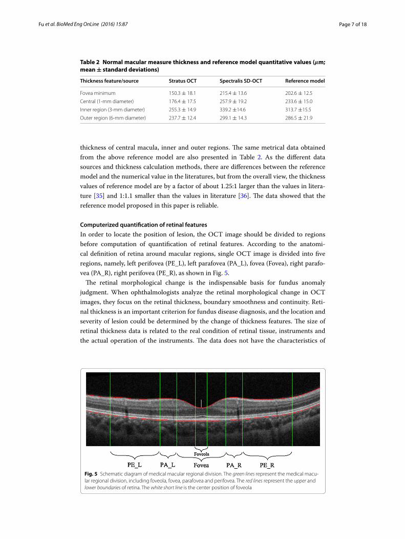
In order to locate the position of lesion, the OCT image should be divided to regions before computation of quantification of retinal features. According to the anatomi-cal definition of retina around macular regions, single OCT image is divided into five regions, namely, left perifovea (PE_L), left parafovea (PA_L), fovea (Fovea), right parafo-vea (PA_R), right perifovea (PE_R), as shown in Fig. 5.

The retinal morphological change is the indispensable basis for fundus anomaly judgment. When ophthalmologists analyze the retinal morphological change in OCT images, they focus on the retinal thickness, boundary smoothness and continuity. Reti-nal thickness is an important criterion for fundus disease diagnosis, and the location and severity of lesion could be determined by the change of thickness features. The size of retinal thickness data is related to the real condition of retinal tissue, instruments and the actual operation of the instruments. The data does not have the characteristics of

Table 2 Normal macular measure thickness and reference model quantitative values (µm; mean ± standard deviations)

Thickness feature/source Stratus OCT Spectralis SD-OCT Reference model

Fovea minimum 150.3 ± 18.1 215.4 ± 13.6 202.6 ± 12.5

Central (1-mm diameter) 176.4 ± 17.5 257.9 ± 19.2 233.6 ± 15.0

Inner region (3-mm diameter) 255.3 ± 14.9 339.2 ±14.6 313.7 ±15.5

Outer region (6-mm diameter) 237.7 ± 12.4 299.1 ± 14.3 286.5 ± 21.9

Fig. 5 Schematic diagram of medical macular regional division. The green lines represent the medical macu-lar regional division, including foveola, fovea, parafovea and perifovea. The red lines represent the upper and lower boundaries of retina. The white short line is the center position of foveola


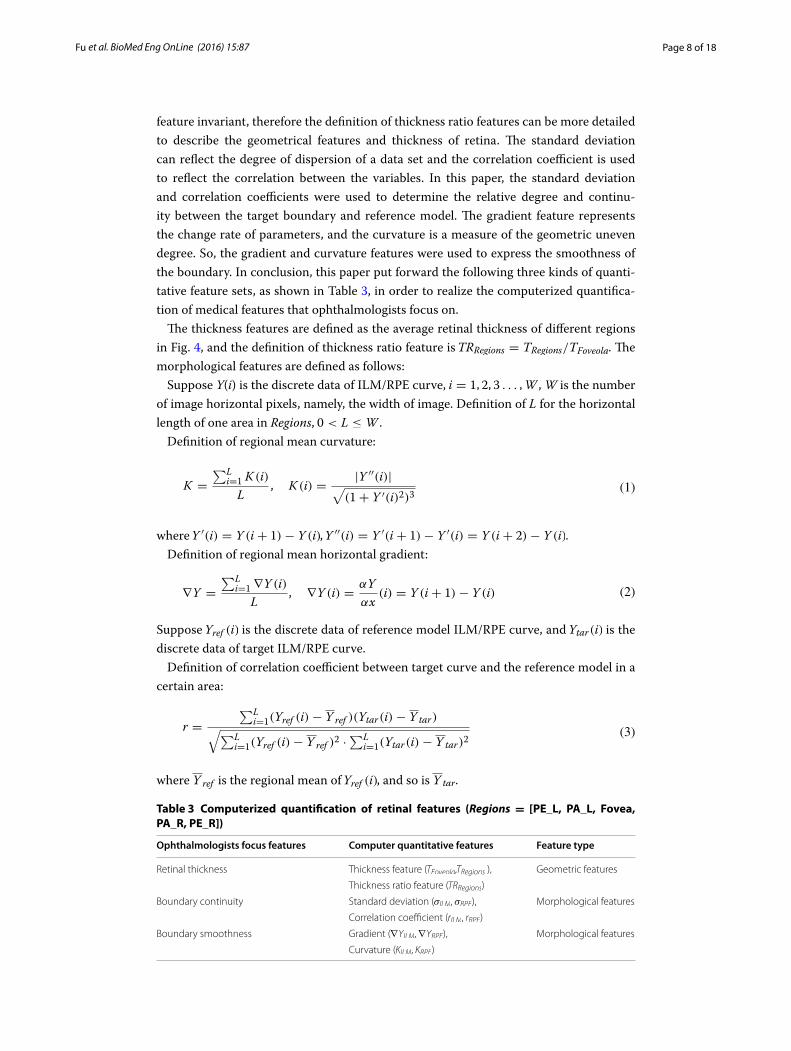
feature invariant, therefore the definition of thickness ratio features can be more detailed to describe the geometrical features and thickness of retina. The standard deviation can reflect the degree of dispersion of a data set and the correlation coefficient is used to reflect the correlation between the variables. In this paper, the standard deviation and correlation coefficients were used to determine the relative degree and continu-ity between the target boundary and reference model. The gradient feature represents the change rate of parameters, and the curvature is a measure of the geometric uneven degree. So, the gradient and curvature features were used to express the smoothness of the boundary. In conclusion, this paper put forward the following three kinds of quanti-tative feature sets, as shown in Table 3, in order to realize the computerized quantifica-tion of medical features that ophthalmologists focus on.

The thickness features are defined as the average retinal thickness of different regions in Fig. 4, and the definition of thickness ratio feature is TRRegions = TRegions/TFoveola. The morphological features are defined as follows:

Suppose Y(i) is the discrete data of ILM/RPE curve, i = 1, 2, 3 . . . ,W , W is the number of image horizontal pixels, namely, the width of image. Definition of L for the horizontal length of one area in Regions, 0 < L ≤ W .

Definition of regional mean curvature:

where Y ′(i) = Y (i + 1)− Y (i), Y ′′(i) = Y ′(i + 1)− Y ′(i) = Y (i + 2)− Y (i).Definition of regional mean horizontal gradient:

Suppose Yref (i) is the discrete data of reference model ILM/RPE curve, and Ytar(i) is the discrete data of target ILM/RPE curve.

Definition of correlation coefficient between target curve and the reference model in a certain area:

where Y ref is the regional mean of Yref (i), and so is Y tar.

(1)K =

∑Li=1 K (i)

L, K (i) =

|Y ′′(i)|√

(1+ Y ′(i)2)3

(2)∇Y =

∑Li=1 ∇Y (i)

L, ∇Y (i) =

αY

αx(i) = Y (i + 1)− Y (i)

(3)r =

∑Li=1(Yref (i)− Y ref )(Ytar(i)− Y tar)

√

∑Li=1(Yref (i)− Y ref )

2 ·∑L

i=1(Ytar(i)− Y tar)2

Table 3 Computerized quantification of retinal features (Regions = [PE_L, PA_L, Fovea, PA_R, PE_R])

Ophthalmologists focus features Computer quantitative features Feature type

Retinal thickness Thickness feature (TFoveola,TRegions ), Geometric features

Thickness ratio feature (TRRegions)

Boundary continuity Standard deviation (σILM, σRPE), Morphological features

Correlation coefficient (rILM, rRPE)

Boundary smoothness Gradient (∇YILM, ∇YRPE), Morphological features

Curvature (KILM, KRPE)


Definition of standard deviation between target curve and the reference model in a certain area:

where D(i) = Ytar(i)− Yref (i), D is the regional mean of D(i).Formulas (1)–(4) are unified expressions. According to the specific condition of ILM

and RPE, these definitions can be respectively represented as KILM, KRPE, ∇YILM, ∇YRPE , rILM, rRPE, σILM, σRPE.

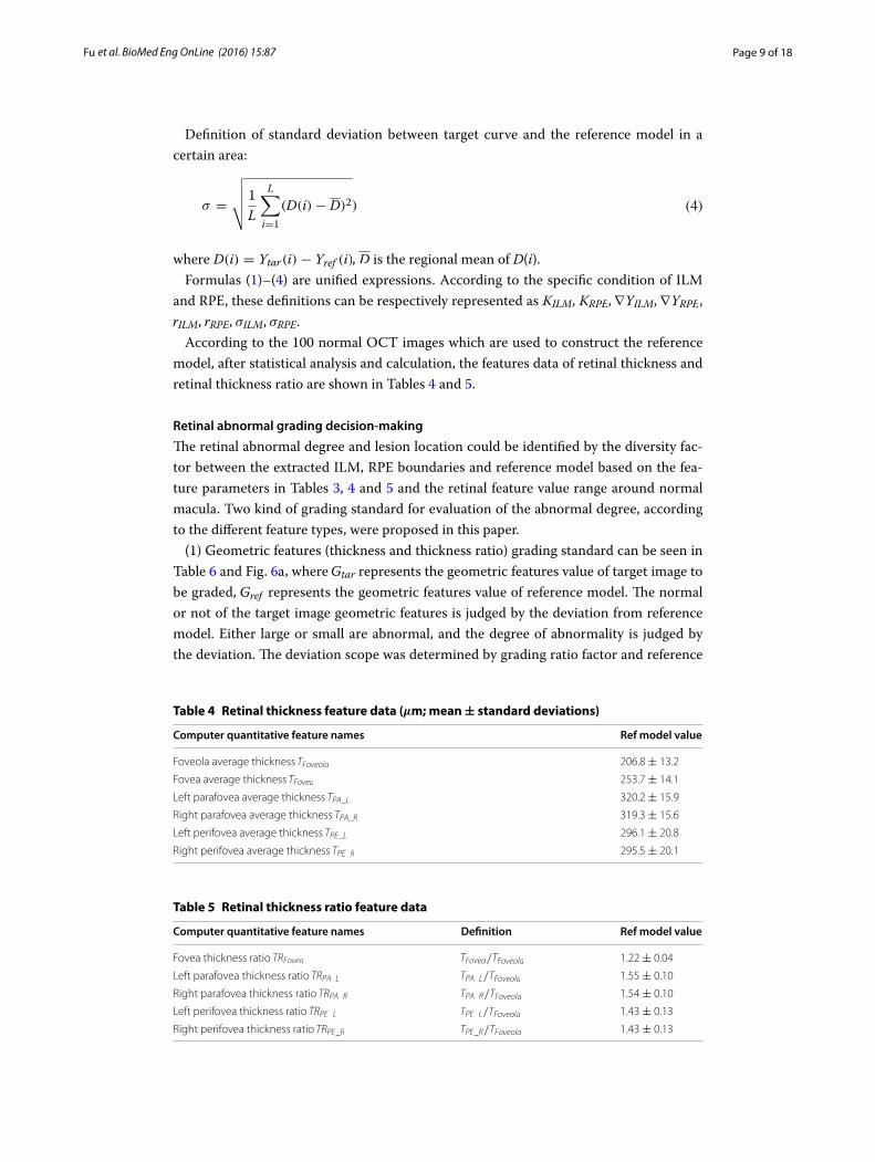
According to the 100 normal OCT images which are used to construct the reference model, after statistical analysis and calculation, the features data of retinal thickness and retinal thickness ratio are shown in Tables 4 and 5.

Retinal abnormal grading decision-making

The retinal abnormal degree and lesion location could be identified by the diversity fac-tor between the extracted ILM, RPE boundaries and reference model based on the fea-ture parameters in Tables 3, 4 and 5 and the retinal feature value range around normal macula. Two kind of grading standard for evaluation of the abnormal degree, according to the different feature types, were proposed in this paper.

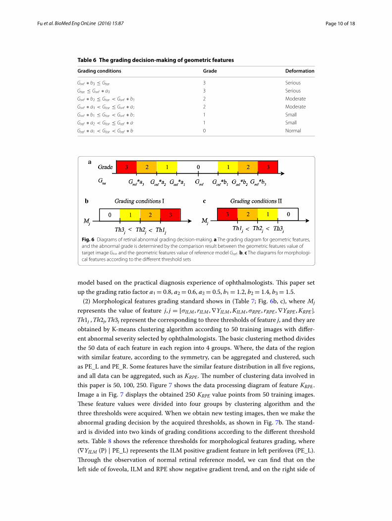
(1) Geometric features (thickness and thickness ratio) grading standard can be seen in Table 6 and Fig. 6a, where Gtar represents the geometric features value of target image to be graded, Gref represents the geometric features value of reference model. The normal or not of the target image geometric features is judged by the deviation from reference model. Either large or small are abnormal, and the degree of abnormality is judged by the deviation. The deviation scope was determined by grading ratio factor and reference

(4)σ =

√

√

√

√

1

L

L∑

i=1

(D(i)− D)2)

Table 4 Retinal thickness feature data (µm; mean ± standard deviations)

Computer quantitative feature names Ref model value

Foveola average thickness TFoveola 206.8 ± 13.2

Fovea average thickness TFovea 253.7 ± 14.1

Left parafovea average thickness TPA_L 320.2 ± 15.9

Right parafovea average thickness TPA_R 319.3 ± 15.6

Left perifovea average thickness TPE_L 296.1 ± 20.8

Right perifovea average thickness TPE_R 295.5 ± 20.1

Table 5 Retinal thickness ratio feature data

Computer quantitative feature names Definition Ref model value

Fovea thickness ratio TRFovea TFovea/TFoveola 1.22 ± 0.04

Left parafovea thickness ratio TRPA_L TPA_L/TFoveola 1.55 ± 0.10

Right parafovea thickness ratio TRPA_R TPA_R/TFoveola 1.54 ± 0.10

Left perifovea thickness ratio TRPE_L TPE_L/TFoveola 1.43 ± 0.13

Right perifovea thickness ratio TRPE_R TPE_R/TFoveola 1.43 ± 0.13


model based on the practical diagnosis experience of ophthalmologists. This paper set up the grading ratio factor a1 = 0.8, a2 = 0.6, a3 = 0.5, b1 = 1.2, b2 = 1.4, b3 = 1.5.

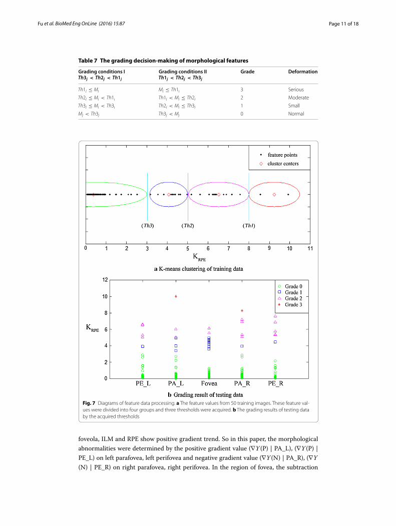
(2) Morphological features grading standard shows in (Table 7; Fig. 6b, c), where Mj represents the value of feature j, j = [σILM , rILM ,∇YILM ,KILM , σRPE , rRPE ,∇YRPE ,KRPE]. Th1j , Th2j, Th3j represent the corresponding to three thresholds of feature j, and they are obtained by K-means clustering algorithm according to 50 training images with differ-ent abnormal severity selected by ophthalmologists. The basic clustering method divides the 50 data of each feature in each region into 4 groups. Where, the data of the region with similar feature, according to the symmetry, can be aggregated and clustered, such as PE_L and PE_R. Some features have the similar feature distribution in all five regions, and all data can be aggregated, such as KRPE. The number of clustering data involved in this paper is 50, 100, 250. Figure 7 shows the data processing diagram of feature KRPE . Image a in Fig. 7 displays the obtained 250 KRPE value points from 50 training images. These feature values were divided into four groups by clustering algorithm and the three thresholds were acquired. When we obtain new testing images, then we make the abnormal grading decision by the acquired thresholds, as shown in Fig. 7b. The stand-ard is divided into two kinds of grading conditions according to the different threshold sets. Table 8 shows the reference thresholds for morphological features grading, where (∇YILM (P) | PE_L) represents the ILM positive gradient feature in left perifovea (PE_L). Through the observation of normal retinal reference model, we can find that on the left side of foveola, ILM and RPE show negative gradient trend, and on the right side of

Fig. 6 Diagrams of retinal abnormal grading decision-making. a The grading diagram for geometric features, and the abnormal grade is determined by the comparison result between the geometric features value of target image Gtar and the geometric features value of reference model Gref . b, c The diagrams for morphologi-cal features according to the different threshold sets

Table 6 The grading decision-making of geometric features

Grading conditions Grade Deformation

Gref ∗ b3 ≤ Gtar 3 Serious

Gtar ≤ Gref ∗ a3 3 Serious

Gref ∗ b2 ≤ Gtar < Gref ∗ b3 2 Moderate

Gref ∗ a3 < Gtar ≤ Gref ∗ a2 2 Moderate

Gref ∗ b1 ≤ Gtar < Gref ∗ b2 1 Small

Gref ∗ a2 < Gtar ≤ Gref ∗ a1 1 Small

Gref ∗ a1 < Gtar < Gref ∗ b1 0 Normal


foveola, ILM and RPE show positive gradient trend. So in this paper, the morphological abnormalities were determined by the positive gradient value (∇Y (P) | PA_L), (∇Y (P) | PE_L) on left parafovea, left perifovea and negative gradient value (∇Y (N) | PA_R), (∇Y

(N) | PE_R) on right parafovea, right perifovea. In the region of fovea, the subtraction

Fig. 7 Diagrams of feature data processing. a The feature values from 50 training images. These feature val-ues were divided into four groups and three thresholds were acquired. b The grading results of testing data by the acquired thresholds

Table 7 The grading decision-making of morphological features

Grading conditions ITh3j < Th2j < Th1j

Grading conditions IITh1j < Th2j < Th3j

Grade Deformation

Th1j ≤ Mj Mj ≤ Th1j 3 Serious

Th2j ≤ Mj < Th1j Th1j < Mj ≤ Th2j 2 Moderate

Th3j ≤ Mj < Th3j Th2j < Mj ≤ Th3j 1 Small

Mj < Th3j Th3j < Mj 0 Normal


between positive gradient values and negative gradient values was used to determine the morphological abnormalities, such as (∇Y | Fovea) = (∇Y (P) | Fovea)-(∇Y (N) | Fovea).

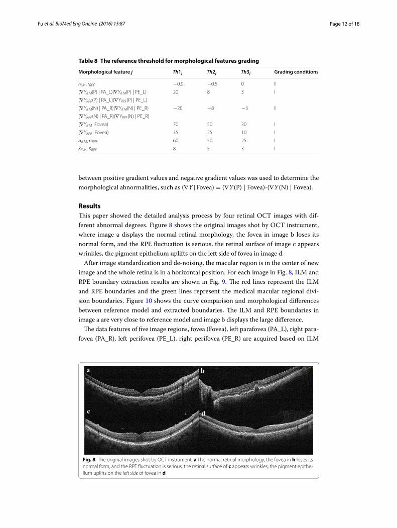
ResultsThis paper showed the detailed analysis process by four retinal OCT images with dif-ferent abnormal degrees. Figure 8 shows the original images shot by OCT instrument, where image a displays the normal retinal morphology, the fovea in image b loses its normal form, and the RPE fluctuation is serious, the retinal surface of image c appears wrinkles, the pigment epithelium uplifts on the left side of fovea in image d.

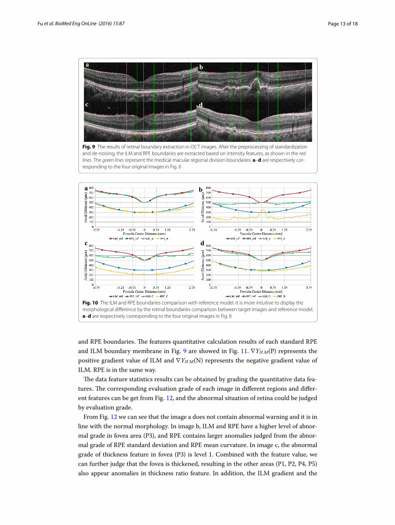
After image standardization and de-noising, the macular region is in the center of new image and the whole retina is in a horizontal position. For each image in Fig. 8, ILM and RPE boundary extraction results are shown in Fig. 9. The red lines represent the ILM and RPE boundaries and the green lines represent the medical macular regional divi-sion boundaries. Figure 10 shows the curve comparison and morphological differences between reference model and extracted boundaries. The ILM and RPE boundaries in image a are very close to reference model and image b displays the large difference.

The data features of five image regions, fovea (Fovea), left parafovea (PA_L), right para-fovea (PA_R), left perifovea (PE_L), right perifovea (PE_R) are acquired based on ILM

Table 8 The reference threshold for morphological features grading

Morphological feature j Th1j Th2j Th3j Grading conditions

rILM , rRPE −0.9 −0.5 0 II

(∇YILM(P) | PA_L)(∇YILM(P) | PE_L) 20 8 3 I

(∇YRPE(P) | PA_L)(∇YRPE(P) | PE_L)

(∇YILM(N) | PA_R)(∇YILM(N) | PE_R) −20 −8 −3 II

(∇YRPE(N) | PA_R)(∇YRPE(N) | PE_R)

(∇YILM| Fovea) 70 50 30 I

(∇YRPE | Fovea) 35 25 10 I

σILM , σRPE 60 50 25 I

KILM , KRPE 8 5 3 I

Fig. 8 The original images shot by OCT instrument. a The normal retinal morphology, the fovea in b loses its normal form, and the RPE fluctuation is serious, the retinal surface of c appears wrinkles, the pigment epithe-lium uplifts on the left side of fovea in d


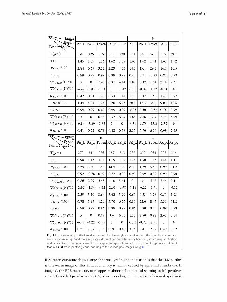
and RPE boundaries. The features quantitative calculation results of each standard RPE and ILM boundary membrane in Fig. 9 are showed in Fig. 11. ∇YILM(P) represents the positive gradient value of ILM and ∇YILM(N) represents the negative gradient value of ILM. RPE is in the same way.

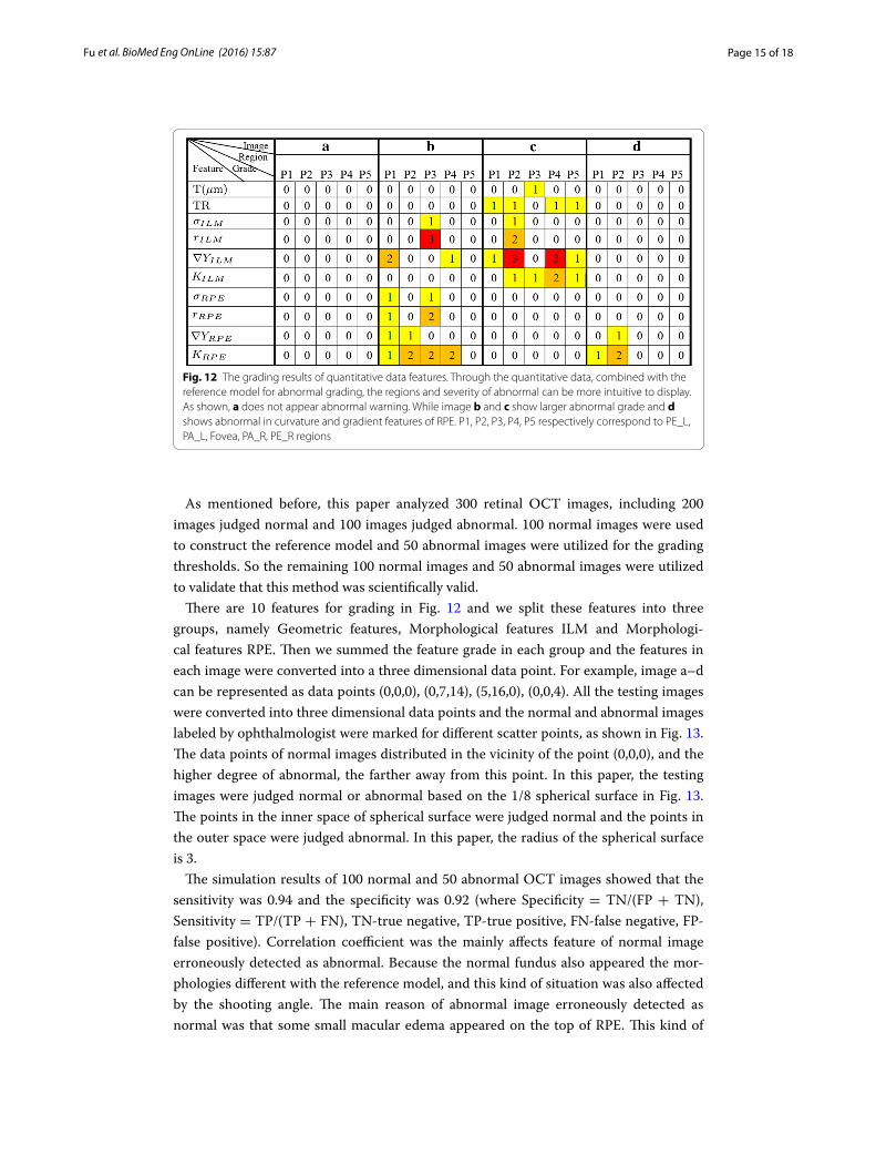
The data feature statistics results can be obtained by grading the quantitative data fea-tures. The corresponding evaluation grade of each image in different regions and differ-ent features can be get from Fig. 12, and the abnormal situation of retina could be judged by evaluation grade.

From Fig. 12 we can see that the image a does not contain abnormal warning and it is in line with the normal morphology. In image b, ILM and RPE have a higher level of abnor-mal grade in fovea area (P3), and RPE contains larger anomalies judged from the abnor-mal grade of RPE standard deviation and RPE mean curvature. In image c, the abnormal grade of thickness feature in fovea (P3) is level 1. Combined with the feature value, we can further judge that the fovea is thickened, resulting in the other areas (P1, P2, P4, P5) also appear anomalies in thickness ratio feature. In addition, the ILM gradient and the

Fig. 9 The results of retinal boundary extraction in OCT images. After the preprocessing of standardization and de-noising, the ILM and RPE boundaries are extracted based on intensity features, as shown in the red lines. The green lines represent the medical macular regional division boundaries. a–d are respectively cor-responding to the four original images in Fig. 8

Fig. 10 The ILM and RPE boundaries comparison with reference model. It is more intuitive to display the morphological difference by the retinal boundaries comparison between target images and reference model. a–d are respectively corresponding to the four original images in Fig. 8


ILM mean curvature show a large abnormal grade, and the reason is that the ILM surface is uneven in image c. This kind of anomaly is mainly caused by epiretinal membrane. In image d, the RPE mean curvature appears abnormal numerical warning in left perifovea area (P1) and left parafovea area (P2), corresponding to the small uplift caused by drusen.

Fig. 11 The features quantitative calculation results. The rough abnormities from the boundaries compari-son are shown in Fig. 7 and more accurate judgment can be obtained by boundary structure quantification and data features. This figure shows the corresponding quantitative values in different regions and different features. a–d are respectively corresponding to the four original images in Fig. 8


As mentioned before, this paper analyzed 300 retinal OCT images, including 200 images judged normal and 100 images judged abnormal. 100 normal images were used to construct the reference model and 50 abnormal images were utilized for the grading thresholds. So the remaining 100 normal images and 50 abnormal images were utilized to validate that this method was scientifically valid.

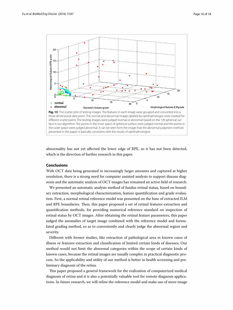
There are 10 features for grading in Fig. 12 and we split these features into three groups, namely Geometric features, Morphological features ILM and Morphologi-cal features RPE. Then we summed the feature grade in each group and the features in each image were converted into a three dimensional data point. For example, image a–d can be represented as data points (0,0,0), (0,7,14), (5,16,0), (0,0,4). All the testing images were converted into three dimensional data points and the normal and abnormal images labeled by ophthalmologist were marked for different scatter points, as shown in Fig. 13. The data points of normal images distributed in the vicinity of the point (0,0,0), and the higher degree of abnormal, the farther away from this point. In this paper, the testing images were judged normal or abnormal based on the 1/8 spherical surface in Fig. 13. The points in the inner space of spherical surface were judged normal and the points in the outer space were judged abnormal. In this paper, the radius of the spherical surface is 3.

The simulation results of 100 normal and 50 abnormal OCT images showed that the sensitivity was 0.94 and the specificity was 0.92 (where Specificity = TN/(FP + TN), Sensitivity = TP/(TP + FN), TN-true negative, TP-true positive, FN-false negative, FP-false positive). Correlation coefficient was the mainly affects feature of normal image erroneously detected as abnormal. Because the normal fundus also appeared the mor-phologies different with the reference model, and this kind of situation was also affected by the shooting angle. The main reason of abnormal image erroneously detected as normal was that some small macular edema appeared on the top of RPE. This kind of

Fig. 12 The grading results of quantitative data features. Through the quantitative data, combined with the reference model for abnormal grading, the regions and severity of abnormal can be more intuitive to display. As shown, a does not appear abnormal warning. While image b and c show larger abnormal grade and d shows abnormal in curvature and gradient features of RPE. P1, P2, P3, P4, P5 respectively correspond to PE_L, PA_L, Fovea, PA_R, PE_R regions


abnormality has not yet affected the lower edge of RPE, so it has not been detected, which is the direction of further research in this paper.

ConclusionsWith OCT data being generated in increasingly larger amounts and captured at higher resolution, there is a strong need for computer assisted analysis to support disease diag-nosis and the automatic analysis of OCT images has remained an active field of research.

We presented an automatic analysis method of fundus retinal status, based on bound-ary extraction, morphological characterization, feature quantification and grade evalua-tion. First, a normal retinal reference model was presented on the base of extracted ILM and RPE boundaries. Then, this paper proposed a set of retinal features extraction and quantification methods, for providing numerical reference standard on inspection of retinal status by OCT images. After obtaining the retinal feature parameters, this paper judged the anomalies of target image combined with the reference model and formu-lated grading method, so as to conveniently and clearly judge the abnormal region and severity.

Different with former studies, like extraction of pathological area in known cases of illness or features extraction and classification of limited certain kinds of diseases, Our method would not limit the abnormal categories within the scope of certain kinds of known cases, because the retinal images are usually complex in practical diagnostic pro-cess. So the applicability and utility of our method is better in health screening and pre-liminary diagnosis of the retina.

This paper proposed a general framework for the realization of computerized medical diagnosis of retina and it is also a potentially valuable tool for remote diagnosis applica-tions. In future research, we will refine the reference model and make use of more image

Fig. 13 The scatter plot of testing images. The features in each image were grouped and converted into a three dimensional data point. The normal and abnormal images labeled by ophthalmologist were marked for different scatter points. The testing images were judged normal or abnormal based on the 1/8 spherical sur-face in our algorithm. The points in the inner space of spherical surface were judged normal and the points in the outer space were judged abnormal. It can be seen from the image that the abnormal judgment method presented in this paper is basically consistent with the results of ophthalmologists


features to realize the distinction between more ophthalmologies and identify different disease categories.

AbbreviationsOCT: optical coherence tomography; BLS-GSM: Bayesian least squares–Gaussian scale mixture approaches; NL Means: non-local means; NCDF: nonlinear complex diffusion filter; CWDL: complex wavelet based dictionary learning methods; BM3D: block-matching and 3D filtering; CNR: contrast-to-noise ratio; TP: texture preservation; EP: edge preservation; ENL: equivalent number of looks; ILM: internal limiting membrane; RPE: retinal pigment epithelium; PA_L: left parafovea; PA_R: right parafovea; PE_L: left perifovea; PE_R: right perifovea; TR: thickness ratio.

Authors’ contributionsDF carried out the study design, the statistical analysis and drafted the manuscript. HT, SZ developed the algorithm, car-ried out the experiments and drafted the manuscript. LL, FG performed the acquisition of the OCT images and consulted the obtained results. JM helped in the results analysis and reviewed the manuscript. All authors read and approved the final manuscript.

Author details1 School of Automation and Electrical Engineering, University of Science and Technology Beijing, Xueyuan Road 30, Haid-ian District, Beijing, China. 2 The 306th Hospital of People’s Liberation Army, Beijing, China. 3 Dept. of Telecommunications, Faculty of Electrical Engineering and Communication, Brno University of Technology, Czech, Brno, Czech Republic.

AcknowledgementsThis research is supported by the National Natural Science Foundation of China (No. 61272358).

Competing interestsThe authors declare that they have no competing interests.

Availability of data and supporting materialsThe raw image data and software are easy to use and available freely at https://zenodo.org/record/56515. The raw data-base includes 200 retinal OCT imagesjudged as normal by ophthalmologists and 100 images with various abnormali-ties.The software includes the main steps introduced in this paper and the four retinalOCT images for simulation. The software was carried out in Matlab.

Received: 7 March 2016 Accepted: 10 July 2016

References 1. Huang D, Swanson EA, Lin CP, Schuman JS, Stinson WG, Chang W, Hee MR, Flotte T, Gregory K, Puliafito CA. Optical

coherence tomography. Science. 1991;254(5035):1178–81. 2. Virgili G, Menchini F, Murro V, Peluso E, Rosa F, Casazza G. Optical coherence tomography (OCT) for detection of

macular oedema in patients with diabetic retinopathy. Cochrane Database Syst Rev. 2011;7:CD008081. 3. Ouyang Y, Heussen FM, Hariri A, Keane PA, Sadda SR. Optical coherence tomography-based observation of

the natural history of drusenoid lesion in eyes with dry age-related macular degeneration. Ophthalmology. 2013;120(12):2656–65.

4. Andreoli MT, Lim JI. Optical coherence tomography retinal thickness and volume measurements in X-linked reti-noschisis. Am J Ophthalmol. 2014;158(3):567–73.

5. Roh YR, Park KH, Woo SJ. Foveal thickness between stratus and spectralis optical coherence tomography in retinal diseases. Korean J Ophthalmol. 2013;27(4):268–75.

6. Wolf-Schnurrbusch UE, Ceklic L, Brinkmann CK, Iliev ME, Frey M, Rothenbuehler SP, Enzmann V, Wolf S. Macular thickness measurements in healthy eyes using six different optical coherence tomography instruments. Invest Ophthalmol Vis Sci. 2009;50(7):3432–7.

7. Quellec G, Lee K, Dolejsi M, Garvin MK, Abramoff MD, Sonka M. Three-dimensional analysis of retinal layer texture: identification of fluid-filled regions in SD-OCT of the macula. IEEE Trans Med Imaging. 2010;29(6):1321–30.

8. Gregori G, Wang F, Rosenfeld PJ, Yehoshua Z, Gregori NZ, Lujan BJ, Puliafito CA, Feuer WJ. Spectral domain optical coherence tomography imaging of drusen in nonexudative age-related macular degeneration. Ophthalmology. 2011;118(7):1373–9.

9. Iwama D, Hangai M, Ooto S, Sakamoto A, Nakanishi H, Fujimura T, Domalpally A, Danis RP, Yoshimura N. Automated assessment of drusen using three-dimensional spectral-domain optical coherence tomography. Invest Ophthalmol Vis Sci. 2012;53(3):1576–83.

10. Chen Q, Leng T, Zheng L, Kutzscher L, Ma J, de Sisternes L, Rubin DL. Automated Drusen segmentation and quantifi-cation in SD-OCT images. Med Image Anal. 2013;17(8):1058–72.

11. Liu YY, Chen M, Ishikawa H, Wollstein G, Schuman JS, Rehg JM. Automated macular pathology diagnosis in retinal OCT images using multi-scale spatial pyramid and local binary patterns in texture and shape encoding. Med Image Anal. 2011;15(5):748–59.

12. Liu YY, Ishikawa H, Chen M, Wollstein G, Duker JS, Fujimoto JG, Schuman JS, Rehg JM. Computerized macular pathol-ogy diagnosis in spectral domain optical coherence tomography scans based on multiscale texture and shape features. Invest Ophthalmol Vis Sci. 2011;52(11):8316–22.

https://zenodo.org/record/56515


• We accept pre-submission inquiries

• Our selector tool helps you to find the most relevant journal

• We provide round the clock customer support

• Convenient online submission

• Thorough peer review

• Inclusion in PubMed and all major indexing services

• Maximum visibility for your research

Submit your manuscript atwww.biomedcentral.com/submit

Submit your next manuscript to BioMed Central and we will help you at every step:

13. Koprowski R, Teper S, Wrobel Z, Wylegala E. Automatic analysis of selected choroidal diseases in OCT images of the eye fundus. Biomed Eng Online. 2013;12:117.

14. Koprowski R, Rzendkowski M, Wrobel Z. Automatic method of analysis of OCT images in assessing the severity degree of glaucoma and the visual field loss. BioMed Eng OnLine. 2014;13:16.

15. Xu J, Ishikawa H, Wollstein G, Bilonick RA, Folio LS, Nadler Z, Kagemann L, Schuman JS. Three-dimensional spectral-domain optical coherence tomography data analysis for glaucoma detection. PLoS One. 2013;8(2):e55476.

16. Hughes M, Spring M, Podoleanu A. Speckle noise reduction in optical coherence tomography of paint layers. Appl Opt. 2010;49(1):99–107.

17. Jorgensen TM, Thomadsen J, Christensen U, Soliman W, Sander B. Enhancing the signal-to-noise ratio in oph-thalmic optical coherence tomography by image registration-method and clinical examples. J Biomed Opt. 2007;12(4):041208–10.

18. Portilla J, Strela V, Wainwright MJ, Simoncelli EP. Image denoising using scale mixtures of Gaussians in the Wavelet domain. IEEE Trans Image Process. 2003;12(11):1338–51.

19. Buades A, Coll B, Morel JM. A review of image denoising algorithms, with a new one. Siam J Multiscale Model Simul. 2005;4(2):490–530.

20. Bernardes R, Maduro C, Serranho P, Araujo A, Barbeiro S, Cunha-Vaz J. Improved adaptive complex diffusion despeckling filter. Opt Express. 2010;18(23):24048–59.

21. Dabov K, Foi A, Katkovnik V, Egiazarian K. Image denoising by sparse 3D transform-domain collaborative filtering. IEEE Trans Image Process. 2007;16(8):2080–95.

22. Duan J, Lu W, Tench C, et al. Denoising optical coherence tomography using second order total generalized varia-tion decomposition. Biomed Signal Process Control. 2016;24:120–7.

23. Wong A, Mishra A, Bizheva K, Clausi DA. General Bayesian estimation for speckle noise reduction in optical coher-ence tomography retinal imagery. Opt Express. 2010;18(8):8338–52.

24. Kafieh R, Rabbani H, Selesnick I. Three dimensional data-driven multi scale atomic representation of optical coher-ence tomography. IEEE Trans Med Imaging. 2015;34(5):1042–62.

25. Mayer MA, Borsdorf A, Wagner M, Hornegger J, Mardin CY, Tornow RP. Wavelet denoising of multiframe optical coherence tomography data. Biomed Opt Express. 2012;3(3):572–89.

26. Kafieh R, Rabbani H, Abramoff MD, Sonka M. Curvature correction of retinal OCTs using graph-based geometry detection. Phys Med Biol. 2013;58(9):2925–38.

27. Pizurica A, Jovanov L, Huysmans B, et al. Multiresolution denoising for optical coherence tomography: a review and evaluation. Curr Med Imaging Rev. 2008;4(4):270–84.

28. Chiu SJ, Li XT, Nicholas P, Toth CA, Izatt JA, Farsiu S. Automatic segmentation of seven retinal layers in SDOCT images congruent with expert manual segmentation. Opt Express. 2010;18(18):19413–28.

29. Niu S, Chen Q, de Sisternes L, Rubin DL, Zhang W, Liu Q. Automated retinal layers segmentation in SD-OCT images using dual-gradient and spatial correlation smoothness constraint. Comput Biol Med. 2014;54:116–28.

30. Yazdanpanah A, Hamarneh G, Smith BR, Sarunic MV. Segmentation of intra-retinal layers from optical coherence tomography images using an active contour approach. IEEE Trans Med Imaging. 2011;30(2):484–96.

31. Lang A, Carass A, Hauser M, Sotirchos ES, Calabresi PA, Ying HS, Prince JL. Retinal layer segmentation of macular OCT images using boundary classification. Biomed Opt Express. 2013;4(7):1133–52.

32. Han JH, Cha YM. High-accuracy retinal layer segmentation for optical coherence tomography using tracking kernels based on Gaussian mixture model. IEEE J Sel Topics Quantum Electron. 2013;20(2):1–10.

33. Dufour PA, Ceklic L, Abdillahi H, Schroder S, De Dzanet S, Wolf-Schnurrbusch U, Kowal J. Graph-based multi-surface segmentation of OCT data using trained hard and soft constraints. IEEE Trans Med Imaging. 2013;32(3):531–43.

34. Song Q, Bai J, Garvin MK, Sonka M, Buatti JM, Wu X. Optimal multiple surface segmentation with shape and context priors. IEEE Trans Med Imaging. 2013;32(2):376–86.

35. Duan XR, Liang YB, Friedman DS, Sun LP, Wong TY, Tao QS, Bao L, Wang NL, Wang JJ. Normal macular thickness measurements using optical coherence tomography in healthy eyes of adult Chinese persons: the Handan Eye Study. Ophthalmology. 2010;117(8):1585–94.

36. Shen L, Gao F, Xu X, Lin Z, Zhang Z, Zhao B, Zhang X, Li B, Jonas JB. Macular thickness in Chinese. Acta Ophthalmol. 2013;91(1):e77–9.