yt Documentation - The yt Project

yt DocumentationRelease 1.5-beta

Matthew Turk

October 08, 2009

CONTENTS

1 Introduction 31.1 History . . . . . . . . . . . . . . . . . . . . . . . . . . . . . . . . . . . . . . . . . . . . . . . . . . 31.2 What yt is and is not . . . . . . . . . . . . . . . . . . . . . . . . . . . . . . . . . . . . . . . . . . . 31.3 What functionality does yt offer? . . . . . . . . . . . . . . . . . . . . . . . . . . . . . . . . . . . . 31.4 How do I cite yt? . . . . . . . . . . . . . . . . . . . . . . . . . . . . . . . . . . . . . . . . . . . . . 5

2 Getting the Code 72.1 Installation . . . . . . . . . . . . . . . . . . . . . . . . . . . . . . . . . . . . . . . . . . . . . . . . 72.2 Notes on Common Installation Locations . . . . . . . . . . . . . . . . . . . . . . . . . . . . . . . . 82.3 Installing by Hand . . . . . . . . . . . . . . . . . . . . . . . . . . . . . . . . . . . . . . . . . . . . 92.4 Starting up YT . . . . . . . . . . . . . . . . . . . . . . . . . . . . . . . . . . . . . . . . . . . . . . 10

3 Analysis Philosophy 113.1 Design Goals . . . . . . . . . . . . . . . . . . . . . . . . . . . . . . . . . . . . . . . . . . . . . . . 113.2 Object Methodology . . . . . . . . . . . . . . . . . . . . . . . . . . . . . . . . . . . . . . . . . . . 123.3 Derived Fields and Derived Quantities . . . . . . . . . . . . . . . . . . . . . . . . . . . . . . . . . . 13

4 How to Use YT 154.1 Quick Start Guide . . . . . . . . . . . . . . . . . . . . . . . . . . . . . . . . . . . . . . . . . . . . 154.2 A Slightly Longer Introduction . . . . . . . . . . . . . . . . . . . . . . . . . . . . . . . . . . . . . 214.3 Command Line Tool . . . . . . . . . . . . . . . . . . . . . . . . . . . . . . . . . . . . . . . . . . . 244.4 Using and Manipulating Objects and Fields . . . . . . . . . . . . . . . . . . . . . . . . . . . . . . . 274.5 Examining and Manipulating Particles . . . . . . . . . . . . . . . . . . . . . . . . . . . . . . . . . 304.6 Creating Derived Fields . . . . . . . . . . . . . . . . . . . . . . . . . . . . . . . . . . . . . . . . . 324.7 Parallel Computation With YT . . . . . . . . . . . . . . . . . . . . . . . . . . . . . . . . . . . . . . 344.8 How to Make Plots . . . . . . . . . . . . . . . . . . . . . . . . . . . . . . . . . . . . . . . . . . . . 36

5 Cookbook 395.1 Simple slice . . . . . . . . . . . . . . . . . . . . . . . . . . . . . . . . . . . . . . . . . . . . . . . 395.2 Simple projection . . . . . . . . . . . . . . . . . . . . . . . . . . . . . . . . . . . . . . . . . . . . . 425.3 Aligned cutting plane . . . . . . . . . . . . . . . . . . . . . . . . . . . . . . . . . . . . . . . . . . 455.4 Sum mass in sphere . . . . . . . . . . . . . . . . . . . . . . . . . . . . . . . . . . . . . . . . . . . 475.5 Simple phase . . . . . . . . . . . . . . . . . . . . . . . . . . . . . . . . . . . . . . . . . . . . . . . 485.6 Simple profile . . . . . . . . . . . . . . . . . . . . . . . . . . . . . . . . . . . . . . . . . . . . . . 495.7 Simple radial profile . . . . . . . . . . . . . . . . . . . . . . . . . . . . . . . . . . . . . . . . . . . 505.8 Halo finding . . . . . . . . . . . . . . . . . . . . . . . . . . . . . . . . . . . . . . . . . . . . . . . 515.9 Arbitrary vectors on slice . . . . . . . . . . . . . . . . . . . . . . . . . . . . . . . . . . . . . . . . 525.10 Contours on slice . . . . . . . . . . . . . . . . . . . . . . . . . . . . . . . . . . . . . . . . . . . . . 525.11 Velocity vectors on slice . . . . . . . . . . . . . . . . . . . . . . . . . . . . . . . . . . . . . . . . . 53

i

5.12 Average value . . . . . . . . . . . . . . . . . . . . . . . . . . . . . . . . . . . . . . . . . . . . . . 555.13 Find clumps . . . . . . . . . . . . . . . . . . . . . . . . . . . . . . . . . . . . . . . . . . . . . . . 565.14 Global phase plots . . . . . . . . . . . . . . . . . . . . . . . . . . . . . . . . . . . . . . . . . . . . 585.15 Halo mass info . . . . . . . . . . . . . . . . . . . . . . . . . . . . . . . . . . . . . . . . . . . . . . 595.16 Multi width save . . . . . . . . . . . . . . . . . . . . . . . . . . . . . . . . . . . . . . . . . . . . . 605.17 Zoomin frames . . . . . . . . . . . . . . . . . . . . . . . . . . . . . . . . . . . . . . . . . . . . . . 645.18 Overplot particles . . . . . . . . . . . . . . . . . . . . . . . . . . . . . . . . . . . . . . . . . . . . 695.19 Multi plot . . . . . . . . . . . . . . . . . . . . . . . . . . . . . . . . . . . . . . . . . . . . . . . . . 705.20 Multi plot 3x2 . . . . . . . . . . . . . . . . . . . . . . . . . . . . . . . . . . . . . . . . . . . . . . 725.21 Time series phase . . . . . . . . . . . . . . . . . . . . . . . . . . . . . . . . . . . . . . . . . . . . . 755.22 Time series quantity . . . . . . . . . . . . . . . . . . . . . . . . . . . . . . . . . . . . . . . . . . . 775.23 Extract fixed resolution data . . . . . . . . . . . . . . . . . . . . . . . . . . . . . . . . . . . . . . . 79

6 Advanced yt Usage 816.1 Derived Quantities . . . . . . . . . . . . . . . . . . . . . . . . . . . . . . . . . . . . . . . . . . . . 816.2 Plot Modification Mechanisms . . . . . . . . . . . . . . . . . . . . . . . . . . . . . . . . . . . . . . 826.3 The Plugin File . . . . . . . . . . . . . . . . . . . . . . . . . . . . . . . . . . . . . . . . . . . . . . 846.4 Creating 3D Datatypes . . . . . . . . . . . . . . . . . . . . . . . . . . . . . . . . . . . . . . . . . . 856.5 Debugging and Driving YT . . . . . . . . . . . . . . . . . . . . . . . . . . . . . . . . . . . . . . . 85

7 Extensions 897.1 Halo Finding . . . . . . . . . . . . . . . . . . . . . . . . . . . . . . . . . . . . . . . . . . . . . . . 897.2 HaloProfiler . . . . . . . . . . . . . . . . . . . . . . . . . . . . . . . . . . . . . . . . . . . . . . . 927.3 Analyzing an Entire Simulation . . . . . . . . . . . . . . . . . . . . . . . . . . . . . . . . . . . . . 96

8 Contributing Code 998.1 Bug Fixes . . . . . . . . . . . . . . . . . . . . . . . . . . . . . . . . . . . . . . . . . . . . . . . . . 998.2 Licensing . . . . . . . . . . . . . . . . . . . . . . . . . . . . . . . . . . . . . . . . . . . . . . . . . 998.3 Fields and Extensions . . . . . . . . . . . . . . . . . . . . . . . . . . . . . . . . . . . . . . . . . . 998.4 Analysis Code and Examples . . . . . . . . . . . . . . . . . . . . . . . . . . . . . . . . . . . . . . 99

9 Asking for Help 1019.1 The Mailing List . . . . . . . . . . . . . . . . . . . . . . . . . . . . . . . . . . . . . . . . . . . . . 1019.2 Installation Issues . . . . . . . . . . . . . . . . . . . . . . . . . . . . . . . . . . . . . . . . . . . . 1019.3 Vanilla Usage Issues . . . . . . . . . . . . . . . . . . . . . . . . . . . . . . . . . . . . . . . . . . . 1029.4 Customization and Scripting Issues . . . . . . . . . . . . . . . . . . . . . . . . . . . . . . . . . . . 1029.5 How To Report A Bug . . . . . . . . . . . . . . . . . . . . . . . . . . . . . . . . . . . . . . . . . . 102

10 FAQ 10310.1 Why Python? . . . . . . . . . . . . . . . . . . . . . . . . . . . . . . . . . . . . . . . . . . . . . . . 10310.2 Where can I learn more about Python? . . . . . . . . . . . . . . . . . . . . . . . . . . . . . . . . . 10310.3 Who works on yt? . . . . . . . . . . . . . . . . . . . . . . . . . . . . . . . . . . . . . . . . . . . . 10310.4 What’s up with the names? . . . . . . . . . . . . . . . . . . . . . . . . . . . . . . . . . . . . . . . . 10310.5 Are there any restrictions on my use of yt? . . . . . . . . . . . . . . . . . . . . . . . . . . . . . . . 10310.6 How do I know what the units returned are? . . . . . . . . . . . . . . . . . . . . . . . . . . . . . . . 10410.7 What are all these .yt files? . . . . . . . . . . . . . . . . . . . . . . . . . . . . . . . . . . . . . . . . 10410.8 How can I help? . . . . . . . . . . . . . . . . . . . . . . . . . . . . . . . . . . . . . . . . . . . . . 10410.9 Something has gone wrong. What do I do? . . . . . . . . . . . . . . . . . . . . . . . . . . . . . . . 10410.10 How do I specify an axis? . . . . . . . . . . . . . . . . . . . . . . . . . . . . . . . . . . . . . . . . 10410.11 Where can I go for support? . . . . . . . . . . . . . . . . . . . . . . . . . . . . . . . . . . . . . . . 105

11 yt Methods 10711.1 Introduction . . . . . . . . . . . . . . . . . . . . . . . . . . . . . . . . . . . . . . . . . . . . . . . 10711.2 Analysis Requirements . . . . . . . . . . . . . . . . . . . . . . . . . . . . . . . . . . . . . . . . . . 10811.3 Community Engagement . . . . . . . . . . . . . . . . . . . . . . . . . . . . . . . . . . . . . . . . . 108

ii

11.4 Data Analysis Layer . . . . . . . . . . . . . . . . . . . . . . . . . . . . . . . . . . . . . . . . . . . 10911.5 Plotting and Visualization Layer . . . . . . . . . . . . . . . . . . . . . . . . . . . . . . . . . . . . . 11911.6 Constraints of Scale . . . . . . . . . . . . . . . . . . . . . . . . . . . . . . . . . . . . . . . . . . . 11911.7 Frontends and Interfaces . . . . . . . . . . . . . . . . . . . . . . . . . . . . . . . . . . . . . . . . . 12011.8 Embedding yt Inside Enzo . . . . . . . . . . . . . . . . . . . . . . . . . . . . . . . . . . . . . . . 12011.9 Generalization to Other AMR Codes . . . . . . . . . . . . . . . . . . . . . . . . . . . . . . . . . . 12111.10 Immersive Visualization with VTK . . . . . . . . . . . . . . . . . . . . . . . . . . . . . . . . . . . 12111.11 Community Involvement . . . . . . . . . . . . . . . . . . . . . . . . . . . . . . . . . . . . . . . . . 12211.12 Future Directions . . . . . . . . . . . . . . . . . . . . . . . . . . . . . . . . . . . . . . . . . . . . . 122

12 API Documentation 12512.1 yt.lagos Native AMR Data Structures . . . . . . . . . . . . . . . . . . . . . . . . . . . . . . . . 12512.2 yt.lagos Physical and Derived Data Objects . . . . . . . . . . . . . . . . . . . . . . . . . . . . . 13112.3 yt.raven Plotting and Plot Interfaces . . . . . . . . . . . . . . . . . . . . . . . . . . . . . . . . . 14012.4 yt.reason GUI Methods and Objects . . . . . . . . . . . . . . . . . . . . . . . . . . . . . . . . 14612.5 Convenience Functions . . . . . . . . . . . . . . . . . . . . . . . . . . . . . . . . . . . . . . . . . . 14612.6 yt.extensions Extensions API . . . . . . . . . . . . . . . . . . . . . . . . . . . . . . . . . . . 14912.7 yt.fido File Storage and Management . . . . . . . . . . . . . . . . . . . . . . . . . . . . . . . . 15112.8 yt.lagos.ParallelTools Parallel Helper Functions . . . . . . . . . . . . . . . . . . . . . . 152

13 ChangeLog 15313.1 Version 1.5 . . . . . . . . . . . . . . . . . . . . . . . . . . . . . . . . . . . . . . . . . . . . . . . . 15313.2 Version 1.0 . . . . . . . . . . . . . . . . . . . . . . . . . . . . . . . . . . . . . . . . . . . . . . . . 154

14 Indices and tables 155

Bibliography 157

Module Index 159

Index 161

iii

yt Documentation, Release 1.5-beta

yt is a general-purpose toolkit designed to analyze, manage and plot adaptive mesh refinement data. It has beendesigned from the ground-up to work natively with the Enzo code, but it also supports analysis of output from theOrion code. It runs both interactively and non-interactively, and has been designed to support as many operations aspossible in parallel.

If you use yt in a paper, I highly encourage you to read about our policy on free repository space for analysis code!

Below you’ll find the table of contents. There’s a super-quick-start guide to interactive data analysis, a tour of theobjects and methodology of yt, a short cookbook, a guide extending, and – perhaps most important of all – a guide tothe classes and functions available!

For more information, please visit our homepage and for help, please see Asking for Help.

CONTENTS 1

http://lca.ucsd.edu/projects/enzo

http://yt.enzotools.org/


2 CONTENTS

CHAPTER

ONE

INTRODUCTION

1.1 History

My name is Matthew Turk, and I am the primary author of yt. I designed and implemented it during the course of mygraduate studies working with Prof. Tom Abel at Stanford University, under the auspices of the Department of Energythrough the SLAC National Accelerator Center and, briefly, at Los Alamos National Lab. It has evolved from a simpledata-reader and exporter into what I believe is a fully-featured toolkit for analysis and visualization of adaptive meshrefinement data.

yt was designed to be a completely Free (as in beer and as in freedom – “free and libre” as the saying goes) user-extensible framework for analyzing and visualizing adaptive mesh refinement data, currently working with both Enzoand Orion data. It relies on no proprietary software – although it can be and has been extended to interface withproprietary software and libraries – and has been designed from the ground up to enable users to be as immersed inthe data as they desire.

yt is currently being developed by a team consisting of me, Britton Smith, Stephen Skory, David Collins and JeffOishi. All development is conducted in the open, accessible at http://yt.enzotools.org/ .

1.2 What yt is and is not

In some sense, yt is also designed to be rather utilitarian. By virtue of the fact that it has been written in an interpretedlanguage, it can be somewhat slower than purely C-based analysis codes, although I believe that to be mitigated by acleverness of algorithms and a substantially improved development time for the user. Several of the most computa-tioanlly intensive problems have been written in C, or rely exclusively on C-based numerical libraries.

The primary goal has been, and will continue to be, to present an interface to the user that enables selection andanalysis of arbitrary subsets of data.

1.3 What functionality does yt offer?

yt has evolved substantially over the time of its development. Here is a non-comprehensive list of features:

• Data Objects

– Arbitrary data objects (Spheres, cylinders, rectangular prisms, arbitrary index selection)

– Covering grids (smoothed and raw) for automatic ghost-zone generation

– Identification of topologically-connected sets in arbitrary fields

– Projections, orthogonal slices, oblique slices

3



– Axially-aligned rays

– Memory-conserving 1-, 2- and 3-D profiles of arbitrary fields and objects.

– Halo-finding (HOP) algorithm with full particle information and sphere access

– Nearly all operations can be conducted in parallel

• Data access

– Arbitrary field definition

– Derived quantities (average values, spin parameter, bulk velocity, etc)

– Custom C- written HDF5 backend for packed and unpacked AMR, NumPy-based HDF4 backend

– CGS units used everywhere

– Per-user field and quantity plugins

• Plotting

– Mathtext TeX-like text formatting

– Slices, projections, oblique slices

– Profiles and phase diagrams

– Linked zooms, colormaps, and saving across multiple plots

– Contours, vector plots, annotated boxes, grid boundary plot overlays.

– Simple 3D plotting of phase plots and volume-rendered boxes via hooks into the S2PLOT library

• GUI

– Linked zooming via slider

– Interactive re-centering

– Length scales in human-readable coordinates

– Drawing of circles for generation of data objects and phase plots

– Image saving

– Arbitrary plots within the GUI namespace

– Full interpreter access to data objects

– Macros and other scripts able to be run from within the namespace

• Command-line tools

– Zooming movies

– Time-series movies

– HOP Halo Finding

• Access to components

– Monetary cost: FREE.

– Source code availability: FULL.

– Portability: YES.

4 Chapter 1. Introduction


1.4 How do I cite yt?

If you use some of the advanced features of yt and would like to cite it in a publication, you should feel free to cite theProceedings Paper with the following BibTeX entry:

@InProceedings{SciPyProceedings_46,author = {Matthew Turk},title = {Analysis and Visualization of Multi-Scale Astrophysical

Simulations Using Python and NumPy},booktitle = {Proceedings of the 7th Python in Science Conference},pages = {46 - 50},address = {Pasadena, CA USA},year = {2008},editor = {Ga\"el Varoquaux and Travis Vaught and Jarrod Millman},

}

1.4. How do I cite yt? 5

http://conference.scipy.org/proceedings/SciPy2008/paper_11


6 Chapter 1. Introduction

CHAPTER

TWO

GETTING THE CODE

2.1 Installation

Warning: At the present time, binary packages are not supplied. The success of the installation script has largelyremoved the need for binaries.

YT comes with a handy installation script. This script will download and install all the necessary dependencies –from Python to YT – and then provide you with some information about how to modify your environment variables toensure it is loaded properly.

To get a copy of the YT install script for Linux and Unix machines, you can obtain it from the subversion repository.

$ svn export http://svn.enzotools.org/yt/branches/yt-1.5/doc/install_script.sh

If you’re running on Mac OSX, there is a different install script to run.

$ svn export http://svn.enzotools.org/yt/branches/yt-1.5/doc/install_script_osx.sh

Typically these scripts can just be run directly, but inside there are several options. Specifically, they can optionallyinstall wxPython for GUI support, ZLIB (typically a good idea on 64-bit systems) and Mercurial (a great idea if youuse the barn!) These options are all explained in Using the Installation Script.

2.1.1 Using the Installation Script

Note: The installation script is now the preferred means of installing a full set of packages – but if you are comfortablewith python, feel free to install the code yourself!

In the doc/ directory in the yt source distribution, there is a script, install_script.sh, designed to set up a fullinstallation of yt, along with all the necessary dependencies. You can run this script from within a checkout of yt or anexpanded tarball. If you are running on Mac OSX, you should run install_script_osx.sh instead.

Note: For convenience, yt will be installed in ‘develop’ mode, which means any changes in the source directory willbe included the next time you import yt!

There are several variabels you can set inside this script.

DEST_DIR This is the location to which all source code will be downloaded and resulting built librariesinstalled.

HDF5_DIR If you wish to link against existing HDF5 (shared) libraries, put the root path to the installa-tion here. Statically linked libraries will not work.

7

http://barn.enzotools.org


INST_WXPYTHON This is a boolean, set to 0 or 1, that governs whether or not wxPython should beinstalled.

INST_ZLIB This is a boolean, set to 0 or 1, that governs whether or not zlib should be installed.

INST_HG This is a boolean, set to 0 or 1, that governs whether or not mercurial should be installed. Thisis useful if you want to use scripts from the barn.

YT_DIR If you’ve got a source checkout of YT somewhere else, point to it with this!

Warning: If you run into problems, particularly anything involving -fPIC, it is likely that there’s a problemwith static libraries. Try asking the installer script to install HDF5 and ZLIB.

2.2 Notes on Common Installation Locations

2.2.1 Ranger (TACC)

YT installs out of the box on Ranger using the installation script. Zlib must be built by the script. The pgi modulemust first be swapped out for the gcc/4.3.2 module. This set of commands has been reported to work for thispurpose:

$ module unload mvapich-devel$ module swap pgi gcc$ module load mvapich-devel

Furthermore, errors citing GLIBC following logging out and logging back in can usually be solved by swapping outgcc for pgi again.

2.2.2 Kraken (NICS)

YT installs out of the box on Kraken using the installation script. Zlib must be built by the script. Before you begin,you must also ensure that the GNU programming environment is being used:

$ module swap PrgEnv-pgi PrgEnv-gnu

If you are going to try to run yt on the compute nodes, be aware that – while it does work – it will take a bit of effortbecause the compute nodes run Compute Node Linux. As a result, all the libraries have to be compiled statically –including all of Python and yt!

Stephen Skory has written a guide to getting Python compiled and running on the compute nodes on the wiki.

2.2.3 Verne (NICS)

YT installs out of the box on Verne using the installation script. Zlib must be built by the script. Before you begin,you must also ensure that the GNU programming environment is being used:

$ module swap PE-pgi PE-gnu

8 Chapter 2. Getting the Code

http://barn.enzotools.org/

http://yt.enzotools.org/wiki/CrayXT5Installation


2.2.4 Orange (SLAC)

YT installs out of the box if you either have the KIPAC gfortran installation in your path or use theNUMPY_ARGS="--fcompiler=fake" option as in the script.

2.2.5 Red (SLAC)

YT installs out of the box if you use the NUMPY_ARGS="--fcompiler=fake" option as in the script.

2.2.6 Cobalt (NCSA)

YT installs out of the box on Cobalt using the installation script. However, Zlib and HDF5 must both be installed viathe installation script or linking errors will ensue. The GCC module, as opposed to the Intel Compiler module, shouldbe loaded, but this may not be a hard requirement.

2.2.7 OS X

OS X installation can be tricky. It is best to use the install_script_osx.sh file, which will download freshPython packages along with all dependencies. The Enthought Python Distribution is also a means of obtaining all thesedependencies; if you use EPD, you will have to set up the file hdf5.cfg to point to the correct HDF5 installationfrom EPD. Users have reported some degree of success. Future versions of YT will leverage packages included in theEPD.

2.3 Installing by Hand

If you’ve ever installed a python package by hand before, YT should be easy to install. You will need to install theprequisites first. A driving factor in the development of yt over the months leading to release 1.5 has been the reductionof dependencies. To that extent, only a few packages are required for the base usage, and a GUI toolkit if you are goingto use the graphical user interface, Reason.

• Python, at least version 2.4, but preferably 2.5 or 2.6.

• HDF5, the data storage backend used by Enzo and yt (if you can run Enzo, this is already installed!)

• NumPy, the fast numerical backend for Python

• MatPlotLib, the plotting package

• wxPython, the GUI toolkit (optional)

(If you are only interested in manipulating data without any graphical plotting or interfaces, you only need to installHDF5, NumPy, and Python!)

Instructions for installing these packages is, unfortunately, beyond the scope of this document. However, there arecopious directions on how to do so elsewhere. You may also consider installing the Enthought Python Distribution,which includes all of the necessary packages.

You’ll need to create a file in the YT directory called hdf5.cfg which points at the base of your HDF5 installationtree – usually this will be something like /usr/local/. Underneath this directory YT will look for include andlib directories containing the HDF5 files.

Once these dependencies have been met, YT can be installed in the standard manner:

2.3. Installing by Hand 9

http://www.enthought.com/products/epd.php

http://python.org/

http://www.hdfgroup.org/

http://numpy.scipy.org/

http://matplotlib.sf.net/

http://www.wxpython.org/

http://www.enthought.com/products/epd.php


$ cd yt/$ python2.6 setup.py install --prefix=/some/where/

2.4 Starting up YT

‘Starting up YT’ is a bit of a misnomer – there are many entry points to data analysis with YT. The simplest possibleway to access YT is with the Command Line Tool. You can try this out just by typing

$ yt

and following the help instructions!

10 Chapter 2. Getting the Code

CHAPTER

THREE

ANALYSIS PHILOSOPHY

Section author: J. S. Oishi <[email protected]>

There are many tools available for analysis and visualization of AMR data; there are many just for enzo. So whyyt? Along the road to answering that question, we shall take a somewhat philosophical scenic route. For the morepragmatically minded, the answer is simple: what yt does not yet do, you can make it do so. This is not as glib as itmay seem: it is in fact the main philosophical tennant that underlies yt. In this section, it is not our goal to show youjust how much yt already does. Instead, we will discuss how it is that yt does anything at all. In doing so, we hopeto give you a sense of whether or not yt will align with your science goals.

At its core, yt is not a set of scripts to visualize AMR data, nor is it a set of low-level routines that return a homo- oreven heterogeneous set of gridded data to your favorite scientific programming language–though yt incorporates bothof these things, if your favorite scientific language is python. Instead, yt provides a series of objects, some commonAMR code structures (such as hierarchies and levels in a nested mesh) and some physical (a cylinder, cube, or spheresomewhere in the problem domain), that allow you to process AMR data in order to get at the fundamental underlyingphysics.

3.1 Design Goals

yt evolved naturally out of three design goals, though when Matt was busy writing it, he never really thought aboutthem. Over time, it became clear that they are real and furthermore that they are important to understanding how touse yt. These three goals are directed analysis, repeatability, and data exploration.

3.1.1 Directed Analysis: Answering a Question

One of the main motivators for yt is to make it possible to sit down with a definite question about an AMR datasetand code up a script that will provide an answer to that question. Indeed much of its object-oriented nature can beviewed as a way perform operations on a data object. Given that AMR simulations are usually used to track some kindof structure formation, be it shocks, stars, or galaxies, the data object may not be the entire domain, but some regionwithin it that is interesting. This data object in hand, yt makes it easy (if possible: some tasks yt can merely makepossible) to manipulate that data in such a way to answer a question related to your research.

3.1.2 Repeatability

In any scientific analysis, being able to repeat the set of steps that prepared an answer or physical quantity is essential.To that end, much of the usage of yt is focused around running scripts, describing actions and plots programmatically.Being able to write a script or conducting a set of commands that will reproduce identical results is fundamentallyimportant, and yt will attempt to make that easy. It’s for this reason that the interactive features of yt are not always

11

mailto:[email protected]


as advanced as they might otherwise be. We are actively working on integrating the SAGE notebook system into yt,which our preliminary tests suggest is a nice compromise between interactivity and repeatability.

3.1.3 Exploration

However, it is the serendipitous nature of science that often finding the right question is not obvious at first. This iscertainly true for astrophysical simulation, especially so for simulations of structure formation. What are we lookingfor, and how will we know when we find it?

Quite often, the best way forward is to explore the simulation data as freely as possible. Without the ability for spot-examination, serendipitous discovery or general wandering, the code would be simply a pipeline, rather than a generaltool. The flexible extensibility of yt, that is, the ability to create new derived quantities easily, as well as the ability toextract and display data regions in a variety of ways allows for this exploration.

3.2 Object Methodology

yt follows a strong object-oriented methodology. There is no real global state of yt; all state is contained withinobjects that encapsulate an AMR code object or physical region.

3.2.1 Physical Objects vs Code Objects

The best way to think about doing things with yt is to think first of objects. The AMR code puts a number ofobjects on disk, and yt has a matching set of objects to mimic these closely as possible. Your code runs (hopefully) asimulacrum of the physical universe, and thus in order to make sense of the output data, yt provides a set of objectsmeant to mimic the kinds of physical regions and processes you are interested in. For example, in a simulation ofstar formation out of some larger structure (the cosmic dark matter web, a turbulent molecular cloud), you might beinterested in a sphere one parsec in radius around the point of maximum density. In a simulation of an accretion disk,you might want a cylindrical region of 1000 AU in radius and 10 AU in height with its axial vector aligned with thenet angular momentum vector, which may be arbitrary with respect to the simulation cardinal axes. These are physicalobjects, and yt has a set of these too. Finally, you may wish to reduce the data to produce some essential data thatrepresent a specific process. These reductions are also objects, and they are included in yt as well.

Somewhat separate from this, but in the same spirit, are plots. In yt, plots are also objects that one can create,manipulate, and save. In the case of plots, however, you tell yt what you want to see, and it can fetch data from theappropriate source.

In list form,

Code Objects These are things that are on the disk that the AMR code knows about – things like grids,data dumps, the grid hierarchy and so on.

Physical Objects These are objects like spheres, rectangular prisms, slices, and so on. These are collec-tions of related data arranged by physical properties, and they are not necessarily associated with asingle code object.

Reduced Objects These are objects created by taking a set of data and reducing it into a smaller format,suitable for a specific purpose. Histograms, 1-D profiles, and averages are all members of thiscategory.

Plots Plots are somewhat different than other objects, as they are neither physical nor code. Instead, theplotting interface accepts information about what you want to see, then goes and fetches what isnecessary–from code, physical, and reduced objects as necessary.

12 Chapter 3. Analysis Philosophy


3.3 Derived Fields and Derived Quantities

While the heart of yt is the large set of basic code, physical, reduced, and plot objects already developed, in ametaphorical sense, its ‘soul’ is the fact that any of the objects can be used as starting points for creating fields andquantities of your own devices. Derived quantities and derived fields are the physical objects yt creates from theprimitive variables the AMR code stores. These may or may not be the so-called primitive variables of fluiddynamics (density, velocity, energy): they are whatever your AMR code writes to disk.

Derived quantities are those data products derived from these variables such that the total amount of returned data isless than the number of cells. Derived fields, on the other hand, return a field with equal numbers of cells and thesame geometry as the primitive variables from which it was derived. For example, yt could compute the gravitationalpotential at every point in space reconstructed from the density field.

yt already includes a large number of both derived fields and quantities, but its real power is that it is easy to createyour own. See Creating Derived Fields for detailed instructions on creating derived fields.

3.3. Derived Fields and Derived Quantities 13


14 Chapter 3. Analysis Philosophy

CHAPTER

FOUR

HOW TO USE YT

There’s a lot inside yt. This section is designed to give you an idea of what’s there, what you can do with it, and howto think about the yt environment.

Contents:

4.1 Quick Start Guide

If you’re impatient, like me, you probably just want to pull up some data and take a look at it. This guide will help youout!

4.1.1 Starting IPython

If you’ve used the installation script that comes with yt, you should have an isolated environment containingPython 2.5, Matplotlib, yt, IPython, and maybe wxPython. Be sure to finish up the instructions by prepending theLD_LIBRARY_PATH, PATH and PYTHONPATH environment variables with the output of the script.

If you’ve done that, go ahead and start up our interactive yt environment:

$ iyt

It should start you up in an interpreter, and the namespace will be populated with the stuff you need. Really, thecommand iyt just opens up IPython and loads up yt, with some special commands available for you.

You’re all set, so let’s move on to the next step – actually opening up your data!

4.1.2 Opening Your Data File

You’ll need to know the location of the parameter file from the output you want to look at. Let’s pretend, for thesake of argument, it’s /home/mturk/data/galaxy1200.dir/galaxy1200 and that we have all the rightpermissions. So let’s open it, and see what the maximum density is.

Note: In IPython, you get filename completion! So hit tab and it’ll guess at what you want to open.

In [1]: pf = load("/home/mturk/data/galaxy1200.dir/galaxy1200")

In [2]: v, c = pf.h.find_max("Density")

And then in the variable v we have the value of the most dense cell, and in c we have the location of that point.

15


4.1.3 Making Plots

But hey, what good is the data if we can’t see it? So let’s make some plots! First we need to get aPlotCollectionInteractive object, and then we’ll add some slices and projections to it. Note that we use 0,1, 2 to refer to ‘x’, ‘y’, ‘z’ axes.

In [3]: pc = PlotCollectionInteractive(pf)In [4]: pc.add_slice("Temperature", 0)yt.raven INFO 2008-10-25 11:42:58,429 Added slice of Temperature at x = 0.953125 with ’center’ = [0.953125, 0.8046875, 0.6171875]Out[4]: <yt.raven.PlotTypes.SlicePlot instance at 0x9882cec>

In [5]: pc.add_slice("Density", 0)yt.raven INFO 2008-10-25 11:43:45,608 Added slice of Density at x = 0.953125 with ’center’ = [0.953125, 0.8046875, 0.6171875]Out[5]: <yt.raven.PlotTypes.SlicePlot instance at 0xab83eec>

A window should now pop up for each of these plots. One will be a line integral through the simulation, and the otherwill be a slice. (If you had used the PlotCollection object, they’d be created off-screen – this is the right way tomake plots programmatically in scripts.)

We can also adjust the width of the plots very easily:

In [6]: pc.set_width(100, ’kpc’)

The center is set to the most dense location by default. (For more information, see the documentation forPlotCollection.)

4.1.4 Saving Plots

Even though the windows are open, we can save these to the file system at high resolution.

In [7]: pc.save()Out[7]: [’galaxy1200_Slice_x_Temperature.png’, ’galaxy1200_Slice_x_Density.png’]

16 Chapter 4. How to Use YT


4.1. Quick Start Guide 17


And that’s it! The plots get saved out, and it returns to you a list of their filenames.

Note: The save command will add some data to the end of the filename – this helps to keep track of what each savedfile is.

4.1.5 A Few More Plots

You can also add profiles – radial or otherwise – and phase diagrams very easily.

In [8]: pc.add_profile_sphere(100.0, ’kpc’, ["Density", "Temperature"])Out[8]: <yt.raven.PlotTypes.Profile1DPlot instance at 0xada03ec>

In [9]: pc.add_phase_sphere(100.0, ’kpc’, [’Density’, ’Temperature’,...: ’VelocityMagnitude’])

Out[9]: <yt.raven.PlotTypes.PhasePlot instance at 0xada91ef>



4.1. Quick Start Guide 19


Note that the phase plots default to showing a weighted-average in each bin – weighted by the cell mass in solarmasses. If you want to see a distribution of mass, you’ll need to specify you don’t want an average:

In [10]: pc.add_phase_sphere(100.0, ’kpc’, [’Density’, ’Temperature’,...: ’CellMassMsun’], weight=None)

Out[10]: <yt.raven.PlotTypes.PhasePlot instance at 0xada91ef>



4.2 A Slightly Longer Introduction

This section will contain a short (but a bit longer than Quick Start Guide) introduction to analyzing and plotting datawith yt, using a scripting interface. If you’re not familiar with Python, you might be able to pick it up from thissection, but you’d probably be better off reading one of the many other sources listed in Where can I learn more aboutPython?.)

Note: If you know Python, you might enjoy reading Cookbook!

4.2.1 Writing a Script

The very first step to using yt is to open up a text editor, write a little script, and then run it. You can use your favoritetext editor (for instance, vim) and then save it as something ending in .py. At the command line, you can execute thisscript by calling the name of the python interpreter that you used to install yt and then the name of the script:

$ python2.6 my_script.py

This will load the interpreter, read and run the script my_script.py and then terminate regardless of the success orfailure of the script.

4.2. A Slightly Longer Introduction 21

http://www.vim.org/


To have the python interpreter load, run, and then return an interactive prompt, you can execute the script with

$ python2.6 -i my_script.py

There’s a bit more information about invocation of python in Debugging and Driving YT .

Okay, so now we know how to launch a script, but what do we put in it? Let’s start with one of the most simple thingsto do. Let’s load some data and find the most dense point. Here’s a sample little script that loads our data, prints themaximum density, and the location of that maximum density.

We first import yt – the very first line in this sample script loads yt, brings a bunch of variables, functions and classesinto the local namespace, and initializes a few settings.

The next line loads the parameter file into memory, and then we find the maximum density.

from yt.mods import *pf = load("RedshiftOutput0010.dir/RedshiftOutput0010")value, position = pf.h.find_max("Density")

print "Maximum density: %0.5e at %s" % (value, position)

The last line in that script is a format string which prints the value and the position. You can find a number of samplerecipes in the Cookbook. Let’s move on to making a script that makes some plots before terminating.

4.2.2 Plots and Plot Types

The next step we might want to take is to visually inspect our data. yt has a facility for creating several linked plots –yt.raven.PlotCollection handles adding multiple plots that are linked by width and parameter files. We canadd a couple slices, along each axis and then zoom in. This is one of the most fundamental idioms in yt – during mythesis work, almost all of my scripts started out like this.

from yt.mods import *pf = load("DataDump0020.dir/DataDump0020")pc = PlotCollection(pf)

pc.add_slice("Density", 0)pc.add_slice("Temperature", 0)

pc.set_width(1000.0, ’au’)

pc.save()

This particular script will create a PlotCollection centered on the most dense point (unless you feed in a center, itsearches for and finds the most dense point) add a Density slice, a Temperature slice, set the width to 1000.0 AU, andthen save the lot of them.

For more complicated examples, be sure to check out the Cookbook and the API for yt.raven.PlotCollectionas well as the yt.raven documentation as a whole.

4.2.3 Plot Modification

yt comes with a number of mechanisms of adding visual and textual information to plots. These include grid bound-aries, scale boxes, vector fields, contour fields and text annotations. More documentation is available in Plot Modifi-cation Mechanisms, with full API documentation in yt.raven.Callbacks.



The plot modifications all follow a uniform interface; the concept is that each plot has a base plot, and on top of thata set of callbacks that are applied, in order, to modify it and produce a final result. To apply a new modification, themodify dictionary of the plot is accessed, and from that the appropriate modification keyword is selected. Each ofthese accepts a set of arguments.

For example, from start to finish, this command will output a slice through the most dense point in the simulation,taken along the x axis, with the grid boundaries drawn.

from yt.mods import *p = plots.get_slice("my_data0001", "Density", 0)p.modify["grids"]()p.save_image("my_data0001_Density")

To add on a contour of the field “Temperature”, you can add on another modification:

p.modify["contour"]("Temperature")p.save_image("my_data0001_Density_Temperature")

The plots returned by the class:~yt.raven.PlotCollection methods also respect this interface, which means that you canalso do things like:

from yt.mods import *pf = load("my_data0001")pc = PlotCollection(pf)for ax in range(3): pc.add_slice("Density", ax).modify["grids"]()pc.save("my_data0001")

Wrapped up into this snippet are the methods for adding slices along all three axes and then instantly applying to themthe grid boundary outlines.

A full list of the different possibilities for plot modifications is available in Plot Modification Mechanisms.

4.2.4 Time Series Movies

Note: The Command Line Tool can also do time series plots. Here we showcase how to do them from a script so thatmore modifications can be made.

The process of constructing a time series movie involves, very simply, constructing a set of plots over a set of parameterfiles. By iterating over a set of data files, or over a set of numbers, a series of plots can be output. These can then beconcatenated into a movie to show changes in features and fields over time.

For example, the simplest possible time series movie script would be:

from yt.mods import *for i in range(1000):

p = plots.get_slice("my_data%04i" % i, "Density", 0)p.save_image("my_data%04i" % i)

Because we are using the full API here, more complicated visualizations can be built up. For instance, with theaddition of

p.set_width(10, ’kpc’)p.set_zlim(1e-27, 1e-24)

the width of each image will be 10 kpc and the color limits will be set to 1e-27 and 1e-24.

4.2. A Slightly Longer Introduction 23


4.2.5 Even More!

There’s quite a bit more that you can do with yt from a scripting perspective – not only can you use the modules thatcome with yt, but you can use all of the modules available for Python as a whole. SciPy is a good starting point, andthere are lots of fun subpackages as well as other scientific plotting packages available.

If you find something cool that you find a neat way to apply to Adaptive Mesh Refinement data, you should be sure toemail The Mailing List to tell us about it!

4.3 Command Line Tool

yt comes with a command-line tool, known as yt, that exposes much of the functionality that would normally beaccessible through a scripts. This is designed to make the process of making immediate plots much easier. All of thefunctionality is described in the help strings:

$ yt help

and then the subcommands all have help options as well:

$ yt plot --help

In order to actually run the command, you’ll need to tell it which outputs to operate on. The yt command-line toolhas three mechanisms for specifying outputs. It will do its best to guess based on the information its provided.

You can specify a base name for a parameter file and then a start and stop number (and optionally a skip parameter):

$ yt plot --basename=RedshiftOutput --skip 5 10 50

This will run your plot command on RedshiftOutput 10 through 50, but only on multiples of five. (And if youroutput is in a subdirectory, yt will check there too, don’t worry!)

You can specify a single parameter file:

$ yt plot RedshiftOutput0010

This will run your plot command on RedshiftOutput0010.

Alternatively, you can specify multiple parameter files on the command line:

$ yt plot RedshiftOutput0010 RedshiftOutput0020 RedshiftOutput0030

This will plot RedshiftOutput0010, RedshiftOutput0020, and RedshiftOutput0030.

4.3.1 Simple Statistics

To get information about a given parameter file, including the maximum density, the level information, the smallestcell size and some timing information, use the stats command:

$ yt stats RedshiftOutput0005


http://www.scipy.org


0 4 327681 34 2534962 304 525784

----------------------------342 812048

z = 0.00000000t = 6.46750660e+02 = 4.57786981e+17 s = 1.45163299e+10 years

Smallest Cell:Width: 7.812e-03 1Width: 7.812e-03 unitaryWidth: 3.906e-02 mpchWidth: 3.906e-02 mpchcmWidth: 6.010e-02 mpcWidth: 7.812e-01 ayeWidth: 3.906e+01 kpchWidth: 3.906e+01 kpchcmWidth: 6.010e+01 kpcWidth: 3.906e+04 pchWidth: 3.906e+04 pchcmWidth: 6.010e+04 pcWidth: 8.059e+09 auhWidth: 8.059e+09 auhcmWidth: 1.240e+10 auWidth: 8.659e+11 rsunhWidth: 8.659e+11 rsunhcmWidth: 1.332e+12 rsunWidth: 7.488e+17 mileshWidth: 7.488e+17 mileshcmWidth: 1.152e+18 milesWidth: 1.205e+23 cmhWidth: 1.205e+23 cmhcmWidth: 1.854e+23 cm

Maximum density: 4.43898e-27 at (0.94921875, 0.80078125, 0.61328125)

4.3.2 Plots

The command line tool can make either projections or slices. To make a projection, supply it with the -p option:

$ yt plot -p RedshiftOutput0005

If you don’t supply the -p option, it will only slice rather than project through the object. Weights can also be suppliedfor an average along the line of sight. This command defaults to the full width, centered on the most dense point, andoutputting along all three axes. The help command has more information:

Create a set of images

Usage:yt plot [ARGS...]

Options:-h, --help show this help message and exit-w WIDTH, --width=WIDTH

4.3. Command Line Tool 25


Width in specified units-u UNIT, --unit=UNIT

Desired units-b BASENAME, --basename=BASENAME

Basename of parameter files-p, --projection Use a projection rather than a slice-c CENTER, --center=CENTER

Center (-1,-1,-1 for max)-z ZLIM, --zlim=ZLIM

Color limits (min, max)-a AXIS, --axis=AXIS

Axis (4 for all three)-f FIELD, --field=FIELD

Field to color by-g WEIGHT, --weight=WEIGHT

Field to weight projections with-s SKIP, --skip=SKIP

Skip factor for outputs--colormap=CMAP Colormap name-o OUTPUT, --output=OUTPUT

Folder in which to place output images--show-grids Show the grid boundaries

4.3.3 Zoomin Movies

The command line tool also has facilities for outputting a set of frames that zoom in on a central position. This workson a single dataset and can zoom in on projections or slices:

$ yt zoomin RedshiftOutput0005

However, as with the other commands, you will likely want to specify your own options.

Create a set of zoomin frames

Options:-h, --help show this help message and exit--max-width=MAX_WIDTH

Maximum width in code units--min-width=MIN_WIDTH

Minimum width in units of smallest dx (default: 50)-p, --projection Use a projection rather than a slice-a AXIS, --axis=AXIS

Axis (4 for all three)-f FIELD, --field=FIELD

Field to color by-g WEIGHT, --weight=WEIGHT

Field to weight projections with-z ZLIM, --zlim=ZLIM

Color limits (min, max)-n NFRAMES, --nframes=NFRAMES

Number of frames to generate-o OUTPUT, --output=OUTPUT

Folder in which to place output images--colormap=CMAP Colormap name--unit-boxes Display helpful unit boxes--dex=DEX Number of dex above min to display



-t TEXT, --text=TEXTTextual annotation

4.3.4 Halo Profiler

4.4 Using and Manipulating Objects and Fields

To generate standard plots, objects rarely need to be directly constructed. However, for detailed data inspection as wellas hand-crafted derived data, objects can be exceptionally useful and even necessary.

4.4.1 Accessing Fields in Objects

yt utilizes load-on-demand objects to represent physical regions in space. (See Object Methodology.) Data objects inyt all respect the following protocol for accessing data:

my_object["Density"]

where "Density" can be any field name. The full list of objects is available in Available Objects, and informationabout how to create an object can be found in Creating 3D Datatypes. The field is returned as a single, flattened arraywithout spatial information. The best mechanism for manipulating spatial data is the CoveringGridBase object.

The full list of fields that are available can be found as a property of the Hierarchy or Static Output object that youwish to access. This property is calculated every time the object is instantiated. The full list of fields that have beenidentified in the output file, which need no processing (besides unit conversion) are in the property field_listand the full list of potentially-accessible derived fields (see Derived Fields and Derived Quantities) is available in theproperty derived_field_list. You can see these by examining the two properties:

pf = load("my_data")print pf.h.field_listprint pf.h.derived_field_list

When a field is added, it is added to a container that hangs off of the parameter file, as well. All of the field creationoptions (Field Options) are accessible through this object:

pf = load("my_data")print pf.h.field_info["Pressure"].units

This is a fast way to examine the units of a given field, and additionally you can useyt.lagos.DerivedField.get_source() to get the source code:

field = pf.h.field_info["Pressure"]print field.get_source()

4.4.2 Available Objects

Objects are instantiated by direct access of a hierarchy. Each of the objects that can be generated by a hierarchy are infact fully-fledged data objects respecting the standard protocol for interaction.

The following objects are available, all of which hang off of the hierarchy object. To access them, you would dosomething like this (as for a region):

4.4. Using and Manipulating Objects and Fields 27


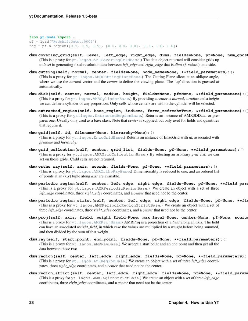
from yt.mods import *pf = load("RedshiftOutput0005")reg = pf.h.region([0.5, 0.5, 0.5], [0.0, 0.0, 0.0], [1.0, 1.0, 1.0])

class covering_grid(self, level, left_edge, right_edge, dims, fields=None, pf=None, num_ghost_zones=0, use_pbar=True, **field_parameters):()(This is a proxy for yt.lagos.AMRCoveringGridBase.) The data object returned will consider grids upto level in generating fixed resolution data between left_edge and right_edge that is dims (3-values) on a side.

class cutting(self, normal, center, fields=None, node_name=None, **field_parameters):()(This is a proxy for yt.lagos.AMRCuttingPlaneBase.) The Cutting Plane slices at an oblique angle,where we use the normal vector and the center to define the viewing plane. The ‘up’ direction is guessed atautomatically.

class disk(self, center, normal, radius, height, fields=None, pf=None, **field_parameters):()(This is a proxy for yt.lagos.AMRCylinderBase.) By providing a center, a normal, a radius and a heightwe can define a cylinder of any proportion. Only cells whose centers are within the cylinder will be selected.

class extracted_region(self, base_region, indices, force_refresh=True, **field_parameters):()(This is a proxy for yt.lagos.ExtractedRegionBase.) Returns an instance of AMR3DData, or pre-pares one. Usually only used as a base class. Note that center is supplied, but only used for fields and quantitiesthat require it.

class grid(self, id, filename=None, hierarchy=None):()(This is a proxy for yt.lagos.EnzoGridBase.) Returns an instance of EnzoGrid with id, associated withfilename and hierarchy.

class grid_collection(self, center, grid_list, fields=None, pf=None, **field_parameters):()(This is a proxy for yt.lagos.AMRGridCollectionBase.) By selecting an arbitrary grid_list, we canact on those grids. Child cells are not returned.

class ortho_ray(self, axis, coords, fields=None, pf=None, **field_parameters):()(This is a proxy for yt.lagos.AMROrthoRayBase.) Dimensionality is reduced to one, and an ordered listof points at an (x,y) tuple along axis are available.

class periodic_region(self, center, left_edge, right_edge, fields=None, pf=None, **field_parameters):()(This is a proxy for yt.lagos.AMRPeriodicRegionBase.) We create an object with a set of threeleft_edge coordinates, three right_edge coordinates, and a center that need not be the center.

class periodic_region_strict(self, center, left_edge, right_edge, fields=None, pf=None, **field_parameters):()(This is a proxy for yt.lagos.AMRPeriodicRegionStrictBase.) We create an object with a set ofthree left_edge coordinates, three right_edge coordinates, and a center that need not be the center.

class proj(self, axis, field, weight_field=None, max_level=None, center=None, pf=None, source=None, node_name=None, field_cuts=None, serialize=True, **field_parameters):()(This is a proxy for yt.lagos.AMRProjBase.) AMRProj is a projection of a field along an axis. The fieldcan have an associated weight_field, in which case the values are multiplied by a weight before being summed,and then divided by the sum of that weight.

class ray(self, start_point, end_point, fields=None, pf=None, **field_parameters):()(This is a proxy for yt.lagos.AMRRayBase.) We accept a start point and an end point and then get all thedata between those two.

class region(self, center, left_edge, right_edge, fields=None, pf=None, **field_parameters):()(This is a proxy for yt.lagos.AMRRegionBase.) We create an object with a set of three left_edge coordi-nates, three right_edge coordinates, and a center that need not be the center.

class region_strict(self, center, left_edge, right_edge, fields=None, pf=None, **field_parameters):()(This is a proxy for yt.lagos.AMRRegionStrictBase.) We create an object with a set of three left_edgecoordinates, three right_edge coordinates, and a center that need not be the center.



class slice(self, axis, coord, fields=None, center=None, pf=None, node_name=False, **field_parameters):()(This is a proxy for yt.lagos.AMRSliceBase.) Slice along axisHow do I specify an axis?, at the coordinatecoord. Optionally supply fields.

class smoothed_covering_grid(self, *args, **field_parameters):()(This is a proxy for yt.lagos.AMRSmoothedCoveringGridBase.) The data object returned will con-sider grids up to level in generating fixed resolution data between left_edge and right_edge that is dims (3-values)on a side.

class sphere(self, center, radius, fields=None, pf=None, **field_parameters):()(This is a proxy for yt.lagos.AMRSphereBase.) The most famous of all the data objects, we define it viaa center and a radius.

4.4.3 Storing and Loading Objects

Often, when operating interactively or via the scripting interface, it is convenient to save an object or multiple objectsout to disk and then restart the calculation later. Personally, I found this most useful when dealing with identificationof clumps and contours (see Cookbook for a recipe on how to find clumps and the API documentation for bothContourFinder and Clump) where the identification step can be quite time-consuming, but the analysis may berelatively fast.

Typically, the save and load operations are used on 3D data objects. yt has a separate set of serialization operationsfor 2D objects such as projections. yt will save out 3D objects to disk under the presupposition that the constructionof the objects is the difficult part, rather than the generation of the data – this means that you can save out an object asa description of how to recreate it in space, but not the actual data arrays affiliated with that object. The informationthat is saved includes the parameter file off of which the object “hangs.” It is this piece of information that is the mostdifficult; the object, when reloaded, must be able to reconstruct a parameter file from whatever limited information ithas in the save file.

To do this, yt is able to identify parameter files based on a “hash” generated from the base file name, the “Current-TimeIdentifier”, and the simulation time. These three characteristics should never be changed outside of a simulation,they are independent of the file location on disk, and in conjunction they should be uniquely identifying. (This processis all done in fido via ParameterFileStore.)

To save an object, you can either save it in the .yt file affiliated with the hierarchy (What are all these .yt files?) or asa standalone file. For instance, using save_object() we can save a sphere.

from yt.mods import *pf = load("my_data")sp = pf.h.sphere([0.5, 0.5, 0.5], 10.0/pf[’kpc’])

pf.h.save_object(sp, "sphere_to_analyze_later")

In a later session, we can load it using save_object():

from yt.mods import *

pf = load("my_data")sphere_to_analyze = pf.h.load_object("sphere_to_analyze_later")

Additionally, if we want to store the object independent of the .yt file, we can save the object directly:


pf = load("my_data")sp = pf.h.sphere([0.5, 0.5, 0.5], 10.0/pf[’kpc’])

4.4. Using and Manipulating Objects and Fields 29


sp.save_object("my_sphere", "my_storage_file.cpkl")

This will store the object as my_sphere in the file my_storage_file.cpkl, which will be created or accessedusing the standard python module shelve. Note that if a filename is not supplied, it will be saved via the hierarchy,as above.

To re-load an object saved this way, you can use the shelve module directly:

from yt.mods import *import shelve

obj_file = shelve.open("my_storage_file.cpkl")pf, obj = obj_file["my_sphere"]

Note here that this behaves slightly differently than above – we do not need to load the parameter file ourselves, as theload process actually does that for us! Additionally, we can store multiple objects in a single shelve file, so we have tocall the sphere by name.

Note: It’s also possible to use the standard cPickle module for loading and storing objects – so in theory you couldeven save a list of objects!

This method works for clumps, as well, and the entire clump hierarchy will be stored and restored upon load.

4.5 Examining and Manipulating Particles

yt has support for reading and manipulating particles. You can access the particles as you would any other data field;additionally, derived fields that operate on particles can be added as would any other derived field, as long as theparameter particle_type is set to True in the call to add_field(). However, with that, there are a few caveats.Particle support in yt is not by any means an afterthought, but it was developed relatively late in comparison to baryonand field-based analysis, and is not as mature.

Note: If you are having trouble with particles, email the mailing list!

4.5.1 Using Particles

Many particle operations can be conducted obliquely, which will serve to reduce memory usage as well as handle anyproblems that might arise from spatial selection of particles.

For instance, Halo objects have a number of operations that can transparently calculate center of mass of parti-cles, bulk velocity, and so on. Use those instead of obtaining the fields directly. Furthermore, any of the spatially-addressable objects described in Using and Manipulating Objects and Fields will automatically select particles basedon the region of space they describe, and the quantities (Derived Quantities) in those objects will operate on particlefields.

(For information on halo finding, see Halo finding and Halo mass info.)

Warning: If you use the built-in methods of interacting with particles, you should be well off. Otherwise, thereare caveats!


http://docs.python.org/library/shelve.html#module-shelve

http://docs.python.org/library/pickle.html#module-cPickle


4.5.2 Selection By Type

Unfortunately, Enzo’s mechanism for storing particle type is inconsistent. The parameter ParticleTypeInFilecontrols whether or not the field particle_type is written to disk; if it is set to 1, the field will be written, butthe default is 0 where the field is not written. Without the field particle_type the discriminator between particletypes is exclusively based on the field creation_time. Particles with creation_time greater than 0.0 are starparticles and those with creation_time equal to zero are dark matter particles.

For simulations only including dark matter particles, this is not important, as all of the particles will be of the sametype. However, selection of – for instance – star particles in other simulations will require some care, and you willneed to do it differently depending on the value of ParticleTypeInFile.

Selecting Particles By Creation Time

To select particles based on creation time, you must first create an index array. Python (and NumPy) allow indexingbased on boolean values, so we will do that. Here is an example of selecting all star particles in the domain.

from yt.mods import *pf = load("galaxy1200.dir/galaxy1200")dd = pf.h.all_data()

star_particles = dd["creation_time"] > 0.0print dd["ParticleMassMsun"][star_particles].max()print dd["ParticleMassMsun"][star_particles].min()print "Number of star particles", star_particles.sum()

Selecting Particles By Particle Type

In Enzo, star particles are type 2. So we will select using the boolean array (as in Selecting Particles By Creation Time)to select only the star particles.

from yt.mods import *pf = load("galaxy1200.dir/galaxy1200")dd = pf.h.all_data()

star_particles = dd["particle_type"] == 2print dd["ParticleMassMsun"][star_particles].max()print dd["ParticleMassMsun"][star_particles].min()print "Number of star particles", star_particles.sum()

4.5.3 Memory

Unfortunately, as of right now, particle loading via spatially-selected objects can be memory intensive. The processthat yt goes through to load particles into memory in a 3D data object is to separate the grids into two classes:

• Fully-contained grids

• Partially-contained grids

For the grids in the former category, the full set of particles residing in those grids are loaded. The ones in the secondrequire that a FakeGridForParticles be created so that the particles residing in the region (as determinedby their values of particle_position_x, particle_position_y and particle_position_z, whichmust be loaded from disk) can be selected and cut from the full set of particles. This requires that the full positioninformation for the particles be loaded, which increases overall memory usage.

4.5. Examining and Manipulating Particles 31


4.5.4 The Future

The next version of yt will have a completely rewritten particle infrastructure. This version is currently in the testingphase, but has shown to reduce memory overhead substantially as well as increase speed by a factor of a few. Bothspatial selection (selection within an object) and selection by type are extremely promising.

4.6 Creating Derived Fields

One of the more powerful means of extending yt is through the usage of derived fields. These are fields that describea value at each cell in a simulation.

4.6.1 Defining a New Field

So once a new field has been conceived of, the best way to create it is to construct a function that performs an arrayoperation – operating on a collection of data, neutral to its size, shape, and type. (All fields should be provided as64-bit floats.)

A simple example of this is the pressure field, which demonstrates the ease of this approach.

def _Pressure(field, data):return (data.pf["Gamma"] - 1.0) * \

data["Density"] * data["ThermalEnergy"]

Note that we do a couple different things here. We access the “Gamma” parameter from the parameter file, we accessthe “Density” field and we access the “ThermalEnergy” field. “ThermalEnergy” is, in fact, another derived field!(“ThermalEnergy” deals with the distinction in storage of energy between dual energy formalism and non-DEF.) Wedon’t do any loops, we don’t do any type-checking, we can simply multiply the three items together.

Once we’ve defined our function, we need to notify yt that the field is available. The add_field() function is themeans of doing this; it has a number of fairly specific parameters that can be passed in, but here we’ll only look at themost basic ones needed for a simple scalar baryon field.

add_field("Pressure", function=_Pressure, units=r"\rm{dyne}/\rm{cm}^{2}")

We feed it the name of the field, the name of the function, and the units. Note that the units parameter is a “raw” string,with some LaTeX-style formatting – Matplotlib actually has a MathText rendering engine, so if you include LaTeX itwill be rendered appropriately.

We suggest that you name the function that creates a derived field with the intended field name prefixed by a singleunderscore, as in the _Pressure example above.

Note one last thing about this definition; we do not do unit conversion. All of the fields fed into the field are pre-supposed to be in CGS. If the field does not need any constants applied after that, you are done. If it does, you shoulddefine a second function that applies the proper multiple in order to return the desired units and use the argumentconvert_function to add_field to point to it.

If you find yourself using the same custom-defined fields over and over, you should put them in your plugins file asdescribed in The Plugin File.



4.6.2 Some More Complicated Examples

But what if we want to do some more fancy stuff? Here’s an example of getting parameters from the data object andusing those to define the field; specifically, here we obtain the center and height_vector parameters and usethose to define an angle of declination of a point with respect to a disk.

def _DiskAngle(field, data):# We make both r_vec and h_vec into unit vectorscenter = data.get_field_parameter("center")r_vec = na.array([data["x"] - center[0],

data["y"] - center[1],data["z"] - center[2]])

r_vec = r_vec/na.sqrt((r_vec**2.0).sum(axis=0))h_vec = na.array(data.get_field_parameter("height_vector"))dp = r_vec[0,:] * h_vec[0] \

+ r_vec[1,:] * h_vec[1] \+ r_vec[2,:] * h_vec[2]

return na.arccos(dp)add_field("DiskAngle", take_log=False,

validators=[ValidateParameter("height_vector"),ValidateParameter("center")],

display_field=False)

Note that we have added a few parameters below the main function; we specify that we do not wish to display thisfield as logged, that we require both height_vector and center to be present in a given data object we wishto calculate this for, and we say that it should not be displayed in a drop-down box of fields to display. This is donethrough the parameter validators, which accepts a list of FieldValidator objects. These objects define the wayin which the field is generated, and when it is able to be created. In this case, we mandate that parameters center andheight_vector are set before creating the field. These are set via set_field_parameter(), which can be calledon any object that has fields.

We can also define vector fields.

def _SpecificAngularMomentum(field, data):if data.has_field_parameter("bulk_velocity"):

bv = data.get_field_parameter("bulk_velocity")else: bv = na.zeros(3, dtype=’float64’)xv = data["x-velocity"] - bv[0]yv = data["y-velocity"] - bv[1]zv = data["z-velocity"] - bv[2]center = data.get_field_parameter(’center’)coords = na.array([data[’x’],data[’y’],data[’z’]], dtype=’float64’)new_shape = tuple([3] + [1]*(len(coords.shape)-1))r_vec = coords - na.reshape(center,new_shape)v_vec = na.array([xv,yv,zv], dtype=’float64’)return na.cross(r_vec, v_vec, axis=0)

def _convertSpecificAngularMomentum(data):return data.convert("cm")

add_field("SpecificAngularMomentum",convert_function=_convertSpecificAngularMomentum, vector_field=True,units=r"\rm{cm}^2/\rm{s}", validators=[ValidateParameter(’center’)])

Here we define the SpecificAngularMomentum field, optionally taking a bulk_velocity, and returning a vectorfield that needs conversion by the function _convertSpecificAngularMomentum.

4.6. Creating Derived Fields 33


4.6.3 Field Options

The arguments to add_field() are passed on to the constructor of DerivedField. add_field() takes careof finding the arguments function and convert_function if it can, however. There are a number of options available, butthe only mandatory ones are name and possibly function.

name This is the name of the field – how you refer to it. For instance, Pressure or H2I_Fraction.

function This is a function handle that defines the field

convert_function This is the function that converts the field to CGS. All inputs to this function aremandated to already be in CGS.

units This is a mathtext (LaTeX-like) string that describes the units.

projected_units This is a mathtext (LaTeX-like) string that describes the units if the field has beenprojected without a weighting.

display_name This is a name used in the plots

take_log This is True or False and describes whether the field should be logged when plotted.

particle_type Is this field a particle field?

validators (Advanced) This is a list of FieldValidator objects, for instance to mandate spatialdata.

vector_field (Advanced) Is this field more than one value per cell?

display_field (Advanced) Should this field appear in the dropdown box in Reason?

not_in_all (Advanced) If this is True, the field may not be in all the grids.

projection_conversion (Advanced) Which unit should we multiply by in a projection?

4.6.4 How Do Units Work?

Everything is done under the assumption that all of the native Enzo fields that yt knows about are converted to cgsbefore being handed to any processing routines.

4.6.5 Which Enzo Fields Does yt Know About?

• Density

• Temperature

• Gas Energy

• Total Energy

• [xyz]-velocity

• Species fields: HI, HII, Electron, HeI, HeII, HeIII, HM, H2I, H2II, DI, DII, HDI

• Particle mass, velocity,

4.7 Parallel Computation With YT

YT has been instrumented with the ability to compute many – most, even – quantities in parallel. This utilizes thepackage mpi4py to parallelize using the Message Passing Interface, typically installed on clusters.


http://code.google.com/p/mpi4py


4.7.1 Capabilities

Currently, YT is able to perform the following actions in parallel:

• Projections

• Slices

• Cutting planes (oblique slices)

• Derived Quantities (total mass, angular momentum, etc)

• 1-, 2- and 3-D profiles

• Halo finding

This list covers just about every action YT can take! Additionally, almost all scripts will benefit from parallelizationwithout any modification. The goal of Parallel-YT has been to retain API compatibility and abstract all parallelism.

4.7.2 Setting Up Parallel YT

To run scripts in parallel, you must first install mpi4py. Instructions for doing so are provided on the MPI4Py website.Once that has been accomplished, you’re all done! You just need to launch your scripts with mpirun and signal toYT that you want to run them in parallel.

For instance, the following script, which we’ll save as my_script.py:

from yt.mods import *pf = load("RD0035/RedshiftOutput0035")v, c = pf.h.find_max("Density")print v, cpc = PlotCollection(pf, center = [0.5, 0.5, 0.5])pc.add_projection("Density", 0)pc.save()

Will execute the finding of the maximum density and the projection in parallel if launched in parallel. To do so, at thecommand line you would execute

$ mpirun -np 16 python2.6 my_script.py --parallel

if you wanted it to run in parallel. If you run into problems, the you can use Remote and Disconnected Debugging toexamine what went wrong.

Warning: If you manually interact with the filesystem, not through YT, you will have to ensure that you onlyexecute your functions on the root processor. You can do this with the function :func:only_on_root.

It’s important to note that all of the processes listed in capabilities work – and no additional work is necessary to paral-lelize those processes. Furthermore, the yt command itself recognizes the --parallel option, so those commandswill work in parallel as well.

4.7.3 Types of Parallelism

In order to divide up the work, YT will attempt to send different tasks to different processors. However, to minimizeinter-process communication, YT will decompose the information in different ways based on the task.

4.7. Parallel Computation With YT 35

http://code.google.com/p/mpi4py


Spatial Decomposition

During this process, the hierarchy will be decomposed along either all three axes or along an image plane, if theprocess is that of projection. This type of parallelism is overall less efficient than grid-based parallelism, but it hasbeen shown to obtain good results overall.

Grid Decomposition

The alternative to spatial decomposition is a simple round-robin of the grids. This process alows YT to pool dataaccess to a given Enzo data file, which ultimately results in faster read times and better parallelism.

4.8 How to Make Plots

Through the plotting interface, you can have yt automatically generate many of the analysis objects available to you!

The primary plotting interface is through a PlotCollection instantiated with a given parameter file and (option-ally) a center. See Making Plots for a brief example of how to generate a PlotCollection.

4.8.1 Two-Dimensional Images

Whenever a two-dimensional image is created, the plotting object first obtains the necessary data at the highest reso-lution. Every time an image is requested of it – for instance, when the width or field is changed – this high-resolutiondata is then pixelized and placed in a buffer of fixed size.

Slices are axially-aligned images of data selected at a fixed point on an axis; these are the fastest type of two-dimensional image, as only the correct coordinate data is read from disk and then plotted.

Cutting planes are oblique slices, aligned with a given normal vector. These can be used for face-on images of disksand other objects, as well as a rotational slices. They work just like slices in other ways, but they tend to be a bitslower.

Projections are closer in style to profiles than slices. They can exist either as a summation of the data along everypossible ray through the simulation, or an average value along every possible ray. If a weight_field is provided, thenthe data returned is an average; typically you will want to weight with Density. If you do not supply a weight_fieldthen the returned data is a column sum. These fields are stored in between invocations – this allows for speedier accessto a relatively slow process!

4.8.2 Profiles and Phase Plots

Profiles and phase plots provide identical API to the generation of profiles themselves, but with a couple convenienceinterfaces. You can have the plot collection generate a sphere automatically for either one:

pc.add_phase_sphere(100.0, ’au’, ["Density", "Temperature", "CellMassMsun"],weight = None)

This will generate a sphere, a phase plot, and then return to you the plot object.



4.8.3 Interactive Plotting

Thanks to the pylab interface in Matplotlib, we have an interactive plot collection available for usage within IPython.Instead of PlotCollection, use PlotCollectionInteractive – this will generate automatically updatingGUI windows with the plots inside them.

4.8.4 Callbacks

Callbacks are means of adding things on top of existing plots – like vectors, overplotted lines, and so on and so forth.They have to be added to the plot objects themselves, rather than the PlotCollection. You can add them like so:

p = pc.add_slice("Density", 0)p.modify["grids"]()

Each Callback has to be instantiated, and then added. You can also access the plot objects inside the PlotCollectiondirectly:

pc.add_slice("Density", 0)pc.plots[-1].modify["grids"]()

Note that if you are plotting interactively, the PlotCollection will need to have redraw called on it.

For more information about Callbacks, see the API reference .

4.8. How to Make Plots 37

CHAPTER

FIVE

COOKBOOK

yt scripts can be a bit intimidating, and at times a bit obtuse. But there’s a lot you can do, and this section of themanual will assist with figuring out how to do some fairly common tasks – which can lead to combining these, withother Python code, into more complicated and advanced tasks.

Note: All of these scripts are located in the mercurial repository at http://hg.enzotools.org/cookbook/

5.1 Simple slice

This is a simple recipe to show how to open a dataset and then plot a slice through it, centered at its most dense point.

The latest version of this recipe can be downloaded here: http://hg.enzotools.org/cookbook/raw-file/tip/recipes/simple_slice.py .

from yt.mods import * # set up our namespace

fn = "RedshiftOutput0005" # parameter file to load

pf = load(fn) # load datapc = PlotCollection(pf) # defaults to center at most dense pointpc.add_slice("Density", 0) # 0 = x-axispc.add_slice("Density", 1) # 1 = y-axispc.add_slice("Density", 2) # 2 = z-axispc.set_width(1.5, ’mpc’) # change width of all plots in pcpc.save(fn) # save all plots

39

http://hg.enzotools.org/cookbook/

http://hg.enzotools.org/cookbook/raw-file/tip/recipes/simple_slice.py

http://hg.enzotools.org/cookbook/raw-file/tip/recipes/simple_slice.py


Sample Output

40 Chapter 5. Cookbook


5.1. Simple slice 41


5.2 Simple projection

This is a simple recipe to show how to open a dataset and then take a weighted-average projection through it, centeredat its most dense point.

The latest version of this recipe can be downloaded here: http://hg.enzotools.org/cookbook/raw-file/tip/recipes/simple_projection.py .



pf = load(fn) # load datapc = PlotCollection(pf) # defaults to center at most dense pointpc.add_projection("Density", 0, weight="Density") # 0 = x-axispc.add_projection("Density", 1, weight="Density") # 1 = y-axispc.add_projection("Density", 2, weight="Density") # 2 = z-axispc.set_width(1.5, ’mpc’) # change width of all plots in pcpc.save(fn) # save all plots


http://hg.enzotools.org/cookbook/raw-file/tip/recipes/simple_projection.py

http://hg.enzotools.org/cookbook/raw-file/tip/recipes/simple_projection.py


Sample Output

5.2. Simple projection 43


5.3 Aligned cutting plane

This is a recipe to show how to open a dataset, calculate the angular momentum vector in a sphere, and then use thatto take an oblique slice.

The latest version of this recipe can be downloaded here: http://hg.enzotools.org/cookbook/raw-file/tip/recipes/aligned_cutting_plane.py .



pf = load(fn) # load data

# Now let’s create a data object that describes the region of which we wish to# take the angular momentum.

# First find the most dense point, which will serve as our center. We get the# most dense value for free, too! This is an operation on the ’hierarchy’,# rather than the parameter file.v, c = pf.h.find_max("Density")print "Found highest density of %0.3e at %s" % (v, c)

5.3. Aligned cutting plane 45

http://hg.enzotools.org/cookbook/raw-file/tip/recipes/aligned_cutting_plane.py

http://hg.enzotools.org/cookbook/raw-file/tip/recipes/aligned_cutting_plane.py


# Now let’s get a sphere centered at this most dense point, c. We have to# convert ’5’ into Mpc, which means we have to use unit conversions provided by# the parameter file. To convert *into* code units, we divide. (To convert# back, we multiply.)sp = pf.h.sphere(c, 5.0 / pf["mpc"])# Now we have an object which contains all of the data within 5 megaparsecs of# the most dense point. So we want to calculate the angular momentum vector of# this 5 Mpc set of gas, and yt provides the facility for that inside a# "derived quantity" property. So we use that, and it returns a vector.L = sp.quantities["AngularMomentumVector"]()

print "Angular momentum vector: %s" % (L)

pc = PlotCollection(pf, center=c) # Make a new plot holderpc.add_cutting_plane("Density", L) # Add our oblique slicepc.set_width(2.5, ’mpc’) # change the widthpc.save(fn) # save out with the pf as a prefix to the image name



Sample Output

5.4 Sum mass in sphere

This recipe shows how to take a sphere, centered on the most dense point, and sum up the total mass in baryons andparticles within that sphere. Note that this recipe will take advantage of multiple CPUs if executed with mpirun andsupplied the –parallel command line argument.

The latest version of this recipe can be downloaded here: http://hg.enzotools.org/cookbook/raw-file/tip/recipes/sum_mass_in_sphere.py .



pf = load(fn) # load datav, c = pf.h.find_max("Density")sp = pf.h.sphere(c, 1.0/pf["mpc"])

baryon_mass, particle_mass = sp.quantities["TotalQuantity"](["CellMassMsun", "ParticleMassMsun"], lazy_reader=True)

5.4. Sum mass in sphere 47

http://hg.enzotools.org/cookbook/raw-file/tip/recipes/sum_mass_in_sphere.py

http://hg.enzotools.org/cookbook/raw-file/tip/recipes/sum_mass_in_sphere.py


print "Total mass in sphere is %0.5e (gas = %0.5e / particles = %0.5e)" % \(baryon_mass + particle_mass, baryon_mass, particle_mass)

5.5 Simple phase

This is a simple recipe to show how to open a dataset and then plot a phase plot showing mass distribution in the rho-Tplane.

The latest version of this recipe can be downloaded here: http://hg.enzotools.org/cookbook/raw-file/tip/recipes/simple_phase.py .



pf = load(fn) # load datapc = PlotCollection(pf) # defaults to center at most dense pointpc.add_phase_sphere(10.0, "mpc", # how many of which unit at pc.center

["Density", "Temperature", "CellMassMsun"], # our fields: x, y, colorweight=None) # don’t take the average value in a cell, just sum them up

pc.save(fn) # save all plots


http://hg.enzotools.org/cookbook/raw-file/tip/recipes/simple_phase.py

http://hg.enzotools.org/cookbook/raw-file/tip/recipes/simple_phase.py


Sample Output

5.6 Simple profile

This is a simple recipe to show how to open a dataset and then plot a profile showing mass-weighted average Temper-ature as a function of Density inside a sphere.

The latest version of this recipe can be downloaded here: http://hg.enzotools.org/cookbook/raw-file/tip/recipes/simple_profile.py .



pf = load(fn) # load datapc = PlotCollection(pf) # defaults to center at most dense pointpc.add_profile_sphere(10.0, "mpc", # how many of which unit at pc.center

["Density", "Temperature"], weight="CellMassMsun") # x, y, weightpc.save(fn) # save all plots

5.6. Simple profile 49

http://hg.enzotools.org/cookbook/raw-file/tip/recipes/simple_profile.py

http://hg.enzotools.org/cookbook/raw-file/tip/recipes/simple_profile.py


Sample Output

5.7 Simple radial profile

This is a simple recipe to show how to open a dataset and then plot a radial profile showing mass-weighted averageDensity inside a sphere.

The latest version of this recipe can be downloaded here: http://hg.enzotools.org/cookbook/raw-file/tip/recipes/simple_radial_profile.py .



pf = load(fn) # load datapc = PlotCollection(pf) # defaults to center at most dense pointpc.add_profile_sphere(10.0, "mpc", # how many of which unit at pc.center

["RadiusMpc", "Density"], weight="CellMassMsun", # x, y, weightx_bounds = (1e-3, 10.0)) # cut out zero-radius and tiny-radius cells

# But ... weight defaults to CellMassMsun, so we’re being redundant here!pc.save(fn) # save all plots


http://hg.enzotools.org/cookbook/raw-file/tip/recipes/simple_radial_profile.py

http://hg.enzotools.org/cookbook/raw-file/tip/recipes/simple_radial_profile.py


Sample Output

5.8 Halo finding

This script shows the simples way of getting halo information.

The latest version of this recipe can be downloaded here: http://hg.enzotools.org/cookbook/raw-file/tip/recipes/halo_finding.py .



pf = load(fn) # load datahalos = HaloFinder(pf)halos.write_out("%s_halos.txt" % pf)

Sample Output

RedshiftOutput0005_halos.txt

5.8. Halo finding 51

http://hg.enzotools.org/cookbook/raw-file/tip/recipes/halo_finding.py

http://hg.enzotools.org/cookbook/raw-file/tip/recipes/halo_finding.py


# HALOS FOUND WITH HOP# Group Mass # part max densx y z center-of-mass x y z vx vy vz max_r

0 3.349212591e+11 822 8.530865463e+03 9.474301815e-01 8.003573695e-01 6.135765693e-01 9.525055889e-01 8.015884263e-01 6.138615237e-01 1.705851494e+06 -1.249580137e+06 2.916880874e+05 3.264138852e-021 2.758414750e+11 677 8.202446551e+03 1.796526850e-01 7.625952107e-01 6.479191838e-01 1.800868084e-01 7.631527126e-01 6.476983977e-01 -2.122530412e+06 1.410529735e+06 -5.558529287e+05 3.346727634e-022 1.947595643e+11 478 4.555572625e+03 5.532828495e-01 3.234508336e-01 1.526681708e-01 5.502839176e-01 3.227445666e-01 1.463095679e-01 4.768146446e+05 5.700263869e+05 7.768371888e+05 2.631150506e-023 1.377170141e+11 338 3.242180406e+03 9.754010795e-01 7.632175520e-01 7.384444522e-01 9.754894863e-01 7.616535505e-01 7.426239921e-01 3.147013348e+05 6.912953967e+05 -3.158456248e+06 2.418755287e-024 1.075659518e+11 264 2.767986753e+03 9.062823292e-01 1.429594372e-01 6.518503248e-01 9.092065242e-01 1.360712140e-01 6.495222326e-01 -5.615869189e+05 -6.366013443e+05 1.681235144e+05 2.159628487e-025 8.311914461e+10 204 2.716905006e+03 7.370274945e-01 1.881616252e-02 2.038525792e-01 7.366971198e-01 1.833388582e-02 2.035289977e-01 1.663413733e+06 7.167873345e+04 -6.195454974e+05 2.220572281e-026 7.985957031e+10 196 3.728141647e+03 7.032178905e-01 4.612143097e-01 2.543813295e-01 7.029408322e-01 4.608586672e-01 2.556131836e-01 5.110343768e+05 7.263383815e+05 -1.357792572e+05 2.069425029e-027 7.374786850e+10 181 2.707414503e+03 8.504477878e-01 4.341667808e-03 1.388950015e-01 8.498287193e-01 3.363578745e-03 1.389072946e-01 -6.683213708e+05 -4.607395365e+05 1.314755282e+06 2.009615603e-028 5.419042271e+10 133 2.289804554e+03 3.776429757e-01 7.283994005e-01 6.446504099e-01 3.777433187e-01 7.269790920e-01 6.443397020e-01 -1.617485927e+06 1.406450423e+06 -3.942225913e+05 1.616496998e-029 5.256063556e+10 129 1.414660466e+03 8.358023677e-02 7.730337546e-01 6.259202318e-01 8.158372163e-02 7.746775670e-01 6.237812975e-01 -2.255594150e+05 -1.998432996e+06 1.754192578e+06 1.681364212e-0210 3.381808334e+10 83 7.426291275e+02 7.586783008e-01 5.565828318e-01 2.499949337e-01 7.615372697e-01 5.602183627e-01 2.516651310e-01 -2.892032842e+05 -4.116040472e+04 1.797132864e+06 1.463921311e-0211 3.218829620e+10 79 1.065896463e+03 7.922319010e-01 6.849626178e-01 3.618562838e-01 7.917738127e-01 6.854323398e-01 3.638244474e-01 2.104084591e+06 -8.047160687e+05 1.661570843e+05 1.497200164e-0212 2.770638154e+10 68 6.274043905e+02 8.762047753e-01 7.390402458e-01 3.784275359e-01 8.745118455e-01 7.389001762e-01 3.775805493e-01 3.619881778e+05 -1.400392085e+06 1.095641286e+06 1.167731823e-0213 2.648404117e+10 65 8.422493962e+02 7.145945477e-01 5.507938405e-01 4.833302836e-02 7.136183340e-01 5.517347708e-01 4.777013265e-02 1.228141163e+06 -9.438224166e+05 9.374767573e+05 1.181447170e-0214 2.526170081e+10 62 5.496262872e+02 2.661371336e-01 4.547039190e-01 2.264844106e-01 2.654044204e-01 4.529011416e-01 2.280199884e-01 5.174012916e+05 1.096946582e+06 -5.720811299e+05 1.202792277e-0215 2.363191366e+10 58 6.261403270e+02 5.537976778e-01 9.321957347e-01 8.870031559e-01 5.536553100e-01 9.301505474e-01 8.885347547e-01 5.270620662e+05 -7.490051223e+04 -1.859688949e+06 1.073805491e-0216 2.240957330e+10 55 7.216382764e+02 2.869443986e-01 6.260920367e-01 1.654761036e-01 2.872379828e-01 6.265364612e-01 1.664006039e-01 -3.583231204e+05 3.269624338e+02 1.092627021e+06 1.221875078e-0217 2.077978615e+10 51 7.207463353e+02 7.925281425e-01 6.605537872e-01 2.972905663e-01 7.922277380e-01 6.615778826e-01 2.962863502e-01 1.213295975e+06 -1.790677992e+06 2.286521021e+06 1.019183230e-0218 1.996489258e+10 49 5.250658436e+02 8.289750280e-01 5.813463800e-01 5.786615919e-01 8.301333188e-01 5.818982175e-01 5.784557151e-01 1.797734829e+06 2.592494092e+06 6.666032929e+05 9.710146517e-0319 1.955744579e+10 48 4.827141235e+02 8.332161433e-01 3.625128149e-01 7.783504082e-01 8.324564064e-01 3.624546115e-01 7.766859379e-01 2.889876718e+05 -2.176831107e+05 -8.195252305e+05 1.219180959e-02

5.9 Arbitrary vectors on slice

This is a simple recipe to show how to open a dataset, plot a slice through it, and add some extra vectors on top. Herewe’ve used the imaginary fields magnetic_field_x, magnetic_field_y and magnetic_field_z.

The latest version of this recipe can be downloaded here: http://hg.enzotools.org/cookbook/raw-file/tip/recipes/arbitrary_vectors_on_slice.py .


fn = "RedshiftOutput0005" # parameter file to loadax = 0 # x-axis

pf = load(fn) # load datapc = PlotCollection(pf) # defaults to center at most dense pointp = pc.add_slice("Density", ax)v1 = "magnetic_field_%s" % (axis_names[x_dict[ax]])v2 = "magnetic_field_%s" % (axis_names[y_dict[ax]])p.modify["quiver"](v1, v2) # This takes a few arguments, but we’ll use the defaults

# here. You can control the ’skip’ factor in the# vectors.

pc.set_width(2.5, ’mpc’) # change width of all plots in pcpc.save(fn) # save all plots

5.10 Contours on slice

This is a simple recipe to show how to open a dataset, plot a slice through it, and add contours of another quantity ontop.


http://hg.enzotools.org/cookbook/raw-file/tip/recipes/arbitrary_vectors_on_slice.py

http://hg.enzotools.org/cookbook/raw-file/tip/recipes/arbitrary_vectors_on_slice.py


The latest version of this recipe can be downloaded here: http://hg.enzotools.org/cookbook/raw-file/tip/recipes/contours_on_slice.py .



pf = load(fn) # load datapc = PlotCollection(pf) # defaults to center at most dense pointp = pc.add_slice("Density", 0) # 0 = x-axisp.modify["contour"]("Temperature")pc.set_width(1.5, ’mpc’) # change width of all plots in pcpc.save(fn) # save all plots

Sample Output

5.11 Velocity vectors on slice

This is a simple recipe to show how to open a dataset, plot a slice through it, and add velocity vectors on top.

5.11. Velocity vectors on slice 53

http://hg.enzotools.org/cookbook/raw-file/tip/recipes/contours_on_slice.py

http://hg.enzotools.org/cookbook/raw-file/tip/recipes/contours_on_slice.py


The latest version of this recipe can be downloaded here: http://hg.enzotools.org/cookbook/raw-file/tip/recipes/velocity_vectors_on_slice.py .



pf = load(fn) # load datapc = PlotCollection(pf) # defaults to center at most dense pointp = pc.add_slice("Density", 0) # 0 = x-axisp.modify["velocity"]() # This takes a few arguments, but we’ll use the defaults

# here. You can control the ’skip’ factor in the# vectors.

pc.set_width(2.5, ’mpc’) # change width of all plots in pcpc.save(fn) # save all plots


http://hg.enzotools.org/cookbook/raw-file/tip/recipes/velocity_vectors_on_slice.py

http://hg.enzotools.org/cookbook/raw-file/tip/recipes/velocity_vectors_on_slice.py


Sample Output

5.12 Average value

This recipe finds the average value of a quantity through the entire box. Note that this recipe will take advantage ofmultiple CPUs if executed with mpirun and supplied the –parallel command line argument.

The latest version of this recipe can be downloaded here: http://hg.enzotools.org/cookbook/raw-file/tip/recipes/average_value.py .


fn = "RedshiftOutput0005" # parameter file to loadpf = load(fn) # load data

field = "Temperature" # The field to averageweight = "CellMassMsun" # The weight for the average

dd = pf.h.all_data() # This is a region describing the entire box,# but note it doesn’t read anything in yet!

# We now use our ’quantities’ call to get the average quantityaverage_value = dd.quantities["WeightedAverageQuantity"](

5.12. Average value 55

http://hg.enzotools.org/cookbook/raw-file/tip/recipes/average_value.py

http://hg.enzotools.org/cookbook/raw-file/tip/recipes/average_value.py


field, weight, lazy_reader=True)

print "Average %s (weighted by %s) is %0.5e" % (field, weight, average_value)

5.13 Find clumps

This is a recipe to show how to find topologicall connected sets of cells inside a dataset. It returns these clumpsand they can be inspected or visualized as would any other data object. More detail on this method can be found inastro-ph/0806.1653.

The latest version of this recipe can be downloaded here: http://hg.enzotools.org/cookbook/raw-file/tip/recipes/find_clumps.py .


fn = "RedshiftOutput0005" # parameter file to loadfield = "Density" # this is the field we look for contours over -- we could do

# this over anything. Other common choices are ’AveragedDensity’# and ’Dark_Matter_Density’.

step = 10.0 # This is the multiplicative interval between contours.


# We want to find clumps over the entire dataset, so we’ll just grab the whole# thing! This is a convenience parameter that prepares an object that covers# the whole domain. Note, though, that it will load on demand and not before!data_source = pf.h.all_data()

# Now we set some sane min/max values between which we want to find contours.# This is how we tell the clump finder what to look for -- it won’t look for# contours connected below or above these threshold values.c_min = 10**na.floor(na.log10(data_source[field]).min() )c_max = 10**na.floor(na.log10(data_source[field]).max()+1)

# Now find get our ’base’ clump -- this one just covers the whole domain.master_clump = Clump(data_source, None, field)

# This next command accepts our base clump and we say the range between which# we want to contour. It recursively finds clumps within the master clump, at# intervals defined by the step size we feed it. The current value is# *multiplied* by step size, rather than added to it -- so this means if you# want to look in log10 space intervals, you would supply step = 10.0.find_clumps(master_clump, c_min, c_max, step)

# As it goes, it appends the information about all the sub-clumps to the# master-clump. Among different ways we can examine it, there’s a convenience# function for outputting the full hierarchy to a file.f = open(’%s_clump_hierarchy.txt’ % pf,’w’)write_clump_hierarchy(master_clump,0,f)f.close()

# We can also output some handy information, as well.f = open(’%s_clumps.txt’ % pf,’w’)write_clumps(master_clump,0,f)f.close()


http://hg.enzotools.org/cookbook/raw-file/tip/recipes/find_clumps.py

http://hg.enzotools.org/cookbook/raw-file/tip/recipes/find_clumps.py


# If you’d like to visualize these clumps, a list of clumps can be supplied to# the "clumps" callback on a plot.

Sample Output

RedshiftOutput0005_clump_hierarchy.txt

Clump at level 0:Cells: 714638Mass: 2.867994e+12 MsolarJeans Mass (vol-weighted): 1.945683e+10 MsolarJeans Mass (mass-weighted): 4.959227e+10 MsolarMax grid level: 2Min number density: 7.299408e-09 cm^-3Max number density: 1.594844e-03 cm^-3





RedshiftOutput0005_clumps.txt

5.13. Find clumps 57


Clump:Cells: 1Mass: 3.698225e+09 MsolarJeans Mass (vol-weighted): 3.532331e+09 MsolarJeans Mass (mass-weighted): 3.532331e+09 MsolarMax grid level: 2Min number density: 4.144234e-04 cm^-3Max number density: 4.144234e-04 cm^-3

Clump:Cells: 2Mass: 1.205801e+10 MsolarJeans Mass (vol-weighted): 2.555663e+09 MsolarJeans Mass (mass-weighted): 2.555660e+09 MsolarMax grid level: 2Min number density: 6.737547e-04 cm^-3Max number density: 6.774670e-04 cm^-3

5.14 Global phase plots

This is a simple recipe to show how to open a dataset and then plot a couple phase diagrams, save them, and quit. Notethat this recipe will take advantage of multiple CPUs if executed with mpirun and supplied the –parallel command lineargument.

The latest version of this recipe can be downloaded here: http://hg.enzotools.org/cookbook/raw-file/tip/recipes/global_phase_plots.py .



pf = load(fn) # load datadd = pf.h.all_data() # This is an object that describes the entire boxpc = PlotCollection(pf) # defaults to center at most dense point

# We plot the average x-velocity (mass-weighted) in our object as a function of# Electron_Density and Temperatureplot=pc.add_phase_object(dd, ["Electron_Density","Temperature","x-velocity"]

lazy_reader = True)

# We now plot the average value of x-velocity as a function of temperatureplot=pc.add_profile_object(dd, ["Temperature", "x-velocity"],

lazy_reader = True)

# Finally, the average electron density as a function of the magnitude of the# velocityplot=pc.add_profile_object(dd, ["Electron_Density", "VelocityMagnitude"],

lazy_reader = True)pc.save() # save all plots


http://hg.enzotools.org/cookbook/raw-file/tip/recipes/global_phase_plots.py

http://hg.enzotools.org/cookbook/raw-file/tip/recipes/global_phase_plots.py


5.15 Halo mass info

This recipe finds halos and then prints out information about them. Note that this recipe will take advantage of multipleCPUs if executed with mpirun and supplied the –parallel command line argument.

The latest version of this recipe can be downloaded here: http://hg.enzotools.org/cookbook/raw-file/tip/recipes/halo_mass_info.py .



# First we run our halo finder to identify all the halos in the dataset. This# can take arguments, but the default are pretty sane.halos = HaloFinder(pf)

f = open("%s_halo_info.txt" % pf, "w")

# Now, for every halo, we get the baryon data and examine it.for halo in halos:

# The halo has a property called ’get_sphere’ that obtains a sphere# centered on the point of maximum density (or the center of mass, if that# argument is supplied) and with the radius the maximum particle radius of# that halo.sphere = halo.get_sphere()# We use the quantities[] method to get the total mass in baryons and in# particles.baryon_mass, particle_mass = sphere.quantities["TotalQuantity"](

["CellMassMsun", "ParticleMassMsun"], lazy_reader=True)# Now we print out this information, along with the ID.f.write("Total mass in HOP group %s is %0.5e (gas = %0.5e / particles = %0.5e)\n" % \

(halo.id, baryon_mass + particle_mass, baryon_mass, particle_mass))f.close()

Sample Output

RedshiftOutput0005_halo_info.txt

Total mass in HOP group 0 is 4.83999e+11 (gas = 6.41403e+10 / particles = 4.19859e+11)Total mass in HOP group 1 is 4.21962e+11 (gas = 6.07831e+10 / particles = 3.61179e+11)Total mass in HOP group 2 is 2.62190e+11 (gas = 3.86250e+10 / particles = 2.23565e+11)Total mass in HOP group 3 is 1.95698e+11 (gas = 3.06816e+10 / particles = 1.65016e+11)Total mass in HOP group 4 is 1.41878e+11 (gas = 2.12738e+10 / particles = 1.20604e+11)Total mass in HOP group 5 is 1.16476e+11 (gas = 1.82813e+10 / particles = 9.81947e+10)Total mass in HOP group 6 is 1.24188e+11 (gas = 2.27342e+10 / particles = 1.01454e+11)Total mass in HOP group 7 is 7.82627e+10 (gas = 1.47010e+10 / particles = 6.35617e+10)Total mass in HOP group 8 is 6.61199e+10 (gas = 6.63271e+09 / particles = 5.94872e+10)Total mass in HOP group 9 is 7.63012e+10 (gas = 1.27395e+10 / particles = 6.35617e+10)Total mass in HOP group 10 is 4.28431e+10 (gas = 4.95060e+09 / particles = 3.78926e+10)Total mass in HOP group 11 is 4.31030e+10 (gas = 3.58066e+09 / particles = 3.95223e+10)Total mass in HOP group 12 is 2.92851e+10 (gas = 1.17132e+09 / particles = 2.81138e+10)Total mass in HOP group 13 is 3.13247e+10 (gas = 1.98850e+09 / particles = 2.93362e+10)Total mass in HOP group 14 is 2.97262e+10 (gas = 7.97481e+08 / particles = 2.89287e+10)Total mass in HOP group 15 is 2.42277e+10 (gas = 5.95763e+08 / particles = 2.36319e+10)

5.15. Halo mass info 59

http://hg.enzotools.org/cookbook/raw-file/tip/recipes/halo_mass_info.py

http://hg.enzotools.org/cookbook/raw-file/tip/recipes/halo_mass_info.py


Total mass in HOP group 16 is 2.76922e+10 (gas = 1.20811e+09 / particles = 2.64840e+10)Total mass in HOP group 17 is 2.18954e+10 (gas = 1.11559e+09 / particles = 2.07798e+10)Total mass in HOP group 18 is 2.09572e+10 (gas = 5.84902e+08 / particles = 2.03723e+10)Total mass in HOP group 19 is 2.55289e+10 (gas = 2.71190e+09 / particles = 2.28170e+10)

5.16 Multi width save

This recipe shows a slightly-fancy way to save a couple plots at a lot of different widths, ensuring that across the plotswe have the same min/max for the colorbar.

The latest version of this recipe can be downloaded here: http://hg.enzotools.org/cookbook/raw-file/tip/recipes/multi_width_save.py .



pc = PlotCollection(pf, center=[0.5, 0.5, 0.5]) # We get our Plot Collection object

# Note that when we save, we will be using string formatting to change all of# the bits in here. You can add more, or remove some, if you like.fn = "%(bn)s_%(width)010i_%(unit)s" # template for image file names

# Now let’s set up the widths we want to use.widths = [ (2, "mpc"), (1000, ’kpc’)]# We could add on more of these with:# widths += [ ... ]

# Now we add a slice for x and y.pc.add_slice("Density", 0)pc.add_slice("Density", 1)

# So for all of our widths, we will set the width of the plot and then make# sure that our limits for the colorbar are the min/max across the three plots.# Then we save! Each saved file will have a descriptive name, so we can tell# them apart.

for width, unit in widths:pc.set_width(width,unit)vmin = min([p.norm.vmin for p in pc.plots])vmax = max([p.norm.vmax for p in pc.plots])pc.set_zlim(vmin,vmax)# This is the string formatting we talked about earlierd = {’bn’:pf.basename, ’width’:width, ’unit’:unit}pc.save(fn % d)


http://hg.enzotools.org/cookbook/raw-file/tip/recipes/multi_width_save.py

http://hg.enzotools.org/cookbook/raw-file/tip/recipes/multi_width_save.py


Sample Output

5.16. Multi width save 61


5.16. Multi width save 63


5.17 Zoomin frames

This is a recipe that takes a slice through the most dense point, then creates a bunch of frames as it zooms in. It’simportant to note that this particular recipe is provided to show how to be more flexible and add annotations and thelike – the base system, of a zoomin, is provided by the yt zoomin command.

The latest version of this recipe can be downloaded here: http://hg.enzotools.org/cookbook/raw-file/tip/recipes/zoomin_frames.py .


fn = "RedshiftOutput0005" # parameter file to loadn_frames = 5 # This is the number of frames to make -- below, you can see how

# this is used.min_dx = 40 # This is the minimum size in smallest_dx of our last frame.

# Usually it should be set to something like 400, but for THIS# dataset, we actually don’t have that great of resolution.

pf = load(fn) # load dataframe_template = "frame_%05i" # Template for frame filenames

pc = PlotCollection(pf, center=[0.5, 0.5, 0.5]) # We make a plot collection that defaults to being


http://hg.enzotools.org/cookbook/raw-file/tip/recipes/zoomin_frames.py

http://hg.enzotools.org/cookbook/raw-file/tip/recipes/zoomin_frames.py


# centered at the most dense point.p = pc.add_slice("Density", 2) # Add our slice, along zp.modify["contour"]("Temperature") # We’ll contour in temperature -- this kind

# of modification can’t be done on the command# line, so that’s why we have the recipe!

# What we do now is a bit fun. "enumerate" returns a tuple for every item --# the index of the item, and the item itself. This saves us having to write# something like "i = 0" and then inside the loop "i += 1" for ever loop. The# argument to enumerate is the ’logspace’ function, which takes a minimum and a# maximum and the number of items to generate. It returns 10^power of each# item it generates.for i,v in enumerate(na.logspace(

0, na.log10(pf.h.get_smallest_dx()*min_dx), n_frames)):# We set our width as necessary for this frame ...pc.set_width(v,’1’)# ... and we save!pc.save(frame_template % (i))

Sample Output

5.17. Zoomin frames 65


5.17. Zoomin frames 67


5.18 Overplot particles

This is a simple recipe to show how to open a dataset, plot a projection through it, and add particles on top

The latest version of this recipe can be downloaded here: http://hg.enzotools.org/cookbook/raw-file/tip/recipes/overplot_particles.py .



pf = load(fn) # load datapc = PlotCollection(pf, center=[0.5,0.5,0.5]) # defaults to center at most dense pointp = pc.add_projection("Density", 0) # 0 = x-axis# "nparticles" is slightly more efficient than "particles"p.modify["nparticles"](1.0) # 1.0 is the ’width’ we want for our slab of

# particles -- this governs the allowable locations# of particles that show up on the image# NOTE: we can also supply a *ptype* to cut based# on a given (integer) particle type

pc.set_width(1.0, ’1’) # change width of our plot to the full domainpc.save(fn) # save all plots

5.18. Overplot particles 69

http://hg.enzotools.org/cookbook/raw-file/tip/recipes/overplot_particles.py

http://hg.enzotools.org/cookbook/raw-file/tip/recipes/overplot_particles.py


Sample Output

5.19 Multi plot


The latest version of this recipe can be downloaded here: http://hg.enzotools.org/cookbook/raw-file/tip/recipes/multi_plot.py .

from yt.mods import * # set up our namespaceimport matplotlib.colorbar as cb

fn = "RedshiftOutput0005" # parameter file to loadorient = ’horizontal’


# There’s a lot in here:# From this we get a containing figure, a list-of-lists of axes into which we# can place plots, and some axes that we’ll put colorbars.# We feed it:# Number of plots on the x-axis, number of plots on the y-axis, and how we


http://hg.enzotools.org/cookbook/raw-file/tip/recipes/multi_plot.py

http://hg.enzotools.org/cookbook/raw-file/tip/recipes/multi_plot.py


# want our colorbars oriented. (This governs where they will go, too.# bw is the base-width in inches, but 4 is about right for most cases.fig, axes, colorbars = raven.get_multi_plot( 2, 1, colorbar=orient, bw = 4)

# We’ll use a plot collection, just for convenience’s sakepc = PlotCollection(pf, center=[0.5, 0.5, 0.5])

# Now we add a slice and set the colormap of that slice, but note that we’re# feeding it an axes -- the zeroth row, the zeroth column, and telling the plot# "Don’t make a colorbar." We’ll make one ourselves.p = pc.add_slice("Density", 0, figure = fig, axes = axes[0][0], use_colorbar=False)p.set_cmap("bds_highcontrast") # this is our colormap

# We do this again, but this time we take the 1-index column.p = pc.add_slice("Temperature", 0, figure=fig, axes=axes[0][1], use_colorbar=False)p.set_cmap("hot") # a different colormap

pc.set_width(5.0, ’mpc’) # change width of both plots

# Each ’p’ is a plot -- this is the Density plot and the Temperature plot.# Each ’cax’ is a colorbar-container, into which we’ll put a colorbar.# zip means, give these two me together.for p, cax in zip(pc.plots, colorbars):

# Now we make a colorbar, using the ’image’ attribute of the plot.# ’image’ is usually not accessed; we’re making a special exception here,# though. ’image’ will tell the colorbar what the limits of the data are.cbar = cb.Colorbar(cax, p.image, orientation=orient)# Now, we have to do a tiny bit of magic -- we tell the plot what its# colorbar is, and then we tell the plot to set the label of that colorbar.p.colorbar = cbarp._autoset_label()

# And now we’re done! Note that we’re calling a method of the figure, not the# PlotCollection.fig.savefig("%s" % pf)

5.19. Multi plot 71


Sample Output

5.20 Multi plot 3x2


The latest version of this recipe can be downloaded here: http://hg.enzotools.org/cookbook/raw-file/tip/recipes/multi_plot_3x2.py .

from yt.mods import * # set up our namespaceimport matplotlib.colorbar as cb

fn = "RedshiftOutput0005" # parameter file to loadorient = ’horizontal’


# There’s a lot in here:# From this we get a containing figure, a list-of-lists of axes into which we# can place plots, and some axes that we’ll put colorbars.# We feed it:# Number of plots on the x-axis, number of plots on the y-axis, and how we# want our colorbars oriented. (This governs where they will go, too.# bw is the base-width in inches, but 4 is about right for most cases.fig, axes, colorbars = raven.get_multi_plot( 2, 3, colorbar=orient, bw = 4)


http://hg.enzotools.org/cookbook/raw-file/tip/recipes/multi_plot_3x2.py

http://hg.enzotools.org/cookbook/raw-file/tip/recipes/multi_plot_3x2.py


# We’ll use a plot collection, just for convenience’s sakepc = PlotCollection(pf, center=[0.5, 0.5, 0.5])

# Now we follow the method of "multi_plot.py" but we’re going to iterate# over the columns, which will become axes of slicing.for ax in range(3):

p = pc.add_slice("Density", ax, figure = fig, axes = axes[ax][0],use_colorbar=False)

p.set_cmap("bds_highcontrast") # this is our colormapp.set_zlim(5e-32, 1e-29)# We do this again, but this time we take the 1-index column.p = pc.add_slice("Temperature", ax, figure=fig, axes=axes[ax][1],

use_colorbar=False)p.set_zlim(1e3, 3e4) # Set this so it’s the same for all.p.set_cmap("hot") # a different colormap

pc.set_width(5.0, ’mpc’) # change width of both plots

# Each ’p’ is a plot -- this is the Density plot and the Temperature plot.# Each ’cax’ is a colorbar-container, into which we’ll put a colorbar.# zip means, give these two me together. Note that it cuts off after the# shortest iterator is exhausted, in this case pc.plots.for p, cax in zip(pc.plots, colorbars):

# Now we make a colorbar, using the ’image’ attribute of the plot.# ’image’ is usually not accessed; we’re making a special exception here,# though. ’image’ will tell the colorbar what the limits of the data are.cbar = cb.Colorbar(cax, p.image, orientation=orient)# Now, we have to do a tiny bit of magic -- we tell the plot what its# colorbar is, and then we tell the plot to set the label of that colorbar.p.colorbar = cbarp._autoset_label()

# And now we’re done! Note that we’re calling a method of the figure, not the# PlotCollection.fig.savefig("%s_3x2" % pf)

5.20. Multi plot 3x2 73


Sample Output

5.21 Time series phase

This is a recipe to sit inside a directory and plot a phase diagram for every one of the outputs in that directory.

5.21. Time series phase 75


If run with mpirun and the –parallel flag, this will take advantage of multiple processors.

The latest version of this recipe can be downloaded here: http://hg.enzotools.org/cookbook/raw-file/tip/recipes/time_series_phase.py .


# this means get all the parameter files that it can autodetect and then supply# them as parameter file objects to the loop.for pf in all_pfs(max_depth=2):

# We create a plot collection to hold our plot# If we don’t specify the center, it will look for one -- but we don’t# really care where it’s centered for this plot.pc = PlotCollection(pf, center=[0.5, 0.5, 0.5])

# Now we add a phase plot of a sphere with radius 1.0 in code units.# If your domain is not 0..1, then this may not cover it completely.p = pc.add_phase_sphere(1.0, ’1’, ["Density", "Temperature", "CellMassMsun"],

weight=None, lazy_reader=True,x_bins=128, x_bounds = (1e-32, 1e-24),y_bins=128, y_bounds = (1e2, 1e7))

# We’ve over-specified things -- but this will help ensure we have constant# bounds. lazy_reader gives it the go-ahead to run in parallel, and we# have asked for 128 bins from 1e-32 .. 1e-24 in Density-space and 128 bins# between 1e2 and 1e7 in Temperature space. This will lead to very fine# points of much lower mass, which is okay. You can reduce the number of# bins to get more mass in each bin. Additionally, weight=None means that# no averaging is done -- it just gets summed up, so the value of each bin# will be all the mass residing within that bin.

# Nowe let’s add a title with some fun information. p is the plot we were# handed previously. We will add the name of the parameter file and the# current redshift.p.modify["title"]("%s (z = %0.2f)" % (pf, pf["CosmologyCurrentRedshift"]))

# Now let’s save it out.pc.save()#"%s" % pf)


http://hg.enzotools.org/cookbook/raw-file/tip/recipes/time_series_phase.py

http://hg.enzotools.org/cookbook/raw-file/tip/recipes/time_series_phase.py


Sample Output

5.22 Time series quantity

This is a recipe to sit inside a directory and calculate a quantity for all of the outputs in that directory.

If run with mpirun and the –parallel flag, this will take advantage of multiple processors.

The latest version of this recipe can be downloaded here: http://hg.enzotools.org/cookbook/raw-file/tip/recipes/time_series_quantity.py .


# First set up our times and quantities liststimes = []values = []

# this means get all the parameter files that it can autodetect and then supply# them as parameter file objects to the loop.for pf in all_pfs(max_depth=2):

# Get the current time, convert to years from code unitstimes.append(pf["InitialTime"] * pf["years"])

5.22. Time series quantity 77

http://hg.enzotools.org/cookbook/raw-file/tip/recipes/time_series_quantity.py

http://hg.enzotools.org/cookbook/raw-file/tip/recipes/time_series_quantity.py


# Now get a box containing the entire datasetdata = pf.h.all_data()# Now we calculate the average. The first argument is the quantity to# average, the second is the weight.# "lazy_reader" has two meanings -- the first is that it will try to# operate on each individual grid, rather than a flattened array of all the# data. The second is that it will also distribute grids across multiple# processors, if multiple processors are in use.val = data.quantities["WeightedAverageQuantity"](

"Temperature", "CellVolume", lazy_reader=True)values.append(val)

# Now we have our values and our time. We can plot this in pylab!

import pylabpylab.semilogy(times, values, ’-x’)pylab.xlabel(r"$Time [years]$")pylab.ylabel(r"$\mathrm{H}^{+}\/\/\mathrm{Fraction}$")pylab.savefig("average_HII_fraction.png")



Sample Output

5.23 Extract fixed resolution data

This is a recipe to show how to open a dataset and extract it to a file at a fixed resolution with no interpolation orsmoothing. Additionally, this recipe shows how to insert a dataset into an external HDF5 file using h5py.

The latest version of this recipe can be downloaded here: http://hg.enzotools.org/cookbook/raw-file/tip/recipes/extract_fixed_resolution_data.py .


# For this example we will use h5py to write to our output file.import h5py


# This is the resolution we will extract atDIMS = 128

# Now, we construct an object that describes the data region and structure we# wantcube = pf.h.covering_grid(2, # The level we are willing to extract to; higher

5.23. Extract fixed resolution data 79

http://hg.enzotools.org/cookbook/raw-file/tip/recipes/extract_fixed_resolution_data.py

http://hg.enzotools.org/cookbook/raw-file/tip/recipes/extract_fixed_resolution_data.py


# levels than this will not contribute to the data!# Now we set our spatial extent...left_edge=[0.0, 0.0, 0.0],right_edge=[1.0, 1.0, 1.0],# How many dimensions along each axisdims=[DIMS,DIMS,DIMS],# And any fields to preload (this is optional!)fields=["Density"])

# Now we open our output file using h5py# Note that we open with ’w’ which will overwrite existing files!f = h5py.File("my_data.h5", "w")

# We create a dataset at the root note, calling it density...f.create_dataset("/density", data=cube["Density"])

# We close our filef.close()


CHAPTER

SIX

ADVANCED YT USAGE

yt has been designed to be flexible, with several entry points.

6.1 Derived Quantities

Derived quantities are a way of operating on a collection of cells and returning a set of values that is fewer in numberthan the number of cells – for instance yt already knows about several.

6.1.1 Using Derived Quantities

Every 3D data object (see Using and Manipulating Objects and Fields and Object Methodology) provides a mechanismfor access to derived quantities. These can be accessed via the quantities interface, like so:

pf = load("my_data")dd = pf.h.all_data()dd.quantities["AngularMomentumVector"]()

The following quantities are available via the quantities interface.

AngularMomentumVector():()(This is a proxy for yt.lagos._AngularMomentumVector().) This function returns the mass-weightedaverage angular momentum vector.

BaryonSpinParameter():()(This is a proxy for yt.lagos._BaryonSpinParameter().) This function returns the spin parameterfor the baryons, but it uses the particles in calculating enclosed mass.

BulkVelocity():()(This is a proxy for yt.lagos._BulkVelocity().) This function returns the mass-weighted averagevelocity in the object.

CenterOfMass():()(This is a proxy for yt.lagos._CenterOfMass().) This function takes no arguments and returns thelocation of the center of mass of the non-particle data in the object.

Extrema(fields):()(This is a proxy for yt.lagos._Extrema().) This function returns the extrema of a set of fields :paramfields: A field name, or a list of field names

IsBound(truncate=True, include_thermal_energy=False):()(This is a proxy for yt.lagos._IsBound().) This returns whether or not the object is gravitationallybound. :param truncate: Should the calculation stop once the ratio of gravitational:kinetic is 1.0? :param

81


include_thermal_energy: Should we add the energy from ThermalEnergy on to the kinetic energy to calculatebinding energy?

MaxLocation(field):()(This is a proxy for yt.lagos._MaxLocation().) This function returns the location of the maximum of aset of fields.

ParticleSpinParameter():()(This is a proxy for yt.lagos._ParticleSpinParameter().) This function returns the spin parameterfor the baryons, but it uses the particles in calculating enclosed mass.

TotalMass():()(This is a proxy for yt.lagos._TotalMass().) This function takes no arguments and returns the sum ofcell masses and particle masses in the object.

TotalQuantity(fields):()(This is a proxy for yt.lagos._TotalQuantity().) This function sums up a given field over the entireregion. :param fields: The fields to sum up

WeightedAverageQuantity(field, weight):()(This is a proxy for yt.lagos._WeightedAverageQuantity().) This function returns an averagedquantity. :param field: The field to average :param weight: The field to weight by

6.1.2 Creating Derived Quantities

The basic idea is that you need to be able to operate both on a set of data, and a set of sets of data. (If this is notpossible, the quantity needs to be added with the force_unlazy option.)

Two functions are necessary. One will operate on arrays of data, either fed from each grid individually or fed from theentire data object at once. The second one takes the results of the first, either as lists of arrays or as single arrays, andreturns the final values. For an example, we look at the TotalMass function:

def _TotalMass(data):baryon_mass = data["CellMassMsun"].sum()particle_mass = data["ParticleMassMsun"].sum()return baryon_mass, particle_mass

def _combTotalMass(data, baryon_mass, particle_mass):return baryon_mass.sum() + particle_mass.sum()

add_quantity("TotalMass", function=_TotalMass,combine_function=_combTotalMass, n_ret = 2)

Once the two functions have been defined, we then call add_quantity() to tell it the function that defines the data,the collator function, and the number of values that get passed between them. In this case we return both the particleand the baryon mass, so we have two total values passed from the main function into the collator.

6.2 Plot Modification Mechanisms

Because the plots in yt are considered to be “volatile” – existing independent of the canvas on which they are plotted– before they are saved, you can have a set of “callbacks” run that modify them before saving to disk. By adding acallback, you are telling the plot that whatever it does it itself, your callback gets the last word.

These can all be accessed through a registry attached to every plot object. When you add a plot to ayt.raven.PlotCollection, you get back that affiliated plot object. By accessing modify on that plot ob-ject, you have access to the available callbacks. For instance,

82 Chapter 6. Advanced yt Usage


p = PlotCollection.add_slice("Density", 0)p.modify["velocity"]()

would add the velocity() callback to the plot object. When you save the plot, the list of callbacks will be iteratedover, and the velocity callback will be handed the current state of the plot. It will then be able to dynamically modifythe plot before saving – in this case, adding on velocity vectors atop the image.

6.2.1 Available Callbacks

These are the callbacks available through the modify[] mechanism. The underlying functions are documented(largely identical to this) in yt.raven.FixedResolution Pixelization Interface.

arrow(self, pos, code_size, plot_args=None):()(This is a proxy for yt.raven.Callbacks.ArrowCallback.) This adds an arrow pointing at pos withsize code_size in code units. plot_args is a dict fed to matplotlib with arrow properties.

clumps(self, clumps, plot_args=None):()(This is a proxy for yt.raven.Callbacks.ClumpContourCallback.) Take a list of clumps and plotthem as a set of contours.

contour(self, field, ncont=5, factor=4, take_log=False, clim=None, plot_args=None):()(This is a proxy for yt.raven.Callbacks.ContourCallback.) Add contours in field to the plot.ncont governs the number of contours generated, factor governs the number of points used in the interpola-tion, take_log governs how it is contoured and clim gives the (upper, lower) limits for contouring.

coord_axes(self, unit=None, coords=False):()(This is a proxy for yt.raven.Callbacks.CoordAxesCallback.) Creates x and y axes for a VMPlot.In the future, it will attempt to guess the proper units to use.

quiver(self, field_x, field_y, factor):()(This is a proxy for yt.raven.Callbacks.CuttingQuiverCallback.) Get a quiver plot on top of acutting plane, using field_x and field_y, skipping every factor datapoint in the discretization.

grids(self, alpha=1.0, min_pix=1):()(This is a proxy for yt.raven.Callbacks.GridBoundaryCallback.) Adds grid boundaries to a plot,optionally with alpha-blending. Cuttoff for display is at min_pix wide.

hop_circles(self, hop_output, max_number=None, annotate=False, min_size=20, max_size=10000000, font_size=8, print_halo_size=False, print_halo_mass=False, width=None):()(This is a proxy for yt.raven.Callbacks.HopCircleCallback.) Accepts a yt.lagos.HopListhop_output and plots up to max_number (None for unlimited) halos as circles.

hop_particles(self, hop_output, p_size=1.0, max_number=None, min_size=20, alpha=0.20000000000000001):()(This is a proxy for yt.raven.Callbacks.HopParticleCallback.) Adds particle positions for themembers of each halo as identified by HOP. Along axis up to max_number groups in hop_output that are largerthan min_size are plotted with p_size pixels per particle; alpha determines the opacity of each particle.

axis_label(self, label):()(This is a proxy for yt.raven.Callbacks.LabelCallback.) This adds a label to the plot.

line(self, x, y, plot_args=None):()(This is a proxy for yt.raven.Callbacks.LinePlotCallback.) Over plot x and y with plot_args fedinto the plot.

marker(self, pos, marker=’x’, plot_args=None):()(This is a proxy for yt.raven.Callbacks.MarkerAnnotateCallback.) Adds text marker at pos incode-arguments. plot_args is a dict that will be forwarded to the plot command.

6.2. Plot Modification Mechanisms 83


nparticles(self, width, p_size=1.0, col=’k’, stride=1.0, ptype=None):()(This is a proxy for yt.raven.Callbacks.NewParticleCallback.) Adds particle positions, basedon a thick slab along axis with a width along the line of sight. p_size controls the number of pixels per particle,and col governs the color. ptype will restrict plotted particles to only those that are of a given type.

particles(self, axis, width, p_size=1.0, col=’k’, stride=1.0):()(This is a proxy for yt.raven.Callbacks.ParticleCallback.) Adds particle positions, based on athick slab along axis with a width along the line of sight. p_size controls the number of pixels per particle, andcol governs the color.

point(self, pos, text, text_args=None):()(This is a proxy for yt.raven.Callbacks.PointAnnotateCallback.) This adds text at position pos,where pos is in code-space. text_args is a dict fed to the text placement code.

quiver(self, field_x, field_y, factor):()(This is a proxy for yt.raven.Callbacks.QuiverCallback.) Adds a ‘quiver’ plot to any plot, usingthe field_x and field_y from the associated data, skipping every factor datapoints.

sphere(self, center, radius, circle_args=None, text=None, text_args=None):()(This is a proxy for yt.raven.Callbacks.SphereCallback.) A sphere centered at center in code unitswith radius radius in code units will be created, with optional circle_args, text, and text_args.

text(self, pos, text, text_args=None):()(This is a proxy for yt.raven.Callbacks.TextLabelCallback.) Accepts a position in (0..1, 0..1) ofthe image, some text and optionally some text arguments.

title(self, title=’Plot’):()(This is a proxy for yt.raven.Callbacks.TitleCallback.) Accepts a title and adds it to the plot

units(self, unit=’au’, factor=4, text_annotate=True, text_which=-2):()(This is a proxy for yt.raven.Callbacks.UnitBoundaryCallback.) Add on a plot indicating wherefactor*s of *unit are shown. Optionally text_annotate on the text_which-indexed box on display.

velocity(self, factor=16):()(This is a proxy for yt.raven.Callbacks.VelocityCallback.) Adds a ‘quiver’ plot of velocity tothe plot, skipping all but every factor datapoint

6.3 The Plugin File

The plugin file is a means of modifying the available fields, quantities, data objects and so on without modifying thesource code of yt.

The following configuration parameters need to be set in the ~/.yt/config file in order to enable the usage of aplugin file:

[lagos]

loadfieldplugins: Truepluginfilename: my_plugins.py

You can call your plugin file whatever you like, and after the imports inside the lagos module are completed, it isexecuted in that namespace.

The code in this file can thus add fields, add derived quantities, add datatypes, and on and on. For example, if I createda plugin file containing:



def _myfunc(field, data):return na.random.random(data["Density"].shape)

add_field("SomeQuantity", function=_myfunc)

then all of my data objects would have access to the field “SomeQuantity” despite its lack of use.

6.4 Creating 3D Datatypes

The three-dimensional datatypes in yt follow a fairly simple protocol. The basic principle is that if you want to definea region in space, that region must be identifable from some sort of cut applied against the cells – typically, in yt, thisis done by examining the geomery. (The yt.lagos.ExtractedRegionBase type is a notable exception to this,as it is defined as a subset of an existing data object.)

In principle, you can define any number of 3D data objects, as long as the following methods are implemented toprotocol specifications.

__init__(self, args, kwargs)This function can accept any number of arguments but must eventually call AMR3DData.__init__. It is used toset up the various parameters that define the object.

_get_list_of_grids(self)This function must set the property _grids to be a list of the grids that should be considered to be a part of thedata object. Each of these will be partly or completely contained within the object.

_is_fully_enclosed(self, grid)This function returns true if the entire grid is part of the data object and false if it is only partly enclosed.

_get_cut_mask(self, grid)This function returns a boolean mask in the shape of the grid. All of the cells set to ‘True’ will be included inthe data object and all of those set to ‘False’ will be excluded. Typically this is done via some logical operation.

For a good example of how to do this, see the yt.lagos.AMRCylinderBase source code.

6.5 Debugging and Driving YT

There are several different convenience functions that allow you to control YT in perhaps unexpected and unorthodoxmanners. These will allow you to conduct in-depth debugging of processes that may be running in parallel on multipleprocessors, as well as providing a mechanism of signalling to YT that you need more information about a runningprocess. Additionally, YT has a built-in mechanism for optional reporting of errors to a central server. All of theseallow for more rapid development and debugging of any problems you might encounter.

Additionally, yt is able to leverage existing developments in the IPython community for parallel, interactive analysis.This allows you to initialize multiple YT processes through mpirun and interact with all of them from a single,unified interactive prompt. This enables and facilitates parallel analysis without sacrificing interactivity and flexibility.

6.5.1 The Pastebin

At http://paste.enzotools.org/ a pastebin is available for placing scripts. With yt the script yt_lodgeit.py isdistributed, which allows for commandline uploading and downloading of pasted snippets. To upload script youwould supply it to the command:

$ yt_lodgeit.py some_script.py

6.4. Creating 3D Datatypes 85

http://paste.enzotools.org/


The URL will be returned. If you’d like it to be marked ‘private’ and not show up in the list of pasted snippets, supplythe argument --private. All snippets are given either numbers or hashes. To download a pasted snippet, you woulduse the --download option:

$ yt_lodgeit.py --download=216

The snippet will be output to the window, so output redirection can be used to store it in a file.

Error Reporting with the Pastebin

If you are having troubles with yt, you can have it paste the error report to the pastebin by running your problematicscript with the --paste option:

$ python2.6 some_problematic_script.py --paste

The --paste option has to come after the name of the script. When the script dies and prints its error, it will alsosubmit that error to the pastebin and return a URL for the error. When reporting your bug, include this URL and thenthe problem can be debugged more easily.

For more information on asking for help, see asking-for-help.

6.5.2 Signaling YT to Do Something

During startup, yt inserts handlers for two operating system-level signals. These provide two diagnostic methods forinteracting with a running process. Signalling the python process that is running your script with these signals willinduce the requested behavior.

SIGUSR1 This will cause the python code to print a stack trace, showing exactly where in the functionstack it is currently executing.

SIGUSR2 This will cause the python code to throw a RuntimeError. If you are running with the --rpdboptions (see Remote and Disconnected Debugging) this will also cause the interpreter to sit inside adebug loop. If you are running inside pdb (see pdb ) then pdb will produce a debug loop.

If your yt-running process has PID 5829, you can signal it to print a traceback with:

$ kill -SIGUSR1 5829

Note, however, that if the code is currently inside a C function, the signal will not be handled, and the stacktrace willnot be printed, until it returns from that function.

6.5.3 Remote and Disconnected Debugging

If you are running a parallel job that fails, often it can be difficult to do a post-mortem analysis to determine what wentwrong. To facilitate this, yt has implemented an XML-RPC interface to the Python debugger (pdb) event loop.

Running with the --rpdb command will cause any uncaught exception during execution to spawn this interface,which will sit and wait for commands, exposing the full Python debugger. Additionally, a frontend to this is providedthrough the yt command. So if you run the command:

$ mpirun -np 4 python2.6 some_script.py --parallel --rpdb

and it reaches an error or an exception, it will launch the debugger. Additionally, instructions will be printed forconnecting to the debugger. Each of the four processes will be accessible via:


http://docs.python.org/library/pdb.html#module-pdb

http://en.wikipedia.org/wiki/XML-RPC


$ yt rpdb 0

where 0 here indicates the process 0.

For security reasons, this will only work on local processes; to connect on a cluster, you will have to execute thecommand yt rpdb on the node on which that process was launched.

6.5.4 Interactive Parallel Processing with IPython

IPython is a powerful mechanism not only for interactive usage, but also for task delegation and parallel analysisdriving. Using the IPython Parallel Multi Engine interface, you can launch multiple ‘engines’ for computation whichcan then be driven by yt. However, to do so, you will have to ensure that the IPython dependencies for parallelcomputation are met – this requires the installation of a few components.

• PyOpenSSL

• Twisted

• Foolscap

Both Twisted and Foolscap can be installed using easy_install but PyOpenSSL requires manual installation. Ofcourse, yt itself requires mpi4py to be installed as well, which is described in Parallel Computation With YT .

The entire section in the IPython manual on parallel computation is essential reading, but for a quick start, you needto launch the engines:

$ ipcontroller$ mpirun -np 4 ipengine

This will launch the controller, which interfaces with the new computation engines launched afterward. Note that youcan launch an arbitrary number of compute processes. Now, launch IPYthon:

$ ipython

and execute the commands:

ipcontroller mpirun -np 4 ipenginemec = client.MultiEngineClient()mec.activate()

You have now obtained an object, mec, which is able to interact with and control all of the launched engines. Anycommand prefixed with the string %px will now be issued on all processors. Any action that would be executed inparallel in yt will be executed in parallel here. For instance,

%px from yt.mods import *%px pf = load("data0050")%px pc = PlotCollection(pf)%px pc.add_projection("Density", 0)

This will load up the name space, the parameter file, and project through data0050 in parallel utilizing all of ourprocessors. IPython can also execute commands on a limited subset of hosts, and it can also turn on auto-execution,to send all of your commands to all of the compute engines, using the %autopx directive.

6.5. Debugging and Driving YT 87

http://ipython.scipy.org/doc/manual/html/parallel/parallel_multiengine.html

http://pyopenssl.sourceforge.net/

http://twistedmatrix.com/trac/

http://foolscap.lothar.com/trac

http://code.google.com/p/mpi4py/

http://ipython.scipy.org/doc/manual/html/parallel/index.html

CHAPTER

SEVEN

EXTENSIONS

Extensions take yt fundamentals and run with them. For certain analysis needs, these tools make life a lot easier.

7.1 Halo Finding

Section author: Stephen Skory <[email protected]>

There are two methods of finding particle haloes in yt. The recommended and default method is called HOP, a methoddescribed in Eisenstein and Hut (1998). A basic friends-of-friends (e.g. Efstathiou et al. (1985)) halo finder is alsoimplemented, however at this time it should be considered experimental.

7.1.1 HOP

The version of HOP used in yt is an upgraded version of the publicly available HOP code. Support for 64-bit floatsand integers has been added, as well as parallel analysis through spatial decomposition. HOP builds groups in thisfashion:

1. Estimates the local density at each particle using a smoothing kernel.

2. Builds chains of linked particles by ‘hopping’ from one particle to its densest neighbor. A particle which is itsown densest neighbor is the end of the chain.

3. All chains that share the same densest particle are grouped together.

4. Groups are included, linked together, or discarded depending on the user-supplied over density threshold pa-rameter. The default is 160.0.

Please see the HOP method paper for full details.

7.1.2 Friends-of-Friends

The version of FoF in yt is based on the publicly available FoF code from the University of Washington. Like HOP,FoF supports parallel analysis through spatial decomposition. FoF is much simpler than HOP:

1. From the total number of particles, and the volume of the region, the average inter-particle spacing is calculated.

2. Pairs of particles closer together than some fraction of the average inter-particle spacing (the default is 0.2) arelinked together. Particles can be paired with more than one other particle.

3. The final groups are formed the networks of particles linked together by friends, hence the name.

89


http://adsabs.harvard.edu/abs/1998ApJ...498..137E

http://adsabs.harvard.edu/abs/1985ApJS...57..241E

http://cmb.as.arizona.edu/~eisenste/hop/hop.html

http://adsabs.harvard.edu/abs/1998ApJ...498..137E

http://www-hpcc.astro.washington.edu/tools/fof.html


Warning: The FoF halo finder in yt is not thoroughly tested! It is probably fine to use, but you are stronglyencouraged to check your results against the data for errors.

7.1.3 Running HaloFinder

Running HOP on a dataset is straightforward

from yt.mods import *pf = load("data0001")halo_list = HaloFinder(pf):language: python

Running FoF is similar:

from yt.mods import *pf = load("data0001")halo_list = FOFHaloFinder(pf)

7.1.4 Halo Data Access

halo_list is a list of Halo class objects ordered by decreasing halo size. A Halo object has convenient ways toaccess halo data. This loop will print the location of the center of mass for each halo found

for halo in halo_list:print halo.center_of_mass()

All the methods are:

• .center_of_mass() - the center of mass for the halo.

• .maximum_density() - the maximum density in “HOP” units.

• .maximum_density_location() - the location of the maximum density particle in the HOP halo.

• .total_mass() - the mass of the halo in Msol (not Msol/h).

• .bulk_velocity() - the velocity of the center of mass of the halo in simulation units.

• .maximum_radius() - the distance from the center of mass to the most distant particle in the halo in simulationunits.

• .get_size() - the number of particles in the halo.

• .get_sphere() - returns an an EnzoSphere object using the center of mass and maximum radius.

Note: For FOF the maximum density value is meaningless and is set to -1 by default. For FOF the maximum densitylocation will be identical to the center of mass location.

The command

halo_list.write_out("HaloAnalysis.out")

will output the results of HOP or FoF to a text file named HaloAnalysis.out. The file contains each of the datavalues listed above except for .get_sphere().

For each halo the data for the particles in the halo can be accessed like this

90 Chapter 7. Extensions


for halo in halo_list:print halo["particle_index"]print halo["particle_position_x"] # in simulation units

7.1.5 Parallel Halo Analysis

Both the HOP and FoF halo finders can run in parallel using spatial decomposition. In order to run them in parallel itis helpful to understand how it works.

Below in the first plot (i) is a simplified depiction of three haloes labeled 1,2 and 3:

Halo 3 is twice reflected around the periodic boundary conditions.

In (ii), the volume has been sub-divided into four equal subregions, A,B,C and D, shown with dotted lines. Notice thathalo 2 is now in two different subregions, C and D, and that halo 3 is now in three, A, B and D. If the halo finder is runon these four separate subregions, halo 1 is be identified as a single halo, but haloes 2 and 3 are split up into multiplehaloes, which is incorrect. The solution is to give each subregion padding to oversample into neighboring regions.

In (iii), subregion C has oversampled into the other three regions, with the periodic boundary conditions taken intoaccount, shown by dot-dashed lines. The other subregions oversample in a similar way.

The halo finder is then run on each padded subregion independently and simultaneously. By oversampling like this,haloes 2 and 3 will both be enclosed fully in at least one subregion and identified completely.

Haloes identified with centers of mass inside the padded part of a subregion are thrown out, eliminating the problemof halo duplication. The centers for the three haloes are shown with stars. Halo 1 will belong to subregion A, 2 to Cand 3 to B.

Parallel HaloFinder padding

To run with parallel halo finding, there is a slight modification to the script

from yt.mods import *pf = load("data0001")halo_list = HaloFinder(pf,padding=0.02)# --or--halo_list = FOFHaloFinder(pf,padding=0.02)

The padding parameter is in simulation units and defaults to 0.02. This parameter is how much padding is added toeach of the six sides of a subregion. This value should be 2x-3x larger than the largest expected halo in the simulation.

7.1. Halo Finding 91


It is unlikely, of course, that the largest object in the simulation will be on a subregion boundary, but there is no wayof knowing before the halo finder is run.

In general, a little bit of padding goes a long way, and too much just slows down the analysis and doesn’t improve theanswer (but doesn’t change it). It may be worth your time to run the parallel halo finder at a few paddings to find theright amount, especially if you’re analyzing many similar datasets.

7.2 HaloProfiler

Section author: Britton Smith <[email protected]>

The HaloProfiler provides a means of performing analysis on multiple points in a dataset at once. This is primarilyintended for use with cosmological simulations, in which gravitationally bound structures composed of dark matterand gas, called halos, form and become the hosts for galaxies and galaxy clusters.

The HaloProfiler performs two primary functions: radial profiles and projections. With only a few exceptions discussedbelow, all of the HaloProfiler’s machinery can be run in parallel, with mpi4py installed, by running your script insidean mpirun call with the –parallel flag at the end.

7.2.1 Configuring the HaloProfiler

A sample script to run the HaloProfiler can be found in examples/run_halo_profiler.py. In order to run theHaloProfiler on a dataset, a HaloProfiler object must be instantiated with the path to the dataset as the only argument:

import yt.extensions.HaloProfiler as HPhp = HP.HaloProfiler("DD0242/DD0242")

Most of the HaloProfiler’s options are configured with keyword arguments given at instantiation. These options are:

• halos (str): “multiple” for profiling more than one halo. In this mode halos are read in from a list or identifiedwith a halo finder. In “single” mode, the one and only halo center is identified automatically as the location ofthe peak in the density field. Default: “multiple”.

• halo_list_file (str): name of file containing the list of halos. The HaloProfiler will look for this file in the datadirectory. Default: “HopAnalysis.out”.

• halo_list_format (str or dict): the format of the halo list file. “yt_hop” for the format given by yt’s halo finders.“enzo_hop” for the format written by enzo_hop. This keyword can also be given in the form of a dictionaryspecifying the column in which various properties can be found. For example, {“id”: 0, “center”: [1, 2, 3],“mass”: 4, “radius”: 5}. Default: “yt_hop”.

• halo_finder_function (function): If halos is set to multiple and the file given by halo_list_file does not exit, thehalo finding function specified here will be called. Default: HaloFinder (yt_hop).

• halo_finder_args (tuple): args given with call to halo finder function. Default: None.

• halo_finder_kwargs (dict): kwargs given with call to halo finder function. Default: None.

• use_density_center (bool): re-center halos before performing profiles with an center of mass weighted byoverdensity. This is generally not needed. Default: False.

• density_center_exponent (flt): when use_density_center set to True, this specifies the exponent, alpha, suchthat the halo center calculation is weighted by overdensity^alpha. Default: 1.0.

• use_field_max_center (str): another alternative for halo re-centering by selecting the location of the maximumof the field given by this keyword. This is generally not needed. Default: None.





• halo_radius (flt): if no halo radii are provided in the halo list file, this parameter is used to specify the radiusout to which radial profiles will be made. This keyword is also used when halos is set to single. Default: 0.1.

• radius_units (str): the units of halo_radius. Default: “1” (code units).

• n_profile_bins (int): the number of bins in the radial profiles. Default: 50.

• profile_output_dir (str): the subdirectory, inside the data directory, in which radial profile output files will becreated. The directory will be created if it does not exist. Default: “radial_profiles”.

• projection_output_dir (str): the subdirectory, inside the data directory, in which projection output files will becreated. The directory will be created if it does not exist. Default: “projections”.

• projection_width (flt): the width of halo projections. Default: 8.0.

• projection_width_units (str): the units of projection_width. Default: “mpc”.

• project_at_level (int or “max”): the maximum refinement level to be included in projections. Default: “max”(maximum level within the dataset).

• velocity_center (list): the method in which the halo bulk velocity is calculated (used for calculation of radialand tangential velocities. Valid options are:

– [”bulk”, “halo”] (Default): the velocity provided in the halo list

– [”bulk”, “sphere”]: the bulk velocity of the sphere centered on the halo center.

– [”max”, field]: the velocity of the cell that is the location of the maximum of the field specified (used onlywhen halos set to single).

• filter_quantities (list): quantities from the original halo list file to be written out in the filtered list file. Default:[’id’,’center’].

Warning: The HaloProfiler runs in parallel in a round-robin style, evenly distributing the list of halos among allprocessors. Hence, the HaloProfiler will not work in parallel when halos is set to single.

7.2.2 Profiles

Once the HaloProfiler object has been instantiated, fields can be added for profiling with the add_profile()method:

hp.add_profile(’CellVolume’, weight_field=None, accumulation=True)hp.add_profile(’TotalMassMsun’, weight_field=None, accumulation=True)hp.add_profile(’Density’, weight_field=None, accumulation=False)hp.add_profile(’Temperature’, weight_field=’CellMassMsun’, accumulation=False)hp.make_profiles()

The make_profiles() method will begin the profiling.

7.2. HaloProfiler 93


Radial profiles of Overdensity (left) and Temperature (right) for five halos.

7.2.3 Projections

The process of making projections is similar to that of profiles:

hp.add_projection(’Density’, weight_field=None)hp.add_projection(’Temperature’, weight_field=’Density’)hp.add_projection(’Metallicity’, weight_field=’Density’)hp.make_projections(axes=[0, 1, 2], save_cube=True, save_images=True, halo_list="filtered")

If save_cube is set to True, the projection data will be written to a set of hdf5 files in the directory given by projec-tion_output_dir. The keyword, halo_list, can be used to select between the full list of halos (“all”), the filtered list(“filtered”), or an entirely new list given in the form of a file name. See Filter Functions for a discussion of filteringhalos.



Projections of Density (top) and Temperature, weighted by Density (bottom), in the x (left), y (middle), and z (right)directions for a single halo with a width of 8 Mpc.

7.2.4 Halo Filters

Filters can be added to create a refined list of halos based on their profiles or to avoid profiling halos altogether basedon information given in the halo list file.

Filter Functions

It is often the case that one is looking to identify halos with a specific set of properties. This can be accomplishedthrough the creation of filter functions. A filter function can take as many args and kwargs as you like, as long as thefirst argument is a profile object, or at least a dictionary which contains the profile arrays for each field. Filter functionsmust return a list of two things. The first is a True or False indicating whether the halo passed the filter. The secondis a dictionary containing quantities calculated for that halo that will be written to a file if the halo passes the filter. Asample filter function based on virial quantities can be found in yt/extensions/HaloFilters.py.

Halo filtering takes place during the call to make_profiles(). The add_halo_filter() method is used toadd a filter to be used during the profiling:

hp.add_halo_filter(HP.VirialFilter, must_be_virialized=True,overdensity_field=’ActualOverdensity’,virial_overdensity=200,virial_filters=[[’TotalMassMsun’,’>=’,’1e14’]],virial_quantities=[’TotalMassMsun’,’RadiusMpc’])

The addition above will calculate and return virial quantities, mass and radius, for an overdensity of 200. In order topass the filter, at least one point in the profile must be above the specified overdensity and the virial mass must be atleast 1e14 solar masses. If the VirialFilter function has been added to the filter list, the HaloProfiler will make sure

7.2. HaloProfiler 95


that the fields necessary for calculating virial quantities are added. As many filters as desired can be added. If filtershave been added, the next call to make_profiles() will filter by all of the added filter functions:

hp.make_profiles(filename="FilteredQuantities.out")

If the filename keyword is set, a file will be written with all of the filtered halos and the quantities returned by the filterfunctions.

Note: If the profiles have already been run, the HaloProfiler will read in the previously created output files insteadof re-running the profiles. The HaloProfiler will check to make sure the output file contains all of the requested halofields. If not, the profile will be made again from scratch.

Pre-filters

A single dataset can contain thousands or tens of thousands of halos. Significant time can be saved by not profilinghalos that are certain to not pass any filter functions in place. Simple filters based on quantities provided in the initialhalo list can be used to filter out unwanted halos using the prefilters keyword:

hp.make_profiles(filename="FilteredQuantities.out",prefilters=["halo[’mass’] > 1e13"])

Arguments provided with the prefilters keyword should be given as a list of strings. Each string in the list will beevaluated with an eval.

Note: If a VirialFilter function has been added with a filter based on mass (as in the example above), a prefilter willbe automatically added to filter out halos with masses greater or less than (depending on the conditional of the filter)a factor of ten of the specified virial mass.

7.3 Analyzing an Entire Simulation

Section author: Britton Smith <[email protected]>

The EnzoSimulation class provides a simple framework for performing the same analysis on multiple datasets in asingle simulation. At its most basic, an EnzoSimulation object gives you access to a time-ordered list of datasets overthe time or redshift interval of your choosing. It also includes more sophisticated machinery for stitching togethercosmological datasets to create a continuous volume spanning a given redshift interval. This is the engine that powersthe light cone generator (see light-gone-generator).

7.3.1 EnzoSimulation Options

The only argument required to instantiate an EnzoSimulation is the path to the parameter file used to run the simulation:

import yt.extensions.EnzoSimulation as ESes = ES.EnzoSimulation("my_simulation.par")

The EnzoSimulation object will then read through the simulation parameter file to figure out what datasets are availableand where they are located. Comment characters are respected, so commented-out lines will be ignored. If no timeand/or redshift interval is specified using the keyword arguments listed below, the EnzoSimulation object will create atime-ordered list of all datasets.

Note: For cosmological simulations, the interval of interest can be specified with a combination of time and redshiftkeywords.

The additional keyword options are:




• initial_time (float): the initial time in code units for the dataset list. Default: None.

• final_time (float): the final time in code units for the dataset list. Default: None.

• initial_redshift (float): the initial (highest) redshift for the dataset list. Only for cosmological simulations.Default: None.

• final_redshift (float): the final (lowest) redshift for the dataset list. Only for cosmological simulations. Default:None.

• links (bool): if True, each entry in the dataset list will contain entries, previous and next, that point to theprevious and next entries on the dataset list. Default: False.

• enzo_parameters (dict): a dictionary specify additional parameters to be retrieved from the parameter file. Theformat should be the name of the parameter as the key and the variable type as the value. For example, {‘Cosmol-ogyComovingBoxSize’:float}. All parameter values will be stored in the dictionary attribute, enzoParameters.Default: None.

• get_time_outputs (bool): if False, the time datasets, specified in Enzo with the dtDataDump, will not be addedto the dataset list. Default: True.

• get_redshift_outputs (bool): if False, the redshift datasets will not be added to the dataset list. Default: True.

Warning: The EnzoSimulation object will use the GlobalDir Enzo parameter to determine the absolute pathto the data, so make sure this is set correctly if the data has been moved. If this parameter is not present in theparameter file, the code will look for the data in the current directory.

7.3.2 The Dataset List

The primary attribute of an EnzoSimulation object is the dataset list, allOutputs. Each list item is a dictionary, con-taining the time, redshift (if cosmological), and filename of the dataset.

>>> es.allOutputs[0]{’filename’: ’/Users/britton/EnzoRuns/cool_core_unreasonable/RD0000/RD0000’,’time’: 0.81631644849936602, ’redshift’: 99.0}

Now, analyzing each dataset is easy:

for output in es.allOutputs:# load up a datasetpf = load(output[’filename’])# do something!

7.3.3 Cosmology Splices

For cosmological simulations, the physical width of the simulation box corresponds to some ∆z, which varies withredshift. Using this logic, one can stitch together a series of datasets to create a continuous volume or length elementfrom one redshift to another. The _create_cosmology_splice method will return such a list:

cosmo = es._create_cosmology_splice(minimal=True, deltaz_min=0.0, initial_redshift=1.0, final_redshift=0.0)

The returned list is of the same format as the allOutputs attribute. The keyword arguments are:

• minimal (bool): if True, the minimum number of datasets is used to connect the initial and final redshift. Iffalse, the list will contain as many entries as possible within the redshift interval.

7.3. Analyzing an Entire Simulation 97


• deltaz_min (float): specifies the minimum ∆z between consecutive datasets in the returned list.

• initial_redshift (float): the initial (highest) redshift in the cosmology splice list. If none given, the highestredshift dataset present will be used.

• final_redshift (float): the final (lowest) redshift in the cosmology splice list. If none given, the lowest redshiftdataset present will be used.

The most well known application of this function is the light cone generator.

7.3.4 Running the HaloProfiler on all Datasets

The following recipe will run the HaloProfiler (see HaloProfiler) on all the datasets in one simulation between z = 10and 0. (cookbook_simulation_halo_profiler.py)

1 import yt.extensions.EnzoSimulation as ES2 import yt.extensions.HaloProfiler as HP3

4 es = ES.EnzoSimulation("simulation_parameter_file", initial_redshift=10, final_redshift=0)5

6 # Loop over all dataset in the requested time interval.7 for output in es.allOutputs:8

9 # Instantiate HaloProfiler for this dataset.10 hp = HP.HaloProfiler(output[’filename’])11

12 # Add a virialization filter.13 hp.add_halo_filter(HP.VirialFilter,must_be_virialized=True,14 overdensity_field=’ActualOverdensity’,15 virial_overdensity=200,16 virial_filters=[[’TotalMassMsun’,’>=’,’1e14’]],17 virial_quantities=[’TotalMassMsun’,’RadiusMpc’])18

19 # Add profile fields.20 hp.add_profile(’CellVolume’,weight_field=None,accumulation=True)21 hp.add_profile(’TotalMassMsun’,weight_field=None,accumulation=True)22 hp.add_profile(’Density’,weight_field=None,accumulation=False)23 hp.add_profile(’Temperature’,weight_field=’CellMassMsun’,accumulation=False)24 # Make profiles and output filtered halo list to FilteredQuantities.out.25 hp.make_profiles(filename="FilteredQuantities.out")26

27 # Add projection fields.28 hp.add_projection(’Density’,weight_field=None)29 hp.add_projection(’Temperature’,weight_field=’Density’)30 hp.add_projection(’Metallicity’,weight_field=’Density’)31 # Make projections for all three axes using the filtered halo list and32 # save data to hdf5 files.33 hp.make_projections(save_cube=True,save_images=True,34 halo_list=’filtered’,axes=[0,1,2])35

36 del hp


CHAPTER

EIGHT

CONTRIBUTING CODE

yt is designed to be accessible to contributions, of both enhancements to the core packages and the library of recipesand scripts for performing common – and not-so-common – tasks.

8.1 Bug Fixes

If you have simple bug fixes, please feel free to attach them to a ticket on the bug tracker (you might have to registerfirst) or to email them to one of the developers directly. We’re always happy to hear about the things we’ve donewrong, and how you’ve fixed them!

8.2 Licensing

All contributed code must be GPL-compatible; we ask that you consider licensing under the GPL version 3, but wewill consider submissions of code that are BSD-like licensed as well. If you’d rather not license in this manner, butstill want to contribute, just drop me a line and I’ll put a link on the main wiki page to wherever you like!

8.3 Fields and Extensions

yt comes with a bunch of derived fields. However, if you have constructed some that add interesting analysis quanti-ties, please feel free to send them to one of the developers!

Additionally, if you have a sub-module that extends yt in a fun or exciting way, we’d be very happy to include it.Recently we’ve added light cone generators, halo profilers, and work is even ongoing on a parallel halo finder!

8.4 Analysis Code and Examples

Because yt can be a bit difficult to become fully acquainted with, we encourage you to share your analysis scripts.Specifically, we will provide you with free repository space to store any analysis scripts that went into the writingof a paper. Through this, we hope to build up a library not only of usage-cases, but of real-world examples of plotgeneration and data analysis.

If you are interested in submitting your scripts, please contact Matt Turk at [email protected].

99

http://yt.enzotools.org/newticket/

http://yt.enzotools.org/register


100 Chapter 8. Contributing Code

CHAPTER

NINE

ASKING FOR HELP

If you run into problems with yt, you should feel encouraged to ask for help – whether this comes in the form ofreporting a bug or emailing the mailing list. If something doesn’t work for you, it’s in everyone’s best interests tomake sure that it gets fixed.

9.1 The Mailing List

The mailing list should be your first stop, every time and always. If you are having a problem, it might be somethingother people have struggled with and fixed on their own, or it might be a bug – in which case it has to be brought tothe attention of the developers!

There are two mailing lists, yt-users and yt-dev. The first should be used for asking for help, suggesting features andso on, and the latter has more chatter about the way the code is developed and discussions of changes and featureimprovements.

If you email yt-users asking for help, there are several things you must provide, or else we won’t be able to domuch:

1. What it is that went wrong, and how you knew it went wrong.

2. A traceback if appropriate – but see Error Reporting with the Pastebin for some help with that.

3. If possible, the smallest number of steps that can reproduce the problem.

4. Which version of the code you are using.

When you email the list, providing this information can help the developers understand what you did, how it wentwrong, and any potential fixes or similar problems they have seen in the past. Without this context, it can be verydifficult to help out!

9.2 Installation Issues

If you are having installation issues, and you’ve read the Installation section of the manual, you should definitelyemail the yt-users email list. You should provide information about the host, the version of the code you are using,and the output of yt_install.log from your installation. We are very interested in making sure that yt installseverywhere!

101

http://lists.spacepope.org/listinfo.cgi/yt-users-spacepope.org

http://lists.spacepope.org/listinfo.cgi/yt-dev-spacepope.org


9.3 Vanilla Usage Issues

If you’re running yt without having made any modifications to the code base, please provide as much of your script asyou are able to. Submitting both the script and the traceback to the pastebin (as described in The Pastebin) is usuallysufficient to reproduce the error.

9.4 Customization and Scripting Issues

If you have customized yt in some way, or created your own plugins file (as described in The Plugin File) then it maybe necessary to supply both your patches to the source and the plugin file, if you are utilizing something defined inthat file.

9.5 How To Report A Bug

The first step, when reporting a bug, is to identify the smallest piece of code that reproduces the bug.

To submit a bug report, register an account on the yt Trac site and submit a new ticket. Alternatively, email theyt-users mailing list and we will construct a new ticket in your stead.

102 Chapter 9. Asking for Help

http://yt.enzotools.org/wiki/

http://yt.enzotools.org/newticket

CHAPTER

TEN

FAQ

10.1 Why Python?

Well, the easiest answer is that I knew it, and it met the requirements. The more interesting answer, though, is acombination of things. Python right now has a lot of momentum behind it, particularly in the scientific community.It’s easy to compile, portable across many architectures, relatively simple to write C-based exntesions for, and it’s well-suited to rapid application development. With access to an interpreter, new avenues of data-exploration are opened,and this can lead to much more rapid and interesting analysis.

10.2 Where can I learn more about Python?

There are several good, free books about Python available on the web. The best place to start is with the official tutorial,but there’s also Dive Into Python, an entire collection of videos on ShowMeDo.com, and a much more specific guideto using NumPy, which is the backend on which all the math done in yt is based.

As far as books go, the only book I’ve found to be absolutely indispensible is the Beazley Book.

10.3 Who works on yt?

Matthew Turk is the lead developer, but Britton Smith, Jeff Oishi, Dave Collins and Stephen Skory have all madesubstantive contributions.

10.4 What’s up with the names?

In the book Snow Crash, yt is Uncle Enzo’s messenger. Lagos is the keeper of the data, Raven is a master slicer, andso on. In version 2.0, many of these names will be eliminated when the code base is reorganized.

10.5 Are there any restrictions on my use of yt?

yt has been released under Version 3 of the GNU General Public License.

If you found it useful, and have extended it in some meaningful way, of course I’d love to see your contributions sothey can be shared with the community. Additionally, if you use yt in a paper, I’d love it if you’d drop me a line to letme know.

103

http://docs.python.org/tut/

http://www.diveintopython.org/

http://showmedo.com/videos/python?topic=beginner_programming

http://showmedo.com/

http://www.scipy.org/Tentative_NumPy_Tutorial

http://www.amazon.com/exec/obidos/ASIN/0735710910

http://en.wikipedia.org/wiki/Snow_Crash

http://www.gnu.org/licenses/gpl.html


10.6 How do I know what the units returned are?

This is a very important question. The derived fields – and the native data types – are returned as CGS units, to thebest knowledge of the code; but if you see something that looks way off, you should investigate. To see, specifically,what yt is returning for a given field, you can do:

print lagos.fieldInfo[some_field].units

and it will show you the units that have been assigned to it.

If you are defining your own derived field, you should assume that the units given to the function you define are alreadyin CGS.

That being said, if for some reason yt is unable to determine the correct units for your simulation, it will notify you. Itknows how to parse output from all of the versions of Enzo I have used or encountered, and the newest public releaseis a target platform. However, the Enzo and Orion codebases are so diverse and – at times – fragmented that it isdifficult if not impossible to know that all the corner cases have been identified and handled.

10.7 What are all these .yt files?

By default, yt attempts to serialize a couple pieces of data that help speed it up in future invocations. Specifically,the entire contents of the hierarchy, the parent-child relationships between the grids, and any projections of the entirevolume that are made. Furthermore, objects that have been saved to the hierarchy are stored here as well.

10.8 How can I help?

If you find a bug, report it. If you do something cool, write it up. If you find a place to improve the code, send in apatch. We’re very interested in contributions! There is a set of hacking guidelines on the wiki.

10.9 Something has gone wrong. What do I do?

Well, first off, double check that you’re giving the code what it needs, and not asking it for something it can’t provide.Use the help() command on an object or a method to get more information.

If you can’t figure out what’s up, please go ahead and copy the resultant traceback information (the error message itprints out) along with any log files, and either send an email to the yt-users mailing list (subscribe first!) or attachthem to a ticket at http://yt.enzotools.org/. If you are running from within a script, re-run the script with --paste onthe command line; this will upload the error message to the pastebin and print a URL. Include the URL in your emailmessage to the mailing list.

10.10 How do I specify an axis?

For now, axes are specified by integers – 0,1,2 for x,y,z. In version 2.0 this will probably change to allow for string-identification as well.

104 Chapter 10. FAQ

http://yt.enzotools.org/wiki/HackingGuidelines


http://paste.enzotools.org


10.11 Where can I go for support?

I’ve set up a yt-users mailing list. There’s more information about it at the yt homepage and in the section Askingfor Help.

10.11. Where can I go for support? 105

http://yt.enzotools.org


106 Chapter 10. FAQ

CHAPTER

ELEVEN

YT METHODS

Warning: This is a subsection of the chapter in Matthew Turk’s thesis on the development and capabilities ofyt. Some of the specifics may be out of date, but the mathematical and algorithmic descriptions are still valid.

11.1 Introduction

The construction and development of analysis tools acts as a rite of passage for computational astrophysics students.As scientists, the goal is always the same: understanding and examining output of a simulation and then processingit to produce some insight about natural phenomena. However, non-intuitive output formats and the relatively time-consuming process of constructing and testing modules to process these outputs delays the process of generatinguseful analysis methods and tools. Furthermore, this leads to non-standard analysis tools, which may conceal bothbugs and creeping errors. Clearly, a flexible and freely-distributed means of analyzing and exploring data would serveto enhance the scientific process, easing the transition from generating data to understanding data.

Adaptive mesh refinement, in particular, usually consists of relatively intuitive but not straightforward data formats.The Enzo code, described in this work, relies on regular, cartesian grid patches consisting of computational elements,and has been used to study a wide variety of astrophysical problems. A competing code called Orion, also built onadaptive mesh refinement technology, is also used to study astrophysical problems, albeit utilizing different underlyingsolvers and physical models. Both start from the presupposition that at all locations in a given computational domain,all quantities governing physical processes are defined by a set of fields. These data fields act in conjunction tocompletely describe the state of the simulation.

Several sets of tools exist to handle adaptive mesh refinement data; in the astrophysical community alone, there areseveral to choose from. Jacques, written in IDL by Tom Abel (http://jacques.enzotools.org), acts as a visualizationsystem for Enzo data. VisIt, developed at Lawrence Livermore National Lab, is a 3D visualization suite that canexamine both Enzo and Orion data. Volume renderers, such as that presented in [vg06-kaehler], allow for interactiveand immersive rendering of adaptive mesh refinement. Additionally, numerous home-grown scripts and modules,developed in isolation, have been designed over the lifetimes of these codes to handle analysis and visualization.However, what was missing was a flexible, lightweight solution built exclusively on freely available open sourcecomponents. This would allow not only for largely unfettered redistribution, but also a complete examination of everycomponent of the analysis process, from data to plot.

I present here an analysis toolkit I have created called yt, which is built exclusively on free and open source compo-nents and is unencumbered by heavyweight libraries and licensing servers. I have designed it to be highly modular,with a clear data analysis module distinct from the visualization and plotting modules, and a graphical user interfacethat builds on rather than supplanting the underlying application programming interface.

yt is written primarily in Python, with some computationally expensive routines written in C for speed. Python is anopen source, freely-available object-oriented language designed for rapid development and ease of use. Python useis increasingly widespread, both inside and outside the scientific domain, for purposes as diverse as serving dynamic

107

http://jacques.enzotools.org


content online to symbolic math processing. Here we use it to provide transparently parallel analysis and visualizationof adaptive mesh refinement simulations of astrophysical phenomena, a task to which it is ideally suited. Additionally,this allows the creation and usage of new analysis modules by users, which can be built on the foundations of the ytframework.

The definition of Free Software requires a number of freedoms: the freedom to use, the freedom to inspect, thefreedom to give away, and the freedom to modify. These principles serve science well, and all of them serve toimprove repeatability and non-locality of results. Not only are all of the components of yt Free Software, but thelibraries it is built upon are Free Software. Enzo, as well, is Free Software and runs on exclusively Free Softwareoperating systems. In this way, the development of yt helps to ensure the entire pipeline of analysis – from thesimulation to the paper – is open and available to all parties.

11.2 Analysis Requirements

Astrophysical systems are inherently multi-scale, and the formation of primordial stars is a good example. Beginningwith cosmological-scale perturbations in the background density of the universe, one must follow the evolution of gasparcels down to the mass scale of the moon to have any hope of resolving the inner structure and thus constrain the massscale of these stars. The Enzo code, used in this work to simulate the formation of the first stars in the universe, is alsoused for simulating large-scale galaxy clusters [2007ApJ-671-27H], and galaxy formation and evolution [2009ApJ-696-96W]. These diverse applications require flexible analysis methods that work for broad but shallow refinementregions – as in a turbulence simulation – as well as narrow and deep refinement, as in a primordial star formationsimulation.

Approaching from the standpoint of examining slices and projected regions in extremely deep adaptive mesh refine-ment datasets, yt was created to approach the problem of off-screen rendering and scriptable interfaces. To accomo-date the relatively diverse computing environments on which Enzo is run, exclusively interactive visualization had tobe replaced with a detached method more suited to remote visualization, ofttimes through a job execution queue on acomputing cluster. By detaching the user interface from the analysis backend, the architecture was restructred to be aloosely federated system of components. Currently, yt is primarily a scripting interface for analysis and visualization,with limited data management capabilities. However, a full graphical user interface for interactive exploration, builton wxPython, remains a crucial part of the toolkit as a whole. These components all interact as modules, and thus canoperate completely independently of each other.

Utilizing commodity Python-based packages, yt is a fully-featured, adaptable and versatile means of analyzing large-scale astrophysical data. It is based primarily on the library NumPy and it is mostly written in Python. It usesMatplotlib for visualization, and optionally PyTables and wxPython for various sub-tasks. Additionally, several coreroutines have been written in C for fast numerical computation, and a simple TVTK-based 3D visualization componenthas been implemented. A community of users and developers has grown around the project; it has been used in severalpublished papers and is now distributed with the Enzo code itself.

The ultimate purpose of yt is to provide a high-level interface to data, which will have the side effect of enablingdifferent entry points to yt itself. This interface includes the creation of publication-quality plots, as well as a con-cealment of difficult, multi-step operations. This allows the creation of multiple frontends, as well as recipe-basedapproaches to analysis script creation. To provide maximum flexibility, as well as a conceptual separation of the dif-ferent components and tasks to which components can be directed, yt is packaged into several sub-packages, for datahandling, data analysis, and plotting.

11.3 Community Engagement

From its beginning, yt has been exclusively free and open source software, and it will never require components thatare not open source and freely available. This eliminates dependencies on licensing servers, as well as contributingback to the community any developed technology. The development has been driven, and will continue to be driven,by the pragmatic analysis needs of working scientists.

108 Chapter 11. yt Methods


Furthermore, no implemented features will be hidden from the community at large. This philosophy has served thetoolkit well already; the analysis toolkit has been examined by outsiders and minor bugs have been found and corrected.While this provision does not extend to components provided by others, it has served well for the development team,as all new features and components are developed in the open with peer review.

The development of yt takes place in a publicly accessible subversion repository with a Trac frontend. Cross-referenced and indexed documentation is available, and automatically updated as changes are made. The source codeis entirely commented and extensive programming interface documentation is automatically generated. In order toease the process of installation, a script is included to install the entire set of dependencies along with the toolkit; fur-thermore, installations of the toolkit are maintained at several different supercomputing centers, and a binary versionfor Mac OS X is provided.

This high-level of community involvement and, more importantly, outreach enables a broader set of diverse needsand desires to guide the long-term development. Enabling direct technology transfer between users, rather than re-quiring re-implementation, allows the the community to disentangle the coding process from the scientific process;simultaneously, by making all code public, inspectable and freely available, it can be openly improved and verified.The availability and relatively approachable nature of yt, in addition to the inclusion of many simple analysis tasks,reduces the barrier to entry for young scientists; furthermore, by orienting the analysis framework development as acommunity project, the learning curve for transforming simulation data into publications is greatly reduced.

11.4 Data Analysis Layer

The analysis layer, lagos, provides several features beyond data access, including extensive analytical capabilities.At its simplest level, lagos is used to access the parameters and data in a given data snapshot output from an AMRsimulation. Objects are described by physical shapes and orientations, rather than the data structures dictated by thecode. This enables an intuitive and physically meaningful entry point to data analysis, rather than a pragmatic approachbased on the underlying simulation code base.

11.4.1 Physical Objects and Data Selection

One of the difficulties in dealing with rectilinear adaptive mesh refinement data is the fundamental disconnect betweenthe geometries of the grid structure and the objects described by the simulation. One does not expect galaxies to formand be shaped as rectangular prisms; as such, access to physically-meaningful structures must be provided. Therefore,yt provides

• Spheres

• Rectangular prisms

• Cylinders (disks)

• Arbitrary regions based on logical operations

• Topologically-connected sets of cells

• Axis-orthogonal and arbitrary-angle rays

• Axis-orthogonal and arbitrary-angle slices

• Arbitrary fixed-resolution grids

• Projected planes

Each of these regional descriptors is presented to the user as a single object, and when accessed the data is returned atthe finest resolution available; all overlapping coarse grid cells are removed transparently. This was first implementedas physical structures resembling spheres were to be analyzed, followed by disk-like structures, each of which needed

11.4. Data Analysis Layer 109


to be characterized and studied as a whole. By making available these intuitive and geometrically meaningful dataselections, the underlying physical structures that they trace become more accessible to analysis and study.

By overloading the normal Python dictionary-like accessor methods, the objects mediate access to data fields definedat every cell. The simple command

>>> some_object["Density"]

initiates a procedure that begins by examining the current contents of the datastore of object some_object, proceedsto read the Density field from the disk from those grids from which it is culled, concatenates the individual fieldsinto a single array, and then returns that to the user.

The abstraction layer is such that there are several means of interacting with these three-dimensional objects, each ofwhich is conceptually unified, and which respects a given set of data protocols. Due to the flexibility of Python, aswell as the versatility of NumPy, this functionality has been easily exposed in the form of multiple returned arrays ofdata, which are fast and easily manipulated. Below can be seen the calculation of the angular momentum vector of asphere, and then the usage of that vector to construct a disk with a height relative to the radius.

sp = amr_hierarchy.sphere(center, radius)print sp["Density"].min()L_vec = sp.quantities["AngularMomentumVector"]()my_disk = amr_hierarchy.disk(center, L_vec,

radius, radius/100.0)print my_disk["Density"].min()

These objects handle cell-based data fields natively, but are also able to appropriately select and return particles con-tained within them. This has facilitated the inclusion of an off-the-shelf halo finder (discussed below) which allowsusers to quantify the clustering of particles within a region.

11.4.2 Object Storage

The construction of objects, as well as derived data fields, can often be a computationally expensive task; in particular,clumps found by the contouring algorithm (see Contour Finding) and the gravitational binding checks that are used todescribe them require a relatively time-consuming set of steps. To save time and enable repeatable analysis, the storageof objects between sessions is essential. Python itself comes with an object serialization protocol called pickle thatcan handle most objects. However, by default the pickle protocol is greedy – it seeks to take all affiliated data. Fora given yt object, this may include the entire hierarchy, the parameter file, all arrays associated with that object, andeven user-space variables. Under the assumption that the data used to generate the fields within a given object will beavailable the next time the object is accessed, we can reduce the size and scope of the pickling process by designing ameans of storing and retrieving these objects across sessions.

Implementing the __reduce__ method on an object allows the description of a pickling protocol. For all yt objects,this protocol has been specified as a description in physical space of the object itself; this usually constitutes replicatingthe arguments to the constructor – the radius and center of a sphere, for instance. For extracted objects based onendices of parent objects, the indices are stored as well. Once the protocol has been executed, binary data designed toreconstruct the object is stored – either in a single, standalone file or in the parameter file-affiliated data store, endingin the extension yt.

The biggest obstacle to retrieving an object is the affiliation of an object with a given parameter file. At their mostbase level, a parameter file can be described by a path. However, while this works for a single instantiation of a ytsession, often between sessions data will be moved – between supercomputing centers, or across mounted externalhard drives, or even within a given computing center to a different storage system. A means of addressing, or at leastuniquely identifying, parameter files is necessary to ensure uniform access across instances of an analysis session. Anabsolute path, while unique, is not necessarily invariant. To this end, the basename (the final element in the absolutepath), the simulation time, and the creation time of the simulation output (CurrentTimeIdentifier in Enzo) areused to identify a given static output. An MD5 hash is generated of these three items, which is then used as a key for


http://docs.python.org/library/pickle.html#module-pickle


the parameter file. By this means, collisions between different parameter files (rather than copies of a single parameterfile) are made extremely unlikely.

Upon retrieval of the object, the key is handed to a parameter file storage object. This object keeps track of allinstantiated parameter files; whenever a new parameter file object is instantiated, its hash is generated and comparedagainst the set of existing parameter files. If a match is found, the current path is compared to the path being usedduring instantiation, and the path in the data store is updated as necessary. If the parameter file is new to the system, itis inserted. By this means, the locations of all known parameter files are kept as up to date as possible; this is by nomeans a foolproof system, but it works in most cases.

11.4.3 Grid Patches

The Enzo and Orion codes are based around “patch-based” refinement. For every set of cells flagged to be refined, aminimally-enclosing box is selected for refinement. This grid patch is then used as a container and as a computationalelement, and cell data output to disk is grouped into the parent grid patches. In addition to field and particle data, eachpossesses a set of attributes that describe its position, its relationship to other grids, and its cell spacing:

• Parent(s)

• Unique identifier

• Level number

• Left edge

• Right edge

• Dimensions

• Children

The cell spacing is easily computed as dxi,j,k = (LEi,j,k − REi,j,k)/Di,j,k where i, j, k are the axes, LE is the leftedge, RE is the right edge and D is the number of cells along that axis. The regions covered by grid patches arenot uniquely covered; higher-level child grids overlap with cells in their parent grid, and often that data needs to beremoved to ensure that only the highest resolution data is used for analysis purposes. For this purpose, yt provides anaffiliated child_mask for every grid; this is a boolean array with identical dimensionality, but wherever a child gridcovers a cell, that cell’s index in the mask is set to zero. Everywhere the grid contains the finest data available, themask cells are set to one. This caching of the locations of child cells enables rapid selection of cells where the data isalready the most refined available.

11.4.4 Data Fields

The model for handling data, and processing fundamental data fields into new fields describing derived quantities,is designed to be built on top of an object model. Presupposing the existence of object sphere, we can access thefield Density by accessing it in a dictionary like fashion. On top of this, we can build automatically recursivefield generators that depend on other fields. All fields, including derived fields, are allowed to be defined by eithera component of a data file, or a function that transforms one or more other fields, thus allowing multiple layers ofdefinition to exist, and allowing the user to extend the existing field set as needed.

By defining simple functions that automatically operate via array operations, generating derived fields is straightfor-ward and fast. For instance, a field such as the magnitude of the velocity in a cell

V =√v2

x + v2y + v2

z

can be defined independently of the source of the data:



def VelocityMagnitude(field, data):return (data["x-velocity"]**2.0 +

data["y-velocity"]**2.0 +data["z-velocity"]**2.0)**0.5

Each operation acts independently on each element of the source data fields; this preserves the abstraction of fields asundifferentiated sets of cells, when in fact those cells could be distributed spatially over the entire dataset, with varyingcell widths and varying grid levels.

Once a function is defined, it is added to a global field container that contains not only the fields, but a set of metadataabout each field – the unit specifier, the unit specifier for projected versions of that field, and any implicit or explicitrequirements for that field. Field definitions can require that certain parameters be provided (such as a height vector,a center point, a bulk velocity and so on) or, most powerfully, that the data object has some given characteristic. Thisis typically applied to ensure that data is given in a spatial context; for finite difference solutions, such as calculatingthe gradient or divergence of a set of fields, yt allows the derived field to mandate that the input data provided in athree-dimensional structure. Furthermore, when specifying that some data object be provided in three dimensions, anumber of buffer cells can be specified as well; the returned data structure will then have those buffer cells taken fromneighboring grids. This enables higher-order methods to be used in the generation of fields, for instance when a givenfinite difference stencil extends beyond the computational domain of a single grid patch.

11.4.5 Two-Dimensional Data Representations

In order to make images and plots, yt has several different classes of two-dimensional data representations, all ofwhich can be turned into images. Each of these objects generates a list of variable-resolution points, which are thenpassed into a C-based pixelization routine that transforms them into a fixed-resolution buffer, defined by a width, aheight, and physical boundaries of the source data.

Slices

The simplest means of examining data is through the usage of grid-axis aligned slices through the dataset. This hasseveral benefits - it is easy to calculate which grids and which cells are required to be read off disk (and most dataformats allow for easy striding of data off disk, which reduces this operation’s IO overhead) and the process of steppingthrough a given dataset is relatively easy to automate.

To construct a set of data points representing a slice, all grids intersected by the slice are first examined, and then theindex of the cell desired is generated

floor(p− vi)/dx

where p is the position of the slice, vi is the coordinate of the left-edge of the grid along the axis of the slice and dxis the cell spacing of the grid along the axis of the slice. By this process we construct a set of data points definedas (xp, dxp, yp, dyp, v) where p indicates that this is in the image plane rather than in the global coordiantes of thesimulation, and v is the value of the field selected; furthermore, every returned (xp, dxp, yp, dyp, v) point does notoverlap with any points where dx < dxp or dy < dyp; thus each point is the finest resolution available.

To construct an image buffer, these cells are pixelized and placed into a fixed-resolution array, defined by(xp,min, xp,max, yp,min, yp,max). Every pixel in the image plane is iterated over, and any cells that overlap with itare deposited into every pixel Iij as:

α = Ac/Ap

αv → Iij

where α is an attempt to anti-alias the output image plane, to account for misalignment in the image and worldcoordinate systems and Ac and Ap are the areas of the cell and pixel respectively. Anti-aliasing can be disabled, aswell.



Projections

The nature of adaptive mesh refinement is such that one often wishes to examine either the sum of values along agiven sight-line or a weighted-average along a given sight-line. yt provides an algorithm for generating line integralsin an adaptive fashion, such that every returned (xp, dxp, yp, dyp, v) point does not contain data from any points wheredx < dxp or dy < dyp; the alternative being a binned histogram, where fixed-width cells are defined perpendicularto the line of sight and then data is filled into those cells. By providing this list of finest-resolution data points ina projected domain, images of any width can be constructed essentially instantaneously; conversely, however, theprojection process takes longer, for reasons described below.

To obtain the finest points available, the grids are iterated over in order of the level of refinement – first the coarsestand then proceeding to the finest levels of refinement. The process of projecting a grid is slightly variant, dependenton the desired output from the projection. For weighted averages,

Vij =∑

n vijnwijndlWij =

∑n wijndl

where Vij is the output value at every cell in the image plane, vijn is every cell in the grid’s data field, wijn is theweight field at every cell in the grid’s data field, and dl is the path length through a single cell. Note that because thisprocess is conducted on a grid-by-grid basis, and the dl does not change within a given grid, this term can be movedoutside of the sum. In the limit of an unweighted integration, Wij is set to 1.0, rather than to the evaluation of thesum. Furthermore, a mask of child cells is reduced with a logical and operation along the axis of projection; any cellwhere this mask is “False” has data of a higher refinement level available to it. This grid is then compared against allgrids on the same level of refinement with which it overlaps; the flattened x and y position arrays are compared viainteger indexing and any collisions are combined. This process is repeated with data from coarser grids that has beenidentified as having subsequent data available to it; each coarse cell is then added to the r2 cells on the current levelof processing, where r is the refinement factor. At this point, all cells in the array of data for the current level wherethe reduced child mask is “True” are removed from subsequent processing, as they are part of the final output of theprojection. All cells where the child mask is “False” are retained to be processed on the next level. In this manner, wecreate a cascading refinement process, where only two levels of refinement have to be compared at a given time.

When the entire data hierarchy has been processed, the final flattened arrays of Vp and Wp are divided to construct theoutput data value

v(x, y) = V (x, y)/W (x, y)

which is kept as the weighted average value along the axis of projection. In the case of direct integration, note thatW (x, y) is in fact unity, so this is a pass-through operation. Once this process is completed, the projection objectrespects the same data protocol, and can be plotted in the same way, as an ordinary slice.

Cutting Planes

At some length scales in star formation problems, gas is likely to collapse into a disk, which is often not alignedwith the axes of the simulation. By slicing along the axes, patterns such as spiral density waves could be missed, andultimately go unexamined. In order to better visualize off-axis phenomena, yt is able to create images misalignedwith the axes.

A cutting plane is an arbitrarily-aligned plane that transforms the intersected points into a new coordinate system suchthat they can be pixelized and made into a publication-quality plot. Identifying the data that is transformed into theimage, at some arbitrary angle to the disk, is a two-step process.

A central point and a single normal vector are required; this normal vector is taken as normal to the desired imageplane. This leaves a degree of freedom for rotation of the image plane about the normal vector and through the centralpoint. A minimization procedure is conducted to determine the appropriate “North” vector in the image plane:

px = a0 × npy = n × px

d = −c · n



where a0 is the axis with which the normal vector (mathbf{n}) has the greatest cross product, c is the vector to thecenter point of the plane, and d is the inclination vector. From this we construct two matrices, the rotation matrix:

R =

pxi pxj pxk

pyi pyj pyk

ni nj nk

and its inverse, which are used to rotate coordiantes into and out of the image plane, respectively. Grids are identifiedas being intersected by the cutting plane through fast array operations on their boundaries. We define a new array, D,where

Dij = vji·d

where the index i is over each grid and the index j refers to which of the eight grid vertices (mathbf{v}) of the grid isbeing examined. Grids are accepted if all three components of every Dj is of identical sign:

all(Dj < 0)or all(Dj > 0).

Upon identification of the grids that are intersected by the cutting plane, we select data points by examining thedistance of the cell-center to the plane, and selecting points where

||p·n + d|| <√dx2 + dy2 + dz2

2.

This generates a small number of false positives (from regarding a cell as a sphere rather than a rectangular prism),which are removed during the pixelization step when creating a plot. Each data point is then rotated into the imageplane via the rotation matrix:

p·px → xp

p·py → yp.

This technique requires a new pixelization routine, in order to ensure that the correct cells are taken and placed on theplot, which requires an additional set of checks to determine if the cell intersected with the image plane. The processhere is similar to the standard pixelization procedure, described above, with the addition of the rotation step. Definingd =

√dx2 + dy2 + dz2, every data point where (xp ± d, yp ± d) is within the bounds of the image is examined by

the pixelization routine for overlap of the data point with a pixel in the output buffer. Every potentially intersectingpixel is then iterated over and the coordinates (xi, yi, 0) of the image buffer are rotated via the inverse rotation matrixback to the world coordinates (x′, y′, z′). These are then compared against the (x, y, z) of this original datapoint. Ifall three conditions

|x− x′| < dx|y − y′| < dy|z − z′| < dz

are satisfied, the data value from the cell is deposited in that image buffer pixel. An unfortunate side effect of therelatively complicated pixelization procedure, as well as the strict intersection-based inclusion, is that the process ofantialising is non-trivial and computationally expensive. As such, these images often appear quite jagged at cell-pixelboundaries. Additionally, utilizing the same transformation and pixelization process, overlaying velocity vectors istrivially accomplished and such a process is included in the toolkit.

11.4.6 Contour Finding

Visual inspection of simulations provides a simple method of identifying distinct hydrodynamic regions; however, aquantitative approach must be taken to describe those regions. Specifically, distinct collapsing regions can be identifiedby locating topologically-connected sets of cells. The nature of adaptive mesh refinement, wherein a given set of cellsmay be connected across grid and refinement boundaries, requires traversing grid and resolution boundaries.



Unfortunately, while locating connected sets inside a single-resolution grid is a straightforward but non-trivial problemin recursive programming, extending this in an efficient way to hierarchical datasets can be problematic. To that end,the algorithm implemented in yt checks on a grid-by-grid basis, utilizing a buffer zone of cells at the grid boundaryto communicate set identification. The algorithm for identifying these sets is a recursive and iterative process:

1. Identify grids to be considered, such as from AMRSphereBase object

2. Give unique identification numbers to all finest-level cells within the desired contour (vmin ≤ v ≤ vmax)

3. Construct expandable queue of grids to be examined

(a) Give unique identification number to all coarse-cells in considered grid within desired contour (vmin ≤v ≤ vmax)

(b) Obtain buffer zone of one cell-width, including contour IDs

(c) Recursively examine all cells identified as contour members

i. Update contour ID to be the maximum of 26 neighboring cells

ii. If current contour ID is greater than original contour ID, repeat until it is not

iii. Notify all neighboring cells with contour ID less than current contour ID to re-examine neighbors andupdate

(d) Flush contour IDs in buffer zone to originating grids

(e) If any buffer zones contour IDs have changed during this process, re-order queue such that the next gridsto be examined are originating grids of changed contour IDs

4. Reorder contour IDs such that the largest contours have the lowest numbers

5. Return extracted contour objects

Any contour that crosses into the buffer zones mandates a reconsideration of all grids that intersect with the currentlyconsidered grid. This process is expensive, as it operates recursively, but ensures that all contours are automaticallyjoined.

Once contours are identified, they are split into individual derived objects that are returned to the user. This presentsan integrated interface for generating and analyzing topologically-connected sets of related cells. This method wasused in [2009ApJ-691-441S] to study fragmentation of collapsing gas clouds, specifically to examine the gravitationalboundedness of these clouds and the length and density scales at which fragmentation occurs.

To determine whether or not an object is bound, we evaluate the inequality

N∑i=1

miv2i

2<

N−1∑i=1

N∑j=i+1

Gmimj

r

where n is the number of cells in the identified contour. The left hand side of this equation is the total kinetic energyin the object; if desired, the internal thermal energy (nkT / (gamma-1)) can also be added to this term. This code hasbeen written to run either in a hand-coded C module or on the graphics processor, using NVIDIA’s CUDA frame-work (http://www.nvidia.com/cuda/) via the PyCUDA (http://mathema.tician.de/software/pycuda) package. Movingthe calculation onto the graphics card speeds the calculation up nearly ideally by two orders of magnitude. This allowsfor binding checks on extremely large datasets in a mangeable amount of time.

11.4.7 Fixed Resolution Grids

The particular structures of multi-resolution data can impede certain classes of algorithms. To address this need, thecreation of fixed-resolution (and three-dimensional) arrays of data must be easy and accessible. However, unless theentire region under consideration is contained within a single grid patch, it can be difficult to construct these arrays.The method included in yt for creating these “covering grids” is to select all grids within a given rectangular prism.


http://www.nvidia.com/cuda/

http://mathema.tician.de/software/pycuda


These grids are then iterated over, starting on the coarsest level, and used to fill in each point in the new array. Onlycells that intersect with the array are considered, and any grid cell that intersects with any cell within the coveringgrid is included, as long as the child mask for that cell indicates no finer data is available. By this method, the entirecovering grid is filled in with the finest cells available to it. This can be utilized for generating ghost zones, as well asfor minimum covering grids out of many single-resolution grids that are disjoint in the domain.

However, because coarse cells are duplicated across all cells in the (possibly finer-resolution) covering grid with whichthey intersect, this can lead to unwanted resolution artifacts. To combat this, a “smoothed” covering grid object is alsoavailable. This object is filled in completely at all levels l < L where L is the level at which the covering grid isbeing extracted. Once a given level has been filled in, the grid is trilinearly interpolated to the next level, and then allnew data points from grids at that level replace existing data points. This method is suitable for generating smoothedmulti-resolution grids and constructing vertex-centered data, as used in Section Immersive Visualization with VTK.

11.4.8 Multi-dimensional Profiles

Distributions of data within the space of other variables are often necessary when examining and analyzing data.For instance, in a collapsing gas cloud, examining the average temperature with increasing radius from a centrallocation provides a convenient means of examining the process of collapse, as well as the effective equation ofstate. To conduct this sort of analysis, typically a multi-dimensional histogram is constructed, wherein the val-ues in every bin are weighted averages of some additional quantity. In yt, the term “profile” is used to describeany weighted average or distribution of a variable with respect to a second, independent variable. Such uses in-clude a histogram of temperature with respect to density, a radial profile of molecular hydrogen fraction, and a ra-dius, temperature, and velocity phase diagram. With the usage of the open-source, 3D rendering engine S2PLOT(http://astronomy.swin.edu.au/s2plot/index.php?title=S2PLOT), these profiles can have up to three independent vari-ables.

One can imagine profiles serving two different purposes: to show the average value of a variable at a fixed location inthe phase space of a set of independent variables, or for the distribution of a variable with respect to a set of independentvariables. The first step is that of binning or histogramming. We define up to three axes of comparison, which will bedesignated x, y, and z, but should not be confused with the spatial axes. These are discretized into x0...xn where n isthe number of bins along the specified axis. Indices j for each value among the set of points being profiled are thengenerated along each axis such that

xj ≤ vi < xj+1.

These indices are then used to calculated the weighted average in each bin:

Vj =∑N

i=1 viwi∑Ni=1 wi

where Vj is now the average value in bin j in our weighted average, and the N points are selected such that theirindex along the considered axis is j. If we wish to examine multiple dimensions, we simply mandate that in alldimensions, the index of all the points used in the average is the index of the bin into which values are being placed.To conduct a non-averaged distribution, the weights are all set to 1.0 in the numerator, and the sum in the denominatoris not calculated. This allows, for example, the examination of mass distribution in a plane defined by chemo-thermalquantities.

11.4.9 Parallel Analysis

As the capabilities of supercomputers grow, the size of datasets grows as well. Most standalone codes are not paral-lelized; the process is time-consuming, complicated, and error-prone. Therefore, the disconnect between simulationtime and data analysis time has grown ever larger. In order to meet these changing needs, yt has been modified to run


http://astronomy.swin.edu.au/s2plot/index.php?title=S2PLOT


in parallel on multiple independent processing units on a single dataset. Specifically, utilizing the Message Passing In-terface (MPI) via the MPI4Py (http://code.google.com/p/mpi4py/) module, a lightweight, NumPy-native wrapper thatenables natural access to the C-based routines for interprocess communication, the code has been able to subdividedatasets into multiple decomposed regions that can then be analyzed independently and joined to provide a final result.A primary goal of this process has been to preserve at all times the API, such that the user can submit an unchangedserial script to a batch processing queue, and the toolkit will recognize it is being run in parallel and distribute tasksappropriately.

The tasks in yt that require parallel analysis can be divided into two broad categories: those tasks that act on data inan unordered, uncorrelated fashion (such as weighted histograms, summations, and some bulk property calculation),and those tasks that act on a decomposed domain (such as halo finding and projection).

Unordered Analysis

To parallelize unordered analysis tasks, a set of convenience functions have been implemented utilizing an initial-ize/finalize formalism; this abstracts the entirety of the analysis task as a transaction. Signaling the beginning andend of the analysis transaction sets in motion several procedures, defined by the analysis task itself, that handle theinitialization of data objects and variables and that combine information across processors. These are abstracted bythe base class ParallelAnalysisInterface, which implements several different methods useful for parallelanalysis. By this means, the intrustion of parallel methods and algorithms into previously serial tasks is kept to aminimum; invasive changes are typically not necessary.

This transaction follows several steps:

1. Call get_grids to obtain list of grids to process

2. Iterator calls object._initialize_parallel

3. Object processes each grid

4. Iterator calls object._finalize_parallel and raises StopIteration.

Inside the routine get_grids the iterator decomposes the full collection of grids into chunks based on the organi-zation of the datasets on disk. Implementation of the parallel analysis interface mandates that objects implement twogatekeeper functions, object._initialize_parallel and object._finalize_parallel. These twofunctions are allowed to broadcast and communicate with other processors. At the end of the finalization step, theobject is expected to be identical on all processors. This enables scripts to be run identically in parallel and in serial.For unordered analysis, this process results in close-to-ideal scaling with the number of processors.

Upon initialization, ParallelAnalysisInterface determines which sets of data will be processed by whichprocessors. In order to decompose a task across processors, a means of assigning grids to processors is required.For spatially oriented-tasks (such as projections) this is simple and accomplished through the decomposition of somespatial domain. For unordered analysis tasks, the clear means by which grids can be selected is through a minimizationof file input overhead. The process of reading a single set of grid data from disk can be outlined as:

1. Open file

2. Seek to grid data position

3. Read data

4. Close file

However, in the case of “packed” Enzo data, as well as all Orion data, multiple grids are written to a single file. If weknow the order in which these grids are written, we can consolidate several data reads into a single operation:

1. Open file

2. For each grid

(a) Seek to grid position




(b) Read each field

3. Close file

If we know the means by which the grids and fields are ordered on disk, we can simplify the seeking requirementsand instead read in large sweeps across the disk. By futher pre-allocating all necessary memory, this becomes a singleoperation that can be accomplished in one “sweep” across each file. By allocating as many grids from a single “gridoutput” file on a single processor, this procedure can be used to minimize file overhead on each processor.

Spatial Decomposition

MPI provides a means of decomposing an arbitrary region across a given number of processors. Because of the in-herently spatial nature of the adaptive projection algorithm implemented in yt, parallelization requires decompositionwith respect to the image plane; however, future revisions of the algorithm may allow for unordered grid projection.To project in parallel, the computational domain is divided such that the image plane is distributed equally among theprocessors; each component of the image plane is then used to construct rectangular prisms along the entire line ofsight. Each processor is thus allocated a rectangular prism of dimensions

(Li, Lj , Ld)

where the axes have been rotated such that the line of sight of the projection is the third dimension, LiLj is constantacross processors, and Ld is the entire computational domain along the axis of projection. Following the projectionalgorithm, each processor will then have a final image plane set of points, as per usual:

(xp, dxp, yp, dyp, v)

but subject to the constraints that all points are contained within the rectangular prism as prescribed by the imageplane decomposition. At the end of the projection step all processors join their image arrays, which are guaranteed tocontain only unique points.

Enzo and Orion utilize different file formats, but both are designed to output a single file per processor with allconstituent grids computed on that processor localized to that file. Unfortunately, both codes conduct “load balancing”operations on the computational domain, so processors are not necessarily guaranteed to have spatially localizedgrids; this results in the output format not being spatially decomposed, but rather unordered. As a result, this methodof projection does not scale as well as desired, because each processor is likely to have to read grid datasets frommany files. Despite that, the communication overhead is essentially irrelevant, because the processors only need tocommunicate the end of the projection process, to share their non-overlapping final result with all other processors inthe computational group.

11.4.10 Halo Finding

In cosmological hydrodynamic simulations, dark matter particles and gas parcels are coupled through gravitationalinteraction. Furthermore, dark matter dominates gravitational interaction on all but the smallest scales. Dark matterparticles act as a collisionless fluid, and are the first component of the simulation to collapse into identifiable structures;as such, they can be used effectively to identify regions of structure formation.

The HOP algorithm [eishut98] is an effective and tested means of identifying collapsed dark matter halos in a sim-ulation, and has been a part of the Enzo code distribution for some time. Typically an Enzo simulation is allowedto execute to completion, an entire dataset is loaded into memory, and then the HOP algorithm processes the entiredomain. This process is memory-intensive, and requires that the entire dataset be loaded into a single computer. Itis not inherently parallel and thus does no domain decomposition. The output from this is a single list of halos andthe associated densities, masses, particle identifiers, positions, and so on. The HOP algorithm works by assigning adensity to every particle; each particle then “hops” to its most dense neighbor. Each set of particles sharing a mostdense neighbor is then called a group, and any groups with a density below the minimum density threshold (a freeparameter) is removed from the final list of groups. These groups are then rejoined along boundaries.



Including this code inside yt, as a means of abstracting away compilation and data access, was trivial; however, to doso the input to HOP was generalized to be an arbitrary three-dimensional data source. As a result, the HOP algorithmcan now be applied on subsets of the domain. By decomposing the domain into multiple tiles with a buffer region,the HOP algorithm can be run on multiple processors, with a final “join” operation performed to construct a full halolist. Any halo whose most dense point is located within the buffer zone is cut, as those halos should be found onneighboring tiles.

However, the free parameter in this calculation is that of the size of the buffer zone. A balance must be struck betweenidentification of objects and memory requirements; clearly, based on the means of identifying, if a halo happens toreside within the buffer zone of a tile and it is greater in spatial extent than that of the buffer zone, it will be truncatedon both sides. This problem is mitigated by the particular set of problems where a parallel halo finder is needed.These problems, with more particles than can fit in the main memory of a standard HPC cluster node, are likely to beextremely large physical domain problems, with relatively small halos. In the circumstances where a large simulationhas very large halos, greater than the size of the buffer zone, this method would be unsuitable, as it would split theidentification of halos over the buffer zones. This situation could arise, for instance, in a relatively small physicaldomain simulation with extremely high resolution dark matter particles, where micro-halos could be missed by thistechnique.

The goal of having a parallel halo finder is to reduce the memory and processing time overhead for large simulations;by distributing the identification of dark matter halos across multiple, independent processors, we gain an increased ef-ficiency, but we must construct creative means of communication. As such, the halo data container objects themselveshave been transformed into “proxy” objects, transparently communicating requests for information.

11.5 Plotting and Visualization Layer

The plotting layer, yt.raven, can plot one-, two- and three-dimensional histograms of quantities, allowing forweighting and binning of those results. A set of pixelization routines have been written in C to provide a means oftaking a set of variable-size pixels and constructing a uniform grid of values, suitable for fast plotting in Matplotlib.Applicable cases include non-axially perpendicular planes, allowing for oblique slices to be plotted and displayedwith publication-quality rendering. Callbacks are available for overlaying analytic solutions, grid-patch boundaries,vectors, contours, and arbitrary annotation.

11.6 Constraints of Scale

In order to manage simulations consisting of hundreds of thousands of discrete grid patches – as well as their attendantgrid cell values – bottlenecks have been located and eliminated using the cProfile module. Additionally, thepractice of storing data about simulation outputs between instantiation of the Python objects has been extended; thisspeeds subsequent startups, and enables faster response times. Because very large hierarchies consume substantialtime during the parsing and instantiation of attributes, a core set of data about the geometry and structure of the gridobjects is stored in a fast array format, eliminating the need to repeatedly convert text values to internal floating pointrepresentation.

Enzo data is written in one of three ways, the most efficient way being via the Hierarchical Data Format (HDF5) witha single file per processor that the simulation was run on. To limit the effect that disk access has on the process ofloading data, hand-written wrappers to the HDF5 have been inserted into the code. These wrappers are lightweight,and operate on a single file at a time, loading data in the order it has been written to the disk. The package PyTableswas used for some time, but the instantiation of the object hierarchy was found to be too much overhead for the briefand well-directed access desired.

11.5. Plotting and Visualization Layer 119

http://docs.python.org/library/profile.html#module-cProfile


11.7 Frontends and Interfaces

yt was originally intended to be used from the command line, and images to be viewed either in a web browser or viaan X11 connection that forwarded the output of an image viewer. However, a happy side-effect of this architecture, aswell as the versatile Matplotlib “Canvas” interface, is that the yt API, designed to have a single interface to analysistasks, is easily accessed and utilized by different interfaces. By ensuring that this API is stable and flexible, GUIs,web-interfaces, and command-line scripts can be constructed to perform common tasks.

Not all environments have access to the same level of interactivity. For large-scale datasets, being able to interactwith the data through a scripting interface enables submission to a batch processing queue, which enables appropriateallocation of resources. For smaller datasets, the process of interactively exploring datasets via graphical user inter-faces, exposing analytical techniques not available to an offline interface, is extremely worthwhile, as it can be highlyimmersive.

The canonical graphical user interface is written in wxPython, and presents to the user a hierarchical listing of dataobjects: static outputs from the simulation, as well as spatially-oriented objects derived from those outputs. Thetabbed display pane shows visual representations of these objects in the form of embedded Matplotlib figures, as seenin Figure ref{fig:yt:reason_bds}.

An interface to the interactive Matplotlib pylab interface, via IPython, has been prepared. This enables the user togenerate plots that are thematically linked, and thus display a uniform spatial extent. Further enhancements to thisIPython interface, via the profile system, have been targeted for the next release.

11.8 Embedding yt Inside Enzo

An outstanding problem in the analysis of large scale data is that of the disk; while data can be written to the disk, readback, and then analyzed in an arbitrary fashion, this process is not only slow but requires substantial intermediate diskspace for a substantial quantity of data that will undergo severely reductionist analysis. To address this problem, thetypical solution is to insert analysis code, generation of derived quantities, images, and so forth, into the simulationcode. However, the usual means of doing this is through either a substantial hand-written framework that attempts toaccount for every analysis task, or a limited framework that only handles very limited analysis tasks.

Furthermore, by enabling in-line analysis, the relative quantity of analysis output is substantially greater than thatenabled by disk-mediated analysis. Removing numerous large files dumped to disk as a prerequisite for conductinganalysis and generating visualization allows for a much more favorable ratio of data to analyzed data. For a typicalPopulation III star formation simulation, the size of the data dumps can be as much as 10 gigabytes per timestep;however, the relative amount of information that can be gleaned from these outputs is significantly smaller. Usingsmaller data output mechanisms as well as more clever streaming methods can improve this ratio; however, by enablingin-line analysis, images of the evolution of a collapsing Population III halo can be output at every single update ofthe hydrodynamical time, allowing for true “movies” of star formation to be produced. By allowing for the creationand exporting of radial profiles and other analytical methods, this technique opens up vast avenues for analysis whilesimulations are being conducted, rather than afterward.

The Python/C API allows for passage of data in-memory to an instance of the Python interpreter; by embedding aPython interpreter within each running Enzo MPI task, Enzo is able to pass existing data to a newly spawned ytanalysis task, and thus disintermediate the disk completely. While this currently works for many relatively simpletasks, it is not currently able to decompose data spatially; as we are constrained by the parallel nature of the Enzodomain decomposition, we attempt to avoid passing data between MPI tasks. This means if a grid is owned by MPItask 1, it will not be passed to MPI task 2 during the analysis stage.



11.9 Generalization to Other AMR Codes

As mentioned above, yt was designed to handle and analyze data output from the AMR code Enzo. The entirecodebase has been ported to work equally well with data from other AMR codes, beginning with the Orion codein use at the University of California, Berkeley. However, different codes make separate sets of assumptions aboutoutputted data, and this must be generalized to be non-Enzo specific. In this process, a balance had to be struckbetween generalizing data reading and specifications, as well as simplicity and speed. This led to a minimally invasiveset of changes, which have been put into place.

The primary architectural change that had to be made was generalizing the means by which data fields were recognizedand handled by yt. Orion, specifically, stores a different set of state vectors than Enzo. For instance, momentumreplaces velocity. To accommodate this, while retaining identical sets of derived fields, a new hierarchy of derived fieldcontainers was created: the base set of fields that are “universal,” the Enzo-specific fields, and the Orion-specific fields.The code-specific field containers are responsible for accepting raw data output by the simulation and converting thatinto a format that the “universal” field set can understand. Unit conversion, as well as transformation of state vectors,and additionally dealing with different assumptions about cell-face and cell-centered field information. Implementingthese field containers following the “Borg” design pattern, wherein all instances of a class share a single state, enabledall derived fields, regardless of how generated, to be shared across all data output types and instances.

In the future, yt will be expanded to handle and analyze other adaptive mesh refinement codes. Work has begun toport it to handle data output by the FLASH code; a major difficulty in doing so, however, is the handling of the FLASHdata format. Unlike both the Enzo and Orion codes, FLASH uses an octree, cell-based refinement scheme. Two waysforward are obvious: either each refined cell is assigned its own grid patch, or a volume segementation algorithm canbe xecuted to place rectangular prisms in refined regions, thus identifying grid patches.

By providing a unified interface to multiple, often competing, AMR codes, we will be able to utilize similar, if notidentical, analysis scripts and algorithms, which will enable direct comparison of results between groups and acrossmethods. Analyzing multiple datasets of identical phenomena at a single time with a single analysis framework isan important and powerful means of comparison across methods and scientific collaborations. Furthermore, utilizingidentical means of data access allows for conversion of data between groups for subsequent analysis and re-simulation.Through this method, the results and methods of computation can be verified and compared.

11.10 Immersive Visualization with VTK

Visualizing multi-resolution three-dimensional datasets requires careful and detailed methods. While yt makes noclaims to be a complete solution for such visualization, it provides hooks for exporting data as well as utilizingexternal libraries for three-dimensional visulization.

A VTK-based frontend has been implemented, utilizing the Traits technology and the TVTK library from Enthought,Inc (http://www.enthought.com/). Traits is a rapid application development environment that provides for semi-statictyping of variables. This provides the ability to rapidly generate GUIs, as well as validation of input and notificationbased on change of state of variables.

The TVTK library provides for the construction of multi-resolution structured grid objects calledvtkHierarchicalBoxDataSets, which are processed as a group rather than as discrete, unique elements. Toenable this computation, I created a patch to expose the functionality of the vtkHierarchicalBoxDataSet to ascripting interface; this was then exposed to the user and interactive widgets provided for manipulation and creationof contour sets (using the marching cubes algorithm) and planes that cut the volume at arbitrary angles.

We are confined to a maximum of twelve levels due to the precision of the VTK positioning mechanism; attemptingto position with finer than single-precision coordinates results in overlapping and indistinguishable elements. In orderto expose the deepest hierarchies (with many levels of refinement) a subsection must be excised and presented tothe library. This consists of an extraction of all grids confined by a box, defined by (x0, y0, z0)...(x1, y1, z1) andKn...Kn+12, where the coordinates define the left and right edges and the K variable refers to the level of the base

11.9. Generalization to Other AMR Codes 121

http://www.enthought.com/


grid presented to VTK. We scale the left and right edges of the grids in this subregion

(L− Lmin) → Ls

rl−l0(R− Lmin) → Rs

where L andR are the sets of (x0, y0, z0) and (x1, y1, z1), r is the refinement factor, l is the level, l0 is the first level ofthe extraction and Ls andRs are the final scaled values. The grids from the coarsest level are replaced with a smoothedminimal covering box, which may incorporate data from lower levels. This enables us to have a base “medium” intowhich the higher-resolution levels are placed, rather than multiple disjoint root-level grids. However, by providing thiscoordinate conversion in both directions, locations in the base data set can be referenced in a straightforward manner.

VTK does not provide the same quality of visualization for AMR data that other solutions do; however, it providesa valuable and flexible means of exploring data, and one that is free and open source. As such, it is currently thepreferred direction for future ventures into immersive visualization with yt. Furthermore, because it is a base librarywith a structured approach to visualizing data, it can be used as a basis for more complicated rendering schemes.Unfortunately, because those schemes likely require a more complicated data structure, the overlap may be minimal.

The VTK camera system is straightforward and easy to manipulate; the interface between yt and VTK has beenequipped with a means of recording, manipulating, playing back and saving camera paths based on points of motion.The user navigates from position to position by whatever means they desire, takes a “snapshot” of the current cameraposition and orientation, and then specifies how many points on the line they desire. By interpolating the rotationand translation between fixed camera positions, a smooth path of arbitrary frame frequency can be generated andexported to other systems of visualization. Currently only linear interpolation between points is supported; higher-order interpolation would produce smoother camera paths.

11.11 Community Involvement

I have conducted the vast majority of development on yt, accounting for 816 of the 968 version control “commits”of the 52,000 lines of code comprising yt (and several included but external packages) as of the end of February,2009. However, in recent months, as distribution of the toolkit has increased and as the user base has increased, a sub-stantial uptick in user involvement and submitted development has ocurred. In particular, several of the developmentsdiscussed here have been explored and implemented by users, including the streamlined halo analyzer, the light conegeneration, the parallel halo finder, and the original implementation of the clump finding process, based on the contourfinding primitives.

The public face to yt is that of a web page (http://yt.enzotools.org/), with integrated source control system, ticket andbug tracker, wiki pages, mailing list, recipe book, and “pastebin” of code snippets. By specifying a command lineoption to any script utilizing yt libraries, users can upload error messages and scripts to a central location, where theycan be examined, commented on, improved, and discussed.

Currently yt is being developed at four different institutions across the United States, and has users in at least tendifferent institutions worldwide. The first official release (yt-1.0) was bundled with Enzo 1.5, and the next release isbeing prepared by a six-person team of developers writing documentation, fixing bugs, adding features, and providingsupport for other users. The availability of Python, the simplified all-in-one installation script and the growing usercommunity are clearly factors in this growth of usage; hopefully, in the future, the project will become less centralizedand more of a community effort.

11.12 Future Directions

As the capabilities of yt expand, the ability to extend it to perform new tasks expands as well. By publishing yt, andgeneralizing it to work on multiple AMR codebases, I hope it will foster collaboration and community efforts towardunderstanding astrophysical problems and physical processes, while enabling reproducible research. The roadmap for




yt has several key milestones; the first of which will be a substantially rewritten set of documentation and the an-nouncement of the general usability of the parallel analysis tasks. Further tasks include better, higher-level interfaces;an expanded scripting interface to yt, and in addition larger-scale “recipes” which would provide easier entry pointsto analysis and visualization.

One of the weakest aspects of yt is that of time-series analysis. Currently, individual parameter files must be examinedand instantiated; this process has been eased by a variety of “recipes” for instantiation and analysis over a set, butunfortunately it is still hobbled by an awkward interface and the tethering of data objects to individual parameterfiles. By disconnecting data objects from the hierarchy, time-series analysis would become much more tractable; thiswould enable the construction of time series outputs, composed of multiple static outputs or a single set of “streaming”outputs. These time series objects could be affiliated with data objects assigned a fixed set of parameters defining theirselection region, but a varying time component.

By extending the ability to generate synthetic observations, yt will become of greater use for the verification ofastrophysical simulations. The ultimate product should be that of telescope-simulated images; ideally, these imagescould be subjected to identical scrutiny and analysis as those taken directly from telescopes. The prospects for utilizingthe same framework for generation of simulated images as well as arbitrary analysis are exciting.

11.12. Future Directions 123

CHAPTER

TWELVE

API DOCUMENTATION

This is a compilation of documentation about the internal data objects of yt. It has been separated into sections basedon purpose and its location within the code base. It’s not meant as a replacement for narrative documentation, butinstead as a supplement.

Contents:

12.1 yt.lagos Native AMR Data Structures

These are data structures for interacting with the various AMR platforms that yt understands and can analyze.

12.1.1 yt.lagos.OutputTypes Output Types

class EnzoStaticOutput(filename, data_style=None, parameter_override=None, conversion_override=None)Enzo-specific output, set at a fixed time.

This class is a stripped down class that simply reads and parses filename without looking at the hierarchy.data_style gets passed to the hierarchy to pre-determine the style of data-output. However, it is not strictly nec-essary. Optionally you may specify a parameter_override dictionary that will override anything in the paarmeterfile and a conversion_override dictionary that consists of {fieldname : conversion_to_cgs} that will override the#DataCGS.

cosmology_get_units()Return an Enzo-fortran style dictionary of units to feed into custom routines. This is typically only neces-sary if you are interacting with fortran code.

get_parameter(parameter, type=None)Gets a parameter not in the parameterDict.

has_key(key)Returns true or false

keys()Returns a list of possible keys, from _units, parameters and _conversion_factors

class OrionStaticOutput(plotname, paramFilename=None, fparamFilename=None, data_style=7, para-noia=False)

This class is a stripped down class that simply reads and parses, without looking at the Orion hierarchy.

@todo:

@param filename: The filename of the parameterfile we want to load @type filename: String

need to override for Orion file structure.

125


the paramfile is usually called “inputs” and there may be a fortran inputs file usually called “probin” plotnamehere will be a directory name as per BoxLib, data_style will be one of

Native IEEE (not implemented in yt) ASCII (not implemented in yt)



class StaticOutput(filename, data_style=None)Base class for generating new output types. Principally consists of a filename and a data_style which will bepassed on to children.



12.1.2 yt.lagos.HierarchyTypes Grid Hierarchies

class EnzoHierarchy(pf, data_style=None)This is the grid structure as Enzo sees it, with some added bonuses. It’s primarily used as a class factory, togenerate data objects and access grids.

It should never be created directly – you should always access it via calls to an affiliated EnzoStaticOutput.

On instantiation, it processes the hierarchy and generates the grids.

export_boxes_pv(filename)Exports the grid structure in partiview text format.

export_particles_pb(filename, filter=1, indexboundary=0, fields=None, scale=1.0)Exports all the star particles, or a subset, to pb-format filename for viewing in partiview. Filters basedon particle_type=*filter*, particle_index>=*indexboundary*, and exports fields, if supplied. Otherwise,index, position(x,y,z). Optionally scale by a given factor before outputting.

findMax(*args, **kwargs)Returns (value, center) of location of maximum for a given field.

find_max(field, finestLevels=True)Returns (value, center) of location of maximum for a given field.

find_min(field)Returns (value, center) of location of minimum for a given field

find_point(coord)Returns the (objects, indices) of grids containing an (x,y,z) point

find_ray_grids(coord, axis)Returns the (objects, indices) of grids that an (x,y) ray intersects along axis

find_slice_grids(coord, axis)Returns the (objects, indices) of grids that a slice intersects along axis

find_sphere_grids(center, radius)Returns objects, indices of grids within a sphere

get_box_grids(left_edge, right_edge)Gets back all the grids between a left edge and right edge

126 Chapter 12. API Documentation


get_data(node, name)Return the dataset with a given name located at node in the datafile.

get_smallest_dx()Returns (in code units) the smallest cell size in the simulation.

load_object(name)Load and return and object from the data_file using the Pickle protocol, under the name name on the node/Objects.

print_stats()Prints out (stdout) relevant information about the simulation

save_data(array, node, name, set_attr=None, force=False, passthrough=False)Arbitrary numpy data will be saved to the region in the datafile described by node and name. If data filedoes not exist, it throws no error and simply does not save.

save_object(obj, name)Save an object (obj) to the data_file using the Pickle protocol, under the name name on the node /Objects.

select_grids(level)Returns an array of grids at level.

class OrionHierarchy(pf, data_style=7)













12.1. yt.lagos Native AMR Data Structures 127




readGlobalHeader(filename, paranoid_read)read the global header file for an Orion plotfile output.




class AMRHierarchy(pf)




















12.1.3 yt.lagos.BaseGridType Grid Types

class EnzoGridBase(id, filename=None, hierarchy=None)Class representing a single Enzo Grid instance.

Returns an instance of EnzoGrid with id, associated with filename and hierarchy.

clear_all()Clears all datafields from memory and calls clear_derived_quantities().

clear_all_grid_references()This clears out all references this grid has to any others, as well as the hierarchy. It’s like extra-cleaningafter clear_data.

clear_data()Clear out the following things: child_mask, child_indices, all fields, all field parameters.

clear_derived_quantities()Clears coordinates, child_indices, child_mask.

convert(datatype)This will attempt to convert a given unit to cgs from code units. It either returns the multiplicative factoror throws a KeyError.

find_max(field)Returns value, index of maximum value of field in this gird

find_min(field)Returns value, index of minimum value of field in this gird

get_data(field)Returns a field or set of fields for a key or set of keys

get_field_parameter(name, default=None)This is typically only used by derived field functions, but it returns parameters used to generate fields.

get_global_startindex()Return the integer starting index for each dimension at the current level.

get_position(index)Returns center position of an index

has_field_parameter(name)Checks if a field parameter is set.

12.1. yt.lagos Native AMR Data Structures 129


has_key(key)Checks if a data field already exists.

save_object(name, filename=None)Save an object. If filename is supplied, it will be stored in a :module:‘shelve‘ file of that name. Otherwise,it will be stored via yt.lagos.AMRHierarchy.save_object().

set_field_parameter(name, val)Here we set up dictionaries that get passed up and down and ultimately to derived fields.

set_filename(filename)Intelligently set the filename.

class OrionGridBase(LeftEdge, RightEdge, index, level, filename, offset, dimensions, start, stop, para-noia=False)















class AMRGridPatch(id, filename=None, hierarchy=None)

















12.2 yt.lagos Physical and Derived Data Objects

12.2.1 yt.lagos.BaseDataTypes Data Containers and Physical Objects

yt provides a number of data containers, defined such that they satisfy a logical need. Each of these provides onlythe finest-resolution cells, unless an option is available to restrict the levels from which they draw, as is the case withAMRCoveringGrid.

Each of these implements the same primary protocol - all data values can be accessed dictionary-style:

>>> object["Density"]>>> object["Density"].max()

For more information about objects, see Object Methodology and Using and Manipulating Objects and Fields.

12.2. yt.lagos Physical and Derived Data Objects 131


Base Classes

class AMRData(pf, fields, **kwargs)Generic AMRData container. By itself, will attempt to generate field, read fields (method defined by derivedclasses) and deal with passing back and forth field parameters.

Typically this is never called directly, but only due to inheritance. It associates a StaticOutput with theclass, sets its initial set of fields, and the remainder of the arguments are passed as field_parameters.

clear_data()Clears out all data from the AMRData instance, freeing memory.







class AMR1DData(pf, fields, **kwargs)Bases: yt.lagos.BaseDataTypes.AMRData, yt.lagos.BaseDataTypes.GridPropertiesMixin







select_grids(level)Return all grids on a given level.




class AMR2DData(axis, fields, pf=None, **kwargs)Bases: yt.lagos.BaseDataTypes.AMRData, yt.lagos.BaseDataTypes.GridPropertiesMixin,yt.lagos.ParallelTools.ParallelAnalysisInterface

Prepares the AMR2DData, normal to axis. If axis is 4, we are not aligned with any axis.



get_data(fields=None)Iterates over the list of fields and generates/reads them all.




interpolate_discretize(LE, RE, field, side, log_spacing=True)This returns a uniform grid of points between LE and RE, interpolated using the nearest neighbor method,with side points on a side.




class AMR3DData(center, fields, pf=None, **kwargs)Bases: yt.lagos.BaseDataTypes.AMRData, yt.lagos.BaseDataTypes.GridPropertiesMixin

Returns an instance of AMR3DData, or prepares one. Usually only used as a base class. Note that center issupplied, but only used for fields and quantities that require it.



cut_region(field_cuts)Return an InLineExtractedRegion, where the grid cells are cut on the fly with a set of field_cuts.

extract_connected_sets(field, num_levels, min_val, max_val, log_space=True, cumulative=True,cache=False)

This function will create a set of contour objects, defined by having connected cell structures, which canthen be studied and used to ‘paint’ their source grids, thus enabling them to be plotted.

extract_region(indices)Return an ExtractedRegion where the points contained in it are defined as the points in this data objectwith the given indices.






paint_grids(field, value, default_value=None)This function paints every cell in our dataset with a given value. If default_value is given, the other valuesfor the given in every grid are discarded and replaced with default_value. Otherwise, the field is mandatedto ‘know how to exist’ in the grid.

Note that this only paints the cells in the dataset, so cells in grids with child cells are left untouched.




class FakeGridForParticles(grid)Mock up a grid to insert particle positions and radii into for purposes of confinement in an AMR3DData.

1D Data Containers

Each of these inherits from AMR1DData, and so has all the member functions defined there.

class AMROrthoRayBase(axis, coords, fields=None, pf=None, **kwargs)Bases: yt.lagos.BaseDataTypes.AMR1DData

Dimensionality is reduced to one, and an ordered list of points at an (x,y) tuple along axis are available.

2D Data Containers

class AMRSliceBase(axis, coord, fields=None, center=None, pf=None, node_name=False, **kwargs)Bases: yt.lagos.BaseDataTypes.AMR2DData

AMRSlice is an orthogonal slice through the data, taking all the points at the finest resolution available and thenindexing them. It is more appropriately thought of as a slice ‘operator’ than an object, however, as its field andcoordinate can both change.

Slice along axisHow do I specify an axis?, at the coordinate coord. Optionally supply fields.

reslice(coord)Change the entire dataset, clearing out the current data and slicing at a new location. Not terribly usefulexcept for in-place plot changes.

shift(val)Moves the slice coordinate up by either a floating point value, or an integer number of indices of the finestgrid.

class AMRCuttingPlaneBase(normal, center, fields=None, node_name=None, **kwargs)Bases: yt.lagos.BaseDataTypes.AMR2DData



AMRCuttingPlane is an oblique plane through the data, defined by a normal vector and a coordinate. It attemptsto guess an ‘up’ vector, which cannot be overridden, and then it pixelizes the appropriate data onto the planewithout interpolation.

The Cutting Plane slices at an oblique angle, where we use the normal vector and the center to define the viewingplane. The ‘up’ direction is guessed at automatically.

class AMRProjBase(axis, field, weight_field=None, max_level=None, center=None, pf=None, source=None,node_name=None, field_cuts=None, serialize=True, **kwargs)

Bases: yt.lagos.BaseDataTypes.AMR2DData

AMRProj is a projection of a field along an axis. The field can have an associated weight_field, in which casethe values are multiplied by a weight before being summed, and then divided by the sum of that weight.

3D Data Containers

class AMRSphereBase(center, radius, fields=None, pf=None, **kwargs)Bases: yt.lagos.BaseDataTypes.AMR3DData

A sphere of points

The most famous of all the data objects, we define it via a center and a radius.

class AMRRegionBase(center, left_edge, right_edge, fields=None, pf=None, **kwargs)Bases: yt.lagos.BaseDataTypes.AMR3DData

AMRRegions are rectangular prisms of data.

We create an object with a set of three left_edge coordinates, three right_edge coordinates, and a center thatneed not be the center.

class AMRCylinderBase(center, normal, radius, height, fields=None, pf=None, **kwargs)Bases: yt.lagos.BaseDataTypes.AMR3DData

We can define a cylinder (or disk) to act as a data object.

By providing a center, a normal, a radius and a height we can define a cylinder of any proportion. Only cellswhose centers are within the cylinder will be selected.

class AMRGridCollection(center, grid_list, fields=None, pf=None, **kwargs)Bases: yt.lagos.BaseDataTypes.AMR3DData

An arbitrary selection of grids, within which we accept all points.

By selecting an arbitrary grid_list, we can act on those grids. Child cells are not returned.

class AMRCoveringGridBase(level, left_edge, right_edge, dims, fields=None, pf=None, num_ghost_zones=0,use_pbar=True, **kwargs)

Bases: yt.lagos.BaseDataTypes.AMR3DData

Covering grids represent fixed-resolution data over a given region. In order to achieve this goal – for instance inorder to obtain ghost zones – grids up to and including the indicated level are included. No interpolation is done(as that would affect the ‘power’ on small scales) on the input data.

The data object returned will consider grids up to level in generating fixed resolution data between left_edge andright_edge that is dims (3-values) on a side.

flush_data(field=None)Any modifications made to the data in this object are pushed back to the originating grids, except the cellswhere those grids are both below the current level and have child cells.

class AMRSmoothedCoveringGridBase(*args, **kwargs)Bases: yt.lagos.BaseDataTypes.AMRCoveringGridBase



class ExtractedRegionBase(base_region, indices, force_refresh=True, **kwargs)Bases: yt.lagos.BaseDataTypes.AMR3DData

ExtractedRegions are arbitrarily defined containers of data, useful for things like selection along a baryon field.

12.2.2 yt.lagos.DerivedQuantities Derived Quantities

All of these are accessed via the .quantities[] object, and feeding it the function name without the leadingunderscore. For instance:

my_sphere.quantities["TotalMass"]()

They all accept the lazy_reader option, which governs whether the calculation is performed out of core or not.For more information, see Derived Quantities.

_AngularMomentumVector(data)This function returns the mass-weighted average angular momentum vector.

_BaryonSpinParameter(data)This function returns the spin parameter for the baryons, but it uses the particles in calculating enclosed mass.

_BulkVelocity(data)This function returns the mass-weighted average velocity in the object.

_CenterOfMass(data)This function takes no arguments and returns the location of the center of mass of the non-particle data in theobject.

_Extrema(data, fields)This function returns the extrema of a set of fields

Parameter fields – A field name, or a list of field names

_IsBound(data, truncate=True, include_thermal_energy=False)This returns whether or not the object is gravitationally bound

Parameters

• truncate – Should the calculation stop once the ratio of gravitational:kinetic is 1.0?

• include_thermal_energy – Should we add the energy from ThermalEnergy on to the kineticenergy to calculate binding energy?

_MaxLocation(data, field)This function returns the location of the maximum of a set of fields.

_ParticleSpinParameter(data)This function returns the spin parameter for the baryons, but it uses the particles in calculating enclosed mass.

_TotalMass(data)This function takes no arguments and returns the sum of cell masses and particle masses in the object.

_TotalQuantity(data, fields)This function sums up a given field over the entire region

Parameter fields – The fields to sum up

_WeightedAverageQuantity(data, field, weight)This function returns an averaged quantity.

Parameters

• field – The field to average



• weight – The field to weight by

12.2.3 yt.lagos.FieldInfoContainer Derived Field Objects

class FieldInfoContainer()This is a generic field container. It contains a list of potential derived fields, all of which know how to act ona data object and return a value. This object handles converting units as well as validating the availability of agiven field.

add_field(name, function=None, **kwargs)Add a new field, along with supplemental metadata, to the list of available fields. This respects a numberof arguments, all of which are passed on to the constructor for DerivedField.

keys()Return all the field names this object knows about.

class EnzoFieldContainer()This is a container for Enzo-specific fields.

class OrionFieldContainer()All Orion-specific fields are stored in here.

class DerivedField(name, function, convert_function=None, units=”, projected_units=”, take_log=True,validators=None, particle_type=False, vector_field=False, display_field=True,not_in_all=False, display_name=None, projection_conversion=’cm’)

This is the base class used to describe a cell-by-cell derived field.

Parameters

• name – is the name of the field.

• function – is a function handle that defines the field

• convert_function – must convert to CGS, if it needs to be done

• units – is a mathtext-formatted string that describes the field

• projected_units – if we display a projection, what should the units be?

• take_log – describes whether the field should be logged

• validators – is a list of FieldValidator objects

• particle_type – is this field based on particles?

• vector_field – describes the dimensionality of the field

• display_field – governs its appearance in the dropdowns in reason

• not_in_all – is used for baryon fields from the data that are not in all the grids

• display_name – a name used in the plots

• projection_conversion – which unit should we multiply by in a projection?

check_available(data)This raises an exception of the appropriate type if the set of validation mechanisms are not met, andotherwise returns True.

get_dependencies(*args, **kwargs)This returns a list of names of fields that this field depends on.

get_label(projected=False)Return a data label for the given field, inluding units.



get_projected_units()Return a string describing the units if the field has been projected.

get_source()Return a string containing the source of the function (if possible.)

get_units()Return a string describing the units.

class ValidateParameter(parameters)This validator ensures that the parameter file has a given parameter.

class ValidateDataField(field)This validator ensures that the output file has a given data field stored in it.

class ValidateProperty(prop)This validator ensures that the data object has a given python attribute.

class ValidateSpatial(ghost_zones=0, fields=None)This validator ensures that the data handed to the field is of spatial nature – that is to say, 3-D.

class ValidateGridType()This validator ensures that the data handed to the field is an actual grid patch, not a covering grid of any kind.

12.2.4 yt.lagos.Profiles Profiling

Profiling in yt is a means of generating arbitrary histograms – for instance, phase diagrams, radial profiles, and evenmore complicated 3D examinations.

class BinnedProfile1D(data_source, n_bins, bin_field, lower_bound, upper_bound, log_space=True,lazy_reader=False, left_collect=False)

Bases: yt.lagos.Profiles.BinnedProfile

A ‘Profile’ produces either a weighted (or unweighted) average or a straight sum of a field in a bin defined byanother field. In the case of a weighted average, we have: p_i = sum( w_i * v_i ) / sum(w_i)

We accept a data_source, which will be binned into n_bins by the field bin_field between the lower_bound andthe upper_bound. These bins may or may not be equally divided in log_space, and the lazy_reader flag controlswhether we use a memory conservative approach.

add_fields(fields, weight=’CellMassMsun’, accumulation=False)We accept a list of fields which will be binned if weight is not None and otherwise summed. accumulationdetermines whether or not they will be accumulated from low to high along the appropriate axes.

class BinnedProfile2D(data_source, x_n_bins, x_bin_field, x_lower_bound, x_upper_bound, x_log,y_n_bins, y_bin_field, y_lower_bound, y_upper_bound, y_log, lazy_reader=False,left_collect=False)


A ‘Profile’ produces either a weighted (or unweighted) average or a straight sum of a field in a bin defined bytwo other fields. In the case of a weighted average, we have: p_i = sum( w_i * v_i ) / sum(w_i)

We accept a data_source, which will be binned into x_n_bins by the field x_bin_field between thex_lower_bound and the x_upper_bound and then again binned into y_n_bins by the field y_bin_field betweenthe y_lower_bound and the y_upper_bound. These bins may or may not be equally divided in log-space as spec-ified by x_log and y_log, and the lazy_reader flag controls whether we use a memory conservative approach.




write_out(filename, format=’%0.16e’)Write out the values of x,y,v in ascii to filename for every field in the profile. Optionally a format can bespecified.

class BinnedProfile3D(data_source, x_n_bins, x_bin_field, x_lower_bound, x_upper_bound, x_log,y_n_bins, y_bin_field, y_lower_bound, y_upper_bound, y_log, z_n_bins, z_bin_field,z_lower_bound, z_upper_bound, z_log, lazy_reader=False)



store_profile(name, force=False)By identifying the profile with a fixed, user-input name we can store it in the serialized data section of thehierarchy file. force governs whether or not an existing profile with that name will be overwritten.

class StoredBinnedProfile3D(pf, name)Bases: yt.lagos.Profiles.BinnedProfile3D

Given a pf parameterfile and the name of a stored profile, retrieve it into a read-only data structure.

12.2.5 yt.lagos.ContourFinder Contour Finding

Typically this is done via the extract_connected_sets() on a data object. However, you can call it manually,as is done in the clump finding scripts.

identify_contours(data_source, field, min_val, max_val, cached_fields=None)Given a data_source, we will search for topologically connected sets in field between min_val and max_val.

class GridConsiderationQueue(white_list, priority_func=None)This class exists to serve the contour finder. It ensures that we can create a cascading set of queue dependencies,and if a grid is touched again ahead of time we can bump it to the top of the queue again. It like has few uses.

12.2.6 yt.lagos.HaloFinding Halo Finding

yt now includes the HOP algorithm and implementation from the Enzo source distribution, with some modificationsby both Stephen Skory and Matthew Turk.

HaloFinderalias of HOPHaloFinder

class HaloList(data_source, dm_only=True)Run hop on data_source with a given density threshold. If dm_only is set, only run it on the dark matter particles,otherwise on all particles. Returns an iterable collection of HopGroup items.

write_out(filename)Write out standard HOP information to filename.

class Halo(halo_list, id, indices=None)A data source that returns particle information about the members of a HOP-identified halo.

bulk_velocity()Returns the mass-weighted average velocity.

center_of_mass()Calculate and return the center of mass.



get_sphere(center_of_mass=True)Returns an EnzoSphere centered on either the point of maximum density or the center_of_mass, with themaximum radius of the halo.

maximum_density()Return the HOP-identified maximum density.

maximum_density_location()Return the location HOP identified as maximally dense.

maximum_radius(center_of_mass=True)Returns the maximum radius in the halo for all particles, either from the point of maximum density or fromthe (default) center_of_mass.

total_mass()Returns the total mass in solar masses of the halo.

The specific halo finding algorithm can be specified by selecting the appropriate HaloFinder object. By default, HOPis used.

class HOPHaloFinder(pf, threshold=160, dm_only=True, padding=0.02)

class FOFHaloFinder(pf, link=0.20000000000000001, dm_only=True, padding=0.02)

12.3 yt.raven Plotting and Plot Interfaces

12.3.1 yt.raven.PlotCollection Plot Collection

PlotCollection is the basic means by which most of your backend-plotting will take place, and it contains a number ofconvenience functions for generating images and manipulating existing plots.

class PlotCollection(pf, center=None, deliverator_id=-1)Generate a collection of linked plots using pf as a source, optionally submitting to the deliverator with deliver-ator_id and with center, which will otherwise be taken to be the point of maximum density.

add_cutting_plane(field, normal, center=None, use_colorbar=True, figure=None, axes=None, fig_size=None,obj=None, **kwargs)

Generate a cutting plane of field with normal, centered at center (defaults to PlotCollection center) withuse_colorbar specifying whether the plot is naked or not and optionally providing pre-existing Matplotlibfigure and axes objects. fig_size in (height_inches, width_inches). If so desired, obj is a pre-existing cuttingplane object.

add_phase_object(data_source, fields, cmap=None, weight=’CellMassMsun’, accumulation=False,x_bins=64, x_log=True, x_bounds=None, y_bins=64, y_log=True, y_bounds=None,lazy_reader=False, id=None, axes=None, figure=None)

Given a data_source, and fields, automatically generate a 2D profile and plot it. id is used internally to addonto the prefix, and will be automatically generated if not given. Remainder of arguments are identical toadd_profile_object().

add_phase_sphere(radius, unit, fields, **kwargs)Given a radius and unit, generate a 2D profile from a sphere, with fields as the x,y,z. Automatically weightsz by CellMassMsun. kwargs get passed onto add_phase_object().

add_profile_object(data_source, fields, weight=’CellMassMsun’, accumulation=False, x_bins=64,x_log=True, x_bounds=None, lazy_reader=False, id=None, axes=None, figure=None)

Use an existing data object, data_source, to be the source of a one-dimensional profile. fields will define thex and y bin-by fields, weight is used to weight the y value, accumulation determines if y is summed alongx, x_bins, x_log and x_bounds define the means of choosing the bins. id is used internally to differentiatebetween multiple plots in a single collection. lazy_reader determines the memory-conservative status.



add_profile_sphere(radius, unit, fields, **kwargs)Generate a spherical 1D profile, given only a radius, a unit, and at least two fields. Any remaining kwargswill be passed onto add_profile_object().

add_projection(*args, **kwargs)Generate a projection of field along axis, optionally giving a weight_field-weighted average withuse_colorbar specifying whether the plot is naked or not and optionally providing pre-existing Matplotlibfigure and axes objects. fig_size in (height_inches, width_inches)

add_projection_interpolated(*args, **kwargs)Generate a projection of field along axis, optionally giving a weight_field-weighted average withuse_colorbar specifying whether the plot is naked or not and optionally providing pre-existing Matplotlibfigure and axes objects. fig_size in (height_inches, width_inches)

The projection will be interpolated using the delaunay module, with natural neighbor interpolation.

add_slice(*args, **kwargs)Generate a slice through field along axis, optionally at [axis]=*coord*, with the center attribute given(some degeneracy with coord, but not complete), with use_colorbar specifying whether the plot is nakedor not and optionally providing pre-existing Matplotlib figure and axes objects. fig_size in (height_inches,width_inches)

add_slice_interpolated(*args, **kwargs)Generate a slice through field along axis, optionally at [axis]=*coord*, with the center attribute given(some degeneracy with coord, but not complete), with use_colorbar specifying whether the plot is nakedor not and optionally providing pre-existing Matplotlib figure and axes objects. fig_size in (height_inches,width_inches)

The slice will be interpolated using the delaunay module, with natural neighbor interpolation.

autoscale()Turn back on autoscaling.

clear_plots()Delete all plots and their attendant data.

save(basename=None, format=’png’, override=False, force_save=False)Same plots with automatically generated names, prefixed with basename (including directory path) unlessoverride is specified, and in format.

set_cmap(cmap)Change the colormap of all plots to cmap.

set_lim(lim)Shorthand for setting x,y at same time. lim should be formatted as (xmin,xmax,ymin,ymax)

set_width(width, unit)Set the witdh of the slices, cutting planes and projections to be width units

set_xlim(xmin, xmax)Set the x boundaries of all plots.

set_ylim(ymin, ymax)Set the y boundaries of all plots.

set_zlim(zmin, zmax, **kwargs)Set the limits of the colorbar. ‘min’ or ‘max’ are possible inputs when combined with dex=value, wherevalue gives the maximum number of dex to go above/below the min/max. If value is larger than the truerange of values, min/max are limited to true range.

Only ONE of the following options can be specified. If all 3 are specified, they will be used in the followingprecedence order:

12.3. yt.raven Plotting and Plot Interfaces 141


ticks - a list of floating point numbers at which to put ticks minmaxtick - display DEFAULT tickswith min & max also displayed nticks - if ticks not specified, can automatically determine a

number of ticks to be evenly spaced in log space

switch_field(field)Change all the fields displayed to be field

switch_z(field)Change all the fields displayed to be field

class PlotCollectionInteractive(*args, **kwargs)

add_cutting_plane(*args, **kwargs)Generate a cutting plane of field with normal, centered at center (defaults to PlotCollection center) withuse_colorbar specifying whether the plot is naked or not and optionally providing pre-existing Matplotlibfigure and axes objects. fig_size in (height_inches, width_inches). If so desired, obj is a pre-existing cuttingplane object.

add_phase_object(*args, **kwargs)Given a data_source, and fields, automatically generate a 2D profile and plot it. id is used internally to addonto the prefix, and will be automatically generated if not given. Remainder of arguments are identical toadd_profile_object().

add_phase_sphere(*args, **kwargs)Given a radius and unit, generate a 2D profile from a sphere, with fields as the x,y,z. Automatically weightsz by CellMassMsun. kwargs get passed onto add_phase_object().

add_profile_object(*args, **kwargs)Use an existing data object, data_source, to be the source of a one-dimensional profile. fields will define thex and y bin-by fields, weight is used to weight the y value, accumulation determines if y is summed alongx, x_bins, x_log and x_bounds define the means of choosing the bins. id is used internally to differentiatebetween multiple plots in a single collection. lazy_reader determines the memory-conservative status.

add_profile_sphere(*args, **kwargs)Generate a spherical 1D profile, given only a radius, a unit, and at least two fields. Any remaining kwargswill be passed onto add_profile_object().

add_projection(*args, **kwargs)Generate a projection of field along axis, optionally giving a weight_field-weighted average withuse_colorbar specifying whether the plot is naked or not and optionally providing pre-existing Matplotlibfigure and axes objects. fig_size in (height_inches, width_inches)

add_projection_interpolated(*args, **kwargs)Generate a projection of field along axis, optionally giving a weight_field-weighted average withuse_colorbar specifying whether the plot is naked or not and optionally providing pre-existing Matplotlibfigure and axes objects. fig_size in (height_inches, width_inches)

The projection will be interpolated using the delaunay module, with natural neighbor interpolation.

add_slice(*args, **kwargs)Generate a slice through field along axis, optionally at [axis]=*coord*, with the center attribute given(some degeneracy with coord, but not complete), with use_colorbar specifying whether the plot is nakedor not and optionally providing pre-existing Matplotlib figure and axes objects. fig_size in (height_inches,width_inches)

add_slice_interpolated(*args, **kwargs)Generate a slice through field along axis, optionally at [axis]=*coord*, with the center attribute given(some degeneracy with coord, but not complete), with use_colorbar specifying whether the plot is naked



or not and optionally providing pre-existing Matplotlib figure and axes objects. fig_size in (height_inches,width_inches)

The slice will be interpolated using the delaunay module, with natural neighbor interpolation.

autoscale(*args, **kwargs)Turn back on autoscaling.

set_cmap(*args, **kwargs)Change the colormap of all plots to cmap.

set_lim(*args, **kwargs)Shorthand for setting x,y at same time. lim should be formatted as (xmin,xmax,ymin,ymax)

set_width(*args, **kwargs)Set the witdh of the slices, cutting planes and projections to be width units

set_xlim(*args, **kwargs)Set the x boundaries of all plots.

set_ylim(*args, **kwargs)Set the y boundaries of all plots.

set_zlim(*args, **kwargs)Set the limits of the colorbar. ‘min’ or ‘max’ are possible inputs when combined with dex=value, wherevalue gives the maximum number of dex to go above/below the min/max. If value is larger than the truerange of values, min/max are limited to true range.

Only ONE of the following options can be specified. If all 3 are specified, they will be used in the followingprecedence order:

ticks - a list of floating point numbers at which to put ticks minmaxtick - display DEFAULT tickswith min & max also displayed nticks - if ticks not specified, can automatically determine a

number of ticks to be evenly spaced in log space

switch_field(*args, **kwargs)Change all the fields displayed to be field

get_multi_plot(nx, ny, colorbar=’vertical’, bw=4, dpi=300)This returns nx and ny axes on a single figure, set up so that the colorbar can be placed either vertically orhorizontally in a bonus column or row, respectively. The axes all have base width of bw inches.

12.3.2 yt.raven.PlotInterface Raw Plot Interface

get_slice(pf, *args, **kwargs)Get a single slice plot, with standard field, axis and center arguments.

get_projection(pf, *args, **kwargs)Get a single projection plot, with standard field, axis and center arguments.

12.3.3 yt.raven.FixedResolution Pixelization Interface

class FixedResolutionBuffer(data_source, bounds, buff_size, antialias=True)Accepts a 2D data object, such as a Projection or Slice, and implements a protocol for generating a pixelized,fixed-resolution buffer. bounds is (px_min,px_max,py_min,py_max), buff_size is (width, height), and antialiasis a boolean referring to whether or not the buffer should have pixel boundary antialiasing.

convert_distance_x(distance)This converts a real distance to a pixel distance in x.



convert_distance_y(distance)This converts a real distance to a pixel distance in y.

convert_to_pixel(coords)This converts a code-location to an image-location

export_fits(filename_prefix, fields=None)This will export a set of FITS images of either the fields specified or all the fields already in the object.The output filenames are filename_prefix plus an underscore plus the name of the field.

This requires the pyfits module, which is a standalone module provided by STSci to interface with FITS-format files.

export_hdf5(filename, fields=None)This function opens (append-mode) an HDF5 file and adds all of the requested fields (default: All) to thetop level of the data file.

open_in_ds9(field, take_log=True)This will open a given field in DS9. This requires the numdisplay package, which is a simple downloadfrom STSci. Furthermore, it presupposed that it can connect to DS9 – that is, that DS9 is already open.

class ObliqueFixedResolutionBuffer(data_source, bounds, buff_size, antialias=True)This object is a subclass of yt.raven.FixedResolution.FixedResolutionBuffer that supportsnon-aligned input data objects, primarily cutting planes.

Accepts a 2D data object, such as a Projection or Slice, and implements a protocol for generating a pixelized,fixed-resolution buffer. bounds is (px_min,px_max,py_min,py_max), buff_size is (width, height), and antialiasis a boolean referring to whether or not the buffer should have pixel boundary antialiasing.

convert_distance_x(distance)This converts a real distance to a pixel distance in x.

convert_distance_y(distance)This converts a real distance to a pixel distance in y.

convert_to_pixel(coords)This converts a code-location to an image-location

export_fits(filename_prefix, fields=None)This will export a set of FITS images of either the fields specified or all the fields already in the object.The output filenames are filename_prefix plus an underscore plus the name of the field.

This requires the pyfits module, which is a standalone module provided by STSci to interface with FITS-format files.

export_hdf5(filename, fields=None)This function opens (append-mode) an HDF5 file and adds all of the requested fields (default: All) to thetop level of the data file.

open_in_ds9(field, take_log=True)This will open a given field in DS9. This requires the numdisplay package, which is a simple downloadfrom STSci. Furthermore, it presupposed that it can connect to DS9 – that is, that DS9 is already open.

class AnnuliProfiler(fixed_buffer, center, num_bins, min_radius, max_radius)This is a very simple class, principally used to sum up total values inside annuli in a fixed resolution buffer. Itaccepts fixed_buffer, which should be a FixedResolutionBuffer, center, which is in pixel coordinates. num_bins,min_radius and max_radius all refer to the binning properties for the annuli. Note that these are all in pixelvalues.

sum(item)Returns the sum of a given field.



12.3.4 yt.raven.Callbacks Plot Modification Callbacks

These are all meant to be instantiated and fed into yt.raven.RavenPlot.add_callback(). For a morenarrative discussion see Plot Modification Mechanisms.

class ArrowCallback(pos, code_size, plot_args=None)This adds an arrow pointing at pos with size code_size in code units. plot_args is a dict fed to matplotlib witharrow properties.

class ClumpContourCallback(clumps, plot_args=None)Take a list of clumps and plot them as a set of contours.

class ContourCallback(field, ncont=5, factor=4, take_log=False, clim=None, plot_args=None)Add contours in field to the plot. ncont governs the number of contours generated, factor governs the numberof points used in the interpolation, take_log governs how it is contoured and clim gives the (upper, lower) limitsfor contouring.

class CoordAxesCallback(unit=None, coords=False)Creates x and y axes for a VMPlot. In the future, it will attempt to guess the proper units to use.

class CuttingQuiverCallback(field_x, field_y, factor)Get a quiver plot on top of a cutting plane, using field_x and field_y, skipping every factor datapoint in thediscretization.

class GridBoundaryCallback(alpha=1.0, min_pix=1)Adds grid boundaries to a plot, optionally with alpha-blending. Cuttoff for display is at min_pix wide.

class HopCircleCallback(hop_output, max_number=None, annotate=False, min_size=20,max_size=10000000, font_size=8, print_halo_size=False, print_halo_mass=False,width=None)

Accepts a yt.lagos.HopList hop_output and plots up to max_number (None for unlimited) halos as cir-cles.

class HopParticleCallback(hop_output, p_size=1.0, max_number=None, min_size=20, al-pha=0.20000000000000001)

Adds particle positions for the members of each halo as identified by HOP. Along axis up to max_numbergroups in hop_output that are larger than min_size are plotted with p_size pixels per particle; alpha determinesthe opacity of each particle.

class LabelCallback(label)This adds a label to the plot.

class LinePlotCallback(x, y, plot_args=None)Over plot x and y with plot_args fed into the plot.

class MarkerAnnotateCallback(pos, marker=’x’, plot_args=None)Adds text marker at pos in code-arguments. plot_args is a dict that will be forwarded to the plot command.

class NewParticleCallback(width, p_size=1.0, col=’k’, stride=1.0, ptype=None)Adds particle positions, based on a thick slab along axis with a width along the line of sight. p_size controls thenumber of pixels per particle, and col governs the color. ptype will restrict plotted particles to only those thatare of a given type.

class ParticleCallback(axis, width, p_size=1.0, col=’k’, stride=1.0)Adds particle positions, based on a thick slab along axis with a width along the line of sight. p_size controls thenumber of pixels per particle, and col governs the color.

class PlotCallback(*args, **kwargs)

class PointAnnotateCallback(pos, text, text_args=None)This adds text at position pos, where pos is in code-space. text_args is a dict fed to the text placement code.



class QuiverCallback(field_x, field_y, factor)Adds a ‘quiver’ plot to any plot, using the field_x and field_y from the associated data, skipping every factordatapoints.

class SphereCallback(center, radius, circle_args=None, text=None, text_args=None)A sphere centered at center in code units with radius radius in code units will be created, with optional cir-cle_args, text, and text_args.

class TextLabelCallback(pos, text, text_args=None)Accepts a position in (0..1, 0..1) of the image, some text and optionally some text arguments.

class TitleCallback(title=’Plot’)Accepts a title and adds it to the plot

class UnitBoundaryCallback(unit=’au’, factor=4, text_annotate=True, text_which=-2)Add on a plot indicating where factor*s of *unit are shown. Optionally text_annotate on the text_which-indexedbox on display.

class VelocityCallback(factor=16)Adds a ‘quiver’ plot of velocity to the plot, skipping all but every factor datapoint

class VobozCircleCallback(voboz_output, max_number=None, annotate=False, min_size=20, font_size=8,print_halo_size=False)

12.4 yt.reason GUI Methods and Objects

When the GUI is onscreen, you can open up a shell to not only interact with the data already in existence but to add newdata objects. The one instance of ReasonMainWindow is known as mainwindow in the namespace of the interpreter.

Additionally, within the namespace of the Reason interpreter, you have access to outputs, which is a list of the outputsopen in the main window, and data_objects, which is every single derived data object generated in the GUI.

class ReasonMainWindow(*args, **kwds)

12.5 Convenience Functions

These are functions that are meant to be used as a quick and easy mechanism for common operations.

12.5.1 yt.convenience Convenience Functions

load(*args, **kwargs)This function attempts to determine the base data type of a filename or other set of arguments by callingyt.lagos.StaticOutput._is_valid() until it finds a match, at which point it returns an instanceof the appropriate yt.lagos.StaticOutput subclass.

all_pfs(max_depth=1, name_spec=’*.hierarchy’, **kwargs)This function searchs a directory and its sub-directories, up to a depth of max_depth, for parameter files. It looksfor the name_spec and then instantiates an EnzoStaticOutput from each. All subsequent kwargs are passed onto the EnzoStaticOutput constructor.

max_spheres(width, unit, **kwargs)This calls all_pfs() and then for each parameter file creates a AMRSphereBase for each one, centered onthe point of highest density, with radius width in units of unit.



12.5.2 yt.funcs Miscellaneous Functions

iterable(obj)Grabbed from Python Cookbook / matploblib.cbook. Returns true/false for obj iterable.

ensure_list(obj)This function ensures that obj is a list. Typically used to convert a string to a list, for instance ensuring the fieldsas an argument is a list.

just_one(obj)

humanize_time(secs)Takes secs and returns a nicely formatted string

time_execution(func)Decorator for seeing how long a given function takes, depending on whether or not the global ‘yt.timefunctions’config parameter is set.

This can be used like so:

@time_execution

def some_longrunning_function(...):

print_tb(func)This function is used as a decorate on a function to have the calling stack printed whenever that function isentered.


@print_tbdef some_deeply_nested_function(...):

rootonly(func)This is a decorator that, when used, will only call the function on the root processor and then broadcast theresults of the function to all other processors.


@rootonlydef some_root_only_function(...):

deprecate(func)This decorator issues a deprecation warning.


@rootonlydef some_really_old_function(...):

pdb_run(func)This decorator inserts a pdb session on top of the call-stack into a function.


@rootonlydef some_function_to_debug(...):

12.5. Convenience Functions 147


insert_ipython(num_up=1)Placed inside a function, this will insert an IPython interpreter at that current location. This will enabled detailedinspection of the current exeuction environment, as well as (optional) modification of that environment. num_uprefers to how many frames of the stack get stripped off, and defaults to 1 so that this function itself is strippedoff.

get_pbar(title, maxval)This returns a progressbar of the most appropriate type, given a title and a maxval.

only_on_root(func, *args, **kwargs)This function accepts a func, a set of args and kwargs and then only on the root processor calls the function. Allother processors get “None” handed back.

paste_traceback(exc_type, exc, tb)This is a traceback handler that knows how to paste to the pastebin. Should only be used in sys.excepthook.

12.5.3 yt.config Configuration System

class YTConfigParser(fn, defaults=None)Bases: ConfigParser.ConfigParser

Simple class providing some functionality I wish existed in the ConfigParser module already

add_section(section)Create a new section in the configuration.

Raise DuplicateSectionError if a section by the specified name already exists. Raise ValueError if name isDEFAULT or any of it’s case-insensitive variants.

get(section, option, raw=False, vars=None)Get an option value for a given section.

All % interpolations are expanded in the return values, based on the defaults passed into the constructor,unless the optional argument ‘raw’ is true. Additional substitutions may be provided using the ‘vars’argument, which must be a dictionary whose contents overrides any pre-existing defaults.

The section DEFAULT is special.

has_option(section, option)Check for the existence of a given option in a given section.

has_section(section)Indicate whether the named section is present in the configuration.

The DEFAULT section is not acknowledged.

items(section, raw=False, vars=None)Return a list of tuples with (name, value) for each option in the section.

All % interpolations are expanded in the return values, based on the defaults passed into the constructor,unless the optional argument ‘raw’ is true. Additional substitutions may be provided using the ‘vars’argument, which must be a dictionary whose contents overrides any pre-existing defaults.

The section DEFAULT is special.

options(section)Return a list of option names for the given section name.

read(filenames)Read and parse a filename or a list of filenames.


http://docs.python.org/library/configparser.html#ConfigParser.ConfigParser


Files that cannot be opened are silently ignored; this is designed so that you can specify a list of potentialconfiguration file locations (e.g. current directory, user’s home directory, systemwide directory), and allexisting configuration files in the list will be read. A single filename may also be given.

Return list of successfully read files.

readfp(fp, filename=None)Like read() but the argument must be a file-like object.

The ‘fp’ argument must have a ‘readline’ method. Optional second argument is the ‘filename’, which ifnot given, is taken from fp.name. If fp has no ‘name’ attribute, ‘<???>’ is used.

remove_option(section, option)Remove an option.

remove_section(section)Remove a file section.

sections()Return a list of section names, excluding [DEFAULT]

set(section, opt, val)This sets an option named opt to val inside section, creating section if necessary.

write(fp)Write an .ini-format representation of the configuration state.

12.6 yt.extensions Extensions API

There are some functions, routines and classes that utilize the yt API but aren’t necessarily a part of the core func-tionality. These live inside the yt/extensions/ subdirectory and are accessible by direct importation.

12.6.1 yt.extensions.coordinate_transforms Coordinate Transforms

This module allows the user to regrid existing data into an arbitrary coordinate system. It comes with the machinery toautomatically regrid onto spherical coordinates. Module author: Matthew Turk <[email protected]>

spherical_regrid(pf, nr, ntheta, nphi, rmax, fields, center=None, smoothed=True)This function takes a parameter file (pf ) along with the nr, ntheta and nphi points to generate out to rmax, andit grids fields onto those points and returns a dict. center if supplied will be the center, otherwise the most densepoint will be chosen. smoothed governs whether regular covering grids or smoothed covering grids will be used.

arbitrary_regrid(new_grid, data_source, fields, smoothed=True)This function accepts a dict of points ‘x’, ‘y’ and ‘z’ and a data source from which to interpolate new points,along with a list of fields it needs to regrid onto those xyz points. It then returns interpolated points. This hasnot been well-tested other than for regular spherical regridding.

Sample Usage

from yt.mods import *from yt.extensions.coordinate_transforms import *

pf = load("galaxy1200.dir/galaxy1200")

nr, ntheta, nphi = 128, 180, 180

12.6. yt.extensions Extensions API 149



fields = ["Density", "Temperature"]center = [0.5, 0.5, 0.5]

regrid = spherical_regrid(pf, nr, ntheta, nphi, fields, center)

12.6.2 yt.extensions.disk_analysis Disk Analysis

The disk stacker is a mechanism for taking many oblique slices (see cutting) and stacking them together. Themechanism here is rather simple – you feed in a normal angle, a disk height, a width, and it makes many slices throughthe domain and adds them all up. This enables a ‘stacked’ image of the disk to be produced.

Once the object has been instantiated, you can access any field as per normal and it will stack it as requested:Module author: Matthew Turk <[email protected]>

class StackedDiskImage(pf, center, norm_vec, thickness, width, nslices=100, buff_size=(800, 800))This class implements an AMR data object that will stack up oblique-slices to generate an image along anarbitrary axis.

Sample Usage

from yt.mods import *from yt.extensions.disk_analysis import StackedDiskImage

pf = load("galaxy1200.dir/galaxy1200")norm_vec = [0.2, 0.4, 0.1]center = [0.8, 0.5, 0.3]thickness = 5.0 / pf[’kpc’]width = 100.0 / pf[’kpc’]n_slices = 200image_size = (800, 800)

disk = StackedDiskImage(pf, center, norm_vec,thickness, width, nslices, image_size)

my_disk_image = disk["Density"]

12.6.3 yt.extensions.HaloProfiler Halo Profiler

This module allows for systematic analysis and imaging of halos found in a simulation. Module author:Britton Smith <[email protected]>

12.6.4 yt.extensions.HierarchySubset Hierarchy Subset

This module provides a mechanism for extracted a subset of a hierarchy. Typically this is used to export data to VTKor Amira format. Module author: Matthew Turk <[email protected]>

class ConstructedRootGrid(pf, level, left_edge, right_edge)This is a fake root grid, constructed by creating a yt.lagos.CoveringGridBase at a given level betweenleft_edge and right_edge.

class ExtractedHierarchy(pf, min_level, max_level=-1, offset=None, always_copy=False)This is a class that extracts a hierarchy from another hierarchy, filling in regions as necessary. It accepts a






parameter file (pf ), a min_level, a max_level, and alternately an offset. This class is typically or exclusively usedto extract for the purposes of visualization.

12.6.5 yt.extensions.SpectralIntegrator Spectral Integrator

This module provides a mechanism for integrating emissivity output from CLOUDY and creating integrated X-rayemissivity fields. Module author: Matthew Turk <[email protected]>

class SpectralFrequencyIntegrator(table, field_names, bounds, ev_bounds)From a table, interpolate over field_names to get resultant luminosity. Table must be of the style such that it isordered by [field_names[0], field_names[1], ev]

add_frequency_bin_field(ev_min, ev_max)Add a new field to the FieldInfoContainer, which is an integrated bin from ev_min to ev_max.

Returns the name of the new field.

create_table_from_textfiles(pattern, rho_spec, e_spec, T_spec)This accepts a CLOUDY text file of emissivities and constructs an interpolation table for spectral integration.

12.6.6 yt.extensions.lightcone Light Cone Generation

yt has the facility to create light cones, which are stacks of images generated from a series of simulations. The codeto generate this is in the module lightcone. Module author: Britton Smith <[email protected]>

12.7 yt.fido File Storage and Management

In times past, this module was used for moving data and storing it in long-term storage. Now it is primarily used as amechanism for loading parameter files without user intervention – in the case of object storage and serialization. (SeeStoring and Loading Objects.) There is still quite a bit of code that might be useful, but recent versions of Enzo havelargely made it obsolete.

However, the yt.fido.ParameterFileStore is still quite useful for object serialization!

class ParameterFileStore(in_memory=False)This class is designed to be a semi-persistent storage for parameter files. By identifying each parameter file witha unique hash, objects can be stored independently of parameter files – when an object is loaded, the parameterfile is as well, based on the hash. For storage concerns, only a few hundred will be retained in cache.

check_pf(pf)This will ensure that the parameter file (pf ) handed to it is recorded in the storage unit. In doing so, it willupdate path and “last_seen” information.

flush_db()This flushes the storage to disk.

get_pf_ctid(ctid)This returns a parameter file based on a CurrentTimeIdentifier.

get_pf_hash(hash)This returns a parameter file based on a hash.

init_db()This function ensures that the storage database exists and can be used.

insert_pf(pf)This will insert a new pf and flush the database to disk.

12.7. yt.fido File Storage and Management 151




read_db()This will read the storage device from disk.

wipe_hash(hash)This removes a hash corresponding to a parameter file from the storage.

12.8 yt.lagos.ParallelTools Parallel Helper Functions

These functions are typically not used except in the construction of new parallel objects, but are documented here forfuture compatibility.

class ParallelAnalysisInterface()This is an interface specification providing several useful utility functions for analyzing something in parallel.

class ObjectIterator(pobj, just_list=False, attr=’_grids’)This is a generalized class that accepts a list of objects and then attempts to intelligently iterate over them.

class ParallelObjectIterator(pobj, just_list=False, attr=’_grids’, round_robin=False)This takes an object, pobj, that implements ParallelAnalysisInterface, and then does its thing, calling initliazeand finalize on the object.

class ParallelDummy(name, bases, d)This is a base class that, on instantiation, replaces all attributes that don’t start with _ withparallel_simple_proxy()-wrapped attributes. Used as a metaclass.

parallel_simple_proxy(func)This is a decorator that broadcasts the result of computation on a single processor to all other processors. Todo so, it uses the _processing and _distributed flags in the object to check for blocks. Meant only to be used onobjects that subclass ParallelAnalysisInterface.

parallel_passthrough(func)If we are not run in parallel, this function passes the input back as output; otherwise, the function gets called.Used as a decorator.

parallel_blocking_call(func)This decorator blocks on entry and exit of a function.

parallel_splitter(f1, f2)This function returns either the function f1 or f2 depending on whether or not we’re the root processor. Mainlyused in class definitions.

parallel_root_only(func)This decorator blocks and calls the function on the root processor, but does not broadcast results to the otherprocessors.


CHAPTER

THIRTEEN

CHANGELOG

This is a non-comprehensive log of changes to the code.

13.1 Version 1.5

Version 1.5 features many new improvements, most prominently that of the addition of parallel computing abilities(see Parallel Computation With YT) and generalization for multiple AMR data formats, specifically both Enzo andOrion.

• Rewritten documentation

• Fully parallel slices, projections, cutting planes, profiles, quantities

• Parallel HOP

• Friends-of-friends halo finder

• Object storage and serialization

• Major performance improvements to the clump finder (factor of five)

• Generalized domain sizes

• Generalized field info containers

• Dark Matter-only simulations

• 1D and 2D simulations

• Better IO for HDF5 sets

• Support for the Orion AMR code

• Spherical re-gridding

• Halo profiler

• Disk image stacker

• Light cone generator

• Callback interface improved

• Several new callbacks

• New data objects – ortho and non-ortho rays, limited ray-tracing

• Fixed resolution buffers

• Spectral integrator for CLOUDY data

153


• Substantially better interactive interface

• Performance improvements everywhere

• Command-line interface to many common tasks

• Isolated plot handling, independent of PlotCollections

13.2 Version 1.0

• Initial release!

154 Chapter 13. ChangeLog

CHAPTER

FOURTEEN

INDICES AND TABLES

• Index

• Module Index

• Search Page

155


156 Chapter 14. Indices and tables

BIBLIOGRAPHY

[vg06-kaehler] Kaehler, R., Wise, J., Abel, T., & Hege, H.-C. 2006, in Proceedings of the International Workshop onVolume Graphics 2006 (Boston: Eurographics / IEEE VGTC 2006), 103–110

[2007ApJ-671-27H] Hallman, E. J., O’Shea, B. W., Burns, J. O., Norman, M. L., Harkness, R., & Wagner, R. 2007,ApJ, 671, 27

[2009ApJ-696-96W] Wang, P. & Abel, T. 2009, ApJ, 696, 96

[2009ApJ-691-441S] Smith, B. D., Turk, M. J., Sigurdsson, S., O’Shea, B. W., & Norman, M. L. 2009, ApJ, 691, 441

[eishut98] Eisenstein, D. J. & Hut, P. 1998, ApJ, 498, 137

157


158 Bibliography

MODULE INDEX

Yyt.config, 148yt.convenience, 146yt.extensions, 149yt.extensions.coordinate_transforms, 149yt.extensions.disk_analysis, 150yt.extensions.HaloProfiler, 150yt.extensions.HierarchySubset, 150yt.extensions.lightcone, 151yt.extensions.SpectralIntegrator, 151yt.fido, 151yt.funcs, 147yt.lagos, 125yt.lagos.BaseDataTypes, 131yt.lagos.ContourFinder, 139yt.lagos.DerivedQuantities, 136yt.lagos.FieldInfoContainer, 137yt.lagos.HaloFinding, 139yt.lagos.ParallelTools, 152yt.lagos.Profiles, 138yt.raven, 140yt.raven.Callbacks, 145yt.raven.FixedResolution, 143yt.raven.PlotCollection, 140yt.raven.PlotInterface, 143yt.reason, 146

159


160 Module Index

INDEX

Symbols_AngularMomentumVector() (in module

yt.lagos.DerivedQuantities), 136_BaryonSpinParameter() (in module

yt.lagos.DerivedQuantities), 136_BulkVelocity() (in module yt.lagos.DerivedQuantities),

136_CenterOfMass() (in module yt.lagos.DerivedQuantities),

136_Extrema() (in module yt.lagos.DerivedQuantities), 136_IsBound() (in module yt.lagos.DerivedQuantities), 136_MaxLocation() (in module yt.lagos.DerivedQuantities),

136_ParticleSpinParameter() (in module

yt.lagos.DerivedQuantities), 136_TotalMass() (in module yt.lagos.DerivedQuantities), 136_TotalQuantity() (in module yt.lagos.DerivedQuantities),

136_WeightedAverageQuantity() (in module

yt.lagos.DerivedQuantities), 136__init__() (built-in function), 85_get_cut_mask() (built-in function), 85_get_list_of_grids() (built-in function), 85_is_fully_enclosed() (built-in function), 85

Aadd_cutting_plane() (yt.raven.PlotCollection method),

140add_cutting_plane() (yt.raven.PlotCollectionInteractive

method), 142add_field() (yt.lagos.FieldInfoContainer method), 137add_fields() (yt.lagos.BinnedProfile1D method), 138add_fields() (yt.lagos.BinnedProfile2D method), 138add_fields() (yt.lagos.BinnedProfile3D method), 139add_frequency_bin_field()

(yt.extensions.SpectralIntegrator.SpectralFrequencyIntegratormethod), 151

add_phase_object() (yt.raven.PlotCollection method),140

add_phase_object() (yt.raven.PlotCollectionInteractivemethod), 142

add_phase_sphere() (yt.raven.PlotCollection method),140

add_phase_sphere() (yt.raven.PlotCollectionInteractivemethod), 142

add_profile_object() (yt.raven.PlotCollection method),140

add_profile_object() (yt.raven.PlotCollectionInteractivemethod), 142

add_profile_sphere() (yt.raven.PlotCollection method),141

add_profile_sphere() (yt.raven.PlotCollectionInteractivemethod), 142

add_projection() (yt.raven.PlotCollection method), 141add_projection() (yt.raven.PlotCollectionInteractive

method), 142add_projection_interpolated() (yt.raven.PlotCollection

method), 141add_projection_interpolated()

(yt.raven.PlotCollectionInteractive method),142

add_section() (yt.config.YTConfigParser method), 148add_slice() (yt.raven.PlotCollection method), 141add_slice() (yt.raven.PlotCollectionInteractive method),

142add_slice_interpolated() (yt.raven.PlotCollection

method), 141add_slice_interpolated() (yt.raven.PlotCollectionInteractive

method), 142all_pfs() (in module yt.convenience), 146AMR1DData (class in yt.lagos), 132AMR2DData (class in yt.lagos), 132AMR3DData (class in yt.lagos), 133AMRCoveringGridBase (class in yt.lagos), 135AMRCuttingPlaneBase (class in yt.lagos), 134AMRCylinderBase (class in yt.lagos), 135AMRData (class in yt.lagos), 132AMRGridCollection (class in yt.lagos), 135AMRGridPatch (class in yt.lagos), 130AMRHierarchy (class in yt.lagos), 128AMROrthoRayBase (class in yt.lagos), 134AMRProjBase (class in yt.lagos), 135AMRRegionBase (class in yt.lagos), 135

161


AMRSliceBase (class in yt.lagos), 134AMRSmoothedCoveringGridBase (class in yt.lagos), 135AMRSphereBase (class in yt.lagos), 135AnnuliProfiler (class in yt.raven.FixedResolution), 144arbitrary_regrid() (in module

yt.extensions.coordinate_transforms), 149ArrowCallback (class in yt.raven.Callbacks), 145autoscale() (yt.raven.PlotCollection method), 141autoscale() (yt.raven.PlotCollectionInteractive method),

143

BBinnedProfile1D (class in yt.lagos), 138BinnedProfile2D (class in yt.lagos), 138BinnedProfile3D (class in yt.lagos), 139bulk_velocity() (yt.lagos.Halo method), 139

Ccenter_of_mass() (yt.lagos.Halo method), 139check_available() (yt.lagos.DerivedField method), 137check_pf() (yt.fido.ParameterFileStore method), 151clear_all() (yt.lagos.AMRGridPatch method), 130clear_all() (yt.lagos.EnzoGridBase method), 129clear_all() (yt.lagos.OrionGridBase method), 130clear_all_grid_references() (yt.lagos.AMRGridPatch

method), 131clear_all_grid_references() (yt.lagos.EnzoGridBase

method), 129clear_all_grid_references() (yt.lagos.OrionGridBase

method), 130clear_data() (yt.lagos.AMR1DData method), 132clear_data() (yt.lagos.AMR2DData method), 133clear_data() (yt.lagos.AMR3DData method), 133clear_data() (yt.lagos.AMRData method), 132clear_data() (yt.lagos.AMRGridPatch method), 131clear_data() (yt.lagos.EnzoGridBase method), 129clear_data() (yt.lagos.OrionGridBase method), 130clear_derived_quantities() (yt.lagos.AMRGridPatch

method), 131clear_derived_quantities() (yt.lagos.EnzoGridBase

method), 129clear_derived_quantities() (yt.lagos.OrionGridBase

method), 130clear_plots() (yt.raven.PlotCollection method), 141ClumpContourCallback (class in yt.raven.Callbacks), 145ConstructedRootGrid (class in

yt.extensions.HierarchySubset), 150ContourCallback (class in yt.raven.Callbacks), 145convert() (yt.lagos.AMR1DData method), 132convert() (yt.lagos.AMR2DData method), 133convert() (yt.lagos.AMR3DData method), 133convert() (yt.lagos.AMRData method), 132convert() (yt.lagos.AMRGridPatch method), 131convert() (yt.lagos.EnzoGridBase method), 129

convert() (yt.lagos.OrionGridBase method), 130convert_distance_x() (yt.raven.FixedResolution.FixedResolutionBuffer

method), 143convert_distance_x() (yt.raven.FixedResolution.ObliqueFixedResolutionBuffer

method), 144convert_distance_y() (yt.raven.FixedResolution.FixedResolutionBuffer

method), 144convert_distance_y() (yt.raven.FixedResolution.ObliqueFixedResolutionBuffer

method), 144convert_to_pixel() (yt.raven.FixedResolution.FixedResolutionBuffer

method), 144convert_to_pixel() (yt.raven.FixedResolution.ObliqueFixedResolutionBuffer

method), 144CoordAxesCallback (class in yt.raven.Callbacks), 145cosmology_get_units() (yt.lagos.EnzoStaticOutput

method), 125create_table_from_textfiles() (in module

yt.extensions.SpectralIntegrator), 151cut_region() (yt.lagos.AMR3DData method), 133CuttingQuiverCallback (class in yt.raven.Callbacks), 145

Ddeprecate() (in module yt.funcs), 147DerivedField (class in yt.lagos), 137

Eensure_list() (in module yt.funcs), 147EnzoFieldContainer (class in yt.lagos), 137EnzoGridBase (class in yt.lagos), 129EnzoHierarchy (class in yt.lagos), 126EnzoStaticOutput (class in yt.lagos), 125export_boxes_pv() (yt.lagos.AMRHierarchy method),

128export_boxes_pv() (yt.lagos.EnzoHierarchy method), 126export_boxes_pv() (yt.lagos.OrionHierarchy method),

127export_fits() (yt.raven.FixedResolution.FixedResolutionBuffer

method), 144export_fits() (yt.raven.FixedResolution.ObliqueFixedResolutionBuffer

method), 144export_hdf5() (yt.raven.FixedResolution.FixedResolutionBuffer

method), 144export_hdf5() (yt.raven.FixedResolution.ObliqueFixedResolutionBuffer

method), 144export_particles_pb() (yt.lagos.AMRHierarchy method),

128export_particles_pb() (yt.lagos.EnzoHierarchy method),

126export_particles_pb() (yt.lagos.OrionHierarchy method),

127extract_connected_sets() (yt.lagos.AMR3DData

method), 133extract_region() (yt.lagos.AMR3DData method), 133

162 Index


ExtractedHierarchy (class inyt.extensions.HierarchySubset), 150

ExtractedRegionBase (class in yt.lagos), 135

FFakeGridForParticles (class in yt.lagos), 134FieldInfoContainer (class in yt.lagos), 137find_max() (yt.lagos.AMRGridPatch method), 131find_max() (yt.lagos.AMRHierarchy method), 128find_max() (yt.lagos.EnzoGridBase method), 129find_max() (yt.lagos.EnzoHierarchy method), 126find_max() (yt.lagos.OrionGridBase method), 130find_max() (yt.lagos.OrionHierarchy method), 127find_min() (yt.lagos.AMRGridPatch method), 131find_min() (yt.lagos.AMRHierarchy method), 128find_min() (yt.lagos.EnzoGridBase method), 129find_min() (yt.lagos.EnzoHierarchy method), 126find_min() (yt.lagos.OrionGridBase method), 130find_min() (yt.lagos.OrionHierarchy method), 127find_point() (yt.lagos.AMRHierarchy method), 128find_point() (yt.lagos.EnzoHierarchy method), 126find_point() (yt.lagos.OrionHierarchy method), 127find_ray_grids() (yt.lagos.AMRHierarchy method), 128find_ray_grids() (yt.lagos.EnzoHierarchy method), 126find_ray_grids() (yt.lagos.OrionHierarchy method), 127find_slice_grids() (yt.lagos.AMRHierarchy method), 128find_slice_grids() (yt.lagos.EnzoHierarchy method), 126find_slice_grids() (yt.lagos.OrionHierarchy method), 127find_sphere_grids() (yt.lagos.AMRHierarchy method),

128find_sphere_grids() (yt.lagos.EnzoHierarchy method),

126find_sphere_grids() (yt.lagos.OrionHierarchy method),

127findMax() (yt.lagos.AMRHierarchy method), 128findMax() (yt.lagos.EnzoHierarchy method), 126findMax() (yt.lagos.OrionHierarchy method), 127FixedResolutionBuffer (class in

yt.raven.FixedResolution), 143flush_data() (yt.lagos.AMRCoveringGridBase method),

135flush_db() (yt.fido.ParameterFileStore method), 151FOFHaloFinder (class in yt.lagos), 140

Gget() (yt.config.YTConfigParser method), 148get_box_grids() (yt.lagos.AMRHierarchy method), 128get_box_grids() (yt.lagos.EnzoHierarchy method), 126get_box_grids() (yt.lagos.OrionHierarchy method), 127get_data() (yt.lagos.AMR2DData method), 133get_data() (yt.lagos.AMRGridPatch method), 131get_data() (yt.lagos.AMRHierarchy method), 128get_data() (yt.lagos.EnzoGridBase method), 129get_data() (yt.lagos.EnzoHierarchy method), 126

get_data() (yt.lagos.OrionGridBase method), 130get_data() (yt.lagos.OrionHierarchy method), 127get_dependencies() (yt.lagos.DerivedField method), 137get_field_parameter() (yt.lagos.AMR1DData method),

132get_field_parameter() (yt.lagos.AMR2DData method),

133get_field_parameter() (yt.lagos.AMR3DData method),

133get_field_parameter() (yt.lagos.AMRData method), 132get_field_parameter() (yt.lagos.AMRGridPatch method),

131get_field_parameter() (yt.lagos.EnzoGridBase method),

129get_field_parameter() (yt.lagos.OrionGridBase method),

130get_global_startindex() (yt.lagos.EnzoGridBase method),

129get_label() (yt.lagos.DerivedField method), 137get_multi_plot() (in module yt.raven), 143get_parameter() (yt.lagos.EnzoStaticOutput method), 125get_pbar() (in module yt.funcs), 148get_pf_ctid() (yt.fido.ParameterFileStore method), 151get_pf_hash() (yt.fido.ParameterFileStore method), 151get_position() (yt.lagos.AMRGridPatch method), 131get_position() (yt.lagos.EnzoGridBase method), 129get_position() (yt.lagos.OrionGridBase method), 130get_projected_units() (yt.lagos.DerivedField method),

137get_projection() (in module yt.raven.PlotInterface), 143get_slice() (in module yt.raven.PlotInterface), 143get_smallest_dx() (yt.lagos.AMRHierarchy method), 128get_smallest_dx() (yt.lagos.EnzoHierarchy method), 127get_smallest_dx() (yt.lagos.OrionHierarchy method), 127get_source() (yt.lagos.DerivedField method), 138get_sphere() (yt.lagos.Halo method), 139get_units() (yt.lagos.DerivedField method), 138GridBoundaryCallback (class in yt.raven.Callbacks), 145GridConsiderationQueue (class in yt.lagos), 139

HHalo (class in yt.lagos), 139HaloFinder (in module yt.lagos), 139HaloList (class in yt.lagos), 139has_field_parameter() (yt.lagos.AMR1DData method),

132has_field_parameter() (yt.lagos.AMR2DData method),

133has_field_parameter() (yt.lagos.AMR3DData method),

134has_field_parameter() (yt.lagos.AMRData method), 132has_field_parameter() (yt.lagos.AMRGridPatch method),

131

Index 163


has_field_parameter() (yt.lagos.EnzoGridBase method),129

has_field_parameter() (yt.lagos.OrionGridBase method),130

has_key() (yt.lagos.AMR1DData method), 132has_key() (yt.lagos.AMR2DData method), 133has_key() (yt.lagos.AMR3DData method), 134has_key() (yt.lagos.AMRData method), 132has_key() (yt.lagos.AMRGridPatch method), 131has_key() (yt.lagos.EnzoGridBase method), 129has_key() (yt.lagos.EnzoStaticOutput method), 125has_key() (yt.lagos.OrionGridBase method), 130has_key() (yt.lagos.OrionStaticOutput method), 126has_key() (yt.lagos.StaticOutput method), 126has_option() (yt.config.YTConfigParser method), 148has_section() (yt.config.YTConfigParser method), 148HopCircleCallback (class in yt.raven.Callbacks), 145HOPHaloFinder (class in yt.lagos), 140HopParticleCallback (class in yt.raven.Callbacks), 145humanize_time() (in module yt.funcs), 147

Iidentify_contours() (in module yt.lagos), 139init_db() (yt.fido.ParameterFileStore method), 151insert_ipython() (in module yt.funcs), 147insert_pf() (yt.fido.ParameterFileStore method), 151interpolate_discretize() (yt.lagos.AMR2DData method),

133items() (yt.config.YTConfigParser method), 148iterable() (in module yt.funcs), 147

Jjust_one() (in module yt.funcs), 147

Kkeys() (yt.lagos.EnzoStaticOutput method), 125keys() (yt.lagos.FieldInfoContainer method), 137keys() (yt.lagos.OrionStaticOutput method), 126keys() (yt.lagos.StaticOutput method), 126

LLabelCallback (class in yt.raven.Callbacks), 145LinePlotCallback (class in yt.raven.Callbacks), 145load() (in module yt.convenience), 146load_object() (yt.lagos.AMRHierarchy method), 128load_object() (yt.lagos.EnzoHierarchy method), 127load_object() (yt.lagos.OrionHierarchy method), 127

MMarkerAnnotateCallback (class in yt.raven.Callbacks),

145max_spheres() (in module yt.convenience), 146maximum_density() (yt.lagos.Halo method), 140

maximum_density_location() (yt.lagos.Halo method),140

maximum_radius() (yt.lagos.Halo method), 140

NNewParticleCallback (class in yt.raven.Callbacks), 145

OObjectIterator (class in yt.lagos), 152ObliqueFixedResolutionBuffer (class in

yt.raven.FixedResolution), 144only_on_root() (in module yt.funcs), 148open_in_ds9() (yt.raven.FixedResolution.FixedResolutionBuffer

method), 144open_in_ds9() (yt.raven.FixedResolution.ObliqueFixedResolutionBuffer

method), 144options() (yt.config.YTConfigParser method), 148OrionFieldContainer (class in yt.lagos), 137OrionGridBase (class in yt.lagos), 130OrionHierarchy (class in yt.lagos), 127OrionStaticOutput (class in yt.lagos), 125

Ppaint_grids() (yt.lagos.AMR3DData method), 134parallel_blocking_call() (in module yt.lagos), 152parallel_passthrough() (in module yt.lagos), 152parallel_root_only() (in module yt.lagos), 152parallel_simple_proxy() (in module yt.lagos), 152parallel_splitter() (in module yt.lagos), 152ParallelAnalysisInterface (class in yt.lagos), 152ParallelDummy (class in yt.lagos), 152ParallelObjectIterator (class in yt.lagos), 152ParameterFileStore (class in yt.fido), 151ParticleCallback (class in yt.raven.Callbacks), 145paste_traceback() (in module yt.funcs), 148pdb_run() (in module yt.funcs), 147PlotCallback (class in yt.raven.Callbacks), 145PlotCollection (class in yt.raven), 140PlotCollectionInteractive (class in yt.raven), 142PointAnnotateCallback (class in yt.raven.Callbacks), 145print_stats() (yt.lagos.AMRHierarchy method), 129print_stats() (yt.lagos.EnzoHierarchy method), 127print_stats() (yt.lagos.OrionHierarchy method), 128print_tb() (in module yt.funcs), 147

QQuiverCallback (class in yt.raven.Callbacks), 145

Rread() (yt.config.YTConfigParser method), 148read_db() (yt.fido.ParameterFileStore method), 152readfp() (yt.config.YTConfigParser method), 149

164 Index


readGlobalHeader() (yt.lagos.OrionHierarchy method),128

ReasonMainWindow (class in yt.reason), 146remove_option() (yt.config.YTConfigParser method),

149remove_section() (yt.config.YTConfigParser method),

149reslice() (yt.lagos.AMRSliceBase method), 134rootonly() (in module yt.funcs), 147

Ssave() (yt.raven.PlotCollection method), 141save_data() (yt.lagos.AMRHierarchy method), 129save_data() (yt.lagos.EnzoHierarchy method), 127save_data() (yt.lagos.OrionHierarchy method), 128save_object() (yt.lagos.AMR1DData method), 132save_object() (yt.lagos.AMR2DData method), 133save_object() (yt.lagos.AMR3DData method), 134save_object() (yt.lagos.AMRData method), 132save_object() (yt.lagos.AMRGridPatch method), 131save_object() (yt.lagos.AMRHierarchy method), 129save_object() (yt.lagos.EnzoGridBase method), 130save_object() (yt.lagos.EnzoHierarchy method), 127save_object() (yt.lagos.OrionGridBase method), 130save_object() (yt.lagos.OrionHierarchy method), 128sections() (yt.config.YTConfigParser method), 149select_grids() (yt.lagos.AMR1DData method), 132select_grids() (yt.lagos.AMR2DData method), 133select_grids() (yt.lagos.AMR3DData method), 134select_grids() (yt.lagos.AMRHierarchy method), 129select_grids() (yt.lagos.EnzoHierarchy method), 127select_grids() (yt.lagos.OrionHierarchy method), 128set() (yt.config.YTConfigParser method), 149set_cmap() (yt.raven.PlotCollection method), 141set_cmap() (yt.raven.PlotCollectionInteractive method),

143set_field_parameter() (yt.lagos.AMR1DData method),



134set_field_parameter() (yt.lagos.AMRData method), 132set_field_parameter() (yt.lagos.AMRGridPatch method),

131set_field_parameter() (yt.lagos.EnzoGridBase method),

130set_field_parameter() (yt.lagos.OrionGridBase method),

130set_filename() (yt.lagos.EnzoGridBase method), 130set_lim() (yt.raven.PlotCollection method), 141set_lim() (yt.raven.PlotCollectionInteractive method),

143set_width() (yt.raven.PlotCollection method), 141

set_width() (yt.raven.PlotCollectionInteractive method),143

set_xlim() (yt.raven.PlotCollection method), 141set_xlim() (yt.raven.PlotCollectionInteractive method),

143set_ylim() (yt.raven.PlotCollection method), 141set_ylim() (yt.raven.PlotCollectionInteractive method),

143set_zlim() (yt.raven.PlotCollection method), 141set_zlim() (yt.raven.PlotCollectionInteractive method),

143shift() (yt.lagos.AMRSliceBase method), 134SpectralFrequencyIntegrator (class in

yt.extensions.SpectralIntegrator), 151SphereCallback (class in yt.raven.Callbacks), 146spherical_regrid() (in module

yt.extensions.coordinate_transforms), 149StackedDiskImage (class in yt.extensions.disk_analysis),

150StaticOutput (class in yt.lagos), 126store_profile() (yt.lagos.BinnedProfile3D method), 139StoredBinnedProfile3D (class in yt.lagos), 139sum() (yt.raven.FixedResolution.AnnuliProfiler method),

144switch_field() (yt.raven.PlotCollection method), 142switch_field() (yt.raven.PlotCollectionInteractive

method), 143switch_z() (yt.raven.PlotCollection method), 142

TTextLabelCallback (class in yt.raven.Callbacks), 146time_execution() (in module yt.funcs), 147TitleCallback (class in yt.raven.Callbacks), 146total_mass() (yt.lagos.Halo method), 140

UUnitBoundaryCallback (class in yt.raven.Callbacks), 146

VValidateDataField (class in yt.lagos), 138ValidateGridType (class in yt.lagos), 138ValidateParameter (class in yt.lagos), 138ValidateProperty (class in yt.lagos), 138ValidateSpatial (class in yt.lagos), 138VelocityCallback (class in yt.raven.Callbacks), 146VobozCircleCallback (class in yt.raven.Callbacks), 146

Wwipe_hash() (yt.fido.ParameterFileStore method), 152write() (yt.config.YTConfigParser method), 149write_out() (yt.lagos.BinnedProfile2D method), 138write_out() (yt.lagos.HaloList method), 139

Index 165


Yyt.config (module), 148yt.convenience (module), 146yt.extensions (module), 149yt.extensions.coordinate_transforms (module), 149yt.extensions.disk_analysis (module), 150yt.extensions.HaloProfiler (module), 150yt.extensions.HierarchySubset (module), 150yt.extensions.lightcone (module), 151yt.extensions.SpectralIntegrator (module), 151yt.fido (module), 151yt.funcs (module), 147yt.lagos (module), 125yt.lagos.BaseDataTypes (module), 131yt.lagos.ContourFinder (module), 139yt.lagos.DerivedQuantities (module), 136yt.lagos.FieldInfoContainer (module), 137yt.lagos.HaloFinding (module), 139yt.lagos.ParallelTools (module), 152yt.lagos.Profiles (module), 138yt.raven (module), 140yt.raven.Callbacks (module), 145yt.raven.FixedResolution (module), 143yt.raven.PlotCollection (module), 140yt.raven.PlotInterface (module), 143yt.reason (module), 146YTConfigParser (class in yt.config), 148

166 Index

yt Documentation - The yt Project

Documents

Transcript of yt Documentation - The yt Project