Working Paper 9 PDF

Fuel Demand Elasticities for Energy andFuel Demand Elasticities for Energy andFuel Demand Elasticities for Energy andFuel Demand Elasticities for Energy andFuel Demand Elasticities for Energy and

Environmental Policies Indian Sample Survey EvidenceEnvironmental Policies Indian Sample Survey EvidenceEnvironmental Policies Indian Sample Survey EvidenceEnvironmental Policies Indian Sample Survey EvidenceEnvironmental Policies Indian Sample Survey Evidence

(JEL Codes: C2, Q2, Q4)(JEL Codes: C2, Q2, Q4)(JEL Codes: C2, Q2, Q4)(JEL Codes: C2, Q2, Q4)(JEL Codes: C2, Q2, Q4)

Haripriya Gundimeda*Associate Professor

Madras School of EconomicsGandhi Mandapam Road, Chennai – 600 025.

Email: [email protected]: +91-44-2235 2157/2230 0304 Fax: +91-44-2235 2155

Gunnar Köhlin1

Associate Professor,Environmental Economics Unit,

Department of Economics,Göteborg University.

Ph: + 46-31-773 4426 Fax: +46-31-773 1326Email: [email protected]

* - Corresponding author.1 Financial support of this work from the Swedish International DevelopmentCooperation Agency is gratefully acknowledged. The authors would like tothank Prof. Lennart Flood, Prof. Thomas Sterner, Dr. Fredrik Carlsson,Prof. Olof Johansson Stenman and Dr. Renato Aguilar, all at Department ofEconomics Göteborg University, for providing very valuable insights.The authors would like to thank the two anonymous reviewers of the Journal,Energy Economics and their constructive suggestions.

WORKING PAPER 9/2006 MADRAS SCHOOL OF ECONOMICSGandhi Mandapam Road

June 2006 Chennai 600 025India

Phone: 2230 0304/ 2230 0307/2235 2157Price: Rs.35 Fax : 2235 4847 /2235 2155

Email : [email protected]: www.mse.ac.in

Fuel Demand Elasticities for Energy and

Environmental Policies Indian Sample Survey Evidence

(JEL Codes: C2, Q2, Q4)

Haripriya Gundimeda and Gunnar Köhlin

Abstract

India has been running large-scale interventions in the energysector over the last decades. Still, there is a dearth of reliable andreadily available price and income elasticities of demand to base theseon, especially for domestic use of traditional fuels. This study uses thelinear approximate almost ideal demand system (LA-AIDS) using microdata of more than 100,000 households sampled across India.The LA-AIDS model is expanded by specifying the intercept as a linearfunction of household characteristics. Marshallian and Hicksian priceand expenditure elasticities of demand for four main fuels are estimatedfor both urban and rural areas by different income groups. These canbe used to evaluate recent and current energy policies. The results canalso be used for energy projections and carbon dioxide simulationsgiven different growth rates for different segments of the Indianpopulation.

Keywords: LA-AIDS, fuel, India, income, price, elasticities, NSSO data

1. Introduction

The main objective of this paper is to estimate the income and

price elasticities of household demand for different kinds of fuels in

India. There are a number of motivations for this. Energy is an important

necessity for any household. In India the households need to choose

not only how much but also which fuel to use. These decisions can

have important consequences for the household budget, time allocation

and health. They can also lead to negative environmental externalities

at local, regional or global level. Price and income elasticities of demand

are important for the choice of domestic energy policies. They are also

useful in the context of energy policies for greenhouse gas abatement.

Given the policy importance of these elasticities, it is striking

that there is such a dearth of reliable and readily available estimates.1

Of course, several studies have examined the elasticities of commercial

fuels like electricity and LPG in India. However, though some studies

have examined the elasticities of fuelwood and also the substitution

between fuelwood and commercial fuels, surprisingly few studies have

done rigorous analysis. Earlier studies that attempted to analyse fuel

demand in India ranged from large-scale macro planning exercises to

local household case studies. There was interest in estimates of

elasticities for different kinds of fuels as part of macro planning exercise,

such as the Energy Survey of India Committee (1965), The Working

Group on Energy Policy (1979), The Advisory Board on Energy (1985),

The Energy Demand Screening Group (1986), The Rajadhyaksha

committee of power sector planning (Gadgil, Sinha and Pillai, 1989)

and the Planning Commission (1998). However, the main limitation of

all the studies at macro level was that the projections that were made

only took into account the aggregates such as population growth rate,

increase in GDP, urbanisation and technological advancements. The

fundamental problem with these studies is that although macro factors

can influence energy consumption patterns indirectly, the actual

determinants of household energy consumption are found at the

household level. Aggregate fuel demand is made up by the day-to-day

decisions at the household level. These decisions are affected by budget

and time constraints of the household, their opportunity costs of time,

the relative accessibility of fuels (relative prices) as well as social and

cultural factors. Given such a perspective, it is obvious that it is e.g.

not only GDP growth that matters but also its distribution.

A second group of studies estimated the consumption of biofuels

mostly for rural regions (e.g. Joshi et al., 1992). Although surveys of

fuelwood consumption at the regional level are an improvement over

macro level studies, as the fuel consumption mix is different for different

agro-climatic zones, the estimates give only consumption per capita

for rural areas. Some studies addressed the urban energy patterns and

only some of these studies analysed the determinants of urban energy

demand (Ray, 1980; Alam, 1985; Macauley, 1989; Dunkerley et al.,1990, ESMAP, 1992, 2001). Other studies have looked into various other

aspects of urban fuel usage. Reddy and Reddy (1983) made a case

study of fuelwood use in Bangalore, India. The studies by Dunkerley et

al. (1990) and Bowonder et al. (1998) did not estimate the demand for

fuelwood or other fuels but looked at consumption and prices of

fuelwood for Indian cities in the aggregate. Soussan et al. (1990)

1 This is actually true also in general for developing countries. In anextraordinarily ambitious survey of energy demand elasticities for thedeveloping world, Carol Dahl only found 20 estimates that included biomass.Out of these two were for India, both from the seventies (Dahl, 1994)

1 2

analysed in a comprehensive study the fuelwood combustion practices

in an urban context. Mishra et al. (1995) and Turare (1998) used

secondary data to analyse the criteria behind choice of domestic fuel.

Alam et al. (1998) too is an investigation into the efficiency aspects of

urban domestic fuel choices. Barnes et al. (2002) looked at aggregated

energy demand in 46 cities in 13 different countries and is the most

comprehensive study of urban fuel in the developing country context

to date. A more recent study by Gupta and Köhlin (2006) analysed the

preferences for domestic fuel for the Indian city of Kolkata.

A third group of studies examined the consumption of fuelwood

in different areas by controlling for income, size of households,

landholdings, type of profession, agro-climatic zones, season,

accessibility of forests etc. While some studies concentrated on the

variation in consumption of fuelwood with different income and

landholdings, others studied the consumption in different seasons. The

studies are scattered across the country and it is very difficult to make

meaningful projections for policy analysis. Some studies are based on

more formal household models that have the potential to give the

elasticities of interest for policy (see for instance, Amacher, Hyde and

Joshee 1993; Pitt 1985; Bluffstone, 1995; Amacher, Hyde and Kanel,

1996; Köhlin and Amacher, 2006; and Heltberg et al., 2000). However,

as such studies are very few in number, and only the latter two use

data from India, extrapolations cannot be made for the entire country

in order to make meaningful policy analyses.

To get reasonably accurate fuel elasticities for a country as big

and diverse as India, a lot of time and money need to be spent in

obtaining information on fuel use and household characteristics, which

is a colossal task. In India, the National Sample Survey Organisation

(NSSO) collects information on quantity and expenditure on various

commodities for a representative sample of the country. Expenditure

and quantity of various fuels are among these commodities. One of the

advantages of NSSO data is that even fuelwood collected for free is

accounted for by imputing some value on it. In countries like India

where majority of the rural people collect fuelwood for free, ignoring

these values can result in biased assessments. This paper makes use

of such a data set in order to estimate the price and income elasticities

of fuelwood. Using a sample that truly reflects the whole population of

India has made it possible to overcome some of the weaknesses of the

previous approaches. The large sample does not only make it more

representative, but it also facilitates disaggregation of the analysis to

relevant sub-samples such as different income groups and for urban

and rural areas separately. This gives us the opportunity to investigate

energy transition in general, and the energy ladder hypothesis in

particular, for the country with the highest domestic consumption of

bio-energy in the world by estimation of expenditure elasticities of

demand. We also analyze the own-price elasticities of different income

groups and address the scope for energy substitution by estimation of

cross-price elasticities of demand for various fuels.

The estimations are made using the linear approximate almost

ideal demand system (LA-AIDS), proposed by Deaton and Muellbauer

(1980), on household data for the year 1999. Instead of income we

consider the total household expenditure as a proxy. The advantage of

the LA-AIDS model is that the demand system is linear in the structural

parameters. The LA-AIDS model has been widely used for analysing

demand for various commodities in India as well as in other countries.

3 4

In this study we use a two-stage budgeting process to obtain the

elasticities of different categories of fuels. In the first stage it is assumed

that the household decides how much to spend on fuel and non-fuel

commodities and in the second stage they allocate expenditure to

different categories of fuel. Such two-stage budgeting has been used

earlier to analyse demand for meat (Ealas and Unnevehr, 1988; Gao,

Wailes and Cramer, 1996), fish (Cheng and Capps, 1993, Dey, 2000),

demand for nondurable commodities (Carpentier and Guyomard, 2001)

etc. However no study has used such an approach to estimate fuel

elasticities. This study is thus an empirical contribution to the domestic

energy literature.

The plan of this paper is as follows: Section 2 presents the

two-stage budgeting model. Section 3 lays out the empirical

specification. Section 4 discusses the issues in estimation of the model

including the methodology to account for zero expenditure. Section 5

describes the data used in the study. Section 6 presents the empirical

results and section 6 concludes with the policy implications.

2. Two-stage budgeting model

In this paper we use a two-stage budgeting process. Under

two-stage budgeting, expenditure decisions on fuels, and all other non-

fuel goods, can be represented by a recursive structure where the

household first allocate income between fuels and non-fuels and then

at a second stage chose its disaggregated fuel expenditures. The

theoretical framework for such a two-stage budgeting approach has

been well established in the literature. The underlying theoretical model

used for our empirical specification is based on the paper Blundell

(1988) and Baker et al. (1989). Here we briefly discuss the theoretical

model given in Blundell (1988) in the context of our paper.

Let the households allocate their total expenditure Y to all

consumption goods, x1, …xm. These consumption goods can then be

uniquely allocated to a smaller number of commodity groups represented

by commodity vectors q1, …qk. For the purposes of this paper, let us

only consider two such commodity vectors, fuel and non-fuel commodity

groups. Let these be represented by qf and qn in the model. Then if

utility is weakly separable across these groups, direct utility may be

written as

U(x1, …, xn) = F[Uf ( fq ), Un( nq )] (1)

The allocation of expenditure to any xi in sq may then be expressed as

pixi = fi(ps,ys) for i = 1, … m and s = f, n (2)

Disaggregated fuel expenditures thus depend only on relative fuel prices

and total fuel expenditure.

This is the second stage of the two stage budgeting rule where fi is

related to the utility function, sp is the vector of prices corresponding

to sq and ys is the allocation of total expenditure to fuel category s.

U(.), F(.) and Us( sq ) are assumed to be concave and continuous and

the budget constraint is assumed to be linear. This assumption implies

that expenditure equation 2 is linear homogeneous in ps and ys and

that the Hicksian or compensated price derivatives are symmetric

forming a negative semi-definite Slutsky substitution matrix.

5 6

Once ys is determined at the first stage, each qs can be

determined without reference to prices outside this group. Assuming

homothetic preferences the expenditure equation (2) can be written as

pixi = fi(ps)ys for i = 1, … m and s = f, n (3)

so that each expenditure share w of good i out of group s expenditure

ys is given by

siw = fi(ps) (4)

Each expenditure share of good i out of group expenditure s is

independent of ys and depends only on within group prices. However

(3) can be generalised to allow linear Engel (expenditure/income) curves

with non-zero intercepts so that expenditure on good i may be written

pixi = ai(ps)pi + fi(ps)ys (5)

Using Roy’s identity, indirect utility takes the form

Vs = Gs{[ys – as(ps)] /bs(ps)] (6)

Where as(ps) = (p )i si sip a∑ . These preferences are known as Gorman

Polar Form.

Assuming quasi-homothetic preferences the cost of achieving

a level of utility Us(qs) is

C(ps, Us) = a(ps) + bs(ps)Us(qs) (7)

Where a(.) and b(.) are linear homogeneous concave function of prices

described by the vector of fuel prices pf. Differentiating the cost function

(7) w.r.t. price and substituting the utility term Us using the identity

C(.) = ys gives the following Marshallian demands

xi = ai(ps) + [ ]

)()(

)()( ss

s

sssi pb

pbpay

pf−

for s = f, n. (8)

where ai(ps) and bi(ps) refer to the corresponding price derivatives of

a(.) and b(.) respectively. However for empirical analysis we need to

choose an appropriate functional form. For this paper we choose the

Price Independent Generalised Linear (PIGL) functional form suggested

by Deaton and Muellbauer (1980). The PIGL has the indirect utility

function of the form

V = G{[Yá – a(p) á]/[b(p) á – a(p) á]} (9)

Where a(p) and b(p) are linear homogeneous, concave functions of

prices. When á = 1 the indirect utility function become quasi-homothetic

and by appropriate choice of a(p) and b(p) can be made to nest the

popular Stone-Geary or LES (linear expenditure system) model. However

the share equations corresponding to equation (9) are highly non-

linear and to avoid this, Deaton and Muellbauer (1980) work with the

logarithmic (PIGLOG) case in which ∝ > 0. Choosing ln a(p) to be of a

translog form and lnb(p) to ln (p)jj jp aβπ + the share model reduces

to the Almost Ideal form

ln ln( / ( ))1

pn

w p y ai i ij i iiα γ β= + +∑

=(10)

7 8

and a(p)is approximated using

ln a(p) = ∑∑∑ ++=

i ii

n

ij paypa ))(/ln(2/1ln

10α (11)

where wi is the expenditure share of the ith commodity, pi is the price of

the ith commodity, y is total expenditure and p is a price index.

The basic demand restrictions are expressed in terms of the

model’s coefficients

0;0;1 === ∑∑∑ i ii iji i βγα (Adding up) (12)

0=∑ j ijγ (Homogeneity) (13)

jiij γγ = , i (i `” j) (Symmetry) (14)

Provided 12, 13 and 14 and 8 hold, equation 10 represents a

system of demand functions which add up to total expenditure (∑wi =

1), are homogeneous of degree zero in prices and total expenditure

taken together, and which satisfy Slutsky symmetry. In addition to these,

the concavity of the expenditure function or the negative semi-

definiteness of the substitution matrix should be satisfied (γij < 0 for all

i). Changes in real expenditure operate through βi coefficients. These

add to zero and are positive for luxuries and negative for necessities.

3. Estimation of the model

We estimate the model using SAS (version 9.1). In line with

the model presented in the previous section, we assume that the

consumer’s utility maximization decision can be decomposed into two

separate stages, i.e. in the first stage, the total expenditure is allocated

over broad groups of goods (here fuel and non-fuel) and in the second

stage, the group expenditures are allocated over subgroups and specific

commodities. For the first stage we estimate a linear relationship

between the budget share of each good and the logarithm of total

expenditure. Since the preference parameters are unlikely to be constant

across all households we allow for demographic variation in the model.

We will thus estimate the following Engel form:

Xw fff lnβα += (15)

∑=

+=K

kkkf dwith

10 δδα

(16)

where αfu βfv δ0 and δk characterise the household preferences. The

parameters are estimated by weighted least squares assuming

independently and identically distributed (iid) error terms.

The expenditure elasticity of the fuel demand for the average

household is given by

f

ffx w

eβ

+=1 . (17)

9 10

The sign of βf determines whether the commodities are necessities/

luxuries. When βf > 0, the commodity is a luxury, if βf < 0 they are

necessities. The coefficients allow assessing the impact of household

characteristics on budget share.

In estimation of the demand system we approximate the price

index by Stone’s index given by

ln a(Ps) = iiipw ln∑ (18)

where iw is the mean of the budget share.

This indicates that we estimate the LA/AIDS model which is

linearly approximated. This is the main difference between the Almost

Ideal Demand System (which uses a price index given by equation 11)

and Linear Approximate Almost Ideal demand system (which uses price

index given by equation 18)

As the differences in the demand for different commodities

can differ across households due to differences in preferences, we use

the demographic translation employed by Pollock and Wales (1981):

ss isii N∑+= ρρα 0 (19)

where the Ns are the demographic variables (s = 1, … d). The above

translation assumes that the other parameters of the demand system

do not depend upon the socio-demographic variables. The resulting

system we finally estimate is

))(/ln(ln0s

ijj ijss isii PaYpNw βγρρ +++= ∑∑ (20)

To preserve the adding up property, eqs (12), (13) and (14) should

hold with 1=∑i iα replaced with 10 =∑s iρ 0=∑ i sρ

In the second stage, some of the fuel types were not consumed

by some of the households. The survey information is usually insufficient

to determine whether the zero value represents a household that never

consumes the item due to non-preference or because of infrequent

consumption. Including only the nonzero observations would result in

selection bias if nonpurchasing households behave systematically

different from the purchasing households. Hence, we used the Heckman-

type sample selectivity correction to account for these nonconsuming

households.

The two decisions - whether or not to consume and how much

to consume - are thus estimated separately. In the first step, the

probability that a given household will purchase a specific good is

determined from a probit regression using all available observations.

More specifically, in the first step the probability that a given household

would purchase the commodity in question is determined using a probit

regression as follows:

Z* = h (xi,a) + u (21)

11 12

s

where the variable Z* takes the value of 1 if expenditures (wi) are

reported by the ith household; otherwise it takes the value zero. Vector

x represents factors affecting choice of a fuel, vector a represents the

corresponding coefficients, and ui is the error term.

This probability is used to compute Inverse Mill’s Ratio (MRHi)

for each household h and each commodity i as follows

λ = ϕ (wi ε) / Φ(wi ε) (for Z* = 1) (22)

λ = ϕ (wi ε) / 1- Φ(wi ε) (for Z* = 0) (23)

Where ϕ represents the standard normal distribution density function

evaluated at the value of the probit function. In the second step the

inverse Mill’s ratio (MRHi) is used as an instrument that incorporates

the censored latent variables in the demand equations, which is included

as an exogenous variable in the estimation of each demand function.

The complete demand model of the allocation of the fuel budget (with

symmetry and homogeneity as maintained hypothesis) is estimated

using Iterated Seemingly Unrelated Regression (ITSUR) technique

proposed by Zellner (1962) so that contemporaneously correlated errors

are accounted for and cross-equation parameter restrictions can be

imposed (see Greene, 203, pp. 340-350). Because of the adding-up

constraint, the dependent variables and the non-stochastic terms in

the equations add up to unity for each household, therefore the

covariance matrix of residuals is singular. To avoid singularity of the

variance-covariance matrix of the disturbance terms one equation has

to be dropped and the parameters of this equation can then be calculated

using the parameter restrictions of the system. The parameter estimates

are invariant to the choice of the deleted equation. The omitted equation

is the budget share of electricity in the fuel categories considered for

analysis. The adding up restrictions can be checked from equation 4,

these ensure that

∑wi = 1.

The uncompensated own, cross-price and income elasticity of

this system are estimated using the formulae suggested by Greene

and Olston (1990)

[ ] 1/)ln(2 −+−= iiiiiiii wYwe ββγ (24)

+−= Y)(jβiβjwiβijγije ln (25)

1/ += iifi we β . (26)

The elasticities in the first state are multiplied with those of

the second stage to obtain integrated elasticities of demand for fuel

type w.r.t. total expenditure.

iffYiY eee *= . (27)

13 14

4. Description of data

The data used for the analysis are taken from a comprehensive

survey carried out by the National Sample Survey Organisation on

consumption of Important Commodities in India (NSSO, 1999). The

data comprises information collected from 68,961 rural households and

50,166 urban households, covering the entire country (26 states and 6

union territories). Such surveys are carried out every five years and

the present study uses the data from the 55th round (for the year

1998-99). The survey includes detailed information on demographic

characteristics, household assets and expenditure on different

commodities. An advantage of using the NSSO data is that in addition

to providing data on purchased quantities and monetary values, the

survey also provides information on the quantities of fuel (and other

goods) that were not purchased but acquired through home production

or collection. The non-purchased quantities were assigned monetary

values by NSSO by evaluating them at (mean) unit-values and then

these values are added to household expenditures in the same way as

purchased goods.

In order to make the data suitable for analysis, the data were

transformed in several ways. The survey data do not classify various

households into different income groups. As we are interested in

obtaining elasticities for different levels of income, we classified the

households into three income groups. For the low-income group we

used a policy relevant poverty definition. Based on the consumer

expenditure statistics published by the National Sample Survey

Organisation, the Planning Commission has estimated state specific

poverty lines, using the original state specific poverty lines identified

by the Lakdawala Committee and updating them to 1999-2000 prices

using the Consumer Price Index for Agricultural Labourers (CPIAL) for

rural households and the Consumer Price Index of Industrial Workers

(CPIIW) for urban households. The all India average of poverty line

based on this is Rs.328 for rural India and Rs.454 for urban areas. We

used this poverty line to define a low-income group. This cut-off

coincided with the lowest quintile. Since there are no similar official

cut-offs for middle and higher incomes, we considered the upper quintile

as high-income group for symmetry and the rest are classified as middle

income. As prices at the household level are reported in the data, unit

values for all fuels were imputed as proxies for prices by dividing

expenditure on a commodity by the corresponding quantity purchased.2

Cross-sectional data typically suffer from limited variation in prices.

This sample is less affected by this problem. When the structure of the

demand is relatively constant, price variation can be attributed to

different supply conditions and be used to identify commodity demand

curves. This sample has sufficient variation in supply conditions. Another

problem with expenditure surveys is, however, that if a household does

not consume a particular type of fuel, there is no data on the price of

that fuel for the household. In order to account for the fuel expenditure

function and the complete system of fuel share equations, price must

be available for all types of fuel for all households. Hence, we used the

average price of that particular kind of fuel within the same village/

town as a proxy for missing price.3

2 In this case the quantities of different fuels are converted to MJ using WorldBank conversion factors that take into consideration both energy contentand stove efficiency (Barnes et al, 2002).

3 Several authors’ use predicted prices but we do not. Neither are potentialbiases due to variation in quality of fuels at different prices taken intoconsideration.

15 16

As can be seen in Table 1, consumption patterns and socio-

economic characteristics differ immensely between poor and rich, rural

and urban. The variations in choice of main fuel are further displayed in

Figures 1 and 2. As can be seen in Figure 2, there is a marked difference

in main fuel use between rich and poor households in urban areas. Poor

urban households still use fuelwood as their main fuel while the richer

households predominantly use electricity, LPG and to some extent still

kerosene. These descriptive statistics does not only support the classical

energy ladder hypothesis but is also consistent with the “multiple fuel,

or fuel stacking, model” which predicts a cooking strategy that involves

more than one fuel at a time (Masera, Saatkamp and Kammen, 2000;

Heltberg, 2004, 2005). We can see indications of this, although this

data reflects only main fuel, particularly among middle income households

that have a significantly more mixed fuel composition. The dramatic

differences, not only between rural and urban households, but also

between expenditure classes call for the division of the sample into

different expenditure groups each for urban and rural areas. The

anticipation is that the price and cross-price elasticities of demand, and

particularly the expenditure elasticities of demand would differ between

these groups. In the analysis we consider fuelwood, kerosene, LPG and

electricity. We have not considered other categories because not enough

people consume them throughout our sample classifications.

Due to the relatively large proportions of households involved

in home production of fuelwood, (see Table 3), demand functions for

these fuel categories should ideally be based on a non-separable utility

maximizing household model such as those used by Cooke (1998) and

Heltberg et al. (2000). Although there is some information at household

level, it still has limitations, e.g. in the availability of ancillary resource

variables. We therefore consider a reduced form specification that draws

as far as possible on the variables provided by the relevant literature,given the limitation of the data set. All relevant fuel prices are of course

included. The household characteristics include total householdexpenditure, household size (expecting economies of scale in fuelconsumption), caste (whether backward or forward caste); occupation(whether self employed, for rural households further distinguished toself-employed in agriculture or non-agriculture, agricultural labourer,casual labourer or other professions), as proxies for taste, life-style

and opportunity cost of time. We have also included five regionaldummies depending on which part of India the household belong to.Table 1 also provides the summary statistics for the correspondingprices, expenditure on fuels and the demographic variables we used in

estimating the LA-AIDS model for low, medium and high-income groups.

5. Empirical results

The estimations behave overall very well with high significance

levels and expected signs. Most variables are significant at the 1%

level throughout the different sub-samples. In Table 2 we present the

results from the Engel estimation, corresponding to equation 15 in

section 3. Only a few of the explanatory variables are not significant at

the 5% level. The results defy early attempts to explain energy

consumption only with population and income growth.4 For example,

geographical area and forest cover are highly significant factors, naturally

affecting the need for (due to climate) and accessibility of various fuels.

The profession can also be important, as in the case of the self-employed

in non-agriculture in rural areas, who increase the share of total

17 18

4 As is done, e.g. in the more simplistic versions of the energy ladderapplications, most gap models and also in earlier official fuelwood usestatistics by the FAO, due to lack of other data.

expenditures devoted to fuels compared to those who stay in agriculture,

with its greater availability of biofuels. We can also see from the negative

sign of the coefficient for ln expenditure (a proxy for income) that

domestic fuel is not a luxury good – as income rises, the share of fuel

in total expenditure goes down.

In Tables 4 and 5 we present the probit estimates of the share

equations, corresponding to equation 21 in section 3. They provide

evidence of some interesting trends in the fuel choice of Indian

households. Caste is a commonly used control variable in Indian demand

studies in general and fuelwood collection specifically (see for example

Heltberg et al, 2000; Köhlin and Amacher, 2006; Gupta and Köhlin,

2006). Although officially abolished, caste has been shown to still affect

both preferences and labor allocation. In Table 4 it is therefore interesting

to note that in rural areas the forward caste dummy is significant and

positive for the choice of electricity and LPG at 5% level. Also in urban

areas we find forward caste having lower probability of adopting

fuelwood and higher probabilities of adoption of electricity and LPG.

The significance for the employment categories indicates the

expected differences in life-styles and opportunity costs of time. In

rural areas the self-employed (often in agriculture) show evidence of

easy access to biomass. This is also true for agricultural laborers, that

show significantly higher probability to use fuelwood and kerosene and

lower probability to use electricity and LPG. The same pattern can be

found among unemployed in urban areas. Household size is expected

to increase the probability of not only higher fuel consumption but also

more kinds of fuels. Heltberg (2004) found a significant negative effect

of household size on Indian households’ probability to have no or full

fuel switching, indicating that they use multiple fuels. It is therefore

interesting to see that in this analysis household size is in general negatively

correlated with the probability of adopting electricity and LPG.

The regions also show different adoption patterns. In the case

of India this is actually a reflection of policy since electrification and

often also LPG and kerosene proliferation is affected by local state

policies. It is therefore not surprising to find the East and the South to

have significantly higher probability of adoption of electricity and LPG

in rural areas. The pattern in urban areas is somewhat different,

indicating that such policies could vary between urban and rural areas.

The complete demand system for the allocation of the fuel

budget is estimated separately for the three different income groups.

In order to test whether such a division of sample into different income

groups is warranted we performed a chow test with break points at

different income levels. The first break point corresponds to the shift

from low income level to middle income and second corresponds to

the shift from middle income to high income. The problem is posed as

a partitioning of the data into two parts of size n1 and n2. All the

observations below the first cut-off point are treated as first group and

the observations above the second cut-off point are treated as second

group. The null hypothesis to be tested is H0 = β1 = β2. This test has p

and n-2p degrees of freedom. The Chow test indicates that the

parameters are different for different income levels. Hence the null

hypothesis that all the income groups are the same is rejected (see

Table 8).

19 20

The results are presented in Tables 6 and 7 for rural and urban

households, respectively. The results reiterate a number of the trends

that we have already seen in terms of significance levels and expected

signs. Household size is correlated with decreasing share of fuelwood

and increasing shares of modern fuels such as electricity. Belonging to

a forward caste decreases the share of fuelwood, particularly in rural

areas. From a forestry point of view it is interesting to note that the

forest cover in the region has a positive impact on fuelwood use both in

rural and urban areas. Furthermore, it has a significant impact also on

the shares of the other fuels. This is consistent with the observation

that households are very sensitive to the relative (implicit) price of various

fuels and fuel sources (Köhlin and Parks, 2001). Based on the same

estimation we will now proceed to the estimation and analysis of price

and expenditure elasticities of demand, which is the focus of the paper.

Own-price and cross-price elasticites of demand

The estimated uncompensated (Marshallian) own-price

elasticities for different income groups for urban and rural areas are

presented in Table 9. The uncompensated elasticities should be

interpreted as conditional elasticities, where it is assumed that the

relative price changes within fuel categories would not affect the real

expenditure on fuel. We can see from Table 9 that all own-price

elasticities have the expected negative sign.

The own-price elasticities for fuelwood are particularly

interesting. We find that both rural and urban people seem to be quite

responsive to higher costs of fuelwood. These elasticities are typically

greater than the elasticities found in a number of smaller samples in

India and elsewhere (Hyde and Köhlin, 2000). It supports the

conventional wisdom that households easily respond to higher prices

(market or shadow) through demand management or substitution to

other fuels. However, this implies that households are affected by higher

fuelwood prices either through increased fuel costs, since alternatives

higher up the ladder are more expensive, or by adaptation to inferior

fuels, or simply by reducing their fuel consumption. Two developments

in Indian local forest management could give rise to local fuelwood

scarcity. One is the recent interest in using forests for carbon

sequestration rather than using them to meet the demand from local

communities. Secondly, there is now evidence that local protection of

natural forests, e.g. by Joint Forest Management, in many cases have a

negative impact on the availability of fuelwood for poor households and

women. For a recent review of such evidence, see Cooke et al. (2006).

The compensated price elasticities are given in Table 10. For

normal goods the Hicksian own price elasticities are in absolute terms

smaller than the Marshallian ones. The Hicksian values in Table 10 give

the most accurate picture of cross-price substitution since they provide

a measure of substitution effects net of income effects. These cross-

price elasticities have some potential important policy implications given

the highly regulated Indian energy sector. The policies over the last

decades have meant implicit or explicit subsidies of fuelwood (through

plantation programs), coal (government owned mining sector with

regulated prices), kerosene (subsidized rations to households),

electricity, particularly to agriculture, and LPG, although the latter is

being deregulated. At the time of the data collection in 1999 the

kerosene subsidy was around 52 percent of the reference price, that of

cooking coal 42 percent, LPG 32 percent, and electricity 64 percent for

21 22

household use (Bussolo and O’Connor, 2001). There are at least two

environmental arguments to decrease fuelwood use through subsidies

of a close substitute. The first one is the classical, but seldom

substantiated, claim that fuelwood collection leads to deforestation.

The second is the evidence that low-grade fuels lead to indoor air

pollution that is associated with a number of diseases (Kammen, 1995;

Smith, 2005; Heltberg, 2005).

The cross-price elasticities reported in Table 10 can be used to

analyze the impact of such policies on urban and rural households at

different levels of income. Few studies have looked at cross-price

elasticities when analysing energy demand in developing countries. In

cases where they have been estimated and found to be significant, the

elasticities are small (Ishiguro and Akimaya, 1995). It is therefore not

surprising to see that all but one of the cross-price elasticities are in-

elastic. Even so, the table indicates overall high significance in these

elasticities and thus potential for policy impact. The cross-price elasticity

of demand for fuelwood with respect to kerosene price ranges from

0.43 for middle income urban households to 0.71 for low income rural

households. The same elasticity with respect to electricity is highest,

0.65, for low income urban households. The greatest impact on fuelwood

demand, however, comes from LPG in rural areas, particularly low

income households that have a cross-price elasticity of 0.84. It should

also be noted again that the energy prices are adjusted for efficiency.

Since fuelwood has the lowest efficiency, this means that these cross-

price elasticities under-estimate the actual quantity changes. It should

also be remembered that the availability and reliability of supplies is

probably as important as price for the choice of fuel, as shown by data

collected in Kolkata (Gupta and Köhlin, 2006). Given the significant

and relatively responsive cross-price elasticities, combined with

substantial subsidies, we can expect that the past energy policies have

actually had a major impact on domestic fuel choices in India.

Expenditure elasticities of demand

Income has been the single most important explanatory factor

in the literature on the choice of domestic fuel over the last decades

(Arnold, Köhlin, Persson, 2006). It is also the basis for the energy

ladder model and although this model has been elaborated lately

(Masera et al, 2000; Heltberg, 2004), income, or its proxy expenditure,

remains as the most important variable in explaining fuel demand.

This can also be understood from Figures 1 and 2 that show the dramatic

change in major domestic fuel choice (i.e. not considering multiple

fuels) in rural and urban areas as per capita expenditure increases. In

rural areas solid fuels such as dung, fuelwood and charcoal decrease

from almost 80 % among the poorest households to 20 % among the

richest. The drop is even more dramatic in urban areas where less

than 10 % of the richest use these fuels as their main fuel while the

proportion among the poorest is the same as in rural areas. As expected

electricity and LPG use increase with increased expenditure while

kerosene and biogas are transitional fuels.

Expenditure elasticities of demand for the different fuel

categories are given in Table 11. The elasticities obtained from the

AIDS model are with respect to the expenditures on fuels only. In order

to get the relevant “total” or “integrated” expenditure elasticities, the

23 24

estimated elasticities have to be multiplied with the Engel elasticities

obtained in step 1. The Engel elasticities are all highly significant and

are positive and below one throughout the sample. This means that

fuel, as a category, should be seen as a necessity.

The integrated expenditure elasticities of demand for fuelwood

are consistently very high compared to previous estimates (Hyde and

Köhlin, 2000; Broadhead et al, 2003). It indicates that fuelwood use

will be pervasive in India for a long time. The highest elasticity of all is

actually for fuelwood – for low income urban households - for whom

fuelwood has an elasticity above 1. The lowest elasticities, around 0.4,

are for electricity in rural areas. One reason for this could be the lack of

availability that would constrain the responsiveness of demand to higher

income. The elasticities presented in Table 11 also indicate non-linearities

over expenditure classes. In order to pursue this aspect further the

expenditure elasticities for more disaggregated expenditure groups are

presented in Figures 3 and 4. In Figure 3 we can see that poor rural

households, who most likely are energy constrained, have comparatively

high expenditure elasticities. For the medium expenditure group the

elasticities are very stable while they drop sharply for the households

with expenditures above 750 Rupees per capita and month. The picture

is similar for urban households although the final drop in elasticities

comes at a much higher level of expenditure.

6. Conclusions and policy implications

Domestic energy is a necessity. Given its importance forhousehold welfare, public investments and environmental considerationsit is surprising that not more formal analyses have been carried out fordeveloping countries to analyse income, own-price and cross-priceelasticities of demand for a full set of domestic energy sources, includingfuelwood. The proliferation of national sample surveys might help toaddress this gap. In this paper we have shown that the Indian NationalSample Survey Organization data, that include quantities and values ofself-collected fuelwood, can be used for this purpose. We have alsoshown that further insights can be sought by disaggregating the datainto relevant sub-samples, in this case in urban and rural samples,which were sub-divided into expenditure classes.

The results from this exercise can be used in a number ofways, depending on the policy objective in mind. For a country likeIndia, with a tradition of implicit and explicit government interventionsthat affect the prices of domestic fuels, the impact of such interventionson demand can be analyzed based on own- and cross-price elasticitiesof demand. Similarly, if the desired policy objective is transition towardsclean fuels (like LPG and electricity) due to the health impacts or localand global pollution, then these elasticities can prove useful in identifyingthe most cost-efficient policy.

Another area of application is simulation for energy planning.As was indicated in the introduction, there have been a number ofenergy planning exercises in India over the last decades. Such exercisescould be made more realistic and accurate it they were based on thekind of analysis provided in this paper. Domestic energy demand inIndia is not only of domestic interest today. Given the population ofIndia, this has become a global concern. For example, global greenhouse

25 26

gas emission models would benefit from such estimates. The sameholds for simulations of GHG emissions given implementation of a globalcarbon tax.

The analysis has already given rise to a wealth of empiricalinformation. The probit analysis highlighted the rural – urban differencesin adoption of modern fuels and indicated that scheduled castesettlements in rural areas might be deprived of electricity with potentiallyalarming health implications as a result. We also identified significantregional differences in adoption. The estimation of the full LA-AIDSmodel gave further evidence of these differences and reminded us alsoof the significance that resources such as forests have in shapingdomestic energy demand. Finally, the expenditure elasticities informedus that dependence on fuelwood will continue for a long time and thatwhen we simulate future demand we will need to be careful inconsidering not only population and income growth, but also thedistribution of this growth.

There are still a number of improvements that could be madeto this approach. Cross-sectional sample surveys are notoriously difficultto use in order to estimate price elasticities, primarily due to the lack ofvariation in price and the potential confounding with quality effects(Deaton, 1990). For future fuel related estimations, panel data analysisis probably worth attempting combined with more flexible functionalforms. Sample surveys combined with collection of fuel prices would ofcourse be ideal. The estimation would probably also be greatly improvedif it were possible to combine the household expenditure data withexogenous information regarding accessibility of different sources offuels. A geographical information system would be useful to structurethe physical information for such analysis. Such rich data sets couldalso be used for much more disaggregated analysis than what has

been made here.

References

Abdulai, A., D.K. Jain and A.K. Sharma (1999), Household Food Demand

Analysis in India, Journal of Agricultural Economics, 50, 316-327.

Advisory Board on Energy (1985), Towards a Perspective on Energy

Demand and Supply in India in 2004/05, (Government of India

Printing Office, New Delhi.).

Alam, M. (1985), Fuelwood use in the cities of the developing countries: two

case studies from India, Natural Resources Forum, 9, 205-213.

Alam, M., Sathaye, J., and Barnes, D. (1998), Urban Household Energy

Use in India: Efficiency and Policy Implications, Energy Policy

26(11), 885-891.

Amacher, G., W. Hyde and K.R. Kanel (1996), Household Fuelwood

Demand and Supply in Nepal’s Tarai and Mid-Hills: Choice

between Cash outlays and Labor Opportunity, World

Development, 24(11), 1725-36.

Amacher, G., W. Hyde, and B. Joshee (1993), Joint Production and

Consumption in Traditional Households: Fuelwood and Crop

Residues in Two Districts of Nepal, Journal of Development

Studies, 30, 206-225.

Michael Arnold, Gunnar Köhlin, Reidar Persson and Gillian Shepherd,

Fuelwood Revisited: What has changed in the last decade?,

with CIFOR Occasional Paper No. 39, 2003.

Baker, P., Blundell, R. W. and Micklewright, J. (1989), Modelling

household energy expenditures using micro-data , Economic

Journal, 99, pp. 720-738.

27 28

Barnes, D. F., K. Krutilla, and W.F. Hyde. (2002), The UrbanEnergyTransition—Energy, Poverty, and the Environment: TwoDecades of Research. Forthcoming book volume.

Bluffstone, R. (1995), The effect of labour markets on deforestation indeveloping countries under open access: an example for ruralNepal, Journal of Environmental Economics and Management,29(1), 42-63.

Blundell, Richard (1988), Consumer Behaviour: Theory and EmpiricalEvidence – A survey, Economic Journal, Vol. 98, No. 389, 16-65.

Bowonder, B. S. S. R. Prasad, and N. V. M. Unni (1988), Dynamics offuelwood prices in India: policy implications, WorldDevelopment, Vol. 16 (10): 1213-1229.

Broadhead, J., J. Bahdon and A. Whiteman (2003), Past trends andfuture prospects for the utilisation of wood for energy, in Köhlin,G. (ed) Fuelwood – Crisis or Balance?, Göteborg University.

Bussolo, M. and D. O’Connor (2001), Clearing the air in India: TheEconomics of climate policy with ancillary benefits, TechnicalPaper 182, OECD, Development Centre, Paris.

Byrne, P.J., O. Capps Jr. and A. Saha (1996), Analysis of Food-Away-From-Home Expenditure Patterns for U.S. Households, 1982-1989, American Journal of Agricultural Economics, 78, 614-627.

Carpentier, A. and H. Guyomard (2001), Unconditional Elasticities inTwo-Stage Demand Systems: an Approximate Solution,American Journal of Agricultural Economics, 83, 222-229.

Cheng, H-T. and O. Capps, Jr. (1993), Demand Analysis of Fresh andFrozen Finfish and Shellfish in the United States, AmericanJournal of Agricultural Economics, 103, 908-915.

Cooke, P. (1998), Intrahousehold Labour Allocation Responses to

Environmental Good Scarcity: a Case Study of Nepal, Economic

Development and Cultural Change, 46,807-830.

Cooke, P., G. Köhlin and W.F. Hyde, Fuelwood (2006), forests and

community management – evidence from household studies,

submitted to Environment and Development Economics.

Dahl, C. (1994), A Survey of Energy Demand Elasticities for the developing

World, Journal of Energy and Development, 18(1), 1-45.

Deaton, A. and J. Muellbauer (1980), An Almost Ideal Demand System,

American Economic Review, 70, 312-26.

Deaton, A. S. (1990), Price Elasticities from Survey Data: Extension

and Indonesian Results, Journal of Econometrics, 44, 281-309.

Dey, M.M. (2000), Analysis of Demand for Fish in Bangladesh,

Aquaculture Economics and Management, 4, 63-79.

Dunkerley, J., M. Macauley, M. Naimuddin and P. C. Agarwal (1990),

Consumption of Fuelwood and Other Household Cooking Fuels

in Indian cities, Energy Policy,18(1), 92-99.

Ealas, J.S. and L.J. Unnevehr (1988), Demand for Beef and Chicken

Products: Separability and Structural change, American Journal

of Agricultural Economics, 70, 521-532.

Energy Demand Screening Group (1986), Report of the Energy Demand

Screening Group, GOI/EDSG, (Planning Commission, New Delhi,)

Energy Survey of India Committee (1965), Report of the Energy Survey

of India Committee, GOI/ESI, New Delhi, Planning Commission.

29 30

ESMAP (Energy Sector Management Assistance Programme) (2001),

Energy Strategies for Rural India: Evidence from Six States

(draft), Joint UNDP/World Bank Programme, Washington DC.

ESMAP/UNDP (1992), Strategy for Household Energy, The World Bank,

Washington, DC.

Gadgil, M., M. Sinha and J. Pillai (1989), India: A Biomass Budget Final

Report of the Study Group on Fuelwood and Fodder, Centre for

Ecological Sciences, Indian Institute of Sciences, Bangalore.

Gao, X. M., E.J. Wailes and G.L. Cramer (1996), A Two-Stage Rural

Household Demand Analysis: Micro data Evidence from Jiangsu

Province, China, American Journal of Agricultural Economics,

78, 604-613.

GOI, (Government of India) (1993), Report of the Expert Group on

Estimation of Proportion and Number of Poor, Perspective

Planning Division, Planning Commission, Government of India.

Greene, W. H. (2003), Econometric Analysis: International Evidence,

Prentice Hall, New Jersey.

Green, R. and J.M. Alston (1990), Elasticities in AIDS models. American

Journal of Agricultural Economics, 72: 442-445.

Gupta, G. and G. Köhlin (2006), Preferences in urban domestic fuel

demand: the case of Kolkata, India, forthcoming Ecological

Economics.

Heckman, J.J. (1979), Sample Selection bias as a specification error,

Econometrica, 46, 1251-1271.

Heltberg, R. (2004), Fuel switching: evidence from eight developing

countries, Energy Economics, 26, 869-887.

Heltberg, R. (2005), Factors determining household fuel choice in Guatemala,

Environment and Development Economics, 10, 337-361.

Heltberg, R., C. Arndt and N. U. Sekhar (2000), Fuelwood Consumption

and Forest Degradation: A Household Model for Domestic Energy

Substitution in Rural India, Land Economics, 76(2), 213-232.

Hyde, W.F. and G. Köhlin (2000), Social Forestry reconsidered, Silva

Fennica, 34(3), 285-314.

Ishiguro, M., and T. Akimaya (1995), Energy Demand in Five Major

Asian Developing Countries, World Bank Discussion Papers 277,

World Bank, Washington D.C.

Joshi, V., C. S. Sinha, M. Karuppaswamy, K. K. Srivastava and P. B.

Singh, (1992), Rural Energy Data Base, TERI, New Delhi.

Kammen, D.M. (1995), Cook stoves for the Developing World, Scientific

American, 273, 72-75.

Köhlin, G. and G. S. Amacher (2006), Welfare Implications of Community

Forest Plantations in Developing Countries: The Orissa Social

Forestry Project, American Journal of Agricultural Economics,

87(4): 855-869.

Köhlin, G. and P. Parks (2001), Spatial Variability and Incentives to

Harvest: Deforestation and Fuelwood Collection in South Asia,

Land Economics 77(2): 206-218.

Leser, C.E. (1963), Forms of Engel functions. Econometrica, 31, 694-703.

31 32

Macauley, M. (1989), Fuelwood use in urban areas: a case study in

Raipur, India, Energy Journal, 10, 157-80.

Masera, O.R., S.D. Saatkamp and D.M. Kammen (2000), From Linear

Fuel Switching to Multiple Cooking Strategies: A Critique and

Alternative to the Energy Ladder Model, World Development,

28(12), 2083-2103.

NCA (1976), Report of the National Commission on Agriculture, Ministry

of Agriculture and Irrigation, New Delhi.

NSSO (1997), Consumption of some Important Commodities in India,

Report No, 404, National Sample Survey Organisation, New Delhi.

NSSO (1999), Consumption of some important commodities in India,

Report No. 461 , National sample Survey Organisation, New Delhi.

Pitt, M.M. (1985), Equity, externalities and energy subsidies – the case

of kerosene in Indonesia. Journal of Development Economics,

17, 201-217.

Planning Commission (1998), Sectoral Energy Demand in the Ninth

Plan and the Perspective Period up to 2011/12, Planning

commission, New Delhi.

Pollock, R. A. and T. J. Wales (1981), Demographic Variables in Demand

Analysis, Econometrica, 49, 1533-58.

Ray, R. (1980), Analysis of a Time Series of Household Expenditure

Surveys for India, Review of Economics and Statistics, 62 (4),

595-602.

Reddy, A.K. N,. and B. S. Reddy (1983), Energy in a stratified society:

case study of firewood in Bangalore, Economic and Political

weekly, New Delhi, 8th October.

Saha, A., Capps, O. and Byrne, P.J. (1997), Calculating marginal effects

in dichotomous-continuous models, Applied Economics Letters,

4, 181-185.

Smith, K.R. (2005), Indoor air pollution: update on the impacts of

household solid fuels, Environment Matters, World Bank,

Washington DC, 14-16.

Soussan, J., P. O’Keefe, and B. Munslow (1990), Urban fuelwood:

challenges and dilemmas, Energy Policy 18: 572-582

Turare C Autom (1998), Energy Options for Households in India (in

Household Energy: The Urban Dimension), Boiling Point NO

41 , Intermediate Technology Development Group, Wales.

WGEP (1979), Report of the Working Group on Energy Policy, Planning

Commission, Government of India, New Delhi.

Working, H. (1943), Statistical laws of family expenditure, Journal of

the American Statistical Association, 33, 43-56.

Zellner, A. (1962), An efficient method of estimating seemingly unrelated

regressions and tests for aggregation bias, Journal of the

American Statistical Association, 57, 348-368.

33 34

Table 1: Mean statistics divided into rural, urban andexpenditure categories

Rural averages Urban averages

Mean SD Mean SD Mean SD Mean SD Mean SD Mean SD

Income group Low Medium High Low Medium HighNumber ofobservations 12296 43923 12742 7430 30937 8810

Household size 5.98 2.52 5.26 2.64 4.23 2.47 5.92 2.37 4.61 2.19 3.18 1.79

Share of fuel intotal expenditure 0.38 0.20 0.32 0.19 0.23 0.16 0.43 0.22 0.33 0.19 0.18 0.13

Price of fuel wood(Rs/Mega Joule) 0.11 0.11 0.16 0.36 0.20 0.54 0.15 0.097 0.16 0.12 0.16 0.12Price of Kerosene(Rs/MJ) 0.16 0.03 0.16 0.04 0.16 0.06 0.17 0.03 0.18 0.03 0.18 0.03

Price of LPG 0.53 0.45 0.52 0.50 0.49 0.45 0.40 0.12 0.40 0.15 0.40 0.16

Price of electricity 0.41 0.13 0.44 0.17 0.46 0.21 0.73 2.36 0.61 1.54 0.55 1.19

Expenditure shareof Fuelwood 0.67 0.25 0.59 0.28 0.38 0.32 0.39 0.34 0.14 0.25 0.03 0.12Expenditure shareof kerosene 0.23 0.23 0.21 0.22 0.16 0.21 0.29 0.28 0.22 0.28 0.09 0.20

Expenditure shareof Electricity 0.10 0.17 0.17 0.22 0.30 0.24 0.26 0.25 0.38 0.23 0.50 0.24

Expenditure shareof LPG 0.00 0.04 0.03 0.12 0.16 0.25 0.06 0.19 0.27 0.29 0.38 0.25

Household monthlyper capita expenditure 270 43 504 119 1184 649 360 67 830 261 2138 1159Share of householdsbelonging to:

Profession 1 0.13 0.34 0.15 0.35 0.169 0.375 0.41 0.49 0.37 0.48 0.28 0.45

Profession 2 0.44 0.50 0.25 0.44 0.07 0.26 0.20 0.40 0.43 0.49 0.56 0.50

Profession 3 0.08 0.28 0.08 0.27 0.06 0.24 0.32 0.47 0.11 0.31 0.02 0.12Profession 4 0.28 0.45 0.40 0.32 0.42 0.49 0.00 0.03 0.00 0.03 0.00 0.03

Forward caste 0.25 0.43 0.33 0.47 0.52 0.50 0.32 0.46 0.53 0.50 0.70 0.46

Scheduled caste/tribe 0.13 0.33 0.18 0.39 0.09 0.28 0.24 0.43 0.12 0.32 0.06 0.23

Southern region 0.09 0.28 0.14 0.35 0.26 0.44 0.27 0.45 0.27 0.45 0.23 0.42Northern region 0.17 0.37 0.22 0.41 0.40 0.49 0.34 0.47 0.33 0.47 0.32 0.47

Eastern Region 0.29 0.45 0.33 0.47 0.12 0.32 0.13 0.33 0.18 0.38 0.17 0.38

Western Region 0.34 0.47 0.10 0.30 0.10 0.30 0.21 0.41 0.13 0.34 0.20 0.40

North-eastern 0.09 0.28 0.21 0.41 0.12 0.33 0.04 0.21 0.09 0.29 0.08 0.27Percentage offorest area 20 11 14 35 21 22 17 12 19 19 19 18

Profession 1: Rural: Self-employed (in non-agriculture/agriculture); Urban: Self-employed.Profession 2: Rural: Agricultural labour; Urban: Regular wage/salary earner.Profession 3: Rural: Other labour; Urban: Casual labour.Profession 4: For Rural and Urban Other Professions/unemployed

Table 2: Engel estimates of share of expenditures on fuels

Rural UrbanDependent variable:share of fuel intotal expenditure (wf) Low Middle High Low Middle HighIntercept 0.862* 0.486* 0.705* 0.092 0.743* 0.475*

(14.35) (22.70) (43.22) (1.25) (39.91) (33.8)Household size 0.031* 0.033* 0.031* 0.042* 0.050* 0.036*

(46.57) (111.1) (70.16) (42.9) (13.3) (75.7)Southern region 0.028* 0.043* 0.0256* 0.103* 0.022* -0.004

(14.19) (18.29) (6.36) (15.7) (8.24) (-1.39)Northern region 0.025* 0.042* 0.022* 0.117* 0.032* 0.006

(6.16) (19.01) (5.62) (18.9) (12.46) (2.61)Eastern region 0.053* 0.063* 0.029* 0.109* 0.032* 0.020*

(8.22) (21.7) (6.39) (13.81) (11.47) (7.24)Western Region -0.0422* -0.0653* -0.0651* -0.078* -0.038* 0.022

(4.98) (18.2) (10.40) (5.12) (7.86) (-2.80)Profession 1 0.005 0.021* 0.009* 0.027 0.005 0.027*

(0.97) (9.78) (3.23) (2.92) (1.80) (9.64)Profession 2 0.030 -0.004 -0.027* 0.029 -0.009* 0.002

(2.99) (-1.87) (-6.11) (2.99) (3.29) (0.81)Profession 3 0.036* 0.023* -0.017* 0.004 -0.022* -0.0252*

(5.58) (7.84) (-3.75) (0.41) (-6.06) (-3.12)Forest 0.002* 0.008* 0.0003* 0.008* -0.0006* 0.00004

(10.10) (12.47) (4.21) (3.33) (-9.25) (0.50)Ln Expenditure -0.128* -0.066* -0.092* -0.006 -0.099* -0.057*

(-12.67) (-19.54) (-41.6) (-0.49) (-37.20) (-32.3)Forward caste 0.022* 0.021* 0.009* 0.021* 0.025* 0.011*

(4.79) (4.79) (4.33) (4.46) (15.19) (5.35)R-square 0.19 0.27 0.40 026 0.46 0.43

Note: The figures in the parentheses are t-ratios & ‘*’ denote the 5% significance level

Table 3: Households classified by source of fuel wood for differentincome groups (rural and urban)

Sector Rural UrbanSource of fuel wood Low Medium High Low Medium HighOnly Purchase 2296 9688 2402 3246 5972 378Only Home grown stock 1466 9596 3659 190 972 181Both purchase and home grown 274 1320 359 99 250 22Only free collection 7607 16993 2404 1162 1167 50Others 434 1229 208 70 160 20Not using Fuel wood 1388 5092 3708 2662 22416 8159

35 36

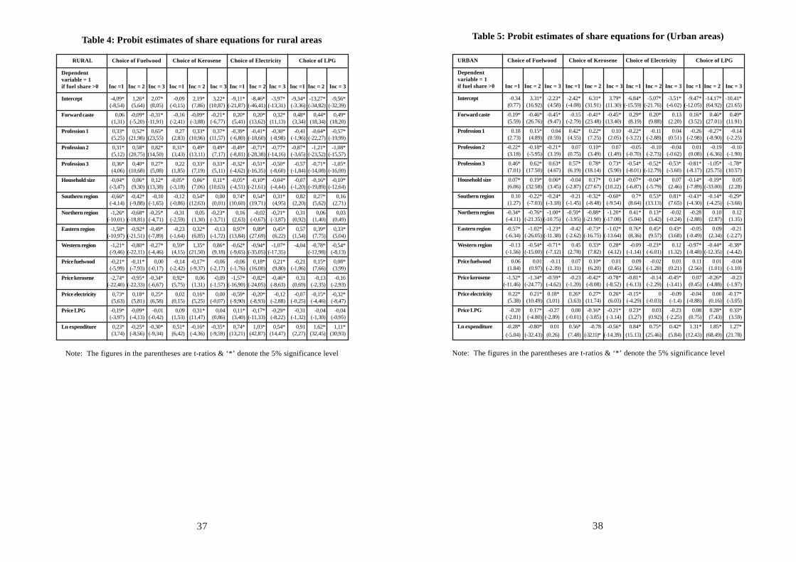
Table 4: Probit estimates of share equations for rural areas

RURAL Choice of Fuelwood Choice of Kerosene Choice of Electricity Choice of LPG

Dependentvariable = 1if fuel share >0 Inc =1 Inc = 2 Inc = 3 Inc =1 Inc = 2 Inc = 3 Inc =1 Inc = 2 Inc = 3 Inc =1 Inc = 2 Inc = 3

Intercept -4,09* 1,26* 2,07* -0,09 2,19* 3,22* -9,11* -8,46* -3,97* -9,34* -13,27* -9,56*(-8,54) (5,64) (8,05) (-0,15) (7,86) (10,87) (-21,87) (-46,41) (-13,31) (-3.36) (-34,82) (-32,39)

Forward caste 0,06 -0,09* -0,31* -0,16 -0,09* -0,21* 0,20* 0,20* 0,32* 0,48* 0,44* 0,49*(1,31) (-5,20) (-11,91) (-2,41) (-3,88) (-6,77) (5,41) (13,62) (11,13) (3,34) (18,34) (18,20)

Profession 1 0,33* 0,52* 0,65* 0,27 0,33* 0,37* -0,39* -0,41* -0,30* -0,41 -0,64* -0,57*(5,25) (21,98) (23,55) (2,83) (10,96) (11,57) (-6,80) (-18,60) (-8,98) (-1,96) (-22,27) (-19,99)

Profession 2 0,31* 0,58* 0,82* 0,31* 0,49* 0,49* -0,49* -0,71* -0,77* -0,87* -1,21* -1,08*(5,12) (20,75) (14,50) (3,43) (13,11) (7,17) (-8,81) (-28,38) (-14,16) (-3,65) (-23,52) (-15,57)

Profession 3 0,36* 0,40* 0,27* 0,22 0,33* 0,33* -0,32* -0,51* -0,50* -0,57 -0,71* -1,05*(4,06) (10,68) (5,08) (1,85) (7,19) (5,11) (-4,62) (-16,35) (-8,60) (-1,84) (-14,08) (-16,00)

Household size -0,04* 0,06* 0,12* -0,05* 0,06* 0,11* -0,05* -0,10* -0,04* -0,07 -0,16* -0,10*(-3,47) (9,30) (13,38) (-3,18) (7,06) (10,63) (-4,51) (-21,61) (-4,44) (-1,20) (-19,89) (-12,64)

Southern region -0,66* -0,42* -0,10 -0,12 0,54* 0,00 0,74* 0,54* 0,31* 0,82 0,27* 0,16(-4,14) (-9,88) (-1,65) (-0,86) (12,63) (0,01) (10,60) (19,71) (4,95) (2,20) (5,62) (2,71)

Northern region -1,26* -0,68* -0,25* -0,31 0,05 -0,23* 0,16 -0,02 -0,21* 0,31 0,06 0,03(-10,01) (-18,81) (-4,71) (-2,59) (1,30) (-3,71) (2,63) (-0,67) (-3,87) (0,92) (1,40) (0,49)

Eastern region -1,58* -0,92* -0,49* -0,23 0,32* -0,13 0,97* 0,89* 0,45* 0,57 0,39* 0,33*(-10,97) (-21,51) (-7,89) (-1,64) (6,85) (-1,72) (13,84) (27,69) (6,22) (1,54) (7,75) (5,04)

Western region -1,21* -0,80* -0,27* 0,59* 1,35* 0,86* -0,62* -0,94* -1,07* -4,04 -0,78* -0,54*(-9,46) (-22,11) (-4,46) (4,15) (21,50) (9,18) (-9,65) (-35,05) (-17,35) (-12,98) (-8,13)

Price fuelwood -0,21* -0,11* 0,00 -0,14 -0,17* -0,06 -0,06 0,18* 0,21* -0,21 0,15* 0,08*(-5,99) (-7,93) (-0,17) (-2,42) (-9,37) (-2,17) (-1,76) (16,00) (9,80) (-1,06) (7,66) (3,99)

Price kerosene -2,74* -0,95* -0,34* 0,92* 0,06 -0,09 -1,57* -0,82* -0,46* 0,31 -0,13 -0,16(-22,40) (-22,33) (-6,67) (5,75) (1,31) (-1,57) (-16,90) (-24,05) (-8,63) (0,69) (-2,35) (-2,93)

Price electricity 0,73* 0,18* 0,25* 0,02 0,16* 0,00 -0,59* -0,20* -0,12 -0,07 -0,15* -0,32*(5,63) (5,81) (6,58) (0,15) (5,25) (-0,07) (-9,90) (-8,93) (-2,88) (-0,25) (-4,46) (-8,47)

Price LPG -0,19* -0,09* -0,01 0,09 0,31* 0,04 0,11* -0,17* -0,29* -0,31 -0,04 -0,04(-3,97) (-4,13) (-0,42) (1,53) (11,47) (0,86) (3,40) (-11,33) (-8,22) (-1,32) (-1,30) (-0,95)

Ln expenditure 0,23* -0,25* -0,30* 0,51* -0,16* -0,35* 0,74* 1,03* 0,54* 0,91 1,62* 1,11*(3,74) (-8,56) (-9,34) (6,42) (-4,36) (-9,59) (13,21) (42,87) (14,47) (2,27) (32,45) (30,93)


Table 5: Probit estimates of share equations for (Urban areas)

URBAN Choice of Fuelwood Choice of Kerosene Choice of Electricity Choice of LPG

Dependentvariable = 1if fuel share >0 Inc =1 Inc = 2 Inc = 3 Inc =1 Inc = 2 Inc = 3 Inc =1 Inc = 2 Inc = 3 Inc =1 Inc = 2 Inc = 3

Intercept -0.34 3.31* -2.23* -2.42* 6.31* 3.79* -6.84* -5.07* -3.51* -9.47* -14.17* -10.41*(0.77) (16.92) (4.58) (-4.08) (31.91) (11.30) (-15.59) (-21.76) (-6.02) (-12.05) (64.92) (21.65)

Forward caste -0.19* -0.46* -0.45* -0.15 -0.41* -0.45* 0.29* 0.20* 0.13 0.16* 0.46* 0.49*(5.59) (26.76) (9.47) (-2.79) (23.48) (13.40) (8.19) (9.88) (2.20) (3.52) (27.01) (11.91)

Profession 1 0.18 0.15* 0.04 0.42* 0.22* 0.10 -0.22* -0.11 0.04 -0.26 -0.27* -0.14(2.73) (4.89) (0.59) (4.55) (7.25) (2.05) (-3.22) (-2.88) (0.51) (-2.98) (-8.90) (-2.25)

Profession 2 -0.22* -0.18* -0.21* 0.07 0.10* 0.07 -0.05 -0.10 -0.04 0.01 -0.19 -0.10(3.18) (-5.95) (3.19) (0.75) (3.49) (1.49) (-0.70) (-2.73) (-0.62) (0.08) (-6.36) (-1.90)

Profession 3 0.46* 0.62* 0.63* 0.57* 0.78* 0.73* -0.54* -0.52* -0.53* -0.81* -1.05* -1.78*(7.01) (17.50) (4.67) (6.19) (18.14) (5.90) (-8.01) (-12.79) (-3.60) (-8.17) (25.75) (10.57)

Household size 0.07* 0.19* 0.06* -0.04 0.17* 0.14* -0.07* -0.04* 0.07 -0.14* -0.19* 0.05(6.06) (32.58) (3.45) (-2.87) (27.67) (10.22) (-6.87) (-5.79) (2.46) (-7.89) (-33.00) (2.28)

Southern region 0.10 -0.22* -0.24* -0.21 -0.32* -0.60* 0.7* 0.53* 0.81* -0.43* -0.14* -0.29*(1.27) (-7.03) (-3.18) (-1.45) (-8.48) (-9.54) (8.64) (13.13) (7.65) (-4.30) (-4.25) (-3.66)

Northern region -0.34* -0.76* -1.00* -0.59* -0.88* -1.20* 0.41* 0.13* -0.02 -0.28 0.10 0.12(-4.11) (-21.35) (-10.75) (-3.95) (-21.90) (-17.08) (5.04) (3.42) (-0.24) (-2.88) (2.87) (1.35)

Eastern region -0.57* -1.02* -1.23* -0.42 -0.73* -1.02* 0.76* 0.45* 0.43* -0.05 0.09 -0.21(-6.34) (-26.05) (-11.38) (-2.62) (-16.75) (-13.64) (8.36) (9.57) (3.68) (-0.49) (2.34) (-2.27)

Western region -0.13 -0.54* -0.71* 0.45 0.33* 0.28* -0.09 -0.23* 0.12 -0.97* -0.44* -0.38*(-1.56) (-15.00) (-7.12) (2.78) (7.82) (4.12) (-1.14) (-6.01) (1.32) (-8.48) (-12.35) (-4.42)

Price fuelwood 0.06 0.01 -0.11 0.07 0.10* 0.01 0.09 -0.02 0.01 0.11 0.01 -0.04(1.84) (0.97) (-2.39) (1.31) (6.20) (0.45) (2.56) (-1.28) (0.21) (2.56) (1.01) (-1.10)

Price kerosene -1.52* -1.34* -0.59* -0.23 -0.42* -0.78* -0.81* -0.14 -0.45* 0.07 -0.26* -0.23(-11.46) (-24.77) (-4.62) (-1.20) (-8.08) (-8.52) (-6.13) (-2.29) (-3.41) (0.45) (-4.88) (-1.97)

Price electricity 0.22* 0.21* 0.18* 0.26* 0.27* 0.26* -0.15* 0 -0.09 -0.04 0.00 -0.17*(5.38) (10.49) (3.01) (3.63) (11.74) (6.03) (-4.29) (-0.03) (-1.4) (-0.88) (0.16) (-3.05)

Price LPG -0.20 0.17* -0.27 0.00 -0.16* -0.21* 0.23* 0.03 -0.23 0.08 0.28* 0.33*(-2.81) (-4.80) (-2.89) (-0.01) (-3.85) (-3.14) (3.27) (0.92) (-2.25) (0.75) (7.43) (3.59)

Ln expenditure -0.28* -0.80* 0.01 0.56* -0.78 -0.56* 0.84* 0.75* 0.42* 1.31* 1.85* 1.27*(-5.04) (-32.43) (0.26) (7.48) (-32.11)* (-14.39) (15.13) (25.46) (5.84) (12.43) (68.49) (21.78)


37 38

Table 6: Estimates of the LA-AIDS model for rural area

RURAL Choice of Fuelwood Choice of Kerosene Choice of Electricity Choice of LPG

Low Medium High Low Medium High Low Medium High Low Medium High

Intercept -0.470* -0.536* -0.470* 0.429* 0.412* 0.332* 1.096* 1.016* 0.919* -0.056* 0.109* 0.219*(-13.24) (-34.21) (-14.96) (18.21) (41.21) (19.32) (30.78) (76.72) (37.47) (-2.60) (8.93) (7.05)

Intercept -0.470* -0.536* -0.470* 0.429* 0.412* 0.332* 1.096* 1.016* 0.919* -0.056* 0.109* 0.219*(-13.24) (-34.21) (-14.96) -18.21 -41.21 -19.32 -30.78 -76.72 -37.47 (-2.60) -8.93 -7.05

Household size -0.009* -0.012* -0.016* 0.003* 0.002* -0.001 0.005* 0.006* 0.006* 0.001* 0.005* 0.010*(-8.40) (-25.65) (-14.09) -4.32 -5.73 (-1.97) -5.23 -14.79 -7.31 -2.97 -14.71 -9.83

Forward Caste -0.019* -0.015* -0.047* -0.004 -0.001 -0.008* 0.020* 0 0.005 0.003* 0.016* 0.050*(-2.98) (-6.13) (-9.03) (-1.22) (-0.48) (-3.12) -3.22 -0.2 -1.31 -2.17 -9.36 -10.05

Self employed inagriculture/ -0.037* 0.040* 0.057* 0.011 -0.006* -0.001 0.026* -0.003 0.003 0.001 -0.032* -0.059*non Agriculture (-3.46) -11.22 -9.51 -1.69 (-2.70) (-0.31) -2.5 (-0.90) -0.69 -0.25 (-13.38) (-10.38)

Agricultural labor -0.006 0.075* 0.166* 0.018* 0 0.013* -0.01 -0.029* -0.058* -0.002 -0.046* -0.122*(-0.53) -17.57 -14.39 -2.97 -0.04 -2.3 (-1.02) (-8.23) (-6.54) (-0.87) (-16.16) (-11.04)

Other labor -0.014 0.058* 0.137* 0.013 0.013* 0.040* 0.001 -0.036* -0.056* 0 -0.034* -0.120*(-1.09) -10.93 -11.25 -1.77 -4.16 -6.46 -0.08 (-8.20) (-5.99) (-0.11) (-9.80) (-10.39)

South region -0.008 -0.027* -0.123* -0.019* -0.011* -0.01 0.021 0.042* 0.056* 0.006 -0.004 0.077*(-0.54) (-4.67) (-8.36) (-2.28) (-2.95) (-1.26) -1.48 -8.59 -4.71 -1.54 (-0.94) -5.16

North region -0.012 -0.020* -0.074* -0.019* -0.011* -0.003 0.034* 0.047* 0.049* -0.003 -0.016* 0.028(-0.98) (-3.41) (-4.64) (-2.38) (-3.21) (-0.34) -2.84 -9.6 -3.97 (-0.89) (-3.83) -1.8

East region -0.003 -0.051 -0.135 -0.008 0.029 0.042 0.007 0.039 0.06 0.003 -0.017 0.033(-0.18) (-7.82) (-7.94) (-0.86) -7.28 (4.783 -0.47 -7.2 -4.51 -0.67 (-3.43) -1.98

West region -0.03 -0.071* -0.085* -0.021* -0.016* 0.009 0.057* 0.110* 0.087* -0.006 -0.023* -0.012(-1.90) (-9.84) (-4.67) (-2.29) (-3.36) -0.97 -3.78 -18 -5.97 (-1.36) (-3.97) (-0.65)

Forest 0.002* 0.001* 0.001* -0.001* -0.001* 0.000* -0.001* 0.000* -0.002* 0 0 0-6.63 -8.39 -6.71 (-6.36) (-8.68) (-2.45) (-3.05) (-3.57) (-8.96) -0.25 (-0.53) -1.53

Log of expenditure 0.193* 0.183* 0.154* -0.042* -0.037* -0.030* -0.149* -0.131* -0.101* -0.002 -0.016* -0.023*-39.58 -83.87 -34.8 (-14.30) (-27.87) (-13.48) (-31.90) (-72.38) (-29.8) (-1.76) (-10.25) (-5.38)

Lambda -0.012 -0.036* 0.018 -0.041* -0.062* -0.013 -0.011* 0.013* 0.013* 0.064* 0.084* -0.018(-1.28) (-3.68) -1.66 (-2.31) (-4.30) (-1.01) (-2.52) -4.87 -3.62 -3.32 -4.97 (-0.91)

Price Fuelwood 0.104* 0.096* 0.059*-18.53 -42.54 -13.69

Price Kerosene -0.003 -0.014* -0.012* 0.011 0.035* 0.016*(-0.78) (-9.19) (-4.99) -1.21 -10.55 -3.14

Price Electricity -0.094* -0.073* -0.044* 0.01 -0.011* -0.007* 0.085* 0.075* 0.071*(-18.97) (-42.83) (-13.92) -1.99 (-5.80) (-2.11) -13.26 -31.53 -14.22

Price Lpg 0.059* 0.025* 0.008 -0.012* -0.007* -0.006 -0.047* -0.020* -0.018* 0 0.001 0.016*-10.66 -8.41 -1.08 (-3.67) (-3.58) (-1.57) (-8.82) (-7.81) (-3.09) -0.01 -0.63 -2.22


Table 7: Estimates of the LA-AIDS model for urban area

Urban Choice of Fuelwood Choice of Kerosene Choice of Electricity Choice of LPG

Low Medium High Low Medium High Low Medium High Low Medium High

Intercept -0.408* -0.405*-0.534* 0.492* 0.541* 0.421* 1.033* 0.990* 0.751* -0.117* -0.125* 0.362*(-7.96) (-10.87) (-3.31) -11.43 -18.24 -3.3 -25.26 -37.57 -6.21 (-3.38) (-3.54) -2.06

Household size -0.012* -0.015*-0.021* 0 -0.007* -0.011* 0.010* 0.011* 0.015* 0.0021* 0.011* 0.018*-7.85 (-11.80) (-4.37) (-0.34) (-7.34) (-3.05) -8.62 -12.32 -3.79 -2.67 -9.61 -3.45

Forward Caste -0.007 -0.036* -0.031 0.005 0.001 -0.012 0.008 -0.006 -0.019 -0.006 0.041* 0.063*-1.02 (-6.62) (-1.65) -1.03 -0.2 (-0.86) -1.43 (-1.50) (-1.28) (-1.69) -8.62 -3.15

Self employed inagriculture/ 0.021 -0.002-0.078* 0.008 0.016* -0.012 -0.006 -0.001 0.005 -0.023* -0.013 0.085*non Agriculture -1.45 (-0.21) (-2.87) -0.75 -2.41 (-0.58) (-0.58) (-0.14) -0.24 (-3.08) (-1.63) -2.95

Agricultural labor -0.024 -0.053*-0.084* 0.023 0.037* 0.007 0.01 0.002 -0.022 -0.009 0.014 0.100*(-1.56) (-5.63) (-3.19) -1.99 -5.45 -0.35 -0.83 -0.32 (-1.06) (-1.14) -1.73 -3.57

Other labor 0.036* 0.065* 0.148* 0.002 0.032* 0.019 -0.006 -0.031* -0.076* -0.031* -0.066* -0.091*-2.42 -6.38 -3.55 -0.19 -4.43 -0.6 (-0.55) (-4.39) (-2.28) (-4.18) (-7.48) (-2.06)

South region -0.052* -0.069*-0.210* 0.036* 0.036* -0.039 0.009 -0.054* -0.033 0.0071 0.087* 0.282*(-2.23) (-4.50) (-3.49) -2.03 -3.2 (-0.77) -0.49 (-4.95) (-0.66) -0.57 -6.38 -4.21

North region -0.023 -0.023 -0.146 0.011 -0.008 -0.0630.046*(2.55)-0.006-0.066 -0.034* 0.037* 0.275*(-0.99) (-1.39) (-1.99) -0.62 (-0.62) (-1.01) (-0.53) (-1.19) (-2.70) -2.47 -3.33

East region -0.136* -0.161*-0.210* 0.095* 0.069* -0.001 0.048* -0.004 -0.041 -0.008 0.096* 0.252*(-5.39) (-9.01) (-2.66) -4.87 -5.24 (-0.02) -2.44 (-0.30) (-0.69) (-0.55) -5.98 -2.92

West region -0.027 -0.029 -0.011 -0.017 -0.015 -0.065 0.055* 0.058* -0.052 -0.012 -0.014 0.129(-1.10) (-1.63) (-0.15) (-0.90) (-1.16) -1.23 -2.88 -4.61 (-0.95) (-0.92) (-0.86) -1.67

Forest 0.002* 0.002* 0 -0.001* -0.001* -0.002* -0.001* -0.002* -0.003*-2.00E-040.002* 0.005*-4.11 -6.24 -0.45 (-2.44) (-7.46) (-2.94) (-2.30) (-11.72) (-3.94) (-0.87) -8.46 -4.78

log of expenditure 0.149* 0.130* 0.136* -0.029* -0.018* -0.008 -0.125* -0.104* -0.056* 0.0054 -0.007 -0.072*-23.02 -26.39 -7.55 (-5.67) (-4.94) (-0.56) (-24.7) (-30.35) (-3.83) -1.52 (-1.61) (-3.69)

Lambda -0.031* 0.029* 0.079* -0.028 0.075* 0.066* -0.007 -0.076* -0.001 0.0656* -0.029 -0.145(-2.87) -5.45 -2.56 (-1.27) -8.84 -2.21 (-0.83) (-6.01) (-0.02) -2.71 (-1.76) (-1.64)

Price Fuelwood 0.060* 0.045* 0.016-8.08 -8.64 -0.75

Price Kerosene -0.045* -0.018* -0.007 0.127* 0.158* 0.081(-7.14) (-4.71) (-0.42) -7.34 -14.31 -1.79

Price Electricity -0.034* -0.035* -0.009 -0.001 -0.014* -0.021 0.009 0.010* 0.035(-6.81) (-10.63) (-0.60) (-0.10) (-3.26) (-1.05) -1.54 -2.28 -1.77

Price LPG -0.01 -0.038* -0.049 0.017 0.031* 0.043 0.001 -0.012 -0.049 -0.009 0.018 0.055(-0.60) (-3.34) (-1.12) -1.41 -3.82 -1.27 -0.09 (-1.50) (-1.40) (-1.01) -1.84 -1.19


39 40

Table 8: Chow Statistics for different income cut-off points

Cut-Off Point Sector Numerator Denominator F-Test Pr> F(Per Capita Income) Degrees Of Degrees Of

Freedom Freedom

328 Rural 48 27358 4.91 < 0.0001

774 Rural 48 27358 21.31 < 0.0001

455 Urban 48 9422 3.31 < 0.0001

1421 Urban 48 9422 8.80 < 0.0001

Table 9: Estimated uncompensated (Marshallian) own-price elasticitiesfor rural and urban areas by expenditure group

Rural Urban

Low Medium High Low Medium High

Fuelwood -1.05* -1.03* -1.03* -1.04* -1.02* -1.05*(-0.009) (-0.004) (-0.008) (-0.013) (-0.011) (-0.046)

Kerosene -0.84* -0.75* -0.86* -0.18* -0.21* -0.14(-0.049) (-0.016) (-0.027) (-0.069) (-0.038) (-0.169)

Electricity -0.59* -0.66 -0.72* -0.85* -0.87* -0.91*(-0.021) (-0.007) (-0.014) (-0.014) (-0.010) (-0.031)

LPG -1.00* -0.98* -0.97* -1.05* -1.01* -0.92*(-0.003) (-0.005) (-0.015) (-0.015) (-0.018) (-0.075)

Note: The figures in the parentheses are standard errors

Table 10: Estimated compensated price elasticities by income groupsfor rural and urban households5

Low income Low income

Rural Urban

Fuelwood Kerosene Electricity LPG Fuelwood Kerosene Electricity LPG

Fuelwood -0.126* 0.239* 0.191* 0.596* Fuelwood -0.292* 0.244 0.2 0.661(-0.010) (-0.007) (-0.007) (-0.010) -0.014 -0.013 -0.011 -0.029

Kerosene 0.712* -0.630* 0.361* 0.470* Kerosene 0.470* 0.112 0.453 0.604(-0.0157) (-0.049) (-0.020) (-0.014) -0.021 -0.07 -0.023 -0.041

Electricity 0.440* 0.279* -0.421* 0.378* Electricity 0.474* 0.348 -0.581 0.586(-0.017) (-0.016) (-0.021) (-0.018) -0.014 -0.018 -0.015 -0.032

LPG 0.843* 0.223* 0.232* -0.484* LPG 0.653* 0.309 0.391 -0.447(-0.011) (-0.007) (-0.011) (-0.003) -0.028 -0.021 -0.021 -0.015

Medium income Medium income


Fuelwood -0.178* 0.199* 0.230* 0.549* Fuelwood -0.395* 0.257* 0.358* 0.536*-0.004 -0.003 -0.004 -0.005 -0.012 -0.01 -0.008 -0.023

Kerosene 0.610* -0.568* 0.302* 0.483* Kerosene 0.431* 0.075* 0.382* 0.648*-0.008 -0.016 -0.009 -0.01 -0.014 -0.038 -0.016 -0.029

Electricity 0.450* 0.193* -0.456* 0.447* Electricity 0.398* 0.254* -0.548* 0.501*-0.006 -0.006 -0.007 -0.008 -0.008 -0.011 -0.011 -0.018

LPG 0.715* 0.205* 0.298* -0.489* LPG 0.489* 0.352* 0.410* -0.513*-0.006 -0.004 -0.005 -0.005 -0.021 -0.016 -0.016 -0.019

High Income High Income


Fuelwood -0.330* 0.174* 0.274* 0.520* Fuelwood -0.584* 0.290* 0.463* 0.507*(-0.009) (-0.006) (-0.008) (-0.014) -0.047 -0.032 -0.031 -0.091

Kerosene 0.495* -0.705* 0.373* 0.458* Kerosene 0.547* 0.082 0.318* 1.102*(-0.013) (-0.027) (-0.019) (-0.021) -0.056 -0.169 -0.076 -0.118

Electricity 0.389* 0.186* -0.443* 0.466* Electricity 0.321* 0.117* -0.444* 0.228*(-0.001) (-0.001) (-0.014) (-0.016) -0.022 -0.029 -0.033 -0.047

LPG 0.565* 0.175* 0.356* -0.512* LPG 0.384* 0.443* 0.250* -0.519*(-0.016) (-0.009) (-0.013) (-0.015) -0.07 -0.049 -0.052 -0.076

41 42

5 The table should be read from left and up. For example, for low-incomerural households a one percent increase in price of kerosene would lead to a0.712 percent increase in fuelwood consumption.

Table 11: Expenditure elasticities for rural and urban areasby income groups

Note: The figures in the parentheses are standard errors.

43 44

Elasticises LA/AIDS Engel Integrated Elasticiseselasticises

Rural Fuelwood Kerosene Electricity LPG Fuelwood Kerosene Electricity LPG

Low 1.261* 0.837* 0.533* 0.994* 0.655 0.792 0.6 0.375 0.657-0.007 -0.012 -0.015 -0.003

Medium 1.278* 0.840* 0.619* 0.960* 0.792 1.012 0.665 0.49 0.76-0.003 -0.006 -0.005 -0.003

High 1.313* 0.854* 0.725** 0.926* 0.604 0.761 0.564 0.399 0.606-0.008 -0.012 -0.009 -0.009

Urban Fuelwood Kerosene Electricity LPG Fuelwood Kerosene Electricity LPG

Low 1.260* 0.934* 0.661* 1.003* 0.986 1.242 0.921 0.652 0.989-0.011 -0.017 -0.013 -0.006

Medium 1.303* 0.977* 0.751* 0.940* 0.7 0.912 0.684 0.526 0.658-0.01 -0.013 -0.008 -0.008

High 1.272* 1.182* 0.895* 0.835* 0.665 0.846 0.787 0.596 0.556-0.032 -0.044 -0.017 -0.027

Figure 1. Choice of main fuel by different expenditure classes (Rural areas)

0%

20%

40%

60%

80%

100%

0-225

225-2

55

255-3

00

300-3

40

340-3

80

380-4

20

420-4

70

470-5

25

525-6

15

615-7

7577

5+

Mean Per capita Expenditure classes

Perc

enta

ge o

f peo

ple

dung cake Fire wood & chips Coke coal charcoal Gobar gaskerosene LPG Electricity others

F igure 2 . C hoice o f m ain fuel b y d ifferent expenditure classes (urb an areas)

0 %

1 0 %

2 0 %

3 0 %

4 0 %

5 0 %

6 0 %

7 0 %

8 0 %

9 0 %

1 0 0 %

0-300300-350

350-425425-500

500-575575-665

665-775775-915

915-11201120-1500

1500-19251925-more

M e an p e r c a p ita e xp e n d itu re

perc

enta

ge o

f sam

pled

pop

ulat

ion

d u n g ca k e F ire w ood & ch ips C oke coa l ch a rcoa l G oba r ga sk erosen e L P G E lectr icity o th ers

Note: The figures in the parentheses are standard errors.

45 46

Figure 4. Expenditure elasticities for different expenditure classes

(Urban India)

00.20.40.60.8

11.21.41.6

0-300300-350

351-425425-525

526-650651-800

801-975976-1175

1176-14751476-1825

1826-22252225+

Expenditure classes

Ela

stic

ity

fuelwood Kerosene Electricity LPG

Appendix 1Table A1. Estimated uncompensated price elasticities by income groups

for rural and urban households6

Low income Low income

Rural Urban


Fuelwood -1.05* -0.071* -0.209* -0.057* -1.04* -0.144* -0.185* -0.097*(-0.009) (-0.005) (-0.007) (-0.008) (-0.013) (-0.011) (-0.009) (-0.028)

Kerosene 0.098* -0.835* 0.095* 0.037* -0.085* -0.176* 0.078* 0.042(-0.015) (-0.049) (-0.019) (-0.014) (-0.021) (-0.069) (-0.022) (-0.041)

Electricity 0.049* 0.148* -0.590* 0.102* 0.081* 0.144* -0.846* 0.188*(-0.016) (-0.015) (-0.021) (-0.017) (-0.013) (-0.017) (-0.014) (-0.032)

LPG 0.115* -0.021* -0.084* -0.998* 0.057* -0.0001 -0.012 -1.05*(-0.011) (-0.007) (-0.011) (-0.003) (-0.028) (-0.021) (-0.021) (-0.015)

Middle Income Middle Income


Fuelwood -1.026* -0.078* -0.203* -0.102* -1.025* -0.119* -0.208* -0.155*(-0.004) (-0.003) (-0.003) (-0.005) (-0.011) (-0.008) (-0.007) (-0.023)

Kerosene 0.052* -0.749* 0.017 0.0551* -0.042* -0.208* -0.043* 0.129*(-0.008) (-0.016) (-0.009) (-0.009) (-0.014) (-0.038) (-0.015) (-0.028)

Electricity 0.040* 0.059* -0.66 0.131* 0.035* 0.037* -0.874* 0.102*(-0.005) (-0.006) (-0.007) (-0.007) (-0.008) (-0.010) (-0.010) (-0.018)

LPG 0.078* -0.003 -0.028 -0.978* 0.034* 0.081* 0.0014 -1.01*(-0.006) (-0.004) (-0.005) (-0.005) (-0.021) (-0.015) (-0.015) (-0.018)

High Income High Income


Fuelwood -1.03* -0.072* -0.218* -0.123* -1.046* 0.045 -0.203* -0.102*(-0.008) (-0.0045) (-0.006) (-0.014) (-0.046) (-0.029) (-0.028) (-0.090)

Kerosene 0.040* -0.865* 0.053* 0.040* 0.118* -0.145 -0.301* 0.536*(-0.013) (-0.027) (-0.018) (-0.020) (-0.055) (-0.169) (-0.075) (-0.118)

Electricity 0.003 0.0507* -0.715* 0.110* -0.004 -0.055 -0.912* -0.200*(-0.009) (-0.009) (-0.014) (-0.016) (-0.020) (-0.028) (-0.031) (-0.046)

LPG 0.072* 0.002 0.009 -0.966* 0.081 0.282* -0.188* -0.919*(-0.015) (-0.008) (-0.012) (-0.015) (-0.069) (-0.047) (-0.050) (-0.075)

6 The table should be read from left and up. For example, for low incomerural households a one percent increase in price of kerosene would lead to a0.712 percent increase in fuelwood consumption.

Figure 3. Expenditure elasticities for different fuels

(Rural India)

-0.2-0.1

00.10.20.30.40.50.60.70.80.9

11.11.21.31.4

0-255

256-3

00

301-3

40

341-3

80

381-4

20

421-4

70

471-5

45

546-6

25

625-7

50

750-1

000

>1000

Expenditure claases

Elas

ticity

Fuelwood Kerosene Electricity LPG

Working Paper 9 PDF

Documents

Transcript of Working Paper 9 PDF